 14 |
15 | Here, w(j) represents the weight for jth feature.
16 |
17 | n is the number of features in the dataset.
18 |
19 | lambda1 is the regularization strength for L-1 norm.
20 |
21 | lambda2 is the regularization strength for L-2 norm.
22 |
23 | ## Advantages
24 |
25 | ▪ Doesn’t have the problem of selecting more than n predictors when n<
14 |
15 | Here, w(j) represents the weight for jth feature.
16 |
17 | n is the number of features in the dataset.
18 |
19 | lambda1 is the regularization strength for L-1 norm.
20 |
21 | lambda2 is the regularization strength for L-2 norm.
22 |
23 | ## Advantages
24 |
25 | ▪ Doesn’t have the problem of selecting more than n predictors when n< Neurons in Neural Network are inspired from biological neurons. This Neural Network would able to do various tasks like classifying images, prediction, and so on. Alexa and Siri use neural network.
5 |
6 | A Perceptron is an algorithm used for supervised learning of binary classifiers. Binary classifiers decide whether an input, usually represented by a series of vectors, belongs to a specific class. In short, a perceptron is a single-layer neural network.
7 |
Working of Perceptron
10 | 11 | Perceptron looks like the following structure: 12 | 13 | 14 |
15 | We have 3 inputs X,Y and Z. When this inputs get into the net input fucntion it firstly get weighted with some weigh value that is w1,w2 and w3 respectively. The net input fucntion(Z) sums up all the value i.e. Z = (Xi * Wi). This Z will determine if a neuron fires or not. Firing of the neuron depends on a function which is called Activation Function. If the sum of the input signals exceeds a certain threshold, it either outputs a signal or does not return an output.
16 |
17 | -
14 |
15 | We have 3 inputs X,Y and Z. When this inputs get into the net input fucntion it firstly get weighted with some weigh value that is w1,w2 and w3 respectively. The net input fucntion(Z) sums up all the value i.e. Z = (Xi * Wi). This Z will determine if a neuron fires or not. Firing of the neuron depends on a function which is called Activation Function. If the sum of the input signals exceeds a certain threshold, it either outputs a signal or does not return an output.
16 |
17 | -
Perceptron Function
18 | 19 | Perceptron is a function that maps its input “x,” which is multiplied with the learned weight coefficient; an output value ”f(x)”is generated. 20 | 21 | ``` If w.x + b > 0, then f(x) = 1 ; else f(x) = 0 ``` 22 | 23 | In the equation given above: 24 | 25 | “w” = vector of real-valued weights 26 | 27 | “b” = bias (an element that adjusts the boundary away from origin without any dependence on the input value) 28 | 29 | “x” = vector of input x values 30 | 31 | ``` Σ (Wi * Xi) ``` 32 | 33 | “m” = number of inputs to the Perceptron 34 | 35 | The output can be represented as “1” or “0.” It can also be represented as “1” or “-1” depending on which activation function is used. 36 | 37 | -
Perceptron Training
38 | Refer:
39 | [Perceptron Training](perceptron_training.py)
--------------------------------------------------------------------------------
/FP-Growth/README.md:
--------------------------------------------------------------------------------
1 | # FP GROWTH ALGORITHM
2 |
3 | ## Introduction
4 |
5 | FP growth algorithm or the Frequent Pattern Growth Algorithm is an improvement of apriori algorithm. The two primary drawbacks of the Apriori Algorithm were that at each step, candidate sets had to be rebuilt and to build those, the algorithm had to repeatedly scan the database. These properties in turn made the algorithm slower. FP algorithm overcomes the disadvantages of the Apriori algorithm by storing all the transactions in a Tree Data Structure.
6 |
7 | ## FP Tree
8 |
9 | FP tree is the core concept of the whole FP Growth algorithm. It is the compressed representation of the itemset database. The tree structure not only reserves the itemset in DB but also keeps track of the association between itemsets. The tree is constructed by taking each itemset and mapping it to a path in the tree one at a time. The whole idea behind this construction is that more frequently occurring items will have better chances of sharing items. We then mine the tree recursively to get the frequent pattern. Pattern growth, the name of the algorithm, is achieved by concatenating the frequent pattern generated from the conditional FP trees.
10 |
11 | A FP tree looks something like this:
12 |
13 | 
14 |
15 | ## Advantages
16 |
17 | ▪ This algorithm needs to scan the database only twice when compared to Apriori which scans the transactions for each iteration.
18 |
19 | ▪ The pairing of items is not done in this algorithm and this makes it faster.
20 |
21 | ▪ The database is stored in a compact version in memory.
22 |
23 | ▪ It is efficient and scalable for mining both long and short frequent patterns.
24 |
25 | ## Disadvantages
26 |
27 | ▪ FP Tree is more cumbersome and difficult to build than Apriori.
28 |
29 | ▪ It may be expensive.
30 |
31 | ▪ When the database is large, the algorithm may not fit in the shared memory.
32 |
33 | ## References
34 |
35 | ▪ https://www.geeksforgeeks.org/ml-frequent-pattern-growth-algorithm/
36 |
37 | ▪ https://www.softwaretestinghelp.com/fp-growth-algorithm-data-mining/
38 |
39 | ▪ https://towardsdatascience.com/fp-growth-frequent-pattern-generation-in-data-mining-with-python-implementation-244e561ab1c3
40 |
--------------------------------------------------------------------------------
/Lowess Regression/README.md:
--------------------------------------------------------------------------------
1 | # LOWESS REGRESSION
2 |
3 | ## Introduction
4 |
5 | LOWESS are non-parametric regression methods that combine multiple regression models in a k-nearest-neighbor-based meta-model. They address situations in which the classical procedures do not perform well or cannot be effectively applied without undue labor. LOWESS combines much of the simplicity of linear least squares regression with the flexibility of nonlinear regression. It does this by fitting simple models to localized subsets of the data to build up a function that describes the variation in the data, point by point.
6 |
7 | ## Procedure
8 |
9 | A linear function is fitted only on a local set of points delimited by a region, using weighted least squares. The weights are given by the heights of a kernel function (i.e. weighting function) giving:
10 |
11 | ▪ more weights to points near the target point x0 whose response is being estimated
12 |
13 | ▪ less weight to points further away
14 |
15 | We obtain then a fitted model that retains only the point of the model that are close to the target point (x0). The target point then moves away on the x axis and the procedure repeats for each point.
16 |
17 | ## Advantages
18 |
19 | ▪ Allows us to put less care into selecting the features in order to avoid overfitting.
20 |
21 | ▪ Does not require specification of a function to fit a model to all of the data in the sample.
22 |
23 | ▪ Only a Kernel function and smoothing / bandwidth parameters are required.
24 |
25 | ▪ Very flexible, can model complex processes for which no theoretical model exists.
26 |
27 | ▪ Considered one of the most attractive of the modern regression methods for applications that fit the general framework of least squares regression but which have a complex deterministic structure.
28 |
29 | ## Disadvantages
30 |
31 | ▪ Requires to keep the entire training set in order to make future predictions.
32 |
33 | ▪ The number of parameters grows linearly with the size of the training set.
34 |
35 | ▪ Computationally intensive, as a regression model is computed for each point.
36 |
37 | ▪ Requires fairly large, densely sampled data sets in order to produce good models. This is because LOWESS relies on the local data structure when performing the local fitting.
38 |
39 | ## References
40 |
41 | ▪ https://xavierbourretsicotte.github.io/loess.html
42 |
--------------------------------------------------------------------------------
/Mini Batch K-means Clustering/README.md:
--------------------------------------------------------------------------------
1 | # MINI BATCH K-MEANS CLUSTERING
2 |
3 | ## Introduction
4 |
5 | Mini Batch K-means algorithm‘s main idea is to use small random batches of data of a fixed size, so they can be stored in memory. Each iteration a new random sample from the dataset is obtained and used to update the clusters and this is repeated until convergence. Each mini batch updates the clusters using a convex combination of the values of the prototypes and the data, applying a learning rate that decreases with the number of iterations. This learning rate is the inverse of the number of data assigned to a cluster during the process. As the number of iterations increases, the effect of new data is reduced, so convergence can be detected when no changes in the clusters occur in several consecutive iterations.
6 |
7 | ## Need for Mini-Batch K-Means Clustering Algorithm
8 |
9 | K-means is one of the most popular clustering algorithms, mainly because of its good time performance. With the increasing size of the datasets being analyzed, the computation time of K-means increases because of its constraint of needing the whole dataset in main memory. For this reason, several methods have been proposed to reduce the temporal and spatial cost of the algorithm. A different approach is the Mini batch K-means algorithm.
10 |
11 | The empirical results suggest that it can obtain a substantial saving of computational time at the expense of some loss of cluster quality, but not extensive study of the algorithm has been done to measure how the characteristics of the datasets, such as the number of clusters or its size, affect the partition quality.
12 |
13 | 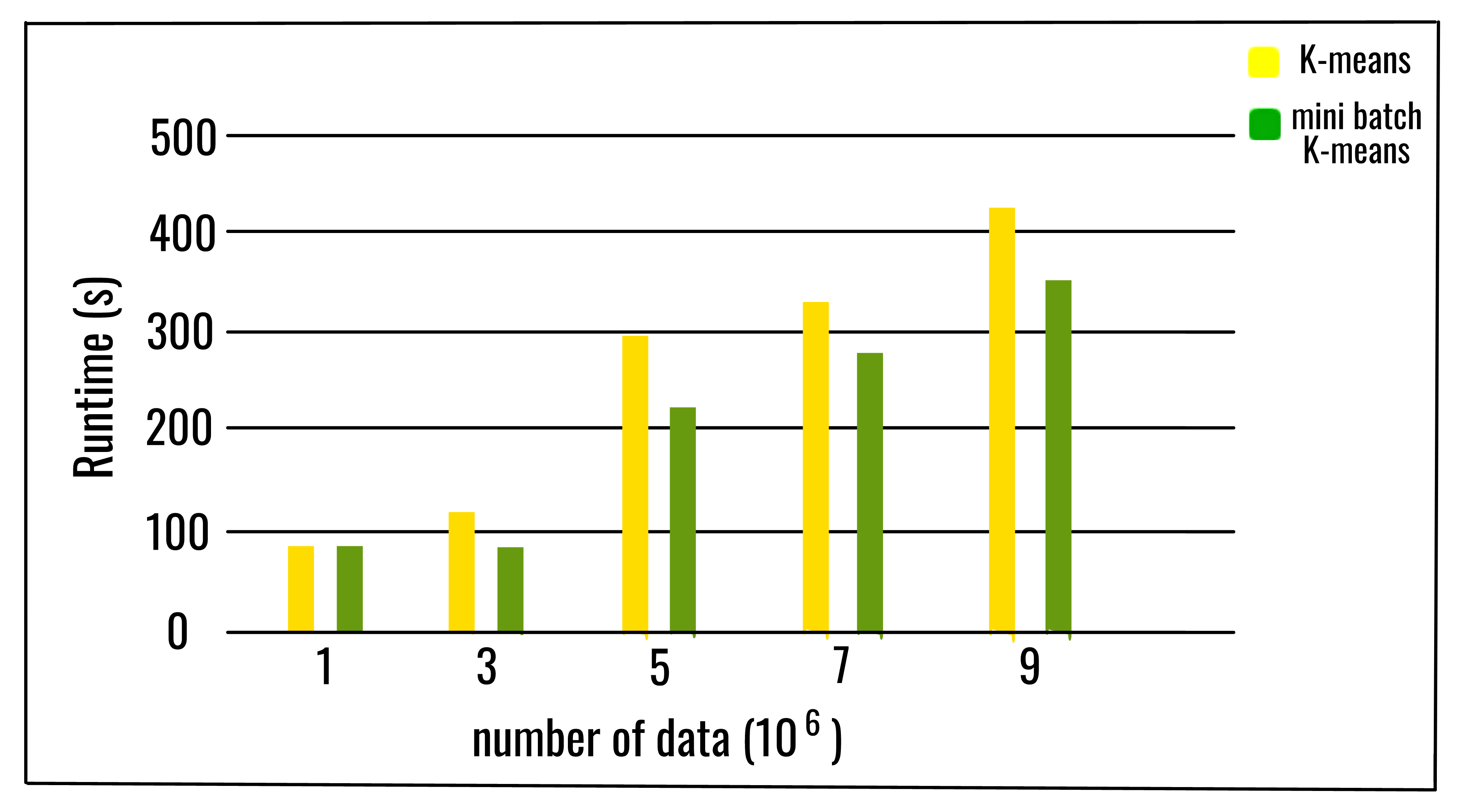 14 |
15 | ## Advantages
16 |
17 | ▪ If variables are huge, then K-Means most of the times gets computationally faster than hierarchical clustering, if we keep k small.
18 |
19 | ▪ K-Means produce tighter clusters than hierarchical clustering.
20 |
21 | ## Disadvantages
22 |
23 | ▪ Difficult to predict K-Value.
24 |
25 | ▪ It may not work well with clusters (in the original data) of different size and different density.
26 |
27 | ## References
28 |
29 | ▪ https://www.geeksforgeeks.org/ml-mini-batch-k-means-clustering-algorithm/
30 |
31 | ▪ http://playwidtech.blogspot.com/2013/02/k-means-clustering-advantages-and.html
32 |
--------------------------------------------------------------------------------
/CONTRIBUTING.md:
--------------------------------------------------------------------------------
1 | # Contributing guidelines
2 |
3 | ## Before contributing
4 |
5 | Welcome to [Algo-Phantoms/Algo-ScriptML](https://github.com/Algo-Phantoms/Algo-ScriptML). Before sending your pull requests, make sure that you **read the whole guidelines**. If you have any doubt on the contributing guide, please feel free to reach out to us.
6 |
7 | ### Contribution
8 |
9 | We appreciate any contribution, from fixing a grammar mistake in a comment to implementing complex algorithms. Please read this section if you are contributing your work.
10 |
11 | #### Coding Style
12 |
13 | We want your work to be readable by others; therefore, we encourage you to note the following:
14 |
15 | - Follow PEP8 guidelines. Read more about it here.
16 | - Please write in Python 3.7+. __print()__ is a function in Python 3 so __print "Hello"__ will _not_ work but __print("Hello")__ will.
17 | - Please focus hard on naming of functions, classes, and variables. Help your reader by using __descriptive names__ that can help you to remove redundant comments.
18 | - Please follow the [Python Naming Conventions](https://pep8.org/#prescriptive-naming-conventions) so variable_names and function_names should be lower_case, CONSTANTS in UPPERCASE, ClassNames should be CamelCase, etc.
19 | - Expand acronyms because __gcf()__ is hard to understand but __greatest_common_factor()__ is not.
20 |
21 | - Avoid importing external libraries for basic algorithms. Only use those libraries for complicated algorithms. **Usage of NumPY is highly recommended.**
22 |
23 |
24 | #### Other points to remember while submitting your work:
25 |
26 | - File extension for code should be `.py`.
27 | - Strictly use snake_case (underscore_separated) in your file_name, as it will be easy to parse in future using scripts.
28 | - Please avoid creating new directories if at all possible. Try to fit your work into the existing directory structure. If you want to. Please contact us before doing so.
29 | - If you have modified/added code work, make sure the code compiles before submitting.
30 | - If you have modified/added documentation work, ensure your language is concise and contains no grammar errors.
31 | - Do not update the [README.md](https://github.com/Algo-Phantoms/Algo-ScriptML/blob/main/README.md) and [Contributing_Guidelines.md](https://github.com/Algo-Phantoms/Algo-ScriptML/blob/main/CONTRIBUTING.md).
32 |
33 | Happy Coding :)
34 |
35 |
--------------------------------------------------------------------------------
/stochastic gradient descent/README.md:
--------------------------------------------------------------------------------
1 | # Stochastic gradient descent(SGD):
2 | * stochastic gradient descent(SGD) is used for regression problems with **very large dataset(in millions).**
3 | * SGD is same as gradient discent algorithm but have difference in optimization function.
4 | * SGD is inspired by Robbins–Monro algorithm of the 1950s.
5 |
6 | ## Basic idea behind SGD:
7 | * SGD works as an iterative algorithm.
8 | * It starts from a random point in dataset
9 | * after that it tries to fit the training sets one by one.
10 |
11 | ## Working of SGD:
12 |
13 | * first it initialize the theta(weights) to some random values.
14 | * than it takes a dataset(a row) from training set and tries to fit perfectly and returns modefied theta(weights).
15 | * that returned theta(weights) are applied over next dataset and tries to fit it perfectly and returns the theta.
16 | * this loop runs untill last dataset.
17 |
18 | ## Intution behind SGD:
19 | * first the algo shuffles the data, so that there should be no pattern can be seen firstly.
20 | * than algo tries to fit nex data more accurately thn the previously.
21 |
22 | ## SGD function:
23 |
24 | 
25 |
26 | ## Difference between SGD and Gradient descent(Batch descent):
27 |
28 | 
29 | * gradient descent goes from 1 to m(no of datasets) in every iterations while SGD iterates one time over one dataset.
30 |
31 | ## Main advantages of SGD:
32 | * computational efficient.
33 | * model with large dataset can be trained eaisly.
34 |
35 | ## Main disadvantages of SGD:
36 |
37 | * not effective over small datasets.
38 |
39 | ## Documentation:
40 |
41 | ```python
42 | Stochastic_gradient_descent(learning_rate=0.1)
43 | ```
44 | it takes the learning rate only, if you will not give it will be initialized to 0.1
45 | ```python
46 | object.fit(X,y)
47 | ```
48 | after making object of SGD type we have to call .fit() method in order to train model.
49 |
50 | * X: feature dataset(shuffeled)
51 | * y:label set(target set)(shuffled)
52 |
53 | ```python
54 | object.predict(X_pred)
55 | ```
56 | X_pred: features for which prediction is to be made.
57 |
58 | ## Example:
59 |
60 | ```python
61 |
62 | algo=Stochastic_gradient_descent(learning_rate=0.03)
63 | model=algo.fit(X,y)
64 | predicted_value=model.predict(X_pred)
65 | ```
66 |
--------------------------------------------------------------------------------
/Apriori/README.md:
--------------------------------------------------------------------------------
1 | # APRIORI ALGORITHM
2 |
3 | ## Introduction
4 |
5 | Apriori algorithm was given by R. Agrawal and R. Srikant in 1994 for finding frequent itemsets in a dataset for boolean association rule. The algorithm is called so because it uses prior knowledge of frequent itemset properties. With the help of the association rule, it determines how strongly or how weakly two objects are connected. This algorithm uses a breadth-first search and Hash Tree to calculate the itemset associations efficiently. It is the iterative process for finding the frequent itemsets from the large dataset.
6 |
7 | To improve the efficiency of level-wise generation of frequent itemsets, **Apriori Property** is used. It helps in reducing the search space.
8 |
9 | Frequent itemsets: Frequent itemsets are those items whose support is greater than the threshold value or user-specified minimum support. It means if A & B are the frequent itemsets together, then individually A and B should also be the frequent itemset. Suppose there are the two transactions: A= {1,2,3,4,5}, and B= {2,3,7}, in these two transactions, 2 and 3 are the frequent itemsets.
10 |
11 | 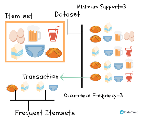
12 |
13 | ## Apriori Property
14 |
15 | According to this property, all subsets of a frequent itemset must also be frequent.
16 |
17 | ## Steps for Apriori Algorithm
18 |
19 | Step 1: Determine the support of itemsets in the transactional database, and select the minimum support and confidence.
20 |
21 | Step 2: Take all supports in the transaction with higher support value than the minimum or selected support value.
22 |
23 | Step 3: Find all the rules of these subsets that have higher confidence value than the threshold or minimum confidence.
24 |
25 | Step 4: Sort the rules as the decreasing order of lift.
26 |
27 | ## Advantages of Apriori Algorithm
28 |
29 | ▪ This is an easy to understand algorithm.
30 |
31 | ▪ The join and prune steps of the algorithm can be easily implemented on large datasets.
32 |
33 | ## Disadvantages of Apriori Algorithm
34 |
35 | ▪ The apriori algorithm works slowly as compared to other algorithms.
36 |
37 | ▪ The overall performance can be reduced as it scans the database for multiple times.
38 |
39 | ▪ The time complexity and space complexity of the apriori algorithm is O(2D), which is very high. Here D represents the horizontal width present in the database.
40 |
41 | ## References
42 |
43 | ▪ https://www.geeksforgeeks.org/apriori-algorithm/
44 |
45 | ▪ https://www.javatpoint.com/apriori-algorithm-in-machine-learning
46 |
--------------------------------------------------------------------------------
/K Nearest Neighbors/README.md:
--------------------------------------------------------------------------------
1 | # K Nearest Neighbors Algorithm
2 | # Introduction
3 | The K-nearest neighbors is a simple and easy-to-implement supervised machine learning algorithm. It can be used to solve both classification as well as regression problems. This algorithm assumes that similar data points are close to each other in the scatter plot.
4 |
5 | # Choosing the right value for K
6 | The best way to decide this is by trying out several values of K (number of nearest neighbors) before settling on one. Low values of K (like K = 1 or K = 2) can be noisy and subject to outliers. If we take large values of K, a category with only a few values in it will always be voted out by other categories. Choose the value of K that reduces the number of errors. We usually make K an odd number to have a tiebreaker.
7 |
8 | # Algorithm
9 | 1. Start with a dataset with known categories.
14 |
15 | ## Advantages
16 |
17 | ▪ If variables are huge, then K-Means most of the times gets computationally faster than hierarchical clustering, if we keep k small.
18 |
19 | ▪ K-Means produce tighter clusters than hierarchical clustering.
20 |
21 | ## Disadvantages
22 |
23 | ▪ Difficult to predict K-Value.
24 |
25 | ▪ It may not work well with clusters (in the original data) of different size and different density.
26 |
27 | ## References
28 |
29 | ▪ https://www.geeksforgeeks.org/ml-mini-batch-k-means-clustering-algorithm/
30 |
31 | ▪ http://playwidtech.blogspot.com/2013/02/k-means-clustering-advantages-and.html
32 |
--------------------------------------------------------------------------------
/CONTRIBUTING.md:
--------------------------------------------------------------------------------
1 | # Contributing guidelines
2 |
3 | ## Before contributing
4 |
5 | Welcome to [Algo-Phantoms/Algo-ScriptML](https://github.com/Algo-Phantoms/Algo-ScriptML). Before sending your pull requests, make sure that you **read the whole guidelines**. If you have any doubt on the contributing guide, please feel free to reach out to us.
6 |
7 | ### Contribution
8 |
9 | We appreciate any contribution, from fixing a grammar mistake in a comment to implementing complex algorithms. Please read this section if you are contributing your work.
10 |
11 | #### Coding Style
12 |
13 | We want your work to be readable by others; therefore, we encourage you to note the following:
14 |
15 | - Follow PEP8 guidelines. Read more about it here.
16 | - Please write in Python 3.7+. __print()__ is a function in Python 3 so __print "Hello"__ will _not_ work but __print("Hello")__ will.
17 | - Please focus hard on naming of functions, classes, and variables. Help your reader by using __descriptive names__ that can help you to remove redundant comments.
18 | - Please follow the [Python Naming Conventions](https://pep8.org/#prescriptive-naming-conventions) so variable_names and function_names should be lower_case, CONSTANTS in UPPERCASE, ClassNames should be CamelCase, etc.
19 | - Expand acronyms because __gcf()__ is hard to understand but __greatest_common_factor()__ is not.
20 |
21 | - Avoid importing external libraries for basic algorithms. Only use those libraries for complicated algorithms. **Usage of NumPY is highly recommended.**
22 |
23 |
24 | #### Other points to remember while submitting your work:
25 |
26 | - File extension for code should be `.py`.
27 | - Strictly use snake_case (underscore_separated) in your file_name, as it will be easy to parse in future using scripts.
28 | - Please avoid creating new directories if at all possible. Try to fit your work into the existing directory structure. If you want to. Please contact us before doing so.
29 | - If you have modified/added code work, make sure the code compiles before submitting.
30 | - If you have modified/added documentation work, ensure your language is concise and contains no grammar errors.
31 | - Do not update the [README.md](https://github.com/Algo-Phantoms/Algo-ScriptML/blob/main/README.md) and [Contributing_Guidelines.md](https://github.com/Algo-Phantoms/Algo-ScriptML/blob/main/CONTRIBUTING.md).
32 |
33 | Happy Coding :)
34 |
35 |
--------------------------------------------------------------------------------
/stochastic gradient descent/README.md:
--------------------------------------------------------------------------------
1 | # Stochastic gradient descent(SGD):
2 | * stochastic gradient descent(SGD) is used for regression problems with **very large dataset(in millions).**
3 | * SGD is same as gradient discent algorithm but have difference in optimization function.
4 | * SGD is inspired by Robbins–Monro algorithm of the 1950s.
5 |
6 | ## Basic idea behind SGD:
7 | * SGD works as an iterative algorithm.
8 | * It starts from a random point in dataset
9 | * after that it tries to fit the training sets one by one.
10 |
11 | ## Working of SGD:
12 |
13 | * first it initialize the theta(weights) to some random values.
14 | * than it takes a dataset(a row) from training set and tries to fit perfectly and returns modefied theta(weights).
15 | * that returned theta(weights) are applied over next dataset and tries to fit it perfectly and returns the theta.
16 | * this loop runs untill last dataset.
17 |
18 | ## Intution behind SGD:
19 | * first the algo shuffles the data, so that there should be no pattern can be seen firstly.
20 | * than algo tries to fit nex data more accurately thn the previously.
21 |
22 | ## SGD function:
23 |
24 | 
25 |
26 | ## Difference between SGD and Gradient descent(Batch descent):
27 |
28 | 
29 | * gradient descent goes from 1 to m(no of datasets) in every iterations while SGD iterates one time over one dataset.
30 |
31 | ## Main advantages of SGD:
32 | * computational efficient.
33 | * model with large dataset can be trained eaisly.
34 |
35 | ## Main disadvantages of SGD:
36 |
37 | * not effective over small datasets.
38 |
39 | ## Documentation:
40 |
41 | ```python
42 | Stochastic_gradient_descent(learning_rate=0.1)
43 | ```
44 | it takes the learning rate only, if you will not give it will be initialized to 0.1
45 | ```python
46 | object.fit(X,y)
47 | ```
48 | after making object of SGD type we have to call .fit() method in order to train model.
49 |
50 | * X: feature dataset(shuffeled)
51 | * y:label set(target set)(shuffled)
52 |
53 | ```python
54 | object.predict(X_pred)
55 | ```
56 | X_pred: features for which prediction is to be made.
57 |
58 | ## Example:
59 |
60 | ```python
61 |
62 | algo=Stochastic_gradient_descent(learning_rate=0.03)
63 | model=algo.fit(X,y)
64 | predicted_value=model.predict(X_pred)
65 | ```
66 |
--------------------------------------------------------------------------------
/Apriori/README.md:
--------------------------------------------------------------------------------
1 | # APRIORI ALGORITHM
2 |
3 | ## Introduction
4 |
5 | Apriori algorithm was given by R. Agrawal and R. Srikant in 1994 for finding frequent itemsets in a dataset for boolean association rule. The algorithm is called so because it uses prior knowledge of frequent itemset properties. With the help of the association rule, it determines how strongly or how weakly two objects are connected. This algorithm uses a breadth-first search and Hash Tree to calculate the itemset associations efficiently. It is the iterative process for finding the frequent itemsets from the large dataset.
6 |
7 | To improve the efficiency of level-wise generation of frequent itemsets, **Apriori Property** is used. It helps in reducing the search space.
8 |
9 | Frequent itemsets: Frequent itemsets are those items whose support is greater than the threshold value or user-specified minimum support. It means if A & B are the frequent itemsets together, then individually A and B should also be the frequent itemset. Suppose there are the two transactions: A= {1,2,3,4,5}, and B= {2,3,7}, in these two transactions, 2 and 3 are the frequent itemsets.
10 |
11 | 
12 |
13 | ## Apriori Property
14 |
15 | According to this property, all subsets of a frequent itemset must also be frequent.
16 |
17 | ## Steps for Apriori Algorithm
18 |
19 | Step 1: Determine the support of itemsets in the transactional database, and select the minimum support and confidence.
20 |
21 | Step 2: Take all supports in the transaction with higher support value than the minimum or selected support value.
22 |
23 | Step 3: Find all the rules of these subsets that have higher confidence value than the threshold or minimum confidence.
24 |
25 | Step 4: Sort the rules as the decreasing order of lift.
26 |
27 | ## Advantages of Apriori Algorithm
28 |
29 | ▪ This is an easy to understand algorithm.
30 |
31 | ▪ The join and prune steps of the algorithm can be easily implemented on large datasets.
32 |
33 | ## Disadvantages of Apriori Algorithm
34 |
35 | ▪ The apriori algorithm works slowly as compared to other algorithms.
36 |
37 | ▪ The overall performance can be reduced as it scans the database for multiple times.
38 |
39 | ▪ The time complexity and space complexity of the apriori algorithm is O(2D), which is very high. Here D represents the horizontal width present in the database.
40 |
41 | ## References
42 |
43 | ▪ https://www.geeksforgeeks.org/apriori-algorithm/
44 |
45 | ▪ https://www.javatpoint.com/apriori-algorithm-in-machine-learning
46 |
--------------------------------------------------------------------------------
/K Nearest Neighbors/README.md:
--------------------------------------------------------------------------------
1 | # K Nearest Neighbors Algorithm
2 | # Introduction
3 | The K-nearest neighbors is a simple and easy-to-implement supervised machine learning algorithm. It can be used to solve both classification as well as regression problems. This algorithm assumes that similar data points are close to each other in the scatter plot.
4 |
5 | # Choosing the right value for K
6 | The best way to decide this is by trying out several values of K (number of nearest neighbors) before settling on one. Low values of K (like K = 1 or K = 2) can be noisy and subject to outliers. If we take large values of K, a category with only a few values in it will always be voted out by other categories. Choose the value of K that reduces the number of errors. We usually make K an odd number to have a tiebreaker.
7 |
8 | # Algorithm
9 | 1. Start with a dataset with known categories.
10 | 2. Initialize K(number of nearest neighbours).
11 | 3. For each data point in the training data:
12 | 3.1 calculate the distance between the data point and the current example from the data.
13 | 3.2 add the distance and the index of the example to an ordered collection.
14 | 4. Sort the ordered collection of distances and indices from smallest to largest (in ascending order) by the distances
15 | 5. Pick the first K entries from the sorted collection.
16 | 6. Get the labels of the selected K entries.
17 | 7. If regression, return the mean of the K labels. (return average of K labels)
18 | 8. If classification, return the mode of the K labels. (return mode of K labels)
19 |
20 |
14 |
15 | ## Advantages
16 |
17 | ▪ If variables are huge, then K-Means most of the times gets computationally faster than hierarchical clustering, if we keep k small.
18 |
19 | ▪ K-Means produce tighter clusters than hierarchical clustering.
20 |
21 | ## Disadvantages
22 |
23 | ▪ Difficult to predict K-Value.
24 |
25 | ▪ It may not work well with clusters (in the original data) of different size and different density.
26 |
27 | ## References
28 |
29 | ▪ https://www.geeksforgeeks.org/ml-mini-batch-k-means-clustering-algorithm/
30 |
31 | ▪ http://playwidtech.blogspot.com/2013/02/k-means-clustering-advantages-and.html
32 |
--------------------------------------------------------------------------------
/CONTRIBUTING.md:
--------------------------------------------------------------------------------
1 | # Contributing guidelines
2 |
3 | ## Before contributing
4 |
5 | Welcome to [Algo-Phantoms/Algo-ScriptML](https://github.com/Algo-Phantoms/Algo-ScriptML). Before sending your pull requests, make sure that you **read the whole guidelines**. If you have any doubt on the contributing guide, please feel free to reach out to us.
6 |
7 | ### Contribution
8 |
9 | We appreciate any contribution, from fixing a grammar mistake in a comment to implementing complex algorithms. Please read this section if you are contributing your work.
10 |
11 | #### Coding Style
12 |
13 | We want your work to be readable by others; therefore, we encourage you to note the following:
14 |
15 | - Follow PEP8 guidelines. Read more about it here.
16 | - Please write in Python 3.7+. __print()__ is a function in Python 3 so __print "Hello"__ will _not_ work but __print("Hello")__ will.
17 | - Please focus hard on naming of functions, classes, and variables. Help your reader by using __descriptive names__ that can help you to remove redundant comments.
18 | - Please follow the [Python Naming Conventions](https://pep8.org/#prescriptive-naming-conventions) so variable_names and function_names should be lower_case, CONSTANTS in UPPERCASE, ClassNames should be CamelCase, etc.
19 | - Expand acronyms because __gcf()__ is hard to understand but __greatest_common_factor()__ is not.
20 |
21 | - Avoid importing external libraries for basic algorithms. Only use those libraries for complicated algorithms. **Usage of NumPY is highly recommended.**
22 |
23 |
24 | #### Other points to remember while submitting your work:
25 |
26 | - File extension for code should be `.py`.
27 | - Strictly use snake_case (underscore_separated) in your file_name, as it will be easy to parse in future using scripts.
28 | - Please avoid creating new directories if at all possible. Try to fit your work into the existing directory structure. If you want to. Please contact us before doing so.
29 | - If you have modified/added code work, make sure the code compiles before submitting.
30 | - If you have modified/added documentation work, ensure your language is concise and contains no grammar errors.
31 | - Do not update the [README.md](https://github.com/Algo-Phantoms/Algo-ScriptML/blob/main/README.md) and [Contributing_Guidelines.md](https://github.com/Algo-Phantoms/Algo-ScriptML/blob/main/CONTRIBUTING.md).
32 |
33 | Happy Coding :)
34 |
35 |
--------------------------------------------------------------------------------
/stochastic gradient descent/README.md:
--------------------------------------------------------------------------------
1 | # Stochastic gradient descent(SGD):
2 | * stochastic gradient descent(SGD) is used for regression problems with **very large dataset(in millions).**
3 | * SGD is same as gradient discent algorithm but have difference in optimization function.
4 | * SGD is inspired by Robbins–Monro algorithm of the 1950s.
5 |
6 | ## Basic idea behind SGD:
7 | * SGD works as an iterative algorithm.
8 | * It starts from a random point in dataset
9 | * after that it tries to fit the training sets one by one.
10 |
11 | ## Working of SGD:
12 |
13 | * first it initialize the theta(weights) to some random values.
14 | * than it takes a dataset(a row) from training set and tries to fit perfectly and returns modefied theta(weights).
15 | * that returned theta(weights) are applied over next dataset and tries to fit it perfectly and returns the theta.
16 | * this loop runs untill last dataset.
17 |
18 | ## Intution behind SGD:
19 | * first the algo shuffles the data, so that there should be no pattern can be seen firstly.
20 | * than algo tries to fit nex data more accurately thn the previously.
21 |
22 | ## SGD function:
23 |
24 | 
25 |
26 | ## Difference between SGD and Gradient descent(Batch descent):
27 |
28 | 
29 | * gradient descent goes from 1 to m(no of datasets) in every iterations while SGD iterates one time over one dataset.
30 |
31 | ## Main advantages of SGD:
32 | * computational efficient.
33 | * model with large dataset can be trained eaisly.
34 |
35 | ## Main disadvantages of SGD:
36 |
37 | * not effective over small datasets.
38 |
39 | ## Documentation:
40 |
41 | ```python
42 | Stochastic_gradient_descent(learning_rate=0.1)
43 | ```
44 | it takes the learning rate only, if you will not give it will be initialized to 0.1
45 | ```python
46 | object.fit(X,y)
47 | ```
48 | after making object of SGD type we have to call .fit() method in order to train model.
49 |
50 | * X: feature dataset(shuffeled)
51 | * y:label set(target set)(shuffled)
52 |
53 | ```python
54 | object.predict(X_pred)
55 | ```
56 | X_pred: features for which prediction is to be made.
57 |
58 | ## Example:
59 |
60 | ```python
61 |
62 | algo=Stochastic_gradient_descent(learning_rate=0.03)
63 | model=algo.fit(X,y)
64 | predicted_value=model.predict(X_pred)
65 | ```
66 |
--------------------------------------------------------------------------------
/Apriori/README.md:
--------------------------------------------------------------------------------
1 | # APRIORI ALGORITHM
2 |
3 | ## Introduction
4 |
5 | Apriori algorithm was given by R. Agrawal and R. Srikant in 1994 for finding frequent itemsets in a dataset for boolean association rule. The algorithm is called so because it uses prior knowledge of frequent itemset properties. With the help of the association rule, it determines how strongly or how weakly two objects are connected. This algorithm uses a breadth-first search and Hash Tree to calculate the itemset associations efficiently. It is the iterative process for finding the frequent itemsets from the large dataset.
6 |
7 | To improve the efficiency of level-wise generation of frequent itemsets, **Apriori Property** is used. It helps in reducing the search space.
8 |
9 | Frequent itemsets: Frequent itemsets are those items whose support is greater than the threshold value or user-specified minimum support. It means if A & B are the frequent itemsets together, then individually A and B should also be the frequent itemset. Suppose there are the two transactions: A= {1,2,3,4,5}, and B= {2,3,7}, in these two transactions, 2 and 3 are the frequent itemsets.
10 |
11 | 
12 |
13 | ## Apriori Property
14 |
15 | According to this property, all subsets of a frequent itemset must also be frequent.
16 |
17 | ## Steps for Apriori Algorithm
18 |
19 | Step 1: Determine the support of itemsets in the transactional database, and select the minimum support and confidence.
20 |
21 | Step 2: Take all supports in the transaction with higher support value than the minimum or selected support value.
22 |
23 | Step 3: Find all the rules of these subsets that have higher confidence value than the threshold or minimum confidence.
24 |
25 | Step 4: Sort the rules as the decreasing order of lift.
26 |
27 | ## Advantages of Apriori Algorithm
28 |
29 | ▪ This is an easy to understand algorithm.
30 |
31 | ▪ The join and prune steps of the algorithm can be easily implemented on large datasets.
32 |
33 | ## Disadvantages of Apriori Algorithm
34 |
35 | ▪ The apriori algorithm works slowly as compared to other algorithms.
36 |
37 | ▪ The overall performance can be reduced as it scans the database for multiple times.
38 |
39 | ▪ The time complexity and space complexity of the apriori algorithm is O(2D), which is very high. Here D represents the horizontal width present in the database.
40 |
41 | ## References
42 |
43 | ▪ https://www.geeksforgeeks.org/apriori-algorithm/
44 |
45 | ▪ https://www.javatpoint.com/apriori-algorithm-in-machine-learning
46 |
--------------------------------------------------------------------------------
/K Nearest Neighbors/README.md:
--------------------------------------------------------------------------------
1 | # K Nearest Neighbors Algorithm
2 | # Introduction
3 | The K-nearest neighbors is a simple and easy-to-implement supervised machine learning algorithm. It can be used to solve both classification as well as regression problems. This algorithm assumes that similar data points are close to each other in the scatter plot.
4 |
5 | # Choosing the right value for K
6 | The best way to decide this is by trying out several values of K (number of nearest neighbors) before settling on one. Low values of K (like K = 1 or K = 2) can be noisy and subject to outliers. If we take large values of K, a category with only a few values in it will always be voted out by other categories. Choose the value of K that reduces the number of errors. We usually make K an odd number to have a tiebreaker.
7 |
8 | # Algorithm
9 | 1. Start with a dataset with known categories.10 | 2. Initialize K(number of nearest neighbours).
11 | 3. For each data point in the training data:
12 | 3.1 calculate the distance between the data point and the current example from the data.
13 | 3.2 add the distance and the index of the example to an ordered collection.
14 | 4. Sort the ordered collection of distances and indices from smallest to largest (in ascending order) by the distances
15 | 5. Pick the first K entries from the sorted collection.
16 | 6. Get the labels of the selected K entries.
17 | 7. If regression, return the mean of the K labels. (return average of K labels)
18 | 8. If classification, return the mode of the K labels. (return mode of K labels)
19 | 20 |
21 | 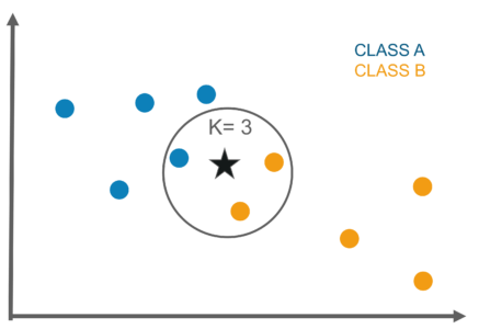 22 |
22 |
26 | 2. There is no need to build a model, tune parameters, or make additional assumptions.
27 | 3. New data can be added seamlessly which will not impact the accuracy of the algorithm.
28 | # Disadvantages 29 | 1. KNN algorithm does not work well with large datasets. In large datasets, the cost of calculating the distance between the new point and the existing points is huge which degrades the performance of the algorithm.
30 | 2. It is sensitive to noisy data, missing values and outliers.
31 | # References 32 | 1. https://www.youtube.com/watch?v=HVXime0nQeI
33 | 2. https://towardsdatascience.com/machine-learning-basics-with-the-k-nearest-neighbors-algorithm-6a6e71d01761
34 | -------------------------------------------------------------------------------- /K-Means/kmeans.py: -------------------------------------------------------------------------------- 1 | # -*- coding: utf-8 -*- 2 | import random 3 | from sklearn.cluster import KMeans 4 | import seaborn as sns 5 | import numpy as np 6 | import matplotlib.pyplot as plt 7 | from sklearn.datasets import make_blobs 8 | 9 | # Library Implementation of K Means 10 | 11 | 12 | X, y = make_blobs(centers=3, random_state=42) 13 | 14 | 15 | sns.scatterplot(X[:, 0], X[:, 1], hue=y) 16 | 17 | sns.scatterplot(X[:, 0], X[:, 1]) 18 | 19 | 20 | model = KMeans(n_clusters=4) 21 | 22 | model.fit(X) 23 | 24 | y_gen = model.labels_ 25 | 26 | sns.scatterplot(X[:, 0], X[:, 1], hue=y_gen) 27 | 28 | model.cluster_centers_ 29 | 30 | sns.scatterplot(X[:, 0], X[:, 1], hue=y_gen) 31 | 32 | for center in model.cluster_centers_: 33 | plt.scatter(center[0], center[1], s=60) 34 | 35 | sns.scatterplot(X[:, 0], X[:, 1]) 36 | 37 | 38 | # Custom Implementation of K Means 39 | 40 | class Cluster: 41 | 42 | def __init__(self, center): 43 | """Initialization of Clusters for K Means.""" 44 | self.center = center 45 | self.points = [] 46 | 47 | def distance(self, point): 48 | return np.sqrt(np.sum((point - self.center) ** 2)) 49 | 50 | 51 | class CustomKMeans: 52 | 53 | def __init__(self, n_clusters=3, max_iters=20): 54 | """Custom Implementation of K Means.""" 55 | self.n_clusters = n_clusters 56 | self.max_iters = max_iters 57 | 58 | def fit(self, X): 59 | 60 | clusters = [] 61 | for _ in range(self.n_clusters): 62 | cluster = Cluster(center=random.choice(X)) 63 | clusters.append(cluster) 64 | 65 | for _ in range(self.max_iters): 66 | 67 | labels = [] 68 | 69 | # going for each point 70 | for point in X: 71 | 72 | # collecting disctances form every cluster 73 | distances = [] 74 | for cluster in clusters: 75 | distances.append(cluster.distance(point)) 76 | 77 | # finding closest cluster 78 | closest_idx = np.argmin(distances) 79 | closest_cluster = clusters[closest_idx] 80 | closest_cluster.points.append(point) 81 | labels.append(closest_idx) 82 | 83 | for cluster in clusters: 84 | cluster.center = np.mean(cluster.points, axis=0) 85 | 86 | self.labels_ = labels 87 | self.cluster_centers_ = [cluster.center for cluster in clusters] 88 | 89 | 90 | model = CustomKMeans(n_clusters=2) 91 | 92 | model.fit(X) 93 | 94 | sns.scatterplot(X[:, 0], X[:, 1], hue=model.labels_) 95 | 96 | for center in model.cluster_centers_: 97 | plt.scatter(center[0], center[1], s=60) 98 | -------------------------------------------------------------------------------- /Neural Network/neural_network.py: -------------------------------------------------------------------------------- 1 | # -*- coding: utf-8 -*- 2 | """Neural Network.ipynb 3 | 4 | Automatically generated by Colaboratory. 5 | 6 | Original file is located at 7 | https://colab.research.google.com/drive/1HMxwkMbHBiP3DnVkR59bFIwQ7WLo8S51 8 | """ 9 | 10 | import pandas as pd 11 | import numpy as np 12 | class NeuralNetwork: 13 | 14 | def __init__(self,input_size,layers,output_size): 15 | np.random.seed(0) 16 | 17 | model = {} #Dictionary 18 | 19 | #First Layer 20 | model['W1'] = np.random.randn(input_size,layers[0]) 21 | model['b1'] = np.zeros((1,layers[0])) 22 | 23 | #Second Layer 24 | model['W2'] = np.random.randn(layers[0],layers[1]) 25 | model['b2'] = np.zeros((1,layers[1])) 26 | 27 | #Third/Output Layer 28 | model['W3'] = np.random.randn(layers[1],output_size) 29 | model['b3'] = np.zeros((1,output_size)) 30 | 31 | self.model = model 32 | self.activation_outputs = None 33 | 34 | def forward(self,x): 35 | 36 | W1,W2,W3 = self.model['W1'],self.model['W2'],self.model['W3'] 37 | b1, b2, b3 = self.model['b1'],self.model['b2'],self.model['b3'] 38 | 39 | z1 = np.dot(x,W1) + b1 40 | a1 = np.tanh(z1) 41 | 42 | z2 = np.dot(a1,W2) + b2 43 | a2 = np.tanh(z2) 44 | 45 | z3 = np.dot(a2,W3) + b3 46 | y_ = softmax(z3) 47 | 48 | self.activation_outputs = (a1,a2,y_) 49 | return y_ 50 | 51 | def backward(self,x,y,learning_rate=0.001): 52 | W1,W2,W3 = self.model['W1'],self.model['W2'],self.model['W3'] 53 | b1, b2, b3 = self.model['b1'],self.model['b2'],self.model['b3'] 54 | m = x.shape[0] 55 | 56 | a1,a2,y_ = self.activation_outputs 57 | 58 | delta3 = y_ - y 59 | dw3 = np.dot(a2.T,delta3) 60 | db3 = np.sum(delta3,axis=0) 61 | 62 | delta2 = (1-np.square(a2))*np.dot(delta3,W3.T) 63 | dw2 = np.dot(a1.T,delta2) 64 | db2 = np.sum(delta2,axis=0) 65 | 66 | delta1 = (1-np.square(a1))*np.dot(delta2,W2.T) 67 | dw1 = np.dot(X.T,delta1) 68 | db1 = np.sum(delta1,axis=0) 69 | 70 | 71 | #Update the Model Parameters using Gradient Descent 72 | self.model["W1"] -= learning_rate*dw1 73 | self.model['b1'] -= learning_rate*db1 74 | 75 | self.model["W2"] -= learning_rate*dw2 76 | self.model['b2'] -= learning_rate*db2 77 | 78 | self.model["W3"] -= learning_rate*dw3 79 | self.model['b3'] -= learning_rate*db3 80 | -------------------------------------------------------------------------------- /Linear Regression/Linear_Regression.py: -------------------------------------------------------------------------------- 1 | import pandas as pd 2 | import numpy as np 3 | import matplotlib.pyplot as plt 4 | 5 | 6 | class LinearRegression: 7 | 8 | def __init__(self): 9 | """ 10 | Linear regression 11 | Arguments - alpha (by default .001) 12 | epochs(by default 100) 13 | plot : bool - plot the cost vs epoch graph 14 | function - fit : (x, y) - train the data 15 | predict : (x) - predict the new y using previus trained model 16 | this module also normalize data brfore training that increase training efficiency 17 | """ 18 | self.costs = [] 19 | self.b = 0 20 | self.w = [] 21 | 22 | @classmethod 23 | def forward(x, w, b): 24 | y_pred = np.dot(x, w) + b 25 | return y_pred 26 | 27 | @classmethod 28 | def compute_cost(y_pred, y, n): 29 | cost = (1/(2*n)) * np.sum(np.square(y_pred - y)) 30 | return cost 31 | 32 | @classmethod 33 | def backward(y_pred, y, x, n): 34 | # print(y_pred.shape, y.shape, x.shape) 35 | dw = (1/n) * np.dot(x.T, (y_pred-y)) 36 | # print(dw.shape) 37 | db = (1/n) * np.sum((y_pred-y)) 38 | return dw, db 39 | 40 | @classmethod 41 | def update(w, b, dw, db, lr): 42 | w -= lr*dw 43 | b -= lr*db 44 | return w, b 45 | 46 | @classmethod 47 | def normalize(df): 48 | result = df.copy() 49 | for feature_name in df.columns: 50 | mean = np.mean(df[feature_name]) 51 | std = np.std(df[feature_name]) 52 | result[feature_name] = (df[feature_name] - mean) / std 53 | return result 54 | 55 | @classmethod 56 | def initialize(m): 57 | w = np.random.normal(size=(m, 1)) 58 | b = 0 59 | return (w, b) 60 | 61 | def fit(self, X, y, lr=.005, epochs=550): 62 | X = pd.DataFrame(X) 63 | X = self.normalize(X) 64 | y = np.reshape(np.array(y), (len(y), 1)) 65 | n, m = X.shape 66 | w, b = self.initialize(m) 67 | w = w 68 | b = b 69 | self.w, self.b = self.initialize(m) 70 | for _ in range(epochs): 71 | y_pred = self.forward(X, self.w, self.b) 72 | cost = self.compute_cost(y_pred, y, n) 73 | dw, db = self.backward(y_pred, y, X, n) 74 | self.w, self.b = self.update(self.w, self.b, dw, db, lr) 75 | self.costs.append(cost) 76 | plt.plot(self.costs) 77 | 78 | def predict(self, X): 79 | X = pd.DataFrame(X) 80 | X = self.normalize(X) 81 | y_pred = self.forward(X, self.w, self.b) 82 | return y_pred 83 | -------------------------------------------------------------------------------- /Preprocessing/standard_scaler.py: -------------------------------------------------------------------------------- 1 | import numpy as np 2 | np.seterr(divide='ignore', invalid='ignore') 3 | 4 | class StandardScaler: 5 | 6 | def __init__(self, *args): 7 | ''' 8 | >>> scaler = StandardScaler() 9 | >>> data = [[0, 0], [0, 0], [1, 1], [1, 1]] 10 | >>> print(scaler.fit(data)) 11 | StandardScaler() 12 | >>> print(scaler.mean_) 13 | [0.5 0.5] 14 | >>> print(scaler.transform(data)) 15 | [[-1. -1.] 16 | [-1. -1.] 17 | [ 1. 1.] 18 | [ 1. 1.]] 19 | >>> print(scaler.transform([[2, 2]])) 20 | [[3. 3.]] 21 | ''' 22 | self._sample_size = None 23 | self._means = None 24 | self._stds = None 25 | 26 | def fit(self, x, *args): 27 | try: 28 | x = np.array(x, dtype=np.float64) 29 | self._sample_size = x.shape[1] 30 | self._means = np.mean(x, axis=0) 31 | self._stds = np.std(x, axis=0) 32 | return self 33 | except Exception as e: 34 | raise e 35 | 36 | def transform(self, x, *args): 37 | try: 38 | x = np.array(x, dtype=np.float64) 39 | if self._means is None and self._stds is None: 40 | return f'NotFittedError: This StandardScaler instance is not fitted yet. Call \'fit\' with appropriate arguments before using this estimator.' 41 | elif x.shape[1] != self._sample_size: 42 | return f'ValueError: X has {x.shape[1]} features, but StandardScaler is expecting {self._sample_size} features as input' 43 | else: 44 | x = (x - self._means) / self._stds 45 | x = self.__remove_outlier_by_zero(x) 46 | return x 47 | except Exception as e: 48 | raise e 49 | 50 | def fit_transform(self, x, *args): 51 | try: 52 | self.fit(x) 53 | return self.transform(x) 54 | except Exception as e: 55 | raise e 56 | 57 | def inverse_transform(self, x, *args): 58 | try: 59 | x = np.array(x, dtype=np.float64) 60 | if self._means is None and self._stds is None: 61 | return f'NotFittedError: This StandardScaler instance is not fitted yet. Call \'fit\' with appropriate arguments before using this estimator.' 62 | else: 63 | x = (x * self._stds) + self._means 64 | x = self.__remove_outlier_by_zero(x) 65 | return x 66 | except Exception as e: 67 | raise e 68 | 69 | def __remove_outlier_by_zero(self, x): 70 | return np.nan_to_num(x, nan=0.0, posinf=0.0, neginf=0.0) 71 | 72 | @property 73 | def mean_(self): 74 | return self._means 75 | 76 | @property 77 | def scale_(self): 78 | return self._stds 79 | 80 | 81 | 82 | 83 | 84 | 85 | 86 | 87 | -------------------------------------------------------------------------------- /Ridge Regression/README.md: -------------------------------------------------------------------------------- 1 | # Ridge Regression 2 | 3 | ## Introduction 4 | - Ridge regression also known as L2 regularization is a special case of Tikhonov regularization in which all parameters are regularized equally. 5 | - It was first introduced by Hoerl and Kennard in 1970. 6 | - It is a technique which is used for analyzing multiple regression data that suffer from multicollinearity. 7 | 8 | 9 | ## Working of Ridge Regression 10 | - The objective of ridge regresion is to minimize the loss function plus the sum of square of the magnitude of coefficients. 11 | - The Ridge regression puts a constraint on the sum of suqare of values of the model parameters,the sum has to be less than a fixed value (upper bound). 12 | - In order to do so, it applies a shrinking (regularization) process where it penalizes the coefficients of the regression variables. 13 | - The goal of this process is to minimize the prediction error. 14 | 15 | 16 | ## Ridge Regression Cost Function 17 |
18 |  19 |
19 |
23 |  24 |
24 |
10 |  11 |
11 |
33 | 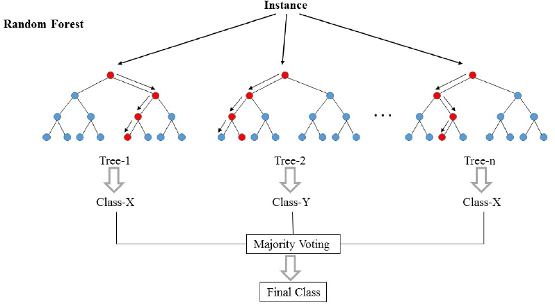 34 |
34 |
19 |  20 |
20 |
24 |  25 |
25 |
array, true values
22 | y_hat --> array, predicted values
23 | Returns:
24 | float, error
25 | '''
26 | error = 0
27 | for i in range(len(y)):
28 | error += (y[i] - y_hat[i]) ** 2
29 | return error / len(y)
30 |
31 | # method for calculating the coefficient of the linear regression model
32 | def fit(self, X, y):
33 | '''
34 | Input parameters:
35 | X --> array, features
36 | y --> array, true values
37 | Returns:
38 | None
39 | '''
40 | # 1. initializing weights and bias to zeros
41 | self.weights = np.zeros(X.shape[1])
42 | self.bias = 0
43 |
44 | # 2. performing gradient descent
45 | for i in range(self.n_iterations):
46 | # line equation
47 | y_hat = np.dot(X, self.weights) + self.bias
48 | loss = self._mean_squared_error(y, y_hat)
49 | self.loss.append(loss)
50 |
51 | # calculating derivatives
52 | partial_w = (1 / X.shape[0]) * (2 * np.dot(X.T, (y_hat - y)))
53 | partial_d = (1 / X.shape[0]) * (2 * np.sum(y_hat - y))
54 |
55 | # updating the coefficients
56 | self.weights -= self.learning_rate * partial_w
57 | self.bias -= self.learning_rate * partial_d
58 |
59 | # method for making predictions using the line equation
60 | def predict(self, X):
61 | '''
62 | Input parameters:
63 | X --> array, features
64 | Returns:
65 | array, predictions
66 | '''
67 | return np.dot(X, self.weights) + self.bias()
68 |
69 | '''
70 |
71 | EXAMPLE:
72 |
73 | # Importing Libraries
74 |
75 | import pandas as pd
76 | from sklearn import preprocessing
77 | from statsmodels.stats.outliers_influence import variance_inflation_factor
78 | from sklearn.model_selection import train_test_split
79 |
80 |
81 | # Getting our Data
82 |
83 | df = pd.read_csv('startups.csv')
84 |
85 |
86 | # Data Preprocessing
87 |
88 | # no null values are present
89 | # but, we need to encode 'State' attribute
90 | label_encoder = preprocessing.LabelEncoder() # encoding data
91 | df['State'] = df['State'].astype('|S')
92 | df['State'] = label_encoder.fit_transform(df['State'])
93 | # checking for null values
94 | df.isnull().any()
95 | # checking vif
96 | variables = df[['R&D Spend', 'Administration', 'Marketing Spend', 'State']]
97 | vif = pd.DataFrame()
98 | vif['VIF'] = [variance_inflation_factor(variables.values, i) for i in range(variables.shape[1])]
99 | vif['Features'] = variables.columns
100 | # as vif for all attributes<10, we need not drop any of them
101 |
102 |
103 | # Splitting Data for Training and Testing
104 |
105 | data = df.values
106 | X,y = data[:,:-1], data[:,-1]
107 | X_train, X_test, y_train, y_test = train_test_split(X, y, test_size = 0.2, random_state = 0) # splitting in the ration 80:20
108 |
109 |
110 | # Fitting the Data
111 |
112 | model = LinearRegression(learning_rate=0.01, n_iterations=10000)
113 | model.fit(X_train,y_train)
114 |
115 |
116 | # Making Predictions
117 |
118 | y_pred = model.predict(X_test)
119 |
120 | '''
--------------------------------------------------------------------------------
/Preprocessing/min_max_scaler.py:
--------------------------------------------------------------------------------
1 | import numpy as np
2 | np.seterr(divide='ignore', invalid='ignore')
3 |
4 | class MinMaxScaler:
5 |
6 | def __init__(self, feature_range=(0,1), *args):
7 | '''
8 | >>> data = [[-1, 2], [-0.5, 6], [0, 10], [1, 18]]
9 | >>> scaler = MinMaxScaler()
10 | >>> print(scaler.fit(data))
11 | MinMaxScaler()
12 | >>> print(scaler.data_max_)
13 | [ 1. 18.]
14 | >>> print(scaler.transform(data))
15 | [[0. 0. ]
16 | [0.25 0.25]
17 | [0.5 0.5 ]
18 | [1. 1. ]]
19 | >>> print(scaler.transform([[2, 2]]))
20 | [[1.5 0. ]]
21 | '''
22 | try:
23 | if (feature_range[0] >= feature_range[1]):
24 | raise ValueError(f'Minimum of desired feature range must be smaller than maximum.')
25 | else:
26 | self._scale_min = feature_range[0]
27 | self._scale_max = feature_range[1]
28 | self._sample_size = None
29 | self._mins = None
30 | self._maxs = None
31 | except Exception as e:
32 | raise e
33 |
34 | def fit(self, x, *args):
35 | try:
36 | x = np.array(x, dtype=np.float64)
37 | self._sample_size = x.shape[1]
38 | self._mins = x.min(axis=0)
39 | self._maxs = x.max(axis=0)
40 | return self
41 | except Exception as e:
42 | raise e
43 |
44 | def transform(self, x, *args):
45 | try:
46 | x = np.array(x, dtype=np.float64)
47 | if self._maxs is None and self._mins is None:
48 | return f'NotFittedError: This MinMaxScaler instance is not fitted yet. Call \'fit\' with appropriate arguments before using this estimator.'
49 | elif x.shape[1] != self._sample_size:
50 | return f'ValueError: X has {x.shape[1]} features, but MinMaxScaler is expecting {self._sample_size} features as input'
51 | else:
52 | x = (x - self._mins) / (self._maxs - self._mins)
53 | x = (x * (self._scale_max - self._scale_min)) + self._scale_min
54 | x = self.__remove_outlier_by_zero(x)
55 | return x
56 | except Exception as e:
57 | raise e
58 |
59 | def fit_transform(self, x, *args):
60 | try:
61 | self.fit(x)
62 | return self.transform(x)
63 | except Exception as e:
64 | raise e
65 |
66 | def inverse_transform(self, x, *args):
67 | try:
68 | x = np.array(x, dtype=np.float64)
69 | if self._maxs is None and self._mins is None:
70 | return f'NotFittedError: This MinMaxScaler instance is not fitted yet. Call \'fit\' with appropriate arguments before using this estimator.'
71 | else:
72 | x = (x - self._scale_min) / (self._scale_max - self._scale_min)
73 | x = (x * (self._maxs - self._mins)) + self._mins
74 | return x
75 | except Exception as e:
76 | raise e
77 |
78 | def __remove_outlier_by_zero(self, x):
79 | return np.nan_to_num(x, nan=0.0, posinf=0.0, neginf=0.0)
80 |
81 | def __remove_outlier_by_one(self, x):
82 | return np.nan_to_num(x, nan=1.0, posinf=1.0, neginf=1.0)
83 |
84 | @property
85 | def min_(self):
86 | _min = self._scale_min - (self._mins * self.scale_)
87 | return _min
88 |
89 | @property
90 | def scale_(self):
91 | _scale = (self._scale_max - self._scale_min) / (self._maxs - self._mins)
92 | _scale = self.__remove_outlier_by_one(_scale)
93 | return _scale
94 |
95 | @property
96 | def data_min_(self):
97 | return self._mins
98 |
99 | @property
100 | def data_max_(self):
101 | return self._maxs
102 |
103 | @property
104 | def data_range_(self):
105 | data_range = self._maxs - self._mins
106 | return data_range
107 |
108 |
109 |
110 |
--------------------------------------------------------------------------------
/Elastic Net/Elastic_Net_Regression.py:
--------------------------------------------------------------------------------
1 | # # ELASTIC NET REGRESSION
2 | # # ''''''''''''''''''''''''''''''''''''''''''''''''''''''''
3 |
4 | # ## Definition
5 | # In statistics and in the fitting of linear or logistic regression models, the elastic net is a regularized regression method that linearly combines the L1 and L2 penalties of the lasso and ridge methods.The elastic net method performs variable selection and regularization simultaneously.
6 | #
7 | # ## Dataset Used
8 | # ### Dataset download link
9 | # https://www.kaggle.com/karthickveerakumar/salary-data-simple-linear-regression
10 | # ### Description
11 | # This dataset consists of company data with 30 employees(30 rows), and 2 columns. The 2 columns are of years of experience and the salary. Thus we aim at finding how years of experience affect salary of employees using elastic-net.
12 | #
13 | # ## Code
14 | # Importing required libraries
15 |
16 | import numpy as np
17 | import matplotlib.pyplot as plt
18 | import pandas as pd
19 | from sklearn.model_selection import train_test_split
20 |
21 | class Elastic_Net_Regression() :
22 | def __init__(self,learning_rate,iterations,l1_penality,l2_penality) :
23 | self.learning_rate=learning_rate
24 | self.iterations=iterations
25 | self.l1_penality=l1_penality
26 | self.l2_penality=l2_penality
27 |
28 | def fit(self,x,y):
29 | self.b=0
30 | self.x=x
31 | self.y=y
32 | self.m=x.shape[0]
33 | self.n=x.shape[1]
34 | self.W=np.zeros(self.n)
35 | self.weight_updation()
36 | return self
37 |
38 | def weight_updation(self):
39 | for i in range(self.iterations):
40 | self.update_weights()
41 |
42 | def update_weights(self):
43 | y_pred=self.predict(self.x)
44 | dW=np.zeros(self.n)
45 | for j in range(self.n):
46 | if self.W[j]<=0:
47 | dW[j] = -(2*(self.x[:,j]).dot(self.y-y_pred))-self.l1_penality+2*self.l2_penality*self.W[j]
48 | dW[j]//=self.m
49 | else :
50 | dW[j]=-(2*(self.x[:,j]).dot(self.y-y_pred))+self.l1_penality+2*self.l2_penality*self.W[j]
51 | dW[j]//=self.m
52 | db=-2*np.sum(self.y-y_pred)
53 | db//=self.m
54 | self.W-=self.learning_rate*dW
55 | self.b-=self.learning_rate*db
56 | return self
57 |
58 | def predict(self,x):
59 | ans=x.dot(self.W)+self.b
60 | return ans
61 |
62 | #UNCOMMENT THE BELOW LINES TO TEST THE ALGORITHM
63 | # def main() :
64 | # df=pd.read_csv("salary_data.csv")
65 | # x=df.iloc[:,:-1].values
66 | # y=df.iloc[:,1].values
67 | # x_train,x_test,y_train,y_test=train_test_split(x,y,test_size=1/3.5,random_state=0)
68 | # model = Elastic_Net_Regression(iterations=3000,
69 | # learning_rate=0.01,
70 | # l1_penality=500,
71 | # l2_penality=1)
72 | # model.fit(x_train,y_train)
73 | # y_pred=model.predict(x_test)
74 | # print("Predicted values of y:",np.round( y_pred[:3], 2))
75 | # print("Test values of y:",y_test[:3])
76 | # print("Trained Weight W:",round(model.W[0],2))
77 | # print("Trained bias b:",round(model.b,2))
78 | # plt.subplot(211)
79 | # plt.title('Salary vs Years of Experience')
80 | # plt.scatter(x_test,y_test,color='blue',label="Test Y")
81 | # plt.scatter(x_test,y_pred,color='red',label="Predicted Y")
82 | # plt.legend(loc=2)
83 | # plt.subplot(212)
84 | # plt.scatter(x_test,y_test,color='green',label="Test Y")
85 | # plt.plot(x_test,y_pred,color='yellow',label="Predicted Y")
86 | # plt.xlabel('Years of Experience')
87 | # plt.ylabel('Salary')
88 | # plt.legend(loc=2)
89 | # plt.show()
90 |
91 |
92 | # if __name__ == "__main__" :
93 | # main()
94 |
95 |
96 | # ### References taken from
97 | # https://corporatefinanceinstitute.com/resources/knowledge/other/elastic-net/
98 | # \
99 | # https://www.geeksforgeeks.org/implementation-of-elastic-net-regression-from-scratch/
100 |
--------------------------------------------------------------------------------
/Linear Regression/README.md:
--------------------------------------------------------------------------------
1 |
2 | Using the script
3 |
4 | ## import the module
5 |
6 | >import linearRegression
7 | >
8 | >linearReg_model = LinearRegression()
9 |
10 | ## train the data
11 |
12 | >linearReg_model.fit(x_train, y_train)
13 |
14 | ## predict the model
15 |
16 | >y_pred = linearReg_model.predict(x_test)
17 | ## Regression:
18 |
19 | Firstly let’s see what's regression. Regression is a technique for predicting a goal value using independent predictors. This method is primarily used for forecasting and determining cause and effect relationships among variables. The number of independent variables and the form of relationship between the independent and dependent variables is the key points that cause the differences in regression techniques.
20 |
21 | ## Linear regression
22 |
23 | One of the most fundamental and commonly used Machine Learning algorithms is linear regression. It's a statistical methodology for conducting the predictive analysis. The linear regression algorithm shows a linear relationship between a dependent (y) variable and one or more independent (y) variables, hence the name. Since linear regression reveals a linear relationship, it determines how the value of the dependent variable changes as the value of the independent variable changes.
24 |
25 | 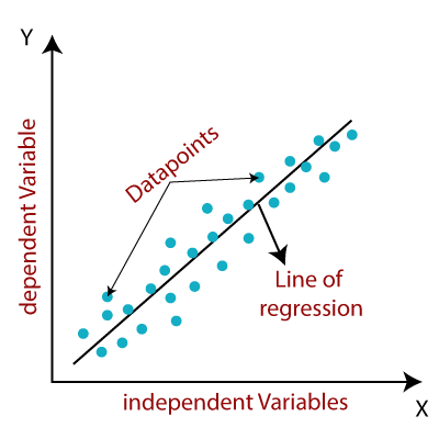
26 |
27 | Linear regression is mathematically represented as:-
28 |
29 | y=a0 +a1.x
30 |
31 | Here,
32 | y= Dependent variable
33 | a0= Intercept of line
34 | a1= Linear regression coefficient
35 | x= Independent variable
36 |
37 | There are two types of linear regression:-
38 |
39 | Simple linear regression- It is a is Linear Regression algorithm that uses a single independent variable to predict the value of a numerical dependent variable.
40 |
41 | Multiple linear regression- It is a Linear Regression algorithm that uses more than one independent variable to estimate the value of a numerical dependent variable.
42 |
43 | ## Cost function(J):
44 |
45 | When using linear regression, our main aim is to find the best fit line, which means that the difference between expected and actual values should be as small as possible. The line with the best fit would have the least amount of error. The cost function assists us in deciding the best possible values for a0 and a1 in order to achieve the best possible fit line for the data points. Since we want the best values for a0 and a1, we transform this into a minimization problem in which we want to minimize the difference between the expected and actual values.
46 | The cost function can be used to determine the accuracy of a mapping function that maps an input variable to an output variable. The hypothesis function is another name for the mapping function. The error discrepancy is determined by the difference between expected and ground truth values. We square the error difference, add all of the data points together, and divide the total number of data points by two. This gives you the average squared error for all of your data points. As a consequence, the Mean Squared Error(MSE) function is another name for this cost function.
47 |
48 | 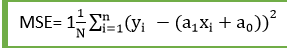
49 |
50 |
51 | Here,
52 | N= total no. of observation
53 | yi= actual value
54 | a1xi+a0=predicted value
55 |
56 | ## Gradient Descent:
57 |
58 | Gradient descent is a method of reducing the cost function by modifying a0 and a1 (MSE). The idea is that we start with some a0 and a1 values and then reduce the cost by adjusting them iteratively. Gradient descent assists us in changing the values. The gradient always points in the direction of the steepest loss function rise. In order to minimize loss as quickly as possible, the gradient descent algorithm takes a step in the direction of the negative gradient. The learning rate in the gradient descent algorithm is the number of steps you take. This dictates how easily the algorithm reaches the minima.
59 | A smaller learning rate will get you closer to the minima, but it will take longer to achieve it; a larger learning rate converges faster, but there is a risk of overshooting the minima.
60 |
61 | 
62 |
63 | The partial derivates are the gradient descent and are used to update the value of a0 and a1
64 |
65 | For more clear perspective you can also go through the following video:
66 | https://www.youtube.com/watch?v=E5RjzSK0fvY
67 |
--------------------------------------------------------------------------------
/Neural Network/README.md:
--------------------------------------------------------------------------------
1 | ## Introduction:
2 |
3 | Neural Network (Artificial) ANN is a high-performance computing device whose core theme is inspired by biological neural networks. The human brain comprises billions of neurons, each of which is linked to several other neurons to form a network, allowing it to recognize and process images. Each biological neuron can process a variety of inputs and generate output. Neurons in the human brain are capable of making extremely complex decisions, which means they can perform several tasks parallel. All of these concepts led to the development of a computer model of the brain using an artificial neural network.
4 | The primary goal of an artificial neural network is to create a system that can perform a variety of computational tasks faster than conventional systems. Pattern recognition and classification, approximation, optimization, and data clustering are some of these functions. ANN collects a large number of units that are linked in some way to enable contact between them. These modules, also known as nodes or neurons, are basic processors that work in a parallel fashion.
5 |
6 | ## Elements of a Neural Network:
7 |
8 | Input Layer - Input features are provided to this layer. It includes information from the outside world to the network; no computation is done at this layer. Nodes here only pass on the data (features) to the hidden layer.
9 |
10 | Hidden Layer - This layer's nodes aren't visible to the outside world; they're part of the abstraction that every neural network provides. The hidden layer computes all of the features entered via the input layer and sends the results to the output layer.
11 |
12 | Output Layer - This layer communicates the network's acquired knowledge to the outside world.
13 |
14 |
15 | ## Artificial Neuron
16 |
17 | 
18 |
19 |
20 | Artificial neurons are the basic unit of a neural network. The artificial neuron takes one or more inputs and adds them together to create an output. Perceptrons are another name for artificial neurons. An artificial neuron is:
21 |
22 | Y= Σ (weights * input) + bias
23 |
24 | wights= It controls the signal between two neurons (or the intensity of the connection) To put it another way, a weight determines how much of an impact the input has on the output.
25 |
26 | Bias= Constant biases are an extra input into the next layer that often has the value of one. The bias unit ensures that even though all of the inputs are zeros, the neuron will still be activated.
27 |
28 | ## Activation Function:
29 |
30 | The activation function calculates a weighted number and then adds bias to it to determine if a neuron should be activated or not. For non-linear complex functional mappings between the inputs and the required variable, activation functions are used. The activation function's goal is to introduce non-linearity into a neuron's output.
31 |
32 | Some commonly used activation functions are:
33 |
34 | ## Sigmoid Function -
35 |
36 | f(x) = 1 / 1 + exp(-x)
37 |
38 | 
39 |
40 | As per looking at the graph its range can be defined from 0 to 1.
41 |
42 | Disadvantages:
43 |
44 | Slow convergence
45 | Vanishing gradient problem
46 | The Sigmoid's output is not zero-centered, causing its gradient to shift in different directions.
47 |
48 | ## tanh Function:
49 |
50 | The hyperbolic tangent function is represented as
51 |
52 | f(x) = 1 — exp(-2x) / 1 + exp(-2x)
53 |
54 | 
55 |
56 |
57 | As per looking at the graph its range can be defined from -1 to 1.
58 |
59 | Unlike the sigmoid function, the output of tanh function is zero-centered. But the vanishing gradient problem still prevails.
60 |
61 | ## ReLu Function:
62 |
63 | Rectified linear units function is the most commonly used function as it solves the problem that the above two functions could not solve. If the function receives any negative input, it returns 0; however, if the function receives any positive value x, it returns that value. It can be represented as
64 |
65 | f(x)= max(0,x)
66 |
67 | 
68 |
69 | As per looking at the graph its range can be defined from 0 to infinite.
70 |
71 |
72 |
73 | For more you can also go through this video
74 | https://www.youtube.com/watch?v=aircAruvnKk
75 |
76 |
--------------------------------------------------------------------------------
/Naive Bayes/naive_bayes.py:
--------------------------------------------------------------------------------
1 | # Naive Bayes Algorithm
2 |
3 | import numpy as np
4 |
5 |
6 | class NaiveBayesClassifier:
7 |
8 |
9 | def __init__(self):
10 | pass
11 |
12 |
13 | # divides the dataset into a subset of data belonging to each class
14 | def divide_classes(self, X, Y):
15 | """
16 | X: list of features
17 | Y: list consisting of target
18 | The function returns: A dictionary with Y as keys and assigned X as values.
19 | """
20 | divided_classes = {}
21 |
22 | for i in range(len(X)):
23 | values = X[i]
24 | target_class_name = Y[i]
25 | if target_class_name not in divided_classes:
26 | divided_classes[target_class_name] = []
27 | divided_classes[target_class_name].append(values)
28 |
29 | return divided_classes
30 |
31 |
32 | # standard deviation and mean are required for the (Gaussian) distribution function
33 | def info(self, X):
34 | """
35 | X: list of features
36 | The function returns: A dictionary with standard deviation and mean as keys and assigned features as values.
37 | """
38 | for i in zip(*X):
39 | yield {
40 | 'std' : np.std(i),
41 | 'mean' : np.mean(i)
42 | }
43 |
44 |
45 | # fitting data that would be required to train the model
46 | def fit_data (self, X, Y):
47 | """
48 | X: training features
49 | y: target variable
50 | The function returns: A dictionary with the probability, mean, and standard deviation of each class.
51 | """
52 |
53 | divided_classes = self.divide_classes(X, Y)
54 | self.summary = {}
55 |
56 | for target_class_name, values in divided_classes.items():
57 | self.summary[target_class_name] = {
58 | 'given_prob': len(values)/len(X),
59 | 'summary': [i for i in self.info(values)]
60 | }
61 | return self.class_summary
62 |
63 |
64 | # Gaussian distribution function
65 | def Gaussian_distribution(self, X, mean, std):
66 | """
67 | X: value of feature
68 | mean: the average value of feature
69 | stdev: the standard deviation of feature
70 | The function returns: A value of normal probability.
71 | """
72 |
73 | exponent = np.exp(-((X-mean)**2 / (2*std**2)))
74 |
75 | return exponent / (np.sqrt(2*np.pi)*std)
76 |
77 |
78 | # finally predicting the class
79 | def predict(self, X):
80 | """
81 | X: test dataset
82 | The function returns: List of predicted class for each row of dataset.
83 | """
84 |
85 | # Maximum a posteriori (MAP): In Bayesian statistics, a maximum a posteriori
86 | # probability (MAP) estimate is an estimate of an unknown quantity, that equals
87 | # the mode of the posterior distribution.
88 |
89 | MAPs = []
90 |
91 | for i in X:
92 | joint_prob = {}
93 |
94 | for target_class_name, values in self.summary.items():
95 | total_values = len(values['summary'])
96 | likelihood = 1
97 |
98 | for idx in range(total_values):
99 | value = i[idx]
100 | mean = value['summary'][idx]['mean']
101 | stdev = value['summary'][idx]['std']
102 | normal_prob = self.Gaussian_distribution(value, mean, stdev)
103 | likelihood *= normal_prob
104 | prior_prob = values['prior_proba']
105 | joint_prob[target_class_name] = prior_prob * likelihood
106 |
107 | MAP = max(joint_prob, key= joint_prob.get)
108 | MAPs.append(MAP)
109 |
110 | return MAPs
111 |
112 |
113 | # calculating accuracy
114 | def model_accuracy(self, y_test, y_pred):
115 | """
116 | y_test: actual values
117 | y_pred: predicted values
118 | The function returns: A number between 0-1, representing the percentage of correct predictions.
119 | """
120 |
121 | correct_true = 0
122 |
123 | for y_t, y_p in zip(y_test, y_pred):
124 | if y_t == y_p:
125 | correct_true += 1
126 |
127 | return correct_true / len(y_test)
128 |
--------------------------------------------------------------------------------
/Markov's Chain/Readme.md:
--------------------------------------------------------------------------------
1 |
2 | # Markov's Chain
3 | ## What is Markov's Chain
4 | _**A stochastic process containing random variables, transitioning from one state to another depending on certain assumptions and definite probabilistic rules.**_
5 |
6 | These random variables transition from one to state to the other, based on an important mathematical property called **Markov Property.**
7 | ### Markov's Property :
8 | _Discrete Time Markov Property states that the calculated probability of a random process transitioning to the next possible state is only dependent on the current state and time and it is independent of the series of states that preceded it._
9 |
10 | The fact that the next possible action/ state of a random process does not depend on the sequence of prior states, renders Markov chains as a memory-less process that solely depends on the current state/action of a variable.
11 |
12 | Let’s derive this mathematically:
13 |
14 | Let the random process be, {Xm, m=0,1,2,⋯}.
15 |
16 | This process is a Markov chain only if,
17 | 
18 |
19 | for all m, j, i, i0, i1, ⋯ im−1
20 |
21 | For a finite number of states, S={0, 1, 2, ⋯, r}, this is called a finite Markov chain.
22 |
23 | P(Xm+1 = j|Xm = i) here represents the transition probabilities to transition from one state to the other. Here, we’re assuming that the transition probabilities are independent of time.
24 |
25 | Which means that P(Xm+1 = j|Xm = i) does not depend on the value of ‘m’. Therefore, we can summarise,v
26 |
27 | 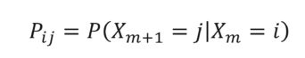
28 | Chain Formula – Introduction To Markov Chains
29 |
30 | So this equation represents the Markov chain.
31 |
32 | ## **What Is A State Transition Diagram?**
33 |
34 | A Markov model is represented by a State Transition Diagram. The diagram shows the transitions among the different states in a Markov Chain. Let’s understand the transition matrix and the state transition matrix with an example.
35 |
36 | ### **Transition Matrix Example**
37 |
38 | Consider a Markov chain with three states 1, 2, and 3 and the following probabilities:
39 |
40 | 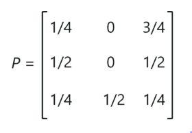
41 |
42 | _Transition Matrix Example – Introduction To Markov Chains
43 |
44 | 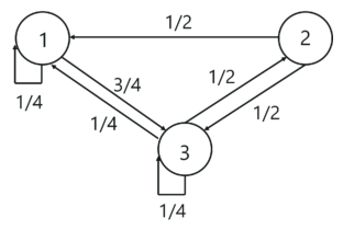
45 |
46 | _State Transition Diagram Example – Introduction To Markov Chains
47 |
48 | The above diagram represents the state transition diagram for the Markov chain. Here, 1,2 and 3 are the three possible states, and the arrows pointing from one state to the other states represents the transition probabilities pij. When, pij=0, it means that there is no transition between state ‘i’ and state ‘j’.
49 |
50 | ## Steps :
51 | - **Step 1: Import the required packages**
52 | - **Step 2: Read the data set**
53 | - **Step 3: Split the data set into individual words**
54 | - **Step 4: Creating pairs to keys and the follow-up words**
55 | - **Step 5: Appending the dictionary**
56 | - **Step 6: Build the Markov model**
57 |
58 | **Markov Chain Applications**
59 |
60 | Here’s a list of real-world applications of Markov chains:
61 |
62 | 1. **Google PageRank:** The entire web can be thought of as a Markov model, where every web page can be a state and the links or references between these pages can be thought of as, transitions with probabilities. So basically, irrespective of which web page you start surfing on, the chance of getting to a certain web page, say, X is a fixed probability.
63 |
64 | 2. **Typing Word Prediction:** Markov chains are known to be used for predicting upcoming words. They can also be used in auto-completion and suggestions.
65 |
66 | 3. **Subreddit Simulation:** Surely you’ve come across Reddit and had an interaction on one of their threads or subreddits. Reddit uses a subreddit simulator that consumes a huge amount of data containing all the comments and discussions held across their groups. By making use of Markov chains, the simulator produces word-to-word probabilities, to create comments and topics.
67 |
68 | 4. **Text generator:** Markov chains are most commonly used to generate dummy texts or produce large essays and compile speeches. It is also used in the name generators that you see on the web.
69 |
70 | ### Resources :
71 |
72 | https://www.edureka.co/community/54020/markov-chain-using-processing-python
73 | https://www.youtube.com/watch?v=Gs2xtNzogSY&t=397s
74 | https://medium.com/sigmoid/rl-markov-chains-dbf2f37e8b69
75 |
--------------------------------------------------------------------------------
/Gaussian Mixture Model/GaussianMixtureModel.py:
--------------------------------------------------------------------------------
1 | import numpy as np
2 | from sklearn.cluster import KMeans
3 |
4 |
5 | class GaussianDistribution:
6 |
7 | def __init__(self, n_clusters, n_epochs):
8 | self.n_clusters = n_clusters
9 | self.n_epochs = n_epochs
10 |
11 | def gaussian(self, X, mu, cov):
12 | ''' here we implement the Gaussian Density function '''
13 | n = X.shape[1]
14 | diff = (X - mu).T
15 | return np.diagonal(1 / ((2 * np.pi) ** (n / 2) * np.linalg.det(cov) ** 0.5) * np.exp(-0.5 * np.dot(np.dot(diff.T, np.linalg.inv(cov)), diff))).reshape(-1, 1)
16 |
17 |
18 | #Step 1: (Intialization)
19 | def initialize_clusters(self, X):
20 |
21 | ''' This is the initialization step of the GMM. At this point, we must initialise our parameters μk, πk and Σk. Here we'll be using results of KMeans as an initial value for μk , πk to one over the number of clusters and Σk to identity matrix.
22 | NOTE: We could also use random numbers for everything, but using a sensible initialisation procedure will help the algorithm achieve better results.
23 | '''
24 |
25 | clusters = []
26 | idx = np.arange(X.shape[0])
27 |
28 | # We use the KMeans centroids to initialise the GMM
29 |
30 | kmeans = KMeans(self.n_clusters).fit(X)
31 | mu_k = kmeans.cluster_centers_
32 |
33 | for i in range(self.n_clusters):
34 | clusters.append({
35 | 'pi_k': 1.0 / self.n_clusters,
36 | 'mu_k': mu_k[i],
37 | 'cov_k': np.identity(X.shape[1], dtype=np.float64)
38 | })
39 |
40 | return clusters
41 |
42 | #Step 2 (Expectation step)
43 | def expectation_step(self, X, clusters):
44 |
45 | ''' Here we calculate the value of ⲅ.
46 | For simplicity, we just calculate the denominator as a sum over all terms in the numerator, and then assign it to a variable named totals
47 | '''
48 |
49 | totals = np.zeros((X.shape[0], 1), dtype=np.float64)
50 |
51 | for cluster in clusters:
52 | pi_k = cluster['pi_k']
53 | mu_k = cluster['mu_k']
54 | cov_k = cluster['cov_k']
55 |
56 | gamma_nk = (pi_k * self.gaussian(X, mu_k, cov_k)).astype(np.float64)
57 |
58 | for i in range(X.shape[0]):
59 | totals[i] += gamma_nk[i]
60 |
61 | cluster['gamma_nk'] = gamma_nk
62 | cluster['totals'] = totals
63 |
64 |
65 | for cluster in clusters:
66 | cluster['gamma_nk'] /= cluster['totals']
67 |
68 |
69 | #Step 3 (Maximization step)
70 | def maximization_step(self, X, clusters):
71 |
72 | ''' Here the value of parameters μk, πk and Σk are updated '''
73 |
74 | N = float(X.shape[0])
75 |
76 | for cluster in clusters:
77 | gamma_nk = cluster['gamma_nk']
78 | cov_k = np.zeros((X.shape[1], X.shape[1]))
79 |
80 | N_k = np.sum(gamma_nk, axis=0)
81 |
82 | pi_k = N_k / N
83 | mu_k = np.sum(gamma_nk * X, axis=0) / N_k
84 |
85 | for j in range(X.shape[0]):
86 | diff = (X[j] - mu_k).reshape(-1, 1)
87 | cov_k += gamma_nk[j] * np.dot(diff, diff.T)
88 |
89 | cov_k /= N_k
90 |
91 | cluster['pi_k'] = pi_k
92 | cluster['mu_k'] = mu_k
93 | cluster['cov_k'] = cov_k
94 |
95 |
96 | #Let us now determine the log-likelihood of the model.
97 | def get_likelihood(self, X, clusters):
98 | sample_likelihoods = np.log(np.array([cluster['totals'] for cluster in clusters]))
99 | return np.sum(sample_likelihoods)
100 |
101 |
102 | #Putting everything together
103 | # 1. Initialise the parameters by using the initialise_clusters function
104 | # 2. perform several expectation-maximization steps
105 | def train_gmm(self, X):
106 | clusters = self.initialize_clusters(X)
107 | likelihoods = np.zeros((self.n_epochs, ))
108 | scores = np.zeros((X.shape[0], self.n_clusters))
109 |
110 | for i in range(self.n_epochs):
111 |
112 | self.expectation_step(X, clusters)
113 | self.maximization_step(X, clusters)
114 |
115 | likelihood = self.get_likelihood(X, clusters)
116 | likelihoods[i] = likelihood
117 |
118 | print('Epoch: ', i + 1, 'Likelihood: ', likelihood)
119 |
120 | for i, cluster in enumerate(clusters):
121 | scores[:, i] = np.log(cluster['gamma_nk']).reshape(-1)
122 |
123 | return likelihoods
124 |
125 |
--------------------------------------------------------------------------------
/Principal Component Analaysis/README.md:
--------------------------------------------------------------------------------
1 | # Principal Component Analysis-PCA
2 | ## Introduction
3 | ### Definition
4 | It is considered to be one of the most used unsupervised algorithms and can be seen as the most popular dimensionality reduction algorithm as it is used to minimize the dimensionality of large dataset
5 | while preserving as much information as possible. The goal of PCA is to identify and detect the correlation between variables.
6 | ### History
7 | The PCA was founded by **KARL PEARSON** in 1901 as an analogue of a major axis theorem in technology; it was also expanded differently and was renamed **HAROLD HOTELLING** in 1930.
8 | 
9 | ## How PCA Algorithm works?
10 | * Standardize the data. It standardize the stage for the first continuous variance such as each of them contributing equally to the analysis.
11 |
12 | 
13 |
14 | Once the standardization is done, all the variables will be transformed to the same scale.
15 | * Calculate the covariance matrix of elements from the database.If we take a 2-dimensional database, this will lead to a 2x2 Covariance matrix.
16 | * Find the Eigenvectors and Eigenvalues from the covariance matrix or corelation matrix, or perform Singular Vector Decomposition.
17 | We will take a square matrix. _**ƛ**_ is an eigenvalue for a matrix **A** if it is a solution of the characteristic equation:
18 | **det( ƛI - A ) = 0**
19 |
20 | _**I**_ is the identity matrix of the same dimension as **A** which is a required condition for the matrix subtraction as well in this case and **det** is the determinant of the matrix. For each eigenvalue **ƛ**, a corresponding eigen-vector v, can be found by solving
21 | **ƛI - A )v = 0**
22 | 
23 | * Sort Eigenvalues in descending order and choose the _**k**_ eigenvectors that correspond to the _**k**_ largest eigenvalues where _**k**_ is the number of dimensions of the new feature subspace (k<=d).
24 | * Create the projection matrix **W** from the selected *k* eigenvectors.
25 | * Change the original dataset **X** via **W** to obtain a k-dimensional feature subspace **Y**
26 |
27 | ## Advantages
28 | * **Deleting Related Features** : After applying PCA to your database, all Principal Components are independent. There is no reunion between them.
29 | * **Reduce excess** : Excessive delays occur especially when there is too much variation in the database. Therefore, PCA helps to overcome the problem of transmission by reducing the number of factors
30 | * **Improving visualization** : It is very difficult to visualize and understand the data in high magnitude. PCA converts high-resolution data into low-level data (size 2) for easy reference. We can use 2D Plot to see which key elements lead to higher fragmentation and have a greater impact compared to other key elements.
31 | * **Improves Algorithm Performance** : With so many features, the performance of your algorithm will be greatly reduced. PCA is the most common way to speed up your machine learning algorithm by removing the corresponding dynamics that do not contribute to decision-making. The training time for algorithms is greatly reduced by a small number of features
32 |
33 | ## Disadvantages
34 | * **Data Loss** : Although the Main components attempt to cover the high variability between the elements in the database, if we do not select the number of Main elements with care, it may lose some information compared to the original list of features.
35 | * **Independent variables have been slightly interpreted** : After applying PCA to the dataset, your original features will become the Main Topics. Key elements are a direct combination of your personal features. Key elements are unreadable and are not interpreted as actual elements.
36 | * **Data setting must be prior to PCA** : We must set up your details before using the PCA, otherwise the PCA will not be able to find the correct Key Features.
37 |
38 | ## Applications
39 | * PCA is widely used as a process to **reduce the size of domains** such as **face recognition**, **computer vision**, **noise filtering** and **image compression**.
40 | * It is also used to **find patterns in high-profile data** in the field of **finance**, **data mining**, **bioinformatics**, **psychology**, etc.
41 | * Gene data Analysis
42 |
43 | ## Reading References
44 | * https://jakevdp.github.io/PythonDataScienceHandbook/05.09-principal-component-analysis.html
45 | * https://towardsdatascience.com/pca-using-python-scikit-learn-e653f8989e60
46 | * https://setosa.io/ev/principal-component-analysis/
47 | ## Video References
48 | * https://www.youtube.com/watch?v=2NEu9dbM4A8
49 | * https://www.youtube.com/watch?v=n7npKX5zIWI
50 | * https://www.youtube.com/watch?v=uFbDWu0tDrE
--------------------------------------------------------------------------------
/Markov's Chain/Trump-Speech.txt:
--------------------------------------------------------------------------------
1 | Thank you. Thank you, thank you, thank you. It’s good to be back. As Mitch and Chuck will understand, it’s good to be almost home, down the hall. Anyway, thank you all.
2 |
3 | Madam Speaker, Madam Vice President. No president has ever said those words from this podium. No president has ever said those words. And it’s about time. The first lady, I’m her husband. Second gentleman. Chief justice. Members of the United States Congress and the cabinet, distinguished guests. My fellow Americans.
4 |
5 | While the setting tonight is familiar, this gathering is just a little bit different. A reminder of the extraordinary times we’re in. Throughout our history, presidents have come to this chamber to speak to Congress, to the nation and to the world. To declare war, to celebrate peace, to announce new plans and possibilities.
6 |
7 |
8 |
9 |
10 |
11 | Tonight, I come to talk about crisis and opportunity. About rebuilding the nation, revitalizing our democracy, and winning the future for America. I stand here tonight one day shy of the 100th day of my administration. A hundred days since I took the oath of office, lifted my hand off our family Bible and inherited a nation — we all did — that was in crisis. The worst pandemic in a century. The worst economic crisis since the Great Depression. The worst attack on our democracy since the Civil War. Now, after just 100 days, I can report to the nation, America is on the move again. Turning peril into possibility, crisis into opportunity, setbacks to strength.
12 |
13 | We all know life can knock us down. But in America, we never, ever, ever stay down. Americans always get up. Today, that’s what we’re doing. America is rising anew. Choosing hope over fear, truth over lies and light over darkness. After 100 days of rescue and renewal, America is ready for a takeoff, in my view. We’re working again, dreaming again, discovering again and leading the world again. We have shown each other and the world that there’s no quit in America. None.
14 |
15 |
16 |
17 | And more than half of all the adults in America have gotten at least one shot. The mass vaccination center in Glendale, Ariz., I asked the nurse, I said, “What’s it like?” She looked at me, she said, “It’s like every shot is giving a dose of hope” was her phrase, a dose of hope.
18 |
19 | A dose of hope for an educator in Florida, who has a child suffering from an autoimmune disease, wrote to me, said she’s worried — that she was worried about bringing the virus home. She said she then got vaccinated at a large site, in her car. She said she sat in her car when she got vaccinated and just cried, cried out of joy, and cried out of relief.
20 |
21 | Parents seeing the smiles on the kids’ faces, for those who are able to go back to school because the teachers and the school bus drivers and the cafeteria workers have been vaccinated. Grandparents, hugging their children and grandchildren, instead of pressing hands against the window to say goodbye. It means everything. Those things mean everything.
22 |
23 | You know, there’s still — you all know it, you know it better than any group of Americans — there’s still more work to do to beat this virus. We can’t let our guard down. But tonight, I can say, because of you, the American people, our progress these past 100 days against one of the worst pandemics in history has been one of the greatest logistical achievements, logistical achievements this country has ever seen. What else have we done in those first 100 days?
24 |
25 | We kept our commitment, Democrats and Republicans, of sending $1,400 rescue checks to 85 percent of American households. We’ve already sent more than 160 million checks out the door. It’s making a difference. You all know it when you go home. For many people, it’s making all the difference in the world.
26 |
27 | A single mom in Texas who wrote me, she said she couldn’t work. She said the relief check put food on the table and saved her and her son from eviction from their apartment. A grandmother in Virginia who told me she immediately took her granddaughter to the eye doctor, something she said she put off for months because she didn’t have the money. One of the defining images, at least from my perspective, in this crisis has been cars lined up, cars lined up for miles. And not people just barely able to start those cars. Nice cars, lined up for miles, waiting for a box of food to be put in their trunk.
28 |
29 | I don’t know about you, but I didn’t ever think I would see that in America. And all of this is through no fault of their own. No fault of their own, these people are in this position. That’s why the rescue plan is delivering food and nutrition assistance to millions of Americans facing hunger. And hunger is down sharply already.
30 |
31 |
32 |
33 |
34 |
35 |
36 | Folks — as I’ve told every world leader I’ve met with over the years — it’s never, ever, ever been a good bet to bet against America and it still isn’t. We are the United States of America. There is not a single thing — nothing, nothing beyond our capacity. We can do whatever we set our mind to if we do it together. So let’s begin to get together.
37 |
38 | God bless you all, and may God protect our troops. Thank you for your patience.
--------------------------------------------------------------------------------
/Random Forest/randomForest.py:
--------------------------------------------------------------------------------
1 | import numpy as np
2 | from collections import Counter
3 |
4 | def entropy(y):
5 | hist = np.bincount(y)
6 | ps = hist / len(y)
7 | return -np.sum([p * np.log2(p) for p in ps if p > 0])
8 |
9 |
10 | class Node:
11 |
12 | def __init__(self, feature=None, threshold=None, left=None, right=None, *, value=None):
13 | self.feature = feature
14 | self.threshold = threshold
15 | self.left = left
16 | self.right = right
17 | self.value = value
18 |
19 | def is_leaf_node(self):
20 | return self.value is not None
21 |
22 |
23 | class decisionTree:
24 |
25 | def __init__(self, min_samples_split=2, max_depth=100, n_feats=None):
26 | self.min_samples_split = min_samples_split
27 | self.max_depth = max_depth
28 | self.n_feats = n_feats
29 | self.root = None
30 |
31 | def fit(self, X, y):
32 | self.n_feats = X.shape[1] if not self.n_feats else min(self.n_feats, X.shape[1])
33 | self.root = self._grow_tree(X, y)
34 |
35 | def predict(self, X):
36 | return np.array([self._traverse_tree(x, self.root) for x in X])
37 |
38 | def _grow_tree(self, X, y, depth=0):
39 | n_samples, n_features = X.shape
40 | n_labels = len(np.unique(y))
41 |
42 | # stopping criteria
43 | if (depth >= self.max_depth
44 | or n_labels == 1
45 | or n_samples < self.min_samples_split):
46 | leaf_value = self._most_common_label(y)
47 | return Node(value=leaf_value)
48 |
49 | feat_idxs = np.random.choice(n_features, self.n_feats, replace=False)
50 |
51 | # greedily select the best split according to information gain
52 | best_feat, best_thresh = self._best_criteria(X, y, feat_idxs)
53 |
54 | # grow the children that result from the split
55 | left_idxs, right_idxs = self._split(X[:, best_feat], best_thresh)
56 | left = self._grow_tree(X[left_idxs, :], y[left_idxs], depth+1)
57 | right = self._grow_tree(X[right_idxs, :], y[right_idxs], depth+1)
58 | return Node(best_feat, best_thresh, left, right)
59 |
60 | def _best_criteria(self, X, y, feat_idxs):
61 | best_gain = -1
62 | split_idx, split_thresh = None, None
63 | for feat_idx in feat_idxs:
64 | X_column = X[:, feat_idx]
65 | thresholds = np.unique(X_column)
66 | for threshold in thresholds:
67 | gain = self._information_gain(y, X_column, threshold)
68 |
69 | if gain > best_gain:
70 | best_gain = gain
71 | split_idx = feat_idx
72 | split_thresh = threshold
73 |
74 | return split_idx, split_thresh
75 |
76 | def _information_gain(self, y, X_column, split_thresh):
77 | # parent loss
78 | parent_entropy = entropy(y)
79 |
80 | # generate split
81 | left_idxs, right_idxs = self._split(X_column, split_thresh)
82 |
83 | if len(left_idxs) == 0 or len(right_idxs) == 0:
84 | return 0
85 |
86 | # compute the weighted avg. of the loss for the children
87 | n = len(y)
88 | n_l, n_r = len(left_idxs), len(right_idxs)
89 | e_l, e_r = entropy(y[left_idxs]), entropy(y[right_idxs])
90 | child_entropy = (n_l / n) * e_l + (n_r / n) * e_r
91 |
92 | # information gain is difference in loss before vs. after split
93 | ig = parent_entropy - child_entropy
94 | return ig
95 |
96 | def _split(self, X_column, split_thresh):
97 | left_idxs = np.argwhere(X_column <= split_thresh).flatten()
98 | right_idxs = np.argwhere(X_column > split_thresh).flatten()
99 | return left_idxs, right_idxs
100 |
101 | def _traverse_tree(self, x, node):
102 | if node.is_leaf_node():
103 | return node.value
104 |
105 | if x[node.feature] <= node.threshold:
106 | return self._traverse_tree(x, node.left)
107 | return self._traverse_tree(x, node.right)
108 |
109 | def _most_common_label(self, y):
110 | counter = Counter(y)
111 | most_common = counter.most_common(1)[0][0]
112 | return most_common
113 |
114 | def bootstrap_sample(X, y):
115 | n_samples = X.shape[0]
116 | idxs = np.random.choice(n_samples, n_samples, replace=True)
117 | return X[idxs], y[idxs]
118 |
119 | def most_common_label(y):
120 | counter = Counter(y)
121 | most_common = counter.most_common(1)[0][0]
122 | return most_common
123 |
124 |
125 | class randomForest:
126 |
127 | def __init__(self, n_trees=10, min_samples_split=2,
128 | max_depth=100, n_feats=None):
129 | self.n_trees = n_trees
130 | self.min_samples_split = min_samples_split
131 | self.max_depth = max_depth
132 | self.n_feats = n_feats
133 | self.trees = []
134 |
135 | def fit(self, X, y):
136 | self.trees = []
137 | for _ in range(self.n_trees):
138 | tree = decisionTree(min_samples_split=self.min_samples_split,
139 | max_depth=self.max_depth, n_feats=self.n_feats)
140 | X_samp, y_samp = bootstrap_sample(X, y)
141 | tree.fit(X_samp, y_samp)
142 | self.trees.append(tree)
143 |
144 | def predict(self, X):
145 | tree_preds = np.array([tree.predict(X) for tree in self.trees])
146 | tree_preds = np.swapaxes(tree_preds, 0, 1)
147 | y_pred = [most_common_label(tree_pred) for tree_pred in tree_preds]
148 | return np.array(y_pred)
--------------------------------------------------------------------------------
/Adaboost/Iris.csv:
--------------------------------------------------------------------------------
1 | Id,SepalLengthCm,SepalWidthCm,PetalLengthCm,PetalWidthCm,Species
2 | 1,5.1,3.5,1.4,0.2,Iris-setosa
3 | 2,4.9,3.0,1.4,0.2,Iris-setosa
4 | 3,4.7,3.2,1.3,0.2,Iris-setosa
5 | 4,4.6,3.1,1.5,0.2,Iris-setosa
6 | 5,5.0,3.6,1.4,0.2,Iris-setosa
7 | 6,5.4,3.9,1.7,0.4,Iris-setosa
8 | 7,4.6,3.4,1.4,0.3,Iris-setosa
9 | 8,5.0,3.4,1.5,0.2,Iris-setosa
10 | 9,4.4,2.9,1.4,0.2,Iris-setosa
11 | 10,4.9,3.1,1.5,0.1,Iris-setosa
12 | 11,5.4,3.7,1.5,0.2,Iris-setosa
13 | 12,4.8,3.4,1.6,0.2,Iris-setosa
14 | 13,4.8,3.0,1.4,0.1,Iris-setosa
15 | 14,4.3,3.0,1.1,0.1,Iris-setosa
16 | 15,5.8,4.0,1.2,0.2,Iris-setosa
17 | 16,5.7,4.4,1.5,0.4,Iris-setosa
18 | 17,5.4,3.9,1.3,0.4,Iris-setosa
19 | 18,5.1,3.5,1.4,0.3,Iris-setosa
20 | 19,5.7,3.8,1.7,0.3,Iris-setosa
21 | 20,5.1,3.8,1.5,0.3,Iris-setosa
22 | 21,5.4,3.4,1.7,0.2,Iris-setosa
23 | 22,5.1,3.7,1.5,0.4,Iris-setosa
24 | 23,4.6,3.6,1.0,0.2,Iris-setosa
25 | 24,5.1,3.3,1.7,0.5,Iris-setosa
26 | 25,4.8,3.4,1.9,0.2,Iris-setosa
27 | 26,5.0,3.0,1.6,0.2,Iris-setosa
28 | 27,5.0,3.4,1.6,0.4,Iris-setosa
29 | 28,5.2,3.5,1.5,0.2,Iris-setosa
30 | 29,5.2,3.4,1.4,0.2,Iris-setosa
31 | 30,4.7,3.2,1.6,0.2,Iris-setosa
32 | 31,4.8,3.1,1.6,0.2,Iris-setosa
33 | 32,5.4,3.4,1.5,0.4,Iris-setosa
34 | 33,5.2,4.1,1.5,0.1,Iris-setosa
35 | 34,5.5,4.2,1.4,0.2,Iris-setosa
36 | 35,4.9,3.1,1.5,0.1,Iris-setosa
37 | 36,5.0,3.2,1.2,0.2,Iris-setosa
38 | 37,5.5,3.5,1.3,0.2,Iris-setosa
39 | 38,4.9,3.1,1.5,0.1,Iris-setosa
40 | 39,4.4,3.0,1.3,0.2,Iris-setosa
41 | 40,5.1,3.4,1.5,0.2,Iris-setosa
42 | 41,5.0,3.5,1.3,0.3,Iris-setosa
43 | 42,4.5,2.3,1.3,0.3,Iris-setosa
44 | 43,4.4,3.2,1.3,0.2,Iris-setosa
45 | 44,5.0,3.5,1.6,0.6,Iris-setosa
46 | 45,5.1,3.8,1.9,0.4,Iris-setosa
47 | 46,4.8,3.0,1.4,0.3,Iris-setosa
48 | 47,5.1,3.8,1.6,0.2,Iris-setosa
49 | 48,4.6,3.2,1.4,0.2,Iris-setosa
50 | 49,5.3,3.7,1.5,0.2,Iris-setosa
51 | 50,5.0,3.3,1.4,0.2,Iris-setosa
52 | 51,7.0,3.2,4.7,1.4,Iris-versicolor
53 | 52,6.4,3.2,4.5,1.5,Iris-versicolor
54 | 53,6.9,3.1,4.9,1.5,Iris-versicolor
55 | 54,5.5,2.3,4.0,1.3,Iris-versicolor
56 | 55,6.5,2.8,4.6,1.5,Iris-versicolor
57 | 56,5.7,2.8,4.5,1.3,Iris-versicolor
58 | 57,6.3,3.3,4.7,1.6,Iris-versicolor
59 | 58,4.9,2.4,3.3,1.0,Iris-versicolor
60 | 59,6.6,2.9,4.6,1.3,Iris-versicolor
61 | 60,5.2,2.7,3.9,1.4,Iris-versicolor
62 | 61,5.0,2.0,3.5,1.0,Iris-versicolor
63 | 62,5.9,3.0,4.2,1.5,Iris-versicolor
64 | 63,6.0,2.2,4.0,1.0,Iris-versicolor
65 | 64,6.1,2.9,4.7,1.4,Iris-versicolor
66 | 65,5.6,2.9,3.6,1.3,Iris-versicolor
67 | 66,6.7,3.1,4.4,1.4,Iris-versicolor
68 | 67,5.6,3.0,4.5,1.5,Iris-versicolor
69 | 68,5.8,2.7,4.1,1.0,Iris-versicolor
70 | 69,6.2,2.2,4.5,1.5,Iris-versicolor
71 | 70,5.6,2.5,3.9,1.1,Iris-versicolor
72 | 71,5.9,3.2,4.8,1.8,Iris-versicolor
73 | 72,6.1,2.8,4.0,1.3,Iris-versicolor
74 | 73,6.3,2.5,4.9,1.5,Iris-versicolor
75 | 74,6.1,2.8,4.7,1.2,Iris-versicolor
76 | 75,6.4,2.9,4.3,1.3,Iris-versicolor
77 | 76,6.6,3.0,4.4,1.4,Iris-versicolor
78 | 77,6.8,2.8,4.8,1.4,Iris-versicolor
79 | 78,6.7,3.0,5.0,1.7,Iris-versicolor
80 | 79,6.0,2.9,4.5,1.5,Iris-versicolor
81 | 80,5.7,2.6,3.5,1.0,Iris-versicolor
82 | 81,5.5,2.4,3.8,1.1,Iris-versicolor
83 | 82,5.5,2.4,3.7,1.0,Iris-versicolor
84 | 83,5.8,2.7,3.9,1.2,Iris-versicolor
85 | 84,6.0,2.7,5.1,1.6,Iris-versicolor
86 | 85,5.4,3.0,4.5,1.5,Iris-versicolor
87 | 86,6.0,3.4,4.5,1.6,Iris-versicolor
88 | 87,6.7,3.1,4.7,1.5,Iris-versicolor
89 | 88,6.3,2.3,4.4,1.3,Iris-versicolor
90 | 89,5.6,3.0,4.1,1.3,Iris-versicolor
91 | 90,5.5,2.5,4.0,1.3,Iris-versicolor
92 | 91,5.5,2.6,4.4,1.2,Iris-versicolor
93 | 92,6.1,3.0,4.6,1.4,Iris-versicolor
94 | 93,5.8,2.6,4.0,1.2,Iris-versicolor
95 | 94,5.0,2.3,3.3,1.0,Iris-versicolor
96 | 95,5.6,2.7,4.2,1.3,Iris-versicolor
97 | 96,5.7,3.0,4.2,1.2,Iris-versicolor
98 | 97,5.7,2.9,4.2,1.3,Iris-versicolor
99 | 98,6.2,2.9,4.3,1.3,Iris-versicolor
100 | 99,5.1,2.5,3.0,1.1,Iris-versicolor
101 | 100,5.7,2.8,4.1,1.3,Iris-versicolor
102 | 101,6.3,3.3,6.0,2.5,Iris-virginica
103 | 102,5.8,2.7,5.1,1.9,Iris-virginica
104 | 103,7.1,3.0,5.9,2.1,Iris-virginica
105 | 104,6.3,2.9,5.6,1.8,Iris-virginica
106 | 105,6.5,3.0,5.8,2.2,Iris-virginica
107 | 106,7.6,3.0,6.6,2.1,Iris-virginica
108 | 107,4.9,2.5,4.5,1.7,Iris-virginica
109 | 108,7.3,2.9,6.3,1.8,Iris-virginica
110 | 109,6.7,2.5,5.8,1.8,Iris-virginica
111 | 110,7.2,3.6,6.1,2.5,Iris-virginica
112 | 111,6.5,3.2,5.1,2.0,Iris-virginica
113 | 112,6.4,2.7,5.3,1.9,Iris-virginica
114 | 113,6.8,3.0,5.5,2.1,Iris-virginica
115 | 114,5.7,2.5,5.0,2.0,Iris-virginica
116 | 115,5.8,2.8,5.1,2.4,Iris-virginica
117 | 116,6.4,3.2,5.3,2.3,Iris-virginica
118 | 117,6.5,3.0,5.5,1.8,Iris-virginica
119 | 118,7.7,3.8,6.7,2.2,Iris-virginica
120 | 119,7.7,2.6,6.9,2.3,Iris-virginica
121 | 120,6.0,2.2,5.0,1.5,Iris-virginica
122 | 121,6.9,3.2,5.7,2.3,Iris-virginica
123 | 122,5.6,2.8,4.9,2.0,Iris-virginica
124 | 123,7.7,2.8,6.7,2.0,Iris-virginica
125 | 124,6.3,2.7,4.9,1.8,Iris-virginica
126 | 125,6.7,3.3,5.7,2.1,Iris-virginica
127 | 126,7.2,3.2,6.0,1.8,Iris-virginica
128 | 127,6.2,2.8,4.8,1.8,Iris-virginica
129 | 128,6.1,3.0,4.9,1.8,Iris-virginica
130 | 129,6.4,2.8,5.6,2.1,Iris-virginica
131 | 130,7.2,3.0,5.8,1.6,Iris-virginica
132 | 131,7.4,2.8,6.1,1.9,Iris-virginica
133 | 132,7.9,3.8,6.4,2.0,Iris-virginica
134 | 133,6.4,2.8,5.6,2.2,Iris-virginica
135 | 134,6.3,2.8,5.1,1.5,Iris-virginica
136 | 135,6.1,2.6,5.6,1.4,Iris-virginica
137 | 136,7.7,3.0,6.1,2.3,Iris-virginica
138 | 137,6.3,3.4,5.6,2.4,Iris-virginica
139 | 138,6.4,3.1,5.5,1.8,Iris-virginica
140 | 139,6.0,3.0,4.8,1.8,Iris-virginica
141 | 140,6.9,3.1,5.4,2.1,Iris-virginica
142 | 141,6.7,3.1,5.6,2.4,Iris-virginica
143 | 142,6.9,3.1,5.1,2.3,Iris-virginica
144 | 143,5.8,2.7,5.1,1.9,Iris-virginica
145 | 144,6.8,3.2,5.9,2.3,Iris-virginica
146 | 145,6.7,3.3,5.7,2.5,Iris-virginica
147 | 146,6.7,3.0,5.2,2.3,Iris-virginica
148 | 147,6.3,2.5,5.0,1.9,Iris-virginica
149 | 148,6.5,3.0,5.2,2.0,Iris-virginica
150 | 149,6.2,3.4,5.4,2.3,Iris-virginica
151 | 150,5.9,3.0,5.1,1.8,Iris-virginica
152 |
--------------------------------------------------------------------------------
/Bayesian Regression/bayessian_regression.py:
--------------------------------------------------------------------------------
1 | #implementation of Bayesian linear regression
2 | import numpy as np
3 | from scipy import stats
4 |
5 | class BayesLinReg:
6 |
7 | def __init__(self, n_features, alpha, beta):
8 | self.n_features = n_features
9 | self.alpha = alpha
10 | self.beta = beta
11 | self.mean = np.zeros(n_features)
12 | self.cov_inv = np.identity(n_features) / alpha
13 |
14 | def learn(self, x, y):
15 |
16 | # Update the inverse covariance matrix (Bishop eq. 3.51)
17 | cov_inv = self.cov_inv + self.beta * np.outer(x, x)
18 |
19 | # Update the mean vector (Bishop eq. 3.50)
20 | cov = np.linalg.inv(cov_inv)
21 | mean = cov @ (self.cov_inv @ self.mean + self.beta * y * x)
22 |
23 | self.cov_inv = cov_inv
24 | self.mean = mean
25 |
26 | return self
27 |
28 | def predict(self, x):
29 |
30 | # Obtain the predictive mean (Bishop eq. 3.58)
31 | y_pred_mean = x @ self.mean
32 |
33 | # Obtain the predictive variance (Bishop eq. 3.59)
34 | w_cov = np.linalg.inv(self.cov_inv)
35 | y_pred_var = 1 / self.beta + x @ w_cov @ x.T
36 |
37 | return stats.norm(loc=y_pred_mean, scale=y_pred_var ** .5)
38 |
39 | @property
40 | def weights_dist(self):
41 | cov = np.linalg.inv(self.cov_inv)
42 | return stats.multivariate_normal(mean=self.mean, cov=cov)
43 |
44 | #progressive validation to measure the performance of a model
45 | from sklearn import datasets
46 | from sklearn import metrics
47 |
48 | X, y = datasets.load_boston(return_X_y=True)
49 |
50 | model = BayesLinReg(n_features=X.shape[1], alpha=.3, beta=1)
51 |
52 | y_pred = np.empty(len(y))
53 |
54 | for i, (xi, yi) in enumerate(zip(X, y)):
55 | y_pred[i] = model.predict(xi).mean()
56 | model.learn(xi, yi)
57 |
58 | print(metrics.mean_absolute_error(y, y_pred))
59 |
60 |
61 |
62 | #In a Bayesian linear regression, the weights follow a distribution that quantifies their uncertainty.
63 | #steps for producing a visualization of both distributions.
64 |
65 | from mpl_toolkits.axes_grid1 import ImageGrid
66 | import matplotlib.pyplot as plt
67 | %matplotlib inline
68 |
69 | np.random.seed(42)
70 |
71 | # Pick some true parameters that the model has to find
72 | weights = np.array([-.3, .5])
73 |
74 | def sample(n):
75 | for _ in range(n):
76 | x = np.array([1, np.random.uniform(-1, 1)])
77 | y = np.dot(weights, x) + np.random.normal(0, .2)
78 | yield x, y
79 |
80 | model = BayesLinReg(n_features=2, alpha=2, beta=25)
81 |
82 | # The following 3 variables are just here for plotting purposes
83 | N = 100
84 | w = np.linspace(-1, 1, 100)
85 | W = np.dstack(np.meshgrid(w, w))
86 |
87 | n_samples = 5
88 | fig = plt.figure(figsize=(7 * n_samples, 21))
89 | grid = ImageGrid(
90 | fig, 111, # similar to subplot(111)
91 | nrows_ncols=(n_samples, 3), # creates a n_samplesx3 grid of axes
92 | axes_pad=.5 # pad between axes in inch.
93 | )
94 |
95 | # We'll store the features and targets for plotting purposes
96 | xs = []
97 | ys = []
98 |
99 | def prettify_ax(ax):
100 | ax.set_xlim(-1, 1)
101 | ax.set_ylim(-1, 1)
102 | ax.set_xlabel('$w_1$')
103 | ax.set_ylabel('$w_2$')
104 | return ax
105 |
106 | for i, (xi, yi) in enumerate(sample(n_samples)):
107 |
108 | pred_dist = model.predict(xi)
109 |
110 | # Prior weight distribution
111 | ax = prettify_ax(grid[3 * i])
112 | ax.set_title(f'Prior weight distribution #{i + 1}')
113 | ax.contourf(w, w, model.weights_dist.pdf(W), N, cmap='viridis')
114 | ax.scatter(*weights, color='red') # true weights the model has to find
115 |
116 | # Update model
117 | model.learn(xi, yi)
118 |
119 | # Prior weight distribution
120 | ax = prettify_ax(grid[3 * i + 1])
121 | ax.set_title(f'Posterior weight distribution #{i + 1}')
122 | ax.contourf(w, w, model.weights_dist.pdf(W), N, cmap='viridis')
123 | ax.scatter(*weights, color='red') # true weights the model has to find
124 |
125 | # Posterior target distribution
126 | xs.append(xi)
127 | ys.append(yi)
128 | posteriors = [model.predict(np.array([1, wi])) for wi in w]
129 | ax = prettify_ax(grid[3 * i + 2])
130 | ax.set_title(f'Posterior target distribution #{i + 1}')
131 | # Plot the old points and the new points
132 | ax.scatter([xi[1] for xi in xs[:-1]], ys[:-1])
133 | ax.scatter(xs[-1][1], ys[-1], marker='*')
134 | # Plot the predictive mean along with the predictive interval
135 | ax.plot(w, [p.mean() for p in posteriors], linestyle='--')
136 | cis = [p.interval(.95) for p in posteriors]
137 | ax.fill_between(
138 | x=w,
139 | y1=[ci[0] for ci in cis],
140 | y2=[ci[1] for ci in cis],
141 | alpha=.1
142 | )
143 | # Plot the true target distribution
144 | ax.plot(w, [np.dot(weights, [1, xi]) for xi in w], color='red')
145 |
146 |
147 |
148 | # A nice property about Bayesian models is that they allow to quantify the uncertainty of predictions.
149 | np.random.seed(42)
150 |
151 | model = BayesLinReg(n_features=2, alpha=1, beta=25)
152 | pct_in_ci = 0
153 | pct_in_ci_hist = []
154 | n = 5_000
155 |
156 | for i, (xi, yi) in enumerate(sample(n)):
157 |
158 | ci = model.predict(xi).interval(.95)
159 | in_ci = ci[0] < yi < ci[1]
160 | pct_in_ci += (in_ci - pct_in_ci) / (i + 1) # online update of an average
161 | pct_in_ci_hist.append(pct_in_ci)
162 |
163 | model.learn(xi, yi)
164 |
165 | fig, ax = plt.subplots(figsize=(9, 6))
166 | ax.plot(range(n), pct_in_ci_hist)
167 | ax.axhline(y=.95, color='red', linestyle='--')
168 | ax.set_title('Quality of the prediction interval along time')
169 | ax.set_xlabel('# of observed samples')
170 | ax.set_ylabel('% of predictions in 95% prediction interval')
171 | ax.set_ylim(.9, 1)
172 | ax.grid()
173 |
--------------------------------------------------------------------------------
/Lowess Regression/lowessregression.py:
--------------------------------------------------------------------------------
1 | import numpy as np
2 | import math
3 |
4 |
5 | class Lowess(object):
6 | def __init__(self):
7 | """
8 | Lowess regression (Locally weighted regression)
9 | Arguments - window (by default 10)
10 | degree(by default 1)
11 | use_matrix(by default False)
12 | function - fit : (x, y) - train the data
13 | predict : (x) - predict the new y using previus trained model
14 | this module also normalize data brfore training that increase training efficiency
15 | """
16 | self.n_xx, self.min_xx, self.max_xx = None, None, None
17 | self.n_yy, self.min_yy, self.max_yy, self.degree = None, None, None, None
18 | self.window, self.use_matrix = None, None
19 |
20 | def _get_min_range(self, distances):
21 | min_idx = np.argmin(distances)
22 | n = len(distances)
23 | if min_idx == 0:
24 | return np.arange(0, self.window)
25 | if min_idx == n-1:
26 | return np.arange(n - self.window, n)
27 |
28 | min_range = [min_idx]
29 | while len(min_range) < self.window:
30 | i0 = min_range[0]
31 | i1 = min_range[-1]
32 | if i0 == 0:
33 | min_range.append(i1 + 1)
34 | elif i1 == n-1:
35 | min_range.insert(0, i0 - 1)
36 | elif distances[i0-1] < distances[i1+1]:
37 | min_range.insert(0, i0 - 1)
38 | else:
39 | min_range.append(i1 + 1)
40 | return np.array(min_range)
41 |
42 | @staticmethod
43 | def tricubic(x):
44 | y = np.zeros_like(x)
45 | idx = (x >= -1) & (x <= 1)
46 | y[idx] = np.power(1.0 - np.power(np.abs(x[idx]), 3), 3)
47 | return y
48 |
49 | def _get_weights(self, distances, min_range):
50 | max_distance = np.max(distances[min_range])
51 | weights = self.tricubic(distances[min_range] / max_distance)
52 | return weights
53 |
54 | def _normalize_x(self, value):
55 | return (value - self.min_xx) / (self.max_xx - self.min_xx)
56 |
57 | def _denormalize_y(self, value):
58 | return value * (self.max_yy - self.min_yy) + self.min_yy
59 |
60 | @staticmethod
61 | def normalize_array(array):
62 | min_val = np.min(array)
63 | max_val = np.max(array)
64 | return (array - min_val) / (max_val - min_val), min_val, max_val
65 |
66 | def fit(self, x, y, window = 10, use_matrix=False, degree=1):
67 | '''
68 | Some pre-defined checks
69 | 1) length of x and y array should be same
70 | 2) Window size cannot exceed the number of data points
71 | '''
72 | if x.shape[0] != y.shape[0]:
73 | raise ValueError("Found input variables with inconsistent numbers of samples: ["+str(x.shape[0])+","+str(y.shape[0])+"]")
74 | if x.shape[0] < window:
75 | raise Exception("Window size cannot exceed the number of data points")
76 | self.n_xx, self.min_xx, self.max_xx = self.normalize_array(x)
77 | self.n_yy, self.min_yy, self.max_yy = self.normalize_array(y)
78 | self.degree = degree
79 | self.window = window
80 | self.use_matrix = use_matrix
81 |
82 | def predict(self, x):
83 | n_x = self._normalize_x(x)
84 | distances = np.abs(self.n_xx - n_x)
85 | min_range = self._get_min_range(distances)
86 | weights = self._get_weights(distances, min_range)
87 |
88 | if self.use_matrix or self.degree > 1:
89 | wm = np.multiply(np.eye(self.window), weights)
90 | xm = np.ones((self.window, self.degree + 1))
91 |
92 | xp = np.array([[math.pow(n_x, p)] for p in range(self.degree + 1)])
93 | for i in range(1, self.degree + 1):
94 | xm[:, i] = np.power(self.n_xx[min_range], i)
95 |
96 | ym = self.n_yy[min_range]
97 | xmt_wm = np.transpose(xm) @ wm
98 | beta = np.linalg.pinv(xmt_wm @ xm) @ xmt_wm @ ym
99 | y = (beta @ xp)[0]
100 | else:
101 | xx = self.n_xx[min_range]
102 | yy = self.n_yy[min_range]
103 | sum_weight = np.sum(weights)
104 | sum_weight_x = np.dot(xx, weights)
105 | sum_weight_y = np.dot(yy, weights)
106 | sum_weight_x2 = np.dot(np.multiply(xx, xx), weights)
107 | sum_weight_xy = np.dot(np.multiply(xx, yy), weights)
108 |
109 | mean_x = sum_weight_x / sum_weight
110 | mean_y = sum_weight_y / sum_weight
111 |
112 | b = (sum_weight_xy - mean_x * mean_y * sum_weight) / \
113 | (sum_weight_x2 - mean_x * mean_x * sum_weight)
114 | a = mean_y - b * mean_x
115 | y = a + b * n_x
116 | return self._denormalize_y(y)
117 |
118 | '''
119 | Here's an example for the usage of Lowess Regression.
120 | xx and yy are the input arrays
121 |
122 | xx = np.array([0.5578196, 2.0217271, 2.5773252, 3.4140288, 4.3014084,
123 | 4.7448394, 5.1073781, 6.5411662, 6.7216176, 7.2600583,
124 | 8.1335874, 9.1224379, 11.9296663, 12.3797674, 13.2728619,
125 | 14.2767453, 15.3731026, 15.6476637, 18.5605355, 18.5866354,
126 | 18.7572812])
127 | yy = np.array([18.63654, 103.49646, 150.35391, 190.51031, 208.70115,
128 | 213.71135, 228.49353, 233.55387, 234.55054, 223.89225,
129 | 227.68339, 223.91982, 168.01999, 164.95750, 152.61107,
130 | 160.78742, 168.55567, 152.42658, 221.70702, 222.69040,
131 | 243.18828])
132 | lowess=Lowess()
133 |
134 | lowess.fit(xx,yy,window=10, use_matrix=False, degree=1)
135 |
136 | for x in xx:
137 | y=lowess.predict(x)
138 | print(x,y)
139 | '''
140 |
--------------------------------------------------------------------------------
/Logistic Regression/Logistic_Regression_base.py:
--------------------------------------------------------------------------------
1 | """
2 | Parameters passed to the functions :
3 |
4 | X - array containing all the features
5 |
6 | y - array containing the classification values
7 |
8 | theta - row vector contaning weights
9 |
10 | alpha - learning rate(default = 0.01)
11 |
12 | num_itr - number of iterations (default = 100)"""
13 |
14 |
15 | import numpy as np
16 | import matplotlib.pyplot as plt
17 |
18 | class LogisticRegression:
19 |
20 | def __init__(self, X, y, theta, alpha=0.01, num_itr = 100):
21 | self.X = X
22 | self.y = y
23 | self.theta = theta
24 | self.alpha = alpha
25 | self.num_itr = num_itr
26 |
27 | def debug(self):
28 | print(self.X.shape[0])
29 | print(self.y)
30 | print(self.theta)
31 |
32 | #normalizing the features (using mean and standard deviation)
33 | def normalize_features(self):
34 | for i in range(1,self.X.shape[1]+1):
35 | mean = np.mean(self.X[:,i-1])
36 | std_dev = np.std(self.X[:,i-1])
37 | self.X[:,i-1] = (self.X[:, i-1]-mean)/std_dev
38 | return mean, std_dev
39 |
40 | #computing the hypothetical function
41 | def hypothetical_function(self):
42 | ones_array = np.ones(shape=[self.X.shape[0]])
43 | X_temp = np.insert(self.X, 0, ones_array, axis = 1).reshape(self.X.shape[0],self.X.shape[1]+1)
44 | return((1/(1+np.exp(-np.sum(self.theta.transpose()*X_temp, axis = 1)))).reshape(self.X.shape[0],1))
45 |
46 | #cost function
47 | def compute_cost(self):
48 | #for y==1
49 | J1 = np.sum(self.y*np.log(self.hypothetical_function()))
50 | #for y==0
51 | J2 = np.sum((1-self.y)*np.log(1-self.hypothetical_function()))
52 | J = (-1/self.X.shape[0])*(J1 + J2)
53 | return J
54 |
55 | #gradient descent for cost function optimization
56 | def gradient_descent(self):
57 | ones_array = np.ones(shape=[self.X.shape[0]])
58 | X_temp = np.insert(self.X, 0, ones_array, axis = 1).reshape(self.X.shape[0],self.X.shape[1]+1)
59 | delta = np.sum((self.hypothetical_function()-self.y)*X_temp,axis = 0).reshape(self.theta.shape[0],1)
60 | self.theta = self.theta - (self.alpha*delta)
61 | return self.theta
62 |
63 | #training the model
64 | def logistic_regression(self):
65 | cost = []
66 | for i in range (1,self.num_itr+1):
67 | self.theta = self.gradient_descent()
68 | cost.append(self.compute_cost())
69 | plt.plot(cost)
70 | plt.show()
71 | return self.theta
72 |
73 | #testing on trained model
74 | def calculate_y_predicted(self, avg, std_dev):
75 | for i in range(1,self.X.shape[1]+1):
76 | self.X[:,i-1] = (self.X[:, i-1]-avg)/std_dev
77 | y_predicted = self.hypothetical_function()
78 | s = 0;
79 | for i in range(1, len(self.y)+1):
80 | if(y_predicted[i-1] >= 0.5):
81 | y_predicted[i-1] = 1
82 | else:
83 | y_predicted[i-1] = 0
84 | if (self.y[i-1] == y_predicted[i-1]):
85 | s = s + 1
86 | #print(self.y[i-1], " ", y_predicted[i-1])
87 | percent_accuracy = (s/(len(self.y)))*100
88 | print( "Accuracy is:", percent_accuracy)
89 |
90 | """
91 | Using the module
92 |
93 | import LogisticRegression
94 | log_reg = LogisticRegression(X, y, theta, alpha, num_itr)
95 | mean, standard_deviation = log_reg.normalize_features()(store the mean and deviation to use for prediction and also normalize the data)
96 | log_reg.logistic_regression()(train the model)
97 |
98 | For predicting
99 | predict = LogisticRegression(X_test, y_test, theta)
100 | predict.calculate_y_predicted(mean, standard_deviation)
101 |
102 | """
103 |
104 |
105 | """
106 | #testing the algorithm
107 | m = 100 #number of training examples
108 | n = 2 #number of features
109 |
110 | X = np.zeros(shape = [m,n])
111 | y = np.zeros(shape = [m,1])
112 |
113 | link of dataset used ->https://github.com/nikhilkumarsingh/Machine-Learning-Samples/blob/master/Logistic_Regression/dataset1.csv
114 |
115 | f = open("dataset1.csv", "r")
116 | i = 0
117 | j = 0
118 | for line in f:
119 | str = ""
120 | for char in line:
121 | if (char == '\n' and j == 2):
122 | y[i] = (float)(str)
123 | str = ""
124 | continue
125 | if(char == ','):
126 | X[i][j] = (float)(str)
127 | str=""
128 | j= j+1
129 | continue
130 | str+=char
131 | i = i+1
132 | j = 0
133 | theta = np.zeros(shape=[n+1,1])
134 |
135 | x = X.copy()
136 | y_a = y.copy()
137 | graph = LogisticRegression(x ,y_a, theta, 0.01,2600)
138 | graph.normalize_features()
139 |
140 | x_ones = []
141 | x_ones2 = []
142 | x_zeros =[]
143 | x_zeros2 =[]
144 | for i in range(1, len(y_a)+1):
145 | if(y_a[i-1] == 1):
146 | temp = []
147 | temp.append(x[i-1][0])
148 | x_ones.append(temp)
149 | temp = []
150 | temp.append(x[i-1][1])
151 | x_ones2.append(temp)
152 | else:
153 | temp = []
154 | temp.append(x[i-1][0])
155 | x_zeros.append(temp)
156 | temp = []
157 | temp.append(x[i-1][1])
158 | x_zeros2.append(temp)
159 | plt.plot(x_ones,x_ones2, 'o', color = 'yellow')
160 | plt.plot(x_zeros,x_zeros2,'o', color = 'red')
161 | plt.show()
162 |
163 | x_train = X.copy()
164 | y_train = y.copy()
165 | l = LogisticRegression(x_train, y_train,theta,0.01,2600)
166 | m, dev = l.normalize_features()
167 | theta = l.logistic_regression()
168 | x_val = np.linspace(-2,2,100)
169 | y_val = -(theta[0]+theta[1]*x_val)/theta[2]
170 | plt.plot(x_ones,x_ones2, 'o', color = 'yellow')
171 | plt.plot(x_zeros,x_zeros2,'o', color = 'red')
172 | plt.plot(x_val,y_val)
173 | plt.show()
174 |
175 | print(theta)
176 | x_test = X[61:101,:].copy()
177 | y_test = y[61:101,:].copy()
178 | p = LogisticRegression(x_test, y_test, theta)
179 | p.calculate_y_predicted(m,dev)
180 | """
181 |
--------------------------------------------------------------------------------
/Spectral Clustering/spectral_clustering.py:
--------------------------------------------------------------------------------
1 | '''
2 | Aim: To implement Spectral Clustering from scratch.
3 |
4 | '''
5 |
6 | import numpy as np
7 |
8 | '''
9 | Primary Functions:
10 | nearest_neighbor_graph(X)
11 | -X: list of data
12 | compute_laplacian(W)
13 | -W: np.array of adjacency matrix
14 | get_eigvecs(L, k)
15 | -L: np.array of graph Laplacian
16 | -k: integer number of clusters
17 | kmeans_clustering(X, k)
18 | -X: np.array of data
19 | -k: integer number of clusters
20 | spectral_clustering(X, k)
21 | -X: list of data
22 | -k: integer number of clusters
23 | '''
24 |
25 | def pairwise_distances(X, Y):
26 |
27 | #Calculate distances from every point of X to every point of Y
28 |
29 | #start with all zeros
30 | distances = np.empty((X.shape[0], Y.shape[0]), dtype='float')
31 |
32 | #compute adjacencies
33 | for i in range(X.shape[0]):
34 | for j in range(Y.shape[0]):
35 | distances[i, j] = np.linalg.norm(X[i]-Y[j])
36 |
37 | return distances
38 |
39 | def nearest_neighbor_graph(X):
40 | '''
41 | Calculates nearest neighbor adjacency graph.
42 | '''
43 | X = np.array(X)
44 |
45 | # for smaller datasets use sqrt(#samples) as n_neighbors. max n_neighbors = 10
46 | n_neighbors = min(int(np.sqrt(X.shape[0])), 10)
47 |
48 | #calculate pairwise distances
49 | A = pairwise_distances(X, X)
50 |
51 | #sort each row by the distance and obtain the sorted indexes
52 | sorted_rows_ix_by_dist = np.argsort(A, axis=1)
53 |
54 | #pick up first n_neighbors for each point (i.e. each row)
55 | #start from sorted_rows_ix_by_dist[:,1] because because sorted_rows_ix_by_dist[:,0] is the point itself
56 | nearest_neighbor_index = sorted_rows_ix_by_dist[:, 1:n_neighbors+1]
57 |
58 | #initialize an nxn zero matrix
59 | W = np.zeros(A.shape)
60 |
61 | #for each row, set the entries corresponding to n_neighbors to 1
62 | for row in range(W.shape[0]):
63 | W[row, nearest_neighbor_index[row]] = 1
64 |
65 | #make matrix symmetric by setting edge between two points if at least one point is in n nearest neighbors of the other
66 | for r in range(W.shape[0]):
67 | for c in range(W.shape[0]):
68 | if(W[r,c] == 1):
69 | W[c,r] = 1
70 |
71 | return W
72 |
73 | def compute_laplacian(W):
74 | # calculate row sums
75 | d = W.sum(axis=1)
76 |
77 | #create degree matrix
78 | D = np.diag(d)
79 | L = D - W
80 | return L
81 |
82 | def get_eigvecs(L, k):
83 | '''
84 | Calculate Eigenvalues and EigenVectors of the Laplacian Matrix.
85 | Return k eigenvectors corresponding to the smallest k eigenvalues.
86 | Uses real part of the complex numbers in eigenvalues and vectors.
87 | The Eigenvalues and Vectors will be complex numbers when using
88 | NearestNeighbor adjacency matrix for W.
89 | '''
90 |
91 | eigvals, eigvecs = np.linalg.eig(L)
92 | # sort eigenvalues and select k smallest values - get their indices
93 | ix_sorted_eig = np.argsort(eigvals)[:k]
94 |
95 | #select k eigenvectors corresponding to k-smallest eigenvalues
96 | return eigvecs[:,ix_sorted_eig]
97 |
98 | def k_means_pass(X, k, n_iters):
99 | '''
100 | Run a single pass of K-Means
101 | X: Input data nxm matrix. n samples, m features per sample.
102 | k: Number of required clusters.
103 | n_iters: Iterations to run for centroid convergence.
104 | Returns: centers, labels
105 | centers: Centroids of the clusters. shape=(k,m)
106 | labels: Labels of each data sample in X. Shape (n,), each label value 0..k-1
107 | '''
108 |
109 | #generate random k indexes
110 | rand_indexes = np.random.permutation(X.shape[0])[:k]
111 |
112 | #pick random k initial centroids
113 | centers = X[rand_indexes]
114 |
115 | for iteration in range(n_iters):
116 | #calculate distances for every point in X to each of the k centers
117 | distance_pairs = pairwise_distances(X, centers)
118 |
119 | #assign label to each point - index of the centroid with smallest distance
120 | labels = np.argmin(distance_pairs, axis=1)
121 | new_centers = [np.nan_to_num(X[labels == i].mean(axis=0)) for i in range(k)]
122 | new_centers = np.array(new_centers)
123 |
124 | #check for convergence of the centers
125 | if np.allclose(centers, new_centers):
126 | break
127 |
128 | #update centers for next iteration
129 | centers = new_centers
130 |
131 |
132 | return centers, labels
133 |
134 | def cluster_distance_metric(X, centers, labels):
135 | '''
136 | Metric to evaluate how close points in the clusters are to their centroid
137 | Returns sum of all distances of points to their corresponding centroid
138 | '''
139 | return sum(np.linalg.norm(X[i]-centers[labels[i]]) for i in range(len(labels)))
140 |
141 | def k_means_clustering(X, k):
142 | solution_labels = None
143 | current_metric = None
144 |
145 | #run k_means pass, so that each pass starts at a different initial random point.
146 | for pass_i in range(10):
147 | #perform a pass
148 | centers, labels = k_means_pass(X, k, 1000)
149 |
150 | #calculate distance metric for the solution
151 | new_metric = cluster_distance_metric(X, centers, labels)
152 | #keep track of the smallest metric and its solution
153 | if current_metric is None or new_metric < current_metric:
154 | current_metric = new_metric
155 | solution_labels = labels
156 |
157 | return solution_labels
158 |
159 |
160 | def spectral_clustering(X, k):
161 |
162 | #create weighted adjacency matrix
163 | W = nearest_neighbor_graph(X)
164 |
165 | #create unnormalized graph Laplacian matrix
166 | L = compute_laplacian(W)
167 |
168 | #create projection matrix with first k eigenvectors of L
169 | E = get_eigvecs(L, k)
170 |
171 | #return clusters using k-means on rows of projection matrix
172 | f = k_means_clustering(E, k)
173 | return np.ndarray.tolist(f)
--------------------------------------------------------------------------------
/Support Vector Machine/SVM_Linear_Kernal_&_documentation.py:
--------------------------------------------------------------------------------
1 | import numpy as np
2 | import pandas as pd
3 |
4 |
5 | # The dataset is from a kaggle competition https://www.kaggle.com/c/titanic The main aim is to find whether a
6 | # passenger of a certain sort is most likely to survive based on features like name, age, gender, socio-economic
7 | # classes, etc)
8 | #class SVM is implementing Support Vector Machine from Scratch
9 | class SVM:
10 |
11 | def __init__(self, alpha=0.001, lambda1=0.01, epochs=1000):
12 | self.alpha = alpha
13 | self.lambda1 = lambda1
14 | self.epochs = epochs
15 | self.weights = None
16 | self.b = None
17 |
18 | def fit(self, X, y):
19 | cols, rows = X.shape
20 | y1 = np.where(y <= 0, -1, 1)
21 | self.weights = np.random.randn(rows)
22 | self.b = 0
23 |
24 | for _ in range(self.epochs):
25 | for i in range(len(y1)):
26 | if y1[i] * (np.dot(X[i], self.weights) - self.b) >= 1:
27 | self.weights -= self.alpha * (2 * self.lambda1 * self.weights)
28 | else:
29 | self.weights -= self.alpha * (2 * self.lambda1 * self.weights - y1[i] * X[i])
30 | self.b -= self.alpha * y1[i]
31 |
32 | def predict(self, X):
33 | predict_ = np.dot(X, self.weights) - self.b
34 | for i in range(len(predict_)):
35 | if predict_[i] == -1:
36 | predict_[i] = 0
37 | return np.sign(predict_)
38 |
39 | #Helps in calculating model accuracy
40 | def model_accuracy(y_test, pred):
41 | global acc
42 | sum = 0
43 | for i in range(len(prediction)):
44 | if y_test[i] == prediction[i]:
45 | sum = sum + 1
46 | acc = sum / len(prediction)
47 |
48 | return acc
49 |
50 |
51 | """def initialization():
52 | #initializing data and performing eda to consider only useful features
53 | X_train = pd.read_csv('train.csv')
54 | X_test = pd.read_csv('test.csv')
55 | test_data = 'gender_submission.csv'
56 | y_test = pd.read_csv(test_data)
57 | y_test = y_test[['Survived']].copy()
58 | y_test = y_test.values
59 |
60 | print(X_train.isnull().values.any()) #checking null values and replacing them with mean values
61 |
62 | mean_X_train = X_train['Age'].mean()
63 | mean_X_test = X_test['Age'].mean()
64 |
65 | print("Replacing age null values with average")
66 |
67 | X_train['Age'].replace(np.nan, mean_X_train, inplace=True)
68 | X_test['Age'].replace(np.nan, mean_X_test, inplace=True)
69 |
70 | X_train.drop('Cabin', axis=1, inplace=True)
71 | X_test.drop('Cabin', axis=1, inplace=True)
72 |
73 | price_X_train = X_train['Fare'].mean()
74 | price_X_test = X_test['Fare'].mean()
75 |
76 | X_train['Fare'].replace(np.nan, price_X_train, inplace=True)
77 | X_test['Fare'].replace(np.nan, price_X_test, inplace=True)
78 |
79 | print("Replacing fare null values with average")
80 |
81 | sex_dummies = pd.get_dummies(X_train['Sex']) #Convert categorical variable(sex) into dummy/indicator variables.
82 | sex_dummies.columns = ['gender', 'sex1']
83 |
84 | X_train['Alone'] = X_train.Parch + X_train.SibSp #Extracting data from two coloumns into a single coloumn
85 | X_train['Alone'].loc[X_train['Alone'] > 0] = 'With Family'
86 | X_train['Alone'].loc[X_train['Alone'] == 0] = 'Without Family'
87 |
88 | X_test['Alone'] = X_test.Parch + X_test.SibSp
89 | X_test['Alone'].loc[X_test['Alone'] > 0] = 'With Family'
90 | X_test['Alone'].loc[X_test['Alone'] == 0] = 'Without Family'
91 |
92 | X_train = X_train.drop(['Ticket'], axis=1) #Since Ticket doesnt have much influence on prediction dropping it
93 | X_test = X_test.drop(['Ticket'], axis=1)
94 |
95 | print("Number of people embarking in Southampton (S):")
96 | southampton = X_train[X_train["Embarked"] == "S"].shape[0]
97 | print(southampton)
98 |
99 | print("Number of people embarking in Cherbourg (C):")
100 | cherbourg = X_train[X_train["Embarked"] == "C"].shape[0]
101 | print(cherbourg)
102 |
103 | print("Number of people embarking in Queenstown (Q):")
104 | queenstown = X_train[X_train["Embarked"] == "Q"].shape[0]
105 | print(queenstown)
106 |
107 | X_train = X_train.fillna({"Embarked": "S"}) #Since majority of people travel to Southampton so replacing null values with this
108 |
109 | X_test = X_test.fillna({"Embarked": "S"})
110 |
111 | print("Replacing Embarked null values with Southampton as most people travel there")
112 |
113 | Alone_mapping = {"With Family": 0, "Without Family": 1} #Mapping categorical variable into indicated variables.
114 | X_train['Alone'] = X_train['Alone'].map(Alone_mapping)
115 |
116 | sex_mapping = {"male": 0, "female": 1}
117 | X_train['Sex'] = X_train['Sex'].map(sex_mapping)
118 |
119 | alone_mapping = {"With Family": 0, "Without Family": 1}
120 | X_test['Alone'] = X_test['Alone'].map(alone_mapping)
121 |
122 | Sex_mapping = {"male": 0, "female": 1}
123 | X_test['Sex'] = X_test['Sex'].map(Sex_mapping)
124 |
125 | embarked_mapping = {"S": 1, "C": 2, "Q": 3}
126 | X_train['Embarked'] = X_train['Embarked'].map(embarked_mapping)
127 |
128 | embarked_mapping = {"S": 1, "C": 2, "Q": 3}
129 | X_test['Embarked'] = X_test['Embarked'].map(embarked_mapping)
130 |
131 | titanic_train = X_train[['Pclass', 'Age', 'Embarked', 'Alone', 'Sex', 'Fare']]
132 | titanic_survived_train = X_train.Survived
133 | titanic_test = X_test[['Pclass', 'Age', 'Embarked', 'Alone', 'Sex', 'Fare']]
134 |
135 | X_training = titanic_train.copy() #Converting to numpy array for SVM operation
136 | X_training = X_training.to_numpy()
137 |
138 | y_training = titanic_survived_train.copy()
139 | y_training = y_training.to_numpy()
140 |
141 | X_testing = titanic_test.copy()
142 | X_testing = X_testing.to_numpy()
143 |
144 | return X_training, y_training, X_testing, y_test
145 |
146 |
147 |
148 | X_training, y_training, X_testing, y_test = initialization()
149 | model = SVM()
150 | model.fit(X_training, y_training)
151 | prediction = model.predict(X_testing)
152 | for i in range(len(prediction)):
153 | if prediction[i] == -1:
154 | prediction[i] = 0
155 |
156 | print("Accuracy of model")
157 | print(model_accuracy(y_test, prediction))"""
158 |
159 |
--------------------------------------------------------------------------------
/Bayesian Regression/README.md:
--------------------------------------------------------------------------------
1 | # Bayesian Linear Regression
2 |
3 | # Introduction
4 | Bayesian linear regression is an approach to linear regression in which the statistical analysis is undertaken within the context of Bayesian inference. When the regression model has errors that have a normalIn baye distribution, and if a particular form of prior distribution is assumed, explicit results are available for the posterior probability distributions of the model's parameters.Bayesian linear regression pushes the idea of the parameter prior a step further and does nt even attempt to compute a point estimate of the parameters,but instead the full posterior distribution over the parameters is taken into account when making predicitions.This means we do not fit any parameters,but we compute a mean over all the plausible parameters settings(ccording to the posterior).
5 | P( θ/y,x)=(P(y/ θ,x)*P( θ/x))/p(y/x)
6 | here P( θ/y,x) is the posterior probability distribution of the model parameters given the input and the output
7 | Posterior =(Likelihood*Prior)/Normalization where:
8 | Priors
9 |
49 |
50 | this is = E[ p(y/x,θ)] where E stands for the expectation of the distribution p wrt θ(in lyman it's the average over the enitre distribution)
51 | for all plausible parameters θ according to the prior distribution only require us to specify the input x,but not training data.
52 |
53 | Posterior:
54 | P(θ/x,y)=(P(y/x,θ)P(θ))/P(y/x)
55 | # Implementing the Bayesian Linear regression
56 | The basic procedure for implementing Bayesian Linear Modellling includes:
57 | 1.Specifiying priors for the model parameters( normal distributions preferable )
70 |
71 | 2.Create a model mapping the training inputs to the training outputs,and
72 | 3. have a Markov Chain maonte carlo (MCMC) algorithm to draw samples from the posterior distributions for the model parameters.
73 | The end result will be posterior distribution for the parameters.
74 | # Application
75 | When we want show the linear fit from a Bayesian model, instead of showing only estimate, we can draw a range of lines, with each one representing a different estimate of the model parameters. As the number of datapoints increases, the lines begin to overlap because there is less uncertainty in the model parameters.
76 | 
77 |
78 | 
79 |
80 | When using less data points, the fits have a lot of variance, which means that the model is more unpredictable. Since the priors are washed out by the likelihoods from the data, the OLS and Bayesian Fits are virtually similar with all of the data points.
81 |
82 | When predicting the output for a single datapoint using our Bayesian Linear Model, we also do not get a single value but a distribution.
83 |
84 | 
85 |
86 | probability density plot for the number of calories burned exercising for 15.5 minutes. The red vertical line indicates the point estimate from OLS.
87 | The chance of burning a certain amount of calories ranges at about 89.3, although the full approximation is a variety of potential values.
88 | # Applications
89 | The Bayesian Linear Regression framework will integrate prior data while still showing our uncertainty. The Bayesian method is reflected in Bayesian Linear Regression: we construct an initial approximation and refine it as more evidence is gathered. The Bayesian perspective is a natural way of seeing the universe.The inference(bayesian) is a much better alternative to its frequentist counterpart.
90 | # Advantages
91 | The bayesian regression algorithm is much better alternative than regular(frequentist) method since MLE can lead to severe overfitting,in particular in small data regime.Maximum apriori approximation does not give a good representation of our uncertainities hence Bayesian regression is considered as a good choice .it does not even attempt to compute a point estimate of the parameters,but instead the full posterior distribution over the parameters is taken into account when making predictions.
92 | # Disadvantages
93 | It does not tell you how to select a prior. There is no correct way to choose a prior. Bayesian inferences require skills to translate subjective prior beliefs into a mathematically formulated prior.
94 | # References
95 | https://statswithr.github.io/book/introduction-to-bayesian-regression.html
96 | https://towardsdatascience.com/introduction-to-bayesian-linear-regression-e66e60791ea7#:~:text=The%20aim%20of%20Bayesian%20Linear,from%20a%20distribution%20as%20well.
97 | https://www.youtube.com/watch?v=0F0QoMCSKJ4
98 | https://www.youtube.com/watch?v=LzZ5b3wdZQk&t=112s
99 | books:mathematics for machine learning:Marc Peter Deisenroth,A.Aldo Faisal,Cheng Soon Ong
100 |
101 | # Thanks For Reading
102 |
--------------------------------------------------------------------------------
/Apriori/apriori.py:
--------------------------------------------------------------------------------
1 | # -*- coding: utf-8 -*-
2 | """Apriori.ipynb
3 |
4 | Automatically generated by Colaboratory.
5 |
6 | Original file is located at
7 | https://colab.research.google.com/drive/1TQnS0jiJIIJC8Jxbr5WAlol6RTaUmTKM
8 |
9 | ## **Apriori Algorithm**
10 |
11 | Apriori is an algorithm which is used for Association Rule Mining. It searches for the series of frequent sets of items in the datasets. It builds associations and correlations between the itemsets.
12 |
13 | There are three major components of Apriori algorithm:
14 |
15 | Support, Confidence, Lift
16 |
17 | ### Environmental Setup
18 | """
19 |
20 | import numpy as np
21 | import pandas as pd
22 |
23 | """### Apriori algorithm"""
24 |
25 | class Apriori:
26 |
27 | def __init__(self, transactions, min_support, min_confidence):
28 | self.transactions = transactions
29 | self.min_support = min_support # The minimum support.
30 | self.min_confidence = min_confidence # The minimum confidence.
31 | self.support_data = {} # A dictionary. The key is frequent itemset and the value is support.
32 |
33 |
34 |
35 | ## create frequent candidate 1-itemset C1 by scaning data set.
36 | def create_C1(self):
37 | C1 = set()
38 | for transaction in self.transactions:
39 | for item in transaction:
40 | C1.add(frozenset([item]))
41 | return C1
42 |
43 |
44 |
45 | ## Create Ck.
46 | def create_Ck(self, Lksub1, k):
47 |
48 | ## Lksub1: Lk-1, a set which contains all frequent candidate (k-1)-itemsets. k: the item number of a frequent itemset.
49 | ## Ck: A set which contains all all frequent candidate k-itemsets.
50 |
51 | Ck = set()
52 | len_Lksub1 = len(Lksub1)
53 | list_Lksub1 = list(Lksub1)
54 | for i in range(len_Lksub1):
55 | for j in range(1, len_Lksub1):
56 | l1 = list(list_Lksub1[i])
57 | l2 = list(list_Lksub1[j])
58 | l1.sort()
59 | l2.sort()
60 | if l1[0:k-2] == l2[0:k-2]:
61 | # TODO: self joining Lk-1
62 | Ck_item = list_Lksub1[i] | list_Lksub1[j]
63 | # TODO: pruning
64 | flag = 1
65 | for item in Ck_item:
66 | sub_Ck = Ck_item - frozenset([item])
67 | if sub_Ck not in Lksub1:
68 | flag = 0
69 | if flag == 1:
70 | Ck.add(Ck_item)
71 |
72 | return Ck
73 |
74 |
75 | ##Generate Lk by executing a delete policy from Ck.
76 |
77 | def generate_Lk_from_Ck(self, Ck):
78 |
79 | ## Ck: A set which contains all all frequent candidate k-itemsets.
80 | ## Lk: A set which contains all all frequent k-itemsets.
81 |
82 | Lk = set()
83 | item_count = {}
84 | for transaction in self.transactions:
85 | for item in Ck:
86 | if item.issubset(transaction):
87 | if item not in item_count:
88 | item_count[item] = 1
89 | else:
90 | item_count[item] += 1
91 | t_num = float(len(self.transactions))
92 | for item in item_count:
93 | support = item_count[item] / t_num
94 | if support >= self.min_support:
95 | Lk.add(item)
96 | self.support_data[item] = support
97 | return Lk
98 |
99 |
100 | ##Generate all frequent item sets..
101 |
102 | def generate_L(self):
103 |
104 | self.support_data = {}
105 |
106 | C1 = self.create_C1()
107 | L1 = self.generate_Lk_from_Ck(C1)
108 | Lksub1 = L1.copy()
109 | L = []
110 | L.append(Lksub1)
111 | i = 2
112 | while True:
113 | Ci = self.create_Ck(Lksub1, i)
114 | Li = self.generate_Lk_from_Ck(Ci)
115 | if Li:
116 | Lksub1 = Li.copy()
117 | L.append(Lksub1)
118 | i += 1
119 | else:
120 | break
121 | return L
122 |
123 |
124 | ## Generate association rules from frequent itemsets.
125 | def generate_rules(self):
126 |
127 | ## big_rule_list: A list which contains all big rules. Each big rule is represented as a 3-tuple.
128 |
129 | L = self.generate_L()
130 | big_rule_list = []
131 | sub_set_list = []
132 | for i in range(0, len(L)):
133 | for freq_set in L[i]:
134 | for sub_set in sub_set_list:
135 | if sub_set.issubset(freq_set):
136 | # TODO : compute the confidence
137 | conf = self.support_data[freq_set] / self.support_data[freq_set - sub_set]
138 | big_rule = (freq_set - sub_set, sub_set, conf)
139 | if conf >= self.min_confidence and big_rule not in big_rule_list:
140 | big_rule_list.append(big_rule)
141 | sub_set_list.append(freq_set)
142 | return big_rule_list
143 |
144 | # """### Data Preparation"""
145 |
146 | # data = pd.read_csv('/content/sample_data/GroceryStoreDataSet.csv', header=None)
147 | # data.head()
148 | # transactions = []
149 | # for i in range(len(data)):
150 | # transactions.append(data.values[i, 0].split(','))
151 | # print(transactions)
152 |
153 | # """### Test Algorithm
154 |
155 | # 1. Model construction
156 | # """
157 |
158 | # model = Apriori(transactions, min_support=0.1, min_confidence=0.75)
159 |
160 | # """2. Frequent item set mining
161 |
162 | # The algorithm generates a list of candidate itemsets, which includes all of the itemsets appearing within the dataset. Of the candidate itemsets generated, an itemset can be determined to be frequent if the number of transactions that it appears in is greater than the support value.
163 | # """
164 |
165 | # L = model.generate_L()
166 |
167 | # for Lk in L:
168 | # print('frequent {}-itemsets:\n'.format(len(list(Lk)[0])))
169 |
170 | # for freq_set in Lk:
171 | # print(freq_set, 'support:', model.support_data[freq_set])
172 |
173 | # print()
174 |
175 | # """3. Association rule mining
176 |
177 | # Association rules can then trivially be generated by traversing the frequent itemsets, and computing associated confidence levels. Confidence is the proportion of the transactions containing item A which also contains item B.
178 | # """
179 |
180 | # rule_list = model.generate_rules()
181 |
182 | # for item in rule_list:
183 | # print(item[0], "=>", item[1], "confidence: ", item[2])
184 |
--------------------------------------------------------------------------------
/README.md:
--------------------------------------------------------------------------------
1 | # Algo-ScriptML
2 |
3 |  4 |
5 | [](https://opensource.org/licenses/MIT) [](https://www.python.org/) [](https://github.com/ellerbrock/open-source-badges/) [](http://makeapullrequest.com)  
6 |
7 |  
8 |
9 | Python implementations of some of the fundamental Machine Learning models and algorithms from scratch.
10 |
11 | The goal of this project is not to create algorithms that are as streamlined and computationally efficient as possible, but rather to present their inner workings in a clear and usable manner.
12 |
13 |
14 | ## Algorithms:
15 |
16 | * [Adaboost](https://github.com/Algo-Phantoms/Algo-ScriptML/tree/main/Adaboost)
17 | * [Apriori](https://github.com/Algo-Phantoms/Algo-ScriptML/tree/main/Apriori)
18 | * [Bayesian Regression](https://github.com/Algo-Phantoms/Algo-ScriptML/tree/main/Bayesian%20Regression)
19 | * [DBSCAN](https://github.com/Algo-Phantoms/Algo-ScriptML/tree/main/DBSCAN)
20 | * [Decision Tree](https://github.com/Algo-Phantoms/Algo-ScriptML/tree/main/Decision%20Tree)
21 | * [Elastic Net](https://github.com/Algo-Phantoms/Algo-ScriptML/tree/main/Elastic%20Net)
22 | * [FP-Growth](https://github.com/Algo-Phantoms/Algo-ScriptML/tree/main/FP-Growth)
23 | * [Gaussian Mixture Model](https://github.com/Algo-Phantoms/Algo-ScriptML/tree/main/Gaussian%20Mixture%20Model)
24 | * [Genetic Algorithm](https://github.com/Algo-Phantoms/Algo-ScriptML/tree/main/Genetic%20Algorithm)
25 | * [K Nearest Neighbors](https://github.com/Algo-Phantoms/Algo-ScriptML/tree/main/K%20Nearest%20Neighbors)
26 | * [K-Means](https://github.com/Algo-Phantoms/Algo-ScriptML/tree/main/K-Means)
27 | * [Lasso Regression](https://github.com/Algo-Phantoms/Algo-ScriptML/tree/main/Lasso%20Regression)
28 | * [Linear Regression](https://github.com/Algo-Phantoms/Algo-ScriptML/tree/main/Linear%20Regression)
29 | * [Logistic Regression](https://github.com/Algo-Phantoms/Algo-ScriptML/tree/main/Logistic%20Regression)
30 | * [Multilayer Perceptron](https://github.com/Algo-Phantoms/Algo-ScriptML/tree/main/Multilayer%20Perceptron)
31 | * [Naive Bayes](https://github.com/Algo-Phantoms/Algo-ScriptML/tree/main/Naive%20Bayes)
32 | * [Perceptron](https://github.com/Algo-Phantoms/Algo-ScriptML/tree/main/Perceptron)
33 | * [Principal Component Analysis](https://github.com/Algo-Phantoms/Algo-ScriptML/tree/main/Principal%20Component%20Analaysis)
34 | * [Random Forest](https://github.com/Algo-Phantoms/Algo-ScriptML/tree/main/Random%20Forest)
35 | * [Ridge Regression](https://github.com/Algo-Phantoms/Algo-ScriptML/tree/main/Ridge%20Regression)
36 | * [Support Vector Machine](https://github.com/Algo-Phantoms/Algo-ScriptML/tree/main/Support%20Vector%20Machine)
37 | * [XGBoost](https://github.com/Algo-Phantoms/Algo-ScriptML/tree/main/XGBoost)
38 |
39 | ## ⚙️ Contribution Guidelines
40 |
41 | **Please go through the whole Contributing Guidelines [here](https://github.com/Algo-Phantoms/Algo-ScriptML/blob/main/Contributing_Guidelines.md).**
42 |
43 | * Make sure you do not copy codes from external sources because that work will not be considered. Plagiarism is strictly not allowed.
44 | * You can only work on issues that have been assigned to you.
45 | * If you want to contribute to an existing algorithm, we prefer that you create an issue before making a PR and link your PR to that issue.
46 | * If you have modified/added code work, make sure the code compiles before submitting.
47 | * Strictly use snake_case (underscore_separated) in your file_name and push it incorrect folder.
48 | * Do not update the **[README.md](https://github.com/Algo-Phantoms/Algo-ScriptML/blob/main/README.md).**
49 |
50 | ## 📂 Where to upload the files
51 |
52 | * Your files should be uploaded inside the *code folder into the corresponding language folder (For instance, if you wrote code for a K-Means Implementation, it goes inside the K-Means folder).
53 | * **Under no circumstances create new folders within the language folders to upload your code unless specifically told to do so.**
54 | * Edit the corresponding README.md file to add the link to your code in the corresponding section ([GitHub Markdown Guide](https://guides.github.com/features/mastering-markdown/))
55 |
56 | ```
57 | The value of a strong contribution stays beyond everything and gives you satisfaction 👍🌟
58 | ```
59 |
60 | ## 📖 Code Of Conduct
61 |
62 | You can find our Code of Conduct [here](https://github.com/Algo-Phantoms/Algo-ScriptML/blob/main/CODE_OF_CONDUCT.md).
63 |
64 | ## 📝 License
65 |
66 | This project follows the [MIT License](https://choosealicense.com/licenses/mit/).
67 |
68 | ## 😇 Maintainers
69 |
70 |
4 |
5 | [](https://opensource.org/licenses/MIT) [](https://www.python.org/) [](https://github.com/ellerbrock/open-source-badges/) [](http://makeapullrequest.com)  
6 |
7 |  
8 |
9 | Python implementations of some of the fundamental Machine Learning models and algorithms from scratch.
10 |
11 | The goal of this project is not to create algorithms that are as streamlined and computationally efficient as possible, but rather to present their inner workings in a clear and usable manner.
12 |
13 |
14 | ## Algorithms:
15 |
16 | * [Adaboost](https://github.com/Algo-Phantoms/Algo-ScriptML/tree/main/Adaboost)
17 | * [Apriori](https://github.com/Algo-Phantoms/Algo-ScriptML/tree/main/Apriori)
18 | * [Bayesian Regression](https://github.com/Algo-Phantoms/Algo-ScriptML/tree/main/Bayesian%20Regression)
19 | * [DBSCAN](https://github.com/Algo-Phantoms/Algo-ScriptML/tree/main/DBSCAN)
20 | * [Decision Tree](https://github.com/Algo-Phantoms/Algo-ScriptML/tree/main/Decision%20Tree)
21 | * [Elastic Net](https://github.com/Algo-Phantoms/Algo-ScriptML/tree/main/Elastic%20Net)
22 | * [FP-Growth](https://github.com/Algo-Phantoms/Algo-ScriptML/tree/main/FP-Growth)
23 | * [Gaussian Mixture Model](https://github.com/Algo-Phantoms/Algo-ScriptML/tree/main/Gaussian%20Mixture%20Model)
24 | * [Genetic Algorithm](https://github.com/Algo-Phantoms/Algo-ScriptML/tree/main/Genetic%20Algorithm)
25 | * [K Nearest Neighbors](https://github.com/Algo-Phantoms/Algo-ScriptML/tree/main/K%20Nearest%20Neighbors)
26 | * [K-Means](https://github.com/Algo-Phantoms/Algo-ScriptML/tree/main/K-Means)
27 | * [Lasso Regression](https://github.com/Algo-Phantoms/Algo-ScriptML/tree/main/Lasso%20Regression)
28 | * [Linear Regression](https://github.com/Algo-Phantoms/Algo-ScriptML/tree/main/Linear%20Regression)
29 | * [Logistic Regression](https://github.com/Algo-Phantoms/Algo-ScriptML/tree/main/Logistic%20Regression)
30 | * [Multilayer Perceptron](https://github.com/Algo-Phantoms/Algo-ScriptML/tree/main/Multilayer%20Perceptron)
31 | * [Naive Bayes](https://github.com/Algo-Phantoms/Algo-ScriptML/tree/main/Naive%20Bayes)
32 | * [Perceptron](https://github.com/Algo-Phantoms/Algo-ScriptML/tree/main/Perceptron)
33 | * [Principal Component Analysis](https://github.com/Algo-Phantoms/Algo-ScriptML/tree/main/Principal%20Component%20Analaysis)
34 | * [Random Forest](https://github.com/Algo-Phantoms/Algo-ScriptML/tree/main/Random%20Forest)
35 | * [Ridge Regression](https://github.com/Algo-Phantoms/Algo-ScriptML/tree/main/Ridge%20Regression)
36 | * [Support Vector Machine](https://github.com/Algo-Phantoms/Algo-ScriptML/tree/main/Support%20Vector%20Machine)
37 | * [XGBoost](https://github.com/Algo-Phantoms/Algo-ScriptML/tree/main/XGBoost)
38 |
39 | ## ⚙️ Contribution Guidelines
40 |
41 | **Please go through the whole Contributing Guidelines [here](https://github.com/Algo-Phantoms/Algo-ScriptML/blob/main/Contributing_Guidelines.md).**
42 |
43 | * Make sure you do not copy codes from external sources because that work will not be considered. Plagiarism is strictly not allowed.
44 | * You can only work on issues that have been assigned to you.
45 | * If you want to contribute to an existing algorithm, we prefer that you create an issue before making a PR and link your PR to that issue.
46 | * If you have modified/added code work, make sure the code compiles before submitting.
47 | * Strictly use snake_case (underscore_separated) in your file_name and push it incorrect folder.
48 | * Do not update the **[README.md](https://github.com/Algo-Phantoms/Algo-ScriptML/blob/main/README.md).**
49 |
50 | ## 📂 Where to upload the files
51 |
52 | * Your files should be uploaded inside the *code folder into the corresponding language folder (For instance, if you wrote code for a K-Means Implementation, it goes inside the K-Means folder).
53 | * **Under no circumstances create new folders within the language folders to upload your code unless specifically told to do so.**
54 | * Edit the corresponding README.md file to add the link to your code in the corresponding section ([GitHub Markdown Guide](https://guides.github.com/features/mastering-markdown/))
55 |
56 | ```
57 | The value of a strong contribution stays beyond everything and gives you satisfaction 👍🌟
58 | ```
59 |
60 | ## 📖 Code Of Conduct
61 |
62 | You can find our Code of Conduct [here](https://github.com/Algo-Phantoms/Algo-ScriptML/blob/main/CODE_OF_CONDUCT.md).
63 |
64 | ## 📝 License
65 |
66 | This project follows the [MIT License](https://choosealicense.com/licenses/mit/).
67 |
68 | ## 😇 Maintainers
69 |
70 |
 Aditya Kumar Gupta 💻 🖋 |
73 |
74 |  Ashwani Rathee 💻 |
75 |
76 |  Yukti Sachdeva 77 | 💻 |
78 |
79 |
80 |
-
24 |
- Presence of missing values in the data. 25 |
- Frequent zero entries in the statistics. 26 |
- Artifacts of feature engineering such as one-hot encoding. 27 |