├── .github
└── workflows
│ ├── black.yml
│ ├── python_publish.yml
│ └── tests.yml
├── .gitignore
├── .readthedocs.yaml
├── LICENSE
├── README.md
├── demos
├── density_estimation_demo.ipynb
├── gaussian_fitting_demo.ipynb
├── gibbs_sampling_demo.ipynb
├── gp_linear_inversion_demo.ipynb
├── gp_optimisation_demo.ipynb
├── gp_regression_demo.ipynb
├── hamiltonian_mcmc_demo.ipynb
├── heteroscedastic_noise.ipynb
├── parallel_tempering_demo.ipynb
└── scripts
│ ├── ChainPool_demo.py
│ ├── GaussianKDE_demo.py
│ ├── GibbsChain_demo.py
│ ├── GpOptimiser_demo.py
│ ├── HamiltonianChain_demo.py
│ ├── ParallelTempering_demo.py
│ └── gaussian_fitting_demo.py
├── docs
├── Makefile
├── docs_requirements.txt
├── make.bat
└── source
│ ├── EnsembleSampler.rst
│ ├── GibbsChain.rst
│ ├── GpLinearInverter.rst
│ ├── GpOptimiser.rst
│ ├── GpRegressor.rst
│ ├── HamiltonianChain.rst
│ ├── ParallelTempering.rst
│ ├── PcaChain.rst
│ ├── acquisition_functions.rst
│ ├── approx.rst
│ ├── conf.py
│ ├── covariance_functions.rst
│ ├── distributions.rst
│ ├── getting_started.rst
│ ├── gp.rst
│ ├── images
│ ├── GibbsChain_images
│ │ ├── GibbsChain_image_production.py
│ │ ├── burned_scatter.png
│ │ ├── gibbs_diagnostics.png
│ │ ├── gibbs_marginals.png
│ │ └── initial_scatter.png
│ ├── GpOptimiser_images
│ │ ├── GpOptimiser_image_production.py
│ │ └── GpOptimiser_iteration.gif
│ ├── GpRegressor_images
│ │ ├── GpRegressor_image_production.py
│ │ ├── gradient_prediction.png
│ │ ├── posterior_samples.png
│ │ ├── regression_estimate.png
│ │ └── sampled_data.png
│ ├── HamiltonianChain_images
│ │ ├── HamiltonianChain_image_production.py
│ │ ├── hmc_matrix_plot.png
│ │ └── hmc_scatterplot.html
│ ├── ParallelTempering_images
│ │ ├── ParallelTempering_image_production.py
│ │ ├── parallel_tempering_matrix.png
│ │ └── parallel_tempering_trace.png
│ ├── gallery_images
│ │ ├── gallery_density_estimation.png
│ │ ├── gallery_density_estimation.py
│ │ ├── gallery_gibbs_sampling.png
│ │ ├── gallery_gibbs_sampling.py
│ │ ├── gallery_gpr.png
│ │ ├── gallery_gpr.py
│ │ ├── gallery_hdi.png
│ │ ├── gallery_hdi.py
│ │ ├── gallery_hmc.png
│ │ ├── gallery_hmc.py
│ │ └── gallery_matrix.py
│ ├── getting_started_images
│ │ ├── gaussian_data.png
│ │ ├── getting_started_image_production.py
│ │ ├── matrix_plot_example.png
│ │ ├── pdf_summary_example.png
│ │ ├── plot_diagnostics_example.png
│ │ └── prediction_uncertainty_example.png
│ └── matrix_plot_images
│ │ ├── matrix_plot_example.png
│ │ └── matrix_plot_image_production.py
│ ├── index.rst
│ ├── likelihoods.rst
│ ├── mcmc.rst
│ ├── pdf.rst
│ ├── plotting.rst
│ ├── posterior.rst
│ └── priors.rst
├── inference
├── __init__.py
├── approx
│ ├── __init__.py
│ └── conditional.py
├── gp
│ ├── __init__.py
│ ├── acquisition.py
│ ├── covariance.py
│ ├── inversion.py
│ ├── mean.py
│ ├── optimisation.py
│ └── regression.py
├── likelihoods.py
├── mcmc
│ ├── __init__.py
│ ├── base.py
│ ├── ensemble.py
│ ├── gibbs.py
│ ├── hmc
│ │ ├── __init__.py
│ │ ├── epsilon.py
│ │ └── mass.py
│ ├── parallel.py
│ ├── pca.py
│ └── utilities.py
├── pdf
│ ├── __init__.py
│ ├── base.py
│ ├── hdi.py
│ ├── kde.py
│ └── unimodal.py
├── plotting.py
├── posterior.py
└── priors.py
├── pyproject.toml
├── setup.py
└── tests
├── approx
└── test_conditional.py
├── gp
├── test_GpLinearInverter.py
├── test_GpOptimiser.py
└── test_GpRegressor.py
├── mcmc
├── mcmc_utils.py
├── test_bounds.py
├── test_ensemble.py
├── test_gibbs.py
├── test_hamiltonian.py
├── test_mass.py
└── test_pca.py
├── test_covariance.py
├── test_likelihoods.py
├── test_pdf.py
├── test_plotting.py
├── test_posterior.py
└── test_priors.py
/.github/workflows/black.yml:
--------------------------------------------------------------------------------
1 | name: black
2 |
3 | on:
4 | push:
5 | paths:
6 | - '**.py'
7 |
8 | defaults:
9 | run:
10 | shell: bash
11 |
12 | jobs:
13 | black:
14 | runs-on: ubuntu-latest
15 | steps:
16 | - uses: actions/checkout@v4
17 | with:
18 | ref: ${{ github.head_ref }}
19 | - name: Setup Python
20 | uses: actions/setup-python@v4
21 | with:
22 | python-version: 3.x
23 | - name: Install black
24 | run: |
25 | python -m pip install --upgrade pip
26 | pip install black
27 | - name: Version
28 | run: |
29 | python --version
30 | black --version
31 | - name: Run black
32 | run: |
33 | black inference setup.py tests
34 | - uses: stefanzweifel/git-auto-commit-action@v4
35 | with:
36 | commit_message: "[skip ci] Apply black changes"
37 |
--------------------------------------------------------------------------------
/.github/workflows/python_publish.yml:
--------------------------------------------------------------------------------
1 | name: Upload Python Package
2 |
3 | on:
4 | release:
5 | types: [published]
6 |
7 | jobs:
8 | deploy:
9 | runs-on: ubuntu-latest
10 | steps:
11 | - uses: actions/checkout@v4
12 | - name: Set up Python
13 | uses: actions/setup-python@v4
14 | with:
15 | python-version: '3.x'
16 | - name: Install dependencies
17 | run: |
18 | python -m pip install --upgrade pip
19 | pip install build twine
20 | - name: Build package
21 | run: python -m build --sdist --wheel
22 | - name: Check build
23 | run: twine check dist/*
24 | - name: Publish package
25 | uses: pypa/gh-action-pypi-publish@release/v1
26 | with:
27 | user: __token__
28 | password: ${{ secrets.PYPI_DEPLOYMENT_TOKEN }}
29 |
--------------------------------------------------------------------------------
/.github/workflows/tests.yml:
--------------------------------------------------------------------------------
1 | name: tests
2 |
3 | on:
4 | push:
5 | paths:
6 | - '**.py'
7 | pull_request:
8 | paths:
9 | - '**.py'
10 |
11 | jobs:
12 | pytest:
13 | runs-on: ubuntu-latest
14 | strategy:
15 | fail-fast: false
16 | matrix:
17 | python-version: ['3.9', '3.10', '3.11', '3.12']
18 |
19 | steps:
20 | - uses: actions/checkout@v4
21 | - name: Set up Python ${{ matrix.python-version }}
22 | uses: actions/setup-python@v4
23 | with:
24 | python-version: ${{ matrix.python-version }}
25 | - name: Install dependencies
26 | run: |
27 | python -m pip install --upgrade pip
28 | pip install .[tests]
29 | - name: Test with pytest
30 | run: |
31 | pytest -v --cov=inference
32 |
33 | build-test:
34 | runs-on: ubuntu-latest
35 | steps:
36 | - uses: actions/checkout@v4
37 | - name: Set up Python
38 | uses: actions/setup-python@v4
39 | with:
40 | python-version: '3.x'
41 | - name: Install dependencies
42 | run: |
43 | python -m pip install --upgrade pip
44 | pip install build twine
45 | - name: Build package
46 | run: python -m build --sdist --wheel
47 | - name: Check build
48 | run: twine check dist/*
49 |
--------------------------------------------------------------------------------
/.gitignore:
--------------------------------------------------------------------------------
1 | # -*- mode: gitignore; -*-
2 |
3 | # Auto-generated by setuptools_scm
4 | inference/_version.py
5 |
6 | *~
7 | \#*\#
8 | /.emacs.desktop
9 | /.emacs.desktop.lock
10 | *.elc
11 | auto-save-list
12 | tramp
13 | .\#*
14 |
15 | # Org-mode
16 | .org-id-locations
17 | *_archive
18 |
19 | # flymake-mode
20 | *_flymake.*
21 |
22 | # eshell files
23 | /eshell/history
24 | /eshell/lastdir
25 |
26 | # elpa packages
27 | /elpa/
28 |
29 | # reftex files
30 | *.rel
31 |
32 | # AUCTeX auto folder
33 | /auto/
34 |
35 | # cask packages
36 | .cask/
37 | dist/
38 |
39 | # Flycheck
40 | flycheck_*.el
41 |
42 | # server auth directory
43 | /server/
44 |
45 | # projectiles files
46 | .projectile
47 |
48 | # directory configuration
49 | .dir-locals.el
50 |
51 | # network security
52 | /network-security.data
53 |
54 | # Byte-compiled / optimized / DLL files
55 | __pycache__/
56 | *.py[cod]
57 | *$py.class
58 |
59 | # C extensions
60 | *.so
61 |
62 | # Distribution / packaging
63 | .Python
64 | build/
65 | develop-eggs/
66 | dist/
67 | downloads/
68 | eggs/
69 | .eggs/
70 | lib/
71 | lib64/
72 | parts/
73 | sdist/
74 | var/
75 | wheels/
76 | share/python-wheels/
77 | *.egg-info/
78 | .installed.cfg
79 | *.egg
80 | MANIFEST
81 |
82 | # PyInstaller
83 | # Usually these files are written by a python script from a template
84 | # before PyInstaller builds the exe, so as to inject date/other infos into it.
85 | *.manifest
86 | *.spec
87 |
88 | # Installer logs
89 | pip-log.txt
90 | pip-delete-this-directory.txt
91 |
92 | # Unit test / coverage reports
93 | htmlcov/
94 | .tox/
95 | .nox/
96 | .coverage
97 | .coverage.*
98 | .cache
99 | nosetests.xml
100 | coverage.xml
101 | *.cover
102 | *.py,cover
103 | .hypothesis/
104 | .pytest_cache/
105 | cover/
106 |
107 | # Translations
108 | *.mo
109 | *.pot
110 |
111 | # Django stuff:
112 | *.log
113 | local_settings.py
114 | db.sqlite3
115 | db.sqlite3-journal
116 |
117 | # Flask stuff:
118 | instance/
119 | .webassets-cache
120 |
121 | # Scrapy stuff:
122 | .scrapy
123 |
124 | # Sphinx documentation
125 | docs/_build/
126 |
127 | # PyBuilder
128 | .pybuilder/
129 | target/
130 |
131 | # Jupyter Notebook
132 | .ipynb_checkpoints
133 |
134 | # IPython
135 | profile_default/
136 | ipython_config.py
137 |
138 | # pyenv
139 | # For a library or package, you might want to ignore these files since the code is
140 | # intended to run in multiple environments; otherwise, check them in:
141 | # .python-version
142 |
143 | # pipenv
144 | # According to pypa/pipenv#598, it is recommended to include Pipfile.lock in version control.
145 | # However, in case of collaboration, if having platform-specific dependencies or dependencies
146 | # having no cross-platform support, pipenv may install dependencies that don't work, or not
147 | # install all needed dependencies.
148 | #Pipfile.lock
149 |
150 | # PEP 582; used by e.g. github.com/David-OConnor/pyflow
151 | __pypackages__/
152 |
153 | # Celery stuff
154 | celerybeat-schedule
155 | celerybeat.pid
156 |
157 | # SageMath parsed files
158 | *.sage.py
159 |
160 | # Environments
161 | .env
162 | .venv
163 | env/
164 | venv/
165 | ENV/
166 | env.bak/
167 | venv.bak/
168 |
169 | # Spyder project settings
170 | .spyderproject
171 | .spyproject
172 |
173 | # Rope project settings
174 | .ropeproject
175 |
176 | # mkdocs documentation
177 | /site
178 |
179 | # mypy
180 | .mypy_cache/
181 | .dmypy.json
182 | dmypy.json
183 |
184 | # Pyre type checker
185 | .pyre/
186 |
187 | # pytype static type analyzer
188 | .pytype/
189 |
190 | # Cython debug symbols
191 | cython_debug/
192 |
193 | *~
194 |
195 | # temporary files which can be created if a process still has a handle open of a deleted file
196 | .fuse_hidden*
197 |
198 | # KDE directory preferences
199 | .directory
200 |
201 | # Linux trash folder which might appear on any partition or disk
202 | .Trash-*
203 |
204 | # .nfs files are created when an open file is removed but is still being accessed
205 | .nfs*
206 |
--------------------------------------------------------------------------------
/.readthedocs.yaml:
--------------------------------------------------------------------------------
1 | # .readthedocs.yaml
2 | # Read the Docs configuration file
3 | # See https://docs.readthedocs.io/en/stable/config-file/v2.html for details
4 |
5 | # Required
6 | version: 2
7 |
8 | # Set the version of Python and other tools you might need
9 | build:
10 | os: ubuntu-22.04
11 | tools:
12 | python: "3.11"
13 |
14 | # Build documentation in the docs/ directory with Sphinx
15 | sphinx:
16 | configuration: docs/source/conf.py
17 |
18 | # Optionally declare the Python requirements required to build your docs
19 | python:
20 | install:
21 | - method: pip
22 | path: .
23 | - requirements: docs/docs_requirements.txt
24 |
--------------------------------------------------------------------------------
/LICENSE:
--------------------------------------------------------------------------------
1 | MIT License
2 |
3 | Copyright (c) 2018 Chris Bowman
4 |
5 | Permission is hereby granted, free of charge, to any person obtaining a copy
6 | of this software and associated documentation files (the "Software"), to deal
7 | in the Software without restriction, including without limitation the rights
8 | to use, copy, modify, merge, publish, distribute, sublicense, and/or sell
9 | copies of the Software, and to permit persons to whom the Software is
10 | furnished to do so, subject to the following conditions:
11 |
12 | The above copyright notice and this permission notice shall be included in all
13 | copies or substantial portions of the Software.
14 |
15 | THE SOFTWARE IS PROVIDED "AS IS", WITHOUT WARRANTY OF ANY KIND, EXPRESS OR
16 | IMPLIED, INCLUDING BUT NOT LIMITED TO THE WARRANTIES OF MERCHANTABILITY,
17 | FITNESS FOR A PARTICULAR PURPOSE AND NONINFRINGEMENT. IN NO EVENT SHALL THE
18 | AUTHORS OR COPYRIGHT HOLDERS BE LIABLE FOR ANY CLAIM, DAMAGES OR OTHER
19 | LIABILITY, WHETHER IN AN ACTION OF CONTRACT, TORT OR OTHERWISE, ARISING FROM,
20 | OUT OF OR IN CONNECTION WITH THE SOFTWARE OR THE USE OR OTHER DEALINGS IN THE
21 | SOFTWARE.
22 |
--------------------------------------------------------------------------------
/README.md:
--------------------------------------------------------------------------------
1 | # inference-tools
2 |
3 | [](https://inference-tools.readthedocs.io/en/stable/?badge=stable)
4 | [](https://github.com/C-bowman/inference-tools/blob/master/LICENSE)
5 | [](https://pypi.org/project/inference-tools/)
6 | 
7 | [](https://zenodo.org/badge/latestdoi/149741362)
8 |
9 | This package provides a set of Python-based tools for Bayesian data analysis
10 | which are simple to use, allowing them to applied quickly and easily.
11 |
12 | Inference-tools is not a framework for Bayesian modelling (e.g. like [PyMC](https://docs.pymc.io/)),
13 | but instead provides tools to sample from user-defined models using MCMC, and to analyse and visualise
14 | the sampling results.
15 |
16 | ## Features
17 |
18 | - Implementations of MCMC algorithms like Gibbs sampling and Hamiltonian Monte-Carlo for
19 | sampling from user-defined posterior distributions.
20 |
21 | - Density estimation and plotting tools for analysing and visualising inference results.
22 |
23 | - Gaussian-process regression and optimisation.
24 |
25 |
26 | | | | |
27 | |:-------------------------:|:-------------------------:|:-------------------------:|
28 | | [Gibbs Sampling](https://github.com/C-bowman/inference-tools/blob/master/demos/gibbs_sampling_demo.ipynb) 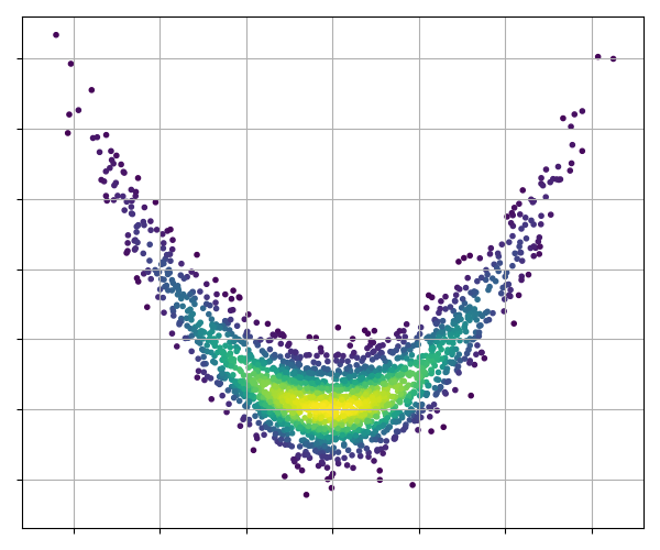 | [Hamiltonian Monte-Carlo](https://github.com/C-bowman/inference-tools/blob/master/demos/hamiltonian_mcmc_demo.ipynb)
 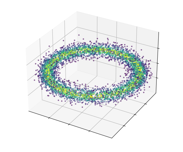 | [Density estimation](https://github.com/C-bowman/inference-tools/blob/master/demos/density_estimation_demo.ipynb)
 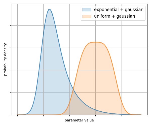 |
29 | | Matrix plotting
|
29 | | Matrix plotting 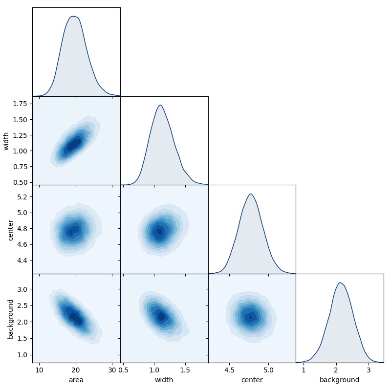 | Highest-density intervals
 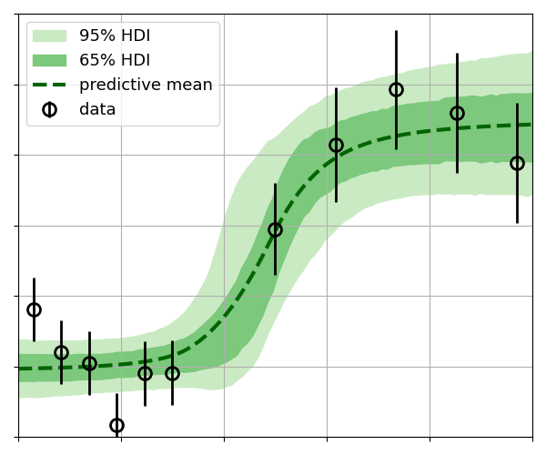 | [GP regression](https://github.com/C-bowman/inference-tools/blob/master/demos/gp_regression_demo.ipynb)
 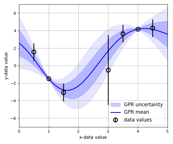 |
30 |
31 | ## Installation
32 |
33 | inference-tools is available from [PyPI](https://pypi.org/project/inference-tools/),
34 | so can be easily installed using [pip](https://pip.pypa.io/en/stable/) as follows:
35 | ```bash
36 | pip install inference-tools
37 | ```
38 |
39 | ## Documentation
40 |
41 | Full documentation is available at [inference-tools.readthedocs.io](https://inference-tools.readthedocs.io/en/stable/).
--------------------------------------------------------------------------------
/demos/scripts/ChainPool_demo.py:
--------------------------------------------------------------------------------
1 | from inference.mcmc import GibbsChain, ChainPool
2 | from time import time
3 |
4 |
5 | def rosenbrock(t):
6 | # This is a modified form of the rosenbrock function, which
7 | # is commonly used to test optimisation algorithms
8 | X, Y = t
9 | X2 = X**2
10 | b = 15 # correlation strength parameter
11 | v = 3 # variance of the gaussian term
12 | return -X2 - b * (Y - X2) ** 2 - 0.5 * (X2 + Y**2) / v
13 |
14 |
15 | # required for multi-process code when running on windows
16 | if __name__ == "__main__":
17 | """
18 | The ChainPool class provides a convenient means to store multiple
19 | chain objects, and simultaneously advance those chains using multiple
20 | python processes.
21 | """
22 |
23 | # for example, here we create a singular chain object
24 | chain = GibbsChain(posterior=rosenbrock, start=[0.0, 0.0])
25 | # then advance it for some number of samples, and note the run-time
26 | t1 = time()
27 | chain.advance(150000)
28 | t2 = time()
29 | print("time elapsed, single chain:", t2 - t1)
30 |
31 | # We may want to run a number of chains in parallel - for example multiple chains
32 | # over different posteriors, or on a single posterior with different starting locations.
33 |
34 | # Here we create two chains with different starting points:
35 | chain_1 = GibbsChain(posterior=rosenbrock, start=[0.5, 0.0])
36 | chain_2 = GibbsChain(posterior=rosenbrock, start=[0.0, 0.5])
37 |
38 | # now we pass those chains to ChainPool in a list
39 | cpool = ChainPool([chain_1, chain_2])
40 |
41 | # if we now wish to advance both of these chains some number of steps, and do so in
42 | # parallel, we can use the advance() method of the ChainPool instance:
43 | t1 = time()
44 | cpool.advance(150000)
45 | t2 = time()
46 | print("time elapsed, two chains:", t2 - t1)
47 |
48 | # assuming you are running this example on a machine with two free cores, advancing
49 | # both chains in this way should have taken a comparable time to advancing just one.
50 |
--------------------------------------------------------------------------------
/demos/scripts/GaussianKDE_demo.py:
--------------------------------------------------------------------------------
1 | from numpy import linspace, zeros, exp, sqrt, pi
2 | from numpy.random import normal
3 | import matplotlib.pyplot as plt
4 | from inference.pdf import GaussianKDE
5 |
6 | """
7 | Code to demonstrate the use of the GaussianKDE class.
8 | """
9 |
10 | # first generate a test sample
11 | N = 150000
12 | sample = zeros(N)
13 | sample[: N // 3] = normal(size=N // 3) * 0.5 + 1.8
14 | sample[N // 3 :] = normal(size=2 * (N // 3)) * 0.5 + 3.5
15 |
16 | # GaussianKDE takes an array of sample values as its only argument
17 | pdf = GaussianKDE(sample)
18 |
19 | # much like the UnimodalPdf class, GaussianKDE returns a density estimator object
20 | # which can be called as a function to return an estimate of the PDF at a set of
21 | # points:
22 | x = linspace(0, 6, 1000)
23 | p = pdf(x)
24 |
25 | # GaussianKDE is fast even for large samples, as it uses a binary tree search to
26 | # match any given spatial location with a slice of the sample array which contains
27 | # all samples that have a non-negligible contribution to the density estimate.
28 |
29 | # We could plot (x, P) manually, but for convenience the plot_summary
30 | # method will generate a plot automatically as well as summary statistics:
31 | pdf.plot_summary()
32 |
33 | # The summary statistics can be accessed via properties or methods:
34 | # the location of the mode is a property
35 | mode = pdf.mode
36 |
37 | # The highest-density interval for any fraction of total probability
38 | # can is returned by the interval() method
39 | hdi_95 = pdf.interval(frac=0.95)
40 |
41 | # the mean, variance, skewness and excess kurtosis are returned
42 | # by the moments() method:
43 | mu, var, skew, kurt = pdf.moments()
44 |
45 | # By default, GaussianKDE uses a simple but easy to compute estimate of the
46 | # bandwidth (the standard deviation of each Gaussian kernel). However, when
47 | # estimating strongly non-normal distributions, this simple approach will
48 | # over-estimate required bandwidth.
49 |
50 | # In these cases, the cross-validation bandwidth selector can be used to
51 | # obtain better results, but with higher computational cost.
52 |
53 | # to demonstrate, lets create a new sample:
54 | N = 30000
55 | sample = zeros(N)
56 | sample[: N // 3] = normal(size=N // 3)
57 | sample[N // 3 :] = normal(size=2 * (N // 3)) + 10
58 |
59 | # now construct estimators using the simple and cross-validation estimators
60 | pdf_simple = GaussianKDE(sample)
61 | pdf_crossval = GaussianKDE(sample, cross_validation=True)
62 |
63 | # now build an axis on which to evaluate the estimates
64 | x = linspace(-4, 14, 500)
65 |
66 | # for comparison also compute the real distribution
67 | exact = (exp(-0.5 * x**2) / 3 + 2 * exp(-0.5 * (x - 10) ** 2) / 3) / sqrt(2 * pi)
68 |
69 | # plot everything together
70 | plt.plot(x, pdf_simple(x), label="simple")
71 | plt.plot(x, pdf_crossval(x), label="cross-validation")
72 | plt.plot(x, exact, label="exact")
73 |
74 | plt.ylabel("probability density")
75 | plt.xlabel("x")
76 |
77 | plt.grid()
78 | plt.legend()
79 | plt.show()
80 |
--------------------------------------------------------------------------------
/demos/scripts/GibbsChain_demo.py:
--------------------------------------------------------------------------------
1 | import matplotlib.pyplot as plt
2 | from numpy import array, exp, linspace
3 |
4 | from inference.mcmc import GibbsChain
5 |
6 |
7 | def rosenbrock(t):
8 | # This is a modified form of the rosenbrock function, which
9 | # is commonly used to test optimisation algorithms
10 | X, Y = t
11 | X2 = X**2
12 | b = 15 # correlation strength parameter
13 | v = 3 # variance of the gaussian term
14 | return -X2 - b * (Y - X2) ** 2 - 0.5 * (X2 + Y**2) / v
15 |
16 |
17 | """
18 | # Gibbs sampling example
19 |
20 | In order to use the GibbsChain sampler from the mcmc module, we must
21 | provide a log-posterior function to sample from, a point in the parameter
22 | space to start the chain, and an initial guess for the proposal width
23 | for each parameter.
24 |
25 | In this example a modified version of the Rosenbrock function (shown
26 | above) is used as the log-posterior.
27 | """
28 |
29 | # The maximum of the rosenbrock function is [0, 0] - here we intentionally
30 | # start the chain far from the mode.
31 | start_location = array([2.0, -4.0])
32 |
33 | # Here we make our initial guess for the proposal widths intentionally
34 | # poor, to demonstrate that gibbs sampling allows each proposal width
35 | # to be adjusted individually toward an optimal value.
36 | width_guesses = array([5.0, 0.05])
37 |
38 | # create the chain object
39 | chain = GibbsChain(posterior=rosenbrock, start=start_location, widths=width_guesses)
40 |
41 | # advance the chain 150k steps
42 | chain.advance(150000)
43 |
44 | # the samples for the n'th parameter can be accessed through the
45 | # get_parameter(n) method. We could use this to plot the path of
46 | # the chain through the 2D parameter space:
47 |
48 | p = chain.get_probabilities() # color the points by their probability value
49 | point_colors = exp(p - p.max())
50 | plt.scatter(
51 | chain.get_parameter(0), chain.get_parameter(1), c=point_colors, marker="."
52 | )
53 | plt.xlabel("parameter 1")
54 | plt.ylabel("parameter 2")
55 | plt.grid()
56 | plt.tight_layout()
57 | plt.show()
58 |
59 |
60 | # We can see from this plot that in order to take a representative sample,
61 | # some early portion of the chain must be removed. This is referred to as
62 | # the 'burn-in' period. This period allows the chain to both find the high
63 | # density areas, and adjust the proposal widths to their optimal values.
64 |
65 | # The plot_diagnostics() method can help us decide what size of burn-in to use:
66 | chain.plot_diagnostics()
67 |
68 | # Occasionally samples are also 'thinned' by a factor of n (where only every
69 | # n'th sample is used) in order to reduce the size of the data set for
70 | # storage, or to produce uncorrelated samples.
71 |
72 | # based on the diagnostics we can choose burn and thin values,
73 | # which can be passed as arguments to methods which act on the samples
74 | burn = 2000
75 | thin = 5
76 |
77 | # After discarding burn-in, what we have left should be a representative
78 | # sample drawn from the posterior. Repeating the previous plot as a
79 | # scatter-plot shows the sample:
80 | p = chain.get_probabilities(burn=burn, thin=thin) # color the points by their probability value
81 | plt.scatter(
82 | chain.get_parameter(index=0, burn=burn, thin=thin),
83 | chain.get_parameter(index=1, burn=burn, thin=thin),
84 | c=exp(p - p.max()),
85 | marker="."
86 | )
87 | plt.xlabel("parameter 1")
88 | plt.ylabel("parameter 2")
89 | plt.grid()
90 | plt.tight_layout()
91 | plt.show()
92 |
93 |
94 | # We can easily estimate 1D marginal distributions for any parameter
95 | # using the 'get_marginal' method:
96 | pdf_1 = chain.get_marginal(0, burn=burn, thin=thin, unimodal=True)
97 | pdf_2 = chain.get_marginal(1, burn=burn, thin=thin, unimodal=True)
98 |
99 | # get_marginal returns a density estimator object, which can be called
100 | # as a function to return the value of the pdf at any point.
101 | # Make an axis on which to evaluate the PDFs:
102 | ax = linspace(-3, 4, 500)
103 |
104 | # plot the results
105 | plt.plot(ax, pdf_1(ax), label="param #1 marginal", lw=2)
106 | plt.plot(ax, pdf_2(ax), label="param #2 marginal", lw=2)
107 |
108 | plt.xlabel("parameter value")
109 | plt.ylabel("probability density")
110 | plt.legend()
111 | plt.grid()
112 | plt.tight_layout()
113 | plt.show()
114 |
115 | # chain objects can be saved in their entirety as a single .npz file using
116 | # the save() method, and then re-built using the load() class method, so
117 | # that to save the chain you may write:
118 |
119 | # chain.save('chain_data.npz')
120 |
121 | # and to re-build a chain object at it was before you would write
122 |
123 | # chain = GibbsChain.load('chain_data.npz')
124 |
125 | # This allows you to advance a chain, store it, then re-load it at a later
126 | # time to analyse the chain data, or re-start the chain should you decide
127 | # more samples are required.
128 |
--------------------------------------------------------------------------------
/demos/scripts/GpOptimiser_demo.py:
--------------------------------------------------------------------------------
1 | from inference.gp import GpOptimiser
2 |
3 | import matplotlib.pyplot as plt
4 | import matplotlib as mpl
5 | from numpy import sin, cos, linspace, array, meshgrid
6 |
7 | mpl.rcParams["axes.autolimit_mode"] = "round_numbers"
8 | mpl.rcParams["axes.xmargin"] = 0
9 | mpl.rcParams["axes.ymargin"] = 0
10 |
11 |
12 | def example_plot_1d():
13 | mu, sig = GP(x_gp)
14 | fig, (ax1, ax2, ax3) = plt.subplots(
15 | 3, 1, gridspec_kw={"height_ratios": [1, 3, 1]}, figsize=(10, 8)
16 | )
17 |
18 | ax1.plot(
19 | evaluations,
20 | max_values,
21 | marker="o",
22 | ls="solid",
23 | c="orange",
24 | label="highest observed value",
25 | zorder=5,
26 | )
27 | ax1.plot(
28 | [2, 12], [max(y_func), max(y_func)], ls="dashed", label="actual max", c="black"
29 | )
30 | ax1.set_xlabel("function evaluations")
31 | ax1.set_xlim([2, 12])
32 | ax1.set_ylim([max(y) - 0.3, max(y_func) + 0.3])
33 | ax1.xaxis.set_label_position("top")
34 | ax1.yaxis.set_label_position("right")
35 | ax1.xaxis.tick_top()
36 | ax1.set_yticks([])
37 | ax1.legend(loc=4)
38 |
39 | ax2.plot(GP.x, GP.y, "o", c="red", label="observations", zorder=5)
40 | ax2.plot(x_gp, y_func, lw=1.5, c="red", ls="dashed", label="actual function")
41 | ax2.plot(x_gp, mu, lw=2, c="blue", label="GP prediction")
42 | ax2.fill_between(
43 | x_gp,
44 | (mu - 2 * sig),
45 | y2=(mu + 2 * sig),
46 | color="blue",
47 | alpha=0.15,
48 | label="95% confidence interval",
49 | )
50 | ax2.set_ylim([-1.5, 4])
51 | ax2.set_ylabel("y")
52 | ax2.set_xticks([])
53 |
54 | aq = array([abs(GP.acquisition(array([k]))) for k in x_gp]).squeeze()
55 | proposal = x_gp[aq.argmax()]
56 | ax3.fill_between(x_gp, 0.9 * aq / aq.max(), color="green", alpha=0.15)
57 | ax3.plot(x_gp, 0.9 * aq / aq.max(), color="green", label="acquisition function")
58 | ax3.plot(
59 | [proposal] * 2, [0.0, 1.0], c="green", ls="dashed", label="acquisition maximum"
60 | )
61 | ax2.plot([proposal] * 2, [-1.5, search_function(proposal)], c="green", ls="dashed")
62 | ax2.plot(
63 | proposal,
64 | search_function(proposal),
65 | "o",
66 | c="green",
67 | label="proposed observation",
68 | )
69 | ax3.set_ylim([0, 1])
70 | ax3.set_yticks([])
71 | ax3.set_xlabel("x")
72 | ax3.legend(loc=1)
73 | ax2.legend(loc=2)
74 |
75 | plt.tight_layout()
76 | plt.subplots_adjust(hspace=0)
77 | plt.show()
78 |
79 |
80 | def example_plot_2d():
81 | fig, (ax1, ax2) = plt.subplots(
82 | 2, 1, gridspec_kw={"height_ratios": [1, 3]}, figsize=(10, 8)
83 | )
84 | plt.subplots_adjust(hspace=0)
85 |
86 | ax1.plot(
87 | evaluations,
88 | max_values,
89 | marker="o",
90 | ls="solid",
91 | c="orange",
92 | label="optimum value",
93 | zorder=5,
94 | )
95 | ax1.plot(
96 | [5, 30],
97 | [z_func.max(), z_func.max()],
98 | ls="dashed",
99 | label="actual max",
100 | c="black",
101 | )
102 | ax1.set_xlabel("function evaluations")
103 | ax1.set_xlim([5, 30])
104 | ax1.set_ylim([max(y) - 0.3, z_func.max() + 0.3])
105 | ax1.xaxis.set_label_position("top")
106 | ax1.yaxis.set_label_position("right")
107 | ax1.xaxis.tick_top()
108 | ax1.set_yticks([])
109 | ax1.legend(loc=4)
110 |
111 | ax2.contour(*mesh, z_func, 40)
112 | ax2.plot(
113 | [i[0] for i in GP.x],
114 | [i[1] for i in GP.x],
115 | "D",
116 | c="red",
117 | markeredgecolor="black",
118 | )
119 | plt.show()
120 |
121 |
122 | """
123 | GpOptimiser extends the functionality of GpRegressor to perform 'Bayesian optimisation'.
124 |
125 | Bayesian optimisation is suited to problems for which a single evaluation of the function
126 | being explored is expensive, such that the total number of function evaluations must be
127 | made as small as possible.
128 | """
129 |
130 |
131 | # define the function whose maximum we will search for
132 | def search_function(x):
133 | return sin(0.5 * x) + 3 / (1 + (x - 1) ** 2)
134 |
135 |
136 | # define bounds for the optimisation
137 | bounds = [(-8.0, 8.0)]
138 |
139 | # create some initialisation data
140 | x = array([-8, 8])
141 | y = search_function(x)
142 |
143 | # create an instance of GpOptimiser
144 | GP = GpOptimiser(x, y, bounds=bounds)
145 |
146 |
147 | # here we evaluate the search function for plotting purposes
148 | M = 500
149 | x_gp = linspace(*bounds[0], M)
150 | y_func = search_function(x_gp)
151 | max_values = [max(GP.y)]
152 | evaluations = [len(GP.y)]
153 |
154 |
155 | for i in range(11):
156 | # plot the current state of the optimisation
157 | example_plot_1d()
158 |
159 | # request the proposed evaluation
160 | new_x = GP.propose_evaluation()
161 |
162 | # evaluate the new point
163 | new_y = search_function(new_x)
164 |
165 | # update the gaussian process with the new information
166 | GP.add_evaluation(new_x, new_y)
167 |
168 | # track the optimum value for plotting
169 | max_values.append(max(GP.y))
170 | evaluations.append(len(GP.y))
171 |
172 |
173 | """
174 | 2D example
175 | """
176 | from mpl_toolkits.mplot3d import Axes3D
177 |
178 |
179 | # define a new 2D search function
180 | def search_function(v):
181 | x, y = v
182 | z = ((x - 1) / 2) ** 2 + ((y + 3) / 1.5) ** 2
183 | return sin(0.5 * x) + cos(0.4 * y) + 5 / (1 + z)
184 |
185 |
186 | # set bounds
187 | bounds = [(-8, 8), (-8, 8)]
188 |
189 | # evaluate function for plotting
190 | N = 80
191 | x = linspace(*bounds[0], N)
192 | y = linspace(*bounds[1], N)
193 | mesh = meshgrid(x, y)
194 | z_func = search_function(mesh)
195 |
196 |
197 | # create some initialisation data
198 | # we've picked a point at each corner and one in the middle
199 | x = [(-8, -8), (8, -8), (-8, 8), (8, 8), (0, 0)]
200 | y = [search_function(k) for k in x]
201 |
202 | # initiate the optimiser
203 | GP = GpOptimiser(x, y, bounds=bounds)
204 |
205 |
206 | max_values = [max(GP.y)]
207 | evaluations = [len(GP.y)]
208 |
209 | for i in range(25):
210 | new_x = GP.propose_evaluation()
211 | new_y = search_function(new_x)
212 | GP.add_evaluation(new_x, new_y)
213 |
214 | # track the optimum value for plotting
215 | max_values.append(max(GP.y))
216 | evaluations.append(len(GP.y))
217 |
218 | # plot the results
219 | example_plot_2d()
220 |
--------------------------------------------------------------------------------
/demos/scripts/HamiltonianChain_demo.py:
--------------------------------------------------------------------------------
1 | from mpl_toolkits.mplot3d import Axes3D
2 | import matplotlib.pyplot as plt
3 | from numpy import sqrt, exp, array
4 | from inference.mcmc import HamiltonianChain
5 |
6 | """
7 | # Hamiltonian sampling example
8 |
9 | Hamiltonian Monte-Carlo (HMC) is a MCMC algorithm which is able to
10 | efficiently sample from complex PDFs which present difficulty for
11 | other algorithms, such as those which strong non-linear correlations.
12 |
13 | However, this requires not only the log-posterior probability but also
14 | its gradient in order to function. In cases where this gradient can be
15 | calculated analytically HMC can be very effective.
16 |
17 | The implementation of HMC shown here as HamiltonianChain is somewhat
18 | naive, and should at some point be replaced with a more advanced
19 | self-tuning version, such as the NUTS algorithm.
20 | """
21 |
22 |
23 | # define a non-linearly correlated posterior distribution
24 | class ToroidalGaussian:
25 | def __init__(self):
26 | self.R0 = 1.0 # torus major radius
27 | self.ar = 10.0 # torus aspect ratio
28 | self.inv_w2 = (self.ar / self.R0) ** 2
29 |
30 | def __call__(self, theta):
31 | x, y, z = theta
32 | r_sqr = z**2 + (sqrt(x**2 + y**2) - self.R0) ** 2
33 | return -0.5 * r_sqr * self.inv_w2
34 |
35 | def gradient(self, theta):
36 | x, y, z = theta
37 | R = sqrt(x**2 + y**2)
38 | K = 1 - self.R0 / R
39 | g = array([K * x, K * y, z])
40 | return -g * self.inv_w2
41 |
42 |
43 | # create an instance of our posterior class
44 | posterior = ToroidalGaussian()
45 |
46 | # create the chain object
47 | chain = HamiltonianChain(
48 | posterior=posterior, grad=posterior.gradient, start=array([1, 0.1, 0.1])
49 | )
50 |
51 | # advance the chain to generate the sample
52 | chain.advance(6000)
53 |
54 | # choose how many samples will be thrown away from the start
55 | # of the chain as 'burn-in'
56 | burn = 2000
57 |
58 | # extract sample and probability data from the chain
59 | probs = chain.get_probabilities(burn=burn)
60 | colors = exp(probs - probs.max())
61 | xs, ys, zs = [chain.get_parameter(i, burn=burn) for i in [0, 1, 2]]
62 |
63 | # Plot the sample we've generated as a 3D scatterplot
64 | fig = plt.figure(figsize=(10, 10))
65 | ax = fig.add_subplot(111, projection="3d")
66 | L = 1.2
67 | ax.set_xlim([-L, L])
68 | ax.set_ylim([-L, L])
69 | ax.set_zlim([-L, L])
70 | ax.set_xlabel("x")
71 | ax.set_ylabel("y")
72 | ax.set_zlabel("z")
73 | ax.scatter(xs, ys, zs, c=colors)
74 | plt.tight_layout()
75 | plt.show()
76 |
77 | # The plot_diagnostics() and matrix_plot() methods described in the GibbsChain demo
78 | # also work for HamiltonianChain:
79 | chain.plot_diagnostics()
80 |
81 | chain.matrix_plot()
82 |
--------------------------------------------------------------------------------
/demos/scripts/ParallelTempering_demo.py:
--------------------------------------------------------------------------------
1 | from numpy import log, sqrt, sin, arctan2, pi
2 |
3 | # define a posterior with multiple separate peaks
4 | def multimodal_posterior(theta):
5 | x, y = theta
6 | r = sqrt(x**2 + y**2)
7 | phi = arctan2(y, x)
8 | z = (r - (0.5 + pi - phi*0.5)) / 0.1
9 | return -0.5*z**2 + 4*log(sin(phi*2.)**2)
10 |
11 |
12 | # required for multi-process code when running on windows
13 | if __name__ == "__main__":
14 |
15 | from inference.mcmc import GibbsChain, ParallelTempering
16 |
17 | # define a set of temperature levels
18 | N_levels = 6
19 | temps = [10**(2.5*k/(N_levels-1.)) for k in range(N_levels)]
20 |
21 | # create a set of chains - one with each temperature
22 | chains = [GibbsChain(posterior=multimodal_posterior, start=[0.5, 0.5], temperature=T) for T in temps]
23 |
24 | # When an instance of ParallelTempering is created, a dedicated process for each chain is spawned.
25 | # These separate processes will automatically make use of the available cpu cores, such that the
26 | # computations to advance the separate chains are performed in parallel.
27 | PT = ParallelTempering(chains=chains)
28 |
29 | # These processes wait for instructions which can be sent using the methods of the
30 | # ParallelTempering object:
31 | PT.run_for(minutes=0.5)
32 |
33 | # To recover a copy of the chains held by the processes
34 | # we can use the return_chains method:
35 | chains = PT.return_chains()
36 |
37 | # by looking at the trace plot for the T = 1 chain, we see that it makes
38 | # large jumps across the parameter space due to the swaps.
39 | chains[0].trace_plot()
40 |
41 | # Even though the posterior has strongly separated peaks, the T = 1 chain
42 | # was able to explore all of them due to the swaps.
43 | chains[0].matrix_plot()
44 |
45 | # We can also visualise the acceptance rates of proposed position swaps between
46 | # each chain using the swap_diagnostics method:
47 | PT.swap_diagnostics()
48 |
49 | # Because each process waits for instructions from the ParallelTempering object,
50 | # they will not self-terminate. To terminate all the processes we have to trigger
51 | # a shutdown even using the shutdown method:
52 | PT.shutdown()
--------------------------------------------------------------------------------
/demos/scripts/gaussian_fitting_demo.py:
--------------------------------------------------------------------------------
1 | from numpy import array, exp, linspace, sqrt, pi
2 | import matplotlib.pyplot as plt
3 |
4 | # Suppose we have the following dataset, which we believe is described by a
5 | # Gaussian peak plus a constant background. Our goal in this example is to
6 | # infer the area of the Gaussian.
7 |
8 | x_data = array([
9 | 0.00, 0.80, 1.60, 2.40, 3.20, 4.00, 4.80, 5.60,
10 | 6.40, 7.20, 8.00, 8.80, 9.60, 10.4, 11.2, 12.0
11 | ])
12 |
13 | y_data = array([
14 | 2.473, 1.329, 2.370, 1.135, 5.861, 7.045, 9.942, 7.335,
15 | 3.329, 5.348, 1.462, 2.476, 3.096, 0.784, 3.342, 1.877
16 | ])
17 |
18 | y_error = array([
19 | 1.0, 1.0, 1.0, 1.0, 1.0, 1.0, 1.0, 1.0,
20 | 1.0, 1.0, 1.0, 1.0, 1.0, 1.0, 1.0, 1.0
21 | ])
22 |
23 | plt.errorbar(
24 | x_data,
25 | y_data,
26 | yerr=y_error,
27 | ls="dashed",
28 | marker="D",
29 | c="red",
30 | markerfacecolor="none",
31 | )
32 | plt.ylabel("y")
33 | plt.xlabel("x")
34 | plt.grid()
35 | plt.show()
36 |
37 | # The first step is to implement our model. For simple models like this one
38 | # this can be done using just a function, but as models become more complex
39 | # it becomes useful to build them as classes.
40 |
41 |
42 | class PeakModel:
43 | def __init__(self, x_data):
44 | """
45 | The __init__ should be used to pass in any data which is required
46 | by the model to produce predictions of the y-data values.
47 | """
48 | self.x = x_data
49 |
50 | def __call__(self, theta):
51 | return self.forward_model(self.x, theta)
52 |
53 | @staticmethod
54 | def forward_model(x, theta):
55 | """
56 | The forward model must make a prediction of the experimental data we would expect to measure
57 | given a specific set model parameters 'theta'.
58 | """
59 | # unpack the model parameters
60 | area, width, center, background = theta
61 | # return the prediction of the data
62 | z = (x - center) / width
63 | gaussian = exp(-0.5 * z**2) / (sqrt(2 * pi) * width)
64 | return area * gaussian + background
65 |
66 |
67 | # inference-tools has a variety of Likelihood classes which allow you to easily construct a
68 | # likelihood function given the measured data and your forward-model.
69 | from inference.likelihoods import GaussianLikelihood
70 |
71 | likelihood = GaussianLikelihood(
72 | y_data=y_data, sigma=y_error, forward_model=PeakModel(x_data)
73 | )
74 |
75 | # Instances of the likelihood classes can be called as functions, and return the log-likelihood
76 | # when passed a vector of model parameters:
77 | initial_guess = array([10.0, 2.0, 5.0, 2.0])
78 | guess_log_likelihood = likelihood(initial_guess)
79 | print(guess_log_likelihood)
80 |
81 | # We could at this stage pair the likelihood object with an optimiser in order to obtain
82 | # the maximum-likelihood estimate of the parameters. In this example however, we want to
83 | # construct the posterior distribution for the model parameters, and that means we need
84 | # a prior.
85 |
86 | # The inference.priors module contains classes which allow for easy construction of
87 | # prior distributions across all model parameters.
88 | from inference.priors import ExponentialPrior, UniformPrior, JointPrior
89 |
90 | # If we want different model parameters to have different prior distributions, as in this
91 | # case where we give three variables an exponential prior and one a uniform prior, we first
92 | # construct each type of prior separately:
93 | prior_components = [
94 | ExponentialPrior(beta=[50.0, 20.0, 20.0], variable_indices=[0, 1, 3]),
95 | UniformPrior(lower=0.0, upper=12.0, variable_indices=[2]),
96 | ]
97 | # Now we use the JointPrior class to combine the various components into a single prior
98 | # distribution which covers all the model parameters.
99 | prior = JointPrior(components=prior_components, n_variables=4)
100 |
101 | # As with the likelihood, prior objects can also be called as function to return a
102 | # log-probability value when passed a vector of model parameters. We can also draw
103 | # samples from the prior directly using the sample() method:
104 | prior_sample = prior.sample()
105 | print(prior_sample)
106 |
107 | # The likelihood and prior can be easily combined into a posterior distribution
108 | # using the Posterior class:
109 | from inference.posterior import Posterior
110 | posterior = Posterior(likelihood=likelihood, prior=prior)
111 |
112 | # Now we have constructed a posterior distribution, we can sample from it
113 | # using Markov-chain Monte-Carlo (MCMC).
114 |
115 | # The inference.mcmc module contains implementations of various MCMC sampling algorithms.
116 | # Here we import the PcaChain class and use it to create a Markov-chain object:
117 | from inference.mcmc import PcaChain
118 | chain = PcaChain(posterior=posterior, start=initial_guess)
119 |
120 | # We generate samples by advancing the chain by a chosen number of steps using the advance method:
121 | chain.advance(25000)
122 |
123 | # we can check the status of the chain using the plot_diagnostics method:
124 | chain.plot_diagnostics()
125 |
126 | # The burn-in (how many samples from the start of the chain are discarded)
127 | # can be specified as an argument to methods which act on the samples:
128 | burn = 5000
129 |
130 | # we can get a quick overview of the posterior using the matrix_plot method
131 | # of chain objects, which plots all possible 1D & 2D marginal distributions
132 | # of the full parameter set (or a chosen sub-set).
133 | chain.matrix_plot(labels=["area", "width", "center", "background"], burn=burn)
134 |
135 | # We can easily estimate 1D marginal distributions for any parameter
136 | # using the get_marginal method:
137 | area_pdf = chain.get_marginal(0, burn=burn)
138 | area_pdf.plot_summary(label="Gaussian area")
139 |
140 |
141 | # We can assess the level of uncertainty in the model predictions by passing each sample
142 | # through the forward-model and observing the distribution of model expressions that result:
143 |
144 | # generate an axis on which to evaluate the model
145 | x_fits = linspace(-2, 14, 500)
146 | # get the sample
147 | sample = chain.get_sample(burn=burn)
148 | # pass each through the forward model
149 | curves = array([PeakModel.forward_model(x_fits, theta) for theta in sample])
150 |
151 | # We could plot the predictions for each sample all on a single graph, but this is
152 | # often cluttered and difficult to interpret.
153 |
154 | # A better option is to use the hdi_plot function from the plotting module to plot
155 | # highest-density intervals for each point where the model is evaluated:
156 | from inference.plotting import hdi_plot
157 |
158 | fig = plt.figure(figsize=(8, 6))
159 | ax = fig.add_subplot(111)
160 | hdi_plot(x_fits, curves, intervals=[0.68, 0.95], axis=ax)
161 |
162 | # plot the MAP estimate (the sample with the single highest posterior probability)
163 | MAP_prediction = PeakModel.forward_model(x_fits, chain.mode())
164 | ax.plot(x_fits, MAP_prediction, ls="dashed", lw=3, c="C0", label="MAP estimate")
165 | # build the rest of the plot
166 | ax.errorbar(
167 | x_data,
168 | y_data,
169 | yerr=y_error,
170 | linestyle="none",
171 | c="red",
172 | label="data",
173 | marker="o",
174 | markerfacecolor="none",
175 | markeredgewidth=1.5,
176 | markersize=8,
177 | )
178 | ax.set_xlabel("x")
179 | ax.set_ylabel("y")
180 | ax.set_xlim([-0.5, 12.5])
181 | ax.legend()
182 | ax.grid()
183 | plt.tight_layout()
184 | plt.show()
185 |
--------------------------------------------------------------------------------
/docs/Makefile:
--------------------------------------------------------------------------------
1 | # Minimal makefile for Sphinx documentation
2 | #
3 |
4 | # You can set these variables from the command line.
5 | SPHINXOPTS =
6 | SPHINXBUILD = sphinx-build
7 | SOURCEDIR = source
8 | BUILDDIR = build
9 |
10 | # Put it first so that "make" without argument is like "make help".
11 | help:
12 | @$(SPHINXBUILD) -M help "$(SOURCEDIR)" "$(BUILDDIR)" $(SPHINXOPTS) $(O)
13 |
14 | .PHONY: help Makefile
15 |
16 | # Catch-all target: route all unknown targets to Sphinx using the new
17 | # "make mode" option. $(O) is meant as a shortcut for $(SPHINXOPTS).
18 | %: Makefile
19 | @$(SPHINXBUILD) -M $@ "$(SOURCEDIR)" "$(BUILDDIR)" $(SPHINXOPTS) $(O)
--------------------------------------------------------------------------------
/docs/docs_requirements.txt:
--------------------------------------------------------------------------------
1 | sphinx==5.3.0
2 | sphinx_rtd_theme==1.1.1
--------------------------------------------------------------------------------
/docs/make.bat:
--------------------------------------------------------------------------------
1 | @ECHO OFF
2 |
3 | pushd %~dp0
4 |
5 | REM Command file for Sphinx documentation
6 |
7 | if "%SPHINXBUILD%" == "" (
8 | set SPHINXBUILD=sphinx-build
9 | )
10 | set SOURCEDIR=source
11 | set BUILDDIR=build
12 |
13 | if "%1" == "" goto help
14 |
15 | %SPHINXBUILD% >NUL 2>NUL
16 | if errorlevel 9009 (
17 | echo.
18 | echo.The 'sphinx-build' command was not found. Make sure you have Sphinx
19 | echo.installed, then set the SPHINXBUILD environment variable to point
20 | echo.to the full path of the 'sphinx-build' executable. Alternatively you
21 | echo.may add the Sphinx directory to PATH.
22 | echo.
23 | echo.If you don't have Sphinx installed, grab it from
24 | echo.http://sphinx-doc.org/
25 | exit /b 1
26 | )
27 |
28 | %SPHINXBUILD% -M %1 %SOURCEDIR% %BUILDDIR% %SPHINXOPTS%
29 | goto end
30 |
31 | :help
32 | %SPHINXBUILD% -M help %SOURCEDIR% %BUILDDIR% %SPHINXOPTS%
33 |
34 | :end
35 | popd
36 |
--------------------------------------------------------------------------------
/docs/source/EnsembleSampler.rst:
--------------------------------------------------------------------------------
1 |
2 | EnsembleSampler
3 | ~~~~~~~~~~~~~~~
4 |
5 | .. autoclass:: inference.mcmc.EnsembleSampler
6 | :members: advance, get_sample, get_parameter, get_probabilities, mode, plot_diagnostics, matrix_plot, trace_plot
7 |
--------------------------------------------------------------------------------
/docs/source/GibbsChain.rst:
--------------------------------------------------------------------------------
1 |
2 | GibbsChain
3 | ~~~~~~~~~~
4 |
5 | .. autoclass:: inference.mcmc.GibbsChain
6 | :members: advance, run_for, mode, get_marginal, get_sample, get_parameter, get_interval, plot_diagnostics, matrix_plot, trace_plot, set_non_negative, set_boundaries
7 |
8 |
9 | GibbsChain example code
10 | ^^^^^^^^^^^^^^^^^^^^^^^
11 |
12 | Define the Rosenbrock density to use as a test case:
13 |
14 | .. code-block:: python
15 |
16 | from numpy import linspace, exp
17 | import matplotlib.pyplot as plt
18 |
19 | def rosenbrock(t):
20 | X, Y = t
21 | X2 = X**2
22 | return -X2 - 15.*(Y - X2)**2 - 0.5*(X2 + Y**2) / 3.
23 |
24 | Create the chain object:
25 |
26 | .. code-block:: python
27 |
28 | from inference.mcmc import GibbsChain
29 | chain = GibbsChain(posterior = rosenbrock, start = [2., -4.])
30 |
31 | Advance the chain 150k steps to generate a sample from the posterior:
32 |
33 | .. code-block:: python
34 |
35 | chain.advance(150000)
36 |
37 | The samples for any parameter can be accessed through the
38 | ``get_parameter`` method. We could use this to plot the path of
39 | the chain through the 2D parameter space:
40 |
41 | .. code-block:: python
42 |
43 | p = chain.get_probabilities() # color the points by their probability value
44 | pnt_colors = exp(p - p.max())
45 | plt.scatter(chain.get_parameter(0), chain.get_parameter(1), c=pnt_colors, marker='.')
46 | plt.xlabel('parameter 1')
47 | plt.ylabel('parameter 2')
48 | plt.grid()
49 | plt.show()
50 |
51 | .. image:: ./images/GibbsChain_images/initial_scatter.png
52 |
53 | We can see from this plot that in order to take a representative sample,
54 | some early portion of the chain must be removed. This is referred to as
55 | the 'burn-in' period. This period allows the chain to both find the high
56 | density areas, and adjust the proposal widths to their optimal values.
57 |
58 | The ``plot_diagnostics`` method can help us decide what size of burn-in to use:
59 |
60 | .. code-block:: python
61 |
62 | chain.plot_diagnostics()
63 |
64 | .. image:: ./images/GibbsChain_images/gibbs_diagnostics.png
65 |
66 | Occasionally samples are also 'thinned' by a factor of n (where only every
67 | n'th sample is used) in order to reduce the size of the data set for
68 | storage, or to produce uncorrelated samples.
69 |
70 | Based on the diagnostics we can choose burn and thin values, which can be passed
71 | to methods of the chain that access or operate on the sample data.
72 |
73 | .. code-block:: python
74 |
75 | burn = 2000
76 | thin = 10
77 |
78 |
79 | By specifying the ``burn`` and ``thin`` values, we can generate a new version of
80 | the earlier plot with the burn-in and thinned samples discarded:
81 |
82 | .. code-block:: python
83 |
84 | p = chain.get_probabilities(burn=burn, thin=thin)
85 | pnt_colors = exp(p - p.max())
86 | plt.scatter(
87 | chain.get_parameter(0, burn=burn, thin=thin),
88 | chain.get_parameter(1, burn=burn, thin=thin),
89 | c=pnt_colors,
90 | marker = '.'
91 | )
92 | plt.xlabel('parameter 1')
93 | plt.ylabel('parameter 2')
94 | plt.grid()
95 | plt.show()
96 |
97 | .. image:: ./images/GibbsChain_images/burned_scatter.png
98 |
99 | We can easily estimate 1D marginal distributions for any parameter
100 | using the ``get_marginal`` method:
101 |
102 | .. code-block:: python
103 |
104 | pdf_1 = chain.get_marginal(0, burn=burn, thin=thin, unimodal=True)
105 | pdf_2 = chain.get_marginal(1, burn=burn, thin=thin, unimodal=True)
106 |
107 | ``get_marginal`` returns a density estimator object, which can be called
108 | as a function to return the value of the pdf at any point:
109 |
110 | .. code-block:: python
111 |
112 | axis = linspace(-3, 4, 500) # axis on which to evaluate the marginal PDFs
113 | # plot the marginal distributions
114 | plt.plot(axis, pdf_1(axis), label='param #1 marginal', lw=2)
115 | plt.plot(axis, pdf_2(axis), label='param #2 marginal', lw=2)
116 | plt.xlabel('parameter value')
117 | plt.ylabel('probability density')
118 | plt.legend()
119 | plt.grid()
120 | plt.show()
121 |
122 | .. image:: ./images/GibbsChain_images/gibbs_marginals.png
--------------------------------------------------------------------------------
/docs/source/GpLinearInverter.rst:
--------------------------------------------------------------------------------
1 |
2 | GpLinearInverter
3 | ~~~~~~~~~~~~~~~~
4 |
5 | .. autoclass:: inference.gp.GpLinearInverter
6 | :members: calculate_posterior, calculate_posterior_mean, optimize_hyperparameters, marginal_likelihood
7 |
8 |
9 | Example code
10 | ^^^^^^^^^^^^
11 |
12 | Example code can be found in the `Gaussian-process linear inversion jupyter notebook demo `_.
--------------------------------------------------------------------------------
/docs/source/GpOptimiser.rst:
--------------------------------------------------------------------------------
1 |
2 | GpOptimiser
3 | ~~~~~~~~~~~
4 |
5 | .. autoclass:: inference.gp.GpOptimiser
6 | :members: propose_evaluation, add_evaluation
7 |
8 | Example code
9 | ^^^^^^^^^^^^
10 |
11 | Gaussian-process optimisation efficiently searches for the global maximum of a function
12 | by iteratively 'learning' the structure of that function as new evaluations are made.
13 |
14 | As an example, define a simple 1D function:
15 |
16 | .. code-block:: python
17 |
18 | from numpy import sin
19 |
20 | def search_function(x): # Lorentzian plus a sine wave
21 | return sin(0.5 * x) + 3 / (1 + (x - 1)**2)
22 |
23 |
24 | Define some bounds for the optimisation, and make some evaluations of the function
25 | that will be used to build the initial gaussian-process estimate:
26 |
27 | .. code-block:: python
28 |
29 | # define bounds for the optimisation
30 | bounds = [(-8.0, 8.0)]
31 |
32 | # create some initialisation data
33 | x = array([-8.0, 8.0])
34 | y = search_function(x)
35 |
36 | Create an instance of GpOptimiser:
37 |
38 | .. code-block:: python
39 |
40 | from inference.gp import GpOptimiser
41 | GP = GpOptimiser(x, y, bounds=bounds)
42 |
43 | By using the ``propose_evaluation`` method, GpOptimiser will propose a new evaluation of
44 | the function. This proposed evaluation is generated by maximising an `acquisition function`,
45 | in this case the 'expected improvement' function. The new evaluation can be used to update
46 | the estimate by using the ``add_evaluation`` method, which leads to the following loop:
47 |
48 | .. code-block:: python
49 |
50 | for i in range(11):
51 | # request the proposed evaluation
52 | new_x = GP.propose_evaluation()
53 |
54 | # evaluate the new point
55 | new_y = search_function(new_x)
56 |
57 | # update the gaussian process with the new information
58 | GP.add_evaluation(new_x, new_y)
59 |
60 |
61 | Here we plot the state of the estimate at each iteration:
62 |
63 | .. image:: ./images/GpOptimiser_images/GpOptimiser_iteration.gif
--------------------------------------------------------------------------------
/docs/source/GpRegressor.rst:
--------------------------------------------------------------------------------
1 |
2 |
3 | GpRegressor
4 | ~~~~~~~~~~~
5 |
6 | .. autoclass:: inference.gp.GpRegressor
7 | :members: __call__, gradient, build_posterior
8 |
9 |
10 | Example code
11 | ^^^^^^^^^^^^
12 |
13 | Example code can be found in the `Gaussian-process regression jupyter notebook demo `_.
--------------------------------------------------------------------------------
/docs/source/HamiltonianChain.rst:
--------------------------------------------------------------------------------
1 |
2 | HamiltonianChain
3 | ~~~~~~~~~~~~~~~~
4 |
5 | .. autoclass:: inference.mcmc.HamiltonianChain
6 | :members: advance, run_for, mode, get_marginal, get_parameter, plot_diagnostics, matrix_plot, trace_plot
7 |
8 |
9 | HamiltonianChain example code
10 | ^^^^^^^^^^^^^^^^^^^^^^^^^^^^^
11 |
12 | Here we define a toroidal (donut-shaped!) posterior distribution which has strong non-linear correlation:
13 |
14 | .. code-block:: python
15 |
16 | from numpy import array, sqrt
17 |
18 | class ToroidalGaussian:
19 | def __init__(self):
20 | self.R0 = 1. # torus major radius
21 | self.ar = 10. # torus aspect ratio
22 | self.inv_w2 = (self.ar / self.R0)**2
23 |
24 | def __call__(self, theta):
25 | x, y, z = theta
26 | r_sqr = z**2 + (sqrt(x**2 + y**2) - self.R0)**2
27 | return -0.5 * self.inv_w2 * r_sqr
28 |
29 | def gradient(self, theta):
30 | x, y, z = theta
31 | R = sqrt(x**2 + y**2)
32 | K = 1 - self.R0 / R
33 | g = array([K*x, K*y, z])
34 | return -g * self.inv_w2
35 |
36 |
37 | Build the posterior and chain objects then generate the sample:
38 |
39 | .. code-block:: python
40 |
41 | # create an instance of our posterior class
42 | posterior = ToroidalGaussian()
43 |
44 | # create the chain object
45 | chain = HamiltonianChain(
46 | posterior = posterior,
47 | grad=posterior.gradient,
48 | start = [1, 0.1, 0.1]
49 | )
50 |
51 | # advance the chain to generate the sample
52 | chain.advance(6000)
53 |
54 | # choose how many samples will be thrown away from the start of the chain as 'burn-in'
55 | burn = 2000
56 |
57 | We can use the `Plotly `_ library to generate an interactive 3D scatterplot of our sample:
58 |
59 | .. code-block:: python
60 |
61 | # extract sample and probability data from the chain
62 | probs = chain.get_probabilities(burn=burn)
63 | point_colors = exp(probs - probs.max())
64 | x, y, z = [chain.get_parameter(i) for i in [0, 1, 2]]
65 |
66 | # build the scatterplot using plotly
67 | import plotly.graph_objects as go
68 |
69 | fig = go.Figure(data=1[go.Scatter3d(
70 | x=x, y=y, z=z, mode='markers',
71 | marker=dict(size=5, color=point_colors, colorscale='Viridis', opacity=0.6)
72 | )])
73 |
74 | fig.update_layout(margin=dict(l=0, r=0, b=0, t=0)) # set a tight layout
75 | fig.show()
76 |
77 | .. raw:: html
78 | :file: ./images/HamiltonianChain_images/hmc_scatterplot.html
79 |
80 | We can view all the corresponding 1D & 2D marginal distributions using the ``matrix_plot`` method of the chain:
81 |
82 | .. code-block:: python
83 |
84 | chain.matrix_plot(burn=burn)
85 |
86 |
87 | .. image:: ./images/HamiltonianChain_images/hmc_matrix_plot.png
--------------------------------------------------------------------------------
/docs/source/ParallelTempering.rst:
--------------------------------------------------------------------------------
1 | ParallelTempering
2 | ~~~~~~~~~~~~~~~~~
3 |
4 | .. autoclass:: inference.mcmc.ParallelTempering
5 | :members: advance, run_for, shutdown, return_chains
6 |
7 |
8 | ParallelTempering example code
9 | ^^^^^^^^^^^^^^^^^^^^^^^^^^^^^^
10 |
11 | Define a posterior with separated maxima, which is difficult
12 | for a single chain to explore:
13 |
14 | .. code-block:: python
15 |
16 | from numpy import log, sqrt, sin, arctan2, pi
17 |
18 | # define a posterior with multiple separate peaks
19 | def multimodal_posterior(theta):
20 | x, y = theta
21 | r = sqrt(x**2 + y**2)
22 | phi = arctan2(y, x)
23 | z = (r - (0.5 + pi - phi*0.5)) / 0.1
24 | return -0.5*z**2 + 4*log(sin(phi*2.)**2)
25 |
26 | Define a set of temperature levels:
27 |
28 | .. code-block:: python
29 |
30 | N_levels = 6
31 | temperatures = [10**(2.5*k/(N_levels-1.)) for k in range(N_levels)]
32 |
33 | Create a set of chains - one with each temperature:
34 |
35 | .. code-block:: python
36 |
37 | from inference.mcmc import GibbsChain, ParallelTempering
38 | chains = [
39 | GibbsChain(posterior=multimodal_posterior, start=[0.5, 0.5], temperature=T)
40 | for T in temperatures
41 | ]
42 |
43 | When an instance of ``ParallelTempering`` is created, a dedicated process for each
44 | chain is spawned. These separate processes will automatically make use of the available
45 | cpu cores, such that the computations to advance the separate chains are performed in parallel.
46 |
47 | .. code-block:: python
48 |
49 | PT = ParallelTempering(chains=chains)
50 |
51 | These processes wait for instructions which can be sent using the methods of the
52 | ``ParallelTempering`` object:
53 |
54 | .. code-block:: python
55 |
56 | PT.run_for(minutes=0.5)
57 |
58 | To recover a copy of the chains held by the processes we can use the
59 | ``return_chains`` method:
60 |
61 | .. code-block:: python
62 |
63 | chains = PT.return_chains()
64 |
65 | By looking at the trace plot for the T = 1 chain, we see that it makes
66 | large jumps across the parameter space due to the swaps:
67 |
68 | .. code-block:: python
69 |
70 | chains[0].trace_plot()
71 |
72 | .. image:: ./images/ParallelTempering_images/parallel_tempering_trace.png
73 |
74 | Even though the posterior has strongly separated peaks, the T = 1 chain
75 | was able to explore all of them due to the swaps.
76 |
77 | .. code-block:: python
78 |
79 | chains[0].matrix_plot()
80 |
81 | .. image:: ./images/ParallelTempering_images/parallel_tempering_matrix.png
82 |
83 | Because each process waits for instructions from the ``ParallelTempering`` object,
84 | they will not self-terminate. To terminate all the processes we have to trigger
85 | a shutdown even using the ``shutdown`` method:
86 |
87 | .. code-block:: python
88 |
89 | PT.shutdown()
90 |
--------------------------------------------------------------------------------
/docs/source/PcaChain.rst:
--------------------------------------------------------------------------------
1 |
2 | PcaChain
3 | ~~~~~~~~
4 |
5 | .. autoclass:: inference.mcmc.PcaChain
6 | :members: advance, run_for, mode, get_marginal, get_sample, get_parameter, get_interval, plot_diagnostics, matrix_plot, trace_plot
7 |
--------------------------------------------------------------------------------
/docs/source/acquisition_functions.rst:
--------------------------------------------------------------------------------
1 |
2 | Acquisition functions
3 | ~~~~~~~~~~~~~~~~~~~~~
4 | Acquisition functions are used to select new points in the search-space to evaluate in
5 | Gaussian-process optimisation.
6 |
7 | The available acquisition functions are implemented as classes within ``inference.gp``,
8 | and can be passed to ``GpOptimiser`` via the ``acquisition`` keyword argument as follows:
9 |
10 | .. code-block:: python
11 |
12 | from inference.gp import GpOptimiser, ExpectedImprovement
13 | GP = GpOptimiser(x, y, bounds=bounds, acquisition=ExpectedImprovement)
14 |
15 | The acquisition function classes can also be passed as instances, allowing settings of the
16 | acquisition function to be altered:
17 |
18 | .. code-block:: python
19 |
20 | from inference.gp import GpOptimiser, UpperConfidenceBound
21 | UCB = UpperConfidenceBound(kappa = 2.)
22 | GP = GpOptimiser(x, y, bounds=bounds, acquisition=UCB)
23 |
24 | ExpectedImprovement
25 | ^^^^^^^^^^^^^^^^^^^
26 |
27 | .. autoclass:: inference.gp.ExpectedImprovement
28 |
29 |
30 | UpperConfidenceBound
31 | ^^^^^^^^^^^^^^^^^^^^
32 |
33 | .. autoclass:: inference.gp.UpperConfidenceBound
--------------------------------------------------------------------------------
/docs/source/approx.rst:
--------------------------------------------------------------------------------
1 | Approximate inference
2 | =====================
3 |
4 | This module provides tools for approximate inference.
5 |
6 |
7 | conditional_sample
8 | ------------------
9 |
10 | .. autofunction:: inference.approx.conditional_sample
11 |
12 | get_conditionals
13 | ----------------
14 |
15 | .. autofunction:: inference.approx.get_conditionals
16 |
17 |
18 | conditional_moments
19 | -------------------
20 |
21 | .. autofunction:: inference.approx.conditional_moments
--------------------------------------------------------------------------------
/docs/source/conf.py:
--------------------------------------------------------------------------------
1 | # -*- coding: utf-8 -*-
2 | #
3 | # Configuration file for the Sphinx documentation builder.
4 | #
5 | # This file does only contain a selection of the most common options. For a
6 | # full list see the documentation:
7 | # http://www.sphinx-doc.org/en/master/config
8 |
9 | # -- Path setup --------------------------------------------------------------
10 |
11 | # If extensions (or modules to document with autodoc) are in another directory,
12 | # add these directories to sys.path here. If the directory is relative to the
13 | # documentation root, use os.path.abspath to make it absolute, like shown here.
14 | #
15 | import os
16 | import sys
17 |
18 | from importlib.metadata import version as get_version
19 |
20 | sys.path.insert(0, os.path.abspath('../../'))
21 | sys.path.insert(0, os.path.abspath('./'))
22 |
23 | # -- Project information -----------------------------------------------------
24 |
25 | project = 'inference-tools'
26 | copyright = '2019, Chris Bowman'
27 | author = 'Chris Bowman'
28 |
29 | # The full version, including alpha/beta/rc tags
30 | release = get_version(project)
31 | # Major.minor version
32 | version = ".".join(release.split(".")[:2])
33 |
34 | # -- General configuration ---------------------------------------------------
35 |
36 | # If your documentation needs a minimal Sphinx version, state it here.
37 | #
38 | # needs_sphinx = '1.0'
39 |
40 | # Add any Sphinx extension module names here, as strings. They can be
41 | # extensions coming with Sphinx (named 'sphinx.ext.*') or your custom
42 | # ones.
43 | extensions = [
44 | 'sphinx.ext.autodoc',
45 | 'sphinx.ext.githubpages',
46 | ]
47 |
48 | # Add any paths that contain templates here, relative to this directory.
49 | templates_path = ['_templates']
50 |
51 | # The suffix(es) of source filenames.
52 | # You can specify multiple suffix as a list of string:
53 | #
54 | # source_suffix = ['.rst', '.md']
55 | source_suffix = '.rst'
56 |
57 | # The master toctree document.
58 | master_doc = 'index'
59 |
60 | # The language for content autogenerated by Sphinx. Refer to documentation
61 | # for a list of supported languages.
62 | #
63 | # This is also used if you do content translation via gettext catalogs.
64 | # Usually you set "language" from the command line for these cases.
65 | language = None
66 |
67 | # List of patterns, relative to source directory, that match files and
68 | # directories to ignore when looking for source files.
69 | # This pattern also affects html_static_path and html_extra_path.
70 | exclude_patterns = []
71 |
72 | # The name of the Pygments (syntax highlighting) style to use.
73 | pygments_style = None
74 |
75 |
76 | # -- Options for HTML output -------------------------------------------------
77 |
78 | # The theme to use for HTML and HTML Help pages. See the documentation for
79 | # a list of builtin themes.
80 | #
81 | html_theme = 'sphinx_rtd_theme'
82 | # html_theme = 'default'
83 | # Theme options are theme-specific and customize the look and feel of a theme
84 | # further. For a list of options available for each theme, see the
85 | # documentation.
86 | #
87 | # html_theme_options = {}
88 |
89 | # Add any paths that contain custom static files (such as style sheets) here,
90 | # relative to this directory. They are copied after the builtin static files,
91 | # so a file named "default.css" will overwrite the builtin "default.css".
92 | html_static_path = ['_static']
93 |
94 | # Custom sidebar templates, must be a dictionary that maps document names
95 | # to template names.
96 | #
97 | # The default sidebars (for documents that don't match any pattern) are
98 | # defined by theme itself. Builtin themes are using these templates by
99 | # default: ``['localtoc.html', 'relations.html', 'sourcelink.html',
100 | # 'searchbox.html']``.
101 | #
102 | # html_sidebars = {}
103 |
104 |
105 | # -- Options for HTMLHelp output ---------------------------------------------
106 |
107 | # Output file base name for HTML help builder.
108 | htmlhelp_basename = 'inference-toolsdoc'
109 |
110 |
111 | # -- Options for LaTeX output ------------------------------------------------
112 |
113 | latex_elements = {
114 | # The paper size ('letterpaper' or 'a4paper').
115 | #
116 | # 'papersize': 'letterpaper',
117 |
118 | # The font size ('10pt', '11pt' or '12pt').
119 | #
120 | # 'pointsize': '10pt',
121 |
122 | # Additional stuff for the LaTeX preamble.
123 | #
124 | # 'preamble': '',
125 |
126 | # Latex figure (float) alignment
127 | #
128 | # 'figure_align': 'htbp',
129 | }
130 |
131 | # Grouping the document tree into LaTeX files. List of tuples
132 | # (source start file, target name, title,
133 | # author, documentclass [howto, manual, or own class]).
134 | latex_documents = [
135 | (master_doc, 'inference-tools.tex', 'inference-tools Documentation',
136 | 'Chris Bowman', 'manual'),
137 | ]
138 |
139 |
140 | # -- Options for manual page output ------------------------------------------
141 |
142 | # One entry per manual page. List of tuples
143 | # (source start file, name, description, authors, manual section).
144 | man_pages = [
145 | (master_doc, 'inference-tools', 'inference-tools Documentation',
146 | [author], 1)
147 | ]
148 |
149 |
150 | # -- Options for Texinfo output ----------------------------------------------
151 |
152 | # Grouping the document tree into Texinfo files. List of tuples
153 | # (source start file, target name, title, author,
154 | # dir menu entry, description, category)
155 | texinfo_documents = [
156 | (master_doc, 'inference-tools', 'inference-tools Documentation',
157 | author, 'inference-tools', 'A set of Python tools for Bayesian data analysis.',
158 | 'Miscellaneous'),
159 | ]
160 |
161 |
162 | # -- Options for Epub output -------------------------------------------------
163 |
164 | # Bibliographic Dublin Core info.
165 | epub_title = project
166 |
167 | # The unique identifier of the text. This can be a ISBN number
168 | # or the project homepage.
169 | #
170 | # epub_identifier = ''
171 |
172 | # A unique identification for the text.
173 | #
174 | # epub_uid = ''
175 |
176 | # A list of files that should not be packed into the epub file.
177 | epub_exclude_files = ['search.html']
178 |
179 |
180 | # -- Extension configuration ------------------------------------------------
181 |
--------------------------------------------------------------------------------
/docs/source/covariance_functions.rst:
--------------------------------------------------------------------------------
1 |
2 | Covariance functions
3 | ~~~~~~~~~~~~~~~~~~~~
4 | Gaussian-process regression & optimisation model the spatial structure of data using a
5 | covariance function which specifies the covariance between any two points in the space.
6 |
7 | The available covariance functions are implemented as classes within ``inference.gp``,
8 | and can be passed either to ``GpRegressor`` or ``GpOptimiser`` via the ``kernel`` keyword
9 | argument as follows
10 |
11 | .. code-block:: python
12 |
13 | from inference.gp import GpRegressor, SquaredExponential
14 | GP = GpRegressor(x, y, kernel=SquaredExponential())
15 |
16 |
17 | SquaredExponential
18 | ^^^^^^^^^^^^^^^^^^
19 |
20 | .. autoclass:: inference.gp.SquaredExponential
21 |
22 |
23 | RationalQuadratic
24 | ^^^^^^^^^^^^^^^^^
25 |
26 | .. autoclass:: inference.gp.RationalQuadratic
27 |
28 |
29 | WhiteNoise
30 | ^^^^^^^^^^
31 |
32 | .. autoclass:: inference.gp.WhiteNoise
33 |
34 |
35 | HeteroscedasticNoise
36 | ^^^^^^^^^^^^^^^^^^^^
37 |
38 | .. autoclass:: inference.gp.HeteroscedasticNoise
39 |
40 |
41 | ChangePoint
42 | ^^^^^^^^^^^
43 |
44 | .. autoclass:: inference.gp.ChangePoint
--------------------------------------------------------------------------------
/docs/source/distributions.rst:
--------------------------------------------------------------------------------
1 | Constructing Likelihoods, Priors and Posteriors
2 | ===============================================
3 | Classes for constructing likelihood, prior and posterior distributions are available
4 | in the ``likelihoods``, ``priors`` and ``posterior`` modules.
5 |
6 | .. toctree::
7 | :maxdepth: 2
8 | :caption: Modules:
9 |
10 | Likelihood classes
11 | Prior classes
12 | The Posterior class
--------------------------------------------------------------------------------
/docs/source/gp.rst:
--------------------------------------------------------------------------------
1 | Gaussian process regression, optimisation and inversion
2 | =======================================================
3 | The ``inference.gp`` provides implementations of some useful applications of 'Gaussian processes';
4 | Gaussian process regression via the `GpRegressor `_ class, Gaussian process
5 | optimisation via the `GpOptimiser `_ class, and Gaussian process linear inversion
6 | via the `GpLinearInverter `_ class.
7 |
8 | .. toctree::
9 | :maxdepth: 2
10 | :caption: Classes:
11 |
12 | GpRegressor - Gaussian process regression
13 | GpOptimiser - Gaussian process optimisation
14 | GpLinearInverter - Gaussian process linear inversion
15 | Covariance functions
16 | Acquisition functions
--------------------------------------------------------------------------------
/docs/source/images/GibbsChain_images/GibbsChain_image_production.py:
--------------------------------------------------------------------------------
1 |
2 | import matplotlib.pyplot as plt
3 | from numpy import array, exp, linspace
4 | from numpy.random import seed
5 |
6 | seed(4)
7 |
8 | from inference.mcmc import GibbsChain
9 |
10 | def rosenbrock(t):
11 | # This is a modified form of the rosenbrock function, which
12 | # is commonly used to test optimisation algorithms
13 | X, Y = t
14 | X2 = X**2
15 | b = 15 # correlation strength parameter
16 | v = 3 # variance of the gaussian term
17 | return -X2 - b*(Y - X2)**2 - 0.5*(X2 + Y**2)/v
18 |
19 | # The maximum of the rosenbrock function is [0,0] - here we intentionally
20 | # start the chain far from the mode.
21 | start_location = array([2.,-4.])
22 |
23 | # Here we make our initial guess for the proposal widths intentionally
24 | # poor, to demonstrate that gibbs sampling allows each proposal width
25 | # to be adjusted individually toward an optimal value.
26 | # width_guesses = array([5.,0.05])
27 |
28 | # create the chain object
29 | chain = GibbsChain(posterior = rosenbrock, start = start_location)# widths = width_guesses)
30 |
31 | # advance the chain 150k steps
32 | chain.advance(150000)
33 |
34 | # the samples for the n'th parameter can be accessed through the
35 | # get_parameter(n) method. We could use this to plot the path of
36 | # the chain through the 2D parameter space:
37 |
38 | p = chain.get_probabilities() # color the points by their probability value
39 | plt.scatter(chain.get_parameter(0), chain.get_parameter(1), c = exp(p-max(p)), marker = '.')
40 | plt.xlabel('parameter 1')
41 | plt.ylabel('parameter 2')
42 | plt.grid()
43 | plt.savefig('initial_scatter.png')
44 | plt.close()
45 |
46 |
47 | # We can see from this plot that in order to take a representative sample,
48 | # some early portion of the chain must be removed. This is referred to as
49 | # the 'burn-in' period. This period allows the chain to both find the high
50 | # density areas, and adjust the proposal widths to their optimal values.
51 |
52 | # The plot_diagnostics() method can help us decide what size of burn-in to use:
53 | chain.plot_diagnostics(filename='gibbs_diagnostics.png')
54 |
55 | # Occasionally samples are also 'thinned' by a factor of n (where only every
56 | # n'th sample is used) in order to reduce the size of the data set for
57 | # storage, or to produce uncorrelated samples.
58 |
59 | # based on the diagnostics we can choose to manually set a global burn and
60 | # thin value, which is used (unless otherwise specified) by all methods which
61 | # access the samples
62 | chain.burn = 10000
63 | chain.thin = 10
64 |
65 | # the burn-in and thinning can also be set automatically as follows:
66 | # chain.autoselect_burn_and_thin()
67 |
68 | # After discarding burn-in, what we have left should be a representative
69 | # sample drawn from the posterior. Repeating the previous plot as a
70 | # scatter-plot shows the sample:
71 | p = chain.get_probabilities() # color the points by their probability value
72 | plt.scatter(chain.get_parameter(0), chain.get_parameter(1), c = exp(p-max(p)), marker = '.')
73 | plt.xlabel('parameter 1')
74 | plt.ylabel('parameter 2')
75 | plt.grid()
76 | plt.savefig('burned_scatter.png')
77 | plt.close()
78 |
79 |
80 | # We can easily estimate 1D marginal distributions for any parameter
81 | # using the 'get_marginal' method:
82 | pdf_1 = chain.get_marginal(0, unimodal = True)
83 | pdf_2 = chain.get_marginal(1, unimodal = True)
84 |
85 | # get_marginal returns a density estimator object, which can be called
86 | # as a function to return the value of the pdf at any point.
87 | # Make an axis on which to evaluate the PDFs:
88 | ax = linspace(-3, 4, 500)
89 |
90 | # plot the results
91 | plt.plot( ax, pdf_1(ax), label = 'param #1 marginal', lw = 2)
92 | plt.plot( ax, pdf_2(ax), label = 'param #2 marginal', lw = 2)
93 | plt.xlabel('parameter value')
94 | plt.ylabel('probability density')
95 | plt.legend()
96 | plt.grid()
97 | plt.savefig('gibbs_marginals.png')
98 | plt.close()
--------------------------------------------------------------------------------
/docs/source/images/GibbsChain_images/burned_scatter.png:
--------------------------------------------------------------------------------
https://raw.githubusercontent.com/C-bowman/inference-tools/beca0da0c2316ca5c9c9226563cd8666316a7421/docs/source/images/GibbsChain_images/burned_scatter.png
--------------------------------------------------------------------------------
/docs/source/images/GibbsChain_images/gibbs_diagnostics.png:
--------------------------------------------------------------------------------
https://raw.githubusercontent.com/C-bowman/inference-tools/beca0da0c2316ca5c9c9226563cd8666316a7421/docs/source/images/GibbsChain_images/gibbs_diagnostics.png
--------------------------------------------------------------------------------
/docs/source/images/GibbsChain_images/gibbs_marginals.png:
--------------------------------------------------------------------------------
https://raw.githubusercontent.com/C-bowman/inference-tools/beca0da0c2316ca5c9c9226563cd8666316a7421/docs/source/images/GibbsChain_images/gibbs_marginals.png
--------------------------------------------------------------------------------
/docs/source/images/GibbsChain_images/initial_scatter.png:
--------------------------------------------------------------------------------
https://raw.githubusercontent.com/C-bowman/inference-tools/beca0da0c2316ca5c9c9226563cd8666316a7421/docs/source/images/GibbsChain_images/initial_scatter.png
--------------------------------------------------------------------------------
/docs/source/images/GpOptimiser_images/GpOptimiser_image_production.py:
--------------------------------------------------------------------------------
1 | from inference.gp import GpOptimiser
2 |
3 | import matplotlib.pyplot as plt
4 | import matplotlib as mpl
5 | from numpy import sin, linspace, array
6 |
7 | mpl.rcParams['axes.autolimit_mode'] = 'round_numbers'
8 | mpl.rcParams['axes.xmargin'] = 0
9 | mpl.rcParams['axes.ymargin'] = 0
10 |
11 | def example_plot_1d(filename):
12 | mu, sig = GP(x_gp)
13 | fig, (ax1, ax2, ax3) = plt.subplots(3, 1, gridspec_kw={'height_ratios': [1, 3, 1]}, figsize = (10,8))
14 |
15 | line, = ax1.plot(evaluations, max_values, c = 'purple', alpha = 0.3, zorder = 5)
16 | mark, = ax1.plot(evaluations, max_values, marker = 'o', ls = 'none', c = 'purple', zorder = 5)
17 | ax1.plot([2,12], [max(y_func), max(y_func)], ls = 'dashed', label = 'actual max', c = 'black')
18 | ax1.set_xlabel('function evaluations', fontsize = 12)
19 | ax1.set_xlim([2,12])
20 | ax1.set_ylim([max(y)-0.3, max(y_func)+0.3])
21 | ax1.xaxis.set_label_position('top')
22 | ax1.yaxis.set_label_position('right')
23 | ax1.xaxis.tick_top()
24 | ax1.set_yticks([])
25 | ax1.legend([(line, mark)], ['best observed value'], loc=4)
26 |
27 | ax2.plot(GP.x, GP.y, 'o', c = 'red', label = 'observations', zorder = 5)
28 | ax2.plot(x_gp, y_func, lw = 1.5, c = 'red', ls = 'dashed', label = 'actual function')
29 | ax2.plot(x_gp, mu, lw = 2, c = 'blue', label = 'GP prediction')
30 | ax2.fill_between(x_gp, (mu-2*sig), y2=(mu+2*sig), color = 'blue', alpha = 0.15, label = r'$\pm 2 \sigma$ interval')
31 | ax2.set_ylim([-1.5,4])
32 | ax2.set_ylabel('function value', fontsize = 12)
33 | ax2.set_xticks([])
34 |
35 | aq = array([abs(GP.acquisition(k)) for k in x_gp])
36 | proposal = x_gp[aq.argmax()]
37 | ax3.fill_between(x_gp, 0.9*aq/aq.max(), color='green', alpha=0.15)
38 | ax3.plot(x_gp, 0.9*aq/aq.max(), c = 'green', label = 'acquisition function')
39 | ax3.plot([proposal]*2, [0.,1.], c = 'green', ls = 'dashed', label = 'acquisition maximum')
40 | ax2.plot([proposal]*2, [-1.5,search_function(proposal)], c = 'green', ls = 'dashed')
41 | ax2.plot(proposal, search_function(proposal), 'D', c = 'green', label = 'proposed observation')
42 | ax3.set_ylim([0,1])
43 | ax3.set_yticks([])
44 | ax3.set_xlabel('spatial coordinate', fontsize = 12)
45 | ax3.legend(loc=1)
46 | ax2.legend(loc=2)
47 |
48 | plt.tight_layout()
49 | plt.subplots_adjust(hspace=0)
50 | plt.savefig(filename)
51 | plt.close()
52 |
53 |
54 |
55 |
56 | """
57 | GpOptimiser extends the functionality of GpRegressor to perform 'Bayesian optimisation'.
58 |
59 | Bayesian optimisation is suited to problems for which a single evaluation of the function
60 | being explored is expensive, such that the total number of function evaluations must be
61 | made as small as possible.
62 | """
63 |
64 | # define the function whose maximum we will search for
65 | def search_function(x):
66 | return sin(0.5*x) + 3 / (1 + (x-1)**2)
67 |
68 | # define bounds for the optimisation
69 | bounds = [(-8,8)]
70 |
71 | # create some initialisation data
72 | x = array([-8,8])
73 | y = search_function(x)
74 |
75 | # create an instance of GpOptimiser
76 | GP = GpOptimiser(x,y,bounds=bounds)
77 |
78 |
79 | # here we evaluate the search function for plotting purposes
80 | M = 1000
81 | x_gp = linspace(*bounds[0],M)
82 | y_func = search_function(x_gp)
83 | max_values = [max(GP.y)]
84 | evaluations = [len(GP.y)]
85 |
86 | N_iterations = 11
87 | files = ['iteration_{}.png'.format(i) for i in range(N_iterations)]
88 | for filename in files:
89 | # plot the current state of the optimisation
90 | example_plot_1d(filename)
91 |
92 | # request the proposed evaluation
93 | aq = array([abs(GP.acquisition(k)) for k in x_gp])
94 | new_x = x_gp[aq.argmax()]
95 | # evaluate the new point
96 | new_y = search_function(new_x)
97 |
98 | # update the gaussian process with the new information
99 | GP.add_evaluation(new_x, new_y)
100 |
101 | # track the optimum value for plotting
102 | max_values.append(max(GP.y))
103 | evaluations.append(len(GP.y))
104 |
105 |
106 |
107 |
108 | from imageio import mimwrite, imread
109 | from itertools import chain
110 | from os import remove
111 |
112 |
113 | images = []
114 | for filename in chain(files, [files[-1]]):
115 | images.append(imread(filename))
116 |
117 | mimwrite('GpOptimiser_iteration.gif', images, duration = 2.)
118 |
119 | for filename in files:
120 | remove(filename)
121 |
122 |
--------------------------------------------------------------------------------
/docs/source/images/GpOptimiser_images/GpOptimiser_iteration.gif:
--------------------------------------------------------------------------------
https://raw.githubusercontent.com/C-bowman/inference-tools/beca0da0c2316ca5c9c9226563cd8666316a7421/docs/source/images/GpOptimiser_images/GpOptimiser_iteration.gif
--------------------------------------------------------------------------------
/docs/source/images/GpRegressor_images/GpRegressor_image_production.py:
--------------------------------------------------------------------------------
1 |
2 | import matplotlib.pyplot as plt
3 | from matplotlib import cm
4 | from numpy import exp, sin, sqrt
5 | from numpy import linspace, zeros, array, meshgrid
6 | from numpy.random import multivariate_normal as mvn
7 | from numpy.random import normal, random, seed
8 | from inference.gp import GpRegressor
9 |
10 | seed(4)
11 |
12 | """
13 | Code demonstrating the use of the GpRegressor class found in inference.gp_tools
14 | """
15 |
16 | # create some testing data
17 | Nx = 24*2
18 | x = list( linspace(-3,1,Nx//2) )
19 | x.extend( list( linspace(4,9,Nx//2) ) )
20 | x = array(x)
21 |
22 | # generate points q at which to evaluate the
23 | # GP regression estimate
24 | Nq = 200
25 | q = linspace(-4, 10, Nq) # cover whole range, including the gap
26 |
27 |
28 | sig = 0.05 # assumed normal error on the data points
29 | y_c = ( 1. / (1 + exp(-q)) ) + 0.1*sin(2*q) # underlying function
30 | y = ( 1. / (1 + exp(-x)) ) + 0.1*sin(2*x) + sig*normal(size=len(x)) # sampled y data
31 | errs = zeros(len(y)) + sig # y data errors
32 |
33 |
34 | # plot the data points plus the underlying function
35 | # from which they are sampled
36 | fig = plt.figure( figsize = (9,6) )
37 | ax = fig.add_subplot(111)
38 | ax.plot(q, y_c, lw = 2, color = 'black', label = 'test function')
39 | ax.plot(x, y, 'o', color = 'red', label = 'sampled data')
40 | ax.errorbar(x, y, yerr = errs, fmt = 'none', ecolor = 'red')
41 | ax.set_ylim([-0.5, 1.5])
42 | ax.set_xlim([-4, 10])
43 | ax.set_title('Generate simulated data from a test function', fontsize = 12)
44 | ax.set_ylabel('function value', fontsize = 12)
45 | ax.set_xlabel('spatial coordinate', fontsize = 12)
46 | ax.grid()
47 | ax.legend(loc=2, fontsize = 12)
48 | plt.tight_layout()
49 | plt.savefig('sampled_data.png')
50 | plt.close()
51 |
52 |
53 | # initialise the class with the data and errors
54 | GP = GpRegressor(x, y, y_err = errs)
55 |
56 | # call the instance to get estimates for the points in q
57 | mu_q, sig_q = GP(q)
58 |
59 | # now plot the regression estimate and the data together
60 | c1 = 'red'; c2 = 'blue'; c3 = 'green'
61 | fig = plt.figure( figsize = (9,6) )
62 | ax = fig.add_subplot(111)
63 | ax.plot(q, mu_q, lw = 2, color = c2, label = 'posterior mean')
64 | ax.fill_between(q, mu_q-sig_q, mu_q-sig_q*2, color = c2, alpha = 0.15, label = r'$\pm 2 \sigma$ interval')
65 | ax.fill_between(q, mu_q+sig_q, mu_q+sig_q*2, color = c2, alpha = 0.15)
66 | ax.fill_between(q, mu_q-sig_q, mu_q+sig_q, color = c2, alpha = 0.3, label = r'$\pm 1 \sigma$ interval')
67 | ax.plot(x, y, 'o', color = c1, label = 'data', markerfacecolor = 'none', markeredgewidth = 2)
68 | ax.set_ylim([-0.5, 1.5])
69 | ax.set_xlim([-4, 10])
70 | ax.set_title('Prediction using posterior mean and covariance', fontsize = 12)
71 | ax.set_ylabel('function value', fontsize = 12)
72 | ax.set_xlabel('spatial coordinate', fontsize = 12)
73 | ax.grid()
74 | ax.legend(loc=2, fontsize = 12)
75 | plt.tight_layout()
76 | plt.savefig('regression_estimate.png')
77 | plt.close()
78 |
79 |
80 | # As the estimate itself is defined by a multivariate normal distribution,
81 | # we can draw samples from that distribution.
82 | # to do this, we need to build the full covariance matrix and mean for the
83 | # desired set of points using the 'build_posterior' method:
84 | mu, sigma = GP.build_posterior(q)
85 | # now draw samples
86 | samples = mvn(mu, sigma, 100)
87 | # and plot all the samples
88 | fig = plt.figure( figsize = (9,6) )
89 | ax = fig.add_subplot(111)
90 | for i in range(100):
91 | ax.plot(q, samples[i,:], lw = 0.5)
92 | ax.set_title('100 samples drawn from the posterior distribution', fontsize = 12)
93 | ax.set_ylabel('function value', fontsize = 12)
94 | ax.set_xlabel('spatial coordinate', fontsize = 12)
95 | ax.set_xlim([-4, 10])
96 | plt.grid()
97 | plt.tight_layout()
98 | plt.savefig('posterior_samples.png')
99 | plt.close()
100 |
101 |
102 | # The gradient of the Gaussian process estimate also has a multivariate normal distribution.
103 | # The mean vector and covariance matrix of the gradient distribution for a series of points
104 | # can be generated using the GP.gradient() method:
105 | gradient_mean, gradient_variance = GP.gradient(q)
106 | # in this example we have only one spatial dimension, so the covariance matrix has size 1x1
107 | sigma = sqrt(gradient_variance) # get the standard deviation at each point in 'q'
108 |
109 | # plot the distribution of the gradient
110 | fig = plt.figure( figsize = (9,6) )
111 | ax = fig.add_subplot(111)
112 | ax.plot(q, gradient_mean, lw = 2, color = 'blue', label = 'gradient mean')
113 | ax.fill_between(q, gradient_mean-sigma, gradient_mean+sigma, alpha = 0.3, color = 'blue', label = r'$\pm 1 \sigma$ interval')
114 | ax.fill_between(q, gradient_mean+sigma, gradient_mean+2*sigma, alpha = 0.15, color = 'blue', label = r'$\pm 2 \sigma$ interval')
115 | ax.fill_between(q, gradient_mean-sigma, gradient_mean-2*sigma, alpha = 0.15, color = 'blue')
116 | ax.set_title('Distribution of the gradient of the GP', fontsize = 12)
117 | ax.set_ylabel('function gradient value', fontsize = 12)
118 | ax.set_xlabel('spatial coordinate', fontsize = 12)
119 | ax.set_xlim([-4, 10])
120 | ax.grid()
121 | ax.legend(fontsize = 12)
122 | plt.tight_layout()
123 | plt.savefig('gradient_prediction.png')
124 | plt.close()
125 |
126 |
127 |
128 |
129 | # """
130 | # 2D example
131 | # """
132 | # from mpl_toolkits.mplot3d import Axes3D
133 | # # define an 2D function as an example
134 | # def solution(v):
135 | # x, y = v
136 | # f = 0.5
137 | # return sin(x*0.5*f)+sin(y*f)
138 | #
139 | # # Sample the function value at some random points
140 | # # to use as our data
141 | # N = 50
142 | # x = random(size=N) * 15
143 | # y = random(size=N) * 15
144 | #
145 | # # build coordinate list for all points in the data grid
146 | # coords = list(zip(x,y))
147 | #
148 | # # evaluate the test function at all points
149 | # z = list(map(solution, coords))
150 | #
151 | # # build a colormap for the points
152 | # colmap = cm.viridis((z - min(z)) / (max(z) - min(z)))
153 | #
154 | # # now 3D scatterplot the test data to visualise
155 | # fig = plt.figure()
156 | # ax = fig.add_subplot(111, projection='3d')
157 | # ax.scatter([i[0] for i in coords], [i[1] for i in coords], z, color = colmap)
158 | # plt.tight_layout()
159 | # plt.show()
160 | #
161 | # # Train the GP on the data
162 | # GP = GpRegressor(coords, z)
163 | #
164 | # # if we provide no error data, a small value is used (compared with
165 | # # spread of values in the data) such that the estimate is forced to
166 | # # pass (almost) through each data point.
167 | #
168 | # # make a set of axes on which to evaluate the GP estimate
169 | # gp_x = linspace(0,15,40)
170 | # gp_y = linspace(0,15,40)
171 | #
172 | # # build a coordinate list from these axes
173 | # gp_coords = [ (i,j) for i in gp_x for j in gp_y ]
174 | #
175 | # # evaluate the estimate
176 | # mu, sig = GP(gp_coords)
177 | #
178 | # # build a colormap for the surface
179 | # Z = mu.reshape([40,40]).T
180 | # Z = (Z-Z.min())/(Z.max()-Z.min())
181 | # colmap = cm.viridis(Z)
182 | # rcount, ccount, _ = colmap.shape
183 | #
184 | # # surface plot the estimate
185 | # fig = plt.figure()
186 | # ax = fig.add_subplot(111, projection='3d')
187 | # surf = ax.plot_surface(*meshgrid(gp_x, gp_y), mu.reshape([40,40]).T, rcount=rcount,
188 | # ccount=ccount, facecolors=colmap, shade=False)
189 | # surf.set_facecolor((0,0,0,0))
190 | #
191 | # # overplot the data points
192 | # ax.scatter([i[0] for i in coords], [i[1] for i in coords], z, color = 'black')
193 | # plt.tight_layout()
194 | # plt.show()
--------------------------------------------------------------------------------
/docs/source/images/GpRegressor_images/gradient_prediction.png:
--------------------------------------------------------------------------------
https://raw.githubusercontent.com/C-bowman/inference-tools/beca0da0c2316ca5c9c9226563cd8666316a7421/docs/source/images/GpRegressor_images/gradient_prediction.png
--------------------------------------------------------------------------------
/docs/source/images/GpRegressor_images/posterior_samples.png:
--------------------------------------------------------------------------------
https://raw.githubusercontent.com/C-bowman/inference-tools/beca0da0c2316ca5c9c9226563cd8666316a7421/docs/source/images/GpRegressor_images/posterior_samples.png
--------------------------------------------------------------------------------
/docs/source/images/GpRegressor_images/regression_estimate.png:
--------------------------------------------------------------------------------
https://raw.githubusercontent.com/C-bowman/inference-tools/beca0da0c2316ca5c9c9226563cd8666316a7421/docs/source/images/GpRegressor_images/regression_estimate.png
--------------------------------------------------------------------------------
/docs/source/images/GpRegressor_images/sampled_data.png:
--------------------------------------------------------------------------------
https://raw.githubusercontent.com/C-bowman/inference-tools/beca0da0c2316ca5c9c9226563cd8666316a7421/docs/source/images/GpRegressor_images/sampled_data.png
--------------------------------------------------------------------------------
/docs/source/images/HamiltonianChain_images/HamiltonianChain_image_production.py:
--------------------------------------------------------------------------------
1 | from mpl_toolkits.mplot3d import Axes3D
2 | import matplotlib.pyplot as plt
3 | from numpy import sqrt, exp, array
4 | from inference.mcmc import HamiltonianChain
5 |
6 | """
7 | # Hamiltonian sampling example
8 |
9 | Hamiltonian Monte-Carlo (HMC) is a MCMC algorithm which is able to
10 | efficiently sample from complex PDFs which present difficulty for
11 | other algorithms, such as those which strong non-linear correlations.
12 |
13 | However, this requires not only the log-posterior probability but also
14 | its gradient in order to function. In cases where this gradient can be
15 | calculated analytically HMC can be very effective.
16 |
17 | The implementation of HMC shown here as HamiltonianChain is somewhat
18 | naive, and should at some point be replaced with a more advanced
19 | self-tuning version, such as the NUTS algorithm.
20 | """
21 |
22 |
23 | # define a non-linearly correlated posterior distribution
24 | class ToroidalGaussian(object):
25 | def __init__(self):
26 | self.R0 = 1. # torus major radius
27 | self.ar = 10. # torus aspect ratio
28 | self.w2 = (self.R0/self.ar)**2
29 |
30 | def __call__(self, theta):
31 | x, y, z = theta
32 | r = sqrt(z**2 + (sqrt(x**2 + y**2) - self.R0)**2)
33 | return -0.5*r**2 / self.w2
34 |
35 | def gradient(self, theta):
36 | x, y, z = theta
37 | R = sqrt(x**2 + y**2)
38 | K = 1 - self.R0/R
39 | g = array([K*x, K*y, z])
40 | return -g/self.w2
41 |
42 |
43 | # create an instance of our posterior class
44 | posterior = ToroidalGaussian()
45 |
46 | # create the chain object
47 | chain = HamiltonianChain(posterior = posterior, grad = posterior.gradient, start = [1,0.1,0.1])
48 |
49 | # advance the chain to generate the sample
50 | chain.advance(6000)
51 |
52 | # choose how many samples will be thrown away from the start
53 | # of the chain as 'burn-in'
54 | chain.burn = 2000
55 |
56 | chain.matrix_plot(filename = 'hmc_matrix_plot.png')
57 |
58 |
59 |
60 |
61 |
62 |
63 |
64 |
65 | # extract sample and probability data from the chain
66 | probs = chain.get_probabilities()
67 | colors = exp(probs - max(probs))
68 | xs, ys, zs = [ chain.get_parameter(i) for i in [0,1,2] ]
69 |
70 |
71 | import plotly.graph_objects as go
72 | from plotly import offline
73 |
74 | fig = go.Figure(data=[go.Scatter3d(
75 | x=xs,
76 | y=ys,
77 | z=zs,
78 | mode='markers',
79 | marker=dict( size=5, color=colors, colorscale='Viridis', opacity=0.6)
80 | )])
81 |
82 | fig.update_layout(margin=dict(l=0, r=0, b=0, t=0)) # tight layout
83 | offline.plot(fig, filename='hmc_scatterplot.html')
84 |
85 |
86 |
87 |
--------------------------------------------------------------------------------
/docs/source/images/HamiltonianChain_images/hmc_matrix_plot.png:
--------------------------------------------------------------------------------
https://raw.githubusercontent.com/C-bowman/inference-tools/beca0da0c2316ca5c9c9226563cd8666316a7421/docs/source/images/HamiltonianChain_images/hmc_matrix_plot.png
--------------------------------------------------------------------------------
/docs/source/images/ParallelTempering_images/ParallelTempering_image_production.py:
--------------------------------------------------------------------------------
1 |
2 | from numpy import log, sqrt, sin, arctan2, pi
3 |
4 | # define a posterior with multiple separate peaks
5 | def multimodal_posterior(theta):
6 | x,y = theta
7 | r = sqrt(x**2 + y**2)
8 | phi = arctan2(y,x)
9 | z = ((r - (0.5 + pi - phi*0.5))/0.1)
10 | return -0.5*z**2 + 4*log(sin(phi*2.)**2)
11 |
12 | from inference.mcmc import GibbsChain, ParallelTempering
13 |
14 | # define a set of temperature levels
15 | N_levels = 6
16 | temps = [10**(2.5*k/(N_levels-1.)) for k in range(N_levels)]
17 |
18 | # create a set of chains - one with each temperature
19 | chains = [ GibbsChain( posterior=multimodal_posterior, start = [0.5,0.5], temperature=T) for T in temps ]
20 |
21 | # When an instance of ParallelTempering is created, a dedicated process for each chain is spawned.
22 | # These separate processes will automatically make use of the available cpu cores, such that the
23 | # computations to advance the separate chains are performed in parallel.
24 | PT = ParallelTempering(chains=chains)
25 |
26 | # These processes wait for instructions which can be sent using the methods of the
27 | # ParallelTempering object:
28 | PT.run_for(minutes=0.5)
29 |
30 | # To recover a copy of the chains held by the processes
31 | # we can use the return_chains method:
32 | chains = PT.return_chains()
33 |
34 | # by looking at the trace plot for the T = 1 chain, we see that it makes
35 | # large jumps across the parameter space due to the swaps.
36 | chains[0].trace_plot(filename = 'parallel_tempering_trace.png')
37 |
38 | # Even though the posterior has strongly separated peaks, the T = 1 chain
39 | # was able to explore all of them due to the swaps.
40 | chains[0].matrix_plot(filename = 'parallel_tempering_matrix.png')
41 |
42 | # Because each process waits for instructions from the ParallelTempering object,
43 | # they will not self-terminate. To terminate all the processes we have to trigger
44 | # a shutdown even using the shutdown method:
45 | PT.shutdown()
--------------------------------------------------------------------------------
/docs/source/images/ParallelTempering_images/parallel_tempering_matrix.png:
--------------------------------------------------------------------------------
https://raw.githubusercontent.com/C-bowman/inference-tools/beca0da0c2316ca5c9c9226563cd8666316a7421/docs/source/images/ParallelTempering_images/parallel_tempering_matrix.png
--------------------------------------------------------------------------------
/docs/source/images/ParallelTempering_images/parallel_tempering_trace.png:
--------------------------------------------------------------------------------
https://raw.githubusercontent.com/C-bowman/inference-tools/beca0da0c2316ca5c9c9226563cd8666316a7421/docs/source/images/ParallelTempering_images/parallel_tempering_trace.png
--------------------------------------------------------------------------------
/docs/source/images/gallery_images/gallery_density_estimation.png:
--------------------------------------------------------------------------------
https://raw.githubusercontent.com/C-bowman/inference-tools/beca0da0c2316ca5c9c9226563cd8666316a7421/docs/source/images/gallery_images/gallery_density_estimation.png
--------------------------------------------------------------------------------
/docs/source/images/gallery_images/gallery_density_estimation.py:
--------------------------------------------------------------------------------
1 | from numpy import linspace
2 | from numpy.random import normal, random, exponential
3 | from inference.pdf.unimodal import UnimodalPdf
4 | import matplotlib.pyplot as plt
5 |
6 | N = 5000
7 | s1 = normal(size=N) * 0.5 + exponential(size=N)
8 | s2 = normal(size=N) * 0.5 + 3 * random(size=N) + 2.5
9 |
10 | pdf_axis = linspace(-2, 7.5, 100)
11 | pdf1 = UnimodalPdf(s1)
12 | pdf2 = UnimodalPdf(s2)
13 |
14 |
15 | fig = plt.figure(figsize=(6, 5))
16 | ax = fig.add_subplot(111)
17 | ax.plot(pdf_axis, pdf1(pdf_axis), alpha=0.75, c="C0", lw=2)
18 | ax.fill_between(
19 | pdf_axis, pdf1(pdf_axis), alpha=0.2, color="C0", label="exponential + gaussian"
20 | )
21 | ax.plot(pdf_axis, pdf2(pdf_axis), alpha=0.75, c="C1", lw=2)
22 | ax.fill_between(
23 | pdf_axis, pdf2(pdf_axis), alpha=0.2, color="C1", label="uniform + gaussian"
24 | )
25 | ax.set_ylim([0.0, None])
26 | ax.set_xticklabels([])
27 | ax.set_yticklabels([])
28 | ax.set_xlabel("parameter value")
29 | ax.set_ylabel("probability density")
30 | ax.grid()
31 | ax.legend(fontsize=12)
32 | plt.tight_layout()
33 | plt.savefig("gallery_density_estimation.png")
34 | plt.show()
35 |
--------------------------------------------------------------------------------
/docs/source/images/gallery_images/gallery_gibbs_sampling.png:
--------------------------------------------------------------------------------
https://raw.githubusercontent.com/C-bowman/inference-tools/beca0da0c2316ca5c9c9226563cd8666316a7421/docs/source/images/gallery_images/gallery_gibbs_sampling.png
--------------------------------------------------------------------------------
/docs/source/images/gallery_images/gallery_gibbs_sampling.py:
--------------------------------------------------------------------------------
1 | from numpy import array, exp
2 | import matplotlib.pyplot as plt
3 | from inference.mcmc import GibbsChain
4 |
5 |
6 | def rosenbrock(t):
7 | x, y = t
8 | x2 = x**2
9 | b = 15. # correlation strength parameter
10 | v = 3. # variance of the gaussian term
11 | return -x2 - b*(y - x2)**2 - 0.5*(x2 + y**2)/v
12 |
13 |
14 | # create the chain object
15 | gibbs = GibbsChain(posterior=rosenbrock, start=array([2., -4.]))
16 | gibbs.advance(150000)
17 | gibbs.burn = 10000
18 | gibbs.thin = 70
19 |
20 |
21 | p = gibbs.get_probabilities() # color the points by their probability value
22 | fig = plt.figure(figsize=(6, 5))
23 | ax1 = fig.add_subplot(111)
24 | ax1.scatter(
25 | gibbs.get_parameter(0),
26 | gibbs.get_parameter(1),
27 | c=exp(p-max(p)),
28 | marker='.'
29 | )
30 | ax1.set_ylim([None, 2.8])
31 | ax1.set_xlim([-1.8, 1.8])
32 | ax1.set_xticklabels([])
33 | ax1.set_yticklabels([])
34 | ax1.grid()
35 | plt.tight_layout()
36 | plt.savefig('gallery_gibbs_sampling.png')
37 | plt.show()
--------------------------------------------------------------------------------
/docs/source/images/gallery_images/gallery_gpr.png:
--------------------------------------------------------------------------------
https://raw.githubusercontent.com/C-bowman/inference-tools/beca0da0c2316ca5c9c9226563cd8666316a7421/docs/source/images/gallery_images/gallery_gpr.png
--------------------------------------------------------------------------------
/docs/source/images/gallery_images/gallery_gpr.py:
--------------------------------------------------------------------------------
1 | import matplotlib.pyplot as plt
2 | from numpy import linspace, array
3 | from inference.gp import GpRegressor, SquaredExponential
4 |
5 |
6 | # initialise the class with the data and errors
7 | x_fit = linspace(0, 5, 200)
8 | x = array([0.5, 1.0, 1.5, 3.0, 3.5, 4.0, 4.5])
9 | y = array([0.157, -0.150, -0.305, -0.049, 0.366, 0.417, 0.430]) * 10.0
10 | y_errors = array([0.1, 0.01, 0.1, 0.4, 0.1, 0.01, 0.1]) * 10.0
11 | gpr = GpRegressor(x, y, y_err=y_errors, kernel=SquaredExponential())
12 | mu, sig = gpr(x_fit)
13 |
14 | # now plot the regression estimate and the data together
15 | col = "blue"
16 | fig = plt.figure(figsize=(6, 5))
17 | ax = fig.add_subplot(111)
18 | ax.fill_between(
19 | x_fit, mu - sig, mu + sig, color=col, alpha=0.2, label="GPR uncertainty"
20 | )
21 | ax.fill_between(x_fit, mu - 2 * sig, mu + 2 * sig, color=col, alpha=0.1)
22 | ax.plot(x_fit, mu, lw=2, c=col, label="GPR mean")
23 | ax.errorbar(
24 | x,
25 | y,
26 | yerr=y_errors,
27 | marker="o",
28 | color="black",
29 | ecolor="black",
30 | ls="none",
31 | label="data values",
32 | markerfacecolor="none",
33 | markeredgewidth=2,
34 | markersize=10,
35 | elinewidth=2
36 | )
37 | ax.set_xlim([0, 5])
38 | ax.set_ylim([-7, 7])
39 | ax.set_xlabel("x-data value", fontsize=11)
40 | ax.set_ylabel("y-data value", fontsize=11)
41 | ax.grid()
42 | ax.legend(loc=4, fontsize=12)
43 | plt.tight_layout()
44 | plt.savefig("gallery_gpr.png")
45 | plt.show()
46 |
--------------------------------------------------------------------------------
/docs/source/images/gallery_images/gallery_hdi.png:
--------------------------------------------------------------------------------
https://raw.githubusercontent.com/C-bowman/inference-tools/beca0da0c2316ca5c9c9226563cd8666316a7421/docs/source/images/gallery_images/gallery_hdi.png
--------------------------------------------------------------------------------
/docs/source/images/gallery_images/gallery_hdi.py:
--------------------------------------------------------------------------------
1 | from numpy import linspace, array, concatenate, exp
2 | from numpy.random import normal, seed
3 | import matplotlib.pyplot as plt
4 | from functools import partial
5 | from inference.mcmc import HamiltonianChain
6 | from inference.likelihoods import GaussianLikelihood
7 | from inference.priors import GaussianPrior, ExponentialPrior, JointPrior
8 | from inference.posterior import Posterior
9 |
10 |
11 | def logistic(z):
12 | return 1.0 / (1.0 + exp(-z))
13 |
14 |
15 | def forward_model(x, theta):
16 | h, w, c, b = theta
17 | z = (x - c) / w
18 | return h * logistic(z) + b
19 |
20 |
21 | seed(3)
22 | x = concatenate([linspace(0.3, 3, 6), linspace(5.0, 9.7, 5)])
23 | start = array([4.0, 0.5, 5.0, 2.0])
24 | y = forward_model(x, start)
25 | sigma = y * 0.1 + 0.25
26 | y += normal(size=y.size, scale=sigma)
27 |
28 | likelihood = GaussianLikelihood(
29 | y_data=y,
30 | sigma=sigma,
31 | forward_model=partial(forward_model, x)
32 | )
33 |
34 | prior = JointPrior(
35 | components=[
36 | ExponentialPrior(beta=20., variable_indices=[0]),
37 | ExponentialPrior(beta=2.0, variable_indices=[1]),
38 | GaussianPrior(mean=5.0, sigma=5.0, variable_indices=[2]),
39 | GaussianPrior(mean=0., sigma=20., variable_indices=[3]),
40 | ],
41 | n_variables=4
42 | )
43 |
44 | posterior = Posterior(likelihood=likelihood, prior=prior)
45 |
46 | bounds = [
47 | array([0., 0., 0., -5.]),
48 | array([15., 20., 10., 10.]),
49 | ]
50 |
51 | chain = HamiltonianChain(
52 | posterior=posterior,
53 | start=start,
54 | bounds=bounds
55 | )
56 | chain.steps = 20
57 | chain.advance(100000)
58 | chain.burn = 200
59 |
60 | chain.plot_diagnostics()
61 | chain.trace_plot()
62 |
63 | x_fits = linspace(0, 10, 100)
64 | sample = array(chain.theta)
65 | # pass each through the forward model
66 | curves = array([forward_model(x_fits, theta) for theta in sample])
67 |
68 | # We can use the hdi_plot function from the plotting module to plot
69 | # highest-density intervals for each point where the model is evaluated:
70 | from inference.plotting import hdi_plot
71 |
72 | fig = plt.figure(figsize=(6, 5))
73 | ax = fig.add_subplot(111)
74 |
75 | hdi_plot(x_fits, curves, axis=ax, colormap="Greens")
76 | ax.plot(
77 | x_fits,
78 | curves.mean(axis=0),
79 | ls="dashed",
80 | lw=3,
81 | color="darkgreen",
82 | label="predictive mean",
83 | )
84 | ax.errorbar(
85 | x,
86 | y,
87 | yerr=sigma,
88 | c="black",
89 | markeredgecolor="black",
90 | markeredgewidth=2,
91 | markerfacecolor="none",
92 | elinewidth=2,
93 | marker="o",
94 | ls="none",
95 | markersize=10,
96 | label="data",
97 | )
98 | ax.set_ylim([1.0, 7.])
99 | ax.set_xlim([0, 10])
100 | ax.set_xticklabels([])
101 | ax.set_yticklabels([])
102 | ax.grid()
103 | ax.legend(loc=2, fontsize=13)
104 | plt.tight_layout()
105 | plt.savefig("gallery_hdi.png")
106 | plt.show()
107 |
--------------------------------------------------------------------------------
/docs/source/images/gallery_images/gallery_hmc.png:
--------------------------------------------------------------------------------
https://raw.githubusercontent.com/C-bowman/inference-tools/beca0da0c2316ca5c9c9226563cd8666316a7421/docs/source/images/gallery_images/gallery_hmc.png
--------------------------------------------------------------------------------
/docs/source/images/gallery_images/gallery_hmc.py:
--------------------------------------------------------------------------------
1 | from numpy import sqrt, array, argsort, exp
2 | import matplotlib.pyplot as plt
3 |
4 |
5 | class ToroidalGaussian:
6 | def __init__(self):
7 | self.R0 = 1.0 # torus major radius
8 | self.ar = 10.0 # torus aspect ratio
9 | self.iw2 = (self.ar / self.R0) ** 2
10 |
11 | def __call__(self, theta):
12 | x, y, z = theta
13 | r_sqr = z**2 + (sqrt(x**2 + y**2) - self.R0) ** 2
14 | return -0.5 * r_sqr * self.iw2
15 |
16 | def gradient(self, theta):
17 | x, y, z = theta
18 | R = sqrt(x**2 + y**2)
19 | K = 1 - self.R0 / R
20 | g = array([K * x, K * y, z])
21 | return -g * self.iw2
22 |
23 |
24 | posterior = ToroidalGaussian()
25 |
26 | from inference.mcmc import HamiltonianChain
27 |
28 | hmc = HamiltonianChain(
29 | posterior=posterior, grad=posterior.gradient, start=[1, 0.1, 0.1]
30 | )
31 |
32 | hmc.advance(6000)
33 | hmc.burn = 1000
34 |
35 |
36 | from mpl_toolkits.mplot3d import Axes3D
37 |
38 | fig = plt.figure(figsize=(6, 5))
39 | ax = fig.add_subplot(111, projection="3d")
40 | ax.set_xticks([-1, -0.5, 0.0, 0.5, 1.0])
41 | ax.set_yticks([-1, -0.5, 0.0, 0.5, 1.0])
42 | ax.set_zticks([-1, -0.5, 0.0, 0.5, 1.0])
43 | ax.set_xticklabels([])
44 | ax.set_yticklabels([])
45 | ax.set_zticklabels([])
46 | # ax.set_title('Hamiltonian Monte-Carlo')
47 | L = 0.99
48 | ax.set_xlim([-L, L])
49 | ax.set_ylim([-L, L])
50 | ax.set_zlim([-L, L])
51 | probs = array(hmc.get_probabilities())
52 | inds = argsort(probs)
53 | colors = exp(probs - max(probs))
54 | xs, ys, zs = [array(hmc.get_parameter(i)) for i in [0, 1, 2]]
55 | ax.scatter(xs, ys, zs, c=colors, marker=".", alpha=0.5)
56 | plt.subplots_adjust(left=0.0, right=1.0, top=1.0, bottom=0.03)
57 | plt.savefig("gallery_hmc.png")
58 | plt.show()
59 |
--------------------------------------------------------------------------------
/docs/source/images/gallery_images/gallery_matrix.py:
--------------------------------------------------------------------------------
https://raw.githubusercontent.com/C-bowman/inference-tools/beca0da0c2316ca5c9c9226563cd8666316a7421/docs/source/images/gallery_images/gallery_matrix.py
--------------------------------------------------------------------------------
/docs/source/images/getting_started_images/gaussian_data.png:
--------------------------------------------------------------------------------
https://raw.githubusercontent.com/C-bowman/inference-tools/beca0da0c2316ca5c9c9226563cd8666316a7421/docs/source/images/getting_started_images/gaussian_data.png
--------------------------------------------------------------------------------
/docs/source/images/getting_started_images/getting_started_image_production.py:
--------------------------------------------------------------------------------
1 |
2 | from numpy import array, exp, linspace, sqrt, pi
3 | from numpy.random import seed
4 | import matplotlib.pyplot as plt
5 |
6 | seed(7)
7 |
8 | # Suppose we have the following dataset, which we believe is described by a
9 | # Gaussian peak plus a constant background. Our goal in this example is to
10 | # infer the area of the Gaussian.
11 |
12 | x_data = [0.00, 0.80, 1.60, 2.40, 3.20, 4.00, 4.80, 5.60,
13 | 6.40, 7.20, 8.00, 8.80, 9.60, 10.4, 11.2, 12.0]
14 |
15 | y_data = [2.473, 1.329, 2.370, 1.135, 5.861, 7.045, 9.942, 7.335,
16 | 3.329, 5.348, 1.462, 2.476, 3.096, 0.784, 3.342, 1.877]
17 |
18 | y_error = [1., 1., 1., 1., 1., 1., 1., 1.,
19 | 1., 1., 1., 1., 1., 1., 1., 1.]
20 |
21 | plt.errorbar(x_data, y_data, yerr=y_error, ls='dashed', marker='D', c='red', markerfacecolor='none')
22 | plt.title('Example dataset')
23 | plt.ylabel('y-data value')
24 | plt.xlabel('x-data value')
25 | plt.grid()
26 | plt.tight_layout()
27 | plt.gcf().set_size_inches([5,3.75])
28 | plt.savefig('gaussian_data.png')
29 | plt.show()
30 |
31 | # The first step is to implement our model. For simple models like this one
32 | # this can be done using just a function, but as models become more complex
33 | # it is becomes useful to build them as classes.
34 |
35 |
36 | class PeakModel(object):
37 | def __init__(self, x_data):
38 | """
39 | The __init__ should be used to pass in any data which is required
40 | by the model to produce predictions of the y-data values.
41 | """
42 | self.x = x_data
43 |
44 | def __call__(self, theta):
45 | return self.forward_model(self.x, theta)
46 |
47 | @staticmethod
48 | def forward_model(x, theta):
49 | """
50 | The forward model must make a prediction of the experimental data we would expect to measure
51 | given a specific set model parameters 'theta'.
52 | """
53 | # unpack the model parameters
54 | area, width, center, background = theta
55 | # return the prediction of the data
56 | z = (x - center) / width
57 | gaussian = exp(-0.5*z**2)/(sqrt(2*pi)*width)
58 | return area*gaussian + background
59 |
60 | # Inference-tools has a variety of Likelihood classes which allow you to easily construct a
61 | # likelihood function given the measured data and your forward-model.
62 | from inference.likelihoods import GaussianLikelihood
63 | likelihood = GaussianLikelihood(y_data=y_data, sigma=y_error, forward_model=PeakModel(x_data))
64 |
65 | # Instances of the likelihood classes can be called as functions, and return the log-likelihood
66 | # when passed a vector of model parameters:
67 | initial_guess = array([10., 2., 5., 2.])
68 | guess_log_likelihood = likelihood(initial_guess)
69 | print(guess_log_likelihood)
70 |
71 | # We could at this stage pair the likelihood object with an optimiser in order to obtain
72 | # the maximum-likelihood estimate of the parameters. In this example however, we want to
73 | # construct the posterior distribution for the model parameters, and that means we need
74 | # a prior.
75 |
76 | # The inference.priors module contains classes which allow for easy construction of
77 | # prior distributions across all model parameters.
78 | from inference.priors import ExponentialPrior, UniformPrior, JointPrior
79 |
80 | # If we want different model parameters to have different prior distributions, as in this
81 | # case where we give three variables an exponential prior and one a uniform prior, we first
82 | # construct each type of prior separately:
83 | prior_components = [
84 | ExponentialPrior(beta=[50., 20., 20.], variable_indices=[0, 1, 3]),
85 | UniformPrior(lower=0., upper=12., variable_indices=[2])
86 | ]
87 | # Now we use the JointPrior class to combine the various components into a single prior
88 | # distribution which covers all the model parameters.
89 | prior = JointPrior(components=prior_components, n_variables=4)
90 |
91 | # As with the likelihood, prior objects can also be called as function to return a
92 | # log-probability value when passed a vector of model parameters. We can also draw
93 | # samples from the prior directly using the sample() method:
94 | prior_sample = prior.sample()
95 | print(prior_sample)
96 |
97 | # The likelihood and prior can be easily combined into a posterior distribution
98 | # using the Posterior class:
99 | from inference.posterior import Posterior
100 | posterior = Posterior(likelihood=likelihood, prior=prior)
101 |
102 | # Now we have constructed a posterior distribution, we can sample from it
103 | # using Markov-chain Monte-Carlo (MCMC).
104 |
105 | # The inference.mcmc module contains implementations of various MCMC sampling algorithms.
106 | # Here we import the PcaChain class and use it to create a Markov-chain object:
107 | from inference.mcmc import PcaChain
108 | chain = PcaChain(posterior=posterior, start=initial_guess)
109 |
110 | # We generate samples by advancing the chain by a chosen number of steps using the advance method:
111 | chain.advance(25000)
112 |
113 | # we can check the status of the chain using the plot_diagnostics method:
114 | chain.plot_diagnostics(filename='plot_diagnostics_example.png')
115 |
116 | # The burn-in (how many samples from the start of the chain are discarded)
117 | # can be chosen by setting the burn attribute of the chain object:
118 | chain.burn = 5000
119 |
120 | # we can get a quick overview of the posterior using the matrix_plot method
121 | # of chain objects, which plots all possible 1D & 2D marginal distributions
122 | # of the full parameter set (or a chosen sub-set).
123 | chain.matrix_plot(labels=['area', 'width', 'center', 'background'], filename='matrix_plot_example.png')
124 |
125 | # We can easily estimate 1D marginal distributions for any parameter
126 | # using the get_marginal method:
127 | area_pdf = chain.get_marginal(0)
128 | area_pdf.plot_summary(label='Gaussian area', filename='pdf_summary_example.png')
129 |
130 |
131 | # We can assess the level of uncertainty in the model predictions by passing each sample
132 | # through the forward-model and observing the distribution of model expressions that result:
133 |
134 | # generate an axis on which to evaluate the model
135 | x_fits = linspace(-1, 13, 500)
136 | # get the sample
137 | sample = chain.get_sample()
138 | # pass each through the forward model
139 | curves = array([PeakModel.forward_model(x_fits, theta) for theta in sample])
140 |
141 | # We could plot the predictions for each sample all on a single graph, but this is
142 | # often cluttered and difficult to interpret.
143 |
144 | # A better option is to use the hdi_plot function from the plotting module to plot
145 | # highest-density intervals for each point where the model is evaluated:
146 | from inference.plotting import hdi_plot
147 | fig = plt.figure(figsize=(8, 6))
148 | ax = fig.add_subplot(111)
149 | hdi_plot(x_fits, curves, intervals=[0.68, 0.95], axis=ax)
150 |
151 | # plot the MAP estimate (the sample with the single highest posterior probability)
152 | ax.plot(x_fits, PeakModel.forward_model(x_fits, chain.mode()), ls='dashed', lw=3, c='C0', label='MAP estimate')
153 | # build the rest of the plot
154 | ax.errorbar(
155 | x_data, y_data, yerr=y_error, linestyle='none', c='red', label='data',
156 | marker='o', markerfacecolor='none', markeredgewidth=1.5, markersize=8
157 | )
158 | ax.set_xlabel('x')
159 | ax.set_ylabel('y')
160 | ax.set_xlim([-0.5, 12.5])
161 | ax.legend()
162 | ax.grid()
163 | plt.tight_layout()
164 | plt.savefig('prediction_uncertainty_example.png')
165 | plt.show()
166 |
167 |
168 |
169 |
170 |
171 |
172 |
173 |
174 |
175 |
176 |
177 |
--------------------------------------------------------------------------------
/docs/source/images/getting_started_images/matrix_plot_example.png:
--------------------------------------------------------------------------------
https://raw.githubusercontent.com/C-bowman/inference-tools/beca0da0c2316ca5c9c9226563cd8666316a7421/docs/source/images/getting_started_images/matrix_plot_example.png
--------------------------------------------------------------------------------
/docs/source/images/getting_started_images/pdf_summary_example.png:
--------------------------------------------------------------------------------
https://raw.githubusercontent.com/C-bowman/inference-tools/beca0da0c2316ca5c9c9226563cd8666316a7421/docs/source/images/getting_started_images/pdf_summary_example.png
--------------------------------------------------------------------------------
/docs/source/images/getting_started_images/plot_diagnostics_example.png:
--------------------------------------------------------------------------------
https://raw.githubusercontent.com/C-bowman/inference-tools/beca0da0c2316ca5c9c9226563cd8666316a7421/docs/source/images/getting_started_images/plot_diagnostics_example.png
--------------------------------------------------------------------------------
/docs/source/images/getting_started_images/prediction_uncertainty_example.png:
--------------------------------------------------------------------------------
https://raw.githubusercontent.com/C-bowman/inference-tools/beca0da0c2316ca5c9c9226563cd8666316a7421/docs/source/images/getting_started_images/prediction_uncertainty_example.png
--------------------------------------------------------------------------------
/docs/source/images/matrix_plot_images/matrix_plot_example.png:
--------------------------------------------------------------------------------
https://raw.githubusercontent.com/C-bowman/inference-tools/beca0da0c2316ca5c9c9226563cd8666316a7421/docs/source/images/matrix_plot_images/matrix_plot_example.png
--------------------------------------------------------------------------------
/docs/source/images/matrix_plot_images/matrix_plot_image_production.py:
--------------------------------------------------------------------------------
1 |
2 | from numpy import linspace, zeros, subtract, exp
3 | from numpy.random import multivariate_normal
4 |
5 | # Create a spatial axis and use it to define a Gaussian process
6 | N = 8
7 | x = linspace(1,N,N)
8 | mean = zeros(N)
9 | covariance = exp(-0.1*subtract.outer(x,x)**2)
10 |
11 | # sample from the Gaussian process
12 | samples = multivariate_normal(mean, covariance, size = 20000)
13 | samples = [ samples[:,i] for i in range(N) ]
14 |
15 | # use matrix_plot to visualise the sample data
16 | from inference.plotting import matrix_plot
17 | matrix_plot(samples, filename = 'matrix_plot_example.png')
--------------------------------------------------------------------------------
/docs/source/index.rst:
--------------------------------------------------------------------------------
1 | The inference-tools package
2 | ===========================
3 |
4 | Introduction
5 | ------------
6 | This package aims to provide a set of python-based tools for Bayesian data analysis
7 | which are simple to use, allowing them to applied quickly and easily.
8 |
9 | Inference tools is not a framework for building Bayesian/probabilistic models - instead it
10 | provides tools to characterise arbitrary posterior distributions (given a function which
11 | maps model parameters to a log-probability) via MCMC sampling.
12 |
13 | This type of 'black-box' functionality allows for inference without the requirement of
14 | first implementing the problem within a modelling framework.
15 |
16 | Additionally, the package provides tools for analysing and plotting sampling results, as
17 | well as implementations of some useful applications of Gaussian processes.
18 |
19 | Requests for features/improvements can be made via the
20 | `issue tracker `_. If you have questions
21 | or are interested in getting involved with the development of this package, please contact
22 | me at ``chris.bowman.physics@gmail.com``.
23 |
24 | .. toctree::
25 | :maxdepth: 2
26 | :caption: Contents:
27 |
28 | getting_started
29 | mcmc
30 | distributions
31 | pdf
32 | gp
33 | approx
34 | plotting
35 |
--------------------------------------------------------------------------------
/docs/source/likelihoods.rst:
--------------------------------------------------------------------------------
1 | Likelihood classes
2 | ~~~~~~~~~~~~~~~~~~
3 | The ``inference.likelihoods`` module provides tools for constructing likelihood functions.
4 | Example code demonstrating their use can be found in the
5 | `Gaussian fitting jupyter notebook demo `_.
6 |
7 | GaussianLikelihood
8 | ^^^^^^^^^^^^^^^^^^
9 |
10 | .. autoclass:: inference.likelihoods.GaussianLikelihood
11 | :members: __call__, gradient
12 |
13 |
14 | CauchyLikelihood
15 | ^^^^^^^^^^^^^^^^
16 |
17 | .. autoclass:: inference.likelihoods.CauchyLikelihood
18 | :members: __call__, gradient
19 |
20 |
21 | LogisticLikelihood
22 | ^^^^^^^^^^^^^^^^^^
23 |
24 | .. autoclass:: inference.likelihoods.LogisticLikelihood
25 | :members: __call__, gradient
--------------------------------------------------------------------------------
/docs/source/mcmc.rst:
--------------------------------------------------------------------------------
1 | Markov-chain Monte-Carlo sampling
2 | =================================
3 | This module provides Markov-Chain Monte-Carlo (MCMC) samplers which can
4 | be easily applied to inference problems.
5 |
6 | .. toctree::
7 | :maxdepth: 2
8 | :caption: Contents:
9 |
10 | GibbsChain
11 | PcaChain
12 | HamiltonianChain
13 | EnsembleSampler
14 | ParallelTempering
--------------------------------------------------------------------------------
/docs/source/pdf.rst:
--------------------------------------------------------------------------------
1 | Density estimation and sample analysis
2 | ======================================
3 | The ``inference.pdf`` module provides tools for analysing sample data, including density
4 | estimation and highest-density interval calculation. Example code for ``GaussianKDE``
5 | and ``UnimodalPdf`` can be found in the `density estimation jupyter notebook demo `_.
6 |
7 | .. _GaussianKDE:
8 |
9 | GaussianKDE
10 | ~~~~~~~~~~~
11 |
12 | .. autoclass:: inference.pdf.GaussianKDE
13 | :members: __call__, interval, plot_summary, mode
14 |
15 | .. _UnimodalPdf:
16 |
17 | UnimodalPdf
18 | ~~~~~~~~~~~
19 |
20 | .. autoclass:: inference.pdf.UnimodalPdf
21 | :members: __call__, interval, plot_summary, mode
22 |
23 | .. _sample_hdi:
24 |
25 | sample_hdi
26 | ~~~~~~~~~~~
27 | .. autofunction:: inference.pdf.sample_hdi
--------------------------------------------------------------------------------
/docs/source/plotting.rst:
--------------------------------------------------------------------------------
1 | Plotting and visualisation of inference results
2 | ===============================================
3 |
4 | This module provides functions to generate common types of plots used to visualise
5 | inference results.
6 |
7 | matrix_plot
8 | -----------
9 |
10 | .. autofunction:: inference.plotting.matrix_plot
11 |
12 | Create a spatial axis and use it to define a Gaussian process
13 |
14 | .. code-block:: python
15 |
16 | from numpy import linspace, zeros, subtract, exp
17 |
18 | N = 8
19 | x = linspace(1, N, N)
20 | mean = zeros(N)
21 | covariance = exp(-0.1 * subtract.outer(x, x)**2)
22 |
23 | Sample from the Gaussian process
24 |
25 | .. code-block:: python
26 |
27 | from numpy.random import multivariate_normal
28 | samples = multivariate_normal(mean, covariance, size=20000)
29 | samples = [samples[:, i] for i in range(N)]
30 |
31 | Use ``matrix_plot`` to visualise the sample data
32 |
33 | .. code-block:: python
34 |
35 | from inference.plotting import matrix_plot
36 | matrix_plot(samples)
37 |
38 | .. image:: ./images/matrix_plot_images/matrix_plot_example.png
39 |
40 | trace_plot
41 | ----------
42 |
43 | .. autofunction:: inference.plotting.trace_plot
44 |
45 | hdi_plot
46 | ----------
47 |
48 | .. autofunction:: inference.plotting.hdi_plot
--------------------------------------------------------------------------------
/docs/source/posterior.rst:
--------------------------------------------------------------------------------
1 |
2 | Posterior
3 | ~~~~~~~~~
4 | The ``Posterior`` class from the ``inference.posterior`` module provides a
5 | simple way to combine a likelihood and a prior to form a posterior distribution.
6 | Example code demonstrating its use can be found in the
7 | the `Gaussian fitting jupyter notebook demo `_.
8 |
9 | .. autoclass:: inference.posterior.Posterior
10 | :members: __call__, gradient, cost, cost_gradient
--------------------------------------------------------------------------------
/docs/source/priors.rst:
--------------------------------------------------------------------------------
1 | Prior classes
2 | ~~~~~~~~~~~~~
3 | The ``inference.priors`` module provides tools for constructing prior distributions over
4 | the model variables. Example code demonstrating their use can be found in
5 | the `Gaussian fitting jupyter notebook demo `_.
6 |
7 | GaussianPrior
8 | ^^^^^^^^^^^^^
9 |
10 | .. autoclass:: inference.priors.GaussianPrior
11 | :members: __call__, gradient, sample
12 |
13 |
14 | UniformPrior
15 | ^^^^^^^^^^^^^
16 |
17 | .. autoclass:: inference.priors.UniformPrior
18 | :members: __call__, gradient, sample
19 |
20 |
21 | ExponentialPrior
22 | ^^^^^^^^^^^^^^^^
23 |
24 | .. autoclass:: inference.priors.ExponentialPrior
25 | :members: __call__, gradient, sample
26 |
27 |
28 | JointPrior
29 | ^^^^^^^^^^
30 |
31 | .. autoclass:: inference.priors.JointPrior
32 | :members: __call__, gradient, sample
--------------------------------------------------------------------------------
/inference/__init__.py:
--------------------------------------------------------------------------------
1 | from importlib.metadata import version, PackageNotFoundError
2 |
3 | try:
4 | __version__ = version("inference-tools")
5 | except PackageNotFoundError:
6 | from setuptools_scm import get_version
7 |
8 | __version__ = get_version(root="..", relative_to=__file__)
9 |
10 | __all__ = ["__version__"]
11 |
--------------------------------------------------------------------------------
/inference/approx/__init__.py:
--------------------------------------------------------------------------------
1 | from inference.approx.conditional import (
2 | conditional_sample,
3 | get_conditionals,
4 | conditional_moments,
5 | )
6 |
7 | __all__ = ["conditional_sample", "get_conditionals", "conditional_moments"]
8 |
--------------------------------------------------------------------------------
/inference/gp/__init__.py:
--------------------------------------------------------------------------------
1 | from inference.gp.regression import GpRegressor
2 | from inference.gp.optimisation import GpOptimiser
3 | from inference.gp.inversion import GpLinearInverter
4 | from inference.gp.acquisition import (
5 | ExpectedImprovement,
6 | UpperConfidenceBound,
7 | MaxVariance,
8 | )
9 | from inference.gp.mean import ConstantMean, LinearMean, QuadraticMean
10 | from inference.gp.covariance import (
11 | SquaredExponential,
12 | RationalQuadratic,
13 | WhiteNoise,
14 | HeteroscedasticNoise,
15 | ChangePoint,
16 | )
17 |
18 | __all__ = [
19 | "GpRegressor",
20 | "GpOptimiser",
21 | "GpLinearInverter",
22 | "ExpectedImprovement",
23 | "UpperConfidenceBound",
24 | "MaxVariance",
25 | "ConstantMean",
26 | "LinearMean",
27 | "QuadraticMean",
28 | "SquaredExponential",
29 | "RationalQuadratic",
30 | "WhiteNoise",
31 | "HeteroscedasticNoise",
32 | "ChangePoint",
33 | ]
34 |
--------------------------------------------------------------------------------
/inference/gp/acquisition.py:
--------------------------------------------------------------------------------
1 | from numpy import sqrt, log, exp, pi
2 | from numpy import array, ndarray, minimum, maximum
3 | from numpy.random import random
4 | from scipy.special import erf, erfcx
5 | from inference.gp.regression import GpRegressor
6 |
7 |
8 | class AcquisitionFunction:
9 | gp: GpRegressor
10 | mu_max: float
11 | opt_func: callable
12 |
13 | def starting_positions(self, bounds):
14 | lwr, upr = [array([k[i] for k in bounds], dtype=float) for i in [0, 1]]
15 | widths = upr - lwr
16 |
17 | lwr += widths * 0.01
18 | upr -= widths * 0.01
19 | starts = []
20 | L = len(widths)
21 | for x0 in self.gp.x:
22 | # first check if the point is inside the search bounds
23 | inside = ((x0 >= lwr) & (x0 <= upr)).all()
24 | if inside:
25 | # a small random search around the point to find a good start
26 | samples = [
27 | x0 + 0.02 * widths * (2 * random(size=L) - 1) for i in range(20)
28 | ]
29 | samples = [minimum(upr, maximum(lwr, s)) for s in samples]
30 | samples = sorted(samples, key=self.opt_func)
31 | starts.append(samples[0])
32 | else:
33 | # draw a sample uniformly from the search bounds hypercube
34 | start = lwr + (upr - lwr) * random(size=L)
35 | starts.append(start)
36 |
37 | return starts
38 |
39 | def update_gp(self, gp: GpRegressor):
40 | self.gp = gp
41 | self.mu_max = gp.y.max()
42 |
43 |
44 | class ExpectedImprovement(AcquisitionFunction):
45 | r"""
46 | ``ExpectedImprovement`` is an acquisition-function class which can be passed to
47 | ``GpOptimiser`` via the ``acquisition`` keyword argument. It implements the
48 | expected-improvement acquisition function given by
49 |
50 | .. math::
51 |
52 | \mathrm{EI}(\underline{x}) = \left( z F(z) + P(z) \right) \sigma(\underline{x})
53 |
54 | where
55 |
56 | .. math::
57 |
58 | z = \frac{\mu(\underline{x}) - y_{\mathrm{max}}}{\sigma(\underline{x})},
59 | \qquad P(z) = \frac{1}{\sqrt{2\pi}}\exp{\left(-\frac{1}{2}z^2 \right)},
60 | \qquad F(z) = \frac{1}{2}\left[ 1 + \mathrm{erf}\left(\frac{z}{\sqrt{2}}\right) \right],
61 |
62 | :math:`\mu(\underline{x}),\,\sigma(\underline{x})` are the predictive mean and standard
63 | deviation of the Gaussian-process regression model at position :math:`\underline{x}`,
64 | and :math:`y_{\mathrm{max}}` is the current maximum observed value of the objective function.
65 | """
66 |
67 | def __init__(self):
68 | self.ir2pi = 1 / sqrt(2 * pi)
69 | self.ir2 = 1.0 / sqrt(2)
70 | self.rpi2 = sqrt(0.5 * pi)
71 | self.ln2pi = log(2 * pi)
72 |
73 | self.name = "Expected improvement"
74 | self.convergence_description = r"$\mathrm{EI}_{\mathrm{max}} \; / \; (y_{\mathrm{max}} - y_{\mathrm{min}})$"
75 |
76 | def __call__(self, x) -> float:
77 | mu, sig = self.gp(x)
78 | Z = (mu[0] - self.mu_max) / sig[0]
79 | if Z < -3:
80 | ln_EI = log(1 + Z * self.cdf_pdf_ratio(Z)) + self.ln_pdf(Z) + log(sig[0])
81 | EI = exp(ln_EI)
82 | else:
83 | pdf = self.normal_pdf(Z)
84 | cdf = self.normal_cdf(Z)
85 | EI = sig[0] * (Z * cdf + pdf)
86 | return EI
87 |
88 | def opt_func(self, x) -> float:
89 | mu, sig = self.gp(x)
90 | Z = (mu[0] - self.mu_max) / sig[0]
91 | if Z < -3:
92 | ln_EI = log(1 + Z * self.cdf_pdf_ratio(Z)) + self.ln_pdf(Z) + log(sig[0])
93 | else:
94 | pdf = self.normal_pdf(Z)
95 | cdf = self.normal_cdf(Z)
96 | ln_EI = log(sig[0] * (Z * cdf + pdf))
97 | return -ln_EI
98 |
99 | def opt_func_gradient(self, x):
100 | mu, sig = self.gp(x)
101 | dmu, dvar = self.gp.spatial_derivatives(x)
102 | Z = (mu[0] - self.mu_max) / sig[0]
103 |
104 | if Z < -3:
105 | R = self.cdf_pdf_ratio(Z)
106 | H = 1 + Z * R
107 | ln_EI = log(H) + self.ln_pdf(Z) + log(sig[0])
108 | grad_ln_EI = (0.5 * dvar / sig[0] + R * dmu) / (H * sig[0])
109 | else:
110 | pdf = self.normal_pdf(Z)
111 | cdf = self.normal_cdf(Z)
112 | EI = sig[0] * (Z * cdf + pdf)
113 | ln_EI = log(EI)
114 | grad_ln_EI = (0.5 * pdf * dvar / sig[0] + dmu * cdf) / EI
115 |
116 | # flip sign on the value and gradient since we're using a minimizer
117 | ln_EI = -ln_EI
118 | grad_ln_EI = -grad_ln_EI
119 | # make sure outputs are ndarray in the 1D case
120 | if type(ln_EI) is not ndarray:
121 | ln_EI = array(ln_EI)
122 | if type(grad_ln_EI) is not ndarray:
123 | grad_ln_EI = array(grad_ln_EI)
124 |
125 | return ln_EI, grad_ln_EI.squeeze()
126 |
127 | def normal_pdf(self, z):
128 | return exp(-0.5 * z**2) * self.ir2pi
129 |
130 | def normal_cdf(self, z):
131 | return 0.5 * (1.0 + erf(z * self.ir2))
132 |
133 | def cdf_pdf_ratio(self, z):
134 | return self.rpi2 * erfcx(-z * self.ir2)
135 |
136 | def ln_pdf(self, z):
137 | return -0.5 * (z**2 + self.ln2pi)
138 |
139 | def convergence_metric(self, x):
140 | return self.__call__(x) / (self.mu_max - self.gp.y.min())
141 |
142 |
143 | class UpperConfidenceBound(AcquisitionFunction):
144 | r"""
145 | ``UpperConfidenceBound`` is an acquisition-function class which can be passed to
146 | ``GpOptimiser`` via the ``acquisition`` keyword argument. It implements the
147 | upper-confidence-bound acquisition function given by
148 |
149 | .. math::
150 |
151 | \mathrm{UCB}(\underline{x}) = \mu(\underline{x}) + \kappa \sigma(\underline{x})
152 |
153 | where :math:`\mu(\underline{x}),\,\sigma(\underline{x})` are the predictive mean and
154 | standard deviation of the Gaussian-process regression model at position :math:`\underline{x}`.
155 |
156 | :param float kappa: Value of the coefficient :math:`\kappa` which scales the contribution
157 | of the predictive standard deviation to the acquisition function. ``kappa`` should be
158 | set so that :math:`\kappa \ge 0`.
159 | """
160 |
161 | def __init__(self, kappa: float = 2.0):
162 | self.kappa = kappa
163 | self.name = "Upper confidence bound"
164 | self.convergence_description = (
165 | r"$\mathrm{UCB}_{\mathrm{max}} - y_{\mathrm{max}}$"
166 | )
167 |
168 | def __call__(self, x) -> float:
169 | mu, sig = self.gp(x)
170 | return mu[0] + self.kappa * sig[0]
171 |
172 | def opt_func(self, x) -> float:
173 | mu, sig = self.gp(x)
174 | return -mu[0] - self.kappa * sig[0]
175 |
176 | def opt_func_gradient(self, x):
177 | mu, sig = self.gp(x)
178 | dmu, dvar = self.gp.spatial_derivatives(x)
179 | ucb = mu[0] + self.kappa * sig[0]
180 | grad_ucb = dmu + 0.5 * self.kappa * dvar / sig[0]
181 | # flip sign on the value and gradient since we're using a minimizer
182 | ucb = -ucb
183 | grad_ucb = -grad_ucb
184 | # make sure outputs are ndarray in the 1D case
185 | if type(ucb) is not ndarray:
186 | ucb = array(ucb)
187 | if type(grad_ucb) is not ndarray:
188 | grad_ucb = array(grad_ucb)
189 | return ucb, grad_ucb.squeeze()
190 |
191 | def convergence_metric(self, x):
192 | return self.__call__(x) - self.mu_max
193 |
194 |
195 | class MaxVariance(AcquisitionFunction):
196 | r"""
197 | ``MaxVariance`` is an acquisition-function class which can be passed to
198 | ``GpOptimiser`` via the ``acquisition`` keyword argument. It selects new
199 | evaluations of the objective function by finding the spatial position
200 | :math:`\underline{x}` with the largest variance :math:`\sigma^2(\underline{x})`
201 | as predicted by the Gaussian-process regression model.
202 |
203 | This is a `pure learning' acquisition function which does not seek to find the
204 | maxima of the objective function, but only to minimize uncertainty in the
205 | prediction of the function.
206 | """
207 |
208 | def __init__(self):
209 | self.name = "Max variance"
210 | self.convergence_description = r"$\sqrt{\mathrm{Var}\left[x\right]}$"
211 |
212 | def __call__(self, x) -> float:
213 | _, sig = self.gp(x)
214 | return sig[0] ** 2
215 |
216 | def opt_func(self, x) -> float:
217 | _, sig = self.gp(x)
218 | return -sig[0] ** 2
219 |
220 | def opt_func_gradient(self, x):
221 | _, sig = self.gp(x)
222 | _, dvar = self.gp.spatial_derivatives(x)
223 | aq = -(sig**2)
224 | aq_grad = -dvar
225 | if type(aq) is not ndarray:
226 | aq = array(aq)
227 | if type(aq_grad) is not ndarray:
228 | aq_grad = array(aq_grad)
229 | return aq.squeeze(), aq_grad.squeeze()
230 |
231 | def convergence_metric(self, x):
232 | return sqrt(self.__call__(x))
233 |
--------------------------------------------------------------------------------
/inference/gp/mean.py:
--------------------------------------------------------------------------------
1 | from numpy import dot, zeros, ones, ndarray
2 | from abc import ABC, abstractmethod
3 |
4 |
5 | class MeanFunction(ABC):
6 | """
7 | Abstract base class for mean functions.
8 | """
9 |
10 | @abstractmethod
11 | def pass_spatial_data(self, x: ndarray):
12 | pass
13 |
14 | @abstractmethod
15 | def estimate_hyperpar_bounds(self, y: ndarray):
16 | pass
17 |
18 | @abstractmethod
19 | def __call__(self, q, theta: ndarray):
20 | pass
21 |
22 | @abstractmethod
23 | def build_mean(self, theta: ndarray):
24 | pass
25 |
26 | @abstractmethod
27 | def mean_and_gradients(self, theta: ndarray):
28 | pass
29 |
30 |
31 | class ConstantMean(MeanFunction):
32 | def __init__(self, hyperpar_bounds=None):
33 | self.bounds = hyperpar_bounds
34 | self.n_params = 1
35 | self.hyperpar_labels = ["ConstantMean"]
36 |
37 | def pass_spatial_data(self, x: ndarray):
38 | self.n_data = x.shape[0]
39 |
40 | def estimate_hyperpar_bounds(self, y: ndarray):
41 | w = y.max() - y.min()
42 | self.bounds = [(y.min() - w, y.max() + w)]
43 |
44 | def __call__(self, q, theta: ndarray):
45 | return theta[0]
46 |
47 | def build_mean(self, theta: ndarray):
48 | return zeros(self.n_data) + theta[0]
49 |
50 | def mean_and_gradients(self, theta: ndarray):
51 | return zeros(self.n_data) + theta[0], [ones(self.n_data)]
52 |
53 |
54 | class LinearMean(MeanFunction):
55 | def __init__(self, hyperpar_bounds=None):
56 | self.bounds = hyperpar_bounds
57 |
58 | def pass_spatial_data(self, x: ndarray):
59 | self.x_mean = x.mean(axis=0)
60 | self.dx = x - self.x_mean[None, :]
61 | self.n_data = x.shape[0]
62 | self.n_params = 1 + x.shape[1]
63 | self.hyperpar_labels = ["LinearMean background"]
64 | self.hyperpar_labels.extend(
65 | [f"LinearMean gradient {i}" for i in range(x.shape[1])]
66 | )
67 |
68 | def estimate_hyperpar_bounds(self, y: ndarray):
69 | w = y.max() - y.min()
70 | grad_bounds = 10 * w / (self.dx.max(axis=0) - self.dx.min(axis=0))
71 | self.bounds = [(y.min() - 2 * w, y.max() + 2 * w)]
72 | self.bounds.extend([(-b, b) for b in grad_bounds])
73 |
74 | def __call__(self, q, theta: ndarray):
75 | return theta[0] + dot(q - self.x_mean, theta[1:]).squeeze()
76 |
77 | def build_mean(self, theta: ndarray):
78 | return theta[0] + dot(self.dx, theta[1:])
79 |
80 | def mean_and_gradients(self, theta: ndarray):
81 | grads = [ones(self.n_data)]
82 | grads.extend([v for v in self.dx.T])
83 | return theta[0] + dot(self.dx, theta[1:]), grads
84 |
85 |
86 | class QuadraticMean(MeanFunction):
87 | def __init__(self, hyperpar_bounds=None):
88 | self.bounds = hyperpar_bounds
89 |
90 | def pass_spatial_data(self, x: ndarray):
91 | n = x.shape[1]
92 | self.x_mean = x.mean(axis=0)
93 | self.dx = x - self.x_mean[None, :]
94 | self.dx_sqr = self.dx**2
95 | self.n_data = x.shape[0]
96 | self.n_params = 1 + 2 * n
97 | self.hyperpar_labels = ["mean_background"]
98 | self.hyperpar_labels.extend([f"mean_linear_coeff_{i}" for i in range(n)])
99 | self.hyperpar_labels.extend([f"mean_quadratic_coeff_{i}" for i in range(n)])
100 |
101 | self.lin_slc = slice(1, n + 1)
102 | self.quad_slc = slice(n + 1, 2 * n + 1)
103 |
104 | def estimate_hyperpar_bounds(self, y: ndarray):
105 | w = y.max() - y.min()
106 | grad_bounds = 10 * w / (self.dx.max(axis=0) - self.dx.min(axis=0))
107 | self.bounds = [(y.min() - 2 * w, y.max() + 2 * w)]
108 | self.bounds.extend([(-b, b) for b in grad_bounds])
109 | self.bounds.extend([(-b, b) for b in grad_bounds])
110 |
111 | def __call__(self, q, theta: ndarray):
112 | d = q - self.x_mean
113 | lin_term = dot(d, theta[self.lin_slc]).squeeze()
114 | quad_term = dot(d**2, theta[self.quad_slc]).squeeze()
115 | return theta[0] + lin_term + quad_term
116 |
117 | def build_mean(self, theta: ndarray):
118 | lin_term = dot(self.dx, theta[self.lin_slc])
119 | quad_term = dot(self.dx_sqr, theta[self.quad_slc])
120 | return theta[0] + lin_term + quad_term
121 |
122 | def mean_and_gradients(self, theta: ndarray):
123 | grads = [ones(self.n_data)]
124 | grads.extend([v for v in self.dx.T])
125 | grads.extend([v for v in self.dx_sqr.T])
126 | return self.build_mean(theta), grads
127 |
--------------------------------------------------------------------------------
/inference/mcmc/__init__.py:
--------------------------------------------------------------------------------
1 | from inference.mcmc.gibbs import GibbsChain
2 | from inference.mcmc.pca import PcaChain
3 | from inference.mcmc.ensemble import EnsembleSampler
4 | from inference.mcmc.hmc import HamiltonianChain
5 | from inference.mcmc.parallel import ParallelTempering, ChainPool
6 | from inference.mcmc.utilities import Bounds
7 |
8 | __all__ = [
9 | "GibbsChain",
10 | "PcaChain",
11 | "EnsembleSampler",
12 | "HamiltonianChain",
13 | "ParallelTempering",
14 | "ChainPool",
15 | "Bounds",
16 | ]
17 |
--------------------------------------------------------------------------------
/inference/mcmc/hmc/epsilon.py:
--------------------------------------------------------------------------------
1 | from copy import copy
2 | from numpy import sqrt, log
3 |
4 |
5 | class EpsilonSelector:
6 | def __init__(self, epsilon: float):
7 | # storage
8 | self.epsilon = epsilon
9 | self.epsilon_values = [copy(epsilon)] # sigma values after each assessment
10 | self.epsilon_checks = [0.0] # chain locations at which sigma was assessed
11 |
12 | # tracking variables
13 | self.avg = 0
14 | self.var = 0
15 | self.num = 0
16 |
17 | # settings for epsilon adjustment algorithm
18 | self.accept_rate = 0.65
19 | self.chk_int = 15 # interval of steps at which proposal widths are adjusted
20 | self.growth_factor = 1.4 # growth factor for self.chk_int
21 |
22 | def add_probability(self, p: float):
23 | self.num += 1
24 | self.avg += p
25 | self.var += max(p * (1 - p), 0.03)
26 |
27 | if self.num >= self.chk_int:
28 | self.update_epsilon()
29 |
30 | def update_epsilon(self):
31 | """
32 | looks at the acceptance rate of proposed steps and adjusts the epsilon
33 | value to bring the acceptance rate toward its target value.
34 | """
35 | # normal approximation of poisson binomial distribution
36 | mu = self.avg / self.num
37 | std = sqrt(self.var) / self.num
38 |
39 | # now check if the desired success rate is within 2-sigma
40 | if ~(mu - 2 * std < self.accept_rate < mu + 2 * std):
41 | adj = (log(self.accept_rate) / log(mu)) ** 0.15
42 | adj = min(adj, 2.0)
43 | adj = max(adj, 0.5)
44 | self.adjust_epsilon(adj)
45 | else: # increase the check interval
46 | self.chk_int = int((self.growth_factor * self.chk_int) * 0.1) * 10
47 |
48 | def adjust_epsilon(self, ratio: float):
49 | self.epsilon *= ratio
50 | self.epsilon_values.append(copy(self.epsilon))
51 | self.epsilon_checks.append(self.epsilon_checks[-1] + self.num)
52 | self.avg = 0
53 | self.var = 0
54 | self.num = 0
55 |
56 | def get_items(self):
57 | return self.__dict__
58 |
59 | def load_items(self, dictionary: dict):
60 | self.epsilon = float(dictionary["epsilon"])
61 | self.epsilon_values = list(dictionary["epsilon_values"])
62 | self.epsilon_checks = list(dictionary["epsilon_checks"])
63 | self.avg = float(dictionary["avg"])
64 | self.var = float(dictionary["var"])
65 | self.num = float(dictionary["num"])
66 | self.accept_rate = float(dictionary["accept_rate"])
67 | self.chk_int = int(dictionary["chk_int"])
68 | self.growth_factor = float(dictionary["growth_factor"])
69 |
--------------------------------------------------------------------------------
/inference/mcmc/hmc/mass.py:
--------------------------------------------------------------------------------
1 | from abc import ABC, abstractmethod
2 | from typing import Union
3 | from numpy import ndarray, sqrt, eye, isscalar
4 | from numpy.random import Generator
5 | from numpy.linalg import cholesky
6 | from scipy.linalg import solve_triangular, issymmetric
7 |
8 |
9 | class ParticleMass(ABC):
10 | inv_mass: Union[float, ndarray]
11 |
12 | @abstractmethod
13 | def get_velocity(self, r: ndarray) -> ndarray:
14 | pass
15 |
16 | @abstractmethod
17 | def sample_momentum(self, rng: Generator) -> ndarray:
18 | pass
19 |
20 |
21 | class ScalarMass(ParticleMass):
22 | def __init__(self, inv_mass: float, n_parameters: int):
23 | self.inv_mass = inv_mass
24 | self.sqrt_mass = 1 / sqrt(self.inv_mass)
25 | self.n_parameters = n_parameters
26 |
27 | def get_velocity(self, r: ndarray) -> ndarray:
28 | return r * self.inv_mass
29 |
30 | def sample_momentum(self, rng: Generator) -> ndarray:
31 | return rng.normal(size=self.n_parameters, scale=self.sqrt_mass)
32 |
33 |
34 | class VectorMass(ScalarMass):
35 | def __init__(self, inv_mass: ndarray, n_parameters: int):
36 | super().__init__(inv_mass, n_parameters)
37 | assert inv_mass.ndim == 1
38 | assert inv_mass.size == n_parameters
39 |
40 | valid_variances = (
41 | inv_mass.ndim == 1
42 | and inv_mass.size == n_parameters
43 | and (inv_mass > 0.0).all()
44 | )
45 |
46 | if not valid_variances:
47 | raise ValueError(
48 | f"""\n
49 | \r[ VectorMass error ]
50 | \r>> The inverse-mass vector must be a 1D array and have size
51 | \r>> equal to the given number of model parameters ({n_parameters})
52 | \r>> and contain only positive values.
53 | """
54 | )
55 |
56 |
57 | class MatrixMass(ParticleMass):
58 | def __init__(self, inv_mass: ndarray, n_parameters: int):
59 |
60 | valid_covariance = (
61 | inv_mass.ndim == 2
62 | and inv_mass.shape[0] == inv_mass.shape[1]
63 | and issymmetric(inv_mass)
64 | )
65 |
66 | if not valid_covariance:
67 | raise ValueError(
68 | """\n
69 | \r[ MatrixMass error ]
70 | \r>> The given inverse-mass matrix must be a valid covariance matrix,
71 | \r>> i.e. 2 dimensional, square and symmetric.
72 | """
73 | )
74 |
75 | if inv_mass.shape[0] != n_parameters:
76 | raise ValueError(
77 | f"""\n
78 | \r[ MatrixMass error ]
79 | \r>> The dimensions of the given inverse-mass matrix {inv_mass.shape}
80 | \r>> do not match the given number of model parameters ({n_parameters}).
81 | """
82 | )
83 |
84 | self.inv_mass = inv_mass
85 | self.n_parameters = n_parameters
86 | # find the cholesky decomp of the mass matrix
87 | iL = cholesky(inv_mass)
88 | self.L = solve_triangular(iL, eye(self.n_parameters), lower=True).T
89 |
90 | def get_velocity(self, r: ndarray) -> ndarray:
91 | return self.inv_mass @ r
92 |
93 | def sample_momentum(self, rng: Generator) -> ndarray:
94 | return self.L @ rng.normal(size=self.n_parameters)
95 |
96 |
97 | def get_particle_mass(
98 | inverse_mass: Union[float, ndarray], n_parameters: int
99 | ) -> ParticleMass:
100 | if isscalar(inverse_mass):
101 | return ScalarMass(inverse_mass, n_parameters)
102 |
103 | if not isinstance(inverse_mass, ndarray):
104 | raise TypeError(
105 | f"""\n
106 | \r[ HamiltonianChain error ]
107 | \r>> The value given to the 'inverse_mass' keyword argument must be either
108 | \r>> a scalar type (e.g. int or float), or a numpy.ndarray.
109 | \r>> Instead, the given value has type:
110 | \r>> {type(inverse_mass)}
111 | """
112 | )
113 |
114 | if inverse_mass.ndim == 1:
115 | return VectorMass(inverse_mass, n_parameters)
116 | else:
117 | return MatrixMass(inverse_mass, n_parameters)
118 |
--------------------------------------------------------------------------------
/inference/mcmc/utilities.py:
--------------------------------------------------------------------------------
1 | import sys
2 | from time import time
3 | from numpy import array, ndarray, mean, argmax
4 | from numpy.fft import rfft, irfft
5 | from numpy import divmod as np_divmod
6 |
7 |
8 | class ChainProgressPrinter:
9 | def __init__(self, display: bool = True, leading_msg: str = None):
10 | self.lead = "" if leading_msg is None else leading_msg
11 |
12 | if not display:
13 | self.iterations_initial = self.__no_status
14 | self.iterations_progress = self.__no_status
15 | self.iterations_final = self.__no_status
16 | self.percent_progress = self.__no_status
17 | self.percent_final = self.__no_status
18 | self.countdown_progress = self.__no_status
19 | self.countdown_final = self.__no_status
20 |
21 | def iterations_initial(self, total_itr: int):
22 | sys.stdout.write("\n")
23 | sys.stdout.write(f"\r {self.lead} [ 0 / {total_itr} iterations completed ]")
24 | sys.stdout.flush()
25 |
26 | def iterations_progress(self, t_start: float, current_itr: int, total_itr: int):
27 | dt = time() - t_start
28 | eta = int(dt * (total_itr / (current_itr + 1) - 1))
29 | sys.stdout.write(
30 | f"\r {self.lead} [ {current_itr + 1} / {total_itr} iterations completed | ETA: {eta} sec ]"
31 | )
32 | sys.stdout.flush()
33 |
34 | def iterations_final(self, total_itr: int):
35 | sys.stdout.write(
36 | f"\r {self.lead} [ {total_itr} / {total_itr} iterations completed ] "
37 | )
38 | sys.stdout.flush()
39 | sys.stdout.write("\n")
40 |
41 | def percent_progress(self, t_start: float, current_itr: int, total_itr: int):
42 | dt = time() - t_start
43 | pct = int(100 * (current_itr + 1) / total_itr)
44 | eta = int(dt * (total_itr / (current_itr + 1) - 1))
45 | sys.stdout.write(
46 | f"\r {self.lead} [ {pct}% complete | ETA: {eta} sec ] "
47 | )
48 | sys.stdout.flush()
49 |
50 | def percent_final(self, t_start: float, total_itr: int):
51 | t_elapsed = int(time() - t_start)
52 | mins, secs = divmod(t_elapsed, 60)
53 | hrs, mins = divmod(mins, 60)
54 | sys.stdout.write(
55 | f"\r {self.lead} [ complete - {total_itr} steps taken in {hrs}:{mins:02d}:{secs:02d} ] "
56 | )
57 | sys.stdout.flush()
58 | sys.stdout.write("\n")
59 |
60 | def countdown_progress(self, t_end, steps_taken):
61 | seconds_remaining = int(t_end - time())
62 | mins, secs = divmod(seconds_remaining, 60)
63 | hrs, mins = divmod(mins, 60)
64 | sys.stdout.write(
65 | f"\r {self.lead} [ {steps_taken} steps taken, time remaining: {hrs}:{mins:02d}:{secs:02d} ] "
66 | )
67 | sys.stdout.flush()
68 |
69 | def countdown_final(self, run_time, steps_taken):
70 | mins, secs = divmod(int(run_time), 60)
71 | hrs, mins = divmod(mins, 60)
72 | sys.stdout.write(
73 | f"\r {self.lead} [ complete - {steps_taken} steps taken in {hrs}:{mins:02d}:{secs:02d} ] "
74 | )
75 | sys.stdout.flush()
76 | sys.stdout.write("\n")
77 |
78 | @staticmethod
79 | def __no_status(*args):
80 | pass
81 |
82 |
83 | def effective_sample_size(x: ndarray) -> int:
84 | # get the autocorrelation
85 | f = irfft(abs(rfft(x - mean(x))) ** 2)
86 | # remove reflected 2nd half
87 | f = f[: len(f) // 2]
88 | # check that the first value is not negative
89 | if f[0] < 0.0:
90 | raise ValueError("First element of the autocorrelation is negative")
91 | # cut to first negative value
92 | f = f[: argmax(f < 0.0)]
93 | # sum and normalise
94 | thin_factor = f.sum() / f[0]
95 | return int(len(x) / thin_factor)
96 |
97 |
98 | class Bounds:
99 | def __init__(self, lower: ndarray, upper: ndarray, error_source="Bounds"):
100 | self.lower = lower if isinstance(lower, ndarray) else array(lower).squeeze()
101 | self.upper = upper if isinstance(upper, ndarray) else array(upper).squeeze()
102 |
103 | if self.lower.ndim > 1 or self.upper.ndim > 1:
104 | raise ValueError(
105 | f"""\n
106 | \r[ {error_source} error ]
107 | \r>> Lower and upper bounds must be one-dimensional arrays, but
108 | \r>> instead have dimensions {self.lower.ndim} and {self.upper.ndim} respectively.
109 | """
110 | )
111 |
112 | if self.lower.size != self.upper.size:
113 | raise ValueError(
114 | f"""\n
115 | \r[ {error_source} error ]
116 | \r>> Lower and upper bounds must be arrays of equal size, but
117 | \r>> instead have sizes {self.lower.size} and {self.upper.size} respectively.
118 | """
119 | )
120 |
121 | if (self.lower >= self.upper).any():
122 | raise ValueError(
123 | f"""\n
124 | \r[ {error_source} error ]
125 | \r>> All given upper bounds must be larger than the corresponding lower bounds.
126 | """
127 | )
128 |
129 | self.width = self.upper - self.lower
130 | self.n_bounds = self.width.size
131 |
132 | def validate_start_point(self, start: ndarray, error_source="Bounds"):
133 | if self.n_bounds != start.size:
134 | raise ValueError(
135 | f"""\n
136 | \r[ {error_source} error ]
137 | \r>> The number of parameters ({start.size}) does not
138 | \r>> match the given number of bounds ({self.n_bounds}).
139 | """
140 | )
141 |
142 | if not self.inside(start):
143 | raise ValueError(
144 | f"""\n
145 | \r[ {error_source} error ]
146 | \r>> Starting location for the chain is outside specified bounds.
147 | """
148 | )
149 |
150 | def reflect(self, theta: ndarray) -> ndarray:
151 | q, rem = np_divmod(theta - self.lower, self.width)
152 | n = q % 2
153 | return self.lower + (1 - 2 * n) * rem + n * self.width
154 |
155 | def reflect_momenta(self, theta: ndarray) -> tuple[ndarray, ndarray]:
156 | q, rem = np_divmod(theta - self.lower, self.width)
157 | n = q % 2
158 | reflection = 1 - 2 * n
159 | return self.lower + reflection * rem + n * self.width, reflection
160 |
161 | def inside(self, theta: ndarray) -> bool:
162 | return ((theta >= self.lower) & (theta <= self.upper)).all()
163 |
--------------------------------------------------------------------------------
/inference/pdf/__init__.py:
--------------------------------------------------------------------------------
1 | from inference.pdf.base import DensityEstimator
2 | from inference.pdf.kde import GaussianKDE, KDE2D
3 | from inference.pdf.unimodal import UnimodalPdf
4 | from inference.pdf.hdi import sample_hdi
5 |
6 | __all__ = ["DensityEstimator", "GaussianKDE", "KDE2D", "UnimodalPdf", "sample_hdi"]
7 |
--------------------------------------------------------------------------------
/inference/pdf/base.py:
--------------------------------------------------------------------------------
1 | from abc import ABC, abstractmethod
2 | from matplotlib import pyplot as plt
3 | from numpy import array, ndarray, linspace, sqrt
4 | from scipy.optimize import minimize
5 | from inference.pdf.hdi import sample_hdi
6 |
7 |
8 | class DensityEstimator(ABC):
9 | """
10 | Abstract base class for 1D density estimators.
11 | """
12 |
13 | sample: ndarray
14 | mode: float
15 |
16 | @abstractmethod
17 | def __call__(self, x: ndarray) -> ndarray:
18 | pass
19 |
20 | @abstractmethod
21 | def cdf(self, x: ndarray) -> ndarray:
22 | pass
23 |
24 | @abstractmethod
25 | def moments(self) -> tuple:
26 | pass
27 |
28 | def interval(self, fraction: float) -> tuple[float, float]:
29 | """
30 | Calculates the 'highest-density interval', the shortest single interval
31 | which contains a chosen fraction of the total probability.
32 |
33 | :param fraction: \
34 | Fraction of the total probability contained by the interval. The given
35 | value must be between 0 and 1.
36 |
37 | :return: \
38 | A tuple of the lower and upper limits of the highest-density interval
39 | in the form ``(lower_limit, upper_limit)``.
40 | """
41 | if not 0.0 < fraction < 1.0:
42 | raise ValueError(
43 | f"""\n
44 | \r[ {self.__class__.__name__} error ]
45 | \r>> The 'fraction' argument must have a value greater than
46 | \r>> zero and less than one, but the value given was {fraction}.
47 | """
48 | )
49 | # use the sample to estimate the HDI
50 | lwr, upr = sample_hdi(self.sample, fraction=fraction)
51 | # switch variables to the centre and width of the interval
52 | c = 0.5 * (lwr + upr)
53 | w = upr - lwr
54 |
55 | simplex = array([[c, w], [c, 0.95 * w], [c - 0.05 * w, w]])
56 | weight = 0.2 / self(self.mode)
57 | result = minimize(
58 | fun=self.__hdi_cost,
59 | x0=simplex[0, :],
60 | method="Nelder-Mead",
61 | options={"initial_simplex": simplex},
62 | args=(fraction, weight),
63 | )
64 | c, w = result.x
65 | return c - 0.5 * w, c + 0.5 * w
66 |
67 | def __hdi_cost(self, theta, fraction, prob_weight):
68 | c, w = theta
69 | v = array([c - 0.5 * w, c + 0.5 * w])
70 | Pa, Pb = self(v)
71 | Fa, Fb = self.cdf(v)
72 | return (prob_weight * (Pa - Pb)) ** 2 + (Fb - Fa - fraction) ** 2
73 |
74 | def plot_summary(self, filename=None, show=True, label=None):
75 | """
76 | Plot the estimated PDF along with summary statistics.
77 |
78 | :keyword str filename: \
79 | Filename to which the plot will be saved. If unspecified, the plot will not be saved.
80 |
81 | :keyword bool show: \
82 | Boolean value indicating whether the plot should be displayed in a window. (Default is True)
83 |
84 | :keyword str label: \
85 | The label to be used for the x-axis on the plot as a string.
86 | """
87 |
88 | sigma_1 = self.interval(fraction=0.68268)
89 | sigma_2 = self.interval(fraction=0.95449)
90 | mu, var, skw, kur = self.moments()
91 | s_min, s_max = sigma_2
92 | maxprob = self(self.mode)
93 |
94 | delta = 0.1 * (s_max - s_min)
95 | lwr = s_min - delta
96 | upr = s_max + delta
97 | while self(lwr) / maxprob > 5e-3:
98 | lwr -= delta
99 | while self(upr) / maxprob > 5e-3:
100 | upr += delta
101 |
102 | axis = linspace(lwr, upr, 500)
103 |
104 | fig, ax = plt.subplots(
105 | nrows=1,
106 | ncols=2,
107 | figsize=(10, 6),
108 | gridspec_kw={"width_ratios": [2, 1]},
109 | )
110 | ax[0].plot(axis, self(axis), lw=1, c="C0")
111 | ax[0].fill_between(axis, self(axis), color="C0", alpha=0.1)
112 | ax[0].plot([self.mode, self.mode], [0.0, maxprob], c="red", ls="dashed")
113 |
114 | ax[0].set_xlabel(label or "argument", fontsize=13)
115 | ax[0].set_ylabel("probability density", fontsize=13)
116 | ax[0].set_ylim([0.0, None])
117 | ax[0].grid()
118 |
119 | gap = 0.05
120 | h = 0.95
121 | x1 = 0.35
122 | x2 = 0.40
123 |
124 | def section_title(height, name):
125 | ax[1].text(0.0, height, name, horizontalalignment="left", fontweight="bold")
126 | return height - gap
127 |
128 | def write_quantity(height, name, value):
129 | ax[1].text(x1, height, f"{name}:", horizontalalignment="right")
130 | ax[1].text(x2, height, f"{value:.5G}", horizontalalignment="left")
131 | return height - gap
132 |
133 | h = section_title(h, "Basics")
134 | h = write_quantity(h, "Mode", self.mode)
135 | h = write_quantity(h, "Mean", mu)
136 | h = write_quantity(h, "Standard dev", sqrt(var))
137 | h -= gap
138 |
139 | h = section_title(h, "Highest-density intervals")
140 |
141 | def write_sigma(height, name, sigma):
142 | ax[1].text(x1, height, name, horizontalalignment="right")
143 | ax[1].text(
144 | x2,
145 | height,
146 | rf"{sigma[0]:.5G} $\rightarrow$ {sigma[1]:.5G}",
147 | horizontalalignment="left",
148 | )
149 | height -= gap
150 | return height
151 |
152 | h = write_sigma(h, "1-sigma:", sigma_1)
153 | h = write_sigma(h, "2-sigma:", sigma_2)
154 | h -= gap
155 |
156 | h = section_title(h, "Higher moments")
157 | h = write_quantity(h, "Variance", var)
158 | h = write_quantity(h, "Skewness", skw)
159 | h = write_quantity(h, "Kurtosis", kur)
160 |
161 | ax[1].axis("off")
162 |
163 | plt.tight_layout()
164 | if filename is not None:
165 | plt.savefig(filename)
166 | if show:
167 | plt.show()
168 |
169 | return fig, ax
170 |
--------------------------------------------------------------------------------
/inference/pdf/hdi.py:
--------------------------------------------------------------------------------
1 | from _warnings import warn
2 | from typing import Sequence
3 | from numpy import ndarray, array, sort, zeros, take_along_axis, expand_dims
4 |
5 |
6 | def sample_hdi(sample: ndarray, fraction: float) -> ndarray:
7 | """
8 | Estimate the highest-density interval(s) for a given sample.
9 |
10 | This function computes the shortest possible interval which contains a chosen
11 | fraction of the elements in the given sample.
12 |
13 | :param sample: \
14 | A sample for which the interval will be determined. If the sample is given
15 | as a 2D numpy array, the interval calculation will be distributed over the
16 | second dimension of the array, i.e. given a sample array of shape ``(m, n)``
17 | the highest-density intervals are returned as an array of shape ``(2, n)``.
18 |
19 | :param float fraction: \
20 | The fraction of the total probability to be contained by the interval.
21 |
22 | :return: \
23 | The lower and upper bounds of the highest-density interval(s) as a numpy array.
24 | """
25 |
26 | # verify inputs are valid
27 | if not 0.0 < fraction < 1.0:
28 | raise ValueError(
29 | f"""\n
30 | \r[ sample_hdi error ]
31 | \r>> The 'fraction' argument must be a float between 0 and 1,
32 | \r>> but the value given was {fraction}.
33 | """
34 | )
35 |
36 | if isinstance(sample, ndarray):
37 | s = sample.copy()
38 | elif isinstance(sample, Sequence):
39 | s = array(sample)
40 | else:
41 | raise ValueError(
42 | f"""\n
43 | \r[ sample_hdi error ]
44 | \r>> The 'sample' argument should be a numpy.ndarray or a
45 | \r>> Sequence which can be converted to an array, but
46 | \r>> instead has type {type(sample)}.
47 | """
48 | )
49 |
50 | if s.ndim > 2 or s.ndim == 0:
51 | raise ValueError(
52 | f"""\n
53 | \r[ sample_hdi error ]
54 | \r>> The 'sample' argument should be a numpy.ndarray
55 | \r>> with either one or two dimensions, but the given
56 | \r>> array has dimensionality {s.ndim}.
57 | """
58 | )
59 |
60 | if s.ndim == 1:
61 | s.resize([s.size, 1])
62 |
63 | n_samples, n_intervals = s.shape
64 | L = int(fraction * n_samples)
65 |
66 | if n_samples < 2:
67 | raise ValueError(
68 | f"""\n
69 | \r[ sample_hdi error ]
70 | \r>> The first dimension of the given 'sample' array must
71 | \r>> have have a length of at least 2.
72 | """
73 | )
74 |
75 | # check that we have enough samples to estimate the HDI for the chosen fraction
76 | if n_samples <= L:
77 | warn(
78 | f"""\n
79 | \r[ sample_hdi warning ]
80 | \r>> The given number of samples is insufficient to estimate the interval
81 | \r>> for the given fraction.
82 | """
83 | )
84 |
85 | elif n_samples - L < 20:
86 | warn(
87 | f"""\n
88 | \r[ sample_hdi warning ]
89 | \r>> n_samples * (1 - fraction) is small - calculated interval may be inaccurate.
90 | """
91 | )
92 |
93 | # check that we have enough samples to estimate the HDI for the chosen fraction
94 | s.sort(axis=0)
95 | hdi = zeros([2, n_intervals])
96 | if n_samples > L:
97 | # find the optimal single HDI
98 | widths = s[L:, :] - s[: n_samples - L, :]
99 | i = expand_dims(widths.argmin(axis=0), axis=0)
100 | hdi[0, :] = take_along_axis(s, i, 0).squeeze()
101 | hdi[1, :] = take_along_axis(s, i + L, 0).squeeze()
102 | else:
103 | hdi[0, :] = s[0, :]
104 | hdi[1, :] = s[-1, :]
105 | return hdi.squeeze()
106 |
107 |
108 | class DoubleIntervalLength:
109 | def __init__(self, sample, fraction):
110 | self.sample = sort(sample)
111 | self.f = fraction
112 | self.N = len(sample)
113 | self.L = int(self.f * self.N)
114 | self.space = self.N - self.L
115 | self.max_length = self.sample[-1] - self.sample[0]
116 |
117 | def get_bounds(self):
118 | return [(0.0, 1.0), (0, self.space - 1), (0, self.space - 1)]
119 |
120 | def __call__(self, paras):
121 | f1 = paras[0]
122 | start = int(paras[1])
123 | gap = int(paras[2])
124 |
125 | if (start + gap) > self.space - 1:
126 | return self.max_length
127 |
128 | w1 = int(f1 * self.L)
129 | w2 = self.L - w1
130 | start_2 = start + w1 + gap
131 |
132 | I1 = self.sample[start + w1] - self.sample[start]
133 | I2 = self.sample[start_2 + w2] - self.sample[start_2]
134 | return I1 + I2
135 |
136 | def return_intervals(self, paras):
137 | f1 = paras[0]
138 | start = int(paras[1])
139 | gap = int(paras[2])
140 |
141 | w1 = int(f1 * self.L)
142 | w2 = self.L - w1
143 | start_2 = start + w1 + gap
144 |
145 | I1 = (self.sample[start], self.sample[start + w1])
146 | I2 = (self.sample[start_2], self.sample[start_2 + w2])
147 | return I1, I2
148 |
--------------------------------------------------------------------------------
/inference/pdf/unimodal.py:
--------------------------------------------------------------------------------
1 | from itertools import product
2 | from numpy import cos, pi, log, exp, mean, sqrt, tanh
3 | from numpy import array, ndarray, linspace, zeros, atleast_1d
4 | from scipy.integrate import simpson, quad
5 | from scipy.optimize import minimize
6 | from inference.pdf.base import DensityEstimator
7 | from inference.pdf.hdi import sample_hdi
8 |
9 |
10 | class UnimodalPdf(DensityEstimator):
11 | """
12 | Construct a UnimodalPdf object, which can be called as a function to
13 | return the estimated PDF of the given sample.
14 |
15 | The UnimodalPdf class is designed to robustly estimate univariate, unimodal probability
16 | distributions given a sample drawn from that distribution. This is a parametric method
17 | based on a heavily modified student-t distribution, which is extremely flexible.
18 |
19 | :param sample: \
20 | 1D array of samples from which to estimate the probability distribution.
21 | """
22 |
23 | def __init__(self, sample: ndarray):
24 | self.sample = array(sample).flatten()
25 | self.n_samps = self.sample.size
26 |
27 | # chebyshev quadrature weights and axes
28 | self.sd = 0.2
29 | self.n_nodes = 128
30 | k = linspace(1, self.n_nodes, self.n_nodes)
31 | t = cos(0.5 * pi * ((2 * k - 1) / self.n_nodes))
32 | self.u = t / (1.0 - t**2)
33 | self.w = (pi / self.n_nodes) * (1 + t**2) / (self.sd * (1 - t**2) ** 1.5)
34 |
35 | # first minimise based on a slice of the sample, if it's large enough
36 | self.cutoff = 2000
37 | self.skip = max(self.n_samps // self.cutoff, 1)
38 | self.fitted_samples = self.sample[:: self.skip]
39 |
40 | # makes guesses based on sample moments
41 | guesses, self.bounds = self.generate_guesses_and_bounds()
42 | # sort the guesses by the lowest cost
43 | cost_func = lambda x: -self.posterior(x)
44 | guesses = sorted(guesses, key=cost_func)
45 |
46 | # minimise based on the best guess
47 | opt_method = "Nelder-Mead"
48 | self.min_result = minimize(
49 | fun=cost_func, x0=guesses[0], bounds=self.bounds, method=opt_method
50 | )
51 | self.MAP = self.min_result.x
52 | self.mode = self.MAP[0]
53 |
54 | # if we were using a reduced sample, use full sample
55 | if self.skip > 1:
56 | self.fitted_samples = self.sample
57 | self.min_result = minimize(
58 | fun=cost_func,
59 | x0=self.MAP,
60 | bounds=self.bounds,
61 | method=opt_method,
62 | )
63 | self.MAP = self.min_result.x
64 | self.mode = self.MAP[0]
65 |
66 | # normalising constant for the MAP estimate curve
67 | self.map_lognorm = log(self.norm(self.MAP))
68 |
69 | # set some bounds for the confidence limits calculation
70 | x0, s0, v, f, k, q = self.MAP
71 | self.upr_limit = x0 + s0 * (4 * exp(f) + 1)
72 | self.lwr_limit = x0 - s0 * (4 * exp(-f) + 1)
73 |
74 | def generate_guesses_and_bounds(self) -> tuple[list, list]:
75 | mu, sigma, skew = self.sample_moments(self.fitted_samples)
76 | lwr, upr = sample_hdi(sample=self.sample, fraction=0.5)
77 |
78 | bounds = [
79 | (lwr, upr),
80 | (sigma * 0.1, sigma * 10),
81 | (0.0, 5.0),
82 | (-3.0, 3.0),
83 | (1e-2, 20.0),
84 | (1.0, 6.0),
85 | ]
86 | x0 = [lwr * (1 - f) + upr * f for f in [0.3, 0.5, 0.7]]
87 | s0 = [sigma, sigma * 2]
88 | ln_v = [0.25, 2.0]
89 | f = [0.5 * skew, skew]
90 | k = [1.0, 4.0, 8.0]
91 | q = [2.0]
92 |
93 | return [array(i) for i in product(x0, s0, ln_v, f, k, q)], bounds
94 |
95 | @staticmethod
96 | def sample_moments(samples: ndarray) -> tuple[float, float, float]:
97 | mu = mean(samples)
98 | x2 = samples**2
99 | x3 = x2 * samples
100 | sig = sqrt(mean(x2) - mu**2)
101 | skew = (mean(x3) - 3 * mu * sig**2 - mu**3) / sig**3
102 | return mu, sig, skew
103 |
104 | def __call__(self, x: ndarray) -> ndarray:
105 | """
106 | Evaluate the PDF estimate at a set of given axis positions.
107 |
108 | :param x: axis location(s) at which to evaluate the estimate.
109 | :return: values of the PDF estimate at the specified locations.
110 | """
111 | return exp(self.log_pdf_model(x, self.MAP) - self.map_lognorm)
112 |
113 | def cdf(self, x: ndarray) -> ndarray:
114 | x = atleast_1d(x)
115 | sorter = x.argsort()
116 | inverse_sort = sorter.argsort()
117 | v = x[sorter]
118 | intervals = zeros(x.size)
119 | intervals[0] = (
120 | quad(self.__call__, self.lwr_limit, v[0])[0]
121 | if v[0] > self.lwr_limit
122 | else 0.0
123 | )
124 | for i in range(1, x.size):
125 | intervals[i] = quad(self.__call__, v[i - 1], v[i])[0]
126 | integral = intervals.cumsum()[inverse_sort]
127 | return integral if x.size > 1 else integral[0]
128 |
129 | def evaluate_model(self, x: ndarray, theta: ndarray) -> ndarray:
130 | return self.pdf_model(x, theta) / self.norm(theta)
131 |
132 | def posterior(self, theta: ndarray) -> float:
133 | normalisation = self.fitted_samples.size * log(self.norm(theta))
134 | return self.log_pdf_model(self.fitted_samples, theta).sum() - normalisation
135 |
136 | def norm(self, theta: ndarray) -> float:
137 | v = self.pdf_model(self.u, [0.0, self.sd, *theta[2:]])
138 | integral = (self.w * v).sum() * theta[1]
139 | return integral
140 |
141 | def pdf_model(self, x: ndarray, theta: ndarray) -> ndarray:
142 | return exp(self.log_pdf_model(x, theta))
143 |
144 | def log_pdf_model(self, x: ndarray, theta: ndarray) -> ndarray:
145 | x0, s0, ln_v, f, k, q = theta
146 | v = exp(ln_v)
147 | z0 = (x - x0) / s0
148 | z = z0 * exp(-f * tanh(z0 / k))
149 |
150 | log_prob = -(0.5 * (1 + v)) * log(1 + (abs(z) ** q) / v)
151 | return log_prob
152 |
153 | def moments(self) -> tuple[float, ...]:
154 | """
155 | Calculate the mean, variance skewness and excess kurtosis of the estimated PDF.
156 |
157 | :return: mean, variance, skewness, ex-kurtosis
158 | """
159 | s = self.MAP[1]
160 | f = self.MAP[3]
161 |
162 | lwr = self.mode - 5 * max(exp(-f), 1.0) * s
163 | upr = self.mode + 5 * max(exp(f), 1.0) * s
164 | x = linspace(lwr, upr, 1000)
165 | p = self(x)
166 |
167 | mu = simpson(p * x, x=x)
168 | var = simpson(p * (x - mu) ** 2, x=x)
169 | skw = simpson(p * (x - mu) ** 3, x=x) / var**1.5
170 | kur = (simpson(p * (x - mu) ** 4, x=x) / var**2) - 3.0
171 | return mu, var, skw, kur
172 |
--------------------------------------------------------------------------------
/inference/posterior.py:
--------------------------------------------------------------------------------
1 | """
2 | .. moduleauthor:: Chris Bowman
3 | """
4 |
5 | from numpy import ndarray
6 |
7 |
8 | class Posterior:
9 | """
10 | Class for constructing a posterior distribution object for a given likelihood and prior.
11 |
12 | :param callable likelihood: \
13 | A callable which returns the log-likelihood probability when passed a vector of
14 | the model parameters.
15 |
16 | :param callable prior: \
17 | A callable which returns the log-prior probability when passed a vector of the
18 | model parameters.
19 | """
20 |
21 | def __init__(self, likelihood, prior):
22 | self.likelihood = likelihood
23 | self.prior = prior
24 |
25 | def __call__(self, theta: ndarray) -> float:
26 | """
27 | Returns the log-posterior probability for the given set of model parameters.
28 |
29 | :param theta: \
30 | The model parameters as a 1D ``numpy.ndarray``.
31 |
32 | :returns: \
33 | The log-posterior probability.
34 | """
35 | return self.likelihood(theta) + self.prior(theta)
36 |
37 | def gradient(self, theta: ndarray) -> ndarray:
38 | """
39 | Returns the gradient of the log-posterior with respect to model parameters.
40 |
41 | :param theta: \
42 | The model parameters as a 1D ``numpy.ndarray``.
43 |
44 | :returns: \
45 | The gradient of the log-posterior as a 1D ``numpy.ndarray``.
46 | """
47 | return self.likelihood.gradient(theta) + self.prior.gradient(theta)
48 |
49 | def cost(self, theta: ndarray) -> float:
50 | """
51 | Returns the 'cost', defined as the negative log-posterior probability, for the
52 | given set of model parameters. Minimising the value of the cost therefore
53 | maximises the log-posterior probability.
54 |
55 | :param theta: \
56 | The model parameters as a 1D ``numpy.ndarray``.
57 |
58 | :returns: \
59 | The negative log-posterior probability.
60 | """
61 | return -(self.likelihood(theta) + self.prior(theta))
62 |
63 | def cost_gradient(self, theta: ndarray) -> ndarray:
64 | """
65 | Returns the gradient of the negative log-posterior with respect to model parameters.
66 |
67 | :param theta: \
68 | The model parameters as a 1D ``numpy.ndarray``.
69 |
70 | :returns: \
71 | The gradient of the negative log-posterior as a 1D ``numpy.ndarray``.
72 | """
73 | return -(self.likelihood.gradient(theta) + self.prior.gradient(theta))
74 |
75 | def generate_initial_guesses(self, n_guesses=1, prior_samples=100):
76 | """
77 | Generates initial guesses for optimisation or MCMC algorithms by drawing samples
78 | from the prior and returning a sub-set having the highest posterior log-probability.
79 |
80 | :param int n_guesses: \
81 | The number of initial guesses returned.
82 |
83 | :param int prior_samples: \
84 | The number of samples which will be drawn from the prior.
85 |
86 | :returns: \
87 | A list containing the initial guesses as 1D numpy arrays.
88 | """
89 | if type(n_guesses) is not int or type(prior_samples) is not int:
90 | raise TypeError("""'n_guesses' and 'prior_samples' must both be integers""")
91 |
92 | if n_guesses < 1 or prior_samples < 1:
93 | raise ValueError(
94 | """'n_guesses' and 'prior_samples' must both be greater than zero"""
95 | )
96 |
97 | if n_guesses > prior_samples:
98 | raise ValueError(
99 | """The value of 'n_guesses' must be less than that of 'prior_samples'"""
100 | )
101 |
102 | samples = sorted(
103 | [self.prior.sample() for _ in range(prior_samples)], key=self.cost
104 | )
105 | return samples[:n_guesses]
106 |
--------------------------------------------------------------------------------
/pyproject.toml:
--------------------------------------------------------------------------------
1 | [build-system]
2 | requires = [
3 | "setuptools >= 42",
4 | "setuptools_scm[toml] >= 6.2",
5 | "setuptools_scm_git_archive",
6 | "wheel >= 0.29.0",
7 | ]
8 | build-backend = "setuptools.build_meta"
9 |
10 | [tool.setuptools]
11 | packages = ["inference"]
12 |
13 | [tool.setuptools_scm]
14 | write_to = "inference/_version.py"
15 | git_describe_command = "git describe --dirty --tags --long --first-parent"
16 |
17 |
18 | [project]
19 | name = "inference-tools"
20 | dynamic = ["version"]
21 | authors = [
22 | {name = "Chris Bowman", email = "chris.bowman.physics@gmail.com"},
23 | ]
24 | description = "A collection of python tools for Bayesian data analysis"
25 | readme = "README.md"
26 | license = {file = "LICENSE"}
27 | classifiers = [
28 | "Programming Language :: Python :: 3",
29 | "License :: OSI Approved :: MIT License",
30 | "Operating System :: OS Independent",
31 | ]
32 |
33 | requires-python = ">=3.9"
34 | dependencies = [
35 | "numpy >= 1.20",
36 | "scipy >= 1.6.3",
37 | "matplotlib >= 3.4.2",
38 | ]
39 |
40 | [project.urls]
41 | Homepage = "https://github.com/C-bowman/inference-tools"
42 | Documentation = "https://inference-tools.readthedocs.io/en/stable/"
43 |
44 | [project.optional-dependencies]
45 | tests = [
46 | "pytest >= 3.3.0",
47 | "pytest-cov >= 3.0.0",
48 | "pyqt5 >= 5.15",
49 | "hypothesis >= 6.24",
50 | "freezegun >= 1.1.0",
51 | ]
52 |
--------------------------------------------------------------------------------
/setup.py:
--------------------------------------------------------------------------------
1 | from setuptools import setup
2 |
3 | setup()
4 |
--------------------------------------------------------------------------------
/tests/approx/test_conditional.py:
--------------------------------------------------------------------------------
1 | from numpy import array, exp, log, pi, sqrt
2 | from scipy.special import gammaln
3 | from inference.approx.conditional import (
4 | get_conditionals,
5 | conditional_sample,
6 | conditional_moments,
7 | )
8 |
9 |
10 | def exponential(x, beta=1.0):
11 | return -x / beta - log(beta)
12 |
13 |
14 | def normal(x, mu=0.0, sigma=1.0):
15 | return -0.5 * ((x - mu) / sigma) ** 2 - log(sigma * sqrt(2 * pi))
16 |
17 |
18 | def log_normal(x, mu=0.0, sigma=0.65):
19 | return -0.5 * ((log(x) - mu) / sigma) ** 2 - log(x * sigma * sqrt(2 * pi))
20 |
21 |
22 | def beta(x, a=2.0, b=2.0):
23 | norm = gammaln(a + b) - gammaln(a) - gammaln(b)
24 | return (a - 1) * log(x) + (b - 1) * log(1 - x) + norm
25 |
26 |
27 | conditionals = [exponential, normal, log_normal, beta]
28 |
29 |
30 | def conditional_test_distribution(theta):
31 | return sum(f(t) for f, t in zip(conditionals, theta))
32 |
33 |
34 | def test_get_conditionals():
35 | bounds = [(0.0, 15.0), (-15, 100), (1e-2, 50), (1e-4, 1.0 - 1e-4)]
36 | conditioning_point = array([0.1, 3.0, 10.0, 0.8])
37 | axes, probs = get_conditionals(
38 | posterior=conditional_test_distribution,
39 | bounds=bounds,
40 | conditioning_point=conditioning_point,
41 | grid_size=128,
42 | )
43 |
44 | for i in range(axes.shape[1]):
45 | f = conditionals[i]
46 | analytic = exp(f(axes[:, i]))
47 | max_error = abs(probs[:, i] / analytic - 1.0).max()
48 | assert max_error < 1e-3
49 |
50 |
51 | def test_conditional_sample():
52 | bounds = [(0.0, 15.0), (-15, 100), (1e-2, 50), (1e-4, 1.0 - 1e-4)]
53 | conditioning_point = array([0.1, 3.0, 10.0, 0.8])
54 | samples = conditional_sample(
55 | posterior=conditional_test_distribution,
56 | bounds=bounds,
57 | conditioning_point=conditioning_point,
58 | n_samples=1000,
59 | )
60 |
61 | # check that all samples produced are inside the bounds
62 | for i in range(samples.shape[1]):
63 | lwr, upr = bounds[i]
64 | assert (samples[:, i] >= lwr).all()
65 | assert (samples[:, i] <= upr).all()
66 |
67 |
68 | def test_conditional_moments():
69 | # set parameters for some different beta distribution shapes
70 | beta_params = ((2, 5), (5, 1), (3, 3))
71 | bounds = [(1e-5, 1.0 - 1e-5)] * len(beta_params)
72 | conditioning_point = array([0.5] * len(beta_params))
73 |
74 | # make a posterior which is a product of these beta distributions
75 | def beta_posterior(theta, params=beta_params):
76 | return sum(beta(x, a=p[0], b=p[1]) for x, p in zip(theta, params))
77 |
78 | def beta_moments(a, b):
79 | mean = a / (a + b)
80 | var = (a * b) / ((a + b) ** 2 * (a + b + 1))
81 | return mean, var
82 |
83 | means, variances = conditional_moments(
84 | posterior=beta_posterior, bounds=bounds, conditioning_point=conditioning_point
85 | )
86 |
87 | # verify numerical moments against analytic values
88 | for i, p in enumerate(beta_params):
89 | analytic_mean, analytic_var = beta_moments(*p)
90 | assert abs(means[i] / analytic_mean - 1) < 1e-3
91 | assert abs(variances[i] / analytic_var - 1) < 1e-2
92 |
--------------------------------------------------------------------------------
/tests/gp/test_GpLinearInverter.py:
--------------------------------------------------------------------------------
1 | from numpy import allclose, sqrt, ndarray, linspace, zeros, ones
2 | from numpy.random import default_rng
3 | from scipy.special import erfc
4 | from inference.gp import SquaredExponential, RationalQuadratic, WhiteNoise
5 | from inference.gp import GpLinearInverter
6 | import pytest
7 |
8 |
9 | def finite_difference(
10 | func: callable, x0: ndarray, delta=1e-4, vectorised_arguments=False
11 | ):
12 | grad = zeros(x0.size)
13 | for i in range(x0.size):
14 | x1 = x0.copy()
15 | x2 = x0.copy()
16 | dx = x0[i] * delta
17 |
18 | x1[i] -= dx
19 | x2[i] += dx
20 |
21 | if vectorised_arguments:
22 | f1 = func(x1)
23 | f2 = func(x2)
24 | else:
25 | f1 = func(*x1)
26 | f2 = func(*x2)
27 |
28 | grad[i] = 0.5 * (f2 - f1) / dx
29 | return grad
30 |
31 |
32 | def normal_cdf(x, mu=0.0, sigma=1.0):
33 | z = -(x - mu) / (sqrt(2) * sigma)
34 | return 0.5 * erfc(z)
35 |
36 |
37 | def lorentzian(x, A, w, c):
38 | z = (x - c) / w
39 | return A / (1 + z**2)
40 |
41 |
42 | def build_test_data():
43 | # construct a test solution
44 | n_data, n_basis = 32, 64
45 | x = linspace(-1, 1, n_basis)
46 | data_axis = linspace(-1, 1, n_data)
47 | dx = 0.5 * (x[1] - x[0])
48 | solution = lorentzian(x, 1.0, 0.1, 0.0)
49 | solution += lorentzian(x, 0.8, 0.15, 0.3)
50 | solution += lorentzian(x, 0.3, 0.1, -0.45)
51 |
52 | # create a gaussian blur forward model matrix
53 | A = zeros([n_data, n_basis])
54 | blur_width = 0.075
55 | for k in range(n_basis):
56 | A[:, k] = normal_cdf(data_axis + dx, mu=x[k], sigma=blur_width)
57 | A[:, k] -= normal_cdf(data_axis - dx, mu=x[k], sigma=blur_width)
58 |
59 | # create some testing data using the forward model
60 | noise_sigma = 0.02
61 | rng = default_rng(123)
62 | y = A @ solution + rng.normal(size=n_data, scale=noise_sigma)
63 | y_err = zeros(n_data) + noise_sigma
64 | return x, y, y_err, A
65 |
66 |
67 | @pytest.mark.parametrize(
68 | "cov_func",
69 | [
70 | SquaredExponential(),
71 | RationalQuadratic(),
72 | WhiteNoise(),
73 | RationalQuadratic() + SquaredExponential(),
74 | ],
75 | )
76 | def test_gp_linear_inverter(cov_func):
77 | x, y, y_err, A = build_test_data()
78 |
79 | # set up the inverter
80 | GLI = GpLinearInverter(
81 | model_matrix=A,
82 | y=y,
83 | y_err=y_err,
84 | parameter_spatial_positions=x.reshape([x.size, 1]),
85 | prior_covariance_function=cov_func,
86 | )
87 |
88 | # solve for the posterior mean and covariance
89 | theta_opt = GLI.optimize_hyperparameters(initial_guess=ones(GLI.n_hyperpars))
90 | mu, cov = GLI.calculate_posterior(theta_opt)
91 | mu_alt = GLI.calculate_posterior_mean(theta_opt)
92 | assert allclose(mu, mu_alt)
93 |
94 | # check that the forward prediction of the solution
95 | # matches the testing data
96 | chi_sqr = (((y - A @ mu) / y_err) ** 2).mean()
97 | assert chi_sqr <= 1.5
98 |
99 |
100 | @pytest.mark.parametrize(
101 | "cov_func",
102 | [
103 | SquaredExponential(),
104 | RationalQuadratic(),
105 | WhiteNoise(),
106 | RationalQuadratic() + SquaredExponential(),
107 | ],
108 | )
109 | def test_gp_linear_inverter_lml_gradient(cov_func):
110 | x, y, y_err, A = build_test_data()
111 |
112 | GLI = GpLinearInverter(
113 | model_matrix=A,
114 | y=y,
115 | y_err=y_err,
116 | parameter_spatial_positions=x.reshape([x.size, 1]),
117 | prior_covariance_function=cov_func,
118 | )
119 |
120 | rng = default_rng(1)
121 | test_points = rng.uniform(low=0.1, high=1.0, size=(20, GLI.n_hyperpars))
122 |
123 | for theta in test_points:
124 | grad_fd = finite_difference(
125 | func=GLI.marginal_likelihood, x0=theta, vectorised_arguments=True
126 | )
127 |
128 | _, grad_analytic = GLI.marginal_likelihood_gradient(theta)
129 | abs_frac_error = abs(grad_fd / grad_analytic - 1.0).max()
130 | assert abs_frac_error < 1e-3
131 |
--------------------------------------------------------------------------------
/tests/gp/test_GpOptimiser.py:
--------------------------------------------------------------------------------
1 | from numpy import array, sin, cos
2 | from inference.gp import (
3 | GpOptimiser,
4 | ExpectedImprovement,
5 | UpperConfidenceBound,
6 | MaxVariance,
7 | )
8 | import pytest
9 |
10 |
11 | def search_function_1d(x):
12 | return sin(0.5 * x) + 3 / (1 + (x - 1) ** 2)
13 |
14 |
15 | def search_function_2d(v):
16 | x, y = v
17 | z = ((x - 1) / 2) ** 2 + ((y + 3) / 1.5) ** 2
18 | return sin(0.5 * x) + cos(0.4 * y) + 5 / (1 + z)
19 |
20 |
21 | @pytest.mark.parametrize(
22 | ["acq_func", "opt_method"],
23 | [
24 | (ExpectedImprovement, "bfgs"),
25 | (UpperConfidenceBound, "bfgs"),
26 | (MaxVariance, "bfgs"),
27 | (ExpectedImprovement, "diffev"),
28 | ],
29 | )
30 | def test_optimizer_1d(acq_func, opt_method):
31 | x = array([-8, -6, 8])
32 | y = array([search_function_1d(k) for k in x])
33 | GpOpt = GpOptimiser(
34 | x=x, y=y, bounds=[(-8.0, 8.0)], acquisition=acq_func, optimizer=opt_method
35 | )
36 |
37 | for i in range(3):
38 | new_x = GpOpt.propose_evaluation()
39 | new_y = search_function_1d(new_x)
40 | GpOpt.add_evaluation(new_x, new_y)
41 |
42 | assert GpOpt.y.size == x.size + 3
43 | assert ((GpOpt.x >= -8) & (GpOpt.x <= 8)).all()
44 |
45 |
46 | @pytest.mark.parametrize(
47 | ["acq_func", "opt_method"],
48 | [
49 | (ExpectedImprovement, "bfgs"),
50 | (UpperConfidenceBound, "bfgs"),
51 | (MaxVariance, "bfgs"),
52 | (ExpectedImprovement, "diffev"),
53 | ],
54 | )
55 | def test_optimizer_2d(acq_func, opt_method):
56 | x = array([(-8, -8), (8, -8), (-8, 8), (8, 8), (0, 0)])
57 | y = array([search_function_2d(k) for k in x])
58 | GpOpt = GpOptimiser(
59 | x=x, y=y, bounds=[(-8, 8), (-8, 8)], acquisition=acq_func, optimizer=opt_method
60 | )
61 |
62 | for i in range(3):
63 | new_x = GpOpt.propose_evaluation()
64 | new_y = search_function_2d(new_x)
65 | GpOpt.add_evaluation(new_x, new_y)
66 |
67 | assert GpOpt.y.size == x.shape[0] + 3
68 | assert ((GpOpt.x >= -8) & (GpOpt.x <= 8)).all()
69 |
--------------------------------------------------------------------------------
/tests/gp/test_GpRegressor.py:
--------------------------------------------------------------------------------
1 | from numpy import linspace, sin, cos, ndarray, full, zeros
2 | from numpy.random import default_rng
3 | from inference.gp import (
4 | GpRegressor,
5 | SquaredExponential,
6 | ChangePoint,
7 | WhiteNoise,
8 | RationalQuadratic,
9 | )
10 | import pytest
11 |
12 |
13 | def finite_difference(
14 | func: callable, x0: ndarray, delta=1e-5, vectorised_arguments=False
15 | ):
16 | grad = zeros(x0.size)
17 | for i in range(x0.size):
18 | x1 = x0.copy()
19 | x2 = x0.copy()
20 | dx = x0[i] * delta
21 |
22 | x1[i] -= dx
23 | x2[i] += dx
24 |
25 | if vectorised_arguments:
26 | f1 = func(x1)
27 | f2 = func(x2)
28 | else:
29 | f1 = func(*x1)
30 | f2 = func(*x2)
31 |
32 | grad[i] = 0.5 * (f2 - f1) / dx
33 | return grad
34 |
35 |
36 | def build_test_data():
37 | n = 32
38 | rng = default_rng(1)
39 | points = rng.uniform(low=0.0, high=2.0, size=(n, 2))
40 | values = sin(points[:, 0]) * cos(points[:, 1]) + rng.normal(scale=0.1, size=n)
41 | errors = full(n, fill_value=0.1)
42 | return points, values, errors
43 |
44 |
45 | @pytest.mark.parametrize(
46 | "kernel",
47 | [
48 | SquaredExponential(),
49 | RationalQuadratic(),
50 | RationalQuadratic() + WhiteNoise(),
51 | ChangePoint(kernels=[SquaredExponential, SquaredExponential]),
52 | ChangePoint(kernels=[SquaredExponential, SquaredExponential]) + WhiteNoise(),
53 | ],
54 | )
55 | def test_gpr_predictions(kernel):
56 | points, values, errors = build_test_data()
57 | gpr = GpRegressor(x=points, y=values, y_err=errors, kernel=kernel)
58 | mu, sig = gpr(points)
59 |
60 |
61 | def test_marginal_likelihood_gradient():
62 | points, values, errors = build_test_data()
63 | gpr = GpRegressor(x=points, y=values, y_err=errors)
64 | # randomly sample some points in the hyperparameter space to test
65 | rng = default_rng(123)
66 | n_samples = 20
67 | theta_vectors = rng.uniform(
68 | low=[-0.3, -1.5, 0.1, 0.1], high=[0.3, 0.5, 1.5, 1.5], size=[n_samples, 4]
69 | )
70 | # check the gradient at each point using finite-difference
71 | for theta in theta_vectors:
72 | _, grad_lml = gpr.marginal_likelihood_gradient(theta)
73 | fd_grad = finite_difference(
74 | func=gpr.marginal_likelihood, x0=theta, vectorised_arguments=True
75 | )
76 | assert abs(fd_grad / grad_lml - 1.0).max() < 1e-5
77 |
78 |
79 | def test_loo_likelihood_gradient():
80 | points, values, errors = build_test_data()
81 | gpr = GpRegressor(x=points, y=values, y_err=errors)
82 | # randomly sample some points in the hyperparameter space to test
83 | rng = default_rng(137)
84 | n_samples = 20
85 | theta_vectors = rng.uniform(
86 | low=[-0.3, -1.5, 0.1, 0.1], high=[0.3, 0.5, 1.5, 1.5], size=[n_samples, 4]
87 | )
88 | # check the gradient at each point using finite-difference
89 | for theta in theta_vectors:
90 | _, grad_lml = gpr.loo_likelihood_gradient(theta)
91 | fd_grad = finite_difference(
92 | func=gpr.loo_likelihood, x0=theta, vectorised_arguments=True
93 | )
94 | assert abs(fd_grad / grad_lml - 1.0).max() < 1e-5
95 |
96 |
97 | def test_gradient():
98 | rng = default_rng(42)
99 | N = 10
100 | S = 1.1
101 | x = linspace(0, 10, N)
102 | y = 0.3 * x + 0.02 * x**3 + 5.0 + rng.normal(size=N) * S
103 | err = zeros(N) + S
104 |
105 | gpr = GpRegressor(x, y, y_err=err)
106 |
107 | sample_x = linspace(0, 10, 120)
108 | delta = 1e-5
109 | grad, grad_sigma = gpr.gradient(sample_x)
110 |
111 | mu_pos, sig_pos = gpr(sample_x + delta)
112 | mu_neg, sig_neg = gpr(sample_x - delta)
113 |
114 | fd_grad = (mu_pos - mu_neg) / (2 * delta)
115 | grad_max_frac_error = abs(grad / fd_grad - 1.0).max()
116 |
117 | assert grad_max_frac_error < 1e-6
118 |
119 |
120 | def test_spatial_derivatives():
121 | rng = default_rng(401)
122 | N = 10
123 | S = 1.1
124 | x = linspace(0, 10, N)
125 | y = 0.3 * x + 0.02 * x**3 + 5.0 + rng.normal(size=N) * S
126 | err = zeros(N) + S
127 |
128 | gpr = GpRegressor(x, y, y_err=err)
129 |
130 | sample_x = linspace(0, 10, 120)
131 | delta = 1e-5
132 | grad_mu, grad_var = gpr.spatial_derivatives(sample_x)
133 |
134 | mu_pos, sig_pos = gpr(sample_x + delta)
135 | mu_neg, sig_neg = gpr(sample_x - delta)
136 |
137 | fd_grad_mu = (mu_pos - mu_neg) / (2 * delta)
138 | fd_grad_var = (sig_pos**2 - sig_neg**2) / (2 * delta)
139 |
140 | mu_max_frac_error = abs(grad_mu / fd_grad_mu - 1.0).max()
141 | var_max_frac_error = abs(grad_var / fd_grad_var - 1.0).max()
142 |
143 | assert mu_max_frac_error < 1e-6
144 | assert var_max_frac_error < 1e-4
145 |
146 |
147 | def test_optimizers():
148 | x, y, errors = build_test_data()
149 | gpr = GpRegressor(x, y, y_err=errors, optimizer="bfgs", n_starts=6)
150 | gpr = GpRegressor(x, y, y_err=errors, optimizer="bfgs", n_processes=2)
151 | gpr = GpRegressor(x, y, y_err=errors, optimizer="diffev")
152 |
153 |
154 | def test_input_consistency_checking():
155 | with pytest.raises(ValueError):
156 | GpRegressor(x=zeros(3), y=zeros(2))
157 | with pytest.raises(ValueError):
158 | GpRegressor(x=zeros([4, 3]), y=zeros(3))
159 | with pytest.raises(ValueError):
160 | GpRegressor(x=zeros([3, 1]), y=zeros([3, 2]))
161 |
--------------------------------------------------------------------------------
/tests/mcmc/mcmc_utils.py:
--------------------------------------------------------------------------------
1 | from numpy import array, sqrt, linspace, ones
2 | from numpy.random import default_rng
3 | import pytest
4 |
5 |
6 | def rosenbrock(t):
7 | # This is a modified form of the rosenbrock function, which
8 | # is commonly used to test optimisation algorithms
9 | X, Y = t
10 | X2 = X**2
11 | b = 15 # correlation strength parameter
12 | v = 3 # variance of the gaussian term
13 | return -X2 - b * (Y - X2) ** 2 - 0.5 * (X2 + Y**2) / v
14 |
15 |
16 | class ToroidalGaussian:
17 | def __init__(self):
18 | self.R0 = 1.0 # torus major radius
19 | self.ar = 10.0 # torus aspect ratio
20 | self.inv_w2 = (self.ar / self.R0) ** 2
21 |
22 | def __call__(self, theta):
23 | x, y, z = theta
24 | r_sqr = z**2 + (sqrt(x**2 + y**2) - self.R0) ** 2
25 | return -0.5 * r_sqr * self.inv_w2
26 |
27 | def gradient(self, theta):
28 | x, y, z = theta
29 | R = sqrt(x**2 + y**2)
30 | K = 1 - self.R0 / R
31 | g = array([K * x, K * y, z])
32 | return -g * self.inv_w2
33 |
34 |
35 | class LinePosterior:
36 | """
37 | This is a simple posterior for straight-line fitting
38 | with gaussian errors.
39 | """
40 |
41 | def __init__(self, x=None, y=None, err=None):
42 | self.x = x
43 | self.y = y
44 | self.err = err
45 |
46 | def __call__(self, theta):
47 | m, c = theta
48 | fwd = m * self.x + c
49 | ln_P = -0.5 * sum(((self.y - fwd) / self.err) ** 2)
50 | return ln_P
51 |
52 |
53 | @pytest.fixture
54 | def line_posterior():
55 | N = 25
56 | x = linspace(-2, 5, N)
57 | m = 0.5
58 | c = 0.05
59 | sigma = 0.3
60 | y = m * x + c + default_rng(1324).normal(size=N) * sigma
61 | return LinePosterior(x=x, y=y, err=ones(N) * sigma)
62 |
63 |
64 | def sliced_length(length, start, step):
65 | return (length - start - 1) // step + 1
66 |
--------------------------------------------------------------------------------
/tests/mcmc/test_bounds.py:
--------------------------------------------------------------------------------
1 | import pytest
2 | from numpy import array, allclose
3 | from inference.mcmc import Bounds
4 |
5 |
6 | def test_bounds_methods():
7 | bnds = Bounds(lower=array([0.0, 0.0]), upper=array([1.0, 1.0]))
8 |
9 | assert bnds.inside(array([0.2, 0.1]))
10 | assert not bnds.inside(array([-0.6, 0.1]))
11 |
12 | assert allclose(bnds.reflect(array([-0.6, 1.1])), array([0.6, 0.9]))
13 | assert allclose(bnds.reflect(array([-1.7, 1.2])), array([0.3, 0.8]))
14 |
15 | positions, reflects = bnds.reflect_momenta(array([-0.6, 0.1]))
16 | assert allclose(positions, array([0.6, 0.1]))
17 | assert allclose(reflects, array([-1, 1]))
18 |
19 | positions, reflects = bnds.reflect_momenta(array([-1.6, 3.1]))
20 | assert allclose(positions, array([0.4, 0.9]))
21 | assert allclose(reflects, array([1, -1]))
22 |
23 |
24 | def test_bounds_error_handling():
25 | with pytest.raises(ValueError):
26 | Bounds(lower=array([3.0, 0.0]), upper=array([3.0, 1.0]))
27 |
28 | with pytest.raises(ValueError):
29 | Bounds(lower=array([0.0, 0.0]), upper=array([1.0, -1.0]))
30 |
31 | with pytest.raises(ValueError):
32 | Bounds(lower=array([0.0, 0.0]), upper=array([1.0, 1]).reshape([2, 1]))
33 |
34 | with pytest.raises(ValueError):
35 | Bounds(lower=array([0.0, 0.0]), upper=array([1.0, 1.0, 1.0]))
36 |
--------------------------------------------------------------------------------
/tests/mcmc/test_ensemble.py:
--------------------------------------------------------------------------------
1 | from mcmc_utils import line_posterior
2 | from numpy import array
3 | from numpy.random import default_rng
4 | from inference.mcmc import EnsembleSampler, Bounds
5 | import pytest
6 |
7 |
8 | def test_ensemble_sampler_advance(line_posterior):
9 | n_walkers = 100
10 | guess = array([2.0, -4.0])
11 | rng = default_rng(256)
12 | starts = rng.normal(scale=0.01, loc=1.0, size=[n_walkers, 2]) * guess[None, :]
13 |
14 | bounds = Bounds(lower=array([-5.0, -10.0]), upper=array([5.0, 10.0]))
15 |
16 | chain = EnsembleSampler(
17 | posterior=line_posterior, starting_positions=starts, bounds=bounds
18 | )
19 |
20 | assert chain.n_walkers == n_walkers
21 | assert chain.n_parameters == 2
22 |
23 | n_iterations = 25
24 | chain.advance(iterations=n_iterations)
25 | assert chain.n_iterations == n_iterations
26 |
27 | sample = chain.get_sample()
28 | assert sample.shape == (n_iterations * n_walkers, 2)
29 |
30 | values = chain.get_parameter(1)
31 | assert values.shape == (n_iterations * n_walkers,)
32 |
33 | probs = chain.get_probabilities()
34 | assert probs.shape == (n_iterations * n_walkers,)
35 |
36 |
37 | def test_ensemble_sampler_restore(line_posterior, tmp_path):
38 | n_walkers = 100
39 | guess = array([2.0, -4.0])
40 | rng = default_rng(256)
41 | starts = rng.normal(scale=0.01, loc=1.0, size=[n_walkers, 2]) * guess[None, :]
42 | bounds = Bounds(lower=array([-5.0, -10.0]), upper=array([5.0, 10.0]))
43 |
44 | chain = EnsembleSampler(
45 | posterior=line_posterior, starting_positions=starts, bounds=bounds
46 | )
47 |
48 | n_iterations = 25
49 | chain.advance(iterations=n_iterations)
50 |
51 | filename = tmp_path / "restore_file.npz"
52 | chain.save(filename)
53 |
54 | new_chain = EnsembleSampler.load(filename)
55 |
56 | assert new_chain.n_iterations == chain.n_iterations
57 | assert (new_chain.walker_positions == chain.walker_positions).all()
58 | assert (new_chain.walker_probs == chain.walker_probs).all()
59 | assert (new_chain.sample == chain.sample).all()
60 | assert (new_chain.sample_probs == chain.sample_probs).all()
61 | assert (new_chain.bounds.lower == chain.bounds.lower).all()
62 | assert (new_chain.bounds.upper == chain.bounds.upper).all()
63 |
64 |
65 | def test_ensemble_sampler_input_parsing(line_posterior):
66 | n_walkers = 100
67 | guess = array([2.0, -4.0])
68 | rng = default_rng(256)
69 |
70 | # case where both variables are co-linear
71 | colinear_starts = (
72 | guess[None, :] * rng.normal(scale=0.05, loc=1.0, size=n_walkers)[:, None]
73 | )
74 |
75 | with pytest.raises(ValueError):
76 | chain = EnsembleSampler(
77 | posterior=line_posterior, starting_positions=colinear_starts
78 | )
79 |
80 | # case where one of the variables has zero variance
81 | zero_var_starts = (
82 | rng.normal(scale=0.01, loc=1.0, size=[n_walkers, 2]) * guess[None, :]
83 | )
84 | zero_var_starts[:, 0] = guess[0]
85 |
86 | with pytest.raises(ValueError):
87 | chain = EnsembleSampler(
88 | posterior=line_posterior, starting_positions=zero_var_starts
89 | )
90 |
91 | # test that incompatible bounds raise errors
92 | starts = rng.normal(scale=0.01, loc=1.0, size=[n_walkers, 2]) * guess[None, :]
93 | bounds = Bounds(lower=array([-5.0, -10.0, -1.0]), upper=array([5.0, 10.0, 1.0]))
94 | with pytest.raises(ValueError):
95 | chain = EnsembleSampler(
96 | posterior=line_posterior, starting_positions=starts, bounds=bounds
97 | )
98 |
99 | bounds = Bounds(lower=array([-5.0, 4.0]), upper=array([5.0, 10.0]))
100 | with pytest.raises(ValueError):
101 | chain = EnsembleSampler(
102 | posterior=line_posterior, starting_positions=starts, bounds=bounds
103 | )
104 |
--------------------------------------------------------------------------------
/tests/mcmc/test_hamiltonian.py:
--------------------------------------------------------------------------------
1 | import pytest
2 | from numpy import array, nan
3 | from itertools import product
4 | from mcmc_utils import ToroidalGaussian, line_posterior, sliced_length
5 | from inference.mcmc import HamiltonianChain, Bounds
6 |
7 |
8 | def test_hamiltonian_chain_take_step():
9 | posterior = ToroidalGaussian()
10 | chain = HamiltonianChain(
11 | posterior=posterior, start=array([1, 0.1, 0.1]), grad=posterior.gradient
12 | )
13 | first_n = chain.chain_length
14 |
15 | chain.take_step()
16 |
17 | assert chain.chain_length == first_n + 1
18 | for i in range(3):
19 | assert chain.get_parameter(i, burn=0).size == chain.chain_length
20 | assert len(chain.probs) == chain.chain_length
21 |
22 |
23 | def test_hamiltonian_chain_advance():
24 | posterior = ToroidalGaussian()
25 | chain = HamiltonianChain(
26 | posterior=posterior, start=array([1, 0.1, 0.1]), grad=posterior.gradient
27 | )
28 | n_params = chain.n_parameters
29 | initial_length = chain.chain_length
30 | steps = 16
31 | chain.advance(steps)
32 | assert chain.chain_length == initial_length + steps
33 |
34 | for i in range(3):
35 | assert chain.chain_length == chain.get_parameter(i, burn=0, thin=1).size
36 | assert chain.chain_length == chain.get_probabilities(burn=0, thin=1).size
37 | assert (chain.chain_length, n_params) == chain.get_sample(burn=0, thin=1).shape
38 |
39 | burns = [0, 5, 8, 15]
40 | thins = [1, 3, 10, 50]
41 | for burn, thin in product(burns, thins):
42 | expected_len = sliced_length(chain.chain_length, start=burn, step=thin)
43 | assert expected_len == chain.get_parameter(0, burn=burn, thin=thin).size
44 | assert expected_len == chain.get_probabilities(burn=burn, thin=thin).size
45 | assert (expected_len, n_params) == chain.get_sample(burn=burn, thin=thin).shape
46 |
47 |
48 | def test_hamiltonian_chain_advance_no_gradient():
49 | posterior = ToroidalGaussian()
50 | chain = HamiltonianChain(posterior=posterior, start=array([1, 0.1, 0.1]))
51 | first_n = chain.chain_length
52 | steps = 10
53 | chain.advance(steps)
54 |
55 | assert chain.chain_length == first_n + steps
56 | for i in range(3):
57 | assert chain.get_parameter(i, burn=0).size == chain.chain_length
58 | assert len(chain.probs) == chain.chain_length
59 |
60 |
61 | def test_hamiltonian_chain_burn_in():
62 | posterior = ToroidalGaussian()
63 | chain = HamiltonianChain(
64 | posterior=posterior, start=array([2, 0.1, 0.1]), grad=posterior.gradient
65 | )
66 | steps = 500
67 | chain.advance(steps)
68 | burn = chain.estimate_burn_in()
69 |
70 | assert 0 < burn <= steps
71 |
72 |
73 | def test_hamiltonian_chain_advance_bounds(line_posterior):
74 | chain = HamiltonianChain(
75 | posterior=line_posterior,
76 | start=array([0.5, 0.1]),
77 | bounds=(array([0.45, 0.0]), array([0.55, 10.0])),
78 | )
79 | chain.advance(10)
80 |
81 | gradient = chain.get_parameter(0)
82 | assert all(gradient >= 0.45)
83 | assert all(gradient <= 0.55)
84 |
85 | offset = chain.get_parameter(1)
86 | assert all(offset >= 0)
87 |
88 |
89 | def test_hamiltonian_chain_restore(tmp_path):
90 | posterior = ToroidalGaussian()
91 | bounds = Bounds(lower=array([-2.0, -2.0, -1.0]), upper=array([2.0, 2.0, 1.0]))
92 | chain = HamiltonianChain(
93 | posterior=posterior,
94 | start=array([1.0, 0.1, 0.1]),
95 | grad=posterior.gradient,
96 | bounds=bounds,
97 | )
98 | steps = 10
99 | chain.advance(steps)
100 |
101 | filename = tmp_path / "restore_file.npz"
102 | chain.save(filename)
103 |
104 | new_chain = HamiltonianChain.load(filename)
105 |
106 | assert new_chain.chain_length == chain.chain_length
107 | assert new_chain.probs == chain.probs
108 | assert (new_chain.get_last() == chain.get_last()).all()
109 | assert (new_chain.bounds.lower == chain.bounds.lower).all()
110 | assert (new_chain.bounds.upper == chain.bounds.upper).all()
111 |
112 |
113 | def test_hamiltonian_chain_plots():
114 | posterior = ToroidalGaussian()
115 | chain = HamiltonianChain(
116 | posterior=posterior, start=array([2, 0.1, 0.1]), grad=posterior.gradient
117 | )
118 |
119 | # confirm that plotting with no samples raises error
120 | with pytest.raises(ValueError):
121 | chain.trace_plot()
122 | with pytest.raises(ValueError):
123 | chain.matrix_plot()
124 |
125 | # check that plots work with samples
126 | steps = 200
127 | chain.advance(steps)
128 | chain.trace_plot(show=False)
129 | chain.matrix_plot(show=False)
130 |
131 | # check plots raise error with bad burn / thin values
132 | with pytest.raises(ValueError):
133 | chain.trace_plot(burn=200)
134 | with pytest.raises(ValueError):
135 | chain.matrix_plot(thin=500)
136 |
137 |
138 | def test_hamiltonian_chain_burn_thin_error():
139 | posterior = ToroidalGaussian()
140 | chain = HamiltonianChain(
141 | posterior=posterior, start=array([1, 0.1, 0.1]), grad=posterior.gradient
142 | )
143 | with pytest.raises(AttributeError):
144 | chain.burn = 10
145 | with pytest.raises(AttributeError):
146 | burn = chain.burn
147 | with pytest.raises(AttributeError):
148 | chain.thin = 5
149 | with pytest.raises(AttributeError):
150 | thin = chain.thin
151 |
152 |
153 | def test_hamiltonian_posterior_validation():
154 | with pytest.raises(ValueError):
155 | chain = HamiltonianChain(posterior="posterior", start=array([1, 0.1]))
156 |
157 | with pytest.raises(ValueError):
158 | chain = HamiltonianChain(posterior=lambda x: 1, start=array([1, 0.1]))
159 |
160 | with pytest.raises(ValueError):
161 | chain = HamiltonianChain(posterior=lambda x: nan, start=array([1, 0.1]))
162 |
--------------------------------------------------------------------------------
/tests/mcmc/test_mass.py:
--------------------------------------------------------------------------------
1 | import pytest
2 |
3 | from numpy import linspace, exp
4 | from numpy.random import default_rng
5 |
6 | from inference.mcmc.hmc.mass import ScalarMass, VectorMass, MatrixMass
7 | from inference.mcmc.hmc.mass import get_particle_mass
8 |
9 |
10 | def test_get_particle_mass():
11 | rng = default_rng(112358)
12 | n_params = 10
13 |
14 | scalar_mass = get_particle_mass(1.0, n_parameters=n_params)
15 | r = scalar_mass.sample_momentum(rng=rng)
16 | v = scalar_mass.get_velocity(r)
17 | assert isinstance(scalar_mass, ScalarMass)
18 | assert r.size == n_params and r.ndim == 1
19 | assert v.size == n_params and v.ndim == 1
20 |
21 | x = linspace(1, n_params, n_params)
22 | vector_mass = get_particle_mass(inverse_mass=x, n_parameters=n_params)
23 | r = vector_mass.sample_momentum(rng=rng)
24 | v = vector_mass.get_velocity(r)
25 | assert isinstance(vector_mass, VectorMass)
26 | assert r.size == n_params and r.ndim == 1
27 | assert v.size == n_params and v.ndim == 1
28 |
29 | cov = exp(-0.5 * (x[:, None] - x[None, :]) ** 2)
30 | matrix_mass = get_particle_mass(inverse_mass=cov, n_parameters=n_params)
31 | r = matrix_mass.sample_momentum(rng=rng)
32 | v = matrix_mass.get_velocity(r)
33 | assert isinstance(matrix_mass, MatrixMass)
34 | assert r.size == n_params and r.ndim == 1
35 | assert v.size == n_params and v.ndim == 1
36 |
37 | with pytest.raises(TypeError):
38 | get_particle_mass([5.0], n_parameters=4)
39 |
--------------------------------------------------------------------------------
/tests/mcmc/test_pca.py:
--------------------------------------------------------------------------------
1 | from numpy import array, nan
2 | from mcmc_utils import line_posterior
3 | from inference.mcmc import PcaChain, Bounds
4 | import pytest
5 |
6 |
7 | def test_pca_chain_take_step(line_posterior):
8 | chain = PcaChain(posterior=line_posterior, start=[0.5, 0.1])
9 | first_n = chain.chain_length
10 |
11 | chain.take_step()
12 |
13 | assert chain.chain_length == first_n + 1
14 | assert len(chain.params[0].samples) == chain.chain_length
15 | assert len(chain.probs) == chain.chain_length
16 |
17 |
18 | def test_pca_chain_advance(line_posterior):
19 | chain = PcaChain(posterior=line_posterior, start=[0.5, 0.1])
20 | first_n = chain.chain_length
21 |
22 | steps = 104
23 | chain.advance(steps)
24 |
25 | assert chain.chain_length == first_n + steps
26 | assert len(chain.params[0].samples) == chain.chain_length
27 | assert len(chain.probs) == chain.chain_length
28 |
29 |
30 | def test_pca_chain_advance_bounded(line_posterior):
31 | bounds = [array([0.4, 0.0]), array([0.6, 0.5])]
32 | chain = PcaChain(posterior=line_posterior, start=[0.5, 0.1], bounds=bounds)
33 | first_n = chain.chain_length
34 |
35 | steps = 104
36 | chain.advance(steps)
37 |
38 | assert chain.chain_length == first_n + steps
39 | assert len(chain.params[0].samples) == chain.chain_length
40 | assert len(chain.probs) == chain.chain_length
41 |
42 |
43 | def test_pca_chain_restore(line_posterior, tmp_path):
44 | bounds = Bounds(lower=array([0.4, 0.0]), upper=array([0.6, 0.5]))
45 | chain = PcaChain(posterior=line_posterior, start=[0.5, 0.1], bounds=bounds)
46 | steps = 200
47 | chain.advance(steps)
48 |
49 | filename = tmp_path / "restore_file.npz"
50 | chain.save(filename)
51 |
52 | new_chain = PcaChain.load(filename)
53 | _ = PcaChain.load(filename, posterior=line_posterior)
54 |
55 | assert new_chain.chain_length == chain.chain_length
56 | assert new_chain.probs == chain.probs
57 | assert (new_chain.get_last() == chain.get_last()).all()
58 | assert (new_chain.bounds.lower == chain.bounds.lower).all()
59 | assert (new_chain.bounds.upper == chain.bounds.upper).all()
60 |
61 |
62 | def test_pca_posterior_validation():
63 | with pytest.raises(ValueError):
64 | chain = PcaChain(posterior="posterior", start=array([1, 0.1]))
65 |
66 | with pytest.raises(ValueError):
67 | chain = PcaChain(posterior=lambda x: 1, start=array([1, 0.1]))
68 |
69 | with pytest.raises(ValueError):
70 | chain = PcaChain(posterior=lambda x: nan, start=array([1, 0.1]))
71 |
--------------------------------------------------------------------------------
/tests/test_covariance.py:
--------------------------------------------------------------------------------
1 | import pytest
2 | from numpy import array, linspace, sin, isfinite
3 | from numpy.random import default_rng
4 | from inference.gp import SquaredExponential, RationalQuadratic, ChangePoint
5 | from inference.gp import WhiteNoise, HeteroscedasticNoise
6 |
7 |
8 | def covar_error_check(K, dK_analytic, dK_findiff):
9 | small_element = abs(K / abs(K).max()) < 1e-4
10 | zero_grads = (dK_analytic == 0.0) & (dK_findiff == 0.0)
11 | ignore = small_element | zero_grads
12 | abs_frac_err = abs((dK_findiff - dK_analytic) / K)
13 | abs_frac_err[ignore] = 0.0
14 |
15 | assert isfinite(abs_frac_err).all()
16 | assert abs_frac_err.max() < 1e-5
17 |
18 |
19 | def covar_findiff(cov_func=None, x0=None, delta=1e-6):
20 | grad = []
21 | for i in range(x0.size):
22 | x1 = x0.copy()
23 | x2 = x0.copy()
24 | dx = x0[i] * delta
25 |
26 | x1[i] -= dx
27 | x2[i] += dx
28 |
29 | f1 = cov_func.covariance_and_gradients(x1)[0]
30 | f2 = cov_func.covariance_and_gradients(x2)[0]
31 | grad.append(0.5 * (f2 - f1) / dx)
32 | return grad
33 |
34 |
35 | def create_data():
36 | rng = default_rng(2)
37 | N = 20
38 | x = linspace(0, 10, N)
39 | y = sin(x) + rng.normal(loc=0.1, scale=0.1, size=N)
40 | return x.reshape([N, 1]), y
41 |
42 |
43 | @pytest.mark.parametrize(
44 | "cov",
45 | [
46 | SquaredExponential(),
47 | RationalQuadratic(),
48 | WhiteNoise(),
49 | HeteroscedasticNoise(),
50 | RationalQuadratic() + WhiteNoise(),
51 | RationalQuadratic() + HeteroscedasticNoise(),
52 | ChangePoint(kernels=[SquaredExponential, SquaredExponential]),
53 | ChangePoint(kernels=[SquaredExponential, RationalQuadratic]) + WhiteNoise(),
54 | ],
55 | )
56 | def test_covariance_and_gradients(cov):
57 | x, y = create_data()
58 | cov.pass_spatial_data(x)
59 | cov.estimate_hyperpar_bounds(y)
60 | low = array([a for a, b in cov.bounds])
61 | high = array([b for a, b in cov.bounds])
62 |
63 | # randomly sample positions in the hyperparameter space to test
64 | rng = default_rng(7)
65 | for _ in range(100):
66 | theta = rng.uniform(low=low, high=high, size=cov.n_params)
67 | K, dK_analytic = cov.covariance_and_gradients(theta)
68 | dK_findiff = covar_findiff(cov_func=cov, x0=theta)
69 |
70 | for dKa, dKf in zip(dK_analytic, dK_findiff):
71 | covar_error_check(K, dKa, dKf)
72 |
--------------------------------------------------------------------------------
/tests/test_pdf.py:
--------------------------------------------------------------------------------
1 | from inference.pdf.hdi import sample_hdi
2 | from inference.pdf.unimodal import UnimodalPdf
3 | from inference.pdf.kde import GaussianKDE, BinaryTree, unique_index_groups
4 |
5 | from dataclasses import dataclass
6 | from numpy.random import default_rng
7 | from numpy import array, ndarray, arange, linspace, concatenate, zeros
8 | from numpy import isclose, allclose
9 |
10 | import pytest
11 | from hypothesis import given, strategies as st
12 |
13 |
14 | @dataclass
15 | class DensityTestCase:
16 | samples: ndarray
17 | fraction: float
18 | interval: tuple[float, float]
19 | mean: float
20 | variance: float
21 | skewness: float
22 | kurtosis: float
23 |
24 | @classmethod
25 | def normal(cls, n_samples=20000):
26 | rng = default_rng(13)
27 | mu, sigma = 5.0, 2.0
28 | samples = rng.normal(loc=mu, scale=sigma, size=n_samples)
29 | return cls(
30 | samples=samples,
31 | fraction=0.68269,
32 | interval=(mu - sigma, mu + sigma),
33 | mean=mu,
34 | variance=sigma**2,
35 | skewness=0.0,
36 | kurtosis=0.0,
37 | )
38 |
39 | @classmethod
40 | def expgauss(cls, n_samples=20000):
41 | rng = default_rng(7)
42 | mu, sigma, lmbda = 5.0, 2.0, 0.25
43 | samples = rng.normal(loc=mu, scale=sigma, size=n_samples) + rng.exponential(
44 | scale=1.0 / lmbda, size=n_samples
45 | )
46 | v = 1 / (sigma * lmbda) ** 2
47 | return cls(
48 | samples=samples,
49 | fraction=0.68269,
50 | interval=(4.047, 11.252),
51 | mean=mu + 1.0 / lmbda,
52 | variance=sigma**2 + lmbda**-2,
53 | skewness=2.0 * (1 + 1 / v) ** -1.5,
54 | kurtosis=3 * (1 + 2 * v + 3 * v**2) / (1 + v) ** 2 - 3,
55 | )
56 |
57 |
58 | def test_gaussian_kde_moments():
59 | testcase = DensityTestCase.expgauss()
60 | pdf = GaussianKDE(testcase.samples)
61 | mu, variance, skew, kurt = pdf.moments()
62 |
63 | tolerance = 0.1
64 | assert isclose(mu, testcase.mean, rtol=tolerance, atol=0.0)
65 | assert isclose(variance, testcase.variance, rtol=tolerance, atol=0.0)
66 | assert isclose(skew, testcase.skewness, rtol=tolerance, atol=0.0)
67 | assert isclose(kurt, testcase.kurtosis, rtol=tolerance, atol=0.0)
68 |
69 |
70 | def test_unimodal_pdf_moments():
71 | testcase = DensityTestCase.expgauss(n_samples=5000)
72 | pdf = UnimodalPdf(testcase.samples)
73 | mu, variance, skew, kurt = pdf.moments()
74 |
75 | assert isclose(mu, testcase.mean, rtol=0.1, atol=0.0)
76 | assert isclose(variance, testcase.variance, rtol=0.1, atol=0.0)
77 | assert isclose(skew, testcase.skewness, rtol=0.1, atol=0.0)
78 | assert isclose(kurt, testcase.kurtosis, rtol=0.2, atol=0.0)
79 |
80 |
81 | @pytest.mark.parametrize(
82 | "testcase",
83 | [DensityTestCase.normal(), DensityTestCase.expgauss()],
84 | )
85 | def test_gaussian_kde_interval(testcase):
86 | pdf = GaussianKDE(testcase.samples)
87 | left, right = pdf.interval(fraction=testcase.fraction)
88 | left_target, right_target = testcase.interval
89 | tolerance = (right_target - left_target) * 0.05
90 | assert isclose(left, left_target, rtol=0.0, atol=tolerance)
91 | assert isclose(right, right_target, rtol=0.0, atol=tolerance)
92 |
93 |
94 | @pytest.mark.parametrize(
95 | "testcase",
96 | [DensityTestCase.normal(n_samples=5000), DensityTestCase.expgauss(n_samples=5000)],
97 | )
98 | def test_unimodal_pdf_interval(testcase):
99 | pdf = UnimodalPdf(testcase.samples)
100 | left, right = pdf.interval(fraction=testcase.fraction)
101 | left_target, right_target = testcase.interval
102 | tolerance = (right_target - left_target) * 0.05
103 | assert isclose(left, left_target, rtol=0.0, atol=tolerance)
104 | assert isclose(right, right_target, rtol=0.0, atol=tolerance)
105 |
106 |
107 | def test_gaussian_kde_plotting():
108 | N = 20000
109 | expected_mu = 5.0
110 | expected_sigma = 2.0
111 |
112 | sample = default_rng(1324).normal(expected_mu, expected_sigma, size=N)
113 | pdf = GaussianKDE(sample)
114 | min_value, max_value = pdf.interval(0.99)
115 |
116 | fig, ax = pdf.plot_summary(show=False, label="test label")
117 | assert ax[0].get_xlabel() == "test label"
118 | left, right, bottom, top = ax[0].axis()
119 | assert left <= min_value
120 | assert right >= max_value
121 | assert bottom <= 0.0
122 | assert top >= pdf(expected_mu)
123 |
124 |
125 | def test_sample_hdi_gaussian():
126 | N = 20000
127 | expected_mu = 5.0
128 | expected_sigma = 3.0
129 | rng = default_rng(1324)
130 |
131 | # test for a single sample
132 | sample = rng.normal(expected_mu, expected_sigma, size=N)
133 | left, right = sample_hdi(sample, fraction=0.9545)
134 |
135 | tolerance = 0.2
136 | assert isclose(
137 | left, expected_mu - 2 * expected_sigma, rtol=tolerance, atol=tolerance
138 | )
139 | assert isclose(
140 | right, expected_mu + 2 * expected_sigma, rtol=tolerance, atol=tolerance
141 | )
142 |
143 | # test for a multiple samples
144 | sample = rng.normal(expected_mu, expected_sigma, size=[N, 3])
145 | intervals = sample_hdi(sample, fraction=0.9545)
146 | assert allclose(
147 | intervals[0, :],
148 | expected_mu - 2 * expected_sigma,
149 | rtol=tolerance,
150 | atol=tolerance,
151 | )
152 | assert allclose(
153 | intervals[1, :],
154 | expected_mu + 2 * expected_sigma,
155 | rtol=tolerance,
156 | atol=tolerance,
157 | )
158 |
159 |
160 | @given(st.floats(min_value=1.0e-4, max_value=1, exclude_min=True, exclude_max=True))
161 | def test_sample_hdi_linear(fraction):
162 | N = 20000
163 | sample = linspace(0, 1, N)
164 |
165 | left, right = sample_hdi(sample, fraction=fraction)
166 |
167 | assert left < right
168 | assert isclose(right - left, fraction, rtol=1e-2, atol=1e-2)
169 |
170 | inverse_sample = 1 - linspace(0, 1, N)
171 |
172 | left, right = sample_hdi(inverse_sample, fraction=fraction)
173 |
174 | assert left < right
175 | assert isclose(right - left, fraction, rtol=1e-2, atol=1e-2)
176 |
177 |
178 | def test_sample_hdi_invalid_fractions():
179 | # Create some samples from the exponentially-modified Gaussian distribution
180 | sample = default_rng(1324).normal(size=3000)
181 | with pytest.raises(ValueError):
182 | sample_hdi(sample, fraction=2.0)
183 | with pytest.raises(ValueError):
184 | sample_hdi(sample, fraction=-0.1)
185 |
186 |
187 | def test_sample_hdi_invalid_shapes():
188 | rng = default_rng(1324)
189 | sample_3D = rng.normal(size=[1000, 2, 2])
190 | with pytest.raises(ValueError):
191 | sample_hdi(sample_3D, fraction=0.65)
192 |
193 | sample_0D = array(0.0)
194 | with pytest.raises(ValueError):
195 | sample_hdi(sample_0D, fraction=0.65)
196 |
197 | sample_len1 = rng.normal(size=[1, 5])
198 | with pytest.raises(ValueError):
199 | sample_hdi(sample_len1, fraction=0.65)
200 |
201 |
202 | def test_binary_tree():
203 | limit_left, limit_right = [-1.0, 1.0]
204 | tree = BinaryTree(2, (limit_left, limit_right))
205 | vals = array([-10.0 - 1.0, -0.9, 0.0, 0.4, 10.0])
206 | region_inds, groups = tree.region_groups(vals)
207 | assert (region_inds == array([0, 1, 2, 3])).all()
208 |
209 |
210 | @pytest.mark.parametrize(
211 | "values",
212 | [
213 | default_rng(1).integers(low=0, high=6, size=124),
214 | default_rng(2).random(size=64),
215 | zeros(5, dtype=int) + 1,
216 | array([5.0]),
217 | ],
218 | )
219 | def test_unique_index_groups(values):
220 | uniques, groups = unique_index_groups(values)
221 |
222 | for u, g in zip(uniques, groups):
223 | assert (u == values[g]).all()
224 |
225 | k = concatenate(groups)
226 | k.sort()
227 | assert (k == arange(k.size)).all()
228 |
--------------------------------------------------------------------------------
/tests/test_plotting.py:
--------------------------------------------------------------------------------
1 | from numpy import linspace, zeros, subtract, exp, array
2 | from numpy.random import default_rng
3 | from inference.plotting import matrix_plot, trace_plot, hdi_plot, transition_matrix_plot
4 | from matplotlib.collections import PolyCollection
5 | import matplotlib.pyplot as plt
6 |
7 | import pytest
8 |
9 |
10 | @pytest.fixture
11 | def gp_samples():
12 | N = 5
13 | x = linspace(1, N, N)
14 | mean = zeros(N)
15 | covariance = exp(-0.1 * subtract.outer(x, x) ** 2)
16 |
17 | samples = default_rng(1234).multivariate_normal(mean, covariance, size=100)
18 | return [samples[:, i] for i in range(N)]
19 |
20 |
21 | def test_matrix_plot(gp_samples):
22 | n = len(gp_samples)
23 | labels = [f"test {i}" for i in range(n)]
24 |
25 | fig = matrix_plot(gp_samples, labels=labels, show=False)
26 | expected_plots = n**2 - n * (n - 1) / 2
27 | assert len(fig.get_axes()) == expected_plots
28 |
29 |
30 | def test_matrix_plot_input_parsing(gp_samples):
31 | n = len(gp_samples)
32 |
33 | labels = [f"test {i}" for i in range(n + 1)]
34 | with pytest.raises(ValueError):
35 | matrix_plot(gp_samples, labels=labels, show=False)
36 |
37 | ref_vals = [i for i in range(n + 1)]
38 | with pytest.raises(ValueError):
39 | matrix_plot(gp_samples, reference=ref_vals, show=False)
40 |
41 | with pytest.raises(ValueError):
42 | matrix_plot(gp_samples, hdi_fractions=[0.95, 1.05], show=False)
43 |
44 | with pytest.raises(ValueError):
45 | matrix_plot(gp_samples, hdi_fractions=0.5, show=False)
46 |
47 |
48 | def test_trace_plot():
49 | N = 11
50 | x = linspace(1, N, N)
51 | mean = zeros(N)
52 | covariance = exp(-0.1 * subtract.outer(x, x) ** 2)
53 |
54 | samples = default_rng(1234).multivariate_normal(mean, covariance, size=100)
55 | samples = [samples[:, i] for i in range(N)]
56 | labels = ["test {}".format(i) for i in range(len(samples))]
57 |
58 | fig = trace_plot(samples, labels=labels, show=False)
59 |
60 | assert len(fig.get_axes()) == N
61 |
62 |
63 | def test_hdi_plot():
64 | N = 10
65 | start = 0
66 | end = 12
67 | x_fits = linspace(start, end, N)
68 | curves = array([default_rng(1324).normal(size=N) for _ in range(N)])
69 | intervals = [0.5, 0.65, 0.95]
70 |
71 | ax = hdi_plot(x_fits, curves, intervals)
72 |
73 | # Not much to check here, so check the viewing portion is sensible
74 | # and we've plotted the same number of PolyCollections as
75 | # requested intervals -- this could fail if the implementation
76 | # changes!
77 | number_of_plotted_intervals = len(
78 | [child for child in ax.get_children() if isinstance(child, PolyCollection)]
79 | )
80 |
81 | assert len(intervals) == number_of_plotted_intervals
82 |
83 | left, right, bottom, top = ax.axis()
84 | assert left <= start
85 | assert right >= end
86 | assert bottom <= curves.min()
87 | assert top >= curves.max()
88 |
89 |
90 | def test_hdi_plot_bad_intervals():
91 | intervals = [0.5, 0.65, 1.2, 0.95]
92 |
93 | with pytest.raises(ValueError):
94 | hdi_plot(zeros(5), zeros(5), intervals)
95 |
96 |
97 | def test_hdi_plot_bad_dimensions():
98 | N = 10
99 | start = 0
100 | end = 12
101 | x_fits = linspace(start, end, N)
102 | curves = array([default_rng(1324).normal(size=N + 1) for _ in range(N + 1)])
103 |
104 | with pytest.raises(ValueError):
105 | hdi_plot(x_fits, curves)
106 |
107 |
108 | def test_transition_matrix_plot():
109 | N = 5
110 | matrix = default_rng(1324).random((N, N))
111 |
112 | ax = transition_matrix_plot(matrix=matrix)
113 |
114 | # Check that every square has some percentile text in it.
115 | # Not a great test, but does check we've plotted something!
116 | def filter_percent_text(child):
117 | if not isinstance(child, plt.Text):
118 | return False
119 | return "%" in child.get_text()
120 |
121 | percentage_texts = len(
122 | [child for child in ax.get_children() if filter_percent_text(child)]
123 | )
124 |
125 | assert percentage_texts == N**2
126 |
127 |
128 | def test_transition_matrix_plot_upper_triangle():
129 | N = 5
130 | matrix = default_rng(1324).random((N, N))
131 |
132 | ax = transition_matrix_plot(
133 | matrix=matrix, exclude_diagonal=True, upper_triangular=True
134 | )
135 |
136 | # Check that every square has some percentile text in it.
137 | # Not a great test, but does check we've plotted something!
138 | def filter_percent_text(child):
139 | if not isinstance(child, plt.Text):
140 | return False
141 | return "%" in child.get_text()
142 |
143 | percentage_texts = len(
144 | [child for child in ax.get_children() if filter_percent_text(child)]
145 | )
146 |
147 | assert percentage_texts == sum(range(N))
148 |
149 |
150 | def test_transition_matrix_plot_bad_shapes():
151 | # Wrong number of dimensions
152 | with pytest.raises(ValueError):
153 | transition_matrix_plot(matrix=zeros((2, 2, 2)))
154 | # Not square
155 | with pytest.raises(ValueError):
156 | transition_matrix_plot(matrix=zeros((2, 3)))
157 | # Too small
158 | with pytest.raises(ValueError):
159 | transition_matrix_plot(matrix=zeros((1, 1)))
160 |
--------------------------------------------------------------------------------
/tests/test_posterior.py:
--------------------------------------------------------------------------------
1 | from inference.posterior import Posterior
2 |
3 | from unittest.mock import MagicMock
4 | import pytest
5 |
6 |
7 | def test_posterior_call():
8 | likelihood = MagicMock(return_value=4)
9 | prior = MagicMock(return_value=5)
10 |
11 | posterior = Posterior(likelihood, prior)
12 |
13 | result = posterior(44.4)
14 | assert result == 9
15 | cost = posterior.cost(55.5)
16 | assert result == -cost
17 |
18 | likelihood.assert_called()
19 | prior.assert_called()
20 |
21 |
22 | def test_posterior_gradient():
23 | likelihood = MagicMock(return_value=4)
24 | prior = MagicMock(return_value=5)
25 |
26 | posterior = Posterior(likelihood, prior)
27 |
28 | posterior.gradient(44.4)
29 |
30 | likelihood.gradient.assert_called()
31 | prior.gradient.assert_called()
32 |
33 |
34 | def test_posterior_cost():
35 | likelihood = MagicMock(return_value=4)
36 | prior = MagicMock(return_value=5)
37 |
38 | posterior = Posterior(likelihood, prior)
39 |
40 | assert posterior(44.4) == -posterior.cost(44.4)
41 |
42 |
43 | def test_posterior_cost_gradient():
44 | likelihood = MagicMock(return_value=4)
45 | likelihood.gradient.return_value = 0
46 | prior = MagicMock(return_value=5)
47 | prior.gradient.return_value = 1
48 |
49 | posterior = Posterior(likelihood, prior)
50 |
51 | assert posterior.gradient(44.4) == -posterior.cost_gradient(44.4)
52 |
53 |
54 | def test_posterior_bad_initial_guess_types():
55 | likelihood = MagicMock(return_value=4)
56 | prior = MagicMock(return_value=5)
57 |
58 | posterior = Posterior(likelihood, prior)
59 |
60 | with pytest.raises(TypeError):
61 | posterior.generate_initial_guesses(2.2)
62 |
63 | with pytest.raises(TypeError):
64 | posterior.generate_initial_guesses(2, 3.3)
65 |
66 |
67 | def test_posterior_bad_initial_guess_values():
68 | likelihood = MagicMock(return_value=4)
69 | prior = MagicMock(return_value=5)
70 |
71 | posterior = Posterior(likelihood, prior)
72 |
73 | with pytest.raises(ValueError):
74 | posterior.generate_initial_guesses(-1)
75 |
76 | with pytest.raises(ValueError):
77 | posterior.generate_initial_guesses(0)
78 |
79 | with pytest.raises(ValueError):
80 | posterior.generate_initial_guesses(1, -3)
81 |
82 | with pytest.raises(ValueError):
83 | posterior.generate_initial_guesses(1, 0)
84 |
85 | with pytest.raises(ValueError):
86 | posterior.generate_initial_guesses(2, 1)
87 |
88 |
89 | def test_posterior_initial_guess_default_args():
90 | likelihood = MagicMock()
91 | likelihood.side_effect = lambda x: x
92 | prior = MagicMock()
93 | prior.side_effect = lambda x: x
94 | prior.sample.side_effect = range(200)
95 |
96 | posterior = Posterior(likelihood, prior)
97 |
98 | samples = posterior.generate_initial_guesses()
99 | assert samples == [99]
100 |
101 |
102 | def test_posterior_initial_guess():
103 | likelihood = MagicMock()
104 | likelihood.side_effect = lambda x: x
105 | prior = MagicMock()
106 | prior.side_effect = lambda x: x
107 | prior.sample.side_effect = range(100)
108 |
109 | posterior = Posterior(likelihood, prior)
110 |
111 | samples = posterior.generate_initial_guesses(n_guesses=2, prior_samples=10)
112 | assert samples == [9, 8]
113 |
114 | prior.sample.side_effect = range(100)
115 |
116 | samples = posterior.generate_initial_guesses(n_guesses=1, prior_samples=1)
117 | assert samples == [0]
118 |
--------------------------------------------------------------------------------
|
30 |
31 | ## Installation
32 |
33 | inference-tools is available from [PyPI](https://pypi.org/project/inference-tools/),
34 | so can be easily installed using [pip](https://pip.pypa.io/en/stable/) as follows:
35 | ```bash
36 | pip install inference-tools
37 | ```
38 |
39 | ## Documentation
40 |
41 | Full documentation is available at [inference-tools.readthedocs.io](https://inference-tools.readthedocs.io/en/stable/).
--------------------------------------------------------------------------------
/demos/scripts/ChainPool_demo.py:
--------------------------------------------------------------------------------
1 | from inference.mcmc import GibbsChain, ChainPool
2 | from time import time
3 |
4 |
5 | def rosenbrock(t):
6 | # This is a modified form of the rosenbrock function, which
7 | # is commonly used to test optimisation algorithms
8 | X, Y = t
9 | X2 = X**2
10 | b = 15 # correlation strength parameter
11 | v = 3 # variance of the gaussian term
12 | return -X2 - b * (Y - X2) ** 2 - 0.5 * (X2 + Y**2) / v
13 |
14 |
15 | # required for multi-process code when running on windows
16 | if __name__ == "__main__":
17 | """
18 | The ChainPool class provides a convenient means to store multiple
19 | chain objects, and simultaneously advance those chains using multiple
20 | python processes.
21 | """
22 |
23 | # for example, here we create a singular chain object
24 | chain = GibbsChain(posterior=rosenbrock, start=[0.0, 0.0])
25 | # then advance it for some number of samples, and note the run-time
26 | t1 = time()
27 | chain.advance(150000)
28 | t2 = time()
29 | print("time elapsed, single chain:", t2 - t1)
30 |
31 | # We may want to run a number of chains in parallel - for example multiple chains
32 | # over different posteriors, or on a single posterior with different starting locations.
33 |
34 | # Here we create two chains with different starting points:
35 | chain_1 = GibbsChain(posterior=rosenbrock, start=[0.5, 0.0])
36 | chain_2 = GibbsChain(posterior=rosenbrock, start=[0.0, 0.5])
37 |
38 | # now we pass those chains to ChainPool in a list
39 | cpool = ChainPool([chain_1, chain_2])
40 |
41 | # if we now wish to advance both of these chains some number of steps, and do so in
42 | # parallel, we can use the advance() method of the ChainPool instance:
43 | t1 = time()
44 | cpool.advance(150000)
45 | t2 = time()
46 | print("time elapsed, two chains:", t2 - t1)
47 |
48 | # assuming you are running this example on a machine with two free cores, advancing
49 | # both chains in this way should have taken a comparable time to advancing just one.
50 |
--------------------------------------------------------------------------------
/demos/scripts/GaussianKDE_demo.py:
--------------------------------------------------------------------------------
1 | from numpy import linspace, zeros, exp, sqrt, pi
2 | from numpy.random import normal
3 | import matplotlib.pyplot as plt
4 | from inference.pdf import GaussianKDE
5 |
6 | """
7 | Code to demonstrate the use of the GaussianKDE class.
8 | """
9 |
10 | # first generate a test sample
11 | N = 150000
12 | sample = zeros(N)
13 | sample[: N // 3] = normal(size=N // 3) * 0.5 + 1.8
14 | sample[N // 3 :] = normal(size=2 * (N // 3)) * 0.5 + 3.5
15 |
16 | # GaussianKDE takes an array of sample values as its only argument
17 | pdf = GaussianKDE(sample)
18 |
19 | # much like the UnimodalPdf class, GaussianKDE returns a density estimator object
20 | # which can be called as a function to return an estimate of the PDF at a set of
21 | # points:
22 | x = linspace(0, 6, 1000)
23 | p = pdf(x)
24 |
25 | # GaussianKDE is fast even for large samples, as it uses a binary tree search to
26 | # match any given spatial location with a slice of the sample array which contains
27 | # all samples that have a non-negligible contribution to the density estimate.
28 |
29 | # We could plot (x, P) manually, but for convenience the plot_summary
30 | # method will generate a plot automatically as well as summary statistics:
31 | pdf.plot_summary()
32 |
33 | # The summary statistics can be accessed via properties or methods:
34 | # the location of the mode is a property
35 | mode = pdf.mode
36 |
37 | # The highest-density interval for any fraction of total probability
38 | # can is returned by the interval() method
39 | hdi_95 = pdf.interval(frac=0.95)
40 |
41 | # the mean, variance, skewness and excess kurtosis are returned
42 | # by the moments() method:
43 | mu, var, skew, kurt = pdf.moments()
44 |
45 | # By default, GaussianKDE uses a simple but easy to compute estimate of the
46 | # bandwidth (the standard deviation of each Gaussian kernel). However, when
47 | # estimating strongly non-normal distributions, this simple approach will
48 | # over-estimate required bandwidth.
49 |
50 | # In these cases, the cross-validation bandwidth selector can be used to
51 | # obtain better results, but with higher computational cost.
52 |
53 | # to demonstrate, lets create a new sample:
54 | N = 30000
55 | sample = zeros(N)
56 | sample[: N // 3] = normal(size=N // 3)
57 | sample[N // 3 :] = normal(size=2 * (N // 3)) + 10
58 |
59 | # now construct estimators using the simple and cross-validation estimators
60 | pdf_simple = GaussianKDE(sample)
61 | pdf_crossval = GaussianKDE(sample, cross_validation=True)
62 |
63 | # now build an axis on which to evaluate the estimates
64 | x = linspace(-4, 14, 500)
65 |
66 | # for comparison also compute the real distribution
67 | exact = (exp(-0.5 * x**2) / 3 + 2 * exp(-0.5 * (x - 10) ** 2) / 3) / sqrt(2 * pi)
68 |
69 | # plot everything together
70 | plt.plot(x, pdf_simple(x), label="simple")
71 | plt.plot(x, pdf_crossval(x), label="cross-validation")
72 | plt.plot(x, exact, label="exact")
73 |
74 | plt.ylabel("probability density")
75 | plt.xlabel("x")
76 |
77 | plt.grid()
78 | plt.legend()
79 | plt.show()
80 |
--------------------------------------------------------------------------------
/demos/scripts/GibbsChain_demo.py:
--------------------------------------------------------------------------------
1 | import matplotlib.pyplot as plt
2 | from numpy import array, exp, linspace
3 |
4 | from inference.mcmc import GibbsChain
5 |
6 |
7 | def rosenbrock(t):
8 | # This is a modified form of the rosenbrock function, which
9 | # is commonly used to test optimisation algorithms
10 | X, Y = t
11 | X2 = X**2
12 | b = 15 # correlation strength parameter
13 | v = 3 # variance of the gaussian term
14 | return -X2 - b * (Y - X2) ** 2 - 0.5 * (X2 + Y**2) / v
15 |
16 |
17 | """
18 | # Gibbs sampling example
19 |
20 | In order to use the GibbsChain sampler from the mcmc module, we must
21 | provide a log-posterior function to sample from, a point in the parameter
22 | space to start the chain, and an initial guess for the proposal width
23 | for each parameter.
24 |
25 | In this example a modified version of the Rosenbrock function (shown
26 | above) is used as the log-posterior.
27 | """
28 |
29 | # The maximum of the rosenbrock function is [0, 0] - here we intentionally
30 | # start the chain far from the mode.
31 | start_location = array([2.0, -4.0])
32 |
33 | # Here we make our initial guess for the proposal widths intentionally
34 | # poor, to demonstrate that gibbs sampling allows each proposal width
35 | # to be adjusted individually toward an optimal value.
36 | width_guesses = array([5.0, 0.05])
37 |
38 | # create the chain object
39 | chain = GibbsChain(posterior=rosenbrock, start=start_location, widths=width_guesses)
40 |
41 | # advance the chain 150k steps
42 | chain.advance(150000)
43 |
44 | # the samples for the n'th parameter can be accessed through the
45 | # get_parameter(n) method. We could use this to plot the path of
46 | # the chain through the 2D parameter space:
47 |
48 | p = chain.get_probabilities() # color the points by their probability value
49 | point_colors = exp(p - p.max())
50 | plt.scatter(
51 | chain.get_parameter(0), chain.get_parameter(1), c=point_colors, marker="."
52 | )
53 | plt.xlabel("parameter 1")
54 | plt.ylabel("parameter 2")
55 | plt.grid()
56 | plt.tight_layout()
57 | plt.show()
58 |
59 |
60 | # We can see from this plot that in order to take a representative sample,
61 | # some early portion of the chain must be removed. This is referred to as
62 | # the 'burn-in' period. This period allows the chain to both find the high
63 | # density areas, and adjust the proposal widths to their optimal values.
64 |
65 | # The plot_diagnostics() method can help us decide what size of burn-in to use:
66 | chain.plot_diagnostics()
67 |
68 | # Occasionally samples are also 'thinned' by a factor of n (where only every
69 | # n'th sample is used) in order to reduce the size of the data set for
70 | # storage, or to produce uncorrelated samples.
71 |
72 | # based on the diagnostics we can choose burn and thin values,
73 | # which can be passed as arguments to methods which act on the samples
74 | burn = 2000
75 | thin = 5
76 |
77 | # After discarding burn-in, what we have left should be a representative
78 | # sample drawn from the posterior. Repeating the previous plot as a
79 | # scatter-plot shows the sample:
80 | p = chain.get_probabilities(burn=burn, thin=thin) # color the points by their probability value
81 | plt.scatter(
82 | chain.get_parameter(index=0, burn=burn, thin=thin),
83 | chain.get_parameter(index=1, burn=burn, thin=thin),
84 | c=exp(p - p.max()),
85 | marker="."
86 | )
87 | plt.xlabel("parameter 1")
88 | plt.ylabel("parameter 2")
89 | plt.grid()
90 | plt.tight_layout()
91 | plt.show()
92 |
93 |
94 | # We can easily estimate 1D marginal distributions for any parameter
95 | # using the 'get_marginal' method:
96 | pdf_1 = chain.get_marginal(0, burn=burn, thin=thin, unimodal=True)
97 | pdf_2 = chain.get_marginal(1, burn=burn, thin=thin, unimodal=True)
98 |
99 | # get_marginal returns a density estimator object, which can be called
100 | # as a function to return the value of the pdf at any point.
101 | # Make an axis on which to evaluate the PDFs:
102 | ax = linspace(-3, 4, 500)
103 |
104 | # plot the results
105 | plt.plot(ax, pdf_1(ax), label="param #1 marginal", lw=2)
106 | plt.plot(ax, pdf_2(ax), label="param #2 marginal", lw=2)
107 |
108 | plt.xlabel("parameter value")
109 | plt.ylabel("probability density")
110 | plt.legend()
111 | plt.grid()
112 | plt.tight_layout()
113 | plt.show()
114 |
115 | # chain objects can be saved in their entirety as a single .npz file using
116 | # the save() method, and then re-built using the load() class method, so
117 | # that to save the chain you may write:
118 |
119 | # chain.save('chain_data.npz')
120 |
121 | # and to re-build a chain object at it was before you would write
122 |
123 | # chain = GibbsChain.load('chain_data.npz')
124 |
125 | # This allows you to advance a chain, store it, then re-load it at a later
126 | # time to analyse the chain data, or re-start the chain should you decide
127 | # more samples are required.
128 |
--------------------------------------------------------------------------------
/demos/scripts/GpOptimiser_demo.py:
--------------------------------------------------------------------------------
1 | from inference.gp import GpOptimiser
2 |
3 | import matplotlib.pyplot as plt
4 | import matplotlib as mpl
5 | from numpy import sin, cos, linspace, array, meshgrid
6 |
7 | mpl.rcParams["axes.autolimit_mode"] = "round_numbers"
8 | mpl.rcParams["axes.xmargin"] = 0
9 | mpl.rcParams["axes.ymargin"] = 0
10 |
11 |
12 | def example_plot_1d():
13 | mu, sig = GP(x_gp)
14 | fig, (ax1, ax2, ax3) = plt.subplots(
15 | 3, 1, gridspec_kw={"height_ratios": [1, 3, 1]}, figsize=(10, 8)
16 | )
17 |
18 | ax1.plot(
19 | evaluations,
20 | max_values,
21 | marker="o",
22 | ls="solid",
23 | c="orange",
24 | label="highest observed value",
25 | zorder=5,
26 | )
27 | ax1.plot(
28 | [2, 12], [max(y_func), max(y_func)], ls="dashed", label="actual max", c="black"
29 | )
30 | ax1.set_xlabel("function evaluations")
31 | ax1.set_xlim([2, 12])
32 | ax1.set_ylim([max(y) - 0.3, max(y_func) + 0.3])
33 | ax1.xaxis.set_label_position("top")
34 | ax1.yaxis.set_label_position("right")
35 | ax1.xaxis.tick_top()
36 | ax1.set_yticks([])
37 | ax1.legend(loc=4)
38 |
39 | ax2.plot(GP.x, GP.y, "o", c="red", label="observations", zorder=5)
40 | ax2.plot(x_gp, y_func, lw=1.5, c="red", ls="dashed", label="actual function")
41 | ax2.plot(x_gp, mu, lw=2, c="blue", label="GP prediction")
42 | ax2.fill_between(
43 | x_gp,
44 | (mu - 2 * sig),
45 | y2=(mu + 2 * sig),
46 | color="blue",
47 | alpha=0.15,
48 | label="95% confidence interval",
49 | )
50 | ax2.set_ylim([-1.5, 4])
51 | ax2.set_ylabel("y")
52 | ax2.set_xticks([])
53 |
54 | aq = array([abs(GP.acquisition(array([k]))) for k in x_gp]).squeeze()
55 | proposal = x_gp[aq.argmax()]
56 | ax3.fill_between(x_gp, 0.9 * aq / aq.max(), color="green", alpha=0.15)
57 | ax3.plot(x_gp, 0.9 * aq / aq.max(), color="green", label="acquisition function")
58 | ax3.plot(
59 | [proposal] * 2, [0.0, 1.0], c="green", ls="dashed", label="acquisition maximum"
60 | )
61 | ax2.plot([proposal] * 2, [-1.5, search_function(proposal)], c="green", ls="dashed")
62 | ax2.plot(
63 | proposal,
64 | search_function(proposal),
65 | "o",
66 | c="green",
67 | label="proposed observation",
68 | )
69 | ax3.set_ylim([0, 1])
70 | ax3.set_yticks([])
71 | ax3.set_xlabel("x")
72 | ax3.legend(loc=1)
73 | ax2.legend(loc=2)
74 |
75 | plt.tight_layout()
76 | plt.subplots_adjust(hspace=0)
77 | plt.show()
78 |
79 |
80 | def example_plot_2d():
81 | fig, (ax1, ax2) = plt.subplots(
82 | 2, 1, gridspec_kw={"height_ratios": [1, 3]}, figsize=(10, 8)
83 | )
84 | plt.subplots_adjust(hspace=0)
85 |
86 | ax1.plot(
87 | evaluations,
88 | max_values,
89 | marker="o",
90 | ls="solid",
91 | c="orange",
92 | label="optimum value",
93 | zorder=5,
94 | )
95 | ax1.plot(
96 | [5, 30],
97 | [z_func.max(), z_func.max()],
98 | ls="dashed",
99 | label="actual max",
100 | c="black",
101 | )
102 | ax1.set_xlabel("function evaluations")
103 | ax1.set_xlim([5, 30])
104 | ax1.set_ylim([max(y) - 0.3, z_func.max() + 0.3])
105 | ax1.xaxis.set_label_position("top")
106 | ax1.yaxis.set_label_position("right")
107 | ax1.xaxis.tick_top()
108 | ax1.set_yticks([])
109 | ax1.legend(loc=4)
110 |
111 | ax2.contour(*mesh, z_func, 40)
112 | ax2.plot(
113 | [i[0] for i in GP.x],
114 | [i[1] for i in GP.x],
115 | "D",
116 | c="red",
117 | markeredgecolor="black",
118 | )
119 | plt.show()
120 |
121 |
122 | """
123 | GpOptimiser extends the functionality of GpRegressor to perform 'Bayesian optimisation'.
124 |
125 | Bayesian optimisation is suited to problems for which a single evaluation of the function
126 | being explored is expensive, such that the total number of function evaluations must be
127 | made as small as possible.
128 | """
129 |
130 |
131 | # define the function whose maximum we will search for
132 | def search_function(x):
133 | return sin(0.5 * x) + 3 / (1 + (x - 1) ** 2)
134 |
135 |
136 | # define bounds for the optimisation
137 | bounds = [(-8.0, 8.0)]
138 |
139 | # create some initialisation data
140 | x = array([-8, 8])
141 | y = search_function(x)
142 |
143 | # create an instance of GpOptimiser
144 | GP = GpOptimiser(x, y, bounds=bounds)
145 |
146 |
147 | # here we evaluate the search function for plotting purposes
148 | M = 500
149 | x_gp = linspace(*bounds[0], M)
150 | y_func = search_function(x_gp)
151 | max_values = [max(GP.y)]
152 | evaluations = [len(GP.y)]
153 |
154 |
155 | for i in range(11):
156 | # plot the current state of the optimisation
157 | example_plot_1d()
158 |
159 | # request the proposed evaluation
160 | new_x = GP.propose_evaluation()
161 |
162 | # evaluate the new point
163 | new_y = search_function(new_x)
164 |
165 | # update the gaussian process with the new information
166 | GP.add_evaluation(new_x, new_y)
167 |
168 | # track the optimum value for plotting
169 | max_values.append(max(GP.y))
170 | evaluations.append(len(GP.y))
171 |
172 |
173 | """
174 | 2D example
175 | """
176 | from mpl_toolkits.mplot3d import Axes3D
177 |
178 |
179 | # define a new 2D search function
180 | def search_function(v):
181 | x, y = v
182 | z = ((x - 1) / 2) ** 2 + ((y + 3) / 1.5) ** 2
183 | return sin(0.5 * x) + cos(0.4 * y) + 5 / (1 + z)
184 |
185 |
186 | # set bounds
187 | bounds = [(-8, 8), (-8, 8)]
188 |
189 | # evaluate function for plotting
190 | N = 80
191 | x = linspace(*bounds[0], N)
192 | y = linspace(*bounds[1], N)
193 | mesh = meshgrid(x, y)
194 | z_func = search_function(mesh)
195 |
196 |
197 | # create some initialisation data
198 | # we've picked a point at each corner and one in the middle
199 | x = [(-8, -8), (8, -8), (-8, 8), (8, 8), (0, 0)]
200 | y = [search_function(k) for k in x]
201 |
202 | # initiate the optimiser
203 | GP = GpOptimiser(x, y, bounds=bounds)
204 |
205 |
206 | max_values = [max(GP.y)]
207 | evaluations = [len(GP.y)]
208 |
209 | for i in range(25):
210 | new_x = GP.propose_evaluation()
211 | new_y = search_function(new_x)
212 | GP.add_evaluation(new_x, new_y)
213 |
214 | # track the optimum value for plotting
215 | max_values.append(max(GP.y))
216 | evaluations.append(len(GP.y))
217 |
218 | # plot the results
219 | example_plot_2d()
220 |
--------------------------------------------------------------------------------
/demos/scripts/HamiltonianChain_demo.py:
--------------------------------------------------------------------------------
1 | from mpl_toolkits.mplot3d import Axes3D
2 | import matplotlib.pyplot as plt
3 | from numpy import sqrt, exp, array
4 | from inference.mcmc import HamiltonianChain
5 |
6 | """
7 | # Hamiltonian sampling example
8 |
9 | Hamiltonian Monte-Carlo (HMC) is a MCMC algorithm which is able to
10 | efficiently sample from complex PDFs which present difficulty for
11 | other algorithms, such as those which strong non-linear correlations.
12 |
13 | However, this requires not only the log-posterior probability but also
14 | its gradient in order to function. In cases where this gradient can be
15 | calculated analytically HMC can be very effective.
16 |
17 | The implementation of HMC shown here as HamiltonianChain is somewhat
18 | naive, and should at some point be replaced with a more advanced
19 | self-tuning version, such as the NUTS algorithm.
20 | """
21 |
22 |
23 | # define a non-linearly correlated posterior distribution
24 | class ToroidalGaussian:
25 | def __init__(self):
26 | self.R0 = 1.0 # torus major radius
27 | self.ar = 10.0 # torus aspect ratio
28 | self.inv_w2 = (self.ar / self.R0) ** 2
29 |
30 | def __call__(self, theta):
31 | x, y, z = theta
32 | r_sqr = z**2 + (sqrt(x**2 + y**2) - self.R0) ** 2
33 | return -0.5 * r_sqr * self.inv_w2
34 |
35 | def gradient(self, theta):
36 | x, y, z = theta
37 | R = sqrt(x**2 + y**2)
38 | K = 1 - self.R0 / R
39 | g = array([K * x, K * y, z])
40 | return -g * self.inv_w2
41 |
42 |
43 | # create an instance of our posterior class
44 | posterior = ToroidalGaussian()
45 |
46 | # create the chain object
47 | chain = HamiltonianChain(
48 | posterior=posterior, grad=posterior.gradient, start=array([1, 0.1, 0.1])
49 | )
50 |
51 | # advance the chain to generate the sample
52 | chain.advance(6000)
53 |
54 | # choose how many samples will be thrown away from the start
55 | # of the chain as 'burn-in'
56 | burn = 2000
57 |
58 | # extract sample and probability data from the chain
59 | probs = chain.get_probabilities(burn=burn)
60 | colors = exp(probs - probs.max())
61 | xs, ys, zs = [chain.get_parameter(i, burn=burn) for i in [0, 1, 2]]
62 |
63 | # Plot the sample we've generated as a 3D scatterplot
64 | fig = plt.figure(figsize=(10, 10))
65 | ax = fig.add_subplot(111, projection="3d")
66 | L = 1.2
67 | ax.set_xlim([-L, L])
68 | ax.set_ylim([-L, L])
69 | ax.set_zlim([-L, L])
70 | ax.set_xlabel("x")
71 | ax.set_ylabel("y")
72 | ax.set_zlabel("z")
73 | ax.scatter(xs, ys, zs, c=colors)
74 | plt.tight_layout()
75 | plt.show()
76 |
77 | # The plot_diagnostics() and matrix_plot() methods described in the GibbsChain demo
78 | # also work for HamiltonianChain:
79 | chain.plot_diagnostics()
80 |
81 | chain.matrix_plot()
82 |
--------------------------------------------------------------------------------
/demos/scripts/ParallelTempering_demo.py:
--------------------------------------------------------------------------------
1 | from numpy import log, sqrt, sin, arctan2, pi
2 |
3 | # define a posterior with multiple separate peaks
4 | def multimodal_posterior(theta):
5 | x, y = theta
6 | r = sqrt(x**2 + y**2)
7 | phi = arctan2(y, x)
8 | z = (r - (0.5 + pi - phi*0.5)) / 0.1
9 | return -0.5*z**2 + 4*log(sin(phi*2.)**2)
10 |
11 |
12 | # required for multi-process code when running on windows
13 | if __name__ == "__main__":
14 |
15 | from inference.mcmc import GibbsChain, ParallelTempering
16 |
17 | # define a set of temperature levels
18 | N_levels = 6
19 | temps = [10**(2.5*k/(N_levels-1.)) for k in range(N_levels)]
20 |
21 | # create a set of chains - one with each temperature
22 | chains = [GibbsChain(posterior=multimodal_posterior, start=[0.5, 0.5], temperature=T) for T in temps]
23 |
24 | # When an instance of ParallelTempering is created, a dedicated process for each chain is spawned.
25 | # These separate processes will automatically make use of the available cpu cores, such that the
26 | # computations to advance the separate chains are performed in parallel.
27 | PT = ParallelTempering(chains=chains)
28 |
29 | # These processes wait for instructions which can be sent using the methods of the
30 | # ParallelTempering object:
31 | PT.run_for(minutes=0.5)
32 |
33 | # To recover a copy of the chains held by the processes
34 | # we can use the return_chains method:
35 | chains = PT.return_chains()
36 |
37 | # by looking at the trace plot for the T = 1 chain, we see that it makes
38 | # large jumps across the parameter space due to the swaps.
39 | chains[0].trace_plot()
40 |
41 | # Even though the posterior has strongly separated peaks, the T = 1 chain
42 | # was able to explore all of them due to the swaps.
43 | chains[0].matrix_plot()
44 |
45 | # We can also visualise the acceptance rates of proposed position swaps between
46 | # each chain using the swap_diagnostics method:
47 | PT.swap_diagnostics()
48 |
49 | # Because each process waits for instructions from the ParallelTempering object,
50 | # they will not self-terminate. To terminate all the processes we have to trigger
51 | # a shutdown even using the shutdown method:
52 | PT.shutdown()
--------------------------------------------------------------------------------
/demos/scripts/gaussian_fitting_demo.py:
--------------------------------------------------------------------------------
1 | from numpy import array, exp, linspace, sqrt, pi
2 | import matplotlib.pyplot as plt
3 |
4 | # Suppose we have the following dataset, which we believe is described by a
5 | # Gaussian peak plus a constant background. Our goal in this example is to
6 | # infer the area of the Gaussian.
7 |
8 | x_data = array([
9 | 0.00, 0.80, 1.60, 2.40, 3.20, 4.00, 4.80, 5.60,
10 | 6.40, 7.20, 8.00, 8.80, 9.60, 10.4, 11.2, 12.0
11 | ])
12 |
13 | y_data = array([
14 | 2.473, 1.329, 2.370, 1.135, 5.861, 7.045, 9.942, 7.335,
15 | 3.329, 5.348, 1.462, 2.476, 3.096, 0.784, 3.342, 1.877
16 | ])
17 |
18 | y_error = array([
19 | 1.0, 1.0, 1.0, 1.0, 1.0, 1.0, 1.0, 1.0,
20 | 1.0, 1.0, 1.0, 1.0, 1.0, 1.0, 1.0, 1.0
21 | ])
22 |
23 | plt.errorbar(
24 | x_data,
25 | y_data,
26 | yerr=y_error,
27 | ls="dashed",
28 | marker="D",
29 | c="red",
30 | markerfacecolor="none",
31 | )
32 | plt.ylabel("y")
33 | plt.xlabel("x")
34 | plt.grid()
35 | plt.show()
36 |
37 | # The first step is to implement our model. For simple models like this one
38 | # this can be done using just a function, but as models become more complex
39 | # it becomes useful to build them as classes.
40 |
41 |
42 | class PeakModel:
43 | def __init__(self, x_data):
44 | """
45 | The __init__ should be used to pass in any data which is required
46 | by the model to produce predictions of the y-data values.
47 | """
48 | self.x = x_data
49 |
50 | def __call__(self, theta):
51 | return self.forward_model(self.x, theta)
52 |
53 | @staticmethod
54 | def forward_model(x, theta):
55 | """
56 | The forward model must make a prediction of the experimental data we would expect to measure
57 | given a specific set model parameters 'theta'.
58 | """
59 | # unpack the model parameters
60 | area, width, center, background = theta
61 | # return the prediction of the data
62 | z = (x - center) / width
63 | gaussian = exp(-0.5 * z**2) / (sqrt(2 * pi) * width)
64 | return area * gaussian + background
65 |
66 |
67 | # inference-tools has a variety of Likelihood classes which allow you to easily construct a
68 | # likelihood function given the measured data and your forward-model.
69 | from inference.likelihoods import GaussianLikelihood
70 |
71 | likelihood = GaussianLikelihood(
72 | y_data=y_data, sigma=y_error, forward_model=PeakModel(x_data)
73 | )
74 |
75 | # Instances of the likelihood classes can be called as functions, and return the log-likelihood
76 | # when passed a vector of model parameters:
77 | initial_guess = array([10.0, 2.0, 5.0, 2.0])
78 | guess_log_likelihood = likelihood(initial_guess)
79 | print(guess_log_likelihood)
80 |
81 | # We could at this stage pair the likelihood object with an optimiser in order to obtain
82 | # the maximum-likelihood estimate of the parameters. In this example however, we want to
83 | # construct the posterior distribution for the model parameters, and that means we need
84 | # a prior.
85 |
86 | # The inference.priors module contains classes which allow for easy construction of
87 | # prior distributions across all model parameters.
88 | from inference.priors import ExponentialPrior, UniformPrior, JointPrior
89 |
90 | # If we want different model parameters to have different prior distributions, as in this
91 | # case where we give three variables an exponential prior and one a uniform prior, we first
92 | # construct each type of prior separately:
93 | prior_components = [
94 | ExponentialPrior(beta=[50.0, 20.0, 20.0], variable_indices=[0, 1, 3]),
95 | UniformPrior(lower=0.0, upper=12.0, variable_indices=[2]),
96 | ]
97 | # Now we use the JointPrior class to combine the various components into a single prior
98 | # distribution which covers all the model parameters.
99 | prior = JointPrior(components=prior_components, n_variables=4)
100 |
101 | # As with the likelihood, prior objects can also be called as function to return a
102 | # log-probability value when passed a vector of model parameters. We can also draw
103 | # samples from the prior directly using the sample() method:
104 | prior_sample = prior.sample()
105 | print(prior_sample)
106 |
107 | # The likelihood and prior can be easily combined into a posterior distribution
108 | # using the Posterior class:
109 | from inference.posterior import Posterior
110 | posterior = Posterior(likelihood=likelihood, prior=prior)
111 |
112 | # Now we have constructed a posterior distribution, we can sample from it
113 | # using Markov-chain Monte-Carlo (MCMC).
114 |
115 | # The inference.mcmc module contains implementations of various MCMC sampling algorithms.
116 | # Here we import the PcaChain class and use it to create a Markov-chain object:
117 | from inference.mcmc import PcaChain
118 | chain = PcaChain(posterior=posterior, start=initial_guess)
119 |
120 | # We generate samples by advancing the chain by a chosen number of steps using the advance method:
121 | chain.advance(25000)
122 |
123 | # we can check the status of the chain using the plot_diagnostics method:
124 | chain.plot_diagnostics()
125 |
126 | # The burn-in (how many samples from the start of the chain are discarded)
127 | # can be specified as an argument to methods which act on the samples:
128 | burn = 5000
129 |
130 | # we can get a quick overview of the posterior using the matrix_plot method
131 | # of chain objects, which plots all possible 1D & 2D marginal distributions
132 | # of the full parameter set (or a chosen sub-set).
133 | chain.matrix_plot(labels=["area", "width", "center", "background"], burn=burn)
134 |
135 | # We can easily estimate 1D marginal distributions for any parameter
136 | # using the get_marginal method:
137 | area_pdf = chain.get_marginal(0, burn=burn)
138 | area_pdf.plot_summary(label="Gaussian area")
139 |
140 |
141 | # We can assess the level of uncertainty in the model predictions by passing each sample
142 | # through the forward-model and observing the distribution of model expressions that result:
143 |
144 | # generate an axis on which to evaluate the model
145 | x_fits = linspace(-2, 14, 500)
146 | # get the sample
147 | sample = chain.get_sample(burn=burn)
148 | # pass each through the forward model
149 | curves = array([PeakModel.forward_model(x_fits, theta) for theta in sample])
150 |
151 | # We could plot the predictions for each sample all on a single graph, but this is
152 | # often cluttered and difficult to interpret.
153 |
154 | # A better option is to use the hdi_plot function from the plotting module to plot
155 | # highest-density intervals for each point where the model is evaluated:
156 | from inference.plotting import hdi_plot
157 |
158 | fig = plt.figure(figsize=(8, 6))
159 | ax = fig.add_subplot(111)
160 | hdi_plot(x_fits, curves, intervals=[0.68, 0.95], axis=ax)
161 |
162 | # plot the MAP estimate (the sample with the single highest posterior probability)
163 | MAP_prediction = PeakModel.forward_model(x_fits, chain.mode())
164 | ax.plot(x_fits, MAP_prediction, ls="dashed", lw=3, c="C0", label="MAP estimate")
165 | # build the rest of the plot
166 | ax.errorbar(
167 | x_data,
168 | y_data,
169 | yerr=y_error,
170 | linestyle="none",
171 | c="red",
172 | label="data",
173 | marker="o",
174 | markerfacecolor="none",
175 | markeredgewidth=1.5,
176 | markersize=8,
177 | )
178 | ax.set_xlabel("x")
179 | ax.set_ylabel("y")
180 | ax.set_xlim([-0.5, 12.5])
181 | ax.legend()
182 | ax.grid()
183 | plt.tight_layout()
184 | plt.show()
185 |
--------------------------------------------------------------------------------
/docs/Makefile:
--------------------------------------------------------------------------------
1 | # Minimal makefile for Sphinx documentation
2 | #
3 |
4 | # You can set these variables from the command line.
5 | SPHINXOPTS =
6 | SPHINXBUILD = sphinx-build
7 | SOURCEDIR = source
8 | BUILDDIR = build
9 |
10 | # Put it first so that "make" without argument is like "make help".
11 | help:
12 | @$(SPHINXBUILD) -M help "$(SOURCEDIR)" "$(BUILDDIR)" $(SPHINXOPTS) $(O)
13 |
14 | .PHONY: help Makefile
15 |
16 | # Catch-all target: route all unknown targets to Sphinx using the new
17 | # "make mode" option. $(O) is meant as a shortcut for $(SPHINXOPTS).
18 | %: Makefile
19 | @$(SPHINXBUILD) -M $@ "$(SOURCEDIR)" "$(BUILDDIR)" $(SPHINXOPTS) $(O)
--------------------------------------------------------------------------------
/docs/docs_requirements.txt:
--------------------------------------------------------------------------------
1 | sphinx==5.3.0
2 | sphinx_rtd_theme==1.1.1
--------------------------------------------------------------------------------
/docs/make.bat:
--------------------------------------------------------------------------------
1 | @ECHO OFF
2 |
3 | pushd %~dp0
4 |
5 | REM Command file for Sphinx documentation
6 |
7 | if "%SPHINXBUILD%" == "" (
8 | set SPHINXBUILD=sphinx-build
9 | )
10 | set SOURCEDIR=source
11 | set BUILDDIR=build
12 |
13 | if "%1" == "" goto help
14 |
15 | %SPHINXBUILD% >NUL 2>NUL
16 | if errorlevel 9009 (
17 | echo.
18 | echo.The 'sphinx-build' command was not found. Make sure you have Sphinx
19 | echo.installed, then set the SPHINXBUILD environment variable to point
20 | echo.to the full path of the 'sphinx-build' executable. Alternatively you
21 | echo.may add the Sphinx directory to PATH.
22 | echo.
23 | echo.If you don't have Sphinx installed, grab it from
24 | echo.http://sphinx-doc.org/
25 | exit /b 1
26 | )
27 |
28 | %SPHINXBUILD% -M %1 %SOURCEDIR% %BUILDDIR% %SPHINXOPTS%
29 | goto end
30 |
31 | :help
32 | %SPHINXBUILD% -M help %SOURCEDIR% %BUILDDIR% %SPHINXOPTS%
33 |
34 | :end
35 | popd
36 |
--------------------------------------------------------------------------------
/docs/source/EnsembleSampler.rst:
--------------------------------------------------------------------------------
1 |
2 | EnsembleSampler
3 | ~~~~~~~~~~~~~~~
4 |
5 | .. autoclass:: inference.mcmc.EnsembleSampler
6 | :members: advance, get_sample, get_parameter, get_probabilities, mode, plot_diagnostics, matrix_plot, trace_plot
7 |
--------------------------------------------------------------------------------
/docs/source/GibbsChain.rst:
--------------------------------------------------------------------------------
1 |
2 | GibbsChain
3 | ~~~~~~~~~~
4 |
5 | .. autoclass:: inference.mcmc.GibbsChain
6 | :members: advance, run_for, mode, get_marginal, get_sample, get_parameter, get_interval, plot_diagnostics, matrix_plot, trace_plot, set_non_negative, set_boundaries
7 |
8 |
9 | GibbsChain example code
10 | ^^^^^^^^^^^^^^^^^^^^^^^
11 |
12 | Define the Rosenbrock density to use as a test case:
13 |
14 | .. code-block:: python
15 |
16 | from numpy import linspace, exp
17 | import matplotlib.pyplot as plt
18 |
19 | def rosenbrock(t):
20 | X, Y = t
21 | X2 = X**2
22 | return -X2 - 15.*(Y - X2)**2 - 0.5*(X2 + Y**2) / 3.
23 |
24 | Create the chain object:
25 |
26 | .. code-block:: python
27 |
28 | from inference.mcmc import GibbsChain
29 | chain = GibbsChain(posterior = rosenbrock, start = [2., -4.])
30 |
31 | Advance the chain 150k steps to generate a sample from the posterior:
32 |
33 | .. code-block:: python
34 |
35 | chain.advance(150000)
36 |
37 | The samples for any parameter can be accessed through the
38 | ``get_parameter`` method. We could use this to plot the path of
39 | the chain through the 2D parameter space:
40 |
41 | .. code-block:: python
42 |
43 | p = chain.get_probabilities() # color the points by their probability value
44 | pnt_colors = exp(p - p.max())
45 | plt.scatter(chain.get_parameter(0), chain.get_parameter(1), c=pnt_colors, marker='.')
46 | plt.xlabel('parameter 1')
47 | plt.ylabel('parameter 2')
48 | plt.grid()
49 | plt.show()
50 |
51 | .. image:: ./images/GibbsChain_images/initial_scatter.png
52 |
53 | We can see from this plot that in order to take a representative sample,
54 | some early portion of the chain must be removed. This is referred to as
55 | the 'burn-in' period. This period allows the chain to both find the high
56 | density areas, and adjust the proposal widths to their optimal values.
57 |
58 | The ``plot_diagnostics`` method can help us decide what size of burn-in to use:
59 |
60 | .. code-block:: python
61 |
62 | chain.plot_diagnostics()
63 |
64 | .. image:: ./images/GibbsChain_images/gibbs_diagnostics.png
65 |
66 | Occasionally samples are also 'thinned' by a factor of n (where only every
67 | n'th sample is used) in order to reduce the size of the data set for
68 | storage, or to produce uncorrelated samples.
69 |
70 | Based on the diagnostics we can choose burn and thin values, which can be passed
71 | to methods of the chain that access or operate on the sample data.
72 |
73 | .. code-block:: python
74 |
75 | burn = 2000
76 | thin = 10
77 |
78 |
79 | By specifying the ``burn`` and ``thin`` values, we can generate a new version of
80 | the earlier plot with the burn-in and thinned samples discarded:
81 |
82 | .. code-block:: python
83 |
84 | p = chain.get_probabilities(burn=burn, thin=thin)
85 | pnt_colors = exp(p - p.max())
86 | plt.scatter(
87 | chain.get_parameter(0, burn=burn, thin=thin),
88 | chain.get_parameter(1, burn=burn, thin=thin),
89 | c=pnt_colors,
90 | marker = '.'
91 | )
92 | plt.xlabel('parameter 1')
93 | plt.ylabel('parameter 2')
94 | plt.grid()
95 | plt.show()
96 |
97 | .. image:: ./images/GibbsChain_images/burned_scatter.png
98 |
99 | We can easily estimate 1D marginal distributions for any parameter
100 | using the ``get_marginal`` method:
101 |
102 | .. code-block:: python
103 |
104 | pdf_1 = chain.get_marginal(0, burn=burn, thin=thin, unimodal=True)
105 | pdf_2 = chain.get_marginal(1, burn=burn, thin=thin, unimodal=True)
106 |
107 | ``get_marginal`` returns a density estimator object, which can be called
108 | as a function to return the value of the pdf at any point:
109 |
110 | .. code-block:: python
111 |
112 | axis = linspace(-3, 4, 500) # axis on which to evaluate the marginal PDFs
113 | # plot the marginal distributions
114 | plt.plot(axis, pdf_1(axis), label='param #1 marginal', lw=2)
115 | plt.plot(axis, pdf_2(axis), label='param #2 marginal', lw=2)
116 | plt.xlabel('parameter value')
117 | plt.ylabel('probability density')
118 | plt.legend()
119 | plt.grid()
120 | plt.show()
121 |
122 | .. image:: ./images/GibbsChain_images/gibbs_marginals.png
--------------------------------------------------------------------------------
/docs/source/GpLinearInverter.rst:
--------------------------------------------------------------------------------
1 |
2 | GpLinearInverter
3 | ~~~~~~~~~~~~~~~~
4 |
5 | .. autoclass:: inference.gp.GpLinearInverter
6 | :members: calculate_posterior, calculate_posterior_mean, optimize_hyperparameters, marginal_likelihood
7 |
8 |
9 | Example code
10 | ^^^^^^^^^^^^
11 |
12 | Example code can be found in the `Gaussian-process linear inversion jupyter notebook demo `_.
--------------------------------------------------------------------------------
/docs/source/GpOptimiser.rst:
--------------------------------------------------------------------------------
1 |
2 | GpOptimiser
3 | ~~~~~~~~~~~
4 |
5 | .. autoclass:: inference.gp.GpOptimiser
6 | :members: propose_evaluation, add_evaluation
7 |
8 | Example code
9 | ^^^^^^^^^^^^
10 |
11 | Gaussian-process optimisation efficiently searches for the global maximum of a function
12 | by iteratively 'learning' the structure of that function as new evaluations are made.
13 |
14 | As an example, define a simple 1D function:
15 |
16 | .. code-block:: python
17 |
18 | from numpy import sin
19 |
20 | def search_function(x): # Lorentzian plus a sine wave
21 | return sin(0.5 * x) + 3 / (1 + (x - 1)**2)
22 |
23 |
24 | Define some bounds for the optimisation, and make some evaluations of the function
25 | that will be used to build the initial gaussian-process estimate:
26 |
27 | .. code-block:: python
28 |
29 | # define bounds for the optimisation
30 | bounds = [(-8.0, 8.0)]
31 |
32 | # create some initialisation data
33 | x = array([-8.0, 8.0])
34 | y = search_function(x)
35 |
36 | Create an instance of GpOptimiser:
37 |
38 | .. code-block:: python
39 |
40 | from inference.gp import GpOptimiser
41 | GP = GpOptimiser(x, y, bounds=bounds)
42 |
43 | By using the ``propose_evaluation`` method, GpOptimiser will propose a new evaluation of
44 | the function. This proposed evaluation is generated by maximising an `acquisition function`,
45 | in this case the 'expected improvement' function. The new evaluation can be used to update
46 | the estimate by using the ``add_evaluation`` method, which leads to the following loop:
47 |
48 | .. code-block:: python
49 |
50 | for i in range(11):
51 | # request the proposed evaluation
52 | new_x = GP.propose_evaluation()
53 |
54 | # evaluate the new point
55 | new_y = search_function(new_x)
56 |
57 | # update the gaussian process with the new information
58 | GP.add_evaluation(new_x, new_y)
59 |
60 |
61 | Here we plot the state of the estimate at each iteration:
62 |
63 | .. image:: ./images/GpOptimiser_images/GpOptimiser_iteration.gif
--------------------------------------------------------------------------------
/docs/source/GpRegressor.rst:
--------------------------------------------------------------------------------
1 |
2 |
3 | GpRegressor
4 | ~~~~~~~~~~~
5 |
6 | .. autoclass:: inference.gp.GpRegressor
7 | :members: __call__, gradient, build_posterior
8 |
9 |
10 | Example code
11 | ^^^^^^^^^^^^
12 |
13 | Example code can be found in the `Gaussian-process regression jupyter notebook demo `_.
--------------------------------------------------------------------------------
/docs/source/HamiltonianChain.rst:
--------------------------------------------------------------------------------
1 |
2 | HamiltonianChain
3 | ~~~~~~~~~~~~~~~~
4 |
5 | .. autoclass:: inference.mcmc.HamiltonianChain
6 | :members: advance, run_for, mode, get_marginal, get_parameter, plot_diagnostics, matrix_plot, trace_plot
7 |
8 |
9 | HamiltonianChain example code
10 | ^^^^^^^^^^^^^^^^^^^^^^^^^^^^^
11 |
12 | Here we define a toroidal (donut-shaped!) posterior distribution which has strong non-linear correlation:
13 |
14 | .. code-block:: python
15 |
16 | from numpy import array, sqrt
17 |
18 | class ToroidalGaussian:
19 | def __init__(self):
20 | self.R0 = 1. # torus major radius
21 | self.ar = 10. # torus aspect ratio
22 | self.inv_w2 = (self.ar / self.R0)**2
23 |
24 | def __call__(self, theta):
25 | x, y, z = theta
26 | r_sqr = z**2 + (sqrt(x**2 + y**2) - self.R0)**2
27 | return -0.5 * self.inv_w2 * r_sqr
28 |
29 | def gradient(self, theta):
30 | x, y, z = theta
31 | R = sqrt(x**2 + y**2)
32 | K = 1 - self.R0 / R
33 | g = array([K*x, K*y, z])
34 | return -g * self.inv_w2
35 |
36 |
37 | Build the posterior and chain objects then generate the sample:
38 |
39 | .. code-block:: python
40 |
41 | # create an instance of our posterior class
42 | posterior = ToroidalGaussian()
43 |
44 | # create the chain object
45 | chain = HamiltonianChain(
46 | posterior = posterior,
47 | grad=posterior.gradient,
48 | start = [1, 0.1, 0.1]
49 | )
50 |
51 | # advance the chain to generate the sample
52 | chain.advance(6000)
53 |
54 | # choose how many samples will be thrown away from the start of the chain as 'burn-in'
55 | burn = 2000
56 |
57 | We can use the `Plotly `_ library to generate an interactive 3D scatterplot of our sample:
58 |
59 | .. code-block:: python
60 |
61 | # extract sample and probability data from the chain
62 | probs = chain.get_probabilities(burn=burn)
63 | point_colors = exp(probs - probs.max())
64 | x, y, z = [chain.get_parameter(i) for i in [0, 1, 2]]
65 |
66 | # build the scatterplot using plotly
67 | import plotly.graph_objects as go
68 |
69 | fig = go.Figure(data=1[go.Scatter3d(
70 | x=x, y=y, z=z, mode='markers',
71 | marker=dict(size=5, color=point_colors, colorscale='Viridis', opacity=0.6)
72 | )])
73 |
74 | fig.update_layout(margin=dict(l=0, r=0, b=0, t=0)) # set a tight layout
75 | fig.show()
76 |
77 | .. raw:: html
78 | :file: ./images/HamiltonianChain_images/hmc_scatterplot.html
79 |
80 | We can view all the corresponding 1D & 2D marginal distributions using the ``matrix_plot`` method of the chain:
81 |
82 | .. code-block:: python
83 |
84 | chain.matrix_plot(burn=burn)
85 |
86 |
87 | .. image:: ./images/HamiltonianChain_images/hmc_matrix_plot.png
--------------------------------------------------------------------------------
/docs/source/ParallelTempering.rst:
--------------------------------------------------------------------------------
1 | ParallelTempering
2 | ~~~~~~~~~~~~~~~~~
3 |
4 | .. autoclass:: inference.mcmc.ParallelTempering
5 | :members: advance, run_for, shutdown, return_chains
6 |
7 |
8 | ParallelTempering example code
9 | ^^^^^^^^^^^^^^^^^^^^^^^^^^^^^^
10 |
11 | Define a posterior with separated maxima, which is difficult
12 | for a single chain to explore:
13 |
14 | .. code-block:: python
15 |
16 | from numpy import log, sqrt, sin, arctan2, pi
17 |
18 | # define a posterior with multiple separate peaks
19 | def multimodal_posterior(theta):
20 | x, y = theta
21 | r = sqrt(x**2 + y**2)
22 | phi = arctan2(y, x)
23 | z = (r - (0.5 + pi - phi*0.5)) / 0.1
24 | return -0.5*z**2 + 4*log(sin(phi*2.)**2)
25 |
26 | Define a set of temperature levels:
27 |
28 | .. code-block:: python
29 |
30 | N_levels = 6
31 | temperatures = [10**(2.5*k/(N_levels-1.)) for k in range(N_levels)]
32 |
33 | Create a set of chains - one with each temperature:
34 |
35 | .. code-block:: python
36 |
37 | from inference.mcmc import GibbsChain, ParallelTempering
38 | chains = [
39 | GibbsChain(posterior=multimodal_posterior, start=[0.5, 0.5], temperature=T)
40 | for T in temperatures
41 | ]
42 |
43 | When an instance of ``ParallelTempering`` is created, a dedicated process for each
44 | chain is spawned. These separate processes will automatically make use of the available
45 | cpu cores, such that the computations to advance the separate chains are performed in parallel.
46 |
47 | .. code-block:: python
48 |
49 | PT = ParallelTempering(chains=chains)
50 |
51 | These processes wait for instructions which can be sent using the methods of the
52 | ``ParallelTempering`` object:
53 |
54 | .. code-block:: python
55 |
56 | PT.run_for(minutes=0.5)
57 |
58 | To recover a copy of the chains held by the processes we can use the
59 | ``return_chains`` method:
60 |
61 | .. code-block:: python
62 |
63 | chains = PT.return_chains()
64 |
65 | By looking at the trace plot for the T = 1 chain, we see that it makes
66 | large jumps across the parameter space due to the swaps:
67 |
68 | .. code-block:: python
69 |
70 | chains[0].trace_plot()
71 |
72 | .. image:: ./images/ParallelTempering_images/parallel_tempering_trace.png
73 |
74 | Even though the posterior has strongly separated peaks, the T = 1 chain
75 | was able to explore all of them due to the swaps.
76 |
77 | .. code-block:: python
78 |
79 | chains[0].matrix_plot()
80 |
81 | .. image:: ./images/ParallelTempering_images/parallel_tempering_matrix.png
82 |
83 | Because each process waits for instructions from the ``ParallelTempering`` object,
84 | they will not self-terminate. To terminate all the processes we have to trigger
85 | a shutdown even using the ``shutdown`` method:
86 |
87 | .. code-block:: python
88 |
89 | PT.shutdown()
90 |
--------------------------------------------------------------------------------
/docs/source/PcaChain.rst:
--------------------------------------------------------------------------------
1 |
2 | PcaChain
3 | ~~~~~~~~
4 |
5 | .. autoclass:: inference.mcmc.PcaChain
6 | :members: advance, run_for, mode, get_marginal, get_sample, get_parameter, get_interval, plot_diagnostics, matrix_plot, trace_plot
7 |
--------------------------------------------------------------------------------
/docs/source/acquisition_functions.rst:
--------------------------------------------------------------------------------
1 |
2 | Acquisition functions
3 | ~~~~~~~~~~~~~~~~~~~~~
4 | Acquisition functions are used to select new points in the search-space to evaluate in
5 | Gaussian-process optimisation.
6 |
7 | The available acquisition functions are implemented as classes within ``inference.gp``,
8 | and can be passed to ``GpOptimiser`` via the ``acquisition`` keyword argument as follows:
9 |
10 | .. code-block:: python
11 |
12 | from inference.gp import GpOptimiser, ExpectedImprovement
13 | GP = GpOptimiser(x, y, bounds=bounds, acquisition=ExpectedImprovement)
14 |
15 | The acquisition function classes can also be passed as instances, allowing settings of the
16 | acquisition function to be altered:
17 |
18 | .. code-block:: python
19 |
20 | from inference.gp import GpOptimiser, UpperConfidenceBound
21 | UCB = UpperConfidenceBound(kappa = 2.)
22 | GP = GpOptimiser(x, y, bounds=bounds, acquisition=UCB)
23 |
24 | ExpectedImprovement
25 | ^^^^^^^^^^^^^^^^^^^
26 |
27 | .. autoclass:: inference.gp.ExpectedImprovement
28 |
29 |
30 | UpperConfidenceBound
31 | ^^^^^^^^^^^^^^^^^^^^
32 |
33 | .. autoclass:: inference.gp.UpperConfidenceBound
--------------------------------------------------------------------------------
/docs/source/approx.rst:
--------------------------------------------------------------------------------
1 | Approximate inference
2 | =====================
3 |
4 | This module provides tools for approximate inference.
5 |
6 |
7 | conditional_sample
8 | ------------------
9 |
10 | .. autofunction:: inference.approx.conditional_sample
11 |
12 | get_conditionals
13 | ----------------
14 |
15 | .. autofunction:: inference.approx.get_conditionals
16 |
17 |
18 | conditional_moments
19 | -------------------
20 |
21 | .. autofunction:: inference.approx.conditional_moments
--------------------------------------------------------------------------------
/docs/source/conf.py:
--------------------------------------------------------------------------------
1 | # -*- coding: utf-8 -*-
2 | #
3 | # Configuration file for the Sphinx documentation builder.
4 | #
5 | # This file does only contain a selection of the most common options. For a
6 | # full list see the documentation:
7 | # http://www.sphinx-doc.org/en/master/config
8 |
9 | # -- Path setup --------------------------------------------------------------
10 |
11 | # If extensions (or modules to document with autodoc) are in another directory,
12 | # add these directories to sys.path here. If the directory is relative to the
13 | # documentation root, use os.path.abspath to make it absolute, like shown here.
14 | #
15 | import os
16 | import sys
17 |
18 | from importlib.metadata import version as get_version
19 |
20 | sys.path.insert(0, os.path.abspath('../../'))
21 | sys.path.insert(0, os.path.abspath('./'))
22 |
23 | # -- Project information -----------------------------------------------------
24 |
25 | project = 'inference-tools'
26 | copyright = '2019, Chris Bowman'
27 | author = 'Chris Bowman'
28 |
29 | # The full version, including alpha/beta/rc tags
30 | release = get_version(project)
31 | # Major.minor version
32 | version = ".".join(release.split(".")[:2])
33 |
34 | # -- General configuration ---------------------------------------------------
35 |
36 | # If your documentation needs a minimal Sphinx version, state it here.
37 | #
38 | # needs_sphinx = '1.0'
39 |
40 | # Add any Sphinx extension module names here, as strings. They can be
41 | # extensions coming with Sphinx (named 'sphinx.ext.*') or your custom
42 | # ones.
43 | extensions = [
44 | 'sphinx.ext.autodoc',
45 | 'sphinx.ext.githubpages',
46 | ]
47 |
48 | # Add any paths that contain templates here, relative to this directory.
49 | templates_path = ['_templates']
50 |
51 | # The suffix(es) of source filenames.
52 | # You can specify multiple suffix as a list of string:
53 | #
54 | # source_suffix = ['.rst', '.md']
55 | source_suffix = '.rst'
56 |
57 | # The master toctree document.
58 | master_doc = 'index'
59 |
60 | # The language for content autogenerated by Sphinx. Refer to documentation
61 | # for a list of supported languages.
62 | #
63 | # This is also used if you do content translation via gettext catalogs.
64 | # Usually you set "language" from the command line for these cases.
65 | language = None
66 |
67 | # List of patterns, relative to source directory, that match files and
68 | # directories to ignore when looking for source files.
69 | # This pattern also affects html_static_path and html_extra_path.
70 | exclude_patterns = []
71 |
72 | # The name of the Pygments (syntax highlighting) style to use.
73 | pygments_style = None
74 |
75 |
76 | # -- Options for HTML output -------------------------------------------------
77 |
78 | # The theme to use for HTML and HTML Help pages. See the documentation for
79 | # a list of builtin themes.
80 | #
81 | html_theme = 'sphinx_rtd_theme'
82 | # html_theme = 'default'
83 | # Theme options are theme-specific and customize the look and feel of a theme
84 | # further. For a list of options available for each theme, see the
85 | # documentation.
86 | #
87 | # html_theme_options = {}
88 |
89 | # Add any paths that contain custom static files (such as style sheets) here,
90 | # relative to this directory. They are copied after the builtin static files,
91 | # so a file named "default.css" will overwrite the builtin "default.css".
92 | html_static_path = ['_static']
93 |
94 | # Custom sidebar templates, must be a dictionary that maps document names
95 | # to template names.
96 | #
97 | # The default sidebars (for documents that don't match any pattern) are
98 | # defined by theme itself. Builtin themes are using these templates by
99 | # default: ``['localtoc.html', 'relations.html', 'sourcelink.html',
100 | # 'searchbox.html']``.
101 | #
102 | # html_sidebars = {}
103 |
104 |
105 | # -- Options for HTMLHelp output ---------------------------------------------
106 |
107 | # Output file base name for HTML help builder.
108 | htmlhelp_basename = 'inference-toolsdoc'
109 |
110 |
111 | # -- Options for LaTeX output ------------------------------------------------
112 |
113 | latex_elements = {
114 | # The paper size ('letterpaper' or 'a4paper').
115 | #
116 | # 'papersize': 'letterpaper',
117 |
118 | # The font size ('10pt', '11pt' or '12pt').
119 | #
120 | # 'pointsize': '10pt',
121 |
122 | # Additional stuff for the LaTeX preamble.
123 | #
124 | # 'preamble': '',
125 |
126 | # Latex figure (float) alignment
127 | #
128 | # 'figure_align': 'htbp',
129 | }
130 |
131 | # Grouping the document tree into LaTeX files. List of tuples
132 | # (source start file, target name, title,
133 | # author, documentclass [howto, manual, or own class]).
134 | latex_documents = [
135 | (master_doc, 'inference-tools.tex', 'inference-tools Documentation',
136 | 'Chris Bowman', 'manual'),
137 | ]
138 |
139 |
140 | # -- Options for manual page output ------------------------------------------
141 |
142 | # One entry per manual page. List of tuples
143 | # (source start file, name, description, authors, manual section).
144 | man_pages = [
145 | (master_doc, 'inference-tools', 'inference-tools Documentation',
146 | [author], 1)
147 | ]
148 |
149 |
150 | # -- Options for Texinfo output ----------------------------------------------
151 |
152 | # Grouping the document tree into Texinfo files. List of tuples
153 | # (source start file, target name, title, author,
154 | # dir menu entry, description, category)
155 | texinfo_documents = [
156 | (master_doc, 'inference-tools', 'inference-tools Documentation',
157 | author, 'inference-tools', 'A set of Python tools for Bayesian data analysis.',
158 | 'Miscellaneous'),
159 | ]
160 |
161 |
162 | # -- Options for Epub output -------------------------------------------------
163 |
164 | # Bibliographic Dublin Core info.
165 | epub_title = project
166 |
167 | # The unique identifier of the text. This can be a ISBN number
168 | # or the project homepage.
169 | #
170 | # epub_identifier = ''
171 |
172 | # A unique identification for the text.
173 | #
174 | # epub_uid = ''
175 |
176 | # A list of files that should not be packed into the epub file.
177 | epub_exclude_files = ['search.html']
178 |
179 |
180 | # -- Extension configuration ------------------------------------------------
181 |
--------------------------------------------------------------------------------
/docs/source/covariance_functions.rst:
--------------------------------------------------------------------------------
1 |
2 | Covariance functions
3 | ~~~~~~~~~~~~~~~~~~~~
4 | Gaussian-process regression & optimisation model the spatial structure of data using a
5 | covariance function which specifies the covariance between any two points in the space.
6 |
7 | The available covariance functions are implemented as classes within ``inference.gp``,
8 | and can be passed either to ``GpRegressor`` or ``GpOptimiser`` via the ``kernel`` keyword
9 | argument as follows
10 |
11 | .. code-block:: python
12 |
13 | from inference.gp import GpRegressor, SquaredExponential
14 | GP = GpRegressor(x, y, kernel=SquaredExponential())
15 |
16 |
17 | SquaredExponential
18 | ^^^^^^^^^^^^^^^^^^
19 |
20 | .. autoclass:: inference.gp.SquaredExponential
21 |
22 |
23 | RationalQuadratic
24 | ^^^^^^^^^^^^^^^^^
25 |
26 | .. autoclass:: inference.gp.RationalQuadratic
27 |
28 |
29 | WhiteNoise
30 | ^^^^^^^^^^
31 |
32 | .. autoclass:: inference.gp.WhiteNoise
33 |
34 |
35 | HeteroscedasticNoise
36 | ^^^^^^^^^^^^^^^^^^^^
37 |
38 | .. autoclass:: inference.gp.HeteroscedasticNoise
39 |
40 |
41 | ChangePoint
42 | ^^^^^^^^^^^
43 |
44 | .. autoclass:: inference.gp.ChangePoint
--------------------------------------------------------------------------------
/docs/source/distributions.rst:
--------------------------------------------------------------------------------
1 | Constructing Likelihoods, Priors and Posteriors
2 | ===============================================
3 | Classes for constructing likelihood, prior and posterior distributions are available
4 | in the ``likelihoods``, ``priors`` and ``posterior`` modules.
5 |
6 | .. toctree::
7 | :maxdepth: 2
8 | :caption: Modules:
9 |
10 | Likelihood classes
11 | Prior classes
12 | The Posterior class
--------------------------------------------------------------------------------
/docs/source/gp.rst:
--------------------------------------------------------------------------------
1 | Gaussian process regression, optimisation and inversion
2 | =======================================================
3 | The ``inference.gp`` provides implementations of some useful applications of 'Gaussian processes';
4 | Gaussian process regression via the `GpRegressor `_ class, Gaussian process
5 | optimisation via the `GpOptimiser `_ class, and Gaussian process linear inversion
6 | via the `GpLinearInverter `_ class.
7 |
8 | .. toctree::
9 | :maxdepth: 2
10 | :caption: Classes:
11 |
12 | GpRegressor - Gaussian process regression
13 | GpOptimiser - Gaussian process optimisation
14 | GpLinearInverter - Gaussian process linear inversion
15 | Covariance functions
16 | Acquisition functions
--------------------------------------------------------------------------------
/docs/source/images/GibbsChain_images/GibbsChain_image_production.py:
--------------------------------------------------------------------------------
1 |
2 | import matplotlib.pyplot as plt
3 | from numpy import array, exp, linspace
4 | from numpy.random import seed
5 |
6 | seed(4)
7 |
8 | from inference.mcmc import GibbsChain
9 |
10 | def rosenbrock(t):
11 | # This is a modified form of the rosenbrock function, which
12 | # is commonly used to test optimisation algorithms
13 | X, Y = t
14 | X2 = X**2
15 | b = 15 # correlation strength parameter
16 | v = 3 # variance of the gaussian term
17 | return -X2 - b*(Y - X2)**2 - 0.5*(X2 + Y**2)/v
18 |
19 | # The maximum of the rosenbrock function is [0,0] - here we intentionally
20 | # start the chain far from the mode.
21 | start_location = array([2.,-4.])
22 |
23 | # Here we make our initial guess for the proposal widths intentionally
24 | # poor, to demonstrate that gibbs sampling allows each proposal width
25 | # to be adjusted individually toward an optimal value.
26 | # width_guesses = array([5.,0.05])
27 |
28 | # create the chain object
29 | chain = GibbsChain(posterior = rosenbrock, start = start_location)# widths = width_guesses)
30 |
31 | # advance the chain 150k steps
32 | chain.advance(150000)
33 |
34 | # the samples for the n'th parameter can be accessed through the
35 | # get_parameter(n) method. We could use this to plot the path of
36 | # the chain through the 2D parameter space:
37 |
38 | p = chain.get_probabilities() # color the points by their probability value
39 | plt.scatter(chain.get_parameter(0), chain.get_parameter(1), c = exp(p-max(p)), marker = '.')
40 | plt.xlabel('parameter 1')
41 | plt.ylabel('parameter 2')
42 | plt.grid()
43 | plt.savefig('initial_scatter.png')
44 | plt.close()
45 |
46 |
47 | # We can see from this plot that in order to take a representative sample,
48 | # some early portion of the chain must be removed. This is referred to as
49 | # the 'burn-in' period. This period allows the chain to both find the high
50 | # density areas, and adjust the proposal widths to their optimal values.
51 |
52 | # The plot_diagnostics() method can help us decide what size of burn-in to use:
53 | chain.plot_diagnostics(filename='gibbs_diagnostics.png')
54 |
55 | # Occasionally samples are also 'thinned' by a factor of n (where only every
56 | # n'th sample is used) in order to reduce the size of the data set for
57 | # storage, or to produce uncorrelated samples.
58 |
59 | # based on the diagnostics we can choose to manually set a global burn and
60 | # thin value, which is used (unless otherwise specified) by all methods which
61 | # access the samples
62 | chain.burn = 10000
63 | chain.thin = 10
64 |
65 | # the burn-in and thinning can also be set automatically as follows:
66 | # chain.autoselect_burn_and_thin()
67 |
68 | # After discarding burn-in, what we have left should be a representative
69 | # sample drawn from the posterior. Repeating the previous plot as a
70 | # scatter-plot shows the sample:
71 | p = chain.get_probabilities() # color the points by their probability value
72 | plt.scatter(chain.get_parameter(0), chain.get_parameter(1), c = exp(p-max(p)), marker = '.')
73 | plt.xlabel('parameter 1')
74 | plt.ylabel('parameter 2')
75 | plt.grid()
76 | plt.savefig('burned_scatter.png')
77 | plt.close()
78 |
79 |
80 | # We can easily estimate 1D marginal distributions for any parameter
81 | # using the 'get_marginal' method:
82 | pdf_1 = chain.get_marginal(0, unimodal = True)
83 | pdf_2 = chain.get_marginal(1, unimodal = True)
84 |
85 | # get_marginal returns a density estimator object, which can be called
86 | # as a function to return the value of the pdf at any point.
87 | # Make an axis on which to evaluate the PDFs:
88 | ax = linspace(-3, 4, 500)
89 |
90 | # plot the results
91 | plt.plot( ax, pdf_1(ax), label = 'param #1 marginal', lw = 2)
92 | plt.plot( ax, pdf_2(ax), label = 'param #2 marginal', lw = 2)
93 | plt.xlabel('parameter value')
94 | plt.ylabel('probability density')
95 | plt.legend()
96 | plt.grid()
97 | plt.savefig('gibbs_marginals.png')
98 | plt.close()
--------------------------------------------------------------------------------
/docs/source/images/GibbsChain_images/burned_scatter.png:
--------------------------------------------------------------------------------
https://raw.githubusercontent.com/C-bowman/inference-tools/beca0da0c2316ca5c9c9226563cd8666316a7421/docs/source/images/GibbsChain_images/burned_scatter.png
--------------------------------------------------------------------------------
/docs/source/images/GibbsChain_images/gibbs_diagnostics.png:
--------------------------------------------------------------------------------
https://raw.githubusercontent.com/C-bowman/inference-tools/beca0da0c2316ca5c9c9226563cd8666316a7421/docs/source/images/GibbsChain_images/gibbs_diagnostics.png
--------------------------------------------------------------------------------
/docs/source/images/GibbsChain_images/gibbs_marginals.png:
--------------------------------------------------------------------------------
https://raw.githubusercontent.com/C-bowman/inference-tools/beca0da0c2316ca5c9c9226563cd8666316a7421/docs/source/images/GibbsChain_images/gibbs_marginals.png
--------------------------------------------------------------------------------
/docs/source/images/GibbsChain_images/initial_scatter.png:
--------------------------------------------------------------------------------
https://raw.githubusercontent.com/C-bowman/inference-tools/beca0da0c2316ca5c9c9226563cd8666316a7421/docs/source/images/GibbsChain_images/initial_scatter.png
--------------------------------------------------------------------------------
/docs/source/images/GpOptimiser_images/GpOptimiser_image_production.py:
--------------------------------------------------------------------------------
1 | from inference.gp import GpOptimiser
2 |
3 | import matplotlib.pyplot as plt
4 | import matplotlib as mpl
5 | from numpy import sin, linspace, array
6 |
7 | mpl.rcParams['axes.autolimit_mode'] = 'round_numbers'
8 | mpl.rcParams['axes.xmargin'] = 0
9 | mpl.rcParams['axes.ymargin'] = 0
10 |
11 | def example_plot_1d(filename):
12 | mu, sig = GP(x_gp)
13 | fig, (ax1, ax2, ax3) = plt.subplots(3, 1, gridspec_kw={'height_ratios': [1, 3, 1]}, figsize = (10,8))
14 |
15 | line, = ax1.plot(evaluations, max_values, c = 'purple', alpha = 0.3, zorder = 5)
16 | mark, = ax1.plot(evaluations, max_values, marker = 'o', ls = 'none', c = 'purple', zorder = 5)
17 | ax1.plot([2,12], [max(y_func), max(y_func)], ls = 'dashed', label = 'actual max', c = 'black')
18 | ax1.set_xlabel('function evaluations', fontsize = 12)
19 | ax1.set_xlim([2,12])
20 | ax1.set_ylim([max(y)-0.3, max(y_func)+0.3])
21 | ax1.xaxis.set_label_position('top')
22 | ax1.yaxis.set_label_position('right')
23 | ax1.xaxis.tick_top()
24 | ax1.set_yticks([])
25 | ax1.legend([(line, mark)], ['best observed value'], loc=4)
26 |
27 | ax2.plot(GP.x, GP.y, 'o', c = 'red', label = 'observations', zorder = 5)
28 | ax2.plot(x_gp, y_func, lw = 1.5, c = 'red', ls = 'dashed', label = 'actual function')
29 | ax2.plot(x_gp, mu, lw = 2, c = 'blue', label = 'GP prediction')
30 | ax2.fill_between(x_gp, (mu-2*sig), y2=(mu+2*sig), color = 'blue', alpha = 0.15, label = r'$\pm 2 \sigma$ interval')
31 | ax2.set_ylim([-1.5,4])
32 | ax2.set_ylabel('function value', fontsize = 12)
33 | ax2.set_xticks([])
34 |
35 | aq = array([abs(GP.acquisition(k)) for k in x_gp])
36 | proposal = x_gp[aq.argmax()]
37 | ax3.fill_between(x_gp, 0.9*aq/aq.max(), color='green', alpha=0.15)
38 | ax3.plot(x_gp, 0.9*aq/aq.max(), c = 'green', label = 'acquisition function')
39 | ax3.plot([proposal]*2, [0.,1.], c = 'green', ls = 'dashed', label = 'acquisition maximum')
40 | ax2.plot([proposal]*2, [-1.5,search_function(proposal)], c = 'green', ls = 'dashed')
41 | ax2.plot(proposal, search_function(proposal), 'D', c = 'green', label = 'proposed observation')
42 | ax3.set_ylim([0,1])
43 | ax3.set_yticks([])
44 | ax3.set_xlabel('spatial coordinate', fontsize = 12)
45 | ax3.legend(loc=1)
46 | ax2.legend(loc=2)
47 |
48 | plt.tight_layout()
49 | plt.subplots_adjust(hspace=0)
50 | plt.savefig(filename)
51 | plt.close()
52 |
53 |
54 |
55 |
56 | """
57 | GpOptimiser extends the functionality of GpRegressor to perform 'Bayesian optimisation'.
58 |
59 | Bayesian optimisation is suited to problems for which a single evaluation of the function
60 | being explored is expensive, such that the total number of function evaluations must be
61 | made as small as possible.
62 | """
63 |
64 | # define the function whose maximum we will search for
65 | def search_function(x):
66 | return sin(0.5*x) + 3 / (1 + (x-1)**2)
67 |
68 | # define bounds for the optimisation
69 | bounds = [(-8,8)]
70 |
71 | # create some initialisation data
72 | x = array([-8,8])
73 | y = search_function(x)
74 |
75 | # create an instance of GpOptimiser
76 | GP = GpOptimiser(x,y,bounds=bounds)
77 |
78 |
79 | # here we evaluate the search function for plotting purposes
80 | M = 1000
81 | x_gp = linspace(*bounds[0],M)
82 | y_func = search_function(x_gp)
83 | max_values = [max(GP.y)]
84 | evaluations = [len(GP.y)]
85 |
86 | N_iterations = 11
87 | files = ['iteration_{}.png'.format(i) for i in range(N_iterations)]
88 | for filename in files:
89 | # plot the current state of the optimisation
90 | example_plot_1d(filename)
91 |
92 | # request the proposed evaluation
93 | aq = array([abs(GP.acquisition(k)) for k in x_gp])
94 | new_x = x_gp[aq.argmax()]
95 | # evaluate the new point
96 | new_y = search_function(new_x)
97 |
98 | # update the gaussian process with the new information
99 | GP.add_evaluation(new_x, new_y)
100 |
101 | # track the optimum value for plotting
102 | max_values.append(max(GP.y))
103 | evaluations.append(len(GP.y))
104 |
105 |
106 |
107 |
108 | from imageio import mimwrite, imread
109 | from itertools import chain
110 | from os import remove
111 |
112 |
113 | images = []
114 | for filename in chain(files, [files[-1]]):
115 | images.append(imread(filename))
116 |
117 | mimwrite('GpOptimiser_iteration.gif', images, duration = 2.)
118 |
119 | for filename in files:
120 | remove(filename)
121 |
122 |
--------------------------------------------------------------------------------
/docs/source/images/GpOptimiser_images/GpOptimiser_iteration.gif:
--------------------------------------------------------------------------------
https://raw.githubusercontent.com/C-bowman/inference-tools/beca0da0c2316ca5c9c9226563cd8666316a7421/docs/source/images/GpOptimiser_images/GpOptimiser_iteration.gif
--------------------------------------------------------------------------------
/docs/source/images/GpRegressor_images/GpRegressor_image_production.py:
--------------------------------------------------------------------------------
1 |
2 | import matplotlib.pyplot as plt
3 | from matplotlib import cm
4 | from numpy import exp, sin, sqrt
5 | from numpy import linspace, zeros, array, meshgrid
6 | from numpy.random import multivariate_normal as mvn
7 | from numpy.random import normal, random, seed
8 | from inference.gp import GpRegressor
9 |
10 | seed(4)
11 |
12 | """
13 | Code demonstrating the use of the GpRegressor class found in inference.gp_tools
14 | """
15 |
16 | # create some testing data
17 | Nx = 24*2
18 | x = list( linspace(-3,1,Nx//2) )
19 | x.extend( list( linspace(4,9,Nx//2) ) )
20 | x = array(x)
21 |
22 | # generate points q at which to evaluate the
23 | # GP regression estimate
24 | Nq = 200
25 | q = linspace(-4, 10, Nq) # cover whole range, including the gap
26 |
27 |
28 | sig = 0.05 # assumed normal error on the data points
29 | y_c = ( 1. / (1 + exp(-q)) ) + 0.1*sin(2*q) # underlying function
30 | y = ( 1. / (1 + exp(-x)) ) + 0.1*sin(2*x) + sig*normal(size=len(x)) # sampled y data
31 | errs = zeros(len(y)) + sig # y data errors
32 |
33 |
34 | # plot the data points plus the underlying function
35 | # from which they are sampled
36 | fig = plt.figure( figsize = (9,6) )
37 | ax = fig.add_subplot(111)
38 | ax.plot(q, y_c, lw = 2, color = 'black', label = 'test function')
39 | ax.plot(x, y, 'o', color = 'red', label = 'sampled data')
40 | ax.errorbar(x, y, yerr = errs, fmt = 'none', ecolor = 'red')
41 | ax.set_ylim([-0.5, 1.5])
42 | ax.set_xlim([-4, 10])
43 | ax.set_title('Generate simulated data from a test function', fontsize = 12)
44 | ax.set_ylabel('function value', fontsize = 12)
45 | ax.set_xlabel('spatial coordinate', fontsize = 12)
46 | ax.grid()
47 | ax.legend(loc=2, fontsize = 12)
48 | plt.tight_layout()
49 | plt.savefig('sampled_data.png')
50 | plt.close()
51 |
52 |
53 | # initialise the class with the data and errors
54 | GP = GpRegressor(x, y, y_err = errs)
55 |
56 | # call the instance to get estimates for the points in q
57 | mu_q, sig_q = GP(q)
58 |
59 | # now plot the regression estimate and the data together
60 | c1 = 'red'; c2 = 'blue'; c3 = 'green'
61 | fig = plt.figure( figsize = (9,6) )
62 | ax = fig.add_subplot(111)
63 | ax.plot(q, mu_q, lw = 2, color = c2, label = 'posterior mean')
64 | ax.fill_between(q, mu_q-sig_q, mu_q-sig_q*2, color = c2, alpha = 0.15, label = r'$\pm 2 \sigma$ interval')
65 | ax.fill_between(q, mu_q+sig_q, mu_q+sig_q*2, color = c2, alpha = 0.15)
66 | ax.fill_between(q, mu_q-sig_q, mu_q+sig_q, color = c2, alpha = 0.3, label = r'$\pm 1 \sigma$ interval')
67 | ax.plot(x, y, 'o', color = c1, label = 'data', markerfacecolor = 'none', markeredgewidth = 2)
68 | ax.set_ylim([-0.5, 1.5])
69 | ax.set_xlim([-4, 10])
70 | ax.set_title('Prediction using posterior mean and covariance', fontsize = 12)
71 | ax.set_ylabel('function value', fontsize = 12)
72 | ax.set_xlabel('spatial coordinate', fontsize = 12)
73 | ax.grid()
74 | ax.legend(loc=2, fontsize = 12)
75 | plt.tight_layout()
76 | plt.savefig('regression_estimate.png')
77 | plt.close()
78 |
79 |
80 | # As the estimate itself is defined by a multivariate normal distribution,
81 | # we can draw samples from that distribution.
82 | # to do this, we need to build the full covariance matrix and mean for the
83 | # desired set of points using the 'build_posterior' method:
84 | mu, sigma = GP.build_posterior(q)
85 | # now draw samples
86 | samples = mvn(mu, sigma, 100)
87 | # and plot all the samples
88 | fig = plt.figure( figsize = (9,6) )
89 | ax = fig.add_subplot(111)
90 | for i in range(100):
91 | ax.plot(q, samples[i,:], lw = 0.5)
92 | ax.set_title('100 samples drawn from the posterior distribution', fontsize = 12)
93 | ax.set_ylabel('function value', fontsize = 12)
94 | ax.set_xlabel('spatial coordinate', fontsize = 12)
95 | ax.set_xlim([-4, 10])
96 | plt.grid()
97 | plt.tight_layout()
98 | plt.savefig('posterior_samples.png')
99 | plt.close()
100 |
101 |
102 | # The gradient of the Gaussian process estimate also has a multivariate normal distribution.
103 | # The mean vector and covariance matrix of the gradient distribution for a series of points
104 | # can be generated using the GP.gradient() method:
105 | gradient_mean, gradient_variance = GP.gradient(q)
106 | # in this example we have only one spatial dimension, so the covariance matrix has size 1x1
107 | sigma = sqrt(gradient_variance) # get the standard deviation at each point in 'q'
108 |
109 | # plot the distribution of the gradient
110 | fig = plt.figure( figsize = (9,6) )
111 | ax = fig.add_subplot(111)
112 | ax.plot(q, gradient_mean, lw = 2, color = 'blue', label = 'gradient mean')
113 | ax.fill_between(q, gradient_mean-sigma, gradient_mean+sigma, alpha = 0.3, color = 'blue', label = r'$\pm 1 \sigma$ interval')
114 | ax.fill_between(q, gradient_mean+sigma, gradient_mean+2*sigma, alpha = 0.15, color = 'blue', label = r'$\pm 2 \sigma$ interval')
115 | ax.fill_between(q, gradient_mean-sigma, gradient_mean-2*sigma, alpha = 0.15, color = 'blue')
116 | ax.set_title('Distribution of the gradient of the GP', fontsize = 12)
117 | ax.set_ylabel('function gradient value', fontsize = 12)
118 | ax.set_xlabel('spatial coordinate', fontsize = 12)
119 | ax.set_xlim([-4, 10])
120 | ax.grid()
121 | ax.legend(fontsize = 12)
122 | plt.tight_layout()
123 | plt.savefig('gradient_prediction.png')
124 | plt.close()
125 |
126 |
127 |
128 |
129 | # """
130 | # 2D example
131 | # """
132 | # from mpl_toolkits.mplot3d import Axes3D
133 | # # define an 2D function as an example
134 | # def solution(v):
135 | # x, y = v
136 | # f = 0.5
137 | # return sin(x*0.5*f)+sin(y*f)
138 | #
139 | # # Sample the function value at some random points
140 | # # to use as our data
141 | # N = 50
142 | # x = random(size=N) * 15
143 | # y = random(size=N) * 15
144 | #
145 | # # build coordinate list for all points in the data grid
146 | # coords = list(zip(x,y))
147 | #
148 | # # evaluate the test function at all points
149 | # z = list(map(solution, coords))
150 | #
151 | # # build a colormap for the points
152 | # colmap = cm.viridis((z - min(z)) / (max(z) - min(z)))
153 | #
154 | # # now 3D scatterplot the test data to visualise
155 | # fig = plt.figure()
156 | # ax = fig.add_subplot(111, projection='3d')
157 | # ax.scatter([i[0] for i in coords], [i[1] for i in coords], z, color = colmap)
158 | # plt.tight_layout()
159 | # plt.show()
160 | #
161 | # # Train the GP on the data
162 | # GP = GpRegressor(coords, z)
163 | #
164 | # # if we provide no error data, a small value is used (compared with
165 | # # spread of values in the data) such that the estimate is forced to
166 | # # pass (almost) through each data point.
167 | #
168 | # # make a set of axes on which to evaluate the GP estimate
169 | # gp_x = linspace(0,15,40)
170 | # gp_y = linspace(0,15,40)
171 | #
172 | # # build a coordinate list from these axes
173 | # gp_coords = [ (i,j) for i in gp_x for j in gp_y ]
174 | #
175 | # # evaluate the estimate
176 | # mu, sig = GP(gp_coords)
177 | #
178 | # # build a colormap for the surface
179 | # Z = mu.reshape([40,40]).T
180 | # Z = (Z-Z.min())/(Z.max()-Z.min())
181 | # colmap = cm.viridis(Z)
182 | # rcount, ccount, _ = colmap.shape
183 | #
184 | # # surface plot the estimate
185 | # fig = plt.figure()
186 | # ax = fig.add_subplot(111, projection='3d')
187 | # surf = ax.plot_surface(*meshgrid(gp_x, gp_y), mu.reshape([40,40]).T, rcount=rcount,
188 | # ccount=ccount, facecolors=colmap, shade=False)
189 | # surf.set_facecolor((0,0,0,0))
190 | #
191 | # # overplot the data points
192 | # ax.scatter([i[0] for i in coords], [i[1] for i in coords], z, color = 'black')
193 | # plt.tight_layout()
194 | # plt.show()
--------------------------------------------------------------------------------
/docs/source/images/GpRegressor_images/gradient_prediction.png:
--------------------------------------------------------------------------------
https://raw.githubusercontent.com/C-bowman/inference-tools/beca0da0c2316ca5c9c9226563cd8666316a7421/docs/source/images/GpRegressor_images/gradient_prediction.png
--------------------------------------------------------------------------------
/docs/source/images/GpRegressor_images/posterior_samples.png:
--------------------------------------------------------------------------------
https://raw.githubusercontent.com/C-bowman/inference-tools/beca0da0c2316ca5c9c9226563cd8666316a7421/docs/source/images/GpRegressor_images/posterior_samples.png
--------------------------------------------------------------------------------
/docs/source/images/GpRegressor_images/regression_estimate.png:
--------------------------------------------------------------------------------
https://raw.githubusercontent.com/C-bowman/inference-tools/beca0da0c2316ca5c9c9226563cd8666316a7421/docs/source/images/GpRegressor_images/regression_estimate.png
--------------------------------------------------------------------------------
/docs/source/images/GpRegressor_images/sampled_data.png:
--------------------------------------------------------------------------------
https://raw.githubusercontent.com/C-bowman/inference-tools/beca0da0c2316ca5c9c9226563cd8666316a7421/docs/source/images/GpRegressor_images/sampled_data.png
--------------------------------------------------------------------------------
/docs/source/images/HamiltonianChain_images/HamiltonianChain_image_production.py:
--------------------------------------------------------------------------------
1 | from mpl_toolkits.mplot3d import Axes3D
2 | import matplotlib.pyplot as plt
3 | from numpy import sqrt, exp, array
4 | from inference.mcmc import HamiltonianChain
5 |
6 | """
7 | # Hamiltonian sampling example
8 |
9 | Hamiltonian Monte-Carlo (HMC) is a MCMC algorithm which is able to
10 | efficiently sample from complex PDFs which present difficulty for
11 | other algorithms, such as those which strong non-linear correlations.
12 |
13 | However, this requires not only the log-posterior probability but also
14 | its gradient in order to function. In cases where this gradient can be
15 | calculated analytically HMC can be very effective.
16 |
17 | The implementation of HMC shown here as HamiltonianChain is somewhat
18 | naive, and should at some point be replaced with a more advanced
19 | self-tuning version, such as the NUTS algorithm.
20 | """
21 |
22 |
23 | # define a non-linearly correlated posterior distribution
24 | class ToroidalGaussian(object):
25 | def __init__(self):
26 | self.R0 = 1. # torus major radius
27 | self.ar = 10. # torus aspect ratio
28 | self.w2 = (self.R0/self.ar)**2
29 |
30 | def __call__(self, theta):
31 | x, y, z = theta
32 | r = sqrt(z**2 + (sqrt(x**2 + y**2) - self.R0)**2)
33 | return -0.5*r**2 / self.w2
34 |
35 | def gradient(self, theta):
36 | x, y, z = theta
37 | R = sqrt(x**2 + y**2)
38 | K = 1 - self.R0/R
39 | g = array([K*x, K*y, z])
40 | return -g/self.w2
41 |
42 |
43 | # create an instance of our posterior class
44 | posterior = ToroidalGaussian()
45 |
46 | # create the chain object
47 | chain = HamiltonianChain(posterior = posterior, grad = posterior.gradient, start = [1,0.1,0.1])
48 |
49 | # advance the chain to generate the sample
50 | chain.advance(6000)
51 |
52 | # choose how many samples will be thrown away from the start
53 | # of the chain as 'burn-in'
54 | chain.burn = 2000
55 |
56 | chain.matrix_plot(filename = 'hmc_matrix_plot.png')
57 |
58 |
59 |
60 |
61 |
62 |
63 |
64 |
65 | # extract sample and probability data from the chain
66 | probs = chain.get_probabilities()
67 | colors = exp(probs - max(probs))
68 | xs, ys, zs = [ chain.get_parameter(i) for i in [0,1,2] ]
69 |
70 |
71 | import plotly.graph_objects as go
72 | from plotly import offline
73 |
74 | fig = go.Figure(data=[go.Scatter3d(
75 | x=xs,
76 | y=ys,
77 | z=zs,
78 | mode='markers',
79 | marker=dict( size=5, color=colors, colorscale='Viridis', opacity=0.6)
80 | )])
81 |
82 | fig.update_layout(margin=dict(l=0, r=0, b=0, t=0)) # tight layout
83 | offline.plot(fig, filename='hmc_scatterplot.html')
84 |
85 |
86 |
87 |
--------------------------------------------------------------------------------
/docs/source/images/HamiltonianChain_images/hmc_matrix_plot.png:
--------------------------------------------------------------------------------
https://raw.githubusercontent.com/C-bowman/inference-tools/beca0da0c2316ca5c9c9226563cd8666316a7421/docs/source/images/HamiltonianChain_images/hmc_matrix_plot.png
--------------------------------------------------------------------------------
/docs/source/images/ParallelTempering_images/ParallelTempering_image_production.py:
--------------------------------------------------------------------------------
1 |
2 | from numpy import log, sqrt, sin, arctan2, pi
3 |
4 | # define a posterior with multiple separate peaks
5 | def multimodal_posterior(theta):
6 | x,y = theta
7 | r = sqrt(x**2 + y**2)
8 | phi = arctan2(y,x)
9 | z = ((r - (0.5 + pi - phi*0.5))/0.1)
10 | return -0.5*z**2 + 4*log(sin(phi*2.)**2)
11 |
12 | from inference.mcmc import GibbsChain, ParallelTempering
13 |
14 | # define a set of temperature levels
15 | N_levels = 6
16 | temps = [10**(2.5*k/(N_levels-1.)) for k in range(N_levels)]
17 |
18 | # create a set of chains - one with each temperature
19 | chains = [ GibbsChain( posterior=multimodal_posterior, start = [0.5,0.5], temperature=T) for T in temps ]
20 |
21 | # When an instance of ParallelTempering is created, a dedicated process for each chain is spawned.
22 | # These separate processes will automatically make use of the available cpu cores, such that the
23 | # computations to advance the separate chains are performed in parallel.
24 | PT = ParallelTempering(chains=chains)
25 |
26 | # These processes wait for instructions which can be sent using the methods of the
27 | # ParallelTempering object:
28 | PT.run_for(minutes=0.5)
29 |
30 | # To recover a copy of the chains held by the processes
31 | # we can use the return_chains method:
32 | chains = PT.return_chains()
33 |
34 | # by looking at the trace plot for the T = 1 chain, we see that it makes
35 | # large jumps across the parameter space due to the swaps.
36 | chains[0].trace_plot(filename = 'parallel_tempering_trace.png')
37 |
38 | # Even though the posterior has strongly separated peaks, the T = 1 chain
39 | # was able to explore all of them due to the swaps.
40 | chains[0].matrix_plot(filename = 'parallel_tempering_matrix.png')
41 |
42 | # Because each process waits for instructions from the ParallelTempering object,
43 | # they will not self-terminate. To terminate all the processes we have to trigger
44 | # a shutdown even using the shutdown method:
45 | PT.shutdown()
--------------------------------------------------------------------------------
/docs/source/images/ParallelTempering_images/parallel_tempering_matrix.png:
--------------------------------------------------------------------------------
https://raw.githubusercontent.com/C-bowman/inference-tools/beca0da0c2316ca5c9c9226563cd8666316a7421/docs/source/images/ParallelTempering_images/parallel_tempering_matrix.png
--------------------------------------------------------------------------------
/docs/source/images/ParallelTempering_images/parallel_tempering_trace.png:
--------------------------------------------------------------------------------
https://raw.githubusercontent.com/C-bowman/inference-tools/beca0da0c2316ca5c9c9226563cd8666316a7421/docs/source/images/ParallelTempering_images/parallel_tempering_trace.png
--------------------------------------------------------------------------------
/docs/source/images/gallery_images/gallery_density_estimation.png:
--------------------------------------------------------------------------------
https://raw.githubusercontent.com/C-bowman/inference-tools/beca0da0c2316ca5c9c9226563cd8666316a7421/docs/source/images/gallery_images/gallery_density_estimation.png
--------------------------------------------------------------------------------
/docs/source/images/gallery_images/gallery_density_estimation.py:
--------------------------------------------------------------------------------
1 | from numpy import linspace
2 | from numpy.random import normal, random, exponential
3 | from inference.pdf.unimodal import UnimodalPdf
4 | import matplotlib.pyplot as plt
5 |
6 | N = 5000
7 | s1 = normal(size=N) * 0.5 + exponential(size=N)
8 | s2 = normal(size=N) * 0.5 + 3 * random(size=N) + 2.5
9 |
10 | pdf_axis = linspace(-2, 7.5, 100)
11 | pdf1 = UnimodalPdf(s1)
12 | pdf2 = UnimodalPdf(s2)
13 |
14 |
15 | fig = plt.figure(figsize=(6, 5))
16 | ax = fig.add_subplot(111)
17 | ax.plot(pdf_axis, pdf1(pdf_axis), alpha=0.75, c="C0", lw=2)
18 | ax.fill_between(
19 | pdf_axis, pdf1(pdf_axis), alpha=0.2, color="C0", label="exponential + gaussian"
20 | )
21 | ax.plot(pdf_axis, pdf2(pdf_axis), alpha=0.75, c="C1", lw=2)
22 | ax.fill_between(
23 | pdf_axis, pdf2(pdf_axis), alpha=0.2, color="C1", label="uniform + gaussian"
24 | )
25 | ax.set_ylim([0.0, None])
26 | ax.set_xticklabels([])
27 | ax.set_yticklabels([])
28 | ax.set_xlabel("parameter value")
29 | ax.set_ylabel("probability density")
30 | ax.grid()
31 | ax.legend(fontsize=12)
32 | plt.tight_layout()
33 | plt.savefig("gallery_density_estimation.png")
34 | plt.show()
35 |
--------------------------------------------------------------------------------
/docs/source/images/gallery_images/gallery_gibbs_sampling.png:
--------------------------------------------------------------------------------
https://raw.githubusercontent.com/C-bowman/inference-tools/beca0da0c2316ca5c9c9226563cd8666316a7421/docs/source/images/gallery_images/gallery_gibbs_sampling.png
--------------------------------------------------------------------------------
/docs/source/images/gallery_images/gallery_gibbs_sampling.py:
--------------------------------------------------------------------------------
1 | from numpy import array, exp
2 | import matplotlib.pyplot as plt
3 | from inference.mcmc import GibbsChain
4 |
5 |
6 | def rosenbrock(t):
7 | x, y = t
8 | x2 = x**2
9 | b = 15. # correlation strength parameter
10 | v = 3. # variance of the gaussian term
11 | return -x2 - b*(y - x2)**2 - 0.5*(x2 + y**2)/v
12 |
13 |
14 | # create the chain object
15 | gibbs = GibbsChain(posterior=rosenbrock, start=array([2., -4.]))
16 | gibbs.advance(150000)
17 | gibbs.burn = 10000
18 | gibbs.thin = 70
19 |
20 |
21 | p = gibbs.get_probabilities() # color the points by their probability value
22 | fig = plt.figure(figsize=(6, 5))
23 | ax1 = fig.add_subplot(111)
24 | ax1.scatter(
25 | gibbs.get_parameter(0),
26 | gibbs.get_parameter(1),
27 | c=exp(p-max(p)),
28 | marker='.'
29 | )
30 | ax1.set_ylim([None, 2.8])
31 | ax1.set_xlim([-1.8, 1.8])
32 | ax1.set_xticklabels([])
33 | ax1.set_yticklabels([])
34 | ax1.grid()
35 | plt.tight_layout()
36 | plt.savefig('gallery_gibbs_sampling.png')
37 | plt.show()
--------------------------------------------------------------------------------
/docs/source/images/gallery_images/gallery_gpr.png:
--------------------------------------------------------------------------------
https://raw.githubusercontent.com/C-bowman/inference-tools/beca0da0c2316ca5c9c9226563cd8666316a7421/docs/source/images/gallery_images/gallery_gpr.png
--------------------------------------------------------------------------------
/docs/source/images/gallery_images/gallery_gpr.py:
--------------------------------------------------------------------------------
1 | import matplotlib.pyplot as plt
2 | from numpy import linspace, array
3 | from inference.gp import GpRegressor, SquaredExponential
4 |
5 |
6 | # initialise the class with the data and errors
7 | x_fit = linspace(0, 5, 200)
8 | x = array([0.5, 1.0, 1.5, 3.0, 3.5, 4.0, 4.5])
9 | y = array([0.157, -0.150, -0.305, -0.049, 0.366, 0.417, 0.430]) * 10.0
10 | y_errors = array([0.1, 0.01, 0.1, 0.4, 0.1, 0.01, 0.1]) * 10.0
11 | gpr = GpRegressor(x, y, y_err=y_errors, kernel=SquaredExponential())
12 | mu, sig = gpr(x_fit)
13 |
14 | # now plot the regression estimate and the data together
15 | col = "blue"
16 | fig = plt.figure(figsize=(6, 5))
17 | ax = fig.add_subplot(111)
18 | ax.fill_between(
19 | x_fit, mu - sig, mu + sig, color=col, alpha=0.2, label="GPR uncertainty"
20 | )
21 | ax.fill_between(x_fit, mu - 2 * sig, mu + 2 * sig, color=col, alpha=0.1)
22 | ax.plot(x_fit, mu, lw=2, c=col, label="GPR mean")
23 | ax.errorbar(
24 | x,
25 | y,
26 | yerr=y_errors,
27 | marker="o",
28 | color="black",
29 | ecolor="black",
30 | ls="none",
31 | label="data values",
32 | markerfacecolor="none",
33 | markeredgewidth=2,
34 | markersize=10,
35 | elinewidth=2
36 | )
37 | ax.set_xlim([0, 5])
38 | ax.set_ylim([-7, 7])
39 | ax.set_xlabel("x-data value", fontsize=11)
40 | ax.set_ylabel("y-data value", fontsize=11)
41 | ax.grid()
42 | ax.legend(loc=4, fontsize=12)
43 | plt.tight_layout()
44 | plt.savefig("gallery_gpr.png")
45 | plt.show()
46 |
--------------------------------------------------------------------------------
/docs/source/images/gallery_images/gallery_hdi.png:
--------------------------------------------------------------------------------
https://raw.githubusercontent.com/C-bowman/inference-tools/beca0da0c2316ca5c9c9226563cd8666316a7421/docs/source/images/gallery_images/gallery_hdi.png
--------------------------------------------------------------------------------
/docs/source/images/gallery_images/gallery_hdi.py:
--------------------------------------------------------------------------------
1 | from numpy import linspace, array, concatenate, exp
2 | from numpy.random import normal, seed
3 | import matplotlib.pyplot as plt
4 | from functools import partial
5 | from inference.mcmc import HamiltonianChain
6 | from inference.likelihoods import GaussianLikelihood
7 | from inference.priors import GaussianPrior, ExponentialPrior, JointPrior
8 | from inference.posterior import Posterior
9 |
10 |
11 | def logistic(z):
12 | return 1.0 / (1.0 + exp(-z))
13 |
14 |
15 | def forward_model(x, theta):
16 | h, w, c, b = theta
17 | z = (x - c) / w
18 | return h * logistic(z) + b
19 |
20 |
21 | seed(3)
22 | x = concatenate([linspace(0.3, 3, 6), linspace(5.0, 9.7, 5)])
23 | start = array([4.0, 0.5, 5.0, 2.0])
24 | y = forward_model(x, start)
25 | sigma = y * 0.1 + 0.25
26 | y += normal(size=y.size, scale=sigma)
27 |
28 | likelihood = GaussianLikelihood(
29 | y_data=y,
30 | sigma=sigma,
31 | forward_model=partial(forward_model, x)
32 | )
33 |
34 | prior = JointPrior(
35 | components=[
36 | ExponentialPrior(beta=20., variable_indices=[0]),
37 | ExponentialPrior(beta=2.0, variable_indices=[1]),
38 | GaussianPrior(mean=5.0, sigma=5.0, variable_indices=[2]),
39 | GaussianPrior(mean=0., sigma=20., variable_indices=[3]),
40 | ],
41 | n_variables=4
42 | )
43 |
44 | posterior = Posterior(likelihood=likelihood, prior=prior)
45 |
46 | bounds = [
47 | array([0., 0., 0., -5.]),
48 | array([15., 20., 10., 10.]),
49 | ]
50 |
51 | chain = HamiltonianChain(
52 | posterior=posterior,
53 | start=start,
54 | bounds=bounds
55 | )
56 | chain.steps = 20
57 | chain.advance(100000)
58 | chain.burn = 200
59 |
60 | chain.plot_diagnostics()
61 | chain.trace_plot()
62 |
63 | x_fits = linspace(0, 10, 100)
64 | sample = array(chain.theta)
65 | # pass each through the forward model
66 | curves = array([forward_model(x_fits, theta) for theta in sample])
67 |
68 | # We can use the hdi_plot function from the plotting module to plot
69 | # highest-density intervals for each point where the model is evaluated:
70 | from inference.plotting import hdi_plot
71 |
72 | fig = plt.figure(figsize=(6, 5))
73 | ax = fig.add_subplot(111)
74 |
75 | hdi_plot(x_fits, curves, axis=ax, colormap="Greens")
76 | ax.plot(
77 | x_fits,
78 | curves.mean(axis=0),
79 | ls="dashed",
80 | lw=3,
81 | color="darkgreen",
82 | label="predictive mean",
83 | )
84 | ax.errorbar(
85 | x,
86 | y,
87 | yerr=sigma,
88 | c="black",
89 | markeredgecolor="black",
90 | markeredgewidth=2,
91 | markerfacecolor="none",
92 | elinewidth=2,
93 | marker="o",
94 | ls="none",
95 | markersize=10,
96 | label="data",
97 | )
98 | ax.set_ylim([1.0, 7.])
99 | ax.set_xlim([0, 10])
100 | ax.set_xticklabels([])
101 | ax.set_yticklabels([])
102 | ax.grid()
103 | ax.legend(loc=2, fontsize=13)
104 | plt.tight_layout()
105 | plt.savefig("gallery_hdi.png")
106 | plt.show()
107 |
--------------------------------------------------------------------------------
/docs/source/images/gallery_images/gallery_hmc.png:
--------------------------------------------------------------------------------
https://raw.githubusercontent.com/C-bowman/inference-tools/beca0da0c2316ca5c9c9226563cd8666316a7421/docs/source/images/gallery_images/gallery_hmc.png
--------------------------------------------------------------------------------
/docs/source/images/gallery_images/gallery_hmc.py:
--------------------------------------------------------------------------------
1 | from numpy import sqrt, array, argsort, exp
2 | import matplotlib.pyplot as plt
3 |
4 |
5 | class ToroidalGaussian:
6 | def __init__(self):
7 | self.R0 = 1.0 # torus major radius
8 | self.ar = 10.0 # torus aspect ratio
9 | self.iw2 = (self.ar / self.R0) ** 2
10 |
11 | def __call__(self, theta):
12 | x, y, z = theta
13 | r_sqr = z**2 + (sqrt(x**2 + y**2) - self.R0) ** 2
14 | return -0.5 * r_sqr * self.iw2
15 |
16 | def gradient(self, theta):
17 | x, y, z = theta
18 | R = sqrt(x**2 + y**2)
19 | K = 1 - self.R0 / R
20 | g = array([K * x, K * y, z])
21 | return -g * self.iw2
22 |
23 |
24 | posterior = ToroidalGaussian()
25 |
26 | from inference.mcmc import HamiltonianChain
27 |
28 | hmc = HamiltonianChain(
29 | posterior=posterior, grad=posterior.gradient, start=[1, 0.1, 0.1]
30 | )
31 |
32 | hmc.advance(6000)
33 | hmc.burn = 1000
34 |
35 |
36 | from mpl_toolkits.mplot3d import Axes3D
37 |
38 | fig = plt.figure(figsize=(6, 5))
39 | ax = fig.add_subplot(111, projection="3d")
40 | ax.set_xticks([-1, -0.5, 0.0, 0.5, 1.0])
41 | ax.set_yticks([-1, -0.5, 0.0, 0.5, 1.0])
42 | ax.set_zticks([-1, -0.5, 0.0, 0.5, 1.0])
43 | ax.set_xticklabels([])
44 | ax.set_yticklabels([])
45 | ax.set_zticklabels([])
46 | # ax.set_title('Hamiltonian Monte-Carlo')
47 | L = 0.99
48 | ax.set_xlim([-L, L])
49 | ax.set_ylim([-L, L])
50 | ax.set_zlim([-L, L])
51 | probs = array(hmc.get_probabilities())
52 | inds = argsort(probs)
53 | colors = exp(probs - max(probs))
54 | xs, ys, zs = [array(hmc.get_parameter(i)) for i in [0, 1, 2]]
55 | ax.scatter(xs, ys, zs, c=colors, marker=".", alpha=0.5)
56 | plt.subplots_adjust(left=0.0, right=1.0, top=1.0, bottom=0.03)
57 | plt.savefig("gallery_hmc.png")
58 | plt.show()
59 |
--------------------------------------------------------------------------------
/docs/source/images/gallery_images/gallery_matrix.py:
--------------------------------------------------------------------------------
https://raw.githubusercontent.com/C-bowman/inference-tools/beca0da0c2316ca5c9c9226563cd8666316a7421/docs/source/images/gallery_images/gallery_matrix.py
--------------------------------------------------------------------------------
/docs/source/images/getting_started_images/gaussian_data.png:
--------------------------------------------------------------------------------
https://raw.githubusercontent.com/C-bowman/inference-tools/beca0da0c2316ca5c9c9226563cd8666316a7421/docs/source/images/getting_started_images/gaussian_data.png
--------------------------------------------------------------------------------
/docs/source/images/getting_started_images/getting_started_image_production.py:
--------------------------------------------------------------------------------
1 |
2 | from numpy import array, exp, linspace, sqrt, pi
3 | from numpy.random import seed
4 | import matplotlib.pyplot as plt
5 |
6 | seed(7)
7 |
8 | # Suppose we have the following dataset, which we believe is described by a
9 | # Gaussian peak plus a constant background. Our goal in this example is to
10 | # infer the area of the Gaussian.
11 |
12 | x_data = [0.00, 0.80, 1.60, 2.40, 3.20, 4.00, 4.80, 5.60,
13 | 6.40, 7.20, 8.00, 8.80, 9.60, 10.4, 11.2, 12.0]
14 |
15 | y_data = [2.473, 1.329, 2.370, 1.135, 5.861, 7.045, 9.942, 7.335,
16 | 3.329, 5.348, 1.462, 2.476, 3.096, 0.784, 3.342, 1.877]
17 |
18 | y_error = [1., 1., 1., 1., 1., 1., 1., 1.,
19 | 1., 1., 1., 1., 1., 1., 1., 1.]
20 |
21 | plt.errorbar(x_data, y_data, yerr=y_error, ls='dashed', marker='D', c='red', markerfacecolor='none')
22 | plt.title('Example dataset')
23 | plt.ylabel('y-data value')
24 | plt.xlabel('x-data value')
25 | plt.grid()
26 | plt.tight_layout()
27 | plt.gcf().set_size_inches([5,3.75])
28 | plt.savefig('gaussian_data.png')
29 | plt.show()
30 |
31 | # The first step is to implement our model. For simple models like this one
32 | # this can be done using just a function, but as models become more complex
33 | # it is becomes useful to build them as classes.
34 |
35 |
36 | class PeakModel(object):
37 | def __init__(self, x_data):
38 | """
39 | The __init__ should be used to pass in any data which is required
40 | by the model to produce predictions of the y-data values.
41 | """
42 | self.x = x_data
43 |
44 | def __call__(self, theta):
45 | return self.forward_model(self.x, theta)
46 |
47 | @staticmethod
48 | def forward_model(x, theta):
49 | """
50 | The forward model must make a prediction of the experimental data we would expect to measure
51 | given a specific set model parameters 'theta'.
52 | """
53 | # unpack the model parameters
54 | area, width, center, background = theta
55 | # return the prediction of the data
56 | z = (x - center) / width
57 | gaussian = exp(-0.5*z**2)/(sqrt(2*pi)*width)
58 | return area*gaussian + background
59 |
60 | # Inference-tools has a variety of Likelihood classes which allow you to easily construct a
61 | # likelihood function given the measured data and your forward-model.
62 | from inference.likelihoods import GaussianLikelihood
63 | likelihood = GaussianLikelihood(y_data=y_data, sigma=y_error, forward_model=PeakModel(x_data))
64 |
65 | # Instances of the likelihood classes can be called as functions, and return the log-likelihood
66 | # when passed a vector of model parameters:
67 | initial_guess = array([10., 2., 5., 2.])
68 | guess_log_likelihood = likelihood(initial_guess)
69 | print(guess_log_likelihood)
70 |
71 | # We could at this stage pair the likelihood object with an optimiser in order to obtain
72 | # the maximum-likelihood estimate of the parameters. In this example however, we want to
73 | # construct the posterior distribution for the model parameters, and that means we need
74 | # a prior.
75 |
76 | # The inference.priors module contains classes which allow for easy construction of
77 | # prior distributions across all model parameters.
78 | from inference.priors import ExponentialPrior, UniformPrior, JointPrior
79 |
80 | # If we want different model parameters to have different prior distributions, as in this
81 | # case where we give three variables an exponential prior and one a uniform prior, we first
82 | # construct each type of prior separately:
83 | prior_components = [
84 | ExponentialPrior(beta=[50., 20., 20.], variable_indices=[0, 1, 3]),
85 | UniformPrior(lower=0., upper=12., variable_indices=[2])
86 | ]
87 | # Now we use the JointPrior class to combine the various components into a single prior
88 | # distribution which covers all the model parameters.
89 | prior = JointPrior(components=prior_components, n_variables=4)
90 |
91 | # As with the likelihood, prior objects can also be called as function to return a
92 | # log-probability value when passed a vector of model parameters. We can also draw
93 | # samples from the prior directly using the sample() method:
94 | prior_sample = prior.sample()
95 | print(prior_sample)
96 |
97 | # The likelihood and prior can be easily combined into a posterior distribution
98 | # using the Posterior class:
99 | from inference.posterior import Posterior
100 | posterior = Posterior(likelihood=likelihood, prior=prior)
101 |
102 | # Now we have constructed a posterior distribution, we can sample from it
103 | # using Markov-chain Monte-Carlo (MCMC).
104 |
105 | # The inference.mcmc module contains implementations of various MCMC sampling algorithms.
106 | # Here we import the PcaChain class and use it to create a Markov-chain object:
107 | from inference.mcmc import PcaChain
108 | chain = PcaChain(posterior=posterior, start=initial_guess)
109 |
110 | # We generate samples by advancing the chain by a chosen number of steps using the advance method:
111 | chain.advance(25000)
112 |
113 | # we can check the status of the chain using the plot_diagnostics method:
114 | chain.plot_diagnostics(filename='plot_diagnostics_example.png')
115 |
116 | # The burn-in (how many samples from the start of the chain are discarded)
117 | # can be chosen by setting the burn attribute of the chain object:
118 | chain.burn = 5000
119 |
120 | # we can get a quick overview of the posterior using the matrix_plot method
121 | # of chain objects, which plots all possible 1D & 2D marginal distributions
122 | # of the full parameter set (or a chosen sub-set).
123 | chain.matrix_plot(labels=['area', 'width', 'center', 'background'], filename='matrix_plot_example.png')
124 |
125 | # We can easily estimate 1D marginal distributions for any parameter
126 | # using the get_marginal method:
127 | area_pdf = chain.get_marginal(0)
128 | area_pdf.plot_summary(label='Gaussian area', filename='pdf_summary_example.png')
129 |
130 |
131 | # We can assess the level of uncertainty in the model predictions by passing each sample
132 | # through the forward-model and observing the distribution of model expressions that result:
133 |
134 | # generate an axis on which to evaluate the model
135 | x_fits = linspace(-1, 13, 500)
136 | # get the sample
137 | sample = chain.get_sample()
138 | # pass each through the forward model
139 | curves = array([PeakModel.forward_model(x_fits, theta) for theta in sample])
140 |
141 | # We could plot the predictions for each sample all on a single graph, but this is
142 | # often cluttered and difficult to interpret.
143 |
144 | # A better option is to use the hdi_plot function from the plotting module to plot
145 | # highest-density intervals for each point where the model is evaluated:
146 | from inference.plotting import hdi_plot
147 | fig = plt.figure(figsize=(8, 6))
148 | ax = fig.add_subplot(111)
149 | hdi_plot(x_fits, curves, intervals=[0.68, 0.95], axis=ax)
150 |
151 | # plot the MAP estimate (the sample with the single highest posterior probability)
152 | ax.plot(x_fits, PeakModel.forward_model(x_fits, chain.mode()), ls='dashed', lw=3, c='C0', label='MAP estimate')
153 | # build the rest of the plot
154 | ax.errorbar(
155 | x_data, y_data, yerr=y_error, linestyle='none', c='red', label='data',
156 | marker='o', markerfacecolor='none', markeredgewidth=1.5, markersize=8
157 | )
158 | ax.set_xlabel('x')
159 | ax.set_ylabel('y')
160 | ax.set_xlim([-0.5, 12.5])
161 | ax.legend()
162 | ax.grid()
163 | plt.tight_layout()
164 | plt.savefig('prediction_uncertainty_example.png')
165 | plt.show()
166 |
167 |
168 |
169 |
170 |
171 |
172 |
173 |
174 |
175 |
176 |
177 |
--------------------------------------------------------------------------------
/docs/source/images/getting_started_images/matrix_plot_example.png:
--------------------------------------------------------------------------------
https://raw.githubusercontent.com/C-bowman/inference-tools/beca0da0c2316ca5c9c9226563cd8666316a7421/docs/source/images/getting_started_images/matrix_plot_example.png
--------------------------------------------------------------------------------
/docs/source/images/getting_started_images/pdf_summary_example.png:
--------------------------------------------------------------------------------
https://raw.githubusercontent.com/C-bowman/inference-tools/beca0da0c2316ca5c9c9226563cd8666316a7421/docs/source/images/getting_started_images/pdf_summary_example.png
--------------------------------------------------------------------------------
/docs/source/images/getting_started_images/plot_diagnostics_example.png:
--------------------------------------------------------------------------------
https://raw.githubusercontent.com/C-bowman/inference-tools/beca0da0c2316ca5c9c9226563cd8666316a7421/docs/source/images/getting_started_images/plot_diagnostics_example.png
--------------------------------------------------------------------------------
/docs/source/images/getting_started_images/prediction_uncertainty_example.png:
--------------------------------------------------------------------------------
https://raw.githubusercontent.com/C-bowman/inference-tools/beca0da0c2316ca5c9c9226563cd8666316a7421/docs/source/images/getting_started_images/prediction_uncertainty_example.png
--------------------------------------------------------------------------------
/docs/source/images/matrix_plot_images/matrix_plot_example.png:
--------------------------------------------------------------------------------
https://raw.githubusercontent.com/C-bowman/inference-tools/beca0da0c2316ca5c9c9226563cd8666316a7421/docs/source/images/matrix_plot_images/matrix_plot_example.png
--------------------------------------------------------------------------------
/docs/source/images/matrix_plot_images/matrix_plot_image_production.py:
--------------------------------------------------------------------------------
1 |
2 | from numpy import linspace, zeros, subtract, exp
3 | from numpy.random import multivariate_normal
4 |
5 | # Create a spatial axis and use it to define a Gaussian process
6 | N = 8
7 | x = linspace(1,N,N)
8 | mean = zeros(N)
9 | covariance = exp(-0.1*subtract.outer(x,x)**2)
10 |
11 | # sample from the Gaussian process
12 | samples = multivariate_normal(mean, covariance, size = 20000)
13 | samples = [ samples[:,i] for i in range(N) ]
14 |
15 | # use matrix_plot to visualise the sample data
16 | from inference.plotting import matrix_plot
17 | matrix_plot(samples, filename = 'matrix_plot_example.png')
--------------------------------------------------------------------------------
/docs/source/index.rst:
--------------------------------------------------------------------------------
1 | The inference-tools package
2 | ===========================
3 |
4 | Introduction
5 | ------------
6 | This package aims to provide a set of python-based tools for Bayesian data analysis
7 | which are simple to use, allowing them to applied quickly and easily.
8 |
9 | Inference tools is not a framework for building Bayesian/probabilistic models - instead it
10 | provides tools to characterise arbitrary posterior distributions (given a function which
11 | maps model parameters to a log-probability) via MCMC sampling.
12 |
13 | This type of 'black-box' functionality allows for inference without the requirement of
14 | first implementing the problem within a modelling framework.
15 |
16 | Additionally, the package provides tools for analysing and plotting sampling results, as
17 | well as implementations of some useful applications of Gaussian processes.
18 |
19 | Requests for features/improvements can be made via the
20 | `issue tracker `_. If you have questions
21 | or are interested in getting involved with the development of this package, please contact
22 | me at ``chris.bowman.physics@gmail.com``.
23 |
24 | .. toctree::
25 | :maxdepth: 2
26 | :caption: Contents:
27 |
28 | getting_started
29 | mcmc
30 | distributions
31 | pdf
32 | gp
33 | approx
34 | plotting
35 |
--------------------------------------------------------------------------------
/docs/source/likelihoods.rst:
--------------------------------------------------------------------------------
1 | Likelihood classes
2 | ~~~~~~~~~~~~~~~~~~
3 | The ``inference.likelihoods`` module provides tools for constructing likelihood functions.
4 | Example code demonstrating their use can be found in the
5 | `Gaussian fitting jupyter notebook demo `_.
6 |
7 | GaussianLikelihood
8 | ^^^^^^^^^^^^^^^^^^
9 |
10 | .. autoclass:: inference.likelihoods.GaussianLikelihood
11 | :members: __call__, gradient
12 |
13 |
14 | CauchyLikelihood
15 | ^^^^^^^^^^^^^^^^
16 |
17 | .. autoclass:: inference.likelihoods.CauchyLikelihood
18 | :members: __call__, gradient
19 |
20 |
21 | LogisticLikelihood
22 | ^^^^^^^^^^^^^^^^^^
23 |
24 | .. autoclass:: inference.likelihoods.LogisticLikelihood
25 | :members: __call__, gradient
--------------------------------------------------------------------------------
/docs/source/mcmc.rst:
--------------------------------------------------------------------------------
1 | Markov-chain Monte-Carlo sampling
2 | =================================
3 | This module provides Markov-Chain Monte-Carlo (MCMC) samplers which can
4 | be easily applied to inference problems.
5 |
6 | .. toctree::
7 | :maxdepth: 2
8 | :caption: Contents:
9 |
10 | GibbsChain
11 | PcaChain
12 | HamiltonianChain
13 | EnsembleSampler
14 | ParallelTempering
--------------------------------------------------------------------------------
/docs/source/pdf.rst:
--------------------------------------------------------------------------------
1 | Density estimation and sample analysis
2 | ======================================
3 | The ``inference.pdf`` module provides tools for analysing sample data, including density
4 | estimation and highest-density interval calculation. Example code for ``GaussianKDE``
5 | and ``UnimodalPdf`` can be found in the `density estimation jupyter notebook demo `_.
6 |
7 | .. _GaussianKDE:
8 |
9 | GaussianKDE
10 | ~~~~~~~~~~~
11 |
12 | .. autoclass:: inference.pdf.GaussianKDE
13 | :members: __call__, interval, plot_summary, mode
14 |
15 | .. _UnimodalPdf:
16 |
17 | UnimodalPdf
18 | ~~~~~~~~~~~
19 |
20 | .. autoclass:: inference.pdf.UnimodalPdf
21 | :members: __call__, interval, plot_summary, mode
22 |
23 | .. _sample_hdi:
24 |
25 | sample_hdi
26 | ~~~~~~~~~~~
27 | .. autofunction:: inference.pdf.sample_hdi
--------------------------------------------------------------------------------
/docs/source/plotting.rst:
--------------------------------------------------------------------------------
1 | Plotting and visualisation of inference results
2 | ===============================================
3 |
4 | This module provides functions to generate common types of plots used to visualise
5 | inference results.
6 |
7 | matrix_plot
8 | -----------
9 |
10 | .. autofunction:: inference.plotting.matrix_plot
11 |
12 | Create a spatial axis and use it to define a Gaussian process
13 |
14 | .. code-block:: python
15 |
16 | from numpy import linspace, zeros, subtract, exp
17 |
18 | N = 8
19 | x = linspace(1, N, N)
20 | mean = zeros(N)
21 | covariance = exp(-0.1 * subtract.outer(x, x)**2)
22 |
23 | Sample from the Gaussian process
24 |
25 | .. code-block:: python
26 |
27 | from numpy.random import multivariate_normal
28 | samples = multivariate_normal(mean, covariance, size=20000)
29 | samples = [samples[:, i] for i in range(N)]
30 |
31 | Use ``matrix_plot`` to visualise the sample data
32 |
33 | .. code-block:: python
34 |
35 | from inference.plotting import matrix_plot
36 | matrix_plot(samples)
37 |
38 | .. image:: ./images/matrix_plot_images/matrix_plot_example.png
39 |
40 | trace_plot
41 | ----------
42 |
43 | .. autofunction:: inference.plotting.trace_plot
44 |
45 | hdi_plot
46 | ----------
47 |
48 | .. autofunction:: inference.plotting.hdi_plot
--------------------------------------------------------------------------------
/docs/source/posterior.rst:
--------------------------------------------------------------------------------
1 |
2 | Posterior
3 | ~~~~~~~~~
4 | The ``Posterior`` class from the ``inference.posterior`` module provides a
5 | simple way to combine a likelihood and a prior to form a posterior distribution.
6 | Example code demonstrating its use can be found in the
7 | the `Gaussian fitting jupyter notebook demo `_.
8 |
9 | .. autoclass:: inference.posterior.Posterior
10 | :members: __call__, gradient, cost, cost_gradient
--------------------------------------------------------------------------------
/docs/source/priors.rst:
--------------------------------------------------------------------------------
1 | Prior classes
2 | ~~~~~~~~~~~~~
3 | The ``inference.priors`` module provides tools for constructing prior distributions over
4 | the model variables. Example code demonstrating their use can be found in
5 | the `Gaussian fitting jupyter notebook demo `_.
6 |
7 | GaussianPrior
8 | ^^^^^^^^^^^^^
9 |
10 | .. autoclass:: inference.priors.GaussianPrior
11 | :members: __call__, gradient, sample
12 |
13 |
14 | UniformPrior
15 | ^^^^^^^^^^^^^
16 |
17 | .. autoclass:: inference.priors.UniformPrior
18 | :members: __call__, gradient, sample
19 |
20 |
21 | ExponentialPrior
22 | ^^^^^^^^^^^^^^^^
23 |
24 | .. autoclass:: inference.priors.ExponentialPrior
25 | :members: __call__, gradient, sample
26 |
27 |
28 | JointPrior
29 | ^^^^^^^^^^
30 |
31 | .. autoclass:: inference.priors.JointPrior
32 | :members: __call__, gradient, sample
--------------------------------------------------------------------------------
/inference/__init__.py:
--------------------------------------------------------------------------------
1 | from importlib.metadata import version, PackageNotFoundError
2 |
3 | try:
4 | __version__ = version("inference-tools")
5 | except PackageNotFoundError:
6 | from setuptools_scm import get_version
7 |
8 | __version__ = get_version(root="..", relative_to=__file__)
9 |
10 | __all__ = ["__version__"]
11 |
--------------------------------------------------------------------------------
/inference/approx/__init__.py:
--------------------------------------------------------------------------------
1 | from inference.approx.conditional import (
2 | conditional_sample,
3 | get_conditionals,
4 | conditional_moments,
5 | )
6 |
7 | __all__ = ["conditional_sample", "get_conditionals", "conditional_moments"]
8 |
--------------------------------------------------------------------------------
/inference/gp/__init__.py:
--------------------------------------------------------------------------------
1 | from inference.gp.regression import GpRegressor
2 | from inference.gp.optimisation import GpOptimiser
3 | from inference.gp.inversion import GpLinearInverter
4 | from inference.gp.acquisition import (
5 | ExpectedImprovement,
6 | UpperConfidenceBound,
7 | MaxVariance,
8 | )
9 | from inference.gp.mean import ConstantMean, LinearMean, QuadraticMean
10 | from inference.gp.covariance import (
11 | SquaredExponential,
12 | RationalQuadratic,
13 | WhiteNoise,
14 | HeteroscedasticNoise,
15 | ChangePoint,
16 | )
17 |
18 | __all__ = [
19 | "GpRegressor",
20 | "GpOptimiser",
21 | "GpLinearInverter",
22 | "ExpectedImprovement",
23 | "UpperConfidenceBound",
24 | "MaxVariance",
25 | "ConstantMean",
26 | "LinearMean",
27 | "QuadraticMean",
28 | "SquaredExponential",
29 | "RationalQuadratic",
30 | "WhiteNoise",
31 | "HeteroscedasticNoise",
32 | "ChangePoint",
33 | ]
34 |
--------------------------------------------------------------------------------
/inference/gp/acquisition.py:
--------------------------------------------------------------------------------
1 | from numpy import sqrt, log, exp, pi
2 | from numpy import array, ndarray, minimum, maximum
3 | from numpy.random import random
4 | from scipy.special import erf, erfcx
5 | from inference.gp.regression import GpRegressor
6 |
7 |
8 | class AcquisitionFunction:
9 | gp: GpRegressor
10 | mu_max: float
11 | opt_func: callable
12 |
13 | def starting_positions(self, bounds):
14 | lwr, upr = [array([k[i] for k in bounds], dtype=float) for i in [0, 1]]
15 | widths = upr - lwr
16 |
17 | lwr += widths * 0.01
18 | upr -= widths * 0.01
19 | starts = []
20 | L = len(widths)
21 | for x0 in self.gp.x:
22 | # first check if the point is inside the search bounds
23 | inside = ((x0 >= lwr) & (x0 <= upr)).all()
24 | if inside:
25 | # a small random search around the point to find a good start
26 | samples = [
27 | x0 + 0.02 * widths * (2 * random(size=L) - 1) for i in range(20)
28 | ]
29 | samples = [minimum(upr, maximum(lwr, s)) for s in samples]
30 | samples = sorted(samples, key=self.opt_func)
31 | starts.append(samples[0])
32 | else:
33 | # draw a sample uniformly from the search bounds hypercube
34 | start = lwr + (upr - lwr) * random(size=L)
35 | starts.append(start)
36 |
37 | return starts
38 |
39 | def update_gp(self, gp: GpRegressor):
40 | self.gp = gp
41 | self.mu_max = gp.y.max()
42 |
43 |
44 | class ExpectedImprovement(AcquisitionFunction):
45 | r"""
46 | ``ExpectedImprovement`` is an acquisition-function class which can be passed to
47 | ``GpOptimiser`` via the ``acquisition`` keyword argument. It implements the
48 | expected-improvement acquisition function given by
49 |
50 | .. math::
51 |
52 | \mathrm{EI}(\underline{x}) = \left( z F(z) + P(z) \right) \sigma(\underline{x})
53 |
54 | where
55 |
56 | .. math::
57 |
58 | z = \frac{\mu(\underline{x}) - y_{\mathrm{max}}}{\sigma(\underline{x})},
59 | \qquad P(z) = \frac{1}{\sqrt{2\pi}}\exp{\left(-\frac{1}{2}z^2 \right)},
60 | \qquad F(z) = \frac{1}{2}\left[ 1 + \mathrm{erf}\left(\frac{z}{\sqrt{2}}\right) \right],
61 |
62 | :math:`\mu(\underline{x}),\,\sigma(\underline{x})` are the predictive mean and standard
63 | deviation of the Gaussian-process regression model at position :math:`\underline{x}`,
64 | and :math:`y_{\mathrm{max}}` is the current maximum observed value of the objective function.
65 | """
66 |
67 | def __init__(self):
68 | self.ir2pi = 1 / sqrt(2 * pi)
69 | self.ir2 = 1.0 / sqrt(2)
70 | self.rpi2 = sqrt(0.5 * pi)
71 | self.ln2pi = log(2 * pi)
72 |
73 | self.name = "Expected improvement"
74 | self.convergence_description = r"$\mathrm{EI}_{\mathrm{max}} \; / \; (y_{\mathrm{max}} - y_{\mathrm{min}})$"
75 |
76 | def __call__(self, x) -> float:
77 | mu, sig = self.gp(x)
78 | Z = (mu[0] - self.mu_max) / sig[0]
79 | if Z < -3:
80 | ln_EI = log(1 + Z * self.cdf_pdf_ratio(Z)) + self.ln_pdf(Z) + log(sig[0])
81 | EI = exp(ln_EI)
82 | else:
83 | pdf = self.normal_pdf(Z)
84 | cdf = self.normal_cdf(Z)
85 | EI = sig[0] * (Z * cdf + pdf)
86 | return EI
87 |
88 | def opt_func(self, x) -> float:
89 | mu, sig = self.gp(x)
90 | Z = (mu[0] - self.mu_max) / sig[0]
91 | if Z < -3:
92 | ln_EI = log(1 + Z * self.cdf_pdf_ratio(Z)) + self.ln_pdf(Z) + log(sig[0])
93 | else:
94 | pdf = self.normal_pdf(Z)
95 | cdf = self.normal_cdf(Z)
96 | ln_EI = log(sig[0] * (Z * cdf + pdf))
97 | return -ln_EI
98 |
99 | def opt_func_gradient(self, x):
100 | mu, sig = self.gp(x)
101 | dmu, dvar = self.gp.spatial_derivatives(x)
102 | Z = (mu[0] - self.mu_max) / sig[0]
103 |
104 | if Z < -3:
105 | R = self.cdf_pdf_ratio(Z)
106 | H = 1 + Z * R
107 | ln_EI = log(H) + self.ln_pdf(Z) + log(sig[0])
108 | grad_ln_EI = (0.5 * dvar / sig[0] + R * dmu) / (H * sig[0])
109 | else:
110 | pdf = self.normal_pdf(Z)
111 | cdf = self.normal_cdf(Z)
112 | EI = sig[0] * (Z * cdf + pdf)
113 | ln_EI = log(EI)
114 | grad_ln_EI = (0.5 * pdf * dvar / sig[0] + dmu * cdf) / EI
115 |
116 | # flip sign on the value and gradient since we're using a minimizer
117 | ln_EI = -ln_EI
118 | grad_ln_EI = -grad_ln_EI
119 | # make sure outputs are ndarray in the 1D case
120 | if type(ln_EI) is not ndarray:
121 | ln_EI = array(ln_EI)
122 | if type(grad_ln_EI) is not ndarray:
123 | grad_ln_EI = array(grad_ln_EI)
124 |
125 | return ln_EI, grad_ln_EI.squeeze()
126 |
127 | def normal_pdf(self, z):
128 | return exp(-0.5 * z**2) * self.ir2pi
129 |
130 | def normal_cdf(self, z):
131 | return 0.5 * (1.0 + erf(z * self.ir2))
132 |
133 | def cdf_pdf_ratio(self, z):
134 | return self.rpi2 * erfcx(-z * self.ir2)
135 |
136 | def ln_pdf(self, z):
137 | return -0.5 * (z**2 + self.ln2pi)
138 |
139 | def convergence_metric(self, x):
140 | return self.__call__(x) / (self.mu_max - self.gp.y.min())
141 |
142 |
143 | class UpperConfidenceBound(AcquisitionFunction):
144 | r"""
145 | ``UpperConfidenceBound`` is an acquisition-function class which can be passed to
146 | ``GpOptimiser`` via the ``acquisition`` keyword argument. It implements the
147 | upper-confidence-bound acquisition function given by
148 |
149 | .. math::
150 |
151 | \mathrm{UCB}(\underline{x}) = \mu(\underline{x}) + \kappa \sigma(\underline{x})
152 |
153 | where :math:`\mu(\underline{x}),\,\sigma(\underline{x})` are the predictive mean and
154 | standard deviation of the Gaussian-process regression model at position :math:`\underline{x}`.
155 |
156 | :param float kappa: Value of the coefficient :math:`\kappa` which scales the contribution
157 | of the predictive standard deviation to the acquisition function. ``kappa`` should be
158 | set so that :math:`\kappa \ge 0`.
159 | """
160 |
161 | def __init__(self, kappa: float = 2.0):
162 | self.kappa = kappa
163 | self.name = "Upper confidence bound"
164 | self.convergence_description = (
165 | r"$\mathrm{UCB}_{\mathrm{max}} - y_{\mathrm{max}}$"
166 | )
167 |
168 | def __call__(self, x) -> float:
169 | mu, sig = self.gp(x)
170 | return mu[0] + self.kappa * sig[0]
171 |
172 | def opt_func(self, x) -> float:
173 | mu, sig = self.gp(x)
174 | return -mu[0] - self.kappa * sig[0]
175 |
176 | def opt_func_gradient(self, x):
177 | mu, sig = self.gp(x)
178 | dmu, dvar = self.gp.spatial_derivatives(x)
179 | ucb = mu[0] + self.kappa * sig[0]
180 | grad_ucb = dmu + 0.5 * self.kappa * dvar / sig[0]
181 | # flip sign on the value and gradient since we're using a minimizer
182 | ucb = -ucb
183 | grad_ucb = -grad_ucb
184 | # make sure outputs are ndarray in the 1D case
185 | if type(ucb) is not ndarray:
186 | ucb = array(ucb)
187 | if type(grad_ucb) is not ndarray:
188 | grad_ucb = array(grad_ucb)
189 | return ucb, grad_ucb.squeeze()
190 |
191 | def convergence_metric(self, x):
192 | return self.__call__(x) - self.mu_max
193 |
194 |
195 | class MaxVariance(AcquisitionFunction):
196 | r"""
197 | ``MaxVariance`` is an acquisition-function class which can be passed to
198 | ``GpOptimiser`` via the ``acquisition`` keyword argument. It selects new
199 | evaluations of the objective function by finding the spatial position
200 | :math:`\underline{x}` with the largest variance :math:`\sigma^2(\underline{x})`
201 | as predicted by the Gaussian-process regression model.
202 |
203 | This is a `pure learning' acquisition function which does not seek to find the
204 | maxima of the objective function, but only to minimize uncertainty in the
205 | prediction of the function.
206 | """
207 |
208 | def __init__(self):
209 | self.name = "Max variance"
210 | self.convergence_description = r"$\sqrt{\mathrm{Var}\left[x\right]}$"
211 |
212 | def __call__(self, x) -> float:
213 | _, sig = self.gp(x)
214 | return sig[0] ** 2
215 |
216 | def opt_func(self, x) -> float:
217 | _, sig = self.gp(x)
218 | return -sig[0] ** 2
219 |
220 | def opt_func_gradient(self, x):
221 | _, sig = self.gp(x)
222 | _, dvar = self.gp.spatial_derivatives(x)
223 | aq = -(sig**2)
224 | aq_grad = -dvar
225 | if type(aq) is not ndarray:
226 | aq = array(aq)
227 | if type(aq_grad) is not ndarray:
228 | aq_grad = array(aq_grad)
229 | return aq.squeeze(), aq_grad.squeeze()
230 |
231 | def convergence_metric(self, x):
232 | return sqrt(self.__call__(x))
233 |
--------------------------------------------------------------------------------
/inference/gp/mean.py:
--------------------------------------------------------------------------------
1 | from numpy import dot, zeros, ones, ndarray
2 | from abc import ABC, abstractmethod
3 |
4 |
5 | class MeanFunction(ABC):
6 | """
7 | Abstract base class for mean functions.
8 | """
9 |
10 | @abstractmethod
11 | def pass_spatial_data(self, x: ndarray):
12 | pass
13 |
14 | @abstractmethod
15 | def estimate_hyperpar_bounds(self, y: ndarray):
16 | pass
17 |
18 | @abstractmethod
19 | def __call__(self, q, theta: ndarray):
20 | pass
21 |
22 | @abstractmethod
23 | def build_mean(self, theta: ndarray):
24 | pass
25 |
26 | @abstractmethod
27 | def mean_and_gradients(self, theta: ndarray):
28 | pass
29 |
30 |
31 | class ConstantMean(MeanFunction):
32 | def __init__(self, hyperpar_bounds=None):
33 | self.bounds = hyperpar_bounds
34 | self.n_params = 1
35 | self.hyperpar_labels = ["ConstantMean"]
36 |
37 | def pass_spatial_data(self, x: ndarray):
38 | self.n_data = x.shape[0]
39 |
40 | def estimate_hyperpar_bounds(self, y: ndarray):
41 | w = y.max() - y.min()
42 | self.bounds = [(y.min() - w, y.max() + w)]
43 |
44 | def __call__(self, q, theta: ndarray):
45 | return theta[0]
46 |
47 | def build_mean(self, theta: ndarray):
48 | return zeros(self.n_data) + theta[0]
49 |
50 | def mean_and_gradients(self, theta: ndarray):
51 | return zeros(self.n_data) + theta[0], [ones(self.n_data)]
52 |
53 |
54 | class LinearMean(MeanFunction):
55 | def __init__(self, hyperpar_bounds=None):
56 | self.bounds = hyperpar_bounds
57 |
58 | def pass_spatial_data(self, x: ndarray):
59 | self.x_mean = x.mean(axis=0)
60 | self.dx = x - self.x_mean[None, :]
61 | self.n_data = x.shape[0]
62 | self.n_params = 1 + x.shape[1]
63 | self.hyperpar_labels = ["LinearMean background"]
64 | self.hyperpar_labels.extend(
65 | [f"LinearMean gradient {i}" for i in range(x.shape[1])]
66 | )
67 |
68 | def estimate_hyperpar_bounds(self, y: ndarray):
69 | w = y.max() - y.min()
70 | grad_bounds = 10 * w / (self.dx.max(axis=0) - self.dx.min(axis=0))
71 | self.bounds = [(y.min() - 2 * w, y.max() + 2 * w)]
72 | self.bounds.extend([(-b, b) for b in grad_bounds])
73 |
74 | def __call__(self, q, theta: ndarray):
75 | return theta[0] + dot(q - self.x_mean, theta[1:]).squeeze()
76 |
77 | def build_mean(self, theta: ndarray):
78 | return theta[0] + dot(self.dx, theta[1:])
79 |
80 | def mean_and_gradients(self, theta: ndarray):
81 | grads = [ones(self.n_data)]
82 | grads.extend([v for v in self.dx.T])
83 | return theta[0] + dot(self.dx, theta[1:]), grads
84 |
85 |
86 | class QuadraticMean(MeanFunction):
87 | def __init__(self, hyperpar_bounds=None):
88 | self.bounds = hyperpar_bounds
89 |
90 | def pass_spatial_data(self, x: ndarray):
91 | n = x.shape[1]
92 | self.x_mean = x.mean(axis=0)
93 | self.dx = x - self.x_mean[None, :]
94 | self.dx_sqr = self.dx**2
95 | self.n_data = x.shape[0]
96 | self.n_params = 1 + 2 * n
97 | self.hyperpar_labels = ["mean_background"]
98 | self.hyperpar_labels.extend([f"mean_linear_coeff_{i}" for i in range(n)])
99 | self.hyperpar_labels.extend([f"mean_quadratic_coeff_{i}" for i in range(n)])
100 |
101 | self.lin_slc = slice(1, n + 1)
102 | self.quad_slc = slice(n + 1, 2 * n + 1)
103 |
104 | def estimate_hyperpar_bounds(self, y: ndarray):
105 | w = y.max() - y.min()
106 | grad_bounds = 10 * w / (self.dx.max(axis=0) - self.dx.min(axis=0))
107 | self.bounds = [(y.min() - 2 * w, y.max() + 2 * w)]
108 | self.bounds.extend([(-b, b) for b in grad_bounds])
109 | self.bounds.extend([(-b, b) for b in grad_bounds])
110 |
111 | def __call__(self, q, theta: ndarray):
112 | d = q - self.x_mean
113 | lin_term = dot(d, theta[self.lin_slc]).squeeze()
114 | quad_term = dot(d**2, theta[self.quad_slc]).squeeze()
115 | return theta[0] + lin_term + quad_term
116 |
117 | def build_mean(self, theta: ndarray):
118 | lin_term = dot(self.dx, theta[self.lin_slc])
119 | quad_term = dot(self.dx_sqr, theta[self.quad_slc])
120 | return theta[0] + lin_term + quad_term
121 |
122 | def mean_and_gradients(self, theta: ndarray):
123 | grads = [ones(self.n_data)]
124 | grads.extend([v for v in self.dx.T])
125 | grads.extend([v for v in self.dx_sqr.T])
126 | return self.build_mean(theta), grads
127 |
--------------------------------------------------------------------------------
/inference/mcmc/__init__.py:
--------------------------------------------------------------------------------
1 | from inference.mcmc.gibbs import GibbsChain
2 | from inference.mcmc.pca import PcaChain
3 | from inference.mcmc.ensemble import EnsembleSampler
4 | from inference.mcmc.hmc import HamiltonianChain
5 | from inference.mcmc.parallel import ParallelTempering, ChainPool
6 | from inference.mcmc.utilities import Bounds
7 |
8 | __all__ = [
9 | "GibbsChain",
10 | "PcaChain",
11 | "EnsembleSampler",
12 | "HamiltonianChain",
13 | "ParallelTempering",
14 | "ChainPool",
15 | "Bounds",
16 | ]
17 |
--------------------------------------------------------------------------------
/inference/mcmc/hmc/epsilon.py:
--------------------------------------------------------------------------------
1 | from copy import copy
2 | from numpy import sqrt, log
3 |
4 |
5 | class EpsilonSelector:
6 | def __init__(self, epsilon: float):
7 | # storage
8 | self.epsilon = epsilon
9 | self.epsilon_values = [copy(epsilon)] # sigma values after each assessment
10 | self.epsilon_checks = [0.0] # chain locations at which sigma was assessed
11 |
12 | # tracking variables
13 | self.avg = 0
14 | self.var = 0
15 | self.num = 0
16 |
17 | # settings for epsilon adjustment algorithm
18 | self.accept_rate = 0.65
19 | self.chk_int = 15 # interval of steps at which proposal widths are adjusted
20 | self.growth_factor = 1.4 # growth factor for self.chk_int
21 |
22 | def add_probability(self, p: float):
23 | self.num += 1
24 | self.avg += p
25 | self.var += max(p * (1 - p), 0.03)
26 |
27 | if self.num >= self.chk_int:
28 | self.update_epsilon()
29 |
30 | def update_epsilon(self):
31 | """
32 | looks at the acceptance rate of proposed steps and adjusts the epsilon
33 | value to bring the acceptance rate toward its target value.
34 | """
35 | # normal approximation of poisson binomial distribution
36 | mu = self.avg / self.num
37 | std = sqrt(self.var) / self.num
38 |
39 | # now check if the desired success rate is within 2-sigma
40 | if ~(mu - 2 * std < self.accept_rate < mu + 2 * std):
41 | adj = (log(self.accept_rate) / log(mu)) ** 0.15
42 | adj = min(adj, 2.0)
43 | adj = max(adj, 0.5)
44 | self.adjust_epsilon(adj)
45 | else: # increase the check interval
46 | self.chk_int = int((self.growth_factor * self.chk_int) * 0.1) * 10
47 |
48 | def adjust_epsilon(self, ratio: float):
49 | self.epsilon *= ratio
50 | self.epsilon_values.append(copy(self.epsilon))
51 | self.epsilon_checks.append(self.epsilon_checks[-1] + self.num)
52 | self.avg = 0
53 | self.var = 0
54 | self.num = 0
55 |
56 | def get_items(self):
57 | return self.__dict__
58 |
59 | def load_items(self, dictionary: dict):
60 | self.epsilon = float(dictionary["epsilon"])
61 | self.epsilon_values = list(dictionary["epsilon_values"])
62 | self.epsilon_checks = list(dictionary["epsilon_checks"])
63 | self.avg = float(dictionary["avg"])
64 | self.var = float(dictionary["var"])
65 | self.num = float(dictionary["num"])
66 | self.accept_rate = float(dictionary["accept_rate"])
67 | self.chk_int = int(dictionary["chk_int"])
68 | self.growth_factor = float(dictionary["growth_factor"])
69 |
--------------------------------------------------------------------------------
/inference/mcmc/hmc/mass.py:
--------------------------------------------------------------------------------
1 | from abc import ABC, abstractmethod
2 | from typing import Union
3 | from numpy import ndarray, sqrt, eye, isscalar
4 | from numpy.random import Generator
5 | from numpy.linalg import cholesky
6 | from scipy.linalg import solve_triangular, issymmetric
7 |
8 |
9 | class ParticleMass(ABC):
10 | inv_mass: Union[float, ndarray]
11 |
12 | @abstractmethod
13 | def get_velocity(self, r: ndarray) -> ndarray:
14 | pass
15 |
16 | @abstractmethod
17 | def sample_momentum(self, rng: Generator) -> ndarray:
18 | pass
19 |
20 |
21 | class ScalarMass(ParticleMass):
22 | def __init__(self, inv_mass: float, n_parameters: int):
23 | self.inv_mass = inv_mass
24 | self.sqrt_mass = 1 / sqrt(self.inv_mass)
25 | self.n_parameters = n_parameters
26 |
27 | def get_velocity(self, r: ndarray) -> ndarray:
28 | return r * self.inv_mass
29 |
30 | def sample_momentum(self, rng: Generator) -> ndarray:
31 | return rng.normal(size=self.n_parameters, scale=self.sqrt_mass)
32 |
33 |
34 | class VectorMass(ScalarMass):
35 | def __init__(self, inv_mass: ndarray, n_parameters: int):
36 | super().__init__(inv_mass, n_parameters)
37 | assert inv_mass.ndim == 1
38 | assert inv_mass.size == n_parameters
39 |
40 | valid_variances = (
41 | inv_mass.ndim == 1
42 | and inv_mass.size == n_parameters
43 | and (inv_mass > 0.0).all()
44 | )
45 |
46 | if not valid_variances:
47 | raise ValueError(
48 | f"""\n
49 | \r[ VectorMass error ]
50 | \r>> The inverse-mass vector must be a 1D array and have size
51 | \r>> equal to the given number of model parameters ({n_parameters})
52 | \r>> and contain only positive values.
53 | """
54 | )
55 |
56 |
57 | class MatrixMass(ParticleMass):
58 | def __init__(self, inv_mass: ndarray, n_parameters: int):
59 |
60 | valid_covariance = (
61 | inv_mass.ndim == 2
62 | and inv_mass.shape[0] == inv_mass.shape[1]
63 | and issymmetric(inv_mass)
64 | )
65 |
66 | if not valid_covariance:
67 | raise ValueError(
68 | """\n
69 | \r[ MatrixMass error ]
70 | \r>> The given inverse-mass matrix must be a valid covariance matrix,
71 | \r>> i.e. 2 dimensional, square and symmetric.
72 | """
73 | )
74 |
75 | if inv_mass.shape[0] != n_parameters:
76 | raise ValueError(
77 | f"""\n
78 | \r[ MatrixMass error ]
79 | \r>> The dimensions of the given inverse-mass matrix {inv_mass.shape}
80 | \r>> do not match the given number of model parameters ({n_parameters}).
81 | """
82 | )
83 |
84 | self.inv_mass = inv_mass
85 | self.n_parameters = n_parameters
86 | # find the cholesky decomp of the mass matrix
87 | iL = cholesky(inv_mass)
88 | self.L = solve_triangular(iL, eye(self.n_parameters), lower=True).T
89 |
90 | def get_velocity(self, r: ndarray) -> ndarray:
91 | return self.inv_mass @ r
92 |
93 | def sample_momentum(self, rng: Generator) -> ndarray:
94 | return self.L @ rng.normal(size=self.n_parameters)
95 |
96 |
97 | def get_particle_mass(
98 | inverse_mass: Union[float, ndarray], n_parameters: int
99 | ) -> ParticleMass:
100 | if isscalar(inverse_mass):
101 | return ScalarMass(inverse_mass, n_parameters)
102 |
103 | if not isinstance(inverse_mass, ndarray):
104 | raise TypeError(
105 | f"""\n
106 | \r[ HamiltonianChain error ]
107 | \r>> The value given to the 'inverse_mass' keyword argument must be either
108 | \r>> a scalar type (e.g. int or float), or a numpy.ndarray.
109 | \r>> Instead, the given value has type:
110 | \r>> {type(inverse_mass)}
111 | """
112 | )
113 |
114 | if inverse_mass.ndim == 1:
115 | return VectorMass(inverse_mass, n_parameters)
116 | else:
117 | return MatrixMass(inverse_mass, n_parameters)
118 |
--------------------------------------------------------------------------------
/inference/mcmc/utilities.py:
--------------------------------------------------------------------------------
1 | import sys
2 | from time import time
3 | from numpy import array, ndarray, mean, argmax
4 | from numpy.fft import rfft, irfft
5 | from numpy import divmod as np_divmod
6 |
7 |
8 | class ChainProgressPrinter:
9 | def __init__(self, display: bool = True, leading_msg: str = None):
10 | self.lead = "" if leading_msg is None else leading_msg
11 |
12 | if not display:
13 | self.iterations_initial = self.__no_status
14 | self.iterations_progress = self.__no_status
15 | self.iterations_final = self.__no_status
16 | self.percent_progress = self.__no_status
17 | self.percent_final = self.__no_status
18 | self.countdown_progress = self.__no_status
19 | self.countdown_final = self.__no_status
20 |
21 | def iterations_initial(self, total_itr: int):
22 | sys.stdout.write("\n")
23 | sys.stdout.write(f"\r {self.lead} [ 0 / {total_itr} iterations completed ]")
24 | sys.stdout.flush()
25 |
26 | def iterations_progress(self, t_start: float, current_itr: int, total_itr: int):
27 | dt = time() - t_start
28 | eta = int(dt * (total_itr / (current_itr + 1) - 1))
29 | sys.stdout.write(
30 | f"\r {self.lead} [ {current_itr + 1} / {total_itr} iterations completed | ETA: {eta} sec ]"
31 | )
32 | sys.stdout.flush()
33 |
34 | def iterations_final(self, total_itr: int):
35 | sys.stdout.write(
36 | f"\r {self.lead} [ {total_itr} / {total_itr} iterations completed ] "
37 | )
38 | sys.stdout.flush()
39 | sys.stdout.write("\n")
40 |
41 | def percent_progress(self, t_start: float, current_itr: int, total_itr: int):
42 | dt = time() - t_start
43 | pct = int(100 * (current_itr + 1) / total_itr)
44 | eta = int(dt * (total_itr / (current_itr + 1) - 1))
45 | sys.stdout.write(
46 | f"\r {self.lead} [ {pct}% complete | ETA: {eta} sec ] "
47 | )
48 | sys.stdout.flush()
49 |
50 | def percent_final(self, t_start: float, total_itr: int):
51 | t_elapsed = int(time() - t_start)
52 | mins, secs = divmod(t_elapsed, 60)
53 | hrs, mins = divmod(mins, 60)
54 | sys.stdout.write(
55 | f"\r {self.lead} [ complete - {total_itr} steps taken in {hrs}:{mins:02d}:{secs:02d} ] "
56 | )
57 | sys.stdout.flush()
58 | sys.stdout.write("\n")
59 |
60 | def countdown_progress(self, t_end, steps_taken):
61 | seconds_remaining = int(t_end - time())
62 | mins, secs = divmod(seconds_remaining, 60)
63 | hrs, mins = divmod(mins, 60)
64 | sys.stdout.write(
65 | f"\r {self.lead} [ {steps_taken} steps taken, time remaining: {hrs}:{mins:02d}:{secs:02d} ] "
66 | )
67 | sys.stdout.flush()
68 |
69 | def countdown_final(self, run_time, steps_taken):
70 | mins, secs = divmod(int(run_time), 60)
71 | hrs, mins = divmod(mins, 60)
72 | sys.stdout.write(
73 | f"\r {self.lead} [ complete - {steps_taken} steps taken in {hrs}:{mins:02d}:{secs:02d} ] "
74 | )
75 | sys.stdout.flush()
76 | sys.stdout.write("\n")
77 |
78 | @staticmethod
79 | def __no_status(*args):
80 | pass
81 |
82 |
83 | def effective_sample_size(x: ndarray) -> int:
84 | # get the autocorrelation
85 | f = irfft(abs(rfft(x - mean(x))) ** 2)
86 | # remove reflected 2nd half
87 | f = f[: len(f) // 2]
88 | # check that the first value is not negative
89 | if f[0] < 0.0:
90 | raise ValueError("First element of the autocorrelation is negative")
91 | # cut to first negative value
92 | f = f[: argmax(f < 0.0)]
93 | # sum and normalise
94 | thin_factor = f.sum() / f[0]
95 | return int(len(x) / thin_factor)
96 |
97 |
98 | class Bounds:
99 | def __init__(self, lower: ndarray, upper: ndarray, error_source="Bounds"):
100 | self.lower = lower if isinstance(lower, ndarray) else array(lower).squeeze()
101 | self.upper = upper if isinstance(upper, ndarray) else array(upper).squeeze()
102 |
103 | if self.lower.ndim > 1 or self.upper.ndim > 1:
104 | raise ValueError(
105 | f"""\n
106 | \r[ {error_source} error ]
107 | \r>> Lower and upper bounds must be one-dimensional arrays, but
108 | \r>> instead have dimensions {self.lower.ndim} and {self.upper.ndim} respectively.
109 | """
110 | )
111 |
112 | if self.lower.size != self.upper.size:
113 | raise ValueError(
114 | f"""\n
115 | \r[ {error_source} error ]
116 | \r>> Lower and upper bounds must be arrays of equal size, but
117 | \r>> instead have sizes {self.lower.size} and {self.upper.size} respectively.
118 | """
119 | )
120 |
121 | if (self.lower >= self.upper).any():
122 | raise ValueError(
123 | f"""\n
124 | \r[ {error_source} error ]
125 | \r>> All given upper bounds must be larger than the corresponding lower bounds.
126 | """
127 | )
128 |
129 | self.width = self.upper - self.lower
130 | self.n_bounds = self.width.size
131 |
132 | def validate_start_point(self, start: ndarray, error_source="Bounds"):
133 | if self.n_bounds != start.size:
134 | raise ValueError(
135 | f"""\n
136 | \r[ {error_source} error ]
137 | \r>> The number of parameters ({start.size}) does not
138 | \r>> match the given number of bounds ({self.n_bounds}).
139 | """
140 | )
141 |
142 | if not self.inside(start):
143 | raise ValueError(
144 | f"""\n
145 | \r[ {error_source} error ]
146 | \r>> Starting location for the chain is outside specified bounds.
147 | """
148 | )
149 |
150 | def reflect(self, theta: ndarray) -> ndarray:
151 | q, rem = np_divmod(theta - self.lower, self.width)
152 | n = q % 2
153 | return self.lower + (1 - 2 * n) * rem + n * self.width
154 |
155 | def reflect_momenta(self, theta: ndarray) -> tuple[ndarray, ndarray]:
156 | q, rem = np_divmod(theta - self.lower, self.width)
157 | n = q % 2
158 | reflection = 1 - 2 * n
159 | return self.lower + reflection * rem + n * self.width, reflection
160 |
161 | def inside(self, theta: ndarray) -> bool:
162 | return ((theta >= self.lower) & (theta <= self.upper)).all()
163 |
--------------------------------------------------------------------------------
/inference/pdf/__init__.py:
--------------------------------------------------------------------------------
1 | from inference.pdf.base import DensityEstimator
2 | from inference.pdf.kde import GaussianKDE, KDE2D
3 | from inference.pdf.unimodal import UnimodalPdf
4 | from inference.pdf.hdi import sample_hdi
5 |
6 | __all__ = ["DensityEstimator", "GaussianKDE", "KDE2D", "UnimodalPdf", "sample_hdi"]
7 |
--------------------------------------------------------------------------------
/inference/pdf/base.py:
--------------------------------------------------------------------------------
1 | from abc import ABC, abstractmethod
2 | from matplotlib import pyplot as plt
3 | from numpy import array, ndarray, linspace, sqrt
4 | from scipy.optimize import minimize
5 | from inference.pdf.hdi import sample_hdi
6 |
7 |
8 | class DensityEstimator(ABC):
9 | """
10 | Abstract base class for 1D density estimators.
11 | """
12 |
13 | sample: ndarray
14 | mode: float
15 |
16 | @abstractmethod
17 | def __call__(self, x: ndarray) -> ndarray:
18 | pass
19 |
20 | @abstractmethod
21 | def cdf(self, x: ndarray) -> ndarray:
22 | pass
23 |
24 | @abstractmethod
25 | def moments(self) -> tuple:
26 | pass
27 |
28 | def interval(self, fraction: float) -> tuple[float, float]:
29 | """
30 | Calculates the 'highest-density interval', the shortest single interval
31 | which contains a chosen fraction of the total probability.
32 |
33 | :param fraction: \
34 | Fraction of the total probability contained by the interval. The given
35 | value must be between 0 and 1.
36 |
37 | :return: \
38 | A tuple of the lower and upper limits of the highest-density interval
39 | in the form ``(lower_limit, upper_limit)``.
40 | """
41 | if not 0.0 < fraction < 1.0:
42 | raise ValueError(
43 | f"""\n
44 | \r[ {self.__class__.__name__} error ]
45 | \r>> The 'fraction' argument must have a value greater than
46 | \r>> zero and less than one, but the value given was {fraction}.
47 | """
48 | )
49 | # use the sample to estimate the HDI
50 | lwr, upr = sample_hdi(self.sample, fraction=fraction)
51 | # switch variables to the centre and width of the interval
52 | c = 0.5 * (lwr + upr)
53 | w = upr - lwr
54 |
55 | simplex = array([[c, w], [c, 0.95 * w], [c - 0.05 * w, w]])
56 | weight = 0.2 / self(self.mode)
57 | result = minimize(
58 | fun=self.__hdi_cost,
59 | x0=simplex[0, :],
60 | method="Nelder-Mead",
61 | options={"initial_simplex": simplex},
62 | args=(fraction, weight),
63 | )
64 | c, w = result.x
65 | return c - 0.5 * w, c + 0.5 * w
66 |
67 | def __hdi_cost(self, theta, fraction, prob_weight):
68 | c, w = theta
69 | v = array([c - 0.5 * w, c + 0.5 * w])
70 | Pa, Pb = self(v)
71 | Fa, Fb = self.cdf(v)
72 | return (prob_weight * (Pa - Pb)) ** 2 + (Fb - Fa - fraction) ** 2
73 |
74 | def plot_summary(self, filename=None, show=True, label=None):
75 | """
76 | Plot the estimated PDF along with summary statistics.
77 |
78 | :keyword str filename: \
79 | Filename to which the plot will be saved. If unspecified, the plot will not be saved.
80 |
81 | :keyword bool show: \
82 | Boolean value indicating whether the plot should be displayed in a window. (Default is True)
83 |
84 | :keyword str label: \
85 | The label to be used for the x-axis on the plot as a string.
86 | """
87 |
88 | sigma_1 = self.interval(fraction=0.68268)
89 | sigma_2 = self.interval(fraction=0.95449)
90 | mu, var, skw, kur = self.moments()
91 | s_min, s_max = sigma_2
92 | maxprob = self(self.mode)
93 |
94 | delta = 0.1 * (s_max - s_min)
95 | lwr = s_min - delta
96 | upr = s_max + delta
97 | while self(lwr) / maxprob > 5e-3:
98 | lwr -= delta
99 | while self(upr) / maxprob > 5e-3:
100 | upr += delta
101 |
102 | axis = linspace(lwr, upr, 500)
103 |
104 | fig, ax = plt.subplots(
105 | nrows=1,
106 | ncols=2,
107 | figsize=(10, 6),
108 | gridspec_kw={"width_ratios": [2, 1]},
109 | )
110 | ax[0].plot(axis, self(axis), lw=1, c="C0")
111 | ax[0].fill_between(axis, self(axis), color="C0", alpha=0.1)
112 | ax[0].plot([self.mode, self.mode], [0.0, maxprob], c="red", ls="dashed")
113 |
114 | ax[0].set_xlabel(label or "argument", fontsize=13)
115 | ax[0].set_ylabel("probability density", fontsize=13)
116 | ax[0].set_ylim([0.0, None])
117 | ax[0].grid()
118 |
119 | gap = 0.05
120 | h = 0.95
121 | x1 = 0.35
122 | x2 = 0.40
123 |
124 | def section_title(height, name):
125 | ax[1].text(0.0, height, name, horizontalalignment="left", fontweight="bold")
126 | return height - gap
127 |
128 | def write_quantity(height, name, value):
129 | ax[1].text(x1, height, f"{name}:", horizontalalignment="right")
130 | ax[1].text(x2, height, f"{value:.5G}", horizontalalignment="left")
131 | return height - gap
132 |
133 | h = section_title(h, "Basics")
134 | h = write_quantity(h, "Mode", self.mode)
135 | h = write_quantity(h, "Mean", mu)
136 | h = write_quantity(h, "Standard dev", sqrt(var))
137 | h -= gap
138 |
139 | h = section_title(h, "Highest-density intervals")
140 |
141 | def write_sigma(height, name, sigma):
142 | ax[1].text(x1, height, name, horizontalalignment="right")
143 | ax[1].text(
144 | x2,
145 | height,
146 | rf"{sigma[0]:.5G} $\rightarrow$ {sigma[1]:.5G}",
147 | horizontalalignment="left",
148 | )
149 | height -= gap
150 | return height
151 |
152 | h = write_sigma(h, "1-sigma:", sigma_1)
153 | h = write_sigma(h, "2-sigma:", sigma_2)
154 | h -= gap
155 |
156 | h = section_title(h, "Higher moments")
157 | h = write_quantity(h, "Variance", var)
158 | h = write_quantity(h, "Skewness", skw)
159 | h = write_quantity(h, "Kurtosis", kur)
160 |
161 | ax[1].axis("off")
162 |
163 | plt.tight_layout()
164 | if filename is not None:
165 | plt.savefig(filename)
166 | if show:
167 | plt.show()
168 |
169 | return fig, ax
170 |
--------------------------------------------------------------------------------
/inference/pdf/hdi.py:
--------------------------------------------------------------------------------
1 | from _warnings import warn
2 | from typing import Sequence
3 | from numpy import ndarray, array, sort, zeros, take_along_axis, expand_dims
4 |
5 |
6 | def sample_hdi(sample: ndarray, fraction: float) -> ndarray:
7 | """
8 | Estimate the highest-density interval(s) for a given sample.
9 |
10 | This function computes the shortest possible interval which contains a chosen
11 | fraction of the elements in the given sample.
12 |
13 | :param sample: \
14 | A sample for which the interval will be determined. If the sample is given
15 | as a 2D numpy array, the interval calculation will be distributed over the
16 | second dimension of the array, i.e. given a sample array of shape ``(m, n)``
17 | the highest-density intervals are returned as an array of shape ``(2, n)``.
18 |
19 | :param float fraction: \
20 | The fraction of the total probability to be contained by the interval.
21 |
22 | :return: \
23 | The lower and upper bounds of the highest-density interval(s) as a numpy array.
24 | """
25 |
26 | # verify inputs are valid
27 | if not 0.0 < fraction < 1.0:
28 | raise ValueError(
29 | f"""\n
30 | \r[ sample_hdi error ]
31 | \r>> The 'fraction' argument must be a float between 0 and 1,
32 | \r>> but the value given was {fraction}.
33 | """
34 | )
35 |
36 | if isinstance(sample, ndarray):
37 | s = sample.copy()
38 | elif isinstance(sample, Sequence):
39 | s = array(sample)
40 | else:
41 | raise ValueError(
42 | f"""\n
43 | \r[ sample_hdi error ]
44 | \r>> The 'sample' argument should be a numpy.ndarray or a
45 | \r>> Sequence which can be converted to an array, but
46 | \r>> instead has type {type(sample)}.
47 | """
48 | )
49 |
50 | if s.ndim > 2 or s.ndim == 0:
51 | raise ValueError(
52 | f"""\n
53 | \r[ sample_hdi error ]
54 | \r>> The 'sample' argument should be a numpy.ndarray
55 | \r>> with either one or two dimensions, but the given
56 | \r>> array has dimensionality {s.ndim}.
57 | """
58 | )
59 |
60 | if s.ndim == 1:
61 | s.resize([s.size, 1])
62 |
63 | n_samples, n_intervals = s.shape
64 | L = int(fraction * n_samples)
65 |
66 | if n_samples < 2:
67 | raise ValueError(
68 | f"""\n
69 | \r[ sample_hdi error ]
70 | \r>> The first dimension of the given 'sample' array must
71 | \r>> have have a length of at least 2.
72 | """
73 | )
74 |
75 | # check that we have enough samples to estimate the HDI for the chosen fraction
76 | if n_samples <= L:
77 | warn(
78 | f"""\n
79 | \r[ sample_hdi warning ]
80 | \r>> The given number of samples is insufficient to estimate the interval
81 | \r>> for the given fraction.
82 | """
83 | )
84 |
85 | elif n_samples - L < 20:
86 | warn(
87 | f"""\n
88 | \r[ sample_hdi warning ]
89 | \r>> n_samples * (1 - fraction) is small - calculated interval may be inaccurate.
90 | """
91 | )
92 |
93 | # check that we have enough samples to estimate the HDI for the chosen fraction
94 | s.sort(axis=0)
95 | hdi = zeros([2, n_intervals])
96 | if n_samples > L:
97 | # find the optimal single HDI
98 | widths = s[L:, :] - s[: n_samples - L, :]
99 | i = expand_dims(widths.argmin(axis=0), axis=0)
100 | hdi[0, :] = take_along_axis(s, i, 0).squeeze()
101 | hdi[1, :] = take_along_axis(s, i + L, 0).squeeze()
102 | else:
103 | hdi[0, :] = s[0, :]
104 | hdi[1, :] = s[-1, :]
105 | return hdi.squeeze()
106 |
107 |
108 | class DoubleIntervalLength:
109 | def __init__(self, sample, fraction):
110 | self.sample = sort(sample)
111 | self.f = fraction
112 | self.N = len(sample)
113 | self.L = int(self.f * self.N)
114 | self.space = self.N - self.L
115 | self.max_length = self.sample[-1] - self.sample[0]
116 |
117 | def get_bounds(self):
118 | return [(0.0, 1.0), (0, self.space - 1), (0, self.space - 1)]
119 |
120 | def __call__(self, paras):
121 | f1 = paras[0]
122 | start = int(paras[1])
123 | gap = int(paras[2])
124 |
125 | if (start + gap) > self.space - 1:
126 | return self.max_length
127 |
128 | w1 = int(f1 * self.L)
129 | w2 = self.L - w1
130 | start_2 = start + w1 + gap
131 |
132 | I1 = self.sample[start + w1] - self.sample[start]
133 | I2 = self.sample[start_2 + w2] - self.sample[start_2]
134 | return I1 + I2
135 |
136 | def return_intervals(self, paras):
137 | f1 = paras[0]
138 | start = int(paras[1])
139 | gap = int(paras[2])
140 |
141 | w1 = int(f1 * self.L)
142 | w2 = self.L - w1
143 | start_2 = start + w1 + gap
144 |
145 | I1 = (self.sample[start], self.sample[start + w1])
146 | I2 = (self.sample[start_2], self.sample[start_2 + w2])
147 | return I1, I2
148 |
--------------------------------------------------------------------------------
/inference/pdf/unimodal.py:
--------------------------------------------------------------------------------
1 | from itertools import product
2 | from numpy import cos, pi, log, exp, mean, sqrt, tanh
3 | from numpy import array, ndarray, linspace, zeros, atleast_1d
4 | from scipy.integrate import simpson, quad
5 | from scipy.optimize import minimize
6 | from inference.pdf.base import DensityEstimator
7 | from inference.pdf.hdi import sample_hdi
8 |
9 |
10 | class UnimodalPdf(DensityEstimator):
11 | """
12 | Construct a UnimodalPdf object, which can be called as a function to
13 | return the estimated PDF of the given sample.
14 |
15 | The UnimodalPdf class is designed to robustly estimate univariate, unimodal probability
16 | distributions given a sample drawn from that distribution. This is a parametric method
17 | based on a heavily modified student-t distribution, which is extremely flexible.
18 |
19 | :param sample: \
20 | 1D array of samples from which to estimate the probability distribution.
21 | """
22 |
23 | def __init__(self, sample: ndarray):
24 | self.sample = array(sample).flatten()
25 | self.n_samps = self.sample.size
26 |
27 | # chebyshev quadrature weights and axes
28 | self.sd = 0.2
29 | self.n_nodes = 128
30 | k = linspace(1, self.n_nodes, self.n_nodes)
31 | t = cos(0.5 * pi * ((2 * k - 1) / self.n_nodes))
32 | self.u = t / (1.0 - t**2)
33 | self.w = (pi / self.n_nodes) * (1 + t**2) / (self.sd * (1 - t**2) ** 1.5)
34 |
35 | # first minimise based on a slice of the sample, if it's large enough
36 | self.cutoff = 2000
37 | self.skip = max(self.n_samps // self.cutoff, 1)
38 | self.fitted_samples = self.sample[:: self.skip]
39 |
40 | # makes guesses based on sample moments
41 | guesses, self.bounds = self.generate_guesses_and_bounds()
42 | # sort the guesses by the lowest cost
43 | cost_func = lambda x: -self.posterior(x)
44 | guesses = sorted(guesses, key=cost_func)
45 |
46 | # minimise based on the best guess
47 | opt_method = "Nelder-Mead"
48 | self.min_result = minimize(
49 | fun=cost_func, x0=guesses[0], bounds=self.bounds, method=opt_method
50 | )
51 | self.MAP = self.min_result.x
52 | self.mode = self.MAP[0]
53 |
54 | # if we were using a reduced sample, use full sample
55 | if self.skip > 1:
56 | self.fitted_samples = self.sample
57 | self.min_result = minimize(
58 | fun=cost_func,
59 | x0=self.MAP,
60 | bounds=self.bounds,
61 | method=opt_method,
62 | )
63 | self.MAP = self.min_result.x
64 | self.mode = self.MAP[0]
65 |
66 | # normalising constant for the MAP estimate curve
67 | self.map_lognorm = log(self.norm(self.MAP))
68 |
69 | # set some bounds for the confidence limits calculation
70 | x0, s0, v, f, k, q = self.MAP
71 | self.upr_limit = x0 + s0 * (4 * exp(f) + 1)
72 | self.lwr_limit = x0 - s0 * (4 * exp(-f) + 1)
73 |
74 | def generate_guesses_and_bounds(self) -> tuple[list, list]:
75 | mu, sigma, skew = self.sample_moments(self.fitted_samples)
76 | lwr, upr = sample_hdi(sample=self.sample, fraction=0.5)
77 |
78 | bounds = [
79 | (lwr, upr),
80 | (sigma * 0.1, sigma * 10),
81 | (0.0, 5.0),
82 | (-3.0, 3.0),
83 | (1e-2, 20.0),
84 | (1.0, 6.0),
85 | ]
86 | x0 = [lwr * (1 - f) + upr * f for f in [0.3, 0.5, 0.7]]
87 | s0 = [sigma, sigma * 2]
88 | ln_v = [0.25, 2.0]
89 | f = [0.5 * skew, skew]
90 | k = [1.0, 4.0, 8.0]
91 | q = [2.0]
92 |
93 | return [array(i) for i in product(x0, s0, ln_v, f, k, q)], bounds
94 |
95 | @staticmethod
96 | def sample_moments(samples: ndarray) -> tuple[float, float, float]:
97 | mu = mean(samples)
98 | x2 = samples**2
99 | x3 = x2 * samples
100 | sig = sqrt(mean(x2) - mu**2)
101 | skew = (mean(x3) - 3 * mu * sig**2 - mu**3) / sig**3
102 | return mu, sig, skew
103 |
104 | def __call__(self, x: ndarray) -> ndarray:
105 | """
106 | Evaluate the PDF estimate at a set of given axis positions.
107 |
108 | :param x: axis location(s) at which to evaluate the estimate.
109 | :return: values of the PDF estimate at the specified locations.
110 | """
111 | return exp(self.log_pdf_model(x, self.MAP) - self.map_lognorm)
112 |
113 | def cdf(self, x: ndarray) -> ndarray:
114 | x = atleast_1d(x)
115 | sorter = x.argsort()
116 | inverse_sort = sorter.argsort()
117 | v = x[sorter]
118 | intervals = zeros(x.size)
119 | intervals[0] = (
120 | quad(self.__call__, self.lwr_limit, v[0])[0]
121 | if v[0] > self.lwr_limit
122 | else 0.0
123 | )
124 | for i in range(1, x.size):
125 | intervals[i] = quad(self.__call__, v[i - 1], v[i])[0]
126 | integral = intervals.cumsum()[inverse_sort]
127 | return integral if x.size > 1 else integral[0]
128 |
129 | def evaluate_model(self, x: ndarray, theta: ndarray) -> ndarray:
130 | return self.pdf_model(x, theta) / self.norm(theta)
131 |
132 | def posterior(self, theta: ndarray) -> float:
133 | normalisation = self.fitted_samples.size * log(self.norm(theta))
134 | return self.log_pdf_model(self.fitted_samples, theta).sum() - normalisation
135 |
136 | def norm(self, theta: ndarray) -> float:
137 | v = self.pdf_model(self.u, [0.0, self.sd, *theta[2:]])
138 | integral = (self.w * v).sum() * theta[1]
139 | return integral
140 |
141 | def pdf_model(self, x: ndarray, theta: ndarray) -> ndarray:
142 | return exp(self.log_pdf_model(x, theta))
143 |
144 | def log_pdf_model(self, x: ndarray, theta: ndarray) -> ndarray:
145 | x0, s0, ln_v, f, k, q = theta
146 | v = exp(ln_v)
147 | z0 = (x - x0) / s0
148 | z = z0 * exp(-f * tanh(z0 / k))
149 |
150 | log_prob = -(0.5 * (1 + v)) * log(1 + (abs(z) ** q) / v)
151 | return log_prob
152 |
153 | def moments(self) -> tuple[float, ...]:
154 | """
155 | Calculate the mean, variance skewness and excess kurtosis of the estimated PDF.
156 |
157 | :return: mean, variance, skewness, ex-kurtosis
158 | """
159 | s = self.MAP[1]
160 | f = self.MAP[3]
161 |
162 | lwr = self.mode - 5 * max(exp(-f), 1.0) * s
163 | upr = self.mode + 5 * max(exp(f), 1.0) * s
164 | x = linspace(lwr, upr, 1000)
165 | p = self(x)
166 |
167 | mu = simpson(p * x, x=x)
168 | var = simpson(p * (x - mu) ** 2, x=x)
169 | skw = simpson(p * (x - mu) ** 3, x=x) / var**1.5
170 | kur = (simpson(p * (x - mu) ** 4, x=x) / var**2) - 3.0
171 | return mu, var, skw, kur
172 |
--------------------------------------------------------------------------------
/inference/posterior.py:
--------------------------------------------------------------------------------
1 | """
2 | .. moduleauthor:: Chris Bowman
3 | """
4 |
5 | from numpy import ndarray
6 |
7 |
8 | class Posterior:
9 | """
10 | Class for constructing a posterior distribution object for a given likelihood and prior.
11 |
12 | :param callable likelihood: \
13 | A callable which returns the log-likelihood probability when passed a vector of
14 | the model parameters.
15 |
16 | :param callable prior: \
17 | A callable which returns the log-prior probability when passed a vector of the
18 | model parameters.
19 | """
20 |
21 | def __init__(self, likelihood, prior):
22 | self.likelihood = likelihood
23 | self.prior = prior
24 |
25 | def __call__(self, theta: ndarray) -> float:
26 | """
27 | Returns the log-posterior probability for the given set of model parameters.
28 |
29 | :param theta: \
30 | The model parameters as a 1D ``numpy.ndarray``.
31 |
32 | :returns: \
33 | The log-posterior probability.
34 | """
35 | return self.likelihood(theta) + self.prior(theta)
36 |
37 | def gradient(self, theta: ndarray) -> ndarray:
38 | """
39 | Returns the gradient of the log-posterior with respect to model parameters.
40 |
41 | :param theta: \
42 | The model parameters as a 1D ``numpy.ndarray``.
43 |
44 | :returns: \
45 | The gradient of the log-posterior as a 1D ``numpy.ndarray``.
46 | """
47 | return self.likelihood.gradient(theta) + self.prior.gradient(theta)
48 |
49 | def cost(self, theta: ndarray) -> float:
50 | """
51 | Returns the 'cost', defined as the negative log-posterior probability, for the
52 | given set of model parameters. Minimising the value of the cost therefore
53 | maximises the log-posterior probability.
54 |
55 | :param theta: \
56 | The model parameters as a 1D ``numpy.ndarray``.
57 |
58 | :returns: \
59 | The negative log-posterior probability.
60 | """
61 | return -(self.likelihood(theta) + self.prior(theta))
62 |
63 | def cost_gradient(self, theta: ndarray) -> ndarray:
64 | """
65 | Returns the gradient of the negative log-posterior with respect to model parameters.
66 |
67 | :param theta: \
68 | The model parameters as a 1D ``numpy.ndarray``.
69 |
70 | :returns: \
71 | The gradient of the negative log-posterior as a 1D ``numpy.ndarray``.
72 | """
73 | return -(self.likelihood.gradient(theta) + self.prior.gradient(theta))
74 |
75 | def generate_initial_guesses(self, n_guesses=1, prior_samples=100):
76 | """
77 | Generates initial guesses for optimisation or MCMC algorithms by drawing samples
78 | from the prior and returning a sub-set having the highest posterior log-probability.
79 |
80 | :param int n_guesses: \
81 | The number of initial guesses returned.
82 |
83 | :param int prior_samples: \
84 | The number of samples which will be drawn from the prior.
85 |
86 | :returns: \
87 | A list containing the initial guesses as 1D numpy arrays.
88 | """
89 | if type(n_guesses) is not int or type(prior_samples) is not int:
90 | raise TypeError("""'n_guesses' and 'prior_samples' must both be integers""")
91 |
92 | if n_guesses < 1 or prior_samples < 1:
93 | raise ValueError(
94 | """'n_guesses' and 'prior_samples' must both be greater than zero"""
95 | )
96 |
97 | if n_guesses > prior_samples:
98 | raise ValueError(
99 | """The value of 'n_guesses' must be less than that of 'prior_samples'"""
100 | )
101 |
102 | samples = sorted(
103 | [self.prior.sample() for _ in range(prior_samples)], key=self.cost
104 | )
105 | return samples[:n_guesses]
106 |
--------------------------------------------------------------------------------
/pyproject.toml:
--------------------------------------------------------------------------------
1 | [build-system]
2 | requires = [
3 | "setuptools >= 42",
4 | "setuptools_scm[toml] >= 6.2",
5 | "setuptools_scm_git_archive",
6 | "wheel >= 0.29.0",
7 | ]
8 | build-backend = "setuptools.build_meta"
9 |
10 | [tool.setuptools]
11 | packages = ["inference"]
12 |
13 | [tool.setuptools_scm]
14 | write_to = "inference/_version.py"
15 | git_describe_command = "git describe --dirty --tags --long --first-parent"
16 |
17 |
18 | [project]
19 | name = "inference-tools"
20 | dynamic = ["version"]
21 | authors = [
22 | {name = "Chris Bowman", email = "chris.bowman.physics@gmail.com"},
23 | ]
24 | description = "A collection of python tools for Bayesian data analysis"
25 | readme = "README.md"
26 | license = {file = "LICENSE"}
27 | classifiers = [
28 | "Programming Language :: Python :: 3",
29 | "License :: OSI Approved :: MIT License",
30 | "Operating System :: OS Independent",
31 | ]
32 |
33 | requires-python = ">=3.9"
34 | dependencies = [
35 | "numpy >= 1.20",
36 | "scipy >= 1.6.3",
37 | "matplotlib >= 3.4.2",
38 | ]
39 |
40 | [project.urls]
41 | Homepage = "https://github.com/C-bowman/inference-tools"
42 | Documentation = "https://inference-tools.readthedocs.io/en/stable/"
43 |
44 | [project.optional-dependencies]
45 | tests = [
46 | "pytest >= 3.3.0",
47 | "pytest-cov >= 3.0.0",
48 | "pyqt5 >= 5.15",
49 | "hypothesis >= 6.24",
50 | "freezegun >= 1.1.0",
51 | ]
52 |
--------------------------------------------------------------------------------
/setup.py:
--------------------------------------------------------------------------------
1 | from setuptools import setup
2 |
3 | setup()
4 |
--------------------------------------------------------------------------------
/tests/approx/test_conditional.py:
--------------------------------------------------------------------------------
1 | from numpy import array, exp, log, pi, sqrt
2 | from scipy.special import gammaln
3 | from inference.approx.conditional import (
4 | get_conditionals,
5 | conditional_sample,
6 | conditional_moments,
7 | )
8 |
9 |
10 | def exponential(x, beta=1.0):
11 | return -x / beta - log(beta)
12 |
13 |
14 | def normal(x, mu=0.0, sigma=1.0):
15 | return -0.5 * ((x - mu) / sigma) ** 2 - log(sigma * sqrt(2 * pi))
16 |
17 |
18 | def log_normal(x, mu=0.0, sigma=0.65):
19 | return -0.5 * ((log(x) - mu) / sigma) ** 2 - log(x * sigma * sqrt(2 * pi))
20 |
21 |
22 | def beta(x, a=2.0, b=2.0):
23 | norm = gammaln(a + b) - gammaln(a) - gammaln(b)
24 | return (a - 1) * log(x) + (b - 1) * log(1 - x) + norm
25 |
26 |
27 | conditionals = [exponential, normal, log_normal, beta]
28 |
29 |
30 | def conditional_test_distribution(theta):
31 | return sum(f(t) for f, t in zip(conditionals, theta))
32 |
33 |
34 | def test_get_conditionals():
35 | bounds = [(0.0, 15.0), (-15, 100), (1e-2, 50), (1e-4, 1.0 - 1e-4)]
36 | conditioning_point = array([0.1, 3.0, 10.0, 0.8])
37 | axes, probs = get_conditionals(
38 | posterior=conditional_test_distribution,
39 | bounds=bounds,
40 | conditioning_point=conditioning_point,
41 | grid_size=128,
42 | )
43 |
44 | for i in range(axes.shape[1]):
45 | f = conditionals[i]
46 | analytic = exp(f(axes[:, i]))
47 | max_error = abs(probs[:, i] / analytic - 1.0).max()
48 | assert max_error < 1e-3
49 |
50 |
51 | def test_conditional_sample():
52 | bounds = [(0.0, 15.0), (-15, 100), (1e-2, 50), (1e-4, 1.0 - 1e-4)]
53 | conditioning_point = array([0.1, 3.0, 10.0, 0.8])
54 | samples = conditional_sample(
55 | posterior=conditional_test_distribution,
56 | bounds=bounds,
57 | conditioning_point=conditioning_point,
58 | n_samples=1000,
59 | )
60 |
61 | # check that all samples produced are inside the bounds
62 | for i in range(samples.shape[1]):
63 | lwr, upr = bounds[i]
64 | assert (samples[:, i] >= lwr).all()
65 | assert (samples[:, i] <= upr).all()
66 |
67 |
68 | def test_conditional_moments():
69 | # set parameters for some different beta distribution shapes
70 | beta_params = ((2, 5), (5, 1), (3, 3))
71 | bounds = [(1e-5, 1.0 - 1e-5)] * len(beta_params)
72 | conditioning_point = array([0.5] * len(beta_params))
73 |
74 | # make a posterior which is a product of these beta distributions
75 | def beta_posterior(theta, params=beta_params):
76 | return sum(beta(x, a=p[0], b=p[1]) for x, p in zip(theta, params))
77 |
78 | def beta_moments(a, b):
79 | mean = a / (a + b)
80 | var = (a * b) / ((a + b) ** 2 * (a + b + 1))
81 | return mean, var
82 |
83 | means, variances = conditional_moments(
84 | posterior=beta_posterior, bounds=bounds, conditioning_point=conditioning_point
85 | )
86 |
87 | # verify numerical moments against analytic values
88 | for i, p in enumerate(beta_params):
89 | analytic_mean, analytic_var = beta_moments(*p)
90 | assert abs(means[i] / analytic_mean - 1) < 1e-3
91 | assert abs(variances[i] / analytic_var - 1) < 1e-2
92 |
--------------------------------------------------------------------------------
/tests/gp/test_GpLinearInverter.py:
--------------------------------------------------------------------------------
1 | from numpy import allclose, sqrt, ndarray, linspace, zeros, ones
2 | from numpy.random import default_rng
3 | from scipy.special import erfc
4 | from inference.gp import SquaredExponential, RationalQuadratic, WhiteNoise
5 | from inference.gp import GpLinearInverter
6 | import pytest
7 |
8 |
9 | def finite_difference(
10 | func: callable, x0: ndarray, delta=1e-4, vectorised_arguments=False
11 | ):
12 | grad = zeros(x0.size)
13 | for i in range(x0.size):
14 | x1 = x0.copy()
15 | x2 = x0.copy()
16 | dx = x0[i] * delta
17 |
18 | x1[i] -= dx
19 | x2[i] += dx
20 |
21 | if vectorised_arguments:
22 | f1 = func(x1)
23 | f2 = func(x2)
24 | else:
25 | f1 = func(*x1)
26 | f2 = func(*x2)
27 |
28 | grad[i] = 0.5 * (f2 - f1) / dx
29 | return grad
30 |
31 |
32 | def normal_cdf(x, mu=0.0, sigma=1.0):
33 | z = -(x - mu) / (sqrt(2) * sigma)
34 | return 0.5 * erfc(z)
35 |
36 |
37 | def lorentzian(x, A, w, c):
38 | z = (x - c) / w
39 | return A / (1 + z**2)
40 |
41 |
42 | def build_test_data():
43 | # construct a test solution
44 | n_data, n_basis = 32, 64
45 | x = linspace(-1, 1, n_basis)
46 | data_axis = linspace(-1, 1, n_data)
47 | dx = 0.5 * (x[1] - x[0])
48 | solution = lorentzian(x, 1.0, 0.1, 0.0)
49 | solution += lorentzian(x, 0.8, 0.15, 0.3)
50 | solution += lorentzian(x, 0.3, 0.1, -0.45)
51 |
52 | # create a gaussian blur forward model matrix
53 | A = zeros([n_data, n_basis])
54 | blur_width = 0.075
55 | for k in range(n_basis):
56 | A[:, k] = normal_cdf(data_axis + dx, mu=x[k], sigma=blur_width)
57 | A[:, k] -= normal_cdf(data_axis - dx, mu=x[k], sigma=blur_width)
58 |
59 | # create some testing data using the forward model
60 | noise_sigma = 0.02
61 | rng = default_rng(123)
62 | y = A @ solution + rng.normal(size=n_data, scale=noise_sigma)
63 | y_err = zeros(n_data) + noise_sigma
64 | return x, y, y_err, A
65 |
66 |
67 | @pytest.mark.parametrize(
68 | "cov_func",
69 | [
70 | SquaredExponential(),
71 | RationalQuadratic(),
72 | WhiteNoise(),
73 | RationalQuadratic() + SquaredExponential(),
74 | ],
75 | )
76 | def test_gp_linear_inverter(cov_func):
77 | x, y, y_err, A = build_test_data()
78 |
79 | # set up the inverter
80 | GLI = GpLinearInverter(
81 | model_matrix=A,
82 | y=y,
83 | y_err=y_err,
84 | parameter_spatial_positions=x.reshape([x.size, 1]),
85 | prior_covariance_function=cov_func,
86 | )
87 |
88 | # solve for the posterior mean and covariance
89 | theta_opt = GLI.optimize_hyperparameters(initial_guess=ones(GLI.n_hyperpars))
90 | mu, cov = GLI.calculate_posterior(theta_opt)
91 | mu_alt = GLI.calculate_posterior_mean(theta_opt)
92 | assert allclose(mu, mu_alt)
93 |
94 | # check that the forward prediction of the solution
95 | # matches the testing data
96 | chi_sqr = (((y - A @ mu) / y_err) ** 2).mean()
97 | assert chi_sqr <= 1.5
98 |
99 |
100 | @pytest.mark.parametrize(
101 | "cov_func",
102 | [
103 | SquaredExponential(),
104 | RationalQuadratic(),
105 | WhiteNoise(),
106 | RationalQuadratic() + SquaredExponential(),
107 | ],
108 | )
109 | def test_gp_linear_inverter_lml_gradient(cov_func):
110 | x, y, y_err, A = build_test_data()
111 |
112 | GLI = GpLinearInverter(
113 | model_matrix=A,
114 | y=y,
115 | y_err=y_err,
116 | parameter_spatial_positions=x.reshape([x.size, 1]),
117 | prior_covariance_function=cov_func,
118 | )
119 |
120 | rng = default_rng(1)
121 | test_points = rng.uniform(low=0.1, high=1.0, size=(20, GLI.n_hyperpars))
122 |
123 | for theta in test_points:
124 | grad_fd = finite_difference(
125 | func=GLI.marginal_likelihood, x0=theta, vectorised_arguments=True
126 | )
127 |
128 | _, grad_analytic = GLI.marginal_likelihood_gradient(theta)
129 | abs_frac_error = abs(grad_fd / grad_analytic - 1.0).max()
130 | assert abs_frac_error < 1e-3
131 |
--------------------------------------------------------------------------------
/tests/gp/test_GpOptimiser.py:
--------------------------------------------------------------------------------
1 | from numpy import array, sin, cos
2 | from inference.gp import (
3 | GpOptimiser,
4 | ExpectedImprovement,
5 | UpperConfidenceBound,
6 | MaxVariance,
7 | )
8 | import pytest
9 |
10 |
11 | def search_function_1d(x):
12 | return sin(0.5 * x) + 3 / (1 + (x - 1) ** 2)
13 |
14 |
15 | def search_function_2d(v):
16 | x, y = v
17 | z = ((x - 1) / 2) ** 2 + ((y + 3) / 1.5) ** 2
18 | return sin(0.5 * x) + cos(0.4 * y) + 5 / (1 + z)
19 |
20 |
21 | @pytest.mark.parametrize(
22 | ["acq_func", "opt_method"],
23 | [
24 | (ExpectedImprovement, "bfgs"),
25 | (UpperConfidenceBound, "bfgs"),
26 | (MaxVariance, "bfgs"),
27 | (ExpectedImprovement, "diffev"),
28 | ],
29 | )
30 | def test_optimizer_1d(acq_func, opt_method):
31 | x = array([-8, -6, 8])
32 | y = array([search_function_1d(k) for k in x])
33 | GpOpt = GpOptimiser(
34 | x=x, y=y, bounds=[(-8.0, 8.0)], acquisition=acq_func, optimizer=opt_method
35 | )
36 |
37 | for i in range(3):
38 | new_x = GpOpt.propose_evaluation()
39 | new_y = search_function_1d(new_x)
40 | GpOpt.add_evaluation(new_x, new_y)
41 |
42 | assert GpOpt.y.size == x.size + 3
43 | assert ((GpOpt.x >= -8) & (GpOpt.x <= 8)).all()
44 |
45 |
46 | @pytest.mark.parametrize(
47 | ["acq_func", "opt_method"],
48 | [
49 | (ExpectedImprovement, "bfgs"),
50 | (UpperConfidenceBound, "bfgs"),
51 | (MaxVariance, "bfgs"),
52 | (ExpectedImprovement, "diffev"),
53 | ],
54 | )
55 | def test_optimizer_2d(acq_func, opt_method):
56 | x = array([(-8, -8), (8, -8), (-8, 8), (8, 8), (0, 0)])
57 | y = array([search_function_2d(k) for k in x])
58 | GpOpt = GpOptimiser(
59 | x=x, y=y, bounds=[(-8, 8), (-8, 8)], acquisition=acq_func, optimizer=opt_method
60 | )
61 |
62 | for i in range(3):
63 | new_x = GpOpt.propose_evaluation()
64 | new_y = search_function_2d(new_x)
65 | GpOpt.add_evaluation(new_x, new_y)
66 |
67 | assert GpOpt.y.size == x.shape[0] + 3
68 | assert ((GpOpt.x >= -8) & (GpOpt.x <= 8)).all()
69 |
--------------------------------------------------------------------------------
/tests/gp/test_GpRegressor.py:
--------------------------------------------------------------------------------
1 | from numpy import linspace, sin, cos, ndarray, full, zeros
2 | from numpy.random import default_rng
3 | from inference.gp import (
4 | GpRegressor,
5 | SquaredExponential,
6 | ChangePoint,
7 | WhiteNoise,
8 | RationalQuadratic,
9 | )
10 | import pytest
11 |
12 |
13 | def finite_difference(
14 | func: callable, x0: ndarray, delta=1e-5, vectorised_arguments=False
15 | ):
16 | grad = zeros(x0.size)
17 | for i in range(x0.size):
18 | x1 = x0.copy()
19 | x2 = x0.copy()
20 | dx = x0[i] * delta
21 |
22 | x1[i] -= dx
23 | x2[i] += dx
24 |
25 | if vectorised_arguments:
26 | f1 = func(x1)
27 | f2 = func(x2)
28 | else:
29 | f1 = func(*x1)
30 | f2 = func(*x2)
31 |
32 | grad[i] = 0.5 * (f2 - f1) / dx
33 | return grad
34 |
35 |
36 | def build_test_data():
37 | n = 32
38 | rng = default_rng(1)
39 | points = rng.uniform(low=0.0, high=2.0, size=(n, 2))
40 | values = sin(points[:, 0]) * cos(points[:, 1]) + rng.normal(scale=0.1, size=n)
41 | errors = full(n, fill_value=0.1)
42 | return points, values, errors
43 |
44 |
45 | @pytest.mark.parametrize(
46 | "kernel",
47 | [
48 | SquaredExponential(),
49 | RationalQuadratic(),
50 | RationalQuadratic() + WhiteNoise(),
51 | ChangePoint(kernels=[SquaredExponential, SquaredExponential]),
52 | ChangePoint(kernels=[SquaredExponential, SquaredExponential]) + WhiteNoise(),
53 | ],
54 | )
55 | def test_gpr_predictions(kernel):
56 | points, values, errors = build_test_data()
57 | gpr = GpRegressor(x=points, y=values, y_err=errors, kernel=kernel)
58 | mu, sig = gpr(points)
59 |
60 |
61 | def test_marginal_likelihood_gradient():
62 | points, values, errors = build_test_data()
63 | gpr = GpRegressor(x=points, y=values, y_err=errors)
64 | # randomly sample some points in the hyperparameter space to test
65 | rng = default_rng(123)
66 | n_samples = 20
67 | theta_vectors = rng.uniform(
68 | low=[-0.3, -1.5, 0.1, 0.1], high=[0.3, 0.5, 1.5, 1.5], size=[n_samples, 4]
69 | )
70 | # check the gradient at each point using finite-difference
71 | for theta in theta_vectors:
72 | _, grad_lml = gpr.marginal_likelihood_gradient(theta)
73 | fd_grad = finite_difference(
74 | func=gpr.marginal_likelihood, x0=theta, vectorised_arguments=True
75 | )
76 | assert abs(fd_grad / grad_lml - 1.0).max() < 1e-5
77 |
78 |
79 | def test_loo_likelihood_gradient():
80 | points, values, errors = build_test_data()
81 | gpr = GpRegressor(x=points, y=values, y_err=errors)
82 | # randomly sample some points in the hyperparameter space to test
83 | rng = default_rng(137)
84 | n_samples = 20
85 | theta_vectors = rng.uniform(
86 | low=[-0.3, -1.5, 0.1, 0.1], high=[0.3, 0.5, 1.5, 1.5], size=[n_samples, 4]
87 | )
88 | # check the gradient at each point using finite-difference
89 | for theta in theta_vectors:
90 | _, grad_lml = gpr.loo_likelihood_gradient(theta)
91 | fd_grad = finite_difference(
92 | func=gpr.loo_likelihood, x0=theta, vectorised_arguments=True
93 | )
94 | assert abs(fd_grad / grad_lml - 1.0).max() < 1e-5
95 |
96 |
97 | def test_gradient():
98 | rng = default_rng(42)
99 | N = 10
100 | S = 1.1
101 | x = linspace(0, 10, N)
102 | y = 0.3 * x + 0.02 * x**3 + 5.0 + rng.normal(size=N) * S
103 | err = zeros(N) + S
104 |
105 | gpr = GpRegressor(x, y, y_err=err)
106 |
107 | sample_x = linspace(0, 10, 120)
108 | delta = 1e-5
109 | grad, grad_sigma = gpr.gradient(sample_x)
110 |
111 | mu_pos, sig_pos = gpr(sample_x + delta)
112 | mu_neg, sig_neg = gpr(sample_x - delta)
113 |
114 | fd_grad = (mu_pos - mu_neg) / (2 * delta)
115 | grad_max_frac_error = abs(grad / fd_grad - 1.0).max()
116 |
117 | assert grad_max_frac_error < 1e-6
118 |
119 |
120 | def test_spatial_derivatives():
121 | rng = default_rng(401)
122 | N = 10
123 | S = 1.1
124 | x = linspace(0, 10, N)
125 | y = 0.3 * x + 0.02 * x**3 + 5.0 + rng.normal(size=N) * S
126 | err = zeros(N) + S
127 |
128 | gpr = GpRegressor(x, y, y_err=err)
129 |
130 | sample_x = linspace(0, 10, 120)
131 | delta = 1e-5
132 | grad_mu, grad_var = gpr.spatial_derivatives(sample_x)
133 |
134 | mu_pos, sig_pos = gpr(sample_x + delta)
135 | mu_neg, sig_neg = gpr(sample_x - delta)
136 |
137 | fd_grad_mu = (mu_pos - mu_neg) / (2 * delta)
138 | fd_grad_var = (sig_pos**2 - sig_neg**2) / (2 * delta)
139 |
140 | mu_max_frac_error = abs(grad_mu / fd_grad_mu - 1.0).max()
141 | var_max_frac_error = abs(grad_var / fd_grad_var - 1.0).max()
142 |
143 | assert mu_max_frac_error < 1e-6
144 | assert var_max_frac_error < 1e-4
145 |
146 |
147 | def test_optimizers():
148 | x, y, errors = build_test_data()
149 | gpr = GpRegressor(x, y, y_err=errors, optimizer="bfgs", n_starts=6)
150 | gpr = GpRegressor(x, y, y_err=errors, optimizer="bfgs", n_processes=2)
151 | gpr = GpRegressor(x, y, y_err=errors, optimizer="diffev")
152 |
153 |
154 | def test_input_consistency_checking():
155 | with pytest.raises(ValueError):
156 | GpRegressor(x=zeros(3), y=zeros(2))
157 | with pytest.raises(ValueError):
158 | GpRegressor(x=zeros([4, 3]), y=zeros(3))
159 | with pytest.raises(ValueError):
160 | GpRegressor(x=zeros([3, 1]), y=zeros([3, 2]))
161 |
--------------------------------------------------------------------------------
/tests/mcmc/mcmc_utils.py:
--------------------------------------------------------------------------------
1 | from numpy import array, sqrt, linspace, ones
2 | from numpy.random import default_rng
3 | import pytest
4 |
5 |
6 | def rosenbrock(t):
7 | # This is a modified form of the rosenbrock function, which
8 | # is commonly used to test optimisation algorithms
9 | X, Y = t
10 | X2 = X**2
11 | b = 15 # correlation strength parameter
12 | v = 3 # variance of the gaussian term
13 | return -X2 - b * (Y - X2) ** 2 - 0.5 * (X2 + Y**2) / v
14 |
15 |
16 | class ToroidalGaussian:
17 | def __init__(self):
18 | self.R0 = 1.0 # torus major radius
19 | self.ar = 10.0 # torus aspect ratio
20 | self.inv_w2 = (self.ar / self.R0) ** 2
21 |
22 | def __call__(self, theta):
23 | x, y, z = theta
24 | r_sqr = z**2 + (sqrt(x**2 + y**2) - self.R0) ** 2
25 | return -0.5 * r_sqr * self.inv_w2
26 |
27 | def gradient(self, theta):
28 | x, y, z = theta
29 | R = sqrt(x**2 + y**2)
30 | K = 1 - self.R0 / R
31 | g = array([K * x, K * y, z])
32 | return -g * self.inv_w2
33 |
34 |
35 | class LinePosterior:
36 | """
37 | This is a simple posterior for straight-line fitting
38 | with gaussian errors.
39 | """
40 |
41 | def __init__(self, x=None, y=None, err=None):
42 | self.x = x
43 | self.y = y
44 | self.err = err
45 |
46 | def __call__(self, theta):
47 | m, c = theta
48 | fwd = m * self.x + c
49 | ln_P = -0.5 * sum(((self.y - fwd) / self.err) ** 2)
50 | return ln_P
51 |
52 |
53 | @pytest.fixture
54 | def line_posterior():
55 | N = 25
56 | x = linspace(-2, 5, N)
57 | m = 0.5
58 | c = 0.05
59 | sigma = 0.3
60 | y = m * x + c + default_rng(1324).normal(size=N) * sigma
61 | return LinePosterior(x=x, y=y, err=ones(N) * sigma)
62 |
63 |
64 | def sliced_length(length, start, step):
65 | return (length - start - 1) // step + 1
66 |
--------------------------------------------------------------------------------
/tests/mcmc/test_bounds.py:
--------------------------------------------------------------------------------
1 | import pytest
2 | from numpy import array, allclose
3 | from inference.mcmc import Bounds
4 |
5 |
6 | def test_bounds_methods():
7 | bnds = Bounds(lower=array([0.0, 0.0]), upper=array([1.0, 1.0]))
8 |
9 | assert bnds.inside(array([0.2, 0.1]))
10 | assert not bnds.inside(array([-0.6, 0.1]))
11 |
12 | assert allclose(bnds.reflect(array([-0.6, 1.1])), array([0.6, 0.9]))
13 | assert allclose(bnds.reflect(array([-1.7, 1.2])), array([0.3, 0.8]))
14 |
15 | positions, reflects = bnds.reflect_momenta(array([-0.6, 0.1]))
16 | assert allclose(positions, array([0.6, 0.1]))
17 | assert allclose(reflects, array([-1, 1]))
18 |
19 | positions, reflects = bnds.reflect_momenta(array([-1.6, 3.1]))
20 | assert allclose(positions, array([0.4, 0.9]))
21 | assert allclose(reflects, array([1, -1]))
22 |
23 |
24 | def test_bounds_error_handling():
25 | with pytest.raises(ValueError):
26 | Bounds(lower=array([3.0, 0.0]), upper=array([3.0, 1.0]))
27 |
28 | with pytest.raises(ValueError):
29 | Bounds(lower=array([0.0, 0.0]), upper=array([1.0, -1.0]))
30 |
31 | with pytest.raises(ValueError):
32 | Bounds(lower=array([0.0, 0.0]), upper=array([1.0, 1]).reshape([2, 1]))
33 |
34 | with pytest.raises(ValueError):
35 | Bounds(lower=array([0.0, 0.0]), upper=array([1.0, 1.0, 1.0]))
36 |
--------------------------------------------------------------------------------
/tests/mcmc/test_ensemble.py:
--------------------------------------------------------------------------------
1 | from mcmc_utils import line_posterior
2 | from numpy import array
3 | from numpy.random import default_rng
4 | from inference.mcmc import EnsembleSampler, Bounds
5 | import pytest
6 |
7 |
8 | def test_ensemble_sampler_advance(line_posterior):
9 | n_walkers = 100
10 | guess = array([2.0, -4.0])
11 | rng = default_rng(256)
12 | starts = rng.normal(scale=0.01, loc=1.0, size=[n_walkers, 2]) * guess[None, :]
13 |
14 | bounds = Bounds(lower=array([-5.0, -10.0]), upper=array([5.0, 10.0]))
15 |
16 | chain = EnsembleSampler(
17 | posterior=line_posterior, starting_positions=starts, bounds=bounds
18 | )
19 |
20 | assert chain.n_walkers == n_walkers
21 | assert chain.n_parameters == 2
22 |
23 | n_iterations = 25
24 | chain.advance(iterations=n_iterations)
25 | assert chain.n_iterations == n_iterations
26 |
27 | sample = chain.get_sample()
28 | assert sample.shape == (n_iterations * n_walkers, 2)
29 |
30 | values = chain.get_parameter(1)
31 | assert values.shape == (n_iterations * n_walkers,)
32 |
33 | probs = chain.get_probabilities()
34 | assert probs.shape == (n_iterations * n_walkers,)
35 |
36 |
37 | def test_ensemble_sampler_restore(line_posterior, tmp_path):
38 | n_walkers = 100
39 | guess = array([2.0, -4.0])
40 | rng = default_rng(256)
41 | starts = rng.normal(scale=0.01, loc=1.0, size=[n_walkers, 2]) * guess[None, :]
42 | bounds = Bounds(lower=array([-5.0, -10.0]), upper=array([5.0, 10.0]))
43 |
44 | chain = EnsembleSampler(
45 | posterior=line_posterior, starting_positions=starts, bounds=bounds
46 | )
47 |
48 | n_iterations = 25
49 | chain.advance(iterations=n_iterations)
50 |
51 | filename = tmp_path / "restore_file.npz"
52 | chain.save(filename)
53 |
54 | new_chain = EnsembleSampler.load(filename)
55 |
56 | assert new_chain.n_iterations == chain.n_iterations
57 | assert (new_chain.walker_positions == chain.walker_positions).all()
58 | assert (new_chain.walker_probs == chain.walker_probs).all()
59 | assert (new_chain.sample == chain.sample).all()
60 | assert (new_chain.sample_probs == chain.sample_probs).all()
61 | assert (new_chain.bounds.lower == chain.bounds.lower).all()
62 | assert (new_chain.bounds.upper == chain.bounds.upper).all()
63 |
64 |
65 | def test_ensemble_sampler_input_parsing(line_posterior):
66 | n_walkers = 100
67 | guess = array([2.0, -4.0])
68 | rng = default_rng(256)
69 |
70 | # case where both variables are co-linear
71 | colinear_starts = (
72 | guess[None, :] * rng.normal(scale=0.05, loc=1.0, size=n_walkers)[:, None]
73 | )
74 |
75 | with pytest.raises(ValueError):
76 | chain = EnsembleSampler(
77 | posterior=line_posterior, starting_positions=colinear_starts
78 | )
79 |
80 | # case where one of the variables has zero variance
81 | zero_var_starts = (
82 | rng.normal(scale=0.01, loc=1.0, size=[n_walkers, 2]) * guess[None, :]
83 | )
84 | zero_var_starts[:, 0] = guess[0]
85 |
86 | with pytest.raises(ValueError):
87 | chain = EnsembleSampler(
88 | posterior=line_posterior, starting_positions=zero_var_starts
89 | )
90 |
91 | # test that incompatible bounds raise errors
92 | starts = rng.normal(scale=0.01, loc=1.0, size=[n_walkers, 2]) * guess[None, :]
93 | bounds = Bounds(lower=array([-5.0, -10.0, -1.0]), upper=array([5.0, 10.0, 1.0]))
94 | with pytest.raises(ValueError):
95 | chain = EnsembleSampler(
96 | posterior=line_posterior, starting_positions=starts, bounds=bounds
97 | )
98 |
99 | bounds = Bounds(lower=array([-5.0, 4.0]), upper=array([5.0, 10.0]))
100 | with pytest.raises(ValueError):
101 | chain = EnsembleSampler(
102 | posterior=line_posterior, starting_positions=starts, bounds=bounds
103 | )
104 |
--------------------------------------------------------------------------------
/tests/mcmc/test_hamiltonian.py:
--------------------------------------------------------------------------------
1 | import pytest
2 | from numpy import array, nan
3 | from itertools import product
4 | from mcmc_utils import ToroidalGaussian, line_posterior, sliced_length
5 | from inference.mcmc import HamiltonianChain, Bounds
6 |
7 |
8 | def test_hamiltonian_chain_take_step():
9 | posterior = ToroidalGaussian()
10 | chain = HamiltonianChain(
11 | posterior=posterior, start=array([1, 0.1, 0.1]), grad=posterior.gradient
12 | )
13 | first_n = chain.chain_length
14 |
15 | chain.take_step()
16 |
17 | assert chain.chain_length == first_n + 1
18 | for i in range(3):
19 | assert chain.get_parameter(i, burn=0).size == chain.chain_length
20 | assert len(chain.probs) == chain.chain_length
21 |
22 |
23 | def test_hamiltonian_chain_advance():
24 | posterior = ToroidalGaussian()
25 | chain = HamiltonianChain(
26 | posterior=posterior, start=array([1, 0.1, 0.1]), grad=posterior.gradient
27 | )
28 | n_params = chain.n_parameters
29 | initial_length = chain.chain_length
30 | steps = 16
31 | chain.advance(steps)
32 | assert chain.chain_length == initial_length + steps
33 |
34 | for i in range(3):
35 | assert chain.chain_length == chain.get_parameter(i, burn=0, thin=1).size
36 | assert chain.chain_length == chain.get_probabilities(burn=0, thin=1).size
37 | assert (chain.chain_length, n_params) == chain.get_sample(burn=0, thin=1).shape
38 |
39 | burns = [0, 5, 8, 15]
40 | thins = [1, 3, 10, 50]
41 | for burn, thin in product(burns, thins):
42 | expected_len = sliced_length(chain.chain_length, start=burn, step=thin)
43 | assert expected_len == chain.get_parameter(0, burn=burn, thin=thin).size
44 | assert expected_len == chain.get_probabilities(burn=burn, thin=thin).size
45 | assert (expected_len, n_params) == chain.get_sample(burn=burn, thin=thin).shape
46 |
47 |
48 | def test_hamiltonian_chain_advance_no_gradient():
49 | posterior = ToroidalGaussian()
50 | chain = HamiltonianChain(posterior=posterior, start=array([1, 0.1, 0.1]))
51 | first_n = chain.chain_length
52 | steps = 10
53 | chain.advance(steps)
54 |
55 | assert chain.chain_length == first_n + steps
56 | for i in range(3):
57 | assert chain.get_parameter(i, burn=0).size == chain.chain_length
58 | assert len(chain.probs) == chain.chain_length
59 |
60 |
61 | def test_hamiltonian_chain_burn_in():
62 | posterior = ToroidalGaussian()
63 | chain = HamiltonianChain(
64 | posterior=posterior, start=array([2, 0.1, 0.1]), grad=posterior.gradient
65 | )
66 | steps = 500
67 | chain.advance(steps)
68 | burn = chain.estimate_burn_in()
69 |
70 | assert 0 < burn <= steps
71 |
72 |
73 | def test_hamiltonian_chain_advance_bounds(line_posterior):
74 | chain = HamiltonianChain(
75 | posterior=line_posterior,
76 | start=array([0.5, 0.1]),
77 | bounds=(array([0.45, 0.0]), array([0.55, 10.0])),
78 | )
79 | chain.advance(10)
80 |
81 | gradient = chain.get_parameter(0)
82 | assert all(gradient >= 0.45)
83 | assert all(gradient <= 0.55)
84 |
85 | offset = chain.get_parameter(1)
86 | assert all(offset >= 0)
87 |
88 |
89 | def test_hamiltonian_chain_restore(tmp_path):
90 | posterior = ToroidalGaussian()
91 | bounds = Bounds(lower=array([-2.0, -2.0, -1.0]), upper=array([2.0, 2.0, 1.0]))
92 | chain = HamiltonianChain(
93 | posterior=posterior,
94 | start=array([1.0, 0.1, 0.1]),
95 | grad=posterior.gradient,
96 | bounds=bounds,
97 | )
98 | steps = 10
99 | chain.advance(steps)
100 |
101 | filename = tmp_path / "restore_file.npz"
102 | chain.save(filename)
103 |
104 | new_chain = HamiltonianChain.load(filename)
105 |
106 | assert new_chain.chain_length == chain.chain_length
107 | assert new_chain.probs == chain.probs
108 | assert (new_chain.get_last() == chain.get_last()).all()
109 | assert (new_chain.bounds.lower == chain.bounds.lower).all()
110 | assert (new_chain.bounds.upper == chain.bounds.upper).all()
111 |
112 |
113 | def test_hamiltonian_chain_plots():
114 | posterior = ToroidalGaussian()
115 | chain = HamiltonianChain(
116 | posterior=posterior, start=array([2, 0.1, 0.1]), grad=posterior.gradient
117 | )
118 |
119 | # confirm that plotting with no samples raises error
120 | with pytest.raises(ValueError):
121 | chain.trace_plot()
122 | with pytest.raises(ValueError):
123 | chain.matrix_plot()
124 |
125 | # check that plots work with samples
126 | steps = 200
127 | chain.advance(steps)
128 | chain.trace_plot(show=False)
129 | chain.matrix_plot(show=False)
130 |
131 | # check plots raise error with bad burn / thin values
132 | with pytest.raises(ValueError):
133 | chain.trace_plot(burn=200)
134 | with pytest.raises(ValueError):
135 | chain.matrix_plot(thin=500)
136 |
137 |
138 | def test_hamiltonian_chain_burn_thin_error():
139 | posterior = ToroidalGaussian()
140 | chain = HamiltonianChain(
141 | posterior=posterior, start=array([1, 0.1, 0.1]), grad=posterior.gradient
142 | )
143 | with pytest.raises(AttributeError):
144 | chain.burn = 10
145 | with pytest.raises(AttributeError):
146 | burn = chain.burn
147 | with pytest.raises(AttributeError):
148 | chain.thin = 5
149 | with pytest.raises(AttributeError):
150 | thin = chain.thin
151 |
152 |
153 | def test_hamiltonian_posterior_validation():
154 | with pytest.raises(ValueError):
155 | chain = HamiltonianChain(posterior="posterior", start=array([1, 0.1]))
156 |
157 | with pytest.raises(ValueError):
158 | chain = HamiltonianChain(posterior=lambda x: 1, start=array([1, 0.1]))
159 |
160 | with pytest.raises(ValueError):
161 | chain = HamiltonianChain(posterior=lambda x: nan, start=array([1, 0.1]))
162 |
--------------------------------------------------------------------------------
/tests/mcmc/test_mass.py:
--------------------------------------------------------------------------------
1 | import pytest
2 |
3 | from numpy import linspace, exp
4 | from numpy.random import default_rng
5 |
6 | from inference.mcmc.hmc.mass import ScalarMass, VectorMass, MatrixMass
7 | from inference.mcmc.hmc.mass import get_particle_mass
8 |
9 |
10 | def test_get_particle_mass():
11 | rng = default_rng(112358)
12 | n_params = 10
13 |
14 | scalar_mass = get_particle_mass(1.0, n_parameters=n_params)
15 | r = scalar_mass.sample_momentum(rng=rng)
16 | v = scalar_mass.get_velocity(r)
17 | assert isinstance(scalar_mass, ScalarMass)
18 | assert r.size == n_params and r.ndim == 1
19 | assert v.size == n_params and v.ndim == 1
20 |
21 | x = linspace(1, n_params, n_params)
22 | vector_mass = get_particle_mass(inverse_mass=x, n_parameters=n_params)
23 | r = vector_mass.sample_momentum(rng=rng)
24 | v = vector_mass.get_velocity(r)
25 | assert isinstance(vector_mass, VectorMass)
26 | assert r.size == n_params and r.ndim == 1
27 | assert v.size == n_params and v.ndim == 1
28 |
29 | cov = exp(-0.5 * (x[:, None] - x[None, :]) ** 2)
30 | matrix_mass = get_particle_mass(inverse_mass=cov, n_parameters=n_params)
31 | r = matrix_mass.sample_momentum(rng=rng)
32 | v = matrix_mass.get_velocity(r)
33 | assert isinstance(matrix_mass, MatrixMass)
34 | assert r.size == n_params and r.ndim == 1
35 | assert v.size == n_params and v.ndim == 1
36 |
37 | with pytest.raises(TypeError):
38 | get_particle_mass([5.0], n_parameters=4)
39 |
--------------------------------------------------------------------------------
/tests/mcmc/test_pca.py:
--------------------------------------------------------------------------------
1 | from numpy import array, nan
2 | from mcmc_utils import line_posterior
3 | from inference.mcmc import PcaChain, Bounds
4 | import pytest
5 |
6 |
7 | def test_pca_chain_take_step(line_posterior):
8 | chain = PcaChain(posterior=line_posterior, start=[0.5, 0.1])
9 | first_n = chain.chain_length
10 |
11 | chain.take_step()
12 |
13 | assert chain.chain_length == first_n + 1
14 | assert len(chain.params[0].samples) == chain.chain_length
15 | assert len(chain.probs) == chain.chain_length
16 |
17 |
18 | def test_pca_chain_advance(line_posterior):
19 | chain = PcaChain(posterior=line_posterior, start=[0.5, 0.1])
20 | first_n = chain.chain_length
21 |
22 | steps = 104
23 | chain.advance(steps)
24 |
25 | assert chain.chain_length == first_n + steps
26 | assert len(chain.params[0].samples) == chain.chain_length
27 | assert len(chain.probs) == chain.chain_length
28 |
29 |
30 | def test_pca_chain_advance_bounded(line_posterior):
31 | bounds = [array([0.4, 0.0]), array([0.6, 0.5])]
32 | chain = PcaChain(posterior=line_posterior, start=[0.5, 0.1], bounds=bounds)
33 | first_n = chain.chain_length
34 |
35 | steps = 104
36 | chain.advance(steps)
37 |
38 | assert chain.chain_length == first_n + steps
39 | assert len(chain.params[0].samples) == chain.chain_length
40 | assert len(chain.probs) == chain.chain_length
41 |
42 |
43 | def test_pca_chain_restore(line_posterior, tmp_path):
44 | bounds = Bounds(lower=array([0.4, 0.0]), upper=array([0.6, 0.5]))
45 | chain = PcaChain(posterior=line_posterior, start=[0.5, 0.1], bounds=bounds)
46 | steps = 200
47 | chain.advance(steps)
48 |
49 | filename = tmp_path / "restore_file.npz"
50 | chain.save(filename)
51 |
52 | new_chain = PcaChain.load(filename)
53 | _ = PcaChain.load(filename, posterior=line_posterior)
54 |
55 | assert new_chain.chain_length == chain.chain_length
56 | assert new_chain.probs == chain.probs
57 | assert (new_chain.get_last() == chain.get_last()).all()
58 | assert (new_chain.bounds.lower == chain.bounds.lower).all()
59 | assert (new_chain.bounds.upper == chain.bounds.upper).all()
60 |
61 |
62 | def test_pca_posterior_validation():
63 | with pytest.raises(ValueError):
64 | chain = PcaChain(posterior="posterior", start=array([1, 0.1]))
65 |
66 | with pytest.raises(ValueError):
67 | chain = PcaChain(posterior=lambda x: 1, start=array([1, 0.1]))
68 |
69 | with pytest.raises(ValueError):
70 | chain = PcaChain(posterior=lambda x: nan, start=array([1, 0.1]))
71 |
--------------------------------------------------------------------------------
/tests/test_covariance.py:
--------------------------------------------------------------------------------
1 | import pytest
2 | from numpy import array, linspace, sin, isfinite
3 | from numpy.random import default_rng
4 | from inference.gp import SquaredExponential, RationalQuadratic, ChangePoint
5 | from inference.gp import WhiteNoise, HeteroscedasticNoise
6 |
7 |
8 | def covar_error_check(K, dK_analytic, dK_findiff):
9 | small_element = abs(K / abs(K).max()) < 1e-4
10 | zero_grads = (dK_analytic == 0.0) & (dK_findiff == 0.0)
11 | ignore = small_element | zero_grads
12 | abs_frac_err = abs((dK_findiff - dK_analytic) / K)
13 | abs_frac_err[ignore] = 0.0
14 |
15 | assert isfinite(abs_frac_err).all()
16 | assert abs_frac_err.max() < 1e-5
17 |
18 |
19 | def covar_findiff(cov_func=None, x0=None, delta=1e-6):
20 | grad = []
21 | for i in range(x0.size):
22 | x1 = x0.copy()
23 | x2 = x0.copy()
24 | dx = x0[i] * delta
25 |
26 | x1[i] -= dx
27 | x2[i] += dx
28 |
29 | f1 = cov_func.covariance_and_gradients(x1)[0]
30 | f2 = cov_func.covariance_and_gradients(x2)[0]
31 | grad.append(0.5 * (f2 - f1) / dx)
32 | return grad
33 |
34 |
35 | def create_data():
36 | rng = default_rng(2)
37 | N = 20
38 | x = linspace(0, 10, N)
39 | y = sin(x) + rng.normal(loc=0.1, scale=0.1, size=N)
40 | return x.reshape([N, 1]), y
41 |
42 |
43 | @pytest.mark.parametrize(
44 | "cov",
45 | [
46 | SquaredExponential(),
47 | RationalQuadratic(),
48 | WhiteNoise(),
49 | HeteroscedasticNoise(),
50 | RationalQuadratic() + WhiteNoise(),
51 | RationalQuadratic() + HeteroscedasticNoise(),
52 | ChangePoint(kernels=[SquaredExponential, SquaredExponential]),
53 | ChangePoint(kernels=[SquaredExponential, RationalQuadratic]) + WhiteNoise(),
54 | ],
55 | )
56 | def test_covariance_and_gradients(cov):
57 | x, y = create_data()
58 | cov.pass_spatial_data(x)
59 | cov.estimate_hyperpar_bounds(y)
60 | low = array([a for a, b in cov.bounds])
61 | high = array([b for a, b in cov.bounds])
62 |
63 | # randomly sample positions in the hyperparameter space to test
64 | rng = default_rng(7)
65 | for _ in range(100):
66 | theta = rng.uniform(low=low, high=high, size=cov.n_params)
67 | K, dK_analytic = cov.covariance_and_gradients(theta)
68 | dK_findiff = covar_findiff(cov_func=cov, x0=theta)
69 |
70 | for dKa, dKf in zip(dK_analytic, dK_findiff):
71 | covar_error_check(K, dKa, dKf)
72 |
--------------------------------------------------------------------------------
/tests/test_pdf.py:
--------------------------------------------------------------------------------
1 | from inference.pdf.hdi import sample_hdi
2 | from inference.pdf.unimodal import UnimodalPdf
3 | from inference.pdf.kde import GaussianKDE, BinaryTree, unique_index_groups
4 |
5 | from dataclasses import dataclass
6 | from numpy.random import default_rng
7 | from numpy import array, ndarray, arange, linspace, concatenate, zeros
8 | from numpy import isclose, allclose
9 |
10 | import pytest
11 | from hypothesis import given, strategies as st
12 |
13 |
14 | @dataclass
15 | class DensityTestCase:
16 | samples: ndarray
17 | fraction: float
18 | interval: tuple[float, float]
19 | mean: float
20 | variance: float
21 | skewness: float
22 | kurtosis: float
23 |
24 | @classmethod
25 | def normal(cls, n_samples=20000):
26 | rng = default_rng(13)
27 | mu, sigma = 5.0, 2.0
28 | samples = rng.normal(loc=mu, scale=sigma, size=n_samples)
29 | return cls(
30 | samples=samples,
31 | fraction=0.68269,
32 | interval=(mu - sigma, mu + sigma),
33 | mean=mu,
34 | variance=sigma**2,
35 | skewness=0.0,
36 | kurtosis=0.0,
37 | )
38 |
39 | @classmethod
40 | def expgauss(cls, n_samples=20000):
41 | rng = default_rng(7)
42 | mu, sigma, lmbda = 5.0, 2.0, 0.25
43 | samples = rng.normal(loc=mu, scale=sigma, size=n_samples) + rng.exponential(
44 | scale=1.0 / lmbda, size=n_samples
45 | )
46 | v = 1 / (sigma * lmbda) ** 2
47 | return cls(
48 | samples=samples,
49 | fraction=0.68269,
50 | interval=(4.047, 11.252),
51 | mean=mu + 1.0 / lmbda,
52 | variance=sigma**2 + lmbda**-2,
53 | skewness=2.0 * (1 + 1 / v) ** -1.5,
54 | kurtosis=3 * (1 + 2 * v + 3 * v**2) / (1 + v) ** 2 - 3,
55 | )
56 |
57 |
58 | def test_gaussian_kde_moments():
59 | testcase = DensityTestCase.expgauss()
60 | pdf = GaussianKDE(testcase.samples)
61 | mu, variance, skew, kurt = pdf.moments()
62 |
63 | tolerance = 0.1
64 | assert isclose(mu, testcase.mean, rtol=tolerance, atol=0.0)
65 | assert isclose(variance, testcase.variance, rtol=tolerance, atol=0.0)
66 | assert isclose(skew, testcase.skewness, rtol=tolerance, atol=0.0)
67 | assert isclose(kurt, testcase.kurtosis, rtol=tolerance, atol=0.0)
68 |
69 |
70 | def test_unimodal_pdf_moments():
71 | testcase = DensityTestCase.expgauss(n_samples=5000)
72 | pdf = UnimodalPdf(testcase.samples)
73 | mu, variance, skew, kurt = pdf.moments()
74 |
75 | assert isclose(mu, testcase.mean, rtol=0.1, atol=0.0)
76 | assert isclose(variance, testcase.variance, rtol=0.1, atol=0.0)
77 | assert isclose(skew, testcase.skewness, rtol=0.1, atol=0.0)
78 | assert isclose(kurt, testcase.kurtosis, rtol=0.2, atol=0.0)
79 |
80 |
81 | @pytest.mark.parametrize(
82 | "testcase",
83 | [DensityTestCase.normal(), DensityTestCase.expgauss()],
84 | )
85 | def test_gaussian_kde_interval(testcase):
86 | pdf = GaussianKDE(testcase.samples)
87 | left, right = pdf.interval(fraction=testcase.fraction)
88 | left_target, right_target = testcase.interval
89 | tolerance = (right_target - left_target) * 0.05
90 | assert isclose(left, left_target, rtol=0.0, atol=tolerance)
91 | assert isclose(right, right_target, rtol=0.0, atol=tolerance)
92 |
93 |
94 | @pytest.mark.parametrize(
95 | "testcase",
96 | [DensityTestCase.normal(n_samples=5000), DensityTestCase.expgauss(n_samples=5000)],
97 | )
98 | def test_unimodal_pdf_interval(testcase):
99 | pdf = UnimodalPdf(testcase.samples)
100 | left, right = pdf.interval(fraction=testcase.fraction)
101 | left_target, right_target = testcase.interval
102 | tolerance = (right_target - left_target) * 0.05
103 | assert isclose(left, left_target, rtol=0.0, atol=tolerance)
104 | assert isclose(right, right_target, rtol=0.0, atol=tolerance)
105 |
106 |
107 | def test_gaussian_kde_plotting():
108 | N = 20000
109 | expected_mu = 5.0
110 | expected_sigma = 2.0
111 |
112 | sample = default_rng(1324).normal(expected_mu, expected_sigma, size=N)
113 | pdf = GaussianKDE(sample)
114 | min_value, max_value = pdf.interval(0.99)
115 |
116 | fig, ax = pdf.plot_summary(show=False, label="test label")
117 | assert ax[0].get_xlabel() == "test label"
118 | left, right, bottom, top = ax[0].axis()
119 | assert left <= min_value
120 | assert right >= max_value
121 | assert bottom <= 0.0
122 | assert top >= pdf(expected_mu)
123 |
124 |
125 | def test_sample_hdi_gaussian():
126 | N = 20000
127 | expected_mu = 5.0
128 | expected_sigma = 3.0
129 | rng = default_rng(1324)
130 |
131 | # test for a single sample
132 | sample = rng.normal(expected_mu, expected_sigma, size=N)
133 | left, right = sample_hdi(sample, fraction=0.9545)
134 |
135 | tolerance = 0.2
136 | assert isclose(
137 | left, expected_mu - 2 * expected_sigma, rtol=tolerance, atol=tolerance
138 | )
139 | assert isclose(
140 | right, expected_mu + 2 * expected_sigma, rtol=tolerance, atol=tolerance
141 | )
142 |
143 | # test for a multiple samples
144 | sample = rng.normal(expected_mu, expected_sigma, size=[N, 3])
145 | intervals = sample_hdi(sample, fraction=0.9545)
146 | assert allclose(
147 | intervals[0, :],
148 | expected_mu - 2 * expected_sigma,
149 | rtol=tolerance,
150 | atol=tolerance,
151 | )
152 | assert allclose(
153 | intervals[1, :],
154 | expected_mu + 2 * expected_sigma,
155 | rtol=tolerance,
156 | atol=tolerance,
157 | )
158 |
159 |
160 | @given(st.floats(min_value=1.0e-4, max_value=1, exclude_min=True, exclude_max=True))
161 | def test_sample_hdi_linear(fraction):
162 | N = 20000
163 | sample = linspace(0, 1, N)
164 |
165 | left, right = sample_hdi(sample, fraction=fraction)
166 |
167 | assert left < right
168 | assert isclose(right - left, fraction, rtol=1e-2, atol=1e-2)
169 |
170 | inverse_sample = 1 - linspace(0, 1, N)
171 |
172 | left, right = sample_hdi(inverse_sample, fraction=fraction)
173 |
174 | assert left < right
175 | assert isclose(right - left, fraction, rtol=1e-2, atol=1e-2)
176 |
177 |
178 | def test_sample_hdi_invalid_fractions():
179 | # Create some samples from the exponentially-modified Gaussian distribution
180 | sample = default_rng(1324).normal(size=3000)
181 | with pytest.raises(ValueError):
182 | sample_hdi(sample, fraction=2.0)
183 | with pytest.raises(ValueError):
184 | sample_hdi(sample, fraction=-0.1)
185 |
186 |
187 | def test_sample_hdi_invalid_shapes():
188 | rng = default_rng(1324)
189 | sample_3D = rng.normal(size=[1000, 2, 2])
190 | with pytest.raises(ValueError):
191 | sample_hdi(sample_3D, fraction=0.65)
192 |
193 | sample_0D = array(0.0)
194 | with pytest.raises(ValueError):
195 | sample_hdi(sample_0D, fraction=0.65)
196 |
197 | sample_len1 = rng.normal(size=[1, 5])
198 | with pytest.raises(ValueError):
199 | sample_hdi(sample_len1, fraction=0.65)
200 |
201 |
202 | def test_binary_tree():
203 | limit_left, limit_right = [-1.0, 1.0]
204 | tree = BinaryTree(2, (limit_left, limit_right))
205 | vals = array([-10.0 - 1.0, -0.9, 0.0, 0.4, 10.0])
206 | region_inds, groups = tree.region_groups(vals)
207 | assert (region_inds == array([0, 1, 2, 3])).all()
208 |
209 |
210 | @pytest.mark.parametrize(
211 | "values",
212 | [
213 | default_rng(1).integers(low=0, high=6, size=124),
214 | default_rng(2).random(size=64),
215 | zeros(5, dtype=int) + 1,
216 | array([5.0]),
217 | ],
218 | )
219 | def test_unique_index_groups(values):
220 | uniques, groups = unique_index_groups(values)
221 |
222 | for u, g in zip(uniques, groups):
223 | assert (u == values[g]).all()
224 |
225 | k = concatenate(groups)
226 | k.sort()
227 | assert (k == arange(k.size)).all()
228 |
--------------------------------------------------------------------------------
/tests/test_plotting.py:
--------------------------------------------------------------------------------
1 | from numpy import linspace, zeros, subtract, exp, array
2 | from numpy.random import default_rng
3 | from inference.plotting import matrix_plot, trace_plot, hdi_plot, transition_matrix_plot
4 | from matplotlib.collections import PolyCollection
5 | import matplotlib.pyplot as plt
6 |
7 | import pytest
8 |
9 |
10 | @pytest.fixture
11 | def gp_samples():
12 | N = 5
13 | x = linspace(1, N, N)
14 | mean = zeros(N)
15 | covariance = exp(-0.1 * subtract.outer(x, x) ** 2)
16 |
17 | samples = default_rng(1234).multivariate_normal(mean, covariance, size=100)
18 | return [samples[:, i] for i in range(N)]
19 |
20 |
21 | def test_matrix_plot(gp_samples):
22 | n = len(gp_samples)
23 | labels = [f"test {i}" for i in range(n)]
24 |
25 | fig = matrix_plot(gp_samples, labels=labels, show=False)
26 | expected_plots = n**2 - n * (n - 1) / 2
27 | assert len(fig.get_axes()) == expected_plots
28 |
29 |
30 | def test_matrix_plot_input_parsing(gp_samples):
31 | n = len(gp_samples)
32 |
33 | labels = [f"test {i}" for i in range(n + 1)]
34 | with pytest.raises(ValueError):
35 | matrix_plot(gp_samples, labels=labels, show=False)
36 |
37 | ref_vals = [i for i in range(n + 1)]
38 | with pytest.raises(ValueError):
39 | matrix_plot(gp_samples, reference=ref_vals, show=False)
40 |
41 | with pytest.raises(ValueError):
42 | matrix_plot(gp_samples, hdi_fractions=[0.95, 1.05], show=False)
43 |
44 | with pytest.raises(ValueError):
45 | matrix_plot(gp_samples, hdi_fractions=0.5, show=False)
46 |
47 |
48 | def test_trace_plot():
49 | N = 11
50 | x = linspace(1, N, N)
51 | mean = zeros(N)
52 | covariance = exp(-0.1 * subtract.outer(x, x) ** 2)
53 |
54 | samples = default_rng(1234).multivariate_normal(mean, covariance, size=100)
55 | samples = [samples[:, i] for i in range(N)]
56 | labels = ["test {}".format(i) for i in range(len(samples))]
57 |
58 | fig = trace_plot(samples, labels=labels, show=False)
59 |
60 | assert len(fig.get_axes()) == N
61 |
62 |
63 | def test_hdi_plot():
64 | N = 10
65 | start = 0
66 | end = 12
67 | x_fits = linspace(start, end, N)
68 | curves = array([default_rng(1324).normal(size=N) for _ in range(N)])
69 | intervals = [0.5, 0.65, 0.95]
70 |
71 | ax = hdi_plot(x_fits, curves, intervals)
72 |
73 | # Not much to check here, so check the viewing portion is sensible
74 | # and we've plotted the same number of PolyCollections as
75 | # requested intervals -- this could fail if the implementation
76 | # changes!
77 | number_of_plotted_intervals = len(
78 | [child for child in ax.get_children() if isinstance(child, PolyCollection)]
79 | )
80 |
81 | assert len(intervals) == number_of_plotted_intervals
82 |
83 | left, right, bottom, top = ax.axis()
84 | assert left <= start
85 | assert right >= end
86 | assert bottom <= curves.min()
87 | assert top >= curves.max()
88 |
89 |
90 | def test_hdi_plot_bad_intervals():
91 | intervals = [0.5, 0.65, 1.2, 0.95]
92 |
93 | with pytest.raises(ValueError):
94 | hdi_plot(zeros(5), zeros(5), intervals)
95 |
96 |
97 | def test_hdi_plot_bad_dimensions():
98 | N = 10
99 | start = 0
100 | end = 12
101 | x_fits = linspace(start, end, N)
102 | curves = array([default_rng(1324).normal(size=N + 1) for _ in range(N + 1)])
103 |
104 | with pytest.raises(ValueError):
105 | hdi_plot(x_fits, curves)
106 |
107 |
108 | def test_transition_matrix_plot():
109 | N = 5
110 | matrix = default_rng(1324).random((N, N))
111 |
112 | ax = transition_matrix_plot(matrix=matrix)
113 |
114 | # Check that every square has some percentile text in it.
115 | # Not a great test, but does check we've plotted something!
116 | def filter_percent_text(child):
117 | if not isinstance(child, plt.Text):
118 | return False
119 | return "%" in child.get_text()
120 |
121 | percentage_texts = len(
122 | [child for child in ax.get_children() if filter_percent_text(child)]
123 | )
124 |
125 | assert percentage_texts == N**2
126 |
127 |
128 | def test_transition_matrix_plot_upper_triangle():
129 | N = 5
130 | matrix = default_rng(1324).random((N, N))
131 |
132 | ax = transition_matrix_plot(
133 | matrix=matrix, exclude_diagonal=True, upper_triangular=True
134 | )
135 |
136 | # Check that every square has some percentile text in it.
137 | # Not a great test, but does check we've plotted something!
138 | def filter_percent_text(child):
139 | if not isinstance(child, plt.Text):
140 | return False
141 | return "%" in child.get_text()
142 |
143 | percentage_texts = len(
144 | [child for child in ax.get_children() if filter_percent_text(child)]
145 | )
146 |
147 | assert percentage_texts == sum(range(N))
148 |
149 |
150 | def test_transition_matrix_plot_bad_shapes():
151 | # Wrong number of dimensions
152 | with pytest.raises(ValueError):
153 | transition_matrix_plot(matrix=zeros((2, 2, 2)))
154 | # Not square
155 | with pytest.raises(ValueError):
156 | transition_matrix_plot(matrix=zeros((2, 3)))
157 | # Too small
158 | with pytest.raises(ValueError):
159 | transition_matrix_plot(matrix=zeros((1, 1)))
160 |
--------------------------------------------------------------------------------
/tests/test_posterior.py:
--------------------------------------------------------------------------------
1 | from inference.posterior import Posterior
2 |
3 | from unittest.mock import MagicMock
4 | import pytest
5 |
6 |
7 | def test_posterior_call():
8 | likelihood = MagicMock(return_value=4)
9 | prior = MagicMock(return_value=5)
10 |
11 | posterior = Posterior(likelihood, prior)
12 |
13 | result = posterior(44.4)
14 | assert result == 9
15 | cost = posterior.cost(55.5)
16 | assert result == -cost
17 |
18 | likelihood.assert_called()
19 | prior.assert_called()
20 |
21 |
22 | def test_posterior_gradient():
23 | likelihood = MagicMock(return_value=4)
24 | prior = MagicMock(return_value=5)
25 |
26 | posterior = Posterior(likelihood, prior)
27 |
28 | posterior.gradient(44.4)
29 |
30 | likelihood.gradient.assert_called()
31 | prior.gradient.assert_called()
32 |
33 |
34 | def test_posterior_cost():
35 | likelihood = MagicMock(return_value=4)
36 | prior = MagicMock(return_value=5)
37 |
38 | posterior = Posterior(likelihood, prior)
39 |
40 | assert posterior(44.4) == -posterior.cost(44.4)
41 |
42 |
43 | def test_posterior_cost_gradient():
44 | likelihood = MagicMock(return_value=4)
45 | likelihood.gradient.return_value = 0
46 | prior = MagicMock(return_value=5)
47 | prior.gradient.return_value = 1
48 |
49 | posterior = Posterior(likelihood, prior)
50 |
51 | assert posterior.gradient(44.4) == -posterior.cost_gradient(44.4)
52 |
53 |
54 | def test_posterior_bad_initial_guess_types():
55 | likelihood = MagicMock(return_value=4)
56 | prior = MagicMock(return_value=5)
57 |
58 | posterior = Posterior(likelihood, prior)
59 |
60 | with pytest.raises(TypeError):
61 | posterior.generate_initial_guesses(2.2)
62 |
63 | with pytest.raises(TypeError):
64 | posterior.generate_initial_guesses(2, 3.3)
65 |
66 |
67 | def test_posterior_bad_initial_guess_values():
68 | likelihood = MagicMock(return_value=4)
69 | prior = MagicMock(return_value=5)
70 |
71 | posterior = Posterior(likelihood, prior)
72 |
73 | with pytest.raises(ValueError):
74 | posterior.generate_initial_guesses(-1)
75 |
76 | with pytest.raises(ValueError):
77 | posterior.generate_initial_guesses(0)
78 |
79 | with pytest.raises(ValueError):
80 | posterior.generate_initial_guesses(1, -3)
81 |
82 | with pytest.raises(ValueError):
83 | posterior.generate_initial_guesses(1, 0)
84 |
85 | with pytest.raises(ValueError):
86 | posterior.generate_initial_guesses(2, 1)
87 |
88 |
89 | def test_posterior_initial_guess_default_args():
90 | likelihood = MagicMock()
91 | likelihood.side_effect = lambda x: x
92 | prior = MagicMock()
93 | prior.side_effect = lambda x: x
94 | prior.sample.side_effect = range(200)
95 |
96 | posterior = Posterior(likelihood, prior)
97 |
98 | samples = posterior.generate_initial_guesses()
99 | assert samples == [99]
100 |
101 |
102 | def test_posterior_initial_guess():
103 | likelihood = MagicMock()
104 | likelihood.side_effect = lambda x: x
105 | prior = MagicMock()
106 | prior.side_effect = lambda x: x
107 | prior.sample.side_effect = range(100)
108 |
109 | posterior = Posterior(likelihood, prior)
110 |
111 | samples = posterior.generate_initial_guesses(n_guesses=2, prior_samples=10)
112 | assert samples == [9, 8]
113 |
114 | prior.sample.side_effect = range(100)
115 |
116 | samples = posterior.generate_initial_guesses(n_guesses=1, prior_samples=1)
117 | assert samples == [0]
118 |
--------------------------------------------------------------------------------