├── rabies
├── __init__.py
├── analysis_pkg
│ ├── __init__.py
│ ├── diagnosis_pkg
│ │ ├── __init__.py
│ │ └── diagnosis_wf.py
│ ├── utils.py
│ └── analysis_math.py
├── preprocess_pkg
│ ├── __init__.py
│ ├── stc.py
│ ├── resampling.py
│ ├── bold_ref.py
│ └── registration.py
├── confound_correction_pkg
│ ├── __init__.py
│ └── mod_ICA_AROMA
│ │ ├── __init__.py
│ │ ├── Manual.pdf
│ │ ├── requirements.txt
│ │ ├── Dockerfile
│ │ ├── ica-aroma-via-docker.py
│ │ ├── README.md
│ │ └── classification_plots.py
├── __version__.py
└── visualization.py
├── .gitignore
├── MANIFEST.in
├── dependencies.txt
├── docs
├── bibliography.md
├── pics
│ ├── QC_framework.png
│ ├── RABIES_schema.png
│ ├── preprocessing.png
│ ├── template_files.png
│ ├── distribution_plot.png
│ ├── atlas_registration.png
│ ├── confound_correction.png
│ ├── scan_QC_thresholds.png
│ ├── diagnosis_key_markers.png
│ ├── spatiotemporal_diagnosis.png
│ ├── example_motion_parameters.png
│ ├── example_temporal_features.png
│ ├── sub-MFC067_ses-1_acq-FLASH_T1w_inho_cor.png
│ ├── sub-MFC067_ses-1_acq-FLASH_T1w_inho_cor_registration.png
│ ├── sub-MFC068_ses-1_task-rest_acq-EPI_run-1_bold_inho_cor.png
│ └── sub-MFC068_ses-1_task-rest_acq-EPI_run-1_bold_registration.png
├── requirements.txt
├── index.md
├── Makefile
├── make.bat
├── nested_docs
│ ├── optim_CR.md
│ ├── distribution_plot.md
│ ├── group_stats.md
│ ├── registration_troubleshoot.md
│ └── scan_diagnosis.md
├── installation.md
├── troubleshooting.md
├── preproc_QC.md
├── conf.py
├── analysis.md
├── confound_correction.md
├── preprocessing.md
├── analysis_QC.md
├── metrics.md
├── contributing.md
└── outputs.md
├── scripts
├── rabies
├── preprocess_scripts
│ ├── plot_overlap.sh
│ ├── null_nonlin.sh
│ ├── multistage_otsu_cor.py
│ └── EPI-preprocessing.sh
├── debug_workflow.py
├── install_DSURQE.sh
├── zeropad
└── gen_DSURQE_masks.py
├── .dockerignore
├── .gitmodules
├── rabies_environment.dev.yml
├── rabies_environment.yml
├── .github
├── workflows
│ ├── docker-build-PR.yml
│ ├── apptainer-attach-on-release.yml
│ └── docker-publish.yml
└── ISSUE_TEMPLATE
│ └── standard-bug-report.md
├── .readthedocs.yml
├── CITATION.cff
├── Dockerfile
├── README.md
└── setup.py
/rabies/__init__.py:
--------------------------------------------------------------------------------
1 |
--------------------------------------------------------------------------------
/.gitignore:
--------------------------------------------------------------------------------
1 | *zip
2 | *sif
3 |
--------------------------------------------------------------------------------
/rabies/analysis_pkg/__init__.py:
--------------------------------------------------------------------------------
1 |
--------------------------------------------------------------------------------
/rabies/preprocess_pkg/__init__.py:
--------------------------------------------------------------------------------
1 |
--------------------------------------------------------------------------------
/MANIFEST.in:
--------------------------------------------------------------------------------
1 | include README.md LICENSE
2 |
--------------------------------------------------------------------------------
/rabies/confound_correction_pkg/__init__.py:
--------------------------------------------------------------------------------
1 |
--------------------------------------------------------------------------------
/rabies/analysis_pkg/diagnosis_pkg/__init__.py:
--------------------------------------------------------------------------------
1 |
--------------------------------------------------------------------------------
/rabies/confound_correction_pkg/mod_ICA_AROMA/__init__.py:
--------------------------------------------------------------------------------
1 |
--------------------------------------------------------------------------------
/dependencies.txt:
--------------------------------------------------------------------------------
1 | minc-toolkit-v2>=1.9.18
2 | ANTs>=v2.4.3
3 | FSL
4 | AFNI
5 |
--------------------------------------------------------------------------------
/docs/bibliography.md:
--------------------------------------------------------------------------------
1 | # Bibliography
2 |
3 | ```{bibliography} _static/refs.bib
4 |
5 | ```
6 |
--------------------------------------------------------------------------------
/docs/pics/QC_framework.png:
--------------------------------------------------------------------------------
https://raw.githubusercontent.com/CoBrALab/RABIES/HEAD/docs/pics/QC_framework.png
--------------------------------------------------------------------------------
/docs/pics/RABIES_schema.png:
--------------------------------------------------------------------------------
https://raw.githubusercontent.com/CoBrALab/RABIES/HEAD/docs/pics/RABIES_schema.png
--------------------------------------------------------------------------------
/docs/pics/preprocessing.png:
--------------------------------------------------------------------------------
https://raw.githubusercontent.com/CoBrALab/RABIES/HEAD/docs/pics/preprocessing.png
--------------------------------------------------------------------------------
/docs/pics/template_files.png:
--------------------------------------------------------------------------------
https://raw.githubusercontent.com/CoBrALab/RABIES/HEAD/docs/pics/template_files.png
--------------------------------------------------------------------------------
/docs/pics/distribution_plot.png:
--------------------------------------------------------------------------------
https://raw.githubusercontent.com/CoBrALab/RABIES/HEAD/docs/pics/distribution_plot.png
--------------------------------------------------------------------------------
/docs/pics/atlas_registration.png:
--------------------------------------------------------------------------------
https://raw.githubusercontent.com/CoBrALab/RABIES/HEAD/docs/pics/atlas_registration.png
--------------------------------------------------------------------------------
/docs/pics/confound_correction.png:
--------------------------------------------------------------------------------
https://raw.githubusercontent.com/CoBrALab/RABIES/HEAD/docs/pics/confound_correction.png
--------------------------------------------------------------------------------
/docs/pics/scan_QC_thresholds.png:
--------------------------------------------------------------------------------
https://raw.githubusercontent.com/CoBrALab/RABIES/HEAD/docs/pics/scan_QC_thresholds.png
--------------------------------------------------------------------------------
/scripts/rabies:
--------------------------------------------------------------------------------
1 | #! /usr/bin/env python
2 | from rabies.run_main import execute_workflow
3 | execute_workflow()
4 |
--------------------------------------------------------------------------------
/docs/pics/diagnosis_key_markers.png:
--------------------------------------------------------------------------------
https://raw.githubusercontent.com/CoBrALab/RABIES/HEAD/docs/pics/diagnosis_key_markers.png
--------------------------------------------------------------------------------
/docs/pics/spatiotemporal_diagnosis.png:
--------------------------------------------------------------------------------
https://raw.githubusercontent.com/CoBrALab/RABIES/HEAD/docs/pics/spatiotemporal_diagnosis.png
--------------------------------------------------------------------------------
/docs/pics/example_motion_parameters.png:
--------------------------------------------------------------------------------
https://raw.githubusercontent.com/CoBrALab/RABIES/HEAD/docs/pics/example_motion_parameters.png
--------------------------------------------------------------------------------
/docs/pics/example_temporal_features.png:
--------------------------------------------------------------------------------
https://raw.githubusercontent.com/CoBrALab/RABIES/HEAD/docs/pics/example_temporal_features.png
--------------------------------------------------------------------------------
/docs/pics/sub-MFC067_ses-1_acq-FLASH_T1w_inho_cor.png:
--------------------------------------------------------------------------------
https://raw.githubusercontent.com/CoBrALab/RABIES/HEAD/docs/pics/sub-MFC067_ses-1_acq-FLASH_T1w_inho_cor.png
--------------------------------------------------------------------------------
/rabies/confound_correction_pkg/mod_ICA_AROMA/Manual.pdf:
--------------------------------------------------------------------------------
https://raw.githubusercontent.com/CoBrALab/RABIES/HEAD/rabies/confound_correction_pkg/mod_ICA_AROMA/Manual.pdf
--------------------------------------------------------------------------------
/docs/pics/sub-MFC067_ses-1_acq-FLASH_T1w_inho_cor_registration.png:
--------------------------------------------------------------------------------
https://raw.githubusercontent.com/CoBrALab/RABIES/HEAD/docs/pics/sub-MFC067_ses-1_acq-FLASH_T1w_inho_cor_registration.png
--------------------------------------------------------------------------------
/docs/pics/sub-MFC068_ses-1_task-rest_acq-EPI_run-1_bold_inho_cor.png:
--------------------------------------------------------------------------------
https://raw.githubusercontent.com/CoBrALab/RABIES/HEAD/docs/pics/sub-MFC068_ses-1_task-rest_acq-EPI_run-1_bold_inho_cor.png
--------------------------------------------------------------------------------
/docs/pics/sub-MFC068_ses-1_task-rest_acq-EPI_run-1_bold_registration.png:
--------------------------------------------------------------------------------
https://raw.githubusercontent.com/CoBrALab/RABIES/HEAD/docs/pics/sub-MFC068_ses-1_task-rest_acq-EPI_run-1_bold_registration.png
--------------------------------------------------------------------------------
/rabies/confound_correction_pkg/mod_ICA_AROMA/requirements.txt:
--------------------------------------------------------------------------------
1 | future
2 | matplotlib==2.2
3 | numpy==1.14
4 | pandas==0.23
5 | seaborn==0.9.0
6 |
7 | ###added dependencies for rodent adaptation
8 | nibabel
9 |
--------------------------------------------------------------------------------
/docs/requirements.txt:
--------------------------------------------------------------------------------
1 | sphinx==5.0
2 | myst-parser
3 | sphinx-rtd-dark-mode
4 | sphinx-rtd-theme
5 | sphinxcontrib-bibtex
6 | sphinxcontrib-programoutput
7 | jinja2==3.1.1
8 | pillow==10.1.0
9 | rabies==0.5.4
10 | traits<7.0
11 |
--------------------------------------------------------------------------------
/.dockerignore:
--------------------------------------------------------------------------------
1 | *zip
2 | *sif
3 | work_dir/
4 |
5 | __pycache__
6 | *.pyc
7 | *.pyo
8 | *.pyd
9 | .Python
10 | env
11 | pip-log.txt
12 | pip-delete-this-directory.txt
13 | .tox
14 | .coverage
15 | .coverage.*
16 | .cache
17 | nosetests.xml
18 | coverage.xml
19 | *.cover
20 | *.log
21 | .git
22 | .mypy_cache
23 | .pytest_cache
24 | .hypothesis
25 |
--------------------------------------------------------------------------------
/.gitmodules:
--------------------------------------------------------------------------------
1 | [submodule "minc-toolkit-extras"]
2 | path = minc-toolkit-extras
3 | url = https://github.com/CoBrALab/minc-toolkit-extras.git
4 | [submodule "optimized_antsMultivariateTemplateConstruction"]
5 | path = optimized_antsMultivariateTemplateConstruction
6 | url = https://github.com/Gab-D-G/optimized_antsMultivariateTemplateConstruction.git
7 |
--------------------------------------------------------------------------------
/docs/index.md:
--------------------------------------------------------------------------------
1 | ```{include} ../README.md
2 | ```
3 |
4 | ```{toctree}
5 | ---
6 | maxdepth: 3
7 | caption: Content
8 | ---
9 | installation.md
10 | running_the_software.md
11 | preprocessing.md
12 | preproc_QC.md
13 | confound_correction.md
14 | analysis.md
15 | analysis_QC.md
16 | outputs.md
17 | metrics.md
18 | troubleshooting.md
19 | contributing.md
20 | bibliography.md
21 |
--------------------------------------------------------------------------------
/rabies/__version__.py:
--------------------------------------------------------------------------------
1 | # 8b d8 Yb dP 88""Yb db dP""b8 88 dP db dP""b8 888888
2 | # 88b d88 YbdP 88__dP dPYb dP `" 88odP dPYb dP `" 88__
3 | # 88YbdP88 8P 88""" dP__Yb Yb 88"Yb dP__Yb Yb "88 88""
4 | # 88 YY 88 dP 88 dP""""Yb YboodP 88 Yb dP""""Yb YboodP 888888
5 |
6 | VERSION = (0, 5, 4)
7 |
8 | __version__ = '.'.join(map(str, VERSION))
9 |
--------------------------------------------------------------------------------
/rabies/confound_correction_pkg/mod_ICA_AROMA/Dockerfile:
--------------------------------------------------------------------------------
1 | # Installs ICA-AROMA to a centos image with FSL pre-installed
2 |
3 | # function provided by Tristan A.A., ttaa9 on github
4 |
5 | FROM mcin/docker-fsl:latest
6 |
7 | # Install necessary python packages
8 | RUN yum update -y; yum clean all
9 | RUN yum install -y numpy scipy
10 |
11 | # Add everything to the container
12 | ADD . /ICA-AROMA
13 |
14 |
--------------------------------------------------------------------------------
/rabies_environment.dev.yml:
--------------------------------------------------------------------------------
1 | name: rabies
2 | channels:
3 | - conda-forge
4 | - simpleitk
5 | - https://fsl.fmrib.ox.ac.uk/fsldownloads/fslconda/public/
6 | dependencies:
7 | - python=3.9
8 | - pip
9 | - future
10 | - matplotlib
11 | - nibabel
12 | - nilearn
13 | - nipype
14 | - numpy
15 | - pandas
16 | - pathos
17 | - pybids
18 | - scikit-learn
19 | - scikit-image
20 | - scipy
21 | - seaborn
22 | - simpleitk
23 | - fsl-base
24 | - fsl-melodic
25 | - traits<7.0
26 | - pip:
27 | - qbatch
28 |
--------------------------------------------------------------------------------
/rabies_environment.yml:
--------------------------------------------------------------------------------
1 | name: rabies
2 | channels:
3 | - conda-forge
4 | - simpleitk
5 | - https://fsl.fmrib.ox.ac.uk/fsldownloads/fslconda/public/
6 | dependencies:
7 | - python=3.9
8 | - pip
9 | - future
10 | - matplotlib=3.3.4
11 | - nibabel=3.2.1
12 | - nilearn=0.7.1
13 | - nipype=1.10.0
14 | - numpy=1.26.4
15 | - pandas=1.2.4
16 | - pathos=0.2.7
17 | - pybids=0.16.3
18 | - scikit-learn=0.24.1
19 | - scikit-image=0.19.3
20 | - scipy=1.13.1
21 | - seaborn=0.11.1
22 | - simpleitk=2.0.2
23 | - networkx<3
24 | - fsl-base=2309.1
25 | - fsl-melodic=2111.3
26 | - traits<7.0
27 | - pip:
28 | - qbatch==2.3
29 |
--------------------------------------------------------------------------------
/docs/Makefile:
--------------------------------------------------------------------------------
1 | # Minimal makefile for Sphinx documentation
2 | #
3 |
4 | # You can set these variables from the command line, and also
5 | # from the environment for the first two.
6 | SPHINXOPTS ?= -n -v -j auto
7 | SPHINXBUILD ?= sphinx-build
8 | SOURCEDIR = .
9 | BUILDDIR = _build
10 |
11 | # Put it first so that "make" without argument is like "make help".
12 | help:
13 | @$(SPHINXBUILD) -M help "$(SOURCEDIR)" "$(BUILDDIR)" $(SPHINXOPTS) $(O)
14 |
15 | .PHONY: help Makefile
16 |
17 | # Catch-all target: route all unknown targets to Sphinx using the new
18 | # "make mode" option. $(O) is meant as a shortcut for $(SPHINXOPTS).
19 | %: Makefile
20 | @$(SPHINXBUILD) -M $@ "$(SOURCEDIR)" "$(BUILDDIR)" $(SPHINXOPTS) $(O)
21 |
--------------------------------------------------------------------------------
/.github/workflows/docker-build-PR.yml:
--------------------------------------------------------------------------------
1 | name: PR Workflow - test that dockerfile will build on a PR to master
2 |
3 | on:
4 | workflow_dispatch:
5 | pull_request:
6 | branches:
7 | - master
8 | jobs:
9 | build:
10 | runs-on: ubuntu-latest
11 | steps:
12 | - name: Checkout repository
13 | uses: actions/checkout@v3
14 | with:
15 | submodules: recursive
16 |
17 | - name: Set up Docker Buildx
18 | uses: docker/setup-buildx-action@v3
19 |
20 | - name: Build and tag image
21 | uses: docker/build-push-action@v4
22 | with:
23 | context: .
24 | push: false
25 | tags: rabies:pr-${{ github.event.pull_request.number || 'manual' }}
26 | cache-from: type=gha
27 | cache-to: type=gha,mode=max
28 |
--------------------------------------------------------------------------------
/.readthedocs.yml:
--------------------------------------------------------------------------------
1 | # .readthedocs.yaml
2 | # Read the Docs configuration file
3 | # See https://docs.readthedocs.io/en/stable/config-file/v2.html for details
4 |
5 | # Required
6 | version: 2
7 |
8 | # Set the version of Python and other tools you might need
9 | build:
10 | os: ubuntu-20.04
11 | tools:
12 | python: "3.9"
13 | # You can also specify other tool versions:
14 | # nodejs: "16"
15 | # rust: "1.55"
16 | # golang: "1.17"
17 |
18 | # Build documentation in the docs/ directory with Sphinx
19 | sphinx:
20 | configuration: docs/conf.py
21 |
22 | # If using Sphinx, optionally build your docs in additional formats such as PDF
23 | formats:
24 | - pdf
25 |
26 | # Optionally declare the Python requirements required to build your docs
27 | python:
28 | install:
29 | - requirements: docs/requirements.txt
--------------------------------------------------------------------------------
/rabies/analysis_pkg/utils.py:
--------------------------------------------------------------------------------
1 | def compute_edge_mask(mask_array, num_edge_voxels=1):
2 | import numpy as np
3 | #custom function for computing edge mask from an input brain mask
4 | shape = mask_array.shape
5 |
6 | #iterate through all voxels from the three dimensions and look if it contains surrounding voxels
7 | edge_mask = np.zeros(shape, dtype=bool)
8 | num_voxel = 0
9 | while num_voxel < num_edge_voxels:
10 | for x in range(shape[0]):
11 | for y in range(shape[1]):
12 | for z in range(shape[2]):
13 | #only look if the voxel is part of the mask
14 | if mask_array[x, y, z]:
15 | if (mask_array[x-1:x+2, y-1:y+2, z-1:z+2] == 0).sum() > 0:
16 | edge_mask[x, y, z] = 1
17 | mask_array = mask_array-edge_mask
18 | num_voxel += 1
19 |
20 | return edge_mask
--------------------------------------------------------------------------------
/docs/make.bat:
--------------------------------------------------------------------------------
1 | @ECHO OFF
2 |
3 | pushd %~dp0
4 |
5 | REM Command file for Sphinx documentation
6 |
7 | if "%SPHINXBUILD%" == "" (
8 | set SPHINXBUILD=sphinx-build
9 | )
10 | set SOURCEDIR=.
11 | set BUILDDIR=_build
12 |
13 | if "%1" == "" goto help
14 |
15 | %SPHINXBUILD% >NUL 2>NUL
16 | if errorlevel 9009 (
17 | echo.
18 | echo.The 'sphinx-build' command was not found. Make sure you have Sphinx
19 | echo.installed, then set the SPHINXBUILD environment variable to point
20 | echo.to the full path of the 'sphinx-build' executable. Alternatively you
21 | echo.may add the Sphinx directory to PATH.
22 | echo.
23 | echo.If you don't have Sphinx installed, grab it from
24 | echo.http://sphinx-doc.org/
25 | exit /b 1
26 | )
27 |
28 | %SPHINXBUILD% -M %1 %SOURCEDIR% %BUILDDIR% %SPHINXOPTS% %O%
29 | goto end
30 |
31 | :help
32 | %SPHINXBUILD% -M help %SOURCEDIR% %BUILDDIR% %SPHINXOPTS% %O%
33 |
34 | :end
35 | popd
36 |
--------------------------------------------------------------------------------
/rabies/confound_correction_pkg/mod_ICA_AROMA/ica-aroma-via-docker.py:
--------------------------------------------------------------------------------
1 | from __future__ import print_function
2 | # Simple wrapper for the ICA-AROMA python scripts, to hand them absolute paths.
3 | # Required to make the tool work in cbrain via the docker container
4 |
5 | # function provided by Tristan A.A., ttaa9 on github
6 |
7 | import os, sys
8 | from subprocess import Popen
9 |
10 | # Input arguments
11 | args = sys.argv[1:]
12 |
13 | # Modify the arguments for existent files and the output dir to be absolute paths
14 | mod_args = [(os.path.abspath(f) if os.path.exists(f) else f) for f in args]
15 | targ_ind = mod_args.index("-out") + 1
16 | mod_args[targ_ind] = os.path.abspath(mod_args[targ_ind])
17 |
18 | # Call the ICA-AROMA process
19 | cmd = "python /ICA-AROMA/ICA_AROMA.py " + " ".join(mod_args)
20 | print("Running: " + cmd + "\n")
21 | process = Popen( cmd.split() )
22 | sys.exit( process.wait() )
23 |
24 |
25 |
--------------------------------------------------------------------------------
/scripts/preprocess_scripts/plot_overlap.sh:
--------------------------------------------------------------------------------
1 | #!/bin/bash
2 | #credit to Joanes Grandjean https://github.com/grandjeanlab/MouseMRIPrep
3 | anat=$1
4 | standard=$2
5 | out=$3
6 |
7 | slicer $anat ${standard} -s 2 -x 0.35 sla.png -x 0.45 slb.png -x 0.55 slc.png -x 0.65 sld.png -y 0.35 sle.png -y 0.45 slf.png -y 0.55 slg.png -y 0.65 slh.png -z 0.35 sli.png -z 0.45 slj.png -z 0.55 slk.png -z 0.65 sll.png
8 | pngappend sla.png + slb.png + slc.png + sld.png + sle.png + slf.png + slg.png + slh.png + sli.png + slj.png + slk.png + sll.png highres2standard1.png
9 | slicer ${standard} $anat -s 2 -x 0.35 sla.png -x 0.45 slb.png -x 0.55 slc.png -x 0.65 sld.png -y 0.35 sle.png -y 0.45 slf.png -y 0.55 slg.png -y 0.65 slh.png -z 0.35 sli.png -z 0.45 slj.png -z 0.55 slk.png -z 0.65 sll.png
10 | pngappend sla.png + slb.png + slc.png + sld.png + sle.png + slf.png + slg.png + slh.png + sli.png + slj.png + slk.png + sll.png highres2standard2.png
11 | pngappend highres2standard1.png - highres2standard2.png $out
12 | rm -f sl?.png highres2standard2.png
13 | rm highres2standard1.png
14 |
--------------------------------------------------------------------------------
/scripts/preprocess_scripts/null_nonlin.sh:
--------------------------------------------------------------------------------
1 | #!/bin/bash
2 |
3 | # Script that doesn't conduct any registration and only provide null transform files
4 | # Allows to keep consistent input/output nipype workflow, even if a step doesn't requiring registration in a particular case
5 |
6 | if [[ -n ${__mb_debug:-} ]]; then
7 |
8 | set -x
9 |
10 | fi
11 |
12 | set -euo pipefail
13 |
14 |
15 | moving=$1
16 | movingmask=$2
17 | fixed=$3
18 | fixedmask=$4
19 | filename_template=$5
20 |
21 | antsRegistration --dimensionality 3 \
22 | --output [${filename_template}_output_,${filename_template}_output_warped_image.nii.gz] \
23 | --transform Rigid[0.1] --metric Mattes[$fixed,$moving,1,128,None] --convergence [0,1e-6,10] --shrink-factors 1 --smoothing-sigmas 1vox \
24 | --transform Affine[0.1] --metric Mattes[$fixed,$moving,1,128,None] --convergence [0,1e-6,10] --shrink-factors 1 --smoothing-sigmas 0vox --masks [$fixedmask,$movingmask] \
25 | --transform SyN[0.2,2,0] --metric CC[$fixed,$moving,1,4] --convergence [0,1e-6,10] \
26 | --shrink-factors 1 \
27 | --smoothing-sigmas 1 \
28 | -z 1
29 |
--------------------------------------------------------------------------------
/CITATION.cff:
--------------------------------------------------------------------------------
1 | cff-version: 1.2.0
2 | message: "If you use this software, please cite it as below."
3 | authors:
4 | - family-names: "Desrosiers-Gregoire"
5 | given-names: "Gabriel"
6 | - family-names: "Devenyi"
7 | given-names: "Gabriel A."
8 | - family-names: "Grandjean"
9 | given-names: "Joanes"
10 | - family-names: "Chakravarty"
11 | given-names: "M. Mallar"
12 | title: "RABIES: Rodent Automated Bold Improvement of EPI Sequences."
13 | version: 0.5.4
14 | date-released: 2025-10-22
15 | url: "https://github.com/CoBrALab/RABIES"
16 |
17 |
18 | preferred-citation:
19 | type: article
20 | authors:
21 | - family-names: "Desrosiers-Gregoire"
22 | given-names: "Gabriel"
23 | - family-names: "Devenyi"
24 | given-names: "Gabriel A."
25 | - family-names: "Grandjean"
26 | given-names: "Joanes"
27 | - family-names: "Chakravarty"
28 | given-names: "M. Mallar"
29 | doi: "10.1038/s41467-024-50826-8"
30 | journal: "Nat. Commun."
31 | month: 8
32 | start: 1 # First page number
33 | end: 15 # Last page number
34 | title: "A standardized image processing and data quality platform for rodent fMRI"
35 | volume: 15
36 | year: 2024
37 |
--------------------------------------------------------------------------------
/.github/workflows/apptainer-attach-on-release.yml:
--------------------------------------------------------------------------------
1 | name: Build and Attach Apptainer Image from Docker URL to Release
2 | on:
3 | release:
4 | types:
5 | - published
6 | workflow_dispatch:
7 | inputs:
8 | tag_name:
9 | description: 'Tag name (e.g., 0.5.0)'
10 | required: true
11 | type: string
12 |
13 | jobs:
14 | build-and-attach:
15 | runs-on: ubuntu-latest
16 | steps:
17 | - name: Checkout code
18 | uses: actions/checkout@v4
19 |
20 | - name: Install Apptainer
21 | run: |
22 | sudo apt-get update
23 | sudo apt-get install -y software-properties-common
24 | sudo add-apt-repository -y ppa:apptainer/ppa
25 | sudo apt-get install -y apptainer
26 |
27 | - name: Get release version
28 | id: get_version
29 | run: |
30 | if [ "${{ github.event_name }}" = "workflow_dispatch" ]; then
31 | echo "VERSION=${{ inputs.tag_name }}" >> "$GITHUB_OUTPUT"
32 | else
33 | echo "VERSION=${GITHUB_REF#refs/tags/}" >> "$GITHUB_OUTPUT"
34 | fi
35 |
36 | - name: Build Apptainer image from Docker URL
37 | run: |
38 | REPO_LOWERCASE=$(echo "${{ github.repository }}" | tr '[:upper:]' '[:lower:]')
39 | VERSION=${{ steps.get_version.outputs.VERSION }}
40 | sudo apptainer build "app-${VERSION}.sif" "docker://ghcr.io/${REPO_LOWERCASE}:${VERSION}"
41 |
42 | - name: Upload image to release
43 | uses: softprops/action-gh-release@v2
44 | with:
45 | tag_name: ${{ steps.get_version.outputs.VERSION }}
46 | files: app-${{ steps.get_version.outputs.VERSION }}.sif
47 | env:
48 | GITHUB_TOKEN: ${{ secrets.GITHUB_TOKEN }}
49 |
--------------------------------------------------------------------------------
/.github/ISSUE_TEMPLATE/standard-bug-report.md:
--------------------------------------------------------------------------------
1 | ---
2 | name: Standard bug report
3 | about: Standard template to report bugs that are encountered
4 | title: ""
5 | labels: ""
6 | assignees: ""
7 | ---
8 |
9 | **Before submitting, please check our [Troubleshooting Guide](https://github.com/CoBrALab/RABIES/blob/master/docs/troubleshooting.md) for common issues and solutions.**
10 |
11 | **Have you checked original image orientation?**
12 | RABIES assumes properly oriented data.
13 | Please ensure image orientation is correct by visualizing images with [ITK-snap](https://www.itksnap.org/pmwiki/pmwiki.php).
14 | See the [troubleshooting guide](https://github.com/CoBrALab/RABIES/blob/master/docs/troubleshooting.md#checking-image-orientation-with-itk-snap) for detailed instructions on verifying image orientation.
15 |
16 | **Describe the bug**
17 | A clear and concise description of what the bug is.
18 |
19 | **Describe your system**
20 |
21 | - RABIES version (e.g., release number or container tag)
22 | - Execution method (e.g., Docker, Singularity/Apptainer, or local install)
23 | - Operating system (e.g., Ubuntu 22.04, macOS 13.5, Windows WSL2)
24 | - (Optional) CPU threads and RAM available; container/runtime version
25 |
26 | **Describe RABIES call**
27 | Include a copy of the command call you executed from the terminal, and any additional information that could be relevant to your execution.
28 |
29 | **Attach log file**
30 | Attach to your issue the .log files present in the output folder. (e.g. rabies_out/rabies_preprocess.log)
31 |
32 | **Attach QC_report**
33 | Attach to your issue the QC_report folder present in the output folder. If QC_report is too large, mention that it couldn't be shared, and if possible, provide an alternative access to the files.
34 |
35 | **Is the bug reproducible?**
36 |
37 | **Additional context**
38 | Add any other context about the problem here.
39 |
--------------------------------------------------------------------------------
/docs/nested_docs/optim_CR.md:
--------------------------------------------------------------------------------
1 | # Optimization of confound correction strategy
2 |
3 | (optim_CR)=
4 |
5 | On this page is a procedure for improving confound correction design based on observations from the data quality assessment reports. These recommendations were originally developed in {cite}`Desrosiers-Gregoire2024-ou`, and consist of a stepwise protocol where confound correction is improved incrementally while referring to data quality reports and the table found on this page, relating data quality features to corresponding corrections. The protocol is as follows:
6 |
7 | 1. Initiate a **minimal** confound correction, and generate data quality reports at the analysis stage. Correction should be minimal at first to mitigate potential issues of over-correction, where network activity itself can be removed by excessive correction. A minimal correction can consist of applying frame censoring using framewise displacement and the regression of 6 motion parameters together with spatial smoothing.
8 | 2. Evaluation of the data quality reports (as described in the [guidelines on the main page](analysis_QC_target))
9 | 3. The most sensible additional correction is selected based on the observations and using the table below.
10 | 4. The confound correction pipeline stage is re-run with **one** additional correction at a time, and the data quality reports are re-evaluated. Only a single correction is tested at a time so its impact can be evaluated, and the correction is only kept if there were beneficial impacts.
11 | 5. Repeat 3. and 4. until desirable quality outcomes are met, or no further options are left for confound correction.
12 |
13 | The table below offers guidance for prioritizing additional corrections based on observations from the data quality reports. The confound correction workflow and the various strategies available are described elsewhere in the [confound correction pipeline](confound_pipeline_target).
14 |
15 | 
--------------------------------------------------------------------------------
/rabies/confound_correction_pkg/mod_ICA_AROMA/README.md:
--------------------------------------------------------------------------------
1 | # ICA-AROMA
2 | ICA-AROMA (i.e. ‘ICA-based Automatic Removal Of Motion Artifacts’) concerns a data-driven method to identify and remove motion-related independent components from fMRI data. To that end it exploits a small, but robust set of theoretically motivated features, preventing the need for classifier re-training and therefore providing direct and easy applicability. This beta-version package requires installation of Python2.7 and FSL. Read the provided 'Manual.pdf' for a description on how to run ICA-AROMA. Make sure to first install all required python packages: `python2.7 -m pip install -r requirements.txt`.
3 |
4 | **! NOTE**: Previous versions of the ICA-AROMA scripts (v0.1-beta & v0.2-beta) contained a crucial mistake at the denoising stage of the method. Unfortunately this means that the output of these scripts is incorrect! The issue is solved in version v0.3-beta onwards. It concerns the Python scripts uploaded before the 27th of April 2015.
5 |
6 | **Log report (applied changes from v0.2-beta to v0.3-beta):**
7 |
8 | 1) Correct for incorrect definition of the string of indices of the components to be removed by *fsl_regfilt*:
9 |
10 | changed denIdxStr = np.char.mod('%i',denIdx)
11 | to denIdxStr = np.char.mod('%i',(denIdx+1))
12 | 2) Now take the maximum of the 'absolute' value of the correlation between the component time-course and set of realignment parameters:
13 |
14 | changed maxTC[i,:] = corMatrix.max(axis=1)
15 | to corMatrixAbs = np.abs(corMatrix)
16 | maxTC[i,:] = corMatrixAbs.max(axis=1)
17 | 3) Correct for the fact that the defined frequency-range, used for the high-frequency content feature, in few cases did not include the final Nyquist frequency due to limited numerical precision:
18 |
19 | changed step = Ny / FT.shape[0]
20 | f = np.arange(step,Ny,step)
21 | to f = Ny*(np.array(range(1,FT.shape[0]+1)))/(FT.shape[0])
22 |
--------------------------------------------------------------------------------
/scripts/debug_workflow.py:
--------------------------------------------------------------------------------
1 | #! /usr/bin/env python
2 |
3 | from rabies.utils import generate_token_data
4 | from rabies.run_main import execute_workflow
5 |
6 | import tempfile
7 | tmppath = tempfile.mkdtemp()
8 |
9 | #### increase the number of scans generated to 3 if running group analysis
10 | generate_token_data(tmppath, number_scans=3)
11 |
12 | output_folder = f'{tmppath}/outputs'
13 |
14 | #### HERE ARE SET THE DESIRED PARAMETERS FOR PREPROCESSING
15 | args = [
16 | f'--exclusion_ids',f'{tmppath}/inputs/sub-token1_bold.nii.gz',
17 | '-f',
18 | #'--debug',
19 | 'preprocess', f'{tmppath}/inputs', output_folder,
20 | '--anat_inho_cor', 'method=disable,otsu_thresh=2,multiotsu=false',
21 | '--bold_inho_cor', 'method=disable,otsu_thresh=2,multiotsu=false',
22 | '--bold2anat_coreg', 'registration=no_reg,masking=false,brain_extraction=false,winsorize_lower_bound=0.005,winsorize_upper_bound=0.995',
23 | '--commonspace_reg', 'masking=false,brain_extraction=false,fast_commonspace=true,template_registration=no_reg,winsorize_lower_bound=0.005,winsorize_upper_bound=0.995',
24 | '--data_type', 'int16',
25 | '--anat_template', f'{tmppath}/inputs/sub-token1_T1w.nii.gz',
26 | '--brain_mask', f'{tmppath}/inputs/token_mask.nii.gz',
27 | '--WM_mask', f'{tmppath}/inputs/token_mask.nii.gz',
28 | '--CSF_mask', f'{tmppath}/inputs/token_mask.nii.gz',
29 | '--vascular_mask', f'{tmppath}/inputs/token_mask.nii.gz',
30 | '--labels', f'{tmppath}/inputs/token_mask.nii.gz',
31 | ]
32 |
33 | execute_workflow(args=args)
34 |
35 |
36 |
37 | '''
38 |
39 | args = [
40 | f'--exclusion_ids',f'{tmppath}/inputs/sub-token1_bold.nii.gz',f'{tmppath}/inputs/sub-token2_bold.nii.gz',
41 | '-f',
42 | 'confound_correction', output_folder, output_folder,
43 | '--nativespace_analysis',
44 | ]
45 | execute_workflow(args=args)
46 |
47 |
48 | args = [
49 | f'--exclusion_ids',f'{tmppath}/inputs/sub-token3_bold.nii.gz',
50 | '-f',
51 | 'analysis', output_folder, output_folder,
52 | '--data_diagnosis'
53 | ]
54 | execute_workflow(args=args)
55 |
56 | '''
57 |
--------------------------------------------------------------------------------
/docs/installation.md:
--------------------------------------------------------------------------------
1 | # Installation
2 |
3 | ## Container (Apptainer/Docker) \*\*RECOMMENDED\*\*
4 | For most uses, we recommend instead using a containerized installation with [Apptainer](https://apptainer.org/) when possible on a Linux system (here's their [quick start guidelines](https://apptainer.org/docs/user/main/quick_start.html)), or [Docker](https://www.docker.com) on other platforms. Containers allow to build entire computing environments, grouping all dependencies required to run the software. This in turn reduces the burden of installing dependencies manually and ensures reproducible behavior of the software. Apptainer is generally preferred over Docker since root permissions are not required, and is thus generally compatible across computing platforms (e.g. high performance computing clusters).
5 |
6 | A [containerized version](https://github.com/CoBrALab/RABIES/pkgs/container/rabies) of RABIES is available from Github. After installing Apptainer or Docker, the following command will pull and build the container:
7 | * Install Apptainer .sif file:
8 | ```
9 | apptainer build rabies-latest.sif docker://ghcr.io/cobralab/rabies:latest
10 | ```
11 | * Install Docker image:
12 | ```
13 | docker pull ghcr.io/cobralab/rabies:latest
14 | ```
15 | A specific tag version can be selected (instead of `latest`) from the [list online](https://github.com/CoBrALab/RABIES/pkgs/container/rabies). Versions prior to 0.5.0 are found on [Docker Hub](https://hub.docker.com/r/gabdesgreg/rabies).
16 |
17 | ## PyPi
18 | The software is available on [PyPi](https://pypi.org/project/rabies/), which makes the rabies python package widely accessible with
19 | ```
20 | pip install rabies
21 | ```
22 | However, this does not account for non-python dependencies found in `dependencies.txt`.
23 |
24 | ## Neurodesk
25 | RABIES is also made available on the [Neurodesk platform](https://neurodesk.github.io/), as part of the [built-in tools](https://neurodesk.github.io/applications/) for neuroimaging. The Neurodesk platform allows for an entirely browser-based neuroimaging computing environment, with pre-built neuroimaging tools from the community, and aims at reducing needs for manual development of computing environments and at improving reproducible neuroimaging. More details on Neurodesk here .
--------------------------------------------------------------------------------
/docs/troubleshooting.md:
--------------------------------------------------------------------------------
1 | # Troubleshooting
2 |
3 | This page provides guidance on common issues encountered when using RABIES.
4 |
5 | ## Checking Image Orientation with ITK-SNAP
6 |
7 | RABIES assumes that input data are properly oriented according to the NIfTI standard (RAS+ orientation).
8 | Incorrectly oriented images are a common source of processing failures and unexpected results.
9 | Before reporting bugs or troubleshooting other issues, it is critical to verify that your images have the correct orientation.
10 |
11 | ### Installing ITK-SNAP
12 |
13 | [ITK-SNAP](https://www.itksnap.org/pmwiki/pmwiki.php) is a free, open-source medical image viewer that properly displays NIfTI orientation information.
14 | RABIES uses ANTs/ITK tools under the hood.
15 | Incorrect image orientation is one of the most common causes of registration failures in RABIES.
16 | Since RABIES expects RAS orientation (Right–Anterior–Superior), you should always verify your anatomical scans in ITK-SNAP before running the pipeline.
17 |
18 | ### How to Check Orientation in ITK-SNAP
19 |
20 | 1. **Open your image in ITK-SNAP**
21 | - Go to **File → Open Main Image…**
22 | - Load your NIfTI anatomical scan.
23 |
24 | 2. **Verify anatomical orientation**
25 | - ITK-SNAP shows three orthogonal views (Axial, Coronal, Sagittal).
26 | - Ensure anatomical structures appear where you expect them (e.g., nose = anterior, top of head = superior).
27 |
28 | 3. **Compare your scan to a correctly oriented atlas/template**
29 | - Open your reference atlas (e.g., SIGMA, Fischer rat, etc.) in another ITK-SNAP window.
30 | - Verify that structures appear in similar positions and that the orientation labels match.
31 |
32 | 4. **Check the orientation labels**
33 | - Inspect axes labels around each view (**R/L**, **A/P**, **S/I**).
34 | - Confirm they correspond to the real anatomical directions in your scan.
35 | - Move the cursor: the crosshair should move consistently across all views (e.g., dragging right corresponds to anatomical right).
36 |
37 | ## See Also
38 |
39 | - For registration-specific troubleshooting, see [Registration Troubleshooting](nested_docs/registration_troubleshoot.md)
40 | - For QC-related guidance, see [Preprocessing QC](preproc_QC.md)
41 | - When reporting bugs, refer to the [issue template](https://github.com/CoBrALab/RABIES/blob/master/.github/ISSUE_TEMPLATE/standard-bug-report.md)
42 |
--------------------------------------------------------------------------------
/docs/nested_docs/distribution_plot.md:
--------------------------------------------------------------------------------
1 | # Distribution plot
2 |
3 | (dist_plot_target)=
4 |
5 | 
6 |
7 | The distribution plot allows visualizing the distribution of data quality measures across the dataset, where measures of network connectivity (specificity and amplitude) are contrasted with measures of confounds across samples (each point in the plot is a scan). Data points labelled in gray were removed using `--scan_QC_thresholds`, where the gray dotted lines correspond to the QC thresholds selected for network specificity (Dice overlap) and DR confound correlation. Among the remaining samples and for each metric separately, scan presenting outlier values were detected based on a modified Z-score threshold (set with `--outlier_threshold`, 3.5 by default) and labelled in orange. The derivation of the quality metrics is described in details on the [metrics documentation](dist_plot_metrics).
8 |
9 |
10 | The report was designed to subserve two main functions: 1. Inspect that network specificity is sufficient and the temporal correlation with confounds (i.e. DR confound corr.) minimal, and set thresholds for scan inclusion using `--scan_QC_thresholds` (top right subplot, more details on this below), and 2. complement the group statistical report to visualize the association between connectivity and the three confound measures included in the report ($CR_{SD}$, mean FD and tDOF). In the later case, it can be possible for instance to determine whether a group-wise correlation in statistical report is driven by outliers.
11 |
12 | ## Scan-level thresholds based on network specificity and confound temporal correlation
13 |
14 | 
15 |
16 | The measures of network specificity (using Dice overlap) and temporal correlation with confounds (where confound timecourses are extracted using confound components specified with `--conf_prior_idx` and measured through dual regression) were defined in {cite}`Desrosiers-Gregoire2024-ou` for conducting scan-level QC (the figure above is reproduced from the study). They were selected as ideal measures for quantifying issues of network detectability and spurious connectivity (the figure above demonstrate how [categories of scan quality outcomes](quality_marker_target) can be distinguished with these metrics), and applying inclusion thresholds to select scans which respect assumptions for network detectability and minimal effects from confounds.
17 |
--------------------------------------------------------------------------------
/.github/workflows/docker-publish.yml:
--------------------------------------------------------------------------------
1 | name: Docker
2 |
3 | # This workflow uses actions that are not certified by GitHub.
4 | # They are provided by a third-party and are governed by
5 | # separate terms of service, privacy policy, and support
6 | # documentation.
7 |
8 | on:
9 | workflow_dispatch:
10 | schedule:
11 | - cron: '31 1 * * *'
12 | push:
13 | branches: [ "master" ]
14 | # Publish semver tags as releases.
15 | tags: [ '*.*.*' ]
16 | pull_request:
17 | branches: [ "master" ]
18 |
19 | env:
20 | # Use docker.io for Docker Hub if empty
21 | REGISTRY: ghcr.io
22 | # github.repository as /
23 | IMAGE_NAME: ${{ github.repository }}
24 |
25 |
26 | jobs:
27 | build:
28 |
29 | runs-on: ubuntu-latest
30 | permissions:
31 | contents: read
32 | packages: write
33 | # This is used to complete the identity challenge
34 | # with sigstore/fulcio when running outside of PRs.
35 | id-token: write
36 |
37 | steps:
38 | - name: Checkout repository
39 | uses: actions/checkout@v3
40 | with:
41 | submodules: recursive
42 |
43 | # Set up BuildKit Docker container builder to be able to build
44 | # multi-platform images and export cache
45 | # https://github.com/docker/setup-buildx-action
46 | - name: Set up Docker Buildx
47 | uses: docker/setup-buildx-action@f95db51fddba0c2d1ec667646a06c2ce06100226 # v3.0.0
48 |
49 | # Login against a Docker registry except on PR
50 | # https://github.com/docker/login-action
51 | - name: Log into registry ${{ env.REGISTRY }}
52 | if: github.event_name != 'pull_request'
53 | uses: docker/login-action@343f7c4344506bcbf9b4de18042ae17996df046d # v3.0.0
54 | with:
55 | registry: ${{ env.REGISTRY }}
56 | username: ${{ github.actor }}
57 | password: ${{ secrets.GITHUB_TOKEN }}
58 |
59 | # Extract metadata (tags, labels) for Docker
60 | # https://github.com/docker/metadata-action
61 | - name: Extract Docker metadata
62 | id: meta
63 | uses: docker/metadata-action@96383f45573cb7f253c731d3b3ab81c87ef81934 # v5.0.0
64 | with:
65 | images: ${{ env.REGISTRY }}/${{ env.IMAGE_NAME }}
66 |
67 | # Build and push Docker image with Buildx (don't push on PR)
68 | # https://github.com/docker/build-push-action
69 | - name: Build and push Docker image
70 | id: build-and-push
71 | uses: docker/build-push-action@0565240e2d4ab88bba5387d719585280857ece09 # v5.0.0
72 | with:
73 | context: .
74 | push: ${{ github.event_name != 'pull_request' }}
75 | tags: ${{ steps.meta.outputs.tags }}
76 | labels: ${{ steps.meta.outputs.labels }}
77 | cache-from: type=gha
78 | cache-to: type=gha,mode=max
79 |
--------------------------------------------------------------------------------
/docs/nested_docs/group_stats.md:
--------------------------------------------------------------------------------
1 | # Group stats
2 |
3 | (group_stats_target)=
4 |
5 | 
6 |
7 | Inspecting scan-level features is insufficient to conclude that inter-scan variability in connectivity isn't itself impacted (which is of primary interest for group analysis). This final report is aimed at inspecting features of connectivity variability at the group level, and focuses on two aspects:
8 |
9 | 1. **Specificity of network variability:** the standard deviation in connectivity across scan is computed voxelwise. This allows to visualize the spatial contrast of network variability. If primarily driven by network connectivity, the contrast should reflect the anatomical extent of the network of interest (as in the example above for the mouse somatomotor network), or otherwise may display spurious or absent features. For more details on the development of this metric, consult {cite}`Desrosiers-Gregoire2024-ou`.
10 | - **Relationship to sample size**: {cite}`Desrosiers-Gregoire2024-ou` demonstrate that the contrast of the network variability map depends on sample size. If network connectivity is observed in individual scans, but not in this statistical report, increasing sample size may improve this contrast.
11 | 2. **Correlation with confounds:** Connectivity is correlated across subject, for each voxel, with either of the three measures of confound included: variance explained from confound correction at a given voxel ($CR_{SD}$, see [predicted confound timeseries $Y_{CR}$](CR_target)), mean framewise displacement (FD), or temporal degrees of freedom. This allows establishing the importance of the association with potential confounds. What constitute a 'concerning' correlation may depend on the study, and the effect size of interest (i.e. is the effect size of interest much higher or similar to the effect size of confounds?).
12 |
13 | **Quantitative CSV report**: A CSV file is also automatically generated along the figure, which records a quantitative assessment of these two aspects. More specifically, the overlap between the network variability map and the reference network map is measuring using Dice overlap, and for confound measures, the mean correlation is measured within the area of the network (consult the [metric details elsewhere](group_QC_metrics)). These measures can be referred to for a quantitative summary instead (although visualization is preferred, as the Dice overlap for network variability may not perfectly distinguish network and spurious features).
14 |
15 | **IMPORTANT**: the validity of this report is dependent on whether [scan-level assumptions](dist_plot_target) of network detectability and minimal confound effects are met. This is because either the lack of network activity or spurious effects in a subset of scan can drive 'apparent' network variability, since there will be differences in the presence VS absence of the network across scans, but these differences may be actually driven by data quality divergences.
--------------------------------------------------------------------------------
/docs/preproc_QC.md:
--------------------------------------------------------------------------------
1 | # Preprocessing quality control (QC)
2 |
3 | Several registration operations during preprocessing are prone to fail in accurately aligning images, and it is thus necessary to visually inspect the quality of registration to prevent errors arising from failed alignment, or biased analyses downstream. For this purpose, RABIES generates automatically a set PNG images allowing for efficient visual assessment of key registration steps. These are found in the `{output_folder}/preprocess_QC_report/` folder, which contains several subfolders belonging to different registration step in the pipeline or providing supportive information about the files:
4 |
5 | - `anat_inho_cor/`: intensity inhomogeneities are corrected for prior to important registration operations. This folder allows to assess the quality of the inhomogeneity correction, which is crucial for the performance of downstream registration. The figure is divided in 4 columns, showing 1-the raw image, 2-an initial correction of the image, 3-an overlay of the anatomical mask used to conduct a final correction (by default obtained through a preliminary registration to the commonspace template), and 4-final corrected output.
6 | 
7 | - `Native2Unbiased/`: alignment between each anatomical image and the generated unbiased template. This registration step controls for the overlap between different scanning sessions.
8 | 
9 | - `Unbiased2Atlas/`: alignment of the generated unbiased template to the external anatomical template in commonspace. This step ensures proper alignment with the commonspace and the associated brain parcellation.
10 | 
11 | - `bold_inho_cor/`: same as `anat_inho_cor/`, but conducted on the 3D reference EPI image which is used for estimating the alignment of the EPI.
12 | 
13 | - `EPI2Anat/`: shows the alignment of the EPI image to its associated anatomical image of the same scanning session. This step resamples the EPI into native space, and corrects for susceptibility distortions through non-linear registration. An example is shown below:
14 | 
15 | - `template_files/`: displays the overlap of the provided external anatomical template with it's associated masks and labels. Allows to validate that proper template files were provided and share those along the RABIES report.
16 | 
17 | - `temporal_features/`: includes the timecourse of the head motion realignment parameters together with framewise displacement, to observe subject motion. Also includes a spatial map of the signal variability at each voxel and then the temporal signal-to-noise ratio (tSNR).
18 | 
19 |
20 |
21 |
22 | ```{toctree}
23 | ---
24 | maxdepth: 3
25 | ---
26 | nested_docs/registration_troubleshoot.md
27 |
--------------------------------------------------------------------------------
/docs/nested_docs/registration_troubleshoot.md:
--------------------------------------------------------------------------------
1 | # Recommendations for registration troubleshooting
2 | When first attemting preprocessing with RABIES, we recommend following the default parameters as they involve less stringent modifications of the images and mostly rely on the original quality of the MR images at acquisition. However, the default parameters do not offer a generalizable robust workflow for every datasets, and to reach ideal outcomes, the workflow parameters may require tuning. We provide below recommendations for common types of registration failures that may be found from the QC report.
3 |
4 |
5 | ## Inhomogeneity correction (anat or BOLD) `--anat_inho_cor`, `--bold_inho_cor`, `--anat_robust_inho_cor`, `--bold_robust_inho_cor`
6 |
7 | * **Only a subset of the scans have failed masking, or the mask is partially misregistered:** Consider using the `--anat_robust_inho_cor/--bold_robust_inho_cor` option, which will register all corrected images to generate a temporary template representing the average of all scans, and this template is then itself masked, and becomes the new target for masking during a second iteration of inhomogeneity correction. This should provide a more robust registration target for masking. The parameters for handling this setp are the same as `--commonspace_reg` below.
8 | * **The inhomogeneity biases are not completely corrected:** if you observe that drops in signal are still present after the connection, you should consider applying `multiotsu=true`. This option will better correct low intensities in an image with important signal drops.
9 | * **Tissue outside the brain is provoking registration failures:** if the intensity of tissue outside the brain was enhanced during the initial inhomogeneity correction and leads to masking failures, you can consider using `--anat_autobox/--bold_autobox` which can automatically crop out extra tissue. You can also modify the `otsu_thresh` to set the threshold for the automatic masking during the initial correction, and attempt to select a threshold that is more specific to the brain tissue.
10 | * **There are still a large proportion of masking failures (mismatched brain sizes or non-linear wraps, or mask outside of the brain):** Consider applying a less stringent registration `method`, going down from `SyN` -> `Affine` -> `Rigid` -> `no_reg` . If `no_reg` is selected, you may have to also adjust the `otsu_thresh` to obtain an automatically-generated brain mask covering only the brain tissues.
11 |
12 |
13 | ## Commonspace registration `--commonspace_reg` or susceptibility distortion correction `--bold2anat_coreg`
14 |
15 | * **Many scans are misregistered, or brain edges are not well-matched:** First, inspect the quality of inhomogeneity correction for those scans, and refer to instructions above if the correction or brain masking was poor. If good quality masks were obtained during inhomogeneity correction, they can be used to improve registration quality by using `masking=true`. If registration errors persist, in particular if brain edges are not well-matched, `brain_extraction=true` can be used to further constrain the matching of brain edges after removing tissue outside the brain. However, the quality of brain edge delineation depends on masks derived during inhomogeneity correction, so this option depends on high quality masking during this previous step.
16 | * **Scans have incomplete brain coverage (e.g. cerebellum/olfactory bulbs), and surrounding brain tissue is streched to fill in missing regions:** The non-linear registration assumes corresponding brain anatomy between the moving image and the target. If brain regions are missing, the surrounding tissue may be improperly stretched to fill missing areas. Using the `brain_extraction=true` can largely mitigate this issue.
17 |
18 |
--------------------------------------------------------------------------------
/Dockerfile:
--------------------------------------------------------------------------------
1 | FROM mambaorg/micromamba:jammy
2 |
3 | USER root
4 |
5 | # System-level dependencies
6 | RUN apt-get update && apt-get install -y --no-install-recommends \
7 | perl \
8 | imagemagick \
9 | parallel \
10 | gdebi-core \
11 | curl \
12 | ca-certificates \
13 | patch \
14 | rsync \
15 | unzip \
16 | && rm -rf /var/lib/apt/lists/*
17 |
18 | # Install a few minimal AFNI components
19 | RUN curl -L -O https://afni.nimh.nih.gov/pub/dist/tgz/linux_ubuntu_16_64.tgz && \
20 | mkdir -p /opt/afni && \
21 | tar xzvf linux_ubuntu_16_64.tgz -C /opt/afni linux_ubuntu_16_64/{libmri.so,libf2c.so,3dDespike,3dTshift,3dWarp,3dAutobox} --strip-components=1 && \
22 | rm -f linux_ubuntu_16_64.tgz
23 | ENV PATH=/opt/afni${PATH:+:$PATH}
24 |
25 | # Install minc-toolkit
26 | RUN curl -L --output /tmp/minc-toolkit-1.9.18.deb \
27 | https://packages.bic.mni.mcgill.ca/minc-toolkit/min/minc-toolkit-1.9.18-20200813-Ubuntu_18.04-x86_64.deb && \
28 | gdebi -n /tmp/minc-toolkit-1.9.18.deb && \
29 | rm -f /tmp/minc-toolkit-1.9.18.deb && \
30 | rm -f /opt/minc/1.9.18/bin/{ants*,ANTS*,ImageMath,AverageImages,ThresholdImage,ExtractRegionFromImageByMask,ConvertImage,AverageAffine*,ResampleImage}
31 |
32 | # minc-toolkit configuration parameters for 1.9.18-20200813
33 | ENV MINC_TOOLKIT=/opt/minc/1.9.18 \
34 | MINC_TOOLKIT_VERSION="1.9.18-20200813"
35 | ENV PATH=${MINC_TOOLKIT}/bin:${MINC_TOOLKIT}/pipeline:${PATH} \
36 | PERL5LIB=${MINC_TOOLKIT}/perl:${MINC_TOOLKIT}/pipeline${PERL5LIB:+:$PERL5LIB} \
37 | LD_LIBRARY_PATH=${MINC_TOOLKIT}/lib:${MINC_TOOLKIT}/lib/InsightToolkit${LD_LIBRARY_PATH:+:$LD_LIBRARY_PATH} \
38 | MNI_DATAPATH=${MINC_TOOLKIT}/../share:${MINC_TOOLKIT}/share \
39 | MINC_FORCE_V2=1 \
40 | MINC_COMPRESS=4 \
41 | VOLUME_CACHE_THRESHOLD=-1 \
42 | MANPATH=${MINC_TOOLKIT}/man${MANPATH:+:$MANPATH}
43 |
44 | # add a patch to nu_estimate_np_and_em
45 | COPY patch/nu_estimate_np_and_em.diff nu_estimate_np_and_em.diff
46 | RUN (cd / && patch -p0) < nu_estimate_np_and_em.diff && rm nu_estimate_np_and_em.diff
47 |
48 | # ANTs install
49 | RUN curl -L --output /tmp/ants.zip https://github.com/ANTsX/ANTs/releases/download/v2.5.0/ants-2.5.0-ubuntu-22.04-X64-gcc.zip && \
50 | unzip -d /opt /tmp/ants.zip && \
51 | rm -rf /opt/ants-2.5.0/lib && \
52 | rm -f /tmp/ants.zip
53 |
54 | ENV PATH=/opt/ants-2.5.0/bin:${PATH}
55 |
56 | USER $MAMBA_USER
57 | ENV HOME=/home/$MAMBA_USER
58 |
59 | # install RABIES
60 | ENV RABIES=${HOME}/RABIES
61 | RUN mkdir $RABIES
62 |
63 | COPY rabies_environment.yml setup.py MANIFEST.in README.md LICENSE dependencies.txt $RABIES/
64 |
65 | COPY rabies $RABIES/rabies
66 | COPY minc-toolkit-extras $RABIES/minc-toolkit-extras
67 | COPY optimized_antsMultivariateTemplateConstruction $RABIES/optimized_antsMultivariateTemplateConstruction
68 | COPY scripts $RABIES/scripts
69 |
70 | RUN micromamba install -y -n base -f $RABIES/rabies_environment.yml && \
71 | micromamba run -n base pip install -e $RABIES && \
72 | micromamba clean --all --yes
73 |
74 | # FSL conda packages don't properly setup FSL, do it manually
75 | ENV FSLDIR=/opt/conda
76 | ENV FSLWISH=/opt/conda/bin/fslwish
77 | ENV FSLTCLSH=/opt/conda/bin/fsltclsh
78 | ENV FSLMULTIFILEQUIT=TRUE
79 | ENV FSL_LOAD_NIFTI_EXTENSIONS=0
80 | ENV FSLGECUDAQ=
81 | ENV FSL_SKIP_GLOBAL=0
82 | ENV FSLOUTPUTTYPE=NIFTI_GZ
83 |
84 | # adding 'agg' as default backend to avoid matplotlib errors
85 | ENV MPLBACKEND agg
86 |
87 | # pre-install the template defaults
88 | ENV XDG_DATA_HOME=${HOME}/.local/share
89 |
90 | RUN micromamba run -n base install_DSURQE.sh $XDG_DATA_HOME/rabies
91 |
92 | # Run a basic test
93 | RUN micromamba run -n base error_check_rabies.py --complete
94 |
95 | ENTRYPOINT ["/usr/local/bin/_entrypoint.sh", "rabies"]
96 |
--------------------------------------------------------------------------------
/docs/conf.py:
--------------------------------------------------------------------------------
1 | # Configuration file for the Sphinx documentation builder.
2 | #
3 | # This file only contains a selection of the most common options. For a full
4 | # list see the documentation:
5 | # https://www.sphinx-doc.org/en/master/usage/configuration.html
6 |
7 | # -- Path setup --------------------------------------------------------------
8 |
9 | # If extensions (or modules to document with autodoc) are in another directory,
10 | # add these directories to sys.path here. If the directory is relative to the
11 | # documentation root, use os.path.abspath to make it absolute, like shown here.
12 | #
13 | # import os
14 | # import sys
15 | # sys.path.insert(0, os.path.abspath('.'))
16 |
17 |
18 | # -- Project information -----------------------------------------------------
19 |
20 | project = 'RABIES Documentation'
21 | copyright = '2019, CoBrALab and Gabriel Desrosiers-Gregoire and Gabriel A. Devenyi and Mallar Chakravarty'
22 | author = 'CoBrALab'
23 |
24 | # The full version, including alpha/beta/rc tags
25 | release = '0.5.4'
26 |
27 |
28 | # -- General configuration ---------------------------------------------------
29 |
30 | # Add any Sphinx extension module names here, as strings. They can be
31 | # extensions coming with Sphinx (named 'sphinx.ext.*') or your custom
32 | # ones.
33 | extensions = [
34 | "myst_parser",
35 | "sphinx.ext.githubpages",
36 | "sphinx_rtd_dark_mode",
37 | "sphinx.ext.autosectionlabel",
38 | "sphinx.ext.todo",
39 | 'sphinxcontrib.bibtex',
40 | 'sphinxcontrib.programoutput',
41 | ]
42 |
43 | # to get bibliography
44 | bibtex_bibfiles = ['_static/refs.bib']
45 |
46 | # Choose to generate TOOD notices or not. Defaults to False
47 | todo_include_todos = False
48 |
49 | # Set MyST specific extensions
50 | myst_enable_extensions = [
51 | "tasklist",
52 | "amsmath",
53 | "dollarmath",
54 | ]
55 |
56 | # enable equation rendering inline
57 | myst_dmath_double_inline = True
58 |
59 | # Make sure the target is unique
60 | autosectionlabel_prefix_document = True
61 |
62 | # Add any paths that contain templates here, relative to this directory.
63 | templates_path = ['_templates']
64 |
65 | # List of patterns, relative to source directory, that match files and
66 | # directories to ignore when looking for source files.
67 | # This pattern also affects html_static_path and html_extra_path.
68 | exclude_patterns = ['_build', 'Thumbs.db', '.DS_Store']
69 |
70 |
71 | # -- Options for HTML output -------------------------------------------------
72 |
73 | # The theme to use for HTML and HTML Help pages. See the documentation for
74 | # a list of builtin themes.
75 | #
76 | html_theme = 'groundwork'
77 |
78 | # Add any paths that contain custom static files (such as style sheets) here,
79 | # relative to this directory. They are copied after the builtin static files,
80 | # so a file named "default.css" will overwrite the builtin "default.css".
81 | html_static_path = ['_static']
82 |
83 |
84 | # -- Options for sphinx_rtd_dark_mode -------
85 | default_dark_mode = False
86 |
87 | # Set some RTD theme config. This includes the entire navigation structure
88 | # into the sidebar of all pages. However, expanding the sections isn't
89 | # provided yet on the RTD theme (see
90 | # https://github.com/readthedocs/sphinx_rtd_theme/issues/455).
91 | html_theme_options = {
92 | 'collapse_navigation': False,
93 | 'navigation_depth': 3,
94 | }
95 |
96 | # Set some RTD theme config. This includes the entire navigation structure
97 | # into the sidebar of all pages. However, expanding the sections isn't
98 | # provided yet on the RTD theme (see
99 | # https://github.com/readthedocs/sphinx_rtd_theme/issues/455).
100 | html_theme_options = {
101 | 'collapse_navigation': False,
102 | 'navigation_depth': 2,
103 | }
104 |
--------------------------------------------------------------------------------
/scripts/install_DSURQE.sh:
--------------------------------------------------------------------------------
1 | #!/bin/bash
2 | set -euo pipefail
3 |
4 | out_dir=$1
5 | mkdir -p "$out_dir"
6 |
7 |
8 | files=(
9 | "DSURQE_40micron_average.nii"
10 | "DSURQE_40micron_labels.nii"
11 | "DSURQE_40micron_mask.nii"
12 | "DSURQE_40micron_R_mapping.csv"
13 | )
14 | fallback_files=(
15 | "DSURQE_40micron_average.nii.gz"
16 | "DSURQE_40micron_labels.nii.gz"
17 | "DSURQE_40micron_mask.nii.gz"
18 | "DSURQE_40micron_R_mapping.csv"
19 | )
20 |
21 | # Primary URLs (mouseimaging.ca)
22 | primary_urls=(
23 | "https://www.mouseimaging.ca/repo/DSURQE_40micron/Dorr_2008_Steadman_2013_Ullmann_2013_Richards_2011_Qiu_2016_Egan_2015_40micron/nifti/DSURQE_40micron_average.nii"
24 | "https://www.mouseimaging.ca/repo/DSURQE_40micron/Dorr_2008_Steadman_2013_Ullmann_2013_Richards_2011_Qiu_2016_Egan_2015_40micron/nifti/DSURQE_40micron_labels.nii"
25 | "https://www.mouseimaging.ca/repo/DSURQE_40micron/Dorr_2008_Steadman_2013_Ullmann_2013_Richards_2011_Qiu_2016_Egan_2015_40micron/nifti/DSURQE_40micron_mask.nii"
26 | "https://www.mouseimaging.ca/repo/DSURQE_40micron/Dorr_2008_Steadman_2013_Ullmann_2013_Richards_2011_Qiu_2016_Egan_2015_40micron/mappings/DSURQE_40micron_R_mapping.csv"
27 | )
28 |
29 | # Fallback URLs (github)
30 | fallback_urls=(
31 | "https://github.com/CoBrALab/RABIES/releases/download/0.5.1/DSURQE_40micron.nii.gz"
32 | "https://github.com/CoBrALab/RABIES/releases/download/0.5.1/DSURQE_40micron_labels.nii.gz"
33 | "https://github.com/CoBrALab/RABIES/releases/download/0.5.1/DSURQE_40micron_mask.nii.gz"
34 | "https://github.com/CoBrALab/RABIES/releases/download/0.5.1/DSURQE_40micron_R_mapping.csv"
35 | )
36 |
37 | # # Try to download from mouseimaging first, if that doesn't work download from github
38 | # primary_success=true
39 | # for i in {0..3}; do
40 | # if ! curl -L --retry 5 --fail --silent --show-error -o "${out_dir}/${files[$i]}" "${primary_urls[$i]}"; then
41 | # primary_success=false
42 | # break
43 | # fi
44 | # done
45 | #
46 | # if [ "$primary_success" = true ]; then
47 | # for f in "${out_dir}"/DSURQE_40micron_*.nii; do
48 | # gzip -f "$f"
49 | # done
50 | # fi
51 |
52 |
53 | # if these fail too exit 1
54 | #
55 | # temporary hotfix to force download from fallback_urls
56 | # remove line 57 when primary_urls can be used again and uncomment lines 38-50
57 | primary_success=false
58 | if [ "$primary_success" = false ]; then
59 | for i in {0..3}; do
60 | if ! curl -L --retry 5 --fail --silent --show-error -o "${out_dir}/${fallback_files[$i]}" "${fallback_urls[$i]}"; then
61 | exit 1
62 | fi
63 | done
64 | fi
65 |
66 | # create regional masks
67 | gen_DSURQE_masks.py ${out_dir}/DSURQE_40micron_labels.nii.gz ${out_dir}/DSURQE_40micron_R_mapping.csv ${out_dir}/DSURQE_40micron
68 |
69 | curl -L --retry 5 "https://zenodo.org/record/5118030/files/melodic_IC.nii.gz" -o "${out_dir}/melodic_IC.nii.gz"
70 | curl -L --retry 5 "https://zenodo.org/record/5118030/files/vascular_mask.nii.gz" -o "${out_dir}/vascular_mask.nii.gz"
71 |
72 | # download atlas file versions for the EPI template
73 | curl -L --retry 5 "https://zenodo.org/record/5118030/files/EPI_template.nii.gz" -o "${out_dir}/EPI_template.nii.gz"
74 | curl -L --retry 5 "https://zenodo.org/record/5118030/files/EPI_brain_mask.nii.gz" -o "${out_dir}/EPI_brain_mask.nii.gz"
75 | curl -L --retry 5 "https://zenodo.org/record/5118030/files/EPI_WM_mask.nii.gz" -o "${out_dir}/EPI_WM_mask.nii.gz"
76 | curl -L --retry 5 "https://zenodo.org/record/5118030/files/EPI_CSF_mask.nii.gz" -o "${out_dir}/EPI_CSF_mask.nii.gz"
77 | curl -L --retry 5 "https://zenodo.org/record/5118030/files/EPI_vascular_mask.nii.gz" -o "${out_dir}/EPI_vascular_mask.nii.gz"
78 | curl -L --retry 5 "https://zenodo.org/record/5118030/files/EPI_labels.nii.gz" -o "${out_dir}/EPI_labels.nii.gz"
79 | curl -L --retry 5 "https://zenodo.org/record/5118030/files/melodic_IC_resampled.nii.gz" -o "${out_dir}/melodic_IC_resampled.nii.gz"
80 |
--------------------------------------------------------------------------------
/rabies/visualization.py:
--------------------------------------------------------------------------------
1 | import os
2 | import numpy as np
3 | import SimpleITK as sitk
4 | import matplotlib.pyplot as plt
5 | # set a dark background
6 | plt.rcParams.update({
7 | "lines.color": "white",
8 | "patch.edgecolor": "white",
9 | "text.color": "black",
10 | "axes.facecolor": "white",
11 | "axes.edgecolor": "lightgray",
12 | "axes.labelcolor": "white",
13 | "xtick.color": "white",
14 | "ytick.color": "white",
15 | "grid.color": "lightgray",
16 | "figure.facecolor": "black",
17 | "figure.edgecolor": "black",
18 | "savefig.facecolor": "black",
19 | "savefig.edgecolor": "black"})
20 |
21 |
22 | def otsu_scaling(image_file):
23 | from skimage.filters import threshold_multiotsu
24 | img = sitk.ReadImage(image_file)
25 | array = sitk.GetArrayFromImage(img)
26 |
27 | thresholds = threshold_multiotsu(array.astype(float).flatten(), classes=5, nbins=100)
28 | voxel_subset=array[array>thresholds[1]] # clip off the background using otsu thresholds
29 | # select a maximal value which encompasses 90% of the voxels
30 | voxel_subset.sort()
31 | vmax=voxel_subset[int(len(voxel_subset)*0.9)]
32 |
33 | scaled = array/vmax
34 | scaled_img=sitk.GetImageFromArray(scaled, isVector=False)
35 | scaled_img.CopyInformation(img)
36 | return scaled_img
37 |
38 |
39 | def plot_3d(axes,sitk_img,fig,vmin=0,vmax=1,cmap='gray', alpha=1, cbar=False, threshold=None, planes=('sagittal', 'coronal', 'horizontal'), num_slices=4, slice_spacing=0.1):
40 | physical_dimensions = (np.array(sitk_img.GetSpacing())*np.array(sitk_img.GetSize()))[::-1] # invert because the array is inverted indices
41 | array=sitk.GetArrayFromImage(sitk_img)
42 |
43 | array[array==0]=None # set 0 values to be empty
44 |
45 | if not threshold is None:
46 | array[np.abs(array) "
75 | echo "e.g. zeropad 1 4 gives 0001"
76 | echo ""
77 | exit 1
78 | }
79 |
80 | [ "$1" = "" ] && Usage
81 | [ "$2" = "" ] && Usage
82 |
83 |
84 | i=`echo $1 | wc -c`;
85 | j=0;
86 | k=` expr $2 - $i`;
87 | k=` expr $k + 1`;
88 | num=$1;
89 | while [ "$j" -lt "$k" ];do
90 | num=0$num;
91 | j=` expr $j + 1`
92 | done
93 | echo $num
94 |
--------------------------------------------------------------------------------
/scripts/preprocess_scripts/multistage_otsu_cor.py:
--------------------------------------------------------------------------------
1 | #! /usr/bin/env python
2 | import sys
3 | import SimpleITK as sitk
4 | from rabies.utils import run_command
5 |
6 | def otsu_bias_cor(target, otsu_ref, out_dir, b_value, mask=None, n_iter=200):
7 | command = f'ImageMath 3 {out_dir}/null_mask.mnc ThresholdAtMean {otsu_ref} 0'
8 | rc = run_command(command)
9 | command = f'ThresholdImage 3 {otsu_ref} {out_dir}/otsu_weight.mnc Otsu 4'
10 | rc = run_command(command)
11 |
12 | otsu_img = sitk.ReadImage(
13 | f'{out_dir}/otsu_weight.mnc', sitk.sitkUInt8)
14 | otsu_array = sitk.GetArrayFromImage(otsu_img)
15 |
16 | if mask is not None:
17 | resampled_mask_img = sitk.ReadImage(
18 | mask, sitk.sitkUInt8)
19 | resampled_mask_array = sitk.GetArrayFromImage(resampled_mask_img)
20 |
21 | otsu_array = otsu_array*resampled_mask_array
22 |
23 | combined_mask=(otsu_array==1.0)+(otsu_array==2.0)
24 | mask_img=sitk.GetImageFromArray(combined_mask.astype('uint8'), isVector=False)
25 | mask_img.CopyInformation(otsu_img)
26 | sitk.WriteImage(mask_img, f'{out_dir}/mask12.mnc')
27 |
28 | combined_mask=(otsu_array==1.0)+(otsu_array==2.0)+(otsu_array==3.0)
29 | mask_img=sitk.GetImageFromArray(combined_mask.astype('uint8'), isVector=False)
30 | mask_img.CopyInformation(otsu_img)
31 | sitk.WriteImage(mask_img, f'{out_dir}/mask123.mnc')
32 |
33 | combined_mask=(otsu_array==1.0)+(otsu_array==2.0)+(otsu_array==3.0)+(otsu_array==4.0)
34 | mask_img=sitk.GetImageFromArray(combined_mask.astype('uint8'), isVector=False)
35 | mask_img.CopyInformation(otsu_img)
36 | sitk.WriteImage(mask_img, f'{out_dir}/mask1234.mnc')
37 |
38 | extend_mask12(target,out_dir, b_value=b_value, mask=mask, n_iter=200)
39 |
40 | command = f'N4BiasFieldCorrection -v -d 3 -i {target} -b {str(b_value)} -s 4 -c [{str(n_iter)}x{str(n_iter)}x{str(n_iter)},1e-4] -w {out_dir}/mask12.mnc -x {out_dir}/null_mask.mnc -o {out_dir}/corrected1_.mnc'
41 | rc = run_command(command)
42 |
43 | #command = 'N4BiasFieldCorrection -v -d 3 -i corrected1_.mnc -b %s -s 4 -c [%sx%sx%s,1e-4] -w mask123.mnc -x null_mask.mnc -o corrected2_.mnc' % (str(b_value), str(n_iter),str(n_iter),str(n_iter),)
44 | #rc = run_command(command)
45 |
46 | command = f'N4BiasFieldCorrection -v -d 3 -i {out_dir}/corrected1_.mnc -b {str(b_value)} -s 4 -c [{str(n_iter)}x{str(n_iter)}x{str(n_iter)},1e-4] -w {out_dir}/mask1234.mnc -x {out_dir}/null_mask.mnc -o {out_dir}/multistage_corrected.mnc'
47 | rc = run_command(command)
48 |
49 | def extend_mask12(target, out_dir, b_value, mask=None, n_iter=200):
50 |
51 | command = f'N4BiasFieldCorrection -d 3 -i {target} -b {str(b_value)} -s 4 -c [{str(n_iter)}x{str(n_iter)}x{str(n_iter)},1e-4] -w {out_dir}/mask12.mnc -x {out_dir}/null_mask.mnc -o {out_dir}/corrected_lower.mnc'
52 | rc = run_command(command)
53 |
54 | command = f'ThresholdImage 3 {out_dir}/corrected_lower.mnc {out_dir}/otsu_weight.mnc Otsu 4'
55 | rc = run_command(command)
56 |
57 | otsu_img = sitk.ReadImage(
58 | f'{out_dir}/otsu_weight.mnc', sitk.sitkUInt8)
59 | otsu_array = sitk.GetArrayFromImage(otsu_img)
60 |
61 | if mask is not None:
62 | resampled_mask_img = sitk.ReadImage(
63 | mask, sitk.sitkUInt8)
64 | resampled_mask_array = sitk.GetArrayFromImage(resampled_mask_img)
65 |
66 | otsu_array = otsu_array*resampled_mask_array
67 |
68 | lower_mask=(otsu_array==1.0)+(otsu_array==2.0)
69 |
70 | def extend_mask(mask, lower_mask):
71 | otsu_img = sitk.ReadImage(
72 | mask, sitk.sitkUInt8)
73 | otsu_array = sitk.GetArrayFromImage(otsu_img)
74 | combined_mask = (otsu_array+lower_mask)>0
75 |
76 | mask_img=sitk.GetImageFromArray(combined_mask.astype('uint8'), isVector=False)
77 | mask_img.CopyInformation(otsu_img)
78 | sitk.WriteImage(mask_img, mask)
79 |
80 | extend_mask(f'{out_dir}/mask12.mnc', lower_mask)
81 | extend_mask(f'{out_dir}/mask123.mnc', lower_mask)
82 | extend_mask(f'{out_dir}/mask1234.mnc', lower_mask)
83 |
84 |
85 | target=sys.argv[1]
86 | out_dir=sys.argv[2]
87 | b_value=sys.argv[3]
88 | otsu_ref=target
89 | otsu_bias_cor(target=target, otsu_ref=otsu_ref, out_dir=out_dir, b_value=b_value, n_iter=100)
90 |
--------------------------------------------------------------------------------
/scripts/gen_DSURQE_masks.py:
--------------------------------------------------------------------------------
1 | #! /usr/bin/env python
2 | import sys
3 | import os
4 | import numpy as np
5 | import pandas as pd
6 | import SimpleITK as sitk
7 |
8 | atlas_file = os.path.abspath(sys.argv[1])
9 | csv_labels = os.path.abspath(sys.argv[2])
10 | prefix = str(sys.argv[3])
11 |
12 |
13 | def compute_masks(atlas, csv_labels, prefix):
14 | df = pd.read_csv(csv_labels)
15 |
16 | '''create lists with the region label numbers'''
17 |
18 | GM_right_labels = df['right label'][np.array(df['tissue type'] == 'GM')]
19 | GM_left_labels = df['left label'][np.array(df['tissue type'] == 'GM')]
20 |
21 | # take only labels that are specific to one axis to avoid overlap
22 | right_hem_labels = list(GM_right_labels[GM_right_labels != GM_left_labels])
23 | left_hem_labels = list(GM_left_labels[GM_right_labels != GM_left_labels])
24 |
25 | GM_labels = \
26 | list(df['right label'][np.array(df['tissue type'] == 'GM')]) + \
27 | list(df['left label'][np.array(df['tissue type'] == 'GM')])
28 |
29 | WM_labels = \
30 | list(df['right label'][np.array(df['tissue type'] == 'WM')]) + \
31 | list(df['left label'][np.array(df['tissue type'] == 'WM')])
32 |
33 | CSF_labels = \
34 | list(df['right label'][np.array(df['tissue type'] == 'CSF')]) + \
35 | list(df['left label'][np.array(df['tissue type'] == 'CSF')])
36 |
37 | '''extract the voxels which fall into the labels'''
38 | atlas_img = sitk.ReadImage(os.path.abspath(atlas), sitk.sitkInt32)
39 | atlas_data = sitk.GetArrayFromImage(atlas_img)
40 | shape = atlas_data.shape
41 |
42 | right_hem_mask = np.zeros(shape).astype(bool)
43 | left_hem_mask = np.zeros(shape).astype(bool)
44 | GM_mask = np.zeros(shape).astype(bool)
45 | WM_mask = np.zeros(shape).astype(bool)
46 | CSF_mask = np.zeros(shape).astype(bool)
47 |
48 | for i in range(atlas_data.max()+1):
49 | roi_mask = atlas_data == i
50 | if i in right_hem_labels:
51 | right_hem_mask += roi_mask
52 | if i in left_hem_labels:
53 | left_hem_mask += roi_mask
54 | if i in GM_labels:
55 | GM_mask += roi_mask
56 | if i in WM_labels:
57 | WM_mask += roi_mask
58 | if i in CSF_labels:
59 | CSF_mask += roi_mask
60 |
61 | GM_mask_file = f'{prefix}_GM_mask.nii.gz'
62 | WM_mask_file = f'{prefix}_WM_mask.nii.gz'
63 | CSF_mask_file = f'{prefix}_CSF_mask.nii.gz'
64 | right_hem_mask_file = f'{prefix}_right_hem_mask.nii.gz'
65 | left_hem_mask_file = f'{prefix}_left_hem_mask.nii.gz'
66 |
67 | GM_mask_img = sitk.GetImageFromArray(
68 | GM_mask.astype('int16'), isVector=False)
69 | GM_mask_img.CopyInformation(atlas_img)
70 | sitk.WriteImage(GM_mask_img, GM_mask_file)
71 |
72 | WM_mask_img = sitk.GetImageFromArray(
73 | WM_mask.astype('int16'), isVector=False)
74 | WM_mask_img.CopyInformation(atlas_img)
75 | sitk.WriteImage(WM_mask_img, WM_mask_file)
76 |
77 | CSF_mask_img = sitk.GetImageFromArray(
78 | CSF_mask.astype('int16'), isVector=False)
79 | CSF_mask_img.CopyInformation(atlas_img)
80 | sitk.WriteImage(CSF_mask_img, CSF_mask_file)
81 |
82 | right_hem_mask_img = sitk.GetImageFromArray(
83 | right_hem_mask.astype('int16'), isVector=False)
84 | right_hem_mask_img.CopyInformation(atlas_img)
85 | sitk.WriteImage(right_hem_mask_img, right_hem_mask_file)
86 |
87 | left_hem_mask_img = sitk.GetImageFromArray(
88 | left_hem_mask.astype('int16'), isVector=False)
89 | left_hem_mask_img.CopyInformation(atlas_img)
90 | sitk.WriteImage(left_hem_mask_img, left_hem_mask_file)
91 |
92 | '''Erode the masks'''
93 | from scipy.ndimage.morphology import binary_erosion
94 | eroded_WM_mask = binary_erosion(WM_mask, iterations=1)
95 | eroded_CSF_mask = binary_erosion(CSF_mask, iterations=1)
96 |
97 | eroded_WM_mask_file = f'{prefix}_eroded_WM_mask.nii.gz'
98 | eroded_CSF_mask_file = f'{prefix}_eroded_CSF_mask.nii.gz'
99 |
100 | eroded_WM_mask_img = sitk.GetImageFromArray(
101 | eroded_WM_mask.astype('int16'), isVector=False)
102 | eroded_WM_mask_img.CopyInformation(atlas_img)
103 | sitk.WriteImage(eroded_WM_mask_img, eroded_WM_mask_file)
104 | eroded_CSF_mask_img = sitk.GetImageFromArray(
105 | eroded_CSF_mask.astype('int16'), isVector=False)
106 | eroded_CSF_mask_img.CopyInformation(atlas_img)
107 | sitk.WriteImage(eroded_CSF_mask_img, eroded_CSF_mask_file)
108 |
109 | return [GM_mask_file, WM_mask_file, CSF_mask_file, right_hem_mask_file,
110 | left_hem_mask_file, eroded_WM_mask_file, eroded_CSF_mask_file]
111 |
112 |
113 | out = compute_masks(atlas_file, csv_labels, prefix)
114 |
--------------------------------------------------------------------------------
/docs/analysis.md:
--------------------------------------------------------------------------------
1 | # Connectivity Analysis
2 |
3 | Following the completion of the confound correction workflow, RABIES allows the estimation of resting-state connectivity using standard analyses: seed-based connectivity, whole-brain connectivity, group independent component analysis (ICA) and dual regression (DR). For each analysis (except for group-ICA), RABIES will compute individualized connectivity maps for each scan separately, which can then be exported for relevant statistical analyses (e.g. group comparison) conducted outside of RABIES.
4 |
5 | ## Correlation-based connectivity
6 | Correlation-based analyses rely on computing a temporal correlation between different brain regions' BOLD fluctuations to estimate their functional coupling. The assessment of connectivity using correlation requires careful a priori cleaning of confounds (see [confound correction](confound_correction) and [data quality assessment](analysis_QC_target)), as various fMRI confounds introduce spurious correlations that won't be distinguished from neural activity.
7 | (SBC_target)=
8 | - **Seed-based connectivity** (`--seed_list`): Seed-based connectivity is the first technique developped for the mapping of connectivity during resting state {cite}`Biswal1995-vh`. The mean timecourse is first extracted from an anatomical seed of interest, and the correlation (Pearson’s r in RABIES) between this timecourse and every other voxel is computed to obtain a correlation map, representing the ‘connectivity strength’ between the seed and every other brain regions.
9 | - **Whole-brain connectivity** (`--FC_matrix`/`--ROI_type`): This technique is an extension of the seed-based connectivity technique to encompass every brain region. That is, using the anatomical parcellation provided along with the atlas during preprocessing, the seed timecourse for every parcel is first extracted, and then the cross-correlation (Pearson’s r) is measured between every region pair. The correlation values are then re-organized into a whole-brain matrix representing the connectivity between every corresponding region pair.
10 |
11 | ## ICA-based connectivity
12 | The second analysis approach available within RABIES rely on the spatial decomposition of BOLD timeseries using ICA, which models the data as a linear combination of independent sources. In contrast with correlation-based connectivity, which models a single linear relationship between regions, the ICA framework accounts for multiple potentially overlapping sources of BOLD fluctuations, which may further separate confound contributions from connectivity estimates. To obtain individualized connectivity estimates, this analysis framework consists of first deriving ICA components at the group level to define sources, and then recovering individual-specific versions of the sources with dual regression {cite}`Nickerson2017-gq`.
13 | (ICA_target)=
14 | - **Group ICA** (`--group_ica`): RABIES uses FSL’s MELODIC ICA algorithm {cite}`Beckmann2004-yw` to derive ICA components. For group-ICA, timeseries for all scans aligned in commonspace are concatenated to group all data, before computing the ICA decomposition, yielding
15 | $$
16 | Y_{concat} = A\hat{S}
17 | $$
18 | where $Y_{concat}$ are the concatenated timeseries, $\hat{S}$ are the set of spatial maps defining the independent sources, and $A$ is the mixing matrix storing timecourses associated to each component.
19 | (DR_target)=
20 | - **Dual regression (DR)** (`--prior_maps`/`--DR_ICA`) : DR builds on the group ICA decomposition to model scan-specific versions of the group-level components, thus allowing to estimate individualized connectivity for a given brain network first identified through group-ICA {cite}`Beckmann2009-cf,Nickerson2017-gq`. DR consists of two consecutive linear regression steps, where scan-specific timecourses are first derived for each ICA component, and then a scan-specific spatial map is obtained for each component timecourse. Using multivariate linear regression (with Ordinary least square (OLS)), component timecourses are obtained with
21 | $${\beta}_{TC} = OLS(\hat{S},Y)$$
22 | describing $Y = \hat{S}{\beta}_{TC} + \epsilon$ where $Y$ are the scan timeseries, $\hat{S}$ are the ICA components and ${\beta}_{TC}$ corresponds to the estimated timecourses for each component. To accurately measure connectivity amplitude in the spatial maps derived from DR, the timecourses from the first regression step must be standardized prior to the second regression{cite}`Nickerson2017-gq`. In RABIES, timecourses are thus variance-normalized using root-mean square (RMS)
23 | $$
24 | {\beta}^*_{TC} = \frac{{\beta}_{TC}}{RMS({\beta}_{TC})}
25 | $$
26 | where $RMS(x) = \sqrt{\frac{1}{n}\sum_{i=1}^{n}x_i^2}$. The normalized timecourses ${\beta}^*_{TC}$ are then inputed into a second regression step to derive the spatial maps ${\beta}_{SM}$ with
27 | $${\beta}_{SM} = OLS({\beta}^*_{TC},Y^T)$$
28 | where $Y = {\beta}^*_{TC}{\beta}_{SM} + \epsilon$, thus completing the linear model of the timeseries. The resulting scan-specific spatial maps ${\beta}_{SM}$ will comprise information about network amplitude and shape, which may be compared across subjects or groups with further statistical tests{cite}`Nickerson2017-gq`.
29 |
--------------------------------------------------------------------------------
/rabies/preprocess_pkg/stc.py:
--------------------------------------------------------------------------------
1 | from nipype.pipeline import engine as pe
2 | from nipype.interfaces.utility import Function
3 | from nipype.interfaces import utility as niu
4 |
5 |
6 | def init_bold_stc_wf(opts, name='bold_stc_wf'):
7 |
8 | workflow = pe.Workflow(name=name)
9 | inputnode = pe.Node(niu.IdentityInterface(
10 | fields=['bold_file']), name='inputnode')
11 | outputnode = pe.Node(niu.IdentityInterface(
12 | fields=['stc_file']), name='outputnode')
13 |
14 | if opts.apply_STC:
15 | slice_timing_correction_node = pe.Node(Function(input_names=['in_file', 'tr', 'tpattern', 'stc_axis', 'interp_method', 'rabies_data_type'],
16 | output_names=[
17 | 'out_file'],
18 | function=slice_timing_correction),
19 | name='slice_timing_correction', mem_gb=1.5*opts.scale_min_memory)
20 | slice_timing_correction_node.inputs.tr = opts.TR
21 | slice_timing_correction_node.inputs.tpattern = opts.tpattern
22 | slice_timing_correction_node.inputs.stc_axis = opts.stc_axis
23 | slice_timing_correction_node.inputs.interp_method = opts.interp_method
24 | slice_timing_correction_node.inputs.rabies_data_type = opts.data_type
25 | slice_timing_correction_node.plugin_args = {
26 | 'qsub_args': f'-pe smp {str(3*opts.min_proc)}', 'overwrite': True}
27 |
28 | workflow.connect([
29 | (inputnode, slice_timing_correction_node, [('bold_file', 'in_file')]),
30 | (slice_timing_correction_node,
31 | outputnode, [('out_file', 'stc_file')]),
32 | ])
33 | else:
34 | workflow.connect([
35 | (inputnode, outputnode, [('bold_file', 'stc_file')]),
36 | ])
37 |
38 | return workflow
39 |
40 |
41 | def slice_timing_correction(in_file, tr='auto', tpattern='alt-z', stc_axis='Y', interp_method = 'fourier', rabies_data_type=8):
42 | '''
43 | This functions applies slice-timing correction on the anterior-posterior
44 | slice acquisition direction. The input image, assumed to be in RAS orientation
45 | (accoring to nibabel; note that the nibabel reading of RAS corresponds to
46 | LPI for AFNI). The A and S dimensions will be swapped to apply AFNI's
47 | 3dTshift STC with a quintic fitting function, which can only be applied to
48 | the Z dimension of the data matrix. The corrected image is then re-created with
49 | proper axes and the corrected timeseries.
50 |
51 | **Inputs**
52 |
53 | in_file
54 | BOLD series NIfTI file in RAS orientation.
55 | tr
56 | TR of the BOLD image.
57 | tpattern
58 | Input to AFNI's 3dTshift -tpattern option, which specifies the
59 | directionality of slice acquisition, or whether it is sequential or
60 | interleaved.
61 | stc_axis
62 | Can specify over which axis between X,Y and Z slices were acquired
63 | interp_method
64 | Input to AFNI's 3dTshift that specifies the interpolation method to be used.
65 |
66 | **Outputs**
67 |
68 | out_file
69 | Slice-timing corrected BOLD series NIfTI file
70 |
71 | '''
72 |
73 | import os
74 | import SimpleITK as sitk
75 | import numpy as np
76 |
77 | img = sitk.ReadImage(in_file, rabies_data_type)
78 |
79 | if tr=='auto':
80 | tr = str(img.GetSpacing()[3])+'s'
81 | else:
82 | tr = str(tr)+'s'
83 |
84 | # get image data
85 | img_array = sitk.GetArrayFromImage(img)
86 | shape = img_array.shape
87 | # 3dTshift applies STC on the Z axis, so swap the desired axis in position before applying STC
88 | if stc_axis=='Z':
89 | # no need to swap axes if it is Z
90 | target_file = in_file
91 | else:
92 | target_file = os.path.abspath('STC_swap.nii.gz')
93 | if stc_axis=='Y':
94 | new_array = img_array.transpose(0,2,1,3)
95 | elif stc_axis=='X':
96 | new_array = img_array.transpose(0,3,2,1)
97 | else:
98 | raise ValueError('Wrong axis name.')
99 |
100 | image_out = sitk.GetImageFromArray(new_array, isVector=False)
101 | sitk.WriteImage(image_out, target_file)
102 |
103 | command = f'3dTshift -{interp_method} -prefix temp_tshift.nii.gz -tpattern {tpattern} -TR {tr} {target_file}'
104 | from rabies.utils import run_command
105 | rc,c_out = run_command(command)
106 |
107 | tshift_img = sitk.ReadImage(
108 | 'temp_tshift.nii.gz', rabies_data_type)
109 | tshift_array = sitk.GetArrayFromImage(tshift_img)
110 |
111 | new_array = np.zeros(shape)
112 | if stc_axis=='Z':
113 | new_array = tshift_array
114 | elif stc_axis=='Y':
115 | new_array = tshift_array.transpose(0,2,1,3)
116 | elif stc_axis=='X':
117 | new_array = tshift_array.transpose(0,3,2,1)
118 | image_out = sitk.GetImageFromArray(new_array, isVector=False)
119 |
120 | from rabies.utils import copyInfo_4DImage
121 | image_out = copyInfo_4DImage(image_out, img, img)
122 |
123 | import pathlib # Better path manipulation
124 | filename_split = pathlib.Path(in_file).name.rsplit(".nii")
125 | out_file = os.path.abspath(filename_split[0]+'_tshift.nii.gz')
126 | sitk.WriteImage(image_out, out_file)
127 | return out_file
128 |
--------------------------------------------------------------------------------
/README.md:
--------------------------------------------------------------------------------
1 | # RABIES: Rodent Automated Bold Improvement of EPI Sequences.
2 |
3 | RABIES is an open source image processing pipeline for rodent fMRI. It conducts state-of-the-art preprocessing and confound correction, and supplies standard resting-state functional connectivity analyses. Visit our documentation at .
4 |
5 | 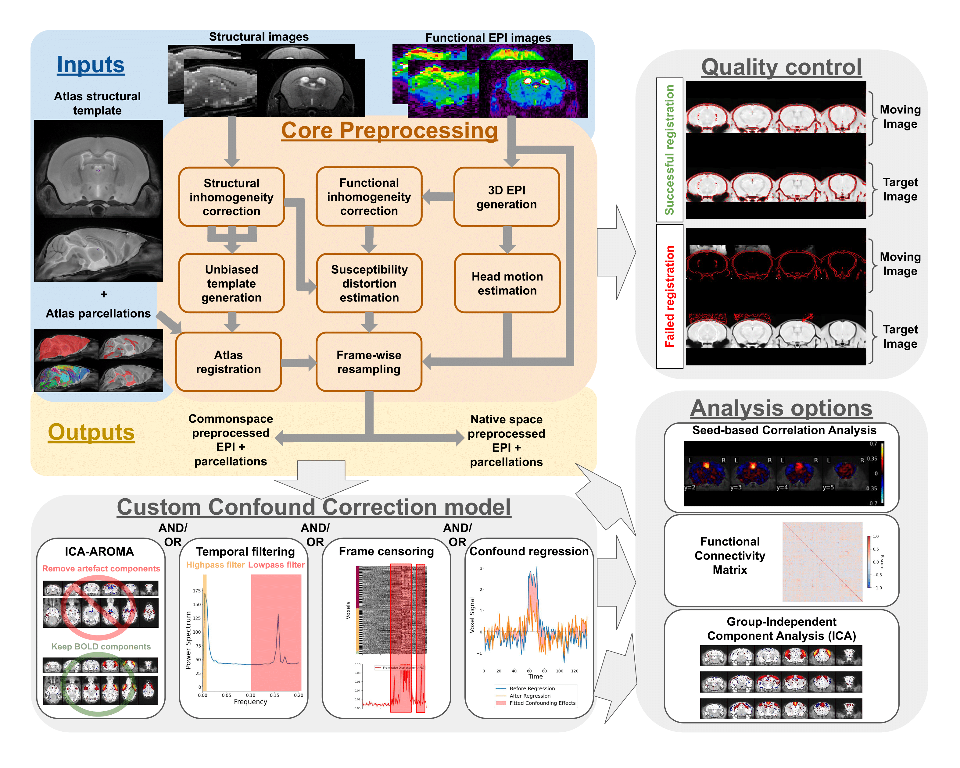
6 |
7 | ## What you can do with RABIES
8 |
9 | The primary purpose of RABIES is to provide rodent fMRI research with a standard, flexible, and reliable image processing platform. The package is complemented with informative data diagnostic features for confound characterization and encourages best practices for quality control and reproducibility. The RABIES software is structured into three main processing stages: **preprocessing**, **confound correction** and **analysis**.
10 |
11 | ### Preprocessing
12 | The preprocessing workflow regroups essential fMRI preprocessing steps prior to analysis. It includes a robust registration workflow with automatically-adapting parameters allowing to succesfully process diverse acquisition types (i.e. rodent species, scan field strength, coil type, ...), and can conduct the following preprocessing steps:
13 | - head motion correction
14 | - susceptibility distortion correction
15 | - resampling to native or common space
16 | - brain parcellation
17 | - slice timing correction (optional)
18 | - despiking (optional)
19 | - visual assessment of registration for quality control
20 |
21 | ### Confound correction
22 | Following preprocessing, a range of strategies to correct fMRI confounds (e.g. motion) can then be conducted within RABIES:
23 | - linear detrending
24 | - confound regression (with several options for nuisance regressors)
25 | - frequency filtering (highpass, lowpass, bandpass)
26 | - frame censoring (or scrubbing)
27 | - ICA-AROMA
28 | - spatial smoothing
29 |
30 | ### Analysis
31 | Simple resting-state connectivity analyses are made available after preprocessing and confound correction. RABIES also provides a 'data diagnosis' workflow, which generates several indices of data quality and potential confounds, and conversaly, aims to improve the correction of confounds and transparency with regards to data quality:
32 | - seed-based functional connectivity
33 | - whole-brain connectivity matrix
34 | - group-ICA
35 | - dual regression
36 | - data diagnosis
37 |
38 |
39 | ## Notes on software design
40 |
41 | **Nipype workflows**: The image processing pipelines are structured using the [Nipype library](https://nipype.readthedocs.io/en/latest/), which allows to build dynamic workflows in the form of a computational graph. Each node in the graph consists of a processing step, and the required inputs/outputs define the links between nodes. In addition to supporting code organization, Nipype workflows also handle several [plugin architectures](https://nipype.readthedocs.io/en/0.11.0/users/plugins.html) for parallel execution as well as memory management. The computational time to run the entire RABIES pipeline will vary substantially depending on data size, but for most uses, it will range **from a few hours to a day** when using proper computational resources and parallel execution.
42 |
43 | **Reproducible and transparent research**: RABIES aims to follow best practices for reproducible and transparent research, including the following:
44 | - open source code
45 | - standardized input data format with [BIDS](https://bids.neuroimaging.io/)
46 | - easily shared, automatically-generated visual outputs for quality control
47 | - containerized distribution of the software hosted on [Docker Hub](https://hub.docker.com/r/gabdesgreg/rabies) which can be downloaded via Docker and Apptainer platforms
48 |
49 | ## Citation
50 |
51 | **Citing RABIES**: Please cite the official publication [Desrosiers-Grégoire, et al. Nat Commun 15, 6708 (2024).](https://doi.org/10.1038/s41467-024-50826-8) when referencing the software.
52 |
53 | **Boilerplate**: a boilerplate summarizing the preprocessing and confound correction operations is automatically generated in the output folder. You can use the boilerplate to help describe your methods in a paper.
54 |
55 | ## License
56 | The [RABIES license](https://github.com/CoBrALab/RABIES/blob/master/LICENSE) allows for uses in academic and educational environments only. Commercial use requires a commercial license from CoBrALab ,
57 |
58 | ## Acknowledgements
59 | This software was developped by the [CoBrALab](https://cobralab.ca/), located at the Cerebral Imaging Center of the Douglas Mental Health University Institute, Montreal, Canada, in affiliation with McGill University, Montreal, Canada. This work was supported by funding from Healthy Brains, Healthy Lives (HBHL), the Fonds de recherche du Québec - Santé (FRQS) and - Nature et technologies (FRQNT), and the Natural Sciences and Engineering Research Council (NSERC) of Canada. [fMRIPrep](https://fmriprep.org/en/stable/) was an important inspirational source for this project, in particular with regards to best practices for software reproducibility and code design using Nipype. We also thank the organizers of [BrainHack School Montreal](https://school.brainhackmtl.org/), which guided the initial steps of this project in 2018.
60 |
61 |
62 | ## Ask for help
63 | If you need support in using the software or experience issues that are not documented, we'll provide support on the [Github discussion](https://github.com/CoBrALab/RABIES/discussions).
64 |
65 | ## Contributing to RABIES
66 |
67 | **Read our dedicated [documentation](https://rabies.readthedocs.io/en/latest/contributing.html)**
68 |
--------------------------------------------------------------------------------
/setup.py:
--------------------------------------------------------------------------------
1 | #!/usr/bin/env python
2 | # -*- coding: utf-8 -*-
3 |
4 | # Note: To use the 'upload' functionality of this file, you must:
5 | # $ pipenv install twine --dev
6 |
7 | import io
8 | import os
9 | import sys
10 | from shutil import rmtree
11 |
12 | from setuptools import Command, find_packages, setup
13 |
14 | # Package meta-data.
15 | NAME = 'rabies'
16 | DESCRIPTION = 'RABIES: Rodent Automated Bold Improvement of EPI Sequences.'
17 | URL = 'https://github.com/CoBrALab/RABIES'
18 | EMAIL = 'contact@cobralab.ca'
19 | AUTHOR = 'CoBrALab'
20 | REQUIRES_PYTHON = '>=3.9.0'
21 |
22 | # What packages are required for this module to be executed?
23 | REQUIRED = [
24 | # 'requests', 'maya', 'records',
25 | 'matplotlib>=3.3.4',
26 | 'nibabel>=3.2.1',
27 | 'nilearn>=0.7.1',
28 | 'nipype>=1.6.1',
29 | 'numpy>=1.20.1',
30 | 'pandas>=1.2.4',
31 | 'pathos>=0.2.7',
32 | 'pybids==0.16.3',
33 | 'scikit-learn>=0.24.1',
34 | 'scikit-image>=0.18.2',
35 | 'scipy>=1.8.1',
36 | 'seaborn>=0.11.1',
37 | 'simpleitk==2.0.2',
38 | 'qbatch==2.3',
39 | 'networkx<3',
40 | 'traits<7.0'
41 | ]
42 |
43 | # What packages are optional?
44 | EXTRAS = {
45 | # 'fancy feature': ['django'],
46 | }
47 |
48 | # The rest you shouldn't have to touch too much :)
49 | # ------------------------------------------------
50 | # Except, perhaps the License and Trove Classifiers!
51 | # If you do change the License, remember to change the Trove Classifier for that!
52 |
53 | here = os.path.abspath(os.path.dirname(__file__))
54 |
55 | # Import the README and use it as the long-description.
56 | # Note: this will only work if 'README.md' is present in your MANIFEST.in file!
57 | try:
58 | with io.open(os.path.join(here, 'README.md'), encoding='utf-8') as f:
59 | long_description = '\n' + f.read()
60 | except FileNotFoundError:
61 | long_description = DESCRIPTION
62 |
63 | # Load the package's __version__.py module as a dictionary.
64 | about = {}
65 | project_slug = NAME.lower().replace("-", "_").replace(" ", "_")
66 | with open(os.path.join(here, project_slug, '__version__.py')) as f:
67 | exec(f.read(), about)
68 |
69 | VERSION = about['__version__']
70 | DOWNLOAD_URL = (
71 | '{url}/archive/{ver}.tar.gz'.format(
72 | url=URL, ver=VERSION))
73 |
74 |
75 | class UploadCommand(Command):
76 | """Support setup.py upload."""
77 |
78 | description = 'Build and publish the package.'
79 | user_options = []
80 |
81 | @staticmethod
82 | def status(s):
83 | """Prints things in bold."""
84 | print('\033[1m{0}\033[0m'.format(s))
85 |
86 | def initialize_options(self):
87 | pass
88 |
89 | def finalize_options(self):
90 | pass
91 |
92 | def run(self):
93 | try:
94 | self.status('Removing previous builds…')
95 | rmtree(os.path.join(here, 'dist'))
96 | except OSError:
97 | pass
98 |
99 | self.status('Building Source and Wheel (universal) distribution…')
100 | os.system(
101 | '{0} setup.py sdist bdist_wheel --universal'.format(sys.executable))
102 |
103 | self.status('Uploading the package to PyPI via Twine…')
104 | os.system('twine upload dist/*')
105 |
106 | # self.status('Pushing git tags…')
107 | # os.system('git tag v{0}'.format(about['__version__']))
108 | # os.system('git push --tags')
109 |
110 | sys.exit()
111 |
112 |
113 | # Where the magic happens:
114 | setup(
115 | name=NAME,
116 | version=about['__version__'],
117 | description=DESCRIPTION,
118 | long_description=long_description,
119 | long_description_content_type='text/markdown',
120 | author=AUTHOR,
121 | author_email=EMAIL,
122 | python_requires=REQUIRES_PYTHON,
123 | url=URL,
124 | packages=find_packages(
125 | exclude=["tests", "*.tests", "*.tests.*", "tests.*"]),
126 | # If your package is a single module, use this instead of 'packages':
127 | # py_modules=['mypackage'],
128 |
129 | # entry_points={
130 | # 'console_scripts': ['mycli=mymodule:cli'],
131 | # },
132 | install_requires=REQUIRED,
133 | extras_require=EXTRAS,
134 | include_package_data=True,
135 | license='LICENSE',
136 | classifiers=[
137 | # Trove classifiers
138 | # Full list: https://pypi.python.org/pypi?%3Aaction=list_classifiers
139 | 'Intended Audience :: Science/Research',
140 | 'License :: Free for non-commercial use',
141 | 'Programming Language :: Python',
142 | 'Programming Language :: Python :: 3',
143 | 'Programming Language :: Python :: 3.6',
144 | 'Programming Language :: Python :: Implementation :: CPython',
145 | 'Programming Language :: Python :: Implementation :: PyPy'
146 | ],
147 | # $ setup.py publish support.
148 | cmdclass={
149 | 'upload': UploadCommand,
150 | },
151 | scripts=[
152 | 'scripts/rabies',
153 | 'scripts/gen_DSURQE_masks.py',
154 | 'scripts/install_DSURQE.sh',
155 | 'scripts/error_check_rabies.py',
156 | 'scripts/zeropad',
157 | 'scripts/preprocess_scripts/multistage_otsu_cor.py',
158 | 'scripts/preprocess_scripts/null_nonlin.sh',
159 | 'scripts/preprocess_scripts/plot_overlap.sh',
160 | 'scripts/preprocess_scripts/structural-preprocessing.sh',
161 | 'scripts/preprocess_scripts/EPI-preprocessing.sh',
162 | 'optimized_antsMultivariateTemplateConstruction/modelbuild.sh',
163 | 'optimized_antsMultivariateTemplateConstruction/modelbuild_averager.py',
164 | 'optimized_antsMultivariateTemplateConstruction/make-dumb-average.sh',
165 | 'minc-toolkit-extras/ants_generate_iterations.py',
166 | 'minc-toolkit-extras/antsRegistration_affine_SyN.sh',
167 | ]
168 | )
169 |
--------------------------------------------------------------------------------
/docs/confound_correction.md:
--------------------------------------------------------------------------------
1 | # Confound Correction pipeline
2 |
3 | (confound_pipeline_target)=
4 |
5 | 
6 |
7 |
8 | The workflow for confound correction regroups a broad set of standard tools from the human litterature. The implementation of each step is structured to follow best practices and prevent re-introduction of confounds, as recommended in {cite}`Power2014-yf` and {cite}`Lindquist2019-lq`. Importantly, each operation is optional (except detrending), and a set of operations can be selected to design a customized workflow. Optimal correction strategy can be dataset-specific, and ideally, should be tuned to address relevant quality issues identified within the dataset (see section on [data quality assessment](analysis_QC_target)).
9 |
10 | 1. **Frame censoring** (`--frame_censoring`): Frame censoring temporal masks are derived from FD and/or DVARS thresholds, and applied first on both BOLD timeseries before any other correction step to exclude signal spikes which may bias downstream corrections, in particular, detrending, frequency filtering and confound regression{cite}`Power2014-yf`.
11 | * Censoring with framewise displacement (see [definition](FD_target)): Apply frame censoring based on a framewise displacement threshold. The frames that exceed the given threshold, together with 1 back and 2 forward frames will be masked out{cite}`Power2012-ji`.
12 | * Censoring with DVARS (see [definition](DVARS_target)): The DVARS values are z-scored ($DVARS_Z = \frac{DVARS-\mu}{\sigma}$, where $\mu$ is the mean DVARS across time, and $\sigma$ the standard deviation), and frames with $|DVARS_Z|>2.5$ (i.e. above 2.5 standard deviations from the mean) are removed. Z-scoring and outlier detection is repeated within the remaining frames, iteratively, until no more outlier is detected, to obtained a final set of frames post-censoring.
13 | * `--match_number_timepoints` : This option can be selected to constrain each scan to retain the same final number of frames, to account for downstream impacts from unequal temporal degrees of freedom (tDOF) on analysis. To do so, a pre-set final number of frames is defined with `minimum_timepoint`, and a number of extra frames remaining post-censoring (taking into account edge removal in 5) ) is randomly selected and removed from the set.
14 |
15 | 2. **Detrending** (`--detrending_order`): Linear (or quadratic) trends are removed from timeseries. Detrended timeseries $\hat{Y}$ are obtained by performing ordinary-least square (OLS) linear regression,
16 | $$
17 | \beta = OLS(X,Y)
18 | $$
19 | $$
20 | \hat{Y} = Y - X\beta
21 | $$
22 | where Y is the timeseries and the predictors are $X = [intercept, time, time^2]$ ($time^2$ is included if removing quadratic trends).
23 |
24 | 3. **ICA-AROMA** (`--ica_aroma`): Cleaning of motion-related sources using the ICA-AROMA{cite}`Pruim2015-nm` classifier. The hard-coded human priors for anatomical masking and the linear coefficients for classification were adapted from the [original code](https://github.com/maartenmennes/ICA-AROMA) to function with rodent images. ICA-AROMA is applied prior to frequency filtering to remove further effects of motion than can result in ringing after filtering{cite}`Carp2013-uf,Pruim2015-nm`.
25 |
26 | 4. **Frequency filtering** (`--TR`/`--highpass`/`--lowpass`/`--edge_cutoff`):
27 | 1. Simulating censored timepoints: frequency filtering requires particular considerations when applied after frame censoring, since conventional filters cannot handle missing data (censoring results in missing timepoints). To address this issue, we implemented a method described in {cite}`Power2014-yf` allowing the simulation of data points while preserving the frequency composition of the data. This method relies on an adaptation of the Lomb-Scargle periodogram, which allows estimating the frequency composition of the timeseries despite missing data points, and from that estimation, missing timepoints can be simulated while preserving the frequency profile {cite}`Mathias2004-rt`.
28 | 2. Butterworth filter: Following the simulation, frequency filtering (highpass and/or lowpass) is applied using a 3rd-order Butterworth filter ([scipy.signal.butter](https://docs.scipy.org/doc/scipy/reference/generated/scipy.signal.butter.html)). If applying highpass, it is recommended to remove 30 seconds at each end of the timeseries using `--edge_cutoff` to account for edge artefacts following filtering{cite}`Power2014-yf`. After frequency filtering, the temporal mask from censoring is re-applied to remove simulated timepoints.
29 |
30 | (CR_target)=
31 | 5. **Confound regression** (`--conf_list`): For each voxel timeseries, a selected set of nuissance regressors (see [regressor options](regressor_target)) are modelled using OLS linear regression and their modelled contribution to the signal is removed. Regressed timeseries $\hat{Y}$ are obtained with
32 | $$\beta = OLS(X,Y)$$
33 | $$ Y_{CR} = X\beta $$
34 | $$ \hat{Y} = Y - Y_{CR} $$
35 | where $Y$ is the timeseries, $X$ is the set of nuisance timecourses and $Y_{CR}$ is the confound timeseries predicted from the model at each voxel ($Y_{CR}$ is a time by voxel 2D matrix).
36 |
37 | 6. **Intensity scaling** (`--image_scaling`): Voxel intensity values should be scaled to improve comparability between scans/datasets. The following options are provided:
38 | * Grand mean (**recommended**): Timeseries are divided by the mean intensity across the brain, and then multiplied by 100 to obtain percent BOLD deviations from the mean. The mean intensity of each voxel is derived from the $\beta$ coefficient from the intercept computed during **Detrending**.
39 | * Voxelwise mean: Same as grand mean, but each voxel is independently scaled by its own mean signal.
40 | * Global standard deviation: Timeseries are divided by the total standard deviation across all voxel timeseries.
41 | * Voxelwise standardization: Each voxel is divided by its standard deviation.
42 | * Homogenize variance voxelwise: if no scaling was already applied voxelwise (voxelwise mean or standardization), by selecting the option `--scale_variance_voxelwise`, timeseries are first scaled voxelwise by their standard deviation (yielding homogeneous variance distribution across voxels), and then re-scaled to preserve the original total standard deviation of the entire 4D timeseries (i.e. the global standard deviation does not change). Inhomogeneous variability distribution can be a [confound signature](quality_marker_target), thus this option may downscale their impact. `--scale_variance_voxelwise` can be applied in combination with grand mean scaling.
43 |
44 | 7. **Smoothing** (`--smoothing_filter`): Timeseries are spatially smoothed using a Gaussian smoothing filter ([nilearn.image.smooth_img](https://nilearn.github.io/dev/modules/generated/nilearn.image.smooth_img.html)).
45 |
46 |
47 | ## rabies.confound_correction_pkg.confound_correction.init_confound_correction_wf [[source code](https://github.com/CoBrALab/RABIES/blob/master/rabies/confound_correction_pkg/confound_correction.py)]
48 |
49 | ```{literalinclude} ../rabies/confound_correction_pkg/confound_correction.py
50 | :start-after: confound_wf_head_start
51 | :end-before: confound_wf_head_end
52 | ```
--------------------------------------------------------------------------------
/rabies/preprocess_pkg/resampling.py:
--------------------------------------------------------------------------------
1 | from nipype.pipeline import engine as pe
2 | from nipype.interfaces import utility as niu
3 |
4 | from .bold_ref import init_bold_reference_wf
5 | from ..utils import ResampleVolumes,ResampleMask
6 |
7 | def init_bold_preproc_trans_wf(opts, resampling_dim, name='bold_native_trans_wf'):
8 | # bold_resampling_head_start
9 | """
10 | This workflow carries out the resampling of the original EPI timeseries into preprocessed timeseries.
11 | This is accomplished by applying at each frame a combined transform which accounts for previously estimated
12 | motion correction and susceptibility distortion correction, together with the alignment to common space (the
13 | exact combination of transforms depends on which anatomical preprocessed timeseries are resampled into).
14 | All transforms are concatenated into a single resampling operation to mitigate interpolation effects from
15 | repeated resampling.
16 |
17 | Command line interface parameters:
18 | Resampling Options:
19 | The following options allow to resample the voxel dimensions for the preprocessed EPIs
20 | or for the anatomical images during registration.
21 | The resampling syntax must be 'dim1xdim2xdim3' (in mm), follwing the RAS axis convention
22 | (dim1=Right-Left, dim2=Anterior-Posterior, dim3=Superior-Inferior). If 'inputs_defined'
23 | is provided instead of axis dimensions, the original dimensions are preserved.
24 |
25 | --nativespace_resampling NATIVESPACE_RESAMPLING
26 | Can specify a resampling dimension for the nativespace fMRI outputs.
27 | (default: inputs_defined)
28 |
29 | --commonspace_resampling COMMONSPACE_RESAMPLING
30 | Can specify a resampling dimension for the commonspace fMRI outputs.
31 | (default: inputs_defined)
32 |
33 | Workflow:
34 | parameters
35 | opts: command line interface parameters
36 | resampling_dim: specify the desired output voxel dimensions after resampling
37 |
38 | inputs
39 | name_source: a reference file for naming the output
40 | bold_file: the EPI timeseries to resample
41 | motcorr_params: the motion correction parameters
42 | transforms_list: a list of transforms to apply onto EPI timeseries, including
43 | susceptibility distortion correction and resampling to common space
44 | inverses: a list specifying whether the inverse affine transforms should be
45 | applied in transforms_list
46 | ref_file: a reference image in the targetted space for resampling. Should be the structural
47 | image from the same session if outputs are in native space, or the atlas template for
48 | outputs in common space
49 |
50 | outputs
51 | bold: the preprocessed EPI timeseries
52 | bold_ref: a volumetric 3D EPI generated from the preprocessed timeseries
53 | """
54 | # bold_resampling_head_end
55 |
56 | workflow = pe.Workflow(name=name)
57 | inputnode = pe.Node(niu.IdentityInterface(fields=[
58 | 'name_source', 'bold_file', 'motcorr_params', 'transforms_list', 'inverses', 'ref_file']),
59 | name='inputnode'
60 | )
61 |
62 | outputnode = pe.Node(
63 | niu.IdentityInterface(
64 | fields=['bold', 'bold_ref']),
65 | name='outputnode')
66 |
67 | bold_transform = pe.Node(ResampleVolumes(
68 | rabies_data_type=opts.data_type, clip_negative=True), name='bold_transform', mem_gb=4*opts.scale_min_memory)
69 | bold_transform.inputs.apply_motcorr = (not opts.apply_slice_mc)
70 | bold_transform.inputs.resampling_dim = resampling_dim
71 | bold_transform.inputs.interpolation = opts.interpolation
72 | bold_transform.plugin_args = {
73 | 'qsub_args': f'-pe smp {str(3*opts.min_proc)}', 'overwrite': True}
74 |
75 | # Generate a new BOLD reference
76 | bold_reference_wf = init_bold_reference_wf(opts=opts)
77 |
78 | workflow.connect([
79 | (inputnode, bold_transform, [
80 | ('bold_file', 'in_file'),
81 | ('motcorr_params', 'motcorr_params'),
82 | ('transforms_list', 'transforms'),
83 | ('inverses', 'inverses'),
84 | ('ref_file', 'ref_file'),
85 | ('name_source', 'name_source'),
86 | ]),
87 | (bold_transform, bold_reference_wf, [('resampled_file', 'inputnode.bold_file')]),
88 | (bold_transform, outputnode, [('resampled_file', 'bold')]),
89 | (bold_reference_wf, outputnode, [
90 | ('outputnode.ref_image', 'bold_ref')]),
91 | ])
92 |
93 | return workflow
94 |
95 |
96 | def init_mask_preproc_trans_wf(opts, name='mask_native_trans_wf'):
97 | # mask_resampling_head_start
98 | """
99 | This workflow carries the resampling of brain masks and labels from the reference
100 | atlas onto the preprocessed EPI timeseries.
101 |
102 | Workflow:
103 | parameters
104 | opts: command line interface parameters
105 |
106 | inputs
107 | name_source: a reference file for naming the output
108 | ref_file: a reference image in the targetted space for resampling. Should be the structural
109 | image from the same session if outputs are in native space, or the atlas template for
110 | outputs in common space
111 | mask_transforms_list: the list of transforms to apply onto the atlas parcellations
112 | to overlap with the EPI
113 | mask_inverses: a list specifying whether the inverse affine transforms should be
114 | applied in mask_transforms_list
115 |
116 | outputs
117 | brain_mask: the brain mask resampled onto preprocessed EPI timeseries
118 | WM_mask: the WM mask resampled onto preprocessed EPI timeseries
119 | CSF_mask: the CSF mask resampled onto preprocessed EPI timeseries
120 | vascular_mask: the vascular mask resampled onto preprocessed EPI timeseries
121 | labels: the atlas labels resampled onto preprocessed EPI timeseries
122 | """
123 | # mask_resampling_head_end
124 |
125 | workflow = pe.Workflow(name=name)
126 | inputnode = pe.Node(niu.IdentityInterface(fields=[
127 | 'name_source', 'ref_file',
128 | 'mask_transforms_list', 'mask_inverses'
129 | ]),
130 | name='inputnode'
131 | )
132 |
133 | outputnode = pe.Node(
134 | niu.IdentityInterface(
135 | fields=['brain_mask', 'WM_mask', 'CSF_mask', 'vascular_mask', 'labels']),
136 | name='outputnode')
137 |
138 | # integrate a node to resample each mask, only if the mask exists
139 | for opt_key in ['brain_mask', 'WM_mask','CSF_mask','vascular_mask','labels']:
140 | opt_file = getattr(opts, opt_key)
141 | if opt_file is not None:
142 | mask_to_EPI = pe.Node(ResampleMask(), name=opt_key+'_resample')
143 | mask_to_EPI.inputs.name_suffix = opt_key+'_resampled'
144 | mask_to_EPI.inputs.mask_file = str(opt_file)
145 |
146 | workflow.connect([
147 | (inputnode, mask_to_EPI, [
148 | ('name_source', 'name_source'),
149 | ('mask_transforms_list', 'transforms'),
150 | ('mask_inverses', 'inverses'),
151 | ('ref_file', 'ref_file'),
152 | ]),
153 | (mask_to_EPI, outputnode, [
154 | ('resampled_file', opt_key)]),
155 | ])
156 |
157 | return workflow
158 |
--------------------------------------------------------------------------------
/docs/preprocessing.md:
--------------------------------------------------------------------------------
1 | # Preprocessing Pipeline
2 | 
3 |
4 | The preprocessing of fMRI scans prior to analysis consists of, at minimum, the anatomical alignment of scans to a common space, head realignment to correct for motion, and the correction of susceptibility distortions arising from the echo-planar imaging (EPI) acquisition of functional scans. The core preprocessing pipeline in RABIES carries each of these steps with state-of-the-art processing tools and techniques.
5 |
6 | To conduct common space alignment, structural images, which were acquired along the EPI scans, are initially corrected for inhomogeneities (**Structural inhomogeneity correction**) and then registered together to allow the alignment of different MRI acquisitions. This registration is conducted by generating an unbiased data-driven template (**Unbiased template generation**) through the iterative non-linear registration of each image to the dataset consensus average, where the average gets updated at each iteration to provide an increasingly representative dataset template (; {cite}`Avants2011-av`). The finalized template after the last iteration provides a representative alignment of each MRI session to a template that shares the acquisition properties of the dataset (e.g. brain shape, FOV, anatomical contrast, ...), making it a stable registration target for cross-subject alignment. This newly-generated unbiased template is then itself registered to an external reference atlas to provide both an anatomical segmentation and a common space comparable across studies defined from the provided reference atlas (**Atlas registration**).
7 |
8 | The remaining preprocessing involves the EPI image. A volumetric EPI image is first derived using a trimmed mean across the EPI frames, after an initial motion realignment step (**3D EPI generation**). Using this volumetric EPI as a target, the head motion parameters are estimated by realigning each EPI frame to the target using a rigid registration (**Head motion estimation**). To correct for EPI susceptibility distortions, the volumetric EPI is first subjected to an inhomogeneity correction step (**Functional inhomogeneity correction**), and then registered non-linearly to the anatomical scan from the same MRI session, which allows to calculate the required geometrical transforms for recovering brain anatomy {cite}`Wang2017-ci` (**Susceptibility distortion estimation**). Finally, after calculating the transformations required to correct for head motion and susceptibility distortions, both transforms are concatenated into a single resampling operation (avoiding multiple resampling) which is applied at each EPI frame, generating the preprocessed EPI timeseries in native space {cite}`Esteban2019-rs` (**Frame-wise resampling**). Preprocessed timeseries in common space are also generated by further concatenating the transforms allowing resampling to the reference atlas.
9 |
10 | The workflow of the RABIES preprocessing pipeline is summarized in the diagram above, and each preprocessing module is further described below.
11 |
12 | ## Structural inhomogeneity correction
13 | 
14 | **Figure:** displays steps of inhomogeneity correction for the structural image.
15 |
16 | ### rabies.preprocess_pkg.inho_correction.init_inho_correction_wf [[source code](https://github.com/CoBrALab/RABIES/blob/master/rabies/preprocess_pkg/inho_correction.py)]
17 |
18 | ```{literalinclude} ../rabies/preprocess_pkg/inho_correction.py
19 | :start-after: inho_correction_head_start
20 | :end-before: inho_correction_head_end
21 | ```
22 |
23 | ## Common space alignment (i.e. Unbiased template generation + Atlas registration)
24 | 
25 | **Figure:** displays the overlap between a structural scan (top) and the dataset-generated unbiased template (bottom).
26 | 
27 | **Figure:** displays the overlap between the unbiased template (top) and the reference atlas template (bottom).
28 |
29 | ### rabies.preprocess_pkg.commonspace_reg.init_commonspace_reg_wf [[source code](https://github.com/CoBrALab/RABIES/blob/master/rabies/preprocess_pkg/commonspace_reg.py)]
30 | ```{literalinclude} ../rabies/preprocess_pkg/commonspace_reg.py
31 | :start-after: commonspace_wf_head_start
32 | :end-before: commonspace_wf_head_end
33 | ```
34 |
35 | (3D_EPI_target)=
36 | ## 3D EPI generation
37 | ### rabies.preprocess_pkg.bold_ref.init_bold_reference_wf [[source code](https://github.com/CoBrALab/RABIES/blob/master/rabies/preprocess_pkg/bold_ref.py)]
38 |
39 | ```{literalinclude} ../rabies/preprocess_pkg/bold_ref.py
40 | :start-after: gen_bold_ref_head_start
41 | :end-before: gen_bold_ref_head_end
42 | ```
43 |
44 | ## Head motion estimation
45 | 
46 | **Figure:** example of the 6 motion parameters.
47 |
48 | ### rabies.preprocess_pkg.hmc.init_bold_hmc_wf [[source code](https://github.com/CoBrALab/RABIES/blob/master/rabies/preprocess_pkg/hmc.py)]
49 |
50 | ```{literalinclude} ../rabies/preprocess_pkg/hmc.py
51 | :start-after: hmc_wf_head_start
52 | :end-before: hmc_wf_head_end
53 | ```
54 |
55 | ### rabies.preprocess_pkg.hmc.EstimateMotionParams [[source code](https://github.com/CoBrALab/RABIES/blob/master/rabies/preprocess_pkg/hmc.py)]
56 |
57 | ```{literalinclude} ../rabies/preprocess_pkg/hmc.py
58 | :start-after: motion_param_head_start
59 | :end-before: motion_param_head_end
60 | ```
61 |
62 | ## Functional inhomogeneity correction
63 | 
64 | **Figure:** displays steps of inhomogeneity correction for the volumetric EPI.
65 |
66 | The workflow is the same as the **structural inhomogeneity correction**.
67 |
68 | ## Susceptibility distortion estimation
69 | 
70 | **Figure:** displays the overlap between the volumetric EPI (top) and structural image (bottom).
71 |
72 | ### rabies.preprocess_pkg.registration.init_cross_modal_reg_wf [[source code](https://github.com/CoBrALab/RABIES/blob/master/rabies/preprocess_pkg/registration.py)]
73 |
74 | ```{literalinclude} ../rabies/preprocess_pkg/registration.py
75 | :start-after: cross_modal_reg_head_start
76 | :end-before: cross_modal_reg_head_end
77 | ```
78 |
79 | ## Frame-wise resampling
80 |
81 | ### rabies.preprocess_pkg.resampling.init_bold_preproc_trans_wf [[source code](https://github.com/CoBrALab/RABIES/blob/master/rabies/preprocess_pkg/resampling.py)]
82 |
83 | ```{literalinclude} ../rabies/preprocess_pkg/resampling.py
84 | :start-after: bold_resampling_head_start
85 | :end-before: bold_resampling_head_end
86 | ```
87 |
88 | ## Resampling of masks and labels
89 |
90 | ### rabies.preprocess_pkg.resampling.init_mask_preproc_trans_wf [[source code](https://github.com/CoBrALab/RABIES/blob/master/rabies/preprocess_pkg/resampling.py)]
91 |
92 | ```{literalinclude} ../rabies/preprocess_pkg/resampling.py
93 | :start-after: mask_resampling_head_start
94 | :end-before: mask_resampling_head_end
95 | ```
96 |
97 | ## Adapted workflow without structural scans (i.e. --bold_only)
98 | Structural scans are recommended, but not required to complete preprocessing with RABIES. An alternative workflow is also implemented to preprocess a input dataset which contains only EPI functional images, and can be selected with the `--bold_only` option. In this alternative workflow, the volumetric EPI corrected for inhomogeneity during **Functional inhomogeneity correction** replaces the structural image for the purpose of common space alignment, and is thus used for generating the unbiased template, in turn, this template is registered to the reference atlas. This final registration to the atlas accounts for estimation of susceptibility distortions instead of the registration to a structural image from the same MRI session.
99 | If using the RABIES default mouse atlas, the default template is changed to a EPI reference template, which offers a more robust target for EPI registration than a structural image as reference template.
100 |
--------------------------------------------------------------------------------
/scripts/preprocess_scripts/EPI-preprocessing.sh:
--------------------------------------------------------------------------------
1 | #!/bin/bash
2 | #Preprocessing script for mouse brains, using Dorr-steadman template and MINC files converted from DICOM from Paravision 5.x
3 | # It seems that this script is only used during inho_correction, not for the main registration
4 |
5 | #If using conversion from PV6, might need to remove the volflip -y command
6 |
7 |
8 | set -euo pipefail
9 | set -x
10 |
11 | calc(){ awk "BEGIN { print "$*" }"; }
12 |
13 | tmpdir=$(mktemp -d)
14 |
15 | input=$1
16 | output=$2
17 | modelfile=$3
18 | modelmask=$4
19 | reg_option=$5
20 | multi_otsu=$6
21 | otsu_thresh=$7
22 |
23 | # convert inputs to mnc
24 | nii2mnc ${input} ${tmpdir}/input.mnc
25 | input=${tmpdir}/input.mnc
26 | nii2mnc ${modelfile} ${tmpdir}/modelfile.mnc
27 | modelfile=${tmpdir}/modelfile.mnc
28 | nii2mnc ${modelmask} ${tmpdir}/modelmask.mnc
29 | modelmask=${tmpdir}/modelmask.mnc
30 |
31 | #Calculate Maximum FOV using the foreground/background of the fixed image
32 | ThresholdImage 3 ${modelfile} ${tmpdir}/bgmask.h5 1e-12 Inf 1 0
33 | ThresholdImage 3 ${modelfile} ${tmpdir}/otsu.h5 Otsu 4 ${tmpdir}/bgmask.h5
34 | ThresholdImage 3 ${tmpdir}/otsu.h5 ${tmpdir}/otsu.h5 2 Inf 1 0
35 | LabelGeometryMeasures 3 ${tmpdir}/otsu.h5 none ${tmpdir}/geometry.csv
36 | fixed_maximum_resolution=$(python -c "print(max([ a*b for a,b in zip( [ a-b for a,b in zip( [float(x) for x in \"$(tail -1 ${tmpdir}/geometry.csv | cut -d, -f 14,16,18)\".split(\",\") ],[float(x) for x in \"$(tail -1 ${tmpdir}/geometry.csv | cut -d, -f 13,15,17)\".split(\",\") ])],[abs(x) for x in [float(x) for x in \"$(PrintHeader ${modelfile} 1)\".split(\"x\")]])]))")
37 |
38 | origdistance=$fixed_maximum_resolution
39 | distance=${origdistance}
40 | levels=4
41 | cycles=3
42 | iters=100
43 | lambda=2e-6
44 | shrink=4.0
45 | fwhm=0.1
46 | stop=1e-5
47 |
48 | do_correct() {
49 | distance=${origdistance}
50 | j=0
51 | while (( j < levels )); do
52 | i=0
53 | while (( i < cycles )); do
54 | nu_correct -clobber -normalize_field \
55 | -stop ${stop} -distance ${distance} -iterations ${iters} -fwhm ${fwhm} -shrink ${shrink} -lambda ${lambda} \
56 | -mask ${tmpdir}/weight.mnc ${n3input} ${tmpdir}/corrected_${distance}_${i}.mnc
57 | n3input=${tmpdir}/corrected_${distance}_${i}.mnc
58 | ((++i))
59 | done
60 | distance=$(calc ${distance}/2)
61 | ((++j))
62 | done
63 |
64 | }
65 |
66 |
67 | minc_modify_header $input -sinsert :history=''
68 |
69 | #Forceably convert to MINC2, and clamp range to avoid negative numbers, rescale to 0-65535
70 | mincconvert -2 ${input} ${tmpdir}/originput.mnc
71 | #Rescale initial data into entirely positive range (fix for completely negative data)
72 | ImageMath 3 ${tmpdir}/originput.mnc RescaleImage ${tmpdir}/originput.mnc 0 65535
73 |
74 |
75 | #Construct Otsu Mask of entire image
76 | input=${tmpdir}/originput.mnc
77 |
78 | #Construct Otsu Mask of entire image
79 | if [ "$multi_otsu" = true ]; then
80 | multistage_otsu_cor.py ${tmpdir}/originput.mnc ${tmpdir} $origdistance
81 | n3input=${tmpdir}/multistage_corrected.mnc
82 | ThresholdImage 3 ${input} ${tmpdir}/bgmask.mnc 1e-12 Inf 1 0
83 | cp ${tmpdir}/mask1234.mnc ${tmpdir}/weight.mnc
84 | do_correct
85 | cp $n3input ${tmpdir}/precorrect.mnc
86 | n3input=${tmpdir}/precorrect.mnc
87 |
88 | else
89 | ImageMath 3 ${tmpdir}/originput.mnc PadImage ${tmpdir}/originput.mnc 20
90 |
91 | ThresholdImage 3 ${input} ${tmpdir}/bgmask.mnc 1e-12 Inf 1 0
92 | ThresholdImage 3 ${input} ${tmpdir}/weight.mnc Otsu 4 ${tmpdir}/bgmask.mnc
93 | ThresholdImage 3 ${tmpdir}/weight.mnc ${tmpdir}/weight.mnc $otsu_thresh Inf 1 0
94 | iMath 3 ${tmpdir}/weight.mnc ME ${tmpdir}/weight.mnc 1 1 ball 1
95 | ImageMath 3 ${tmpdir}/weight.mnc GetLargestComponent ${tmpdir}/weight.mnc
96 | iMath 3 ${tmpdir}/weight.mnc MD ${tmpdir}/weight.mnc 1 1 ball 1
97 | ExtractRegionFromImageByMask 3 ${input} ${tmpdir}/repad.mnc ${tmpdir}/weight.mnc 1 10
98 | ExtractRegionFromImageByMask 3 ${tmpdir}/originput.mnc ${tmpdir}/repad_orig.mnc ${tmpdir}/weight.mnc 1 10
99 | mv -f ${tmpdir}/repad_orig.mnc ${tmpdir}/originput.mnc
100 | mv -f ${tmpdir}/repad.mnc ${input}
101 | ThresholdImage 3 ${input} ${tmpdir}/bgmask.mnc 1e-12 Inf 1 0
102 | mincresample -like ${input} -keep -near -labels ${tmpdir}/weight.mnc ${tmpdir}/weight2.mnc
103 | mv -f ${tmpdir}/weight2.mnc ${tmpdir}/weight.mnc
104 |
105 | n3input=${tmpdir}/originput.mnc
106 | do_correct
107 |
108 | for file in ${tmpdir}/*imp; do
109 | echo nu_evaluate -clobber -mapping ${file} -mask ${tmpdir}/weight.mnc -field ${tmpdir}/$(basename $file .imp)_field.mnc ${input} ${tmpdir}/$(basename $file .imp).mnc
110 | done | parallel
111 |
112 | mincmath -clobber -mult ${tmpdir}/*field.mnc ${tmpdir}/precorrect_field_combined.mnc
113 | mincmath -clobber -copy_header -zero -div ${tmpdir}/originput.mnc ${tmpdir}/precorrect_field_combined.mnc ${tmpdir}/precorrect.mnc
114 | fi
115 |
116 | if [ $reg_option == 'Rigid' ]; then
117 | reg_type="--linear-type rigid --skip-nonlinear"
118 | antsRegistration_affine_SyN.sh $reg_type --convergence 1e-7 \
119 | ${tmpdir}/precorrect.mnc ${modelfile} ${tmpdir}/tomodel
120 |
121 | antsApplyTransforms -d 3 -i ${modelmask} -t [ ${tmpdir}/tomodel0_GenericAffine.xfm,1 ] \
122 | -o ${tmpdir}/newmask.mnc -n GenericLabel -r ${n3input} --verbose
123 |
124 | elif [ $reg_option == 'Affine' ]; then
125 | reg_type="--linear-type affine --skip-nonlinear"
126 | antsRegistration_affine_SyN.sh $reg_type --convergence 1e-7 \
127 | ${tmpdir}/precorrect.mnc ${modelfile} ${tmpdir}/tomodel
128 |
129 | antsApplyTransforms -d 3 -i ${modelmask} -t [ ${tmpdir}/tomodel0_GenericAffine.xfm,1 ] \
130 | -o ${tmpdir}/newmask.mnc -n GenericLabel -r ${n3input} --verbose
131 |
132 | elif [ $reg_option == 'SyN' ]; then
133 | reg_type="--linear-type affine"
134 | antsRegistration_affine_SyN.sh $reg_type --convergence 1e-7 \
135 | ${tmpdir}/precorrect.mnc ${modelfile} ${tmpdir}/tomodel
136 |
137 | antsApplyTransforms -d 3 -i ${modelmask} -t [ ${tmpdir}/tomodel0_GenericAffine.xfm,1 ] -t ${tmpdir}/tomodel1_inverse_NL.xfm \
138 | -o ${tmpdir}/newmask.mnc -n GenericLabel -r ${n3input} --verbose
139 |
140 | fi
141 |
142 | if [ $reg_option == 'no_reg' ]; then
143 | cp ${tmpdir}/precorrect.mnc ${tmpdir}/correct.mnc
144 | else
145 |
146 | iMath 3 ${tmpdir}/newmask.mnc MD ${tmpdir}/newmask.mnc 1 1 ball 1
147 | ThresholdImage 3 ${n3input} ${tmpdir}/weight.mnc Otsu 4 ${tmpdir}/newmask.mnc
148 | #ThresholdImage 3 ${tmpdir}/weight.mnc ${tmpdir}/weight.mnc 2 Inf 1 0
149 | ThresholdImage 3 ${tmpdir}/weight.mnc ${tmpdir}/weight.mnc $otsu_thresh Inf 1 0
150 |
151 | ImageMath 3 ${tmpdir}/weight.mnc m ${tmpdir}/newmask.mnc ${tmpdir}/weight.mnc
152 | iMath 3 ${tmpdir}/weight.mnc ME ${tmpdir}/weight.mnc 1 1 ball 1
153 | ImageMath 3 ${tmpdir}/weight.mnc GetLargestComponent ${tmpdir}/weight.mnc
154 | iMath 3 ${tmpdir}/weight.mnc MD ${tmpdir}/weight.mnc 1 1 ball 1
155 | mincresample -like ${input} -keep -near -labels ${tmpdir}/weight.mnc ${tmpdir}/weight2.mnc
156 | mv -f ${tmpdir}/weight2.mnc ${tmpdir}/weight.mnc
157 |
158 | n3input=${tmpdir}/precorrect.mnc
159 | do_correct
160 |
161 | if [ "$multi_otsu" = true ]; then
162 | cp $n3input ${tmpdir}/correct.mnc
163 | else
164 | for file in ${tmpdir}/*imp; do
165 | echo nu_evaluate -clobber -mapping ${file} -mask ${tmpdir}/weight.mnc -field ${tmpdir}/$(basename $file .imp)_field.mnc ${input} ${tmpdir}/$(basename $file .imp).mnc
166 | done | parallel
167 |
168 | mincmath -clobber -mult ${tmpdir}/*field.mnc ${tmpdir}/precorrect_field_combined.mnc ${tmpdir}/field_final.mnc
169 | mincmath -clobber -copy_header -zero -div ${tmpdir}/originput.mnc ${tmpdir}/field_final.mnc ${tmpdir}/correct.mnc
170 | fi
171 |
172 | fi
173 |
174 | ExtractRegionFromImageByMask 3 ${tmpdir}/correct.mnc ${tmpdir}/recrop.mnc ${tmpdir}/weight.mnc 1 10
175 | mv -f ${tmpdir}/recrop.mnc ${tmpdir}/correct.mnc
176 | mincresample -keep -near -like ${tmpdir}/correct.mnc ${tmpdir}/weight.mnc ${tmpdir}/weight2.mnc
177 | mv -f ${tmpdir}/weight2.mnc ${tmpdir}/weight.mnc
178 |
179 | # reconvert to .nii
180 | mnc2nii ${tmpdir}/correct.mnc ${tmpdir}/correct.nii
181 | mnc2nii ${tmpdir}/weight.mnc ${tmpdir}/weight.nii
182 | mnc2nii ${tmpdir}/precorrect.mnc ${tmpdir}/init_denoise.nii
183 | gzip ${tmpdir}/*.nii
184 | cp ${tmpdir}/correct.nii.gz $(dirname ${output})/$(basename ${output} .nii.gz).nii.gz
185 | cp ${tmpdir}/weight.nii.gz $(dirname ${output})/$(basename ${output} .nii.gz)_mask.nii.gz
186 | cp ${tmpdir}/init_denoise.nii.gz $(dirname ${output})/$(basename ${output} .nii.gz)_init_denoise.nii.gz
187 |
188 | rm -rf ${tmpdir}
189 |
--------------------------------------------------------------------------------
/docs/analysis_QC.md:
--------------------------------------------------------------------------------
1 | # Data quality assessment
2 |
3 | (analysis_QC_target)=
4 |
5 | ```{toctree}
6 | ---
7 | maxdepth: 3
8 | ---
9 | nested_docs/scan_diagnosis.md
10 | nested_docs/distribution_plot.md
11 | nested_docs/group_stats.md
12 | nested_docs/optim_CR.md
13 | ```
14 |
15 | Data quality can have serious impacts on analysis outcomes, leading to false findings. Rodent imaging can suffer from spurious effects on connectivity measures if potential confounds are not well accounted for, or acquisition factors, such as anesthesia levels, can influence network activity {cite}`Desrosiers-Gregoire2024-ou,Grandjean2020-fa`. To support interpretability, troubleshooting and reproducible research, RABIES includes a set of reports for conducting data quality assessment in individual scans and conducting quality control prior to network analysis at the group level. The reports are designed most specifically to evaluate the detectability of canonical brain networks and the impact of potential confounds (motion, physiological instabilities, and more).
16 |
17 | This page describes how to generate the reports, our guidelines for conducting quality network of network analysis, and how to include those reports in a publication.
18 |
19 | ## Generating the reports
20 |
21 | At the analysis stage of the pipeline, the `--data_diagnosis` option can be selected to generate the data quality reports. To generate the report, ICA components must also be provided with `--prior_maps` and a set of components corresponding to confounds must be selected using `--conf_prior_idx` (see further details below). Connectivity can be evaluated for both dual regression and seed-based connectivity:
22 | * **For [dual regression](DR_target)**: dual regression is always conducted using the set components from `--prior_maps`, since certain features are derived from confound components defined in `--conf_prior_idx`. On the other hand, connectivity will be evaluated in the reports for each network included in `--bold_prior_idx`.
23 | * **For [seed-based connectivity](SBC_target)**: reports will be generated for each seed provided to `--seed_list`. However, each seed needs to be supplemented with a reference network map (a 3D Nifti file for each seed, provided with `--seed_prior_list`) which should represent the expected connectivity for the canonical network corresponding to that seed.
24 |
25 | The set of reports are generated in the `data_diagnosis_datasink/` (details [here](diagnosis_datasink_target)). The interpretation of each report is described within its dedicated documentation page, and include:
26 |
27 | * [Spatiotemporal diagnosis](diagnosis_target): this qualitative report generated for each scan regroups a set of temporal and spatial features allowing to characterize the specific origin of data quality issues.
28 | * [Distribution plots](dist_plot_target): quantitative report displaying the distribution of scans along measures of: specificity of network connectivity, network amplitude (for dual regression), and confound measures. Visualizing the dataset distribution can help identify outliers.
29 | * [Group statistics](group_stats_target): for a given network, this group-level report regroups brain maps for visualizing cross-scan variability in connectivity and the group-wise correlation between connectivity and confounds.
30 |
31 | ### Classification of group ICA components
32 |
33 | Ideally, the ICA components should be derived directly from the dataset analyzed by using [group ICA](ICA_target), although a [pre-computed set](https://zenodo.org/record/5118030/files/melodic_IC.nii.gz) is available by default. Newly-generated components must be visually inspected to identify the set of components corresponding to confound sources (which is inputted with `--conf_prior_idx`). This can be done by visualizing the group_melodic.ica/melodic_IC.nii.gz file, or using the automatically-generated FSL report in group_melodic.ica/report. Similarly, components corresponding to networks of interest can be identified and inputted with `--bold_prior_idx`.
34 |
35 | Classifying components requires careful considerations, and we recommend a conservative inclusion (i.e. not every components need to be classified, only include components which have clear feature delineating a network or a confound). Consult {cite}`Zerbi2015-nl` or {cite}`Desrosiers-Gregoire2024-ou` for more information on classifying ICA components in rodents, or the [pre-computed set](https://zenodo.org/record/5118030/files/melodic_IC.nii.gz) can be consulted as reference (the defaults for `--bold_prior_idx` and `--conf_prior_idx` correspond to the classification of these components).
36 |
37 | ## Guidelines for analysis quality control
38 |
39 | 
40 |
41 | Below are our recommendations for how the set of quality reports can be used identify and control for the impact of data quality issues on downstream group analysis. Although the reports may be used for a breadth of applications, these guidelines are formulated most specifically for a standard resting-state fMRI design aiming to compare network connectivity between subjects or groups. In particular, the following guidelines aim to identify features of spurious or absent connectivity, remove scans where these features are prominent to avoid false results (e.g. connectivity difference is driven by motion), and determine whether these issues may confound group statistics.
42 |
43 | 1. Inspect the [spatiotemporal diagnosis](diagnosis_target) for each scan. Particular attention should be given to the 4 main quality markers defining [categories of scan quality](quality_marker_target), and whether features of spurious or absent connectivity are prominent.
44 | 2. If spurious or absent connectivity is prominent in a subset of scans, these scans should be detected and removed to mitigate false results. This is done by setting thresholds using `--scan_QC_thresholds` for scan-level measures of network specificity and confound correlation. These measures are documented in the [distribution plots](dist_plot_target), and the specific measures for each scan ID can be consulted in the CSV file accompanying the plot. Using this CSV file, sensible threshold values can be selected for delineating scans with spurious or absent connectivity. Additionally, for dual regression analysis, `--scan_QC_thresholds` can be used to automatically detect and remove scans which present outlier values in network amplitude, which can be an indicator of spurious connectivity {cite}`Nickerson2017-gq`. By applying `--scan_QC_thresholds`, these scans won't be included for generating the group statistical report (thus the reports must re-generated after defining `--scan_QC_thresholds`).
45 | 3. Finally, the [group statistical report](group_stats_target) can be consulted to identify the main driven of variability in connectivity across scans, and whether it relates primarily to network activity or to confounds.
46 |
47 | If significant issues are found from this evaluation, the design of the confound correction stage may be revisited to improve quality outcomes (see [dedicated documentation](optim_CR)).
48 |
49 | **Disclaimer**: Although these guidelines are meant to support identifying analysis pitfalls and improve research transparency, they are not meant to be prescriptive. The judgement of the experimenter is paramount in the adopting adequate practices (e.g. network detectability may not always be expected, if studying the impact of anesthesia or inspecting a visual network in blind subjects), and the conversation surrounding what should constitute proper standards for resting-state fMRI is evolving.
50 |
51 | ### Reporting in a publication
52 |
53 | All figures from the report are generated in PNG (or SVG) format, and can be shared along a publication for data transparency. Ideally, a version of the spatiotemporal diagnosis can be shared for each scan used in deriving connectivity results, together with a group statistical report and its affiliated distribution plot for each groups/datasets if the analysis involves comparing connectivity differences across subjects and/or group.
54 |
55 | The set of ICA components classified as networks and confounds should be reported appropriately (e.g. melodic_IC.nii.gz file can be shared with its associated component classification). If certain scan inclusion/exclusion criteria were selected based on the quality control guidelines described above, it is particularly important to describe the observations motivating these criteria and make the associated reports readily accessible for consultation (e.g. the set of spatiotemporal diagnosis files for scans displaying spurious/absent connectivity and motivated setting a particular QC threshold with `--scan_QC_thresholds`). If the design of confound correction was defined using these tools, this should also be appropriately reported.
56 |
57 |
--------------------------------------------------------------------------------
/docs/metrics.md:
--------------------------------------------------------------------------------
1 | # Metric definitions
2 | (metrics_target)=
3 | On this page, the root-mean square (RMS) corresponds to $||x||_2 = \sqrt{\frac{1}{n}\sum_{i=1}^{n}x_i^2}$
4 |
5 | (regressor_target)=
6 | ## Nuisance regressors for confound regression
7 | * **mot_6**: Corresponds to the head motion translation and rotation parameters. Prior to the regression, the motion regressors are also subjected to the same frame censoring, detrending and frequency filtering which were applied to the BOLD timeseries to avoid the re-introduction of previously corrected confounds, as recommend in {cite}`Power2014-yf` and {cite}`Lindquist2019-lq`.
8 | * **mot_24**: Corresponds to the 6 motion parameters together with their temporal derivatives, and 12 additional parameters are obtained by taking the squared terms (i.e. Friston 24 parameters {cite}`Friston1996-sa`)
9 | $$
10 | mot24_t = [mot6_t,(mot6_t-mot6_{t-1}),(mot6_t)^2,(mot6_t-mot6_{t-1})^2]
11 | $$
12 | with $mot24_t$ representing the list of 24 regressors for timepoint $t$. As with mot_6, the 24 regressors are additionally subjected to censoring, detrending and frequency filtering if applied on BOLD.
13 | * **WM/CSF/vascular/global signal**: The mean signal is computed within the corresponding brain mask (WM,CSF,vascular or whole-brain mask) from the partially cleaned timeseries (i.e. after the confound correction steps 1-4 up to frequency filtering).
14 | * **aCompCor_percent**: Principal component timecourses are derived from timeseries within the combined WM and CSF masks (aCompCor technique {cite}`Muschelli2014-vi`). From the timeseries within the WM/CSF masks $Y_{WM/CSF}$, a principal component analysis (PCA) decomposition is conducted to derive
15 | $$
16 | Y_{WM/CSF} = W_{aCompCor}C^T
17 | $$
18 | with $C$ corresponding to a set of spatial principal components, and $W$ to their associated loadings across time. The set of first components explaining 50% of the variance are kept, and their loadings $W_{aCompCor}$ provide the set of aCompCor nuisance regressors. PCA is conducted on the partially cleaned timeseries (i.e. after the confound correction steps 1-4 up to frequency filtering).
19 | * **aCompCor_5**: Same as **aCompCor_percent**, but the first 5 components are kept instead of a set explaining 50% of the variance.
20 |
21 |
22 | ## Temporal scan diagnosis
23 |
24 | (mot6_target)=
25 | * **Head motion translation and rotation parameters**: Corresponds to 3 rotations (Euler angles in radians) and 3 translations (in mm) measured for head motion realignment at each timeframe.
26 | (FD_target)=
27 | * **Framewise displacement**: For each timepoint, corresponds to the displacement (mean across the brain voxels) between the current and the next frame. For each brain voxel within the referential space for head realignment (i.e. the [3D EPI](3D_EPI_target) which was provided as reference for realignment) and for each timepoint, the inverse transform of the head motion parameters (from the corresponding timepoint) is applied to obtain the voxel position pre-motion correction. Framewise displacement can then be computed for each voxel by computing the Euclidean distance between the positions pre-motion correction for the current and next timepoints. Thus, the mean framewise displacement $FD_t$ at timepoint $t$ is computed as
28 | $$
29 | FD_t = \frac{1}{n}\sum_{i=1}^{n}\sqrt{(x_{i,t+1}-x_{i,t})^2+(y_{i,t+1}-y_{i,t})^2+(z_{i,t+1}-z_{i,t})^2}
30 | $$
31 | using the 3D $x$,$y$ and $z$ spatial coordinates in mm for timepoints $t$ and $t+1$ and for each voxel indices $i$. Framewise displacement for the last frame (which has no future timepoint) is set to 0.
32 | (DVARS_target)=
33 | * **DVARS**: represents the estimation of temporal shifts in global signal at each timepoint, measured as the root-mean-square of the timeseries’ temporal derivative
34 | $$
35 | DVARS_t = \sqrt{\frac{1}{n}\sum_{i=1}^{n}(Y_{i,t}-Y_{i,t-1})^2}
36 | $$
37 | where $Y_{i,t}$ corresponds to the BOLD signal in brain voxel $i$ at timepoint $t$. The first timepoint is set to 0 (has no previous timepoint).
38 | * **Global signal**: The mean across the whole-brain mask over time.
39 | * **Edge/WM/CSF mask**: The RMS across voxels within a mask, at each timepoint.
40 | * **$CR_{var}$**: The variance estimated by confound regression is computed for each timepoint. This is done by taking $CR_{var} = RMS(Y_{CR})$ across voxels at each timepoints, where $Y_{CR}$ is the [predicted confound timeseries](CR_target).
41 | * **CR $R^2$**: Represents the proportion of variance explained (and removed) by confound regression. This is obtained with $CR_{R^2}= 1-\frac{Var(\hat{Y})}{Var(Y)}$ at each timepoint, where $Y$ and $\hat{Y}$ are the timeseries pre- and post-regression respectively, and $Var(x) = \frac{1}{n}\sum_{i=1}^{n}(x_i - \mu_x)^2$ calculates the variance, with $\mu$ as the mean.
42 | * **Mean amplitude**: A set of timecourse are averaged as $\frac{1}{n}\sum_{i=1}^{n}|X_i|$, where $X_i$ is the timecourse $i$. Timecourses can correspond to either of the following sets:
43 | * DR confounds: timecourses from the first stage of dual regression, using confound components provided to `--prior_confound_idx`.
44 | * DR networks: network timecourses from the first stage of dual regression as specified with `--prior_bold_idx`.
45 | * SBC networks: network timecourses derived from the set of seeds provided in `--seed_list`.
46 |
47 | ## Spatial scan diagnosis
48 |
49 | * **BOLDSD**: The temporal standard deviation is computed for each voxel from the BOLD timeseries.
50 | * **CRSD**: The temporal standard deviation computed on each voxel from the predicted confound timeseries during confound regression (i.e. [$Y_{CR}$](CR_target)).
51 | * **CR R2**: The proportion of variance explained by confound regression at each voxel. This is obtained with $CR_{R^2}= 1-\frac{Var(\hat{Y})}{Var(Y)}$ at each voxel, where $Y$ and $\hat{Y}$ are the timeseries pre- and post-regression respectively, and $Var(x) = \frac{1}{n}\sum_{i=1}^{n}(x_i - \mu_x)^2$ is variance of $x$, with $\mu$ as the mean.
52 | * **Global signal covariance (GScov)**: The covariance between the global signal and the timeseries at each voxel is measured as $GS_{cov} = \frac{1}{n}\sum_{t=1}^{n}Y_t \times GS_t$, where $GS_t = \frac{1}{n}\sum_{i=1}^{n}Y_i$, i.e. the mean across all brain voxels for a given timepoint.
53 | * **DR network X**: The linear coefficients resulting from the [second regression with dual regression](DR_target), corresponding to a network amplitude map (for the Xth network specified for analysis with `--prior_bold_idx`).
54 | * **SBC network X**: The voxelwise correlation coefficients (pearson's r) estimated with seed-based connectivity (for the Xth seed provided for analysis with `--seed_list`).
55 |
56 |
57 | ## Distribution plot
58 | (dist_plot_metrics)=
59 |
60 | * **Network amplitude (not computed for seed-based connectivity)**: The overall network amplitude is summarized by computing the L2-norm across the network connectivity map outputed from dual regression (i.e. linear coefficients from the [second regression ${\beta}_{SM}$](DR_target))
61 | * **Network specificity**: The network map (seed-based or dual regression) and the corresponding canonical network map are thresholded to include the top 4% of voxels with highest connectivity, and the overlap of the thresholded area is computed using Dice overlap. For dual regression, the 'canonical network' map will consist of the original ICA component corresponding to that network provided with `--prior_maps`, and for seed-based connectivity, the reference network maps are provided using the `--seed_prior_list` parameter.
62 | * **Dual regression confound correlation**: The timecourse for a single network (from a seed or dual regression) is correlated with the timecourse from each confound component (provided using `--prior_confound_idx`) modelled through dual regression, then the absolute mean correlation is computed to obtain the average amplitude of confound correlations for this specific network analysis.
63 | * **Total $CR_{SD}$**: The total standard deviation across the [predicted confound timeseries $Y_{CR}$](CR_target).
64 | * **Mean framewise displacement**: The mean framewise displacement computed across time (only including frames after censoring applied for confound correction).
65 | * **Temporal degrees of freedom**: The remaining degrees of freedom post-confound correction are calculated as `tDOF = Original number of timepoints - Number of censored timepoints - Number of AROMA components removed - Number of nuisance regressors`.
66 |
67 | ## Group statistical QC report
68 | (group_QC_metrics)=
69 | * **Specificity of network variability**: similarly to network specificity in the distribution plot, the network variability map and the corresponding canonical network map are thresholded to include the top 4% of voxels, and then the overlap is estimated using Dice overlap.
70 | * **Mean confound correlation**: for each confound correlation map (either $CR_{SD}$, mean FD or tDOF), the mean is computed across voxels included within the thresholded area of the canonical network map, to obtain a mean correlation within the network's core region.
--------------------------------------------------------------------------------
/docs/contributing.md:
--------------------------------------------------------------------------------
1 | # Contributing to RABIES
2 |
3 | RABIES aims to provide an accessible tool responding to growing needs across the preclinical fMRI community. This effort should be community-driven, and community involvement will be paramount in achieving this goal in several respects:
4 | - Adapting and maintaining **accessibility** for users across the broader community
5 | - **Reproducibility and transparency**, as well as scientific scrutiny and rigor
6 | - Defining and incorporating **best practices** across the different aspects of image processing and analysis, as well as quality control
7 | - Leveraging appropriate expertise for the **integration of new tools**
8 |
9 | Suggestions for improvements can be shared using the Github [issues system](https://github.com/CoBrALab/RABIES/issues) and [discussion board](https://github.com/CoBrALab/RABIES/discussions). Contributions from developers are welcomed and encouraged. This page provides preliminary guidelines for getting started as a RABIES developer, and covers: setting a developer environment, submitting a pull request, testing and debugging, and basic instructions for adding a new module to the pipeline. We recommend discussing your proposed updates on the Github discussion board or issues prior to creating a pull request. Thank you for your support!
10 |
11 | ## Dev environment
12 |
13 | For development, it is recommend to install RABIES locally, as this will make the testing and debugging process smoother. This requires installing the dependencies listed in dependencies.txt, and then installing RABIES in an appropriate python environment (e.g. using anaconda) from the Github repository. This can be done by cloning the repository, and then running ```python setup.py install```.
14 |
15 | ### ...using a container
16 |
17 | It is possible to run operations using a container to avoid installing dependencies manually (however, it won't be possible to use an interface for debugging (e.g. Spyder)). This can be with `docker exec`. First, an instance of the container must be opened, which can be done by including `-d --entrypoint sh --name mycontainer` when calling `docker run`. The paths to access from the container must be set with `-v`. Here's an example:
18 | ```sh
19 | docker run -it -v $PWD:/work_dir -v /path_to_local_RABIES_package:/RABIES:ro \
20 | --rm --entrypoint sh -d --name mycontainer rabies:local_testing
21 | ```
22 | You can then execute commands from inside the container as follows (`mycontainer` corresponds to the name set above):
23 | ```sh
24 | docker exec mycontainer micromamba run $COMMAND
25 | ```
26 | To test for error, `$COMMAND` can correspond to `error_check_rabies.py --complete`.
27 |
28 | **Upgrading the RABIES package**: to test your updates, you must re-install RABIES inside the container. Below is a method to do so:
29 | ```sh
30 | mkdir -p /tmp/RABIES
31 | # copy all files from your upgraded package inside the container (/RABIES must be related to your local package with -v)
32 | rsync -avz /RABIES/* /tmp/RABIES/.
33 | # re-install package
34 | cd /tmp/RABIES
35 | python setup.py install
36 | ```
37 | These can be compiled into a .sh script to execute in place of `$COMMAND` above.
38 |
39 | ## Instructions to create a pull request
40 |
41 | 1. On github, fork the RABIES repository to have your own copy.
42 | 2. Clone your repository to carry out local modifications and testing. Use the `--recursive` option to download the submodules together with the main RABIES package.
43 | 3. Create and checkout into a new branch with `git checkout -b my_new_branch` (provide a sensible name for the branch). You are ready to make modifications to the code.
44 | 4. Testing and debugging: install your updated version of the package with ```python setup.py install```, using a proper dev environment (see above). Your can test the workflow with specific parameters by editing the ```debug_workflow.py``` script, and executing in debug mode with Spyder (see below). Before commiting changes, make sure that running ```error_check_rabies.py --complete``` completes with no error.
45 | 5. Commit and push your modifications to Github, and create a pull request from your forked repo to the original.
46 |
47 | ## Interactive debugging with Spyder and debug_workflow.py
48 |
49 | Here are some recommendations for debugging using Spyder:
50 | 1. open the debug_workflow.py file in Spyder
51 | 2. find the scrips with your local installation to add breakpoints for debugging. Using `import rabies; os.path.abspath(rabies.__file__)` will provide the path to the __init__.py file of your installed package, and from there you can find file of interest and add a breakpoint where desired.
52 | 3. execute debug_workflow.py in debug mode, and run until it finds the breakpoint, and debug from there.
53 |
54 | ## Creation of a new module and integration within a Nipype workflow
55 |
56 | RABIES' workflow is structured using Nipype (for more info on Nipype, see online [documentation](https://nipype.readthedocs.io/en/latest/) and [tutorial](https://miykael.github.io/nipype_tutorial/)). Preferably, a new function should be created as a Nipype interface, which has the following syntax:
57 |
58 | ```python
59 | from nipype.interfaces.base import (
60 | traits, TraitedSpec, BaseInterfaceInputSpec,
61 | File, BaseInterface
62 | )
63 | class NewInterfaceInputSpec(BaseInterfaceInputSpec):
64 | # you must select an appropriate input type with traits.type (can be Dict, File, Int, ...)
65 | input_str = traits.Str(exists=True, mandatory=True,
66 | desc="An input string.")
67 |
68 | class NewInterfaceOutputSpec(TraitedSpec):
69 | out_file = File(
70 | exists=True, desc="An output file.")
71 |
72 |
73 | class NewInterface(BaseInterface):
74 | """
75 | Describe your module.
76 | """
77 |
78 | input_spec = NewInterfaceInputSpec
79 | output_spec = NewInterfaceOutputSpec
80 |
81 | def _run_interface(self, runtime):
82 | input_str = self.inputs.input_str
83 |
84 | '''
85 | YOUR CODE
86 | '''
87 |
88 | setattr(self, 'out_file', out_file)
89 |
90 | return runtime
91 |
92 | def _list_outputs(self):
93 | return {'out_file': getattr(self, 'out_file')}
94 |
95 |
96 | ```
97 |
98 | You can then create a Nipype node for your interface:
99 | ```python
100 | from .other_script import NewInterface # import your interface if from a different script
101 | from nipype.pipeline import engine as pe
102 |
103 | new_interface_node = pe.Node(NewInterface(),
104 | name='new_interface')
105 | ```
106 |
107 | Instead of an interface, it is also possible to create a Nipype node from any python function:
108 | ```python
109 | from nipype.pipeline import engine as pe
110 | from nipype.interfaces.utility import Function
111 |
112 | new_function_node = pe.Node(Function(input_names=['input_1', 'input_2', ...],
113 | output_names=['output_1', 'output_2', ...],
114 | function=NewFunction),
115 | name='new_function')
116 | ```
117 |
118 | After creating a node which can carry the desired operation, it must be integrated within a workflow by linking up the inputs and outputs with other nodes. Below is an example of a simple workflow which conducts slice-timing correction:
119 |
120 | ```python
121 | from nipype.pipeline import engine as pe
122 | from nipype.interfaces.utility import Function
123 | from nipype.interfaces import utility as niu
124 |
125 | # this function creates and return a Nipype workflow which conducts slice timing correction
126 | def init_bold_stc_wf(name='bold_stc_wf'):
127 |
128 | workflow = pe.Workflow(name=name) # creating a new Nipype workflow
129 | # creating an intermediate node for storing inputs to the workflow
130 | inputnode = pe.Node(niu.IdentityInterface(
131 | fields=['bold_file']), name='inputnode')
132 | # creating an intermediate node for storing outputs to the workflow
133 | outputnode = pe.Node(niu.IdentityInterface(
134 | fields=['stc_file']), name='outputnode')
135 |
136 | # preparing the node conducting STC
137 | slice_timing_correction_node = pe.Node(Function(input_names=['in_file', 'tr', 'tpattern', 'stc_axis',
138 | 'interp_method', 'rabies_data_type'],
139 | output_names=[
140 | 'out_file'],
141 | function=slice_timing_correction),
142 | name='slice_timing_correction', mem_gb=1.5*opts.scale_min_memory)
143 |
144 | # linking up the inputnode to provide inputs to the STC node, and outputs from STC to the outputnode of the workflow
145 | workflow.connect([
146 | (inputnode, slice_timing_correction_node, [('bold_file', 'in_file')]),
147 | (slice_timing_correction_node,
148 | outputnode, [('out_file', 'stc_file')]),
149 | ])
150 | return workflow
151 |
152 | ```
153 |
154 | This example demonstrates the basic syntax of a Nipype workflow. Most likely, a new interface will be integrated as part of a pre-existing workflow (instead of creating a new one), in which case the right nodes must be linked up with the new interface.
155 |
--------------------------------------------------------------------------------
/docs/nested_docs/scan_diagnosis.md:
--------------------------------------------------------------------------------
1 | # Scan diagnosis report
2 | (diagnosis_target)=
3 |
4 | By executing `--data_diagnosis` at the analysis stage of the pipeline, a set of visual reports are generated to support data quality assessment in relationship to connectivity analysis. Here, the *spatiotemporal diagnosis* report is described. The diagnosis is a visual report generated for each scan independently after conducting dual regression or seed-based connectivity analysis. It will display a large set of temporal and spatial features for the scan supporting the assessment of potential data quality issues, and whether network connectivity is impacted. Unless specified otherwise, all metrics are computed from fMRI timeseries after the confound correction stage. This page first covers an example of the report with the description for the set of features, and second provides guidance for interpreting the report.
5 |
6 |
7 | ## Spatiotemporal diagnosis
8 | 
9 | Above is an example of the report (files generated into the `data_diagnosis_datasink/figure_temporal_diagnosis/` and `data_diagnosis_datasink/figure_spatial_diagnosis/` folders) for a scan with little confound signatures and clear network connectivity. Each spatial map is represented along 6 cortical slices, overlapped onto the anatomical template in common space. The network maps from dual regression (DR) or seed-based connectivity (SBC) are thresholded to include the top 4% of the voxels with the highest values. In this example, both dual regression and seed-based connectivity was conducted, where DR network 0 and SBC network 1 correspond to analysis of the somatomotor network, whereas DR network 1 and SBC network 0 correspond to the default mode network. Below we detail the interpretation of each feature included in the diagnosis (whereas the detailed computations for each metric are further described in the [Metric definitions](metrics_target) page):
10 |
11 | * **A) Power spectrum:** the frequency power spectrum (averaged across voxels) is displayed to assess the dominant frequency profile.
12 |
13 | * **B) Carpet plot:** the entire fMRI timeseries are displayed in a time by voxel 2D matrix. This allows to visualize global fluctuations in signal intensity, which can be a proxy for various global artefacts {cite}`Power2017-wn`.
14 |
15 | * **C) The translation and rotation head motion parameters:** those are the 6 rigid body parameters estimated during preprocessing, and allow tracking of head position across scan duration.
16 |
17 | * **D) The framewise displacement and the temporal shifts in global signal from the root-mean-square of the timeseries’ temporal derivative (DVARS) {cite}`Power2012-ji`:** Framewise displacement quantifies movement between consecutive frames, which reveals the timing and amplitude of spontaneous motion, whereas DVARS reveals shifts in global fMRI signal intensities (which can also indicate suspicious spikes in signal).
18 |
19 | * **E) Markers of confounded fMRI signal fluctuation with anatomical masks and confound regression:** A representative timecourse is derived within a set of anatomical masks (edge, white matter and CSF masks) using the root-mean square (RMS) across voxels. Each of these anatomical regions is susceptible to motion {cite}`Pruim2015-nm`, and the white matter and CSF signal can reveal physiological confounds, thus offering broader insights into potential confound sources. Furthermore, the diagnosis leverages the confound regression step, where nuisance timecourses (e.g. the 6 realignment parameters) are fitted against the fMRI signal at each voxel to obtain a modelled timecourse representing the confounded portion of the fMRI signal. To obtain an average confound timecourse across the brain, we compute the RMS across voxels. The proportion of variance explained by confound regression is also provided. These features allow both to visualize confound effects, and evaluate whether confound regression appropriately modelled confounds detected from other temporal features.
20 |
21 | * **F) Mean amplitude of network VS confound timecourses:** The averaged timecourse between network analyses and confound sources are compared to assess whether network amplitude is spurious (i.e. correlated with confound timecourse). To model confound timecourses, dual regression analysis is conducted with a complete set of components from Independent Component Analysis representing a mixture of networks and confounds from various origins, and the timecourses from confound components are compiled to summarize a broad set of potential confounds (by default, RABIES [this set](https://zenodo.org/record/5118030/files/melodic_IC.nii.gz) of ICA components for mice).
22 |
23 | * **G) Spatial distribution in signal variability (BOLDSD):** The first spatial feature of the diagnosis is the signal variability (standard deviation) at each voxel. This map offers an index of whether significant confounds are contributing to the signal (see other examples in **Interpretation of the report and main features to inspect**). Without the influence from confounds, as in this example, signal variability is largely homogeneous.
24 |
25 | * **H) Confound regression variance explained (CRSD):** The variance explained from confound regression is quantified at each voxel by taking the standard deviation from the modelled confound timecourse. This allows to contrast spatially the amplitude of confound effects. This feature can specifically delineate the presence of confounds and identify the type of confound. In this example, minor motion signatures are identified.
26 |
27 | * **I) Confound regression variance explained proportion:** Similar to CRSD, but showing instead the proportion of variance explained (R2).
28 |
29 | * **J) Global signal covariance:** This map displays the covariance of each voxel with the global signal. The contrast from this map allows to evaluate the predominant source of global signal fluctuation, which can take various forms depending on the contributions from neural network and confounds (see examples below in **Interpretation of the report and main features to inspect**). In the ideal case, there is predominant contrast found in gray matter, with a shape reminescent of brain network, as in the example shown above.
30 |
31 | * **K) Network spatial maps:** Finally, the diagnosis shows the spatial network maps fitted using dual regression (or seed-based analysis) from the selected set of brain networks of interest (in this case the somatomotor and default mode networks). These fits provide insights into the quality of network analysis, and how they may affect downstream statistical analyses.
32 |
33 | * Note that if frame censoring was applied, the time axis is discontinued (i.e. there are holes that are not shown.)
34 | * Note that $CR_{SD}$ and $CR_{R^2}$ are computing according to the specified list of regressors `--conf_list` during confound correction. If no regressor was specified, $CR_{SD}$ and $CR_{R^2}$ are still estimated with a regression of the 6 motion parameters, but the regression isn't applied to remove signal from the timeseries.
35 |
36 | ## Interpretation of the report and main features to inspect
37 | (quality_marker_target)=
38 | 
39 |
40 | A subset of the features in the spatiotemporal diagnosis are most crucial in determining scan quality in relationship to connectivity analysis, and are displayed above across 4 main categories of scan quality. Below we describe the key role of these four features in relationship to those 4 scan categories:
41 |
42 | * **BOLD variability:** The resulting BOLD variability map presents an homogeneous contrast in uncorrupted scans, and can otherwise reveal the anatomical signature of confounds, thus allowing to identify the type of confound.
43 |
44 | * **Global signal covariance:** The global signal covariance map is sensitive to both non-neural confounds (e.g. the spurious category) and network signatures (e.g. the specific category). The global signal covariance thus reflects whether network or confound sources dominate coordinated fluctuations, and can delineate the most likely contributors to downstream connectivity measures.
45 |
46 | * **Network map:** Allows inspecting whether the expected anatomical features of the network are effectively captured (i.e. network specificity). This is most crucial in ensuring that the network is not absent (see the absent category), or to ensure that the network shape is not distorded with spurious features (see spurious category).
47 |
48 | * **Network and confound timecourses:** Finally, the respective timecourses for networks and confounds can be compared to reveal direct relationships between network amplitude and confounds in the temporal domain. Although this metric does not describe the type of confound, it is the most direct indicator of spurious connectivity. It is an important complement to the inspection of network shape, since spurious effects may only affect amplitude with minimal impact on shape.
49 |
50 | These 4 features are sufficient to capture the essential characteristics of network detectability and spurious connectivity at the single scan level. The remaining features from the spatiotemporal diagnosis provide additional details regarding timeseries properties, the motion parameters, or confound regression, and can further support characterizing the specific origin of confounds (e.g. determining that a correlation between network and confound timecourse is originating from framewise displacement (i.e. motion)).
51 |
--------------------------------------------------------------------------------
/rabies/analysis_pkg/diagnosis_pkg/diagnosis_wf.py:
--------------------------------------------------------------------------------
1 | import os
2 | from nipype.pipeline import engine as pe
3 | from nipype.interfaces import utility as niu
4 | from nipype import Function
5 |
6 | from rabies.analysis_pkg.diagnosis_pkg.interfaces import ScanDiagnosis, DatasetDiagnosis
7 | from rabies.analysis_pkg.diagnosis_pkg.diagnosis_functions import temporal_external_formating, spatial_external_formating
8 |
9 |
10 | def init_diagnosis_wf(analysis_opts, nativespace_analysis, preprocess_opts, split_name_list, name="diagnosis_wf"):
11 |
12 | workflow = pe.Workflow(name=name)
13 | inputnode = pe.Node(niu.IdentityInterface(
14 | fields=['CR_dict_file', 'common_maps_dict_file', 'sub_maps_dict_file', 'analysis_dict', 'native_to_commonspace_transform_list', 'native_to_commonspace_inverse_list']), name='inputnode')
15 | outputnode = pe.Node(niu.IdentityInterface(fields=['figure_temporal_diagnosis', 'figure_spatial_diagnosis',
16 | 'analysis_QC', 'temporal_info_csv', 'spatial_VE_nii', 'temporal_std_nii', 'GS_corr_nii', 'GS_cov_nii',
17 | 'CR_prediction_std_nii']), name='outputnode')
18 |
19 | if os.path.basename(preprocess_opts.anat_template)=='DSURQE_40micron_average.nii.gz':
20 | DSURQE_regions=True
21 | else:
22 | DSURQE_regions=False
23 |
24 | ScanDiagnosis_node = pe.Node(ScanDiagnosis(prior_bold_idx=analysis_opts.prior_bold_idx,
25 | prior_confound_idx=analysis_opts.prior_confound_idx,
26 | DSURQE_regions=DSURQE_regions,
27 | plot_seed_frequencies=analysis_opts.plot_seed_frequencies,
28 | figure_format=analysis_opts.figure_format,
29 | nativespace_analysis=nativespace_analysis,
30 | interpolation=analysis_opts.interpolation,
31 | brainmap_percent_threshold=analysis_opts.brainmap_percent_threshold,
32 | rabies_data_type=analysis_opts.data_type,
33 | ),
34 | name='ScanDiagnosis')
35 |
36 | temporal_external_formating_node = pe.Node(Function(input_names=['temporal_info'],
37 | output_names=[
38 | 'temporal_info_csv'],
39 | function=temporal_external_formating),
40 | name='temporal_external_formating')
41 |
42 | spatial_external_formating_node = pe.Node(Function(input_names=['spatial_info'],
43 | output_names=[
44 | 'VE_filename', 'std_filename', 'predicted_std_filename',
45 | 'GS_corr_filename', 'GS_cov_filename'],
46 | function=spatial_external_formating),
47 | name='spatial_external_formating')
48 | workflow.connect([
49 | (inputnode, ScanDiagnosis_node, [
50 | ("CR_dict_file", "CR_dict_file"),
51 | ("common_maps_dict_file", "common_maps_dict_file"),
52 | ("sub_maps_dict_file", "sub_maps_dict_file"),
53 | ("analysis_dict", "analysis_dict"),
54 | ("native_to_commonspace_transform_list", "native_to_common_transforms"),
55 | ("native_to_commonspace_inverse_list", "native_to_common_inverses"),
56 | ]),
57 | (ScanDiagnosis_node, temporal_external_formating_node, [
58 | ("temporal_info", "temporal_info"),
59 | ]),
60 | (ScanDiagnosis_node, spatial_external_formating_node, [
61 | ("spatial_info", "spatial_info"),
62 | ]),
63 | ])
64 |
65 | workflow.connect([
66 | (ScanDiagnosis_node, outputnode, [
67 | ("figure_temporal_diagnosis", "figure_temporal_diagnosis"),
68 | ("figure_spatial_diagnosis", "figure_spatial_diagnosis"),
69 | ]),
70 | (temporal_external_formating_node, outputnode, [
71 | ("temporal_info_csv", "temporal_info_csv"),
72 | ]),
73 | (spatial_external_formating_node, outputnode, [
74 | ("VE_filename", "spatial_VE_nii"),
75 | ("std_filename", "temporal_std_nii"),
76 | ("predicted_std_filename", "CR_prediction_std_nii"),
77 | ("GS_corr_filename", "GS_corr_nii"),
78 | ("GS_cov_filename", "GS_cov_nii"),
79 | ]),
80 | ])
81 |
82 | if not len(split_name_list)<3:
83 |
84 | # this function prepares a dictionary with necessary scan-level inputs for group diagnosis
85 | def prep_scan_data(CR_dict_file, maps_dict_file, spatial_info, temporal_info):
86 | import pickle
87 | with open(CR_dict_file, 'rb') as handle:
88 | CR_data_dict = pickle.load(handle)
89 | with open(maps_dict_file, 'rb') as handle:
90 | maps_data_dict = pickle.load(handle)
91 |
92 | scan_data={}
93 |
94 | dict_keys = ['temporal_std', 'VE_spatial', 'predicted_std', 'GS_corr', 'GS_cov',
95 | 'DR_BOLD', 'NPR_maps', 'prior_maps', 'seed_map_list']
96 | for key in dict_keys:
97 | scan_data[key] = spatial_info[key]
98 |
99 | # prepare the network and confound timecourses
100 | scan_data['DR_confound_time'] = temporal_info['DR_confound']
101 | scan_data['DR_network_time'] = temporal_info['DR_bold']
102 | scan_data['NPR_network_time'] = temporal_info['NPR_time']
103 | scan_data['SBC_network_time'] = temporal_info['SBC_time']
104 |
105 | scan_data['FD_trace'] = CR_data_dict['CR_data_dict']['FD_trace']
106 | scan_data['tDOF'] = CR_data_dict['CR_data_dict']['tDOF']
107 | scan_data['CR_global_std'] = CR_data_dict['CR_data_dict']['CR_global_std']
108 | scan_data['VE_total_ratio'] = CR_data_dict['CR_data_dict']['VE_total_ratio']
109 | scan_data['voxelwise_mean'] = CR_data_dict['CR_data_dict']['voxelwise_mean']
110 |
111 | scan_data['name_source'] = CR_data_dict['name_source']
112 | scan_data['anat_ref_file'] = maps_data_dict['anat_ref_file']
113 | scan_data['mask_file'] = maps_data_dict['mask_file']
114 | return scan_data
115 |
116 | prep_scan_data_node = pe.Node(Function(input_names=['CR_dict_file', 'maps_dict_file', 'spatial_info', 'temporal_info'],
117 | output_names=['scan_data'],
118 | function=prep_scan_data),
119 | name='prep_scan_data_node')
120 |
121 | # calculate the number of scans combined in diagnosis
122 | num_scan = len(split_name_list)
123 | num_procs = min(analysis_opts.local_threads, num_scan)
124 |
125 | data_diagnosis_split_joinnode = pe.JoinNode(niu.IdentityInterface(fields=['scan_data_list']),
126 | name='diagnosis_split_joinnode',
127 | joinsource='main_split',
128 | joinfield=['scan_data_list'],
129 | n_procs=num_procs, mem_gb=1*num_scan*analysis_opts.scale_min_memory)
130 |
131 | DatasetDiagnosis_node = pe.Node(DatasetDiagnosis(),
132 | name='DatasetDiagnosis',
133 | n_procs=num_procs, mem_gb=1*num_scan*analysis_opts.scale_min_memory)
134 | DatasetDiagnosis_node.inputs.seed_prior_maps = analysis_opts.seed_prior_list
135 | DatasetDiagnosis_node.inputs.outlier_threshold = analysis_opts.outlier_threshold
136 | DatasetDiagnosis_node.inputs.network_weighting = analysis_opts.network_weighting
137 | DatasetDiagnosis_node.inputs.scan_QC_thresholds = analysis_opts.scan_QC_thresholds
138 | DatasetDiagnosis_node.inputs.figure_format = analysis_opts.figure_format
139 | DatasetDiagnosis_node.inputs.extended_QC = analysis_opts.extended_QC
140 | DatasetDiagnosis_node.inputs.group_avg_prior = analysis_opts.group_avg_prior
141 | DatasetDiagnosis_node.inputs.brainmap_percent_threshold = analysis_opts.brainmap_percent_threshold
142 |
143 | workflow.connect([
144 | (inputnode, prep_scan_data_node, [
145 | ("CR_dict_file", "CR_dict_file"),
146 | ("common_maps_dict_file", "maps_dict_file"),
147 | ]),
148 | (ScanDiagnosis_node, prep_scan_data_node, [
149 | ("spatial_info", "spatial_info"),
150 | ("temporal_info", "temporal_info"),
151 | ]),
152 | (prep_scan_data_node, data_diagnosis_split_joinnode, [
153 | ("scan_data", "scan_data_list"),
154 | ]),
155 | (data_diagnosis_split_joinnode, DatasetDiagnosis_node, [
156 | ("scan_data_list", "scan_data_list"),
157 | ]),
158 | (DatasetDiagnosis_node, outputnode, [
159 | ("analysis_QC", "analysis_QC"),
160 | ]),
161 | ])
162 | else:
163 | from nipype import logging
164 | log = logging.getLogger('nipype.workflow')
165 | log.warning(
166 | "Cannot run statistics on a sample size smaller than 3, so dataset diagnosis is not run.")
167 |
168 | return workflow
169 |
--------------------------------------------------------------------------------
/rabies/confound_correction_pkg/mod_ICA_AROMA/classification_plots.py:
--------------------------------------------------------------------------------
1 | from __future__ import print_function
2 |
3 |
4 | def classification_plot(myinput, outDir):
5 |
6 | import pandas as pd
7 | import numpy as np
8 | import matplotlib as mpl
9 | mpl.use('Agg')
10 | import matplotlib.pyplot as plt
11 | from matplotlib import gridspec
12 | import seaborn as sns
13 | import glob
14 | import os
15 |
16 | ###---Start---###
17 | # find files
18 | myfiles = glob.glob(myinput)
19 | print('Found', len(myfiles), 'file(s)')
20 |
21 | # load in data from files
22 | count = 0
23 | for m in myfiles:
24 |
25 | res = []
26 |
27 | tmp = open(m, 'r').read().split('\n')
28 |
29 | for t in tmp[1:-1]:
30 | vals = t.split('\t')
31 | res.append([vals[1],
32 | float(vals[2]),
33 | float(vals[3]),
34 | float(vals[4]),
35 | float(vals[5])])
36 |
37 | if count == 0:
38 | df = pd.DataFrame.from_records(res)
39 | else:
40 | df2 = pd.DataFrame.from_records(res)
41 | df = df.append(df2, ignore_index=True)
42 |
43 | count += 1
44 |
45 | # get counts
46 | ncomp = len(df)
47 | nmot = len(df.loc[df[0] == "True"])
48 | print('Found', nmot, 'head motion-related components in a total of', ncomp, 'components.')
49 |
50 | # add dummy components if needed, this is just for making the plots look nice
51 | tmp = df.loc[df[0] == "True"]
52 | if len(tmp) < 3:
53 | df3 = pd.DataFrame.from_records([["True", 1., 1., 0., 0.],
54 | ["True", 1., 1., 0., 0.],
55 | ["True", 1., 1., 0., 0.]])
56 | df = df.append(df3, ignore_index=True)
57 | tmp = df.loc[df[0] == "False"]
58 | if len(tmp) < 3:
59 | df3 = pd.DataFrame.from_records([["False", 0., 0., 0., 0.],
60 | ["False", 0., 0., 0., 0.],
61 | ["False", 0., 0., 0., 0.]])
62 | df = df.append(df3, ignore_index=True)
63 |
64 | # rename columns
65 | df = df.rename(index=str, columns={0: 'Motion',
66 | 1: 'RP',
67 | 2: 'Edge',
68 | 3: 'Freq',
69 | 4: 'CSF'})
70 |
71 | # Make pretty figure
72 | # styling
73 | sns.set_style('white')
74 | colortrue = "#FFBF17"
75 | colorfalse = "#69A00A"
76 |
77 | # create figure
78 | fig = plt.figure(figsize=[12, 4])
79 |
80 | # define grids
81 | gs = gridspec.GridSpec(4, 7, wspace=1)
82 | gs00 = gridspec.GridSpecFromSubplotSpec(4, 4, subplot_spec=gs[:, 0:3])
83 | gs01 = gridspec.GridSpecFromSubplotSpec(4, 1, subplot_spec=gs[:, 3:5])
84 | gs02 = gridspec.GridSpecFromSubplotSpec(4, 1, subplot_spec=gs[:, 5:7])
85 |
86 | # define subplots
87 | # Edge/RP
88 | ax1 = fig.add_subplot(gs00[1:4, 0:3])
89 | # distribution edge (ax1 top)
90 | ax1t = fig.add_subplot(gs00[0, 0:3])
91 | # distribution RP (ax1 right)
92 | ax1r = fig.add_subplot(gs00[1:4, 3])
93 | # Freq
94 | ax2 = fig.add_subplot(gs01[1:4, :])
95 | # CSF
96 | ax3 = fig.add_subplot(gs02[1:4, :])
97 |
98 | # plot Freq
99 | sns.boxplot(x="Motion",
100 | y="Freq",
101 | data=df,
102 | ax=ax2,
103 | palette=[colortrue, colorfalse],
104 | order=['True', 'False'])
105 | ax2.hlines(0.35, -1, 2, zorder=0, linestyles='dotted', linewidth=0.5)
106 | ax2.set_ylim([0, 1])
107 | ax2.set_xlabel('Classification', fontsize=14, labelpad=10)
108 | ax2.set_ylabel('High-Frequency Content', fontsize=14)
109 | ax2.set_xticklabels(['Motion', 'Other'])
110 | ax2.tick_params(axis='both', labelsize=12)
111 | sns.despine(ax=ax2)
112 |
113 | # plot CSF
114 | sns.boxplot(x="Motion",
115 | y="CSF",
116 | data=df,
117 | ax=ax3,
118 | palette=[colortrue, colorfalse],
119 | order=['True', 'False'])
120 | ax3.hlines(0.1, -1, 2, zorder=0, linestyles='dotted', linewidth=0.5)
121 | ax3.set_ylim([0, 1])
122 | ax3.set_xlabel('Classification', fontsize=14, labelpad=10)
123 | ax3.set_ylabel('CSF Fraction', fontsize=14)
124 | ax3.set_xticklabels(['Motion', 'Other'])
125 | ax3.tick_params(axis='both', labelsize=12)
126 | sns.despine(ax=ax3)
127 |
128 | # plot Edge/RP relationship
129 | # obtain projection line
130 | hyp = np.array([-19.9751070082159, 9.95127547670627, 24.8333160239175])
131 | a = -hyp[1] / hyp[2]
132 | xx = np.linspace(0, 1)
133 | yy = a * xx - hyp[0] / hyp[2]
134 | # plot scatter and line
135 | if len(df) > 100:
136 | sizemarker = 6
137 | else:
138 | sizemarker = 10
139 | ax1.scatter(x="RP",
140 | y="Edge",
141 | data=df.loc[df['Motion'] == "False"],
142 | color=colorfalse,
143 | s=sizemarker)
144 | # plot true ones on top to see how much the go over the border
145 | # this gives an indication for how many were selected using the
146 | # two other features
147 | ax1.scatter(x="RP",
148 | y="Edge",
149 | data=df.loc[df['Motion'] == "True"],
150 | color=colortrue,
151 | s=sizemarker)
152 | # add decision boundary
153 | ax1.plot(xx, yy, '.', color="k", markersize=1)
154 | # styling
155 | ax1.set_ylim([0, 1])
156 | ax1.set_xlim([0, 1])
157 | ax1.set_xlabel('Maximum RP Correlation', fontsize=14, labelpad=10)
158 | ax1.set_ylabel('Edge Fraction', fontsize=14)
159 | ax1.set_xticks(np.arange(0, 1.2, 0.2))
160 | ax1.set_yticks(np.arange(0, 1.2, 0.2))
161 | ax1.tick_params(axis='both', labelsize=12)
162 |
163 | # plot distributions
164 | # RP
165 | sns.distplot(df.loc[df['Motion'] == "True", "RP"],
166 | ax=ax1t,
167 | color=colortrue,
168 | hist_kws={'alpha': 0.2})
169 | sns.distplot(df.loc[df['Motion'] == "False", "RP"],
170 | ax=ax1t,
171 | color=colorfalse,
172 | hist_kws={'alpha': 0.2})
173 | ax1t.set_xlim([0, 1])
174 |
175 | # Edge
176 | sns.distplot(df.loc[df['Motion'] == "True", "Edge"],
177 | ax=ax1r,
178 | vertical=True,
179 | color=colortrue,
180 | hist_kws={'alpha': 0.2})
181 | sns.distplot(df.loc[df['Motion'] == "False", "Edge"],
182 | ax=ax1r,
183 | vertical=True,
184 | color=colorfalse,
185 | hist_kws={'alpha': 0.2})
186 | ax1r.set_ylim([0, 1])
187 |
188 | # cosmetics
189 | for myax in [ax1t, ax1r]:
190 | myax.set_xticks([])
191 | myax.set_yticks([])
192 | myax.set_xlabel('')
193 | myax.set_ylabel('')
194 | myax.spines['right'].set_visible(False)
195 | myax.spines['top'].set_visible(False)
196 | myax.spines['bottom'].set_visible(False)
197 | myax.spines['left'].set_visible(False)
198 |
199 | # bring tickmarks back
200 | for myax in fig.get_axes():
201 | myax.tick_params(which="major", direction='in', length=3)
202 |
203 | # add figure title
204 | plt.suptitle('Component Assessment', fontsize=20)
205 |
206 | # outtakes
207 | plt.savefig(os.path.join(outDir, 'ICA_AROMA_component_assessment.pdf'),
208 | bbox_inches='tight')
209 |
210 | return
211 |
212 |
213 | # allow use of module on its own
214 | if __name__ == '__main__':
215 |
216 | import argparse
217 |
218 | parser = argparse.ArgumentParser(description="""Plot component classification overview
219 | similar to plot in the main AROMA paper""")
220 | # Required options
221 | reqoptions = parser.add_argument_group('Required arguments')
222 | reqoptions.add_argument('-i', '-in',
223 | dest='myinput',
224 | required=True,
225 | help="""Input query or filename.
226 | Use quotes when specifying a query""")
227 |
228 | optoptions = parser.add_argument_group('Optional arguments')
229 | optoptions.add_argument('-outdir',
230 | dest='outDir',
231 | required=False,
232 | default='.',
233 | help="""Specification of directory
234 | where figure will be saved""")
235 | optoptions.add_argument('-type',
236 | dest='plottype',
237 | required=False,
238 | default='assessment',
239 | help="""Specification of the type of plot you want.
240 | Currently this is a placeholder option for
241 | potential other plots that might be added
242 | in the future.""")
243 | # parse arguments
244 | args = parser.parse_args()
245 |
246 | if args.plottype == 'assessment':
247 | classification_plot(args.myinput, args.outDir)
248 |
--------------------------------------------------------------------------------
/rabies/preprocess_pkg/bold_ref.py:
--------------------------------------------------------------------------------
1 | import os
2 | import pathlib
3 | import SimpleITK as sitk
4 | import numpy as np
5 | from nipype.interfaces.base import (
6 | traits, TraitedSpec, BaseInterfaceInputSpec,
7 | File, BaseInterface
8 | )
9 | from nipype.pipeline import engine as pe
10 | from nipype.interfaces import utility as niu
11 | from rabies.utils import copyInfo_4DImage, copyInfo_3DImage, run_command
12 | from .hmc import antsMotionCorr
13 |
14 | def init_bold_reference_wf(opts, name='gen_bold_ref'):
15 | # gen_bold_ref_head_start
16 | """
17 | The 4D raw EPI file is used to generate a representative volumetric 3D EPI. This volume later becomes the target for
18 | motion realignment and the estimation of susceptibility distortions through registration to the structural image.
19 | Two iterations of motion realignment to an initial median of the volumes are conducted, then a trimmed mean is
20 | computed on the realignment volumes, ignoring 5% extreme, and this average becomes the reference image. The final
21 | image is then corrected using non-local means denoising (Manjón et al., 2010).
22 |
23 | References:
24 | Manjón, J. V., Coupé, P., Martí-Bonmatí, L., Collins, D. L., & Robles, M. (2010). Adaptive non-local means
25 | denoising of MR images with spatially varying noise levels. Journal of Magnetic Resonance Imaging:
26 | JMRI, 31(1), 192–203.
27 |
28 | Command line interface parameters:
29 | --detect_dummy Detect and remove initial dummy volumes from the EPI, and generate a reference EPI based on
30 | these volumes if detected. Dummy volumes will be removed from the output preprocessed EPI.
31 | (default: False)
32 |
33 | Workflow:
34 | parameters
35 | opts: command line interface parameters
36 |
37 | inputs
38 | bold_file: Nifti file with EPI timeseries
39 |
40 | outputs
41 | ref_image: the reference EPI volume
42 | bold_file: the input EPI timeseries, but after removing dummy volumes if --detect_dummy is selected
43 | """
44 | # gen_bold_ref_head_end
45 |
46 | workflow = pe.Workflow(name=name)
47 |
48 | inputnode = pe.Node(niu.IdentityInterface(
49 | fields=['bold_file']), name='inputnode')
50 |
51 | outputnode = pe.Node(
52 | niu.IdentityInterface(fields=['ref_image']),
53 | name='outputnode')
54 |
55 | gen_ref = pe.Node(EstimateReferenceImage(HMC_option=opts.HMC_option, detect_dummy=opts.detect_dummy, rabies_data_type=opts.data_type),
56 | name='gen_ref', mem_gb=2*opts.scale_min_memory, n_procs=int(os.environ['RABIES_ITK_NUM_THREADS']))
57 | gen_ref.plugin_args = {
58 | 'qsub_args': f'-pe smp {str(2*opts.min_proc)}', 'overwrite': True}
59 |
60 | workflow.connect([
61 | (inputnode, gen_ref, [
62 | ('bold_file', 'in_file'),
63 | ]),
64 | (gen_ref, outputnode, [('ref_image', 'ref_image')]),
65 | ])
66 |
67 | return workflow
68 |
69 |
70 | class EstimateReferenceImageInputSpec(BaseInterfaceInputSpec):
71 | in_file = File(exists=True, mandatory=True, desc="4D EPI file")
72 | HMC_option = traits.Str(desc="Select one of the pre-defined HMC registration command.")
73 | detect_dummy = traits.Bool(
74 | desc="specify if should detect and remove dummy scans, and use these volumes as reference image.")
75 | rabies_data_type = traits.Int(mandatory=True,
76 | desc="Integer specifying SimpleITK data type.")
77 |
78 | class EstimateReferenceImageOutputSpec(TraitedSpec):
79 | ref_image = File(exists=True, desc="3D reference image")
80 |
81 | class EstimateReferenceImage(BaseInterface):
82 | """
83 | Given a 4D EPI file, estimates an optimal reference image that could be later
84 | used for motion estimation and coregistration purposes. If the detect_dummy
85 | option is selected, it will use detected anat saturated volumes (non-steady
86 | state). Otherwise, a median of a subset of motion corrected volumes is used.
87 | In the later case, a first median is extracted from the raw data and used as
88 | reference for motion correction, then a new median image is extracted from
89 | the corrected series, and the process is repeated one more time to generate
90 | a final image reference image.
91 | The final image is corrected using non-local means denoising. (Manjon et al. Journal of Magnetic Resonance Imaging, June 2010.)
92 | """
93 |
94 | input_spec = EstimateReferenceImageInputSpec
95 | output_spec = EstimateReferenceImageOutputSpec
96 |
97 | def _run_interface(self, runtime):
98 |
99 | from nipype import logging
100 | log = logging.getLogger('nipype.workflow')
101 |
102 | in_nii = sitk.ReadImage(self.inputs.in_file,
103 | self.inputs.rabies_data_type)
104 | if not in_nii.GetDimension()==4:
105 | raise ValueError(f"Input image {self.inputs.in_file} is not 4-dimensional.")
106 |
107 | data_array = sitk.GetArrayFromImage(in_nii)
108 |
109 | n_volumes_to_discard = _get_vols_to_discard(in_nii)
110 |
111 | filename_split = pathlib.Path(self.inputs.in_file).name.rsplit(".nii")
112 | out_ref_fname = os.path.abspath(
113 | f'{filename_split[0]}_bold_ref.nii.gz')
114 |
115 | if (not n_volumes_to_discard == 0) and self.inputs.detect_dummy:
116 | log.info("Detected "+str(n_volumes_to_discard)
117 | + " dummy scans. Taking the median of these volumes as reference EPI.")
118 | median_image_data = np.median(
119 | data_array[:n_volumes_to_discard, :, :, :], axis=0)
120 |
121 | else:
122 | n_volumes_to_discard = 0
123 | if self.inputs.detect_dummy:
124 | log.info(
125 | "Detected no dummy scans. Generating the ref EPI based on multiple volumes.")
126 | # if no dummy scans, will generate a median from a subset of max 50
127 | # slices of the time series
128 |
129 | num_timepoints = in_nii.GetSize()[-1]
130 | # select a set of 50 frames spread uniformally across time to avoid temporal biases
131 | subset_idx = np.linspace(0,num_timepoints-1,50).astype(int)
132 | data_slice = data_array[subset_idx,:,:,:]
133 | if num_timepoints > 50:
134 | slice_fname = os.path.abspath("slice.nii.gz")
135 | image_4d = copyInfo_4DImage(sitk.GetImageFromArray(
136 | data_slice, isVector=False), in_nii, in_nii)
137 | sitk.WriteImage(image_4d, slice_fname)
138 | else:
139 | slice_fname = self.inputs.in_file
140 |
141 | median_fname = os.path.abspath("median.nii.gz")
142 | image_3d = copyInfo_3DImage(sitk.GetImageFromArray(
143 | np.median(data_slice, axis=0), isVector=False), in_nii)
144 | sitk.WriteImage(image_3d, median_fname)
145 |
146 | # First iteration to generate reference image.
147 | res = antsMotionCorr(in_file=slice_fname,
148 | ref_file=median_fname, prebuilt_option=self.inputs.HMC_option, transform_type='Rigid', second=False, rabies_data_type=self.inputs.rabies_data_type).run()
149 |
150 | median = np.median(sitk.GetArrayFromImage(sitk.ReadImage(
151 | res.outputs.mc_corrected_bold, self.inputs.rabies_data_type)), axis=0)
152 | tmp_median_fname = os.path.abspath("tmp_median.nii.gz")
153 | image_3d = copyInfo_3DImage(
154 | sitk.GetImageFromArray(median, isVector=False), in_nii)
155 | sitk.WriteImage(image_3d, tmp_median_fname)
156 |
157 | # Second iteration to generate reference image.
158 | res = antsMotionCorr(in_file=slice_fname,
159 | ref_file=tmp_median_fname, prebuilt_option=self.inputs.HMC_option, transform_type='Rigid', second=True, rabies_data_type=self.inputs.rabies_data_type).run()
160 |
161 | # evaluate a trimmed mean instead of a median, trimming the 5% extreme values
162 | from scipy import stats
163 | median_image_data = stats.trim_mean(sitk.GetArrayFromImage(sitk.ReadImage(
164 | res.outputs.mc_corrected_bold, self.inputs.rabies_data_type)), 0.05, axis=0)
165 |
166 | # median_image_data is a 3D array of the median image, so creates a new nii image
167 | # saves it
168 | image_3d = copyInfo_3DImage(sitk.GetImageFromArray(
169 | median_image_data, isVector=False), in_nii)
170 | sitk.WriteImage(image_3d, out_ref_fname)
171 |
172 | # denoise the resulting reference image through non-local mean denoising
173 | # Denoising reference image.
174 | command = f'DenoiseImage -d 3 -i {out_ref_fname} -o {out_ref_fname}'
175 | rc,c_out = run_command(command)
176 |
177 | setattr(self, 'ref_image', out_ref_fname)
178 |
179 | return runtime
180 |
181 | def _list_outputs(self):
182 | return {'ref_image': getattr(self, 'ref_image')}
183 |
184 |
185 | def _get_vols_to_discard(img):
186 | '''
187 | Takes a nifti file, extracts the mean signal of the first 50 volumes and computes which are outliers.
188 | is_outlier function: computes Modified Z-Scores (https://www.itl.nist.gov/div898/handbook/eda/section3/eda35h.htm) to determine which volumes are outliers.
189 | '''
190 | from nipype.algorithms.confounds import is_outlier
191 | data_slice = sitk.GetArrayFromImage(img)[:50, :, :, :]
192 | global_signal = data_slice.mean(axis=-1).mean(axis=-1).mean(axis=-1)
193 | return is_outlier(global_signal)
194 |
--------------------------------------------------------------------------------
/rabies/preprocess_pkg/registration.py:
--------------------------------------------------------------------------------
1 | from nipype.pipeline import engine as pe
2 | from nipype.interfaces import utility as niu
3 | from nipype import Function
4 | import os
5 |
6 | def init_cross_modal_reg_wf(opts, name='cross_modal_reg_wf'):
7 | # cross_modal_reg_head_start
8 | """
9 | The input volumetric EPI image is registered non-linearly to an associated structural MRI image.
10 | The non-linear transform estimates the correction for EPI susceptibility distortions (Wang et al., 2017).
11 |
12 | References:
13 | Wang, S., Peterson, D. J., Gatenby, J. C., Li, W., Grabowski, T. J., & Madhyastha, T. M. (2017).
14 | Evaluation of Field Map and Nonlinear Registration Methods for Correction of Susceptibility Artifacts
15 | in Diffusion MRI. Frontiers in Neuroinformatics, 11, 17.
16 |
17 | Command line interface parameters:
18 | --bold2anat_coreg BOLD2ANAT_COREG
19 | Specify the registration script for cross-modal alignment between the EPI and structural
20 | images. This operation is responsible for correcting EPI susceptibility distortions.
21 | * masking: With this option, the brain masks obtained from the EPI inhomogeneity correction
22 | step are used to support registration.
23 | *** Specify 'true' or 'false'.
24 | * brain_extraction: conducts brain extraction prior to registration using the EPI masks from
25 | inhomogeneity correction. This will enhance brain edge-matching, but requires good quality
26 | masks. This should be selected along the 'masking' option.
27 | *** Specify 'true' or 'false'.
28 | * winsorize_lower_bound: the lower bound for the antsRegistration winsorize-image-intensities option, useful for fUS images with intensity outliers.
29 | *** Specify a value between 0 and 1.
30 | * winsorize_upper_bound: the upper bound for the antsRegistration winsorize-image-intensities option, useful for fUS images with intensity outliers.
31 | *** Specify a value between 0 and 1.
32 | * keep_mask_after_extract: If using brain_extraction, use the mask to compute the registration metric
33 | within the mask only. Choose to prevent stretching of the images beyond the limit of the brain mask
34 | (e.g. if the moving and target images don't have the same brain coverage).
35 | *** Specify 'true' or 'false'.
36 | * registration: Specify a registration script.
37 | *** Rigid: conducts only rigid registration.
38 | *** Affine: conducts Rigid then Affine registration.
39 | *** SyN: conducts Rigid, Affine then non-linear registration.
40 | *** no_reg: skip registration.
41 | (default: masking=false,brain_extraction=false,winsorize_lower_bound=0.0,winsorize_upper_bound=1.0,keep_mask_after_extract=false,registration=SyN)
42 |
43 | Workflow:
44 | parameters
45 | opts: command line interface parameters
46 |
47 | inputs
48 | ref_bold_brain: volumetric EPI image to register
49 | anat_ref: the target structural image
50 | anat_mask: the brain mask of the structural image
51 | moving_mask: a EPI mask inherited from inhomogeneity correction
52 |
53 | outputs
54 | bold_to_anat_affine: affine transform from the EPI to the anatomical image
55 | bold_to_anat_warp: non-linear transform from the EPI to the anatomical image
56 | bold_to_anat_inverse_warp: inverse non-linear transform from the EPI to the anatomical image
57 | output_warped_bold: the EPI image warped onto the structural image
58 | """
59 | # cross_modal_reg_head_end
60 |
61 | workflow = pe.Workflow(name=name)
62 | inputnode = pe.Node(
63 | niu.IdentityInterface(
64 | fields=['ref_bold_brain', 'anat_ref', 'anat_mask', 'moving_mask']),
65 | name='inputnode'
66 | )
67 |
68 | outputnode = pe.Node(
69 | niu.IdentityInterface(fields=[
70 | 'bold_to_anat_affine', 'bold_to_anat_warp', 'bold_to_anat_inverse_warp', 'output_warped_bold']),
71 | name='outputnode'
72 | )
73 |
74 | run_reg = pe.Node(Function(input_names=["reg_method", "brain_extraction", "keep_mask_after_extract", "moving_image", "moving_mask", "fixed_image",
75 | "fixed_mask", "winsorize_lower_bound", "winsorize_upper_bound", "rabies_data_type"],
76 | output_names=['bold_to_anat_affine', 'bold_to_anat_warp',
77 | 'bold_to_anat_inverse_warp', 'output_warped_bold'],
78 | function=run_antsRegistration), name='EPI_Coregistration', mem_gb=3*opts.scale_min_memory,
79 | n_procs=int(os.environ['RABIES_ITK_NUM_THREADS']))
80 |
81 | # don't use brain extraction without a moving mask
82 | run_reg.inputs.winsorize_lower_bound = opts.bold2anat_coreg['winsorize_lower_bound']
83 | run_reg.inputs.winsorize_upper_bound = opts.bold2anat_coreg['winsorize_upper_bound']
84 | run_reg.inputs.reg_method = opts.bold2anat_coreg['registration']
85 | run_reg.inputs.brain_extraction = opts.bold2anat_coreg['brain_extraction']
86 | run_reg.inputs.keep_mask_after_extract = opts.bold2anat_coreg['keep_mask_after_extract']
87 | run_reg.inputs.rabies_data_type = opts.data_type
88 | run_reg.plugin_args = {
89 | 'qsub_args': f'-pe smp {str(3*opts.min_proc)}', 'overwrite': True}
90 |
91 | if opts.bold2anat_coreg['masking']:
92 | workflow.connect([
93 | (inputnode, run_reg, [
94 | ('moving_mask', 'moving_mask')]),
95 | ])
96 |
97 |
98 | workflow.connect([
99 | (inputnode, run_reg, [
100 | ('ref_bold_brain', 'moving_image'),
101 | ('anat_ref', 'fixed_image'),
102 | ('anat_mask', 'fixed_mask')]),
103 | (run_reg, outputnode, [
104 | ('bold_to_anat_affine', 'bold_to_anat_affine'),
105 | ('bold_to_anat_warp', 'bold_to_anat_warp'),
106 | ('bold_to_anat_inverse_warp', 'bold_to_anat_inverse_warp'),
107 | ('output_warped_bold', 'output_warped_bold'),
108 | ]),
109 | ])
110 |
111 | return workflow
112 |
113 |
114 | def run_antsRegistration(reg_method, brain_extraction=False, keep_mask_after_extract=False, moving_image='NULL', moving_mask='NOMASK', fixed_image='NULL', fixed_mask='NOMASK', winsorize_lower_bound = 0.0, winsorize_upper_bound = 1.0, rabies_data_type=8):
115 | import os
116 | import pathlib # Better path manipulation
117 | filename_split = pathlib.Path(moving_image).name.rsplit(".nii")
118 |
119 | from rabies.preprocess_pkg.registration import define_reg_script
120 | reg_call = define_reg_script(reg_method)
121 |
122 | if reg_method == 'Rigid' or reg_method == 'Affine' or reg_method == 'SyN':
123 | if not 'NULL' in fixed_mask:
124 | reg_call+=f" --fixed-mask {fixed_mask}"
125 | if not 'NULL' in moving_mask:
126 | reg_call+=f" --moving-mask {moving_mask}"
127 | if brain_extraction:
128 | reg_call+=" --mask-extract"
129 | if keep_mask_after_extract:
130 | reg_call+=" --keep-mask-after-extract"
131 | if winsorize_lower_bound>0.0 or winsorize_upper_bound<1.0: # only specify an input if they differ from the default
132 | reg_call+=f" --winsorize-image-intensities {winsorize_lower_bound},{winsorize_upper_bound}"
133 |
134 | command = f"{reg_call} --resampled-output {filename_split[0]}_output_warped_image.nii.gz {moving_image} {fixed_image} {filename_split[0]}_output_"
135 | else:
136 | command = f'{reg_call} {moving_image} {moving_mask} {fixed_image} {fixed_mask} {filename_split[0]}'
137 | from rabies.utils import run_command
138 | rc,c_out = run_command(command)
139 |
140 | cwd = os.getcwd()
141 | warped_image = f'{cwd}/{filename_split[0]}_output_warped_image.nii.gz'
142 | affine = f'{cwd}/{filename_split[0]}_output_0GenericAffine.mat'
143 | warp = f'{cwd}/{filename_split[0]}_output_1Warp.nii.gz'
144 | inverse_warp = f'{cwd}/{filename_split[0]}_output_1InverseWarp.nii.gz'
145 | if not os.path.isfile(warped_image) or not os.path.isfile(affine):
146 | raise ValueError(
147 | 'REGISTRATION ERROR: OUTPUT FILES MISSING. Make sure the provided registration script runs properly.')
148 | if not os.path.isfile(warp) or not os.path.isfile(inverse_warp):
149 | from nipype import logging
150 | log = logging.getLogger('nipype.workflow')
151 | log.debug('No non-linear warp files as output. Assumes linear registration.')
152 | warp = 'NULL'
153 | inverse_warp = 'NULL'
154 |
155 | import SimpleITK as sitk
156 | sitk.WriteImage(sitk.ReadImage(warped_image, rabies_data_type), warped_image)
157 |
158 | return [affine, warp, inverse_warp, warped_image]
159 |
160 |
161 | def define_reg_script(reg_option):
162 | import os
163 | if reg_option == 'Rigid':
164 | reg_call = "antsRegistration_affine_SyN.sh --linear-type rigid --skip-nonlinear"
165 | elif reg_option == 'Affine':
166 | reg_call = "antsRegistration_affine_SyN.sh --linear-type affine --skip-nonlinear"
167 | elif reg_option == 'SyN':
168 | reg_call = "antsRegistration_affine_SyN.sh --linear-type affine"
169 | elif reg_option == 'no_reg':
170 | reg_call = 'null_nonlin.sh'
171 | else:
172 | raise ValueError(
173 | 'The registration option must be among Rigid,Affine,SyN or NULL.')
174 | return reg_call
175 |
--------------------------------------------------------------------------------
/rabies/analysis_pkg/analysis_math.py:
--------------------------------------------------------------------------------
1 | import numpy as np
2 |
3 | def vcorrcoef(X, y): # return a correlation between each row of X with y
4 | Xm = np.reshape(np.mean(X, axis=1), (X.shape[0], 1))
5 | ym = np.mean(y)
6 | r_num = np.sum((X-Xm)*(y-ym), axis=1)
7 | r_den = np.sqrt(np.sum((X-Xm)**2, axis=1)*np.sum((y-ym)**2))
8 | r = r_num/r_den
9 | return r
10 |
11 |
12 | def elementwise_corrcoef(X, Y):
13 | # X and Y are each of shape num_observations X num_element
14 | # computes the correlation between each element of X and Y
15 | Xm = X.mean(axis=0)
16 | Ym = Y.mean(axis=0)
17 | r_num = np.sum((X-Xm)*(Y-Ym), axis=0)
18 |
19 | r_den = np.sqrt(np.sum((X-Xm)**2, axis=0)*np.sum((Y-Ym)**2, axis=0))
20 | r = r_num/r_den
21 | return r
22 |
23 |
24 | def elementwise_spearman(X,Y):
25 | order = X.argsort(axis=0)
26 | X_ranks = order.argsort(axis=0)
27 | order = Y.argsort(axis=0)
28 | Y_ranks = order.argsort(axis=0)
29 | return elementwise_corrcoef(X_ranks, Y_ranks)
30 |
31 |
32 | def dice_coefficient(mask1,mask2):
33 | dice = np.sum(mask1*mask2)*2.0 / (np.sum(mask1) + np.sum(mask2))
34 | return dice
35 |
36 |
37 | '''
38 | LINEAR REGRESSION --- CLOSED-FORM SOLUTION
39 | '''
40 |
41 |
42 | def closed_form(X, Y, intercept=False): # functions that computes the Least Squares Estimates
43 | if intercept:
44 | X = np.concatenate((X, np.ones([X.shape[0], 1])), axis=1)
45 | return np.linalg.inv(X.transpose().dot(X)).dot(X.transpose()).dot(Y)
46 |
47 |
48 | def mse(X, Y, w): # function that computes the Mean Square Error (MSE)
49 | return np.mean((Y-np.matmul(X, w))**2)
50 |
51 |
52 | def dual_regression(all_IC_vectors, timeseries):
53 | ### compute dual regression
54 | ### Here, we adopt an approach where the algorithm should explain the data
55 | ### as a linear combination of spatial maps. The data itself, is only temporally
56 | ### detrended, and not spatially centered, which could cause inconsistencies during
57 | ### linear regression according to https://mandymejia.com/2018/03/29/the-role-of-centering-in-dual-regression/#:~:text=Dual%20regression%20requires%20centering%20across%20time%20and%20space&text=time%20points.,each%20time%20course%20at%20zero
58 | ### The fMRI timeseries aren't assumed theoretically to be spatially centered, and
59 | ### this measure would be removing global signal variations which we are interested in.
60 | ### Thus we prefer to avoid this step here, despite modelling limitations.
61 | X = all_IC_vectors.T
62 | Y = timeseries.T
63 | # for one given volume, it's values can be expressed through a linear combination of the components
64 | W = closed_form(X, Y, intercept=False).T
65 | W /= np.sqrt((W ** 2).mean(axis=0)) # the temporal domain is variance-normalized so that the weights are contained in the spatial maps
66 |
67 | # for a given voxel timeseries, it's signal can be explained a linear combination of the component timecourses
68 | C = closed_form(W, Y.T, intercept=False).T
69 |
70 | S = np.sqrt((C ** 2).mean(axis=0)) # the component variance/scaling is taken from the spatial maps
71 | C /= S # the spatial maps are variance normalized; the variance is stored in S
72 |
73 | # we thus output a model of the timeseries of the form X = W.dot((S*C).T)
74 | DR = {'C':C, 'W':W, 'S':S}
75 | return DR
76 |
77 |
78 | '''
79 | Convergence through alternating minimization using OLS
80 | '''
81 |
82 | from sklearn.utils import check_random_state
83 |
84 | def dual_OLS_fit(X, q=1, c_init=None, C_prior=None, W_prior=None, tol=1e-6, max_iter=200, verbose=1):
85 | # X: time by voxel matrix
86 | # q: number of new components to fit
87 | # c_init: can specify an voxel by component number matrix for initiating weights
88 | # C_prior: a voxel by component matrix of priors that are included in the fitting, but fixed as constant components
89 |
90 | # q defines the number of new sources to fit
91 | if c_init is None:
92 | random_state = check_random_state(None)
93 | c_init = random_state.normal(
94 | size=(X.shape[1], q))
95 |
96 | if C_prior is None:
97 | C_prior = np.zeros([X.shape[1], 0])
98 | C_prior /= np.sqrt((C_prior ** 2).sum(axis=0))
99 |
100 | C = c_init
101 | C /= np.sqrt((C ** 2).sum(axis=0))
102 |
103 | if W_prior is None:
104 | W_prior = np.zeros([X.shape[0], 0])
105 | W_prior /= np.sqrt((W_prior ** 2).sum(axis=0))
106 | num_prior_W = W_prior.shape[1]
107 |
108 | Cw = closed_form(W_prior, X).T # compute an initial C representation of W_prior
109 |
110 | for i in range(max_iter):
111 | C_prev = C
112 | C_ = np.concatenate((C, C_prior, Cw), axis=1) # add in the prior to contribute to the fitting
113 |
114 | ##### first OLS convergence step
115 | W = closed_form(C_, X.T).T
116 |
117 | if num_prior_W>0:
118 | W[:,-num_prior_W:] = W_prior # add back W_prior
119 |
120 | ##### second OLS convergence step
121 | C_ = closed_form(W, X).T
122 | C_ /= np.sqrt((C_ ** 2).sum(axis=0))
123 |
124 | if num_prior_W>0:
125 | Cw = C_[:,-num_prior_W:] # update Cw
126 |
127 | C = C_[:,:q] # take out the fitted components
128 |
129 | ##### evaluate convergence
130 | if q<1: # break if no new component is being fitted
131 | break
132 | lim = np.abs(np.abs((C * C_prev).sum(axis=0)) - 1).mean()
133 | if verbose > 2:
134 | print('lim:'+str(lim))
135 | if lim < tol:
136 | if verbose > 1:
137 | print(str(i)+' iterations to converge.')
138 | break
139 | if i == max_iter-1:
140 | if verbose > 0:
141 | print(
142 | 'Convergence failed. Consider increasing max_iter or decreasing tol.')
143 | return C, C_,W
144 |
145 |
146 | def spatiotemporal_prior_fit(X, C_prior, num_W, num_C):
147 | num_priors = C_prior.shape[1]
148 | # first fit data-driven temporal components
149 | W_extra,W_, C = dual_OLS_fit(X.T, q=num_W, c_init=None, C_prior=None, W_prior = C_prior, tol=1e-6, max_iter=200, verbose=1)
150 | # second fit data-driven spatial components
151 | C_extra,C_, W = dual_OLS_fit(X, q=num_C, c_init=None, C_prior=C_prior, W_prior = W_extra, tol=1e-6, max_iter=200, verbose=1)
152 | Cw = C_[:,num_priors+num_C:] # take out the Cw before fitting the priors, so that it's estimation was not biased by any particular prior
153 |
154 | C_fitted_prior = np.zeros([X.shape[1], num_priors])
155 | for i in range(num_priors):
156 | prior = C_prior[:,i] # the prior that will be fitted
157 | C_extra_prior = np.concatenate((C_extra, C_prior[:,:i], C_prior[:,i+1:]), axis=1) # combine previously-fitted extra components with priors not getting fitted
158 | C_fit,C_, W_fit = dual_OLS_fit(X, q=1, c_init=None, C_prior=C_extra_prior, W_prior = W_extra, tol=1e-6, max_iter=200, verbose=1)
159 |
160 | C_fitted_prior[:,i] = C_fit[:,0]
161 |
162 | corr = np.corrcoef(C_fitted_prior[:,i].T, prior.T)[0,1]
163 | if corr<0: # if the correlation is negative, invert the weights on the fitted component
164 | C_fitted_prior[:,i]*=-1
165 |
166 | # estimate a final set for C and W, offering a final linear fit to X = WtC
167 | C = np.concatenate((C_fitted_prior, C_extra, Cw), axis=1)
168 | W = closed_form(C, X.T).T
169 | if num_W>0:
170 | W[:,-num_W:] = W_extra # add back W_prior
171 | W /= np.sqrt((W ** 2).mean(axis=0)) # the temporal domain is variance-normalized so that the weights are contained in the spatial maps
172 | C = closed_form(W, X).T
173 |
174 | S = np.sqrt((C ** 2).mean(axis=0)) # the component variance/scaling is taken from the spatial maps
175 | C /= S # the spatial maps are variance normalized; the variance is stored in S
176 |
177 | # Fitted priors are at the first indices
178 | C_fitted_prior = C[:,:num_priors]
179 | W_fitted_prior = W[:,:num_priors]
180 | S_fitted_prior = S[:num_priors]
181 |
182 | # temporal components are at the last indices
183 | C_temporal = C[:,num_priors+num_C:]
184 | W_temporal = W[:,num_priors+num_C:]
185 | S_temporal = S[num_priors+num_C:]
186 |
187 | # spatial components are in the middle
188 | C_spatial = C[:,num_priors:num_priors+num_C]
189 | W_spatial = W[:,num_priors:num_priors+num_C]
190 | S_spatial = S[num_priors:num_priors+num_C]
191 |
192 | corr_list=[]
193 | for i in range(num_priors):
194 | corr = np.corrcoef(C_fitted_prior[:,i].T, C_prior[:,i].T)[0,1]
195 | corr_list.append(corr)
196 |
197 | # we thus output a model of the timeseries of the form X = W.dot((S*C).T)
198 | return {'C_fitted_prior':C_fitted_prior, 'C_spatial':C_spatial, 'C_temporal':C_temporal,
199 | 'W_fitted_prior':W_fitted_prior, 'W_spatial':W_spatial, 'W_temporal':W_temporal,
200 | 'S_fitted_prior':S_fitted_prior, 'S_spatial':S_spatial, 'S_temporal':S_temporal,
201 | 'corr_list':corr_list}
202 |
203 | '''
204 |
205 | def closed_form_3d(X,Y):
206 | return np.matmul(np.matmul(np.linalg.inv(np.matmul(X.transpose(0,2,1),X)),X.transpose(0,2,1)),Y)
207 |
208 | def lme_stats_3d(X,Y):
209 | #add an intercept
210 | X=np.concatenate((X,np.ones((X.shape[0],X.shape[1],1))),axis=2)
211 | [num_comparisons,num_observations,num_predictors] = X.shape
212 | [num_comparisons,num_observations,num_features] = Y.shape
213 |
214 | w=closed_form_3d(X,Y)
215 |
216 | residuals = Y-np.matmul(X, w)
217 | MSE = (((residuals)**2).sum(axis=1)/(num_observations-num_predictors))
218 |
219 |
220 | var_b = np.expand_dims(MSE, axis=1)*np.expand_dims(np.linalg.inv(np.matmul(X.transpose(0,2,1),X)).diagonal(axis1=1,axis2=2), axis=2)
221 | sd_b = np.sqrt(var_b) # standard error on the Betas
222 | ts_b = w/sd_b # calculate t-values for the Betas
223 | p_values =[2*(1-stats.t.cdf(np.abs(ts_b[:,i,:]),(num_observations-num_predictors))) for i in range(ts_b.shape[1])] # calculate a p-value map for each predictor
224 |
225 | return ts_b,p_values,w,residuals
226 |
227 | '''
228 |
--------------------------------------------------------------------------------
/docs/outputs.md:
--------------------------------------------------------------------------------
1 | # Understanding the Outputs
2 |
3 | In this section, there is a description for all the output files provided at each processing stage. Important outputs from RABIES are stored into `datasink/` folders, which will be generated in the output folder specified at execution.
4 |
5 | ## Preprocessing Outputs
6 |
7 | Multiple datasink folders are generated during preprocessing for different output types: `anat_datasink/`, `bold_datasink/`, `unbiased_template_datasink/`, `transforms_datasink/` and `confounds_datasink/`.
8 |
9 | - `anat_datasink/`: Includes the inhomogeneity-correction anatomical scans.
10 | - `anat_preproc/`: anatomical scans after inhomogeneity correction
11 |
12 | - `bold_datasink/`: Includes all outputs related to the functional scans, where files are either resampled onto the native or commonspace of the EPI. The native space outputs are resampled over the anatomical scan from each corresponding MRI session, whereas the commonspace outputs are resampled over the reference atlas (the original EPI voxel resolution is unchanged during resampling unless specified otherwise in the RABIES command).
13 | - `native_bold/`: preprocessed EPI timeseries resampled to nativespace
14 | - `native_brain_mask/`: brain mask in nativespace
15 | - `native_WM_mask/`: WM mask in nativespace
16 | - `native_CSF_mask/`: CSF mask in nativespace
17 | - `native_labels/`: atlas labels in nativespace
18 | - `native_bold_ref/`: a volumetric 3D EPI average generated from the 4D `native_bold/`
19 | - `commonspace_bold/`: preprocessed EPI timeseries resampled to commonspace
20 | - `commonspace_mask/`: brain mask in commonspace
21 | - `commonspace_WM_mask/`: WM mask in commonspace
22 | - `commonspace_CSF_mask/`: CSF mask in commonspace
23 | - `commonspace_vascular_mask/`: vascular mask in commonspace
24 | - `commonspace_labels/`: atlas labels in commonspace
25 | - `commonspace_resampled_template/`: the commonspace anatomical template, resampled to the EPI's dimensions
26 | - `input_bold/`: the raw EPI scans provided as inputs in the BIDS data folder
27 | - `initial_bold_ref/`: the initial volumetric 3D EPI average generated from the 4D `input_bold/`
28 | - `raw_brain_mask/`: brain mask resampled onto the 4D `input_bold/`
29 | - `inho_cor_bold/`: the volumetric 3D EPI (`initial_bold_ref/`) after inhomogeneity correction, which is later used for registration of the EPI
30 | - `inho_cor_bold_warped2anat/`: inho_cor_bold after co-registration to the associated anatomical image (`anat_preproc/`)
31 | - `std_map_preprocess/`: the temporal standard deviation at each voxel on the `commonspace_bold/`
32 | - `tSNR_map_preprocess/`: the temporal signal-to-noise ratio (tSNR) of the `commonspace_bold/`
33 |
34 | - `unbiased_template_datasink/`: Outputs related to the generation of the unbiased template using https://github.com/CoBrALab/optimized_antsMultivariateTemplateConstruction. The unbiased template corresponds to the average of all anatomical (or functional with `--bold_only`) scans after their alignment.
35 | - `unbiased_template/`: the unbiased template generated from the input dataset scans
36 | - `warped_unbiased_template/`: the unbiased template, registered to the reference atlas in commonspace
37 |
38 | - `transforms_datasink/`: datasink for all the relevant transform files resampling between the different spaces. The bold_to_anat registration transformed the raw EPI to overlap with the anatomical image, correcting for susceptibility distortions, which corresponds to the native space. The native_to_unbiased registration overlaps every scans to the generated unbiased template, and then the unbiased_to_atlas corresponds to the registration of the unbiased template with the reference atlas, which defines the commonspace.
39 | - `bold_to_anat_affine/`: affine transforms from the EPI co-registration to the anatomical image
40 | - `bold_to_anat_warp/`: non-linear transforms from the EPI co-registration to the anatomical image
41 | - `bold_to_anat_inverse_warp/`: inverse of the non-linear transforms from the EPI co-registration to the anatomical image
42 | - `native_to_unbiased_affine/`: affine transforms for the alignment between native space and the unbiased template
43 | - `native_to_unbiased_warp/`: non-linear transforms for the alignment between native space and the unbiased template
44 | - `native_to_unbiased_inverse_warp/`: inverse of the non-linear transforms for the alignment between native space and the unbiased template
45 | - `unbiased_to_atlas_affine/`: affine transforms for the alignment between unbiased template and the atlas in commonspace
46 | - `unbiased_to_atlas_warp/`: non-linear transforms for the alignment between unbiased template and the atlas in commonspace
47 | - `unbiased_to_atlas_inverse_warp/`: inverse of the non-linear transforms for the alignment between unbiased template and the atlas in commonspace
48 |
49 | - `motion_datasink/`: files derivated from motion estimation
50 | - `motion_params_csv/`: contains the 24 motion parameters which can be used as nuisance regressors at the confound correction pipeline stage.
51 | - `FD_csv/`: a CSV file with timescourses for either the mean or maximal framewise displacement (FD) estimations.
52 | - `FD_voxelwise/`: a Nifti image which contains framewise displacement evaluated at each voxel
53 | - `pos_voxelwise/`: a Nifti image which tracks the displacement (derived from the head motion realignment parameters) of each voxel across time
54 |
55 |
56 | ## Confound Correction Outputs
57 | Important outputs from confound correction will be found in the `confound_correction_datasink/`:
58 | - `confound_correction_datasink/`:
59 | - `cleaned_timeseries/`: cleaned timeseries after the application of confound correction
60 | - `frame_censoring_mask/`: contains CSV files each recording as a boolean vector which timepoints were censored if frame censoring was applied.
61 | - `aroma_out/`: if `--ica_aroma` is applied, this folder contains outputs from running ICA-AROMA, which includes the MELODIC ICA outputs and the component classification results
62 | - `plot_CR_overfit/`: will contain figures illustrating the variance explained by random regressors during confound correction, and the variance explained by the real regressors after substrating the variance from random regressors.
63 |
64 |
65 | ## Analysis Outputs
66 |
67 | Outputs from analyses will be found in the `analysis_datasink/`, whereas outputs relevant to the `--data_diagnosis` are found in `data_diagnosis_datasink/`:
68 | - `analysis_datasink/`:
69 | - `group_ICA_dir/`: complete output from MELODIC ICA, which the melodic_IC.nii.gz Nifti which gives all spatial components, and `report/` folder which includes a HTML visualization.
70 | - `matrix_data_file/`: .pkl file which contains a 2D numpy array representing the whole-brain correlation matrix. If `--ROI_type parcellated` is selected, the row/column indices of the array are matched in increasing order of the atlas ROI label number.
71 | - `matrix_fig/`: .png file which displays the correlation matrix
72 | - `seed_correlation_maps/`: nifti files for seed-based connectivity analysis, where each seed provided in `--seed_list` has an associated voxelwise correlation maps
73 | - `dual_regression_nii/`: the spatial maps from dual regression, which correspond to the linear coefficients from the second regression. The list of 3D spatial maps obtained are concatenated into a 4D Nifti file, where the order of component is consistent with the priors provided in `--prior_maps`.
74 | - `dual_regression_timecourse_csv/`: a CSV file which stores the outputs from the first linear regression during dual regression. This corresponds to a timecourse associated to each prior component from `--prior_maps`.
75 | - `NPR_prior_filename/`: spatial components fitted during NPR
76 | - `NPR_prior_timecourse_csv/`: timecourses associated to each components from NPR_prior_filename
77 | - `NPR_extra_filename/`: the extra spatial components fitted during NPR which were not part of priors
78 | - `NPR_extra_timecourse_csv/`: timecourses associated to each components from NPR_extra_filename
79 | (diagnosis_datasink_target)=
80 | - `data_diagnosis_datasink/`:
81 | - `figure_temporal_diagnosis/`: figure which displays scan-level temporal features from the [spatiotemporal diagnosis](diagnosis_target)
82 | - `figure_spatial_diagnosis/`: figure which displays scan-level spatial features from the [spatiotemporal diagnosis](diagnosis_target)
83 | - `analysis_QC/`: group-level features of data quality from `--data_diagnosis`
84 | - `sample_distributions/`: contains the [distribution plots](dist_plot_target)
85 | - `{analysis}_sample_distribution.png`: the distribution plot for a given network analysis
86 | - `{analysis}_outlier_detection.csv`: a CSV which associates the measures displayed in the distribution plot with corresponding scan IDs
87 | - `parametric_stats/`: [group statistical report](group_stats_target) for analysis quality control (using parametric measures)
88 | - `DR{component #}_QC_maps.png`: The _QC_maps.png files are displaying statistical maps relevant to analysis quality control. The DR refers to dual regression analysis, and the {component #} is relating the file to one of the BOLD components specified in `--prior_bold_idx`
89 | - `DR{component #}_QC_stats.csv`: a follow-up to _QC_maps.png which allows for the quantitative categorization of data quality outcomes as in {cite}`Desrosiers-Gregoire2024-ou`
90 | - `seed_FC{seed #}_QC_maps.png`: same statistical maps as with `DR{component #}_QC_maps.png`, but for seed-based connectivity analysis
91 | - `seed_FC{seed #}_QC_stats.csv`: same measures as with `DR{component #}_QC_maps.png`, but for seed-based connectivity analysis
92 | - `non_parametric_stats/`: same as `parametric_stats/`, but using non-parametric measures
93 | - `temporal_info_csv/`: CSV file containing the data plotted with `figure_temporal_diagnosis/`
94 | - `spatial_VE_nii/`: Nifti file with the confound regression percentage variance explained (R^2) at each voxel
95 | - `CR_prediction_std_nii/`: Nifti file with the confound regression variance explained at each voxel
96 | - `random_CR_std_nii/`: Nifti file with the variance explained from random regressors at each voxel
97 | - `corrected_CR_std_nii/`: Nifti file with the confound regression variance explained at each voxel after removing the variance explained by random regressors
98 | - `temporal_std_nii/`: the standard deviation at each voxel after confound correction
99 | - `GS_cov_nii/`: the covariance of each voxel with the global signal
100 |
--------------------------------------------------------------------------------