├── .Rbuildignore
├── .github
├── .gitignore
└── workflows
│ └── check-bioc.yml
├── .gitignore
├── .travis.yml
├── DESCRIPTION
├── NAMESPACE
├── R
├── CPD.R
├── KNC.R
├── KNN.R
├── computeStructuralMetrics.R
├── evidenceToMatrix.R
├── globals.R
├── msImpute.R
├── mspip.R
├── plotCV2.R
├── pxd007959.R
├── pxd010943.R
├── pxd014777.R
├── scaleData.R
└── selectFeatures.R
├── README.md
├── data
├── pxd007959.RData
├── pxd010943.RData
└── pxd014777.RData
├── inst
├── NEWS.Rd
└── python
│ └── gw.py
├── man
├── CPD.Rd
├── KNC.Rd
├── KNN.Rd
├── computeStructuralMetrics.Rd
├── evidenceToMatrix.Rd
├── msImpute.Rd
├── mspip.Rd
├── plotCV2.Rd
├── pxd007959.Rd
├── pxd010943.Rd
├── pxd014777.Rd
├── scaleData.Rd
└── selectFeatures.Rd
└── vignettes
├── .gitignore
└── msImpute-vignette.Rmd
/.Rbuildignore:
--------------------------------------------------------------------------------
1 | ^.*\.Rproj$
2 | ^\.Rproj\.user$
3 | ^doc$
4 | ^Meta$
5 | ^\.travis\.yml$
6 | ^\.github$
7 |
--------------------------------------------------------------------------------
/.github/.gitignore:
--------------------------------------------------------------------------------
1 | *.html
2 |
--------------------------------------------------------------------------------
/.github/workflows/check-bioc.yml:
--------------------------------------------------------------------------------
1 | ## Read more about GitHub actions the features of this GitHub Actions workflow
2 | ## at https://lcolladotor.github.io/biocthis/articles/biocthis.html#use_bioc_github_action
3 | ##
4 | ## For more details, check the biocthis developer notes vignette at
5 | ## https://lcolladotor.github.io/biocthis/articles/biocthis_dev_notes.html
6 | ##
7 | ## You can add this workflow to other packages using:
8 | ## > biocthis::use_bioc_github_action()
9 | ##
10 | ## Using GitHub Actions exposes you to many details about how R packages are
11 | ## compiled and installed in several operating system.s
12 | ### If you need help, please follow the steps listed at
13 | ## https://github.com/r-lib/actions#where-to-find-help
14 | ##
15 | ## If you found an issue specific to biocthis's GHA workflow, please report it
16 | ## with the information that will make it easier for others to help you.
17 | ## Thank you!
18 |
19 | ## Acronyms:
20 | ## * GHA: GitHub Action
21 | ## * OS: operating system
22 |
23 | on:
24 | push:
25 | pull_request:
26 |
27 | name: BiocCheck
28 |
29 | ## These environment variables control whether to run GHA code later on that is
30 | ## specific to testthat, covr, and pkgdown.
31 | ##
32 | ## If you need to clear the cache of packages, update the number inside
33 | ## cache-version as discussed at https://github.com/r-lib/actions/issues/86.
34 | ## Note that you can always run a GHA test without the cache by using the word
35 | ## "/nocache" in the commit message.
36 | env:
37 | has_testthat: 'true'
38 | run_covr: 'false'
39 | run_pkgdown: 'false'
40 | has_RUnit: 'false'
41 | cache-version: 'cache-v1'
42 |
43 | jobs:
44 | build-check:
45 | runs-on: ${{ matrix.config.os }}
46 | name: ${{ matrix.config.os }} (${{ matrix.config.r }})
47 | container: ${{ matrix.config.cont }}
48 | ## Environment variables unique to this job.
49 |
50 | strategy:
51 | fail-fast: false
52 | matrix:
53 | config:
54 | - { os: ubuntu-latest, r: 'devel', bioc: '3.14', cont: "bioconductor/bioconductor_docker:devel", rspm: "https://packagemanager.rstudio.com/cran/__linux__/focal/latest" }
55 | - { os: ubuntu-latest, r: '4.1', bioc: '3.13', cont: "bioconductor/bioconductor_docker:RELEASE_3_13", rspm: "https://packagemanager.rstudio.com/cran/__linux__/focal/latest" }
56 | - { os: macOS-latest, r: '4.1', bioc: '3.13'}
57 | - { os: windows-latest, r: '4.1', bioc: '3.13'}
58 | env:
59 | R_REMOTES_NO_ERRORS_FROM_WARNINGS: true
60 | RSPM: ${{ matrix.config.rspm }}
61 | NOT_CRAN: true
62 | TZ: UTC
63 | GITHUB_TOKEN: ${{ secrets.GITHUB_TOKEN }}
64 | GITHUB_PAT: ${{ secrets.GITHUB_TOKEN }}
65 |
66 | steps:
67 |
68 | ## Set the R library to the directory matching the
69 | ## R packages cache step further below when running on Docker (Linux).
70 | - name: Set R Library home on Linux
71 | if: runner.os == 'Linux'
72 | run: |
73 | mkdir /__w/_temp/Library
74 | echo ".libPaths('/__w/_temp/Library')" > ~/.Rprofile
75 |
76 | ## Most of these steps are the same as the ones in
77 | ## https://github.com/r-lib/actions/blob/master/examples/check-standard.yaml
78 | ## If they update their steps, we will also need to update ours.
79 | - name: Checkout Repository
80 | uses: actions/checkout@v2
81 |
82 | ## R is already included in the Bioconductor docker images
83 | - name: Setup R from r-lib
84 | if: runner.os != 'Linux'
85 | uses: r-lib/actions/setup-r@master
86 | with:
87 | r-version: ${{ matrix.config.r }}
88 |
89 | ## pandoc is already included in the Bioconductor docker images
90 | - name: Setup pandoc from r-lib
91 | if: runner.os != 'Linux'
92 | uses: r-lib/actions/setup-pandoc@master
93 |
94 | - name: Query dependencies
95 | run: |
96 | install.packages('remotes')
97 | saveRDS(remotes::dev_package_deps(dependencies = TRUE), ".github/depends.Rds", version = 2)
98 | shell: Rscript {0}
99 |
100 | - name: Cache R packages
101 | if: "!contains(github.event.head_commit.message, '/nocache') && runner.os != 'Linux'"
102 | uses: actions/cache@v2
103 | with:
104 | path: ${{ env.R_LIBS_USER }}
105 | key: ${{ env.cache-version }}-${{ runner.os }}-biocversion-RELEASE_3_13-r-4.0-${{ hashFiles('.github/depends.Rds') }}
106 | restore-keys: ${{ env.cache-version }}-${{ runner.os }}-biocversion-RELEASE_3_13-r-4.0-
107 |
108 | - name: Cache R packages on Linux
109 | if: "!contains(github.event.head_commit.message, '/nocache') && runner.os == 'Linux' "
110 | uses: actions/cache@v2
111 | with:
112 | path: /home/runner/work/_temp/Library
113 | key: ${{ env.cache-version }}-${{ runner.os }}-biocversion-RELEASE_3_13-r-4.0-${{ hashFiles('.github/depends.Rds') }}
114 | restore-keys: ${{ env.cache-version }}-${{ runner.os }}-biocversion-RELEASE_3_13-r-4.0-
115 |
116 | - name: Install Linux system dependencies
117 | if: runner.os == 'Linux'
118 | run: |
119 | sysreqs=$(Rscript -e 'cat("apt-get update -y && apt-get install -y", paste(gsub("apt-get install -y ", "", remotes::system_requirements("ubuntu", "20.04")), collapse = " "))')
120 | echo $sysreqs
121 | sudo -s eval "$sysreqs"
122 |
123 | - name: Install macOS system dependencies
124 | if: matrix.config.os == 'macOS-latest'
125 | run: |
126 | ## Enable installing XML from source if needed
127 | brew install libxml2
128 | echo "XML_CONFIG=/usr/local/opt/libxml2/bin/xml2-config" >> $GITHUB_ENV
129 |
130 | ## Required to install magick as noted at
131 | ## https://github.com/r-lib/usethis/commit/f1f1e0d10c1ebc75fd4c18fa7e2de4551fd9978f#diff-9bfee71065492f63457918efcd912cf2
132 | brew install imagemagick@6
133 |
134 | ## For textshaping, required by ragg, and required by pkgdown
135 | brew install harfbuzz fribidi
136 |
137 | ## For installing usethis's dependency gert
138 | brew install libgit2
139 |
140 | - name: Install Windows system dependencies
141 | if: runner.os == 'Windows'
142 | run: |
143 | ## Edit below if you have any Windows system dependencies
144 | shell: Rscript {0}
145 |
146 | - name: Install BiocManager
147 | run: |
148 | message(paste('****', Sys.time(), 'installing BiocManager ****'))
149 | remotes::install_cran("BiocManager")
150 | shell: Rscript {0}
151 |
152 | - name: Set BiocVersion
153 | run: |
154 | BiocManager::install(version = "${{ matrix.config.bioc }}", ask = FALSE)
155 | shell: Rscript {0}
156 |
157 | - name: Install dependencies pass 1
158 | run: |
159 | ## Try installing the package dependencies in steps. First the local
160 | ## dependencies, then any remaining dependencies to avoid the
161 | ## issues described at
162 | ## https://stat.ethz.ch/pipermail/bioc-devel/2020-April/016675.html
163 | ## https://github.com/r-lib/remotes/issues/296
164 | ## Ideally, all dependencies should get installed in the first pass.
165 |
166 | ## Pass #1 at installing dependencies
167 | message(paste('****', Sys.time(), 'pass number 1 at installing dependencies: local dependencies ****'))
168 | remotes::install_local(dependencies = TRUE, repos = BiocManager::repositories(), build_vignettes = TRUE, upgrade = TRUE)
169 | continue-on-error: true
170 | shell: Rscript {0}
171 |
172 | - name: Install dependencies pass 2
173 | run: |
174 | ## Pass #2 at installing dependencies
175 | message(paste('****', Sys.time(), 'pass number 2 at installing dependencies: any remaining dependencies ****'))
176 | remotes::install_local(dependencies = TRUE, repos = BiocManager::repositories(), build_vignettes = TRUE, upgrade = TRUE)
177 |
178 | ## For running the checks
179 | message(paste('****', Sys.time(), 'installing rcmdcheck and BiocCheck ****'))
180 | remotes::install_cran("rcmdcheck")
181 | BiocManager::install("BiocCheck")
182 | shell: Rscript {0}
183 |
184 | - name: Install BiocGenerics
185 | if: env.has_RUnit == 'true'
186 | run: |
187 | ## Install BiocGenerics
188 | BiocManager::install("BiocGenerics")
189 | shell: Rscript {0}
190 |
191 | - name: Install covr
192 | if: github.ref == 'refs/heads/master' && env.run_covr == 'true' && runner.os == 'Linux' && matrix.config.r != 'devel'
193 | run: |
194 | remotes::install_cran("covr")
195 | shell: Rscript {0}
196 |
197 | - name: Install pkgdown and deps
198 | if: github.ref == 'refs/heads/master' && env.run_pkgdown == 'true' && runner.os == 'Linux' && matrix.config.r != 'devel'
199 | run: |
200 | remotes::install_cran(c("pkgdown", "widgetframe"))
201 | shell: Rscript {0}
202 |
203 | - name: Session info
204 | run: |
205 | options(width = 100)
206 | pkgs <- installed.packages()[, "Package"]
207 | sessioninfo::session_info(pkgs, include_base = TRUE)
208 | shell: Rscript {0}
209 |
210 | - name: Run CMD check
211 | env:
212 | _R_CHECK_CRAN_INCOMING_: false
213 | run: |
214 | rcmdcheck::rcmdcheck(
215 | args = c("--no-build-vignettes", "--no-manual", "--timings"),
216 | build_args = c("--no-manual", "--no-resave-data"),
217 | error_on = "warning",
218 | check_dir = "check"
219 | )
220 | shell: Rscript {0}
221 |
222 | ## Might need an to add this to the if: && runner.os == 'Linux'
223 | - name: Reveal testthat details
224 | if: env.has_testthat == 'true'
225 | run: find . -name testthat.Rout -exec cat '{}' ';'
226 |
227 | - name: Run RUnit tests
228 | if: env.has_RUnit == 'true'
229 | run: |
230 | BiocGenerics:::testPackage()
231 | shell: Rscript {0}
232 |
233 | - name: Run BiocCheck
234 | run: |
235 | BiocCheck::BiocCheck(
236 | dir('check', 'tar.gz$', full.names = TRUE),
237 | `quit-with-status` = TRUE,
238 | `no-check-R-ver` = TRUE,
239 | `no-check-bioc-help` = TRUE
240 | )
241 | shell: Rscript {0}
242 |
243 | - name: Test coverage
244 | if: github.ref == 'refs/heads/master' && env.run_covr == 'true' && runner.os == 'Linux' && matrix.config.r != 'devel'
245 | run: |
246 | covr::codecov(type="all", commentDontrun=FALSE)
247 | shell: Rscript {0}
248 |
249 | - name: Install package
250 | if: github.ref == 'refs/heads/master' && env.run_pkgdown == 'true' && runner.os == 'Linux' && matrix.config.r != 'devel'
251 | run: R CMD INSTALL .
252 |
253 | - name: Deploy package
254 | if: github.ref == 'refs/heads/master' && env.run_pkgdown == 'true' && runner.os == 'Linux' && matrix.config.r != 'devel'
255 | run: |
256 | git config --local user.email "actions@github.com"
257 | git config --local user.name "GitHub Actions"
258 | Rscript -e "pkgdown::deploy_to_branch(new_process = FALSE)"
259 | shell: bash {0}
260 | ## Note that you need to run pkgdown::deploy_to_branch(new_process = FALSE)
261 | ## at least one locally before this will work. This creates the gh-pages
262 | ## branch (erasing anything you haven't version controlled!) and
263 | ## makes the git history recognizable by pkgdown.
264 |
265 | - name: Upload check results
266 | if: failure()
267 | uses: actions/upload-artifact@master
268 | with:
269 | name: ${{ runner.os }}-biocversion-RELEASE_3_13-r-4.0-results
270 | path: check
271 |
--------------------------------------------------------------------------------
/.gitignore:
--------------------------------------------------------------------------------
1 | # History files
2 | .Rhistory
3 | .Rapp.history
4 |
5 | # Session Data files
6 | .RData
7 |
8 | # User-specific files
9 | .Ruserdata
10 |
11 | # Example code in package build process
12 | *-Ex.R
13 |
14 | # Output files from R CMD build
15 | /*.tar.gz
16 |
17 | # Output files from R CMD check
18 | /*.Rcheck/
19 |
20 | # RStudio files
21 | .Rproj.user/
22 | *.Rproj
23 |
24 | # produced vignettes
25 | vignettes/*.html
26 | vignettes/*.pdf
27 |
28 | # OAuth2 token, see https://github.com/hadley/httr/releases/tag/v0.3
29 | .httr-oauth
30 |
31 | # knitr and R markdown default cache directories
32 | *_cache/
33 | /cache/
34 |
35 | # Temporary files created by R markdown
36 | *.utf8.md
37 | *.knit.md
38 |
39 | # R Environment Variables
40 | .Renviron
41 | inst/doc
42 | doc
43 | Meta
44 |
--------------------------------------------------------------------------------
/.travis.yml:
--------------------------------------------------------------------------------
1 | # R for travis: see documentation at https://docs.travis-ci.com/user/languages/r
2 |
3 | language: r
4 | r: bioc-devel
5 | cache: packages
6 | warnings_are_erros: true
7 | bioc_check: true
8 |
--------------------------------------------------------------------------------
/DESCRIPTION:
--------------------------------------------------------------------------------
1 | Package: msImpute
2 | Type: Package
3 | Title: Imputation of label-free mass spectrometry peptides
4 | Version: 1.17.0
5 | Authors@R:
6 | person(given = "Soroor",
7 | family = "Hediyeh-zadeh",
8 | role = c("aut", "cre"),
9 | email = "hediyehzadeh.s@wehi.edu.au",
10 | comment = c(ORCID = "0000-0001-7513-6779"))
11 | Description: MsImpute is a package for imputation of peptide intensity in proteomics experiments.
12 | It additionally contains tools for MAR/MNAR diagnosis and assessment of distortions to the probability
13 | distribution of the data post imputation. The missing values are imputed by low-rank approximation of
14 | the underlying data matrix if they are MAR (method = "v2"), by Barycenter approach if missingness is
15 | MNAR ("v2-mnar"), or by Peptide Identity Propagation (PIP).
16 | Depends: R (> 4.1.0)
17 | SystemRequirements: python
18 | Imports: softImpute, methods, stats, graphics, pdist, LaplacesDemon,
19 | data.table, FNN, matrixStats, limma, mvtnorm,
20 | tidyr, dplyr
21 | License: GPL (>=2)
22 | Encoding: UTF-8
23 | LazyData: true
24 | BugReports: https://github.com/DavisLaboratory/msImpute/issues
25 | RoxygenNote: 7.3.2
26 | Suggests: BiocStyle, knitr, rmarkdown, ComplexHeatmap, imputeLCMD
27 | VignetteBuilder: knitr
28 | biocViews: MassSpectrometry, Proteomics, Software
29 |
--------------------------------------------------------------------------------
/NAMESPACE:
--------------------------------------------------------------------------------
1 | # Generated by roxygen2: do not edit by hand
2 |
3 | export(CPD)
4 | export(KNC)
5 | export(KNN)
6 | export(evidenceToMatrix)
7 | export(msImpute)
8 | export(mspip)
9 | export(plotCV2)
10 | export(scaleData)
11 | export(selectFeatures)
12 | importFrom(FNN,get.knnx)
13 | importFrom(dplyr,anti_join)
14 | importFrom(dplyr,semi_join)
15 | importFrom(graphics,abline)
16 | importFrom(graphics,lines)
17 | importFrom(graphics,plot)
18 | importFrom(graphics,points)
19 | importFrom(limma,loessFit)
20 | importFrom(matrixStats,rowSds)
21 | importFrom(methods,is)
22 | importFrom(methods,new)
23 | importFrom(stats,aggregate)
24 | importFrom(stats,complete.cases)
25 | importFrom(stats,cor)
26 | importFrom(stats,dist)
27 | importFrom(stats,lm)
28 | importFrom(stats,na.pass)
29 | importFrom(stats,prcomp)
30 | importFrom(stats,quantile)
31 | importFrom(stats,residuals)
32 | importFrom(stats,sd)
33 | importFrom(stats,var)
34 | importFrom(tidyr,spread)
35 | importFrom(utils,read.delim)
36 |
--------------------------------------------------------------------------------
/R/CPD.R:
--------------------------------------------------------------------------------
1 | #' CPD
2 | #'
3 | #' Spearman correlation between pairwise distances in the original data and imputed data.
4 | #' CPD quantifies preservation of the global structure after imputation.
5 | #' Requires complete datasets - for developers/use in benchmark studies only.
6 | #'
7 | #' @param xorigin numeric matrix. The original log-intensity data. Can not contain missing values.
8 | #' @param ximputed numeric matrix. The imputed log-intensity data. Can not contain missing values.
9 | #'
10 | #' @return numeric
11 | #' @examples
12 | #' data(pxd007959)
13 | #' y <- pxd007959$y
14 | #' y <- y[complete.cases(y),]
15 | #' # for demonstration we use same y for xorigin and ximputed
16 | #' CPD(y, y)
17 | #'
18 | #' @importFrom stats cor dist
19 | #' @export
20 | CPD <- function(xorigin, ximputed){
21 | return(cor(x=as.numeric(dist(t(xorigin))),
22 | y = as.numeric(dist(t(ximputed))),
23 | method = "spearman"))
24 | }
25 |
--------------------------------------------------------------------------------
/R/KNC.R:
--------------------------------------------------------------------------------
1 | #' k-nearest class means (KNC)
2 | #'
3 | #' The fraction of k-nearest class means in the original data that are preserved as k-nearest class means in imputed data. KNC
4 | #' quantifies preservation of the mesoscopic structure after imputation.
5 | #' Requires complete datasets - for developers/use in benchmark studies only.
6 | #'
7 | #' @param xorigin numeric matrix. The original log-intensity data. Can contain missing values.
8 | #' @param ximputed numeric matrix. The imputed log-intensity data.
9 | #' @param class factor. A vector of length number of columns (samples) in the data specifying the class/label (i.e. experimental group) of each sample.
10 | #' @param k number of nearest class means. default to k=3.
11 | #'
12 | #' @return numeric The proportion of preserved k-nearest class means in imputed data.
13 | #'
14 | #' @examples
15 | #' data(pxd007959)
16 | #' y <- pxd007959$y
17 | #' y <- y[complete.cases(y),]
18 | #' # for demonstration we use same y for xorigin and ximputed
19 | #' KNC(y, y, class = as.factor(pxd007959$samples$group))
20 | #'
21 | #' @export
22 | KNC <- function(xorigin, ximputed, class, k=3){
23 | class_means_org <- list()
24 | for(G in unique(class)){
25 | class_means_org[[G]] <- rowMeans(xorigin[,class ==G], na.rm = TRUE)
26 | }
27 | NN_org <- FNN::get.knn(t(data.frame(class_means_org)), k = k)
28 | KNC_org <- NN_org$nn.index
29 |
30 | class_means_amp <- list()
31 | for(G in unique(class)){
32 | class_means_amp[[G]] <- rowMeans(ximputed[,class==G])
33 | }
34 |
35 | NN_amp <- FNN::get.knn(t(data.frame(class_means_amp)), k = k)
36 | KNC_amp <- NN_amp$nn.index
37 | pmeans <- c()
38 | for(i in seq_along(levels(class))){
39 | pmeans <- c(pmeans, mean(KNC_amp[i,] %in% KNC_org[i,]))
40 | }
41 | return(mean(pmeans))
42 | }
43 |
--------------------------------------------------------------------------------
/R/KNN.R:
--------------------------------------------------------------------------------
1 | #' k-nearest neighbour (KNN)
2 | #'
3 | #' The fraction of k-nearest neighbours in the original data that are preserved as k-nearest neighbours in imputed data.
4 | #' KNN quantifies preservation of the local, or microscopic structure.
5 | #' Requires complete datasets - for developers/use in benchmark studies only.
6 | #'
7 | #' @param xorigin numeric matrix. The original log-intensity data. Can not contain missing values.
8 | #' @param ximputed numeric matrix. The imputed log-intensity data. Can not contain missing values.
9 | #' @param k number of nearest neighbours. default to k=3.
10 | #'
11 | #' @return numeric The proportion of preserved k-nearest neighbours in imputed data.
12 | #' @examples
13 | #' data(pxd007959)
14 | #' y <- pxd007959$y
15 | #' y <- y[complete.cases(y),]
16 | #' # for demonstration we use same y for xorigin and ximputed
17 | #' KNN(y, y)
18 | #'
19 | #'
20 | #' @export
21 | KNN <- function(xorigin, ximputed, k=3){
22 |
23 | NN_org <- FNN::get.knn(t(xorigin), k = k)
24 | KNC_org <- NN_org$nn.index
25 |
26 |
27 | NN_amp <- FNN::get.knn(t(ximputed), k = k)
28 | KNC_amp <- NN_amp$nn.index
29 | pmeans <- c()
30 | for(i in seq_len(ncol(xorigin))){
31 | pmeans <- c(pmeans, mean(KNC_amp[i,] %in% KNC_org[i,]))
32 | }
33 | return(mean(pmeans))
34 | }
35 |
--------------------------------------------------------------------------------
/R/computeStructuralMetrics.R:
--------------------------------------------------------------------------------
1 | #' Metrics for the assessment of post-imputation structural preservation
2 | #'
3 | #' DEPRECATED. For an imputed dataset, it computes within phenotype/experimental condition similarity
4 | #' (i.e. preservation of local structures), between phenotype distances
5 | #' (preservation of global structures), and the Gromov-Wasserstein (GW)
6 | #' distance between original (source) and imputed data.
7 | #'
8 | #' @param x numeric matrix. An imputed data matrix of log-intensity.
9 | #' @param group factor. A vector of biological groups, experimental conditions or
10 | #' phenotypes (e.g. control, treatment).
11 | #' @param y numeric matrix. The source data (i.e. the original log-intensity matrix),
12 | #' preferably subsetted on highly variable peptides (see \code{findVariableFeatures}).
13 | #' @param k numeric. Number of Principal Components used to compute the GW distance.
14 | #' default to 2.
15 | #'
16 | #' @details For each group of experimental conditions (e.g. treatment and control), the group centroid is
17 | #' calculated as the average of observed peptide intensities. Withinness for each group is computed as
18 | #' sum of the squared distances between samples in that group and
19 | #' the group centroid. Betweenness is computed as sum of the squared distances between group centroids.
20 | #' When comparing imputation approaches, the optimal imputation strategy should minimize the within
21 | #' group distances, hence smaller withinness, and maximizes between group distances, hence larger betweenness.
22 | #' The GW metric considers preservation of both local and global structures simultaneously. A small GW distance
23 | #' suggests that imputation has introduced small distortions to global and local structures overall, whereas a
24 | #' large distance implies significant distortions. When comparing two or more imputation methods, the optimal
25 | #' method is the method with smallest GW distance. The GW distance is computed on Principal Components (PCs)
26 | #' of the source and imputed data, instead of peptides. Principal components capture the geometry of the data,
27 | #' hence GW computed on PCs is a better measure of preservation of local and global structures. The PCs in the
28 | #' source data are recommended to be computed on peptides with high biological variance. Hence, users are
29 | #' recommended to subset the source data only on highly variable peptides (hvp) (see \code{findVariableFeatures}).
30 | #' Since the hvp peptides have high biological variance, they are likely to have enough information to discriminate
31 | #' samples from different experimental groups. Hence, PCs computed on those peptides should be representative
32 | #' of the original source data with missing values. If the samples cluster by experimental group in the first
33 | #' couple of PCs, then a choice of k=2 is reasonable. If the desired separation/clustering of samples
34 | #' occurs in later PCs (i.e. the first few PCs are dominated by batches or unwanted variability), then
35 | #' it is recommended to use a larger number of PCs to compute the GW metric.
36 | #' If you are interested in how well the imputed data represent the original data in all possible dimensions,
37 | #' then set k to the number of samples in the data (i.e. the number of columns in the intensity matrix).
38 | #' GW distance estimation requires \code{python}. See example. All metrics are on log scale.
39 | #'
40 | #'
41 | #' @return list of three metrics: withinness (sum of squared distances within a phenotype group),
42 | #' betweenness (sum of squared distances between the phenotypes), and gromov-wasserstein distance (if \code{xna} is not NULL).
43 | #' if \code{group} is NULL only the GW distance is returned. All metrics are on log scale.
44 | #'
45 | #' @references
46 | #' Hediyeh-zadeh, S., Webb, A. I., & Davis, M. J. (2020). MSImpute: Imputation of label-free mass spectrometry peptides by low-rank approximation. bioRxiv.
47 | #'
48 | #' @examples
49 | #' data(pxd010943)
50 | #' y <- log2(data.matrix(pxd010943))
51 | #' y <- y[complete.cases(y),]
52 | #' group <- as.factor(gsub("_[1234]", "", colnames(y)))
53 | #' computeStructuralMetrics(y, group, y=NULL)
54 | #'
55 | #'
56 | computeStructuralMetrics <- function(x, group=NULL, y = NULL, k=2){
57 | if(!is.null(group)){
58 | out <- list(withinness = log(withinness(x, group)),
59 | betweenness = log(betweenness(x,group)))
60 | }
61 | if(!is.null(y)){
62 | GW <- gromov_wasserstein(x, y, k=k)
63 | out[['gw_dist']] <- GW[[2]]$gw_dist
64 | }
65 | return(out)
66 | }
67 |
68 |
69 |
70 | #' @keywords internal
71 | withinness <- function(x, class_label){
72 | within_class_dist <- list()
73 | for(class in class_label){
74 | centroid <- colMeans(t(x[,class_label==class]))
75 | within_class_dist[class] <- sum(as.matrix(pdist::pdist(t(x[,class_label==class]), centroid))^2)
76 | }
77 | return(unlist(within_class_dist))
78 | }
79 |
80 |
81 | #' @importFrom stats dist aggregate
82 | #' @keywords internal
83 | betweenness <- function(x, class_label){
84 | centroids <- aggregate(t(x), list(as.factor(class_label)), mean)
85 | # the fist column is the group and should be dropped for distance calculation
86 | return(sum(dist(centroids[,-1])^2))
87 | #return(lsa::cosine(centroids))
88 |
89 | }
90 |
91 |
92 | #' @importFrom stats prcomp
93 | #' @keywords internal
94 | gromov_wasserstein <- function(x, y, k, min.mean = 0.1){
95 | if (k > ncol(x)) stop("Number of Principal Components cannot be greater than number of columns (samples) in the data.")
96 | if (any(!is.finite(x))) stop("Non-finite values (NA, Inf, NaN) encountered in imputed data")
97 | if (any(!is.finite(y))) stop("Non-finite values (NA, Inf, NaN) encountered in source data")
98 |
99 | means <- rowMeans(x)
100 | vars <- matrixStats::rowSds(x)
101 |
102 | # Filtering out zero-variance and low-abundance peptides
103 | is.okay <- !is.na(vars) & vars > 1e-8 & means >= min.mean
104 |
105 | xt <- t(x)
106 | yt <- t(y)
107 |
108 | # compute PCA
109 | xt_pca <- prcomp(xt[,is.okay], scale. = TRUE, center = TRUE)
110 | yt_pca <- prcomp(yt, scale. = TRUE, center = TRUE)
111 |
112 | C1 <- yt_pca$x[, seq_len(k)]
113 | C2 <- xt_pca$x[, seq_len(k)]
114 |
115 |
116 | cat("Computing GW distance using k=", k, "Principal Components\n")
117 | # reticulate::source_python(system.file("python", "gw.py", package = "msImpute"))
118 | # return(gw(C1,C2, ncol(x)))
119 | }
120 |
121 |
122 |
123 |
124 |
--------------------------------------------------------------------------------
/R/evidenceToMatrix.R:
--------------------------------------------------------------------------------
1 | #' Creates intensity matrix from tabular data in evidence table of MaxQuant
2 | #'
3 | #' Every \code{Modified sequence} - \code{Charge} is considered as a precursor feature.
4 | #' Only the feature with maximum intensity is retained. The columns are run names, the rows
5 | #' are peptide ids (in the \code{Modified.sequence_Charge} format)
6 | #'
7 | #' @param evidence data.frame. The evidence table read from evidence.txt, or data.frame created by \code{mspip}.
8 | #' @param run_id character. The name of the column of evidence containing the run/raw file name.
9 | #' These form the columns of the intensity data matrix.
10 | #' @param peptide_id character. The name of the column of evidence containing the peptide ids.
11 | #' These form the rows of the intensity data matrix.
12 | #' @param return_EList logical. If TRUE, returns a \code{EListRaw} object storing both the
13 | #' intensity data matrix and observation-level weights from
14 | #' \code{mspip} (propagation confidence score), otherwise returns a matrix.
15 | #' @param weights character. The name of the column of evidence containing weights from \code{mspip}. default to NULL.
16 | #' Set this to "weight" if you want the weights from PIP stored in the \code{weights} slot of the \code{EListRaw} object.
17 | #'
18 | #'
19 | #' @return a numeric matrix of intensity data, or a \code{EListRaw} object containing
20 | #' such data and observation-level weights from \code{mspip}.
21 | #'
22 | #' @details The \code{EListRaw} object created by the function is intended to bridge \code{msImpute} and statistical
23 | #' methods of \code{limma}. The object can be passed to \code{normalizeBetweenArrays} for normalisation, which can then
24 | #' be passed to \code{lmFit} and \code{eBayes} for fitting linear models per peptide and Empirical Bayes moderation of t-statistics
25 | #' respectively. The \code{weights} slot is recognized by \code{lmFit}, which incorporates the uncertainty in intensity values
26 | #' inferred by PIP into the test statistic.
27 | #' The function is also a generic tool to create a matrix or \code{limma}-compatible objects from the evidence table of MaxQuant.
28 | #'
29 | #' @importFrom stats aggregate
30 | #' @importFrom tidyr spread
31 | #' @importFrom stats na.pass complete.cases
32 | #' @importFrom methods new
33 | #' @seealso mspip
34 | #' @export
35 | #' @author Soroor Hediyeh-zadeh
36 | evidenceToMatrix <- function(evidence, run_id = "Raw.file", peptide_id = "PeptideID",
37 | return_EList = FALSE, weights = NULL){
38 |
39 |
40 |
41 | y <- aggregate(evidence[,"Intensity"] ~ evidence[, run_id] + evidence[, peptide_id],
42 | FUN = function(x) max(x, na.rm=TRUE),
43 | na.action = na.pass)
44 |
45 | colnames(y) <- c(run_id, peptide_id, "Intensity")
46 | y[y==-Inf] <- NA
47 |
48 | E <- tidyr::spread(y, key = 1, value = 3)
49 |
50 | rownames(E) <- E[,1]
51 | E <- E[,-1]
52 | #E[E == -Inf] <- NA
53 |
54 | E <- data.matrix(E)
55 |
56 | if(return_EList){
57 |
58 | meta_attrs <- c( peptide_id, "Sequence", "Length", "Modifications",
59 | "Modified.sequence",
60 | "Leading.razor.protein","Gene.Names", "Protein.Names",
61 | "Charge")
62 | evidence_colnames <- tolower(colnames(evidence))
63 |
64 | # genes <- evidence[,match(tolower(meta_attrs), evidence_colnames)]
65 | genes <- evidence[, evidence_colnames %in% tolower(meta_attrs),drop=FALSE]
66 | genes <- genes[!duplicated(genes),,drop=FALSE]
67 | genes <- genes[match(rownames(E), genes[,peptide_id]),]
68 |
69 |
70 | if(!is.null(weights)){
71 | if (!weights %in% colnames(evidence)) {
72 | message("No weight column in the input. Returning an EList without the weights slot")
73 | return(new("EListRaw", list(E=E, genes = genes)))
74 | } else{
75 | idx <- match(paste0(y[,run_id], y[,peptide_id],y[,"Intensity"]),
76 | paste0(evidence[,run_id], evidence[,peptide_id], evidence[,"Intensity"])
77 | )
78 | w <- evidence[idx, c(run_id, peptide_id, "weight")]
79 | weights <- tidyr::spread(w, key = 1, value = 3)
80 | rownames(weights) <- weights[,1]
81 | weights <- weights[,-1]
82 | weights[is.na(weights)] <- 0 # when pip idents are filtered, NAs will appear in weight matrix.
83 |
84 | return(new("EListRaw", list(E=E, weights=weights, genes = genes)))
85 | }
86 |
87 | } else{
88 | return(new("EListRaw", list(E=E, genes = genes)))
89 | }
90 | } else {
91 | return(E)
92 | }
93 |
94 | }
95 |
--------------------------------------------------------------------------------
/R/globals.R:
--------------------------------------------------------------------------------
1 | utils::globalVariables("gw")
2 |
--------------------------------------------------------------------------------
/R/msImpute.R:
--------------------------------------------------------------------------------
1 | #' Imputation of peptide log-intensity in mass spectrometry label-free proteomics by low-rank approximation
2 | #'
3 | #' Returns a completed matrix of peptide log-intensity where missing values (NAs) are imputated
4 | #' by low-rank approximation of the input matrix. Non-NA entries remain unmodified. \code{msImpute} requires at least 4
5 | #' non-missing measurements per peptide across all samples. It is assumed that peptide intensities (DDA), or MS1/MS2 normalised peak areas (DIA),
6 | #' are log2-transformed and normalised (e.g. by quantile normalisation).
7 | #'
8 | #' @details
9 | #'
10 | #' \code{msImpute} operates on the \code{softImpute-als} algorithm in \code{\link[softImpute]{softImpute}} package.
11 | #' The algorithm estimates a low-rank matrix ( a smaller matrix
12 | #' than the input matrix) that approximates the data with a reasonable accuracy. \code{SoftImpute-als} determines the optimal
13 | #' rank of the matrix through the \code{lambda} parameter, which it learns from the data.
14 | #' This algorithm is implemented in \code{method="v1"}.
15 | #' In v2 we have used a information theoretic approach to estimate the optimal rank, instead of relying on \code{softImpute-als}
16 | #' defaults. Similarly, we have implemented a new approach to estimate \code{lambda} from the data. Low-rank approximation
17 | #' is a linear reconstruction of the data, and is only appropriate for imputation of MAR data. In order to make the
18 | #' algorithm applicable to MNAR data, we have implemented \code{method="v2-mnar"} which imputes the missing observations
19 | #' as weighted sum of values imputed by msImpute v2 (\code{method="v2"}) and random draws from a Gaussian distribution.
20 | #' Missing values that tend to be missing completely in one or more experimental groups will be weighted more (shrunken) towards
21 | #' imputation by sampling from a Gaussian parameterised by smallest observed values in the sample (similar to minProb, or
22 | #' Perseus). However, if the missing value distribution is even across the samples for a peptide, the imputed values
23 | #' for that peptide are shrunken towards
24 | #' low-rank imputed values. The judgment of distribution of missing values is based on the EBM metric implemented in
25 | #' \code{selectFeatures}, which is also a information theory measure.
26 | #'
27 | #'
28 | #' @param y Numeric matrix giving log-intensity where missing values are denoted by NA. Rows are peptides, columns are samples.
29 | #' @param method Character. Allowed values are \code{"v2"} for \code{msImputev2} imputation (enhanced version) for MAR.
30 | #' \code{method="v2-mnar"} (modified low-rank approx for MNAR), and \code{"v1"} initial release of \code{msImpute}.
31 | #' @param group Character or factor vector of length \code{ncol(y)}. DEPRECATED. Please specify the \code{design} argument.
32 | #' @param design Object from model.matrix(); A zero-intercept design matrix (see example).
33 | #' @param alpha Numeric. The weight parameter. Default to 0.2. Weights the MAR-imputed distribution in the imputation scheme. DEPRECATED
34 | #' @param rank.max Numeric. This restricts the rank of the solution. is set to min(dim(\code{y})-1) by default in "v1".
35 | #' @param lambda Numeric. Nuclear-norm regularization parameter. Controls the low-rank property of the solution
36 | #' to the matrix completion problem. By default, it is determined at the scaling step. If set to zero
37 | #' the algorithm reverts to "hardImputation", where the convergence will be slower. Applicable to "v1" only.
38 | #' @param thresh Numeric. Convergence threshold. Set to 1e-05, by default. Applicable to "v1" only.
39 | #' @param maxit Numeric. Maximum number of iterations of the algorithm before the algorithm is converged. 100 by default.
40 | #' Applicable to "v1" only.
41 | #' @param trace.it Logical. Prints traces of progress of the algorithm.
42 | #' Applicable to "v1" only.
43 | #' @param warm.start List. A SVD object can be used to initialize the algorithm instead of random initialization.
44 | #' Applicable to "v1" only.
45 | #' @param final.svd Logical. Shall final SVD object be saved?
46 | #' The solutions to the matrix completion problems are computed from U, D and V components of final SVD.
47 | #' Applicable to "v1" only.
48 | #' @param biScale_maxit Number of iteration for the scaling algorithm to converge . See \code{scaleData}. You may need to change this
49 | #' parameter only if you're running \code{method=v1}. Applicable to "v1" only.
50 | #' @param gauss_width Numeric. The width parameter of the Gaussian distribution to impute the MNAR peptides (features). This the width parameter in the down-shift imputation method.
51 | #' @param gauss_shift Numeric. The shift parameter of the Gaussian distribution to impute the MNAR peptides (features). This the width parameter in the down-shift imputation method.
52 | #' @param use_seed Logical. Makes random draw from the lower Normal component of the mixture (corresponding to imputation by down-shift) deterministic, so that results are reproducible.
53 | #' @return Missing values are imputed by low-rank approximation of the input matrix. If input is a numeric matrix,
54 | #' a numeric matrix of identical dimensions is returned.
55 | #'
56 | #'
57 | #' @examples
58 | #' data(pxd010943)
59 | #' y <- log2(data.matrix(pxd010943))
60 | #' group <- as.factor(gsub("_[1234]","", colnames(y)))
61 | #' design <- model.matrix(~0+group)
62 | #' yimp <- msImpute(y, method="v2-mnar", design=design, max.rank=2)
63 | #' @seealso selectFeatures
64 | #' @author Soroor Hediyeh-zadeh
65 | #' @references
66 | #' Hastie, T., Mazumder, R., Lee, J. D., & Zadeh, R. (2015). Matrix completion and low-rank SVD via fast alternating least squares. The Journal of Machine Learning Research, 16(1), 3367-3402.
67 | #' @references
68 | #' Hediyeh-Zadeh, S., Webb, A. I., & Davis, M. J. (2023). MsImpute: Estimation of missing peptide intensity data in label-free quantitative mass spectrometry. Molecular & Cellular Proteomics, 22(8).
69 | #' @importFrom methods is
70 | #' @export
71 | msImpute <- function(y, method=c("v2-mnar", "v2", "v1"),
72 | group = NULL,
73 | design = NULL,
74 | alpha = NULL,
75 | relax_min_obs=TRUE,
76 | rank.max = NULL, lambda = NULL, thresh = 1e-05,
77 | maxit = 100, trace.it = FALSE, warm.start = NULL,
78 | final.svd = TRUE, biScale_maxit=20, gauss_width = 0.3,
79 | gauss_shift = 1.8, use_seed = TRUE) {
80 |
81 | method <- match.arg(method, c("v2-mnar","v2", "v1"))
82 | if (use_seed){
83 | set.seed(123)
84 | }
85 |
86 | if (is.null(rownames(y))){
87 | stop("Input row names are null. Please assign row names")
88 | }else{
89 | roworder <- rownames(y)
90 | }
91 |
92 |
93 | if(any(is.nan(y) | is.infinite(y))) stop("Inf or NaN values encountered.")
94 |
95 | if(!relax_min_obs & any(rowSums(!is.na(y)) <= 3)) {
96 |
97 | stop("Peptides with excessive NAs are detected. Please revisit your fitering step (at least 4 non-missing measurements are required for any peptide) or set relax_min_obs=TRUE.")
98 | }
99 | else if(relax_min_obs & any(rowSums(!is.na(y)) <= 3)){
100 | critical_obs <- which(rowSums(!is.na(y)) <= 3)
101 | message("Features with less than 4 non-missing measurements detected. These will be treated as MNAR.")
102 | }else{
103 | critical_obs <- NULL
104 | }
105 |
106 | if(any(y < 0, na.rm = TRUE)){
107 | warning("Negative values encountered in imputed data. Please consider revising filtering and/or normalisation steps.")
108 | }
109 |
110 |
111 | if(!is.null(critical_obs)){
112 | y_critical_obs <- y[critical_obs,, drop=FALSE]
113 | y <- y[-critical_obs,, drop=FALSE]
114 | }
115 |
116 | if(method=="v1"){
117 | message(paste("Running msImpute version", method))
118 |
119 | yimp <- scaleData(y, maxit = biScale_maxit)
120 | yimp <- msImputev1(yimp,
121 | rank.max = rank.max, lambda = lambda, thresh = thresh,
122 | maxit = maxit, trace.it = trace.it, warm.start = warm.start,
123 | final.svd = final.svd)
124 | }else{
125 | # message(paste("Running msImpute version 2", method))
126 | message("Running msImpute version 2")
127 | message("Estimate distribution under MAR assumption")
128 |
129 | rank.max <- ifelse(is.null(rank.max), ceiling(erank(y)) , rank.max)
130 | yimp <- msImputev1(y, rank.max = rank.max , lambda = estimateLambda(y, rank = rank.max)) #
131 | if (method == "v2-mnar"){
132 | message(paste("Compute barycenter of MAR and NMAR distributions", method))
133 | if (!is.null(group) & is.null(design)) stop("'group' argument is deprecated. Please specify the 'design' argument.")
134 | if (is.null(group) & is.null(design)) stop("Please specify the 'design' argument. This is required for the 'v2-mnar' method.")
135 | ygauss <- gaussimpute(y, width = gauss_width, shift = gauss_shift)
136 | # yimp <- l2bary(y=y, ygauss = ygauss, yerank = yimp, group = group, a=alpha)
137 | yimp <- l2bary(y=y, ygauss = ygauss, yerank = yimp, design = design, a=alpha)
138 |
139 | }
140 |
141 |
142 |
143 | }
144 |
145 | yimp[!is.na(y)] <- y[!is.na(y)]
146 | if (!is.null(critical_obs)){
147 | yimp_critical_obs <- gaussimpute(y_critical_obs, width = gauss_width, shift = gauss_shift)
148 | yimp_critical_obs[!is.na(y_critical_obs)] <- y_critical_obs[!is.na(y_critical_obs)]
149 | yimp <- rbind(yimp,yimp_critical_obs)
150 | yimp <- yimp[match(roworder, rownames(yimp)),]
151 | }
152 |
153 |
154 |
155 | return(yimp)
156 |
157 |
158 | }
159 |
160 |
161 | #' @importFrom methods is
162 | #' @keywords internal
163 | msImputev1 <- function(object, rank.max = NULL, lambda = NULL, thresh = 1e-05,
164 | maxit = 100, trace.it = FALSE, warm.start = NULL, final.svd = TRUE) {
165 | # data scaled by biScale
166 | if(is(object,"list")) {
167 | x <- object$E
168 | xnas <- object$E.scaled
169 | }
170 |
171 | # data is not scaled by biscale
172 | if(is(object, "matrix")) {
173 | xnas <- x <- object
174 | #warning("Input is not scaled. Data scaling is recommended for msImpute optimal performance.")
175 | }
176 | # MAList object
177 | # or \code{MAList} object from \link{limma}
178 | # if(is(object,"MAList")) x <- object$E
179 |
180 | if(any(is.nan(x) | is.infinite(x))) stop("Inf or NaN values encountered.")
181 | #if(any(rowSums(!is.na(x)) <= 3)) stop("Peptides with excessive NAs are detected. Please revisit your fitering step. At least 4 non-missing measurements are required for any peptide.")
182 | if(any(x < 0, na.rm = TRUE)){
183 | warning("Negative values encountered in imputed data. Please consider revising filtering and/or normalisation steps.")
184 | }
185 | if(is.null(rank.max)) rank.max <- min(dim(x) - 1)
186 | message(paste("rank is", rank.max))
187 | message("computing lambda0 ...")
188 | if(is.null(lambda)) lambda <- softImpute::lambda0(xnas)
189 | message(paste("lambda0 is", lambda))
190 | message("fit the low-rank model ...")
191 | fit <- softImpute::softImpute(x, rank.max=rank.max, lambda=lambda,
192 | type = "als", thresh = thresh,
193 | maxit = maxit, trace.it = trace.it,
194 | warm.start = warm.start, final.svd = final.svd)
195 | message("model fitted. \nImputting missing entries ...")
196 | ximp <- softImpute::complete(x, fit)
197 | message("Imputation completed") # need to define a print method for final rank model fitted
198 |
199 | return(ximp)
200 | #
201 | # if(is(object,"MAList")) {
202 | # object$E <- ximp
203 | # return(object)
204 | # }else{
205 | # return(ximp)
206 | # }
207 |
208 |
209 | }
210 |
211 | #' @keywords internal
212 | eigenpdf <- function(y, rank=NULL){
213 | s <- softImpute::softImpute(y, rank.max = ifelse(!is.null(rank), rank, min(dim(y)-1)), lambda =0)$d
214 | return(s/sum(abs(s)))
215 | }
216 |
217 |
218 | #' @importFrom stats var sd
219 | #' @keywords internal
220 | estimateS0 <- function(y, rank=NULL){
221 | # set.seed(123)
222 | s0 <- vector(length = 100L)
223 | for(i in seq_len(100)){
224 | s0[i] <- var(eigenpdf(y, rank=rank))
225 | }
226 | return(list("s0" = mean(s0), "s0.1sd"= (mean(s0) + sd(s0))))
227 | }
228 |
229 | #' @keywords internal
230 | erank <- function(y) {
231 | P <- eigenpdf(y, rank = NULL)
232 | return(exp(-sum(P*log(P)))) # shannon entropy
233 | }
234 |
235 |
236 | #' @keywords internal
237 | estimateLambda <- function(y, rank=NULL) mean(matrixStats::colSds(y, na.rm = TRUE))/estimateS0(y, rank=rank)$"s0.1sd"
238 |
239 |
240 | #' @importFrom stats quantile
241 | #' @keywords internal
242 | l2bary <- function(y, ygauss, yerank, group, design = NULL, a=0.2){
243 |
244 | pepSds <- matrixStats::rowSds(y, na.rm = TRUE)
245 | pepMeans <- rowMeans(y, na.rm = TRUE)
246 | pepCVs <- pepSds/pepMeans
247 | CV_cutoff <- min(0.2, median(pepCVs))
248 | varq75 <- quantile(pepSds, p = 0.75, na.rm=TRUE)
249 | #varq75 <- mean(pepVars)
250 | # EBM <- ebm(y, group)
251 | mv_design <- apply(design, 2, FUN=function(x) ebm(y, as.factor(x)))
252 | dirich_alpha_1 <- rowSums(!is.nan(mv_design))
253 | dirich_alpha_2 <- ncol(mv_design) - dirich_alpha_1
254 | dirich_alpha <- cbind(dirich_alpha_1, dirich_alpha_2)
255 |
256 |
257 | # if entropy is nan and variance is low, it is most likely detection limit missing
258 | # w1 <- ifelse(is.nan(EBM) & (pepCVs < CV_cutoff), 1-a, a)
259 | # w1 <- ifelse(is.nan(EBM), 1-a, a)
260 | # w2 <- 1-w1
261 |
262 | w <- apply(dirich_alpha, 1, FUN= function(alpha) LaplacesDemon::rdirichlet(1, alpha))
263 | w <- t(w)
264 | w1 <- w[,2]
265 | w2 <- w[,1]
266 |
267 | # yl2 <- list()
268 | # for(j in colnames(y)){
269 | # yl2[[j]] <- rowSums(cbind(w1*ygauss[,j], w2*yerank[,j]))
270 | # }
271 |
272 | # yl2 <- do.call(cbind, yl2)
273 | yl2 <- w1*ygauss + w2*yerank
274 | yl2[!is.na(y)] <- y[!is.na(y)]
275 | return(yl2)
276 |
277 |
278 | }
279 |
280 | #' @keywords internal
281 | gaussimpute <- function(x, width=0.3, shift=1.8) {
282 | # distributions are induced by measured values in each sample
283 | data.mean <- colMeans(x, na.rm = TRUE)
284 | data.sd <- matrixStats::colSds(x, na.rm = TRUE)
285 | n <- nrow(x)
286 | z <- mvtnorm::rmvnorm(n, mean = data.mean - shift*data.sd , sigma = diag(data.sd*width))
287 | x[is.na(x)] <- z[is.na(x)]
288 | return(x)
289 | }
290 |
291 |
292 |
--------------------------------------------------------------------------------
/R/mspip.R:
--------------------------------------------------------------------------------
1 | #' Fills missing values by Peptide Identity Propagation (PIP)
2 | #'
3 | #' Peptide identity (sequence and charge) is propagated from MS-MS or PASEF identified features in evidence.txt to
4 | #' MS1 features in allPeptides.txt that are detected but not identified. A confidence score (probability)
5 | #' is assigned to every propagation. The confidence scores can be used as observation-level weights
6 | #' in \code{limma::lmFit} to account for uncertainty in inferred peptide intensity values.
7 | #'
8 | #' @details
9 | #' Data completeness is maximised by Peptide Identity Propagation (PIP) from runs where
10 | #' a peptide is identified by MSMS or PASEF to runs where peptide is not fragmented
11 | #' (hence MS2 information is not available), but is detected at the MS1 level. \code{mspip} reports a
12 | #' confidence score for each peptide that was identified by PIP. The intensity values of PIP peptides
13 | #' can be used to reduce missing values, while the reported confidence scores can be used to
14 | #' weight the contribution of these peptide intensity values to variance estimation in linear models fitted in
15 | #' \code{limma}.
16 | #'
17 | #' @param path_txt character. The path to MaxQuant \code{txt} directory
18 | #' @param k numeric. The \code{k} nearest neighbors to be used for identity propagation. default to 10.
19 | #' @param thresh numeric. The uncertainty threshold for calling a Identity Transfer as confident. Sequence to peptide
20 | #' feature assignments with confidence score (probability) above a threshold (specified by \code{thresh}) are
21 | #' considered as confident assignments.The rest of the assignments are discarded and not reported in the output.
22 | #' @param skip_weights logical. If TRUE, the propagation confidence scores are also reported.
23 | #' The confidence scores can be used as observation-level weights in \code{limma} linear models
24 | #' to improve differential expression testing. default to FALSE.
25 | #' @param tims_ms logical. Is data acquired by TIMS-MS? default to FALSE.
26 | #' @param group_restriction A data.frame with two columns named Raw.file and group, specifying run file and the (experimental) group to which the run belongs.
27 | #' Use this option for Unbalanced PIP
28 | #' @param nlandmarks numeric. Number of landmark peptides used for measuring neighborhood/coelution similarity. Default to 50.
29 | #'
30 | #' @author Soroor Hediyeh-zadeh
31 | #' @seealso evidenceToMatrix
32 | #'
33 | #' @importFrom dplyr anti_join semi_join
34 | #' @importFrom FNN get.knnx
35 | #' @importFrom utils read.delim
36 | #' @export
37 | mspip <- function(path_txt, k = 10, thresh = 0, skip_weights = TRUE, tims_ms = FALSE, group_restriction = NULL,
38 | nlandmarks = 50){
39 |
40 | evidence_path <- list.files(path=path_txt, pattern = "evidence.txt", full.names = TRUE)
41 | allPeptides_path <- list.files(path=path_txt, pattern = "allPeptides.txt", full.names = TRUE)
42 |
43 | if(!isTRUE(file.exists(evidence_path)) | !isTRUE(file.exists(allPeptides_path))) stop("Required MaxQuant tables are not found in the specified directory")
44 |
45 | message("Reading evidence table")
46 | evidence <- read.delim(evidence_path,
47 | header = TRUE,
48 | stringsAsFactors = FALSE)
49 |
50 | # create peptide id
51 | evidence$PeptideID <- paste0(evidence$Modified.sequence, evidence$Charge)
52 |
53 | # remove mbr idents as they could be erroneous
54 | # evidence <- evidence[grepl("MULTI-MSMS|MULTI-SECPEP", evidence$Type),]
55 |
56 | # keep only the most intense feature?
57 |
58 |
59 | message("Reading allPeptides table")
60 | allPeptides <- read.delim(allPeptides_path,
61 | header = TRUE,
62 | stringsAsFactors = FALSE)
63 |
64 |
65 | message("Extracting unidentified MS1 peptide features")
66 |
67 | #
68 | # ms1_anchors_pasef <- c("Raw.file","Charge", "Intensity",
69 | # #"Number.of.isotopic.peaks",
70 | # "Ion.mobility.index")
71 | #
72 | # ## MSMS types are problematic here. They aren't proper idents though, so all good.
73 | # ms1_anchors_msms <- c("Raw.file","Charge", "Intensity",
74 | # # "Number.of.isotopic.peaks",
75 | # "Number.of.scans")
76 | #
77 | # ms1_anchors <- ms1_anchors_msms
78 | # if(tims_ms) ms1_anchors <- ms1_anchors_pasef
79 |
80 |
81 |
82 | # identified_peptides <- dplyr::semi_join(evidence, allPeptides,
83 | # # by = ms1_anchors
84 | # by = c("Raw.file", "Charge", "Intensity")
85 | # )
86 |
87 |
88 |
89 | evidence$Raw.file.id <- as.numeric(as.factor(evidence$Raw.file))
90 | allPeptides$Raw.file.id <- as.numeric(as.factor(allPeptides$Raw.file))
91 |
92 |
93 |
94 |
95 | # LC-MS of identified features
96 | # identified_peptides <- dplyr::semi_join(allPeptides, evidence,
97 | # # by = ms1_anchors
98 | # by = c("Raw.file", "Charge",
99 | # "Number.of.isotopic.peaks",
100 | # "Intensity")
101 | # )
102 |
103 |
104 |
105 |
106 |
107 |
108 | lc_ms_anchors <- c("Raw.file.id", "Charge","m.z", "Mass", "Intensity","Retention.time")
109 |
110 | attr_msms <- c(lc_ms_anchors[grep("Raw.file", lc_ms_anchors, invert=TRUE)]
111 |
112 |
113 | # "Min.scan.number",
114 | # "Max.scan.number",
115 |
116 |
117 | # "Retention.length",
118 | # "Retention.length..FWHM."
119 | )
120 |
121 | attr_pasef <- c(lc_ms_anchors[grep("Raw.file", lc_ms_anchors, invert=TRUE)],
122 |
123 | c(
124 | # "Retention.length",
125 | # "Retention.length..FWHM.",
126 | "Min.frame.index",
127 | "Max.frame.index",
128 |
129 | "Ion.mobility.index",
130 | "Ion.mobility.index.length",
131 | "Ion.mobility.index.length..FWHM."))
132 | anchors <- attr_msms
133 | if(tims_ms) anchors <- attr_pasef
134 |
135 |
136 |
137 | evidence <- evidence[complete.cases(evidence[,lc_ms_anchors]),]
138 | allPeptides <- allPeptides[complete.cases(allPeptides[,lc_ms_anchors]),]
139 |
140 | # identified_peptides <- evidence
141 | # identified_peptides$Raw.file.id <- as.numeric(as.factor(identified_peptides$Raw.file))
142 | # pep_ids <- as.numeric(as.factor(identified_peptides$PeptideID))
143 | # # pep_f <- as.factor(identified_peptides$PeptideID)
144 |
145 |
146 |
147 | dists <- FNN::get.knnx(allPeptides[, lc_ms_anchors], evidence[,lc_ms_anchors], k = 1)
148 |
149 | identified_peptides <- allPeptides[dists$nn.index, tolower(colnames(allPeptides)) %in% tolower(c("Raw.file.id", anchors))]
150 | identified_peptides$PeptideID <- evidence$PeptideID
151 |
152 |
153 |
154 |
155 |
156 | # do we need RT for matching here? not in PASEF
157 | # LC-MS of unidentified features
158 | unidentified_peptides <- dplyr::anti_join(allPeptides, identified_peptides,
159 | by = lc_ms_anchors)
160 |
161 |
162 |
163 |
164 | unidentified_peptides <- unidentified_peptides[, tolower(colnames(unidentified_peptides)) %in% tolower(c("Raw.file.id", anchors))]
165 |
166 | landmark_idents <- evidence[,c("PeptideID", "Raw.file")]
167 | landmark_idents <- landmark_idents[!duplicated(landmark_idents),]
168 | landmark_idents <- table(landmark_idents$PeptideID)
169 | landmark_idents <- names(landmark_idents)[landmark_idents == max(evidence$Raw.file.id)]
170 |
171 |
172 |
173 | # landmarks are randomly selected subset of data points
174 | landmark_idents <- landmark_idents[sample(seq_along(landmark_idents), nlandmarks, replace = FALSE)]
175 | landmark_lcms <- identified_peptides[identified_peptides$PeptideID %in% landmark_idents,
176 | tolower(colnames(identified_peptides)) %in% tolower(c(anchors, "Raw.file.id"))]
177 |
178 |
179 |
180 | query_data <- unidentified_peptides
181 |
182 |
183 | message("Computing distance of idents to landmarks")
184 |
185 |
186 | mapping_features <- grep("Intensity", anchors, invert=TRUE, value = TRUE)
187 |
188 | identified_peptides$index <- 1:nrow(identified_peptides)
189 |
190 | # landmarklcms <- landmark_lcms[, c(mapping_features,"Raw.file.id")]
191 | # landmarklcms <- cbind(landmarklcms, one_hot(as.factor(landmarklcms$Raw.file.id)))
192 | # landmarklcms$Raw.file.id <- NULL
193 | #
194 | #
195 | # idents <- identified_peptides[, c(mapping_features,"Raw.file.id")]
196 | # idents <- cbind(idents, one_hot(as.factor(idents$Raw.file.id)))
197 | # idents$Raw.file.id <- NULL
198 | #
199 | #
200 | # ident_dist_to_landmarks <- FNN::get.knnx(landmarklcms, idents, k = nlandmarks)$nn.dist
201 |
202 |
203 | ident_list <- list()
204 | landmark_lcms <- landmark_lcms[, tolower(colnames(landmark_lcms)) %in% tolower(c(mapping_features,"Raw.file.id"))]
205 |
206 | for (run in unique(evidence$Raw.file.id) ) {
207 |
208 | landmarklcms <- landmark_lcms[landmark_lcms$Raw.file.id %in% run,]
209 | idents <- identified_peptides[, tolower(colnames(identified_peptides)) %in% tolower(c(mapping_features,"Raw.file.id"))]
210 | ident_index <- identified_peptides[identified_peptides$Raw.file.id %in% run, "index"]
211 | idents <- idents[idents$Raw.file.id %in% run, ]
212 |
213 |
214 | ident_dist_to_landmarks <- FNN::get.knnx(landmarklcms, idents,
215 | k = nlandmarks)$nn.dist
216 |
217 |
218 | colnames(ident_dist_to_landmarks) <- paste("N_", 1:nlandmarks, sep="")
219 |
220 | ident_list[[run]] <- cbind(ident_dist_to_landmarks, index = ident_index)
221 |
222 | }
223 |
224 |
225 | ident_list <- do.call(rbind, ident_list)
226 | ident_list <- ident_list[match(identified_peptides$index,ident_list[,"index"]),]
227 |
228 | # message("Computing one-hot encoding of identifications")
229 | # one_hot_idents_encoding <- model.matrix(~ 0 + pep_f)
230 | # C1 <- dplyr::bind_cols(identified_peptides[ , # no keep_idents for rows as what to retain idents in same run as query run
231 | # c("Retention.time",
232 | # # "Charge",
233 | # #"m.z",
234 | # #"Mass",
235 | # "Raw.file.id")],
236 | # as.data.frame(one_hot_idents_encoding))
237 |
238 |
239 |
240 | transfered_idents <- list()
241 |
242 | message(paste("Propagating Peptide Identities within", k, "nearest neighbors per run"))
243 | for (run_id in unique(evidence$Raw.file)){
244 | message(run_id)
245 | id <- unique(evidence$Raw.file.id[evidence$Raw.file %in% run_id])
246 | missing_idents <- setdiff(identified_peptides$PeptideID[!identified_peptides$Raw.file.id %in% id & !is.na(identified_peptides$Intensity)],
247 | identified_peptides$PeptideID[identified_peptides$Raw.file.id %in% id & !is.na(identified_peptides$Intensity)])
248 |
249 |
250 | if(!is.null(group_restriction)){ # group_restriction is the name of the column in evidence table specifying group/batch names (e.g. the Experiment column)
251 | experiments <- group_restriction
252 | reference_runs <- experiments$Raw.file[experiments[,"group"] == experiments[experiments$Raw.file == run_id, "group"]]
253 |
254 | reference_runs_ids <- unique(evidence$Raw.file.id[evidence$Raw.file %in% reference_runs])
255 |
256 | missing_idents <- setdiff(identified_peptides$PeptideID[identified_peptides$Raw.file.id %in% reference_runs_ids & !is.na(identified_peptides$Intensity)],
257 | identified_peptides$PeptideID[identified_peptides$Raw.file.id %in% id & !is.na(identified_peptides$Intensity)])
258 |
259 | }
260 |
261 | # run_idents <- unique(identified_peptides$PeptideID[identified_peptides$Raw.file %in% run_id & !is.na(identified_peptides$Intensity)])
262 |
263 | message("Number of missing idents")
264 | message(length(missing_idents))
265 |
266 |
267 |
268 |
269 | keep1 <- (identified_peptides$PeptideID %in% missing_idents) & (!identified_peptides$Raw.file.id %in% id)
270 | # keep2 <- complete.cases(identified_peptides[,anchors])
271 | # keep_idents <- keep1 & keep2
272 | keep_idents <- keep1
273 |
274 |
275 | # compute width of Random Walk
276 |
277 | # sigma <- matrixStats::rowMedians(FNN::get.knn(identified_peptides[keep_idents,
278 | # c("Retention.time","Charge",
279 | # "m.z","Mass",
280 | # "Mod..peptide.ID",
281 | # "Number.of.isotopic.peaks","Intensity")],
282 | # k = 5)$nn.dist)
283 |
284 |
285 | # message("sigma")
286 | # message(sqrt(sigma))
287 |
288 |
289 |
290 |
291 |
292 | # C2 <- query_data[query_data$Raw.file %in% run_id, c("Raw.file.id","Retention.time")]
293 | # one_hot_encoding_query <- matrix(0,nrow(C2), max(pep_ids))
294 | # C2 <- cbind(C2, one_hot_encoding_query)
295 | # elutions <- rbind(C1,C2)
296 | # coelutions <- dbscan::sNN(elutions, k = 5, kt = 5)
297 |
298 |
299 | # message("Building sNN graphs")
300 | # elutions <- identified_peptides[keep_idents , c("Retention.time", "Raw.file.id")]
301 | # snn_elutions_donor_runs <- dbscan::sNN(elutions, k = 5, kt = 3)
302 | #
303 | #
304 | #
305 | # coelute_idents <- matrix(pep_ids[keep_idents][snn_elutions_donor_runs$id],
306 | # byrow=FALSE,
307 | # nrow = nrow(snn_elutions_donor_runs$id),
308 | # ncol = ncol(snn_elutions_donor_runs$id))
309 | #
310 | # coelute_idents[is.na(coelute_idents)] <- 0
311 |
312 | # coelute_mz <- matrix(identified_peptides$m.z[keep_idents][coelutions$nn.index],
313 | # byrow=FALSE,
314 | # nrow = nrow(coelutions$nn.index),
315 | # ncol = ncol(coelutions$nn.index))
316 | #
317 | # coelute_rt <- matrix(identified_peptides$Retention.time[keep_idents][coelutions$nn.index],
318 | # byrow=FALSE,
319 | # nrow = nrow(coelutions$nn.index),
320 | # ncol = ncol(coelutions$nn.index))
321 |
322 |
323 |
324 |
325 | # identifications
326 | run_prototypes <- identified_peptides[keep_idents, tolower(colnames(identified_peptides)) %in% tolower(anchors)]
327 | # run_prototypes <- cbind(run_prototypes, coelute_idents)
328 |
329 | ident_dist_to_landmarks <- ident_list
330 | ident_dist_to_landmarks_run <- ident_dist_to_landmarks[keep_idents, grep("index", colnames(ident_dist_to_landmarks), invert = TRUE)]
331 |
332 | # run_prototypes <- cbind(run_prototypes, ident_dist_to_landmarks_run)
333 |
334 |
335 | # ident_dist_to_landmarks_run <- (ident_dist_to_landmarks_run - rowMeans(ident_dist_to_landmarks_run))/matrixStats::rowSds(ident_dist_to_landmarks_run)
336 | # run_prototypes <- cbind(run_prototypes, exp(-(0.5/0.1)*(ident_dist_to_landmarks_run^2)))
337 | # sigma <- 0.01
338 | # A_idents <- exp(-0.5*((ident_dist_to_landmarks_run^2)/sigma))
339 |
340 | A_idents <- exp(-0.5*((ident_dist_to_landmarks_run^2)/matrixStats::rowSds(ident_dist_to_landmarks_run^2)))
341 | M_idents <- A_idents/rowSums(A_idents, na.rm=TRUE)
342 | run_prototypes <- cbind(run_prototypes, M_idents)
343 |
344 |
345 | ident_labels <- identified_peptides[keep_idents, "PeptideID"]
346 | prototype_charges <- as.numeric(run_prototypes$Charge)
347 |
348 |
349 | # detected features
350 | query_embedding <- query_data[query_data$Raw.file.id %in% id, tolower(colnames(query_data)) %in% tolower(anchors)]
351 | query_charge <- as.numeric(query_embedding$Charge)
352 |
353 | message("Computing distance of queries to landmarks")
354 | # query_run_dist_to_landmarks <- FNN::get.knnx(landmark_lcms[, c(mapping_features,"Raw.file.id")],
355 | # query_data[query_data$Raw.file.id %in% id, c(mapping_features,"Raw.file.id")],
356 | # k = nlandmarks)$nn.dist
357 | # # query_run_dist_to_landmarks <- (query_run_dist_to_landmarks - rowMeans(query_run_dist_to_landmarks))/matrixStats::rowSds(query_run_dist_to_landmarks)
358 | # #
359 | # # query_embedding <- cbind(query_embedding, exp(-(0.5/0.1)*(query_run_dist_to_landmarks^2)))
360 | # A_query <- exp(-0.5*((query_run_dist_to_landmarks^2)/matrixStats::rowSds(query_run_dist_to_landmarks^2)))
361 | # M_query <- A_query/rowSums(A_query, na.rm=TRUE)
362 | # query_embedding <- cbind(query_embedding, M_query)
363 |
364 |
365 |
366 |
367 |
368 |
369 | landmarklcms_q <- landmark_lcms[landmark_lcms$Raw.file.id %in% id,]
370 | queries <- query_data[query_data$Raw.file.id %in% id, tolower(colnames(query_data)) %in% tolower(c(mapping_features,"Raw.file.id"))]
371 |
372 | query_run_dist_to_landmarks <- FNN::get.knnx(landmarklcms_q, queries,
373 | k = nlandmarks)$nn.dist
374 |
375 |
376 | colnames(query_run_dist_to_landmarks) <- paste("N_", 1:nlandmarks, sep="")
377 |
378 |
379 | # query_embedding <- cbind(query_embedding, query_run_dist_to_landmarks)
380 |
381 | A_query <- exp(-0.5*((query_run_dist_to_landmarks^2)/matrixStats::rowSds(query_run_dist_to_landmarks^2)))
382 | M_query <- A_query/rowSums(A_query, na.rm=TRUE)
383 | query_embedding <- cbind(query_embedding, M_query)
384 |
385 |
386 |
387 |
388 |
389 |
390 |
391 |
392 |
393 |
394 |
395 | ### add coelution for query LC-MS features
396 | # C1 <- identified_peptides[(identified_peptides$Raw.file %in% run_id) & is.finite(identified_peptides$Retention.time),
397 | # c("Raw.file.id","Retention.time")]
398 | #
399 | # # query_coelutions <- FNN::get.knnx(query_elutions,
400 | # # query_data[query_data$Raw.file %in% run_id, c("Raw.file.id","Retention.time")],
401 | # # k = 5)
402 | #
403 | #
404 | # C2 <- query_data[query_data$Raw.file %in% run_id, c("Raw.file.id","Retention.time")]
405 | #
406 | # query_elutions <- rbind(C1, C2)
407 | # snn_elutions_query <- dbscan::sNN(query_elutions, k = 5, kt = 3)
408 | #
409 | # snn_elutions_query_ids <- snn_elutions_query$id[(nrow(C1) + 1):nrow(query_elutions),]
410 | #
411 | # # NA indicies or those larger than nrow C1 are unidentified sNN and should be removed
412 | # snn_elutions_query_ids[snn_elutions_query_ids > nrow(C1) | is.na(snn_elutions_query_ids)] <- NA
413 | #
414 | # query_coelute_idents <- matrix(pep_ids[(identified_peptides$Raw.file %in% run_id)][snn_elutions_query_ids],
415 | # byrow=FALSE,
416 | # nrow = nrow(snn_elutions_query_ids),
417 | # ncol = ncol(snn_elutions_query_ids))
418 | #
419 | # query_coelute_idents[is.na(query_coelute_idents)] <- 0
420 |
421 | # query_coelute_mz <- matrix(identified_peptides$m.z[identified_peptides$Raw.file %in% run_id][query_coelutions$nn.index],
422 | # byrow=FALSE,
423 | # nrow = nrow(query_coelutions$nn.index),
424 | # ncol = ncol(query_coelutions$nn.index))
425 | #
426 | # query_coelute_rt <- matrix(identified_peptides$Retention.time[identified_peptides$Raw.file %in% run_id][query_coelutions$nn.index],
427 | # byrow=FALSE,
428 | # nrow = nrow(query_coelutions$nn.index),
429 | # ncol = ncol(query_coelutions$nn.index))
430 |
431 | # query_embedding <- cbind(query_embedding, query_coelute_idents)
432 |
433 |
434 | message("Number of detected features available for PIP in the run")
435 | message(nrow(query_embedding))
436 | # knn_prototypes <- FNN::get.knnx(run_prototypes[, grep("Intensity", colnames(run_prototypes), invert = TRUE)],
437 | # query_embedding[, grep("Intensity", colnames(query_embedding), invert = TRUE)], k = 10) # nsamples - 1
438 |
439 |
440 |
441 |
442 | ### data can contain nan or missing values
443 |
444 |
445 | query_features <- query_embedding[, grep("Intensity", colnames(query_embedding), invert = TRUE)]
446 | # query_features <- apply(query_features, 1, FUN=function(x) x/sqrt(sum(x^2)))
447 | # query_features <- t(query_features)
448 |
449 | reference_features <- run_prototypes[, grep("Intensity", colnames(run_prototypes), invert = TRUE)]
450 | # reference_features <- apply(reference_features, 1, FUN=function(x) x/sqrt(sum(x^2)))
451 | # reference_features <- t(reference_features)
452 |
453 |
454 | message("Computing prototype-query distances")
455 | knn_prototypes <- FNN::get.knnx(
456 |
457 | # Propagation on Euclidean space
458 | # query_embedding[, grep("Intensity", colnames(query_embedding), invert = TRUE)],
459 | # run_prototypes[, grep("Intensity", colnames(run_prototypes), invert = TRUE)],
460 |
461 | # On Cosine vector space
462 | query_features,
463 | reference_features,
464 | k = k) # nsamples - 1
465 |
466 |
467 | # probs <- exp(-0.5*((knn_prototypes$nn.dist^2))) # i.e. sigma = 1
468 | # probs <- exp(-0.5*((knn_prototypes$nn.dist^2)/sigma))
469 | # ww <- matrix(prototype_charges[knn_prototypes$nn.index], nrow = nrow(probs), ncol = ncol(probs))
470 | # charge <- matrix(query_charge, nrow = nrow(ww), ncol = ncol(ww), byrow = FALSE)
471 |
472 |
473 |
474 | probs <- exp(-0.5*((knn_prototypes$nn.dist^2)/matrixStats::rowSds(knn_prototypes$nn.dist^2)))
475 | # probs <- exp(-0.5*(knn_prototypes$nn.dist^2))
476 |
477 | # probs <- 1 - knn_prototypes$nn.dist^2
478 |
479 | # probs <- exp(-0.5*((knn_prototypes$nn.dist^2)/matrixStats::rowMedians(knn_prototypes$nn.dist^2)))
480 | ww <- matrix(query_charge[knn_prototypes$nn.index], nrow = nrow(probs), ncol = ncol(probs))
481 | charge <- matrix(prototype_charges, nrow = nrow(ww), ncol = ncol(ww), byrow = FALSE)
482 |
483 | w <- ifelse(ww==charge, 1, 0)
484 |
485 | wprobs <- w*probs
486 |
487 | p1 <- wprobs
488 | p2 <- wprobs/rowSums(probs)
489 | p3 <- wprobs/rowSums(wprobs)
490 |
491 |
492 | normalised_probs <- p3
493 |
494 | if(sum(!complete.cases(normalised_probs)) > 0 ) {
495 | message("Warning: No MS1 feature was found for some identifications.You may wish to increase k.")
496 | }
497 |
498 | valid_features <- rowSums(is.finite(normalised_probs)) > 1
499 |
500 | normalised_probs <- normalised_probs[valid_features,]
501 | nn_indices <- knn_prototypes$nn.index[valid_features,]
502 |
503 | idxs <- apply(normalised_probs, 1, FUN= function(x) {
504 | z <- logical(length(x)); z[which.max(x)] <- TRUE; return(z)
505 | })
506 |
507 | idxs <- matrix(as.vector(idxs), nrow = nrow(normalised_probs),
508 | ncol = ncol(normalised_probs),
509 | byrow = FALSE)
510 | max_probs <- t(normalised_probs)[idxs]
511 |
512 | query_max_probs <- t(nn_indices)[idxs]
513 |
514 | df_query_idents <- cbind(
515 | Raw.file = run_id,
516 | query_embedding[query_max_probs, grep("[1-9]", colnames(query_embedding), invert = TRUE)],
517 | data.frame(probability = max_probs, PeptideID = ident_labels[valid_features])
518 | )
519 |
520 | # hist(df_query_idents$probability)
521 |
522 | rownames(df_query_idents) <- NULL
523 | transfered_idents[[run_id]] <- df_query_idents
524 |
525 | }
526 |
527 | transfered_idents <- do.call(rbind, transfered_idents)
528 | message(paste("Discarding", sum(!(transfered_idents$probability > thresh)),
529 | "low-confidence PIPs at threshold", thresh))
530 | if(skip_weights){
531 | evidence_pip <- rbind(evidence[,c("Raw.file","PeptideID", "Intensity")],
532 | transfered_idents[transfered_idents$probability > thresh,
533 | c("Raw.file","PeptideID", "Intensity")])
534 | }else{
535 | evidence_pip <- rbind(
536 | cbind(evidence[,c("Raw.file","PeptideID", "Intensity")], weight = 1),
537 | cbind(transfered_idents[transfered_idents$probability > thresh,
538 | c("Raw.file","PeptideID", "Intensity")],
539 | weight = transfered_idents$probability[transfered_idents$probability > thresh])
540 | )
541 |
542 |
543 | meta_anchors <- c( "PeptideID", "Sequence", "Length", "Modifications",
544 | "Modified.sequence",
545 | "Leading.razor.protein","Gene.Names", "Protein.Names",
546 | "Charge")
547 | evidence_colnames <- tolower(colnames(evidence))
548 |
549 | # genes <- evidence[,match(tolower(meta_anchors), evidence_colnames)]
550 | genes <- evidence[, evidence_colnames %in% tolower(meta_anchors), drop=FALSE]
551 | genes <- genes[!duplicated(genes),, drop=FALSE]
552 | evidence_pip <- cbind(evidence_pip, genes[match(evidence_pip$PeptideID, genes$PeptideID),
553 | grep("PeptideID", colnames(genes), invert=TRUE)])
554 | }
555 | message("PIP completed")
556 | return(evidence_pip)
557 |
558 | }
559 |
560 |
561 |
562 | one_hot <- function(x){
563 | h <- matrix(0, length(x), nlevels(x))
564 | for (i in seq_len(nrow(h))){
565 | h[i, levels(x) == x[i]] <- 1
566 | }
567 |
568 | return(h)
569 |
570 | }
571 |
--------------------------------------------------------------------------------
/R/plotCV2.R:
--------------------------------------------------------------------------------
1 | #' Plot mean-CV^2 trend
2 | #'
3 | #' For each peptide, the squares of coefficient of variations are computed and plotted against average log-intensity.
4 | #' Additionally, a loess trend is fitted to the plotted values.
5 | #' Outlier observations (possibly originated from incorrect match between runs), are detected and highlighted.
6 | #' Users can use this plot as a diagnostic plot to determine if filtering by average intensity is required.
7 | #'
8 | #' @details
9 | #' Outliers are determined by computing the RBF kernels, which reflect the chance that an observed point
10 | #' belong to the dataset (i.e. is close enough in distance to other data points). Users can determine the cut-off
11 | #' for intensity-based filtering with respect to the mean log-intensity of the outlier points.
12 | #'
13 | #' @param y numeric matrix of log-intensity
14 | #' @param trend logical. Should a loess trend be fitted to CV^2 and mean values. Default to TRUE.
15 | #' @param main character string. Title of the plot. Default to NULL.
16 | #' @param ... any parameter passed to \code{plot}.
17 | #'
18 | #' @return A plot is created on the current graphics device.
19 | #' @examples
20 | #' data(pxd010943)
21 | #' y <- pxd010943
22 | #' y <- log2(y)
23 | #' ppCV2 <- plotCV2(y)
24 | #'
25 | #' @importFrom limma loessFit
26 | #' @importFrom matrixStats rowSds
27 | #' @importFrom graphics plot lines points
28 | #' @export
29 | plotCV2 <- function(y, trend = TRUE, main=NULL, ...){
30 | A <- rowMeans(y, na.rm = TRUE)
31 | CV <- (matrixStats::rowSds(data.matrix(y), na.rm = TRUE)/A)^2
32 | res <- data.frame(mean = A, CV = CV)
33 | plot(A, CV, cex = 0.3, pch = 16,
34 | xlab="Average log-intensity", ylab=expression("CV"^2), main=main, ...)
35 | if(trend){
36 | fit <- limma::loessFit(CV, A)
37 | o <- order(A)
38 | lines(A[o], fit$fitted[o], lwd =2, col = "red")
39 | }
40 |
41 | return(res)
42 | }
43 |
--------------------------------------------------------------------------------
/R/pxd007959.R:
--------------------------------------------------------------------------------
1 | #' Processed peptide intensity matrix and experimental design table from PXD007959 study
2 | #'
3 | #' Extracellular vesicles isolated from the descending colon of pediatric patients with inflammatory bowel disease
4 | #' and control patients. Characterizes the proteomic profile of extracellular vesicles isolated from the descending colon
5 | #' of pediatric patients with inflammatory bowel disease and control participants. This object contains data from peptide.txt
6 | #' table output by MaxQuant. Rows are Modified Peptide IDs. Charge state variations are treated as distinct peptide species.
7 | #' Reverse complements and contaminant peptides are discarded. Peptides with more than 4 observed intensity values are retained.
8 | #' Additionally, qualified peptides are required to map uniquely to proteins.
9 | #' Two of the samples with missing group annotation were excluded.
10 | #' The peptide.txt and experimentalDesignTemplate files can be downloaded as RDS object from \url{https://github.com/soroorh/proteomicscasestudies}.
11 | #' Code for data processing is provided in package vignette.
12 | #'
13 | #' @format A list of two: samples (data frame of sample descriptions), and y (numeric matrix of peptide intensity values)
14 | #' @references
15 | #' Zhang X, Deeke SA, Ning Z, Starr AE, Butcher J, Li J, Mayne J, Cheng K, Liao B, Li L, Singleton R, Mack D, Stintzi A, Figeys D, Metaproteomics reveals associations between microbiome and intestinal extracellular vesicle proteins in pediatric inflammatory bowel disease. Nat Commun, 9(1):2873(2018)
16 | #' @source \url{http://proteomecentral.proteomexchange.org/cgi/GetDataset?ID=PXD007959}
17 | "pxd007959"
18 |
--------------------------------------------------------------------------------
/R/pxd010943.R:
--------------------------------------------------------------------------------
1 | #' SWATH-MS Analysis of Gfi1-mutant bone marrow neutrophils
2 | #'
3 | #' Contains Peak Area for peptides in PXD010943.
4 | #' This study investigates the proteomic alterations in bone marrow neutrophils isolated from 5-8 week old Gfi1+/-, Gfi1K403R/-,
5 | #' Gfi1R412X/-, and Gfi1R412X/R412X mice using the SWATH-MS technique. This dataset consists of 13 SWATH-DIA runs on a TripleTOF 5600 plus (SCIEX).
6 | #' Rows are peptides. Charge state variations are treated as distinct peptide species. Peptides with more than 4 observed intensity values are retained.
7 | #' The peptide.txt and experimentalDesignTemplate files can be downloaded as RDS object from \url{https://github.com/soroorh/proteomicscasestudies}.
8 | #' Code for data processing is provided in package vignette.
9 | #'
10 | #' @format A matrix
11 | #' @references
12 | #' Muench DE, Olsson A, Ferchen K, Pham G, Serafin RA, Chutipongtanate S, Dwivedi P, Song B, Hay S, Chetal K, Trump-Durbin LR, Mookerjee-Basu J, Zhang K, Yu JC, Lutzko C, Myers KC, Nazor KL, Greis KD, Kappes DJ, Way SS, Salomonis N, Grimes HL, Mouse models of neutropenia reveal progenitor-stage-specific defects. Nature, 582(7810):109-114(2020)
13 | #'
14 | #' @source \url{http://proteomecentral.proteomexchange.org/cgi/GetDataset?ID=PXD010943}
15 | "pxd010943"
16 |
--------------------------------------------------------------------------------
/R/pxd014777.R:
--------------------------------------------------------------------------------
1 | #' Processed peptide intensity matrix from PXD014777 study
2 | #'
3 | #' A Trapped Ion Mobility Spectrometry (TIMS) dataset of blood plasma from a number of patients acquired in two batches.
4 | #' This is a technical dataset
5 | #' published by MaxQuant to benchmark their software for ion mobility enhanced shotgun proteomics.
6 | #' Rows are Modified Peptide IDs. Charge state variations are treated as distinct peptide species.
7 | #' For peptides with multiple identification types, the intensity is considered to be the median of reported intensity values.
8 | #' Reverse complememts and contaminant peptides are discarded.
9 | #' Peptides with more than 4 observed intensity values are retained.
10 | #' This object contains data from peptide.txt table output by MaxQuant.
11 | #' The evidence.txt file can be downloaded as RDS object from \url{https://github.com/soroorh/proteomicscasestudies}.
12 | #' Code for data processing is provided in package vignette.
13 | #'
14 | #' @format A matrix
15 | #' @references
16 | #' Prianichnikov N, Koch H, Koch S, Lubeck M, Heilig R, Brehmer S, Fischer R, Cox J, MaxQuant Software for Ion Mobility Enhanced Shotgun Proteomics. Mol Cell Proteomics, 19(6):1058-1069(2020)
17 | #' @source \url{http://proteomecentral.proteomexchange.org/cgi/GetDataset?ID=PXD014777}
18 | "pxd014777"
19 |
--------------------------------------------------------------------------------
/R/scaleData.R:
--------------------------------------------------------------------------------
1 | #' Standardize a matrix to have optionally row means zero and variances one, and/or column means zero and variances one.
2 | #'
3 | #'
4 | #' @param object numeric matrix giving log-intensity where missing values are denoted by NA. Rows are peptides, columns are samples.
5 | #' @param maxit numeric. maximum iteration for the algorithm to converge (default to 20). When both row and column centering/scaling is requested, iteration may be necessary.
6 | #' @param thresh numeric. Convergence threshold (default to 1e-09).
7 | #' @param row.center logical. if row.center==TRUE (the default), row centering will be performed resulting in a matrix with row means zero. If row.center is a vector, it will be used to center the rows. If row.center=FALSE nothing is done.
8 | #' @param row.scale if row.scale==TRUE, the rows are scaled (after possibly centering, to have variance one. Alternatively, if a positive vector is supplied, it is used for row centering.
9 | #' @param col.center Similar to row.center
10 | #' @param col.scale Similar to row.scale
11 | #' @param trace logical. With trace=TRUE, convergence progress is reported, when iteration is needed.
12 | #'
13 | #' @details
14 | #' Standardizes rows and/or columns of a matrix with missing values, according to the \code{biScale} algorithm in Hastie et al. 2015.
15 | #' Data is assumed to be normalised and log-transformed. Please note that data scaling might not be appropriate for MS1 data. A good strategy
16 | #' is to compare mean-variance plot (\code{plotCV2}) before and after imputation. If the plots look differently, you may need to skip
17 | #' data scaling. The MS1 data are more variable (tend to have higher CV^2), and may contain outliers which will skew the scaling.
18 | #'
19 | #'
20 | #'
21 | #' @return
22 | #' A list of two components: E and E.scaled. E contains the input matrix, E.scaled contains the scaled data
23 | #'
24 | #'
25 | #' @examples
26 | #' data(pxd010943)
27 | #' y <- pxd010943
28 | #' y <- log2(y)
29 | #' keep <- (rowSums(!is.na(y)) >= 4)
30 | #' y <- as.matrix.data.frame(y[keep,])
31 | #' y <- scaleData(y, maxit=30)
32 | #' @seealso selectFeatures, msImpute
33 | #' @references
34 | #' Hastie, T., Mazumder, R., Lee, J. D., & Zadeh, R. (2015). Matrix completion and low-rank SVD via fast alternating least squares. The Journal of Machine Learning Research, 16(1), 3367-3402.
35 | #' @references
36 | #' Hediyeh-Zadeh, S., Webb, A. I., & Davis, M. J. (2023). MsImpute: Estimation of missing peptide intensity data in label-free quantitative mass spectrometry. Molecular & Cellular Proteomics, 22(8).
37 | #' @importFrom methods is
38 | #' @export
39 | scaleData <- function(object, maxit = 20, thresh = 1e-09, row.center = TRUE, row.scale =TRUE,
40 | col.center = TRUE, col.scale = TRUE, trace = FALSE){
41 | if(is(object,"MAList")){
42 | x <- object$E
43 | }else{
44 | x <- object
45 | }
46 |
47 | if(!is.matrix(x)) message("Input is a data frame. A numeric matrix is required.")
48 |
49 | if(any(is.nan(x) | is.infinite(x))) stop("Inf or NaN values encountered.")
50 | if(any(rowSums(!is.na(x)) <= 3)) stop("Peptides with excessive NAs are detected. Please revisit your fitering step. At least 4 non-missing measurements are required for any peptide.")
51 | if(any(x < 0, na.rm = TRUE)){
52 | warning("Negative values encountered in imputed data. Please consider revisting the filtering and/or normalisation steps, if appropriate.")
53 | }
54 |
55 | cat("bi-scaling ...\n")
56 | xnas <- softImpute::biScale(x, maxit = maxit, thresh = thresh, row.center = row.center, row.scale =row.scale,
57 | col.center = col.center, col.scale = col.scale, trace = trace)
58 | cat("data scaled \n")
59 |
60 | return(list(E = object, E.scaled = xnas))
61 |
62 | # if(is(object,"MAList")) {
63 | # object$scaledData <- xnas
64 | # return(object)
65 | # }else{
66 | # return(list(object = x, scaledData = xnas))
67 | # }
68 |
69 |
70 | }
71 |
--------------------------------------------------------------------------------
/R/selectFeatures.R:
--------------------------------------------------------------------------------
1 | #' Select features for MAR/MNAR pattern examination
2 | #'
3 | #' Two methods are provided to identify features (peptides or proteins) that can be informative of missing patterns.
4 | #' Method \code{hvp} fits a linear model to peptide dropout rate (proportion of samples were peptide is missing)
5 | #' against peptide abundance (average log2-intensity). Method \code{emb} is a information theoretic approach to
6 | #' identify missing patterns. It quantifies the heterogeneity (entropy) of missing patterns per
7 | #' biological (experimental group). This is the default method.
8 | #'
9 | #' @details
10 | #' In general, the presence of group-wise (structured) blocks of missing values,
11 | #' where peptides are missing in one experimental group can indicate MNAR, whereas if
12 | #' such patterns are absent (or missingness is uniform across the samples), peptides are likely MAR.
13 | #' In the presence of MNAR, left-censored MNAR imputation methods should
14 | #' be chosen. Two methods are provided to explore missing patterns: \code{method=hvp} identifies top \code{n_features}
15 | #' peptides with high average expression that also have high dropout rate, defined as the proportion of samples where
16 | #' peptide is missing. Peptides with high (potentially) biological dropouts are marked in the \code{hvp} column in the
17 | #' output dataframe. This method does not use any information about experimental conditions (i.e. group).
18 | #' Another approach to explore and quantify missing patterns is by looking at how homogeneous or heterogeneous
19 | #' missing patterns are in each experimental group. This is done by computing entropy of distribution of observed values.
20 | #' This is the default and recommended method for \code{selectFeatures}. Entropy is reported in \code{EBM} column
21 | #' of the output. A \code{NaN} EBM indicates peptide is missing at least in one experimental group. Features set to
22 | #' \code{TRUE} in \code{msImpute_feature} column are the features selected by the selected method. Users are encouraged
23 | #' to use the EBM metric to find informative features, hence why the \code{group} argument is required.
24 | #'
25 | #'
26 | #'
27 | #' @param x Numeric matrix giving log-intensity where missing values are denoted by NA.
28 | #' Rows are peptides, columns are samples.
29 | #' @param method character. What method should be used to find features? options include \code{method='hvp'} and \code{method='ebm'}
30 | #' @param group character or factor vector specifying biological (experimental) group e.g. control, treatment, WT, KO
31 | #' @param n_features Numeric, number of features with high dropout rate. 500 by default. Applicable if \code{method="hvp"}.
32 | #' @param suppress_plot Logical show plot of dropouts vs abundances. Default to TRUE. Applicable if \code{method="hvp"}.
33 | #'
34 | #' @return A data frame with a logical column denoting the selected features
35 | #'
36 | #' @examples
37 | #' data(pxd007959)
38 | #' group <- pxd007959$samples$group
39 | #' y <- data.matrix(pxd007959$y)
40 | #' y <- log2(y)
41 | #' hdp <- selectFeatures(y, method="ebm", group = group)
42 | #' # construct matrix M to capture missing entries
43 | #' M <- ifelse(is.na(y),1,0)
44 | #' M <- M[hdp$msImpute_feature,]
45 | #' # plot a heatmap of missingness patterns for the selected peptides
46 | #' require(ComplexHeatmap)
47 | #' hm <- Heatmap(M,
48 | #' column_title = "dropout pattern, columns ordered by dropout similarity",
49 | #' name = "Intensity",
50 | #' col = c("#8FBC8F", "#FFEFDB"),
51 | #' show_row_names = FALSE,
52 | #' show_column_names = TRUE,
53 | #' cluster_rows = TRUE,
54 | #' cluster_columns = TRUE,
55 | #' show_column_dend = TRUE,
56 | #' show_row_dend = FALSE,
57 | #' row_names_gp = gpar(fontsize = 7),
58 | #' column_names_gp = gpar(fontsize = 8),
59 | #' heatmap_legend_param = list(#direction = "horizontal",
60 | #' heatmap_legend_side = "bottom",
61 | #' labels = c("observed","missing"),
62 | #' legend_width = unit(6, "cm")),
63 | #' )
64 | #' hm <- draw(hm, heatmap_legend_side = "left")
65 | #' @author Soroor Hediyeh-zadeh
66 | #' @seealso msImpute
67 | #' @references
68 | #' Hediyeh-Zadeh, S., Webb, A. I., & Davis, M. J. (2023). MsImpute: Estimation of missing peptide intensity data in label-free quantitative mass spectrometry. Molecular & Cellular Proteomics, 22(8).
69 | #' @importFrom stats lm residuals
70 | #' @importFrom methods is
71 | #' @importFrom graphics abline plot
72 | #' @export
73 | selectFeatures <- function(x, method=c("ebm","hvp"), group, n_features=500, suppress_plot = TRUE) {
74 |
75 | if(is.null(rownames(x))) stop("No row names in input. Please provide input with named rows.")
76 | if(any(is.nan(x) | is.infinite(x))) stop("Inf or NaN values encountered.")
77 |
78 | AveExpr <- rowMeans(x, na.rm = TRUE)
79 | dropout <- rowMeans(is.na(x))
80 |
81 | linear_fit <- lm(dropout ~ AveExpr)
82 | resids <- residuals(linear_fit)
83 | lin_res_o <- order(resids, decreasing = TRUE)
84 |
85 | # Entropy of batch mixing----
86 | EBM <- ebm(x=x,group=group)
87 |
88 |
89 | # default method is ebm
90 | method <- match.arg(method, c("ebm","hvp"))
91 |
92 | if(!suppress_plot & method=="hvp"){
93 | cols <- rep("#3E71A8", length(resids))
94 | cols[lin_res_o[seq_len(n_features)]] <- "#DE1A1A"
95 | plot(x = AveExpr, y = dropout, pch = 16,
96 | cex = 0.5, col = cols, main = paste("Top ",n_features," high droupout peptides", sep =""))
97 | abline(linear_fit)
98 | }
99 |
100 | hdrp <- data.frame(name = rownames(x), AveExpr = AveExpr, dropout = dropout,
101 | residual = resids, hvp=FALSE, EBM=EBM, msImpute_feature=FALSE)
102 |
103 |
104 | hdrp$hvp[lin_res_o[seq_len(n_features)]] <- TRUE
105 |
106 |
107 | if(method=="hvp"){
108 | hdrp$msImpute_feature[lin_res_o[seq_len(n_features)]] <- TRUE
109 | }
110 |
111 | if(method=="ebm"){
112 | if(all(!is.nan(EBM))){
113 | message("No NaN EBMs detected. Peptides are missing evenly across samples.")
114 | message("Switchted to 'hvp' method as final msImpute features")
115 | hdrp$msImpute_feature[lin_res_o[seq_len(n_features)]] <- TRUE
116 | }else{
117 | hdrp$msImpute_feature[is.nan(EBM)] <- TRUE
118 | }
119 |
120 | }
121 |
122 | hdrp <- data.table::as.data.table(hdrp)
123 |
124 | return(hdrp)
125 |
126 | }
127 |
128 | #' @keywords internal
129 | ebm <- function(x, group){
130 | M <- ifelse(is.na(x), 1,0)
131 | P <- list()
132 | for(i in unique(group)){
133 | P[[i]] <- rowMeans(M[,group==i]==0)*log(rowMeans(M[,group==i]==0)) # i.e. number observed entries per group
134 | }
135 |
136 | Pmat <- do.call(cbind, P)
137 | return(-rowSums(Pmat))
138 | }
139 |
--------------------------------------------------------------------------------
/README.md:
--------------------------------------------------------------------------------
1 |
2 |
3 | [](https://zenodo.org/badge/latestdoi/239129382)
4 | [](https://anaconda.org/bioconda/bioconductor-msimpute)
5 | [](https://anaconda.org/bioconda/bioconductor-msimpute)
6 | [](https://anaconda.org/bioconda/bioconductor-msimpute)
7 |
8 | [](https://anaconda.org/bioconda/bioconductor-msimpute)
9 |
10 |
11 |
12 | msImpute - Methods for label-free mass spectrometry proteomics imputation
13 | ========================================
14 |
15 | MsImpute is a R package for imputation of peptide intensity in proteomics experiments.
16 | It additionally contains tools for MAR/MNAR diagnosis and assessment of distortions to the probability
17 | distribution of the data post imputation.
18 |
19 | The missing values are imputed by low-rank approximation of the underlying data matrix if they are MAR (method = "v2"), by Barycenter approach if missingness is MNAR ("v2-mnar"), or by Peptide Identity Propagation (PIP). While "v2" approach is more appropriate for imputation of data acquired by DIA, "v2-mnar" is designed for imputation of DDA, TMT and time-series datasets. However, the true dynamic range can not be reliably recovered by imputation, particularly in datasets with small sample sizes (for example, 3-5 replicates per experimental condition).
20 |
21 | Our PIP approach infers the missing intensity values for an identification based on similarity of LC-MS features of peptide-like signals detected in MS1 (e.g. by a feature detector) and the identified peptides. We currently support MaxQuant outputs, including DDA-PASEF datasets. **We strongly recommend the PIP approach for imputation of time-series, or datasets which suffer from large (> 50%) missing values per run**. Our PIP enhances data completeness, while reporting *weights* that measure the confidence in propagation. These can be used as observation-level weights in *limma* linear models to improve differential abundance testing, by incorporating the uncertainty in intensity values that are inferred by PIP into the model. **We have given a demo of PIP approach on a published DDA dataset below.**
22 |
23 |
24 | Installation
25 | --------------
26 | **Please note R version 4.1.1 or later is required**
27 |
28 | Install from Github:
29 |
30 | ```{r}
31 | install.packages("devtools") # devtools is required to download and install the package
32 | devtools::install_github("DavisLaboratory/msImpute")
33 | ```
34 |
35 | Install from Bioconductor:
36 | ```{r}
37 | if(!requireNamespace("BiocManager", quietly = TRUE))
38 | install.packages("BiocManager")
39 | BiocManager::install("msImpute")
40 | ```
41 |
42 |
43 |
44 | Quick Start
45 | ----------------
46 |
47 | ```{r}
48 |
49 | library(msImpute)
50 |
51 | # Let xna be a numeric matrix of (unormalised) log-intensity with NAs
52 | # Let "group" define a single experimental condition (e.g. control, treatment etc).
53 | # Let "design" define the experimental design (e.g. model.matrix(~0+group+batch)).
54 |
55 | # select peptides missing in at least one experimental group
56 | group <- factor(c('control','control','conditionA','conditionA'))
57 | selectFeatures(xna, method="ebm", group=group)
58 |
59 |
60 | # select peptides that can be informative for
61 | # exploring missing value patterns at high abundance
62 | selectFeatures(xna, method="hvp", n_features=500)
63 |
64 |
65 | # Impute MAR data by low-rank approximation (v2 is enhanced version of v1 implementation tailored to small data)
66 | xcomplete <- msImpute(xna, method="v2")
67 |
68 |
69 | # Impute complex MV mechanims (MNAR and MAR) as mixture of two normal distributions (known as the Barycenter approach)
70 | design <- model.matrix(~0+group+batch)
71 | xcomplete <- msImpute(xna, method="v2-mnar", design=design)
72 |
73 |
74 | # Allow for features with very few (less than 4) measurements
75 | xcomplete <- msImpute(xna, method="v2-mnar", design=design, relax_min_obs = TRUE)
76 |
77 | # Rank-2 approximation for the modeling MAR MVs in small sample regimes
78 | xcomplete <- msImpute(xna, method="v2-mnar", design=design, relax_min_obs = TRUE, rank.max = 2)
79 |
80 |
81 | # Disable seed generator such that the lower component of the mixture corresponding to MNAR is stochastic and returns a different results with each call (Note this is not recommended for reproducibility)
82 | xcomplete <- msImpute(xna, method="v2-mnar", design=design, relax_min_obs = TRUE, rank.max = 2, use_seed = FALSE)
83 |
84 | ```
85 |
86 | News
87 | ---------------------
88 | **22.03.2025**
89 |
90 | The following changes have been made to function calls:
91 | - The use of `group` is now deprecated. msImpute now allows specifying a design matrix (which has to have zero intercept) to accommodate more complex missing value (MV) data generation processes such as LC batch.
92 | - The new version models log-intensity as a mixture of two normal distributions, one for the MAR and one for the MNAR component. The weights of the mixture (equivalent to `a` or `alpha` in the old API) are determined according to a Dirichlet distribution learned from mv patterns, so you no longer need to specify the weights of the two distributions manually.
93 | - The new version also allows for retaining peptides/proteins with very few measurements (e.g. less than 4) via `relax_min_obs`.
94 | - In the old API, imputation was set to be deterministic for reproducibility purposes. If you wish to keep it stochastic for the lower component of the mixture that corresponds to MNAR distribution (sampling from down-shifted distribution) please set the `use_seed` argument.
95 |
96 | The following dependencies were removed:
97 | - reticulate
98 | - scran
99 |
100 | The following functions are deprecated:
101 | - computeStructuralMetrics()
102 |
103 | Tutorials
104 | ---------------------
105 | Example workflows can be found under `figures/` in the [reproducibility repository](https://github.com/DavisLaboratory/msImpute-reproducibility) associated with the manuscript.
106 |
107 |
108 | New feature : msPIP
109 | ---------------------
110 |
111 | We applied the PIP framework to a DDA dataset.The dataset consists of eight experimental condition, each with three replicates (total of 24 runs). Twelve non-human proteins were spiked at known concentrations into constant HEK-293 background.
112 | We examined proportion of missing peptides per run before and after PIP. The volcano plots represent data for comparing group 8 vs group 1.
113 |
114 | **PIP reduces the proportion of missing values substantially, almost to zero.**
115 |
116 | Figure: The proportion of missing peptides per sample in PASS00589 DDA dataset before and after PIP.
117 |
118 | 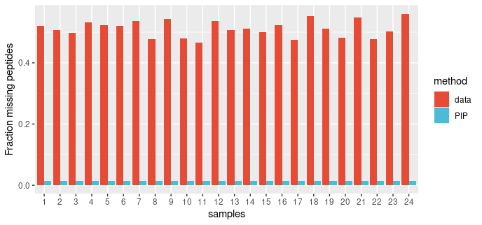 119 |
120 |
121 | **PIP recovers the low abundance peptides and re-constructs the true dynamic range**
122 |
123 | Low-abundance peptides not quantified by MaxQuant are recovered, and differential abundance results are improved. Note down regulated peptides that are not present in the volcano plot of DE test on MQ-reported data (bottom left), that are recovered by PIP (bottom right volcano plot) for the same experimental contrast.
124 |
125 |
119 |
120 |
121 | **PIP recovers the low abundance peptides and re-constructs the true dynamic range**
122 |
123 | Low-abundance peptides not quantified by MaxQuant are recovered, and differential abundance results are improved. Note down regulated peptides that are not present in the volcano plot of DE test on MQ-reported data (bottom left), that are recovered by PIP (bottom right volcano plot) for the same experimental contrast.
124 |
125 | 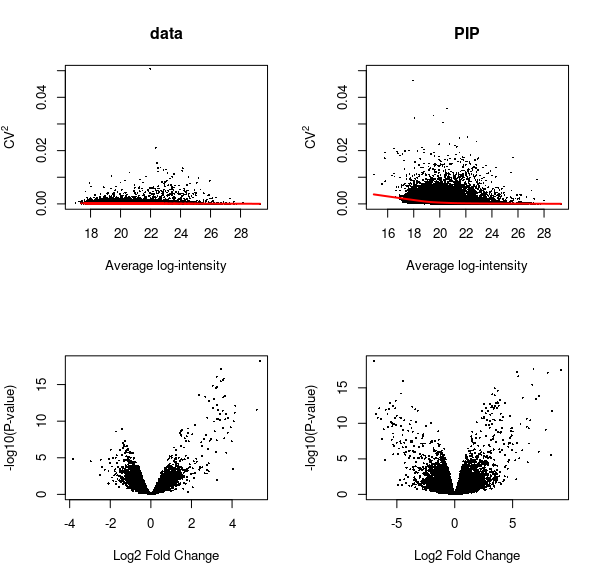 126 |
127 |
128 | The PIP workflow involves the following two function calls:
129 |
130 | ```{r}
131 | dda_pip <- mspip("/path/to/combined/txt", k=3, thresh = 0.0, tims_ms = FALSE, skip_weights = FALSE)
132 | y_pip <- evidenceToMatrix(dda_pip, return_EList = TRUE)
133 | ```
134 | Test for differential abundance in *limma*:
135 |
136 | ```{r}
137 | y_pip <- normalizeBetweenArrays(y_pip, method = "quantile")
138 | design <- model.matrix(~ group)
139 | fit <- lmFit(y_pip, design)
140 | fit <- eBayes(fit)
141 | summary(decideTests(fit))
142 | ```
143 | *limma* automatically recognizes the `EListRaw` object created by `evidenceToMatrix`, applies log2 transformation to intensity
144 | values, and passes the PIP confidence scores as observation-level weights to `lmFit`.
145 |
146 |
147 | Need more help to start? Please see documentation. We have also collected a number of **case studies** [here]()
148 |
149 | **Questions?** Please consider openning an issue.
150 |
151 |
152 | Reference
153 | -----------
154 | ```
155 | @article{hediyeh2023msimpute,
156 | title={MsImpute: Estimation of missing peptide intensity data in label-free quantitative mass spectrometry},
157 | author={Hediyeh-Zadeh, Soroor and Webb, Andrew I and Davis, Melissa J},
158 | journal={Molecular \& Cellular Proteomics},
159 | pages={100558},
160 | year={2023},
161 | publisher={Elsevier}
162 | }
163 | ```
164 |
165 |
--------------------------------------------------------------------------------
/data/pxd007959.RData:
--------------------------------------------------------------------------------
https://raw.githubusercontent.com/DavisLaboratory/msImpute/989841ed69a0b9624d3dba0eee58aef240f71134/data/pxd007959.RData
--------------------------------------------------------------------------------
/data/pxd010943.RData:
--------------------------------------------------------------------------------
https://raw.githubusercontent.com/DavisLaboratory/msImpute/989841ed69a0b9624d3dba0eee58aef240f71134/data/pxd010943.RData
--------------------------------------------------------------------------------
/data/pxd014777.RData:
--------------------------------------------------------------------------------
https://raw.githubusercontent.com/DavisLaboratory/msImpute/989841ed69a0b9624d3dba0eee58aef240f71134/data/pxd014777.RData
--------------------------------------------------------------------------------
/inst/NEWS.Rd:
--------------------------------------------------------------------------------
1 | \name{msImputenews}
2 | \title{msImpute News}
3 | \encoding{UTF-8}
4 |
5 |
6 | \section{Version 1.3.0}{\itemize{
7 | \item Users can now specify the rank of the model to fit by \code{msImpute}
8 | \item Added \code{mspip} for identification transfer between runs using Maxquant results (Beta phase only)
9 | \item Added \code{evidenceToMatrix} which creates \code{limma} compatible objects from MaxQuant evidence table
10 | }}
11 |
12 |
13 | \section{Version 0.99.26}{\itemize{
14 | \item update doc for \code{msImpute}
15 | }}
16 |
17 | \section{Version 0.99.25}{\itemize{
18 | \item fix typo in \code{msImpute} man page
19 | }}
20 |
21 | \section{Version 0.99.24}{\itemize{
22 | \item Bug fix in the internal function \code{l2bary}
23 | }}
24 |
25 | \section{Version 0.99.23}{\itemize{
26 | \item \code{selectFeatures} and \code{msImpute} now use information theoretic approaches
27 | to find informative features for MAR/MNAR diagnosis and estimation of optimal rank, respectively.
28 |
29 | \item \code{lambda} in \code{msImpute} is now estimated from the data, using the bayesian interpretation of
30 | this shrinkage operator.
31 |
32 | \item \code{msImpute} can be run in three modes: "v1" is the original implementation of softImpute-als
33 | algorithm, "v2" is the enhanced low-rank estimation implemented in this version update, "v2-mnar"
34 | is adaptation of low-rank models for MNAR data. More details about methods in documentation.
35 | }}
36 |
37 |
38 | \section{Version 0.99.22}{\itemize{
39 | \item Submitted to Bioconductor
40 | }}
41 |
42 |
43 |
--------------------------------------------------------------------------------
/inst/python/gw.py:
--------------------------------------------------------------------------------
1 | import scipy as sp
2 | import ot
3 |
4 | def gw(xs, xt, n_samples):
5 | # compute distance kernels
6 | C1 = sp.spatial.distance.cdist(xs, xs)
7 | C2 = sp.spatial.distance.cdist(xt, xt)
8 | # normalize distance kernels
9 | C1 /= C1.max()
10 | C2 /= C2.max()
11 | # Compute Gromov-Wasserstein distance
12 | p = ot.unif(n_samples)
13 | q = ot.unif(n_samples)
14 | return ot.gromov.gromov_wasserstein(C1, C2, p, q, 'square_loss', verbose=False, log=True)
15 |
--------------------------------------------------------------------------------
/man/CPD.Rd:
--------------------------------------------------------------------------------
1 | % Generated by roxygen2: do not edit by hand
2 | % Please edit documentation in R/CPD.R
3 | \name{CPD}
4 | \alias{CPD}
5 | \title{CPD}
6 | \usage{
7 | CPD(xorigin, ximputed)
8 | }
9 | \arguments{
10 | \item{xorigin}{numeric matrix. The original log-intensity data. Can not contain missing values.}
11 |
12 | \item{ximputed}{numeric matrix. The imputed log-intensity data. Can not contain missing values.}
13 | }
14 | \value{
15 | numeric
16 | }
17 | \description{
18 | Spearman correlation between pairwise distances in the original data and imputed data.
19 | CPD quantifies preservation of the global structure after imputation.
20 | Requires complete datasets - for developers/use in benchmark studies only.
21 | }
22 | \examples{
23 | data(pxd007959)
24 | y <- pxd007959$y
25 | y <- y[complete.cases(y),]
26 | # for demonstration we use same y for xorigin and ximputed
27 | CPD(y, y)
28 |
29 | }
30 |
--------------------------------------------------------------------------------
/man/KNC.Rd:
--------------------------------------------------------------------------------
1 | % Generated by roxygen2: do not edit by hand
2 | % Please edit documentation in R/KNC.R
3 | \name{KNC}
4 | \alias{KNC}
5 | \title{k-nearest class means (KNC)}
6 | \usage{
7 | KNC(xorigin, ximputed, class, k = 3)
8 | }
9 | \arguments{
10 | \item{xorigin}{numeric matrix. The original log-intensity data. Can contain missing values.}
11 |
12 | \item{ximputed}{numeric matrix. The imputed log-intensity data.}
13 |
14 | \item{class}{factor. A vector of length number of columns (samples) in the data specifying the class/label (i.e. experimental group) of each sample.}
15 |
16 | \item{k}{number of nearest class means. default to k=3.}
17 | }
18 | \value{
19 | numeric The proportion of preserved k-nearest class means in imputed data.
20 | }
21 | \description{
22 | The fraction of k-nearest class means in the original data that are preserved as k-nearest class means in imputed data. KNC
23 | quantifies preservation of the mesoscopic structure after imputation.
24 | Requires complete datasets - for developers/use in benchmark studies only.
25 | }
26 | \examples{
27 | data(pxd007959)
28 | y <- pxd007959$y
29 | y <- y[complete.cases(y),]
30 | # for demonstration we use same y for xorigin and ximputed
31 | KNC(y, y, class = as.factor(pxd007959$samples$group))
32 |
33 | }
34 |
--------------------------------------------------------------------------------
/man/KNN.Rd:
--------------------------------------------------------------------------------
1 | % Generated by roxygen2: do not edit by hand
2 | % Please edit documentation in R/KNN.R
3 | \name{KNN}
4 | \alias{KNN}
5 | \title{k-nearest neighbour (KNN)}
6 | \usage{
7 | KNN(xorigin, ximputed, k = 3)
8 | }
9 | \arguments{
10 | \item{xorigin}{numeric matrix. The original log-intensity data. Can not contain missing values.}
11 |
12 | \item{ximputed}{numeric matrix. The imputed log-intensity data. Can not contain missing values.}
13 |
14 | \item{k}{number of nearest neighbours. default to k=3.}
15 | }
16 | \value{
17 | numeric The proportion of preserved k-nearest neighbours in imputed data.
18 | }
19 | \description{
20 | The fraction of k-nearest neighbours in the original data that are preserved as k-nearest neighbours in imputed data.
21 | KNN quantifies preservation of the local, or microscopic structure.
22 | Requires complete datasets - for developers/use in benchmark studies only.
23 | }
24 | \examples{
25 | data(pxd007959)
26 | y <- pxd007959$y
27 | y <- y[complete.cases(y),]
28 | # for demonstration we use same y for xorigin and ximputed
29 | KNN(y, y)
30 |
31 |
32 | }
33 |
--------------------------------------------------------------------------------
/man/computeStructuralMetrics.Rd:
--------------------------------------------------------------------------------
1 | % Generated by roxygen2: do not edit by hand
2 | % Please edit documentation in R/computeStructuralMetrics.R
3 | \name{computeStructuralMetrics}
4 | \alias{computeStructuralMetrics}
5 | \title{Metrics for the assessment of post-imputation structural preservation}
6 | \usage{
7 | computeStructuralMetrics(x, group = NULL, y = NULL, k = 2)
8 | }
9 | \arguments{
10 | \item{x}{numeric matrix. An imputed data matrix of log-intensity.}
11 |
12 | \item{group}{factor. A vector of biological groups, experimental conditions or
13 | phenotypes (e.g. control, treatment).}
14 |
15 | \item{y}{numeric matrix. The source data (i.e. the original log-intensity matrix),
16 | preferably subsetted on highly variable peptides (see \code{findVariableFeatures}).}
17 |
18 | \item{k}{numeric. Number of Principal Components used to compute the GW distance.
19 | default to 2.}
20 | }
21 | \value{
22 | list of three metrics: withinness (sum of squared distances within a phenotype group),
23 | betweenness (sum of squared distances between the phenotypes), and gromov-wasserstein distance (if \code{xna} is not NULL).
24 | if \code{group} is NULL only the GW distance is returned. All metrics are on log scale.
25 | }
26 | \description{
27 | DEPRECATED. For an imputed dataset, it computes within phenotype/experimental condition similarity
28 | (i.e. preservation of local structures), between phenotype distances
29 | (preservation of global structures), and the Gromov-Wasserstein (GW)
30 | distance between original (source) and imputed data.
31 | }
32 | \details{
33 | For each group of experimental conditions (e.g. treatment and control), the group centroid is
34 | calculated as the average of observed peptide intensities. Withinness for each group is computed as
35 | sum of the squared distances between samples in that group and
36 | the group centroid. Betweenness is computed as sum of the squared distances between group centroids.
37 | When comparing imputation approaches, the optimal imputation strategy should minimize the within
38 | group distances, hence smaller withinness, and maximizes between group distances, hence larger betweenness.
39 | The GW metric considers preservation of both local and global structures simultaneously. A small GW distance
40 | suggests that imputation has introduced small distortions to global and local structures overall, whereas a
41 | large distance implies significant distortions. When comparing two or more imputation methods, the optimal
42 | method is the method with smallest GW distance. The GW distance is computed on Principal Components (PCs)
43 | of the source and imputed data, instead of peptides. Principal components capture the geometry of the data,
44 | hence GW computed on PCs is a better measure of preservation of local and global structures. The PCs in the
45 | source data are recommended to be computed on peptides with high biological variance. Hence, users are
46 | recommended to subset the source data only on highly variable peptides (hvp) (see \code{findVariableFeatures}).
47 | Since the hvp peptides have high biological variance, they are likely to have enough information to discriminate
48 | samples from different experimental groups. Hence, PCs computed on those peptides should be representative
49 | of the original source data with missing values. If the samples cluster by experimental group in the first
50 | couple of PCs, then a choice of k=2 is reasonable. If the desired separation/clustering of samples
51 | occurs in later PCs (i.e. the first few PCs are dominated by batches or unwanted variability), then
52 | it is recommended to use a larger number of PCs to compute the GW metric.
53 | If you are interested in how well the imputed data represent the original data in all possible dimensions,
54 | then set k to the number of samples in the data (i.e. the number of columns in the intensity matrix).
55 | GW distance estimation requires \code{python}. See example. All metrics are on log scale.
56 | }
57 | \examples{
58 | data(pxd010943)
59 | y <- log2(data.matrix(pxd010943))
60 | y <- y[complete.cases(y),]
61 | group <- as.factor(gsub("_[1234]", "", colnames(y)))
62 | computeStructuralMetrics(y, group, y=NULL)
63 |
64 |
65 | }
66 | \references{
67 | Hediyeh-zadeh, S., Webb, A. I., & Davis, M. J. (2020). MSImpute: Imputation of label-free mass spectrometry peptides by low-rank approximation. bioRxiv.
68 | }
69 |
--------------------------------------------------------------------------------
/man/evidenceToMatrix.Rd:
--------------------------------------------------------------------------------
1 | % Generated by roxygen2: do not edit by hand
2 | % Please edit documentation in R/evidenceToMatrix.R
3 | \name{evidenceToMatrix}
4 | \alias{evidenceToMatrix}
5 | \title{Creates intensity matrix from tabular data in evidence table of MaxQuant}
6 | \usage{
7 | evidenceToMatrix(
8 | evidence,
9 | run_id = "Raw.file",
10 | peptide_id = "PeptideID",
11 | return_EList = FALSE,
12 | weights = NULL
13 | )
14 | }
15 | \arguments{
16 | \item{evidence}{data.frame. The evidence table read from evidence.txt, or data.frame created by \code{mspip}.}
17 |
18 | \item{run_id}{character. The name of the column of evidence containing the run/raw file name.
19 | These form the columns of the intensity data matrix.}
20 |
21 | \item{peptide_id}{character. The name of the column of evidence containing the peptide ids.
22 | These form the rows of the intensity data matrix.}
23 |
24 | \item{return_EList}{logical. If TRUE, returns a \code{EListRaw} object storing both the
25 | intensity data matrix and observation-level weights from
26 | \code{mspip} (propagation confidence score), otherwise returns a matrix.}
27 |
28 | \item{weights}{character. The name of the column of evidence containing weights from \code{mspip}. default to NULL.
29 | Set this to "weight" if you want the weights from PIP stored in the \code{weights} slot of the \code{EListRaw} object.}
30 | }
31 | \value{
32 | a numeric matrix of intensity data, or a \code{EListRaw} object containing
33 | such data and observation-level weights from \code{mspip}.
34 | }
35 | \description{
36 | Every \code{Modified sequence} - \code{Charge} is considered as a precursor feature.
37 | Only the feature with maximum intensity is retained. The columns are run names, the rows
38 | are peptide ids (in the \code{Modified.sequence_Charge} format)
39 | }
40 | \details{
41 | The \code{EListRaw} object created by the function is intended to bridge \code{msImpute} and statistical
42 | methods of \code{limma}. The object can be passed to \code{normalizeBetweenArrays} for normalisation, which can then
43 | be passed to \code{lmFit} and \code{eBayes} for fitting linear models per peptide and Empirical Bayes moderation of t-statistics
44 | respectively. The \code{weights} slot is recognized by \code{lmFit}, which incorporates the uncertainty in intensity values
45 | inferred by PIP into the test statistic.
46 | The function is also a generic tool to create a matrix or \code{limma}-compatible objects from the evidence table of MaxQuant.
47 | }
48 | \seealso{
49 | mspip
50 | }
51 | \author{
52 | Soroor Hediyeh-zadeh
53 | }
54 |
--------------------------------------------------------------------------------
/man/msImpute.Rd:
--------------------------------------------------------------------------------
1 | % Generated by roxygen2: do not edit by hand
2 | % Please edit documentation in R/msImpute.R
3 | \name{msImpute}
4 | \alias{msImpute}
5 | \title{Imputation of peptide log-intensity in mass spectrometry label-free proteomics by low-rank approximation}
6 | \usage{
7 | msImpute(
8 | y,
9 | method = c("v2-mnar", "v2", "v1"),
10 | group = NULL,
11 | design = NULL,
12 | alpha = NULL,
13 | relax_min_obs = TRUE,
14 | rank.max = NULL,
15 | lambda = NULL,
16 | thresh = 1e-05,
17 | maxit = 100,
18 | trace.it = FALSE,
19 | warm.start = NULL,
20 | final.svd = TRUE,
21 | biScale_maxit = 20,
22 | gauss_width = 0.3,
23 | gauss_shift = 1.8,
24 | use_seed = TRUE
25 | )
26 | }
27 | \arguments{
28 | \item{y}{Numeric matrix giving log-intensity where missing values are denoted by NA. Rows are peptides, columns are samples.}
29 |
30 | \item{method}{Character. Allowed values are \code{"v2"} for \code{msImputev2} imputation (enhanced version) for MAR.
31 | \code{method="v2-mnar"} (modified low-rank approx for MNAR), and \code{"v1"} initial release of \code{msImpute}.}
32 |
33 | \item{group}{Character or factor vector of length \code{ncol(y)}. DEPRECATED. Please specify the \code{design} argument.}
34 |
35 | \item{design}{Object from model.matrix(); A zero-intercept design matrix (see example).}
36 |
37 | \item{alpha}{Numeric. The weight parameter. Default to 0.2. Weights the MAR-imputed distribution in the imputation scheme. DEPRECATED}
38 |
39 | \item{rank.max}{Numeric. This restricts the rank of the solution. is set to min(dim(\code{y})-1) by default in "v1".}
40 |
41 | \item{lambda}{Numeric. Nuclear-norm regularization parameter. Controls the low-rank property of the solution
42 | to the matrix completion problem. By default, it is determined at the scaling step. If set to zero
43 | the algorithm reverts to "hardImputation", where the convergence will be slower. Applicable to "v1" only.}
44 |
45 | \item{thresh}{Numeric. Convergence threshold. Set to 1e-05, by default. Applicable to "v1" only.}
46 |
47 | \item{maxit}{Numeric. Maximum number of iterations of the algorithm before the algorithm is converged. 100 by default.
48 | Applicable to "v1" only.}
49 |
50 | \item{trace.it}{Logical. Prints traces of progress of the algorithm.
51 | Applicable to "v1" only.}
52 |
53 | \item{warm.start}{List. A SVD object can be used to initialize the algorithm instead of random initialization.
54 | Applicable to "v1" only.}
55 |
56 | \item{final.svd}{Logical. Shall final SVD object be saved?
57 | The solutions to the matrix completion problems are computed from U, D and V components of final SVD.
58 | Applicable to "v1" only.}
59 |
60 | \item{biScale_maxit}{Number of iteration for the scaling algorithm to converge . See \code{scaleData}. You may need to change this
61 | parameter only if you're running \code{method=v1}. Applicable to "v1" only.}
62 |
63 | \item{gauss_width}{Numeric. The width parameter of the Gaussian distribution to impute the MNAR peptides (features). This the width parameter in the down-shift imputation method.}
64 |
65 | \item{gauss_shift}{Numeric. The shift parameter of the Gaussian distribution to impute the MNAR peptides (features). This the width parameter in the down-shift imputation method.}
66 |
67 | \item{use_seed}{Logical. Makes random draw from the lower Normal component of the mixture (corresponding to imputation by down-shift) deterministic, so that results are reproducible.}
68 | }
69 | \value{
70 | Missing values are imputed by low-rank approximation of the input matrix. If input is a numeric matrix,
71 | a numeric matrix of identical dimensions is returned.
72 | }
73 | \description{
74 | Returns a completed matrix of peptide log-intensity where missing values (NAs) are imputated
75 | by low-rank approximation of the input matrix. Non-NA entries remain unmodified. \code{msImpute} requires at least 4
76 | non-missing measurements per peptide across all samples. It is assumed that peptide intensities (DDA), or MS1/MS2 normalised peak areas (DIA),
77 | are log2-transformed and normalised (e.g. by quantile normalisation).
78 | }
79 | \details{
80 | \code{msImpute} operates on the \code{softImpute-als} algorithm in \code{\link[softImpute]{softImpute}} package.
81 | The algorithm estimates a low-rank matrix ( a smaller matrix
82 | than the input matrix) that approximates the data with a reasonable accuracy. \code{SoftImpute-als} determines the optimal
83 | rank of the matrix through the \code{lambda} parameter, which it learns from the data.
84 | This algorithm is implemented in \code{method="v1"}.
85 | In v2 we have used a information theoretic approach to estimate the optimal rank, instead of relying on \code{softImpute-als}
86 | defaults. Similarly, we have implemented a new approach to estimate \code{lambda} from the data. Low-rank approximation
87 | is a linear reconstruction of the data, and is only appropriate for imputation of MAR data. In order to make the
88 | algorithm applicable to MNAR data, we have implemented \code{method="v2-mnar"} which imputes the missing observations
89 | as weighted sum of values imputed by msImpute v2 (\code{method="v2"}) and random draws from a Gaussian distribution.
90 | Missing values that tend to be missing completely in one or more experimental groups will be weighted more (shrunken) towards
91 | imputation by sampling from a Gaussian parameterised by smallest observed values in the sample (similar to minProb, or
92 | Perseus). However, if the missing value distribution is even across the samples for a peptide, the imputed values
93 | for that peptide are shrunken towards
94 | low-rank imputed values. The judgment of distribution of missing values is based on the EBM metric implemented in
95 | \code{selectFeatures}, which is also a information theory measure.
96 | }
97 | \examples{
98 | data(pxd010943)
99 | y <- log2(data.matrix(pxd010943))
100 | group <- as.factor(gsub("_[1234]","", colnames(y)))
101 | design <- model.matrix(~0+group)
102 | yimp <- msImpute(y, method="v2-mnar", design=design, max.rank=2)
103 | }
104 | \references{
105 | Hastie, T., Mazumder, R., Lee, J. D., & Zadeh, R. (2015). Matrix completion and low-rank SVD via fast alternating least squares. The Journal of Machine Learning Research, 16(1), 3367-3402.
106 |
107 | Hediyeh-Zadeh, S., Webb, A. I., & Davis, M. J. (2023). MsImpute: Estimation of missing peptide intensity data in label-free quantitative mass spectrometry. Molecular & Cellular Proteomics, 22(8).
108 | }
109 | \seealso{
110 | selectFeatures
111 | }
112 | \author{
113 | Soroor Hediyeh-zadeh
114 | }
115 |
--------------------------------------------------------------------------------
/man/mspip.Rd:
--------------------------------------------------------------------------------
1 | % Generated by roxygen2: do not edit by hand
2 | % Please edit documentation in R/mspip.R
3 | \name{mspip}
4 | \alias{mspip}
5 | \title{Fills missing values by Peptide Identity Propagation (PIP)}
6 | \usage{
7 | mspip(
8 | path_txt,
9 | k = 10,
10 | thresh = 0,
11 | skip_weights = TRUE,
12 | tims_ms = FALSE,
13 | group_restriction = NULL,
14 | nlandmarks = 50
15 | )
16 | }
17 | \arguments{
18 | \item{path_txt}{character. The path to MaxQuant \code{txt} directory}
19 |
20 | \item{k}{numeric. The \code{k} nearest neighbors to be used for identity propagation. default to 10.}
21 |
22 | \item{thresh}{numeric. The uncertainty threshold for calling a Identity Transfer as confident. Sequence to peptide
23 | feature assignments with confidence score (probability) above a threshold (specified by \code{thresh}) are
24 | considered as confident assignments.The rest of the assignments are discarded and not reported in the output.}
25 |
26 | \item{skip_weights}{logical. If TRUE, the propagation confidence scores are also reported.
27 | The confidence scores can be used as observation-level weights in \code{limma} linear models
28 | to improve differential expression testing. default to FALSE.}
29 |
30 | \item{tims_ms}{logical. Is data acquired by TIMS-MS? default to FALSE.}
31 |
32 | \item{group_restriction}{A data.frame with two columns named Raw.file and group, specifying run file and the (experimental) group to which the run belongs.
33 | Use this option for Unbalanced PIP}
34 |
35 | \item{nlandmarks}{numeric. Number of landmark peptides used for measuring neighborhood/coelution similarity. Default to 50.}
36 | }
37 | \description{
38 | Peptide identity (sequence and charge) is propagated from MS-MS or PASEF identified features in evidence.txt to
39 | MS1 features in allPeptides.txt that are detected but not identified. A confidence score (probability)
40 | is assigned to every propagation. The confidence scores can be used as observation-level weights
41 | in \code{limma::lmFit} to account for uncertainty in inferred peptide intensity values.
42 | }
43 | \details{
44 | Data completeness is maximised by Peptide Identity Propagation (PIP) from runs where
45 | a peptide is identified by MSMS or PASEF to runs where peptide is not fragmented
46 | (hence MS2 information is not available), but is detected at the MS1 level. \code{mspip} reports a
47 | confidence score for each peptide that was identified by PIP. The intensity values of PIP peptides
48 | can be used to reduce missing values, while the reported confidence scores can be used to
49 | weight the contribution of these peptide intensity values to variance estimation in linear models fitted in
50 | \code{limma}.
51 | }
52 | \seealso{
53 | evidenceToMatrix
54 | }
55 | \author{
56 | Soroor Hediyeh-zadeh
57 | }
58 |
--------------------------------------------------------------------------------
/man/plotCV2.Rd:
--------------------------------------------------------------------------------
1 | % Generated by roxygen2: do not edit by hand
2 | % Please edit documentation in R/plotCV2.R
3 | \name{plotCV2}
4 | \alias{plotCV2}
5 | \title{Plot mean-CV^2 trend}
6 | \usage{
7 | plotCV2(y, trend = TRUE, main = NULL, ...)
8 | }
9 | \arguments{
10 | \item{y}{numeric matrix of log-intensity}
11 |
12 | \item{trend}{logical. Should a loess trend be fitted to CV^2 and mean values. Default to TRUE.}
13 |
14 | \item{main}{character string. Title of the plot. Default to NULL.}
15 |
16 | \item{...}{any parameter passed to \code{plot}.}
17 | }
18 | \value{
19 | A plot is created on the current graphics device.
20 | }
21 | \description{
22 | For each peptide, the squares of coefficient of variations are computed and plotted against average log-intensity.
23 | Additionally, a loess trend is fitted to the plotted values.
24 | Outlier observations (possibly originated from incorrect match between runs), are detected and highlighted.
25 | Users can use this plot as a diagnostic plot to determine if filtering by average intensity is required.
26 | }
27 | \details{
28 | Outliers are determined by computing the RBF kernels, which reflect the chance that an observed point
29 | belong to the dataset (i.e. is close enough in distance to other data points). Users can determine the cut-off
30 | for intensity-based filtering with respect to the mean log-intensity of the outlier points.
31 | }
32 | \examples{
33 | data(pxd010943)
34 | y <- pxd010943
35 | y <- log2(y)
36 | ppCV2 <- plotCV2(y)
37 |
38 | }
39 |
--------------------------------------------------------------------------------
/man/pxd007959.Rd:
--------------------------------------------------------------------------------
1 | % Generated by roxygen2: do not edit by hand
2 | % Please edit documentation in R/pxd007959.R
3 | \docType{data}
4 | \name{pxd007959}
5 | \alias{pxd007959}
6 | \title{Processed peptide intensity matrix and experimental design table from PXD007959 study}
7 | \format{
8 | A list of two: samples (data frame of sample descriptions), and y (numeric matrix of peptide intensity values)
9 | }
10 | \source{
11 | \url{http://proteomecentral.proteomexchange.org/cgi/GetDataset?ID=PXD007959}
12 | }
13 | \usage{
14 | pxd007959
15 | }
16 | \description{
17 | Extracellular vesicles isolated from the descending colon of pediatric patients with inflammatory bowel disease
18 | and control patients. Characterizes the proteomic profile of extracellular vesicles isolated from the descending colon
19 | of pediatric patients with inflammatory bowel disease and control participants. This object contains data from peptide.txt
20 | table output by MaxQuant. Rows are Modified Peptide IDs. Charge state variations are treated as distinct peptide species.
21 | Reverse complements and contaminant peptides are discarded. Peptides with more than 4 observed intensity values are retained.
22 | Additionally, qualified peptides are required to map uniquely to proteins.
23 | Two of the samples with missing group annotation were excluded.
24 | The peptide.txt and experimentalDesignTemplate files can be downloaded as RDS object from \url{https://github.com/soroorh/proteomicscasestudies}.
25 | Code for data processing is provided in package vignette.
26 | }
27 | \references{
28 | Zhang X, Deeke SA, Ning Z, Starr AE, Butcher J, Li J, Mayne J, Cheng K, Liao B, Li L, Singleton R, Mack D, Stintzi A, Figeys D, Metaproteomics reveals associations between microbiome and intestinal extracellular vesicle proteins in pediatric inflammatory bowel disease. Nat Commun, 9(1):2873(2018)
29 | }
30 | \keyword{datasets}
31 |
--------------------------------------------------------------------------------
/man/pxd010943.Rd:
--------------------------------------------------------------------------------
1 | % Generated by roxygen2: do not edit by hand
2 | % Please edit documentation in R/pxd010943.R
3 | \docType{data}
4 | \name{pxd010943}
5 | \alias{pxd010943}
6 | \title{SWATH-MS Analysis of Gfi1-mutant bone marrow neutrophils}
7 | \format{
8 | A matrix
9 | }
10 | \source{
11 | \url{http://proteomecentral.proteomexchange.org/cgi/GetDataset?ID=PXD010943}
12 | }
13 | \usage{
14 | pxd010943
15 | }
16 | \description{
17 | Contains Peak Area for peptides in PXD010943.
18 | This study investigates the proteomic alterations in bone marrow neutrophils isolated from 5-8 week old Gfi1+/-, Gfi1K403R/-,
19 | Gfi1R412X/-, and Gfi1R412X/R412X mice using the SWATH-MS technique. This dataset consists of 13 SWATH-DIA runs on a TripleTOF 5600 plus (SCIEX).
20 | Rows are peptides. Charge state variations are treated as distinct peptide species. Peptides with more than 4 observed intensity values are retained.
21 | The peptide.txt and experimentalDesignTemplate files can be downloaded as RDS object from \url{https://github.com/soroorh/proteomicscasestudies}.
22 | Code for data processing is provided in package vignette.
23 | }
24 | \references{
25 | Muench DE, Olsson A, Ferchen K, Pham G, Serafin RA, Chutipongtanate S, Dwivedi P, Song B, Hay S, Chetal K, Trump-Durbin LR, Mookerjee-Basu J, Zhang K, Yu JC, Lutzko C, Myers KC, Nazor KL, Greis KD, Kappes DJ, Way SS, Salomonis N, Grimes HL, Mouse models of neutropenia reveal progenitor-stage-specific defects. Nature, 582(7810):109-114(2020)
26 | }
27 | \keyword{datasets}
28 |
--------------------------------------------------------------------------------
/man/pxd014777.Rd:
--------------------------------------------------------------------------------
1 | % Generated by roxygen2: do not edit by hand
2 | % Please edit documentation in R/pxd014777.R
3 | \docType{data}
4 | \name{pxd014777}
5 | \alias{pxd014777}
6 | \title{Processed peptide intensity matrix from PXD014777 study}
7 | \format{
8 | A matrix
9 | }
10 | \source{
11 | \url{http://proteomecentral.proteomexchange.org/cgi/GetDataset?ID=PXD014777}
12 | }
13 | \usage{
14 | pxd014777
15 | }
16 | \description{
17 | A Trapped Ion Mobility Spectrometry (TIMS) dataset of blood plasma from a number of patients acquired in two batches.
18 | This is a technical dataset
19 | published by MaxQuant to benchmark their software for ion mobility enhanced shotgun proteomics.
20 | Rows are Modified Peptide IDs. Charge state variations are treated as distinct peptide species.
21 | For peptides with multiple identification types, the intensity is considered to be the median of reported intensity values.
22 | Reverse complememts and contaminant peptides are discarded.
23 | Peptides with more than 4 observed intensity values are retained.
24 | This object contains data from peptide.txt table output by MaxQuant.
25 | The evidence.txt file can be downloaded as RDS object from \url{https://github.com/soroorh/proteomicscasestudies}.
26 | Code for data processing is provided in package vignette.
27 | }
28 | \references{
29 | Prianichnikov N, Koch H, Koch S, Lubeck M, Heilig R, Brehmer S, Fischer R, Cox J, MaxQuant Software for Ion Mobility Enhanced Shotgun Proteomics. Mol Cell Proteomics, 19(6):1058-1069(2020)
30 | }
31 | \keyword{datasets}
32 |
--------------------------------------------------------------------------------
/man/scaleData.Rd:
--------------------------------------------------------------------------------
1 | % Generated by roxygen2: do not edit by hand
2 | % Please edit documentation in R/scaleData.R
3 | \name{scaleData}
4 | \alias{scaleData}
5 | \title{Standardize a matrix to have optionally row means zero and variances one, and/or column means zero and variances one.}
6 | \usage{
7 | scaleData(
8 | object,
9 | maxit = 20,
10 | thresh = 1e-09,
11 | row.center = TRUE,
12 | row.scale = TRUE,
13 | col.center = TRUE,
14 | col.scale = TRUE,
15 | trace = FALSE
16 | )
17 | }
18 | \arguments{
19 | \item{object}{numeric matrix giving log-intensity where missing values are denoted by NA. Rows are peptides, columns are samples.}
20 |
21 | \item{maxit}{numeric. maximum iteration for the algorithm to converge (default to 20). When both row and column centering/scaling is requested, iteration may be necessary.}
22 |
23 | \item{thresh}{numeric. Convergence threshold (default to 1e-09).}
24 |
25 | \item{row.center}{logical. if row.center==TRUE (the default), row centering will be performed resulting in a matrix with row means zero. If row.center is a vector, it will be used to center the rows. If row.center=FALSE nothing is done.}
26 |
27 | \item{row.scale}{if row.scale==TRUE, the rows are scaled (after possibly centering, to have variance one. Alternatively, if a positive vector is supplied, it is used for row centering.}
28 |
29 | \item{col.center}{Similar to row.center}
30 |
31 | \item{col.scale}{Similar to row.scale}
32 |
33 | \item{trace}{logical. With trace=TRUE, convergence progress is reported, when iteration is needed.}
34 | }
35 | \value{
36 | A list of two components: E and E.scaled. E contains the input matrix, E.scaled contains the scaled data
37 | }
38 | \description{
39 | Standardize a matrix to have optionally row means zero and variances one, and/or column means zero and variances one.
40 | }
41 | \details{
42 | Standardizes rows and/or columns of a matrix with missing values, according to the \code{biScale} algorithm in Hastie et al. 2015.
43 | Data is assumed to be normalised and log-transformed. Please note that data scaling might not be appropriate for MS1 data. A good strategy
44 | is to compare mean-variance plot (\code{plotCV2}) before and after imputation. If the plots look differently, you may need to skip
45 | data scaling. The MS1 data are more variable (tend to have higher CV^2), and may contain outliers which will skew the scaling.
46 | }
47 | \examples{
48 | data(pxd010943)
49 | y <- pxd010943
50 | y <- log2(y)
51 | keep <- (rowSums(!is.na(y)) >= 4)
52 | y <- as.matrix.data.frame(y[keep,])
53 | y <- scaleData(y, maxit=30)
54 | }
55 | \references{
56 | Hastie, T., Mazumder, R., Lee, J. D., & Zadeh, R. (2015). Matrix completion and low-rank SVD via fast alternating least squares. The Journal of Machine Learning Research, 16(1), 3367-3402.
57 |
58 | Hediyeh-Zadeh, S., Webb, A. I., & Davis, M. J. (2023). MsImpute: Estimation of missing peptide intensity data in label-free quantitative mass spectrometry. Molecular & Cellular Proteomics, 22(8).
59 | }
60 | \seealso{
61 | selectFeatures, msImpute
62 | }
63 |
--------------------------------------------------------------------------------
/man/selectFeatures.Rd:
--------------------------------------------------------------------------------
1 | % Generated by roxygen2: do not edit by hand
2 | % Please edit documentation in R/selectFeatures.R
3 | \name{selectFeatures}
4 | \alias{selectFeatures}
5 | \title{Select features for MAR/MNAR pattern examination}
6 | \usage{
7 | selectFeatures(
8 | x,
9 | method = c("ebm", "hvp"),
10 | group,
11 | n_features = 500,
12 | suppress_plot = TRUE
13 | )
14 | }
15 | \arguments{
16 | \item{x}{Numeric matrix giving log-intensity where missing values are denoted by NA.
17 | Rows are peptides, columns are samples.}
18 |
19 | \item{method}{character. What method should be used to find features? options include \code{method='hvp'} and \code{method='ebm'}}
20 |
21 | \item{group}{character or factor vector specifying biological (experimental) group e.g. control, treatment, WT, KO}
22 |
23 | \item{n_features}{Numeric, number of features with high dropout rate. 500 by default. Applicable if \code{method="hvp"}.}
24 |
25 | \item{suppress_plot}{Logical show plot of dropouts vs abundances. Default to TRUE. Applicable if \code{method="hvp"}.}
26 | }
27 | \value{
28 | A data frame with a logical column denoting the selected features
29 | }
30 | \description{
31 | Two methods are provided to identify features (peptides or proteins) that can be informative of missing patterns.
32 | Method \code{hvp} fits a linear model to peptide dropout rate (proportion of samples were peptide is missing)
33 | against peptide abundance (average log2-intensity). Method \code{emb} is a information theoretic approach to
34 | identify missing patterns. It quantifies the heterogeneity (entropy) of missing patterns per
35 | biological (experimental group). This is the default method.
36 | }
37 | \details{
38 | In general, the presence of group-wise (structured) blocks of missing values,
39 | where peptides are missing in one experimental group can indicate MNAR, whereas if
40 | such patterns are absent (or missingness is uniform across the samples), peptides are likely MAR.
41 | In the presence of MNAR, left-censored MNAR imputation methods should
42 | be chosen. Two methods are provided to explore missing patterns: \code{method=hvp} identifies top \code{n_features}
43 | peptides with high average expression that also have high dropout rate, defined as the proportion of samples where
44 | peptide is missing. Peptides with high (potentially) biological dropouts are marked in the \code{hvp} column in the
45 | output dataframe. This method does not use any information about experimental conditions (i.e. group).
46 | Another approach to explore and quantify missing patterns is by looking at how homogeneous or heterogeneous
47 | missing patterns are in each experimental group. This is done by computing entropy of distribution of observed values.
48 | This is the default and recommended method for \code{selectFeatures}. Entropy is reported in \code{EBM} column
49 | of the output. A \code{NaN} EBM indicates peptide is missing at least in one experimental group. Features set to
50 | \code{TRUE} in \code{msImpute_feature} column are the features selected by the selected method. Users are encouraged
51 | to use the EBM metric to find informative features, hence why the \code{group} argument is required.
52 | }
53 | \examples{
54 | data(pxd007959)
55 | group <- pxd007959$samples$group
56 | y <- data.matrix(pxd007959$y)
57 | y <- log2(y)
58 | hdp <- selectFeatures(y, method="ebm", group = group)
59 | # construct matrix M to capture missing entries
60 | M <- ifelse(is.na(y),1,0)
61 | M <- M[hdp$msImpute_feature,]
62 | # plot a heatmap of missingness patterns for the selected peptides
63 | require(ComplexHeatmap)
64 | hm <- Heatmap(M,
65 | column_title = "dropout pattern, columns ordered by dropout similarity",
66 | name = "Intensity",
67 | col = c("#8FBC8F", "#FFEFDB"),
68 | show_row_names = FALSE,
69 | show_column_names = TRUE,
70 | cluster_rows = TRUE,
71 | cluster_columns = TRUE,
72 | show_column_dend = TRUE,
73 | show_row_dend = FALSE,
74 | row_names_gp = gpar(fontsize = 7),
75 | column_names_gp = gpar(fontsize = 8),
76 | heatmap_legend_param = list(#direction = "horizontal",
77 | heatmap_legend_side = "bottom",
78 | labels = c("observed","missing"),
79 | legend_width = unit(6, "cm")),
80 | )
81 | hm <- draw(hm, heatmap_legend_side = "left")
82 | }
83 | \references{
84 | Hediyeh-Zadeh, S., Webb, A. I., & Davis, M. J. (2023). MsImpute: Estimation of missing peptide intensity data in label-free quantitative mass spectrometry. Molecular & Cellular Proteomics, 22(8).
85 | }
86 | \seealso{
87 | msImpute
88 | }
89 | \author{
90 | Soroor Hediyeh-zadeh
91 | }
92 |
--------------------------------------------------------------------------------
/vignettes/.gitignore:
--------------------------------------------------------------------------------
1 | *.html
2 | *.R
3 |
--------------------------------------------------------------------------------
/vignettes/msImpute-vignette.Rmd:
--------------------------------------------------------------------------------
1 | ---
2 | title: "msImpute: Imputation of peptide intensity by low-rank approximation"
3 | author:
4 | - name: Soroor Hediyeh-zadeh
5 | affiliation: &id The Walter and Eliza Hall Institute of Medical Research
6 | - name: Andrew I. Webb
7 | affiliation: *id
8 | - name: Melissa J. Davis
9 | affiliation: *id
10 | package: msImpute
11 | abstract: |
12 | MsImpute is a package for imputation of peptide intensity in proteomics experiments. It additionally contains tools for MAR/MNAR diagnosis and assessment of distortions to the probability distribution of the data post imputation. This document covers case studies featuring data obtained by various Mass Spectrometry (MS) acquisition modes to demonstrate applications of tools implemented in the package. The datasets selected here represent data with MAR and left-censored MNAR missingness patterns. We demonstrate msImpute is able to correctly identify these patterns and inform user's decisions in downstream analyses.
13 | output:
14 | BiocStyle::html_document:
15 | toc_float: true
16 | BiocStyle::pdf_document: default
17 | vignette: >
18 | %\VignetteIndexEntry{msImpute: proteomics missing values imputation and diagnosis}
19 | %\VignetteEngine{knitr::rmarkdown}
20 | %\VignetteEncoding{UTF-8}
21 | ---
22 |
23 |
24 |
25 |
26 | # Installation
27 |
28 |
29 | ```{r eval=FALSE}
30 | if(!requireNamespace("BiocManager", quietly = TRUE))
31 | install.packages("BiocManager")
32 | BiocManager::install("msImpute")
33 | ```
34 |
35 |
36 | # Quick Start
37 |
38 | The package consists of the following main functions:
39 |
40 | - `selectFeatures`: identifies informative peptides that can be used to examine MAR/MNAR missingness in the data.
41 |
42 | - `msImpute`: Main function that imputes missing values by learning a low-rank approximation of the data.
43 |
44 | - `findVariableFeatures`: finds peptide with high biological variance. We use this in `computeStructuralMetrics`
45 |
46 | - `plotCV2`: Plots the square of coefficient of variation versus average log-expression i.e. mean-$CV^2$ plot
47 |
48 |
49 | These functions overall are designed to inform user's decision in choosing a proper imputation strategy. For a more detailed workflow, please see [User's Manual](https://github.com/soroorh/proteomicscasestudies/blob/master/msImputeUsersGuide.pdf).
50 |
51 |
52 | # TIMS Case Study: Blood plasma
53 |
54 | The aim is to assess the missing patterns in ion mobility data by Prianichnikov et al. (2020), available from PXD014777. The `evidence` table of MaxQuant output was processed as described below. Rows are Modified Peptide IDs. Charge state variations are treated as distinct peptide species. For peptides with multiple identification types, the intensity is considered to be the median of reported intensity values. Reverse complements and contaminant peptides are discarded. Peptides with more than 4 observed intensity values are retained.
55 |
56 | The data was acquired in two batches (over two days). We are interested to know if missing values are evenly distributed across batches, or there is a batch-specific dropout trend. The runs are also labeled by S1, S2 and S4 (source unknown). The aim is to use this information to work out if missing values occur due to technical or biological effects.
57 |
58 |
59 | ```{r setup, message=FALSE}
60 | library(msImpute)
61 | library(limma)
62 | library(imputeLCMD)
63 | library(ComplexHeatmap)
64 | ```
65 |
66 | ## Data processing
67 |
68 | The following procedures were applied to process the data, which we later load from the package data.
69 |
70 | ### Filter by detection
71 |
72 |
73 | ```{r}
74 | data(pxd014777)
75 | y <- pxd014777
76 | ```
77 |
78 |
79 | Zero values that will be converted to Inf/-Inf after log- transformation. Check if there are valid values in the data before log transformation
80 | ```{r}
81 | table(is.infinite(data.matrix(log2(y))))
82 | ```
83 |
84 | There are zero values that will be converted to Inf/-Inf after log- transformation. Add a small offset to avoid infinite values:
85 | ```{r}
86 | y <- log2(y+0.25)
87 | ```
88 |
89 | ### Normalization
90 | ```{r}
91 | # quantile normalisation
92 | y <- normalizeBetweenArrays(y, method = "quantile")
93 | ```
94 |
95 | ## Determine missing values pattern
96 |
97 | Determine dominant patterns of missing values by investigating the distribution of missing values. Peptides that are missing in at least one experimental group (here batch), and therefore exhibit structured missing patterns can be identified by the EBM metric implemented in `selectFeatures`. We then make a heatmap of their dropout pattern.
98 | ```{r}
99 |
100 | batch <- as.factor(gsub("(2018.*)_RF.*","\\1", colnames(y)))
101 | experiment <- as.factor(gsub(".*(S[1-9]).*","\\1", colnames(y)))
102 |
103 |
104 | hdp <- selectFeatures(y, method = "ebm", group = batch)
105 |
106 |
107 | # peptides missing in one or more experimental group will have a NaN EBM, which is a measure of entropy of
108 | # distribution of observed values
109 | table(is.nan(hdp$EBM))
110 |
111 | # construct matrix M to capture missing entries
112 | M <- ifelse(is.na(y),1,0)
113 | M <- M[hdp$msImpute_feature,]
114 |
115 | # plot a heatmap of missingness patterns for the selected peptides
116 |
117 |
118 |
119 | ```
120 |
121 | ```{r fig.cap="Heatmap of missing value patterns for peptides selected as informative peptides", fig.align="center"}
122 | ha_column <- HeatmapAnnotation(batch = batch,
123 | experiment = experiment,
124 | col = list(batch = c('20181023' = "#B24745FF",
125 | '20181024'= "#00A1D5FF"),
126 | experiment=c("S1"="#DF8F44FF",
127 | "S2"="#374E55FF",
128 | "S4"="#79AF97FF")))
129 |
130 | hm <- Heatmap(M,
131 | column_title = "dropout pattern, columns ordered by dropout similarity",
132 | name = "Intensity",
133 | col = c("#8FBC8F", "#FFEFDB"),
134 | show_row_names = FALSE,
135 | show_column_names = FALSE,
136 | cluster_rows = TRUE,
137 | cluster_columns = TRUE,
138 | show_column_dend = FALSE,
139 | show_row_dend = FALSE,
140 | top_annotation = ha_column,
141 | row_names_gp = gpar(fontsize = 7),
142 | column_names_gp = gpar(fontsize = 8),
143 | heatmap_legend_param = list(#direction = "horizontal",
144 | heatmap_legend_side = "bottom",
145 | labels = c("observed","missing"),
146 | legend_width = unit(6, "cm")),
147 | )
148 | hm <- draw(hm, heatmap_legend_side = "left")
149 | ```
150 | The larger the EBM, the more scattered the missing values will be. If missing values are scattered across samples, their value can be estimated from the neighborhood, hence missing type is likely MNAR. If however, peptides are missing completely in one experimental condition, or they have much more concentrated (or dense) distributions, their EBM value will be lower. A `NaN` EBM suggests peptide is missing in at least one experimental group, defined by the `group` argument. Since there are 103 such peptides with `EBM=NaN`, this data
151 | has peptides that are missing not at random i.e. the missingness is batch-specific. Given that this is a technical dataset, MNAR missing here can not be biological, and reflects batch-to-batch variations, such as differences in limit of detection of MS etc.
152 | `selectFeatures` just enables to detect any peptides that appear to exhibit structured missing, and hence might be left-censored.
153 | you can also set `method="hvp"` which will select top `n_features` peptides with high dropout rate, defined as proportion of samples where a given peptide is missing, that are also highly expressed as the `msImpute_feature` in the output `dataframe`. If `method="ebm"`,
154 | the features marked in `msImpute_feature` column will be peptides (or proteins, depending on the input expression matrix), will the ones
155 | with `NaN` EBM (i.e. peptides with structured missing patterns). The `"hvp"` method can detect missingness patterns at high abundance,
156 | whereas `"ebm"` is for detection of peptides (completely) missing in at least one experimental group.
157 |
158 |
159 | # DDA Case Study: Extracellular vesicles isolated from inflammatory bowel disease patients and controls
160 |
161 | The study aims to characterize the proteomic profile of extracellular vesicles isolated from the descending colon of pediatric patients with inflammatory bowel disease and control participants. The following analysis is based on the `peptide` table from MaxQuant output, available from PXD007959. Rows are Modified Peptide IDs. Charge state variations are treated as distinct peptide species. Reverse complements and contaminant peptides are discarded. Peptides with more than 4 observed intensity values are retained. Additionally, qualified peptides are required to map uniquely to proteins. Two of the samples with missing group annotation were excluded.
162 |
163 | ## Filter by detection
164 |
165 |
166 | The sample descriptions can be accessed via `pxd007959$samples`. Intensity values are stored in `pxd007959$y`.
167 | ```{r}
168 | data(pxd007959)
169 |
170 | sample_annot <- pxd007959$samples
171 | y <- pxd007959$y
172 | y <- log2(y)
173 | ```
174 |
175 | ## Normalization
176 | We apply `cyclic loess` normalisation from `limma` to normalise log-intensities. We have justified use of `cyclic loess` method in depth in the user's guide.
177 | ```{r}
178 | y <- normalizeBetweenArrays(y, method = "cyclicloess")
179 | ```
180 |
181 |
182 | ## Determine missing values pattern
183 |
184 | ```{r fig.align="center"}
185 | # determine missing values pattern
186 | group <- sample_annot$group
187 | hdp <- selectFeatures(y, method="ebm", group = group)
188 | ```
189 |
190 |
191 |
192 | ```{r fig.cap="Dropout pattern of informative peptides", fig.align="center"}
193 | # construct matrix M to capture missing entries
194 | M <- ifelse(is.na(y),1,0)
195 | M <- M[hdp$msImpute_feature,]
196 |
197 |
198 |
199 | # plot a heatmap of missingness patterns for the selected peptides
200 | ha_column <- HeatmapAnnotation(group = as.factor(sample_annot$group),
201 | col=list(group=c('Control' = "#E64B35FF",
202 | 'Mild' = "#3C5488FF",
203 | 'Moderate' = "#00A087FF",
204 | 'Severe'="#F39B7FFF")))
205 |
206 | hm <- Heatmap(M,
207 | column_title = "dropout pattern, columns ordered by dropout similarity",
208 | name = "Intensity",
209 | col = c("#8FBC8F", "#FFEFDB"),
210 | show_row_names = FALSE,
211 | show_column_names = FALSE,
212 | cluster_rows = TRUE,
213 | cluster_columns = TRUE,
214 | show_column_dend = FALSE,
215 | show_row_dend = FALSE,
216 | top_annotation = ha_column,
217 | row_names_gp = gpar(fontsize = 7),
218 | column_names_gp = gpar(fontsize = 8),
219 | heatmap_legend_param = list(#direction = "horizontal",
220 | heatmap_legend_side = "bottom",
221 | labels = c("observed","missing"),
222 | legend_width = unit(6, "cm")),
223 | )
224 | hm <- draw(hm, heatmap_legend_side = "left")
225 | ```
226 | As it can be seen, samples from the control group cluster together. There is a structured, block-wise pattern of missing values in the 'Control' and 'Severe' groups. This suggests that missing in not at random. This is an example of **MNAR** dataset. Given this knowledge, we impute using `QRILC` and `msImpute`, setting method to `v2-mnar`. We then compare these methods by preservation of local (within experimental group) and global (between experimental group) similarities. Note that low-rank approximation generally works for data of MAR types. However, the algorithm implemented in `v2-mnar` makes it applicable to MNAR data. To make low-rank models applicable to
227 | MNAR data, we need to use it in a supervised mode, hence why we need to provide information about groups or biological/experimental
228 | condition of each sample.
229 |
230 | ## Imputation
231 | ```{r}
232 | # imputation
233 |
234 | y_qrilc <- impute.QRILC(y)[[1]]
235 |
236 | group <- as.factor(sample_annot$group)
237 | design <- model.matrix(~0+group)
238 | y_msImpute <- msImpute(y, method = "v2-mnar", design = design)
239 |
240 | ```
241 |
242 |
243 |
244 |
245 | Note that that, unlike `QRILC`, msImpute `v2-mnar` dose not drastically increase the variance of peptides (measured by squared coefficient of variation) post imputation.
246 | ```{r}
247 | par(mfrow=c(2,2))
248 | pcv <- plotCV2(y, main = "data")
249 | pcv <- plotCV2(y_msImpute, main = "msImpute v2-mnar")
250 | pcv <- plotCV2(y_qrilc, main = "qrilc")
251 | ```
252 |
253 |
254 |
255 |
256 | # SWATH-DIA Case Study: SWATH-MS analysis of Gfi1-mutant bone marrow neutrophils
257 |
258 | This study investigates the proteomic alterations in bone marrow neutrophils isolated from 5-8 week old Gfi1+/-, Gfi1K403R/-, Gfi1R412X/-, and Gfi1R412X/R412X mice using the SWATH-MS technique. This dataset consists of 13 DIA (for SWATH) runs on a TripleTOF 5600 plus (SCIEX). Data available from PXD010943. Peak areas extracted from `13DIAs_SWATHprocessing_area_score_FDR_observedRT.xlsx`.^[Accessible via ProteomXchange]
259 |
260 | Rows are peptides. Charge state variations are treated as distinct peptide species. Peptides with more than 4 observed intensity values are retained.
261 |
262 | ### Normalization
263 |
264 | We normalize using `quantile normalization`.
265 | ```{r}
266 | data(pxd010943)
267 | y <- pxd010943
268 | # no problematic values for log- transformation
269 | table(is.infinite(data.matrix(log2(y))))
270 |
271 | y <- log2(y)
272 | y <- normalizeBetweenArrays(y, method = "quantile")
273 | ```
274 |
275 | ## Determine missing values pattern
276 |
277 | ```{r}
278 | group <- as.factor(gsub("_[1234]", "", colnames(y)))
279 | group
280 |
281 | hdp <- selectFeatures(y, method = "ebm", group = group)
282 |
283 | table(hdp$msImpute_feature)
284 | table(is.nan(hdp$EBM))
285 |
286 | table(complete.cases(y))
287 |
288 | ```
289 | A very small number of peptides (17) tend to be missing in at least one experimental group.
290 |
291 | ```{r fig.cap="Dropout pattern of informative peptides", fig.align="center"}
292 |
293 | # construct matrix M to capture missing entries
294 | M <- ifelse(is.na(y),1,0)
295 | M <- M[hdp$msImpute_feature,]
296 |
297 | # plot a heatmap of missingness patterns for the selected peptides
298 |
299 |
300 |
301 | ha_column <- HeatmapAnnotation(group = group)
302 |
303 | hm <- Heatmap(M,
304 | column_title = "dropout pattern, columns ordered by dropout similarity",
305 | name = "Intensity",
306 | col = c("#8FBC8F", "#FFEFDB"),
307 | show_row_names = FALSE,
308 | show_column_names = FALSE,
309 | cluster_rows = TRUE,
310 | cluster_columns = TRUE,
311 | show_column_dend = FALSE,
312 | show_row_dend = FALSE,
313 | top_annotation = ha_column,
314 | row_names_gp = gpar(fontsize = 7),
315 | column_names_gp = gpar(fontsize = 8),
316 | heatmap_legend_param = list(#direction = "horizontal",
317 | heatmap_legend_side = "bottom",
318 | labels = c("observed","missing"),
319 | legend_width = unit(6, "cm")),
320 | )
321 | hm <- draw(hm, heatmap_legend_side = "left")
322 | ```
323 | It can be seen that peptides with structured missing tend to come from the `R412Xhomo` group. Given that a very small number of
324 | missing peptides exhibit structured missing out of total number of partially observed peptides (17/182), we try both
325 | `method="v2-mnar"` (default, for MNAR data) and `method="v2"` (for MAR data) and compare structural metrics:
326 |
327 | ## Imputation
328 |
329 |
330 | ```{r}
331 | design <- model.matrix(~0+group)
332 | y_msImpute_mar <- msImpute(y, method = "v2") # no need to specify group/design if data is MAR.
333 | y_msImpute_mnar <- msImpute(y, method = "v2-mnar", design = design)
334 |
335 | # rank-2 approximation allowing peptides with less than 4 measurements
336 | y_msImpute_mnar <- msImpute(y, method = "v2-mnar", design = design, rank.max = 2, relax_min_obs = TRUE)
337 | ```
338 |
339 |
340 |
341 | Additionally, both of the method preserve variations in the data well:
342 | ```{r}
343 | par(mfrow=c(2,2))
344 | pcv <- plotCV2(y, main = "data")
345 | pcv <- plotCV2(y_msImpute_mnar, main = "msImpute v2-mnar")
346 | pcv <- plotCV2(y_msImpute_mar, main = "msImpute v2")
347 | ```
348 |
349 |
350 | # References
351 |
352 | Prianichnikov, N., Koch, H., Koch, S., Lubeck, M., Heilig, R., Brehmer, S., Fischer, R., & Cox, J. (2020). MaxQuant Software for Ion Mobility Enhanced Shotgun Proteomics. Molecular & cellular proteomics : MCP, 19(6), 1058–1069. https://doi.org/10.1074/mcp.TIR119.001720
353 |
354 | Zhang, X., Deeke, S.A., Ning, Z. et al. Metaproteomics reveals associations between microbiome and intestinal extracellular vesicle proteins in pediatric inflammatory bowel disease. Nat Commun 9, 2873 (2018). https://doi.org/10.1038/s41467-018-05357-4
355 |
356 | Muench, D.E., Olsson, A., Ferchen, K. et al. Mouse models of neutropenia reveal progenitor-stage-specific defects. Nature 582, 109–114 (2020). https://doi.org/10.1038/s41586-020-2227-7
357 |
358 | # Session info {-}
359 | ```{r echo=FALSE}
360 | sessionInfo()
361 | ```
362 |
--------------------------------------------------------------------------------
126 |
127 |
128 | The PIP workflow involves the following two function calls:
129 |
130 | ```{r}
131 | dda_pip <- mspip("/path/to/combined/txt", k=3, thresh = 0.0, tims_ms = FALSE, skip_weights = FALSE)
132 | y_pip <- evidenceToMatrix(dda_pip, return_EList = TRUE)
133 | ```
134 | Test for differential abundance in *limma*:
135 |
136 | ```{r}
137 | y_pip <- normalizeBetweenArrays(y_pip, method = "quantile")
138 | design <- model.matrix(~ group)
139 | fit <- lmFit(y_pip, design)
140 | fit <- eBayes(fit)
141 | summary(decideTests(fit))
142 | ```
143 | *limma* automatically recognizes the `EListRaw` object created by `evidenceToMatrix`, applies log2 transformation to intensity
144 | values, and passes the PIP confidence scores as observation-level weights to `lmFit`.
145 |
146 |
147 | Need more help to start? Please see documentation. We have also collected a number of **case studies** [here]()
148 |
149 | **Questions?** Please consider openning an issue.
150 |
151 |
152 | Reference
153 | -----------
154 | ```
155 | @article{hediyeh2023msimpute,
156 | title={MsImpute: Estimation of missing peptide intensity data in label-free quantitative mass spectrometry},
157 | author={Hediyeh-Zadeh, Soroor and Webb, Andrew I and Davis, Melissa J},
158 | journal={Molecular \& Cellular Proteomics},
159 | pages={100558},
160 | year={2023},
161 | publisher={Elsevier}
162 | }
163 | ```
164 |
165 |
--------------------------------------------------------------------------------
/data/pxd007959.RData:
--------------------------------------------------------------------------------
https://raw.githubusercontent.com/DavisLaboratory/msImpute/989841ed69a0b9624d3dba0eee58aef240f71134/data/pxd007959.RData
--------------------------------------------------------------------------------
/data/pxd010943.RData:
--------------------------------------------------------------------------------
https://raw.githubusercontent.com/DavisLaboratory/msImpute/989841ed69a0b9624d3dba0eee58aef240f71134/data/pxd010943.RData
--------------------------------------------------------------------------------
/data/pxd014777.RData:
--------------------------------------------------------------------------------
https://raw.githubusercontent.com/DavisLaboratory/msImpute/989841ed69a0b9624d3dba0eee58aef240f71134/data/pxd014777.RData
--------------------------------------------------------------------------------
/inst/NEWS.Rd:
--------------------------------------------------------------------------------
1 | \name{msImputenews}
2 | \title{msImpute News}
3 | \encoding{UTF-8}
4 |
5 |
6 | \section{Version 1.3.0}{\itemize{
7 | \item Users can now specify the rank of the model to fit by \code{msImpute}
8 | \item Added \code{mspip} for identification transfer between runs using Maxquant results (Beta phase only)
9 | \item Added \code{evidenceToMatrix} which creates \code{limma} compatible objects from MaxQuant evidence table
10 | }}
11 |
12 |
13 | \section{Version 0.99.26}{\itemize{
14 | \item update doc for \code{msImpute}
15 | }}
16 |
17 | \section{Version 0.99.25}{\itemize{
18 | \item fix typo in \code{msImpute} man page
19 | }}
20 |
21 | \section{Version 0.99.24}{\itemize{
22 | \item Bug fix in the internal function \code{l2bary}
23 | }}
24 |
25 | \section{Version 0.99.23}{\itemize{
26 | \item \code{selectFeatures} and \code{msImpute} now use information theoretic approaches
27 | to find informative features for MAR/MNAR diagnosis and estimation of optimal rank, respectively.
28 |
29 | \item \code{lambda} in \code{msImpute} is now estimated from the data, using the bayesian interpretation of
30 | this shrinkage operator.
31 |
32 | \item \code{msImpute} can be run in three modes: "v1" is the original implementation of softImpute-als
33 | algorithm, "v2" is the enhanced low-rank estimation implemented in this version update, "v2-mnar"
34 | is adaptation of low-rank models for MNAR data. More details about methods in documentation.
35 | }}
36 |
37 |
38 | \section{Version 0.99.22}{\itemize{
39 | \item Submitted to Bioconductor
40 | }}
41 |
42 |
43 |
--------------------------------------------------------------------------------
/inst/python/gw.py:
--------------------------------------------------------------------------------
1 | import scipy as sp
2 | import ot
3 |
4 | def gw(xs, xt, n_samples):
5 | # compute distance kernels
6 | C1 = sp.spatial.distance.cdist(xs, xs)
7 | C2 = sp.spatial.distance.cdist(xt, xt)
8 | # normalize distance kernels
9 | C1 /= C1.max()
10 | C2 /= C2.max()
11 | # Compute Gromov-Wasserstein distance
12 | p = ot.unif(n_samples)
13 | q = ot.unif(n_samples)
14 | return ot.gromov.gromov_wasserstein(C1, C2, p, q, 'square_loss', verbose=False, log=True)
15 |
--------------------------------------------------------------------------------
/man/CPD.Rd:
--------------------------------------------------------------------------------
1 | % Generated by roxygen2: do not edit by hand
2 | % Please edit documentation in R/CPD.R
3 | \name{CPD}
4 | \alias{CPD}
5 | \title{CPD}
6 | \usage{
7 | CPD(xorigin, ximputed)
8 | }
9 | \arguments{
10 | \item{xorigin}{numeric matrix. The original log-intensity data. Can not contain missing values.}
11 |
12 | \item{ximputed}{numeric matrix. The imputed log-intensity data. Can not contain missing values.}
13 | }
14 | \value{
15 | numeric
16 | }
17 | \description{
18 | Spearman correlation between pairwise distances in the original data and imputed data.
19 | CPD quantifies preservation of the global structure after imputation.
20 | Requires complete datasets - for developers/use in benchmark studies only.
21 | }
22 | \examples{
23 | data(pxd007959)
24 | y <- pxd007959$y
25 | y <- y[complete.cases(y),]
26 | # for demonstration we use same y for xorigin and ximputed
27 | CPD(y, y)
28 |
29 | }
30 |
--------------------------------------------------------------------------------
/man/KNC.Rd:
--------------------------------------------------------------------------------
1 | % Generated by roxygen2: do not edit by hand
2 | % Please edit documentation in R/KNC.R
3 | \name{KNC}
4 | \alias{KNC}
5 | \title{k-nearest class means (KNC)}
6 | \usage{
7 | KNC(xorigin, ximputed, class, k = 3)
8 | }
9 | \arguments{
10 | \item{xorigin}{numeric matrix. The original log-intensity data. Can contain missing values.}
11 |
12 | \item{ximputed}{numeric matrix. The imputed log-intensity data.}
13 |
14 | \item{class}{factor. A vector of length number of columns (samples) in the data specifying the class/label (i.e. experimental group) of each sample.}
15 |
16 | \item{k}{number of nearest class means. default to k=3.}
17 | }
18 | \value{
19 | numeric The proportion of preserved k-nearest class means in imputed data.
20 | }
21 | \description{
22 | The fraction of k-nearest class means in the original data that are preserved as k-nearest class means in imputed data. KNC
23 | quantifies preservation of the mesoscopic structure after imputation.
24 | Requires complete datasets - for developers/use in benchmark studies only.
25 | }
26 | \examples{
27 | data(pxd007959)
28 | y <- pxd007959$y
29 | y <- y[complete.cases(y),]
30 | # for demonstration we use same y for xorigin and ximputed
31 | KNC(y, y, class = as.factor(pxd007959$samples$group))
32 |
33 | }
34 |
--------------------------------------------------------------------------------
/man/KNN.Rd:
--------------------------------------------------------------------------------
1 | % Generated by roxygen2: do not edit by hand
2 | % Please edit documentation in R/KNN.R
3 | \name{KNN}
4 | \alias{KNN}
5 | \title{k-nearest neighbour (KNN)}
6 | \usage{
7 | KNN(xorigin, ximputed, k = 3)
8 | }
9 | \arguments{
10 | \item{xorigin}{numeric matrix. The original log-intensity data. Can not contain missing values.}
11 |
12 | \item{ximputed}{numeric matrix. The imputed log-intensity data. Can not contain missing values.}
13 |
14 | \item{k}{number of nearest neighbours. default to k=3.}
15 | }
16 | \value{
17 | numeric The proportion of preserved k-nearest neighbours in imputed data.
18 | }
19 | \description{
20 | The fraction of k-nearest neighbours in the original data that are preserved as k-nearest neighbours in imputed data.
21 | KNN quantifies preservation of the local, or microscopic structure.
22 | Requires complete datasets - for developers/use in benchmark studies only.
23 | }
24 | \examples{
25 | data(pxd007959)
26 | y <- pxd007959$y
27 | y <- y[complete.cases(y),]
28 | # for demonstration we use same y for xorigin and ximputed
29 | KNN(y, y)
30 |
31 |
32 | }
33 |
--------------------------------------------------------------------------------
/man/computeStructuralMetrics.Rd:
--------------------------------------------------------------------------------
1 | % Generated by roxygen2: do not edit by hand
2 | % Please edit documentation in R/computeStructuralMetrics.R
3 | \name{computeStructuralMetrics}
4 | \alias{computeStructuralMetrics}
5 | \title{Metrics for the assessment of post-imputation structural preservation}
6 | \usage{
7 | computeStructuralMetrics(x, group = NULL, y = NULL, k = 2)
8 | }
9 | \arguments{
10 | \item{x}{numeric matrix. An imputed data matrix of log-intensity.}
11 |
12 | \item{group}{factor. A vector of biological groups, experimental conditions or
13 | phenotypes (e.g. control, treatment).}
14 |
15 | \item{y}{numeric matrix. The source data (i.e. the original log-intensity matrix),
16 | preferably subsetted on highly variable peptides (see \code{findVariableFeatures}).}
17 |
18 | \item{k}{numeric. Number of Principal Components used to compute the GW distance.
19 | default to 2.}
20 | }
21 | \value{
22 | list of three metrics: withinness (sum of squared distances within a phenotype group),
23 | betweenness (sum of squared distances between the phenotypes), and gromov-wasserstein distance (if \code{xna} is not NULL).
24 | if \code{group} is NULL only the GW distance is returned. All metrics are on log scale.
25 | }
26 | \description{
27 | DEPRECATED. For an imputed dataset, it computes within phenotype/experimental condition similarity
28 | (i.e. preservation of local structures), between phenotype distances
29 | (preservation of global structures), and the Gromov-Wasserstein (GW)
30 | distance between original (source) and imputed data.
31 | }
32 | \details{
33 | For each group of experimental conditions (e.g. treatment and control), the group centroid is
34 | calculated as the average of observed peptide intensities. Withinness for each group is computed as
35 | sum of the squared distances between samples in that group and
36 | the group centroid. Betweenness is computed as sum of the squared distances between group centroids.
37 | When comparing imputation approaches, the optimal imputation strategy should minimize the within
38 | group distances, hence smaller withinness, and maximizes between group distances, hence larger betweenness.
39 | The GW metric considers preservation of both local and global structures simultaneously. A small GW distance
40 | suggests that imputation has introduced small distortions to global and local structures overall, whereas a
41 | large distance implies significant distortions. When comparing two or more imputation methods, the optimal
42 | method is the method with smallest GW distance. The GW distance is computed on Principal Components (PCs)
43 | of the source and imputed data, instead of peptides. Principal components capture the geometry of the data,
44 | hence GW computed on PCs is a better measure of preservation of local and global structures. The PCs in the
45 | source data are recommended to be computed on peptides with high biological variance. Hence, users are
46 | recommended to subset the source data only on highly variable peptides (hvp) (see \code{findVariableFeatures}).
47 | Since the hvp peptides have high biological variance, they are likely to have enough information to discriminate
48 | samples from different experimental groups. Hence, PCs computed on those peptides should be representative
49 | of the original source data with missing values. If the samples cluster by experimental group in the first
50 | couple of PCs, then a choice of k=2 is reasonable. If the desired separation/clustering of samples
51 | occurs in later PCs (i.e. the first few PCs are dominated by batches or unwanted variability), then
52 | it is recommended to use a larger number of PCs to compute the GW metric.
53 | If you are interested in how well the imputed data represent the original data in all possible dimensions,
54 | then set k to the number of samples in the data (i.e. the number of columns in the intensity matrix).
55 | GW distance estimation requires \code{python}. See example. All metrics are on log scale.
56 | }
57 | \examples{
58 | data(pxd010943)
59 | y <- log2(data.matrix(pxd010943))
60 | y <- y[complete.cases(y),]
61 | group <- as.factor(gsub("_[1234]", "", colnames(y)))
62 | computeStructuralMetrics(y, group, y=NULL)
63 |
64 |
65 | }
66 | \references{
67 | Hediyeh-zadeh, S., Webb, A. I., & Davis, M. J. (2020). MSImpute: Imputation of label-free mass spectrometry peptides by low-rank approximation. bioRxiv.
68 | }
69 |
--------------------------------------------------------------------------------
/man/evidenceToMatrix.Rd:
--------------------------------------------------------------------------------
1 | % Generated by roxygen2: do not edit by hand
2 | % Please edit documentation in R/evidenceToMatrix.R
3 | \name{evidenceToMatrix}
4 | \alias{evidenceToMatrix}
5 | \title{Creates intensity matrix from tabular data in evidence table of MaxQuant}
6 | \usage{
7 | evidenceToMatrix(
8 | evidence,
9 | run_id = "Raw.file",
10 | peptide_id = "PeptideID",
11 | return_EList = FALSE,
12 | weights = NULL
13 | )
14 | }
15 | \arguments{
16 | \item{evidence}{data.frame. The evidence table read from evidence.txt, or data.frame created by \code{mspip}.}
17 |
18 | \item{run_id}{character. The name of the column of evidence containing the run/raw file name.
19 | These form the columns of the intensity data matrix.}
20 |
21 | \item{peptide_id}{character. The name of the column of evidence containing the peptide ids.
22 | These form the rows of the intensity data matrix.}
23 |
24 | \item{return_EList}{logical. If TRUE, returns a \code{EListRaw} object storing both the
25 | intensity data matrix and observation-level weights from
26 | \code{mspip} (propagation confidence score), otherwise returns a matrix.}
27 |
28 | \item{weights}{character. The name of the column of evidence containing weights from \code{mspip}. default to NULL.
29 | Set this to "weight" if you want the weights from PIP stored in the \code{weights} slot of the \code{EListRaw} object.}
30 | }
31 | \value{
32 | a numeric matrix of intensity data, or a \code{EListRaw} object containing
33 | such data and observation-level weights from \code{mspip}.
34 | }
35 | \description{
36 | Every \code{Modified sequence} - \code{Charge} is considered as a precursor feature.
37 | Only the feature with maximum intensity is retained. The columns are run names, the rows
38 | are peptide ids (in the \code{Modified.sequence_Charge} format)
39 | }
40 | \details{
41 | The \code{EListRaw} object created by the function is intended to bridge \code{msImpute} and statistical
42 | methods of \code{limma}. The object can be passed to \code{normalizeBetweenArrays} for normalisation, which can then
43 | be passed to \code{lmFit} and \code{eBayes} for fitting linear models per peptide and Empirical Bayes moderation of t-statistics
44 | respectively. The \code{weights} slot is recognized by \code{lmFit}, which incorporates the uncertainty in intensity values
45 | inferred by PIP into the test statistic.
46 | The function is also a generic tool to create a matrix or \code{limma}-compatible objects from the evidence table of MaxQuant.
47 | }
48 | \seealso{
49 | mspip
50 | }
51 | \author{
52 | Soroor Hediyeh-zadeh
53 | }
54 |
--------------------------------------------------------------------------------
/man/msImpute.Rd:
--------------------------------------------------------------------------------
1 | % Generated by roxygen2: do not edit by hand
2 | % Please edit documentation in R/msImpute.R
3 | \name{msImpute}
4 | \alias{msImpute}
5 | \title{Imputation of peptide log-intensity in mass spectrometry label-free proteomics by low-rank approximation}
6 | \usage{
7 | msImpute(
8 | y,
9 | method = c("v2-mnar", "v2", "v1"),
10 | group = NULL,
11 | design = NULL,
12 | alpha = NULL,
13 | relax_min_obs = TRUE,
14 | rank.max = NULL,
15 | lambda = NULL,
16 | thresh = 1e-05,
17 | maxit = 100,
18 | trace.it = FALSE,
19 | warm.start = NULL,
20 | final.svd = TRUE,
21 | biScale_maxit = 20,
22 | gauss_width = 0.3,
23 | gauss_shift = 1.8,
24 | use_seed = TRUE
25 | )
26 | }
27 | \arguments{
28 | \item{y}{Numeric matrix giving log-intensity where missing values are denoted by NA. Rows are peptides, columns are samples.}
29 |
30 | \item{method}{Character. Allowed values are \code{"v2"} for \code{msImputev2} imputation (enhanced version) for MAR.
31 | \code{method="v2-mnar"} (modified low-rank approx for MNAR), and \code{"v1"} initial release of \code{msImpute}.}
32 |
33 | \item{group}{Character or factor vector of length \code{ncol(y)}. DEPRECATED. Please specify the \code{design} argument.}
34 |
35 | \item{design}{Object from model.matrix(); A zero-intercept design matrix (see example).}
36 |
37 | \item{alpha}{Numeric. The weight parameter. Default to 0.2. Weights the MAR-imputed distribution in the imputation scheme. DEPRECATED}
38 |
39 | \item{rank.max}{Numeric. This restricts the rank of the solution. is set to min(dim(\code{y})-1) by default in "v1".}
40 |
41 | \item{lambda}{Numeric. Nuclear-norm regularization parameter. Controls the low-rank property of the solution
42 | to the matrix completion problem. By default, it is determined at the scaling step. If set to zero
43 | the algorithm reverts to "hardImputation", where the convergence will be slower. Applicable to "v1" only.}
44 |
45 | \item{thresh}{Numeric. Convergence threshold. Set to 1e-05, by default. Applicable to "v1" only.}
46 |
47 | \item{maxit}{Numeric. Maximum number of iterations of the algorithm before the algorithm is converged. 100 by default.
48 | Applicable to "v1" only.}
49 |
50 | \item{trace.it}{Logical. Prints traces of progress of the algorithm.
51 | Applicable to "v1" only.}
52 |
53 | \item{warm.start}{List. A SVD object can be used to initialize the algorithm instead of random initialization.
54 | Applicable to "v1" only.}
55 |
56 | \item{final.svd}{Logical. Shall final SVD object be saved?
57 | The solutions to the matrix completion problems are computed from U, D and V components of final SVD.
58 | Applicable to "v1" only.}
59 |
60 | \item{biScale_maxit}{Number of iteration for the scaling algorithm to converge . See \code{scaleData}. You may need to change this
61 | parameter only if you're running \code{method=v1}. Applicable to "v1" only.}
62 |
63 | \item{gauss_width}{Numeric. The width parameter of the Gaussian distribution to impute the MNAR peptides (features). This the width parameter in the down-shift imputation method.}
64 |
65 | \item{gauss_shift}{Numeric. The shift parameter of the Gaussian distribution to impute the MNAR peptides (features). This the width parameter in the down-shift imputation method.}
66 |
67 | \item{use_seed}{Logical. Makes random draw from the lower Normal component of the mixture (corresponding to imputation by down-shift) deterministic, so that results are reproducible.}
68 | }
69 | \value{
70 | Missing values are imputed by low-rank approximation of the input matrix. If input is a numeric matrix,
71 | a numeric matrix of identical dimensions is returned.
72 | }
73 | \description{
74 | Returns a completed matrix of peptide log-intensity where missing values (NAs) are imputated
75 | by low-rank approximation of the input matrix. Non-NA entries remain unmodified. \code{msImpute} requires at least 4
76 | non-missing measurements per peptide across all samples. It is assumed that peptide intensities (DDA), or MS1/MS2 normalised peak areas (DIA),
77 | are log2-transformed and normalised (e.g. by quantile normalisation).
78 | }
79 | \details{
80 | \code{msImpute} operates on the \code{softImpute-als} algorithm in \code{\link[softImpute]{softImpute}} package.
81 | The algorithm estimates a low-rank matrix ( a smaller matrix
82 | than the input matrix) that approximates the data with a reasonable accuracy. \code{SoftImpute-als} determines the optimal
83 | rank of the matrix through the \code{lambda} parameter, which it learns from the data.
84 | This algorithm is implemented in \code{method="v1"}.
85 | In v2 we have used a information theoretic approach to estimate the optimal rank, instead of relying on \code{softImpute-als}
86 | defaults. Similarly, we have implemented a new approach to estimate \code{lambda} from the data. Low-rank approximation
87 | is a linear reconstruction of the data, and is only appropriate for imputation of MAR data. In order to make the
88 | algorithm applicable to MNAR data, we have implemented \code{method="v2-mnar"} which imputes the missing observations
89 | as weighted sum of values imputed by msImpute v2 (\code{method="v2"}) and random draws from a Gaussian distribution.
90 | Missing values that tend to be missing completely in one or more experimental groups will be weighted more (shrunken) towards
91 | imputation by sampling from a Gaussian parameterised by smallest observed values in the sample (similar to minProb, or
92 | Perseus). However, if the missing value distribution is even across the samples for a peptide, the imputed values
93 | for that peptide are shrunken towards
94 | low-rank imputed values. The judgment of distribution of missing values is based on the EBM metric implemented in
95 | \code{selectFeatures}, which is also a information theory measure.
96 | }
97 | \examples{
98 | data(pxd010943)
99 | y <- log2(data.matrix(pxd010943))
100 | group <- as.factor(gsub("_[1234]","", colnames(y)))
101 | design <- model.matrix(~0+group)
102 | yimp <- msImpute(y, method="v2-mnar", design=design, max.rank=2)
103 | }
104 | \references{
105 | Hastie, T., Mazumder, R., Lee, J. D., & Zadeh, R. (2015). Matrix completion and low-rank SVD via fast alternating least squares. The Journal of Machine Learning Research, 16(1), 3367-3402.
106 |
107 | Hediyeh-Zadeh, S., Webb, A. I., & Davis, M. J. (2023). MsImpute: Estimation of missing peptide intensity data in label-free quantitative mass spectrometry. Molecular & Cellular Proteomics, 22(8).
108 | }
109 | \seealso{
110 | selectFeatures
111 | }
112 | \author{
113 | Soroor Hediyeh-zadeh
114 | }
115 |
--------------------------------------------------------------------------------
/man/mspip.Rd:
--------------------------------------------------------------------------------
1 | % Generated by roxygen2: do not edit by hand
2 | % Please edit documentation in R/mspip.R
3 | \name{mspip}
4 | \alias{mspip}
5 | \title{Fills missing values by Peptide Identity Propagation (PIP)}
6 | \usage{
7 | mspip(
8 | path_txt,
9 | k = 10,
10 | thresh = 0,
11 | skip_weights = TRUE,
12 | tims_ms = FALSE,
13 | group_restriction = NULL,
14 | nlandmarks = 50
15 | )
16 | }
17 | \arguments{
18 | \item{path_txt}{character. The path to MaxQuant \code{txt} directory}
19 |
20 | \item{k}{numeric. The \code{k} nearest neighbors to be used for identity propagation. default to 10.}
21 |
22 | \item{thresh}{numeric. The uncertainty threshold for calling a Identity Transfer as confident. Sequence to peptide
23 | feature assignments with confidence score (probability) above a threshold (specified by \code{thresh}) are
24 | considered as confident assignments.The rest of the assignments are discarded and not reported in the output.}
25 |
26 | \item{skip_weights}{logical. If TRUE, the propagation confidence scores are also reported.
27 | The confidence scores can be used as observation-level weights in \code{limma} linear models
28 | to improve differential expression testing. default to FALSE.}
29 |
30 | \item{tims_ms}{logical. Is data acquired by TIMS-MS? default to FALSE.}
31 |
32 | \item{group_restriction}{A data.frame with two columns named Raw.file and group, specifying run file and the (experimental) group to which the run belongs.
33 | Use this option for Unbalanced PIP}
34 |
35 | \item{nlandmarks}{numeric. Number of landmark peptides used for measuring neighborhood/coelution similarity. Default to 50.}
36 | }
37 | \description{
38 | Peptide identity (sequence and charge) is propagated from MS-MS or PASEF identified features in evidence.txt to
39 | MS1 features in allPeptides.txt that are detected but not identified. A confidence score (probability)
40 | is assigned to every propagation. The confidence scores can be used as observation-level weights
41 | in \code{limma::lmFit} to account for uncertainty in inferred peptide intensity values.
42 | }
43 | \details{
44 | Data completeness is maximised by Peptide Identity Propagation (PIP) from runs where
45 | a peptide is identified by MSMS or PASEF to runs where peptide is not fragmented
46 | (hence MS2 information is not available), but is detected at the MS1 level. \code{mspip} reports a
47 | confidence score for each peptide that was identified by PIP. The intensity values of PIP peptides
48 | can be used to reduce missing values, while the reported confidence scores can be used to
49 | weight the contribution of these peptide intensity values to variance estimation in linear models fitted in
50 | \code{limma}.
51 | }
52 | \seealso{
53 | evidenceToMatrix
54 | }
55 | \author{
56 | Soroor Hediyeh-zadeh
57 | }
58 |
--------------------------------------------------------------------------------
/man/plotCV2.Rd:
--------------------------------------------------------------------------------
1 | % Generated by roxygen2: do not edit by hand
2 | % Please edit documentation in R/plotCV2.R
3 | \name{plotCV2}
4 | \alias{plotCV2}
5 | \title{Plot mean-CV^2 trend}
6 | \usage{
7 | plotCV2(y, trend = TRUE, main = NULL, ...)
8 | }
9 | \arguments{
10 | \item{y}{numeric matrix of log-intensity}
11 |
12 | \item{trend}{logical. Should a loess trend be fitted to CV^2 and mean values. Default to TRUE.}
13 |
14 | \item{main}{character string. Title of the plot. Default to NULL.}
15 |
16 | \item{...}{any parameter passed to \code{plot}.}
17 | }
18 | \value{
19 | A plot is created on the current graphics device.
20 | }
21 | \description{
22 | For each peptide, the squares of coefficient of variations are computed and plotted against average log-intensity.
23 | Additionally, a loess trend is fitted to the plotted values.
24 | Outlier observations (possibly originated from incorrect match between runs), are detected and highlighted.
25 | Users can use this plot as a diagnostic plot to determine if filtering by average intensity is required.
26 | }
27 | \details{
28 | Outliers are determined by computing the RBF kernels, which reflect the chance that an observed point
29 | belong to the dataset (i.e. is close enough in distance to other data points). Users can determine the cut-off
30 | for intensity-based filtering with respect to the mean log-intensity of the outlier points.
31 | }
32 | \examples{
33 | data(pxd010943)
34 | y <- pxd010943
35 | y <- log2(y)
36 | ppCV2 <- plotCV2(y)
37 |
38 | }
39 |
--------------------------------------------------------------------------------
/man/pxd007959.Rd:
--------------------------------------------------------------------------------
1 | % Generated by roxygen2: do not edit by hand
2 | % Please edit documentation in R/pxd007959.R
3 | \docType{data}
4 | \name{pxd007959}
5 | \alias{pxd007959}
6 | \title{Processed peptide intensity matrix and experimental design table from PXD007959 study}
7 | \format{
8 | A list of two: samples (data frame of sample descriptions), and y (numeric matrix of peptide intensity values)
9 | }
10 | \source{
11 | \url{http://proteomecentral.proteomexchange.org/cgi/GetDataset?ID=PXD007959}
12 | }
13 | \usage{
14 | pxd007959
15 | }
16 | \description{
17 | Extracellular vesicles isolated from the descending colon of pediatric patients with inflammatory bowel disease
18 | and control patients. Characterizes the proteomic profile of extracellular vesicles isolated from the descending colon
19 | of pediatric patients with inflammatory bowel disease and control participants. This object contains data from peptide.txt
20 | table output by MaxQuant. Rows are Modified Peptide IDs. Charge state variations are treated as distinct peptide species.
21 | Reverse complements and contaminant peptides are discarded. Peptides with more than 4 observed intensity values are retained.
22 | Additionally, qualified peptides are required to map uniquely to proteins.
23 | Two of the samples with missing group annotation were excluded.
24 | The peptide.txt and experimentalDesignTemplate files can be downloaded as RDS object from \url{https://github.com/soroorh/proteomicscasestudies}.
25 | Code for data processing is provided in package vignette.
26 | }
27 | \references{
28 | Zhang X, Deeke SA, Ning Z, Starr AE, Butcher J, Li J, Mayne J, Cheng K, Liao B, Li L, Singleton R, Mack D, Stintzi A, Figeys D, Metaproteomics reveals associations between microbiome and intestinal extracellular vesicle proteins in pediatric inflammatory bowel disease. Nat Commun, 9(1):2873(2018)
29 | }
30 | \keyword{datasets}
31 |
--------------------------------------------------------------------------------
/man/pxd010943.Rd:
--------------------------------------------------------------------------------
1 | % Generated by roxygen2: do not edit by hand
2 | % Please edit documentation in R/pxd010943.R
3 | \docType{data}
4 | \name{pxd010943}
5 | \alias{pxd010943}
6 | \title{SWATH-MS Analysis of Gfi1-mutant bone marrow neutrophils}
7 | \format{
8 | A matrix
9 | }
10 | \source{
11 | \url{http://proteomecentral.proteomexchange.org/cgi/GetDataset?ID=PXD010943}
12 | }
13 | \usage{
14 | pxd010943
15 | }
16 | \description{
17 | Contains Peak Area for peptides in PXD010943.
18 | This study investigates the proteomic alterations in bone marrow neutrophils isolated from 5-8 week old Gfi1+/-, Gfi1K403R/-,
19 | Gfi1R412X/-, and Gfi1R412X/R412X mice using the SWATH-MS technique. This dataset consists of 13 SWATH-DIA runs on a TripleTOF 5600 plus (SCIEX).
20 | Rows are peptides. Charge state variations are treated as distinct peptide species. Peptides with more than 4 observed intensity values are retained.
21 | The peptide.txt and experimentalDesignTemplate files can be downloaded as RDS object from \url{https://github.com/soroorh/proteomicscasestudies}.
22 | Code for data processing is provided in package vignette.
23 | }
24 | \references{
25 | Muench DE, Olsson A, Ferchen K, Pham G, Serafin RA, Chutipongtanate S, Dwivedi P, Song B, Hay S, Chetal K, Trump-Durbin LR, Mookerjee-Basu J, Zhang K, Yu JC, Lutzko C, Myers KC, Nazor KL, Greis KD, Kappes DJ, Way SS, Salomonis N, Grimes HL, Mouse models of neutropenia reveal progenitor-stage-specific defects. Nature, 582(7810):109-114(2020)
26 | }
27 | \keyword{datasets}
28 |
--------------------------------------------------------------------------------
/man/pxd014777.Rd:
--------------------------------------------------------------------------------
1 | % Generated by roxygen2: do not edit by hand
2 | % Please edit documentation in R/pxd014777.R
3 | \docType{data}
4 | \name{pxd014777}
5 | \alias{pxd014777}
6 | \title{Processed peptide intensity matrix from PXD014777 study}
7 | \format{
8 | A matrix
9 | }
10 | \source{
11 | \url{http://proteomecentral.proteomexchange.org/cgi/GetDataset?ID=PXD014777}
12 | }
13 | \usage{
14 | pxd014777
15 | }
16 | \description{
17 | A Trapped Ion Mobility Spectrometry (TIMS) dataset of blood plasma from a number of patients acquired in two batches.
18 | This is a technical dataset
19 | published by MaxQuant to benchmark their software for ion mobility enhanced shotgun proteomics.
20 | Rows are Modified Peptide IDs. Charge state variations are treated as distinct peptide species.
21 | For peptides with multiple identification types, the intensity is considered to be the median of reported intensity values.
22 | Reverse complememts and contaminant peptides are discarded.
23 | Peptides with more than 4 observed intensity values are retained.
24 | This object contains data from peptide.txt table output by MaxQuant.
25 | The evidence.txt file can be downloaded as RDS object from \url{https://github.com/soroorh/proteomicscasestudies}.
26 | Code for data processing is provided in package vignette.
27 | }
28 | \references{
29 | Prianichnikov N, Koch H, Koch S, Lubeck M, Heilig R, Brehmer S, Fischer R, Cox J, MaxQuant Software for Ion Mobility Enhanced Shotgun Proteomics. Mol Cell Proteomics, 19(6):1058-1069(2020)
30 | }
31 | \keyword{datasets}
32 |
--------------------------------------------------------------------------------
/man/scaleData.Rd:
--------------------------------------------------------------------------------
1 | % Generated by roxygen2: do not edit by hand
2 | % Please edit documentation in R/scaleData.R
3 | \name{scaleData}
4 | \alias{scaleData}
5 | \title{Standardize a matrix to have optionally row means zero and variances one, and/or column means zero and variances one.}
6 | \usage{
7 | scaleData(
8 | object,
9 | maxit = 20,
10 | thresh = 1e-09,
11 | row.center = TRUE,
12 | row.scale = TRUE,
13 | col.center = TRUE,
14 | col.scale = TRUE,
15 | trace = FALSE
16 | )
17 | }
18 | \arguments{
19 | \item{object}{numeric matrix giving log-intensity where missing values are denoted by NA. Rows are peptides, columns are samples.}
20 |
21 | \item{maxit}{numeric. maximum iteration for the algorithm to converge (default to 20). When both row and column centering/scaling is requested, iteration may be necessary.}
22 |
23 | \item{thresh}{numeric. Convergence threshold (default to 1e-09).}
24 |
25 | \item{row.center}{logical. if row.center==TRUE (the default), row centering will be performed resulting in a matrix with row means zero. If row.center is a vector, it will be used to center the rows. If row.center=FALSE nothing is done.}
26 |
27 | \item{row.scale}{if row.scale==TRUE, the rows are scaled (after possibly centering, to have variance one. Alternatively, if a positive vector is supplied, it is used for row centering.}
28 |
29 | \item{col.center}{Similar to row.center}
30 |
31 | \item{col.scale}{Similar to row.scale}
32 |
33 | \item{trace}{logical. With trace=TRUE, convergence progress is reported, when iteration is needed.}
34 | }
35 | \value{
36 | A list of two components: E and E.scaled. E contains the input matrix, E.scaled contains the scaled data
37 | }
38 | \description{
39 | Standardize a matrix to have optionally row means zero and variances one, and/or column means zero and variances one.
40 | }
41 | \details{
42 | Standardizes rows and/or columns of a matrix with missing values, according to the \code{biScale} algorithm in Hastie et al. 2015.
43 | Data is assumed to be normalised and log-transformed. Please note that data scaling might not be appropriate for MS1 data. A good strategy
44 | is to compare mean-variance plot (\code{plotCV2}) before and after imputation. If the plots look differently, you may need to skip
45 | data scaling. The MS1 data are more variable (tend to have higher CV^2), and may contain outliers which will skew the scaling.
46 | }
47 | \examples{
48 | data(pxd010943)
49 | y <- pxd010943
50 | y <- log2(y)
51 | keep <- (rowSums(!is.na(y)) >= 4)
52 | y <- as.matrix.data.frame(y[keep,])
53 | y <- scaleData(y, maxit=30)
54 | }
55 | \references{
56 | Hastie, T., Mazumder, R., Lee, J. D., & Zadeh, R. (2015). Matrix completion and low-rank SVD via fast alternating least squares. The Journal of Machine Learning Research, 16(1), 3367-3402.
57 |
58 | Hediyeh-Zadeh, S., Webb, A. I., & Davis, M. J. (2023). MsImpute: Estimation of missing peptide intensity data in label-free quantitative mass spectrometry. Molecular & Cellular Proteomics, 22(8).
59 | }
60 | \seealso{
61 | selectFeatures, msImpute
62 | }
63 |
--------------------------------------------------------------------------------
/man/selectFeatures.Rd:
--------------------------------------------------------------------------------
1 | % Generated by roxygen2: do not edit by hand
2 | % Please edit documentation in R/selectFeatures.R
3 | \name{selectFeatures}
4 | \alias{selectFeatures}
5 | \title{Select features for MAR/MNAR pattern examination}
6 | \usage{
7 | selectFeatures(
8 | x,
9 | method = c("ebm", "hvp"),
10 | group,
11 | n_features = 500,
12 | suppress_plot = TRUE
13 | )
14 | }
15 | \arguments{
16 | \item{x}{Numeric matrix giving log-intensity where missing values are denoted by NA.
17 | Rows are peptides, columns are samples.}
18 |
19 | \item{method}{character. What method should be used to find features? options include \code{method='hvp'} and \code{method='ebm'}}
20 |
21 | \item{group}{character or factor vector specifying biological (experimental) group e.g. control, treatment, WT, KO}
22 |
23 | \item{n_features}{Numeric, number of features with high dropout rate. 500 by default. Applicable if \code{method="hvp"}.}
24 |
25 | \item{suppress_plot}{Logical show plot of dropouts vs abundances. Default to TRUE. Applicable if \code{method="hvp"}.}
26 | }
27 | \value{
28 | A data frame with a logical column denoting the selected features
29 | }
30 | \description{
31 | Two methods are provided to identify features (peptides or proteins) that can be informative of missing patterns.
32 | Method \code{hvp} fits a linear model to peptide dropout rate (proportion of samples were peptide is missing)
33 | against peptide abundance (average log2-intensity). Method \code{emb} is a information theoretic approach to
34 | identify missing patterns. It quantifies the heterogeneity (entropy) of missing patterns per
35 | biological (experimental group). This is the default method.
36 | }
37 | \details{
38 | In general, the presence of group-wise (structured) blocks of missing values,
39 | where peptides are missing in one experimental group can indicate MNAR, whereas if
40 | such patterns are absent (or missingness is uniform across the samples), peptides are likely MAR.
41 | In the presence of MNAR, left-censored MNAR imputation methods should
42 | be chosen. Two methods are provided to explore missing patterns: \code{method=hvp} identifies top \code{n_features}
43 | peptides with high average expression that also have high dropout rate, defined as the proportion of samples where
44 | peptide is missing. Peptides with high (potentially) biological dropouts are marked in the \code{hvp} column in the
45 | output dataframe. This method does not use any information about experimental conditions (i.e. group).
46 | Another approach to explore and quantify missing patterns is by looking at how homogeneous or heterogeneous
47 | missing patterns are in each experimental group. This is done by computing entropy of distribution of observed values.
48 | This is the default and recommended method for \code{selectFeatures}. Entropy is reported in \code{EBM} column
49 | of the output. A \code{NaN} EBM indicates peptide is missing at least in one experimental group. Features set to
50 | \code{TRUE} in \code{msImpute_feature} column are the features selected by the selected method. Users are encouraged
51 | to use the EBM metric to find informative features, hence why the \code{group} argument is required.
52 | }
53 | \examples{
54 | data(pxd007959)
55 | group <- pxd007959$samples$group
56 | y <- data.matrix(pxd007959$y)
57 | y <- log2(y)
58 | hdp <- selectFeatures(y, method="ebm", group = group)
59 | # construct matrix M to capture missing entries
60 | M <- ifelse(is.na(y),1,0)
61 | M <- M[hdp$msImpute_feature,]
62 | # plot a heatmap of missingness patterns for the selected peptides
63 | require(ComplexHeatmap)
64 | hm <- Heatmap(M,
65 | column_title = "dropout pattern, columns ordered by dropout similarity",
66 | name = "Intensity",
67 | col = c("#8FBC8F", "#FFEFDB"),
68 | show_row_names = FALSE,
69 | show_column_names = TRUE,
70 | cluster_rows = TRUE,
71 | cluster_columns = TRUE,
72 | show_column_dend = TRUE,
73 | show_row_dend = FALSE,
74 | row_names_gp = gpar(fontsize = 7),
75 | column_names_gp = gpar(fontsize = 8),
76 | heatmap_legend_param = list(#direction = "horizontal",
77 | heatmap_legend_side = "bottom",
78 | labels = c("observed","missing"),
79 | legend_width = unit(6, "cm")),
80 | )
81 | hm <- draw(hm, heatmap_legend_side = "left")
82 | }
83 | \references{
84 | Hediyeh-Zadeh, S., Webb, A. I., & Davis, M. J. (2023). MsImpute: Estimation of missing peptide intensity data in label-free quantitative mass spectrometry. Molecular & Cellular Proteomics, 22(8).
85 | }
86 | \seealso{
87 | msImpute
88 | }
89 | \author{
90 | Soroor Hediyeh-zadeh
91 | }
92 |
--------------------------------------------------------------------------------
/vignettes/.gitignore:
--------------------------------------------------------------------------------
1 | *.html
2 | *.R
3 |
--------------------------------------------------------------------------------
/vignettes/msImpute-vignette.Rmd:
--------------------------------------------------------------------------------
1 | ---
2 | title: "msImpute: Imputation of peptide intensity by low-rank approximation"
3 | author:
4 | - name: Soroor Hediyeh-zadeh
5 | affiliation: &id The Walter and Eliza Hall Institute of Medical Research
6 | - name: Andrew I. Webb
7 | affiliation: *id
8 | - name: Melissa J. Davis
9 | affiliation: *id
10 | package: msImpute
11 | abstract: |
12 | MsImpute is a package for imputation of peptide intensity in proteomics experiments. It additionally contains tools for MAR/MNAR diagnosis and assessment of distortions to the probability distribution of the data post imputation. This document covers case studies featuring data obtained by various Mass Spectrometry (MS) acquisition modes to demonstrate applications of tools implemented in the package. The datasets selected here represent data with MAR and left-censored MNAR missingness patterns. We demonstrate msImpute is able to correctly identify these patterns and inform user's decisions in downstream analyses.
13 | output:
14 | BiocStyle::html_document:
15 | toc_float: true
16 | BiocStyle::pdf_document: default
17 | vignette: >
18 | %\VignetteIndexEntry{msImpute: proteomics missing values imputation and diagnosis}
19 | %\VignetteEngine{knitr::rmarkdown}
20 | %\VignetteEncoding{UTF-8}
21 | ---
22 |
23 |
24 |
25 |
26 | # Installation
27 |
28 |
29 | ```{r eval=FALSE}
30 | if(!requireNamespace("BiocManager", quietly = TRUE))
31 | install.packages("BiocManager")
32 | BiocManager::install("msImpute")
33 | ```
34 |
35 |
36 | # Quick Start
37 |
38 | The package consists of the following main functions:
39 |
40 | - `selectFeatures`: identifies informative peptides that can be used to examine MAR/MNAR missingness in the data.
41 |
42 | - `msImpute`: Main function that imputes missing values by learning a low-rank approximation of the data.
43 |
44 | - `findVariableFeatures`: finds peptide with high biological variance. We use this in `computeStructuralMetrics`
45 |
46 | - `plotCV2`: Plots the square of coefficient of variation versus average log-expression i.e. mean-$CV^2$ plot
47 |
48 |
49 | These functions overall are designed to inform user's decision in choosing a proper imputation strategy. For a more detailed workflow, please see [User's Manual](https://github.com/soroorh/proteomicscasestudies/blob/master/msImputeUsersGuide.pdf).
50 |
51 |
52 | # TIMS Case Study: Blood plasma
53 |
54 | The aim is to assess the missing patterns in ion mobility data by Prianichnikov et al. (2020), available from PXD014777. The `evidence` table of MaxQuant output was processed as described below. Rows are Modified Peptide IDs. Charge state variations are treated as distinct peptide species. For peptides with multiple identification types, the intensity is considered to be the median of reported intensity values. Reverse complements and contaminant peptides are discarded. Peptides with more than 4 observed intensity values are retained.
55 |
56 | The data was acquired in two batches (over two days). We are interested to know if missing values are evenly distributed across batches, or there is a batch-specific dropout trend. The runs are also labeled by S1, S2 and S4 (source unknown). The aim is to use this information to work out if missing values occur due to technical or biological effects.
57 |
58 |
59 | ```{r setup, message=FALSE}
60 | library(msImpute)
61 | library(limma)
62 | library(imputeLCMD)
63 | library(ComplexHeatmap)
64 | ```
65 |
66 | ## Data processing
67 |
68 | The following procedures were applied to process the data, which we later load from the package data.
69 |
70 | ### Filter by detection
71 |
72 |
73 | ```{r}
74 | data(pxd014777)
75 | y <- pxd014777
76 | ```
77 |
78 |
79 | Zero values that will be converted to Inf/-Inf after log- transformation. Check if there are valid values in the data before log transformation
80 | ```{r}
81 | table(is.infinite(data.matrix(log2(y))))
82 | ```
83 |
84 | There are zero values that will be converted to Inf/-Inf after log- transformation. Add a small offset to avoid infinite values:
85 | ```{r}
86 | y <- log2(y+0.25)
87 | ```
88 |
89 | ### Normalization
90 | ```{r}
91 | # quantile normalisation
92 | y <- normalizeBetweenArrays(y, method = "quantile")
93 | ```
94 |
95 | ## Determine missing values pattern
96 |
97 | Determine dominant patterns of missing values by investigating the distribution of missing values. Peptides that are missing in at least one experimental group (here batch), and therefore exhibit structured missing patterns can be identified by the EBM metric implemented in `selectFeatures`. We then make a heatmap of their dropout pattern.
98 | ```{r}
99 |
100 | batch <- as.factor(gsub("(2018.*)_RF.*","\\1", colnames(y)))
101 | experiment <- as.factor(gsub(".*(S[1-9]).*","\\1", colnames(y)))
102 |
103 |
104 | hdp <- selectFeatures(y, method = "ebm", group = batch)
105 |
106 |
107 | # peptides missing in one or more experimental group will have a NaN EBM, which is a measure of entropy of
108 | # distribution of observed values
109 | table(is.nan(hdp$EBM))
110 |
111 | # construct matrix M to capture missing entries
112 | M <- ifelse(is.na(y),1,0)
113 | M <- M[hdp$msImpute_feature,]
114 |
115 | # plot a heatmap of missingness patterns for the selected peptides
116 |
117 |
118 |
119 | ```
120 |
121 | ```{r fig.cap="Heatmap of missing value patterns for peptides selected as informative peptides", fig.align="center"}
122 | ha_column <- HeatmapAnnotation(batch = batch,
123 | experiment = experiment,
124 | col = list(batch = c('20181023' = "#B24745FF",
125 | '20181024'= "#00A1D5FF"),
126 | experiment=c("S1"="#DF8F44FF",
127 | "S2"="#374E55FF",
128 | "S4"="#79AF97FF")))
129 |
130 | hm <- Heatmap(M,
131 | column_title = "dropout pattern, columns ordered by dropout similarity",
132 | name = "Intensity",
133 | col = c("#8FBC8F", "#FFEFDB"),
134 | show_row_names = FALSE,
135 | show_column_names = FALSE,
136 | cluster_rows = TRUE,
137 | cluster_columns = TRUE,
138 | show_column_dend = FALSE,
139 | show_row_dend = FALSE,
140 | top_annotation = ha_column,
141 | row_names_gp = gpar(fontsize = 7),
142 | column_names_gp = gpar(fontsize = 8),
143 | heatmap_legend_param = list(#direction = "horizontal",
144 | heatmap_legend_side = "bottom",
145 | labels = c("observed","missing"),
146 | legend_width = unit(6, "cm")),
147 | )
148 | hm <- draw(hm, heatmap_legend_side = "left")
149 | ```
150 | The larger the EBM, the more scattered the missing values will be. If missing values are scattered across samples, their value can be estimated from the neighborhood, hence missing type is likely MNAR. If however, peptides are missing completely in one experimental condition, or they have much more concentrated (or dense) distributions, their EBM value will be lower. A `NaN` EBM suggests peptide is missing in at least one experimental group, defined by the `group` argument. Since there are 103 such peptides with `EBM=NaN`, this data
151 | has peptides that are missing not at random i.e. the missingness is batch-specific. Given that this is a technical dataset, MNAR missing here can not be biological, and reflects batch-to-batch variations, such as differences in limit of detection of MS etc.
152 | `selectFeatures` just enables to detect any peptides that appear to exhibit structured missing, and hence might be left-censored.
153 | you can also set `method="hvp"` which will select top `n_features` peptides with high dropout rate, defined as proportion of samples where a given peptide is missing, that are also highly expressed as the `msImpute_feature` in the output `dataframe`. If `method="ebm"`,
154 | the features marked in `msImpute_feature` column will be peptides (or proteins, depending on the input expression matrix), will the ones
155 | with `NaN` EBM (i.e. peptides with structured missing patterns). The `"hvp"` method can detect missingness patterns at high abundance,
156 | whereas `"ebm"` is for detection of peptides (completely) missing in at least one experimental group.
157 |
158 |
159 | # DDA Case Study: Extracellular vesicles isolated from inflammatory bowel disease patients and controls
160 |
161 | The study aims to characterize the proteomic profile of extracellular vesicles isolated from the descending colon of pediatric patients with inflammatory bowel disease and control participants. The following analysis is based on the `peptide` table from MaxQuant output, available from PXD007959. Rows are Modified Peptide IDs. Charge state variations are treated as distinct peptide species. Reverse complements and contaminant peptides are discarded. Peptides with more than 4 observed intensity values are retained. Additionally, qualified peptides are required to map uniquely to proteins. Two of the samples with missing group annotation were excluded.
162 |
163 | ## Filter by detection
164 |
165 |
166 | The sample descriptions can be accessed via `pxd007959$samples`. Intensity values are stored in `pxd007959$y`.
167 | ```{r}
168 | data(pxd007959)
169 |
170 | sample_annot <- pxd007959$samples
171 | y <- pxd007959$y
172 | y <- log2(y)
173 | ```
174 |
175 | ## Normalization
176 | We apply `cyclic loess` normalisation from `limma` to normalise log-intensities. We have justified use of `cyclic loess` method in depth in the user's guide.
177 | ```{r}
178 | y <- normalizeBetweenArrays(y, method = "cyclicloess")
179 | ```
180 |
181 |
182 | ## Determine missing values pattern
183 |
184 | ```{r fig.align="center"}
185 | # determine missing values pattern
186 | group <- sample_annot$group
187 | hdp <- selectFeatures(y, method="ebm", group = group)
188 | ```
189 |
190 |
191 |
192 | ```{r fig.cap="Dropout pattern of informative peptides", fig.align="center"}
193 | # construct matrix M to capture missing entries
194 | M <- ifelse(is.na(y),1,0)
195 | M <- M[hdp$msImpute_feature,]
196 |
197 |
198 |
199 | # plot a heatmap of missingness patterns for the selected peptides
200 | ha_column <- HeatmapAnnotation(group = as.factor(sample_annot$group),
201 | col=list(group=c('Control' = "#E64B35FF",
202 | 'Mild' = "#3C5488FF",
203 | 'Moderate' = "#00A087FF",
204 | 'Severe'="#F39B7FFF")))
205 |
206 | hm <- Heatmap(M,
207 | column_title = "dropout pattern, columns ordered by dropout similarity",
208 | name = "Intensity",
209 | col = c("#8FBC8F", "#FFEFDB"),
210 | show_row_names = FALSE,
211 | show_column_names = FALSE,
212 | cluster_rows = TRUE,
213 | cluster_columns = TRUE,
214 | show_column_dend = FALSE,
215 | show_row_dend = FALSE,
216 | top_annotation = ha_column,
217 | row_names_gp = gpar(fontsize = 7),
218 | column_names_gp = gpar(fontsize = 8),
219 | heatmap_legend_param = list(#direction = "horizontal",
220 | heatmap_legend_side = "bottom",
221 | labels = c("observed","missing"),
222 | legend_width = unit(6, "cm")),
223 | )
224 | hm <- draw(hm, heatmap_legend_side = "left")
225 | ```
226 | As it can be seen, samples from the control group cluster together. There is a structured, block-wise pattern of missing values in the 'Control' and 'Severe' groups. This suggests that missing in not at random. This is an example of **MNAR** dataset. Given this knowledge, we impute using `QRILC` and `msImpute`, setting method to `v2-mnar`. We then compare these methods by preservation of local (within experimental group) and global (between experimental group) similarities. Note that low-rank approximation generally works for data of MAR types. However, the algorithm implemented in `v2-mnar` makes it applicable to MNAR data. To make low-rank models applicable to
227 | MNAR data, we need to use it in a supervised mode, hence why we need to provide information about groups or biological/experimental
228 | condition of each sample.
229 |
230 | ## Imputation
231 | ```{r}
232 | # imputation
233 |
234 | y_qrilc <- impute.QRILC(y)[[1]]
235 |
236 | group <- as.factor(sample_annot$group)
237 | design <- model.matrix(~0+group)
238 | y_msImpute <- msImpute(y, method = "v2-mnar", design = design)
239 |
240 | ```
241 |
242 |
243 |
244 |
245 | Note that that, unlike `QRILC`, msImpute `v2-mnar` dose not drastically increase the variance of peptides (measured by squared coefficient of variation) post imputation.
246 | ```{r}
247 | par(mfrow=c(2,2))
248 | pcv <- plotCV2(y, main = "data")
249 | pcv <- plotCV2(y_msImpute, main = "msImpute v2-mnar")
250 | pcv <- plotCV2(y_qrilc, main = "qrilc")
251 | ```
252 |
253 |
254 |
255 |
256 | # SWATH-DIA Case Study: SWATH-MS analysis of Gfi1-mutant bone marrow neutrophils
257 |
258 | This study investigates the proteomic alterations in bone marrow neutrophils isolated from 5-8 week old Gfi1+/-, Gfi1K403R/-, Gfi1R412X/-, and Gfi1R412X/R412X mice using the SWATH-MS technique. This dataset consists of 13 DIA (for SWATH) runs on a TripleTOF 5600 plus (SCIEX). Data available from PXD010943. Peak areas extracted from `13DIAs_SWATHprocessing_area_score_FDR_observedRT.xlsx`.^[Accessible via ProteomXchange]
259 |
260 | Rows are peptides. Charge state variations are treated as distinct peptide species. Peptides with more than 4 observed intensity values are retained.
261 |
262 | ### Normalization
263 |
264 | We normalize using `quantile normalization`.
265 | ```{r}
266 | data(pxd010943)
267 | y <- pxd010943
268 | # no problematic values for log- transformation
269 | table(is.infinite(data.matrix(log2(y))))
270 |
271 | y <- log2(y)
272 | y <- normalizeBetweenArrays(y, method = "quantile")
273 | ```
274 |
275 | ## Determine missing values pattern
276 |
277 | ```{r}
278 | group <- as.factor(gsub("_[1234]", "", colnames(y)))
279 | group
280 |
281 | hdp <- selectFeatures(y, method = "ebm", group = group)
282 |
283 | table(hdp$msImpute_feature)
284 | table(is.nan(hdp$EBM))
285 |
286 | table(complete.cases(y))
287 |
288 | ```
289 | A very small number of peptides (17) tend to be missing in at least one experimental group.
290 |
291 | ```{r fig.cap="Dropout pattern of informative peptides", fig.align="center"}
292 |
293 | # construct matrix M to capture missing entries
294 | M <- ifelse(is.na(y),1,0)
295 | M <- M[hdp$msImpute_feature,]
296 |
297 | # plot a heatmap of missingness patterns for the selected peptides
298 |
299 |
300 |
301 | ha_column <- HeatmapAnnotation(group = group)
302 |
303 | hm <- Heatmap(M,
304 | column_title = "dropout pattern, columns ordered by dropout similarity",
305 | name = "Intensity",
306 | col = c("#8FBC8F", "#FFEFDB"),
307 | show_row_names = FALSE,
308 | show_column_names = FALSE,
309 | cluster_rows = TRUE,
310 | cluster_columns = TRUE,
311 | show_column_dend = FALSE,
312 | show_row_dend = FALSE,
313 | top_annotation = ha_column,
314 | row_names_gp = gpar(fontsize = 7),
315 | column_names_gp = gpar(fontsize = 8),
316 | heatmap_legend_param = list(#direction = "horizontal",
317 | heatmap_legend_side = "bottom",
318 | labels = c("observed","missing"),
319 | legend_width = unit(6, "cm")),
320 | )
321 | hm <- draw(hm, heatmap_legend_side = "left")
322 | ```
323 | It can be seen that peptides with structured missing tend to come from the `R412Xhomo` group. Given that a very small number of
324 | missing peptides exhibit structured missing out of total number of partially observed peptides (17/182), we try both
325 | `method="v2-mnar"` (default, for MNAR data) and `method="v2"` (for MAR data) and compare structural metrics:
326 |
327 | ## Imputation
328 |
329 |
330 | ```{r}
331 | design <- model.matrix(~0+group)
332 | y_msImpute_mar <- msImpute(y, method = "v2") # no need to specify group/design if data is MAR.
333 | y_msImpute_mnar <- msImpute(y, method = "v2-mnar", design = design)
334 |
335 | # rank-2 approximation allowing peptides with less than 4 measurements
336 | y_msImpute_mnar <- msImpute(y, method = "v2-mnar", design = design, rank.max = 2, relax_min_obs = TRUE)
337 | ```
338 |
339 |
340 |
341 | Additionally, both of the method preserve variations in the data well:
342 | ```{r}
343 | par(mfrow=c(2,2))
344 | pcv <- plotCV2(y, main = "data")
345 | pcv <- plotCV2(y_msImpute_mnar, main = "msImpute v2-mnar")
346 | pcv <- plotCV2(y_msImpute_mar, main = "msImpute v2")
347 | ```
348 |
349 |
350 | # References
351 |
352 | Prianichnikov, N., Koch, H., Koch, S., Lubeck, M., Heilig, R., Brehmer, S., Fischer, R., & Cox, J. (2020). MaxQuant Software for Ion Mobility Enhanced Shotgun Proteomics. Molecular & cellular proteomics : MCP, 19(6), 1058–1069. https://doi.org/10.1074/mcp.TIR119.001720
353 |
354 | Zhang, X., Deeke, S.A., Ning, Z. et al. Metaproteomics reveals associations between microbiome and intestinal extracellular vesicle proteins in pediatric inflammatory bowel disease. Nat Commun 9, 2873 (2018). https://doi.org/10.1038/s41467-018-05357-4
355 |
356 | Muench, D.E., Olsson, A., Ferchen, K. et al. Mouse models of neutropenia reveal progenitor-stage-specific defects. Nature 582, 109–114 (2020). https://doi.org/10.1038/s41586-020-2227-7
357 |
358 | # Session info {-}
359 | ```{r echo=FALSE}
360 | sessionInfo()
361 | ```
362 |
--------------------------------------------------------------------------------