├── .DS_Store
├── Endterm
└── README.md
├── LICENSE
├── README.md
├── Recordings
├── README.md
├── session1.txt
├── session2.txt
└── session3.txt
├── Week 1
├── Intro Numpy Pandas Matplotlib.ipynb
├── Iris.csv
├── README.md
└── numpy-pandas-matplotlib.ipynb
├── Week 2
├── Points To Ponder.md
├── README.md
├── data_preprocessing_tools.ipynb
├── datasets
│ ├── USA_Housing.csv
│ └── preprocessing-data.csv
└── linear-regression.ipynb
├── Week 3
└── README.md
├── Week 4
├── Pragmatics.md
└── README.md
├── Week 5
└── README.md
├── Week 6
└── README.md
└── midterm
├── About the data.md
├── MT Assignment.zip
├── MT-Assignment-Test.zip
├── README.md
└── data.json
/.DS_Store:
--------------------------------------------------------------------------------
https://raw.githubusercontent.com/GDSC-BPHC-ML/Machine-Learning_Bootcamp/b2b9746c5f75a9d464e6b921eb03adc61423ba50/.DS_Store
--------------------------------------------------------------------------------
/Endterm/README.md:
--------------------------------------------------------------------------------
1 | # End Term Assignment for LS Machine Learning - Image Classification
2 |
3 | For the end term assignment, you will be building an Image Classifier which will be trained on the **CIFAR-10 Dataset**. Note that you are free to use the Tensorflow and Keras for this assignment, along with any libraries and modules you wish to import.
4 |
5 | ## Dataset
6 | The link to the dataset - **https://www.cs.toronto.edu/~kriz/cifar.html**.
7 |
8 | You should know that the first step before building any Machine Learning model is to **know** your dataset. This is done by performing extensive analysis and visualisation on your data. where libraries like Matplotlib, pandas and numpy come in handy. Explore as much as you can and make sure you analyse the dataset properly before moving onto defining your model.
9 |
10 | ## Model Architechture
11 | Your model should consist of the following layers :
12 |
13 | Conv2D -> Dropout -> Max Pooling -> Flatten -> Dense -> Dropout -> Dense
14 |
15 | You have the freedom to choose the activations and kernel size in these layers. Feel free to experiment by addind or deleting layers, changing activations or kernel sizes. Make sure to use enough parameters to capture sufficient information from the data, but at the same time keep in mind that the number of trainable paramters should not be huge, because that will simply result in a longer training time.
16 |
17 | ## Loss Function and Optimizer
18 | Again, you are free to choose a loss function and optimizer of your choice. But make sure that the output of your model and the true labels are compatible with the loss function. For example; If the output of your model is a Softmax output, your true labels should be one hot encoded and the loss should be 'categortical crossentropy'. So keep in mind whether the loss of your choice make sense with your output or not.
19 |
20 | ## Training and Testing
21 | There are no specific instructions on training. The Tensorflow framework makes it extremely easy to compile and fit your model. Make sure that you split your dataset into training and testing data and then evaluate your trained model on the testing data. The final accuracy value will be used for submission.
22 |
23 | ## Submission
24 | You have to submit your final code (with outputs), either as a Google Colab link or a Google Drive Link (upload your code to Google drive, give viewing access, and submit the link). Your code should show the final classification accuracy on the **test dataset**, along with the predicted class for a few sample images (from the test dataset). Try to include graphs for any data analysis or visualisation you performed on the dataset. Make it as visually appealing as possible, with proper labelling and legends.
25 |
26 |
27 | **Note** : When you are using predefined modules from the Tensorflow and Keras libraries, you don't need to remember any syntax. To search for modules, simply google whatever task you want to perform and most likely you will find a module for it.
28 |
29 |
30 |
31 |
--------------------------------------------------------------------------------
/LICENSE:
--------------------------------------------------------------------------------
1 | MIT License
2 |
3 | Copyright (c) 2023 GDSC Machine Learning
4 |
5 | Permission is hereby granted, free of charge, to any person obtaining a copy
6 | of this software and associated documentation files (the "Software"), to deal
7 | in the Software without restriction, including without limitation the rights
8 | to use, copy, modify, merge, publish, distribute, sublicense, and/or sell
9 | copies of the Software, and to permit persons to whom the Software is
10 | furnished to do so, subject to the following conditions:
11 |
12 | The above copyright notice and this permission notice shall be included in all
13 | copies or substantial portions of the Software.
14 |
15 | THE SOFTWARE IS PROVIDED "AS IS", WITHOUT WARRANTY OF ANY KIND, EXPRESS OR
16 | IMPLIED, INCLUDING BUT NOT LIMITED TO THE WARRANTIES OF MERCHANTABILITY,
17 | FITNESS FOR A PARTICULAR PURPOSE AND NONINFRINGEMENT. IN NO EVENT SHALL THE
18 | AUTHORS OR COPYRIGHT HOLDERS BE LIABLE FOR ANY CLAIM, DAMAGES OR OTHER
19 | LIABILITY, WHETHER IN AN ACTION OF CONTRACT, TORT OR OTHERWISE, ARISING FROM,
20 | OUT OF OR IN CONNECTION WITH THE SOFTWARE OR THE USE OR OTHER DEALINGS IN THE
21 | SOFTWARE.
22 |
--------------------------------------------------------------------------------
/README.md:
--------------------------------------------------------------------------------
1 | # Machine Learning Bootcamp
2 |
3 | Hello everyone, Welcome to the Machine learning course offered by Google Developer Society.
4 |
5 | In this course, we cover the essentials of Classical Machine Learning or the Pre-Deep Learning era. The readers are then introduced to Deep Learning - the backbone of Artifical Intelligence today. This course requires one to be familiar with basics of Python and some background in Calculus.
6 |
7 | ## Weekly Course Structure
8 | * **Week 1-1: Brushing up the Basics and Concepts**
9 | * **Week 1-2: Linear Models and hyperparameters**
10 | * **Week 2-1: Classification - 1**
11 | * **Week 2-2: Classification - 2**
12 | * **Week 3-1: Unsupervised Learning**
13 | * **Week 3-2: Introduction to Neural Networks**
14 | * **Week 4-1: Introduction to Tensorflow**
15 | * **Week 4-2: Introduction to Convolutional Neural Networks**
16 | * *Exploring Beyond...*
17 |
18 |
19 |
20 | # Insights of this course
21 |
22 | You may be wondering, *"Why should I study this course when there are numerous other courses and tutorials available online?"* It's a valid question, considering the overwhelming amount of information on the internet.
23 |
24 | The internet is brimming with tens of thousands of resources for learning Machine Learning, but not all of them are of equal quality. Some fail to provide in-depth insights into concepts or explanations of why things work the way they do. Additionally, there are resources that contain inaccurate or misleading information.
25 |
26 | We've encountered these challenges ourselves while learning Machine Learning, which is why we've developed this course with a unique and user-friendly approach. Instead of overwhelming you with exhaustive analyses and intricate details, we've carefully curated the best available resources for each topic. These references are chosen to offer you comprehensive insights and to address any doubts you may have, ensuring a crystal-clear understanding.
27 |
28 | In essence, we've taken on the Herculean task of conducting thorough internet searches for you, so you don't have to. Our aim is to empower you on your journey to explore Data Science by providing concise explanations and guiding you to the most valuable resources. Happy Learning!
29 |
30 | # Structure of the Course
31 |
32 | ## Week 1
33 |
34 | Our journey into the realm of Machine Learning commences with the establishment of a solid groundwork in different interconnected areas, such as Mathematics and coding abilities.
35 |
36 | - We commence with **Python**, which is undeniably one of the most widely used programming languages worldwide, particularly in the context of Machine Learning and broader programming applications.
37 |
38 | - Our next step involves delving into one of the fundamental skills in Machine Learning – **Data Plotting and Visualization**. This skill serves as an initial and crucial stage in addressing Machine Learning challenges. Understanding the data you're working with is imperative for developing effective Machine Learning models tailored to the task at hand.
39 |
40 | - We also explore the concept of **Data Distribution**, which holds central importance in comprehending the types of models suitable for solving specific problems.
41 |
42 | - Assuming we have a grasp of the data we're dealing with and understand its distribution, we encounter the need to **prepare** and **pre-process** the data to align it with the requirements of our chosen model. To address this, we introduce a highly useful library known as Pandas.
43 |
44 | - Once the data is prepared, the next question is how to efficiently process it. This is where **Numpy – Numerical Python** comes into play. Numpy is extensively employed for numerical computation and is renowned for accelerating various computational tasks.
45 |
46 | - We then aim to familiarize readers with the foundational concepts of Machine Learning, namely **Calculus and Linear Algebra**.
47 |
48 | With this foundational knowledge in place, we are primed to delve deeply into the world of Machine Learning and explore every facet of it in detail, commencing in week 2.
49 |
50 |
51 | ## Week 2
52 |
53 | We begin our walk with basics of Machine Learning i.e. Regression and Classification in this week.
54 |
55 | - **Linear Regression** stands as one of the most fundamental concepts in Machine Learning, serving as a cornerstone upon which Machine Learning is built.
56 |
57 | - Moving beyond simple Linear Regression, we explore a more efficient model commonly known as **Segmented Regression** and assess its performance relative to Simple Linear Regression.
58 |
59 | - We delve into the intricacies of **Locally Weighted Regression**, a powerful Linear Regression model that thrives on high-quality observations, and we provide an in-depth exploration of this approach.
60 |
61 | - Transitioning from the linear realm, we venture into **Logistic Regression**, a pivotal tool for data classification tasks.
62 |
63 | - We introduce the relatively advanced **Naive Bayes Classifier**, extensively utilized in the era of Machine Learning.
64 |
65 | - Building upon the Data Analysis skills acquired in Week 1, we delve into the realms of **Exploratory Data Analysis** and **Data Pre-Processing**.
66 |
67 | - Our journey culminates in the exploration of **Generalized Linear Models (GLM)**, a comprehensive approach that unifies various linear models. Although this topic involves mathematical concepts, we strive to present it in an intuitive manner, minimizing the focus on mathematical intricacies.
68 |
69 | ## Week 3
70 |
71 | In Week 3, we move beyond Linear Models and delve into the realm of non-linear models while also exploring some Unsupervised Learning techniques.
72 |
73 | - We kick things off with a look at the non-parametric learning model known as the **Decision Tree**. While it might appear deceptively simple at first, this model proves to be remarkably powerful, serving purposes in both Regression and Classification tasks. Understanding the intricacies of Decision Trees is crucial, given their extensive historical and ongoing usage.
74 |
75 | - Additionally, we discuss the algorithm employed for constructing Decision Trees, providing insights into the inner workings of this model.
76 |
77 | - Our exploration extends to the concept of **Ensemble Learning**, where we delve into an ensemble of Decision Trees known as the **Random Forest**. We dissect the various ways to effectively combine Decision Trees and evaluate the advantages and disadvantages of this approach in comparison to standalone Decision Trees.
78 |
79 | - We address the challenge posed by high-dimensional images and explore the feasibility of using the original image data in conventional models. To tackle this, we introduce the technique of **Principal Component Analysis (PCA)**, a powerful tool widely utilized in applications such as Face Recognition. PCA essentially functions as a Dimensionality Reduction Technique.
80 |
81 | - Transitioning to the realm of Unsupervised Learning, we introduce the **k Nearest Neighbours (kNN)** model, a valuable approach for clustering data and often employed as a Classifier. kNN represents a Non-Parametric Learning model that helps make sense of data by grouping it into clusters.
82 |
83 | ## Week 4
84 |
85 | In this week's module, we explore the realm of **Neural Networks**, a groundbreaking development that has transformed the field of Artificial Intelligence. Neural Networks are extensively employed across various domains of Artificial Learning, and their advent has reshaped the landscape of machine learning. In many ways, they serve as a unifying model capable of handling a wide range of tasks that traditional machine learning models address.
86 |
87 | - We delve into the fundamental concepts of **Neural Networks**, along with the associated mathematics, to provide a comprehensive understanding of how they operate.
88 |
89 | - We also cover essential concepts like **Loss Functions** and **Optimization Techniques** that play pivotal roles in the training and performance of Neural Networks.
90 |
91 | - Starting this week, we shift our focus to the **practical aspects** of machine learning models. These practical considerations are crucial determinants of a model's efficiency and effectiveness, and they represent critical factors to address before tackling real-world problem-solving tasks.
92 |
93 | - We introduce relevant **statistical** concepts that closely intertwine with Machine Learning, forming the bedrock of understanding for various machine learning models.
94 |
95 | - To reinforce your understanding of this pivotal model, we provide a set of practice exercises aimed at clarifying key concepts.
96 |
97 |
98 | ## Week 5
99 |
100 | This week, we start with implementation details of Neural Networks in Standard Libraries like Tensorflow and Keras. We also try to further our knowledge of Neural Nets with more advanced concepts.
101 |
102 | * We start with tutorials on **tensorflow** and **Keras** where we learn about the implementation of Neural Nets and applying them to tasks.
103 | * We then head on to Convolutional Neural Nets. Probaby one of the greatest developments in the field of Deep Learning that has indeed changed the field of Computer Vision completely.
104 | * We talk a lot of detail about CNN's and introduce you to **Conv Layers** and **Pooling Layers**.
105 | * A few exercises have been given to acquaint readers with Neural Nets and Convolutional Neural Nets.
106 |
107 | ## Week 6
108 |
109 | In this week, we dive into the practical intricacies of Neural Networks and their pivotal role in shaping our model's performance.
110 |
111 | - We commence by delving into the **Initialization of Parameters** and provide a comprehensive discussion on how it significantly impacts the learning process of a model.
112 |
113 | - We aim to consolidate various techniques into a standardized expression of **Standard Deviation**, as elucidated in a Research Paper included in the content section.
114 |
115 | - Our final topic of discussion in this week is **Dropouts**. Google introduced this ingenious concept of Dropouts, which, in a way, enables an ensemble approach using a single neural network, resulting in substantial performance improvements.
116 |
117 | ## Week 7
118 |
119 | In this final week, we give a well thought assignemnt to the readers so that they can get try their hands on a problem using all the concepts that they have learnt throughout the course. This assignment is also used to judge and evaluate the performance of the student based on how well the code is written and the accuracy of the model.
120 |
121 | This assignment is based on Neural Networks that was first designed some 70 years back by Frank RosenBalt. Neural networks form the backbone of the entire Artifical Intelligence Industry today. Deep Learning has really taken off recently and through this assignment we try to give you a flavour of the Deep Learning domain through a very basic exercise.
122 |
123 |
124 | ## Some Highly Valuable Resources
125 |
126 | - **[Towards Data Science](https://towardsdatascience.com/):** This website is frequently utilized by Data Scientists and offers a vast repository of articles contributed by individuals ranging from students to seasoned Data Scientists.
127 |
128 | - **[Stanford CS 229](https://www.youtube.com/watch?v=jGwO_UgTS7I&list=PLoROMvodv4rMiGQp3WXShtMGgzqpfVfbU):** Taught by renowned AI expert Andrew Ng at Stanford, this course provides advanced content in Machine Learning. It delves deep into the mathematical foundations of Machine Learning and is a comprehensive resource for those seeking in-depth knowledge.
129 |
130 |
131 |
132 |
--------------------------------------------------------------------------------
/Recordings/README.md:
--------------------------------------------------------------------------------
1 | Please login using BITS MAIL on TLDC website to access the recordings.
2 |
--------------------------------------------------------------------------------
/Recordings/session1.txt:
--------------------------------------------------------------------------------
1 | Recording for first session - https://tldv.io/app/meetings/65391a1cd2c85a0013a29cab
2 |
--------------------------------------------------------------------------------
/Recordings/session2.txt:
--------------------------------------------------------------------------------
1 | The link to the 2nd session is - https://tldv.io/app/meetings/653fa2fe9a2e98001307b221
2 |
--------------------------------------------------------------------------------
/Recordings/session3.txt:
--------------------------------------------------------------------------------
1 | https://tldv.io/app/meetings/654b876b3437f700135aea6f/
2 |
--------------------------------------------------------------------------------
/Week 1/Intro Numpy Pandas Matplotlib.ipynb:
--------------------------------------------------------------------------------
1 | {"cells":[{"attachments":{},"cell_type":"markdown","metadata":{"_uuid":"e829dfe21eb6f932696dcc1346f2a821aab41114"},"source":["# Introduction to NumPy, Pandas and Matplotlib "]},{"attachments":{},"cell_type":"markdown","metadata":{"_uuid":"c9b7c9d03d7d0b526583a4aad8896ce78ed8b8dc"},"source":["## Data Analysis "]},{"attachments":{},"cell_type":"markdown","metadata":{"_uuid":"b88b4cc9b3eae8d2a5178a0df022738a62e3e575"},"source":["Data Analysis is a process of inspecting, cleaning, transforming, and modeling data with the goal of discovering useful information, suggesting conclusions, and supporting decision-making."]},{"attachments":{},"cell_type":"markdown","metadata":{"_uuid":"d9b62f8552c6e1b2625e216ee5fe663cd3915815"},"source":["Stpes for Data Analysis, Data Manipulation and Data Visualization:\n","1. Tranform Raw Data in a Desired Format \n","2. Clean the Transformed Data (Step 1 and 2 also called as a Pre-processing of Data)\n","3. Prepare a Model\n","4. Analyse Trends and Make Decisions"]},{"attachments":{},"cell_type":"markdown","metadata":{"_uuid":"b5164a9222662a7b85c0ca33715a5dcb42fb80f1"},"source":["## NumPy "]},{"attachments":{},"cell_type":"markdown","metadata":{"_uuid":"511de43c14f77c30297d793b83910f5cf3f708a5"},"source":["NumPy is a package for scientific computing.\n","1. Multi dimensional array\n","2. Methods for processing arrays\n","3. Element by element operations\n","4. Mathematical operations like logical, Fourier transform, shape manipulation, linear algebra and random number generation"]},{"cell_type":"code","execution_count":1,"metadata":{"_uuid":"08c7be017b26d279f29cc310e8e4d963d4ae2da2","trusted":true},"outputs":[],"source":["import numpy as np"]},{"attachments":{},"cell_type":"markdown","metadata":{"_uuid":"9d775a851fc9ad7b84f4b16266f02561f1ffb12d"},"source":["### Ndarray - NumPy Array "]},{"attachments":{},"cell_type":"markdown","metadata":{"_uuid":"3bc220d56c3b07beed11029091e9c7787e99f753"},"source":["The ndarray is a multi-dimensional array object consisting of two parts -- the actual data, some metadata which describes the stored data. They are indexed just like sequence are in Python, starting from 0\n","1. Each element in ndarray is an object of data-type object called dtype\n","2. An item extracted from ndarray, is represented by a Python object of an array scalar type"]},{"attachments":{},"cell_type":"markdown","metadata":{"_uuid":"45cfdeebd3976fa47f5ce79bccf379196371e55b"},"source":["### Single Dimensional Array "]},{"attachments":{},"cell_type":"markdown","metadata":{"_uuid":"989e570fe8b7b3bf1d3fce5d53d8d953bd38ff15"},"source":["### Creating a Numpy Array "]},{"cell_type":"code","execution_count":2,"metadata":{"_uuid":"5a05543b043853c0e56055efdd424ca407d21d54","trusted":true},"outputs":[{"name":"stdout","output_type":"stream","text":["[1 2 3]\n"]}],"source":["# Creating a single-dimensional array\n","a = np.array([1,2,3]) # Calling the array function\n","print(a)"]},{"cell_type":"code","execution_count":3,"metadata":{"_uuid":"6b1bb7ccac0ef9e1bb10ae32067d657f4ad41d9b","trusted":true},"outputs":[{"name":"stdout","output_type":"stream","text":["[[1 2]\n"," [3 4]]\n"]}],"source":["# Creating a multi-dimensional array\n","# Each set of elements within a square bracket indicates a row\n","# Array of two rows and two columns\n","b = np.array([[1,2], [3,4]])\n","print(b)"]},{"cell_type":"code","execution_count":4,"metadata":{"_uuid":"f51dd35c6086518fdee722aadadd73737a31cfca","trusted":true},"outputs":[{"name":"stdout","output_type":"stream","text":["[1 2 3 4 5]\n"]}],"source":["# Creating an ndarray by wrapping a list\n","list1 = [1,2,3,4,5] # Creating a list\n","arr = np.array(list1) # Wrapping the list\n","print(arr)"]},{"cell_type":"code","execution_count":5,"metadata":{"_uuid":"da1fb0cf270ff4952d9212593c15dc35af0c2924","trusted":true},"outputs":[{"name":"stdout","output_type":"stream","text":["[10 11 12 13 14 15 16 17 18 19 20 21 22 23 24 25 26 27 28 29 30 31 32 33\n"," 34 35 36 37 38 39 40 41 42 43 44 45 46 47 48 49 50 51 52 53 54 55 56 57\n"," 58 59 60 61 62 63 64 65 66 67 68 69 70 71 72 73 74 75 76 77 78 79 80 81\n"," 82 83 84 85 86 87 88 89 90 91 92 93 94 95 96 97 98 99]\n"]}],"source":["# Creating an array of numbers of a specified range\n","arr1 = np.arange(10, 100) # Array of numbers from 10 up to and excluding 100\n","print(arr1)"]},{"cell_type":"code","execution_count":6,"metadata":{"_uuid":"b4005dd1d350d82e2495c15e31a763108492f720","trusted":true},"outputs":[{"name":"stdout","output_type":"stream","text":["[[0. 0. 0. 0. 0.]\n"," [0. 0. 0. 0. 0.]\n"," [0. 0. 0. 0. 0.]\n"," [0. 0. 0. 0. 0.]\n"," [0. 0. 0. 0. 0.]]\n"]}],"source":["# Creating a 5x5 array of zeroes\n","arr2 = np.zeros((5,5))\n","print(arr2)"]},{"cell_type":"code","execution_count":7,"metadata":{"_uuid":"0cb37460c80a903c9b30148d4316278130481d0d","trusted":true},"outputs":[{"name":"stdout","output_type":"stream","text":["[ 0. 5. 10. 15. 20.]\n"]}],"source":["# Creating a linearly spaced vector, with spacing\n","vector = np.linspace(0, 20, 5) # Start, stop, step\n","print(vector)"]},{"cell_type":"code","execution_count":8,"metadata":{"_uuid":"fe579e99445ed895fbf948723d1b4b3294a0f38f","trusted":true},"outputs":[{"name":"stdout","output_type":"stream","text":["[1 2 3]\n"]}],"source":["# Creating Arrays from Existing Data\n","x = [1,2,3]\n","# Used for converting Python sequences into ndarrays\n","c = np.asarray(x) #np.asarray(a, dtype = None, order = None)\n","print(c)"]},{"cell_type":"code","execution_count":9,"metadata":{"_uuid":"e7d3a247e74a3e225aef62fd82f28daad313e4d0","trusted":true},"outputs":[{"name":"stdout","output_type":"stream","text":["[[[0. 0.]\n"," [0. 0.]]\n","\n"," [[0. 0.]\n"," [0. 0.]]]\n"]}],"source":["# Converting a linear array of 8 elements into a 2x2x2 3D array\n","arr3 = np.zeros(8) # Flat array of eight zeroes\n","arr3d = arr3.reshape((2,2,2)) # Restructured array\n","print(arr3d)"]},{"cell_type":"code","execution_count":10,"metadata":{"_uuid":"c30ef25050592ce5a900713de2456181e8d8da3a","trusted":true},"outputs":[{"name":"stdout","output_type":"stream","text":["[0. 0. 0. 0. 0. 0. 0. 0.]\n"]}],"source":["# Flatten rgw 3d array to get back the linear array\n","arr4 = arr3d.ravel()\n","print(arr4)"]},{"attachments":{},"cell_type":"markdown","metadata":{"_uuid":"8e8318d564d9d9beeb914c87fd44d8959ec90cb5"},"source":["### Indexing of NumPy Arrays "]},{"cell_type":"code","execution_count":11,"metadata":{"_uuid":"598f958c1b21eba42ae4a5bebc3945085412c0ae","trusted":true},"outputs":[{"name":"stdout","output_type":"stream","text":["8\n"]}],"source":["# NumPy array indexing is identical to Python's indexing scheme\n","arr5 = np.arange(2, 20)\n","element = arr5[6]\n","print(element)"]},{"cell_type":"code","execution_count":12,"metadata":{"_uuid":"6fea915f4f4e21dba0134e29839d4c0315db87b4","trusted":true},"outputs":[{"name":"stdout","output_type":"stream","text":["[1 3 5 7 9]\n"]}],"source":["# Python's concept of lists slicing is extended to NumPy.\n","# The slice object is constructed by providing start, stop, and step parameters to slice()\n","arr6 = np.arange(20)\n","arr_slice = slice(1, 10, 2) # Start, stop & step\n","element2 = arr6[6]\n","print(arr6[arr_slice])"]},{"cell_type":"code","execution_count":13,"metadata":{"_uuid":"60f5e32d48848bcb22cf159f7c90f4b962785897","trusted":true},"outputs":[{"name":"stdout","output_type":"stream","text":["[ 2 3 4 5 6 7 8 9 10 11 12 13 14 15 16 17 18 19]\n"]}],"source":["# Slicing items beginning with a specified index\n","arr7 = np.arange(20)\n","print(arr7[2:])"]},{"cell_type":"code","execution_count":14,"metadata":{"_uuid":"5407ed48df87cfd936330f2fdf5b6b1b8df4add9","trusted":true},"outputs":[{"name":"stdout","output_type":"stream","text":["[ 0 1 2 3 4 5 6 7 8 9 10 11 12 13 14]\n"]}],"source":["# Slicing items until a specified index\n","print(arr7[:15])"]},{"cell_type":"code","execution_count":15,"metadata":{"_uuid":"5a4e22182b627ce467d8208050fd534c74f554b5","trusted":true},"outputs":[{"name":"stdout","output_type":"stream","text":["[[1 2]\n"," [3 4]]\n"]}],"source":["# Extracting specific rows and columns using Slicing\n","d = np.array([[1,2,3], [3,4,5], [4,5,6]])\n","print(d[0:2, 0:2]) # Slice the first two rows and the first two columns"]},{"attachments":{},"cell_type":"markdown","metadata":{"_uuid":"1611c831b12cbd9f9a99f1e6abc72a38a5cd413f"},"source":["### NumPy Array Attributes "]},{"cell_type":"code","execution_count":16,"metadata":{"_uuid":"65fa3b450304e43d42ca7e749a7da9d45c287902","trusted":true},"outputs":[{"name":"stdout","output_type":"stream","text":["(3, 3)\n","2\n","8\n"]}],"source":["print(d.shape) # Returns a tuple consisting of array dimensions\n","print(d.ndim) # Attribute returns the number of array dimensions\n","print(a.itemsize) # Returns the length of each element of array in bytes"]},{"cell_type":"code","execution_count":17,"metadata":{"_uuid":"ca39c694460aceb9e7a04fc746c21f618034d930","trusted":true},"outputs":[{"name":"stdout","output_type":"stream","text":["[[0 0]\n"," [0 0]\n"," [0 0]]\n"]}],"source":["y = np.empty([3,2], dtype = int) # Creates an uninitialized array of specified shape and dtype\n","print(y)"]},{"cell_type":"code","execution_count":18,"metadata":{"_uuid":"3ba1fd700bd7a9adc0f88b6edf91b0dac60ef4f4","trusted":true},"outputs":[{"name":"stdout","output_type":"stream","text":["[0. 0. 0. 0. 0.]\n"]}],"source":["# Returns a new array of specified size, filled with zeros\n","z = np.zeros(5) # np.zeros(shape, dtype = float)\n","print(z)"]},{"attachments":{},"cell_type":"markdown","metadata":{"_uuid":"a38b047cdd6a7080ff285508f5f1cb7129f9a7c1"},"source":["## Pandas "]},{"attachments":{},"cell_type":"markdown","metadata":{"_uuid":"3b26c19b1903e0d95dacc1311519a88378f30303"},"source":["Pandas is an open-source Python library providing efficient, easy-to-use data structure and data analysis tools. The name Pandas is derived from \"Panel Data\" - an Econometrics from Multidimensional Data. Pandas is well suited for many different kinds of data:\n","1. Tabular data with heterogeneously-type columns.\n","2. Ordered and unordered time series data.\n","3. Arbitary matrix data with row and column labels.\n","4. Any other form observational/statistical data sets. The data actually need not be labeled at all to be placed into a pandas data structure."]},{"attachments":{},"cell_type":"markdown","metadata":{"_uuid":"cf78f2b9bacaa59e12a7e2e61aff46dff1f666dd"},"source":["Pandas provides three data structure - all of which are build on top of the NumPy array - all the data structures are value-mutable\n","1. Series (1D) - labeled, homogenous array of immutable size\n","2. DataFrames (2D) - labeled, heterogeneously typed, size-mutable tabular data structures\n","3. Panels (3D) - Labeled, size-mutable array"]},{"cell_type":"code","execution_count":19,"metadata":{"_uuid":"38adb2d5da62d084057781b45de06f95cb3ed1e5","trusted":true},"outputs":[{"ename":"ModuleNotFoundError","evalue":"No module named 'pandas'","output_type":"error","traceback":["\u001b[0;31m---------------------------------------------------------------------------\u001b[0m","\u001b[0;31mModuleNotFoundError\u001b[0m Traceback (most recent call last)","Cell \u001b[0;32mIn[19], line 1\u001b[0m\n\u001b[0;32m----> 1\u001b[0m \u001b[39mimport\u001b[39;00m \u001b[39mpandas\u001b[39;00m \u001b[39mas\u001b[39;00m \u001b[39mpd\u001b[39;00m\n","\u001b[0;31mModuleNotFoundError\u001b[0m: No module named 'pandas'"]}],"source":["import pandas as pd"]},{"attachments":{},"cell_type":"markdown","metadata":{"_uuid":"d21ec7b9f4e4fe941d18bf3fb10d4960ad10359a"},"source":["### Series "]},{"attachments":{},"cell_type":"markdown","metadata":{"_uuid":"bae41f67082d4d920b8c9832cb3a60899cfe71d6"},"source":["1. A Series is a single-dimensional array structures that stores homogenous data i.e., data of a single type.\n","2. All the elements of a Series are value-mutable and size-immutable\n","3. Data can be of multiple data types such as ndarray, lists, constants, series, dict etc.\n","4. Indexes must be unique, hashable and have the same length as data. Defaults to np.arrange(n) if no index is passed.\n","5. Data type of each column; if none is mentioned, it will be inferred; automatically\n","6. Deep copies data, set to false as default"]},{"attachments":{},"cell_type":"markdown","metadata":{"_uuid":"4c32ac1eb23d07db65fbdf7250f389a5b04f82b5"},"source":["### Creating a Series "]},{"cell_type":"code","execution_count":null,"metadata":{"_uuid":"5ed63fa17b2b538e539daab302d67114c258cc42","trusted":true},"outputs":[],"source":["# Creating an empty Series\n","series = pd.Series() # The Series() function creates a new Series\n","print(series)"]},{"cell_type":"code","execution_count":null,"metadata":{"_uuid":"a9cfc77a3db1afb393811ab0307faac08fe39460","trusted":true},"outputs":[],"source":["# Creating a series from an ndarray\n","# Note that indexes are a assigned automatically if not specifies\n","arr = np.array([10,20,30,40,50])\n","series1 = pd.Series(arr)\n","print(series1)"]},{"cell_type":"code","execution_count":null,"metadata":{"_uuid":"1201e00798671b9bac1a3403b1d5583d35986850","trusted":true},"outputs":[],"source":["# Creating a series from a Python dict\n","# Note that the keys of the dictionary are used to assign indexes during conversion\n","data = {'a':10, 'b':20, 'c':30}\n","series2 = pd.Series(data)\n","print(series2)"]},{"cell_type":"code","execution_count":null,"metadata":{"_uuid":"2ea35ad1409457953e5f77c6ca9fd67a98e9ff2e","trusted":true},"outputs":[],"source":["# Retrieving a part of the series using slicing\n","print(series1[1:4])"]},{"attachments":{},"cell_type":"markdown","metadata":{"_uuid":"708e0e057e001451d59746cce980253ff00ca4c2"},"source":["### DataFrames "]},{"attachments":{},"cell_type":"markdown","metadata":{"_uuid":"daa0ab53912a912ccc020f2faca4107e3c5fae93"},"source":["1. A DataFrame is a 2D data structure in which data is aligned in a tabular fashion consisting of rows & columns\n","2. A DataFrame can be created using the following constructor - pandas.DataFrame(data, index, dtype, copy)\n","3. Data can be of multiple data types such as ndarray, list, constants, series, dict etc.\n","4. Index Row and column labels of the dataframe; defaults to np.arrange(n) if no index is passed\n","5. Data type of each column\n","6. Creates a deep copy of the data, set to false as default"]},{"attachments":{},"cell_type":"markdown","metadata":{"_uuid":"d3598cac5d32d3297b2ca111f5c0e2f235bc4a0e"},"source":["### Creating a DataFrame "]},{"cell_type":"code","execution_count":null,"metadata":{"_uuid":"227c5d6f90ad6d56a34f085ceb61b4c5fed276cc","trusted":true},"outputs":[],"source":["# Converting a list into a DataFrame\n","list1 = [10, 20, 30, 40]\n","table = pd.DataFrame(list1)\n","print(table)"]},{"cell_type":"code","execution_count":null,"metadata":{"_uuid":"7ded0db32d7b0fc09128aaf2e5491d8f73a87426","trusted":true},"outputs":[],"source":["# Creating a DataFrame from a list of dictionaries\n","data = [{'a':1, 'b':2}, {'a':2, 'b':4, 'c':8}]\n","table1 = pd.DataFrame(data)\n","print(table1)\n","# NaN (not a number) is stored in areas where no data is provided"]},{"cell_type":"code","execution_count":null,"metadata":{"_uuid":"1c0542d329e786a77a142b89088d8895f69cd716","trusted":true},"outputs":[],"source":["# Creating a DataFrame from a list of dictionaries and accompaying row indices\n","table2 = pd.DataFrame(data, index = ['first', 'second'])\n","# Dict keys become column lables\n","print(table2)"]},{"cell_type":"code","execution_count":null,"metadata":{"_uuid":"4d2c55d48beb731c5524fa4513500844ea1c0746","trusted":true},"outputs":[],"source":["# Converting a dictionary of series into a DataFrame\n","data1 = {'one':pd.Series([1,2,3], index = ['a', 'b', 'c']),\n"," 'two':pd.Series([1,2,3,4], index = ['a', 'b', 'c', 'd'])}\n","table3 = pd.DataFrame(data1)\n","print(table3)\n","# the resultant index is the union of all the series indexes passed"]},{"attachments":{},"cell_type":"markdown","metadata":{"_uuid":"2cf4ac79f04f67e5852d4e9631676c97252859b9","trusted":true},"source":["### DataFrame - Addition & Deletion of Columns "]},{"cell_type":"code","execution_count":null,"metadata":{"_uuid":"235327bdb0eaf8476a8d66b49765215dfab464ba","trusted":true},"outputs":[],"source":["# A new column can be added to a DataFrame when the data is passed as a Series\n","table3['three'] = pd.Series([10,20,30], index = ['a', 'b', 'c'])\n","print(table3)"]},{"cell_type":"code","execution_count":null,"metadata":{"_uuid":"6374a26f589f7d361fd8239674ecaeba0ec7bbf1","trusted":true},"outputs":[],"source":["# DataFrame columns can be deleted using the del() function\n","del table3['one']\n","print(table3)"]},{"cell_type":"code","execution_count":null,"metadata":{"_uuid":"e4fa44918c61d8dbeb3a00ac1e18d4bf6a5ff712","trusted":true},"outputs":[],"source":["# DataFrame columns can be deleted using the pop() function\n","table3.pop('two')\n","print(table3)"]},{"attachments":{},"cell_type":"markdown","metadata":{"_uuid":"48a19c1f6b546447587aaf1ab5ff7fc0a89ac6c7"},"source":["### DataFrame - Addition & Deletion of Rows "]},{"cell_type":"code","execution_count":null,"metadata":{"_uuid":"2eac69204e5dbdd9ce95a9d56ca175c6d0ee5118","trusted":true},"outputs":[],"source":["# DataFrame rows can be selected by passing the row lable to the loc() function\n","print(table3.loc['c'])"]},{"cell_type":"code","execution_count":null,"metadata":{"_uuid":"da79c9d4e4f2bb650780ae18284cedd85d29f564","trusted":true},"outputs":[],"source":["# Row selection can also be done using the row index\n","print(table3.iloc[2])"]},{"cell_type":"code","execution_count":null,"metadata":{"_uuid":"f1b6454c112417a9c4e6be5f4b72a36572ff5cd4","trusted":true},"outputs":[],"source":["# The append() function can be used to add more rows to the DataFrame\n","data2 = {'one':pd.Series([1,2,3], index = ['a', 'b', 'c']),\n"," 'two':pd.Series([1,2,3,4], index = ['a', 'b', 'c', 'd'])}\n","table5 = pd.DataFrame(data2)\n","table5['three'] = pd.Series([10,20,30], index = ['a', 'b', 'c'])\n","row = pd.DataFrame([[11,13],[17,19]], columns = ['two', 'three'])\n","table6 = table5.append(row)\n","print(table6)"]},{"cell_type":"code","execution_count":null,"metadata":{"_uuid":"143c1cb32ef90922dee7bef4cef27df3dd9037b7","trusted":true},"outputs":[],"source":["# The drop() function can be used to drop rows whose labels are provided\n","table7 = table6.drop('a')\n","print(table7)"]},{"attachments":{},"cell_type":"markdown","metadata":{"_uuid":"17b7ebd2c04dbffb401162bf8da05ee13ebce397"},"source":["### Importing & Exporting Data "]},{"cell_type":"code","execution_count":null,"metadata":{"_uuid":"5a3eb1090913736f1f19a808d2dcf32f873d7de0","trusted":true},"outputs":[],"source":["# Data can be loaded into DataFrames from input data stored in the CSV format using the read_csv() function\n","table_csv = pd.read_csv('../input/Cars2015.csv')"]},{"cell_type":"code","execution_count":null,"metadata":{"_uuid":"5f36b9c05638af526e6960d971c140dbace933d1","trusted":true},"outputs":[],"source":["# Data present in DataFrames can be written to a CSV file using the to_csv() function\n","# If the specified path doesn't exist, a file of the same name is automatically created\n","table_csv.to_csv('newcars2015.csv')"]},{"attachments":{},"cell_type":"markdown","metadata":{"_uuid":"904d2b7af43896885e018826a55aeef7f8aa4658"},"source":["## Matplotlib "]},{"attachments":{},"cell_type":"markdown","metadata":{"_uuid":"68e4b1ea9c5851e816438a697f899bc63e1deb0d"},"source":["1. Matplotlib is a Python library that is specially designed for the development of graphs, charts etc., in order to provide interactive data visualisation\n","2. Matplotlib is inspired from the MATLAB software and reproduces many of it's features"]},{"cell_type":"code","execution_count":20,"metadata":{"_uuid":"f4b547e7fafdaad4999dde4dda46dad1cf31c89f","trusted":true},"outputs":[],"source":["# Import Matplotlib submodule for plotting\n","import matplotlib.pyplot as plt"]},{"attachments":{},"cell_type":"markdown","metadata":{"_uuid":"86a99764d719fab6d6f1f6e5ff108869eef15936"},"source":["### Plotting in Matplotlib "]},{"cell_type":"code","execution_count":21,"metadata":{"_uuid":"d66714fdd84d0942fa729f7dc554b3e16b88fa6e","trusted":true},"outputs":[{"data":{"image/png":"iVBORw0KGgoAAAANSUhEUgAAAiMAAAGdCAYAAADAAnMpAAAAOXRFWHRTb2Z0d2FyZQBNYXRwbG90bGliIHZlcnNpb24zLjcuMSwgaHR0cHM6Ly9tYXRwbG90bGliLm9yZy/bCgiHAAAACXBIWXMAAA9hAAAPYQGoP6dpAABArUlEQVR4nO3daXxUhd328d9MlkkgC2sSIGEz7CEbFQ0uoKKIiKQqS/ApttXerU0UxKVArYq0BquoIBRtvZXerQFEBBRBRBQQARWykLDvCUsS1uyZJDPneWFLixJIQpIzk1zfz2dezMk5mWsO45nL8z8zsRiGYSAiIiJiEqvZAURERKR5UxkRERERU6mMiIiIiKlURkRERMRUKiMiIiJiKpURERERMZXKiIiIiJhKZURERERM5Wl2gJpwOp2cOHECf39/LBaL2XFERESkBgzDoKioiI4dO2K1Vn/+wy3KyIkTJwgLCzM7hoiIiNRBTk4OoaGh1f7cLcqIv78/8P2TCQgIMDmNiIiI1ERhYSFhYWEX3ser4xZl5N+jmYCAAJURERERN3OlSyx0AauIiIiYSmVERERETKUyIiIiIqZSGRERERFTqYyIiIiIqVRGRERExFQqIyIiImIqlRERERExlcqIiIiImOqqysjMmTOxWCxMmjTpsustWbKE3r174+PjQ//+/Vm1atXVPKyIiIg0IXUuI9999x1vvfUWkZGRl11v8+bNJCQk8NBDD5GWlkZ8fDzx8fFkZWXV9aFFRESkCalTGSkuLuaBBx7gb3/7G61bt77surNnz+bOO+/kqaeeok+fPsyYMYPY2Fjmzp1bp8AiIiLStNSpjCQmJjJixAiGDh16xXW3bNnyo/WGDRvGli1bqt3GbrdTWFh40U1ERETq36dZJ/nNP7bjcBqmZaj1X+1dtGgRqampfPfddzVaPzc3l+Dg4IuWBQcHk5ubW+02ycnJTJ8+vbbRREREpIbKKx0kr9rN37ccBWDJthzGDexsSpZanRnJyclh4sSJvPfee/j4+DRUJqZOnUpBQcGFW05OToM9loiISHNz5HQJ983ffKGI/Hpwd+4bEGpanlqdGdm+fTv5+fnExsZeWOZwONi4cSNz587Fbrfj4eFx0TYhISHk5eVdtCwvL4+QkJBqH8dms2Gz2WoTTURERGrg44wTTP0wk2J7FW1aejNrTBS39AoyNVOtyshtt91GZmbmRct+8Ytf0Lt3b373u9/9qIgAxMXFsW7duos+/rt27Vri4uLqllhERERqrbzSwfSPd7Hw22wABnZtw5yEGEICG27SUVO1KiP+/v5ERERctKxly5a0bdv2wvIJEybQqVMnkpOTAZg4cSKDBw9m1qxZjBgxgkWLFrFt2zb++te/1tNTEBERkcs5eKqYxPdS2ZNbhMUCSbeEM/G2Hnh6uMZ3n9b6AtYryc7Oxmr9z5MbNGgQKSkpPPPMM0ybNo0ePXqwfPnyH5UaERERqX/L0o7x+2VZlFY4aOfnzWtjo7mpR3uzY13EYhiGeZ/lqaHCwkICAwMpKCggICDA7DgiIiIur6zCwbMrsliy/RgAcd3bMntcNEEBjTeWqen7d72fGRERERFz7csrIvG9VPbnF2OxwMTbevDorT3wsFrMjnZJKiMiIiJNhGEYLNl+jGdXZFFe6aS9v43Z46IZdE07s6NdlsqIiIhIE1Bir+IPy7P4MO04ADf1aMdrY6Np5+f6X5WhMiIiIuLmdp8sJDEllUOnSrBa4Ik7evHI4GuwuuhY5odURkRERNyUYRgs/DaH6R/vxF7lJCTAhzkJMQzs1sbsaLWiMiIiIuKGisormbYsi48zTgBwS6/2zBoTTZuW3iYnqz2VERERETeTdbyApJRUjpwpxdNq4alhvfjVTd3dZizzQyojIiIibsIwDP6x9Sh/XLmbCoeTTq18mZMQw4Aurc2OdlVURkRERNxAQVklU5buYHVWLgBD+wTzyuhIWrVwv7HMD6mMiIiIuLiMnPMkLUwl52wZXh4Wpgzvwy9v6IrF4p5jmR9SGREREXFRhmHwztdHmLl6N5UOg7A2vsxNiCUqrJXZ0eqVyoiIiIgLOl9awZNLdvD57jwAhkeEMPO+SAJ9vUxOVv9URkRERFzM9qPneGxhGsfPl+HtYeWZu/vws+u7NJmxzA+pjIiIiLgIp9Pgb18d4uU1e6lyGnRt24K542OJ6BRodrQGpTIiIiLiAs6WVPDE++l8ufcUACOjOvLiTyPw92l6Y5kfUhkREREx2beHz/LYwjRyC8uxeVp5bmQ/EgaGNdmxzA+pjIiIiJjE6TSYv+Egr67dh8Np0L19S+aNj6VPhwCzozUqlRERERETnC628/jidL7afxqAe2M6MSM+gpa25vfW3PyesYiIiMk2HzzNxEXpnCqy4+Nl5YVREYweENpsxjI/pDIiIiLSSBxOgze+2M+cdftxGtAjyI95D8TSM9jf7GimUhkRERFpBPmF5UxanM7mg2cAGPOTUKbfE4Gvt4fJycynMiIiItLAvtp/iscXp3O6uIIW3h78MT6Ce2NDzY7lMlRGREREGkiVw8nrn+9n3voDGAb0DvFn7vhYwoP8zI7mUlRGREREGsDJgjImLkzn2yNnARh/XWeevbsvPl4ay/yQyoiIiEg9+3JvPpMXp3OutBI/mycv3tufe6I6mh3LZamMiIiI1JNKh5NXPtvLWxsOAdCvYwDzxsfStV1Lk5O5NpURERGRenD8fBmPpqSSmn0egAfjujD1rj4ay9SAyoiIiMhVWrsrjyeXZFBQVom/jyd/vi+S4f07mB3LbaiMiIiI1FFFlZOXPt3D/246DEBUaCBvJMTSuW0Lk5O5F5URERGROsg5W0rSwjQycs4D8MsbujFleG+8Pa3mBnNDKiMiIiK19GnWSZ76YAdF5VUE+nrxyugobu8bbHYst6UyIiIiUkP2KgcvfrKbv285CkBM51a8kRBDaGuNZa6GyoiIiEgNHDldQtLCVLKOFwLw68HdefKOXnh5aCxztVRGREREruDjjBNM/TCTYnsVrVt48eqYaG7pHWR2rCZDZURERKQa5ZUOXli5i5RvsgG4tmtr5iTE0CHQ1+RkTYvKiIiIyCUcPFVM4nup7MktwmKBxCHhTBraA0+NZeqdyoiIiMgPLEs7xu+XZVFa4aBtS29eHxfNTT3amx2ryVIZERER+ZeyCgfPfZTF+9uOARDXvS2zx0UTFOBjcrKmTWVEREQE2J9XxG/fS2V/fjEWCzx2aw8eu60HHlaL2dGaPJURERFp1gzDYMn2Yzy7IovySift/W3MHhvNoPB2ZkdrNlRGRESk2SqxV/GH5Vl8mHYcgJt6tOPVMdG097eZnKx5URkREZFmaffJQpJSUjl4qgSrBSbf3pPfDgnHqrFMo1MZERGRZsUwDBZ+m8P0j3dir3ISHGBjzrgYruve1uxozZbKiIiINBtF5ZVMW5bFxxknABjSqz2zRkfR1k9jGTOpjIiISLOQdbyApJRUjpwpxcNq4elhvfjVTd01lnEBtfoaufnz5xMZGUlAQAABAQHExcWxevXqatdfsGABFovlopuPjz6rLSIijccwDP6x5Qj3/mUzR86U0jHQh/d/HcevB1+jIuIianVmJDQ0lJkzZ9KjRw8Mw+Dvf/87o0aNIi0tjX79+l1ym4CAAPbu3XvhvsWif3gREWkcBWWVTP1wB6sycwEY2ieYV0ZH0qqFt8nJ5L/VqoyMHDnyovt/+tOfmD9/Plu3bq22jFgsFkJCQuqeUEREpA4ycs6TtDCVnLNleHlY+N2dvXnoxm76n2IXVOdrRhwOB0uWLKGkpIS4uLhq1ysuLqZLly44nU5iY2N58cUXqy0u/2a327Hb7RfuFxYW1jWmiIg0M4Zh8M7XR5i5ejeVDoPQ1r7MHR9LdFgrs6NJNWpdRjIzM4mLi6O8vBw/Pz+WLVtG3759L7lur169eOedd4iMjKSgoIBXXnmFQYMGsXPnTkJDQ6t9jOTkZKZPn17baCIi0sydL63gqQ92sHZXHgB39gvhpfsjCfT1MjmZXI7FMAyjNhtUVFSQnZ1NQUEBH3zwAW+//TYbNmyotpD8t8rKSvr06UNCQgIzZsyodr1LnRkJCwujoKCAgICA2sQVEZFmIjX7HI+mpHH8fBneHlZ+P6IPE+K6aCxjosLCQgIDA6/4/l3rMyPe3t6Eh4cDMGDAAL777jtmz57NW2+9dcVtvby8iImJ4cCBA5ddz2azYbPpM98iInJlTqfB3746xMtr9lLlNOjStgXzxscS0SnQ7GhSQ1f9PSNOp/OisxiX43A4yMzM5K677rrahxUREeFsSQVPLsngiz35ANwd2YHke/vj76OxjDupVRmZOnUqw4cPp3PnzhQVFZGSksL69etZs2YNABMmTKBTp04kJycD8MILL3D99dcTHh7O+fPnefnllzl69CgPP/xw/T8TERFpVr47cpZHU9LILSzH29PK8yP7kTAwTGMZN1SrMpKfn8+ECRM4efIkgYGBREZGsmbNGm6//XYAsrOzsVr/8z1q586d41e/+hW5ubm0bt2aAQMGsHnz5hpdXyIiInIpTqfB/A0HeXXtPhxOg+7tWjLvgVj6dNA1he6q1hewmqGmF8CIiEjTdrrYzuOL0/lq/2kAfhrTiT/GR9DSpr9u4ooa7AJWERERM2w5eIaJi9LIL7Lj42XlhXsiGP2TUI1lmgCVERERcWkOp8EbX+xnzrr9OA3oEeTHvAdi6Rnsb3Y0qScqIyIi4rLyi8qZtCidzQfPADB6QCjTR/WjhbfevpoS/WuKiIhL2rT/NJMWp3G6uIIW3h78MT6Ce2Or//ZucV8qIyIi4lKqHE5e/3w/89YfwDCgd4g/c8fHEh7kZ3Y0aSAqIyIi4jJyC8p5bFEa3x4+C0DCwM48N7IvPl4eJieThqQyIiIiLmH93nwmv5/B2ZIKWnp7kHxfJPdEdTQ7ljQClRERETFVpcPJrM/28eaGgwD07RDAvAdi6daupcnJpLGojIiIiGmOny/jsYVpbD96DoAJcV2YdlcfjWWaGZURERExxee78nhiSQYFZZX42zx56f5I7urfwexYYgKVERERaVQVVU7+/Oke3t50GIDI0EDmJsTSuW0Lk5OJWVRGRESk0eScLSVpYRoZOecB+OUN3ZgyvDfentbLbyhNmsqIiIg0ik+zTvLUBzsoKq8iwMeTV0ZHcUe/ELNjiQtQGRERkQZlr3Lw4ie7+fuWowDEdG7FGwkxhLbWWEa+pzIiIiIN5sjpEpIWppJ1vBCAX9/cnSeH9cLLQ2MZ+Q+VERERaRArd5xgytJMiu1VtG7hxawxUdzaO9jsWOKCVEZERKRelVc6eGHlLlK+yQbg2q6tmZMQQ4dAX5OTiatSGRERkXpz8FQxie+lsie3CIsFfjvkGh4f2hNPjWXkMlRGRESkXixPO860ZZmUVjho29Kb18ZGc3PP9mbHEjegMiIiIlelrMLB8x/tZPG2HACu796G2eNiCA7wMTmZuAuVERERqbP9eUUkpqSyL68YiwUeu7UHj93WAw+rxexo4kZURkREpE6WbMvh2RU7Kat00N7fxuyx0QwKb2d2LHFDKiMiIlIrJfYq/rAiiw9TjwNwY3g7XhsbTXt/m8nJxF2pjIiISI3tyS0k8b1UDp4qwWqBybf35JEh4RrLyFVRGRERkSsyDINF3+Xw/Ec7sVc5CQ6wMWdcDNd1b2t2NGkCVEZEROSyisormbYsi48zTgAwuGd7Xh0TRVs/jWWkfqiMiIhItbKOF5CUksqRM6V4WC08eUcvfn1zd6way0g9UhkREZEfMQyDf249yoyVu6lwOOkY6MMb42MY0KWN2dGkCVIZERGRixSWVzJl6Q5WZeYCMLRPEC/fH0Xrlt4mJ5OmSmVEREQu2HHsPIkpqeScLcPTamHK8N48dGM3LBaNZaThqIyIiAiGYfDu10dIXr2bSodBaGtf5o6PJTqsldnRpBlQGRERaeYKSit56oMMPtuVB8CwfsH8+f4oAn29TE4mzYXKiIhIM5aafY5HU9I4fr4Mbw8rvx/RhwlxXTSWkUalMiIi0gw5nQZvbzrEnz/dS5XToEvbFsxNiKV/aKDZ0aQZUhkREWlmzpZU8OSSDL7Ykw/AiMgOJN/bnwAfjWXEHCojIiLNyHdHzvLYwjROFpTj7Wnl2bv78sB1nTWWEVOpjIiINANOp8H8DQd5de0+HE6D7u1aMnd8LH07BpgdTURlRESkqTtdbOfxxel8tf80APHRHfnjT/vjZ9NbgLgGvRJFRJqwLQfPMHFRGvlFdny8rLxwTwSjfxKqsYy4FJUREZEmyOE0mPvFAWav24fTgPAgP+aNj6VXiL/Z0UR+RGVERKSJyS8qZ9KidDYfPAPA/QNCeWFUP1p465AvrkmvTBGRJmTT/tNMWpzO6WI7vl4e/DE+gvsGhJodS+SyVEZERJqAKoeT2ev2M/fLAxgG9Ar2Z94DsYQH+ZkdTeSKVEZERNxcbkE5jy1K49vDZwFIGBjGcyP74ePlYXIykZpRGRERcWPr9+Yz+f0MzpZU0NLbgxfv7c+o6E5mxxKpFWttVp4/fz6RkZEEBAQQEBBAXFwcq1evvuw2S5YsoXfv3vj4+NC/f39WrVp1VYFFRAQqHU5mrt7Dz9/9jrMlFfTtEMDHj96oIiJuqVZlJDQ0lJkzZ7J9+3a2bdvGrbfeyqhRo9i5c+cl19+8eTMJCQk89NBDpKWlER8fT3x8PFlZWfUSXkSkOTpxvoxxf93KmxsOAvCz67vw4W8H0b29rg8R92QxDMO4ml/Qpk0bXn75ZR566KEf/Wzs2LGUlJSwcuXKC8uuv/56oqOjefPNN2v8GIWFhQQGBlJQUEBAgL66WESar8935fHkBxmcL63E3+bJzPsiGRHZwexYIpdU0/fvOl8z4nA4WLJkCSUlJcTFxV1ynS1btjB58uSLlg0bNozly5df9nfb7XbsdvuF+4WFhXWNKSLSJFRUOfnzp3t4e9NhACJDA5mbEEvnti1MTiZy9WpdRjIzM4mLi6O8vBw/Pz+WLVtG3759L7lubm4uwcHBFy0LDg4mNzf3so+RnJzM9OnTaxtNRKRJyjlbStLCNDJyzgPwixu6MmV4b2ye+rSMNA21umYEoFevXqSnp/PNN9/wyCOP8OCDD7Jr1656DTV16lQKCgou3HJycur194uIuItPs3K5a85XZOScJ8DHk7d+NoDnRvZTEZEmpdZnRry9vQkPDwdgwIABfPfdd8yePZu33nrrR+uGhISQl5d30bK8vDxCQkIu+xg2mw2bzVbbaCIiTYa9ykHyqj0s2HwEgOiwVswdH0Noa41lpOmp9ZmRH3I6nRdd3/Hf4uLiWLdu3UXL1q5dW+01JiIiAkfPlHD//C0Xisj/3NydJb+JUxGRJqtWZ0amTp3K8OHD6dy5M0VFRaSkpLB+/XrWrFkDwIQJE+jUqRPJyckATJw4kcGDBzNr1ixGjBjBokWL2LZtG3/961/r/5mIiDQBK3ecYMrSTIrtVbRq4cWrY6K4tXfwlTcUcWO1KiP5+flMmDCBkydPEhgYSGRkJGvWrOH2228HIDs7G6v1PydbBg0aREpKCs888wzTpk2jR48eLF++nIiIiPp9FiIibq680sGMlbt475tsAH7SpTVzEmLo2MrX5GQiDe+qv2ekMeh7RkSkKTt0qpjElDR2n/z+awx+O+QaJt/eE0+Pq56ki5iqwb9nRERErt7ytONMW5ZJaYWDti29eXVsNIN7tjc7lkijUhkRETFBWYWD5z/ayeJt3391wfXd2zB7XAzBAT4mJxNpfCojIiKN7EB+EYnvpbE3rwiLBR69tQcTb+uBh9VidjQRU6iMiIg0og+2H+MPy7Moq3TQzs/G7HHR3BDezuxYIqZSGRERaQSlFVU8szyLD1OPA3BDeFteGxtNkL/GMiIqIyIiDWxPbiGJ76Vy8FQJVgs8PrQnv70lXGMZkX9RGRERaSCGYbD4uxye+2gn9ionwQE2Zo+L4frubc2OJuJSVEZERBpAsb2KaR9m8lHGCQAG92zPq2OiaOunv7sl8kMqIyIi9WzniQKSUtI4fLoED6uFJ+/oxa9v7o5VYxmRS1IZERGpJ4Zh8M9vspmxchcVVU46BPrwRkIMP+naxuxoIi5NZUREpB4UllcydWkmn2SeBOC23kG8MjqK1i29TU4m4vpURkRErtKOY+dJSkkj+2wpnlYLU4b35qEbu2GxaCwjUhMqIyIidWQYBgs2H+HFVbupdBh0auXL3PExxHRubXY0EbeiMiIiUgcFpZU89UEGn+3KA+COvsG8fH8UgS28TE4m4n5URkREaikt+xxJKWkcP1+Gt4eVaXf15sFBXTWWEakjlRERkRoyDIO3vzrMS5/uocpp0LlNC+aNj6V/aKDZ0UTcmsqIiEgNnCup4MklGazbkw/AiP4dSL6vPwE+GsuIXC2VERGRK9h25CyPLkzjZEE53p5Wnr27Lw9c11ljGZF6ojIiIlINp9PgzY0HmfXZPhxOg27tWjJ3fAz9OmosI1KfVEZERC7hdLGdye9nsHHfKQBGRXfkTz/tj59Nh02R+qb/qkREfmDroTM8tjCN/CI7Nk8rL4zqx5ifhGksI9JAVEZERP7F4TSY9+UBXv98H04DwoP8mDc+ll4h/mZHE2nSVEZERID8onIeX5zO1wfOAHBfbCgz4vvRwluHSZGGpv/KRKTZ+/rAaSYuSud0sR1fLw9mxEdw/4BQs2OJNBsqIyLSbDmcBrM/38cbXx7AMKBXsD/zHoghPEhjGZHGpDIiIs1SXmE5jy1M45vDZwEYd20Yz43sh6+3h8nJRJoflRERaXY27DvF44vTOVtSQUtvD168tz+jojuZHUuk2VIZEZFmo8rhZNbafcxffxCAPh0CmDc+hu7t/UxOJtK8qYyISLNw4nwZjy1MY9vRcwD87Pou/H5EH3y8NJYRMZvKiIg0eet25/HEkgzOl1bib/Nk5n2RjIjsYHYsEfkXlRERabIqqpy8vGYPf/vqMAD9OwUyd3wMXdq2NDmZiPw3lRERaZJyzpby6MI00nPOA/DzQV2ZeldvbJ4ay4i4GpUREWly1uzM5aklGRSWVxHg48nLo6MY1i/E7FgiUg2VERFpMuxVDpJX7WHB5iMARIe14o2EGMLatDA3mIhclsqIiDQJR8+UkJSSRubxAgB+dVM3nhrWG29Pq8nJRORKVEZExO19suMkU5buoMheRasWXswaHcVtfYLNjiUiNaQyIiJuq7zSwR8/2cU/t2YD8JMurZmTEEPHVr4mJxOR2lAZERG3dPh0CYnvpbLrZCEAjwy5hsm398TLQ2MZEXejMiIibmdF+nGmfZhJSYWDNi29eXVMFEN6BZkdS0TqSGVERNxGWYWD6R/vZNF3OQBc160NcxJiCA7wMTmZiFwNlRERcQsH8otIfC+NvXlFWCzw6C3hPHZbDzw1lhFxeyojIuLyPth+jD8sz6Ks0kE7Pxuvj43mxh7tzI4lIvVEZUREXFZpRRV/WL6TpanHALghvC2vjY0myF9jGZGmRGVERFzS3twiElNSOZBfjNUCk4b2JPGWcDysFrOjiUg9UxkREZdiGAbvb8vh2RU7sVc5CfK3MSchhuu7tzU7mog0kFpd+ZWcnMy1116Lv78/QUFBxMfHs3fv3stus2DBAiwWy0U3Hx+dYhWRHyu2V/H44nR+tzQTe5WTm3u2Z9XEm1RERJq4Wp0Z2bBhA4mJiVx77bVUVVUxbdo07rjjDnbt2kXLli2r3S4gIOCi0mKx6DSriFxs14lCklJSOXS6BA+rhSfu6Mlvbr4Gq8YyIk1ercrIp59+etH9BQsWEBQUxPbt27n55pur3c5isRASoj/fLSI/ZhgG732TzQsrd1FR5aRDoA9zEmK4tmsbs6OJSCO5qmtGCgq+/+uYbdpc/qBRXFxMly5dcDqdxMbG8uKLL9KvX79q17fb7djt9gv3CwsLryamiLiowvJKpn6YySc7TgJwW+8gXhkdReuW3iYnE5HGVOdvC3I6nUyaNIkbbriBiIiIatfr1asX77zzDitWrOCf//wnTqeTQYMGcezYsWq3SU5OJjAw8MItLCysrjFFxEVlHitg5Bub+GTHSTytFn5/Vx/efvAnKiIizZDFMAyjLhs+8sgjrF69mk2bNhEaGlrj7SorK+nTpw8JCQnMmDHjkutc6sxIWFgYBQUFBAQE1CWuiLgIwzD4++YjvLhqDxUOJ51a+fLG+BhiO7c2O5qI1LPCwkICAwOv+P5dpzFNUlISK1euZOPGjbUqIgBeXl7ExMRw4MCBatex2WzYbLa6RBMRF1ZQWsnTSzNYszMPgDv6BvPy/VEEtvAyOZmImKlWZcQwDB599FGWLVvG+vXr6datW60f0OFwkJmZyV133VXrbUXEfaVln+PRhWkcO1eGl4eFaXf14eeDuurTdSJSuzKSmJhISkoKK1aswN/fn9zcXAACAwPx9fUFYMKECXTq1Ink5GQAXnjhBa6//nrCw8M5f/48L7/8MkePHuXhhx+u56ciIq7IMAz+d9NhZq7eQ5XToHObFswdH0NkaCuzo4mIi6hVGZk/fz4AQ4YMuWj5u+++y89//nMAsrOzsVr/c13suXPn+NWvfkVubi6tW7dmwIABbN68mb59+15dchFxeedKKnhySQbr9uQDcFf/EGbeF0mAj8YyIvIfdb6AtTHV9AIYEXEd24+e5dGUNE4UlOPtaeUPd/fl/13XWWMZkWakQS9gFRGpjtNp8NbGQ7zy2V4cToNu7Voyd3wM/ToGmh1NRFyUyoiI1JszxXYmv5/Bhn2nABgV3ZE//bQ/fjYdakSkejpCiEi9+ObQGR5blEZeoR2bp5Xp9/Rj7LVhGsuIyBWpjIjIVXE4Df7y5QFe+3wfTgOuad+SeQ/E0jtE13eJSM2ojIhInZ0qsvP44nQ2HTgNwH2xocyI70cLbx1aRKTmdMQQkTr5+sBpJi5K53SxHV8vD2bER3D/gNp9I7OICKiMiEgtOZwGs9ft540v9mMY0DPYj3njY+kR7G92NBFxUyojIlJjeYXlTFyUxtZDZwEYd20Yz43sh6+3h8nJRMSdqYyISI1s2HeKyYvTOVNSQUtvD168tz+jojuZHUtEmgCVERG5rCqHk1fX7uMv6w8C0KdDAPPGx9C9vZ/JyUSkqVAZEZFqnSwo47GFaXx35BwA/+/6zjwzoi8+XhrLiEj9URkRkUv6Yk8eT7yfwbnSSvxsnsy8rz93R3Y0O5aINEEqIyJykUqHk5fX7OWvGw8B0L9TIHPHx9ClbUuTk4lIU6UyIiIXHDtXyqML00jLPg/Azwd1ZepdvbF5aiwjIg1HZUREAPhsZy5PLsmgsLyKAB9P/nx/FHdGhJgdS0SaAZURkWauospJ8urdvPv1EQCiwloxNyGGsDYtzA0mIs2GyohIM5Z9ppSkhansOFYAwK9u6sZTw3rj7Wk1OZmINCcqIyLN1KrMk/zugx0U2ato1cKLV+6PYmjfYLNjiUgzpDIi0syUVzr40ye7+cfWowAM6NKaOQkxdGrla3IyEWmuVEZEmpHDp0tIfC+VXScLAXhkyDVMvr0nXh4ay4iIeVRGRJqJFenHmfZhJiUVDtq09ObVMVEM6RVkdiwREZURkaauvNLB9I93svDbHAAGdmvDnHExhAT6mJxMROR7KiMiTdiB/GKSUlLZk1uExQJJt4Qz8bYeeGosIyIuRGVEpIlauv0YzyzPoqzSQTs/G6+PjebGHu3MjiUi8iMqIyJNTGlFFc+u2MkH248BMOiatrw+Lpogf41lRMQ1qYyINCH78opIfC+V/fnFWC0w8baeJN0ajofVYnY0EZFqqYyINAGGYbBk2zGe/SiL8konQf42Zo+LIe6atmZHExG5IpURETdXbK/imWWZLE8/AcBNPdrx2tho2vnZTE4mIlIzKiMibmzXiUKSUlI5dLoED6uFJ+7oyW9uvgarxjIi4kZURkTckGEYpHybzfSPd1FR5aRDoA9zEmK4tmsbs6OJiNSayoiImykqr2TKh5l8suMkALf2DuKV0VG0aeltcjIRkbpRGRFxI1nHC0hMSeXomVI8rRaevrMXD9/YXWMZEXFrKiMibsAwDP5vy1H+9MluKhxOOrXy5Y3xMcR2bm12NBGRq6YyIuLiCsoq+d0HO/h0Zy4At/cN5pX7owhs4WVyMhGR+qEyIuLC0nPOk5SSyrFzZXh5WJg6vA+/uKErFovGMiLSdKiMiLggwzD4302HeenTPVQ6DMLa+DI3IZaosFZmRxMRqXcqIyIu5nxpBU8uyeDz3fkA3NU/hJn3RRLgo7GMiDRNKiMiLmT70bM8mpLGiYJyvD2s/OHuPvy/67toLCMiTZrKiIgLcDoN/vrVIV5esxeH06Br2xbMHR9LRKdAs6OJiDQ4lRERk50ptvPEkgzW7z0FwD1RHXnx3v742fSfp4g0DzraiZjom0NneGxRGnmFdmyeVp6/px/jrg3TWEZEmhWVERETOJ0Gf1l/gFfX7sNpwDXtWzLvgVh6hwSYHU1EpNGpjIg0slNFdia/n85X+08DcG9sJ2aMiqClxjIi0kzp6CfSiDYfOM3ExemcKrLj6+XBC6P6MfonYWbHEhExlcqISCNwOA3mrNvPnC/2YxjQM9iPeeNj6RHsb3Y0ERHTWWuzcnJyMtdeey3+/v4EBQURHx/P3r17r7jdkiVL6N27Nz4+PvTv359Vq1bVObCIu8kvLOeBt7cye933RWTsT8JYkXijioiIyL/Uqoxs2LCBxMREtm7dytq1a6msrOSOO+6gpKSk2m02b95MQkICDz30EGlpacTHxxMfH09WVtZVhxdxdRv3nWL47K/YeugsLbw9eH1sNC/dH4mvt4fZ0UREXIbFMAyjrhufOnWKoKAgNmzYwM0333zJdcaOHUtJSQkrV668sOz6668nOjqaN998s0aPU1hYSGBgIAUFBQQE6NMG4vqqHE5e+3wff1l/EMOA3iH+zHsglmva+5kdTUSk0dT0/fuqrhkpKCgAoE2bNtWus2XLFiZPnnzRsmHDhrF8+fJqt7Hb7djt9gv3CwsLryamSKM6WVDGxIXpfHvkLAAPXNeZP9zdFx8vnQ0REbmUOpcRp9PJpEmTuOGGG4iIiKh2vdzcXIKDgy9aFhwcTG5ubrXbJCcnM3369LpGEzHNl3vymfx+OudKK/GzeTLzvv7cHdnR7FgiIi6tzmUkMTGRrKwsNm3aVJ95AJg6depFZ1MKCwsJC9PHH8V1VTqcvLJmL29tPARARKcA5ibE0rVdS5OTiYi4vjqVkaSkJFauXMnGjRsJDQ297LohISHk5eVdtCwvL4+QkJBqt7HZbNhstrpEE2l0x86V8ujCNNKyzwPw80FdmXpXb2yeGsuIiNRErT5NYxgGSUlJLFu2jC+++IJu3bpdcZu4uDjWrVt30bK1a9cSFxdXu6QiLuiznbmMmLOJtOzz+Pt48ub/i+X5e/qpiIiI1EKtzowkJiaSkpLCihUr8Pf3v3DdR2BgIL6+vgBMmDCBTp06kZycDMDEiRMZPHgws2bNYsSIESxatIht27bx17/+tZ6fikjjqahyMnP1Ht75+jAAUaGBzB0fS1ibFiYnExFxP7UqI/PnzwdgyJAhFy1/9913+fnPfw5AdnY2Vut/TrgMGjSIlJQUnnnmGaZNm0aPHj1Yvnz5ZS96FXFlOWdLSUpJJePY958me/jGbjx9Z2+8PWt1olFERP7lqr5npLHoe0bEVazOPMnTS3dQVF5FoK8Xs0ZHMbRv8JU3FBFphhrle0ZEmovySgcvrtrN/205CkBs51a8MT6WTq18TU4mIuL+VEZEruDI6RISU1LZeeL7L9/7zeBreOKOnnh5aCwjIlIfVEZELuOjjBNM+zCTYnsVbVp6M2tMFLf0CjI7lohIk6IyInIJ5ZUOpn+8i4XfZgMwsGsb5iTEEBLoY3IyEZGmR2VE5AcO5BeTlJLKntwiLBZIuiWcibf1wFNjGRGRBqEyIvJfPkw9xjPLsyitcNDOz5vXxkZzU4/2ZscSEWnSVEZEgNKKKp5bsZMl248BENe9LbPHRRMUoLGMiEhDUxmRZm9fXhGJ76WyP78YqwUm3taTpFvD8bBazI4mItIsqIxIs2UYBku2H+PZFVmUVzpp729jzrgY4q5pa3Y0EZFmRWVEmqUSexXPLM9iWdpxAG7q0Y7XxkbTzk9/LVpEpLGpjEizs/tkIYkpqRw6VYLVAk/c0YtHBl+DVWMZERFTqIxIs2EYBgu/zeH5j3dSUeUkJMCHOQkxDOzWxuxoIiLNmsqINAtF5ZVMW5bFxxknALilV3tmjYmmTUtvk5OJiIjKiDR5WccLSEpJ5ciZUjytFp6+sxcP39hdYxkRERehMiJNlmEY/GPrUf64cjcVDiedWvkyJyGGAV1amx1NRET+i8qINEkFZZVMWbqD1Vm5AAztE8wroyNp1UJjGRERV6MyIk1ORs55khamknO2DC8PC1OH9+EXN3TFYtFYRkTEFamMSJNhGAbvfH2Emat3U+kwCGvjy9yEWKLCWpkdTURELkNlRJqE86UVPLlkB5/vzgNgeEQIM++LJNDXy+RkIiJyJSoj4va2Hz3HYwvTOH6+DG8PK8/c3YefXd9FYxkRETehMiJuy+k0+NtXh3h5zV6qnAZd27Zg7vhYIjoFmh1NRERqQWVE3NLZkgqeeD+dL/eeAmBkVEde/GkE/j4ay4iIuBuVEXE73x4+y2ML08gtLMfmaeX5e/ox7towjWVERNyUyoi4DafTYP6Gg7y6dh8Op0H39i2ZNz6WPh0CzI4mIiJXQWVE3MLpYjuPL07nq/2nAbg3phMz4iNoadNLWETE3elILi5v88HTTFyUzqkiOz5eVl4YFcHoAaEay4iINBEqI+KyHE6DN77Yz5x1+3Ea0CPIj788EEuPYH+zo4mISD1SGRGXlF9YzsRF6Ww5dAaAMT8JZfo9Efh6e5icTERE6pvKiLicr/af4vHF6ZwurqCFtwd/+mkEP40JNTuWiIg0EJURcRlVDievf76feesPYBjQO8SfueNjCQ/yMzuaiIg0IJURcQknC8qYuDCdb4+cBWD8dZ159u6++HhpLCMi0tSpjIjpvtybz+TF6ZwrrcTP5smL9/bnnqiOZscSEZFGojIipql0OHnls728teEQABGdApibEEvXdi1NTiYiIo1JZURMcfx8GY+mpJKafR6AB+O6MG1EH2yeGsuIiDQ3KiPS6NbuyuPJJRkUlFXi7+PJn++LZHj/DmbHEhERk6iMSKOpqHLy0qd7+N9NhwGICg1k7vhYwtq0MDmZiIiYSWVEGkXO2VKSFqaRkXMegIdu7Mbv7uyNt6fV3GAiImI6lRFpcJ9mneSpD3ZQVF5FoK8Xr4yO4va+wWbHEhERF6EyIg3GXuXgxU928/ctRwGI7dyKOQkxhLbWWEZERP5DZUQaxJHTJSQtTCXreCEAvx7cnSfv6IWXh8YyIiJyMZURqXcfZ5xg6oeZFNuraN3Ci1fHRHNL7yCzY4mIiItSGZF6U17p4IWVu0j5JhuAgV3bMDshmg6BviYnExERV6YyIvXi4KliEt9LZU9uERYLJA4JZ9LQHnhqLCMiIlegMiJXbVnaMX6/LIvSCgft/Lx5bWw0N/Vob3YsERFxEyojUmdlFQ6e+yiL97cdAyCue1tmj4smKMDH5GQiIuJOan0OfePGjYwcOZKOHTtisVhYvnz5Zddfv349FovlR7fc3Ny6ZhYXsD+viFHzNvH+tmNYLDBpaA/++fB1KiIiIlJrtT4zUlJSQlRUFL/85S+59957a7zd3r17CQgIuHA/KEifrnBHhmGwZPsxnl2RRXmlk/b+NmaPi2bQNe3MjiYiIm6q1mVk+PDhDB8+vNYPFBQURKtWrWq9nbiOEnsVf1iexYdpxwG4qUc7Xh0TTXt/m8nJRETEnTXaNSPR0dHY7XYiIiJ4/vnnueGGG6pd1263Y7fbL9wvLCxsjIhyGbtPFpKUksrBUyVYLfDEHb14ZPA1WK0Ws6OJiIiba/DPXXbo0IE333yTpUuXsnTpUsLCwhgyZAipqanVbpOcnExgYOCFW1hYWEPHlGoYhkHKN9nEz/uag6dKCAnwYdH/xJF4S7iKiIiI1AuLYRhGnTe2WFi2bBnx8fG12m7w4MF07tyZf/zjH5f8+aXOjISFhVFQUHDRdSfSsIrKK5m2LIuPM04AMKRXe14dE02blt4mJxMREXdQWFhIYGDgFd+/Tflo78CBA9m0aVO1P7fZbNhsug7BTFnHC0hKSeXImVI8rBaeHtaLX93UXWdDRESk3plSRtLT0+nQoYMZDy1XYBgG/9x6lBkrd1PhcNKplS9zEmIY0KW12dFERKSJqnUZKS4u5sCBAxfuHz58mPT0dNq0aUPnzp2ZOnUqx48f5//+7/8AeP311+nWrRv9+vWjvLyct99+my+++ILPPvus/p6F1IvC8kqmLN3BqszvvwNmaJ9gXhkdSasWGsuIiEjDqXUZ2bZtG7fccsuF+5MnTwbgwQcfZMGCBZw8eZLs7OwLP6+oqOCJJ57g+PHjtGjRgsjISD7//POLfoeYLyPnPEkLU8k5W4aXh4Upw/vwyxu6YrFoLCMiIg3rqi5gbSw1vQBGas8wDN79+gjJq3dT6TAIbe3LvPGxRIW1MjuaiIi4OZe+gFVcw/nSCp76YAdrd+UBcGe/EF66P5JAXy+Tk4mISHOiMtJMpWaf49GUNI6fL8Pbw8ozd/fhZ9d30VhGREQancpIM+N0Gvztq0O8vGYvVU6DLm1bMG98LBGdAs2OJiIizZTKSDNytqSCJ5dk8MWefADujuxA8r398ffRWEZERMyjMtJMfHfkLI+mpJFbWI63p5XnR/YjYWCYxjIiImI6lZEmzuk0mL/hIK+u3YfDadC9fUvmjY+lTwd9KklERFyDykgTdrrYzuOL0/lq/2kAfhrTiT/GR9DSpn92ERFxHXpXaqK2HDzDxEVp5BfZ8fGy8sKoCEYPCNVYRkREXI7KSBPjcBrM/eIAs9ftw2lAjyA/5j0QS89gf7OjiYiIXJLKSBOSX1TOpEXpbD54BoDRA0KZPqofLbz1zywiIq5L71JNxKb9p5m0OI3TxRW08Pbgj/ER3BsbanYsERGRK1IZcXNVDiez1+1n7pcHMAzoHeLP3PGxhAf5mR1NRESkRlRG3FhuQTmPLUrj28NnAUgY2JnnRvbFx8vD5GQiIiI1pzLiptbvzWfy+xmcLamgpbcHyfdFck9UR7NjiYiI1JrKiJupdDiZ9dk+3txwEIB+HQOYOz6Wbu1ampxMRESkblRG3Mjx82U8tjCN7UfPATAhrgvT7uqjsYyIiLg1lRE38fmuPJ78IIPzpZX4+3jy5/siGd6/g9mxRERErprKiIurqHLy50/38PamwwBEhQbyRkIsndu2MDmZiIhI/VAZcWE5Z0tJWphGRs55AH55QzemDO+Nt6fV3GAiIiL1SGXERX2alctTH2RQVF5FgI8nr4yO4o5+IWbHEhERqXcqIy7GXuUgedUeFmw+AkBM51a8kRBDaGuNZUREpGlSGXEhR8+UkJSSRubxAgB+fXN3nhzWCy8PjWVERKTpUhlxESt3nGDK0kyK7VW0buHFrDFR3No72OxYIiIiDU5lxGTllQ5mrNzFe99kA3Bt19bMSYihQ6CvyclEREQah8qIiQ6eKibxvVT25BZhscBvh1zD40N74qmxjIiINCMqIyZZnnacacsyKa1w0LalN6+Njebmnu3NjiUiItLoVEYaWVmFg+c/2snibTkAXN+9DXPGxRAU4GNyMhEREXOojDSi/XlFJKaksi+vGIsFHru1B4/d1gMPq8XsaCIiIqZRGWkkS7bl8OyKnZRVOmjvb2P22GgGhbczO5aIiIjpVEYaWIm9ij+syOLD1OMA3BjejtfGRtPe32ZyMhEREdegMtKA9uQWkvheKgdPlWC1wOTbe/LbIeFYNZYRERG5QGWkARiGweLvcnjuo53Yq5wEB9iYMy6G67q3NTuaiIiIy1EZqWfF9iqmfZjJRxknABjcsz2vjomirZ/GMiIiIpeiMlKPdp4oICkljcOnS/CwWnhqWC/+56buGsuIiIhchspIPTAMg39uPcqMT3ZTUeWkY6APb4yPYUCXNmZHExERcXkqI1epsLySKUt3sCozF4ChfYJ4ZXQUrVp4m5xMRETEPaiMXIUdx86TlJJG9tlSvDws/O7O3jx0YzcsFo1lREREakplpA4Mw+Ddr4+QvHo3lQ6D0Na+zB0fS3RYK7OjiYiIuB2VkVoqKK3kqQ8y+GxXHgB39gvhpfsjCfT1MjmZiIiIe1IZqYW07HMkpaRx/HwZ3h5Wfj+iDxPiumgsIyIichVURmrA6TT4302HeenTPVQ5Dbq0bcHchFj6hwaaHU1ERMTtqYxcwbmSCp5YksEXe/IBGBHZgZn39sffR2MZERGR+qAychnbjpzl0YVpnCwox9vTynMj+zJ+YGeNZUREROqRysglOJ0G8zcc5NW1+3A4Dbq3a8nc8bH07RhgdjQREZEmR2XkB04X25n8fgYb950CID66I3/8aX/8bNpVIiIiDcFa2w02btzIyJEj6dixIxaLheXLl19xm/Xr1xMbG4vNZiM8PJwFCxbUIWrD23roDHfN/oqN+07h42Xlz/dF8trYaBURERGRBlTrMlJSUkJUVBTz5s2r0fqHDx9mxIgR3HLLLaSnpzNp0iQefvhh1qxZU+uwDcXhNJj9+X7G/20r+UV2woP8+CjpRsZcG6brQ0RERBpYrf+Xf/jw4QwfPrzG67/55pt069aNWbNmAdCnTx82bdrEa6+9xrBhw2r78PUuv6icxxen8/WBMwCMHhDK9FH9aOGtsyEiIiKNocHfcbds2cLQoUMvWjZs2DAmTZpU7TZ2ux273X7hfmFhYYNk+/rAaSYuSud0sR1fLw/+9NMI7o0NbZDHEhERkUur9ZimtnJzcwkODr5oWXBwMIWFhZSVlV1ym+TkZAIDAy/cwsLC6j1XWYXjQhHpHeLPx4/eqCIiIiJiggYvI3UxdepUCgoKLtxycnLq/TF8vT2YNSaKhIGdWZ54A+FBfvX+GCIiInJlDT6mCQkJIS8v76JleXl5BAQE4Ovre8ltbDYbNputoaMxuGd7Bvds3+CPIyIiItVr8DMjcXFxrFu37qJla9euJS4urqEfWkRERNxArctIcXEx6enppKenA99/dDc9PZ3s7Gzg+xHLhAkTLqz/m9/8hkOHDvH000+zZ88e/vKXv/D+++/z+OOP188zEBEREbdW6zKybds2YmJiiImJAWDy5MnExMTw7LPPAnDy5MkLxQSgW7dufPLJJ6xdu5aoqChmzZrF22+/7RIf6xURERHzWQzDMMwOcSWFhYUEBgZSUFBAQID+PoyIiIg7qOn7t0t+mkZERESaD5URERERMZXKiIiIiJhKZURERERMpTIiIiIiplIZEREREVOpjIiIiIipVEZERETEVCojIiIiYqoG/6u99eHfXxJbWFhochIRERGpqX+/b1/py97doowUFRUBEBYWZnISERERqa2ioiICAwOr/blb/G0ap9PJiRMn8Pf3x2Kx1NvvLSwsJCwsjJycHP3NmyvQvqod7a+a076qOe2rmtO+qrmG3FeGYVBUVETHjh2xWqu/MsQtzoxYrVZCQ0Mb7PcHBAToxVpD2le1o/1Vc9pXNad9VXPaVzXXUPvqcmdE/k0XsIqIiIipVEZERETEVM26jNhsNp577jlsNpvZUVye9lXtaH/VnPZVzWlf1Zz2Vc25wr5yiwtYRUREpOlq1mdGRERExHwqIyIiImIqlRERERExlcqIiIiImKrJl5F58+bRtWtXfHx8uO666/j2228vu/6SJUvo3bs3Pj4+9O/fn1WrVjVSUvPVZl8tWLAAi8Vy0c3Hx6cR05pn48aNjBw5ko4dO2KxWFi+fPkVt1m/fj2xsbHYbDbCw8NZsGBBg+d0BbXdV+vXr//R68pisZCbm9s4gU2UnJzMtddei7+/P0FBQcTHx7N3794rbtccj1l12VfN9Zg1f/58IiMjL3yhWVxcHKtXr77sNma8ppp0GVm8eDGTJ0/mueeeIzU1laioKIYNG0Z+fv4l19+8eTMJCQk89NBDpKWlER8fT3x8PFlZWY2cvPHVdl/B99/Wd/LkyQu3o0ePNmJi85SUlBAVFcW8efNqtP7hw4cZMWIEt9xyC+np6UyaNImHH36YNWvWNHBS89V2X/3b3r17L3ptBQUFNVBC17FhwwYSExPZunUra9eupbKykjvuuIOSkpJqt2mux6y67Ctonses0NBQZs6cyfbt29m2bRu33noro0aNYufOnZdc37TXlNGEDRw40EhMTLxw3+FwGB07djSSk5Mvuf6YMWOMESNGXLTsuuuuM3796183aE5XUNt99e677xqBgYGNlM51AcayZcsuu87TTz9t9OvX76JlY8eONYYNG9aAyVxPTfbVl19+aQDGuXPnGiWTK8vPzzcAY8OGDdWu05yPWf+tJvtKx6z/aN26tfH2229f8mdmvaaa7JmRiooKtm/fztChQy8ss1qtDB06lC1btlxymy1btly0PsCwYcOqXb+pqMu+AiguLqZLly6EhYVdtmk3d831dXU1oqOj6dChA7fffjtff/212XFMUVBQAECbNm2qXUevre/VZF+BjlkOh4NFixZRUlJCXFzcJdcx6zXVZMvI6dOncTgcBAcHX7Q8ODi42vlzbm5urdZvKuqyr3r16sU777zDihUr+Oc//4nT6WTQoEEcO3asMSK7lepeV4WFhZSVlZmUyjV16NCBN998k6VLl7J06VLCwsIYMmQIqampZkdrVE6nk0mTJnHDDTcQERFR7XrN9Zj132q6r5rzMSszMxM/Pz9sNhu/+c1vWLZsGX379r3kuma9ptzir/aK64mLi7uoWQ8aNIg+ffrw1ltvMWPGDBOTiTvr1asXvXr1unB/0KBBHDx4kNdee41//OMfJiZrXImJiWRlZbFp0yazo7i8mu6r5nzM6tWrF+np6RQUFPDBBx/w4IMPsmHDhmoLiRma7JmRdu3a4eHhQV5e3kXL8/LyCAkJueQ2ISEhtVq/qajLvvohLy8vYmJiOHDgQENEdGvVva4CAgLw9fU1KZX7GDhwYLN6XSUlJbFy5Uq+/PJLQkNDL7tucz1m/Vtt9tUPNadjlre3N+Hh4QwYMIDk5GSioqKYPXv2Jdc16zXVZMuIt7c3AwYMYN26dReWOZ1O1q1bV+2sLC4u7qL1AdauXVvt+k1FXfbVDzkcDjIzM+nQoUNDxXRbzfV1VV/S09ObxevKMAySkpJYtmwZX3zxBd26dbviNs31tVWXffVDzfmY5XQ6sdvtl/yZaa+pBr081mSLFi0ybDabsWDBAmPXrl3G//zP/xitWrUycnNzDcMwjJ/97GfGlClTLqz/9ddfG56ensYrr7xi7N6923juuecMLy8vIzMz06yn0Ghqu6+mT59urFmzxjh48KCxfft2Y9y4cYaPj4+xc+dOs55CoykqKjLS0tKMtLQ0AzBeffVVIy0tzTh69KhhGIYxZcoU42c/+9mF9Q8dOmS0aNHCeOqpp4zdu3cb8+bNMzw8PIxPP/3UrKfQaGq7r1577TVj+fLlxv79+43MzExj4sSJhtVqNT7//HOznkKjeeSRR4zAwEBj/fr1xsmTJy/cSktLL6yjY9b36rKvmusxa8qUKcaGDRuMw4cPGzt27DCmTJliWCwW47PPPjMMw3VeU026jBiGYbzxxhtG586dDW9vb2PgwIHG1q1bL/xs8ODBxoMPPnjR+u+//77Rs2dPw9vb2+jXr5/xySefNHJi89RmX02aNOnCusHBwcZdd91lpKammpC68f3746c/vP17/zz44IPG4MGDf7RNdHS04e3tbXTv3t149913Gz23GWq7r1566SXjmmuuMXx8fIw2bdoYQ4YMMb744gtzwjeyS+0n4KLXio5Z36vLvmqux6xf/vKXRpcuXQxvb2+jffv2xm233XahiBiG67ymLIZhGA177kVERESkek32mhERERFxDyojIiIiYiqVERERETGVyoiIiIiYSmVERERETKUyIiIiIqZSGRERERFTqYyIiIiIqVRGRERExFQqIyIiImIqlRERERExlcqIiIiImOr/A7T5RPqz5YEgAAAAAElFTkSuQmCC","text/plain":[""]},"metadata":{},"output_type":"display_data"}],"source":["plt.plot([1,2,3,4]) # List of vertical co-ordinates of the points plotted\n","plt.show() # Displays plot\n","# Implicit X-axis values from 0 to (N-1) where N is the length of the list"]},{"cell_type":"code","execution_count":null,"metadata":{"_uuid":"0c69eb3c06ed11469232121e1e5b434da4a6c417","trusted":true},"outputs":[],"source":["# We can specify the values for both axes\n","x = range(5) # Sequence of values for the x-axis\n","# X-axis values specified - [0,1,2,3,4]\n","plt.plot(x, [x1**2 for x1 in x]) # vertical co-ordinates of the points plotted: y = x^2\n","plt.show()"]},{"cell_type":"code","execution_count":null,"metadata":{"_uuid":"3c48d1ee2591b04ac33ea2072e5ad0d1f23d177f","trusted":true},"outputs":[],"source":["# We can use NumPy to specify the values for both axes with greater precision\n","x = np.arange(0, 5, 0.01)\n","plt.plot(x, [x1**2 for x1 in x]) # vertical co-ordinates of the points plotted: y = x^2\n","plt.show()"]},{"attachments":{},"cell_type":"markdown","metadata":{"_uuid":"5a85d8b3d7361d4490bb994bdc4b9ffb982b34b3"},"source":["### Multiline Plots "]},{"cell_type":"code","execution_count":null,"metadata":{"_uuid":"89882db0d96110ab8372d085aaf7cb6a887283be","trusted":true},"outputs":[],"source":["# Multiple functions can be drawn on the same plot\n","x = range(5)\n","plt.plot(x, [x1 for x1 in x])\n","plt.plot(x, [x1*x1 for x1 in x])\n","plt.plot(x, [x1*x1*x1 for x1 in x])\n","plt.show()"]},{"cell_type":"code","execution_count":null,"metadata":{"_uuid":"de97da239b07d2349f73a3390fff7e4b5c367e44","trusted":true},"outputs":[],"source":["# Different colours are used for different lines\n","x = range(5)\n","plt.plot(x, [x1 for x1 in x],\n"," x, [x1*x1 for x1 in x],\n"," x, [x1*x1*x1 for x1 in x])\n","plt.show()"]},{"attachments":{},"cell_type":"markdown","metadata":{"_uuid":"9cd45bf593f881c791bcff4d4c0fe1e5c61e1fc7"},"source":["### Grids "]},{"cell_type":"code","execution_count":null,"metadata":{"_uuid":"73b88ebef410242f116af8e509869af2a6ea19b9","trusted":true},"outputs":[],"source":["# The grid() function adds a grid to the plot\n","# grid() takes a single Boolean parameter\n","# grid appears in the background of the plot\n","x = range(5)\n","plt.plot(x, [x1 for x1 in x],\n"," x, [x1*2 for x1 in x],\n"," x, [x1*4 for x1 in x])\n","plt.grid(True)\n","plt.show()"]},{"attachments":{},"cell_type":"markdown","metadata":{"_uuid":"231a396290779a9d8e52ed10fef8aa4bbe9d47fa"},"source":["### Limiting the Axes "]},{"cell_type":"code","execution_count":null,"metadata":{"_uuid":"74034e58aeb7ae32b01ed7ae319f23348c349b22","trusted":true},"outputs":[],"source":["# The scale of the plot can be set using axis()\n","x = range(5)\n","plt.plot(x, [x1 for x1 in x],\n"," x, [x1*2 for x1 in x],\n"," x, [x1*4 for x1 in x])\n","plt.grid(True)\n","plt.axis([-1, 5, -1, 10]) # Sets new axes limits\n","plt.show()"]},{"cell_type":"code","execution_count":null,"metadata":{"_uuid":"072cbd4d32eb29645ca3ee15f5281e5fa9c11e06","trusted":true},"outputs":[],"source":["# The scale of the plot can also be set using xlim() and ylim()\n","x = range(5)\n","plt.plot(x, [x1 for x1 in x],\n"," x, [x1*2 for x1 in x],\n"," x, [x1*4 for x1 in x])\n","plt.grid(True)\n","plt.xlim(-1, 5)\n","plt.ylim(-1, 10)\n","plt.show()"]},{"attachments":{},"cell_type":"markdown","metadata":{"_uuid":"8cc38d6770e2f10609866bf296fa15459b6fb7f3"},"source":["### Adding Labels "]},{"cell_type":"code","execution_count":null,"metadata":{"_uuid":"be88c8566bda7feaaf9b9c8b70bcbd36892139d3","trusted":true},"outputs":[],"source":["# Labels can be added to the axes of the plot\n","x = range(5)\n","plt.plot(x, [x1 for x1 in x],\n"," x, [x1*2 for x1 in x],\n"," x, [x1*4 for x1 in x])\n","plt.grid(True)\n","plt.xlabel('X-axis')\n","plt.ylabel('Y-axis')\n","plt.show()"]},{"attachments":{},"cell_type":"markdown","metadata":{"_uuid":"5169d447c2d92d6fe31ee1c18179e6b11491858a"},"source":["### Adding the Title "]},{"cell_type":"code","execution_count":null,"metadata":{"_uuid":"b94aae589c431fb5fcecbe03f6570f437a7d0228","trusted":true},"outputs":[],"source":["# The title defines the data plotted on the graph\n","x = range(5)\n","plt.plot(x, [x1 for x1 in x],\n"," x, [x1*2 for x1 in x],\n"," x, [x1*4 for x1 in x])\n","plt.grid(True)\n","plt.xlabel('X-axis')\n","plt.ylabel('Y-axis')\n","plt.title(\"Polynomial Graph\") # Pass the title as a parameter to title()\n","plt.show()"]},{"attachments":{},"cell_type":"markdown","metadata":{"_uuid":"172f61af59f5a8ad35c59ae3df347de5af35bce4"},"source":["### Adding a Legend "]},{"cell_type":"code","execution_count":null,"metadata":{"_uuid":"814d4b6c6130370dee9ab6f9e99bc2e01b65fbbf","trusted":true},"outputs":[],"source":["# Legends explain the meaning of each line in the graph\n","x = np.arange(5)\n","plt.plot(x, x, label = 'linear')\n","plt.plot(x, x*x, label = 'square')\n","plt.plot(x, x*x*x, label = 'cube')\n","plt.grid(True)\n","plt.xlabel('X-axis')\n","plt.ylabel('Y-axis')\n","plt.title(\"Polynomial Graph\")\n","plt.legend()\n","plt.show()"]},{"attachments":{},"cell_type":"markdown","metadata":{"_uuid":"57dff004230d951523b4a62ba9d6e809bd588f15"},"source":["### Adding a Markers "]},{"cell_type":"code","execution_count":null,"metadata":{"_uuid":"21f95e777e4c6917c33bedf753f382a91e79633b","trusted":true},"outputs":[],"source":["x = [1, 2, 3, 4, 5, 6]\n","y = [11, 22, 33, 44, 55, 66]\n","plt.plot(x, y, 'bo')\n","for i in range(len(x)):\n"," x_cord = x[i]\n"," y_cord = y[i]\n"," plt.text(x_cord, y_cord, (x_cord, y_cord), fontsize = 10)\n","plt.show()"]},{"attachments":{},"cell_type":"markdown","metadata":{"_uuid":"98731e989a1f6d56ddd51ac5a11dd4e8b70f16e1"},"source":["### Saving Plots "]},{"cell_type":"code","execution_count":null,"metadata":{"_uuid":"f7805cfc4fe4a2fa21d52cb65c9e6dce59b19307","trusted":true},"outputs":[],"source":["# Plots can be saved using savefig()\n","x = np.arange(5)\n","plt.plot(x, x, label = 'linear')\n","plt.plot(x, x*x, label = 'square')\n","plt.plot(x, x*x*x, label = 'cube')\n","plt.grid(True)\n","plt.xlabel('X-axis')\n","plt.ylabel('Y-axis')\n","plt.title(\"Polynomial Graph\")\n","plt.legend()\n","plt.savefig('plot.png') # Saves an image names 'plot.png' in the current directory\n","plt.show()"]},{"attachments":{},"cell_type":"markdown","metadata":{"_uuid":"d29a166f7287ac8fb1546500d1f35e22551846bf"},"source":["### Plot Types "]},{"attachments":{},"cell_type":"markdown","metadata":{"_uuid":"74861621a9e2c05cb3ad3f049c1cb7d4d7f8c898"},"source":["Matplotlib provides many types of plot formats for visualising information\n","1. Scatter Plot\n","2. Histogram\n","3. Bar Graph\n","4. Pie Chart"]},{"attachments":{},"cell_type":"markdown","metadata":{"_uuid":"da78a859581c6ea5f494209ed5d1137e21bae067"},"source":["### Histogram "]},{"cell_type":"code","execution_count":null,"metadata":{"_uuid":"07f9d1e6cc0b19b171682b2569cff740944bcc99","trusted":true},"outputs":[],"source":["# Histograms display the distribution of a variable over a range of frequencies or values\n","y = np.random.randn(100, 100) # 100x100 array of a Gaussian distribution\n","plt.hist(y) # Function to plot the histogram takes the dataset as the parameter\n","plt.show()"]},{"cell_type":"code","execution_count":null,"metadata":{"_uuid":"c48f91fe7b9049934d81529961d437deba41263e","trusted":true},"outputs":[],"source":["# Histogram groups values into non-overlapping categories called bins\n","# Default bin value of the histogram plot is 10\n","y = np.random.randn(1000)\n","plt.hist(y, 100)\n","plt.show()"]},{"attachments":{},"cell_type":"markdown","metadata":{"_uuid":"1275a1de4261dcd82518f331378f69d7d358608b"},"source":["### Bar Chart "]},{"cell_type":"code","execution_count":null,"metadata":{"_uuid":"a1f25ce1fe76a701fc83510efaccb5ab576b8636","trusted":true},"outputs":[],"source":["# Bar charts are used to visually compare two or more values using rectangular bars\n","# Default width of each bar is 0.8 units\n","# [1,2,3] Mid-point of the lower face of every bar\n","# [1,4,9] Heights of the successive bars in the plot\n","plt.bar([1,2,3], [1,4,9])\n","plt.show()"]},{"cell_type":"code","execution_count":null,"metadata":{"_uuid":"c82164448b4ec1ff485cffd03ede3de7b31d3667","trusted":true},"outputs":[],"source":["dictionary = {'A':25, 'B':70, 'C':55, 'D':90}\n","for i, key in enumerate(dictionary):\n"," plt.bar(i, dictionary[key]) # Each key-value pair is plotted individually as dictionaries are not iterable\n","plt.show()"]},{"cell_type":"code","execution_count":null,"metadata":{"_uuid":"8e368f70500b7b7c603a60854f2525ac8f737edb","trusted":true},"outputs":[],"source":["dictionary = {'A':25, 'B':70, 'C':55, 'D':90}\n","for i, key in enumerate(dictionary):\n"," plt.bar(i, dictionary[key])\n","plt.xticks(np.arange(len(dictionary)), dictionary.keys()) # Adds the keys as labels on the x-axis\n","plt.show()"]},{"attachments":{},"cell_type":"markdown","metadata":{"_uuid":"9195735d8fc3b6a42ad8c03c24f628ee1e715a32"},"source":["### Pie Chart "]},{"cell_type":"code","execution_count":null,"metadata":{"_uuid":"71823d0849f9ca477619d95940cd8c15da89898f","trusted":true},"outputs":[],"source":["plt.figure(figsize = (3,3)) # Size of the plot in inches\n","x = [40, 20, 5] # Proportions of the sectors\n","labels = ['Bikes', 'Cars', 'Buses']\n","plt.pie(x, labels = labels)\n","plt.show()"]},{"attachments":{},"cell_type":"markdown","metadata":{"_uuid":"d822c7ae1a456073223dc037cc9171040bbc7f84"},"source":["### Scatter Plot "]},{"cell_type":"code","execution_count":null,"metadata":{"_uuid":"6c0584e7fa4d5ee9a12b8912552a840ea7055955","trusted":true},"outputs":[],"source":["# Scatter plots display values for two sets of data, visualised as a collection of points\n","# Two Gaussion distribution plotted\n","x = np.random.rand(1000)\n","y = np.random.rand(1000)\n","plt.scatter(x, y)\n","plt.show()"]},{"attachments":{},"cell_type":"markdown","metadata":{"_uuid":"f7581aa4d0b981323ee0749dead69228820b71e2"},"source":["### Styling "]},{"cell_type":"code","execution_count":null,"metadata":{"_uuid":"8bdecd2648a9546f7ce5855125a21ffc8fea30ce","trusted":true},"outputs":[],"source":["# Matplotlib allows to choose custom colours for plots\n","y = np.arange(1, 3)\n","plt.plot(y, 'y') # Specifying line colours\n","plt.plot(y+5, 'm')\n","plt.plot(y+10, 'c')\n","plt.show()"]},{"attachments":{},"cell_type":"markdown","metadata":{"_uuid":"04fc2ae81d1958f28bbbbac031ec2a068f071cb3"},"source":["Color code:\n","1. b = Blue\n","2. c = Cyan\n","3. g = Green\n","4. k = Black\n","5. m = Magenta\n","6. r = Red\n","7. w = White\n","8. y = Yellow"]},{"cell_type":"code","execution_count":null,"metadata":{"_uuid":"20cf6a6db7f23468ec7e0faa4d2e01207cd63f70","trusted":true},"outputs":[],"source":["# Matplotlib allows different line styles for plots\n","y = np.arange(1, 100)\n","plt.plot(y, '--', y*5, '-.', y*10, ':')\n","plt.show()\n","# - Solid line\n","# -- Dashed line\n","# -. Dash-Dot line\n","# : Dotted Line"]},{"cell_type":"code","execution_count":null,"metadata":{"_uuid":"bd8de81dda276dc4517e302a628de7b35cd3886d","trusted":true},"outputs":[],"source":["# Matplotlib provides customization options for markers\n","y = np.arange(1, 3, 0.2)\n","plt.plot(y, '*',\n"," y+0.5, 'o',\n"," y+1, 'D',\n"," y+2, '^',\n"," y+3, 's') # Specifying line styling\n","plt.show()"]}],"metadata":{"kernelspec":{"display_name":"Python 3","language":"python","name":"python3"},"language_info":{"codemirror_mode":{"name":"ipython","version":3},"file_extension":".py","mimetype":"text/x-python","name":"python","nbconvert_exporter":"python","pygments_lexer":"ipython3","version":"3.11.3"}},"nbformat":4,"nbformat_minor":1}
2 |
--------------------------------------------------------------------------------
/Week 1/Iris.csv:
--------------------------------------------------------------------------------
1 | Id,SepalLengthCm,SepalWidthCm,PetalLengthCm,PetalWidthCm,Species
2 | 1,5.1,3.5,1.4,0.2,Iris-setosa
3 | 2,4.9,3.0,1.4,0.2,Iris-setosa
4 | 3,4.7,3.2,1.3,0.2,Iris-setosa
5 | 4,4.6,3.1,1.5,0.2,Iris-setosa
6 | 5,5.0,3.6,1.4,0.2,Iris-setosa
7 | 6,5.4,3.9,1.7,0.4,Iris-setosa
8 | 7,4.6,3.4,1.4,0.3,Iris-setosa
9 | 8,5.0,3.4,1.5,0.2,Iris-setosa
10 | 9,4.4,2.9,1.4,0.2,Iris-setosa
11 | 10,4.9,3.1,1.5,0.1,Iris-setosa
12 | 11,5.4,3.7,1.5,0.2,Iris-setosa
13 | 12,4.8,3.4,1.6,0.2,Iris-setosa
14 | 13,4.8,3.0,1.4,0.1,Iris-setosa
15 | 14,4.3,3.0,1.1,0.1,Iris-setosa
16 | 15,5.8,4.0,1.2,0.2,Iris-setosa
17 | 16,5.7,4.4,1.5,0.4,Iris-setosa
18 | 17,5.4,3.9,1.3,0.4,Iris-setosa
19 | 18,5.1,3.5,1.4,0.3,Iris-setosa
20 | 19,5.7,3.8,1.7,0.3,Iris-setosa
21 | 20,5.1,3.8,1.5,0.3,Iris-setosa
22 | 21,5.4,3.4,1.7,0.2,Iris-setosa
23 | 22,5.1,3.7,1.5,0.4,Iris-setosa
24 | 23,4.6,3.6,1.0,0.2,Iris-setosa
25 | 24,5.1,3.3,1.7,0.5,Iris-setosa
26 | 25,4.8,3.4,1.9,0.2,Iris-setosa
27 | 26,5.0,3.0,1.6,0.2,Iris-setosa
28 | 27,5.0,3.4,1.6,0.4,Iris-setosa
29 | 28,5.2,3.5,1.5,0.2,Iris-setosa
30 | 29,5.2,3.4,1.4,0.2,Iris-setosa
31 | 30,4.7,3.2,1.6,0.2,Iris-setosa
32 | 31,4.8,3.1,1.6,0.2,Iris-setosa
33 | 32,5.4,3.4,1.5,0.4,Iris-setosa
34 | 33,5.2,4.1,1.5,0.1,Iris-setosa
35 | 34,5.5,4.2,1.4,0.2,Iris-setosa
36 | 35,4.9,3.1,1.5,0.1,Iris-setosa
37 | 36,5.0,3.2,1.2,0.2,Iris-setosa
38 | 37,5.5,3.5,1.3,0.2,Iris-setosa
39 | 38,4.9,3.1,1.5,0.1,Iris-setosa
40 | 39,4.4,3.0,1.3,0.2,Iris-setosa
41 | 40,5.1,3.4,1.5,0.2,Iris-setosa
42 | 41,5.0,3.5,1.3,0.3,Iris-setosa
43 | 42,4.5,2.3,1.3,0.3,Iris-setosa
44 | 43,4.4,3.2,1.3,0.2,Iris-setosa
45 | 44,5.0,3.5,1.6,0.6,Iris-setosa
46 | 45,5.1,3.8,1.9,0.4,Iris-setosa
47 | 46,4.8,3.0,1.4,0.3,Iris-setosa
48 | 47,5.1,3.8,1.6,0.2,Iris-setosa
49 | 48,4.6,3.2,1.4,0.2,Iris-setosa
50 | 49,5.3,3.7,1.5,0.2,Iris-setosa
51 | 50,5.0,3.3,1.4,0.2,Iris-setosa
52 | 51,7.0,3.2,4.7,1.4,Iris-versicolor
53 | 52,6.4,3.2,4.5,1.5,Iris-versicolor
54 | 53,6.9,3.1,4.9,1.5,Iris-versicolor
55 | 54,5.5,2.3,4.0,1.3,Iris-versicolor
56 | 55,6.5,2.8,4.6,1.5,Iris-versicolor
57 | 56,5.7,2.8,4.5,1.3,Iris-versicolor
58 | 57,6.3,3.3,4.7,1.6,Iris-versicolor
59 | 58,4.9,2.4,3.3,1.0,Iris-versicolor
60 | 59,6.6,2.9,4.6,1.3,Iris-versicolor
61 | 60,5.2,2.7,3.9,1.4,Iris-versicolor
62 | 61,5.0,2.0,3.5,1.0,Iris-versicolor
63 | 62,5.9,3.0,4.2,1.5,Iris-versicolor
64 | 63,6.0,2.2,4.0,1.0,Iris-versicolor
65 | 64,6.1,2.9,4.7,1.4,Iris-versicolor
66 | 65,5.6,2.9,3.6,1.3,Iris-versicolor
67 | 66,6.7,3.1,4.4,1.4,Iris-versicolor
68 | 67,5.6,3.0,4.5,1.5,Iris-versicolor
69 | 68,5.8,2.7,4.1,1.0,Iris-versicolor
70 | 69,6.2,2.2,4.5,1.5,Iris-versicolor
71 | 70,5.6,2.5,3.9,1.1,Iris-versicolor
72 | 71,5.9,3.2,4.8,1.8,Iris-versicolor
73 | 72,6.1,2.8,4.0,1.3,Iris-versicolor
74 | 73,6.3,2.5,4.9,1.5,Iris-versicolor
75 | 74,6.1,2.8,4.7,1.2,Iris-versicolor
76 | 75,6.4,2.9,4.3,1.3,Iris-versicolor
77 | 76,6.6,3.0,4.4,1.4,Iris-versicolor
78 | 77,6.8,2.8,4.8,1.4,Iris-versicolor
79 | 78,6.7,3.0,5.0,1.7,Iris-versicolor
80 | 79,6.0,2.9,4.5,1.5,Iris-versicolor
81 | 80,5.7,2.6,3.5,1.0,Iris-versicolor
82 | 81,5.5,2.4,3.8,1.1,Iris-versicolor
83 | 82,5.5,2.4,3.7,1.0,Iris-versicolor
84 | 83,5.8,2.7,3.9,1.2,Iris-versicolor
85 | 84,6.0,2.7,5.1,1.6,Iris-versicolor
86 | 85,5.4,3.0,4.5,1.5,Iris-versicolor
87 | 86,6.0,3.4,4.5,1.6,Iris-versicolor
88 | 87,6.7,3.1,4.7,1.5,Iris-versicolor
89 | 88,6.3,2.3,4.4,1.3,Iris-versicolor
90 | 89,5.6,3.0,4.1,1.3,Iris-versicolor
91 | 90,5.5,2.5,4.0,1.3,Iris-versicolor
92 | 91,5.5,2.6,4.4,1.2,Iris-versicolor
93 | 92,6.1,3.0,4.6,1.4,Iris-versicolor
94 | 93,5.8,2.6,4.0,1.2,Iris-versicolor
95 | 94,5.0,2.3,3.3,1.0,Iris-versicolor
96 | 95,5.6,2.7,4.2,1.3,Iris-versicolor
97 | 96,5.7,3.0,4.2,1.2,Iris-versicolor
98 | 97,5.7,2.9,4.2,1.3,Iris-versicolor
99 | 98,6.2,2.9,4.3,1.3,Iris-versicolor
100 | 99,5.1,2.5,3.0,1.1,Iris-versicolor
101 | 100,5.7,2.8,4.1,1.3,Iris-versicolor
102 | 101,6.3,3.3,6.0,2.5,Iris-virginica
103 | 102,5.8,2.7,5.1,1.9,Iris-virginica
104 | 103,7.1,3.0,5.9,2.1,Iris-virginica
105 | 104,6.3,2.9,5.6,1.8,Iris-virginica
106 | 105,6.5,3.0,5.8,2.2,Iris-virginica
107 | 106,7.6,3.0,6.6,2.1,Iris-virginica
108 | 107,4.9,2.5,4.5,1.7,Iris-virginica
109 | 108,7.3,2.9,6.3,1.8,Iris-virginica
110 | 109,6.7,2.5,5.8,1.8,Iris-virginica
111 | 110,7.2,3.6,6.1,2.5,Iris-virginica
112 | 111,6.5,3.2,5.1,2.0,Iris-virginica
113 | 112,6.4,2.7,5.3,1.9,Iris-virginica
114 | 113,6.8,3.0,5.5,2.1,Iris-virginica
115 | 114,5.7,2.5,5.0,2.0,Iris-virginica
116 | 115,5.8,2.8,5.1,2.4,Iris-virginica
117 | 116,6.4,3.2,5.3,2.3,Iris-virginica
118 | 117,6.5,3.0,5.5,1.8,Iris-virginica
119 | 118,7.7,3.8,6.7,2.2,Iris-virginica
120 | 119,7.7,2.6,6.9,2.3,Iris-virginica
121 | 120,6.0,2.2,5.0,1.5,Iris-virginica
122 | 121,6.9,3.2,5.7,2.3,Iris-virginica
123 | 122,5.6,2.8,4.9,2.0,Iris-virginica
124 | 123,7.7,2.8,6.7,2.0,Iris-virginica
125 | 124,6.3,2.7,4.9,1.8,Iris-virginica
126 | 125,6.7,3.3,5.7,2.1,Iris-virginica
127 | 126,7.2,3.2,6.0,1.8,Iris-virginica
128 | 127,6.2,2.8,4.8,1.8,Iris-virginica
129 | 128,6.1,3.0,4.9,1.8,Iris-virginica
130 | 129,6.4,2.8,5.6,2.1,Iris-virginica
131 | 130,7.2,3.0,5.8,1.6,Iris-virginica
132 | 131,7.4,2.8,6.1,1.9,Iris-virginica
133 | 132,7.9,3.8,6.4,2.0,Iris-virginica
134 | 133,6.4,2.8,5.6,2.2,Iris-virginica
135 | 134,6.3,2.8,5.1,1.5,Iris-virginica
136 | 135,6.1,2.6,5.6,1.4,Iris-virginica
137 | 136,7.7,3.0,6.1,2.3,Iris-virginica
138 | 137,6.3,3.4,5.6,2.4,Iris-virginica
139 | 138,6.4,3.1,5.5,1.8,Iris-virginica
140 | 139,6.0,3.0,4.8,1.8,Iris-virginica
141 | 140,6.9,3.1,5.4,2.1,Iris-virginica
142 | 141,6.7,3.1,5.6,2.4,Iris-virginica
143 | 142,6.9,3.1,5.1,2.3,Iris-virginica
144 | 143,5.8,2.7,5.1,1.9,Iris-virginica
145 | 144,6.8,3.2,5.9,2.3,Iris-virginica
146 | 145,6.7,3.3,5.7,2.5,Iris-virginica
147 | 146,6.7,3.0,5.2,2.3,Iris-virginica
148 | 147,6.3,2.5,5.0,1.9,Iris-virginica
149 | 148,6.5,3.0,5.2,2.0,Iris-virginica
150 | 149,6.2,3.4,5.4,2.3,Iris-virginica
151 | 150,5.9,3.0,5.1,1.8,Iris-virginica
152 |
--------------------------------------------------------------------------------
/Week 1/README.md:
--------------------------------------------------------------------------------
1 | # Week 1
2 |
3 | Welcome to the BootCamp!
4 | This week we talk about -
5 | * Basic Python
6 | * Data Visualisation using Matplotlib
7 | * Data Distribution
8 | * Data Preparation using Pandas
9 | * Numpy
10 | * Calculus
11 | * Linear Algebra
12 |
13 | To make sure that you understand things well, we have given a brief description of the topics followed by links ranging from beginner's to advanced material. It is okay if you don't understand everything in the first go. The topics covered lay the foundations of Machine Learning, so take your time to understand things well. Also, it is not so important to get into everything rigorously, you can do that as per your needs later in the course, but do read the things and get an overall notion.
14 |
15 | ## Basic Python Tutorials
16 | Before beginning with the course, you should have very little but some experience of coding in Python. This should include the different data types and data structures in python, basic syntax for different types of loops, defining functions, reading from and writing to files, etc. For basic Python Tutorials refer to the links below -
17 |
18 | * **[Playlist #1](https://www.youtube.com/playlist?list=PLzMcBGfZo4-mFu00qxl0a67RhjjZj3jXm)**.
19 | * **[Playlist #2](https://www.youtube.com/playlist?list=PL6gx4Cwl9DGAcbMi1sH6oAMk4JHw91mC_)**.
20 |
21 | For the purpose of this course you need to watch till Tutorial #15 (for the first link) or till Tutorial #24 (for the second link), but we strongly recommend that you go through all the tutorials, as it will help you figure things out much faster later on when you try out new stuff.
22 |
23 | Once you are clear with elementary Python, you should have a basic idea about what are Jupyter Notebooks and how to run code in them. For an introduction to Jupyter Notebooks, refer **[here](https://realpython.com/jupyter-notebook-introduction/)**
24 |
25 | That's it! You are now ready to get started.
26 |
27 | ## Data Visualization using Matplotlib
28 |
29 | Before creating analytical models, a data scientist must develop an understanding of the properties and relationships in a dataset. There are two goals for data exploration and visualization -
30 | * To understand the relationships between the data columns.
31 | * To identify features that may be useful for predicting labels in machine learning projects. Additionally, redundant, collinear features can be identified.
32 |
33 | Thus, visualization for data exploration is an essential data science skill.
34 | Here, we’ll learn to analyze data via various types of plots offered by matplotlib and seaborn library.
35 |
36 | ### Useful Resources
37 |
38 | * **[Light Introduction](https://www.geeksforgeeks.org/python-introduction-matplotlib/)**
39 | * **[Beginner's Guide](https://www.analyticsvidhya.com/blog/2020/02/beginner-guide-matplotlib-data-visualization-exploration-python)**
40 | * **[Data Visualisation](https://towardsdatascience.com/data-visualization-for-machine-learning-and-data-science-a45178970be7)**
41 |
42 | Don't worry if you don't understand everything now. We will get hands on experience on Exploratory Data Analysis in the next week after we have covered Linear and Logistic Regression.
43 |
44 | ## Data Distribution
45 |
46 | The data that we have for our model can come from a variety of distributions. Having an understanding of the data distribution helps in making an informed decision about the model that we can use.
47 | Let us briefly talk about some data distributions -
48 |
49 | * **[Bernoulli Distribution](https://towardsdatascience.com/understanding-bernoulli-and-binomial-distributions-a1eef4e0da8f)** - It has only two outcomes.
50 | * **[Uniform Distribution](https://www.probabilitycourse.com/chapter4/4_2_1_uniform.php)** - The probability of occurrence of all outcomes is the same.
51 | * **[Normal Distribution](https://www.mathsisfun.com/data/standard-normal-distribution.html)** - The probability distribution is given by some expression that forms a bell - shaped curve.
52 |
53 | Go through **[this](https://towardsdatascience.com/probability-distributions-in-data-science-cce6e64873a7)** article to go deeper into the various data distributions that are common in Machine Learning.
54 |
55 | ## Data Preparation using Pandas
56 |
57 | ### What is pandas?
58 |
59 | It's an open source data analysis library for providing easy-to-use data structures and data analysis tools. It comes handy for data manipulation and analysis.
60 |
61 | ### Benefits
62 | * A lot of functionality
63 | * Active community
64 | * Extensive documentation
65 | * Plays well with other packages
66 | * Built on top of NumPy
67 | * Works well with scikit-learn
68 |
69 | ### Useful Resources
70 | * **[Installation](https://pandas.pydata.org/pandas-docs/stable/getting_started/install.html)**
71 | * **[Introduction](https://www.learndatasci.com/tutorials/python-pandas-tutorial-complete-introduction-for-beginners/)**
72 | * **[Cheatsheet](https://medium.com/simple-ai/pandas-library-in-a-nutshell-intro-to-machine-learning-3-acbd39ec5c9c)**
73 |
74 | For a hands on experience, check **[this](https://github.com/MicrosoftLearning/Principles-of-Machine-Learning-Python/blob/master/Module3/DataPreparation.ipynb)** out.
75 |
76 | ## Numpy
77 |
78 | ### Why Numpy?
79 |
80 | NumPy (Numerical Python) is a linear algebra library in Python. It is a very important library on which almost every data science or machine learning Python package such as SciPy (Scientific Python), Mat−plotlib (plotting library), Scikit-learn, etc depends on to a great extent.
81 |
82 | ### What is it used for ?
83 |
84 | NumPy is very useful for performing mathematical and logical operations on Arrays. It provides an abundance of useful features for operations on n-arrays and matrices in Python.
85 |
86 | One of the main advantages of Numpy is that vectorisation using numpy arrays makes it super time efiicient. It enables parallel computation that makes it so fast and hence extremely useful.
87 |
88 | ### Useful Resources
89 |
90 | * **[Quickstart](https://numpy.org/doc/stable/user/quickstart.html)**
91 | * **[Numpy Basics](https://medium.com/dataseries/python-basics-in-numpy-for-machine-learning-data-science-6641c8c3892f)**
92 |
93 |
94 | ## Mathematics
95 |
96 | Calculus and Linear Algebra are an integral part of Machine Learning. Let us brush up the basics so that our study of Machine Learning can be smooth and rigorous.
97 |
98 | * Calculus - Read **[this](https://towardsdatascience.com/calculus-in-data-science-and-its-uses-3f3e1b5e5b35)** thoroughly and understand the concepts well so that it becomes easy for you to explore the field well.
99 | * Linear Algebra - Read **[this](https://towardsdatascience.com/boost-your-data-sciences-skills-learn-linear-algebra-2c30fdd008cf)** to get a hang of the concepts that are employed in Machine Learning. Don’t worry if you don’t understand all of it at once. You can skip this for now and maybe read it later as per your need.
100 |
101 | ## Useful Links
102 |
103 | * **[Numpy and Pandas](https://www.hackerearth.com/practice/machine-learning/data-manipulation-visualisation-r-python/tutorial-data-manipulation-numpy-pandas-python/tutorial/)**
104 | * **[Ipython Notebooks and Scikit-Learn](https://www.youtube.com/watch?v=IsXXlYVBt1M&feature=youtu.be&t=5m17s)**
105 |
--------------------------------------------------------------------------------
/Week 2/Points To Ponder.md:
--------------------------------------------------------------------------------
1 | # Points to Ponder
2 |
3 | Below are a few questions that are aimed at enhancing your understanding of week 2 's material. Try to think about possible reasons and then explore it online
4 | and discuss in the group for a clear understanding of the concepts.
5 |
6 | * Why Mean Squared Error is used in Linear Regression? Why not Absolute error or some other loss functions?
7 |
8 | * What makes Learning Rate so powerful in determining the stability of the algorithm? Why is it called a hyper-parameter?
9 |
10 | * What do you think is the advantage of Segemented Regression?
11 |
12 | * Is Locally Weighted Regression good for tasks that have say a million training examples?
13 |
14 | * Why is Locally Weighted Regression called 'Non - Parametric Learning' model?
15 |
16 | * Why is Linear Regression not suitable for Classification problems in it's original form?
17 |
18 | * Why do we choose sigmoid function in Logistic Regression? Why not some other functions?
19 |
20 | * Why do we use the log-loss (techincally called, cross-entropy loss) in Logistic Regression? Why not Mean Squared Error as in Linear Regression?
21 |
--------------------------------------------------------------------------------
/Week 2/README.md:
--------------------------------------------------------------------------------
1 | # Week 2
2 |
3 | Welcome to Week 2! Having laid the foundations of Machine Learning, this week we start exploring algorithms and concepts of Machine Learning. We discuss about the fudamentals of Machine Learning -
4 |
5 | * **[Linear Regression](#linear-regression)**
6 | * **[Polynomial Regression](#polynomial-regression)**
7 | * **[Segmented Regression](#segmented-regression)**
8 | * **[Locally Weighted Regression](#locally-weighted-regression)**
9 | * **[Exploratory Data Analysis](#exploratory-data-analysis)**
10 | * **[Data Pre-Processing](#data-pre-processing)**
11 | * **[Generalised Linear Models](#generalised-linear-models)** (Advanced optional content)
12 |
13 | First we shall go into Machine Learning models for estimation of values. This is termed as regression. A good example would be using regression to obtain the least square fit line equation which we all have used in PH117 to obtain a good estimate of a linear model of the data points given. There are other models as well however linear regression is the simplest.
14 | ## Recap of Basic Linear Algebra, Probability and Statistics
15 |
16 | The crux of machine learning and any subsets of it lie within the mathematics involved in them. To get a good grasp of how a machine learning algorithm truly works, we must first ensure that our basics in linear algebra, probability theory and statistics are firm (Thankfully, these topics are covered in the college curriculum). However, in case you do need to brush up here is a list of the most important topics and some resources to revise them.
17 | ### Linear Algebra topics to revise:
18 | * Scalar, Vectors, Matrices and Tensors
19 | * Dimensions and Transpose of a Matrix
20 | * The various products that can be performed on Matrices (Dot Product, Matrix Multiplication, Hadarmard Product...)
21 | * Norms of vectors and matrices
22 | * Derivatives of a Matrix
23 |
24 | ### Probability Topics to revise:
25 | * Basics of Probability
26 | * Bayes Theorem
27 | * Types of Probability distributions
28 | #### Optionally, knowing concepts of statistics can be useful in understanding data cleaning and some correction terms used in Machine Learning and Deep Learning Algorithms.
29 |
30 | #### Here are a few useful links:
31 |
32 | * **[Linear Algebra Refresher - Stanford](https://stanford.edu/~shervine/teaching/cs-229/refresher-algebra-calculus)**
33 | * **[Linear Algebra Refresher - CERN](https://cas.web.cern.ch/sites/default/files/lectures/thessaloniki-2018/linalg-lect-1.pdf)**
34 | * **[Linear Algebra - CMU](http://mlsp.cs.cmu.edu/courses/fall2019/lectures/lecture3_linear_algebra_part2.pdf)**
35 | * **[Probability and Statistics - NYU](https://cims.nyu.edu/~cfgranda/pages/stuff/probability_stats_for_DS.pdf)**
36 | * **[Probability and Statistics Refresher - Baylor](http://cs.baylor.edu/~hamerly/courses/5325_17s/resources/haas_prob_stats_refresher.pdf)**
37 | * **[Probability Refresher - Stanford](https://stanford.edu/~shervine/teaching/cs-229/refresher-probabilities-statistics)**
38 |
39 | ## Linear Regression
40 |
41 | Linear Regression is one of the most fundamental models in Machine Learning. It assumes a linear relationship between target variable *(y)* and predictors (input variables) *(x)*. Formally stating, *(y)* can be estimated assuming a linear combination of the input variables *(x)*.
42 |
43 | When we have a single predictor as the input, the model is called as **Simple Linear Regression** and when we have multiple predictors, the model is called **Multiple Linear Regression**.
44 | The input variable *(x)* is a vector of the features of our dataset, for eg. when we are predicting housing prices from a dataset, the features of the dataset will be Area of the house, Locality, etc. and the output variable *(y)* in this case will be the housing price. The general representation of a Simple Linear Regression Model is -
45 |
46 | y = β(0) + β(1)*x
47 |
48 | where *β(0)* is known as the **bias term**, and *β* in general is called as the **weight vector**, there are the parameters of the linear regression model. This **[video](https://www.coursera.org/learn/machine-learning/lecture/db3jS/model-representation)** gives a detailed explanation of how we arrived at this representation. For multiple linear regression, the equation modifies to -
49 |
50 | y = transpose(β)*(X)
51 |
52 | where *X* is a vector containing all the features and *β* is a vector containing all the corresponding weights (bias and weights both) i.e. the parameters of the linear model. Also note that *X* here has an additonal feature - the constant term 1 which accounts for the intercept of the linear fit.
53 |
54 | We define a function called the **Cost Function** that accounts for the prediction errors of the model. We try to minimize the cost function so that we can obtain a model that fits the data as good as possible. To reach the optima of the cost function, we employ a method that is used in almost all of machine learning called **Gradient Descent**.
55 |
56 | ---
57 |
58 | #### Note
59 |
60 | The relationship established between the target and the predictors is a statistical relation and not determinsitic. A deterministic relation is possible only when the data is actually prefectly linear.
61 |
62 | ---
63 |
64 | #### Useful Resources
65 |
66 | * **[Overview of Gradient Descent](https://medium.com/@saishruthi.tn/math-behind-gradient-descent-4d66eb96d68d)**
67 |
68 | * This **[video](https://www.coursera.org/learn/machine-learning/lecture/Z9DKX/gradient-descent-for-multiple-variables)** here explains an optimisation technique for Machine learning models, (Linear Regression in our case), known as **Gradient Descent** to reach at the minima of the **[Cost Function](https://www.coursera.org/lecture/machine-learning/cost-function-rkTp3)** so as to arrive at the optimum parameters/weights, i.e., find a value of *Θ* (the weight vector) such that the prediction of our model is the most accurate. And this is what we mean by **Model Training**, provide training data to the model, then the model is optimized according to the training data, and the predictions become more accurate. This process is repeated every time we provide new training data to the model.
69 |
70 | * (Optional) This **[article's](http://www.stat.cmu.edu/~cshalizi/mreg/15/lectures/03/lecture-03.pdf)** sections 2 and 3 explain the concept of Linear Regression as a Statistical Model, where you can calculate certain statistical quantities to determine and improve the accuracy of your model. This is known as **Optimisation**.
71 |
72 |
73 | ## Polynomial Regression
74 |
75 | In Linear Regression, we only try to classify the data based on the assumption that the relationship between the variables is linear. As such we draw a line of best fit and try to minimize the distance of each point from that line. However, in reality this is not always the case. The relationship between variables is often more complex than a simple linear relationship and there is a need to introduce some element of non-linearity into the models to help them achieve better results for such data.
76 |
77 | This is where Polynomial Regression comes into play. We introduce non-linear terms into the mix as follows:
78 |
79 | y = β(0) + β(1)*x + β(2)*x^2 + β(3)*x^3 + ...
80 |
81 | Now if we had multiple input features the number of terms would grow similar based on their interaction with each other. In this case we take a case where we have 2 input features and they both have an effect on each other:
82 |
83 | 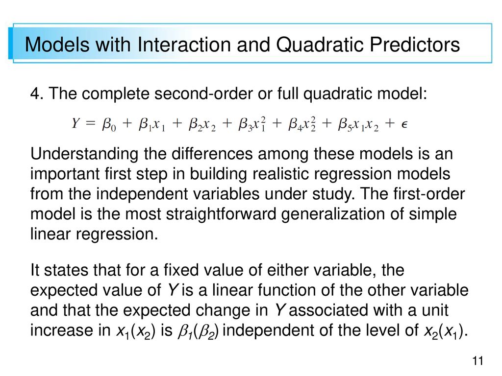
84 |
85 | ## Exploratory Data Analysis
86 |
87 | Last week, we learned about Data Visualisation and Exploration. To get hands on experience on Data Analysis on Regression and Classification, refer to the links below -
88 | * **[Regression](https://github.com/MicrosoftLearning/Principles-of-Machine-Learning-Python/blob/master/Module2/VisualizingDataForRegression.ipynb)**
89 | * **[Classification](https://github.com/MicrosoftLearning/Principles-of-Machine-Learning-Python/blob/master/Module2/VisualizingDataForClassification.ipynb)**
90 |
91 | Now finally let us look into one important aspect of data analysis that is important for machine learning, data cleaning.
92 |
93 | ## Data Pre-Processing
94 |
95 | Let us consider a simple classification problem using logistic regression. Suppose you have 10 columns in your data which would make up the raw features given to you. A naive model would involve training your classifier using all these columns as features. However are all the features equally relevant? This may not be the case. As a worst case example suppose all the data entries in your training set have the same value. Then it does not make sense to consider this as a feature since any tweaking to the parameter corresponding to this feature that you do can be done by changing the bias term as well. This is a redundant input feature that you should remove. Similarly if you have a column that has very low variance it may make sense to remove this feature from your dataset as well. When we work with high dimensional data sometimes it makes sense to work with fewer dimensions. Thus it makes sense to remove the lower variance dimensions. Note that sometimes this reduction of dimension may not be as straightforward and next week we will see how to do this using PCA.
96 |
97 | * This **[article](https://machinelearningmastery.com/basic-data-cleaning-for-machine-learning/)** provides a proper introduction to data cleaning for machine learning
98 | * This **[article](https://www.dataquest.io/blog/machine-learning-preparing-data/)** is also useful for data cleaning.
99 |
100 | Another way we can clean and improve our data is by performing appropriate transformations on the data. Consider the task of Sentiment Classification using Logistic Regression. You are given a tweet and you have to state whether it expresses happy or sad sentiment. You could just take the tweet in and feed it into the classifier (using a particular representation, the details aren't important). But do all the words really matter?
101 |
102 | Consider a sample tweet
103 | ```
104 | #FollowFriday @France_Inte @PKuchly57 @Milipol_Paris for being top engaged members in my community this week :)
105 | ```
106 | Clearly any tags in this tweet are irrelevant. Similarly symbols like '#' are also not needed. Thus we need to clean the input data to remove all this unnecesary information. Further in Natural Language Processing words like 'for', 'in' do not contribute to the sentiment and a proper classification would require us to remove this as well. All of this comes under data cleaning and preprocessing.
107 |
108 | The preprocessed version of the above tweet would be:
109 | ```
110 | ['followfriday', 'top', 'engag', 'member', 'commun', 'week', ':)']
111 | ```
112 |
113 | * This **[article](https://towardsdatascience.com/data-preprocessing-concepts-fa946d11c825)** explains data preprocessing.
114 | * This **[tutorial](https://towardsdatascience.com/twitter-sentiment-analysis-classification-using-nltk-python-fa912578614c)** uses Naive Bayes to solve the above tweet classification problem. Please go through this to acquaint yourself with the various data processing methods needed for natural language processing (Note that this tutorial uses sklearn to implement naive bayes instead of doing it from scratch. Feel free to skip the implementational details if you are facing issues with it as we will not be covering sklearn in this course)
115 |
116 | The concepts of feature aggregration, data cleaning, dimensionality reduction are important for a data scientist and it is essential to have a proper understanding of them before continuing.
117 |
118 |
119 | ## How to choose the right model? Can a model be too good?
120 | Now that we have learnt all about exploratory analysis and data pre-processing, we can get a better idea of how the input features are related to each other using these. We can also test out multiple models and see how they perform for our *testing data*.
121 |
122 | The most important part is understanding that our model could be perfect on our training data but still perform poorly on testing data. Let us take an example where the data has a complex non-linear relationship. Obviously, the more non-linear the relationship, the more it makes sense for us to use a higher degree model. Right? Unfortunately, this does not always result in the desired outcome.
123 |
124 | Why does this happen?
125 |
126 | This is due to a phenomenon called overfitting where the model learns the training data too well and accounts even for outliars that may otherwise have been ignored by less complex models. In doing so, the general trend is given up for exactly matching the pattern of the data it is trained on which may lead to poor testing performance and lower accuracy as compared to a lower degree model
127 | 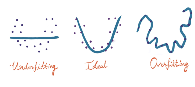
128 |
129 |
130 | ---
131 | ## Here are some topics for additional reading
132 |
133 | ## Segmented Regression
134 |
135 | It is also referred to as **Piecewise Regression** or **Broken Stick Regression**. Unlike standard Linear Regression, we fit separate line segments to intervals of independent variables. Formally stating, independent linear models are assigned to individual partitions of feature spaces. This is pretty useful in the cases when the data assumes different linear relationships in separate intervals of the feature values. Generally, applying linear regression on such tasks can incur large statistical losses.
136 |
137 | It is important to note that despite it's better accuracy, it can be computationally inefficient because many independent linear regressions have to be performed.
138 |
139 | The points where the data is split into intervals are called **Break Points**. There are various statistical tests that are to be performed in order to determine the break points but the details of those tests are beyond the scope of this course.
140 |
141 | #### Useful Resources
142 |
143 | * To get an overview of the concepts, go through **[this](https://storybydata.com/datacated-challenge/piecewise-linear-regression/)** article and **[this](https://en.wikipedia.org/wiki/Segmented_regression)** page.
144 |
145 | * Refer to the **[repo](https://github.com/srivatsan88/piecewise-regression/blob/master/piecewise_linear_regression.ipynb)** for a small demo on Piecewise Linear Regression.
146 |
147 | * (Optional) To delve deeper into the mathematical aspects and get hands on experience, go through **[this](https://www.fs.fed.us/rm/pubs/rmrs_gtr189.pdf)**. This is pretty complicated to understand and it is upto the interest of the reader.
148 |
149 | ## Locally Weighted Regression
150 |
151 | In Locally Weighted Regression, we try to fit a line locally to the point of prediction. What it means is that we give more emphasis to the training data points that are close to the point where prediction is to be made. A weight function (generally a bell shaped function) is used to determine the amount of emphasis given to a data point for prediction. This kind of model comes under **Non Parametric Learning** unlike the **Parametric Learning** models that we have seen so far.
152 |
153 | Such models are useful when the training data is small and has small number of features. It is computationally inefficient because a linear regression is performed everytime we need to predict some value. But at the same time, this allows us to fit even complicated non-linear curves with ease.
154 |
155 | #### Useful Resources
156 |
157 | * Follow this article to get an [overview](https://medium.com/100-days-of-algorithms/day-97-locally-weighted-regression-c9cfaff087fb) of this model.
158 |
159 | For classification tasks we need a different architecture. In the next section, we discuss about Logistic Regression - a regression tool employed for classification.
160 |
161 |
162 | ## Generalised Linear Models
163 |
164 | On a very high level, Generalised Linear Models (GLM) are a superclass of all linear models including Linear and Logistic Regression that we talked about earlier.
165 |
166 | * Linear Regression is based on the assumption that the data assumes **Gaussian/Normal Distribution**.
167 | * Binary Logistic Regression is based on the assumption that data assumes **Bernoulli Distribution**.
168 |
169 | GLM's are based on Exponential Family Functions. **[Exponential Family](https://en.wikipedia.org/wiki/Exponential_family)** includes these two and a lot of other distributions of data that we talked about in week 1. So therefore GLM's serve as a generalisation of all linear models. To get a firm hold on generalised linear models, head **[here](https://towardsdatascience.com/generalized-linear-models-9cbf848bb8ab)**.
170 |
171 | ---
172 |
173 | Next week we will be looking at more supervised machine learning techniques. Till then stay safe and have fun.
174 |
--------------------------------------------------------------------------------
/Week 2/data_preprocessing_tools.ipynb:
--------------------------------------------------------------------------------
1 | {"cells":[{"cell_type":"markdown","metadata":{"id":"37puETfgRzzg"},"source":["# Data Preprocessing Tools\n","Notebook authored by Haledin de Ponteves"]},{"cell_type":"markdown","metadata":{"id":"EoRP98MpR-qj"},"source":["## Importing the libraries"]},{"cell_type":"code","execution_count":5,"metadata":{"id":"N-qiINBQSK2g"},"outputs":[],"source":["import numpy as np\n","import matplotlib.pyplot as plt\n","import pandas as pd"]},{"cell_type":"markdown","metadata":{"id":"RopL7tUZSQkT"},"source":["## Importing the dataset"]},{"cell_type":"code","execution_count":6,"metadata":{"id":"WwEPNDWySTKm"},"outputs":[],"source":["dataset = pd.read_csv('./datasets/preprocessing-data.csv')\n","X = dataset.iloc[:, :-1].values\n","y = dataset.iloc[:, -1].values"]},{"cell_type":"code","execution_count":7,"metadata":{"id":"hCsz2yCebe1R"},"outputs":[{"name":"stdout","output_type":"stream","text":["[['France' 44.0 72000.0]\n"," ['Spain' 27.0 48000.0]\n"," ['Germany' 30.0 54000.0]\n"," ['Spain' 38.0 61000.0]\n"," ['Germany' 40.0 nan]\n"," ['France' 35.0 58000.0]\n"," ['Spain' nan 52000.0]\n"," ['France' 48.0 79000.0]\n"," ['Germany' 50.0 83000.0]\n"," ['France' 37.0 67000.0]]\n"]}],"source":["print(X)"]},{"cell_type":"code","execution_count":8,"metadata":{"id":"eYrOQ43XcJR3"},"outputs":[{"name":"stdout","output_type":"stream","text":["['No' 'Yes' 'No' 'No' 'Yes' 'Yes' 'No' 'Yes' 'No' 'Yes']\n"]}],"source":["print(y)"]},{"cell_type":"markdown","metadata":{"id":"nhfKXNxlSabC"},"source":["## Taking care of missing data"]},{"cell_type":"code","execution_count":9,"metadata":{"id":"c93k7ipkSexq"},"outputs":[],"source":["from sklearn.impute import SimpleImputer\n","imputer = SimpleImputer(missing_values=np.nan, strategy='mean')\n","imputer.fit(X[:, 1:3])\n","X[:, 1:3] = imputer.transform(X[:, 1:3])"]},{"cell_type":"code","execution_count":10,"metadata":{"id":"3UgLdMS_bjq_"},"outputs":[{"name":"stdout","output_type":"stream","text":["[['France' 44.0 72000.0]\n"," ['Spain' 27.0 48000.0]\n"," ['Germany' 30.0 54000.0]\n"," ['Spain' 38.0 61000.0]\n"," ['Germany' 40.0 63777.77777777778]\n"," ['France' 35.0 58000.0]\n"," ['Spain' 38.77777777777778 52000.0]\n"," ['France' 48.0 79000.0]\n"," ['Germany' 50.0 83000.0]\n"," ['France' 37.0 67000.0]]\n"]}],"source":["print(X)"]},{"cell_type":"markdown","metadata":{"id":"CriG6VzVSjcK"},"source":["## Encoding categorical data"]},{"cell_type":"markdown","metadata":{"id":"AhSpdQWeSsFh"},"source":["### Encoding the Independent Variable"]},{"cell_type":"code","execution_count":11,"metadata":{"id":"5hwuVddlSwVi"},"outputs":[],"source":["from sklearn.compose import ColumnTransformer\n","from sklearn.preprocessing import OneHotEncoder\n","ct = ColumnTransformer(transformers=[('encoder', OneHotEncoder(), [0])], remainder='passthrough')\n","X = np.array(ct.fit_transform(X))"]},{"cell_type":"code","execution_count":12,"metadata":{"id":"f7QspewyeBfx"},"outputs":[{"name":"stdout","output_type":"stream","text":["[[1.0 0.0 0.0 44.0 72000.0]\n"," [0.0 0.0 1.0 27.0 48000.0]\n"," [0.0 1.0 0.0 30.0 54000.0]\n"," [0.0 0.0 1.0 38.0 61000.0]\n"," [0.0 1.0 0.0 40.0 63777.77777777778]\n"," [1.0 0.0 0.0 35.0 58000.0]\n"," [0.0 0.0 1.0 38.77777777777778 52000.0]\n"," [1.0 0.0 0.0 48.0 79000.0]\n"," [0.0 1.0 0.0 50.0 83000.0]\n"," [1.0 0.0 0.0 37.0 67000.0]]\n"]}],"source":["print(X)"]},{"cell_type":"markdown","metadata":{"id":"DXh8oVSITIc6"},"source":["### Encoding the Dependent Variable"]},{"cell_type":"code","execution_count":13,"metadata":{"id":"XgHCShVyTOYY"},"outputs":[],"source":["from sklearn.preprocessing import LabelEncoder\n","le = LabelEncoder()\n","y = le.fit_transform(y)"]},{"cell_type":"code","execution_count":14,"metadata":{"id":"FyhY8-gPpFCa"},"outputs":[{"name":"stdout","output_type":"stream","text":["[0 1 0 0 1 1 0 1 0 1]\n"]}],"source":["print(y)"]},{"cell_type":"markdown","metadata":{"id":"qb_vcgm3qZKW"},"source":["## Splitting the dataset into the Training set and Test set"]},{"cell_type":"code","execution_count":15,"metadata":{"id":"pXgA6CzlqbCl"},"outputs":[],"source":["from sklearn.model_selection import train_test_split\n","X_train, X_test, y_train, y_test = train_test_split(X, y, test_size = 0.2, random_state = 1)"]},{"cell_type":"code","execution_count":16,"metadata":{"id":"GuwQhFdKrYTM"},"outputs":[{"name":"stdout","output_type":"stream","text":["[[0.0 0.0 1.0 38.77777777777778 52000.0]\n"," [0.0 1.0 0.0 40.0 63777.77777777778]\n"," [1.0 0.0 0.0 44.0 72000.0]\n"," [0.0 0.0 1.0 38.0 61000.0]\n"," [0.0 0.0 1.0 27.0 48000.0]\n"," [1.0 0.0 0.0 48.0 79000.0]\n"," [0.0 1.0 0.0 50.0 83000.0]\n"," [1.0 0.0 0.0 35.0 58000.0]]\n"]}],"source":["print(X_train)"]},{"cell_type":"code","execution_count":17,"metadata":{"id":"TUrX_Tvcrbi4"},"outputs":[{"name":"stdout","output_type":"stream","text":["[[0.0 1.0 0.0 30.0 54000.0]\n"," [1.0 0.0 0.0 37.0 67000.0]]\n"]}],"source":["print(X_test)"]},{"cell_type":"code","execution_count":18,"metadata":{"id":"pSMHiIsWreQY"},"outputs":[{"name":"stdout","output_type":"stream","text":["[0 1 0 0 1 1 0 1]\n"]}],"source":["print(y_train)"]},{"cell_type":"code","execution_count":19,"metadata":{"id":"I_tW7H56rgtW"},"outputs":[{"name":"stdout","output_type":"stream","text":["[0 1]\n"]}],"source":["print(y_test)"]},{"cell_type":"markdown","metadata":{"id":"TpGqbS4TqkIR"},"source":["## Feature Scaling"]},{"cell_type":"code","execution_count":20,"metadata":{"id":"AxjSUXFQqo-3"},"outputs":[],"source":["from sklearn.preprocessing import StandardScaler\n","sc = StandardScaler()\n","X_train = sc.fit_transform(X_train)\n","X_test = sc.transform(X_test)"]},{"cell_type":"code","execution_count":21,"metadata":{"id":"DWPET8ZdlMnu"},"outputs":[{"name":"stdout","output_type":"stream","text":["[[-0.77459667 -0.57735027 1.29099445 -0.19159184 -1.07812594]\n"," [-0.77459667 1.73205081 -0.77459667 -0.01411729 -0.07013168]\n"," [ 1.29099445 -0.57735027 -0.77459667 0.56670851 0.63356243]\n"," [-0.77459667 -0.57735027 1.29099445 -0.30453019 -0.30786617]\n"," [-0.77459667 -0.57735027 1.29099445 -1.90180114 -1.42046362]\n"," [ 1.29099445 -0.57735027 -0.77459667 1.14753431 1.23265336]\n"," [-0.77459667 1.73205081 -0.77459667 1.43794721 1.57499104]\n"," [ 1.29099445 -0.57735027 -0.77459667 -0.74014954 -0.56461943]]\n"]}],"source":["print(X_train)"]},{"cell_type":"code","execution_count":22,"metadata":{"id":"sTXykB_QlRjE"},"outputs":[{"name":"stdout","output_type":"stream","text":["[[-0.77459667 1.73205081 -0.77459667 -1.46618179 -0.9069571 ]\n"," [ 1.29099445 -0.57735027 -0.77459667 -0.44973664 0.20564034]]\n"]}],"source":["print(X_test)"]}],"metadata":{"colab":{"authorship_tag":"ABX9TyOihYlX/ooG5h+qw0sLIjn8","collapsed_sections":[],"provenance":[]},"kernelspec":{"display_name":"Python 3","name":"python3"},"language_info":{"codemirror_mode":{"name":"ipython","version":3},"file_extension":".py","mimetype":"text/x-python","name":"python","nbconvert_exporter":"python","pygments_lexer":"ipython3","version":"3.11.1"}},"nbformat":4,"nbformat_minor":0}
2 |
--------------------------------------------------------------------------------
/Week 2/datasets/preprocessing-data.csv:
--------------------------------------------------------------------------------
1 | Country,Age,Salary,Purchased
2 | France,44,72000,No
3 | Spain,27,48000,Yes
4 | Germany,30,54000,No
5 | Spain,38,61000,No
6 | Germany,40,,Yes
7 | France,35,58000,Yes
8 | Spain,,52000,No
9 | France,48,79000,Yes
10 | Germany,50,83000,No
11 | France,37,67000,Yes
--------------------------------------------------------------------------------
/Week 3/README.md:
--------------------------------------------------------------------------------
1 | # Week 3
2 |
3 | Welcome to Week 3! This week we will be covering many powerful classical machine learning algorithms before moving onto modern (aka deep learning) algorithms next week.
4 |
5 | We'll begin with a model that appears rather simple at first, Decision Tree. However this is an incredibly powerful model that relies a lot on information theory and entropy (remember thermodynamics anyone?) and we will discuss some of the fundamentals behind this (although I myself am not an expert on this and most of the advanced ideas are beyond the scope of this course). Then we will look at an extension of this model called Random Forest and then we will consider an important data dimensionality reduction technique called PCA and we end it by talking about kth nearest neighbours.
6 |
7 | So let's get started we have a busy week ahead of us!
8 |
9 | ## Decision Trees
10 |
11 | Let's forget about machine learning for some time and focus on you. You are trying to learn machine learning through this course. It's probably due to a lot of decisions that you ended up here. And it was always a sequence of decisions. When you decided to wake up early (or late) you made a decision. Then you decided to study. Then you decided to study machine learning.
12 |
13 | Indeed all a decision tree tries to do is create a sequence of decisions that would result in the machine learning algorithm come to an outcome. As an extremely simple example consider a machine learning algorithm that classifies all points in the xy plane to the right of the y axis as positive and others as negative.
14 |
15 | Then the decision tree is a very simple one here, the algorithm will check if `x>0` and then label positive else it would label negative. However rarely will the decision tree be this simple.
16 |
17 | This **[link](https://heartbeat.fritz.ai/introduction-to-decision-tree-learning-cd604f85e236)** provides an introduction to decision trees (please read only the beginning part without going into construction).
18 |
19 | All this may seem very simple to you but one question remains. How will the algorithm construct this tree? Clearly figuring out what questions to ask is far from simple. Note that we only ask questions related to the features given to us in the dataset and use these questions to come to a conclusion. Note that although decision trees can be used for both regression and classfication we only consider classification here. So our aim is to come up with a set of questions that will allow us to classify a dataset into labels.
20 |
21 | ### Constructing Decision Trees
22 |
23 | Basically we will use recursion. Observe that every point when you (aka the algorithm) ask any question the dataset splits. For instance consider the titanic dataset. You may ask one question regarding the age. If the age is `>= 30` go to the right half else go to the left half. Both the left and right half are themselves decision trees.
24 |
25 | So what we can do is look for the locally most optimum question. That is the question that would result in most amount of information about the classes being conveyed. For instance if all people above the age of 30 survived the titanic disaster then this is a very good question to ask since all elements in the right half belong to the survived category and so we can terminate the right half immediately.
26 |
27 | But how do we know which questions are best to ask? There are metrics for this and we investigate two of them namely information entropy and gini impurity.
28 |
29 | #### Information Entropy
30 |
31 | Remember thermodynamics? Yeah we all probably hated that chapter during JEE (I didn't but that's another story). The idea that entropy leads to disorder is not only a physical idea but also a mathematical one. Observe that we want after asking a question to split the dataset into halves such that each halves are as homogenous as possible (only then would your question be the most discriminating). But wait. That would mean the entropy increased since we are moving towards order! (Second law doesn't hold since this is not physics xD).
32 |
33 | This gives us an idea. Ask those questions that increase the entropy the most! Or in other words we want to increase the information gain. How do we compute this entropy? We have to use information entropy for this.
34 |
35 | * This **[link](https://www.kdnuggets.com/2020/01/decision-tree-algorithm-explained.html)** talks in brief about information entropy and you may go over it once.
36 | * This **[wikipedia section](https://en.wikipedia.org/wiki/Decision_tree_learning#Information_gain)** talks in detail about the math behind decision tree learning.
37 | * This **[article](https://www.geeksforgeeks.org/decision-tree-implementation-python/)** provides the code for using information gain based decision trees using sklearn.
38 |
39 |
40 | #### Gini Impurity
41 |
42 | Instead of looking at entropy we can look at another metric. Split the dataset with a question in such a way such that each of the split datasets are as pure as possible. Pure means homogenous. Although entropy was also doing the same thing we can use a simpler way at estimating this. This way is termed gini impurity.
43 |
44 | Essentially Gini Impurity is a measurement of the likelihood of an incorrect classification of a new instance of a random variable, if that new instance were randomly classified according to the distribution of class labels from the data set.
45 |
46 | This **[article](https://towardsdatascience.com/decision-tree-in-machine-learning-e380942a4c96)** uses Gini Impurity for creating decision trees. Please go through this to understand the mathematical formulation of gini impurity and the code as well.
47 |
48 | That is all we want to cover in standalone Decision Trees. We will talk a bit more about them in pragmatics later on (overfitting).
49 |
50 | ## Random Forests
51 |
52 | THe main idea behing using random forests is that maybe a single decision tree could be inaccurate. But what if we have 10 or 20 decision trees that are uncorrelated and working independently? Then our probability of getting the correct classification would skyrocket! And indeed a random forest is basically a collection of decision trees that achieves this.
53 |
54 | * This **[article](https://towardsdatascience.com/understanding-random-forest-58381e0602d2)** covers random forests in theory.
55 | * This **[article](https://towardsdatascience.com/random-forest-in-python-24d0893d51c0)** provides you with a step by step implementation in Python.
56 |
57 | Now let's get onto PCA.
58 |
59 | ## Principle Component Analysis
60 |
61 | The main idea of PCA is the following:
62 |
63 | Suppose we have a highdimensional dataset of dimension `d` that we want to compress along `k` dimensions.
64 | Given this high dimensional dataset retain the `k` dimensions along the eigenvectors of the covariance matrix of the data inputs with the highest eigenvalues (out of the total `d` eigenvectors (this is actually `d-1` after normalisation)). This compression will retain the maximum variance among all other compressions.
65 |
66 | That probably made no sense. If you just implement this you are done with PCA. Finding covariance matrix and eigenvectors is pretty easy with numpy.
67 |
68 | But don't do that yet. Let's understand why this works.
69 |
70 | * This **[video](https://www.youtube.com/watch?v=TJdH6rPA-TI)** beautifully explains what PCA does.
71 | * These **[notes](http://cs229.stanford.edu/notes/cs229-notes10.pdf)** by Andrew NG brilliantly explain the math behind PCA.
72 | * This **[lecture](https://www.youtube.com/watch?v=rng04VJxUt4)** explains PCA in a simpler manner.
73 | * (Optional) These CS663 IITB **[slides](https://www.cse.iitb.ac.in/~ajitvr/CS663_Fall2016/face_recognition.pdf)** explain how PCA is derived and a beautiful application of PCA for face recognition is given (bonus points to those who code this up!)
74 |
75 |
76 | That should be all for PCA. Let's talk about kNNs
77 |
78 | ## kth Nearest Neighbour
79 |
80 | This is probably the simplest algorithm that we'll talk about today.
81 |
82 | Suppose you want to classify data. You have a training set of `d` dimensions. What you can do is simply find the kth nearest points in the training set to any datapoint in your test set. Then simply return the label which appears the maximum times among these k labels.
83 |
84 | Why would this work? Well because birds of a feather flock together! Assuming that there is indeed a proper boundary separting different classification regions you would hope that points belong to the same class are clustured together at different regions. Thus by looking at the class of the closest points you can get an estimate of which class your test point belongs to.
85 |
86 | What should `k` be though? This is a hyperparameter that you should tweak! (Hyperparamter refers to variables that you tweak in your algorithm to get the best performance).
87 |
88 | * This **[article](https://www.geeksforgeeks.org/k-nearest-neighbours/)** talks about kNNs in a simple manner.
89 | * For more insight refer to this **[article](https://towardsdatascience.com/machine-learning-basics-with-the-k-nearest-neighbors-algorithm-6a6e71d01761)**.
90 |
91 | We could end here but wait. How do you really find the kth nearest neighbours? You have to loop through all examples in your training set every time you want to evaluate your machine learning algorithm. This would be incredibly SLOW!
92 |
93 | We could give up here but there is seemingly a way out of this. We use what is termed as locality sensitive hashing for kNNs. Note that this is a bit more advanced so go through it slowly.
94 |
95 | * This **[article](https://towardsdatascience.com/fast-near-duplicate-image-search-using-locality-sensitive-hashing-d4c16058efcb)** talks about using LSH with kNNs for findind duplicate images. (Note this uses deep learning to encode images feel free to skip this and just go through how hashing is done to generate hyperplanes that are then used with kNNs).
96 |
97 | * This **[video](https://www.youtube.com/watch?v=LqcwaW2YE_c)** also goes over kNNs with locality sensitive hashing.
98 |
99 | You can also refer to this **[playlist](https://www.youtube.com/playlist?list=PLBv09BD7ez_48heon5Az-TsyoXVYOJtDZ)** to know more about kNNs.
100 |
101 |
102 | That's it for this week! Stay tuned for the graded assignment that will be due by the end of this week! Have fun with the assignment and we hope to see you next week.
103 |
--------------------------------------------------------------------------------
/Week 4/Pragmatics.md:
--------------------------------------------------------------------------------
1 | # Practical Aspects of Machine Learning Models - 1
2 |
3 | So far, we have discussed about a multitude of models starting with Linear Regression model, Logisitic Regression, Decision trees to Neural Nets this week. As you
4 | might have seen so far, when we say 'fit the data', we mean some sort of a generalised fit. It is not desirable to fit the data perfectly. A model that accommodates
5 | each point of the curve may not be the optimal model for the data. There are several aspects of model fitting and there are factors that in some sense govern the
6 | desired accuracy of our model on the training data. Let us first get familiar with some concepts which we also explore in a greater depth in the coming weeks.
7 |
8 |
9 |
10 | ## Generalization
11 |
12 | Let us try to understand what we are actually trying to do with a Machine learning model. We train it on some data and want to use the same weights/parameters on
13 | some other data points to predict the target variable as accurately as possible. So when we say 'fit the data' perfectly, we don't actually mean to accommodate all
14 | the data points of our training data as perfectly as possible, what we actually mean is to figure out the underlying variations and try to generalise the data and
15 | accommodate the generalisation in our model so that accurate predictions can be made on unseen data.
16 |
17 | This leads us to kind of end results that are not desirable after training on the data -
18 |
19 | ### Underfitting
20 |
21 | It is a situation when the model doesn't fit the data properly. The values of the parameters in the parameters' space are far from global optima. It either means
22 | that the training of the model wasn't good or that the model is itself incapable of fitting the data points accurately. Predicting the line ( y = 2*x ) for the points
23 | lying roughly on ( y = x ) is an example for the former case wherein the slope can be optimised to fit the data accurately. Trying to fit a straight line on a data set
24 | that comes from some quadratic curve is an example for the second case.
25 |
26 | Such a result is obviously not desirable because it would lead to bad prediction results.
27 | Solution to this would be -
28 |
29 | * To figure out modifications in training
30 | * Train for a longer duration to give more time to reach the global minima in the parameter space
31 | * Change the model itself and find a suitable one to fit the data well
32 |
33 | ### Overfitting
34 |
35 | It is a situation when the model fits the data points too accurately by keeping generalisation at the back seat. The model in the wake of reaching the global minima
36 | in the parameter space tries to accommodate the training data set points accurately and fails to predict the test data points accurately. Let us try to figure out
37 | why this can be the case.
38 |
39 | Let us say that we have data points coming from the distribution ( y = x**2 ), since the data cannot lie perfecty on the curve, there are some
40 | outliers to this generalisation. Now, since we defined our loss function to be mean squared error, so to minimise this, the model tries to accommodate this outlier
41 | on the curve too. So, maybe it tries to fit some higher degree complex polynomial on this data and it fails to identify the generalisation in the data that is a
42 | simple quadratic curve.
43 |
44 | At first such a result may appear good as the accuracy on the training set would be great but when tried on the test data is likely to give poor results.
45 |
46 | There are several solutions for this, many of which are model - specific
47 |
48 | * Reduce the training time
49 | * Enrich the training set with a wide variety of examples
50 | * Add Regularisation to the model
51 |
52 | #### Useful Resources
53 |
54 | * **[Underfitting and Overfitting Simplified](https://www.youtube.com/watch?v=BqzgUnrNhFM)**
55 | * **[Underfitting vs Overfitting](https://www.analyticsvidhya.com/blog/2020/02/underfitting-overfitting-best-fitting-machine-learning/)**
56 | * **[How to Deal with Underfitting and Overfitting](https://towardsdatascience.com/underfitting-and-overfitting-in-machine-learning-and-how-to-deal-with-it-6fe4a8a49dbf)**
57 | * **[The Problem of Overfitting](https://www.youtube.com/watch?v=BqzgUnrNhFM)**
58 |
59 | ## Regularisation
60 |
61 | Basically, this tends to reduce the magnitude of the weights/paramteres of the model in order to reduce the extent of overfitting and thus lead to better generalisations. This is called Regularisation. We look at a few techniques to regularise the network -
62 | * **Lasso Regression** - Also referred to as the **L1 regularisation**. This technique involves addition of magnitude of the weights to the loss function as a penalty so that they don't become large enough and overfit the data.
63 |
64 | * **Ridge Regression** - Also referred to as the **L2 regularisation**. Unlike the L1 method, this method adds the squared values of the weights to the loss function on a similar note.
65 |
66 | Let us try to understand what is it helpful in reducing overfitting. One of the popular ideas behind this is that adding that term leads to reduced magnitude of weights and that leads to lower value of activations. If you see the activation functions used, the graph is pretty much linear at values close to 0 and thus model becomes simpler and it is difficult for it to fit complicated functions and hence reduces overfitting.
67 |
68 | #### Useful Resources
69 |
70 | * **[Regularisation in Machine Learning](https://towardsdatascience.com/regularization-in-machine-learning-76441ddcf99a#:~:text=increasing%20model%20interpretability.-,Regularization,linear%20regression%20looks%20like%20this.)**
71 |
72 | * Read the **[article](https://towardsdatascience.com/l1-and-l2-regularization-methods-ce25e7fc831c)** to get into the details of L1 and L2 regularisation techniques.
73 |
74 | #### Probabilistic Intrepretation of Regularisation (Optional)
75 | There is a rigorous proof for Ridge Regression but that requires a bit of knowledge about statistics. Head **[here](https://www.quora.com/What-is-the-difference-between-Bayesian-and-frequentist-statisticians)** to get an overview of the statistics involved. Now, for those of you who read about Generalised Linear Models in Week 2 know the proof of how Linear Model Relations come up. There, we used the likelihood formula for the parameters but that was on the basis of Frequentistic Statistics, but if the same is done using the Bayesian Distribution, then in addition to the Standard Loss function, a **L2** loss shows up in the loss function. This can be in some sense related to **Maximum Likelihood Estimate** vs **Maximum A Posterior**
76 |
77 | #### Useful Resources
78 | * **[Probabilistic Interpretation of Regularisation](http://bjlkeng.github.io/posts/probabilistic-interpretation-of-regularization/)**
79 |
80 | There are a lot more things in regularisation specific to neural nets. We will talk about them the next week after we have a clear understanding of neural networks.
81 |
--------------------------------------------------------------------------------
/Week 4/README.md:
--------------------------------------------------------------------------------
1 | # Week 4
2 |
3 | Welcome to Week 4! This week you are going to develop your understanding about neural networks and deep learning.
4 |
5 | Last week you studied about various machine learning algorithms.It’s a pertinent question. There is no shortage of machine learning algorithms so why should we gravitate towards deep learning algorithms? What do neural networks offer that traditional machine learning algorithms don’t?
6 | ### Why are neural nets preferred over traditional machine learning algorithms ?
7 | Well, here are two key reasons why researchers and experts tend to prefer Deep Learning over Machine Learning:
8 | * **Decision Boundary:** In the case of classification problems, the algorithm learns the function that separates 2 classes, this is known as a Decision boundary.This [video](https://www.coursera.org/lecture/machine-learning/decision-boundary-WuL1H) beautifully explains about decision boundaries and some good examples. ***Every Machine Learning algorithm is not capable of learning all the functions. This limits the problems these algorithms can solve that involve a complex relationship whereas Neural Nets can compute any function.*** OPTIONAL: If you wish to see the proof behind the same, refer to this [link](http://neuralnetworksanddeeplearning.com/chap4.html) for intuitive proof.
9 |
10 | * **Feature Engineering:** Feature engineering is a key step in the model building process. It is a two-step process:
11 | * Feature extraction: In feature extraction, we extract all the required features for our problem statement
12 | * Feature selection: In feature selection, we select the important features that improve the performance of our machine learning or deep learning model.
13 | Consider an image classification problem. Extracting features manually from an image needs strong knowledge of the subject as well as the domain. It is an extremely time-consuming process. Thanks to Deep Learning, we can automate the process of Feature Engineering! All you need to do is just enter raw data, and the neural nets will classify it into features with appropiate weights on it's own.
14 |
15 | This week, we'll study about feedforward neural networks
16 |
17 | ## FeedForward Neural Networks
18 | The feedforward neural network was the first and simplest type of artificial neural network devised. In this network, the information moves in only one direction, forward, from the input nodes, through the hidden nodes (if any) and to the output nodes. There are no cycles or loops in the network. If we include loops, then it becomes **Recurrent Neural Network** which we'll learn in the upcoming week.
19 |
20 | ## **Forward Propagation**:
21 | To put it simply, the process that runs inside a neuron for forward propagation is, the neuron takes n input data (training examples) x1, x2,..., xn and first assigns random weights and biases to all the input variables and calculate their weighted sum Z, and further pass it inside an activation function, g(x) such as a sigmoid (later we'll also talk about other alternatives for it),giving g(Z) = A.
22 |
23 | Similarly, we calculate this activation, A for all the neurons in all the layers. The activations of the previous layer act as input data for the next layer and the activation of the last layer gives the output, y^(y-hat)
24 | * Refer to this [3blue1brown video](https://www.youtube.com/watch?v=aircAruvnKk) to have a good visualisation
25 | * Refer to this [article](https://towardsdatascience.com/forward-propagation-in-neural-networks-simplified-math-and-code-version-bbcfef6f9250) to understand more and implement code as well.
26 |
27 | ### **Activation Functions**
28 | We can use different types of activation functions such as sigmoid, tanh, Relu (rectified linear unit), leaky relu.
29 | - Refer to this [website](https://www.analyticsvidhya.com/blog/2020/01/fundamentals-deep-learning-activation-functions-when-to-use-them/) and [video](https://www.youtube.com/watch?v=Xvg00QnyaIY&list=PLkDaE6sCZn6Ec-XTbcX1uRg2_u4xOEky0&index=30) to know about all of them.
30 | - [Why do we need non-linear activation functions](https://www.youtube.com/watch?v=NkOv_k7r6no&list=PLkDaE6sCZn6Ec-XTbcX1uRg2_u4xOEky0&index=31)
31 | Though, we generally prefer tanh over sigmoid since, both have similar properties, but tanh gives output whose mean can be centralised to 0 and has some other benefits which can be seen in [this](https://www.youtube.com/watch?v=nD5ag-Q1sms&t=405s) video.
32 | Both of these activation functions, share one disadvantage that the slope tends to 0 when the numbers are very large or very small, thus the process of making improvememts slows down here, the leaky Relu function serves as a benefit in this case as it's slope never collapses. However, for practical purposes even relu function works well. While using for classification, we prefer the output of the last layer to be between 0 and 1, thus we use L-1 layers with relu activation and the last year with sigmoid activation for good results in a L layer NN.
33 | Refer to [this](https://www.youtube.com/watch?v=G6djH3I0rG0&list=PLreVlKwe2Z0TTN9vNEsMhA2JVswctec2g) playlist to have a good idea about activation functions and their advantages.
34 |
35 |
36 | By now, our model has made it's first prediction, but this was with random weights and biases, hence the results were very random, we need to train our model. Now, to begin it's training the model must know where it went wrong. thus it needs a function to compute loss.
37 |
38 | ### **Optimization Problem**
39 | Typically, a neural network model is trained using the gradient descent optimization algorithm and weights are updated using the backpropagation of error algorithm.The gradient descent algorithm seeks to change the weights so that the next evaluation reduces the error, meaning the optimization algorithm is navigating down the gradient (or slope) of error.Now that we know that training neural nets solves an optimization problem, we can look at how the error of a given set of weights is calculated.
40 |
41 | ## **Loss Function**
42 | With neural networks, we seek to minimize the error. As such, the objective function is often referred to as a cost function or a loss function and the value calculated by the loss function is referred to as simply “loss.”
43 |
44 | ### **Maximum Likelihood And Cross Entropy**
45 | Maximum likelihood seeks to find the optimum values for the parameters by maximizing a likelihood function derived from the training data.
46 | When modeling a classification problem where we are interested in mapping input variables to a class label, we can model the problem as predicting the probability of an example belonging to each class. In a binary classification problem, there would be two classes, so we may predict the probability of the example belonging to the first class.
47 | Therefore, under maximum likelihood estimation, we would seek a set of model weights that minimize the difference between the model’s predicted probability distribution given the dataset and the distribution of probabilities in the training dataset. This is called the cross-entropy.
48 |
49 | **Cross Entropy Loss and Mean Squared Loss(MSE)** are the losses we use of classification and regression problems respectively. To know the reasons behind chck [this video](https://www.youtube.com/watch?v=2ca_K2rgNVA). PS: since, this is a NPTEL video i would suggest watching on 1.5x speed or higher xD
50 |
51 | ## Back Propagation
52 |
53 | Under Back Propagation, we use the loss calculated using loss function to make currections to our model. For this, we use Gradient Descent and then update our parameters accordingly. Here, are some really awesome videos to make your understanding much clear.
54 | - To visualize how gradient descent helps in improving results watch this [video](https://www.youtube.com/watch?v=IHZwWFHWa-w)
55 | - To get an intuition about what we do in Backpropagation, watch this [video](https://www.youtube.com/watch?v=Ilg3gGewQ5U)
56 | - To understand the calculus involved in backpropagation, watch this [video](https://www.youtube.com/watch?v=tIeHLnjs5U8&t=530s)
57 |
58 | We keep on repeating forward and backward propagation for many epochs to decrease value of cost function and increase accuracy.
59 |
60 | ## Multi-class Classification using NN
61 | Rather than just to classify an object between yes/no. If we wish to classify it into more than 2 items using NN, we can do it similarly just the only difference will be that the output yhat will be a Mx1 matrix rather than 1x1 for a m class classifier.
62 | - refer this [video](https://www.youtube.com/watch?v=gAKQOZ5zIWg) to understand how we do it
63 | - refer this [article](https://towardsdatascience.com/multi-label-image-classification-with-neural-network-keras-ddc1ab1afede) to see it's implementatin.
64 | - For implementation, if you prefer videos refer [this](https://www.youtube.com/watch?v=oOSXQP7C7ck)
65 |
66 | ## Useful Resources
67 | - A read to these notes: [CS229](http://cs229.stanford.edu/notes/cs229-notes-deep_learning.pdf) , [Multi Layer NN](http://ufldl.stanford.edu/tutorial/supervised/MultiLayerNeuralNetworks/) and [CS229:Backprop](http://cs229.stanford.edu/notes/cs229-notes-backprop.pdf) is a worth to compile your understandings
68 | - Refer to this [playlist](https://www.youtube.com/watch?v=bxe2T-V8XRs&list=PLiaHhY2iBX9hdHaRr6b7XevZtgZRa1PoU) to see implementation of a complete NN
69 | - Check this [link](https://medium.com/@shaistha24/basic-concepts-you-should-know-before-starting-with-the-neural-networks-nn-3-6db79028e56d) for an intuitive run through and answers to few questions rising inside you.
70 | ## Additional Resources to explore
71 | - Refer to this [article](http://neuralnetworksanddeeplearning.com/chap3.html) to know more intuitively about various topics and learn how to improve your model.
72 | ## Exercises
73 | Implementing all of this in a code and making a neural network of your own will make your understanding better.
74 | Use Vectorization to do so rather than using for loops. If you don't know how to do so refer to [this](https://towardsdatascience.com/vectorization-implementation-in-machine-learning-ca652920c55d) article.
75 | 1. First, build a code for a perceptron(i.e. a single neuron and no hidden layers) and build a AND gate using it.
76 | 2. Now, try to build a XOR gate using a perceptron and share your results with us.
77 | 3. Implement a XOR gate again, this time you can use a single hidden layer.
78 |
79 |
80 | **IMPortant:** Do not use scikit learn or keras or any other libraries. Implement the codes from scratch using numpy.
81 | Implement seperate functions such as initialization, forward propagation, cost calculation and back propagation and then compile all of it in a class/function and test your neural net.
82 |
83 | ---
84 |
85 | That's it for this week. Next week you'll learn tensorflow and pytorch which will work as very helpful tools to implement all the algorithms you would have learnt upto then. If time permits, we'll also continue more with other NN such as CNNs and RNNs. Next week's going to last of fun learning, Stay Tuned.
86 |
87 |
88 |
89 |
--------------------------------------------------------------------------------
/Week 5/README.md:
--------------------------------------------------------------------------------
1 | # Welcome to Week 5 of LS Machine Learning!
2 | This week we will be covering the following topics:
3 | * Introduction to Tensorflow and Keras
4 | * Introduction to Convolutional Neural Networks
5 | * Practice Assignment - Basic Image Classification in Tensorflow
6 |
7 | ## Tensorflow and Keras
8 | Last week, you learned about Neural Networks, Backpropagation, Loss Function, Optimizers, Activation functions and how all of these are used together for training a Machine Learning model. But each and every function you defined was written from scratch in Python using classes. Tensorflow is an end-to-end open source tool developed by Google which contains pre-defined modules for all the different loss functions, optimisers, activation functions, layers, data pre-processing tools and much more which can speed up the process of performing machine learning by a huge amount.
9 | Even though all the modules and libraries can be accessed just using Tensorflow, you can also use the **Keras** API with the Tensorflow framework, which also contains pre-trained models like ResNet50, VGG16, etc. in addition to all the functions offered in Tensorflow. For this tutorial, we will be working with Tensorflow keras.
10 |
11 | To get started, first pip install tensorflow and keras and then simply import them in your code.
12 | ~~~
13 | pip install tensorflow
14 | pip install keras
15 | import tensorflow as tf
16 | from tensorflow import keras
17 | ~~~
18 | Note that you don't need to remember any of the syntax for importing different modules, just google whatever you need. The documentation provided by Tensorflow is already extremely detailed and easy to understand.
19 |
20 | ## Convolutional Nerual Networks
21 | ### Introduction
22 | In the previous week, you studied about Neural Networks, specifically Feed Forward Neural Networks, in which you either have one or two hidden layers to map your input to the output. When several hidden layers are used in a Nerual Network, it is known as a **Deep Neural Network (DNN)** and this is where Deep Learning comes into the picture. A DNN is a basic unit of any Deep Learning architecture.
23 |
24 | Till now, you are familiar only with fully connected layers, where each input is mapped to every activation of the next hidden layer with a weight (parameter) associated with it. The total number of parameters between the input layer and the hidden layer thus become equal to the product of elements in both the layers. You are also aware the process of 'Back Propagation' deals with optimising the values of these parameters. Hence, larger the number of parameters of the model, longer the time it will take for training.
25 |
26 | Now let's say you were to do the same process described above, but with image pixel values as your input. Considering even a small image, of say **50x50** pixels, number of input variables will be equal to **2500**. And lets say you are mapping these input pixel values to a fully connected layer with **1000** elements. Obviously, you cannot directly map the input to a smaller feature space, since that will result in a lot of image features not getting learnt by your model, defeating the purpose of using a DNN. So, the number of parameters for this layer is equal to **2500 x 1000 = 2,500,000**. The number of parameters already cross a million and imagine what will happen with more layers. The total number of parameters to be trained will be huge! And remember, this is just for a **50x50** pixel input image. What if you were to use a **1024x1024** sized image? The training time for your model will be even larger this time and hence using fully connected layers is not an efficient approach to deal with image inputs.
27 | This is where the concept of Convolutional Layers comes in, and a network comprised of convolutional layers (along with fully connected and other layers) is known as a **Convolutional Neural Network** (ConvNet).
28 |
29 | ### Convolutional Layers
30 | Convolutional layers are specifically used in ConvNets when working with images. The use of a Convolutional layer instead of a fully connected layer results in significant decrease in the number of trainable parameters of the model without negligible loss in feature learning. The basic idea of a convolutional layer is to use a filter over the input image, where the filter is a 2D matrix custom designed to learn a particular feature (eg: a vertical edge). The output of the operation is another matrix but of reduced dimensions.
31 | * Read about Convolutional layers from this detailed article - **[Convolutional Layer](https://cs231n.github.io/convolutional-networks/#conv)**
32 | * You can also checkout this article for an alternate source - **[Convolution Reading](https://machinelearningmastery.com/convolutional-layers-for-deep-learning-neural-networks/)**
33 | * Additionally, you can watch the following videos for a better understanding - **[Video #1](https://www.youtube.com/watch?v=XuD4C8vJzEQ&list=PLkDaE6sCZn6Gl29AoE31iwdVwSG-KnDzF&index=2), [Video #2](https://www.youtube.com/watch?v=am36dePheDc&list=PLkDaE6sCZn6Gl29AoE31iwdVwSG-KnDzF&index=3), [Video #3](https://www.youtube.com/watch?v=smHa2442Ah4&list=PLkDaE6sCZn6Gl29AoE31iwdVwSG-KnDzF&index=4), [Video #4](https://www.youtube.com/watch?v=tQYZaDn_kSg&list=PLkDaE6sCZn6Gl29AoE31iwdVwSG-KnDzF&index=5)**
34 | * Checkout this video to get an idea of how to apply filter/kernels to multichannel RGB images - **[Convolution over volumes](https://www.youtube.com/watch?v=KTB_OFoAQcc&list=PLkDaE6sCZn6Gl29AoE31iwdVwSG-KnDzF&index=6)**
35 |
36 | ### Pooling Layers
37 | Pooling layers are based on the same concept as convolutional layers, that is, even they perform a filtering operation on the input image matrix, but a pooling filter is not used to detect a particular feature. The aim of a pooling layer is to simply reduce the dimensions of the input matrix to reduce the number of trainable parameters and hence decrease the number of computations, without a huge loss in the features of the input image. Even though there is a trade off between the accuracy of the learned features and computation time, it is very common to make use of pooling layers since the latter is a bigger concern for deep learning models. Pooling layers can be of different types, such as, Max Pooling, Global Average pooling, etc.
38 | * Read more about Pooling layers from this link - **[Pooling Layers](https://cs231n.github.io/convolutional-networks/#pool)**
39 | * Watch the video for a better understanding - **[Pooling layers Video](https://www.youtube.com/watch?v=8oOgPUO-TBY&list=PLkDaE6sCZn6Gl29AoE31iwdVwSG-KnDzF&index=9)**
40 |
41 | ### ConvNets
42 | Now that you are familiar with the different layers that any Convolutional Neural Network is comprised of, namely the Fully Connected Layer, Convolutional Layer and the Pooling Layer, let us look at some examples.
43 | * Go through this article which talks about ConvNet architectures in detail, along with the things you should keep in mind when desigining your own model architecture - **[ConvNet Architectures](https://cs231n.github.io/convolutional-networks/#architectures)**
44 | * Additionally, go through these videos for a better grasp on ConvNets - **[Example ConvNet #1](https://www.youtube.com/watch?v=3PyJA9AfwSk&list=PLkDaE6sCZn6Gl29AoE31iwdVwSG-KnDzF&index=8), [Example ConvNet #1](https://www.youtube.com/watch?v=bXJx7y51cl0&list=PLkDaE6sCZn6Gl29AoE31iwdVwSG-KnDzF&index=10)**
45 |
46 | As you might have seen in the links, there are many pre-defined architectures which are widely used for many Deep Learning applications. Some of these are ResNet50, VGG16, Inception and many more. Try to find more information about these architectures and figure out the different layers that are being used in them. This will familiarise you with the ConvNet architectures used in common practice for different applications.
47 | It is important to note here that these architectures are readily available as modules in the Keras' applications library, so you don't need to build these architectures from scratch!
48 |
49 | ## Practice Assignment
50 | Finally, we will end this week's tutorial by performing an Image Classification task accomplished using Convolutional Neural Networks. Tensorflow officially provides many basic and advanced tutorials on different topics of Machine Learning. You can learn a lot about different Tensorflow and Keras functions just by following their notebooks step-by-step and referring to the official documentation wherever you get stuck.
51 |
52 | Head over to this link for a basic tutorial on Image Classification in Tensorflow using CNNs - **[Tensorflow Image Classification](https://www.tensorflow.org/tutorials/images/cnn)**
53 |
54 | **Optionally**, you can also go through the tutorial below, which is also on Image classification, but adds more complexity to the task. It will help you visualize the concept of Overfitting on an actual dataset after you have trained the model and then elaborates on techniques to avoid it. But remember, this is an optional resource only meant for those who have completed and understood all the previous content before. - **[Image Classification Complex (Optional)](https://www.tensorflow.org/tutorials/images/classification#visualize_training_results)**
55 |
56 |
57 | ## Links to resources
58 | Many of the links provided above are from the [CNN Course on Coursera](https://www.coursera.org/programs/indian-institute-of-technology-bombay-gkhfq/browse?productId=kWGvJivBEeeW5RJUyz1uFA&productType=course&query=Convolutional+Neural+Networks&showMiniModal=true) (By Andrew Ng) and [Stanford's CS231n course](https://cs231n.github.io) on Convolutional Neural Networks. These courses are extremely detailed and act as a starting point for many ML enthusiasts. So it is recommended that you checkout the entire course if you want a deeper understanding of the underlying math of CNNs.
59 |
60 |
61 | We Hope that you enjoyed Week 5 of LS ML!
62 | See you in Week 6!
63 |
64 |
65 |
66 |
67 |
--------------------------------------------------------------------------------
/Week 6/README.md:
--------------------------------------------------------------------------------
1 | # Week 6
2 |
3 | This week we talk a lot about the pragmatics of Machine Learning/Deep Learning and explore the various techniques that enhance performance of our models greatly.
4 |
5 | ## Intialisation
6 |
7 | Correct initialisation of weights in a neural net is extremely important for an efficient training of a neural net. There are several ways to initialise the weights which we discuss below -
8 |
9 | ### Zero Initialisation
10 |
11 | We can initialise all the weights and baises of a network to be 0. Though this might seem okay at the first sight but this poses a big hindernace to the learning of a neural net. If two weights associated with a neuron are same then they continue to have the same value throughout as the derivative will be the same during entire training. This limits the learning of a neural net as the neurons don't learn different aspects of the data. So initialising two weights with the same value is not at all desirable and initialising all weights to 0 makes your neural net worthless. Although it is okay to initialise biases to the same value (including 0).
12 |
13 | ### Random Initialisation
14 |
15 | As we have seen earlier, assigning same values to weights can hamper performance, so a solution to fix this can be to initialise weights randomly (say with a given mean and variance). Now, this random initialisation when done with different values of variance and mean 0 can lead to different kinds of initialisation techniques as described below -
16 |
17 | #### He Initialisation
18 |
19 | This initialisation technique multiplies a dynamic number for each layer of the neural net, in particular it is proportional to the inverse square root of the number of incoming neurons. Read **[this](https://medium.com/@prateekvishnu/xavier-and-he-normal-he-et-al-initialization-8e3d7a087528)** for more info.
20 |
21 | #### Xavier Initialisation
22 |
23 | This is specifically for the tanh activation function, similar to the He Initialisation, the technqiue involves multiplication with a number proportional to the inverse square root of the number incoming neurons. Though the constants differ by the a factor of square root of 2. Read **[this](https://medium.com/@prateekvishnu/xavier-and-he-normal-he-et-al-initialization-8e3d7a087528)** for more info.
24 |
25 | There are some techniques that involve multiplcation with a constant inversely proportional to the square root of sum of the number incoming and outgoing neurons. This proves to be a better initialisation stratergy for neural nets.
26 |
27 | ### Uniform Initialisation
28 |
29 | Similar to the logic behind random initialisation, one can also think about initialising weights drawn from a uniform distribution with a specific mean and variance.
30 |
31 | #### Glorot Uniform Intialisation
32 |
33 | The weights are drawn from a uniform distribution with a specific variance. The details of which can be read in the resources provided below.
34 |
35 | ### Why so Many Intialisation Techniques
36 |
37 | Let us try to understand why are there so many intialisation techniques and how to think of them as special cases of a standard thing.
38 |
39 | The baisc funda is that normalised inputs with mean 0 is always desirable for a neural net to be trained efficiently as it makes the optimization terrain more symmetrical with respect to the input features. On a similar note, it is desirable to make the derivatives normalised with mean 0 because that helps in faster training. So, the intialisation stratergy is to try to maintain that thing by assinging good intial values to the weights. So, there are two things to this -
40 |
41 | * Incoming neurons are related to normalised derivatives
42 | * Outgoing neurons are related to the normalised activation values (inputs)
43 |
44 | So, now, the various initialisation stratergies are associated with this fact that some of them use only the first condition, some of them the second one and some of them combine the two conditions. Also, depending upon the fact whether the technique draws values from a uniform or random distribution, one can derive these variance values. So in effect, at the heart of all initialisation techniques lies the two fundae mentioned above.
45 |
46 | ### Useful Resources
47 |
48 | There are several articles one can read to get a grip on this technique. Also, links to two research papers have also been added for the interested people.
49 |
50 | * **[Weight Initialisation Techniques](https://towardsdatascience.com/weight-initialization-techniques-in-neural-networks-26c649eb3b78)**
51 | * **[Journey of Initialisation in Neural Nets](https://towardsdatascience.com/weight-initialization-in-neural-networks-a-journey-from-the-basics-to-kaiming-954fb9b47c79)**
52 | * **[Research Paper on Glorot Initialisation](http://proceedings.mlr.press/v9/glorot10a/glorot10a.pdf)**
53 | * **[Xavier and He Initialisation](https://medium.com/@prateekvishnu/xavier-and-he-normal-he-et-al-initialization-8e3d7a087528)**
54 | * **[Mathematical Aspects of Initialisation](https://mmuratarat.github.io/2019-02-25/xavier-glorot-he-weight-init)**
55 | * **[Research Paper on Exploring Initialisation Stratergies on Several Activation Functions](https://arxiv.org/pdf/1704.08863.pdf)**
56 |
57 | ## Dropouts
58 |
59 | We studied earlier how Neural Nets and any machine learning model in general is prone to overfitting. Dropouts are an ingenius way to prevent this in the case of neural nets. Basically, some of the neurons are turned off in some sense at every forward pass during training. What is done is that the activation of some of the neurons of the network are set to 0 for one forward pass. This disallows any neuron to specialise in some aspect of the data that in turn reduces overfitting by allowing several neurons in the layer to learn things. Hence the learning gets distributed which leads to better generalisations.
60 |
61 | Basically, to implement this, a probabiity value is fixed and it is with this probability for every neuron that it is turned on or off.
62 |
63 | This technique has become really popular recently and the good thing is that the frameworks like Tensorflow already have Dropouts implemented that reduces the burden of implementing this.
64 |
65 | To read more about Dropouts, go through the following links -
66 |
67 | * **[Dropouts](https://medium.com/@amarbudhiraja/https-medium-com-amarbudhiraja-learning-less-to-learn-better-dropout-in-deep-machine-learning-74334da4bfc5)**
68 | * **[Math Behind Dropouts](https://towardsdatascience.com/simplified-math-behind-dropout-in-deep-learning-6d50f3f47275)** (Advanced Content)
69 |
--------------------------------------------------------------------------------
/midterm /About the data.md:
--------------------------------------------------------------------------------
1 | ## About the data
2 |
3 |
4 | This data consists of three files, containing data that was collected on January 1st 1998.
5 | Clone this repo and use the folders provided in this repo
6 |
7 | AdvWorksCusts.csv
8 |
9 |
10 | Customer demographic data consisting of the following fields:
11 |
12 | CustomerID (integer): A unique customer identifier.
13 | Title (string): The customer's formal title (Mr, Mrs, Ms, Miss Dr, etc.)
14 | FirstName (string): The customer's first name.
15 | MiddleName (string): The customer's middle name.
16 | LastName (string): The customer's last name.
17 | Suffix (string): A suffix for the customer name (Jr, Sr, etc.)
18 | AddressLine1 (string): The first line of the customer's home address.
19 | AddressLine2 (string): The second line of the customer's home address.
20 | City (string): The city where the customer lives.
21 | StateProvince (string): The state or province where the customer lives.
22 | CountryRegion (string): The country or region where the customer lives.
23 | PostalCode (string): The postal code for the customer's address.
24 | PhoneNumber (string): The customer's telephone number.
25 | BirthDate (date): The customer's date of birth in the format YYYY-MM-DD.
26 | Education (string): The maximum level of education achieved by the customer:
27 | Partial High School
28 | High School
29 | Partial College
30 | Bachelors
31 | Graduate Degree
32 | Occupation (string): The type of job in which the customer is employed:
33 | Manual
34 | Skilled Manual
35 | Clerical
36 | Management
37 | Professional
38 | Gender (string): The customer's gender (for example, M for male, F for female, etc.)
39 | MaritalStatus (string): Whether the customer is married (M) or single (S).
40 | HomeOwnerFlag (integer): A Boolean flag indicating whether the customer owns their own home (1) or not (0).
41 | NumberCarsOwned (integer): The number of cars owned by the customer.
42 | NumberChildrenAtHome (integer): The number of children the customer has who live at home.
43 | TotalChildren (integer): The total number of children the customer has.
44 | YearlyIncome (decimal): The annual income of the customer.
45 |
46 | AW_AveMonthSpend.csv
47 |
48 | Sales data for existing customers, consisting of the following fields:
49 |
50 | CustomerID (integer): The unique identifier for the customer.
51 | AveMonthSpend (decimal): The amount of money the customer spends with Adventure Works Cycles on average each month.
52 |
53 | AW_BikeBuyer.csv
54 |
55 | Sales data for existing customers, consisting of the following fields:
56 |
57 | CustomerID (integer): The unique identifier for the customer.
58 | BikeBuyer (integer): A Boolean flag indicating whether a customer has previously purchased a bike (1) or not (0).
59 |
--------------------------------------------------------------------------------
/midterm /MT Assignment.zip:
--------------------------------------------------------------------------------
https://raw.githubusercontent.com/GDSC-BPHC-ML/Machine-Learning_Bootcamp/b2b9746c5f75a9d464e6b921eb03adc61423ba50/midterm /MT Assignment.zip
--------------------------------------------------------------------------------
/midterm /MT-Assignment-Test.zip:
--------------------------------------------------------------------------------
https://raw.githubusercontent.com/GDSC-BPHC-ML/Machine-Learning_Bootcamp/b2b9746c5f75a9d464e6b921eb03adc61423ba50/midterm /MT-Assignment-Test.zip
--------------------------------------------------------------------------------
/midterm /README.md:
--------------------------------------------------------------------------------
1 | # Mid-Term Assignment
2 | In this assignment, you will put into practice some of the key principles and techniques you have learned in the course upto now. You are free to use any algorithm out of all of those which you have learned in this course,to implement regression models to the datasets. **To complete this assignment you have to complete both the problems, to get a detailed description about them, refer below**.
3 |
4 | ## Problem 1:
5 |
6 | We find this as a very good dataset for you to practice your hands on exploring data and building regression models.
7 |
8 | ### Problem Overview
9 | In 1998, the Adventure Works Cycles company collected a large volume of data about their existing customers, including demographic features and information about purchases they have made. The analysis should endeavor to determine whether a customer's average monthly spend with the company can be predicted from known customer characteristics.
10 |
11 | To complete this problem, you must tackle two challenges:
12 | - Challenge 1: Explore the data and gain some insights into Adventure Works customer characteristics and purchasing behavior.
13 | - Challenge 2: Build a regression model to predict customer purchasing behavior.
14 |
15 |
16 | ### About the Data
17 | To know about the data, refer to [this](https://github.com/wncc/learners-space/blob/master/Machine%20Learning/MId%20Term%20Assignment/About%20the%20data.md) link.
18 |
19 | ### Challenge 1: Data Exploration
20 |
21 | To complete this challenge:
22 | 1. Download the Adventure Works data files present inside this folder.
23 | 2. Clean the data by replacing any missing values and removing duplicate rows. In this dataset, each customer is identified by a unique customer ID. The most recent version of a duplicated record should be retained.
24 | 3. Explore the data by calculating summary and descriptive statistics for the features in the dataset, calculating correlations between features, and creating data visualizations to determine apparent relationships in the data.
25 | 4. Based on your analysis of the customer data after removing all duplicate customer records, answer the questions in this [form](https://forms.gle/CJ7cLSZY145yBnmh9).
26 |
27 | ### Challenge 2: Regression
28 | Create a regression model that predicts the average monthly spend of a new customers.
29 |
30 | To complete this challenge:
31 | 1. Use the Adventure Works Cycles customer data you worked with in challenge 1 to create a regression model that predicts a customer's average monthly spend. The model should predict average monthly spend for new customers for whom no information about average monthly spend or previous bike purchases is available.
32 | 2. Download the test data. This data includes customer features but does not include bike purchasing or average monthly spend values.
33 | 3. Use your model to predict on the corresponding test dataset. Don't forget to apply what you've learned throughout this course upto now.
34 | 4. For every Customer in the dataset, submission files should contain two columns: CustomerID and Prediction1.
35 | The file should contain a header and have the format given below to:
36 |
37 | > CustomerID,Prediction1
38 | > 18988,1
39 | > 29135,0
40 | > 12156,1
41 | > 13749,1
42 | > etc.
43 |
44 | For the submission, you will have to provide a github repo link/drive link/google colab notebook to a form we will be releasing soon.
45 | ## Problem 2:
46 | You are given a dataset of points in `data.json` of the form [x, y, label]. The label is either 0 or 1. You need to implement logistic regression to predict the label of a dataset similar to `data.json`. Please note that the test data is not given, this is the training data. However both the training data and the test data will follow the same distribution (so the curve you see will indeed be the decision boundary).
47 |
48 | You should submit two python files: `train.py` and `test.py`. `train.py` reads in `data.json` and outputs the parameters that will be used in your logistic regression model along with the training accuracy.
49 |
50 | `test.py` reads a file called `input.json` (this is not given, this is the test data) which is similar to `data.json` but does not have the label, hence the file is an array with elements of the form `[x, y]`. You need to use the parameters you obtained in the previous `train.py` and use these parameters to output another file called `result.json` which will take all the points `[x, y]` from `input.json` and output the corresponding label as well (so that outputs are of the form `[x, y, label]`)
51 |
52 | Weightage:
53 | 80%: `train.py`: Penalty for using libraries other than numpy and python standard library
54 | 20%: `test.py`: Penalty for using parameters other than that obtained in `train.py`
55 |
56 | (Hint: The data can be fit by a four degree polynomial of the form x^4 + x^3y + x^2y^2 along with lower degree terms..)
57 |
58 | ***We have made these assignments for you to have a better learning experience, if you get stuck discuss to a moderator about it and refrain from plagiarism. All the best, it's time to get started.***
59 |
60 |
61 |
62 |
63 |
--------------------------------------------------------------------------------