├── .github
└── workflows
│ └── deploy-book.yml
├── .gitignore
├── CITATION.cff
├── LICENSE.txt
├── README.md
├── book
├── _config.yml
├── _toc.yml
├── ecosystem.ipynb
├── first-figure.ipynb
├── intro.md
├── lidar_to_surface.ipynb
├── logo.svg
├── mars_maps.ipynb
├── mars_maps_extended.ipynb
└── references.bib
├── conda-lock.yml
└── environment.yml
/.github/workflows/deploy-book.yml:
--------------------------------------------------------------------------------
1 | # https://jupyterbook.org/en/stable/publish/gh-pages.html#automatically-host-your-book-with-github-actions
2 | name: deploy-book
3 |
4 | # Only run this when the main branch changes
5 | on:
6 | # Uncomment the 'pull_request' line below to manually re-build Jupyter Book
7 | # pull_request:
8 | push:
9 | branches:
10 | - main
11 | # If your git repository has the Jupyter Book within some-subfolder next to
12 | # unrelated files, you can make this run only if a file within that specific
13 | # folder has been modified.
14 | paths:
15 | - '.github/workflows/deploy-book.yml'
16 | - 'book/**'
17 |
18 | # This job installs dependencies, builds the book, and pushes it to `gh-pages`
19 | jobs:
20 | deploy-book:
21 | runs-on: ubuntu-latest
22 | defaults:
23 | run:
24 | shell: bash -l {0}
25 |
26 | steps:
27 | # Checkout current git repository
28 | - name: Checkout
29 | uses: actions/checkout@v3.0.2
30 |
31 | # Install Mambaforge with conda-forge dependencies
32 | - name: Setup Mambaforge
33 | uses: mamba-org/setup-micromamba@v1.9.0
34 | with:
35 | environment-name: egu22pygmt
36 | environment-file: conda-lock.yml
37 | create-args: >-
38 | python=${{ matrix.python-version }}
39 | condarc: |
40 | channels:
41 | - conda-forge
42 | - nodefaults
43 |
44 | # Build the book
45 | - name: Build the book
46 | run: jupyter-book build book/
47 |
48 | # Push the book's HTML to github-pages
49 | - name: GitHub Pages action
50 | uses: peaceiris/actions-gh-pages@v3.8.0
51 | with:
52 | github_token: ${{ secrets.GITHUB_TOKEN }}
53 | publish_dir: book/_build/html
54 |
--------------------------------------------------------------------------------
/.gitignore:
--------------------------------------------------------------------------------
1 | # Data files
2 | *.laz
3 | *.nc
4 | *.png
5 | *.tif
6 |
7 | # Jupyter Book
8 | /book/_build/
9 |
10 | # Jupyter Notebook
11 | .ipynb_checkpoints/
12 |
--------------------------------------------------------------------------------
/CITATION.cff:
--------------------------------------------------------------------------------
1 | # This CITATION.cff file was generated with cffinit.
2 | # Visit https://citation-file-format.github.io to generate yours today!
3 |
4 | cff-version: 1.2.0
5 | title: Crafting beautiful maps with PyGMT
6 | message: >-
7 | If you use this short course, please cite it as
8 | below.
9 | authors:
10 | - given-names: Wei Ji
11 | family-names: Leong
12 | affiliation: 'The Ohio State University, USA'
13 | orcid: 'https://orcid.org/0000-0003-2354-1988'
14 | - given-names: Leonardo
15 | family-names: Uieda
16 | affiliation: 'University of Liverpool, United Kingdom'
17 | orcid: 'https://orcid.org/0000-0001-6123-9515'
18 | - given-names: Max
19 | family-names: Jones
20 | affiliation: 'CarbonPlan, USA'
21 | orcid: 'https://orcid.org/0000-0003-0180-8928'
22 | - given-names: André
23 | family-names: Belém
24 | affiliation: 'Universidade Federal Fluminense, Brazil'
25 | orcid: 'https://orcid.org/0000-0002-8865-6180'
26 | date-released: '2022-05-24'
27 | doi: 10.5281/zenodo.12631465
28 | license: CC-BY-4.0
29 | references:
30 | - conference:
31 | name: "EGU General Assembly 2022"
32 | country: AT
33 | repository-code: 'https://github.com/GenericMappingTools/egu22pygmt'
34 | type: software
35 | url: 'https://www.generic-mapping-tools.org/egu22pygmt'
36 | version: 1.0.0
37 |
--------------------------------------------------------------------------------
/LICENSE.txt:
--------------------------------------------------------------------------------
1 | Attribution 4.0 International
2 |
3 | =======================================================================
4 |
5 | Creative Commons Corporation ("Creative Commons") is not a law firm and
6 | does not provide legal services or legal advice. Distribution of
7 | Creative Commons public licenses does not create a lawyer-client or
8 | other relationship. Creative Commons makes its licenses and related
9 | information available on an "as-is" basis. Creative Commons gives no
10 | warranties regarding its licenses, any material licensed under their
11 | terms and conditions, or any related information. Creative Commons
12 | disclaims all liability for damages resulting from their use to the
13 | fullest extent possible.
14 |
15 | Using Creative Commons Public Licenses
16 |
17 | Creative Commons public licenses provide a standard set of terms and
18 | conditions that creators and other rights holders may use to share
19 | original works of authorship and other material subject to copyright
20 | and certain other rights specified in the public license below. The
21 | following considerations are for informational purposes only, are not
22 | exhaustive, and do not form part of our licenses.
23 |
24 | Considerations for licensors: Our public licenses are
25 | intended for use by those authorized to give the public
26 | permission to use material in ways otherwise restricted by
27 | copyright and certain other rights. Our licenses are
28 | irrevocable. Licensors should read and understand the terms
29 | and conditions of the license they choose before applying it.
30 | Licensors should also secure all rights necessary before
31 | applying our licenses so that the public can reuse the
32 | material as expected. Licensors should clearly mark any
33 | material not subject to the license. This includes other CC-
34 | licensed material, or material used under an exception or
35 | limitation to copyright. More considerations for licensors:
36 | wiki.creativecommons.org/Considerations_for_licensors
37 |
38 | Considerations for the public: By using one of our public
39 | licenses, a licensor grants the public permission to use the
40 | licensed material under specified terms and conditions. If
41 | the licensor's permission is not necessary for any reason--for
42 | example, because of any applicable exception or limitation to
43 | copyright--then that use is not regulated by the license. Our
44 | licenses grant only permissions under copyright and certain
45 | other rights that a licensor has authority to grant. Use of
46 | the licensed material may still be restricted for other
47 | reasons, including because others have copyright or other
48 | rights in the material. A licensor may make special requests,
49 | such as asking that all changes be marked or described.
50 | Although not required by our licenses, you are encouraged to
51 | respect those requests where reasonable. More considerations
52 | for the public:
53 | wiki.creativecommons.org/Considerations_for_licensees
54 |
55 | =======================================================================
56 |
57 | Creative Commons Attribution 4.0 International Public License
58 |
59 | By exercising the Licensed Rights (defined below), You accept and agree
60 | to be bound by the terms and conditions of this Creative Commons
61 | Attribution 4.0 International Public License ("Public License"). To the
62 | extent this Public License may be interpreted as a contract, You are
63 | granted the Licensed Rights in consideration of Your acceptance of
64 | these terms and conditions, and the Licensor grants You such rights in
65 | consideration of benefits the Licensor receives from making the
66 | Licensed Material available under these terms and conditions.
67 |
68 |
69 | Section 1 -- Definitions.
70 |
71 | a. Adapted Material means material subject to Copyright and Similar
72 | Rights that is derived from or based upon the Licensed Material
73 | and in which the Licensed Material is translated, altered,
74 | arranged, transformed, or otherwise modified in a manner requiring
75 | permission under the Copyright and Similar Rights held by the
76 | Licensor. For purposes of this Public License, where the Licensed
77 | Material is a musical work, performance, or sound recording,
78 | Adapted Material is always produced where the Licensed Material is
79 | synched in timed relation with a moving image.
80 |
81 | b. Adapter's License means the license You apply to Your Copyright
82 | and Similar Rights in Your contributions to Adapted Material in
83 | accordance with the terms and conditions of this Public License.
84 |
85 | c. Copyright and Similar Rights means copyright and/or similar rights
86 | closely related to copyright including, without limitation,
87 | performance, broadcast, sound recording, and Sui Generis Database
88 | Rights, without regard to how the rights are labeled or
89 | categorized. For purposes of this Public License, the rights
90 | specified in Section 2(b)(1)-(2) are not Copyright and Similar
91 | Rights.
92 |
93 | d. Effective Technological Measures means those measures that, in the
94 | absence of proper authority, may not be circumvented under laws
95 | fulfilling obligations under Article 11 of the WIPO Copyright
96 | Treaty adopted on December 20, 1996, and/or similar international
97 | agreements.
98 |
99 | e. Exceptions and Limitations means fair use, fair dealing, and/or
100 | any other exception or limitation to Copyright and Similar Rights
101 | that applies to Your use of the Licensed Material.
102 |
103 | f. Licensed Material means the artistic or literary work, database,
104 | or other material to which the Licensor applied this Public
105 | License.
106 |
107 | g. Licensed Rights means the rights granted to You subject to the
108 | terms and conditions of this Public License, which are limited to
109 | all Copyright and Similar Rights that apply to Your use of the
110 | Licensed Material and that the Licensor has authority to license.
111 |
112 | h. Licensor means the individual(s) or entity(ies) granting rights
113 | under this Public License.
114 |
115 | i. Share means to provide material to the public by any means or
116 | process that requires permission under the Licensed Rights, such
117 | as reproduction, public display, public performance, distribution,
118 | dissemination, communication, or importation, and to make material
119 | available to the public including in ways that members of the
120 | public may access the material from a place and at a time
121 | individually chosen by them.
122 |
123 | j. Sui Generis Database Rights means rights other than copyright
124 | resulting from Directive 96/9/EC of the European Parliament and of
125 | the Council of 11 March 1996 on the legal protection of databases,
126 | as amended and/or succeeded, as well as other essentially
127 | equivalent rights anywhere in the world.
128 |
129 | k. You means the individual or entity exercising the Licensed Rights
130 | under this Public License. Your has a corresponding meaning.
131 |
132 |
133 | Section 2 -- Scope.
134 |
135 | a. License grant.
136 |
137 | 1. Subject to the terms and conditions of this Public License,
138 | the Licensor hereby grants You a worldwide, royalty-free,
139 | non-sublicensable, non-exclusive, irrevocable license to
140 | exercise the Licensed Rights in the Licensed Material to:
141 |
142 | a. reproduce and Share the Licensed Material, in whole or
143 | in part; and
144 |
145 | b. produce, reproduce, and Share Adapted Material.
146 |
147 | 2. Exceptions and Limitations. For the avoidance of doubt, where
148 | Exceptions and Limitations apply to Your use, this Public
149 | License does not apply, and You do not need to comply with
150 | its terms and conditions.
151 |
152 | 3. Term. The term of this Public License is specified in Section
153 | 6(a).
154 |
155 | 4. Media and formats; technical modifications allowed. The
156 | Licensor authorizes You to exercise the Licensed Rights in
157 | all media and formats whether now known or hereafter created,
158 | and to make technical modifications necessary to do so. The
159 | Licensor waives and/or agrees not to assert any right or
160 | authority to forbid You from making technical modifications
161 | necessary to exercise the Licensed Rights, including
162 | technical modifications necessary to circumvent Effective
163 | Technological Measures. For purposes of this Public License,
164 | simply making modifications authorized by this Section 2(a)
165 | (4) never produces Adapted Material.
166 |
167 | 5. Downstream recipients.
168 |
169 | a. Offer from the Licensor -- Licensed Material. Every
170 | recipient of the Licensed Material automatically
171 | receives an offer from the Licensor to exercise the
172 | Licensed Rights under the terms and conditions of this
173 | Public License.
174 |
175 | b. No downstream restrictions. You may not offer or impose
176 | any additional or different terms or conditions on, or
177 | apply any Effective Technological Measures to, the
178 | Licensed Material if doing so restricts exercise of the
179 | Licensed Rights by any recipient of the Licensed
180 | Material.
181 |
182 | 6. No endorsement. Nothing in this Public License constitutes or
183 | may be construed as permission to assert or imply that You
184 | are, or that Your use of the Licensed Material is, connected
185 | with, or sponsored, endorsed, or granted official status by,
186 | the Licensor or others designated to receive attribution as
187 | provided in Section 3(a)(1)(A)(i).
188 |
189 | b. Other rights.
190 |
191 | 1. Moral rights, such as the right of integrity, are not
192 | licensed under this Public License, nor are publicity,
193 | privacy, and/or other similar personality rights; however, to
194 | the extent possible, the Licensor waives and/or agrees not to
195 | assert any such rights held by the Licensor to the limited
196 | extent necessary to allow You to exercise the Licensed
197 | Rights, but not otherwise.
198 |
199 | 2. Patent and trademark rights are not licensed under this
200 | Public License.
201 |
202 | 3. To the extent possible, the Licensor waives any right to
203 | collect royalties from You for the exercise of the Licensed
204 | Rights, whether directly or through a collecting society
205 | under any voluntary or waivable statutory or compulsory
206 | licensing scheme. In all other cases the Licensor expressly
207 | reserves any right to collect such royalties.
208 |
209 |
210 | Section 3 -- License Conditions.
211 |
212 | Your exercise of the Licensed Rights is expressly made subject to the
213 | following conditions.
214 |
215 | a. Attribution.
216 |
217 | 1. If You Share the Licensed Material (including in modified
218 | form), You must:
219 |
220 | a. retain the following if it is supplied by the Licensor
221 | with the Licensed Material:
222 |
223 | i. identification of the creator(s) of the Licensed
224 | Material and any others designated to receive
225 | attribution, in any reasonable manner requested by
226 | the Licensor (including by pseudonym if
227 | designated);
228 |
229 | ii. a copyright notice;
230 |
231 | iii. a notice that refers to this Public License;
232 |
233 | iv. a notice that refers to the disclaimer of
234 | warranties;
235 |
236 | v. a URI or hyperlink to the Licensed Material to the
237 | extent reasonably practicable;
238 |
239 | b. indicate if You modified the Licensed Material and
240 | retain an indication of any previous modifications; and
241 |
242 | c. indicate the Licensed Material is licensed under this
243 | Public License, and include the text of, or the URI or
244 | hyperlink to, this Public License.
245 |
246 | 2. You may satisfy the conditions in Section 3(a)(1) in any
247 | reasonable manner based on the medium, means, and context in
248 | which You Share the Licensed Material. For example, it may be
249 | reasonable to satisfy the conditions by providing a URI or
250 | hyperlink to a resource that includes the required
251 | information.
252 |
253 | 3. If requested by the Licensor, You must remove any of the
254 | information required by Section 3(a)(1)(A) to the extent
255 | reasonably practicable.
256 |
257 | 4. If You Share Adapted Material You produce, the Adapter's
258 | License You apply must not prevent recipients of the Adapted
259 | Material from complying with this Public License.
260 |
261 |
262 | Section 4 -- Sui Generis Database Rights.
263 |
264 | Where the Licensed Rights include Sui Generis Database Rights that
265 | apply to Your use of the Licensed Material:
266 |
267 | a. for the avoidance of doubt, Section 2(a)(1) grants You the right
268 | to extract, reuse, reproduce, and Share all or a substantial
269 | portion of the contents of the database;
270 |
271 | b. if You include all or a substantial portion of the database
272 | contents in a database in which You have Sui Generis Database
273 | Rights, then the database in which You have Sui Generis Database
274 | Rights (but not its individual contents) is Adapted Material; and
275 |
276 | c. You must comply with the conditions in Section 3(a) if You Share
277 | all or a substantial portion of the contents of the database.
278 |
279 | For the avoidance of doubt, this Section 4 supplements and does not
280 | replace Your obligations under this Public License where the Licensed
281 | Rights include other Copyright and Similar Rights.
282 |
283 |
284 | Section 5 -- Disclaimer of Warranties and Limitation of Liability.
285 |
286 | a. UNLESS OTHERWISE SEPARATELY UNDERTAKEN BY THE LICENSOR, TO THE
287 | EXTENT POSSIBLE, THE LICENSOR OFFERS THE LICENSED MATERIAL AS-IS
288 | AND AS-AVAILABLE, AND MAKES NO REPRESENTATIONS OR WARRANTIES OF
289 | ANY KIND CONCERNING THE LICENSED MATERIAL, WHETHER EXPRESS,
290 | IMPLIED, STATUTORY, OR OTHER. THIS INCLUDES, WITHOUT LIMITATION,
291 | WARRANTIES OF TITLE, MERCHANTABILITY, FITNESS FOR A PARTICULAR
292 | PURPOSE, NON-INFRINGEMENT, ABSENCE OF LATENT OR OTHER DEFECTS,
293 | ACCURACY, OR THE PRESENCE OR ABSENCE OF ERRORS, WHETHER OR NOT
294 | KNOWN OR DISCOVERABLE. WHERE DISCLAIMERS OF WARRANTIES ARE NOT
295 | ALLOWED IN FULL OR IN PART, THIS DISCLAIMER MAY NOT APPLY TO YOU.
296 |
297 | b. TO THE EXTENT POSSIBLE, IN NO EVENT WILL THE LICENSOR BE LIABLE
298 | TO YOU ON ANY LEGAL THEORY (INCLUDING, WITHOUT LIMITATION,
299 | NEGLIGENCE) OR OTHERWISE FOR ANY DIRECT, SPECIAL, INDIRECT,
300 | INCIDENTAL, CONSEQUENTIAL, PUNITIVE, EXEMPLARY, OR OTHER LOSSES,
301 | COSTS, EXPENSES, OR DAMAGES ARISING OUT OF THIS PUBLIC LICENSE OR
302 | USE OF THE LICENSED MATERIAL, EVEN IF THE LICENSOR HAS BEEN
303 | ADVISED OF THE POSSIBILITY OF SUCH LOSSES, COSTS, EXPENSES, OR
304 | DAMAGES. WHERE A LIMITATION OF LIABILITY IS NOT ALLOWED IN FULL OR
305 | IN PART, THIS LIMITATION MAY NOT APPLY TO YOU.
306 |
307 | c. The disclaimer of warranties and limitation of liability provided
308 | above shall be interpreted in a manner that, to the extent
309 | possible, most closely approximates an absolute disclaimer and
310 | waiver of all liability.
311 |
312 |
313 | Section 6 -- Term and Termination.
314 |
315 | a. This Public License applies for the term of the Copyright and
316 | Similar Rights licensed here. However, if You fail to comply with
317 | this Public License, then Your rights under this Public License
318 | terminate automatically.
319 |
320 | b. Where Your right to use the Licensed Material has terminated under
321 | Section 6(a), it reinstates:
322 |
323 | 1. automatically as of the date the violation is cured, provided
324 | it is cured within 30 days of Your discovery of the
325 | violation; or
326 |
327 | 2. upon express reinstatement by the Licensor.
328 |
329 | For the avoidance of doubt, this Section 6(b) does not affect any
330 | right the Licensor may have to seek remedies for Your violations
331 | of this Public License.
332 |
333 | c. For the avoidance of doubt, the Licensor may also offer the
334 | Licensed Material under separate terms or conditions or stop
335 | distributing the Licensed Material at any time; however, doing so
336 | will not terminate this Public License.
337 |
338 | d. Sections 1, 5, 6, 7, and 8 survive termination of this Public
339 | License.
340 |
341 |
342 | Section 7 -- Other Terms and Conditions.
343 |
344 | a. The Licensor shall not be bound by any additional or different
345 | terms or conditions communicated by You unless expressly agreed.
346 |
347 | b. Any arrangements, understandings, or agreements regarding the
348 | Licensed Material not stated herein are separate from and
349 | independent of the terms and conditions of this Public License.
350 |
351 |
352 | Section 8 -- Interpretation.
353 |
354 | a. For the avoidance of doubt, this Public License does not, and
355 | shall not be interpreted to, reduce, limit, restrict, or impose
356 | conditions on any use of the Licensed Material that could lawfully
357 | be made without permission under this Public License.
358 |
359 | b. To the extent possible, if any provision of this Public License is
360 | deemed unenforceable, it shall be automatically reformed to the
361 | minimum extent necessary to make it enforceable. If the provision
362 | cannot be reformed, it shall be severed from this Public License
363 | without affecting the enforceability of the remaining terms and
364 | conditions.
365 |
366 | c. No term or condition of this Public License will be waived and no
367 | failure to comply consented to unless expressly agreed to by the
368 | Licensor.
369 |
370 | d. Nothing in this Public License constitutes or may be interpreted
371 | as a limitation upon, or waiver of, any privileges and immunities
372 | that apply to the Licensor or You, including from the legal
373 | processes of any jurisdiction or authority.
374 |
375 |
376 | =======================================================================
377 |
378 | Creative Commons is not a party to its public licenses.
379 | Notwithstanding, Creative Commons may elect to apply one of its public
380 | licenses to material it publishes and in those instances will be
381 | considered the “Licensor.” The text of the Creative Commons public
382 | licenses is dedicated to the public domain under the CC0 Public Domain
383 | Dedication. Except for the limited purpose of indicating that material
384 | is shared under a Creative Commons public license or as otherwise
385 | permitted by the Creative Commons policies published at
386 | creativecommons.org/policies, Creative Commons does not authorize the
387 | use of the trademark "Creative Commons" or any other trademark or logo
388 | of Creative Commons without its prior written consent including,
389 | without limitation, in connection with any unauthorized modifications
390 | to any of its public licenses or any other arrangements,
391 | understandings, or agreements concerning use of licensed material. For
392 | the avoidance of doubt, this paragraph does not form part of the public
393 | licenses.
394 |
395 | Creative Commons may be contacted at creativecommons.org.
396 |
--------------------------------------------------------------------------------
/README.md:
--------------------------------------------------------------------------------
1 | # EGU22 SC5.2: Crafting beautiful maps with PyGMT
2 |
3 | [](https://www.generic-mapping-tools.org/egu22pygmt)
4 | [](https://github.com/GenericMappingTools/egu22pygmt/actions/workflows/deploy-book.yml)
5 |
6 | Material for the [PyGMT](https://github.com/GenericMappingTools/pygmt)
7 | short course at [EGU General Assembly 2022](https://www.egu22.eu)!
8 |
9 | **Recording**:
10 |
11 | A recording of the full short course is available on YouTube:
12 |
13 | [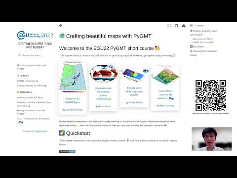](https://youtube.com/playlist?list=PL3GHXjKa-p6VBA_MlUP7T_ByCFYQZ5uDG)
14 |
15 | **Conveners**:
16 | - [Wei Ji Leong](https://github.com/weiji14)
17 | - [Leonardo Uieda](https://github.com/leouieda)
18 | - [Max Jones](https://github.com/meghanrjones)
19 | - [Andre Belem](https://github.com/andrebelem)
20 |
21 | **When**:
22 | - Tuesday 24 May 2022, 13:10-14:40 (UTC) / 15:10-16:40 (CEST)
23 | - [Event Time Zone Converter](https://www.timeanddate.com/worldclock/fixedtime.html?msg=EGU22+SC5.2%3A+Crafting+beautiful+maps+with+PyGMT&iso=20220524T1510&p1=259&ah=1&am=30)
24 |
25 | **Where**: Online/Virtual
26 |
27 | **Website**: https://meetingorganizer.copernicus.org/EGU22/session/43186
28 |
29 | ## Schedule
30 |
31 | | Time (UTC) | Event |
32 | |:------------|:------------------------------------------------------|
33 | | 13:10-13:17 | [Introduction](https://www.youtube.com/watch?v=Dgf6ijduNoE&list=PL3GHXjKa-p6VBA_MlUP7T_ByCFYQZ5uDG&index=1) |
34 | | 13:17-13.39 | [Anatomy of a PyGMT figure](https://www.youtube.com/watch?v=96_reU_yh5I&list=PL3GHXjKa-p6VBA_MlUP7T_ByCFYQZ5uDG&index=2) |
35 | | 13:39-13.55 | [Integration with the scientific Python ecosystem](https://www.youtube.com/watch?v=72war16Mvxs&list=PL3GHXjKa-p6VBA_MlUP7T_ByCFYQZ5uDG&index=3) |
36 | | 13:55-14.15 | [Making some Mars maps with pygmt](https://www.youtube.com/watch?v=OMxn08pT8hw&list=PL3GHXjKa-p6VBA_MlUP7T_ByCFYQZ5uDG&index=4) |
37 | | 14:15-14.40 | [LiDAR Point clouds to 3D surfaces](https://www.youtube.com/watch?v=n1C4wyqJY_o&list=PL3GHXjKa-p6VBA_MlUP7T_ByCFYQZ5uDG&index=5) |
38 |
39 | ## Getting started
40 |
41 | ### Quickstart
42 |
43 | Launch on regular [Binder](https://mybinder.readthedocs.io/en/latest/index.html).
44 | Try this first!
45 |
46 | [](https://mybinder.org/v2/gh/GenericMappingTools/egu22pygmt/main)
47 |
48 | Launch on Pangeo Binder. Hosted on AWS US West2 region.
49 | Requires [GitHub account](https://github.com/signup), but is more powerful (more CPU/RAM).
50 |
51 | [](https://aws-uswest2-binder.pangeo.io/v2/gh/GenericMappingTools/egu22pygmt/main)
52 |
53 | ## Code of Conduct
54 |
55 | All involved individuals must follow the
56 | [EGU General Assembly rules of conduct](https://egu22.eu/about/egu_general_assembly_rules_of_conduct.html)
57 | and [PyGMT Code of Conduct](https://github.com/GenericMappingTools/pygmt/blob/main/CODE_OF_CONDUCT.md).
58 | Act and interact in ways that contribute to an open, welcoming, diverse,
59 | inclusive, and healthy community. Any questions/concerns can be raised
60 | in private via email to the EGU programme committee and/or any of the short
61 | course conveners.
62 |
63 | ## License
64 |
65 | This content is licensed under a
66 | Creative Commons Attribution 4.0 International License.
67 |
--------------------------------------------------------------------------------
/book/_config.yml:
--------------------------------------------------------------------------------
1 | # Book settings
2 | # Learn more at https://jupyterbook.org/customize/config.html
3 |
4 | title: Crafting beautiful maps with PyGMT
5 | author: The PyGMT Team
6 | logo: logo.svg
7 |
8 | # Force re-execution of notebooks on each build.
9 | # See https://jupyterbook.org/content/execute.html
10 | execute:
11 | execute_notebooks: force
12 |
13 | # Define the name of the latex output file for PDF builds
14 | latex:
15 | latex_documents:
16 | targetname: egu22pygmt.tex
17 |
18 | # Add a bibtex file so that we can create citations
19 | bibtex_bibfiles:
20 | - references.bib
21 |
22 | # Launch button settings
23 | launch_buttons:
24 | notebook_interface: jupyterlab
25 | binderhub_url: https://mybinder.org
26 |
27 | # Information about where the book exists on the web
28 | repository:
29 | url: https://github.com/GenericMappingTools/egu22pygmt # Online location of your book
30 | path_to_book: book # Optional path to your book, relative to the repository root
31 | branch: main # Which branch of the repository should be used when creating links (optional)
32 |
33 | # Add GitHub buttons to your book
34 | # See https://jupyterbook.org/customize/config.html#add-a-link-to-your-repository
35 | html:
36 | use_edit_page_button: true
37 | use_issues_button: true
38 | use_repository_button: true
39 | extra_footer: |
40 |
41 | This content is licensed under a
42 | Creative Commons Attribution 4.0 International License.
43 |
44 | sphinx:
45 | config:
46 | bibtex_reference_style: author_year
47 | html_show_copyright: false
48 |
--------------------------------------------------------------------------------
/book/_toc.yml:
--------------------------------------------------------------------------------
1 | # Table of contents
2 | # Learn more at https://jupyterbook.org/customize/toc.html
3 |
4 | format: jb-book
5 | root: intro
6 | parts:
7 | - caption: 🔗 Details
8 | chapters:
9 | - title: EGU22 Homepage
10 | url: https://www.egu22.eu
11 | - title: Course materials on GitHub
12 | url: https://github.com/GenericMappingTools/egu22pygmt
13 | - caption: 🧑🏫 Tutorials
14 | chapters:
15 | - file: first-figure
16 | - file: ecosystem
17 | - file: mars_maps
18 | sections:
19 | - file: mars_maps_extended
20 | - file: lidar_to_surface
21 |
--------------------------------------------------------------------------------
/book/ecosystem.ipynb:
--------------------------------------------------------------------------------
1 | {
2 | "cells": [
3 | {
4 | "cell_type": "markdown",
5 | "id": "b862b964-62fc-48b7-96db-d7f3b868ced1",
6 | "metadata": {
7 | "tags": []
8 | },
9 | "source": [
10 | "# Integration with the scientific Python ecosystem 🐍\n",
11 | "\n",
12 | "In this tutorial, we'll try out the integration between PyGMT and other common packages in the scientific Python ecosystem.\n",
13 | "\n",
14 | "\n",
15 | "Besides [pygmt](https://www.pygmt.org), we'll also be using:\n",
16 | "\n",
17 | "- [GeoPandas](https://geopandas.org/en/stable/) for managing geospatial tabular data\n",
18 | "- [Panel](https://panel.holoviz.org/index.html) for interactive visualizations\n",
19 | "- [Xarray](https://xarray.dev/) for managing n-dimensional labelled arrays\n"
20 | ]
21 | },
22 | {
23 | "cell_type": "markdown",
24 | "id": "62d489cd-c901-42a2-b51a-9b21842b34df",
25 | "metadata": {},
26 | "source": [
27 | "## Plotting geospatial vector data with GeoPandas and PyGMT\n",
28 | "\n",
29 | "We'll extend the GeoPandas [Mapping and Plotting Tools Examples](https://geopandas.org/en/stable/docs/user_guide/mapping.html) to show how to create choropleth maps using PyGMT.\n",
30 | "\n",
31 | "**References**:\n",
32 | "\n",
33 | " - GeoPandas User Guide - https://geopandas.org/en/stable/docs/user_guide/"
34 | ]
35 | },
36 | {
37 | "cell_type": "code",
38 | "execution_count": null,
39 | "id": "6436dfbb-be9c-4c2b-901a-a8fc7cde4ae8",
40 | "metadata": {},
41 | "outputs": [],
42 | "source": [
43 | "import pygmt\n",
44 | "import geopandas as gpd"
45 | ]
46 | },
47 | {
48 | "cell_type": "markdown",
49 | "id": "a0f88acb-e463-4193-a7ef-33837b2f5fdf",
50 | "metadata": {},
51 | "source": [
52 | "We'll load sample data provided through the GeoPandas package and inspect the GeoDataFrame."
53 | ]
54 | },
55 | {
56 | "cell_type": "code",
57 | "execution_count": null,
58 | "id": "8cf79e91-8ce0-48ec-8812-1395d3d0eddf",
59 | "metadata": {},
60 | "outputs": [],
61 | "source": [
62 | "world = gpd.read_file(gpd.datasets.get_path('naturalearth_lowres'))\n",
63 | "world.head()"
64 | ]
65 | },
66 | {
67 | "cell_type": "markdown",
68 | "id": "65adae6a-3933-453b-bd4b-4e04e018d02d",
69 | "metadata": {},
70 | "source": [
71 | "Following the [GeoPandas example](https://geopandas.org/en/stable/docs/user_guide/mapping.html#choropleth-maps), we'll create a Choropleth map showing world population estimates, but will use PyGMT to plot the data using the [Hammer projection](https://www.pygmt.org/latest/projections/misc/misc_hammer.html#hammer)."
72 | ]
73 | },
74 | {
75 | "cell_type": "code",
76 | "execution_count": null,
77 | "id": "76b850c4-e5bc-42bd-ba13-7b52b4f60dc2",
78 | "metadata": {},
79 | "outputs": [],
80 | "source": [
81 | "# Calculate the populations in millions per capita\n",
82 | "world = world[(world.pop_est>0) & (world.name!=\"Antarctica\")]\n",
83 | "world['pop_est'] = world.pop_est * 1e-6\n",
84 | "\n",
85 | "# Find the range of data values for creating a colormap\n",
86 | "cmap_bounds = pygmt.info(data=world['pop_est'], per_column=True)\n",
87 | "cmap_bounds"
88 | ]
89 | },
90 | {
91 | "cell_type": "markdown",
92 | "id": "864091e5-85e2-4452-ab44-5cbeaa2ac8a9",
93 | "metadata": {},
94 | "source": [
95 | "Now, we'll plot the data on a PyGMT figure, by creating a figure instance, laying down a basemap, plotting the GeoDataFrame, and adding a colorbar!"
96 | ]
97 | },
98 | {
99 | "cell_type": "code",
100 | "execution_count": null,
101 | "id": "15a21a74-8531-4e74-86e1-a85e6eaef793",
102 | "metadata": {},
103 | "outputs": [],
104 | "source": [
105 | "# Create an instance of the pygmt.Figure class\n",
106 | "fig = pygmt.Figure()\n",
107 | "# Create a colormap for the figure\n",
108 | "pygmt.makecpt(cmap=\"bilbao\", series=cmap_bounds)\n",
109 | "# Create a basemap\n",
110 | "fig.basemap(region=\"d\", projection=\"H15c\", frame=True)\n",
111 | "# Plot the GeoDataFrame\n",
112 | "# - Use `close=True` to specify that the polygons should be forced closed\n",
113 | "# - Plot the polygon outlines with a 1 point, black pen\n",
114 | "# - Set that the color should be based on the `pop_est` using the `color, `cmap`, and `aspatial` parameters\n",
115 | "fig.plot(data=world, pen=\"1p,black\", close=True, color=\"+z\", cmap=True, aspatial=\"Z=pop_est\")\n",
116 | "# Add a colorbar\n",
117 | "fig.colorbar(position=\"JMR\", frame='a200+lPopulation (millions)')\n",
118 | "# Display the output\n",
119 | "fig.show()\n"
120 | ]
121 | },
122 | {
123 | "cell_type": "markdown",
124 | "id": "b73a6666-6c2c-4f49-a92b-995ade576ccc",
125 | "metadata": {},
126 | "source": [
127 | "## Interactive data visualization with Xarray, Panel, and PyGMT"
128 | ]
129 | },
130 | {
131 | "cell_type": "markdown",
132 | "id": "1bf15df6-6a4f-4221-af66-0db1c5b1e328",
133 | "metadata": {},
134 | "source": [
135 | "In this section, we'll create some interactive visualizations of oceanographic data!\n",
136 | "\n",
137 | "We'll use [Panel](https://panel.holoviz.org/index.html), which is a Python library\n",
138 | "for connecting interactive widgets with plots! We'll use Panel with\n",
139 | "[PyGMT](https://www.pygmt.org) and [xarray](https://www.xarray.dev) to visualize\n",
140 | "the objectively interpolated mean field for in-situ temperature from the World Ocean Atlas.\n",
141 | "\n",
142 | "**References**:\n",
143 | "\n",
144 | "- Temperature visualization based on https://rabernat.github.io/intro_to_physical_oceanography/02-c_ocean_temperature_salinity_stratification.html\n",
145 | "- Interactive setup based on https://github.com/weiji14/30DayMapChallenge2021/blob/main/day25_interactive.py\n",
146 | "- Data from the NOAA World Ocean Atlas, stored on the IRI Data Library at http://iridl.ldeo.columbia.edu/SOURCES/.NOAA/.NODC/.WOA09/."
147 | ]
148 | },
149 | {
150 | "cell_type": "code",
151 | "execution_count": null,
152 | "id": "dbcff01f-fac0-4c1d-bb66-89dcb2e7711b",
153 | "metadata": {},
154 | "outputs": [],
155 | "source": [
156 | "import panel as pn\n",
157 | "import xarray as xr\n",
158 | "import pygmt\n",
159 | "pn.extension()\n"
160 | ]
161 | },
162 | {
163 | "cell_type": "code",
164 | "execution_count": null,
165 | "id": "7b2f9cb8-add6-45c2-9f54-8e33ed9e6f02",
166 | "metadata": {},
167 | "outputs": [],
168 | "source": [
169 | "# Download the dataset from the IRI Data Library\n",
170 | "url = 'https://iridl.ldeo.columbia.edu/SOURCES/.NOAA/.NODC/.WOA09/.Grid-1x1/.Annual/.temperature/.t_an/data.nc'\n",
171 | "netcdf_file = pygmt.which(fname=url, download=True)\n",
172 | "woa_temp = xr.open_dataset(netcdf_file).isel(time=0)\n",
173 | "woa_temp"
174 | ]
175 | },
176 | {
177 | "cell_type": "code",
178 | "execution_count": null,
179 | "id": "1c72a673",
180 | "metadata": {},
181 | "outputs": [],
182 | "source": [
183 | "# Make a static plot of sea surface temperature\n",
184 | "fig = pygmt.Figure()\n",
185 | "fig.grdimage(grid=woa_temp.t_an.sel(depth=0), cmap=\"vik\", projection=\"R15c\", frame=True)\n",
186 | "fig.show()"
187 | ]
188 | },
189 | {
190 | "cell_type": "code",
191 | "execution_count": null,
192 | "id": "b11ea510-7540-475e-9217-be4204cb1ea3",
193 | "metadata": {},
194 | "outputs": [],
195 | "source": [
196 | "# Make a panel widget for controlling the depth plotted\n",
197 | "depth_slider = pn.widgets.DiscreteSlider(name='Depth (m)', options=woa_temp.depth.values.astype(int).tolist(), value=0)"
198 | ]
199 | },
200 | {
201 | "cell_type": "code",
202 | "execution_count": null,
203 | "id": "3496d4db-92d9-45ee-9d48-6b4f00a19361",
204 | "metadata": {},
205 | "outputs": [],
206 | "source": [
207 | "# Make a function for plotting the depth slice with PyGMT\n",
208 | "\n",
209 | "@pn.depends(depth=depth_slider)\n",
210 | "def view(depth: int):\n",
211 | " fig = pygmt.Figure()\n",
212 | " pygmt.makecpt(cmap=\"vik\", series=[-2,30])\n",
213 | " fig.grdimage(grid=woa_temp.t_an.sel(depth=depth), cmap=True, projection=\"R15c\", frame=True)\n",
214 | " fig.colorbar(frame=\"a5\")\n",
215 | " return fig"
216 | ]
217 | },
218 | {
219 | "cell_type": "markdown",
220 | "id": "d339433c-1c7a-4769-8986-edfb2a9897ed",
221 | "metadata": {},
222 | "source": [
223 | "### Make the interactive dashboard!\n",
224 | "\n",
225 | "Now to put everything together! The 'dashboard' will be very simple.\n",
226 | "The 'depth' slider is placed next to the map using `panel.Column`.\n",
227 | "Selecting different depths will update the data plotted! Find out more at\n",
228 | "https://panel.holoviz.org/getting_started/index.html#using-panel.\n",
229 | "\n",
230 | "Note: This is meant to run in a Jupyter lab/notebook environment.\n",
231 | "The grdinfo warning can be ignored."
232 | ]
233 | },
234 | {
235 | "cell_type": "code",
236 | "execution_count": null,
237 | "id": "cc8d2f88-6e37-4ca4-9ebc-4bdf1e00ec8e",
238 | "metadata": {},
239 | "outputs": [],
240 | "source": [
241 | "pn.Column(depth_slider, view)"
242 | ]
243 | }
244 | ],
245 | "metadata": {
246 | "kernelspec": {
247 | "display_name": "Python 3 (ipykernel)",
248 | "language": "python",
249 | "name": "python3"
250 | },
251 | "language_info": {
252 | "codemirror_mode": {
253 | "name": "ipython",
254 | "version": 3
255 | },
256 | "file_extension": ".py",
257 | "mimetype": "text/x-python",
258 | "name": "python",
259 | "nbconvert_exporter": "python",
260 | "pygments_lexer": "ipython3",
261 | "version": "3.9.12"
262 | }
263 | },
264 | "nbformat": 4,
265 | "nbformat_minor": 5
266 | }
267 |
--------------------------------------------------------------------------------
/book/first-figure.ipynb:
--------------------------------------------------------------------------------
1 | {
2 | "cells": [
3 | {
4 | "cell_type": "markdown",
5 | "id": "79c5f84e-3c5b-49f0-80a6-d4bd43aed2f8",
6 | "metadata": {},
7 | "source": [
8 | "# Anatomy of a PyGMT figure\n",
9 | "\n",
10 | "This tutorial will cover the fundamental concepts behind making figures with PyGMT: importing the package, creating a blank figure, drawing coastlines, drawing a map frame, choosing a projection, and adding some data to the map.\n",
11 | "\n",
12 | "Let's get started!"
13 | ]
14 | },
15 | {
16 | "cell_type": "markdown",
17 | "id": "dc74cdd5-e7b0-4365-a3c2-97d71d9f22f1",
18 | "metadata": {},
19 | "source": [
20 | "## Importing \n",
21 | "\n",
22 | "First thing to do is load PyGMT (`import`) so that we can access its functionality. PyGMT has a flat package layout, meaning that you can access everything in it with a single `import`."
23 | ]
24 | },
25 | {
26 | "cell_type": "code",
27 | "execution_count": null,
28 | "id": "19ef3de2-9333-4b0e-81ac-e518415ab9fe",
29 | "metadata": {},
30 | "outputs": [],
31 | "source": [
32 | "import pygmt"
33 | ]
34 | },
35 | {
36 | "cell_type": "markdown",
37 | "id": "1faeb548-5d01-47e7-a91b-0df582a330b1",
38 | "metadata": {},
39 | "source": [
40 | ":::{tip}\n",
41 | "In Jupyter, you can find out what PyGMT has to offer by typing into a code cell `pygmt.` and hitting the TAB key. This will give you a menu of all our functions.\n",
42 | ":::"
43 | ]
44 | },
45 | {
46 | "cell_type": "markdown",
47 | "id": "81e6ae36-f6b1-49d2-af5a-44d591366a1a",
48 | "metadata": {},
49 | "source": [
50 | "## Creating a figure\n",
51 | "\n",
52 | "All plotting is handled by the `pygmt.Figure` class. Here is a good analogy for it:\n",
53 | "\n",
54 | "> `pygmt.Figure` is a blank canvas onto which you can lay down plot elements in order.\n",
55 | "\n",
56 | "Here is how you can create a figure:"
57 | ]
58 | },
59 | {
60 | "cell_type": "code",
61 | "execution_count": null,
62 | "id": "024a9121-9c6d-4378-ba1b-d25d676c8df0",
63 | "metadata": {},
64 | "outputs": [],
65 | "source": [
66 | "fig = pygmt.Figure()"
67 | ]
68 | },
69 | {
70 | "cell_type": "markdown",
71 | "id": "7e966881-5ee7-43dc-a288-d550901dd0d7",
72 | "metadata": {},
73 | "source": [
74 | "Now that we have a blank canvas in the `fig` variable, we can start laying down plot elements that we want to show. We'll start by putting down some coast lines around Japan."
75 | ]
76 | },
77 | {
78 | "cell_type": "markdown",
79 | "id": "bed48601-63c5-485e-89a6-e55f37e26bdb",
80 | "metadata": {},
81 | "source": [
82 | "## Drawing coastlines\n",
83 | "\n",
84 | "Before we can actually include anything in our figure, we need to specify the geographic bounding box that contains the data/features we want to plot. This bounding box is referenced throughout PyGMT as the **region** of a figure and it has the format of a list containing the **West, East, South, and North** (WESN) coordinates of the bounding box."
85 | ]
86 | },
87 | {
88 | "cell_type": "code",
89 | "execution_count": null,
90 | "id": "def9a5de-1756-4bd3-8b3e-81507e42fdfc",
91 | "metadata": {},
92 | "outputs": [],
93 | "source": [
94 | "region = [125, 155, 30, 55]"
95 | ]
96 | },
97 | {
98 | "cell_type": "markdown",
99 | "id": "1f2db4e2-c7f5-4ff6-9aa8-8ae1d14f109f",
100 | "metadata": {},
101 | "source": [
102 | "Now that our region is defined, we can lay down the coastlines for this region using the `coast` method of `pygmt.Figure`."
103 | ]
104 | },
105 | {
106 | "cell_type": "code",
107 | "execution_count": null,
108 | "id": "d384b527-8ed5-4eb2-8708-d478d7cbcca8",
109 | "metadata": {},
110 | "outputs": [],
111 | "source": [
112 | "fig.coast(region=region, shorelines=True)"
113 | ]
114 | },
115 | {
116 | "cell_type": "markdown",
117 | "id": "93df5653-88cc-48e7-a667-a411e1ea8b69",
118 | "metadata": {},
119 | "source": [
120 | "And to see what the figure looks like, we call the `show` method of `pygmt.Figure`."
121 | ]
122 | },
123 | {
124 | "cell_type": "code",
125 | "execution_count": null,
126 | "id": "11881d49-cb8b-48df-ab86-c377e34ac7ed",
127 | "metadata": {},
128 | "outputs": [],
129 | "source": [
130 | "fig.show()"
131 | ]
132 | },
133 | {
134 | "cell_type": "markdown",
135 | "id": "692368d0-f1ff-4ebf-8759-37b10adb764b",
136 | "metadata": {},
137 | "source": [
138 | ":::{seealso}\n",
139 | "On Jupyter, `show` will embed a PNG of the figure directly into the notebook. But it can also open a PDF in an external viewer, which is probably what you want if you're using a plain Python script. See the documentation for [`pygmt.Figure.show`](https://www.pygmt.org/v0.6.1/api/generated/pygmt.Figure.show.html#pygmt.Figure.show) for more information.\n",
140 | ":::"
141 | ]
142 | },
143 | {
144 | "cell_type": "markdown",
145 | "id": "92171f29-21f1-4966-bc5d-0b596cba7462",
146 | "metadata": {},
147 | "source": [
148 | "Beyond the outlines, we can also color the land and water regions to make them stand out. Lets start with the water."
149 | ]
150 | },
151 | {
152 | "cell_type": "code",
153 | "execution_count": null,
154 | "id": "b891be6c-db39-4dee-84cc-4df98c79ab6a",
155 | "metadata": {},
156 | "outputs": [],
157 | "source": [
158 | "fig.coast(water=\"lightblue\")\n",
159 | "fig.show()"
160 | ]
161 | },
162 | {
163 | "cell_type": "markdown",
164 | "id": "1576b6d6-e3f2-489f-bd9d-4838a07928a7",
165 | "metadata": {},
166 | "source": [
167 | "And now add the land in a light green color."
168 | ]
169 | },
170 | {
171 | "cell_type": "code",
172 | "execution_count": null,
173 | "id": "9b715796-fa3b-45ba-bd10-7f1fa086ec0d",
174 | "metadata": {},
175 | "outputs": [],
176 | "source": [
177 | "fig.coast(land=\"lightgreen\")\n",
178 | "fig.show()"
179 | ]
180 | },
181 | {
182 | "cell_type": "markdown",
183 | "id": "8e150571-07b7-4140-af7a-78cd8244a357",
184 | "metadata": {},
185 | "source": [
186 | "A few things to note here:\n",
187 | "\n",
188 | "1. We added the colored land and water on top of what was already on our canvas (the shorelines), which means that they are still there but we don't see them because they are below the solid colors.\n",
189 | "1. We didn't need to provide a `region` this time around because PyGMT remembers the last region that was provided. But you could provide one if you want to use a different value.\n",
190 | "\n",
191 | "If we want to have a figure with the shorelines laid out on top of the solid colors, we can make a new figure and add them in the correct order."
192 | ]
193 | },
194 | {
195 | "cell_type": "code",
196 | "execution_count": null,
197 | "id": "db6723b4-1fa4-459c-8e7c-40af6301e09a",
198 | "metadata": {},
199 | "outputs": [],
200 | "source": [
201 | "fig = pygmt.Figure()\n",
202 | "# First draw the solid colors\n",
203 | "fig.coast(region=region, land=\"lightgreen\", water=\"lightblue\") # Pass region to the first plot element\n",
204 | "# Then lay down the shorelines on top\n",
205 | "fig.coast(shorelines=True)\n",
206 | "fig.show()"
207 | ]
208 | },
209 | {
210 | "cell_type": "markdown",
211 | "id": "a3615a91-697b-4cc5-9043-b0d2d729c1e2",
212 | "metadata": {},
213 | "source": [
214 | "Since these are both part of the same method (`coast`) we can actually combine both into the same call and PyGMT will know that it needs to plot the shorelines on top."
215 | ]
216 | },
217 | {
218 | "cell_type": "code",
219 | "execution_count": null,
220 | "id": "29d50636-c98d-4fd2-96d5-70354aea65ae",
221 | "metadata": {},
222 | "outputs": [],
223 | "source": [
224 | "fig = pygmt.Figure()\n",
225 | "fig.coast(region=region, shorelines=True, land=\"lightgreen\", water=\"lightblue\")\n",
226 | "fig.show()"
227 | ]
228 | },
229 | {
230 | "cell_type": "markdown",
231 | "id": "793e6eb3-cb67-4482-9214-d15aaccdd14f",
232 | "metadata": {},
233 | "source": [
234 | "Alright, now we have a lovely figure with colored land and water plus some shorelines. But what are the coordinates associated with this map? Lets add a map frame to find out."
235 | ]
236 | },
237 | {
238 | "cell_type": "markdown",
239 | "id": "bb465476-c73c-4e13-9da8-82982037b6f9",
240 | "metadata": {},
241 | "source": [
242 | "## Drawing a map frame\n",
243 | "\n",
244 | "Adding a nice frame with coordinates, ticks, and labels is one of the jobs of the `basemap` method of `pygmt.Figure`. Here, we'll use it to add automatic annotations (`\"a\"`) around the figure we just made above. It will be the last item we lay on our figure canvas to guarantee that it sits above any other plot elements."
245 | ]
246 | },
247 | {
248 | "cell_type": "code",
249 | "execution_count": null,
250 | "id": "683d3190-0c5d-4240-af56-3f71e171cd9a",
251 | "metadata": {},
252 | "outputs": [],
253 | "source": [
254 | "fig = pygmt.Figure()\n",
255 | "fig.coast(region=region, shorelines=True, land=\"lightgreen\", water=\"lightblue\")\n",
256 | "fig.basemap(frame=\"a\")\n",
257 | "fig.show()"
258 | ]
259 | },
260 | {
261 | "cell_type": "markdown",
262 | "id": "62da8cfa-cbc7-4c26-830a-ab313ef62f92",
263 | "metadata": {},
264 | "source": [
265 | "Notice that the coordinates are automatically recognized as longitude and latitude and the tick spacing is chosen sensibly as well. \n",
266 | "\n",
267 | "There are many different ways in which we can customize the frame, from the ticks to the interval to the labels. Here we'll only cover a few of the most common things you'd want to do. Starting with..."
268 | ]
269 | },
270 | {
271 | "cell_type": "markdown",
272 | "id": "476a5c34-d5ba-419d-822c-c87818fbae43",
273 | "metadata": {},
274 | "source": [
275 | "## Adding minor ticks\n",
276 | "\n",
277 | "The ticks with annotations are known as \"major ticks\" (controlled by the `\"a\"`) value. You can also add automatic \"minor ticks\" which have a smaller interval and won't have annotations by adding `\"f\"` to the `frame` argument."
278 | ]
279 | },
280 | {
281 | "cell_type": "code",
282 | "execution_count": null,
283 | "id": "f2806711-a174-472d-84c7-5cb02d941f32",
284 | "metadata": {},
285 | "outputs": [],
286 | "source": [
287 | "fig = pygmt.Figure()\n",
288 | "fig.coast(region=region, shorelines=True, land=\"lightgreen\", water=\"lightblue\")\n",
289 | "fig.basemap(frame=\"af\")\n",
290 | "fig.show()"
291 | ]
292 | },
293 | {
294 | "cell_type": "markdown",
295 | "id": "b3e7f5be-0126-48f5-8356-b00ad891523a",
296 | "metadata": {},
297 | "source": [
298 | "The frame is now set to have both annotations and minor ticks, both of which are optional (so `frame=\"f\"` would mean only having minor un-annotated ticks). Try it out!"
299 | ]
300 | },
301 | {
302 | "cell_type": "markdown",
303 | "id": "8b252f24-bd39-43c0-82ab-cfb815ca10c2",
304 | "metadata": {},
305 | "source": [
306 | "## Adding grid lines\n",
307 | "\n",
308 | "Grid lines are enabled by adding `\"g\"` to `frame`, just like we did for minor ticks. Again you can mix and match the three arguments `\"a\"`, `\"f\"`, and `\"g\"`."
309 | ]
310 | },
311 | {
312 | "cell_type": "code",
313 | "execution_count": null,
314 | "id": "58cda76a-5d1d-4fc9-9740-1007c2bcbb5f",
315 | "metadata": {},
316 | "outputs": [],
317 | "source": [
318 | "fig = pygmt.Figure()\n",
319 | "fig.coast(region=region, shorelines=True, land=\"lightgreen\", water=\"lightblue\")\n",
320 | "fig.basemap(frame=\"afg\")\n",
321 | "fig.show()"
322 | ]
323 | },
324 | {
325 | "cell_type": "markdown",
326 | "id": "9bd6b281-c1eb-4ac4-b343-3e3bbf360247",
327 | "metadata": {},
328 | "source": [
329 | "By default the spacing of the grid lines is the same as the annotated major ticks.\n",
330 | "\n",
331 | ":::{note}\n",
332 | "Adding a frame with grid lines before you plot the colored land and water or an image will hide the grid lines beneath the subsequent plot. Make sure you put the call to `basemap` last to avoid this.\n",
333 | ":::"
334 | ]
335 | },
336 | {
337 | "cell_type": "markdown",
338 | "id": "08910ea2-f2a1-4673-a11e-78e2a64dbeaf",
339 | "metadata": {},
340 | "source": [
341 | "## Adding a title\n",
342 | "\n",
343 | "To add a title to the figure, we need to pass in more than one argument to `frame`. We can do this by passing it a list instead of a single string. The extra argument for adding a title is a string with the format `\"+tMy title goes here\"`."
344 | ]
345 | },
346 | {
347 | "cell_type": "code",
348 | "execution_count": null,
349 | "id": "a8fdc242-9747-484d-aef2-ec618ad33579",
350 | "metadata": {},
351 | "outputs": [],
352 | "source": [
353 | "fig = pygmt.Figure()\n",
354 | "fig.coast(region=region, shorelines=True, land=\"lightgreen\", water=\"lightblue\")\n",
355 | "fig.basemap(frame=[\"afg\", \"+tCoastlines around Japan\"])\n",
356 | "fig.show()"
357 | ]
358 | },
359 | {
360 | "cell_type": "markdown",
361 | "id": "57568142-fe18-45a4-8b5f-32b566b7be8e",
362 | "metadata": {},
363 | "source": [
364 | "## Choosing a projection\n",
365 | "\n",
366 | "By default, PyGMT will use an equidistant cylindrical projection if the region seems to be geographic longitude and latitude. Many other projections are also supported, which may often be better suited for your plots (particularly around the polar regions or for larger global maps).\n",
367 | "\n",
368 | "For our case, let's go with a [Cassini projection](https://www.pygmt.org/v0.6.1/projections/cyl/cyl_cassini.html#sphx-glr-projections-cyl-cyl-cassini-py). To specify this, we need to pass the `projection` argument to the first plot method we call. The projection specification is a string starting with a 1-letter code for the projection followed by the projection arguments (particular to each projection) and finishing off with the physical width of the figure (in centimeters or inches, usually). For the Cassini projection, this is what it would look like: `projection=\"C142.5/40/15c\"` in which `C` is for Cassini projection, `142.5` is the central longitude of the projection set to the center of our region, `40` is the same for the central latitude, and `15c` means the plot will be 15 centimeters wide on the page (this influences the relative size of fonts and tick labels). "
369 | ]
370 | },
371 | {
372 | "cell_type": "code",
373 | "execution_count": null,
374 | "id": "0f88d938-9451-46cc-9f49-0e4e57bfb2be",
375 | "metadata": {},
376 | "outputs": [],
377 | "source": [
378 | "fig = pygmt.Figure()\n",
379 | "fig.coast(\n",
380 | " projection=\"C140/40/15c\", \n",
381 | " region=region, \n",
382 | " land=\"lightgreen\", \n",
383 | " water=\"lightblue\",\n",
384 | " shorelines=True,\n",
385 | ")\n",
386 | "fig.basemap(frame=[\"afg\", \"+tCoastlines around Japan\"])\n",
387 | "fig.show()"
388 | ]
389 | },
390 | {
391 | "cell_type": "markdown",
392 | "id": "3a16f6ec-03e6-48dc-b6af-04234858a5d9",
393 | "metadata": {},
394 | "source": [
395 | ":::{seealso}\n",
396 | "The [Projections Gallery](https://www.pygmt.org/v0.6.1/projections/index.html) has examples of each projection along with a description of their parameters, properties, and use cases.\n",
397 | ":::"
398 | ]
399 | },
400 | {
401 | "cell_type": "markdown",
402 | "id": "688e32af-2f0e-4c9e-bacb-2b1324df50de",
403 | "metadata": {},
404 | "source": [
405 | "## Adding some data to the map\n",
406 | "\n",
407 | "Finally, we have a great base map onto which we can plot some data. PyGMT offers a variety of example datasets that we can easily fetch to try things out. Since we're looking at Japan, we can use the `japan-quakes` data to get a table of earthquake hypocenters and magnitudes around this area. The data are returned in a `pandas.DataFrame` to make it easier to handle."
408 | ]
409 | },
410 | {
411 | "cell_type": "code",
412 | "execution_count": null,
413 | "id": "12555f0a-363b-4235-a2d4-d5eeda1f4cb0",
414 | "metadata": {},
415 | "outputs": [],
416 | "source": [
417 | "data = pygmt.datasets.load_sample_data(name=\"japan_quakes\")\n",
418 | "data"
419 | ]
420 | },
421 | {
422 | "cell_type": "markdown",
423 | "id": "56ed9a71-f19c-47de-a2f4-342e25b84141",
424 | "metadata": {},
425 | "source": [
426 | ":::{seealso}\n",
427 | "Use function [`pygmt.datasets.list_sample_data`](https://www.pygmt.org/v0.6.1/api/generated/pygmt.datasets.list_sample_data.html#pygmt.datasets.list_sample_data) to get a list of all datasets available.\n",
428 | ":::"
429 | ]
430 | },
431 | {
432 | "cell_type": "markdown",
433 | "id": "4d876269-58fc-4cae-9d13-75672639b590",
434 | "metadata": {},
435 | "source": [
436 | "To add point and line data to a figure, use the `plot` method of `pygmt.Figure`. Lets start by plotting the earthquake epicenters. To do this, we'll pass the data longitude and latitude coordinates as the `x` and `y` arguments to `plot`."
437 | ]
438 | },
439 | {
440 | "cell_type": "code",
441 | "execution_count": null,
442 | "id": "e67e865c-2fd6-4470-86e0-2eea9a448599",
443 | "metadata": {},
444 | "outputs": [],
445 | "source": [
446 | "fig = pygmt.Figure()\n",
447 | "fig.coast(\n",
448 | " projection=\"C140/40/15c\", \n",
449 | " region=region, \n",
450 | " land=\"lightgreen\", \n",
451 | " water=\"lightblue\",\n",
452 | " shorelines=True,\n",
453 | ")\n",
454 | "fig.plot(x=data.longitude, y=data.latitude)\n",
455 | "fig.basemap(frame=[\"afg\", \"+tEarthquakes around Japan\"])\n",
456 | "fig.show()"
457 | ]
458 | },
459 | {
460 | "cell_type": "markdown",
461 | "id": "d46dd1e0-442c-4378-8a51-ba88b125c142",
462 | "metadata": {},
463 | "source": [
464 | "By default, PyGMT will plot lines connecting each of the points in our data. This is probably not what we want to do given that our data are epicenters. Instead, lets plot using **circles**. This requires passing in the `style` argument to `plot`, which should be a string like `c0.3c` with the first `c` specifying a circle and `0.3c` specifying that circles should be 0.3 centimeters in size. We'll also pass in `color` to make the circles opaque with a given color (otherwise they would be just the outlines by default)."
465 | ]
466 | },
467 | {
468 | "cell_type": "code",
469 | "execution_count": null,
470 | "id": "c82d18de-7760-4e43-9932-b15469aa199c",
471 | "metadata": {},
472 | "outputs": [],
473 | "source": [
474 | "fig = pygmt.Figure()\n",
475 | "fig.coast(\n",
476 | " projection=\"C140/40/15c\", \n",
477 | " region=region, \n",
478 | " land=\"lightgreen\", \n",
479 | " water=\"lightblue\",\n",
480 | " shorelines=True,\n",
481 | ")\n",
482 | "fig.plot(x=data.longitude, y=data.latitude, style=\"c0.3c\", color=\"white\")\n",
483 | "fig.basemap(frame=[\"afg\", \"+tEarthquakes around Japan\"])\n",
484 | "fig.show()"
485 | ]
486 | },
487 | {
488 | "cell_type": "markdown",
489 | "id": "f935e455-cc67-46b4-8f98-28cb16673ab4",
490 | "metadata": {},
491 | "source": [
492 | ":::{tip}\n",
493 | "Pass `pen` to `plot` to control how the outline of the circles are drawn. For example, `pen=\"black\"` will draw a black outline.\n",
494 | ":::"
495 | ]
496 | },
497 | {
498 | "cell_type": "markdown",
499 | "id": "2135181f-1ea7-4bd8-b7be-0c9b4beb6726",
500 | "metadata": {},
501 | "source": [
502 | "It would be great to also represent the depth of the earthquakes somehow. We can do this by encoding the depth information as the color of the circles. We need to make 2 changes to the code above to achieve this:\n",
503 | "\n",
504 | "1. Configure a \"color palette table (CPT)\" that maps colors to data values. In matplotlib, this is known as a colormap or `cmap`.\n",
505 | "2. Tell `plot` to use the depth values and the CPT/cmap created to pain the circles.\n",
506 | "\n",
507 | "Step 1 is done using `pygmt.makecpt`, which takes a colormap name through the `cmap` argument and the min/max values of the data through the `series` argument.\n",
508 | "\n",
509 | "Step 2 is done by passing in the `data.depth_km` values to `color` and `cmap=True`, telling PyGMT to use the current CPT created through `makecpt`."
510 | ]
511 | },
512 | {
513 | "cell_type": "code",
514 | "execution_count": null,
515 | "id": "c9f84eda-22f6-4617-88dd-25062072d980",
516 | "metadata": {},
517 | "outputs": [],
518 | "source": [
519 | "fig = pygmt.Figure()\n",
520 | "fig.coast(\n",
521 | " projection=\"C140/40/15c\", \n",
522 | " region=region, \n",
523 | " land=\"lightgreen\", \n",
524 | " water=\"lightblue\",\n",
525 | " shorelines=True,\n",
526 | ")\n",
527 | "pygmt.makecpt(cmap=\"plasma\", series=[data.depth_km.min(), data.depth_km.max()])\n",
528 | "fig.plot(x=data.longitude, y=data.latitude, style=\"c0.3c\", color=data.depth_km, cmap=True)\n",
529 | "fig.basemap(frame=[\"afg\", \"+tEarthquakes around Japan\"])\n",
530 | "fig.show()"
531 | ]
532 | },
533 | {
534 | "cell_type": "markdown",
535 | "id": "1c9b1e55-47a9-4abf-9605-fb2d25ff301d",
536 | "metadata": {},
537 | "source": [
538 | ":::{seealso}\n",
539 | "The GMT documentation has a [list of all available colormaps/CPTs](https://docs.generic-mapping-tools.org/6.3/cookbook/cpts.html). There are many to choose from!\n",
540 | ":::"
541 | ]
542 | },
543 | {
544 | "cell_type": "markdown",
545 | "id": "66584e59-ba73-4e28-a232-9f74fe6a229c",
546 | "metadata": {},
547 | "source": [
548 | "As a final step, we need to add a colorbar to the figure so we know what value each color represents. This is done using the `colorbar` method of `pygmt.Figure`, which takes a `frame` argument much like the one we use to set the map frame. Only this time, it sets the frame of the colorbar. To make our colorbar look nice, we'll set the frame to have automatically annotated major ticks and a label on the y-axis specifying the variable and units. "
549 | ]
550 | },
551 | {
552 | "cell_type": "code",
553 | "execution_count": null,
554 | "id": "3a586a12-d3c1-4688-aa5a-692d1f9a66f1",
555 | "metadata": {},
556 | "outputs": [],
557 | "source": [
558 | "fig = pygmt.Figure()\n",
559 | "fig.coast(\n",
560 | " projection=\"C140/40/15c\", \n",
561 | " region=region, \n",
562 | " land=\"lightgreen\", \n",
563 | " water=\"lightblue\",\n",
564 | " shorelines=True,\n",
565 | ")\n",
566 | "pygmt.makecpt(cmap=\"plasma\", series=[data.depth_km.min(), data.depth_km.max()])\n",
567 | "fig.plot(x=data.longitude, y=data.latitude, style=\"c0.3c\", color=data.depth_km, cmap=True)\n",
568 | "fig.basemap(frame=[\"afg\", \"+tEarthquakes around Japan\"])\n",
569 | "fig.colorbar(frame=[\"a\", \"y+lDepth (km)\"])\n",
570 | "fig.show()"
571 | ]
572 | }
573 | ],
574 | "metadata": {
575 | "kernelspec": {
576 | "display_name": "Python 3 (ipykernel)",
577 | "language": "python",
578 | "name": "python3"
579 | },
580 | "language_info": {
581 | "codemirror_mode": {
582 | "name": "ipython",
583 | "version": 3
584 | },
585 | "file_extension": ".py",
586 | "mimetype": "text/x-python",
587 | "name": "python",
588 | "nbconvert_exporter": "python",
589 | "pygments_lexer": "ipython3",
590 | "version": "3.9.12"
591 | }
592 | },
593 | "nbformat": 4,
594 | "nbformat_minor": 5
595 | }
596 |
--------------------------------------------------------------------------------
/book/intro.md:
--------------------------------------------------------------------------------
1 | # 🌍 Crafting beautiful maps with PyGMT
2 |
3 | ## Welcome to the EGU22 PyGMT short course 🥳
4 |
5 | This Jupyter book 📖 contains [PyGMT](https://www.pygmt.org/v0.6.1) tutorials
6 | for producing maps 🗺️ and doing geospatial data processing 🌐
7 |
8 | ````{panels}
9 | :column: col-3 align-items-center p-2
10 | :body: text-center
11 |
12 | ---
13 | :img-top: _images/first-figure_49_0.png
14 | ```{link-button} first-figure
15 | :text: Anatomy of a PyGMT figure
16 | :type: ref
17 | ```
18 | by [Leonardo Uieda](https://orcid.org/0000-0001-6123-9515)
19 |
20 | ---
21 | :img-top: _images/ecosystem_13_1.png
22 | ```{link-button} ecosystem
23 | :text: Integration with the scientific Python ecosystem 🐍
24 | :type: ref
25 | ```
26 | by [Max Jones](https://orcid.org/0000-0003-0180-8928)
27 |
28 | ---
29 | :img-top: _images/mars_maps_11_0.png
30 | ```{link-button} mars_maps
31 | :text: Making some Mars maps with PyGMT
32 | :type: ref
33 | ```
34 | by [André Belém](https://orcid.org/0000-0002-8865-6180)
35 |
36 | ---
37 | :img-top: _images/lidar_to_surface_36_0.png
38 | ```{link-button} lidar_to_surface
39 | :text: LiDAR Point clouds to 3D surfaces ✨➡️🏔
40 | :type: ref
41 | ```
42 | by [Wei Ji Leong](https://orcid.org/0000-0003-2354-1988)
43 |
44 | ````
45 |
46 | Each tutorial is rendered on this website for easy viewing 👀, but they are all
47 | Jupyter notebooks designed to be ran interactively 💫. See the instructions
48 | below on how you can start running the tutorials in no time! 🚀
49 |
50 | # Recording
51 |
52 | A recording of the full short course is available on YouTube:
53 |
54 | [](https://youtube.com/playlist?list=PL3GHXjKa-p6VBA_MlUP7T_ByCFYQZ5uDG)
55 |
56 | # 🌠 Quickstart
57 |
58 | To run these notebooks in an interactive Jupyter session online,
59 | 🖱️ click on the button below to launch on regular
60 | [Binder](https://mybinder.readthedocs.io/en/latest/index.html).
61 |
62 | [](https://mybinder.org/v2/gh/GenericMappingTools/egu22pygmt/main)
63 |
64 | Alternatively, you can go to a specific tutorial page, hover over the rocket 🚀
65 | icon on the top right, and click 'Binder'.
66 |
67 | :::{note}
68 | If you see an error like `toomanyrequests: You have reached your pull rate
69 | limit`, you can try this Pangeo Binder link instead as a backup, though it
70 | will require a [GitHub account](https://github.com/signup) to work:
71 |
72 | [](https://aws-uswest2-binder.pangeo.io/v2/gh/GenericMappingTools/egu22pygmt/main)
73 | :::
74 |
75 | # 💻 Running the notebooks locally
76 |
77 | If you prefer to run the 🧑🏫 tutorials with a local installation of PyGMT, then
78 | follow along! For this EGU22 short course, we recommend creating a virtual
79 | conda environment and installing the 🐍 Python libraries inside.
80 |
81 | :::{tip} For users comfortable with using `git`, feel free to ⬇️ download or
82 | clone the repository containing the short course materials directly using
83 | `git clone https://github.com/GenericMappingTools/egu22pygmt.git`
84 | :::
85 |
86 | Here's the instructions to install the `egu22pygmt` environment:
87 |
88 | 1. Ensure that you have the
89 | [`conda`](https://docs.conda.io/projects/conda/en/latest/user-guide/index.html)
90 | package manager installed (e.g. via
91 | [`miniconda`](https://docs.conda.io/en/latest/miniconda.html) or
92 | [Anaconda](https://www.anaconda.com/products/distribution)).
93 | You can also use [`mamba`](https://mamba.readthedocs.io/en/latest/installation.html#fresh-install)
94 | which tends to be a ⚡ faster alternative.
95 |
96 | 2. Make a folder called 'egu22pygmt'. This will be where you will put all the
97 | Jupyter notebooks and data files 🗃️ used in the short course.
98 |
99 | 3. Download a copy of the 'environment.yml' file which contains a 📄 list of
100 | dependencies required to run the tutorials in this short course. Get it at
101 | https://github.com/GenericMappingTools/egu22pygmt/blob/main/environment.yml.
102 |
103 | 4. Run the following commands on the 🧑💻 command-line to create the virtual
104 | environment
105 |
106 | ```bash
107 | cd /path/to/egu22pygmt
108 | conda env create --name egu22pygmt --file environment.yml
109 | ```
110 |
111 | 5. Once the installation is completed 🏁, launch
112 | [Jupyter Lab](https://jupyterlab.readthedocs.io) as follows:
113 |
114 | ```bash
115 | conda activate egu22pygmt
116 | jupyter lab
117 | ```
118 |
119 | This should open up a page in your default browser. If not, you can click
120 | and open the 🔗 link that says `http://localhost:8888/lab?token=...` in your
121 | command-line terminal and this will will take you to the Jupyter Lab page.
122 |
123 | 6. Download the Jupyter notebook(s) you want to run (e.g.
124 | https://www.generic-mapping-tools.org/egu22pygmt/first-figure.html) using
125 | either the download button on the ↗️ top right (select '.ipynb') or from
126 | GitHub at https://github.com/GenericMappingTools/egu22pygmt/tree/main/book.
127 | Make sure to put the *.ipynb file(s) inside of the 'egu22pygmt' folder.
128 |
129 | 7. Open the Jupyter notebook in the left-pane file browser, e.g. by
130 | 🖱️ double-clicking on `first-figure.ipynb`. You are now ready to run through
131 | the course materials 🎉!
132 |
133 | ```{note}
134 | If you're intending to use PyGMT in another project outside of this course,
135 | please follow the official installation instructions at
136 | https://www.pygmt.org/latest/install.html
137 | ```
138 |
--------------------------------------------------------------------------------
/book/lidar_to_surface.ipynb:
--------------------------------------------------------------------------------
1 | {
2 | "cells": [
3 | {
4 | "cell_type": "markdown",
5 | "metadata": {},
6 | "source": [
7 | "# LiDAR Point clouds to 3D surfaces ✨➡️🏔️\n",
8 | "\n",
9 | "In this tutorial, let's use PyGMT to\n",
10 | "perform a more advanced geoprocessing workflow 😎\n",
11 | "\n",
12 | "Specifically, we'll learn to filter and interpolate\n",
13 | "a LiDAR point cloud onto a regular grid surface 🏁\n",
14 | "\n",
15 | "At the end, we'll also make a 🚠 3D perspective plot for\n",
16 | "the Digital Surface Model (DSM) produced through this exercise!"
17 | ]
18 | },
19 | {
20 | "cell_type": "markdown",
21 | "metadata": {},
22 | "source": [
23 | "## 🎉 Getting started\n",
24 | "\n",
25 | "Begin by importing some Python 🐍 libraries.\n",
26 | "\n",
27 | "Besides [pygmt](https://www.pygmt.org), we'll also be using:\n",
28 | "\n",
29 | "- [laspy](https://github.com/laspy/laspy) to read in LAZ LiDAR files 🌃\n",
30 | "- [pandas](https://pandas.pydata.org) for managing tabular data 🀤\n",
31 | "- [rioxarray](https://corteva.github.io/rioxarray) to export our DSM to a GeoTIFF 🗺️"
32 | ]
33 | },
34 | {
35 | "cell_type": "code",
36 | "execution_count": null,
37 | "metadata": {},
38 | "outputs": [],
39 | "source": [
40 | "import laspy\n",
41 | "import pandas as pd\n",
42 | "import pygmt\n",
43 | "import rioxarray\n",
44 | "import xarray as xr"
45 | ]
46 | },
47 | {
48 | "cell_type": "markdown",
49 | "metadata": {},
50 | "source": [
51 | "# 0️⃣ The LiDAR data\n",
52 | "\n",
53 | "Let's visit [Wellington](https://en.wikipedia.org/wiki/Wellington)\n",
54 | "which is the capital city of New Zealand 🇳🇿.\n",
55 | "\n",
56 | "They recently had a LiDAR survey done between March 2019 to March 2020 🛩️,\n",
57 | "with the point cloud and derived products published under an open\n",
58 | "[CC BY 4.0](https://creativecommons.org/licenses/by/4.0/) license.\n",
59 | "\n",
60 | "- OpenTopography link: https://doi.org/10.5069/G9K935QX\n",
61 | "- Bulk download location: https://opentopography.s3.sdsc.edu/minio/pc-bulk/NZ19_Wellington\n",
62 | "- Official 1m DSM from LINZ: https://data.linz.govt.nz/layer/105024-wellington-city-lidar-1m-dsm-2019-2020\n",
63 | "\n",
64 | "🔖 References:\n",
65 | "- https://medium.com/on-location/from-points-to-pixels-creating-digital-elevation-models-from-open-topography-point-clouds-abe616d06860\n",
66 | "- https://github.com/GenericMappingTools/foss4g2019oceania/blob/v1/3_lidar_to_surface.ipynb\n",
67 | "- https://github.com/weiji14/30DayMapChallenge2021/blob/v0.3.1/day17_land.py"
68 | ]
69 | },
70 | {
71 | "cell_type": "markdown",
72 | "metadata": {},
73 | "source": [
74 | "First though, we'll need to download a sample file to play with 🎮\n",
75 | "\n",
76 | "Luckily for us,\n",
77 | "there is a function called [pygmt.which](https://www.pygmt.org/v0.6.1/api/generated/pygmt.which)\n",
78 | "that has to ability to do just that!\n",
79 | "\n",
80 | "The `download=True` option can be used to download ⬇️ a remote file to our local working directory."
81 | ]
82 | },
83 | {
84 | "cell_type": "code",
85 | "execution_count": null,
86 | "metadata": {},
87 | "outputs": [],
88 | "source": [
89 | "# Download LiDAR LAZ file from a URL\n",
90 | "lazfile = pygmt.which(\n",
91 | " fname=\"https://opentopography.s3.sdsc.edu/pc-bulk/NZ19_Wellington/CL2_BQ31_2019_1000_2138.laz\",\n",
92 | " download=True,\n",
93 | ")\n",
94 | "print(lazfile)"
95 | ]
96 | },
97 | {
98 | "cell_type": "markdown",
99 | "metadata": {},
100 | "source": [
101 | "## Loading a point cloud 🌧️"
102 | ]
103 | },
104 | {
105 | "cell_type": "markdown",
106 | "metadata": {},
107 | "source": [
108 | "Now we can use [laspy](https://laspy.readthedocs.io) to read in our example LAZ file\n",
109 | "into a [pandas.DataFrame](https://pandas.pydata.org/pandas-docs/version/1.4/reference/api/pandas.DataFrame.html).\n",
110 | "\n",
111 | "The data will be kept in a variable called 'df' which stands for dataframe."
112 | ]
113 | },
114 | {
115 | "cell_type": "code",
116 | "execution_count": null,
117 | "metadata": {},
118 | "outputs": [],
119 | "source": [
120 | "# Load LAZ data into a pandas DataFrame\n",
121 | "lazdata = laspy.read(source=lazfile)\n",
122 | "df = pd.DataFrame(\n",
123 | " data={\n",
124 | " \"x\": lazdata.x.scaled_array(),\n",
125 | " \"y\": lazdata.y.scaled_array(),\n",
126 | " \"z\": lazdata.z.scaled_array(),\n",
127 | " \"classification\": lazdata.classification,\n",
128 | " }\n",
129 | ")"
130 | ]
131 | },
132 | {
133 | "cell_type": "markdown",
134 | "metadata": {},
135 | "source": [
136 | "## Quick data preview ⚡"
137 | ]
138 | },
139 | {
140 | "cell_type": "markdown",
141 | "metadata": {},
142 | "source": [
143 | "Let's get the bounding box 📦 region of our study area using\n",
144 | "[pygmt.info](https://www.pygmt.org/v0.6.1/api/generated/pygmt.info.html)."
145 | ]
146 | },
147 | {
148 | "cell_type": "code",
149 | "execution_count": null,
150 | "metadata": {},
151 | "outputs": [],
152 | "source": [
153 | "# Get bounding box region\n",
154 | "region = pygmt.info(data=df[[\"x\", \"y\"]], spacing=1) # West, East, South, North\n",
155 | "print(f\"Data points covers region: {region}\")"
156 | ]
157 | },
158 | {
159 | "cell_type": "markdown",
160 | "metadata": {},
161 | "source": [
162 | "Check how many 🗃️ data points (rows) are in the table\n",
163 | "and get some summary statistics printed out."
164 | ]
165 | },
166 | {
167 | "cell_type": "code",
168 | "execution_count": null,
169 | "metadata": {},
170 | "outputs": [],
171 | "source": [
172 | "# Print summary statistics\n",
173 | "print(f\"Total of {len(df)} data points\")\n",
174 | "df.describe()"
175 | ]
176 | },
177 | {
178 | "cell_type": "markdown",
179 | "metadata": {},
180 | "source": [
181 | "More than 7 million points, that's a lot! 🤯\n",
182 | "\n",
183 | "Let's try to take a quick look of our LiDAR elevation points on a map 🗺️\n",
184 | "\n",
185 | "PyGMT *can* plot these many points, but it might take a long time ⏳,\n",
186 | "so let's do a quick filter by taking every\n",
187 | "[n-th row](https://stackoverflow.com/questions/25055712/pandas-every-nth-row)\n",
188 | "from our dataframe table."
189 | ]
190 | },
191 | {
192 | "cell_type": "code",
193 | "execution_count": null,
194 | "metadata": {},
195 | "outputs": [],
196 | "source": [
197 | "df_filtered = df.iloc[::20]\n",
198 | "print(f\"Filtered down to {len(df_filtered)} data points\")"
199 | ]
200 | },
201 | {
202 | "cell_type": "markdown",
203 | "metadata": {},
204 | "source": [
205 | "Now we can visualize these quickly on a map with PyGMT 😀"
206 | ]
207 | },
208 | {
209 | "cell_type": "code",
210 | "execution_count": null,
211 | "metadata": {},
212 | "outputs": [],
213 | "source": [
214 | "# Plot XYZ points on a map\n",
215 | "fig = pygmt.Figure()\n",
216 | "fig.basemap(frame=True, region=region, projection=\"x1:5000\")\n",
217 | "pygmt.makecpt(cmap=\"bukavu\", series=[df.z.min(), df.z.max()])\n",
218 | "fig.plot(\n",
219 | " x=df_filtered.x, y=df_filtered.y, color=df_filtered.z, style=\"c0.03c\", cmap=True\n",
220 | ")\n",
221 | "fig.colorbar(position=\"JMR\", frame=[\"af+lElevation\", \"y+lm\"])\n",
222 | "fig.show()"
223 | ]
224 | },
225 | {
226 | "cell_type": "markdown",
227 | "metadata": {},
228 | "source": [
229 | "It's hard to make out what the objects are,\n",
230 | "but hopefully you'll see what looks like a wharf with ⛵ boats on the top left corner.\n",
231 | "\n",
232 | "This is showing us a part of Oriental Bay in Wellington,\n",
233 | "with Mount Victoria ⛰️ towards the Southeast corner of the map."
234 | ]
235 | },
236 | {
237 | "cell_type": "markdown",
238 | "metadata": {},
239 | "source": [
240 | "# 1️⃣ Creating a Digital Surface Model (DSM)\n",
241 | "\n",
242 | "Let's now produce a digital surface model from our point cloud 🌧️\n",
243 | "\n",
244 | "We'll first do some proper spatial data cleaning 🧹 using both\n",
245 | "[pandas](https://pandas.pydata.org) and [pygmt](https://www.pygmt.org)."
246 | ]
247 | },
248 | {
249 | "cell_type": "markdown",
250 | "metadata": {},
251 | "source": [
252 | "First step is to remove the LiDAR points classified as high noise 🔊\n",
253 | "which is done by querying all the points that are not '18'.\n",
254 | "\n",
255 | "🔖 References:\n",
256 | "- Table 17 of [ASPRS LAS Specification](https://www.asprs.org/a/society/committees/standards/LAS_1_4_r13.pdf)"
257 | ]
258 | },
259 | {
260 | "cell_type": "code",
261 | "execution_count": null,
262 | "metadata": {},
263 | "outputs": [],
264 | "source": [
265 | "df = df.query(expr=\"classification != 18\")\n",
266 | "df"
267 | ]
268 | },
269 | {
270 | "cell_type": "markdown",
271 | "metadata": {},
272 | "source": [
273 | "## Get highest elevation points 🍫"
274 | ]
275 | },
276 | {
277 | "cell_type": "markdown",
278 | "metadata": {},
279 | "source": [
280 | "Next, we'll use the\n",
281 | "[blockmedian](https://www.pygmt.org/v0.6.1/api/generated/pygmt.blockmedian.html)\n",
282 | "function to trim 🪒 down the points spatially.\n",
283 | "\n",
284 | "By default, this function computes a single median elevation\n",
285 | "for every pixel on an equally spaced grid 🏁\n",
286 | "\n",
287 | "For a Digital **Surface** Elevation Model (DSM) though,\n",
288 | "we should pick the highest elevation 🔝 instead of the median.\n",
289 | "\n",
290 | "So we'll tell blockmedian to use the 99th\n",
291 | "[quantile](https://docs.generic-mapping-tools.org/latest/blockmedian.html#t) (T) instead,\n",
292 | "and set our output grid spacing to be exactly 1 metre (1+e) 📏\n",
293 | "\n",
294 | "Note that we'll only be taking the 🇽, 🇾, 🇿 (elevation) columns for this."
295 | ]
296 | },
297 | {
298 | "cell_type": "code",
299 | "execution_count": null,
300 | "metadata": {},
301 | "outputs": [],
302 | "source": [
303 | "# Preprocess LiDAR data using blockmedian\n",
304 | "df_trimmed = pygmt.blockmedian(\n",
305 | " data=df[[\"x\", \"y\", \"z\"]],\n",
306 | " T=0.99, # 99th quantile, i.e. the highest point\n",
307 | " spacing=\"1+e\",\n",
308 | " region=region,\n",
309 | ")\n",
310 | "df_trimmed"
311 | ]
312 | },
313 | {
314 | "cell_type": "markdown",
315 | "metadata": {},
316 | "source": [
317 | "## Turn points into a grid 🫓"
318 | ]
319 | },
320 | {
321 | "cell_type": "markdown",
322 | "metadata": {},
323 | "source": [
324 | "Lastly, we'll use [pygmt.surface](https://www.pygmt.org/v0.6.1/api/generated/pygmt.surface.html)\n",
325 | "to produce a grid from the 🇽, 🇾, 🇿 data points.\n",
326 | "\n",
327 | "Make sure to set our desired grid spacing to be exactly 📏 1 metre (1+e) again.\n",
328 | "\n",
329 | "Also, we'll set a tension factor (T) of 0.35 which is suitable for steep topography\n",
330 | "(since we have some 🏠 buildings with 'steep' vertical edges).\n",
331 | "\n",
332 | "🚨 Note that this might take some time to run."
333 | ]
334 | },
335 | {
336 | "cell_type": "code",
337 | "execution_count": null,
338 | "metadata": {},
339 | "outputs": [],
340 | "source": [
341 | "# Create a Digital Surface Elevation Model with\n",
342 | "# a spatial resolution of 1m.\n",
343 | "grid = pygmt.surface(\n",
344 | " x=df_trimmed.x,\n",
345 | " y=df_trimmed.y,\n",
346 | " z=df_trimmed.z,\n",
347 | " spacing=\"1+e\",\n",
348 | " region=region, # xmin, xmax, ymin, ymax\n",
349 | " T=0.35, # tension factor\n",
350 | ")"
351 | ]
352 | },
353 | {
354 | "cell_type": "markdown",
355 | "metadata": {},
356 | "source": [
357 | "Let's take a look 👀 at the grid output.\n",
358 | "\n",
359 | "The grid will be returned as an\n",
360 | "[xarray.DataArray](https://docs.xarray.dev/en/v2022.03.0/generated/xarray.DataArray.html),\n",
361 | "with each pixel's elevation (🇿 value in metres) stored at every 🇽 and 🇾 coordinate."
362 | ]
363 | },
364 | {
365 | "cell_type": "code",
366 | "execution_count": null,
367 | "metadata": {},
368 | "outputs": [],
369 | "source": [
370 | "grid"
371 | ]
372 | },
373 | {
374 | "cell_type": "markdown",
375 | "metadata": {},
376 | "source": [
377 | "# 2️⃣ Plotting a Digital Surface Model (DSM)"
378 | ]
379 | },
380 | {
381 | "cell_type": "markdown",
382 | "metadata": {},
383 | "source": [
384 | "## **Plot in 2D** 🏳️🌈\n",
385 | "\n",
386 | "Now we can plot our Digital Surface Model (DSM) grid 🏁\n",
387 | "\n",
388 | "This can be done by passing the\n",
389 | "[xarray.DataArray](https://docs.xarray.dev/en/v2022.03.0/generated/xarray.DataArray.html)\n",
390 | "grid into\n",
391 | "[pygmt.Figure.grdimage](https://www.pygmt.org/v0.6.1/api/generated/pygmt.Figure.grdimage)."
392 | ]
393 | },
394 | {
395 | "cell_type": "code",
396 | "execution_count": null,
397 | "metadata": {},
398 | "outputs": [],
399 | "source": [
400 | "fig2 = pygmt.Figure()\n",
401 | "fig2.basemap(\n",
402 | " frame=True,\n",
403 | " region=[1_749_760, 1_750_240, 5_426_880, 5_427_600],\n",
404 | " projection=\"x1:5000\",\n",
405 | ")\n",
406 | "pygmt.makecpt(cmap=\"bukavu\", series=[-10, 200])\n",
407 | "fig2.grdimage(grid=grid, cmap=True)\n",
408 | "fig2.colorbar(position=\"JMR\", frame=[\"af+lElevation\", \"y+lm\"])\n",
409 | "fig2.show()"
410 | ]
411 | },
412 | {
413 | "cell_type": "markdown",
414 | "metadata": {},
415 | "source": [
416 | "## Plot 3D perspective view ⛰️\n",
417 | "\n",
418 | "Now comes the cool part 💯\n",
419 | "\n",
420 | "PyGMT has a [grdview](https://pygmt-git-foss4g2019oceania.gmt.now.sh/api/generated/pygmt.Figure.grdview.html#pygmt.Figure.grdview)\n",
421 | "function to make high quality 3D perspective plots of our elevation surface!\n",
422 | "\n",
423 | "Besides providing the elevation 'grid', there are a few basic things to configure:\n",
424 | "- cmap - name of 🌈 [colormap](https://docs.generic-mapping-tools.org/6.3/cookbook/cpts.html#id3) to use\n",
425 | "- surftype - we'll use 's' here which just creates a regular surface 🏄\n",
426 | "- perspective - set azimuth angle (e.g. 315 for NorthWest) and 📐 elevation (e.g 30 degrees) of the viewpoint\n",
427 | "- zscale - a vertical exaggeration 🔺 factor, we'll use 0.02 here"
428 | ]
429 | },
430 | {
431 | "cell_type": "code",
432 | "execution_count": null,
433 | "metadata": {},
434 | "outputs": [],
435 | "source": [
436 | "fig3 = pygmt.Figure()\n",
437 | "fig3.grdview(\n",
438 | " grid=grid,\n",
439 | " cmap=\"bukavu\",\n",
440 | " surftype=\"s\", # surface plot\n",
441 | " perspective=[315, 30], # azimuth bearing, and elevation angle\n",
442 | " zscale=0.02, # vertical exaggeration\n",
443 | ")\n",
444 | "fig3.show()"
445 | ]
446 | },
447 | {
448 | "cell_type": "markdown",
449 | "metadata": {},
450 | "source": [
451 | "There are also other things we can 🧰 configure such as:\n",
452 | "\n",
453 | "- Hillshading ⛱️ using `shading=True`\n",
454 | "- A proper 3D map frame 🖼️ with:\n",
455 | " - automatic tick marks on x and y axis (e.g. `xaf+lLabel`)\n",
456 | " - z-axis automatic tick marks (`zaf+lLabel`)\n",
457 | " - plot title (`+tMy Title`)"
458 | ]
459 | },
460 | {
461 | "cell_type": "code",
462 | "execution_count": null,
463 | "metadata": {},
464 | "outputs": [],
465 | "source": [
466 | "fig3 = pygmt.Figure()\n",
467 | "fig3.grdview(\n",
468 | " grid=grid,\n",
469 | " cmap=\"bukavu\",\n",
470 | " surftype=\"s\", # surface plot\n",
471 | " perspective=[315, 30], # azimuth bearing, and elevation angle\n",
472 | " zscale=0.02, # vertical exaggeration\n",
473 | " shading=True, # hillshading\n",
474 | " frame=[\n",
475 | " \"xaf+lEasting\",\n",
476 | " \"yaf+lNorthing\",\n",
477 | " \"zaf+lElevation (m)\",\n",
478 | " \"+tOriental Bay, Wellington\",\n",
479 | " ],\n",
480 | ")\n",
481 | "fig3.show()"
482 | ]
483 | },
484 | {
485 | "cell_type": "markdown",
486 | "metadata": {},
487 | "source": [
488 | "Feel free to have a go at changing the azimuth and elevation angle to get a different view 🔭\n",
489 | "\n",
490 | "You can also try to tweak the vertical exaggeration factor 🗼\n",
491 | "and play around with the map frame!"
492 | ]
493 | },
494 | {
495 | "cell_type": "markdown",
496 | "metadata": {},
497 | "source": [
498 | "## Save figures and output DSM to GeoTIFF 💾\n",
499 | "\n",
500 | "Time to save your work!\n",
501 | "\n",
502 | "We'll save each of our figures into separate files first 🗃️"
503 | ]
504 | },
505 | {
506 | "cell_type": "code",
507 | "execution_count": null,
508 | "metadata": {},
509 | "outputs": [],
510 | "source": [
511 | "fig.savefig(fname=\"wellington_1d_lidar.png\")\n",
512 | "fig2.savefig(fname=\"wellington_2d_dsm_map.png\")\n",
513 | "fig3.savefig(fname=\"wellington_3d_dsm_view.png\")"
514 | ]
515 | },
516 | {
517 | "cell_type": "markdown",
518 | "metadata": {},
519 | "source": [
520 | "Also, it'll be good to have a proper GeoTIFF of the DSM we made.\n",
521 | "This can be done using\n",
522 | "[rioxarray's to_raster method](https://corteva.github.io/rioxarray/html/examples/convert_to_raster.html)."
523 | ]
524 | },
525 | {
526 | "cell_type": "code",
527 | "execution_count": null,
528 | "metadata": {},
529 | "outputs": [],
530 | "source": [
531 | "grid.rio.to_raster(raster_path=\"DSM_of_Wellington.tif\")"
532 | ]
533 | },
534 | {
535 | "cell_type": "markdown",
536 | "metadata": {},
537 | "source": [
538 | "The files should now appear on the file list on the left,\n",
539 | "and you can download them to your computer."
540 | ]
541 | },
542 | {
543 | "cell_type": "markdown",
544 | "metadata": {},
545 | "source": [
546 | "# 3️⃣ Bonus exercise - Create a 3D surface map of another area\n",
547 | "\n",
548 | "Here's a challenge to test your PyGMT skills 🤹\n",
549 | "\n",
550 | "You'll be processing a LiDAR point cloud of a different area 📍 from start to finish.\n",
551 | "\n",
552 | "Good luck! 🥳"
553 | ]
554 | },
555 | {
556 | "cell_type": "markdown",
557 | "metadata": {},
558 | "source": [
559 | "Feel free to find a dataset from an area you're interested in using\n",
560 | "[OpenTopography](https://portal.opentopography.org/datasets).\n",
561 | "\n",
562 | "To make it easier though, I've provided an example for Queenstown, New Zealand 🇳🇿\n",
563 | "\n",
564 | "- OpenTopography link: https://doi.org/10.5069/G9MP51G0\n",
565 | "- Bulk download location: https://opentopography.s3.sdsc.edu/minio/pc-bulk/NZ21_Otago\n",
566 | "- Official 1m DSM from LINZ: https://data.linz.govt.nz/layer/105905-otago-queenstown-lidar-index-tiles-2021\n",
567 | "\n",
568 | "These files covers the Central Queenstown area:\n",
569 | " - https://opentopography.s3.sdsc.edu/pc-bulk/NZ21_Otago/CL2_CC11_2021_1000_0813.laz\n",
570 | " - https://opentopography.s3.sdsc.edu/pc-bulk/NZ21_Otago/CL2_CC11_2021_1000_0814.laz\n",
571 | " - https://opentopography.s3.sdsc.edu/pc-bulk/NZ21_Otago/CL2_CC11_2021_1000_0913.laz\n",
572 | " - https://opentopography.s3.sdsc.edu/pc-bulk/NZ21_Otago/CL2_CC11_2021_1000_0914.laz"
573 | ]
574 | },
575 | {
576 | "cell_type": "markdown",
577 | "metadata": {},
578 | "source": [
579 | "## Download and load data"
580 | ]
581 | },
582 | {
583 | "cell_type": "code",
584 | "execution_count": null,
585 | "metadata": {},
586 | "outputs": [],
587 | "source": [
588 | "filenames = [\n",
589 | " # \"\",\n",
590 | "]\n",
591 | "\n",
592 | "df = pd.DataFrame() # Start an empty DataFrame\n",
593 | "for fname in filenames:\n",
594 | " lazfile = pygmt.which(fname=fname, download=True)\n",
595 | "\n",
596 | " lazdata = laspy.read(source=lazfile)\n",
597 | " temp_df = pd.DataFrame(\n",
598 | " data={\n",
599 | " \"x\": lazdata.x.scaled_array(),\n",
600 | " \"y\": lazdata.y.scaled_array(),\n",
601 | " \"z\": lazdata.z.scaled_array(),\n",
602 | " \"classification\": lazdata.classification,\n",
603 | " }\n",
604 | " )\n",
605 | " # load each point cloud into the DataFrame\n",
606 | " df = df.append(temp_df, ignore_index=True)"
607 | ]
608 | },
609 | {
610 | "cell_type": "code",
611 | "execution_count": null,
612 | "metadata": {},
613 | "outputs": [],
614 | "source": [
615 | "df"
616 | ]
617 | },
618 | {
619 | "cell_type": "markdown",
620 | "metadata": {},
621 | "source": [
622 | "## Create a DSM"
623 | ]
624 | },
625 | {
626 | "cell_type": "code",
627 | "execution_count": null,
628 | "metadata": {},
629 | "outputs": [],
630 | "source": [
631 | "# Run blockmedian"
632 | ]
633 | },
634 | {
635 | "cell_type": "code",
636 | "execution_count": null,
637 | "metadata": {},
638 | "outputs": [],
639 | "source": [
640 | "# Run surface"
641 | ]
642 | },
643 | {
644 | "cell_type": "markdown",
645 | "metadata": {},
646 | "source": [
647 | "## Plot the DSM"
648 | ]
649 | },
650 | {
651 | "cell_type": "code",
652 | "execution_count": null,
653 | "metadata": {},
654 | "outputs": [],
655 | "source": [
656 | "# Run grdimage"
657 | ]
658 | },
659 | {
660 | "cell_type": "code",
661 | "execution_count": null,
662 | "metadata": {},
663 | "outputs": [],
664 | "source": [
665 | "# Run grdview"
666 | ]
667 | },
668 | {
669 | "cell_type": "markdown",
670 | "metadata": {},
671 | "source": [
672 | "That’s all 🎉!\n",
673 | "For more information on how to customize your map 🗺️,\n",
674 | "check out:\n",
675 | "\n",
676 | "- Tutorials at https://www.pygmt.org/v0.6.1/tutorials/index.html\n",
677 | "- Gallery examples at https://www.pygmt.org/v0.6.1/gallery/index.html\n",
678 | "\n",
679 | "If you have any questions 🙋,\n",
680 | "feel free to visit the PyGMT forum at\n",
681 | "https://forum.generic-mapping-tools.org/c/questions/pygmt-q-a/11.\n",
682 | "\n",
683 | "Submit any ✨ feature requests/bug reports to the GitHub repo at\n",
684 | "https://github.com/GenericMappingTools/pygmt\n",
685 | "\n",
686 | "Cheers!"
687 | ]
688 | }
689 | ],
690 | "metadata": {
691 | "jupytext": {
692 | "formats": "ipynb,py:hydrogen"
693 | },
694 | "kernelspec": {
695 | "display_name": "Python 3 (ipykernel)",
696 | "language": "python",
697 | "name": "python3"
698 | },
699 | "language_info": {
700 | "codemirror_mode": {
701 | "name": "ipython",
702 | "version": 3
703 | },
704 | "file_extension": ".py",
705 | "mimetype": "text/x-python",
706 | "name": "python",
707 | "nbconvert_exporter": "python",
708 | "pygments_lexer": "ipython3",
709 | "version": "3.9.12"
710 | }
711 | },
712 | "nbformat": 4,
713 | "nbformat_minor": 4
714 | }
715 |
--------------------------------------------------------------------------------
/book/logo.svg:
--------------------------------------------------------------------------------
1 |
2 |
3 |
86 |
--------------------------------------------------------------------------------
/book/mars_maps.ipynb:
--------------------------------------------------------------------------------
1 | {
2 | "cells": [
3 | {
4 | "cell_type": "markdown",
5 | "id": "19f4dff3",
6 | "metadata": {},
7 | "source": [
8 | "# Making some Mars maps with pygmt\n",
9 | "\n",
10 | "This tutorial page covers the basics of creating some maps and 3D plot of Mars (yes! Mars). The idea here is to demonstrate that you can use a simple sequence of commands with PyGMT, a Python wrapper for the Generic Mapping Tools (GMT), and with some public data about the topography of Mars, create your own maps, as well as compare this topography with what we know of our own planet Earth."
11 | ]
12 | },
13 | {
14 | "cell_type": "markdown",
15 | "id": "b48dd300",
16 | "metadata": {},
17 | "source": [
18 | "## Mars dataset\n",
19 | "\n",
20 | "First, we open the `mola32.nc` file using xarray. Note the longitudes are from 0-360°, latitudes are distributed from North to South and the `alt` variable is the MOLA Topography at 32 pixels/degree built from original MOLA file `megt90n000fb.img`. The source is the Mars Climate Database from the European Space Agency."
21 | ]
22 | },
23 | {
24 | "cell_type": "code",
25 | "execution_count": null,
26 | "id": "2f913d8d",
27 | "metadata": {
28 | "tags": [
29 | "remove-stdout"
30 | ]
31 | },
32 | "outputs": [],
33 | "source": [
34 | "# Also, if you are in colab or trying from your jupyter, you will need the Mars Topography (MOLA) already in Netcdf\n",
35 | "# a copy of the original file distributed from the Mars Climate Database,\n",
36 | "# from the European Space Agency under ESTEC contract 11369/95/NL/JG(SC) and Centre National D'Etude Spatial\n",
37 | "# is on GitHub.\n",
38 | "\n",
39 | "!wget https://github.com/andrebelem/PlanetaryMaps/raw/v1.0/mola32.nc"
40 | ]
41 | },
42 | {
43 | "cell_type": "code",
44 | "execution_count": null,
45 | "id": "11b04ce1",
46 | "metadata": {},
47 | "outputs": [],
48 | "source": [
49 | "import xarray as xr\n",
50 | "\n",
51 | "dset_mars = xr.open_dataset('mola32.nc')\n",
52 | "dset_mars"
53 | ]
54 | },
55 | {
56 | "cell_type": "markdown",
57 | "id": "e9d6ef48",
58 | "metadata": {},
59 | "source": [
60 | "Just like any other notebook with pygmt, we import the library and manipulate other data. To make a map of the entire Martian surface without a lot of time and memory, let's reduce the resolution using `grdsample`. We also take the opportunity to transform an `alt` variable into a `float` to be used in maps."
61 | ]
62 | },
63 | {
64 | "cell_type": "code",
65 | "execution_count": null,
66 | "id": "8e7374cf",
67 | "metadata": {},
68 | "outputs": [],
69 | "source": [
70 | "import pygmt\n",
71 | "\n",
72 | "dset_mars_topo = dset_mars.alt.astype(float)\n",
73 | "dset_mars_topo = pygmt.grdsample(grid=dset_mars_topo, translate=True, spacing=[1,1])"
74 | ]
75 | },
76 | {
77 | "cell_type": "markdown",
78 | "id": "700d1d1d",
79 | "metadata": {},
80 | "source": [
81 | "Here we can create a map of the entire Martian surface, in the same projections we use for our planet."
82 | ]
83 | },
84 | {
85 | "cell_type": "code",
86 | "execution_count": null,
87 | "id": "feecaa82",
88 | "metadata": {
89 | "scrolled": true
90 | },
91 | "outputs": [],
92 | "source": [
93 | "fig = pygmt.Figure()\n",
94 | "\n",
95 | "fig.grdimage(grid=dset_mars_topo,region='g',frame=True,projection='W12c')\n",
96 | "fig.colorbar(frame=['a5000','x+lElevation','y+lm'])\n",
97 | "\n",
98 | "fig.show()"
99 | ]
100 | },
101 | {
102 | "cell_type": "markdown",
103 | "id": "3e3530ac",
104 | "metadata": {},
105 | "source": [
106 | "A very interesting feature is Mount Olympus (Olympus Mons - see more details at https://mars.nasa.gov/resources/22587/olympus-mons), centered at approximately 19°N and 133°W, with a height of 22 km (14 miles) and approximately 700 km (435 miles) in diameter. Let's use the original dataset at 32 pixels/degree resolution and plot a (not so interesting) map with `xarray`."
107 | ]
108 | },
109 | {
110 | "cell_type": "code",
111 | "execution_count": null,
112 | "id": "01fac891",
113 | "metadata": {},
114 | "outputs": [],
115 | "source": [
116 | "dset_olympus = dset_mars.sel(latitude=slice(25,13),longitude=slice(210,240)).alt.astype(float)\n",
117 | "dset_olympus.plot()"
118 | ]
119 | },
120 | {
121 | "cell_type": "markdown",
122 | "id": "fe62c4a7",
123 | "metadata": {},
124 | "source": [
125 | "We use the same sequence as other pygmt tutorial notebooks to make a map."
126 | ]
127 | },
128 | {
129 | "cell_type": "code",
130 | "execution_count": null,
131 | "id": "9f18b522",
132 | "metadata": {},
133 | "outputs": [],
134 | "source": [
135 | "fig = pygmt.Figure()\n",
136 | "\n",
137 | "fig.grdview(grid=dset_olympus,\n",
138 | " region=[210,240,13,25,-5000,23000],\n",
139 | " surftype='s',\n",
140 | " projection='M12c',\n",
141 | " perspective=[150,45],\n",
142 | " zsize='4c',\n",
143 | " frame=['xa5f1','ya5f1','z5000+lmeters','wSEnZ'],shading='+a50+nt1')\n",
144 | "\n",
145 | "bounds = [[210,13],\n",
146 | " [210,25],\n",
147 | " [240,25],\n",
148 | " [240,13],\n",
149 | " [210,13]]\n",
150 | "\n",
151 | "fig.colorbar(perspective=True,frame=['a5000','x+lElevation','y+lm'])\n",
152 | "with fig.inset(position='JTR+w3.5c+o0.2c',margin=0,box=None):\n",
153 | " fig.grdimage(grid=dset_mars_topo,region='g',frame=True,projection='W3.5c')\n",
154 | " fig.plot(bounds, pen='1p,red')\n",
155 | "\n",
156 | "fig.show()"
157 | ]
158 | },
159 | {
160 | "cell_type": "markdown",
161 | "id": "55a14a22",
162 | "metadata": {},
163 | "source": [
164 | "And we're going to add some perspective, as well as a more interesting color scale. For ease of understanding, let's separate the region of interest with the same cutout that we created the base of the Olympus Mons topography dataset.\n",
165 | "\n",
166 | "**A few notes**\n",
167 | "\n",
168 | "`zsize` is a bit critical here because the volcano is very big (28 km if we consider -5000 to +23000 m). Likewise, `perspective=[150,45]` was chosen attempting (it's a matter of taste) and depends of which flank of the volcano you want to show. But this choice has to be made according to `shading` since to give a good 3D impression, the lighting must be adjusted according to the elevation and azimuth of the perspective. Finally, the pen outline is made smooth and small to enhance the contours of the topography.\n",
169 | "\n",
170 | "Finally, let's make a combined map showing the planet in an inset in the upper right corner. We use the same bounding box coordinates used to cut out the topography, drawing in red on the map. Obviously here the color scale is the same."
171 | ]
172 | },
173 | {
174 | "cell_type": "markdown",
175 | "id": "ac07a1c0",
176 | "metadata": {},
177 | "source": [
178 | "There are a few bonus maps in the *extended version* in github.\n",
179 | "\n",
180 | "Have fun."
181 | ]
182 | }
183 | ],
184 | "metadata": {
185 | "kernelspec": {
186 | "display_name": "Python 3 (ipykernel)",
187 | "language": "python",
188 | "name": "python3"
189 | },
190 | "language_info": {
191 | "codemirror_mode": {
192 | "name": "ipython",
193 | "version": 3
194 | },
195 | "file_extension": ".py",
196 | "mimetype": "text/x-python",
197 | "name": "python",
198 | "nbconvert_exporter": "python",
199 | "pygments_lexer": "ipython3",
200 | "version": "3.10.2"
201 | }
202 | },
203 | "nbformat": 4,
204 | "nbformat_minor": 5
205 | }
206 |
--------------------------------------------------------------------------------
/book/mars_maps_extended.ipynb:
--------------------------------------------------------------------------------
1 | {
2 | "cells": [
3 | {
4 | "cell_type": "markdown",
5 | "metadata": {},
6 | "source": [
7 | "# Making some Mars maps with pygmt (extended)\n",
8 | "\n",
9 | "This tutorial page covers the basics of creating some maps and 3D plot of Mars (yes! Mars). The idea here is to demonstrate that you can use a simple sequence of commands with PyGMT, a Python wrapper for the Generic Mapping Tools (GMT), and with some public data about the topography of Mars, create your own maps, as well as compare this topography with what we know of our own planet Earth.\n",
10 | "\n",
11 | "## first, some options\n",
12 | "\n",
13 | "You can run this notebook using your local pygmt installation, or via Binder, or even Google Colaboratory. See comments for each option below. "
14 | ]
15 | },
16 | {
17 | "cell_type": "markdown",
18 | "metadata": {},
19 | "source": [
20 | "**A)** A short note if you are using COLAB\n",
21 | "\n",
22 | "The version of python in COLAB is different from what the newer GMT needs to install along with pygmt. So, one way around this problem is to reinstall GMT from scratch, along with other important packages. This is done with this block of commands below.\n",
23 | "\n",
24 | "**comment out the first line of the block (%%script echo skipping) if you want to use colab**"
25 | ]
26 | },
27 | {
28 | "cell_type": "code",
29 | "execution_count": null,
30 | "metadata": {
31 | "colab": {
32 | "base_uri": "https://localhost:8080/"
33 | },
34 | "id": "nnMDokWZuQyN",
35 | "outputId": "0be69909-5cb9-4d8c-acfb-1b0b6b303b8f"
36 | },
37 | "outputs": [],
38 | "source": [
39 | "%%script echo skipping\n",
40 | "\n",
41 | "# because I like to enjoy my coffee in silence, it takes time. \n",
42 | "# (3 runs averaged 6 minutes to install everything ! keep drinking your coffee)\n",
43 | "# comment the %%capture line if you want to see the colab VM working\n",
44 | "%%capture\n",
45 | "!sudo apt update \n",
46 | "!sudo apt upgrade -y\n",
47 | "!sudo apt install -y build-essential cmake libcurl4-gnutls-dev libnetcdf-dev gdal-bin libgdal-dev libfftw3-dev libpcre3-dev liblapack-dev libblas-dev libglib2.0-dev ghostscript ghostscript-x graphicsmagick ffmpeg xdg-utils\n",
48 | "# clone gmt from source\n",
49 | "!git clone --depth 50 https://github.com/GenericMappingTools/gmt\n",
50 | "# cmake everything\n",
51 | "!cmake /content/gmt\n",
52 | "# build and install\n",
53 | "!cmake --build . --target install\n",
54 | "\n",
55 | "# and last but not least\n",
56 | "!pip install pygmt\n",
57 | "\n",
58 | "# and if you don't believe in it\n",
59 | "!gmt --version\n",
60 | "!python --version"
61 | ]
62 | },
63 | {
64 | "cell_type": "code",
65 | "execution_count": null,
66 | "metadata": {
67 | "colab": {
68 | "base_uri": "https://localhost:8080/"
69 | },
70 | "id": "oIdVNbxrr1lw",
71 | "outputId": "05379551-c66c-4d0b-917c-74cc25fb8942",
72 | "tags": [
73 | "remove-stdout"
74 | ]
75 | },
76 | "outputs": [],
77 | "source": [
78 | "# Also, if you are in colab or trying from your jupyter, you will need the Mars Topography (MOLA) already in Netcdf\n",
79 | "# a copy of the original file distributed from the Mars Climate Database,\n",
80 | "# from the European Space Agency under ESTEC contract 11369/95/NL/JG(SC) and Centre National D'Etude Spatial\n",
81 | "# is on GitHub.\n",
82 | "\n",
83 | "!wget https://github.com/andrebelem/PlanetaryMaps/raw/v1.0/mola32.nc"
84 | ]
85 | },
86 | {
87 | "cell_type": "markdown",
88 | "metadata": {},
89 | "source": [
90 | "**B)** Now, if you are using Binder or in your local jupyter\n",
91 | "\n",
92 | "You just skip the block above. Make sure you have the `mola32.nc` in your folder.\n"
93 | ]
94 | },
95 | {
96 | "cell_type": "code",
97 | "execution_count": null,
98 | "metadata": {},
99 | "outputs": [],
100 | "source": [
101 | "%matplotlib inline"
102 | ]
103 | },
104 | {
105 | "cell_type": "markdown",
106 | "metadata": {},
107 | "source": [
108 | "## Mars dataset\n",
109 | "\n",
110 | "First, we open the `mola32.nc` file using xarray. Note the longitudes are from 0-360°, latitudes are distributed from North to South and the `alt`variable is the MOLA Topography at 32 pixels/degree built from original MOLA file `megt90n000fb.img`."
111 | ]
112 | },
113 | {
114 | "cell_type": "code",
115 | "execution_count": null,
116 | "metadata": {
117 | "id": "IImGpHBZrwG0",
118 | "scrolled": true
119 | },
120 | "outputs": [],
121 | "source": [
122 | "import xarray as xr \n",
123 | "\n",
124 | "dset_mars = xr.open_dataset('mola32.nc')\n",
125 | "dset_mars"
126 | ]
127 | },
128 | {
129 | "cell_type": "markdown",
130 | "metadata": {},
131 | "source": [
132 | "Just like any other notebook with pygmt, we import the library and manipulate other data. To make a map of the entire Martian surface without a lot of time and memory, let's reduce the resolution using `grdsample`. We also take the opportunity to transform an `alt` variable into a `float` to be used in maps."
133 | ]
134 | },
135 | {
136 | "cell_type": "code",
137 | "execution_count": null,
138 | "metadata": {
139 | "colab": {
140 | "base_uri": "https://localhost:8080/"
141 | },
142 | "id": "XFfzKq4-42S2",
143 | "outputId": "e1697b32-8a4c-46c6-cccf-bed9c5f9d421"
144 | },
145 | "outputs": [],
146 | "source": [
147 | "import pygmt \n",
148 | "\n",
149 | "# convert from int16 to float\n",
150 | "dset_mars_topo = dset_mars.alt.astype(float)\n",
151 | "\n",
152 | "# May be a global Mars map is very interesting. We just need to get a better resolution not to consume all memory\n",
153 | "# translate here changes from grid to pixel registration and spacing sets to 1 degree resolution\n",
154 | "dset_mars_topo = pygmt.grdsample(grid=dset_mars_topo,translate=True,spacing=[1,1])\n",
155 | "\n",
156 | "# don't be worried about the warnings."
157 | ]
158 | },
159 | {
160 | "cell_type": "markdown",
161 | "metadata": {},
162 | "source": [
163 | "Here we can create a map of the entire Martian surface, in the same projections we use for our planet."
164 | ]
165 | },
166 | {
167 | "cell_type": "code",
168 | "execution_count": null,
169 | "metadata": {
170 | "colab": {
171 | "base_uri": "https://localhost:8080/",
172 | "height": 50
173 | },
174 | "id": "4jmXhEsk0kYi",
175 | "outputId": "cfeef10d-e42f-4ce4-9d21-97c1c6828d72"
176 | },
177 | "outputs": [],
178 | "source": [
179 | "fig = pygmt.Figure()\n",
180 | "\n",
181 | "fig.grdimage(grid=dset_mars_topo,region='g',frame=True,projection='Cyl_stere/0/0/12c')\n",
182 | "# you can try with different cylindrical or miscellaneous projections\n",
183 | "# see at https://www.pygmt.org/dev/projections/index.html\n",
184 | "# some ideas: Eckert IV = Kf; Hammer = H; Mollweide = W\n",
185 | "\n",
186 | "fig.colorbar(frame=[\"a5000\", \"x+lElevation\", \"y+lm\"])\n",
187 | "fig.show()"
188 | ]
189 | },
190 | {
191 | "cell_type": "markdown",
192 | "metadata": {},
193 | "source": [
194 | "A very interesting feature is Mount Olympus (Olympus Mons - see more details at https://mars.nasa.gov/resources/22587/olympus-mons), centered at approximately 19°N and 133°W, with a height of 22 km (14 miles) and approximately 700 km (435 miles) in diameter. Let's use the original dataset at 32 pixels/degree resolution and plot a (not so interesting) map with `xarray`."
195 | ]
196 | },
197 | {
198 | "cell_type": "code",
199 | "execution_count": null,
200 | "metadata": {
201 | "colab": {
202 | "base_uri": "https://localhost:8080/",
203 | "height": 297
204 | },
205 | "id": "ypeLac-gtjVI",
206 | "outputId": "f9013715-c01e-484c-b63a-8714852ea755"
207 | },
208 | "outputs": [],
209 | "source": [
210 | "# Olympus Mons is located in these slices of 12 degrees of latitude and 30 degrees of longitude\n",
211 | "# note we are cutting the region of interest and converting here the original \"alt\" data in int16 to float (for grid)\n",
212 | "dset_olympus = dset_mars.sel(latitude=slice(25,13),longitude=slice(210,240)).alt.astype('float')\n",
213 | "dset_olympus.plot()"
214 | ]
215 | },
216 | {
217 | "cell_type": "markdown",
218 | "metadata": {},
219 | "source": [
220 | "We use the same sequence as other pygmt tutorial notebooks to make a map."
221 | ]
222 | },
223 | {
224 | "cell_type": "code",
225 | "execution_count": null,
226 | "metadata": {
227 | "colab": {
228 | "base_uri": "https://localhost:8080/",
229 | "height": 301
230 | },
231 | "id": "4xPXldUJsbha",
232 | "outputId": "4e68b731-68ff-46d2-f5b2-3fcd39c46f7f",
233 | "scrolled": true
234 | },
235 | "outputs": [],
236 | "source": [
237 | "# first things, first\n",
238 | "fig = pygmt.Figure()\n",
239 | "# note I can add projection, after cmap and after, frame (and control frame)\n",
240 | "fig.grdimage(grid=dset_olympus,projection='M12c',frame='a5f1',cmap='geo')\n",
241 | "# also, I can add a colorbar (later)\n",
242 | "fig.colorbar(frame=[\"a2500\", \"x+lElevation\", \"y+lm\"])\n",
243 | "\n",
244 | "fig.show()"
245 | ]
246 | },
247 | {
248 | "cell_type": "markdown",
249 | "metadata": {},
250 | "source": [
251 | "And we're going to add some perspective, as well as a more interesting color scale. For ease of understanding, let's separate the region of interest with the same cutout that we created the base of the Olympus Mons topography dataset.\n",
252 | "\n",
253 | "**A few notes**\n",
254 | "\n",
255 | "`zsize` is a bit critical here because the volcano is very big (28 km if we consider -5000 to +23000 m). Likewise, `perspective=[150.45]` was chosen attempting (it's a matter of taste) and depends of which flank of the volcano you want to show. But this choice has to be made according to `shading` since to give a good 3D impression, the lighting must be adjusted according to the elevation and azimuth of the perspective. Finally, the pen outline is made smooth and small to enhance the contours of the topography.\n",
256 | "\n",
257 | "Finally, let's make a combined map showing the planet in an inset in the upper right corner. We use the same bounding box coordinates used to cut out the topography, drawing in red on the map. Obviously here the color scale is the same."
258 | ]
259 | },
260 | {
261 | "cell_type": "code",
262 | "execution_count": null,
263 | "metadata": {
264 | "colab": {
265 | "base_uri": "https://localhost:8080/",
266 | "height": 283
267 | },
268 | "id": "GwCV6HIJ_Aa6",
269 | "outputId": "7ccb2823-bbb8-4921-8ebd-e07cf3ba9ddc",
270 | "scrolled": true
271 | },
272 | "outputs": [],
273 | "source": [
274 | "# a little perspective\n",
275 | "\n",
276 | "fig = pygmt.Figure()\n",
277 | "# note I can add projection, after cmap and after, frame (and control frame)\n",
278 | "topo_cpt = pygmt.makecpt(cmap='sealand',series=f'-5000/24000/1000',continuous=True)\n",
279 | "frame = [\"xa5f1\",\"ya5f1\", \"z5000+lmeters\", \"wSEnZ\"]\n",
280 | "\n",
281 | "fig.grdview(grid=dset_olympus,\n",
282 | " region=[210,240,13,25,-5000,23000],\n",
283 | " frame=frame,\n",
284 | " perspective=[150,45],\n",
285 | " projection='M18c',\n",
286 | " zsize='4c',\n",
287 | " surftype='s',\n",
288 | " cmap=topo_cpt,\n",
289 | " plane=\"-5000+ggrey\",\n",
290 | " shading='+a100+nt1',\n",
291 | " # Set the contour pen thickness to \"0.1p\"\n",
292 | " contourpen=\"0.1p\",)\n",
293 | "\n",
294 | "fig.colorbar(perspective=True, frame=[\"a5000\", \"x+lElevation\", \"y+lm\"])\n",
295 | "\n",
296 | "bounds = [[210.,13.],\n",
297 | " [210.,25.],\n",
298 | " [240.,25.],\n",
299 | " [240.,13.],\n",
300 | " [210.,13.]]\n",
301 | "\n",
302 | "with fig.inset(position=\"JTR+w3.5c+o0.2c\", margin=0, box=None):\n",
303 | " # Create a figure in the inset using the global projection centered at Olympus MOns\n",
304 | " fig.grdimage(grid=dset_mars_topo,region='g',frame='g',projection='G225/19/3.5c\"')\n",
305 | " fig.plot(bounds,pen=\"1p,red\")\n",
306 | "fig.show()"
307 | ]
308 | },
309 | {
310 | "cell_type": "markdown",
311 | "metadata": {},
312 | "source": [
313 | "## Now, how about Hawaii?\n",
314 | "\n",
315 | "When we read about Olympus Mons, it is usually compared to Everest here on Earth. However, the most interesting thing is to compare it with another mountain range taking as a reference the abyssal seabed (without the ocean) - Hawaii. Interestingly, in terms of latitudes and longitudes on the planet, these two features are in almost the same position. To match the approximate dimensions, let's crop a sample of the `Earth Global Relief` using `pygmt.datasets` with slices of 12 degrees of latitude and 30 degrees of longitude."
316 | ]
317 | },
318 | {
319 | "cell_type": "code",
320 | "execution_count": null,
321 | "metadata": {
322 | "colab": {
323 | "base_uri": "https://localhost:8080/"
324 | },
325 | "id": "XkeCs3NaLSbY",
326 | "outputId": "920cd17f-cbe1-43d6-b6b2-7cfce418bfb8"
327 | },
328 | "outputs": [],
329 | "source": [
330 | "# get SRTM around Hawaii \n",
331 | "topo_hawaii = pygmt.datasets.load_earth_relief(region=[-170,-140,13,25],resolution=\"05m\")\n",
332 | "\n",
333 | "# and get the whole Earth at the same resolution of our low resolution Mars dataset\n",
334 | "topo_globe = pygmt.datasets.load_earth_relief(region=[-180,180,-90,90],resolution=\"01d\")"
335 | ]
336 | },
337 | {
338 | "cell_type": "markdown",
339 | "metadata": {},
340 | "source": [
341 | "And we use the same sequence as above to make a map."
342 | ]
343 | },
344 | {
345 | "cell_type": "code",
346 | "execution_count": null,
347 | "metadata": {
348 | "colab": {
349 | "base_uri": "https://localhost:8080/",
350 | "height": 295
351 | },
352 | "id": "SUsRWFJ-MZ3Y",
353 | "outputId": "1830e744-b7a8-4c51-b543-c403716d8785"
354 | },
355 | "outputs": [],
356 | "source": [
357 | "# second things, second\n",
358 | "\n",
359 | "fig = pygmt.Figure()\n",
360 | "# note I can add projection, after cmap and after, frame (and control frame)\n",
361 | "fig.grdimage(grid=topo_hawaii,projection='M12c',frame='a5f1',cmap='geo')\n",
362 | "# also, I can add a colorbar (later)\n",
363 | "fig.colorbar(frame=[\"a2500\", \"x+lElevation\", \"y+lm\"])\n",
364 | "\n",
365 | "fig.show()"
366 | ]
367 | },
368 | {
369 | "cell_type": "markdown",
370 | "metadata": {},
371 | "source": [
372 | "**Another few notes**\n",
373 | "\n",
374 | "As we want to make a comparison, let's keep the same color scale as Mars, still using as a basis for the Z plane, -5000 meters (see the line `plane=\"-5000+ggrey\"` exactly like the map above. The inset in the upper right corner is the same and we adjust the bounding box coordinates used to cut out the topography, drawing in red on the map. "
375 | ]
376 | },
377 | {
378 | "cell_type": "code",
379 | "execution_count": null,
380 | "metadata": {
381 | "colab": {
382 | "base_uri": "https://localhost:8080/",
383 | "height": 283
384 | },
385 | "id": "Q4IiufkLG5cW",
386 | "outputId": "57e43215-a8b5-45e2-c9ea-9544eaea1ef8"
387 | },
388 | "outputs": [],
389 | "source": [
390 | "fig = pygmt.Figure()\n",
391 | "# note I can add projection, after cmap and after, frame (and control frame)\n",
392 | "frame = [\"xa5f1\",\"ya5f1\", \"z5000+lmeters\", \"wSEnZ\"]\n",
393 | "\n",
394 | "topo_cpt = pygmt.makecpt(cmap='sealand',series=f'-5000/24000/1000',continuous=True)\n",
395 | "\n",
396 | "fig.grdview(grid=topo_hawaii,\n",
397 | " region=[-170,-140,13,25,-5000,23000],\n",
398 | " frame=frame,\n",
399 | " perspective=[150,45],\n",
400 | " projection='M15c',\n",
401 | " zsize='4c',\n",
402 | " surftype='s',\n",
403 | " cmap=topo_cpt,\n",
404 | " plane=\"-5000+ggrey\",\n",
405 | " shading='+a100+nt1',\n",
406 | " # Set the contour pen thickness to \"0.1p\"\n",
407 | " contourpen=\"0.1p\",)\n",
408 | "\n",
409 | "fig.colorbar(perspective=True, frame=[\"a5000\", \"x+lElevation\", \"y+lm\"])\n",
410 | "\n",
411 | "bounds = [[-170.,13.],\n",
412 | " [-170.,25.],\n",
413 | " [-140.,25.],\n",
414 | " [-140.,13.],\n",
415 | " [-170.,13.]]\n",
416 | "\n",
417 | "with fig.inset(position=\"JTR+w3.5c+o0.2c\", margin=0, box=None):\n",
418 | " # Create a figure in the inset using the global projection centered at Olympus MOns\n",
419 | " fig.grdimage(grid=topo_globe,region='g',frame='g',projection='G-160/19/3.5c\"')\n",
420 | " fig.coast(region='g',shorelines=\"thin\", frame=\"g\")\n",
421 | " fig.plot(bounds,pen=\"1p,red\")\n",
422 | " \n",
423 | "fig.show()"
424 | ]
425 | },
426 | {
427 | "cell_type": "markdown",
428 | "metadata": {},
429 | "source": [
430 | "## Combining the two maps side by side\n",
431 | "\n",
432 | "Basically it's the same blocks as above, just using `pygmt`'s `Figure.set_panel` mechanism to tile."
433 | ]
434 | },
435 | {
436 | "cell_type": "code",
437 | "execution_count": null,
438 | "metadata": {
439 | "colab": {
440 | "base_uri": "https://localhost:8080/",
441 | "height": 166
442 | },
443 | "id": "UiBEecTSRp6T",
444 | "outputId": "1bd76a70-5892-40c8-8209-5414e6e4a46f"
445 | },
446 | "outputs": [],
447 | "source": [
448 | "fig = pygmt.Figure()\n",
449 | "\n",
450 | "with fig.subplot(\n",
451 | " nrows=1, ncols=2, figsize=(\"28c\", \"16c\"), autolabel=True, margins=\"1c\"\n",
452 | "):\n",
453 | " with fig.set_panel(panel=0):\n",
454 | "\n",
455 | " topo_cpt = pygmt.makecpt(cmap='sealand',series=f'-5000/24000/1000',continuous=True)\n",
456 | "\n",
457 | " frame = [\"xa5f1\",\"ya5f1\", \"z5000+lmeters\", \"wSEnZ\"]\n",
458 | "\n",
459 | " fig.grdview(grid=dset_olympus,\n",
460 | " region=[210,240,13,25,-5000,23000],\n",
461 | " frame=frame,\n",
462 | " perspective=[150,45],\n",
463 | " projection='M',\n",
464 | " zsize='4c',\n",
465 | " surftype='s',\n",
466 | " cmap=topo_cpt,\n",
467 | " plane=\"-5000+ggrey\",\n",
468 | " shading='+a100+nt1',\n",
469 | " # Set the contour pen thickness to \"0.1p\"\n",
470 | " contourpen=\"0.1p\",)\n",
471 | "\n",
472 | " # we don't need the colormap in both figures\n",
473 | " #fig.colorbar(perspective=True, frame=[\"a5000\", \"x+lElevation\", \"y+lm\"])\n",
474 | " \n",
475 | " with fig.set_panel(panel=1):\n",
476 | " frame = [\"xa5f1\",\"ya5f1\", \"z5000+lmeters\", \"wSEnZ\"]\n",
477 | "\n",
478 | " topo_cpt = pygmt.makecpt(cmap='sealand',series=f'-5000/24000/1000',continuous=True)\n",
479 | "\n",
480 | " fig.grdview(grid=topo_hawaii,\n",
481 | " region=[-170,-140,13,25,-5000,23000],\n",
482 | " frame=frame,\n",
483 | " perspective=[150,45],\n",
484 | " projection='M',\n",
485 | " zsize='4c',\n",
486 | " surftype='s',\n",
487 | " cmap=topo_cpt,\n",
488 | " plane=\"-5000+ggrey\",\n",
489 | " shading='+a100+nt1',\n",
490 | " # Set the contour pen thickness to \"0.1p\"\n",
491 | " contourpen=\"0.1p\",)\n",
492 | "\n",
493 | " fig.colorbar(perspective=True, frame=[\"a5000\", \"x+lElevation\", \"y+lm\"]) \n",
494 | "\n",
495 | "fig.show()"
496 | ]
497 | },
498 | {
499 | "cell_type": "markdown",
500 | "metadata": {},
501 | "source": [
502 | "## Bonus map\n",
503 | "\n",
504 | "Recently the rover Zhurong from the Tianwen-1's mission landed successfully at 109.926°E, 25.066°N, in southern Utopia Planitia on Mars (check out the article of Ye, B., Qian, Y., Xiao, L., Michalski, J. R., Li, Y., Wu, B., & Qiao, L. (2021). Geomorphologic exploration targets at the Zhurong landing site in the southern Utopia Planitia of Mars. Earth and Planetary Science Letters, 576, 117199. https://doi.org/10.1016/j.epsl.2021.117199). We can create a map of the region with the landing point.\n",
505 | "\n",
506 | "First, let's locate Utopia Planitia. Take a look at Figure 1 by Ye et al. (2021)."
507 | ]
508 | },
509 | {
510 | "cell_type": "code",
511 | "execution_count": null,
512 | "metadata": {},
513 | "outputs": [],
514 | "source": [
515 | "fig = pygmt.Figure()\n",
516 | "\n",
517 | "# we are using a Orthographic view centered at the landing site\n",
518 | "fig.grdimage(grid=dset_mars_topo,region='g',frame='g',projection='G109.926/25.066/12c\"',shading='+a100+nt1')\n",
519 | "\n",
520 | "zhurong = [109.926,25.066]\n",
521 | "Olympus = [360-210,19.0] #position for Olympus Mons - see the letf border of the area\n",
522 | "\n",
523 | "# and we drop a \"star\" in the landing site and write with a small displacement of text\n",
524 | "fig.plot(x=zhurong[0],y=zhurong[1],style=\"a0.5c\", pen=\"1p,black\", color=\"darkorange\")\n",
525 | "fig.text(x=zhurong[0]+5,y=zhurong[1]+5, text=\"Zhurong\", font='10p,Helvetica-Bold')\n",
526 | "\n",
527 | "fig.text(x=Olympus[0],y=Olympus[1], text=\"Olympus Mons\", font='10p,Helvetica-Bold')\n",
528 | "\n",
529 | "fig.colorbar(frame=[\"a5000\", \"x+lElevation\", \"y+lm\"])\n",
530 | "fig.show()"
531 | ]
532 | },
533 | {
534 | "cell_type": "markdown",
535 | "metadata": {},
536 | "source": [
537 | "# additional maps\n",
538 | "\n",
539 | "1. You can use the same strategy as above to make a 3D map of the Zhurong landing and exploration area\n",
540 | "2. Note that in this case you should use the MOLA dataset with the highest resolution.\n",
541 | "3. Test different color palettes to see the result, and don't forget to manipulate perspective and shading accordingly.\n",
542 | "\n",
543 | "We hope you enjoyed it."
544 | ]
545 | }
546 | ],
547 | "metadata": {
548 | "colab": {
549 | "name": "Mars Maps.ipynb",
550 | "provenance": []
551 | },
552 | "kernelspec": {
553 | "display_name": "Python 3 (ipykernel)",
554 | "language": "python",
555 | "name": "python3"
556 | },
557 | "language_info": {
558 | "codemirror_mode": {
559 | "name": "ipython",
560 | "version": 3
561 | },
562 | "file_extension": ".py",
563 | "mimetype": "text/x-python",
564 | "name": "python",
565 | "nbconvert_exporter": "python",
566 | "pygments_lexer": "ipython3",
567 | "version": "3.10.2"
568 | },
569 | "varInspector": {
570 | "cols": {
571 | "lenName": 16,
572 | "lenType": 16,
573 | "lenVar": 40
574 | },
575 | "kernels_config": {
576 | "python": {
577 | "delete_cmd_postfix": "",
578 | "delete_cmd_prefix": "del ",
579 | "library": "var_list.py",
580 | "varRefreshCmd": "print(var_dic_list())"
581 | },
582 | "r": {
583 | "delete_cmd_postfix": ") ",
584 | "delete_cmd_prefix": "rm(",
585 | "library": "var_list.r",
586 | "varRefreshCmd": "cat(var_dic_list()) "
587 | }
588 | },
589 | "types_to_exclude": [
590 | "module",
591 | "function",
592 | "builtin_function_or_method",
593 | "instance",
594 | "_Feature"
595 | ],
596 | "window_display": false
597 | }
598 | },
599 | "nbformat": 4,
600 | "nbformat_minor": 1
601 | }
602 |
--------------------------------------------------------------------------------
/book/references.bib:
--------------------------------------------------------------------------------
1 | ---
2 | ---
3 |
4 | @article{WesselGenericMappingTools2019,
5 | title = {The {{Generic Mapping Tools Version}} 6},
6 | author = {Wessel, P. and Luis, J. and Uieda, L. and Scharroo, R. and Wobbe, F. and Smith, W.H.F. and Tian, D.},
7 | year = {2019},
8 | month = sep,
9 | journal = {Geochemistry, Geophysics, Geosystems},
10 | volume = {20},
11 | number = {11},
12 | pages = {5556--5564},
13 | issn = {1525-2027, 1525-2027},
14 | doi = {10.1029/2019GC008515},
15 | langid = {english},
16 | keywords = {template}
17 | }
18 |
--------------------------------------------------------------------------------
/environment.yml:
--------------------------------------------------------------------------------
1 | name: egu22pygmt
2 | channels:
3 | - conda-forge
4 | - nodefaults
5 | dependencies:
6 | - gmt=6.3.0
7 | - jupyterlab=3.4.0
8 | - pygmt=0.6.1
9 | - python=3.9
10 | - pip=22
11 | # Optional dependencies
12 | - panel=0.13.0
13 | - geopandas=0.10.2
14 | - gdown=4.4.0
15 | - jupyter-book=0.12.3
16 | - laspy=2.1.2
17 | - rioxarray=0.11.1
18 | - pip:
19 | - lazrs==0.4.3
20 |
--------------------------------------------------------------------------------
