 41 |
42 | 2. Our two maps from a multi-figure script:
43 |
44 |
41 |
42 | 2. Our two maps from a multi-figure script:
43 |
44 |  45 |
45 |  46 |
47 | 3. Our final subplot example:
48 |
49 |
46 |
47 | 3. Our final subplot example:
48 |
49 |  50 |
--------------------------------------------------------------------------------
/02_basics/italy.png:
--------------------------------------------------------------------------------
https://raw.githubusercontent.com/GenericMappingTools/gmt-for-geodesy/34799147d87fc96a9ae9c6300331641fa286f321/02_basics/italy.png
--------------------------------------------------------------------------------
/02_basics/italy.sh:
--------------------------------------------------------------------------------
1 | #!/usr/bin/env -S bash -e
2 | # Purpose: Make our completed GMT map of Italy
3 | export GMT_SESSION_NAME=$$ # Set a unique session name
4 | gmt begin italy pdf,png # Starting our new gmt modern mode session, calling plot italy and ask for pdf and png
5 | # Lay down painted continent with national borders on a Mercator map
6 | gmt coast -R5/20/35/50 -Wthin -Gwheat -EIT+gred -Df -Sazure -B -N1/thick,red -JM15c
7 | # Show where Italy is in the world via a map inset
8 | gmt inset begin -DjTR+w4c+o0.2c -F+gwhite+pthick
9 | gmt coast -Rg -JG10E/25N/? -Gwheat -Bg -EIT+gred
10 | gmt inset end
11 | gmt end show # end will finish the plots and open them in a viewer
12 |
--------------------------------------------------------------------------------
/02_basics/world.sh:
--------------------------------------------------------------------------------
1 | #!/usr/bin/env -S bash -e
2 | # To make more than one plot per session you need to use gmt figure
3 | gmt begin
4 | # Initiate a new figure called world1
5 | gmt figure world1 png
6 | gmt coast -Rg -JH0/15c -Gpurple -Bg
7 | # Initiate a second figure called world2
8 | gmt figure world2 png
9 | gmt coast -Rg -JR0/15c -Ggreen -Bg
10 | gmt end show
11 |
--------------------------------------------------------------------------------
/02_basics/world1.png:
--------------------------------------------------------------------------------
https://raw.githubusercontent.com/GenericMappingTools/gmt-for-geodesy/34799147d87fc96a9ae9c6300331641fa286f321/02_basics/world1.png
--------------------------------------------------------------------------------
/02_basics/world2.png:
--------------------------------------------------------------------------------
https://raw.githubusercontent.com/GenericMappingTools/gmt-for-geodesy/34799147d87fc96a9ae9c6300331641fa286f321/02_basics/world2.png
--------------------------------------------------------------------------------
/02_basics/worlds.png:
--------------------------------------------------------------------------------
https://raw.githubusercontent.com/GenericMappingTools/gmt-for-geodesy/34799147d87fc96a9ae9c6300331641fa286f321/02_basics/worlds.png
--------------------------------------------------------------------------------
/02_basics/worlds.sh:
--------------------------------------------------------------------------------
1 | #!/usr/bin/env -S bash -e
2 | # Show how subplot works. Here a 3 by 1.
3 | gmt begin worlds png
4 | # See subplot man page for the mysterious -F option
5 | gmt subplot begin 3x1 -Ff16c/25c -M0 -A
6 | gmt coast -Rg -JH0/? -Gpurple -Bg
7 | gmt coast -Rg -JR0/? -Ggreen -Bg -c
8 | gmt coast -Rg -JN0/? -Gorange -Bg -c
9 | gmt subplot end
10 | gmt end show
11 |
--------------------------------------------------------------------------------
/03_lines_polygons_symbols/README.md:
--------------------------------------------------------------------------------
1 | # Plotting Lines, Polygons & Symbols
2 |
3 | The goal of this session is to show how to draw lines & polygons, how to make use of the rich pen and fill options and finally introduce you to the rabbit hole that are symbols.
4 |
5 | ## Topics
6 |
7 | Links to [the documentation](https://docs.generic-mapping-tools.org/):
8 |
9 | * [Line styles](https://docs.generic-mapping-tools.org/latest/cookbook/features.html#specifying-pen-attributes)
10 | * [Polygon filling](https://docs.generic-mapping-tools.org/latest/cookbook/features.html#specifying-area-fill-attributes)
11 | * [Symbols](https://docs.generic-mapping-tools.org/latest/plot.html#s)
12 | * [Custom Symbols](https://docs.generic-mapping-tools.org/latest/cookbook/custom-symbols.html#custom-plot-symbols)
13 |
14 | ## Lines & Polygons
15 |
16 | First steps: Open your editor and create a text file with two coordinates and have GMT plot it.
17 |
18 | ```
19 | #!/usr/bin/env bash
20 |
21 | # Create the text file with two coordinates
22 | cat > line.txt << END
23 | 1 1
24 | 10 4
25 | END
26 |
27 | # Plot the line
28 | gmt begin lines png
29 | gmt plot line.txt
30 | gmt end show
31 | ```
32 |
33 | Lets have a closer look at the GMT commands used:
34 |
35 | `gmt begin` starts a GMT modern mode session and `lines` is the name of the resulting file. If you want another output file format than PDF, specify it after the file name. In our case we want a PNG file so we specify `png`.
36 |
37 | `gmt plot` calls the plotting module and `line.txt` is the text file we want to plot.
38 |
39 | `gmt end` finalises the plot and outputs the result. Adding `show` opens your plot right away with your systems default viewer for that file type.
40 |
41 | Now execute the script and see what we get:
42 |
43 |
50 |
--------------------------------------------------------------------------------
/02_basics/italy.png:
--------------------------------------------------------------------------------
https://raw.githubusercontent.com/GenericMappingTools/gmt-for-geodesy/34799147d87fc96a9ae9c6300331641fa286f321/02_basics/italy.png
--------------------------------------------------------------------------------
/02_basics/italy.sh:
--------------------------------------------------------------------------------
1 | #!/usr/bin/env -S bash -e
2 | # Purpose: Make our completed GMT map of Italy
3 | export GMT_SESSION_NAME=$$ # Set a unique session name
4 | gmt begin italy pdf,png # Starting our new gmt modern mode session, calling plot italy and ask for pdf and png
5 | # Lay down painted continent with national borders on a Mercator map
6 | gmt coast -R5/20/35/50 -Wthin -Gwheat -EIT+gred -Df -Sazure -B -N1/thick,red -JM15c
7 | # Show where Italy is in the world via a map inset
8 | gmt inset begin -DjTR+w4c+o0.2c -F+gwhite+pthick
9 | gmt coast -Rg -JG10E/25N/? -Gwheat -Bg -EIT+gred
10 | gmt inset end
11 | gmt end show # end will finish the plots and open them in a viewer
12 |
--------------------------------------------------------------------------------
/02_basics/world.sh:
--------------------------------------------------------------------------------
1 | #!/usr/bin/env -S bash -e
2 | # To make more than one plot per session you need to use gmt figure
3 | gmt begin
4 | # Initiate a new figure called world1
5 | gmt figure world1 png
6 | gmt coast -Rg -JH0/15c -Gpurple -Bg
7 | # Initiate a second figure called world2
8 | gmt figure world2 png
9 | gmt coast -Rg -JR0/15c -Ggreen -Bg
10 | gmt end show
11 |
--------------------------------------------------------------------------------
/02_basics/world1.png:
--------------------------------------------------------------------------------
https://raw.githubusercontent.com/GenericMappingTools/gmt-for-geodesy/34799147d87fc96a9ae9c6300331641fa286f321/02_basics/world1.png
--------------------------------------------------------------------------------
/02_basics/world2.png:
--------------------------------------------------------------------------------
https://raw.githubusercontent.com/GenericMappingTools/gmt-for-geodesy/34799147d87fc96a9ae9c6300331641fa286f321/02_basics/world2.png
--------------------------------------------------------------------------------
/02_basics/worlds.png:
--------------------------------------------------------------------------------
https://raw.githubusercontent.com/GenericMappingTools/gmt-for-geodesy/34799147d87fc96a9ae9c6300331641fa286f321/02_basics/worlds.png
--------------------------------------------------------------------------------
/02_basics/worlds.sh:
--------------------------------------------------------------------------------
1 | #!/usr/bin/env -S bash -e
2 | # Show how subplot works. Here a 3 by 1.
3 | gmt begin worlds png
4 | # See subplot man page for the mysterious -F option
5 | gmt subplot begin 3x1 -Ff16c/25c -M0 -A
6 | gmt coast -Rg -JH0/? -Gpurple -Bg
7 | gmt coast -Rg -JR0/? -Ggreen -Bg -c
8 | gmt coast -Rg -JN0/? -Gorange -Bg -c
9 | gmt subplot end
10 | gmt end show
11 |
--------------------------------------------------------------------------------
/03_lines_polygons_symbols/README.md:
--------------------------------------------------------------------------------
1 | # Plotting Lines, Polygons & Symbols
2 |
3 | The goal of this session is to show how to draw lines & polygons, how to make use of the rich pen and fill options and finally introduce you to the rabbit hole that are symbols.
4 |
5 | ## Topics
6 |
7 | Links to [the documentation](https://docs.generic-mapping-tools.org/):
8 |
9 | * [Line styles](https://docs.generic-mapping-tools.org/latest/cookbook/features.html#specifying-pen-attributes)
10 | * [Polygon filling](https://docs.generic-mapping-tools.org/latest/cookbook/features.html#specifying-area-fill-attributes)
11 | * [Symbols](https://docs.generic-mapping-tools.org/latest/plot.html#s)
12 | * [Custom Symbols](https://docs.generic-mapping-tools.org/latest/cookbook/custom-symbols.html#custom-plot-symbols)
13 |
14 | ## Lines & Polygons
15 |
16 | First steps: Open your editor and create a text file with two coordinates and have GMT plot it.
17 |
18 | ```
19 | #!/usr/bin/env bash
20 |
21 | # Create the text file with two coordinates
22 | cat > line.txt << END
23 | 1 1
24 | 10 4
25 | END
26 |
27 | # Plot the line
28 | gmt begin lines png
29 | gmt plot line.txt
30 | gmt end show
31 | ```
32 |
33 | Lets have a closer look at the GMT commands used:
34 |
35 | `gmt begin` starts a GMT modern mode session and `lines` is the name of the resulting file. If you want another output file format than PDF, specify it after the file name. In our case we want a PNG file so we specify `png`.
36 |
37 | `gmt plot` calls the plotting module and `line.txt` is the text file we want to plot.
38 |
39 | `gmt end` finalises the plot and outputs the result. Adding `show` opens your plot right away with your systems default viewer for that file type.
40 |
41 | Now execute the script and see what we get:
42 |
43 |  44 |
45 | Not really what we expected to see. The `plot` module needs some more arguments:
46 |
47 | ```
48 | gmt plot line.txt -JX22c/10c -R0/11/0/5 -Ba1 -W9p
49 | ```
50 |
51 | `-JX22c/10c` specifies a cartesian plot 22cm wide by 10cm tall while `-R0/11/0/5` defines the data ranges in X (0 to 11 units) and Y (0 to 5 units) direction.
52 |
53 | `-Ba1` is a very simple argument for annotations. The [-B option](https://docs.generic-mapping-tools.org/latest/gmt.html#b-full) is a powerful beast. Here we just tell it to place annotations every one plot unit.
54 |
55 | `-W9p` defines the pen to be plotted 9 point wide. One point equals 1/72 inch.
56 |
57 | Lets run the script again:
58 |
59 |
44 |
45 | Not really what we expected to see. The `plot` module needs some more arguments:
46 |
47 | ```
48 | gmt plot line.txt -JX22c/10c -R0/11/0/5 -Ba1 -W9p
49 | ```
50 |
51 | `-JX22c/10c` specifies a cartesian plot 22cm wide by 10cm tall while `-R0/11/0/5` defines the data ranges in X (0 to 11 units) and Y (0 to 5 units) direction.
52 |
53 | `-Ba1` is a very simple argument for annotations. The [-B option](https://docs.generic-mapping-tools.org/latest/gmt.html#b-full) is a powerful beast. Here we just tell it to place annotations every one plot unit.
54 |
55 | `-W9p` defines the pen to be plotted 9 point wide. One point equals 1/72 inch.
56 |
57 | Lets run the script again:
58 |
59 |  60 |
61 | Way better. Now add some color to the line. That's rather easy by adding the color to the pen definition:
62 |
63 | `-W9p,red`
64 |
65 |
60 |
61 | Way better. Now add some color to the line. That's rather easy by adding the color to the pen definition:
62 |
63 | `-W9p,red`
64 |
65 |  66 |
67 | You can specify colors by name as we did here but also by RGB triplets, RGB Hex values, HSV, CMYK and grey values. See [gmtcolors](https://docs.generic-mapping-tools.org/latest/gmtcolors.html#gmtcolors) for more details and a chart with all 663 unique color names that can be used in GMT.
68 |
69 | ### Line styling
70 |
71 | *Note*: See also the chapter [3.14. Specifying pen attributes](https://docs.generic-mapping-tools.org/latest/cookbook/features.html#specifying-pen-attributes) in the cookbook.
72 |
73 | What if you're not happy with a solid line and want a dashed or a dotted line? GMT has a shorthand for those as well. Just append `,-` for dashed or `,.` for dotted lines after the color in the pen definition.
74 |
75 | `-W9p,red,-` gives you an automatic dashed line:
76 |
77 |
66 |
67 | You can specify colors by name as we did here but also by RGB triplets, RGB Hex values, HSV, CMYK and grey values. See [gmtcolors](https://docs.generic-mapping-tools.org/latest/gmtcolors.html#gmtcolors) for more details and a chart with all 663 unique color names that can be used in GMT.
68 |
69 | ### Line styling
70 |
71 | *Note*: See also the chapter [3.14. Specifying pen attributes](https://docs.generic-mapping-tools.org/latest/cookbook/features.html#specifying-pen-attributes) in the cookbook.
72 |
73 | What if you're not happy with a solid line and want a dashed or a dotted line? GMT has a shorthand for those as well. Just append `,-` for dashed or `,.` for dotted lines after the color in the pen definition.
74 |
75 | `-W9p,red,-` gives you an automatic dashed line:
76 |
77 |  78 |
79 | while `-W9p,red,.` gives you an automatic dotted line:
80 |
81 |
78 |
79 | while `-W9p,red,.` gives you an automatic dotted line:
80 |
81 |  82 |
83 | You can combine those as you want, e.g. `-W9p,red,.-`
84 |
85 |
82 |
83 | You can combine those as you want, e.g. `-W9p,red,.-`
84 |
85 |  86 |
87 | But you can also have finer control by directly specifying the length of dashes and gaps with a syntax of `
86 |
87 | But you can also have finer control by directly specifying the length of dashes and gaps with a syntax of ` 90 |
91 | And of course you can daisychain those to something like this: `-W9p,red,20_20_5_20`
92 |
93 |
90 |
91 | And of course you can daisychain those to something like this: `-W9p,red,20_20_5_20`
92 |
93 |  94 |
95 | ### Line caps
96 |
97 | A quick note on line caps. The [PostScript option `PS_LINE_CAP`](https://docs.generic-mapping-tools.org/latest/gmt.conf.html#term-PS_LINE_CAP) determines how the ends of a line segment will be drawn. You have the choice between
98 |
99 | * **butt** cap – no projection beyond the end of the path (default)
100 | * **round** cap – a semicircular arc with diameter equal to the line-width is drawn around the end points
101 | * **square** cap – a half square of size equal to the line-width extends beyond the end of the path
102 |
103 | ```
104 | #!/usr/bin/env bash
105 |
106 | cat > line.txt << END
107 | 1 1
108 | 10 4
109 | END
110 |
111 | gmt begin lines png
112 | gmt plot line.txt -JX22c/10c -R0/11/0/5 -Ba1 -W9p,red,20_20_5_20 --PS_LINE_CAP=butt
113 | gmt plot line.txt -W1p,white,20_20_5_20
114 | gmt end show
115 | ```
116 |
117 | The thin white line illustrates the extend of the input coordinates:
118 |
119 | `--PS_LINE_CAP=butt`
120 |
121 |
94 |
95 | ### Line caps
96 |
97 | A quick note on line caps. The [PostScript option `PS_LINE_CAP`](https://docs.generic-mapping-tools.org/latest/gmt.conf.html#term-PS_LINE_CAP) determines how the ends of a line segment will be drawn. You have the choice between
98 |
99 | * **butt** cap – no projection beyond the end of the path (default)
100 | * **round** cap – a semicircular arc with diameter equal to the line-width is drawn around the end points
101 | * **square** cap – a half square of size equal to the line-width extends beyond the end of the path
102 |
103 | ```
104 | #!/usr/bin/env bash
105 |
106 | cat > line.txt << END
107 | 1 1
108 | 10 4
109 | END
110 |
111 | gmt begin lines png
112 | gmt plot line.txt -JX22c/10c -R0/11/0/5 -Ba1 -W9p,red,20_20_5_20 --PS_LINE_CAP=butt
113 | gmt plot line.txt -W1p,white,20_20_5_20
114 | gmt end show
115 | ```
116 |
117 | The thin white line illustrates the extend of the input coordinates:
118 |
119 | `--PS_LINE_CAP=butt`
120 |
121 |  122 |
123 | `--PS_LINE_CAP=round`
124 |
125 |
122 |
123 | `--PS_LINE_CAP=round`
124 |
125 |  126 |
127 | `--PS_LINE_CAP=square`
128 |
129 |
126 |
127 | `--PS_LINE_CAP=square`
128 |
129 |  130 |
131 | ### Bezier Splines
132 |
133 | Normally, all PostScript line drawing is implemented as a linear spline, i.e., we simply draw straight line-segments between the map-projected data points. Use the `+s` modifier after your pen definition to render the line using Bezier splines for a smoother curve.
134 |
135 | *Note*: The spline is fit to the projected 2-D coordinates, not the raw user coordinates (i.e., it is not a spherical surface spline).
136 |
137 | ```
138 | #!/usr/bin/env bash
139 |
140 | cat > line.txt << END
141 | 1 1
142 | 5 1
143 | 10 4
144 | END
145 |
146 | gmt begin lines png
147 | gmt plot line.txt -JX22c/10c -R0/11/0/5 -Ba1 -W9p,red
148 | gmt end show
149 | ```
150 |
151 | Linear spline: `-W9p,red`
152 |
153 |
130 |
131 | ### Bezier Splines
132 |
133 | Normally, all PostScript line drawing is implemented as a linear spline, i.e., we simply draw straight line-segments between the map-projected data points. Use the `+s` modifier after your pen definition to render the line using Bezier splines for a smoother curve.
134 |
135 | *Note*: The spline is fit to the projected 2-D coordinates, not the raw user coordinates (i.e., it is not a spherical surface spline).
136 |
137 | ```
138 | #!/usr/bin/env bash
139 |
140 | cat > line.txt << END
141 | 1 1
142 | 5 1
143 | 10 4
144 | END
145 |
146 | gmt begin lines png
147 | gmt plot line.txt -JX22c/10c -R0/11/0/5 -Ba1 -W9p,red
148 | gmt end show
149 | ```
150 |
151 | Linear spline: `-W9p,red`
152 |
153 |  154 |
155 | Bezier spline: `-W9p,red+s` - the only difference is the `+s` at the end
156 |
157 |
154 |
155 | Bezier spline: `-W9p,red+s` - the only difference is the `+s` at the end
156 |
157 |  158 |
159 | ### Closed Polygons
160 |
161 | Closed polygons are similar to lines. The only difference is that the first coordinate is repeated again at the end of the text file. This signals GMT that it should plot a closed polygon.
162 |
163 | ```
164 | #!/usr/bin/env bash
165 |
166 | cat > line.txt << END
167 | 1 1
168 | 10 4
169 | 1 4
170 | 1 1
171 | END
172 |
173 | gmt begin lines png
174 | gmt plot line.txt -JX22c/10c -R0/11/0/5 -Ba1 -W9p,red
175 | gmt end show
176 | ```
177 |
178 |
158 |
159 | ### Closed Polygons
160 |
161 | Closed polygons are similar to lines. The only difference is that the first coordinate is repeated again at the end of the text file. This signals GMT that it should plot a closed polygon.
162 |
163 | ```
164 | #!/usr/bin/env bash
165 |
166 | cat > line.txt << END
167 | 1 1
168 | 10 4
169 | 1 4
170 | 1 1
171 | END
172 |
173 | gmt begin lines png
174 | gmt plot line.txt -JX22c/10c -R0/11/0/5 -Ba1 -W9p,red
175 | gmt end show
176 | ```
177 |
178 |  179 |
180 | Observe how we get a proper line joint at (1|1) closing the polygon nicely.
181 |
182 | ## Polygon fill
183 |
184 | Filling Polygons is easy. Just add the [fill argument `-G`](https://docs.generic-mapping-tools.org/latest/cookbook/features.html#gfill-attrib) and off you go. `-G` takes colors or patterns.
185 |
186 | First the simplest case: we want to fill our polygon with a `lightorange` color so we specify `-Glightorange`:
187 |
188 | ```
189 | #!/usr/bin/env bash
190 |
191 | cat > line.txt << END
192 | 1 1
193 | 10 4
194 | 1 4
195 | 1 1
196 | END
197 |
198 | gmt begin lines png
199 | gmt plot line.txt -JX22c/10c -R0/11/0/5 -Ba1 -W9p,red -Glightorange
200 | gmt end show
201 | ```
202 |
203 |
179 |
180 | Observe how we get a proper line joint at (1|1) closing the polygon nicely.
181 |
182 | ## Polygon fill
183 |
184 | Filling Polygons is easy. Just add the [fill argument `-G`](https://docs.generic-mapping-tools.org/latest/cookbook/features.html#gfill-attrib) and off you go. `-G` takes colors or patterns.
185 |
186 | First the simplest case: we want to fill our polygon with a `lightorange` color so we specify `-Glightorange`:
187 |
188 | ```
189 | #!/usr/bin/env bash
190 |
191 | cat > line.txt << END
192 | 1 1
193 | 10 4
194 | 1 4
195 | 1 1
196 | END
197 |
198 | gmt begin lines png
199 | gmt plot line.txt -JX22c/10c -R0/11/0/5 -Ba1 -W9p,red -Glightorange
200 | gmt end show
201 | ```
202 |
203 |  204 |
205 | On to the patterns. Have a look at `-GP|p` in the cookbook chapter [3.16. Specifying area fill attributes](https://docs.generic-mapping-tools.org/latest/cookbook/features.html#gfill-attrib) and choose one of the [90 predefined patterns](https://docs.generic-mapping-tools.org/latest/cookbook/predefined-patterns.html#predefined-bit-and-hachure-patterns-in-gmt) that come with GMT.
206 |
207 | Lets take pattern 19 and specify `-Gp19` instead of `-Glightorange`:
208 |
209 |
204 |
205 | On to the patterns. Have a look at `-GP|p` in the cookbook chapter [3.16. Specifying area fill attributes](https://docs.generic-mapping-tools.org/latest/cookbook/features.html#gfill-attrib) and choose one of the [90 predefined patterns](https://docs.generic-mapping-tools.org/latest/cookbook/predefined-patterns.html#predefined-bit-and-hachure-patterns-in-gmt) that come with GMT.
206 |
207 | Lets take pattern 19 and specify `-Gp19` instead of `-Glightorange`:
208 |
209 |  210 |
211 | And of course there is a way to add color to a pattern. Lets say we want the same `lightorange` color for pattern 19. `-Gp19+flightorange` replaces the black with the orange color. Again, check chapter [3.16. Specifying area fill attributes](https://docs.generic-mapping-tools.org/latest/cookbook/features.html#specifying-area-fill-attributes) in the cookbook for details.
212 |
213 |
210 |
211 | And of course there is a way to add color to a pattern. Lets say we want the same `lightorange` color for pattern 19. `-Gp19+flightorange` replaces the black with the orange color. Again, check chapter [3.16. Specifying area fill attributes](https://docs.generic-mapping-tools.org/latest/cookbook/features.html#specifying-area-fill-attributes) in the cookbook for details.
212 |
213 |  214 |
215 | ## Excercise 1
216 |
217 | * Draw a polygon around the coordinate system origin. Don’t forget to change the range.
218 | * Draw the line in a 10 point wide green pen
219 | * Fill the polygon with a blue zig-zag pattern
220 |
221 | ## Symbols
222 |
223 | GMT comes with 14 basic geometric symbols and offers endless possibilities when diving into the world of custom symbols. First we will use some of the basic symbols and later we will examine custom symbols in greater detail.
224 |
225 | Read up on the [`-S` argument in `plot`](https://docs.generic-mapping-tools.org/latest/plot.html#s) and study chapter [18. Custom Plot Symbols](https://docs.generic-mapping-tools.org/latest/cookbook/custom-symbols.html#custom-plot-symbols) in the cookbook.
226 |
227 | For our first example we will make a nice background map with the help of the [`coast` module](https://docs.generic-mapping-tools.org/latest/coast.html) and plot a star from the basic geometric symbols and a volcano symbol from the built-in custom symbols on top of it. You are already familiar with the `-W` pen definition and the `-G` fill definition to change both outline and fill.
228 |
229 | ```
230 | #!/usr/bin/env bash
231 |
232 | gmt begin symbols png
233 | gmt coast -JM0/20c -R-87/50/-57/60 -W0.5p,grey43 -Sgrey88 -A300 -B
234 | echo -10 -30 | gmt plot -Sa2c -W2p,blue -Gorange
235 | echo -40 20 | gmt plot -Skvolcano/2c -W2p,red -Gorange
236 | gmt end show
237 | ```
238 |
239 |
214 |
215 | ## Excercise 1
216 |
217 | * Draw a polygon around the coordinate system origin. Don’t forget to change the range.
218 | * Draw the line in a 10 point wide green pen
219 | * Fill the polygon with a blue zig-zag pattern
220 |
221 | ## Symbols
222 |
223 | GMT comes with 14 basic geometric symbols and offers endless possibilities when diving into the world of custom symbols. First we will use some of the basic symbols and later we will examine custom symbols in greater detail.
224 |
225 | Read up on the [`-S` argument in `plot`](https://docs.generic-mapping-tools.org/latest/plot.html#s) and study chapter [18. Custom Plot Symbols](https://docs.generic-mapping-tools.org/latest/cookbook/custom-symbols.html#custom-plot-symbols) in the cookbook.
226 |
227 | For our first example we will make a nice background map with the help of the [`coast` module](https://docs.generic-mapping-tools.org/latest/coast.html) and plot a star from the basic geometric symbols and a volcano symbol from the built-in custom symbols on top of it. You are already familiar with the `-W` pen definition and the `-G` fill definition to change both outline and fill.
228 |
229 | ```
230 | #!/usr/bin/env bash
231 |
232 | gmt begin symbols png
233 | gmt coast -JM0/20c -R-87/50/-57/60 -W0.5p,grey43 -Sgrey88 -A300 -B
234 | echo -10 -30 | gmt plot -Sa2c -W2p,blue -Gorange
235 | echo -40 20 | gmt plot -Skvolcano/2c -W2p,red -Gorange
236 | gmt end show
237 | ```
238 |
239 |  240 |
241 | ### Custom-built Symbol
242 |
243 | As a quick demo how to build your own custom symbol we are going to build a map marker you might recognize from your favourite mapping application:
244 |
245 |
240 |
241 | ### Custom-built Symbol
242 |
243 | As a quick demo how to build your own custom symbol we are going to build a map marker you might recognize from your favourite mapping application:
244 |
245 |  246 |
247 | Having a look at the cookbook chapter [18. Custom Plot Symbols](https://docs.generic-mapping-tools.org/latest/cookbook/custom-symbols.html#custom-plot-symbols) gives you everything you need to build a custom plot symbol. We will layer some basic shapes (diamond and circle) to achieve the desired goal.
248 |
249 | Create a new text file and name it `map_marker.def`. This will be our custom symbol definition file. First we plot a diamond with a black outline:
250 |
251 | ```
252 | 0 0.354 0.707 d -W0.1,black
253 | ```
254 |
255 |
246 |
247 | Having a look at the cookbook chapter [18. Custom Plot Symbols](https://docs.generic-mapping-tools.org/latest/cookbook/custom-symbols.html#custom-plot-symbols) gives you everything you need to build a custom plot symbol. We will layer some basic shapes (diamond and circle) to achieve the desired goal.
248 |
249 | Create a new text file and name it `map_marker.def`. This will be our custom symbol definition file. First we plot a diamond with a black outline:
250 |
251 | ```
252 | 0 0.354 0.707 d -W0.1,black
253 | ```
254 |
255 |  256 |
257 | Then on to the upper part of the symbol, a nice round circle:
258 |
259 | ```
260 | 0 0.354 0.707 d -W0.1,black
261 | 0 0.707 1 c -W0.1,black
262 | ```
263 |
264 |
256 |
257 | Then on to the upper part of the symbol, a nice round circle:
258 |
259 | ```
260 | 0 0.354 0.707 d -W0.1,black
261 | 0 0.707 1 c -W0.1,black
262 | ```
263 |
264 |  265 |
266 | As we got the basic shape nailed down, we can now move on to the fill. It is just a repeat of the two shapes already in our file. But we are making sure that there is only fill and no outlines (`-W-` defines no outline) as it would break our illusion of a solid symbol. First the diamond:
267 |
268 | ```
269 | 0 0.354 0.707 d -W0.1,black
270 | 0 0.707 1 c -W0.1,black
271 | 0 0.354 0.707 d -W- -Gorange
272 | ```
273 |
274 |
265 |
266 | As we got the basic shape nailed down, we can now move on to the fill. It is just a repeat of the two shapes already in our file. But we are making sure that there is only fill and no outlines (`-W-` defines no outline) as it would break our illusion of a solid symbol. First the diamond:
267 |
268 | ```
269 | 0 0.354 0.707 d -W0.1,black
270 | 0 0.707 1 c -W0.1,black
271 | 0 0.354 0.707 d -W- -Gorange
272 | ```
273 |
274 |  275 |
276 | Followed by the circle:
277 |
278 | ```
279 | 0 0.354 0.707 d -W0.1,black
280 | 0 0.707 1 c -W0.1,black
281 | 0 0.354 0.707 d -W- -Gorange
282 | 0 0.707 1 c -W- -Gorange
283 | ```
284 |
285 |
275 |
276 | Followed by the circle:
277 |
278 | ```
279 | 0 0.354 0.707 d -W0.1,black
280 | 0 0.707 1 c -W0.1,black
281 | 0 0.354 0.707 d -W- -Gorange
282 | 0 0.707 1 c -W- -Gorange
283 | ```
284 |
285 |  286 |
287 | As a finishing touch we add the black dot which is just another circle with a smaller radius and we have our finished custom map marker symbol:
288 |
289 | ```
290 | 0 0.354 0.707 d -W0.1,black
291 | 0 0.707 1 c -W0.1,black
292 | 0 0.354 0.707 d -W- -Gorange
293 | 0 0.707 1 c -W- -Gorange
294 | 0 0.707 0.4 c -Gblack
295 | ```
296 |
297 |
298 |
299 | Lets place our newly-built marker on our map:
300 |
301 | ```
302 | #!/usr/bin/env bash
303 |
304 | gmt begin symbols png
305 | gmt coast -JM0/20c -R-87/50/-57/60 -W0.5p,grey43 -Sgrey88 -A300 -B
306 | echo -10 -30 | gmt plot -Sa2c -W2p,blue -Gorange
307 | echo -40 20 | gmt plot -Skmap_marker/1c
308 | gmt end show
309 | ```
310 |
311 |
286 |
287 | As a finishing touch we add the black dot which is just another circle with a smaller radius and we have our finished custom map marker symbol:
288 |
289 | ```
290 | 0 0.354 0.707 d -W0.1,black
291 | 0 0.707 1 c -W0.1,black
292 | 0 0.354 0.707 d -W- -Gorange
293 | 0 0.707 1 c -W- -Gorange
294 | 0 0.707 0.4 c -Gblack
295 | ```
296 |
297 |
298 |
299 | Lets place our newly-built marker on our map:
300 |
301 | ```
302 | #!/usr/bin/env bash
303 |
304 | gmt begin symbols png
305 | gmt coast -JM0/20c -R-87/50/-57/60 -W0.5p,grey43 -Sgrey88 -A300 -B
306 | echo -10 -30 | gmt plot -Sa2c -W2p,blue -Gorange
307 | echo -40 20 | gmt plot -Skmap_marker/1c
308 | gmt end show
309 | ```
310 |
311 |  312 |
313 | ## Excercise 2
314 |
315 | * Make a plot of the continent you are living on
316 | * Build a simple house custom symbol and place it where you live
317 |
318 | ## Quoted Lines
319 |
320 | Lets revisit lines once more. They can also have labels to show information associated with them. The possibilities are very powerful, so have a good look at chapter [19. Annotation of Contours and “Quoted Lines”](https://docs.generic-mapping-tools.org/latest/cookbook/contour-annotations.html#annotation-of-contours-and-quoted-lines) in the cookbook.
321 |
322 | First we generate a text file with two line segments and plot those on our background map from before:
323 |
324 | ```
325 | #!/usr/bin/env bash
326 |
327 | cat > flights.txt << END
328 | >
329 | -58.54 -34.82
330 | 8.57 50.03
331 | >
332 | 8.57 50.03
333 | 28.24 -26.13
334 | END
335 |
336 | gmt begin symbols png
337 | gmt coast -JM0/20c -R-87/50/-57/60 -W0.5p,grey43 -Sgrey88 -A300 -B
338 | gmt plot flights.txt -W5p,red --PS_LINE_CAP=round
339 | gmt end show
340 | ```
341 |
342 |
312 |
313 | ## Excercise 2
314 |
315 | * Make a plot of the continent you are living on
316 | * Build a simple house custom symbol and place it where you live
317 |
318 | ## Quoted Lines
319 |
320 | Lets revisit lines once more. They can also have labels to show information associated with them. The possibilities are very powerful, so have a good look at chapter [19. Annotation of Contours and “Quoted Lines”](https://docs.generic-mapping-tools.org/latest/cookbook/contour-annotations.html#annotation-of-contours-and-quoted-lines) in the cookbook.
321 |
322 | First we generate a text file with two line segments and plot those on our background map from before:
323 |
324 | ```
325 | #!/usr/bin/env bash
326 |
327 | cat > flights.txt << END
328 | >
329 | -58.54 -34.82
330 | 8.57 50.03
331 | >
332 | 8.57 50.03
333 | 28.24 -26.13
334 | END
335 |
336 | gmt begin symbols png
337 | gmt coast -JM0/20c -R-87/50/-57/60 -W0.5p,grey43 -Sgrey88 -A300 -B
338 | gmt plot flights.txt -W5p,red --PS_LINE_CAP=round
339 | gmt end show
340 | ```
341 |
342 |  343 |
344 | Lets add some labels to our two line segments. As we want different labels for each line we add the labels in the text file:
345 |
346 | ```
347 | cat > flights.txt << END
348 | > "Buenos Aires to Frankfurt - 11483 km in 12:24h"
349 | -58.54 -34.82
350 | 8.57 50.03
351 | > "Frankfurt to Johannesburg - 8658 km in 9:21h"
352 | 8.57 50.03
353 | 28.24 -26.13
354 | END
355 | ```
356 |
357 | Now it is time to tackle the [`-Sq` argument](https://docs.generic-mapping-tools.org/latest/plot.html#s). We use `-Sqn1:+f12p,Helvetica-Bold+Lh+v` where `-Sq` indicates a quoted line, `n1` says "one centered label", `+f12p,Helvetica-Bold` specifies the font for the label to be 12p tall Helvetica-Bold, `+Lh` tells `plot` to look in the line headers for the label text and `+v` makes the label follow the line:
358 |
359 | ```
360 | gmt begin symbols png
361 | gmt coast -JM0/20c -R-87/50/-57/60 -W0.5p,grey43 -Sgrey88 -A300 -B
362 | gmt plot flights.txt -W5p,red --PS_LINE_CAP=round \
363 | -Sqn1:+f12p,Helvetica-Bold+Lh+v
364 | gmt end show
365 | ```
366 |
367 |
343 |
344 | Lets add some labels to our two line segments. As we want different labels for each line we add the labels in the text file:
345 |
346 | ```
347 | cat > flights.txt << END
348 | > "Buenos Aires to Frankfurt - 11483 km in 12:24h"
349 | -58.54 -34.82
350 | 8.57 50.03
351 | > "Frankfurt to Johannesburg - 8658 km in 9:21h"
352 | 8.57 50.03
353 | 28.24 -26.13
354 | END
355 | ```
356 |
357 | Now it is time to tackle the [`-Sq` argument](https://docs.generic-mapping-tools.org/latest/plot.html#s). We use `-Sqn1:+f12p,Helvetica-Bold+Lh+v` where `-Sq` indicates a quoted line, `n1` says "one centered label", `+f12p,Helvetica-Bold` specifies the font for the label to be 12p tall Helvetica-Bold, `+Lh` tells `plot` to look in the line headers for the label text and `+v` makes the label follow the line:
358 |
359 | ```
360 | gmt begin symbols png
361 | gmt coast -JM0/20c -R-87/50/-57/60 -W0.5p,grey43 -Sgrey88 -A300 -B
362 | gmt plot flights.txt -W5p,red --PS_LINE_CAP=round \
363 | -Sqn1:+f12p,Helvetica-Bold+Lh+v
364 | gmt end show
365 | ```
366 |
367 |  368 |
369 | As we made such a beautiful label marker why not include it in the map:
370 |
371 | ```
372 | gmt begin symbols png
373 | gmt coast -JM0/20c -R-87/50/-57/60 -W0.5p,grey43 -Sgrey88 -A300 -B
374 | gmt plot flights.txt -W5p,red --PS_LINE_CAP=round \
375 | -Sqn1:+f12p,Helvetica-Bold+Lh+v
376 | gmt plot flights.txt -Skmap_marker/0.5c
377 | gmt end show
378 | ```
379 |
380 |
368 |
369 | As we made such a beautiful label marker why not include it in the map:
370 |
371 | ```
372 | gmt begin symbols png
373 | gmt coast -JM0/20c -R-87/50/-57/60 -W0.5p,grey43 -Sgrey88 -A300 -B
374 | gmt plot flights.txt -W5p,red --PS_LINE_CAP=round \
375 | -Sqn1:+f12p,Helvetica-Bold+Lh+v
376 | gmt plot flights.txt -Skmap_marker/0.5c
377 | gmt end show
378 | ```
379 |
380 |  381 |
382 | And, as a final touch, add some labels to the places. That needs to be done in the `flights.txt` file again:
383 |
384 |
385 |
386 | And a call to the [`text` module](https://docs.generic-mapping-tools.org/latest/text.html) does the rest:
387 |
388 | ```
389 | gmt begin symbols png
390 | gmt coast -JM0/20c -R-87/50/-57/60 -W0.5p,grey43 -Sgrey88 -A300 -B
391 | gmt plot flights.txt -W5p,red --PS_LINE_CAP=round \
392 | -Sqn1:+f12p,Helvetica-Bold+Lh+v
393 | gmt plot flights.txt -Skmap_marker/0.5c
394 | gmt text flights.txt -F+f12p,Helvetica-Bold+j -Dj11p/7p
395 | gmt end show
396 | ```
397 |
398 | Our final script in all its glory:
399 |
400 | ```
401 | #!/usr/bin/env bash
402 |
403 | cat > flights.txt << END
404 | > "Buenos Aires to Frankfurt - 11483 km in 12:24h"
405 | -58.54 -34.82 RB Buenos Aires
406 | 8.57 50.03 LB Frankfurt
407 | > "Frankfurt to Johannesburg - 8658 km in 9:21h"
408 | 8.57 50.03 LB Frankfurt
409 | 28.24 -26.13 RB Johannesburg
410 | END
411 |
412 | gmt begin symbols png
413 | gmt coast -JM0/20c -R-87/50/-57/60 -W0.5p,grey43 -Sgrey88 -A300 -B
414 | gmt plot flights.txt -W5p,red --PS_LINE_CAP=round \
415 | -Sqn1:+f12p,Helvetica-Bold+Lh+v
416 | gmt plot flights.txt -Skmap_marker/0.5c
417 | gmt text flights.txt -F+f12p,Helvetica-Bold+j -Dj11p/7p
418 | gmt end show
419 | ```
420 |
421 |
381 |
382 | And, as a final touch, add some labels to the places. That needs to be done in the `flights.txt` file again:
383 |
384 |
385 |
386 | And a call to the [`text` module](https://docs.generic-mapping-tools.org/latest/text.html) does the rest:
387 |
388 | ```
389 | gmt begin symbols png
390 | gmt coast -JM0/20c -R-87/50/-57/60 -W0.5p,grey43 -Sgrey88 -A300 -B
391 | gmt plot flights.txt -W5p,red --PS_LINE_CAP=round \
392 | -Sqn1:+f12p,Helvetica-Bold+Lh+v
393 | gmt plot flights.txt -Skmap_marker/0.5c
394 | gmt text flights.txt -F+f12p,Helvetica-Bold+j -Dj11p/7p
395 | gmt end show
396 | ```
397 |
398 | Our final script in all its glory:
399 |
400 | ```
401 | #!/usr/bin/env bash
402 |
403 | cat > flights.txt << END
404 | > "Buenos Aires to Frankfurt - 11483 km in 12:24h"
405 | -58.54 -34.82 RB Buenos Aires
406 | 8.57 50.03 LB Frankfurt
407 | > "Frankfurt to Johannesburg - 8658 km in 9:21h"
408 | 8.57 50.03 LB Frankfurt
409 | 28.24 -26.13 RB Johannesburg
410 | END
411 |
412 | gmt begin symbols png
413 | gmt coast -JM0/20c -R-87/50/-57/60 -W0.5p,grey43 -Sgrey88 -A300 -B
414 | gmt plot flights.txt -W5p,red --PS_LINE_CAP=round \
415 | -Sqn1:+f12p,Helvetica-Bold+Lh+v
416 | gmt plot flights.txt -Skmap_marker/0.5c
417 | gmt text flights.txt -F+f12p,Helvetica-Bold+j -Dj11p/7p
418 | gmt end show
419 | ```
420 |
421 |  422 |
423 | ## Excercise 3
424 |
425 | * Draw two Quoted Lines to two different cities on you continent and label the lines with the city names
426 | * Fill the land polygon with an orange pattern of your choice
--------------------------------------------------------------------------------
/03_lines_polygons_symbols/plots/lines_1.png:
--------------------------------------------------------------------------------
https://raw.githubusercontent.com/GenericMappingTools/gmt-for-geodesy/34799147d87fc96a9ae9c6300331641fa286f321/03_lines_polygons_symbols/plots/lines_1.png
--------------------------------------------------------------------------------
/03_lines_polygons_symbols/plots/lines_10.png:
--------------------------------------------------------------------------------
https://raw.githubusercontent.com/GenericMappingTools/gmt-for-geodesy/34799147d87fc96a9ae9c6300331641fa286f321/03_lines_polygons_symbols/plots/lines_10.png
--------------------------------------------------------------------------------
/03_lines_polygons_symbols/plots/lines_11.png:
--------------------------------------------------------------------------------
https://raw.githubusercontent.com/GenericMappingTools/gmt-for-geodesy/34799147d87fc96a9ae9c6300331641fa286f321/03_lines_polygons_symbols/plots/lines_11.png
--------------------------------------------------------------------------------
/03_lines_polygons_symbols/plots/lines_12.png:
--------------------------------------------------------------------------------
https://raw.githubusercontent.com/GenericMappingTools/gmt-for-geodesy/34799147d87fc96a9ae9c6300331641fa286f321/03_lines_polygons_symbols/plots/lines_12.png
--------------------------------------------------------------------------------
/03_lines_polygons_symbols/plots/lines_13.png:
--------------------------------------------------------------------------------
https://raw.githubusercontent.com/GenericMappingTools/gmt-for-geodesy/34799147d87fc96a9ae9c6300331641fa286f321/03_lines_polygons_symbols/plots/lines_13.png
--------------------------------------------------------------------------------
/03_lines_polygons_symbols/plots/lines_14.png:
--------------------------------------------------------------------------------
https://raw.githubusercontent.com/GenericMappingTools/gmt-for-geodesy/34799147d87fc96a9ae9c6300331641fa286f321/03_lines_polygons_symbols/plots/lines_14.png
--------------------------------------------------------------------------------
/03_lines_polygons_symbols/plots/lines_15.png:
--------------------------------------------------------------------------------
https://raw.githubusercontent.com/GenericMappingTools/gmt-for-geodesy/34799147d87fc96a9ae9c6300331641fa286f321/03_lines_polygons_symbols/plots/lines_15.png
--------------------------------------------------------------------------------
/03_lines_polygons_symbols/plots/lines_16.png:
--------------------------------------------------------------------------------
https://raw.githubusercontent.com/GenericMappingTools/gmt-for-geodesy/34799147d87fc96a9ae9c6300331641fa286f321/03_lines_polygons_symbols/plots/lines_16.png
--------------------------------------------------------------------------------
/03_lines_polygons_symbols/plots/lines_17.png:
--------------------------------------------------------------------------------
https://raw.githubusercontent.com/GenericMappingTools/gmt-for-geodesy/34799147d87fc96a9ae9c6300331641fa286f321/03_lines_polygons_symbols/plots/lines_17.png
--------------------------------------------------------------------------------
/03_lines_polygons_symbols/plots/lines_2.png:
--------------------------------------------------------------------------------
https://raw.githubusercontent.com/GenericMappingTools/gmt-for-geodesy/34799147d87fc96a9ae9c6300331641fa286f321/03_lines_polygons_symbols/plots/lines_2.png
--------------------------------------------------------------------------------
/03_lines_polygons_symbols/plots/lines_3.png:
--------------------------------------------------------------------------------
https://raw.githubusercontent.com/GenericMappingTools/gmt-for-geodesy/34799147d87fc96a9ae9c6300331641fa286f321/03_lines_polygons_symbols/plots/lines_3.png
--------------------------------------------------------------------------------
/03_lines_polygons_symbols/plots/lines_4.png:
--------------------------------------------------------------------------------
https://raw.githubusercontent.com/GenericMappingTools/gmt-for-geodesy/34799147d87fc96a9ae9c6300331641fa286f321/03_lines_polygons_symbols/plots/lines_4.png
--------------------------------------------------------------------------------
/03_lines_polygons_symbols/plots/lines_5.png:
--------------------------------------------------------------------------------
https://raw.githubusercontent.com/GenericMappingTools/gmt-for-geodesy/34799147d87fc96a9ae9c6300331641fa286f321/03_lines_polygons_symbols/plots/lines_5.png
--------------------------------------------------------------------------------
/03_lines_polygons_symbols/plots/lines_6.png:
--------------------------------------------------------------------------------
https://raw.githubusercontent.com/GenericMappingTools/gmt-for-geodesy/34799147d87fc96a9ae9c6300331641fa286f321/03_lines_polygons_symbols/plots/lines_6.png
--------------------------------------------------------------------------------
/03_lines_polygons_symbols/plots/lines_7.png:
--------------------------------------------------------------------------------
https://raw.githubusercontent.com/GenericMappingTools/gmt-for-geodesy/34799147d87fc96a9ae9c6300331641fa286f321/03_lines_polygons_symbols/plots/lines_7.png
--------------------------------------------------------------------------------
/03_lines_polygons_symbols/plots/lines_8.png:
--------------------------------------------------------------------------------
https://raw.githubusercontent.com/GenericMappingTools/gmt-for-geodesy/34799147d87fc96a9ae9c6300331641fa286f321/03_lines_polygons_symbols/plots/lines_8.png
--------------------------------------------------------------------------------
/03_lines_polygons_symbols/plots/lines_9.png:
--------------------------------------------------------------------------------
https://raw.githubusercontent.com/GenericMappingTools/gmt-for-geodesy/34799147d87fc96a9ae9c6300331641fa286f321/03_lines_polygons_symbols/plots/lines_9.png
--------------------------------------------------------------------------------
/03_lines_polygons_symbols/plots/mm1.png:
--------------------------------------------------------------------------------
https://raw.githubusercontent.com/GenericMappingTools/gmt-for-geodesy/34799147d87fc96a9ae9c6300331641fa286f321/03_lines_polygons_symbols/plots/mm1.png
--------------------------------------------------------------------------------
/03_lines_polygons_symbols/plots/mm2.png:
--------------------------------------------------------------------------------
https://raw.githubusercontent.com/GenericMappingTools/gmt-for-geodesy/34799147d87fc96a9ae9c6300331641fa286f321/03_lines_polygons_symbols/plots/mm2.png
--------------------------------------------------------------------------------
/03_lines_polygons_symbols/plots/mm3.png:
--------------------------------------------------------------------------------
https://raw.githubusercontent.com/GenericMappingTools/gmt-for-geodesy/34799147d87fc96a9ae9c6300331641fa286f321/03_lines_polygons_symbols/plots/mm3.png
--------------------------------------------------------------------------------
/03_lines_polygons_symbols/plots/mm4.png:
--------------------------------------------------------------------------------
https://raw.githubusercontent.com/GenericMappingTools/gmt-for-geodesy/34799147d87fc96a9ae9c6300331641fa286f321/03_lines_polygons_symbols/plots/mm4.png
--------------------------------------------------------------------------------
/03_lines_polygons_symbols/plots/mm5.png:
--------------------------------------------------------------------------------
https://raw.githubusercontent.com/GenericMappingTools/gmt-for-geodesy/34799147d87fc96a9ae9c6300331641fa286f321/03_lines_polygons_symbols/plots/mm5.png
--------------------------------------------------------------------------------
/03_lines_polygons_symbols/plots/symbols_1.png:
--------------------------------------------------------------------------------
https://raw.githubusercontent.com/GenericMappingTools/gmt-for-geodesy/34799147d87fc96a9ae9c6300331641fa286f321/03_lines_polygons_symbols/plots/symbols_1.png
--------------------------------------------------------------------------------
/03_lines_polygons_symbols/plots/symbols_2.png:
--------------------------------------------------------------------------------
https://raw.githubusercontent.com/GenericMappingTools/gmt-for-geodesy/34799147d87fc96a9ae9c6300331641fa286f321/03_lines_polygons_symbols/plots/symbols_2.png
--------------------------------------------------------------------------------
/03_lines_polygons_symbols/plots/symbols_3.png:
--------------------------------------------------------------------------------
https://raw.githubusercontent.com/GenericMappingTools/gmt-for-geodesy/34799147d87fc96a9ae9c6300331641fa286f321/03_lines_polygons_symbols/plots/symbols_3.png
--------------------------------------------------------------------------------
/03_lines_polygons_symbols/plots/symbols_4.png:
--------------------------------------------------------------------------------
https://raw.githubusercontent.com/GenericMappingTools/gmt-for-geodesy/34799147d87fc96a9ae9c6300331641fa286f321/03_lines_polygons_symbols/plots/symbols_4.png
--------------------------------------------------------------------------------
/03_lines_polygons_symbols/plots/symbols_5.png:
--------------------------------------------------------------------------------
https://raw.githubusercontent.com/GenericMappingTools/gmt-for-geodesy/34799147d87fc96a9ae9c6300331641fa286f321/03_lines_polygons_symbols/plots/symbols_5.png
--------------------------------------------------------------------------------
/03_lines_polygons_symbols/plots/symbols_6.png:
--------------------------------------------------------------------------------
https://raw.githubusercontent.com/GenericMappingTools/gmt-for-geodesy/34799147d87fc96a9ae9c6300331641fa286f321/03_lines_polygons_symbols/plots/symbols_6.png
--------------------------------------------------------------------------------
/04_grids/1_earth-day.png:
--------------------------------------------------------------------------------
https://raw.githubusercontent.com/GenericMappingTools/gmt-for-geodesy/34799147d87fc96a9ae9c6300331641fa286f321/04_grids/1_earth-day.png
--------------------------------------------------------------------------------
/04_grids/1_earth-day.sh:
--------------------------------------------------------------------------------
1 | #!/usr/bin/env bash
2 | #
3 | # Make a global Mollweide map center at 65º W (W-65) from the Day Satelital Image (Blue Marble).
4 |
5 | gmt begin 1_earth-day png
6 | # 1. Set the region and projection of the map for the map (-B+n plots nothing)
7 | # -Rg: specify the global domain (0/360/-90/90)
8 | gmt basemap -Rg -JW-65/15c -B+n
9 |
10 | # 2. Use the Day Image to make the map
11 | gmt grdimage @earth_day_30m # Resolution define by the user
12 | #gmt grdimage @earth_day # Resolution define by GMT
13 | #gmt grdimage @earth_night # Nighttime view
14 |
15 | # 3. Plot other things on top of the image
16 | gmt coast -N1/thinnest,red # National Boundaries
17 |
18 | # 4. Draw simple border
19 | gmt basemap -B0
20 |
21 | gmt end #show
22 |
23 | # Bonus exercise:
24 | # Try other resolutions for the earth_day image.
--------------------------------------------------------------------------------
/04_grids/1_earth-night.png:
--------------------------------------------------------------------------------
https://raw.githubusercontent.com/GenericMappingTools/gmt-for-geodesy/34799147d87fc96a9ae9c6300331641fa286f321/04_grids/1_earth-night.png
--------------------------------------------------------------------------------
/04_grids/2_earth-relief.sh:
--------------------------------------------------------------------------------
1 | #!/usr/bin/env bash
2 | #
3 | # Pseudo-color plot of the Earth relief data.
4 | # How to make a Mercator relief map of the Caribbean Sea
5 | # How to add hill-shading efect and colorbar.
6 |
7 | gmt begin 2_earth-relief png
8 | # 1. Set the region and projection of the map for the map (-B+n plots nothing).
9 | gmt basemap -JM15c -B+n -R-88.9369/-59.3818/7.9049/22.7054
10 |
11 | # 2. Plot the GMT Earth relief data
12 | gmt grdimage @earth_synbath # Using default CPT
13 | #gmt grdimage @earth_synbath -Coleron # Using another CPT
14 |
15 | # 4. With automatic hill shading (-I)
16 | #gmt grdimage @earth_synbath -Coleron -I
17 |
18 | # 3. Add a colorbar
19 | #gmt colorbar # Using the default placement and style.
20 |
21 | # 5. Other options for the colorbar.
22 | #gmt colorbar -DJRM # Place outside the map to the Right Middle
23 | #gmt colorbar -DJRM -Ba1000f # Anotation every 1000 values
24 | #gmt colorbar -DJRM -Ba1000f -By+l"m" # Add label in Y axis
25 | #gmt colorbar -DJRM -Baf -By+l"km" -W0.001 # Scale the values (to km)
26 |
27 | # 6. Map Frame
28 | gmt basemap -Baf
29 | gmt end #show
30 |
31 | # Bonus exercise:
32 | # Try other CPT for the map.
--------------------------------------------------------------------------------
/04_grids/2_earth-relief_0.png:
--------------------------------------------------------------------------------
https://raw.githubusercontent.com/GenericMappingTools/gmt-for-geodesy/34799147d87fc96a9ae9c6300331641fa286f321/04_grids/2_earth-relief_0.png
--------------------------------------------------------------------------------
/04_grids/2_earth-relief_1.png:
--------------------------------------------------------------------------------
https://raw.githubusercontent.com/GenericMappingTools/gmt-for-geodesy/34799147d87fc96a9ae9c6300331641fa286f321/04_grids/2_earth-relief_1.png
--------------------------------------------------------------------------------
/04_grids/2_earth-relief_2.png:
--------------------------------------------------------------------------------
https://raw.githubusercontent.com/GenericMappingTools/gmt-for-geodesy/34799147d87fc96a9ae9c6300331641fa286f321/04_grids/2_earth-relief_2.png
--------------------------------------------------------------------------------
/04_grids/2_earth-relief_3.png:
--------------------------------------------------------------------------------
https://raw.githubusercontent.com/GenericMappingTools/gmt-for-geodesy/34799147d87fc96a9ae9c6300331641fa286f321/04_grids/2_earth-relief_3.png
--------------------------------------------------------------------------------
/04_grids/2_earth-relief_4.png:
--------------------------------------------------------------------------------
https://raw.githubusercontent.com/GenericMappingTools/gmt-for-geodesy/34799147d87fc96a9ae9c6300331641fa286f321/04_grids/2_earth-relief_4.png
--------------------------------------------------------------------------------
/04_grids/2_earth-relief_5.png:
--------------------------------------------------------------------------------
https://raw.githubusercontent.com/GenericMappingTools/gmt-for-geodesy/34799147d87fc96a9ae9c6300331641fa286f321/04_grids/2_earth-relief_5.png
--------------------------------------------------------------------------------
/04_grids/3_earth-day-shading.png:
--------------------------------------------------------------------------------
https://raw.githubusercontent.com/GenericMappingTools/gmt-for-geodesy/34799147d87fc96a9ae9c6300331641fa286f321/04_grids/3_earth-day-shading.png
--------------------------------------------------------------------------------
/04_grids/3_earth-day-shading.sh:
--------------------------------------------------------------------------------
1 | #!/usr/bin/env bash
2 | #
3 | # Add a hill-shading effect on a satelital map.
4 | # Use DCW-Collections
5 |
6 | # Resolution of the data
7 | RES=10m
8 |
9 | gmt begin 3_earth-day-shading png
10 | # 0. Set the region and projection of the map for the map (-B+n plots nothing).
11 | gmt basemap -Rd -JW-65/15c -B+nc
12 |
13 | # 4. Use DCW-Collections to set the region
14 | # gmt basemap -JM15c -B+n -RIHO27 # Caribbean Sea
15 | # gmt basemap -JM15c -B+n -RIHO1 # Baltic Sea
16 | # gmt basemap -JM15c -B+n -RCSPS # Caspian Sea
17 | # gmt basemap -JM15c -B+n -RBRNI # Borneo Island
18 | # gmt basemap -JM15c -B+n -RUN005 # South America (Based on list of countries by the UN)
19 | # gmt basemap -JM15c -B+n -RSAM # South America (geographically)
20 | # gmt basemap -JM15c -B+n -RSHRD # Sahara Desert
21 |
22 | # 1. Calculate intesity grids from the relief grid
23 | # Here I must indicate a resolution since grdgradient do not plot anything.
24 | gmt grdgradient @earth_synbath_${RES} -Grelief_gradient.nc -A45 -Nt1
25 |
26 | # 2. Plot satelital image with hill shading efect (from the grid created in 1)
27 | gmt grdimage @earth_day_${RES} -Irelief_gradient.nc
28 |
29 | # 3. Map frame. Add a border
30 | gmt basemap -B0
31 | gmt end #show
32 |
33 | # Delete intensity files
34 | rm relief_gradient.nc
35 |
36 | # Bonus exercise:
37 | # Try the DCW Collections to define the region. You can get the full list with:
38 | # gmt pscoast -E+n
--------------------------------------------------------------------------------
/04_grids/4_contours.sh:
--------------------------------------------------------------------------------
1 | #!/usr/bin/env bash
2 | #
3 | # Add contour lines to the Caribbean Sea Map
4 |
5 | gmt begin 4_contours png
6 | # 1. Set the region and projection of the map for the map (-B+n plots nothing).
7 | gmt basemap -RIHO27 -JM15c -B+n
8 |
9 | # 2. Plot relief
10 | gmt grdimage @earth_synbath -Coleron -I
11 |
12 | # 3. Draw contour lines from grid.
13 | #gmt grdcontour @earth_synbath # Draw default contours.
14 | #gmt grdcontour @earth_synbath -Ln # Draw only negative contours.
15 | #gmt grdcontour @earth_synbath -Ln -Q500k # Do NOT draw countour shorter than 500 km.
16 | #gmt grdcontour @earth_synbath -Ln -Q500k -C200 # Draw contours every 200 m.
17 | #gmt grdcontour @earth_synbath -Ln -Q500k -C200 -Wc0,gray15,dashed # Sets the contour lines attributes
18 | gmt grdcontour @earth_synbath -Ln -Q500k -C200 -Wc0,gray15,dashed \
19 | -A2000+f5+p+gwhite -Wa0 # Set annotation attributes
20 |
21 | # 4. Map frame
22 | gmt basemap -Baf
23 | gmt end #show
24 |
25 | # Bonus exercise:
26 | # Change the values for the modifiers of the contours.
--------------------------------------------------------------------------------
/04_grids/4_contours_0.png:
--------------------------------------------------------------------------------
https://raw.githubusercontent.com/GenericMappingTools/gmt-for-geodesy/34799147d87fc96a9ae9c6300331641fa286f321/04_grids/4_contours_0.png
--------------------------------------------------------------------------------
/04_grids/4_contours_1.png:
--------------------------------------------------------------------------------
https://raw.githubusercontent.com/GenericMappingTools/gmt-for-geodesy/34799147d87fc96a9ae9c6300331641fa286f321/04_grids/4_contours_1.png
--------------------------------------------------------------------------------
/04_grids/4_contours_2.png:
--------------------------------------------------------------------------------
https://raw.githubusercontent.com/GenericMappingTools/gmt-for-geodesy/34799147d87fc96a9ae9c6300331641fa286f321/04_grids/4_contours_2.png
--------------------------------------------------------------------------------
/04_grids/4_contours_3.png:
--------------------------------------------------------------------------------
https://raw.githubusercontent.com/GenericMappingTools/gmt-for-geodesy/34799147d87fc96a9ae9c6300331641fa286f321/04_grids/4_contours_3.png
--------------------------------------------------------------------------------
/04_grids/4_contours_4.png:
--------------------------------------------------------------------------------
https://raw.githubusercontent.com/GenericMappingTools/gmt-for-geodesy/34799147d87fc96a9ae9c6300331641fa286f321/04_grids/4_contours_4.png
--------------------------------------------------------------------------------
/04_grids/4_contours_5.png:
--------------------------------------------------------------------------------
https://raw.githubusercontent.com/GenericMappingTools/gmt-for-geodesy/34799147d87fc96a9ae9c6300331641fa286f321/04_grids/4_contours_5.png
--------------------------------------------------------------------------------
/04_grids/4_contours_6.png:
--------------------------------------------------------------------------------
https://raw.githubusercontent.com/GenericMappingTools/gmt-for-geodesy/34799147d87fc96a9ae9c6300331641fa286f321/04_grids/4_contours_6.png
--------------------------------------------------------------------------------
/04_grids/5_exercise.png:
--------------------------------------------------------------------------------
https://raw.githubusercontent.com/GenericMappingTools/gmt-for-geodesy/34799147d87fc96a9ae9c6300331641fa286f321/04_grids/5_exercise.png
--------------------------------------------------------------------------------
/04_grids/5_exercise.sh:
--------------------------------------------------------------------------------
1 | #!/usr/bin/env bash
2 | #
3 | # Script adapted from https://github.com/GenericMappingTools/2021-unavco-course/blob/main/grids/exercise.sh)
4 | # done by Leonardo Uieda.
5 | # Exercise: make a pseudo-color map with overlayed contours and hillshading of
6 | # the country of your choice.
7 | #
8 | # This is my solution for my home country of Argentina.
9 |
10 | gmt begin 5_exercise png
11 |
12 | # 1. Set a Mercator projection, and region for Argentina.
13 | gmt basemap -RAR,FK,GS+r2 -JM15c -B+n
14 |
15 | # 2. Set the default freme (-Baf) and add a title to the plot (-B+t).
16 | gmt basemap -Baf -B+t"Relief map of Argentina"
17 |
18 | # 3. Plot the earth synbath data using the "oleron" CPT. Adding shading at a 45
19 | # degree azimuth (+a45) with intensity scaled to 2 (+nt2)
20 | gmt grdimage @earth_synbath -I+a45+nt2 -Coleron
21 |
22 | # 4. Plot contours on top of the shaded grid. Limit to negative contours only
23 | # (-Ln) and ommit contours less 1000 km long (-Q). For the annotations,
24 | # configure the font size to be 6pt (+f).
25 | gmt grdcontour @earth_synbath -Ln -Q1000k \
26 | -C200 -Wcthinnest,gray20 \
27 | -A1000+f6p+gwhite+p -Wathinnest,gray20
28 |
29 | # 5. Plot the country borders (-N1) in white.
30 | gmt coast -N1/white
31 |
32 | # 6. Plate a colorbar inside ner the right top with and offset in x (+o) and
33 | # customize the width and height (+w). Set the label interval (-B) and add
34 | # an annotation to the x axis (-Bx+l). Add a frame around the colorbar (-F).
35 |
36 | gmt colorbar -DjTR+o1.7c/0.4c+w70%/0.5c -I -Ba1 -Bx+l"km" -W0.001 -F+gwhite+p+r+s
37 |
38 | gmt end #show
39 |
--------------------------------------------------------------------------------
/04_grids/README.md:
--------------------------------------------------------------------------------
1 | # Plotting grids and images
2 |
3 |
422 |
423 | ## Excercise 3
424 |
425 | * Draw two Quoted Lines to two different cities on you continent and label the lines with the city names
426 | * Fill the land polygon with an orange pattern of your choice
--------------------------------------------------------------------------------
/03_lines_polygons_symbols/plots/lines_1.png:
--------------------------------------------------------------------------------
https://raw.githubusercontent.com/GenericMappingTools/gmt-for-geodesy/34799147d87fc96a9ae9c6300331641fa286f321/03_lines_polygons_symbols/plots/lines_1.png
--------------------------------------------------------------------------------
/03_lines_polygons_symbols/plots/lines_10.png:
--------------------------------------------------------------------------------
https://raw.githubusercontent.com/GenericMappingTools/gmt-for-geodesy/34799147d87fc96a9ae9c6300331641fa286f321/03_lines_polygons_symbols/plots/lines_10.png
--------------------------------------------------------------------------------
/03_lines_polygons_symbols/plots/lines_11.png:
--------------------------------------------------------------------------------
https://raw.githubusercontent.com/GenericMappingTools/gmt-for-geodesy/34799147d87fc96a9ae9c6300331641fa286f321/03_lines_polygons_symbols/plots/lines_11.png
--------------------------------------------------------------------------------
/03_lines_polygons_symbols/plots/lines_12.png:
--------------------------------------------------------------------------------
https://raw.githubusercontent.com/GenericMappingTools/gmt-for-geodesy/34799147d87fc96a9ae9c6300331641fa286f321/03_lines_polygons_symbols/plots/lines_12.png
--------------------------------------------------------------------------------
/03_lines_polygons_symbols/plots/lines_13.png:
--------------------------------------------------------------------------------
https://raw.githubusercontent.com/GenericMappingTools/gmt-for-geodesy/34799147d87fc96a9ae9c6300331641fa286f321/03_lines_polygons_symbols/plots/lines_13.png
--------------------------------------------------------------------------------
/03_lines_polygons_symbols/plots/lines_14.png:
--------------------------------------------------------------------------------
https://raw.githubusercontent.com/GenericMappingTools/gmt-for-geodesy/34799147d87fc96a9ae9c6300331641fa286f321/03_lines_polygons_symbols/plots/lines_14.png
--------------------------------------------------------------------------------
/03_lines_polygons_symbols/plots/lines_15.png:
--------------------------------------------------------------------------------
https://raw.githubusercontent.com/GenericMappingTools/gmt-for-geodesy/34799147d87fc96a9ae9c6300331641fa286f321/03_lines_polygons_symbols/plots/lines_15.png
--------------------------------------------------------------------------------
/03_lines_polygons_symbols/plots/lines_16.png:
--------------------------------------------------------------------------------
https://raw.githubusercontent.com/GenericMappingTools/gmt-for-geodesy/34799147d87fc96a9ae9c6300331641fa286f321/03_lines_polygons_symbols/plots/lines_16.png
--------------------------------------------------------------------------------
/03_lines_polygons_symbols/plots/lines_17.png:
--------------------------------------------------------------------------------
https://raw.githubusercontent.com/GenericMappingTools/gmt-for-geodesy/34799147d87fc96a9ae9c6300331641fa286f321/03_lines_polygons_symbols/plots/lines_17.png
--------------------------------------------------------------------------------
/03_lines_polygons_symbols/plots/lines_2.png:
--------------------------------------------------------------------------------
https://raw.githubusercontent.com/GenericMappingTools/gmt-for-geodesy/34799147d87fc96a9ae9c6300331641fa286f321/03_lines_polygons_symbols/plots/lines_2.png
--------------------------------------------------------------------------------
/03_lines_polygons_symbols/plots/lines_3.png:
--------------------------------------------------------------------------------
https://raw.githubusercontent.com/GenericMappingTools/gmt-for-geodesy/34799147d87fc96a9ae9c6300331641fa286f321/03_lines_polygons_symbols/plots/lines_3.png
--------------------------------------------------------------------------------
/03_lines_polygons_symbols/plots/lines_4.png:
--------------------------------------------------------------------------------
https://raw.githubusercontent.com/GenericMappingTools/gmt-for-geodesy/34799147d87fc96a9ae9c6300331641fa286f321/03_lines_polygons_symbols/plots/lines_4.png
--------------------------------------------------------------------------------
/03_lines_polygons_symbols/plots/lines_5.png:
--------------------------------------------------------------------------------
https://raw.githubusercontent.com/GenericMappingTools/gmt-for-geodesy/34799147d87fc96a9ae9c6300331641fa286f321/03_lines_polygons_symbols/plots/lines_5.png
--------------------------------------------------------------------------------
/03_lines_polygons_symbols/plots/lines_6.png:
--------------------------------------------------------------------------------
https://raw.githubusercontent.com/GenericMappingTools/gmt-for-geodesy/34799147d87fc96a9ae9c6300331641fa286f321/03_lines_polygons_symbols/plots/lines_6.png
--------------------------------------------------------------------------------
/03_lines_polygons_symbols/plots/lines_7.png:
--------------------------------------------------------------------------------
https://raw.githubusercontent.com/GenericMappingTools/gmt-for-geodesy/34799147d87fc96a9ae9c6300331641fa286f321/03_lines_polygons_symbols/plots/lines_7.png
--------------------------------------------------------------------------------
/03_lines_polygons_symbols/plots/lines_8.png:
--------------------------------------------------------------------------------
https://raw.githubusercontent.com/GenericMappingTools/gmt-for-geodesy/34799147d87fc96a9ae9c6300331641fa286f321/03_lines_polygons_symbols/plots/lines_8.png
--------------------------------------------------------------------------------
/03_lines_polygons_symbols/plots/lines_9.png:
--------------------------------------------------------------------------------
https://raw.githubusercontent.com/GenericMappingTools/gmt-for-geodesy/34799147d87fc96a9ae9c6300331641fa286f321/03_lines_polygons_symbols/plots/lines_9.png
--------------------------------------------------------------------------------
/03_lines_polygons_symbols/plots/mm1.png:
--------------------------------------------------------------------------------
https://raw.githubusercontent.com/GenericMappingTools/gmt-for-geodesy/34799147d87fc96a9ae9c6300331641fa286f321/03_lines_polygons_symbols/plots/mm1.png
--------------------------------------------------------------------------------
/03_lines_polygons_symbols/plots/mm2.png:
--------------------------------------------------------------------------------
https://raw.githubusercontent.com/GenericMappingTools/gmt-for-geodesy/34799147d87fc96a9ae9c6300331641fa286f321/03_lines_polygons_symbols/plots/mm2.png
--------------------------------------------------------------------------------
/03_lines_polygons_symbols/plots/mm3.png:
--------------------------------------------------------------------------------
https://raw.githubusercontent.com/GenericMappingTools/gmt-for-geodesy/34799147d87fc96a9ae9c6300331641fa286f321/03_lines_polygons_symbols/plots/mm3.png
--------------------------------------------------------------------------------
/03_lines_polygons_symbols/plots/mm4.png:
--------------------------------------------------------------------------------
https://raw.githubusercontent.com/GenericMappingTools/gmt-for-geodesy/34799147d87fc96a9ae9c6300331641fa286f321/03_lines_polygons_symbols/plots/mm4.png
--------------------------------------------------------------------------------
/03_lines_polygons_symbols/plots/mm5.png:
--------------------------------------------------------------------------------
https://raw.githubusercontent.com/GenericMappingTools/gmt-for-geodesy/34799147d87fc96a9ae9c6300331641fa286f321/03_lines_polygons_symbols/plots/mm5.png
--------------------------------------------------------------------------------
/03_lines_polygons_symbols/plots/symbols_1.png:
--------------------------------------------------------------------------------
https://raw.githubusercontent.com/GenericMappingTools/gmt-for-geodesy/34799147d87fc96a9ae9c6300331641fa286f321/03_lines_polygons_symbols/plots/symbols_1.png
--------------------------------------------------------------------------------
/03_lines_polygons_symbols/plots/symbols_2.png:
--------------------------------------------------------------------------------
https://raw.githubusercontent.com/GenericMappingTools/gmt-for-geodesy/34799147d87fc96a9ae9c6300331641fa286f321/03_lines_polygons_symbols/plots/symbols_2.png
--------------------------------------------------------------------------------
/03_lines_polygons_symbols/plots/symbols_3.png:
--------------------------------------------------------------------------------
https://raw.githubusercontent.com/GenericMappingTools/gmt-for-geodesy/34799147d87fc96a9ae9c6300331641fa286f321/03_lines_polygons_symbols/plots/symbols_3.png
--------------------------------------------------------------------------------
/03_lines_polygons_symbols/plots/symbols_4.png:
--------------------------------------------------------------------------------
https://raw.githubusercontent.com/GenericMappingTools/gmt-for-geodesy/34799147d87fc96a9ae9c6300331641fa286f321/03_lines_polygons_symbols/plots/symbols_4.png
--------------------------------------------------------------------------------
/03_lines_polygons_symbols/plots/symbols_5.png:
--------------------------------------------------------------------------------
https://raw.githubusercontent.com/GenericMappingTools/gmt-for-geodesy/34799147d87fc96a9ae9c6300331641fa286f321/03_lines_polygons_symbols/plots/symbols_5.png
--------------------------------------------------------------------------------
/03_lines_polygons_symbols/plots/symbols_6.png:
--------------------------------------------------------------------------------
https://raw.githubusercontent.com/GenericMappingTools/gmt-for-geodesy/34799147d87fc96a9ae9c6300331641fa286f321/03_lines_polygons_symbols/plots/symbols_6.png
--------------------------------------------------------------------------------
/04_grids/1_earth-day.png:
--------------------------------------------------------------------------------
https://raw.githubusercontent.com/GenericMappingTools/gmt-for-geodesy/34799147d87fc96a9ae9c6300331641fa286f321/04_grids/1_earth-day.png
--------------------------------------------------------------------------------
/04_grids/1_earth-day.sh:
--------------------------------------------------------------------------------
1 | #!/usr/bin/env bash
2 | #
3 | # Make a global Mollweide map center at 65º W (W-65) from the Day Satelital Image (Blue Marble).
4 |
5 | gmt begin 1_earth-day png
6 | # 1. Set the region and projection of the map for the map (-B+n plots nothing)
7 | # -Rg: specify the global domain (0/360/-90/90)
8 | gmt basemap -Rg -JW-65/15c -B+n
9 |
10 | # 2. Use the Day Image to make the map
11 | gmt grdimage @earth_day_30m # Resolution define by the user
12 | #gmt grdimage @earth_day # Resolution define by GMT
13 | #gmt grdimage @earth_night # Nighttime view
14 |
15 | # 3. Plot other things on top of the image
16 | gmt coast -N1/thinnest,red # National Boundaries
17 |
18 | # 4. Draw simple border
19 | gmt basemap -B0
20 |
21 | gmt end #show
22 |
23 | # Bonus exercise:
24 | # Try other resolutions for the earth_day image.
--------------------------------------------------------------------------------
/04_grids/1_earth-night.png:
--------------------------------------------------------------------------------
https://raw.githubusercontent.com/GenericMappingTools/gmt-for-geodesy/34799147d87fc96a9ae9c6300331641fa286f321/04_grids/1_earth-night.png
--------------------------------------------------------------------------------
/04_grids/2_earth-relief.sh:
--------------------------------------------------------------------------------
1 | #!/usr/bin/env bash
2 | #
3 | # Pseudo-color plot of the Earth relief data.
4 | # How to make a Mercator relief map of the Caribbean Sea
5 | # How to add hill-shading efect and colorbar.
6 |
7 | gmt begin 2_earth-relief png
8 | # 1. Set the region and projection of the map for the map (-B+n plots nothing).
9 | gmt basemap -JM15c -B+n -R-88.9369/-59.3818/7.9049/22.7054
10 |
11 | # 2. Plot the GMT Earth relief data
12 | gmt grdimage @earth_synbath # Using default CPT
13 | #gmt grdimage @earth_synbath -Coleron # Using another CPT
14 |
15 | # 4. With automatic hill shading (-I)
16 | #gmt grdimage @earth_synbath -Coleron -I
17 |
18 | # 3. Add a colorbar
19 | #gmt colorbar # Using the default placement and style.
20 |
21 | # 5. Other options for the colorbar.
22 | #gmt colorbar -DJRM # Place outside the map to the Right Middle
23 | #gmt colorbar -DJRM -Ba1000f # Anotation every 1000 values
24 | #gmt colorbar -DJRM -Ba1000f -By+l"m" # Add label in Y axis
25 | #gmt colorbar -DJRM -Baf -By+l"km" -W0.001 # Scale the values (to km)
26 |
27 | # 6. Map Frame
28 | gmt basemap -Baf
29 | gmt end #show
30 |
31 | # Bonus exercise:
32 | # Try other CPT for the map.
--------------------------------------------------------------------------------
/04_grids/2_earth-relief_0.png:
--------------------------------------------------------------------------------
https://raw.githubusercontent.com/GenericMappingTools/gmt-for-geodesy/34799147d87fc96a9ae9c6300331641fa286f321/04_grids/2_earth-relief_0.png
--------------------------------------------------------------------------------
/04_grids/2_earth-relief_1.png:
--------------------------------------------------------------------------------
https://raw.githubusercontent.com/GenericMappingTools/gmt-for-geodesy/34799147d87fc96a9ae9c6300331641fa286f321/04_grids/2_earth-relief_1.png
--------------------------------------------------------------------------------
/04_grids/2_earth-relief_2.png:
--------------------------------------------------------------------------------
https://raw.githubusercontent.com/GenericMappingTools/gmt-for-geodesy/34799147d87fc96a9ae9c6300331641fa286f321/04_grids/2_earth-relief_2.png
--------------------------------------------------------------------------------
/04_grids/2_earth-relief_3.png:
--------------------------------------------------------------------------------
https://raw.githubusercontent.com/GenericMappingTools/gmt-for-geodesy/34799147d87fc96a9ae9c6300331641fa286f321/04_grids/2_earth-relief_3.png
--------------------------------------------------------------------------------
/04_grids/2_earth-relief_4.png:
--------------------------------------------------------------------------------
https://raw.githubusercontent.com/GenericMappingTools/gmt-for-geodesy/34799147d87fc96a9ae9c6300331641fa286f321/04_grids/2_earth-relief_4.png
--------------------------------------------------------------------------------
/04_grids/2_earth-relief_5.png:
--------------------------------------------------------------------------------
https://raw.githubusercontent.com/GenericMappingTools/gmt-for-geodesy/34799147d87fc96a9ae9c6300331641fa286f321/04_grids/2_earth-relief_5.png
--------------------------------------------------------------------------------
/04_grids/3_earth-day-shading.png:
--------------------------------------------------------------------------------
https://raw.githubusercontent.com/GenericMappingTools/gmt-for-geodesy/34799147d87fc96a9ae9c6300331641fa286f321/04_grids/3_earth-day-shading.png
--------------------------------------------------------------------------------
/04_grids/3_earth-day-shading.sh:
--------------------------------------------------------------------------------
1 | #!/usr/bin/env bash
2 | #
3 | # Add a hill-shading effect on a satelital map.
4 | # Use DCW-Collections
5 |
6 | # Resolution of the data
7 | RES=10m
8 |
9 | gmt begin 3_earth-day-shading png
10 | # 0. Set the region and projection of the map for the map (-B+n plots nothing).
11 | gmt basemap -Rd -JW-65/15c -B+nc
12 |
13 | # 4. Use DCW-Collections to set the region
14 | # gmt basemap -JM15c -B+n -RIHO27 # Caribbean Sea
15 | # gmt basemap -JM15c -B+n -RIHO1 # Baltic Sea
16 | # gmt basemap -JM15c -B+n -RCSPS # Caspian Sea
17 | # gmt basemap -JM15c -B+n -RBRNI # Borneo Island
18 | # gmt basemap -JM15c -B+n -RUN005 # South America (Based on list of countries by the UN)
19 | # gmt basemap -JM15c -B+n -RSAM # South America (geographically)
20 | # gmt basemap -JM15c -B+n -RSHRD # Sahara Desert
21 |
22 | # 1. Calculate intesity grids from the relief grid
23 | # Here I must indicate a resolution since grdgradient do not plot anything.
24 | gmt grdgradient @earth_synbath_${RES} -Grelief_gradient.nc -A45 -Nt1
25 |
26 | # 2. Plot satelital image with hill shading efect (from the grid created in 1)
27 | gmt grdimage @earth_day_${RES} -Irelief_gradient.nc
28 |
29 | # 3. Map frame. Add a border
30 | gmt basemap -B0
31 | gmt end #show
32 |
33 | # Delete intensity files
34 | rm relief_gradient.nc
35 |
36 | # Bonus exercise:
37 | # Try the DCW Collections to define the region. You can get the full list with:
38 | # gmt pscoast -E+n
--------------------------------------------------------------------------------
/04_grids/4_contours.sh:
--------------------------------------------------------------------------------
1 | #!/usr/bin/env bash
2 | #
3 | # Add contour lines to the Caribbean Sea Map
4 |
5 | gmt begin 4_contours png
6 | # 1. Set the region and projection of the map for the map (-B+n plots nothing).
7 | gmt basemap -RIHO27 -JM15c -B+n
8 |
9 | # 2. Plot relief
10 | gmt grdimage @earth_synbath -Coleron -I
11 |
12 | # 3. Draw contour lines from grid.
13 | #gmt grdcontour @earth_synbath # Draw default contours.
14 | #gmt grdcontour @earth_synbath -Ln # Draw only negative contours.
15 | #gmt grdcontour @earth_synbath -Ln -Q500k # Do NOT draw countour shorter than 500 km.
16 | #gmt grdcontour @earth_synbath -Ln -Q500k -C200 # Draw contours every 200 m.
17 | #gmt grdcontour @earth_synbath -Ln -Q500k -C200 -Wc0,gray15,dashed # Sets the contour lines attributes
18 | gmt grdcontour @earth_synbath -Ln -Q500k -C200 -Wc0,gray15,dashed \
19 | -A2000+f5+p+gwhite -Wa0 # Set annotation attributes
20 |
21 | # 4. Map frame
22 | gmt basemap -Baf
23 | gmt end #show
24 |
25 | # Bonus exercise:
26 | # Change the values for the modifiers of the contours.
--------------------------------------------------------------------------------
/04_grids/4_contours_0.png:
--------------------------------------------------------------------------------
https://raw.githubusercontent.com/GenericMappingTools/gmt-for-geodesy/34799147d87fc96a9ae9c6300331641fa286f321/04_grids/4_contours_0.png
--------------------------------------------------------------------------------
/04_grids/4_contours_1.png:
--------------------------------------------------------------------------------
https://raw.githubusercontent.com/GenericMappingTools/gmt-for-geodesy/34799147d87fc96a9ae9c6300331641fa286f321/04_grids/4_contours_1.png
--------------------------------------------------------------------------------
/04_grids/4_contours_2.png:
--------------------------------------------------------------------------------
https://raw.githubusercontent.com/GenericMappingTools/gmt-for-geodesy/34799147d87fc96a9ae9c6300331641fa286f321/04_grids/4_contours_2.png
--------------------------------------------------------------------------------
/04_grids/4_contours_3.png:
--------------------------------------------------------------------------------
https://raw.githubusercontent.com/GenericMappingTools/gmt-for-geodesy/34799147d87fc96a9ae9c6300331641fa286f321/04_grids/4_contours_3.png
--------------------------------------------------------------------------------
/04_grids/4_contours_4.png:
--------------------------------------------------------------------------------
https://raw.githubusercontent.com/GenericMappingTools/gmt-for-geodesy/34799147d87fc96a9ae9c6300331641fa286f321/04_grids/4_contours_4.png
--------------------------------------------------------------------------------
/04_grids/4_contours_5.png:
--------------------------------------------------------------------------------
https://raw.githubusercontent.com/GenericMappingTools/gmt-for-geodesy/34799147d87fc96a9ae9c6300331641fa286f321/04_grids/4_contours_5.png
--------------------------------------------------------------------------------
/04_grids/4_contours_6.png:
--------------------------------------------------------------------------------
https://raw.githubusercontent.com/GenericMappingTools/gmt-for-geodesy/34799147d87fc96a9ae9c6300331641fa286f321/04_grids/4_contours_6.png
--------------------------------------------------------------------------------
/04_grids/5_exercise.png:
--------------------------------------------------------------------------------
https://raw.githubusercontent.com/GenericMappingTools/gmt-for-geodesy/34799147d87fc96a9ae9c6300331641fa286f321/04_grids/5_exercise.png
--------------------------------------------------------------------------------
/04_grids/5_exercise.sh:
--------------------------------------------------------------------------------
1 | #!/usr/bin/env bash
2 | #
3 | # Script adapted from https://github.com/GenericMappingTools/2021-unavco-course/blob/main/grids/exercise.sh)
4 | # done by Leonardo Uieda.
5 | # Exercise: make a pseudo-color map with overlayed contours and hillshading of
6 | # the country of your choice.
7 | #
8 | # This is my solution for my home country of Argentina.
9 |
10 | gmt begin 5_exercise png
11 |
12 | # 1. Set a Mercator projection, and region for Argentina.
13 | gmt basemap -RAR,FK,GS+r2 -JM15c -B+n
14 |
15 | # 2. Set the default freme (-Baf) and add a title to the plot (-B+t).
16 | gmt basemap -Baf -B+t"Relief map of Argentina"
17 |
18 | # 3. Plot the earth synbath data using the "oleron" CPT. Adding shading at a 45
19 | # degree azimuth (+a45) with intensity scaled to 2 (+nt2)
20 | gmt grdimage @earth_synbath -I+a45+nt2 -Coleron
21 |
22 | # 4. Plot contours on top of the shaded grid. Limit to negative contours only
23 | # (-Ln) and ommit contours less 1000 km long (-Q). For the annotations,
24 | # configure the font size to be 6pt (+f).
25 | gmt grdcontour @earth_synbath -Ln -Q1000k \
26 | -C200 -Wcthinnest,gray20 \
27 | -A1000+f6p+gwhite+p -Wathinnest,gray20
28 |
29 | # 5. Plot the country borders (-N1) in white.
30 | gmt coast -N1/white
31 |
32 | # 6. Plate a colorbar inside ner the right top with and offset in x (+o) and
33 | # customize the width and height (+w). Set the label interval (-B) and add
34 | # an annotation to the x axis (-Bx+l). Add a frame around the colorbar (-F).
35 |
36 | gmt colorbar -DjTR+o1.7c/0.4c+w70%/0.5c -I -Ba1 -Bx+l"km" -W0.001 -F+gwhite+p+r+s
37 |
38 | gmt end #show
39 |
--------------------------------------------------------------------------------
/04_grids/README.md:
--------------------------------------------------------------------------------
1 | # Plotting grids and images
2 |
3 |  4 |
5 | **Instructor:**
6 | [Federico D. Esteban](https://github.com/Esteban82) (University of Buenos Aires)
7 |
8 | ## GMT Modules
9 | * [grdimage](https://docs.generic-mapping-tools.org/latest/grdimage.html)
10 | * [colorbar](https://docs.generic-mapping-tools.org/latest/colorbar.html)
11 | * [grdgradient](https://docs.generic-mapping-tools.org/latest/grdgradient.html)
12 | * [grdcontour](https://docs.generic-mapping-tools.org/latest/grdcontour.html)
13 |
14 | ## Topics
15 |
16 | 1. [GMT Remote Data sets](#1.-gmt-remote-data-sets)
17 | 2. [Plotting Satelital images](#2.-satelital-image-plots)
18 | 3. [Relief images](#3.-relief-plots)
19 | 4. [Color Palette Table (CPT)](#4.-color-palette-table-(cpt))
20 | 5. [Color bar](#5.-color-bar)
21 | 6. [Hill shading](#6.-hill-shading)
22 | 7. [DCW-Collections](#dcw-collections)
23 | 8. [Contour plots](#7.-contour-plots)
24 |
25 | ## 1. GMT Remote Data sets
26 |
27 | Throughout this section, we'll use GMT's built-in Earth [remote data sets](https://docs.generic-mapping-tools.org/latest/datasets/remote-data.html#remote-data-sets).
28 |
29 | GMT offers several remote global data grids that you can access via our remote file mechanism. The first time you access one of these files, GMT will download the file and save it to the *server* directory under your GMT user directory [~/.gmt]. From then on we read the local file from there.
30 |
31 | **GMT user directory**: Run this code to show the full path
32 | ```
33 | gmt --show-userdir
34 | ```
35 | **Tip**: You can place your own data files in this directory as GMT programs will search for files here.
36 |
37 | ### **Currently available datasets**:
38 |
39 | Currently, there are 10 data sets available. You can see them [here](https://www.generic-mapping-tools.org/remote-datasets/index.html).
40 |
41 | ### **Usage**
42 |
43 | In GMT, you may access such data by specifying the special name:
44 |
45 | @remote_name[_rru]
46 |
47 | **Example**: To use a relief grid of the earth with 10 minute-arc resolution:
48 |
49 | @earth_relief_10m
50 |
51 | * **@**: tells GMT to search the files in the GMT servers.
52 | * **remote_name**: name of the remote data set.
53 | * **rru**: Defines the desired resolution and unit.
54 |
55 | **Only** when used in plots the data resolution is optional. If it is not given then we determine a resolution that will result in a nice-looking image.
56 |
57 | ***
58 |
59 | ## 2. Satelital image plots
60 |
61 |
4 |
5 | **Instructor:**
6 | [Federico D. Esteban](https://github.com/Esteban82) (University of Buenos Aires)
7 |
8 | ## GMT Modules
9 | * [grdimage](https://docs.generic-mapping-tools.org/latest/grdimage.html)
10 | * [colorbar](https://docs.generic-mapping-tools.org/latest/colorbar.html)
11 | * [grdgradient](https://docs.generic-mapping-tools.org/latest/grdgradient.html)
12 | * [grdcontour](https://docs.generic-mapping-tools.org/latest/grdcontour.html)
13 |
14 | ## Topics
15 |
16 | 1. [GMT Remote Data sets](#1.-gmt-remote-data-sets)
17 | 2. [Plotting Satelital images](#2.-satelital-image-plots)
18 | 3. [Relief images](#3.-relief-plots)
19 | 4. [Color Palette Table (CPT)](#4.-color-palette-table-(cpt))
20 | 5. [Color bar](#5.-color-bar)
21 | 6. [Hill shading](#6.-hill-shading)
22 | 7. [DCW-Collections](#dcw-collections)
23 | 8. [Contour plots](#7.-contour-plots)
24 |
25 | ## 1. GMT Remote Data sets
26 |
27 | Throughout this section, we'll use GMT's built-in Earth [remote data sets](https://docs.generic-mapping-tools.org/latest/datasets/remote-data.html#remote-data-sets).
28 |
29 | GMT offers several remote global data grids that you can access via our remote file mechanism. The first time you access one of these files, GMT will download the file and save it to the *server* directory under your GMT user directory [~/.gmt]. From then on we read the local file from there.
30 |
31 | **GMT user directory**: Run this code to show the full path
32 | ```
33 | gmt --show-userdir
34 | ```
35 | **Tip**: You can place your own data files in this directory as GMT programs will search for files here.
36 |
37 | ### **Currently available datasets**:
38 |
39 | Currently, there are 10 data sets available. You can see them [here](https://www.generic-mapping-tools.org/remote-datasets/index.html).
40 |
41 | ### **Usage**
42 |
43 | In GMT, you may access such data by specifying the special name:
44 |
45 | @remote_name[_rru]
46 |
47 | **Example**: To use a relief grid of the earth with 10 minute-arc resolution:
48 |
49 | @earth_relief_10m
50 |
51 | * **@**: tells GMT to search the files in the GMT servers.
52 | * **remote_name**: name of the remote data set.
53 | * **rru**: Defines the desired resolution and unit.
54 |
55 | **Only** when used in plots the data resolution is optional. If it is not given then we determine a resolution that will result in a nice-looking image.
56 |
57 | ***
58 |
59 | ## 2. Satelital image plots
60 |
61 | 
 62 |
63 | Let's start by making a satellite image of the earth. The command for plotting images from grids or images is
64 | [`grdimage`](https://docs.generic-mapping-tools.org/latest/grdimage.html).
65 |
66 | We serve two [NASA image products](https://www.generic-mapping-tools.org/remote-datasets/earth-daynight.html):
67 |
68 | * Blue Marble (Daytime view): @earth_day
69 | * Black Marble (Nighttime view): @earth_night
70 |
71 | ### Exercise
72 |
73 | Let's see script [`1_earth-day.sh`](1_earth-day.sh) to make the above maps.
74 |
75 | ***
76 | ## 3. Relief plots
77 |
78 |
79 |
80 | Each elevation data is paint with the same color.
81 |
82 | We serve four global relief grids:
83 | * GEBCO: @earth_gebco
84 | * GEBCO sub-ice: @earth_gebcosi
85 | * SRTM15+v2.4: @earth_relief
86 | * SYNBATH_V1.2: @earth_synbath
87 |
88 |
89 | ### Exercise:
90 |
91 | Run script [`2_earth-relief.sh`](2_earth-relief.sh) to make a relief map of the Caribbean Sea. The output should look like this:
92 |
93 |
62 |
63 | Let's start by making a satellite image of the earth. The command for plotting images from grids or images is
64 | [`grdimage`](https://docs.generic-mapping-tools.org/latest/grdimage.html).
65 |
66 | We serve two [NASA image products](https://www.generic-mapping-tools.org/remote-datasets/earth-daynight.html):
67 |
68 | * Blue Marble (Daytime view): @earth_day
69 | * Black Marble (Nighttime view): @earth_night
70 |
71 | ### Exercise
72 |
73 | Let's see script [`1_earth-day.sh`](1_earth-day.sh) to make the above maps.
74 |
75 | ***
76 | ## 3. Relief plots
77 |
78 |
79 |
80 | Each elevation data is paint with the same color.
81 |
82 | We serve four global relief grids:
83 | * GEBCO: @earth_gebco
84 | * GEBCO sub-ice: @earth_gebcosi
85 | * SRTM15+v2.4: @earth_relief
86 | * SYNBATH_V1.2: @earth_synbath
87 |
88 |
89 | ### Exercise:
90 |
91 | Run script [`2_earth-relief.sh`](2_earth-relief.sh) to make a relief map of the Caribbean Sea. The output should look like this:
92 |
93 |  94 |
95 | ***
96 | ## 4. Color Palette Table (CPT)
97 |
98 | In the previous map each elevation value was assigned to a color through a colormap or **color palette table** (CPT) as they are called in GMT. By default, it will choose a CPT for you depending on the input grid.
99 |
100 | The Earth relief data is automatically assigned to the topographic CPT named *geo*.
101 | GMT has **many** CPTs: https://docs.generic-mapping-tools.org/latest/cookbook/cpts.html#of-colors-and-color-legends
102 |
103 | ### Exercise:
104 | Go back to script [`2_earth-day.sh`](2_earth-relief.sh) and choose another CPT.
105 |
106 | For example, if you choose the *oleron* CPT then the should look like this:
107 |
108 | gmt grdimage @earth_synbath -Coleron
109 |
110 |
94 |
95 | ***
96 | ## 4. Color Palette Table (CPT)
97 |
98 | In the previous map each elevation value was assigned to a color through a colormap or **color palette table** (CPT) as they are called in GMT. By default, it will choose a CPT for you depending on the input grid.
99 |
100 | The Earth relief data is automatically assigned to the topographic CPT named *geo*.
101 | GMT has **many** CPTs: https://docs.generic-mapping-tools.org/latest/cookbook/cpts.html#of-colors-and-color-legends
102 |
103 | ### Exercise:
104 | Go back to script [`2_earth-day.sh`](2_earth-relief.sh) and choose another CPT.
105 |
106 | For example, if you choose the *oleron* CPT then the should look like this:
107 |
108 | gmt grdimage @earth_synbath -Coleron
109 |
110 |  111 |
112 | ***
113 | ## 5. Color bar
114 |
115 | As can be seen in the map above, it would be useful to add a color bar to see the relationship between colors and elevation.
116 | For that, we use the module [`colorbar`](https://docs.generic-mapping-tools.org/latest/colorbar.html). To just add a colorbar with the defaults values use:
117 |
118 | gmt colorbar
119 |
120 |
111 |
112 | ***
113 | ## 5. Color bar
114 |
115 | As can be seen in the map above, it would be useful to add a color bar to see the relationship between colors and elevation.
116 | For that, we use the module [`colorbar`](https://docs.generic-mapping-tools.org/latest/colorbar.html). To just add a colorbar with the defaults values use:
117 |
118 | gmt colorbar
119 |
120 |  121 |
122 |
123 | ### 5.1 Improving the Color bar
124 |
125 | Within [`colorbar`](https://docs.generic-mapping-tools.org/latest/colorbar.html) there are many optional arguments to modify the default values:
126 | * [-B](https://docs.generic-mapping-tools.org/latest/colorbar.html#b): Set annotations.
127 | * [-D](https://docs.generic-mapping-tools.org/latest/colorbar.html#d): defines its location and dimensions.
128 | * [-W](https://docs.generic-mapping-tools.org/latest/colorbar.html#w): scale the values.
129 |
130 | For example, if you want a vertical colormap located to the right of the map, with a label and values expressed as km use:
131 |
132 |
133 | gmt colorbar -DJRM -Baf -By+l"km" -W0.001
134 |
135 |
121 |
122 |
123 | ### 5.1 Improving the Color bar
124 |
125 | Within [`colorbar`](https://docs.generic-mapping-tools.org/latest/colorbar.html) there are many optional arguments to modify the default values:
126 | * [-B](https://docs.generic-mapping-tools.org/latest/colorbar.html#b): Set annotations.
127 | * [-D](https://docs.generic-mapping-tools.org/latest/colorbar.html#d): defines its location and dimensions.
128 | * [-W](https://docs.generic-mapping-tools.org/latest/colorbar.html#w): scale the values.
129 |
130 | For example, if you want a vertical colormap located to the right of the map, with a label and values expressed as km use:
131 |
132 |
133 | gmt colorbar -DJRM -Baf -By+l"km" -W0.001
134 |
135 |  136 |
137 | ***
138 | ## 6. Hill shading
139 |
140 | GMT supports automatic hill shading (adding a shadow effect to the image based
141 | on the gradient of the data values).
142 | For the relief grids this can be done with [`grdimage -I`](https://docs.generic-mapping-tools.org/latest/grdimage.html#i) argument. To add a default hill shading effect just use:
143 |
144 | gmt grdimage @earth_synbath -Coleron -I
145 |
146 |
147 |
136 |
137 | ***
138 | ## 6. Hill shading
139 |
140 | GMT supports automatic hill shading (adding a shadow effect to the image based
141 | on the gradient of the data values).
142 | For the relief grids this can be done with [`grdimage -I`](https://docs.generic-mapping-tools.org/latest/grdimage.html#i) argument. To add a default hill shading effect just use:
143 |
144 | gmt grdimage @earth_synbath -Coleron -I
145 |
146 |
147 |  148 |
149 | ***
150 | ## Challenge: Adding Hill Shading effect to a Satellital Image
151 |
152 | If you want to apply a Hill Shading effect to a satellite image you have to use
153 | [`grdgradient`](https://docs.generic-mapping-tools.org/latest/grdgradient.html)
154 | to calculate an intensity grid first.
155 |
156 | See the script [`3_earth_day-shading.sh`](3_earth_day-shading.sh). The output should look like:
157 |
158 |
148 |
149 | ***
150 | ## Challenge: Adding Hill Shading effect to a Satellital Image
151 |
152 | If you want to apply a Hill Shading effect to a satellite image you have to use
153 | [`grdgradient`](https://docs.generic-mapping-tools.org/latest/grdgradient.html)
154 | to calculate an intensity grid first.
155 |
156 | See the script [`3_earth_day-shading.sh`](3_earth_day-shading.sh). The output should look like:
157 |
158 |  159 |
160 | ### DCW Collections
161 |
162 | GMT also offers [collections](https://github.com/GenericMappingTools/dcw-gmt#dcw-collections) of countries and geographic regions to make your maps easily that include:
163 | * 37 geographics region (e.g. Sahara Desert)
164 | * 104 seas (e.g. Caribbean sea)
165 | * 57 lakes, islands and archipelagos (e.g. Sicily Island)
166 | * 4 continental sector of some countries (Continental Portugal)
167 | * 46 list of countries (30 are from [UN49](https://unstats.un.org/unsd/methodology/m49/)).
168 |
169 |
170 | ### Usage:
171 |
172 | You can use them using the TAG or its name:
173 |
174 | gmt coast -RScandinavia -Glightgray -B -pdf Scandinavia
175 | gmt coast -RIHO28 -Glightgray -B -pdf MediterraneanSea
176 | gmt coast -RSAM -Glightgray -B -pdf SouthAmerica
177 |
178 | You can see the full list [here](https://github.com/GenericMappingTools/dcw-gmt/blob/master/dcw-collections.txt) or with this command:
179 |
180 | gmt pscoast -E+n
181 |
182 |
183 | ***
184 | ## 7. Contour plots
185 |
186 | The command for making contour plots from grids is
187 | [`grdcontour`](https://docs.generic-mapping-tools.org/latest/grdcontour.html).
188 |
189 | By default, it will plot using black contours with a reasonable interval.
190 | It has many options for configurations, which you are encouraged to explore.
191 | We will use the following arguments to modify the contours:
192 |
193 | * [-C](https://docs.generic-mapping-tools.org/latest/grdcontour.html#c): Sets the contour interval.
194 | * [-L](https://docs.generic-mapping-tools.org/latest/grdcontour.html#l): Limit range.
195 | * [-Q](https://docs.generic-mapping-tools.org/latest/grdcontour.html#q): Do not draw smaller contours.
196 | * [-W](https://docs.generic-mapping-tools.org/latest/colorbar.html#w): set pen attributes for regular contour (-Wc) or annoted contours (-Wa).
197 |
198 | ### 7.1. Plot with the default contour arguments
199 |
200 | We'll make contour plots of our Synbath relief grid for the Caribbean Sea,
201 | starting with the default options and adding some tweaks to make it look a bit nicer.
202 |
203 | This is the base map (without contour lines) for the script [`4_contours.sh`](4_contours.sh).
204 |
205 |
159 |
160 | ### DCW Collections
161 |
162 | GMT also offers [collections](https://github.com/GenericMappingTools/dcw-gmt#dcw-collections) of countries and geographic regions to make your maps easily that include:
163 | * 37 geographics region (e.g. Sahara Desert)
164 | * 104 seas (e.g. Caribbean sea)
165 | * 57 lakes, islands and archipelagos (e.g. Sicily Island)
166 | * 4 continental sector of some countries (Continental Portugal)
167 | * 46 list of countries (30 are from [UN49](https://unstats.un.org/unsd/methodology/m49/)).
168 |
169 |
170 | ### Usage:
171 |
172 | You can use them using the TAG or its name:
173 |
174 | gmt coast -RScandinavia -Glightgray -B -pdf Scandinavia
175 | gmt coast -RIHO28 -Glightgray -B -pdf MediterraneanSea
176 | gmt coast -RSAM -Glightgray -B -pdf SouthAmerica
177 |
178 | You can see the full list [here](https://github.com/GenericMappingTools/dcw-gmt/blob/master/dcw-collections.txt) or with this command:
179 |
180 | gmt pscoast -E+n
181 |
182 |
183 | ***
184 | ## 7. Contour plots
185 |
186 | The command for making contour plots from grids is
187 | [`grdcontour`](https://docs.generic-mapping-tools.org/latest/grdcontour.html).
188 |
189 | By default, it will plot using black contours with a reasonable interval.
190 | It has many options for configurations, which you are encouraged to explore.
191 | We will use the following arguments to modify the contours:
192 |
193 | * [-C](https://docs.generic-mapping-tools.org/latest/grdcontour.html#c): Sets the contour interval.
194 | * [-L](https://docs.generic-mapping-tools.org/latest/grdcontour.html#l): Limit range.
195 | * [-Q](https://docs.generic-mapping-tools.org/latest/grdcontour.html#q): Do not draw smaller contours.
196 | * [-W](https://docs.generic-mapping-tools.org/latest/colorbar.html#w): set pen attributes for regular contour (-Wc) or annoted contours (-Wa).
197 |
198 | ### 7.1. Plot with the default contour arguments
199 |
200 | We'll make contour plots of our Synbath relief grid for the Caribbean Sea,
201 | starting with the default options and adding some tweaks to make it look a bit nicer.
202 |
203 | This is the base map (without contour lines) for the script [`4_contours.sh`](4_contours.sh).
204 |
205 |  206 |
207 | For adding default contour lines just use:
208 |
209 | gmt grdcontour @earth_synbath
210 |
211 |
206 |
207 | For adding default contour lines just use:
208 |
209 | gmt grdcontour @earth_synbath
210 |
211 |  212 |
213 | **Note**: the contour 0 does not exactly matches with the coastline because they are two different data sets.
214 |
215 | ### 7.2. Limit range of contour lines
216 |
217 | To only draw the contour lines for negative values (bathymetry) use:
218 |
219 | gmt grdcontour @earth_synbath -Ln
220 |
221 |
212 |
213 | **Note**: the contour 0 does not exactly matches with the coastline because they are two different data sets.
214 |
215 | ### 7.2. Limit range of contour lines
216 |
217 | To only draw the contour lines for negative values (bathymetry) use:
218 |
219 | gmt grdcontour @earth_synbath -Ln
220 |
221 |  222 |
223 | ### 7.3. Only draw greatest contour lines
224 |
225 | The previous map looks overloaded. You can filter out the contour lines shorter than 500 km with:
226 |
227 | gmt grdcontour @earth_synbath -Ln -Q500k
228 |
229 |
222 |
223 | ### 7.3. Only draw greatest contour lines
224 |
225 | The previous map looks overloaded. You can filter out the contour lines shorter than 500 km with:
226 |
227 | gmt grdcontour @earth_synbath -Ln -Q500k
228 |
229 |  230 |
231 | ### 7.4. Sets the contour interval
232 |
233 | On the previous map, the contour lines are drawn every 1000 m. If you want to draw contours every 200 (m) you can use:
234 |
235 | gmt grdcontour @earth_synbath -Ln -Q500k -C200
236 |
237 |
230 |
231 | ### 7.4. Sets the contour interval
232 |
233 | On the previous map, the contour lines are drawn every 1000 m. If you want to draw contours every 200 (m) you can use:
234 |
235 | gmt grdcontour @earth_synbath -Ln -Q500k -C200
236 |
237 |  238 |
239 | ### 7.5. Customize the line properties
240 |
241 | If you want to draw dark gray thinnest dashed contour lines you can use:
242 |
243 | gmt grdcontour @earth_synbath -Ln -Q500k -C200 -Wc0,gray15,dashed
244 |
245 |
238 |
239 | ### 7.5. Customize the line properties
240 |
241 | If you want to draw dark gray thinnest dashed contour lines you can use:
242 |
243 | gmt grdcontour @earth_synbath -Ln -Q500k -C200 -Wc0,gray15,dashed
244 |
245 |  246 |
247 |
248 | ### 7.6. Add annotated contour lines
249 |
250 | Finally, you can use -A to add annotated contour lines. For example, if you want to add labels with font 5, within a white box with border for every 2000 contour line you can use:
251 |
252 | gmt grdcontour @earth_synbath -Ln -Q500k -C200 -Wc0,gray15,dashed -A2000+f5+p+gwhite -Wa0
253 |
254 |
246 |
247 |
248 | ### 7.6. Add annotated contour lines
249 |
250 | Finally, you can use -A to add annotated contour lines. For example, if you want to add labels with font 5, within a white box with border for every 2000 contour line you can use:
251 |
252 | gmt grdcontour @earth_synbath -Ln -Q500k -C200 -Wc0,gray15,dashed -A2000+f5+p+gwhite -Wa0
253 |
254 |  255 |
256 |
257 | ## Final exercise
258 |
259 | **Make a relief map of a country of your choice:**
260 |
261 | * Choose a country. Find its [ISO country
262 | code](https://en.wikipedia.org/wiki/List_of_ISO_3166_country_codes) to use as the region.
263 | * Choose a [projection](https://docs.generic-mapping-tools.org/latest/cookbook/map-projections.html).
264 | * Make a hillshaded pseudo-color plot of Earth relief (with either default CPT
265 | or not).
266 | * Overlay contours on your plot. Be careful not to make your plot too busy with
267 | the contours.
268 | * Add a colorbar.
269 | * BONUS: Add a label to the colorbar indicating that the units.
270 | * BONUS: Add a frame around the colorbar.
271 | * BONUS: Add a title to your plot.
272 |
273 | Your map should look something like this:
274 |
275 |
255 |
256 |
257 | ## Final exercise
258 |
259 | **Make a relief map of a country of your choice:**
260 |
261 | * Choose a country. Find its [ISO country
262 | code](https://en.wikipedia.org/wiki/List_of_ISO_3166_country_codes) to use as the region.
263 | * Choose a [projection](https://docs.generic-mapping-tools.org/latest/cookbook/map-projections.html).
264 | * Make a hillshaded pseudo-color plot of Earth relief (with either default CPT
265 | or not).
266 | * Overlay contours on your plot. Be careful not to make your plot too busy with
267 | the contours.
268 | * Add a colorbar.
269 | * BONUS: Add a label to the colorbar indicating that the units.
270 | * BONUS: Add a frame around the colorbar.
271 | * BONUS: Add a title to your plot.
272 |
273 | Your map should look something like this:
274 |
275 |  276 |
277 | If you have any questions, ask on the Slack chatroom, on the office hours and/or in the [GMT forum](https://forum.generic-mapping-tools.org/).
278 |
279 | SOLUTION
280 |
281 | Don't look at *one* [`solution`](5_excercise.sh) until you finish you own script.
282 |
283 | ## Bonus: Grid registration
284 |
285 | The coordinates of grids and what the data values represent can be specified in
286 | two ways (known as the grid *registration*):
287 |
288 | * **Grid lines:** the coordinates correspond to the center of the area that is
289 | represented by the data value (where grid lines intersect)
290 | * **Pixels:** the coordinates correspond to the borders of the area (pixel)
291 |
292 | 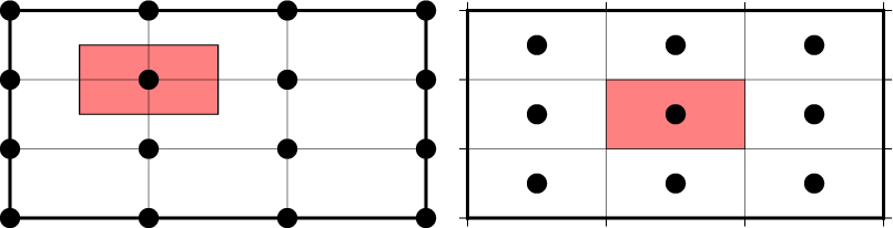
293 |
294 | *Gridline (left) and pixel (right) registration of data nodes. The red shade
295 | indicates the areas represented by the value at the node (solid circle).*
296 |
297 | Grids are generated using one of the two options and it's **very important to
298 | know which you have** (hint: `grdinfo` can tell you). The plotting modules in
299 | GMT can usually automatically detect this. When generating output grids, you
300 | can specify which one you want using the `-r` option.
301 |
302 | Further reading: https://docs.generic-mapping-tools.org/latest/cookbook/options.html#grid-registration-the-r-option
303 |
304 | Use `grdinfo` to figure out if the Earth relief grids are gridline or pixel
305 | registered:
306 |
307 | ```
308 | gmt grdinfo @earth_relief_10m
309 | ```
310 |
311 | GMT actually distributes both versions of the Earth relief data. You can
312 | specify which version you want by appending `_p` (for pixel) or `_g` (for
313 | gridline) to the file name (for example, `@earth_relief_10m_p`).
314 |
315 | Further reading: https://docs.generic-mapping-tools.org/latest/datasets/remote-data.html#global-earth-relief-grids
316 |
317 | # Credits
318 | The group excerise and bonus sections were taken from the [2021 edition](https://github.com/GenericMappingTools/2021-unavco-course/blob/main/grids/README.md) done by Leonardo Uieda.
319 |
--------------------------------------------------------------------------------
/05_seismology/README.md:
--------------------------------------------------------------------------------
1 | # GMT for Seismology: Plotting beachballs
2 |
3 | **Instructor:**
4 | [Max Jones](https://github.com/maxrjones) (Material developed by [Dongdong Tian](https://me.seisman.info/))
5 |
6 | GMT provides 4 seismology modules (see the summary figure below). The goal of this session is to show how to plot beachballs on maps and cross-sections.
7 |
8 |
276 |
277 | If you have any questions, ask on the Slack chatroom, on the office hours and/or in the [GMT forum](https://forum.generic-mapping-tools.org/).
278 |
279 | SOLUTION
280 |
281 | Don't look at *one* [`solution`](5_excercise.sh) until you finish you own script.
282 |
283 | ## Bonus: Grid registration
284 |
285 | The coordinates of grids and what the data values represent can be specified in
286 | two ways (known as the grid *registration*):
287 |
288 | * **Grid lines:** the coordinates correspond to the center of the area that is
289 | represented by the data value (where grid lines intersect)
290 | * **Pixels:** the coordinates correspond to the borders of the area (pixel)
291 |
292 | 
293 |
294 | *Gridline (left) and pixel (right) registration of data nodes. The red shade
295 | indicates the areas represented by the value at the node (solid circle).*
296 |
297 | Grids are generated using one of the two options and it's **very important to
298 | know which you have** (hint: `grdinfo` can tell you). The plotting modules in
299 | GMT can usually automatically detect this. When generating output grids, you
300 | can specify which one you want using the `-r` option.
301 |
302 | Further reading: https://docs.generic-mapping-tools.org/latest/cookbook/options.html#grid-registration-the-r-option
303 |
304 | Use `grdinfo` to figure out if the Earth relief grids are gridline or pixel
305 | registered:
306 |
307 | ```
308 | gmt grdinfo @earth_relief_10m
309 | ```
310 |
311 | GMT actually distributes both versions of the Earth relief data. You can
312 | specify which version you want by appending `_p` (for pixel) or `_g` (for
313 | gridline) to the file name (for example, `@earth_relief_10m_p`).
314 |
315 | Further reading: https://docs.generic-mapping-tools.org/latest/datasets/remote-data.html#global-earth-relief-grids
316 |
317 | # Credits
318 | The group excerise and bonus sections were taken from the [2021 edition](https://github.com/GenericMappingTools/2021-unavco-course/blob/main/grids/README.md) done by Leonardo Uieda.
319 |
--------------------------------------------------------------------------------
/05_seismology/README.md:
--------------------------------------------------------------------------------
1 | # GMT for Seismology: Plotting beachballs
2 |
3 | **Instructor:**
4 | [Max Jones](https://github.com/maxrjones) (Material developed by [Dongdong Tian](https://me.seisman.info/))
5 |
6 | GMT provides 4 seismology modules (see the summary figure below). The goal of this session is to show how to plot beachballs on maps and cross-sections.
7 |
8 |  9 |
10 | **Contents**
11 |
12 | - [Explain Focal Mechanism](#focal-mechanism-and-beachball)
13 | - [Plot beachballs on maps](#plot-beachballs-on-maps)
14 | - [Plot beachballs on cross-sections](#plot-beachballs-on-cross-sections)
15 | - [Get focal mechanism solutions from Global CMT](#get-focal-mechanism-solutions-from-global-cmt)
16 | - [Group Exercise](#group-exercise)
17 |
18 | **Resources**
19 |
20 | - Focal Mechanisms Explained: What are those “beach balls”? https://www.youtube.com/watch?v=MomVOkyDdLo (about 6 minutes)
21 | - manpage of [meca](https://docs.generic-mapping-tools.org/6.4/supplements/seis/meca.html)
22 | - manpage of [coupe](https://docs.generic-mapping-tools.org/6.4/supplements/seis/coupe.html)
23 | - [Global CMT project](https://www.globalcmt.org/)
24 |
25 | ## Focal mechanism and beachball
26 |
27 | Focal mechanism describes the movement of the fault that generates the
28 | seismic waves. From focal mechanism solutions, we can know the orientation of the fault plane and the slip direction.
29 |
30 |
9 |
10 | **Contents**
11 |
12 | - [Explain Focal Mechanism](#focal-mechanism-and-beachball)
13 | - [Plot beachballs on maps](#plot-beachballs-on-maps)
14 | - [Plot beachballs on cross-sections](#plot-beachballs-on-cross-sections)
15 | - [Get focal mechanism solutions from Global CMT](#get-focal-mechanism-solutions-from-global-cmt)
16 | - [Group Exercise](#group-exercise)
17 |
18 | **Resources**
19 |
20 | - Focal Mechanisms Explained: What are those “beach balls”? https://www.youtube.com/watch?v=MomVOkyDdLo (about 6 minutes)
21 | - manpage of [meca](https://docs.generic-mapping-tools.org/6.4/supplements/seis/meca.html)
22 | - manpage of [coupe](https://docs.generic-mapping-tools.org/6.4/supplements/seis/coupe.html)
23 | - [Global CMT project](https://www.globalcmt.org/)
24 |
25 | ## Focal mechanism and beachball
26 |
27 | Focal mechanism describes the movement of the fault that generates the
28 | seismic waves. From focal mechanism solutions, we can know the orientation of the fault plane and the slip direction.
29 |
30 |  31 |
32 | Beachball is a graphic represention of focal mechanism. Here are three simple focal mechanism solutions for normal fault, reverse fault, and strike-slip fault.
33 |
34 |
31 |
32 | Beachball is a graphic represention of focal mechanism. Here are three simple focal mechanism solutions for normal fault, reverse fault, and strike-slip fault.
33 |
34 |  35 |
36 | We will use these three focal mechanisms as the example data.
37 | ```
38 | # longitude latitude depth strike dip rake magnitude [event_title]
39 | 112 32 25 30 90 0 4 Strike-slip
40 | 115 34 15 30 60 90 5 Reverse
41 | 118 32 45 30 60 -90 6 Normal
42 | ```
43 |
44 | First, we need to copy the data and save it into a plaintext file `meca.dat`,
45 | which will be used in the following scripts.
46 |
47 | ## Plot beachballs on maps
48 |
49 | The [meca](https://docs.generic-mapping-tools.org/6.4/supplements/seis/meca.html) module
50 | can plot beachballs on maps.
51 |
52 | [`-S`](https://docs.generic-mapping-tools.org/6.4/supplements/seis/meca.html#s) is the most important option of **meca**. It tells GMT the format of the input data,
53 | beachball size, and other properties of optional title string.
54 |
55 | Other useful options:
56 |
57 | - **-E**: color for extensive quadrants
58 | - **-G**: color for compressional quadrants
59 | - **-C**: paint the compressional quadrants based on depth (you need to create a CPT by calling [`makecpt`](https://docs.generic-mapping-tools.org/6.4/makecpt.html) module first)
60 |
61 | **The simplest example**: [beachball.sh](beachball.sh)
62 |
63 |
35 |
36 | We will use these three focal mechanisms as the example data.
37 | ```
38 | # longitude latitude depth strike dip rake magnitude [event_title]
39 | 112 32 25 30 90 0 4 Strike-slip
40 | 115 34 15 30 60 90 5 Reverse
41 | 118 32 45 30 60 -90 6 Normal
42 | ```
43 |
44 | First, we need to copy the data and save it into a plaintext file `meca.dat`,
45 | which will be used in the following scripts.
46 |
47 | ## Plot beachballs on maps
48 |
49 | The [meca](https://docs.generic-mapping-tools.org/6.4/supplements/seis/meca.html) module
50 | can plot beachballs on maps.
51 |
52 | [`-S`](https://docs.generic-mapping-tools.org/6.4/supplements/seis/meca.html#s) is the most important option of **meca**. It tells GMT the format of the input data,
53 | beachball size, and other properties of optional title string.
54 |
55 | Other useful options:
56 |
57 | - **-E**: color for extensive quadrants
58 | - **-G**: color for compressional quadrants
59 | - **-C**: paint the compressional quadrants based on depth (you need to create a CPT by calling [`makecpt`](https://docs.generic-mapping-tools.org/6.4/makecpt.html) module first)
60 |
61 | **The simplest example**: [beachball.sh](beachball.sh)
62 |
63 |  64 |
65 | **Beachballs with the same size**: [beachball-same-size.sh](beachball-same-size.sh)
66 |
67 |
64 |
65 | **Beachballs with the same size**: [beachball-same-size.sh](beachball-same-size.sh)
66 |
67 |  68 |
69 | **Beachballs with customized event labels**: [beachball-customized-labels.sh](beachball-customized-labels.sh)
70 |
71 |
68 |
69 | **Beachballs with customized event labels**: [beachball-customized-labels.sh](beachball-customized-labels.sh)
70 |
71 |  72 |
73 | **Beachballs without event labels**: [beachball-no-labels.sh](beachball-no-labels.sh)
74 |
75 |
72 |
73 | **Beachballs without event labels**: [beachball-no-labels.sh](beachball-no-labels.sh)
74 |
75 |  76 |
77 | **Different colors**: [beachball-colors.sh](beachball-colors.sh)
78 |
79 |
76 |
77 | **Different colors**: [beachball-colors.sh](beachball-colors.sh)
78 |
79 |  80 |
81 | **Color by depth**: [beachball-color-by-depth.sh](beachball-color-by-depth.sh)
82 |
83 |
80 |
81 | **Color by depth**: [beachball-color-by-depth.sh](beachball-color-by-depth.sh)
82 |
83 |  84 |
85 | ## Plot beachballs on cross-sections
86 |
87 | [`coupe`](https://docs.generic-mapping-tools.org/6.4/supplements/seis/coupe.html) module can cut and plot beachballs in cross-sections (e.g., a vertical cross-section).
88 |
89 | Most options of **coupe** have the same meaning as in **meca**. The most important
90 | and unique option is [`-A`](https://docs.generic-mapping-tools.org/6.4/supplements/seis/coupe.html#a), to determine the cross-section.
91 |
92 | There are different ways to specify the geometry of a cross-section. Here we will
93 | use **-Aa** as an example. The full syntax of the **-A** option is:
94 |
95 | **-Aa***lon1/lat1/lon2/lat2*[**+d***dip*][**+w***width*][**+z***dmin/dmax*][**+r**]
96 |
97 | - *lon1/lat1*: location of the starting point
98 | - *lon2/lat2*: location of the end point
99 | - *dip*: dip angle of the cross-section: 0 for horizontal slice, 90 for vertical slice
100 | - *width*: width of the cross-section
101 | - *dmin/dmax*: depth range of the cross-section
102 | - **+r**: automatically determine the plot region! **-R** is not necessary!
103 |
104 | **Cross-section view**: [beachball-cross-section.sh](beachball-cross-section.sh)
105 |
106 |
84 |
85 | ## Plot beachballs on cross-sections
86 |
87 | [`coupe`](https://docs.generic-mapping-tools.org/6.4/supplements/seis/coupe.html) module can cut and plot beachballs in cross-sections (e.g., a vertical cross-section).
88 |
89 | Most options of **coupe** have the same meaning as in **meca**. The most important
90 | and unique option is [`-A`](https://docs.generic-mapping-tools.org/6.4/supplements/seis/coupe.html#a), to determine the cross-section.
91 |
92 | There are different ways to specify the geometry of a cross-section. Here we will
93 | use **-Aa** as an example. The full syntax of the **-A** option is:
94 |
95 | **-Aa***lon1/lat1/lon2/lat2*[**+d***dip*][**+w***width*][**+z***dmin/dmax*][**+r**]
96 |
97 | - *lon1/lat1*: location of the starting point
98 | - *lon2/lat2*: location of the end point
99 | - *dip*: dip angle of the cross-section: 0 for horizontal slice, 90 for vertical slice
100 | - *width*: width of the cross-section
101 | - *dmin/dmax*: depth range of the cross-section
102 | - **+r**: automatically determine the plot region! **-R** is not necessary!
103 |
104 | **Cross-section view**: [beachball-cross-section.sh](beachball-cross-section.sh)
105 |
106 |  107 |
108 | ## Get focal mechanism solutions from Global CMT
109 |
110 | Global CMT: https://www.globalcmt.org/
111 |
112 | The GCMT project provides focal mechasnism solutions for global earthquakes with M>5 since 1976.
113 |
114 | 1. Go to the [GCMT official site](https://www.globalcmt.org/), and click the
115 | [CMT catalog web search](https://www.globalcmt.org/CMTsearch.html) link.
116 |
117 | 2. Enter the parameters to select earthquakes:
118 |
119 | - start time and end time
120 | - magnitude range
121 | - location
122 | - etc
123 |
124 | 3. Select "Output type": "**GMT psmeca input**" (NOT "GMT psvelomeca input")
125 |
126 | 4. Click the "Done" button
127 | 5. Copy/paste the solutions into a plaintext file and save it.
128 | 6. Now you can plot the beachballs using **meca** or **coupe**
129 |
130 | **NOTE**: Use `-Sd`, `-Sm` or `-Sz` for GCMT solutions, **NOT** `-Sa`.
131 |
132 | ## Group Exercise
133 |
134 | You will be split into teams to work on an exercise:
135 |
136 | - Discuss with your team which commands and options you would use
137 | - Work together to make a script that generates the desired plot
138 | - If you have any questions, ask on the Slack chatroom
139 |
140 | **Make a regional map with beachballs colored by depth**
141 |
142 | - Select the region you want to work on
143 | - Go to [GCMT web search site](https://www.globalcmt.org/CMTsearch.html),
144 | select the focal mechanism solutions by specifying geographic range, time range,
145 | and magnitude range. Save the solutions to a file.
146 | - Make a map view of beachballs with colors determined by depth
147 | - Based on a the map view plot, choose a cross-section, and make a cross-section view
148 |
149 | **TIPS**
150 |
151 | - You need to use `-Sd`, `-Sm` or `-Sz` for GCMT solutions, **NOT** `-Sa`.
152 | - Use `+f0p` in the `-S` option to set the font size of the event labels to zero,
153 | so that **meca** and **coupe** won't plot the event lables
154 | - You may have white beachballs if the event depth is out of the CPT range
155 |
156 | Map view (**meca**) | Cross-section view (**coupe**)
157 | :-------------------------:|:-------------------------:
158 |  | 
159 |
160 | **SOLUTION**
161 |
162 | Don't look at the solutions until you finish you own script.
163 |
164 | The examples above are plotted using data [`japan-focal.dat`](japan-focal.dat)
165 | using script [`japan-beachballs.sh`](japan-beachballs.sh).
166 |
--------------------------------------------------------------------------------
/05_seismology/beachball-color-by-depth.png:
--------------------------------------------------------------------------------
https://raw.githubusercontent.com/GenericMappingTools/gmt-for-geodesy/34799147d87fc96a9ae9c6300331641fa286f321/05_seismology/beachball-color-by-depth.png
--------------------------------------------------------------------------------
/05_seismology/beachball-color-by-depth.sh:
--------------------------------------------------------------------------------
1 | #!/usr/bin/env bash
2 | #
3 | # Plot beachballs of three basic faults, with the colors of the compressive quadrants
4 | # determined by earthquake depths.
5 | #
6 | gmt begin beachball-color-by-depth png
7 | gmt basemap -JM15c -R110/120/30/35 -Baf
8 | # create a CPT from the batlow CPT, for earthquake depth from 0 to 50 km
9 | gmt makecpt -Cbatlow -T0/50
10 | # -C: let compressive part color be determined by the z-value in the third column.
11 | gmt meca meca.dat -Sa1c -C
12 | # Plot the colorbar in the Middle Right (MR) and set the label using -Bxaf+l
13 | gmt colorbar -Bxaf+l"Depth (km)" -DJMR
14 | gmt end show
15 |
--------------------------------------------------------------------------------
/05_seismology/beachball-colors.png:
--------------------------------------------------------------------------------
https://raw.githubusercontent.com/GenericMappingTools/gmt-for-geodesy/34799147d87fc96a9ae9c6300331641fa286f321/05_seismology/beachball-colors.png
--------------------------------------------------------------------------------
/05_seismology/beachball-colors.sh:
--------------------------------------------------------------------------------
1 | #!/usr/bin/env bash
2 | #
3 | # Plot beachballs of three basic faults (strike-slip, normal and reverse faults),
4 | # with the compressional and extensive quadrants filled by different colors.
5 | #
6 | gmt begin beachball-colors png
7 | # -G select the filling of the compressional quadrants
8 | # -E select the filling of the extensive quadrants
9 | gmt basemap -JM10c -R110/120/30/35 -Baf
10 | gmt meca meca.dat -Sa1c -Gred -Elightblue
11 | gmt end show
12 |
--------------------------------------------------------------------------------
/05_seismology/beachball-cross-section.png:
--------------------------------------------------------------------------------
https://raw.githubusercontent.com/GenericMappingTools/gmt-for-geodesy/34799147d87fc96a9ae9c6300331641fa286f321/05_seismology/beachball-cross-section.png
--------------------------------------------------------------------------------
/05_seismology/beachball-cross-section.sh:
--------------------------------------------------------------------------------
1 | #!/usr/bin/env bash
2 | #
3 | # Plot cross-section of beachballs
4 | #
5 | gmt begin beachball-cross-section png
6 | # The cross-section is selected by specifying the locations (longitude and latitude)
7 | # of a starting point (110/33), and an ending point (120/33).
8 | #
9 | # To reverse the Y axis, set the figure heigth to a negative value (-5c)
10 | gmt coupe meca.dat -Sa1c -Aa110/33/120/33 \
11 | -JX15c/-5c -Bxaf+l"Distance (km)" -Byaf+l"Depth (km)" -BWSen \
12 | -R0/1000/0/60
13 | gmt end show
14 |
--------------------------------------------------------------------------------
/05_seismology/beachball-customized-labels.png:
--------------------------------------------------------------------------------
https://raw.githubusercontent.com/GenericMappingTools/gmt-for-geodesy/34799147d87fc96a9ae9c6300331641fa286f321/05_seismology/beachball-customized-labels.png
--------------------------------------------------------------------------------
/05_seismology/beachball-customized-labels.sh:
--------------------------------------------------------------------------------
1 | #!/usr/bin/env bash
2 | #
3 | # Plot beachballs with customized labels
4 | #
5 |
6 | gmt begin beachball-customized-labels png
7 | gmt basemap -JM10c -R110/120/30/35 -Baf
8 | # +a: angle of lables
9 | # +f: size and color of labels
10 | # +j: location of labels
11 | # +o: extra offsets in x- and y- directions
12 | gmt meca meca.dat -Sa1c+a30+f6p,blue+jBC+o0.2c/0c
13 | gmt end show
14 |
--------------------------------------------------------------------------------
/05_seismology/beachball-no-labels.png:
--------------------------------------------------------------------------------
https://raw.githubusercontent.com/GenericMappingTools/gmt-for-geodesy/34799147d87fc96a9ae9c6300331641fa286f321/05_seismology/beachball-no-labels.png
--------------------------------------------------------------------------------
/05_seismology/beachball-no-labels.sh:
--------------------------------------------------------------------------------
1 | #!/usr/bin/env bash
2 | #
3 | # Plot beachballs without labels
4 | #
5 | gmt begin beachball-no-labels png
6 | gmt basemap -JM10c -R110/120/30/35 -Baf
7 | # set lable font size to 0p to hide the labels
8 | gmt meca meca.dat -Sa1c+f0p
9 | gmt end show
10 |
--------------------------------------------------------------------------------
/05_seismology/beachball-same-size.png:
--------------------------------------------------------------------------------
https://raw.githubusercontent.com/GenericMappingTools/gmt-for-geodesy/34799147d87fc96a9ae9c6300331641fa286f321/05_seismology/beachball-same-size.png
--------------------------------------------------------------------------------
/05_seismology/beachball-same-size.sh:
--------------------------------------------------------------------------------
1 | #!/usr/bin/env bash
2 | #
3 | # Plot beachballs with the same size.
4 | #
5 | gmt begin beachball-same-size png
6 | gmt basemap -JM10c -R110/120/30/35 -Baf
7 | gmt meca meca.dat -Sa1c+m
8 | gmt end show
9 |
--------------------------------------------------------------------------------
/05_seismology/beachball.png:
--------------------------------------------------------------------------------
https://raw.githubusercontent.com/GenericMappingTools/gmt-for-geodesy/34799147d87fc96a9ae9c6300331641fa286f321/05_seismology/beachball.png
--------------------------------------------------------------------------------
/05_seismology/beachball.sh:
--------------------------------------------------------------------------------
1 | #!/usr/bin/env bash
2 | gmt begin beachball png
3 | gmt basemap -JM10c -R110/120/30/35 -Baf
4 | gmt meca meca.dat -Sa1c
5 | gmt end show
6 |
--------------------------------------------------------------------------------
/05_seismology/images/basic-faults.png:
--------------------------------------------------------------------------------
https://raw.githubusercontent.com/GenericMappingTools/gmt-for-geodesy/34799147d87fc96a9ae9c6300331641fa286f321/05_seismology/images/basic-faults.png
--------------------------------------------------------------------------------
/05_seismology/images/faults.png:
--------------------------------------------------------------------------------
https://raw.githubusercontent.com/GenericMappingTools/gmt-for-geodesy/34799147d87fc96a9ae9c6300331641fa286f321/05_seismology/images/faults.png
--------------------------------------------------------------------------------
/05_seismology/japan-beachballs-mapview.png:
--------------------------------------------------------------------------------
https://raw.githubusercontent.com/GenericMappingTools/gmt-for-geodesy/34799147d87fc96a9ae9c6300331641fa286f321/05_seismology/japan-beachballs-mapview.png
--------------------------------------------------------------------------------
/05_seismology/japan-beachballs-sideview.png:
--------------------------------------------------------------------------------
https://raw.githubusercontent.com/GenericMappingTools/gmt-for-geodesy/34799147d87fc96a9ae9c6300331641fa286f321/05_seismology/japan-beachballs-sideview.png
--------------------------------------------------------------------------------
/05_seismology/japan-beachballs.sh:
--------------------------------------------------------------------------------
1 | #!/usr/bin/env bash
2 | #
3 | # Plot real-world beachballs on maps and cross-sections
4 | #
5 | # The focal mechanism information is obtained from Global CMT project
6 | # - region: 125E-150E, 30N-47N
7 | # - time range: 2010-01-01 to 2019-07-01
8 | # - magnitude: >=5.5
9 |
10 | gmt begin
11 | # Figure 1: Beachballs on maps
12 | gmt figure japan-beachballs-mapview png
13 |
14 | # plot basemap, setting map width, region and frames
15 | gmt basemap -R122/147/30/48 -JM15c -BWSen -Baf
16 | # Plot Earth relief by mapping values to colors using the "globe" CPT
17 | # Set automatic shading effects
18 | gmt grdimage @earth_relief_02m -I+d
19 | # Add the colorbar to the Top Right (TR) and shift to the right by 2 cm.
20 | # The colorbar width is set to be 6 cm.
21 | gmt colorbar -DjTR+o-2c/0c+w6c+ml -Ba2000+l"Earth relief (m)"
22 |
23 | # Customize the jet CPT for earthquake depth from 0 to 700
24 | gmt makecpt -Cjet -T0/700/100
25 | # -C: Color the beachballs based on earthquake depths and the "current" CPT
26 | gmt meca japan-focal.dat -Sd0.5c+f0p -C
27 | # Add the colorbar to the Bottom Right (BR) and shift to the right by 2 cm.
28 | # The colorbar is reversed by giving a negative length (+w-6c).
29 | gmt colorbar -DjBR+o-2c/0c+w-6c+ml -Ba100+l"Focal depth (km)"
30 |
31 | # Prepare data file for plotting and label the cross-section line
32 | echo 126 42 A > xsection.dat
33 | echo 146 40 B >> xsection.dat
34 | # plot the cross-section line, with a 2 point, red pen
35 | # the plot column only needs the longitude and latitude of the input file, and ignores the third column
36 | gmt plot xsection.dat -W2p,red
37 | # label the cross-section by "A" and "B", with a font size of 15 points
38 | gmt text xsection.dat -F+f15p
39 |
40 |
41 | # Figure 2: Beachball cross-sections
42 | gmt figure japan-beachballs-sideview png
43 | # Customize the jet CPT for earthquake depth from 0 -700
44 | gmt makecpt -Cjet -T0/700/100
45 | # The cross-section is selected by specifly the locations (longitude and latitude) of a starting point (126/42),
46 | # and a ending point (146/40). The cross-section plane is vertical (dip angle=90), with the width set to be 500 km,
47 | # and depth to be 0-70 km.
48 | #
49 | # To reverse the Y axis, set the figure heigth to a negative value (-10 cm)
50 | gmt coupe japan-focal.dat -Sd0.5c+f0p -Aa126/42/146/40/700+r+w500 -Q -C \
51 | -JX15c/-10c -BWSen -Bxaf+l"Distance (km)" -Byaf+l"Depth (km)"
52 | # Add the colorbar to the Bottom Right (BR) and shift to the right by 2 cm.
53 | # The colorbar is reversed by giving a negative length (+w-10c).
54 | gmt colorbar -DjBR+o-2c/0c+w-10c+ml -Np -Ba100+l"Focal depth (km)"
55 |
56 | # cleanup temporary files
57 | rm xsection.dat
58 | gmt end show
59 |
--------------------------------------------------------------------------------
/05_seismology/japan-focal.dat:
--------------------------------------------------------------------------------
1 | 143.60 38.00 19 -0.76 -1.34 2.10 0.28 2.17 1.45 24 X Y 201001170604A
2 | 131.08 30.91 39 0.20 -1.18 0.98 0.50 0.93 1.28 24 X Y 201001250715A
3 | 130.66 42.48 579 0.27 0.19 -0.46 0.23 -2.50 -0.59 26 X Y 201002180113A
4 | 147.78 44.08 52 1.19 -3.40 2.20 1.90 -1.97 -0.02 24 X Y 201003061331A
5 | 141.45 37.62 75 -2.11 0.25 1.86 0.52 0.67 0.79 24 X Y 201003131246A
6 | 141.98 37.70 46 5.55 -0.28 -5.27 1.83 4.97 -2.07 25 X Y 201003140808A
7 | 138.45 43.28 12 5.07 -0.51 -4.57 -0.23 -1.15 -1.67 24 X Y 201003300102A
8 | 141.76 37.42 33 0.88 -0.98 0.09 0.02 -0.30 -0.16 25 X Y 201006130332A
9 | 148.94 44.34 31 1.39 -0.37 -1.02 0.46 1.45 -1.03 25 X Y 201006180223A
10 | 141.84 30.61 18 3.86 0.40 -4.26 0.19 3.76 0.58 24 X Y 201006281207A
11 | 142.77 39.68 35 2.15 0.23 -2.37 0.47 2.35 -0.23 25 X Y 201007042155A
12 | 142.32 41.47 61 5.50 -0.10 -5.40 1.76 3.23 -2.03 24 X Y 201009130547A
13 | 140.01 37.31 12 1.87 0.03 -1.89 -0.32 0.01 0.37 24 X Y 201009290759A
14 | 143.15 42.14 62 2.06 -0.72 -1.34 0.30 1.35 -1.44 24 X Y 201010141358A
15 | 146.87 46.82 362 0.71 0.18 -0.89 0.35 -1.57 -0.81 24 X Y 201011021810A
16 | 143.26 40.89 24 2.79 0.03 -2.82 1.84 3.46 -0.63 24 X Y 201012060730A
17 | 142.29 31.49 12 -2.88 -0.21 3.09 0.25 0.81 -0.56 24 X Y 201101050057A
18 | 142.78 38.56 14 0.49 -0.02 -0.47 0.42 1.05 -0.13 27 X Y 201103090245A
19 | 142.80 38.33 29 0.95 -0.05 -0.90 0.51 1.15 -0.29 25 X Y 201103091816A
20 | 143.50 38.47 18 4.61 -0.24 -4.36 3.09 6.49 -1.45 24 X Y 201103091844A
21 | 142.91 38.29 23 0.70 -0.02 -0.68 0.27 0.79 -0.23 25 X Y 201103092122A
22 | 142.82 38.27 23 3.79 -0.28 -3.51 1.90 4.42 -1.04 25 X Y 201103092124B
23 | 143.61 38.53 17 2.08 -0.12 -1.96 1.50 2.83 -0.64 24 X Y 201103100808A
24 | 143.05 37.52 20 1.73 -0.28 -1.45 2.12 4.55 -0.66 29 X Y 201103110546A
25 | 141.38 35.92 29 4.39 -0.31 -4.07 3.17 6.34 -1.97 27 X Y 201103110615A
26 | 144.63 38.27 21 -3.03 0.03 3.00 -0.41 -0.34 0.47 27 X Y 201103110625A
27 | 138.60 37.06 12 2.35 -1.43 -0.92 -2.03 -0.51 -1.96 25 X Y 201103111859A
28 | 143.01 39.43 30 -2.84 2.25 0.58 0.70 1.07 0.45 25 X Y 201103111902A
29 | 139.09 40.37 14 -0.00 1.92 -1.92 0.42 -0.47 1.48 25 X Y 201103111946A
30 | 142.68 38.98 12 -1.93 1.08 0.85 0.41 0.03 -0.73 25 X Y 201103112011A
31 | 142.85 38.81 19 -6.09 2.84 3.25 0.43 1.23 -1.45 24 X Y 201103120134A
32 | 142.84 37.57 14 -4.95 1.21 3.74 -3.62 -2.70 2.37 25 X Y 201103120147A
33 | 143.71 37.63 15 -0.16 -0.57 0.73 0.10 0.30 0.33 25 X Y 201103120247A
34 | 141.54 36.03 35 -1.09 0.66 0.42 -0.07 -0.03 0.00 25 X Y 201103120311A
35 | 143.52 40.07 29 3.95 -0.88 -3.06 1.74 3.37 -0.31 24 X Y 201103120452A
36 | 142.35 39.30 37 -1.82 1.10 0.72 0.50 1.01 0.55 24 X Y 201103120618A
37 | 142.28 39.04 36 -3.10 1.27 1.83 -0.42 3.23 -1.15 24 X Y 201103121053A
38 | 143.60 37.71 21 -0.60 -0.43 1.02 0.19 0.41 0.29 25 X Y 201103121253A
39 | 141.53 37.23 46 1.67 -0.34 -1.34 0.93 1.22 -0.65 25 X Y 201103121315A
40 | 142.72 38.76 26 -2.30 0.18 2.12 -0.80 -1.31 -0.69 24 X Y 201103121403A
41 | 142.52 39.52 15 0.88 0.14 -1.02 0.15 5.80 0.14 24 X Y 201103121443A
42 | 142.94 36.47 12 2.24 -0.46 -1.77 0.88 1.67 -0.95 24 X Y 201103121719A
43 | 141.99 37.56 15 -0.86 0.20 0.67 -0.03 0.20 -0.26 25 X Y 201103122212A
44 | 141.94 38.07 23 3.05 -0.71 -2.34 0.69 4.59 -1.27 24 X Y 201103122324A
45 | 141.81 35.74 12 -1.59 0.29 1.30 0.89 -1.37 -0.52 25 X Y 201103130126A
46 | 142.24 36.35 12 5.87 -3.75 -2.12 -1.93 0.61 -1.06 24 X Y 201103130223A
47 | 143.55 39.60 22 2.20 -0.09 -2.11 1.65 3.01 -0.55 24 X Y 201103130756A
48 | 142.20 38.90 50 2.36 0.07 -2.43 0.87 1.68 -0.51 24 X Y 201103130952A
49 | 142.34 37.42 15 -4.88 1.40 3.48 4.55 3.72 -1.85 24 X Y 201103131137A
50 | 141.30 35.28 15 0.66 -0.11 -0.56 2.78 2.14 -0.80 24 X Y 201103131755A
51 | 141.08 36.43 12 -1.55 -2.98 4.53 1.22 0.30 1.24 24 X Y 201103140102A
52 | 142.62 37.77 20 -0.54 -0.34 0.88 -0.69 -0.81 0.13 25 X Y 201103140612A
53 | 142.42 37.23 16 2.19 -0.64 -1.54 2.38 2.31 -1.15 24 X Y 201103141759A
54 | 142.29 37.44 12 -5.90 0.98 4.92 1.95 2.84 1.93 24 X Y 201103150949A
55 | 142.13 37.67 28 0.20 0.35 -0.55 -1.26 0.96 0.19 25 X Y 201103151327A
56 | 138.58 35.27 19 0.38 -1.03 0.65 0.04 0.20 -0.66 25 X Y 201103151331A
57 | 143.50 40.36 23 0.77 -0.03 -0.73 0.44 0.95 -0.16 25 X Y 201103151523A
58 | 141.16 35.17 22 1.87 -2.86 0.99 1.79 1.16 0.13 24 X Y 201103152030A
59 | 140.83 35.78 12 -5.92 -0.87 6.79 0.10 2.54 -0.42 24 X Y 201103160352A
60 | 142.33 39.87 48 4.40 -0.18 -4.22 1.64 3.29 -1.16 24 X Y 201103160629A
61 | 142.55 40.17 41 1.29 0.07 -1.36 0.56 1.21 -0.29 25 X Y 201103170413A
62 | 143.46 37.79 12 -1.96 0.24 1.72 0.81 1.95 0.58 24 X Y 201103170612A
63 | 140.89 35.58 29 2.39 -1.78 -0.61 0.59 1.03 -0.94 24 X Y 201103171232A
64 | 141.42 36.80 39 -6.67 3.07 3.61 -0.82 -0.07 2.22 24 X Y 201103171254A
65 | 143.47 37.86 12 -1.49 0.06 1.43 0.29 1.22 0.34 24 X Y 201103180323A
66 | 142.36 39.24 25 0.09 0.09 -0.18 1.00 2.86 -0.15 24 X Y 201103182333A
67 | 143.29 39.67 22 4.65 -0.06 -4.59 2.44 5.90 -0.92 24 X Y 201103190122A
68 | 140.48 36.86 12 -6.88 3.01 3.87 1.33 2.14 -2.71 24 X Y 201103190956A
69 | 141.67 37.73 49 2.16 -0.38 -1.78 0.63 1.62 -0.57 24 X Y 201103200555A
70 | 142.14 39.39 51 5.07 -0.25 -4.82 2.12 3.67 -1.02 24 X Y 201103201203A
71 | 140.99 35.18 18 1.29 -2.53 1.24 3.08 1.39 0.59 24 X Y 201103220338A
72 | 144.00 37.11 12 -4.82 1.86 2.96 0.14 1.61 2.57 25 X Y 201103220718A
73 | 141.78 37.38 30 -0.20 0.44 -0.24 -2.45 0.52 0.65 25 X Y 201103220919A
74 | 143.81 39.84 13 2.14 0.05 -2.20 1.12 2.86 -0.57 25 X Y 201103220944A
75 | 143.34 39.90 26 1.91 -0.25 -1.67 1.01 2.43 -0.31 24 X Y 201103221121A
76 | 143.29 36.83 12 -2.80 1.12 1.68 -0.04 -0.10 1.30 24 X Y 201103221201A
77 | 141.79 36.12 34 3.42 -1.27 -2.15 1.17 1.96 -1.12 24 X Y 201103221204A
78 | 141.66 35.77 19 4.57 0.18 -4.75 4.13 1.88 -1.63 24 X Y 201103221350A
79 | 141.56 35.88 15 3.37 -3.18 -0.19 -0.64 -1.13 0.40 24 X Y 201103221503A
80 | 140.76 37.09 12 -3.65 0.14 3.51 0.71 1.72 1.14 24 X Y 201103222212A
81 | 142.34 39.08 37 0.58 0.07 -0.64 0.31 0.69 -0.06 25 X Y 201103240821A
82 | 142.17 38.78 46 1.88 -0.04 -1.83 0.82 1.60 -0.49 25 X Y 201103251136A
83 | 142.09 38.40 22 -2.28 1.88 0.39 1.85 0.32 -0.64 25 X Y 201103272223A
84 | 142.37 37.47 18 -1.64 0.13 1.51 1.55 0.90 0.77 25 X Y 201103291054A
85 | 142.63 36.09 12 5.51 -2.11 -3.40 -0.07 0.86 -2.08 24 X Y 201103300529A
86 | 142.05 38.97 50 1.07 -0.00 -1.07 0.42 0.84 -0.25 25 X Y 201103310715A
87 | 142.17 39.38 48 0.76 -0.03 -0.73 0.33 0.57 -0.16 25 X Y 201104011157A
88 | 143.54 40.27 22 1.95 -0.10 -1.85 0.88 2.09 -0.41 24 X Y 201104011703A
89 | 141.85 38.32 53 5.99 -1.43 -4.55 -1.11 -1.25 -1.65 26 X Y 201104071432A
90 | 131.84 30.04 12 -1.04 -0.05 1.09 0.25 0.35 0.18 25 X Y 201104091257A
91 | 140.54 37.00 12 -1.27 0.76 0.51 -0.01 0.44 -0.33 26 X Y 201104110816A
92 | 140.53 37.01 12 -1.86 1.95 -0.09 0.45 0.96 0.01 24 X Y 201104111142A
93 | 144.50 37.70 15 -2.03 1.37 0.66 0.11 0.47 0.81 24 X Y 201104111753A
94 | 140.85 35.42 16 -0.27 -1.88 2.15 -1.71 0.16 -0.48 25 X Y 201104112308A
95 | 140.63 37.08 18 0.24 0.22 -0.46 0.55 0.11 -0.73 25 X Y 201104120507A
96 | 142.13 39.39 52 2.45 -0.18 -2.26 1.04 1.88 -0.64 24 X Y 201104121937A
97 | 143.59 39.63 15 0.81 0.04 -0.85 0.42 1.12 -0.18 25 X Y 201104131957A
98 | 143.48 39.64 24 1.40 -0.17 -1.23 0.72 1.45 -0.31 24 X Y 201104132032A
99 | 142.25 35.50 12 2.36 -0.34 -2.02 0.91 2.38 -0.79 24 X Y 201104140608A
100 | 140.00 36.40 81 3.34 0.44 -3.77 3.17 2.95 -1.13 24 X Y 201104160219A
101 | 143.92 36.95 12 -1.75 1.41 0.34 0.42 0.91 0.81 24 X Y 201104162036A
102 | 143.85 40.30 15 1.60 -0.09 -1.51 1.24 3.23 -0.53 24 X Y 201104210039A
103 | 143.87 40.33 15 1.47 0.17 -1.65 1.90 6.47 -0.08 24 X Y 201104210154A
104 | 140.78 35.56 42 1.81 0.09 -1.90 -0.17 1.42 -0.28 25 X Y 201104211337A
105 | 141.49 37.55 53 2.74 -0.30 -2.43 0.78 1.88 -0.85 24 X Y 201104211611A
106 | 142.91 39.21 30 1.05 -1.00 -0.05 -0.30 0.21 0.19 25 X Y 201104231012A
107 | 141.85 37.50 43 2.98 -0.38 -2.60 -0.05 -0.38 -0.73 24 X Y 201104280927A
108 | 144.17 38.24 14 -1.12 -0.39 1.51 0.11 0.37 0.84 25 X Y 201105051458A
109 | 142.53 40.29 42 3.85 0.09 -3.94 1.32 3.16 -0.84 24 X Y 201105072052A
110 | 143.67 37.85 13 -3.13 1.17 1.96 0.30 0.61 1.84 24 X Y 201105092015A
111 | 130.98 43.61 564 0.74 2.16 -2.91 1.53 -3.24 2.33 24 X Y 201105101526A
112 | 141.67 37.31 41 1.23 -0.14 -1.09 0.40 1.06 -0.40 25 X Y 201105132335A
113 | 141.22 35.74 37 4.38 -0.50 -3.88 1.02 3.63 -1.34 24 X Y 201105200046A
114 | 140.79 35.64 49 2.10 -0.06 -2.04 -0.15 1.32 -0.39 24 X Y 201105212206A
115 | 143.59 37.59 17 -0.86 -2.17 3.02 0.05 1.05 1.36 24 X Y 201105221446A
116 | 143.42 39.75 25 3.45 -0.04 -3.41 3.08 6.37 -0.90 24 X Y 201105240340A
117 | 143.96 37.35 21 -1.41 0.85 0.56 -0.37 0.41 0.99 25 X Y 201106030005A
118 | 143.58 37.73 20 -1.51 -4.76 6.27 2.16 2.81 1.33 24 X Y 201106141306A
119 | 141.76 37.68 16 -1.89 3.02 -1.13 -1.90 5.86 -1.17 24 X Y 201106181131A
120 | 142.89 40.13 32 2.28 -0.12 -2.16 1.35 2.75 -0.52 24 X Y 201106221429A
121 | 142.51 39.99 41 1.05 0.05 -1.09 0.12 1.12 -0.03 26 X Y 201106222150A
122 | 141.91 36.33 23 3.51 -0.49 -3.02 1.21 3.07 -1.12 24 X Y 201107061515A
123 | 141.11 37.18 55 2.31 -0.59 -1.72 -0.04 0.05 -0.68 24 X Y 201107071835A
124 | 143.33 37.98 22 0.49 -3.25 2.76 0.41 1.36 2.12 26 X Y 201107100057A
125 | 140.16 36.13 67 2.07 0.27 -2.33 -0.12 1.29 -0.29 24 X Y 201107151201A
126 | 142.10 38.96 47 2.82 -0.12 -2.70 1.20 2.50 -0.71 25 X Y 201107230434A
127 | 141.66 37.70 48 2.67 -0.41 -2.26 0.95 2.38 -0.88 25 X Y 201107241851A
128 | 140.97 35.18 15 0.84 -1.12 0.28 2.73 1.06 0.11 24 X Y 201107251154A
129 | 143.60 40.31 19 1.85 -0.03 -1.81 1.08 2.83 -0.39 24 X Y 201107280901A
130 | 141.16 37.00 53 3.86 0.09 -3.95 0.84 -1.41 -1.22 25 X Y 201107301853A
131 | 142.31 39.87 48 3.36 -0.15 -3.22 1.37 2.65 -0.83 24 X Y 201108011344A
132 | 138.39 34.65 19 0.94 -0.97 0.04 0.42 -0.15 0.13 25 X Y 201108011458A
133 | 141.25 37.02 50 0.66 -0.10 -0.56 0.37 0.43 -0.27 25 X Y 201108111822A
134 | 143.84 36.80 12 -2.18 1.24 0.94 0.22 0.58 1.06 25 X Y 201108171144A
135 | 141.71 37.69 48 3.19 -0.07 -3.12 -0.17 -1.19 -0.61 25 X Y 201108190536A
136 | 141.99 36.01 18 0.55 -0.10 -0.46 0.32 0.69 -0.22 25 X Y 201108221123A
137 | 141.54 36.22 28 1.75 -0.19 -1.55 0.73 2.08 -0.74 25 X Y 201109150800A
138 | 143.22 40.20 22 0.71 -0.00 -0.71 0.44 0.94 -0.13 26 X Y 201109161926A
139 | 143.82 40.25 32 3.11 -0.44 -2.67 1.20 2.61 -0.74 24 X Y 201109162011A
140 | 143.28 40.28 28 0.92 -0.05 -0.87 0.33 1.07 -0.16 25 X Y 201109162108A
141 | 143.55 40.11 28 3.78 -0.05 -3.73 1.84 4.54 -0.88 24 X Y 201109162136A
142 | 143.51 40.30 24 3.18 -0.39 -2.79 1.25 3.00 -0.64 24 X Y 201109162240A
143 | 142.93 40.33 33 2.89 -0.06 -2.83 1.89 2.93 -0.78 24 X Y 201109170734A
144 | 143.13 39.93 24 2.38 -0.16 -2.22 1.07 2.41 -0.54 24 X Y 201109180704A
145 | 141.48 37.56 53 3.25 -0.40 -2.85 0.84 2.38 -0.93 24 X Y 201110100245A
146 | 142.52 43.83 191 -0.76 0.93 -0.17 1.41 -0.25 1.40 25 X Y 201110210802A
147 | 141.65 37.32 41 1.35 -0.16 -1.19 0.48 1.27 -0.46 25 X Y 201111231924A
148 | 142.94 41.79 43 1.54 -0.36 -1.19 0.58 1.42 -0.68 25 X Y 201111241025A
149 | 144.60 46.93 390 0.69 2.34 -3.03 -2.90 -3.32 -2.19 24 X Y 201112091942A
150 | 141.89 31.73 12 3.20 0.20 -3.40 -0.33 1.26 -0.25 24 X Y 201112151512A
151 | 138.17 31.61 352 -0.37 -0.11 0.48 -0.26 -1.77 -0.52 26 X Y 201201010527A
152 | 141.25 37.06 16 -2.81 1.30 1.51 1.18 1.81 1.38 24 X Y 201201120320A
153 | 142.51 40.23 44 2.12 0.03 -2.15 0.91 1.74 -0.42 24 X Y 201201280022A
154 | 141.68 36.19 27 1.42 -0.32 -1.10 0.71 1.69 -0.75 24 X Y 201202140327A
155 | 141.73 36.17 26 4.56 -0.81 -3.75 2.48 5.22 -1.82 24 X Y 201202140621A
156 | 141.12 35.47 23 -1.95 0.56 1.39 2.77 0.62 1.15 24 X Y 201202291432A
157 | 147.87 45.09 125 0.22 0.97 -1.19 -1.16 -2.63 0.09 24 X Y 201203121232A
158 | 144.93 40.88 13 -3.50 3.11 0.38 -0.04 0.57 -0.13 26 X Y 201203140908A
159 | 144.90 40.91 19 -1.90 0.50 1.40 0.56 -0.16 0.52 25 X Y 201203141049A
160 | 140.89 35.83 23 -1.17 0.20 0.97 0.46 0.04 0.23 25 X Y 201203141205A
161 | 139.52 35.86 102 1.57 0.20 -1.77 -1.15 0.76 0.66 24 X Y 201203151920A
162 | 142.22 39.76 14 0.84 -0.66 -0.19 -0.66 -0.19 0.86 25 X Y 201203271100A
163 | 141.23 37.10 52 4.21 -0.69 -3.52 1.07 3.07 -1.56 24 X Y 201204011404A
164 | 141.66 37.48 14 -0.21 0.61 -0.40 0.69 0.51 1.72 24 X Y 201204121450A
165 | 141.35 36.98 12 -4.32 0.08 4.24 0.25 -0.15 1.62 24 X Y 201204131010A
166 | 140.80 35.68 45 1.92 0.08 -2.00 0.33 1.19 -0.37 24 X Y 201204242022A
167 | 140.71 35.62 48 5.09 0.26 -5.35 -0.51 4.20 -0.41 24 X Y 201204291028A
168 | 143.60 39.67 17 3.47 -0.01 -3.46 2.26 5.53 -0.61 24 X Y 201205191905A
169 | 143.58 39.61 17 2.06 0.03 -2.09 1.45 3.44 -0.34 25 X Y 201205200719A
170 | 143.41 39.72 15 0.68 -0.04 -0.64 0.84 2.06 -0.18 24 X Y 201205200820A
171 | 142.22 41.39 54 0.90 -0.03 -0.88 0.37 0.61 -0.23 25 X Y 201205231502A
172 | 141.21 34.96 15 0.34 -1.99 1.65 0.37 -0.48 -0.05 25 X Y 201206051931A
173 | 142.15 38.92 47 2.65 -0.06 -2.59 1.01 2.32 -0.58 25 X Y 201206172032A
174 | 142.86 42.39 50 4.85 -3.85 -1.00 -6.30 2.79 -0.46 24 X Y 201208251416A
175 | 143.30 39.86 21 0.73 0.02 -0.74 0.60 1.01 -0.20 25 X Y 201210012221A
176 | 141.91 38.35 51 2.39 -0.11 -2.28 1.18 1.82 -0.68 24 X Y 201210251032A
177 | 143.69 37.86 17 -1.58 -1.09 2.67 0.30 1.62 1.32 24 X Y 201211050430A
178 | 144.09 38.01 58 0.51 0.44 -0.95 0.08 -0.14 -0.16 27 X Y 201212070818A
179 | 143.83 37.77 20 -0.65 -0.12 0.76 0.04 0.12 0.31 27 X Y 201212070818B
180 | 143.90 37.94 25 -2.36 0.16 2.20 0.30 -0.08 1.04 25 X Y 201212070831A
181 | 142.24 38.79 44 1.63 -0.11 -1.53 0.71 1.33 -0.44 24 X Y 201212291459A
182 | 142.51 40.18 44 1.57 0.05 -1.62 0.73 1.26 -0.35 24 X Y 201301080751A
183 | 143.24 42.85 105 -0.33 0.67 -0.35 3.06 -0.16 0.21 26 X Y 201302021417A
184 | 141.00 35.22 25 0.60 -1.06 0.47 1.45 0.88 0.05 24 X Y 201302191227A
185 | 139.39 36.89 13 -0.55 3.26 -2.71 -0.50 -0.12 -5.55 24 X Y 201302250723A
186 | 143.23 39.56 23 0.60 -0.01 -0.59 0.39 0.78 -0.15 25 X Y 201304011853A
187 | 143.43 39.50 21 1.18 -0.04 -1.14 0.83 1.78 -0.28 24 X Y 201304020208A
188 | 131.02 42.77 572 0.66 -0.25 -0.41 0.10 -3.09 0.45 25 X Y 201304051300A
189 | 131.05 42.82 575 2.38 -0.86 -1.52 0.29 -5.18 1.01 24 X Y 201304060029A
190 | 134.69 34.43 18 0.57 0.02 -0.59 -0.04 -0.58 0.12 25 X Y 201304122033A
191 | 139.37 34.00 12 -0.34 -1.59 1.94 -0.44 -0.44 -4.66 24 X Y 201304170857A
192 | 141.70 38.51 56 0.77 -0.07 -0.70 0.20 0.59 -0.18 25 X Y 201304171203A
193 | 138.88 30.02 430 -1.34 1.58 -0.25 0.15 -1.02 0.56 25 X Y 201304210322A
194 | 141.19 35.73 34 2.58 -0.20 -2.38 0.83 2.37 -0.85 24 X Y 201304291301A
195 | 141.72 37.71 50 1.00 -0.14 -0.85 0.35 0.82 -0.36 25 X Y 201305180548A
196 | 141.83 38.23 54 0.67 0.09 -0.76 -0.02 -0.14 -0.10 25 X Y 201308040328A
197 | 145.22 46.97 378 1.17 3.11 -4.28 -4.68 -3.47 -1.78 24 X Y 201308041556A
198 | 133.65 42.19 455 -0.05 -0.21 0.26 0.06 -3.99 0.49 24 X Y 201309020251A
199 | 138.79 30.02 412 -2.80 2.56 0.23 2.41 -6.17 -1.64 25 X Y 201309040018A
200 | 144.66 37.17 25 -6.29 0.05 6.24 -1.38 -0.64 0.23 26 X Y 201310251710A
201 | 144.69 37.21 34 -5.89 1.63 4.26 -0.10 -0.24 0.54 24 X Y 201310252127A
202 | 144.53 37.21 32 -3.17 -0.17 3.34 0.73 0.84 0.69 24 X Y 201310271813A
203 | 140.21 35.95 65 2.88 0.24 -3.12 -0.27 1.63 -0.56 24 X Y 201311092237A
204 | 142.26 41.51 56 1.96 -0.07 -1.89 0.64 1.19 -0.77 24 X Y 201311150200A
205 | 140.26 35.57 58 2.13 0.22 -2.35 -0.24 0.48 -0.05 24 X Y 201311161144A
206 | 136.86 34.35 340 3.07 -0.44 -2.62 1.33 -2.82 0.74 24 X Y 201311181910A
207 | 149.24 44.53 28 0.33 -0.06 -0.28 1.55 0.45 -0.82 25 X Y 201312081724A
208 | 140.79 35.60 41 2.46 -0.22 -2.24 0.35 1.46 -1.03 24 X Y 201312140406A
209 | 140.79 35.61 45 2.26 -0.13 -2.13 -0.14 1.54 -0.36 24 X Y 201312210134A
210 | 142.23 35.52 12 1.50 -0.26 -1.25 0.44 1.15 -0.60 24 X Y 201312230657A
211 | 131.82 33.62 83 1.07 -0.37 -0.71 -1.06 3.00 -1.66 25 X Y 201403131706A
212 | 141.92 36.35 23 1.44 -0.15 -1.29 0.44 1.17 -0.50 24 X Y 201403290153A
213 | 144.22 37.91 12 -3.13 2.63 0.50 0.02 0.81 0.93 24 X Y 201405020915A
214 | 139.48 34.89 165 -0.35 -0.37 0.73 0.63 0.99 0.22 25 X Y 201405042018A
215 | 141.07 39.45 89 -1.22 -0.06 1.28 -0.90 -2.38 0.28 24 X Y 201406141731A
216 | 141.71 36.64 20 -3.24 0.31 2.93 0.20 0.22 0.61 24 X Y 201406151819A
217 | 141.21 37.12 53 3.22 -0.51 -2.71 0.82 2.22 -1.28 24 X Y 201406152014A
218 | 142.18 39.73 52 3.23 -0.01 -3.21 0.82 2.67 -0.65 24 X Y 201407042242A
219 | 142.39 36.97 12 -5.42 -0.83 6.25 -2.13 -4.31 2.13 25 X Y 201407111922A
220 | 148.94 44.63 67 2.11 0.43 -2.54 1.72 1.36 -0.69 25 X Y 201407201832A
221 | 142.37 41.25 49 1.32 0.03 -1.36 0.58 1.03 -0.35 25 X Y 201408100343A
222 | 132.11 32.07 28 5.19 -2.02 -3.17 2.94 5.41 -3.19 24 X Y 201408281914A
223 | 139.85 36.07 51 1.76 -1.20 -0.55 0.85 1.06 -0.75 24 X Y 201409160328A
224 | 142.68 40.23 37 2.76 -0.25 -2.51 1.15 1.78 -0.81 24 X Y 201410030057A
225 | 143.25 41.06 24 0.86 -0.05 -0.81 0.48 1.02 -0.24 25 X Y 201410110235A
226 | 143.42 41.01 31 1.33 -0.06 -1.28 0.59 1.43 -0.33 24 X Y 201410110520A
227 | 140.60 31.86 71 -2.21 1.43 0.78 -1.09 0.03 1.22 24 X Y 201410152353A
228 | 141.69 37.37 42 2.49 -0.27 -2.23 0.94 1.98 -0.80 24 X Y 201411200151A
229 | 137.88 36.76 12 2.03 -0.72 -1.31 -1.22 -0.25 -2.07 25 X Y 201411221308A
230 | 141.69 37.43 44 0.80 -0.14 -0.66 0.23 0.67 -0.30 25 X Y 201412200929A
231 | 143.22 39.78 22 0.86 -0.02 -0.84 0.62 1.16 -0.22 26 X Y 201502162306B
232 | 143.83 39.85 12 1.36 0.07 -1.43 0.66 1.77 -0.41 25 X Y 201502200425A
233 | 143.74 39.83 12 0.58 0.02 -0.60 0.36 0.78 -0.17 25 X Y 201502211013A
234 | 143.32 39.65 22 3.57 -0.20 -3.37 1.65 4.06 -0.82 24 X Y 201502240228A
235 | 141.93 30.99 13 0.65 0.04 -0.69 -0.09 0.35 0.13 25 X Y 201502250701A
236 | 139.94 31.47 12 4.44 -2.73 -1.72 -1.06 -2.81 -0.83 24 X Y 201505021650A
237 | 142.05 31.09 12 0.72 -0.01 -0.72 -0.04 0.25 0.00 25 X Y 201505102125A
238 | 142.29 38.89 44 1.37 -0.03 -1.34 0.68 1.30 -0.38 26 X Y 201505122112A
239 | 143.00 30.80 17 -2.62 0.67 1.95 -0.25 -0.42 -1.39 25 X Y 201505301849A
240 | 142.24 41.49 54 1.19 -0.06 -1.12 0.39 0.86 -0.37 25 X Y 201506080601A
241 | 143.64 39.66 22 3.16 -0.18 -2.98 1.32 2.78 -0.63 24 X Y 201506100833A
242 | 143.54 39.65 19 2.23 0.00 -2.23 0.64 3.23 -0.20 24 X Y 201506110445A
243 | 143.52 39.61 25 1.80 -0.06 -1.74 1.49 2.91 -0.41 24 X Y 201506110451A
244 | 148.12 43.93 54 2.18 0.07 -2.25 2.58 1.30 -0.73 25 X Y 201507070510A
245 | 141.44 40.43 87 2.13 -0.55 -1.58 0.53 -1.43 -1.59 24 X Y 201507091832A
246 | 131.77 33.04 58 0.14 -0.82 0.68 0.15 1.10 1.68 24 X Y 201507121752A
247 | 141.80 31.16 12 0.60 0.14 -0.74 -0.03 0.28 -0.12 25 X Y 201509011524A
248 | 142.72 41.89 51 1.66 -0.45 -1.21 0.54 1.04 -0.69 24 X Y 201509121338A
249 | 128.67 31.13 12 -0.37 0.80 -0.44 0.08 0.38 1.53 26 X Y 201511132051B
250 | 128.69 31.39 12 -0.90 2.04 -1.13 2.00 0.60 4.56 24 X Y 201511141920A
251 | 146.56 43.33 76 -0.43 1.27 -0.84 2.00 1.34 -0.27 24 X Y 201511280251A
252 | 129.75 44.83 587 2.43 0.80 -3.23 -3.50 -3.66 -4.05 24 X Y 201601020422A
253 | 132.83 30.57 13 -0.38 -0.44 0.83 -0.05 0.36 0.25 25 X Y 201601050221A
254 | 141.01 44.46 254 -2.07 0.93 1.14 1.69 0.24 -1.80 25 X Y 201601111708A
255 | 142.78 42.00 54 0.93 -0.19 -0.74 0.29 0.73 -0.38 26 X Y 201601140325B
256 | 138.67 30.43 422 -4.00 4.11 -0.11 2.93 -1.29 1.38 24 X Y 201602141809A
257 | 136.45 33.22 19 0.54 -0.31 -0.23 0.56 0.49 -0.26 25 X Y 201604010239A
258 | 130.74 32.77 15 -0.33 2.06 -1.74 0.10 -0.47 1.08 25 X Y 201604141226A
259 | 130.74 32.81 19 -0.98 1.73 -0.75 0.29 -0.45 1.23 24 X Y 201604141307A
260 | 130.69 32.71 12 0.01 0.97 -0.98 0.22 -0.12 0.58 25 X Y 201604141503A
261 | 130.77 32.84 13 -1.66 5.06 -3.40 0.38 0.94 0.82 26 X Y 201604151625A
262 | 131.12 33.00 13 0.10 2.21 -2.31 0.16 -0.51 0.09 24 X Y 201604181142A
263 | 141.77 37.81 48 0.70 -0.06 -0.64 0.28 0.62 -0.22 25 X Y 201604201219A
264 | 147.65 43.66 74 -0.90 2.99 -2.09 2.66 1.87 -2.63 24 X Y 201605030000A
265 | 140.07 30.98 144 0.84 -0.12 -0.72 -0.44 -2.24 -1.05 24 X Y 201605210606A
266 | 142.24 37.08 22 2.58 -0.22 -2.35 1.03 2.59 -0.92 24 X Y 201606262257A
267 | 141.73 37.37 39 0.54 0.31 -0.85 -0.23 1.76 -0.65 24 X Y 201608150704A
268 | 143.91 40.33 12 0.68 -0.01 -0.67 0.41 1.03 -0.17 25 X Y 201608200901A
269 | 143.79 40.30 15 0.41 -0.04 -0.37 0.43 0.84 -0.14 25 X Y 201608201558A
270 | 137.78 30.69 473 -0.28 0.66 -0.38 0.46 -0.38 0.41 25 X Y 201608251704A
271 | 137.96 31.78 343 -0.24 -0.30 0.54 -1.47 -1.37 -0.04 24 X Y 201609031226A
272 | 141.13 36.35 40 1.79 -0.09 -1.70 0.51 1.29 -0.73 24 X Y 201609091153A
273 | 129.12 35.79 20 0.23 1.55 -1.78 0.72 -0.26 1.39 24 X Y 201609121132A
274 | 142.09 30.53 12 1.02 -0.02 -0.99 -0.47 0.40 0.20 25 X Y 201609201621A
275 | 141.74 34.47 12 1.97 -0.10 -1.87 -0.10 0.95 0.30 25 X Y 201609230014A
276 | 133.72 35.40 16 -0.19 1.94 -1.74 -0.15 -0.86 -2.07 25 X Y 201610210507B
277 | 148.26 44.07 35 0.64 -0.25 -0.39 0.17 0.46 -0.42 25 X Y 201610232025A
278 | 141.76 38.46 54 1.65 -0.06 -1.59 0.44 1.37 -0.41 25 X Y 201611112142A
279 | 141.46 37.31 12 -2.97 1.67 1.30 0.80 0.75 1.50 26 X Y 201611212059A
280 | 141.28 37.19 12 -6.41 0.84 5.58 1.50 2.18 1.97 24 X Y 201611232123A
281 | 140.52 36.82 12 -0.77 0.26 0.52 0.17 0.21 -0.32 25 X Y 201612281238A
282 | 140.74 35.64 45 1.84 -0.16 -1.68 0.03 1.13 -0.40 24 X Y 201702190919A
283 | 141.45 37.56 53 4.74 -0.40 -4.34 0.96 3.16 -1.30 24 X Y 201702280749A
284 | 142.16 41.49 55 3.56 -0.43 -3.13 1.23 2.32 -1.27 24 X Y 201703071608A
285 | 131.43 30.82 26 -4.89 -0.02 4.91 1.84 2.89 0.71 24 X Y 201704291232A
286 | 147.85 43.88 55 1.56 1.09 -2.65 1.55 0.79 -0.85 24 X Y 201705221100A
287 | 147.98 43.77 65 -0.50 1.78 -1.27 1.52 1.27 -0.44 24 X Y 201706281207A
288 | 131.56 40.89 556 -0.08 0.67 -0.59 -0.15 -0.47 -0.54 25 X Y 201707121948A
289 | 141.70 37.32 42 6.22 -0.83 -5.39 2.09 4.80 -1.88 24 X Y 201707200011A
290 | 143.47 40.09 24 2.09 -0.20 -1.88 0.83 1.84 -0.35 24 X Y 201707231535A
291 | 142.96 41.80 45 2.93 -0.73 -2.21 0.82 1.87 -1.04 24 X Y 201709100844A
292 | 144.69 38.02 17 -1.83 0.17 1.66 0.43 1.75 0.95 25 X Y 201709201637A
293 | 142.53 40.31 44 0.72 -0.01 -0.71 0.28 0.56 -0.17 25 X Y 201709262022A
294 | 144.00 37.48 14 -1.84 -0.18 2.01 0.25 0.88 1.43 25 X Y 201710060759A
295 | 141.25 37.10 53 4.48 -0.77 -3.71 1.14 2.92 -1.58 24 X Y 201710061456A
296 | 141.52 32.45 19 1.07 0.08 -1.15 -0.07 0.46 -0.03 25 X Y 201711090742A
297 | 145.01 38.07 14 -1.10 0.42 0.69 0.09 0.08 0.48 25 X Y 201711122224A
298 | 129.21 36.13 12 1.12 1.08 -2.21 -0.62 -0.82 -0.62 24 X Y 201711150529A
299 | 140.55 32.29 84 2.24 -0.04 -2.20 0.12 -6.24 -4.15 24 X Y 201711160943A
300 | 146.34 45.31 17 1.91 -0.81 -1.11 -0.87 -1.08 -0.95 24 X Y 201711292232A
301 | 132.14 30.77 12 -2.14 -0.02 2.17 0.92 0.31 0.40 24 X Y 201712201340A
302 | 142.55 41.07 44 3.97 0.16 -4.13 1.79 3.32 -1.12 25 X Y 201801241051A
303 | 141.71 37.55 38 1.75 -0.97 -0.78 3.54 1.00 -0.98 24 X Y 201802251628A
304 | 147.96 44.98 109 -0.51 0.53 -0.02 -0.89 -1.94 0.27 24 X Y 201803041952A
305 | 140.75 32.58 66 2.60 0.51 -3.11 0.66 -2.19 -2.91 24 X Y 201803251437A
306 | 132.48 35.17 18 -0.15 4.28 -4.13 -0.23 -1.18 -2.05 24 X Y 201804081632A
307 | 145.73 43.34 92 -1.39 1.36 0.04 1.94 0.66 0.76 24 X Y 201804240853A
308 | 145.49 42.72 31 3.97 -2.21 -1.75 2.08 3.75 -2.66 24 X Y 201805171842A
309 | 148.05 43.94 15 0.72 0.63 -1.35 -1.43 -1.45 0.87 24 X Y 201806020948A
310 | 131.69 31.23 37 1.97 -0.25 -1.73 0.58 1.05 -0.55 24 X Y 201806111954A
311 | 135.47 34.83 17 1.65 1.84 -3.50 0.22 -1.13 -0.87 24 X Y 201806172258A
312 | 140.56 35.11 45 0.22 0.64 -0.86 -0.11 0.30 -0.48 25 X Y 201807071123A
313 | 141.20 37.21 12 -1.74 1.22 0.51 0.26 0.62 0.85 24 X Y 201807310842A
314 | 144.01 37.87 30 -2.68 -0.20 2.88 -1.18 0.21 1.52 24 X Y 201808071512A
315 | 142.04 42.75 31 0.77 0.01 -0.78 -0.11 0.83 0.42 26 X Y 201809051807A
316 | 142.01 42.78 36 2.30 -0.28 -2.02 -0.03 -0.45 0.45 24 X Y 201809052111A
317 | 141.94 38.31 50 4.54 -0.12 -4.43 1.86 3.17 -1.20 24 X Y 201810251836A
318 | 145.68 44.59 12 3.83 -1.85 -1.98 -1.18 -1.39 -2.12 24 X Y 201810260304A
319 | 140.37 31.67 105 -0.81 1.20 -0.39 -0.03 -1.95 -0.32 24 X Y 201810290127A
320 | 145.68 44.60 12 1.06 -0.13 -0.93 -0.36 -0.41 -0.41 25 X Y 201811041926A
321 | 130.11 30.43 129 0.83 -0.23 -0.60 0.40 2.47 -0.30 24 X Y 201811201909A
322 | 143.18 41.47 12 1.53 -2.12 0.59 -0.35 -1.00 -0.31 24 X Y 201811280223A
323 | 141.83 33.98 20 3.90 -0.43 -3.46 0.51 1.33 -0.10 24 X Y 201812240018A
324 | 141.96 33.94 22 3.47 -0.57 -2.90 0.15 1.37 0.01 24 X Y 201812240043A
325 |
--------------------------------------------------------------------------------
/05_seismology/meca.dat:
--------------------------------------------------------------------------------
1 | 112 32 25 30 90 0 4 111 31 Strike-slip
2 | 115 34 15 30 60 90 5 114 34 Reverse
3 | 118 32 45 30 60 -90 6 117 31 Normal
4 |
--------------------------------------------------------------------------------
/05_seismology/seis-modules.png:
--------------------------------------------------------------------------------
https://raw.githubusercontent.com/GenericMappingTools/gmt-for-geodesy/34799147d87fc96a9ae9c6300331641fa286f321/05_seismology/seis-modules.png
--------------------------------------------------------------------------------
/05_seismology/seis-modules.sh:
--------------------------------------------------------------------------------
1 | #!/usr/bin/env bash
2 | gmt begin seis-modules png
3 | gmt subplot begin 2x2 -Fs10c/8c -T"GMT for Seismology" -M1c/1c
4 | # meca
5 | gmt meca meca.dat -JX?d/?d -R110/120/30/35 -Sa1c -Baf -BWSen+t"meca" -c
6 |
7 | # coupe
8 | gmt coupe meca.dat -Sa1c -Aa111/33/119/33/90/500/0/60+f -JX?/-? \
9 | -Bxaf+l"Distance (km)" -Byaf+l"Depth (km)" -BWSen+t"coupe" -Q -c
10 |
11 | # polar
12 | gmt meca -R85/89/25/50 -JX? -B0 -M -Sm5c -N -L -G150 -T0 -c <<- EOF
13 | 87 35 50 -0.26 -0.71 0.97 -0.20 -0.61 2.60 27
14 | EOF
15 | gmt polar -D87/35 -M5c -N -Sc0.2c -Qe -B+t"polar" <<- EOF
16 | 1 147.8 53 c
17 | 2 318.6 53 c
18 | 3 311.9 53 c
19 | 4 122.5 45 c
20 | 5 87.1 44 c
21 | 6 259.9 44 c
22 | 7 358.0 43 d
23 | 8 32.3 40 d
24 | 9 144.5 40 c
25 | 10 206.2 40 d
26 | 11 30.0 36 d
27 | 12 88.3 31 c
28 | 13 326.5 31 c
29 | 14 298.4 29 c
30 | 15 298.3 29 c
31 | 16 316.2 28 c
32 | 17 301.5 27 c
33 | 18 300.7 27 c
34 | 19 303.0 27 d
35 | 20 302.7 26 c
36 | 21 301.7 26 c
37 | 22 302.3 26 c
38 | 23 302.2 26 c
39 | 24 314.1 26 c
40 | 25 296.2 26 c
41 | 26 302.3 26 c
42 | 27 146.8 26 c
43 | 28 145.7 26 d
44 | 29 145.7 26 c
45 | 30 307.0 26 c
46 | 31 311.9 26 c
47 | 32 136.4 25 c
48 | 33 297.6 25 c
49 | 34 306.1 25 c
50 | 35 306.8 25 c
51 | 36 307.6 25 c
52 | 37 346.5 25 c
53 | 39 306.5 24 c
54 | 40 317.3 24 c
55 | 41 305.2 24 c
56 | 42 305.9 24 c
57 | 43 311.9 24 c
58 | 44 307.5 24 c
59 | 45 138.7 24 d
60 | 46 322.4 24 c
61 | 47 305.3 24 c
62 | 48 304.9 24 c
63 | 49 309.3 24 c
64 | 50 307.6 24 c
65 | 51 315.5 24 d
66 | 52 310.3 24 c
67 | 53 308.5 24 c
68 | 54 307.4 24 c
69 | 55 307.5 24 c
70 | 56 307.4 24 c
71 | 57 307.6 24 c
72 | 58 307.1 24 c
73 | 59 311.5 23 d
74 | 61 243.5 23 d
75 | 63 345.2 23 c
76 | 64 117.0 21 d
77 | 65 133.1 20 c
78 | 66 116.0 20 c
79 | 67 231.3 17 d
80 | 68 139.9 16 c
81 | 69 131.7 15 d
82 | 70 114.1 15 c
83 | EOF
84 |
85 | # sac
86 | gmt sac -R200/1600/12/45 -JX? -Bxa200+l'Time (s)' -By5+l"Distance (\260)" -BWSen+t'sac' \
87 | -Ed -M1.5c -W1.5p,red -c \
88 | https://github.com/GenericMappingTools/gmt/raw/master/test/pssac/ntkl.z \
89 | https://github.com/GenericMappingTools/gmt/raw/master/test/pssac/nykl.z \
90 | https://github.com/GenericMappingTools/gmt/raw/master/test/pssac/onkl.z \
91 | https://github.com/GenericMappingTools/gmt/raw/master/test/pssac/sdkl.z
92 | gmt subplot end
93 | gmt end show
94 |
--------------------------------------------------------------------------------
/06_geodesy/GPS.dat:
--------------------------------------------------------------------------------
1 | -117.403000 35.698000 76.329440 -25.000480 1 1 0.5
2 | -117.192000 35.621000 27.095100 -2.691520 1 1 0.5
3 | -117.671000 35.565000 -10.286750 21.200060 1 1 0.5
4 | -117.390000 35.897000 8.217060 -14.642710 1 1 0.5
5 | -118.074000 35.878000 -11.926880 1.301980 1 1 0.5
6 | -117.410000 36.159000 -2.285910 -10.125160 1 1 0.5
7 | -117.683000 35.339000 1.884550 9.751980 1 1 0.5
8 | -116.888000 35.711000 7.506940 -0.494140 1 1 0.5
9 | -118.260000 35.667000 -6.703340 -0.060000 1 1 0.5
10 | -116.889000 35.425000 4.448480 -0.990150 1 1 0.5
11 | -116.889000 35.425000 4.324910 -1.113800 1 1 0.5
12 | -117.893000 35.425000 -0.957670 4.303760 1 1 0.5
13 | -117.303000 35.239000 -0.370710 4.332840 1 1 0.5
14 | -117.573000 35.072000 0.308920 3.896570 1 1 0.5
15 | -116.890000 35.998000 3.830180 -0.247000 1 1 0.5
16 | -117.365000 35.117000 -0.308910 3.742150 1 1 0.5
17 | -117.165000 36.022000 2.193390 -2.786500 1 1 0.5
18 | -118.474000 35.662000 -3.521580 -0.309430 1 1 0.5
19 | -118.261000 36.093000 -3.367900 0.681920 1 1 0.5
20 | -117.205000 35.388000 2.934950 1.517030 1 1 0.5
21 | -118.557000 35.738000 -3.182270 -0.279280 1 1 0.5
22 | -118.498000 35.591000 -3.150880 0.125090 1 1 0.5
23 | -117.543000 34.987000 0.247130 2.812910 1 1 0.5
24 | -117.789000 36.531000 -0.092700 -2.758170 1 1 0.5
25 | -117.532000 36.614000 -0.525210 -2.664400 1 1 0.5
26 | -117.299000 35.012000 0.308910 2.411960 1 1 0.5
27 | -116.572000 35.321000 1.946200 -0.654500 1 1 0.5
28 | -118.016000 35.152000 0.556040 1.886770 1 1 0.5
29 | -118.017000 35.152000 0.432480 1.886640 1 1 0.5
30 | -116.122000 35.526000 1.915130 -0.186100 1 1 0.5
31 | -118.017000 35.152000 0.432480 1.794020 1 1 0.5
32 | -118.124000 35.378000 -1.575580 0.955220 1 1 0.5
33 | -118.006000 35.039000 0.401590 1.701240 1 1 0.5
34 | -117.407000 36.804000 -0.308950 -1.640910 1 1 0.5
35 | -118.754000 35.421000 -1.668110 -0.000460 1 1 0.5
36 | -119.045000 35.413000 -1.451740 -0.062670 1 1 0.5
37 | -119.063000 36.027000 -1.389910 -0.033200 1 1 0.5
38 | -117.799000 34.760000 0.339820 1.297970 1 1 0.5
39 | -118.127000 35.254000 -0.586980 1.206400 1 1 0.5
40 | -117.268000 34.785000 0.339820 1.295610 1 1 0.5
41 | -117.994000 36.606000 0.123570 -1.329350 1 1 0.5
42 | -117.549000 34.634000 0.401610 1.269730 1 1 0.5
43 | -116.763000 35.205000 1.297490 -0.029530 1 1 0.5
44 | -117.729000 34.510000 0.185360 1.174600 1 1 0.5
45 | -118.132000 36.467000 -0.061800 -1.146600 1 1 0.5
46 | -117.828000 34.640000 0.092680 1.144260 1 1 0.5
47 | -118.193000 34.875000 -0.092670 1.144230 1 1 0.5
48 | -117.388000 34.607000 -0.308930 1.052420 1 1 0.5
49 | -116.080000 35.287000 1.050220 -0.183450 1 1 0.5
50 | -117.955000 34.449000 -0.339840 0.992110 1 1 0.5
51 | -118.091000 36.570000 0.401600 -0.925930 1 1 0.5
52 | -118.139000 34.662000 0.061790 0.990030 1 1 0.5
53 | -118.415000 35.158000 -0.772400 0.464980 1 1 0.5
54 | -117.845000 34.458000 0.247160 0.865350 1 1 0.5
55 | -116.671000 34.937000 0.895840 0.061340 1 1 0.5
56 | -117.838000 34.586000 0.030890 0.895190 1 1 0.5
57 | -118.399000 34.618000 -0.834120 0.306680 1 1 0.5
58 | -117.281000 34.535000 -0.030900 0.864550 1 1 0.5
59 | -118.911000 35.201000 -0.833980 0.060980 1 1 0.5
60 | -117.678000 34.382000 0.309000 0.772330 1 1 0.5
61 | -117.704000 37.201000 0.000000 -0.805300 1 1 0.5
62 | -117.923000 34.508000 -0.123570 0.772670 1 1 0.5
63 | -118.470000 35.143000 -0.648760 0.430100 1 1 0.5
64 | -119.243000 35.750000 -0.772180 0.064230 1 1 0.5
65 | -118.541000 34.822000 -0.092670 0.742170 1 1 0.5
66 | -116.940000 35.090000 0.556100 0.495920 1 1 0.5
67 | -119.237000 35.744000 -0.741290 0.064120 1 1 0.5
68 | -118.121000 34.501000 0.494300 0.554110 1 1 0.5
69 | -119.237000 35.744000 -0.741290 0.033180 1 1 0.5
70 | -117.012000 34.919000 -0.030900 0.738720 1 1 0.5
71 | -118.939000 34.962000 -0.710470 0.154520 1 1 0.5
72 | -118.848000 34.792000 -0.308940 0.650950 1 1 0.5
73 | -118.245000 34.629000 -0.123580 0.679190 1 1 0.5
74 | -118.030000 34.527000 0.092680 0.678820 1 1 0.5
75 | -119.237000 35.744000 -0.679520 0.064540 1 1 0.5
76 | -118.118000 36.976000 -0.061790 -0.679440 1 1 0.5
77 | -117.110000 34.621000 0.154470 0.648800 1 1 0.5
78 | -117.835000 34.485000 0.247150 0.616110 1 1 0.5
79 | -117.394000 34.462000 0.000000 0.650930 1 1 0.5
80 | -117.154000 34.468000 0.030900 0.648370 1 1 0.5
81 | -119.229000 36.324000 -0.617730 -0.029430 1 1 0.5
82 | -118.612000 35.139000 -0.587000 0.092130 1 1 0.5
83 | -118.955000 36.586000 -0.586930 0.031690 1 1 0.5
84 | -119.349000 35.623000 -0.586860 -0.030740 1 1 0.5
85 | -116.104000 35.142000 0.401560 -0.402530 1 1 0.5
86 | -116.932000 34.669000 0.092690 0.553080 1 1 0.5
87 | -118.830000 34.946000 -0.525130 0.187450 1 1 0.5
88 | -118.656000 34.944000 -0.463460 0.277790 1 1 0.5
89 | -118.893000 34.800000 0.308950 0.434890 1 1 0.5
90 | -116.815000 34.675000 0.061800 0.527030 1 1 0.5
91 | -118.545000 34.771000 -0.278030 0.434700 1 1 0.5
92 | -118.868000 34.808000 -0.339850 0.310030 1 1 0.5
93 | -118.879000 34.835000 -0.432530 0.121570 1 1 0.5
94 | -116.468000 36.840000 -0.154460 -0.401700 1 1 0.5
95 | -116.880000 34.462000 0.092680 0.339250 1 1 0.5
96 | -116.336000 34.829000 0.339820 -0.064890 1 1 0.5
97 | -118.984000 35.011000 -0.339790 0.029390 1 1 0.5
98 | -116.430000 34.755000 0.185350 0.279980 1 1 0.5
99 | -116.625000 34.644000 -0.278070 -0.033090 1 1 0.5
100 | -118.669000 34.695000 -0.247160 -0.064840 1 1 0.5
101 |
--------------------------------------------------------------------------------
/06_geodesy/README.md:
--------------------------------------------------------------------------------
1 | # Plotting deformation map with vectors
2 |
3 | **Instructor:**
4 | [Xiaohua Xu](https://www.researchgate.net/profile/Xiaohua_Xu7)
5 |
6 | This part of the tutorial is to plot vector (GNSS) data. The needed data for this session is at https://drive.google.com/file/d/1gBDG_bT3feLecKqQrwU1mV18SkC70h9A/view?usp=sharing
7 |
8 | ## Topics
9 | * [Vector attributes and examples](#vector-attributes)
10 | * [Plotting deformation field with vectors - Ridgecrest earthquakes](#Plotting-deformation-field-with-vectors---Ridgecrest-earthquakes)
11 |
12 | ## Vector attributes and examples
13 | This part we will experiment with plotting velocity vectors mainly using the ***gmt velo -Se*** command.
14 |
15 | ### Vector attributes
16 | The ***-Se*** option allows to plot arrows with uncertainty ellipses, the followed options are ***-Se*velscale/confidence/fontsize**
17 |
18 | The input file requires input of ***longitude latitude E-vel N-vel E-sig N-sig CorrEN [Sitename]***
19 |
20 | The arrow attributes are mainly controlled by the ***-A[size]*** option with additional attributes that can be specified by
21 |
22 | ***+a*** angle (of the arrow head apex, default 30)
23 |
24 | ***+b/e/m[t/c/a/i]*** placing arrow at ***b***eginning/***e***nd/***m***iddle of the vector with symbols of ***t***erminal-line/***c***ircle/***a***rrow/ta***i***l
25 |
26 | ***+g*** filling arrow color
27 |
28 | ***+p*** width of the vector line (note the common ***-W*** for ***-Se*** is the width of the uncertainty ellipse and the vector segment)
29 |
30 | ***+l/r*** plotting ***l***eft or ***r***ight half of the arrow
31 |
32 | ***+n[norm]*** ***n***ormalizing the vectors with decreasing length (norm/length)
33 |
34 | ### Examples
35 | Below we will try these attributes with examples, first we'll create a script with the following command in your terminal
36 | ```
37 | gmt --new-script=bash > demo.sh
38 | chmod +x demo.sh
39 | ```
40 | Then open the script for editing in your script editor. Change the corresponding shell in the first line to your designated shell, and change the following lines to
41 | ```
42 | echo "0 0 1 1 0.2 0.2 0" > tmp.dat
43 | JRB="-JX3/3 -R-1/2/-1/2 -Ba1f1g1"
44 | gmt begin vectors jpg
45 | gmt velo tmp.dat $JRB -Se1.0/0.65/10 -W1p
46 | gmt end show
47 | ```
48 | Inside we are plotting with 1.0 scale, and 0.65 confidence level corresponds to 1 sigma gaussian error. The resulting plot looks like
49 |
50 |
107 |
108 | ## Get focal mechanism solutions from Global CMT
109 |
110 | Global CMT: https://www.globalcmt.org/
111 |
112 | The GCMT project provides focal mechasnism solutions for global earthquakes with M>5 since 1976.
113 |
114 | 1. Go to the [GCMT official site](https://www.globalcmt.org/), and click the
115 | [CMT catalog web search](https://www.globalcmt.org/CMTsearch.html) link.
116 |
117 | 2. Enter the parameters to select earthquakes:
118 |
119 | - start time and end time
120 | - magnitude range
121 | - location
122 | - etc
123 |
124 | 3. Select "Output type": "**GMT psmeca input**" (NOT "GMT psvelomeca input")
125 |
126 | 4. Click the "Done" button
127 | 5. Copy/paste the solutions into a plaintext file and save it.
128 | 6. Now you can plot the beachballs using **meca** or **coupe**
129 |
130 | **NOTE**: Use `-Sd`, `-Sm` or `-Sz` for GCMT solutions, **NOT** `-Sa`.
131 |
132 | ## Group Exercise
133 |
134 | You will be split into teams to work on an exercise:
135 |
136 | - Discuss with your team which commands and options you would use
137 | - Work together to make a script that generates the desired plot
138 | - If you have any questions, ask on the Slack chatroom
139 |
140 | **Make a regional map with beachballs colored by depth**
141 |
142 | - Select the region you want to work on
143 | - Go to [GCMT web search site](https://www.globalcmt.org/CMTsearch.html),
144 | select the focal mechanism solutions by specifying geographic range, time range,
145 | and magnitude range. Save the solutions to a file.
146 | - Make a map view of beachballs with colors determined by depth
147 | - Based on a the map view plot, choose a cross-section, and make a cross-section view
148 |
149 | **TIPS**
150 |
151 | - You need to use `-Sd`, `-Sm` or `-Sz` for GCMT solutions, **NOT** `-Sa`.
152 | - Use `+f0p` in the `-S` option to set the font size of the event labels to zero,
153 | so that **meca** and **coupe** won't plot the event lables
154 | - You may have white beachballs if the event depth is out of the CPT range
155 |
156 | Map view (**meca**) | Cross-section view (**coupe**)
157 | :-------------------------:|:-------------------------:
158 |  | 
159 |
160 | **SOLUTION**
161 |
162 | Don't look at the solutions until you finish you own script.
163 |
164 | The examples above are plotted using data [`japan-focal.dat`](japan-focal.dat)
165 | using script [`japan-beachballs.sh`](japan-beachballs.sh).
166 |
--------------------------------------------------------------------------------
/05_seismology/beachball-color-by-depth.png:
--------------------------------------------------------------------------------
https://raw.githubusercontent.com/GenericMappingTools/gmt-for-geodesy/34799147d87fc96a9ae9c6300331641fa286f321/05_seismology/beachball-color-by-depth.png
--------------------------------------------------------------------------------
/05_seismology/beachball-color-by-depth.sh:
--------------------------------------------------------------------------------
1 | #!/usr/bin/env bash
2 | #
3 | # Plot beachballs of three basic faults, with the colors of the compressive quadrants
4 | # determined by earthquake depths.
5 | #
6 | gmt begin beachball-color-by-depth png
7 | gmt basemap -JM15c -R110/120/30/35 -Baf
8 | # create a CPT from the batlow CPT, for earthquake depth from 0 to 50 km
9 | gmt makecpt -Cbatlow -T0/50
10 | # -C: let compressive part color be determined by the z-value in the third column.
11 | gmt meca meca.dat -Sa1c -C
12 | # Plot the colorbar in the Middle Right (MR) and set the label using -Bxaf+l
13 | gmt colorbar -Bxaf+l"Depth (km)" -DJMR
14 | gmt end show
15 |
--------------------------------------------------------------------------------
/05_seismology/beachball-colors.png:
--------------------------------------------------------------------------------
https://raw.githubusercontent.com/GenericMappingTools/gmt-for-geodesy/34799147d87fc96a9ae9c6300331641fa286f321/05_seismology/beachball-colors.png
--------------------------------------------------------------------------------
/05_seismology/beachball-colors.sh:
--------------------------------------------------------------------------------
1 | #!/usr/bin/env bash
2 | #
3 | # Plot beachballs of three basic faults (strike-slip, normal and reverse faults),
4 | # with the compressional and extensive quadrants filled by different colors.
5 | #
6 | gmt begin beachball-colors png
7 | # -G select the filling of the compressional quadrants
8 | # -E select the filling of the extensive quadrants
9 | gmt basemap -JM10c -R110/120/30/35 -Baf
10 | gmt meca meca.dat -Sa1c -Gred -Elightblue
11 | gmt end show
12 |
--------------------------------------------------------------------------------
/05_seismology/beachball-cross-section.png:
--------------------------------------------------------------------------------
https://raw.githubusercontent.com/GenericMappingTools/gmt-for-geodesy/34799147d87fc96a9ae9c6300331641fa286f321/05_seismology/beachball-cross-section.png
--------------------------------------------------------------------------------
/05_seismology/beachball-cross-section.sh:
--------------------------------------------------------------------------------
1 | #!/usr/bin/env bash
2 | #
3 | # Plot cross-section of beachballs
4 | #
5 | gmt begin beachball-cross-section png
6 | # The cross-section is selected by specifying the locations (longitude and latitude)
7 | # of a starting point (110/33), and an ending point (120/33).
8 | #
9 | # To reverse the Y axis, set the figure heigth to a negative value (-5c)
10 | gmt coupe meca.dat -Sa1c -Aa110/33/120/33 \
11 | -JX15c/-5c -Bxaf+l"Distance (km)" -Byaf+l"Depth (km)" -BWSen \
12 | -R0/1000/0/60
13 | gmt end show
14 |
--------------------------------------------------------------------------------
/05_seismology/beachball-customized-labels.png:
--------------------------------------------------------------------------------
https://raw.githubusercontent.com/GenericMappingTools/gmt-for-geodesy/34799147d87fc96a9ae9c6300331641fa286f321/05_seismology/beachball-customized-labels.png
--------------------------------------------------------------------------------
/05_seismology/beachball-customized-labels.sh:
--------------------------------------------------------------------------------
1 | #!/usr/bin/env bash
2 | #
3 | # Plot beachballs with customized labels
4 | #
5 |
6 | gmt begin beachball-customized-labels png
7 | gmt basemap -JM10c -R110/120/30/35 -Baf
8 | # +a: angle of lables
9 | # +f: size and color of labels
10 | # +j: location of labels
11 | # +o: extra offsets in x- and y- directions
12 | gmt meca meca.dat -Sa1c+a30+f6p,blue+jBC+o0.2c/0c
13 | gmt end show
14 |
--------------------------------------------------------------------------------
/05_seismology/beachball-no-labels.png:
--------------------------------------------------------------------------------
https://raw.githubusercontent.com/GenericMappingTools/gmt-for-geodesy/34799147d87fc96a9ae9c6300331641fa286f321/05_seismology/beachball-no-labels.png
--------------------------------------------------------------------------------
/05_seismology/beachball-no-labels.sh:
--------------------------------------------------------------------------------
1 | #!/usr/bin/env bash
2 | #
3 | # Plot beachballs without labels
4 | #
5 | gmt begin beachball-no-labels png
6 | gmt basemap -JM10c -R110/120/30/35 -Baf
7 | # set lable font size to 0p to hide the labels
8 | gmt meca meca.dat -Sa1c+f0p
9 | gmt end show
10 |
--------------------------------------------------------------------------------
/05_seismology/beachball-same-size.png:
--------------------------------------------------------------------------------
https://raw.githubusercontent.com/GenericMappingTools/gmt-for-geodesy/34799147d87fc96a9ae9c6300331641fa286f321/05_seismology/beachball-same-size.png
--------------------------------------------------------------------------------
/05_seismology/beachball-same-size.sh:
--------------------------------------------------------------------------------
1 | #!/usr/bin/env bash
2 | #
3 | # Plot beachballs with the same size.
4 | #
5 | gmt begin beachball-same-size png
6 | gmt basemap -JM10c -R110/120/30/35 -Baf
7 | gmt meca meca.dat -Sa1c+m
8 | gmt end show
9 |
--------------------------------------------------------------------------------
/05_seismology/beachball.png:
--------------------------------------------------------------------------------
https://raw.githubusercontent.com/GenericMappingTools/gmt-for-geodesy/34799147d87fc96a9ae9c6300331641fa286f321/05_seismology/beachball.png
--------------------------------------------------------------------------------
/05_seismology/beachball.sh:
--------------------------------------------------------------------------------
1 | #!/usr/bin/env bash
2 | gmt begin beachball png
3 | gmt basemap -JM10c -R110/120/30/35 -Baf
4 | gmt meca meca.dat -Sa1c
5 | gmt end show
6 |
--------------------------------------------------------------------------------
/05_seismology/images/basic-faults.png:
--------------------------------------------------------------------------------
https://raw.githubusercontent.com/GenericMappingTools/gmt-for-geodesy/34799147d87fc96a9ae9c6300331641fa286f321/05_seismology/images/basic-faults.png
--------------------------------------------------------------------------------
/05_seismology/images/faults.png:
--------------------------------------------------------------------------------
https://raw.githubusercontent.com/GenericMappingTools/gmt-for-geodesy/34799147d87fc96a9ae9c6300331641fa286f321/05_seismology/images/faults.png
--------------------------------------------------------------------------------
/05_seismology/japan-beachballs-mapview.png:
--------------------------------------------------------------------------------
https://raw.githubusercontent.com/GenericMappingTools/gmt-for-geodesy/34799147d87fc96a9ae9c6300331641fa286f321/05_seismology/japan-beachballs-mapview.png
--------------------------------------------------------------------------------
/05_seismology/japan-beachballs-sideview.png:
--------------------------------------------------------------------------------
https://raw.githubusercontent.com/GenericMappingTools/gmt-for-geodesy/34799147d87fc96a9ae9c6300331641fa286f321/05_seismology/japan-beachballs-sideview.png
--------------------------------------------------------------------------------
/05_seismology/japan-beachballs.sh:
--------------------------------------------------------------------------------
1 | #!/usr/bin/env bash
2 | #
3 | # Plot real-world beachballs on maps and cross-sections
4 | #
5 | # The focal mechanism information is obtained from Global CMT project
6 | # - region: 125E-150E, 30N-47N
7 | # - time range: 2010-01-01 to 2019-07-01
8 | # - magnitude: >=5.5
9 |
10 | gmt begin
11 | # Figure 1: Beachballs on maps
12 | gmt figure japan-beachballs-mapview png
13 |
14 | # plot basemap, setting map width, region and frames
15 | gmt basemap -R122/147/30/48 -JM15c -BWSen -Baf
16 | # Plot Earth relief by mapping values to colors using the "globe" CPT
17 | # Set automatic shading effects
18 | gmt grdimage @earth_relief_02m -I+d
19 | # Add the colorbar to the Top Right (TR) and shift to the right by 2 cm.
20 | # The colorbar width is set to be 6 cm.
21 | gmt colorbar -DjTR+o-2c/0c+w6c+ml -Ba2000+l"Earth relief (m)"
22 |
23 | # Customize the jet CPT for earthquake depth from 0 to 700
24 | gmt makecpt -Cjet -T0/700/100
25 | # -C: Color the beachballs based on earthquake depths and the "current" CPT
26 | gmt meca japan-focal.dat -Sd0.5c+f0p -C
27 | # Add the colorbar to the Bottom Right (BR) and shift to the right by 2 cm.
28 | # The colorbar is reversed by giving a negative length (+w-6c).
29 | gmt colorbar -DjBR+o-2c/0c+w-6c+ml -Ba100+l"Focal depth (km)"
30 |
31 | # Prepare data file for plotting and label the cross-section line
32 | echo 126 42 A > xsection.dat
33 | echo 146 40 B >> xsection.dat
34 | # plot the cross-section line, with a 2 point, red pen
35 | # the plot column only needs the longitude and latitude of the input file, and ignores the third column
36 | gmt plot xsection.dat -W2p,red
37 | # label the cross-section by "A" and "B", with a font size of 15 points
38 | gmt text xsection.dat -F+f15p
39 |
40 |
41 | # Figure 2: Beachball cross-sections
42 | gmt figure japan-beachballs-sideview png
43 | # Customize the jet CPT for earthquake depth from 0 -700
44 | gmt makecpt -Cjet -T0/700/100
45 | # The cross-section is selected by specifly the locations (longitude and latitude) of a starting point (126/42),
46 | # and a ending point (146/40). The cross-section plane is vertical (dip angle=90), with the width set to be 500 km,
47 | # and depth to be 0-70 km.
48 | #
49 | # To reverse the Y axis, set the figure heigth to a negative value (-10 cm)
50 | gmt coupe japan-focal.dat -Sd0.5c+f0p -Aa126/42/146/40/700+r+w500 -Q -C \
51 | -JX15c/-10c -BWSen -Bxaf+l"Distance (km)" -Byaf+l"Depth (km)"
52 | # Add the colorbar to the Bottom Right (BR) and shift to the right by 2 cm.
53 | # The colorbar is reversed by giving a negative length (+w-10c).
54 | gmt colorbar -DjBR+o-2c/0c+w-10c+ml -Np -Ba100+l"Focal depth (km)"
55 |
56 | # cleanup temporary files
57 | rm xsection.dat
58 | gmt end show
59 |
--------------------------------------------------------------------------------
/05_seismology/japan-focal.dat:
--------------------------------------------------------------------------------
1 | 143.60 38.00 19 -0.76 -1.34 2.10 0.28 2.17 1.45 24 X Y 201001170604A
2 | 131.08 30.91 39 0.20 -1.18 0.98 0.50 0.93 1.28 24 X Y 201001250715A
3 | 130.66 42.48 579 0.27 0.19 -0.46 0.23 -2.50 -0.59 26 X Y 201002180113A
4 | 147.78 44.08 52 1.19 -3.40 2.20 1.90 -1.97 -0.02 24 X Y 201003061331A
5 | 141.45 37.62 75 -2.11 0.25 1.86 0.52 0.67 0.79 24 X Y 201003131246A
6 | 141.98 37.70 46 5.55 -0.28 -5.27 1.83 4.97 -2.07 25 X Y 201003140808A
7 | 138.45 43.28 12 5.07 -0.51 -4.57 -0.23 -1.15 -1.67 24 X Y 201003300102A
8 | 141.76 37.42 33 0.88 -0.98 0.09 0.02 -0.30 -0.16 25 X Y 201006130332A
9 | 148.94 44.34 31 1.39 -0.37 -1.02 0.46 1.45 -1.03 25 X Y 201006180223A
10 | 141.84 30.61 18 3.86 0.40 -4.26 0.19 3.76 0.58 24 X Y 201006281207A
11 | 142.77 39.68 35 2.15 0.23 -2.37 0.47 2.35 -0.23 25 X Y 201007042155A
12 | 142.32 41.47 61 5.50 -0.10 -5.40 1.76 3.23 -2.03 24 X Y 201009130547A
13 | 140.01 37.31 12 1.87 0.03 -1.89 -0.32 0.01 0.37 24 X Y 201009290759A
14 | 143.15 42.14 62 2.06 -0.72 -1.34 0.30 1.35 -1.44 24 X Y 201010141358A
15 | 146.87 46.82 362 0.71 0.18 -0.89 0.35 -1.57 -0.81 24 X Y 201011021810A
16 | 143.26 40.89 24 2.79 0.03 -2.82 1.84 3.46 -0.63 24 X Y 201012060730A
17 | 142.29 31.49 12 -2.88 -0.21 3.09 0.25 0.81 -0.56 24 X Y 201101050057A
18 | 142.78 38.56 14 0.49 -0.02 -0.47 0.42 1.05 -0.13 27 X Y 201103090245A
19 | 142.80 38.33 29 0.95 -0.05 -0.90 0.51 1.15 -0.29 25 X Y 201103091816A
20 | 143.50 38.47 18 4.61 -0.24 -4.36 3.09 6.49 -1.45 24 X Y 201103091844A
21 | 142.91 38.29 23 0.70 -0.02 -0.68 0.27 0.79 -0.23 25 X Y 201103092122A
22 | 142.82 38.27 23 3.79 -0.28 -3.51 1.90 4.42 -1.04 25 X Y 201103092124B
23 | 143.61 38.53 17 2.08 -0.12 -1.96 1.50 2.83 -0.64 24 X Y 201103100808A
24 | 143.05 37.52 20 1.73 -0.28 -1.45 2.12 4.55 -0.66 29 X Y 201103110546A
25 | 141.38 35.92 29 4.39 -0.31 -4.07 3.17 6.34 -1.97 27 X Y 201103110615A
26 | 144.63 38.27 21 -3.03 0.03 3.00 -0.41 -0.34 0.47 27 X Y 201103110625A
27 | 138.60 37.06 12 2.35 -1.43 -0.92 -2.03 -0.51 -1.96 25 X Y 201103111859A
28 | 143.01 39.43 30 -2.84 2.25 0.58 0.70 1.07 0.45 25 X Y 201103111902A
29 | 139.09 40.37 14 -0.00 1.92 -1.92 0.42 -0.47 1.48 25 X Y 201103111946A
30 | 142.68 38.98 12 -1.93 1.08 0.85 0.41 0.03 -0.73 25 X Y 201103112011A
31 | 142.85 38.81 19 -6.09 2.84 3.25 0.43 1.23 -1.45 24 X Y 201103120134A
32 | 142.84 37.57 14 -4.95 1.21 3.74 -3.62 -2.70 2.37 25 X Y 201103120147A
33 | 143.71 37.63 15 -0.16 -0.57 0.73 0.10 0.30 0.33 25 X Y 201103120247A
34 | 141.54 36.03 35 -1.09 0.66 0.42 -0.07 -0.03 0.00 25 X Y 201103120311A
35 | 143.52 40.07 29 3.95 -0.88 -3.06 1.74 3.37 -0.31 24 X Y 201103120452A
36 | 142.35 39.30 37 -1.82 1.10 0.72 0.50 1.01 0.55 24 X Y 201103120618A
37 | 142.28 39.04 36 -3.10 1.27 1.83 -0.42 3.23 -1.15 24 X Y 201103121053A
38 | 143.60 37.71 21 -0.60 -0.43 1.02 0.19 0.41 0.29 25 X Y 201103121253A
39 | 141.53 37.23 46 1.67 -0.34 -1.34 0.93 1.22 -0.65 25 X Y 201103121315A
40 | 142.72 38.76 26 -2.30 0.18 2.12 -0.80 -1.31 -0.69 24 X Y 201103121403A
41 | 142.52 39.52 15 0.88 0.14 -1.02 0.15 5.80 0.14 24 X Y 201103121443A
42 | 142.94 36.47 12 2.24 -0.46 -1.77 0.88 1.67 -0.95 24 X Y 201103121719A
43 | 141.99 37.56 15 -0.86 0.20 0.67 -0.03 0.20 -0.26 25 X Y 201103122212A
44 | 141.94 38.07 23 3.05 -0.71 -2.34 0.69 4.59 -1.27 24 X Y 201103122324A
45 | 141.81 35.74 12 -1.59 0.29 1.30 0.89 -1.37 -0.52 25 X Y 201103130126A
46 | 142.24 36.35 12 5.87 -3.75 -2.12 -1.93 0.61 -1.06 24 X Y 201103130223A
47 | 143.55 39.60 22 2.20 -0.09 -2.11 1.65 3.01 -0.55 24 X Y 201103130756A
48 | 142.20 38.90 50 2.36 0.07 -2.43 0.87 1.68 -0.51 24 X Y 201103130952A
49 | 142.34 37.42 15 -4.88 1.40 3.48 4.55 3.72 -1.85 24 X Y 201103131137A
50 | 141.30 35.28 15 0.66 -0.11 -0.56 2.78 2.14 -0.80 24 X Y 201103131755A
51 | 141.08 36.43 12 -1.55 -2.98 4.53 1.22 0.30 1.24 24 X Y 201103140102A
52 | 142.62 37.77 20 -0.54 -0.34 0.88 -0.69 -0.81 0.13 25 X Y 201103140612A
53 | 142.42 37.23 16 2.19 -0.64 -1.54 2.38 2.31 -1.15 24 X Y 201103141759A
54 | 142.29 37.44 12 -5.90 0.98 4.92 1.95 2.84 1.93 24 X Y 201103150949A
55 | 142.13 37.67 28 0.20 0.35 -0.55 -1.26 0.96 0.19 25 X Y 201103151327A
56 | 138.58 35.27 19 0.38 -1.03 0.65 0.04 0.20 -0.66 25 X Y 201103151331A
57 | 143.50 40.36 23 0.77 -0.03 -0.73 0.44 0.95 -0.16 25 X Y 201103151523A
58 | 141.16 35.17 22 1.87 -2.86 0.99 1.79 1.16 0.13 24 X Y 201103152030A
59 | 140.83 35.78 12 -5.92 -0.87 6.79 0.10 2.54 -0.42 24 X Y 201103160352A
60 | 142.33 39.87 48 4.40 -0.18 -4.22 1.64 3.29 -1.16 24 X Y 201103160629A
61 | 142.55 40.17 41 1.29 0.07 -1.36 0.56 1.21 -0.29 25 X Y 201103170413A
62 | 143.46 37.79 12 -1.96 0.24 1.72 0.81 1.95 0.58 24 X Y 201103170612A
63 | 140.89 35.58 29 2.39 -1.78 -0.61 0.59 1.03 -0.94 24 X Y 201103171232A
64 | 141.42 36.80 39 -6.67 3.07 3.61 -0.82 -0.07 2.22 24 X Y 201103171254A
65 | 143.47 37.86 12 -1.49 0.06 1.43 0.29 1.22 0.34 24 X Y 201103180323A
66 | 142.36 39.24 25 0.09 0.09 -0.18 1.00 2.86 -0.15 24 X Y 201103182333A
67 | 143.29 39.67 22 4.65 -0.06 -4.59 2.44 5.90 -0.92 24 X Y 201103190122A
68 | 140.48 36.86 12 -6.88 3.01 3.87 1.33 2.14 -2.71 24 X Y 201103190956A
69 | 141.67 37.73 49 2.16 -0.38 -1.78 0.63 1.62 -0.57 24 X Y 201103200555A
70 | 142.14 39.39 51 5.07 -0.25 -4.82 2.12 3.67 -1.02 24 X Y 201103201203A
71 | 140.99 35.18 18 1.29 -2.53 1.24 3.08 1.39 0.59 24 X Y 201103220338A
72 | 144.00 37.11 12 -4.82 1.86 2.96 0.14 1.61 2.57 25 X Y 201103220718A
73 | 141.78 37.38 30 -0.20 0.44 -0.24 -2.45 0.52 0.65 25 X Y 201103220919A
74 | 143.81 39.84 13 2.14 0.05 -2.20 1.12 2.86 -0.57 25 X Y 201103220944A
75 | 143.34 39.90 26 1.91 -0.25 -1.67 1.01 2.43 -0.31 24 X Y 201103221121A
76 | 143.29 36.83 12 -2.80 1.12 1.68 -0.04 -0.10 1.30 24 X Y 201103221201A
77 | 141.79 36.12 34 3.42 -1.27 -2.15 1.17 1.96 -1.12 24 X Y 201103221204A
78 | 141.66 35.77 19 4.57 0.18 -4.75 4.13 1.88 -1.63 24 X Y 201103221350A
79 | 141.56 35.88 15 3.37 -3.18 -0.19 -0.64 -1.13 0.40 24 X Y 201103221503A
80 | 140.76 37.09 12 -3.65 0.14 3.51 0.71 1.72 1.14 24 X Y 201103222212A
81 | 142.34 39.08 37 0.58 0.07 -0.64 0.31 0.69 -0.06 25 X Y 201103240821A
82 | 142.17 38.78 46 1.88 -0.04 -1.83 0.82 1.60 -0.49 25 X Y 201103251136A
83 | 142.09 38.40 22 -2.28 1.88 0.39 1.85 0.32 -0.64 25 X Y 201103272223A
84 | 142.37 37.47 18 -1.64 0.13 1.51 1.55 0.90 0.77 25 X Y 201103291054A
85 | 142.63 36.09 12 5.51 -2.11 -3.40 -0.07 0.86 -2.08 24 X Y 201103300529A
86 | 142.05 38.97 50 1.07 -0.00 -1.07 0.42 0.84 -0.25 25 X Y 201103310715A
87 | 142.17 39.38 48 0.76 -0.03 -0.73 0.33 0.57 -0.16 25 X Y 201104011157A
88 | 143.54 40.27 22 1.95 -0.10 -1.85 0.88 2.09 -0.41 24 X Y 201104011703A
89 | 141.85 38.32 53 5.99 -1.43 -4.55 -1.11 -1.25 -1.65 26 X Y 201104071432A
90 | 131.84 30.04 12 -1.04 -0.05 1.09 0.25 0.35 0.18 25 X Y 201104091257A
91 | 140.54 37.00 12 -1.27 0.76 0.51 -0.01 0.44 -0.33 26 X Y 201104110816A
92 | 140.53 37.01 12 -1.86 1.95 -0.09 0.45 0.96 0.01 24 X Y 201104111142A
93 | 144.50 37.70 15 -2.03 1.37 0.66 0.11 0.47 0.81 24 X Y 201104111753A
94 | 140.85 35.42 16 -0.27 -1.88 2.15 -1.71 0.16 -0.48 25 X Y 201104112308A
95 | 140.63 37.08 18 0.24 0.22 -0.46 0.55 0.11 -0.73 25 X Y 201104120507A
96 | 142.13 39.39 52 2.45 -0.18 -2.26 1.04 1.88 -0.64 24 X Y 201104121937A
97 | 143.59 39.63 15 0.81 0.04 -0.85 0.42 1.12 -0.18 25 X Y 201104131957A
98 | 143.48 39.64 24 1.40 -0.17 -1.23 0.72 1.45 -0.31 24 X Y 201104132032A
99 | 142.25 35.50 12 2.36 -0.34 -2.02 0.91 2.38 -0.79 24 X Y 201104140608A
100 | 140.00 36.40 81 3.34 0.44 -3.77 3.17 2.95 -1.13 24 X Y 201104160219A
101 | 143.92 36.95 12 -1.75 1.41 0.34 0.42 0.91 0.81 24 X Y 201104162036A
102 | 143.85 40.30 15 1.60 -0.09 -1.51 1.24 3.23 -0.53 24 X Y 201104210039A
103 | 143.87 40.33 15 1.47 0.17 -1.65 1.90 6.47 -0.08 24 X Y 201104210154A
104 | 140.78 35.56 42 1.81 0.09 -1.90 -0.17 1.42 -0.28 25 X Y 201104211337A
105 | 141.49 37.55 53 2.74 -0.30 -2.43 0.78 1.88 -0.85 24 X Y 201104211611A
106 | 142.91 39.21 30 1.05 -1.00 -0.05 -0.30 0.21 0.19 25 X Y 201104231012A
107 | 141.85 37.50 43 2.98 -0.38 -2.60 -0.05 -0.38 -0.73 24 X Y 201104280927A
108 | 144.17 38.24 14 -1.12 -0.39 1.51 0.11 0.37 0.84 25 X Y 201105051458A
109 | 142.53 40.29 42 3.85 0.09 -3.94 1.32 3.16 -0.84 24 X Y 201105072052A
110 | 143.67 37.85 13 -3.13 1.17 1.96 0.30 0.61 1.84 24 X Y 201105092015A
111 | 130.98 43.61 564 0.74 2.16 -2.91 1.53 -3.24 2.33 24 X Y 201105101526A
112 | 141.67 37.31 41 1.23 -0.14 -1.09 0.40 1.06 -0.40 25 X Y 201105132335A
113 | 141.22 35.74 37 4.38 -0.50 -3.88 1.02 3.63 -1.34 24 X Y 201105200046A
114 | 140.79 35.64 49 2.10 -0.06 -2.04 -0.15 1.32 -0.39 24 X Y 201105212206A
115 | 143.59 37.59 17 -0.86 -2.17 3.02 0.05 1.05 1.36 24 X Y 201105221446A
116 | 143.42 39.75 25 3.45 -0.04 -3.41 3.08 6.37 -0.90 24 X Y 201105240340A
117 | 143.96 37.35 21 -1.41 0.85 0.56 -0.37 0.41 0.99 25 X Y 201106030005A
118 | 143.58 37.73 20 -1.51 -4.76 6.27 2.16 2.81 1.33 24 X Y 201106141306A
119 | 141.76 37.68 16 -1.89 3.02 -1.13 -1.90 5.86 -1.17 24 X Y 201106181131A
120 | 142.89 40.13 32 2.28 -0.12 -2.16 1.35 2.75 -0.52 24 X Y 201106221429A
121 | 142.51 39.99 41 1.05 0.05 -1.09 0.12 1.12 -0.03 26 X Y 201106222150A
122 | 141.91 36.33 23 3.51 -0.49 -3.02 1.21 3.07 -1.12 24 X Y 201107061515A
123 | 141.11 37.18 55 2.31 -0.59 -1.72 -0.04 0.05 -0.68 24 X Y 201107071835A
124 | 143.33 37.98 22 0.49 -3.25 2.76 0.41 1.36 2.12 26 X Y 201107100057A
125 | 140.16 36.13 67 2.07 0.27 -2.33 -0.12 1.29 -0.29 24 X Y 201107151201A
126 | 142.10 38.96 47 2.82 -0.12 -2.70 1.20 2.50 -0.71 25 X Y 201107230434A
127 | 141.66 37.70 48 2.67 -0.41 -2.26 0.95 2.38 -0.88 25 X Y 201107241851A
128 | 140.97 35.18 15 0.84 -1.12 0.28 2.73 1.06 0.11 24 X Y 201107251154A
129 | 143.60 40.31 19 1.85 -0.03 -1.81 1.08 2.83 -0.39 24 X Y 201107280901A
130 | 141.16 37.00 53 3.86 0.09 -3.95 0.84 -1.41 -1.22 25 X Y 201107301853A
131 | 142.31 39.87 48 3.36 -0.15 -3.22 1.37 2.65 -0.83 24 X Y 201108011344A
132 | 138.39 34.65 19 0.94 -0.97 0.04 0.42 -0.15 0.13 25 X Y 201108011458A
133 | 141.25 37.02 50 0.66 -0.10 -0.56 0.37 0.43 -0.27 25 X Y 201108111822A
134 | 143.84 36.80 12 -2.18 1.24 0.94 0.22 0.58 1.06 25 X Y 201108171144A
135 | 141.71 37.69 48 3.19 -0.07 -3.12 -0.17 -1.19 -0.61 25 X Y 201108190536A
136 | 141.99 36.01 18 0.55 -0.10 -0.46 0.32 0.69 -0.22 25 X Y 201108221123A
137 | 141.54 36.22 28 1.75 -0.19 -1.55 0.73 2.08 -0.74 25 X Y 201109150800A
138 | 143.22 40.20 22 0.71 -0.00 -0.71 0.44 0.94 -0.13 26 X Y 201109161926A
139 | 143.82 40.25 32 3.11 -0.44 -2.67 1.20 2.61 -0.74 24 X Y 201109162011A
140 | 143.28 40.28 28 0.92 -0.05 -0.87 0.33 1.07 -0.16 25 X Y 201109162108A
141 | 143.55 40.11 28 3.78 -0.05 -3.73 1.84 4.54 -0.88 24 X Y 201109162136A
142 | 143.51 40.30 24 3.18 -0.39 -2.79 1.25 3.00 -0.64 24 X Y 201109162240A
143 | 142.93 40.33 33 2.89 -0.06 -2.83 1.89 2.93 -0.78 24 X Y 201109170734A
144 | 143.13 39.93 24 2.38 -0.16 -2.22 1.07 2.41 -0.54 24 X Y 201109180704A
145 | 141.48 37.56 53 3.25 -0.40 -2.85 0.84 2.38 -0.93 24 X Y 201110100245A
146 | 142.52 43.83 191 -0.76 0.93 -0.17 1.41 -0.25 1.40 25 X Y 201110210802A
147 | 141.65 37.32 41 1.35 -0.16 -1.19 0.48 1.27 -0.46 25 X Y 201111231924A
148 | 142.94 41.79 43 1.54 -0.36 -1.19 0.58 1.42 -0.68 25 X Y 201111241025A
149 | 144.60 46.93 390 0.69 2.34 -3.03 -2.90 -3.32 -2.19 24 X Y 201112091942A
150 | 141.89 31.73 12 3.20 0.20 -3.40 -0.33 1.26 -0.25 24 X Y 201112151512A
151 | 138.17 31.61 352 -0.37 -0.11 0.48 -0.26 -1.77 -0.52 26 X Y 201201010527A
152 | 141.25 37.06 16 -2.81 1.30 1.51 1.18 1.81 1.38 24 X Y 201201120320A
153 | 142.51 40.23 44 2.12 0.03 -2.15 0.91 1.74 -0.42 24 X Y 201201280022A
154 | 141.68 36.19 27 1.42 -0.32 -1.10 0.71 1.69 -0.75 24 X Y 201202140327A
155 | 141.73 36.17 26 4.56 -0.81 -3.75 2.48 5.22 -1.82 24 X Y 201202140621A
156 | 141.12 35.47 23 -1.95 0.56 1.39 2.77 0.62 1.15 24 X Y 201202291432A
157 | 147.87 45.09 125 0.22 0.97 -1.19 -1.16 -2.63 0.09 24 X Y 201203121232A
158 | 144.93 40.88 13 -3.50 3.11 0.38 -0.04 0.57 -0.13 26 X Y 201203140908A
159 | 144.90 40.91 19 -1.90 0.50 1.40 0.56 -0.16 0.52 25 X Y 201203141049A
160 | 140.89 35.83 23 -1.17 0.20 0.97 0.46 0.04 0.23 25 X Y 201203141205A
161 | 139.52 35.86 102 1.57 0.20 -1.77 -1.15 0.76 0.66 24 X Y 201203151920A
162 | 142.22 39.76 14 0.84 -0.66 -0.19 -0.66 -0.19 0.86 25 X Y 201203271100A
163 | 141.23 37.10 52 4.21 -0.69 -3.52 1.07 3.07 -1.56 24 X Y 201204011404A
164 | 141.66 37.48 14 -0.21 0.61 -0.40 0.69 0.51 1.72 24 X Y 201204121450A
165 | 141.35 36.98 12 -4.32 0.08 4.24 0.25 -0.15 1.62 24 X Y 201204131010A
166 | 140.80 35.68 45 1.92 0.08 -2.00 0.33 1.19 -0.37 24 X Y 201204242022A
167 | 140.71 35.62 48 5.09 0.26 -5.35 -0.51 4.20 -0.41 24 X Y 201204291028A
168 | 143.60 39.67 17 3.47 -0.01 -3.46 2.26 5.53 -0.61 24 X Y 201205191905A
169 | 143.58 39.61 17 2.06 0.03 -2.09 1.45 3.44 -0.34 25 X Y 201205200719A
170 | 143.41 39.72 15 0.68 -0.04 -0.64 0.84 2.06 -0.18 24 X Y 201205200820A
171 | 142.22 41.39 54 0.90 -0.03 -0.88 0.37 0.61 -0.23 25 X Y 201205231502A
172 | 141.21 34.96 15 0.34 -1.99 1.65 0.37 -0.48 -0.05 25 X Y 201206051931A
173 | 142.15 38.92 47 2.65 -0.06 -2.59 1.01 2.32 -0.58 25 X Y 201206172032A
174 | 142.86 42.39 50 4.85 -3.85 -1.00 -6.30 2.79 -0.46 24 X Y 201208251416A
175 | 143.30 39.86 21 0.73 0.02 -0.74 0.60 1.01 -0.20 25 X Y 201210012221A
176 | 141.91 38.35 51 2.39 -0.11 -2.28 1.18 1.82 -0.68 24 X Y 201210251032A
177 | 143.69 37.86 17 -1.58 -1.09 2.67 0.30 1.62 1.32 24 X Y 201211050430A
178 | 144.09 38.01 58 0.51 0.44 -0.95 0.08 -0.14 -0.16 27 X Y 201212070818A
179 | 143.83 37.77 20 -0.65 -0.12 0.76 0.04 0.12 0.31 27 X Y 201212070818B
180 | 143.90 37.94 25 -2.36 0.16 2.20 0.30 -0.08 1.04 25 X Y 201212070831A
181 | 142.24 38.79 44 1.63 -0.11 -1.53 0.71 1.33 -0.44 24 X Y 201212291459A
182 | 142.51 40.18 44 1.57 0.05 -1.62 0.73 1.26 -0.35 24 X Y 201301080751A
183 | 143.24 42.85 105 -0.33 0.67 -0.35 3.06 -0.16 0.21 26 X Y 201302021417A
184 | 141.00 35.22 25 0.60 -1.06 0.47 1.45 0.88 0.05 24 X Y 201302191227A
185 | 139.39 36.89 13 -0.55 3.26 -2.71 -0.50 -0.12 -5.55 24 X Y 201302250723A
186 | 143.23 39.56 23 0.60 -0.01 -0.59 0.39 0.78 -0.15 25 X Y 201304011853A
187 | 143.43 39.50 21 1.18 -0.04 -1.14 0.83 1.78 -0.28 24 X Y 201304020208A
188 | 131.02 42.77 572 0.66 -0.25 -0.41 0.10 -3.09 0.45 25 X Y 201304051300A
189 | 131.05 42.82 575 2.38 -0.86 -1.52 0.29 -5.18 1.01 24 X Y 201304060029A
190 | 134.69 34.43 18 0.57 0.02 -0.59 -0.04 -0.58 0.12 25 X Y 201304122033A
191 | 139.37 34.00 12 -0.34 -1.59 1.94 -0.44 -0.44 -4.66 24 X Y 201304170857A
192 | 141.70 38.51 56 0.77 -0.07 -0.70 0.20 0.59 -0.18 25 X Y 201304171203A
193 | 138.88 30.02 430 -1.34 1.58 -0.25 0.15 -1.02 0.56 25 X Y 201304210322A
194 | 141.19 35.73 34 2.58 -0.20 -2.38 0.83 2.37 -0.85 24 X Y 201304291301A
195 | 141.72 37.71 50 1.00 -0.14 -0.85 0.35 0.82 -0.36 25 X Y 201305180548A
196 | 141.83 38.23 54 0.67 0.09 -0.76 -0.02 -0.14 -0.10 25 X Y 201308040328A
197 | 145.22 46.97 378 1.17 3.11 -4.28 -4.68 -3.47 -1.78 24 X Y 201308041556A
198 | 133.65 42.19 455 -0.05 -0.21 0.26 0.06 -3.99 0.49 24 X Y 201309020251A
199 | 138.79 30.02 412 -2.80 2.56 0.23 2.41 -6.17 -1.64 25 X Y 201309040018A
200 | 144.66 37.17 25 -6.29 0.05 6.24 -1.38 -0.64 0.23 26 X Y 201310251710A
201 | 144.69 37.21 34 -5.89 1.63 4.26 -0.10 -0.24 0.54 24 X Y 201310252127A
202 | 144.53 37.21 32 -3.17 -0.17 3.34 0.73 0.84 0.69 24 X Y 201310271813A
203 | 140.21 35.95 65 2.88 0.24 -3.12 -0.27 1.63 -0.56 24 X Y 201311092237A
204 | 142.26 41.51 56 1.96 -0.07 -1.89 0.64 1.19 -0.77 24 X Y 201311150200A
205 | 140.26 35.57 58 2.13 0.22 -2.35 -0.24 0.48 -0.05 24 X Y 201311161144A
206 | 136.86 34.35 340 3.07 -0.44 -2.62 1.33 -2.82 0.74 24 X Y 201311181910A
207 | 149.24 44.53 28 0.33 -0.06 -0.28 1.55 0.45 -0.82 25 X Y 201312081724A
208 | 140.79 35.60 41 2.46 -0.22 -2.24 0.35 1.46 -1.03 24 X Y 201312140406A
209 | 140.79 35.61 45 2.26 -0.13 -2.13 -0.14 1.54 -0.36 24 X Y 201312210134A
210 | 142.23 35.52 12 1.50 -0.26 -1.25 0.44 1.15 -0.60 24 X Y 201312230657A
211 | 131.82 33.62 83 1.07 -0.37 -0.71 -1.06 3.00 -1.66 25 X Y 201403131706A
212 | 141.92 36.35 23 1.44 -0.15 -1.29 0.44 1.17 -0.50 24 X Y 201403290153A
213 | 144.22 37.91 12 -3.13 2.63 0.50 0.02 0.81 0.93 24 X Y 201405020915A
214 | 139.48 34.89 165 -0.35 -0.37 0.73 0.63 0.99 0.22 25 X Y 201405042018A
215 | 141.07 39.45 89 -1.22 -0.06 1.28 -0.90 -2.38 0.28 24 X Y 201406141731A
216 | 141.71 36.64 20 -3.24 0.31 2.93 0.20 0.22 0.61 24 X Y 201406151819A
217 | 141.21 37.12 53 3.22 -0.51 -2.71 0.82 2.22 -1.28 24 X Y 201406152014A
218 | 142.18 39.73 52 3.23 -0.01 -3.21 0.82 2.67 -0.65 24 X Y 201407042242A
219 | 142.39 36.97 12 -5.42 -0.83 6.25 -2.13 -4.31 2.13 25 X Y 201407111922A
220 | 148.94 44.63 67 2.11 0.43 -2.54 1.72 1.36 -0.69 25 X Y 201407201832A
221 | 142.37 41.25 49 1.32 0.03 -1.36 0.58 1.03 -0.35 25 X Y 201408100343A
222 | 132.11 32.07 28 5.19 -2.02 -3.17 2.94 5.41 -3.19 24 X Y 201408281914A
223 | 139.85 36.07 51 1.76 -1.20 -0.55 0.85 1.06 -0.75 24 X Y 201409160328A
224 | 142.68 40.23 37 2.76 -0.25 -2.51 1.15 1.78 -0.81 24 X Y 201410030057A
225 | 143.25 41.06 24 0.86 -0.05 -0.81 0.48 1.02 -0.24 25 X Y 201410110235A
226 | 143.42 41.01 31 1.33 -0.06 -1.28 0.59 1.43 -0.33 24 X Y 201410110520A
227 | 140.60 31.86 71 -2.21 1.43 0.78 -1.09 0.03 1.22 24 X Y 201410152353A
228 | 141.69 37.37 42 2.49 -0.27 -2.23 0.94 1.98 -0.80 24 X Y 201411200151A
229 | 137.88 36.76 12 2.03 -0.72 -1.31 -1.22 -0.25 -2.07 25 X Y 201411221308A
230 | 141.69 37.43 44 0.80 -0.14 -0.66 0.23 0.67 -0.30 25 X Y 201412200929A
231 | 143.22 39.78 22 0.86 -0.02 -0.84 0.62 1.16 -0.22 26 X Y 201502162306B
232 | 143.83 39.85 12 1.36 0.07 -1.43 0.66 1.77 -0.41 25 X Y 201502200425A
233 | 143.74 39.83 12 0.58 0.02 -0.60 0.36 0.78 -0.17 25 X Y 201502211013A
234 | 143.32 39.65 22 3.57 -0.20 -3.37 1.65 4.06 -0.82 24 X Y 201502240228A
235 | 141.93 30.99 13 0.65 0.04 -0.69 -0.09 0.35 0.13 25 X Y 201502250701A
236 | 139.94 31.47 12 4.44 -2.73 -1.72 -1.06 -2.81 -0.83 24 X Y 201505021650A
237 | 142.05 31.09 12 0.72 -0.01 -0.72 -0.04 0.25 0.00 25 X Y 201505102125A
238 | 142.29 38.89 44 1.37 -0.03 -1.34 0.68 1.30 -0.38 26 X Y 201505122112A
239 | 143.00 30.80 17 -2.62 0.67 1.95 -0.25 -0.42 -1.39 25 X Y 201505301849A
240 | 142.24 41.49 54 1.19 -0.06 -1.12 0.39 0.86 -0.37 25 X Y 201506080601A
241 | 143.64 39.66 22 3.16 -0.18 -2.98 1.32 2.78 -0.63 24 X Y 201506100833A
242 | 143.54 39.65 19 2.23 0.00 -2.23 0.64 3.23 -0.20 24 X Y 201506110445A
243 | 143.52 39.61 25 1.80 -0.06 -1.74 1.49 2.91 -0.41 24 X Y 201506110451A
244 | 148.12 43.93 54 2.18 0.07 -2.25 2.58 1.30 -0.73 25 X Y 201507070510A
245 | 141.44 40.43 87 2.13 -0.55 -1.58 0.53 -1.43 -1.59 24 X Y 201507091832A
246 | 131.77 33.04 58 0.14 -0.82 0.68 0.15 1.10 1.68 24 X Y 201507121752A
247 | 141.80 31.16 12 0.60 0.14 -0.74 -0.03 0.28 -0.12 25 X Y 201509011524A
248 | 142.72 41.89 51 1.66 -0.45 -1.21 0.54 1.04 -0.69 24 X Y 201509121338A
249 | 128.67 31.13 12 -0.37 0.80 -0.44 0.08 0.38 1.53 26 X Y 201511132051B
250 | 128.69 31.39 12 -0.90 2.04 -1.13 2.00 0.60 4.56 24 X Y 201511141920A
251 | 146.56 43.33 76 -0.43 1.27 -0.84 2.00 1.34 -0.27 24 X Y 201511280251A
252 | 129.75 44.83 587 2.43 0.80 -3.23 -3.50 -3.66 -4.05 24 X Y 201601020422A
253 | 132.83 30.57 13 -0.38 -0.44 0.83 -0.05 0.36 0.25 25 X Y 201601050221A
254 | 141.01 44.46 254 -2.07 0.93 1.14 1.69 0.24 -1.80 25 X Y 201601111708A
255 | 142.78 42.00 54 0.93 -0.19 -0.74 0.29 0.73 -0.38 26 X Y 201601140325B
256 | 138.67 30.43 422 -4.00 4.11 -0.11 2.93 -1.29 1.38 24 X Y 201602141809A
257 | 136.45 33.22 19 0.54 -0.31 -0.23 0.56 0.49 -0.26 25 X Y 201604010239A
258 | 130.74 32.77 15 -0.33 2.06 -1.74 0.10 -0.47 1.08 25 X Y 201604141226A
259 | 130.74 32.81 19 -0.98 1.73 -0.75 0.29 -0.45 1.23 24 X Y 201604141307A
260 | 130.69 32.71 12 0.01 0.97 -0.98 0.22 -0.12 0.58 25 X Y 201604141503A
261 | 130.77 32.84 13 -1.66 5.06 -3.40 0.38 0.94 0.82 26 X Y 201604151625A
262 | 131.12 33.00 13 0.10 2.21 -2.31 0.16 -0.51 0.09 24 X Y 201604181142A
263 | 141.77 37.81 48 0.70 -0.06 -0.64 0.28 0.62 -0.22 25 X Y 201604201219A
264 | 147.65 43.66 74 -0.90 2.99 -2.09 2.66 1.87 -2.63 24 X Y 201605030000A
265 | 140.07 30.98 144 0.84 -0.12 -0.72 -0.44 -2.24 -1.05 24 X Y 201605210606A
266 | 142.24 37.08 22 2.58 -0.22 -2.35 1.03 2.59 -0.92 24 X Y 201606262257A
267 | 141.73 37.37 39 0.54 0.31 -0.85 -0.23 1.76 -0.65 24 X Y 201608150704A
268 | 143.91 40.33 12 0.68 -0.01 -0.67 0.41 1.03 -0.17 25 X Y 201608200901A
269 | 143.79 40.30 15 0.41 -0.04 -0.37 0.43 0.84 -0.14 25 X Y 201608201558A
270 | 137.78 30.69 473 -0.28 0.66 -0.38 0.46 -0.38 0.41 25 X Y 201608251704A
271 | 137.96 31.78 343 -0.24 -0.30 0.54 -1.47 -1.37 -0.04 24 X Y 201609031226A
272 | 141.13 36.35 40 1.79 -0.09 -1.70 0.51 1.29 -0.73 24 X Y 201609091153A
273 | 129.12 35.79 20 0.23 1.55 -1.78 0.72 -0.26 1.39 24 X Y 201609121132A
274 | 142.09 30.53 12 1.02 -0.02 -0.99 -0.47 0.40 0.20 25 X Y 201609201621A
275 | 141.74 34.47 12 1.97 -0.10 -1.87 -0.10 0.95 0.30 25 X Y 201609230014A
276 | 133.72 35.40 16 -0.19 1.94 -1.74 -0.15 -0.86 -2.07 25 X Y 201610210507B
277 | 148.26 44.07 35 0.64 -0.25 -0.39 0.17 0.46 -0.42 25 X Y 201610232025A
278 | 141.76 38.46 54 1.65 -0.06 -1.59 0.44 1.37 -0.41 25 X Y 201611112142A
279 | 141.46 37.31 12 -2.97 1.67 1.30 0.80 0.75 1.50 26 X Y 201611212059A
280 | 141.28 37.19 12 -6.41 0.84 5.58 1.50 2.18 1.97 24 X Y 201611232123A
281 | 140.52 36.82 12 -0.77 0.26 0.52 0.17 0.21 -0.32 25 X Y 201612281238A
282 | 140.74 35.64 45 1.84 -0.16 -1.68 0.03 1.13 -0.40 24 X Y 201702190919A
283 | 141.45 37.56 53 4.74 -0.40 -4.34 0.96 3.16 -1.30 24 X Y 201702280749A
284 | 142.16 41.49 55 3.56 -0.43 -3.13 1.23 2.32 -1.27 24 X Y 201703071608A
285 | 131.43 30.82 26 -4.89 -0.02 4.91 1.84 2.89 0.71 24 X Y 201704291232A
286 | 147.85 43.88 55 1.56 1.09 -2.65 1.55 0.79 -0.85 24 X Y 201705221100A
287 | 147.98 43.77 65 -0.50 1.78 -1.27 1.52 1.27 -0.44 24 X Y 201706281207A
288 | 131.56 40.89 556 -0.08 0.67 -0.59 -0.15 -0.47 -0.54 25 X Y 201707121948A
289 | 141.70 37.32 42 6.22 -0.83 -5.39 2.09 4.80 -1.88 24 X Y 201707200011A
290 | 143.47 40.09 24 2.09 -0.20 -1.88 0.83 1.84 -0.35 24 X Y 201707231535A
291 | 142.96 41.80 45 2.93 -0.73 -2.21 0.82 1.87 -1.04 24 X Y 201709100844A
292 | 144.69 38.02 17 -1.83 0.17 1.66 0.43 1.75 0.95 25 X Y 201709201637A
293 | 142.53 40.31 44 0.72 -0.01 -0.71 0.28 0.56 -0.17 25 X Y 201709262022A
294 | 144.00 37.48 14 -1.84 -0.18 2.01 0.25 0.88 1.43 25 X Y 201710060759A
295 | 141.25 37.10 53 4.48 -0.77 -3.71 1.14 2.92 -1.58 24 X Y 201710061456A
296 | 141.52 32.45 19 1.07 0.08 -1.15 -0.07 0.46 -0.03 25 X Y 201711090742A
297 | 145.01 38.07 14 -1.10 0.42 0.69 0.09 0.08 0.48 25 X Y 201711122224A
298 | 129.21 36.13 12 1.12 1.08 -2.21 -0.62 -0.82 -0.62 24 X Y 201711150529A
299 | 140.55 32.29 84 2.24 -0.04 -2.20 0.12 -6.24 -4.15 24 X Y 201711160943A
300 | 146.34 45.31 17 1.91 -0.81 -1.11 -0.87 -1.08 -0.95 24 X Y 201711292232A
301 | 132.14 30.77 12 -2.14 -0.02 2.17 0.92 0.31 0.40 24 X Y 201712201340A
302 | 142.55 41.07 44 3.97 0.16 -4.13 1.79 3.32 -1.12 25 X Y 201801241051A
303 | 141.71 37.55 38 1.75 -0.97 -0.78 3.54 1.00 -0.98 24 X Y 201802251628A
304 | 147.96 44.98 109 -0.51 0.53 -0.02 -0.89 -1.94 0.27 24 X Y 201803041952A
305 | 140.75 32.58 66 2.60 0.51 -3.11 0.66 -2.19 -2.91 24 X Y 201803251437A
306 | 132.48 35.17 18 -0.15 4.28 -4.13 -0.23 -1.18 -2.05 24 X Y 201804081632A
307 | 145.73 43.34 92 -1.39 1.36 0.04 1.94 0.66 0.76 24 X Y 201804240853A
308 | 145.49 42.72 31 3.97 -2.21 -1.75 2.08 3.75 -2.66 24 X Y 201805171842A
309 | 148.05 43.94 15 0.72 0.63 -1.35 -1.43 -1.45 0.87 24 X Y 201806020948A
310 | 131.69 31.23 37 1.97 -0.25 -1.73 0.58 1.05 -0.55 24 X Y 201806111954A
311 | 135.47 34.83 17 1.65 1.84 -3.50 0.22 -1.13 -0.87 24 X Y 201806172258A
312 | 140.56 35.11 45 0.22 0.64 -0.86 -0.11 0.30 -0.48 25 X Y 201807071123A
313 | 141.20 37.21 12 -1.74 1.22 0.51 0.26 0.62 0.85 24 X Y 201807310842A
314 | 144.01 37.87 30 -2.68 -0.20 2.88 -1.18 0.21 1.52 24 X Y 201808071512A
315 | 142.04 42.75 31 0.77 0.01 -0.78 -0.11 0.83 0.42 26 X Y 201809051807A
316 | 142.01 42.78 36 2.30 -0.28 -2.02 -0.03 -0.45 0.45 24 X Y 201809052111A
317 | 141.94 38.31 50 4.54 -0.12 -4.43 1.86 3.17 -1.20 24 X Y 201810251836A
318 | 145.68 44.59 12 3.83 -1.85 -1.98 -1.18 -1.39 -2.12 24 X Y 201810260304A
319 | 140.37 31.67 105 -0.81 1.20 -0.39 -0.03 -1.95 -0.32 24 X Y 201810290127A
320 | 145.68 44.60 12 1.06 -0.13 -0.93 -0.36 -0.41 -0.41 25 X Y 201811041926A
321 | 130.11 30.43 129 0.83 -0.23 -0.60 0.40 2.47 -0.30 24 X Y 201811201909A
322 | 143.18 41.47 12 1.53 -2.12 0.59 -0.35 -1.00 -0.31 24 X Y 201811280223A
323 | 141.83 33.98 20 3.90 -0.43 -3.46 0.51 1.33 -0.10 24 X Y 201812240018A
324 | 141.96 33.94 22 3.47 -0.57 -2.90 0.15 1.37 0.01 24 X Y 201812240043A
325 |
--------------------------------------------------------------------------------
/05_seismology/meca.dat:
--------------------------------------------------------------------------------
1 | 112 32 25 30 90 0 4 111 31 Strike-slip
2 | 115 34 15 30 60 90 5 114 34 Reverse
3 | 118 32 45 30 60 -90 6 117 31 Normal
4 |
--------------------------------------------------------------------------------
/05_seismology/seis-modules.png:
--------------------------------------------------------------------------------
https://raw.githubusercontent.com/GenericMappingTools/gmt-for-geodesy/34799147d87fc96a9ae9c6300331641fa286f321/05_seismology/seis-modules.png
--------------------------------------------------------------------------------
/05_seismology/seis-modules.sh:
--------------------------------------------------------------------------------
1 | #!/usr/bin/env bash
2 | gmt begin seis-modules png
3 | gmt subplot begin 2x2 -Fs10c/8c -T"GMT for Seismology" -M1c/1c
4 | # meca
5 | gmt meca meca.dat -JX?d/?d -R110/120/30/35 -Sa1c -Baf -BWSen+t"meca" -c
6 |
7 | # coupe
8 | gmt coupe meca.dat -Sa1c -Aa111/33/119/33/90/500/0/60+f -JX?/-? \
9 | -Bxaf+l"Distance (km)" -Byaf+l"Depth (km)" -BWSen+t"coupe" -Q -c
10 |
11 | # polar
12 | gmt meca -R85/89/25/50 -JX? -B0 -M -Sm5c -N -L -G150 -T0 -c <<- EOF
13 | 87 35 50 -0.26 -0.71 0.97 -0.20 -0.61 2.60 27
14 | EOF
15 | gmt polar -D87/35 -M5c -N -Sc0.2c -Qe -B+t"polar" <<- EOF
16 | 1 147.8 53 c
17 | 2 318.6 53 c
18 | 3 311.9 53 c
19 | 4 122.5 45 c
20 | 5 87.1 44 c
21 | 6 259.9 44 c
22 | 7 358.0 43 d
23 | 8 32.3 40 d
24 | 9 144.5 40 c
25 | 10 206.2 40 d
26 | 11 30.0 36 d
27 | 12 88.3 31 c
28 | 13 326.5 31 c
29 | 14 298.4 29 c
30 | 15 298.3 29 c
31 | 16 316.2 28 c
32 | 17 301.5 27 c
33 | 18 300.7 27 c
34 | 19 303.0 27 d
35 | 20 302.7 26 c
36 | 21 301.7 26 c
37 | 22 302.3 26 c
38 | 23 302.2 26 c
39 | 24 314.1 26 c
40 | 25 296.2 26 c
41 | 26 302.3 26 c
42 | 27 146.8 26 c
43 | 28 145.7 26 d
44 | 29 145.7 26 c
45 | 30 307.0 26 c
46 | 31 311.9 26 c
47 | 32 136.4 25 c
48 | 33 297.6 25 c
49 | 34 306.1 25 c
50 | 35 306.8 25 c
51 | 36 307.6 25 c
52 | 37 346.5 25 c
53 | 39 306.5 24 c
54 | 40 317.3 24 c
55 | 41 305.2 24 c
56 | 42 305.9 24 c
57 | 43 311.9 24 c
58 | 44 307.5 24 c
59 | 45 138.7 24 d
60 | 46 322.4 24 c
61 | 47 305.3 24 c
62 | 48 304.9 24 c
63 | 49 309.3 24 c
64 | 50 307.6 24 c
65 | 51 315.5 24 d
66 | 52 310.3 24 c
67 | 53 308.5 24 c
68 | 54 307.4 24 c
69 | 55 307.5 24 c
70 | 56 307.4 24 c
71 | 57 307.6 24 c
72 | 58 307.1 24 c
73 | 59 311.5 23 d
74 | 61 243.5 23 d
75 | 63 345.2 23 c
76 | 64 117.0 21 d
77 | 65 133.1 20 c
78 | 66 116.0 20 c
79 | 67 231.3 17 d
80 | 68 139.9 16 c
81 | 69 131.7 15 d
82 | 70 114.1 15 c
83 | EOF
84 |
85 | # sac
86 | gmt sac -R200/1600/12/45 -JX? -Bxa200+l'Time (s)' -By5+l"Distance (\260)" -BWSen+t'sac' \
87 | -Ed -M1.5c -W1.5p,red -c \
88 | https://github.com/GenericMappingTools/gmt/raw/master/test/pssac/ntkl.z \
89 | https://github.com/GenericMappingTools/gmt/raw/master/test/pssac/nykl.z \
90 | https://github.com/GenericMappingTools/gmt/raw/master/test/pssac/onkl.z \
91 | https://github.com/GenericMappingTools/gmt/raw/master/test/pssac/sdkl.z
92 | gmt subplot end
93 | gmt end show
94 |
--------------------------------------------------------------------------------
/06_geodesy/GPS.dat:
--------------------------------------------------------------------------------
1 | -117.403000 35.698000 76.329440 -25.000480 1 1 0.5
2 | -117.192000 35.621000 27.095100 -2.691520 1 1 0.5
3 | -117.671000 35.565000 -10.286750 21.200060 1 1 0.5
4 | -117.390000 35.897000 8.217060 -14.642710 1 1 0.5
5 | -118.074000 35.878000 -11.926880 1.301980 1 1 0.5
6 | -117.410000 36.159000 -2.285910 -10.125160 1 1 0.5
7 | -117.683000 35.339000 1.884550 9.751980 1 1 0.5
8 | -116.888000 35.711000 7.506940 -0.494140 1 1 0.5
9 | -118.260000 35.667000 -6.703340 -0.060000 1 1 0.5
10 | -116.889000 35.425000 4.448480 -0.990150 1 1 0.5
11 | -116.889000 35.425000 4.324910 -1.113800 1 1 0.5
12 | -117.893000 35.425000 -0.957670 4.303760 1 1 0.5
13 | -117.303000 35.239000 -0.370710 4.332840 1 1 0.5
14 | -117.573000 35.072000 0.308920 3.896570 1 1 0.5
15 | -116.890000 35.998000 3.830180 -0.247000 1 1 0.5
16 | -117.365000 35.117000 -0.308910 3.742150 1 1 0.5
17 | -117.165000 36.022000 2.193390 -2.786500 1 1 0.5
18 | -118.474000 35.662000 -3.521580 -0.309430 1 1 0.5
19 | -118.261000 36.093000 -3.367900 0.681920 1 1 0.5
20 | -117.205000 35.388000 2.934950 1.517030 1 1 0.5
21 | -118.557000 35.738000 -3.182270 -0.279280 1 1 0.5
22 | -118.498000 35.591000 -3.150880 0.125090 1 1 0.5
23 | -117.543000 34.987000 0.247130 2.812910 1 1 0.5
24 | -117.789000 36.531000 -0.092700 -2.758170 1 1 0.5
25 | -117.532000 36.614000 -0.525210 -2.664400 1 1 0.5
26 | -117.299000 35.012000 0.308910 2.411960 1 1 0.5
27 | -116.572000 35.321000 1.946200 -0.654500 1 1 0.5
28 | -118.016000 35.152000 0.556040 1.886770 1 1 0.5
29 | -118.017000 35.152000 0.432480 1.886640 1 1 0.5
30 | -116.122000 35.526000 1.915130 -0.186100 1 1 0.5
31 | -118.017000 35.152000 0.432480 1.794020 1 1 0.5
32 | -118.124000 35.378000 -1.575580 0.955220 1 1 0.5
33 | -118.006000 35.039000 0.401590 1.701240 1 1 0.5
34 | -117.407000 36.804000 -0.308950 -1.640910 1 1 0.5
35 | -118.754000 35.421000 -1.668110 -0.000460 1 1 0.5
36 | -119.045000 35.413000 -1.451740 -0.062670 1 1 0.5
37 | -119.063000 36.027000 -1.389910 -0.033200 1 1 0.5
38 | -117.799000 34.760000 0.339820 1.297970 1 1 0.5
39 | -118.127000 35.254000 -0.586980 1.206400 1 1 0.5
40 | -117.268000 34.785000 0.339820 1.295610 1 1 0.5
41 | -117.994000 36.606000 0.123570 -1.329350 1 1 0.5
42 | -117.549000 34.634000 0.401610 1.269730 1 1 0.5
43 | -116.763000 35.205000 1.297490 -0.029530 1 1 0.5
44 | -117.729000 34.510000 0.185360 1.174600 1 1 0.5
45 | -118.132000 36.467000 -0.061800 -1.146600 1 1 0.5
46 | -117.828000 34.640000 0.092680 1.144260 1 1 0.5
47 | -118.193000 34.875000 -0.092670 1.144230 1 1 0.5
48 | -117.388000 34.607000 -0.308930 1.052420 1 1 0.5
49 | -116.080000 35.287000 1.050220 -0.183450 1 1 0.5
50 | -117.955000 34.449000 -0.339840 0.992110 1 1 0.5
51 | -118.091000 36.570000 0.401600 -0.925930 1 1 0.5
52 | -118.139000 34.662000 0.061790 0.990030 1 1 0.5
53 | -118.415000 35.158000 -0.772400 0.464980 1 1 0.5
54 | -117.845000 34.458000 0.247160 0.865350 1 1 0.5
55 | -116.671000 34.937000 0.895840 0.061340 1 1 0.5
56 | -117.838000 34.586000 0.030890 0.895190 1 1 0.5
57 | -118.399000 34.618000 -0.834120 0.306680 1 1 0.5
58 | -117.281000 34.535000 -0.030900 0.864550 1 1 0.5
59 | -118.911000 35.201000 -0.833980 0.060980 1 1 0.5
60 | -117.678000 34.382000 0.309000 0.772330 1 1 0.5
61 | -117.704000 37.201000 0.000000 -0.805300 1 1 0.5
62 | -117.923000 34.508000 -0.123570 0.772670 1 1 0.5
63 | -118.470000 35.143000 -0.648760 0.430100 1 1 0.5
64 | -119.243000 35.750000 -0.772180 0.064230 1 1 0.5
65 | -118.541000 34.822000 -0.092670 0.742170 1 1 0.5
66 | -116.940000 35.090000 0.556100 0.495920 1 1 0.5
67 | -119.237000 35.744000 -0.741290 0.064120 1 1 0.5
68 | -118.121000 34.501000 0.494300 0.554110 1 1 0.5
69 | -119.237000 35.744000 -0.741290 0.033180 1 1 0.5
70 | -117.012000 34.919000 -0.030900 0.738720 1 1 0.5
71 | -118.939000 34.962000 -0.710470 0.154520 1 1 0.5
72 | -118.848000 34.792000 -0.308940 0.650950 1 1 0.5
73 | -118.245000 34.629000 -0.123580 0.679190 1 1 0.5
74 | -118.030000 34.527000 0.092680 0.678820 1 1 0.5
75 | -119.237000 35.744000 -0.679520 0.064540 1 1 0.5
76 | -118.118000 36.976000 -0.061790 -0.679440 1 1 0.5
77 | -117.110000 34.621000 0.154470 0.648800 1 1 0.5
78 | -117.835000 34.485000 0.247150 0.616110 1 1 0.5
79 | -117.394000 34.462000 0.000000 0.650930 1 1 0.5
80 | -117.154000 34.468000 0.030900 0.648370 1 1 0.5
81 | -119.229000 36.324000 -0.617730 -0.029430 1 1 0.5
82 | -118.612000 35.139000 -0.587000 0.092130 1 1 0.5
83 | -118.955000 36.586000 -0.586930 0.031690 1 1 0.5
84 | -119.349000 35.623000 -0.586860 -0.030740 1 1 0.5
85 | -116.104000 35.142000 0.401560 -0.402530 1 1 0.5
86 | -116.932000 34.669000 0.092690 0.553080 1 1 0.5
87 | -118.830000 34.946000 -0.525130 0.187450 1 1 0.5
88 | -118.656000 34.944000 -0.463460 0.277790 1 1 0.5
89 | -118.893000 34.800000 0.308950 0.434890 1 1 0.5
90 | -116.815000 34.675000 0.061800 0.527030 1 1 0.5
91 | -118.545000 34.771000 -0.278030 0.434700 1 1 0.5
92 | -118.868000 34.808000 -0.339850 0.310030 1 1 0.5
93 | -118.879000 34.835000 -0.432530 0.121570 1 1 0.5
94 | -116.468000 36.840000 -0.154460 -0.401700 1 1 0.5
95 | -116.880000 34.462000 0.092680 0.339250 1 1 0.5
96 | -116.336000 34.829000 0.339820 -0.064890 1 1 0.5
97 | -118.984000 35.011000 -0.339790 0.029390 1 1 0.5
98 | -116.430000 34.755000 0.185350 0.279980 1 1 0.5
99 | -116.625000 34.644000 -0.278070 -0.033090 1 1 0.5
100 | -118.669000 34.695000 -0.247160 -0.064840 1 1 0.5
101 |
--------------------------------------------------------------------------------
/06_geodesy/README.md:
--------------------------------------------------------------------------------
1 | # Plotting deformation map with vectors
2 |
3 | **Instructor:**
4 | [Xiaohua Xu](https://www.researchgate.net/profile/Xiaohua_Xu7)
5 |
6 | This part of the tutorial is to plot vector (GNSS) data. The needed data for this session is at https://drive.google.com/file/d/1gBDG_bT3feLecKqQrwU1mV18SkC70h9A/view?usp=sharing
7 |
8 | ## Topics
9 | * [Vector attributes and examples](#vector-attributes)
10 | * [Plotting deformation field with vectors - Ridgecrest earthquakes](#Plotting-deformation-field-with-vectors---Ridgecrest-earthquakes)
11 |
12 | ## Vector attributes and examples
13 | This part we will experiment with plotting velocity vectors mainly using the ***gmt velo -Se*** command.
14 |
15 | ### Vector attributes
16 | The ***-Se*** option allows to plot arrows with uncertainty ellipses, the followed options are ***-Se*velscale/confidence/fontsize**
17 |
18 | The input file requires input of ***longitude latitude E-vel N-vel E-sig N-sig CorrEN [Sitename]***
19 |
20 | The arrow attributes are mainly controlled by the ***-A[size]*** option with additional attributes that can be specified by
21 |
22 | ***+a*** angle (of the arrow head apex, default 30)
23 |
24 | ***+b/e/m[t/c/a/i]*** placing arrow at ***b***eginning/***e***nd/***m***iddle of the vector with symbols of ***t***erminal-line/***c***ircle/***a***rrow/ta***i***l
25 |
26 | ***+g*** filling arrow color
27 |
28 | ***+p*** width of the vector line (note the common ***-W*** for ***-Se*** is the width of the uncertainty ellipse and the vector segment)
29 |
30 | ***+l/r*** plotting ***l***eft or ***r***ight half of the arrow
31 |
32 | ***+n[norm]*** ***n***ormalizing the vectors with decreasing length (norm/length)
33 |
34 | ### Examples
35 | Below we will try these attributes with examples, first we'll create a script with the following command in your terminal
36 | ```
37 | gmt --new-script=bash > demo.sh
38 | chmod +x demo.sh
39 | ```
40 | Then open the script for editing in your script editor. Change the corresponding shell in the first line to your designated shell, and change the following lines to
41 | ```
42 | echo "0 0 1 1 0.2 0.2 0" > tmp.dat
43 | JRB="-JX3/3 -R-1/2/-1/2 -Ba1f1g1"
44 | gmt begin vectors jpg
45 | gmt velo tmp.dat $JRB -Se1.0/0.65/10 -W1p
46 | gmt end show
47 | ```
48 | Inside we are plotting with 1.0 scale, and 0.65 confidence level corresponds to 1 sigma gaussian error. The resulting plot looks like
49 |
50 |  51 |
52 | If you find the image of a different scale from yours, try setting a different PROJ_LENGTH_UNIT, e.g. `gmt set PROJ_LENGTH_UNIT in`
53 |
54 | If we change the ***-Se1.0/0.65/10*** to ***-Se1.0/0.99/10***, which correspond to 3 sigma, the circle will increase
55 |
56 |
51 |
52 | If you find the image of a different scale from yours, try setting a different PROJ_LENGTH_UNIT, e.g. `gmt set PROJ_LENGTH_UNIT in`
53 |
54 | If we change the ***-Se1.0/0.65/10*** to ***-Se1.0/0.99/10***, which correspond to 3 sigma, the circle will increase
55 |
56 |  57 |
58 | If we then add a correlation of 0.5 between east and north error by replacing the ***echo*** line with ***echo "0 0 1 1 0.2 0.2 0.5" > tmp.dat***, the shape of the circle will be squeezed toward the correlated direction.
59 |
60 |
57 |
58 | If we then add a correlation of 0.5 between east and north error by replacing the ***echo*** line with ***echo "0 0 1 1 0.2 0.2 0.5" > tmp.dat***, the shape of the circle will be squeezed toward the correlated direction.
59 |
60 |  61 |
62 | To learn about the attributes, we'll modify based on the following lines
63 | ```
64 | echo 0 0 1 1 0.2 0.2 0.5 > tmp.dat
65 | JRB="-JX3/3 -R-1/2/-1/2 -Ba1f1g1"
66 | gmt begin vectors jpg
67 | gmt velo tmp.dat $JRB -Se1.0/0.65/10 -W1p -A20p+ea
68 | gmt end show
69 | ```
70 | This will produce an ***A***rrow with an ***a***rrow at the ***e***nd of the vector that has the size of ***20p***
71 |
72 |
61 |
62 | To learn about the attributes, we'll modify based on the following lines
63 | ```
64 | echo 0 0 1 1 0.2 0.2 0.5 > tmp.dat
65 | JRB="-JX3/3 -R-1/2/-1/2 -Ba1f1g1"
66 | gmt begin vectors jpg
67 | gmt velo tmp.dat $JRB -Se1.0/0.65/10 -W1p -A20p+ea
68 | gmt end show
69 | ```
70 | This will produce an ***A***rrow with an ***a***rrow at the ***e***nd of the vector that has the size of ***20p***
71 |
72 |  73 |
74 | Then if we tweek the ***-A*** option to ***-A20p+ea+bi*** or ***-A20p+ea+gblue*** or ***-A20p+ea+a90*** or ***-A20p+ea+p5*** or ***-A20p+ea+l***
75 |
76 |
73 |
74 | Then if we tweek the ***-A*** option to ***-A20p+ea+bi*** or ***-A20p+ea+gblue*** or ***-A20p+ea+a90*** or ***-A20p+ea+p5*** or ***-A20p+ea+l***
75 |
76 | 


 77 |
78 | ### Bonus challenge
79 |
80 | How to plot a right-lateral strike slip sign like below?
81 |
82 |
77 |
78 | ### Bonus challenge
79 |
80 | How to plot a right-lateral strike slip sign like below?
81 |
82 |  83 |
84 | Try coloring your arrows with the ***-C*** option, you may need to create a new input dataset with multiple `echo` command and make a new colortable using `gmt makecpt`
85 | ```
86 | echo 0 0 1 1 0.2 0.2 0.2 > tmp.dat
87 | echo 0 0.5 0.5 0.5 0.1 0.1 0.5 >> tmp.dat
88 | echo 0 -0.5 1.5 1.5 0.3 0.3 0.8 >> tmp.dat
89 | ...
90 | gmt makecpt -Crainbow -T0/2.5/0.5 -Z -D > vec.cpt
91 | ...
92 | gmt velo tmp.dat $JRB -Se1.0/0.65/10 -W1p[+c] -A10p+ea+p[0.1] -Cvec.cpt
93 | ```
94 |
83 |
84 | Try coloring your arrows with the ***-C*** option, you may need to create a new input dataset with multiple `echo` command and make a new colortable using `gmt makecpt`
85 | ```
86 | echo 0 0 1 1 0.2 0.2 0.2 > tmp.dat
87 | echo 0 0.5 0.5 0.5 0.1 0.1 0.5 >> tmp.dat
88 | echo 0 -0.5 1.5 1.5 0.3 0.3 0.8 >> tmp.dat
89 | ...
90 | gmt makecpt -Crainbow -T0/2.5/0.5 -Z -D > vec.cpt
91 | ...
92 | gmt velo tmp.dat $JRB -Se1.0/0.65/10 -W1p[+c] -A10p+ea+p[0.1] -Cvec.cpt
93 | ```
94 |  95 |
96 | ## Plotting deformation field with vectors - Ridgecrest earthquakes
97 | This part we will plot a vectorized deformation map + shaded dem + GNSS data + fault traces + etc ...
98 |
99 | First we use the commands similar as above to create an executable script with a name called make_map.sh
100 |
101 | Then we set up some variables inside the map
102 | ```
103 | dem="dem_dsamp.grd" # DEM file name
104 | gps="GPS.dat" # GNSS data table
105 | RR=`gmt grdinfo -I- $dem` # use gmt grdinfo to get the range of longitude and latitude of the grid
106 | output="demo" # output file name
107 | format="jpg" # output file format
108 | ```
109 | Then we could start plotting with the commands below. We'll first generate a basemap.
110 | ```
111 | gmt begin $output $format
112 | gmt basemap -JM6 $RR -Ba1f0.5
113 | gmt end show
114 | ```
115 |
95 |
96 | ## Plotting deformation field with vectors - Ridgecrest earthquakes
97 | This part we will plot a vectorized deformation map + shaded dem + GNSS data + fault traces + etc ...
98 |
99 | First we use the commands similar as above to create an executable script with a name called make_map.sh
100 |
101 | Then we set up some variables inside the map
102 | ```
103 | dem="dem_dsamp.grd" # DEM file name
104 | gps="GPS.dat" # GNSS data table
105 | RR=`gmt grdinfo -I- $dem` # use gmt grdinfo to get the range of longitude and latitude of the grid
106 | output="demo" # output file name
107 | format="jpg" # output file format
108 | ```
109 | Then we could start plotting with the commands below. We'll first generate a basemap.
110 | ```
111 | gmt begin $output $format
112 | gmt basemap -JM6 $RR -Ba1f0.5
113 | gmt end show
114 | ```
115 |  116 |
117 | Next we'll append lines to the script before ***gmt end show***, and continue our plotting. We'll plot shaded DEM first. The ***-I+nt.3*** is used to compute the shading based on a ***N***ormalized gradient with arc***t***angent transform, then scale to an amplitude of ***.3***. The ***C***olor table is chosen to be dem.cpt.
118 | ```
119 | gmt grdimage $dem -I+nt.3 -Cdem.cpt
120 | ```
121 |
116 |
117 | Next we'll append lines to the script before ***gmt end show***, and continue our plotting. We'll plot shaded DEM first. The ***-I+nt.3*** is used to compute the shading based on a ***N***ormalized gradient with arc***t***angent transform, then scale to an amplitude of ***.3***. The ***C***olor table is chosen to be dem.cpt.
118 | ```
119 | gmt grdimage $dem -I+nt.3 -Cdem.cpt
120 | ```
121 |  122 |
123 | Following that the next step we plot we region for the area with the ***gmt coast*** command. Bellow we choose to plot ***a***ll ***N***ational boarders with ***0.5p*** thickness, ***black*** dashed dotted lines (-.-); wet region with (***-S***)light blue color; at ***f***ull ***D***efinition.
124 | ```
125 | gmt coast -Na/0.5p,black,-.- -Slightblue -Df
126 | ```
127 |
122 |
123 | Following that the next step we plot we region for the area with the ***gmt coast*** command. Bellow we choose to plot ***a***ll ***N***ational boarders with ***0.5p*** thickness, ***black*** dashed dotted lines (-.-); wet region with (***-S***)light blue color; at ***f***ull ***D***efinition.
124 | ```
125 | gmt coast -Na/0.5p,black,-.- -Slightblue -Df
126 | ```
127 |  128 |
129 | Then we prepare the deformation field vector data with GMT. GMT is a strong plotting tool as well as a powerful data processing code. Below we use ***gmt grdsample*** to downsample the east and north deformation field derived from a half-space source solution for the Ridgecrest earthquake sequence (see https://topex.ucsd.edu/SV_7.1/). We chose to downsample everything to an ***I***ncrement of ***0.1*** degree and then use ***gmt grd2xyz*** to output to text tables. Then we paste two tables together and output longitude, latitude, east, north, "0", "0", "0" to the a new table to be plotted with ***gmt velo***
130 | ```
131 | gmt grdsample dE.grd -I0.1 -Gtmpe.grd
132 | gmt grdsample dN.grd -I0.1 -Gtmpn.grd
133 | gmt grd2xyz tmpe.grd > tmpe.lld
134 | gmt grd2xyz tmpn.grd > tmpn.lld
135 | paste tmpe.lld tmpn.lld | awk '{print $1,$2,$3,$6,"0","0","0"}' > defo.dat
136 | ```
137 |
138 | Next, we plot these vectors with ***gmt velo***. We chose to plot them with a ***W***idth of ***0.1p***, ***black*** color. We plot the vectors at a scale of ***0.02***, with ***A***rrow head being ***10p*** size, plain ***A***rrow at ***e***nd, and ***n***ormalized with a norm size being ***10***.
139 | ```
140 | gmt velo defo.dat -W0.1p,black -Se0.02/0.65/10 -A10p+eA+n10
141 | ```
142 |
128 |
129 | Then we prepare the deformation field vector data with GMT. GMT is a strong plotting tool as well as a powerful data processing code. Below we use ***gmt grdsample*** to downsample the east and north deformation field derived from a half-space source solution for the Ridgecrest earthquake sequence (see https://topex.ucsd.edu/SV_7.1/). We chose to downsample everything to an ***I***ncrement of ***0.1*** degree and then use ***gmt grd2xyz*** to output to text tables. Then we paste two tables together and output longitude, latitude, east, north, "0", "0", "0" to the a new table to be plotted with ***gmt velo***
130 | ```
131 | gmt grdsample dE.grd -I0.1 -Gtmpe.grd
132 | gmt grdsample dN.grd -I0.1 -Gtmpn.grd
133 | gmt grd2xyz tmpe.grd > tmpe.lld
134 | gmt grd2xyz tmpn.grd > tmpn.lld
135 | paste tmpe.lld tmpn.lld | awk '{print $1,$2,$3,$6,"0","0","0"}' > defo.dat
136 | ```
137 |
138 | Next, we plot these vectors with ***gmt velo***. We chose to plot them with a ***W***idth of ***0.1p***, ***black*** color. We plot the vectors at a scale of ***0.02***, with ***A***rrow head being ***10p*** size, plain ***A***rrow at ***e***nd, and ***n***ormalized with a norm size being ***10***.
139 | ```
140 | gmt velo defo.dat -W0.1p,black -Se0.02/0.65/10 -A10p+eA+n10
141 | ```
142 |  143 |
144 | Instead of using the above commands to fully control the sampling, one could also use the default ***gmt grdvector*** command to plot the arrows. Replace the above commands with
145 | ```
146 | gmt grdvector dE.grd dN.grd -S50i -I0.1 -W0.1p -Q10p+eA+n10
147 | ```
148 | Note here the ***-S*** option is attached with scale factor that's a inverse of the ***velscale***, the default unit could be others like cm, so if you are not sure, just ignore the appending i.
149 |
150 | Then we plot the new faults that are derived from surface fracture maps from a phase-gradient technique (see https://topex.ucsd.edu/SV_7.1/), with a ***W***idth of ***0.5p***, ***red*** line segments.
151 | ```
152 | gmt plot new_faults.gmt -W0.5p,red
153 | ```
154 |
143 |
144 | Instead of using the above commands to fully control the sampling, one could also use the default ***gmt grdvector*** command to plot the arrows. Replace the above commands with
145 | ```
146 | gmt grdvector dE.grd dN.grd -S50i -I0.1 -W0.1p -Q10p+eA+n10
147 | ```
148 | Note here the ***-S*** option is attached with scale factor that's a inverse of the ***velscale***, the default unit could be others like cm, so if you are not sure, just ignore the appending i.
149 |
150 | Then we plot the new faults that are derived from surface fracture maps from a phase-gradient technique (see https://topex.ucsd.edu/SV_7.1/), with a ***W***idth of ***0.5p***, ***red*** line segments.
151 | ```
152 | gmt plot new_faults.gmt -W0.5p,red
153 | ```
154 |  155 |
156 | At last, we plot the GNSS data that are stored in a file named GPS.dat. This time, we plot the vector lines with a ***W***idth of ***0.5p***, ***blue*** color, filling the arrow head with (-G)***black*** color, with ***A***rrow head being ***10p*** size, fancy ***a***rrow at ***e***nd, and ***n***ormalized with a norm size being ***10***.
157 | ```
158 | gmt velo $gps -W1p,blue -Gblack -Se0.02/0.65/12 -A10p+ea+n10
159 | ```
160 |
155 |
156 | At last, we plot the GNSS data that are stored in a file named GPS.dat. This time, we plot the vector lines with a ***W***idth of ***0.5p***, ***blue*** color, filling the arrow head with (-G)***black*** color, with ***A***rrow head being ***10p*** size, fancy ***a***rrow at ***e***nd, and ***n***ormalized with a norm size being ***10***.
157 | ```
158 | gmt velo $gps -W1p,blue -Gblack -Se0.02/0.65/12 -A10p+ea+n10
159 | ```
160 |  161 |
162 |
163 | Last, we add some details like beach ball, epicenters, etc to the map.
164 |
165 |
161 |
162 |
163 | Last, we add some details like beach ball, epicenters, etc to the map.
164 |
165 |  166 |
167 | ### Bonus challenges
168 |
169 | Figure out what's inside the final map and complete the rest of the plot. Focal mechanisms and epicenters can be found here: 7.1 https://earthquake.usgs.gov/earthquakes/eventpage/ci38457511/executive and 6.4 https://earthquake.usgs.gov/earthquakes/eventpage/ci38443183/executive
170 |
171 | For the two methods of plotting deformation vectors, what are their differences? (run ***gmt grdinfo*** on the sampled grids)
172 |
173 | Pick an event at the UNAVCO geophysical event response page https://www.unavco.org/projects/project-support/geophysical-event-response/geophysical-event-response.html and plot the GNSS vectors on top of earth relief. Search "GAGE GPS/GNSS Displacement Estimates" to locate the correct file.
174 |
175 | Some more options to experiment here: imposing the shading from topography to the deformation field. Use `gmt makecpt` to produce a colortable (e.g. -30 to 30), use `gmt grdmath` to create the amplitude of deformation, use `gmt grdsample` to sampled your DEM to the size of your deformation grid, run `gmt grdgradient` to produce shading that matches the deformation grid, use the ***-I*** option in `gmt grdimage` to call the gradient grid for shading. You could also use the ***-l*** option in `gmt grdvector` to create an automatic label for the vector field. Some useful commands are
176 | ```
177 | gmt makecpt -Cjet -T-30/30/5 -Z -D > d.cpt
178 | gmt grdmath dE.grd dE.grd MUL dN.grd dN.grd MUL ADD SQRT = d.grd
179 | gmt grdsample $dem -RdE.grd -Gdem_tmp.grd
180 | gmt grdgradient dem_tmp.grd -Ne.3 -A-45 -Gdem_tmp_gradient.grd
181 | ...
182 | gmt grdimage d.grd -Cd.cpt -Idem_tmp_gradient.grd
183 | ...
184 | gmt grdvector dE.grd dN.grd -S50 -I0.1 -W0.1p -Q10p+eA -l"30mm"+s0.6
185 |
186 | ```
187 |
188 |
166 |
167 | ### Bonus challenges
168 |
169 | Figure out what's inside the final map and complete the rest of the plot. Focal mechanisms and epicenters can be found here: 7.1 https://earthquake.usgs.gov/earthquakes/eventpage/ci38457511/executive and 6.4 https://earthquake.usgs.gov/earthquakes/eventpage/ci38443183/executive
170 |
171 | For the two methods of plotting deformation vectors, what are their differences? (run ***gmt grdinfo*** on the sampled grids)
172 |
173 | Pick an event at the UNAVCO geophysical event response page https://www.unavco.org/projects/project-support/geophysical-event-response/geophysical-event-response.html and plot the GNSS vectors on top of earth relief. Search "GAGE GPS/GNSS Displacement Estimates" to locate the correct file.
174 |
175 | Some more options to experiment here: imposing the shading from topography to the deformation field. Use `gmt makecpt` to produce a colortable (e.g. -30 to 30), use `gmt grdmath` to create the amplitude of deformation, use `gmt grdsample` to sampled your DEM to the size of your deformation grid, run `gmt grdgradient` to produce shading that matches the deformation grid, use the ***-I*** option in `gmt grdimage` to call the gradient grid for shading. You could also use the ***-l*** option in `gmt grdvector` to create an automatic label for the vector field. Some useful commands are
176 | ```
177 | gmt makecpt -Cjet -T-30/30/5 -Z -D > d.cpt
178 | gmt grdmath dE.grd dE.grd MUL dN.grd dN.grd MUL ADD SQRT = d.grd
179 | gmt grdsample $dem -RdE.grd -Gdem_tmp.grd
180 | gmt grdgradient dem_tmp.grd -Ne.3 -A-45 -Gdem_tmp_gradient.grd
181 | ...
182 | gmt grdimage d.grd -Cd.cpt -Idem_tmp_gradient.grd
183 | ...
184 | gmt grdvector dE.grd dN.grd -S50 -I0.1 -W0.1p -Q10p+eA -l"30mm"+s0.6
185 |
186 | ```
187 |
188 |  189 |
--------------------------------------------------------------------------------
/06_geodesy/dE.grd:
--------------------------------------------------------------------------------
https://raw.githubusercontent.com/GenericMappingTools/gmt-for-geodesy/34799147d87fc96a9ae9c6300331641fa286f321/06_geodesy/dE.grd
--------------------------------------------------------------------------------
/06_geodesy/dN.grd:
--------------------------------------------------------------------------------
https://raw.githubusercontent.com/GenericMappingTools/gmt-for-geodesy/34799147d87fc96a9ae9c6300331641fa286f321/06_geodesy/dN.grd
--------------------------------------------------------------------------------
/06_geodesy/dem.cpt:
--------------------------------------------------------------------------------
1 | # cpt file created by: Thomas Dewez for printing
2 | #
3 | # COLOR_MODEL = RGB
4 | 0 51 102 0 100 129 195 31
5 | 100 129 195 31 200 255 255 204
6 | 200 255 255 204 400 244 189 69
7 | 400 244 189 69 500 102 51 12
8 | 500 102 51 12 600 102 51 0
9 | 600 102 51 0 800 255 255 255
10 | B 51 102 0
11 | F 255 255 255
12 | N 51 102 0
13 |
--------------------------------------------------------------------------------
/06_geodesy/dem_dsamp.grd:
--------------------------------------------------------------------------------
https://raw.githubusercontent.com/GenericMappingTools/gmt-for-geodesy/34799147d87fc96a9ae9c6300331641fa286f321/06_geodesy/dem_dsamp.grd
--------------------------------------------------------------------------------
/06_geodesy/demo1.jpg:
--------------------------------------------------------------------------------
https://raw.githubusercontent.com/GenericMappingTools/gmt-for-geodesy/34799147d87fc96a9ae9c6300331641fa286f321/06_geodesy/demo1.jpg
--------------------------------------------------------------------------------
/06_geodesy/demo2.jpg:
--------------------------------------------------------------------------------
https://raw.githubusercontent.com/GenericMappingTools/gmt-for-geodesy/34799147d87fc96a9ae9c6300331641fa286f321/06_geodesy/demo2.jpg
--------------------------------------------------------------------------------
/06_geodesy/demo3.jpg:
--------------------------------------------------------------------------------
https://raw.githubusercontent.com/GenericMappingTools/gmt-for-geodesy/34799147d87fc96a9ae9c6300331641fa286f321/06_geodesy/demo3.jpg
--------------------------------------------------------------------------------
/06_geodesy/demo4.jpg:
--------------------------------------------------------------------------------
https://raw.githubusercontent.com/GenericMappingTools/gmt-for-geodesy/34799147d87fc96a9ae9c6300331641fa286f321/06_geodesy/demo4.jpg
--------------------------------------------------------------------------------
/06_geodesy/demo5.jpg:
--------------------------------------------------------------------------------
https://raw.githubusercontent.com/GenericMappingTools/gmt-for-geodesy/34799147d87fc96a9ae9c6300331641fa286f321/06_geodesy/demo5.jpg
--------------------------------------------------------------------------------
/06_geodesy/demo6.jpg:
--------------------------------------------------------------------------------
https://raw.githubusercontent.com/GenericMappingTools/gmt-for-geodesy/34799147d87fc96a9ae9c6300331641fa286f321/06_geodesy/demo6.jpg
--------------------------------------------------------------------------------
/06_geodesy/demo7.jpg:
--------------------------------------------------------------------------------
https://raw.githubusercontent.com/GenericMappingTools/gmt-for-geodesy/34799147d87fc96a9ae9c6300331641fa286f321/06_geodesy/demo7.jpg
--------------------------------------------------------------------------------
/06_geodesy/demo8.jpg:
--------------------------------------------------------------------------------
https://raw.githubusercontent.com/GenericMappingTools/gmt-for-geodesy/34799147d87fc96a9ae9c6300331641fa286f321/06_geodesy/demo8.jpg
--------------------------------------------------------------------------------
/06_geodesy/make_map.sh:
--------------------------------------------------------------------------------
1 | #!/bin/bash
2 | dem="dem_dsamp.grd"
3 | gps="GPS.dat"
4 | RR=`gmt grdinfo -I- $dem`
5 | output="demo"
6 | format="jpg"
7 |
8 | gmt begin $output $format
9 | gmt basemap -JM6 $RR -Ba1f0.5
10 | gmt grdimage $dem -I+nt.3 -Cdem.cpt
11 | gmt coast -Na/0.5p,black,-.- -Slightblue -Df
12 | gmt grdsample dE.grd -I0.1 -Gtmpe.grd
13 | gmt grdsample dN.grd -I0.1 -Gtmpn.grd
14 | gmt grd2xyz tmpe.grd > tmpe.lld
15 | gmt grd2xyz tmpn.grd > tmpn.lld
16 | paste tmpe.lld tmpn.lld | awk '{print $1,$2,$3,$6,"0","0","0"}' > defo.dat
17 |
18 | gmt velo defo.dat -W0.1p,black -Se0.02/0.65/10 -A10p+eA+n10
19 | gmt plot new_faults.gmt -W0.5p,red
20 | gmt velo $gps -W1p,blue -Gblack -Se0.02/0.65/12 -A10p+ea+n10
21 |
22 | gmt plot -W1p,black << EOF
23 | -117.54 35.70
24 | -117.0 35.25
25 | EOF
26 |
27 | gmt plot -Sa0.2 -W0.5p,black -Ggreen <
189 |
--------------------------------------------------------------------------------
/06_geodesy/dE.grd:
--------------------------------------------------------------------------------
https://raw.githubusercontent.com/GenericMappingTools/gmt-for-geodesy/34799147d87fc96a9ae9c6300331641fa286f321/06_geodesy/dE.grd
--------------------------------------------------------------------------------
/06_geodesy/dN.grd:
--------------------------------------------------------------------------------
https://raw.githubusercontent.com/GenericMappingTools/gmt-for-geodesy/34799147d87fc96a9ae9c6300331641fa286f321/06_geodesy/dN.grd
--------------------------------------------------------------------------------
/06_geodesy/dem.cpt:
--------------------------------------------------------------------------------
1 | # cpt file created by: Thomas Dewez for printing
2 | #
3 | # COLOR_MODEL = RGB
4 | 0 51 102 0 100 129 195 31
5 | 100 129 195 31 200 255 255 204
6 | 200 255 255 204 400 244 189 69
7 | 400 244 189 69 500 102 51 12
8 | 500 102 51 12 600 102 51 0
9 | 600 102 51 0 800 255 255 255
10 | B 51 102 0
11 | F 255 255 255
12 | N 51 102 0
13 |
--------------------------------------------------------------------------------
/06_geodesy/dem_dsamp.grd:
--------------------------------------------------------------------------------
https://raw.githubusercontent.com/GenericMappingTools/gmt-for-geodesy/34799147d87fc96a9ae9c6300331641fa286f321/06_geodesy/dem_dsamp.grd
--------------------------------------------------------------------------------
/06_geodesy/demo1.jpg:
--------------------------------------------------------------------------------
https://raw.githubusercontent.com/GenericMappingTools/gmt-for-geodesy/34799147d87fc96a9ae9c6300331641fa286f321/06_geodesy/demo1.jpg
--------------------------------------------------------------------------------
/06_geodesy/demo2.jpg:
--------------------------------------------------------------------------------
https://raw.githubusercontent.com/GenericMappingTools/gmt-for-geodesy/34799147d87fc96a9ae9c6300331641fa286f321/06_geodesy/demo2.jpg
--------------------------------------------------------------------------------
/06_geodesy/demo3.jpg:
--------------------------------------------------------------------------------
https://raw.githubusercontent.com/GenericMappingTools/gmt-for-geodesy/34799147d87fc96a9ae9c6300331641fa286f321/06_geodesy/demo3.jpg
--------------------------------------------------------------------------------
/06_geodesy/demo4.jpg:
--------------------------------------------------------------------------------
https://raw.githubusercontent.com/GenericMappingTools/gmt-for-geodesy/34799147d87fc96a9ae9c6300331641fa286f321/06_geodesy/demo4.jpg
--------------------------------------------------------------------------------
/06_geodesy/demo5.jpg:
--------------------------------------------------------------------------------
https://raw.githubusercontent.com/GenericMappingTools/gmt-for-geodesy/34799147d87fc96a9ae9c6300331641fa286f321/06_geodesy/demo5.jpg
--------------------------------------------------------------------------------
/06_geodesy/demo6.jpg:
--------------------------------------------------------------------------------
https://raw.githubusercontent.com/GenericMappingTools/gmt-for-geodesy/34799147d87fc96a9ae9c6300331641fa286f321/06_geodesy/demo6.jpg
--------------------------------------------------------------------------------
/06_geodesy/demo7.jpg:
--------------------------------------------------------------------------------
https://raw.githubusercontent.com/GenericMappingTools/gmt-for-geodesy/34799147d87fc96a9ae9c6300331641fa286f321/06_geodesy/demo7.jpg
--------------------------------------------------------------------------------
/06_geodesy/demo8.jpg:
--------------------------------------------------------------------------------
https://raw.githubusercontent.com/GenericMappingTools/gmt-for-geodesy/34799147d87fc96a9ae9c6300331641fa286f321/06_geodesy/demo8.jpg
--------------------------------------------------------------------------------
/06_geodesy/make_map.sh:
--------------------------------------------------------------------------------
1 | #!/bin/bash
2 | dem="dem_dsamp.grd"
3 | gps="GPS.dat"
4 | RR=`gmt grdinfo -I- $dem`
5 | output="demo"
6 | format="jpg"
7 |
8 | gmt begin $output $format
9 | gmt basemap -JM6 $RR -Ba1f0.5
10 | gmt grdimage $dem -I+nt.3 -Cdem.cpt
11 | gmt coast -Na/0.5p,black,-.- -Slightblue -Df
12 | gmt grdsample dE.grd -I0.1 -Gtmpe.grd
13 | gmt grdsample dN.grd -I0.1 -Gtmpn.grd
14 | gmt grd2xyz tmpe.grd > tmpe.lld
15 | gmt grd2xyz tmpn.grd > tmpn.lld
16 | paste tmpe.lld tmpn.lld | awk '{print $1,$2,$3,$6,"0","0","0"}' > defo.dat
17 |
18 | gmt velo defo.dat -W0.1p,black -Se0.02/0.65/10 -A10p+eA+n10
19 | gmt plot new_faults.gmt -W0.5p,red
20 | gmt velo $gps -W1p,blue -Gblack -Se0.02/0.65/12 -A10p+ea+n10
21 |
22 | gmt plot -W1p,black << EOF
23 | -117.54 35.70
24 | -117.0 35.25
25 | EOF
26 |
27 | gmt plot -Sa0.2 -W0.5p,black -Ggreen < 41 |
42 | 2. Our master frame from the spinning Earth script:
43 |
44 |
41 |
42 | 2. Our master frame from the spinning Earth script:
43 |
44 |  45 |
46 | 3. Our final spinning Earth movie (the MP4 at 360p is full 360 degrees)
47 |
48 | 
49 |
50 | 4. Our final earthquake movie master frame:
51 |
52 |
45 |
46 | 3. Our final spinning Earth movie (the MP4 at 360p is full 360 degrees)
47 |
48 | 
49 |
50 | 4. Our final earthquake movie master frame:
51 |
52 |  53 |
54 | 5. Our final earthquake movie at 360p
55 |
56 | 
57 |
--------------------------------------------------------------------------------
/08_julia/EEZ.shp.zip:
--------------------------------------------------------------------------------
https://raw.githubusercontent.com/GenericMappingTools/gmt-for-geodesy/34799147d87fc96a9ae9c6300331641fa286f321/08_julia/EEZ.shp.zip
--------------------------------------------------------------------------------
/08_julia/README.md:
--------------------------------------------------------------------------------
1 | # GMT.jl wrapper
2 |
3 | Resources for the GMT.jl demo:
4 |
5 | **Instructor:**
6 |
7 | Joaquim Luis
8 |
9 | **Resources**
10 |
11 | * The [GMT.jl documentation](https://www.generic-mapping-tools.org/GMTjl_doc/)
12 | * The [GMT.jl repository](https://github.com/GenericMappingTools/GMT.jl)
13 |
14 | **Files**
15 |
16 | The Jupyter notebook in this directory reproduces the demonstration of GMT.jl and
17 | can be run from Visual Studio Code if the Jupyter Notebook extension has been installed.
18 | Only one little extra file with a zipped shapefile is needed to run this demo.
19 |
--------------------------------------------------------------------------------
/08_julia/demo_julia.ipynb:
--------------------------------------------------------------------------------
1 | {
2 | "cells": [
3 | {
4 | "cell_type": "markdown",
5 | "metadata": {},
6 | "source": [
7 | "# Using GMT from Julia ... and never come back\n",
8 | "\n",
9 | "See the [manual](https://www.generic-mapping-tools.org/GMTjl_doc/) with lots of examples"
10 | ]
11 | },
12 | {
13 | "cell_type": "code",
14 | "execution_count": 1,
15 | "metadata": {},
16 | "outputs": [],
17 | "source": [
18 | "# Start the GMT session\n",
19 | "using GMT"
20 | ]
21 | },
22 | {
23 | "cell_type": "markdown",
24 | "metadata": {},
25 | "source": [
26 | "Download a chunk of the earth_relief grid at 5 minutes grid spacing.\n",
27 | "The first time it has to download the data so it may take a little."
28 | ]
29 | },
30 | {
31 | "cell_type": "code",
32 | "execution_count": null,
33 | "metadata": {},
34 | "outputs": [],
35 | "source": [
36 | "G = grdcut(\"@earth_relief_05m\", region=\"IHO23\");"
37 | ]
38 | },
39 | {
40 | "cell_type": "code",
41 | "execution_count": null,
42 | "metadata": {},
43 | "outputs": [],
44 | "source": [
45 | "# Display some of the grid's metadata\n",
46 | "show(G)"
47 | ]
48 | },
49 | {
50 | "cell_type": "markdown",
51 | "metadata": {},
52 | "source": [
53 | "We can make crazy things with this grid object addressing to it with just its variable name, *G*,\n",
54 | "as for example use it in a *calculator*"
55 | ]
56 | },
57 | {
58 | "cell_type": "code",
59 | "execution_count": null,
60 | "metadata": {},
61 | "outputs": [],
62 | "source": [
63 | "# Get the array's minmax (like gmtinfo)\n",
64 | "extrema(G)"
65 | ]
66 | },
67 | {
68 | "cell_type": "code",
69 | "execution_count": null,
70 | "metadata": {},
71 | "outputs": [],
72 | "source": [
73 | "# Some dumb calculations\n",
74 | "G2 = sqrt.(G .+ 10000) ./ 2;\t# Does NOT make grid copies\n",
75 | "setgrdminmax!(G2)\t\t\t\t# Need to update z_min/max\n",
76 | "extrema(G2)"
77 | ]
78 | },
79 | {
80 | "cell_type": "markdown",
81 | "metadata": {},
82 | "source": [
83 | "OK, but let's go back to the bathymetry grid and make a quick but very nice image that uses the\n",
84 | "GMT.jl guessing powers. The command automatically pick an apropriate projection, adds coastlines,\n",
85 | "a colorbar and shows the result."
86 | ]
87 | },
88 | {
89 | "cell_type": "code",
90 | "execution_count": null,
91 | "metadata": {},
92 | "outputs": [],
93 | "source": [
94 | "imshow(G, proj=:guess, cmap=:geo, shade=true, coast=true, colorbar=true)"
95 | ]
96 | },
97 | {
98 | "cell_type": "markdown",
99 | "metadata": {},
100 | "source": [
101 | "But if we want to add more elements to the figure and can't do it in a single shot. In that case\n",
102 | "the `imshow` command is not the most appropriate. We will use `grdimge`, `meca` and `plot` modules to\n",
103 | "add a focal mechanism and a volcano. We plot also the Maritime Boundaries extracted directly from a\n",
104 | "zipped shapefile without even uncompress it."
105 | ]
106 | },
107 | {
108 | "cell_type": "code",
109 | "execution_count": null,
110 | "metadata": {},
111 | "outputs": [],
112 | "source": [
113 | "# Lay down the basemap that includes a shaded image, coastlines and a colorbar \n",
114 | "grdimage(G, proj=:guess, cmap=:geo, shade=true, coast=true, colorbar=true)\n",
115 | "\n",
116 | "# Read and plot the EEZ from a low resolution zipped shapefile (no unzipping is needed)\n",
117 | "eez = gmtread(\"/vsizip/EEZ.shp.zip\", ogr=true);\n",
118 | "plot!(eez, lw=0.75, ls=:dash, lc=:blue)\n",
119 | "\n",
120 | "# Create an example focal mechanism of a strike slip event\n",
121 | "D = mat2ds([-42.4 10.7 0.0 0 90 0 5 -40 17],[\"Right Strike-slip\"]);\n",
122 | "gmtwrite(\"onemeca.dat\", D)\t\t# Due to a GMT bug we need to plot it from file otherwise the offset won't work\n",
123 | "meca!(\"onemeca.dat\", aki=(scale=0.6, font=(10,\"Helvetica\",:white)), fill=:black, offset=true)\n",
124 | "\n",
125 | "# Add a little volcano symbol where an eruption was about to happen this year (2022) ... and it's not over yet.\n",
126 | "plot!([-28 38.5], marker=(custom=\"volcano\", size=0.4), ml=0.5, fill=:red, show=true)"
127 | ]
128 | },
129 | {
130 | "cell_type": "markdown",
131 | "metadata": {},
132 | "source": [
133 | "### Change subject and let's look at tides\n",
134 | "\n",
135 | "Did you know that the solid Earth also has tides? And they are not that small.\n",
136 | "\n",
137 | "#### Compute the vertical component of the solid Earth tide for the day July 7 2022"
138 | ]
139 | },
140 | {
141 | "cell_type": "code",
142 | "execution_count": null,
143 | "metadata": {},
144 | "outputs": [],
145 | "source": [
146 | "G = earthtide(T=\"2022-07-07T12:00:00\");"
147 | ]
148 | },
149 | {
150 | "cell_type": "code",
151 | "execution_count": null,
152 | "metadata": {},
153 | "outputs": [],
154 | "source": [
155 | "# Display it\n",
156 | "imshow(G, coast=true, colorbar=true, title=\"Earth tide at noon 7-July-2022\")"
157 | ]
158 | },
159 | {
160 | "cell_type": "markdown",
161 | "metadata": {},
162 | "source": [
163 | "Let's look also at the individual components. For that we specify a location and a time period.\n",
164 | "We will start be looking at one day worth of tides."
165 | ]
166 | },
167 | {
168 | "cell_type": "code",
169 | "execution_count": null,
170 | "metadata": {},
171 | "outputs": [],
172 | "source": [
173 | "D = earthtide(range=\"2022-07-07T/2022-07-08T/1m\", location=(-82,9))\n",
174 | "show(D)"
175 | ]
176 | },
177 | {
178 | "cell_type": "markdown",
179 | "metadata": {},
180 | "source": [
181 | "And now we plot all three of them in the same figure."
182 | ]
183 | },
184 | {
185 | "cell_type": "code",
186 | "execution_count": null,
187 | "metadata": {},
188 | "outputs": [],
189 | "source": [
190 | "plot(D[:Time, :Vertical], lc=:red, lw=1, legend=:Vertical,\n",
191 | " title=\"Earth tide components (m) at Panama Cannal\")\n",
192 | "plot!(D[:Time, :East], lc=:green, lw=1, legend=:East)\n",
193 | "plot!(D[:Time, :North], lc=:blue, lw=1, legend=:North, show=true)"
194 | ]
195 | },
196 | {
197 | "cell_type": "markdown",
198 | "metadata": {},
199 | "source": [
200 | "What does it look like over one month?"
201 | ]
202 | },
203 | {
204 | "cell_type": "code",
205 | "execution_count": null,
206 | "metadata": {},
207 | "outputs": [],
208 | "source": [
209 | "D = earthtide(range=(\"2022-07-01T\", \"2022-07-31T\", \"1m\"), location=(-82,9));\n",
210 | "plot(D[:Time, :Vertical], lc=:blue, legend=:Vertical, title=\"Tides (m), one month\", show=true)"
211 | ]
212 | }
213 | ],
214 | "metadata": {
215 | "kernelspec": {
216 | "display_name": "Julia 1.7.0",
217 | "language": "julia",
218 | "name": "julia-1.7"
219 | },
220 | "language_info": {
221 | "file_extension": ".jl",
222 | "mimetype": "application/julia",
223 | "name": "julia",
224 | "version": "1.7.0"
225 | },
226 | "orig_nbformat": 4
227 | },
228 | "nbformat": 4,
229 | "nbformat_minor": 2
230 | }
231 |
--------------------------------------------------------------------------------
/09_python/README.md:
--------------------------------------------------------------------------------
1 | # PyGMT wrapper
2 |
3 | **Instructor:**
4 |
5 | [Max Jones](https://github.com/maxrjones)
6 |
7 | **Resources**
8 |
9 | * The [PyGMT documentation](https://www.pygmt.org)
10 | * The [PyGMT repository](https://github.com/GenericMappingTools/pygmt)
11 | * The [PyGMT installation instructions](https://www.pygmt.org/latest/install.html)
12 |
13 | **Files**
14 |
15 | The Jupyter notebook in this directory reproduces some examples from earlier in the
16 | short course. The notebook can be run from Visual Studio Code if PyGMT and the
17 | Jupyter Notebook extension has been installed.
18 |
--------------------------------------------------------------------------------
/09_python/demo_pygmt.ipynb:
--------------------------------------------------------------------------------
1 | {
2 | "cells": [
3 | {
4 | "cell_type": "markdown",
5 | "id": "26bc0f4f-914c-48c1-abf9-f2a1da587dda",
6 | "metadata": {},
7 | "source": [
8 | "# PyGMT - A Python interface for the Generic Mapping Tools"
9 | ]
10 | },
11 | {
12 | "cell_type": "markdown",
13 | "id": "052e0e10-dbdf-4e74-acb7-645e969b731c",
14 | "metadata": {},
15 | "source": [
16 | "## Why use PyGMT?\n",
17 | "\n",
18 | "To get access to GMT's functionality directly from Python!\n"
19 | ]
20 | },
21 | {
22 | "cell_type": "markdown",
23 | "id": "79e28c31-17d6-404d-b771-64236a146001",
24 | "metadata": {},
25 | "source": [
26 | "## Project goals\n",
27 | "\n",
28 | "- Make GMT more accessible to new users.\n",
29 | "- Build a Pythonic API for GMT.\n",
30 | "- Interface with the GMT C API directly using ctypes (no system calls).\n",
31 | "- Support for rich display in the Jupyter notebook.\n",
32 | "- Integration with the PyData ecosystem: numpy ndarray or pandas DataFrame for data tables, xarray DataArray for grids and geopandas GeoDataFrame for geographical data."
33 | ]
34 | },
35 | {
36 | "cell_type": "markdown",
37 | "id": "721c6353-ca54-4d86-8a47-ebad11cff9cd",
38 | "metadata": {},
39 | "source": [
40 | "## Where to find out more\n",
41 | "\n",
42 | "Take a look at our [Tutorials](https://www.pygmt.org/latest/tutorials),\n",
43 | "visit the [PyGMT Gallery](https://www.pygmt.org/latest/gallery), and\n",
44 | "some [external PyGMT examples](https://www.pygmt.org/latest/external_resources.html)!"
45 | ]
46 | },
47 | {
48 | "cell_type": "markdown",
49 | "id": "6edc3564",
50 | "metadata": {},
51 | "source": [
52 | "### About this demo\n",
53 | "\n",
54 | "In this demo, we will go over the same examples from earlier in this short course but in Python! The workflow for each example would likely be different if starting in Python, but hopefully this will be a helpful learning exercise for the differences between CLI GMT and PyGMT."
55 | ]
56 | },
57 | {
58 | "cell_type": "markdown",
59 | "id": "bbb546a3-b6f4-4907-b6e3-d3f878041f9d",
60 | "metadata": {},
61 | "source": [
62 | "## Basics"
63 | ]
64 | },
65 | {
66 | "cell_type": "code",
67 | "execution_count": null,
68 | "id": "4f811065-9e41-40bc-b364-f975d0bfb84b",
69 | "metadata": {},
70 | "outputs": [],
71 | "source": [
72 | "import pygmt\n",
73 | "import numpy as np\n",
74 | "import pandas as pd"
75 | ]
76 | },
77 | {
78 | "cell_type": "code",
79 | "execution_count": null,
80 | "id": "9b8d8e89-43f5-4576-bcc3-eabea1366f6b",
81 | "metadata": {},
82 | "outputs": [],
83 | "source": [
84 | "# Load the class first. This only needs to be run once\n",
85 | "from IPython.display import Image"
86 | ]
87 | },
88 | {
89 | "cell_type": "markdown",
90 | "id": "6a26c53d-c49e-4a65-a269-d0d8f9b242fd",
91 | "metadata": {},
92 | "source": [
93 | "### Bash example"
94 | ]
95 | },
96 | {
97 | "cell_type": "code",
98 | "execution_count": null,
99 | "id": "b1e38aa3-b7c5-40f4-9d8b-f80319c5cc08",
100 | "metadata": {},
101 | "outputs": [],
102 | "source": [
103 | "%%bash\n",
104 | "# GMT version\n",
105 | "gmt begin italy png\n",
106 | " gmt coast -R5/20/35/50 -Wthin -Gwheat -EIT+gred -Df -Sazure -B -N1/thick,red -JM15c\n",
107 | " gmt inset begin -DjTR+w4c+o0.2c -F+gwhite+pthick\n",
108 | " gmt coast -Rg -JG10E/25N/? -Gwheat -Bg -EIT+gred\n",
109 | " gmt inset end\n",
110 | "gmt end"
111 | ]
112 | },
113 | {
114 | "cell_type": "code",
115 | "execution_count": null,
116 | "id": "3d9e6b6c-0ea5-4651-a46a-a51a9e06ace0",
117 | "metadata": {},
118 | "outputs": [],
119 | "source": [
120 | "Image('italy.png', width=500)"
121 | ]
122 | },
123 | {
124 | "cell_type": "markdown",
125 | "id": "056c53c2-5057-4e18-bb1e-a15ed6a18463",
126 | "metadata": {},
127 | "source": [
128 | "### Python example"
129 | ]
130 | },
131 | {
132 | "cell_type": "code",
133 | "execution_count": null,
134 | "id": "69d7c5c7-3723-4831-9a89-e82b6820581b",
135 | "metadata": {},
136 | "outputs": [],
137 | "source": [
138 | "# Create an instance of the figure class\n",
139 | "fig = pygmt.Figure()\n",
140 | "# Plot coastlines, land, water, country borders, and a map frame\n",
141 | "fig.coast(\n",
142 | " region=[5,20,35,50],\n",
143 | " shorelines=\"thin\",\n",
144 | " land=\"wheat\",\n",
145 | " dcw=\"IT+gred\",\n",
146 | " water=\"azure\",\n",
147 | " frame=True,\n",
148 | " borders=\"1/thick,red\",\n",
149 | " projection=\"M15c\"\n",
150 | ")\n",
151 | "# Plot an inset with global map\n",
152 | "with fig.inset(position=\"jTR+w4c+o0.2c\", box=\"+gwhite+pthick\"):\n",
153 | " fig.coast(region=\"g\", projection=\"G10E/25N/?\", land=\"wheat\", frame=\"g\", dcw=\"IT+gred\")\n",
154 | "# Display the result\n",
155 | "fig.show()"
156 | ]
157 | },
158 | {
159 | "cell_type": "markdown",
160 | "id": "c2ec70e1-5ff9-4cff-82f3-1e67a70b1181",
161 | "metadata": {},
162 | "source": [
163 | "## Lines and Symbols"
164 | ]
165 | },
166 | {
167 | "cell_type": "markdown",
168 | "id": "96bbf063-de37-4c93-995a-af50ac02a156",
169 | "metadata": {},
170 | "source": [
171 | "### Bash example"
172 | ]
173 | },
174 | {
175 | "cell_type": "code",
176 | "execution_count": null,
177 | "id": "f15cb8aa-2640-4840-9144-bd64bf8bb93b",
178 | "metadata": {},
179 | "outputs": [],
180 | "source": [
181 | "%%bash\n",
182 | "gmt begin lines png\n",
183 | " # Continous red line\n",
184 | " echo 0 0 > t.dat\n",
185 | " echo 10 1 >> t.dat\n",
186 | " gmt plot t.dat -R-1/11/-1/11 -JX14 -Baf -BWSen -W1,red\n",
187 | "\n",
188 | " # Continous thick green line\n",
189 | " echo 0 1 > t.dat\n",
190 | " echo 10 2 >> t.dat\n",
191 | " gmt plot t.dat -W3,green\n",
192 | "\n",
193 | " # Dashed thick blue line\n",
194 | " echo 0 2 > t.dat\n",
195 | " echo 10 3 >> t.dat\n",
196 | " gmt plot t.dat -W3,blue,dashed\n",
197 | "\n",
198 | " # Dotted black line\n",
199 | " echo 0 3 > t.dat\n",
200 | " echo 10 4 >> t.dat\n",
201 | " gmt plot t.dat -W1,black,dotted\n",
202 | "\n",
203 | " # Dash-Dot green line\n",
204 | " echo 0 4 > t.dat\n",
205 | " echo 10 5 >> t.dat\n",
206 | " gmt plot t.dat -W1,0/150/0,-.\n",
207 | "\n",
208 | " # Using round corners\n",
209 | " echo 0 5 > t.dat\n",
210 | " echo 10 6 >> t.dat\n",
211 | " gmt plot t.dat --PS_LINE_CAP=round -W4,black,dashed\n",
212 | "\n",
213 | " # Annotated line\n",
214 | " echo 0 7 > t.dat\n",
215 | " echo 10 7 >> t.dat\n",
216 | " gmt plot t.dat -Sqn15:+f25+l~ -W1,sienna\n",
217 | "\n",
218 | " echo 5 7.1 Now, a bit harder | gmt text -C -F+f18+jMC -Gwhite \n",
219 | " # Simulating circles with a dashed line\n",
220 | " echo 0 8 > t.dat\n",
221 | " echo 10 9 >> t.dat\n",
222 | " gmt plot t.dat --PS_LINE_CAP=round -W10,orange,0_20:0\n",
223 | "\n",
224 | " # Alternating larger and smaller circles\n",
225 | " echo 0 9 > t.dat\n",
226 | " echo 10 10 >> t.dat\n",
227 | " gmt plot t.dat --PS_LINE_CAP=round -W6,brown,0_20:0\n",
228 | "\n",
229 | " echo 0 9 > t.dat\n",
230 | " echo 10 10 >> t.dat\n",
231 | " gmt plot t.dat --PS_LINE_CAP=round -W3,green,0_20:10\n",
232 | "gmt end\n"
233 | ]
234 | },
235 | {
236 | "cell_type": "code",
237 | "execution_count": null,
238 | "id": "190ac0fd-9de9-4604-a3a4-016ad68cfbf4",
239 | "metadata": {},
240 | "outputs": [],
241 | "source": [
242 | "Image('lines.png', width=500)"
243 | ]
244 | },
245 | {
246 | "cell_type": "markdown",
247 | "id": "3b81182e-4966-44e5-b13f-db89c2c16807",
248 | "metadata": {},
249 | "source": [
250 | "### Python example"
251 | ]
252 | },
253 | {
254 | "cell_type": "code",
255 | "execution_count": null,
256 | "id": "c99ed770-7ec8-45bd-927f-f78efa27bfe0",
257 | "metadata": {},
258 | "outputs": [],
259 | "source": [
260 | "x = np.array([0, 10])\n",
261 | "y = np.array([0, 1])\n",
262 | "\n",
263 | "\n",
264 | "fig = pygmt.Figure()\n",
265 | "fig.plot(x=x, y=y, region=[-1, 11, -1, 11], projection=\"X14\", frame=[\"af\", \"WSen\"], pen=\"1,red\")\n",
266 | "fig.plot(x=x, y=y+1, pen=\"3,green\")\n",
267 | "fig.plot(x=x, y=y+2, pen=\"3,blue,dashed\")\n",
268 | "fig.plot(x=x, y=y+3, pen=\"1,black,dotted\")\n",
269 | "fig.plot(x=x, y=y+4, pen=\"1,0/150/0,-.\")\n",
270 | "with pygmt.config(PS_LINE_CAP=\"round\"):\n",
271 | " fig.plot(x=x, y=y+5, pen=\"4,black,dashed\")\n",
272 | "fig.plot(x=x, y=y+6, pen=\"1,sienna\", style=\"qn15:+f25+l~\")\n",
273 | "with pygmt.config(PS_LINE_CAP=\"round\"):\n",
274 | " fig.plot(x=x, y=y+7, pen=\"10,orange,0_20:0\")\n",
275 | " fig.plot(x=x, y=y+8, pen=\"6,brown,0_20:0\")\n",
276 | " fig.plot(x=x, y=y+8, pen=\"3,green,0_20:10\")\n",
277 | "fig.show()"
278 | ]
279 | },
280 | {
281 | "cell_type": "markdown",
282 | "id": "99362fc6-98b4-40e1-9f93-3c83407a316c",
283 | "metadata": {},
284 | "source": [
285 | "## Grids"
286 | ]
287 | },
288 | {
289 | "cell_type": "markdown",
290 | "id": "88939bd6-1c44-4c36-99d4-10f9f8ba8df7",
291 | "metadata": {},
292 | "source": [
293 | "### Bash example"
294 | ]
295 | },
296 | {
297 | "cell_type": "code",
298 | "execution_count": null,
299 | "id": "36216592-abca-4c29-8d30-4e64f7beca52",
300 | "metadata": {},
301 | "outputs": [],
302 | "source": [
303 | "%%bash\n",
304 | "gmt begin 5_exercise png\n",
305 | "\n",
306 | " # Set a Mercator projection, and region for Argentina.\n",
307 | " gmt basemap -RAR,FK,GS+r2 -JM15c -B+n\n",
308 | " \n",
309 | " # Set the default freme (-Baf) and add a title to the plot (-B+t).\n",
310 | " gmt basemap -Baf -B+t\"Relief map of Argentina\"\n",
311 | "\n",
312 | " # Plot the earth synbath data using the \"oleron\" CPT. Adding shading at a 45\n",
313 | " # degree azimuth (+a45) with intensity scaled to 2 (+nt2)\n",
314 | " gmt grdimage @earth_synbath -I+a45+nt2 -Coleron\n",
315 | "\n",
316 | " # Plot contours on top of the shaded grid. Limit to negative contours only\n",
317 | " # (-Ln) and ommit contours less 1000 km long (-Q). For the annotations,\n",
318 | " # configure the font size to be 6pt (+f).\n",
319 | " gmt grdcontour @earth_synbath -Ln -Q1000k \\\n",
320 | " -C200 -Wcthinnest,gray20 \\\n",
321 | " -A1000+f6p+gwhite+p -Wathinnest,gray20\n",
322 | "\n",
323 | " # Plot the country borders (-N1) in white.\n",
324 | " gmt coast -N1/white\n",
325 | "\n",
326 | " # Plate a colorbar inside ner the right top with and offset in x (+o) and\n",
327 | " # customize the width and height (+w). Set the label interval (-B) and add\n",
328 | " # an annotation to the x axis (-Bx+l). Add a frame around the colorbar (-F).\n",
329 | " gmt colorbar -DjTR+o1.7c/0.4c+w70%/0.5c -I -Ba1 -Bx+l\"km\" -W0.001 -F+gwhite+p+r+s\n",
330 | "\n",
331 | "gmt end"
332 | ]
333 | },
334 | {
335 | "cell_type": "code",
336 | "execution_count": null,
337 | "id": "646cf1f1-bbf3-4e9e-a9ad-44924ff1a608",
338 | "metadata": {},
339 | "outputs": [],
340 | "source": [
341 | "Image('5_exercise.png', width=500)"
342 | ]
343 | },
344 | {
345 | "cell_type": "markdown",
346 | "id": "1de79980-2efd-4598-90ce-3ecc74bd36b1",
347 | "metadata": {},
348 | "source": [
349 | "### Python example"
350 | ]
351 | },
352 | {
353 | "cell_type": "code",
354 | "execution_count": null,
355 | "id": "c4b364fc-2a6a-4df5-808f-391727e1b67a",
356 | "metadata": {},
357 | "outputs": [],
358 | "source": [
359 | "fig = pygmt.Figure()\n",
360 | "fig.basemap(region=\"AR,FK,GS+r2\", projection=\"M15c\", frame=\"+n\")\n",
361 | "fig.basemap(frame=[\"af\",\"+tRelief map of Argentina\"])\n",
362 | "fig.grdimage(\"@earth_synbath\", shading=\"+a45+nt2\", cmap=\"oleron\")\n",
363 | "fig.grdcontour(\n",
364 | " \"@earth_synbath\",\n",
365 | " limit=\"n\",\n",
366 | " cut=\"1000k\",\n",
367 | " interval=200,\n",
368 | " pen=[\"cthinnest,gray20\", \"athinnest,gray20\"],\n",
369 | " annotation=\"1000+f6p+gwhite+p\"\n",
370 | ")\n",
371 | "fig.coast(borders=\"1/white\")\n",
372 | "fig.colorbar(\n",
373 | " position=\"jTR+o1.7c/0.4c+w70%/0.5c\",\n",
374 | " shading=True,\n",
375 | " frame=[\"a1\", \"x+lkm\"],\n",
376 | " scale=0.001,\n",
377 | " box=\"+gwhite+p+r+s\"\n",
378 | ")\n",
379 | "fig.show()"
380 | ]
381 | },
382 | {
383 | "cell_type": "markdown",
384 | "id": "14b71ea2-c341-4a82-889c-28dac55182e2",
385 | "metadata": {},
386 | "source": [
387 | "## Seismology"
388 | ]
389 | },
390 | {
391 | "cell_type": "markdown",
392 | "id": "c619542b-8da7-48a4-a986-762c07675a39",
393 | "metadata": {},
394 | "source": [
395 | "### Bash example"
396 | ]
397 | },
398 | {
399 | "cell_type": "code",
400 | "execution_count": null,
401 | "id": "971919a6-1302-4b6f-a74f-ff5460966071",
402 | "metadata": {},
403 | "outputs": [],
404 | "source": [
405 | "%%bash\n",
406 | "gmt begin\n",
407 | " # Figure 1: Beachballs on maps\n",
408 | " gmt figure japan-beachballs-mapview png\n",
409 | "\n",
410 | " # plot basemap, setting map width, region and frames\n",
411 | " gmt basemap -R122/147/30/48 -JM15c -BWSen -Baf\n",
412 | " # Plot Earth relief by mapping values to colors using the \"globe\" CPT\n",
413 | " # Set automatic shading effects\n",
414 | " gmt grdimage @earth_relief_02m -I+d\n",
415 | " # Add the colorbar to the Top Right (TR) and shift to the right by 2 cm.\n",
416 | " # The colorbar width is set to be 6 cm.\n",
417 | " gmt colorbar -DjTR+o-2c/0c+w6c+ml -Ba2000+l\"Earth relief (m)\"\n",
418 | "\n",
419 | " # Customize the jet CPT for earthquake depth from 0 to 700\n",
420 | " gmt makecpt -Cjet -T0/700/100\n",
421 | " # -C: Color the beachballs based on earthquake depths and the \"current\" CPT\n",
422 | " gmt meca ../5_seismology/japan-focal.dat -Sd0.5c+f0p -C\n",
423 | " # Add the colorbar to the Bottom Right (BR) and shift to the right by 2 cm.\n",
424 | " # The colorbar is reversed by giving a negative length (+w-6c).\n",
425 | " gmt colorbar -DjBR+o-2c/0c+w-6c+ml -Ba100+l\"Focal depth (km)\"\n",
426 | "\n",
427 | " # Prepare data file for plotting and label the cross-section line\n",
428 | " echo 126 42 A > xsection.dat\n",
429 | " echo 146 40 B >> xsection.dat\n",
430 | " # plot the cross-section line, with a 2 point, red pen\n",
431 | " # the plot column only needs the longitude and latitude of the input file, and ignores the third column\n",
432 | " gmt plot xsection.dat -W2p,red\n",
433 | " # label the cross-section by \"A\" and \"B\", with a font size of 15 points\n",
434 | " gmt text xsection.dat -F+f15p\n",
435 | "\n",
436 | "\n",
437 | " # Figure 2: Beachball cross-sections\n",
438 | " gmt figure japan-beachballs-sideview png\n",
439 | " # Customize the jet CPT for earthquake depth from 0 -700\n",
440 | " gmt makecpt -Cjet -T0/700/100\n",
441 | " # The cross-section is selected by specifly the locations (longitude and latitude) of a starting point (126/42),\n",
442 | " # and a ending point (146/40). The cross-section plane is vertical (dip angle=90), with the width set to be 500 km,\n",
443 | " # and depth to be 0-70 km.\n",
444 | " #\n",
445 | " # To reverse the Y axis, set the figure heigth to a negative value (-10 cm)\n",
446 | " gmt coupe ../5_seismology/japan-focal.dat -Sd0.5c+f0p -Aa126/42/146/40/700+r+w500 -Q -C \\\n",
447 | " -JX15c/-10c -BWSen -Bxaf+l\"Distance (km)\" -Byaf+l\"Depth (km)\"\n",
448 | " # Add the colorbar to the Bottom Right (BR) and shift to the right by 2 cm.\n",
449 | " # The colorbar is reversed by giving a negative length (+w-10c).\n",
450 | " gmt colorbar -DjBR+o-2c/0c+w-10c+ml -Np -Ba100+l\"Focal depth (km)\"\n",
451 | "\n",
452 | " # cleanup temporary files\n",
453 | " rm xsection.dat\n",
454 | "gmt end\n"
455 | ]
456 | },
457 | {
458 | "cell_type": "code",
459 | "execution_count": null,
460 | "id": "55b411fb-129b-4fa7-82d3-e102b33aa117",
461 | "metadata": {},
462 | "outputs": [],
463 | "source": [
464 | "Image('japan-beachballs-mapview.png', width=500)"
465 | ]
466 | },
467 | {
468 | "cell_type": "markdown",
469 | "id": "6aac7d14-13c1-49fc-b739-7c6b9ab47f1c",
470 | "metadata": {},
471 | "source": [
472 | "### Python example"
473 | ]
474 | },
475 | {
476 | "cell_type": "code",
477 | "execution_count": null,
478 | "id": "a286c54a-e188-4c36-ac75-75713a50a6ca",
479 | "metadata": {},
480 | "outputs": [],
481 | "source": [
482 | "Image('japan-beachballs-sideview.png', width=500)"
483 | ]
484 | },
485 | {
486 | "cell_type": "code",
487 | "execution_count": null,
488 | "id": "f3e033ba-0137-4501-8234-0cab43f1f05f",
489 | "metadata": {},
490 | "outputs": [],
491 | "source": [
492 | "xcross = np.array([126, 146])\n",
493 | "ycross = np.array([42, 40])\n",
494 | "text = np.array([\"A\", \"B\"])\n",
495 | "fig = pygmt.Figure()\n",
496 | "fig.basemap(region=[122,147,30,48], projection=\"M15c\", frame=[\"WSen\", \"af\"])\n",
497 | "fig.grdimage(\"@earth_relief_02m\", shading=\"+a\")\n",
498 | "fig.colorbar(position=\"jTR+o-2c/0c+w6c+ml\", frame='a2000+l\"Earth relief (m)\"')\n",
499 | "pygmt.makecpt(cmap=\"jet\", series=[0, 700, 100])\n",
500 | "fig.meca('../5_seismology/japan-focal.dat', convention=\"mt\", scale=\"0.5c+f0p\", C=True)\n",
501 | "fig.colorbar(position=\"jBR+o-2c/0c+w-6c+ml\", frame='a100+l\"Focal depth (km)\"')\n",
502 | "fig.plot(x=xcross, y=ycross, pen=\"2p,red\")\n",
503 | "fig.text(x=xcross, y=ycross, text=text, font=\"15p\")\n",
504 | "fig.show()"
505 | ]
506 | },
507 | {
508 | "cell_type": "markdown",
509 | "id": "dd61c143-f8ab-4d0a-85a8-ed0270970bfb",
510 | "metadata": {},
511 | "source": [
512 | "### Python example"
513 | ]
514 | },
515 | {
516 | "cell_type": "code",
517 | "execution_count": null,
518 | "id": "77691bd5-f81c-42e1-a44f-e21a5a170a71",
519 | "metadata": {},
520 | "outputs": [],
521 | "source": [
522 | "fig = pygmt.Figure()\n",
523 | "pygmt.makecpt(cmap=\"jet\", series=[0, 700, 100])\n",
524 | "with pygmt.clib.Session() as session:\n",
525 | " session.call_module(\n",
526 | " \"coupe\",\n",
527 | " '../5_seismology/japan-focal.dat -Sd0.5c+f0p -Aa126/42/146/40/700+r+w500 -Q -C -JX15c/-10c -BWSen -Bxaf+l\"Distance (km)\" -Byaf+l\"Depth (km)\"'\n",
528 | " )\n",
529 | "fig.colorbar(position=\"jBR+o-2c/0c+w-10c+ml\", N=\"p\", frame='a100+l\"Focal depth (km)\"')\n",
530 | "fig.show()"
531 | ]
532 | },
533 | {
534 | "cell_type": "markdown",
535 | "id": "b792cc39-b8b3-4bb6-b24b-52c7df066e58",
536 | "metadata": {},
537 | "source": [
538 | "## Geodesy"
539 | ]
540 | },
541 | {
542 | "cell_type": "markdown",
543 | "id": "be112695-4aba-444f-a3ee-78388e0c10f9",
544 | "metadata": {},
545 | "source": [
546 | "### Bash example"
547 | ]
548 | },
549 | {
550 | "cell_type": "code",
551 | "execution_count": null,
552 | "id": "3d8f74eb-97cd-46fa-b631-5141ab1b6d8f",
553 | "metadata": {},
554 | "outputs": [],
555 | "source": [
556 | "%%bash\n",
557 | "#!/bin/bash\n",
558 | "dem=\"../6_geodesy/dem_dsamp.grd\"\n",
559 | "gps=\"../6_geodesy/GPS.dat\"\n",
560 | "RR=`gmt grdinfo -I- $dem`\n",
561 | "output=\"demo\"\n",
562 | "format=\"png\"\n",
563 | "\n",
564 | "gmt begin $output $format\n",
565 | " gmt basemap -JM6 $RR -Ba1f0.5\n",
566 | " gmt grdimage $dem -I+nt.3 -Cgeo\n",
567 | " gmt coast -Na/0.5p,black,-.- -Slightblue -Df\n",
568 | " gmt grdsample ../6_geodesy/dE.grd -I0.1 -Gtmpe.grd\n",
569 | " gmt grdsample ../6_geodesy/dN.grd -I0.1 -Gtmpn.grd\n",
570 | " gmt grd2xyz tmpe.grd > tmpe.lld\n",
571 | " gmt grd2xyz tmpn.grd > tmpn.lld\n",
572 | " paste tmpe.lld tmpn.lld | awk '{print $1,$2,$3,$6,\"0\",\"0\",\"0\"}' > defo.dat\n",
573 | "\n",
574 | " gmt velo defo.dat -W0.1p,black -Se0.02/0.65/10 -A10p+eA+n10\n",
575 | " gmt plot ../6_geodesy/new_faults.gmt -W0.5p,red\n",
576 | " gmt velo $gps -W1p,blue -Gblack -Se0.02/0.65/12 -A10p+ea+n10 \n",
577 | "gmt end"
578 | ]
579 | },
580 | {
581 | "cell_type": "code",
582 | "execution_count": null,
583 | "id": "03f193ae-9e55-46dd-8537-f42755de3a77",
584 | "metadata": {},
585 | "outputs": [],
586 | "source": [
587 | "Image('demo.png', width=500)"
588 | ]
589 | },
590 | {
591 | "cell_type": "markdown",
592 | "id": "ae9a598a-c71d-4f34-b950-3236cac07f83",
593 | "metadata": {},
594 | "source": [
595 | "### Python example"
596 | ]
597 | },
598 | {
599 | "cell_type": "code",
600 | "execution_count": null,
601 | "id": "59c11d9f-abc7-41d9-bd21-0a13c555080e",
602 | "metadata": {},
603 | "outputs": [],
604 | "source": [
605 | "dem='../6_geodesy/dem_dsamp.grd'\n",
606 | "region = pygmt.grdinfo(dem, spacing=\"-\")[2:-1]\n",
607 | "fig = pygmt.Figure()\n",
608 | "fig.basemap(projection=\"M6\", region=region, frame=\"a1f0.5\")\n",
609 | "fig.grdimage(dem, shading=\"+nt.3\", cmap=\"geo\")\n",
610 | "fig.coast(borders=\"a/0.5p,black,-.-\", water=\"lightblue\", resolution=\"f\")\n",
611 | "tmpe = pygmt.grdsample('../6_geodesy/dE.grd', spacing=0.1)\n",
612 | "tmpn = pygmt.grdsample('../6_geodesy/dN.grd', spacing=0.1)\n",
613 | "tmpe_lld = pygmt.grd2xyz(tmpe)\n",
614 | "tmpn_lld = pygmt.grd2xyz(tmpn)\n",
615 | "data = pd.concat([tmpn_lld[['x', 'y']], tmpe_lld['z'], tmpn_lld['z'], pd.DataFrame(np.zeros((len(tmpn_lld['z']), 3)))], axis=1)\n",
616 | "fig.velo(data, pen=\"0.1p,black\", spec=\"e0.02/0.65/10\", vector=\"10p+eA+n10\")\n",
617 | "fig.plot('../6_geodesy/new_faults.gmt', pen=\"0.5p,red\")\n",
618 | "fig.velo('../6_geodesy/GPS.dat', pen=\"1p,blue\", color=\"black\", spec=\"e0.02/0.65/12\", vector=\"10p+ea+n10\")\n",
619 | "fig.show()"
620 | ]
621 | },
622 | {
623 | "cell_type": "markdown",
624 | "id": "38dbdb92-eb73-4d80-8575-da9aff46d965",
625 | "metadata": {},
626 | "source": [
627 | "## Stay involved!\n",
628 | "\n",
629 | "We'd love for you to get more involved in PyGMT! Some ideas are to [post on the PyGMT forum Q&A](https://forum.generic-mapping-tools.org/c/questions/pygmt-q-a/11), help [contribute to our documentation](https://github.com/GenericMappingTools/pygmt/issues?q=is%3Aopen+is%3Aissue+label%3Adocumentation), or [add some features](https://github.com/GenericMappingTools/pygmt/issues?q=is%3Aopen+is%3Aissue+label%3A%22feature+request%22)! As always, get in touch with any questions!"
630 | ]
631 | },
632 | {
633 | "cell_type": "code",
634 | "execution_count": null,
635 | "id": "fe037704-6b3d-4be2-b542-46516291d428",
636 | "metadata": {},
637 | "outputs": [],
638 | "source": []
639 | }
640 | ],
641 | "metadata": {
642 | "kernelspec": {
643 | "display_name": "Python 3 (ipykernel)",
644 | "language": "python",
645 | "name": "python3"
646 | },
647 | "language_info": {
648 | "codemirror_mode": {
649 | "name": "ipython",
650 | "version": 3
651 | },
652 | "file_extension": ".py",
653 | "mimetype": "text/x-python",
654 | "name": "python",
655 | "nbconvert_exporter": "python",
656 | "pygments_lexer": "ipython3",
657 | "version": "3.10.5"
658 | }
659 | },
660 | "nbformat": 4,
661 | "nbformat_minor": 5
662 | }
663 |
--------------------------------------------------------------------------------
/10_matlab/JP.nc:
--------------------------------------------------------------------------------
https://raw.githubusercontent.com/GenericMappingTools/gmt-for-geodesy/34799147d87fc96a9ae9c6300331641fa286f321/10_matlab/JP.nc
--------------------------------------------------------------------------------
/10_matlab/JP.txt:
--------------------------------------------------------------------------------
1 | # Trace of the Japan Trench
2 | 143.0175 36.3400
3 | 143.1533 36.5193
4 | 143.2774 36.6477
5 | 143.4073 36.8615
6 | 143.5182 37.0583
7 | 143.6350 37.2884
8 | 143.7445 37.4783
9 | 143.8438 37.7106
10 | 143.8891 37.9295
11 | 143.9299 38.1662
12 | 143.9737 38.3595
13 | 144.0161 38.5352
14 | 144.0628 38.7093
15 | 144.1197 38.9092
16 | 144.1869 39.1233
17 | 144.2044 39.3741
18 | 144.2380 39.5575
19 | 144.2263 39.7673
20 | 144.2540 39.9282
21 | 144.2818 40.0686
22 | 144.3285 40.2042
23 | 144.3985 40.3674
24 | 144.4803 40.5503
25 | 144.6117 40.7204
26 |
--------------------------------------------------------------------------------
/10_matlab/README.md:
--------------------------------------------------------------------------------
1 | # GMT/MEX Toolbox
2 |
3 | Resources for the GMT/MEX demo:
4 |
5 | **Instructor:**
6 | [Paul Wessel](http://www.soest.hawaii.edu/wessel/)
7 |
8 | **Resources**
9 |
10 | * The [GMT/MEX documentation](https://github.com/GenericMappingTools/gmtmex/wiki)
11 | * The [GMT/MEX publication](https://doi.org/10.1002/2016GC006723)
12 | * The [GMT/MEX repository](https://github.com/GenericMappingTools/gmtmex)
13 |
14 | **Files**
15 |
16 | The Live Script gmtmex_demo.mlx in this directory reproduces the demonstration of GMT/MEX
17 | and duplicates some of the examples in the GMT/MEX publication. Various data sets are
18 | provided that are used by the demo.
19 |
20 | **Common Problems**:
21 |
22 | * While the GMT Windows installer comes with GMT/MEX (assuming you have MATLAB installed), the macOS and Linux builds are more complicated at this point; see links above.
23 | * GMT/MEX was designed before GMT Modern mode and works best for classic GMT
24 | * GMT/MEX can also be compiled to work with the Open Source clone Octave
25 | * There have been some regression problems in GMT/MEX since 6.2 that we will need to fix; thus I am avoiding running
26 | examples that experiences those problems.
27 |
--------------------------------------------------------------------------------
/10_matlab/depths.txt:
--------------------------------------------------------------------------------
1 | -33.8462 575.385 870
2 | 25.3846 581.538 793
3 | 79.2308 575.385 755
4 | 143.846 581.538 690
5 | 256.923 581.538 800
6 | 36.1538 520 800
7 | 106.154 513.846 730
8 | 133.077 526.154 728
9 | 133.077 550.769 710
10 | 208.462 544.615 780
11 | 235.385 507.692 804
12 | 283.846 520 855
13 | -39.2308 464.615 830
14 | -1.53846 458.462 813
15 | 73.8462 495.385 762
16 | 84.6154 476.923 765
17 | 111.538 476.923 740
18 | 138.462 476.923 765
19 | 170.769 483.077 760
20 | 213.846 458.462 790
21 | 289.231 464.615 820
22 | -1.53846 396.923 855
23 | 41.5385 433.846 812
24 | 79.2308 433.846 773
25 | 149.231 415.385 812
26 | 192.308 396.923 827
27 | 230 396.923 805
28 | 289.231 409.231 840
29 | -33.8462 347.692 890
30 | 57.6923 366.154 820
31 | 154.615 341.538 873
32 | 289.231 335.385 875
33 | -17.6923 304.615 873
34 | 30.7692 310.769 865
35 | 63.0769 310.769 841
36 | 63.0769 267.692 862
37 | 116.923 267.692 908
38 | 192.308 310.769 855
39 | 246.154 304.615 850
40 | 256.923 261.538 882
41 | 283.846 261.538 910
42 | -28.4615 230.769 940
43 | 25.3846 236.923 915
44 | 25.3846 206.154 890
45 | 63.0769 243.077 880
46 | 73.8462 218.462 870
47 | 116.923 200 880
48 | 170.769 249.231 960
49 | 240.769 224.615 890
50 | 273.077 206.154 860
51 | 256.923 384.615 830
52 | 143.846 569.231 705
53 |
--------------------------------------------------------------------------------
/10_matlab/gmtmex_demo.mlx:
--------------------------------------------------------------------------------
https://raw.githubusercontent.com/GenericMappingTools/gmt-for-geodesy/34799147d87fc96a9ae9c6300331641fa286f321/10_matlab/gmtmex_demo.mlx
--------------------------------------------------------------------------------
/10_matlab/points.txt:
--------------------------------------------------------------------------------
1 | -33.8462 575.385 870
2 | 25.3846 581.538 793
3 | 79.2308 575.385 755
4 | 143.846 581.538 690
5 | 256.923 581.538 800
6 | 36.1538 520 800
7 | 106.154 513.846 730
8 | 133.077 526.154 728
9 | 133.077 550.769 710
10 | 208.462 544.615 780
11 | 235.385 507.692 804
12 | 283.846 520 855
13 | -39.2308 464.615 830
14 | -1.53846 458.462 813
15 | 73.8462 495.385 762
16 | 84.6154 476.923 765
17 | 111.538 476.923 740
18 | 138.462 476.923 765
19 | 170.769 483.077 760
20 | 213.846 458.462 790
21 | 289.231 464.615 820
22 | -1.53846 396.923 855
23 | 41.5385 433.846 812
24 | 79.2308 433.846 773
25 | 149.231 415.385 812
26 | 192.308 396.923 827
27 | 230 396.923 805
28 | 289.231 409.231 840
29 | -33.8462 347.692 890
30 | 57.6923 366.154 820
31 | 154.615 341.538 873
32 | 289.231 335.385 875
33 | -17.6923 304.615 873
34 | 30.7692 310.769 865
35 | 63.0769 310.769 841
36 | 63.0769 267.692 862
37 | 116.923 267.692 908
38 | 192.308 310.769 855
39 | 246.154 304.615 850
40 | 256.923 261.538 882
41 | 283.846 261.538 910
42 | -28.4615 230.769 940
43 | 25.3846 236.923 915
44 | 25.3846 206.154 890
45 | 63.0769 243.077 880
46 | 73.8462 218.462 870
47 | 116.923 200 880
48 | 170.769 249.231 960
49 | 240.769 224.615 890
50 | 273.077 206.154 860
51 | 256.923 384.615 830
52 | 143.846 569.231 705
53 |
--------------------------------------------------------------------------------
/10_matlab/polygon.txt:
--------------------------------------------------------------------------------
1 | -1.4919355e+01 4.3032070e+02
2 | -9.2741935e+00 3.7434402e+02
3 | 5.8467742e+01 3.4169096e+02
4 | 1.1895161e+02 3.3352770e+02
5 | 1.6250000e+02 3.7667638e+02
6 | 2.7217742e+02 3.6851312e+02
7 | 1.8266129e+02 5.4344023e+02
8 | 1.1733871e+02 4.9795918e+02
9 | -4.0322581e-01 5.3994169e+02
10 | -1.4919355e+01 4.3032070e+02
11 |
--------------------------------------------------------------------------------
/10_matlab/raw_data.txt:
--------------------------------------------------------------------------------
1 | 0.0000000e+00 8.6130014e+00
2 | 1.0000000e+00 1.2501655e+01
3 | 2.0000000e+00 2.2345942e-01
4 | 3.0000000e+00 9.5865200e+00
5 | 4.0000000e+00 7.9562957e+00
6 | 5.0000000e+00 3.0769351e+00
7 | 6.0000000e+00 5.6992239e+00
8 | 7.0000000e+00 8.0278734e+00
9 | 8.0000000e+00 1.7735191e+01
10 | 9.0000000e+00 1.5308311e+01
11 | 1.0000000e+01 2.9503392e+00
12 | 1.1000000e+01 1.6104770e+01
13 | 1.2000000e+01 9.1762127e+00
14 | 1.3000000e+01 6.8108354e+00
15 | 1.4000000e+01 9.1442287e+00
16 | 1.5000000e+01 6.3851018e+00
17 | 1.6000000e+01 6.6275670e+00
18 | 1.7000000e+01 1.1469093e+01
19 | 1.8000000e+01 1.1227103e+01
20 | 1.9000000e+01 1.1251577e+01
21 | 2.0000000e+01 9.0144914e+00
22 | 2.1000000e+01 3.3775392e+00
23 | 2.2000000e+01 9.1517160e+00
24 | 2.3000000e+01 1.1890706e+01
25 | 2.4000000e+01 8.4666813e+00
26 | 2.5000000e+01 1.0104079e+01
27 | 2.6000000e+01 9.1806554e+00
28 | 2.7000000e+01 6.0896772e+00
29 | 2.8000000e+01 7.8816144e+00
30 | 2.9000000e+01 4.6381516e+00
31 | 3.0000000e+01 9.6651869e+00
32 | 3.1000000e+01 3.5587897e+00
33 | 3.2000000e+01 3.7933886e+00
34 | 3.3000000e+01 4.5715039e+00
35 | 3.4000000e+01 -4.8328525e+00
36 | 3.5000000e+01 1.1315141e+01
37 | 3.6000000e+01 7.9755716e+00
38 | 3.7000000e+01 4.7352150e+00
39 | 3.8000000e+01 1.1110896e+01
40 | 3.9000000e+01 1.8654507e+00
41 | 4.0000000e+01 6.6932727e+00
42 | 4.1000000e+01 6.2756589e+00
43 | 4.2000000e+01 7.9576202e+00
44 | 4.3000000e+01 7.9385758e+00
45 | 4.4000000e+01 4.4053602e+00
46 | 4.5000000e+01 6.9098461e+00
47 | 4.6000000e+01 6.5053629e+00
48 | 4.7000000e+01 8.8831219e+00
49 | 4.8000000e+01 1.0279797e+01
50 | 4.9000000e+01 1.0327820e+01
51 | 5.0000000e+01 4.4090415e+00
52 | 5.1000000e+01 7.2320773e+00
53 | 5.2000000e+01 3.3576489e+00
54 | 5.3000000e+01 3.6594978e+00
55 | 5.4000000e+01 6.9794520e+00
56 | 5.5000000e+01 1.1597891e+01
57 | 5.6000000e+01 4.6910023e+00
58 | 5.7000000e+01 8.1141364e+00
59 | 5.8000000e+01 6.3232468e+00
60 | 5.9000000e+01 1.0352068e+01
61 | 6.0000000e+01 3.7328071e+00
62 | 6.1000000e+01 7.0976724e+00
63 | 6.2000000e+01 8.6575811e+00
64 | 6.3000000e+01 1.0301831e+01
65 | 6.4000000e+01 1.1632636e+01
66 | 6.5000000e+01 7.2577934e+00
67 | 6.6000000e+01 2.5252291e+00
68 | 6.7000000e+01 4.7730945e+00
69 | 6.8000000e+01 3.8152548e+00
70 | 6.9000000e+01 2.4051372e+01
71 | 7.0000000e+01 5.1531944e+00
72 | 7.1000000e+01 9.2442304e+00
73 | 7.2000000e+01 6.4227445e+00
74 | 7.3000000e+01 9.6658313e+00
75 | 7.4000000e+01 4.7054523e+00
76 | 7.5000000e+01 2.7931931e+00
77 | 7.6000000e+01 2.7328722e+00
78 | 7.7000000e+01 8.4645817e+00
79 | 7.8000000e+01 6.4678745e+00
80 | 7.9000000e+01 6.4118395e+00
81 | 8.0000000e+01 1.1257930e+01
82 | 8.1000000e+01 7.8747531e+00
83 | 8.2000000e+01 7.5934332e+00
84 | 8.3000000e+01 1.1763097e+01
85 | 8.4000000e+01 4.5866021e+00
86 | 8.5000000e+01 9.0898732e+00
87 | 8.6000000e+01 9.5052645e+00
88 | 8.7000000e+01 6.2688546e+00
89 | 8.8000000e+01 7.6470103e+00
90 | 8.9000000e+01 3.5024682e+00
91 | 9.0000000e+01 3.5561417e+00
92 | 9.1000000e+01 7.3146241e+00
93 | 9.2000000e+01 9.1667621e+00
94 | 9.3000000e+01 1.4756474e+01
95 | 9.4000000e+01 4.9993280e+00
96 | 9.5000000e+01 7.5619931e+00
97 | 9.6000000e+01 6.7525167e+00
98 | 9.7000000e+01 1.2009312e+00
99 | 9.8000000e+01 5.6831015e+00
100 | 9.9000000e+01 1.6159635e+00
101 | 1.0000000e+02 9.5211266e+00
102 |
--------------------------------------------------------------------------------
/INSTALL.md:
--------------------------------------------------------------------------------
1 | # Installing the required software
2 |
3 |
4 | > 🚨 **IMPORTANT NOTE** 🚨
5 | > Installing GMT and its dependencies, especially for Linux, can be a difficult task even for experienced
6 | > users (including the developers themselves). So **don't be discouraged** if you
7 | > have any trouble or questions. [We're here to help you work through it!](#need-help)
8 |
9 |
10 | Please follow these instructions to install **GMT 6.4.0**
11 | and other software that will be used. Here is a summary of what you'll need:
12 |
13 | * GMT 6.4.0 and its dependencies
14 | * [Ghostscript](https://ghostscript.com/): Used by GMT to convert postscript (GMT's
15 | native graphics format) into PNG, PDF, etc. (pre-installed on Windows)
16 | * [GDAL](https://gdal.org/): Library used by GMT for reading and writing raster and
17 | vector geospatial data formats (pre-installed on Windows).
18 | * [ffmpeg](https://ffmpeg.org/): Video creating and conversion software used to make GMT
19 | animations (pre-installed on Windows).
20 | * A text editor of your choice (see [instructions below](#install-a-text-editor)).
21 |
22 | See specific instructions for your operating system below:
23 |
24 | * [Linux](#linux)
25 | * [macOS](#macos)
26 | * [Windows](#windows)
27 |
28 |
29 | ## Need help?
30 |
31 | If have any trouble installing, there are a few you ways to ask for help:
32 |
33 | * Open an *Issue* on this repository by
34 | [clicking here](https://github.com/GenericMappingTools/gmt-for-geodesy/issues/new/choose).
35 | You'll need a GitHub account to do this.
36 | * Post to the [GMT Community Forum](https://forum.generic-mapping-tools.org/)
37 |
38 | Key things you need to tell us so that we can help you:
39 |
40 | 1. Your operating system
41 | 2. The commands you ran or things you installed
42 | 3. Which step is giving you trouble
43 | 4. What is the exact error message (copy and paste it)
44 |
45 |
46 | ## Linux
47 |
48 | There are 2 options for installing GMT 6.4.0:
49 |
50 | 1. Use the [conda package manager](https://conda.io/en/latest/) to install
51 | binaries for GMT and all dependencies (**recommended**)
52 | 2. Build GMT from source and install dependencies from your system package manager (see
53 | [instructions below](#building-gmt-from-source))
54 |
55 | Unfortunately, you cannot use your system package manager to install GMT because this
56 | course requires GMT 6.4.0, which is not available on most distributions yet.
57 |
58 | Most Linux distributions come with a text editor installed. You may also
59 | [install Visual Studio Code](#install-a-text-editor) if you want but it is not required.
60 |
61 | ### Installing with conda
62 |
63 | 1. Download and install the [Python **3.9** **64-bit** version of Miniconda](https://conda.io/en/latest/miniconda.html).
64 | This will give you access to the conda package manager. **Make sure you select to
65 | have conda added to your `PATH` when asked by the installer**. If you have
66 | the Anaconda Python distribution installed, you won't need to do this step.
67 | 2. Install GMT 6.4.0 and its dependencies (including ghostscript, gdal, ffmpeg and graphicsmagick) by running
68 | the following in a terminal:
69 |
70 | ```
71 | conda install gmt=6.4.0 -c conda-forge
72 | conda install ffmpeg graphicsmagick -c conda-forge
73 | ```
74 |
75 | ## macOS
76 |
77 | There are 4 options for installing GMT 6.4.0 under macOS:
78 |
79 | 1. Use the GMT bundle installer (follow [this instruction](https://github.com/GenericMappingTools/gmt/blob/master/INSTALL.md#application-bundle))
80 | (**requires** macOS >= 13 for 6.4.0; if you have an older macOS version consider upgrading first so you can use the installer)
81 | 2. Use homebrew (follow the ["Install instruction"](https://github.com/GenericMappingTools/gmt/blob/master/INSTALL.md#install-via-homebrew))
82 | 3. Use the [conda package manager](https://conda.io/en/latest/) to install
83 | binaries for GMT and all dependencies
84 | (follow the same [instructions for conda on Linux](#installing-with-conda))
85 | 4. Build GMT from source and install dependencies separately (see
86 | [instructions below](#building-gmt-from-source))
87 |
88 | Make sure you also [have a text editor installed](#install-a-text-editor).
89 |
90 | We will use a bash shell during the course. To set your default shell to bash, enter `chsh -s /bin/bash` in the Terminal.
91 |
92 |
93 | ## Windows
94 |
95 | Before installing GMT, you will need access to a UNIX style terminal with a
96 | [bash shell](https://en.wikipedia.org/wiki/Bash_%28Unix_shell%29) for GMT scripting.
97 | **Don't worry if you don't know what this means. We'll go through it in the first day of
98 | the workshop.**
99 | Linux and macOS usually come with one installed but Windows users aren't so lucky.
100 | To install a terminal with a bash shell on Windows:
101 |
102 | 1. Download and install Git-for-Windows `Git-2.36.1-64-bit.exe` from
103 | [their official website](https://gitforwindows.org/).
104 | There are
105 | [video instructions for installing](https://www.youtube.com/watch?v=339AEqk9c-8)
106 | provided by [Software Carpentry](https://software-carpentry.org/)
107 | 2. In this course, when you see/hear "Terminal" you should open the "Git Bash" program.
108 |
109 | To install GMT, we'll use the Windows installer:
110 |
111 | 1. Download and install the GMT Windows installer `gmt-6.4.0-win64.exe`
112 | from [this link](https://github.com/GenericMappingTools/gmt/releases/download/6.4.0/gmt-6.4.0-win64.exe).
113 | It comes with GDAL, ghostscript, and ffmpeg pre-installed.
114 |
115 | Make sure you also [have a text editor installed](#install-a-text-editor).
116 |
117 |
118 | ## Install a text editor
119 |
120 | You'll need a [text editor](https://en.wikipedia.org/wiki/Text_editor) to write GMT
121 | scripts.
122 | Any editor is fine and you may use your preferred one. However, we will **strongly**
123 | recommend installing the "Stable" version of [Visual Studio
124 | Code](https://code.visualstudio.com/) on Linux, macOS, or Windows.
125 | Installers and instructions are available on their website. Some good reasons to use VSC:
126 |
127 | 1. You can open a terminal window in VSC and run your scripts directly in it.
128 | 2. You can install the [Code Runner](https://marketplace.visualstudio.com/items?itemName=formulahendry.code-runner) extension, which adds a button you click
129 | to run the active script in the terminal.
130 | 3. You can add a [keyboard shortcut](https://stackoverflow.com/a/54439971) to run a highlighted script line in the terminal.
131 | 4. For Windows users using Git Bash, you install the Windows version but access it from the Git bash
132 | command line using "code *file*". You will need to edit the shell used by VSC to be Git bash as well.
133 |
--------------------------------------------------------------------------------
/README.md:
--------------------------------------------------------------------------------
1 | # GMT for Geodesy Short Course
2 |
3 | Planning and material for the [2023 EarthScope](https://www.earthscope.org/event/2023-the-generic-mapping-tools-gmt-for-geodesy-short-course/) GMT for Geodesy course.
4 |
5 | ## Instructors
6 | [Paul Wessel](http://www.soest.hawaii.edu/wessel/),
7 | [Max Jones](https://github.com/maxrjones),
8 | [Joaquim Luis](http://joa-quim.pt),
9 | [Federico Esteban](https://github.com/Esteban82),
10 | [Kristof Koch](https://github.com/KristofKoch),
11 | [Xiaohua Xu](https://www.ig.utexas.edu/staff/xiaohua-eric-xu/).
12 |
13 | ## When
14 |
15 | June 26-28 (Monday-Wednesday), 2023.
16 |
17 | Topic: GMT Basics, Symbols and lines, Grids and images, Seismology.
18 |
19 | - Monday June 26 8:30 AM - 10 AM EST - [Time zone converter](https://www.timeanddate.com/worldclock/fixedtime.html?msg=GMT+for+Geodesy+Office+Hours+Part+1+-+GMT+Basics%2C+Symbols+and+lines%2C+Grids+and+images%2C+Seismology&iso=20230626T0830&p1=3918&ah=1&am=30)
20 | - Wednesday June 28 8:30 AM - 10 AM EST - [Time zone converter](https://www.timeanddate.com/worldclock/fixedtime.html?msg=GMT+for+Geodesy+Office+Hours+Part+2+-+GMT+Basics%2C+Symbols+and+lines%2C+Grids+and+images%2C+Seismology&iso=20230628T0830&p1=3918&ah=1&am=30)
21 |
22 | Topic: Geodesy
23 |
24 | - Tuesday June 27 9:00 PM - 10:30 PM EST - [Time Zone converter](https://www.timeanddate.com/worldclock/fixedtime.html?msg=GMT+for+Geodesy+Office+Hours+Part+3+-+Geodesy&iso=20230628T21&p1=3918&ah=1&am=30)
25 |
26 | **Where**:
27 | On-line via zoom.
28 |
29 | **Planning**:
30 | Participants must **have their own computers** (macOS, Windows, or Linux) with the
31 | required **software already installed** (see [Installing](#installing) below).
32 |
33 | This course will cover the use of Generic Mapping Tools (GMT) in geodesy
34 | using UNIX shell scripting. Lectures and exercises will be given to teach the
35 | basic conventions of using GMT, such as plotting grids, images, and vector data
36 | (points, lines, polygons, GPS velocities) as well as making animations. Instructors will help participants with processing and mapping of various data sets relevant to geodesy during the office hours.
37 |
38 | ## Installing
39 |
40 | Participants will need to install some software for the workshop.
41 | Please follow [these instructions](INSTALL.md) **before the workshop**.
42 |
43 | ## Need help?
44 |
45 | If you have any trouble installing or questions about the course/homework,
46 | there are a few ways to ask for help:
47 |
48 | * Open an *Issue* on this repository by
49 | [clicking here](https://github.com/GenericMappingTools/gmt-for-geodesy/issues/new/choose).
50 | You'll need a GitHub account to do this.
51 | * Post to the [GMT Community Forum](https://forum.generic-mapping-tools.org/).
52 |
53 | ## Video, Slides and Notes
54 |
55 | The lectures are available on [this YouTube playlist](https://www.youtube.com/watch?v=OmtQ1yTWqC4&list=PL3GHXjKa-p6XP5sL0XPdRJhklVNX-N5ht). The material for each section is available in the folders in this repository.
56 |
57 | ## Schedule
58 |
59 | Please make sure you know the local time for the sessions! Use the time zone converter provided for each office hour and compare UTC to your time zone.
60 | Participants will receive the zoom invitation at least 24 hours before the start of each session. The lectures are available on YouTube one week in advance of the course.
61 |
62 | ### Sections:
63 |
64 | | **Theme** | **Lecture Video** |
65 | |-----------|----|
66 | | Welcome | [Intro Video](https://www.youtube.com/watch?v=OmtQ1yTWqC4&list=PL3GHXjKa-p6XP5sL0XPdRJhklVNX-N5ht&index=1) |
67 | | [UNIX and bash](1_bash) | [Lecture 1](https://www.youtube.com/watch?v=488grV1zwac&list=PL3GHXjKa-p6XP5sL0XPdRJhklVNX-N5ht&index=2) |
68 | | [GMT Basics](2_basics) | [Lecture 2](https://www.youtube.com/watch?v=wsw7zQg7Bso&list=PL3GHXjKa-p6XP5sL0XPdRJhklVNX-N5ht&index=3) |
69 | | [Symbols and lines](3_line_symbols) | [Lecture 3](https://www.youtube.com/watch?v=rx7kmQPmn8o&list=PL3GHXjKa-p6XP5sL0XPdRJhklVNX-N5ht&index=4) |
70 | | [Grids and images](4_grids) | [Lecture 4](https://www.youtube.com/watch?v=wZpt-PYe9O8&list=PL3GHXjKa-p6XP5sL0XPdRJhklVNX-N5ht&index=5) |
71 | | [Seismology](5_seismology) | [Lecture 5](https://www.youtube.com/watch?v=m96mw4xo3zs&list=PL3GHXjKa-p6XP5sL0XPdRJhklVNX-N5ht&index=7) |
72 | | [Geodesy](6_geodesy) | [Lecture 6](https://www.youtube.com/watch?v=bFNTFJ75gmo&list=PL3GHXjKa-p6XP5sL0XPdRJhklVNX-N5ht&index=8) |
73 | | [Animations](7_animation) | [Lecture 7](https://www.youtube.com/watch?v=XnG_fZPxji4&list=PL3GHXjKa-p6XP5sL0XPdRJhklVNX-N5ht&index=9) |
74 | | [Julia Wrapper](9_julia) | [Lecture 8](https://www.youtube.com/watch?v=o0eCPNGfl6A&list=PL3GHXjKa-p6XP5sL0XPdRJhklVNX-N5ht&index=10) |
75 |
76 | ## Communication During the Course
77 |
78 | We will use the Slack workspace, the Zoom Chat window, and the GitHub Issue Tracker to help you during the course:
79 |
80 | ## License
81 |
82 |
53 |
54 | 5. Our final earthquake movie at 360p
55 |
56 | 
57 |
--------------------------------------------------------------------------------
/08_julia/EEZ.shp.zip:
--------------------------------------------------------------------------------
https://raw.githubusercontent.com/GenericMappingTools/gmt-for-geodesy/34799147d87fc96a9ae9c6300331641fa286f321/08_julia/EEZ.shp.zip
--------------------------------------------------------------------------------
/08_julia/README.md:
--------------------------------------------------------------------------------
1 | # GMT.jl wrapper
2 |
3 | Resources for the GMT.jl demo:
4 |
5 | **Instructor:**
6 |
7 | Joaquim Luis
8 |
9 | **Resources**
10 |
11 | * The [GMT.jl documentation](https://www.generic-mapping-tools.org/GMTjl_doc/)
12 | * The [GMT.jl repository](https://github.com/GenericMappingTools/GMT.jl)
13 |
14 | **Files**
15 |
16 | The Jupyter notebook in this directory reproduces the demonstration of GMT.jl and
17 | can be run from Visual Studio Code if the Jupyter Notebook extension has been installed.
18 | Only one little extra file with a zipped shapefile is needed to run this demo.
19 |
--------------------------------------------------------------------------------
/08_julia/demo_julia.ipynb:
--------------------------------------------------------------------------------
1 | {
2 | "cells": [
3 | {
4 | "cell_type": "markdown",
5 | "metadata": {},
6 | "source": [
7 | "# Using GMT from Julia ... and never come back\n",
8 | "\n",
9 | "See the [manual](https://www.generic-mapping-tools.org/GMTjl_doc/) with lots of examples"
10 | ]
11 | },
12 | {
13 | "cell_type": "code",
14 | "execution_count": 1,
15 | "metadata": {},
16 | "outputs": [],
17 | "source": [
18 | "# Start the GMT session\n",
19 | "using GMT"
20 | ]
21 | },
22 | {
23 | "cell_type": "markdown",
24 | "metadata": {},
25 | "source": [
26 | "Download a chunk of the earth_relief grid at 5 minutes grid spacing.\n",
27 | "The first time it has to download the data so it may take a little."
28 | ]
29 | },
30 | {
31 | "cell_type": "code",
32 | "execution_count": null,
33 | "metadata": {},
34 | "outputs": [],
35 | "source": [
36 | "G = grdcut(\"@earth_relief_05m\", region=\"IHO23\");"
37 | ]
38 | },
39 | {
40 | "cell_type": "code",
41 | "execution_count": null,
42 | "metadata": {},
43 | "outputs": [],
44 | "source": [
45 | "# Display some of the grid's metadata\n",
46 | "show(G)"
47 | ]
48 | },
49 | {
50 | "cell_type": "markdown",
51 | "metadata": {},
52 | "source": [
53 | "We can make crazy things with this grid object addressing to it with just its variable name, *G*,\n",
54 | "as for example use it in a *calculator*"
55 | ]
56 | },
57 | {
58 | "cell_type": "code",
59 | "execution_count": null,
60 | "metadata": {},
61 | "outputs": [],
62 | "source": [
63 | "# Get the array's minmax (like gmtinfo)\n",
64 | "extrema(G)"
65 | ]
66 | },
67 | {
68 | "cell_type": "code",
69 | "execution_count": null,
70 | "metadata": {},
71 | "outputs": [],
72 | "source": [
73 | "# Some dumb calculations\n",
74 | "G2 = sqrt.(G .+ 10000) ./ 2;\t# Does NOT make grid copies\n",
75 | "setgrdminmax!(G2)\t\t\t\t# Need to update z_min/max\n",
76 | "extrema(G2)"
77 | ]
78 | },
79 | {
80 | "cell_type": "markdown",
81 | "metadata": {},
82 | "source": [
83 | "OK, but let's go back to the bathymetry grid and make a quick but very nice image that uses the\n",
84 | "GMT.jl guessing powers. The command automatically pick an apropriate projection, adds coastlines,\n",
85 | "a colorbar and shows the result."
86 | ]
87 | },
88 | {
89 | "cell_type": "code",
90 | "execution_count": null,
91 | "metadata": {},
92 | "outputs": [],
93 | "source": [
94 | "imshow(G, proj=:guess, cmap=:geo, shade=true, coast=true, colorbar=true)"
95 | ]
96 | },
97 | {
98 | "cell_type": "markdown",
99 | "metadata": {},
100 | "source": [
101 | "But if we want to add more elements to the figure and can't do it in a single shot. In that case\n",
102 | "the `imshow` command is not the most appropriate. We will use `grdimge`, `meca` and `plot` modules to\n",
103 | "add a focal mechanism and a volcano. We plot also the Maritime Boundaries extracted directly from a\n",
104 | "zipped shapefile without even uncompress it."
105 | ]
106 | },
107 | {
108 | "cell_type": "code",
109 | "execution_count": null,
110 | "metadata": {},
111 | "outputs": [],
112 | "source": [
113 | "# Lay down the basemap that includes a shaded image, coastlines and a colorbar \n",
114 | "grdimage(G, proj=:guess, cmap=:geo, shade=true, coast=true, colorbar=true)\n",
115 | "\n",
116 | "# Read and plot the EEZ from a low resolution zipped shapefile (no unzipping is needed)\n",
117 | "eez = gmtread(\"/vsizip/EEZ.shp.zip\", ogr=true);\n",
118 | "plot!(eez, lw=0.75, ls=:dash, lc=:blue)\n",
119 | "\n",
120 | "# Create an example focal mechanism of a strike slip event\n",
121 | "D = mat2ds([-42.4 10.7 0.0 0 90 0 5 -40 17],[\"Right Strike-slip\"]);\n",
122 | "gmtwrite(\"onemeca.dat\", D)\t\t# Due to a GMT bug we need to plot it from file otherwise the offset won't work\n",
123 | "meca!(\"onemeca.dat\", aki=(scale=0.6, font=(10,\"Helvetica\",:white)), fill=:black, offset=true)\n",
124 | "\n",
125 | "# Add a little volcano symbol where an eruption was about to happen this year (2022) ... and it's not over yet.\n",
126 | "plot!([-28 38.5], marker=(custom=\"volcano\", size=0.4), ml=0.5, fill=:red, show=true)"
127 | ]
128 | },
129 | {
130 | "cell_type": "markdown",
131 | "metadata": {},
132 | "source": [
133 | "### Change subject and let's look at tides\n",
134 | "\n",
135 | "Did you know that the solid Earth also has tides? And they are not that small.\n",
136 | "\n",
137 | "#### Compute the vertical component of the solid Earth tide for the day July 7 2022"
138 | ]
139 | },
140 | {
141 | "cell_type": "code",
142 | "execution_count": null,
143 | "metadata": {},
144 | "outputs": [],
145 | "source": [
146 | "G = earthtide(T=\"2022-07-07T12:00:00\");"
147 | ]
148 | },
149 | {
150 | "cell_type": "code",
151 | "execution_count": null,
152 | "metadata": {},
153 | "outputs": [],
154 | "source": [
155 | "# Display it\n",
156 | "imshow(G, coast=true, colorbar=true, title=\"Earth tide at noon 7-July-2022\")"
157 | ]
158 | },
159 | {
160 | "cell_type": "markdown",
161 | "metadata": {},
162 | "source": [
163 | "Let's look also at the individual components. For that we specify a location and a time period.\n",
164 | "We will start be looking at one day worth of tides."
165 | ]
166 | },
167 | {
168 | "cell_type": "code",
169 | "execution_count": null,
170 | "metadata": {},
171 | "outputs": [],
172 | "source": [
173 | "D = earthtide(range=\"2022-07-07T/2022-07-08T/1m\", location=(-82,9))\n",
174 | "show(D)"
175 | ]
176 | },
177 | {
178 | "cell_type": "markdown",
179 | "metadata": {},
180 | "source": [
181 | "And now we plot all three of them in the same figure."
182 | ]
183 | },
184 | {
185 | "cell_type": "code",
186 | "execution_count": null,
187 | "metadata": {},
188 | "outputs": [],
189 | "source": [
190 | "plot(D[:Time, :Vertical], lc=:red, lw=1, legend=:Vertical,\n",
191 | " title=\"Earth tide components (m) at Panama Cannal\")\n",
192 | "plot!(D[:Time, :East], lc=:green, lw=1, legend=:East)\n",
193 | "plot!(D[:Time, :North], lc=:blue, lw=1, legend=:North, show=true)"
194 | ]
195 | },
196 | {
197 | "cell_type": "markdown",
198 | "metadata": {},
199 | "source": [
200 | "What does it look like over one month?"
201 | ]
202 | },
203 | {
204 | "cell_type": "code",
205 | "execution_count": null,
206 | "metadata": {},
207 | "outputs": [],
208 | "source": [
209 | "D = earthtide(range=(\"2022-07-01T\", \"2022-07-31T\", \"1m\"), location=(-82,9));\n",
210 | "plot(D[:Time, :Vertical], lc=:blue, legend=:Vertical, title=\"Tides (m), one month\", show=true)"
211 | ]
212 | }
213 | ],
214 | "metadata": {
215 | "kernelspec": {
216 | "display_name": "Julia 1.7.0",
217 | "language": "julia",
218 | "name": "julia-1.7"
219 | },
220 | "language_info": {
221 | "file_extension": ".jl",
222 | "mimetype": "application/julia",
223 | "name": "julia",
224 | "version": "1.7.0"
225 | },
226 | "orig_nbformat": 4
227 | },
228 | "nbformat": 4,
229 | "nbformat_minor": 2
230 | }
231 |
--------------------------------------------------------------------------------
/09_python/README.md:
--------------------------------------------------------------------------------
1 | # PyGMT wrapper
2 |
3 | **Instructor:**
4 |
5 | [Max Jones](https://github.com/maxrjones)
6 |
7 | **Resources**
8 |
9 | * The [PyGMT documentation](https://www.pygmt.org)
10 | * The [PyGMT repository](https://github.com/GenericMappingTools/pygmt)
11 | * The [PyGMT installation instructions](https://www.pygmt.org/latest/install.html)
12 |
13 | **Files**
14 |
15 | The Jupyter notebook in this directory reproduces some examples from earlier in the
16 | short course. The notebook can be run from Visual Studio Code if PyGMT and the
17 | Jupyter Notebook extension has been installed.
18 |
--------------------------------------------------------------------------------
/09_python/demo_pygmt.ipynb:
--------------------------------------------------------------------------------
1 | {
2 | "cells": [
3 | {
4 | "cell_type": "markdown",
5 | "id": "26bc0f4f-914c-48c1-abf9-f2a1da587dda",
6 | "metadata": {},
7 | "source": [
8 | "# PyGMT - A Python interface for the Generic Mapping Tools"
9 | ]
10 | },
11 | {
12 | "cell_type": "markdown",
13 | "id": "052e0e10-dbdf-4e74-acb7-645e969b731c",
14 | "metadata": {},
15 | "source": [
16 | "## Why use PyGMT?\n",
17 | "\n",
18 | "To get access to GMT's functionality directly from Python!\n"
19 | ]
20 | },
21 | {
22 | "cell_type": "markdown",
23 | "id": "79e28c31-17d6-404d-b771-64236a146001",
24 | "metadata": {},
25 | "source": [
26 | "## Project goals\n",
27 | "\n",
28 | "- Make GMT more accessible to new users.\n",
29 | "- Build a Pythonic API for GMT.\n",
30 | "- Interface with the GMT C API directly using ctypes (no system calls).\n",
31 | "- Support for rich display in the Jupyter notebook.\n",
32 | "- Integration with the PyData ecosystem: numpy ndarray or pandas DataFrame for data tables, xarray DataArray for grids and geopandas GeoDataFrame for geographical data."
33 | ]
34 | },
35 | {
36 | "cell_type": "markdown",
37 | "id": "721c6353-ca54-4d86-8a47-ebad11cff9cd",
38 | "metadata": {},
39 | "source": [
40 | "## Where to find out more\n",
41 | "\n",
42 | "Take a look at our [Tutorials](https://www.pygmt.org/latest/tutorials),\n",
43 | "visit the [PyGMT Gallery](https://www.pygmt.org/latest/gallery), and\n",
44 | "some [external PyGMT examples](https://www.pygmt.org/latest/external_resources.html)!"
45 | ]
46 | },
47 | {
48 | "cell_type": "markdown",
49 | "id": "6edc3564",
50 | "metadata": {},
51 | "source": [
52 | "### About this demo\n",
53 | "\n",
54 | "In this demo, we will go over the same examples from earlier in this short course but in Python! The workflow for each example would likely be different if starting in Python, but hopefully this will be a helpful learning exercise for the differences between CLI GMT and PyGMT."
55 | ]
56 | },
57 | {
58 | "cell_type": "markdown",
59 | "id": "bbb546a3-b6f4-4907-b6e3-d3f878041f9d",
60 | "metadata": {},
61 | "source": [
62 | "## Basics"
63 | ]
64 | },
65 | {
66 | "cell_type": "code",
67 | "execution_count": null,
68 | "id": "4f811065-9e41-40bc-b364-f975d0bfb84b",
69 | "metadata": {},
70 | "outputs": [],
71 | "source": [
72 | "import pygmt\n",
73 | "import numpy as np\n",
74 | "import pandas as pd"
75 | ]
76 | },
77 | {
78 | "cell_type": "code",
79 | "execution_count": null,
80 | "id": "9b8d8e89-43f5-4576-bcc3-eabea1366f6b",
81 | "metadata": {},
82 | "outputs": [],
83 | "source": [
84 | "# Load the class first. This only needs to be run once\n",
85 | "from IPython.display import Image"
86 | ]
87 | },
88 | {
89 | "cell_type": "markdown",
90 | "id": "6a26c53d-c49e-4a65-a269-d0d8f9b242fd",
91 | "metadata": {},
92 | "source": [
93 | "### Bash example"
94 | ]
95 | },
96 | {
97 | "cell_type": "code",
98 | "execution_count": null,
99 | "id": "b1e38aa3-b7c5-40f4-9d8b-f80319c5cc08",
100 | "metadata": {},
101 | "outputs": [],
102 | "source": [
103 | "%%bash\n",
104 | "# GMT version\n",
105 | "gmt begin italy png\n",
106 | " gmt coast -R5/20/35/50 -Wthin -Gwheat -EIT+gred -Df -Sazure -B -N1/thick,red -JM15c\n",
107 | " gmt inset begin -DjTR+w4c+o0.2c -F+gwhite+pthick\n",
108 | " gmt coast -Rg -JG10E/25N/? -Gwheat -Bg -EIT+gred\n",
109 | " gmt inset end\n",
110 | "gmt end"
111 | ]
112 | },
113 | {
114 | "cell_type": "code",
115 | "execution_count": null,
116 | "id": "3d9e6b6c-0ea5-4651-a46a-a51a9e06ace0",
117 | "metadata": {},
118 | "outputs": [],
119 | "source": [
120 | "Image('italy.png', width=500)"
121 | ]
122 | },
123 | {
124 | "cell_type": "markdown",
125 | "id": "056c53c2-5057-4e18-bb1e-a15ed6a18463",
126 | "metadata": {},
127 | "source": [
128 | "### Python example"
129 | ]
130 | },
131 | {
132 | "cell_type": "code",
133 | "execution_count": null,
134 | "id": "69d7c5c7-3723-4831-9a89-e82b6820581b",
135 | "metadata": {},
136 | "outputs": [],
137 | "source": [
138 | "# Create an instance of the figure class\n",
139 | "fig = pygmt.Figure()\n",
140 | "# Plot coastlines, land, water, country borders, and a map frame\n",
141 | "fig.coast(\n",
142 | " region=[5,20,35,50],\n",
143 | " shorelines=\"thin\",\n",
144 | " land=\"wheat\",\n",
145 | " dcw=\"IT+gred\",\n",
146 | " water=\"azure\",\n",
147 | " frame=True,\n",
148 | " borders=\"1/thick,red\",\n",
149 | " projection=\"M15c\"\n",
150 | ")\n",
151 | "# Plot an inset with global map\n",
152 | "with fig.inset(position=\"jTR+w4c+o0.2c\", box=\"+gwhite+pthick\"):\n",
153 | " fig.coast(region=\"g\", projection=\"G10E/25N/?\", land=\"wheat\", frame=\"g\", dcw=\"IT+gred\")\n",
154 | "# Display the result\n",
155 | "fig.show()"
156 | ]
157 | },
158 | {
159 | "cell_type": "markdown",
160 | "id": "c2ec70e1-5ff9-4cff-82f3-1e67a70b1181",
161 | "metadata": {},
162 | "source": [
163 | "## Lines and Symbols"
164 | ]
165 | },
166 | {
167 | "cell_type": "markdown",
168 | "id": "96bbf063-de37-4c93-995a-af50ac02a156",
169 | "metadata": {},
170 | "source": [
171 | "### Bash example"
172 | ]
173 | },
174 | {
175 | "cell_type": "code",
176 | "execution_count": null,
177 | "id": "f15cb8aa-2640-4840-9144-bd64bf8bb93b",
178 | "metadata": {},
179 | "outputs": [],
180 | "source": [
181 | "%%bash\n",
182 | "gmt begin lines png\n",
183 | " # Continous red line\n",
184 | " echo 0 0 > t.dat\n",
185 | " echo 10 1 >> t.dat\n",
186 | " gmt plot t.dat -R-1/11/-1/11 -JX14 -Baf -BWSen -W1,red\n",
187 | "\n",
188 | " # Continous thick green line\n",
189 | " echo 0 1 > t.dat\n",
190 | " echo 10 2 >> t.dat\n",
191 | " gmt plot t.dat -W3,green\n",
192 | "\n",
193 | " # Dashed thick blue line\n",
194 | " echo 0 2 > t.dat\n",
195 | " echo 10 3 >> t.dat\n",
196 | " gmt plot t.dat -W3,blue,dashed\n",
197 | "\n",
198 | " # Dotted black line\n",
199 | " echo 0 3 > t.dat\n",
200 | " echo 10 4 >> t.dat\n",
201 | " gmt plot t.dat -W1,black,dotted\n",
202 | "\n",
203 | " # Dash-Dot green line\n",
204 | " echo 0 4 > t.dat\n",
205 | " echo 10 5 >> t.dat\n",
206 | " gmt plot t.dat -W1,0/150/0,-.\n",
207 | "\n",
208 | " # Using round corners\n",
209 | " echo 0 5 > t.dat\n",
210 | " echo 10 6 >> t.dat\n",
211 | " gmt plot t.dat --PS_LINE_CAP=round -W4,black,dashed\n",
212 | "\n",
213 | " # Annotated line\n",
214 | " echo 0 7 > t.dat\n",
215 | " echo 10 7 >> t.dat\n",
216 | " gmt plot t.dat -Sqn15:+f25+l~ -W1,sienna\n",
217 | "\n",
218 | " echo 5 7.1 Now, a bit harder | gmt text -C -F+f18+jMC -Gwhite \n",
219 | " # Simulating circles with a dashed line\n",
220 | " echo 0 8 > t.dat\n",
221 | " echo 10 9 >> t.dat\n",
222 | " gmt plot t.dat --PS_LINE_CAP=round -W10,orange,0_20:0\n",
223 | "\n",
224 | " # Alternating larger and smaller circles\n",
225 | " echo 0 9 > t.dat\n",
226 | " echo 10 10 >> t.dat\n",
227 | " gmt plot t.dat --PS_LINE_CAP=round -W6,brown,0_20:0\n",
228 | "\n",
229 | " echo 0 9 > t.dat\n",
230 | " echo 10 10 >> t.dat\n",
231 | " gmt plot t.dat --PS_LINE_CAP=round -W3,green,0_20:10\n",
232 | "gmt end\n"
233 | ]
234 | },
235 | {
236 | "cell_type": "code",
237 | "execution_count": null,
238 | "id": "190ac0fd-9de9-4604-a3a4-016ad68cfbf4",
239 | "metadata": {},
240 | "outputs": [],
241 | "source": [
242 | "Image('lines.png', width=500)"
243 | ]
244 | },
245 | {
246 | "cell_type": "markdown",
247 | "id": "3b81182e-4966-44e5-b13f-db89c2c16807",
248 | "metadata": {},
249 | "source": [
250 | "### Python example"
251 | ]
252 | },
253 | {
254 | "cell_type": "code",
255 | "execution_count": null,
256 | "id": "c99ed770-7ec8-45bd-927f-f78efa27bfe0",
257 | "metadata": {},
258 | "outputs": [],
259 | "source": [
260 | "x = np.array([0, 10])\n",
261 | "y = np.array([0, 1])\n",
262 | "\n",
263 | "\n",
264 | "fig = pygmt.Figure()\n",
265 | "fig.plot(x=x, y=y, region=[-1, 11, -1, 11], projection=\"X14\", frame=[\"af\", \"WSen\"], pen=\"1,red\")\n",
266 | "fig.plot(x=x, y=y+1, pen=\"3,green\")\n",
267 | "fig.plot(x=x, y=y+2, pen=\"3,blue,dashed\")\n",
268 | "fig.plot(x=x, y=y+3, pen=\"1,black,dotted\")\n",
269 | "fig.plot(x=x, y=y+4, pen=\"1,0/150/0,-.\")\n",
270 | "with pygmt.config(PS_LINE_CAP=\"round\"):\n",
271 | " fig.plot(x=x, y=y+5, pen=\"4,black,dashed\")\n",
272 | "fig.plot(x=x, y=y+6, pen=\"1,sienna\", style=\"qn15:+f25+l~\")\n",
273 | "with pygmt.config(PS_LINE_CAP=\"round\"):\n",
274 | " fig.plot(x=x, y=y+7, pen=\"10,orange,0_20:0\")\n",
275 | " fig.plot(x=x, y=y+8, pen=\"6,brown,0_20:0\")\n",
276 | " fig.plot(x=x, y=y+8, pen=\"3,green,0_20:10\")\n",
277 | "fig.show()"
278 | ]
279 | },
280 | {
281 | "cell_type": "markdown",
282 | "id": "99362fc6-98b4-40e1-9f93-3c83407a316c",
283 | "metadata": {},
284 | "source": [
285 | "## Grids"
286 | ]
287 | },
288 | {
289 | "cell_type": "markdown",
290 | "id": "88939bd6-1c44-4c36-99d4-10f9f8ba8df7",
291 | "metadata": {},
292 | "source": [
293 | "### Bash example"
294 | ]
295 | },
296 | {
297 | "cell_type": "code",
298 | "execution_count": null,
299 | "id": "36216592-abca-4c29-8d30-4e64f7beca52",
300 | "metadata": {},
301 | "outputs": [],
302 | "source": [
303 | "%%bash\n",
304 | "gmt begin 5_exercise png\n",
305 | "\n",
306 | " # Set a Mercator projection, and region for Argentina.\n",
307 | " gmt basemap -RAR,FK,GS+r2 -JM15c -B+n\n",
308 | " \n",
309 | " # Set the default freme (-Baf) and add a title to the plot (-B+t).\n",
310 | " gmt basemap -Baf -B+t\"Relief map of Argentina\"\n",
311 | "\n",
312 | " # Plot the earth synbath data using the \"oleron\" CPT. Adding shading at a 45\n",
313 | " # degree azimuth (+a45) with intensity scaled to 2 (+nt2)\n",
314 | " gmt grdimage @earth_synbath -I+a45+nt2 -Coleron\n",
315 | "\n",
316 | " # Plot contours on top of the shaded grid. Limit to negative contours only\n",
317 | " # (-Ln) and ommit contours less 1000 km long (-Q). For the annotations,\n",
318 | " # configure the font size to be 6pt (+f).\n",
319 | " gmt grdcontour @earth_synbath -Ln -Q1000k \\\n",
320 | " -C200 -Wcthinnest,gray20 \\\n",
321 | " -A1000+f6p+gwhite+p -Wathinnest,gray20\n",
322 | "\n",
323 | " # Plot the country borders (-N1) in white.\n",
324 | " gmt coast -N1/white\n",
325 | "\n",
326 | " # Plate a colorbar inside ner the right top with and offset in x (+o) and\n",
327 | " # customize the width and height (+w). Set the label interval (-B) and add\n",
328 | " # an annotation to the x axis (-Bx+l). Add a frame around the colorbar (-F).\n",
329 | " gmt colorbar -DjTR+o1.7c/0.4c+w70%/0.5c -I -Ba1 -Bx+l\"km\" -W0.001 -F+gwhite+p+r+s\n",
330 | "\n",
331 | "gmt end"
332 | ]
333 | },
334 | {
335 | "cell_type": "code",
336 | "execution_count": null,
337 | "id": "646cf1f1-bbf3-4e9e-a9ad-44924ff1a608",
338 | "metadata": {},
339 | "outputs": [],
340 | "source": [
341 | "Image('5_exercise.png', width=500)"
342 | ]
343 | },
344 | {
345 | "cell_type": "markdown",
346 | "id": "1de79980-2efd-4598-90ce-3ecc74bd36b1",
347 | "metadata": {},
348 | "source": [
349 | "### Python example"
350 | ]
351 | },
352 | {
353 | "cell_type": "code",
354 | "execution_count": null,
355 | "id": "c4b364fc-2a6a-4df5-808f-391727e1b67a",
356 | "metadata": {},
357 | "outputs": [],
358 | "source": [
359 | "fig = pygmt.Figure()\n",
360 | "fig.basemap(region=\"AR,FK,GS+r2\", projection=\"M15c\", frame=\"+n\")\n",
361 | "fig.basemap(frame=[\"af\",\"+tRelief map of Argentina\"])\n",
362 | "fig.grdimage(\"@earth_synbath\", shading=\"+a45+nt2\", cmap=\"oleron\")\n",
363 | "fig.grdcontour(\n",
364 | " \"@earth_synbath\",\n",
365 | " limit=\"n\",\n",
366 | " cut=\"1000k\",\n",
367 | " interval=200,\n",
368 | " pen=[\"cthinnest,gray20\", \"athinnest,gray20\"],\n",
369 | " annotation=\"1000+f6p+gwhite+p\"\n",
370 | ")\n",
371 | "fig.coast(borders=\"1/white\")\n",
372 | "fig.colorbar(\n",
373 | " position=\"jTR+o1.7c/0.4c+w70%/0.5c\",\n",
374 | " shading=True,\n",
375 | " frame=[\"a1\", \"x+lkm\"],\n",
376 | " scale=0.001,\n",
377 | " box=\"+gwhite+p+r+s\"\n",
378 | ")\n",
379 | "fig.show()"
380 | ]
381 | },
382 | {
383 | "cell_type": "markdown",
384 | "id": "14b71ea2-c341-4a82-889c-28dac55182e2",
385 | "metadata": {},
386 | "source": [
387 | "## Seismology"
388 | ]
389 | },
390 | {
391 | "cell_type": "markdown",
392 | "id": "c619542b-8da7-48a4-a986-762c07675a39",
393 | "metadata": {},
394 | "source": [
395 | "### Bash example"
396 | ]
397 | },
398 | {
399 | "cell_type": "code",
400 | "execution_count": null,
401 | "id": "971919a6-1302-4b6f-a74f-ff5460966071",
402 | "metadata": {},
403 | "outputs": [],
404 | "source": [
405 | "%%bash\n",
406 | "gmt begin\n",
407 | " # Figure 1: Beachballs on maps\n",
408 | " gmt figure japan-beachballs-mapview png\n",
409 | "\n",
410 | " # plot basemap, setting map width, region and frames\n",
411 | " gmt basemap -R122/147/30/48 -JM15c -BWSen -Baf\n",
412 | " # Plot Earth relief by mapping values to colors using the \"globe\" CPT\n",
413 | " # Set automatic shading effects\n",
414 | " gmt grdimage @earth_relief_02m -I+d\n",
415 | " # Add the colorbar to the Top Right (TR) and shift to the right by 2 cm.\n",
416 | " # The colorbar width is set to be 6 cm.\n",
417 | " gmt colorbar -DjTR+o-2c/0c+w6c+ml -Ba2000+l\"Earth relief (m)\"\n",
418 | "\n",
419 | " # Customize the jet CPT for earthquake depth from 0 to 700\n",
420 | " gmt makecpt -Cjet -T0/700/100\n",
421 | " # -C: Color the beachballs based on earthquake depths and the \"current\" CPT\n",
422 | " gmt meca ../5_seismology/japan-focal.dat -Sd0.5c+f0p -C\n",
423 | " # Add the colorbar to the Bottom Right (BR) and shift to the right by 2 cm.\n",
424 | " # The colorbar is reversed by giving a negative length (+w-6c).\n",
425 | " gmt colorbar -DjBR+o-2c/0c+w-6c+ml -Ba100+l\"Focal depth (km)\"\n",
426 | "\n",
427 | " # Prepare data file for plotting and label the cross-section line\n",
428 | " echo 126 42 A > xsection.dat\n",
429 | " echo 146 40 B >> xsection.dat\n",
430 | " # plot the cross-section line, with a 2 point, red pen\n",
431 | " # the plot column only needs the longitude and latitude of the input file, and ignores the third column\n",
432 | " gmt plot xsection.dat -W2p,red\n",
433 | " # label the cross-section by \"A\" and \"B\", with a font size of 15 points\n",
434 | " gmt text xsection.dat -F+f15p\n",
435 | "\n",
436 | "\n",
437 | " # Figure 2: Beachball cross-sections\n",
438 | " gmt figure japan-beachballs-sideview png\n",
439 | " # Customize the jet CPT for earthquake depth from 0 -700\n",
440 | " gmt makecpt -Cjet -T0/700/100\n",
441 | " # The cross-section is selected by specifly the locations (longitude and latitude) of a starting point (126/42),\n",
442 | " # and a ending point (146/40). The cross-section plane is vertical (dip angle=90), with the width set to be 500 km,\n",
443 | " # and depth to be 0-70 km.\n",
444 | " #\n",
445 | " # To reverse the Y axis, set the figure heigth to a negative value (-10 cm)\n",
446 | " gmt coupe ../5_seismology/japan-focal.dat -Sd0.5c+f0p -Aa126/42/146/40/700+r+w500 -Q -C \\\n",
447 | " -JX15c/-10c -BWSen -Bxaf+l\"Distance (km)\" -Byaf+l\"Depth (km)\"\n",
448 | " # Add the colorbar to the Bottom Right (BR) and shift to the right by 2 cm.\n",
449 | " # The colorbar is reversed by giving a negative length (+w-10c).\n",
450 | " gmt colorbar -DjBR+o-2c/0c+w-10c+ml -Np -Ba100+l\"Focal depth (km)\"\n",
451 | "\n",
452 | " # cleanup temporary files\n",
453 | " rm xsection.dat\n",
454 | "gmt end\n"
455 | ]
456 | },
457 | {
458 | "cell_type": "code",
459 | "execution_count": null,
460 | "id": "55b411fb-129b-4fa7-82d3-e102b33aa117",
461 | "metadata": {},
462 | "outputs": [],
463 | "source": [
464 | "Image('japan-beachballs-mapview.png', width=500)"
465 | ]
466 | },
467 | {
468 | "cell_type": "markdown",
469 | "id": "6aac7d14-13c1-49fc-b739-7c6b9ab47f1c",
470 | "metadata": {},
471 | "source": [
472 | "### Python example"
473 | ]
474 | },
475 | {
476 | "cell_type": "code",
477 | "execution_count": null,
478 | "id": "a286c54a-e188-4c36-ac75-75713a50a6ca",
479 | "metadata": {},
480 | "outputs": [],
481 | "source": [
482 | "Image('japan-beachballs-sideview.png', width=500)"
483 | ]
484 | },
485 | {
486 | "cell_type": "code",
487 | "execution_count": null,
488 | "id": "f3e033ba-0137-4501-8234-0cab43f1f05f",
489 | "metadata": {},
490 | "outputs": [],
491 | "source": [
492 | "xcross = np.array([126, 146])\n",
493 | "ycross = np.array([42, 40])\n",
494 | "text = np.array([\"A\", \"B\"])\n",
495 | "fig = pygmt.Figure()\n",
496 | "fig.basemap(region=[122,147,30,48], projection=\"M15c\", frame=[\"WSen\", \"af\"])\n",
497 | "fig.grdimage(\"@earth_relief_02m\", shading=\"+a\")\n",
498 | "fig.colorbar(position=\"jTR+o-2c/0c+w6c+ml\", frame='a2000+l\"Earth relief (m)\"')\n",
499 | "pygmt.makecpt(cmap=\"jet\", series=[0, 700, 100])\n",
500 | "fig.meca('../5_seismology/japan-focal.dat', convention=\"mt\", scale=\"0.5c+f0p\", C=True)\n",
501 | "fig.colorbar(position=\"jBR+o-2c/0c+w-6c+ml\", frame='a100+l\"Focal depth (km)\"')\n",
502 | "fig.plot(x=xcross, y=ycross, pen=\"2p,red\")\n",
503 | "fig.text(x=xcross, y=ycross, text=text, font=\"15p\")\n",
504 | "fig.show()"
505 | ]
506 | },
507 | {
508 | "cell_type": "markdown",
509 | "id": "dd61c143-f8ab-4d0a-85a8-ed0270970bfb",
510 | "metadata": {},
511 | "source": [
512 | "### Python example"
513 | ]
514 | },
515 | {
516 | "cell_type": "code",
517 | "execution_count": null,
518 | "id": "77691bd5-f81c-42e1-a44f-e21a5a170a71",
519 | "metadata": {},
520 | "outputs": [],
521 | "source": [
522 | "fig = pygmt.Figure()\n",
523 | "pygmt.makecpt(cmap=\"jet\", series=[0, 700, 100])\n",
524 | "with pygmt.clib.Session() as session:\n",
525 | " session.call_module(\n",
526 | " \"coupe\",\n",
527 | " '../5_seismology/japan-focal.dat -Sd0.5c+f0p -Aa126/42/146/40/700+r+w500 -Q -C -JX15c/-10c -BWSen -Bxaf+l\"Distance (km)\" -Byaf+l\"Depth (km)\"'\n",
528 | " )\n",
529 | "fig.colorbar(position=\"jBR+o-2c/0c+w-10c+ml\", N=\"p\", frame='a100+l\"Focal depth (km)\"')\n",
530 | "fig.show()"
531 | ]
532 | },
533 | {
534 | "cell_type": "markdown",
535 | "id": "b792cc39-b8b3-4bb6-b24b-52c7df066e58",
536 | "metadata": {},
537 | "source": [
538 | "## Geodesy"
539 | ]
540 | },
541 | {
542 | "cell_type": "markdown",
543 | "id": "be112695-4aba-444f-a3ee-78388e0c10f9",
544 | "metadata": {},
545 | "source": [
546 | "### Bash example"
547 | ]
548 | },
549 | {
550 | "cell_type": "code",
551 | "execution_count": null,
552 | "id": "3d8f74eb-97cd-46fa-b631-5141ab1b6d8f",
553 | "metadata": {},
554 | "outputs": [],
555 | "source": [
556 | "%%bash\n",
557 | "#!/bin/bash\n",
558 | "dem=\"../6_geodesy/dem_dsamp.grd\"\n",
559 | "gps=\"../6_geodesy/GPS.dat\"\n",
560 | "RR=`gmt grdinfo -I- $dem`\n",
561 | "output=\"demo\"\n",
562 | "format=\"png\"\n",
563 | "\n",
564 | "gmt begin $output $format\n",
565 | " gmt basemap -JM6 $RR -Ba1f0.5\n",
566 | " gmt grdimage $dem -I+nt.3 -Cgeo\n",
567 | " gmt coast -Na/0.5p,black,-.- -Slightblue -Df\n",
568 | " gmt grdsample ../6_geodesy/dE.grd -I0.1 -Gtmpe.grd\n",
569 | " gmt grdsample ../6_geodesy/dN.grd -I0.1 -Gtmpn.grd\n",
570 | " gmt grd2xyz tmpe.grd > tmpe.lld\n",
571 | " gmt grd2xyz tmpn.grd > tmpn.lld\n",
572 | " paste tmpe.lld tmpn.lld | awk '{print $1,$2,$3,$6,\"0\",\"0\",\"0\"}' > defo.dat\n",
573 | "\n",
574 | " gmt velo defo.dat -W0.1p,black -Se0.02/0.65/10 -A10p+eA+n10\n",
575 | " gmt plot ../6_geodesy/new_faults.gmt -W0.5p,red\n",
576 | " gmt velo $gps -W1p,blue -Gblack -Se0.02/0.65/12 -A10p+ea+n10 \n",
577 | "gmt end"
578 | ]
579 | },
580 | {
581 | "cell_type": "code",
582 | "execution_count": null,
583 | "id": "03f193ae-9e55-46dd-8537-f42755de3a77",
584 | "metadata": {},
585 | "outputs": [],
586 | "source": [
587 | "Image('demo.png', width=500)"
588 | ]
589 | },
590 | {
591 | "cell_type": "markdown",
592 | "id": "ae9a598a-c71d-4f34-b950-3236cac07f83",
593 | "metadata": {},
594 | "source": [
595 | "### Python example"
596 | ]
597 | },
598 | {
599 | "cell_type": "code",
600 | "execution_count": null,
601 | "id": "59c11d9f-abc7-41d9-bd21-0a13c555080e",
602 | "metadata": {},
603 | "outputs": [],
604 | "source": [
605 | "dem='../6_geodesy/dem_dsamp.grd'\n",
606 | "region = pygmt.grdinfo(dem, spacing=\"-\")[2:-1]\n",
607 | "fig = pygmt.Figure()\n",
608 | "fig.basemap(projection=\"M6\", region=region, frame=\"a1f0.5\")\n",
609 | "fig.grdimage(dem, shading=\"+nt.3\", cmap=\"geo\")\n",
610 | "fig.coast(borders=\"a/0.5p,black,-.-\", water=\"lightblue\", resolution=\"f\")\n",
611 | "tmpe = pygmt.grdsample('../6_geodesy/dE.grd', spacing=0.1)\n",
612 | "tmpn = pygmt.grdsample('../6_geodesy/dN.grd', spacing=0.1)\n",
613 | "tmpe_lld = pygmt.grd2xyz(tmpe)\n",
614 | "tmpn_lld = pygmt.grd2xyz(tmpn)\n",
615 | "data = pd.concat([tmpn_lld[['x', 'y']], tmpe_lld['z'], tmpn_lld['z'], pd.DataFrame(np.zeros((len(tmpn_lld['z']), 3)))], axis=1)\n",
616 | "fig.velo(data, pen=\"0.1p,black\", spec=\"e0.02/0.65/10\", vector=\"10p+eA+n10\")\n",
617 | "fig.plot('../6_geodesy/new_faults.gmt', pen=\"0.5p,red\")\n",
618 | "fig.velo('../6_geodesy/GPS.dat', pen=\"1p,blue\", color=\"black\", spec=\"e0.02/0.65/12\", vector=\"10p+ea+n10\")\n",
619 | "fig.show()"
620 | ]
621 | },
622 | {
623 | "cell_type": "markdown",
624 | "id": "38dbdb92-eb73-4d80-8575-da9aff46d965",
625 | "metadata": {},
626 | "source": [
627 | "## Stay involved!\n",
628 | "\n",
629 | "We'd love for you to get more involved in PyGMT! Some ideas are to [post on the PyGMT forum Q&A](https://forum.generic-mapping-tools.org/c/questions/pygmt-q-a/11), help [contribute to our documentation](https://github.com/GenericMappingTools/pygmt/issues?q=is%3Aopen+is%3Aissue+label%3Adocumentation), or [add some features](https://github.com/GenericMappingTools/pygmt/issues?q=is%3Aopen+is%3Aissue+label%3A%22feature+request%22)! As always, get in touch with any questions!"
630 | ]
631 | },
632 | {
633 | "cell_type": "code",
634 | "execution_count": null,
635 | "id": "fe037704-6b3d-4be2-b542-46516291d428",
636 | "metadata": {},
637 | "outputs": [],
638 | "source": []
639 | }
640 | ],
641 | "metadata": {
642 | "kernelspec": {
643 | "display_name": "Python 3 (ipykernel)",
644 | "language": "python",
645 | "name": "python3"
646 | },
647 | "language_info": {
648 | "codemirror_mode": {
649 | "name": "ipython",
650 | "version": 3
651 | },
652 | "file_extension": ".py",
653 | "mimetype": "text/x-python",
654 | "name": "python",
655 | "nbconvert_exporter": "python",
656 | "pygments_lexer": "ipython3",
657 | "version": "3.10.5"
658 | }
659 | },
660 | "nbformat": 4,
661 | "nbformat_minor": 5
662 | }
663 |
--------------------------------------------------------------------------------
/10_matlab/JP.nc:
--------------------------------------------------------------------------------
https://raw.githubusercontent.com/GenericMappingTools/gmt-for-geodesy/34799147d87fc96a9ae9c6300331641fa286f321/10_matlab/JP.nc
--------------------------------------------------------------------------------
/10_matlab/JP.txt:
--------------------------------------------------------------------------------
1 | # Trace of the Japan Trench
2 | 143.0175 36.3400
3 | 143.1533 36.5193
4 | 143.2774 36.6477
5 | 143.4073 36.8615
6 | 143.5182 37.0583
7 | 143.6350 37.2884
8 | 143.7445 37.4783
9 | 143.8438 37.7106
10 | 143.8891 37.9295
11 | 143.9299 38.1662
12 | 143.9737 38.3595
13 | 144.0161 38.5352
14 | 144.0628 38.7093
15 | 144.1197 38.9092
16 | 144.1869 39.1233
17 | 144.2044 39.3741
18 | 144.2380 39.5575
19 | 144.2263 39.7673
20 | 144.2540 39.9282
21 | 144.2818 40.0686
22 | 144.3285 40.2042
23 | 144.3985 40.3674
24 | 144.4803 40.5503
25 | 144.6117 40.7204
26 |
--------------------------------------------------------------------------------
/10_matlab/README.md:
--------------------------------------------------------------------------------
1 | # GMT/MEX Toolbox
2 |
3 | Resources for the GMT/MEX demo:
4 |
5 | **Instructor:**
6 | [Paul Wessel](http://www.soest.hawaii.edu/wessel/)
7 |
8 | **Resources**
9 |
10 | * The [GMT/MEX documentation](https://github.com/GenericMappingTools/gmtmex/wiki)
11 | * The [GMT/MEX publication](https://doi.org/10.1002/2016GC006723)
12 | * The [GMT/MEX repository](https://github.com/GenericMappingTools/gmtmex)
13 |
14 | **Files**
15 |
16 | The Live Script gmtmex_demo.mlx in this directory reproduces the demonstration of GMT/MEX
17 | and duplicates some of the examples in the GMT/MEX publication. Various data sets are
18 | provided that are used by the demo.
19 |
20 | **Common Problems**:
21 |
22 | * While the GMT Windows installer comes with GMT/MEX (assuming you have MATLAB installed), the macOS and Linux builds are more complicated at this point; see links above.
23 | * GMT/MEX was designed before GMT Modern mode and works best for classic GMT
24 | * GMT/MEX can also be compiled to work with the Open Source clone Octave
25 | * There have been some regression problems in GMT/MEX since 6.2 that we will need to fix; thus I am avoiding running
26 | examples that experiences those problems.
27 |
--------------------------------------------------------------------------------
/10_matlab/depths.txt:
--------------------------------------------------------------------------------
1 | -33.8462 575.385 870
2 | 25.3846 581.538 793
3 | 79.2308 575.385 755
4 | 143.846 581.538 690
5 | 256.923 581.538 800
6 | 36.1538 520 800
7 | 106.154 513.846 730
8 | 133.077 526.154 728
9 | 133.077 550.769 710
10 | 208.462 544.615 780
11 | 235.385 507.692 804
12 | 283.846 520 855
13 | -39.2308 464.615 830
14 | -1.53846 458.462 813
15 | 73.8462 495.385 762
16 | 84.6154 476.923 765
17 | 111.538 476.923 740
18 | 138.462 476.923 765
19 | 170.769 483.077 760
20 | 213.846 458.462 790
21 | 289.231 464.615 820
22 | -1.53846 396.923 855
23 | 41.5385 433.846 812
24 | 79.2308 433.846 773
25 | 149.231 415.385 812
26 | 192.308 396.923 827
27 | 230 396.923 805
28 | 289.231 409.231 840
29 | -33.8462 347.692 890
30 | 57.6923 366.154 820
31 | 154.615 341.538 873
32 | 289.231 335.385 875
33 | -17.6923 304.615 873
34 | 30.7692 310.769 865
35 | 63.0769 310.769 841
36 | 63.0769 267.692 862
37 | 116.923 267.692 908
38 | 192.308 310.769 855
39 | 246.154 304.615 850
40 | 256.923 261.538 882
41 | 283.846 261.538 910
42 | -28.4615 230.769 940
43 | 25.3846 236.923 915
44 | 25.3846 206.154 890
45 | 63.0769 243.077 880
46 | 73.8462 218.462 870
47 | 116.923 200 880
48 | 170.769 249.231 960
49 | 240.769 224.615 890
50 | 273.077 206.154 860
51 | 256.923 384.615 830
52 | 143.846 569.231 705
53 |
--------------------------------------------------------------------------------
/10_matlab/gmtmex_demo.mlx:
--------------------------------------------------------------------------------
https://raw.githubusercontent.com/GenericMappingTools/gmt-for-geodesy/34799147d87fc96a9ae9c6300331641fa286f321/10_matlab/gmtmex_demo.mlx
--------------------------------------------------------------------------------
/10_matlab/points.txt:
--------------------------------------------------------------------------------
1 | -33.8462 575.385 870
2 | 25.3846 581.538 793
3 | 79.2308 575.385 755
4 | 143.846 581.538 690
5 | 256.923 581.538 800
6 | 36.1538 520 800
7 | 106.154 513.846 730
8 | 133.077 526.154 728
9 | 133.077 550.769 710
10 | 208.462 544.615 780
11 | 235.385 507.692 804
12 | 283.846 520 855
13 | -39.2308 464.615 830
14 | -1.53846 458.462 813
15 | 73.8462 495.385 762
16 | 84.6154 476.923 765
17 | 111.538 476.923 740
18 | 138.462 476.923 765
19 | 170.769 483.077 760
20 | 213.846 458.462 790
21 | 289.231 464.615 820
22 | -1.53846 396.923 855
23 | 41.5385 433.846 812
24 | 79.2308 433.846 773
25 | 149.231 415.385 812
26 | 192.308 396.923 827
27 | 230 396.923 805
28 | 289.231 409.231 840
29 | -33.8462 347.692 890
30 | 57.6923 366.154 820
31 | 154.615 341.538 873
32 | 289.231 335.385 875
33 | -17.6923 304.615 873
34 | 30.7692 310.769 865
35 | 63.0769 310.769 841
36 | 63.0769 267.692 862
37 | 116.923 267.692 908
38 | 192.308 310.769 855
39 | 246.154 304.615 850
40 | 256.923 261.538 882
41 | 283.846 261.538 910
42 | -28.4615 230.769 940
43 | 25.3846 236.923 915
44 | 25.3846 206.154 890
45 | 63.0769 243.077 880
46 | 73.8462 218.462 870
47 | 116.923 200 880
48 | 170.769 249.231 960
49 | 240.769 224.615 890
50 | 273.077 206.154 860
51 | 256.923 384.615 830
52 | 143.846 569.231 705
53 |
--------------------------------------------------------------------------------
/10_matlab/polygon.txt:
--------------------------------------------------------------------------------
1 | -1.4919355e+01 4.3032070e+02
2 | -9.2741935e+00 3.7434402e+02
3 | 5.8467742e+01 3.4169096e+02
4 | 1.1895161e+02 3.3352770e+02
5 | 1.6250000e+02 3.7667638e+02
6 | 2.7217742e+02 3.6851312e+02
7 | 1.8266129e+02 5.4344023e+02
8 | 1.1733871e+02 4.9795918e+02
9 | -4.0322581e-01 5.3994169e+02
10 | -1.4919355e+01 4.3032070e+02
11 |
--------------------------------------------------------------------------------
/10_matlab/raw_data.txt:
--------------------------------------------------------------------------------
1 | 0.0000000e+00 8.6130014e+00
2 | 1.0000000e+00 1.2501655e+01
3 | 2.0000000e+00 2.2345942e-01
4 | 3.0000000e+00 9.5865200e+00
5 | 4.0000000e+00 7.9562957e+00
6 | 5.0000000e+00 3.0769351e+00
7 | 6.0000000e+00 5.6992239e+00
8 | 7.0000000e+00 8.0278734e+00
9 | 8.0000000e+00 1.7735191e+01
10 | 9.0000000e+00 1.5308311e+01
11 | 1.0000000e+01 2.9503392e+00
12 | 1.1000000e+01 1.6104770e+01
13 | 1.2000000e+01 9.1762127e+00
14 | 1.3000000e+01 6.8108354e+00
15 | 1.4000000e+01 9.1442287e+00
16 | 1.5000000e+01 6.3851018e+00
17 | 1.6000000e+01 6.6275670e+00
18 | 1.7000000e+01 1.1469093e+01
19 | 1.8000000e+01 1.1227103e+01
20 | 1.9000000e+01 1.1251577e+01
21 | 2.0000000e+01 9.0144914e+00
22 | 2.1000000e+01 3.3775392e+00
23 | 2.2000000e+01 9.1517160e+00
24 | 2.3000000e+01 1.1890706e+01
25 | 2.4000000e+01 8.4666813e+00
26 | 2.5000000e+01 1.0104079e+01
27 | 2.6000000e+01 9.1806554e+00
28 | 2.7000000e+01 6.0896772e+00
29 | 2.8000000e+01 7.8816144e+00
30 | 2.9000000e+01 4.6381516e+00
31 | 3.0000000e+01 9.6651869e+00
32 | 3.1000000e+01 3.5587897e+00
33 | 3.2000000e+01 3.7933886e+00
34 | 3.3000000e+01 4.5715039e+00
35 | 3.4000000e+01 -4.8328525e+00
36 | 3.5000000e+01 1.1315141e+01
37 | 3.6000000e+01 7.9755716e+00
38 | 3.7000000e+01 4.7352150e+00
39 | 3.8000000e+01 1.1110896e+01
40 | 3.9000000e+01 1.8654507e+00
41 | 4.0000000e+01 6.6932727e+00
42 | 4.1000000e+01 6.2756589e+00
43 | 4.2000000e+01 7.9576202e+00
44 | 4.3000000e+01 7.9385758e+00
45 | 4.4000000e+01 4.4053602e+00
46 | 4.5000000e+01 6.9098461e+00
47 | 4.6000000e+01 6.5053629e+00
48 | 4.7000000e+01 8.8831219e+00
49 | 4.8000000e+01 1.0279797e+01
50 | 4.9000000e+01 1.0327820e+01
51 | 5.0000000e+01 4.4090415e+00
52 | 5.1000000e+01 7.2320773e+00
53 | 5.2000000e+01 3.3576489e+00
54 | 5.3000000e+01 3.6594978e+00
55 | 5.4000000e+01 6.9794520e+00
56 | 5.5000000e+01 1.1597891e+01
57 | 5.6000000e+01 4.6910023e+00
58 | 5.7000000e+01 8.1141364e+00
59 | 5.8000000e+01 6.3232468e+00
60 | 5.9000000e+01 1.0352068e+01
61 | 6.0000000e+01 3.7328071e+00
62 | 6.1000000e+01 7.0976724e+00
63 | 6.2000000e+01 8.6575811e+00
64 | 6.3000000e+01 1.0301831e+01
65 | 6.4000000e+01 1.1632636e+01
66 | 6.5000000e+01 7.2577934e+00
67 | 6.6000000e+01 2.5252291e+00
68 | 6.7000000e+01 4.7730945e+00
69 | 6.8000000e+01 3.8152548e+00
70 | 6.9000000e+01 2.4051372e+01
71 | 7.0000000e+01 5.1531944e+00
72 | 7.1000000e+01 9.2442304e+00
73 | 7.2000000e+01 6.4227445e+00
74 | 7.3000000e+01 9.6658313e+00
75 | 7.4000000e+01 4.7054523e+00
76 | 7.5000000e+01 2.7931931e+00
77 | 7.6000000e+01 2.7328722e+00
78 | 7.7000000e+01 8.4645817e+00
79 | 7.8000000e+01 6.4678745e+00
80 | 7.9000000e+01 6.4118395e+00
81 | 8.0000000e+01 1.1257930e+01
82 | 8.1000000e+01 7.8747531e+00
83 | 8.2000000e+01 7.5934332e+00
84 | 8.3000000e+01 1.1763097e+01
85 | 8.4000000e+01 4.5866021e+00
86 | 8.5000000e+01 9.0898732e+00
87 | 8.6000000e+01 9.5052645e+00
88 | 8.7000000e+01 6.2688546e+00
89 | 8.8000000e+01 7.6470103e+00
90 | 8.9000000e+01 3.5024682e+00
91 | 9.0000000e+01 3.5561417e+00
92 | 9.1000000e+01 7.3146241e+00
93 | 9.2000000e+01 9.1667621e+00
94 | 9.3000000e+01 1.4756474e+01
95 | 9.4000000e+01 4.9993280e+00
96 | 9.5000000e+01 7.5619931e+00
97 | 9.6000000e+01 6.7525167e+00
98 | 9.7000000e+01 1.2009312e+00
99 | 9.8000000e+01 5.6831015e+00
100 | 9.9000000e+01 1.6159635e+00
101 | 1.0000000e+02 9.5211266e+00
102 |
--------------------------------------------------------------------------------
/INSTALL.md:
--------------------------------------------------------------------------------
1 | # Installing the required software
2 |
3 |
4 | > 🚨 **IMPORTANT NOTE** 🚨
5 | > Installing GMT and its dependencies, especially for Linux, can be a difficult task even for experienced
6 | > users (including the developers themselves). So **don't be discouraged** if you
7 | > have any trouble or questions. [We're here to help you work through it!](#need-help)
8 |
9 |
10 | Please follow these instructions to install **GMT 6.4.0**
11 | and other software that will be used. Here is a summary of what you'll need:
12 |
13 | * GMT 6.4.0 and its dependencies
14 | * [Ghostscript](https://ghostscript.com/): Used by GMT to convert postscript (GMT's
15 | native graphics format) into PNG, PDF, etc. (pre-installed on Windows)
16 | * [GDAL](https://gdal.org/): Library used by GMT for reading and writing raster and
17 | vector geospatial data formats (pre-installed on Windows).
18 | * [ffmpeg](https://ffmpeg.org/): Video creating and conversion software used to make GMT
19 | animations (pre-installed on Windows).
20 | * A text editor of your choice (see [instructions below](#install-a-text-editor)).
21 |
22 | See specific instructions for your operating system below:
23 |
24 | * [Linux](#linux)
25 | * [macOS](#macos)
26 | * [Windows](#windows)
27 |
28 |
29 | ## Need help?
30 |
31 | If have any trouble installing, there are a few you ways to ask for help:
32 |
33 | * Open an *Issue* on this repository by
34 | [clicking here](https://github.com/GenericMappingTools/gmt-for-geodesy/issues/new/choose).
35 | You'll need a GitHub account to do this.
36 | * Post to the [GMT Community Forum](https://forum.generic-mapping-tools.org/)
37 |
38 | Key things you need to tell us so that we can help you:
39 |
40 | 1. Your operating system
41 | 2. The commands you ran or things you installed
42 | 3. Which step is giving you trouble
43 | 4. What is the exact error message (copy and paste it)
44 |
45 |
46 | ## Linux
47 |
48 | There are 2 options for installing GMT 6.4.0:
49 |
50 | 1. Use the [conda package manager](https://conda.io/en/latest/) to install
51 | binaries for GMT and all dependencies (**recommended**)
52 | 2. Build GMT from source and install dependencies from your system package manager (see
53 | [instructions below](#building-gmt-from-source))
54 |
55 | Unfortunately, you cannot use your system package manager to install GMT because this
56 | course requires GMT 6.4.0, which is not available on most distributions yet.
57 |
58 | Most Linux distributions come with a text editor installed. You may also
59 | [install Visual Studio Code](#install-a-text-editor) if you want but it is not required.
60 |
61 | ### Installing with conda
62 |
63 | 1. Download and install the [Python **3.9** **64-bit** version of Miniconda](https://conda.io/en/latest/miniconda.html).
64 | This will give you access to the conda package manager. **Make sure you select to
65 | have conda added to your `PATH` when asked by the installer**. If you have
66 | the Anaconda Python distribution installed, you won't need to do this step.
67 | 2. Install GMT 6.4.0 and its dependencies (including ghostscript, gdal, ffmpeg and graphicsmagick) by running
68 | the following in a terminal:
69 |
70 | ```
71 | conda install gmt=6.4.0 -c conda-forge
72 | conda install ffmpeg graphicsmagick -c conda-forge
73 | ```
74 |
75 | ## macOS
76 |
77 | There are 4 options for installing GMT 6.4.0 under macOS:
78 |
79 | 1. Use the GMT bundle installer (follow [this instruction](https://github.com/GenericMappingTools/gmt/blob/master/INSTALL.md#application-bundle))
80 | (**requires** macOS >= 13 for 6.4.0; if you have an older macOS version consider upgrading first so you can use the installer)
81 | 2. Use homebrew (follow the ["Install instruction"](https://github.com/GenericMappingTools/gmt/blob/master/INSTALL.md#install-via-homebrew))
82 | 3. Use the [conda package manager](https://conda.io/en/latest/) to install
83 | binaries for GMT and all dependencies
84 | (follow the same [instructions for conda on Linux](#installing-with-conda))
85 | 4. Build GMT from source and install dependencies separately (see
86 | [instructions below](#building-gmt-from-source))
87 |
88 | Make sure you also [have a text editor installed](#install-a-text-editor).
89 |
90 | We will use a bash shell during the course. To set your default shell to bash, enter `chsh -s /bin/bash` in the Terminal.
91 |
92 |
93 | ## Windows
94 |
95 | Before installing GMT, you will need access to a UNIX style terminal with a
96 | [bash shell](https://en.wikipedia.org/wiki/Bash_%28Unix_shell%29) for GMT scripting.
97 | **Don't worry if you don't know what this means. We'll go through it in the first day of
98 | the workshop.**
99 | Linux and macOS usually come with one installed but Windows users aren't so lucky.
100 | To install a terminal with a bash shell on Windows:
101 |
102 | 1. Download and install Git-for-Windows `Git-2.36.1-64-bit.exe` from
103 | [their official website](https://gitforwindows.org/).
104 | There are
105 | [video instructions for installing](https://www.youtube.com/watch?v=339AEqk9c-8)
106 | provided by [Software Carpentry](https://software-carpentry.org/)
107 | 2. In this course, when you see/hear "Terminal" you should open the "Git Bash" program.
108 |
109 | To install GMT, we'll use the Windows installer:
110 |
111 | 1. Download and install the GMT Windows installer `gmt-6.4.0-win64.exe`
112 | from [this link](https://github.com/GenericMappingTools/gmt/releases/download/6.4.0/gmt-6.4.0-win64.exe).
113 | It comes with GDAL, ghostscript, and ffmpeg pre-installed.
114 |
115 | Make sure you also [have a text editor installed](#install-a-text-editor).
116 |
117 |
118 | ## Install a text editor
119 |
120 | You'll need a [text editor](https://en.wikipedia.org/wiki/Text_editor) to write GMT
121 | scripts.
122 | Any editor is fine and you may use your preferred one. However, we will **strongly**
123 | recommend installing the "Stable" version of [Visual Studio
124 | Code](https://code.visualstudio.com/) on Linux, macOS, or Windows.
125 | Installers and instructions are available on their website. Some good reasons to use VSC:
126 |
127 | 1. You can open a terminal window in VSC and run your scripts directly in it.
128 | 2. You can install the [Code Runner](https://marketplace.visualstudio.com/items?itemName=formulahendry.code-runner) extension, which adds a button you click
129 | to run the active script in the terminal.
130 | 3. You can add a [keyboard shortcut](https://stackoverflow.com/a/54439971) to run a highlighted script line in the terminal.
131 | 4. For Windows users using Git Bash, you install the Windows version but access it from the Git bash
132 | command line using "code *file*". You will need to edit the shell used by VSC to be Git bash as well.
133 |
--------------------------------------------------------------------------------
/README.md:
--------------------------------------------------------------------------------
1 | # GMT for Geodesy Short Course
2 |
3 | Planning and material for the [2023 EarthScope](https://www.earthscope.org/event/2023-the-generic-mapping-tools-gmt-for-geodesy-short-course/) GMT for Geodesy course.
4 |
5 | ## Instructors
6 | [Paul Wessel](http://www.soest.hawaii.edu/wessel/),
7 | [Max Jones](https://github.com/maxrjones),
8 | [Joaquim Luis](http://joa-quim.pt),
9 | [Federico Esteban](https://github.com/Esteban82),
10 | [Kristof Koch](https://github.com/KristofKoch),
11 | [Xiaohua Xu](https://www.ig.utexas.edu/staff/xiaohua-eric-xu/).
12 |
13 | ## When
14 |
15 | June 26-28 (Monday-Wednesday), 2023.
16 |
17 | Topic: GMT Basics, Symbols and lines, Grids and images, Seismology.
18 |
19 | - Monday June 26 8:30 AM - 10 AM EST - [Time zone converter](https://www.timeanddate.com/worldclock/fixedtime.html?msg=GMT+for+Geodesy+Office+Hours+Part+1+-+GMT+Basics%2C+Symbols+and+lines%2C+Grids+and+images%2C+Seismology&iso=20230626T0830&p1=3918&ah=1&am=30)
20 | - Wednesday June 28 8:30 AM - 10 AM EST - [Time zone converter](https://www.timeanddate.com/worldclock/fixedtime.html?msg=GMT+for+Geodesy+Office+Hours+Part+2+-+GMT+Basics%2C+Symbols+and+lines%2C+Grids+and+images%2C+Seismology&iso=20230628T0830&p1=3918&ah=1&am=30)
21 |
22 | Topic: Geodesy
23 |
24 | - Tuesday June 27 9:00 PM - 10:30 PM EST - [Time Zone converter](https://www.timeanddate.com/worldclock/fixedtime.html?msg=GMT+for+Geodesy+Office+Hours+Part+3+-+Geodesy&iso=20230628T21&p1=3918&ah=1&am=30)
25 |
26 | **Where**:
27 | On-line via zoom.
28 |
29 | **Planning**:
30 | Participants must **have their own computers** (macOS, Windows, or Linux) with the
31 | required **software already installed** (see [Installing](#installing) below).
32 |
33 | This course will cover the use of Generic Mapping Tools (GMT) in geodesy
34 | using UNIX shell scripting. Lectures and exercises will be given to teach the
35 | basic conventions of using GMT, such as plotting grids, images, and vector data
36 | (points, lines, polygons, GPS velocities) as well as making animations. Instructors will help participants with processing and mapping of various data sets relevant to geodesy during the office hours.
37 |
38 | ## Installing
39 |
40 | Participants will need to install some software for the workshop.
41 | Please follow [these instructions](INSTALL.md) **before the workshop**.
42 |
43 | ## Need help?
44 |
45 | If you have any trouble installing or questions about the course/homework,
46 | there are a few ways to ask for help:
47 |
48 | * Open an *Issue* on this repository by
49 | [clicking here](https://github.com/GenericMappingTools/gmt-for-geodesy/issues/new/choose).
50 | You'll need a GitHub account to do this.
51 | * Post to the [GMT Community Forum](https://forum.generic-mapping-tools.org/).
52 |
53 | ## Video, Slides and Notes
54 |
55 | The lectures are available on [this YouTube playlist](https://www.youtube.com/watch?v=OmtQ1yTWqC4&list=PL3GHXjKa-p6XP5sL0XPdRJhklVNX-N5ht). The material for each section is available in the folders in this repository.
56 |
57 | ## Schedule
58 |
59 | Please make sure you know the local time for the sessions! Use the time zone converter provided for each office hour and compare UTC to your time zone.
60 | Participants will receive the zoom invitation at least 24 hours before the start of each session. The lectures are available on YouTube one week in advance of the course.
61 |
62 | ### Sections:
63 |
64 | | **Theme** | **Lecture Video** |
65 | |-----------|----|
66 | | Welcome | [Intro Video](https://www.youtube.com/watch?v=OmtQ1yTWqC4&list=PL3GHXjKa-p6XP5sL0XPdRJhklVNX-N5ht&index=1) |
67 | | [UNIX and bash](1_bash) | [Lecture 1](https://www.youtube.com/watch?v=488grV1zwac&list=PL3GHXjKa-p6XP5sL0XPdRJhklVNX-N5ht&index=2) |
68 | | [GMT Basics](2_basics) | [Lecture 2](https://www.youtube.com/watch?v=wsw7zQg7Bso&list=PL3GHXjKa-p6XP5sL0XPdRJhklVNX-N5ht&index=3) |
69 | | [Symbols and lines](3_line_symbols) | [Lecture 3](https://www.youtube.com/watch?v=rx7kmQPmn8o&list=PL3GHXjKa-p6XP5sL0XPdRJhklVNX-N5ht&index=4) |
70 | | [Grids and images](4_grids) | [Lecture 4](https://www.youtube.com/watch?v=wZpt-PYe9O8&list=PL3GHXjKa-p6XP5sL0XPdRJhklVNX-N5ht&index=5) |
71 | | [Seismology](5_seismology) | [Lecture 5](https://www.youtube.com/watch?v=m96mw4xo3zs&list=PL3GHXjKa-p6XP5sL0XPdRJhklVNX-N5ht&index=7) |
72 | | [Geodesy](6_geodesy) | [Lecture 6](https://www.youtube.com/watch?v=bFNTFJ75gmo&list=PL3GHXjKa-p6XP5sL0XPdRJhklVNX-N5ht&index=8) |
73 | | [Animations](7_animation) | [Lecture 7](https://www.youtube.com/watch?v=XnG_fZPxji4&list=PL3GHXjKa-p6XP5sL0XPdRJhklVNX-N5ht&index=9) |
74 | | [Julia Wrapper](9_julia) | [Lecture 8](https://www.youtube.com/watch?v=o0eCPNGfl6A&list=PL3GHXjKa-p6XP5sL0XPdRJhklVNX-N5ht&index=10) |
75 |
76 | ## Communication During the Course
77 |
78 | We will use the Slack workspace, the Zoom Chat window, and the GitHub Issue Tracker to help you during the course:
79 |
80 | ## License
81 |
82 | 
This content is licensed under a 83 | Creative Commons Attribution 4.0 International License. 84 | -------------------------------------------------------------------------------- /environment.yml: -------------------------------------------------------------------------------- 1 | name: gmt-for-geodesy 2 | channels: 3 | - conda-forge 4 | - nodefaults 5 | dependencies: 6 | # Required dependencies 7 | - gmt=6.4.0 8 | - ffmpeg 9 | - graphicsmagick 10 | --------------------------------------------------------------------------------