├── .gitignore
├── 00_intro.ipynb
├── 01_covmodel
├── 00_intro.ipynb
├── 01_basic_methods.ipynb
├── 02_aniso_rotation.ipynb
├── 03_different_scales.ipynb
├── 04_fitting_para_ranges.ipynb
├── README.md
├── extra_00_spectral_methods.ipynb
└── extra_02_additional_para.ipynb
├── 02_random_field
├── 00_gaussian.ipynb
├── 01_srf_ensemble.ipynb
├── 02_fancier.ipynb
├── 03_unstr_srf_export.ipynb
├── 04_pyvista_support.ipynb
├── README.md
├── extra_00_srf_merge.ipynb
├── extra_01_mesh_ensemble.ipynb
├── extra_02_higher_dimensions.ipynb
├── field.vtu
└── mesh_ensemble.vtk
├── 03_variogram
├── 00_fit_variogram.ipynb
├── 01_find_best_model.ipynb
├── 02_directional_2d.ipynb
├── 03_auto_fit_variogram.ipynb
├── README.md
├── extra_00_multi_vario.ipynb
├── extra_01_directional_3d.ipynb
└── extra_02_auto_bin_latlon.ipynb
├── 04_kriging
├── 00_simple_kriging.ipynb
├── 01_ordinary_kriging.ipynb
├── 02_extdrift_kriging.ipynb
├── 03_universal_kriging.ipynb
├── 04_detrended_kriging.ipynb
├── 05_measurement_errors.ipynb
├── README.md
├── extra_00_compare_kriging.ipynb
├── extra_01_pykrige_interface.ipynb
├── extra_02_detrended_ordinary_kriging.ipynb
└── extra_03_pseudo_inverse.ipynb
├── 05_conditioning
├── 00_condition_ensemble.ipynb
├── 01_2D_condition_ensemble.ipynb
└── README.md
├── 06_geocoordinates
├── 00_field_generation.ipynb
├── 01_dwd_krige.ipynb
├── README.md
├── de_borders.txt
└── temp_obs.txt
├── 07_normalizers
├── 00_lognormal_kriging.ipynb
├── 01_auto_fit.ipynb
├── 02_compare.ipynb
└── README.md
├── 08_transformations
├── 00_log_normal.ipynb
├── 01_binary.ipynb
├── 02_zinn_harvey.ipynb
├── 03_combinations.ipynb
├── README.md
├── extra_00_discrete.ipynb
└── extra_01_bimodal.ipynb
├── LICENSE
├── README.md
├── environment.yml
├── extra_00_spatiotemporal
├── 00_precip_1d.ipynb
├── 01_precip_2d.ipynb
└── README.md
└── extra_01_misc
├── 00_export.ipynb
├── 01_check_rand_meth_sampling.ipynb
├── 02_herten.ipynb
├── 03_standalone_field.ipynb
├── field.vtr
├── grid_dim_origin_spacing.txt
└── herten_transmissivity.gz
/.gitignore:
--------------------------------------------------------------------------------
1 | # Byte-compiled / optimized / DLL files
2 | __pycache__/
3 | *.py[cod]
4 | *$py.class
5 |
6 | # C extensions
7 | *.so
8 |
9 | # Distribution / packaging
10 | .Python
11 | build/
12 | develop-eggs/
13 | dist/
14 | downloads/
15 | eggs/
16 | .eggs/
17 | lib/
18 | lib64/
19 | parts/
20 | sdist/
21 | var/
22 | wheels/
23 | pip-wheel-metadata/
24 | share/python-wheels/
25 | *.egg-info/
26 | .installed.cfg
27 | *.egg
28 | MANIFEST
29 |
30 | # PyInstaller
31 | # Usually these files are written by a python script from a template
32 | # before PyInstaller builds the exe, so as to inject date/other infos into it.
33 | *.manifest
34 | *.spec
35 |
36 | # Installer logs
37 | pip-log.txt
38 | pip-delete-this-directory.txt
39 |
40 | # Unit test / coverage reports
41 | htmlcov/
42 | .tox/
43 | .nox/
44 | .coverage
45 | .coverage.*
46 | .cache
47 | nosetests.xml
48 | coverage.xml
49 | *.cover
50 | *.py,cover
51 | .hypothesis/
52 | .pytest_cache/
53 |
54 | # Translations
55 | *.mo
56 | *.pot
57 |
58 | # Django stuff:
59 | *.log
60 | local_settings.py
61 | db.sqlite3
62 | db.sqlite3-journal
63 |
64 | # Flask stuff:
65 | instance/
66 | .webassets-cache
67 |
68 | # Scrapy stuff:
69 | .scrapy
70 |
71 | # Sphinx documentation
72 | docs/_build/
73 |
74 | # PyBuilder
75 | target/
76 |
77 | # Jupyter Notebook
78 | .ipynb_checkpoints
79 |
80 | # IPython
81 | profile_default/
82 | ipython_config.py
83 |
84 | # pyenv
85 | .python-version
86 |
87 | # pipenv
88 | # According to pypa/pipenv#598, it is recommended to include Pipfile.lock in version control.
89 | # However, in case of collaboration, if having platform-specific dependencies or dependencies
90 | # having no cross-platform support, pipenv may install dependencies that don't work, or not
91 | # install all needed dependencies.
92 | #Pipfile.lock
93 |
94 | # PEP 582; used by e.g. github.com/David-OConnor/pyflow
95 | __pypackages__/
96 |
97 | # Celery stuff
98 | celerybeat-schedule
99 | celerybeat.pid
100 |
101 | # SageMath parsed files
102 | *.sage.py
103 |
104 | # Environments
105 | .env
106 | .venv
107 | env/
108 | venv/
109 | ENV/
110 | env.bak/
111 | venv.bak/
112 |
113 | # Spyder project settings
114 | .spyderproject
115 | .spyproject
116 |
117 | # Rope project settings
118 | .ropeproject
119 |
120 | # mkdocs documentation
121 | /site
122 |
123 | # mypy
124 | .mypy_cache/
125 | .dmypy.json
126 | dmypy.json
127 |
128 | # Pyre type checker
129 | .pyre/
130 |
--------------------------------------------------------------------------------
/00_intro.ipynb:
--------------------------------------------------------------------------------
1 | {
2 | "cells": [
3 | {
4 | "cell_type": "code",
5 | "execution_count": null,
6 | "id": "6f49bcbd-1ba1-4c79-9050-a9265497f755",
7 | "metadata": {
8 | "tags": []
9 | },
10 | "outputs": [],
11 | "source": [
12 | "%matplotlib widget\n",
13 | "import matplotlib.pyplot as plt\n",
14 | "plt.ioff()\n",
15 | "# turn of warnings\n",
16 | "import warnings\n",
17 | "warnings.filterwarnings('ignore')"
18 | ]
19 | }
20 | ],
21 | "metadata": {
22 | "kernelspec": {
23 | "display_name": "Python 3 (ipykernel)",
24 | "language": "python",
25 | "name": "python3"
26 | },
27 | "language_info": {
28 | "codemirror_mode": {
29 | "name": "ipython",
30 | "version": 3
31 | },
32 | "file_extension": ".py",
33 | "mimetype": "text/x-python",
34 | "name": "python",
35 | "nbconvert_exporter": "python",
36 | "pygments_lexer": "ipython3",
37 | "version": "3.9.12"
38 | }
39 | },
40 | "nbformat": 4,
41 | "nbformat_minor": 5
42 | }
43 |
--------------------------------------------------------------------------------
/01_covmodel/00_intro.ipynb:
--------------------------------------------------------------------------------
1 | {
2 | "cells": [
3 | {
4 | "cell_type": "code",
5 | "execution_count": null,
6 | "metadata": {
7 | "collapsed": false,
8 | "jupyter": {
9 | "outputs_hidden": false
10 | }
11 | },
12 | "outputs": [],
13 | "source": [
14 | "%matplotlib widget\n",
15 | "import matplotlib.pyplot as plt\n",
16 | "plt.ioff()\n",
17 | "# turn of warnings\n",
18 | "import warnings\n",
19 | "warnings.filterwarnings('ignore')"
20 | ]
21 | },
22 | {
23 | "cell_type": "markdown",
24 | "metadata": {},
25 | "source": [
26 | "\n",
27 | "# Introductory example\n",
28 | "\n",
29 | "Let us start with a short example of a self defined model (Of course, we\n",
30 | "provide a lot of predefined models `gstools.covmodel`,\n",
31 | "but they all work the same way).\n",
32 | "Therefore we reimplement the Gaussian covariance model\n",
33 | "by defining just the \"normalized\"\n",
34 | "[correlation](https://en.wikipedia.org/wiki/Autocovariance#Normalization>) function:"
35 | ]
36 | },
37 | {
38 | "cell_type": "code",
39 | "execution_count": null,
40 | "metadata": {
41 | "collapsed": false,
42 | "jupyter": {
43 | "outputs_hidden": false
44 | }
45 | },
46 | "outputs": [],
47 | "source": [
48 | "import numpy as np\n",
49 | "import gstools as gs\n",
50 | "\n",
51 | "# use CovModel as the base-class\n",
52 | "class Gau(gs.CovModel):\n",
53 | " def cor(self, h):\n",
54 | " return np.exp(-(h ** 2))"
55 | ]
56 | },
57 | {
58 | "cell_type": "markdown",
59 | "metadata": {},
60 | "source": [
61 | "Here the parameter `h` stands for the normalized range `r / len_scale`.\n",
62 | "Now we can instantiate this model:"
63 | ]
64 | },
65 | {
66 | "cell_type": "code",
67 | "execution_count": null,
68 | "metadata": {
69 | "tags": []
70 | },
71 | "outputs": [],
72 | "source": [
73 | "model = Gau(dim=2, var=2.0, len_scale=10)\n",
74 | "ax = model.plot()\n",
75 | "model.plot(\"covariance\", ax=ax)\n",
76 | "model.plot(\"correlation\", ax=ax)"
77 | ]
78 | },
79 | {
80 | "cell_type": "markdown",
81 | "metadata": {},
82 | "source": [
83 | "This is almost identical to the already provided `Gaussian` model.\n",
84 | "There, a scaling factor is implemented so the len_scale coincides with the\n",
85 | "integral scale:"
86 | ]
87 | },
88 | {
89 | "cell_type": "code",
90 | "execution_count": null,
91 | "metadata": {
92 | "collapsed": false,
93 | "jupyter": {
94 | "outputs_hidden": false
95 | }
96 | },
97 | "outputs": [],
98 | "source": [
99 | "gau_model = gs.Gaussian(dim=2, var=2.0, len_scale=10)\n",
100 | "ax = gau_model.plot(ax=ax)"
101 | ]
102 | },
103 | {
104 | "cell_type": "markdown",
105 | "metadata": {},
106 | "source": [
107 | "## Parameters\n",
108 | "\n",
109 | "We already used some parameters, which every covariance models has.\n",
110 | "The basic ones are:\n",
111 | "\n",
112 | "- `dim` : dimension of the model\n",
113 | "- `var` : variance of the model (on top of the subscale variance)\n",
114 | "- `len_scale` : length scale of the model\n",
115 | "- `nugget` : nugget (subscale variance) of the model\n",
116 | "\n",
117 | "These are the common parameters used to characterize\n",
118 | "a covariance model and are therefore used by every model in GSTools.\n",
119 | "You can also access and reset them:"
120 | ]
121 | },
122 | {
123 | "cell_type": "code",
124 | "execution_count": null,
125 | "metadata": {
126 | "collapsed": false,
127 | "jupyter": {
128 | "outputs_hidden": false
129 | }
130 | },
131 | "outputs": [],
132 | "source": [
133 | "print(\"old model:\", model)\n",
134 | "model.dim = 3\n",
135 | "model.var = 1\n",
136 | "model.len_scale = 15\n",
137 | "model.nugget = 0.1\n",
138 | "print(\"new model:\", model)"
139 | ]
140 | },
141 | {
142 | "cell_type": "markdown",
143 | "metadata": {},
144 | "source": [
145 | "## Note\n",
146 | "- The sill of the variogram is calculated by `sill = variance + nugget`\n",
147 | " So we treat the variance as everything **above** the nugget,\n",
148 | " which is sometimes called **partial sill**.\n",
149 | "- A covariance model can also have additional parameters."
150 | ]
151 | }
152 | ],
153 | "metadata": {
154 | "kernelspec": {
155 | "display_name": "Python 3 (ipykernel)",
156 | "language": "python",
157 | "name": "python3"
158 | },
159 | "language_info": {
160 | "codemirror_mode": {
161 | "name": "ipython",
162 | "version": 3
163 | },
164 | "file_extension": ".py",
165 | "mimetype": "text/x-python",
166 | "name": "python",
167 | "nbconvert_exporter": "python",
168 | "pygments_lexer": "ipython3",
169 | "version": "3.9.12"
170 | }
171 | },
172 | "nbformat": 4,
173 | "nbformat_minor": 4
174 | }
175 |
--------------------------------------------------------------------------------
/01_covmodel/01_basic_methods.ipynb:
--------------------------------------------------------------------------------
1 | {
2 | "cells": [
3 | {
4 | "cell_type": "code",
5 | "execution_count": null,
6 | "metadata": {
7 | "collapsed": false,
8 | "jupyter": {
9 | "outputs_hidden": false
10 | }
11 | },
12 | "outputs": [],
13 | "source": [
14 | "%matplotlib widget\n",
15 | "import matplotlib.pyplot as plt\n",
16 | "plt.ioff()\n",
17 | "# turn of warnings\n",
18 | "import warnings\n",
19 | "warnings.filterwarnings('ignore')"
20 | ]
21 | },
22 | {
23 | "cell_type": "markdown",
24 | "metadata": {
25 | "tags": []
26 | },
27 | "source": [
28 | "\n",
29 | "# Basic Methods\n",
30 | "\n",
31 | "The covariance model class `CovModel` of GSTools provides a set of handy\n",
32 | "methods.\n",
33 | "\n",
34 | "One of the following functions defines the main characterization of the\n",
35 | "variogram:\n",
36 | "\n",
37 | "- `CovModel.variogram` : The variogram of the model given by\n",
38 | "\n",
39 | " $\\gamma\\left(r\\right)= \\sigma^2\\cdot\\left(1-\\mathrm{cor}\\left(s\\cdot\\frac{r}{\\ell}\\right)\\right)+n$\n",
40 | " \n",
41 | "- `CovModel.covariance` : The (auto-)covariance of the model given by\n",
42 | "\n",
43 | " $C\\left(r\\right)= \\sigma^2\\cdot\\mathrm{cor}\\left(s\\cdot\\frac{r}{\\ell}\\right)$\n",
44 | "\n",
45 | "- `CovModel.correlation` : The (auto-)correlation\n",
46 | " (or normalized covariance) of the model given by\n",
47 | "\n",
48 | " $\\rho\\left(r\\right) = \\mathrm{cor}\\left(s\\cdot\\frac{r}{\\ell}\\right)$\n",
49 | "\n",
50 | "- `CovModel.cor` : The normalized correlation taking a\n",
51 | " normalized range given by:\n",
52 | "\n",
53 | " $\\mathrm{cor}\\left(h\\right)$\n",
54 | "\n",
55 | "\n",
56 | "As you can see, it is the easiest way to define a covariance model by giving a\n",
57 | "correlation function as demonstrated in the introductory example.\n",
58 | "If one of the above functions is given, the others will be determined:\n"
59 | ]
60 | },
61 | {
62 | "cell_type": "code",
63 | "execution_count": null,
64 | "metadata": {
65 | "collapsed": false,
66 | "jupyter": {
67 | "outputs_hidden": false
68 | }
69 | },
70 | "outputs": [],
71 | "source": [
72 | "import gstools as gs\n",
73 | "\n",
74 | "model = gs.Exponential(dim=3, var=2.0, len_scale=10, nugget=0.5)\n",
75 | "ax = model.plot(\"variogram\")\n",
76 | "model.plot(\"covariance\", ax=ax)\n",
77 | "model.plot(\"correlation\", ax=ax)"
78 | ]
79 | }
80 | ],
81 | "metadata": {
82 | "kernelspec": {
83 | "display_name": "Python 3 (ipykernel)",
84 | "language": "python",
85 | "name": "python3"
86 | },
87 | "language_info": {
88 | "codemirror_mode": {
89 | "name": "ipython",
90 | "version": 3
91 | },
92 | "file_extension": ".py",
93 | "mimetype": "text/x-python",
94 | "name": "python",
95 | "nbconvert_exporter": "python",
96 | "pygments_lexer": "ipython3",
97 | "version": "3.9.12"
98 | }
99 | },
100 | "nbformat": 4,
101 | "nbformat_minor": 4
102 | }
103 |
--------------------------------------------------------------------------------
/01_covmodel/02_aniso_rotation.ipynb:
--------------------------------------------------------------------------------
1 | {
2 | "cells": [
3 | {
4 | "cell_type": "code",
5 | "execution_count": null,
6 | "metadata": {
7 | "collapsed": false,
8 | "jupyter": {
9 | "outputs_hidden": false
10 | }
11 | },
12 | "outputs": [],
13 | "source": [
14 | "%matplotlib widget\n",
15 | "import matplotlib.pyplot as plt\n",
16 | "plt.ioff()\n",
17 | "# turn of warnings\n",
18 | "import warnings\n",
19 | "warnings.filterwarnings('ignore')"
20 | ]
21 | },
22 | {
23 | "cell_type": "markdown",
24 | "metadata": {},
25 | "source": [
26 | "\n",
27 | "# Anisotropy and Rotation\n",
28 | "\n",
29 | "The internally used (semi-) variogram\n",
30 | "represents the isotropic case for the model.\n",
31 | "Nevertheless, you can provide anisotropy ratios by:\n"
32 | ]
33 | },
34 | {
35 | "cell_type": "code",
36 | "execution_count": null,
37 | "metadata": {
38 | "collapsed": false,
39 | "jupyter": {
40 | "outputs_hidden": false
41 | }
42 | },
43 | "outputs": [],
44 | "source": [
45 | "import gstools as gs\n",
46 | "\n",
47 | "model = gs.Gaussian(dim=3, var=2.0, len_scale=10, anis=0.5)\n",
48 | "print(model)\n",
49 | "print(model.anis)\n",
50 | "print(model.len_scale_vec)"
51 | ]
52 | },
53 | {
54 | "cell_type": "markdown",
55 | "metadata": {},
56 | "source": [
57 | "As you can see, we defined just one anisotropy-ratio\n",
58 | "and the second transversal direction was filled up with ``1.``.\n",
59 | "You can get the length-scales in each direction by\n",
60 | "the attribute :any:`CovModel.len_scale_vec`. For full control you can set\n",
61 | "a list of anistropy ratios: ``anis=[0.5, 0.4]``.\n",
62 | "\n",
63 | "Alternatively you can provide a list of length-scales:\n",
64 | "\n"
65 | ]
66 | },
67 | {
68 | "cell_type": "code",
69 | "execution_count": null,
70 | "metadata": {
71 | "collapsed": false,
72 | "jupyter": {
73 | "outputs_hidden": false
74 | }
75 | },
76 | "outputs": [],
77 | "source": [
78 | "model = gs.Gaussian(dim=3, var=2.0, len_scale=[10, 5, 4])\n",
79 | "model.plot(\"cov_spatial\")\n",
80 | "print(\"Anisotropy representations:\")\n",
81 | "print(\"Anis. ratios:\", model.anis)\n",
82 | "print(\"Main length scale\", model.len_scale)\n",
83 | "print(\"All length scales\", model.len_scale_vec)"
84 | ]
85 | },
86 | {
87 | "cell_type": "markdown",
88 | "metadata": {},
89 | "source": [
90 | "## Rotation Angles\n",
91 | "\n",
92 | "The main directions of the field don't have to coincide with the spatial\n",
93 | "directions $x$, $y$ and $z$. Therefore you can provide\n",
94 | "rotation angles for the model:\n",
95 | "\n"
96 | ]
97 | },
98 | {
99 | "cell_type": "code",
100 | "execution_count": null,
101 | "metadata": {
102 | "collapsed": false,
103 | "jupyter": {
104 | "outputs_hidden": false
105 | }
106 | },
107 | "outputs": [],
108 | "source": [
109 | "model = gs.Gaussian(dim=3, var=2.0, len_scale=[10, 2], angles=2.5)\n",
110 | "model.plot(\"cov_spatial\")\n",
111 | "print(\"Rotation angles\", model.angles)"
112 | ]
113 | },
114 | {
115 | "cell_type": "markdown",
116 | "metadata": {},
117 | "source": [
118 | "Again, the angles were filled up with `0.` to match the dimension and you\n",
119 | "could also provide a list of angles. The number of angles depends on the\n",
120 | "given dimension:\n",
121 | "\n",
122 | "- in 1D: no rotation performable\n",
123 | "- in 2D: given as rotation around z-axis\n",
124 | "- in 3D: given by yaw, pitch, and roll (known as [Tait–Bryan](https://en.wikipedia.org/wiki/Euler_angles#Tait-Bryan_angles) angles)\n",
125 | "- in nD: See the random field example about higher dimensions\n",
126 | "\n"
127 | ]
128 | }
129 | ],
130 | "metadata": {
131 | "kernelspec": {
132 | "display_name": "Python 3 (ipykernel)",
133 | "language": "python",
134 | "name": "python3"
135 | },
136 | "language_info": {
137 | "codemirror_mode": {
138 | "name": "ipython",
139 | "version": 3
140 | },
141 | "file_extension": ".py",
142 | "mimetype": "text/x-python",
143 | "name": "python",
144 | "nbconvert_exporter": "python",
145 | "pygments_lexer": "ipython3",
146 | "version": "3.9.12"
147 | }
148 | },
149 | "nbformat": 4,
150 | "nbformat_minor": 4
151 | }
152 |
--------------------------------------------------------------------------------
/01_covmodel/03_different_scales.ipynb:
--------------------------------------------------------------------------------
1 | {
2 | "cells": [
3 | {
4 | "cell_type": "code",
5 | "execution_count": null,
6 | "metadata": {
7 | "collapsed": false,
8 | "jupyter": {
9 | "outputs_hidden": false
10 | }
11 | },
12 | "outputs": [],
13 | "source": [
14 | "%matplotlib widget\n",
15 | "import matplotlib.pyplot as plt\n",
16 | "plt.ioff()\n",
17 | "# turn of warnings\n",
18 | "import warnings\n",
19 | "warnings.filterwarnings('ignore')"
20 | ]
21 | },
22 | {
23 | "cell_type": "markdown",
24 | "metadata": {},
25 | "source": [
26 | "\n",
27 | "# Different scales\n",
28 | "\n",
29 | "Besides the length-scale, there are many other ways of characterizing a certain\n",
30 | "scale of a covariance model. We provide two common scales with the covariance\n",
31 | "model.\n",
32 | "\n",
33 | "## Integral scale\n",
34 | "\n",
35 | "The [integral scale](https://en.wikipedia.org/wiki/Integral_length_scale) of a covariance model is calculated by:\n",
36 | "\n",
37 | "$I = \\int_0^\\infty \\rho(r) dr$\n",
38 | "\n",
39 | "You can access it by:\n"
40 | ]
41 | },
42 | {
43 | "cell_type": "code",
44 | "execution_count": null,
45 | "metadata": {
46 | "collapsed": false,
47 | "jupyter": {
48 | "outputs_hidden": false
49 | }
50 | },
51 | "outputs": [],
52 | "source": [
53 | "import gstools as gs\n",
54 | "\n",
55 | "model = gs.Stable(dim=3, var=2.0, len_scale=10)\n",
56 | "print(\"Main integral scale:\", model.integral_scale)\n",
57 | "print(\"All integral scales:\", model.integral_scale_vec)"
58 | ]
59 | },
60 | {
61 | "cell_type": "markdown",
62 | "metadata": {},
63 | "source": [
64 | "You can also specify integral length scales like the ordinary length scale,\n",
65 | "and len_scale/anis will be recalculated:\n",
66 | "\n"
67 | ]
68 | },
69 | {
70 | "cell_type": "code",
71 | "execution_count": null,
72 | "metadata": {
73 | "collapsed": false,
74 | "jupyter": {
75 | "outputs_hidden": false
76 | }
77 | },
78 | "outputs": [],
79 | "source": [
80 | "model = gs.Stable(dim=3, var=2.0, integral_scale=[10, 4, 2])\n",
81 | "print(\"Anisotropy ratios:\", model.anis)\n",
82 | "print(\"Main length scale:\", model.len_scale)\n",
83 | "print(\"All length scales:\", model.len_scale_vec)\n",
84 | "print(\"Main integral scale:\", model.integral_scale)\n",
85 | "print(\"All integral scales:\", model.integral_scale_vec)"
86 | ]
87 | },
88 | {
89 | "cell_type": "markdown",
90 | "metadata": {},
91 | "source": [
92 | "## Percentile scale\n",
93 | "\n",
94 | "Another scale characterizing the covariance model, is the percentile scale.\n",
95 | "It is the distance, where the normalized\n",
96 | "variogram reaches a certain percentage of its sill.\n",
97 | "\n"
98 | ]
99 | },
100 | {
101 | "cell_type": "code",
102 | "execution_count": null,
103 | "metadata": {
104 | "collapsed": false,
105 | "jupyter": {
106 | "outputs_hidden": false
107 | }
108 | },
109 | "outputs": [],
110 | "source": [
111 | "model = gs.Stable(dim=3, var=2.0, len_scale=10)\n",
112 | "per_scale = model.percentile_scale(0.9)\n",
113 | "int_scale = model.integral_scale\n",
114 | "len_scale = model.len_scale\n",
115 | "print(\"90% Percentile scale:\", per_scale)\n",
116 | "print(\"Integral scale:\", int_scale)\n",
117 | "print(\"Length scale:\", len_scale)"
118 | ]
119 | },
120 | {
121 | "cell_type": "markdown",
122 | "metadata": {},
123 | "source": [
124 | "## Note\n",
125 | "The nugget is neglected by the percentile scale.\n",
126 | "\n",
127 | "## Comparison"
128 | ]
129 | },
130 | {
131 | "cell_type": "code",
132 | "execution_count": null,
133 | "metadata": {
134 | "collapsed": false,
135 | "jupyter": {
136 | "outputs_hidden": false
137 | }
138 | },
139 | "outputs": [],
140 | "source": [
141 | "ax = model.plot()\n",
142 | "ax.axhline(1.8, color=\"k\", label=r\"90% percentile\")\n",
143 | "ax.axvline(per_scale, color=\"k\", linestyle=\"--\", label=r\"90% percentile scale\")\n",
144 | "ax.axvline(int_scale, color=\"k\", linestyle=\"-.\", label=r\"integral scale\")\n",
145 | "ax.axvline(len_scale, color=\"k\", linestyle=\":\", label=r\"length scale\")\n",
146 | "ax.legend()"
147 | ]
148 | }
149 | ],
150 | "metadata": {
151 | "kernelspec": {
152 | "display_name": "Python 3 (ipykernel)",
153 | "language": "python",
154 | "name": "python3"
155 | },
156 | "language_info": {
157 | "codemirror_mode": {
158 | "name": "ipython",
159 | "version": 3
160 | },
161 | "file_extension": ".py",
162 | "mimetype": "text/x-python",
163 | "name": "python",
164 | "nbconvert_exporter": "python",
165 | "pygments_lexer": "ipython3",
166 | "version": "3.9.12"
167 | }
168 | },
169 | "nbformat": 4,
170 | "nbformat_minor": 4
171 | }
172 |
--------------------------------------------------------------------------------
/01_covmodel/04_fitting_para_ranges.ipynb:
--------------------------------------------------------------------------------
1 | {
2 | "cells": [
3 | {
4 | "cell_type": "code",
5 | "execution_count": null,
6 | "metadata": {
7 | "collapsed": false,
8 | "jupyter": {
9 | "outputs_hidden": false
10 | }
11 | },
12 | "outputs": [],
13 | "source": [
14 | "%matplotlib widget\n",
15 | "import matplotlib.pyplot as plt\n",
16 | "plt.ioff()\n",
17 | "# turn of warnings\n",
18 | "import warnings\n",
19 | "warnings.filterwarnings('ignore')"
20 | ]
21 | },
22 | {
23 | "cell_type": "markdown",
24 | "metadata": {},
25 | "source": [
26 | "\n",
27 | "# Fitting variogram data\n",
28 | "\n",
29 | "The model class comes with a routine to fit the model-parameters to given\n",
30 | "variogram data. In the following we will use the self defined stable model\n",
31 | "from a previous example.\n"
32 | ]
33 | },
34 | {
35 | "cell_type": "code",
36 | "execution_count": null,
37 | "metadata": {
38 | "collapsed": false,
39 | "jupyter": {
40 | "outputs_hidden": false
41 | }
42 | },
43 | "outputs": [],
44 | "source": [
45 | "import numpy as np\n",
46 | "import gstools as gs\n",
47 | "\n",
48 | "class Stab(gs.CovModel):\n",
49 | " def default_opt_arg(self):\n",
50 | " return {\"alpha\": 1.5}\n",
51 | "\n",
52 | " def cor(self, h):\n",
53 | " return np.exp(-(h ** self.alpha))\n",
54 | "\n",
55 | "# Exemplary variogram data (e.g. estimated from field observations)\n",
56 | "bins = [1.0, 3.0, 5.0, 7.0, 9.0, 11.0]\n",
57 | "est_vario = [0.2, 0.5, 0.6, 0.8, 0.8, 0.9]\n",
58 | "# fitting model\n",
59 | "model = Stab(dim=2)\n",
60 | "# we have to provide boundaries for the parameters\n",
61 | "model.set_arg_bounds(alpha=[0, 3])\n",
62 | "results, pcov = model.fit_variogram(bins, est_vario, nugget=False)\n",
63 | "print(\"Results:\", results)\n",
64 | "print(model)"
65 | ]
66 | },
67 | {
68 | "cell_type": "code",
69 | "execution_count": null,
70 | "metadata": {
71 | "collapsed": false,
72 | "jupyter": {
73 | "outputs_hidden": false
74 | }
75 | },
76 | "outputs": [],
77 | "source": [
78 | "ax = model.plot()\n",
79 | "ax.scatter(bins, est_vario, color=\"k\", label=\"sample variogram\")\n",
80 | "ax.legend()"
81 | ]
82 | },
83 | {
84 | "cell_type": "markdown",
85 | "metadata": {},
86 | "source": [
87 | "As you can see, we have to provide boundaries for the parameters.\n",
88 | "As a default, the following bounds are set:\n",
89 | "\n",
90 | "- additional parameters: `[-np.inf, np.inf]`\n",
91 | "- variance: `[0.0, np.inf]`\n",
92 | "- len_scale: `[0.0, np.inf]`\n",
93 | "- nugget: `[0.0, np.inf]`\n",
94 | "\n",
95 | "Also, you can deselect parameters from fitting, so their predefined values\n",
96 | "will be kept. In our case, we fixed a `nugget` of `0.0`, which was set\n",
97 | "by default. You can deselect any standard or optional argument of the covariance model.\n",
98 | "The second return value `pcov` is the estimated covariance of `popt` from the used scipy routine `scipy.optimize.curve_fit`.\n",
99 | "\n",
100 | "You can use the following methods to manipulate the used bounds:\n",
101 | "\n",
102 | "- `CovModel.default_opt_arg_bounds`\n",
103 | "- `CovModel.default_arg_bounds`\n",
104 | "- `CovModel.set_arg_bounds`\n",
105 | "- `CovModel.check_arg_bounds`\n",
106 | "\n",
107 | "You can override the `CovModel.default_opt_arg_bounds` to provide standard bounds for your additional parameters.\n",
108 | "\n",
109 | "To access the bounds you can use:\n",
110 | "\n",
111 | "- `CovModel.var_bounds`\n",
112 | "- `CovModel.len_scale_bounds`\n",
113 | "- `CovModel.nugget_bounds`\n",
114 | "- `CovModel.opt_arg_bounds`\n",
115 | "- `CovModel.arg_bounds`\n",
116 | "\n"
117 | ]
118 | }
119 | ],
120 | "metadata": {
121 | "kernelspec": {
122 | "display_name": "Python 3 (ipykernel)",
123 | "language": "python",
124 | "name": "python3"
125 | },
126 | "language_info": {
127 | "codemirror_mode": {
128 | "name": "ipython",
129 | "version": 3
130 | },
131 | "file_extension": ".py",
132 | "mimetype": "text/x-python",
133 | "name": "python",
134 | "nbconvert_exporter": "python",
135 | "pygments_lexer": "ipython3",
136 | "version": "3.9.12"
137 | }
138 | },
139 | "nbformat": 4,
140 | "nbformat_minor": 4
141 | }
142 |
--------------------------------------------------------------------------------
/01_covmodel/README.md:
--------------------------------------------------------------------------------
1 | # The Covariance Model
2 |
3 | One of the fundamental features of GSTools is the powerful `CovModel` class, which allows you to easily define arbitrary covariance models by
4 | yourself. The resulting models provide a bunch of nice features to explore the
5 | covariance models.
6 |
7 | A covariance model is used to characterize the
8 | [semi-variogram](https://en.wikipedia.org/wiki/Variogram#Semivariogram),
9 | denoted by $\gamma$, of a spatial random field.
10 | In GSTools, we use the following formulation for an isotropic and stationary field:
11 |
12 | $\gamma\left(r\right)=\sigma^2\cdot\left(1-\mathrm{cor}\left(s\cdot\frac{r}{\ell}\right)\right)+n$
13 |
14 | Where:
15 |
16 | - $ r $ is the lag distance
17 | - $ \ell $ is the main correlation length
18 | - $ s $ is a scaling factor for unit conversion or normalization
19 | - $ \sigma^2 $ is the variance
20 | - $ n $ is the nugget (subscale variance)
21 | - $ \mathrm{cor}(h) $ is the normalized correlation function depending on
22 | the non-dimensional distance $ h=s\cdot\frac{r}{\ell} $
23 |
24 | Depending on the normalized correlation function, all covariance models in
25 | GSTools are providing the following functions:
26 |
27 | - $ \rho(r)=\mathrm{cor}\left(s\cdot\frac{r}{\ell}\right) $
28 | is the so called
29 | [correlation](https://en.wikipedia.org/wiki/Autocovariance#Normalization)
30 | function
31 | - $ C(r)=\sigma^2\cdot\rho(r) $ is the so called
32 | [covariance](https://en.wikipedia.org/wiki/Covariance_function)
33 | function, which gives the name for our GSTools class
34 |
35 | .. note::
36 |
37 | We are not limited to isotropic models. GSTools supports anisotropy ratios
38 | for length scales in orthogonal transversal directions like:
39 |
40 | - $ x_0 $ (main direction)
41 | - $ x_1 $ (1. transversal direction)
42 | - $ x_2 $ (2. transversal direction)
43 | - ...
44 |
45 | These main directions can also be rotated.
46 | Just have a look at the corresponding examples.
47 |
48 | ## Provided Covariance Models
49 |
50 | 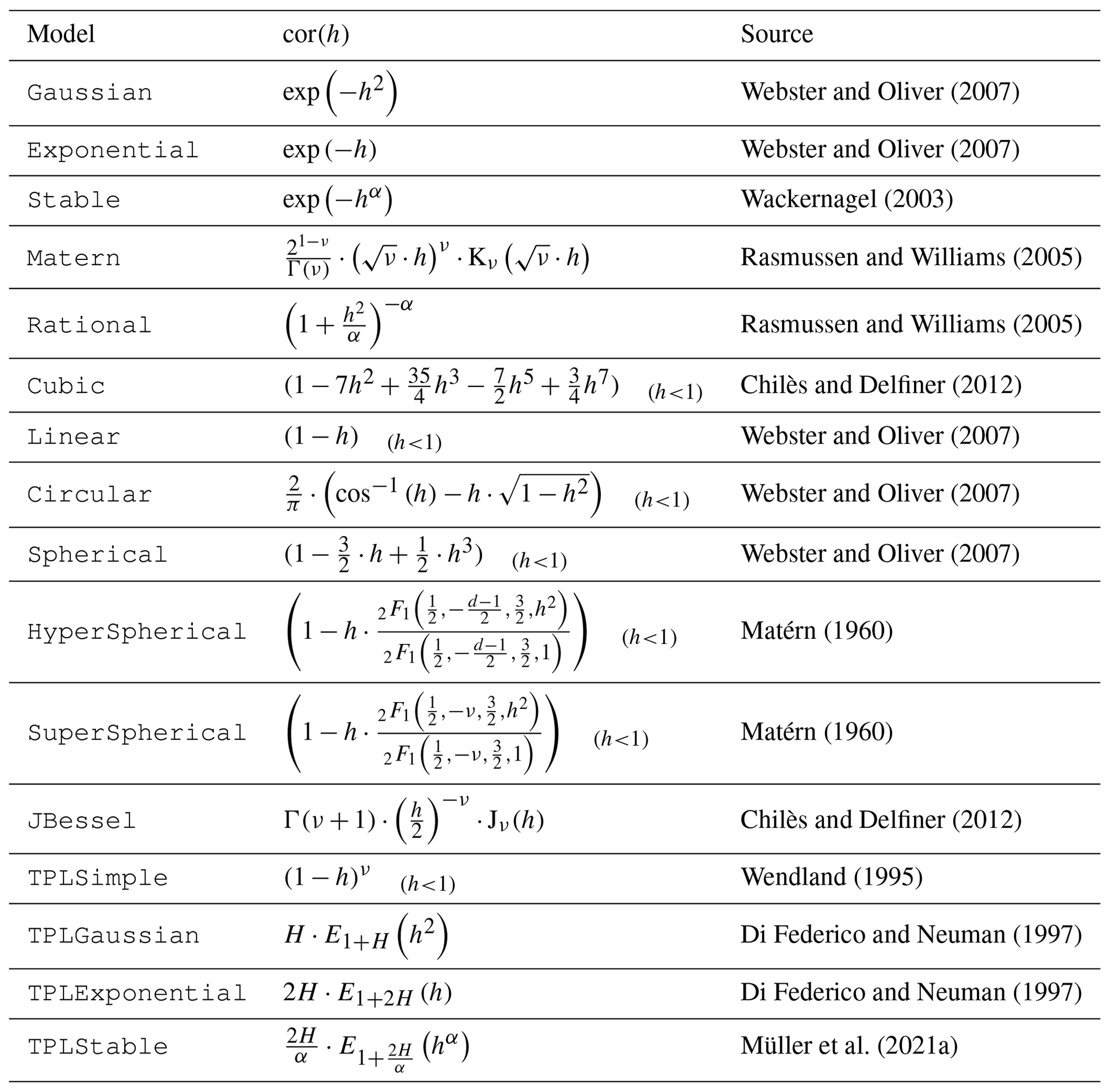 51 |
52 | Taken from [Müller et al. (2022)](https://doi.org/10.5194/gmd-15-3161-2022).
53 |
--------------------------------------------------------------------------------
/01_covmodel/extra_00_spectral_methods.ipynb:
--------------------------------------------------------------------------------
1 | {
2 | "cells": [
3 | {
4 | "cell_type": "code",
5 | "execution_count": null,
6 | "metadata": {
7 | "collapsed": false,
8 | "jupyter": {
9 | "outputs_hidden": false
10 | }
11 | },
12 | "outputs": [],
13 | "source": [
14 | "%matplotlib widget\n",
15 | "import matplotlib.pyplot as plt\n",
16 | "plt.ioff()\n",
17 | "# turn of warnings\n",
18 | "import warnings\n",
19 | "warnings.filterwarnings('ignore')"
20 | ]
21 | },
22 | {
23 | "cell_type": "markdown",
24 | "metadata": {
25 | "tags": []
26 | },
27 | "source": [
28 | "\n",
29 | "# Spectral methods\n",
30 | "\n",
31 | "The spectrum of a covariance model is given by:\n",
32 | "\n",
33 | "\\begin{align}S(\\mathbf{k}) = \\left(\\frac{1}{2\\pi}\\right)^n\n",
34 | " \\int C(\\Vert\\mathbf{r}\\Vert) e^{i b\\mathbf{k}\\cdot\\mathbf{r}} d^n\\mathbf{r}\\end{align}\n",
35 | "\n",
36 | "Since the covariance function $C(r)$ is radially symmetric, we can\n",
37 | "calculate this by the [hankel-transformation](https://en.wikipedia.org/wiki/Hankel_transform):\n",
38 | "\n",
39 | "\\begin{align}S(k) = \\left(\\frac{1}{2\\pi}\\right)^n \\cdot\n",
40 | " \\frac{(2\\pi)^{n/2}}{(bk)^{n/2-1}}\n",
41 | " \\int_0^\\infty r^{n/2-1} C(r) J_{n/2-1}(bkr) r dr\\end{align}\n",
42 | "\n",
43 | "Where $k=\\left\\Vert\\mathbf{k}\\right\\Vert$.\n",
44 | "\n",
45 | "Depending on the spectrum, the spectral-density is defined by:\n",
46 | "\n",
47 | "\\begin{align}\\tilde{S}(k) = \\frac{S(k)}{\\sigma^2}\\end{align}\n",
48 | "\n",
49 | "You can access these methods by:\n"
50 | ]
51 | },
52 | {
53 | "cell_type": "code",
54 | "execution_count": null,
55 | "metadata": {
56 | "collapsed": false,
57 | "jupyter": {
58 | "outputs_hidden": false
59 | }
60 | },
61 | "outputs": [],
62 | "source": [
63 | "import gstools as gs\n",
64 | "\n",
65 | "model = gs.Gaussian(dim=3, var=2.0, len_scale=10)\n",
66 | "ax = model.plot(\"spectrum\")\n",
67 | "model.plot(\"spectral_density\", ax=ax)"
68 | ]
69 | },
70 | {
71 | "cell_type": "markdown",
72 | "metadata": {},
73 | "source": [
74 | "## Note\n",
75 | "The spectral-density is given by the radius of the input phase. But it is **not** a probability density function for the radius of the phase.\n",
76 | "\n",
77 | "To obtain the pdf for the phase-radius, you can use the methods `CovModel.spectral_rad_pdf` or `CovModel.ln_spectral_rad_pdf` for the logarithm.\n",
78 | "\n",
79 | "The user can also provide a cdf (cumulative distribution function) by defining a method called `spectral_rad_cdf`\n",
80 | "and/or a ppf (percent-point function) by `spectral_rad_ppf`.\n",
81 | "\n",
82 | "The attributes `CovModel.has_cdf` and `CovModel.has_ppf` will check for that."
83 | ]
84 | }
85 | ],
86 | "metadata": {
87 | "kernelspec": {
88 | "display_name": "Python 3 (ipykernel)",
89 | "language": "python",
90 | "name": "python3"
91 | },
92 | "language_info": {
93 | "codemirror_mode": {
94 | "name": "ipython",
95 | "version": 3
96 | },
97 | "file_extension": ".py",
98 | "mimetype": "text/x-python",
99 | "name": "python",
100 | "nbconvert_exporter": "python",
101 | "pygments_lexer": "ipython3",
102 | "version": "3.9.12"
103 | }
104 | },
105 | "nbformat": 4,
106 | "nbformat_minor": 4
107 | }
108 |
--------------------------------------------------------------------------------
/01_covmodel/extra_02_additional_para.ipynb:
--------------------------------------------------------------------------------
1 | {
2 | "cells": [
3 | {
4 | "cell_type": "code",
5 | "execution_count": null,
6 | "metadata": {
7 | "collapsed": false,
8 | "jupyter": {
9 | "outputs_hidden": false
10 | }
11 | },
12 | "outputs": [],
13 | "source": [
14 | "%matplotlib widget\n",
15 | "import matplotlib.pyplot as plt\n",
16 | "plt.ioff()\n",
17 | "# turn of warnings\n",
18 | "import warnings\n",
19 | "warnings.filterwarnings('ignore')"
20 | ]
21 | },
22 | {
23 | "cell_type": "markdown",
24 | "metadata": {},
25 | "source": [
26 | "\n",
27 | "# Additional Parameters\n",
28 | "\n",
29 | "Let's pimp our self-defined model ``Gau`` from the introductory example\n",
30 | "by setting the exponent as an additional parameter:\n",
31 | "\n",
32 | "\\begin{align}\\rho(r) := \\exp\\left(-\\left(s\\cdot\\frac{r}{\\ell}\\right)^{\\alpha}\\right)\\end{align}\n",
33 | "\n",
34 | "This leads to the so called **stable** covariance model and we can define it by\n"
35 | ]
36 | },
37 | {
38 | "cell_type": "code",
39 | "execution_count": null,
40 | "metadata": {
41 | "collapsed": false,
42 | "jupyter": {
43 | "outputs_hidden": false
44 | }
45 | },
46 | "outputs": [],
47 | "source": [
48 | "import numpy as np\n",
49 | "import gstools as gs\n",
50 | "\n",
51 | "class Stab(gs.CovModel):\n",
52 | " def default_opt_arg(self):\n",
53 | " return {\"alpha\": 1.5}\n",
54 | "\n",
55 | " def cor(self, h):\n",
56 | " return np.exp(-(h ** self.alpha))"
57 | ]
58 | },
59 | {
60 | "cell_type": "markdown",
61 | "metadata": {},
62 | "source": [
63 | "As you can see, we override the method `CovModel.default_opt_arg`\n",
64 | "to provide a standard value for the optional argument `alpha`.\n",
65 | "We can access it in the correlation function by `self.alpha`\n",
66 | "\n",
67 | "Now we can instantiate this model by either setting alpha implicitly with\n",
68 | "the default value or explicitly:"
69 | ]
70 | },
71 | {
72 | "cell_type": "code",
73 | "execution_count": null,
74 | "metadata": {
75 | "collapsed": false,
76 | "jupyter": {
77 | "outputs_hidden": false
78 | }
79 | },
80 | "outputs": [],
81 | "source": [
82 | "model1 = Stab(dim=2, var=2.0, len_scale=10)\n",
83 | "model2 = Stab(dim=2, var=2.0, len_scale=10, alpha=0.5)\n",
84 | "ax = model1.plot()\n",
85 | "model2.plot(ax=ax)"
86 | ]
87 | },
88 | {
89 | "cell_type": "markdown",
90 | "metadata": {},
91 | "source": [
92 | "Apparently, the parameter alpha controls the slope of the variogram\n",
93 | "and consequently the roughness of a generated random field.\n",
94 | "\n",
95 | "## Note\n",
96 | "You don't have to override the `CovModel.default_opt_arg`, but you will get a ValueError if you don't set it on creation."
97 | ]
98 | }
99 | ],
100 | "metadata": {
101 | "kernelspec": {
102 | "display_name": "Python 3 (ipykernel)",
103 | "language": "python",
104 | "name": "python3"
105 | },
106 | "language_info": {
107 | "codemirror_mode": {
108 | "name": "ipython",
109 | "version": 3
110 | },
111 | "file_extension": ".py",
112 | "mimetype": "text/x-python",
113 | "name": "python",
114 | "nbconvert_exporter": "python",
115 | "pygments_lexer": "ipython3",
116 | "version": "3.9.12"
117 | }
118 | },
119 | "nbformat": 4,
120 | "nbformat_minor": 4
121 | }
122 |
--------------------------------------------------------------------------------
/02_random_field/00_gaussian.ipynb:
--------------------------------------------------------------------------------
1 | {
2 | "cells": [
3 | {
4 | "cell_type": "code",
5 | "execution_count": null,
6 | "metadata": {
7 | "jupyter": {
8 | "source_hidden": true
9 | },
10 | "tags": []
11 | },
12 | "outputs": [],
13 | "source": [
14 | "%matplotlib widget\n",
15 | "import matplotlib.pyplot as plt\n",
16 | "plt.ioff()\n",
17 | "# turn of warnings\n",
18 | "import warnings\n",
19 | "warnings.filterwarnings('ignore')"
20 | ]
21 | },
22 | {
23 | "cell_type": "markdown",
24 | "metadata": {},
25 | "source": [
26 | "\n",
27 | "# A Very Simple Example\n",
28 | "\n",
29 | "We are going to start with a very simple example of a spatial random field\n",
30 | "with an isotropic Gaussian covariance model and following parameters:\n",
31 | "\n",
32 | "- variance $\\sigma^2=1$\n",
33 | "- correlation length $\\lambda=10$\n",
34 | "\n",
35 | "First, we set things up and create the axes for the field. We are going to need the `SRF` class for the actual generation of the spatial random field.\n",
36 | "But `SRF` also needs a covariance model and we will simply take the `Gaussian` model.\n"
37 | ]
38 | },
39 | {
40 | "cell_type": "code",
41 | "execution_count": null,
42 | "metadata": {
43 | "collapsed": false,
44 | "jupyter": {
45 | "outputs_hidden": false
46 | }
47 | },
48 | "outputs": [],
49 | "source": [
50 | "import gstools as gs\n",
51 | "\n",
52 | "x = y = range(101)"
53 | ]
54 | },
55 | {
56 | "cell_type": "markdown",
57 | "metadata": {},
58 | "source": [
59 | "Now we create the covariance model with the parameters $\\sigma^2$ and\n",
60 | "$\\lambda$ and hand it over to :any:`SRF`. By specifying a seed,\n",
61 | "we make sure to create reproducible results:\n",
62 | "\n"
63 | ]
64 | },
65 | {
66 | "cell_type": "code",
67 | "execution_count": null,
68 | "metadata": {
69 | "collapsed": false,
70 | "jupyter": {
71 | "outputs_hidden": false
72 | }
73 | },
74 | "outputs": [],
75 | "source": [
76 | "model = gs.Gaussian(dim=2, var=1, len_scale=10, nugget=0)\n",
77 | "srf = gs.SRF(model, seed=20220425)"
78 | ]
79 | },
80 | {
81 | "cell_type": "markdown",
82 | "metadata": {},
83 | "source": [
84 | "With these simple steps, everything is ready to create our first random field.\n",
85 | "We will create the field on a structured grid (as you might have guessed from\n",
86 | "the `x` and `y`), which makes it easier to plot.\n",
87 | "\n"
88 | ]
89 | },
90 | {
91 | "cell_type": "code",
92 | "execution_count": null,
93 | "metadata": {
94 | "collapsed": false,
95 | "jupyter": {
96 | "outputs_hidden": false
97 | }
98 | },
99 | "outputs": [],
100 | "source": [
101 | "field = srf.structured([x, y])\n",
102 | "srf.plot()"
103 | ]
104 | },
105 | {
106 | "cell_type": "markdown",
107 | "metadata": {},
108 | "source": [
109 | "Wow, that was pretty easy!\n",
110 | "\n"
111 | ]
112 | },
113 | {
114 | "cell_type": "code",
115 | "execution_count": null,
116 | "metadata": {},
117 | "outputs": [],
118 | "source": [
119 | "model.plot()"
120 | ]
121 | }
122 | ],
123 | "metadata": {
124 | "kernelspec": {
125 | "display_name": "Python 3 (ipykernel)",
126 | "language": "python",
127 | "name": "python3"
128 | },
129 | "language_info": {
130 | "codemirror_mode": {
131 | "name": "ipython",
132 | "version": 3
133 | },
134 | "file_extension": ".py",
135 | "mimetype": "text/x-python",
136 | "name": "python",
137 | "nbconvert_exporter": "python",
138 | "pygments_lexer": "ipython3",
139 | "version": "3.9.12"
140 | }
141 | },
142 | "nbformat": 4,
143 | "nbformat_minor": 4
144 | }
145 |
--------------------------------------------------------------------------------
/02_random_field/01_srf_ensemble.ipynb:
--------------------------------------------------------------------------------
1 | {
2 | "cells": [
3 | {
4 | "cell_type": "code",
5 | "execution_count": null,
6 | "metadata": {
7 | "jupyter": {
8 | "source_hidden": true
9 | },
10 | "tags": []
11 | },
12 | "outputs": [],
13 | "source": [
14 | "%matplotlib widget\n",
15 | "import matplotlib.pyplot as plt\n",
16 | "plt.ioff()\n",
17 | "# turn of warnings\n",
18 | "import warnings\n",
19 | "warnings.filterwarnings('ignore')"
20 | ]
21 | },
22 | {
23 | "cell_type": "markdown",
24 | "metadata": {},
25 | "source": [
26 | "\n",
27 | "# Creating an Ensemble of Fields\n",
28 | "\n",
29 | "Creating an ensemble of random fields would also be\n",
30 | "a great idea. Let's reuse most of the previous code.\n",
31 | "\n",
32 | "We will set the position tuple `pos` before generation to reuse it afterwards.\n"
33 | ]
34 | },
35 | {
36 | "cell_type": "code",
37 | "execution_count": null,
38 | "metadata": {
39 | "collapsed": false,
40 | "jupyter": {
41 | "outputs_hidden": false
42 | }
43 | },
44 | "outputs": [],
45 | "source": [
46 | "import numpy as np\n",
47 | "import gstools as gs\n",
48 | "\n",
49 | "x = y = np.arange(100)\n",
50 | "\n",
51 | "model = gs.Gaussian(dim=2, var=1, len_scale=10)\n",
52 | "srf = gs.SRF(model)\n",
53 | "srf.set_pos([x, y], \"structured\")"
54 | ]
55 | },
56 | {
57 | "cell_type": "markdown",
58 | "metadata": {},
59 | "source": [
60 | "This time, we did not provide a seed to `SRF`, as the seeds will used\n",
61 | "during the actual computation of the fields. We will create four ensemble\n",
62 | "members, for better visualisation, save them in to srf class and in a first\n",
63 | "step, we will be using the loop counter as the seeds.\n",
64 | "\n"
65 | ]
66 | },
67 | {
68 | "cell_type": "code",
69 | "execution_count": null,
70 | "metadata": {
71 | "collapsed": false,
72 | "jupyter": {
73 | "outputs_hidden": false
74 | }
75 | },
76 | "outputs": [],
77 | "source": [
78 | "ens_no = 4\n",
79 | "for i in range(ens_no):\n",
80 | " srf(seed=i, store=f\"field{i}\")"
81 | ]
82 | },
83 | {
84 | "cell_type": "markdown",
85 | "metadata": {},
86 | "source": [
87 | "Now let's have a look at the results. We can access the fields by name or\n",
88 | "index:\n",
89 | "\n"
90 | ]
91 | },
92 | {
93 | "cell_type": "code",
94 | "execution_count": null,
95 | "metadata": {
96 | "collapsed": false,
97 | "jupyter": {
98 | "outputs_hidden": false
99 | }
100 | },
101 | "outputs": [],
102 | "source": [
103 | "fig, ax = plt.subplots(2, 2, sharex=True, sharey=True)\n",
104 | "ax = ax.flatten()\n",
105 | "for i in range(ens_no):\n",
106 | " ax[i].imshow(srf[i].T, origin=\"lower\")\n",
107 | "plt.show()"
108 | ]
109 | },
110 | {
111 | "cell_type": "markdown",
112 | "metadata": {},
113 | "source": [
114 | "## Using better Seeds\n",
115 | "\n",
116 | "It is not always a good idea to use incrementing seeds. Therefore GSTools\n",
117 | "provides a seed generator `MasterRNG`. The loop, in which the fields are\n",
118 | "generated would then look like\n",
119 | "\n"
120 | ]
121 | },
122 | {
123 | "cell_type": "code",
124 | "execution_count": null,
125 | "metadata": {
126 | "collapsed": false,
127 | "jupyter": {
128 | "outputs_hidden": false
129 | }
130 | },
131 | "outputs": [],
132 | "source": [
133 | "from gstools.random import MasterRNG\n",
134 | "\n",
135 | "seed = MasterRNG(20220425)\n",
136 | "for i in range(ens_no):\n",
137 | " srf(seed=seed(), store=f\"better_field{i}\")\n",
138 | "\n",
139 | "fig, ax = plt.subplots(2, 2, sharex=True, sharey=True)\n",
140 | "ax = ax.flatten()\n",
141 | "for i in range(ens_no):\n",
142 | " ax[i].imshow(srf[f\"better_field{i}\"].T, origin=\"lower\")\n",
143 | "plt.show()"
144 | ]
145 | },
146 | {
147 | "cell_type": "code",
148 | "execution_count": null,
149 | "metadata": {},
150 | "outputs": [],
151 | "source": [
152 | "srf.field_names"
153 | ]
154 | }
155 | ],
156 | "metadata": {
157 | "kernelspec": {
158 | "display_name": "Python 3 (ipykernel)",
159 | "language": "python",
160 | "name": "python3"
161 | },
162 | "language_info": {
163 | "codemirror_mode": {
164 | "name": "ipython",
165 | "version": 3
166 | },
167 | "file_extension": ".py",
168 | "mimetype": "text/x-python",
169 | "name": "python",
170 | "nbconvert_exporter": "python",
171 | "pygments_lexer": "ipython3",
172 | "version": "3.9.12"
173 | }
174 | },
175 | "nbformat": 4,
176 | "nbformat_minor": 4
177 | }
178 |
--------------------------------------------------------------------------------
/02_random_field/02_fancier.ipynb:
--------------------------------------------------------------------------------
1 | {
2 | "cells": [
3 | {
4 | "cell_type": "code",
5 | "execution_count": null,
6 | "metadata": {
7 | "jupyter": {
8 | "source_hidden": true
9 | },
10 | "tags": []
11 | },
12 | "outputs": [],
13 | "source": [
14 | "%matplotlib widget\n",
15 | "import matplotlib.pyplot as plt\n",
16 | "plt.ioff()\n",
17 | "# turn of warnings\n",
18 | "import warnings\n",
19 | "warnings.filterwarnings('ignore')"
20 | ]
21 | },
22 | {
23 | "cell_type": "markdown",
24 | "metadata": {},
25 | "source": [
26 | "\n",
27 | "# Creating Fancier Fields\n",
28 | "\n",
29 | "Only using Gaussian covariance fields gets boring. Now we are going to create\n",
30 | "much rougher random fields by using an exponential covariance model and we are going to make them anisotropic.\n",
31 | "\n",
32 | "The code is very similar to the previous examples, but with a different\n",
33 | "covariance model class `Exponential`. As model parameters we a using\n",
34 | "following\n",
35 | "\n",
36 | "- variance $\\sigma^2=1$\n",
37 | "- correlation length $\\ell=(12, 3)^T$\n",
38 | "- rotation angle $\\theta=\\pi/8$\n"
39 | ]
40 | },
41 | {
42 | "cell_type": "code",
43 | "execution_count": null,
44 | "metadata": {
45 | "collapsed": false,
46 | "jupyter": {
47 | "outputs_hidden": false
48 | }
49 | },
50 | "outputs": [],
51 | "source": [
52 | "import numpy as np\n",
53 | "import gstools as gs\n",
54 | "\n",
55 | "x = y = np.arange(0, 101)\n",
56 | "model = gs.Exponential(\n",
57 | " dim=2,\n",
58 | " var=1,\n",
59 | " len_scale=[12.0, 3.0],\n",
60 | " angles=np.deg2rad(22.5),\n",
61 | ")\n",
62 | "srf = gs.SRF(model, seed=20170519)\n",
63 | "srf.structured([x, y])\n",
64 | "srf.plot()\n",
65 | "print(model)"
66 | ]
67 | },
68 | {
69 | "cell_type": "markdown",
70 | "metadata": {},
71 | "source": [
72 | "The anisotropy ratio could also have been set with\n",
73 | "\n"
74 | ]
75 | },
76 | {
77 | "cell_type": "code",
78 | "execution_count": null,
79 | "metadata": {
80 | "collapsed": false,
81 | "jupyter": {
82 | "outputs_hidden": false
83 | }
84 | },
85 | "outputs": [],
86 | "source": [
87 | "model = gs.Exponential(dim=2, var=1, len_scale=12, anis=1/4, angles=np.deg2rad(22.5))\n",
88 | "print(model)"
89 | ]
90 | }
91 | ],
92 | "metadata": {
93 | "kernelspec": {
94 | "display_name": "Python 3 (ipykernel)",
95 | "language": "python",
96 | "name": "python3"
97 | },
98 | "language_info": {
99 | "codemirror_mode": {
100 | "name": "ipython",
101 | "version": 3
102 | },
103 | "file_extension": ".py",
104 | "mimetype": "text/x-python",
105 | "name": "python",
106 | "nbconvert_exporter": "python",
107 | "pygments_lexer": "ipython3",
108 | "version": "3.9.12"
109 | }
110 | },
111 | "nbformat": 4,
112 | "nbformat_minor": 4
113 | }
114 |
--------------------------------------------------------------------------------
/02_random_field/03_unstr_srf_export.ipynb:
--------------------------------------------------------------------------------
1 | {
2 | "cells": [
3 | {
4 | "cell_type": "code",
5 | "execution_count": null,
6 | "metadata": {
7 | "collapsed": false,
8 | "jupyter": {
9 | "outputs_hidden": false
10 | }
11 | },
12 | "outputs": [],
13 | "source": [
14 | "%matplotlib widget\n",
15 | "import matplotlib.pyplot as plt\n",
16 | "plt.ioff()\n",
17 | "# turn of warnings\n",
18 | "import warnings\n",
19 | "warnings.filterwarnings('ignore')"
20 | ]
21 | },
22 | {
23 | "cell_type": "markdown",
24 | "metadata": {},
25 | "source": [
26 | "\n",
27 | "# Using an Unstructured Grid\n",
28 | "\n",
29 | "For many applications, the random fields are needed on an unstructured grid.\n",
30 | "Normally, such a grid would be read in, but we can simply generate one and\n",
31 | "then create a random field at those coordinates.\n"
32 | ]
33 | },
34 | {
35 | "cell_type": "code",
36 | "execution_count": null,
37 | "metadata": {
38 | "collapsed": false,
39 | "jupyter": {
40 | "outputs_hidden": false
41 | }
42 | },
43 | "outputs": [],
44 | "source": [
45 | "import numpy as np\n",
46 | "import gstools as gs"
47 | ]
48 | },
49 | {
50 | "cell_type": "markdown",
51 | "metadata": {},
52 | "source": [
53 | "Creating our own unstructured grid\n",
54 | "\n"
55 | ]
56 | },
57 | {
58 | "cell_type": "code",
59 | "execution_count": null,
60 | "metadata": {
61 | "collapsed": false,
62 | "jupyter": {
63 | "outputs_hidden": false
64 | }
65 | },
66 | "outputs": [],
67 | "source": [
68 | "seed = gs.random.MasterRNG(20220425)\n",
69 | "rng = np.random.RandomState(seed())\n",
70 | "x = rng.randint(0, 100, size=10000)\n",
71 | "y = rng.randint(0, 100, size=10000)\n",
72 | "\n",
73 | "model = gs.Exponential(dim=2, var=1, len_scale=[12, 3], angles=np.pi / 8)\n",
74 | "srf = gs.SRF(model, seed=20220425)\n",
75 | "field = srf((x, y))\n",
76 | "srf.vtk_export(\"field\")"
77 | ]
78 | },
79 | {
80 | "cell_type": "code",
81 | "execution_count": null,
82 | "metadata": {
83 | "collapsed": false,
84 | "jupyter": {
85 | "outputs_hidden": false
86 | }
87 | },
88 | "outputs": [],
89 | "source": [
90 | "ax = srf.plot(contour_plot=True)\n",
91 | "ax.set_aspect(\"equal\")"
92 | ]
93 | },
94 | {
95 | "cell_type": "markdown",
96 | "metadata": {},
97 | "source": [
98 | "Comparing this image to the previous one, you can see that be using the same\n",
99 | "seed, the same field can be computed on different grids.\n",
100 | "\n"
101 | ]
102 | },
103 | {
104 | "cell_type": "code",
105 | "execution_count": null,
106 | "metadata": {},
107 | "outputs": [],
108 | "source": [
109 | "mesh = srf.to_pyvista()\n",
110 | "mesh.plot()"
111 | ]
112 | }
113 | ],
114 | "metadata": {
115 | "kernelspec": {
116 | "display_name": "Python 3 (ipykernel)",
117 | "language": "python",
118 | "name": "python3"
119 | },
120 | "language_info": {
121 | "codemirror_mode": {
122 | "name": "ipython",
123 | "version": 3
124 | },
125 | "file_extension": ".py",
126 | "mimetype": "text/x-python",
127 | "name": "python",
128 | "nbconvert_exporter": "python",
129 | "pygments_lexer": "ipython3",
130 | "version": "3.9.12"
131 | }
132 | },
133 | "nbformat": 4,
134 | "nbformat_minor": 4
135 | }
136 |
--------------------------------------------------------------------------------
/02_random_field/04_pyvista_support.ipynb:
--------------------------------------------------------------------------------
1 | {
2 | "cells": [
3 | {
4 | "cell_type": "code",
5 | "execution_count": null,
6 | "metadata": {
7 | "collapsed": false,
8 | "jupyter": {
9 | "outputs_hidden": false
10 | }
11 | },
12 | "outputs": [],
13 | "source": [
14 | "%matplotlib widget\n",
15 | "import matplotlib.pyplot as plt\n",
16 | "plt.ioff()\n",
17 | "# turn of warnings\n",
18 | "import warnings\n",
19 | "warnings.filterwarnings('ignore')"
20 | ]
21 | },
22 | {
23 | "cell_type": "markdown",
24 | "metadata": {},
25 | "source": [
26 | "\n",
27 | "# Using PyVista meshes\n",
28 | "\n",
29 | "[PyVista](https://www.pyvista.org) is a helper module for the\n",
30 | "Visualization Toolkit (VTK) that takes a different approach on interfacing with\n",
31 | "VTK through NumPy and direct array access.\n",
32 | "\n",
33 | "It provides mesh data structures and filtering methods for spatial datasets,\n",
34 | "makes 3D plotting simple and is built for large/complex data geometries.\n",
35 | "\n",
36 | "The `Field.mesh` method enables easy field creation on PyVista meshes\n",
37 | "used by the `SRF` or `Krige` class.\n"
38 | ]
39 | },
40 | {
41 | "cell_type": "code",
42 | "execution_count": null,
43 | "metadata": {
44 | "collapsed": false,
45 | "jupyter": {
46 | "outputs_hidden": false
47 | }
48 | },
49 | "outputs": [],
50 | "source": [
51 | "import pyvista as pv\n",
52 | "import gstools as gs"
53 | ]
54 | },
55 | {
56 | "cell_type": "markdown",
57 | "metadata": {},
58 | "source": [
59 | "We create a structured grid with PyVista containing 50 segments on all three\n",
60 | "axes each with a length of 2 (whatever unit).\n",
61 | "\n"
62 | ]
63 | },
64 | {
65 | "cell_type": "code",
66 | "execution_count": null,
67 | "metadata": {
68 | "collapsed": false,
69 | "jupyter": {
70 | "outputs_hidden": false
71 | }
72 | },
73 | "outputs": [],
74 | "source": [
75 | "dim, spacing = (50, 50, 50), (2, 2, 2)\n",
76 | "grid = pv.UniformGrid(dim, spacing)"
77 | ]
78 | },
79 | {
80 | "cell_type": "markdown",
81 | "metadata": {},
82 | "source": [
83 | "Now we set up the SRF class as always. We'll use an anisotropic model.\n",
84 | "\n"
85 | ]
86 | },
87 | {
88 | "cell_type": "code",
89 | "execution_count": null,
90 | "metadata": {
91 | "collapsed": false,
92 | "jupyter": {
93 | "outputs_hidden": false
94 | }
95 | },
96 | "outputs": [],
97 | "source": [
98 | "model = gs.Gaussian(dim=3, len_scale=[16, 8, 4], angles=(0.8, 0.4, 0.2))\n",
99 | "srf = gs.SRF(model, seed=19970221)"
100 | ]
101 | },
102 | {
103 | "cell_type": "markdown",
104 | "metadata": {},
105 | "source": [
106 | "The PyVista mesh can now be directly passed to the :any:`SRF.mesh` method.\n",
107 | "When dealing with meshes, one can choose if the field should be generated\n",
108 | "on the mesh-points (`\"points\"`) or the cell-centroids (`\"centroids\"`).\n",
109 | "\n",
110 | "In addition we can set a name, under which the resulting field is stored\n",
111 | "in the mesh.\n",
112 | "\n"
113 | ]
114 | },
115 | {
116 | "cell_type": "code",
117 | "execution_count": null,
118 | "metadata": {
119 | "collapsed": false,
120 | "jupyter": {
121 | "outputs_hidden": false
122 | }
123 | },
124 | "outputs": [],
125 | "source": [
126 | "field = srf.mesh(grid, points=\"points\", name=\"random-field\")"
127 | ]
128 | },
129 | {
130 | "cell_type": "markdown",
131 | "metadata": {},
132 | "source": [
133 | "Now we have access to PyVista's abundancy of methods to explore the field.\n",
134 | "\n",
135 | "## Note\n",
136 | "PyVista is not working on readthedocs, but you can try it out yourself by uncommenting the following line of code.\n",
137 | "\n"
138 | ]
139 | },
140 | {
141 | "cell_type": "code",
142 | "execution_count": null,
143 | "metadata": {
144 | "collapsed": false,
145 | "jupyter": {
146 | "outputs_hidden": false
147 | }
148 | },
149 | "outputs": [],
150 | "source": [
151 | "grid.contour(isosurfaces=8).plot()"
152 | ]
153 | }
154 | ],
155 | "metadata": {
156 | "kernelspec": {
157 | "display_name": "Python 3 (ipykernel)",
158 | "language": "python",
159 | "name": "python3"
160 | },
161 | "language_info": {
162 | "codemirror_mode": {
163 | "name": "ipython",
164 | "version": 3
165 | },
166 | "file_extension": ".py",
167 | "mimetype": "text/x-python",
168 | "name": "python",
169 | "nbconvert_exporter": "python",
170 | "pygments_lexer": "ipython3",
171 | "version": "3.9.12"
172 | }
173 | },
174 | "nbformat": 4,
175 | "nbformat_minor": 4
176 | }
177 |
--------------------------------------------------------------------------------
/02_random_field/README.md:
--------------------------------------------------------------------------------
1 | # Random Field Generation
2 |
3 | The main feature of GSTools is the spatial random field generator `SRF`,
4 | which can generate random fields following a given covariance model.
5 | The generator provides a lot of nice features, which will be explained in
6 | the following
7 |
8 | GSTools generates spatial random fields with a given covariance model or
9 | semi-variogram. This is done by using the so-called randomization method.
10 | The spatial random field is represented by a stochastic Fourier integral
11 | and its discretised modes are evaluated at random frequencies.
12 |
13 | GSTools supports arbitrary and non-isotropic covariance models.
14 |
--------------------------------------------------------------------------------
/02_random_field/extra_00_srf_merge.ipynb:
--------------------------------------------------------------------------------
1 | {
2 | "cells": [
3 | {
4 | "cell_type": "code",
5 | "execution_count": null,
6 | "metadata": {
7 | "collapsed": false,
8 | "jupyter": {
9 | "outputs_hidden": false
10 | }
11 | },
12 | "outputs": [],
13 | "source": [
14 | "%matplotlib widget\n",
15 | "import matplotlib.pyplot as plt\n",
16 | "plt.ioff()\n",
17 | "# turn of warnings\n",
18 | "import warnings\n",
19 | "warnings.filterwarnings('ignore')"
20 | ]
21 | },
22 | {
23 | "cell_type": "markdown",
24 | "metadata": {},
25 | "source": [
26 | "\n",
27 | "# Merging two Fields\n",
28 | "\n",
29 | "We can even generate the same field realisation on different grids. Let's try\n",
30 | "to merge two unstructured rectangular fields.\n"
31 | ]
32 | },
33 | {
34 | "cell_type": "code",
35 | "execution_count": null,
36 | "metadata": {
37 | "collapsed": false,
38 | "jupyter": {
39 | "outputs_hidden": false
40 | }
41 | },
42 | "outputs": [],
43 | "source": [
44 | "import numpy as np\n",
45 | "\n",
46 | "import gstools as gs\n",
47 | "\n",
48 | "# creating our own unstructured grid\n",
49 | "seed = gs.random.MasterRNG(20220425)\n",
50 | "rng = np.random.RandomState(seed())\n",
51 | "x = rng.randint(0, 100, size=10000)\n",
52 | "y = rng.randint(0, 100, size=10000)\n",
53 | "\n",
54 | "model = gs.Exponential(dim=2, var=1, len_scale=[12, 3], angles=np.pi / 8)\n",
55 | "srf = gs.SRF(model, seed=20220425)\n",
56 | "field1 = srf((x, y))\n",
57 | "srf.plot()"
58 | ]
59 | },
60 | {
61 | "cell_type": "markdown",
62 | "metadata": {},
63 | "source": [
64 | "But now we extend the field on the right hand side by creating a new\n",
65 | "unstructured grid and calculating a field with the same parameters and the\n",
66 | "same seed on it:\n",
67 | "\n"
68 | ]
69 | },
70 | {
71 | "cell_type": "code",
72 | "execution_count": null,
73 | "metadata": {
74 | "collapsed": false,
75 | "jupyter": {
76 | "outputs_hidden": false
77 | }
78 | },
79 | "outputs": [],
80 | "source": [
81 | "# new grid\n",
82 | "seed = gs.random.MasterRNG(20220425)\n",
83 | "rng = np.random.RandomState(seed())\n",
84 | "x2 = rng.randint(99, 150, size=10000)\n",
85 | "y2 = rng.randint(20, 80, size=10000)\n",
86 | "\n",
87 | "field2 = srf((x2, y2))\n",
88 | "ax = srf.plot()\n",
89 | "ax.tricontourf(x, y, field1.T, levels=256)\n",
90 | "ax.set_aspect(\"equal\")"
91 | ]
92 | },
93 | {
94 | "cell_type": "markdown",
95 | "metadata": {},
96 | "source": [
97 | "The slight mismatch where the two fields were merged is merely due to\n",
98 | "interpolation problems of the plotting routine. You can convince yourself\n",
99 | "be increasing the resolution of the grids by a factor of 10.\n",
100 | "\n",
101 | "Of course, this merging could also have been done by appending the grid\n",
102 | "point ``(x2, y2)`` to the original grid ``(x, y)`` before generating the field.\n",
103 | "But one application scenario would be to generate hugh fields, which would not\n",
104 | "fit into memory anymore.\n",
105 | "\n"
106 | ]
107 | }
108 | ],
109 | "metadata": {
110 | "kernelspec": {
111 | "display_name": "Python 3 (ipykernel)",
112 | "language": "python",
113 | "name": "python3"
114 | },
115 | "language_info": {
116 | "codemirror_mode": {
117 | "name": "ipython",
118 | "version": 3
119 | },
120 | "file_extension": ".py",
121 | "mimetype": "text/x-python",
122 | "name": "python",
123 | "nbconvert_exporter": "python",
124 | "pygments_lexer": "ipython3",
125 | "version": "3.9.12"
126 | }
127 | },
128 | "nbformat": 4,
129 | "nbformat_minor": 4
130 | }
131 |
--------------------------------------------------------------------------------
/02_random_field/extra_01_mesh_ensemble.ipynb:
--------------------------------------------------------------------------------
1 | {
2 | "cells": [
3 | {
4 | "cell_type": "code",
5 | "execution_count": null,
6 | "metadata": {
7 | "collapsed": false,
8 | "jupyter": {
9 | "outputs_hidden": false
10 | }
11 | },
12 | "outputs": [],
13 | "source": [
14 | "%matplotlib widget\n",
15 | "import matplotlib.pyplot as plt\n",
16 | "plt.ioff()\n",
17 | "# turn of warnings\n",
18 | "import warnings\n",
19 | "warnings.filterwarnings('ignore')"
20 | ]
21 | },
22 | {
23 | "cell_type": "markdown",
24 | "metadata": {},
25 | "source": [
26 | "\n",
27 | "# Generating Fields on Meshes\n",
28 | "\n",
29 | "GSTools provides an interface for meshes, to support\n",
30 | "[meshio](https://github.com/nschloe/meshio) and [ogs5py](https://github.com/GeoStat-Framework/ogs5py) meshes.\n",
31 | "\n",
32 | "When using `meshio`, the generated fields will be stored immediately in the mesh container.\n",
33 | "\n",
34 | "There are two options to generate a field on a given mesh:\n",
35 | "\n",
36 | "- `points=\"points\"` will generate a field on the mesh points\n",
37 | "- `points=\"centroids\"` will generate a field on the cell centroids\n",
38 | "\n",
39 | "In this example, we will generate a simple mesh with the aid of [meshzoo](https://github.com/nschloe/meshzoo).\n"
40 | ]
41 | },
42 | {
43 | "cell_type": "code",
44 | "execution_count": null,
45 | "metadata": {
46 | "collapsed": false,
47 | "jupyter": {
48 | "outputs_hidden": false
49 | }
50 | },
51 | "outputs": [],
52 | "source": [
53 | "import matplotlib.pyplot as plt\n",
54 | "import matplotlib.tri as tri\n",
55 | "import meshio\n",
56 | "import meshzoo\n",
57 | "import numpy as np\n",
58 | "\n",
59 | "import gstools as gs\n",
60 | "\n",
61 | "# generate a triangulated hexagon with meshzoo\n",
62 | "points, cells = meshzoo.ngon(6, 4)\n",
63 | "mesh = meshio.Mesh(points, {\"triangle\": cells})"
64 | ]
65 | },
66 | {
67 | "cell_type": "markdown",
68 | "metadata": {},
69 | "source": [
70 | "Now we prepare the SRF class as always. We will generate an ensemble of\n",
71 | "fields on the generated mesh.\n",
72 | "\n"
73 | ]
74 | },
75 | {
76 | "cell_type": "code",
77 | "execution_count": null,
78 | "metadata": {
79 | "collapsed": false,
80 | "jupyter": {
81 | "outputs_hidden": false
82 | }
83 | },
84 | "outputs": [],
85 | "source": [
86 | "# number of fields\n",
87 | "fields_no = 12\n",
88 | "# model setup\n",
89 | "model = gs.Gaussian(dim=2, len_scale=0.5)\n",
90 | "srf = gs.SRF(model, mean=1)"
91 | ]
92 | },
93 | {
94 | "cell_type": "markdown",
95 | "metadata": {},
96 | "source": [
97 | "To generate fields on a mesh, we provide a separate method: :any:`SRF.mesh`.\n",
98 | "First we generate fields on the mesh-centroids controlled by a seed.\n",
99 | "You can specify the field name by the keyword `name`.\n",
100 | "\n"
101 | ]
102 | },
103 | {
104 | "cell_type": "code",
105 | "execution_count": null,
106 | "metadata": {
107 | "collapsed": false,
108 | "jupyter": {
109 | "outputs_hidden": false
110 | }
111 | },
112 | "outputs": [],
113 | "source": [
114 | "for i in range(fields_no):\n",
115 | " srf.mesh(mesh, points=\"centroids\", name=\"c-field-{}\".format(i), seed=i)"
116 | ]
117 | },
118 | {
119 | "cell_type": "markdown",
120 | "metadata": {},
121 | "source": [
122 | "Now we generate fields on the mesh-points again controlled by a seed.\n",
123 | "\n"
124 | ]
125 | },
126 | {
127 | "cell_type": "code",
128 | "execution_count": null,
129 | "metadata": {
130 | "collapsed": false,
131 | "jupyter": {
132 | "outputs_hidden": false
133 | }
134 | },
135 | "outputs": [],
136 | "source": [
137 | "for i in range(fields_no):\n",
138 | " srf.mesh(mesh, points=\"points\", name=\"p-field-{}\".format(i), seed=i)"
139 | ]
140 | },
141 | {
142 | "cell_type": "markdown",
143 | "metadata": {},
144 | "source": [
145 | "To get an impression we now want to plot the generated fields.\n",
146 | "Luckily, matplotlib supports triangular meshes.\n",
147 | "\n"
148 | ]
149 | },
150 | {
151 | "cell_type": "code",
152 | "execution_count": null,
153 | "metadata": {
154 | "collapsed": false,
155 | "jupyter": {
156 | "outputs_hidden": false
157 | }
158 | },
159 | "outputs": [],
160 | "source": [
161 | "triangulation = tri.Triangulation(points[:, 0], points[:, 1], cells)\n",
162 | "# figure setup\n",
163 | "cols = 4\n",
164 | "rows = int(np.ceil(fields_no / cols))"
165 | ]
166 | },
167 | {
168 | "cell_type": "markdown",
169 | "metadata": {},
170 | "source": [
171 | "Cell data can be easily visualized with matplotlibs `tripcolor`.\n",
172 | "To highlight the cell structure, we use `triplot`.\n",
173 | "\n"
174 | ]
175 | },
176 | {
177 | "cell_type": "code",
178 | "execution_count": null,
179 | "metadata": {
180 | "collapsed": false,
181 | "jupyter": {
182 | "outputs_hidden": false
183 | }
184 | },
185 | "outputs": [],
186 | "source": [
187 | "fig = plt.figure(figsize=[2 * cols, 2 * rows])\n",
188 | "for i, field in enumerate(mesh.cell_data, 1):\n",
189 | " ax = fig.add_subplot(rows, cols, i)\n",
190 | " ax.tripcolor(triangulation, mesh.cell_data[field][0])\n",
191 | " ax.triplot(triangulation, linewidth=0.5, color=\"k\")\n",
192 | " ax.set_aspect(\"equal\")\n",
193 | "fig.tight_layout()\n",
194 | "fig.show()"
195 | ]
196 | },
197 | {
198 | "cell_type": "markdown",
199 | "metadata": {},
200 | "source": [
201 | "Point data is plotted via `tricontourf`.\n",
202 | "\n"
203 | ]
204 | },
205 | {
206 | "cell_type": "code",
207 | "execution_count": null,
208 | "metadata": {
209 | "collapsed": false,
210 | "jupyter": {
211 | "outputs_hidden": false
212 | }
213 | },
214 | "outputs": [],
215 | "source": [
216 | "fig = plt.figure(figsize=[2 * cols, 2 * rows])\n",
217 | "for i, field in enumerate(mesh.point_data, 1):\n",
218 | " ax = fig.add_subplot(rows, cols, i)\n",
219 | " ax.tricontourf(triangulation, mesh.point_data[field])\n",
220 | " ax.triplot(triangulation, linewidth=0.5, color=\"k\")\n",
221 | " ax.set_aspect(\"equal\")\n",
222 | "fig.tight_layout()\n",
223 | "plt.show()"
224 | ]
225 | },
226 | {
227 | "cell_type": "markdown",
228 | "metadata": {},
229 | "source": [
230 | "Last but not least, `meshio` can be used for what is does best: Exporting.\n",
231 | "Tada!\n",
232 | "\n"
233 | ]
234 | },
235 | {
236 | "cell_type": "code",
237 | "execution_count": null,
238 | "metadata": {
239 | "collapsed": false,
240 | "jupyter": {
241 | "outputs_hidden": false
242 | }
243 | },
244 | "outputs": [],
245 | "source": [
246 | "mesh.write(\"mesh_ensemble.vtk\")"
247 | ]
248 | }
249 | ],
250 | "metadata": {
251 | "kernelspec": {
252 | "display_name": "Python 3 (ipykernel)",
253 | "language": "python",
254 | "name": "python3"
255 | },
256 | "language_info": {
257 | "codemirror_mode": {
258 | "name": "ipython",
259 | "version": 3
260 | },
261 | "file_extension": ".py",
262 | "mimetype": "text/x-python",
263 | "name": "python",
264 | "nbconvert_exporter": "python",
265 | "pygments_lexer": "ipython3",
266 | "version": "3.9.12"
267 | }
268 | },
269 | "nbformat": 4,
270 | "nbformat_minor": 4
271 | }
272 |
--------------------------------------------------------------------------------
/02_random_field/extra_02_higher_dimensions.ipynb:
--------------------------------------------------------------------------------
1 | {
2 | "cells": [
3 | {
4 | "cell_type": "code",
5 | "execution_count": null,
6 | "metadata": {
7 | "collapsed": false,
8 | "jupyter": {
9 | "outputs_hidden": false
10 | }
11 | },
12 | "outputs": [],
13 | "source": [
14 | "%matplotlib widget\n",
15 | "import matplotlib.pyplot as plt\n",
16 | "plt.ioff()\n",
17 | "# turn of warnings\n",
18 | "import warnings\n",
19 | "warnings.filterwarnings('ignore')"
20 | ]
21 | },
22 | {
23 | "cell_type": "markdown",
24 | "metadata": {},
25 | "source": [
26 | "\n",
27 | "# Higher Dimensions\n",
28 | "\n",
29 | "GSTools provides experimental support for higher dimensions.\n",
30 | "Anisotropy is the same as in lower dimensions:\n",
31 | "\n",
32 | "- in `n` dimensions we need `(n-1)` anisotropy ratios\n",
33 | "\n",
34 | "Rotation on the other hand is a bit more complex.\n",
35 | "With increasing dimensions more and more rotation angles are added in order\n",
36 | "to properply describe the rotated axes of anisotropy.\n",
37 | "\n",
38 | "By design the first rotation angles coincide with the lower ones:\n",
39 | "\n",
40 | "- 2D (rotation in x-y plane) -> 3D: first angle describes xy-plane rotation\n",
41 | "- 3D (Tait-Bryan angles) -> 4D: first 3 angles coincide with Tait-Bryan angles\n",
42 | "\n",
43 | "By increasing the dimension from `n` to `(n+1)`, `n` angles are added:\n",
44 | "\n",
45 | "- 2D (1 angle) -> 3D: 3 angles (2 added)\n",
46 | "- 3D (3 angles) -> 4D: 6 angles (3 added)\n",
47 | "\n",
48 | "the following list of rotation-planes are described by the list of\n",
49 | "angles in the model:\n",
50 | "\n",
51 | "1. x-y plane\n",
52 | "2. x-z plane\n",
53 | "3. y-z plane\n",
54 | "4. x-v plane\n",
55 | "5. y-v plane\n",
56 | "6. z-v plane\n",
57 | "7. ...\n",
58 | "\n",
59 | "The rotation direction in these planes have alternating signs\n",
60 | "in order to match Tait-Bryan in 3D.\n",
61 | "\n",
62 | "Let's have a look at a 4D example, where we naively add a 4th dimension.\n"
63 | ]
64 | },
65 | {
66 | "cell_type": "code",
67 | "execution_count": null,
68 | "metadata": {
69 | "collapsed": false,
70 | "jupyter": {
71 | "outputs_hidden": false
72 | }
73 | },
74 | "outputs": [],
75 | "source": [
76 | "import matplotlib.pyplot as plt\n",
77 | "\n",
78 | "import gstools as gs\n",
79 | "\n",
80 | "dim = 4\n",
81 | "size = 20\n",
82 | "pos = [range(size)] * dim\n",
83 | "model = gs.Exponential(dim=dim, len_scale=5)\n",
84 | "srf = gs.SRF(model, seed=20170519)\n",
85 | "field = srf.structured(pos)"
86 | ]
87 | },
88 | {
89 | "cell_type": "markdown",
90 | "metadata": {},
91 | "source": [
92 | "In order to \"prove\" correctness, we can calculate an empirical variogram\n",
93 | "of the generated field and fit our model to it.\n",
94 | "\n"
95 | ]
96 | },
97 | {
98 | "cell_type": "code",
99 | "execution_count": null,
100 | "metadata": {
101 | "collapsed": false,
102 | "jupyter": {
103 | "outputs_hidden": false
104 | }
105 | },
106 | "outputs": [],
107 | "source": [
108 | "bin_center, vario = gs.vario_estimate(\n",
109 | " pos, field, sampling_size=2000, mesh_type=\"structured\"\n",
110 | ")\n",
111 | "model.fit_variogram(bin_center, vario)\n",
112 | "print(model)"
113 | ]
114 | },
115 | {
116 | "cell_type": "markdown",
117 | "metadata": {},
118 | "source": [
119 | "As you can see, the estimated variance and length scale match our input\n",
120 | "quite well.\n",
121 | "\n",
122 | "Let's have a look at the fit and a x-y cross-section of the 4D field:\n",
123 | "\n"
124 | ]
125 | },
126 | {
127 | "cell_type": "code",
128 | "execution_count": null,
129 | "metadata": {
130 | "collapsed": false,
131 | "jupyter": {
132 | "outputs_hidden": false
133 | }
134 | },
135 | "outputs": [],
136 | "source": [
137 | "f, a = plt.subplots(1, 2, gridspec_kw={\"width_ratios\": [2, 1]}, figsize=[9, 3])\n",
138 | "model.plot(x_max=max(bin_center), ax=a[0])\n",
139 | "a[0].scatter(bin_center, vario)\n",
140 | "a[1].imshow(field[:, :, 0, 0].T, origin=\"lower\")\n",
141 | "a[0].set_title(\"isotropic empirical variogram with fitted model\")\n",
142 | "a[1].set_title(\"x-y cross-section\")\n",
143 | "f.show()"
144 | ]
145 | },
146 | {
147 | "cell_type": "markdown",
148 | "metadata": {},
149 | "source": [
150 | "GSTools also provides plotting routines for higher dimensions.\n",
151 | "Fields are shown by 2D cross-sections, where other dimensions can be\n",
152 | "controlled via sliders.\n",
153 | "\n"
154 | ]
155 | },
156 | {
157 | "cell_type": "code",
158 | "execution_count": null,
159 | "metadata": {
160 | "collapsed": false,
161 | "jupyter": {
162 | "outputs_hidden": false
163 | }
164 | },
165 | "outputs": [],
166 | "source": [
167 | "srf.plot()"
168 | ]
169 | }
170 | ],
171 | "metadata": {
172 | "kernelspec": {
173 | "display_name": "Python 3 (ipykernel)",
174 | "language": "python",
175 | "name": "python3"
176 | },
177 | "language_info": {
178 | "codemirror_mode": {
179 | "name": "ipython",
180 | "version": 3
181 | },
182 | "file_extension": ".py",
183 | "mimetype": "text/x-python",
184 | "name": "python",
185 | "nbconvert_exporter": "python",
186 | "pygments_lexer": "ipython3",
187 | "version": "3.9.12"
188 | }
189 | },
190 | "nbformat": 4,
191 | "nbformat_minor": 4
192 | }
193 |
--------------------------------------------------------------------------------
/02_random_field/field.vtu:
--------------------------------------------------------------------------------
https://raw.githubusercontent.com/GeoStat-Examples/gstools-transform22-tutorial/0a82bc41691b7e9fe9c394a5f3e8cc55c9e9dca2/02_random_field/field.vtu
--------------------------------------------------------------------------------
/02_random_field/mesh_ensemble.vtk:
--------------------------------------------------------------------------------
https://raw.githubusercontent.com/GeoStat-Examples/gstools-transform22-tutorial/0a82bc41691b7e9fe9c394a5f3e8cc55c9e9dca2/02_random_field/mesh_ensemble.vtk
--------------------------------------------------------------------------------
/03_variogram/00_fit_variogram.ipynb:
--------------------------------------------------------------------------------
1 | {
2 | "cells": [
3 | {
4 | "cell_type": "code",
5 | "execution_count": null,
6 | "metadata": {
7 | "collapsed": false,
8 | "jupyter": {
9 | "outputs_hidden": false
10 | }
11 | },
12 | "outputs": [],
13 | "source": [
14 | "%matplotlib widget\n",
15 | "import matplotlib.pyplot as plt\n",
16 | "plt.ioff()\n",
17 | "# turn of warnings\n",
18 | "import warnings\n",
19 | "warnings.filterwarnings('ignore')"
20 | ]
21 | },
22 | {
23 | "cell_type": "markdown",
24 | "metadata": {},
25 | "source": [
26 | "\n",
27 | "# Fit Variogram\n"
28 | ]
29 | },
30 | {
31 | "cell_type": "code",
32 | "execution_count": null,
33 | "metadata": {
34 | "collapsed": false,
35 | "jupyter": {
36 | "outputs_hidden": false
37 | }
38 | },
39 | "outputs": [],
40 | "source": [
41 | "import numpy as np\n",
42 | "import gstools as gs"
43 | ]
44 | },
45 | {
46 | "cell_type": "markdown",
47 | "metadata": {},
48 | "source": [
49 | "Generate a synthetic field with an exponential model.\n",
50 | "\n"
51 | ]
52 | },
53 | {
54 | "cell_type": "code",
55 | "execution_count": null,
56 | "metadata": {
57 | "collapsed": false,
58 | "jupyter": {
59 | "outputs_hidden": false
60 | }
61 | },
62 | "outputs": [],
63 | "source": [
64 | "x = np.random.RandomState(20220425).rand(1000) * 100.0\n",
65 | "y = np.random.RandomState(20220426).rand(1000) * 100.0\n",
66 | "\n",
67 | "model = gs.Exponential(dim=2, var=2, len_scale=8)\n",
68 | "srf = gs.SRF(model, mean=1, seed=20220425)\n",
69 | "field = srf((x, y))\n",
70 | "# scatter plot\n",
71 | "fig, ax = plt.subplots()\n",
72 | "ax.scatter(x, y, c=field)\n",
73 | "ax.set_aspect(\"equal\")\n",
74 | "fig.show()"
75 | ]
76 | },
77 | {
78 | "cell_type": "markdown",
79 | "metadata": {},
80 | "source": [
81 | "Estimate and fit the variogram with a stable model (no nugget fitted)."
82 | ]
83 | },
84 | {
85 | "cell_type": "code",
86 | "execution_count": null,
87 | "metadata": {
88 | "collapsed": false,
89 | "jupyter": {
90 | "outputs_hidden": false
91 | }
92 | },
93 | "outputs": [],
94 | "source": [
95 | "# estimate\n",
96 | "bin_center, gamma = gs.vario_estimate((x, y), field)\n",
97 | "# fit\n",
98 | "fit_model = gs.Stable(dim=2)\n",
99 | "fit_model.fit_variogram(bin_center, gamma, nugget=False)\n",
100 | "ax = fit_model.plot(x_max=max(bin_center))\n",
101 | "ax.scatter(bin_center, gamma)\n",
102 | "print(fit_model)"
103 | ]
104 | }
105 | ],
106 | "metadata": {
107 | "kernelspec": {
108 | "display_name": "Python 3 (ipykernel)",
109 | "language": "python",
110 | "name": "python3"
111 | },
112 | "language_info": {
113 | "codemirror_mode": {
114 | "name": "ipython",
115 | "version": 3
116 | },
117 | "file_extension": ".py",
118 | "mimetype": "text/x-python",
119 | "name": "python",
120 | "nbconvert_exporter": "python",
121 | "pygments_lexer": "ipython3",
122 | "version": "3.9.12"
123 | }
124 | },
125 | "nbformat": 4,
126 | "nbformat_minor": 4
127 | }
128 |
--------------------------------------------------------------------------------
/03_variogram/01_find_best_model.ipynb:
--------------------------------------------------------------------------------
1 | {
2 | "cells": [
3 | {
4 | "cell_type": "code",
5 | "execution_count": null,
6 | "metadata": {
7 | "collapsed": false,
8 | "jupyter": {
9 | "outputs_hidden": false
10 | }
11 | },
12 | "outputs": [],
13 | "source": [
14 | "%matplotlib widget\n",
15 | "import matplotlib.pyplot as plt\n",
16 | "plt.ioff()\n",
17 | "# turn of warnings\n",
18 | "import warnings\n",
19 | "warnings.filterwarnings('ignore')"
20 | ]
21 | },
22 | {
23 | "cell_type": "markdown",
24 | "metadata": {},
25 | "source": [
26 | "\n",
27 | "# Finding the best fitting variogram model\n"
28 | ]
29 | },
30 | {
31 | "cell_type": "code",
32 | "execution_count": null,
33 | "metadata": {
34 | "collapsed": false,
35 | "jupyter": {
36 | "outputs_hidden": false
37 | }
38 | },
39 | "outputs": [],
40 | "source": [
41 | "import numpy as np\n",
42 | "import gstools as gs"
43 | ]
44 | },
45 | {
46 | "cell_type": "markdown",
47 | "metadata": {},
48 | "source": [
49 | "Generate a synthetic field with an exponential model.\n",
50 | "\n"
51 | ]
52 | },
53 | {
54 | "cell_type": "code",
55 | "execution_count": null,
56 | "metadata": {
57 | "collapsed": false,
58 | "jupyter": {
59 | "outputs_hidden": false
60 | }
61 | },
62 | "outputs": [],
63 | "source": [
64 | "x = np.random.RandomState(20220425).rand(1000) * 100.0\n",
65 | "y = np.random.RandomState(20220426).rand(1000) * 100.0\n",
66 | "\n",
67 | "model = gs.Exponential(dim=2, var=2, len_scale=8)\n",
68 | "srf = gs.SRF(model, mean=0, seed=20220425)\n",
69 | "field = srf((x, y))"
70 | ]
71 | },
72 | {
73 | "cell_type": "markdown",
74 | "metadata": {},
75 | "source": [
76 | "Estimate the variogram of the field with 40 bins and plot the result.\n",
77 | "\n"
78 | ]
79 | },
80 | {
81 | "cell_type": "code",
82 | "execution_count": null,
83 | "metadata": {
84 | "collapsed": false,
85 | "jupyter": {
86 | "outputs_hidden": false
87 | }
88 | },
89 | "outputs": [],
90 | "source": [
91 | "bin_center, gamma = gs.vario_estimate((x, y), field)"
92 | ]
93 | },
94 | {
95 | "cell_type": "markdown",
96 | "metadata": {},
97 | "source": [
98 | "Define a set of models to test.\n",
99 | "\n"
100 | ]
101 | },
102 | {
103 | "cell_type": "code",
104 | "execution_count": null,
105 | "metadata": {
106 | "collapsed": false,
107 | "jupyter": {
108 | "outputs_hidden": false
109 | }
110 | },
111 | "outputs": [],
112 | "source": [
113 | "models = {\n",
114 | " \"Gaussian\": gs.Gaussian,\n",
115 | " \"Exponential\": gs.Exponential,\n",
116 | " \"Matern\": gs.Matern,\n",
117 | " \"Stable\": gs.Stable,\n",
118 | " \"Rational\": gs.Rational,\n",
119 | " \"Circular\": gs.Circular,\n",
120 | " \"Spherical\": gs.Spherical,\n",
121 | " \"SuperSpherical\": gs.SuperSpherical,\n",
122 | " \"JBessel\": gs.JBessel,\n",
123 | "}\n",
124 | "scores = {}"
125 | ]
126 | },
127 | {
128 | "cell_type": "markdown",
129 | "metadata": {},
130 | "source": [
131 | "Iterate over all models, fit their variogram and calculate the r2 score.\n",
132 | "\n"
133 | ]
134 | },
135 | {
136 | "cell_type": "code",
137 | "execution_count": null,
138 | "metadata": {
139 | "collapsed": false,
140 | "jupyter": {
141 | "outputs_hidden": false
142 | }
143 | },
144 | "outputs": [],
145 | "source": [
146 | "# plot the estimated variogram\n",
147 | "plt.scatter(bin_center, gamma, color=\"k\", label=\"data\")\n",
148 | "ax = plt.gca()\n",
149 | "\n",
150 | "# fit all models to the estimated variogram\n",
151 | "for name, model in models.items():\n",
152 | " fit_model = model(dim=2)\n",
153 | " para, pcov, r2 = fit_model.fit_variogram(bin_center, gamma, return_r2=True)\n",
154 | " fit_model.plot(x_max=max(bin_center), ax=ax)\n",
155 | " scores[name] = r2"
156 | ]
157 | },
158 | {
159 | "cell_type": "markdown",
160 | "metadata": {},
161 | "source": [
162 | "Create a ranking based on the score and determine the best models\n",
163 | "\n"
164 | ]
165 | },
166 | {
167 | "cell_type": "code",
168 | "execution_count": null,
169 | "metadata": {
170 | "collapsed": false,
171 | "jupyter": {
172 | "outputs_hidden": false
173 | }
174 | },
175 | "outputs": [],
176 | "source": [
177 | "ranking = sorted(scores.items(), key=lambda item: item[1], reverse=True)\n",
178 | "print(\"RANKING by Pseudo-r2 score\")\n",
179 | "for i, (model, score) in enumerate(ranking, 1):\n",
180 | " print(f\"{i:>6}. {model:>15}: {score:.5}\")"
181 | ]
182 | }
183 | ],
184 | "metadata": {
185 | "kernelspec": {
186 | "display_name": "Python 3 (ipykernel)",
187 | "language": "python",
188 | "name": "python3"
189 | },
190 | "language_info": {
191 | "codemirror_mode": {
192 | "name": "ipython",
193 | "version": 3
194 | },
195 | "file_extension": ".py",
196 | "mimetype": "text/x-python",
197 | "name": "python",
198 | "nbconvert_exporter": "python",
199 | "pygments_lexer": "ipython3",
200 | "version": "3.9.12"
201 | }
202 | },
203 | "nbformat": 4,
204 | "nbformat_minor": 4
205 | }
206 |
--------------------------------------------------------------------------------
/03_variogram/02_directional_2d.ipynb:
--------------------------------------------------------------------------------
1 | {
2 | "cells": [
3 | {
4 | "cell_type": "code",
5 | "execution_count": null,
6 | "metadata": {
7 | "collapsed": false,
8 | "jupyter": {
9 | "outputs_hidden": false
10 | }
11 | },
12 | "outputs": [],
13 | "source": [
14 | "%matplotlib widget\n",
15 | "import matplotlib.pyplot as plt\n",
16 | "plt.ioff()\n",
17 | "# turn of warnings\n",
18 | "import warnings\n",
19 | "warnings.filterwarnings('ignore')"
20 | ]
21 | },
22 | {
23 | "cell_type": "markdown",
24 | "metadata": {},
25 | "source": [
26 | "\n",
27 | "# Directional variogram estimation and fitting in 2D\n",
28 | "\n",
29 | "In this example, we demonstrate how to estimate a directional variogram by\n",
30 | "setting the direction angles in 2D.\n",
31 | "\n",
32 | "Afterwards we will fit a model to this estimated variogram and show the result.\n"
33 | ]
34 | },
35 | {
36 | "cell_type": "code",
37 | "execution_count": null,
38 | "metadata": {
39 | "collapsed": false,
40 | "jupyter": {
41 | "outputs_hidden": false
42 | }
43 | },
44 | "outputs": [],
45 | "source": [
46 | "import numpy as np\n",
47 | "import gstools as gs"
48 | ]
49 | },
50 | {
51 | "cell_type": "markdown",
52 | "metadata": {},
53 | "source": [
54 | "Generating synthetic field with anisotropy and a rotation of 22.5 degree.\n",
55 | "\n"
56 | ]
57 | },
58 | {
59 | "cell_type": "code",
60 | "execution_count": null,
61 | "metadata": {
62 | "collapsed": false,
63 | "jupyter": {
64 | "outputs_hidden": false
65 | }
66 | },
67 | "outputs": [],
68 | "source": [
69 | "angle = np.pi / 8\n",
70 | "model = gs.Exponential(dim=2, len_scale=[10, 5], angles=angle)\n",
71 | "x = y = range(101)\n",
72 | "srf = gs.SRF(model, seed=20220425)\n",
73 | "field = srf((x, y), mesh_type=\"structured\")"
74 | ]
75 | },
76 | {
77 | "cell_type": "markdown",
78 | "metadata": {},
79 | "source": [
80 | "Now we are going to estimate a directional variogram with an angular\n",
81 | "tolerance of 11.25 degree and a bandwith of 8.\n",
82 | "\n"
83 | ]
84 | },
85 | {
86 | "cell_type": "code",
87 | "execution_count": null,
88 | "metadata": {
89 | "collapsed": false,
90 | "jupyter": {
91 | "outputs_hidden": false
92 | }
93 | },
94 | "outputs": [],
95 | "source": [
96 | "bins = range(0, 40, 2)\n",
97 | "bin_center, dir_vario, counts = gs.vario_estimate(\n",
98 | " pos=(x, y),\n",
99 | " field=field,\n",
100 | " bin_edges=bins,\n",
101 | " direction=gs.rotated_main_axes(dim=2, angles=angle),\n",
102 | " angles_tol=np.pi / 16,\n",
103 | " bandwidth=8,\n",
104 | " mesh_type=\"structured\",\n",
105 | " return_counts=True,\n",
106 | ")"
107 | ]
108 | },
109 | {
110 | "cell_type": "markdown",
111 | "metadata": {},
112 | "source": [
113 | "Afterwards we can use the estimated variogram to fit a model to it:\n",
114 | "\n"
115 | ]
116 | },
117 | {
118 | "cell_type": "code",
119 | "execution_count": null,
120 | "metadata": {
121 | "collapsed": false,
122 | "jupyter": {
123 | "outputs_hidden": false
124 | }
125 | },
126 | "outputs": [],
127 | "source": [
128 | "print(\"Original:\")\n",
129 | "print(model)\n",
130 | "model.fit_variogram(bin_center, dir_vario)\n",
131 | "print(\"Fitted:\")\n",
132 | "print(model)"
133 | ]
134 | },
135 | {
136 | "cell_type": "markdown",
137 | "metadata": {},
138 | "source": [
139 | "Plotting.\n",
140 | "\n"
141 | ]
142 | },
143 | {
144 | "cell_type": "code",
145 | "execution_count": null,
146 | "metadata": {
147 | "collapsed": false,
148 | "jupyter": {
149 | "outputs_hidden": false
150 | }
151 | },
152 | "outputs": [],
153 | "source": [
154 | "fig, (ax1, ax2) = plt.subplots(1, 2, figsize=[10, 5])\n",
155 | "\n",
156 | "ax1.scatter(bin_center, dir_vario[0], label=\"emp. vario: 1/8 $\\pi$\")\n",
157 | "ax1.scatter(bin_center, dir_vario[1], label=\"emp. vario: 5/8 $\\pi$\")\n",
158 | "ax1.legend(loc=\"lower right\")\n",
159 | "\n",
160 | "model.plot(\"vario_axis\", axis=0, ax=ax1, x_max=max(bin_center), label=\"fit on axis 0\")\n",
161 | "model.plot(\"vario_axis\", axis=1, ax=ax1, x_max=max(bin_center), label=\"fit on axis 1\")\n",
162 | "ax1.set_title(\"Fitting an anisotropic model\")\n",
163 | "\n",
164 | "srf.plot(ax=ax2)\n",
165 | "ax2.set_aspect(\"equal\")"
166 | ]
167 | },
168 | {
169 | "cell_type": "markdown",
170 | "metadata": {},
171 | "source": [
172 | "Without fitting a model, we see that the correlation length in the main\n",
173 | "direction is greater than the transversal one.\n",
174 | "\n"
175 | ]
176 | }
177 | ],
178 | "metadata": {
179 | "kernelspec": {
180 | "display_name": "Python 3 (ipykernel)",
181 | "language": "python",
182 | "name": "python3"
183 | },
184 | "language_info": {
185 | "codemirror_mode": {
186 | "name": "ipython",
187 | "version": 3
188 | },
189 | "file_extension": ".py",
190 | "mimetype": "text/x-python",
191 | "name": "python",
192 | "nbconvert_exporter": "python",
193 | "pygments_lexer": "ipython3",
194 | "version": "3.9.12"
195 | }
196 | },
197 | "nbformat": 4,
198 | "nbformat_minor": 4
199 | }
200 |
--------------------------------------------------------------------------------
/03_variogram/03_auto_fit_variogram.ipynb:
--------------------------------------------------------------------------------
1 | {
2 | "cells": [
3 | {
4 | "cell_type": "code",
5 | "execution_count": null,
6 | "metadata": {
7 | "collapsed": false,
8 | "jupyter": {
9 | "outputs_hidden": false
10 | }
11 | },
12 | "outputs": [],
13 | "source": [
14 | "%matplotlib widget\n",
15 | "import matplotlib.pyplot as plt\n",
16 | "plt.ioff()\n",
17 | "# turn of warnings\n",
18 | "import warnings\n",
19 | "warnings.filterwarnings('ignore')"
20 | ]
21 | },
22 | {
23 | "cell_type": "markdown",
24 | "metadata": {},
25 | "source": [
26 | "\n",
27 | "# Fit Variogram with automatic binning\n"
28 | ]
29 | },
30 | {
31 | "cell_type": "code",
32 | "execution_count": null,
33 | "metadata": {
34 | "collapsed": false,
35 | "jupyter": {
36 | "outputs_hidden": false
37 | }
38 | },
39 | "outputs": [],
40 | "source": [
41 | "import numpy as np\n",
42 | "import gstools as gs"
43 | ]
44 | },
45 | {
46 | "cell_type": "markdown",
47 | "metadata": {},
48 | "source": [
49 | "Generate a synthetic field with an exponential model.\n",
50 | "\n"
51 | ]
52 | },
53 | {
54 | "cell_type": "code",
55 | "execution_count": null,
56 | "metadata": {
57 | "collapsed": false,
58 | "jupyter": {
59 | "outputs_hidden": false
60 | }
61 | },
62 | "outputs": [],
63 | "source": [
64 | "x = np.random.RandomState(20220425).rand(1000) * 100.0\n",
65 | "y = np.random.RandomState(20220426).rand(1000) * 100.0\n",
66 | "model = gs.Exponential(dim=2, var=2, len_scale=8)\n",
67 | "srf = gs.SRF(model, mean=0, seed=20220425)\n",
68 | "field = srf((x, y))\n",
69 | "srf.plot(contour_plot=False)\n",
70 | "print(field.var())"
71 | ]
72 | },
73 | {
74 | "cell_type": "markdown",
75 | "metadata": {},
76 | "source": [
77 | "Estimate the variogram of the field with automatic binning.\n",
78 | "\n"
79 | ]
80 | },
81 | {
82 | "cell_type": "code",
83 | "execution_count": null,
84 | "metadata": {
85 | "collapsed": false,
86 | "jupyter": {
87 | "outputs_hidden": false
88 | }
89 | },
90 | "outputs": [],
91 | "source": [
92 | "bin_center, gamma = gs.vario_estimate((x, y), field)\n",
93 | "print(\"estimated bin number:\", len(bin_center))\n",
94 | "print(\"maximal bin distance:\", max(bin_center))"
95 | ]
96 | },
97 | {
98 | "cell_type": "markdown",
99 | "metadata": {},
100 | "source": [
101 | "Fit the variogram with a stable model (no nugget fitted).\n",
102 | "\n"
103 | ]
104 | },
105 | {
106 | "cell_type": "code",
107 | "execution_count": null,
108 | "metadata": {
109 | "collapsed": false,
110 | "jupyter": {
111 | "outputs_hidden": false
112 | }
113 | },
114 | "outputs": [],
115 | "source": [
116 | "fit_model = gs.Stable(dim=2)\n",
117 | "fit_model.fit_variogram(bin_center, gamma, nugget=False)\n",
118 | "print(fit_model)"
119 | ]
120 | },
121 | {
122 | "cell_type": "markdown",
123 | "metadata": {},
124 | "source": [
125 | "Plot the fitting result.\n",
126 | "\n"
127 | ]
128 | },
129 | {
130 | "cell_type": "code",
131 | "execution_count": null,
132 | "metadata": {
133 | "collapsed": false,
134 | "jupyter": {
135 | "outputs_hidden": false
136 | }
137 | },
138 | "outputs": [],
139 | "source": [
140 | "ax = fit_model.plot(x_max=max(bin_center))\n",
141 | "ax.scatter(bin_center, gamma)"
142 | ]
143 | }
144 | ],
145 | "metadata": {
146 | "kernelspec": {
147 | "display_name": "Python 3 (ipykernel)",
148 | "language": "python",
149 | "name": "python3"
150 | },
151 | "language_info": {
152 | "codemirror_mode": {
153 | "name": "ipython",
154 | "version": 3
155 | },
156 | "file_extension": ".py",
157 | "mimetype": "text/x-python",
158 | "name": "python",
159 | "nbconvert_exporter": "python",
160 | "pygments_lexer": "ipython3",
161 | "version": "3.9.12"
162 | }
163 | },
164 | "nbformat": 4,
165 | "nbformat_minor": 4
166 | }
167 |
--------------------------------------------------------------------------------
/03_variogram/README.md:
--------------------------------------------------------------------------------
1 | # Variogram Estimation
2 |
3 | Estimating the spatial correlations is an important part of geostatistics.
4 | These spatial correlations can be expressed by the variogram, which can be
5 | estimated with the subpackage `gstools.variogram`. The variograms can be
6 | estimated on structured and unstructured grids.
7 |
8 | See Wikipedia: [(semi-)variogram](https://en.wikipedia.org/wiki/Variogram#Semivariogram).
9 |
--------------------------------------------------------------------------------
/03_variogram/extra_00_multi_vario.ipynb:
--------------------------------------------------------------------------------
1 | {
2 | "cells": [
3 | {
4 | "cell_type": "code",
5 | "execution_count": null,
6 | "metadata": {
7 | "collapsed": false,
8 | "jupyter": {
9 | "outputs_hidden": false
10 | }
11 | },
12 | "outputs": [],
13 | "source": [
14 | "%matplotlib widget\n",
15 | "import matplotlib.pyplot as plt\n",
16 | "plt.ioff()\n",
17 | "# turn of warnings\n",
18 | "import warnings\n",
19 | "warnings.filterwarnings('ignore')"
20 | ]
21 | },
22 | {
23 | "cell_type": "markdown",
24 | "metadata": {},
25 | "source": [
26 | "\n",
27 | "# Multi-field variogram estimation\n",
28 | "\n",
29 | "In this example, we demonstrate how to estimate a variogram from multiple\n",
30 | "fields on the same point-set that should have the same statistical properties.\n"
31 | ]
32 | },
33 | {
34 | "cell_type": "code",
35 | "execution_count": null,
36 | "metadata": {},
37 | "outputs": [],
38 | "source": [
39 | "import numpy as np\n",
40 | "import gstools as gs"
41 | ]
42 | },
43 | {
44 | "cell_type": "code",
45 | "execution_count": null,
46 | "metadata": {
47 | "collapsed": false,
48 | "jupyter": {
49 | "outputs_hidden": false
50 | }
51 | },
52 | "outputs": [],
53 | "source": [
54 | "x = np.random.RandomState(19970221).rand(1000) * 100.0\n",
55 | "y = np.random.RandomState(20011012).rand(1000) * 100.0\n",
56 | "\n",
57 | "model = gs.Exponential(dim=2, var=2, len_scale=8)\n",
58 | "srf = gs.SRF(model, mean=0)"
59 | ]
60 | },
61 | {
62 | "cell_type": "markdown",
63 | "metadata": {},
64 | "source": [
65 | "Generate two synthetic fields with an exponential model.\n",
66 | "\n"
67 | ]
68 | },
69 | {
70 | "cell_type": "code",
71 | "execution_count": null,
72 | "metadata": {
73 | "collapsed": false,
74 | "jupyter": {
75 | "outputs_hidden": false
76 | }
77 | },
78 | "outputs": [],
79 | "source": [
80 | "field1 = srf((x, y), seed=19970221)\n",
81 | "field2 = srf((x, y), seed=20011012)\n",
82 | "fields = [field1, field2]"
83 | ]
84 | },
85 | {
86 | "cell_type": "markdown",
87 | "metadata": {},
88 | "source": [
89 | "Now we estimate the variograms for both fields individually and then again\n",
90 | "simultaneously with only one call.\n",
91 | "\n"
92 | ]
93 | },
94 | {
95 | "cell_type": "code",
96 | "execution_count": null,
97 | "metadata": {
98 | "collapsed": false,
99 | "jupyter": {
100 | "outputs_hidden": false
101 | }
102 | },
103 | "outputs": [],
104 | "source": [
105 | "bins = np.arange(40)\n",
106 | "bin_center, gamma1 = gs.vario_estimate((x, y), field1, bins)\n",
107 | "bin_center, gamma2 = gs.vario_estimate((x, y), field2, bins)\n",
108 | "bin_center, gamma = gs.vario_estimate((x, y), fields, bins)"
109 | ]
110 | },
111 | {
112 | "cell_type": "markdown",
113 | "metadata": {},
114 | "source": [
115 | "Now we demonstrate that the mean variogram from both fields coincides\n",
116 | "with the joined estimated one.\n",
117 | "\n"
118 | ]
119 | },
120 | {
121 | "cell_type": "code",
122 | "execution_count": null,
123 | "metadata": {
124 | "collapsed": false,
125 | "jupyter": {
126 | "outputs_hidden": false
127 | }
128 | },
129 | "outputs": [],
130 | "source": [
131 | "plt.plot(bin_center, gamma1, label=\"field 1\")\n",
132 | "plt.plot(bin_center, gamma2, label=\"field 2\")\n",
133 | "plt.plot(bin_center, gamma, label=\"joined fields\")\n",
134 | "plt.plot(bin_center, 0.5 * (gamma1 + gamma2), \":\", label=\"field 1+2 mean\")\n",
135 | "plt.legend()\n",
136 | "plt.show()"
137 | ]
138 | }
139 | ],
140 | "metadata": {
141 | "kernelspec": {
142 | "display_name": "Python 3 (ipykernel)",
143 | "language": "python",
144 | "name": "python3"
145 | },
146 | "language_info": {
147 | "codemirror_mode": {
148 | "name": "ipython",
149 | "version": 3
150 | },
151 | "file_extension": ".py",
152 | "mimetype": "text/x-python",
153 | "name": "python",
154 | "nbconvert_exporter": "python",
155 | "pygments_lexer": "ipython3",
156 | "version": "3.9.12"
157 | }
158 | },
159 | "nbformat": 4,
160 | "nbformat_minor": 4
161 | }
162 |
--------------------------------------------------------------------------------
/03_variogram/extra_01_directional_3d.ipynb:
--------------------------------------------------------------------------------
1 | {
2 | "cells": [
3 | {
4 | "cell_type": "code",
5 | "execution_count": null,
6 | "metadata": {
7 | "collapsed": false,
8 | "jupyter": {
9 | "outputs_hidden": false
10 | }
11 | },
12 | "outputs": [],
13 | "source": [
14 | "%matplotlib widget\n",
15 | "import matplotlib.pyplot as plt\n",
16 | "plt.ioff()\n",
17 | "# turn of warnings\n",
18 | "import warnings\n",
19 | "warnings.filterwarnings('ignore')"
20 | ]
21 | },
22 | {
23 | "cell_type": "markdown",
24 | "metadata": {},
25 | "source": [
26 | "\n",
27 | "# Directional variogram estimation and fitting in 3D\n",
28 | "\n",
29 | "In this example, we demonstrate how to estimate a directional variogram by\n",
30 | "setting the estimation directions in 3D.\n",
31 | "\n",
32 | "Afterwards we will fit a model to this estimated variogram and show the result.\n"
33 | ]
34 | },
35 | {
36 | "cell_type": "code",
37 | "execution_count": null,
38 | "metadata": {
39 | "collapsed": false,
40 | "jupyter": {
41 | "outputs_hidden": false
42 | }
43 | },
44 | "outputs": [],
45 | "source": [
46 | "from mpl_toolkits.mplot3d import Axes3D\n",
47 | "import numpy as np\n",
48 | "import gstools as gs"
49 | ]
50 | },
51 | {
52 | "cell_type": "markdown",
53 | "metadata": {},
54 | "source": [
55 | "Generating synthetic field with anisotropy and rotation by Tait-Bryan angles.\n",
56 | "\n"
57 | ]
58 | },
59 | {
60 | "cell_type": "code",
61 | "execution_count": null,
62 | "metadata": {
63 | "collapsed": false,
64 | "jupyter": {
65 | "outputs_hidden": false
66 | }
67 | },
68 | "outputs": [],
69 | "source": [
70 | "dim = 3\n",
71 | "# rotation around z, y, x\n",
72 | "angles = [np.deg2rad(90), np.deg2rad(45), np.deg2rad(22.5)]\n",
73 | "model = gs.Gaussian(dim=3, len_scale=[16, 8, 4], angles=angles)\n",
74 | "x = y = z = range(50)\n",
75 | "pos = (x, y, z)\n",
76 | "srf = gs.SRF(model, seed=1001)\n",
77 | "field = srf.structured(pos)"
78 | ]
79 | },
80 | {
81 | "cell_type": "markdown",
82 | "metadata": {},
83 | "source": [
84 | "Here we generate the axes of the rotated coordinate system\n",
85 | "to get an impression what the rotation angles do.\n",
86 | "\n"
87 | ]
88 | },
89 | {
90 | "cell_type": "code",
91 | "execution_count": null,
92 | "metadata": {
93 | "collapsed": false,
94 | "jupyter": {
95 | "outputs_hidden": false
96 | }
97 | },
98 | "outputs": [],
99 | "source": [
100 | "# All 3 axes of the rotated coordinate-system\n",
101 | "main_axes = gs.rotated_main_axes(dim, angles)\n",
102 | "axis1, axis2, axis3 = main_axes"
103 | ]
104 | },
105 | {
106 | "cell_type": "markdown",
107 | "metadata": {},
108 | "source": [
109 | "Now we estimate the variogram along the main axes. When the main axes are\n",
110 | "unknown, one would need to sample multiple directions and look for the one\n",
111 | "with the longest correlation length (flattest gradient).\n",
112 | "Then check the transversal directions and so on.\n",
113 | "\n"
114 | ]
115 | },
116 | {
117 | "cell_type": "code",
118 | "execution_count": null,
119 | "metadata": {
120 | "collapsed": false,
121 | "jupyter": {
122 | "outputs_hidden": false
123 | }
124 | },
125 | "outputs": [],
126 | "source": [
127 | "bin_center, dir_vario, counts = gs.vario_estimate(\n",
128 | " pos,\n",
129 | " field,\n",
130 | " direction=main_axes,\n",
131 | " bandwidth=10,\n",
132 | " sampling_size=2000,\n",
133 | " sampling_seed=1001,\n",
134 | " mesh_type=\"structured\",\n",
135 | " return_counts=True,\n",
136 | ")"
137 | ]
138 | },
139 | {
140 | "cell_type": "markdown",
141 | "metadata": {},
142 | "source": [
143 | "Afterwards we can use the estimated variogram to fit a model to it.\n",
144 | "Note, that the rotation angles need to be set beforehand.\n",
145 | "\n"
146 | ]
147 | },
148 | {
149 | "cell_type": "code",
150 | "execution_count": null,
151 | "metadata": {
152 | "collapsed": false,
153 | "jupyter": {
154 | "outputs_hidden": false
155 | }
156 | },
157 | "outputs": [],
158 | "source": [
159 | "print(\"Original:\")\n",
160 | "print(model)\n",
161 | "model.fit_variogram(bin_center, dir_vario)\n",
162 | "print(\"Fitted:\")\n",
163 | "print(model)"
164 | ]
165 | },
166 | {
167 | "cell_type": "markdown",
168 | "metadata": {},
169 | "source": [
170 | "Plotting main axes and the fitted directional variogram.\n",
171 | "\n"
172 | ]
173 | },
174 | {
175 | "cell_type": "code",
176 | "execution_count": null,
177 | "metadata": {
178 | "collapsed": false,
179 | "jupyter": {
180 | "outputs_hidden": false
181 | }
182 | },
183 | "outputs": [],
184 | "source": [
185 | "fig = plt.figure(figsize=[10, 5])\n",
186 | "ax1 = fig.add_subplot(121, projection=Axes3D.name)\n",
187 | "ax2 = fig.add_subplot(122)\n",
188 | "\n",
189 | "ax1.plot([0, axis1[0]], [0, axis1[1]], [0, axis1[2]], label=\"0.\")\n",
190 | "ax1.plot([0, axis2[0]], [0, axis2[1]], [0, axis2[2]], label=\"1.\")\n",
191 | "ax1.plot([0, axis3[0]], [0, axis3[1]], [0, axis3[2]], label=\"2.\")\n",
192 | "ax1.set_xlim(-1, 1)\n",
193 | "ax1.set_ylim(-1, 1)\n",
194 | "ax1.set_zlim(-1, 1)\n",
195 | "ax1.set_xlabel(\"X\")\n",
196 | "ax1.set_ylabel(\"Y\")\n",
197 | "ax1.set_zlabel(\"Z\")\n",
198 | "ax1.set_title(\"Tait-Bryan main axis\")\n",
199 | "ax1.legend(loc=\"lower left\")\n",
200 | "\n",
201 | "x_max = max(bin_center)\n",
202 | "ax2.scatter(bin_center, dir_vario[0], label=\"0. axis\")\n",
203 | "ax2.scatter(bin_center, dir_vario[1], label=\"1. axis\")\n",
204 | "ax2.scatter(bin_center, dir_vario[2], label=\"2. axis\")\n",
205 | "model.plot(\"vario_axis\", axis=0, ax=ax2, x_max=x_max, label=\"fit on axis 0\")\n",
206 | "model.plot(\"vario_axis\", axis=1, ax=ax2, x_max=x_max, label=\"fit on axis 1\")\n",
207 | "model.plot(\"vario_axis\", axis=2, ax=ax2, x_max=x_max, label=\"fit on axis 2\")\n",
208 | "ax2.set_title(\"Fitting an anisotropic model\")\n",
209 | "ax2.legend()"
210 | ]
211 | },
212 | {
213 | "cell_type": "markdown",
214 | "metadata": {},
215 | "source": [
216 | "Also, let's have a look at the field.\n",
217 | "\n"
218 | ]
219 | },
220 | {
221 | "cell_type": "code",
222 | "execution_count": null,
223 | "metadata": {
224 | "collapsed": false,
225 | "jupyter": {
226 | "outputs_hidden": false
227 | }
228 | },
229 | "outputs": [],
230 | "source": [
231 | "srf.plot()"
232 | ]
233 | }
234 | ],
235 | "metadata": {
236 | "kernelspec": {
237 | "display_name": "Python 3 (ipykernel)",
238 | "language": "python",
239 | "name": "python3"
240 | },
241 | "language_info": {
242 | "codemirror_mode": {
243 | "name": "ipython",
244 | "version": 3
245 | },
246 | "file_extension": ".py",
247 | "mimetype": "text/x-python",
248 | "name": "python",
249 | "nbconvert_exporter": "python",
250 | "pygments_lexer": "ipython3",
251 | "version": "3.9.12"
252 | }
253 | },
254 | "nbformat": 4,
255 | "nbformat_minor": 4
256 | }
257 |
--------------------------------------------------------------------------------
/03_variogram/extra_02_auto_bin_latlon.ipynb:
--------------------------------------------------------------------------------
1 | {
2 | "cells": [
3 | {
4 | "cell_type": "code",
5 | "execution_count": null,
6 | "metadata": {
7 | "collapsed": false,
8 | "jupyter": {
9 | "outputs_hidden": false
10 | }
11 | },
12 | "outputs": [],
13 | "source": [
14 | "%matplotlib widget\n",
15 | "import matplotlib.pyplot as plt\n",
16 | "plt.ioff()\n",
17 | "# turn of warnings\n",
18 | "import warnings\n",
19 | "warnings.filterwarnings('ignore')"
20 | ]
21 | },
22 | {
23 | "cell_type": "markdown",
24 | "metadata": {},
25 | "source": [
26 | "\n",
27 | "# Automatic binning with lat-lon data\n",
28 | "\n",
29 | "In this example we demonstrate automatic binning for a tiny data set\n",
30 | "containing temperature records from Germany\n",
31 | "(See the detailed DWD example for more information on the data).\n",
32 | "\n",
33 | "We use a data set from 20 meteo-stations choosen randomly.\n"
34 | ]
35 | },
36 | {
37 | "cell_type": "code",
38 | "execution_count": null,
39 | "metadata": {
40 | "collapsed": false,
41 | "jupyter": {
42 | "outputs_hidden": false
43 | }
44 | },
45 | "outputs": [],
46 | "source": [
47 | "import numpy as np\n",
48 | "import gstools as gs\n",
49 | "\n",
50 | "# lat, lon, temperature\n",
51 | "data = np.array(\n",
52 | " [\n",
53 | " [52.9336, 8.237, 15.7],\n",
54 | " [48.6159, 13.0506, 13.9],\n",
55 | " [52.4853, 7.9126, 15.1],\n",
56 | " [50.7446, 9.345, 17.0],\n",
57 | " [52.9437, 12.8518, 21.9],\n",
58 | " [53.8633, 8.1275, 11.9],\n",
59 | " [47.8342, 10.8667, 11.4],\n",
60 | " [51.0881, 12.9326, 17.2],\n",
61 | " [48.406, 11.3117, 12.9],\n",
62 | " [49.7273, 8.1164, 17.2],\n",
63 | " [49.4691, 11.8546, 13.4],\n",
64 | " [48.0197, 12.2925, 13.9],\n",
65 | " [50.4237, 7.4202, 18.1],\n",
66 | " [53.0316, 13.9908, 21.3],\n",
67 | " [53.8412, 13.6846, 21.3],\n",
68 | " [54.6792, 13.4343, 17.4],\n",
69 | " [49.9694, 9.9114, 18.6],\n",
70 | " [51.3745, 11.292, 20.2],\n",
71 | " [47.8774, 11.3643, 12.7],\n",
72 | " [50.5908, 12.7139, 15.8],\n",
73 | " ]\n",
74 | ")\n",
75 | "lat, lon = data.T[:2] # lat, lon\n",
76 | "field = data.T[2] # temperature\n",
77 | "plt.scatter(lon, lat, c=field, label=\"temperature / °C\")\n",
78 | "plt.xlabel(\"lat\")\n",
79 | "plt.ylabel(\"lon\")\n",
80 | "plt.legend()\n",
81 | "plt.show()"
82 | ]
83 | },
84 | {
85 | "cell_type": "markdown",
86 | "metadata": {},
87 | "source": [
88 | "Since the overall range of these meteo-stations is too low, we can use the\n",
89 | "data-variance as additional information during the fit of the variogram.\n",
90 | "\n"
91 | ]
92 | },
93 | {
94 | "cell_type": "code",
95 | "execution_count": null,
96 | "metadata": {
97 | "collapsed": false,
98 | "jupyter": {
99 | "outputs_hidden": false
100 | }
101 | },
102 | "outputs": [],
103 | "source": [
104 | "# estimate\n",
105 | "bin_center, vario = gs.vario_estimate((lat, lon), field, latlon=True)\n",
106 | "# fit\n",
107 | "model = gs.Spherical(latlon=True, rescale=gs.EARTH_RADIUS)\n",
108 | "model.fit_variogram(bin_center, vario, sill=np.var(field))\n",
109 | "# show\n",
110 | "ax = model.plot(\"vario_yadrenko\", x_max=2*np.max(bin_center))\n",
111 | "ax.scatter(bin_center, vario, label=\"Empirical variogram\")\n",
112 | "ax.legend()\n",
113 | "print(model)"
114 | ]
115 | },
116 | {
117 | "cell_type": "markdown",
118 | "metadata": {},
119 | "source": [
120 | "As we can see, the variogram fitting was successful and providing the data\n",
121 | "variance helped finding the right length-scale.\n",
122 | "\n",
123 | "Now, we'll use this covariance model to interpolate the given data with\n",
124 | "ordinary kriging.\n",
125 | "\n"
126 | ]
127 | },
128 | {
129 | "cell_type": "code",
130 | "execution_count": null,
131 | "metadata": {
132 | "collapsed": false,
133 | "jupyter": {
134 | "outputs_hidden": false
135 | }
136 | },
137 | "outputs": [],
138 | "source": [
139 | "# enclosing box for data points\n",
140 | "grid_lat = np.linspace(np.min(lat), np.max(lat))\n",
141 | "grid_lon = np.linspace(np.min(lon), np.max(lon))\n",
142 | "# ordinary kriging\n",
143 | "krige = gs.krige.Ordinary(model, (lat, lon), field)\n",
144 | "krige.structured((grid_lat, grid_lon))\n",
145 | "ax = krige.plot()\n",
146 | "# plotting lat on y-axis and lon on x-axis\n",
147 | "ax.scatter(lon, lat, 50, c=field, edgecolors=\"k\", label=\"input\")\n",
148 | "ax.legend()"
149 | ]
150 | },
151 | {
152 | "cell_type": "markdown",
153 | "metadata": {},
154 | "source": [
155 | "Looks good, doesn't it?\n",
156 | "\n",
157 | "This workflow is also implemented in the `Krige` class, by setting\n",
158 | "`fit_variogram=True`. Then the whole procedure shortens:"
159 | ]
160 | },
161 | {
162 | "cell_type": "code",
163 | "execution_count": null,
164 | "metadata": {
165 | "collapsed": false,
166 | "jupyter": {
167 | "outputs_hidden": false
168 | }
169 | },
170 | "outputs": [],
171 | "source": [
172 | "krige = gs.krige.Ordinary(model, (lat, lon), field, fit_variogram=True)\n",
173 | "krige.structured((grid_lat, grid_lon))\n",
174 | "\n",
175 | "# plot the result\n",
176 | "krige.plot()\n",
177 | "# show the fitting results\n",
178 | "print(krige.model)"
179 | ]
180 | },
181 | {
182 | "cell_type": "markdown",
183 | "metadata": {},
184 | "source": [
185 | "This example shows, that setting up variogram estimation and kriging routines\n",
186 | "is straight forward with GSTools!\n",
187 | "\n"
188 | ]
189 | }
190 | ],
191 | "metadata": {
192 | "kernelspec": {
193 | "display_name": "Python 3 (ipykernel)",
194 | "language": "python",
195 | "name": "python3"
196 | },
197 | "language_info": {
198 | "codemirror_mode": {
199 | "name": "ipython",
200 | "version": 3
201 | },
202 | "file_extension": ".py",
203 | "mimetype": "text/x-python",
204 | "name": "python",
205 | "nbconvert_exporter": "python",
206 | "pygments_lexer": "ipython3",
207 | "version": "3.9.12"
208 | }
209 | },
210 | "nbformat": 4,
211 | "nbformat_minor": 4
212 | }
213 |
--------------------------------------------------------------------------------
/04_kriging/00_simple_kriging.ipynb:
--------------------------------------------------------------------------------
1 | {
2 | "cells": [
3 | {
4 | "cell_type": "code",
5 | "execution_count": null,
6 | "metadata": {
7 | "collapsed": false,
8 | "jupyter": {
9 | "outputs_hidden": false
10 | }
11 | },
12 | "outputs": [],
13 | "source": [
14 | "%matplotlib widget\n",
15 | "import matplotlib.pyplot as plt\n",
16 | "plt.ioff()\n",
17 | "# turn of warnings\n",
18 | "import warnings\n",
19 | "warnings.filterwarnings('ignore')"
20 | ]
21 | },
22 | {
23 | "cell_type": "markdown",
24 | "metadata": {},
25 | "source": [
26 | "\n",
27 | "# Simple Kriging\n",
28 | "\n",
29 | "Simple kriging assumes a known mean of the data.\n",
30 | "For simplicity we assume a mean of 0,\n",
31 | "which can be achieved by subtracting the mean from the observed values and\n",
32 | "subsequently adding it to the resulting data.\n",
33 | "\n",
34 | "The resulting equation system for $W$ is given by:\n",
35 | "\n",
36 | "\\begin{align}W = \\begin{pmatrix}C(x_1,x_1) & \\cdots & C(x_1,x_n) \\\\\n",
37 | " \\vdots & \\ddots & \\vdots \\\\\n",
38 | " C(x_n,x_1) & \\cdots & C(x_n,x_n)\n",
39 | " \\end{pmatrix}^{-1}\n",
40 | " \\begin{pmatrix}C(x_1,x_0) \\\\ \\vdots \\\\ C(x_n,x_0) \\end{pmatrix}\\end{align}\n",
41 | "\n",
42 | "Here, $C(x_i,x_j)$ is the directional covariance of the given observations.\n",
43 | "\n",
44 | "\n",
45 | "## Example\n",
46 | "\n",
47 | "Here we use simple kriging in 1D (for plotting reasons) with 5 given observations/conditions.\n",
48 | "The mean of the field has to be given beforehand.\n"
49 | ]
50 | },
51 | {
52 | "cell_type": "code",
53 | "execution_count": null,
54 | "metadata": {
55 | "collapsed": false,
56 | "jupyter": {
57 | "outputs_hidden": false
58 | }
59 | },
60 | "outputs": [],
61 | "source": [
62 | "import numpy as np\n",
63 | "import gstools as gs\n",
64 | "\n",
65 | "# condtions\n",
66 | "cond_pos = [0.3, 1.9, 1.1, 3.3, 4.7]\n",
67 | "cond_val = [0.47, 0.56, 0.74, 1.47, 1.74]\n",
68 | "# resulting grid\n",
69 | "gridx = np.linspace(0.0, 15.0, 151)\n",
70 | "# spatial random field class\n",
71 | "model = gs.Gaussian(dim=1, var=0.5, len_scale=2)"
72 | ]
73 | },
74 | {
75 | "cell_type": "code",
76 | "execution_count": null,
77 | "metadata": {
78 | "collapsed": false,
79 | "jupyter": {
80 | "outputs_hidden": false
81 | }
82 | },
83 | "outputs": [],
84 | "source": [
85 | "krig = gs.krige.Simple(\n",
86 | " model,\n",
87 | " mean=1,\n",
88 | " cond_pos=cond_pos, \n",
89 | " cond_val=cond_val,\n",
90 | ")\n",
91 | "field, var = krig(gridx)"
92 | ]
93 | },
94 | {
95 | "cell_type": "code",
96 | "execution_count": null,
97 | "metadata": {
98 | "collapsed": false,
99 | "jupyter": {
100 | "outputs_hidden": false
101 | }
102 | },
103 | "outputs": [],
104 | "source": [
105 | "ax = krig.plot()\n",
106 | "ax.scatter(cond_pos, cond_val, color=\"k\", zorder=10, label=\"Conditions\")\n",
107 | "ax.legend()"
108 | ]
109 | }
110 | ],
111 | "metadata": {
112 | "kernelspec": {
113 | "display_name": "Python 3 (ipykernel)",
114 | "language": "python",
115 | "name": "python3"
116 | },
117 | "language_info": {
118 | "codemirror_mode": {
119 | "name": "ipython",
120 | "version": 3
121 | },
122 | "file_extension": ".py",
123 | "mimetype": "text/x-python",
124 | "name": "python",
125 | "nbconvert_exporter": "python",
126 | "pygments_lexer": "ipython3",
127 | "version": "3.9.12"
128 | }
129 | },
130 | "nbformat": 4,
131 | "nbformat_minor": 4
132 | }
133 |
--------------------------------------------------------------------------------
/04_kriging/01_ordinary_kriging.ipynb:
--------------------------------------------------------------------------------
1 | {
2 | "cells": [
3 | {
4 | "cell_type": "code",
5 | "execution_count": null,
6 | "metadata": {
7 | "collapsed": false,
8 | "jupyter": {
9 | "outputs_hidden": false
10 | }
11 | },
12 | "outputs": [],
13 | "source": [
14 | "%matplotlib widget\n",
15 | "import matplotlib.pyplot as plt\n",
16 | "plt.ioff()\n",
17 | "# turn of warnings\n",
18 | "import warnings\n",
19 | "warnings.filterwarnings('ignore')"
20 | ]
21 | },
22 | {
23 | "cell_type": "markdown",
24 | "metadata": {},
25 | "source": [
26 | "\n",
27 | "# Ordinary Kriging\n",
28 | "\n",
29 | "Ordinary kriging will estimate an appropriate mean of the field,\n",
30 | "based on the given observations/conditions and the covariance model used.\n",
31 | "\n",
32 | "The resulting system of equations for $W$ is given by:\n",
33 | "\n",
34 | "\\begin{align}\\begin{pmatrix}W\\\\\\mu\\end{pmatrix} = \\begin{pmatrix}\n",
35 | " C(x_1,x_1) & \\cdots & C(x_1,x_n) &1 \\\\\n",
36 | " \\vdots & \\ddots & \\vdots & \\vdots \\\\\n",
37 | " C(x_n,x_1) & \\cdots & C(x_n,x_n) & 1 \\\\\n",
38 | " 1 &\\cdots& 1 & 0\n",
39 | " \\end{pmatrix}^{-1}\n",
40 | " \\begin{pmatrix}C(x_1,x_0) \\\\ \\vdots \\\\ C(x_n,x_0) \\\\ 1\\end{pmatrix}\\end{align}\n",
41 | "\n",
42 | "Here, $C(x_i,x_j)$ is the directional covariance of the given observations\n",
43 | "and $\\mu$ is a Lagrange multiplier to minimize the kriging error and estimate the mean.\n",
44 | "\n",
45 | "\n",
46 | "## Example\n",
47 | "\n",
48 | "Here we use ordinary kriging in 1D (for plotting reasons) with 5 given observations/conditions.\n",
49 | "The estimated mean can be accessed by ``krig.mean``.\n"
50 | ]
51 | },
52 | {
53 | "cell_type": "code",
54 | "execution_count": null,
55 | "metadata": {
56 | "collapsed": false,
57 | "jupyter": {
58 | "outputs_hidden": false
59 | }
60 | },
61 | "outputs": [],
62 | "source": [
63 | "import numpy as np\n",
64 | "import gstools as gs\n",
65 | "\n",
66 | "# condtions\n",
67 | "cond_pos = [0.3, 1.9, 1.1, 3.3, 4.7]\n",
68 | "cond_val = [0.47, 0.56, 0.74, 1.47, 1.74]\n",
69 | "# resulting grid\n",
70 | "gridx = np.linspace(0.0, 15.0, 151)\n",
71 | "# spatial random field class\n",
72 | "model = gs.Gaussian(dim=1, var=0.5, len_scale=2)"
73 | ]
74 | },
75 | {
76 | "cell_type": "code",
77 | "execution_count": null,
78 | "metadata": {
79 | "collapsed": false,
80 | "jupyter": {
81 | "outputs_hidden": false
82 | }
83 | },
84 | "outputs": [],
85 | "source": [
86 | "krig = gs.Krige(model, cond_pos=cond_pos, cond_val=cond_val, unbiased=True)\n",
87 | "field, var = krig(gridx)"
88 | ]
89 | },
90 | {
91 | "cell_type": "code",
92 | "execution_count": null,
93 | "metadata": {
94 | "collapsed": false,
95 | "jupyter": {
96 | "outputs_hidden": false
97 | }
98 | },
99 | "outputs": [],
100 | "source": [
101 | "ax = krig.plot()\n",
102 | "ax.scatter(cond_pos, cond_val, color=\"k\", zorder=10, label=\"Conditions\")\n",
103 | "ax.legend()"
104 | ]
105 | },
106 | {
107 | "cell_type": "code",
108 | "execution_count": null,
109 | "metadata": {},
110 | "outputs": [],
111 | "source": [
112 | "krig.get_mean()"
113 | ]
114 | }
115 | ],
116 | "metadata": {
117 | "kernelspec": {
118 | "display_name": "Python 3 (ipykernel)",
119 | "language": "python",
120 | "name": "python3"
121 | },
122 | "language_info": {
123 | "codemirror_mode": {
124 | "name": "ipython",
125 | "version": 3
126 | },
127 | "file_extension": ".py",
128 | "mimetype": "text/x-python",
129 | "name": "python",
130 | "nbconvert_exporter": "python",
131 | "pygments_lexer": "ipython3",
132 | "version": "3.9.12"
133 | }
134 | },
135 | "nbformat": 4,
136 | "nbformat_minor": 4
137 | }
138 |
--------------------------------------------------------------------------------
/04_kriging/02_extdrift_kriging.ipynb:
--------------------------------------------------------------------------------
1 | {
2 | "cells": [
3 | {
4 | "cell_type": "code",
5 | "execution_count": null,
6 | "metadata": {
7 | "collapsed": false,
8 | "jupyter": {
9 | "outputs_hidden": false
10 | }
11 | },
12 | "outputs": [],
13 | "source": [
14 | "%matplotlib widget\n",
15 | "import matplotlib.pyplot as plt\n",
16 | "plt.ioff()\n",
17 | "# turn of warnings\n",
18 | "import warnings\n",
19 | "warnings.filterwarnings('ignore')"
20 | ]
21 | },
22 | {
23 | "cell_type": "markdown",
24 | "metadata": {},
25 | "source": [
26 | "\n",
27 | "# External Drift Kriging\n"
28 | ]
29 | },
30 | {
31 | "cell_type": "code",
32 | "execution_count": null,
33 | "metadata": {
34 | "collapsed": false,
35 | "jupyter": {
36 | "outputs_hidden": false
37 | }
38 | },
39 | "outputs": [],
40 | "source": [
41 | "import numpy as np\n",
42 | "import gstools as gs\n",
43 | "\n",
44 | "# synthetic condtions with a drift\n",
45 | "drift_model = gs.Gaussian(dim=1, len_scale=4)\n",
46 | "drift = gs.SRF(drift_model, seed=1010)\n",
47 | "cond_pos = [0.3, 1.9, 1.1, 3.3, 4.7]\n",
48 | "ext_drift = drift(cond_pos)\n",
49 | "cond_val = ext_drift * 2 + 1\n",
50 | "# resulting grid\n",
51 | "gridx = np.linspace(0.0, 15.0, 151)\n",
52 | "grid_drift = drift(gridx)"
53 | ]
54 | },
55 | {
56 | "cell_type": "code",
57 | "execution_count": null,
58 | "metadata": {},
59 | "outputs": [],
60 | "source": [
61 | "# kriging\n",
62 | "model = gs.Gaussian(dim=1, var=2, len_scale=4)\n",
63 | "krig = gs.krige.ExtDrift(model, cond_pos, cond_val, ext_drift)\n",
64 | "krig(gridx, ext_drift=grid_drift)\n",
65 | "ax = krig.plot()\n",
66 | "ax.scatter(cond_pos, cond_val, color=\"k\", zorder=10, label=\"Conditions\")\n",
67 | "ax.plot(gridx, grid_drift, label=\"drift\")\n",
68 | "ax.legend()"
69 | ]
70 | },
71 | {
72 | "cell_type": "code",
73 | "execution_count": null,
74 | "metadata": {},
75 | "outputs": [],
76 | "source": [
77 | "#krig2 = gs.krige.Ordinary(model, cond_pos, cond_val)\n",
78 | "#krig2(gridx)\n",
79 | "#ax = krig2.plot(ax=ax)"
80 | ]
81 | }
82 | ],
83 | "metadata": {
84 | "kernelspec": {
85 | "display_name": "Python 3 (ipykernel)",
86 | "language": "python",
87 | "name": "python3"
88 | },
89 | "language_info": {
90 | "codemirror_mode": {
91 | "name": "ipython",
92 | "version": 3
93 | },
94 | "file_extension": ".py",
95 | "mimetype": "text/x-python",
96 | "name": "python",
97 | "nbconvert_exporter": "python",
98 | "pygments_lexer": "ipython3",
99 | "version": "3.9.12"
100 | }
101 | },
102 | "nbformat": 4,
103 | "nbformat_minor": 4
104 | }
105 |
--------------------------------------------------------------------------------
/04_kriging/03_universal_kriging.ipynb:
--------------------------------------------------------------------------------
1 | {
2 | "cells": [
3 | {
4 | "cell_type": "code",
5 | "execution_count": null,
6 | "metadata": {
7 | "collapsed": false,
8 | "jupyter": {
9 | "outputs_hidden": false
10 | }
11 | },
12 | "outputs": [],
13 | "source": [
14 | "%matplotlib widget\n",
15 | "import matplotlib.pyplot as plt\n",
16 | "plt.ioff()\n",
17 | "# turn of warnings\n",
18 | "import warnings\n",
19 | "warnings.filterwarnings('ignore')"
20 | ]
21 | },
22 | {
23 | "cell_type": "markdown",
24 | "metadata": {},
25 | "source": [
26 | "\n",
27 | "# Universal Kriging\n",
28 | "\n",
29 | "You can give a polynomial order or a list of self defined\n",
30 | "functions representing the internal drift of the given values.\n",
31 | "This drift will be fitted internally during the kriging interpolation.\n",
32 | "\n",
33 | "In the following we are creating artificial data, where a linear drift\n",
34 | "was added. The resulting samples are then used as input for Universal kriging.\n",
35 | "\n",
36 | "The \"linear\" drift is then estimated during the interpolation.\n",
37 | "To access only the estimated mean/drift, we provide a switch `only_mean`\n",
38 | "in the call routine.\n"
39 | ]
40 | },
41 | {
42 | "cell_type": "code",
43 | "execution_count": null,
44 | "metadata": {
45 | "collapsed": false,
46 | "jupyter": {
47 | "outputs_hidden": false
48 | }
49 | },
50 | "outputs": [],
51 | "source": [
52 | "import numpy as np\n",
53 | "import gstools as gs\n",
54 | "\n",
55 | "# synthetic condtions with a drift\n",
56 | "drift_model = gs.Gaussian(dim=1, var=0.1, len_scale=2)\n",
57 | "drift = gs.SRF(drift_model, seed=101)\n",
58 | "cond_pos = np.linspace(0.1, 8, 10)\n",
59 | "# adding a drift\n",
60 | "cond_val = drift(cond_pos) + cond_pos * 0.1 + 1\n",
61 | "# resulting grid\n",
62 | "gridx = np.linspace(0.0, 15.0, 151)\n",
63 | "drift_field = drift(gridx) + gridx * 0.1 + 1"
64 | ]
65 | },
66 | {
67 | "cell_type": "code",
68 | "execution_count": null,
69 | "metadata": {},
70 | "outputs": [],
71 | "source": [
72 | "# kriging\n",
73 | "model = gs.Gaussian(dim=1, var=0.1, len_scale=2)\n",
74 | "krig = gs.krige.Universal(model, cond_pos, cond_val, drift_functions=\"linear\")\n",
75 | "krig(gridx)\n",
76 | "ax = krig.plot()\n",
77 | "ax.scatter(cond_pos, cond_val, color=\"k\", zorder=10, label=\"Conditions\")\n",
78 | "ax.plot(gridx, gridx * 0.1 + 1, \":\", label=\"linear drift\")\n",
79 | "ax.plot(gridx, drift_field, \"--\", label=\"original field\")\n",
80 | "\n",
81 | "mean = krig(gridx, only_mean=True)\n",
82 | "ax.plot(gridx, mean, label=\"estimated drift\")\n",
83 | "\n",
84 | "ax.legend()"
85 | ]
86 | }
87 | ],
88 | "metadata": {
89 | "kernelspec": {
90 | "display_name": "Python 3 (ipykernel)",
91 | "language": "python",
92 | "name": "python3"
93 | },
94 | "language_info": {
95 | "codemirror_mode": {
96 | "name": "ipython",
97 | "version": 3
98 | },
99 | "file_extension": ".py",
100 | "mimetype": "text/x-python",
101 | "name": "python",
102 | "nbconvert_exporter": "python",
103 | "pygments_lexer": "ipython3",
104 | "version": "3.9.12"
105 | }
106 | },
107 | "nbformat": 4,
108 | "nbformat_minor": 4
109 | }
110 |
--------------------------------------------------------------------------------
/04_kriging/04_detrended_kriging.ipynb:
--------------------------------------------------------------------------------
1 | {
2 | "cells": [
3 | {
4 | "cell_type": "code",
5 | "execution_count": null,
6 | "metadata": {
7 | "collapsed": false,
8 | "jupyter": {
9 | "outputs_hidden": false
10 | }
11 | },
12 | "outputs": [],
13 | "source": [
14 | "%matplotlib widget\n",
15 | "import matplotlib.pyplot as plt\n",
16 | "plt.ioff()\n",
17 | "# turn of warnings\n",
18 | "import warnings\n",
19 | "warnings.filterwarnings('ignore')"
20 | ]
21 | },
22 | {
23 | "cell_type": "markdown",
24 | "metadata": {},
25 | "source": [
26 | "\n",
27 | "# Detrended Kriging\n"
28 | ]
29 | },
30 | {
31 | "cell_type": "code",
32 | "execution_count": null,
33 | "metadata": {
34 | "collapsed": false,
35 | "jupyter": {
36 | "outputs_hidden": false
37 | }
38 | },
39 | "outputs": [],
40 | "source": [
41 | "import numpy as np\n",
42 | "import gstools as gs\n",
43 | "\n",
44 | "\n",
45 | "def trend(*pos):\n",
46 | " \"\"\"Example for a simple linear trend.\"\"\"\n",
47 | " return pos[0] * 0.1 + 1\n",
48 | "\n",
49 | "\n",
50 | "# synthetic condtions with trend/drift\n",
51 | "drift_model = gs.Gaussian(dim=1, var=0.1, len_scale=2)\n",
52 | "drift = gs.SRF(drift_model, seed=101, trend=trend)\n",
53 | "cond_pos = np.linspace(0.1, 8, 10)\n",
54 | "cond_val = drift(cond_pos)\n",
55 | "# resulting grid\n",
56 | "gridx = np.linspace(0.0, 15.0, 151)\n",
57 | "drift_field = drift(gridx)"
58 | ]
59 | },
60 | {
61 | "cell_type": "code",
62 | "execution_count": null,
63 | "metadata": {},
64 | "outputs": [],
65 | "source": [
66 | "# kriging\n",
67 | "model = gs.Gaussian(dim=1, var=0.1, len_scale=2)\n",
68 | "krig_trend = gs.krige.Detrended(model, cond_pos, cond_val, trend)\n",
69 | "krig_trend(gridx)\n",
70 | "ax = krig_trend.plot()\n",
71 | "ax.scatter(cond_pos, cond_val, color=\"k\", zorder=10, label=\"Conditions\")\n",
72 | "ax.plot(gridx, trend(gridx), \":\", label=\"linear trend\")\n",
73 | "ax.plot(gridx, drift_field, \"--\", label=\"original field\")\n",
74 | "ax.legend()"
75 | ]
76 | }
77 | ],
78 | "metadata": {
79 | "kernelspec": {
80 | "display_name": "Python 3 (ipykernel)",
81 | "language": "python",
82 | "name": "python3"
83 | },
84 | "language_info": {
85 | "codemirror_mode": {
86 | "name": "ipython",
87 | "version": 3
88 | },
89 | "file_extension": ".py",
90 | "mimetype": "text/x-python",
91 | "name": "python",
92 | "nbconvert_exporter": "python",
93 | "pygments_lexer": "ipython3",
94 | "version": "3.9.12"
95 | }
96 | },
97 | "nbformat": 4,
98 | "nbformat_minor": 4
99 | }
100 |
--------------------------------------------------------------------------------
/04_kriging/05_measurement_errors.ipynb:
--------------------------------------------------------------------------------
1 | {
2 | "cells": [
3 | {
4 | "cell_type": "code",
5 | "execution_count": null,
6 | "metadata": {
7 | "collapsed": false,
8 | "jupyter": {
9 | "outputs_hidden": false
10 | }
11 | },
12 | "outputs": [],
13 | "source": [
14 | "%matplotlib widget\n",
15 | "import matplotlib.pyplot as plt\n",
16 | "plt.ioff()\n",
17 | "# turn of warnings\n",
18 | "import warnings\n",
19 | "warnings.filterwarnings('ignore')"
20 | ]
21 | },
22 | {
23 | "cell_type": "markdown",
24 | "metadata": {},
25 | "source": [
26 | "\n",
27 | "# Incorporating measurement errors\n",
28 | "\n",
29 | "To incorporate the nugget effect and/or given measurement errors,\n",
30 | "one can set `exact` to `False` and provide either individual measurement errors\n",
31 | "for each point or set the nugget as a constant measurement error everywhere.\n",
32 | "\n",
33 | "In the following we will show the influence of the nugget and\n",
34 | "measurement errors.\n"
35 | ]
36 | },
37 | {
38 | "cell_type": "code",
39 | "execution_count": null,
40 | "metadata": {
41 | "collapsed": false,
42 | "jupyter": {
43 | "outputs_hidden": false
44 | }
45 | },
46 | "outputs": [],
47 | "source": [
48 | "import numpy as np\n",
49 | "\n",
50 | "import gstools as gs\n",
51 | "\n",
52 | "# condtions\n",
53 | "cond_pos = [0.3, 1.1, 1.9, 3.3, 4.7]\n",
54 | "cond_val = [0.47, 0.74, 0.56, 1.47, 1.74]\n",
55 | "cond_err = [0.01, 0.0, 0.1, 0.05, 0]\n",
56 | "# resulting grid\n",
57 | "gridx = np.linspace(0.0, 15.0, 151)\n",
58 | "# spatial random field class\n",
59 | "model = gs.Gaussian(dim=1, var=0.9, len_scale=1, nugget=0.1)"
60 | ]
61 | },
62 | {
63 | "cell_type": "markdown",
64 | "metadata": {},
65 | "source": [
66 | "Here we will use Simple kriging (`unbiased=False`) to interpolate the given\n",
67 | "conditions.\n",
68 | "\n"
69 | ]
70 | },
71 | {
72 | "cell_type": "code",
73 | "execution_count": null,
74 | "metadata": {
75 | "collapsed": false,
76 | "jupyter": {
77 | "outputs_hidden": false
78 | }
79 | },
80 | "outputs": [],
81 | "source": [
82 | "krig = gs.Krige(\n",
83 | " model=model,\n",
84 | " cond_pos=cond_pos,\n",
85 | " cond_val=cond_val,\n",
86 | " mean=1,\n",
87 | " unbiased=False,\n",
88 | " exact=False,\n",
89 | " cond_err=cond_err,\n",
90 | ")\n",
91 | "field, var = krig(gridx)"
92 | ]
93 | },
94 | {
95 | "cell_type": "markdown",
96 | "metadata": {},
97 | "source": [
98 | "Let's plot the data. You can see, that the estimated values differ more from\n",
99 | "the input, when the given measurement errors get bigger.\n",
100 | "In addition we plot the standard deviation.\n",
101 | "\n"
102 | ]
103 | },
104 | {
105 | "cell_type": "code",
106 | "execution_count": null,
107 | "metadata": {
108 | "collapsed": false,
109 | "jupyter": {
110 | "outputs_hidden": false
111 | }
112 | },
113 | "outputs": [],
114 | "source": [
115 | "ax = krig.plot()\n",
116 | "ax.scatter(cond_pos, cond_val, color=\"k\", zorder=10, label=\"Conditions\")\n",
117 | "conf = gs.tools.confidence_scaling(0.7)\n",
118 | "ax.fill_between(\n",
119 | " gridx,\n",
120 | " # plus/minus standard deviation (70 percent confidence interval)\n",
121 | " krig.field - conf * np.sqrt(krig.krige_var),\n",
122 | " krig.field + conf * np.sqrt(krig.krige_var),\n",
123 | " alpha=0.3,\n",
124 | " label=\"70 percent confidence interval\",\n",
125 | ")\n",
126 | "ax.legend()"
127 | ]
128 | }
129 | ],
130 | "metadata": {
131 | "kernelspec": {
132 | "display_name": "Python 3 (ipykernel)",
133 | "language": "python",
134 | "name": "python3"
135 | },
136 | "language_info": {
137 | "codemirror_mode": {
138 | "name": "ipython",
139 | "version": 3
140 | },
141 | "file_extension": ".py",
142 | "mimetype": "text/x-python",
143 | "name": "python",
144 | "nbconvert_exporter": "python",
145 | "pygments_lexer": "ipython3",
146 | "version": "3.9.12"
147 | }
148 | },
149 | "nbformat": 4,
150 | "nbformat_minor": 4
151 | }
152 |
--------------------------------------------------------------------------------
/04_kriging/README.md:
--------------------------------------------------------------------------------
1 | # Kriging
2 |
3 | The subpackage `gstools.krige` provides routines for Gaussian process regression,
4 | also known as kriging.
5 | Kriging is a method of data interpolation based on predefined covariance models.
6 |
7 | The aim of kriging is to derive the value of a field at some point $ x_0 $,
8 | when there are fixed observed values $ z(x_1)\ldots z(x_n) $ at given points $ x_i $.
9 |
10 | The resluting value $ z_0 $ at $ x_0 $ is calculated as a weighted mean:
11 |
12 | $z_0 = \sum_{i=1}^n w_i \cdot z_i$
13 |
14 | The weights $ W = (w_1,\ldots,w_n) $ depent on the given covariance model and the location of the target point.
15 |
16 | The different kriging approaches provide different ways of calculating $ W $.
17 |
18 | The `Krige` class provides everything in one place and you can switch on/off
19 | the features you want:
20 |
21 | * `unbiased`: the weights have to sum up to `1`. If true, this results in
22 | `Ordinary` kriging, where the mean is estimated, otherwise it will result in
23 | `Simple` kriging, where the mean has to be given.
24 | * `drift_functions`: you can give a polynomial order or a list of self defined
25 | functions representing the internal drift of the given values. This drift will
26 | be fitted internally during the kriging interpolation. This results in `Universal` kriging.
27 | * `ext_drift`: You can also give an external drift per point to the routine.
28 | In contrast to the internal drift, that is evaluated at the desired points with
29 | the given functions, the external drift has to given for each point form an "external"
30 | source. This results in `ExtDrift` kriging.
31 | * `trend`, `mean`, `normalizer`: These are used to pre- and post-process data.
32 | If you already have fitted a trend model that is provided as a callable function,
33 | you can give it to the kriging routine. Normalizer are power-transformations
34 | to gain normality.
35 | `mean` behaves similar to `trend` but is applied at another position:
36 |
37 | 1. conditioning data is de-trended (substracting trend)
38 | 2. detrended conditioning data is then normalized (in order to follow a normal distribution)
39 | 3. normalized conditioning data is set to zero mean (subtracting mean)
40 |
41 | Cosequently, when there is no normalizer given, trend and mean are the same thing
42 | and only one should be used.
43 | `Detrended` kriging is a shortcut to provide only a trend and simple kriging
44 | with normal data.
45 | * `exact` and `cond_err`: To incorporate the nugget effect and/or measurement errors,
46 | one can set `exact` to `False` and provide either individual measurement errors
47 | for each point or set the nugget as a constant measurement error everywhere.
48 | * `pseudo_inv`: Sometimes the inversion of the kriging matrix can be numerically unstable.
49 | This occurs for examples in cases of redundant input values. In this case we provide a switch to
50 | use the pseudo-inverse of the matrix. Then redundant conditional values will automatically
51 | be averaged.
52 |
53 | ## Note
54 | All mentioned features can be combined within the `Krige` class.
55 | All other kriging classes are just shortcuts to this class with a limited list of input parameters.
56 |
57 | The routines for kriging are almost identical to the routines for spatial random fields,
58 | with regard to their handling.
59 | First you define a covariance model, as described in :ref:`tutorial_02_cov`,
60 | then you initialize the kriging class with this model:
61 |
62 | ```python
63 | import gstools as gs
64 | # condtions
65 | cond_pos = [...]
66 | cond_val = [...]
67 | model = gs.Gaussian(dim=1, var=0.5, len_scale=2)
68 | krig = gs.krige.Simple(model, cond_pos=cond_pos, cond_val=cond_val, mean=1)
69 | ```
70 |
71 | The resulting field instance `krig` has the same methods as the
72 | `SRF` class.
73 | You can call it to evaluate the kriged field at different points,
74 | you can plot the latest field or you can export the field and so on.
75 |
76 | ## Provided Kriging Methods
77 |
78 | The following kriging methods are provided within the
79 | submodule `gstools.krige`.
80 |
81 | - `Krige`: swiss army knife for kriging
82 | - `Simple`: `Krige` shortcut for simple kriging
83 | - `Ordinary`: `Krige` shortcut for ordinary kriging
84 | - `Universal`: `Krige` shortcut for universal kriging
85 | - `ExtDrift`: `Krige` shortcut for external drift kriging
86 | - `Detrended`: `Krige` shortcut for detrended kriging
87 |
--------------------------------------------------------------------------------
/04_kriging/extra_00_compare_kriging.ipynb:
--------------------------------------------------------------------------------
1 | {
2 | "cells": [
3 | {
4 | "cell_type": "code",
5 | "execution_count": null,
6 | "metadata": {
7 | "collapsed": false,
8 | "jupyter": {
9 | "outputs_hidden": false
10 | }
11 | },
12 | "outputs": [],
13 | "source": [
14 | "%matplotlib widget\n",
15 | "import matplotlib.pyplot as plt\n",
16 | "plt.ioff()\n",
17 | "# turn of warnings\n",
18 | "import warnings\n",
19 | "warnings.filterwarnings('ignore')"
20 | ]
21 | },
22 | {
23 | "cell_type": "markdown",
24 | "metadata": {},
25 | "source": [
26 | "\n",
27 | "# Compare Kriging\n"
28 | ]
29 | },
30 | {
31 | "cell_type": "code",
32 | "execution_count": null,
33 | "metadata": {
34 | "collapsed": false,
35 | "jupyter": {
36 | "outputs_hidden": false
37 | }
38 | },
39 | "outputs": [],
40 | "source": [
41 | "import numpy as np\n",
42 | "import gstools as gs\n",
43 | "\n",
44 | "# condtions\n",
45 | "cond_pos = [0.3, 1.9, 1.1, 3.3, 4.7]\n",
46 | "cond_val = [0.47, 0.56, 0.74, 1.47, 1.74]\n",
47 | "# resulting grid\n",
48 | "gridx = np.linspace(0.0, 15.0, 151)"
49 | ]
50 | },
51 | {
52 | "cell_type": "markdown",
53 | "metadata": {},
54 | "source": [
55 | "A gaussian variogram model."
56 | ]
57 | },
58 | {
59 | "cell_type": "code",
60 | "execution_count": null,
61 | "metadata": {
62 | "collapsed": false,
63 | "jupyter": {
64 | "outputs_hidden": false
65 | }
66 | },
67 | "outputs": [],
68 | "source": [
69 | "model = gs.Gaussian(dim=1, var=0.5, len_scale=2)"
70 | ]
71 | },
72 | {
73 | "cell_type": "markdown",
74 | "metadata": {},
75 | "source": [
76 | "Two kriged fields. One with simple and one with ordinary kriging."
77 | ]
78 | },
79 | {
80 | "cell_type": "code",
81 | "execution_count": null,
82 | "metadata": {
83 | "collapsed": false,
84 | "jupyter": {
85 | "outputs_hidden": false
86 | }
87 | },
88 | "outputs": [],
89 | "source": [
90 | "kr1 = gs.krige.Simple(model=model, mean=1, cond_pos=cond_pos, cond_val=cond_val)\n",
91 | "kr2 = gs.krige.Ordinary(model=model, cond_pos=cond_pos, cond_val=cond_val)\n",
92 | "field1, var1 = kr1(gridx)\n",
93 | "field2, var2 = kr2(gridx)"
94 | ]
95 | },
96 | {
97 | "cell_type": "code",
98 | "execution_count": null,
99 | "metadata": {
100 | "collapsed": false,
101 | "jupyter": {
102 | "outputs_hidden": false
103 | }
104 | },
105 | "outputs": [],
106 | "source": [
107 | "plt.plot(gridx, kr1.field, label=\"simple kriged field\")\n",
108 | "plt.plot(gridx, kr2.field, label=\"ordinary kriged field\")\n",
109 | "plt.scatter(cond_pos, cond_val, color=\"k\", zorder=10, label=\"Conditions\")\n",
110 | "plt.legend()\n",
111 | "plt.show()"
112 | ]
113 | }
114 | ],
115 | "metadata": {
116 | "kernelspec": {
117 | "display_name": "Python 3 (ipykernel)",
118 | "language": "python",
119 | "name": "python3"
120 | },
121 | "language_info": {
122 | "codemirror_mode": {
123 | "name": "ipython",
124 | "version": 3
125 | },
126 | "file_extension": ".py",
127 | "mimetype": "text/x-python",
128 | "name": "python",
129 | "nbconvert_exporter": "python",
130 | "pygments_lexer": "ipython3",
131 | "version": "3.9.12"
132 | }
133 | },
134 | "nbformat": 4,
135 | "nbformat_minor": 4
136 | }
137 |
--------------------------------------------------------------------------------
/04_kriging/extra_01_pykrige_interface.ipynb:
--------------------------------------------------------------------------------
1 | {
2 | "cells": [
3 | {
4 | "cell_type": "code",
5 | "execution_count": null,
6 | "metadata": {
7 | "collapsed": false,
8 | "jupyter": {
9 | "outputs_hidden": false
10 | }
11 | },
12 | "outputs": [],
13 | "source": [
14 | "%matplotlib widget\n",
15 | "import matplotlib.pyplot as plt\n",
16 | "plt.ioff()\n",
17 | "# turn of warnings\n",
18 | "import warnings\n",
19 | "warnings.filterwarnings('ignore')"
20 | ]
21 | },
22 | {
23 | "cell_type": "markdown",
24 | "metadata": {},
25 | "source": [
26 | "\n",
27 | "# Interface to PyKrige\n",
28 | "\n",
29 | "To use fancier methods like [regression kriging](https://en.wikipedia.org/wiki/Regression-kriging), we provide an interface to\n",
30 | "[PyKrige](https://github.com/GeoStat-Framework/PyKrige) (>v1.5), which means\n",
31 | "you can pass a GSTools covariance model to the kriging routines of PyKrige.\n",
32 | "\n",
33 | "To demonstrate the general workflow, we compare ordinary kriging of PyKrige\n",
34 | "with the corresponding GSTools routine in 2D:"
35 | ]
36 | },
37 | {
38 | "cell_type": "code",
39 | "execution_count": null,
40 | "metadata": {
41 | "collapsed": false,
42 | "jupyter": {
43 | "outputs_hidden": false
44 | }
45 | },
46 | "outputs": [],
47 | "source": [
48 | "import numpy as np\n",
49 | "from matplotlib import pyplot as plt\n",
50 | "from pykrige.ok import OrdinaryKriging\n",
51 | "import gstools as gs\n",
52 | "\n",
53 | "# conditioning data\n",
54 | "cond_x = [0.3, 1.9, 1.1, 3.3, 4.7]\n",
55 | "cond_y = [1.2, 0.6, 3.2, 4.4, 3.8]\n",
56 | "cond_val = [0.47, 0.56, 0.74, 1.47, 1.74]\n",
57 | "\n",
58 | "# grid definition for output field\n",
59 | "gridx = np.arange(0.0, 5.5, 0.1)\n",
60 | "gridy = np.arange(0.0, 6.5, 0.1)"
61 | ]
62 | },
63 | {
64 | "cell_type": "markdown",
65 | "metadata": {},
66 | "source": [
67 | "A GSTools based `Gaussian` covariance model:Gaussian"
68 | ]
69 | },
70 | {
71 | "cell_type": "code",
72 | "execution_count": null,
73 | "metadata": {
74 | "collapsed": false,
75 | "jupyter": {
76 | "outputs_hidden": false
77 | }
78 | },
79 | "outputs": [],
80 | "source": [
81 | "model = gs.Gaussian(\n",
82 | " dim=2, len_scale=1, anis=0.2, angles=-0.5, var=0.5, nugget=0.1\n",
83 | ")"
84 | ]
85 | },
86 | {
87 | "cell_type": "markdown",
88 | "metadata": {},
89 | "source": [
90 | "## Ordinary Kriging with PyKrige\n",
91 | "\n",
92 | "One can pass the defined GSTools model as\n",
93 | "variogram model, which will `not` be fitted to the given data.\n",
94 | "By providing the GSTools model, rotation and anisotropy are also\n",
95 | "automatically defined:\n",
96 | "\n"
97 | ]
98 | },
99 | {
100 | "cell_type": "code",
101 | "execution_count": null,
102 | "metadata": {
103 | "collapsed": false,
104 | "jupyter": {
105 | "outputs_hidden": false
106 | }
107 | },
108 | "outputs": [],
109 | "source": [
110 | "OK1 = OrdinaryKriging(cond_x, cond_y, cond_val, variogram_model=model)\n",
111 | "z1, ss1 = OK1.execute(\"grid\", gridx, gridy)\n",
112 | "plt.imshow(z1, origin=\"lower\")\n",
113 | "plt.show()"
114 | ]
115 | },
116 | {
117 | "cell_type": "markdown",
118 | "metadata": {},
119 | "source": [
120 | "## Ordinary Kriging with GSTools\n",
121 | "\n",
122 | "The `Ordinary` kriging class is provided by GSTools as a shortcut to\n",
123 | "define ordinary kriging with the general `Krige` class.\n",
124 | "\n",
125 | "PyKrige's routines are using exact kriging by default (when given a nugget).\n",
126 | "To reproduce this behavior in GSTools, we have to set `exact=True`."
127 | ]
128 | },
129 | {
130 | "cell_type": "code",
131 | "execution_count": null,
132 | "metadata": {
133 | "collapsed": false,
134 | "jupyter": {
135 | "outputs_hidden": false
136 | }
137 | },
138 | "outputs": [],
139 | "source": [
140 | "OK2 = gs.krige.Ordinary(model, [cond_x, cond_y], cond_val, exact=True)\n",
141 | "OK2.structured([gridx, gridy])\n",
142 | "ax = OK2.plot()\n",
143 | "ax.set_aspect(\"equal\")"
144 | ]
145 | }
146 | ],
147 | "metadata": {
148 | "kernelspec": {
149 | "display_name": "Python 3 (ipykernel)",
150 | "language": "python",
151 | "name": "python3"
152 | },
153 | "language_info": {
154 | "codemirror_mode": {
155 | "name": "ipython",
156 | "version": 3
157 | },
158 | "file_extension": ".py",
159 | "mimetype": "text/x-python",
160 | "name": "python",
161 | "nbconvert_exporter": "python",
162 | "pygments_lexer": "ipython3",
163 | "version": "3.9.12"
164 | }
165 | },
166 | "nbformat": 4,
167 | "nbformat_minor": 4
168 | }
169 |
--------------------------------------------------------------------------------
/04_kriging/extra_02_detrended_ordinary_kriging.ipynb:
--------------------------------------------------------------------------------
1 | {
2 | "cells": [
3 | {
4 | "cell_type": "code",
5 | "execution_count": null,
6 | "metadata": {
7 | "collapsed": false,
8 | "jupyter": {
9 | "outputs_hidden": false
10 | }
11 | },
12 | "outputs": [],
13 | "source": [
14 | "%matplotlib widget\n",
15 | "import matplotlib.pyplot as plt\n",
16 | "plt.ioff()\n",
17 | "# turn of warnings\n",
18 | "import warnings\n",
19 | "warnings.filterwarnings('ignore')"
20 | ]
21 | },
22 | {
23 | "cell_type": "markdown",
24 | "metadata": {},
25 | "source": [
26 | "\n",
27 | "# Detrended Ordinary Kriging\n"
28 | ]
29 | },
30 | {
31 | "cell_type": "code",
32 | "execution_count": null,
33 | "metadata": {
34 | "collapsed": false,
35 | "jupyter": {
36 | "outputs_hidden": false
37 | }
38 | },
39 | "outputs": [],
40 | "source": [
41 | "import numpy as np\n",
42 | "import gstools as gs\n",
43 | "\n",
44 | "\n",
45 | "def trend(x):\n",
46 | " \"\"\"Example for a simple linear trend.\"\"\"\n",
47 | " return x * 0.1 + 1\n",
48 | "\n",
49 | "\n",
50 | "# synthetic condtions with trend/drift\n",
51 | "drift_model = gs.Gaussian(dim=1, var=0.1, len_scale=2)\n",
52 | "drift = gs.SRF(drift_model, seed=101, trend=trend)\n",
53 | "cond_pos = np.linspace(0.1, 8, 10)\n",
54 | "cond_val = drift(cond_pos)\n",
55 | "# resulting grid\n",
56 | "gridx = np.linspace(0.0, 15.0, 151)\n",
57 | "drift_field = drift(gridx)\n"
58 | ]
59 | },
60 | {
61 | "cell_type": "code",
62 | "execution_count": null,
63 | "metadata": {},
64 | "outputs": [],
65 | "source": [
66 | "# kriging\n",
67 | "model = gs.Gaussian(dim=1, var=0.1, len_scale=2)\n",
68 | "krig_trend = gs.krige.Ordinary(model, cond_pos, cond_val, trend=trend)\n",
69 | "krig_trend(gridx)\n",
70 | "ax = krig_trend.plot()\n",
71 | "ax.scatter(cond_pos, cond_val, color=\"k\", zorder=10, label=\"Conditions\")\n",
72 | "ax.plot(gridx, trend(gridx), \":\", label=\"linear trend\")\n",
73 | "ax.plot(gridx, drift_field, \"--\", label=\"original field\")\n",
74 | "ax.legend()"
75 | ]
76 | }
77 | ],
78 | "metadata": {
79 | "kernelspec": {
80 | "display_name": "Python 3 (ipykernel)",
81 | "language": "python",
82 | "name": "python3"
83 | },
84 | "language_info": {
85 | "codemirror_mode": {
86 | "name": "ipython",
87 | "version": 3
88 | },
89 | "file_extension": ".py",
90 | "mimetype": "text/x-python",
91 | "name": "python",
92 | "nbconvert_exporter": "python",
93 | "pygments_lexer": "ipython3",
94 | "version": "3.9.12"
95 | }
96 | },
97 | "nbformat": 4,
98 | "nbformat_minor": 4
99 | }
100 |
--------------------------------------------------------------------------------
/04_kriging/extra_03_pseudo_inverse.ipynb:
--------------------------------------------------------------------------------
1 | {
2 | "cells": [
3 | {
4 | "cell_type": "code",
5 | "execution_count": null,
6 | "metadata": {
7 | "collapsed": false,
8 | "jupyter": {
9 | "outputs_hidden": false
10 | }
11 | },
12 | "outputs": [],
13 | "source": [
14 | "%matplotlib widget\n",
15 | "import matplotlib.pyplot as plt\n",
16 | "plt.ioff()\n",
17 | "# turn of warnings\n",
18 | "import warnings\n",
19 | "warnings.filterwarnings('ignore')"
20 | ]
21 | },
22 | {
23 | "cell_type": "markdown",
24 | "metadata": {},
25 | "source": [
26 | "\n",
27 | "# Redundant data and pseudo-inverse\n",
28 | "\n",
29 | "It can happen, that the kriging system gets numerically unstable.\n",
30 | "One reason could be, that the input data contains redundant conditioning points\n",
31 | "that hold different values.\n",
32 | "\n",
33 | "To smoothly deal with such situations, you can use the pseudo\n",
34 | "inverse for the kriging matrix, which is enabled by default.\n",
35 | "\n",
36 | "This will result in the average value for the redundant data.\n",
37 | "\n",
38 | "## Example\n",
39 | "\n",
40 | "In the following we have two different values at the same location.\n",
41 | "The resulting kriging field will hold the average at this point.\n"
42 | ]
43 | },
44 | {
45 | "cell_type": "code",
46 | "execution_count": null,
47 | "metadata": {
48 | "collapsed": false,
49 | "jupyter": {
50 | "outputs_hidden": false
51 | }
52 | },
53 | "outputs": [],
54 | "source": [
55 | "import numpy as np\n",
56 | "import gstools as gs\n",
57 | "\n",
58 | "# condtions\n",
59 | "cond_pos = [0.3, 1.9, 1.1, 3.3, 1.1]\n",
60 | "cond_val = [0.47, 0.56, 0.74, 1.47, 1.14]\n",
61 | "# resulting grid\n",
62 | "gridx = np.linspace(0.0, 8.0, 81)\n",
63 | "# spatial random field class\n",
64 | "model = gs.Gaussian(dim=1, var=0.5, len_scale=1)"
65 | ]
66 | },
67 | {
68 | "cell_type": "code",
69 | "execution_count": null,
70 | "metadata": {
71 | "collapsed": false,
72 | "jupyter": {
73 | "outputs_hidden": false
74 | }
75 | },
76 | "outputs": [],
77 | "source": [
78 | "krig = gs.krige.Ordinary(model, cond_pos=cond_pos, cond_val=cond_val)\n",
79 | "field, var = krig(gridx)"
80 | ]
81 | },
82 | {
83 | "cell_type": "code",
84 | "execution_count": null,
85 | "metadata": {
86 | "collapsed": false,
87 | "jupyter": {
88 | "outputs_hidden": false
89 | }
90 | },
91 | "outputs": [],
92 | "source": [
93 | "ax = krig.plot()\n",
94 | "ax.scatter(cond_pos, cond_val, color=\"k\", zorder=10, label=\"Conditions\")\n",
95 | "ax.legend()"
96 | ]
97 | }
98 | ],
99 | "metadata": {
100 | "kernelspec": {
101 | "display_name": "Python 3 (ipykernel)",
102 | "language": "python",
103 | "name": "python3"
104 | },
105 | "language_info": {
106 | "codemirror_mode": {
107 | "name": "ipython",
108 | "version": 3
109 | },
110 | "file_extension": ".py",
111 | "mimetype": "text/x-python",
112 | "name": "python",
113 | "nbconvert_exporter": "python",
114 | "pygments_lexer": "ipython3",
115 | "version": "3.9.12"
116 | }
117 | },
118 | "nbformat": 4,
119 | "nbformat_minor": 4
120 | }
121 |
--------------------------------------------------------------------------------
/05_conditioning/00_condition_ensemble.ipynb:
--------------------------------------------------------------------------------
1 | {
2 | "cells": [
3 | {
4 | "cell_type": "code",
5 | "execution_count": null,
6 | "metadata": {
7 | "collapsed": false,
8 | "jupyter": {
9 | "outputs_hidden": false
10 | }
11 | },
12 | "outputs": [],
13 | "source": [
14 | "%matplotlib widget\n",
15 | "import matplotlib.pyplot as plt\n",
16 | "plt.ioff()\n",
17 | "# turn of warnings\n",
18 | "import warnings\n",
19 | "warnings.filterwarnings('ignore')"
20 | ]
21 | },
22 | {
23 | "cell_type": "markdown",
24 | "metadata": {
25 | "tags": []
26 | },
27 | "source": [
28 | "\n",
29 | "# Conditioning with Ordinary Kriging\n",
30 | "\n",
31 | "Here we use ordinary kriging in 1D (for plotting reasons)\n",
32 | "with 5 given observations/conditions,\n",
33 | "to generate an ensemble of conditioned random fields.\n"
34 | ]
35 | },
36 | {
37 | "cell_type": "code",
38 | "execution_count": null,
39 | "metadata": {
40 | "collapsed": false,
41 | "jupyter": {
42 | "outputs_hidden": false
43 | }
44 | },
45 | "outputs": [],
46 | "source": [
47 | "import numpy as np\n",
48 | "import gstools as gs\n",
49 | "\n",
50 | "# condtions\n",
51 | "cond_pos = [0.3, 1.9, 1.1, 3.3, 4.7]\n",
52 | "cond_val = [0.47, 0.56, 0.74, 1.47, 1.74]\n",
53 | "gridx = np.linspace(0.0, 15.0, 151)\n",
54 | "\n",
55 | "plt.scatter(cond_pos, cond_val)\n",
56 | "plt.show()"
57 | ]
58 | },
59 | {
60 | "cell_type": "markdown",
61 | "metadata": {},
62 | "source": [
63 | "The conditioned spatial random field class depends on a Krige class in order\n",
64 | "to handle the conditions.\n",
65 | "This is created as described in the kriging tutorial.\n",
66 | "\n",
67 | "Here we use a Gaussian covariance model and ordinary kriging for conditioning\n",
68 | "the spatial random field.\n",
69 | "\n"
70 | ]
71 | },
72 | {
73 | "cell_type": "code",
74 | "execution_count": null,
75 | "metadata": {
76 | "collapsed": false,
77 | "jupyter": {
78 | "outputs_hidden": false
79 | }
80 | },
81 | "outputs": [],
82 | "source": [
83 | "model = gs.Gaussian(dim=1, var=0.5, len_scale=1.5)\n",
84 | "krige = gs.krige.Ordinary(model, cond_pos, cond_val)\n",
85 | "cond_srf = gs.CondSRF(krige)\n",
86 | "# set position prior to generation\n",
87 | "cond_srf.set_pos(gridx)"
88 | ]
89 | },
90 | {
91 | "cell_type": "markdown",
92 | "metadata": {},
93 | "source": [
94 | "To generate the ensemble we will use a seed-generator.\n",
95 | "We can specify individual names for each field by the keyword `store`:\n",
96 | "\n"
97 | ]
98 | },
99 | {
100 | "cell_type": "code",
101 | "execution_count": null,
102 | "metadata": {
103 | "collapsed": false,
104 | "jupyter": {
105 | "outputs_hidden": false
106 | }
107 | },
108 | "outputs": [],
109 | "source": [
110 | "seed = gs.random.MasterRNG(20170519)\n",
111 | "for i in range(100):\n",
112 | " cond_srf(seed=seed(), store=f\"f{i}\")\n",
113 | " label = \"Conditioned ensemble\" if i == 0 else None\n",
114 | " plt.plot(gridx, cond_srf[f\"f{i}\"], color=\"k\", alpha=0.1, label=label)"
115 | ]
116 | },
117 | {
118 | "cell_type": "code",
119 | "execution_count": null,
120 | "metadata": {
121 | "collapsed": false,
122 | "jupyter": {
123 | "outputs_hidden": false
124 | }
125 | },
126 | "outputs": [],
127 | "source": [
128 | "fields = [cond_srf[f\"f{i}\"] for i in range(100)]\n",
129 | "plt.plot(gridx, cond_srf.krige(only_mean=True), label=\"estimated mean\")\n",
130 | "plt.plot(gridx, np.mean(fields, axis=0), linestyle=\":\", label=\"Ensemble mean\")\n",
131 | "plt.plot(gridx, cond_srf.krige.field, linestyle=\"dashed\", label=\"kriged field\")\n",
132 | "plt.scatter(cond_pos, cond_val, color=\"k\", zorder=10, label=\"Conditions\")\n",
133 | "# 99 percent confidence interval\n",
134 | "conf = gs.tools.confidence_scaling(0.99)\n",
135 | "plt.fill_between(\n",
136 | " gridx,\n",
137 | " cond_srf.krige.field - conf * np.sqrt(cond_srf.krige.krige_var),\n",
138 | " cond_srf.krige.field + conf * np.sqrt(cond_srf.krige.krige_var),\n",
139 | " alpha=0.3,\n",
140 | " label=\"99% confidence interval\",\n",
141 | ")\n",
142 | "plt.legend()\n",
143 | "plt.show()"
144 | ]
145 | },
146 | {
147 | "cell_type": "markdown",
148 | "metadata": {},
149 | "source": [
150 | "As you can see, the kriging field coincides with the ensemble mean of the\n",
151 | "conditioned random fields and the estimated mean\n",
152 | "is the mean of the far-field.\n",
153 | "\n"
154 | ]
155 | }
156 | ],
157 | "metadata": {
158 | "kernelspec": {
159 | "display_name": "Python 3 (ipykernel)",
160 | "language": "python",
161 | "name": "python3"
162 | },
163 | "language_info": {
164 | "codemirror_mode": {
165 | "name": "ipython",
166 | "version": 3
167 | },
168 | "file_extension": ".py",
169 | "mimetype": "text/x-python",
170 | "name": "python",
171 | "nbconvert_exporter": "python",
172 | "pygments_lexer": "ipython3",
173 | "version": "3.9.12"
174 | }
175 | },
176 | "nbformat": 4,
177 | "nbformat_minor": 4
178 | }
179 |
--------------------------------------------------------------------------------
/05_conditioning/01_2D_condition_ensemble.ipynb:
--------------------------------------------------------------------------------
1 | {
2 | "cells": [
3 | {
4 | "cell_type": "code",
5 | "execution_count": null,
6 | "metadata": {
7 | "collapsed": false,
8 | "jupyter": {
9 | "outputs_hidden": false
10 | }
11 | },
12 | "outputs": [],
13 | "source": [
14 | "%matplotlib widget\n",
15 | "import matplotlib.pyplot as plt\n",
16 | "plt.ioff()\n",
17 | "# turn of warnings\n",
18 | "import warnings\n",
19 | "warnings.filterwarnings('ignore')"
20 | ]
21 | },
22 | {
23 | "cell_type": "markdown",
24 | "metadata": {},
25 | "source": [
26 | "\n",
27 | "# Creating an Ensemble of conditioned 2D Fields\n",
28 | "\n",
29 | "Let's create an ensemble of conditioned random fields in 2D.\n"
30 | ]
31 | },
32 | {
33 | "cell_type": "code",
34 | "execution_count": null,
35 | "metadata": {
36 | "collapsed": false,
37 | "jupyter": {
38 | "outputs_hidden": false
39 | }
40 | },
41 | "outputs": [],
42 | "source": [
43 | "import numpy as np\n",
44 | "import gstools as gs\n",
45 | "\n",
46 | "# conditioning data (x, y, value)\n",
47 | "cond_pos = [[0.3, 1.9, 1.1, 3.3, 4.7], [1.2, 0.6, 3.2, 4.4, 3.8]]\n",
48 | "cond_val = [0.47, 0.56, 0.74, 1.47, 1.74]\n",
49 | "\n",
50 | "# grid definition for output field\n",
51 | "x = np.arange(0, 5, 0.1)\n",
52 | "y = np.arange(0, 5, 0.1)\n",
53 | "\n",
54 | "model = gs.Gaussian(dim=2, var=0.5, len_scale=5, anis=0.5, angles=-0.5)\n",
55 | "krige = gs.Krige(model, cond_pos=cond_pos, cond_val=cond_val)\n",
56 | "cond_srf = gs.CondSRF(krige)\n",
57 | "cond_srf.set_pos([x, y], \"structured\")"
58 | ]
59 | },
60 | {
61 | "cell_type": "markdown",
62 | "metadata": {},
63 | "source": [
64 | "To generate the ensemble we will use a seed-generator.\n",
65 | "By specifying ``store=[f\"fld{i}\", False, False]``, only the conditioned field\n",
66 | "is stored with the specified name. The raw random field and the raw kriging\n",
67 | "field is not stored. This way, we can access each conditioned field by index\n",
68 | "``cond_srf[i]``:\n",
69 | "\n"
70 | ]
71 | },
72 | {
73 | "cell_type": "code",
74 | "execution_count": null,
75 | "metadata": {
76 | "collapsed": false,
77 | "jupyter": {
78 | "outputs_hidden": false
79 | }
80 | },
81 | "outputs": [],
82 | "source": [
83 | "seed = gs.random.MasterRNG(20220425)\n",
84 | "ens_no = 4\n",
85 | "for i in range(ens_no):\n",
86 | " cond_srf(seed=seed(), store=[f\"fld{i}\", False, False])"
87 | ]
88 | },
89 | {
90 | "cell_type": "markdown",
91 | "metadata": {},
92 | "source": [
93 | "Now let's have a look at the pairwise differences between the generated\n",
94 | "fields. We will see, that they coincide at the given conditions.\n",
95 | "\n"
96 | ]
97 | },
98 | {
99 | "cell_type": "code",
100 | "execution_count": null,
101 | "metadata": {
102 | "collapsed": false,
103 | "jupyter": {
104 | "outputs_hidden": false
105 | }
106 | },
107 | "outputs": [],
108 | "source": [
109 | "fig, ax = plt.subplots(ens_no + 1, ens_no + 1, figsize=(7, 7))\n",
110 | "# plotting kwargs for scatter and image\n",
111 | "vmax = np.max(cond_srf.all_fields)\n",
112 | "sc_kw = dict(c=cond_val, edgecolors=\"k\", vmin=0, vmax=vmax)\n",
113 | "im_kw = dict(extent=2 * [0, 5], origin=\"lower\", vmin=0, vmax=vmax)\n",
114 | "\n",
115 | "for i in range(ens_no):\n",
116 | " # conditioned fields and conditions\n",
117 | " ax[i + 1, 0].imshow(cond_srf[i].T, **im_kw)\n",
118 | " ax[i + 1, 0].scatter(*cond_pos, **sc_kw)\n",
119 | " ax[i + 1, 0].set_ylabel(f\"Field {i}\", fontsize=10)\n",
120 | " ax[0, i + 1].imshow(cond_srf[i].T, **im_kw)\n",
121 | " ax[0, i + 1].scatter(*cond_pos, **sc_kw)\n",
122 | " ax[0, i + 1].set_title(f\"Field {i}\", fontsize=10)\n",
123 | " # absolute differences\n",
124 | " for j in range(ens_no):\n",
125 | " ax[i + 1, j + 1].imshow(np.abs(cond_srf[i] - cond_srf[j]).T, **im_kw)\n",
126 | "\n",
127 | "# beautify plots\n",
128 | "ax[0, 0].axis(\"off\")\n",
129 | "for a in ax.flatten():\n",
130 | " a.set_xticklabels([]), a.set_yticklabels([])\n",
131 | " a.set_xticks([]), a.set_yticks([])\n",
132 | "fig.subplots_adjust(wspace=0, hspace=0)\n",
133 | "fig.show()"
134 | ]
135 | },
136 | {
137 | "cell_type": "markdown",
138 | "metadata": {},
139 | "source": [
140 | "To check if the generated fields are correct, we can have a look at their\n",
141 | "names:\n",
142 | "\n"
143 | ]
144 | },
145 | {
146 | "cell_type": "code",
147 | "execution_count": null,
148 | "metadata": {
149 | "collapsed": false,
150 | "jupyter": {
151 | "outputs_hidden": false
152 | }
153 | },
154 | "outputs": [],
155 | "source": [
156 | "print(cond_srf.field_names)"
157 | ]
158 | }
159 | ],
160 | "metadata": {
161 | "kernelspec": {
162 | "display_name": "Python 3 (ipykernel)",
163 | "language": "python",
164 | "name": "python3"
165 | },
166 | "language_info": {
167 | "codemirror_mode": {
168 | "name": "ipython",
169 | "version": 3
170 | },
171 | "file_extension": ".py",
172 | "mimetype": "text/x-python",
173 | "name": "python",
174 | "nbconvert_exporter": "python",
175 | "pygments_lexer": "ipython3",
176 | "version": "3.9.12"
177 | }
178 | },
179 | "nbformat": 4,
180 | "nbformat_minor": 4
181 | }
182 |
--------------------------------------------------------------------------------
/05_conditioning/README.md:
--------------------------------------------------------------------------------
1 | # Conditioned Fields
2 |
3 | Kriged fields tend to approach the field mean outside the area of observations.
4 | To generate random fields, that coincide with given observations, but are still
5 | random according to a given covariance model away from the observations proximity,
6 | we provide the generation of conditioned random fields.
7 |
8 | The idea behind conditioned random fields builds up on kriging.
9 | First we generate a field with a kriging method, then we generate a random field,
10 | with 0 as mean and 1 as variance that will be multiplied with the kriging
11 | standard deviation.
12 |
13 | To do so, you can instantiate a `CondSRF` class with a configured
14 | `Krige` class.
15 |
16 | The setup of the a conditioned random field should be as follows:
17 |
18 | ```python
19 | krige = gs.Krige(model, cond_pos, cond_val)
20 | cond_srf = gs.CondSRF(krige)
21 | field = cond_srf(grid)
22 | ```
23 |
--------------------------------------------------------------------------------
/06_geocoordinates/00_field_generation.ipynb:
--------------------------------------------------------------------------------
1 | {
2 | "cells": [
3 | {
4 | "cell_type": "code",
5 | "execution_count": null,
6 | "metadata": {
7 | "collapsed": false,
8 | "jupyter": {
9 | "outputs_hidden": false
10 | }
11 | },
12 | "outputs": [],
13 | "source": [
14 | "%matplotlib widget\n",
15 | "import matplotlib.pyplot as plt\n",
16 | "plt.ioff()\n",
17 | "# turn of warnings\n",
18 | "import warnings\n",
19 | "warnings.filterwarnings('ignore')"
20 | ]
21 | },
22 | {
23 | "cell_type": "markdown",
24 | "metadata": {},
25 | "source": [
26 | "\n",
27 | "# Working with lat-lon random fields\n",
28 | "\n",
29 | "In this example, we demonstrate how to generate a random field on\n",
30 | "geographical coordinates.\n",
31 | "\n",
32 | "First we setup a model, with `latlon=True`, to get the associated\n",
33 | "Yadrenko model.\n",
34 | "\n",
35 | "In addition, we will use the earth radius provided by `EARTH_RADIUS`,\n",
36 | "to have a meaningful length scale in km.\n",
37 | "\n",
38 | "To generate the field, we simply pass `(lat, lon)` as the position tuple\n",
39 | "to the `SRF` class.\n"
40 | ]
41 | },
42 | {
43 | "cell_type": "code",
44 | "execution_count": null,
45 | "metadata": {
46 | "collapsed": false,
47 | "jupyter": {
48 | "outputs_hidden": false
49 | }
50 | },
51 | "outputs": [],
52 | "source": [
53 | "import gstools as gs\n",
54 | "\n",
55 | "model = gs.Gaussian(latlon=True, var=1, len_scale=777, rescale=gs.EARTH_RADIUS)\n",
56 | "\n",
57 | "lat = lon = range(-80, 81)\n",
58 | "srf = gs.SRF(model, seed=1234)\n",
59 | "field = srf.structured((lat, lon))\n",
60 | "srf.plot()"
61 | ]
62 | },
63 | {
64 | "cell_type": "markdown",
65 | "metadata": {},
66 | "source": [
67 | "This was easy as always! Now we can use this field to estimate the empirical\n",
68 | "variogram in order to prove, that the generated field has the correct\n",
69 | "geo-statistical properties.\n",
70 | "The `vario_estimate` routine also provides a `latlon` switch to\n",
71 | "indicate, that the given field is defined on geographical variables.\n",
72 | "\n",
73 | "As we will see, everthing went well... phew!"
74 | ]
75 | },
76 | {
77 | "cell_type": "code",
78 | "execution_count": null,
79 | "metadata": {
80 | "collapsed": false,
81 | "jupyter": {
82 | "outputs_hidden": false
83 | }
84 | },
85 | "outputs": [],
86 | "source": [
87 | "bin_edges = [0.01 * i for i in range(30)]\n",
88 | "bin_center, emp_vario = gs.vario_estimate(\n",
89 | " (lat, lon),\n",
90 | " field,\n",
91 | " bin_edges,\n",
92 | " latlon=True,\n",
93 | " mesh_type=\"structured\",\n",
94 | " sampling_size=2000,\n",
95 | " sampling_seed=12345,\n",
96 | ")\n",
97 | "\n",
98 | "ax = model.plot(\"vario_yadrenko\", x_max=max(bin_center))\n",
99 | "model.fit_variogram(bin_center, emp_vario, nugget=False)\n",
100 | "model.plot(\"vario_yadrenko\", ax=ax, label=\"fitted\", x_max=max(bin_center))\n",
101 | "ax.scatter(bin_center, emp_vario, color=\"k\")\n",
102 | "print(model)"
103 | ]
104 | },
105 | {
106 | "cell_type": "markdown",
107 | "metadata": {},
108 | "source": [
109 | "## Note\n",
110 | "Note, that the estimated variogram coincides with the yadrenko variogram,\n",
111 | "which means it depends on the great-circle distance given in radians.\n",
112 | "\n",
113 | "Keep that in mind when defining bins: The range is at most\n",
114 | "$\\pi\\approx 3.14$, which corresponds to the half globe.\n",
115 | "\n"
116 | ]
117 | }
118 | ],
119 | "metadata": {
120 | "kernelspec": {
121 | "display_name": "Python 3 (ipykernel)",
122 | "language": "python",
123 | "name": "python3"
124 | },
125 | "language_info": {
126 | "codemirror_mode": {
127 | "name": "ipython",
128 | "version": 3
129 | },
130 | "file_extension": ".py",
131 | "mimetype": "text/x-python",
132 | "name": "python",
133 | "nbconvert_exporter": "python",
134 | "pygments_lexer": "ipython3",
135 | "version": "3.9.12"
136 | }
137 | },
138 | "nbformat": 4,
139 | "nbformat_minor": 4
140 | }
141 |
--------------------------------------------------------------------------------
/06_geocoordinates/README.md:
--------------------------------------------------------------------------------
1 | # Geographic Coordinates
2 |
3 | GSTools provides support for
4 | [geographic coordinates](https://en.wikipedia.org/wiki/Geographic_coordinate_system)
5 | given by:
6 |
7 | - latitude `lat`: specifies the north–south position of a point on the Earth's surface
8 | - longitude `lon`: specifies the east–west position of a point on the Earth's surface
9 |
10 | If you want to use this feature for field generation or Kriging, you
11 | have to set up a geographical covariance Model by setting `latlon=True`
12 | in your desired model (see `CovModel`):
13 |
14 | ```python
15 | import numpy as np
16 | import gstools as gs
17 |
18 | model = gs.Gaussian(latlon=True, var=2, len_scale=np.pi / 16)
19 | ```
20 |
21 | By doing so, the model will use the associated `Yadrenko` model on a sphere
22 | (see [here](https://onlinelibrary.wiley.com/doi/abs/10.1002/sta4.84)).
23 | The `len_scale` is given in radians to scale the arc-length.
24 | In order to have a more meaningful length scale, one can use the `rescale`
25 | argument:
26 |
27 | ```python
28 | import gstools as gs
29 |
30 | model = gs.Gaussian(latlon=True, var=2, len_scale=500, rescale=gs.EARTH_RADIUS)
31 | ```
32 |
33 | Then `len_scale` can be interpreted as given in km.
34 |
35 | A `Yadrenko` model $ C $ is derived from a valid
36 | isotropic covariance model in 3D $ C_{3D} $ by the following relation:
37 |
38 | $C(\zeta)=C_{3D}\left(2 \cdot \sin\left(\frac{\zeta}{2}\right)\right)$
39 |
40 | Where $ \zeta $ is the
41 | [great-circle distance](https://en.wikipedia.org/wiki/Great-circle_distance).
42 |
43 | ## Note
44 | `lat` and `lon` are given in degree, whereas the great-circle distance
45 | $ zeta $ is given in radians.
46 |
47 | Note, that $ 2 \cdot \sin\left(\frac{\zeta}{2}\right) $ is the
48 | [chordal distance](https://en.wikipedia.org/wiki/Chord_(geometry))
49 | of two points on a sphere, which means we simply think of the earth surface
50 | as a sphere, that is cut out of the surrounding three dimensional space,
51 | when using the `Yadrenko` model.
52 |
53 | ## Note
54 | Anisotropy is not available with the geographical models, since their
55 | geometry is not euclidean. When passing values for `CovModel.anis`
56 | or `CovModel.angles`, they will be ignored.
57 |
58 | Since the Yadrenko model comes from a 3D model, the model dimension will
59 | be 3 (see `CovModel.dim`) but the `field_dim` will be 2 in this case
60 | (see `CovModel.field_dim`).
61 |
--------------------------------------------------------------------------------
/07_normalizers/00_lognormal_kriging.ipynb:
--------------------------------------------------------------------------------
1 | {
2 | "cells": [
3 | {
4 | "cell_type": "code",
5 | "execution_count": null,
6 | "metadata": {
7 | "collapsed": false,
8 | "jupyter": {
9 | "outputs_hidden": false
10 | }
11 | },
12 | "outputs": [],
13 | "source": [
14 | "%matplotlib widget\n",
15 | "import matplotlib.pyplot as plt\n",
16 | "plt.ioff()\n",
17 | "# turn of warnings\n",
18 | "import warnings\n",
19 | "warnings.filterwarnings('ignore')"
20 | ]
21 | },
22 | {
23 | "cell_type": "markdown",
24 | "metadata": {},
25 | "source": [
26 | "\n",
27 | "# Log-Normal Kriging\n",
28 | "\n",
29 | "Log Normal kriging is a term to describe a special workflow for kriging to\n",
30 | "deal with log-normal data, like conductivity or transmissivity in hydrogeology.\n",
31 | "\n",
32 | "It simply means to first convert the input data to a normal distribution, i.e.\n",
33 | "applying a logarithic function, then interpolating these values with kriging\n",
34 | "and transforming the result back with the exponential function.\n",
35 | "\n",
36 | "The resulting kriging variance describes the error variance of the log-values\n",
37 | "of the target variable.\n",
38 | "\n",
39 | "In this example we will use ordinary kriging.\n"
40 | ]
41 | },
42 | {
43 | "cell_type": "code",
44 | "execution_count": null,
45 | "metadata": {
46 | "collapsed": false,
47 | "jupyter": {
48 | "outputs_hidden": false
49 | }
50 | },
51 | "outputs": [],
52 | "source": [
53 | "import numpy as np\n",
54 | "import gstools as gs\n",
55 | "\n",
56 | "# condtions\n",
57 | "cond_pos = [0.3, 1.9, 1.1, 3.3, 4.7]\n",
58 | "cond_val = [0.47, 0.56, 0.74, 1.47, 1.74]\n",
59 | "# resulting grid\n",
60 | "gridx = np.linspace(0.0, 15.0, 151)\n",
61 | "# stable covariance model\n",
62 | "model = gs.Stable(dim=1, var=0.5, len_scale=2.56, alpha=1.9)"
63 | ]
64 | },
65 | {
66 | "cell_type": "markdown",
67 | "metadata": {},
68 | "source": [
69 | "In order to result in log-normal kriging, we will use the `LogNormal`\n",
70 | "Normalizer. This is a parameter-less normalizer, so we don't have to fit it.\n",
71 | "\n"
72 | ]
73 | },
74 | {
75 | "cell_type": "code",
76 | "execution_count": null,
77 | "metadata": {
78 | "collapsed": false,
79 | "jupyter": {
80 | "outputs_hidden": false
81 | }
82 | },
83 | "outputs": [],
84 | "source": [
85 | "normalizer = gs.normalizer.LogNormal"
86 | ]
87 | },
88 | {
89 | "cell_type": "markdown",
90 | "metadata": {},
91 | "source": [
92 | "Now we generate the interpolated field as well as the mean field.\n",
93 | "This can be done by setting `only_mean=True` in `Krige.__call__`.\n",
94 | "The result is then stored as `mean_field`.\n",
95 | "\n",
96 | "In terms of log-normal kriging, this mean represents the geometric mean of\n",
97 | "the field."
98 | ]
99 | },
100 | {
101 | "cell_type": "code",
102 | "execution_count": null,
103 | "metadata": {
104 | "collapsed": false,
105 | "jupyter": {
106 | "outputs_hidden": false
107 | }
108 | },
109 | "outputs": [],
110 | "source": [
111 | "krige = gs.krige.Ordinary(model, cond_pos, cond_val, normalizer=normalizer)\n",
112 | "# interpolate the field\n",
113 | "field = krige(gridx, return_var=False)\n",
114 | "# also generate the mean field\n",
115 | "mean = krige(gridx, only_mean=True)"
116 | ]
117 | },
118 | {
119 | "cell_type": "markdown",
120 | "metadata": {},
121 | "source": [
122 | "And that's it. Let's have a look at the results.\n",
123 | "\n"
124 | ]
125 | },
126 | {
127 | "cell_type": "code",
128 | "execution_count": null,
129 | "metadata": {
130 | "collapsed": false,
131 | "jupyter": {
132 | "outputs_hidden": false
133 | }
134 | },
135 | "outputs": [],
136 | "source": [
137 | "ax = krige.plot()\n",
138 | "# plotting the geometric mean\n",
139 | "krige.plot(\"mean_field\", ax=ax)\n",
140 | "# plotting the conditioning data\n",
141 | "ax.scatter(cond_pos, cond_val, color=\"k\", zorder=10, label=\"Conditions\")\n",
142 | "ax.legend()"
143 | ]
144 | }
145 | ],
146 | "metadata": {
147 | "kernelspec": {
148 | "display_name": "Python 3 (ipykernel)",
149 | "language": "python",
150 | "name": "python3"
151 | },
152 | "language_info": {
153 | "codemirror_mode": {
154 | "name": "ipython",
155 | "version": 3
156 | },
157 | "file_extension": ".py",
158 | "mimetype": "text/x-python",
159 | "name": "python",
160 | "nbconvert_exporter": "python",
161 | "pygments_lexer": "ipython3",
162 | "version": "3.9.12"
163 | }
164 | },
165 | "nbformat": 4,
166 | "nbformat_minor": 4
167 | }
168 |
--------------------------------------------------------------------------------
/07_normalizers/01_auto_fit.ipynb:
--------------------------------------------------------------------------------
1 | {
2 | "cells": [
3 | {
4 | "cell_type": "code",
5 | "execution_count": null,
6 | "metadata": {
7 | "collapsed": false,
8 | "jupyter": {
9 | "outputs_hidden": false
10 | }
11 | },
12 | "outputs": [],
13 | "source": [
14 | "%matplotlib widget\n",
15 | "import matplotlib.pyplot as plt\n",
16 | "plt.ioff()\n",
17 | "# turn of warnings\n",
18 | "import warnings\n",
19 | "warnings.filterwarnings('ignore')"
20 | ]
21 | },
22 | {
23 | "cell_type": "markdown",
24 | "metadata": {},
25 | "source": [
26 | "\n",
27 | "# Automatic fitting\n",
28 | "\n",
29 | "In order to demonstrate how to automatically fit normalizer and variograms,\n",
30 | "we generate synthetic log-normal data, that should be interpolated with\n",
31 | "ordinary kriging.\n",
32 | "\n",
33 | "Normalizers are fitted by minimizing the likelihood function and variograms\n",
34 | "are fitted by estimating the empirical variogram with automatic binning and\n",
35 | "fitting the theoretical model to it. Thereby the sill is constrained to match\n",
36 | "the field variance.\n",
37 | "\n",
38 | "## Artificial data\n",
39 | "\n",
40 | "Here we generate log-normal data following a Gaussian covariance model.\n",
41 | "We will generate the \"original\" field on a 50x50 mesh, from which we will take\n",
42 | "samples in order to pretend a situation of data-scarcity.\n"
43 | ]
44 | },
45 | {
46 | "cell_type": "code",
47 | "execution_count": null,
48 | "metadata": {
49 | "collapsed": false,
50 | "jupyter": {
51 | "outputs_hidden": false
52 | }
53 | },
54 | "outputs": [],
55 | "source": [
56 | "import numpy as np\n",
57 | "import gstools as gs\n",
58 | "\n",
59 | "# structured field with edge length of 50\n",
60 | "x = y = range(51)\n",
61 | "pos = gs.generate_grid([x, y])\n",
62 | "model = gs.Gaussian(dim=2, var=1, len_scale=10)\n",
63 | "srf = gs.SRF(model, seed=20170519, normalizer=gs.normalizer.LogNormal())\n",
64 | "# generate the \"true\" field\n",
65 | "field = srf(pos)"
66 | ]
67 | },
68 | {
69 | "cell_type": "markdown",
70 | "metadata": {},
71 | "source": [
72 | "Here, we sample 60 points and set the conditioning points and values.\n",
73 | "\n"
74 | ]
75 | },
76 | {
77 | "cell_type": "code",
78 | "execution_count": null,
79 | "metadata": {
80 | "collapsed": false,
81 | "jupyter": {
82 | "outputs_hidden": false
83 | }
84 | },
85 | "outputs": [],
86 | "source": [
87 | "ids = np.arange(srf.field.size)\n",
88 | "samples = np.random.RandomState(20210201).choice(ids, size=60, replace=False)\n",
89 | "\n",
90 | "# sample conditioning points from generated field\n",
91 | "cond_pos = pos[:, samples]\n",
92 | "cond_val = srf.field[samples]"
93 | ]
94 | },
95 | {
96 | "cell_type": "markdown",
97 | "metadata": {},
98 | "source": [
99 | "## Fitting and Interpolation\n",
100 | "\n",
101 | "Now we want to interpolate the \"measured\" samples\n",
102 | "and we want to normalize the given data with the BoxCox transformation.\n",
103 | "\n",
104 | "Here we set up the kriging routine and use a `Stable` model, that should\n",
105 | "be fitted automatically to the given data\n",
106 | "and we pass the `BoxCox` normalizer in order to gain normality.\n",
107 | "\n",
108 | "The normalizer will be fitted automatically to the data,\n",
109 | "by setting `fit_normalizer=True`.\n",
110 | "\n",
111 | "The covariance/variogram model will be fitted by an automatic workflow\n",
112 | "by setting `fit_variogram=True`."
113 | ]
114 | },
115 | {
116 | "cell_type": "code",
117 | "execution_count": null,
118 | "metadata": {
119 | "collapsed": false,
120 | "jupyter": {
121 | "outputs_hidden": false
122 | }
123 | },
124 | "outputs": [],
125 | "source": [
126 | "krige = gs.krige.Ordinary(\n",
127 | " model=gs.Stable(dim=2),\n",
128 | " cond_pos=cond_pos,\n",
129 | " cond_val=cond_val,\n",
130 | " normalizer=gs.normalizer.BoxCox(),\n",
131 | " fit_normalizer=True,\n",
132 | " fit_variogram=True,\n",
133 | ")"
134 | ]
135 | },
136 | {
137 | "cell_type": "markdown",
138 | "metadata": {},
139 | "source": [
140 | "First, let's have a look at the fitting results:\n",
141 | "\n"
142 | ]
143 | },
144 | {
145 | "cell_type": "code",
146 | "execution_count": null,
147 | "metadata": {
148 | "collapsed": false,
149 | "jupyter": {
150 | "outputs_hidden": false
151 | }
152 | },
153 | "outputs": [],
154 | "source": [
155 | "print(krige.model)\n",
156 | "print(\"Integral scale\", krige.model.integral_scale)\n",
157 | "print(krige.normalizer)"
158 | ]
159 | },
160 | {
161 | "cell_type": "markdown",
162 | "metadata": {},
163 | "source": [
164 | "As we see, it went quite well. Variance is a bit underestimated, but\n",
165 | "length scale and nugget are good. The shape parameter of the stable model\n",
166 | "is correctly estimated to be close to `2`,\n",
167 | "so we result in a Gaussian like model.\n",
168 | "\n",
169 | "The BoxCox parameter `lmbda` was estimated to be almost 0, which means,\n",
170 | "the log-normal distribution was correctly fitted.\n",
171 | "\n",
172 | "Now let's run the kriging interpolation.\n",
173 | "\n"
174 | ]
175 | },
176 | {
177 | "cell_type": "code",
178 | "execution_count": null,
179 | "metadata": {
180 | "collapsed": false,
181 | "jupyter": {
182 | "outputs_hidden": false
183 | }
184 | },
185 | "outputs": [],
186 | "source": [
187 | "k_field, var = krige(pos)"
188 | ]
189 | },
190 | {
191 | "cell_type": "markdown",
192 | "metadata": {},
193 | "source": [
194 | "## Plotting\n",
195 | "\n",
196 | "Finally let's compare the original, sampled and interpolated fields.\n",
197 | "As we'll see, there is a lot of information in the covariance structure\n",
198 | "of the measurement samples and the field is reconstructed quite accurately.\n",
199 | "\n"
200 | ]
201 | },
202 | {
203 | "cell_type": "code",
204 | "execution_count": null,
205 | "metadata": {
206 | "collapsed": false,
207 | "jupyter": {
208 | "outputs_hidden": false
209 | }
210 | },
211 | "outputs": [],
212 | "source": [
213 | "fig, ax = plt.subplots(1, 3, figsize=[8, 3])\n",
214 | "ax[0].imshow(srf.field.reshape(len(x), len(y)).T, origin=\"lower\")\n",
215 | "ax[1].scatter(*cond_pos, c=cond_val)\n",
216 | "ax[2].imshow(krige.field.reshape(len(x), len(y)).T, origin=\"lower\")\n",
217 | "# titles\n",
218 | "ax[0].set_title(\"original field\")\n",
219 | "ax[1].set_title(\"sampled field\")\n",
220 | "ax[2].set_title(\"interpolated field\")\n",
221 | "# set aspect ratio to equal in all plots\n",
222 | "[ax[i].set_aspect(\"equal\") for i in range(3)]\n",
223 | "\n",
224 | "fig.show()"
225 | ]
226 | }
227 | ],
228 | "metadata": {
229 | "kernelspec": {
230 | "display_name": "Python 3 (ipykernel)",
231 | "language": "python",
232 | "name": "python3"
233 | },
234 | "language_info": {
235 | "codemirror_mode": {
236 | "name": "ipython",
237 | "version": 3
238 | },
239 | "file_extension": ".py",
240 | "mimetype": "text/x-python",
241 | "name": "python",
242 | "nbconvert_exporter": "python",
243 | "pygments_lexer": "ipython3",
244 | "version": "3.9.12"
245 | }
246 | },
247 | "nbformat": 4,
248 | "nbformat_minor": 4
249 | }
250 |
--------------------------------------------------------------------------------
/07_normalizers/02_compare.ipynb:
--------------------------------------------------------------------------------
1 | {
2 | "cells": [
3 | {
4 | "cell_type": "code",
5 | "execution_count": null,
6 | "metadata": {
7 | "collapsed": false,
8 | "jupyter": {
9 | "outputs_hidden": false
10 | }
11 | },
12 | "outputs": [],
13 | "source": [
14 | "%matplotlib widget\n",
15 | "import matplotlib.pyplot as plt\n",
16 | "plt.ioff()\n",
17 | "# turn of warnings\n",
18 | "import warnings\n",
19 | "warnings.filterwarnings('ignore')"
20 | ]
21 | },
22 | {
23 | "cell_type": "markdown",
24 | "metadata": {},
25 | "source": [
26 | "\n",
27 | "# Normalizer Comparison\n",
28 | "\n",
29 | "Let's compare the transformation behavior of the provided normalizers.\n",
30 | "\n",
31 | "But first, we define a convenience routine and make some imports as always.\n"
32 | ]
33 | },
34 | {
35 | "cell_type": "code",
36 | "execution_count": null,
37 | "metadata": {
38 | "collapsed": false,
39 | "jupyter": {
40 | "outputs_hidden": false
41 | }
42 | },
43 | "outputs": [],
44 | "source": [
45 | "import numpy as np\n",
46 | "import gstools as gs\n",
47 | "\n",
48 | "def dashes(i=1, max_n=12, width=1):\n",
49 | " \"\"\"Return line dashes.\"\"\"\n",
50 | " return i * [width, width] + [max_n * 2 * width - 2 * i * width, width]"
51 | ]
52 | },
53 | {
54 | "cell_type": "markdown",
55 | "metadata": {},
56 | "source": [
57 | "We select 4 normalizers depending on a single parameter lambda and\n",
58 | "plot their transformation behavior within the interval [-5, 5].\n",
59 | "\n",
60 | "For the shape parameter lambda, we create a list of 8 values ranging from\n",
61 | "-1 to 2.5.\n",
62 | "\n"
63 | ]
64 | },
65 | {
66 | "cell_type": "code",
67 | "execution_count": null,
68 | "metadata": {
69 | "collapsed": false,
70 | "jupyter": {
71 | "outputs_hidden": false
72 | }
73 | },
74 | "outputs": [],
75 | "source": [
76 | "lmbdas = [i * 0.5 for i in range(-2, 6)]\n",
77 | "normalizers = [\n",
78 | " gs.normalizer.BoxCox,\n",
79 | " gs.normalizer.YeoJohnson,\n",
80 | " gs.normalizer.Modulus,\n",
81 | " gs.normalizer.Manly,\n",
82 | "]"
83 | ]
84 | },
85 | {
86 | "cell_type": "markdown",
87 | "metadata": {},
88 | "source": [
89 | "Let's plot them!\n",
90 | "\n"
91 | ]
92 | },
93 | {
94 | "cell_type": "code",
95 | "execution_count": null,
96 | "metadata": {
97 | "collapsed": false,
98 | "jupyter": {
99 | "outputs_hidden": false
100 | }
101 | },
102 | "outputs": [],
103 | "source": [
104 | "fig, ax = plt.subplots(2, 2, figsize=[8, 8])\n",
105 | "for i, norm in enumerate(normalizers):\n",
106 | " # correctly setting the data range\n",
107 | " x_rng = norm().normalize_range\n",
108 | " x = np.linspace(max(-5, x_rng[0] + 0.01), min(5, x_rng[1] - 0.01))\n",
109 | " for j, lmbda in enumerate(lmbdas):\n",
110 | " ax.flat[i].plot(\n",
111 | " x,\n",
112 | " norm(lmbda=lmbda).normalize(x),\n",
113 | " label=r\"$\\lambda=\" + str(lmbda) + \"$\",\n",
114 | " color=\"k\",\n",
115 | " alpha=0.2 + j * 0.1,\n",
116 | " dashes=dashes(j),\n",
117 | " )\n",
118 | " # axis formatting\n",
119 | " ax.flat[i].grid(which=\"both\", color=\"grey\", linestyle=\"-\", alpha=0.2)\n",
120 | " ax.flat[i].set_ylim((-5, 5))\n",
121 | " ax.flat[i].set_xlim((-5, 5))\n",
122 | " ax.flat[i].set_title(norm().name)\n",
123 | "# figure formatting\n",
124 | "handles, labels = ax.flat[-1].get_legend_handles_labels()\n",
125 | "fig.legend(handles, labels, loc=\"lower center\", ncol=4, handlelength=3.0)\n",
126 | "fig.suptitle(\"Normalizer Comparison\", fontsize=20)\n",
127 | "fig.show()"
128 | ]
129 | },
130 | {
131 | "cell_type": "markdown",
132 | "metadata": {},
133 | "source": [
134 | "The missing `LogNormal` transformation is covered by the `BoxCox`\n",
135 | "transformation for lambda=0. The `BoxCoxShift` transformation is\n",
136 | "simply the `BoxCox` transformation shifted on the X-axis."
137 | ]
138 | }
139 | ],
140 | "metadata": {
141 | "kernelspec": {
142 | "display_name": "Python 3 (ipykernel)",
143 | "language": "python",
144 | "name": "python3"
145 | },
146 | "language_info": {
147 | "codemirror_mode": {
148 | "name": "ipython",
149 | "version": 3
150 | },
151 | "file_extension": ".py",
152 | "mimetype": "text/x-python",
153 | "name": "python",
154 | "nbconvert_exporter": "python",
155 | "pygments_lexer": "ipython3",
156 | "version": "3.9.12"
157 | }
158 | },
159 | "nbformat": 4,
160 | "nbformat_minor": 4
161 | }
162 |
--------------------------------------------------------------------------------
/07_normalizers/README.md:
--------------------------------------------------------------------------------
1 | # Normalizing Data
2 |
3 | When dealing with real-world data, one can't assume it to be normal distributed.
4 | In fact, many properties are modeled by applying different transformations,
5 | for example conductivity is often assumed to be log-normal or precipitation
6 | is transformed using the famous box-cox power transformation.
7 |
8 | These "normalizers" are often represented as parameteric power transforms and
9 | one is interested in finding the best parameter to gain normality in the input
10 | data.
11 |
12 | This is of special interest when kriging should be applied, since the target
13 | variable of the kriging interpolation is assumed to be normal distributed.
14 |
15 | GSTools provides a set of Normalizers and routines to automatically fit these
16 | to input data by minimizing the likelihood function.
17 |
18 | ## Mean, Trend and Normalizers
19 |
20 | All Field classes (`SRF`, `Krige` or `CondSRF`) provide the input
21 | of `mean`, `normalizer` and `trend`:
22 |
23 | - A `trend` can be a callable function, that represents a trend in input data.
24 | For example a linear decrease of temperature with height.
25 | - The `normalizer` will be applied after the data was detrended, i.e. the trend
26 | was substracted from the data, in order to gain normality.
27 | - The `mean` is now interpreted as the mean of the normalized data. The user
28 | could also provide a callable mean, but it is mostly meant to be constant.
29 |
30 | When no normalizer is given, `trend` and `mean` basically behave the same.
31 | We just decided that a trend is associated with raw data and a mean is used
32 | in the context of normally distributed data.
33 |
34 | ## Provided Normalizers
35 |
36 | The following normalizers can be passed to all Field-classes and variogram
37 | estimation routines or can be used as standalone tools to analyse data.
38 |
39 | - `LogNormal`
40 | - `BoxCox`
41 | - `BoxCoxShift`
42 | - `YeoJohnson`
43 | - `Modulus`
44 | - `Manly`
--------------------------------------------------------------------------------
/08_transformations/00_log_normal.ipynb:
--------------------------------------------------------------------------------
1 | {
2 | "cells": [
3 | {
4 | "cell_type": "code",
5 | "execution_count": null,
6 | "metadata": {
7 | "tags": []
8 | },
9 | "outputs": [],
10 | "source": [
11 | "%matplotlib widget\n",
12 | "import matplotlib.pyplot as plt\n",
13 | "plt.ioff()\n",
14 | "# turn of warnings\n",
15 | "import warnings\n",
16 | "warnings.filterwarnings('ignore')"
17 | ]
18 | },
19 | {
20 | "cell_type": "markdown",
21 | "metadata": {},
22 | "source": [
23 | "# log-normal fields\n",
24 | "\n",
25 | "Here we transform a field to a log-normal distribution:\n",
26 | "\n",
27 | "See `transform.normal_to_lognormal`"
28 | ]
29 | },
30 | {
31 | "cell_type": "code",
32 | "execution_count": null,
33 | "metadata": {
34 | "collapsed": false,
35 | "jupyter": {
36 | "outputs_hidden": false
37 | }
38 | },
39 | "outputs": [],
40 | "source": [
41 | "import gstools as gs\n",
42 | "\n",
43 | "# structured field with a size of 100x100 and a grid-size of 1x1\n",
44 | "x = y = range(101)\n",
45 | "model = gs.Gaussian(dim=2, var=1, len_scale=10)\n",
46 | "srf = gs.SRF(model, seed=20220425)\n",
47 | "srf.structured([x, y])\n",
48 | "srf.transform(\"normal_to_lognormal\") # also \"lognormal\" works\n",
49 | "srf.plot()"
50 | ]
51 | }
52 | ],
53 | "metadata": {
54 | "kernelspec": {
55 | "display_name": "Python 3 (ipykernel)",
56 | "language": "python",
57 | "name": "python3"
58 | },
59 | "language_info": {
60 | "codemirror_mode": {
61 | "name": "ipython",
62 | "version": 3
63 | },
64 | "file_extension": ".py",
65 | "mimetype": "text/x-python",
66 | "name": "python",
67 | "nbconvert_exporter": "python",
68 | "pygments_lexer": "ipython3",
69 | "version": "3.9.12"
70 | }
71 | },
72 | "nbformat": 4,
73 | "nbformat_minor": 4
74 | }
75 |
--------------------------------------------------------------------------------
/08_transformations/01_binary.ipynb:
--------------------------------------------------------------------------------
1 | {
2 | "cells": [
3 | {
4 | "cell_type": "code",
5 | "execution_count": null,
6 | "metadata": {
7 | "collapsed": false,
8 | "jupyter": {
9 | "outputs_hidden": false
10 | }
11 | },
12 | "outputs": [],
13 | "source": [
14 | "%matplotlib widget\n",
15 | "import matplotlib.pyplot as plt\n",
16 | "plt.ioff()\n",
17 | "# turn of warnings\n",
18 | "import warnings\n",
19 | "warnings.filterwarnings('ignore')"
20 | ]
21 | },
22 | {
23 | "cell_type": "markdown",
24 | "metadata": {},
25 | "source": [
26 | "\n",
27 | "# binary fields\n",
28 | "\n",
29 | "Here we transform a field to a binary field with only two values.\n",
30 | "The dividing value is the mean by default and the upper and lower values\n",
31 | "are derived to preserve the variance.\n",
32 | "\n",
33 | "See `transform.binary`\n"
34 | ]
35 | },
36 | {
37 | "cell_type": "code",
38 | "execution_count": null,
39 | "metadata": {
40 | "collapsed": false,
41 | "jupyter": {
42 | "outputs_hidden": false
43 | }
44 | },
45 | "outputs": [],
46 | "source": [
47 | "import gstools as gs\n",
48 | "\n",
49 | "# structured field with a size of 100x100 and a grid-size of 1x1\n",
50 | "x = y = range(100)\n",
51 | "model = gs.Gaussian(dim=2, var=1, len_scale=10)\n",
52 | "srf = gs.SRF(model, seed=20170519)\n",
53 | "srf.structured([x, y])\n",
54 | "srf.transform(\"binary\")\n",
55 | "srf.plot()"
56 | ]
57 | }
58 | ],
59 | "metadata": {
60 | "kernelspec": {
61 | "display_name": "Python 3 (ipykernel)",
62 | "language": "python",
63 | "name": "python3"
64 | },
65 | "language_info": {
66 | "codemirror_mode": {
67 | "name": "ipython",
68 | "version": 3
69 | },
70 | "file_extension": ".py",
71 | "mimetype": "text/x-python",
72 | "name": "python",
73 | "nbconvert_exporter": "python",
74 | "pygments_lexer": "ipython3",
75 | "version": "3.9.12"
76 | }
77 | },
78 | "nbformat": 4,
79 | "nbformat_minor": 4
80 | }
81 |
--------------------------------------------------------------------------------
/08_transformations/02_zinn_harvey.ipynb:
--------------------------------------------------------------------------------
1 | {
2 | "cells": [
3 | {
4 | "cell_type": "code",
5 | "execution_count": null,
6 | "metadata": {
7 | "collapsed": false,
8 | "jupyter": {
9 | "outputs_hidden": false
10 | }
11 | },
12 | "outputs": [],
13 | "source": [
14 | "%matplotlib widget\n",
15 | "import matplotlib.pyplot as plt\n",
16 | "plt.ioff()\n",
17 | "# turn of warnings\n",
18 | "import warnings\n",
19 | "warnings.filterwarnings('ignore')"
20 | ]
21 | },
22 | {
23 | "cell_type": "markdown",
24 | "metadata": {},
25 | "source": [
26 | "\n",
27 | "# Zinn & Harvey transformation\n",
28 | "\n",
29 | "Here, we transform a field with the so called \"Zinn & Harvey\" transformation presented in\n",
30 | "[Zinn & Harvey (2003)](https://www.researchgate.net/publication/282442995_zinnharvey2003).\n",
31 | "With this transformation, one could overcome the restriction that in ordinary\n",
32 | "Gaussian random fields the mean values are the ones being the most connected.\n",
33 | "\n",
34 | "See `transform.zinnharvey`\n"
35 | ]
36 | },
37 | {
38 | "cell_type": "code",
39 | "execution_count": null,
40 | "metadata": {
41 | "collapsed": false,
42 | "jupyter": {
43 | "outputs_hidden": false
44 | }
45 | },
46 | "outputs": [],
47 | "source": [
48 | "import gstools as gs\n",
49 | "\n",
50 | "# structured field with a size of 100x100 and a grid-size of 1x1\n",
51 | "x = y = range(101)\n",
52 | "model = gs.Gaussian(dim=2, var=1, len_scale=10)\n",
53 | "srf = gs.SRF(model, seed=20220425)\n",
54 | "srf.structured([x, y])\n",
55 | "srf.transform(\"zinnharvey\", conn=\"high\")\n",
56 | "srf.plot()"
57 | ]
58 | }
59 | ],
60 | "metadata": {
61 | "kernelspec": {
62 | "display_name": "Python 3 (ipykernel)",
63 | "language": "python",
64 | "name": "python3"
65 | },
66 | "language_info": {
67 | "codemirror_mode": {
68 | "name": "ipython",
69 | "version": 3
70 | },
71 | "file_extension": ".py",
72 | "mimetype": "text/x-python",
73 | "name": "python",
74 | "nbconvert_exporter": "python",
75 | "pygments_lexer": "ipython3",
76 | "version": "3.9.12"
77 | }
78 | },
79 | "nbformat": 4,
80 | "nbformat_minor": 4
81 | }
82 |
--------------------------------------------------------------------------------
/08_transformations/03_combinations.ipynb:
--------------------------------------------------------------------------------
1 | {
2 | "cells": [
3 | {
4 | "cell_type": "code",
5 | "execution_count": null,
6 | "metadata": {
7 | "collapsed": false,
8 | "jupyter": {
9 | "outputs_hidden": false
10 | }
11 | },
12 | "outputs": [],
13 | "source": [
14 | "%matplotlib widget\n",
15 | "import matplotlib.pyplot as plt\n",
16 | "plt.ioff()\n",
17 | "# turn of warnings\n",
18 | "import warnings\n",
19 | "warnings.filterwarnings('ignore')"
20 | ]
21 | },
22 | {
23 | "cell_type": "markdown",
24 | "metadata": {},
25 | "source": [
26 | "\n",
27 | "# Combinations\n",
28 | "\n",
29 | "You can combine different transformations simply by successively applying them.\n",
30 | "\n",
31 | "Here, we first force the single field realization to hold the given moments,\n",
32 | "namely mean and variance.\n",
33 | "Then we apply the Zinn & Harvey transformation to connect the low values.\n",
34 | "Afterwards the field is transformed to a binary field and last but not least,\n",
35 | "we transform it to log-values.\n",
36 | "\n",
37 | "We can select the desired field by its name and we can define an output name\n",
38 | "to store the field.\n",
39 | "\n",
40 | "If you don't specify `field` and `store` everything happens inplace.\n"
41 | ]
42 | },
43 | {
44 | "cell_type": "code",
45 | "execution_count": null,
46 | "metadata": {
47 | "collapsed": false,
48 | "jupyter": {
49 | "outputs_hidden": false
50 | }
51 | },
52 | "outputs": [],
53 | "source": [
54 | "import gstools as gs\n",
55 | "\n",
56 | "# structured field with a size of 100x100 and a grid-size of 1x1\n",
57 | "x = y = range(101)\n",
58 | "model = gs.Gaussian(dim=2, var=1, len_scale=10)\n",
59 | "srf = gs.SRF(model, mean=-9, seed=20220425)\n",
60 | "srf.structured([x, y])\n",
61 | "srf.transform(\"force_moments\", field=\"field\", store=\"f_forced\")\n",
62 | "srf.transform(\"zinnharvey\", field=\"f_forced\", store=\"f_zinnharvey\", conn=\"low\")\n",
63 | "srf.transform(\"binary\", field=\"f_zinnharvey\", store=\"f_binary\")\n",
64 | "srf.transform(\"lognormal\", field=\"f_binary\", store=\"f_result\")\n",
65 | "srf.plot(field=\"f_result\")"
66 | ]
67 | },
68 | {
69 | "cell_type": "markdown",
70 | "metadata": {},
71 | "source": [
72 | "The resulting field could be interpreted as a transmissivity field, where\n",
73 | "the values of low permeability are the ones being the most connected\n",
74 | "and only two kinds of soil exist.\n",
75 | "\n",
76 | "All stored fields can be accessed and plotted by name:\n",
77 | "\n"
78 | ]
79 | },
80 | {
81 | "cell_type": "code",
82 | "execution_count": null,
83 | "metadata": {
84 | "collapsed": false,
85 | "jupyter": {
86 | "outputs_hidden": false
87 | }
88 | },
89 | "outputs": [],
90 | "source": [
91 | "print(\"Max binary value:\", srf.f_binary.max())\n",
92 | "srf.plot(field=\"f_zinnharvey\")"
93 | ]
94 | }
95 | ],
96 | "metadata": {
97 | "kernelspec": {
98 | "display_name": "Python 3 (ipykernel)",
99 | "language": "python",
100 | "name": "python3"
101 | },
102 | "language_info": {
103 | "codemirror_mode": {
104 | "name": "ipython",
105 | "version": 3
106 | },
107 | "file_extension": ".py",
108 | "mimetype": "text/x-python",
109 | "name": "python",
110 | "nbconvert_exporter": "python",
111 | "pygments_lexer": "ipython3",
112 | "version": "3.9.12"
113 | }
114 | },
115 | "nbformat": 4,
116 | "nbformat_minor": 4
117 | }
118 |
--------------------------------------------------------------------------------
/08_transformations/README.md:
--------------------------------------------------------------------------------
1 | # Field transformations
2 |
3 | The generated fields of gstools are ordinary Gaussian random fields.
4 | In application there are several transformations to describe real world
5 | problems in an appropriate manner.
6 |
7 | GStools provides a submodule `gstools.transform` with a range of
8 | common transformations:
9 |
10 | - `binary`
11 | - `discrete`
12 | - `boxcox`
13 | - `zinnharvey`
14 | - `normal_force_moments`
15 | - `normal_to_lognormal`
16 | - `normal_to_uniform`
17 | - `normal_to_arcsin`
18 | - `normal_to_uquad`
19 | - `apply_function`
20 |
21 | All the transformations take a field class, that holds a generated field,
22 | as input and will manipulate this field inplace or store it with a given name.
23 |
24 | Simply apply a transformation to a field class:
25 |
26 | ```python
27 | import gstools as gs
28 | ...
29 | srf = gs.SRF(model)
30 | srf(...)
31 | gs.transform.normal_to_lognormal(srf)
32 | ```
33 |
34 | Or use the provided wrapper in all `Field` classes:
35 |
36 | ```python
37 | import gstools as gs
38 | ...
39 | srf = gs.SRF(model)
40 | srf(...)
41 | srf.transform("lognormal")
42 | ```
--------------------------------------------------------------------------------
/08_transformations/extra_00_discrete.ipynb:
--------------------------------------------------------------------------------
1 | {
2 | "cells": [
3 | {
4 | "cell_type": "code",
5 | "execution_count": null,
6 | "metadata": {
7 | "collapsed": false,
8 | "jupyter": {
9 | "outputs_hidden": false
10 | }
11 | },
12 | "outputs": [],
13 | "source": [
14 | "%matplotlib widget\n",
15 | "import matplotlib.pyplot as plt\n",
16 | "plt.ioff()\n",
17 | "# turn of warnings\n",
18 | "import warnings\n",
19 | "warnings.filterwarnings('ignore')"
20 | ]
21 | },
22 | {
23 | "cell_type": "markdown",
24 | "metadata": {},
25 | "source": [
26 | "\n",
27 | "# Discrete fields\n",
28 | "\n",
29 | "Here we transform a field to a discrete field with values.\n",
30 | "If we do not give thresholds, the pairwise means of the given\n",
31 | "values are taken as thresholds.\n",
32 | "If thresholds are given, arbitrary values can be applied to the field.\n",
33 | "\n",
34 | "See `transform.discrete`\n"
35 | ]
36 | },
37 | {
38 | "cell_type": "code",
39 | "execution_count": null,
40 | "metadata": {
41 | "collapsed": false,
42 | "jupyter": {
43 | "outputs_hidden": false
44 | }
45 | },
46 | "outputs": [],
47 | "source": [
48 | "import numpy as np\n",
49 | "\n",
50 | "import gstools as gs\n",
51 | "\n",
52 | "# Structured field with a size of 100x100 and a grid-size of 0.5x0.5\n",
53 | "x = y = np.arange(201) * 0.5\n",
54 | "model = gs.Gaussian(dim=2, var=1, len_scale=5)\n",
55 | "srf = gs.SRF(model, seed=20220425)\n",
56 | "field = srf.structured([x, y])"
57 | ]
58 | },
59 | {
60 | "cell_type": "markdown",
61 | "metadata": {},
62 | "source": [
63 | "Create 5 equidistanly spaced values, thresholds are the arithmetic means\n",
64 | "\n"
65 | ]
66 | },
67 | {
68 | "cell_type": "code",
69 | "execution_count": null,
70 | "metadata": {
71 | "collapsed": false,
72 | "jupyter": {
73 | "outputs_hidden": false
74 | }
75 | },
76 | "outputs": [],
77 | "source": [
78 | "values1 = np.linspace(np.min(srf.field), np.max(srf.field), 5)\n",
79 | "srf.transform(\"discrete\", store=\"f1\", values=values1)\n",
80 | "srf.plot(\"f1\")"
81 | ]
82 | },
83 | {
84 | "cell_type": "markdown",
85 | "metadata": {},
86 | "source": [
87 | "Calculate thresholds for equal shares\n",
88 | "but apply different values to the separated classes\n",
89 | "\n"
90 | ]
91 | },
92 | {
93 | "cell_type": "code",
94 | "execution_count": null,
95 | "metadata": {
96 | "collapsed": false,
97 | "jupyter": {
98 | "outputs_hidden": false
99 | }
100 | },
101 | "outputs": [],
102 | "source": [
103 | "values2 = [0, -1, 2, -3, 4]\n",
104 | "srf.transform(\"discrete\", store=\"f2\", values=values2, thresholds=\"equal\")\n",
105 | "srf.plot(\"f2\")"
106 | ]
107 | },
108 | {
109 | "cell_type": "markdown",
110 | "metadata": {},
111 | "source": [
112 | "Create user defined thresholds\n",
113 | "and apply different values to the separated classes\n",
114 | "\n"
115 | ]
116 | },
117 | {
118 | "cell_type": "code",
119 | "execution_count": null,
120 | "metadata": {
121 | "collapsed": false,
122 | "jupyter": {
123 | "outputs_hidden": false
124 | }
125 | },
126 | "outputs": [],
127 | "source": [
128 | "values3 = [0, 1, 10]\n",
129 | "thresholds = [-1, 1]\n",
130 | "srf.transform(\"discrete\", store=\"f3\", values=values3, thresholds=thresholds)\n",
131 | "srf.plot(\"f3\")"
132 | ]
133 | }
134 | ],
135 | "metadata": {
136 | "kernelspec": {
137 | "display_name": "Python 3 (ipykernel)",
138 | "language": "python",
139 | "name": "python3"
140 | },
141 | "language_info": {
142 | "codemirror_mode": {
143 | "name": "ipython",
144 | "version": 3
145 | },
146 | "file_extension": ".py",
147 | "mimetype": "text/x-python",
148 | "name": "python",
149 | "nbconvert_exporter": "python",
150 | "pygments_lexer": "ipython3",
151 | "version": "3.9.12"
152 | }
153 | },
154 | "nbformat": 4,
155 | "nbformat_minor": 4
156 | }
157 |
--------------------------------------------------------------------------------
/08_transformations/extra_01_bimodal.ipynb:
--------------------------------------------------------------------------------
1 | {
2 | "cells": [
3 | {
4 | "cell_type": "code",
5 | "execution_count": null,
6 | "metadata": {
7 | "collapsed": false,
8 | "jupyter": {
9 | "outputs_hidden": false
10 | }
11 | },
12 | "outputs": [],
13 | "source": [
14 | "%matplotlib widget\n",
15 | "import matplotlib.pyplot as plt\n",
16 | "plt.ioff()\n",
17 | "# turn of warnings\n",
18 | "import warnings\n",
19 | "warnings.filterwarnings('ignore')"
20 | ]
21 | },
22 | {
23 | "cell_type": "markdown",
24 | "metadata": {},
25 | "source": [
26 | "\n",
27 | "# Bimodal fields\n",
28 | "\n",
29 | "We provide two transformations to obtain bimodal distributions:\n",
30 | "\n",
31 | "* [arcsin](https://en.wikipedia.org/wiki/Arcsine_distribution)\n",
32 | "* [uquad](https://en.wikipedia.org/wiki/U-quadratic_distribution)\n",
33 | "\n",
34 | "Both transformations will preserve the mean and variance of the given field by default.\n",
35 | "\n",
36 | "See: `transform.normal_to_arcsin` and `transform.normal_to_uquad`"
37 | ]
38 | },
39 | {
40 | "cell_type": "code",
41 | "execution_count": null,
42 | "metadata": {
43 | "collapsed": false,
44 | "jupyter": {
45 | "outputs_hidden": false
46 | }
47 | },
48 | "outputs": [],
49 | "source": [
50 | "import gstools as gs\n",
51 | "\n",
52 | "# structured field with a size of 100x100 and a grid-size of 1x1\n",
53 | "x = y = range(101)\n",
54 | "model = gs.Gaussian(dim=2, var=1, len_scale=10)\n",
55 | "srf = gs.SRF(model, seed=20220425)\n",
56 | "field = srf.structured([x, y])\n",
57 | "srf.transform(\"normal_to_arcsin\") # also \"arcsin\" works\n",
58 | "srf.plot()"
59 | ]
60 | },
61 | {
62 | "cell_type": "code",
63 | "execution_count": null,
64 | "metadata": {},
65 | "outputs": [],
66 | "source": [
67 | "plt.figure()\n",
68 | "plt.hist(srf.field.ravel(), bins=50)\n",
69 | "plt.show()"
70 | ]
71 | }
72 | ],
73 | "metadata": {
74 | "kernelspec": {
75 | "display_name": "Python 3 (ipykernel)",
76 | "language": "python",
77 | "name": "python3"
78 | },
79 | "language_info": {
80 | "codemirror_mode": {
81 | "name": "ipython",
82 | "version": 3
83 | },
84 | "file_extension": ".py",
85 | "mimetype": "text/x-python",
86 | "name": "python",
87 | "nbconvert_exporter": "python",
88 | "pygments_lexer": "ipython3",
89 | "version": "3.9.12"
90 | }
91 | },
92 | "nbformat": 4,
93 | "nbformat_minor": 4
94 | }
95 |
--------------------------------------------------------------------------------
/LICENSE:
--------------------------------------------------------------------------------
1 | MIT License
2 |
3 | Copyright (c) 2022 GeoStat Examples
4 |
5 | Permission is hereby granted, free of charge, to any person obtaining a copy
6 | of this software and associated documentation files (the "Software"), to deal
7 | in the Software without restriction, including without limitation the rights
8 | to use, copy, modify, merge, publish, distribute, sublicense, and/or sell
9 | copies of the Software, and to permit persons to whom the Software is
10 | furnished to do so, subject to the following conditions:
11 |
12 | The above copyright notice and this permission notice shall be included in all
13 | copies or substantial portions of the Software.
14 |
15 | THE SOFTWARE IS PROVIDED "AS IS", WITHOUT WARRANTY OF ANY KIND, EXPRESS OR
16 | IMPLIED, INCLUDING BUT NOT LIMITED TO THE WARRANTIES OF MERCHANTABILITY,
17 | FITNESS FOR A PARTICULAR PURPOSE AND NONINFRINGEMENT. IN NO EVENT SHALL THE
18 | AUTHORS OR COPYRIGHT HOLDERS BE LIABLE FOR ANY CLAIM, DAMAGES OR OTHER
19 | LIABILITY, WHETHER IN AN ACTION OF CONTRACT, TORT OR OTHERWISE, ARISING FROM,
20 | OUT OF OR IN CONNECTION WITH THE SOFTWARE OR THE USE OR OTHER DEALINGS IN THE
21 | SOFTWARE.
22 |
--------------------------------------------------------------------------------
/environment.yml:
--------------------------------------------------------------------------------
1 | name: t22-gstools
2 | channels:
3 | - conda-forge
4 | - defaults
5 | dependencies:
6 | - python=3.9
7 | - nodejs
8 | - jupyterlab
9 | - ipywidgets
10 | - pyvista
11 | - ipyvtklink
12 | - matplotlib
13 | - ipympl
14 | - gstools
15 | - pykrige
16 | - meshzoo
17 | - cartopy
--------------------------------------------------------------------------------
/extra_00_spatiotemporal/01_precip_2d.ipynb:
--------------------------------------------------------------------------------
1 | {
2 | "cells": [
3 | {
4 | "cell_type": "code",
5 | "execution_count": null,
6 | "metadata": {
7 | "collapsed": false,
8 | "jupyter": {
9 | "outputs_hidden": false
10 | }
11 | },
12 | "outputs": [],
13 | "source": [
14 | "%matplotlib widget\n",
15 | "import matplotlib.pyplot as plt\n",
16 | "plt.ioff()\n",
17 | "# turn of warnings\n",
18 | "import warnings\n",
19 | "warnings.filterwarnings('ignore')"
20 | ]
21 | },
22 | {
23 | "cell_type": "markdown",
24 | "metadata": {},
25 | "source": [
26 | "\n",
27 | "# Creating a 2D Synthetic Precipitation Field\n",
28 | "\n",
29 | "In this example we'll create a time series of a 2D synthetic precipitation\n",
30 | "field.\n",
31 | "\n",
32 | "Very similar to the previous tutorial, we'll start off by creating a Gaussian\n",
33 | "random field with an exponential variogram, which seems to reproduce the\n",
34 | "spatial correlations of precipitation fields quite well. We'll create a daily\n",
35 | "timeseries over a two dimensional domain of 50km x 40km. This workflow is\n",
36 | "suited for sub daily precipitation time series.\n"
37 | ]
38 | },
39 | {
40 | "cell_type": "code",
41 | "execution_count": null,
42 | "metadata": {
43 | "collapsed": false,
44 | "jupyter": {
45 | "outputs_hidden": false
46 | }
47 | },
48 | "outputs": [],
49 | "source": [
50 | "import matplotlib.animation as animation\n",
51 | "import numpy as np\n",
52 | "import gstools as gs\n",
53 | "\n",
54 | "# fix the seed for reproducibility\n",
55 | "seed = 20170521\n",
56 | "# 1st spatial axis of 50km with a resolution of 1km\n",
57 | "x = np.arange(0, 50, 1.0)\n",
58 | "# 2nd spatial axis of 40km with a resolution of 1km\n",
59 | "y = np.arange(0, 40, 1.0)\n",
60 | "# half daily timesteps over three months\n",
61 | "t = np.arange(0.0, 90.0, 0.5)\n",
62 | "\n",
63 | "# total spatio-temporal dimension\n",
64 | "st_dim = 2 + 1\n",
65 | "# space-time anisotropy ratio given in units d / km\n",
66 | "st_anis = 0.4\n",
67 | "\n",
68 | "# an exponential variogram with a corr. lengths of 5km, 5km, and 2d\n",
69 | "model = gs.Exponential(dim=st_dim, var=1.0, len_scale=5.0, anis=st_anis)\n",
70 | "# create a spatial random field instance\n",
71 | "srf = gs.SRF(model, seed=seed)\n",
72 | "\n",
73 | "pos, time = [x, y], [t]\n",
74 | "\n",
75 | "# the Gaussian random field\n",
76 | "srf.structured(pos + time)\n",
77 | "\n",
78 | "# account for the skewness and the dry periods\n",
79 | "cutoff = 0.55\n",
80 | "gs.transform.boxcox(srf, lmbda=0.5, shift=-1.0 / cutoff)\n",
81 | "\n",
82 | "# adjust the amount of precipitation\n",
83 | "amount = 4.0\n",
84 | "srf.field *= amount"
85 | ]
86 | },
87 | {
88 | "cell_type": "markdown",
89 | "metadata": {},
90 | "source": [
91 | "plot the 2d precipitation field over time as an animation.\n",
92 | "\n"
93 | ]
94 | },
95 | {
96 | "cell_type": "code",
97 | "execution_count": null,
98 | "metadata": {
99 | "collapsed": false,
100 | "jupyter": {
101 | "outputs_hidden": false
102 | }
103 | },
104 | "outputs": [],
105 | "source": [
106 | "def _update_ani(time_step):\n",
107 | " im.set_array(srf.field[:, :, time_step].T)\n",
108 | " return (im,)\n",
109 | "\n",
110 | "\n",
111 | "fig, ax = plt.subplots()\n",
112 | "im = ax.imshow(\n",
113 | " srf.field[:, :, 0].T,\n",
114 | " cmap=\"Blues\",\n",
115 | " interpolation=\"bicubic\",\n",
116 | " origin=\"lower\",\n",
117 | ")\n",
118 | "cbar = fig.colorbar(im)\n",
119 | "cbar.ax.set_ylabel(r\"Precipitation $P$ / mm\")\n",
120 | "ax.set_xlabel(r\"$x$ / km\")\n",
121 | "ax.set_ylabel(r\"$y$ / km\")\n",
122 | "\n",
123 | "ani = animation.FuncAnimation(\n",
124 | " fig, _update_ani, len(t), interval=100, blit=True\n",
125 | ")\n",
126 | "fig.show()"
127 | ]
128 | }
129 | ],
130 | "metadata": {
131 | "kernelspec": {
132 | "display_name": "Python 3 (ipykernel)",
133 | "language": "python",
134 | "name": "python3"
135 | },
136 | "language_info": {
137 | "codemirror_mode": {
138 | "name": "ipython",
139 | "version": 3
140 | },
141 | "file_extension": ".py",
142 | "mimetype": "text/x-python",
143 | "name": "python",
144 | "nbconvert_exporter": "python",
145 | "pygments_lexer": "ipython3",
146 | "version": "3.9.12"
147 | }
148 | },
149 | "nbformat": 4,
150 | "nbformat_minor": 4
151 | }
152 |
--------------------------------------------------------------------------------
/extra_00_spatiotemporal/README.md:
--------------------------------------------------------------------------------
1 | # Spatio-Temporal Modeling
2 |
3 | Spatio-Temporal modelling can provide insights into time dependent processes
4 | like rainfall, air temperature or crop yield.
5 |
6 | GSTools provides the metric spatio-temporal model for all covariance models
7 | by enhancing the spatial model dimension with a time dimension to result in
8 | the spatio-temporal dimension `st_dim` and setting a
9 | spatio-temporal anisotropy ratio with `st_anis`:
10 |
11 | ```python
12 | import gstools as gs
13 | dim = 3 # spatial dimension
14 | st_dim = dim + 1
15 | st_anis = 0.4
16 | st_model = gs.Exponential(dim=st_dim, anis=st_anis)
17 | ```
18 |
19 | Since it is given in the name "spatio-temporal",
20 | we will always treat the time as last dimension.
21 | This enables us to have spatial anisotropy and rotation defined as in
22 | non-temporal models, without altering the behavior in the time dimension:
23 |
24 | ```python
25 | anis = [0.4, 0.2] # spatial anisotropy in 3D
26 | angles = [0.5, 0.4, 0.3] # spatial rotation in 3D
27 | st_model = gs.Exponential(dim=st_dim, anis=anis+[st_anis], angles=angles)
28 | ```
29 |
30 | In order to generate spatio-temporal position tuples, GSTools provides a
31 | convenient function `generate_st_grid`. The output can be used for
32 | spatio-temporal random field generation (or kriging resp. conditioned fields):
33 |
34 | ```python
35 | pos = dim * [1, 2, 3] # 3 points in space (1,1,1), (2,2,2) and (3,3,3)
36 | time = range(10) # 10 time steps
37 | st_grid = gs.generate_st_grid(pos, time)
38 | st_rf = gs.SRF(st_model)
39 | st_field = st_rf(st_grid).reshape(-1, len(time))
40 | ```
41 |
42 | Then we can access the different time-steps by the last array index.
43 |
--------------------------------------------------------------------------------
/extra_01_misc/00_export.ipynb:
--------------------------------------------------------------------------------
1 | {
2 | "cells": [
3 | {
4 | "cell_type": "markdown",
5 | "metadata": {},
6 | "source": [
7 | "\n",
8 | "# Exporting Fields\n",
9 | "\n",
10 | "GSTools provides simple exporting routines to convert generated fields to\n",
11 | "[VTK](https://vtk.org/) files.\n",
12 | "\n",
13 | "These can be viewed for example with [Paraview](https://www.paraview.org).\n"
14 | ]
15 | },
16 | {
17 | "cell_type": "code",
18 | "execution_count": null,
19 | "metadata": {
20 | "collapsed": false,
21 | "jupyter": {
22 | "outputs_hidden": false
23 | }
24 | },
25 | "outputs": [],
26 | "source": [
27 | "import gstools as gs\n",
28 | "\n",
29 | "x = y = range(100)\n",
30 | "model = gs.Gaussian(dim=2, var=1, len_scale=10)\n",
31 | "srf = gs.SRF(model)\n",
32 | "field = srf((x, y), mesh_type=\"structured\")\n",
33 | "srf.vtk_export(filename=\"field\")"
34 | ]
35 | },
36 | {
37 | "cell_type": "markdown",
38 | "metadata": {},
39 | "source": [
40 | "The result displayed with Paraview:\n",
41 | "\n",
42 | "
51 |
52 | Taken from [Müller et al. (2022)](https://doi.org/10.5194/gmd-15-3161-2022).
53 |
--------------------------------------------------------------------------------
/01_covmodel/extra_00_spectral_methods.ipynb:
--------------------------------------------------------------------------------
1 | {
2 | "cells": [
3 | {
4 | "cell_type": "code",
5 | "execution_count": null,
6 | "metadata": {
7 | "collapsed": false,
8 | "jupyter": {
9 | "outputs_hidden": false
10 | }
11 | },
12 | "outputs": [],
13 | "source": [
14 | "%matplotlib widget\n",
15 | "import matplotlib.pyplot as plt\n",
16 | "plt.ioff()\n",
17 | "# turn of warnings\n",
18 | "import warnings\n",
19 | "warnings.filterwarnings('ignore')"
20 | ]
21 | },
22 | {
23 | "cell_type": "markdown",
24 | "metadata": {
25 | "tags": []
26 | },
27 | "source": [
28 | "\n",
29 | "# Spectral methods\n",
30 | "\n",
31 | "The spectrum of a covariance model is given by:\n",
32 | "\n",
33 | "\\begin{align}S(\\mathbf{k}) = \\left(\\frac{1}{2\\pi}\\right)^n\n",
34 | " \\int C(\\Vert\\mathbf{r}\\Vert) e^{i b\\mathbf{k}\\cdot\\mathbf{r}} d^n\\mathbf{r}\\end{align}\n",
35 | "\n",
36 | "Since the covariance function $C(r)$ is radially symmetric, we can\n",
37 | "calculate this by the [hankel-transformation](https://en.wikipedia.org/wiki/Hankel_transform):\n",
38 | "\n",
39 | "\\begin{align}S(k) = \\left(\\frac{1}{2\\pi}\\right)^n \\cdot\n",
40 | " \\frac{(2\\pi)^{n/2}}{(bk)^{n/2-1}}\n",
41 | " \\int_0^\\infty r^{n/2-1} C(r) J_{n/2-1}(bkr) r dr\\end{align}\n",
42 | "\n",
43 | "Where $k=\\left\\Vert\\mathbf{k}\\right\\Vert$.\n",
44 | "\n",
45 | "Depending on the spectrum, the spectral-density is defined by:\n",
46 | "\n",
47 | "\\begin{align}\\tilde{S}(k) = \\frac{S(k)}{\\sigma^2}\\end{align}\n",
48 | "\n",
49 | "You can access these methods by:\n"
50 | ]
51 | },
52 | {
53 | "cell_type": "code",
54 | "execution_count": null,
55 | "metadata": {
56 | "collapsed": false,
57 | "jupyter": {
58 | "outputs_hidden": false
59 | }
60 | },
61 | "outputs": [],
62 | "source": [
63 | "import gstools as gs\n",
64 | "\n",
65 | "model = gs.Gaussian(dim=3, var=2.0, len_scale=10)\n",
66 | "ax = model.plot(\"spectrum\")\n",
67 | "model.plot(\"spectral_density\", ax=ax)"
68 | ]
69 | },
70 | {
71 | "cell_type": "markdown",
72 | "metadata": {},
73 | "source": [
74 | "## Note\n",
75 | "The spectral-density is given by the radius of the input phase. But it is **not** a probability density function for the radius of the phase.\n",
76 | "\n",
77 | "To obtain the pdf for the phase-radius, you can use the methods `CovModel.spectral_rad_pdf` or `CovModel.ln_spectral_rad_pdf` for the logarithm.\n",
78 | "\n",
79 | "The user can also provide a cdf (cumulative distribution function) by defining a method called `spectral_rad_cdf`\n",
80 | "and/or a ppf (percent-point function) by `spectral_rad_ppf`.\n",
81 | "\n",
82 | "The attributes `CovModel.has_cdf` and `CovModel.has_ppf` will check for that."
83 | ]
84 | }
85 | ],
86 | "metadata": {
87 | "kernelspec": {
88 | "display_name": "Python 3 (ipykernel)",
89 | "language": "python",
90 | "name": "python3"
91 | },
92 | "language_info": {
93 | "codemirror_mode": {
94 | "name": "ipython",
95 | "version": 3
96 | },
97 | "file_extension": ".py",
98 | "mimetype": "text/x-python",
99 | "name": "python",
100 | "nbconvert_exporter": "python",
101 | "pygments_lexer": "ipython3",
102 | "version": "3.9.12"
103 | }
104 | },
105 | "nbformat": 4,
106 | "nbformat_minor": 4
107 | }
108 |
--------------------------------------------------------------------------------
/01_covmodel/extra_02_additional_para.ipynb:
--------------------------------------------------------------------------------
1 | {
2 | "cells": [
3 | {
4 | "cell_type": "code",
5 | "execution_count": null,
6 | "metadata": {
7 | "collapsed": false,
8 | "jupyter": {
9 | "outputs_hidden": false
10 | }
11 | },
12 | "outputs": [],
13 | "source": [
14 | "%matplotlib widget\n",
15 | "import matplotlib.pyplot as plt\n",
16 | "plt.ioff()\n",
17 | "# turn of warnings\n",
18 | "import warnings\n",
19 | "warnings.filterwarnings('ignore')"
20 | ]
21 | },
22 | {
23 | "cell_type": "markdown",
24 | "metadata": {},
25 | "source": [
26 | "\n",
27 | "# Additional Parameters\n",
28 | "\n",
29 | "Let's pimp our self-defined model ``Gau`` from the introductory example\n",
30 | "by setting the exponent as an additional parameter:\n",
31 | "\n",
32 | "\\begin{align}\\rho(r) := \\exp\\left(-\\left(s\\cdot\\frac{r}{\\ell}\\right)^{\\alpha}\\right)\\end{align}\n",
33 | "\n",
34 | "This leads to the so called **stable** covariance model and we can define it by\n"
35 | ]
36 | },
37 | {
38 | "cell_type": "code",
39 | "execution_count": null,
40 | "metadata": {
41 | "collapsed": false,
42 | "jupyter": {
43 | "outputs_hidden": false
44 | }
45 | },
46 | "outputs": [],
47 | "source": [
48 | "import numpy as np\n",
49 | "import gstools as gs\n",
50 | "\n",
51 | "class Stab(gs.CovModel):\n",
52 | " def default_opt_arg(self):\n",
53 | " return {\"alpha\": 1.5}\n",
54 | "\n",
55 | " def cor(self, h):\n",
56 | " return np.exp(-(h ** self.alpha))"
57 | ]
58 | },
59 | {
60 | "cell_type": "markdown",
61 | "metadata": {},
62 | "source": [
63 | "As you can see, we override the method `CovModel.default_opt_arg`\n",
64 | "to provide a standard value for the optional argument `alpha`.\n",
65 | "We can access it in the correlation function by `self.alpha`\n",
66 | "\n",
67 | "Now we can instantiate this model by either setting alpha implicitly with\n",
68 | "the default value or explicitly:"
69 | ]
70 | },
71 | {
72 | "cell_type": "code",
73 | "execution_count": null,
74 | "metadata": {
75 | "collapsed": false,
76 | "jupyter": {
77 | "outputs_hidden": false
78 | }
79 | },
80 | "outputs": [],
81 | "source": [
82 | "model1 = Stab(dim=2, var=2.0, len_scale=10)\n",
83 | "model2 = Stab(dim=2, var=2.0, len_scale=10, alpha=0.5)\n",
84 | "ax = model1.plot()\n",
85 | "model2.plot(ax=ax)"
86 | ]
87 | },
88 | {
89 | "cell_type": "markdown",
90 | "metadata": {},
91 | "source": [
92 | "Apparently, the parameter alpha controls the slope of the variogram\n",
93 | "and consequently the roughness of a generated random field.\n",
94 | "\n",
95 | "## Note\n",
96 | "You don't have to override the `CovModel.default_opt_arg`, but you will get a ValueError if you don't set it on creation."
97 | ]
98 | }
99 | ],
100 | "metadata": {
101 | "kernelspec": {
102 | "display_name": "Python 3 (ipykernel)",
103 | "language": "python",
104 | "name": "python3"
105 | },
106 | "language_info": {
107 | "codemirror_mode": {
108 | "name": "ipython",
109 | "version": 3
110 | },
111 | "file_extension": ".py",
112 | "mimetype": "text/x-python",
113 | "name": "python",
114 | "nbconvert_exporter": "python",
115 | "pygments_lexer": "ipython3",
116 | "version": "3.9.12"
117 | }
118 | },
119 | "nbformat": 4,
120 | "nbformat_minor": 4
121 | }
122 |
--------------------------------------------------------------------------------
/02_random_field/00_gaussian.ipynb:
--------------------------------------------------------------------------------
1 | {
2 | "cells": [
3 | {
4 | "cell_type": "code",
5 | "execution_count": null,
6 | "metadata": {
7 | "jupyter": {
8 | "source_hidden": true
9 | },
10 | "tags": []
11 | },
12 | "outputs": [],
13 | "source": [
14 | "%matplotlib widget\n",
15 | "import matplotlib.pyplot as plt\n",
16 | "plt.ioff()\n",
17 | "# turn of warnings\n",
18 | "import warnings\n",
19 | "warnings.filterwarnings('ignore')"
20 | ]
21 | },
22 | {
23 | "cell_type": "markdown",
24 | "metadata": {},
25 | "source": [
26 | "\n",
27 | "# A Very Simple Example\n",
28 | "\n",
29 | "We are going to start with a very simple example of a spatial random field\n",
30 | "with an isotropic Gaussian covariance model and following parameters:\n",
31 | "\n",
32 | "- variance $\\sigma^2=1$\n",
33 | "- correlation length $\\lambda=10$\n",
34 | "\n",
35 | "First, we set things up and create the axes for the field. We are going to need the `SRF` class for the actual generation of the spatial random field.\n",
36 | "But `SRF` also needs a covariance model and we will simply take the `Gaussian` model.\n"
37 | ]
38 | },
39 | {
40 | "cell_type": "code",
41 | "execution_count": null,
42 | "metadata": {
43 | "collapsed": false,
44 | "jupyter": {
45 | "outputs_hidden": false
46 | }
47 | },
48 | "outputs": [],
49 | "source": [
50 | "import gstools as gs\n",
51 | "\n",
52 | "x = y = range(101)"
53 | ]
54 | },
55 | {
56 | "cell_type": "markdown",
57 | "metadata": {},
58 | "source": [
59 | "Now we create the covariance model with the parameters $\\sigma^2$ and\n",
60 | "$\\lambda$ and hand it over to :any:`SRF`. By specifying a seed,\n",
61 | "we make sure to create reproducible results:\n",
62 | "\n"
63 | ]
64 | },
65 | {
66 | "cell_type": "code",
67 | "execution_count": null,
68 | "metadata": {
69 | "collapsed": false,
70 | "jupyter": {
71 | "outputs_hidden": false
72 | }
73 | },
74 | "outputs": [],
75 | "source": [
76 | "model = gs.Gaussian(dim=2, var=1, len_scale=10, nugget=0)\n",
77 | "srf = gs.SRF(model, seed=20220425)"
78 | ]
79 | },
80 | {
81 | "cell_type": "markdown",
82 | "metadata": {},
83 | "source": [
84 | "With these simple steps, everything is ready to create our first random field.\n",
85 | "We will create the field on a structured grid (as you might have guessed from\n",
86 | "the `x` and `y`), which makes it easier to plot.\n",
87 | "\n"
88 | ]
89 | },
90 | {
91 | "cell_type": "code",
92 | "execution_count": null,
93 | "metadata": {
94 | "collapsed": false,
95 | "jupyter": {
96 | "outputs_hidden": false
97 | }
98 | },
99 | "outputs": [],
100 | "source": [
101 | "field = srf.structured([x, y])\n",
102 | "srf.plot()"
103 | ]
104 | },
105 | {
106 | "cell_type": "markdown",
107 | "metadata": {},
108 | "source": [
109 | "Wow, that was pretty easy!\n",
110 | "\n"
111 | ]
112 | },
113 | {
114 | "cell_type": "code",
115 | "execution_count": null,
116 | "metadata": {},
117 | "outputs": [],
118 | "source": [
119 | "model.plot()"
120 | ]
121 | }
122 | ],
123 | "metadata": {
124 | "kernelspec": {
125 | "display_name": "Python 3 (ipykernel)",
126 | "language": "python",
127 | "name": "python3"
128 | },
129 | "language_info": {
130 | "codemirror_mode": {
131 | "name": "ipython",
132 | "version": 3
133 | },
134 | "file_extension": ".py",
135 | "mimetype": "text/x-python",
136 | "name": "python",
137 | "nbconvert_exporter": "python",
138 | "pygments_lexer": "ipython3",
139 | "version": "3.9.12"
140 | }
141 | },
142 | "nbformat": 4,
143 | "nbformat_minor": 4
144 | }
145 |
--------------------------------------------------------------------------------
/02_random_field/01_srf_ensemble.ipynb:
--------------------------------------------------------------------------------
1 | {
2 | "cells": [
3 | {
4 | "cell_type": "code",
5 | "execution_count": null,
6 | "metadata": {
7 | "jupyter": {
8 | "source_hidden": true
9 | },
10 | "tags": []
11 | },
12 | "outputs": [],
13 | "source": [
14 | "%matplotlib widget\n",
15 | "import matplotlib.pyplot as plt\n",
16 | "plt.ioff()\n",
17 | "# turn of warnings\n",
18 | "import warnings\n",
19 | "warnings.filterwarnings('ignore')"
20 | ]
21 | },
22 | {
23 | "cell_type": "markdown",
24 | "metadata": {},
25 | "source": [
26 | "\n",
27 | "# Creating an Ensemble of Fields\n",
28 | "\n",
29 | "Creating an ensemble of random fields would also be\n",
30 | "a great idea. Let's reuse most of the previous code.\n",
31 | "\n",
32 | "We will set the position tuple `pos` before generation to reuse it afterwards.\n"
33 | ]
34 | },
35 | {
36 | "cell_type": "code",
37 | "execution_count": null,
38 | "metadata": {
39 | "collapsed": false,
40 | "jupyter": {
41 | "outputs_hidden": false
42 | }
43 | },
44 | "outputs": [],
45 | "source": [
46 | "import numpy as np\n",
47 | "import gstools as gs\n",
48 | "\n",
49 | "x = y = np.arange(100)\n",
50 | "\n",
51 | "model = gs.Gaussian(dim=2, var=1, len_scale=10)\n",
52 | "srf = gs.SRF(model)\n",
53 | "srf.set_pos([x, y], \"structured\")"
54 | ]
55 | },
56 | {
57 | "cell_type": "markdown",
58 | "metadata": {},
59 | "source": [
60 | "This time, we did not provide a seed to `SRF`, as the seeds will used\n",
61 | "during the actual computation of the fields. We will create four ensemble\n",
62 | "members, for better visualisation, save them in to srf class and in a first\n",
63 | "step, we will be using the loop counter as the seeds.\n",
64 | "\n"
65 | ]
66 | },
67 | {
68 | "cell_type": "code",
69 | "execution_count": null,
70 | "metadata": {
71 | "collapsed": false,
72 | "jupyter": {
73 | "outputs_hidden": false
74 | }
75 | },
76 | "outputs": [],
77 | "source": [
78 | "ens_no = 4\n",
79 | "for i in range(ens_no):\n",
80 | " srf(seed=i, store=f\"field{i}\")"
81 | ]
82 | },
83 | {
84 | "cell_type": "markdown",
85 | "metadata": {},
86 | "source": [
87 | "Now let's have a look at the results. We can access the fields by name or\n",
88 | "index:\n",
89 | "\n"
90 | ]
91 | },
92 | {
93 | "cell_type": "code",
94 | "execution_count": null,
95 | "metadata": {
96 | "collapsed": false,
97 | "jupyter": {
98 | "outputs_hidden": false
99 | }
100 | },
101 | "outputs": [],
102 | "source": [
103 | "fig, ax = plt.subplots(2, 2, sharex=True, sharey=True)\n",
104 | "ax = ax.flatten()\n",
105 | "for i in range(ens_no):\n",
106 | " ax[i].imshow(srf[i].T, origin=\"lower\")\n",
107 | "plt.show()"
108 | ]
109 | },
110 | {
111 | "cell_type": "markdown",
112 | "metadata": {},
113 | "source": [
114 | "## Using better Seeds\n",
115 | "\n",
116 | "It is not always a good idea to use incrementing seeds. Therefore GSTools\n",
117 | "provides a seed generator `MasterRNG`. The loop, in which the fields are\n",
118 | "generated would then look like\n",
119 | "\n"
120 | ]
121 | },
122 | {
123 | "cell_type": "code",
124 | "execution_count": null,
125 | "metadata": {
126 | "collapsed": false,
127 | "jupyter": {
128 | "outputs_hidden": false
129 | }
130 | },
131 | "outputs": [],
132 | "source": [
133 | "from gstools.random import MasterRNG\n",
134 | "\n",
135 | "seed = MasterRNG(20220425)\n",
136 | "for i in range(ens_no):\n",
137 | " srf(seed=seed(), store=f\"better_field{i}\")\n",
138 | "\n",
139 | "fig, ax = plt.subplots(2, 2, sharex=True, sharey=True)\n",
140 | "ax = ax.flatten()\n",
141 | "for i in range(ens_no):\n",
142 | " ax[i].imshow(srf[f\"better_field{i}\"].T, origin=\"lower\")\n",
143 | "plt.show()"
144 | ]
145 | },
146 | {
147 | "cell_type": "code",
148 | "execution_count": null,
149 | "metadata": {},
150 | "outputs": [],
151 | "source": [
152 | "srf.field_names"
153 | ]
154 | }
155 | ],
156 | "metadata": {
157 | "kernelspec": {
158 | "display_name": "Python 3 (ipykernel)",
159 | "language": "python",
160 | "name": "python3"
161 | },
162 | "language_info": {
163 | "codemirror_mode": {
164 | "name": "ipython",
165 | "version": 3
166 | },
167 | "file_extension": ".py",
168 | "mimetype": "text/x-python",
169 | "name": "python",
170 | "nbconvert_exporter": "python",
171 | "pygments_lexer": "ipython3",
172 | "version": "3.9.12"
173 | }
174 | },
175 | "nbformat": 4,
176 | "nbformat_minor": 4
177 | }
178 |
--------------------------------------------------------------------------------
/02_random_field/02_fancier.ipynb:
--------------------------------------------------------------------------------
1 | {
2 | "cells": [
3 | {
4 | "cell_type": "code",
5 | "execution_count": null,
6 | "metadata": {
7 | "jupyter": {
8 | "source_hidden": true
9 | },
10 | "tags": []
11 | },
12 | "outputs": [],
13 | "source": [
14 | "%matplotlib widget\n",
15 | "import matplotlib.pyplot as plt\n",
16 | "plt.ioff()\n",
17 | "# turn of warnings\n",
18 | "import warnings\n",
19 | "warnings.filterwarnings('ignore')"
20 | ]
21 | },
22 | {
23 | "cell_type": "markdown",
24 | "metadata": {},
25 | "source": [
26 | "\n",
27 | "# Creating Fancier Fields\n",
28 | "\n",
29 | "Only using Gaussian covariance fields gets boring. Now we are going to create\n",
30 | "much rougher random fields by using an exponential covariance model and we are going to make them anisotropic.\n",
31 | "\n",
32 | "The code is very similar to the previous examples, but with a different\n",
33 | "covariance model class `Exponential`. As model parameters we a using\n",
34 | "following\n",
35 | "\n",
36 | "- variance $\\sigma^2=1$\n",
37 | "- correlation length $\\ell=(12, 3)^T$\n",
38 | "- rotation angle $\\theta=\\pi/8$\n"
39 | ]
40 | },
41 | {
42 | "cell_type": "code",
43 | "execution_count": null,
44 | "metadata": {
45 | "collapsed": false,
46 | "jupyter": {
47 | "outputs_hidden": false
48 | }
49 | },
50 | "outputs": [],
51 | "source": [
52 | "import numpy as np\n",
53 | "import gstools as gs\n",
54 | "\n",
55 | "x = y = np.arange(0, 101)\n",
56 | "model = gs.Exponential(\n",
57 | " dim=2,\n",
58 | " var=1,\n",
59 | " len_scale=[12.0, 3.0],\n",
60 | " angles=np.deg2rad(22.5),\n",
61 | ")\n",
62 | "srf = gs.SRF(model, seed=20170519)\n",
63 | "srf.structured([x, y])\n",
64 | "srf.plot()\n",
65 | "print(model)"
66 | ]
67 | },
68 | {
69 | "cell_type": "markdown",
70 | "metadata": {},
71 | "source": [
72 | "The anisotropy ratio could also have been set with\n",
73 | "\n"
74 | ]
75 | },
76 | {
77 | "cell_type": "code",
78 | "execution_count": null,
79 | "metadata": {
80 | "collapsed": false,
81 | "jupyter": {
82 | "outputs_hidden": false
83 | }
84 | },
85 | "outputs": [],
86 | "source": [
87 | "model = gs.Exponential(dim=2, var=1, len_scale=12, anis=1/4, angles=np.deg2rad(22.5))\n",
88 | "print(model)"
89 | ]
90 | }
91 | ],
92 | "metadata": {
93 | "kernelspec": {
94 | "display_name": "Python 3 (ipykernel)",
95 | "language": "python",
96 | "name": "python3"
97 | },
98 | "language_info": {
99 | "codemirror_mode": {
100 | "name": "ipython",
101 | "version": 3
102 | },
103 | "file_extension": ".py",
104 | "mimetype": "text/x-python",
105 | "name": "python",
106 | "nbconvert_exporter": "python",
107 | "pygments_lexer": "ipython3",
108 | "version": "3.9.12"
109 | }
110 | },
111 | "nbformat": 4,
112 | "nbformat_minor": 4
113 | }
114 |
--------------------------------------------------------------------------------
/02_random_field/03_unstr_srf_export.ipynb:
--------------------------------------------------------------------------------
1 | {
2 | "cells": [
3 | {
4 | "cell_type": "code",
5 | "execution_count": null,
6 | "metadata": {
7 | "collapsed": false,
8 | "jupyter": {
9 | "outputs_hidden": false
10 | }
11 | },
12 | "outputs": [],
13 | "source": [
14 | "%matplotlib widget\n",
15 | "import matplotlib.pyplot as plt\n",
16 | "plt.ioff()\n",
17 | "# turn of warnings\n",
18 | "import warnings\n",
19 | "warnings.filterwarnings('ignore')"
20 | ]
21 | },
22 | {
23 | "cell_type": "markdown",
24 | "metadata": {},
25 | "source": [
26 | "\n",
27 | "# Using an Unstructured Grid\n",
28 | "\n",
29 | "For many applications, the random fields are needed on an unstructured grid.\n",
30 | "Normally, such a grid would be read in, but we can simply generate one and\n",
31 | "then create a random field at those coordinates.\n"
32 | ]
33 | },
34 | {
35 | "cell_type": "code",
36 | "execution_count": null,
37 | "metadata": {
38 | "collapsed": false,
39 | "jupyter": {
40 | "outputs_hidden": false
41 | }
42 | },
43 | "outputs": [],
44 | "source": [
45 | "import numpy as np\n",
46 | "import gstools as gs"
47 | ]
48 | },
49 | {
50 | "cell_type": "markdown",
51 | "metadata": {},
52 | "source": [
53 | "Creating our own unstructured grid\n",
54 | "\n"
55 | ]
56 | },
57 | {
58 | "cell_type": "code",
59 | "execution_count": null,
60 | "metadata": {
61 | "collapsed": false,
62 | "jupyter": {
63 | "outputs_hidden": false
64 | }
65 | },
66 | "outputs": [],
67 | "source": [
68 | "seed = gs.random.MasterRNG(20220425)\n",
69 | "rng = np.random.RandomState(seed())\n",
70 | "x = rng.randint(0, 100, size=10000)\n",
71 | "y = rng.randint(0, 100, size=10000)\n",
72 | "\n",
73 | "model = gs.Exponential(dim=2, var=1, len_scale=[12, 3], angles=np.pi / 8)\n",
74 | "srf = gs.SRF(model, seed=20220425)\n",
75 | "field = srf((x, y))\n",
76 | "srf.vtk_export(\"field\")"
77 | ]
78 | },
79 | {
80 | "cell_type": "code",
81 | "execution_count": null,
82 | "metadata": {
83 | "collapsed": false,
84 | "jupyter": {
85 | "outputs_hidden": false
86 | }
87 | },
88 | "outputs": [],
89 | "source": [
90 | "ax = srf.plot(contour_plot=True)\n",
91 | "ax.set_aspect(\"equal\")"
92 | ]
93 | },
94 | {
95 | "cell_type": "markdown",
96 | "metadata": {},
97 | "source": [
98 | "Comparing this image to the previous one, you can see that be using the same\n",
99 | "seed, the same field can be computed on different grids.\n",
100 | "\n"
101 | ]
102 | },
103 | {
104 | "cell_type": "code",
105 | "execution_count": null,
106 | "metadata": {},
107 | "outputs": [],
108 | "source": [
109 | "mesh = srf.to_pyvista()\n",
110 | "mesh.plot()"
111 | ]
112 | }
113 | ],
114 | "metadata": {
115 | "kernelspec": {
116 | "display_name": "Python 3 (ipykernel)",
117 | "language": "python",
118 | "name": "python3"
119 | },
120 | "language_info": {
121 | "codemirror_mode": {
122 | "name": "ipython",
123 | "version": 3
124 | },
125 | "file_extension": ".py",
126 | "mimetype": "text/x-python",
127 | "name": "python",
128 | "nbconvert_exporter": "python",
129 | "pygments_lexer": "ipython3",
130 | "version": "3.9.12"
131 | }
132 | },
133 | "nbformat": 4,
134 | "nbformat_minor": 4
135 | }
136 |
--------------------------------------------------------------------------------
/02_random_field/04_pyvista_support.ipynb:
--------------------------------------------------------------------------------
1 | {
2 | "cells": [
3 | {
4 | "cell_type": "code",
5 | "execution_count": null,
6 | "metadata": {
7 | "collapsed": false,
8 | "jupyter": {
9 | "outputs_hidden": false
10 | }
11 | },
12 | "outputs": [],
13 | "source": [
14 | "%matplotlib widget\n",
15 | "import matplotlib.pyplot as plt\n",
16 | "plt.ioff()\n",
17 | "# turn of warnings\n",
18 | "import warnings\n",
19 | "warnings.filterwarnings('ignore')"
20 | ]
21 | },
22 | {
23 | "cell_type": "markdown",
24 | "metadata": {},
25 | "source": [
26 | "\n",
27 | "# Using PyVista meshes\n",
28 | "\n",
29 | "[PyVista](https://www.pyvista.org) is a helper module for the\n",
30 | "Visualization Toolkit (VTK) that takes a different approach on interfacing with\n",
31 | "VTK through NumPy and direct array access.\n",
32 | "\n",
33 | "It provides mesh data structures and filtering methods for spatial datasets,\n",
34 | "makes 3D plotting simple and is built for large/complex data geometries.\n",
35 | "\n",
36 | "The `Field.mesh` method enables easy field creation on PyVista meshes\n",
37 | "used by the `SRF` or `Krige` class.\n"
38 | ]
39 | },
40 | {
41 | "cell_type": "code",
42 | "execution_count": null,
43 | "metadata": {
44 | "collapsed": false,
45 | "jupyter": {
46 | "outputs_hidden": false
47 | }
48 | },
49 | "outputs": [],
50 | "source": [
51 | "import pyvista as pv\n",
52 | "import gstools as gs"
53 | ]
54 | },
55 | {
56 | "cell_type": "markdown",
57 | "metadata": {},
58 | "source": [
59 | "We create a structured grid with PyVista containing 50 segments on all three\n",
60 | "axes each with a length of 2 (whatever unit).\n",
61 | "\n"
62 | ]
63 | },
64 | {
65 | "cell_type": "code",
66 | "execution_count": null,
67 | "metadata": {
68 | "collapsed": false,
69 | "jupyter": {
70 | "outputs_hidden": false
71 | }
72 | },
73 | "outputs": [],
74 | "source": [
75 | "dim, spacing = (50, 50, 50), (2, 2, 2)\n",
76 | "grid = pv.UniformGrid(dim, spacing)"
77 | ]
78 | },
79 | {
80 | "cell_type": "markdown",
81 | "metadata": {},
82 | "source": [
83 | "Now we set up the SRF class as always. We'll use an anisotropic model.\n",
84 | "\n"
85 | ]
86 | },
87 | {
88 | "cell_type": "code",
89 | "execution_count": null,
90 | "metadata": {
91 | "collapsed": false,
92 | "jupyter": {
93 | "outputs_hidden": false
94 | }
95 | },
96 | "outputs": [],
97 | "source": [
98 | "model = gs.Gaussian(dim=3, len_scale=[16, 8, 4], angles=(0.8, 0.4, 0.2))\n",
99 | "srf = gs.SRF(model, seed=19970221)"
100 | ]
101 | },
102 | {
103 | "cell_type": "markdown",
104 | "metadata": {},
105 | "source": [
106 | "The PyVista mesh can now be directly passed to the :any:`SRF.mesh` method.\n",
107 | "When dealing with meshes, one can choose if the field should be generated\n",
108 | "on the mesh-points (`\"points\"`) or the cell-centroids (`\"centroids\"`).\n",
109 | "\n",
110 | "In addition we can set a name, under which the resulting field is stored\n",
111 | "in the mesh.\n",
112 | "\n"
113 | ]
114 | },
115 | {
116 | "cell_type": "code",
117 | "execution_count": null,
118 | "metadata": {
119 | "collapsed": false,
120 | "jupyter": {
121 | "outputs_hidden": false
122 | }
123 | },
124 | "outputs": [],
125 | "source": [
126 | "field = srf.mesh(grid, points=\"points\", name=\"random-field\")"
127 | ]
128 | },
129 | {
130 | "cell_type": "markdown",
131 | "metadata": {},
132 | "source": [
133 | "Now we have access to PyVista's abundancy of methods to explore the field.\n",
134 | "\n",
135 | "## Note\n",
136 | "PyVista is not working on readthedocs, but you can try it out yourself by uncommenting the following line of code.\n",
137 | "\n"
138 | ]
139 | },
140 | {
141 | "cell_type": "code",
142 | "execution_count": null,
143 | "metadata": {
144 | "collapsed": false,
145 | "jupyter": {
146 | "outputs_hidden": false
147 | }
148 | },
149 | "outputs": [],
150 | "source": [
151 | "grid.contour(isosurfaces=8).plot()"
152 | ]
153 | }
154 | ],
155 | "metadata": {
156 | "kernelspec": {
157 | "display_name": "Python 3 (ipykernel)",
158 | "language": "python",
159 | "name": "python3"
160 | },
161 | "language_info": {
162 | "codemirror_mode": {
163 | "name": "ipython",
164 | "version": 3
165 | },
166 | "file_extension": ".py",
167 | "mimetype": "text/x-python",
168 | "name": "python",
169 | "nbconvert_exporter": "python",
170 | "pygments_lexer": "ipython3",
171 | "version": "3.9.12"
172 | }
173 | },
174 | "nbformat": 4,
175 | "nbformat_minor": 4
176 | }
177 |
--------------------------------------------------------------------------------
/02_random_field/README.md:
--------------------------------------------------------------------------------
1 | # Random Field Generation
2 |
3 | The main feature of GSTools is the spatial random field generator `SRF`,
4 | which can generate random fields following a given covariance model.
5 | The generator provides a lot of nice features, which will be explained in
6 | the following
7 |
8 | GSTools generates spatial random fields with a given covariance model or
9 | semi-variogram. This is done by using the so-called randomization method.
10 | The spatial random field is represented by a stochastic Fourier integral
11 | and its discretised modes are evaluated at random frequencies.
12 |
13 | GSTools supports arbitrary and non-isotropic covariance models.
14 |
--------------------------------------------------------------------------------
/02_random_field/extra_00_srf_merge.ipynb:
--------------------------------------------------------------------------------
1 | {
2 | "cells": [
3 | {
4 | "cell_type": "code",
5 | "execution_count": null,
6 | "metadata": {
7 | "collapsed": false,
8 | "jupyter": {
9 | "outputs_hidden": false
10 | }
11 | },
12 | "outputs": [],
13 | "source": [
14 | "%matplotlib widget\n",
15 | "import matplotlib.pyplot as plt\n",
16 | "plt.ioff()\n",
17 | "# turn of warnings\n",
18 | "import warnings\n",
19 | "warnings.filterwarnings('ignore')"
20 | ]
21 | },
22 | {
23 | "cell_type": "markdown",
24 | "metadata": {},
25 | "source": [
26 | "\n",
27 | "# Merging two Fields\n",
28 | "\n",
29 | "We can even generate the same field realisation on different grids. Let's try\n",
30 | "to merge two unstructured rectangular fields.\n"
31 | ]
32 | },
33 | {
34 | "cell_type": "code",
35 | "execution_count": null,
36 | "metadata": {
37 | "collapsed": false,
38 | "jupyter": {
39 | "outputs_hidden": false
40 | }
41 | },
42 | "outputs": [],
43 | "source": [
44 | "import numpy as np\n",
45 | "\n",
46 | "import gstools as gs\n",
47 | "\n",
48 | "# creating our own unstructured grid\n",
49 | "seed = gs.random.MasterRNG(20220425)\n",
50 | "rng = np.random.RandomState(seed())\n",
51 | "x = rng.randint(0, 100, size=10000)\n",
52 | "y = rng.randint(0, 100, size=10000)\n",
53 | "\n",
54 | "model = gs.Exponential(dim=2, var=1, len_scale=[12, 3], angles=np.pi / 8)\n",
55 | "srf = gs.SRF(model, seed=20220425)\n",
56 | "field1 = srf((x, y))\n",
57 | "srf.plot()"
58 | ]
59 | },
60 | {
61 | "cell_type": "markdown",
62 | "metadata": {},
63 | "source": [
64 | "But now we extend the field on the right hand side by creating a new\n",
65 | "unstructured grid and calculating a field with the same parameters and the\n",
66 | "same seed on it:\n",
67 | "\n"
68 | ]
69 | },
70 | {
71 | "cell_type": "code",
72 | "execution_count": null,
73 | "metadata": {
74 | "collapsed": false,
75 | "jupyter": {
76 | "outputs_hidden": false
77 | }
78 | },
79 | "outputs": [],
80 | "source": [
81 | "# new grid\n",
82 | "seed = gs.random.MasterRNG(20220425)\n",
83 | "rng = np.random.RandomState(seed())\n",
84 | "x2 = rng.randint(99, 150, size=10000)\n",
85 | "y2 = rng.randint(20, 80, size=10000)\n",
86 | "\n",
87 | "field2 = srf((x2, y2))\n",
88 | "ax = srf.plot()\n",
89 | "ax.tricontourf(x, y, field1.T, levels=256)\n",
90 | "ax.set_aspect(\"equal\")"
91 | ]
92 | },
93 | {
94 | "cell_type": "markdown",
95 | "metadata": {},
96 | "source": [
97 | "The slight mismatch where the two fields were merged is merely due to\n",
98 | "interpolation problems of the plotting routine. You can convince yourself\n",
99 | "be increasing the resolution of the grids by a factor of 10.\n",
100 | "\n",
101 | "Of course, this merging could also have been done by appending the grid\n",
102 | "point ``(x2, y2)`` to the original grid ``(x, y)`` before generating the field.\n",
103 | "But one application scenario would be to generate hugh fields, which would not\n",
104 | "fit into memory anymore.\n",
105 | "\n"
106 | ]
107 | }
108 | ],
109 | "metadata": {
110 | "kernelspec": {
111 | "display_name": "Python 3 (ipykernel)",
112 | "language": "python",
113 | "name": "python3"
114 | },
115 | "language_info": {
116 | "codemirror_mode": {
117 | "name": "ipython",
118 | "version": 3
119 | },
120 | "file_extension": ".py",
121 | "mimetype": "text/x-python",
122 | "name": "python",
123 | "nbconvert_exporter": "python",
124 | "pygments_lexer": "ipython3",
125 | "version": "3.9.12"
126 | }
127 | },
128 | "nbformat": 4,
129 | "nbformat_minor": 4
130 | }
131 |
--------------------------------------------------------------------------------
/02_random_field/extra_01_mesh_ensemble.ipynb:
--------------------------------------------------------------------------------
1 | {
2 | "cells": [
3 | {
4 | "cell_type": "code",
5 | "execution_count": null,
6 | "metadata": {
7 | "collapsed": false,
8 | "jupyter": {
9 | "outputs_hidden": false
10 | }
11 | },
12 | "outputs": [],
13 | "source": [
14 | "%matplotlib widget\n",
15 | "import matplotlib.pyplot as plt\n",
16 | "plt.ioff()\n",
17 | "# turn of warnings\n",
18 | "import warnings\n",
19 | "warnings.filterwarnings('ignore')"
20 | ]
21 | },
22 | {
23 | "cell_type": "markdown",
24 | "metadata": {},
25 | "source": [
26 | "\n",
27 | "# Generating Fields on Meshes\n",
28 | "\n",
29 | "GSTools provides an interface for meshes, to support\n",
30 | "[meshio](https://github.com/nschloe/meshio) and [ogs5py](https://github.com/GeoStat-Framework/ogs5py) meshes.\n",
31 | "\n",
32 | "When using `meshio`, the generated fields will be stored immediately in the mesh container.\n",
33 | "\n",
34 | "There are two options to generate a field on a given mesh:\n",
35 | "\n",
36 | "- `points=\"points\"` will generate a field on the mesh points\n",
37 | "- `points=\"centroids\"` will generate a field on the cell centroids\n",
38 | "\n",
39 | "In this example, we will generate a simple mesh with the aid of [meshzoo](https://github.com/nschloe/meshzoo).\n"
40 | ]
41 | },
42 | {
43 | "cell_type": "code",
44 | "execution_count": null,
45 | "metadata": {
46 | "collapsed": false,
47 | "jupyter": {
48 | "outputs_hidden": false
49 | }
50 | },
51 | "outputs": [],
52 | "source": [
53 | "import matplotlib.pyplot as plt\n",
54 | "import matplotlib.tri as tri\n",
55 | "import meshio\n",
56 | "import meshzoo\n",
57 | "import numpy as np\n",
58 | "\n",
59 | "import gstools as gs\n",
60 | "\n",
61 | "# generate a triangulated hexagon with meshzoo\n",
62 | "points, cells = meshzoo.ngon(6, 4)\n",
63 | "mesh = meshio.Mesh(points, {\"triangle\": cells})"
64 | ]
65 | },
66 | {
67 | "cell_type": "markdown",
68 | "metadata": {},
69 | "source": [
70 | "Now we prepare the SRF class as always. We will generate an ensemble of\n",
71 | "fields on the generated mesh.\n",
72 | "\n"
73 | ]
74 | },
75 | {
76 | "cell_type": "code",
77 | "execution_count": null,
78 | "metadata": {
79 | "collapsed": false,
80 | "jupyter": {
81 | "outputs_hidden": false
82 | }
83 | },
84 | "outputs": [],
85 | "source": [
86 | "# number of fields\n",
87 | "fields_no = 12\n",
88 | "# model setup\n",
89 | "model = gs.Gaussian(dim=2, len_scale=0.5)\n",
90 | "srf = gs.SRF(model, mean=1)"
91 | ]
92 | },
93 | {
94 | "cell_type": "markdown",
95 | "metadata": {},
96 | "source": [
97 | "To generate fields on a mesh, we provide a separate method: :any:`SRF.mesh`.\n",
98 | "First we generate fields on the mesh-centroids controlled by a seed.\n",
99 | "You can specify the field name by the keyword `name`.\n",
100 | "\n"
101 | ]
102 | },
103 | {
104 | "cell_type": "code",
105 | "execution_count": null,
106 | "metadata": {
107 | "collapsed": false,
108 | "jupyter": {
109 | "outputs_hidden": false
110 | }
111 | },
112 | "outputs": [],
113 | "source": [
114 | "for i in range(fields_no):\n",
115 | " srf.mesh(mesh, points=\"centroids\", name=\"c-field-{}\".format(i), seed=i)"
116 | ]
117 | },
118 | {
119 | "cell_type": "markdown",
120 | "metadata": {},
121 | "source": [
122 | "Now we generate fields on the mesh-points again controlled by a seed.\n",
123 | "\n"
124 | ]
125 | },
126 | {
127 | "cell_type": "code",
128 | "execution_count": null,
129 | "metadata": {
130 | "collapsed": false,
131 | "jupyter": {
132 | "outputs_hidden": false
133 | }
134 | },
135 | "outputs": [],
136 | "source": [
137 | "for i in range(fields_no):\n",
138 | " srf.mesh(mesh, points=\"points\", name=\"p-field-{}\".format(i), seed=i)"
139 | ]
140 | },
141 | {
142 | "cell_type": "markdown",
143 | "metadata": {},
144 | "source": [
145 | "To get an impression we now want to plot the generated fields.\n",
146 | "Luckily, matplotlib supports triangular meshes.\n",
147 | "\n"
148 | ]
149 | },
150 | {
151 | "cell_type": "code",
152 | "execution_count": null,
153 | "metadata": {
154 | "collapsed": false,
155 | "jupyter": {
156 | "outputs_hidden": false
157 | }
158 | },
159 | "outputs": [],
160 | "source": [
161 | "triangulation = tri.Triangulation(points[:, 0], points[:, 1], cells)\n",
162 | "# figure setup\n",
163 | "cols = 4\n",
164 | "rows = int(np.ceil(fields_no / cols))"
165 | ]
166 | },
167 | {
168 | "cell_type": "markdown",
169 | "metadata": {},
170 | "source": [
171 | "Cell data can be easily visualized with matplotlibs `tripcolor`.\n",
172 | "To highlight the cell structure, we use `triplot`.\n",
173 | "\n"
174 | ]
175 | },
176 | {
177 | "cell_type": "code",
178 | "execution_count": null,
179 | "metadata": {
180 | "collapsed": false,
181 | "jupyter": {
182 | "outputs_hidden": false
183 | }
184 | },
185 | "outputs": [],
186 | "source": [
187 | "fig = plt.figure(figsize=[2 * cols, 2 * rows])\n",
188 | "for i, field in enumerate(mesh.cell_data, 1):\n",
189 | " ax = fig.add_subplot(rows, cols, i)\n",
190 | " ax.tripcolor(triangulation, mesh.cell_data[field][0])\n",
191 | " ax.triplot(triangulation, linewidth=0.5, color=\"k\")\n",
192 | " ax.set_aspect(\"equal\")\n",
193 | "fig.tight_layout()\n",
194 | "fig.show()"
195 | ]
196 | },
197 | {
198 | "cell_type": "markdown",
199 | "metadata": {},
200 | "source": [
201 | "Point data is plotted via `tricontourf`.\n",
202 | "\n"
203 | ]
204 | },
205 | {
206 | "cell_type": "code",
207 | "execution_count": null,
208 | "metadata": {
209 | "collapsed": false,
210 | "jupyter": {
211 | "outputs_hidden": false
212 | }
213 | },
214 | "outputs": [],
215 | "source": [
216 | "fig = plt.figure(figsize=[2 * cols, 2 * rows])\n",
217 | "for i, field in enumerate(mesh.point_data, 1):\n",
218 | " ax = fig.add_subplot(rows, cols, i)\n",
219 | " ax.tricontourf(triangulation, mesh.point_data[field])\n",
220 | " ax.triplot(triangulation, linewidth=0.5, color=\"k\")\n",
221 | " ax.set_aspect(\"equal\")\n",
222 | "fig.tight_layout()\n",
223 | "plt.show()"
224 | ]
225 | },
226 | {
227 | "cell_type": "markdown",
228 | "metadata": {},
229 | "source": [
230 | "Last but not least, `meshio` can be used for what is does best: Exporting.\n",
231 | "Tada!\n",
232 | "\n"
233 | ]
234 | },
235 | {
236 | "cell_type": "code",
237 | "execution_count": null,
238 | "metadata": {
239 | "collapsed": false,
240 | "jupyter": {
241 | "outputs_hidden": false
242 | }
243 | },
244 | "outputs": [],
245 | "source": [
246 | "mesh.write(\"mesh_ensemble.vtk\")"
247 | ]
248 | }
249 | ],
250 | "metadata": {
251 | "kernelspec": {
252 | "display_name": "Python 3 (ipykernel)",
253 | "language": "python",
254 | "name": "python3"
255 | },
256 | "language_info": {
257 | "codemirror_mode": {
258 | "name": "ipython",
259 | "version": 3
260 | },
261 | "file_extension": ".py",
262 | "mimetype": "text/x-python",
263 | "name": "python",
264 | "nbconvert_exporter": "python",
265 | "pygments_lexer": "ipython3",
266 | "version": "3.9.12"
267 | }
268 | },
269 | "nbformat": 4,
270 | "nbformat_minor": 4
271 | }
272 |
--------------------------------------------------------------------------------
/02_random_field/extra_02_higher_dimensions.ipynb:
--------------------------------------------------------------------------------
1 | {
2 | "cells": [
3 | {
4 | "cell_type": "code",
5 | "execution_count": null,
6 | "metadata": {
7 | "collapsed": false,
8 | "jupyter": {
9 | "outputs_hidden": false
10 | }
11 | },
12 | "outputs": [],
13 | "source": [
14 | "%matplotlib widget\n",
15 | "import matplotlib.pyplot as plt\n",
16 | "plt.ioff()\n",
17 | "# turn of warnings\n",
18 | "import warnings\n",
19 | "warnings.filterwarnings('ignore')"
20 | ]
21 | },
22 | {
23 | "cell_type": "markdown",
24 | "metadata": {},
25 | "source": [
26 | "\n",
27 | "# Higher Dimensions\n",
28 | "\n",
29 | "GSTools provides experimental support for higher dimensions.\n",
30 | "Anisotropy is the same as in lower dimensions:\n",
31 | "\n",
32 | "- in `n` dimensions we need `(n-1)` anisotropy ratios\n",
33 | "\n",
34 | "Rotation on the other hand is a bit more complex.\n",
35 | "With increasing dimensions more and more rotation angles are added in order\n",
36 | "to properply describe the rotated axes of anisotropy.\n",
37 | "\n",
38 | "By design the first rotation angles coincide with the lower ones:\n",
39 | "\n",
40 | "- 2D (rotation in x-y plane) -> 3D: first angle describes xy-plane rotation\n",
41 | "- 3D (Tait-Bryan angles) -> 4D: first 3 angles coincide with Tait-Bryan angles\n",
42 | "\n",
43 | "By increasing the dimension from `n` to `(n+1)`, `n` angles are added:\n",
44 | "\n",
45 | "- 2D (1 angle) -> 3D: 3 angles (2 added)\n",
46 | "- 3D (3 angles) -> 4D: 6 angles (3 added)\n",
47 | "\n",
48 | "the following list of rotation-planes are described by the list of\n",
49 | "angles in the model:\n",
50 | "\n",
51 | "1. x-y plane\n",
52 | "2. x-z plane\n",
53 | "3. y-z plane\n",
54 | "4. x-v plane\n",
55 | "5. y-v plane\n",
56 | "6. z-v plane\n",
57 | "7. ...\n",
58 | "\n",
59 | "The rotation direction in these planes have alternating signs\n",
60 | "in order to match Tait-Bryan in 3D.\n",
61 | "\n",
62 | "Let's have a look at a 4D example, where we naively add a 4th dimension.\n"
63 | ]
64 | },
65 | {
66 | "cell_type": "code",
67 | "execution_count": null,
68 | "metadata": {
69 | "collapsed": false,
70 | "jupyter": {
71 | "outputs_hidden": false
72 | }
73 | },
74 | "outputs": [],
75 | "source": [
76 | "import matplotlib.pyplot as plt\n",
77 | "\n",
78 | "import gstools as gs\n",
79 | "\n",
80 | "dim = 4\n",
81 | "size = 20\n",
82 | "pos = [range(size)] * dim\n",
83 | "model = gs.Exponential(dim=dim, len_scale=5)\n",
84 | "srf = gs.SRF(model, seed=20170519)\n",
85 | "field = srf.structured(pos)"
86 | ]
87 | },
88 | {
89 | "cell_type": "markdown",
90 | "metadata": {},
91 | "source": [
92 | "In order to \"prove\" correctness, we can calculate an empirical variogram\n",
93 | "of the generated field and fit our model to it.\n",
94 | "\n"
95 | ]
96 | },
97 | {
98 | "cell_type": "code",
99 | "execution_count": null,
100 | "metadata": {
101 | "collapsed": false,
102 | "jupyter": {
103 | "outputs_hidden": false
104 | }
105 | },
106 | "outputs": [],
107 | "source": [
108 | "bin_center, vario = gs.vario_estimate(\n",
109 | " pos, field, sampling_size=2000, mesh_type=\"structured\"\n",
110 | ")\n",
111 | "model.fit_variogram(bin_center, vario)\n",
112 | "print(model)"
113 | ]
114 | },
115 | {
116 | "cell_type": "markdown",
117 | "metadata": {},
118 | "source": [
119 | "As you can see, the estimated variance and length scale match our input\n",
120 | "quite well.\n",
121 | "\n",
122 | "Let's have a look at the fit and a x-y cross-section of the 4D field:\n",
123 | "\n"
124 | ]
125 | },
126 | {
127 | "cell_type": "code",
128 | "execution_count": null,
129 | "metadata": {
130 | "collapsed": false,
131 | "jupyter": {
132 | "outputs_hidden": false
133 | }
134 | },
135 | "outputs": [],
136 | "source": [
137 | "f, a = plt.subplots(1, 2, gridspec_kw={\"width_ratios\": [2, 1]}, figsize=[9, 3])\n",
138 | "model.plot(x_max=max(bin_center), ax=a[0])\n",
139 | "a[0].scatter(bin_center, vario)\n",
140 | "a[1].imshow(field[:, :, 0, 0].T, origin=\"lower\")\n",
141 | "a[0].set_title(\"isotropic empirical variogram with fitted model\")\n",
142 | "a[1].set_title(\"x-y cross-section\")\n",
143 | "f.show()"
144 | ]
145 | },
146 | {
147 | "cell_type": "markdown",
148 | "metadata": {},
149 | "source": [
150 | "GSTools also provides plotting routines for higher dimensions.\n",
151 | "Fields are shown by 2D cross-sections, where other dimensions can be\n",
152 | "controlled via sliders.\n",
153 | "\n"
154 | ]
155 | },
156 | {
157 | "cell_type": "code",
158 | "execution_count": null,
159 | "metadata": {
160 | "collapsed": false,
161 | "jupyter": {
162 | "outputs_hidden": false
163 | }
164 | },
165 | "outputs": [],
166 | "source": [
167 | "srf.plot()"
168 | ]
169 | }
170 | ],
171 | "metadata": {
172 | "kernelspec": {
173 | "display_name": "Python 3 (ipykernel)",
174 | "language": "python",
175 | "name": "python3"
176 | },
177 | "language_info": {
178 | "codemirror_mode": {
179 | "name": "ipython",
180 | "version": 3
181 | },
182 | "file_extension": ".py",
183 | "mimetype": "text/x-python",
184 | "name": "python",
185 | "nbconvert_exporter": "python",
186 | "pygments_lexer": "ipython3",
187 | "version": "3.9.12"
188 | }
189 | },
190 | "nbformat": 4,
191 | "nbformat_minor": 4
192 | }
193 |
--------------------------------------------------------------------------------
/02_random_field/field.vtu:
--------------------------------------------------------------------------------
https://raw.githubusercontent.com/GeoStat-Examples/gstools-transform22-tutorial/0a82bc41691b7e9fe9c394a5f3e8cc55c9e9dca2/02_random_field/field.vtu
--------------------------------------------------------------------------------
/02_random_field/mesh_ensemble.vtk:
--------------------------------------------------------------------------------
https://raw.githubusercontent.com/GeoStat-Examples/gstools-transform22-tutorial/0a82bc41691b7e9fe9c394a5f3e8cc55c9e9dca2/02_random_field/mesh_ensemble.vtk
--------------------------------------------------------------------------------
/03_variogram/00_fit_variogram.ipynb:
--------------------------------------------------------------------------------
1 | {
2 | "cells": [
3 | {
4 | "cell_type": "code",
5 | "execution_count": null,
6 | "metadata": {
7 | "collapsed": false,
8 | "jupyter": {
9 | "outputs_hidden": false
10 | }
11 | },
12 | "outputs": [],
13 | "source": [
14 | "%matplotlib widget\n",
15 | "import matplotlib.pyplot as plt\n",
16 | "plt.ioff()\n",
17 | "# turn of warnings\n",
18 | "import warnings\n",
19 | "warnings.filterwarnings('ignore')"
20 | ]
21 | },
22 | {
23 | "cell_type": "markdown",
24 | "metadata": {},
25 | "source": [
26 | "\n",
27 | "# Fit Variogram\n"
28 | ]
29 | },
30 | {
31 | "cell_type": "code",
32 | "execution_count": null,
33 | "metadata": {
34 | "collapsed": false,
35 | "jupyter": {
36 | "outputs_hidden": false
37 | }
38 | },
39 | "outputs": [],
40 | "source": [
41 | "import numpy as np\n",
42 | "import gstools as gs"
43 | ]
44 | },
45 | {
46 | "cell_type": "markdown",
47 | "metadata": {},
48 | "source": [
49 | "Generate a synthetic field with an exponential model.\n",
50 | "\n"
51 | ]
52 | },
53 | {
54 | "cell_type": "code",
55 | "execution_count": null,
56 | "metadata": {
57 | "collapsed": false,
58 | "jupyter": {
59 | "outputs_hidden": false
60 | }
61 | },
62 | "outputs": [],
63 | "source": [
64 | "x = np.random.RandomState(20220425).rand(1000) * 100.0\n",
65 | "y = np.random.RandomState(20220426).rand(1000) * 100.0\n",
66 | "\n",
67 | "model = gs.Exponential(dim=2, var=2, len_scale=8)\n",
68 | "srf = gs.SRF(model, mean=1, seed=20220425)\n",
69 | "field = srf((x, y))\n",
70 | "# scatter plot\n",
71 | "fig, ax = plt.subplots()\n",
72 | "ax.scatter(x, y, c=field)\n",
73 | "ax.set_aspect(\"equal\")\n",
74 | "fig.show()"
75 | ]
76 | },
77 | {
78 | "cell_type": "markdown",
79 | "metadata": {},
80 | "source": [
81 | "Estimate and fit the variogram with a stable model (no nugget fitted)."
82 | ]
83 | },
84 | {
85 | "cell_type": "code",
86 | "execution_count": null,
87 | "metadata": {
88 | "collapsed": false,
89 | "jupyter": {
90 | "outputs_hidden": false
91 | }
92 | },
93 | "outputs": [],
94 | "source": [
95 | "# estimate\n",
96 | "bin_center, gamma = gs.vario_estimate((x, y), field)\n",
97 | "# fit\n",
98 | "fit_model = gs.Stable(dim=2)\n",
99 | "fit_model.fit_variogram(bin_center, gamma, nugget=False)\n",
100 | "ax = fit_model.plot(x_max=max(bin_center))\n",
101 | "ax.scatter(bin_center, gamma)\n",
102 | "print(fit_model)"
103 | ]
104 | }
105 | ],
106 | "metadata": {
107 | "kernelspec": {
108 | "display_name": "Python 3 (ipykernel)",
109 | "language": "python",
110 | "name": "python3"
111 | },
112 | "language_info": {
113 | "codemirror_mode": {
114 | "name": "ipython",
115 | "version": 3
116 | },
117 | "file_extension": ".py",
118 | "mimetype": "text/x-python",
119 | "name": "python",
120 | "nbconvert_exporter": "python",
121 | "pygments_lexer": "ipython3",
122 | "version": "3.9.12"
123 | }
124 | },
125 | "nbformat": 4,
126 | "nbformat_minor": 4
127 | }
128 |
--------------------------------------------------------------------------------
/03_variogram/01_find_best_model.ipynb:
--------------------------------------------------------------------------------
1 | {
2 | "cells": [
3 | {
4 | "cell_type": "code",
5 | "execution_count": null,
6 | "metadata": {
7 | "collapsed": false,
8 | "jupyter": {
9 | "outputs_hidden": false
10 | }
11 | },
12 | "outputs": [],
13 | "source": [
14 | "%matplotlib widget\n",
15 | "import matplotlib.pyplot as plt\n",
16 | "plt.ioff()\n",
17 | "# turn of warnings\n",
18 | "import warnings\n",
19 | "warnings.filterwarnings('ignore')"
20 | ]
21 | },
22 | {
23 | "cell_type": "markdown",
24 | "metadata": {},
25 | "source": [
26 | "\n",
27 | "# Finding the best fitting variogram model\n"
28 | ]
29 | },
30 | {
31 | "cell_type": "code",
32 | "execution_count": null,
33 | "metadata": {
34 | "collapsed": false,
35 | "jupyter": {
36 | "outputs_hidden": false
37 | }
38 | },
39 | "outputs": [],
40 | "source": [
41 | "import numpy as np\n",
42 | "import gstools as gs"
43 | ]
44 | },
45 | {
46 | "cell_type": "markdown",
47 | "metadata": {},
48 | "source": [
49 | "Generate a synthetic field with an exponential model.\n",
50 | "\n"
51 | ]
52 | },
53 | {
54 | "cell_type": "code",
55 | "execution_count": null,
56 | "metadata": {
57 | "collapsed": false,
58 | "jupyter": {
59 | "outputs_hidden": false
60 | }
61 | },
62 | "outputs": [],
63 | "source": [
64 | "x = np.random.RandomState(20220425).rand(1000) * 100.0\n",
65 | "y = np.random.RandomState(20220426).rand(1000) * 100.0\n",
66 | "\n",
67 | "model = gs.Exponential(dim=2, var=2, len_scale=8)\n",
68 | "srf = gs.SRF(model, mean=0, seed=20220425)\n",
69 | "field = srf((x, y))"
70 | ]
71 | },
72 | {
73 | "cell_type": "markdown",
74 | "metadata": {},
75 | "source": [
76 | "Estimate the variogram of the field with 40 bins and plot the result.\n",
77 | "\n"
78 | ]
79 | },
80 | {
81 | "cell_type": "code",
82 | "execution_count": null,
83 | "metadata": {
84 | "collapsed": false,
85 | "jupyter": {
86 | "outputs_hidden": false
87 | }
88 | },
89 | "outputs": [],
90 | "source": [
91 | "bin_center, gamma = gs.vario_estimate((x, y), field)"
92 | ]
93 | },
94 | {
95 | "cell_type": "markdown",
96 | "metadata": {},
97 | "source": [
98 | "Define a set of models to test.\n",
99 | "\n"
100 | ]
101 | },
102 | {
103 | "cell_type": "code",
104 | "execution_count": null,
105 | "metadata": {
106 | "collapsed": false,
107 | "jupyter": {
108 | "outputs_hidden": false
109 | }
110 | },
111 | "outputs": [],
112 | "source": [
113 | "models = {\n",
114 | " \"Gaussian\": gs.Gaussian,\n",
115 | " \"Exponential\": gs.Exponential,\n",
116 | " \"Matern\": gs.Matern,\n",
117 | " \"Stable\": gs.Stable,\n",
118 | " \"Rational\": gs.Rational,\n",
119 | " \"Circular\": gs.Circular,\n",
120 | " \"Spherical\": gs.Spherical,\n",
121 | " \"SuperSpherical\": gs.SuperSpherical,\n",
122 | " \"JBessel\": gs.JBessel,\n",
123 | "}\n",
124 | "scores = {}"
125 | ]
126 | },
127 | {
128 | "cell_type": "markdown",
129 | "metadata": {},
130 | "source": [
131 | "Iterate over all models, fit their variogram and calculate the r2 score.\n",
132 | "\n"
133 | ]
134 | },
135 | {
136 | "cell_type": "code",
137 | "execution_count": null,
138 | "metadata": {
139 | "collapsed": false,
140 | "jupyter": {
141 | "outputs_hidden": false
142 | }
143 | },
144 | "outputs": [],
145 | "source": [
146 | "# plot the estimated variogram\n",
147 | "plt.scatter(bin_center, gamma, color=\"k\", label=\"data\")\n",
148 | "ax = plt.gca()\n",
149 | "\n",
150 | "# fit all models to the estimated variogram\n",
151 | "for name, model in models.items():\n",
152 | " fit_model = model(dim=2)\n",
153 | " para, pcov, r2 = fit_model.fit_variogram(bin_center, gamma, return_r2=True)\n",
154 | " fit_model.plot(x_max=max(bin_center), ax=ax)\n",
155 | " scores[name] = r2"
156 | ]
157 | },
158 | {
159 | "cell_type": "markdown",
160 | "metadata": {},
161 | "source": [
162 | "Create a ranking based on the score and determine the best models\n",
163 | "\n"
164 | ]
165 | },
166 | {
167 | "cell_type": "code",
168 | "execution_count": null,
169 | "metadata": {
170 | "collapsed": false,
171 | "jupyter": {
172 | "outputs_hidden": false
173 | }
174 | },
175 | "outputs": [],
176 | "source": [
177 | "ranking = sorted(scores.items(), key=lambda item: item[1], reverse=True)\n",
178 | "print(\"RANKING by Pseudo-r2 score\")\n",
179 | "for i, (model, score) in enumerate(ranking, 1):\n",
180 | " print(f\"{i:>6}. {model:>15}: {score:.5}\")"
181 | ]
182 | }
183 | ],
184 | "metadata": {
185 | "kernelspec": {
186 | "display_name": "Python 3 (ipykernel)",
187 | "language": "python",
188 | "name": "python3"
189 | },
190 | "language_info": {
191 | "codemirror_mode": {
192 | "name": "ipython",
193 | "version": 3
194 | },
195 | "file_extension": ".py",
196 | "mimetype": "text/x-python",
197 | "name": "python",
198 | "nbconvert_exporter": "python",
199 | "pygments_lexer": "ipython3",
200 | "version": "3.9.12"
201 | }
202 | },
203 | "nbformat": 4,
204 | "nbformat_minor": 4
205 | }
206 |
--------------------------------------------------------------------------------
/03_variogram/02_directional_2d.ipynb:
--------------------------------------------------------------------------------
1 | {
2 | "cells": [
3 | {
4 | "cell_type": "code",
5 | "execution_count": null,
6 | "metadata": {
7 | "collapsed": false,
8 | "jupyter": {
9 | "outputs_hidden": false
10 | }
11 | },
12 | "outputs": [],
13 | "source": [
14 | "%matplotlib widget\n",
15 | "import matplotlib.pyplot as plt\n",
16 | "plt.ioff()\n",
17 | "# turn of warnings\n",
18 | "import warnings\n",
19 | "warnings.filterwarnings('ignore')"
20 | ]
21 | },
22 | {
23 | "cell_type": "markdown",
24 | "metadata": {},
25 | "source": [
26 | "\n",
27 | "# Directional variogram estimation and fitting in 2D\n",
28 | "\n",
29 | "In this example, we demonstrate how to estimate a directional variogram by\n",
30 | "setting the direction angles in 2D.\n",
31 | "\n",
32 | "Afterwards we will fit a model to this estimated variogram and show the result.\n"
33 | ]
34 | },
35 | {
36 | "cell_type": "code",
37 | "execution_count": null,
38 | "metadata": {
39 | "collapsed": false,
40 | "jupyter": {
41 | "outputs_hidden": false
42 | }
43 | },
44 | "outputs": [],
45 | "source": [
46 | "import numpy as np\n",
47 | "import gstools as gs"
48 | ]
49 | },
50 | {
51 | "cell_type": "markdown",
52 | "metadata": {},
53 | "source": [
54 | "Generating synthetic field with anisotropy and a rotation of 22.5 degree.\n",
55 | "\n"
56 | ]
57 | },
58 | {
59 | "cell_type": "code",
60 | "execution_count": null,
61 | "metadata": {
62 | "collapsed": false,
63 | "jupyter": {
64 | "outputs_hidden": false
65 | }
66 | },
67 | "outputs": [],
68 | "source": [
69 | "angle = np.pi / 8\n",
70 | "model = gs.Exponential(dim=2, len_scale=[10, 5], angles=angle)\n",
71 | "x = y = range(101)\n",
72 | "srf = gs.SRF(model, seed=20220425)\n",
73 | "field = srf((x, y), mesh_type=\"structured\")"
74 | ]
75 | },
76 | {
77 | "cell_type": "markdown",
78 | "metadata": {},
79 | "source": [
80 | "Now we are going to estimate a directional variogram with an angular\n",
81 | "tolerance of 11.25 degree and a bandwith of 8.\n",
82 | "\n"
83 | ]
84 | },
85 | {
86 | "cell_type": "code",
87 | "execution_count": null,
88 | "metadata": {
89 | "collapsed": false,
90 | "jupyter": {
91 | "outputs_hidden": false
92 | }
93 | },
94 | "outputs": [],
95 | "source": [
96 | "bins = range(0, 40, 2)\n",
97 | "bin_center, dir_vario, counts = gs.vario_estimate(\n",
98 | " pos=(x, y),\n",
99 | " field=field,\n",
100 | " bin_edges=bins,\n",
101 | " direction=gs.rotated_main_axes(dim=2, angles=angle),\n",
102 | " angles_tol=np.pi / 16,\n",
103 | " bandwidth=8,\n",
104 | " mesh_type=\"structured\",\n",
105 | " return_counts=True,\n",
106 | ")"
107 | ]
108 | },
109 | {
110 | "cell_type": "markdown",
111 | "metadata": {},
112 | "source": [
113 | "Afterwards we can use the estimated variogram to fit a model to it:\n",
114 | "\n"
115 | ]
116 | },
117 | {
118 | "cell_type": "code",
119 | "execution_count": null,
120 | "metadata": {
121 | "collapsed": false,
122 | "jupyter": {
123 | "outputs_hidden": false
124 | }
125 | },
126 | "outputs": [],
127 | "source": [
128 | "print(\"Original:\")\n",
129 | "print(model)\n",
130 | "model.fit_variogram(bin_center, dir_vario)\n",
131 | "print(\"Fitted:\")\n",
132 | "print(model)"
133 | ]
134 | },
135 | {
136 | "cell_type": "markdown",
137 | "metadata": {},
138 | "source": [
139 | "Plotting.\n",
140 | "\n"
141 | ]
142 | },
143 | {
144 | "cell_type": "code",
145 | "execution_count": null,
146 | "metadata": {
147 | "collapsed": false,
148 | "jupyter": {
149 | "outputs_hidden": false
150 | }
151 | },
152 | "outputs": [],
153 | "source": [
154 | "fig, (ax1, ax2) = plt.subplots(1, 2, figsize=[10, 5])\n",
155 | "\n",
156 | "ax1.scatter(bin_center, dir_vario[0], label=\"emp. vario: 1/8 $\\pi$\")\n",
157 | "ax1.scatter(bin_center, dir_vario[1], label=\"emp. vario: 5/8 $\\pi$\")\n",
158 | "ax1.legend(loc=\"lower right\")\n",
159 | "\n",
160 | "model.plot(\"vario_axis\", axis=0, ax=ax1, x_max=max(bin_center), label=\"fit on axis 0\")\n",
161 | "model.plot(\"vario_axis\", axis=1, ax=ax1, x_max=max(bin_center), label=\"fit on axis 1\")\n",
162 | "ax1.set_title(\"Fitting an anisotropic model\")\n",
163 | "\n",
164 | "srf.plot(ax=ax2)\n",
165 | "ax2.set_aspect(\"equal\")"
166 | ]
167 | },
168 | {
169 | "cell_type": "markdown",
170 | "metadata": {},
171 | "source": [
172 | "Without fitting a model, we see that the correlation length in the main\n",
173 | "direction is greater than the transversal one.\n",
174 | "\n"
175 | ]
176 | }
177 | ],
178 | "metadata": {
179 | "kernelspec": {
180 | "display_name": "Python 3 (ipykernel)",
181 | "language": "python",
182 | "name": "python3"
183 | },
184 | "language_info": {
185 | "codemirror_mode": {
186 | "name": "ipython",
187 | "version": 3
188 | },
189 | "file_extension": ".py",
190 | "mimetype": "text/x-python",
191 | "name": "python",
192 | "nbconvert_exporter": "python",
193 | "pygments_lexer": "ipython3",
194 | "version": "3.9.12"
195 | }
196 | },
197 | "nbformat": 4,
198 | "nbformat_minor": 4
199 | }
200 |
--------------------------------------------------------------------------------
/03_variogram/03_auto_fit_variogram.ipynb:
--------------------------------------------------------------------------------
1 | {
2 | "cells": [
3 | {
4 | "cell_type": "code",
5 | "execution_count": null,
6 | "metadata": {
7 | "collapsed": false,
8 | "jupyter": {
9 | "outputs_hidden": false
10 | }
11 | },
12 | "outputs": [],
13 | "source": [
14 | "%matplotlib widget\n",
15 | "import matplotlib.pyplot as plt\n",
16 | "plt.ioff()\n",
17 | "# turn of warnings\n",
18 | "import warnings\n",
19 | "warnings.filterwarnings('ignore')"
20 | ]
21 | },
22 | {
23 | "cell_type": "markdown",
24 | "metadata": {},
25 | "source": [
26 | "\n",
27 | "# Fit Variogram with automatic binning\n"
28 | ]
29 | },
30 | {
31 | "cell_type": "code",
32 | "execution_count": null,
33 | "metadata": {
34 | "collapsed": false,
35 | "jupyter": {
36 | "outputs_hidden": false
37 | }
38 | },
39 | "outputs": [],
40 | "source": [
41 | "import numpy as np\n",
42 | "import gstools as gs"
43 | ]
44 | },
45 | {
46 | "cell_type": "markdown",
47 | "metadata": {},
48 | "source": [
49 | "Generate a synthetic field with an exponential model.\n",
50 | "\n"
51 | ]
52 | },
53 | {
54 | "cell_type": "code",
55 | "execution_count": null,
56 | "metadata": {
57 | "collapsed": false,
58 | "jupyter": {
59 | "outputs_hidden": false
60 | }
61 | },
62 | "outputs": [],
63 | "source": [
64 | "x = np.random.RandomState(20220425).rand(1000) * 100.0\n",
65 | "y = np.random.RandomState(20220426).rand(1000) * 100.0\n",
66 | "model = gs.Exponential(dim=2, var=2, len_scale=8)\n",
67 | "srf = gs.SRF(model, mean=0, seed=20220425)\n",
68 | "field = srf((x, y))\n",
69 | "srf.plot(contour_plot=False)\n",
70 | "print(field.var())"
71 | ]
72 | },
73 | {
74 | "cell_type": "markdown",
75 | "metadata": {},
76 | "source": [
77 | "Estimate the variogram of the field with automatic binning.\n",
78 | "\n"
79 | ]
80 | },
81 | {
82 | "cell_type": "code",
83 | "execution_count": null,
84 | "metadata": {
85 | "collapsed": false,
86 | "jupyter": {
87 | "outputs_hidden": false
88 | }
89 | },
90 | "outputs": [],
91 | "source": [
92 | "bin_center, gamma = gs.vario_estimate((x, y), field)\n",
93 | "print(\"estimated bin number:\", len(bin_center))\n",
94 | "print(\"maximal bin distance:\", max(bin_center))"
95 | ]
96 | },
97 | {
98 | "cell_type": "markdown",
99 | "metadata": {},
100 | "source": [
101 | "Fit the variogram with a stable model (no nugget fitted).\n",
102 | "\n"
103 | ]
104 | },
105 | {
106 | "cell_type": "code",
107 | "execution_count": null,
108 | "metadata": {
109 | "collapsed": false,
110 | "jupyter": {
111 | "outputs_hidden": false
112 | }
113 | },
114 | "outputs": [],
115 | "source": [
116 | "fit_model = gs.Stable(dim=2)\n",
117 | "fit_model.fit_variogram(bin_center, gamma, nugget=False)\n",
118 | "print(fit_model)"
119 | ]
120 | },
121 | {
122 | "cell_type": "markdown",
123 | "metadata": {},
124 | "source": [
125 | "Plot the fitting result.\n",
126 | "\n"
127 | ]
128 | },
129 | {
130 | "cell_type": "code",
131 | "execution_count": null,
132 | "metadata": {
133 | "collapsed": false,
134 | "jupyter": {
135 | "outputs_hidden": false
136 | }
137 | },
138 | "outputs": [],
139 | "source": [
140 | "ax = fit_model.plot(x_max=max(bin_center))\n",
141 | "ax.scatter(bin_center, gamma)"
142 | ]
143 | }
144 | ],
145 | "metadata": {
146 | "kernelspec": {
147 | "display_name": "Python 3 (ipykernel)",
148 | "language": "python",
149 | "name": "python3"
150 | },
151 | "language_info": {
152 | "codemirror_mode": {
153 | "name": "ipython",
154 | "version": 3
155 | },
156 | "file_extension": ".py",
157 | "mimetype": "text/x-python",
158 | "name": "python",
159 | "nbconvert_exporter": "python",
160 | "pygments_lexer": "ipython3",
161 | "version": "3.9.12"
162 | }
163 | },
164 | "nbformat": 4,
165 | "nbformat_minor": 4
166 | }
167 |
--------------------------------------------------------------------------------
/03_variogram/README.md:
--------------------------------------------------------------------------------
1 | # Variogram Estimation
2 |
3 | Estimating the spatial correlations is an important part of geostatistics.
4 | These spatial correlations can be expressed by the variogram, which can be
5 | estimated with the subpackage `gstools.variogram`. The variograms can be
6 | estimated on structured and unstructured grids.
7 |
8 | See Wikipedia: [(semi-)variogram](https://en.wikipedia.org/wiki/Variogram#Semivariogram).
9 |
--------------------------------------------------------------------------------
/03_variogram/extra_00_multi_vario.ipynb:
--------------------------------------------------------------------------------
1 | {
2 | "cells": [
3 | {
4 | "cell_type": "code",
5 | "execution_count": null,
6 | "metadata": {
7 | "collapsed": false,
8 | "jupyter": {
9 | "outputs_hidden": false
10 | }
11 | },
12 | "outputs": [],
13 | "source": [
14 | "%matplotlib widget\n",
15 | "import matplotlib.pyplot as plt\n",
16 | "plt.ioff()\n",
17 | "# turn of warnings\n",
18 | "import warnings\n",
19 | "warnings.filterwarnings('ignore')"
20 | ]
21 | },
22 | {
23 | "cell_type": "markdown",
24 | "metadata": {},
25 | "source": [
26 | "\n",
27 | "# Multi-field variogram estimation\n",
28 | "\n",
29 | "In this example, we demonstrate how to estimate a variogram from multiple\n",
30 | "fields on the same point-set that should have the same statistical properties.\n"
31 | ]
32 | },
33 | {
34 | "cell_type": "code",
35 | "execution_count": null,
36 | "metadata": {},
37 | "outputs": [],
38 | "source": [
39 | "import numpy as np\n",
40 | "import gstools as gs"
41 | ]
42 | },
43 | {
44 | "cell_type": "code",
45 | "execution_count": null,
46 | "metadata": {
47 | "collapsed": false,
48 | "jupyter": {
49 | "outputs_hidden": false
50 | }
51 | },
52 | "outputs": [],
53 | "source": [
54 | "x = np.random.RandomState(19970221).rand(1000) * 100.0\n",
55 | "y = np.random.RandomState(20011012).rand(1000) * 100.0\n",
56 | "\n",
57 | "model = gs.Exponential(dim=2, var=2, len_scale=8)\n",
58 | "srf = gs.SRF(model, mean=0)"
59 | ]
60 | },
61 | {
62 | "cell_type": "markdown",
63 | "metadata": {},
64 | "source": [
65 | "Generate two synthetic fields with an exponential model.\n",
66 | "\n"
67 | ]
68 | },
69 | {
70 | "cell_type": "code",
71 | "execution_count": null,
72 | "metadata": {
73 | "collapsed": false,
74 | "jupyter": {
75 | "outputs_hidden": false
76 | }
77 | },
78 | "outputs": [],
79 | "source": [
80 | "field1 = srf((x, y), seed=19970221)\n",
81 | "field2 = srf((x, y), seed=20011012)\n",
82 | "fields = [field1, field2]"
83 | ]
84 | },
85 | {
86 | "cell_type": "markdown",
87 | "metadata": {},
88 | "source": [
89 | "Now we estimate the variograms for both fields individually and then again\n",
90 | "simultaneously with only one call.\n",
91 | "\n"
92 | ]
93 | },
94 | {
95 | "cell_type": "code",
96 | "execution_count": null,
97 | "metadata": {
98 | "collapsed": false,
99 | "jupyter": {
100 | "outputs_hidden": false
101 | }
102 | },
103 | "outputs": [],
104 | "source": [
105 | "bins = np.arange(40)\n",
106 | "bin_center, gamma1 = gs.vario_estimate((x, y), field1, bins)\n",
107 | "bin_center, gamma2 = gs.vario_estimate((x, y), field2, bins)\n",
108 | "bin_center, gamma = gs.vario_estimate((x, y), fields, bins)"
109 | ]
110 | },
111 | {
112 | "cell_type": "markdown",
113 | "metadata": {},
114 | "source": [
115 | "Now we demonstrate that the mean variogram from both fields coincides\n",
116 | "with the joined estimated one.\n",
117 | "\n"
118 | ]
119 | },
120 | {
121 | "cell_type": "code",
122 | "execution_count": null,
123 | "metadata": {
124 | "collapsed": false,
125 | "jupyter": {
126 | "outputs_hidden": false
127 | }
128 | },
129 | "outputs": [],
130 | "source": [
131 | "plt.plot(bin_center, gamma1, label=\"field 1\")\n",
132 | "plt.plot(bin_center, gamma2, label=\"field 2\")\n",
133 | "plt.plot(bin_center, gamma, label=\"joined fields\")\n",
134 | "plt.plot(bin_center, 0.5 * (gamma1 + gamma2), \":\", label=\"field 1+2 mean\")\n",
135 | "plt.legend()\n",
136 | "plt.show()"
137 | ]
138 | }
139 | ],
140 | "metadata": {
141 | "kernelspec": {
142 | "display_name": "Python 3 (ipykernel)",
143 | "language": "python",
144 | "name": "python3"
145 | },
146 | "language_info": {
147 | "codemirror_mode": {
148 | "name": "ipython",
149 | "version": 3
150 | },
151 | "file_extension": ".py",
152 | "mimetype": "text/x-python",
153 | "name": "python",
154 | "nbconvert_exporter": "python",
155 | "pygments_lexer": "ipython3",
156 | "version": "3.9.12"
157 | }
158 | },
159 | "nbformat": 4,
160 | "nbformat_minor": 4
161 | }
162 |
--------------------------------------------------------------------------------
/03_variogram/extra_01_directional_3d.ipynb:
--------------------------------------------------------------------------------
1 | {
2 | "cells": [
3 | {
4 | "cell_type": "code",
5 | "execution_count": null,
6 | "metadata": {
7 | "collapsed": false,
8 | "jupyter": {
9 | "outputs_hidden": false
10 | }
11 | },
12 | "outputs": [],
13 | "source": [
14 | "%matplotlib widget\n",
15 | "import matplotlib.pyplot as plt\n",
16 | "plt.ioff()\n",
17 | "# turn of warnings\n",
18 | "import warnings\n",
19 | "warnings.filterwarnings('ignore')"
20 | ]
21 | },
22 | {
23 | "cell_type": "markdown",
24 | "metadata": {},
25 | "source": [
26 | "\n",
27 | "# Directional variogram estimation and fitting in 3D\n",
28 | "\n",
29 | "In this example, we demonstrate how to estimate a directional variogram by\n",
30 | "setting the estimation directions in 3D.\n",
31 | "\n",
32 | "Afterwards we will fit a model to this estimated variogram and show the result.\n"
33 | ]
34 | },
35 | {
36 | "cell_type": "code",
37 | "execution_count": null,
38 | "metadata": {
39 | "collapsed": false,
40 | "jupyter": {
41 | "outputs_hidden": false
42 | }
43 | },
44 | "outputs": [],
45 | "source": [
46 | "from mpl_toolkits.mplot3d import Axes3D\n",
47 | "import numpy as np\n",
48 | "import gstools as gs"
49 | ]
50 | },
51 | {
52 | "cell_type": "markdown",
53 | "metadata": {},
54 | "source": [
55 | "Generating synthetic field with anisotropy and rotation by Tait-Bryan angles.\n",
56 | "\n"
57 | ]
58 | },
59 | {
60 | "cell_type": "code",
61 | "execution_count": null,
62 | "metadata": {
63 | "collapsed": false,
64 | "jupyter": {
65 | "outputs_hidden": false
66 | }
67 | },
68 | "outputs": [],
69 | "source": [
70 | "dim = 3\n",
71 | "# rotation around z, y, x\n",
72 | "angles = [np.deg2rad(90), np.deg2rad(45), np.deg2rad(22.5)]\n",
73 | "model = gs.Gaussian(dim=3, len_scale=[16, 8, 4], angles=angles)\n",
74 | "x = y = z = range(50)\n",
75 | "pos = (x, y, z)\n",
76 | "srf = gs.SRF(model, seed=1001)\n",
77 | "field = srf.structured(pos)"
78 | ]
79 | },
80 | {
81 | "cell_type": "markdown",
82 | "metadata": {},
83 | "source": [
84 | "Here we generate the axes of the rotated coordinate system\n",
85 | "to get an impression what the rotation angles do.\n",
86 | "\n"
87 | ]
88 | },
89 | {
90 | "cell_type": "code",
91 | "execution_count": null,
92 | "metadata": {
93 | "collapsed": false,
94 | "jupyter": {
95 | "outputs_hidden": false
96 | }
97 | },
98 | "outputs": [],
99 | "source": [
100 | "# All 3 axes of the rotated coordinate-system\n",
101 | "main_axes = gs.rotated_main_axes(dim, angles)\n",
102 | "axis1, axis2, axis3 = main_axes"
103 | ]
104 | },
105 | {
106 | "cell_type": "markdown",
107 | "metadata": {},
108 | "source": [
109 | "Now we estimate the variogram along the main axes. When the main axes are\n",
110 | "unknown, one would need to sample multiple directions and look for the one\n",
111 | "with the longest correlation length (flattest gradient).\n",
112 | "Then check the transversal directions and so on.\n",
113 | "\n"
114 | ]
115 | },
116 | {
117 | "cell_type": "code",
118 | "execution_count": null,
119 | "metadata": {
120 | "collapsed": false,
121 | "jupyter": {
122 | "outputs_hidden": false
123 | }
124 | },
125 | "outputs": [],
126 | "source": [
127 | "bin_center, dir_vario, counts = gs.vario_estimate(\n",
128 | " pos,\n",
129 | " field,\n",
130 | " direction=main_axes,\n",
131 | " bandwidth=10,\n",
132 | " sampling_size=2000,\n",
133 | " sampling_seed=1001,\n",
134 | " mesh_type=\"structured\",\n",
135 | " return_counts=True,\n",
136 | ")"
137 | ]
138 | },
139 | {
140 | "cell_type": "markdown",
141 | "metadata": {},
142 | "source": [
143 | "Afterwards we can use the estimated variogram to fit a model to it.\n",
144 | "Note, that the rotation angles need to be set beforehand.\n",
145 | "\n"
146 | ]
147 | },
148 | {
149 | "cell_type": "code",
150 | "execution_count": null,
151 | "metadata": {
152 | "collapsed": false,
153 | "jupyter": {
154 | "outputs_hidden": false
155 | }
156 | },
157 | "outputs": [],
158 | "source": [
159 | "print(\"Original:\")\n",
160 | "print(model)\n",
161 | "model.fit_variogram(bin_center, dir_vario)\n",
162 | "print(\"Fitted:\")\n",
163 | "print(model)"
164 | ]
165 | },
166 | {
167 | "cell_type": "markdown",
168 | "metadata": {},
169 | "source": [
170 | "Plotting main axes and the fitted directional variogram.\n",
171 | "\n"
172 | ]
173 | },
174 | {
175 | "cell_type": "code",
176 | "execution_count": null,
177 | "metadata": {
178 | "collapsed": false,
179 | "jupyter": {
180 | "outputs_hidden": false
181 | }
182 | },
183 | "outputs": [],
184 | "source": [
185 | "fig = plt.figure(figsize=[10, 5])\n",
186 | "ax1 = fig.add_subplot(121, projection=Axes3D.name)\n",
187 | "ax2 = fig.add_subplot(122)\n",
188 | "\n",
189 | "ax1.plot([0, axis1[0]], [0, axis1[1]], [0, axis1[2]], label=\"0.\")\n",
190 | "ax1.plot([0, axis2[0]], [0, axis2[1]], [0, axis2[2]], label=\"1.\")\n",
191 | "ax1.plot([0, axis3[0]], [0, axis3[1]], [0, axis3[2]], label=\"2.\")\n",
192 | "ax1.set_xlim(-1, 1)\n",
193 | "ax1.set_ylim(-1, 1)\n",
194 | "ax1.set_zlim(-1, 1)\n",
195 | "ax1.set_xlabel(\"X\")\n",
196 | "ax1.set_ylabel(\"Y\")\n",
197 | "ax1.set_zlabel(\"Z\")\n",
198 | "ax1.set_title(\"Tait-Bryan main axis\")\n",
199 | "ax1.legend(loc=\"lower left\")\n",
200 | "\n",
201 | "x_max = max(bin_center)\n",
202 | "ax2.scatter(bin_center, dir_vario[0], label=\"0. axis\")\n",
203 | "ax2.scatter(bin_center, dir_vario[1], label=\"1. axis\")\n",
204 | "ax2.scatter(bin_center, dir_vario[2], label=\"2. axis\")\n",
205 | "model.plot(\"vario_axis\", axis=0, ax=ax2, x_max=x_max, label=\"fit on axis 0\")\n",
206 | "model.plot(\"vario_axis\", axis=1, ax=ax2, x_max=x_max, label=\"fit on axis 1\")\n",
207 | "model.plot(\"vario_axis\", axis=2, ax=ax2, x_max=x_max, label=\"fit on axis 2\")\n",
208 | "ax2.set_title(\"Fitting an anisotropic model\")\n",
209 | "ax2.legend()"
210 | ]
211 | },
212 | {
213 | "cell_type": "markdown",
214 | "metadata": {},
215 | "source": [
216 | "Also, let's have a look at the field.\n",
217 | "\n"
218 | ]
219 | },
220 | {
221 | "cell_type": "code",
222 | "execution_count": null,
223 | "metadata": {
224 | "collapsed": false,
225 | "jupyter": {
226 | "outputs_hidden": false
227 | }
228 | },
229 | "outputs": [],
230 | "source": [
231 | "srf.plot()"
232 | ]
233 | }
234 | ],
235 | "metadata": {
236 | "kernelspec": {
237 | "display_name": "Python 3 (ipykernel)",
238 | "language": "python",
239 | "name": "python3"
240 | },
241 | "language_info": {
242 | "codemirror_mode": {
243 | "name": "ipython",
244 | "version": 3
245 | },
246 | "file_extension": ".py",
247 | "mimetype": "text/x-python",
248 | "name": "python",
249 | "nbconvert_exporter": "python",
250 | "pygments_lexer": "ipython3",
251 | "version": "3.9.12"
252 | }
253 | },
254 | "nbformat": 4,
255 | "nbformat_minor": 4
256 | }
257 |
--------------------------------------------------------------------------------
/03_variogram/extra_02_auto_bin_latlon.ipynb:
--------------------------------------------------------------------------------
1 | {
2 | "cells": [
3 | {
4 | "cell_type": "code",
5 | "execution_count": null,
6 | "metadata": {
7 | "collapsed": false,
8 | "jupyter": {
9 | "outputs_hidden": false
10 | }
11 | },
12 | "outputs": [],
13 | "source": [
14 | "%matplotlib widget\n",
15 | "import matplotlib.pyplot as plt\n",
16 | "plt.ioff()\n",
17 | "# turn of warnings\n",
18 | "import warnings\n",
19 | "warnings.filterwarnings('ignore')"
20 | ]
21 | },
22 | {
23 | "cell_type": "markdown",
24 | "metadata": {},
25 | "source": [
26 | "\n",
27 | "# Automatic binning with lat-lon data\n",
28 | "\n",
29 | "In this example we demonstrate automatic binning for a tiny data set\n",
30 | "containing temperature records from Germany\n",
31 | "(See the detailed DWD example for more information on the data).\n",
32 | "\n",
33 | "We use a data set from 20 meteo-stations choosen randomly.\n"
34 | ]
35 | },
36 | {
37 | "cell_type": "code",
38 | "execution_count": null,
39 | "metadata": {
40 | "collapsed": false,
41 | "jupyter": {
42 | "outputs_hidden": false
43 | }
44 | },
45 | "outputs": [],
46 | "source": [
47 | "import numpy as np\n",
48 | "import gstools as gs\n",
49 | "\n",
50 | "# lat, lon, temperature\n",
51 | "data = np.array(\n",
52 | " [\n",
53 | " [52.9336, 8.237, 15.7],\n",
54 | " [48.6159, 13.0506, 13.9],\n",
55 | " [52.4853, 7.9126, 15.1],\n",
56 | " [50.7446, 9.345, 17.0],\n",
57 | " [52.9437, 12.8518, 21.9],\n",
58 | " [53.8633, 8.1275, 11.9],\n",
59 | " [47.8342, 10.8667, 11.4],\n",
60 | " [51.0881, 12.9326, 17.2],\n",
61 | " [48.406, 11.3117, 12.9],\n",
62 | " [49.7273, 8.1164, 17.2],\n",
63 | " [49.4691, 11.8546, 13.4],\n",
64 | " [48.0197, 12.2925, 13.9],\n",
65 | " [50.4237, 7.4202, 18.1],\n",
66 | " [53.0316, 13.9908, 21.3],\n",
67 | " [53.8412, 13.6846, 21.3],\n",
68 | " [54.6792, 13.4343, 17.4],\n",
69 | " [49.9694, 9.9114, 18.6],\n",
70 | " [51.3745, 11.292, 20.2],\n",
71 | " [47.8774, 11.3643, 12.7],\n",
72 | " [50.5908, 12.7139, 15.8],\n",
73 | " ]\n",
74 | ")\n",
75 | "lat, lon = data.T[:2] # lat, lon\n",
76 | "field = data.T[2] # temperature\n",
77 | "plt.scatter(lon, lat, c=field, label=\"temperature / °C\")\n",
78 | "plt.xlabel(\"lat\")\n",
79 | "plt.ylabel(\"lon\")\n",
80 | "plt.legend()\n",
81 | "plt.show()"
82 | ]
83 | },
84 | {
85 | "cell_type": "markdown",
86 | "metadata": {},
87 | "source": [
88 | "Since the overall range of these meteo-stations is too low, we can use the\n",
89 | "data-variance as additional information during the fit of the variogram.\n",
90 | "\n"
91 | ]
92 | },
93 | {
94 | "cell_type": "code",
95 | "execution_count": null,
96 | "metadata": {
97 | "collapsed": false,
98 | "jupyter": {
99 | "outputs_hidden": false
100 | }
101 | },
102 | "outputs": [],
103 | "source": [
104 | "# estimate\n",
105 | "bin_center, vario = gs.vario_estimate((lat, lon), field, latlon=True)\n",
106 | "# fit\n",
107 | "model = gs.Spherical(latlon=True, rescale=gs.EARTH_RADIUS)\n",
108 | "model.fit_variogram(bin_center, vario, sill=np.var(field))\n",
109 | "# show\n",
110 | "ax = model.plot(\"vario_yadrenko\", x_max=2*np.max(bin_center))\n",
111 | "ax.scatter(bin_center, vario, label=\"Empirical variogram\")\n",
112 | "ax.legend()\n",
113 | "print(model)"
114 | ]
115 | },
116 | {
117 | "cell_type": "markdown",
118 | "metadata": {},
119 | "source": [
120 | "As we can see, the variogram fitting was successful and providing the data\n",
121 | "variance helped finding the right length-scale.\n",
122 | "\n",
123 | "Now, we'll use this covariance model to interpolate the given data with\n",
124 | "ordinary kriging.\n",
125 | "\n"
126 | ]
127 | },
128 | {
129 | "cell_type": "code",
130 | "execution_count": null,
131 | "metadata": {
132 | "collapsed": false,
133 | "jupyter": {
134 | "outputs_hidden": false
135 | }
136 | },
137 | "outputs": [],
138 | "source": [
139 | "# enclosing box for data points\n",
140 | "grid_lat = np.linspace(np.min(lat), np.max(lat))\n",
141 | "grid_lon = np.linspace(np.min(lon), np.max(lon))\n",
142 | "# ordinary kriging\n",
143 | "krige = gs.krige.Ordinary(model, (lat, lon), field)\n",
144 | "krige.structured((grid_lat, grid_lon))\n",
145 | "ax = krige.plot()\n",
146 | "# plotting lat on y-axis and lon on x-axis\n",
147 | "ax.scatter(lon, lat, 50, c=field, edgecolors=\"k\", label=\"input\")\n",
148 | "ax.legend()"
149 | ]
150 | },
151 | {
152 | "cell_type": "markdown",
153 | "metadata": {},
154 | "source": [
155 | "Looks good, doesn't it?\n",
156 | "\n",
157 | "This workflow is also implemented in the `Krige` class, by setting\n",
158 | "`fit_variogram=True`. Then the whole procedure shortens:"
159 | ]
160 | },
161 | {
162 | "cell_type": "code",
163 | "execution_count": null,
164 | "metadata": {
165 | "collapsed": false,
166 | "jupyter": {
167 | "outputs_hidden": false
168 | }
169 | },
170 | "outputs": [],
171 | "source": [
172 | "krige = gs.krige.Ordinary(model, (lat, lon), field, fit_variogram=True)\n",
173 | "krige.structured((grid_lat, grid_lon))\n",
174 | "\n",
175 | "# plot the result\n",
176 | "krige.plot()\n",
177 | "# show the fitting results\n",
178 | "print(krige.model)"
179 | ]
180 | },
181 | {
182 | "cell_type": "markdown",
183 | "metadata": {},
184 | "source": [
185 | "This example shows, that setting up variogram estimation and kriging routines\n",
186 | "is straight forward with GSTools!\n",
187 | "\n"
188 | ]
189 | }
190 | ],
191 | "metadata": {
192 | "kernelspec": {
193 | "display_name": "Python 3 (ipykernel)",
194 | "language": "python",
195 | "name": "python3"
196 | },
197 | "language_info": {
198 | "codemirror_mode": {
199 | "name": "ipython",
200 | "version": 3
201 | },
202 | "file_extension": ".py",
203 | "mimetype": "text/x-python",
204 | "name": "python",
205 | "nbconvert_exporter": "python",
206 | "pygments_lexer": "ipython3",
207 | "version": "3.9.12"
208 | }
209 | },
210 | "nbformat": 4,
211 | "nbformat_minor": 4
212 | }
213 |
--------------------------------------------------------------------------------
/04_kriging/00_simple_kriging.ipynb:
--------------------------------------------------------------------------------
1 | {
2 | "cells": [
3 | {
4 | "cell_type": "code",
5 | "execution_count": null,
6 | "metadata": {
7 | "collapsed": false,
8 | "jupyter": {
9 | "outputs_hidden": false
10 | }
11 | },
12 | "outputs": [],
13 | "source": [
14 | "%matplotlib widget\n",
15 | "import matplotlib.pyplot as plt\n",
16 | "plt.ioff()\n",
17 | "# turn of warnings\n",
18 | "import warnings\n",
19 | "warnings.filterwarnings('ignore')"
20 | ]
21 | },
22 | {
23 | "cell_type": "markdown",
24 | "metadata": {},
25 | "source": [
26 | "\n",
27 | "# Simple Kriging\n",
28 | "\n",
29 | "Simple kriging assumes a known mean of the data.\n",
30 | "For simplicity we assume a mean of 0,\n",
31 | "which can be achieved by subtracting the mean from the observed values and\n",
32 | "subsequently adding it to the resulting data.\n",
33 | "\n",
34 | "The resulting equation system for $W$ is given by:\n",
35 | "\n",
36 | "\\begin{align}W = \\begin{pmatrix}C(x_1,x_1) & \\cdots & C(x_1,x_n) \\\\\n",
37 | " \\vdots & \\ddots & \\vdots \\\\\n",
38 | " C(x_n,x_1) & \\cdots & C(x_n,x_n)\n",
39 | " \\end{pmatrix}^{-1}\n",
40 | " \\begin{pmatrix}C(x_1,x_0) \\\\ \\vdots \\\\ C(x_n,x_0) \\end{pmatrix}\\end{align}\n",
41 | "\n",
42 | "Here, $C(x_i,x_j)$ is the directional covariance of the given observations.\n",
43 | "\n",
44 | "\n",
45 | "## Example\n",
46 | "\n",
47 | "Here we use simple kriging in 1D (for plotting reasons) with 5 given observations/conditions.\n",
48 | "The mean of the field has to be given beforehand.\n"
49 | ]
50 | },
51 | {
52 | "cell_type": "code",
53 | "execution_count": null,
54 | "metadata": {
55 | "collapsed": false,
56 | "jupyter": {
57 | "outputs_hidden": false
58 | }
59 | },
60 | "outputs": [],
61 | "source": [
62 | "import numpy as np\n",
63 | "import gstools as gs\n",
64 | "\n",
65 | "# condtions\n",
66 | "cond_pos = [0.3, 1.9, 1.1, 3.3, 4.7]\n",
67 | "cond_val = [0.47, 0.56, 0.74, 1.47, 1.74]\n",
68 | "# resulting grid\n",
69 | "gridx = np.linspace(0.0, 15.0, 151)\n",
70 | "# spatial random field class\n",
71 | "model = gs.Gaussian(dim=1, var=0.5, len_scale=2)"
72 | ]
73 | },
74 | {
75 | "cell_type": "code",
76 | "execution_count": null,
77 | "metadata": {
78 | "collapsed": false,
79 | "jupyter": {
80 | "outputs_hidden": false
81 | }
82 | },
83 | "outputs": [],
84 | "source": [
85 | "krig = gs.krige.Simple(\n",
86 | " model,\n",
87 | " mean=1,\n",
88 | " cond_pos=cond_pos, \n",
89 | " cond_val=cond_val,\n",
90 | ")\n",
91 | "field, var = krig(gridx)"
92 | ]
93 | },
94 | {
95 | "cell_type": "code",
96 | "execution_count": null,
97 | "metadata": {
98 | "collapsed": false,
99 | "jupyter": {
100 | "outputs_hidden": false
101 | }
102 | },
103 | "outputs": [],
104 | "source": [
105 | "ax = krig.plot()\n",
106 | "ax.scatter(cond_pos, cond_val, color=\"k\", zorder=10, label=\"Conditions\")\n",
107 | "ax.legend()"
108 | ]
109 | }
110 | ],
111 | "metadata": {
112 | "kernelspec": {
113 | "display_name": "Python 3 (ipykernel)",
114 | "language": "python",
115 | "name": "python3"
116 | },
117 | "language_info": {
118 | "codemirror_mode": {
119 | "name": "ipython",
120 | "version": 3
121 | },
122 | "file_extension": ".py",
123 | "mimetype": "text/x-python",
124 | "name": "python",
125 | "nbconvert_exporter": "python",
126 | "pygments_lexer": "ipython3",
127 | "version": "3.9.12"
128 | }
129 | },
130 | "nbformat": 4,
131 | "nbformat_minor": 4
132 | }
133 |
--------------------------------------------------------------------------------
/04_kriging/01_ordinary_kriging.ipynb:
--------------------------------------------------------------------------------
1 | {
2 | "cells": [
3 | {
4 | "cell_type": "code",
5 | "execution_count": null,
6 | "metadata": {
7 | "collapsed": false,
8 | "jupyter": {
9 | "outputs_hidden": false
10 | }
11 | },
12 | "outputs": [],
13 | "source": [
14 | "%matplotlib widget\n",
15 | "import matplotlib.pyplot as plt\n",
16 | "plt.ioff()\n",
17 | "# turn of warnings\n",
18 | "import warnings\n",
19 | "warnings.filterwarnings('ignore')"
20 | ]
21 | },
22 | {
23 | "cell_type": "markdown",
24 | "metadata": {},
25 | "source": [
26 | "\n",
27 | "# Ordinary Kriging\n",
28 | "\n",
29 | "Ordinary kriging will estimate an appropriate mean of the field,\n",
30 | "based on the given observations/conditions and the covariance model used.\n",
31 | "\n",
32 | "The resulting system of equations for $W$ is given by:\n",
33 | "\n",
34 | "\\begin{align}\\begin{pmatrix}W\\\\\\mu\\end{pmatrix} = \\begin{pmatrix}\n",
35 | " C(x_1,x_1) & \\cdots & C(x_1,x_n) &1 \\\\\n",
36 | " \\vdots & \\ddots & \\vdots & \\vdots \\\\\n",
37 | " C(x_n,x_1) & \\cdots & C(x_n,x_n) & 1 \\\\\n",
38 | " 1 &\\cdots& 1 & 0\n",
39 | " \\end{pmatrix}^{-1}\n",
40 | " \\begin{pmatrix}C(x_1,x_0) \\\\ \\vdots \\\\ C(x_n,x_0) \\\\ 1\\end{pmatrix}\\end{align}\n",
41 | "\n",
42 | "Here, $C(x_i,x_j)$ is the directional covariance of the given observations\n",
43 | "and $\\mu$ is a Lagrange multiplier to minimize the kriging error and estimate the mean.\n",
44 | "\n",
45 | "\n",
46 | "## Example\n",
47 | "\n",
48 | "Here we use ordinary kriging in 1D (for plotting reasons) with 5 given observations/conditions.\n",
49 | "The estimated mean can be accessed by ``krig.mean``.\n"
50 | ]
51 | },
52 | {
53 | "cell_type": "code",
54 | "execution_count": null,
55 | "metadata": {
56 | "collapsed": false,
57 | "jupyter": {
58 | "outputs_hidden": false
59 | }
60 | },
61 | "outputs": [],
62 | "source": [
63 | "import numpy as np\n",
64 | "import gstools as gs\n",
65 | "\n",
66 | "# condtions\n",
67 | "cond_pos = [0.3, 1.9, 1.1, 3.3, 4.7]\n",
68 | "cond_val = [0.47, 0.56, 0.74, 1.47, 1.74]\n",
69 | "# resulting grid\n",
70 | "gridx = np.linspace(0.0, 15.0, 151)\n",
71 | "# spatial random field class\n",
72 | "model = gs.Gaussian(dim=1, var=0.5, len_scale=2)"
73 | ]
74 | },
75 | {
76 | "cell_type": "code",
77 | "execution_count": null,
78 | "metadata": {
79 | "collapsed": false,
80 | "jupyter": {
81 | "outputs_hidden": false
82 | }
83 | },
84 | "outputs": [],
85 | "source": [
86 | "krig = gs.Krige(model, cond_pos=cond_pos, cond_val=cond_val, unbiased=True)\n",
87 | "field, var = krig(gridx)"
88 | ]
89 | },
90 | {
91 | "cell_type": "code",
92 | "execution_count": null,
93 | "metadata": {
94 | "collapsed": false,
95 | "jupyter": {
96 | "outputs_hidden": false
97 | }
98 | },
99 | "outputs": [],
100 | "source": [
101 | "ax = krig.plot()\n",
102 | "ax.scatter(cond_pos, cond_val, color=\"k\", zorder=10, label=\"Conditions\")\n",
103 | "ax.legend()"
104 | ]
105 | },
106 | {
107 | "cell_type": "code",
108 | "execution_count": null,
109 | "metadata": {},
110 | "outputs": [],
111 | "source": [
112 | "krig.get_mean()"
113 | ]
114 | }
115 | ],
116 | "metadata": {
117 | "kernelspec": {
118 | "display_name": "Python 3 (ipykernel)",
119 | "language": "python",
120 | "name": "python3"
121 | },
122 | "language_info": {
123 | "codemirror_mode": {
124 | "name": "ipython",
125 | "version": 3
126 | },
127 | "file_extension": ".py",
128 | "mimetype": "text/x-python",
129 | "name": "python",
130 | "nbconvert_exporter": "python",
131 | "pygments_lexer": "ipython3",
132 | "version": "3.9.12"
133 | }
134 | },
135 | "nbformat": 4,
136 | "nbformat_minor": 4
137 | }
138 |
--------------------------------------------------------------------------------
/04_kriging/02_extdrift_kriging.ipynb:
--------------------------------------------------------------------------------
1 | {
2 | "cells": [
3 | {
4 | "cell_type": "code",
5 | "execution_count": null,
6 | "metadata": {
7 | "collapsed": false,
8 | "jupyter": {
9 | "outputs_hidden": false
10 | }
11 | },
12 | "outputs": [],
13 | "source": [
14 | "%matplotlib widget\n",
15 | "import matplotlib.pyplot as plt\n",
16 | "plt.ioff()\n",
17 | "# turn of warnings\n",
18 | "import warnings\n",
19 | "warnings.filterwarnings('ignore')"
20 | ]
21 | },
22 | {
23 | "cell_type": "markdown",
24 | "metadata": {},
25 | "source": [
26 | "\n",
27 | "# External Drift Kriging\n"
28 | ]
29 | },
30 | {
31 | "cell_type": "code",
32 | "execution_count": null,
33 | "metadata": {
34 | "collapsed": false,
35 | "jupyter": {
36 | "outputs_hidden": false
37 | }
38 | },
39 | "outputs": [],
40 | "source": [
41 | "import numpy as np\n",
42 | "import gstools as gs\n",
43 | "\n",
44 | "# synthetic condtions with a drift\n",
45 | "drift_model = gs.Gaussian(dim=1, len_scale=4)\n",
46 | "drift = gs.SRF(drift_model, seed=1010)\n",
47 | "cond_pos = [0.3, 1.9, 1.1, 3.3, 4.7]\n",
48 | "ext_drift = drift(cond_pos)\n",
49 | "cond_val = ext_drift * 2 + 1\n",
50 | "# resulting grid\n",
51 | "gridx = np.linspace(0.0, 15.0, 151)\n",
52 | "grid_drift = drift(gridx)"
53 | ]
54 | },
55 | {
56 | "cell_type": "code",
57 | "execution_count": null,
58 | "metadata": {},
59 | "outputs": [],
60 | "source": [
61 | "# kriging\n",
62 | "model = gs.Gaussian(dim=1, var=2, len_scale=4)\n",
63 | "krig = gs.krige.ExtDrift(model, cond_pos, cond_val, ext_drift)\n",
64 | "krig(gridx, ext_drift=grid_drift)\n",
65 | "ax = krig.plot()\n",
66 | "ax.scatter(cond_pos, cond_val, color=\"k\", zorder=10, label=\"Conditions\")\n",
67 | "ax.plot(gridx, grid_drift, label=\"drift\")\n",
68 | "ax.legend()"
69 | ]
70 | },
71 | {
72 | "cell_type": "code",
73 | "execution_count": null,
74 | "metadata": {},
75 | "outputs": [],
76 | "source": [
77 | "#krig2 = gs.krige.Ordinary(model, cond_pos, cond_val)\n",
78 | "#krig2(gridx)\n",
79 | "#ax = krig2.plot(ax=ax)"
80 | ]
81 | }
82 | ],
83 | "metadata": {
84 | "kernelspec": {
85 | "display_name": "Python 3 (ipykernel)",
86 | "language": "python",
87 | "name": "python3"
88 | },
89 | "language_info": {
90 | "codemirror_mode": {
91 | "name": "ipython",
92 | "version": 3
93 | },
94 | "file_extension": ".py",
95 | "mimetype": "text/x-python",
96 | "name": "python",
97 | "nbconvert_exporter": "python",
98 | "pygments_lexer": "ipython3",
99 | "version": "3.9.12"
100 | }
101 | },
102 | "nbformat": 4,
103 | "nbformat_minor": 4
104 | }
105 |
--------------------------------------------------------------------------------
/04_kriging/03_universal_kriging.ipynb:
--------------------------------------------------------------------------------
1 | {
2 | "cells": [
3 | {
4 | "cell_type": "code",
5 | "execution_count": null,
6 | "metadata": {
7 | "collapsed": false,
8 | "jupyter": {
9 | "outputs_hidden": false
10 | }
11 | },
12 | "outputs": [],
13 | "source": [
14 | "%matplotlib widget\n",
15 | "import matplotlib.pyplot as plt\n",
16 | "plt.ioff()\n",
17 | "# turn of warnings\n",
18 | "import warnings\n",
19 | "warnings.filterwarnings('ignore')"
20 | ]
21 | },
22 | {
23 | "cell_type": "markdown",
24 | "metadata": {},
25 | "source": [
26 | "\n",
27 | "# Universal Kriging\n",
28 | "\n",
29 | "You can give a polynomial order or a list of self defined\n",
30 | "functions representing the internal drift of the given values.\n",
31 | "This drift will be fitted internally during the kriging interpolation.\n",
32 | "\n",
33 | "In the following we are creating artificial data, where a linear drift\n",
34 | "was added. The resulting samples are then used as input for Universal kriging.\n",
35 | "\n",
36 | "The \"linear\" drift is then estimated during the interpolation.\n",
37 | "To access only the estimated mean/drift, we provide a switch `only_mean`\n",
38 | "in the call routine.\n"
39 | ]
40 | },
41 | {
42 | "cell_type": "code",
43 | "execution_count": null,
44 | "metadata": {
45 | "collapsed": false,
46 | "jupyter": {
47 | "outputs_hidden": false
48 | }
49 | },
50 | "outputs": [],
51 | "source": [
52 | "import numpy as np\n",
53 | "import gstools as gs\n",
54 | "\n",
55 | "# synthetic condtions with a drift\n",
56 | "drift_model = gs.Gaussian(dim=1, var=0.1, len_scale=2)\n",
57 | "drift = gs.SRF(drift_model, seed=101)\n",
58 | "cond_pos = np.linspace(0.1, 8, 10)\n",
59 | "# adding a drift\n",
60 | "cond_val = drift(cond_pos) + cond_pos * 0.1 + 1\n",
61 | "# resulting grid\n",
62 | "gridx = np.linspace(0.0, 15.0, 151)\n",
63 | "drift_field = drift(gridx) + gridx * 0.1 + 1"
64 | ]
65 | },
66 | {
67 | "cell_type": "code",
68 | "execution_count": null,
69 | "metadata": {},
70 | "outputs": [],
71 | "source": [
72 | "# kriging\n",
73 | "model = gs.Gaussian(dim=1, var=0.1, len_scale=2)\n",
74 | "krig = gs.krige.Universal(model, cond_pos, cond_val, drift_functions=\"linear\")\n",
75 | "krig(gridx)\n",
76 | "ax = krig.plot()\n",
77 | "ax.scatter(cond_pos, cond_val, color=\"k\", zorder=10, label=\"Conditions\")\n",
78 | "ax.plot(gridx, gridx * 0.1 + 1, \":\", label=\"linear drift\")\n",
79 | "ax.plot(gridx, drift_field, \"--\", label=\"original field\")\n",
80 | "\n",
81 | "mean = krig(gridx, only_mean=True)\n",
82 | "ax.plot(gridx, mean, label=\"estimated drift\")\n",
83 | "\n",
84 | "ax.legend()"
85 | ]
86 | }
87 | ],
88 | "metadata": {
89 | "kernelspec": {
90 | "display_name": "Python 3 (ipykernel)",
91 | "language": "python",
92 | "name": "python3"
93 | },
94 | "language_info": {
95 | "codemirror_mode": {
96 | "name": "ipython",
97 | "version": 3
98 | },
99 | "file_extension": ".py",
100 | "mimetype": "text/x-python",
101 | "name": "python",
102 | "nbconvert_exporter": "python",
103 | "pygments_lexer": "ipython3",
104 | "version": "3.9.12"
105 | }
106 | },
107 | "nbformat": 4,
108 | "nbformat_minor": 4
109 | }
110 |
--------------------------------------------------------------------------------
/04_kriging/04_detrended_kriging.ipynb:
--------------------------------------------------------------------------------
1 | {
2 | "cells": [
3 | {
4 | "cell_type": "code",
5 | "execution_count": null,
6 | "metadata": {
7 | "collapsed": false,
8 | "jupyter": {
9 | "outputs_hidden": false
10 | }
11 | },
12 | "outputs": [],
13 | "source": [
14 | "%matplotlib widget\n",
15 | "import matplotlib.pyplot as plt\n",
16 | "plt.ioff()\n",
17 | "# turn of warnings\n",
18 | "import warnings\n",
19 | "warnings.filterwarnings('ignore')"
20 | ]
21 | },
22 | {
23 | "cell_type": "markdown",
24 | "metadata": {},
25 | "source": [
26 | "\n",
27 | "# Detrended Kriging\n"
28 | ]
29 | },
30 | {
31 | "cell_type": "code",
32 | "execution_count": null,
33 | "metadata": {
34 | "collapsed": false,
35 | "jupyter": {
36 | "outputs_hidden": false
37 | }
38 | },
39 | "outputs": [],
40 | "source": [
41 | "import numpy as np\n",
42 | "import gstools as gs\n",
43 | "\n",
44 | "\n",
45 | "def trend(*pos):\n",
46 | " \"\"\"Example for a simple linear trend.\"\"\"\n",
47 | " return pos[0] * 0.1 + 1\n",
48 | "\n",
49 | "\n",
50 | "# synthetic condtions with trend/drift\n",
51 | "drift_model = gs.Gaussian(dim=1, var=0.1, len_scale=2)\n",
52 | "drift = gs.SRF(drift_model, seed=101, trend=trend)\n",
53 | "cond_pos = np.linspace(0.1, 8, 10)\n",
54 | "cond_val = drift(cond_pos)\n",
55 | "# resulting grid\n",
56 | "gridx = np.linspace(0.0, 15.0, 151)\n",
57 | "drift_field = drift(gridx)"
58 | ]
59 | },
60 | {
61 | "cell_type": "code",
62 | "execution_count": null,
63 | "metadata": {},
64 | "outputs": [],
65 | "source": [
66 | "# kriging\n",
67 | "model = gs.Gaussian(dim=1, var=0.1, len_scale=2)\n",
68 | "krig_trend = gs.krige.Detrended(model, cond_pos, cond_val, trend)\n",
69 | "krig_trend(gridx)\n",
70 | "ax = krig_trend.plot()\n",
71 | "ax.scatter(cond_pos, cond_val, color=\"k\", zorder=10, label=\"Conditions\")\n",
72 | "ax.plot(gridx, trend(gridx), \":\", label=\"linear trend\")\n",
73 | "ax.plot(gridx, drift_field, \"--\", label=\"original field\")\n",
74 | "ax.legend()"
75 | ]
76 | }
77 | ],
78 | "metadata": {
79 | "kernelspec": {
80 | "display_name": "Python 3 (ipykernel)",
81 | "language": "python",
82 | "name": "python3"
83 | },
84 | "language_info": {
85 | "codemirror_mode": {
86 | "name": "ipython",
87 | "version": 3
88 | },
89 | "file_extension": ".py",
90 | "mimetype": "text/x-python",
91 | "name": "python",
92 | "nbconvert_exporter": "python",
93 | "pygments_lexer": "ipython3",
94 | "version": "3.9.12"
95 | }
96 | },
97 | "nbformat": 4,
98 | "nbformat_minor": 4
99 | }
100 |
--------------------------------------------------------------------------------
/04_kriging/05_measurement_errors.ipynb:
--------------------------------------------------------------------------------
1 | {
2 | "cells": [
3 | {
4 | "cell_type": "code",
5 | "execution_count": null,
6 | "metadata": {
7 | "collapsed": false,
8 | "jupyter": {
9 | "outputs_hidden": false
10 | }
11 | },
12 | "outputs": [],
13 | "source": [
14 | "%matplotlib widget\n",
15 | "import matplotlib.pyplot as plt\n",
16 | "plt.ioff()\n",
17 | "# turn of warnings\n",
18 | "import warnings\n",
19 | "warnings.filterwarnings('ignore')"
20 | ]
21 | },
22 | {
23 | "cell_type": "markdown",
24 | "metadata": {},
25 | "source": [
26 | "\n",
27 | "# Incorporating measurement errors\n",
28 | "\n",
29 | "To incorporate the nugget effect and/or given measurement errors,\n",
30 | "one can set `exact` to `False` and provide either individual measurement errors\n",
31 | "for each point or set the nugget as a constant measurement error everywhere.\n",
32 | "\n",
33 | "In the following we will show the influence of the nugget and\n",
34 | "measurement errors.\n"
35 | ]
36 | },
37 | {
38 | "cell_type": "code",
39 | "execution_count": null,
40 | "metadata": {
41 | "collapsed": false,
42 | "jupyter": {
43 | "outputs_hidden": false
44 | }
45 | },
46 | "outputs": [],
47 | "source": [
48 | "import numpy as np\n",
49 | "\n",
50 | "import gstools as gs\n",
51 | "\n",
52 | "# condtions\n",
53 | "cond_pos = [0.3, 1.1, 1.9, 3.3, 4.7]\n",
54 | "cond_val = [0.47, 0.74, 0.56, 1.47, 1.74]\n",
55 | "cond_err = [0.01, 0.0, 0.1, 0.05, 0]\n",
56 | "# resulting grid\n",
57 | "gridx = np.linspace(0.0, 15.0, 151)\n",
58 | "# spatial random field class\n",
59 | "model = gs.Gaussian(dim=1, var=0.9, len_scale=1, nugget=0.1)"
60 | ]
61 | },
62 | {
63 | "cell_type": "markdown",
64 | "metadata": {},
65 | "source": [
66 | "Here we will use Simple kriging (`unbiased=False`) to interpolate the given\n",
67 | "conditions.\n",
68 | "\n"
69 | ]
70 | },
71 | {
72 | "cell_type": "code",
73 | "execution_count": null,
74 | "metadata": {
75 | "collapsed": false,
76 | "jupyter": {
77 | "outputs_hidden": false
78 | }
79 | },
80 | "outputs": [],
81 | "source": [
82 | "krig = gs.Krige(\n",
83 | " model=model,\n",
84 | " cond_pos=cond_pos,\n",
85 | " cond_val=cond_val,\n",
86 | " mean=1,\n",
87 | " unbiased=False,\n",
88 | " exact=False,\n",
89 | " cond_err=cond_err,\n",
90 | ")\n",
91 | "field, var = krig(gridx)"
92 | ]
93 | },
94 | {
95 | "cell_type": "markdown",
96 | "metadata": {},
97 | "source": [
98 | "Let's plot the data. You can see, that the estimated values differ more from\n",
99 | "the input, when the given measurement errors get bigger.\n",
100 | "In addition we plot the standard deviation.\n",
101 | "\n"
102 | ]
103 | },
104 | {
105 | "cell_type": "code",
106 | "execution_count": null,
107 | "metadata": {
108 | "collapsed": false,
109 | "jupyter": {
110 | "outputs_hidden": false
111 | }
112 | },
113 | "outputs": [],
114 | "source": [
115 | "ax = krig.plot()\n",
116 | "ax.scatter(cond_pos, cond_val, color=\"k\", zorder=10, label=\"Conditions\")\n",
117 | "conf = gs.tools.confidence_scaling(0.7)\n",
118 | "ax.fill_between(\n",
119 | " gridx,\n",
120 | " # plus/minus standard deviation (70 percent confidence interval)\n",
121 | " krig.field - conf * np.sqrt(krig.krige_var),\n",
122 | " krig.field + conf * np.sqrt(krig.krige_var),\n",
123 | " alpha=0.3,\n",
124 | " label=\"70 percent confidence interval\",\n",
125 | ")\n",
126 | "ax.legend()"
127 | ]
128 | }
129 | ],
130 | "metadata": {
131 | "kernelspec": {
132 | "display_name": "Python 3 (ipykernel)",
133 | "language": "python",
134 | "name": "python3"
135 | },
136 | "language_info": {
137 | "codemirror_mode": {
138 | "name": "ipython",
139 | "version": 3
140 | },
141 | "file_extension": ".py",
142 | "mimetype": "text/x-python",
143 | "name": "python",
144 | "nbconvert_exporter": "python",
145 | "pygments_lexer": "ipython3",
146 | "version": "3.9.12"
147 | }
148 | },
149 | "nbformat": 4,
150 | "nbformat_minor": 4
151 | }
152 |
--------------------------------------------------------------------------------
/04_kriging/README.md:
--------------------------------------------------------------------------------
1 | # Kriging
2 |
3 | The subpackage `gstools.krige` provides routines for Gaussian process regression,
4 | also known as kriging.
5 | Kriging is a method of data interpolation based on predefined covariance models.
6 |
7 | The aim of kriging is to derive the value of a field at some point $ x_0 $,
8 | when there are fixed observed values $ z(x_1)\ldots z(x_n) $ at given points $ x_i $.
9 |
10 | The resluting value $ z_0 $ at $ x_0 $ is calculated as a weighted mean:
11 |
12 | $z_0 = \sum_{i=1}^n w_i \cdot z_i$
13 |
14 | The weights $ W = (w_1,\ldots,w_n) $ depent on the given covariance model and the location of the target point.
15 |
16 | The different kriging approaches provide different ways of calculating $ W $.
17 |
18 | The `Krige` class provides everything in one place and you can switch on/off
19 | the features you want:
20 |
21 | * `unbiased`: the weights have to sum up to `1`. If true, this results in
22 | `Ordinary` kriging, where the mean is estimated, otherwise it will result in
23 | `Simple` kriging, where the mean has to be given.
24 | * `drift_functions`: you can give a polynomial order or a list of self defined
25 | functions representing the internal drift of the given values. This drift will
26 | be fitted internally during the kriging interpolation. This results in `Universal` kriging.
27 | * `ext_drift`: You can also give an external drift per point to the routine.
28 | In contrast to the internal drift, that is evaluated at the desired points with
29 | the given functions, the external drift has to given for each point form an "external"
30 | source. This results in `ExtDrift` kriging.
31 | * `trend`, `mean`, `normalizer`: These are used to pre- and post-process data.
32 | If you already have fitted a trend model that is provided as a callable function,
33 | you can give it to the kriging routine. Normalizer are power-transformations
34 | to gain normality.
35 | `mean` behaves similar to `trend` but is applied at another position:
36 |
37 | 1. conditioning data is de-trended (substracting trend)
38 | 2. detrended conditioning data is then normalized (in order to follow a normal distribution)
39 | 3. normalized conditioning data is set to zero mean (subtracting mean)
40 |
41 | Cosequently, when there is no normalizer given, trend and mean are the same thing
42 | and only one should be used.
43 | `Detrended` kriging is a shortcut to provide only a trend and simple kriging
44 | with normal data.
45 | * `exact` and `cond_err`: To incorporate the nugget effect and/or measurement errors,
46 | one can set `exact` to `False` and provide either individual measurement errors
47 | for each point or set the nugget as a constant measurement error everywhere.
48 | * `pseudo_inv`: Sometimes the inversion of the kriging matrix can be numerically unstable.
49 | This occurs for examples in cases of redundant input values. In this case we provide a switch to
50 | use the pseudo-inverse of the matrix. Then redundant conditional values will automatically
51 | be averaged.
52 |
53 | ## Note
54 | All mentioned features can be combined within the `Krige` class.
55 | All other kriging classes are just shortcuts to this class with a limited list of input parameters.
56 |
57 | The routines for kriging are almost identical to the routines for spatial random fields,
58 | with regard to their handling.
59 | First you define a covariance model, as described in :ref:`tutorial_02_cov`,
60 | then you initialize the kriging class with this model:
61 |
62 | ```python
63 | import gstools as gs
64 | # condtions
65 | cond_pos = [...]
66 | cond_val = [...]
67 | model = gs.Gaussian(dim=1, var=0.5, len_scale=2)
68 | krig = gs.krige.Simple(model, cond_pos=cond_pos, cond_val=cond_val, mean=1)
69 | ```
70 |
71 | The resulting field instance `krig` has the same methods as the
72 | `SRF` class.
73 | You can call it to evaluate the kriged field at different points,
74 | you can plot the latest field or you can export the field and so on.
75 |
76 | ## Provided Kriging Methods
77 |
78 | The following kriging methods are provided within the
79 | submodule `gstools.krige`.
80 |
81 | - `Krige`: swiss army knife for kriging
82 | - `Simple`: `Krige` shortcut for simple kriging
83 | - `Ordinary`: `Krige` shortcut for ordinary kriging
84 | - `Universal`: `Krige` shortcut for universal kriging
85 | - `ExtDrift`: `Krige` shortcut for external drift kriging
86 | - `Detrended`: `Krige` shortcut for detrended kriging
87 |
--------------------------------------------------------------------------------
/04_kriging/extra_00_compare_kriging.ipynb:
--------------------------------------------------------------------------------
1 | {
2 | "cells": [
3 | {
4 | "cell_type": "code",
5 | "execution_count": null,
6 | "metadata": {
7 | "collapsed": false,
8 | "jupyter": {
9 | "outputs_hidden": false
10 | }
11 | },
12 | "outputs": [],
13 | "source": [
14 | "%matplotlib widget\n",
15 | "import matplotlib.pyplot as plt\n",
16 | "plt.ioff()\n",
17 | "# turn of warnings\n",
18 | "import warnings\n",
19 | "warnings.filterwarnings('ignore')"
20 | ]
21 | },
22 | {
23 | "cell_type": "markdown",
24 | "metadata": {},
25 | "source": [
26 | "\n",
27 | "# Compare Kriging\n"
28 | ]
29 | },
30 | {
31 | "cell_type": "code",
32 | "execution_count": null,
33 | "metadata": {
34 | "collapsed": false,
35 | "jupyter": {
36 | "outputs_hidden": false
37 | }
38 | },
39 | "outputs": [],
40 | "source": [
41 | "import numpy as np\n",
42 | "import gstools as gs\n",
43 | "\n",
44 | "# condtions\n",
45 | "cond_pos = [0.3, 1.9, 1.1, 3.3, 4.7]\n",
46 | "cond_val = [0.47, 0.56, 0.74, 1.47, 1.74]\n",
47 | "# resulting grid\n",
48 | "gridx = np.linspace(0.0, 15.0, 151)"
49 | ]
50 | },
51 | {
52 | "cell_type": "markdown",
53 | "metadata": {},
54 | "source": [
55 | "A gaussian variogram model."
56 | ]
57 | },
58 | {
59 | "cell_type": "code",
60 | "execution_count": null,
61 | "metadata": {
62 | "collapsed": false,
63 | "jupyter": {
64 | "outputs_hidden": false
65 | }
66 | },
67 | "outputs": [],
68 | "source": [
69 | "model = gs.Gaussian(dim=1, var=0.5, len_scale=2)"
70 | ]
71 | },
72 | {
73 | "cell_type": "markdown",
74 | "metadata": {},
75 | "source": [
76 | "Two kriged fields. One with simple and one with ordinary kriging."
77 | ]
78 | },
79 | {
80 | "cell_type": "code",
81 | "execution_count": null,
82 | "metadata": {
83 | "collapsed": false,
84 | "jupyter": {
85 | "outputs_hidden": false
86 | }
87 | },
88 | "outputs": [],
89 | "source": [
90 | "kr1 = gs.krige.Simple(model=model, mean=1, cond_pos=cond_pos, cond_val=cond_val)\n",
91 | "kr2 = gs.krige.Ordinary(model=model, cond_pos=cond_pos, cond_val=cond_val)\n",
92 | "field1, var1 = kr1(gridx)\n",
93 | "field2, var2 = kr2(gridx)"
94 | ]
95 | },
96 | {
97 | "cell_type": "code",
98 | "execution_count": null,
99 | "metadata": {
100 | "collapsed": false,
101 | "jupyter": {
102 | "outputs_hidden": false
103 | }
104 | },
105 | "outputs": [],
106 | "source": [
107 | "plt.plot(gridx, kr1.field, label=\"simple kriged field\")\n",
108 | "plt.plot(gridx, kr2.field, label=\"ordinary kriged field\")\n",
109 | "plt.scatter(cond_pos, cond_val, color=\"k\", zorder=10, label=\"Conditions\")\n",
110 | "plt.legend()\n",
111 | "plt.show()"
112 | ]
113 | }
114 | ],
115 | "metadata": {
116 | "kernelspec": {
117 | "display_name": "Python 3 (ipykernel)",
118 | "language": "python",
119 | "name": "python3"
120 | },
121 | "language_info": {
122 | "codemirror_mode": {
123 | "name": "ipython",
124 | "version": 3
125 | },
126 | "file_extension": ".py",
127 | "mimetype": "text/x-python",
128 | "name": "python",
129 | "nbconvert_exporter": "python",
130 | "pygments_lexer": "ipython3",
131 | "version": "3.9.12"
132 | }
133 | },
134 | "nbformat": 4,
135 | "nbformat_minor": 4
136 | }
137 |
--------------------------------------------------------------------------------
/04_kriging/extra_01_pykrige_interface.ipynb:
--------------------------------------------------------------------------------
1 | {
2 | "cells": [
3 | {
4 | "cell_type": "code",
5 | "execution_count": null,
6 | "metadata": {
7 | "collapsed": false,
8 | "jupyter": {
9 | "outputs_hidden": false
10 | }
11 | },
12 | "outputs": [],
13 | "source": [
14 | "%matplotlib widget\n",
15 | "import matplotlib.pyplot as plt\n",
16 | "plt.ioff()\n",
17 | "# turn of warnings\n",
18 | "import warnings\n",
19 | "warnings.filterwarnings('ignore')"
20 | ]
21 | },
22 | {
23 | "cell_type": "markdown",
24 | "metadata": {},
25 | "source": [
26 | "\n",
27 | "# Interface to PyKrige\n",
28 | "\n",
29 | "To use fancier methods like [regression kriging](https://en.wikipedia.org/wiki/Regression-kriging), we provide an interface to\n",
30 | "[PyKrige](https://github.com/GeoStat-Framework/PyKrige) (>v1.5), which means\n",
31 | "you can pass a GSTools covariance model to the kriging routines of PyKrige.\n",
32 | "\n",
33 | "To demonstrate the general workflow, we compare ordinary kriging of PyKrige\n",
34 | "with the corresponding GSTools routine in 2D:"
35 | ]
36 | },
37 | {
38 | "cell_type": "code",
39 | "execution_count": null,
40 | "metadata": {
41 | "collapsed": false,
42 | "jupyter": {
43 | "outputs_hidden": false
44 | }
45 | },
46 | "outputs": [],
47 | "source": [
48 | "import numpy as np\n",
49 | "from matplotlib import pyplot as plt\n",
50 | "from pykrige.ok import OrdinaryKriging\n",
51 | "import gstools as gs\n",
52 | "\n",
53 | "# conditioning data\n",
54 | "cond_x = [0.3, 1.9, 1.1, 3.3, 4.7]\n",
55 | "cond_y = [1.2, 0.6, 3.2, 4.4, 3.8]\n",
56 | "cond_val = [0.47, 0.56, 0.74, 1.47, 1.74]\n",
57 | "\n",
58 | "# grid definition for output field\n",
59 | "gridx = np.arange(0.0, 5.5, 0.1)\n",
60 | "gridy = np.arange(0.0, 6.5, 0.1)"
61 | ]
62 | },
63 | {
64 | "cell_type": "markdown",
65 | "metadata": {},
66 | "source": [
67 | "A GSTools based `Gaussian` covariance model:Gaussian"
68 | ]
69 | },
70 | {
71 | "cell_type": "code",
72 | "execution_count": null,
73 | "metadata": {
74 | "collapsed": false,
75 | "jupyter": {
76 | "outputs_hidden": false
77 | }
78 | },
79 | "outputs": [],
80 | "source": [
81 | "model = gs.Gaussian(\n",
82 | " dim=2, len_scale=1, anis=0.2, angles=-0.5, var=0.5, nugget=0.1\n",
83 | ")"
84 | ]
85 | },
86 | {
87 | "cell_type": "markdown",
88 | "metadata": {},
89 | "source": [
90 | "## Ordinary Kriging with PyKrige\n",
91 | "\n",
92 | "One can pass the defined GSTools model as\n",
93 | "variogram model, which will `not` be fitted to the given data.\n",
94 | "By providing the GSTools model, rotation and anisotropy are also\n",
95 | "automatically defined:\n",
96 | "\n"
97 | ]
98 | },
99 | {
100 | "cell_type": "code",
101 | "execution_count": null,
102 | "metadata": {
103 | "collapsed": false,
104 | "jupyter": {
105 | "outputs_hidden": false
106 | }
107 | },
108 | "outputs": [],
109 | "source": [
110 | "OK1 = OrdinaryKriging(cond_x, cond_y, cond_val, variogram_model=model)\n",
111 | "z1, ss1 = OK1.execute(\"grid\", gridx, gridy)\n",
112 | "plt.imshow(z1, origin=\"lower\")\n",
113 | "plt.show()"
114 | ]
115 | },
116 | {
117 | "cell_type": "markdown",
118 | "metadata": {},
119 | "source": [
120 | "## Ordinary Kriging with GSTools\n",
121 | "\n",
122 | "The `Ordinary` kriging class is provided by GSTools as a shortcut to\n",
123 | "define ordinary kriging with the general `Krige` class.\n",
124 | "\n",
125 | "PyKrige's routines are using exact kriging by default (when given a nugget).\n",
126 | "To reproduce this behavior in GSTools, we have to set `exact=True`."
127 | ]
128 | },
129 | {
130 | "cell_type": "code",
131 | "execution_count": null,
132 | "metadata": {
133 | "collapsed": false,
134 | "jupyter": {
135 | "outputs_hidden": false
136 | }
137 | },
138 | "outputs": [],
139 | "source": [
140 | "OK2 = gs.krige.Ordinary(model, [cond_x, cond_y], cond_val, exact=True)\n",
141 | "OK2.structured([gridx, gridy])\n",
142 | "ax = OK2.plot()\n",
143 | "ax.set_aspect(\"equal\")"
144 | ]
145 | }
146 | ],
147 | "metadata": {
148 | "kernelspec": {
149 | "display_name": "Python 3 (ipykernel)",
150 | "language": "python",
151 | "name": "python3"
152 | },
153 | "language_info": {
154 | "codemirror_mode": {
155 | "name": "ipython",
156 | "version": 3
157 | },
158 | "file_extension": ".py",
159 | "mimetype": "text/x-python",
160 | "name": "python",
161 | "nbconvert_exporter": "python",
162 | "pygments_lexer": "ipython3",
163 | "version": "3.9.12"
164 | }
165 | },
166 | "nbformat": 4,
167 | "nbformat_minor": 4
168 | }
169 |
--------------------------------------------------------------------------------
/04_kriging/extra_02_detrended_ordinary_kriging.ipynb:
--------------------------------------------------------------------------------
1 | {
2 | "cells": [
3 | {
4 | "cell_type": "code",
5 | "execution_count": null,
6 | "metadata": {
7 | "collapsed": false,
8 | "jupyter": {
9 | "outputs_hidden": false
10 | }
11 | },
12 | "outputs": [],
13 | "source": [
14 | "%matplotlib widget\n",
15 | "import matplotlib.pyplot as plt\n",
16 | "plt.ioff()\n",
17 | "# turn of warnings\n",
18 | "import warnings\n",
19 | "warnings.filterwarnings('ignore')"
20 | ]
21 | },
22 | {
23 | "cell_type": "markdown",
24 | "metadata": {},
25 | "source": [
26 | "\n",
27 | "# Detrended Ordinary Kriging\n"
28 | ]
29 | },
30 | {
31 | "cell_type": "code",
32 | "execution_count": null,
33 | "metadata": {
34 | "collapsed": false,
35 | "jupyter": {
36 | "outputs_hidden": false
37 | }
38 | },
39 | "outputs": [],
40 | "source": [
41 | "import numpy as np\n",
42 | "import gstools as gs\n",
43 | "\n",
44 | "\n",
45 | "def trend(x):\n",
46 | " \"\"\"Example for a simple linear trend.\"\"\"\n",
47 | " return x * 0.1 + 1\n",
48 | "\n",
49 | "\n",
50 | "# synthetic condtions with trend/drift\n",
51 | "drift_model = gs.Gaussian(dim=1, var=0.1, len_scale=2)\n",
52 | "drift = gs.SRF(drift_model, seed=101, trend=trend)\n",
53 | "cond_pos = np.linspace(0.1, 8, 10)\n",
54 | "cond_val = drift(cond_pos)\n",
55 | "# resulting grid\n",
56 | "gridx = np.linspace(0.0, 15.0, 151)\n",
57 | "drift_field = drift(gridx)\n"
58 | ]
59 | },
60 | {
61 | "cell_type": "code",
62 | "execution_count": null,
63 | "metadata": {},
64 | "outputs": [],
65 | "source": [
66 | "# kriging\n",
67 | "model = gs.Gaussian(dim=1, var=0.1, len_scale=2)\n",
68 | "krig_trend = gs.krige.Ordinary(model, cond_pos, cond_val, trend=trend)\n",
69 | "krig_trend(gridx)\n",
70 | "ax = krig_trend.plot()\n",
71 | "ax.scatter(cond_pos, cond_val, color=\"k\", zorder=10, label=\"Conditions\")\n",
72 | "ax.plot(gridx, trend(gridx), \":\", label=\"linear trend\")\n",
73 | "ax.plot(gridx, drift_field, \"--\", label=\"original field\")\n",
74 | "ax.legend()"
75 | ]
76 | }
77 | ],
78 | "metadata": {
79 | "kernelspec": {
80 | "display_name": "Python 3 (ipykernel)",
81 | "language": "python",
82 | "name": "python3"
83 | },
84 | "language_info": {
85 | "codemirror_mode": {
86 | "name": "ipython",
87 | "version": 3
88 | },
89 | "file_extension": ".py",
90 | "mimetype": "text/x-python",
91 | "name": "python",
92 | "nbconvert_exporter": "python",
93 | "pygments_lexer": "ipython3",
94 | "version": "3.9.12"
95 | }
96 | },
97 | "nbformat": 4,
98 | "nbformat_minor": 4
99 | }
100 |
--------------------------------------------------------------------------------
/04_kriging/extra_03_pseudo_inverse.ipynb:
--------------------------------------------------------------------------------
1 | {
2 | "cells": [
3 | {
4 | "cell_type": "code",
5 | "execution_count": null,
6 | "metadata": {
7 | "collapsed": false,
8 | "jupyter": {
9 | "outputs_hidden": false
10 | }
11 | },
12 | "outputs": [],
13 | "source": [
14 | "%matplotlib widget\n",
15 | "import matplotlib.pyplot as plt\n",
16 | "plt.ioff()\n",
17 | "# turn of warnings\n",
18 | "import warnings\n",
19 | "warnings.filterwarnings('ignore')"
20 | ]
21 | },
22 | {
23 | "cell_type": "markdown",
24 | "metadata": {},
25 | "source": [
26 | "\n",
27 | "# Redundant data and pseudo-inverse\n",
28 | "\n",
29 | "It can happen, that the kriging system gets numerically unstable.\n",
30 | "One reason could be, that the input data contains redundant conditioning points\n",
31 | "that hold different values.\n",
32 | "\n",
33 | "To smoothly deal with such situations, you can use the pseudo\n",
34 | "inverse for the kriging matrix, which is enabled by default.\n",
35 | "\n",
36 | "This will result in the average value for the redundant data.\n",
37 | "\n",
38 | "## Example\n",
39 | "\n",
40 | "In the following we have two different values at the same location.\n",
41 | "The resulting kriging field will hold the average at this point.\n"
42 | ]
43 | },
44 | {
45 | "cell_type": "code",
46 | "execution_count": null,
47 | "metadata": {
48 | "collapsed": false,
49 | "jupyter": {
50 | "outputs_hidden": false
51 | }
52 | },
53 | "outputs": [],
54 | "source": [
55 | "import numpy as np\n",
56 | "import gstools as gs\n",
57 | "\n",
58 | "# condtions\n",
59 | "cond_pos = [0.3, 1.9, 1.1, 3.3, 1.1]\n",
60 | "cond_val = [0.47, 0.56, 0.74, 1.47, 1.14]\n",
61 | "# resulting grid\n",
62 | "gridx = np.linspace(0.0, 8.0, 81)\n",
63 | "# spatial random field class\n",
64 | "model = gs.Gaussian(dim=1, var=0.5, len_scale=1)"
65 | ]
66 | },
67 | {
68 | "cell_type": "code",
69 | "execution_count": null,
70 | "metadata": {
71 | "collapsed": false,
72 | "jupyter": {
73 | "outputs_hidden": false
74 | }
75 | },
76 | "outputs": [],
77 | "source": [
78 | "krig = gs.krige.Ordinary(model, cond_pos=cond_pos, cond_val=cond_val)\n",
79 | "field, var = krig(gridx)"
80 | ]
81 | },
82 | {
83 | "cell_type": "code",
84 | "execution_count": null,
85 | "metadata": {
86 | "collapsed": false,
87 | "jupyter": {
88 | "outputs_hidden": false
89 | }
90 | },
91 | "outputs": [],
92 | "source": [
93 | "ax = krig.plot()\n",
94 | "ax.scatter(cond_pos, cond_val, color=\"k\", zorder=10, label=\"Conditions\")\n",
95 | "ax.legend()"
96 | ]
97 | }
98 | ],
99 | "metadata": {
100 | "kernelspec": {
101 | "display_name": "Python 3 (ipykernel)",
102 | "language": "python",
103 | "name": "python3"
104 | },
105 | "language_info": {
106 | "codemirror_mode": {
107 | "name": "ipython",
108 | "version": 3
109 | },
110 | "file_extension": ".py",
111 | "mimetype": "text/x-python",
112 | "name": "python",
113 | "nbconvert_exporter": "python",
114 | "pygments_lexer": "ipython3",
115 | "version": "3.9.12"
116 | }
117 | },
118 | "nbformat": 4,
119 | "nbformat_minor": 4
120 | }
121 |
--------------------------------------------------------------------------------
/05_conditioning/00_condition_ensemble.ipynb:
--------------------------------------------------------------------------------
1 | {
2 | "cells": [
3 | {
4 | "cell_type": "code",
5 | "execution_count": null,
6 | "metadata": {
7 | "collapsed": false,
8 | "jupyter": {
9 | "outputs_hidden": false
10 | }
11 | },
12 | "outputs": [],
13 | "source": [
14 | "%matplotlib widget\n",
15 | "import matplotlib.pyplot as plt\n",
16 | "plt.ioff()\n",
17 | "# turn of warnings\n",
18 | "import warnings\n",
19 | "warnings.filterwarnings('ignore')"
20 | ]
21 | },
22 | {
23 | "cell_type": "markdown",
24 | "metadata": {
25 | "tags": []
26 | },
27 | "source": [
28 | "\n",
29 | "# Conditioning with Ordinary Kriging\n",
30 | "\n",
31 | "Here we use ordinary kriging in 1D (for plotting reasons)\n",
32 | "with 5 given observations/conditions,\n",
33 | "to generate an ensemble of conditioned random fields.\n"
34 | ]
35 | },
36 | {
37 | "cell_type": "code",
38 | "execution_count": null,
39 | "metadata": {
40 | "collapsed": false,
41 | "jupyter": {
42 | "outputs_hidden": false
43 | }
44 | },
45 | "outputs": [],
46 | "source": [
47 | "import numpy as np\n",
48 | "import gstools as gs\n",
49 | "\n",
50 | "# condtions\n",
51 | "cond_pos = [0.3, 1.9, 1.1, 3.3, 4.7]\n",
52 | "cond_val = [0.47, 0.56, 0.74, 1.47, 1.74]\n",
53 | "gridx = np.linspace(0.0, 15.0, 151)\n",
54 | "\n",
55 | "plt.scatter(cond_pos, cond_val)\n",
56 | "plt.show()"
57 | ]
58 | },
59 | {
60 | "cell_type": "markdown",
61 | "metadata": {},
62 | "source": [
63 | "The conditioned spatial random field class depends on a Krige class in order\n",
64 | "to handle the conditions.\n",
65 | "This is created as described in the kriging tutorial.\n",
66 | "\n",
67 | "Here we use a Gaussian covariance model and ordinary kriging for conditioning\n",
68 | "the spatial random field.\n",
69 | "\n"
70 | ]
71 | },
72 | {
73 | "cell_type": "code",
74 | "execution_count": null,
75 | "metadata": {
76 | "collapsed": false,
77 | "jupyter": {
78 | "outputs_hidden": false
79 | }
80 | },
81 | "outputs": [],
82 | "source": [
83 | "model = gs.Gaussian(dim=1, var=0.5, len_scale=1.5)\n",
84 | "krige = gs.krige.Ordinary(model, cond_pos, cond_val)\n",
85 | "cond_srf = gs.CondSRF(krige)\n",
86 | "# set position prior to generation\n",
87 | "cond_srf.set_pos(gridx)"
88 | ]
89 | },
90 | {
91 | "cell_type": "markdown",
92 | "metadata": {},
93 | "source": [
94 | "To generate the ensemble we will use a seed-generator.\n",
95 | "We can specify individual names for each field by the keyword `store`:\n",
96 | "\n"
97 | ]
98 | },
99 | {
100 | "cell_type": "code",
101 | "execution_count": null,
102 | "metadata": {
103 | "collapsed": false,
104 | "jupyter": {
105 | "outputs_hidden": false
106 | }
107 | },
108 | "outputs": [],
109 | "source": [
110 | "seed = gs.random.MasterRNG(20170519)\n",
111 | "for i in range(100):\n",
112 | " cond_srf(seed=seed(), store=f\"f{i}\")\n",
113 | " label = \"Conditioned ensemble\" if i == 0 else None\n",
114 | " plt.plot(gridx, cond_srf[f\"f{i}\"], color=\"k\", alpha=0.1, label=label)"
115 | ]
116 | },
117 | {
118 | "cell_type": "code",
119 | "execution_count": null,
120 | "metadata": {
121 | "collapsed": false,
122 | "jupyter": {
123 | "outputs_hidden": false
124 | }
125 | },
126 | "outputs": [],
127 | "source": [
128 | "fields = [cond_srf[f\"f{i}\"] for i in range(100)]\n",
129 | "plt.plot(gridx, cond_srf.krige(only_mean=True), label=\"estimated mean\")\n",
130 | "plt.plot(gridx, np.mean(fields, axis=0), linestyle=\":\", label=\"Ensemble mean\")\n",
131 | "plt.plot(gridx, cond_srf.krige.field, linestyle=\"dashed\", label=\"kriged field\")\n",
132 | "plt.scatter(cond_pos, cond_val, color=\"k\", zorder=10, label=\"Conditions\")\n",
133 | "# 99 percent confidence interval\n",
134 | "conf = gs.tools.confidence_scaling(0.99)\n",
135 | "plt.fill_between(\n",
136 | " gridx,\n",
137 | " cond_srf.krige.field - conf * np.sqrt(cond_srf.krige.krige_var),\n",
138 | " cond_srf.krige.field + conf * np.sqrt(cond_srf.krige.krige_var),\n",
139 | " alpha=0.3,\n",
140 | " label=\"99% confidence interval\",\n",
141 | ")\n",
142 | "plt.legend()\n",
143 | "plt.show()"
144 | ]
145 | },
146 | {
147 | "cell_type": "markdown",
148 | "metadata": {},
149 | "source": [
150 | "As you can see, the kriging field coincides with the ensemble mean of the\n",
151 | "conditioned random fields and the estimated mean\n",
152 | "is the mean of the far-field.\n",
153 | "\n"
154 | ]
155 | }
156 | ],
157 | "metadata": {
158 | "kernelspec": {
159 | "display_name": "Python 3 (ipykernel)",
160 | "language": "python",
161 | "name": "python3"
162 | },
163 | "language_info": {
164 | "codemirror_mode": {
165 | "name": "ipython",
166 | "version": 3
167 | },
168 | "file_extension": ".py",
169 | "mimetype": "text/x-python",
170 | "name": "python",
171 | "nbconvert_exporter": "python",
172 | "pygments_lexer": "ipython3",
173 | "version": "3.9.12"
174 | }
175 | },
176 | "nbformat": 4,
177 | "nbformat_minor": 4
178 | }
179 |
--------------------------------------------------------------------------------
/05_conditioning/01_2D_condition_ensemble.ipynb:
--------------------------------------------------------------------------------
1 | {
2 | "cells": [
3 | {
4 | "cell_type": "code",
5 | "execution_count": null,
6 | "metadata": {
7 | "collapsed": false,
8 | "jupyter": {
9 | "outputs_hidden": false
10 | }
11 | },
12 | "outputs": [],
13 | "source": [
14 | "%matplotlib widget\n",
15 | "import matplotlib.pyplot as plt\n",
16 | "plt.ioff()\n",
17 | "# turn of warnings\n",
18 | "import warnings\n",
19 | "warnings.filterwarnings('ignore')"
20 | ]
21 | },
22 | {
23 | "cell_type": "markdown",
24 | "metadata": {},
25 | "source": [
26 | "\n",
27 | "# Creating an Ensemble of conditioned 2D Fields\n",
28 | "\n",
29 | "Let's create an ensemble of conditioned random fields in 2D.\n"
30 | ]
31 | },
32 | {
33 | "cell_type": "code",
34 | "execution_count": null,
35 | "metadata": {
36 | "collapsed": false,
37 | "jupyter": {
38 | "outputs_hidden": false
39 | }
40 | },
41 | "outputs": [],
42 | "source": [
43 | "import numpy as np\n",
44 | "import gstools as gs\n",
45 | "\n",
46 | "# conditioning data (x, y, value)\n",
47 | "cond_pos = [[0.3, 1.9, 1.1, 3.3, 4.7], [1.2, 0.6, 3.2, 4.4, 3.8]]\n",
48 | "cond_val = [0.47, 0.56, 0.74, 1.47, 1.74]\n",
49 | "\n",
50 | "# grid definition for output field\n",
51 | "x = np.arange(0, 5, 0.1)\n",
52 | "y = np.arange(0, 5, 0.1)\n",
53 | "\n",
54 | "model = gs.Gaussian(dim=2, var=0.5, len_scale=5, anis=0.5, angles=-0.5)\n",
55 | "krige = gs.Krige(model, cond_pos=cond_pos, cond_val=cond_val)\n",
56 | "cond_srf = gs.CondSRF(krige)\n",
57 | "cond_srf.set_pos([x, y], \"structured\")"
58 | ]
59 | },
60 | {
61 | "cell_type": "markdown",
62 | "metadata": {},
63 | "source": [
64 | "To generate the ensemble we will use a seed-generator.\n",
65 | "By specifying ``store=[f\"fld{i}\", False, False]``, only the conditioned field\n",
66 | "is stored with the specified name. The raw random field and the raw kriging\n",
67 | "field is not stored. This way, we can access each conditioned field by index\n",
68 | "``cond_srf[i]``:\n",
69 | "\n"
70 | ]
71 | },
72 | {
73 | "cell_type": "code",
74 | "execution_count": null,
75 | "metadata": {
76 | "collapsed": false,
77 | "jupyter": {
78 | "outputs_hidden": false
79 | }
80 | },
81 | "outputs": [],
82 | "source": [
83 | "seed = gs.random.MasterRNG(20220425)\n",
84 | "ens_no = 4\n",
85 | "for i in range(ens_no):\n",
86 | " cond_srf(seed=seed(), store=[f\"fld{i}\", False, False])"
87 | ]
88 | },
89 | {
90 | "cell_type": "markdown",
91 | "metadata": {},
92 | "source": [
93 | "Now let's have a look at the pairwise differences between the generated\n",
94 | "fields. We will see, that they coincide at the given conditions.\n",
95 | "\n"
96 | ]
97 | },
98 | {
99 | "cell_type": "code",
100 | "execution_count": null,
101 | "metadata": {
102 | "collapsed": false,
103 | "jupyter": {
104 | "outputs_hidden": false
105 | }
106 | },
107 | "outputs": [],
108 | "source": [
109 | "fig, ax = plt.subplots(ens_no + 1, ens_no + 1, figsize=(7, 7))\n",
110 | "# plotting kwargs for scatter and image\n",
111 | "vmax = np.max(cond_srf.all_fields)\n",
112 | "sc_kw = dict(c=cond_val, edgecolors=\"k\", vmin=0, vmax=vmax)\n",
113 | "im_kw = dict(extent=2 * [0, 5], origin=\"lower\", vmin=0, vmax=vmax)\n",
114 | "\n",
115 | "for i in range(ens_no):\n",
116 | " # conditioned fields and conditions\n",
117 | " ax[i + 1, 0].imshow(cond_srf[i].T, **im_kw)\n",
118 | " ax[i + 1, 0].scatter(*cond_pos, **sc_kw)\n",
119 | " ax[i + 1, 0].set_ylabel(f\"Field {i}\", fontsize=10)\n",
120 | " ax[0, i + 1].imshow(cond_srf[i].T, **im_kw)\n",
121 | " ax[0, i + 1].scatter(*cond_pos, **sc_kw)\n",
122 | " ax[0, i + 1].set_title(f\"Field {i}\", fontsize=10)\n",
123 | " # absolute differences\n",
124 | " for j in range(ens_no):\n",
125 | " ax[i + 1, j + 1].imshow(np.abs(cond_srf[i] - cond_srf[j]).T, **im_kw)\n",
126 | "\n",
127 | "# beautify plots\n",
128 | "ax[0, 0].axis(\"off\")\n",
129 | "for a in ax.flatten():\n",
130 | " a.set_xticklabels([]), a.set_yticklabels([])\n",
131 | " a.set_xticks([]), a.set_yticks([])\n",
132 | "fig.subplots_adjust(wspace=0, hspace=0)\n",
133 | "fig.show()"
134 | ]
135 | },
136 | {
137 | "cell_type": "markdown",
138 | "metadata": {},
139 | "source": [
140 | "To check if the generated fields are correct, we can have a look at their\n",
141 | "names:\n",
142 | "\n"
143 | ]
144 | },
145 | {
146 | "cell_type": "code",
147 | "execution_count": null,
148 | "metadata": {
149 | "collapsed": false,
150 | "jupyter": {
151 | "outputs_hidden": false
152 | }
153 | },
154 | "outputs": [],
155 | "source": [
156 | "print(cond_srf.field_names)"
157 | ]
158 | }
159 | ],
160 | "metadata": {
161 | "kernelspec": {
162 | "display_name": "Python 3 (ipykernel)",
163 | "language": "python",
164 | "name": "python3"
165 | },
166 | "language_info": {
167 | "codemirror_mode": {
168 | "name": "ipython",
169 | "version": 3
170 | },
171 | "file_extension": ".py",
172 | "mimetype": "text/x-python",
173 | "name": "python",
174 | "nbconvert_exporter": "python",
175 | "pygments_lexer": "ipython3",
176 | "version": "3.9.12"
177 | }
178 | },
179 | "nbformat": 4,
180 | "nbformat_minor": 4
181 | }
182 |
--------------------------------------------------------------------------------
/05_conditioning/README.md:
--------------------------------------------------------------------------------
1 | # Conditioned Fields
2 |
3 | Kriged fields tend to approach the field mean outside the area of observations.
4 | To generate random fields, that coincide with given observations, but are still
5 | random according to a given covariance model away from the observations proximity,
6 | we provide the generation of conditioned random fields.
7 |
8 | The idea behind conditioned random fields builds up on kriging.
9 | First we generate a field with a kriging method, then we generate a random field,
10 | with 0 as mean and 1 as variance that will be multiplied with the kriging
11 | standard deviation.
12 |
13 | To do so, you can instantiate a `CondSRF` class with a configured
14 | `Krige` class.
15 |
16 | The setup of the a conditioned random field should be as follows:
17 |
18 | ```python
19 | krige = gs.Krige(model, cond_pos, cond_val)
20 | cond_srf = gs.CondSRF(krige)
21 | field = cond_srf(grid)
22 | ```
23 |
--------------------------------------------------------------------------------
/06_geocoordinates/00_field_generation.ipynb:
--------------------------------------------------------------------------------
1 | {
2 | "cells": [
3 | {
4 | "cell_type": "code",
5 | "execution_count": null,
6 | "metadata": {
7 | "collapsed": false,
8 | "jupyter": {
9 | "outputs_hidden": false
10 | }
11 | },
12 | "outputs": [],
13 | "source": [
14 | "%matplotlib widget\n",
15 | "import matplotlib.pyplot as plt\n",
16 | "plt.ioff()\n",
17 | "# turn of warnings\n",
18 | "import warnings\n",
19 | "warnings.filterwarnings('ignore')"
20 | ]
21 | },
22 | {
23 | "cell_type": "markdown",
24 | "metadata": {},
25 | "source": [
26 | "\n",
27 | "# Working with lat-lon random fields\n",
28 | "\n",
29 | "In this example, we demonstrate how to generate a random field on\n",
30 | "geographical coordinates.\n",
31 | "\n",
32 | "First we setup a model, with `latlon=True`, to get the associated\n",
33 | "Yadrenko model.\n",
34 | "\n",
35 | "In addition, we will use the earth radius provided by `EARTH_RADIUS`,\n",
36 | "to have a meaningful length scale in km.\n",
37 | "\n",
38 | "To generate the field, we simply pass `(lat, lon)` as the position tuple\n",
39 | "to the `SRF` class.\n"
40 | ]
41 | },
42 | {
43 | "cell_type": "code",
44 | "execution_count": null,
45 | "metadata": {
46 | "collapsed": false,
47 | "jupyter": {
48 | "outputs_hidden": false
49 | }
50 | },
51 | "outputs": [],
52 | "source": [
53 | "import gstools as gs\n",
54 | "\n",
55 | "model = gs.Gaussian(latlon=True, var=1, len_scale=777, rescale=gs.EARTH_RADIUS)\n",
56 | "\n",
57 | "lat = lon = range(-80, 81)\n",
58 | "srf = gs.SRF(model, seed=1234)\n",
59 | "field = srf.structured((lat, lon))\n",
60 | "srf.plot()"
61 | ]
62 | },
63 | {
64 | "cell_type": "markdown",
65 | "metadata": {},
66 | "source": [
67 | "This was easy as always! Now we can use this field to estimate the empirical\n",
68 | "variogram in order to prove, that the generated field has the correct\n",
69 | "geo-statistical properties.\n",
70 | "The `vario_estimate` routine also provides a `latlon` switch to\n",
71 | "indicate, that the given field is defined on geographical variables.\n",
72 | "\n",
73 | "As we will see, everthing went well... phew!"
74 | ]
75 | },
76 | {
77 | "cell_type": "code",
78 | "execution_count": null,
79 | "metadata": {
80 | "collapsed": false,
81 | "jupyter": {
82 | "outputs_hidden": false
83 | }
84 | },
85 | "outputs": [],
86 | "source": [
87 | "bin_edges = [0.01 * i for i in range(30)]\n",
88 | "bin_center, emp_vario = gs.vario_estimate(\n",
89 | " (lat, lon),\n",
90 | " field,\n",
91 | " bin_edges,\n",
92 | " latlon=True,\n",
93 | " mesh_type=\"structured\",\n",
94 | " sampling_size=2000,\n",
95 | " sampling_seed=12345,\n",
96 | ")\n",
97 | "\n",
98 | "ax = model.plot(\"vario_yadrenko\", x_max=max(bin_center))\n",
99 | "model.fit_variogram(bin_center, emp_vario, nugget=False)\n",
100 | "model.plot(\"vario_yadrenko\", ax=ax, label=\"fitted\", x_max=max(bin_center))\n",
101 | "ax.scatter(bin_center, emp_vario, color=\"k\")\n",
102 | "print(model)"
103 | ]
104 | },
105 | {
106 | "cell_type": "markdown",
107 | "metadata": {},
108 | "source": [
109 | "## Note\n",
110 | "Note, that the estimated variogram coincides with the yadrenko variogram,\n",
111 | "which means it depends on the great-circle distance given in radians.\n",
112 | "\n",
113 | "Keep that in mind when defining bins: The range is at most\n",
114 | "$\\pi\\approx 3.14$, which corresponds to the half globe.\n",
115 | "\n"
116 | ]
117 | }
118 | ],
119 | "metadata": {
120 | "kernelspec": {
121 | "display_name": "Python 3 (ipykernel)",
122 | "language": "python",
123 | "name": "python3"
124 | },
125 | "language_info": {
126 | "codemirror_mode": {
127 | "name": "ipython",
128 | "version": 3
129 | },
130 | "file_extension": ".py",
131 | "mimetype": "text/x-python",
132 | "name": "python",
133 | "nbconvert_exporter": "python",
134 | "pygments_lexer": "ipython3",
135 | "version": "3.9.12"
136 | }
137 | },
138 | "nbformat": 4,
139 | "nbformat_minor": 4
140 | }
141 |
--------------------------------------------------------------------------------
/06_geocoordinates/README.md:
--------------------------------------------------------------------------------
1 | # Geographic Coordinates
2 |
3 | GSTools provides support for
4 | [geographic coordinates](https://en.wikipedia.org/wiki/Geographic_coordinate_system)
5 | given by:
6 |
7 | - latitude `lat`: specifies the north–south position of a point on the Earth's surface
8 | - longitude `lon`: specifies the east–west position of a point on the Earth's surface
9 |
10 | If you want to use this feature for field generation or Kriging, you
11 | have to set up a geographical covariance Model by setting `latlon=True`
12 | in your desired model (see `CovModel`):
13 |
14 | ```python
15 | import numpy as np
16 | import gstools as gs
17 |
18 | model = gs.Gaussian(latlon=True, var=2, len_scale=np.pi / 16)
19 | ```
20 |
21 | By doing so, the model will use the associated `Yadrenko` model on a sphere
22 | (see [here](https://onlinelibrary.wiley.com/doi/abs/10.1002/sta4.84)).
23 | The `len_scale` is given in radians to scale the arc-length.
24 | In order to have a more meaningful length scale, one can use the `rescale`
25 | argument:
26 |
27 | ```python
28 | import gstools as gs
29 |
30 | model = gs.Gaussian(latlon=True, var=2, len_scale=500, rescale=gs.EARTH_RADIUS)
31 | ```
32 |
33 | Then `len_scale` can be interpreted as given in km.
34 |
35 | A `Yadrenko` model $ C $ is derived from a valid
36 | isotropic covariance model in 3D $ C_{3D} $ by the following relation:
37 |
38 | $C(\zeta)=C_{3D}\left(2 \cdot \sin\left(\frac{\zeta}{2}\right)\right)$
39 |
40 | Where $ \zeta $ is the
41 | [great-circle distance](https://en.wikipedia.org/wiki/Great-circle_distance).
42 |
43 | ## Note
44 | `lat` and `lon` are given in degree, whereas the great-circle distance
45 | $ zeta $ is given in radians.
46 |
47 | Note, that $ 2 \cdot \sin\left(\frac{\zeta}{2}\right) $ is the
48 | [chordal distance](https://en.wikipedia.org/wiki/Chord_(geometry))
49 | of two points on a sphere, which means we simply think of the earth surface
50 | as a sphere, that is cut out of the surrounding three dimensional space,
51 | when using the `Yadrenko` model.
52 |
53 | ## Note
54 | Anisotropy is not available with the geographical models, since their
55 | geometry is not euclidean. When passing values for `CovModel.anis`
56 | or `CovModel.angles`, they will be ignored.
57 |
58 | Since the Yadrenko model comes from a 3D model, the model dimension will
59 | be 3 (see `CovModel.dim`) but the `field_dim` will be 2 in this case
60 | (see `CovModel.field_dim`).
61 |
--------------------------------------------------------------------------------
/07_normalizers/00_lognormal_kriging.ipynb:
--------------------------------------------------------------------------------
1 | {
2 | "cells": [
3 | {
4 | "cell_type": "code",
5 | "execution_count": null,
6 | "metadata": {
7 | "collapsed": false,
8 | "jupyter": {
9 | "outputs_hidden": false
10 | }
11 | },
12 | "outputs": [],
13 | "source": [
14 | "%matplotlib widget\n",
15 | "import matplotlib.pyplot as plt\n",
16 | "plt.ioff()\n",
17 | "# turn of warnings\n",
18 | "import warnings\n",
19 | "warnings.filterwarnings('ignore')"
20 | ]
21 | },
22 | {
23 | "cell_type": "markdown",
24 | "metadata": {},
25 | "source": [
26 | "\n",
27 | "# Log-Normal Kriging\n",
28 | "\n",
29 | "Log Normal kriging is a term to describe a special workflow for kriging to\n",
30 | "deal with log-normal data, like conductivity or transmissivity in hydrogeology.\n",
31 | "\n",
32 | "It simply means to first convert the input data to a normal distribution, i.e.\n",
33 | "applying a logarithic function, then interpolating these values with kriging\n",
34 | "and transforming the result back with the exponential function.\n",
35 | "\n",
36 | "The resulting kriging variance describes the error variance of the log-values\n",
37 | "of the target variable.\n",
38 | "\n",
39 | "In this example we will use ordinary kriging.\n"
40 | ]
41 | },
42 | {
43 | "cell_type": "code",
44 | "execution_count": null,
45 | "metadata": {
46 | "collapsed": false,
47 | "jupyter": {
48 | "outputs_hidden": false
49 | }
50 | },
51 | "outputs": [],
52 | "source": [
53 | "import numpy as np\n",
54 | "import gstools as gs\n",
55 | "\n",
56 | "# condtions\n",
57 | "cond_pos = [0.3, 1.9, 1.1, 3.3, 4.7]\n",
58 | "cond_val = [0.47, 0.56, 0.74, 1.47, 1.74]\n",
59 | "# resulting grid\n",
60 | "gridx = np.linspace(0.0, 15.0, 151)\n",
61 | "# stable covariance model\n",
62 | "model = gs.Stable(dim=1, var=0.5, len_scale=2.56, alpha=1.9)"
63 | ]
64 | },
65 | {
66 | "cell_type": "markdown",
67 | "metadata": {},
68 | "source": [
69 | "In order to result in log-normal kriging, we will use the `LogNormal`\n",
70 | "Normalizer. This is a parameter-less normalizer, so we don't have to fit it.\n",
71 | "\n"
72 | ]
73 | },
74 | {
75 | "cell_type": "code",
76 | "execution_count": null,
77 | "metadata": {
78 | "collapsed": false,
79 | "jupyter": {
80 | "outputs_hidden": false
81 | }
82 | },
83 | "outputs": [],
84 | "source": [
85 | "normalizer = gs.normalizer.LogNormal"
86 | ]
87 | },
88 | {
89 | "cell_type": "markdown",
90 | "metadata": {},
91 | "source": [
92 | "Now we generate the interpolated field as well as the mean field.\n",
93 | "This can be done by setting `only_mean=True` in `Krige.__call__`.\n",
94 | "The result is then stored as `mean_field`.\n",
95 | "\n",
96 | "In terms of log-normal kriging, this mean represents the geometric mean of\n",
97 | "the field."
98 | ]
99 | },
100 | {
101 | "cell_type": "code",
102 | "execution_count": null,
103 | "metadata": {
104 | "collapsed": false,
105 | "jupyter": {
106 | "outputs_hidden": false
107 | }
108 | },
109 | "outputs": [],
110 | "source": [
111 | "krige = gs.krige.Ordinary(model, cond_pos, cond_val, normalizer=normalizer)\n",
112 | "# interpolate the field\n",
113 | "field = krige(gridx, return_var=False)\n",
114 | "# also generate the mean field\n",
115 | "mean = krige(gridx, only_mean=True)"
116 | ]
117 | },
118 | {
119 | "cell_type": "markdown",
120 | "metadata": {},
121 | "source": [
122 | "And that's it. Let's have a look at the results.\n",
123 | "\n"
124 | ]
125 | },
126 | {
127 | "cell_type": "code",
128 | "execution_count": null,
129 | "metadata": {
130 | "collapsed": false,
131 | "jupyter": {
132 | "outputs_hidden": false
133 | }
134 | },
135 | "outputs": [],
136 | "source": [
137 | "ax = krige.plot()\n",
138 | "# plotting the geometric mean\n",
139 | "krige.plot(\"mean_field\", ax=ax)\n",
140 | "# plotting the conditioning data\n",
141 | "ax.scatter(cond_pos, cond_val, color=\"k\", zorder=10, label=\"Conditions\")\n",
142 | "ax.legend()"
143 | ]
144 | }
145 | ],
146 | "metadata": {
147 | "kernelspec": {
148 | "display_name": "Python 3 (ipykernel)",
149 | "language": "python",
150 | "name": "python3"
151 | },
152 | "language_info": {
153 | "codemirror_mode": {
154 | "name": "ipython",
155 | "version": 3
156 | },
157 | "file_extension": ".py",
158 | "mimetype": "text/x-python",
159 | "name": "python",
160 | "nbconvert_exporter": "python",
161 | "pygments_lexer": "ipython3",
162 | "version": "3.9.12"
163 | }
164 | },
165 | "nbformat": 4,
166 | "nbformat_minor": 4
167 | }
168 |
--------------------------------------------------------------------------------
/07_normalizers/01_auto_fit.ipynb:
--------------------------------------------------------------------------------
1 | {
2 | "cells": [
3 | {
4 | "cell_type": "code",
5 | "execution_count": null,
6 | "metadata": {
7 | "collapsed": false,
8 | "jupyter": {
9 | "outputs_hidden": false
10 | }
11 | },
12 | "outputs": [],
13 | "source": [
14 | "%matplotlib widget\n",
15 | "import matplotlib.pyplot as plt\n",
16 | "plt.ioff()\n",
17 | "# turn of warnings\n",
18 | "import warnings\n",
19 | "warnings.filterwarnings('ignore')"
20 | ]
21 | },
22 | {
23 | "cell_type": "markdown",
24 | "metadata": {},
25 | "source": [
26 | "\n",
27 | "# Automatic fitting\n",
28 | "\n",
29 | "In order to demonstrate how to automatically fit normalizer and variograms,\n",
30 | "we generate synthetic log-normal data, that should be interpolated with\n",
31 | "ordinary kriging.\n",
32 | "\n",
33 | "Normalizers are fitted by minimizing the likelihood function and variograms\n",
34 | "are fitted by estimating the empirical variogram with automatic binning and\n",
35 | "fitting the theoretical model to it. Thereby the sill is constrained to match\n",
36 | "the field variance.\n",
37 | "\n",
38 | "## Artificial data\n",
39 | "\n",
40 | "Here we generate log-normal data following a Gaussian covariance model.\n",
41 | "We will generate the \"original\" field on a 50x50 mesh, from which we will take\n",
42 | "samples in order to pretend a situation of data-scarcity.\n"
43 | ]
44 | },
45 | {
46 | "cell_type": "code",
47 | "execution_count": null,
48 | "metadata": {
49 | "collapsed": false,
50 | "jupyter": {
51 | "outputs_hidden": false
52 | }
53 | },
54 | "outputs": [],
55 | "source": [
56 | "import numpy as np\n",
57 | "import gstools as gs\n",
58 | "\n",
59 | "# structured field with edge length of 50\n",
60 | "x = y = range(51)\n",
61 | "pos = gs.generate_grid([x, y])\n",
62 | "model = gs.Gaussian(dim=2, var=1, len_scale=10)\n",
63 | "srf = gs.SRF(model, seed=20170519, normalizer=gs.normalizer.LogNormal())\n",
64 | "# generate the \"true\" field\n",
65 | "field = srf(pos)"
66 | ]
67 | },
68 | {
69 | "cell_type": "markdown",
70 | "metadata": {},
71 | "source": [
72 | "Here, we sample 60 points and set the conditioning points and values.\n",
73 | "\n"
74 | ]
75 | },
76 | {
77 | "cell_type": "code",
78 | "execution_count": null,
79 | "metadata": {
80 | "collapsed": false,
81 | "jupyter": {
82 | "outputs_hidden": false
83 | }
84 | },
85 | "outputs": [],
86 | "source": [
87 | "ids = np.arange(srf.field.size)\n",
88 | "samples = np.random.RandomState(20210201).choice(ids, size=60, replace=False)\n",
89 | "\n",
90 | "# sample conditioning points from generated field\n",
91 | "cond_pos = pos[:, samples]\n",
92 | "cond_val = srf.field[samples]"
93 | ]
94 | },
95 | {
96 | "cell_type": "markdown",
97 | "metadata": {},
98 | "source": [
99 | "## Fitting and Interpolation\n",
100 | "\n",
101 | "Now we want to interpolate the \"measured\" samples\n",
102 | "and we want to normalize the given data with the BoxCox transformation.\n",
103 | "\n",
104 | "Here we set up the kriging routine and use a `Stable` model, that should\n",
105 | "be fitted automatically to the given data\n",
106 | "and we pass the `BoxCox` normalizer in order to gain normality.\n",
107 | "\n",
108 | "The normalizer will be fitted automatically to the data,\n",
109 | "by setting `fit_normalizer=True`.\n",
110 | "\n",
111 | "The covariance/variogram model will be fitted by an automatic workflow\n",
112 | "by setting `fit_variogram=True`."
113 | ]
114 | },
115 | {
116 | "cell_type": "code",
117 | "execution_count": null,
118 | "metadata": {
119 | "collapsed": false,
120 | "jupyter": {
121 | "outputs_hidden": false
122 | }
123 | },
124 | "outputs": [],
125 | "source": [
126 | "krige = gs.krige.Ordinary(\n",
127 | " model=gs.Stable(dim=2),\n",
128 | " cond_pos=cond_pos,\n",
129 | " cond_val=cond_val,\n",
130 | " normalizer=gs.normalizer.BoxCox(),\n",
131 | " fit_normalizer=True,\n",
132 | " fit_variogram=True,\n",
133 | ")"
134 | ]
135 | },
136 | {
137 | "cell_type": "markdown",
138 | "metadata": {},
139 | "source": [
140 | "First, let's have a look at the fitting results:\n",
141 | "\n"
142 | ]
143 | },
144 | {
145 | "cell_type": "code",
146 | "execution_count": null,
147 | "metadata": {
148 | "collapsed": false,
149 | "jupyter": {
150 | "outputs_hidden": false
151 | }
152 | },
153 | "outputs": [],
154 | "source": [
155 | "print(krige.model)\n",
156 | "print(\"Integral scale\", krige.model.integral_scale)\n",
157 | "print(krige.normalizer)"
158 | ]
159 | },
160 | {
161 | "cell_type": "markdown",
162 | "metadata": {},
163 | "source": [
164 | "As we see, it went quite well. Variance is a bit underestimated, but\n",
165 | "length scale and nugget are good. The shape parameter of the stable model\n",
166 | "is correctly estimated to be close to `2`,\n",
167 | "so we result in a Gaussian like model.\n",
168 | "\n",
169 | "The BoxCox parameter `lmbda` was estimated to be almost 0, which means,\n",
170 | "the log-normal distribution was correctly fitted.\n",
171 | "\n",
172 | "Now let's run the kriging interpolation.\n",
173 | "\n"
174 | ]
175 | },
176 | {
177 | "cell_type": "code",
178 | "execution_count": null,
179 | "metadata": {
180 | "collapsed": false,
181 | "jupyter": {
182 | "outputs_hidden": false
183 | }
184 | },
185 | "outputs": [],
186 | "source": [
187 | "k_field, var = krige(pos)"
188 | ]
189 | },
190 | {
191 | "cell_type": "markdown",
192 | "metadata": {},
193 | "source": [
194 | "## Plotting\n",
195 | "\n",
196 | "Finally let's compare the original, sampled and interpolated fields.\n",
197 | "As we'll see, there is a lot of information in the covariance structure\n",
198 | "of the measurement samples and the field is reconstructed quite accurately.\n",
199 | "\n"
200 | ]
201 | },
202 | {
203 | "cell_type": "code",
204 | "execution_count": null,
205 | "metadata": {
206 | "collapsed": false,
207 | "jupyter": {
208 | "outputs_hidden": false
209 | }
210 | },
211 | "outputs": [],
212 | "source": [
213 | "fig, ax = plt.subplots(1, 3, figsize=[8, 3])\n",
214 | "ax[0].imshow(srf.field.reshape(len(x), len(y)).T, origin=\"lower\")\n",
215 | "ax[1].scatter(*cond_pos, c=cond_val)\n",
216 | "ax[2].imshow(krige.field.reshape(len(x), len(y)).T, origin=\"lower\")\n",
217 | "# titles\n",
218 | "ax[0].set_title(\"original field\")\n",
219 | "ax[1].set_title(\"sampled field\")\n",
220 | "ax[2].set_title(\"interpolated field\")\n",
221 | "# set aspect ratio to equal in all plots\n",
222 | "[ax[i].set_aspect(\"equal\") for i in range(3)]\n",
223 | "\n",
224 | "fig.show()"
225 | ]
226 | }
227 | ],
228 | "metadata": {
229 | "kernelspec": {
230 | "display_name": "Python 3 (ipykernel)",
231 | "language": "python",
232 | "name": "python3"
233 | },
234 | "language_info": {
235 | "codemirror_mode": {
236 | "name": "ipython",
237 | "version": 3
238 | },
239 | "file_extension": ".py",
240 | "mimetype": "text/x-python",
241 | "name": "python",
242 | "nbconvert_exporter": "python",
243 | "pygments_lexer": "ipython3",
244 | "version": "3.9.12"
245 | }
246 | },
247 | "nbformat": 4,
248 | "nbformat_minor": 4
249 | }
250 |
--------------------------------------------------------------------------------
/07_normalizers/02_compare.ipynb:
--------------------------------------------------------------------------------
1 | {
2 | "cells": [
3 | {
4 | "cell_type": "code",
5 | "execution_count": null,
6 | "metadata": {
7 | "collapsed": false,
8 | "jupyter": {
9 | "outputs_hidden": false
10 | }
11 | },
12 | "outputs": [],
13 | "source": [
14 | "%matplotlib widget\n",
15 | "import matplotlib.pyplot as plt\n",
16 | "plt.ioff()\n",
17 | "# turn of warnings\n",
18 | "import warnings\n",
19 | "warnings.filterwarnings('ignore')"
20 | ]
21 | },
22 | {
23 | "cell_type": "markdown",
24 | "metadata": {},
25 | "source": [
26 | "\n",
27 | "# Normalizer Comparison\n",
28 | "\n",
29 | "Let's compare the transformation behavior of the provided normalizers.\n",
30 | "\n",
31 | "But first, we define a convenience routine and make some imports as always.\n"
32 | ]
33 | },
34 | {
35 | "cell_type": "code",
36 | "execution_count": null,
37 | "metadata": {
38 | "collapsed": false,
39 | "jupyter": {
40 | "outputs_hidden": false
41 | }
42 | },
43 | "outputs": [],
44 | "source": [
45 | "import numpy as np\n",
46 | "import gstools as gs\n",
47 | "\n",
48 | "def dashes(i=1, max_n=12, width=1):\n",
49 | " \"\"\"Return line dashes.\"\"\"\n",
50 | " return i * [width, width] + [max_n * 2 * width - 2 * i * width, width]"
51 | ]
52 | },
53 | {
54 | "cell_type": "markdown",
55 | "metadata": {},
56 | "source": [
57 | "We select 4 normalizers depending on a single parameter lambda and\n",
58 | "plot their transformation behavior within the interval [-5, 5].\n",
59 | "\n",
60 | "For the shape parameter lambda, we create a list of 8 values ranging from\n",
61 | "-1 to 2.5.\n",
62 | "\n"
63 | ]
64 | },
65 | {
66 | "cell_type": "code",
67 | "execution_count": null,
68 | "metadata": {
69 | "collapsed": false,
70 | "jupyter": {
71 | "outputs_hidden": false
72 | }
73 | },
74 | "outputs": [],
75 | "source": [
76 | "lmbdas = [i * 0.5 for i in range(-2, 6)]\n",
77 | "normalizers = [\n",
78 | " gs.normalizer.BoxCox,\n",
79 | " gs.normalizer.YeoJohnson,\n",
80 | " gs.normalizer.Modulus,\n",
81 | " gs.normalizer.Manly,\n",
82 | "]"
83 | ]
84 | },
85 | {
86 | "cell_type": "markdown",
87 | "metadata": {},
88 | "source": [
89 | "Let's plot them!\n",
90 | "\n"
91 | ]
92 | },
93 | {
94 | "cell_type": "code",
95 | "execution_count": null,
96 | "metadata": {
97 | "collapsed": false,
98 | "jupyter": {
99 | "outputs_hidden": false
100 | }
101 | },
102 | "outputs": [],
103 | "source": [
104 | "fig, ax = plt.subplots(2, 2, figsize=[8, 8])\n",
105 | "for i, norm in enumerate(normalizers):\n",
106 | " # correctly setting the data range\n",
107 | " x_rng = norm().normalize_range\n",
108 | " x = np.linspace(max(-5, x_rng[0] + 0.01), min(5, x_rng[1] - 0.01))\n",
109 | " for j, lmbda in enumerate(lmbdas):\n",
110 | " ax.flat[i].plot(\n",
111 | " x,\n",
112 | " norm(lmbda=lmbda).normalize(x),\n",
113 | " label=r\"$\\lambda=\" + str(lmbda) + \"$\",\n",
114 | " color=\"k\",\n",
115 | " alpha=0.2 + j * 0.1,\n",
116 | " dashes=dashes(j),\n",
117 | " )\n",
118 | " # axis formatting\n",
119 | " ax.flat[i].grid(which=\"both\", color=\"grey\", linestyle=\"-\", alpha=0.2)\n",
120 | " ax.flat[i].set_ylim((-5, 5))\n",
121 | " ax.flat[i].set_xlim((-5, 5))\n",
122 | " ax.flat[i].set_title(norm().name)\n",
123 | "# figure formatting\n",
124 | "handles, labels = ax.flat[-1].get_legend_handles_labels()\n",
125 | "fig.legend(handles, labels, loc=\"lower center\", ncol=4, handlelength=3.0)\n",
126 | "fig.suptitle(\"Normalizer Comparison\", fontsize=20)\n",
127 | "fig.show()"
128 | ]
129 | },
130 | {
131 | "cell_type": "markdown",
132 | "metadata": {},
133 | "source": [
134 | "The missing `LogNormal` transformation is covered by the `BoxCox`\n",
135 | "transformation for lambda=0. The `BoxCoxShift` transformation is\n",
136 | "simply the `BoxCox` transformation shifted on the X-axis."
137 | ]
138 | }
139 | ],
140 | "metadata": {
141 | "kernelspec": {
142 | "display_name": "Python 3 (ipykernel)",
143 | "language": "python",
144 | "name": "python3"
145 | },
146 | "language_info": {
147 | "codemirror_mode": {
148 | "name": "ipython",
149 | "version": 3
150 | },
151 | "file_extension": ".py",
152 | "mimetype": "text/x-python",
153 | "name": "python",
154 | "nbconvert_exporter": "python",
155 | "pygments_lexer": "ipython3",
156 | "version": "3.9.12"
157 | }
158 | },
159 | "nbformat": 4,
160 | "nbformat_minor": 4
161 | }
162 |
--------------------------------------------------------------------------------
/07_normalizers/README.md:
--------------------------------------------------------------------------------
1 | # Normalizing Data
2 |
3 | When dealing with real-world data, one can't assume it to be normal distributed.
4 | In fact, many properties are modeled by applying different transformations,
5 | for example conductivity is often assumed to be log-normal or precipitation
6 | is transformed using the famous box-cox power transformation.
7 |
8 | These "normalizers" are often represented as parameteric power transforms and
9 | one is interested in finding the best parameter to gain normality in the input
10 | data.
11 |
12 | This is of special interest when kriging should be applied, since the target
13 | variable of the kriging interpolation is assumed to be normal distributed.
14 |
15 | GSTools provides a set of Normalizers and routines to automatically fit these
16 | to input data by minimizing the likelihood function.
17 |
18 | ## Mean, Trend and Normalizers
19 |
20 | All Field classes (`SRF`, `Krige` or `CondSRF`) provide the input
21 | of `mean`, `normalizer` and `trend`:
22 |
23 | - A `trend` can be a callable function, that represents a trend in input data.
24 | For example a linear decrease of temperature with height.
25 | - The `normalizer` will be applied after the data was detrended, i.e. the trend
26 | was substracted from the data, in order to gain normality.
27 | - The `mean` is now interpreted as the mean of the normalized data. The user
28 | could also provide a callable mean, but it is mostly meant to be constant.
29 |
30 | When no normalizer is given, `trend` and `mean` basically behave the same.
31 | We just decided that a trend is associated with raw data and a mean is used
32 | in the context of normally distributed data.
33 |
34 | ## Provided Normalizers
35 |
36 | The following normalizers can be passed to all Field-classes and variogram
37 | estimation routines or can be used as standalone tools to analyse data.
38 |
39 | - `LogNormal`
40 | - `BoxCox`
41 | - `BoxCoxShift`
42 | - `YeoJohnson`
43 | - `Modulus`
44 | - `Manly`
--------------------------------------------------------------------------------
/08_transformations/00_log_normal.ipynb:
--------------------------------------------------------------------------------
1 | {
2 | "cells": [
3 | {
4 | "cell_type": "code",
5 | "execution_count": null,
6 | "metadata": {
7 | "tags": []
8 | },
9 | "outputs": [],
10 | "source": [
11 | "%matplotlib widget\n",
12 | "import matplotlib.pyplot as plt\n",
13 | "plt.ioff()\n",
14 | "# turn of warnings\n",
15 | "import warnings\n",
16 | "warnings.filterwarnings('ignore')"
17 | ]
18 | },
19 | {
20 | "cell_type": "markdown",
21 | "metadata": {},
22 | "source": [
23 | "# log-normal fields\n",
24 | "\n",
25 | "Here we transform a field to a log-normal distribution:\n",
26 | "\n",
27 | "See `transform.normal_to_lognormal`"
28 | ]
29 | },
30 | {
31 | "cell_type": "code",
32 | "execution_count": null,
33 | "metadata": {
34 | "collapsed": false,
35 | "jupyter": {
36 | "outputs_hidden": false
37 | }
38 | },
39 | "outputs": [],
40 | "source": [
41 | "import gstools as gs\n",
42 | "\n",
43 | "# structured field with a size of 100x100 and a grid-size of 1x1\n",
44 | "x = y = range(101)\n",
45 | "model = gs.Gaussian(dim=2, var=1, len_scale=10)\n",
46 | "srf = gs.SRF(model, seed=20220425)\n",
47 | "srf.structured([x, y])\n",
48 | "srf.transform(\"normal_to_lognormal\") # also \"lognormal\" works\n",
49 | "srf.plot()"
50 | ]
51 | }
52 | ],
53 | "metadata": {
54 | "kernelspec": {
55 | "display_name": "Python 3 (ipykernel)",
56 | "language": "python",
57 | "name": "python3"
58 | },
59 | "language_info": {
60 | "codemirror_mode": {
61 | "name": "ipython",
62 | "version": 3
63 | },
64 | "file_extension": ".py",
65 | "mimetype": "text/x-python",
66 | "name": "python",
67 | "nbconvert_exporter": "python",
68 | "pygments_lexer": "ipython3",
69 | "version": "3.9.12"
70 | }
71 | },
72 | "nbformat": 4,
73 | "nbformat_minor": 4
74 | }
75 |
--------------------------------------------------------------------------------
/08_transformations/01_binary.ipynb:
--------------------------------------------------------------------------------
1 | {
2 | "cells": [
3 | {
4 | "cell_type": "code",
5 | "execution_count": null,
6 | "metadata": {
7 | "collapsed": false,
8 | "jupyter": {
9 | "outputs_hidden": false
10 | }
11 | },
12 | "outputs": [],
13 | "source": [
14 | "%matplotlib widget\n",
15 | "import matplotlib.pyplot as plt\n",
16 | "plt.ioff()\n",
17 | "# turn of warnings\n",
18 | "import warnings\n",
19 | "warnings.filterwarnings('ignore')"
20 | ]
21 | },
22 | {
23 | "cell_type": "markdown",
24 | "metadata": {},
25 | "source": [
26 | "\n",
27 | "# binary fields\n",
28 | "\n",
29 | "Here we transform a field to a binary field with only two values.\n",
30 | "The dividing value is the mean by default and the upper and lower values\n",
31 | "are derived to preserve the variance.\n",
32 | "\n",
33 | "See `transform.binary`\n"
34 | ]
35 | },
36 | {
37 | "cell_type": "code",
38 | "execution_count": null,
39 | "metadata": {
40 | "collapsed": false,
41 | "jupyter": {
42 | "outputs_hidden": false
43 | }
44 | },
45 | "outputs": [],
46 | "source": [
47 | "import gstools as gs\n",
48 | "\n",
49 | "# structured field with a size of 100x100 and a grid-size of 1x1\n",
50 | "x = y = range(100)\n",
51 | "model = gs.Gaussian(dim=2, var=1, len_scale=10)\n",
52 | "srf = gs.SRF(model, seed=20170519)\n",
53 | "srf.structured([x, y])\n",
54 | "srf.transform(\"binary\")\n",
55 | "srf.plot()"
56 | ]
57 | }
58 | ],
59 | "metadata": {
60 | "kernelspec": {
61 | "display_name": "Python 3 (ipykernel)",
62 | "language": "python",
63 | "name": "python3"
64 | },
65 | "language_info": {
66 | "codemirror_mode": {
67 | "name": "ipython",
68 | "version": 3
69 | },
70 | "file_extension": ".py",
71 | "mimetype": "text/x-python",
72 | "name": "python",
73 | "nbconvert_exporter": "python",
74 | "pygments_lexer": "ipython3",
75 | "version": "3.9.12"
76 | }
77 | },
78 | "nbformat": 4,
79 | "nbformat_minor": 4
80 | }
81 |
--------------------------------------------------------------------------------
/08_transformations/02_zinn_harvey.ipynb:
--------------------------------------------------------------------------------
1 | {
2 | "cells": [
3 | {
4 | "cell_type": "code",
5 | "execution_count": null,
6 | "metadata": {
7 | "collapsed": false,
8 | "jupyter": {
9 | "outputs_hidden": false
10 | }
11 | },
12 | "outputs": [],
13 | "source": [
14 | "%matplotlib widget\n",
15 | "import matplotlib.pyplot as plt\n",
16 | "plt.ioff()\n",
17 | "# turn of warnings\n",
18 | "import warnings\n",
19 | "warnings.filterwarnings('ignore')"
20 | ]
21 | },
22 | {
23 | "cell_type": "markdown",
24 | "metadata": {},
25 | "source": [
26 | "\n",
27 | "# Zinn & Harvey transformation\n",
28 | "\n",
29 | "Here, we transform a field with the so called \"Zinn & Harvey\" transformation presented in\n",
30 | "[Zinn & Harvey (2003)](https://www.researchgate.net/publication/282442995_zinnharvey2003).\n",
31 | "With this transformation, one could overcome the restriction that in ordinary\n",
32 | "Gaussian random fields the mean values are the ones being the most connected.\n",
33 | "\n",
34 | "See `transform.zinnharvey`\n"
35 | ]
36 | },
37 | {
38 | "cell_type": "code",
39 | "execution_count": null,
40 | "metadata": {
41 | "collapsed": false,
42 | "jupyter": {
43 | "outputs_hidden": false
44 | }
45 | },
46 | "outputs": [],
47 | "source": [
48 | "import gstools as gs\n",
49 | "\n",
50 | "# structured field with a size of 100x100 and a grid-size of 1x1\n",
51 | "x = y = range(101)\n",
52 | "model = gs.Gaussian(dim=2, var=1, len_scale=10)\n",
53 | "srf = gs.SRF(model, seed=20220425)\n",
54 | "srf.structured([x, y])\n",
55 | "srf.transform(\"zinnharvey\", conn=\"high\")\n",
56 | "srf.plot()"
57 | ]
58 | }
59 | ],
60 | "metadata": {
61 | "kernelspec": {
62 | "display_name": "Python 3 (ipykernel)",
63 | "language": "python",
64 | "name": "python3"
65 | },
66 | "language_info": {
67 | "codemirror_mode": {
68 | "name": "ipython",
69 | "version": 3
70 | },
71 | "file_extension": ".py",
72 | "mimetype": "text/x-python",
73 | "name": "python",
74 | "nbconvert_exporter": "python",
75 | "pygments_lexer": "ipython3",
76 | "version": "3.9.12"
77 | }
78 | },
79 | "nbformat": 4,
80 | "nbformat_minor": 4
81 | }
82 |
--------------------------------------------------------------------------------
/08_transformations/03_combinations.ipynb:
--------------------------------------------------------------------------------
1 | {
2 | "cells": [
3 | {
4 | "cell_type": "code",
5 | "execution_count": null,
6 | "metadata": {
7 | "collapsed": false,
8 | "jupyter": {
9 | "outputs_hidden": false
10 | }
11 | },
12 | "outputs": [],
13 | "source": [
14 | "%matplotlib widget\n",
15 | "import matplotlib.pyplot as plt\n",
16 | "plt.ioff()\n",
17 | "# turn of warnings\n",
18 | "import warnings\n",
19 | "warnings.filterwarnings('ignore')"
20 | ]
21 | },
22 | {
23 | "cell_type": "markdown",
24 | "metadata": {},
25 | "source": [
26 | "\n",
27 | "# Combinations\n",
28 | "\n",
29 | "You can combine different transformations simply by successively applying them.\n",
30 | "\n",
31 | "Here, we first force the single field realization to hold the given moments,\n",
32 | "namely mean and variance.\n",
33 | "Then we apply the Zinn & Harvey transformation to connect the low values.\n",
34 | "Afterwards the field is transformed to a binary field and last but not least,\n",
35 | "we transform it to log-values.\n",
36 | "\n",
37 | "We can select the desired field by its name and we can define an output name\n",
38 | "to store the field.\n",
39 | "\n",
40 | "If you don't specify `field` and `store` everything happens inplace.\n"
41 | ]
42 | },
43 | {
44 | "cell_type": "code",
45 | "execution_count": null,
46 | "metadata": {
47 | "collapsed": false,
48 | "jupyter": {
49 | "outputs_hidden": false
50 | }
51 | },
52 | "outputs": [],
53 | "source": [
54 | "import gstools as gs\n",
55 | "\n",
56 | "# structured field with a size of 100x100 and a grid-size of 1x1\n",
57 | "x = y = range(101)\n",
58 | "model = gs.Gaussian(dim=2, var=1, len_scale=10)\n",
59 | "srf = gs.SRF(model, mean=-9, seed=20220425)\n",
60 | "srf.structured([x, y])\n",
61 | "srf.transform(\"force_moments\", field=\"field\", store=\"f_forced\")\n",
62 | "srf.transform(\"zinnharvey\", field=\"f_forced\", store=\"f_zinnharvey\", conn=\"low\")\n",
63 | "srf.transform(\"binary\", field=\"f_zinnharvey\", store=\"f_binary\")\n",
64 | "srf.transform(\"lognormal\", field=\"f_binary\", store=\"f_result\")\n",
65 | "srf.plot(field=\"f_result\")"
66 | ]
67 | },
68 | {
69 | "cell_type": "markdown",
70 | "metadata": {},
71 | "source": [
72 | "The resulting field could be interpreted as a transmissivity field, where\n",
73 | "the values of low permeability are the ones being the most connected\n",
74 | "and only two kinds of soil exist.\n",
75 | "\n",
76 | "All stored fields can be accessed and plotted by name:\n",
77 | "\n"
78 | ]
79 | },
80 | {
81 | "cell_type": "code",
82 | "execution_count": null,
83 | "metadata": {
84 | "collapsed": false,
85 | "jupyter": {
86 | "outputs_hidden": false
87 | }
88 | },
89 | "outputs": [],
90 | "source": [
91 | "print(\"Max binary value:\", srf.f_binary.max())\n",
92 | "srf.plot(field=\"f_zinnharvey\")"
93 | ]
94 | }
95 | ],
96 | "metadata": {
97 | "kernelspec": {
98 | "display_name": "Python 3 (ipykernel)",
99 | "language": "python",
100 | "name": "python3"
101 | },
102 | "language_info": {
103 | "codemirror_mode": {
104 | "name": "ipython",
105 | "version": 3
106 | },
107 | "file_extension": ".py",
108 | "mimetype": "text/x-python",
109 | "name": "python",
110 | "nbconvert_exporter": "python",
111 | "pygments_lexer": "ipython3",
112 | "version": "3.9.12"
113 | }
114 | },
115 | "nbformat": 4,
116 | "nbformat_minor": 4
117 | }
118 |
--------------------------------------------------------------------------------
/08_transformations/README.md:
--------------------------------------------------------------------------------
1 | # Field transformations
2 |
3 | The generated fields of gstools are ordinary Gaussian random fields.
4 | In application there are several transformations to describe real world
5 | problems in an appropriate manner.
6 |
7 | GStools provides a submodule `gstools.transform` with a range of
8 | common transformations:
9 |
10 | - `binary`
11 | - `discrete`
12 | - `boxcox`
13 | - `zinnharvey`
14 | - `normal_force_moments`
15 | - `normal_to_lognormal`
16 | - `normal_to_uniform`
17 | - `normal_to_arcsin`
18 | - `normal_to_uquad`
19 | - `apply_function`
20 |
21 | All the transformations take a field class, that holds a generated field,
22 | as input and will manipulate this field inplace or store it with a given name.
23 |
24 | Simply apply a transformation to a field class:
25 |
26 | ```python
27 | import gstools as gs
28 | ...
29 | srf = gs.SRF(model)
30 | srf(...)
31 | gs.transform.normal_to_lognormal(srf)
32 | ```
33 |
34 | Or use the provided wrapper in all `Field` classes:
35 |
36 | ```python
37 | import gstools as gs
38 | ...
39 | srf = gs.SRF(model)
40 | srf(...)
41 | srf.transform("lognormal")
42 | ```
--------------------------------------------------------------------------------
/08_transformations/extra_00_discrete.ipynb:
--------------------------------------------------------------------------------
1 | {
2 | "cells": [
3 | {
4 | "cell_type": "code",
5 | "execution_count": null,
6 | "metadata": {
7 | "collapsed": false,
8 | "jupyter": {
9 | "outputs_hidden": false
10 | }
11 | },
12 | "outputs": [],
13 | "source": [
14 | "%matplotlib widget\n",
15 | "import matplotlib.pyplot as plt\n",
16 | "plt.ioff()\n",
17 | "# turn of warnings\n",
18 | "import warnings\n",
19 | "warnings.filterwarnings('ignore')"
20 | ]
21 | },
22 | {
23 | "cell_type": "markdown",
24 | "metadata": {},
25 | "source": [
26 | "\n",
27 | "# Discrete fields\n",
28 | "\n",
29 | "Here we transform a field to a discrete field with values.\n",
30 | "If we do not give thresholds, the pairwise means of the given\n",
31 | "values are taken as thresholds.\n",
32 | "If thresholds are given, arbitrary values can be applied to the field.\n",
33 | "\n",
34 | "See `transform.discrete`\n"
35 | ]
36 | },
37 | {
38 | "cell_type": "code",
39 | "execution_count": null,
40 | "metadata": {
41 | "collapsed": false,
42 | "jupyter": {
43 | "outputs_hidden": false
44 | }
45 | },
46 | "outputs": [],
47 | "source": [
48 | "import numpy as np\n",
49 | "\n",
50 | "import gstools as gs\n",
51 | "\n",
52 | "# Structured field with a size of 100x100 and a grid-size of 0.5x0.5\n",
53 | "x = y = np.arange(201) * 0.5\n",
54 | "model = gs.Gaussian(dim=2, var=1, len_scale=5)\n",
55 | "srf = gs.SRF(model, seed=20220425)\n",
56 | "field = srf.structured([x, y])"
57 | ]
58 | },
59 | {
60 | "cell_type": "markdown",
61 | "metadata": {},
62 | "source": [
63 | "Create 5 equidistanly spaced values, thresholds are the arithmetic means\n",
64 | "\n"
65 | ]
66 | },
67 | {
68 | "cell_type": "code",
69 | "execution_count": null,
70 | "metadata": {
71 | "collapsed": false,
72 | "jupyter": {
73 | "outputs_hidden": false
74 | }
75 | },
76 | "outputs": [],
77 | "source": [
78 | "values1 = np.linspace(np.min(srf.field), np.max(srf.field), 5)\n",
79 | "srf.transform(\"discrete\", store=\"f1\", values=values1)\n",
80 | "srf.plot(\"f1\")"
81 | ]
82 | },
83 | {
84 | "cell_type": "markdown",
85 | "metadata": {},
86 | "source": [
87 | "Calculate thresholds for equal shares\n",
88 | "but apply different values to the separated classes\n",
89 | "\n"
90 | ]
91 | },
92 | {
93 | "cell_type": "code",
94 | "execution_count": null,
95 | "metadata": {
96 | "collapsed": false,
97 | "jupyter": {
98 | "outputs_hidden": false
99 | }
100 | },
101 | "outputs": [],
102 | "source": [
103 | "values2 = [0, -1, 2, -3, 4]\n",
104 | "srf.transform(\"discrete\", store=\"f2\", values=values2, thresholds=\"equal\")\n",
105 | "srf.plot(\"f2\")"
106 | ]
107 | },
108 | {
109 | "cell_type": "markdown",
110 | "metadata": {},
111 | "source": [
112 | "Create user defined thresholds\n",
113 | "and apply different values to the separated classes\n",
114 | "\n"
115 | ]
116 | },
117 | {
118 | "cell_type": "code",
119 | "execution_count": null,
120 | "metadata": {
121 | "collapsed": false,
122 | "jupyter": {
123 | "outputs_hidden": false
124 | }
125 | },
126 | "outputs": [],
127 | "source": [
128 | "values3 = [0, 1, 10]\n",
129 | "thresholds = [-1, 1]\n",
130 | "srf.transform(\"discrete\", store=\"f3\", values=values3, thresholds=thresholds)\n",
131 | "srf.plot(\"f3\")"
132 | ]
133 | }
134 | ],
135 | "metadata": {
136 | "kernelspec": {
137 | "display_name": "Python 3 (ipykernel)",
138 | "language": "python",
139 | "name": "python3"
140 | },
141 | "language_info": {
142 | "codemirror_mode": {
143 | "name": "ipython",
144 | "version": 3
145 | },
146 | "file_extension": ".py",
147 | "mimetype": "text/x-python",
148 | "name": "python",
149 | "nbconvert_exporter": "python",
150 | "pygments_lexer": "ipython3",
151 | "version": "3.9.12"
152 | }
153 | },
154 | "nbformat": 4,
155 | "nbformat_minor": 4
156 | }
157 |
--------------------------------------------------------------------------------
/08_transformations/extra_01_bimodal.ipynb:
--------------------------------------------------------------------------------
1 | {
2 | "cells": [
3 | {
4 | "cell_type": "code",
5 | "execution_count": null,
6 | "metadata": {
7 | "collapsed": false,
8 | "jupyter": {
9 | "outputs_hidden": false
10 | }
11 | },
12 | "outputs": [],
13 | "source": [
14 | "%matplotlib widget\n",
15 | "import matplotlib.pyplot as plt\n",
16 | "plt.ioff()\n",
17 | "# turn of warnings\n",
18 | "import warnings\n",
19 | "warnings.filterwarnings('ignore')"
20 | ]
21 | },
22 | {
23 | "cell_type": "markdown",
24 | "metadata": {},
25 | "source": [
26 | "\n",
27 | "# Bimodal fields\n",
28 | "\n",
29 | "We provide two transformations to obtain bimodal distributions:\n",
30 | "\n",
31 | "* [arcsin](https://en.wikipedia.org/wiki/Arcsine_distribution)\n",
32 | "* [uquad](https://en.wikipedia.org/wiki/U-quadratic_distribution)\n",
33 | "\n",
34 | "Both transformations will preserve the mean and variance of the given field by default.\n",
35 | "\n",
36 | "See: `transform.normal_to_arcsin` and `transform.normal_to_uquad`"
37 | ]
38 | },
39 | {
40 | "cell_type": "code",
41 | "execution_count": null,
42 | "metadata": {
43 | "collapsed": false,
44 | "jupyter": {
45 | "outputs_hidden": false
46 | }
47 | },
48 | "outputs": [],
49 | "source": [
50 | "import gstools as gs\n",
51 | "\n",
52 | "# structured field with a size of 100x100 and a grid-size of 1x1\n",
53 | "x = y = range(101)\n",
54 | "model = gs.Gaussian(dim=2, var=1, len_scale=10)\n",
55 | "srf = gs.SRF(model, seed=20220425)\n",
56 | "field = srf.structured([x, y])\n",
57 | "srf.transform(\"normal_to_arcsin\") # also \"arcsin\" works\n",
58 | "srf.plot()"
59 | ]
60 | },
61 | {
62 | "cell_type": "code",
63 | "execution_count": null,
64 | "metadata": {},
65 | "outputs": [],
66 | "source": [
67 | "plt.figure()\n",
68 | "plt.hist(srf.field.ravel(), bins=50)\n",
69 | "plt.show()"
70 | ]
71 | }
72 | ],
73 | "metadata": {
74 | "kernelspec": {
75 | "display_name": "Python 3 (ipykernel)",
76 | "language": "python",
77 | "name": "python3"
78 | },
79 | "language_info": {
80 | "codemirror_mode": {
81 | "name": "ipython",
82 | "version": 3
83 | },
84 | "file_extension": ".py",
85 | "mimetype": "text/x-python",
86 | "name": "python",
87 | "nbconvert_exporter": "python",
88 | "pygments_lexer": "ipython3",
89 | "version": "3.9.12"
90 | }
91 | },
92 | "nbformat": 4,
93 | "nbformat_minor": 4
94 | }
95 |
--------------------------------------------------------------------------------
/LICENSE:
--------------------------------------------------------------------------------
1 | MIT License
2 |
3 | Copyright (c) 2022 GeoStat Examples
4 |
5 | Permission is hereby granted, free of charge, to any person obtaining a copy
6 | of this software and associated documentation files (the "Software"), to deal
7 | in the Software without restriction, including without limitation the rights
8 | to use, copy, modify, merge, publish, distribute, sublicense, and/or sell
9 | copies of the Software, and to permit persons to whom the Software is
10 | furnished to do so, subject to the following conditions:
11 |
12 | The above copyright notice and this permission notice shall be included in all
13 | copies or substantial portions of the Software.
14 |
15 | THE SOFTWARE IS PROVIDED "AS IS", WITHOUT WARRANTY OF ANY KIND, EXPRESS OR
16 | IMPLIED, INCLUDING BUT NOT LIMITED TO THE WARRANTIES OF MERCHANTABILITY,
17 | FITNESS FOR A PARTICULAR PURPOSE AND NONINFRINGEMENT. IN NO EVENT SHALL THE
18 | AUTHORS OR COPYRIGHT HOLDERS BE LIABLE FOR ANY CLAIM, DAMAGES OR OTHER
19 | LIABILITY, WHETHER IN AN ACTION OF CONTRACT, TORT OR OTHERWISE, ARISING FROM,
20 | OUT OF OR IN CONNECTION WITH THE SOFTWARE OR THE USE OR OTHER DEALINGS IN THE
21 | SOFTWARE.
22 |
--------------------------------------------------------------------------------
/environment.yml:
--------------------------------------------------------------------------------
1 | name: t22-gstools
2 | channels:
3 | - conda-forge
4 | - defaults
5 | dependencies:
6 | - python=3.9
7 | - nodejs
8 | - jupyterlab
9 | - ipywidgets
10 | - pyvista
11 | - ipyvtklink
12 | - matplotlib
13 | - ipympl
14 | - gstools
15 | - pykrige
16 | - meshzoo
17 | - cartopy
--------------------------------------------------------------------------------
/extra_00_spatiotemporal/01_precip_2d.ipynb:
--------------------------------------------------------------------------------
1 | {
2 | "cells": [
3 | {
4 | "cell_type": "code",
5 | "execution_count": null,
6 | "metadata": {
7 | "collapsed": false,
8 | "jupyter": {
9 | "outputs_hidden": false
10 | }
11 | },
12 | "outputs": [],
13 | "source": [
14 | "%matplotlib widget\n",
15 | "import matplotlib.pyplot as plt\n",
16 | "plt.ioff()\n",
17 | "# turn of warnings\n",
18 | "import warnings\n",
19 | "warnings.filterwarnings('ignore')"
20 | ]
21 | },
22 | {
23 | "cell_type": "markdown",
24 | "metadata": {},
25 | "source": [
26 | "\n",
27 | "# Creating a 2D Synthetic Precipitation Field\n",
28 | "\n",
29 | "In this example we'll create a time series of a 2D synthetic precipitation\n",
30 | "field.\n",
31 | "\n",
32 | "Very similar to the previous tutorial, we'll start off by creating a Gaussian\n",
33 | "random field with an exponential variogram, which seems to reproduce the\n",
34 | "spatial correlations of precipitation fields quite well. We'll create a daily\n",
35 | "timeseries over a two dimensional domain of 50km x 40km. This workflow is\n",
36 | "suited for sub daily precipitation time series.\n"
37 | ]
38 | },
39 | {
40 | "cell_type": "code",
41 | "execution_count": null,
42 | "metadata": {
43 | "collapsed": false,
44 | "jupyter": {
45 | "outputs_hidden": false
46 | }
47 | },
48 | "outputs": [],
49 | "source": [
50 | "import matplotlib.animation as animation\n",
51 | "import numpy as np\n",
52 | "import gstools as gs\n",
53 | "\n",
54 | "# fix the seed for reproducibility\n",
55 | "seed = 20170521\n",
56 | "# 1st spatial axis of 50km with a resolution of 1km\n",
57 | "x = np.arange(0, 50, 1.0)\n",
58 | "# 2nd spatial axis of 40km with a resolution of 1km\n",
59 | "y = np.arange(0, 40, 1.0)\n",
60 | "# half daily timesteps over three months\n",
61 | "t = np.arange(0.0, 90.0, 0.5)\n",
62 | "\n",
63 | "# total spatio-temporal dimension\n",
64 | "st_dim = 2 + 1\n",
65 | "# space-time anisotropy ratio given in units d / km\n",
66 | "st_anis = 0.4\n",
67 | "\n",
68 | "# an exponential variogram with a corr. lengths of 5km, 5km, and 2d\n",
69 | "model = gs.Exponential(dim=st_dim, var=1.0, len_scale=5.0, anis=st_anis)\n",
70 | "# create a spatial random field instance\n",
71 | "srf = gs.SRF(model, seed=seed)\n",
72 | "\n",
73 | "pos, time = [x, y], [t]\n",
74 | "\n",
75 | "# the Gaussian random field\n",
76 | "srf.structured(pos + time)\n",
77 | "\n",
78 | "# account for the skewness and the dry periods\n",
79 | "cutoff = 0.55\n",
80 | "gs.transform.boxcox(srf, lmbda=0.5, shift=-1.0 / cutoff)\n",
81 | "\n",
82 | "# adjust the amount of precipitation\n",
83 | "amount = 4.0\n",
84 | "srf.field *= amount"
85 | ]
86 | },
87 | {
88 | "cell_type": "markdown",
89 | "metadata": {},
90 | "source": [
91 | "plot the 2d precipitation field over time as an animation.\n",
92 | "\n"
93 | ]
94 | },
95 | {
96 | "cell_type": "code",
97 | "execution_count": null,
98 | "metadata": {
99 | "collapsed": false,
100 | "jupyter": {
101 | "outputs_hidden": false
102 | }
103 | },
104 | "outputs": [],
105 | "source": [
106 | "def _update_ani(time_step):\n",
107 | " im.set_array(srf.field[:, :, time_step].T)\n",
108 | " return (im,)\n",
109 | "\n",
110 | "\n",
111 | "fig, ax = plt.subplots()\n",
112 | "im = ax.imshow(\n",
113 | " srf.field[:, :, 0].T,\n",
114 | " cmap=\"Blues\",\n",
115 | " interpolation=\"bicubic\",\n",
116 | " origin=\"lower\",\n",
117 | ")\n",
118 | "cbar = fig.colorbar(im)\n",
119 | "cbar.ax.set_ylabel(r\"Precipitation $P$ / mm\")\n",
120 | "ax.set_xlabel(r\"$x$ / km\")\n",
121 | "ax.set_ylabel(r\"$y$ / km\")\n",
122 | "\n",
123 | "ani = animation.FuncAnimation(\n",
124 | " fig, _update_ani, len(t), interval=100, blit=True\n",
125 | ")\n",
126 | "fig.show()"
127 | ]
128 | }
129 | ],
130 | "metadata": {
131 | "kernelspec": {
132 | "display_name": "Python 3 (ipykernel)",
133 | "language": "python",
134 | "name": "python3"
135 | },
136 | "language_info": {
137 | "codemirror_mode": {
138 | "name": "ipython",
139 | "version": 3
140 | },
141 | "file_extension": ".py",
142 | "mimetype": "text/x-python",
143 | "name": "python",
144 | "nbconvert_exporter": "python",
145 | "pygments_lexer": "ipython3",
146 | "version": "3.9.12"
147 | }
148 | },
149 | "nbformat": 4,
150 | "nbformat_minor": 4
151 | }
152 |
--------------------------------------------------------------------------------
/extra_00_spatiotemporal/README.md:
--------------------------------------------------------------------------------
1 | # Spatio-Temporal Modeling
2 |
3 | Spatio-Temporal modelling can provide insights into time dependent processes
4 | like rainfall, air temperature or crop yield.
5 |
6 | GSTools provides the metric spatio-temporal model for all covariance models
7 | by enhancing the spatial model dimension with a time dimension to result in
8 | the spatio-temporal dimension `st_dim` and setting a
9 | spatio-temporal anisotropy ratio with `st_anis`:
10 |
11 | ```python
12 | import gstools as gs
13 | dim = 3 # spatial dimension
14 | st_dim = dim + 1
15 | st_anis = 0.4
16 | st_model = gs.Exponential(dim=st_dim, anis=st_anis)
17 | ```
18 |
19 | Since it is given in the name "spatio-temporal",
20 | we will always treat the time as last dimension.
21 | This enables us to have spatial anisotropy and rotation defined as in
22 | non-temporal models, without altering the behavior in the time dimension:
23 |
24 | ```python
25 | anis = [0.4, 0.2] # spatial anisotropy in 3D
26 | angles = [0.5, 0.4, 0.3] # spatial rotation in 3D
27 | st_model = gs.Exponential(dim=st_dim, anis=anis+[st_anis], angles=angles)
28 | ```
29 |
30 | In order to generate spatio-temporal position tuples, GSTools provides a
31 | convenient function `generate_st_grid`. The output can be used for
32 | spatio-temporal random field generation (or kriging resp. conditioned fields):
33 |
34 | ```python
35 | pos = dim * [1, 2, 3] # 3 points in space (1,1,1), (2,2,2) and (3,3,3)
36 | time = range(10) # 10 time steps
37 | st_grid = gs.generate_st_grid(pos, time)
38 | st_rf = gs.SRF(st_model)
39 | st_field = st_rf(st_grid).reshape(-1, len(time))
40 | ```
41 |
42 | Then we can access the different time-steps by the last array index.
43 |
--------------------------------------------------------------------------------
/extra_01_misc/00_export.ipynb:
--------------------------------------------------------------------------------
1 | {
2 | "cells": [
3 | {
4 | "cell_type": "markdown",
5 | "metadata": {},
6 | "source": [
7 | "\n",
8 | "# Exporting Fields\n",
9 | "\n",
10 | "GSTools provides simple exporting routines to convert generated fields to\n",
11 | "[VTK](https://vtk.org/) files.\n",
12 | "\n",
13 | "These can be viewed for example with [Paraview](https://www.paraview.org).\n"
14 | ]
15 | },
16 | {
17 | "cell_type": "code",
18 | "execution_count": null,
19 | "metadata": {
20 | "collapsed": false,
21 | "jupyter": {
22 | "outputs_hidden": false
23 | }
24 | },
25 | "outputs": [],
26 | "source": [
27 | "import gstools as gs\n",
28 | "\n",
29 | "x = y = range(100)\n",
30 | "model = gs.Gaussian(dim=2, var=1, len_scale=10)\n",
31 | "srf = gs.SRF(model)\n",
32 | "field = srf((x, y), mesh_type=\"structured\")\n",
33 | "srf.vtk_export(filename=\"field\")"
34 | ]
35 | },
36 | {
37 | "cell_type": "markdown",
38 | "metadata": {},
39 | "source": [
40 | "The result displayed with Paraview:\n",
41 | "\n",
42 | " \n",
43 | "\n"
44 | ]
45 | }
46 | ],
47 | "metadata": {
48 | "kernelspec": {
49 | "display_name": "Python 3 (ipykernel)",
50 | "language": "python",
51 | "name": "python3"
52 | },
53 | "language_info": {
54 | "codemirror_mode": {
55 | "name": "ipython",
56 | "version": 3
57 | },
58 | "file_extension": ".py",
59 | "mimetype": "text/x-python",
60 | "name": "python",
61 | "nbconvert_exporter": "python",
62 | "pygments_lexer": "ipython3",
63 | "version": "3.9.12"
64 | }
65 | },
66 | "nbformat": 4,
67 | "nbformat_minor": 4
68 | }
69 |
--------------------------------------------------------------------------------
/extra_01_misc/01_check_rand_meth_sampling.ipynb:
--------------------------------------------------------------------------------
1 | {
2 | "cells": [
3 | {
4 | "cell_type": "code",
5 | "execution_count": null,
6 | "metadata": {
7 | "collapsed": false,
8 | "jupyter": {
9 | "outputs_hidden": false
10 | }
11 | },
12 | "outputs": [],
13 | "source": [
14 | "%matplotlib widget\n",
15 | "import matplotlib.pyplot as plt\n",
16 | "plt.ioff()\n",
17 | "# turn of warnings\n",
18 | "import warnings\n",
19 | "warnings.filterwarnings('ignore')"
20 | ]
21 | },
22 | {
23 | "cell_type": "markdown",
24 | "metadata": {},
25 | "source": [
26 | "\n",
27 | "# Check Random Sampling\n"
28 | ]
29 | },
30 | {
31 | "cell_type": "code",
32 | "execution_count": null,
33 | "metadata": {
34 | "collapsed": false,
35 | "jupyter": {
36 | "outputs_hidden": false
37 | }
38 | },
39 | "outputs": [],
40 | "source": [
41 | "from mpl_toolkits.mplot3d import Axes3D\n",
42 | "import numpy as np\n",
43 | "import gstools as gs\n",
44 | "\n",
45 | "\n",
46 | "def norm_rad(vec):\n",
47 | " \"\"\"Direction on the unit sphere.\"\"\"\n",
48 | " vec = np.array(vec, ndmin=2)\n",
49 | " norm = np.zeros(vec.shape[1])\n",
50 | " for i in range(vec.shape[0]):\n",
51 | " norm += vec[i] ** 2\n",
52 | " norm = np.sqrt(norm)\n",
53 | " return np.einsum(\"j,ij->ij\", 1 / norm, vec), norm\n",
54 | "\n",
55 | "\n",
56 | "def plot_rand_meth_samples(generator):\n",
57 | " \"\"\"Plot the samples of the rand meth class.\"\"\"\n",
58 | " norm, rad = norm_rad(generator._cov_sample)\n",
59 | "\n",
60 | " fig = plt.figure(figsize=(10, 4))\n",
61 | "\n",
62 | " if generator.model.dim == 3:\n",
63 | " ax = fig.add_subplot(121, projection=Axes3D.name)\n",
64 | " u = np.linspace(0, 2 * np.pi, 100)\n",
65 | " v = np.linspace(0, np.pi, 100)\n",
66 | " x = np.outer(np.cos(u), np.sin(v))\n",
67 | " y = np.outer(np.sin(u), np.sin(v))\n",
68 | " z = np.outer(np.ones(np.size(u)), np.cos(v))\n",
69 | " ax.plot_surface(x, y, z, rstride=4, cstride=4, color=\"b\", alpha=0.1)\n",
70 | " ax.scatter(norm[0], norm[1], norm[2])\n",
71 | " elif generator.model.dim == 2:\n",
72 | " ax = fig.add_subplot(121)\n",
73 | " u = np.linspace(0, 2 * np.pi, 100)\n",
74 | " x = np.cos(u)\n",
75 | " y = np.sin(u)\n",
76 | " ax.plot(x, y, color=\"b\", alpha=0.1)\n",
77 | " ax.scatter(norm[0], norm[1])\n",
78 | " ax.set_aspect(\"equal\")\n",
79 | " else:\n",
80 | " ax = fig.add_subplot(121)\n",
81 | " ax.bar(-1, np.sum(np.isclose(norm, -1)), color=\"C0\")\n",
82 | " ax.bar(1, np.sum(np.isclose(norm, 1)), color=\"C0\")\n",
83 | " ax.set_xticks([-1, 1])\n",
84 | " ax.set_xticklabels((\"-1\", \"1\"))\n",
85 | " ax.set_title(\"Direction sampling\")\n",
86 | "\n",
87 | " ax = fig.add_subplot(122)\n",
88 | " x = np.linspace(0, 10 / generator.model.integral_scale)\n",
89 | " y = generator.model.spectral_rad_pdf(x)\n",
90 | " ax.plot(x, y, label=\"radial spectral density\")\n",
91 | " sample_in = np.sum(rad <= np.max(x))\n",
92 | " ax.hist(rad[rad <= np.max(x)], bins=sample_in // 50, density=True)\n",
93 | " ax.set_xlim([0, np.max(x)])\n",
94 | " ax.set_title(\"Radius samples shown {}/{}\".format(sample_in, len(rad)))\n",
95 | " ax.legend()\n",
96 | " plt.show()\n",
97 | "\n",
98 | "\n",
99 | "model = gs.Stable(dim=3, alpha=1.5)\n",
100 | "srf = gs.SRF(model, seed=2020)\n",
101 | "plot_rand_meth_samples(srf.generator)"
102 | ]
103 | }
104 | ],
105 | "metadata": {
106 | "kernelspec": {
107 | "display_name": "Python 3 (ipykernel)",
108 | "language": "python",
109 | "name": "python3"
110 | },
111 | "language_info": {
112 | "codemirror_mode": {
113 | "name": "ipython",
114 | "version": 3
115 | },
116 | "file_extension": ".py",
117 | "mimetype": "text/x-python",
118 | "name": "python",
119 | "nbconvert_exporter": "python",
120 | "pygments_lexer": "ipython3",
121 | "version": "3.9.12"
122 | }
123 | },
124 | "nbformat": 4,
125 | "nbformat_minor": 4
126 | }
127 |
--------------------------------------------------------------------------------
/extra_01_misc/03_standalone_field.ipynb:
--------------------------------------------------------------------------------
1 | {
2 | "cells": [
3 | {
4 | "cell_type": "code",
5 | "execution_count": null,
6 | "metadata": {
7 | "collapsed": false,
8 | "jupyter": {
9 | "outputs_hidden": false
10 | }
11 | },
12 | "outputs": [],
13 | "source": [
14 | "%matplotlib widget\n",
15 | "import matplotlib.pyplot as plt\n",
16 | "plt.ioff()\n",
17 | "# turn of warnings\n",
18 | "import warnings\n",
19 | "warnings.filterwarnings('ignore')"
20 | ]
21 | },
22 | {
23 | "cell_type": "markdown",
24 | "metadata": {},
25 | "source": [
26 | "\n",
27 | "# Standalone Field class\n",
28 | "\n",
29 | "The `Field` class of GSTools can be used to plot arbitrary data in nD.\n",
30 | "\n",
31 | "In the following example we will produce 10000 random points in 4D with\n",
32 | "random values and plot them.\n"
33 | ]
34 | },
35 | {
36 | "cell_type": "code",
37 | "execution_count": null,
38 | "metadata": {
39 | "collapsed": false,
40 | "jupyter": {
41 | "outputs_hidden": false
42 | }
43 | },
44 | "outputs": [],
45 | "source": [
46 | "import numpy as np\n",
47 | "import gstools as gs\n",
48 | "\n",
49 | "rng = np.random.RandomState(19970221)\n",
50 | "x0 = rng.rand(10000) * 100.0\n",
51 | "x1 = rng.rand(10000) * 100.0\n",
52 | "x2 = rng.rand(10000) * 100.0\n",
53 | "x3 = rng.rand(10000) * 100.0\n",
54 | "values = rng.rand(10000) * 100.0"
55 | ]
56 | },
57 | {
58 | "cell_type": "markdown",
59 | "metadata": {},
60 | "source": [
61 | "Only thing needed to instantiate the Field is the dimension.\n",
62 | "\n",
63 | "Afterwards we can call the instance like all other Fields\n",
64 | "(`SRF`, `Krige` or `CondSRF`), but with an additional field.\n",
65 | "\n"
66 | ]
67 | },
68 | {
69 | "cell_type": "code",
70 | "execution_count": null,
71 | "metadata": {
72 | "collapsed": false,
73 | "jupyter": {
74 | "outputs_hidden": false
75 | }
76 | },
77 | "outputs": [],
78 | "source": [
79 | "plotter = gs.field.Field(dim=4)\n",
80 | "plotter(pos=(x0, x1, x2, x3), field=values)\n",
81 | "plotter.plot()"
82 | ]
83 | }
84 | ],
85 | "metadata": {
86 | "kernelspec": {
87 | "display_name": "Python 3 (ipykernel)",
88 | "language": "python",
89 | "name": "python3"
90 | },
91 | "language_info": {
92 | "codemirror_mode": {
93 | "name": "ipython",
94 | "version": 3
95 | },
96 | "file_extension": ".py",
97 | "mimetype": "text/x-python",
98 | "name": "python",
99 | "nbconvert_exporter": "python",
100 | "pygments_lexer": "ipython3",
101 | "version": "3.9.12"
102 | }
103 | },
104 | "nbformat": 4,
105 | "nbformat_minor": 4
106 | }
107 |
--------------------------------------------------------------------------------
/extra_01_misc/field.vtr:
--------------------------------------------------------------------------------
https://raw.githubusercontent.com/GeoStat-Examples/gstools-transform22-tutorial/0a82bc41691b7e9fe9c394a5f3e8cc55c9e9dca2/extra_01_misc/field.vtr
--------------------------------------------------------------------------------
/extra_01_misc/grid_dim_origin_spacing.txt:
--------------------------------------------------------------------------------
1 | 1.000000000000000000e+03 1.000000000000000000e+03
2 | 0.000000000000000000e+00 0.000000000000000000e+00
3 | 5.000000000000000278e-02 5.000000000000000278e-02
4 |
--------------------------------------------------------------------------------
/extra_01_misc/herten_transmissivity.gz:
--------------------------------------------------------------------------------
https://raw.githubusercontent.com/GeoStat-Examples/gstools-transform22-tutorial/0a82bc41691b7e9fe9c394a5f3e8cc55c9e9dca2/extra_01_misc/herten_transmissivity.gz
--------------------------------------------------------------------------------
\n",
43 | "\n"
44 | ]
45 | }
46 | ],
47 | "metadata": {
48 | "kernelspec": {
49 | "display_name": "Python 3 (ipykernel)",
50 | "language": "python",
51 | "name": "python3"
52 | },
53 | "language_info": {
54 | "codemirror_mode": {
55 | "name": "ipython",
56 | "version": 3
57 | },
58 | "file_extension": ".py",
59 | "mimetype": "text/x-python",
60 | "name": "python",
61 | "nbconvert_exporter": "python",
62 | "pygments_lexer": "ipython3",
63 | "version": "3.9.12"
64 | }
65 | },
66 | "nbformat": 4,
67 | "nbformat_minor": 4
68 | }
69 |
--------------------------------------------------------------------------------
/extra_01_misc/01_check_rand_meth_sampling.ipynb:
--------------------------------------------------------------------------------
1 | {
2 | "cells": [
3 | {
4 | "cell_type": "code",
5 | "execution_count": null,
6 | "metadata": {
7 | "collapsed": false,
8 | "jupyter": {
9 | "outputs_hidden": false
10 | }
11 | },
12 | "outputs": [],
13 | "source": [
14 | "%matplotlib widget\n",
15 | "import matplotlib.pyplot as plt\n",
16 | "plt.ioff()\n",
17 | "# turn of warnings\n",
18 | "import warnings\n",
19 | "warnings.filterwarnings('ignore')"
20 | ]
21 | },
22 | {
23 | "cell_type": "markdown",
24 | "metadata": {},
25 | "source": [
26 | "\n",
27 | "# Check Random Sampling\n"
28 | ]
29 | },
30 | {
31 | "cell_type": "code",
32 | "execution_count": null,
33 | "metadata": {
34 | "collapsed": false,
35 | "jupyter": {
36 | "outputs_hidden": false
37 | }
38 | },
39 | "outputs": [],
40 | "source": [
41 | "from mpl_toolkits.mplot3d import Axes3D\n",
42 | "import numpy as np\n",
43 | "import gstools as gs\n",
44 | "\n",
45 | "\n",
46 | "def norm_rad(vec):\n",
47 | " \"\"\"Direction on the unit sphere.\"\"\"\n",
48 | " vec = np.array(vec, ndmin=2)\n",
49 | " norm = np.zeros(vec.shape[1])\n",
50 | " for i in range(vec.shape[0]):\n",
51 | " norm += vec[i] ** 2\n",
52 | " norm = np.sqrt(norm)\n",
53 | " return np.einsum(\"j,ij->ij\", 1 / norm, vec), norm\n",
54 | "\n",
55 | "\n",
56 | "def plot_rand_meth_samples(generator):\n",
57 | " \"\"\"Plot the samples of the rand meth class.\"\"\"\n",
58 | " norm, rad = norm_rad(generator._cov_sample)\n",
59 | "\n",
60 | " fig = plt.figure(figsize=(10, 4))\n",
61 | "\n",
62 | " if generator.model.dim == 3:\n",
63 | " ax = fig.add_subplot(121, projection=Axes3D.name)\n",
64 | " u = np.linspace(0, 2 * np.pi, 100)\n",
65 | " v = np.linspace(0, np.pi, 100)\n",
66 | " x = np.outer(np.cos(u), np.sin(v))\n",
67 | " y = np.outer(np.sin(u), np.sin(v))\n",
68 | " z = np.outer(np.ones(np.size(u)), np.cos(v))\n",
69 | " ax.plot_surface(x, y, z, rstride=4, cstride=4, color=\"b\", alpha=0.1)\n",
70 | " ax.scatter(norm[0], norm[1], norm[2])\n",
71 | " elif generator.model.dim == 2:\n",
72 | " ax = fig.add_subplot(121)\n",
73 | " u = np.linspace(0, 2 * np.pi, 100)\n",
74 | " x = np.cos(u)\n",
75 | " y = np.sin(u)\n",
76 | " ax.plot(x, y, color=\"b\", alpha=0.1)\n",
77 | " ax.scatter(norm[0], norm[1])\n",
78 | " ax.set_aspect(\"equal\")\n",
79 | " else:\n",
80 | " ax = fig.add_subplot(121)\n",
81 | " ax.bar(-1, np.sum(np.isclose(norm, -1)), color=\"C0\")\n",
82 | " ax.bar(1, np.sum(np.isclose(norm, 1)), color=\"C0\")\n",
83 | " ax.set_xticks([-1, 1])\n",
84 | " ax.set_xticklabels((\"-1\", \"1\"))\n",
85 | " ax.set_title(\"Direction sampling\")\n",
86 | "\n",
87 | " ax = fig.add_subplot(122)\n",
88 | " x = np.linspace(0, 10 / generator.model.integral_scale)\n",
89 | " y = generator.model.spectral_rad_pdf(x)\n",
90 | " ax.plot(x, y, label=\"radial spectral density\")\n",
91 | " sample_in = np.sum(rad <= np.max(x))\n",
92 | " ax.hist(rad[rad <= np.max(x)], bins=sample_in // 50, density=True)\n",
93 | " ax.set_xlim([0, np.max(x)])\n",
94 | " ax.set_title(\"Radius samples shown {}/{}\".format(sample_in, len(rad)))\n",
95 | " ax.legend()\n",
96 | " plt.show()\n",
97 | "\n",
98 | "\n",
99 | "model = gs.Stable(dim=3, alpha=1.5)\n",
100 | "srf = gs.SRF(model, seed=2020)\n",
101 | "plot_rand_meth_samples(srf.generator)"
102 | ]
103 | }
104 | ],
105 | "metadata": {
106 | "kernelspec": {
107 | "display_name": "Python 3 (ipykernel)",
108 | "language": "python",
109 | "name": "python3"
110 | },
111 | "language_info": {
112 | "codemirror_mode": {
113 | "name": "ipython",
114 | "version": 3
115 | },
116 | "file_extension": ".py",
117 | "mimetype": "text/x-python",
118 | "name": "python",
119 | "nbconvert_exporter": "python",
120 | "pygments_lexer": "ipython3",
121 | "version": "3.9.12"
122 | }
123 | },
124 | "nbformat": 4,
125 | "nbformat_minor": 4
126 | }
127 |
--------------------------------------------------------------------------------
/extra_01_misc/03_standalone_field.ipynb:
--------------------------------------------------------------------------------
1 | {
2 | "cells": [
3 | {
4 | "cell_type": "code",
5 | "execution_count": null,
6 | "metadata": {
7 | "collapsed": false,
8 | "jupyter": {
9 | "outputs_hidden": false
10 | }
11 | },
12 | "outputs": [],
13 | "source": [
14 | "%matplotlib widget\n",
15 | "import matplotlib.pyplot as plt\n",
16 | "plt.ioff()\n",
17 | "# turn of warnings\n",
18 | "import warnings\n",
19 | "warnings.filterwarnings('ignore')"
20 | ]
21 | },
22 | {
23 | "cell_type": "markdown",
24 | "metadata": {},
25 | "source": [
26 | "\n",
27 | "# Standalone Field class\n",
28 | "\n",
29 | "The `Field` class of GSTools can be used to plot arbitrary data in nD.\n",
30 | "\n",
31 | "In the following example we will produce 10000 random points in 4D with\n",
32 | "random values and plot them.\n"
33 | ]
34 | },
35 | {
36 | "cell_type": "code",
37 | "execution_count": null,
38 | "metadata": {
39 | "collapsed": false,
40 | "jupyter": {
41 | "outputs_hidden": false
42 | }
43 | },
44 | "outputs": [],
45 | "source": [
46 | "import numpy as np\n",
47 | "import gstools as gs\n",
48 | "\n",
49 | "rng = np.random.RandomState(19970221)\n",
50 | "x0 = rng.rand(10000) * 100.0\n",
51 | "x1 = rng.rand(10000) * 100.0\n",
52 | "x2 = rng.rand(10000) * 100.0\n",
53 | "x3 = rng.rand(10000) * 100.0\n",
54 | "values = rng.rand(10000) * 100.0"
55 | ]
56 | },
57 | {
58 | "cell_type": "markdown",
59 | "metadata": {},
60 | "source": [
61 | "Only thing needed to instantiate the Field is the dimension.\n",
62 | "\n",
63 | "Afterwards we can call the instance like all other Fields\n",
64 | "(`SRF`, `Krige` or `CondSRF`), but with an additional field.\n",
65 | "\n"
66 | ]
67 | },
68 | {
69 | "cell_type": "code",
70 | "execution_count": null,
71 | "metadata": {
72 | "collapsed": false,
73 | "jupyter": {
74 | "outputs_hidden": false
75 | }
76 | },
77 | "outputs": [],
78 | "source": [
79 | "plotter = gs.field.Field(dim=4)\n",
80 | "plotter(pos=(x0, x1, x2, x3), field=values)\n",
81 | "plotter.plot()"
82 | ]
83 | }
84 | ],
85 | "metadata": {
86 | "kernelspec": {
87 | "display_name": "Python 3 (ipykernel)",
88 | "language": "python",
89 | "name": "python3"
90 | },
91 | "language_info": {
92 | "codemirror_mode": {
93 | "name": "ipython",
94 | "version": 3
95 | },
96 | "file_extension": ".py",
97 | "mimetype": "text/x-python",
98 | "name": "python",
99 | "nbconvert_exporter": "python",
100 | "pygments_lexer": "ipython3",
101 | "version": "3.9.12"
102 | }
103 | },
104 | "nbformat": 4,
105 | "nbformat_minor": 4
106 | }
107 |
--------------------------------------------------------------------------------
/extra_01_misc/field.vtr:
--------------------------------------------------------------------------------
https://raw.githubusercontent.com/GeoStat-Examples/gstools-transform22-tutorial/0a82bc41691b7e9fe9c394a5f3e8cc55c9e9dca2/extra_01_misc/field.vtr
--------------------------------------------------------------------------------
/extra_01_misc/grid_dim_origin_spacing.txt:
--------------------------------------------------------------------------------
1 | 1.000000000000000000e+03 1.000000000000000000e+03
2 | 0.000000000000000000e+00 0.000000000000000000e+00
3 | 5.000000000000000278e-02 5.000000000000000278e-02
4 |
--------------------------------------------------------------------------------
/extra_01_misc/herten_transmissivity.gz:
--------------------------------------------------------------------------------
https://raw.githubusercontent.com/GeoStat-Examples/gstools-transform22-tutorial/0a82bc41691b7e9fe9c394a5f3e8cc55c9e9dca2/extra_01_misc/herten_transmissivity.gz
--------------------------------------------------------------------------------