.
675 |
--------------------------------------------------------------------------------
/README.md:
--------------------------------------------------------------------------------
1 | # Pointer NN Pytorch
2 |
3 | Hello and welcome to my blog! Today we are going to implement a Neural Network capable of sorting arrays of variable lengths. Note that when sorting arrays, the neural network output should refer to the input space, and therefore the output size directly depends on the input size.
4 |
5 | After reading this short introduction a question may pop up into your mind: "What!? How can a neural network handle variable input lengths and therefore variable output sizes?". Well, we will achieve this thanks to a simple Neural Network architecture called **Pointer Networks**[1].
6 |
7 | ## Perquisites
8 |
9 | To properly understand this blog post you should be familiar with the following points (Among the points we list resources that can help you to better understand them):
10 |
11 | - Basic PyTorch implementations - Learn more [here](https://pytorch.org/tutorials/beginner/deep_learning_60min_blitz.html)
12 | - Sequence2Sequence models understanding - Learn more [here](https://www.tensorflow.org/tutorials/text/nmt_with_attention), [here](https://pytorch.org/tutorials/intermediate/seq2seq_translation_tutorial.html#sphx-glr-intermediate-seq2seq-translation-tutorial-py) and [2].
13 | - Attention mechanisms - Lern more [here](https://lilianweng.github.io/lil-log/2018/06/24/attention-attention.html) and [3]
14 |
15 | ## Pointer Network Overview
16 |
17 | Pointer Network (Ptr-NN) is a neural network architecture, based on sequence2sequence models, which is able to learn the conditional probability of an output sequence (Eq 1.) with elements that are discrete tokens corresponding to positions in an input sequence. Problems with this characteristics cannot be easily handled with most common architectures like simple RNN or even more complex ones as sequence-to-sequence.
18 |
19 |
20 | $ p\left ( C^{P} \right|P; \theta ) = \prod_{I=0}^{m(P)} p \theta ( C_i | C_1 ... C_n; P; \theta ) $
21 |
22 | Eq 1: Conditional probability of output sequence $ C $ given NN parameters ($ \theta $) and an input sequence $ P $
23 |
24 | Ptr-NN solves problems such as sorting arrays using neural attention mechanism. It differs from other attentions because instead of using it as a mask to weight the encoder outputs it is used as a "C pointer" to select a member of the input.
25 |
26 | 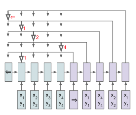
27 |
28 | An encoding RNN converts the input sequence to a code (blue) that is fed to the decoder network (purple). At each step, the decoder network produces a vector that modulates a content-based attention mechanism over inputs. The output of the attention mechanism is a softmax distribution used to select one element of the input (Eq 2.).
29 |
30 |
31 | $ u^i_{j} = v^T tanh(W_1e_j + W_2d_j) \quad j \in \{1...n\}\\
32 | p ( C_i | C_1 ... C_n; P) = softmax(u^i) $
33 |
34 | Eq 2: Softmax distribution over the input
35 |
36 | ## Sorting arrays overview
37 |
38 | The goal of our implementation is to sort arrays of variable length without applying any algorithm but forward step through out Ptr-NN.
39 |
40 | ```python
41 | unsorted = [5., 4., 3., 7.]
42 | sort_array = ptr_nn(unsorted)
43 | assert sort_array == [3., 4., 5., 7.]
44 | ```
45 |
46 | As we said at the 'Ptr-NN overview' the desired outputs of our function estimator are expressed using discrete tokens corresponding to the position of the input. In sorting arrays problem, our output will be the resulting tensor of applying `argsort` function to an unsorted array.
47 |
48 | ```python
49 | >>> import torch
50 | >>> input = torch.randint(high=5, size=(5,))
51 | >>> input
52 | tensor([4, 2, 3, 0, 4])
53 | >>> label = input.argsort()
54 | >>> label
55 | tensor([3, 1, 2, 0, 4])
56 | >>> input[label]
57 | tensor([0, 2, 3, 4, 4])
58 | ```
59 |
60 | Knowing that relation between the output and the input, we can easily create random batches of training data.
61 |
62 | ```python
63 | def batch(batch_size, min_len=5, max_len=10):
64 | array_len = torch.randint(low=min_len,
65 | high=max_len + 1,
66 | size=(1,))
67 |
68 | x = torch.randint(high=10, size=(batch_size, array_len))
69 | y = x.argsort(dim=1) # Note that we are not sorting along batch axis
70 | return x, y
71 | ```
72 |
73 | Let's see an small output of our `data generator`.
74 |
75 | ```python
76 | >>> batch_size = 3
77 | >>> x, y = batch(batch_size, min_len=3, max_len=6)
78 | >>> list(zip(x, y)) # list of tuples (tensor, tensor.argsort)
79 | [(tensor([4, 0, 4, 0]), tensor([1, 3, 0, 2])),
80 | (tensor([9, 7, 1, 2]), tensor([2, 3, 1, 0])),
81 | (tensor([1, 5, 8, 7]), tensor([0, 1, 3, 2]))]
82 | ```
83 |
84 | ## Ptr-NN implementation
85 |
86 | ### Architecture and hyperparameters
87 |
88 | The paper [1] states that no extensive hyperparameter tuning has been done. So to keep things simple we will implement an `Encoder` with a single LSTM layer and a `Decoder` with an `Attention` layer and a single LSTM layer too. Both `Encoder` and `Decoder` will have a hidden size of 256. The accomplish our goal we will maximize log likelihood probability with Adam optimizer with the default learning rate set by PyTorch.
89 |
90 | 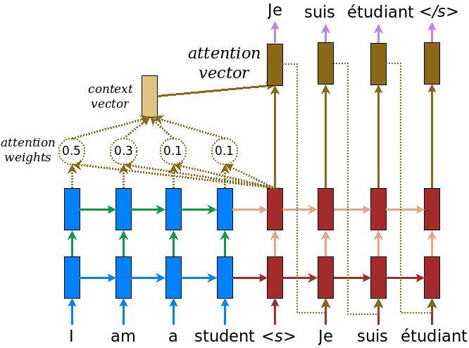
91 | Figure 2: Seq2Seq model with attention. Similar to our Ptr-NN architecture
92 |
93 | ### Encoder
94 |
95 | As our encoder is a single LSTM layer, we can declare it as a one-liner `nn.Module`.
96 |
97 | The encoder input size is 1 because our input sequences are 1-dimensional arrays. Therefore, to make arrays 'compatible' with RNNs, we are going to feed them to our encoder reshaped to size `(BATCH_LEN, ARRAY_LEN, 1)`.
98 |
99 | ```python
100 | encoder = nn.LSTM(1, hidden_size=256, batch_first=True)
101 |
102 | # sample input
103 | x, _ = batch(batch_size=4, min_len=3, max_len=6)
104 | x = x.view(4, -1, 1).float()
105 | out, (hidden, cell_state) = encoder(x)
106 | print (f'Encoder output shape: (batch size, array len, hidden size) {out.shape}')
107 | # Encoder output shape: (batch size, array len, hidden size) torch.Size([4, 6, 256])
108 | print (f'Encoder Hidden state shape: (batch size, hidden size) {hidden.shape}')
109 | # Encoder Hidden state shape: (batch size, hidden size) torch.Size([1, 4, 256])
110 | ```
111 |
112 | ### Attention
113 |
114 | We are going to declare a new `nn.Module` that will implement the operations listed in the Equation 2.
115 |
116 | The result of this implementation is an Attention layer, which their outputs are a softmax distribution over the inputs. This probability distribution is the one that the Ptr-NN will use to predict the outputs of the model.
117 |
118 | ```python
119 | class Attention(nn.Module):
120 | def __init__(self, hidden_size, units):
121 | super(Attention, self).__init__()
122 | self.W1 = nn.Linear(hidden_size, units, bias=False)
123 | self.W2 = nn.Linear(hidden_size, units, bias=False)
124 | self.V = nn.Linear(units, 1, bias=False)
125 |
126 | def forward(self,
127 | encoder_out: torch.Tensor,
128 | decoder_hidden: torch.Tensor):
129 | # encoder_out: (BATCH, ARRAY_LEN, HIDDEN_SIZE)
130 | # decoder_hidden: (BATCH, HIDDEN_SIZE)
131 |
132 | # Add time axis to decoder hidden state
133 | # in order to make operations compatible with encoder_out
134 | # decoder_hidden_time: (BATCH, 1, HIDDEN_SIZE)
135 | decoder_hidden_time = decoder_hidden.unsqueeze(1)
136 |
137 | # uj: (BATCH, ARRAY_LEN, ATTENTION_UNITS)
138 | # Note: we can add the both linear outputs thanks to broadcasting
139 | uj = self.W1(encoder_out) + self.W2(decoder_hidden_time)
140 | uj = torch.tanh(uj)
141 |
142 | # uj: (BATCH, ARRAY_LEN, 1)
143 | uj = self.V(uj)
144 |
145 | # Attention mask over inputs
146 | # aj: (BATCH, ARRAY_LEN, 1)
147 | aj = F.softmax(uj, dim=1)
148 |
149 | # di_prime: (BATCH, HIDDEN_SIZE)
150 | di_prime = aj * encoder_out
151 | di_prime = di_prime.sum(1)
152 |
153 | return di_prime, uj.squeeze(-1)
154 |
155 | # Forward example
156 | att = Attention(256, 10)
157 | di_prime, att_w = att(out, hidden[0])
158 | print(f'Attention aware hidden states: {di_prime.shape}')
159 | # Attention aware hidden states: torch.Size([4, 256])
160 | print(f'Attention weights over inputs: {att_w.shape}')
161 | # Attention weights over inputs: torch.Size([4, 6])
162 | ```
163 |
164 | Notice that our Attention layer is not returning the normalized (not 'softmaxed') attention weights, that is because [CrossEntropyLoss](https://pytorch.org/docs/stable/nn.html#torch.nn.CrossEntropyLoss) will take care of first apply `log_softmax` and finally compute the Negative Log Likelihood Loss ([NLLLoss](https://pytorch.org/docs/stable/nn.html?highlight=nllloss#torch.nn.NLLLoss)).
165 |
166 | ### Decoder
167 |
168 | The decoder implementation is straightforward as we only have to do 2 steps:
169 |
170 | 1. Make the decoder input aware of the attention mask, which is computed using the previous hidden states and encoder outputs.
171 | 2. Feed the attention aware input to the LSTM and retrieve only the hidden states from it.
172 |
173 | ```python
174 | class Decoder(nn.Module):
175 | def __init__(self,
176 | hidden_size: int,
177 | attention_units: int = 10):
178 | super(Decoder, self).__init__()
179 | self.lstm = nn.LSTM(hidden_size + 1, hidden_size, batch_first=True)
180 | self.attention = Attention(hidden_size, attention_units)
181 |
182 | def forward(self,
183 | x: torch.Tensor,
184 | hidden: Tuple[torch.Tensor],
185 | encoder_out: torch.Tensor):
186 | # x: (BATCH, 1, 1)
187 | # hidden: (1, BATCH, HIDDEN_SIZE)
188 | # encoder_out: (BATCH, ARRAY_LEN, HIDDEN_SIZE)
189 |
190 | # Get hidden states (not cell states)
191 | # from the first and unique LSTM layer
192 | ht = hidden[0][0] # ht: (BATCH, HIDDEN_SIZE)
193 |
194 | # di: Attention aware hidden state -> (BATCH, HIDDEN_SIZE)
195 | di, att_w = self.attention(encoder_out, ht)
196 |
197 | # Append attention aware hidden state to our input
198 | # x: (BATCH, 1, 1 + HIDDEN_SIZE)
199 | x = torch.cat([di.unsqueeze(1), x], dim=2)
200 |
201 | # Generate the hidden state for next timestep
202 | _, hidden = self.lstm(x, hidden)
203 | return hidden, att_w
204 | ```
205 |
206 | ## Training
207 |
208 | 1. Feed the input through the encoder, which return encoder output and hidden state.
209 | 2. Feed the encoder output, the encoder's hidden state (as the first decoder's hidden state) and the first decoder's input (in our case the first token is always 0).
210 | 3. The decoder returns a prediction pointing to one element in the input and their hidden states. The decoder hidden state is then passed back to into the model and the predictions are used to compute the loss.
211 | To decide the next decoder input we use teacher force only 50% of the times. Teacher forcing is the technique where the target number is passed as the next input to the decoder, even if the prediction at previous time step was wrong.
212 | 4. The final step is to calculate the gradients and apply it to the optimizer and backpropagate.
213 |
214 | To make training code more semantically understandable, we group all the forward pass in a single `nn.Module` called `PointerNetwork`.
215 |
216 | ```python
217 | class PointerNetwork(nn.Module):
218 | def __init__(self,
219 | encoder: nn.Module,
220 | decoder: nn.Module):
221 | super(PointerNetwork, self).__init__()
222 | self.encoder = encoder
223 | self.decoder = decoder
224 |
225 | def forward(self,
226 | x: torch.Tensor,
227 | y: torch.Tensor,
228 | teacher_force_ratio=.5):
229 | # x: (BATCH_SIZE, ARRAY_LEN)
230 | # y: (BATCH_SIZE, ARRAY_LEN)
231 |
232 | # Array elements as features
233 | # encoder_in: (BATCH, ARRAY_LEN, 1)
234 | encoder_in = x.unsqueeze(-1).type(torch.float)
235 |
236 | # out: (BATCH, ARRAY_LEN, HIDDEN_SIZE)
237 | # hs: tuple of (NUM_LAYERS, BATCH, HIDDEN_SIZE)
238 | out, hs = encoder(encoder_in)
239 |
240 | # Accum loss throughout timesteps
241 | loss = 0
242 |
243 | # Save outputs at each timestep
244 | # outputs: (ARRAY_LEN, BATCH)
245 | outputs = torch.zeros(out.size(1), out.size(0), dtype=torch.long)
246 |
247 | # First decoder input is always 0
248 | # dec_in: (BATCH, 1, 1)
249 | dec_in = torch.zeros(out.size(0), 1, 1, dtype=torch.float)
250 |
251 | for t in range(out.size(1)):
252 | hs, att_w = decoder(dec_in, hs, out)
253 | predictions = F.softmax(att_w, dim=1).argmax(1)
254 |
255 | # Pick next index
256 | # If teacher force the next element will we the ground truth
257 | # otherwise will be the predicted value at current timestep
258 | teacher_force = random.random() < teacher_force_ratio
259 | idx = y[:, t] if teacher_force else predictions
260 | dec_in = torch.stack([x[b, idx[b].item()] for b in range(x.size(0))])
261 | dec_in = dec_in.view(out.size(0), 1, 1).type(torch.float)
262 |
263 | # Add cross entropy loss (F.log_softmax + nll_loss)
264 | loss += F.cross_entropy(att_w, y[:, t])
265 | outputs[t] = predictions
266 |
267 | # Weight losses, so every element in the batch
268 | # has the same 'importance'
269 | batch_loss = loss / y.size(0)
270 |
271 | return outputs, batch_loss
272 | ```
273 |
274 | Also to make training steps encapsulate the forward and backward steps in a single function called `train`.
275 |
276 | ```python
277 | BATCH_SIZE = 32
278 | STEPS_PER_EPOCH = 500
279 | EPOCHS = 10
280 |
281 | def train(model, optimizer, epoch):
282 | """Train single epoch"""
283 | print('Epoch [{}] -- Train'.format(epoch))
284 | for step in range(STEPS_PER_EPOCH):
285 | optimizer.zero_grad()
286 |
287 | x, y = batch(BATCH_SIZE)
288 | out, loss = model(x, y)
289 |
290 | loss.backward()
291 | optimizer.step()
292 |
293 | if (step + 1) % 100 == 0:
294 | print('Epoch [{}] loss: {}'.format(epoch, loss.item()))
295 | ```
296 |
297 | Finally to train the model we run the following code.
298 |
299 | ```python
300 | ptr_net = PointerNetwork(Encoder(HIDDEN_SIZE),
301 | Decoder(HIDDEN_SIZE))
302 |
303 | optimizer = optim.Adam(ptr_net.parameters())
304 |
305 | for epoch in range(EPOCHS):
306 | train(ptr_net, optimizer, epoch + 1)
307 |
308 | # Output
309 | # Epoch [1] -- Train
310 | # Epoch [1] loss: 0.2310
311 | # Epoch [1] loss: 0.3385
312 | # Epoch [1] loss: 0.4668
313 | # Epoch [1] loss: 0.1158
314 | ...
315 | # Epoch [5] -- Train
316 | # Epoch [5] loss: 0.0836
317 | ```
318 |
319 | ## Evaluating the model
320 |
321 | A Ptr-NN doesn't output the 'solution' directly, instead it outputs a set of indices referring to the input positions. This fact forces us to du a small post process step.
322 |
323 | ```python
324 | @torch.no_grad()
325 | def evaluate(model, epoch):
326 | x_val, y_val = batch(4)
327 |
328 | # No use teacher force when evaluating
329 | out, _ = model(x_val, y_val, teacher_force_ratio=0.)
330 | out = out.permute(1, 0)
331 |
332 | for i in range(out.size(0)):
333 | print('{} --> {}'.format(
334 | x_val[i],
335 | x_val[i].gather(0, out[i]),
336 | ))
337 |
338 | # Output: Unsorted --> Sorted by PtrNN
339 | # tensor([5, 0, 5, 3, 5, 2, 3, 9]) -> tensor([0, 2, 3, 3, 5, 5, 5, 9])
340 | # tensor([3, 9, 9, 7, 6, 2, 0, 9]) -> tensor([0, 2, 3, 6, 7, 9, 9, 9])
341 | # tensor([6, 9, 4, 3, 7, 6, 4, 5]) -> tensor([3, 4, 4, 5, 6, 6, 7, 9])
342 | # tensor([7, 3, 3, 5, 2, 4, 1, 9]) -> tensor([1, 2, 3, 3, 4, 5, 7, 9])
343 | ```
344 |
345 | ## Conclusions
346 |
347 | Wow! Interesting wasn't it? In my opinion the fact that NN can solve mathematical problems is amazing. Some mathematical problems are computationally complex, but imagine that in a future we are able to train a NN to solve this complex problems and therefore simplify their computational cost.
348 |
349 | Important takeaways
350 |
351 | - *Seq2Seq* models are not only creative, they can solve mathematical problems too.
352 | - Attention mechanism is useful for a lot of tasks, not only for NLP ones.
353 | - Using Pointer Networks we can have a NN supporting outputs of variable sizes.
354 |
355 | ## Reference
356 |
357 | - 1. [Pointer Networks](https://arxiv.org/abs/1506.03134) - Vinyals et al.
358 | - 2. [Sequence to Sequence Learning with Neural Networks](https://arxiv.org/abs/1409.3215) - Ilya Sutskever, Oriol Vinyals, Quoc V. Le
359 | - 3. [Neural Machine Translation by Jointly Learning to Align and Translate](https://arxiv.org/abs/1409.0473) - Dzmitry Bahdanau, Kyunghyun Cho, Yoshua Bengio
360 |
--------------------------------------------------------------------------------
/blog.yml:
--------------------------------------------------------------------------------
1 | title: Sorting arrays with Pointer Networks
2 | description: In this blog post we are going to sort arrays of variable sizes using a special Neural Network architecture.
3 | image: https://upload.wikimedia.org/wikipedia/commons/8/89/Scottish_fold_cat.jpg
4 | content: README.md
--------------------------------------------------------------------------------
/data.py:
--------------------------------------------------------------------------------
1 | """
2 | Generate random data for pointer network
3 | """
4 | import torch
5 | from torch.utils.data import Dataset
6 |
7 |
8 | def sample(min_length=5, max_length=12):
9 | """
10 | Generates a single example for a pointer network. The example consist in a tuple of two
11 | elements. First element is an unsorted array and the second element
12 | is the result of applying argsort on the first element
13 | """
14 | array_len = torch.randint(low=min_length,
15 | high=max_length + 1,
16 | size=(1,))
17 | x = torch.randint(high=array_len.item(), size=(array_len,))
18 | return x, x.argsort()
19 |
20 |
21 | def batch(batch_size, min_len=5, max_len=12):
22 | array_len = torch.randint(low=min_len,
23 | high=max_len + 1,
24 | size=(1,))
25 |
26 | x = torch.randint(high=10, size=(batch_size, array_len))
27 | return x, x.argsort(dim=1)
28 |
29 |
--------------------------------------------------------------------------------
/img/figure-1.png:
--------------------------------------------------------------------------------
https://raw.githubusercontent.com/Guillem96/pointer-nn-pytorch/f4e645aa035324593933420979c030430682a4b5/img/figure-1.png
--------------------------------------------------------------------------------
/img/model-architecture.jpg:
--------------------------------------------------------------------------------
https://raw.githubusercontent.com/Guillem96/pointer-nn-pytorch/f4e645aa035324593933420979c030430682a4b5/img/model-architecture.jpg
--------------------------------------------------------------------------------
/ptr_net.py:
--------------------------------------------------------------------------------
1 | """
2 | Module implementing the pointer network proposed at: https://arxiv.org/abs/1506.03134
3 |
4 | The implementation try to follows the variables naming conventions
5 |
6 | ei: Encoder hidden state
7 |
8 | di: Decoder hidden state
9 | di_prime: Attention aware decoder state
10 |
11 | W1: Learnable matrix (Attention layer)
12 | W2: Learnable matrix (Attention layer)
13 | V: Learnable parameter (Attention layer)
14 |
15 | uj: Energy vector (Attention Layer)
16 | aj: Attention mask over the input
17 | """
18 | import random
19 | from typing import Tuple
20 |
21 | import torch
22 | import torch.nn as nn
23 | import torch.optim as optim
24 | import torch.nn.functional as F
25 |
26 | from data import sample, batch
27 |
28 | HIDDEN_SIZE = 256
29 |
30 | BATCH_SIZE = 32
31 | STEPS_PER_EPOCH = 500
32 | EPOCHS = 10
33 |
34 |
35 | class Encoder(nn.Module):
36 | def __init__(self, hidden_size: int):
37 | super(Encoder, self).__init__()
38 | self.lstm = nn.LSTM(1, hidden_size, batch_first=True)
39 |
40 | def forward(self, x: torch.Tensor):
41 | # x: (BATCH, ARRAY_LEN, 1)
42 | return self.lstm(x)
43 |
44 |
45 | class Attention(nn.Module):
46 | def __init__(self, hidden_size, units):
47 | super(Attention, self).__init__()
48 | self.W1 = nn.Linear(hidden_size, units, bias=False)
49 | self.W2 = nn.Linear(hidden_size, units, bias=False)
50 | self.V = nn.Linear(units, 1, bias=False)
51 |
52 | def forward(self,
53 | encoder_out: torch.Tensor,
54 | decoder_hidden: torch.Tensor):
55 | # encoder_out: (BATCH, ARRAY_LEN, HIDDEN_SIZE)
56 | # decoder_hidden: (BATCH, HIDDEN_SIZE)
57 |
58 | # Add time axis to decoder hidden state
59 | # in order to make operations compatible with encoder_out
60 | # decoder_hidden_time: (BATCH, 1, HIDDEN_SIZE)
61 | decoder_hidden_time = decoder_hidden.unsqueeze(1)
62 |
63 | # uj: (BATCH, ARRAY_LEN, ATTENTION_UNITS)
64 | # Note: we can add the both linear outputs thanks to broadcasting
65 | uj = self.W1(encoder_out) + self.W2(decoder_hidden_time)
66 | uj = torch.tanh(uj)
67 |
68 | # uj: (BATCH, ARRAY_LEN, 1)
69 | uj = self.V(uj)
70 |
71 | # Attention mask over inputs
72 | # aj: (BATCH, ARRAY_LEN, 1)
73 | aj = F.softmax(uj, dim=1)
74 |
75 | # di_prime: (BATCH, HIDDEN_SIZE)
76 | di_prime = aj * encoder_out
77 | di_prime = di_prime.sum(1)
78 |
79 | return di_prime, uj.squeeze(-1)
80 |
81 |
82 | class Decoder(nn.Module):
83 | def __init__(self,
84 | hidden_size: int,
85 | attention_units: int = 10):
86 | super(Decoder, self).__init__()
87 | self.lstm = nn.LSTM(hidden_size + 1, hidden_size, batch_first=True)
88 | self.attention = Attention(hidden_size, attention_units)
89 |
90 | def forward(self,
91 | x: torch.Tensor,
92 | hidden: Tuple[torch.Tensor],
93 | encoder_out: torch.Tensor):
94 | # x: (BATCH, 1, 1)
95 | # hidden: (1, BATCH, HIDDEN_SIZE)
96 | # encoder_out: (BATCH, ARRAY_LEN, HIDDEN_SIZE)
97 | # For a better understanding about hidden shapes read: https://pytorch.org/docs/stable/nn.html#lstm
98 |
99 | # Get hidden states (not cell states)
100 | # from the first and unique LSTM layer
101 | ht = hidden[0][0] # ht: (BATCH, HIDDEN_SIZE)
102 |
103 | # di: Attention aware hidden state -> (BATCH, HIDDEN_SIZE)
104 | # att_w: Not 'softmaxed', torch will take care of it -> (BATCH, ARRAY_LEN)
105 | di, att_w = self.attention(encoder_out, ht)
106 |
107 | # Append attention aware hidden state to our input
108 | # x: (BATCH, 1, 1 + HIDDEN_SIZE)
109 | x = torch.cat([di.unsqueeze(1), x], dim=2)
110 |
111 | # Generate the hidden state for next timestep
112 | _, hidden = self.lstm(x, hidden)
113 | return hidden, att_w
114 |
115 |
116 | class PointerNetwork(nn.Module):
117 | def __init__(self,
118 | encoder: nn.Module,
119 | decoder: nn.Module):
120 | super(PointerNetwork, self).__init__()
121 | self.encoder = encoder
122 | self.decoder = decoder
123 |
124 | def forward(self,
125 | x: torch.Tensor,
126 | y: torch.Tensor,
127 | teacher_force_ratio=.5):
128 | # x: (BATCH_SIZE, ARRAY_LEN)
129 | # y: (BATCH_SIZE, ARRAY_LEN)
130 |
131 | # Array elements as features
132 | # encoder_in: (BATCH, ARRAY_LEN, 1)
133 | encoder_in = x.unsqueeze(-1).type(torch.float)
134 |
135 | # out: (BATCH, ARRAY_LEN, HIDDEN_SIZE)
136 | # hs: tuple of (NUM_LAYERS, BATCH, HIDDEN_SIZE)
137 | out, hs = encoder(encoder_in)
138 |
139 | # Accum loss throughout timesteps
140 | loss = 0
141 |
142 | # Save outputs at each timestep
143 | # outputs: (ARRAY_LEN, BATCH)
144 | outputs = torch.zeros(out.size(1), out.size(0), dtype=torch.long)
145 |
146 | # First decoder input is always 0
147 | # dec_in: (BATCH, 1, 1)
148 | dec_in = torch.zeros(out.size(0), 1, 1, dtype=torch.float)
149 |
150 | for t in range(out.size(1)):
151 | hs, att_w = decoder(dec_in, hs, out)
152 | predictions = F.softmax(att_w, dim=1).argmax(1)
153 |
154 | # Pick next index
155 | # If teacher force the next element will we the ground truth
156 | # otherwise will be the predicted value at current timestep
157 | teacher_force = random.random() < teacher_force_ratio
158 | idx = y[:, t] if teacher_force else predictions
159 | dec_in = torch.stack([x[b, idx[b].item()] for b in range(x.size(0))])
160 | dec_in = dec_in.view(out.size(0), 1, 1).type(torch.float)
161 |
162 | # Add cross entropy loss (F.log_softmax + nll_loss)
163 | loss += F.cross_entropy(att_w, y[:, t])
164 | outputs[t] = predictions
165 |
166 | # Weight losses, so every element in the batch
167 | # has the same 'importance'
168 | batch_loss = loss / y.size(0)
169 |
170 | return outputs, batch_loss
171 |
172 |
173 | def train(model, optimizer, epoch, clip=1.):
174 | """Train single epoch"""
175 | print('Epoch [{}] -- Train'.format(epoch))
176 | for step in range(STEPS_PER_EPOCH):
177 | optimizer.zero_grad()
178 |
179 | # Forward
180 | x, y = batch(BATCH_SIZE)
181 | out, loss = model(x, y)
182 |
183 | # Backward
184 | loss.backward()
185 | nn.utils.clip_grad_norm_(model.parameters(), clip)
186 | optimizer.step()
187 |
188 | if (step + 1) % 100 == 0:
189 | print('Epoch [{}] loss: {}'.format(epoch, loss.item()))
190 |
191 |
192 | @torch.no_grad()
193 | def evaluate(model, epoch):
194 | """Evaluate after a train epoch"""
195 | print('Epoch [{}] -- Evaluate'.format(epoch))
196 |
197 | x_val, y_val = batch(4)
198 |
199 | out, _ = model(x_val, y_val, teacher_force_ratio=0.)
200 | out = out.permute(1, 0)
201 |
202 | for i in range(out.size(0)):
203 | print('{} --> {} --> {}'.format(
204 | x_val[i],
205 | x_val[i].gather(0, out[i]),
206 | x_val[i].gather(0, y_val[i])
207 | ))
208 |
209 |
210 | encoder = Encoder(HIDDEN_SIZE)
211 | decoder = Decoder(HIDDEN_SIZE)
212 | ptr_net = PointerNetwork(encoder, decoder)
213 |
214 | optimizer = optim.Adam(ptr_net.parameters())
215 |
216 | for epoch in range(EPOCHS):
217 | train(ptr_net, optimizer, epoch + 1)
218 | evaluate(ptr_net, epoch + 1)
219 |
--------------------------------------------------------------------------------