nums[i] + nums[j] + nums[k] == 0. 9 | 10 | Notice that the solution set must not contain duplicate triplets. 11 | 12 | ### Example 1: 13 | 14 | Input: nums = [-1,0,1,2,-1,-4]
15 | Output: [[-1,-1,2],[-1,0,1]] 16 | 17 | ### Example 2: 18 | 19 | Input: nums = [0,1,1]
20 | Output: []
21 | Explanation: The only possible triplet does not sum up to 0. 22 | 23 | ### Solution : Efficient Solution 24 | - Using three pointers 25 | - The idea is to sort the array first, then run two loops to process the triplets. We fix the outer loop and move the two pointers (indexes) of the inner loop inwards to arrive at the result. 26 | 27 | ### Algorithm 28 | 29 | 1) Sort the given array.
30 | 2) Loop over the array and fix the first element of the possible triplet, arr[i].
31 | 3) Then fix two pointers, one at i + 1 and the other at n – 1. And look at the sum,
32 | a) If the sum is smaller than the required sum, increment the first pointer.
33 | b) Else, If the sum is bigger, Decrease the end pointer to reduce the sum.
34 | c) Else, if the sum of elements at two-pointer is equal to given sum then print the triplet and break. 35 | 36 | 37 | ### Implementation 38 | 39 | #### In Python 40 | ```c 41 | class Solution: 42 | def threeSum(self, nums: List[int]) -> List[List[int]]: 43 | res = [] 44 | nums.sort() 45 | 46 | for i, a in enumerate(nums): 47 | if i > 0 and a == nums[i - 1]: 48 | continue 49 | 50 | l, r = i + 1, len(nums) - 1 51 | while l < r: 52 | threeSum = a + nums[l] + nums[r] 53 | if threeSum > 0: 54 | r -= 1 55 | elif threeSum < 0: 56 | l += 1 57 | else: 58 | res.append([a, nums[l], nums[r]]) 59 | l += 1 60 | while nums[l] == nums[l - 1] and l < r: 61 | l += 1 62 | return res 63 | ``` 64 | ### Time Complexity - O(n^2) 65 | ### Space Complexity - O(1) 66 | -------------------------------------------------------------------------------- /Algorithms/Searching Algorithms/Linear_Search.md: -------------------------------------------------------------------------------- 1 | ## Linear Search 2 | 3 | Linear search algorithm is the most simplest algorithm to do sequential search and this technique iterates over the sequence and checks one item at a time, until the desired item is found or all items have been examined. There are two types of linear search methods : 4 | 5 | * **Unordered Linear Search** 6 | 7 | * **Ordered Linear Search** 8 | 9 | ### Unordered Linear Search: 10 | Let us assume we are given an array where the order of elements is not known. That means the elements of the array are not sorted. In this case, to search for an element we have to scan the complete array and see if the element is there in the given list or not. 11 | 12 | #### Pseudocode: 13 | 14 | ```cpp 15 | int UnorderedLS(int A[], int n, int data) { 16 | for(int i = 0; i < n; i++) { 17 | if(A[i] == data) 18 | return i; 19 | } 20 | return -1; 21 | } 22 | ``` 23 | #### Time Complexity: 24 | O(n) in the worst case we need to scan the complete array. 25 | #### Space Complexity: 26 | O(1) 27 | 28 | ### Ordered Linear Search: 29 | If the elements of the array are already sorted (i.e user inputs sorted data) then in many cases we don't have to scan the complete array to see if it the element is there in the given array or not. In the pseudocode below, you can see that, at any point if the value at A[i] is greater than the data to be searched, then we just return -1 without searching the remaining array. 30 | 31 | #### Pseudocode: 32 | 33 | ```cpp 34 | int OrderedLS(int A[], int n, int data) { 35 | for(int i = 0; i < n; i++) { 36 | if(A[i] == data) 37 | return i; 38 | else if(A[i] > data) 39 | return -1; 40 | } 41 | return -1; 42 | } 43 | ``` 44 | #### Time Complexity: 45 | O(n) in the worst case we need to scan the complete array. 46 | #### Space Complexity: 47 | O(1) 48 | 49 | ### Program 50 | 51 | ```cpp 52 | #include
8 | Values from the unsorted part are picked and placed at the correct position in the sorted part. 9 |
10 |
11 | 12 | ## Algorithm 13 | 14 | To sort an array of size n in ascending order: 15 | 16 | 1. Iterate from arr[1] to arr[n] over the array. 17 | 2. Compare the current element (key) to its predecessor. 18 | 3. If the key element is smaller than its predecessor, compare it to the elements before. Move the greater elements one position up to make space for the swapped element. 19 | 20 |
21 | 22 | ## Code: 23 | 24 | Here is the code for Insertion Sort using C++
25 |
26 | 27 | ``` 28 | #include
76 | 77 | ``` 78 | Input : 12, 11, 13, 5, 6 79 | Output : 5, 6, 11, 12, 13 80 | ``` 81 | 82 |
83 | 84 | ## Time Complexity 85 | 86 | The time complexity for insertion sort is O(n^2) in the worst case 87 | 88 |
89 | 90 | ### Auxiliary Space: 91 | 92 | The sorting algorithm takes a constant space O(1) 93 | 94 |
95 | 96 | ### Boundary Cases: 97 | 98 | Insertion sort takes maximum time to sort if elements are sorted in reverse order. And it takes minimum time (Order of n) when elements are already sorted. 99 | 100 |
101 | 102 | ### Algorithmic Paradigm: 103 | 104 | Insertion sort uses the Incremental Approach 105 | 106 |
107 | 108 | ### Sorting In Place: 109 | 110 | The sorting are done in place to avoid extra memory. 111 | -------------------------------------------------------------------------------- /Data Structures/Arrays/Intro_to_Arrays.md: -------------------------------------------------------------------------------- 1 | # Arrays 2 | 3 | ``` 4 | An array in C/C++ or be it in any programming language 5 | is a collection of similar data items stored at contiguous 6 | memory locations and elements can be accessed randomly 7 | using indices of an array 8 | ``` 9 | 10 | # Declaration of Arrays in C++ 11 | 12 | ## 1-> Size Specification 13 | int arr[10]; //this is one of the ways to declare an array with size *10* in this case 14 | int n = 10; 15 | int arr[n]; // the size the arrray can be an user input as well 16 | 17 | ## 2-> With values but no size 18 | int arr[] = {1,2,3,4,5}; //This way we can declare an array of some elements 19 | ## 3-> With values and size as well 20 | int arr2[6] = {19,10,8,17,9,15}; //This way we can declare an array of n elements where n = 6 in this case 21 | 22 | 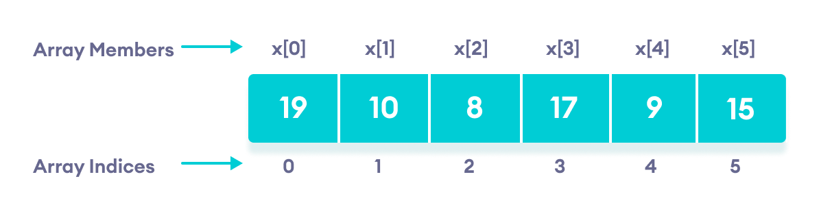 23 |
24 | ## 4-> Dynamic array allocation 25 | int * arr = new int[5];//this way we can allocate dynamic contiguous memory for our array 26 | 27 | --One more way to do it is with user input size-- 28 | 29 | int n; 30 | cin>>n; 31 | 32 | int * arr = new int[n];//This way array memory will be allocated at the runtime of our program 33 | 34 | Accessing indices in this type of arrays is quite interesting for example, 35 | 36 | arr[i] //will allow us to access the integer value at the ith index; 37 | 38 | i[arr] //this will work same as the above 39 | 40 | * (i + arr) //even this way is just another way of accessing the ith index 41 | 42 | -- all thanks to the pointers in c++ -- 43 | 44 | 45 | ## Code Snippets 46 | 47 | 48 | # Example1 : 49 | 50 | #include
19 | - Recursively traverse the current node's left subtree. 20 | - Visit the current node (in the figure: position green). 21 | - Recursively traverse the current node's right subtree. 22 | 23 | ##### Note 24 | In a binary search tree ordered such that in each node the key is greater than all keys in its left subtree and less than all keys in its right subtree, in-order traversal retrieves the keys in ascending sorted order. 25 | > #### Recursive 26 | ### Pseudo Code 27 | ``` js 28 | procedure inorder(node) 29 | // if no node then backtrack 30 | if node = null 31 | return 32 | 33 | inorder(node.left) 34 | visit(node) 35 | inorder(node.right) 36 | ``` 37 | ### Code `Python` 38 | ``` py 39 | def inorder(root): 40 | if not root: 41 | return 42 | inorder(root.left) 43 | print(root.data) 44 | inorder(root.right) 45 | ``` 46 | 47 | > #### Iterative 48 | ### Pseudo Code 49 | ``` js 50 | procedure iterativeInorder(node) 51 | stack ← empty stack 52 | while not stack.isEmpty() or node ≠ null 53 | if node ≠ null 54 | stack.push(node) 55 | node ← node.left 56 | else 57 | node ← stack.pop() 58 | visit(node) 59 | node ← node.right 60 | ``` 61 | ### Code `Python` 62 | ``` py 63 | def iterativeInorder(root): 64 | stack = [] 65 | temp = root 66 | while len(stack) and temp: 67 | if temp: 68 | stack.append(temp) 69 | temp = temp.left 70 | else: 71 | temp = stack.pop() 72 | print(temp.data) 73 | temp = temp.right 74 | ``` 75 | 76 | 77 | #### ⏲️ Time Complexities: 78 | `O(n)` *As we are visiting every node* 79 |
80 | #### 👾 Space complexities: 81 | `O(n)` *recursion stack space* 82 | -------------------------------------------------------------------------------- /Data Structures/Hashingtechnique.md: -------------------------------------------------------------------------------- 1 | # Hashing 2 | - The technique of mapping a large chunk of data into small tables with the help of a hashing function is called as Hashing. 3 | - Hashing is an data structure which is designed in order to solve the problem of efficiently storing and finding data in an array. 4 | - Hash tables are used to store the data in an array format. 5 | - Hashing is a two-step process. 6 | 1. In Hashing the hash function converts the item into a small integer or hash value and this integer is used as an index which stores the original data. 7 | 2. Data is stored in an hash table. A hash key can be used to locate data quickly. 8 | 9 | 10 | 11 | ## Examples of Hashing in Data Structure 12 | 13 | - In school, teacher assigns a unique roll number to each student. Later, teacher uses that roll number to retrieve information about that student. 14 | 15 | ## Hash Function 16 | - The function which maps arbitary size of data to fixed-sized data is called as hash function. 17 | - It returns hash value, hash codes, and hash sums. 18 | hash = hashfunc(key) 19 | index = hash % array_size 20 | - The hash function must satisfy the following requirements: 21 | 1. A good hash function should be easy to compute. 22 | 2. A good hash function should never get stuck in clustering and should distribute keys evenly across the hash table. 23 | 3. A good hash function should avoid collision whenever two elements or items get assigned to the same hash value. 24 | 25 | ## Hash Table 26 | - Hashing uses hash tables to store the key-value pairs. 27 | - The hash table uses the hash function and generates an index. 28 | - This unique index is used to perform insert, update, and search operations. 29 | 30 | # Collision Resolution Techniques 31 | - If two keys are assigned the same index number in the hash table hashing falls into a collision. 32 | - As each index in a hash table is supposed to store only one value the collision creates a problem . 33 | - Hashing uses several collision resolution techniques for managing performance of a hash table. 34 | 35 | ## Linear Probing 36 | - Hashing results into an array index which is already occupied for storing a value. 37 | - In such case, hashing performs search operation and linearly probes for the next empty cell. 38 | 39 | ## Double Hashing 40 | - Double hashing technique uses two hash functions. 41 | - Second hash function is used only when the first function causes a collision. 42 | - An offset is provided for the index to store the value. 43 | - The formula for the double hashing technique is as follows: 44 | (firstHash(key) + i * secondHash(key)) % sizeOfTable 45 | 46 | - As compared to linear probing double hashing has a high computation cost as it searches the next free slot faster than the linear probing method. 47 | -------------------------------------------------------------------------------- /Data Structures/Arrays/Implementation_of_queue_using_array.md: -------------------------------------------------------------------------------- 1 | # C++ Program to Implement Queue using Array 2 | 3 | ``` 4 | A queue is an abstract data structure that contains a collection of elements. Queue implements the FIFO mechanism i.e. the element that is inserted first is also deleted first. In other words, the least recently added element is removed first in a queue. 5 | ``` 6 | 7 | 8 | ### 1-> The function Insert() inserts an element into the queue. If the rear is equal to n-1, then the queue is full and overflow is displayed. If front is -1, it is incremented by 1. Then rear is incremented by 1 and the element is inserted in index of rear. This is shown below − 9 | void Insert() { 10 | int val; 11 | if (rear == n - 1) 12 | cout<<"Queue Overflow"<
8 | Heap Sort is similar to selection sort. In this first the minimum element is fetched and placed at beginning. 9 |
10 |
11 | 12 | ## Algorithm 13 | 14 | To arrange list of elements in ascending order using heap sort algorithm is done as follows: 15 | 16 | 1. With the given list of elements construct Binary tree. 17 | 2. Now, the Binary tree should be transformed in a Minimum Heap. 18 | 3. By Using the Heapify method the root element must be deleted from the Minimum Heap. 19 | 4. A sorted list must be created and the deleted element should be put in it. 20 | 5. Until the minimum heap becomes empty keep on repeating the same procedure. 21 | 6. Lastly the sorted list must be displayed. 22 | 23 |
24 | 25 | ## Code: 26 | 27 | Here is the code for Heap Sort using C++
28 |
29 | 30 | ``` 31 | 32 | #include
92 | 93 | ``` 94 | Input : 7, 12, 11, 13, 5, 6 95 | Output : 5, 6, 7, 11, 12, 13 96 | ``` 97 | 98 |
99 | 100 | ## Time Complexity 101 | 102 | The time complexity for heap sort is O(nlog n). 103 | 104 |
105 | 106 | ## Space Complexity 107 | 108 | The space complexity for heap sort is O(1). 109 | 110 |
111 | 112 | ### Auxiliary Space: 113 | 114 | Heap Sort uses O(1) auxiliary space. 115 | 116 |
117 | 118 | ### Stability 119 | 120 | Heap Sort is not stable by nature. 121 | 122 |
123 | 124 | ### Sorting In Place: 125 | 126 | Heap sort is inplace algorithm. 127 | 128 |
129 | 130 | ### Advantages of Heap sort: 131 | 132 | 1. Heap Sort is efficient. 133 | 2. In Heap Sort memory usage is minimal. 134 | 3. Heap Sort is simpler to understand. 135 | -------------------------------------------------------------------------------- /Data Structures/Arrays/Subarray_vs_Subsequence.md: -------------------------------------------------------------------------------- 1 | # Subarrays Vs Subsequence 2 | 3 | ## Subarays 4 | 5 | ``` 6 | Subarrays are arrays within another array. 7 | It contains contiguous elements 8 | Example: Let's consider an array 9 | A = {1,2,3,4,5} 10 | Then the subarray of given array are {}, {1}, {2}, {3}, {4}, {5}, {1,2}, 11 | {1,2,3}, {1,2,3,4}, {1,2,3,4,5}, {2,3}, {2,3,4}, {2,3,4,5}, {3,4}, 12 | {3,4,5}, {4,5}. 13 | Number of Subarray an array of 'n' element can have (excluding empty subarray) = (n*(n+1))/2 . 14 | ``` 15 | 16 | ### Program to print all non empty subarrays: 17 | 18 | ``` 19 | #include
23 | int arr[5] = {1,2,3,4,5}; 24 | for (int i=0; i<5; i++) { 25 | for (int j=i; j<5; j++) { 26 | for (int k=i; k<=j; k++) { 27 | cout<
Let these two numbers be numbers[index1] and numbers[index2] where 1 <= index1 < index2 <= numbers.length. 6 | Return the indices of the two numbers, index1 and index2, added by one as an integer array [index1, index2] of length 2. 7 | You may not use the same element twice. 8 | 9 | 10 | ### Example : 11 | 12 | Input: numbers = [2,7,11,15], target = 9
13 | Output: [1,2]
14 | Explanation: The sum of 2 and 7 is 9. Therefore, index1 = 1, index2 = 2. We return [1, 2]. 15 | 16 | 17 | ### Simple Python Solution with HashMap 18 | 19 | This method works in O(n) time if range of numbers is known.
20 | Let sum be the given sum and A[] be the array in which we need to find pair. 21 | 22 | #### Algorithm 23 | 24 | 1) Initialize Binary Hash Map M[] = {0, 0}
25 | 2) Do following for each element A[i] in A[]
26 | (a) If M[x - A[i]] is set then print the pair (A[i], x A[i])
27 | (b) Set M[A[i]] 28 | 29 | #### Implementation 30 | ```c 31 | class Solution: 32 | def twoSum(self, numbers: List[int], target: int) -> List[int]: 33 | subtract = {} 34 | for i, num in enumerate(numbers): 35 | if num in subtract: 36 | return [subtract[num]+1, i+1] 37 | subtract[target-num] = i 38 | return [] 39 | ``` 40 | #### Time Complexity - O(n) 41 | #### Space Complexity - O(R) where R is range of integers 42 | 43 | ### Using Two pointers 44 | 45 | #### Algorithm: 46 | hasArrayTwoCandidates (A[], ar_size, sum) 47 | 48 | 1) Initialize two index variables to find the candidate 49 | elements in the sorted array.
50 | (a) Initialize first to the left most index: l = 0
51 | (b) Initialize second the right most index: r = ar_size-1
52 | 2) Loop while l < r.
53 | (a) If (A[l] + A[r] == sum) then return 1
54 | (b) Else if( A[l] + A[r] < sum ) then l++
55 | (c) Else r--
56 | 3) No candidates in whole array - return 0 57 | 58 | #### Example: 59 | Let Array be A= {-8, 1, 4, 6, 10, 45} and sum to find be 16 60 | 61 | Initialize l= 0, r = 5
62 | A[l] + A[r] ( -8 + 45) > 16 => decrement r. Nowr = 10
63 | A[l] + A[r] ( -8 + 10) < 2 => increment l. Nowl= 1
64 | A[l] + A[r] ( 1 + 10) < 16 => increment l. Nowl= 2
65 | A[l] + A[r] ( 4 + 10) < 14 => increment l. Nowl= 3
66 | A[l] + A[r] ( 6 + 10) == 16 => Found candidates (return [l+1, r+1]) 67 | 68 | #### Implementation 69 | 70 | ```c 71 | class Solution: 72 | def twoSum(self, numbers: List[int], target: int) -> List[int]: 73 | l, r = 0, len(numbers) - 1 74 | 75 | while l < r: 76 | curSum = numbers[l] + numbers[r] 77 | 78 | if curSum > target: 79 | r -= 1 80 | elif curSum < target: 81 | l += 1 82 | else: 83 | return [l + 1, r + 1] 84 | ``` 85 | 86 | #### Time Complexity - O(n) 87 | #### Space Complexity - O(1) 88 | -------------------------------------------------------------------------------- /Algorithms/Sorting Algorithms/Bubble_Sort.md: -------------------------------------------------------------------------------- 1 | # ⭐ BUBBLE SORT 2 | 3 | Bubble Sort is the simplest and most classical sorting algorithm that works by comparing and swapping the adjacent elements if they are in wrong order. While this may not be the most efficient sorting way, it is certainly easiest to understand and implement. 4 | 5 | #### Example: 6 | 7 | ##### Input: [5 1 4 2 8] 8 | 9 | ##### First Pass: 10 | ( 5 1 4 2 8 ) –> ( 1 5 4 2 8 ), Here, algorithm compares the first two elements, and swaps since 5 > 1. 11 | ( 1 5 4 2 8 ) –> ( 1 4 5 2 8 ), Swap since 5 > 4 12 | ( 1 4 5 2 8 ) –> ( 1 4 2 5 8 ), Swap since 5 > 2 13 | ( 1 4 2 5 8 ) –> ( 1 4 2 5 8 ), Now, since these elements are already in order (8 > 5), algorithm does not swap them. 14 | 15 | ##### Second Pass: 16 | ( 1 4 2 5 8 ) –> ( 1 4 2 5 8 ) 17 | ( 1 4 2 5 8 ) –> ( 1 2 4 5 8 ), Swap since 4 > 2 18 | ( 1 2 4 5 8 ) –> ( 1 2 4 5 8 ) 19 | ( 1 2 4 5 8 ) –> ( 1 2 4 5 8 ) 20 | Now, the array is already sorted, but our algorithm does not know if it is completed. The algorithm needs one whole pass without any swap to know it is sorted. 21 | 22 | ##### Third Pass: 23 | ( 1 2 4 5 8 ) –> ( 1 2 4 5 8 ) 24 | ( 1 2 4 5 8 ) –> ( 1 2 4 5 8 ) 25 | ( 1 2 4 5 8 ) –> ( 1 2 4 5 8 ) 26 | ( 1 2 4 5 8 ) –> ( 1 2 4 5 8 ) 27 | 28 | ##### Output: [1 2 4 5 8] 29 | 30 | Now, generally we would resort to the above method of implementing bubble sort. Since we are iterating through the array N number of times (N is the numbr of elements in the input array), the time complexity would be O(N^2). We are not using any additional space, so the space complexity would be O(1). 31 | 32 | However, if we can somehow inform our algorithm that the array is already sorted, then we wont have to traverse the remaining passes. To do this we can use a flag. Two solutions implementing this approach will be given below. This wont change the worst time complexity but the best time complexity would improve to O(N). 33 | 34 | ### SOLUTION 1 35 | ``` 36 | def bubbleSort(array): 37 | # Write your code here. 38 | for i in range(len(array)): 39 | // This check is to ensure that the array is not already sorted before going through another pass. 40 | alreadySorted = True 41 | for j in range(len(array) - i - 1): 42 | if array[j] > array[j+1]: 43 | // Setting alreadySorted to false when the condition is true. 44 | alreadySorted = False 45 | array[j], array[j+1] = array[j+1], array[j] 46 | if alreadySorted: 47 | break 48 | 49 | return array 50 | ``` 51 | 52 | ### SOLUTION 2. A variation to the above solution using while loop. 53 | ``` 54 | def bubbleSort(array): 55 | # Write your code here. 56 | alreadySorted = False 57 | i = 0 58 | // This check is to ensure that the array is not already sorted before going through another pass. 59 | while not alreadySorted: 60 | alreadySorted = True 61 | for j in range(len(array) - i - 1): 62 | if array[j] > array[j+1]: 63 | alreadySorted = False 64 | array[j], array[j+1] = array[j+1], array[j] 65 | i += 1 66 | 67 | return array 68 | ``` 69 | 70 | #### ⏲️ Time Complexities: 71 | Best: O(N) 72 |
73 | Average: O(N^2) 74 |
75 | Worst: O(N^2) 76 | 77 | #### 👾 Space complexities: 78 | Best: O(1) 79 |
80 | Average: O(1) 81 |
82 | Worst: O(1) 83 | -------------------------------------------------------------------------------- /Data Structures/Arrays/queue.md: -------------------------------------------------------------------------------- 1 | # Queue 2 | 3 | Queue is linear Data Structure in which insertion can take place at one 4 | end called rear of the queue, and deletion can take place at other end 5 | called front of queue. 6 | 7 | - The terms front and rear are used in describing a linear list only when it is implemented as a queue. 8 | - Queue is also called FIFO (First In First Out) list. 9 | - Example: Peoples standing in queue at ATM. 10 | 11 | ### Types of Queue 12 | 13 | - There are 4 types of queue. 14 | 15 | 1. Linear Queue/ (Simple Queue) 16 | 2. Circular Queue 17 | 3. Priority Queue 18 | 4. Double ended Queue. 19 | 20 | ### Operations in Queue 21 | 22 | 1. Enqueue : The process to add an element into Queue is called enqueue. 23 | 2. Dequeue : The process of removing an element from queue is called dequeue. 24 | 3. Overflow (Is full) : If there is no space to add new element in list then it is called as overflow. 25 | 4. Underflow (Is empty) : If there is no any element to remove form list then it is called as underflow 26 | 27 | ### Linear Queue (Simple Queue) 28 | 29 | - In this type of queue, the array is used for implementation. 30 | - The elements are arranged in sequential mode such that front position 31 | is always be less than or equal to the rear position. 32 | - The rear is incremented, when an element is added, and front is 33 | incremented when an element is removed. Thus, the front follows the 34 | rear. 35 | 36 | #### program to implement Linear Queue and perform Insert, Delete, Traverse operation in C 37 | 38 | ```c 39 | 40 | #include
7 | 8 | # What is the type of contribution? 9 | 10 | 1) Contribution to this repository is going to be in the form of documentation 11 | 12 | 2) Preferred language should be English 13 | 14 | 3) The documentation should be clear, consise and complete 15 | 16 | 4) The starting letter of every word should be in uppercase, do not use spaces or hyphen(-), instead use underscore (_) to join words 17 | 18 | 5) There are two separate folders to contribute data-structures & algorithms respectively 19 | 20 | 6) Make sure the issue you are creating does not exist or is merged already,issue can be created to write the same code with different logic in different languages 21 | (but not the theoritical part) 22 | 23 | # How to contribute? 24 | 25 | **1.** Fork [this](https://github.com/HackClubRAIT/Wizard-Of-Docs) repository. 26 | 27 | **2.** Clone your forked copy of the project. 28 | 29 | ``` 30 | git clone https://github.com/
94 | 95 | # **Project Contributors** 96 | 97 | 98 |
102 |
103 | 104 | ## This repository is a part of the following Open Source Program:
105 | Hack Club RAIT 106 | 107 | 108 |  109 | 110 | -------------------------------------------------------------------------------- /Data Structures/Linked List/Implementation_of_queue_using_linkedlist.md: -------------------------------------------------------------------------------- 1 | # C++ Program to Implement Queue using Linked List 2 | ``` 3 | A queue is an abstract data structure that contains a collection of elements. Queue implements the FIFO mechanism i.e the element that is inserted first is also deleted first. In other words, the least recently added element is removed first in a queue. 4 | ``` 5 | 6 | 7 | ### 1-> The function Insert() inserts an element into the queue. If rear is NULL,then the queue is empty and a single element is inserted. Otherwise, a node is inserted after rear with the required element and then that node is set to rear. This is shown below − 8 | void Insert() { 9 | int val; 10 | cout<<"Insert the element in queue : "<
95 | 96 | ### Algorithmic Paradigm: 97 | 98 | Merge Sort uses Divide and Conquer approach. 99 | 100 | ### Stability 101 | 102 | Merge Sort is stable by nature. 103 | 104 | ### Sorting In Place: 105 | 106 | Merge Sort is not in place because it requires additional memory space to store the auxiliary arrays. -------------------------------------------------------------------------------- /CODE_OF_CONDUCT.md: -------------------------------------------------------------------------------- 1 | # Contributor Covenant Code of Conduct 2 | 3 | ## Our Pledge 4 | 5 | We as members, contributors, and leaders pledge to make participation in our 6 | community a harassment-free experience for everyone, regardless of age, body 7 | size, visible or invisible disability, ethnicity, sex characteristics, gender 8 | identity and expression, level of experience, education, socio-economic status, 9 | nationality, personal appearance, race, religion, or sexual identity 10 | and orientation. 11 | 12 | We pledge to act and interact in ways that contribute to an open, welcoming, 13 | diverse, inclusive, and healthy community. 14 | 15 | ## Our Standards 16 | 17 | Examples of behavior that contributes to a positive environment for our 18 | community include: 19 | 20 | * Demonstrating empathy and kindness toward other people 21 | * Being respectful of differing opinions, viewpoints, and experiences 22 | * Giving and gracefully accepting constructive feedback 23 | * Accepting responsibility and apologizing to those affected by our mistakes, 24 | and learning from the experience 25 | * Focusing on what is best not just for us as individuals, but for the 26 | overall community 27 | 28 | Examples of unacceptable behavior include: 29 | 30 | * The use of sexualized language or imagery, and sexual attention or 31 | advances of any kind 32 | * Trolling, insulting or derogatory comments, and personal or political attacks 33 | * Public or private harassment 34 | * Publishing others' private information, such as a physical or email 35 | address, without their explicit permission 36 | * Other conduct which could reasonably be considered inappropriate in a 37 | professional setting 38 | 39 | ## Our Responsibilities 40 | 41 | Project maintainers are responsible for clarifying the standards of acceptable 42 | behavior and are expected to take appropriate and fair corrective action in 43 | response to any instances of unacceptable behavior. 44 | 45 | Project maintainers have the right and responsibility to remove, edit, or 46 | reject comments, commits, code, wiki edits, issues, and other contributions 47 | that are not aligned to this Code of Conduct, or to ban temporarily or 48 | permanently any contributor for other behaviors that they deem inappropriate, 49 | threatening, offensive, or harmful. 50 | 51 | 52 | ## Scope 53 | 54 | This Code of Conduct applies within all community spaces, and also applies when 55 | an individual is officially representing the community in public spaces. 56 | Examples of representing our community include using an official e-mail address, 57 | posting via an official social media account, or acting as an appointed 58 | representative at an online or offline event. 59 | 60 | ## Enforcement 61 | 62 | Instances of abusive, harassing, or otherwise unacceptable behavior may be 63 | reported to the community leaders responsible for enforcement. 64 | All complaints will be reviewed and investigated promptly and fairly. 65 | 66 | All community leaders are obligated to respect the privacy and security of the 67 | reporter of any incident. 68 | 69 | 70 | ## Attribution 71 | 72 | This Code of Conduct is adapted from the [Contributor Covenant][homepage]. 73 | 74 | Community Impact Guidelines were inspired by [Mozilla's code of conduct 75 | enforcement ladder](https://github.com/mozilla/diversity). 76 | 77 | [homepage]: https://www.contributor-covenant.org 78 | 79 | For answers to common questions about this code of conduct, see the FAQ at 80 | [Contributor Covenant FAQ](https://www.contributor-covenant.org/faq). 81 | -------------------------------------------------------------------------------- /Algorithms/Sorting Algorithms/Selection_sort.md: -------------------------------------------------------------------------------- 1 | # Selection Sort 2 | 3 | ## What is Selection sort? 4 | 5 | It is a simple sorting algorithm and is an in-place comparison-based algorithm which sort the given array repeatedly by finding the minimum element from unsorted part and putting it at the beginning of the array. 6 | 7 | ## Algorithm 8 | ``` 9 | Step 1 - Set the MIN to location 0. 10 | Step 2 - Search the minimum element in the array. 11 | Step 3 - Swap the value at location MIN. 12 | Step 4 - Increment MIN to point to next element. 13 | Step 5 - Repeat until array is sorted. 14 | ``` 15 | #### Following Example explain the above steps. 16 | 17 | 1.First pass: 18 | A[ ] = {8, 6, 3, 2, 5, 4} 19 | Set MIN at index 0. 20 | Find the minimum element in A[0 . . . 5] and swap it with element at MIN. 21 | 22 | 2.Second Pass: 23 | A[ ] = {2, 6, 3, 8, 5, 4} 24 | Increment MIN to index 1. 25 | Find the minimum element in A[1 . . . 5] and swap it with element at MIN. 26 | 27 | 3.Third pass: 28 | A[ ] = {2, 3, 6, 8, 5, 4} 29 | Increment MIN to index 2. 30 | Find the minimum element in A[2 . . . 5] and swap it with element at MIN. 31 | 32 | 4.Fourth pass: 33 | A[ ] = {2, 3, 4, 8, 5, 6} 34 | Increment MIN to index 3. 35 | Find the minimum element in A[3 . . . 5] and swap it with element at MIN. 36 | 37 | 5.Fifth pass: 38 | A[ ] = {2, 3, 4, 5, 8, 6} 39 | Increment MIN to index 4. 40 | Find the minimum element in A[4 . . . 5] and swap it with element at MIN. 41 | 42 | A[ ] = {2, 3, 4, 5, 6, 8} 43 | We got the sorted array. 44 | 45 | Here we can observe that for 6 elements we need 5 pass(iterations) so, for n elements (n-1) passes are required. 46 | 47 | ## Code: 48 | 49 | #include
3 | 🎯 Insertion at the end
4 | 🎯 Insertion at a given position
5 | 6 | ## Let's start by creating a ListNode: 7 | ``` 8 | #include
18 | 1. We check if *head* already exists 19 | 2. If it does, we point the new node's next to it and make the new node as the new head. 20 | 21 | ``` 22 | struct ListNode *insertAtBeginning(struct ListNode *head, int data){ 23 | 24 | struct ListNode *temp; 25 | 26 | temp = (struct ListNode *)malloc(sizeof(struct ListNode)); 27 | temp ->data = data; 28 | temp ->next = NULL; 29 | 30 | if (head == NULL){ 31 | head = temp; 32 | head->next = NULL; 33 | } 34 | 35 | else{ 36 | temp -> next = head; 37 | head = temp; 38 | } 39 | 40 | return head; 41 | } 42 | ``` 43 | 44 | ## Inserting an element at the end:
45 | 1. We traverse the list till the next pointer points to *NULL* 46 | 2. Then point the next pointer to the new node. 47 | 3. The new node's next pointer points to *NULL* 48 | 49 | ``` 50 | struct ListNode *insertAtEnd(struct ListNode *head, int data){ 51 | struct ListNode *temp, *curr; 52 | 53 | temp = (struct ListNode *)malloc(sizeof(struct ListNode)); 54 | temp -> data = data; 55 | temp -> next = NULL; 56 | 57 | curr = head; 58 | if (curr == NULL) 59 | head = temp; 60 | 61 | else{ 62 | 63 | while (curr -> next != NULL) 64 | curr = curr -> next; 65 | 66 | curr -> next = temp; 67 | } 68 | 69 | return head; 70 | } 71 | ``` 72 | 73 | ## Inserting an element at the given position:
74 | 1. Run a loop to reach the given position. 75 | 2. Point new node's next pointer to previous node's next. 76 | 3. And make the new node as the next of previous node. 77 | ``` 78 | struct ListNode *insertAtGivenPosition(struct ListNode *head, struct ListNode *newNode, int n){ 79 | 80 | struct ListNode *pred = head; 81 | 82 | if (n <= 1){ 83 | newNode -> next = head; 84 | return newNode; 85 | } 86 | 87 | while (--n && pred != NULL) 88 | pred = pred -> next; 89 | 90 | if (pred == NULL) 91 | return NULL; 92 | 93 | newNode -> next = pred -> next; 94 | pred -> next = newNode; 95 | return head; 96 | } 97 | ``` 98 | 99 | ## Print List: 100 | ``` 101 | void printList(ListNode* n) 102 | { 103 | while (n != NULL) { 104 | cout << n->data << " "; 105 | n = n->next; 106 | } 107 | } 108 | ``` 109 | 110 | ## *MAIN* function (): 111 | ``` 112 | int main() 113 | { 114 | ListNode* head = NULL; 115 | ListNode* second = NULL; 116 | ListNode* third = NULL; 117 | ListNode* newNode = NULL; 118 | 119 | //allocate 3 nodes in the heap 120 | head = new ListNode(); 121 | second = new ListNode(); 122 | third = new ListNode(); 123 | 124 | head->data = 1; // assign data in first node 125 | head->next = second; // Link first node with second 126 | 127 | second->data = 2; // assign data to second node 128 | second->next = third; 129 | 130 | third->data = 3; // assign data to third node 131 | third->next = NULL; 132 | 133 | head = insertAtBeginning(head, 4); 134 | 135 | newNode = new ListNode(); 136 | newNode->data = 5; 137 | newNode->next = NULL; 138 | 139 | head = insertAtGivenPosition(head, newNode, 5); 140 | 141 | head = insertAtEnd(head, 6); 142 | 143 | printList(head); 144 | 145 | return 0; 146 | } 147 | ``` 148 | -------------------------------------------------------------------------------- /Algorithms/Floyd_Warshall/Floyd_Warshall.md: -------------------------------------------------------------------------------- 1 | # ⭐ Floyd_Warshall 2 | 3 | 4 | Floyd–Warshall algorithm is an algorithm for finding shortest paths in a weighted graph with positive or negative edge weights (but with no negative cycles) 5 | 6 | ##### Algorithm 7 | Create a |V| x |V| matrix // It represents the distance between every pair of vertices as given 8 | For each cell (i,j) in M do- 9 | if i = = j 10 | M[ i ][ j ] = 0 // For all diagonal elements, value = 0 11 | if (i , j) is an edge in E 12 | M[ i ][ j ] = weight(i,j) // If there exists a direct edge between the vertices, value = weight of edge 13 | else 14 | M[ i ][ j ] = infinity // If there is no direct edge between the vertices, value = ∞ 15 | for k from 1 to |V| 16 | for i from 1 to |V| 17 | for j from 1 to |V| 18 | if M[ i ][ j ] > M[ i ][ k ] + M[ k ][ j ] 19 | M[ i ][ j ] = M[ i ][ k ] + M[ k ][ j ] 20 | 21 | ##### Problem : 22 |  23 | 24 | #### STEPS 25 | We initialize the solution matrix same as the input graph matrix as a first step. Then we update the solution matrix by considering all vertices as an intermediate vertex. 26 | The idea is to one by one pick all vertices and update all shortest paths which include the picked vertex as an intermediate vertex in the shortest path. 27 | When we pick vertex number k as an intermediate vertex, we already have considered vertices {0, 1, 2, .. k-1} as intermediate vertices. 28 | For every pair (i, j) of source and destination vertices respectively, there are two possible cases. 29 | k is not an intermediate vertex in shortest path from i to j. We keep the value of dist[i][j] as it is. 30 | k is an intermediate vertex in shortest path from i to j. We update the value of dist[i][j] as dist[i][k] + dist[k][j]. 31 | 32 | ### Program in C : 33 | #include
Stack
2 | 3 | Stack is a linear data structure built upon the **LIFO** principle, i.e. Last-In-First-Out. It can perform insertion and deletion at only one of its ends, called the **top**. 4 | 5 | ## Implementation 6 | 7 | ### 1. Using array 8 | 9 | A stack can be implemented using an array, and an integer representing the current number of elements in the stack. The size of the array can be anything as per a problem's requirement, though usually set as INT_MAX to maximize the stack's capacity and avoid overflow. 10 | 11 | ``` cpp 12 | int stk[INT_MAX]; 13 | int i; 14 | ``` 15 | 16 | ### 2. Using linked list 17 | 18 | A stack can also be implemented using a linked list. One of the members of the structure is a 'next' pointer pointing to the next node in the stack, and a variable 'data' for storing the value at that node. This implementation is useful when hardcoding the capacity of the stack is not preferred. 19 | 20 | ``` cpp 21 | struct stack 22 | { 23 | stack *next; 24 | int data; 25 | }; 26 | ``` 27 | 28 | ## Operations 29 | 30 | A stack should be able to perform a certain number of standard operations like push, pop, is_empty, and display. 31 | 32 | Insertion of an element into a stack is known as 'push' while deletion of an element from it is known as 'pop'. Both operations can be performed only at the top of the stack. 33 | 34 | An is_empty function is used to determine whether or not the stack has no elements left. It comes handy while performing the pop operation. 35 | 36 | ### 1. In Array Implementation 37 | 38 | #### Insertion 39 | 40 | - Check if the stack is full or not 41 | - If not, assign the value of data to the ith position of arr 42 | - Increment the value of i, to ensure the next element is inserted at the correct position. 43 | 44 | ``` cpp 45 | void push(int data) 46 | { 47 | if(i == INT_MAX) 48 | cout << "Insetion failed! Stack is full"; 49 | else 50 | { 51 | arr[i] = data; 52 | i++; 53 | } 54 | } 55 | ``` 56 | 57 | #### Deletion 58 | 59 | - Check if the stack is empty or not 60 | - If not, decrement the value of i 61 | 62 | Note: We do not need to actually remove the value or replace it with a default value since it will be overwritten when insertion is performed. 63 | 64 | ``` cpp 65 | void pop() 66 | { 67 | if(is_empty()) 68 | cout << "Deletion failed! Stack is empty"; 69 | else 70 | i--; 71 | } 72 | ``` 73 | 74 | #### is_empty() 75 | 76 | - i represents the current number of elements in the stack 77 | - if i is zero, the stack is empty. 78 | 79 | ``` cpp 80 | bool is_empty() 81 | { 82 | if(i == 0) 83 | return 1; 84 | return 0; 85 | } 86 | ``` 87 | 88 | #### Display 89 | 90 | ``` cpp 91 | void display() 92 | { 93 | for(int j = 0; j < i; ++j) 94 | cout << arr[j] << " "; 95 | } 96 | ``` 97 | 98 | ### 2. In Linked List Implementation 99 | 100 | #### Insertion 101 | 102 | - Create a new node temp 103 | - Initialise temp with data 104 | - Point the next pointer of temp to the top of the stack stk 105 | - Now that temp is the topmost node, assign it to stk 106 | 107 | 108 | ``` cpp 109 | void push(int data) 110 | { 111 | stack temp = new stack(data); 112 | // stk is the topmost node of the stack 113 | temp -> next = stk; 114 | stk = temp; 115 | } 116 | ``` 117 | 118 | #### Deletion 119 | 120 | - Check if the stack is empty or not 121 | - If not, reassign the topmost node stk to its next node 122 | 123 | ``` cpp 124 | void pop() 125 | { 126 | if(is_empty()) 127 | cout << "Deletion failed! Stack is empty"; 128 | else 129 | stk = stk -> next; 130 | } 131 | ``` 132 | 133 | #### is_empty() 134 | 135 | ``` cpp 136 | bool is_empty() 137 | { 138 | if(stk == NULL) 139 | return 1; 140 | return 0; 141 | } 142 | ``` 143 | 144 | #### Display 145 | - Initialise a temp pointer to topmost node stk 146 | - Traverse stack via temp pointer until NULL is encountered 147 | - Display value at nodes throughout iteration 148 | ``` cpp 149 | void display() 150 | { 151 | stack temp = stk; 152 | while(temp != NULL) 153 | { 154 | cout << temp -> data; 155 | temp = temp -> next; 156 | } 157 | } 158 | ``` 159 | -------------------------------------------------------------------------------- /Algorithms/Searching Algorithms/Binary_Search.md: -------------------------------------------------------------------------------- 1 | # ⭐ Binary search 2 | 3 | In computer science, binary search, also known as half-interval search, logarithmic search, or binary chop, is a search algorithm that finds the position of a target value within a sorted array. Binary search compares the target value to the middle element of the array. If they are not equal, the half in which the target cannot lie is eliminated and the search continues on the remaining half, again taking the middle element to compare to the target value, and repeating this until the target value is found. If the search ends with the remaining half being empty, the target is not in the array. 4 | > Input must be in sorted order 5 | #### Example 1: 6 | 7 | ##### Input: `[20, 30, 40, 50, 80, 90, 100], 40` 8 | ###### input1: `array` 9 | ###### input2: `Target` 10 | 11 | ##### Explanation: 12 | `[20, 30, 40, 50, 80, 90, 100]`13 | consider above array as a `Binary search tree` 14 | 15 | 
16 | Here, middle element be root of a tree and left part is left sub tree and right part is right sub tree
17 | calculate middle index and compare it with target
18 | if target is equal to value at middle index then simply return the current index
19 | if value at current index is greater then target then we can conclude that our target is present in left half of array
20 | if value at current index is less then target then we can conclude that our target is present in right half of array
21 | perform same operation again to reach at target
22 | 23 | ##### Visual explanation 24 | ```py 25 | Target = 40 26 | [20, 30, 40, 50, 80, 90, 100] -> mid [50] ( target < 50 ) // skipping right half of array 27 | | 28 | [20, 30, 40] -> mid [30] (target > 30) // skipping left half of array 29 | | 30 | [40] -> mid [40] (target == 40) // return index 31 | 32 | output -> 2 33 | ``` 34 | 35 | 36 | 37 | ##### Output: `2` 38 | 39 | 40 | ### Pseudo Code 41 | ``` js 42 | function binary_search(A, n, T) is 43 | L := 0 44 | R := n − 1 45 | while L ≤ R do 46 | m := floor((L + R) / 2) 47 | if A[m] < T then 48 | L := m + 1 49 | else if A[m] > T then 50 | R := m − 1 51 | else: 52 | return m 53 | return unsuccessful 54 | ``` 55 | 56 | ### Code `Python` 57 | ``` py 58 | def binarySearch(arr, size, target): 59 | leftBound = 0 60 | rightBound = size - 1 61 | 62 | while leftBound <= rightBound: 63 | mid = leftBound + (rightBound - leftBound) // 2 # also take care of overflow situation 64 | if arr[mid] < target: 65 | leftBound = mid + 1 66 | elif arr[mid] > target: 67 | rightBound := mid − 1 68 | else: 69 | return mid 70 | return -1 71 | ``` 72 | ### `Output` 73 | Target element `40` is found at `index 2`. 74 | Output: `2` 75 | 76 | #### Example 2: 77 | 78 | ##### Input: `[-21 -19 -18 1 4 6 8 9 11 18 22], -18` 79 | ###### input1: `array` 80 | ###### input2: `Target` 81 | ### Code `Java` 82 | ```java 83 | static int binarySearch(int[] arr, int target) { //Declaring the binary search function 84 | int start = 0; 85 | int end = arr.length - 1; 86 | 87 | while (start <= end) { 88 | // Find the index of middle element 89 | int mid = start + (end - start) / 2; 90 | 91 | // check if element at the mid index is greater or smaller or equal to the target element 92 | if (target > arr[mid]) { 93 | start = mid + 1; 94 | } else if (target < arr[mid]) { 95 | end = mid - 1; 96 | } else { //the case when arr[mid]==target 97 | return mid; //ans found 98 | } 99 | } 100 | return 0; //when target not found return 0 101 | } 102 | ``` 103 | >Note: The while loop runs until the value of start index is less than equal to the end index. When start=end at that time mid=start=end thus arr[mid] 104 | >is the target. After that start>end which breaks the while loop. 105 | 106 | ### `Output` 107 | Target element `-18` is found at `index 2`. 108 | Output: `2` 109 | 110 | #### ⏲️ Time Complexities: 111 | `The time complexity of the binary search algorithm is O(log n).` 112 | `The best-case time complexity would be O(1) when the central index would directly match the desired value.` 113 |
114 | #### 👾 Space complexities: 115 | `O(1)` 116 | -------------------------------------------------------------------------------- /Data Structures/BinarySearch/Peak_Element_in_MountainArray.md: -------------------------------------------------------------------------------- 1 | ## Problem Description 2 | 3 | An array `arr` a **mountain** if the following properties hold: 4 | 5 | - `arr.length >= 3` 6 | - There exists some `i` with `0 < i < arr.length - 1` such that: 7 | - `arr[0] < arr[1] < ... < arr[i - 1] < arr[i]` 8 | - `arr[i] > arr[i + 1] > ... > arr[arr.length - 1]` 9 | 10 | Given a mountain array `arr`, return the index `i` such that `arr[0] < arr[1] < ... < arr[i - 1] < arr[i] > arr[i + 1] > ... > arr[arr.length - 1]`. 11 | 12 | You must solve it in `O(log(arr.length))` time complexity. 13 | 14 | The Problems aks us to find out the Index of the element which has a decreasing/Increasing list of element on the left side from that element as well as Increasing / decreasing list of elements on its right side. 15 | 16 | Basically If you imagine a Mountain 🗻, and elements to be trees we need to find the element on top of the mountain where the pattern of elements changes Below are few examples 👇🏽 17 | 18 | **Example 1:** 19 | 20 | ```markdown 21 | Input: arr = [0,1,0] 22 | Output: 1 23 | ``` 24 | Here Value 1 is the Mountain Peak Element and its Index is 1 25 | 26 | **Example 2:** 27 | 28 | ```markdown 29 | Input: arr = [0,2,1,0] 30 | Output: 1 31 | ``` 32 | Here Value 1 is the Mountain Peak Element and its Index is 1 33 | 34 | **Example 3:** 35 | ```markdown 36 | Input: arr = [0,5,10,2] 37 | Output: 2 38 | ``` 39 | Here Value 1 is the Mountain Peak Element and its Index is 1 40 | 41 | ## Solution 42 | 43 | ## With Java 44 | 45 | By using basic Principle of binary Search and making small adjustment for this question we can solve the question. 46 | 47 | ```java 48 | public class Mountain { 49 | public static void main(String[] args) { 50 | int[] array = { 10, 20, 30, 40, 30, 20, 10}; 51 | int result = peakIndexInMountainArray(array); 52 | System.out.println(result); 53 | 54 | } 55 | // here we mentioned the method to be static, because if the method is static we can access that method without an object(i.e , we can access the method directly with its name). 56 | 57 | public static int peakIndexInMountainArray(int[] arr) { 58 | int start = 0; 59 | int end = arr.length - 1; 60 | 61 | while (start < end) { 62 | int mid = start + (end - start) / 2; 63 | if (arr[mid] > arr[mid+1]) { 64 | // you are in dec part of array 65 | // this may be the ans, but look at left 66 | // this is why end != mid - 1 67 | end = mid; 68 | } else { 69 | // you are in asc part of array 70 | start = mid + 1; // because we know that mid+1 element > mid element 71 | } 72 | } 73 | // in the end, start == end and pointing to the largest number because of the 2 checks above 74 | // start and end are always trying to find max element in the above 2 checks 75 | // hence, when they are pointing to just one element, that is the max one because that is what the checks say 76 | // more elaboration: at every point of time for start and end, they have the best possible answer till that time 77 | // and if we are saying that only one item is remaining, hence cuz of above line that is the best possible ans 78 | return start; // or return end as both are = 79 | } 80 | } 81 | ``` 82 | ## With Python 83 | ```python 84 | 85 | def Peak_Index_In_Mountainarray(arr): 86 | start = 0 87 | end = len(arr)-1 88 | while(start
 1 Data
  5 |  2 Pointer(reference) to the next node.
6 | ● A linked list is a linear data structure, in which the elements are not stored at 7 | contiguous memory locations.\ 8 | ● The first node of a linked list is known as head.\ 9 | ● The last node of a linked list is known as tail.\ 10 | ● The last node has a reference to null. 11 | 12 | ## Linked list class 13 | ``` 14 | class Node { 15 | public : 16 | int data; // to store the data stored 17 | Node *next; // to store the address of next pointer 18 | Node(int data) { 19 | this -> data = data; 20 | next = NULL; 21 | } 22 | ``` 23 | Note: The first node in the linked list is known as Head pointer and the last node is 24 | referenced as Tail pointer. We must never lose the address of the head pointer as it 25 | references the starting address of the linked list and is, if lost, would lead to losing of the 26 | list. 27 | 28 | ## Printing of the linked list 29 | To print the linked list, we will start traversing the list from the beginning of the list(head) 30 | until we reach the NULL pointer which will always be the tail pointer. Follow the code 31 | below: 32 | ``` 33 | void print(Node *head) { 34 | Node *tmp = head; 35 | while(tmp != NULL) { 36 | cout << tmp->data << “ “; 37 | tmp = tmp->next; 38 | } 39 | cout << endl; 40 | } 41 | ``` 42 | 43 | ## Types Of LinkedList 44 | There are generally three types of linked list:\ 45 | ● Singly: Each node contains only one link which points to the subsequent node in the 46 | list.\ 47 | ● Doubly: It’s a two-way linked list as each node points not only to the next pointer 48 | but also to the previous pointer.\ 49 | ● Circular: There is no tail node i.e., the next field is never NULL and the next field for 50 | the last node points to the head node. 51 | 52 | ## Taking Input in a list 53 | ``` 54 | Node* takeInput() { 55 | int data; 56 | cin >> data; 57 | Node *head = NULL; 58 | Node *tail = NULL; 59 | while(data != -1) { // -1 is used for terminating 60 | Node *newNode = new Node(data); 61 | if(head == NULL) { 62 | head = newNode; 63 | tail = newNode; 64 | } 65 | else { 66 | tail -> next = newNode; 67 | tail = tail -> next; 68 | // OR 69 | // tail = newNode; 70 | } 71 | cin >> data; 72 | } 73 | return head; 74 | } 75 | ``` 76 | To take input in the user, we need to keep few things in the mind:\ 77 | ● Always use the first pointer as the head pointer.\ 78 | ● When initialising the new pointer the next pointer should always be referenced to 79 | NULL.\ 80 | ● The current node’s next pointer should always point to the next node to connect the 81 | linked list. 82 | 83 | ## Operations on Linked Lists 84 | 85 | ### Insertion 86 | There are 3 cases:\ 87 | ● Case 1: Insert node at the last\ 88 | This can be directly done by normal insertion as discussed above while we took input.\ 89 | 90 | ● Case 2: Insert node at the beginning\ 91 | ○ First-of-all store the head pointer in some other pointer.\ 92 | ○ Now, mark the new pointer as the head and store the previous head to the\ 93 | next pointer of the current head.\ 94 | ○ Update the new head.\ 95 | 96 | ● Case 3: Insert node anywhere in the middle\ 97 | ○ For this case, we always need to store the address of the previous pointer as 98 | well as the current pointer of the location at which new pointer is to be 99 | inserted.\ 100 | ○ Now let the new inserted pointer be curr. Point the previous pointer’s next to 101 | curr and curr’s next to the original pointer at the given location.\ 102 | ○ This way the new pointer will be inserted easily. 103 | 104 | ``` 105 | Node* insertNode(Node *head, int i, int data) { 106 | Node *newNode = new Node(data); 107 | int count = 0; 108 | Node *temp = head; 109 | if(i == 0) { //Case 2 110 | newNode -> next = head; 111 | head = newNode; 112 | return head; 113 | } 114 | while(temp != NULL && count < i - 1) { //Case 3 115 | temp = temp -> next; 116 | count++; 117 | } 118 | if(temp != NULL) { 119 | Node *a = temp -> next; 120 | temp -> next = newNode; 121 | newNode -> next = a; 122 | } 123 | return head; //Returns the new head pointer after insertion 124 | } 125 | ``` 126 | 127 | ## Deletion of node 128 | There are 2 cases:\ 129 | ● Case 1: Deletion of the head pointer\ 130 | In order to delete the head node, we can directly remove it from the linked list by 131 | pointing the head to the next.\ 132 | ● Case 2: Deletion of any node in the list\ 133 | In order to delete the node from the middle/last, we would need the previous 134 | pointer as well as the next pointer to the node to be deleted. Now directly point the 135 | previous pointer to the current node’s next pointer. 136 | 137 | 138 | 139 | 140 | -------------------------------------------------------------------------------- /Algorithms/Sieve of Eratosthenes/Sieve of Eratosthenes.md: -------------------------------------------------------------------------------- 1 | # Sieve of Eratosthenes Algorithm 2 | 3 | A Prime Number has a unique property which states that the number can only be divisible by itself or 1. 4 | 5 | ## What does it do? 6 | For a given upper limit, this algorithm computes all the prime numbers upto the given limit by using the precomputed prime numbers repeatedly. 7 | 8 | The traditional algorithm for checking prime property would iterate over all the composites multiple times for each number for checking its properties. 9 | Whereas this algorithm only has to iterate over all numbers only once while crossing out the composites and marking out the primes. 10 | Once all the primes are marked, they are collected inside a list/vector and are used as required. 11 | Hence the time complexity for the traditional algorithm increases with increase in range as well as size of numbers whereas Sieve of Eratosthenes only takes O(N). 12 | 13 | Sieve of Eratosthenes algorithm is the most efficient for collecting multiple primes for a huge range of numbers of big magnitudes. 14 | 15 | 16 | ## Steps 17 | **Step 1)** A list/vector is created where all the primes would be stored. 18 | 19 | **Step 2)** All the numbers upto the given range is initially marked as Prime (true) [except for 0 and 1]. 20 | 21 | **Step 3)** As the primes are marked true, all the multiples of those primes are marked as composites (false). If a number is already marked false, their multiples are skipped. 22 | 23 | **Step 4)** All the numbers which were multiples are marked false and only those numbers remain marked as prime (true) which are not a multiple of any other number, hence it is a prime number. 24 | 25 | **Step 5)** The marked primes are then collected in the list/vector for their required use. 26 | 27 | 28 | ## Code in C++ 29 | ```cpp 30 | #include
12 | step 1: Iterate from arr[1] to arr[N] over the array.
13 | step 2: Compare the current element (key) to its predecessor.
14 | step 3:If the key element is smaller than its predecessor, compare it to the elements before. Move the greater elements one position up to make space for the swapped element. 15 |
16 | ## Code 17 | Here is the code of Insertion Sort in Java 18 | ``` Java 19 | package com.company; 20 | import java.util.*; 21 | public class InsertionSort { 22 | static void swap(int[]arr,int a,int b) 23 | { 24 | int temp =arr[a]; 25 | arr[a]= arr[b]; 26 | arr[b]= temp; 27 | } 28 | static void insertionSort(int[]arr) 29 | { 30 | int n = arr.length; 31 | // Number of Passes 32 | for(int i=0;i<=n-2;i++) 33 | { 34 | //no of comparisons 35 | for (int j =i+1;j>0;j--) 36 | { 37 | if(arr[j-1]>arr[j]) 38 | swap(arr,j,j-1); 39 | else 40 | break; 41 | } 42 | } 43 | System.out.println(Arrays.toString(arr)); 44 | } 45 | public static void main(String[] args) { 46 | Scanner sc = new Scanner(System.in); 47 | int n; 48 | System.out.println("Enter Array Size"); 49 | n = sc.nextInt(); 50 | int[]arr = new int[n]; 51 | System.out.println("Enter Array elements"); 52 | for(int i=0;i
67 | Output: Array before Sorting
68 | [9, 7, 5, 4, 1]
69 | Array after Sorting
70 | [1, 4, 5, 7, 9] 71 |
72 | ## Time Complexity 73 | **Worst Case:** When elements are arranged in descending order we take to iterators i(for countong pass) and j(for comparisons)
74 | [9, 7, 5, 4, 1]
75 | For Pass 1: when i=0 76 | [9, 7, 5, 4, 1] -> [7, 9, 5, 4, 1]
no. of comparisons here is 1 hence j=1.
77 | For Pass 2: when i=1 78 | [7, 9, 5, 4, 1] -> [7, 5, 9, 4, 1]->[5, 7, 9, 4, 1]
no. of comparisons here is 2 hence j=2.
79 | For Pass 3: when i=2 80 | [5, 7, 9, 4, 1] -> [5, 7, 4, 9, 1]->[5, 4, 7, 9, 1]->[4, 5, 7, 9, 1]
no. of comparisons here is 3 hence j=3.
81 | For Pass 4: when i=3
82 | [4, 5, 7, 9, 1]->[4, 5, 7, 1, 9]->[4, 5, 1, 7, 9]->[4, 1, 5, 7, 9]->[1, 4, 5, 7, 9]
83 | no. of comparisons here is 4 hence j=4.
84 | **Note:** Here we see for 5 elements there are 4 passes and i runs from 0 to 3,therefore if there are n elements there will be n-1 passes and i will run from 0 to n-2 times which we have already done in the code section. 85 |
86 | **Analysis:** For pass 1 we have made 1 comparison, for pass 2 we have made 2 comparisons and so on.
87 | For 5 elements we have made 1+2+3+4 comparisons.
So according to it for n elements,we would have made 1+2+3+...+(n-1)comparisons.
88 | Summation of (n-1)terms: (n-1)n/2=(n*n-n)/2
89 | Therefore, time complexity in worst case is O(n^2). 90 |
91 | 92 | **Best Case:** When elemnts are already arranged in ascending order
93 | For pass 1: [1, 2, 3, 4, 5,] no of comparisons 1,j=1.
94 | For pass 2: [1, 2, 3, 4, 5,] no of comparisons 1,j=1.
95 | For pass 3: [1, 2, 3, 4, 5,] no of comparisons 1,j=1.
96 | For pass 4: [1, 2, 3, 4, 5,] no of comparisons 1,j=1.
97 |
98 | Here,for 5 elements we have made only 1 comparison in each step that is total 4 comparisons. Therefore, for n elments already sorted we would make total(n-1) comparisons hence Time complexity in best case is O(n). 99 |
100 | ## Algorithm Paradigm: 101 | It uses incremental Approach. 102 |
103 | --- 104 | # Conclusion 105 | This is a documentation of Insertion Sort in java. 106 |
107 | Resource for detailed study of Insertion Sort: 108 | [GeeksforGeeks](https://www.geeksforgeeks.org/insertion-sort/)
109 | Resource for detailed study of Other DSA topics:[Wizard-of_docs github repo](https://github.com/HackClubRAIT/Wizard-Of-Docs) 110 | --- 111 | --- 112 | Don't forget to give a ⭐ to [Wizard-Of-Docs](https://github.com/HackClubRAIT/Wizard-Of-Docs) and keep contributing. 113 |
114 | Happy Coding! 115 | --- -------------------------------------------------------------------------------- /Algorithms/Dynammic programming/Longest Common Subsequence.md: -------------------------------------------------------------------------------- 1 | # Longest Common Subsequence 2 | 3 | A subsequence is a sequence that can be derived from another sequence by deleting some elements without changing the order of the remaining elements. 4 | 5 | Longest common subsequence (LCS) of 2 sequences is a subsequence, with maximal length, which is common to both the sequences. 6 | eg. Given strings "ace" and "abcde" , longest common subsequence is 3, which is "ace" 7 | 8 | ### Note : Subsequence doesn't need to be contiguous. 9 | 10 | ## Solution 11 | We can solve this problem either recursively or by using Dynamic Programming. 12 | 13 | ### 1. Recursive Approach 14 | 15 | 1. If any one of the string is empty then longest common subsequence will be of length 0. (Base case) 16 | e.g. "" and "abc" the longest common substring will be of length 0, because there is nothing common, between these two strings. 17 | 18 | 2. If str1[i] == str2[j], then move to next character for both the strings (str1 and str2) 19 | 20 | 3. If str1[i] != str2[j], then try both the cases and return the one which results in longest common subsequence. 21 | 1. Move to the next character in str1 22 | 2. Move to the next character in str2 23 | 24 | 25 | ```java 26 | public class App { 27 | 28 | public static void main(String[] args) { 29 | System.out.println(longestCommonSubsequence("pmjghexybyrgzczy", "hafcdqbgncrcbihkd")); 30 | } 31 | 32 | public static int longestCommonSubsequence(String text1, String text2) { 33 | if (text1.length() == 0 || text2.length() == 0) { 34 | return 0; 35 | } 36 | 37 | if (text1.charAt(0) == text2.charAt(0)) { 38 | return 1 + longestCommonSubsequence(text1.substring(1), text2.substring(1)); 39 | } else { 40 | return Math.max(longestCommonSubsequence(text1.substring(1), text2), 41 | longestCommonSubsequence(text1, text2.substring(1))); 42 | } 43 | } 44 | } 45 | 46 | ``` 47 | 48 | The recursive approach solves the same subproblem everytime, we can improve the runtime by using the Dynamic Programming approach. 49 | 50 | ### Recursive implementation will result in Time Limit Exceeded error on Leetcode 😟 51 | 52 | ### 2. Dynamic Programming - Bottom Up (Tabulation) Approach 53 | For example lets find the longest common subsequence for strings, "abc" and "cab". 54 | 55 | Approach: We start filling the dpTable, row by row, and we fill all the columns in a single row, before moving to next row. 56 | By doing this we are solving the subproblems, which will help us, to get to the result of our actual problem. 57 | 58 | Since there can't be anything common when anyone of the two strings is empty, the longest common subsequence will be 0. So in dpTable all the values in first row and first column will be 0. 59 | 60 | 61 | Now while filling the cell dpTable[i][j], there can be two cases 62 | 1. str1[i] == str2[j], in this case dpTable[i][j] = dpTable[i - 1][j - 1] + 1 63 | 2. str1[i] != str2[j], in this case dpTable[i][j] = Math.max(dpTable[i - 1][j], dpTable[i][j - 1]) 64 | 65 | ### Case 1 : When str1[i] == str2[j] 66 | When we can move to only right left 67 |
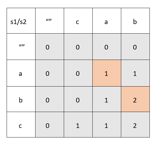 68 |
69 |
70 | ### Case 2 : When str1[i] != str2[j]
71 | When we can move to only right left
72 |
68 |
69 |
70 | ### Case 2 : When str1[i] != str2[j]
71 | When we can move to only right left
72 | 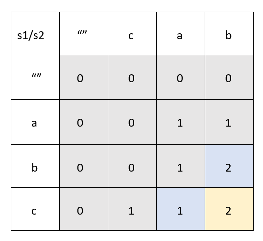 73 |
74 | ```java
75 | public class App {
76 |
77 | public static void main(String[] args) {
78 | System.out.println(longestCommonSubsequence("abc", "cab"));
79 | }
80 |
81 | public static int longestCommonSubsequence(String text1, String text2) {
82 |
83 | int rows = text1.length();
84 | int columns = text2.length();
85 |
86 | if(rows == 0 || columns == 0)
87 | return 0;
88 |
89 | int[][] dpTable = new int[rows+1][columns+1];
90 | for(int i = 1; i <= rows; i++) {
91 | for(int j = 1; j <= columns; j++) {
92 | if(text1.charAt(i-1) == text2.charAt(j-1)) {
93 | dpTable[i][j] = dpTable[i-1][j-1] + 1;
94 | } else {
95 | dpTable[i][j] = Math.max(dpTable[i-1][j], dpTable[i][j-1]);
96 | }
97 | }
98 | }
99 |
100 | System.out.println(subSequence(text1, text2, dpTable));
101 | return dpTable[rows][columns];
102 | }
103 |
104 | public static StringBuilder subSequence(String text1, String text2, int[][] dpTable) {
105 | String subsequence = "";
106 | int row = text1.length();
107 | int column = text2.length();
108 | while(row > 0 && column > 0 && dpTable[row][column] != 0) {
109 | if(dpTable[row][column] == dpTable[row - 1][column]) {
110 | row = row - 1;
111 | } else if(dpTable[row][column] == dpTable[row][column-1]) {
112 | column = column -1;
113 | } else {
114 | subsequence += text1.charAt(row-1);
115 | row = row - 1;
116 | column = column - 1;
117 | }
118 | }
119 | StringBuilder sb = new StringBuilder(subsequence);
120 | return sb.reverse();
121 | }
122 |
123 | }
124 | ```
125 | **Note the order of checks in the `subSequence()` method 💥 , for constructing the subsequence.**
126 |
--------------------------------------------------------------------------------
/Algorithms/Tree/Prim's_Algorithm.md:
--------------------------------------------------------------------------------
1 | # Prim's Algorithm
2 |
3 | - Prim’s algorithm is used to find the Minimum Spanning Tree(MST) of a connected or undirected graph. Spanning Tree of a graph is a subgraph that is also a tree and includes all the vertices. Minimum Spanning Tree is the spanning tree with a minimum edge weight sum.
4 |
5 | ## Algorithm
6 | - Step 1: Keep a track of all the vertices that have been visited and added to the spanning tree.
7 |
8 | - Step 2: Initially the spanning tree is empty.
9 |
10 | - Step 3: Choose a random vertex, and add it to the spanning tree. This becomes the root node.
11 |
12 | - Step 4: Add a new vertex, say x, such that x is not in the already built spanning tree. x is connected to the built spanning tree using minimum weight edge. (Thus, x can be adjacent to any of the nodes that have already been added in the spanning tree).
13 | Adding x to the spanning tree should not form cycles.
14 | - Step 5: Repeat the Step 4, till all the vertices of the graph are added to the spanning tree.
15 |
16 | - Step 6: Print the total cost of the spanning tree.
17 |
18 |
19 | ## Code (In C++)
20 |
21 | #include
73 |
74 | ```java
75 | public class App {
76 |
77 | public static void main(String[] args) {
78 | System.out.println(longestCommonSubsequence("abc", "cab"));
79 | }
80 |
81 | public static int longestCommonSubsequence(String text1, String text2) {
82 |
83 | int rows = text1.length();
84 | int columns = text2.length();
85 |
86 | if(rows == 0 || columns == 0)
87 | return 0;
88 |
89 | int[][] dpTable = new int[rows+1][columns+1];
90 | for(int i = 1; i <= rows; i++) {
91 | for(int j = 1; j <= columns; j++) {
92 | if(text1.charAt(i-1) == text2.charAt(j-1)) {
93 | dpTable[i][j] = dpTable[i-1][j-1] + 1;
94 | } else {
95 | dpTable[i][j] = Math.max(dpTable[i-1][j], dpTable[i][j-1]);
96 | }
97 | }
98 | }
99 |
100 | System.out.println(subSequence(text1, text2, dpTable));
101 | return dpTable[rows][columns];
102 | }
103 |
104 | public static StringBuilder subSequence(String text1, String text2, int[][] dpTable) {
105 | String subsequence = "";
106 | int row = text1.length();
107 | int column = text2.length();
108 | while(row > 0 && column > 0 && dpTable[row][column] != 0) {
109 | if(dpTable[row][column] == dpTable[row - 1][column]) {
110 | row = row - 1;
111 | } else if(dpTable[row][column] == dpTable[row][column-1]) {
112 | column = column -1;
113 | } else {
114 | subsequence += text1.charAt(row-1);
115 | row = row - 1;
116 | column = column - 1;
117 | }
118 | }
119 | StringBuilder sb = new StringBuilder(subsequence);
120 | return sb.reverse();
121 | }
122 |
123 | }
124 | ```
125 | **Note the order of checks in the `subSequence()` method 💥 , for constructing the subsequence.**
126 |
--------------------------------------------------------------------------------
/Algorithms/Tree/Prim's_Algorithm.md:
--------------------------------------------------------------------------------
1 | # Prim's Algorithm
2 |
3 | - Prim’s algorithm is used to find the Minimum Spanning Tree(MST) of a connected or undirected graph. Spanning Tree of a graph is a subgraph that is also a tree and includes all the vertices. Minimum Spanning Tree is the spanning tree with a minimum edge weight sum.
4 |
5 | ## Algorithm
6 | - Step 1: Keep a track of all the vertices that have been visited and added to the spanning tree.
7 |
8 | - Step 2: Initially the spanning tree is empty.
9 |
10 | - Step 3: Choose a random vertex, and add it to the spanning tree. This becomes the root node.
11 |
12 | - Step 4: Add a new vertex, say x, such that x is not in the already built spanning tree. x is connected to the built spanning tree using minimum weight edge. (Thus, x can be adjacent to any of the nodes that have already been added in the spanning tree).
13 | Adding x to the spanning tree should not form cycles.
14 | - Step 5: Repeat the Step 4, till all the vertices of the graph are added to the spanning tree.
15 |
16 | - Step 6: Print the total cost of the spanning tree.
17 |
18 |
19 | ## Code (In C++)
20 |
21 | #includeAlgorithm: The rule is, if the given value (to be searched) is greater than the current node’s value, we continue the search in only the right subtree of the current node. And if the given value is lesser, the search goes on only in the left subtree. Since we are using recursion here, the recursive calls foe the left and the right subtree are referred to as the traversal here.12 | 13 | ### Code for SEARCHING in a BST:- 14 | 15 | ``` 16 | bool searchInTree(node *root, int val) 17 | { 18 | bool a = false, b = false; 19 | if (!root) 20 | return false; 21 | if (root->val == val) 22 | return true; 23 | else if (val > root->val) 24 | a = searchInTree(root->right, val); 25 | else 26 | b = searchInTree(root->left, val); 27 | return a || b; //if it finds the given value in either left or right subtree, TRUE will be returned, otherwise FALSE 28 | } 29 | ``` 30 | 31 | ### Time Complexity:- 32 | For searching an element, we have to traverse all elements. Therefore, searching in binary search tree has worst case time complexity of O(n). In general, time complexity is O(h) where h is height of BST. 33 | 34 | ## INSERTING a node with given value in BST:- 35 | Insertion in BST takes place quite similar to the search algorithm, the only difference being that whenever any of the nodes while traversal is found to be NULL, the given value is inserted there. 36 | 37 |
ALGORITHM: Similar to binary search, if the given value to be inserted is greater than the value of the current node, we traverse in its right subtree, and if given value is lesser than the current node value, we traverse in the left subtree. Our aim is to find an empty branch where we can insert the given value node.38 | 39 | ### Code for INSERTING in a BST:- 40 | 41 | ``` 42 | node *insert(node *root, int val) 43 | { 44 | if (!root) //whenever the current node passed to tbe recursive function is NULL, we know that there's a vacancy here 45 | return new node(val); // creating a new node with the given value and returning that 46 | if (val > root->val) 47 | root->right = insert(root->right, val); 48 | else 49 | root->left = insert(root->left, val); 50 | return root; 51 | } 52 | 53 | ``` 54 | 55 | ### Time Complexity:- 56 | In order to insert an element as left child, we have to traverse all elements. Therefore, insertion in binary tree has worst case complexity of O(n). 57 | 58 | ## DELETION of a node with given value in BST:- 59 | The deletion algorithm in a BST is comparatively easy as compared to that in a Binary Tree. We just have to delete the current node if its value is equal to the given value, and put its right node in its place if it exists, otherwise the left node. 60 | 61 |
ALGORITHM: Let's take an example of the BST, suppose we want to delete the node with value x. We will traverse to that node and see if its right node exists and is not NULL. If it exists, we create a new node with the right node’s value and put it at the current node’s place. If the right node doesn’t exist,we connect the left node in place of the current node.62 | 63 | ### Code for Deleting a node in a BST:- 64 | 65 | ``` 66 | struct node* deleteNode(struct node* root, int key){ 67 | if (root == NULL) return root; //base case of recursion 68 | if (key < root->key) 69 | root->left = deleteNode(root->left, key); //traversing in the left subtree 70 | else if (key > root->key) 71 | root->right = deleteNode(root->right, key); //traversing in the right subtree 72 | else{ 73 | if (root->left == NULL){ //if only right node present 74 | struct node *temp = root->right; 75 | free(root); 76 | return temp; 77 | } 78 | else if (root->right == NULL){ //if only left node present 79 | struct node *temp = root->left; 80 | free(root); 81 | return temp; 82 | } 83 | struct node* temp = minValueNode(root->right); //if both left and right nodes are NULL, none present 84 | root->key = temp->key; 85 | root->right = deleteNode(root->right, temp->key); 86 | } 87 | return root; 88 | } 89 | 90 | ``` 91 | ### Time Complexity:- 92 | For deletion of element, we have to traverse all elements to find that element(assuming we do breadth first traversal). Therefore, deletion in binary tree has worst case complexity of O(n). 93 | 94 | ## Note: 95 | So, now you know why using a BST is a really time efficient data structure. Its basic operations such as insertion, deletion and search take O(log N) time complexity to be processed. -------------------------------------------------------------------------------- /Algorithms/Sorting Algorithms/Quick sort.md: -------------------------------------------------------------------------------- 1 | # ⭐ QUICK SORT 2 | 3 | Quicksort is an in-place sorting algorithm.Quicksort is a divide-and-conquer algorithm. 4 | It works by selecting a 'pivot' element from the array and partitioning the other elements into two sub-arrays, 5 | according to whether they are less than or greater than the pivot. For this reason, 6 | it is sometimes called partition-exchange sort.The sub-arrays are then sorted recursively. 7 | This can be done in-place, requiring small additional amounts of memory to perform the sorting. 8 | #### Example: 9 | 10 | ##### Input: `[9, 0, 1, 12, 3], 0, 4` 11 | ###### input1: `array` 12 | ###### input0: `start index` 13 | ###### input1: `end index` 14 | 15 | ##### Partition phase: 16 | `[9, 0, 1, 12, 3]`
17 | Here, algorithm select `9` as pivot element and swap all the elements less than pivot to the left side of pivot
18 | and large elements to right side.From start index to end index
19 | `[3, 0, 1, 9, 12]`
20 | this is array after first pass as you can see that all the element less than 9 (pivot) are to the left side and large element to right side
21 | **we can also conclude on thing that pivot is in it's sorted position**
22 | ##### Recursion phase 23 | As we get sorted index of pivot element after that we just have to perform same operation of quick sort on other 2 sides of array
24 | ie 25 | ```py 26 | [9, 0, 1, 12, 3] -> pivot [9] 27 | | 28 | [3, 0, 1, 9, 12] -> 9 is at its sorted index 29 | | 30 | | | 31 | [3, 0, 1] -> pivot [3] [12] -> pivot [12] -> sorted 32 | | 33 | [0, 1, 3] -> 3 is its srted index 34 | | 35 | | | 36 | [0, 1] -> pivot [0] no element to right side 37 | | 38 | [0, 1] 39 | | 40 | [1] -> pivot [1] -> sorted 41 | 42 | output -> [0, 1, 3, 9, 12] 43 | ``` 44 | 45 | 46 | 47 | ##### Output: `[0, 1, 3, 9, 12]` 48 | 49 | 50 | ### Pseudo Code 51 | ``` js 52 | // Sorts a (portion of an) array, divides it into partitions, then sorts those 53 | algorithm quicksort(A, lo, hi) is 54 | // If indices are in correct order 55 | if lo < hi then 56 | // Partition array and get pivot index 57 | p := partition(A, lo, hi) 58 | 59 | // Sort the two partitions 60 | quicksort(A, lo, p - 1) // Left side of pivot 61 | quicksort(A, p + 1, hi) // Right side of pivot 62 | 63 | // Divides array into two partitions 64 | algorithm partition(A, lo, hi) is 65 | pivot := A[lo] // The pivot as first element 66 | 67 | // Pivot index 68 | i := lo 69 | 70 | for j := lo+1 to hi do 71 | // If the current element is less than or equal to the pivot 72 | if A[j] <= pivot then 73 | // Move the pivot index forward 74 | i := i + 1 75 | 76 | // Swap the current element with the element at the pivot 77 | swap A[i] with A[j] 78 | // swap last pivot element with low index 79 | swap A[i] with A[lo] 80 | return i // the pivot index 81 | ``` 82 | 83 | ### Code `Python` 84 | ``` py 85 | def partition(arr, start, end): 86 | pivot = arr[start] 87 | i = start 88 | j = i + 1 89 | 90 | while j <= end: 91 | if arr[j] < pivot: 92 | i += 1 93 | temp = arr[j] 94 | arr[j] = arr[i] 95 | arr[i] = temp 96 | j += 1 97 | 98 | temp = arr[start] 99 | arr[start] = arr[i] 100 | arr[i] = temp 101 | 102 | return i 103 | 104 | 105 | def quickSort(arr, start, end): 106 | if start <= end: 107 | index = partition(arr, start, end) 108 | quickSort(arr, start, index - 1) 109 | quickSort(arr, index + 1, end) 110 | 111 | ``` 112 | 113 | ### Quick Sort Optimization 114 | 115 | Quick Sort can be optimized from O(N) and O(N logN) to O(logN) using tail recursion.It reduces the complexity by solving smallest partition first which improves the time complexity of Quick Sort to O(log N). 116 | ### Code `C++` 117 | ``` 118 | void QuickSortOptimized(int arr[],int start,int end){ 119 | while(start
5 | **Master Theorem:** If the sub-problems are of the same size, we use the Master Theorem. Those are the ones where T(n), the number of steps an algorithm makes while solving a problem of size n, is a recurrence of the form:
6 | $[T(n) = aT\left(\frac{n}{b}\right) + g(n)]$ 7 |
where g(n) is a real-valued function. More specifically, the recurrence describes the complexity of an algorithm that divides a problem of size n into a sub-problems each of size n/b. It performs g(n) steps to break down the problem and combine the solutions to its sub-problems. 8 | 9 | # Akra Bazzi Theorem 10 | The Akra Bazzi theorem was developed by Mohammad Akra and Louay Bazzi in the year 1996. It can be applied in the recurrence of the form: 11 |
 12 | or T(n)=$a_1T$($b_1x$+$E_1(x)$)+$a_2T$($b_2x$+$E_2(x)$)+....+$a_kT$($b_kx$+$E_k(x)$)+g(x) 13 |
14 | where, $a_{i}$ and $b_{i}$ are constants such that:
15 | - $n_0$ belongs in R is large enough so that T is well-defined. 16 | - For each i=1,2,\ldots,k: 17 | - the constant $a_i$ >0 18 | - the constant $b_{i}$ lies in (0, 1) 19 | - $|h_i(n)| \in O\left(\frac{n}{\log^2 n}\right)$ 20 | ## Formula 21 | *T(x)=θ($x^p$+$x^p$ $∫_1^x$ (g(u)/ $u^p$ $^+$ $^1$)du )* 22 | ## What is p? 23 | $a_1b_1^p$+$a_2b_2^p$+.....+$a_nb_n^p$ =1 24 |
25 | Therefore, $∑_1^k$ $a_ib_i^p$=1. 26 | ## Examples 27 | 1. T(N) = 2T(N/2)+(N-1). 28 |
Here, a1=2,b1=1/2,g(x)=x-1 29 |
30 | $∑_1^k$ $^=$ $^1$ $a_1b_1^p$=1 31 |
32 | => 2 X $(1/2)^p$ = 1 33 |
34 | => for p=1, the equation becomes 1. 35 |
putting p in formula 36 |
T(x)=θ($x^p$+$x^p$ $∫_1^x$ (g(u)/ $u^p$ $^+$ $^1$)du )
37 | T(x)=θ($x^1$+$x^1$ $∫_1^x$ (u-1/ $u^2$)du ) 38 |
=> θ(x+x $[logx]_1^x$- $[-1/u]_1^x$) 39 |
=> θ(x+x[logx+(1/x)-1]) 40 |
=> θ(x+xlogx+1-x) 41 |
θ(~~x~~+xlogx+1-~~x~~) 42 |
θ(xlogx+1) 43 |
θ(xlogx).
44 | 2. Suppose T(n) is defined as 1 for integers 0 less than equal to n less than equal to 3 and $n^2$ +7/4*T([1/2*n])+T[(3/4*n)] for integers n>3.In applying the Akra–Bazzi method, the first step is to find the value of p for which 45 | In time complexity we ignore constant hence final answer is 7/4 $(1/2)^p$ + $(3/4)^p$=1.In this example,p=2. Then using akra-bazzi theorem:
46 | T(x)=θ($x^p$+$x^p$ $∫_1^x$ (g(u)/ $u^p$ $^+$ $^1$)du ) 47 |
=>θ($x^2$+$x^2$ $∫_1^x$ ($u^2$/ $u^3$ )du )
48 | =>θ($x^2$+$x^2$ lnx) 49 |
=>θ($x^2$ lnx)
50 | 3. T(n)= $1/3T(n/3)+1/n$
51 | Here,a1=1/3,b1=1/3,g(n)=1/n 52 |
$\large\frac{1}{2}\normalsize*\large\frac{1}{2}^p\normalsize=1$
53 | Here,p=-1 satisfies the equation
54 | => $n^{-1}(1+\int_{1}^{n}\large\frac{\frac{1}{u}}{u^{-1+1}}\normalsize du)$ 55 | 56 |
=> $\large\frac{1}{n}\normalsize(1+\int_{1}^{n}$ $\large\frac{1}{u}\normalsize du)$ 57 | 58 | => $\large\frac{1}{n}\normalsize(1+[\log u]_{1}^{n})$ 59 | 60 | => $\large\frac{1}{n}\normalsize(1+\log n)$ 61 | 62 | 63 | => $\theta(\large\frac{\log n}{n}\normalsize)$
64 | 4.T(n)=9T(n/3+logn)+n 65 |
Here,a1=9,b1=1/3,g(n)=n.
66 | from $∑_1^k$ $^=$ $^1$ $a_1b_1^p$=1 67 |
$9*\large\frac{1}{3}^p\normalsize=1$ 68 |
we get p =2 69 |
=> $n^{2}(1+\int_{1}^{n}\large\frac{u}{u^{2+1}}\normalsize du)$ 70 | 71 | => $n^{2}(1+\int_{1}^{n}\large\frac{1}{u^{2}}\normalsize du)$ 72 | 73 | => $n^{2}(1+[-\large\frac{1}{u}\normalsize]_{1}^{n})$ 74 | 75 | => $n^{2}(2-\large\frac{1}{n}\normalsize)$ 76 | 77 | => $2n^{2}-n$ 78 | 79 | => $\theta(n^{2})$ 80 | ## Significance 81 | The Akra–Bazzi method is more useful than most other techniques for determining asymptotic behavior because it covers such a wide variety of cases. Its primary application is the approximation of the running time of many divide-and-conquer algorithms. For example, in the merge sort, the number of comparisons required in the worst case, which is roughly proportional to its runtime, is given recursively as T(1)=0 and 82 |
T(n)=T([1/2*n])+T([1/2*n])+n-1
83 | for integers n>0, and can thus be computed using the Akra–Bazzi method to be θ(nlogn) . 84 | 85 | 86 | 87 | 88 | ## Advantages 89 | - Works for many divides and conquer algorithms. 90 | - Has a lesser constraint over the format of the recurrence than Master’s Theorem. 91 | - p can be calculated using numerical methods for complex recurrence relations. 92 | ## Disadvantages 93 | - Doesn't work if growth of the function g(n) is not bounded polynomial. 94 | - Doesn't deal with ceil and floor functions. 95 |
96 | --- 97 | # Resource 98 | For More Practice You Can Visit: [Link](https://github.com/kunal-kushwaha/DSA-Bootcamp-Java/blob/main/assignments/13-complexities.md) 99 |
100 | For getting clear conception on Time Complexities: [Video](https://youtu.be/mV3wrLBbuuE) 101 | 102 | --- 103 | # Conclusion 104 | This is a documentation of Akra Bazzi theorem. 105 |
106 | Resource for dother examples of Akra Bazzi: 107 | [GeeksforGeeks](https://www.geeksforgeeks.org/akra-bazzi-method-for-finding-the-time-complexities/)
108 | Resource for detailed study of Other DSA topics:[Wizard-of_docs github repo](https://github.com/HackClubRAIT/Wizard-Of-Docs) 109 | --- 110 | --- 111 | Don't forget to give a ⭐ to [Wizard-Of-Docs](https://github.com/HackClubRAIT/Wizard-Of-Docs) and keep contributing. 112 |
113 | Happy Coding! 114 | --- -------------------------------------------------------------------------------- /Algorithms/Segmented Sieve/Segmented Sieve.md: -------------------------------------------------------------------------------- 1 | # Segmented Sieve Algorithm 2 | 3 | A Prime Number has a unique property which states that the number can only be divisible by itself or 1. 4 | 5 | ### Sieve of Eratosthenes 6 | An algorithm known as Sieve of Eratosthenes can distinguish primes upto a given maximum number by marking off the multiples of smaller primes as composite numbers. 7 | 8 | But this algorithm has a disadvantage. 9 | If there is also given a lower limit, then this algorithm would not be much efficient as it would be also finding out primes below the lower limit as part of the process. 10 | This algorithm takes up a lot of unnecessary memory in order to process the calculations. 11 | 12 | 13 | Hence to find out prime numbers within a certain range having a lower limit, Segmented Sieve Algorithm is used which is an adaptation of the Sieve of Eratosthenes Algorithm and works perfectly for given lower and upper boundaries. 14 | 15 | 16 | ## Steps 17 | **Step 1)** A list/vector is created which is going to store all primes upto the root of the higher limit. This is because primes after the root of the higher limit would not be used for determining the primes in the given range. 18 | 19 | **Step 2)** The list is filled with the inital primes, using the Sieve of Eratosthenes method, as it is the most efficient in this case. 20 | 21 | **Step 3)** Then similar to the Sieve of Eratosthenes, the multiples of the initial primes inside that range/segment are marked as composites. 22 | 23 | **Step 4)** The numbers left unmarked are the required primes and is extracted. 24 | 25 | 26 | ## Code using C++ 27 | ```cpp 28 | #include
15 | `Search ternm: 6` 16 | 17 | ## Steps to Perform Ternary Serach: 18 | 19 | - First, we compare the key with the element at mid1. If found equal, we return mid1. 20 | - If not, then we compare the key with the element at mid2. If found equal, we return mid2. 21 | - If not, then we check whether the key is less than the element at mid1. If yes, then recur to the first part. 22 | - If not, then we check whether the key is greater than the element at mid2. If yes, then recur to the third part. 23 | - If not, then we recur to the second (middle) part. 24 | 25 | ## Visual Explanation: 26 | 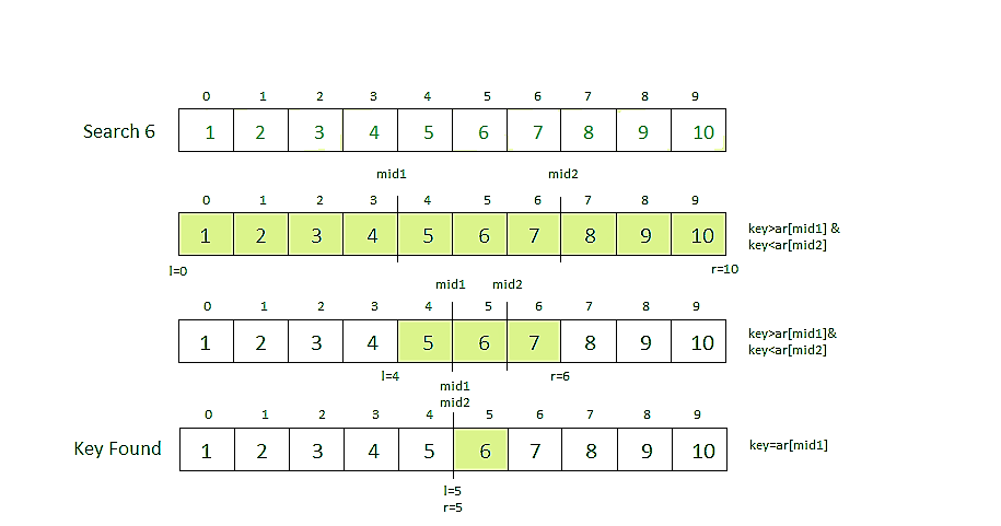
27 | 28 | 29 | ### Pseudo Code (Iterative Approach) 30 | ``` py 31 | function ternary_search(ar, n, key) is 32 | l := 0 33 | r := n − 1 34 | while r >= l do 35 | if key == ar[mid1]: 36 | return mid1 37 | if key == mid2: 38 | return mid2 39 | mid1 = l + (r - l) //3 40 | mid2 = r - (r - l) //3 41 | if key < ar[mid1]: 42 | r = mid1 - 1 43 | else if key > ar[mid2]: 44 | l = mid2 + 1 45 | else: 46 | l = mid1 + 1 47 | r = mid2 - 1 48 | return unsuccessful 49 | ``` 50 | 51 | ### Code `Python` (Iterative Approach) 52 | ``` python 3 53 | def ternarySearch(r, key, ar): 54 | while r >= l: 55 | # Setting the upper and lower bounds 56 | l = 0 57 | r = r-1 58 | 59 | # Find mid1 and mid2 60 | mid1 = l + (r-l) // 3 61 | mid2 = r - (r-l) // 3 62 | 63 | # Check if key is at any mid 64 | if key == ar[mid1]: 65 | return mid1 66 | if key == mid2: 67 | return mid2 68 | 69 | # Since key is not present at mid, 70 | # Check in which region it is present 71 | # Then repeat the search operation in that region 72 | if key < ar[mid1]: 73 | # key lies between l and mid1 74 | r = mid1 - 1 75 | elif key > ar[mid2]: 76 | # key lies between mid2 and r 77 | l = mid2 + 1 78 | else: 79 | # key lies between mid1 and mid2 80 | l = mid1 + 1 81 | r = mid2 - 1 82 | 83 | # key not found 84 | return -1 85 | 86 | # Driver code 87 | if __name__ == '__main__': 88 | # Getting the sorted list 89 | ar = [1, 2, 3, 4, 5, 6, 7, 8, 9, 10] 90 | 91 | # Length of list 92 | r = len(ar) 93 | 94 | ### Test 1 ### 95 | 96 | # Checking for 5 97 | # Key to be searched in the list 98 | key = 5 99 | 100 | # Search the key using ternary search 101 | p = ternarySearch(r, key, ar) 102 | 103 | # Print the result 104 | print(p) 105 | 106 | ### Test 2 ### 107 | 108 | # Checking for 50 109 | # Key to be searched in the list 110 | key = 50 111 | 112 | # Search the key using ternary search 113 | p = ternarySearch(r, key, ar) 114 | 115 | # Print the result 116 | print(p) 117 | ``` 118 | 119 | ### Pseudo Code (Recursive Approach) 120 | ``` py 121 | function ternary_search(ar, n, key) is 122 | l := 0 123 | r := n − 1 124 | if r >= l 125 | if key == ar[mid1]: 126 | return mid1 127 | if key == mid2: 128 | return mid2 129 | mid1 = l + (r - l) //3 130 | mid2 = r - (r - l) //3 131 | if key < ar[mid1]: 132 | ternary_search(l, mid1 - 1, key, ar) 133 | else if key > ar[mid2]: 134 | ternarySearch(mid2 + 1, r, key, ar) 135 | else: 136 | return ternarySearch(mid1 + 1, mid2 - 1, key, ar) 137 | return unsuccessful 138 | ``` 139 | ### Code `Python` (Recursive Approach) 140 | ``` python 3 141 | # Function to perform Ternary Search 142 | def ternarySearch(r, key, ar): 143 | 144 | if (r >= l): 145 | # Setting the upper and lower bounds 146 | l = 0 147 | r = r-1 148 | 149 | # Find the mid1 and mid2 150 | mid1 = l + (r - l) //3 151 | mid2 = r - (r - l) //3 152 | 153 | # Check if key is present at any mid 154 | if (ar[mid1] == key): 155 | return mid1 156 | 157 | if (ar[mid2] == key): 158 | return mid2 159 | 160 | # Since key is not present at mid, 161 | # check in which region it is present 162 | # then repeat the Search operation 163 | # in that region 164 | if (key < ar[mid1]): 165 | 166 | # The key lies in between l and mid1 167 | return ternarySearch(l, mid1 - 1, key, ar) 168 | 169 | elif (key > ar[mid2]): 170 | 171 | # The key lies in between mid2 and r 172 | return ternarySearch(mid2 + 1, r, key, ar) 173 | 174 | else: 175 | 176 | # The key lies in between mid1 and mid2 177 | return ternarySearch(mid1 + 1, 178 | mid2 - 1, key, ar) 179 | 180 | # Key not found 181 | return -1 182 | 183 | # Driver code 184 | if __name__ == '__main__': 185 | # Getting the sorted array 186 | ar = [ 1, 2, 3, 4, 5, 6, 7, 8, 9, 10 ] 187 | 188 | # Starting index 189 | l = 0 190 | 191 | # length of array 192 | r = len(ar) 193 | 194 | ### Test 1 ### 195 | 196 | # Checking for 5 197 | # Key to be searched in the array 198 | key = 5 199 | 200 | # Search the key using ternarySearch 201 | p = ternarySearch(r, key, ar) 202 | 203 | # Print the result 204 | print(p) 205 | 206 | ### Test 2 ### 207 | 208 | # Checking for 50 209 | # Key to be searched in the array 210 | key = 50 211 | 212 | # Search the key using ternarySearch 213 | p = ternarySearch(r, key, ar) 214 | 215 | # Print the result 216 | print(p) 217 | ``` 218 | 219 | 220 | #### ⏲️ Time Complexities: 221 | `O(log``3`` n) (array is divided into 1/3rd of it's size at each iteration/recursive call).` 222 |
223 | #### 👾 Space complexities: 224 | `O(1) (no extra space is used, no extra array space is used).` --------------------------------------------------------------------------------