├── .Rbuildignore
├── .gitignore
├── .idea
└── .gitignore
├── DESCRIPTION
├── NAMESPACE
├── R
├── package.R
├── soccerFlipDirection.R
├── soccerFlow.R
├── soccerHeatmap.R
├── soccerPassmap.R
├── soccerPath.R
├── soccerPitch.R
├── soccerPitchBG.R
├── soccerPitchFG.R
├── soccerPitchHalf.R
├── soccerPositionMap.R
├── soccerResample.R
├── soccerShortenName.R
├── soccerShotmap.R
├── soccerSpokes.R
├── soccerStandardiseCols.R
├── soccerTransform.R
├── soccerVelocity.R
├── soccermatics-deprecated.R
├── soccerxGTimeline.R
├── statsbomb.R
├── tromso.R
└── tromso_extra.R
├── README.md
├── data
├── statsbomb.rda
├── tromso.rda
└── tromso_extra.rda
├── man
├── soccerFlipDirection.Rd
├── soccerFlow.Rd
├── soccerHeatmap.Rd
├── soccerPassmap.Rd
├── soccerPath.Rd
├── soccerPitch.Rd
├── soccerPitchFG.Rd
├── soccerPitchHalf.Rd
├── soccerPositionMap.Rd
├── soccerResample.Rd
├── soccerShortenName.Rd
├── soccerShotmap.Rd
├── soccerSpokes.Rd
├── soccerStandardiseCols.Rd
├── soccerTransform.Rd
├── soccerVelocity.Rd
├── soccermatics-deprecated.Rd
├── soccerxGTimeline.Rd
├── statsbomb.Rd
├── tromso.Rd
└── tromso_extra.Rd
├── pitch_dimensions.csv
├── soccermatics.Rproj
└── soccermatics_0.9.5.pdf
/.Rbuildignore:
--------------------------------------------------------------------------------
1 | ^.*\.Rproj$
2 | ^\.Rproj\.user$
3 |
--------------------------------------------------------------------------------
/.gitignore:
--------------------------------------------------------------------------------
1 | .Rproj.user
2 | .Rhistory
3 | .RData
4 | .Ruserdata
5 | .Rbuildignore
6 | soccermatics.Rproj
7 |
--------------------------------------------------------------------------------
/.idea/.gitignore:
--------------------------------------------------------------------------------
1 | # Default ignored files
2 | /.idea/*
3 |
4 | /shelf/
5 | /workspace.xml
6 | # Datasource local storage ignored files
7 | /dataSources/
8 | /dataSources.local.xml
9 | # Editor-based HTTP Client requests
10 | /httpRequests/
11 |
--------------------------------------------------------------------------------
/DESCRIPTION:
--------------------------------------------------------------------------------
1 | Package: soccermatics
2 | Version: 0.9.5
3 | Authors@R: person("Joe", "Gallagher", email = "joedgallagher@gmail.com", role = c("aut", "cre"))
4 | Title: Visualise football (soccer) tracking and event data
5 | Description: Provides tools to visualise x,y-coordinates of soccer players and event data (e.g. passes, shots). Uses ggplot to draw soccer pitch and overplot expected goal maps, pass maps, average player positions, player heatmaps, individual player paths, player flow fields, and more.
6 | Depends: R (>= 3.4.1)
7 | Imports: cowplot, dplyr, forcats, ggforce, ggplot2, ggrepel, magrittr, MASS, plyr, rlang, scales, tidyr, xts, zoo
8 | License: GPL (>=3.0) Note: Use of the name 'soccermatics' was kindly permitted by David Sumpter and is protected from commercial use under EU copyright law.
9 | Encoding: UTF-8
10 | Collate:
11 | 'package.R'
12 | 'soccerFlipDirection.R'
13 | 'soccerPitch.R'
14 | 'soccerHeatmap.R'
15 | 'soccerSpokes.R'
16 | 'soccerFlow.R'
17 | 'soccerPassmap.R'
18 | 'soccerPath.R'
19 | 'soccerPitchBG.R'
20 | 'soccerPitchFG.R'
21 | 'soccerShotmap.R'
22 | 'soccerPitchHalf.R'
23 | 'soccerPositionMap.R'
24 | 'soccerResample.R'
25 | 'soccerShortenName.R'
26 | 'soccerStandardiseCols.R'
27 | 'soccerTransform.R'
28 | 'soccerVelocity.R'
29 | 'soccermatics-deprecated.R'
30 | 'soccerxGTimeline.R'
31 | 'statsbomb.R'
32 | 'tromso.R'
33 | 'tromso_extra.R'
34 | RoxygenNote: 7.1.1
35 |
--------------------------------------------------------------------------------
/NAMESPACE:
--------------------------------------------------------------------------------
1 | # Generated by roxygen2: do not edit by hand
2 |
3 | export("%>%")
4 | export(soccerFlipDirection)
5 | export(soccerFlow)
6 | export(soccerHeatmap)
7 | export(soccerPassmap)
8 | export(soccerPath)
9 | export(soccerPitch)
10 | export(soccerPitchBG)
11 | export(soccerPitchFG)
12 | export(soccerPitchHalf)
13 | export(soccerPositionMap)
14 | export(soccerResample)
15 | export(soccerShortenName)
16 | export(soccerShotmap)
17 | export(soccerSpokes)
18 | export(soccerStandardiseCols)
19 | export(soccerTransform)
20 | export(soccerVelocity)
21 | export(soccerxGTimeline)
22 | import(dplyr)
23 | import(ggplot2)
24 | importFrom(MASS,kde2d)
25 | importFrom(cowplot,draw_text)
26 | importFrom(dplyr,filter)
27 | importFrom(forcats,fct_explicit_na)
28 | importFrom(ggforce,geom_arc)
29 | importFrom(ggforce,geom_circle)
30 | importFrom(ggrepel,geom_label_repel)
31 | importFrom(ggrepel,geom_text_repel)
32 | importFrom(magrittr,"%>%")
33 | importFrom(plyr,rbind.fill)
34 | importFrom(rlang,"!!")
35 | importFrom(rlang,":=")
36 | importFrom(rlang,enquo)
37 | importFrom(scales,rescale)
38 | importFrom(tidyr,replace_na)
39 | importFrom(xts,xts)
40 | importFrom(zoo,na.approx)
41 |
--------------------------------------------------------------------------------
/R/package.R:
--------------------------------------------------------------------------------
1 | #' @importFrom magrittr %>%
2 | #' @export %>%
3 | NULL
--------------------------------------------------------------------------------
/R/soccerFlipDirection.R:
--------------------------------------------------------------------------------
1 | #' @import ggplot2
2 | #' @import dplyr
3 | #' @importFrom magrittr "%>%"
4 | #' @importFrom ggforce geom_arc geom_circle
5 | #' @importFrom rlang enquo ":=" "!!"
6 | NULL
7 | #' Flips x,y-coordinates horizontally in one half to account for changing sides at half-time
8 | #'
9 | #' @description Normalises direction of attack in both halves of both teams by
10 | #' flipping x,y-coordinates horizontally in either the first or second half;
11 | #' i.e. teams attack in the same direction all game despite changing sides at
12 | #' half-time.
13 | #'
14 | #' @param df dataframe containing unnormalised x,y-coordinates
15 | #' @param lengthPitch,widthPitch length, width of pitch in metres
16 | #' @param teamToFlip character, name of team to flip. If \code{NULL}, all x,y-coordinates in \code{df} will be flipped
17 | #' @param periodToFlip integer, period(s) to flip
18 | #' @param team character, name of variables containing x,y-coordinates
19 | #' @param period character, name of variable containing period labels
20 | #' @param x,y character, name of variables containing x,y-coordinates
21 | #' @return a dataframe
22 | #' @examples
23 | #' library(dplyr)
24 | #'
25 | #' # flip x,y-coords of France in both halves of statsbomb data
26 | #' data(statsbomb)
27 | #' statsbomb %>%
28 | #' soccerFlipDirection(team = "team.name", x = "location.x", y = "location.y",
29 | #' teamToFlip = "France")
30 | #'
31 | #' # flip x,y-coords in 2nd half of Tromso, based on a dummy period variable
32 | #' data(tromso)
33 | #' tromso %>%
34 | #' mutate(period = if_else(t > as.POSIXct("2013-11-07 21:14:00 GMT"), 1, 2)) %>%
35 | #' soccerFlipDirection(periodToFlip = 2)
36 | #'
37 | #' @export
38 | soccerFlipDirection <- function(df, lengthPitch = 105, widthPitch = 68, teamToFlip = NULL, periodToFlip = 1:2, team = "team", period = "period", x = "x", y = "y") {
39 |
40 | # flip all x,y-coordinates in df
41 | if(is.null(teamToFlip)) {
42 | df <- df %>%
43 | mutate(!!x := if_else(!!sym(period) %in% periodToFlip, lengthPitch - !!sym(x), !!sym(x)),
44 | !!y := if_else(!!sym(period) %in% periodToFlip, widthPitch - !!sym(y), !!sym(y)))
45 |
46 | # flip x,y-coords of only one team
47 | } else {
48 | df <- df %>%
49 | mutate(!!x := if_else(!!sym(team) == teamToFlip & !!sym(period) %in% periodToFlip, lengthPitch - !!sym(x), !!sym(x)),
50 | !!y := if_else(!!sym(team) == teamToFlip & !!sym(period) %in% periodToFlip, widthPitch - !!sym(y), !!sym(y)))
51 | }
52 |
53 | return(df)
54 | }
55 |
--------------------------------------------------------------------------------
/R/soccerFlow.R:
--------------------------------------------------------------------------------
1 | #' @include soccerHeatmap.R
2 | #' @include soccerSpokes.R
3 | #' @import ggplot2
4 | #' @import dplyr
5 | #' @importFrom magrittr "%>%"
6 | NULL
7 | #' Draw a flow field of passing direction on a soccer pitch
8 | #' @description A flow field to show the mean angle and distance of passes in zones of the pitch
9 | #'
10 | #' @param df dataframe of event data containing fields of start x,y-coordinates, pass distance, and pass angle
11 | #' @param lengthPitch,widthPitch numeric, length and width of pitch in metres.
12 | #' @param xBins,yBins integer, the number of horizontal (length-wise) and vertical (width-wise) bins the soccer pitch is to be divided up into; if \code{yBins} is NULL (default), it will take the value of \code{xBins}
13 | #' @param x,y,angle,distance names of variables containing pass start x,y-coordinates, angle, and distance
14 | #' @param col colour of arrows
15 | #' @param lwd thickness of arrow segments
16 | #' @param arrow adds team direction of play arrow as right (\code{'r'}) or left (\code{'l'}); \code{'none'} by default
17 | #' @param title,subtitle adds title and subtitle to plot; NULL by default
18 | #' @param theme palette of pitch background and lines, either \code{light} (default), \code{dark}, \code{grey}, or \code{grass}
19 | #' @param plot base plot to add path layer to; NULL by default
20 | #' @return a ggplot object of a heatmap on a soccer pitch
21 | #' @examples
22 | #' library(dplyr)
23 | #' data(statsbomb)
24 | #'
25 | #' # transform x,y-coords, filter only France pass events,
26 | #' # draw flow field showing mean angle, distance of passes per pitch zone
27 | #' statsbomb %>%
28 | #' soccerTransform(method = 'statsbomb') %>%
29 | #' filter(team.name == "France" & type.name == "Pass") %>%
30 | #' soccerFlow(xBins=7, yBins=5,
31 | #' x="location.x", y="location.y", angle="pass.angle", distance="pass.length")
32 | #'
33 | #' # transform x,y-coords, standarise column names,
34 | #' # filter only France pass events
35 | #' my_df <- statsbomb %>%
36 | #' soccerTransform(method = 'statsbomb') %>%
37 | #' soccerStandardiseCols(method = 'statsbomb') %>%
38 | #' filter(team_name == "France" & event_name == "Pass")
39 | #'
40 | #' # overlay flow field onto heatmap showing proportion of team passes per pitch zone
41 | #' soccerHeatmap(my_df, xBins=7, yBins=5) %>%
42 | #' soccerFlow(my_df, xBins=7, yBins=5, plot = .)
43 | #'
44 | #' @seealso \code{\link{soccerHeatmap}} for drawing a heatmap of player position, or \code{\link{soccerSpokes}} for drawing spokes to show all directions in each area of the pitch.
45 | #' @export
46 | soccerFlow <- function(df, lengthPitch = 105, widthPitch = 68, xBins = 5, yBins = NULL, x = "x", y = "y", angle = "angle", distance = "distance", col = "black", lwd = 0.5, arrow = c("none", "r", "l"), title = NULL, subtitle = NULL, theme = c("light", "dark", "grey", "grass"), plot = NULL) {
47 | x.bin<-y.bin<-bin<-x.bin.coord<-y.bin.coord<-angle.mean<-radius.mean<-NULL
48 |
49 | # check value for vertical bins and match to horizontal bins if NULL
50 | if(is.null(yBins)) yBins <- xBins
51 |
52 | # adjust range and n bins
53 | x.range <- seq(0, lengthPitch, length.out = xBins+1)
54 | y.range <- seq(0, widthPitch, length.out = yBins+1)
55 |
56 | # bin plot values
57 | x.bin.coords <- data.frame(x.bin = 1:xBins,
58 | x.bin.coord = (x.range + (lengthPitch / (xBins) / 2))[1:xBins])
59 | y.bin.coords <- data.frame(y.bin = 1:yBins,
60 | y.bin.coord = (y.range + (widthPitch / (yBins) / 2))[1:yBins])
61 |
62 | # bin data
63 | suppressWarnings( #suppress warnings about empty bins
64 | df <- df %>%
65 | rowwise() %>%
66 | mutate(x.bin = max(which(!!sym(x) > x.range)),
67 | y.bin = max(which(!!sym(y) > y.range)),
68 | bin = paste(x.bin, y.bin, sep = "_")) %>%
69 | ungroup() %>%
70 | filter(is.finite(x.bin) & is.finite(y.bin))
71 | )
72 |
73 | # summarise angle for each bin
74 | df <- df %>%
75 | group_by(bin) %>%
76 | mutate(x.mean = mean(!!sym(x), na.rm=T),
77 | y.mean = mean(!!sym(y), na.rm=T),
78 | angle.mean = mean(!!sym(angle), na.rm=T),
79 | radius.mean = mean(!!sym(distance), na.rm=T)) %>%
80 | ungroup()
81 |
82 | # add bin centre x,y-coords for plotting
83 | df <- left_join(df, x.bin.coords, by = "x.bin")
84 | df <- left_join(df, y.bin.coords, by = "y.bin")
85 |
86 | # scale radius
87 | df$radius.mean <- scales::rescale(df$radius.mean, c(2, lengthPitch / xBins))
88 |
89 | if(missing(plot)) {
90 | soccerPitch(lengthPitch = lengthPitch, widthPitch = widthPitch, theme = theme) +
91 | geom_spoke(data = df, aes(x = x.bin.coord, y = y.bin.coord,
92 | angle = angle.mean, radius = radius.mean),
93 | size = lwd, col = col, arrow=arrow(length = unit(0.2,"cm"))) +
94 | guides(fill="none")
95 | } else {
96 | plot +
97 | geom_spoke(data = df, aes(x = x.bin.coord, y = y.bin.coord,
98 | angle = angle.mean, radius = radius.mean),
99 | size = lwd, col = col, arrow=arrow(length = unit(0.2,"cm"))) +
100 | guides(fill="none")
101 | }
102 | }
103 |
--------------------------------------------------------------------------------
/R/soccerHeatmap.R:
--------------------------------------------------------------------------------
1 | #' @include soccerPitch.R
2 | #' @import ggplot2
3 | #' @import dplyr
4 | #' @importFrom magrittr "%>%"
5 | #' @importFrom MASS kde2d
6 | NULL
7 | #' Draw a heatmap on a soccer pitch using any event or tracking data.
8 | #' @description Draws a heatmap showing player position frequency in each area of the pitch and adds soccer pitch outlines.
9 | #'
10 | #' @param df dataframe containing x,y-coordinates of player position
11 | #' @param xBins,yBins integer, the number of horizontal (length-wise) and vertical (width-wise) bins the soccer pitch is to be divided up into. If no value for \code{yBins} is provided, it will take the value of \code{xBins}.
12 | #' @param kde use kernel density estimates for a smoother heatmap; FALSE by default
13 | #' @param lengthPitch,widthPitch numeric, length and width of pitch in metres.
14 | #' @param arrow adds team direction of play arrow as right (\code{'r'}) or left (\code{'l'}); \code{'none'} by default
15 | #' @param colLow,colHigh character, colours for the low and high ends of the heatmap gradient; white and red respectively by default
16 | #' @param title,subtitle adds title and subtitle to plot; NULL by default
17 | #' @param x,y name of variables containing x,y-coordinates
18 | #' @return a ggplot object of a heatmap on a soccer pitch.
19 | #' @details uses \code{ggplot2::geom_bin2d} to map 2D bin counts
20 | #' @examples
21 | #' library(dplyr)
22 | #'
23 | #' # tracking data heatmap with 21x5 zones(~5x5m)
24 | #' data(tromso)
25 | #' tromso %>%
26 | #' filter(id == 8) %>%
27 | #' soccerHeatmap(xBins = 10)
28 | #'
29 | #' # transform x,y-coords, filter only France pressure events,
30 | #' # heatmap with 6x3 zones
31 | #' data(statsbomb)
32 | #' statsbomb %>%
33 | #' soccerTransform(method='statsbomb') %>%
34 | #' filter(type.name == "Pressure" & team.name == "France") %>%
35 | #' soccerHeatmap(x = "location.x", y = "location.y",
36 | #' xBins = 6, yBins = 3, arrow = "r",
37 | #' title = "France (vs Argentina, 30th June 2016)",
38 | #' subtitle = "Defensive pressure heatmap")
39 | #'
40 | #' # transform x,y-coords, standardise column names,
41 | #' # filter player defensive actions, plot kernel density estimate heatmap
42 | #' statsbomb %>%
43 | #' soccerTransform(method='statsbomb') %>%
44 | #' soccerStandardiseCols() %>%
45 | #' filter(event_name %in% c("Duel", "Interception", "Clearance", "Block") &
46 | #' player_name == "Samuel Yves Umtiti") %>%
47 | #' soccerHeatmap(kde = TRUE, arrow = "r",
48 | #' title = "Umtiti (vs Argentina, 30th June 2016)",
49 | #' subtitle = "Defensive actions heatmap")
50 | #'
51 | #' @export
52 | soccerHeatmap <- function(df, lengthPitch = 105, widthPitch = 68, xBins = 10, yBins = NULL, kde = FALSE, arrow = c("none", "r", "l"), colLow = "white", colHigh = "red", title = NULL, subtitle = NULL, x = "x", y = "y") {
53 | z <- NULL
54 |
55 | # ensure input is dataframe
56 | df <- as.data.frame(df)
57 |
58 | # rename variables
59 | df$x <- df[,x]
60 | df$y <- df[,y]
61 |
62 | # zonal heatmap
63 | if(!kde) {
64 | # check value for vertical bins and match to horizontal bins if NULL
65 | if(is.null(yBins)) yBins <- xBins
66 |
67 | # filter invalid values outside pitch limits
68 | df <- df[df$x > 0 & df$x < lengthPitch & df$y > 0 & df$y < widthPitch,]
69 |
70 | # define bin ranges
71 | x.range <- seq(0, lengthPitch, length.out = xBins+1)
72 | y.range <- seq(0, widthPitch, length.out = yBins+1)
73 |
74 | # plot heatmap on blank pitch lines
75 | p <- soccerPitch(lengthPitch, widthPitch, arrow = arrow, title = title, subtitle = subtitle, theme = "blank") +
76 | geom_bin2d(data = df, aes(x, y), binwidth = c(diff(x.range)[1], diff(y.range)[1])) +
77 | scale_fill_gradient(low = colLow, high = colHigh) +
78 | guides(fill="none")
79 |
80 | # redraw pitch lines
81 | p <- soccerPitchFG(p, title = !is.null(subtitle), subtitle = !is.null(title))
82 |
83 | # kernel density estimate heatmap
84 | } else {
85 | dens <- kde2d(df$x, df$y, n=200, lims=c(c(0.25, lengthPitch-0.25), c(0.25, widthPitch-0.25)))
86 | dens_df <- data.frame(expand.grid(x = dens$x, y = dens$y), z = as.vector(dens$z))
87 |
88 | p <- soccerPitch(lengthPitch, widthPitch, arrow = arrow, title = title, subtitle = subtitle, theme = "light") +
89 | geom_tile(data = dens_df, aes(x = x, y = y, fill = z)) +
90 | scale_fill_distiller(palette="Spectral", na.value="white") +
91 | guides(fill="none")
92 |
93 | p <- soccerPitchFG(p, title = !is.null(subtitle), subtitle = !is.null(title))
94 | }
95 |
96 | return(p)
97 |
98 | }
99 |
--------------------------------------------------------------------------------
/R/soccerPassmap.R:
--------------------------------------------------------------------------------
1 | #' @include soccerPitch.R
2 | #' @import ggplot2
3 | #' @import dplyr
4 | #' @importFrom magrittr "%>%"
5 | #' @importFrom ggrepel geom_label_repel
6 | #' @importFrom forcats fct_explicit_na
7 | #' @importFrom scales rescale
8 | NULL
9 | #' Draw a passing network using StatsBomb data
10 | #'
11 | #' @description Draw an undirected passing network of completed passes on pitch from StatsBomb data. Nodes are scaled by number of successful passes; edge width is scaled by number of successful passes between each node pair. Only passes made until first substition shown (ability to specify custom minutes will be added soon). Total number of passes attempted and percentage of completed passes shown. Compatability with other (non-StatsBomb) shot data will be added soon.
12 | #'
13 | #' @param df dataframe containing x,y-coordinates of player passes
14 | #' @param lengthPitch,widthPitch numeric, length and width of pitch, in metres
15 | #' @param minPass minimum number of passes between players for edge to be drawn
16 | #' @param fill,col fill and border colour of nodes
17 | #' @param edgeCol colour of edge lines. Default is complementary to \code{theme} colours.
18 | #' @param edgeAlpha transparency of edge lines, from \code{0} - \code{1}. Defaults to \code{0.6} so overlapping edges are visible.
19 | #' @param label boolean, draw labels
20 | #' @param shortNames shorten player names to display last name as label
21 | #' @param maxNodeSize maximum size of nodes
22 | #' @param maxEdgeSize maximum width of edge lines
23 | #' @param labelSize size of player name labels
24 | #' @param arrow optional, adds team direction of play arrow as right (\code{'r'}) or left (\code{'l'})
25 | #' @param theme draws a \code{light}, \code{dark}, \code{grey}, or \code{grass} coloured pitch
26 | #' @param title adds custom title to plot. Defaults to team name.
27 | #' @examples
28 | #' # France vs. Argentina, minimum of three passes
29 | #' library(dplyr)
30 | #' data(statsbomb)
31 | #'
32 | #' # transform x,y-coords,
33 | #' # Argentina pass map until first substituton with transparent edges
34 | #' statsbomb %>%
35 | #' soccerTransform(method='statsbomb') %>%
36 | #' filter(team.name == "Argentina") %>%
37 | #' soccerPassmap(fill = "lightblue", arrow = "r",
38 | #' title = "Argentina (vs France, 30th June 2018)")
39 | #'
40 | #' # transform x,y-coords,
41 | #' # France pass map until first substitution with opaque edges
42 | #' statsbomb %>%
43 | #' filter(team.name == "France") %>%
44 | #' soccerTransform(method='statsbomb') %>%
45 | #' soccerPassmap(fill = "blue", minPass = 3,
46 | #' maxEdgeSize = 30, edgeCol = "grey40", edgeAlpha = 1,
47 | #' title = "France (vs Argentina, 30th June 2018)")
48 | #' @export
49 | soccerPassmap <- function(df, lengthPitch = 105, widthPitch = 68, minPass = 3, fill = "red", col = "black", edgeAlpha = 0.6, edgeCol = NULL, label = TRUE, shortNames = TRUE, maxNodeSize = 30, maxEdgeSize = 30, labelSize = 4, arrow = c("none", "r", "l"), theme = c("light", "dark", "grey", "grass"), title = NULL) {
50 | type.name<-pass.outcome.name<-period<-timestamp<-player.name<-pass.recipient.name<-from<-to<-xend<-yend<-events<-NULL
51 |
52 | if(length(unique(df$team.name)) > 1) stop("Data contains more than one team")
53 |
54 | # define colours by theme
55 | if(theme[1] == "grass") {
56 | colText <- "white"
57 | if(is.null(edgeCol)) edgeCol <- "black"
58 | } else if(theme[1] == "light") {
59 | colText <- "black"
60 | if(is.null(edgeCol)) edgeCol <- "black"
61 | } else if(theme[1] %in% c("grey", "gray")) {
62 | colText <- "black"
63 | if(is.null(edgeCol)) edgeCol <- "black"
64 | } else {
65 | colText <- "white"
66 | if(is.null(edgeCol)) edgeCol <- "white"
67 | }
68 |
69 | # ensure input is dataframe
70 | df <- as.data.frame(df)
71 |
72 | # set variable names
73 | x <- "location.x"
74 | y <- "location.y"
75 | id <- "player.id"
76 | name <- "player.name"
77 | team <- "team.name"
78 |
79 | df$x <- df[,x]
80 | df$y <- df[,y]
81 | df$id <- df[,id]
82 | df$name <- df[,name]
83 | df$team <- df[,team]
84 |
85 |
86 | # full game passing stats for labels
87 | passes <- df %>%
88 | filter(type.name == "Pass") %>%
89 | group_by(pass.outcome.name) %>%
90 | tally() %>%
91 | filter(!pass.outcome.name %in% c("Injury Clearance", "Unknown")) %>%
92 | mutate(pass.outcome.name = fct_explicit_na(pass.outcome.name, "Complete"))
93 | pass_n <- sum(passes$n)
94 | pass_pc <- passes[passes$pass.outcome.name == "Complete",]$n / pass_n * 100
95 |
96 |
97 | # filter events before time of first substitution, if at least one substitution
98 | min_events <- df %>%
99 | group_by(id) %>%
100 | dplyr::summarise(period = min(period), timestamp = min(timestamp)) %>%
101 | stats::na.omit() %>%
102 | arrange(period, timestamp)
103 |
104 | if(nrow(min_events) > 11) {
105 | max_event <- min_events[12,]
106 | idx <- which(df$period == max_event$period & df$timestamp == max_event$timestamp) - 1
107 | df <- df[1:idx,]
108 | }
109 |
110 |
111 | # get nodes and edges for plotting
112 | # node position and size based on touches
113 | nodes <- df %>%
114 | filter(type.name %in% c("Pass", "Ball Receipt*", "Ball Recovery", "Shot", "Dispossessed", "Interception", "Clearance", "Dribble", "Shot", "Goal Keeper", "Miscontrol", "Error")) %>%
115 | group_by(id, name) %>%
116 | dplyr::summarise(x = mean(x, na.rm=T), y = mean(y, na.rm=T), events = n()) %>%
117 | stats::na.omit() %>%
118 | as.data.frame()
119 |
120 | # edges based only on completed passes
121 | edgelist <- df %>%
122 | mutate(pass.outcome.name = fct_explicit_na(pass.outcome.name, "Complete")) %>%
123 | filter(type.name == "Pass" & pass.outcome.name == "Complete") %>%
124 | select(from = player.name, to = pass.recipient.name) %>%
125 | group_by(from, to) %>%
126 | dplyr::summarise(n = n()) %>%
127 | stats::na.omit()
128 |
129 | edges <- left_join(edgelist,
130 | nodes %>% select(id, name, x, y),
131 | by = c("from" = "name"))
132 |
133 | edges <- left_join(edges,
134 | nodes %>% select(id, name, xend = x, yend = y),
135 | by = c("to" = "name"))
136 |
137 | edges <- edges %>%
138 | group_by(player1 = pmin(from, to), player2 = pmax(from, to)) %>%
139 | dplyr::summarise(n = sum(n), x = x[1], y = y[1], xend = xend[1], yend = yend[1])
140 |
141 |
142 | # filter minimum number of passes and rescale line width
143 | nodes <- nodes %>%
144 | mutate(events = rescale(events, c(2, maxNodeSize), c(1, 200)))
145 |
146 | # rescale node size
147 | edges <- edges %>%
148 | filter(n >= minPass) %>%
149 | mutate(n = rescale(n, c(1, maxEdgeSize), c(minPass, 75)))
150 |
151 |
152 | # shorten player name
153 | if(shortNames) {
154 | nodes$name <- soccerShortenName(nodes$name)
155 | }
156 |
157 | # if no title given, use team
158 | if(is.null(title)) {
159 | title <- unique(df$team)
160 | }
161 |
162 | subtitle <- paste0(min(df$minute)+1, "' - ", max(df$minute)+1, "', ", minPass, "+ passes shown")
163 |
164 | # plot network
165 | p <- soccerPitch(lengthPitch, widthPitch,
166 | arrow = arrow[1], theme = theme[1],
167 | title = title,
168 | subtitle = subtitle) +
169 | geom_segment(data = edges, aes(x, y, xend = xend, yend = yend, size = n), col = edgeCol, alpha = edgeAlpha) +
170 | geom_point(data = nodes, aes(x, y, size = events), pch = 21, fill = fill, col = col) +
171 | scale_size_identity() +
172 | guides(size="none") +
173 | annotate("text", 104, 1, label = paste0("Passes: ", pass_n, "\nCompleted: ", sprintf("%.1f", pass_pc), "%"), hjust = 1, vjust = 0, size = labelSize * 7/8, col = colText)
174 |
175 | # add labels
176 | if(label) {
177 | p <- p +
178 | geom_label_repel(data = nodes, aes(x, y, label = name), size = labelSize)
179 | }
180 |
181 | return(p)
182 |
183 | }
184 |
--------------------------------------------------------------------------------
/R/soccerPath.R:
--------------------------------------------------------------------------------
1 | #' @import ggplot2
2 | #' @import dplyr
3 | #' @importFrom magrittr "%>%"
4 | NULL
5 | #' Draw a path of player trajectory on a soccer pitch using any tracking data
6 | #'
7 | #' @description Draws a path connecting consecutive x,y-coordinates of a player on a soccer pitch.
8 | #'
9 | #' @param df dataframe containing x,y-coordinates of player position
10 | #' @param lengthPitch,widthPitch length and width of pitch in metres
11 | #' @param col colour of path if no \code{'id'} is provided; if an \code{'id'} is present, uses ColorBrewer's 'Paired' palette by default
12 | #' @param arrow adds team direction of play arrow as right (\code{'r'}) or left (\code{'l'}); \code{'none'} by default
13 | #' @param theme draws a \code{light}, \code{dark}, \code{grey}, or \code{grass} coloured pitch
14 | #' @param lwd player path thickness
15 | #' @param title,subtitle adds title and subtitle to plot; NULL by default
16 | #' @param legend boolean, include legend
17 | #' @param x,y name of variables containing x,y-coordinates
18 | #' @param id character, the name of the column containing player identity (only required if \code{'df'} contains multiple players)
19 | #' @param plot base plot to add path layer to; NULL by default
20 | #' @return a ggplot object
21 | #' @examples
22 | #' library(dplyr)
23 | #' data(tromso)
24 | #'
25 | #' # draw path of Tromso #8 over first 3 minutes (1800 frames)
26 | #' tromso %>%
27 | #' filter(id == 8) %>%
28 | #' top_n(1800) %>%
29 | #' soccerPath(col = "red", theme = "grass", arrow = "r")
30 | #'
31 | #' # draw path of all Tromso players over first minute (600 frames)
32 | #' tromso %>%
33 | #' group_by(id) %>%
34 | #' slice(1:1200) %>%
35 | #' soccerPath(id = "id", theme = "light")
36 | #'
37 | #' @export
38 | soccerPath <- function(df, lengthPitch = 105, widthPitch = 68, col = "black", arrow = c("none", "r", "l"), theme = c("light", "dark", "grey", "grass"), lwd = 1, title = NULL, subtitle = NULL, legend = FALSE, x = "x", y = "y", id = NULL, plot = NULL) {
39 |
40 | # ensure input is dataframe
41 | df <- as.data.frame(df)
42 |
43 | if(is.null(id)) {
44 | # one player
45 | if(missing(plot)) {
46 | p <- soccerPitch(lengthPitch, widthPitch, arrow = arrow, theme = theme[1], title = title, subtitle = subtitle) +
47 | geom_path(data = df, aes(x, y), col = col, lwd = lwd)
48 | } else {
49 | p <- plot +
50 | geom_path(data = df, aes(x, y), col = col, lwd = lwd)
51 | }
52 | } else {
53 | # multiple players
54 | if(missing(plot)) {
55 | p <- soccerPitch(lengthPitch, widthPitch, arrow = arrow, theme = theme[1], title = title, subtitle = subtitle) +
56 | geom_path(data = df, aes_string("x", "y", group = id, colour = id), lwd = lwd) +
57 | scale_colour_brewer(type = "seq", palette = "Paired", labels = 1:12)
58 | } else {
59 | p <- plot +
60 | geom_path(data = df, aes_string("x", "y", group = id, colour = id), lwd = lwd) +
61 | scale_colour_brewer(type = "seq", palette = "Paired", labels = 1:12)
62 | }
63 |
64 | #legend
65 | if(legend == FALSE) {
66 | p <- p +
67 | guides(colour="none")
68 | }
69 | }
70 |
71 | return(p)
72 |
73 | }
74 |
--------------------------------------------------------------------------------
/R/soccerPitch.R:
--------------------------------------------------------------------------------
1 | #' @import ggplot2
2 | #' @importFrom dplyr filter
3 | #' @importFrom magrittr "%>%"
4 | #' @importFrom ggforce geom_arc geom_circle
5 | #' @importFrom cowplot draw_text
6 | NULL
7 | #' Plot a full soccer pitch
8 | #'
9 | #' @description Draws a soccer pitch as a ggplot object for the purpose of adding layers such as player positions, player trajectories, etc..
10 | #'
11 | #' @param lengthPitch,widthPitch length and width of pitch in metres
12 | #' @param arrow adds team direction of play arrow as right (\code{'r'}) or left (\code{'l'}); \code{'none'} by default
13 | #' @param title,subtitle adds title and subtitle to plot; NULL by default
14 | #' @param theme palette of pitch background and lines, either \code{light} (default), \code{dark}, \code{grey}, or \code{grass}
15 | #' @param data a default dataset for plotting in subsequent layers; NULL by default
16 | #' @return a ggplot object
17 | #' @examples
18 | #' library(ggplot2)
19 | #' data(statsbomb)
20 | #'
21 | #' # transform Statsbomb coordinates to metre units for plotting
22 | #' my_df <- soccerTransform(statsbomb, method = "statsbomb")
23 | #'
24 | #' # filter events of interest (France defensive pressure events vs. Argentina)
25 | #' my_df <- my_df %>%
26 | #' dplyr::filter(team.name == "France" & type.name == "Pressure")
27 | #'
28 | #' # add custom layers to soccerPitch base
29 | #' soccerPitch(data = my_df,
30 | #' arrow = "r", theme = "grass",
31 | #' title = "France (vs. Argentina)",
32 | #' subtitle = "Pressure events") +
33 | #' geom_point(aes(x = location.x, y = location.y),
34 | #' col = "blue", alpha = 0.5)
35 | #'
36 | #' @export
37 | soccerPitch <- function(lengthPitch = 105, widthPitch = 68, arrow = c("none", "r", "l"), title = NULL, subtitle = NULL, theme = c("light", "dark", "grey", "grass"), data = NULL) {
38 | start<-end<-NULL
39 |
40 | # define colours by theme
41 | if(theme[1] == "grass") {
42 | fill1 <- "#008000"
43 | fill2 <- "#328422"
44 | colPitch <- "grey85"
45 | arrowCol <- "white"
46 | colText <- "white"
47 | } else if(theme[1] == "light") {
48 | fill1 <- "grey98"
49 | fill2 <- "grey98"
50 | colPitch <- "grey60"
51 | arrowCol = "black"
52 | colText <- "black"
53 | } else if(theme[1] %in% c("grey", "gray")) {
54 | fill1 <- "#A3A1A3"
55 | fill2 <- "#A3A1A3"
56 | colPitch <- "white"
57 | arrowCol <- "white"
58 | colText <- "black"
59 | } else if(theme[1] == "dark") {
60 | fill1 <- "#1a1e2c"
61 | fill2 <- "#1a1e2c"
62 | colPitch <- "#F0F0F0"
63 | arrowCol <- "#F0F0F0"
64 | colText <- "#F0F0F0"
65 | } else if(theme[1] == "blank") {
66 | fill1 <- "white"
67 | fill2 <- "white"
68 | colPitch <- "white"
69 | arrowCol <- "black"
70 | colText <- "black"
71 | }
72 | lwd <- 0.5
73 |
74 | # outer border (t,r,b,l)
75 | border <- c(10, 6, 5, 6)
76 |
77 | # mowed grass lines
78 | lines <- (lengthPitch + border[2] + border[4]) / 13
79 | boxes <- data.frame(start = lines * 0:12 - border[4], end = lines * 1:13 - border[2])[seq(2, 12, 2),]
80 |
81 | # draw pitch
82 | p <- ggplot(data) +
83 | # background
84 | geom_rect(aes(xmin = -border[4], xmax = lengthPitch + border[2], ymin = -border[3], ymax = widthPitch + border[1]), fill = fill1) +
85 | # mowed pitch lines
86 | geom_rect(data = boxes, aes(xmin = start, xmax = end, ymin = -border[3], ymax = widthPitch + border[1]), fill = fill2) +
87 | # perimeter line
88 | geom_rect(aes(xmin = 0, xmax = lengthPitch, ymin = 0, ymax = widthPitch), fill = NA, col = colPitch, lwd = lwd) +
89 | # centre circle
90 | geom_circle(aes(x0 = lengthPitch/2, y0 = widthPitch/2, r = 9.15), col = colPitch, lwd = lwd) +
91 | # kick off spot
92 | geom_circle(aes(x0 = lengthPitch/2, y0 = widthPitch/2, r = 0.25), fill = colPitch, col = colPitch, lwd = lwd) +
93 | # halfway line
94 | geom_segment(aes(x = lengthPitch/2, y = 0, xend = lengthPitch/2, yend = widthPitch), col = colPitch, lwd = lwd) +
95 | # penalty arcs
96 | geom_arc(aes(x0= 11, y0 = widthPitch/2, r = 9.15, start = pi/2 + 0.9259284, end = pi/2 - 0.9259284), col = colPitch, lwd = lwd) +
97 | geom_arc(aes(x0 = lengthPitch - 11, y0 = widthPitch/2, r = 9.15, start = pi/2*3 - 0.9259284, end = pi/2*3 + 0.9259284), col = colPitch, lwd = lwd) +
98 | # penalty areas
99 | geom_rect(aes(xmin = 0, xmax = 16.5, ymin = widthPitch/2 - 20.15, ymax = widthPitch/2 + 20.15), fill = NA, col = colPitch, lwd = lwd) +
100 | geom_rect(aes(xmin = lengthPitch - 16.5, xmax = lengthPitch, ymin = widthPitch/2 - 20.15, ymax = widthPitch/2 + 20.15), fill = NA, col = colPitch, lwd = lwd) +
101 | # penalty spots
102 | geom_circle(aes(x0 = 11, y0 = widthPitch/2, r = 0.25), fill = colPitch, col = colPitch, lwd = lwd) +
103 | geom_circle(aes(x0 = lengthPitch - 11, y0 = widthPitch/2, r = 0.25), fill = colPitch, col = colPitch, lwd = lwd) +
104 | # six yard boxes
105 | geom_rect(aes(xmin = 0, xmax = 5.5, ymin = (widthPitch/2) - 9.16, ymax = (widthPitch/2) + 9.16), fill = NA, col = colPitch, lwd = lwd) +
106 | geom_rect(aes(xmin = lengthPitch - 5.5, xmax = lengthPitch, ymin = (widthPitch/2) - 9.16, ymax = (widthPitch/2) + 9.16), fill = NA, col = colPitch, lwd = lwd) +
107 | # goals
108 | geom_rect(aes(xmin = -2, xmax = 0, ymin = (widthPitch/2) - 3.66, ymax = (widthPitch/2) + 3.66), fill = NA, col = colPitch, lwd = lwd) +
109 | geom_rect(aes(xmin = lengthPitch, xmax = lengthPitch + 2, ymin = (widthPitch/2) - 3.66, ymax = (widthPitch/2) + 3.66), fill = NA, col = colPitch, lwd = lwd) +
110 | coord_fixed() +
111 | theme(rect = element_blank(),
112 | line = element_blank(),
113 | axis.text = element_blank(),
114 | axis.title = element_blank())
115 |
116 | # add arrow
117 | if(arrow[1] == "r") {
118 | p <- p +
119 | geom_segment(aes(x = 0, y = -2, xend = lengthPitch / 3, yend = -2), colour = arrowCol, size = 1.5, arrow = arrow(length = unit(0.2, "cm"), type="closed"), linejoin='mitre')
120 | } else if(arrow[1] == "l") {
121 | p <- p +
122 | geom_segment(aes(x = lengthPitch, y = -2, xend = lengthPitch / 3 * 2, yend = -2), colour = arrowCol, size = 1.5, arrow = arrow(length = unit(0.2, "cm"), type="closed"), linejoin='mitre')
123 | }
124 |
125 | # add title and/or subtitle
126 | theme_buffer <- ifelse(theme[1] == "light", 0, 4)
127 | if(!is.null(title) & !is.null(subtitle)) {
128 | p <- p +
129 | draw_text(title,
130 | x = 0, y = widthPitch + 9, hjust = 0, vjust = 1,
131 | size = 15, fontface = 'bold', col = colText) +
132 | draw_text(subtitle,
133 | x = 0, y = widthPitch + 4.5, hjust = 0, vjust = 1,
134 | size = 13, col = colText) +
135 | theme(plot.margin = unit(c(-0.525,-0.9,-0.7,-0.9), "cm"))
136 | } else if(!is.null(title) & is.null(subtitle)) {
137 | p <- p +
138 | draw_text(title,
139 | x = 0, y = widthPitch + 4.5, hjust = 0, vjust = 1,
140 | size = 15, fontface = 'bold', col = colText) +
141 | theme(plot.margin = unit(c(-0.9,-0.9,-0.7,-0.9), "cm"))
142 | } else if(is.null(title) & !is.null(subtitle)) {
143 | p <- p +
144 | draw_text(subtitle,
145 | x = 0, y = widthPitch + 4.5, hjust = 0, vjust = 1,
146 | size = 13, col = colText) +
147 | theme(plot.margin = unit(c(-0.9,-0.9,-0.7,-0.9), "cm"))
148 | } else if(is.null(title) & is.null(subtitle)){
149 | p <- p +
150 | theme(plot.margin = unit(c(-1.2,-0.9,-0.7,-0.9), "cm"))
151 | }
152 |
153 |
154 | return(p)
155 |
156 | }
157 |
--------------------------------------------------------------------------------
/R/soccerPitchBG.R:
--------------------------------------------------------------------------------
1 | #' @import ggplot2
2 | #' @importFrom dplyr filter
3 | #' @importFrom magrittr "%>%"
4 | #' @importFrom ggforce geom_arc geom_circle
5 | #' @importFrom cowplot draw_text
6 | NULL
7 | #' Plot a full soccer pitch
8 | #'
9 | #' @description Draws a soccer pitch as a ggplot object for the purpose of adding layers such as player positions, player trajectories, etc..
10 | #'
11 | #' @param lengthPitch,widthPitch length and width of pitch in metres
12 | #' @param fillPitch,colPitch pitch fill and line colour
13 | #' @param arrow adds team direction of play arrow as right (\code{'r'}) or left (\code{'l'}); \code{'none'} by default
14 | #' @param title,subtitle adds title and subtitle to plot; NULL by default
15 | #' @param theme palette of pitch background and lines, either \code{light} (default), \code{dark}, \code{grey}, or \code{grass}
16 | #' @param data a default dataset for plotting in subsequent layers; NULL by default
17 | #' @return a ggplot object
18 | #' @seealso \code{\link{soccermatics-deprecated}}
19 | #' @keywords internal
20 | #' @rdname soccermatics-deprecated
21 | #' @export
22 | soccerPitchBG <- function(lengthPitch = 105, widthPitch = 68, arrow = c("none", "r", "l"), title = NULL, subtitle = NULL, theme = c("light", "dark", "grey", "grass"), data = NULL) {
23 | .Deprecated("soccerPitch")
24 | start<-end<-NULL
25 |
26 | # define colours by theme
27 | if(theme[1] == "grass") {
28 | fill1 <- "#008000"
29 | fill2 <- "#328422"
30 | colPitch <- "grey85"
31 | arrowCol <- "white"
32 | colText <- "white"
33 | } else if(theme[1] == "light") {
34 | fill1 <- "grey98"
35 | fill2 <- "grey98"
36 | colPitch <- "grey60"
37 | arrowCol = "black"
38 | colText <- "black"
39 | } else if(theme[1] %in% c("grey", "gray")) {
40 | fill1 <- "#A3A1A3"
41 | fill2 <- "#A3A1A3"
42 | colPitch <- "white"
43 | arrowCol <- "white"
44 | colText <- "black"
45 | } else if(theme[1] == "dark") {
46 | fill1 <- "#1C1F26"
47 | fill2 <- "#1C1F26"
48 | colPitch <- "white"
49 | arrowCol <- "white"
50 | colText <- "white"
51 | } else if(theme[1] == "blank") {
52 | fill1 <- "white"
53 | fill2 <- "white"
54 | colPitch <- "white"
55 | arrowCol <- "black"
56 | colText <- "black"
57 | }
58 | lwd <- 0.5
59 |
60 | # outer border (t,r,b,l)
61 | border <- c(10, 6, 5, 6)
62 |
63 | # mowed grass lines
64 | lines <- (lengthPitch + border[2] + border[4]) / 13
65 | boxes <- data.frame(start = lines * 0:12 - border[4], end = lines * 1:13 - border[2])[seq(2, 12, 2),]
66 |
67 | # draw pitch
68 | p <- ggplot(data) +
69 | # background
70 | geom_rect(aes(xmin = -border[4], xmax = lengthPitch + border[2], ymin = -border[3], ymax = widthPitch + border[1]), fill = fill1) +
71 | # mowed pitch lines
72 | geom_rect(data = boxes, aes(xmin = start, xmax = end, ymin = -border[3], ymax = widthPitch + border[1]), fill = fill2) +
73 | # perimeter line
74 | geom_rect(aes(xmin = 0, xmax = lengthPitch, ymin = 0, ymax = widthPitch), fill = NA, col = colPitch, lwd = lwd) +
75 | # centre circle
76 | geom_circle(aes(x0 = lengthPitch/2, y0 = widthPitch/2, r = 9.15), col = colPitch, lwd = lwd) +
77 | # kick off spot
78 | geom_circle(aes(x0 = lengthPitch/2, y0 = widthPitch/2, r = 0.25), fill = colPitch, col = colPitch, lwd = lwd) +
79 | # halfway line
80 | geom_segment(aes(x = lengthPitch/2, y = 0, xend = lengthPitch/2, yend = widthPitch), col = colPitch, lwd = lwd) +
81 | # penalty arcs
82 | geom_arc(aes(x0= 11, y0 = widthPitch/2, r = 9.15, start = pi/2 + 0.9259284, end = pi/2 - 0.9259284), col = colPitch, lwd = lwd) +
83 | geom_arc(aes(x0 = lengthPitch - 11, y0 = widthPitch/2, r = 9.15, start = pi/2*3 - 0.9259284, end = pi/2*3 + 0.9259284), col = colPitch, lwd = lwd) +
84 | # penalty areas
85 | geom_rect(aes(xmin = 0, xmax = 16.5, ymin = widthPitch/2 - 20.15, ymax = widthPitch/2 + 20.15), fill = NA, col = colPitch, lwd = lwd) +
86 | geom_rect(aes(xmin = lengthPitch - 16.5, xmax = lengthPitch, ymin = widthPitch/2 - 20.15, ymax = widthPitch/2 + 20.15), fill = NA, col = colPitch, lwd = lwd) +
87 | # penalty spots
88 | geom_circle(aes(x0 = 11, y0 = widthPitch/2, r = 0.25), fill = colPitch, col = colPitch, lwd = lwd) +
89 | geom_circle(aes(x0 = lengthPitch - 11, y0 = widthPitch/2, r = 0.25), fill = colPitch, col = colPitch, lwd = lwd) +
90 | # six yard boxes
91 | geom_rect(aes(xmin = 0, xmax = 5.5, ymin = (widthPitch/2) - 9.16, ymax = (widthPitch/2) + 9.16), fill = NA, col = colPitch, lwd = lwd) +
92 | geom_rect(aes(xmin = lengthPitch - 5.5, xmax = lengthPitch, ymin = (widthPitch/2) - 9.16, ymax = (widthPitch/2) + 9.16), fill = NA, col = colPitch, lwd = lwd) +
93 | # goals
94 | geom_rect(aes(xmin = -2, xmax = 0, ymin = (widthPitch/2) - 3.66, ymax = (widthPitch/2) + 3.66), fill = NA, col = colPitch, lwd = lwd) +
95 | geom_rect(aes(xmin = lengthPitch, xmax = lengthPitch + 2, ymin = (widthPitch/2) - 3.66, ymax = (widthPitch/2) + 3.66), fill = NA, col = colPitch, lwd = lwd) +
96 | coord_fixed() +
97 | theme(rect = element_blank(),
98 | line = element_blank(),
99 | axis.text = element_blank(),
100 | axis.title = element_blank())
101 |
102 | # add arrow
103 | if(arrow[1] == "r") {
104 | p <- p +
105 | geom_segment(aes(x = 0, y = -2, xend = lengthPitch / 3, yend = -2), colour = arrowCol, size = 1.5, arrow = arrow(length = unit(0.2, "cm"), type="closed"), linejoin='mitre')
106 | } else if(arrow[1] == "l") {
107 | p <- p +
108 | geom_segment(aes(x = lengthPitch, y = -2, xend = lengthPitch / 3 * 2, yend = -2), colour = arrowCol, size = 1.5, arrow = arrow(length = unit(0.2, "cm"), type="closed"), linejoin='mitre')
109 | }
110 |
111 | # add title and/or subtitle
112 | theme_buffer <- ifelse(theme[1] == "light", 0, 4)
113 | if(!is.null(title) & !is.null(subtitle)) {
114 | p <- p +
115 | draw_text(title,
116 | x = 0, y = widthPitch + 9, hjust = 0, vjust = 1,
117 | size = 15, fontface = 'bold', col = colText) +
118 | draw_text(subtitle,
119 | x = 0, y = widthPitch + 4.5, hjust = 0, vjust = 1,
120 | size = 13, col = colText) +
121 | theme(plot.margin = unit(c(-0.525,-0.9,-0.7,-0.9), "cm"))
122 | } else if(!is.null(title) & is.null(subtitle)) {
123 | p <- p +
124 | draw_text(title,
125 | x = 0, y = widthPitch + 4.5, hjust = 0, vjust = 1,
126 | size = 15, fontface = 'bold', col = colText) +
127 | theme(plot.margin = unit(c(-0.9,-0.9,-0.7,-0.9), "cm"))
128 | } else if(is.null(title) & !is.null(subtitle)) {
129 | p <- p +
130 | draw_text(subtitle,
131 | x = 0, y = widthPitch + 4.5, hjust = 0, vjust = 1,
132 | size = 13, col = colText) +
133 | theme(plot.margin = unit(c(-0.9,-0.9,-0.7,-0.9), "cm"))
134 | } else if(is.null(title) & is.null(subtitle)){
135 | p <- p +
136 | theme(plot.margin = unit(c(-1.2,-0.9,-0.7,-0.9), "cm"))
137 | }
138 |
139 |
140 | return(p)
141 |
142 | }
143 |
--------------------------------------------------------------------------------
/R/soccerPitchFG.R:
--------------------------------------------------------------------------------
1 | #' @include soccerPitchFG.R
2 | #' @import ggplot2
3 | #' @import dplyr
4 | #' @importFrom magrittr "%>%"
5 | #' @importFrom ggforce geom_arc geom_circle
6 | NULL
7 | #' Helper function to draw soccer pitch outlines over an existing ggplot object
8 | #'
9 | #' @description Adds soccer pitch outlines (with transparent fill) to an existing ggplot object (e.g. heatmaps, passing maps, etc..)
10 | #'
11 | #' @param plot an existing ggplot object to add pitch lines layer to
12 | #' @param lengthPitch,widthPitch length and width of pitch in metres
13 | #' @param colPitch colour of pitch markings
14 | #' @param arrow adds team direction of play arrow as right (\code{'r'}) or left (\code{'l'}); \code{'none'} by default
15 | #' @param title,subtitle adds title and subtitle to plot; NULL by default
16 | #' @return a ggplot object
17 | #'
18 | #' @seealso \code{\link{soccerPitch}} for plotting a soccer pitch as background layer
19 | #' @export
20 | soccerPitchFG <- function(plot, lengthPitch = 105, widthPitch = 68, colPitch = "black", arrow = c("none", "r", "l"), title = NULL, subtitle = NULL) {
21 |
22 | lwd <- 0.5
23 |
24 | p <- plot +
25 | geom_rect(aes(xmin = -4, xmax = lengthPitch + 4, ymin = -4, ymax = widthPitch + 4), fill = "NA") +
26 | # outer lines
27 | geom_rect(aes(xmin = 0, xmax = lengthPitch, ymin = 0, ymax = widthPitch), fill = "NA", col = colPitch, lwd = lwd) +
28 | # centre circle
29 | geom_circle(aes(x0 = lengthPitch / 2, y0 = widthPitch / 2, r = 9.15), fill = "NA", col = colPitch, lwd = lwd) +
30 | # kick off spot
31 | geom_circle(aes(x0 = lengthPitch / 2, y0 = widthPitch / 2, r = 0.25), fill = colPitch, col = colPitch, lwd = lwd) +
32 | # halfway line
33 | geom_segment(aes(x = lengthPitch / 2, y = 0, xend = lengthPitch / 2, yend = widthPitch), col = colPitch, lwd = lwd) +
34 | # penalty areas
35 | geom_rect(aes(xmin = 0, xmax = 16.5, ymin = widthPitch / 2 - (40.3 / 2), ymax = widthPitch / 2 + (40.3 / 2)), fill = "NA", col = colPitch, lwd = lwd) +
36 | geom_rect(aes(xmin = lengthPitch - 16.5, xmax = lengthPitch, ymin = widthPitch / 2 - (40.3 / 2), ymax = widthPitch / 2 + (40.3 / 2)), fill = "NA", col = colPitch, lwd = lwd) +
37 | # penalty spots
38 | geom_circle(aes(x0 = 11, y0 = widthPitch / 2, r = 0.25), fill = colPitch, col = colPitch, lwd = lwd) +
39 | geom_circle(aes(x0 = lengthPitch - 11, y0 = widthPitch / 2, r = 0.25), fill = colPitch, col = colPitch, lwd = lwd) +
40 | # penalty arcs
41 | geom_arc(aes(x0= 11, y0 = widthPitch/2, r = 9.15, start = pi/2 + 0.9259284, end = pi/2 - 0.9259284), col = colPitch, lwd = lwd) +
42 | geom_arc(aes(x0 = lengthPitch - 11, y0 = widthPitch/2, r = 9.15, start = pi/2*3 - 0.9259284, end = pi/2*3 + 0.9259284), col = colPitch, lwd = lwd) +
43 | # six yard boxes
44 | geom_rect(aes(xmin = 0, xmax = 5.5, ymin = (widthPitch / 2) - 9.16, ymax = (widthPitch / 2) + 9.16), fill = "NA", col = colPitch, lwd = lwd) +
45 | geom_rect(aes(xmin = lengthPitch - 5.5, xmax = lengthPitch, ymin = (widthPitch / 2) - 9.16, ymax = (widthPitch / 2) + 9.16), fill = "NA", col = colPitch, lwd = lwd) +
46 | # goals
47 | geom_rect(aes(xmin = -2, xmax = 0, ymin = (widthPitch / 2) - 3.66, ymax = (widthPitch / 2) + 3.66), fill = "NA", col = colPitch, lwd = lwd) +
48 | geom_rect(aes(xmin = lengthPitch, xmax = lengthPitch + 2, ymin = (widthPitch / 2) - 3.66, ymax = (widthPitch / 2) + 3.66), fill = "NA", col = colPitch, lwd = lwd) +
49 | theme(rect = element_blank(),
50 | line = element_blank(),
51 | axis.text = element_blank(),
52 | axis.title = element_blank())
53 |
54 | # add title and/or subtitle
55 | if(title & subtitle) {
56 | p <- p +
57 | theme(plot.margin = unit(c(-0.525,-0.9,-0.7,-0.9), "cm"))
58 | } else if(title & !subtitle) {
59 | p <- p +
60 | theme(plot.margin = unit(c(-0.9,-0.9,-0.7,-0.9), "cm"))
61 | } else if(!title & subtitle) {
62 | p <- p +
63 | theme(plot.margin = unit(c(-0.9,-0.9,-0.7,-0.9), "cm"))
64 | } else if(!title & !subtitle) {
65 | p <- p +
66 | theme(plot.margin = unit(c(-1.2,-0.9,-0.7,-0.9), "cm"))
67 | }
68 |
69 | return(p)
70 |
71 | }
72 |
--------------------------------------------------------------------------------
/R/soccerPitchHalf.R:
--------------------------------------------------------------------------------
1 | #' @include soccerPitch.R
2 | #' @include soccerShotmap.R
3 | #' @import ggplot2
4 | #' @import dplyr
5 | #' @importFrom magrittr "%>%"
6 | #' @importFrom ggforce geom_arc geom_circle
7 | #' @importFrom cowplot draw_text
8 | NULL
9 | #' Draws a vertical half soccer pitch for the purpose of plotting shotmaps
10 | #'
11 | #' @description Adds soccer pitch outlines (with transparent fill) to an existing ggplot object (e.g. heatmaps, passing maps, etc..)
12 | #'
13 | #' @param lengthPitch,widthPitch length and width of pitch in metres
14 | #' @param arrow adds team direction of play arrow as right (\code{'r'}) or left (\code{'l'}); \code{'none'} by default
15 | #' @param theme palette of pitch background and lines, either \code{light} (default), \code{dark}, \code{grey}, or \code{grass};
16 | #' @param title,subtitle adds title and subtitle to plot; NULL by default
17 | #' @param data a default dataset for plotting in subsequent layers; NULL by default
18 | #' @return a ggplot object
19 | #' @seealso \code{\link{soccerShotmap}} for plotting a shotmap on a half pitch for a single player or \code{\link{soccerPitch}} for drawing a full size soccer pitch
20 | #' @examples
21 | #' library(ggplot2)
22 | #' library(dplyr)
23 | #' data(statsbomb)
24 | #'
25 | #' # normalise data, get non-penalty shots for France,
26 | #' # add boolean variable 'goal' for plotting
27 | #' my_df <- statsbomb %>%
28 | #' soccerTransform(method = 'statsbomb') %>%
29 | #' filter(team.name == "France" &
30 | #' type.name == "Shot" &
31 | #' shot.type.name != 'penalty') %>%
32 | #' mutate(goal = as.factor(if_else(shot.outcome.name == "Goal", 1, 0)))
33 | #'
34 | #' soccerPitchHalf(data = my_df, theme = 'light') +
35 | #' geom_point(aes(x = location.y, y = location.x,
36 | #' size = shot.statsbomb_xg, colour = goal),
37 | #' alpha = 0.7)
38 | #'
39 | #' @export
40 | soccerPitchHalf <- function(lengthPitch = 105, widthPitch = 68, arrow = c("none", "r", "l"), theme = c("light", "dark", "grey", "grass"), title = NULL, subtitle = NULL, data = NULL) {
41 | start<-end<-NULL
42 |
43 | # define colours by theme
44 | if(theme[1] == "grass") {
45 | fill1 <- "#008000"
46 | fill2 <- "#328422"
47 | colPitch <- "grey85"
48 | arrowCol <- "white"
49 | colText <- "white"
50 | } else if(theme[1] == "light") {
51 | fill1 <- "white"
52 | fill2 <- "white"
53 | colPitch <- "grey60"
54 | arrowCol = "black"
55 | colText <- "black"
56 | } else if(theme[1] %in% c("grey", "gray")) {
57 | fill1 <- "#A3A1A3"
58 | fill2 <- "#A3A1A3"
59 | colPitch <- "white"
60 | arrowCol <- "white"
61 | colText <- "black"
62 | } else {
63 | fill1 <- "#1a1e2c"
64 | fill2 <- "#1a1e2c"
65 | colPitch <- "#F0F0F0"
66 | arrowCol <- "#F0F0F0"
67 | colText <- "#F0F0F0"
68 | }
69 | lwd <- 0.5
70 |
71 | # outer border (t,r,b,l)
72 | border <- c(12, 6, 1, 6)
73 |
74 | # mowed grass lines
75 | lines <- (lengthPitch + border[2] + border[4]) / 13
76 | boxes <- data.frame(start = lines * 0:12 - border[4], end = lines * 1:13 - border[2])[seq(2, 12, 2),]
77 |
78 | # draw pitch
79 | p <- ggplot(data) +
80 | # background
81 | geom_rect(aes(xmin = -border[4], xmax = widthPitch + border[2], ymin = lengthPitch/2 - border[3], ymax = lengthPitch + border[1]), fill = fill1) +
82 | # mowed pitch lines
83 | geom_rect(data = boxes, aes(ymin = start, ymax = end, xmin = -border[4], xmax = widthPitch + border[2]), fill = fill2) +
84 | # perimeter line
85 | geom_rect(aes(xmin = 0, xmax = widthPitch, ymin = lengthPitch/2, ymax = lengthPitch), fill = NA, col = colPitch, lwd = lwd) +
86 | # centre circle
87 | geom_arc(aes(x0 = widthPitch/2, y0 = lengthPitch/2, r = 9.15, start = pi/2, end = -pi/2), col = colPitch, lwd = lwd) +
88 | # kick off spot
89 | geom_circle(aes(x0 = widthPitch/2, y0 = lengthPitch/2, r = 0.25), fill = colPitch, col = colPitch, lwd = lwd) +
90 | # halfway line
91 | geom_segment(aes(x = 0, y = lengthPitch/2, xend = widthPitch, yend = lengthPitch/2), col = colPitch, lwd = lwd) +
92 | # penalty arc
93 | geom_arc(aes(x0 = widthPitch/2, y0 = lengthPitch - 11, r = 9.15, start = pi * 0.705, end = 1.295 * pi), col = colPitch, lwd = lwd) +
94 | # penalty area
95 | geom_rect(aes(xmin = widthPitch/2 - 20.15, xmax = widthPitch/2 + 20.15, ymin = lengthPitch - 16.5, ymax = lengthPitch), fill = NA, col = colPitch, lwd = lwd) +
96 | # penalty spot
97 | geom_circle(aes(x0 = widthPitch/2, y0 = lengthPitch - 11, r = 0.25), fill = colPitch, col = colPitch, lwd = lwd) +
98 | # six yard box
99 | geom_rect(aes(xmin = (widthPitch/2) - 9.16, xmax = (widthPitch/2) + 9.16, ymin = lengthPitch - 5.5, ymax = lengthPitch), fill = NA, col = colPitch, lwd = lwd) +
100 | # goal
101 | geom_rect(aes(xmin = (widthPitch/2) - 3.66, xmax = (widthPitch/2) + 3.66, ymin = lengthPitch, ymax = lengthPitch + 2), fill = NA, col = colPitch, lwd = lwd) +
102 | coord_fixed(ylim = c(lengthPitch/2 - border[3], lengthPitch + border[1])) +
103 | theme(rect = element_blank(),
104 | line = element_blank(),
105 | axis.text = element_blank(),
106 | axis.title = element_blank())
107 |
108 | # add title and/or subtitle
109 | theme_buffer <- ifelse(theme[1] == "light", 0, 4)
110 | if(!is.null(title) & !is.null(subtitle)) {
111 | p <- p +
112 | draw_text(title,
113 | x = widthPitch/2, y = lengthPitch + 10, hjust = 0.5, vjust = 1,
114 | size = 15, fontface = 'bold', col = colText) +
115 | draw_text(subtitle,
116 | x = widthPitch/2, y = lengthPitch + 6.5, hjust = 0.5, vjust = 1,
117 | size = 13, col = colText) +
118 | theme(plot.margin = unit(c(-0.7,-1.4,-0.7,-1.4), "cm"))
119 | } else if(!is.null(title) & is.null(subtitle)) {
120 | p <- p +
121 | draw_text(title,
122 | x = widthPitch/2, y = lengthPitch + 6.5, hjust = 0.5, vjust = 1,
123 | size = 15, fontface = 'bold', col = colText) +
124 | theme(plot.margin = unit(c(-1.2,-1.4,-0.7,-1.4), "cm"))
125 | } else if(is.null(title) & !is.null(subtitle)) {
126 | p <- p +
127 | draw_text(subtitle,
128 | x = widthPitch/2, y = lengthPitch + 6.5, hjust = 0.5, vjust = 1,
129 | size = 13, col = colText) +
130 | theme(plot.margin = unit(c(-1.2,-1.4,-0.7,-1.4), "cm"))
131 | } else if(is.null(title) & is.null(subtitle)){
132 | p <- p +
133 | theme(plot.margin = unit(c(-1.85,-1.4,-0.7,-1.4), "cm"))
134 | }
135 |
136 |
137 | return(p)
138 |
139 | }
140 |
--------------------------------------------------------------------------------
/R/soccerPositionMap.R:
--------------------------------------------------------------------------------
1 | #' @include soccerPitch.R
2 | #' @import ggplot2
3 | #' @import dplyr
4 | #' @importFrom magrittr "%>%"
5 | #' @importFrom ggrepel geom_text_repel geom_label_repel
6 | NULL
7 | #' Plot average player position using any event or tracking data
8 | #' @description Draws the average x,y-positions of each player from one or both teams on a soccer pitch.
9 | #'
10 | #' @param df a dataframe containing x,y-coordinates of player position and a player identifier variable
11 | #' @param lengthPitch,widthPitch numeric, length and width of pitch in metres
12 | #' @param fill1,fill2 character, fill colour of position points of team 1, team 2 (team 2 \code{NULL} by default)
13 | #' @param col1,col2 character, border colour of position points of team 1, team 2 (team 2 \code{NULL} by default)
14 | #' @param labelCol character, label text colour
15 | #' @param homeTeam if \code{df} contains two teams, the name of the home team to be displayed on the left hand side of the pitch (i.e. attacking from left to right). If \code{NULL}, infers home team as the team of the first event in \code{df}.
16 | #' @param flipAwayTeam flip x,y-coordinates of away team so attacking from right to left
17 | #' @param label type of label to draw, player names (\code{name}), jersey numbers (\code{number}), or \code{none}
18 | #' @param labelBox add box around label text
19 | #' @param shortNames shorten player names to display last name as label
20 | #' @param nodeSize numeric, size of position points
21 | #' @param labelSize numeric, size of labels
22 | #' @param arrow optional, adds team direction of play arrow as right (\code{'r'}) or left (\code{'l'})
23 | #' @param theme draws a \code{light}, \code{dark}, \code{grey}, or \code{grass} coloured pitch
24 | #' @param title,subtitle optional, adds title and subtitle to plot
25 | #' @param source if \code{statsbomb}, uses StatsBomb definitions of required variable names (i.e. `location.x`, `location.y`, `player.id`, `team.name`); if \code{manual} (default), respects variable names defined in function arguments \code{x}, \code{y}, \code{id}, \code{name}, and \code{team}.
26 | #' @param x,y,id,name,team names of variables containing x,y-coordinates, unique player ids, player names, and team names, respectively; \code{name} and \code{team} NULL by default
27 | #' @examples
28 | #' library(dplyr)
29 | #' data(statsbomb)
30 | #'
31 | #' # average player position from tracking data for one team
32 | #' # w/ jersey numbers labelled
33 | #' data(tromso)
34 | #' tromso %>%
35 | #' soccerPositionMap(label = "number", id ="id",
36 | #' labelCol = "white", nodeSize = 8,
37 | #' arrow = "r", theme = "grass",
38 | #' title = "Tromso IL (vs. Stromsgodset, 3rd Nov 2013)",
39 | #' subtitle = "Average player position (1' - 16')")
40 | #'
41 | #' # transform x,y-coords, standarise column names,
42 | #' # average pass position for one team using 'statsbomb' method
43 | #' # w/ player name as labels
44 | #' statsbomb %>%
45 | #' soccerTransform(method='statsbomb') %>%
46 | #' filter(type.name == "Pass" & team.name == "France" & period == 1) %>%
47 | #' soccerPositionMap(source = "statsbomb",
48 | #' fill1 = "blue", arrow = "r", theme = "light",
49 | #' title = "France (vs Argentina, 30th June 2018)",
50 | #' subtitle = "Average pass position (1' - 45')")
51 | #'
52 | #' # transform x,y-coords, standarise column names,
53 | #' # average pass position for two teams using 'manual' method
54 | #' # w/ player names labelled
55 | #' statsbomb %>%
56 | #' soccerTransform(method='statsbomb') %>%
57 | #' soccerStandardiseCols(method='statsbomb') %>%
58 | #' filter(event_name == "Pass" & period == 1) %>%
59 | #' soccerPositionMap(fill1 = "lightblue", fill2 = "blue",
60 | #' title = "Argentina vs France, 30th June 2018",
61 | #' subtitle = "Average pass position (1' - 45')")
62 | #'
63 | #' @export
64 | soccerPositionMap <- function(df, lengthPitch = 105, widthPitch = 68, fill1 = "red", col1 = NULL, fill2 = "blue", col2 = NULL, labelCol = "black", homeTeam = NULL, flipAwayTeam = TRUE, label = c("name", "number", "none"), labelBox = TRUE, shortNames = TRUE, nodeSize = 5, labelSize = 4, arrow = c("none", "r", "l"), theme = c("light", "dark", "grey", "grass"), title = NULL, subtitle = NULL, source = c("manual", "statsbomb"), x = "x", y = "y", id = "player_id", name = "player_name", team = "team_name") {
65 | x.mean<-y.mean<-NULL
66 |
67 | # define colours by theme
68 | if(theme[1] == "grass") {
69 | colText <- "white"
70 | } else if(theme[1] == "light") {
71 | colText <- "black"
72 | } else if(theme[1] %in% c("grey", "gray")) {
73 | colText <- "black"
74 | } else {
75 | colText <- "white"
76 | }
77 | if(is.null(col1)) col1 <- fill1
78 | if(is.null(col2)) col2 <- fill2
79 |
80 | # ensure input is dataframe
81 | df <- as.data.frame(df)
82 |
83 | # set variable names
84 | if(source[1] == "statsbomb") {
85 | x <- "location.x"
86 | y <- "location.y"
87 | id <- "player.id"
88 | team <- "team.name"
89 | name <- "player.name"
90 | }
91 |
92 | df$x <- df[,x]
93 | df$y <- df[,y]
94 | df$id <- df[,id]
95 | if(!name %in% colnames(df)) {
96 | name <- id
97 | }
98 | df$name <- df[,name]
99 | if(team %in% colnames(df)) {
100 | df$team <- df[,team]
101 | } else {
102 | team <- "Team A"
103 | df$team <- team
104 | }
105 |
106 | # shorten player name
107 | if(!is.null(name) & shortNames == TRUE) {
108 | df$name <- soccerShortenName(df$name)
109 | }
110 |
111 | # if two teams in df
112 | if(length(unique(df$team)) > 1) {
113 |
114 | # home team taken as first team in df if unspecified
115 | if(is.null(homeTeam)) homeTeam <- df[,team][1]
116 |
117 | # flip x,y-coordinates of home team
118 | if(flipAwayTeam) {
119 | df <- df %>%
120 | soccerFlipDirection(teamToFlip = homeTeam, periodToFlip = 1:2)
121 | }
122 |
123 | # get average positions
124 | pos <- df %>%
125 | group_by(team, id, name) %>%
126 | dplyr::summarise(x.mean = mean(x), y.mean = mean(y)) %>%
127 | ungroup() %>%
128 | mutate(team = as.factor(team), id = as.factor(id)) %>%
129 | as.data.frame()
130 |
131 | # plot
132 | p <- soccerPitch(theme = theme[1], title = title, subtitle = subtitle) +
133 | geom_point(data = pos, aes(x.mean, y.mean, group = team, fill = team, colour = team), shape = 21, size = 6, stroke = 1.3) +
134 | scale_colour_manual(values = c(col1, col2)) +
135 | scale_fill_manual(values = c(fill1, fill2)) +
136 | guides(colour="none", fill="none")
137 |
138 | # if one team
139 | } else {
140 | # get average positions
141 | pos <- df %>%
142 | group_by(id, name) %>%
143 | dplyr::summarise(x.mean = mean(x), y.mean = mean(y)) %>%
144 | # ungroup() %>%
145 | # mutate(id = as.factor(id)) %>%
146 | as.data.frame()
147 |
148 | # plot
149 | p <- soccerPitch(arrow = arrow, theme = theme[1], title = title, subtitle = subtitle) +
150 | geom_point(data = pos, aes(x.mean, y.mean), col = col1, fill = fill1, shape = 21, size = nodeSize, stroke = 1.3)
151 | }
152 |
153 | # add non-overlapping names as labels
154 | if(label[1] == "name") {
155 | if(labelBox) {
156 | p <- p +
157 | geom_label_repel(data = pos, aes(x.mean, y.mean, label = name), segment.colour = colText, segment.size = 0.3, max.iter = 1000, size = labelSize, fontface = "bold")
158 | } else {
159 | p <- p +
160 | geom_text_repel(data = pos, aes(x.mean, y.mean, label = name), col = labelCol, segment.colour = colText, segment.size = 0.3, max.iter = 1000, size = labelSize, fontface = "bold")
161 | }
162 | # add jersey numbers directly to points
163 | } else if(label[1] == "number") {
164 | p <- p +
165 | geom_text(data = pos, aes(x.mean, y.mean, label = name), col = labelCol, fontface = "bold")
166 | }
167 |
168 | return(p)
169 |
170 | }
171 |
--------------------------------------------------------------------------------
/R/soccerResample.R:
--------------------------------------------------------------------------------
1 | #' @import ggplot2
2 | #' @import dplyr
3 | #' @importFrom zoo na.approx
4 | #' @importFrom plyr rbind.fill
5 | #' @importFrom xts xts
6 | NULL
7 | #' Resample the frames per second of any tracking data using linear interpolation
8 | #'
9 | #' @description Downsample or upsample any tracking data containing x,y,t data using linear interpolation of x,y-coordinates (plus constant interpolation of all other variables in dataframe)
10 | #'
11 | #' @param df a dataframe containing x,y-coordinates and time variable
12 | #' @param r resampling rate in frames per second
13 | #' @param x,y name of variables containing x,y-coordinates
14 | #' @param t name of variable containing time data
15 | #' @param id name of variable containing player identifier
16 | #' @return a dataframe with interpolated rows added
17 | #' @examples
18 | #' data(tromso)
19 | #'
20 | #' # resample tromso dataset from ~21 fps to 10 fps
21 | #' soccerResample(tromso, r=10)
22 | #'
23 | #' @export
24 | soccerResample <- function(df, r = 10, x = "x", y = "y", t = "t", id = "id") {
25 | Index<-NULL
26 |
27 | # create new time index
28 | time.index <- seq(min(df[,t]), max(df[,t]), by = as.difftime(1/r, units='secs'))
29 |
30 | # remove all rows that have duplicated timestamps
31 | df <- df %>%
32 | group_by(!!sym(id)) %>%
33 | filter(!(duplicated(!!sym(t)) | duplicated(!!sym(t), fromLast = TRUE))) %>%
34 | ungroup()
35 |
36 | # resample and interpolate for each id
37 | ids <- as.numeric(as.vector(unique(df[[id]])))
38 | df_resampled <- lapply(ids, function(i) {
39 | #subset
40 | ss <- df[df[,id] == i,]
41 |
42 | # convert data to xts object
43 | ss.xts <- xts(ss[, names(ss) != t], ss[[t]])
44 |
45 | # join to time index
46 | ss.join <- merge(ss.xts, time.index, all=TRUE) %>%
47 | ggplot2::fortify() %>%
48 | rename_at(vars(Index),~"t")
49 |
50 | # linear interpolatation of x,y-coords with omission of leading / lagging NAs; constant interpolation of other variables
51 | ss.join %>%
52 | mutate_at(vars(-one_of(t, x, y)), function(x) na.approx(x, method = "constant", na.rm=FALSE)) %>%
53 | mutate_at(vars(one_of(x, y)), function(x) na.approx(x, na.rm=FALSE)) %>%
54 | filter(!!sym(t) %in% time.index)
55 |
56 | }) %>%
57 | plyr::rbind.fill()
58 |
59 | # generate frame variable
60 | time.index2 <- data.frame(t = time.index, frame = 1:length(time.index))
61 | names(time.index2)[names(time.index2) == "t"] <- t
62 | df_resampled <- left_join(df_resampled, time.index2, by = t)
63 |
64 | return(df_resampled)
65 |
66 | }
67 |
68 |
--------------------------------------------------------------------------------
/R/soccerShortenName.R:
--------------------------------------------------------------------------------
1 | #' Extract player surname
2 | #' @description Helper function to extract last name (including common nobiliary particles) from full player names
3 | #'
4 | #' @param names vector of strings containing full player name
5 | #' @examples
6 | #' data(statsbomb)
7 | #' statsbomb$name <- soccerShortenName(statsbomb$player.name)
8 | #'
9 | #' @export
10 | soccerShortenName <- function(names) {
11 |
12 | # collapse special cases with >1 prefix separated by a space
13 | names <- sub("van der", "_vander_", names)
14 | names <- sub("van de", "_vande_", names)
15 |
16 | # define prefixes
17 | prefixes <- " (Di|di|De|de|El|el|Da|da|Dos|dos|Van|van|Von|von|Le|le|La|la|N'|_vander_|_vande_) "
18 |
19 | # remove all of string before last name and any defined prefixes
20 | names <- sub(":", " ", sub(".* ", "", sub(prefixes, " \\1:", names)))
21 |
22 | # expand special cases
23 | names <- sub("_vander_", "van der", names)
24 | names <- sub("_vande_", "van de", names)
25 |
26 | return(names)
27 |
28 | }
29 |
--------------------------------------------------------------------------------
/R/soccerShotmap.R:
--------------------------------------------------------------------------------
1 | #' @include soccerPitch.R
2 | #' @include soccerPitchHalf.R
3 | #' @import ggplot2
4 | #' @import dplyr
5 | #' @importFrom magrittr "%>%"
6 | #' @importFrom cowplot draw_text
7 | NULL
8 | #' Draw an individual, team, or two team shotmap using StatsBomb data
9 | #'
10 | #' @description If \code{df} contains two teams, draws a shotmap of each team at either end of a full pitch. If \code{df} contains one or more players from a single team, draws a vertical half pitch. Currently only works with StatsBomb data but compatability with other (non-StatsBomb) shot data will be added soon.
11 | #'
12 | #' @param df dataframe containing x,y-coordinates of player passes
13 | #' @param lengthPitch,widthPitch length and width of pitch, in metres
14 | #' @param homeTeam if \code{df} contains two teams, the name of the home team to be displayed on the left hand side of the pitch. If \code{NULL}, infers home team as the team of the first event in \code{df}.
15 | #' @param adj adjust xG using conditional probability to account for multiple shots per possession
16 | #' @param n_players number of highest xG players to display
17 | #' @param size_lim minimum and maximum size of points, \code{c(min, max)}
18 | #' @param theme draws a \code{light}, \code{dark}, \code{grey}, or \code{grass} coloured pitch with appropriate point colours
19 | #' @param title,subtitle optional, adds title and subtitle to half pitch plot. Title defaults to scoreline and team identity when two teams are defined in \code{df}.
20 | #' @return a ggplot object
21 | #' @examples
22 | #' data(statsbomb)
23 | #'
24 | #' # shot map of two teams on full pitch
25 | #' statsbomb %>%
26 | #' soccerTransform(method='statsbomb') %>%
27 | #' soccerShotmap(theme = "gray")
28 | #'
29 | #' # shot map of one player on half pitch
30 | #' statsbomb %>%
31 | #' dplyr::filter(player.name == "Antoine Griezmann") %>%
32 | #' soccerTransform(method='statsbomb') %>%
33 | #' soccerShotmap(theme = "grass",
34 | #' title = "Antoine Griezmann",
35 | #' subtitle = "vs. Argentina, World Cup 2018")
36 | #'
37 | #' @export
38 | soccerShotmap <- function(df, lengthPitch = 105, widthPitch = 68, homeTeam = NULL, adj = TRUE, n_players = 0, size_lim = c(2,15), title = NULL, subtitle = NULL, theme = c("light", "dark", "grey", "grass")) {
39 | shot.type.name<-team.name<-shot.statsbomb_xg<-type.name<-shot.outcome<-penalty<-possession<-xg_cond<-xg_adj<-size<-location.x<-location.y<-player.name<-name<-rowid<-x<-y<-label<-hjust<-.<-position_name<-shot.outcome.name<-position.name<-NULL
40 |
41 | # define colours by theme
42 | if(theme[1] == "grass") {
43 | colGoal <- "#E77100"
44 | colMiss <- "#234987"
45 | colText <- "white"
46 | } else if(theme[1] == "light") {
47 | colGoal <- "#E77100"
48 | colMiss <- "#93a5c1"
49 | colText <- "black"
50 | } else if(theme[1] %in% c("grey", "gray")) {
51 | colGoal <- "#efa340"
52 | colMiss <- "#4c6896"
53 | colText <- "black"
54 | } else {
55 | colGoal <- "#E77100"
56 | colMiss <- "#88adea"
57 | colText <- "white"
58 | }
59 |
60 | # ensure input is dataframe
61 | df <- as.data.frame(df)
62 |
63 | # full pitch shotmap for two teams
64 | if(length(unique(df$team.name)) > 1) {
65 |
66 | # home team taken as first team in df if unspecified
67 | if(is.null(homeTeam)) homeTeam <- df$team.name[1]
68 | awayTeam <- unique(df$team.name)[unique(df$team.name) != homeTeam]
69 |
70 | # flip x,y-coordinates of home team and factorise variables
71 | df <- df %>%
72 | soccerFlipDirection(teamToFlip = homeTeam, x = "location.x", y = "location.y", team = "team.name") %>%
73 | mutate(shot.outcome = as.factor(if_else(shot.outcome.name == "Goal", 1, 0)),
74 | penalty = as.factor(if_else(shot.type.name == "Penalty", 1, 0)),
75 | team.name = factor(team.name, levels = c(homeTeam, awayTeam))) %>%
76 | rename(xg = shot.statsbomb_xg)
77 |
78 | # actual goals (including own goals)
79 | goals <- df %>%
80 | group_by(team.name) %>%
81 | filter(type.name == "Shot") %>%
82 | dplyr::summarise(g = length(shot.outcome.name[shot.outcome.name == "Goal"]) + length(type.name[type.name == "Own Goal For"]))
83 |
84 | # penalties
85 | pen_totals <- df %>%
86 | group_by(team.name) %>%
87 | filter(type.name == "Shot") %>%
88 | dplyr::summarise(pen = length(shot.outcome[penalty == 1 & shot.outcome == 1]))
89 |
90 | # own goals
91 | og_totals <- df %>%
92 | group_by(team.name) %>%
93 | dplyr::summarise(og = length(type.name[type.name == "Own Goal For"]))
94 |
95 | # adjust xG using conditional probability when there are multiple shots in a single possession
96 | if(adj) {
97 | df <- df %>%
98 | filter(type.name == "Shot" & penalty == 0) %>%
99 | group_by(team.name, possession) %>%
100 | mutate(xg_cond = (1 - prod(1 - xg))) %>%
101 | mutate(xg_adj = xg_cond * (xg / sum(xg))) %>%
102 | ungroup() %>%
103 | select(-xg, -xg_cond) %>%
104 | rename(xg = xg_adj)
105 | }
106 |
107 | # expected goals
108 | xg_totals <- df %>%
109 | filter(penalty == 0) %>%
110 | group_by(team.name) %>%
111 | dplyr::summarise(xg = sum(xg))
112 |
113 | # labels
114 | score1 <- goals$g[1] + og_totals$og[1]
115 | score2 <- goals$g[2] + og_totals$og[2]
116 |
117 | xg1 <- sprintf("%.2f", xg_totals$xg[1])
118 | if(pen_totals$pen[1] > 0 & og_totals$og[1] == 0) {
119 | xg1 <- paste0("(+", pen_totals$pen[1], " P) ", xg1)
120 | } else if(pen_totals$pen[1] == 0 & og_totals$og[1] > 0) {
121 | xg1 <- paste0("(+", og_totals$og[1], " OG) ", xg1)
122 | } else if(pen_totals$pen[1] > 0 & og_totals$og[1] > 0) {
123 | xg1 <- paste0("(+", pen_totals$pen[1], " P, +", og_totals$og[1], " OG) ", xg1)
124 | }
125 | xg2 <- sprintf("%.2f", xg_totals$xg[2])
126 | if(pen_totals$pen[2] > 0) {
127 | xg2 <- paste0(xg2, " (+", pen_totals$pen[2], " P)")
128 | } else if(pen_totals$pen[2] == 0 & og_totals$og[2] > 0) {
129 | xg2 <- paste0(xg2, " (+", og_totals$og[2], " OG)")
130 | } else if(pen_totals$pen[2] > 0 & og_totals$og[2] > 0) {
131 | xg2 <- paste0(xg2, " (+", pen_totals$pen[2], " P, +", og_totals$og[2], " OG) )")
132 | }
133 |
134 | # subset shots for plotting
135 | df <- df %>%
136 | filter(type.name == "Shot" & penalty == 0) %>%
137 | mutate(size = scales::rescale(xg, size_lim, c(0, 1))) %>%
138 | arrange(as.numeric(shot.outcome), size)
139 |
140 | # plot
141 | p <- soccerPitch(lengthPitch, widthPitch, theme = theme[1]) +
142 | geom_point(data = df, aes(x = location.x, y = location.y, size = size, colour = shot.outcome), alpha = 0.8) +
143 | scale_size_identity() +
144 | scale_colour_manual(name = "Outcome", breaks = c(0,1), values = c(colMiss, colGoal)) +
145 | guides(colour="none", size="none")
146 |
147 | # add labels
148 | p <- p +
149 | draw_text(paste0(xg_totals$team.name[1], " ", score1), x = lengthPitch / 2 - 1, y = widthPitch + 5, hjust = 1, vjust = 1, size = 15, fontface = 'bold', colour = colText) +
150 | draw_text(":", x = lengthPitch / 2, y = widthPitch + 5, hjust = 0.5, vjust = 1, size = 15, fontface = 'bold', colour = colText) +
151 | draw_text(paste0(score2, " ", xg_totals$team.name[2]), x = lengthPitch / 2 + 1, y = widthPitch + 5, hjust = 0, vjust = 1, size = 15, fontface = 'bold', colour = colText) +
152 | draw_text(xg1, x = lengthPitch / 2 - 1, y = widthPitch - 5, hjust = 1, vjust = 0, size = 15, colour = colText) +
153 | draw_text(xg2, x = lengthPitch / 2 + 1, y = widthPitch - 5, hjust = 0, vjust = 0, size = 15, colour = colText) +
154 | theme(plot.margin = unit(c(-0.9,-0.9,-0.7,-0.9), "cm"))
155 |
156 | # top xG by player
157 | if(n_players > 0) {
158 | top_xgs <- df %>%
159 | group_by(player.name, team.name) %>%
160 | summarise(xg = sum(xg, na.rm=T)) %>%
161 | ungroup() %>%
162 | mutate(name = soccerShortenName(player.name)) %>%
163 | arrange(-xg) %>%
164 | utils::head(n_players) %>%
165 | group_by(team.name) %>%
166 | mutate(rowid = 1:n()) %>%
167 | ungroup() %>%
168 | mutate(label = if_else(team.name == homeTeam,
169 | sprintf("%s %s", name, sprintf("%.2f", xg)),
170 | sprintf("%s %s", sprintf("%.2f", xg), name)),
171 | x = if_else(team.name == homeTeam, lengthPitch/2 - 1, lengthPitch/2 + 1),
172 | hjust = if_else(team.name == homeTeam, 1, 0),
173 | y = widthPitch - 5 - (rowid * 2.5))
174 |
175 | p <- p +
176 | geom_text(data = top_xgs[top_xgs$team.name == homeTeam,], aes(x, y, label = label, hjust = hjust), size = 4, colour = colText) +
177 | geom_text(data = top_xgs[top_xgs$team.name != homeTeam,], aes(x, y, label = label, hjust = hjust), size = 4, colour = colText)
178 | }
179 |
180 | # half pitch if one team
181 | } else {
182 |
183 | df <- df %>%
184 | mutate(shot.outcome = as.factor(if_else(shot.outcome.name == "Goal", 1, 0)),
185 | penalty = as.factor(if_else(shot.type.name == "Penalty", 1, 0))) %>%
186 | rename(xg = shot.statsbomb_xg)
187 |
188 | # goals
189 | goals <- df %>%
190 | filter(type.name == "Shot") %>%
191 | dplyr::summarise(g = length(shot.outcome.name[shot.outcome.name == "Goal"]) + length(type.name[type.name == "Own Goal For"]))
192 |
193 | # penalties
194 | pen_totals <- df %>%
195 | filter(type.name == "Shot") %>%
196 | dplyr::summarise(pen = length(shot.outcome[penalty == 1 & shot.outcome == 1]))
197 |
198 | # adjust xG using conditional probability when multiple shots in a single possession
199 | if(adj) {
200 | df <- df %>%
201 | filter(type.name == "Shot" & penalty == 0) %>%
202 | group_by(team.name, possession) %>%
203 | mutate(xg_cond = (1 - prod(1 - xg))) %>%
204 | mutate(xg_adj = xg_cond * (xg / sum(xg))) %>%
205 | ungroup() %>%
206 | select(-xg, -xg_cond) %>%
207 | rename(xg = xg_adj)
208 | }
209 |
210 | # expected goals
211 | xg <- df %>%
212 | filter(penalty == 0) %>%
213 | dplyr::summarise(xg = sum(xg)) %>%
214 | pull %>%
215 | sprintf("%.2f", .)
216 |
217 | df <- df %>%
218 | filter(type.name == "Shot" & penalty == 0) %>%
219 | mutate(size = scales::rescale(xg, size_lim, c(0, 1))) %>%
220 | arrange(as.numeric(shot.outcome), size)
221 |
222 | p <- soccerPitchHalf(lengthPitch, widthPitch, theme = theme[1], title = title, subtitle = subtitle) +
223 | geom_point(data = df, aes(x = location.y, y = location.x, size = size, colour = shot.outcome), alpha = 0.7) +
224 | scale_size_identity() +
225 | scale_colour_manual(name = "Outcome", breaks = c(0,1), values = c(colMiss, colGoal)) +
226 | guides(colour="none", size="none")
227 |
228 | # top xG by player
229 | if(n_players > 0) {
230 | top_xgs <- df %>%
231 | group_by(player.name, position.name) %>%
232 | summarise(xg = sum(xg, na.rm=T)) %>%
233 | ungroup() %>%
234 | mutate(name = soccerShortenName(player.name)) %>%
235 | arrange(-xg) %>%
236 | slice(1:n_players) %>%
237 | arrange(xg) %>%
238 | mutate(rowid = 1:n()) %>%
239 | mutate(label = sprintf("%s %s", sprintf("%.2f", xg), name),
240 | y = lengthPitch/2 + (rowid * 2.5))
241 |
242 | p <- p +
243 | geom_text(data = top_xgs, aes(x = 2, y, label = label, hjust = 0), size = 4, colour = colText) +
244 | annotate("text", x = 2, y = lengthPitch/2 + 6 + max(top_xgs$rowid * 2.5), label = paste0("Goals: ", goals$g), hjust = 0, vjust = 0, size = 5, colour = colText) +
245 | annotate("text", x = 2, y = lengthPitch/2 + 2 + max(top_xgs$rowid * 2.5), label = paste0("xG: ", xg), hjust = 0, vjust = 0, size = 5, colour = colText)
246 | } else {
247 | p <- p +
248 | annotate("text", x = 2, y = lengthPitch/2 + 6, label = paste0("Goals: ", goals$g), hjust = 0, vjust = 0, size = 5, colour = colText) +
249 | annotate("text", x = 2, y = lengthPitch/2 + 2, label = paste0("xG: ", xg), hjust = 0, vjust = 0, size = 5, colour = colText)
250 | }
251 |
252 | }
253 |
254 | return(p)
255 |
256 | }
257 |
--------------------------------------------------------------------------------
/R/soccerSpokes.R:
--------------------------------------------------------------------------------
1 | #' @include soccerHeatmap.R
2 | #' @include soccerFlow.R
3 | #' @import ggplot2
4 | #' @import dplyr
5 | NULL
6 | #' Draw spokes of passing direction on a soccer pitch
7 | #'
8 | #' @description Multiple arrows to show the distribution of pass angle and distance in zones of the pitch; similar to a radar plot but grouped by pitch location rather than player
9 | #'
10 | #' @param df a dataframe of event data containing fields of start x,y-coordinates, pass distance, and pass angle
11 | #' @param lengthPitch,widthPitch numeric, length and width of pitch in metres
12 | #' @param xBins,yBins integer, the number of horizontal (length-wise) and vertical (width-wise) bins the soccer pitch is to be divided up into; if \code{yBins} is NULL (default), it will take the value of \code{xBins}
13 | #' @param angleBins integer, the number of arrows to draw in each zone of the pitch; for example, a value of 4 clusters has direction vectors up, down, left, and right
14 | #' @param x,y,angle names of variables containing pass start x,y-coordinates and angle
15 | #' @param minLength numeric, ratio between size of shortest arrow and longest arrow depending on number of events
16 | #' @param minAlpha,minWidth numeric, minimum alpha and line width of arrows drawn
17 | #' @param col colour of arrows
18 | #' @param legend if \code{TRUE}, adds legend for arrow transparency
19 | #' @param arrow adds team direction of play arrow as right (\code{'r'}) or left (\code{'l'}); \code{'none'} by default
20 | #' @param title,subtitle adds title and subtitle to plot; NULL by default
21 | #' @param theme palette of pitch background and lines, either \code{light} (default), \code{dark}, \code{grey}, or \code{grass}
22 | #' @param plot base plot to add path layer to; NULL by default
23 | #' @return a ggplot object of a heatmap on a soccer pitch
24 | #' @examples
25 | #' library(dplyr)
26 | #' data(statsbomb)
27 | #'
28 | #' # transform x,y-coords, filter only France pass events,
29 | #' # draw flow field showing mean angle, distance of passes per pitch zone
30 | #' statsbomb %>%
31 | #' soccerTransform(method = 'statsbomb') %>%
32 | #' filter(team.name == "France" & type.name == "Pass") %>%
33 | #' soccerSpokes(xBins=7, yBins=5, angleBins=12, legend=FALSE)
34 | #'
35 | #' # transform x,y-coords, standarise column names,
36 | #' # filter only France pass events
37 | #' my_df <- statsbomb %>%
38 | #' soccerTransform(method = 'statsbomb') %>%
39 | #' soccerStandardiseCols(method = 'statsbomb') %>%
40 | #' filter(team_name == "France" & event_name == "Pass")
41 | #'
42 | #' # overlay flow field onto heatmap showing proportion of team passes per pitch zone
43 | #' soccerHeatmap(my_df, xBins=7, yBins=5,
44 | #' title = "France passing radar") %>%
45 | #' soccerSpokes(my_df, xBins=7, yBins=5, angleBins=8, legend=FALSE, plot = .)
46 | #'
47 | #' @seealso \code{\link{soccerHeatmap}} for drawing a heatmap of player position, or \code{\link{soccerFlow}} for drawing a single arrow for pass distance and angle per pitch zone.
48 | #' @export
49 | soccerSpokes <- function(df, lengthPitch=105, widthPitch=68, xBins=5, yBins=NULL, angleBins=8, x="x", y="y", angle="angle", minLength=0.6, minAlpha=0.5, minWidth=0.5, col="black", legend=TRUE, arrow=c("none", "r", "l"), title=NULL, subtitle=NULL, theme=c("light", "dark", "grey", "grass"), plot=NULL) {
50 | x.bin<-y.bin<-bin<-x.bin.coord<-y.bin.coord<-angle.theta<-radius<-lwd<-NULL
51 |
52 | border <- c(4, 4, 4, 4)
53 |
54 | # check value for vertical bins and match to horizontal bins if NULL
55 | if(is.null(yBins)) yBins <- xBins
56 |
57 | x.range <- seq(0, lengthPitch, length.out=xBins+1)
58 | y.range <- seq(0, widthPitch, length.out=yBins+1)
59 |
60 | angle.bin <- seq(-pi, pi, length.out=angleBins+1)
61 |
62 | # bin plot values
63 | x.bin.coords <- data.frame(x.bin=1:xBins,
64 | x.bin.coord=(x.range + (lengthPitch / (xBins) / 2))[1:xBins])
65 | y.bin.coords <- data.frame(y.bin=1:yBins,
66 | y.bin.coord=(y.range + (widthPitch / (yBins) / 2))[1:yBins])
67 |
68 | angle.bin.theta <- data.frame(angle.bin=1:angleBins,
69 | angle.theta=angle.bin[1:angleBins])
70 |
71 | # bin by x,y
72 | suppressWarnings( #suppress warnings about empty bins
73 | df <- df %>%
74 | rowwise() %>%
75 | mutate(x.bin=max(which(!!sym(x) > x.range)),
76 | y.bin=max(which(!!sym(y) > y.range)),
77 | bin=paste(x.bin, y.bin, sep="_")) %>%
78 | ungroup() %>%
79 | filter(is.finite(x.bin) & is.finite(y.bin))
80 | )
81 |
82 | # bin by angle
83 | suppressWarnings( #suppress warnings about empty bins
84 | df <- df %>%
85 | group_by(bin) %>%
86 | rowwise() %>%
87 | mutate(angle.bin=max(which(!!sym(angle) > angle.bin))) %>%
88 | ungroup() %>%
89 | filter(is.finite(angle.bin))
90 | )
91 |
92 | # count number of events in each angle bin
93 | df <- df %>%
94 | group_by(bin, angle.bin) %>%
95 | summarise(n.angles=n(),
96 | x.bin=x.bin[1],
97 | y.bin=y.bin[1]) %>%
98 | ungroup()
99 |
100 | # join x,y-coords and theta to each bin
101 | df <- left_join(df, x.bin.coords, by="x.bin")
102 | df <- left_join(df, y.bin.coords, by="y.bin")
103 | df <- left_join(df, angle.bin.theta, by="angle.bin")
104 |
105 | df$alpha <- minAlpha + ((1-minAlpha) / max(df$n.angles) * df$n.angles)
106 | df$lwd <- 0.5 + ((1.6-0.5) / max(df$n.angles) * df$n.angles)
107 | df$radius <- (minLength * widthPitch / (yBins+5)) + ((1-minLength) * (df$n.angles / max(df$n.angles)) * widthPitch / (yBins+5))
108 |
109 | # plot
110 | if(missing(plot)) {
111 | plot <- soccerPitch(lengthPitch=lengthPitch, widthPitch=widthPitch,
112 | title=title, subtitle=subtitle,
113 | arrow=arrow, theme=theme)
114 | }
115 |
116 | plot <- plot +
117 | geom_spoke(data=df,
118 | aes(x=x.bin.coord, y=y.bin.coord,
119 | angle=angle.theta, radius=radius,
120 | size=lwd, alpha=alpha),
121 | col=col, arrow=arrow(length=unit(0.15,"cm"))) +
122 | scale_size_continuous(range=c(minWidth, 1.6)) +
123 | scale_alpha(range=c(minAlpha, 1))
124 |
125 | # add legend
126 | if(!legend) {
127 | plot <- plot +
128 | guides(radius="none", size="none", alpha="none")
129 | }
130 |
131 | return(plot)
132 | }
133 |
--------------------------------------------------------------------------------
/R/soccerStandardiseCols.R:
--------------------------------------------------------------------------------
1 | #' @import dplyr
2 | #' @importFrom magrittr "%>%"
3 | NULL
4 | #' Rename columns in a dataframe for easier use with other {soccermatics} functions
5 | #'
6 | #' @description Rename columns (e.g. \code{"location.x"} -> \code{"x"}, \code{"team.name"} -> \code{"team"}, etc...) to interface directly with other soccermatics functions without having to explicitly define column names as arguments. Currently only supports Statsbomb data.
7 | #'
8 | #' @param df a dataframe of Statsbomb event data
9 | #' @param method source of data; only \code{"statsbomb"} currently supported
10 | #' @return a dataframe with column names x, y, distance, angle, player_id, player_name, team_name, event_name
11 | #' @examples
12 | #' library(dplyr)
13 | #' data(statsbomb)
14 | #'
15 | #' # transform x,y-coords, standardise column names
16 | #' my_df <- statsbomb %>%
17 | #' soccerTransform(method = 'statsbomb') %>%
18 | #' soccerStandardiseCols(method = 'statsbomb')
19 | #'
20 | #' # feed to other functions without defining variables,
21 | #' # x, y, id,distance, angle, etc...
22 | #' soccerHeatmap(my_df)
23 | #'
24 | #' @export
25 | soccerStandardiseCols <- function(df, method = c("statsbomb")) {
26 | location.x<-location.y<-pass.length<-pass.angle<-player.id<-player.name<-team.name<-type.name<-NULL
27 |
28 | if(method[1] == "statsbomb") {
29 |
30 | df <- df %>%
31 | select(-id) %>%
32 | rename(x = location.x,
33 | y = location.y,
34 | distance = pass.length,
35 | angle = pass.angle,
36 | player_id = player.id,
37 | player_name = player.name,
38 | team_name = team.name,
39 | event_name = type.name)
40 |
41 | }
42 |
43 | return(df)
44 |
45 | }
46 |
--------------------------------------------------------------------------------
/R/soccerTransform.R:
--------------------------------------------------------------------------------
1 | #' @import dplyr
2 | #' @importFrom magrittr "%>%"
3 | #' @importFrom rlang enquo ":=" "!!"
4 | NULL
5 | #' Normalises x,y-coordinates to metres units for use with soccermatics functions
6 | #'
7 | #' @description Normalise x,y-coordinates from between arbitrary limits to metre units bounded by [0 < \code{"x"} < \code{"pitchLength"}, 0 < \code{"y"} < \code{"pitchWidth"}]
8 | #'
9 | #' @param df dataframe containing arbitrary x,y-coordinates
10 | #' @param xMin,xMax,yMin,yMax range of possible x,y-coordinates in the raw dataframe
11 | #' @param lengthPitch,widthPitch length, width of pitch in metres
12 | #' @param method source of data, either \code{"opta"}, \code{"statsbomb"}, \code{"chyronhego"} (ChryonHego), or \code{"manual"}
13 | #' @param x,y variable names of x,y-coordinates. Not required when \code{method} other than \code{"manual"} is defined; defaults to \code{"x"} and \code{"y"} if manual.
14 | #' @return a dataframe
15 | #'
16 | #' @examples
17 | #' # Three examples with true pitch dimensions (in metres):
18 | #' lengthPitch <- 105
19 | #' widthPitch <- 68
20 | #'
21 | #' # Example 1. Opta ----------------------------------------------------------
22 | #'
23 | #' # limits = [0 < x < 100, 0 < y < 100]
24 | #' opta_df <- data.frame(team_id = as.factor(c(1, 1, 1, 2, 2)),
25 | #' x = c(50.0, 41.2, 44.4, 78.6, 76.7),
26 | #' y = c(50.0, 55.8, 47.5, 55.1, 45.5),
27 | #' endx = c(42.9, 40.2, 78.0, 80.5, 72.4),
28 | #' endy = c(57.6, 47.2, 55.6, 48.1, 26.3))
29 | #'
30 | #' soccerTransform(opta_df, method = "opta")
31 | #'
32 | #'
33 | #' # Example 2. StatsBomb -----------------------------------------------------
34 | #'
35 | #' # limits = [0 < x < 120, 0 < y < 80]
36 | #' data(statsbomb)
37 | #' soccerTransform(statsbomb, method = "statsbomb")
38 | #'
39 | #'
40 | #' # Example 3. ChyronHego --------------------------------------------------------
41 | #'
42 | #' # limits = [-5250 < x < 5250, -3400 < y < 3400]
43 | #'
44 | #' xMin <- -5250
45 | #' xMax <- 5250
46 | #' yMin <- -3400
47 | #' yMax <- 3400
48 | #'
49 | #' ch_df <- data.frame(x = c(0,-452,-982,-1099,-1586,-2088,-2422,-2999,-3200,-3857),
50 | #' y = c(0,150,300,550,820,915,750,620,400,264))
51 | #'
52 | #' soccerTransform(ch_df, -5250, 5250, -3400, 3400, method = "chyronhego")
53 | #'
54 | #'
55 | #' # Example 4. Manual -----------------------------------------------------
56 | #'
57 | #' # limits = [0 < x < 420, -136 < y < 136]
58 | #'
59 | #' my_df <- data.frame(team = as.factor(c(1, 1, 1, 2, 2)),
60 | #' my_x = c(210, 173, 187, 330, 322),
61 | #' my_y = c(0, 16, -7, 14, -12),
62 | #' my_endx = c(180, 169, 328, 338, 304),
63 | #' my_endy = c(21, -8, 15, -5, -65))
64 | #'
65 | #' soccerTransform(my_df, 0, 420, -136, 136, x = c("my_x", "my_endx"), y = c("my_y", "my_endy"))
66 | #'
67 | #' @export
68 | soccerTransform <- function(df, xMin, xMax, yMin, yMax, lengthPitch = 105, widthPitch = 68, method = c("manual", "statsbomb", "opta", "chyronhego", "ch"), x = "x", y = "y") {
69 |
70 | if(method[1] == "statsbomb") {
71 |
72 | xMin <- 1
73 | xMax <- 120
74 | yMin <- 1
75 | yMax <- 80
76 |
77 | df <- df %>%
78 | mutate_at(vars(contains('.x')), list(~ (. - xMin) / diff(c(xMin, xMax)) * lengthPitch)) %>%
79 | mutate_at(vars(contains('.y')), list(~ (. - yMin) / diff(c(yMin, yMax)) * widthPitch))
80 |
81 | } else if(method[1] == "opta") {
82 |
83 | xMin <- 0
84 | xMax <- 100
85 | yMin <- 0
86 | yMax <- 100
87 |
88 | df$x <- (df$x - xMin) / diff(c(xMin,xMax)) * lengthPitch
89 | df$y <- (df$y - yMin) / diff(c(yMin,yMax)) * widthPitch
90 | df$endx <- (df$endx - xMin) / diff(c(xMin,xMax)) * lengthPitch
91 | df$endy <- (df$endy - yMin) / diff(c(yMin,yMax)) * widthPitch
92 |
93 | } else if(method[1] %in% c("chyronhego", "ch")) {
94 |
95 | xMin <- -5250
96 | xMax <- 5250
97 | yMin <- -3400
98 | yMax <- 3400
99 |
100 | df$x <- (df$x - xMin) / diff(c(xMin,xMax)) * lengthPitch
101 | df$y <- (df$y - yMin) / diff(c(yMin,yMax)) * widthPitch
102 |
103 | } else {
104 |
105 | df <- df %>%
106 | mutate_at(vars(!!enquo(x)), list(~ (. - xMin) / diff(c(xMin,xMax)) * lengthPitch)) %>%
107 | mutate_at(vars(!!enquo(y)), list(~ (. - yMin) / diff(c(yMin,yMax)) * widthPitch))
108 |
109 | }
110 |
111 | return(df)
112 |
113 | }
114 |
--------------------------------------------------------------------------------
/R/soccerVelocity.R:
--------------------------------------------------------------------------------
1 | #' @import dplyr
2 | #' @importFrom magrittr "%>%"
3 | NULL
4 | #' Compute instantaneous distance, speed and direction from x,y-coordinates
5 | #'
6 | #' @description Compute instantaneous distance moved (in metres), speed (in metres per second), and direction (in radians) between subsequent frames in a dataframe of x,y-coordinates.
7 | #'
8 | #' @param dat dataframe containing unnormalised x,y-coordinates \code{x} and \code{y}, time variable \code{'t'}, and player identifier \code{'id'}
9 | #' @return a dataframe with columns \code{'dist'}, \code{'speed'}, and \code{'direction'} added
10 | #' @examples
11 | #' data(tromso)
12 | #'
13 | #' # calculate distance, speed, and direction for \code{tromso} dataset
14 | #' soccerVelocity(tromso)
15 | #'
16 | #' @export
17 | soccerVelocity <- function(dat) {
18 | delta_t<-x<-y<-velocity<-distance<-NULL
19 |
20 | dat %>%
21 | group_by(id) %>%
22 | mutate(delta_t = c(NA, diff(t)),
23 | velocity = c(NA, diff(complex(real = x, imaginary = y))),
24 | direction = c(diff(Arg(velocity)) %% (2*pi), NA) - pi,
25 | distance = Mod(velocity),
26 | speed = distance / delta_t) %>%
27 | select(-delta_t, -velocity) %>%
28 | ungroup()
29 |
30 | }
--------------------------------------------------------------------------------
/R/soccermatics-deprecated.R:
--------------------------------------------------------------------------------
1 | ## soccermatics-deprecated.R
2 | #' @title Deprecated functions in package \pkg{soccermatics}.
3 | #' @description The functions listed below are deprecated and will be defunct in
4 | #' the near future. When possible, alternative functions with similar
5 | #' functionality are also mentioned. Help pages for deprecated functions are
6 | #' available at \code{help("soccermatics-deprecated")}.
7 | #' @name soccermatics-deprecated
8 | #' @keywords internal
9 | NULL
--------------------------------------------------------------------------------
/R/soccerxGTimeline.R:
--------------------------------------------------------------------------------
1 | #' @include soccerShortenName.R
2 | #' @import ggplot2
3 | #' @import dplyr
4 | #' @importFrom magrittr "%>%"
5 | #' @importFrom tidyr replace_na
6 | NULL
7 | #' Draw a timeline showing cumulative expected goals (xG) over the course of a match using StatsBomb data.
8 | #'
9 | #' @description Draw a timeline showing cumulative expected goals (xG, excluding penalties and own goals) by two teams over the course of a match, as well as plotting the scoreline and goalscorer at goal events. Currently only works with StatsBomb data but compatability with other (non-StatsBomb) shot data will be added soon.
10 | #'
11 | #' @param df a dataframe containing StatsBomb data from one full match
12 | #' @param homeCol,awayCol colours of the home and away team, respectively
13 | #' @param adj adjust xG using conditional probability to account for multiple shots per possession
14 | #' @param labels include scoreline and goalscorer labels for goals
15 | #' @param y_buffer vertical space to add at the top of the y-axis (a quick and dirty way to ensure text annotations are not cropped).
16 | #' @return a ggplot object
17 | #' @examples
18 | #' library(dplyr)
19 | #' data(statsbomb)
20 | #'
21 | #' # xG timeline of France vs. Argentina
22 | #' # w/ goalscorer labels, adjusted xG data
23 | #' statsbomb %>%
24 | #' soccerxGTimeline(homeCol = "blue", awayCol = "lightblue", y_buffer = 0.4)
25 | #'
26 | #' # no goalscorer labels, raw xG data
27 | #' statsbomb %>%
28 | #' soccerxGTimeline(homeCol = "blue", awayCol = "lightblue", adj = FALSE)
29 | #'
30 | #' @export
31 | soccerxGTimeline <- function(df, homeCol = "red", awayCol = "blue", adj = TRUE, labels = TRUE, y_buffer = 0.3) {
32 | minute<-second<-type.name<-shot.type.name<-type<-shot.outcome.name<-shot.statsbomb_xg<-team.name<-possession<-xg_total<-xg_adj<-outcome<-player.name<-hg<-ag<-name<-label<-NULL
33 |
34 | # ensure input is dataframe
35 | df <- as.data.frame(df)
36 |
37 | # preprocess data
38 | df <- df %>%
39 | mutate(t = minute * 60 + second) %>%
40 | mutate(type = if_else(type.name == "Own Goal For", "OG",
41 | if_else(shot.type.name == "Penalty", "Pen",
42 | if_else(type.name == "Shot", "Open", "NA")))) %>%
43 | mutate(outcome = if_else(type == "OG", 1,
44 | if_else(shot.outcome.name == "Goal", 1, 0)))
45 |
46 | # set variable names
47 | home_team <- df$team.name[1]
48 | away_team <- df[df$team.name != home_team,]$team.name %>% unique
49 | ht_t <- df[df$type.name == "Half End",]$t[1] #HT in seconds
50 | et_first <- ht_t - (45 * 60) #1H stoppage time
51 | df[df$period == 2,]$t <- df[df$period == 2,]$t + et_first #add 1H stoppage time to 2H
52 | ft_t <- df[df$type.name == "Half End",]$t[4] # FT in seconds
53 |
54 | # shot types
55 | df <- df %>%
56 | filter(!is.na(type)) %>%
57 | mutate(xg = shot.statsbomb_xg,
58 | xg = if_else(type %in% c("Pen", "OG"), 0, xg))
59 |
60 | # adjust xG using conditional probability when there are multiple shots in a single possession
61 | if(adj) {
62 | xg <- df %>%
63 | filter(type == "Open") %>%
64 | group_by(team.name, possession) %>%
65 | mutate(xg_total = (1 - prod(1 - xg))) %>%
66 | mutate(xg_adj = xg_total * (xg / sum(xg))) %>%
67 | ungroup() %>%
68 | select(id, xg_adj)
69 |
70 | df <- left_join(df, xg, by = "id") %>%
71 | mutate(xg_adj = replace_na(xg_adj, 0)) %>%
72 | select(-xg) %>%
73 | rename(xg = xg_adj)
74 | }
75 |
76 | # compute cumulative xG (non-penalty, non-OG goals only)
77 | shots <- df %>%
78 | group_by(team.name) %>%
79 | mutate(xg = cumsum(xg)) %>%
80 | ungroup() %>%
81 | select(team.name, xg, t, id)
82 | # dummy first row at KO for start of geom_line
83 | shots_start <- shots %>%
84 | group_by(team.name) %>%
85 | summarise(xg = 0,
86 | t = 0,
87 | id = NA)
88 | # dummy final row at FT for end of geom_line
89 | shots_end <- shots %>%
90 | group_by(team.name) %>%
91 | summarise(xg = max(xg),
92 | t = ft_t,
93 | id = NA)
94 | # join shots data
95 | shots <- rbind(shots, shots_start, shots_end)
96 |
97 | # get goals
98 | goals <- df %>%
99 | filter(outcome == 1) %>%
100 | select(id, team.name, player.name, t, type)
101 |
102 | # join cumulative xG
103 | goals <- left_join(goals,
104 | shots %>% select(id, xg),
105 | by = "id")
106 |
107 |
108 | # set plotting options and labels
109 | # score and goalscorer labels
110 | goals <- goals %>%
111 | mutate(hg = if_else(team.name == home_team, 1, 0),
112 | ag = if_else(team.name != home_team, 1, 0)) %>%
113 | mutate(hg = cumsum(hg),
114 | ag = cumsum(ag)) %>%
115 | mutate(name = soccermatics::soccerShortenName(player.name)) %>%
116 | mutate(label = paste0(hg, "-", ag, " ", name)) %>%
117 | mutate(label = if_else(type == "Pen", paste0(label, " (P)"),
118 | if_else(type == "OG", paste0(label, " (OG)"),
119 | label)))
120 |
121 | y_lim <- ifelse(labels, max(shots$xg) + y_buffer, max(shots$xg) + 0.2)
122 | title_a <- paste0(home_team, " ", max(goals$hg), " (", sprintf("%.1f", max(shots[shots$team.name == home_team,]$xg)), ")")
123 | title_b <- paste0(away_team, " ", max(goals$ag), " (", sprintf("%.1f", max(shots[shots$team.name == away_team,]$xg)), ")")
124 |
125 | shots$team.name <- factor(shots$team.name, levels = c(home_team, away_team))
126 | goals$team.name <- factor(goals$team.name, levels = c(home_team, away_team))
127 |
128 | # plot
129 | p <- ggplot() +
130 | geom_vline(xintercept = ht_t, linetype = "longdash", col = "grey70") +
131 | geom_vline(xintercept = ft_t, linetype = "longdash", col = "grey70") +
132 | annotate("text", ht_t - 30, y_lim - 0.02, label = "HT", hjust = 1, vjust = 1, col = "grey70") +
133 | annotate("text", ft_t - 30, y_lim - 0.02, label = "FT", hjust = 1, vjust = 1, col = "grey70") +
134 | geom_step(data = shots, aes(t, xg, group = team.name, colour = team.name), lwd = 1) +
135 | geom_point(data = goals, aes(t, xg, group = team.name, colour = team.name), size = 3) +
136 | scale_y_continuous(limits = c(0, y_lim), expand = c(0,0)) +
137 | scale_x_continuous(breaks = c(seq(0, 45*60, 15*60), ht_t + seq(0, 45*60, 15*60)), labels = c("0'","15'","30'","","45'","60'","75'","90'"), limits = c(0, ft_t+60), expand = c(0, 0)) +
138 | scale_color_manual(breaks = c(home_team, away_team), values = c(homeCol, awayCol)) +
139 | guides(col="none") +
140 | labs(title = title_a,
141 | subtitle = title_b,
142 | y = "xG") +
143 | theme_bw(base_size = 14) +
144 | theme(panel.grid.minor = element_blank(),
145 | axis.title.x = element_blank(),
146 | plot.title = element_text(size = 16, face = 'bold', colour = homeCol),
147 | plot.subtitle = element_text(size = 16, face = 'bold', colour = awayCol))
148 |
149 | if(labels) {
150 | p <- p +
151 | geom_text(data = goals, aes(t, xg + (y_lim/30), group = team.name, colour = team.name, label = label), angle = 90, hjust = 0)
152 | }
153 |
154 | return(p)
155 |
156 | }
157 |
--------------------------------------------------------------------------------
/R/statsbomb.R:
--------------------------------------------------------------------------------
1 | #' Sample StatsBomb event data containing the x,y-locations and identity of players involved in pass events, shot events, defensive actions, and more.
2 | #'
3 | #' Sample StatsBomb event data from the France vs. Argentina World Cup 2018 game on the 30th June 2018, made publicly available by StatsBomb \href{https://github.com/statsbomb/open-data}{here}. Data contains 145 variables in total, including x,y-coordinates (\code{location.x}, \code{location.y}). StatsBomb pitch dimensions are 120m long and 80m wide, meaning \code{lengthPitch} should be specified as \code{120} and \code{widthPitch} as \code{80}. Event data for all World Cup games (and other competitions) are accessible via the StatsBombR package available \href{https://github.com/statsbomb/StatsBombR}{here}.
4 | #' @docType data
5 | #' @name statsbomb
6 | #' @format A dataframe containing 12000 frames of x,y-coordinates and timestamps from 11 players.
7 | #' @source \href{http://home.ifi.uio.no/paalh/dataset/alfheim/}{ZXY Sport Tracking}
8 | #' @references \href{https://github.com/statsbomb/open-data}{StatsBomb Open Data}
9 | #' @usage data(statsbomb)
10 | NULL
11 |
--------------------------------------------------------------------------------
/R/tromso.R:
--------------------------------------------------------------------------------
1 | #' x,y-coordinates of 11 soccer players over 12000 frames each
2 | #'
3 | #' x,y-coordinates of 11 soccer players over 10 minutes (Tromsø IL vs. Anzhi, 2013-11-07), captured at 20 Hz using the ZXY Sport Tracking system and made available in the publication \href{http://home.ifi.uio.no/paalh/dataset/alfheim/}{ZXY Sport Tracking}.
4 | #' @docType data
5 | #' @name tromso
6 | #' @format A dataframe containing 12000 frames of x,y-coordinates and timestamps from 11 players.
7 | #' @source \href{http://home.ifi.uio.no/paalh/dataset/alfheim/}{ZXY Sport Tracking}
8 | #' @references \href{http://home.ifi.uio.no/paalh/publications/files/mmsys2014-dataset.pdf}{Pettersen et al. (2014)} Proceedings of the International Conference on Multimedia Systems (MMSys)
9 | #' @usage data(tromso)
10 | NULL
11 |
--------------------------------------------------------------------------------
/R/tromso_extra.R:
--------------------------------------------------------------------------------
1 | #' x,y-coordinates and additional positional information on 11 soccer players over 12000 frames each
2 | #'
3 | #' x,y-coordinates of 11 soccer players over 10 minutes (Tromsø IL vs. Anzhi, 2013-11-07), plus additional information on player heading, direction, energy, speed, and total distance. Data captured at 20 Hz using the ZXY Sport Tracking system and made available in the publication \href{http://home.ifi.uio.no/paalh/dataset/alfheim/}{ZXY Sport Tracking}.
4 | #' @docType data
5 | #' @name tromso_extra
6 | #' @format A dataframe containing 12000 frames of x,y-coordinates and timestamps from 11 players.
7 | #' @source \href{http://home.ifi.uio.no/paalh/dataset/alfheim/}{ZXY Sport Tracking}
8 | #' @references Pettersen et al. (2014) Proceedings of the International Conference on Multimedia Systems (MMSys)
9 | #' (\href{http://home.ifi.uio.no/paalh/publications/files/mmsys2014-dataset.pdf}{pdf})
10 | #' @usage data(tromso_extra)
11 | NULL
12 |
--------------------------------------------------------------------------------
/README.md:
--------------------------------------------------------------------------------
1 | soccermatics
2 | =====
3 |
4 | soccermatics provides tools to visualise spatial tracking and event data from football (soccer) matches. There are currently functions to visualise shot maps (with xG), average positions, heatmaps, and individual player trajectories. There are also helper functions to smooth, interpolate, and prepare x,y-coordinate tracking data for plotting and calculating further metrics.
5 |
6 | Many more functions are planned - see [To Do List](https://github.com/JoGall/soccermatics/issues/8) - suggestions and/or help welcomed!
7 |
8 | The sample x,y-coordinate tracking data in `tromso` and `tromso_extra` were made available by [Pettersen et al. (2014)](http://home.ifi.uio.no/paalh/dataset/alfheim/), whilst the event data in `statsbomb` is taken from the World Cup 2018 data [made public by StatsBomb](https://github.com/statsbomb/open-data).
9 |
10 | Use of the name soccermatics kindly permitted by the eponymous book's author, [David Sumpter](https://www.bloomsbury.com/uk/soccermatics-9781472924124/).
11 |
12 | soccermatics is built on R v3.4.2.
13 |
14 | ---
15 |
16 | ### Installation
17 | You can install `soccermatics` from GitHub in R using [`devtools`](https://github.com/hadley/devtools):
18 |
19 | ```{r}
20 | if (!require("devtools")) install.packages("devtools")
21 | devtools::install_github("jogall/soccermatics")
22 |
23 | library(soccermatics)
24 | ```
25 |
26 | ---
27 |
28 | ### Examples
29 |
30 | Below are some sample visualisations produced by `soccermetrics` with code snippets underneath. See the individual help files for each function (e.g. `?soccerHeatmap`) for more information.
31 |
32 | #### Shotmaps (showing xG)
33 |
34 | Dark theme:
35 |
36 | 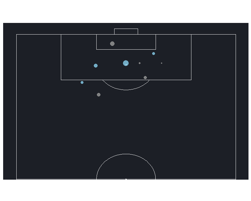 37 |
38 | ```{r}
39 | statsbomb %>%
40 | filter(team.name == "France") %>%
41 | soccerShotmap(theme = "dark")
42 | ```
43 |
44 |
45 | Grass theme with custom colours:
46 |
47 |
37 |
38 | ```{r}
39 | statsbomb %>%
40 | filter(team.name == "France") %>%
41 | soccerShotmap(theme = "dark")
42 | ```
43 |
44 |
45 | Grass theme with custom colours:
46 |
47 |  48 |
49 | ```{r}
50 | statsbomb %>%
51 | filter(team.name == "Argentina") %>%
52 | soccerShotmap(theme = "grass", colGoal = "yellow", colMiss = "blue", legend = T)
53 | ```
54 |
55 |
56 | #### Passing networks
57 |
58 | Default aesthetics:
59 |
60 |
48 |
49 | ```{r}
50 | statsbomb %>%
51 | filter(team.name == "Argentina") %>%
52 | soccerShotmap(theme = "grass", colGoal = "yellow", colMiss = "blue", legend = T)
53 | ```
54 |
55 |
56 | #### Passing networks
57 |
58 | Default aesthetics:
59 |
60 |  61 |
62 | ```{r}
63 | statsbomb %>%
64 | filter(team.name == "Argentina") %>%
65 | soccerPassmap(fill = "lightblue", arrow = "r",
66 | title = "Argentina (vs France, 30th June 2018)")
67 | ```
68 |
69 | Grass background, non-transparent edges:
70 |
71 |
61 |
62 | ```{r}
63 | statsbomb %>%
64 | filter(team.name == "Argentina") %>%
65 | soccerPassmap(fill = "lightblue", arrow = "r",
66 | title = "Argentina (vs France, 30th June 2018)")
67 | ```
68 |
69 | Grass background, non-transparent edges:
70 |
71 |  72 |
73 | ```{r}
74 | statsbomb %>%
75 | filter(team.name == "France") %>%
76 | soccerPassmap(fill = "blue", minPass = 3,
77 | edge_max_width = 30, edge_col = "grey40", edge_alpha = 1,
78 | title = "France (vs Argentina, 30th June 2018)")
79 | ```
80 |
81 |
82 | #### Heatmaps
83 |
84 | Passing heatmap with approx 10x10m bins:
85 |
86 |
72 |
73 | ```{r}
74 | statsbomb %>%
75 | filter(team.name == "France") %>%
76 | soccerPassmap(fill = "blue", minPass = 3,
77 | edge_max_width = 30, edge_col = "grey40", edge_alpha = 1,
78 | title = "France (vs Argentina, 30th June 2018)")
79 | ```
80 |
81 |
82 | #### Heatmaps
83 |
84 | Passing heatmap with approx 10x10m bins:
85 |
86 | 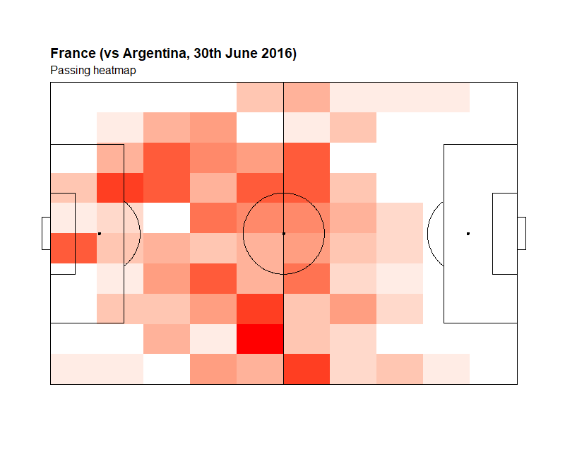 87 |
88 | ```{r}
89 | statsbomb %>%
90 | filter(type.name == "Pass" & team.name == "France") %>%
91 | soccerHeatmap(x = "location.x", y = "location.y",
92 | title = "France (vs Argentina, 30th June 2016)",
93 | subtitle = "Passing heatmap")
94 | ```
95 |
96 |
97 | Defensive pressure heatmap with approx 5x5m bins:
98 |
99 |
87 |
88 | ```{r}
89 | statsbomb %>%
90 | filter(type.name == "Pass" & team.name == "France") %>%
91 | soccerHeatmap(x = "location.x", y = "location.y",
92 | title = "France (vs Argentina, 30th June 2016)",
93 | subtitle = "Passing heatmap")
94 | ```
95 |
96 |
97 | Defensive pressure heatmap with approx 5x5m bins:
98 |
99 |  100 |
101 | ```{r}
102 | statsbomb %>%
103 | filter(type.name == "Pressure" & team.name == "France") %>%
104 | soccerHeatmap(x = "location.x", y = "location.y", xBins = 21, yBins = 14,
105 | title = "France (vs Argentina, 30th June 2016)",
106 | subtitle = "Defensive pressure heatmap")
107 | ```
108 |
109 | Player position heatmaps also possible using TRACAB-style x,y-location data.
110 |
111 |
112 | #### Average position
113 |
114 | Average pass position:
115 |
116 |
100 |
101 | ```{r}
102 | statsbomb %>%
103 | filter(type.name == "Pressure" & team.name == "France") %>%
104 | soccerHeatmap(x = "location.x", y = "location.y", xBins = 21, yBins = 14,
105 | title = "France (vs Argentina, 30th June 2016)",
106 | subtitle = "Defensive pressure heatmap")
107 | ```
108 |
109 | Player position heatmaps also possible using TRACAB-style x,y-location data.
110 |
111 |
112 | #### Average position
113 |
114 | Average pass position:
115 |
116 |  117 |
118 | ```{r}
119 | statsbomb %>%
120 | filter(type.name == "Pass" & team.name == "France" & minute < 43) %>%
121 | soccerPositionMap(id = "player.name", x = "location.x", y = "location.y",
122 | fill1 = "blue", grass = T,
123 | arrow = "r",
124 | title = "France (vs Argentina, 30th June 2016)",
125 | subtitle = "Average pass position (1' - 42')")
126 | ```
127 |
128 |
129 | Average pass position (both teams):
130 |
131 |
117 |
118 | ```{r}
119 | statsbomb %>%
120 | filter(type.name == "Pass" & team.name == "France" & minute < 43) %>%
121 | soccerPositionMap(id = "player.name", x = "location.x", y = "location.y",
122 | fill1 = "blue", grass = T,
123 | arrow = "r",
124 | title = "France (vs Argentina, 30th June 2016)",
125 | subtitle = "Average pass position (1' - 42')")
126 | ```
127 |
128 |
129 | Average pass position (both teams):
130 |
131 |  132 |
133 | ```{r}
134 | statsbomb %>%
135 | filter(type.name == "Pass" & minute < 43) %>%
136 | soccerPositionMap(id = "player.name", team = "team.name", x = "location.x", y = "location.y",
137 | fill1 = "lightblue", fill2 = "blue", label_col = "black",
138 | repel = T, teamToFlip = 2,
139 | title = "France vs Argentina, 30th June 2018",
140 | subtitle = "Average pass position (1' - 42')")
141 | ```
142 |
143 |
144 | Average player position using TRACAB-style x,y-location data:
145 |
146 |
132 |
133 | ```{r}
134 | statsbomb %>%
135 | filter(type.name == "Pass" & minute < 43) %>%
136 | soccerPositionMap(id = "player.name", team = "team.name", x = "location.x", y = "location.y",
137 | fill1 = "lightblue", fill2 = "blue", label_col = "black",
138 | repel = T, teamToFlip = 2,
139 | title = "France vs Argentina, 30th June 2018",
140 | subtitle = "Average pass position (1' - 42')")
141 | ```
142 |
143 |
144 | Average player position using TRACAB-style x,y-location data:
145 |
146 |  147 |
148 | ```{r}
149 | tromso_extra[1:11,] %>%
150 | soccerPositionMap(grass = T, title = "Tromsø IL (vs. Strømsgodset, 3rd Nov 2013)", subtitle = "Average player position (1' - 16')")
151 | ```
152 |
153 |
154 | #### Custom plots
155 |
156 | Inbuilt functions for many of these will be added soon.
157 |
158 |
159 | Locations of multiple events:
160 |
161 |
147 |
148 | ```{r}
149 | tromso_extra[1:11,] %>%
150 | soccerPositionMap(grass = T, title = "Tromsø IL (vs. Strømsgodset, 3rd Nov 2013)", subtitle = "Average player position (1' - 16')")
151 | ```
152 |
153 |
154 | #### Custom plots
155 |
156 | Inbuilt functions for many of these will be added soon.
157 |
158 |
159 | Locations of multiple events:
160 |
161 | 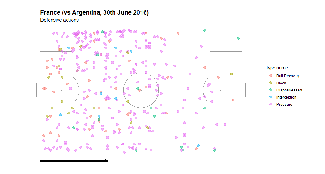 162 |
163 | ```{r}
164 | d2 <- statsbomb %>%
165 | filter(type.name %in% c("Pressure", "Interception", "Block", "Dispossessed", "Ball Recovery") & team.name == "France")
166 |
167 | soccerPitch(arrow = "r",
168 | title = "France (vs Argentina, 30th June 2016)",
169 | subtitle = "Defensive actions") +
170 | geom_point(data = d2, aes(x = location.x, y = location.y, col = type.name), size = 3, alpha = 0.5)
171 | ```
172 |
173 |
174 | Start and end locations of passes:
175 |
176 |
177 |
162 |
163 | ```{r}
164 | d2 <- statsbomb %>%
165 | filter(type.name %in% c("Pressure", "Interception", "Block", "Dispossessed", "Ball Recovery") & team.name == "France")
166 |
167 | soccerPitch(arrow = "r",
168 | title = "France (vs Argentina, 30th June 2016)",
169 | subtitle = "Defensive actions") +
170 | geom_point(data = d2, aes(x = location.x, y = location.y, col = type.name), size = 3, alpha = 0.5)
171 | ```
172 |
173 |
174 | Start and end locations of passes:
175 |
176 |
177 |  178 |
179 | ```{r}
180 | d3 <- statsbomb %>%
181 | filter(type.name == "Pass" & team.name == "France") %>%
182 | mutate(pass.outcome = as.factor(if_else(is.na(pass.outcome.name), 1, 0)))
183 |
184 | soccerPitch(arrow = "r",
185 | title = "France (vs Argentina, 30th June 2016)",
186 | subtitle = "Pass map") +
187 | geom_segment(data = d3, aes(x = location.x, xend = pass.end_location.x, y = location.y, yend = pass.end_location.y, col = pass.outcome), alpha = 0.75) +
188 | geom_point(data = d3, aes(x = location.x, y = location.y, col = pass.outcome), alpha = 0.5) +
189 | guides(colour = FALSE)
190 | ```
191 |
192 |
193 | #### Player paths
194 |
195 | Path of a single player:
196 |
197 |
178 |
179 | ```{r}
180 | d3 <- statsbomb %>%
181 | filter(type.name == "Pass" & team.name == "France") %>%
182 | mutate(pass.outcome = as.factor(if_else(is.na(pass.outcome.name), 1, 0)))
183 |
184 | soccerPitch(arrow = "r",
185 | title = "France (vs Argentina, 30th June 2016)",
186 | subtitle = "Pass map") +
187 | geom_segment(data = d3, aes(x = location.x, xend = pass.end_location.x, y = location.y, yend = pass.end_location.y, col = pass.outcome), alpha = 0.75) +
188 | geom_point(data = d3, aes(x = location.x, y = location.y, col = pass.outcome), alpha = 0.5) +
189 | guides(colour = FALSE)
190 | ```
191 |
192 |
193 | #### Player paths
194 |
195 | Path of a single player:
196 |
197 |  198 |
199 | ```{r}
200 | subset(tromso, id == 8)[1:1800,] %>%
201 | soccerPath(col = "red", grass = TRUE, arrow = "r",
202 | title = "Tromsø IL (vs. Strømsgodset, 3rd Nov 2013)",
203 | subtitle = "Player #8 path (1' - 3')")
204 | ```
205 |
206 |
207 | Path of multiple players:
208 |
209 |
198 |
199 | ```{r}
200 | subset(tromso, id == 8)[1:1800,] %>%
201 | soccerPath(col = "red", grass = TRUE, arrow = "r",
202 | title = "Tromsø IL (vs. Strømsgodset, 3rd Nov 2013)",
203 | subtitle = "Player #8 path (1' - 3')")
204 | ```
205 |
206 |
207 | Path of multiple players:
208 |
209 | 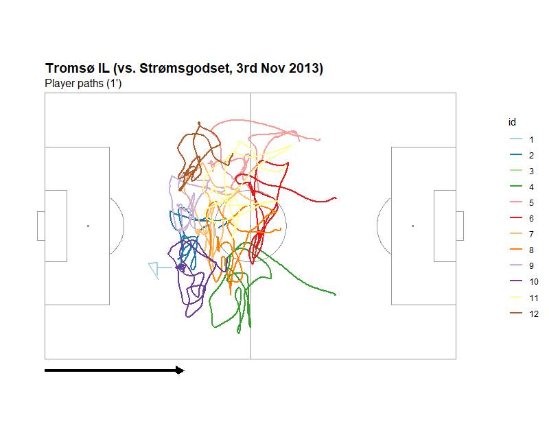 210 |
211 | ```{r}
212 | tromso %>%
213 | dplyr::group_by(id) %>%
214 | dplyr::slice(1:1200) %>%
215 | soccerPath(id = "id", arrow = "r",
216 | title = "Tromsø IL (vs. Strømsgodset, 3rd Nov 2013)",
217 | subtitle = "Player paths (1')")
218 | ```
219 |
220 | ---
221 |
--------------------------------------------------------------------------------
/data/statsbomb.rda:
--------------------------------------------------------------------------------
https://raw.githubusercontent.com/JoGall/soccermatics/4dfbfebc345b28103bfa08db89884626dcbe2a80/data/statsbomb.rda
--------------------------------------------------------------------------------
/data/tromso.rda:
--------------------------------------------------------------------------------
https://raw.githubusercontent.com/JoGall/soccermatics/4dfbfebc345b28103bfa08db89884626dcbe2a80/data/tromso.rda
--------------------------------------------------------------------------------
/data/tromso_extra.rda:
--------------------------------------------------------------------------------
https://raw.githubusercontent.com/JoGall/soccermatics/4dfbfebc345b28103bfa08db89884626dcbe2a80/data/tromso_extra.rda
--------------------------------------------------------------------------------
/man/soccerFlipDirection.Rd:
--------------------------------------------------------------------------------
1 | % Generated by roxygen2: do not edit by hand
2 | % Please edit documentation in R/soccerFlipDirection.R
3 | \name{soccerFlipDirection}
4 | \alias{soccerFlipDirection}
5 | \title{Flips x,y-coordinates horizontally in one half to account for changing sides at half-time}
6 | \usage{
7 | soccerFlipDirection(
8 | df,
9 | lengthPitch = 105,
10 | widthPitch = 68,
11 | teamToFlip = NULL,
12 | periodToFlip = 1:2,
13 | team = "team",
14 | period = "period",
15 | x = "x",
16 | y = "y"
17 | )
18 | }
19 | \arguments{
20 | \item{df}{dataframe containing unnormalised x,y-coordinates}
21 |
22 | \item{lengthPitch, widthPitch}{length, width of pitch in metres}
23 |
24 | \item{teamToFlip}{character, name of team to flip. If \code{NULL}, all x,y-coordinates in \code{df} will be flipped}
25 |
26 | \item{periodToFlip}{integer, period(s) to flip}
27 |
28 | \item{team}{character, name of variables containing x,y-coordinates}
29 |
30 | \item{period}{character, name of variable containing period labels}
31 |
32 | \item{x, y}{character, name of variables containing x,y-coordinates}
33 | }
34 | \value{
35 | a dataframe
36 | }
37 | \description{
38 | Normalises direction of attack in both halves of both teams by
39 | flipping x,y-coordinates horizontally in either the first or second half;
40 | i.e. teams attack in the same direction all game despite changing sides at
41 | half-time.
42 | }
43 | \examples{
44 | library(dplyr)
45 |
46 | # flip x,y-coords of France in both halves of statsbomb data
47 | data(statsbomb)
48 | statsbomb \%>\%
49 | soccerFlipDirection(team = "team.name", x = "location.x", y = "location.y",
50 | teamToFlip = "France")
51 |
52 | # flip x,y-coords in 2nd half of Tromso, based on a dummy period variable
53 | data(tromso)
54 | tromso \%>\%
55 | mutate(period = if_else(t > as.POSIXct("2013-11-07 21:14:00 GMT"), 1, 2)) \%>\%
56 | soccerFlipDirection(periodToFlip = 2)
57 |
58 | }
59 |
--------------------------------------------------------------------------------
/man/soccerFlow.Rd:
--------------------------------------------------------------------------------
1 | % Generated by roxygen2: do not edit by hand
2 | % Please edit documentation in R/soccerFlow.R
3 | \name{soccerFlow}
4 | \alias{soccerFlow}
5 | \title{Draw a flow field of passing direction on a soccer pitch}
6 | \usage{
7 | soccerFlow(
8 | df,
9 | lengthPitch = 105,
10 | widthPitch = 68,
11 | xBins = 5,
12 | yBins = NULL,
13 | x = "x",
14 | y = "y",
15 | angle = "angle",
16 | distance = "distance",
17 | col = "black",
18 | lwd = 0.5,
19 | arrow = c("none", "r", "l"),
20 | title = NULL,
21 | subtitle = NULL,
22 | theme = c("light", "dark", "grey", "grass"),
23 | plot = NULL
24 | )
25 | }
26 | \arguments{
27 | \item{df}{dataframe of event data containing fields of start x,y-coordinates, pass distance, and pass angle}
28 |
29 | \item{lengthPitch, widthPitch}{numeric, length and width of pitch in metres.}
30 |
31 | \item{xBins, yBins}{integer, the number of horizontal (length-wise) and vertical (width-wise) bins the soccer pitch is to be divided up into; if \code{yBins} is NULL (default), it will take the value of \code{xBins}}
32 |
33 | \item{x, y, angle, distance}{names of variables containing pass start x,y-coordinates, angle, and distance}
34 |
35 | \item{col}{colour of arrows}
36 |
37 | \item{lwd}{thickness of arrow segments}
38 |
39 | \item{arrow}{adds team direction of play arrow as right (\code{'r'}) or left (\code{'l'}); \code{'none'} by default}
40 |
41 | \item{title, subtitle}{adds title and subtitle to plot; NULL by default}
42 |
43 | \item{theme}{palette of pitch background and lines, either \code{light} (default), \code{dark}, \code{grey}, or \code{grass}}
44 |
45 | \item{plot}{base plot to add path layer to; NULL by default}
46 | }
47 | \value{
48 | a ggplot object of a heatmap on a soccer pitch
49 | }
50 | \description{
51 | A flow field to show the mean angle and distance of passes in zones of the pitch
52 | }
53 | \examples{
54 | library(dplyr)
55 | data(statsbomb)
56 |
57 | # transform x,y-coords, filter only France pass events,
58 | # draw flow field showing mean angle, distance of passes per pitch zone
59 | statsbomb \%>\%
60 | soccerTransform(method = 'statsbomb') \%>\%
61 | filter(team.name == "France" & type.name == "Pass") \%>\%
62 | soccerFlow(xBins=7, yBins=5,
63 | x="location.x", y="location.y", angle="pass.angle", distance="pass.length")
64 |
65 | # transform x,y-coords, standarise column names,
66 | # filter only France pass events
67 | my_df <- statsbomb \%>\%
68 | soccerTransform(method = 'statsbomb') \%>\%
69 | soccerStandardiseCols(method = 'statsbomb') \%>\%
70 | filter(team_name == "France" & event_name == "Pass")
71 |
72 | # overlay flow field onto heatmap showing proportion of team passes per pitch zone
73 | soccerHeatmap(my_df, xBins=7, yBins=5) \%>\%
74 | soccerFlow(my_df, xBins=7, yBins=5, plot = .)
75 |
76 | }
77 | \seealso{
78 | \code{\link{soccerHeatmap}} for drawing a heatmap of player position, or \code{\link{soccerSpokes}} for drawing spokes to show all directions in each area of the pitch.
79 | }
80 |
--------------------------------------------------------------------------------
/man/soccerHeatmap.Rd:
--------------------------------------------------------------------------------
1 | % Generated by roxygen2: do not edit by hand
2 | % Please edit documentation in R/soccerHeatmap.R
3 | \name{soccerHeatmap}
4 | \alias{soccerHeatmap}
5 | \title{Draw a heatmap on a soccer pitch using any event or tracking data.}
6 | \usage{
7 | soccerHeatmap(
8 | df,
9 | lengthPitch = 105,
10 | widthPitch = 68,
11 | xBins = 10,
12 | yBins = NULL,
13 | kde = FALSE,
14 | arrow = c("none", "r", "l"),
15 | colLow = "white",
16 | colHigh = "red",
17 | title = NULL,
18 | subtitle = NULL,
19 | x = "x",
20 | y = "y"
21 | )
22 | }
23 | \arguments{
24 | \item{df}{dataframe containing x,y-coordinates of player position}
25 |
26 | \item{lengthPitch, widthPitch}{numeric, length and width of pitch in metres.}
27 |
28 | \item{xBins, yBins}{integer, the number of horizontal (length-wise) and vertical (width-wise) bins the soccer pitch is to be divided up into. If no value for \code{yBins} is provided, it will take the value of \code{xBins}.}
29 |
30 | \item{kde}{use kernel density estimates for a smoother heatmap; FALSE by default}
31 |
32 | \item{arrow}{adds team direction of play arrow as right (\code{'r'}) or left (\code{'l'}); \code{'none'} by default}
33 |
34 | \item{colLow, colHigh}{character, colours for the low and high ends of the heatmap gradient; white and red respectively by default}
35 |
36 | \item{title, subtitle}{adds title and subtitle to plot; NULL by default}
37 |
38 | \item{x, y}{name of variables containing x,y-coordinates}
39 | }
40 | \value{
41 | a ggplot object of a heatmap on a soccer pitch.
42 | }
43 | \description{
44 | Draws a heatmap showing player position frequency in each area of the pitch and adds soccer pitch outlines.
45 | }
46 | \details{
47 | uses \code{ggplot2::geom_bin2d} to map 2D bin counts
48 | }
49 | \examples{
50 | library(dplyr)
51 |
52 | # tracking data heatmap with 21x5 zones(~5x5m)
53 | data(tromso)
54 | tromso \%>\%
55 | filter(id == 8) \%>\%
56 | soccerHeatmap(xBins = 10)
57 |
58 | # transform x,y-coords, filter only France pressure events,
59 | # heatmap with 6x3 zones
60 | data(statsbomb)
61 | statsbomb \%>\%
62 | soccerTransform(method='statsbomb') \%>\%
63 | filter(type.name == "Pressure" & team.name == "France") \%>\%
64 | soccerHeatmap(x = "location.x", y = "location.y",
65 | xBins = 6, yBins = 3, arrow = "r",
66 | title = "France (vs Argentina, 30th June 2016)",
67 | subtitle = "Defensive pressure heatmap")
68 |
69 | # transform x,y-coords, standardise column names,
70 | # filter player defensive actions, plot kernel density estimate heatmap
71 | statsbomb \%>\%
72 | soccerTransform(method='statsbomb') \%>\%
73 | soccerStandardiseCols() \%>\%
74 | filter(event_name \%in\% c("Duel", "Interception", "Clearance", "Block") &
75 | player_name == "Samuel Yves Umtiti") \%>\%
76 | soccerHeatmap(kde = TRUE, arrow = "r",
77 | title = "Umtiti (vs Argentina, 30th June 2016)",
78 | subtitle = "Defensive actions heatmap")
79 |
80 | }
81 |
--------------------------------------------------------------------------------
/man/soccerPassmap.Rd:
--------------------------------------------------------------------------------
1 | % Generated by roxygen2: do not edit by hand
2 | % Please edit documentation in R/soccerPassmap.R
3 | \name{soccerPassmap}
4 | \alias{soccerPassmap}
5 | \title{Draw a passing network using StatsBomb data}
6 | \usage{
7 | soccerPassmap(
8 | df,
9 | lengthPitch = 105,
10 | widthPitch = 68,
11 | minPass = 3,
12 | fill = "red",
13 | col = "black",
14 | edgeAlpha = 0.6,
15 | edgeCol = NULL,
16 | label = TRUE,
17 | shortNames = TRUE,
18 | maxNodeSize = 30,
19 | maxEdgeSize = 30,
20 | labelSize = 4,
21 | arrow = c("none", "r", "l"),
22 | theme = c("light", "dark", "grey", "grass"),
23 | title = NULL
24 | )
25 | }
26 | \arguments{
27 | \item{df}{dataframe containing x,y-coordinates of player passes}
28 |
29 | \item{lengthPitch, widthPitch}{numeric, length and width of pitch, in metres}
30 |
31 | \item{minPass}{minimum number of passes between players for edge to be drawn}
32 |
33 | \item{fill, col}{fill and border colour of nodes}
34 |
35 | \item{edgeAlpha}{transparency of edge lines, from \code{0} - \code{1}. Defaults to \code{0.6} so overlapping edges are visible.}
36 |
37 | \item{edgeCol}{colour of edge lines. Default is complementary to \code{theme} colours.}
38 |
39 | \item{label}{boolean, draw labels}
40 |
41 | \item{shortNames}{shorten player names to display last name as label}
42 |
43 | \item{maxNodeSize}{maximum size of nodes}
44 |
45 | \item{maxEdgeSize}{maximum width of edge lines}
46 |
47 | \item{labelSize}{size of player name labels}
48 |
49 | \item{arrow}{optional, adds team direction of play arrow as right (\code{'r'}) or left (\code{'l'})}
50 |
51 | \item{theme}{draws a \code{light}, \code{dark}, \code{grey}, or \code{grass} coloured pitch}
52 |
53 | \item{title}{adds custom title to plot. Defaults to team name.}
54 | }
55 | \description{
56 | Draw an undirected passing network of completed passes on pitch from StatsBomb data. Nodes are scaled by number of successful passes; edge width is scaled by number of successful passes between each node pair. Only passes made until first substition shown (ability to specify custom minutes will be added soon). Total number of passes attempted and percentage of completed passes shown. Compatability with other (non-StatsBomb) shot data will be added soon.
57 | }
58 | \examples{
59 | # France vs. Argentina, minimum of three passes
60 | library(dplyr)
61 | data(statsbomb)
62 |
63 | # transform x,y-coords,
64 | # Argentina pass map until first substituton with transparent edges
65 | statsbomb \%>\%
66 | soccerTransform(method='statsbomb') \%>\%
67 | filter(team.name == "Argentina") \%>\%
68 | soccerPassmap(fill = "lightblue", arrow = "r",
69 | title = "Argentina (vs France, 30th June 2018)")
70 |
71 | # transform x,y-coords,
72 | # France pass map until first substitution with opaque edges
73 | statsbomb \%>\%
74 | filter(team.name == "France") \%>\%
75 | soccerTransform(method='statsbomb') \%>\%
76 | soccerPassmap(fill = "blue", minPass = 3,
77 | maxEdgeSize = 30, edgeCol = "grey40", edgeAlpha = 1,
78 | title = "France (vs Argentina, 30th June 2018)")
79 | }
80 |
--------------------------------------------------------------------------------
/man/soccerPath.Rd:
--------------------------------------------------------------------------------
1 | % Generated by roxygen2: do not edit by hand
2 | % Please edit documentation in R/soccerPath.R
3 | \name{soccerPath}
4 | \alias{soccerPath}
5 | \title{Draw a path of player trajectory on a soccer pitch using any tracking data}
6 | \usage{
7 | soccerPath(
8 | df,
9 | lengthPitch = 105,
10 | widthPitch = 68,
11 | col = "black",
12 | arrow = c("none", "r", "l"),
13 | theme = c("light", "dark", "grey", "grass"),
14 | lwd = 1,
15 | title = NULL,
16 | subtitle = NULL,
17 | legend = FALSE,
18 | x = "x",
19 | y = "y",
20 | id = NULL,
21 | plot = NULL
22 | )
23 | }
24 | \arguments{
25 | \item{df}{dataframe containing x,y-coordinates of player position}
26 |
27 | \item{lengthPitch, widthPitch}{length and width of pitch in metres}
28 |
29 | \item{col}{colour of path if no \code{'id'} is provided; if an \code{'id'} is present, uses ColorBrewer's 'Paired' palette by default}
30 |
31 | \item{arrow}{adds team direction of play arrow as right (\code{'r'}) or left (\code{'l'}); \code{'none'} by default}
32 |
33 | \item{theme}{draws a \code{light}, \code{dark}, \code{grey}, or \code{grass} coloured pitch}
34 |
35 | \item{lwd}{player path thickness}
36 |
37 | \item{title, subtitle}{adds title and subtitle to plot; NULL by default}
38 |
39 | \item{legend}{boolean, include legend}
40 |
41 | \item{x, y}{name of variables containing x,y-coordinates}
42 |
43 | \item{id}{character, the name of the column containing player identity (only required if \code{'df'} contains multiple players)}
44 |
45 | \item{plot}{base plot to add path layer to; NULL by default}
46 | }
47 | \value{
48 | a ggplot object
49 | }
50 | \description{
51 | Draws a path connecting consecutive x,y-coordinates of a player on a soccer pitch.
52 | }
53 | \examples{
54 | library(dplyr)
55 | data(tromso)
56 |
57 | # draw path of Tromso #8 over first 3 minutes (1800 frames)
58 | tromso \%>\%
59 | filter(id == 8) \%>\%
60 | top_n(1800) \%>\%
61 | soccerPath(col = "red", theme = "grass", arrow = "r")
62 |
63 | # draw path of all Tromso players over first minute (600 frames)
64 | tromso \%>\%
65 | group_by(id) \%>\%
66 | slice(1:1200) \%>\%
67 | soccerPath(id = "id", theme = "light")
68 |
69 | }
70 |
--------------------------------------------------------------------------------
/man/soccerPitch.Rd:
--------------------------------------------------------------------------------
1 | % Generated by roxygen2: do not edit by hand
2 | % Please edit documentation in R/soccerPitch.R
3 | \name{soccerPitch}
4 | \alias{soccerPitch}
5 | \title{Plot a full soccer pitch}
6 | \usage{
7 | soccerPitch(
8 | lengthPitch = 105,
9 | widthPitch = 68,
10 | arrow = c("none", "r", "l"),
11 | title = NULL,
12 | subtitle = NULL,
13 | theme = c("light", "dark", "grey", "grass"),
14 | data = NULL
15 | )
16 | }
17 | \arguments{
18 | \item{lengthPitch, widthPitch}{length and width of pitch in metres}
19 |
20 | \item{arrow}{adds team direction of play arrow as right (\code{'r'}) or left (\code{'l'}); \code{'none'} by default}
21 |
22 | \item{title, subtitle}{adds title and subtitle to plot; NULL by default}
23 |
24 | \item{theme}{palette of pitch background and lines, either \code{light} (default), \code{dark}, \code{grey}, or \code{grass}}
25 |
26 | \item{data}{a default dataset for plotting in subsequent layers; NULL by default}
27 | }
28 | \value{
29 | a ggplot object
30 | }
31 | \description{
32 | Draws a soccer pitch as a ggplot object for the purpose of adding layers such as player positions, player trajectories, etc..
33 | }
34 | \examples{
35 | library(ggplot2)
36 | data(statsbomb)
37 |
38 | # transform Statsbomb coordinates to metre units for plotting
39 | my_df <- soccerTransform(statsbomb, method = "statsbomb")
40 |
41 | # filter events of interest (France defensive pressure events vs. Argentina)
42 | my_df <- my_df \%>\%
43 | dplyr::filter(team.name == "France" & type.name == "Pressure")
44 |
45 | # add custom layers to soccerPitch base
46 | soccerPitch(data = my_df,
47 | arrow = "r", theme = "grass",
48 | title = "France (vs. Argentina)",
49 | subtitle = "Pressure events") +
50 | geom_point(aes(x = location.x, y = location.y),
51 | col = "blue", alpha = 0.5)
52 |
53 | }
54 |
--------------------------------------------------------------------------------
/man/soccerPitchFG.Rd:
--------------------------------------------------------------------------------
1 | % Generated by roxygen2: do not edit by hand
2 | % Please edit documentation in R/soccerPitchFG.R
3 | \name{soccerPitchFG}
4 | \alias{soccerPitchFG}
5 | \title{Helper function to draw soccer pitch outlines over an existing ggplot object}
6 | \usage{
7 | soccerPitchFG(
8 | plot,
9 | lengthPitch = 105,
10 | widthPitch = 68,
11 | colPitch = "black",
12 | arrow = c("none", "r", "l"),
13 | title = NULL,
14 | subtitle = NULL
15 | )
16 | }
17 | \arguments{
18 | \item{plot}{an existing ggplot object to add pitch lines layer to}
19 |
20 | \item{lengthPitch, widthPitch}{length and width of pitch in metres}
21 |
22 | \item{colPitch}{colour of pitch markings}
23 |
24 | \item{arrow}{adds team direction of play arrow as right (\code{'r'}) or left (\code{'l'}); \code{'none'} by default}
25 |
26 | \item{title, subtitle}{adds title and subtitle to plot; NULL by default}
27 | }
28 | \value{
29 | a ggplot object
30 | }
31 | \description{
32 | Adds soccer pitch outlines (with transparent fill) to an existing ggplot object (e.g. heatmaps, passing maps, etc..)
33 | }
34 | \seealso{
35 | \code{\link{soccerPitch}} for plotting a soccer pitch as background layer
36 | }
37 |
--------------------------------------------------------------------------------
/man/soccerPitchHalf.Rd:
--------------------------------------------------------------------------------
1 | % Generated by roxygen2: do not edit by hand
2 | % Please edit documentation in R/soccerPitchHalf.R
3 | \name{soccerPitchHalf}
4 | \alias{soccerPitchHalf}
5 | \title{Draws a vertical half soccer pitch for the purpose of plotting shotmaps}
6 | \usage{
7 | soccerPitchHalf(
8 | lengthPitch = 105,
9 | widthPitch = 68,
10 | arrow = c("none", "r", "l"),
11 | theme = c("light", "dark", "grey", "grass"),
12 | title = NULL,
13 | subtitle = NULL,
14 | data = NULL
15 | )
16 | }
17 | \arguments{
18 | \item{lengthPitch, widthPitch}{length and width of pitch in metres}
19 |
20 | \item{arrow}{adds team direction of play arrow as right (\code{'r'}) or left (\code{'l'}); \code{'none'} by default}
21 |
22 | \item{theme}{palette of pitch background and lines, either \code{light} (default), \code{dark}, \code{grey}, or \code{grass};}
23 |
24 | \item{title, subtitle}{adds title and subtitle to plot; NULL by default}
25 |
26 | \item{data}{a default dataset for plotting in subsequent layers; NULL by default}
27 | }
28 | \value{
29 | a ggplot object
30 | }
31 | \description{
32 | Adds soccer pitch outlines (with transparent fill) to an existing ggplot object (e.g. heatmaps, passing maps, etc..)
33 | }
34 | \examples{
35 | library(ggplot2)
36 | library(dplyr)
37 | data(statsbomb)
38 |
39 | # normalise data, get non-penalty shots for France,
40 | # add boolean variable 'goal' for plotting
41 | my_df <- statsbomb \%>\%
42 | soccerTransform(method = 'statsbomb') \%>\%
43 | filter(team.name == "France" &
44 | type.name == "Shot" &
45 | shot.type.name != 'penalty') \%>\%
46 | mutate(goal = as.factor(if_else(shot.outcome.name == "Goal", 1, 0)))
47 |
48 | soccerPitchHalf(data = my_df, theme = 'light') +
49 | geom_point(aes(x = location.y, y = location.x,
50 | size = shot.statsbomb_xg, colour = goal),
51 | alpha = 0.7)
52 |
53 | }
54 | \seealso{
55 | \code{\link{soccerShotmap}} for plotting a shotmap on a half pitch for a single player or \code{\link{soccerPitch}} for drawing a full size soccer pitch
56 | }
57 |
--------------------------------------------------------------------------------
/man/soccerPositionMap.Rd:
--------------------------------------------------------------------------------
1 | % Generated by roxygen2: do not edit by hand
2 | % Please edit documentation in R/soccerPositionMap.R
3 | \name{soccerPositionMap}
4 | \alias{soccerPositionMap}
5 | \title{Plot average player position using any event or tracking data}
6 | \usage{
7 | soccerPositionMap(
8 | df,
9 | lengthPitch = 105,
10 | widthPitch = 68,
11 | fill1 = "red",
12 | col1 = NULL,
13 | fill2 = "blue",
14 | col2 = NULL,
15 | labelCol = "black",
16 | homeTeam = NULL,
17 | flipAwayTeam = TRUE,
18 | label = c("name", "number", "none"),
19 | labelBox = TRUE,
20 | shortNames = TRUE,
21 | nodeSize = 5,
22 | labelSize = 4,
23 | arrow = c("none", "r", "l"),
24 | theme = c("light", "dark", "grey", "grass"),
25 | title = NULL,
26 | subtitle = NULL,
27 | source = c("manual", "statsbomb"),
28 | x = "x",
29 | y = "y",
30 | id = "player_id",
31 | name = "player_name",
32 | team = "team_name"
33 | )
34 | }
35 | \arguments{
36 | \item{df}{a dataframe containing x,y-coordinates of player position and a player identifier variable}
37 |
38 | \item{lengthPitch, widthPitch}{numeric, length and width of pitch in metres}
39 |
40 | \item{fill1, fill2}{character, fill colour of position points of team 1, team 2 (team 2 \code{NULL} by default)}
41 |
42 | \item{col1, col2}{character, border colour of position points of team 1, team 2 (team 2 \code{NULL} by default)}
43 |
44 | \item{labelCol}{character, label text colour}
45 |
46 | \item{homeTeam}{if \code{df} contains two teams, the name of the home team to be displayed on the left hand side of the pitch (i.e. attacking from left to right). If \code{NULL}, infers home team as the team of the first event in \code{df}.}
47 |
48 | \item{flipAwayTeam}{flip x,y-coordinates of away team so attacking from right to left}
49 |
50 | \item{label}{type of label to draw, player names (\code{name}), jersey numbers (\code{number}), or \code{none}}
51 |
52 | \item{labelBox}{add box around label text}
53 |
54 | \item{shortNames}{shorten player names to display last name as label}
55 |
56 | \item{nodeSize}{numeric, size of position points}
57 |
58 | \item{labelSize}{numeric, size of labels}
59 |
60 | \item{arrow}{optional, adds team direction of play arrow as right (\code{'r'}) or left (\code{'l'})}
61 |
62 | \item{theme}{draws a \code{light}, \code{dark}, \code{grey}, or \code{grass} coloured pitch}
63 |
64 | \item{title, subtitle}{optional, adds title and subtitle to plot}
65 |
66 | \item{source}{if \code{statsbomb}, uses StatsBomb definitions of required variable names (i.e. `location.x`, `location.y`, `player.id`, `team.name`); if \code{manual} (default), respects variable names defined in function arguments \code{x}, \code{y}, \code{id}, \code{name}, and \code{team}.}
67 |
68 | \item{x, y, id, name, team}{names of variables containing x,y-coordinates, unique player ids, player names, and team names, respectively; \code{name} and \code{team} NULL by default}
69 | }
70 | \description{
71 | Draws the average x,y-positions of each player from one or both teams on a soccer pitch.
72 | }
73 | \examples{
74 | library(dplyr)
75 | data(statsbomb)
76 |
77 | # average player position from tracking data for one team
78 | # w/ jersey numbers labelled
79 | data(tromso)
80 | tromso \%>\%
81 | soccerPositionMap(label = "number", id ="id",
82 | labelCol = "white", nodeSize = 8,
83 | arrow = "r", theme = "grass",
84 | title = "Tromso IL (vs. Stromsgodset, 3rd Nov 2013)",
85 | subtitle = "Average player position (1' - 16')")
86 |
87 | # transform x,y-coords, standarise column names,
88 | # average pass position for one team using 'statsbomb' method
89 | # w/ player name as labels
90 | statsbomb \%>\%
91 | soccerTransform(method='statsbomb') \%>\%
92 | filter(type.name == "Pass" & team.name == "France" & period == 1) \%>\%
93 | soccerPositionMap(source = "statsbomb",
94 | fill1 = "blue", arrow = "r", theme = "light",
95 | title = "France (vs Argentina, 30th June 2018)",
96 | subtitle = "Average pass position (1' - 45')")
97 |
98 | # transform x,y-coords, standarise column names,
99 | # average pass position for two teams using 'manual' method
100 | # w/ player names labelled
101 | statsbomb \%>\%
102 | soccerTransform(method='statsbomb') \%>\%
103 | soccerStandardiseCols(method='statsbomb') \%>\%
104 | filter(event_name == "Pass" & period == 1) \%>\%
105 | soccerPositionMap(fill1 = "lightblue", fill2 = "blue",
106 | title = "Argentina vs France, 30th June 2018",
107 | subtitle = "Average pass position (1' - 45')")
108 |
109 | }
110 |
--------------------------------------------------------------------------------
/man/soccerResample.Rd:
--------------------------------------------------------------------------------
1 | % Generated by roxygen2: do not edit by hand
2 | % Please edit documentation in R/soccerResample.R
3 | \name{soccerResample}
4 | \alias{soccerResample}
5 | \title{Resample the frames per second of any tracking data using linear interpolation}
6 | \usage{
7 | soccerResample(df, r = 10, x = "x", y = "y", t = "t", id = "id")
8 | }
9 | \arguments{
10 | \item{df}{a dataframe containing x,y-coordinates and time variable}
11 |
12 | \item{r}{resampling rate in frames per second}
13 |
14 | \item{x, y}{name of variables containing x,y-coordinates}
15 |
16 | \item{t}{name of variable containing time data}
17 |
18 | \item{id}{name of variable containing player identifier}
19 | }
20 | \value{
21 | a dataframe with interpolated rows added
22 | }
23 | \description{
24 | Downsample or upsample any tracking data containing x,y,t data using linear interpolation of x,y-coordinates (plus constant interpolation of all other variables in dataframe)
25 | }
26 | \examples{
27 | data(tromso)
28 |
29 | # resample tromso dataset from ~21 fps to 10 fps
30 | soccerResample(tromso, r=10)
31 |
32 | }
33 |
--------------------------------------------------------------------------------
/man/soccerShortenName.Rd:
--------------------------------------------------------------------------------
1 | % Generated by roxygen2: do not edit by hand
2 | % Please edit documentation in R/soccerShortenName.R
3 | \name{soccerShortenName}
4 | \alias{soccerShortenName}
5 | \title{Extract player surname}
6 | \usage{
7 | soccerShortenName(names)
8 | }
9 | \arguments{
10 | \item{names}{vector of strings containing full player name}
11 | }
12 | \description{
13 | Helper function to extract last name (including common nobiliary particles) from full player names
14 | }
15 | \examples{
16 | data(statsbomb)
17 | statsbomb$name <- soccerShortenName(statsbomb$player.name)
18 |
19 | }
20 |
--------------------------------------------------------------------------------
/man/soccerShotmap.Rd:
--------------------------------------------------------------------------------
1 | % Generated by roxygen2: do not edit by hand
2 | % Please edit documentation in R/soccerShotmap.R
3 | \name{soccerShotmap}
4 | \alias{soccerShotmap}
5 | \title{Draw an individual, team, or two team shotmap using StatsBomb data}
6 | \usage{
7 | soccerShotmap(
8 | df,
9 | lengthPitch = 105,
10 | widthPitch = 68,
11 | homeTeam = NULL,
12 | adj = TRUE,
13 | n_players = 0,
14 | size_lim = c(2, 15),
15 | title = NULL,
16 | subtitle = NULL,
17 | theme = c("light", "dark", "grey", "grass")
18 | )
19 | }
20 | \arguments{
21 | \item{df}{dataframe containing x,y-coordinates of player passes}
22 |
23 | \item{lengthPitch, widthPitch}{length and width of pitch, in metres}
24 |
25 | \item{homeTeam}{if \code{df} contains two teams, the name of the home team to be displayed on the left hand side of the pitch. If \code{NULL}, infers home team as the team of the first event in \code{df}.}
26 |
27 | \item{adj}{adjust xG using conditional probability to account for multiple shots per possession}
28 |
29 | \item{n_players}{number of highest xG players to display}
30 |
31 | \item{size_lim}{minimum and maximum size of points, \code{c(min, max)}}
32 |
33 | \item{title, subtitle}{optional, adds title and subtitle to half pitch plot. Title defaults to scoreline and team identity when two teams are defined in \code{df}.}
34 |
35 | \item{theme}{draws a \code{light}, \code{dark}, \code{grey}, or \code{grass} coloured pitch with appropriate point colours}
36 | }
37 | \value{
38 | a ggplot object
39 | }
40 | \description{
41 | If \code{df} contains two teams, draws a shotmap of each team at either end of a full pitch. If \code{df} contains one or more players from a single team, draws a vertical half pitch. Currently only works with StatsBomb data but compatability with other (non-StatsBomb) shot data will be added soon.
42 | }
43 | \examples{
44 | data(statsbomb)
45 |
46 | # shot map of two teams on full pitch
47 | statsbomb \%>\%
48 | soccerTransform(method='statsbomb') \%>\%
49 | soccerShotmap(theme = "gray")
50 |
51 | # shot map of one player on half pitch
52 | statsbomb \%>\%
53 | dplyr::filter(player.name == "Antoine Griezmann") \%>\%
54 | soccerTransform(method='statsbomb') \%>\%
55 | soccerShotmap(theme = "grass",
56 | title = "Antoine Griezmann",
57 | subtitle = "vs. Argentina, World Cup 2018")
58 |
59 | }
60 |
--------------------------------------------------------------------------------
/man/soccerSpokes.Rd:
--------------------------------------------------------------------------------
1 | % Generated by roxygen2: do not edit by hand
2 | % Please edit documentation in R/soccerSpokes.R
3 | \name{soccerSpokes}
4 | \alias{soccerSpokes}
5 | \title{Draw spokes of passing direction on a soccer pitch}
6 | \usage{
7 | soccerSpokes(
8 | df,
9 | lengthPitch = 105,
10 | widthPitch = 68,
11 | xBins = 5,
12 | yBins = NULL,
13 | angleBins = 8,
14 | x = "x",
15 | y = "y",
16 | angle = "angle",
17 | minLength = 0.6,
18 | minAlpha = 0.5,
19 | minWidth = 0.5,
20 | col = "black",
21 | legend = TRUE,
22 | arrow = c("none", "r", "l"),
23 | title = NULL,
24 | subtitle = NULL,
25 | theme = c("light", "dark", "grey", "grass"),
26 | plot = NULL
27 | )
28 | }
29 | \arguments{
30 | \item{df}{a dataframe of event data containing fields of start x,y-coordinates, pass distance, and pass angle}
31 |
32 | \item{lengthPitch, widthPitch}{numeric, length and width of pitch in metres}
33 |
34 | \item{xBins, yBins}{integer, the number of horizontal (length-wise) and vertical (width-wise) bins the soccer pitch is to be divided up into; if \code{yBins} is NULL (default), it will take the value of \code{xBins}}
35 |
36 | \item{angleBins}{integer, the number of arrows to draw in each zone of the pitch; for example, a value of 4 clusters has direction vectors up, down, left, and right}
37 |
38 | \item{x, y, angle}{names of variables containing pass start x,y-coordinates and angle}
39 |
40 | \item{minLength}{numeric, ratio between size of shortest arrow and longest arrow depending on number of events}
41 |
42 | \item{minAlpha, minWidth}{numeric, minimum alpha and line width of arrows drawn}
43 |
44 | \item{col}{colour of arrows}
45 |
46 | \item{legend}{if \code{TRUE}, adds legend for arrow transparency}
47 |
48 | \item{arrow}{adds team direction of play arrow as right (\code{'r'}) or left (\code{'l'}); \code{'none'} by default}
49 |
50 | \item{title, subtitle}{adds title and subtitle to plot; NULL by default}
51 |
52 | \item{theme}{palette of pitch background and lines, either \code{light} (default), \code{dark}, \code{grey}, or \code{grass}}
53 |
54 | \item{plot}{base plot to add path layer to; NULL by default}
55 | }
56 | \value{
57 | a ggplot object of a heatmap on a soccer pitch
58 | }
59 | \description{
60 | Multiple arrows to show the distribution of pass angle and distance in zones of the pitch; similar to a radar plot but grouped by pitch location rather than player
61 | }
62 | \examples{
63 | library(dplyr)
64 | data(statsbomb)
65 |
66 | # transform x,y-coords, filter only France pass events,
67 | # draw flow field showing mean angle, distance of passes per pitch zone
68 | statsbomb \%>\%
69 | soccerTransform(method = 'statsbomb') \%>\%
70 | filter(team.name == "France" & type.name == "Pass") \%>\%
71 | soccerSpokes(xBins=7, yBins=5, angleBins=12, legend=FALSE)
72 |
73 | # transform x,y-coords, standarise column names,
74 | # filter only France pass events
75 | my_df <- statsbomb \%>\%
76 | soccerTransform(method = 'statsbomb') \%>\%
77 | soccerStandardiseCols(method = 'statsbomb') \%>\%
78 | filter(team_name == "France" & event_name == "Pass")
79 |
80 | # overlay flow field onto heatmap showing proportion of team passes per pitch zone
81 | soccerHeatmap(my_df, xBins=7, yBins=5,
82 | title = "France passing radar") \%>\%
83 | soccerSpokes(my_df, xBins=7, yBins=5, angleBins=8, legend=FALSE, plot = .)
84 |
85 | }
86 | \seealso{
87 | \code{\link{soccerHeatmap}} for drawing a heatmap of player position, or \code{\link{soccerFlow}} for drawing a single arrow for pass distance and angle per pitch zone.
88 | }
89 |
--------------------------------------------------------------------------------
/man/soccerStandardiseCols.Rd:
--------------------------------------------------------------------------------
1 | % Generated by roxygen2: do not edit by hand
2 | % Please edit documentation in R/soccerStandardiseCols.R
3 | \name{soccerStandardiseCols}
4 | \alias{soccerStandardiseCols}
5 | \title{Rename columns in a dataframe for easier use with other {soccermatics} functions}
6 | \usage{
7 | soccerStandardiseCols(df, method = c("statsbomb"))
8 | }
9 | \arguments{
10 | \item{df}{a dataframe of Statsbomb event data}
11 |
12 | \item{method}{source of data; only \code{"statsbomb"} currently supported}
13 | }
14 | \value{
15 | a dataframe with column names x, y, distance, angle, player_id, player_name, team_name, event_name
16 | }
17 | \description{
18 | Rename columns (e.g. \code{"location.x"} -> \code{"x"}, \code{"team.name"} -> \code{"team"}, etc...) to interface directly with other soccermatics functions without having to explicitly define column names as arguments. Currently only supports Statsbomb data.
19 | }
20 | \examples{
21 | library(dplyr)
22 | data(statsbomb)
23 |
24 | # transform x,y-coords, standardise column names
25 | my_df <- statsbomb \%>\%
26 | soccerTransform(method = 'statsbomb') \%>\%
27 | soccerStandardiseCols(method = 'statsbomb')
28 |
29 | # feed to other functions without defining variables,
30 | # x, y, id,distance, angle, etc...
31 | soccerHeatmap(my_df)
32 |
33 | }
34 |
--------------------------------------------------------------------------------
/man/soccerTransform.Rd:
--------------------------------------------------------------------------------
1 | % Generated by roxygen2: do not edit by hand
2 | % Please edit documentation in R/soccerTransform.R
3 | \name{soccerTransform}
4 | \alias{soccerTransform}
5 | \title{Normalises x,y-coordinates to metres units for use with soccermatics functions}
6 | \usage{
7 | soccerTransform(
8 | df,
9 | xMin,
10 | xMax,
11 | yMin,
12 | yMax,
13 | lengthPitch = 105,
14 | widthPitch = 68,
15 | method = c("manual", "statsbomb", "opta", "chyronhego", "ch"),
16 | x = "x",
17 | y = "y"
18 | )
19 | }
20 | \arguments{
21 | \item{df}{dataframe containing arbitrary x,y-coordinates}
22 |
23 | \item{xMin, xMax, yMin, yMax}{range of possible x,y-coordinates in the raw dataframe}
24 |
25 | \item{lengthPitch, widthPitch}{length, width of pitch in metres}
26 |
27 | \item{method}{source of data, either \code{"opta"}, \code{"statsbomb"}, \code{"chyronhego"} (ChryonHego), or \code{"manual"}}
28 |
29 | \item{x, y}{variable names of x,y-coordinates. Not required when \code{method} other than \code{"manual"} is defined; defaults to \code{"x"} and \code{"y"} if manual.}
30 | }
31 | \value{
32 | a dataframe
33 | }
34 | \description{
35 | Normalise x,y-coordinates from between arbitrary limits to metre units bounded by [0 < \code{"x"} < \code{"pitchLength"}, 0 < \code{"y"} < \code{"pitchWidth"}]
36 | }
37 | \examples{
38 | # Three examples with true pitch dimensions (in metres):
39 | lengthPitch <- 105
40 | widthPitch <- 68
41 |
42 | # Example 1. Opta ----------------------------------------------------------
43 |
44 | # limits = [0 < x < 100, 0 < y < 100]
45 | opta_df <- data.frame(team_id = as.factor(c(1, 1, 1, 2, 2)),
46 | x = c(50.0, 41.2, 44.4, 78.6, 76.7),
47 | y = c(50.0, 55.8, 47.5, 55.1, 45.5),
48 | endx = c(42.9, 40.2, 78.0, 80.5, 72.4),
49 | endy = c(57.6, 47.2, 55.6, 48.1, 26.3))
50 |
51 | soccerTransform(opta_df, method = "opta")
52 |
53 |
54 | # Example 2. StatsBomb -----------------------------------------------------
55 |
56 | # limits = [0 < x < 120, 0 < y < 80]
57 | data(statsbomb)
58 | soccerTransform(statsbomb, method = "statsbomb")
59 |
60 |
61 | # Example 3. ChyronHego --------------------------------------------------------
62 |
63 | # limits = [-5250 < x < 5250, -3400 < y < 3400]
64 |
65 | xMin <- -5250
66 | xMax <- 5250
67 | yMin <- -3400
68 | yMax <- 3400
69 |
70 | ch_df <- data.frame(x = c(0,-452,-982,-1099,-1586,-2088,-2422,-2999,-3200,-3857),
71 | y = c(0,150,300,550,820,915,750,620,400,264))
72 |
73 | soccerTransform(ch_df, -5250, 5250, -3400, 3400, method = "chyronhego")
74 |
75 |
76 | # Example 4. Manual -----------------------------------------------------
77 |
78 | # limits = [0 < x < 420, -136 < y < 136]
79 |
80 | my_df <- data.frame(team = as.factor(c(1, 1, 1, 2, 2)),
81 | my_x = c(210, 173, 187, 330, 322),
82 | my_y = c(0, 16, -7, 14, -12),
83 | my_endx = c(180, 169, 328, 338, 304),
84 | my_endy = c(21, -8, 15, -5, -65))
85 |
86 | soccerTransform(my_df, 0, 420, -136, 136, x = c("my_x", "my_endx"), y = c("my_y", "my_endy"))
87 |
88 | }
89 |
--------------------------------------------------------------------------------
/man/soccerVelocity.Rd:
--------------------------------------------------------------------------------
1 | % Generated by roxygen2: do not edit by hand
2 | % Please edit documentation in R/soccerVelocity.R
3 | \name{soccerVelocity}
4 | \alias{soccerVelocity}
5 | \title{Compute instantaneous distance, speed and direction from x,y-coordinates}
6 | \usage{
7 | soccerVelocity(dat)
8 | }
9 | \arguments{
10 | \item{dat}{dataframe containing unnormalised x,y-coordinates \code{x} and \code{y}, time variable \code{'t'}, and player identifier \code{'id'}}
11 | }
12 | \value{
13 | a dataframe with columns \code{'dist'}, \code{'speed'}, and \code{'direction'} added
14 | }
15 | \description{
16 | Compute instantaneous distance moved (in metres), speed (in metres per second), and direction (in radians) between subsequent frames in a dataframe of x,y-coordinates.
17 | }
18 | \examples{
19 | data(tromso)
20 |
21 | # calculate distance, speed, and direction for \code{tromso} dataset
22 | soccerVelocity(tromso)
23 |
24 | }
25 |
--------------------------------------------------------------------------------
/man/soccermatics-deprecated.Rd:
--------------------------------------------------------------------------------
1 | % Generated by roxygen2: do not edit by hand
2 | % Please edit documentation in R/soccerPitchBG.R, R/soccermatics-deprecated.R
3 | \name{soccerPitchBG}
4 | \alias{soccerPitchBG}
5 | \alias{soccermatics-deprecated}
6 | \title{Plot a full soccer pitch}
7 | \usage{
8 | soccerPitchBG(
9 | lengthPitch = 105,
10 | widthPitch = 68,
11 | arrow = c("none", "r", "l"),
12 | title = NULL,
13 | subtitle = NULL,
14 | theme = c("light", "dark", "grey", "grass"),
15 | data = NULL
16 | )
17 | }
18 | \arguments{
19 | \item{lengthPitch, widthPitch}{length and width of pitch in metres}
20 |
21 | \item{arrow}{adds team direction of play arrow as right (\code{'r'}) or left (\code{'l'}); \code{'none'} by default}
22 |
23 | \item{title, subtitle}{adds title and subtitle to plot; NULL by default}
24 |
25 | \item{theme}{palette of pitch background and lines, either \code{light} (default), \code{dark}, \code{grey}, or \code{grass}}
26 |
27 | \item{data}{a default dataset for plotting in subsequent layers; NULL by default}
28 |
29 | \item{fillPitch, colPitch}{pitch fill and line colour}
30 | }
31 | \value{
32 | a ggplot object
33 | }
34 | \description{
35 | Draws a soccer pitch as a ggplot object for the purpose of adding layers such as player positions, player trajectories, etc..
36 |
37 | The functions listed below are deprecated and will be defunct in
38 | the near future. When possible, alternative functions with similar
39 | functionality are also mentioned. Help pages for deprecated functions are
40 | available at \code{help("soccermatics-deprecated")}.
41 | }
42 | \seealso{
43 | \code{\link{soccermatics-deprecated}}
44 | }
45 | \keyword{internal}
46 |
--------------------------------------------------------------------------------
/man/soccerxGTimeline.Rd:
--------------------------------------------------------------------------------
1 | % Generated by roxygen2: do not edit by hand
2 | % Please edit documentation in R/soccerxGTimeline.R
3 | \name{soccerxGTimeline}
4 | \alias{soccerxGTimeline}
5 | \title{Draw a timeline showing cumulative expected goals (xG) over the course of a match using StatsBomb data.}
6 | \usage{
7 | soccerxGTimeline(
8 | df,
9 | homeCol = "red",
10 | awayCol = "blue",
11 | adj = TRUE,
12 | labels = TRUE,
13 | y_buffer = 0.3
14 | )
15 | }
16 | \arguments{
17 | \item{df}{a dataframe containing StatsBomb data from one full match}
18 |
19 | \item{homeCol, awayCol}{colours of the home and away team, respectively}
20 |
21 | \item{adj}{adjust xG using conditional probability to account for multiple shots per possession}
22 |
23 | \item{labels}{include scoreline and goalscorer labels for goals}
24 |
25 | \item{y_buffer}{vertical space to add at the top of the y-axis (a quick and dirty way to ensure text annotations are not cropped).}
26 | }
27 | \value{
28 | a ggplot object
29 | }
30 | \description{
31 | Draw a timeline showing cumulative expected goals (xG, excluding penalties and own goals) by two teams over the course of a match, as well as plotting the scoreline and goalscorer at goal events. Currently only works with StatsBomb data but compatability with other (non-StatsBomb) shot data will be added soon.
32 | }
33 | \examples{
34 | library(dplyr)
35 | data(statsbomb)
36 |
37 | # xG timeline of France vs. Argentina
38 | # w/ goalscorer labels, adjusted xG data
39 | statsbomb \%>\%
40 | soccerxGTimeline(homeCol = "blue", awayCol = "lightblue", y_buffer = 0.4)
41 |
42 | # no goalscorer labels, raw xG data
43 | statsbomb \%>\%
44 | soccerxGTimeline(homeCol = "blue", awayCol = "lightblue", adj = FALSE)
45 |
46 | }
47 |
--------------------------------------------------------------------------------
/man/statsbomb.Rd:
--------------------------------------------------------------------------------
1 | % Generated by roxygen2: do not edit by hand
2 | % Please edit documentation in R/statsbomb.R
3 | \docType{data}
4 | \name{statsbomb}
5 | \alias{statsbomb}
6 | \title{Sample StatsBomb event data containing the x,y-locations and identity of players involved in pass events, shot events, defensive actions, and more.}
7 | \format{
8 | A dataframe containing 12000 frames of x,y-coordinates and timestamps from 11 players.
9 | }
10 | \source{
11 | \href{http://home.ifi.uio.no/paalh/dataset/alfheim/}{ZXY Sport Tracking}
12 | }
13 | \usage{
14 | data(statsbomb)
15 | }
16 | \description{
17 | Sample StatsBomb event data from the France vs. Argentina World Cup 2018 game on the 30th June 2018, made publicly available by StatsBomb \href{https://github.com/statsbomb/open-data}{here}. Data contains 145 variables in total, including x,y-coordinates (\code{location.x}, \code{location.y}). StatsBomb pitch dimensions are 120m long and 80m wide, meaning \code{lengthPitch} should be specified as \code{120} and \code{widthPitch} as \code{80}. Event data for all World Cup games (and other competitions) are accessible via the StatsBombR package available \href{https://github.com/statsbomb/StatsBombR}{here}.
18 | }
19 | \references{
20 | \href{https://github.com/statsbomb/open-data}{StatsBomb Open Data}
21 | }
22 |
--------------------------------------------------------------------------------
/man/tromso.Rd:
--------------------------------------------------------------------------------
1 | % Generated by roxygen2: do not edit by hand
2 | % Please edit documentation in R/tromso.R
3 | \docType{data}
4 | \name{tromso}
5 | \alias{tromso}
6 | \title{x,y-coordinates of 11 soccer players over 12000 frames each}
7 | \format{
8 | A dataframe containing 12000 frames of x,y-coordinates and timestamps from 11 players.
9 | }
10 | \source{
11 | \href{http://home.ifi.uio.no/paalh/dataset/alfheim/}{ZXY Sport Tracking}
12 | }
13 | \usage{
14 | data(tromso)
15 | }
16 | \description{
17 | x,y-coordinates of 11 soccer players over 10 minutes (Tromsø IL vs. Anzhi, 2013-11-07), captured at 20 Hz using the ZXY Sport Tracking system and made available in the publication \href{http://home.ifi.uio.no/paalh/dataset/alfheim/}{ZXY Sport Tracking}.
18 | }
19 | \references{
20 | \href{http://home.ifi.uio.no/paalh/publications/files/mmsys2014-dataset.pdf}{Pettersen et al. (2014)} Proceedings of the International Conference on Multimedia Systems (MMSys)
21 | }
22 |
--------------------------------------------------------------------------------
/man/tromso_extra.Rd:
--------------------------------------------------------------------------------
1 | % Generated by roxygen2: do not edit by hand
2 | % Please edit documentation in R/tromso_extra.R
3 | \docType{data}
4 | \name{tromso_extra}
5 | \alias{tromso_extra}
6 | \title{x,y-coordinates and additional positional information on 11 soccer players over 12000 frames each}
7 | \format{
8 | A dataframe containing 12000 frames of x,y-coordinates and timestamps from 11 players.
9 | }
10 | \source{
11 | \href{http://home.ifi.uio.no/paalh/dataset/alfheim/}{ZXY Sport Tracking}
12 | }
13 | \usage{
14 | data(tromso_extra)
15 | }
16 | \description{
17 | x,y-coordinates of 11 soccer players over 10 minutes (Tromsø IL vs. Anzhi, 2013-11-07), plus additional information on player heading, direction, energy, speed, and total distance. Data captured at 20 Hz using the ZXY Sport Tracking system and made available in the publication \href{http://home.ifi.uio.no/paalh/dataset/alfheim/}{ZXY Sport Tracking}.
18 | }
19 | \references{
20 | Pettersen et al. (2014) Proceedings of the International Conference on Multimedia Systems (MMSys)
21 | (\href{http://home.ifi.uio.no/paalh/publications/files/mmsys2014-dataset.pdf}{pdf})
22 | }
23 |
--------------------------------------------------------------------------------
/pitch_dimensions.csv:
--------------------------------------------------------------------------------
1 | team,alt_name,stadium,length,width
2 | Arsenal,Arsenal,Emirates Stadium,105,68
3 | Bournemouth,AFC Bournemouth,Dean Court,105,78
4 | Chelsea,Chelsea,Stamford Bridge,103,67
5 | Crystal Palace,Crystal Palace,Selhurst Park,100.58,67.67
6 | Everton,Everton,Goodison Park,100.48,68
7 | Hull City,Hull,KCOM Stadium,114,74
8 | Leicester City,Leicester,King Power Stadium,102,67
9 | Liverpool,Liverpool,Anfield,101,68
10 | Manchester City,Man City,Etihad Stadium,105,68
11 | Manchester United,Man United,Old Trafford,105,68
12 | Middlesbrough,Middlesbrough,Riverside Stadium,105,69
13 | Southampton,Southampton,St Mary's Stadium,105,68
14 | Stoke City,Stoke,bet365 Stadium,105,68
15 | Sunderland,Sunderland,Stadium of Light,105,68
16 | Swansea City,Swansea,Liberty Stadium,105.16,67.67
17 | Tottenham Hotspur,Tottenham,White Hart Lane,100,67
18 | Watford,Watford,Vicarage Road,109.73,73.15
19 | West Bromwich Albion,West Brom,The Hawthorns,105,68
20 | West Ham United,West Ham,Olympic Stadium,105,68
21 | Tromso,Tromsø IL,Alfheim Stadion,105,68
22 | Brighton & Hove Albion,Brighton,Falmer Stadium,105,69
23 | Huddersfield Town,Huddersfield,Kirklees Stadium,105,69
24 | Burnley,Burnley,Turf Moor,105,68
25 | Newcastle United,Newcastle,St James' Park,105,68
26 | Ipswich Town,Ipswich,Portman Road,102,75
27 | Nottingham Forest,Nott'm Forest,The City Ground,105,71
28 | Sheffield Wednesday,Sheffield Weds,Hillsborough,106,69
29 | Blackburn Rovers,Blackburn,Ewood Park,105,69
30 | Millwall,Millwall,The Den,106,68
31 | Leeds United,Leeds,Elland Road,105,68
32 | Reading,Reading,Madjeski Stadium,105,68
33 | Bristol City,Bristol City,Ashton Gate,105,68
34 | Derby County,Derby,Pride Park,105,68
35 | Aston Villa FC,Aston Villa,Villa Park,105,68
36 | Wigan Athletic,Wigan,DW Stadium,105,68
37 | Norwich City FC,Norwich,Carrow Road,104,68
38 | Preston North End,Preston,Deepdale,101,69
39 | Queens Park Rangers,QPR,Loftus Road,102,66
40 | Rotherham United,Rotherham,New York Stadium,102,66
41 | Brentford,Brentford,Griffin Park,100,67
42 | Sheffield United,Sheffield United,Bramall Lane,102,65
43 | Birmingham City,Birmingham,St Andrew's,100,66
44 | Bolton Wanderers,Bolton,The Macron Stadium,100,66
45 | Real Sociedad,Sociedad,anoeta stadium,105,68
46 | Celta Vigo,Celta,balaidos,105,68
47 | FC Barcelona,Barcelona,camp nou,105,68
48 | Villarreal CF,Villarreal,estadio el madrigal,105,68
49 | SD Eibar,Eibar,ipurua municipal stadium,103,65
50 | Deportivo Alaves,Alaves,mendizorroza stadium,105,67
51 | Sevilla,Sevilla,ramon sanchez pizjuan stadium,105,68
52 | Espanyol,Espanol,rcde stadium,105,68
53 | Athletic Bilbao,Ath Bilbao,san mames,105,68
54 | Real Madrid,Real Madrid,santiago bernabeu,105,68
55 | Valencia,Valencia,the mestalla,105,70
56 | Atletico Madrid,Ath Madrid,wanda metropolitano,105,68
57 | Real Betis,Betis,Estadio Benito Villamarín,107,64
58 | Getafe,Getafe,Coliseum Alfonso Pérez,105,71
59 | Girona,Girona,Estadi Montilivi,100,68
60 | Levante,Levante,Estadi Ciutat de València,107,68
61 | Real Valladolid,Valladolid,Estadio José Zorrilla,105,68
62 |
--------------------------------------------------------------------------------
/soccermatics.Rproj:
--------------------------------------------------------------------------------
1 | Version: 1.0
2 |
3 | RestoreWorkspace: Default
4 | SaveWorkspace: Default
5 | AlwaysSaveHistory: Default
6 |
7 | EnableCodeIndexing: Yes
8 | UseSpacesForTab: Yes
9 | NumSpacesForTab: 2
10 | Encoding: UTF-8
11 |
12 | RnwWeave: Sweave
13 | LaTeX: pdfLaTeX
14 |
15 | BuildType: Package
16 | PackageUseDevtools: Yes
17 | PackageInstallArgs: --no-multiarch --with-keep.source
18 |
--------------------------------------------------------------------------------
/soccermatics_0.9.5.pdf:
--------------------------------------------------------------------------------
https://raw.githubusercontent.com/JoGall/soccermatics/4dfbfebc345b28103bfa08db89884626dcbe2a80/soccermatics_0.9.5.pdf
--------------------------------------------------------------------------------
210 |
211 | ```{r}
212 | tromso %>%
213 | dplyr::group_by(id) %>%
214 | dplyr::slice(1:1200) %>%
215 | soccerPath(id = "id", arrow = "r",
216 | title = "Tromsø IL (vs. Strømsgodset, 3rd Nov 2013)",
217 | subtitle = "Player paths (1')")
218 | ```
219 |
220 | ---
221 |
--------------------------------------------------------------------------------
/data/statsbomb.rda:
--------------------------------------------------------------------------------
https://raw.githubusercontent.com/JoGall/soccermatics/4dfbfebc345b28103bfa08db89884626dcbe2a80/data/statsbomb.rda
--------------------------------------------------------------------------------
/data/tromso.rda:
--------------------------------------------------------------------------------
https://raw.githubusercontent.com/JoGall/soccermatics/4dfbfebc345b28103bfa08db89884626dcbe2a80/data/tromso.rda
--------------------------------------------------------------------------------
/data/tromso_extra.rda:
--------------------------------------------------------------------------------
https://raw.githubusercontent.com/JoGall/soccermatics/4dfbfebc345b28103bfa08db89884626dcbe2a80/data/tromso_extra.rda
--------------------------------------------------------------------------------
/man/soccerFlipDirection.Rd:
--------------------------------------------------------------------------------
1 | % Generated by roxygen2: do not edit by hand
2 | % Please edit documentation in R/soccerFlipDirection.R
3 | \name{soccerFlipDirection}
4 | \alias{soccerFlipDirection}
5 | \title{Flips x,y-coordinates horizontally in one half to account for changing sides at half-time}
6 | \usage{
7 | soccerFlipDirection(
8 | df,
9 | lengthPitch = 105,
10 | widthPitch = 68,
11 | teamToFlip = NULL,
12 | periodToFlip = 1:2,
13 | team = "team",
14 | period = "period",
15 | x = "x",
16 | y = "y"
17 | )
18 | }
19 | \arguments{
20 | \item{df}{dataframe containing unnormalised x,y-coordinates}
21 |
22 | \item{lengthPitch, widthPitch}{length, width of pitch in metres}
23 |
24 | \item{teamToFlip}{character, name of team to flip. If \code{NULL}, all x,y-coordinates in \code{df} will be flipped}
25 |
26 | \item{periodToFlip}{integer, period(s) to flip}
27 |
28 | \item{team}{character, name of variables containing x,y-coordinates}
29 |
30 | \item{period}{character, name of variable containing period labels}
31 |
32 | \item{x, y}{character, name of variables containing x,y-coordinates}
33 | }
34 | \value{
35 | a dataframe
36 | }
37 | \description{
38 | Normalises direction of attack in both halves of both teams by
39 | flipping x,y-coordinates horizontally in either the first or second half;
40 | i.e. teams attack in the same direction all game despite changing sides at
41 | half-time.
42 | }
43 | \examples{
44 | library(dplyr)
45 |
46 | # flip x,y-coords of France in both halves of statsbomb data
47 | data(statsbomb)
48 | statsbomb \%>\%
49 | soccerFlipDirection(team = "team.name", x = "location.x", y = "location.y",
50 | teamToFlip = "France")
51 |
52 | # flip x,y-coords in 2nd half of Tromso, based on a dummy period variable
53 | data(tromso)
54 | tromso \%>\%
55 | mutate(period = if_else(t > as.POSIXct("2013-11-07 21:14:00 GMT"), 1, 2)) \%>\%
56 | soccerFlipDirection(periodToFlip = 2)
57 |
58 | }
59 |
--------------------------------------------------------------------------------
/man/soccerFlow.Rd:
--------------------------------------------------------------------------------
1 | % Generated by roxygen2: do not edit by hand
2 | % Please edit documentation in R/soccerFlow.R
3 | \name{soccerFlow}
4 | \alias{soccerFlow}
5 | \title{Draw a flow field of passing direction on a soccer pitch}
6 | \usage{
7 | soccerFlow(
8 | df,
9 | lengthPitch = 105,
10 | widthPitch = 68,
11 | xBins = 5,
12 | yBins = NULL,
13 | x = "x",
14 | y = "y",
15 | angle = "angle",
16 | distance = "distance",
17 | col = "black",
18 | lwd = 0.5,
19 | arrow = c("none", "r", "l"),
20 | title = NULL,
21 | subtitle = NULL,
22 | theme = c("light", "dark", "grey", "grass"),
23 | plot = NULL
24 | )
25 | }
26 | \arguments{
27 | \item{df}{dataframe of event data containing fields of start x,y-coordinates, pass distance, and pass angle}
28 |
29 | \item{lengthPitch, widthPitch}{numeric, length and width of pitch in metres.}
30 |
31 | \item{xBins, yBins}{integer, the number of horizontal (length-wise) and vertical (width-wise) bins the soccer pitch is to be divided up into; if \code{yBins} is NULL (default), it will take the value of \code{xBins}}
32 |
33 | \item{x, y, angle, distance}{names of variables containing pass start x,y-coordinates, angle, and distance}
34 |
35 | \item{col}{colour of arrows}
36 |
37 | \item{lwd}{thickness of arrow segments}
38 |
39 | \item{arrow}{adds team direction of play arrow as right (\code{'r'}) or left (\code{'l'}); \code{'none'} by default}
40 |
41 | \item{title, subtitle}{adds title and subtitle to plot; NULL by default}
42 |
43 | \item{theme}{palette of pitch background and lines, either \code{light} (default), \code{dark}, \code{grey}, or \code{grass}}
44 |
45 | \item{plot}{base plot to add path layer to; NULL by default}
46 | }
47 | \value{
48 | a ggplot object of a heatmap on a soccer pitch
49 | }
50 | \description{
51 | A flow field to show the mean angle and distance of passes in zones of the pitch
52 | }
53 | \examples{
54 | library(dplyr)
55 | data(statsbomb)
56 |
57 | # transform x,y-coords, filter only France pass events,
58 | # draw flow field showing mean angle, distance of passes per pitch zone
59 | statsbomb \%>\%
60 | soccerTransform(method = 'statsbomb') \%>\%
61 | filter(team.name == "France" & type.name == "Pass") \%>\%
62 | soccerFlow(xBins=7, yBins=5,
63 | x="location.x", y="location.y", angle="pass.angle", distance="pass.length")
64 |
65 | # transform x,y-coords, standarise column names,
66 | # filter only France pass events
67 | my_df <- statsbomb \%>\%
68 | soccerTransform(method = 'statsbomb') \%>\%
69 | soccerStandardiseCols(method = 'statsbomb') \%>\%
70 | filter(team_name == "France" & event_name == "Pass")
71 |
72 | # overlay flow field onto heatmap showing proportion of team passes per pitch zone
73 | soccerHeatmap(my_df, xBins=7, yBins=5) \%>\%
74 | soccerFlow(my_df, xBins=7, yBins=5, plot = .)
75 |
76 | }
77 | \seealso{
78 | \code{\link{soccerHeatmap}} for drawing a heatmap of player position, or \code{\link{soccerSpokes}} for drawing spokes to show all directions in each area of the pitch.
79 | }
80 |
--------------------------------------------------------------------------------
/man/soccerHeatmap.Rd:
--------------------------------------------------------------------------------
1 | % Generated by roxygen2: do not edit by hand
2 | % Please edit documentation in R/soccerHeatmap.R
3 | \name{soccerHeatmap}
4 | \alias{soccerHeatmap}
5 | \title{Draw a heatmap on a soccer pitch using any event or tracking data.}
6 | \usage{
7 | soccerHeatmap(
8 | df,
9 | lengthPitch = 105,
10 | widthPitch = 68,
11 | xBins = 10,
12 | yBins = NULL,
13 | kde = FALSE,
14 | arrow = c("none", "r", "l"),
15 | colLow = "white",
16 | colHigh = "red",
17 | title = NULL,
18 | subtitle = NULL,
19 | x = "x",
20 | y = "y"
21 | )
22 | }
23 | \arguments{
24 | \item{df}{dataframe containing x,y-coordinates of player position}
25 |
26 | \item{lengthPitch, widthPitch}{numeric, length and width of pitch in metres.}
27 |
28 | \item{xBins, yBins}{integer, the number of horizontal (length-wise) and vertical (width-wise) bins the soccer pitch is to be divided up into. If no value for \code{yBins} is provided, it will take the value of \code{xBins}.}
29 |
30 | \item{kde}{use kernel density estimates for a smoother heatmap; FALSE by default}
31 |
32 | \item{arrow}{adds team direction of play arrow as right (\code{'r'}) or left (\code{'l'}); \code{'none'} by default}
33 |
34 | \item{colLow, colHigh}{character, colours for the low and high ends of the heatmap gradient; white and red respectively by default}
35 |
36 | \item{title, subtitle}{adds title and subtitle to plot; NULL by default}
37 |
38 | \item{x, y}{name of variables containing x,y-coordinates}
39 | }
40 | \value{
41 | a ggplot object of a heatmap on a soccer pitch.
42 | }
43 | \description{
44 | Draws a heatmap showing player position frequency in each area of the pitch and adds soccer pitch outlines.
45 | }
46 | \details{
47 | uses \code{ggplot2::geom_bin2d} to map 2D bin counts
48 | }
49 | \examples{
50 | library(dplyr)
51 |
52 | # tracking data heatmap with 21x5 zones(~5x5m)
53 | data(tromso)
54 | tromso \%>\%
55 | filter(id == 8) \%>\%
56 | soccerHeatmap(xBins = 10)
57 |
58 | # transform x,y-coords, filter only France pressure events,
59 | # heatmap with 6x3 zones
60 | data(statsbomb)
61 | statsbomb \%>\%
62 | soccerTransform(method='statsbomb') \%>\%
63 | filter(type.name == "Pressure" & team.name == "France") \%>\%
64 | soccerHeatmap(x = "location.x", y = "location.y",
65 | xBins = 6, yBins = 3, arrow = "r",
66 | title = "France (vs Argentina, 30th June 2016)",
67 | subtitle = "Defensive pressure heatmap")
68 |
69 | # transform x,y-coords, standardise column names,
70 | # filter player defensive actions, plot kernel density estimate heatmap
71 | statsbomb \%>\%
72 | soccerTransform(method='statsbomb') \%>\%
73 | soccerStandardiseCols() \%>\%
74 | filter(event_name \%in\% c("Duel", "Interception", "Clearance", "Block") &
75 | player_name == "Samuel Yves Umtiti") \%>\%
76 | soccerHeatmap(kde = TRUE, arrow = "r",
77 | title = "Umtiti (vs Argentina, 30th June 2016)",
78 | subtitle = "Defensive actions heatmap")
79 |
80 | }
81 |
--------------------------------------------------------------------------------
/man/soccerPassmap.Rd:
--------------------------------------------------------------------------------
1 | % Generated by roxygen2: do not edit by hand
2 | % Please edit documentation in R/soccerPassmap.R
3 | \name{soccerPassmap}
4 | \alias{soccerPassmap}
5 | \title{Draw a passing network using StatsBomb data}
6 | \usage{
7 | soccerPassmap(
8 | df,
9 | lengthPitch = 105,
10 | widthPitch = 68,
11 | minPass = 3,
12 | fill = "red",
13 | col = "black",
14 | edgeAlpha = 0.6,
15 | edgeCol = NULL,
16 | label = TRUE,
17 | shortNames = TRUE,
18 | maxNodeSize = 30,
19 | maxEdgeSize = 30,
20 | labelSize = 4,
21 | arrow = c("none", "r", "l"),
22 | theme = c("light", "dark", "grey", "grass"),
23 | title = NULL
24 | )
25 | }
26 | \arguments{
27 | \item{df}{dataframe containing x,y-coordinates of player passes}
28 |
29 | \item{lengthPitch, widthPitch}{numeric, length and width of pitch, in metres}
30 |
31 | \item{minPass}{minimum number of passes between players for edge to be drawn}
32 |
33 | \item{fill, col}{fill and border colour of nodes}
34 |
35 | \item{edgeAlpha}{transparency of edge lines, from \code{0} - \code{1}. Defaults to \code{0.6} so overlapping edges are visible.}
36 |
37 | \item{edgeCol}{colour of edge lines. Default is complementary to \code{theme} colours.}
38 |
39 | \item{label}{boolean, draw labels}
40 |
41 | \item{shortNames}{shorten player names to display last name as label}
42 |
43 | \item{maxNodeSize}{maximum size of nodes}
44 |
45 | \item{maxEdgeSize}{maximum width of edge lines}
46 |
47 | \item{labelSize}{size of player name labels}
48 |
49 | \item{arrow}{optional, adds team direction of play arrow as right (\code{'r'}) or left (\code{'l'})}
50 |
51 | \item{theme}{draws a \code{light}, \code{dark}, \code{grey}, or \code{grass} coloured pitch}
52 |
53 | \item{title}{adds custom title to plot. Defaults to team name.}
54 | }
55 | \description{
56 | Draw an undirected passing network of completed passes on pitch from StatsBomb data. Nodes are scaled by number of successful passes; edge width is scaled by number of successful passes between each node pair. Only passes made until first substition shown (ability to specify custom minutes will be added soon). Total number of passes attempted and percentage of completed passes shown. Compatability with other (non-StatsBomb) shot data will be added soon.
57 | }
58 | \examples{
59 | # France vs. Argentina, minimum of three passes
60 | library(dplyr)
61 | data(statsbomb)
62 |
63 | # transform x,y-coords,
64 | # Argentina pass map until first substituton with transparent edges
65 | statsbomb \%>\%
66 | soccerTransform(method='statsbomb') \%>\%
67 | filter(team.name == "Argentina") \%>\%
68 | soccerPassmap(fill = "lightblue", arrow = "r",
69 | title = "Argentina (vs France, 30th June 2018)")
70 |
71 | # transform x,y-coords,
72 | # France pass map until first substitution with opaque edges
73 | statsbomb \%>\%
74 | filter(team.name == "France") \%>\%
75 | soccerTransform(method='statsbomb') \%>\%
76 | soccerPassmap(fill = "blue", minPass = 3,
77 | maxEdgeSize = 30, edgeCol = "grey40", edgeAlpha = 1,
78 | title = "France (vs Argentina, 30th June 2018)")
79 | }
80 |
--------------------------------------------------------------------------------
/man/soccerPath.Rd:
--------------------------------------------------------------------------------
1 | % Generated by roxygen2: do not edit by hand
2 | % Please edit documentation in R/soccerPath.R
3 | \name{soccerPath}
4 | \alias{soccerPath}
5 | \title{Draw a path of player trajectory on a soccer pitch using any tracking data}
6 | \usage{
7 | soccerPath(
8 | df,
9 | lengthPitch = 105,
10 | widthPitch = 68,
11 | col = "black",
12 | arrow = c("none", "r", "l"),
13 | theme = c("light", "dark", "grey", "grass"),
14 | lwd = 1,
15 | title = NULL,
16 | subtitle = NULL,
17 | legend = FALSE,
18 | x = "x",
19 | y = "y",
20 | id = NULL,
21 | plot = NULL
22 | )
23 | }
24 | \arguments{
25 | \item{df}{dataframe containing x,y-coordinates of player position}
26 |
27 | \item{lengthPitch, widthPitch}{length and width of pitch in metres}
28 |
29 | \item{col}{colour of path if no \code{'id'} is provided; if an \code{'id'} is present, uses ColorBrewer's 'Paired' palette by default}
30 |
31 | \item{arrow}{adds team direction of play arrow as right (\code{'r'}) or left (\code{'l'}); \code{'none'} by default}
32 |
33 | \item{theme}{draws a \code{light}, \code{dark}, \code{grey}, or \code{grass} coloured pitch}
34 |
35 | \item{lwd}{player path thickness}
36 |
37 | \item{title, subtitle}{adds title and subtitle to plot; NULL by default}
38 |
39 | \item{legend}{boolean, include legend}
40 |
41 | \item{x, y}{name of variables containing x,y-coordinates}
42 |
43 | \item{id}{character, the name of the column containing player identity (only required if \code{'df'} contains multiple players)}
44 |
45 | \item{plot}{base plot to add path layer to; NULL by default}
46 | }
47 | \value{
48 | a ggplot object
49 | }
50 | \description{
51 | Draws a path connecting consecutive x,y-coordinates of a player on a soccer pitch.
52 | }
53 | \examples{
54 | library(dplyr)
55 | data(tromso)
56 |
57 | # draw path of Tromso #8 over first 3 minutes (1800 frames)
58 | tromso \%>\%
59 | filter(id == 8) \%>\%
60 | top_n(1800) \%>\%
61 | soccerPath(col = "red", theme = "grass", arrow = "r")
62 |
63 | # draw path of all Tromso players over first minute (600 frames)
64 | tromso \%>\%
65 | group_by(id) \%>\%
66 | slice(1:1200) \%>\%
67 | soccerPath(id = "id", theme = "light")
68 |
69 | }
70 |
--------------------------------------------------------------------------------
/man/soccerPitch.Rd:
--------------------------------------------------------------------------------
1 | % Generated by roxygen2: do not edit by hand
2 | % Please edit documentation in R/soccerPitch.R
3 | \name{soccerPitch}
4 | \alias{soccerPitch}
5 | \title{Plot a full soccer pitch}
6 | \usage{
7 | soccerPitch(
8 | lengthPitch = 105,
9 | widthPitch = 68,
10 | arrow = c("none", "r", "l"),
11 | title = NULL,
12 | subtitle = NULL,
13 | theme = c("light", "dark", "grey", "grass"),
14 | data = NULL
15 | )
16 | }
17 | \arguments{
18 | \item{lengthPitch, widthPitch}{length and width of pitch in metres}
19 |
20 | \item{arrow}{adds team direction of play arrow as right (\code{'r'}) or left (\code{'l'}); \code{'none'} by default}
21 |
22 | \item{title, subtitle}{adds title and subtitle to plot; NULL by default}
23 |
24 | \item{theme}{palette of pitch background and lines, either \code{light} (default), \code{dark}, \code{grey}, or \code{grass}}
25 |
26 | \item{data}{a default dataset for plotting in subsequent layers; NULL by default}
27 | }
28 | \value{
29 | a ggplot object
30 | }
31 | \description{
32 | Draws a soccer pitch as a ggplot object for the purpose of adding layers such as player positions, player trajectories, etc..
33 | }
34 | \examples{
35 | library(ggplot2)
36 | data(statsbomb)
37 |
38 | # transform Statsbomb coordinates to metre units for plotting
39 | my_df <- soccerTransform(statsbomb, method = "statsbomb")
40 |
41 | # filter events of interest (France defensive pressure events vs. Argentina)
42 | my_df <- my_df \%>\%
43 | dplyr::filter(team.name == "France" & type.name == "Pressure")
44 |
45 | # add custom layers to soccerPitch base
46 | soccerPitch(data = my_df,
47 | arrow = "r", theme = "grass",
48 | title = "France (vs. Argentina)",
49 | subtitle = "Pressure events") +
50 | geom_point(aes(x = location.x, y = location.y),
51 | col = "blue", alpha = 0.5)
52 |
53 | }
54 |
--------------------------------------------------------------------------------
/man/soccerPitchFG.Rd:
--------------------------------------------------------------------------------
1 | % Generated by roxygen2: do not edit by hand
2 | % Please edit documentation in R/soccerPitchFG.R
3 | \name{soccerPitchFG}
4 | \alias{soccerPitchFG}
5 | \title{Helper function to draw soccer pitch outlines over an existing ggplot object}
6 | \usage{
7 | soccerPitchFG(
8 | plot,
9 | lengthPitch = 105,
10 | widthPitch = 68,
11 | colPitch = "black",
12 | arrow = c("none", "r", "l"),
13 | title = NULL,
14 | subtitle = NULL
15 | )
16 | }
17 | \arguments{
18 | \item{plot}{an existing ggplot object to add pitch lines layer to}
19 |
20 | \item{lengthPitch, widthPitch}{length and width of pitch in metres}
21 |
22 | \item{colPitch}{colour of pitch markings}
23 |
24 | \item{arrow}{adds team direction of play arrow as right (\code{'r'}) or left (\code{'l'}); \code{'none'} by default}
25 |
26 | \item{title, subtitle}{adds title and subtitle to plot; NULL by default}
27 | }
28 | \value{
29 | a ggplot object
30 | }
31 | \description{
32 | Adds soccer pitch outlines (with transparent fill) to an existing ggplot object (e.g. heatmaps, passing maps, etc..)
33 | }
34 | \seealso{
35 | \code{\link{soccerPitch}} for plotting a soccer pitch as background layer
36 | }
37 |
--------------------------------------------------------------------------------
/man/soccerPitchHalf.Rd:
--------------------------------------------------------------------------------
1 | % Generated by roxygen2: do not edit by hand
2 | % Please edit documentation in R/soccerPitchHalf.R
3 | \name{soccerPitchHalf}
4 | \alias{soccerPitchHalf}
5 | \title{Draws a vertical half soccer pitch for the purpose of plotting shotmaps}
6 | \usage{
7 | soccerPitchHalf(
8 | lengthPitch = 105,
9 | widthPitch = 68,
10 | arrow = c("none", "r", "l"),
11 | theme = c("light", "dark", "grey", "grass"),
12 | title = NULL,
13 | subtitle = NULL,
14 | data = NULL
15 | )
16 | }
17 | \arguments{
18 | \item{lengthPitch, widthPitch}{length and width of pitch in metres}
19 |
20 | \item{arrow}{adds team direction of play arrow as right (\code{'r'}) or left (\code{'l'}); \code{'none'} by default}
21 |
22 | \item{theme}{palette of pitch background and lines, either \code{light} (default), \code{dark}, \code{grey}, or \code{grass};}
23 |
24 | \item{title, subtitle}{adds title and subtitle to plot; NULL by default}
25 |
26 | \item{data}{a default dataset for plotting in subsequent layers; NULL by default}
27 | }
28 | \value{
29 | a ggplot object
30 | }
31 | \description{
32 | Adds soccer pitch outlines (with transparent fill) to an existing ggplot object (e.g. heatmaps, passing maps, etc..)
33 | }
34 | \examples{
35 | library(ggplot2)
36 | library(dplyr)
37 | data(statsbomb)
38 |
39 | # normalise data, get non-penalty shots for France,
40 | # add boolean variable 'goal' for plotting
41 | my_df <- statsbomb \%>\%
42 | soccerTransform(method = 'statsbomb') \%>\%
43 | filter(team.name == "France" &
44 | type.name == "Shot" &
45 | shot.type.name != 'penalty') \%>\%
46 | mutate(goal = as.factor(if_else(shot.outcome.name == "Goal", 1, 0)))
47 |
48 | soccerPitchHalf(data = my_df, theme = 'light') +
49 | geom_point(aes(x = location.y, y = location.x,
50 | size = shot.statsbomb_xg, colour = goal),
51 | alpha = 0.7)
52 |
53 | }
54 | \seealso{
55 | \code{\link{soccerShotmap}} for plotting a shotmap on a half pitch for a single player or \code{\link{soccerPitch}} for drawing a full size soccer pitch
56 | }
57 |
--------------------------------------------------------------------------------
/man/soccerPositionMap.Rd:
--------------------------------------------------------------------------------
1 | % Generated by roxygen2: do not edit by hand
2 | % Please edit documentation in R/soccerPositionMap.R
3 | \name{soccerPositionMap}
4 | \alias{soccerPositionMap}
5 | \title{Plot average player position using any event or tracking data}
6 | \usage{
7 | soccerPositionMap(
8 | df,
9 | lengthPitch = 105,
10 | widthPitch = 68,
11 | fill1 = "red",
12 | col1 = NULL,
13 | fill2 = "blue",
14 | col2 = NULL,
15 | labelCol = "black",
16 | homeTeam = NULL,
17 | flipAwayTeam = TRUE,
18 | label = c("name", "number", "none"),
19 | labelBox = TRUE,
20 | shortNames = TRUE,
21 | nodeSize = 5,
22 | labelSize = 4,
23 | arrow = c("none", "r", "l"),
24 | theme = c("light", "dark", "grey", "grass"),
25 | title = NULL,
26 | subtitle = NULL,
27 | source = c("manual", "statsbomb"),
28 | x = "x",
29 | y = "y",
30 | id = "player_id",
31 | name = "player_name",
32 | team = "team_name"
33 | )
34 | }
35 | \arguments{
36 | \item{df}{a dataframe containing x,y-coordinates of player position and a player identifier variable}
37 |
38 | \item{lengthPitch, widthPitch}{numeric, length and width of pitch in metres}
39 |
40 | \item{fill1, fill2}{character, fill colour of position points of team 1, team 2 (team 2 \code{NULL} by default)}
41 |
42 | \item{col1, col2}{character, border colour of position points of team 1, team 2 (team 2 \code{NULL} by default)}
43 |
44 | \item{labelCol}{character, label text colour}
45 |
46 | \item{homeTeam}{if \code{df} contains two teams, the name of the home team to be displayed on the left hand side of the pitch (i.e. attacking from left to right). If \code{NULL}, infers home team as the team of the first event in \code{df}.}
47 |
48 | \item{flipAwayTeam}{flip x,y-coordinates of away team so attacking from right to left}
49 |
50 | \item{label}{type of label to draw, player names (\code{name}), jersey numbers (\code{number}), or \code{none}}
51 |
52 | \item{labelBox}{add box around label text}
53 |
54 | \item{shortNames}{shorten player names to display last name as label}
55 |
56 | \item{nodeSize}{numeric, size of position points}
57 |
58 | \item{labelSize}{numeric, size of labels}
59 |
60 | \item{arrow}{optional, adds team direction of play arrow as right (\code{'r'}) or left (\code{'l'})}
61 |
62 | \item{theme}{draws a \code{light}, \code{dark}, \code{grey}, or \code{grass} coloured pitch}
63 |
64 | \item{title, subtitle}{optional, adds title and subtitle to plot}
65 |
66 | \item{source}{if \code{statsbomb}, uses StatsBomb definitions of required variable names (i.e. `location.x`, `location.y`, `player.id`, `team.name`); if \code{manual} (default), respects variable names defined in function arguments \code{x}, \code{y}, \code{id}, \code{name}, and \code{team}.}
67 |
68 | \item{x, y, id, name, team}{names of variables containing x,y-coordinates, unique player ids, player names, and team names, respectively; \code{name} and \code{team} NULL by default}
69 | }
70 | \description{
71 | Draws the average x,y-positions of each player from one or both teams on a soccer pitch.
72 | }
73 | \examples{
74 | library(dplyr)
75 | data(statsbomb)
76 |
77 | # average player position from tracking data for one team
78 | # w/ jersey numbers labelled
79 | data(tromso)
80 | tromso \%>\%
81 | soccerPositionMap(label = "number", id ="id",
82 | labelCol = "white", nodeSize = 8,
83 | arrow = "r", theme = "grass",
84 | title = "Tromso IL (vs. Stromsgodset, 3rd Nov 2013)",
85 | subtitle = "Average player position (1' - 16')")
86 |
87 | # transform x,y-coords, standarise column names,
88 | # average pass position for one team using 'statsbomb' method
89 | # w/ player name as labels
90 | statsbomb \%>\%
91 | soccerTransform(method='statsbomb') \%>\%
92 | filter(type.name == "Pass" & team.name == "France" & period == 1) \%>\%
93 | soccerPositionMap(source = "statsbomb",
94 | fill1 = "blue", arrow = "r", theme = "light",
95 | title = "France (vs Argentina, 30th June 2018)",
96 | subtitle = "Average pass position (1' - 45')")
97 |
98 | # transform x,y-coords, standarise column names,
99 | # average pass position for two teams using 'manual' method
100 | # w/ player names labelled
101 | statsbomb \%>\%
102 | soccerTransform(method='statsbomb') \%>\%
103 | soccerStandardiseCols(method='statsbomb') \%>\%
104 | filter(event_name == "Pass" & period == 1) \%>\%
105 | soccerPositionMap(fill1 = "lightblue", fill2 = "blue",
106 | title = "Argentina vs France, 30th June 2018",
107 | subtitle = "Average pass position (1' - 45')")
108 |
109 | }
110 |
--------------------------------------------------------------------------------
/man/soccerResample.Rd:
--------------------------------------------------------------------------------
1 | % Generated by roxygen2: do not edit by hand
2 | % Please edit documentation in R/soccerResample.R
3 | \name{soccerResample}
4 | \alias{soccerResample}
5 | \title{Resample the frames per second of any tracking data using linear interpolation}
6 | \usage{
7 | soccerResample(df, r = 10, x = "x", y = "y", t = "t", id = "id")
8 | }
9 | \arguments{
10 | \item{df}{a dataframe containing x,y-coordinates and time variable}
11 |
12 | \item{r}{resampling rate in frames per second}
13 |
14 | \item{x, y}{name of variables containing x,y-coordinates}
15 |
16 | \item{t}{name of variable containing time data}
17 |
18 | \item{id}{name of variable containing player identifier}
19 | }
20 | \value{
21 | a dataframe with interpolated rows added
22 | }
23 | \description{
24 | Downsample or upsample any tracking data containing x,y,t data using linear interpolation of x,y-coordinates (plus constant interpolation of all other variables in dataframe)
25 | }
26 | \examples{
27 | data(tromso)
28 |
29 | # resample tromso dataset from ~21 fps to 10 fps
30 | soccerResample(tromso, r=10)
31 |
32 | }
33 |
--------------------------------------------------------------------------------
/man/soccerShortenName.Rd:
--------------------------------------------------------------------------------
1 | % Generated by roxygen2: do not edit by hand
2 | % Please edit documentation in R/soccerShortenName.R
3 | \name{soccerShortenName}
4 | \alias{soccerShortenName}
5 | \title{Extract player surname}
6 | \usage{
7 | soccerShortenName(names)
8 | }
9 | \arguments{
10 | \item{names}{vector of strings containing full player name}
11 | }
12 | \description{
13 | Helper function to extract last name (including common nobiliary particles) from full player names
14 | }
15 | \examples{
16 | data(statsbomb)
17 | statsbomb$name <- soccerShortenName(statsbomb$player.name)
18 |
19 | }
20 |
--------------------------------------------------------------------------------
/man/soccerShotmap.Rd:
--------------------------------------------------------------------------------
1 | % Generated by roxygen2: do not edit by hand
2 | % Please edit documentation in R/soccerShotmap.R
3 | \name{soccerShotmap}
4 | \alias{soccerShotmap}
5 | \title{Draw an individual, team, or two team shotmap using StatsBomb data}
6 | \usage{
7 | soccerShotmap(
8 | df,
9 | lengthPitch = 105,
10 | widthPitch = 68,
11 | homeTeam = NULL,
12 | adj = TRUE,
13 | n_players = 0,
14 | size_lim = c(2, 15),
15 | title = NULL,
16 | subtitle = NULL,
17 | theme = c("light", "dark", "grey", "grass")
18 | )
19 | }
20 | \arguments{
21 | \item{df}{dataframe containing x,y-coordinates of player passes}
22 |
23 | \item{lengthPitch, widthPitch}{length and width of pitch, in metres}
24 |
25 | \item{homeTeam}{if \code{df} contains two teams, the name of the home team to be displayed on the left hand side of the pitch. If \code{NULL}, infers home team as the team of the first event in \code{df}.}
26 |
27 | \item{adj}{adjust xG using conditional probability to account for multiple shots per possession}
28 |
29 | \item{n_players}{number of highest xG players to display}
30 |
31 | \item{size_lim}{minimum and maximum size of points, \code{c(min, max)}}
32 |
33 | \item{title, subtitle}{optional, adds title and subtitle to half pitch plot. Title defaults to scoreline and team identity when two teams are defined in \code{df}.}
34 |
35 | \item{theme}{draws a \code{light}, \code{dark}, \code{grey}, or \code{grass} coloured pitch with appropriate point colours}
36 | }
37 | \value{
38 | a ggplot object
39 | }
40 | \description{
41 | If \code{df} contains two teams, draws a shotmap of each team at either end of a full pitch. If \code{df} contains one or more players from a single team, draws a vertical half pitch. Currently only works with StatsBomb data but compatability with other (non-StatsBomb) shot data will be added soon.
42 | }
43 | \examples{
44 | data(statsbomb)
45 |
46 | # shot map of two teams on full pitch
47 | statsbomb \%>\%
48 | soccerTransform(method='statsbomb') \%>\%
49 | soccerShotmap(theme = "gray")
50 |
51 | # shot map of one player on half pitch
52 | statsbomb \%>\%
53 | dplyr::filter(player.name == "Antoine Griezmann") \%>\%
54 | soccerTransform(method='statsbomb') \%>\%
55 | soccerShotmap(theme = "grass",
56 | title = "Antoine Griezmann",
57 | subtitle = "vs. Argentina, World Cup 2018")
58 |
59 | }
60 |
--------------------------------------------------------------------------------
/man/soccerSpokes.Rd:
--------------------------------------------------------------------------------
1 | % Generated by roxygen2: do not edit by hand
2 | % Please edit documentation in R/soccerSpokes.R
3 | \name{soccerSpokes}
4 | \alias{soccerSpokes}
5 | \title{Draw spokes of passing direction on a soccer pitch}
6 | \usage{
7 | soccerSpokes(
8 | df,
9 | lengthPitch = 105,
10 | widthPitch = 68,
11 | xBins = 5,
12 | yBins = NULL,
13 | angleBins = 8,
14 | x = "x",
15 | y = "y",
16 | angle = "angle",
17 | minLength = 0.6,
18 | minAlpha = 0.5,
19 | minWidth = 0.5,
20 | col = "black",
21 | legend = TRUE,
22 | arrow = c("none", "r", "l"),
23 | title = NULL,
24 | subtitle = NULL,
25 | theme = c("light", "dark", "grey", "grass"),
26 | plot = NULL
27 | )
28 | }
29 | \arguments{
30 | \item{df}{a dataframe of event data containing fields of start x,y-coordinates, pass distance, and pass angle}
31 |
32 | \item{lengthPitch, widthPitch}{numeric, length and width of pitch in metres}
33 |
34 | \item{xBins, yBins}{integer, the number of horizontal (length-wise) and vertical (width-wise) bins the soccer pitch is to be divided up into; if \code{yBins} is NULL (default), it will take the value of \code{xBins}}
35 |
36 | \item{angleBins}{integer, the number of arrows to draw in each zone of the pitch; for example, a value of 4 clusters has direction vectors up, down, left, and right}
37 |
38 | \item{x, y, angle}{names of variables containing pass start x,y-coordinates and angle}
39 |
40 | \item{minLength}{numeric, ratio between size of shortest arrow and longest arrow depending on number of events}
41 |
42 | \item{minAlpha, minWidth}{numeric, minimum alpha and line width of arrows drawn}
43 |
44 | \item{col}{colour of arrows}
45 |
46 | \item{legend}{if \code{TRUE}, adds legend for arrow transparency}
47 |
48 | \item{arrow}{adds team direction of play arrow as right (\code{'r'}) or left (\code{'l'}); \code{'none'} by default}
49 |
50 | \item{title, subtitle}{adds title and subtitle to plot; NULL by default}
51 |
52 | \item{theme}{palette of pitch background and lines, either \code{light} (default), \code{dark}, \code{grey}, or \code{grass}}
53 |
54 | \item{plot}{base plot to add path layer to; NULL by default}
55 | }
56 | \value{
57 | a ggplot object of a heatmap on a soccer pitch
58 | }
59 | \description{
60 | Multiple arrows to show the distribution of pass angle and distance in zones of the pitch; similar to a radar plot but grouped by pitch location rather than player
61 | }
62 | \examples{
63 | library(dplyr)
64 | data(statsbomb)
65 |
66 | # transform x,y-coords, filter only France pass events,
67 | # draw flow field showing mean angle, distance of passes per pitch zone
68 | statsbomb \%>\%
69 | soccerTransform(method = 'statsbomb') \%>\%
70 | filter(team.name == "France" & type.name == "Pass") \%>\%
71 | soccerSpokes(xBins=7, yBins=5, angleBins=12, legend=FALSE)
72 |
73 | # transform x,y-coords, standarise column names,
74 | # filter only France pass events
75 | my_df <- statsbomb \%>\%
76 | soccerTransform(method = 'statsbomb') \%>\%
77 | soccerStandardiseCols(method = 'statsbomb') \%>\%
78 | filter(team_name == "France" & event_name == "Pass")
79 |
80 | # overlay flow field onto heatmap showing proportion of team passes per pitch zone
81 | soccerHeatmap(my_df, xBins=7, yBins=5,
82 | title = "France passing radar") \%>\%
83 | soccerSpokes(my_df, xBins=7, yBins=5, angleBins=8, legend=FALSE, plot = .)
84 |
85 | }
86 | \seealso{
87 | \code{\link{soccerHeatmap}} for drawing a heatmap of player position, or \code{\link{soccerFlow}} for drawing a single arrow for pass distance and angle per pitch zone.
88 | }
89 |
--------------------------------------------------------------------------------
/man/soccerStandardiseCols.Rd:
--------------------------------------------------------------------------------
1 | % Generated by roxygen2: do not edit by hand
2 | % Please edit documentation in R/soccerStandardiseCols.R
3 | \name{soccerStandardiseCols}
4 | \alias{soccerStandardiseCols}
5 | \title{Rename columns in a dataframe for easier use with other {soccermatics} functions}
6 | \usage{
7 | soccerStandardiseCols(df, method = c("statsbomb"))
8 | }
9 | \arguments{
10 | \item{df}{a dataframe of Statsbomb event data}
11 |
12 | \item{method}{source of data; only \code{"statsbomb"} currently supported}
13 | }
14 | \value{
15 | a dataframe with column names x, y, distance, angle, player_id, player_name, team_name, event_name
16 | }
17 | \description{
18 | Rename columns (e.g. \code{"location.x"} -> \code{"x"}, \code{"team.name"} -> \code{"team"}, etc...) to interface directly with other soccermatics functions without having to explicitly define column names as arguments. Currently only supports Statsbomb data.
19 | }
20 | \examples{
21 | library(dplyr)
22 | data(statsbomb)
23 |
24 | # transform x,y-coords, standardise column names
25 | my_df <- statsbomb \%>\%
26 | soccerTransform(method = 'statsbomb') \%>\%
27 | soccerStandardiseCols(method = 'statsbomb')
28 |
29 | # feed to other functions without defining variables,
30 | # x, y, id,distance, angle, etc...
31 | soccerHeatmap(my_df)
32 |
33 | }
34 |
--------------------------------------------------------------------------------
/man/soccerTransform.Rd:
--------------------------------------------------------------------------------
1 | % Generated by roxygen2: do not edit by hand
2 | % Please edit documentation in R/soccerTransform.R
3 | \name{soccerTransform}
4 | \alias{soccerTransform}
5 | \title{Normalises x,y-coordinates to metres units for use with soccermatics functions}
6 | \usage{
7 | soccerTransform(
8 | df,
9 | xMin,
10 | xMax,
11 | yMin,
12 | yMax,
13 | lengthPitch = 105,
14 | widthPitch = 68,
15 | method = c("manual", "statsbomb", "opta", "chyronhego", "ch"),
16 | x = "x",
17 | y = "y"
18 | )
19 | }
20 | \arguments{
21 | \item{df}{dataframe containing arbitrary x,y-coordinates}
22 |
23 | \item{xMin, xMax, yMin, yMax}{range of possible x,y-coordinates in the raw dataframe}
24 |
25 | \item{lengthPitch, widthPitch}{length, width of pitch in metres}
26 |
27 | \item{method}{source of data, either \code{"opta"}, \code{"statsbomb"}, \code{"chyronhego"} (ChryonHego), or \code{"manual"}}
28 |
29 | \item{x, y}{variable names of x,y-coordinates. Not required when \code{method} other than \code{"manual"} is defined; defaults to \code{"x"} and \code{"y"} if manual.}
30 | }
31 | \value{
32 | a dataframe
33 | }
34 | \description{
35 | Normalise x,y-coordinates from between arbitrary limits to metre units bounded by [0 < \code{"x"} < \code{"pitchLength"}, 0 < \code{"y"} < \code{"pitchWidth"}]
36 | }
37 | \examples{
38 | # Three examples with true pitch dimensions (in metres):
39 | lengthPitch <- 105
40 | widthPitch <- 68
41 |
42 | # Example 1. Opta ----------------------------------------------------------
43 |
44 | # limits = [0 < x < 100, 0 < y < 100]
45 | opta_df <- data.frame(team_id = as.factor(c(1, 1, 1, 2, 2)),
46 | x = c(50.0, 41.2, 44.4, 78.6, 76.7),
47 | y = c(50.0, 55.8, 47.5, 55.1, 45.5),
48 | endx = c(42.9, 40.2, 78.0, 80.5, 72.4),
49 | endy = c(57.6, 47.2, 55.6, 48.1, 26.3))
50 |
51 | soccerTransform(opta_df, method = "opta")
52 |
53 |
54 | # Example 2. StatsBomb -----------------------------------------------------
55 |
56 | # limits = [0 < x < 120, 0 < y < 80]
57 | data(statsbomb)
58 | soccerTransform(statsbomb, method = "statsbomb")
59 |
60 |
61 | # Example 3. ChyronHego --------------------------------------------------------
62 |
63 | # limits = [-5250 < x < 5250, -3400 < y < 3400]
64 |
65 | xMin <- -5250
66 | xMax <- 5250
67 | yMin <- -3400
68 | yMax <- 3400
69 |
70 | ch_df <- data.frame(x = c(0,-452,-982,-1099,-1586,-2088,-2422,-2999,-3200,-3857),
71 | y = c(0,150,300,550,820,915,750,620,400,264))
72 |
73 | soccerTransform(ch_df, -5250, 5250, -3400, 3400, method = "chyronhego")
74 |
75 |
76 | # Example 4. Manual -----------------------------------------------------
77 |
78 | # limits = [0 < x < 420, -136 < y < 136]
79 |
80 | my_df <- data.frame(team = as.factor(c(1, 1, 1, 2, 2)),
81 | my_x = c(210, 173, 187, 330, 322),
82 | my_y = c(0, 16, -7, 14, -12),
83 | my_endx = c(180, 169, 328, 338, 304),
84 | my_endy = c(21, -8, 15, -5, -65))
85 |
86 | soccerTransform(my_df, 0, 420, -136, 136, x = c("my_x", "my_endx"), y = c("my_y", "my_endy"))
87 |
88 | }
89 |
--------------------------------------------------------------------------------
/man/soccerVelocity.Rd:
--------------------------------------------------------------------------------
1 | % Generated by roxygen2: do not edit by hand
2 | % Please edit documentation in R/soccerVelocity.R
3 | \name{soccerVelocity}
4 | \alias{soccerVelocity}
5 | \title{Compute instantaneous distance, speed and direction from x,y-coordinates}
6 | \usage{
7 | soccerVelocity(dat)
8 | }
9 | \arguments{
10 | \item{dat}{dataframe containing unnormalised x,y-coordinates \code{x} and \code{y}, time variable \code{'t'}, and player identifier \code{'id'}}
11 | }
12 | \value{
13 | a dataframe with columns \code{'dist'}, \code{'speed'}, and \code{'direction'} added
14 | }
15 | \description{
16 | Compute instantaneous distance moved (in metres), speed (in metres per second), and direction (in radians) between subsequent frames in a dataframe of x,y-coordinates.
17 | }
18 | \examples{
19 | data(tromso)
20 |
21 | # calculate distance, speed, and direction for \code{tromso} dataset
22 | soccerVelocity(tromso)
23 |
24 | }
25 |
--------------------------------------------------------------------------------
/man/soccermatics-deprecated.Rd:
--------------------------------------------------------------------------------
1 | % Generated by roxygen2: do not edit by hand
2 | % Please edit documentation in R/soccerPitchBG.R, R/soccermatics-deprecated.R
3 | \name{soccerPitchBG}
4 | \alias{soccerPitchBG}
5 | \alias{soccermatics-deprecated}
6 | \title{Plot a full soccer pitch}
7 | \usage{
8 | soccerPitchBG(
9 | lengthPitch = 105,
10 | widthPitch = 68,
11 | arrow = c("none", "r", "l"),
12 | title = NULL,
13 | subtitle = NULL,
14 | theme = c("light", "dark", "grey", "grass"),
15 | data = NULL
16 | )
17 | }
18 | \arguments{
19 | \item{lengthPitch, widthPitch}{length and width of pitch in metres}
20 |
21 | \item{arrow}{adds team direction of play arrow as right (\code{'r'}) or left (\code{'l'}); \code{'none'} by default}
22 |
23 | \item{title, subtitle}{adds title and subtitle to plot; NULL by default}
24 |
25 | \item{theme}{palette of pitch background and lines, either \code{light} (default), \code{dark}, \code{grey}, or \code{grass}}
26 |
27 | \item{data}{a default dataset for plotting in subsequent layers; NULL by default}
28 |
29 | \item{fillPitch, colPitch}{pitch fill and line colour}
30 | }
31 | \value{
32 | a ggplot object
33 | }
34 | \description{
35 | Draws a soccer pitch as a ggplot object for the purpose of adding layers such as player positions, player trajectories, etc..
36 |
37 | The functions listed below are deprecated and will be defunct in
38 | the near future. When possible, alternative functions with similar
39 | functionality are also mentioned. Help pages for deprecated functions are
40 | available at \code{help("soccermatics-deprecated")}.
41 | }
42 | \seealso{
43 | \code{\link{soccermatics-deprecated}}
44 | }
45 | \keyword{internal}
46 |
--------------------------------------------------------------------------------
/man/soccerxGTimeline.Rd:
--------------------------------------------------------------------------------
1 | % Generated by roxygen2: do not edit by hand
2 | % Please edit documentation in R/soccerxGTimeline.R
3 | \name{soccerxGTimeline}
4 | \alias{soccerxGTimeline}
5 | \title{Draw a timeline showing cumulative expected goals (xG) over the course of a match using StatsBomb data.}
6 | \usage{
7 | soccerxGTimeline(
8 | df,
9 | homeCol = "red",
10 | awayCol = "blue",
11 | adj = TRUE,
12 | labels = TRUE,
13 | y_buffer = 0.3
14 | )
15 | }
16 | \arguments{
17 | \item{df}{a dataframe containing StatsBomb data from one full match}
18 |
19 | \item{homeCol, awayCol}{colours of the home and away team, respectively}
20 |
21 | \item{adj}{adjust xG using conditional probability to account for multiple shots per possession}
22 |
23 | \item{labels}{include scoreline and goalscorer labels for goals}
24 |
25 | \item{y_buffer}{vertical space to add at the top of the y-axis (a quick and dirty way to ensure text annotations are not cropped).}
26 | }
27 | \value{
28 | a ggplot object
29 | }
30 | \description{
31 | Draw a timeline showing cumulative expected goals (xG, excluding penalties and own goals) by two teams over the course of a match, as well as plotting the scoreline and goalscorer at goal events. Currently only works with StatsBomb data but compatability with other (non-StatsBomb) shot data will be added soon.
32 | }
33 | \examples{
34 | library(dplyr)
35 | data(statsbomb)
36 |
37 | # xG timeline of France vs. Argentina
38 | # w/ goalscorer labels, adjusted xG data
39 | statsbomb \%>\%
40 | soccerxGTimeline(homeCol = "blue", awayCol = "lightblue", y_buffer = 0.4)
41 |
42 | # no goalscorer labels, raw xG data
43 | statsbomb \%>\%
44 | soccerxGTimeline(homeCol = "blue", awayCol = "lightblue", adj = FALSE)
45 |
46 | }
47 |
--------------------------------------------------------------------------------
/man/statsbomb.Rd:
--------------------------------------------------------------------------------
1 | % Generated by roxygen2: do not edit by hand
2 | % Please edit documentation in R/statsbomb.R
3 | \docType{data}
4 | \name{statsbomb}
5 | \alias{statsbomb}
6 | \title{Sample StatsBomb event data containing the x,y-locations and identity of players involved in pass events, shot events, defensive actions, and more.}
7 | \format{
8 | A dataframe containing 12000 frames of x,y-coordinates and timestamps from 11 players.
9 | }
10 | \source{
11 | \href{http://home.ifi.uio.no/paalh/dataset/alfheim/}{ZXY Sport Tracking}
12 | }
13 | \usage{
14 | data(statsbomb)
15 | }
16 | \description{
17 | Sample StatsBomb event data from the France vs. Argentina World Cup 2018 game on the 30th June 2018, made publicly available by StatsBomb \href{https://github.com/statsbomb/open-data}{here}. Data contains 145 variables in total, including x,y-coordinates (\code{location.x}, \code{location.y}). StatsBomb pitch dimensions are 120m long and 80m wide, meaning \code{lengthPitch} should be specified as \code{120} and \code{widthPitch} as \code{80}. Event data for all World Cup games (and other competitions) are accessible via the StatsBombR package available \href{https://github.com/statsbomb/StatsBombR}{here}.
18 | }
19 | \references{
20 | \href{https://github.com/statsbomb/open-data}{StatsBomb Open Data}
21 | }
22 |
--------------------------------------------------------------------------------
/man/tromso.Rd:
--------------------------------------------------------------------------------
1 | % Generated by roxygen2: do not edit by hand
2 | % Please edit documentation in R/tromso.R
3 | \docType{data}
4 | \name{tromso}
5 | \alias{tromso}
6 | \title{x,y-coordinates of 11 soccer players over 12000 frames each}
7 | \format{
8 | A dataframe containing 12000 frames of x,y-coordinates and timestamps from 11 players.
9 | }
10 | \source{
11 | \href{http://home.ifi.uio.no/paalh/dataset/alfheim/}{ZXY Sport Tracking}
12 | }
13 | \usage{
14 | data(tromso)
15 | }
16 | \description{
17 | x,y-coordinates of 11 soccer players over 10 minutes (Tromsø IL vs. Anzhi, 2013-11-07), captured at 20 Hz using the ZXY Sport Tracking system and made available in the publication \href{http://home.ifi.uio.no/paalh/dataset/alfheim/}{ZXY Sport Tracking}.
18 | }
19 | \references{
20 | \href{http://home.ifi.uio.no/paalh/publications/files/mmsys2014-dataset.pdf}{Pettersen et al. (2014)} Proceedings of the International Conference on Multimedia Systems (MMSys)
21 | }
22 |
--------------------------------------------------------------------------------
/man/tromso_extra.Rd:
--------------------------------------------------------------------------------
1 | % Generated by roxygen2: do not edit by hand
2 | % Please edit documentation in R/tromso_extra.R
3 | \docType{data}
4 | \name{tromso_extra}
5 | \alias{tromso_extra}
6 | \title{x,y-coordinates and additional positional information on 11 soccer players over 12000 frames each}
7 | \format{
8 | A dataframe containing 12000 frames of x,y-coordinates and timestamps from 11 players.
9 | }
10 | \source{
11 | \href{http://home.ifi.uio.no/paalh/dataset/alfheim/}{ZXY Sport Tracking}
12 | }
13 | \usage{
14 | data(tromso_extra)
15 | }
16 | \description{
17 | x,y-coordinates of 11 soccer players over 10 minutes (Tromsø IL vs. Anzhi, 2013-11-07), plus additional information on player heading, direction, energy, speed, and total distance. Data captured at 20 Hz using the ZXY Sport Tracking system and made available in the publication \href{http://home.ifi.uio.no/paalh/dataset/alfheim/}{ZXY Sport Tracking}.
18 | }
19 | \references{
20 | Pettersen et al. (2014) Proceedings of the International Conference on Multimedia Systems (MMSys)
21 | (\href{http://home.ifi.uio.no/paalh/publications/files/mmsys2014-dataset.pdf}{pdf})
22 | }
23 |
--------------------------------------------------------------------------------
/pitch_dimensions.csv:
--------------------------------------------------------------------------------
1 | team,alt_name,stadium,length,width
2 | Arsenal,Arsenal,Emirates Stadium,105,68
3 | Bournemouth,AFC Bournemouth,Dean Court,105,78
4 | Chelsea,Chelsea,Stamford Bridge,103,67
5 | Crystal Palace,Crystal Palace,Selhurst Park,100.58,67.67
6 | Everton,Everton,Goodison Park,100.48,68
7 | Hull City,Hull,KCOM Stadium,114,74
8 | Leicester City,Leicester,King Power Stadium,102,67
9 | Liverpool,Liverpool,Anfield,101,68
10 | Manchester City,Man City,Etihad Stadium,105,68
11 | Manchester United,Man United,Old Trafford,105,68
12 | Middlesbrough,Middlesbrough,Riverside Stadium,105,69
13 | Southampton,Southampton,St Mary's Stadium,105,68
14 | Stoke City,Stoke,bet365 Stadium,105,68
15 | Sunderland,Sunderland,Stadium of Light,105,68
16 | Swansea City,Swansea,Liberty Stadium,105.16,67.67
17 | Tottenham Hotspur,Tottenham,White Hart Lane,100,67
18 | Watford,Watford,Vicarage Road,109.73,73.15
19 | West Bromwich Albion,West Brom,The Hawthorns,105,68
20 | West Ham United,West Ham,Olympic Stadium,105,68
21 | Tromso,Tromsø IL,Alfheim Stadion,105,68
22 | Brighton & Hove Albion,Brighton,Falmer Stadium,105,69
23 | Huddersfield Town,Huddersfield,Kirklees Stadium,105,69
24 | Burnley,Burnley,Turf Moor,105,68
25 | Newcastle United,Newcastle,St James' Park,105,68
26 | Ipswich Town,Ipswich,Portman Road,102,75
27 | Nottingham Forest,Nott'm Forest,The City Ground,105,71
28 | Sheffield Wednesday,Sheffield Weds,Hillsborough,106,69
29 | Blackburn Rovers,Blackburn,Ewood Park,105,69
30 | Millwall,Millwall,The Den,106,68
31 | Leeds United,Leeds,Elland Road,105,68
32 | Reading,Reading,Madjeski Stadium,105,68
33 | Bristol City,Bristol City,Ashton Gate,105,68
34 | Derby County,Derby,Pride Park,105,68
35 | Aston Villa FC,Aston Villa,Villa Park,105,68
36 | Wigan Athletic,Wigan,DW Stadium,105,68
37 | Norwich City FC,Norwich,Carrow Road,104,68
38 | Preston North End,Preston,Deepdale,101,69
39 | Queens Park Rangers,QPR,Loftus Road,102,66
40 | Rotherham United,Rotherham,New York Stadium,102,66
41 | Brentford,Brentford,Griffin Park,100,67
42 | Sheffield United,Sheffield United,Bramall Lane,102,65
43 | Birmingham City,Birmingham,St Andrew's,100,66
44 | Bolton Wanderers,Bolton,The Macron Stadium,100,66
45 | Real Sociedad,Sociedad,anoeta stadium,105,68
46 | Celta Vigo,Celta,balaidos,105,68
47 | FC Barcelona,Barcelona,camp nou,105,68
48 | Villarreal CF,Villarreal,estadio el madrigal,105,68
49 | SD Eibar,Eibar,ipurua municipal stadium,103,65
50 | Deportivo Alaves,Alaves,mendizorroza stadium,105,67
51 | Sevilla,Sevilla,ramon sanchez pizjuan stadium,105,68
52 | Espanyol,Espanol,rcde stadium,105,68
53 | Athletic Bilbao,Ath Bilbao,san mames,105,68
54 | Real Madrid,Real Madrid,santiago bernabeu,105,68
55 | Valencia,Valencia,the mestalla,105,70
56 | Atletico Madrid,Ath Madrid,wanda metropolitano,105,68
57 | Real Betis,Betis,Estadio Benito Villamarín,107,64
58 | Getafe,Getafe,Coliseum Alfonso Pérez,105,71
59 | Girona,Girona,Estadi Montilivi,100,68
60 | Levante,Levante,Estadi Ciutat de València,107,68
61 | Real Valladolid,Valladolid,Estadio José Zorrilla,105,68
62 |
--------------------------------------------------------------------------------
/soccermatics.Rproj:
--------------------------------------------------------------------------------
1 | Version: 1.0
2 |
3 | RestoreWorkspace: Default
4 | SaveWorkspace: Default
5 | AlwaysSaveHistory: Default
6 |
7 | EnableCodeIndexing: Yes
8 | UseSpacesForTab: Yes
9 | NumSpacesForTab: 2
10 | Encoding: UTF-8
11 |
12 | RnwWeave: Sweave
13 | LaTeX: pdfLaTeX
14 |
15 | BuildType: Package
16 | PackageUseDevtools: Yes
17 | PackageInstallArgs: --no-multiarch --with-keep.source
18 |
--------------------------------------------------------------------------------
/soccermatics_0.9.5.pdf:
--------------------------------------------------------------------------------
https://raw.githubusercontent.com/JoGall/soccermatics/4dfbfebc345b28103bfa08db89884626dcbe2a80/soccermatics_0.9.5.pdf
--------------------------------------------------------------------------------