├── .gitignore
├── LICENCE
├── README.md
├── Reinforcement_learning_TUT
└── README.md
├── basic
├── .ipynb_checkpoints
│ └── 36_regex-checkpoint.ipynb
├── 25_import.py
├── 28_try.py
├── 29_zip_lambda_map.py
├── 30_copy_deepcopy.py
├── 34_pickle.py
├── 35_set.py
├── 36_RegEx.py
└── 36_regex.ipynb
├── gitTUT
├── for_gitTUT_2-2.zip
├── for_gitTUT_3-1.zip
├── for_gitTUT_3-2.zip
├── for_gitTUT_4-1.zip
├── for_gitTUT_4-2.zip
├── for_gitTUT_4-3.zip
├── for_gitTUT_4-4.zip
└── for_gitTUT_5-1.zip
├── kerasTUT
├── 10-save.py
├── 2-installation.py
├── 3-backend.py
├── 4-regressor_example.py
├── 5-classifier_example.py
├── 6-CNN_example.py
├── 7-RNN_Classifier_example.py
├── 8-RNN_LSTM_Regressor_example.py
├── 9-Autoencoder_example.py
└── README.md
├── matplotlibTUT
├── README.md
├── plt10_scatter.py
├── plt11_bar.py
├── plt12_contours.py
├── plt13_image.py
├── plt14_3d.py
├── plt15_subplot.py
├── plt16_grid_subplot.py
├── plt17_plot_in_plot.py
├── plt18_secondary_yaxis.py
├── plt19_animation.py
├── plt1_why.py
├── plt2_install.py
├── plt3_simple_plot.py
├── plt4_figure.py
├── plt5_ax_setting1.py
├── plt6_ax_setting2.py
├── plt7_legend.py
├── plt8_annotation.py
└── plt9_tick_visibility.py
├── multiprocessingTUT
├── multiprocessing3_queue.py
├── multiprocessing4_efficiency_comparison.py
├── multiprocessing5_pool.py
└── multiprocessing7_lock.py
├── numpy&pandas
├── 11_pandas_intro.py
├── 12_selection.py
├── 13_set_value.py
├── 14_nan.py
├── 15_read_to
│ ├── 15_read_to.py
│ └── student.csv
├── 16_concat.py
├── 17_merge.py
└── 18_plot.py
├── pyTorch tutorial
└── README.md
├── sklearnTUT
├── sk10_cross_validation3.py
├── sk11_save.py
├── sk4_learning_pattern.py
├── sk5_datasets.py
├── sk6_model_attribute_method.py
├── sk7_normalization.py
├── sk8_cross_validation
│ ├── for_you_to_practice.py
│ └── full_code.py
└── sk9_cross_validation2.py
├── tensorflowTUT
├── README.md
├── logo.jpeg
├── tensorflow10_def_add_layer.py
├── tensorflow11_build_network.py
├── tensorflow12_plut_result.py
├── tensorflow6_session.py
├── tensorflow7_variable.py
├── tensorflow8_feeds.py
├── tf11_build_network
│ └── full_code.py
├── tf12_plot_result
│ └── full_code.py
├── tf14_tensorboard
│ └── full_code.py
├── tf15_tensorboard
│ ├── full_code.py
│ └── logs
│ │ └── events.out.tfevents.1494075549.Morvan
├── tf16_classification
│ └── full_code.py
├── tf17_dropout
│ └── full_code.py
├── tf18_CNN2
│ └── full_code.py
├── tf18_CNN3
│ └── full_code.py
├── tf19_saver.py
├── tf20_RNN2.2
│ ├── full_code.py
│ └── logs
│ │ ├── events.out.tfevents.1490697566.Morvan
│ │ ├── events.out.tfevents.1490697588.Morvan
│ │ ├── events.out.tfevents.1493818356.Morvan
│ │ ├── events.out.tfevents.1493818411.Morvan
│ │ ├── events.out.tfevents.1493818762.Morvan
│ │ ├── events.out.tfevents.1509756112.Morvan
│ │ └── events.out.tfevents.1509756156.Morvan
├── tf20_RNN2
│ ├── MNIST_data
│ │ ├── t10k-images-idx3-ubyte.gz
│ │ ├── t10k-labels-idx1-ubyte.gz
│ │ ├── train-images-idx3-ubyte.gz
│ │ └── train-labels-idx1-ubyte.gz
│ └── full_code.py
├── tf21_autoencoder
│ └── full_code.py
├── tf22_scope
│ ├── tf22_RNN_scope.py
│ └── tf22_scope.py
├── tf23_BN
│ └── tf23_BN.py
└── tf5_example2
│ └── full_code.py
├── theanoTUT
├── README.md
├── theano10_regression_visualization
│ ├── for_you_to_practice.py
│ └── full_code.py
├── theano11_classification_nn
│ ├── for_you_to_practice.py
│ └── full_code.py
├── theano12_regularization
│ ├── for_you_to_practice.py
│ └── full_code.py
├── theano13_save
│ ├── for_you_to_practice.py
│ └── full_code.py
├── theano14_summary.py
├── theano2_install.py
├── theano3_what_does_ML_do.py
├── theano4_basic_usage.py
├── theano5_function.py
├── theano6_shared_variable.py
├── theano7_activation_function.py
├── theano8_Layer_class.py
└── theano9_regression_nn
│ ├── for_you_to_practice.py
│ └── full_code.py
├── threadingTUT
├── thread2_add_thread.py
├── thread3_join.py
├── thread4_queue.py
├── thread5_GIL.py
└── thread6_lock.py
├── tkinterTUT
├── ins.gif
├── tk10_frame.py
├── tk11_msgbox.py
├── tk12_position.py
├── tk13_login_example
│ ├── tk13_login_example.py
│ └── welcome.gif
├── tk14_login_example
│ ├── tk14_login_example.py
│ └── welcome.gif
├── tk15_login_example
│ ├── tk15_login_example.py
│ └── welcome.gif
├── tk2_label_button.py
├── tk3_entry_text.py
├── tk4_listbox.py
├── tk5_radiobutton.py
├── tk6_scale.py
├── tk7_checkbutton.py
├── tk8_canvas.py
└── tk9_menubar.py
└── 片头.png
/.gitignore:
--------------------------------------------------------------------------------
1 | .idea
--------------------------------------------------------------------------------
/LICENCE:
--------------------------------------------------------------------------------
1 | MIT License
2 |
3 | Copyright (c) 2017
4 |
5 | Permission is hereby granted, free of charge, to any person obtaining a copy
6 | of this software and associated documentation files (the "Software"), to deal
7 | in the Software without restriction, including without limitation the rights
8 | to use, copy, modify, merge, publish, distribute, sublicense, and/or sell
9 | copies of the Software, and to permit persons to whom the Software is
10 | furnished to do so, subject to the following conditions:
11 |
12 | The above copyright notice and this permission notice shall be included in all
13 | copies or substantial portions of the Software.
14 |
15 | THE SOFTWARE IS PROVIDED "AS IS", WITHOUT WARRANTY OF ANY KIND, EXPRESS OR
16 | IMPLIED, INCLUDING BUT NOT LIMITED TO THE WARRANTIES OF MERCHANTABILITY,
17 | FITNESS FOR A PARTICULAR PURPOSE AND NONINFRINGEMENT. IN NO EVENT SHALL THE
18 | AUTHORS OR COPYRIGHT HOLDERS BE LIABLE FOR ANY CLAIM, DAMAGES OR OTHER
19 | LIABILITY, WHETHER IN AN ACTION OF CONTRACT, TORT OR OTHERWISE, ARISING FROM,
20 | OUT OF OR IN CONNECTION WITH THE SOFTWARE OR THE USE OR OTHER DEALINGS IN THE
21 | SOFTWARE.
--------------------------------------------------------------------------------
/README.md:
--------------------------------------------------------------------------------
1 |
2 |
3 |  4 |
5 |
4 |
5 |
6 |
7 |
8 |
9 |
10 | 我是 周沫凡, [莫烦Python](https://mofanpy.com/) 只是谐音, 我喜欢制作,
11 | 分享所学的东西, 所以你能在这里找到很多有用的东西, 少走弯路. 你能在[这里](https://mofanpy.com/about/)找到关于我的所有东西.
12 |
13 | ## 这个 Python tutorial 的一些内容:
14 |
15 | * [Python 基础](https://mofanpy.com/tutorials/python-basic/)
16 | * [基础](https://mofanpy.com/tutorials/python-basic/basic/)
17 | * [多线程 threading](https://mofanpy.com/tutorials/python-basic/threading/)
18 | * [多进程 multiprocessing](https://mofanpy.com/tutorials/python-basic/multiprocessing/)
19 | * [简单窗口 tkinter](https://mofanpy.com/tutorials/python-basic/tkinter/)
20 | * [机器学习](https://mofanpy.com/tutorials/machine-learning/)
21 | * [有趣的机器学习](https://mofanpy.com/tutorials/machine-learning/ML-intro/)
22 | * [强化学习 (Reinforcement Learning)](https://mofanpy.com/tutorials/machine-learning/reinforcement-learning/)
23 | * [进化算法 (Evolutionary Algorithm) 如遗传算法等](https://mofanpy.com/tutorials/machine-learning/evolutionary-algorithm/)
24 | * [Tensorflow (神经网络)](https://mofanpy.com/tutorials/machine-learning/tensorflow/)
25 | * [PyTorch (神经网络)](https://mofanpy.com/tutorials/machine-learning/torch/)
26 | * [Theano (神经网络)](https://mofanpy.com/tutorials/machine-learning/theano/)
27 | * [Keras (快速神经网络)](https://mofanpy.com/tutorials/machine-learning/keras/)
28 | * [Scikit-Learn (机器学习)](https://mofanpy.com/tutorials/machine-learning/sklearn/)
29 | * [机器学习实战](https://mofanpy.com/tutorials/machine-learning/ML-practice/)
30 | * [数据处理](https://mofanpy.com/tutorials/data-manipulation/)
31 | * [Numpy & Pandas (处理数据)](https://mofanpy.com/tutorials/data-manipulation/np-pd/)
32 | * [Matplotlib (绘图)](https://mofanpy.com/tutorials/data-manipulation/plt/)
33 | * [爬虫](https://mofanpy.com/tutorials/data-manipulation/scraping/)
34 | * [其他](https://mofanpy.com/tutorials/others/)
35 | * [Git (版本管理)](https://mofanpy.com/tutorials/others/git/)
36 | * [Linux 简易教学](https://mofanpy.com/tutorials/others/linux-basic/)
37 |
38 | ## 赞助和支持
39 |
40 | 这些 tutorial 都是我用业余时间写出来, 录成视频, 如果你觉得它对你很有帮助, 请你也分享给需要学习的朋友们.
41 | 如果你看好我的经验分享, 也请考虑适当的 [赞助打赏](https://mofanpy.com/support/), 让我能继续分享更好的内容给大家.
--------------------------------------------------------------------------------
/Reinforcement_learning_TUT/README.md:
--------------------------------------------------------------------------------
1 |
2 |
3 |  4 |
5 |
4 |
5 |
6 |
7 | ---
8 |
9 |
10 |
11 | # Note! This Reinforcement Learning Tutorial has been moved to anther independent repo:
12 |
13 | [/MorvanZhou/Reinforcement-learning-with-tensorflow](/MorvanZhou/Reinforcement-learning-with-tensorflow)
14 |
15 | # 请注意! 这个 强化学习 的教程代码已经被移至另一个网页:
16 |
17 | [/MorvanZhou/Reinforcement-learning-with-tensorflow](/MorvanZhou/Reinforcement-learning-with-tensorflow)
18 |
19 |
20 | # Donation
21 |
22 | *If this does help you, please consider donating to support me for better tutorials. Any contribution is greatly appreciated!*
23 |
24 |
31 |
32 |
38 |
--------------------------------------------------------------------------------
/basic/25_import.py:
--------------------------------------------------------------------------------
1 | # View more python learning tutorial on my Youtube and Youku channel!!!
2 |
3 | # Youtube video tutorial: https://www.youtube.com/channel/UCdyjiB5H8Pu7aDTNVXTTpcg
4 | # Youku video tutorial: http://i.youku.com/pythontutorial
5 |
6 | import time
7 | print(time.localtime())
8 |
9 | import time as t
10 | print(t.localtime())
11 |
12 | from time import localtime, time
13 | print(localtime())
14 | print(time())
15 |
16 | from time import *
17 | print(localtime())
18 |
--------------------------------------------------------------------------------
/basic/28_try.py:
--------------------------------------------------------------------------------
1 | # View more python learning tutorial on my Youtube and Youku channel!!!
2 |
3 | # Youtube video tutorial: https://www.youtube.com/channel/UCdyjiB5H8Pu7aDTNVXTTpcg
4 | # Youku video tutorial: http://i.youku.com/pythontutorial
5 |
6 | try:
7 | file = open('eeee', 'r+')
8 | except Exception as e:
9 | print('there is no file named as eeeee')
10 | response = input('do you want to create a new file')
11 | if response =='y':
12 | file = open('eeee','w')
13 | else:
14 | pass
15 | else:
16 | file.write('ssss')
17 | file.close()
18 |
19 |
20 |
--------------------------------------------------------------------------------
/basic/29_zip_lambda_map.py:
--------------------------------------------------------------------------------
1 | # View more python learning tutorial on my Youtube and Youku channel!!!
2 |
3 | # Youtube video tutorial: https://www.youtube.com/channel/UCdyjiB5H8Pu7aDTNVXTTpcg
4 | # Youku video tutorial: http://i.youku.com/pythontutorial
5 |
6 | a = [1,2,3]
7 | b = [4,5,6]
8 |
9 | # for zip
10 | list(zip(a,b))
11 | list(zip(a,a,b))
12 | for i, j in zip(a,b):
13 | print(i,j)
14 |
15 | #for lambda
16 | def f1(x,y):
17 | return x+y
18 | f2= lambda x, y : x + y
19 | print(f1(1,2))
20 | print(f2(1,2))
21 |
22 | # for map
23 | print(list(map(f1, [1],[2])))
24 | print(list(map(f2, [2,3],[4,5])))
25 |
--------------------------------------------------------------------------------
/basic/30_copy_deepcopy.py:
--------------------------------------------------------------------------------
1 | # View more python learning tutorial on my Youtube and Youku channel!!!
2 |
3 | # Youtube video tutorial: https://www.youtube.com/channel/UCdyjiB5H8Pu7aDTNVXTTpcg
4 | # Youku video tutorial: http://i.youku.com/pythontutorial
5 |
6 | import copy
7 |
8 | a = [1,2,3]
9 | b = a
10 | b[1]=22
11 | print(a)
12 | print(id(a) == id(b))
13 |
14 | # deep copy
15 | c = copy.deepcopy(a)
16 | print(id(a) == id(c))
17 | c[1] = 2
18 | print(a)
19 | a[1] = 111
20 | print(c)
21 |
22 | # shallow copy
23 | a = [1,2,[3,4]]
24 | d = copy.copy(a)
25 | print(id(a) == id(d))
26 | print(id(a[2]) == id(d[2]))
27 |
--------------------------------------------------------------------------------
/basic/34_pickle.py:
--------------------------------------------------------------------------------
1 | # View more python learning tutorial on my Youtube and Youku channel!!!
2 |
3 | # Youtube video tutorial: https://www.youtube.com/channel/UCdyjiB5H8Pu7aDTNVXTTpcg
4 | # Youku video tutorial: http://i.youku.com/pythontutorial
5 |
6 | import pickle
7 |
8 | a_dict = {'da': 111, 2: [23,1,4], '23': {1:2,'d':'sad'}}
9 |
10 | # pickle a variable to a file
11 | file = open('pickle_example.pickle', 'wb')
12 | pickle.dump(a_dict, file)
13 | file.close()
14 |
15 | # reload a file to a variable
16 | with open('pickle_example.pickle', 'rb') as file:
17 | a_dict1 =pickle.load(file)
18 |
19 | print(a_dict1)
20 |
21 |
22 |
23 |
24 |
25 |
26 |
27 |
--------------------------------------------------------------------------------
/basic/35_set.py:
--------------------------------------------------------------------------------
1 | # View more python learning tutorial on my Youtube and Youku channel!!!
2 |
3 | # Youtube video tutorial: https://www.youtube.com/channel/UCdyjiB5H8Pu7aDTNVXTTpcg
4 | # Youku video tutorial: http://i.youku.com/pythontutorial
5 |
6 | char_list = ['a', 'b', 'c', 'c', 'd', 'd', 'd']
7 |
8 | sentence = 'Welcome Back to This Tutorial'
9 |
10 | print(set(char_list))
11 | print(set(sentence))
12 |
13 | print(set(char_list + list(sentence)))
14 |
15 | unique_char = set(char_list)
16 | unique_char.add('x')
17 | # unique_char.add(['y', 'z']) this is wrong
18 | print(unique_char)
19 |
20 | unique_char.remove('x')
21 | print(unique_char)
22 | unique_char.discard('d')
23 | print(unique_char)
24 | unique_char.clear()
25 | print(unique_char)
26 |
27 | unique_char = set(char_list)
28 | print(unique_char.difference({'a', 'e', 'i'}))
29 | print(unique_char.intersection({'a', 'e', 'i'}))
--------------------------------------------------------------------------------
/basic/36_RegEx.py:
--------------------------------------------------------------------------------
1 | import re
2 |
3 | # matching string
4 | pattern1 = "cat"
5 | pattern2 = "bird"
6 | string = "dog runs to cat"
7 | print(pattern1 in string) # True
8 | print(pattern2 in string) # False
9 |
10 |
11 | # regular expression
12 | pattern1 = "cat"
13 | pattern2 = "bird"
14 | string = "dog runs to cat"
15 | print(re.search(pattern1, string)) # <_sre.SRE_Match object; span=(12, 15), match='cat'>
16 | print(re.search(pattern2, string)) # None
17 |
18 |
19 | # multiple patterns ("run" or "ran")
20 | ptn = r"r[au]n" # start with "r" means raw string
21 | print(re.search(ptn, "dog runs to cat")) # <_sre.SRE_Match object; span=(4, 7), match='run'>
22 |
23 |
24 | # continue
25 | print(re.search(r"r[A-Z]n", "dog runs to cat")) # None
26 | print(re.search(r"r[a-z]n", "dog runs to cat")) # <_sre.SRE_Match object; span=(4, 7), match='run'>
27 | print(re.search(r"r[0-9]n", "dog r2ns to cat")) # <_sre.SRE_Match object; span=(4, 7), match='r2n'>
28 | print(re.search(r"r[0-9a-z]n", "dog runs to cat")) # <_sre.SRE_Match object; span=(4, 7), match='run'>
29 |
30 |
31 | # \d : decimal digit
32 | print(re.search(r"r\dn", "run r4n")) # <_sre.SRE_Match object; span=(4, 7), match='r4n'>
33 | # \D : any non-decimal digit
34 | print(re.search(r"r\Dn", "run r4n")) # <_sre.SRE_Match object; span=(0, 3), match='run'>
35 | # \s : any white space [\t\n\r\f\v]
36 | print(re.search(r"r\sn", "r\nn r4n")) # <_sre.SRE_Match object; span=(0, 3), match='r\nn'>
37 | # \S : opposite to \s, any non-white space
38 | print(re.search(r"r\Sn", "r\nn r4n")) # <_sre.SRE_Match object; span=(4, 7), match='r4n'>
39 | # \w : [a-zA-Z0-9_]
40 | print(re.search(r"r\wn", "r\nn r4n")) # <_sre.SRE_Match object; span=(4, 7), match='r4n'>
41 | # \W : opposite to \w
42 | print(re.search(r"r\Wn", "r\nn r4n")) # <_sre.SRE_Match object; span=(0, 3), match='r\nn'>
43 | # \b : empty string (only at the start or end of the word)
44 | print(re.search(r"\bruns\b", "dog runs to cat")) # <_sre.SRE_Match object; span=(4, 8), match='runs'>
45 | # \B : empty string (but not at the start or end of a word)
46 | print(re.search(r"\B runs \B", "dog runs to cat")) # <_sre.SRE_Match object; span=(8, 14), match=' runs '>
47 | # \\ : match \
48 | print(re.search(r"runs\\", "runs\ to me")) # <_sre.SRE_Match object; span=(0, 5), match='runs\\'>
49 | # . : match anything (except \n)
50 | print(re.search(r"r.n", "r[ns to me")) # <_sre.SRE_Match object; span=(0, 3), match='r[n'>
51 | # ^ : match line beginning
52 | print(re.search(r"^dog", "dog runs to cat")) # <_sre.SRE_Match object; span=(0, 3), match='dog'>
53 | # $ : match line ending
54 | print(re.search(r"cat$", "dog runs to cat")) # <_sre.SRE_Match object; span=(12, 15), match='cat'>
55 | # ? : may or may not occur
56 | print(re.search(r"Mon(day)?", "Monday")) # <_sre.SRE_Match object; span=(0, 6), match='Monday'>
57 | print(re.search(r"Mon(day)?", "Mon")) # <_sre.SRE_Match object; span=(0, 3), match='Mon'>
58 |
59 |
60 | # multi-line
61 | string = """
62 | dog runs to cat.
63 | I run to dog.
64 | """
65 | print(re.search(r"^I", string)) # None
66 | print(re.search(r"^I", string, flags=re.M)) # <_sre.SRE_Match object; span=(18, 19), match='I'>
67 |
68 |
69 | # * : occur 0 or more times
70 | print(re.search(r"ab*", "a")) # <_sre.SRE_Match object; span=(0, 1), match='a'>
71 | print(re.search(r"ab*", "abbbbb")) # <_sre.SRE_Match object; span=(0, 6), match='abbbbb'>
72 |
73 | # + : occur 1 or more times
74 | print(re.search(r"ab+", "a")) # None
75 | print(re.search(r"ab+", "abbbbb")) # <_sre.SRE_Match object; span=(0, 6), match='abbbbb'>
76 |
77 | # {n, m} : occur n to m times
78 | print(re.search(r"ab{2,10}", "a")) # None
79 | print(re.search(r"ab{2,10}", "abbbbb")) # <_sre.SRE_Match object; span=(0, 6), match='abbbbb'>
80 |
81 |
82 | # group
83 | match = re.search(r"(\d+), Date: (.+)", "ID: 021523, Date: Feb/12/2017")
84 | print(match.group()) # 021523, Date: Feb/12/2017
85 | print(match.group(1)) # 021523
86 | print(match.group(2)) # Date: Feb/12/2017
87 |
88 | match = re.search(r"(?P\d+), Date: (?P.+)", "ID: 021523, Date: Feb/12/2017")
89 | print(match.group('id')) # 021523
90 | print(match.group('date')) # Date: Feb/12/2017
91 |
92 | # findall
93 | print(re.findall(r"r[ua]n", "run ran ren")) # ['run', 'ran']
94 |
95 | # | : or
96 | print(re.findall(r"(run|ran)", "run ran ren")) # ['run', 'ran']
97 |
98 | # re.sub() replace
99 | print(re.sub(r"r[au]ns", "catches", "dog runs to cat")) # dog catches to cat
100 |
101 | # re.split()
102 | print(re.split(r"[,;\.]", "a;b,c.d;e")) # ['a', 'b', 'c', 'd', 'e']
103 |
104 |
105 | # compile
106 | compiled_re = re.compile(r"r[ua]n")
107 | print(compiled_re.search("dog ran to cat")) # <_sre.SRE_Match object; span=(4, 7), match='ran'>
108 |
109 |
110 |
111 |
--------------------------------------------------------------------------------
/gitTUT/for_gitTUT_2-2.zip:
--------------------------------------------------------------------------------
https://raw.githubusercontent.com/MorvanZhou/tutorials/c36c8995951bc09890efd329635c2b74bd532610/gitTUT/for_gitTUT_2-2.zip
--------------------------------------------------------------------------------
/gitTUT/for_gitTUT_3-1.zip:
--------------------------------------------------------------------------------
https://raw.githubusercontent.com/MorvanZhou/tutorials/c36c8995951bc09890efd329635c2b74bd532610/gitTUT/for_gitTUT_3-1.zip
--------------------------------------------------------------------------------
/gitTUT/for_gitTUT_3-2.zip:
--------------------------------------------------------------------------------
https://raw.githubusercontent.com/MorvanZhou/tutorials/c36c8995951bc09890efd329635c2b74bd532610/gitTUT/for_gitTUT_3-2.zip
--------------------------------------------------------------------------------
/gitTUT/for_gitTUT_4-1.zip:
--------------------------------------------------------------------------------
https://raw.githubusercontent.com/MorvanZhou/tutorials/c36c8995951bc09890efd329635c2b74bd532610/gitTUT/for_gitTUT_4-1.zip
--------------------------------------------------------------------------------
/gitTUT/for_gitTUT_4-2.zip:
--------------------------------------------------------------------------------
https://raw.githubusercontent.com/MorvanZhou/tutorials/c36c8995951bc09890efd329635c2b74bd532610/gitTUT/for_gitTUT_4-2.zip
--------------------------------------------------------------------------------
/gitTUT/for_gitTUT_4-3.zip:
--------------------------------------------------------------------------------
https://raw.githubusercontent.com/MorvanZhou/tutorials/c36c8995951bc09890efd329635c2b74bd532610/gitTUT/for_gitTUT_4-3.zip
--------------------------------------------------------------------------------
/gitTUT/for_gitTUT_4-4.zip:
--------------------------------------------------------------------------------
https://raw.githubusercontent.com/MorvanZhou/tutorials/c36c8995951bc09890efd329635c2b74bd532610/gitTUT/for_gitTUT_4-4.zip
--------------------------------------------------------------------------------
/gitTUT/for_gitTUT_5-1.zip:
--------------------------------------------------------------------------------
https://raw.githubusercontent.com/MorvanZhou/tutorials/c36c8995951bc09890efd329635c2b74bd532610/gitTUT/for_gitTUT_5-1.zip
--------------------------------------------------------------------------------
/kerasTUT/10-save.py:
--------------------------------------------------------------------------------
1 | """
2 | To know more or get code samples, please visit my website:
3 | https://mofanpy.com/tutorials/
4 | Or search: 莫烦Python
5 | Thank you for supporting!
6 | """
7 |
8 | # please note, all tutorial code are running under python3.5.
9 | # If you use the version like python2.7, please modify the code accordingly
10 |
11 | # 10 - save
12 |
13 | import numpy as np
14 | np.random.seed(1337) # for reproducibility
15 |
16 | from keras.models import Sequential
17 | from keras.layers import Dense
18 | from keras.models import load_model
19 |
20 | # create some data
21 | X = np.linspace(-1, 1, 200)
22 | np.random.shuffle(X) # randomize the data
23 | Y = 0.5 * X + 2 + np.random.normal(0, 0.05, (200, ))
24 | X_train, Y_train = X[:160], Y[:160] # first 160 data points
25 | X_test, Y_test = X[160:], Y[160:] # last 40 data points
26 | model = Sequential()
27 | model.add(Dense(output_dim=1, input_dim=1))
28 | model.compile(loss='mse', optimizer='sgd')
29 | for step in range(301):
30 | cost = model.train_on_batch(X_train, Y_train)
31 |
32 | # save
33 | print('test before save: ', model.predict(X_test[0:2]))
34 | model.save('my_model.h5') # HDF5 file, you have to pip3 install h5py if don't have it
35 | del model # deletes the existing model
36 |
37 | # load
38 | model = load_model('my_model.h5')
39 | print('test after load: ', model.predict(X_test[0:2]))
40 | """
41 | # save and load weights
42 | model.save_weights('my_model_weights.h5')
43 | model.load_weights('my_model_weights.h5')
44 |
45 | # save and load fresh network without trained weights
46 | from keras.models import model_from_json
47 | json_string = model.to_json()
48 | model = model_from_json(json_string)
49 | """
50 |
51 |
52 |
53 |
--------------------------------------------------------------------------------
/kerasTUT/2-installation.py:
--------------------------------------------------------------------------------
1 | """
2 | To know more or get code samples, please visit my website:
3 | https://mofanpy.com/tutorials/
4 | Or search: 莫烦Python
5 | Thank you for supporting!
6 | """
7 |
8 | # please note, all tutorial code are running under python3.5.
9 | # If you use the version like python2.7, please modify the code accordingly
10 |
11 | # 2 - Installation
12 |
13 | """
14 | ---------------------------
15 | 1. Make sure you have installed the following dependencies for Keras:
16 | - Numpy
17 | - Scipy
18 |
19 | for install numpy and scipy, please refer to my video tutorial:
20 | https://www.youtube.com/watch?v=JauGYB-Bzuw&list=PLXO45tsB95cKKyC45gatc8wEc3Ue7BlI4&index=2
21 | ---------------------------
22 | 2. run 'pip install keras' in command line for python 2+
23 | Or 'pip3 install keras' for python 3+
24 |
25 | If encounter the error related to permission, then use 'sudo pip install ***'
26 | ---------------------------
27 |
28 | """
--------------------------------------------------------------------------------
/kerasTUT/3-backend.py:
--------------------------------------------------------------------------------
1 | """
2 | To know more or get code samples, please visit my website:
3 | https://mofanpy.com/tutorials/
4 | Or search: 莫烦Python
5 | Thank you for supporting!
6 | """
7 |
8 | # please note, all tutorial code are running under python3.5.
9 | # If you use the version like python2.7, please modify the code accordingly
10 |
11 | # 3 - backend
12 |
13 |
14 | """
15 | Details are showing in the video.
16 |
17 | ----------------------
18 | Method 1:
19 | If you have run Keras at least once, you will find the Keras configuration file at:
20 |
21 | ~/.keras/keras.json
22 |
23 | If it isn't there, you can create it.
24 |
25 | The default configuration file looks like this:
26 |
27 | {
28 | "image_dim_ordering": "tf",
29 | "epsilon": 1e-07,
30 | "floatx": "float32",
31 | "backend": "theano"
32 | }
33 |
34 | Simply change the field backend to either "theano" or "tensorflow",
35 | and Keras will use the new configuration next time you run any Keras code.
36 | ----------------------------
37 | Method 2:
38 |
39 | define this before import keras:
40 |
41 | >>> import os
42 | >>> os.environ['KERAS_BACKEND']='theano'
43 | >>> import keras
44 | Using Theano backend.
45 |
46 | """
47 |
48 |
--------------------------------------------------------------------------------
/kerasTUT/4-regressor_example.py:
--------------------------------------------------------------------------------
1 | """
2 | To know more or get code samples, please visit my website:
3 | https://mofanpy.com/tutorials/
4 | Or search: 莫烦Python
5 | Thank you for supporting!
6 | """
7 |
8 | # please note, all tutorial code are running under python3.5.
9 | # If you use the version like python2.7, please modify the code accordingly
10 |
11 | # 4 - Regressor example
12 |
13 | import numpy as np
14 | np.random.seed(1337) # for reproducibility
15 | from keras.models import Sequential
16 | from keras.layers import Dense
17 | import matplotlib.pyplot as plt
18 |
19 | # create some data
20 | X = np.linspace(-1, 1, 200)
21 | np.random.shuffle(X) # randomize the data
22 | Y = 0.5 * X + 2 + np.random.normal(0, 0.05, (200, ))
23 | # plot data
24 | plt.scatter(X, Y)
25 | plt.show()
26 |
27 | X_train, Y_train = X[:160], Y[:160] # first 160 data points
28 | X_test, Y_test = X[160:], Y[160:] # last 40 data points
29 |
30 | # build a neural network from the 1st layer to the last layer
31 | model = Sequential()
32 |
33 | model.add(Dense(units=1, input_dim=1))
34 |
35 | # choose loss function and optimizing method
36 | model.compile(loss='mse', optimizer='sgd')
37 |
38 | # training
39 | print('Training -----------')
40 | for step in range(301):
41 | cost = model.train_on_batch(X_train, Y_train)
42 | if step % 100 == 0:
43 | print('train cost: ', cost)
44 |
45 | # test
46 | print('\nTesting ------------')
47 | cost = model.evaluate(X_test, Y_test, batch_size=40)
48 | print('test cost:', cost)
49 | W, b = model.layers[0].get_weights()
50 | print('Weights=', W, '\nbiases=', b)
51 |
52 | # plotting the prediction
53 | Y_pred = model.predict(X_test)
54 | plt.scatter(X_test, Y_test)
55 | plt.plot(X_test, Y_pred)
56 | plt.show()
57 |
--------------------------------------------------------------------------------
/kerasTUT/5-classifier_example.py:
--------------------------------------------------------------------------------
1 | """
2 | To know more or get code samples, please visit my website:
3 | https://mofanpy.com/tutorials/
4 | Or search: 莫烦Python
5 | Thank you for supporting!
6 | """
7 |
8 | # please note, all tutorial code are running under python3.5.
9 | # If you use the version like python2.7, please modify the code accordingly
10 |
11 | # 5 - Classifier example
12 |
13 | import numpy as np
14 | np.random.seed(1337) # for reproducibility
15 | from keras.datasets import mnist
16 | from keras.utils import np_utils
17 | from keras.models import Sequential
18 | from keras.layers import Dense, Activation
19 | from keras.optimizers import RMSprop
20 |
21 | # download the mnist to the path '~/.keras/datasets/' if it is the first time to be called
22 | # X shape (60,000 28x28), y shape (10,000, )
23 | (X_train, y_train), (X_test, y_test) = mnist.load_data()
24 |
25 | # data pre-processing
26 | X_train = X_train.reshape(X_train.shape[0], -1) / 255. # normalize
27 | X_test = X_test.reshape(X_test.shape[0], -1) / 255. # normalize
28 | y_train = np_utils.to_categorical(y_train, num_classes=10)
29 | y_test = np_utils.to_categorical(y_test, num_classes=10)
30 |
31 | # Another way to build your neural net
32 | model = Sequential([
33 | Dense(32, input_dim=784),
34 | Activation('relu'),
35 | Dense(10),
36 | Activation('softmax'),
37 | ])
38 |
39 | # Another way to define your optimizer
40 | rmsprop = RMSprop(lr=0.001, rho=0.9, epsilon=1e-08, decay=0.0)
41 |
42 | # We add metrics to get more results you want to see
43 | model.compile(optimizer=rmsprop,
44 | loss='categorical_crossentropy',
45 | metrics=['accuracy'])
46 |
47 | print('Training ------------')
48 | # Another way to train the model
49 | model.fit(X_train, y_train, epochs=2, batch_size=32)
50 |
51 | print('\nTesting ------------')
52 | # Evaluate the model with the metrics we defined earlier
53 | loss, accuracy = model.evaluate(X_test, y_test)
54 |
55 | print('test loss: ', loss)
56 | print('test accuracy: ', accuracy)
57 |
58 |
59 |
--------------------------------------------------------------------------------
/kerasTUT/6-CNN_example.py:
--------------------------------------------------------------------------------
1 | """
2 | To know more or get code samples, please visit my website:
3 | https://mofanpy.com/tutorials/
4 | Or search: 莫烦Python
5 | Thank you for supporting!
6 | """
7 |
8 | # please note, all tutorial code are running under python3.5.
9 | # If you use the version like python2.7, please modify the code accordingly
10 |
11 | # 6 - CNN example
12 |
13 | # to try tensorflow, un-comment following two lines
14 | # import os
15 | # os.environ['KERAS_BACKEND']='tensorflow'
16 |
17 | import numpy as np
18 | np.random.seed(1337) # for reproducibility
19 | from keras.datasets import mnist
20 | from keras.utils import np_utils
21 | from keras.models import Sequential
22 | from keras.layers import Dense, Activation, Convolution2D, MaxPooling2D, Flatten
23 | from keras.optimizers import Adam
24 |
25 | # download the mnist to the path '~/.keras/datasets/' if it is the first time to be called
26 | # training X shape (60000, 28x28), Y shape (60000, ). test X shape (10000, 28x28), Y shape (10000, )
27 | (X_train, y_train), (X_test, y_test) = mnist.load_data()
28 |
29 | # data pre-processing
30 | X_train = X_train.reshape(-1, 1,28, 28)/255.
31 | X_test = X_test.reshape(-1, 1,28, 28)/255.
32 | y_train = np_utils.to_categorical(y_train, num_classes=10)
33 | y_test = np_utils.to_categorical(y_test, num_classes=10)
34 |
35 | # Another way to build your CNN
36 | model = Sequential()
37 |
38 | # Conv layer 1 output shape (32, 28, 28)
39 | model.add(Convolution2D(
40 | batch_input_shape=(None, 1, 28, 28),
41 | filters=32,
42 | kernel_size=5,
43 | strides=1,
44 | padding='same', # Padding method
45 | data_format='channels_first',
46 | ))
47 | model.add(Activation('relu'))
48 |
49 | # Pooling layer 1 (max pooling) output shape (32, 14, 14)
50 | model.add(MaxPooling2D(
51 | pool_size=2,
52 | strides=2,
53 | padding='same', # Padding method
54 | data_format='channels_first',
55 | ))
56 |
57 | # Conv layer 2 output shape (64, 14, 14)
58 | model.add(Convolution2D(64, 5, strides=1, padding='same', data_format='channels_first'))
59 | model.add(Activation('relu'))
60 |
61 | # Pooling layer 2 (max pooling) output shape (64, 7, 7)
62 | model.add(MaxPooling2D(2, 2, 'same', data_format='channels_first'))
63 |
64 | # Fully connected layer 1 input shape (64 * 7 * 7) = (3136), output shape (1024)
65 | model.add(Flatten())
66 | model.add(Dense(1024))
67 | model.add(Activation('relu'))
68 |
69 | # Fully connected layer 2 to shape (10) for 10 classes
70 | model.add(Dense(10))
71 | model.add(Activation('softmax'))
72 |
73 | # Another way to define your optimizer
74 | adam = Adam(lr=1e-4)
75 |
76 | # We add metrics to get more results you want to see
77 | model.compile(optimizer=adam,
78 | loss='categorical_crossentropy',
79 | metrics=['accuracy'])
80 |
81 | print('Training ------------')
82 | # Another way to train the model
83 | model.fit(X_train, y_train, epochs=1, batch_size=64,)
84 |
85 | print('\nTesting ------------')
86 | # Evaluate the model with the metrics we defined earlier
87 | loss, accuracy = model.evaluate(X_test, y_test)
88 |
89 | print('\ntest loss: ', loss)
90 | print('\ntest accuracy: ', accuracy)
91 |
92 |
93 |
--------------------------------------------------------------------------------
/kerasTUT/7-RNN_Classifier_example.py:
--------------------------------------------------------------------------------
1 | """
2 | To know more or get code samples, please visit my website:
3 | https://mofanpy.com/tutorials/
4 | Or search: 莫烦Python
5 | Thank you for supporting!
6 | """
7 |
8 | # please note, all tutorial code are running under python3.5.
9 | # If you use the version like python2.7, please modify the code accordingly
10 |
11 | # 8 - RNN Classifier example
12 |
13 | # to try tensorflow, un-comment following two lines
14 | # import os
15 | # os.environ['KERAS_BACKEND']='tensorflow'
16 |
17 | import numpy as np
18 | np.random.seed(1337) # for reproducibility
19 |
20 | from keras.datasets import mnist
21 | from keras.utils import np_utils
22 | from keras.models import Sequential
23 | from keras.layers import SimpleRNN, Activation, Dense
24 | from keras.optimizers import Adam
25 |
26 | TIME_STEPS = 28 # same as the height of the image
27 | INPUT_SIZE = 28 # same as the width of the image
28 | BATCH_SIZE = 50
29 | BATCH_INDEX = 0
30 | OUTPUT_SIZE = 10
31 | CELL_SIZE = 50
32 | LR = 0.001
33 |
34 |
35 | # download the mnist to the path '~/.keras/datasets/' if it is the first time to be called
36 | # X shape (60,000 28x28), y shape (10,000, )
37 | (X_train, y_train), (X_test, y_test) = mnist.load_data()
38 |
39 | # data pre-processing
40 | X_train = X_train.reshape(-1, 28, 28) / 255. # normalize
41 | X_test = X_test.reshape(-1, 28, 28) / 255. # normalize
42 | y_train = np_utils.to_categorical(y_train, num_classes=10)
43 | y_test = np_utils.to_categorical(y_test, num_classes=10)
44 |
45 | # build RNN model
46 | model = Sequential()
47 |
48 | # RNN cell
49 | model.add(SimpleRNN(
50 | # for batch_input_shape, if using tensorflow as the backend, we have to put None for the batch_size.
51 | # Otherwise, model.evaluate() will get error.
52 | batch_input_shape=(None, TIME_STEPS, INPUT_SIZE), # Or: input_dim=INPUT_SIZE, input_length=TIME_STEPS,
53 | output_dim=CELL_SIZE,
54 | unroll=True,
55 | ))
56 |
57 | # output layer
58 | model.add(Dense(OUTPUT_SIZE))
59 | model.add(Activation('softmax'))
60 |
61 | # optimizer
62 | adam = Adam(LR)
63 | model.compile(optimizer=adam,
64 | loss='categorical_crossentropy',
65 | metrics=['accuracy'])
66 |
67 | # training
68 | for step in range(4001):
69 | # data shape = (batch_num, steps, inputs/outputs)
70 | X_batch = X_train[BATCH_INDEX: BATCH_INDEX+BATCH_SIZE, :, :]
71 | Y_batch = y_train[BATCH_INDEX: BATCH_INDEX+BATCH_SIZE, :]
72 | cost = model.train_on_batch(X_batch, Y_batch)
73 | BATCH_INDEX += BATCH_SIZE
74 | BATCH_INDEX = 0 if BATCH_INDEX >= X_train.shape[0] else BATCH_INDEX
75 |
76 | if step % 500 == 0:
77 | cost, accuracy = model.evaluate(X_test, y_test, batch_size=y_test.shape[0], verbose=False)
78 | print('test cost: ', cost, 'test accuracy: ', accuracy)
79 |
80 |
81 |
82 |
83 |
--------------------------------------------------------------------------------
/kerasTUT/8-RNN_LSTM_Regressor_example.py:
--------------------------------------------------------------------------------
1 | """
2 | To know more or get code samples, please visit my website:
3 | https://mofanpy.com/tutorials/
4 | Or search: 莫烦Python
5 | Thank you for supporting!
6 | """
7 |
8 | # please note, all tutorial code are running under python3.5.
9 | # If you use the version like python2.7, please modify the code accordingly
10 |
11 | # 8 - RNN LSTM Regressor example
12 |
13 | # to try tensorflow, un-comment following two lines
14 | # import os
15 | # os.environ['KERAS_BACKEND']='tensorflow'
16 | import numpy as np
17 | np.random.seed(1337) # for reproducibility
18 | import matplotlib.pyplot as plt
19 | from keras.models import Sequential
20 | from keras.layers import LSTM, TimeDistributed, Dense
21 | from keras.optimizers import Adam
22 |
23 | BATCH_START = 0
24 | TIME_STEPS = 20
25 | BATCH_SIZE = 50
26 | INPUT_SIZE = 1
27 | OUTPUT_SIZE = 1
28 | CELL_SIZE = 20
29 | LR = 0.006
30 |
31 |
32 | def get_batch():
33 | global BATCH_START, TIME_STEPS
34 | # xs shape (50batch, 20steps)
35 | xs = np.arange(BATCH_START, BATCH_START+TIME_STEPS*BATCH_SIZE).reshape((BATCH_SIZE, TIME_STEPS)) / (10*np.pi)
36 | seq = np.sin(xs)
37 | res = np.cos(xs)
38 | BATCH_START += TIME_STEPS
39 | # plt.plot(xs[0, :], res[0, :], 'r', xs[0, :], seq[0, :], 'b--')
40 | # plt.show()
41 | return [seq[:, :, np.newaxis], res[:, :, np.newaxis], xs]
42 |
43 | model = Sequential()
44 | # build a LSTM RNN
45 | model.add(LSTM(
46 | batch_input_shape=(BATCH_SIZE, TIME_STEPS, INPUT_SIZE), # Or: input_dim=INPUT_SIZE, input_length=TIME_STEPS,
47 | output_dim=CELL_SIZE,
48 | return_sequences=True, # True: output at all steps. False: output as last step.
49 | stateful=True, # True: the final state of batch1 is feed into the initial state of batch2
50 | ))
51 | # add output layer
52 | model.add(TimeDistributed(Dense(OUTPUT_SIZE)))
53 | adam = Adam(LR)
54 | model.compile(optimizer=adam,
55 | loss='mse',)
56 |
57 | print('Training ------------')
58 | for step in range(501):
59 | # data shape = (batch_num, steps, inputs/outputs)
60 | X_batch, Y_batch, xs = get_batch()
61 | cost = model.train_on_batch(X_batch, Y_batch)
62 | pred = model.predict(X_batch, BATCH_SIZE)
63 | plt.plot(xs[0, :], Y_batch[0].flatten(), 'r', xs[0, :], pred.flatten()[:TIME_STEPS], 'b--')
64 | plt.ylim((-1.2, 1.2))
65 | plt.draw()
66 | plt.pause(0.1)
67 | if step % 10 == 0:
68 | print('train cost: ', cost)
69 |
70 |
71 |
72 |
73 |
--------------------------------------------------------------------------------
/kerasTUT/9-Autoencoder_example.py:
--------------------------------------------------------------------------------
1 | """
2 | To know more or get code samples, please visit my website:
3 | https://mofanpy.com/tutorials/
4 | Or search: 莫烦Python
5 | Thank you for supporting!
6 | """
7 |
8 | # please note, all tutorial code are running under python3.5.
9 | # If you use the version like python2.7, please modify the code accordingly
10 |
11 | # 9 - Autoencoder example
12 |
13 | # to try tensorflow, un-comment following two lines
14 | # import os
15 | # os.environ['KERAS_BACKEND']='tensorflow'
16 | import numpy as np
17 | np.random.seed(1337) # for reproducibility
18 |
19 | from keras.datasets import mnist
20 | from keras.models import Model
21 | from keras.layers import Dense, Input
22 | import matplotlib.pyplot as plt
23 |
24 | # download the mnist to the path '~/.keras/datasets/' if it is the first time to be called
25 | # X shape (60,000 28x28), y shape (10,000, )
26 | (x_train, _), (x_test, y_test) = mnist.load_data()
27 |
28 | # data pre-processing
29 | x_train = x_train.astype('float32') / 255. - 0.5 # minmax_normalized
30 | x_test = x_test.astype('float32') / 255. - 0.5 # minmax_normalized
31 | x_train = x_train.reshape((x_train.shape[0], -1))
32 | x_test = x_test.reshape((x_test.shape[0], -1))
33 | print(x_train.shape)
34 | print(x_test.shape)
35 |
36 | # in order to plot in a 2D figure
37 | encoding_dim = 2
38 |
39 | # this is our input placeholder
40 | input_img = Input(shape=(784,))
41 |
42 | # encoder layers
43 | encoded = Dense(128, activation='relu')(input_img)
44 | encoded = Dense(64, activation='relu')(encoded)
45 | encoded = Dense(10, activation='relu')(encoded)
46 | encoder_output = Dense(encoding_dim)(encoded)
47 |
48 | # decoder layers
49 | decoded = Dense(10, activation='relu')(encoder_output)
50 | decoded = Dense(64, activation='relu')(decoded)
51 | decoded = Dense(128, activation='relu')(decoded)
52 | decoded = Dense(784, activation='tanh')(decoded)
53 |
54 | # construct the autoencoder model
55 | autoencoder = Model(input=input_img, output=decoded)
56 |
57 | # construct the encoder model for plotting
58 | encoder = Model(input=input_img, output=encoder_output)
59 |
60 | # compile autoencoder
61 | autoencoder.compile(optimizer='adam', loss='mse')
62 |
63 | # training
64 | autoencoder.fit(x_train, x_train,
65 | epochs=20,
66 | batch_size=256,
67 | shuffle=True)
68 |
69 | # plotting
70 | encoded_imgs = encoder.predict(x_test)
71 | plt.scatter(encoded_imgs[:, 0], encoded_imgs[:, 1], c=y_test)
72 | plt.colorbar()
73 | plt.show()
74 |
75 |
76 |
77 |
78 |
--------------------------------------------------------------------------------
/kerasTUT/README.md:
--------------------------------------------------------------------------------
1 | # Python Keras tutorials
2 |
3 | In these tutorials for Tensorflow, we will build our first Neural Network and try to build some advanced Neural Network architectures developed recent years.
4 |
5 | All methods mentioned below have their video and text tutorial in Chinese. Visit [莫烦 Python](https://mofanpy.com/) for more.
6 | If you speak Chinese, you can watch my [Youtube channel](https://www.youtube.com/channel/UCdyjiB5H8Pu7aDTNVXTTpcg) as well.
7 |
8 |
9 | * [Install](2-installation.py)
10 | * [Backend (Tensorflow/Theano)](3-backend.py)
11 | * Networks
12 | * [Simple Regressor](4-regressor_example.py)
13 | * [Simple Classifier](5-classifier_example.py)
14 | * [CNN](6-CNN_example.py)
15 | * [RNN classifier](7-RNN_Classifier_example.py)
16 | * [RNN LSTM regressor](8-RNN_LSTM_Regressor_example.py)
17 | * [Autoencoder](9-Autoencoder_example.py)
18 |
19 |
20 | # Donation
21 |
22 | *If this does help you, please consider donating to support me for better tutorials. Any contribution is greatly appreciated!*
23 |
24 |
31 |
32 |
--------------------------------------------------------------------------------
/matplotlibTUT/README.md:
--------------------------------------------------------------------------------
1 | # Python Matplotlib methods and tutorials
2 |
3 | All methods mentioned below have their video and text tutorial in Chinese. Visit [莫烦 Python](https://mofanpy.com/tutorials/) for more.
4 |
5 |
6 | * [Install](plt2_install.py)
7 | * [Basic usage](plt3_simple_plot.py)
8 | * [Figure](plt4_figure.py)
9 | * [Axis setting1](plt5_ax_setting1.py)
10 | * [Axis setting2](plt6_ax_setting2.py)
11 | * [Legend](plt7_legend.py)
12 | * [Annotation](plt8_annotation.py)
13 | * [Deal with Tick](plt9_tick_visibility.py)
14 | * Drawing
15 | * [Scatter](plt10_scatter.py)
16 | * [Bar](plt11_bar.py)
17 | * [Contours](plt12_contours.py)
18 | * [Image](plt13_image.py)
19 | * [3D plot](plt14_3d.py)
20 | * Subplots
21 | * [Subplot1](plt15_subplot.py)
22 | * [Grid Subplot](plt16_grid_subplot.py)
23 | * [Plot in Plot](plt17_plot_in_plot.py)
24 | * [Second y-axis](plt18_secondary_yaxis.py)
25 | * Animation
26 | * [Function Animation](plt19_animation.py)
27 |
28 |
29 | # Some plots from these tutorials:
30 |
31 | 
32 |
33 | 
34 |
35 | 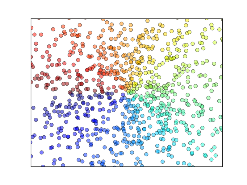
36 |
37 | 
38 |
39 | 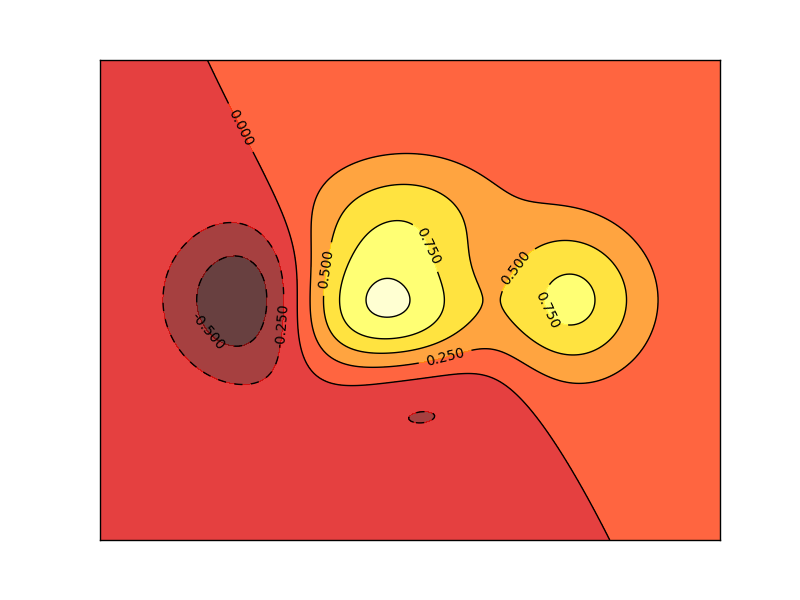
40 |
41 | 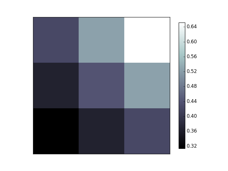
42 |
43 | 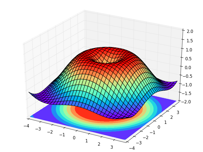
44 |
45 | 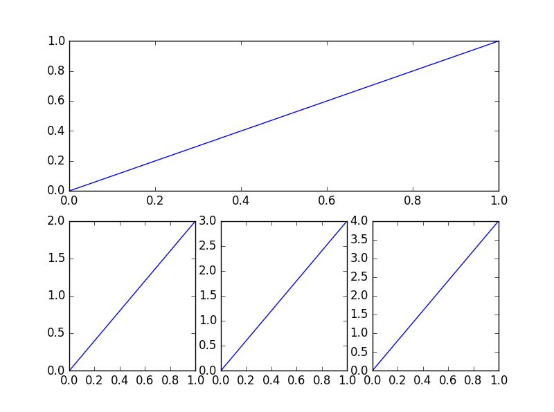
46 |
47 | 
48 |
49 | # Donation
50 |
51 | *If this does help you, please consider donating to support me for better tutorials. Any contribution is greatly appreciated!*
52 |
53 |
60 |
61 |
--------------------------------------------------------------------------------
/matplotlibTUT/plt10_scatter.py:
--------------------------------------------------------------------------------
1 | # View more python tutorials on my Youtube and Youku channel!!!
2 |
3 | # Youtube video tutorial: https://www.youtube.com/channel/UCdyjiB5H8Pu7aDTNVXTTpcg
4 | # Youku video tutorial: http://i.youku.com/pythontutorial
5 |
6 | # 10 - scatter
7 | """
8 | Please note, this script is for python3+.
9 | If you are using python2+, please modify it accordingly.
10 | Tutorial reference:
11 | http://www.scipy-lectures.org/intro/matplotlib/matplotlib.html
12 | """
13 |
14 | import matplotlib.pyplot as plt
15 | import numpy as np
16 |
17 | n = 1024 # data size
18 | X = np.random.normal(0, 1, n)
19 | Y = np.random.normal(0, 1, n)
20 | T = np.arctan2(Y, X) # for color later on
21 |
22 | plt.scatter(X, Y, s=75, c=T, alpha=.5)
23 |
24 | plt.xlim(-1.5, 1.5)
25 | plt.xticks(()) # ignore xticks
26 | plt.ylim(-1.5, 1.5)
27 | plt.yticks(()) # ignore yticks
28 |
29 | plt.show()
30 |
--------------------------------------------------------------------------------
/matplotlibTUT/plt11_bar.py:
--------------------------------------------------------------------------------
1 | # View more python tutorials on my Youtube and Youku channel!!!
2 |
3 | # Youtube video tutorial: https://www.youtube.com/channel/UCdyjiB5H8Pu7aDTNVXTTpcg
4 | # Youku video tutorial: http://i.youku.com/pythontutorial
5 |
6 | # 11 - bar
7 | """
8 | Please note, this script is for python3+.
9 | If you are using python2+, please modify it accordingly.
10 | Tutorial reference:
11 | http://www.scipy-lectures.org/intro/matplotlib/matplotlib.html
12 | """
13 |
14 | import matplotlib.pyplot as plt
15 | import numpy as np
16 |
17 | n = 12
18 | X = np.arange(n)
19 | Y1 = (1 - X / float(n)) * np.random.uniform(0.5, 1.0, n)
20 | Y2 = (1 - X / float(n)) * np.random.uniform(0.5, 1.0, n)
21 |
22 | plt.bar(X, +Y1, facecolor='#9999ff', edgecolor='white')
23 | plt.bar(X, -Y2, facecolor='#ff9999', edgecolor='white')
24 |
25 | for x, y in zip(X, Y1):
26 | # ha: horizontal alignment
27 | # va: vertical alignment
28 | plt.text(x + 0.4, y + 0.05, '%.2f' % y, ha='center', va='bottom')
29 |
30 | for x, y in zip(X, Y2):
31 | # ha: horizontal alignment
32 | # va: vertical alignment
33 | plt.text(x + 0.4, -y - 0.05, '%.2f' % y, ha='center', va='top')
34 |
35 | plt.xlim(-.5, n)
36 | plt.xticks(())
37 | plt.ylim(-1.25, 1.25)
38 | plt.yticks(())
39 |
40 | plt.show()
41 |
--------------------------------------------------------------------------------
/matplotlibTUT/plt12_contours.py:
--------------------------------------------------------------------------------
1 | # View more python tutorials on my Youtube and Youku channel!!!
2 |
3 | # Youtube video tutorial: https://www.youtube.com/channel/UCdyjiB5H8Pu7aDTNVXTTpcg
4 | # Youku video tutorial: http://i.youku.com/pythontutorial
5 |
6 | # 12 - contours
7 | """
8 | Please note, this script is for python3+.
9 | If you are using python2+, please modify it accordingly.
10 | Tutorial reference:
11 | http://www.scipy-lectures.org/intro/matplotlib/matplotlib.html
12 | """
13 |
14 | import matplotlib.pyplot as plt
15 | import numpy as np
16 |
17 | def f(x,y):
18 | # the height function
19 | return (1 - x / 2 + x**5 + y**3) * np.exp(-x**2 -y**2)
20 |
21 | n = 256
22 | x = np.linspace(-3, 3, n)
23 | y = np.linspace(-3, 3, n)
24 | X,Y = np.meshgrid(x, y)
25 |
26 | # use plt.contourf to filling contours
27 | # X, Y and value for (X,Y) point
28 | plt.contourf(X, Y, f(X, Y), 8, alpha=.75, cmap=plt.cm.hot)
29 |
30 | # use plt.contour to add contour lines
31 | C = plt.contour(X, Y, f(X, Y), 8, colors='black', linewidth=.5)
32 | # adding label
33 | plt.clabel(C, inline=True, fontsize=10)
34 |
35 | plt.xticks(())
36 | plt.yticks(())
37 | plt.show()
38 |
39 |
--------------------------------------------------------------------------------
/matplotlibTUT/plt13_image.py:
--------------------------------------------------------------------------------
1 | # View more python tutorials on my Youtube and Youku channel!!!
2 |
3 | # Youtube video tutorial: https://www.youtube.com/channel/UCdyjiB5H8Pu7aDTNVXTTpcg
4 | # Youku video tutorial: http://i.youku.com/pythontutorial
5 |
6 | # 13 - image
7 | """
8 | Please note, this script is for python3+.
9 | If you are using python2+, please modify it accordingly.
10 | """
11 |
12 | import matplotlib.pyplot as plt
13 | import numpy as np
14 |
15 | # image data
16 | a = np.array([0.313660827978, 0.365348418405, 0.423733120134,
17 | 0.365348418405, 0.439599930621, 0.525083754405,
18 | 0.423733120134, 0.525083754405, 0.651536351379]).reshape(3,3)
19 |
20 | """
21 | for the value of "interpolation", check this:
22 | http://matplotlib.org/examples/images_contours_and_fields/interpolation_methods.html
23 | for the value of "origin"= ['upper', 'lower'], check this:
24 | http://matplotlib.org/examples/pylab_examples/image_origin.html
25 | """
26 | plt.imshow(a, interpolation='nearest', cmap='bone', origin='lower')
27 | plt.colorbar(shrink=.92)
28 |
29 | plt.xticks(())
30 | plt.yticks(())
31 | plt.show()
32 |
33 |
--------------------------------------------------------------------------------
/matplotlibTUT/plt14_3d.py:
--------------------------------------------------------------------------------
1 | # View more python tutorials on my Youtube and Youku channel!!!
2 |
3 | # Youtube video tutorial: https://www.youtube.com/channel/UCdyjiB5H8Pu7aDTNVXTTpcg
4 | # Youku video tutorial: http://i.youku.com/pythontutorial
5 |
6 | # 14 - 3d
7 | """
8 | Please note, this script is for python3+.
9 | If you are using python2+, please modify it accordingly.
10 | Tutorial reference:
11 | http://www.python-course.eu/matplotlib_multiple_figures.php
12 | """
13 |
14 | import numpy as np
15 | import matplotlib.pyplot as plt
16 | from mpl_toolkits.mplot3d import Axes3D
17 |
18 | fig = plt.figure()
19 | ax = Axes3D(fig)
20 | # X, Y value
21 | X = np.arange(-4, 4, 0.25)
22 | Y = np.arange(-4, 4, 0.25)
23 | X, Y = np.meshgrid(X, Y)
24 | R = np.sqrt(X ** 2 + Y ** 2)
25 | # height value
26 | Z = np.sin(R)
27 |
28 | ax.plot_surface(X, Y, Z, rstride=1, cstride=1, cmap=plt.get_cmap('rainbow'))
29 | """
30 | ============= ================================================
31 | Argument Description
32 | ============= ================================================
33 | *X*, *Y*, *Z* Data values as 2D arrays
34 | *rstride* Array row stride (step size), defaults to 10
35 | *cstride* Array column stride (step size), defaults to 10
36 | *color* Color of the surface patches
37 | *cmap* A colormap for the surface patches.
38 | *facecolors* Face colors for the individual patches
39 | *norm* An instance of Normalize to map values to colors
40 | *vmin* Minimum value to map
41 | *vmax* Maximum value to map
42 | *shade* Whether to shade the facecolors
43 | ============= ================================================
44 | """
45 |
46 | # I think this is different from plt12_contours
47 | ax.contourf(X, Y, Z, zdir='z', offset=-2, cmap=plt.get_cmap('rainbow'))
48 | """
49 | ========== ================================================
50 | Argument Description
51 | ========== ================================================
52 | *X*, *Y*, Data values as numpy.arrays
53 | *Z*
54 | *zdir* The direction to use: x, y or z (default)
55 | *offset* If specified plot a projection of the filled contour
56 | on this position in plane normal to zdir
57 | ========== ================================================
58 | """
59 |
60 | ax.set_zlim(-2, 2)
61 |
62 | plt.show()
63 |
64 |
--------------------------------------------------------------------------------
/matplotlibTUT/plt15_subplot.py:
--------------------------------------------------------------------------------
1 | # View more python tutorials on my Youtube and Youku channel!!!
2 |
3 | # Youtube video tutorial: https://www.youtube.com/channel/UCdyjiB5H8Pu7aDTNVXTTpcg
4 | # Youku video tutorial: http://i.youku.com/pythontutorial
5 |
6 | # 15 - subplot
7 | """
8 | Please note, this script is for python3+.
9 | If you are using python2+, please modify it accordingly.
10 | Tutorial reference:
11 | http://www.scipy-lectures.org/intro/matplotlib/matplotlib.html
12 | """
13 |
14 | import matplotlib.pyplot as plt
15 |
16 | # example 1:
17 | ###############################
18 | plt.figure(figsize=(6, 4))
19 | # plt.subplot(n_rows, n_cols, plot_num)
20 | plt.subplot(2, 2, 1)
21 | plt.plot([0, 1], [0, 1])
22 |
23 | plt.subplot(222)
24 | plt.plot([0, 1], [0, 2])
25 |
26 | plt.subplot(223)
27 | plt.plot([0, 1], [0, 3])
28 |
29 | plt.subplot(224)
30 | plt.plot([0, 1], [0, 4])
31 |
32 | plt.tight_layout()
33 |
34 | # example 2:
35 | ###############################
36 | plt.figure(figsize=(6, 4))
37 | # plt.subplot(n_rows, n_cols, plot_num)
38 | plt.subplot(2, 1, 1)
39 | # figure splits into 2 rows, 1 col, plot to the 1st sub-fig
40 | plt.plot([0, 1], [0, 1])
41 |
42 | plt.subplot(234)
43 | # figure splits into 2 rows, 3 col, plot to the 4th sub-fig
44 | plt.plot([0, 1], [0, 2])
45 |
46 | plt.subplot(235)
47 | # figure splits into 2 rows, 3 col, plot to the 5th sub-fig
48 | plt.plot([0, 1], [0, 3])
49 |
50 | plt.subplot(236)
51 | # figure splits into 2 rows, 3 col, plot to the 6th sub-fig
52 | plt.plot([0, 1], [0, 4])
53 |
54 |
55 | plt.tight_layout()
56 | plt.show()
57 |
--------------------------------------------------------------------------------
/matplotlibTUT/plt16_grid_subplot.py:
--------------------------------------------------------------------------------
1 | # View more python tutorials on my Youtube and Youku channel!!!
2 |
3 | # Youtube video tutorial: https://www.youtube.com/channel/UCdyjiB5H8Pu7aDTNVXTTpcg
4 | # Youku video tutorial: http://i.youku.com/pythontutorial
5 |
6 | # 16 - grid
7 | """
8 | Please note, this script is for python3+.
9 | If you are using python2+, please modify it accordingly.
10 | Tutorial reference:
11 | http://matplotlib.org/users/gridspec.html
12 | """
13 |
14 | import matplotlib.pyplot as plt
15 | import matplotlib.gridspec as gridspec
16 |
17 | # method 1: subplot2grid
18 | ##########################
19 | plt.figure()
20 | ax1 = plt.subplot2grid((3, 3), (0, 0), colspan=3) # stands for axes
21 | ax1.plot([1, 2], [1, 2])
22 | ax1.set_title('ax1_title')
23 | ax2 = plt.subplot2grid((3, 3), (1, 0), colspan=2)
24 | ax3 = plt.subplot2grid((3, 3), (1, 2), rowspan=2)
25 | ax4 = plt.subplot2grid((3, 3), (2, 0))
26 | ax4.scatter([1, 2], [2, 2])
27 | ax4.set_xlabel('ax4_x')
28 | ax4.set_ylabel('ax4_y')
29 | ax5 = plt.subplot2grid((3, 3), (2, 1))
30 |
31 | # method 2: gridspec
32 | #########################
33 | plt.figure()
34 | gs = gridspec.GridSpec(3, 3)
35 | # use index from 0
36 | ax6 = plt.subplot(gs[0, :])
37 | ax7 = plt.subplot(gs[1, :2])
38 | ax8 = plt.subplot(gs[1:, 2])
39 | ax9 = plt.subplot(gs[-1, 0])
40 | ax10 = plt.subplot(gs[-1, -2])
41 |
42 | # method 3: easy to define structure
43 | ####################################
44 | f, ((ax11, ax12), (ax13, ax14)) = plt.subplots(2, 2, sharex=True, sharey=True)
45 | ax11.scatter([1,2], [1,2])
46 |
47 | plt.tight_layout()
48 | plt.show()
49 |
--------------------------------------------------------------------------------
/matplotlibTUT/plt17_plot_in_plot.py:
--------------------------------------------------------------------------------
1 | # View more python tutorials on my Youtube and Youku channel!!!
2 |
3 | # Youtube video tutorial: https://www.youtube.com/channel/UCdyjiB5H8Pu7aDTNVXTTpcg
4 | # Youku video tutorial: http://i.youku.com/pythontutorial
5 |
6 | # 17 - plot in plot
7 | """
8 | Please note, this script is for python3+.
9 | If you are using python2+, please modify it accordingly.
10 | Tutorial reference:
11 | http://www.python-course.eu/matplotlib_multiple_figures.php
12 | """
13 |
14 | import matplotlib.pyplot as plt
15 |
16 | fig = plt.figure()
17 | x = [1, 2, 3, 4, 5, 6, 7]
18 | y = [1, 3, 4, 2, 5, 8, 6]
19 |
20 | # below are all percentage
21 | left, bottom, width, height = 0.1, 0.1, 0.8, 0.8
22 | ax1 = fig.add_axes([left, bottom, width, height]) # main axes
23 | ax1.plot(x, y, 'r')
24 | ax1.set_xlabel('x')
25 | ax1.set_ylabel('y')
26 | ax1.set_title('title')
27 |
28 | ax2 = fig.add_axes([0.2, 0.6, 0.25, 0.25]) # inside axes
29 | ax2.plot(y, x, 'b')
30 | ax2.set_xlabel('x')
31 | ax2.set_ylabel('y')
32 | ax2.set_title('title inside 1')
33 |
34 |
35 | # different method to add axes
36 | ####################################
37 | plt.axes([0.6, 0.2, 0.25, 0.25])
38 | plt.plot(y[::-1], x, 'g')
39 | plt.xlabel('x')
40 | plt.ylabel('y')
41 | plt.title('title inside 2')
42 |
43 | plt.show()
44 |
--------------------------------------------------------------------------------
/matplotlibTUT/plt18_secondary_yaxis.py:
--------------------------------------------------------------------------------
1 | # View more python tutorials on my Youtube and Youku channel!!!
2 |
3 | # Youtube video tutorial: https://www.youtube.com/channel/UCdyjiB5H8Pu7aDTNVXTTpcg
4 | # Youku video tutorial: http://i.youku.com/pythontutorial
5 |
6 | # 18 - secondary y axis
7 | """
8 | Please note, this script is for python3+.
9 | If you are using python2+, please modify it accordingly.
10 | Tutorial reference:
11 | http://www.python-course.eu/matplotlib_multiple_figures.php
12 | """
13 |
14 | import matplotlib.pyplot as plt
15 | import numpy as np
16 |
17 | x = np.arange(0, 10, 0.1)
18 | y1 = 0.05 * x**2
19 | y2 = -1 *y1
20 |
21 | fig, ax1 = plt.subplots()
22 |
23 | ax2 = ax1.twinx() # mirror the ax1
24 | ax1.plot(x, y1, 'g-')
25 | ax2.plot(x, y2, 'b-')
26 |
27 | ax1.set_xlabel('X data')
28 | ax1.set_ylabel('Y1 data', color='g')
29 | ax2.set_ylabel('Y2 data', color='b')
30 |
31 | plt.show()
32 |
--------------------------------------------------------------------------------
/matplotlibTUT/plt19_animation.py:
--------------------------------------------------------------------------------
1 | # View more python tutorials on my Youtube and Youku channel!!!
2 |
3 | # Youtube video tutorial: https://www.youtube.com/channel/UCdyjiB5H8Pu7aDTNVXTTpcg
4 | # Youku video tutorial: http://i.youku.com/pythontutorial
5 |
6 | # 19 - animation
7 | """
8 | Please note, this script is for python3+.
9 | If you are using python2+, please modify it accordingly.
10 |
11 | Tutorial reference:
12 | http://matplotlib.org/examples/animation/simple_anim.html
13 |
14 | More animation example code:
15 | http://matplotlib.org/examples/animation/
16 | """
17 |
18 | import numpy as np
19 | from matplotlib import pyplot as plt
20 | from matplotlib import animation
21 |
22 | fig, ax = plt.subplots()
23 |
24 | x = np.arange(0, 2*np.pi, 0.01)
25 | line, = ax.plot(x, np.sin(x))
26 |
27 |
28 | def animate(i):
29 | line.set_ydata(np.sin(x + i/10.0)) # update the data
30 | return line,
31 |
32 |
33 | # Init only required for blitting to give a clean slate.
34 | def init():
35 | line.set_ydata(np.sin(x))
36 | return line,
37 |
38 | # call the animator. blit=True means only re-draw the parts that have changed.
39 | # blit=True dose not work on Mac, set blit=False
40 | # interval= update frequency
41 | ani = animation.FuncAnimation(fig=fig, func=animate, frames=100, init_func=init,
42 | interval=20, blit=False)
43 |
44 | # save the animation as an mp4. This requires ffmpeg or mencoder to be
45 | # installed. The extra_args ensure that the x264 codec is used, so that
46 | # the video can be embedded in html5. You may need to adjust this for
47 | # your system: for more information, see
48 | # http://matplotlib.sourceforge.net/api/animation_api.html
49 | # anim.save('basic_animation.mp4', fps=30, extra_args=['-vcodec', 'libx264'])
50 |
51 | plt.show()
--------------------------------------------------------------------------------
/matplotlibTUT/plt1_why.py:
--------------------------------------------------------------------------------
1 | # View more python tutorials on my Youtube and Youku channel!!!
2 |
3 | # Youtube video tutorial: https://www.youtube.com/channel/UCdyjiB5H8Pu7aDTNVXTTpcg
4 | # Youku video tutorial: http://i.youku.com/pythontutorial
5 |
6 | # 1 - why
7 |
8 | """
9 | 1. matplotlib is a powerful python data visualization tool;
10 | 2. similar with MATLAB. If know matlab, easy to move over to python;
11 | 3. easy to plot 2D, 3D data;
12 | 4. you can even make animation.
13 | """
--------------------------------------------------------------------------------
/matplotlibTUT/plt2_install.py:
--------------------------------------------------------------------------------
1 | # View more python tutorials on my Youtube and Youku channel!!!
2 |
3 | # Youtube video tutorial: https://www.youtube.com/channel/UCdyjiB5H8Pu7aDTNVXTTpcg
4 | # Youku video tutorial: http://i.youku.com/pythontutorial
5 |
6 | # 2 - install
7 |
8 | """
9 | Make sure you have installed numpy.
10 |
11 | ------------------------------
12 | INSTALL on Linux:
13 | If you have python3, in terminal you will type:
14 | $ sudo apt-get install python3-matplotlib
15 |
16 | Otherwise, if python2, type:
17 | $ sudo apt-get install python-matplotlib
18 |
19 | -------------------------------
20 | INSTALL on MacOS
21 | For python3:
22 | $ pip3 install matplotlib
23 |
24 | For python2:
25 | $ pip install matplotlib
26 |
27 | --------------------------------
28 | INSTALL on Windows:
29 | 1. make sure you install Visual Studio;
30 | 2. go to: https://pypi.python.org/pypi/matplotlib/
31 | 3. find the wheel file (a file ending in .whl) matches your python version and system
32 | (e.g. cp35 for python3.5, win32 for 32-bit system, win_amd64 for 64-bit system);
33 | 4. Copy the .whl file to your project folder, open a command window,
34 | and navigate to the project folder. Then use pip to install matplotlib:
35 |
36 | e.g.
37 | > cd python_work
38 | python_work> python -m pip3 install matplotlib-1.4.3-cp35-none-win32.whl
39 |
40 | If not success. Try the alternative way: using "Anaconda" to install.
41 | Please search this by yourself.
42 |
43 | """
--------------------------------------------------------------------------------
/matplotlibTUT/plt3_simple_plot.py:
--------------------------------------------------------------------------------
1 | # View more python tutorials on my Youtube and Youku channel!!!
2 |
3 | # Youtube video tutorial: https://www.youtube.com/channel/UCdyjiB5H8Pu7aDTNVXTTpcg
4 | # Youku video tutorial: http://i.youku.com/pythontutorial
5 |
6 | # 3 - simple plot
7 | """
8 | Please note, this script is for python3+.
9 | If you are using python2+, please modify it accordingly.
10 | """
11 |
12 | import matplotlib.pyplot as plt
13 | import numpy as np
14 |
15 | x = np.linspace(-1, 1, 50)
16 | y = 2*x + 1
17 | # y = x**2
18 | plt.plot(x, y)
19 | plt.show()
20 |
--------------------------------------------------------------------------------
/matplotlibTUT/plt4_figure.py:
--------------------------------------------------------------------------------
1 | # View more python tutorials on my Youtube and Youku channel!!!
2 |
3 | # Youtube video tutorial: https://www.youtube.com/channel/UCdyjiB5H8Pu7aDTNVXTTpcg
4 | # Youku video tutorial: http://i.youku.com/pythontutorial
5 |
6 | # 4 - figure
7 | """
8 | Please note, this script is for python3+.
9 | If you are using python2+, please modify it accordingly.
10 | Tutorial reference:
11 | http://www.scipy-lectures.org/intro/matplotlib/matplotlib.html
12 | """
13 |
14 | import matplotlib.pyplot as plt
15 | import numpy as np
16 |
17 | x = np.linspace(-3, 3, 50)
18 | y1 = 2*x + 1
19 | y2 = x**2
20 |
21 | plt.figure()
22 | plt.plot(x, y1)
23 |
24 |
25 | plt.figure(num=3, figsize=(8, 5),)
26 | plt.plot(x, y2)
27 | # plot the second curve in this figure with certain parameters
28 | plt.plot(x, y1, color='red', linewidth=1.0, linestyle='--')
29 | plt.show()
30 |
--------------------------------------------------------------------------------
/matplotlibTUT/plt5_ax_setting1.py:
--------------------------------------------------------------------------------
1 | # View more python tutorials on my Youtube and Youku channel!!!
2 |
3 | # Youtube video tutorial: https://www.youtube.com/channel/UCdyjiB5H8Pu7aDTNVXTTpcg
4 | # Youku video tutorial: http://i.youku.com/pythontutorial
5 |
6 | # 5 - axis setting
7 | """
8 | Please note, this script is for python3+.
9 | If you are using python2+, please modify it accordingly.
10 | Tutorial reference:
11 | http://www.scipy-lectures.org/intro/matplotlib/matplotlib.html
12 | """
13 |
14 | import matplotlib.pyplot as plt
15 | import numpy as np
16 |
17 | x = np.linspace(-3, 3, 50)
18 | y1 = 2*x + 1
19 | y2 = x**2
20 |
21 | plt.figure()
22 | plt.plot(x, y2)
23 | # plot the second curve in this figure with certain parameters
24 | plt.plot(x, y1, color='red', linewidth=1.0, linestyle='--')
25 | # set x limits
26 | plt.xlim((-1, 2))
27 | plt.ylim((-2, 3))
28 | plt.xlabel('I am x')
29 | plt.ylabel('I am y')
30 |
31 | # set new sticks
32 | new_ticks = np.linspace(-1, 2, 5)
33 | print(new_ticks)
34 | plt.xticks(new_ticks)
35 | # set tick labels
36 | plt.yticks([-2, -1.8, -1, 1.22, 3],
37 | [r'$really\ bad$', r'$bad$', r'$normal$', r'$good$', r'$really\ good$'])
38 | plt.show()
39 |
--------------------------------------------------------------------------------
/matplotlibTUT/plt6_ax_setting2.py:
--------------------------------------------------------------------------------
1 | # View more python tutorials on my Youtube and Youku channel!!!
2 |
3 | # Youtube video tutorial: https://www.youtube.com/channel/UCdyjiB5H8Pu7aDTNVXTTpcg
4 | # Youku video tutorial: http://i.youku.com/pythontutorial
5 |
6 | # 6 - axis setting
7 | """
8 | Please note, this script is for python3+.
9 | If you are using python2+, please modify it accordingly.
10 | Tutorial reference:
11 | http://www.scipy-lectures.org/intro/matplotlib/matplotlib.html
12 | """
13 |
14 | import matplotlib.pyplot as plt
15 | import numpy as np
16 |
17 | x = np.linspace(-3, 3, 50)
18 | y1 = 2*x + 1
19 | y2 = x**2
20 |
21 | plt.figure()
22 | plt.plot(x, y2)
23 | # plot the second curve in this figure with certain parameters
24 | plt.plot(x, y1, color='red', linewidth=1.0, linestyle='--')
25 | # set x limits
26 | plt.xlim((-1, 2))
27 | plt.ylim((-2, 3))
28 |
29 | # set new ticks
30 | new_ticks = np.linspace(-1, 2, 5)
31 | plt.xticks(new_ticks)
32 | # set tick labels
33 | plt.yticks([-2, -1.8, -1, 1.22, 3],
34 | ['$really\ bad$', '$bad$', '$normal$', '$good$', '$really\ good$'])
35 | # to use '$ $' for math text and nice looking, e.g. '$\pi$'
36 |
37 | # gca = 'get current axis'
38 | ax = plt.gca()
39 | ax.spines['right'].set_color('none')
40 | ax.spines['top'].set_color('none')
41 |
42 | ax.xaxis.set_ticks_position('bottom')
43 | # ACCEPTS: [ 'top' | 'bottom' | 'both' | 'default' | 'none' ]
44 |
45 | ax.spines['bottom'].set_position(('data', 0))
46 | # the 1st is in 'outward' | 'axes' | 'data'
47 | # axes: percentage of y axis
48 | # data: depend on y data
49 |
50 | ax.yaxis.set_ticks_position('left')
51 | # ACCEPTS: [ 'left' | 'right' | 'both' | 'default' | 'none' ]
52 |
53 | ax.spines['left'].set_position(('data',0))
54 | plt.show()
55 |
--------------------------------------------------------------------------------
/matplotlibTUT/plt7_legend.py:
--------------------------------------------------------------------------------
1 | # View more python tutorials on my Youtube and Youku channel!!!
2 |
3 | # Youtube video tutorial: https://www.youtube.com/channel/UCdyjiB5H8Pu7aDTNVXTTpcg
4 | # Youku video tutorial: http://i.youku.com/pythontutorial
5 |
6 | # 7 - legend
7 | """
8 | Please note, this script is for python3+.
9 | If you are using python2+, please modify it accordingly.
10 | Tutorial reference:
11 | http://www.scipy-lectures.org/intro/matplotlib/matplotlib.html
12 | """
13 |
14 | import matplotlib.pyplot as plt
15 | import numpy as np
16 |
17 | x = np.linspace(-3, 3, 50)
18 | y1 = 2*x + 1
19 | y2 = x**2
20 |
21 | plt.figure()
22 | # set x limits
23 | plt.xlim((-1, 2))
24 | plt.ylim((-2, 3))
25 |
26 | # set new sticks
27 | new_sticks = np.linspace(-1, 2, 5)
28 | plt.xticks(new_sticks)
29 | # set tick labels
30 | plt.yticks([-2, -1.8, -1, 1.22, 3],
31 | [r'$really\ bad$', r'$bad$', r'$normal$', r'$good$', r'$really\ good$'])
32 |
33 | l1, = plt.plot(x, y1, label='linear line')
34 | l2, = plt.plot(x, y2, color='red', linewidth=1.0, linestyle='--', label='square line')
35 |
36 | plt.legend(loc='upper right')
37 | # plt.legend(handles=[l1, l2], labels=['up', 'down'], loc='best')
38 | # the "," is very important in here l1, = plt... and l2, = plt... for this step
39 | """legend( handles=(line1, line2, line3),
40 | labels=('label1', 'label2', 'label3'),
41 | 'upper right')
42 | The *loc* location codes are::
43 |
44 | 'best' : 0, (currently not supported for figure legends)
45 | 'upper right' : 1,
46 | 'upper left' : 2,
47 | 'lower left' : 3,
48 | 'lower right' : 4,
49 | 'right' : 5,
50 | 'center left' : 6,
51 | 'center right' : 7,
52 | 'lower center' : 8,
53 | 'upper center' : 9,
54 | 'center' : 10,"""
55 |
56 | plt.show()
57 |
--------------------------------------------------------------------------------
/matplotlibTUT/plt8_annotation.py:
--------------------------------------------------------------------------------
1 | # View more python tutorials on my Youtube and Youku channel!!!
2 |
3 | # Youtube video tutorial: https://www.youtube.com/channel/UCdyjiB5H8Pu7aDTNVXTTpcg
4 | # Youku video tutorial: http://i.youku.com/pythontutorial
5 |
6 | # 8 - annotation
7 | """
8 | Please note, this script is for python3+.
9 | If you are using python2+, please modify it accordingly.
10 |
11 | Tutorial reference:
12 | http://www.scipy-lectures.org/intro/matplotlib/matplotlib.html
13 |
14 | Mathematical expressions:
15 | http://matplotlib.org/users/mathtext.html#mathtext-tutorial
16 | """
17 |
18 | import matplotlib.pyplot as plt
19 | import numpy as np
20 |
21 | x = np.linspace(-3, 3, 50)
22 | y = 2*x + 1
23 |
24 | plt.figure(num=1, figsize=(8, 5),)
25 | plt.plot(x, y,)
26 |
27 | ax = plt.gca()
28 | ax.spines['right'].set_color('none')
29 | ax.spines['top'].set_color('none')
30 | ax.spines['top'].set_color('none')
31 | ax.xaxis.set_ticks_position('bottom')
32 | ax.spines['bottom'].set_position(('data', 0))
33 | ax.yaxis.set_ticks_position('left')
34 | ax.spines['left'].set_position(('data', 0))
35 |
36 | x0 = 1
37 | y0 = 2*x0 + 1
38 | plt.plot([x0, x0,], [0, y0,], 'k--', linewidth=2.5)
39 | plt.scatter([x0, ], [y0, ], s=50, color='b')
40 |
41 | # method 1:
42 | #####################
43 | plt.annotate(r'$2x+1=%s$' % y0, xy=(x0, y0), xycoords='data', xytext=(+30, -30),
44 | textcoords='offset points', fontsize=16,
45 | arrowprops=dict(arrowstyle='->', connectionstyle="arc3,rad=.2"))
46 |
47 | # method 2:
48 | ########################
49 | plt.text(-3.7, 3, r'$This\ is\ the\ some\ text. \mu\ \sigma_i\ \alpha_t$',
50 | fontdict={'size': 16, 'color': 'r'})
51 |
52 | plt.show()
53 |
--------------------------------------------------------------------------------
/matplotlibTUT/plt9_tick_visibility.py:
--------------------------------------------------------------------------------
1 | # View more python tutorials on my Youtube and Youku channel!!!
2 |
3 | # Youtube video tutorial: https://www.youtube.com/channel/UCdyjiB5H8Pu7aDTNVXTTpcg
4 | # Youku video tutorial: http://i.youku.com/pythontutorial
5 |
6 | # 9 - tick_visibility
7 | """
8 | Please note, this script is for python3+.
9 | If you are using python2+, please modify it accordingly.
10 | Tutorial reference:
11 | http://www.scipy-lectures.org/intro/matplotlib/matplotlib.html
12 | """
13 |
14 | import matplotlib.pyplot as plt
15 | import numpy as np
16 |
17 | x = np.linspace(-3, 3, 50)
18 | y = 0.1*x
19 |
20 | plt.figure()
21 | plt.plot(x, y, linewidth=10, zorder=1) # set zorder for ordering the plot in plt 2.0.2 or higher
22 | plt.ylim(-2, 2)
23 | ax = plt.gca()
24 | ax.spines['right'].set_color('none')
25 | ax.spines['top'].set_color('none')
26 | ax.spines['top'].set_color('none')
27 | ax.xaxis.set_ticks_position('bottom')
28 | ax.spines['bottom'].set_position(('data', 0))
29 | ax.yaxis.set_ticks_position('left')
30 | ax.spines['left'].set_position(('data', 0))
31 |
32 |
33 | for label in ax.get_xticklabels() + ax.get_yticklabels():
34 | label.set_fontsize(12)
35 | # set zorder for ordering the plot in plt 2.0.2 or higher
36 | label.set_bbox(dict(facecolor='white', edgecolor='none', alpha=0.8, zorder=2))
37 | plt.show()
38 |
--------------------------------------------------------------------------------
/multiprocessingTUT/multiprocessing3_queue.py:
--------------------------------------------------------------------------------
1 | # View more python learning tutorial on my Youtube and Youku channel!!!
2 |
3 | # Youtube video tutorial: https://www.youtube.com/channel/UCdyjiB5H8Pu7aDTNVXTTpcg
4 | # Youku video tutorial: http://i.youku.com/pythontutorial
5 |
6 | import multiprocessing as mp
7 |
8 | def job(q):
9 | res = 0
10 | for i in range(1000):
11 | res += i+i**2+i**3
12 | q.put(res) # queue
13 |
14 | if __name__ == '__main__':
15 | q = mp.Queue()
16 | p1 = mp.Process(target=job, args=(q,))
17 | p2 = mp.Process(target=job, args=(q,))
18 | p1.start()
19 | p2.start()
20 | p1.join()
21 | p2.join()
22 | res1 = q.get()
23 | res2 = q.get()
24 | print(res1+res2)
25 |
26 |
--------------------------------------------------------------------------------
/multiprocessingTUT/multiprocessing4_efficiency_comparison.py:
--------------------------------------------------------------------------------
1 | # View more python learning tutorial on my Youtube and Youku channel!!!
2 |
3 | # Youtube video tutorial: https://www.youtube.com/channel/UCdyjiB5H8Pu7aDTNVXTTpcg
4 | # Youku video tutorial: http://i.youku.com/pythontutorial
5 |
6 | import multiprocessing as mp
7 | import threading as td
8 | import time
9 |
10 | def job(q):
11 | res = 0
12 | for i in range(1000000):
13 | res += i+i**2+i**3
14 | q.put(res) # queue
15 |
16 | def multicore():
17 | q = mp.Queue()
18 | p1 = mp.Process(target=job, args=(q,))
19 | p2 = mp.Process(target=job, args=(q,))
20 | p1.start()
21 | p2.start()
22 | p1.join()
23 | p2.join()
24 | res1 = q.get()
25 | res2 = q.get()
26 | print('multicore:' , res1+res2)
27 |
28 | def normal():
29 | res = 0
30 | for _ in range(2):
31 | for i in range(1000000):
32 | res += i+i**2+i**3
33 | print('normal:', res)
34 |
35 | def multithread():
36 | q = mp.Queue()
37 | t1 = td.Thread(target=job, args=(q,))
38 | t2 = td.Thread(target=job, args=(q,))
39 | t1.start()
40 | t2.start()
41 | t1.join()
42 | t2.join()
43 | res1 = q.get()
44 | res2 = q.get()
45 | print('multithread:', res1+res2)
46 |
47 | if __name__ == '__main__':
48 | st = time.time()
49 | normal()
50 | st1= time.time()
51 | print('normal time:', st1 - st)
52 | multithread()
53 | st2 = time.time()
54 | print('multithread time:', st2 - st1)
55 | multicore()
56 | print('multicore time:', time.time()-st2)
57 |
58 |
--------------------------------------------------------------------------------
/multiprocessingTUT/multiprocessing5_pool.py:
--------------------------------------------------------------------------------
1 | # View more python learning tutorial on my Youtube and Youku channel!!!
2 |
3 | # Youtube video tutorial: https://www.youtube.com/channel/UCdyjiB5H8Pu7aDTNVXTTpcg
4 | # Youku video tutorial: http://i.youku.com/pythontutorial
5 |
6 | import multiprocessing as mp
7 |
8 | def job(x):
9 | return x*x
10 |
11 | def multicore():
12 | pool = mp.Pool(processes=2)
13 | res = pool.map(job, range(10))
14 | print(res)
15 | res = pool.apply_async(job, (2,))
16 | print(res.get())
17 | multi_res =[pool.apply_async(job, (i,)) for i in range(10)]
18 | print([res.get() for res in multi_res])
19 |
20 | if __name__ == '__main__':
21 | multicore()
22 |
23 |
24 |
--------------------------------------------------------------------------------
/multiprocessingTUT/multiprocessing7_lock.py:
--------------------------------------------------------------------------------
1 | # View more python learning tutorial on my Youtube and Youku channel!!!
2 |
3 | # Youtube video tutorial: https://www.youtube.com/channel/UCdyjiB5H8Pu7aDTNVXTTpcg
4 | # Youku video tutorial: http://i.youku.com/pythontutorial
5 |
6 | import multiprocessing as mp
7 | import time
8 |
9 | def job(v, num, l):
10 | l.acquire()
11 | for _ in range(10):
12 | time.sleep(0.1)
13 | v.value += num
14 | print(v.value)
15 | l.release()
16 |
17 | def multicore():
18 | l = mp.Lock()
19 | v = mp.Value('i', 0)
20 | p1 = mp.Process(target=job, args=(v, 1, l))
21 | p2 = mp.Process(target=job, args=(v, 3, l))
22 | p1.start()
23 | p2.start()
24 | p1.join()
25 | p2.join()
26 |
27 | if __name__ == '__main__':
28 | multicore()
29 |
30 |
31 |
32 |
--------------------------------------------------------------------------------
/numpy&pandas/11_pandas_intro.py:
--------------------------------------------------------------------------------
1 | # View more python tutorials on my Youtube and Youku channel!!!
2 |
3 | # Youtube video tutorial: https://www.youtube.com/channel/UCdyjiB5H8Pu7aDTNVXTTpcg
4 | # Youku video tutorial: http://i.youku.com/pythontutorial
5 |
6 | """
7 | Please note, this code is only for python 3+. If you are using python 2+, please modify the code accordingly.
8 | """
9 | from __future__ import print_function
10 | import pandas as pd
11 | import numpy as np
12 |
13 | s = pd.Series([1,3,6,np.nan,4,1]) # similar with 1D numpy
14 | print(s)
15 | dates = pd.date_range('20160101', periods=6)
16 | df = pd.DataFrame(np.random.randn(6,4), index=dates, columns=['A','B','C','D'])
17 | print(df['B'])
18 | df2 = pd.DataFrame({'A' : 1.,
19 | 'B' : pd.Timestamp('20130102'),
20 | 'C' : pd.Series(1,index=list(range(4)),dtype='float32'),
21 | 'D' : np.array([3] * 4,dtype='int32'),
22 | 'E' : pd.Categorical(["test","train","test","train"]),
23 | 'F' : 'foo'})
24 | print(df2)
25 | print(df2.dtypes)
26 |
27 | print(df.index)
28 | print(df.columns)
29 | print(df.values)
30 | print(df.describe())
31 | print(df.T)
32 | print(df.sort_index(axis=1, ascending=False))
33 | print(df.sort_values(by='B'))
--------------------------------------------------------------------------------
/numpy&pandas/12_selection.py:
--------------------------------------------------------------------------------
1 | # View more python tutorials on my Youtube and Youku channel!!!
2 |
3 | # Youtube video tutorial: https://www.youtube.com/channel/UCdyjiB5H8Pu7aDTNVXTTpcg
4 | # Youku video tutorial: http://i.youku.com/pythontutorial
5 | """
6 | Please note, this code is only for python 3+. If you are using python 2+, please modify the code accordingly.
7 | """
8 | from __future__ import print_function
9 | import pandas as pd
10 | import numpy as np
11 |
12 | dates = pd.date_range('20130101', periods=6)
13 | df = pd.DataFrame(np.random.randn(6,4), index=dates, columns=['A', 'B', 'C', 'D'])
14 |
15 | print(df['A'], df.A)
16 | print(df[0:3], df['20130102':'20130104'])
17 |
18 | # select by label: loc
19 | print(df.loc['20130102'])
20 | print(df.loc[:,['A','B']])
21 | print(df.loc['20130102', ['A','B']])
22 |
23 | # select by position: iloc
24 | print(df.iloc[3])
25 | print(df.iloc[3, 1])
26 | print(df.iloc[3:5,0:2])
27 | print(df.iloc[[1,2,4],[0,2]])
28 |
29 | # mixed selection: ix
30 | print(df.ix[:3, ['A', 'C']])
31 | # Boolean indexing
32 | print(df[df.A > 0])
33 |
34 |
35 |
--------------------------------------------------------------------------------
/numpy&pandas/13_set_value.py:
--------------------------------------------------------------------------------
1 | # View more python tutorials on my Youtube and Youku channel!!!
2 |
3 | # Youtube video tutorial: https://www.youtube.com/channel/UCdyjiB5H8Pu7aDTNVXTTpcg
4 | # Youku video tutorial: http://i.youku.com/pythontutorial
5 |
6 | """
7 | Please note, this code is only for python 3+. If you are using python 2+, please modify the code accordingly.
8 | """
9 | from __future__ import print_function
10 | import pandas as pd
11 | import numpy as np
12 |
13 | dates = pd.date_range('20130101', periods=6)
14 | df = pd.DataFrame(np.random.randn(6,4), index=dates, columns=['A', 'B', 'C', 'D'])
15 |
16 | df.iloc[2,2] = 1111
17 | df.loc['2013-01-03', 'D'] = 2222
18 | df.A[df.A>0] = 0
19 | df['F'] = np.nan
20 | df['G'] = pd.Series([1,2,3,4,5,6], index=pd.date_range('20130101', periods=6))
21 | print(df)
--------------------------------------------------------------------------------
/numpy&pandas/14_nan.py:
--------------------------------------------------------------------------------
1 | # View more python tutorials on my Youtube and Youku channel!!!
2 |
3 | # Youtube video tutorial: https://www.youtube.com/channel/UCdyjiB5H8Pu7aDTNVXTTpcg
4 | # Youku video tutorial: http://i.youku.com/pythontutorial
5 |
6 | """
7 | Please note, this code is only for python 3+. If you are using python 2+, please modify the code accordingly.
8 | """
9 | from __future__ import print_function
10 | import pandas as pd
11 | import numpy as np
12 |
13 | dates = pd.date_range('20130101', periods=6)
14 | df = pd.DataFrame(np.arange(24).reshape((6,4)), index=dates, columns=['A', 'B', 'C', 'D'])
15 |
16 | df.iloc[0,1] = np.nan
17 | df.iloc[1,2] = np.nan
18 | print(df.dropna(axis=0, how='any')) # how={'any', 'all'}
19 | print(df.fillna(value=0))
20 | print(pd.isnull(df))
--------------------------------------------------------------------------------
/numpy&pandas/15_read_to/15_read_to.py:
--------------------------------------------------------------------------------
1 | # View more python tutorials on my Youtube and Youku channel!!!
2 |
3 | # Youtube video tutorial: https://www.youtube.com/channel/UCdyjiB5H8Pu7aDTNVXTTpcg
4 | # Youku video tutorial: http://i.youku.com/pythontutorial
5 | """
6 | Please note, this code is only for python 3+. If you are using python 2+, please modify the code accordingly.
7 | """
8 | from __future__ import print_function
9 | import pandas as pd
10 |
11 | # read from
12 | data = pd.read_csv('student.csv')
13 | print(data)
14 |
15 | # save to
16 | data.to_pickle('student.pickle')
--------------------------------------------------------------------------------
/numpy&pandas/15_read_to/student.csv:
--------------------------------------------------------------------------------
1 | Student ID,name ,age,gender
2 | 1100,Kelly,22,Female
3 | 1101,Clo,21,Female
4 | 1102,Tilly,22,Female
5 | 1103,Tony,24,Male
6 | 1104,David,20,Male
7 | 1105,Catty,22,Female
8 | 1106,M,3,Female
9 | 1107,N,43,Male
10 | 1108,A,13,Male
11 | 1109,S,12,Male
12 | 1110,David,33,Male
13 | 1111,Dw,3,Female
14 | 1112,Q,23,Male
15 | 1113,W,21,Female
--------------------------------------------------------------------------------
/numpy&pandas/16_concat.py:
--------------------------------------------------------------------------------
1 | # View more python tutorials on my Youtube and Youku channel!!!
2 |
3 | # Youtube video tutorial: https://www.youtube.com/channel/UCdyjiB5H8Pu7aDTNVXTTpcg
4 | # Youku video tutorial: http://i.youku.com/pythontutorial
5 |
6 | """
7 | Please note, this code is only for python 3+. If you are using python 2+, please modify the code accordingly.
8 | """
9 | from __future__ import print_function
10 | import pandas as pd
11 | import numpy as np
12 |
13 | # concatenating
14 | # ignore index
15 | df1 = pd.DataFrame(np.ones((3,4))*0, columns=['a','b','c','d'])
16 | df2 = pd.DataFrame(np.ones((3,4))*1, columns=['a','b','c','d'])
17 | df3 = pd.DataFrame(np.ones((3,4))*2, columns=['a','b','c','d'])
18 | res = pd.concat([df1, df2, df3], axis=0, ignore_index=True)
19 |
20 | # join, ('inner', 'outer')
21 | df1 = pd.DataFrame(np.ones((3,4))*0, columns=['a','b','c','d'], index=[1,2,3])
22 | df2 = pd.DataFrame(np.ones((3,4))*1, columns=['b','c','d', 'e'], index=[2,3,4])
23 | res = pd.concat([df1, df2], axis=1, join='outer')
24 | res = pd.concat([df1, df2], axis=1, join='inner')
25 |
26 | # join_axes
27 | res = pd.concat([df1, df2], axis=1, join_axes=[df1.index])
28 |
29 | # append
30 | df1 = pd.DataFrame(np.ones((3,4))*0, columns=['a','b','c','d'])
31 | df2 = pd.DataFrame(np.ones((3,4))*1, columns=['a','b','c','d'])
32 | df2 = pd.DataFrame(np.ones((3,4))*1, columns=['b','c','d', 'e'], index=[2,3,4])
33 | res = df1.append(df2, ignore_index=True)
34 | res = df1.append([df2, df3])
35 |
36 | s1 = pd.Series([1,2,3,4], index=['a','b','c','d'])
37 | res = df1.append(s1, ignore_index=True)
38 |
39 | print(res)
--------------------------------------------------------------------------------
/numpy&pandas/17_merge.py:
--------------------------------------------------------------------------------
1 | # View more python tutorials on my Youtube and Youku channel!!!
2 |
3 | # Youtube video tutorial: https://www.youtube.com/channel/UCdyjiB5H8Pu7aDTNVXTTpcg
4 | # Youku video tutorial: http://i.youku.com/pythontutorial
5 |
6 | """
7 | Please note, this code is only for python 3+. If you are using python 2+, please modify the code accordingly.
8 | """
9 | from __future__ import print_function
10 | import pandas as pd
11 |
12 | # merging two df by key/keys. (may be used in database)
13 | # simple example
14 | left = pd.DataFrame({'key': ['K0', 'K1', 'K2', 'K3'],
15 | 'A': ['A0', 'A1', 'A2', 'A3'],
16 | 'B': ['B0', 'B1', 'B2', 'B3']})
17 | right = pd.DataFrame({'key': ['K0', 'K1', 'K2', 'K3'],
18 | 'C': ['C0', 'C1', 'C2', 'C3'],
19 | 'D': ['D0', 'D1', 'D2', 'D3']})
20 | print(left)
21 | print(right)
22 | res = pd.merge(left, right, on='key')
23 | print(res)
24 |
25 | # consider two keys
26 | left = pd.DataFrame({'key1': ['K0', 'K0', 'K1', 'K2'],
27 | 'key2': ['K0', 'K1', 'K0', 'K1'],
28 | 'A': ['A0', 'A1', 'A2', 'A3'],
29 | 'B': ['B0', 'B1', 'B2', 'B3']})
30 | right = pd.DataFrame({'key1': ['K0', 'K1', 'K1', 'K2'],
31 | 'key2': ['K0', 'K0', 'K0', 'K0'],
32 | 'C': ['C0', 'C1', 'C2', 'C3'],
33 | 'D': ['D0', 'D1', 'D2', 'D3']})
34 | print(left)
35 | print(right)
36 | res = pd.merge(left, right, on=['key1', 'key2'], how='inner') # default for how='inner'
37 | # how = ['left', 'right', 'outer', 'inner']
38 | res = pd.merge(left, right, on=['key1', 'key2'], how='left')
39 | print(res)
40 |
41 | # indicator
42 | df1 = pd.DataFrame({'col1':[0,1], 'col_left':['a','b']})
43 | df2 = pd.DataFrame({'col1':[1,2,2],'col_right':[2,2,2]})
44 | print(df1)
45 | print(df2)
46 | res = pd.merge(df1, df2, on='col1', how='outer', indicator=True)
47 | # give the indicator a custom name
48 | res = pd.merge(df1, df2, on='col1', how='outer', indicator='indicator_column')
49 |
50 |
51 | # merged by index
52 | left = pd.DataFrame({'A': ['A0', 'A1', 'A2'],
53 | 'B': ['B0', 'B1', 'B2']},
54 | index=['K0', 'K1', 'K2'])
55 | right = pd.DataFrame({'C': ['C0', 'C2', 'C3'],
56 | 'D': ['D0', 'D2', 'D3']},
57 | index=['K0', 'K2', 'K3'])
58 | print(left)
59 | print(right)
60 | # left_index and right_index
61 | res = pd.merge(left, right, left_index=True, right_index=True, how='outer')
62 | res = pd.merge(left, right, left_index=True, right_index=True, how='inner')
63 |
64 | # handle overlapping
65 | boys = pd.DataFrame({'k': ['K0', 'K1', 'K2'], 'age': [1, 2, 3]})
66 | girls = pd.DataFrame({'k': ['K0', 'K0', 'K3'], 'age': [4, 5, 6]})
67 | res = pd.merge(boys, girls, on='k', suffixes=['_boy', '_girl'], how='inner')
68 | print(res)
69 |
70 | # join function in pandas is similar with merge. If know merge, you will understand join
71 |
--------------------------------------------------------------------------------
/numpy&pandas/18_plot.py:
--------------------------------------------------------------------------------
1 | # View more python tutorials on my Youtube and Youku channel!!!
2 |
3 | # Youtube video tutorial: https://www.youtube.com/channel/UCdyjiB5H8Pu7aDTNVXTTpcg
4 | # Youku video tutorial: http://i.youku.com/pythontutorial
5 |
6 | """
7 | Please note, this code is only for python 3+. If you are using python 2+, please modify the code accordingly.
8 | """
9 | from __future__ import print_function
10 | import pandas as pd
11 | import numpy as np
12 | import matplotlib.pyplot as plt
13 |
14 | # plot data
15 |
16 | # Series
17 | data = pd.Series(np.random.randn(1000), index=np.arange(1000))
18 | data = data.cumsum()
19 | ##data.plot()
20 |
21 | # DataFrame
22 | data = pd.DataFrame(np.random.randn(1000, 4), index=np.arange(1000), columns=list("ABCD"))
23 | data = data.cumsum()
24 | # plot methods:
25 | # 'bar', 'hist', 'box', 'kde', 'area', scatter', hexbin', 'pie'
26 | ax = data.plot.scatter(x='A', y='B', color='DarkBlue', label="Class 1")
27 | data.plot.scatter(x='A', y='C', color='LightGreen', label='Class 2', ax=ax)
28 |
29 | plt.show()
--------------------------------------------------------------------------------
/pyTorch tutorial/README.md:
--------------------------------------------------------------------------------
1 |
2 |
3 |  4 |
5 |
4 |
5 |
6 |
7 | ---
8 |
9 |
10 |
11 | # This pyTorch Tutorial has been moved to anther independent repo:
12 |
13 | [/MorvanZhou/PyTorch-Tutorial](/MorvanZhou/PyTorch-Tutorial)
14 |
15 | # 请注意, 这个 PyTorch 的教程代码已经被移至另一个网页:
16 |
17 | [/MorvanZhou/PyTorch-Tutorial](/MorvanZhou/PyTorch-Tutorial)
18 |
19 |
20 | # Donation
21 |
22 | *If this does help you, please consider donating to support me for better tutorials. Any contribution is greatly appreciated!*
23 |
24 |
31 |
32 |
38 |
--------------------------------------------------------------------------------
/sklearnTUT/sk10_cross_validation3.py:
--------------------------------------------------------------------------------
1 | # View more python learning tutorial on my Youtube and Youku channel!!!
2 |
3 | # Youtube video tutorial: https://www.youtube.com/channel/UCdyjiB5H8Pu7aDTNVXTTpcg
4 | # Youku video tutorial: http://i.youku.com/pythontutorial
5 |
6 | """
7 | Please note, this code is only for python 3+. If you are using python 2+, please modify the code accordingly.
8 | """
9 | from __future__ import print_function
10 | from sklearn.learning_curve import validation_curve
11 | from sklearn.datasets import load_digits
12 | from sklearn.svm import SVC
13 | import matplotlib.pyplot as plt
14 | import numpy as np
15 |
16 | digits = load_digits()
17 | X = digits.data
18 | y = digits.target
19 | param_range = np.logspace(-6, -2.3, 5)
20 | train_loss, test_loss = validation_curve(
21 | SVC(), X, y, param_name='gamma', param_range=param_range, cv=10,
22 | scoring='mean_squared_error')
23 | train_loss_mean = -np.mean(train_loss, axis=1)
24 | test_loss_mean = -np.mean(test_loss, axis=1)
25 |
26 | plt.plot(param_range, train_loss_mean, 'o-', color="r",
27 | label="Training")
28 | plt.plot(param_range, test_loss_mean, 'o-', color="g",
29 | label="Cross-validation")
30 |
31 | plt.xlabel("gamma")
32 | plt.ylabel("Loss")
33 | plt.legend(loc="best")
34 | plt.show()
--------------------------------------------------------------------------------
/sklearnTUT/sk11_save.py:
--------------------------------------------------------------------------------
1 | # View more python tutorials on my Youtube and Youku channel!!!
2 |
3 | # Youtube video tutorial: https://www.youtube.com/channel/UCdyjiB5H8Pu7aDTNVXTTpcg
4 | # Youku video tutorial: http://i.youku.com/pythontutorial
5 |
6 | """
7 | Please note, this code is only for python 3+. If you are using python 2+, please modify the code accordingly.
8 | """
9 | from __future__ import print_function
10 | from sklearn import svm
11 | from sklearn import datasets
12 |
13 | clf = svm.SVC()
14 | iris = datasets.load_iris()
15 | X, y = iris.data, iris.target
16 | clf.fit(X, y)
17 |
18 | # method 1: pickle
19 | import pickle
20 | # save
21 | with open('save/clf.pickle', 'wb') as f:
22 | pickle.dump(clf, f)
23 | # restore
24 | with open('save/clf.pickle', 'rb') as f:
25 | clf2 = pickle.load(f)
26 | print(clf2.predict(X[0:1]))
27 |
28 | # method 2: joblib
29 | from sklearn.externals import joblib
30 | # Save
31 | joblib.dump(clf, 'save/clf.pkl')
32 | # restore
33 | clf3 = joblib.load('save/clf.pkl')
34 | print(clf3.predict(X[0:1]))
--------------------------------------------------------------------------------
/sklearnTUT/sk4_learning_pattern.py:
--------------------------------------------------------------------------------
1 | # View more python learning tutorial on my Youtube and Youku channel!!!
2 |
3 | # Youtube video tutorial: https://www.youtube.com/channel/UCdyjiB5H8Pu7aDTNVXTTpcg
4 | # Youku video tutorial: http://i.youku.com/pythontutorial
5 |
6 | """
7 | Please note, this code is only for python 3+. If you are using python 2+, please modify the code accordingly.
8 | """
9 | from __future__ import print_function
10 | from sklearn import datasets
11 | from sklearn.model_selection import train_test_split
12 | from sklearn.neighbors import KNeighborsClassifier
13 |
14 | iris = datasets.load_iris()
15 | iris_X = iris.data
16 | iris_y = iris.target
17 |
18 | ##print(iris_X[:2, :])
19 | ##print(iris_y)
20 |
21 | X_train, X_test, y_train, y_test = train_test_split(
22 | iris_X, iris_y, test_size=0.3)
23 |
24 | ##print(y_train)
25 |
26 | knn = KNeighborsClassifier()
27 | knn.fit(X_train, y_train)
28 | print(knn.predict(X_test))
29 | print(y_test)
30 |
31 |
32 |
--------------------------------------------------------------------------------
/sklearnTUT/sk5_datasets.py:
--------------------------------------------------------------------------------
1 | # View more python learning tutorial on my Youtube and Youku channel!!!
2 |
3 | # Youtube video tutorial: https://www.youtube.com/channel/UCdyjiB5H8Pu7aDTNVXTTpcg
4 | # Youku video tutorial: http://i.youku.com/pythontutorial
5 |
6 | """
7 | Please note, this code is only for python 3+. If you are using python 2+, please modify the code accordingly.
8 | """
9 | from __future__ import print_function
10 | from sklearn import datasets
11 | from sklearn.linear_model import LinearRegression
12 | import matplotlib.pyplot as plt
13 |
14 | loaded_data = datasets.load_boston()
15 | data_X = loaded_data.data
16 | data_y = loaded_data.target
17 |
18 | model = LinearRegression()
19 | model.fit(data_X, data_y)
20 |
21 | print(model.predict(data_X[:4, :]))
22 | print(data_y[:4])
23 |
24 | X, y = datasets.make_regression(n_samples=100, n_features=1, n_targets=1, noise=10)
25 | plt.scatter(X, y)
26 | plt.show()
27 |
28 |
29 |
30 |
31 |
32 |
33 |
--------------------------------------------------------------------------------
/sklearnTUT/sk6_model_attribute_method.py:
--------------------------------------------------------------------------------
1 | # View more python learning tutorial on my Youtube and Youku channel!!!
2 |
3 | # Youtube video tutorial: https://www.youtube.com/channel/UCdyjiB5H8Pu7aDTNVXTTpcg
4 | # Youku video tutorial: http://i.youku.com/pythontutorial
5 |
6 | """
7 | Please note, this code is only for python 3+. If you are using python 2+, please modify the code accordingly.
8 | """
9 | from __future__ import print_function
10 | from sklearn import datasets
11 | from sklearn.linear_model import LinearRegression
12 |
13 | loaded_data = datasets.load_boston()
14 | data_X = loaded_data.data
15 | data_y = loaded_data.target
16 |
17 | model = LinearRegression()
18 | model.fit(data_X, data_y)
19 |
20 | print(model.predict(data_X[:4, :]))
21 | print(model.coef_)
22 | print(model.intercept_)
23 | print(model.get_params())
24 | print(model.score(data_X, data_y)) # R^2 coefficient of determination
25 |
--------------------------------------------------------------------------------
/sklearnTUT/sk7_normalization.py:
--------------------------------------------------------------------------------
1 | # View more python learning tutorial on my Youtube and Youku channel!!!
2 |
3 | # Youtube video tutorial: https://www.youtube.com/channel/UCdyjiB5H8Pu7aDTNVXTTpcg
4 | # Youku video tutorial: http://i.youku.com/pythontutorial
5 |
6 | """
7 | Please note, this code is only for python 3+. If you are using python 2+, please modify the code accordingly.
8 | """
9 | from __future__ import print_function
10 | from sklearn import preprocessing
11 | import numpy as np
12 | from sklearn.model_selection import train_test_split
13 | from sklearn.datasets.samples_generator import make_classification
14 | from sklearn.svm import SVC
15 | import matplotlib.pyplot as plt
16 |
17 | a = np.array([[10, 2.7, 3.6],
18 | [-100, 5, -2],
19 | [120, 20, 40]], dtype=np.float64)
20 | print(a)
21 | print(preprocessing.scale(a))
22 |
23 | X, y = make_classification(n_samples=300, n_features=2 , n_redundant=0, n_informative=2,
24 | random_state=22, n_clusters_per_class=1, scale=100)
25 | plt.scatter(X[:, 0], X[:, 1], c=y)
26 | plt.show()
27 | X = preprocessing.scale(X) # normalization step
28 | X_train, X_test, y_train, y_test = train_test_split(X, y, test_size=.3)
29 | clf = SVC()
30 | clf.fit(X_train, y_train)
31 | print(clf.score(X_test, y_test))
32 |
33 |
34 |
35 |
36 |
37 |
38 |
39 |
40 |
41 |
42 |
43 |
44 |
45 |
46 |
47 |
48 |
--------------------------------------------------------------------------------
/sklearnTUT/sk8_cross_validation/for_you_to_practice.py:
--------------------------------------------------------------------------------
1 | # View more python learning tutorial on my Youtube and Youku channel!!!
2 |
3 | # Youtube video tutorial: https://www.youtube.com/channel/UCdyjiB5H8Pu7aDTNVXTTpcg
4 | # Youku video tutorial: http://i.youku.com/pythontutorial
5 |
6 | """
7 | Please note, this code is only for python 3+. If you are using python 2+, please modify the code accordingly.
8 | """
9 | from __future__ import print_function
10 | from sklearn.datasets import load_iris
11 | from sklearn.cross_validation import train_test_split
12 | from sklearn.neighbors import KNeighborsClassifier
13 |
14 | iris = load_iris()
15 | X = iris.data
16 | y = iris.target
17 |
18 | # test train split #
19 |
20 |
21 | # this is cross_val_score #
22 |
23 |
24 | # this is how to use cross_val_score to choose model and configs #
25 |
26 |
27 |
28 |
29 |
30 |
31 |
32 |
33 |
34 |
35 |
36 |
37 |
38 |
39 |
--------------------------------------------------------------------------------
/sklearnTUT/sk8_cross_validation/full_code.py:
--------------------------------------------------------------------------------
1 | # View more python learning tutorial on my Youtube and Youku channel!!!
2 |
3 | # Youtube video tutorial: https://www.youtube.com/channel/UCdyjiB5H8Pu7aDTNVXTTpcg
4 | # Youku video tutorial: http://i.youku.com/pythontutorial
5 |
6 | """
7 | Please note, this code is only for python 3+. If you are using python 2+, please modify the code accordingly.
8 | """
9 | from __future__ import print_function
10 | from sklearn.datasets import load_iris
11 | from sklearn.cross_validation import train_test_split
12 | from sklearn.neighbors import KNeighborsClassifier
13 |
14 | iris = load_iris()
15 | X = iris.data
16 | y = iris.target
17 |
18 | # test train split #
19 | X_train, X_test, y_train, y_test = train_test_split(X, y, random_state=4)
20 | knn = KNeighborsClassifier(n_neighbors=5)
21 | knn.fit(X_train, y_train)
22 | y_pred = knn.predict(X_test)
23 | print(knn.score(X_test, y_test))
24 |
25 | # this is cross_val_score #
26 | from sklearn.cross_validation import cross_val_score
27 | knn = KNeighborsClassifier(n_neighbors=5)
28 | scores = cross_val_score(knn, X, y, cv=5, scoring='accuracy')
29 | print(scores)
30 |
31 | # this is how to use cross_val_score to choose model and configs #
32 | from sklearn.cross_validation import cross_val_score
33 | import matplotlib.pyplot as plt
34 | k_range = range(1, 31)
35 | k_scores = []
36 | for k in k_range:
37 | knn = KNeighborsClassifier(n_neighbors=k)
38 | ## loss = -cross_val_score(knn, X, y, cv=10, scoring='mean_squared_error') # for regression
39 | scores = cross_val_score(knn, X, y, cv=10, scoring='accuracy') # for classification
40 | k_scores.append(scores.mean())
41 |
42 | plt.plot(k_range, k_scores)
43 | plt.xlabel('Value of K for KNN')
44 | plt.ylabel('Cross-Validated Accuracy')
45 | plt.show()
46 |
47 |
48 |
49 |
50 |
51 |
52 |
53 |
54 |
55 |
56 |
57 |
58 |
59 |
--------------------------------------------------------------------------------
/sklearnTUT/sk9_cross_validation2.py:
--------------------------------------------------------------------------------
1 | # View more python learning tutorial on my Youtube and Youku channel!!!
2 |
3 | # Youtube video tutorial: https://www.youtube.com/channel/UCdyjiB5H8Pu7aDTNVXTTpcg
4 | # Youku video tutorial: http://i.youku.com/pythontutorial
5 |
6 | """
7 | Please note, this code is only for python 3+. If you are using python 2+, please modify the code accordingly.
8 | """
9 | from __future__ import print_function
10 | from sklearn.learning_curve import learning_curve
11 | from sklearn.datasets import load_digits
12 | from sklearn.svm import SVC
13 | import matplotlib.pyplot as plt
14 | import numpy as np
15 |
16 | digits = load_digits()
17 | X = digits.data
18 | y = digits.target
19 | train_sizes, train_loss, test_loss= learning_curve(
20 | SVC(gamma=0.01), X, y, cv=10, scoring='mean_squared_error',
21 | train_sizes=[0.1, 0.25, 0.5, 0.75, 1])
22 | train_loss_mean = -np.mean(train_loss, axis=1)
23 | test_loss_mean = -np.mean(test_loss, axis=1)
24 |
25 | plt.plot(train_sizes, train_loss_mean, 'o-', color="r",
26 | label="Training")
27 | plt.plot(train_sizes, test_loss_mean, 'o-', color="g",
28 | label="Cross-validation")
29 |
30 | plt.xlabel("Training examples")
31 | plt.ylabel("Loss")
32 | plt.legend(loc="best")
33 | plt.show()
34 |
35 |
36 |
37 |
--------------------------------------------------------------------------------
/tensorflowTUT/README.md:
--------------------------------------------------------------------------------
1 |
2 |
3 |  4 |
5 |
4 |
5 |
6 |
7 | ---
8 |
9 |
10 |
11 | ### This tutorial codes are old, so I made a [new series of Tensorflow tutorial](https://github.com/MorvanZhou/Tensorflow-Tutorial). In the new tutorials, codes are updated, contents are better organized. If you like that, please star it!
12 |
13 | # Tensorflow Tutorials
14 |
15 | In these tutorials for Tensorflow, we will build our first Neural Network and try to build some advanced Neural Network architectures developed recent years.
16 |
17 | All methods mentioned below have their video and text tutorial in Chinese. Visit [莫烦 Python](https://mofanpy.com/tutorials/) for more.
18 | If you speak Chinese, you can watch my [Youtube channel](https://www.youtube.com/channel/UCdyjiB5H8Pu7aDTNVXTTpcg) as well.
19 |
20 | **As many requests about making these tutorials available in English, please find them in this playlist:** ([https://www.youtube.com/playlist?list=PLXO45tsB95cJHXaDKpbwr5fC_CCYylw1f](https://www.youtube.com/playlist?list=PLXO45tsB95cJHXaDKpbwr5fC_CCYylw1f))
21 |
22 |
23 | * Tensorflow Basic
24 | * [Basic example](tf5_example2/full_code.py)
25 | * [Session](tensorflow6_session.py)
26 | * [Variable](tensorflow7_variable.py)
27 | * [Placeholder](tensorflow8_feeds.py)
28 | * Build your first NN
29 | * [Adding layer](tensorflow10_def_add_layer.py)
30 | * [Build NN](tf11_build_network/full_code.py)
31 | * [Visualize update](tf12_plot_result/full_code.py)
32 | * Tensorboard
33 | * [Visualization 1](tf14_tensorboard/full_code.py)
34 | * [Visualization 2](tf15_tensorboard/full_code.py)
35 | * [Classification](tf16_classification/full_code.py)
36 | * [Overfitting and dropout](tf17_dropout/full_code.py)
37 | * [Save Network](tf19_saver.py)
38 | * CNN
39 | * [CNN layers](tf18_CNN2/full_code.py)
40 | * [CNN training](tf18_CNN3/full_code.py)
41 | * RNN
42 | * [Classification](tf20_RNN2/full_code.py)
43 | * [Regression](tf20_RNN2.2/full_code.py)
44 | * [Autoencoder](tf21_autoencoder/full_code.py)
45 | * Scope
46 | * [Scope in TF](tf22_scope/tf22_scope.py)
47 | * [Training Testing for RNN](tf22_scope/tf22_RNN_scope.py)
48 | * [Batch Normalization](tf23_BN/tf23_BN.py)
49 |
50 |
51 |
52 | # Donation
53 |
54 | *If this does help you, please consider donating to support me for better tutorials. Any contribution is greatly appreciated!*
55 |
56 |
63 |
64 |
70 |
--------------------------------------------------------------------------------
/tensorflowTUT/logo.jpeg:
--------------------------------------------------------------------------------
https://raw.githubusercontent.com/MorvanZhou/tutorials/c36c8995951bc09890efd329635c2b74bd532610/tensorflowTUT/logo.jpeg
--------------------------------------------------------------------------------
/tensorflowTUT/tensorflow10_def_add_layer.py:
--------------------------------------------------------------------------------
1 | # View more python learning tutorial on my Youtube and Youku channel!!!
2 |
3 | # Youtube video tutorial: https://www.youtube.com/channel/UCdyjiB5H8Pu7aDTNVXTTpcg
4 | # Youku video tutorial: http://i.youku.com/pythontutorial
5 |
6 | """
7 | Please note, this code is only for python 3+. If you are using python 2+, please modify the code accordingly.
8 | """
9 | from __future__ import print_function
10 | import tensorflow as tf
11 |
12 |
13 | def add_layer(inputs, in_size, out_size, activation_function=None):
14 | Weights = tf.Variable(tf.random_normal([in_size, out_size]))
15 | biases = tf.Variable(tf.zeros([1, out_size]) + 0.1)
16 | Wx_plus_b = tf.matmul(inputs, Weights) + biases
17 | if activation_function is None:
18 | outputs = Wx_plus_b
19 | else:
20 | outputs = activation_function(Wx_plus_b)
21 | return outputs
22 |
--------------------------------------------------------------------------------
/tensorflowTUT/tensorflow11_build_network.py:
--------------------------------------------------------------------------------
1 | # View more python learning tutorial on my Youtube and Youku channel!!!
2 |
3 | # Youtube video tutorial: https://www.youtube.com/channel/UCdyjiB5H8Pu7aDTNVXTTpcg
4 | # Youku video tutorial: http://i.youku.com/pythontutorial
5 |
6 | """
7 | Please note, this code is only for python 3+. If you are using python 2+, please modify the code accordingly.
8 | """
9 | from __future__ import print_function
10 | import tensorflow as tf
11 | import numpy as np
12 |
13 | def add_layer(inputs, in_size, out_size, activation_function=None):
14 | # add one more layer and return the output of this layer
15 | Weights = tf.Variable(tf.random_normal([in_size, out_size]))
16 | biases = tf.Variable(tf.zeros([1, out_size]) + 0.1)
17 | Wx_plus_b = tf.matmul(inputs, Weights) + biases
18 | if activation_function is None:
19 | outputs = Wx_plus_b
20 | else:
21 | outputs = activation_function(Wx_plus_b)
22 | return outputs
23 |
24 | # Make up some real data
25 | x_data = np.linspace(-1,1,300)[:, np.newaxis]
26 | noise = np.random.normal(0, 0.05, x_data.shape)
27 | y_data = np.square(x_data) - 0.5 + noise
28 |
29 | # define placeholder for inputs to network
30 | xs = tf.placeholder(tf.float32, [None, 1])
31 | ys = tf.placeholder(tf.float32, [None, 1])
32 | # add hidden layer
33 | l1 = add_layer(xs, 1, 10, activation_function=tf.nn.relu)
34 | # add output layer
35 | prediction = add_layer(l1, 10, 1, activation_function=None)
36 |
37 | # the error between prediction and real data
38 | loss = tf.reduce_mean(tf.reduce_sum(tf.square(ys - prediction),
39 | reduction_indices=[1]))
40 | train_step = tf.train.GradientDescentOptimizer(0.1).minimize(loss)
41 |
42 | # important step
43 | # tf.initialize_all_variables() no long valid from
44 | # 2017-03-02 if using tensorflow >= 0.12
45 | if int((tf.__version__).split('.')[1]) < 12:
46 | init = tf.initialize_all_variables()
47 | else:
48 | init = tf.global_variables_initializer()
49 | sess = tf.Session()
50 | sess.run(init)
51 |
52 | for i in range(1000):
53 | # training
54 | sess.run(train_step, feed_dict={xs: x_data, ys: y_data})
55 | if i % 50 == 0:
56 | # to see the step improvement
57 | print(sess.run(loss, feed_dict={xs: x_data, ys: y_data}))
58 |
59 |
--------------------------------------------------------------------------------
/tensorflowTUT/tensorflow12_plut_result.py:
--------------------------------------------------------------------------------
1 | # View more python learning tutorial on my Youtube and Youku channel!!!
2 |
3 | # Youtube video tutorial: https://www.youtube.com/channel/UCdyjiB5H8Pu7aDTNVXTTpcg
4 | # Youku video tutorial: http://i.youku.com/pythontutorial
5 |
6 | """
7 | Please note, this code is only for python 3+. If you are using python 2+, please modify the code accordingly.
8 | """
9 | from __future__ import print_function
10 | import tensorflow as tf
11 | import numpy as np
12 | import matplotlib.pyplot as plt
13 |
14 | def add_layer(inputs, in_size, out_size, activation_function=None):
15 | # add one more layer and return the output of this layer
16 | Weights = tf.Variable(tf.random_normal([in_size, out_size]))
17 | biases = tf.Variable(tf.zeros([1, out_size]) + 0.1)
18 | Wx_plus_b = tf.matmul(inputs, Weights) + biases
19 | if activation_function is None:
20 | outputs = Wx_plus_b
21 | else:
22 | outputs = activation_function(Wx_plus_b)
23 | return outputs
24 |
25 | # Make up some real data
26 | x_data = np.linspace(-1,1,300)[:, np.newaxis]
27 | noise = np.random.normal(0, 0.05, x_data.shape)
28 | y_data = np.square(x_data) - 0.5 + noise
29 |
30 | # define placeholder for inputs to network
31 | xs = tf.placeholder(tf.float32, [None, 1])
32 | ys = tf.placeholder(tf.float32, [None, 1])
33 | # add hidden layer
34 | l1 = add_layer(xs, 1, 10, activation_function=tf.nn.relu)
35 | # add output layer
36 | prediction = add_layer(l1, 10, 1, activation_function=None)
37 |
38 | # the error between prediciton and real data
39 | loss = tf.reduce_mean(tf.reduce_sum(tf.square(ys - prediction),
40 | reduction_indices=[1]))
41 | train_step = tf.train.GradientDescentOptimizer(0.1).minimize(loss)
42 |
43 | # important step
44 | # tf.initialize_all_variables() no long valid from
45 | # 2017-03-02 if using tensorflow >= 0.12
46 | if int((tf.__version__).split('.')[1]) < 12 and int((tf.__version__).split('.')[0]) < 1:
47 | init = tf.initialize_all_variables()
48 | else:
49 | init = tf.global_variables_initializer()
50 | sess = tf.Session()
51 | sess.run(init)
52 |
53 | # plot the real data
54 | fig = plt.figure()
55 | ax = fig.add_subplot(1,1,1)
56 | ax.scatter(x_data, y_data)
57 | plt.ion()
58 | plt.show()
59 |
60 | for i in range(1000):
61 | # training
62 | sess.run(train_step, feed_dict={xs: x_data, ys: y_data})
63 | if i % 50 == 0:
64 | # to visualize the result and improvement
65 | try:
66 | ax.lines.remove(lines[0])
67 | except Exception:
68 | pass
69 | prediction_value = sess.run(prediction, feed_dict={xs: x_data})
70 | # plot the prediction
71 | lines = ax.plot(x_data, prediction_value, 'r-', lw=5)
72 | plt.pause(0.1)
73 |
74 |
75 |
76 |
77 |
--------------------------------------------------------------------------------
/tensorflowTUT/tensorflow6_session.py:
--------------------------------------------------------------------------------
1 | # View more python learning tutorial on my Youtube and Youku channel!!!
2 |
3 | # Youtube video tutorial: https://www.youtube.com/channel/UCdyjiB5H8Pu7aDTNVXTTpcg
4 | # Youku video tutorial: http://i.youku.com/pythontutorial
5 |
6 | """
7 | Please note, this code is only for python 3+. If you are using python 2+, please modify the code accordingly.
8 | """
9 | from __future__ import print_function
10 | import tensorflow as tf
11 |
12 | matrix1 = tf.constant([[3, 3]])
13 | matrix2 = tf.constant([[2],
14 | [2]])
15 | product = tf.matmul(matrix1, matrix2) # matrix multiply np.dot(m1, m2)
16 |
17 | # method 1
18 | sess = tf.Session()
19 | result = sess.run(product)
20 | print(result)
21 | sess.close()
22 |
23 | # method 2
24 | with tf.Session() as sess:
25 | result2 = sess.run(product)
26 | print(result2)
27 |
28 |
29 |
30 |
31 |
32 |
--------------------------------------------------------------------------------
/tensorflowTUT/tensorflow7_variable.py:
--------------------------------------------------------------------------------
1 | # View more python learning tutorial on my Youtube and Youku channel!!!
2 |
3 | # Youtube video tutorial: https://www.youtube.com/channel/UCdyjiB5H8Pu7aDTNVXTTpcg
4 | # Youku video tutorial: http://i.youku.com/pythontutorial
5 |
6 | """
7 | Please note, this code is only for python 3+. If you are using python 2+, please modify the code accordingly.
8 | """
9 | from __future__ import print_function
10 | import tensorflow as tf
11 |
12 | state = tf.Variable(0, name='counter')
13 | #print(state.name)
14 | one = tf.constant(1)
15 |
16 | new_value = tf.add(state, one)
17 | update = tf.assign(state, new_value)
18 |
19 | # tf.initialize_all_variables() no long valid from
20 | # 2017-03-02 if using tensorflow >= 0.12
21 | if int((tf.__version__).split('.')[1]) < 12 and int((tf.__version__).split('.')[0]) < 1:
22 | init = tf.initialize_all_variables()
23 | else:
24 | init = tf.global_variables_initializer()
25 |
26 | with tf.Session() as sess:
27 | sess.run(init)
28 | for _ in range(3):
29 | sess.run(update)
30 | print(sess.run(state))
31 |
32 |
--------------------------------------------------------------------------------
/tensorflowTUT/tensorflow8_feeds.py:
--------------------------------------------------------------------------------
1 | # View more python learning tutorial on my Youtube and Youku channel!!!
2 |
3 | # Youtube video tutorial: https://www.youtube.com/channel/UCdyjiB5H8Pu7aDTNVXTTpcg
4 | # Youku video tutorial: http://i.youku.com/pythontutorial
5 |
6 | """
7 | Please note, this code is only for python 3+. If you are using python 2+, please modify the code accordingly.
8 | """
9 | from __future__ import print_function
10 | import tensorflow as tf
11 |
12 | input1 = tf.placeholder(tf.float32)
13 | input2 = tf.placeholder(tf.float32)
14 | output = tf.multiply(input1, input2)
15 |
16 | with tf.Session() as sess:
17 | print(sess.run(output, feed_dict={input1: [7.], input2: [2.]}))
18 |
--------------------------------------------------------------------------------
/tensorflowTUT/tf11_build_network/full_code.py:
--------------------------------------------------------------------------------
1 | # View more python learning tutorial on my Youtube and Youku channel!!!
2 |
3 | # Youtube video tutorial: https://www.youtube.com/channel/UCdyjiB5H8Pu7aDTNVXTTpcg
4 | # Youku video tutorial: http://i.youku.com/pythontutorial
5 |
6 | """
7 | Please note, this code is only for python 3+. If you are using python 2+, please modify the code accordingly.
8 | """
9 | from __future__ import print_function
10 | import tensorflow as tf
11 | import numpy as np
12 | import matplotlib.pyplot as plt
13 |
14 | def add_layer(inputs, in_size, out_size, activation_function=None):
15 | Weights = tf.Variable(tf.random_normal([in_size, out_size]))
16 | biases = tf.Variable(tf.zeros([1, out_size]) + 0.1)
17 | Wx_plus_b = tf.matmul(inputs, Weights) + biases
18 | if activation_function is None:
19 | outputs = Wx_plus_b
20 | else:
21 | outputs = activation_function(Wx_plus_b)
22 | return outputs
23 |
24 | # Make up some real data
25 | x_data = np.linspace(-1, 1, 300, dtype=np.float32)[:, np.newaxis]
26 | noise = np.random.normal(0, 0.05, x_data.shape).astype(np.float32)
27 | y_data = np.square(x_data) - 0.5 + noise
28 |
29 | ##plt.scatter(x_data, y_data)
30 | ##plt.show()
31 |
32 | # define placeholder for inputs to network
33 | xs = tf.placeholder(tf.float32, [None, 1])
34 | ys = tf.placeholder(tf.float32, [None, 1])
35 | # add hidden layer
36 | l1 = add_layer(xs, 1, 10, activation_function=tf.nn.relu)
37 | # add output layer
38 | prediction = add_layer(l1, 10, 1, activation_function=None)
39 |
40 | # the error between prediction and real data
41 | loss = tf.reduce_mean(tf.reduce_sum(tf.square(ys-prediction), reduction_indices=[1]))
42 | train_step = tf.train.GradientDescentOptimizer(0.1).minimize(loss)
43 | # important step
44 | sess = tf.Session()
45 | # tf.initialize_all_variables() no long valid from
46 | # 2017-03-02 if using tensorflow >= 0.12
47 | if int((tf.__version__).split('.')[1]) < 12 and int((tf.__version__).split('.')[0]) < 1:
48 | init = tf.initialize_all_variables()
49 | else:
50 | init = tf.global_variables_initializer()
51 | sess.run(init)
52 |
53 | for i in range(1000):
54 | # training
55 | sess.run(train_step, feed_dict={xs: x_data, ys: y_data})
56 | if i % 50 == 0:
57 | # to see the step improvement
58 | print(sess.run(loss, feed_dict={xs: x_data, ys: y_data}))
59 |
--------------------------------------------------------------------------------
/tensorflowTUT/tf12_plot_result/full_code.py:
--------------------------------------------------------------------------------
1 | # View more python learning tutorial on my Youtube and Youku channel!!!
2 |
3 | # Youtube video tutorial: https://www.youtube.com/channel/UCdyjiB5H8Pu7aDTNVXTTpcg
4 | # Youku video tutorial: http://i.youku.com/pythontutorial
5 |
6 | """
7 | Please note, this code is only for python 3+. If you are using python 2+, please modify the code accordingly.
8 | """
9 | from __future__ import print_function
10 | import tensorflow as tf
11 | import numpy as np
12 | import matplotlib.pyplot as plt
13 |
14 | def add_layer(inputs, in_size, out_size, activation_function=None):
15 | Weights = tf.Variable(tf.random_normal([in_size, out_size]))
16 | biases = tf.Variable(tf.zeros([1, out_size]) + 0.1)
17 | Wx_plus_b = tf.matmul(inputs, Weights) + biases
18 | if activation_function is None:
19 | outputs = Wx_plus_b
20 | else:
21 | outputs = activation_function(Wx_plus_b)
22 | return outputs
23 |
24 | # Make up some real data
25 | x_data = np.linspace(-1, 1, 300)[:, np.newaxis]
26 | noise = np.random.normal(0, 0.05, x_data.shape)
27 | y_data = np.square(x_data) - 0.5 + noise
28 |
29 | ##plt.scatter(x_data, y_data)
30 | ##plt.show()
31 |
32 | # define placeholder for inputs to network
33 | xs = tf.placeholder(tf.float32, [None, 1])
34 | ys = tf.placeholder(tf.float32, [None, 1])
35 | # add hidden layer
36 | l1 = add_layer(xs, 1, 10, activation_function=tf.nn.relu)
37 | # add output layer
38 | prediction = add_layer(l1, 10, 1, activation_function=None)
39 |
40 | # the error between prediction and real data
41 | loss = tf.reduce_mean(tf.reduce_sum(tf.square(ys-prediction), reduction_indices=[1]))
42 | train_step = tf.train.GradientDescentOptimizer(0.1).minimize(loss)
43 | # important step
44 | sess = tf.Session()
45 | # tf.initialize_all_variables() no long valid from
46 | # 2017-03-02 if using tensorflow >= 0.12
47 | if int((tf.__version__).split('.')[1]) < 12 and int((tf.__version__).split('.')[0]) < 1:
48 | init = tf.initialize_all_variables()
49 | else:
50 | init = tf.global_variables_initializer()
51 | sess.run(init)
52 |
53 | # plot the real data
54 | fig = plt.figure()
55 | ax = fig.add_subplot(1,1,1)
56 | ax.scatter(x_data, y_data)
57 | plt.ion()
58 | plt.show()
59 |
60 |
61 | for i in range(1000):
62 | # training
63 | sess.run(train_step, feed_dict={xs: x_data, ys: y_data})
64 | if i % 50 == 0:
65 | # to visualize the result and improvement
66 | try:
67 | ax.lines.remove(lines[0])
68 | except Exception:
69 | pass
70 | prediction_value = sess.run(prediction, feed_dict={xs: x_data})
71 | # plot the prediction
72 | lines = ax.plot(x_data, prediction_value, 'r-', lw=5)
73 | plt.pause(1)
74 |
75 |
76 |
77 |
78 |
79 |
80 |
81 |
82 |
83 |
84 |
85 |
--------------------------------------------------------------------------------
/tensorflowTUT/tf14_tensorboard/full_code.py:
--------------------------------------------------------------------------------
1 | # View more python learning tutorial on my Youtube and Youku channel!!!
2 |
3 | # Youtube video tutorial: https://www.youtube.com/channel/UCdyjiB5H8Pu7aDTNVXTTpcg
4 | # Youku video tutorial: http://i.youku.com/pythontutorial
5 |
6 | """
7 | Please note, this code is only for python 3+. If you are using python 2+, please modify the code accordingly.
8 | """
9 | from __future__ import print_function
10 | import tensorflow as tf
11 |
12 |
13 | def add_layer(inputs, in_size, out_size, activation_function=None):
14 | # add one more layer and return the output of this layer
15 | with tf.name_scope('layer'):
16 | with tf.name_scope('weights'):
17 | Weights = tf.Variable(tf.random_normal([in_size, out_size]), name='W')
18 | with tf.name_scope('biases'):
19 | biases = tf.Variable(tf.zeros([1, out_size]) + 0.1, name='b')
20 | with tf.name_scope('Wx_plus_b'):
21 | Wx_plus_b = tf.add(tf.matmul(inputs, Weights), biases)
22 | if activation_function is None:
23 | outputs = Wx_plus_b
24 | else:
25 | outputs = activation_function(Wx_plus_b, )
26 | return outputs
27 |
28 |
29 | # define placeholder for inputs to network
30 | with tf.name_scope('inputs'):
31 | xs = tf.placeholder(tf.float32, [None, 1], name='x_input')
32 | ys = tf.placeholder(tf.float32, [None, 1], name='y_input')
33 |
34 | # add hidden layer
35 | l1 = add_layer(xs, 1, 10, activation_function=tf.nn.relu)
36 | # add output layer
37 | prediction = add_layer(l1, 10, 1, activation_function=None)
38 |
39 | # the error between prediciton and real data
40 | with tf.name_scope('loss'):
41 | loss = tf.reduce_mean(tf.reduce_sum(tf.square(ys - prediction),
42 | reduction_indices=[1]))
43 |
44 | with tf.name_scope('train'):
45 | train_step = tf.train.GradientDescentOptimizer(0.1).minimize(loss)
46 |
47 | sess = tf.Session()
48 |
49 | # tf.train.SummaryWriter soon be deprecated, use following
50 | if int((tf.__version__).split('.')[1]) < 12 and int((tf.__version__).split('.')[0]) < 1: # tensorflow version < 0.12
51 | writer = tf.train.SummaryWriter('logs/', sess.graph)
52 | else: # tensorflow version >= 0.12
53 | writer = tf.summary.FileWriter("logs/", sess.graph)
54 |
55 | # tf.initialize_all_variables() no long valid from
56 | # 2017-03-02 if using tensorflow >= 0.12
57 | if int((tf.__version__).split('.')[1]) < 12 and int((tf.__version__).split('.')[0]) < 1:
58 | init = tf.initialize_all_variables()
59 | else:
60 | init = tf.global_variables_initializer()
61 | sess.run(init)
62 |
63 | # direct to the local dir and run this in terminal:
64 | # $ tensorboard --logdir=logs
65 |
66 |
67 |
--------------------------------------------------------------------------------
/tensorflowTUT/tf15_tensorboard/full_code.py:
--------------------------------------------------------------------------------
1 | # View more python learning tutorial on my Youtube and Youku channel!!!
2 |
3 | # Youtube video tutorial: https://www.youtube.com/channel/UCdyjiB5H8Pu7aDTNVXTTpcg
4 | # Youku video tutorial: http://i.youku.com/pythontutorial
5 |
6 | """
7 | Please note, this code is only for python 3+. If you are using python 2+, please modify the code accordingly.
8 | """
9 | from __future__ import print_function
10 | import tensorflow as tf
11 | import numpy as np
12 |
13 |
14 | def add_layer(inputs, in_size, out_size, n_layer, activation_function=None):
15 | # add one more layer and return the output of this layer
16 | layer_name = 'layer%s' % n_layer
17 | with tf.name_scope(layer_name):
18 | with tf.name_scope('weights'):
19 | Weights = tf.Variable(tf.random_normal([in_size, out_size]), name='W')
20 | tf.summary.histogram(layer_name + '/weights', Weights)
21 | with tf.name_scope('biases'):
22 | biases = tf.Variable(tf.zeros([1, out_size]) + 0.1, name='b')
23 | tf.summary.histogram(layer_name + '/biases', biases)
24 | with tf.name_scope('Wx_plus_b'):
25 | Wx_plus_b = tf.add(tf.matmul(inputs, Weights), biases)
26 | if activation_function is None:
27 | outputs = Wx_plus_b
28 | else:
29 | outputs = activation_function(Wx_plus_b, )
30 | tf.summary.histogram(layer_name + '/outputs', outputs)
31 | return outputs
32 |
33 |
34 | # Make up some real data
35 | x_data = np.linspace(-1, 1, 300)[:, np.newaxis]
36 | noise = np.random.normal(0, 0.05, x_data.shape)
37 | y_data = np.square(x_data) - 0.5 + noise
38 |
39 | # define placeholder for inputs to network
40 | with tf.name_scope('inputs'):
41 | xs = tf.placeholder(tf.float32, [None, 1], name='x_input')
42 | ys = tf.placeholder(tf.float32, [None, 1], name='y_input')
43 |
44 | # add hidden layer
45 | l1 = add_layer(xs, 1, 10, n_layer=1, activation_function=tf.nn.relu)
46 | # add output layer
47 | prediction = add_layer(l1, 10, 1, n_layer=2, activation_function=None)
48 |
49 | # the error between prediciton and real data
50 | with tf.name_scope('loss'):
51 | loss = tf.reduce_mean(tf.reduce_sum(tf.square(ys - prediction),
52 | reduction_indices=[1]))
53 | tf.summary.scalar('loss', loss)
54 |
55 | with tf.name_scope('train'):
56 | train_step = tf.train.GradientDescentOptimizer(0.1).minimize(loss)
57 |
58 | sess = tf.Session()
59 | merged = tf.summary.merge_all()
60 |
61 | writer = tf.summary.FileWriter("logs/", sess.graph)
62 |
63 | init = tf.global_variables_initializer()
64 | sess.run(init)
65 |
66 | for i in range(1000):
67 | sess.run(train_step, feed_dict={xs: x_data, ys: y_data})
68 | if i % 50 == 0:
69 | result = sess.run(merged,
70 | feed_dict={xs: x_data, ys: y_data})
71 | writer.add_summary(result, i)
72 |
73 | # direct to the local dir and run this in terminal:
74 | # $ tensorboard --logdir logs
--------------------------------------------------------------------------------
/tensorflowTUT/tf15_tensorboard/logs/events.out.tfevents.1494075549.Morvan:
--------------------------------------------------------------------------------
https://raw.githubusercontent.com/MorvanZhou/tutorials/c36c8995951bc09890efd329635c2b74bd532610/tensorflowTUT/tf15_tensorboard/logs/events.out.tfevents.1494075549.Morvan
--------------------------------------------------------------------------------
/tensorflowTUT/tf16_classification/full_code.py:
--------------------------------------------------------------------------------
1 | # View more python learning tutorial on my Youtube and Youku channel!!!
2 |
3 | # Youtube video tutorial: https://www.youtube.com/channel/UCdyjiB5H8Pu7aDTNVXTTpcg
4 | # Youku video tutorial: http://i.youku.com/pythontutorial
5 |
6 | """
7 | Please note, this code is only for python 3+. If you are using python 2+, please modify the code accordingly.
8 | """
9 | from __future__ import print_function
10 | import tensorflow as tf
11 | from tensorflow.examples.tutorials.mnist import input_data
12 | # number 1 to 10 data
13 | mnist = input_data.read_data_sets('MNIST_data', one_hot=True)
14 |
15 | def add_layer(inputs, in_size, out_size, activation_function=None,):
16 | # add one more layer and return the output of this layer
17 | Weights = tf.Variable(tf.random_normal([in_size, out_size]))
18 | biases = tf.Variable(tf.zeros([1, out_size]) + 0.1,)
19 | Wx_plus_b = tf.matmul(inputs, Weights) + biases
20 | if activation_function is None:
21 | outputs = Wx_plus_b
22 | else:
23 | outputs = activation_function(Wx_plus_b,)
24 | return outputs
25 |
26 | def compute_accuracy(v_xs, v_ys):
27 | global prediction
28 | y_pre = sess.run(prediction, feed_dict={xs: v_xs})
29 | correct_prediction = tf.equal(tf.argmax(y_pre,1), tf.argmax(v_ys,1))
30 | accuracy = tf.reduce_mean(tf.cast(correct_prediction, tf.float32))
31 | result = sess.run(accuracy, feed_dict={xs: v_xs, ys: v_ys})
32 | return result
33 |
34 | # define placeholder for inputs to network
35 | xs = tf.placeholder(tf.float32, [None, 784]) # 28x28
36 | ys = tf.placeholder(tf.float32, [None, 10])
37 |
38 | # add output layer
39 | prediction = add_layer(xs, 784, 10, activation_function=tf.nn.softmax)
40 |
41 | # the error between prediction and real data
42 | cross_entropy = tf.reduce_mean(-tf.reduce_sum(ys * tf.log(prediction),
43 | reduction_indices=[1])) # loss
44 | train_step = tf.train.GradientDescentOptimizer(0.5).minimize(cross_entropy)
45 |
46 | sess = tf.Session()
47 | # important step
48 | # tf.initialize_all_variables() no long valid from
49 | # 2017-03-02 if using tensorflow >= 0.12
50 | if int((tf.__version__).split('.')[1]) < 12 and int((tf.__version__).split('.')[0]) < 1:
51 | init = tf.initialize_all_variables()
52 | else:
53 | init = tf.global_variables_initializer()
54 | sess.run(init)
55 |
56 | for i in range(1000):
57 | batch_xs, batch_ys = mnist.train.next_batch(100)
58 | sess.run(train_step, feed_dict={xs: batch_xs, ys: batch_ys})
59 | if i % 50 == 0:
60 | print(compute_accuracy(
61 | mnist.test.images, mnist.test.labels))
62 |
63 |
--------------------------------------------------------------------------------
/tensorflowTUT/tf17_dropout/full_code.py:
--------------------------------------------------------------------------------
1 | # View more python learning tutorial on my Youtube and Youku channel!!!
2 |
3 | # Youtube video tutorial: https://www.youtube.com/channel/UCdyjiB5H8Pu7aDTNVXTTpcg
4 | # Youku video tutorial: http://i.youku.com/pythontutorial
5 |
6 | """
7 | Please note, this code is only for python 3+. If you are using python 2+, please modify the code accordingly.
8 | """
9 | from __future__ import print_function
10 | import tensorflow as tf
11 | from sklearn.datasets import load_digits
12 | from sklearn.model_selection import train_test_split
13 | from sklearn.preprocessing import LabelBinarizer
14 |
15 | # load data
16 | digits = load_digits()
17 | X = digits.data
18 | y = digits.target
19 | y = LabelBinarizer().fit_transform(y)
20 | X_train, X_test, y_train, y_test = train_test_split(X, y, test_size=.3)
21 |
22 |
23 | def add_layer(inputs, in_size, out_size, layer_name, activation_function=None, ):
24 | # add one more layer and return the output of this layer
25 | Weights = tf.Variable(tf.random_normal([in_size, out_size]))
26 | biases = tf.Variable(tf.zeros([1, out_size]) + 0.1, )
27 | Wx_plus_b = tf.matmul(inputs, Weights) + biases
28 | # here to dropout
29 | Wx_plus_b = tf.nn.dropout(Wx_plus_b, keep_prob)
30 | if activation_function is None:
31 | outputs = Wx_plus_b
32 | else:
33 | outputs = activation_function(Wx_plus_b, )
34 | tf.summary.histogram(layer_name + '/outputs', outputs)
35 | return outputs
36 |
37 |
38 | # define placeholder for inputs to network
39 | keep_prob = tf.placeholder(tf.float32)
40 | xs = tf.placeholder(tf.float32, [None, 64]) # 8x8
41 | ys = tf.placeholder(tf.float32, [None, 10])
42 |
43 | # add output layer
44 | l1 = add_layer(xs, 64, 50, 'l1', activation_function=tf.nn.tanh)
45 | prediction = add_layer(l1, 50, 10, 'l2', activation_function=tf.nn.softmax)
46 |
47 | # the loss between prediction and real data
48 | cross_entropy = tf.reduce_mean(-tf.reduce_sum(ys * tf.log(prediction),
49 | reduction_indices=[1])) # loss
50 | tf.summary.scalar('loss', cross_entropy)
51 | train_step = tf.train.GradientDescentOptimizer(0.5).minimize(cross_entropy)
52 |
53 | sess = tf.Session()
54 | merged = tf.summary.merge_all()
55 | # summary writer goes in here
56 | train_writer = tf.summary.FileWriter("logs/train", sess.graph)
57 | test_writer = tf.summary.FileWriter("logs/test", sess.graph)
58 |
59 | # tf.initialize_all_variables() no long valid from
60 | # 2017-03-02 if using tensorflow >= 0.12
61 | if int((tf.__version__).split('.')[1]) < 12 and int((tf.__version__).split('.')[0]) < 1:
62 | init = tf.initialize_all_variables()
63 | else:
64 | init = tf.global_variables_initializer()
65 | sess.run(init)
66 | for i in range(500):
67 | # here to determine the keeping probability
68 | sess.run(train_step, feed_dict={xs: X_train, ys: y_train, keep_prob: 0.5})
69 | if i % 50 == 0:
70 | # record loss
71 | train_result = sess.run(merged, feed_dict={xs: X_train, ys: y_train, keep_prob: 1})
72 | test_result = sess.run(merged, feed_dict={xs: X_test, ys: y_test, keep_prob: 1})
73 | train_writer.add_summary(train_result, i)
74 | test_writer.add_summary(test_result, i)
75 |
--------------------------------------------------------------------------------
/tensorflowTUT/tf18_CNN2/full_code.py:
--------------------------------------------------------------------------------
1 | # View more python tutorial on my Youtube and Youku channel!!!
2 |
3 | # Youtube video tutorial: https://www.youtube.com/channel/UCdyjiB5H8Pu7aDTNVXTTpcg
4 | # Youku video tutorial: http://i.youku.com/pythontutorial
5 |
6 | """
7 | Please note, this code is only for python 3+. If you are using python 2+, please modify the code accordingly.
8 | """
9 | from __future__ import print_function
10 | import tensorflow as tf
11 | from tensorflow.examples.tutorials.mnist import input_data
12 | # number 1 to 10 data
13 | mnist = input_data.read_data_sets('MNIST_data', one_hot=True)
14 |
15 | def compute_accuracy(v_xs, v_ys):
16 | global prediction
17 | y_pre = sess.run(prediction, feed_dict={xs: v_xs, keep_prob: 1})
18 | correct_prediction = tf.equal(tf.argmax(y_pre,1), tf.argmax(v_ys,1))
19 | accuracy = tf.reduce_mean(tf.cast(correct_prediction, tf.float32))
20 | result = sess.run(accuracy, feed_dict={xs: v_xs, ys: v_ys, keep_prob: 1})
21 | return result
22 |
23 | def weight_variable(shape):
24 | initial = tf.truncated_normal(shape, stddev=0.1)
25 | return tf.Variable(initial)
26 |
27 | def bias_variable(shape):
28 | initial = tf.constant(0.1, shape=shape)
29 | return tf.Variable(initial)
30 |
31 | def conv2d(x, W):
32 | # stride [1, x_movement, y_movement, 1]
33 | # Must have strides[0] = strides[3] = 1
34 | return tf.nn.conv2d(x, W, strides=[1, 1, 1, 1], padding='SAME')
35 |
36 | def max_pool_2x2(x):
37 | # stride [1, x_movement, y_movement, 1]
38 | return tf.nn.max_pool(x, ksize=[1,2,2,1], strides=[1,2,2,1], padding='SAME')
39 |
40 | # define placeholder for inputs to network
41 | xs = tf.placeholder(tf.float32, [None, 784]) # 28x28
42 | ys = tf.placeholder(tf.float32, [None, 10])
43 | keep_prob = tf.placeholder(tf.float32)
44 |
45 | ## conv1 layer ##
46 |
47 | ## conv2 layer ##
48 |
49 | ## func1 layer ##
50 |
51 | ## func2 layer ##
52 |
53 |
54 | # the error between prediction and real data
55 | cross_entropy = tf.reduce_mean(-tf.reduce_sum(ys * tf.log(prediction),
56 | reduction_indices=[1])) # loss
57 | train_step = tf.train.AdamOptimizer(1e-4).minimize(cross_entropy)
58 |
59 | sess = tf.Session()
60 | # important step
61 | # tf.initialize_all_variables() no long valid from
62 | # 2017-03-02 if using tensorflow >= 0.12
63 | if int((tf.__version__).split('.')[1]) < 12 and int((tf.__version__).split('.')[0]) < 1:
64 | init = tf.initialize_all_variables()
65 | else:
66 | init = tf.global_variables_initializer()
67 | sess.run(init)
68 |
69 | for i in range(1000):
70 | batch_xs, batch_ys = mnist.train.next_batch(100)
71 | sess.run(train_step, feed_dict={xs: batch_xs, ys: batch_ys, keep_prob: 0.5})
72 | if i % 50 == 0:
73 | print(compute_accuracy(
74 | mnist.test.images[:1000], mnist.test.labels[:1000]))
75 |
76 |
--------------------------------------------------------------------------------
/tensorflowTUT/tf18_CNN3/full_code.py:
--------------------------------------------------------------------------------
1 | # View more python tutorial on my Youtube and Youku channel!!!
2 |
3 | # Youtube video tutorial: https://www.youtube.com/channel/UCdyjiB5H8Pu7aDTNVXTTpcg
4 | # Youku video tutorial: http://i.youku.com/pythontutorial
5 |
6 | """
7 | Please note, this code is only for python 3+. If you are using python 2+, please modify the code accordingly.
8 | """
9 | from __future__ import print_function
10 | import tensorflow as tf
11 | from tensorflow.examples.tutorials.mnist import input_data
12 | # number 1 to 10 data
13 | mnist = input_data.read_data_sets('MNIST_data', one_hot=True)
14 |
15 | def compute_accuracy(v_xs, v_ys):
16 | global prediction
17 | y_pre = sess.run(prediction, feed_dict={xs: v_xs, keep_prob: 1})
18 | correct_prediction = tf.equal(tf.argmax(y_pre,1), tf.argmax(v_ys,1))
19 | accuracy = tf.reduce_mean(tf.cast(correct_prediction, tf.float32))
20 | result = sess.run(accuracy, feed_dict={xs: v_xs, ys: v_ys, keep_prob: 1})
21 | return result
22 |
23 | def weight_variable(shape):
24 | initial = tf.truncated_normal(shape, stddev=0.1)
25 | return tf.Variable(initial)
26 |
27 | def bias_variable(shape):
28 | initial = tf.constant(0.1, shape=shape)
29 | return tf.Variable(initial)
30 |
31 | def conv2d(x, W):
32 | # stride [1, x_movement, y_movement, 1]
33 | # Must have strides[0] = strides[3] = 1
34 | return tf.nn.conv2d(x, W, strides=[1, 1, 1, 1], padding='SAME')
35 |
36 | def max_pool_2x2(x):
37 | # stride [1, x_movement, y_movement, 1]
38 | return tf.nn.max_pool(x, ksize=[1,2,2,1], strides=[1,2,2,1], padding='SAME')
39 |
40 | # define placeholder for inputs to network
41 | xs = tf.placeholder(tf.float32, [None, 784])/255. # 28x28
42 | ys = tf.placeholder(tf.float32, [None, 10])
43 | keep_prob = tf.placeholder(tf.float32)
44 | x_image = tf.reshape(xs, [-1, 28, 28, 1])
45 | # print(x_image.shape) # [n_samples, 28,28,1]
46 |
47 | ## conv1 layer ##
48 | W_conv1 = weight_variable([5,5, 1,32]) # patch 5x5, in size 1, out size 32
49 | b_conv1 = bias_variable([32])
50 | h_conv1 = tf.nn.relu(conv2d(x_image, W_conv1) + b_conv1) # output size 28x28x32
51 | h_pool1 = max_pool_2x2(h_conv1) # output size 14x14x32
52 |
53 | ## conv2 layer ##
54 | W_conv2 = weight_variable([5,5, 32, 64]) # patch 5x5, in size 32, out size 64
55 | b_conv2 = bias_variable([64])
56 | h_conv2 = tf.nn.relu(conv2d(h_pool1, W_conv2) + b_conv2) # output size 14x14x64
57 | h_pool2 = max_pool_2x2(h_conv2) # output size 7x7x64
58 |
59 | ## fc1 layer ##
60 | W_fc1 = weight_variable([7*7*64, 1024])
61 | b_fc1 = bias_variable([1024])
62 | # [n_samples, 7, 7, 64] ->> [n_samples, 7*7*64]
63 | h_pool2_flat = tf.reshape(h_pool2, [-1, 7*7*64])
64 | h_fc1 = tf.nn.relu(tf.matmul(h_pool2_flat, W_fc1) + b_fc1)
65 | h_fc1_drop = tf.nn.dropout(h_fc1, keep_prob)
66 |
67 | ## fc2 layer ##
68 | W_fc2 = weight_variable([1024, 10])
69 | b_fc2 = bias_variable([10])
70 | prediction = tf.nn.softmax(tf.matmul(h_fc1_drop, W_fc2) + b_fc2)
71 |
72 |
73 | # the error between prediction and real data
74 | cross_entropy = tf.reduce_mean(-tf.reduce_sum(ys * tf.log(prediction),
75 | reduction_indices=[1])) # loss
76 | train_step = tf.train.AdamOptimizer(1e-4).minimize(cross_entropy)
77 |
78 | sess = tf.Session()
79 | # important step
80 | # tf.initialize_all_variables() no long valid from
81 | # 2017-03-02 if using tensorflow >= 0.12
82 | if int((tf.__version__).split('.')[1]) < 12 and int((tf.__version__).split('.')[0]) < 1:
83 | init = tf.initialize_all_variables()
84 | else:
85 | init = tf.global_variables_initializer()
86 | sess.run(init)
87 |
88 | for i in range(1000):
89 | batch_xs, batch_ys = mnist.train.next_batch(100)
90 | sess.run(train_step, feed_dict={xs: batch_xs, ys: batch_ys, keep_prob: 0.5})
91 | if i % 50 == 0:
92 | print(compute_accuracy(
93 | mnist.test.images[:1000], mnist.test.labels[:1000]))
94 |
95 |
--------------------------------------------------------------------------------
/tensorflowTUT/tf19_saver.py:
--------------------------------------------------------------------------------
1 | # View more python tutorials on my Youtube and Youku channel!!!
2 |
3 | # Youtube video tutorial: https://www.youtube.com/channel/UCdyjiB5H8Pu7aDTNVXTTpcg
4 | # Youku video tutorial: http://i.youku.com/pythontutorial
5 |
6 | """
7 | Please note, this code is only for python 3+. If you are using python 2+, please modify the code accordingly.
8 | """
9 | from __future__ import print_function
10 | import tensorflow as tf
11 | import numpy as np
12 |
13 | # Save to file
14 | # remember to define the same dtype and shape when restore
15 | # W = tf.Variable([[1,2,3],[3,4,5]], dtype=tf.float32, name='weights')
16 | # b = tf.Variable([[1,2,3]], dtype=tf.float32, name='biases')
17 |
18 | # tf.initialize_all_variables() no long valid from
19 | # 2017-03-02 if using tensorflow >= 0.12
20 | # if int((tf.__version__).split('.')[1]) < 12 and int((tf.__version__).split('.')[0]) < 1:
21 | # init = tf.initialize_all_variables()
22 | # else:
23 | # init = tf.global_variables_initializer()
24 | #
25 | # saver = tf.train.Saver()
26 | #
27 | # with tf.Session() as sess:
28 | # sess.run(init)
29 | # save_path = saver.save(sess, "my_net/save_net.ckpt")
30 | # print("Save to path: ", save_path)
31 |
32 |
33 | ################################################
34 | # restore variables
35 | # redefine the same shape and same type for your variables
36 | W = tf.Variable(np.arange(6).reshape((2, 3)), dtype=tf.float32, name="weights")
37 | b = tf.Variable(np.arange(3).reshape((1, 3)), dtype=tf.float32, name="biases")
38 |
39 | # not need init step
40 |
41 | saver = tf.train.Saver()
42 | with tf.Session() as sess:
43 | saver.restore(sess, "my_net/save_net.ckpt")
44 | print("weights:", sess.run(W))
45 | print("biases:", sess.run(b))
46 |
47 |
48 |
49 |
50 |
51 |
52 |
53 |
54 |
55 |
56 |
57 |
58 |
59 |
60 |
61 |
--------------------------------------------------------------------------------
/tensorflowTUT/tf20_RNN2.2/full_code.py:
--------------------------------------------------------------------------------
1 | # View more python learning tutorial on my Youtube and Youku channel!!!
2 |
3 | # Youtube video tutorial: https://www.youtube.com/channel/UCdyjiB5H8Pu7aDTNVXTTpcg
4 | # Youku video tutorial: http://i.youku.com/pythontutorial
5 |
6 | """
7 | Please note, this code is only for python 3+. If you are using python 2+, please modify the code accordingly.
8 |
9 | Run this script on tensorflow r0.10. Errors appear when using lower versions.
10 | """
11 | import tensorflow as tf
12 | import numpy as np
13 | import matplotlib.pyplot as plt
14 |
15 |
16 | BATCH_START = 0
17 | TIME_STEPS = 20
18 | BATCH_SIZE = 50
19 | INPUT_SIZE = 1
20 | OUTPUT_SIZE = 1
21 | CELL_SIZE = 10
22 | LR = 0.006
23 |
24 |
25 | def get_batch():
26 | global BATCH_START, TIME_STEPS
27 | # xs shape (50batch, 20steps)
28 | xs = np.arange(BATCH_START, BATCH_START+TIME_STEPS*BATCH_SIZE).reshape((BATCH_SIZE, TIME_STEPS)) / (10*np.pi)
29 | seq = np.sin(xs)
30 | res = np.cos(xs)
31 | BATCH_START += TIME_STEPS
32 | # plt.plot(xs[0, :], res[0, :], 'r', xs[0, :], seq[0, :], 'b--')
33 | # plt.show()
34 | # returned seq, res and xs: shape (batch, step, input)
35 | return [seq[:, :, np.newaxis], res[:, :, np.newaxis], xs]
36 |
37 |
38 | class LSTMRNN(object):
39 | def __init__(self, n_steps, input_size, output_size, cell_size, batch_size):
40 | self.n_steps = n_steps
41 | self.input_size = input_size
42 | self.output_size = output_size
43 | self.cell_size = cell_size
44 | self.batch_size = batch_size
45 | with tf.name_scope('inputs'):
46 | self.xs = tf.placeholder(tf.float32, [None, n_steps, input_size], name='xs')
47 | self.ys = tf.placeholder(tf.float32, [None, n_steps, output_size], name='ys')
48 | with tf.variable_scope('in_hidden'):
49 | self.add_input_layer()
50 | with tf.variable_scope('LSTM_cell'):
51 | self.add_cell()
52 | with tf.variable_scope('out_hidden'):
53 | self.add_output_layer()
54 | with tf.name_scope('cost'):
55 | self.compute_cost()
56 | with tf.name_scope('train'):
57 | self.train_op = tf.train.AdamOptimizer(LR).minimize(self.cost)
58 |
59 | def add_input_layer(self,):
60 | l_in_x = tf.reshape(self.xs, [-1, self.input_size], name='2_2D') # (batch*n_step, in_size)
61 | # Ws (in_size, cell_size)
62 | Ws_in = self._weight_variable([self.input_size, self.cell_size])
63 | # bs (cell_size, )
64 | bs_in = self._bias_variable([self.cell_size,])
65 | # l_in_y = (batch * n_steps, cell_size)
66 | with tf.name_scope('Wx_plus_b'):
67 | l_in_y = tf.matmul(l_in_x, Ws_in) + bs_in
68 | # reshape l_in_y ==> (batch, n_steps, cell_size)
69 | self.l_in_y = tf.reshape(l_in_y, [-1, self.n_steps, self.cell_size], name='2_3D')
70 |
71 | def add_cell(self):
72 | lstm_cell = tf.contrib.rnn.BasicLSTMCell(self.cell_size, forget_bias=1.0, state_is_tuple=True)
73 | with tf.name_scope('initial_state'):
74 | self.cell_init_state = lstm_cell.zero_state(self.batch_size, dtype=tf.float32)
75 | self.cell_outputs, self.cell_final_state = tf.nn.dynamic_rnn(
76 | lstm_cell, self.l_in_y, initial_state=self.cell_init_state, time_major=False)
77 |
78 | def add_output_layer(self):
79 | # shape = (batch * steps, cell_size)
80 | l_out_x = tf.reshape(self.cell_outputs, [-1, self.cell_size], name='2_2D')
81 | Ws_out = self._weight_variable([self.cell_size, self.output_size])
82 | bs_out = self._bias_variable([self.output_size, ])
83 | # shape = (batch * steps, output_size)
84 | with tf.name_scope('Wx_plus_b'):
85 | self.pred = tf.matmul(l_out_x, Ws_out) + bs_out
86 |
87 | def compute_cost(self):
88 | losses = tf.contrib.legacy_seq2seq.sequence_loss_by_example(
89 | [tf.reshape(self.pred, [-1], name='reshape_pred')],
90 | [tf.reshape(self.ys, [-1], name='reshape_target')],
91 | [tf.ones([self.batch_size * self.n_steps], dtype=tf.float32)],
92 | average_across_timesteps=True,
93 | softmax_loss_function=self.ms_error,
94 | name='losses'
95 | )
96 | with tf.name_scope('average_cost'):
97 | self.cost = tf.div(
98 | tf.reduce_sum(losses, name='losses_sum'),
99 | self.batch_size,
100 | name='average_cost')
101 | tf.summary.scalar('cost', self.cost)
102 |
103 | @staticmethod
104 | def ms_error(labels, logits):
105 | return tf.square(tf.subtract(labels, logits))
106 |
107 | def _weight_variable(self, shape, name='weights'):
108 | initializer = tf.random_normal_initializer(mean=0., stddev=1.,)
109 | return tf.get_variable(shape=shape, initializer=initializer, name=name)
110 |
111 | def _bias_variable(self, shape, name='biases'):
112 | initializer = tf.constant_initializer(0.1)
113 | return tf.get_variable(name=name, shape=shape, initializer=initializer)
114 |
115 |
116 | if __name__ == '__main__':
117 | model = LSTMRNN(TIME_STEPS, INPUT_SIZE, OUTPUT_SIZE, CELL_SIZE, BATCH_SIZE)
118 | sess = tf.Session()
119 | merged = tf.summary.merge_all()
120 | writer = tf.summary.FileWriter("logs", sess.graph)
121 | # tf.initialize_all_variables() no long valid from
122 | # 2017-03-02 if using tensorflow >= 0.12
123 | if int((tf.__version__).split('.')[1]) < 12 and int((tf.__version__).split('.')[0]) < 1:
124 | init = tf.initialize_all_variables()
125 | else:
126 | init = tf.global_variables_initializer()
127 | sess.run(init)
128 | # relocate to the local dir and run this line to view it on Chrome (http://0.0.0.0:6006/):
129 | # $ tensorboard --logdir='logs'
130 |
131 | plt.ion()
132 | plt.show()
133 | for i in range(200):
134 | seq, res, xs = get_batch()
135 | if i == 0:
136 | feed_dict = {
137 | model.xs: seq,
138 | model.ys: res,
139 | # create initial state
140 | }
141 | else:
142 | feed_dict = {
143 | model.xs: seq,
144 | model.ys: res,
145 | model.cell_init_state: state # use last state as the initial state for this run
146 | }
147 |
148 | _, cost, state, pred = sess.run(
149 | [model.train_op, model.cost, model.cell_final_state, model.pred],
150 | feed_dict=feed_dict)
151 |
152 | # plotting
153 | plt.plot(xs[0, :], res[0].flatten(), 'r', xs[0, :], pred.flatten()[:TIME_STEPS], 'b--')
154 | plt.ylim((-1.2, 1.2))
155 | plt.draw()
156 | plt.pause(0.3)
157 |
158 | if i % 20 == 0:
159 | print('cost: ', round(cost, 4))
160 | result = sess.run(merged, feed_dict)
161 | writer.add_summary(result, i)
162 |
--------------------------------------------------------------------------------
/tensorflowTUT/tf20_RNN2.2/logs/events.out.tfevents.1490697566.Morvan:
--------------------------------------------------------------------------------
https://raw.githubusercontent.com/MorvanZhou/tutorials/c36c8995951bc09890efd329635c2b74bd532610/tensorflowTUT/tf20_RNN2.2/logs/events.out.tfevents.1490697566.Morvan
--------------------------------------------------------------------------------
/tensorflowTUT/tf20_RNN2.2/logs/events.out.tfevents.1490697588.Morvan:
--------------------------------------------------------------------------------
https://raw.githubusercontent.com/MorvanZhou/tutorials/c36c8995951bc09890efd329635c2b74bd532610/tensorflowTUT/tf20_RNN2.2/logs/events.out.tfevents.1490697588.Morvan
--------------------------------------------------------------------------------
/tensorflowTUT/tf20_RNN2.2/logs/events.out.tfevents.1493818356.Morvan:
--------------------------------------------------------------------------------
https://raw.githubusercontent.com/MorvanZhou/tutorials/c36c8995951bc09890efd329635c2b74bd532610/tensorflowTUT/tf20_RNN2.2/logs/events.out.tfevents.1493818356.Morvan
--------------------------------------------------------------------------------
/tensorflowTUT/tf20_RNN2.2/logs/events.out.tfevents.1493818411.Morvan:
--------------------------------------------------------------------------------
https://raw.githubusercontent.com/MorvanZhou/tutorials/c36c8995951bc09890efd329635c2b74bd532610/tensorflowTUT/tf20_RNN2.2/logs/events.out.tfevents.1493818411.Morvan
--------------------------------------------------------------------------------
/tensorflowTUT/tf20_RNN2.2/logs/events.out.tfevents.1493818762.Morvan:
--------------------------------------------------------------------------------
https://raw.githubusercontent.com/MorvanZhou/tutorials/c36c8995951bc09890efd329635c2b74bd532610/tensorflowTUT/tf20_RNN2.2/logs/events.out.tfevents.1493818762.Morvan
--------------------------------------------------------------------------------
/tensorflowTUT/tf20_RNN2.2/logs/events.out.tfevents.1509756112.Morvan:
--------------------------------------------------------------------------------
https://raw.githubusercontent.com/MorvanZhou/tutorials/c36c8995951bc09890efd329635c2b74bd532610/tensorflowTUT/tf20_RNN2.2/logs/events.out.tfevents.1509756112.Morvan
--------------------------------------------------------------------------------
/tensorflowTUT/tf20_RNN2.2/logs/events.out.tfevents.1509756156.Morvan:
--------------------------------------------------------------------------------
https://raw.githubusercontent.com/MorvanZhou/tutorials/c36c8995951bc09890efd329635c2b74bd532610/tensorflowTUT/tf20_RNN2.2/logs/events.out.tfevents.1509756156.Morvan
--------------------------------------------------------------------------------
/tensorflowTUT/tf20_RNN2/MNIST_data/t10k-images-idx3-ubyte.gz:
--------------------------------------------------------------------------------
https://raw.githubusercontent.com/MorvanZhou/tutorials/c36c8995951bc09890efd329635c2b74bd532610/tensorflowTUT/tf20_RNN2/MNIST_data/t10k-images-idx3-ubyte.gz
--------------------------------------------------------------------------------
/tensorflowTUT/tf20_RNN2/MNIST_data/t10k-labels-idx1-ubyte.gz:
--------------------------------------------------------------------------------
https://raw.githubusercontent.com/MorvanZhou/tutorials/c36c8995951bc09890efd329635c2b74bd532610/tensorflowTUT/tf20_RNN2/MNIST_data/t10k-labels-idx1-ubyte.gz
--------------------------------------------------------------------------------
/tensorflowTUT/tf20_RNN2/MNIST_data/train-images-idx3-ubyte.gz:
--------------------------------------------------------------------------------
https://raw.githubusercontent.com/MorvanZhou/tutorials/c36c8995951bc09890efd329635c2b74bd532610/tensorflowTUT/tf20_RNN2/MNIST_data/train-images-idx3-ubyte.gz
--------------------------------------------------------------------------------
/tensorflowTUT/tf20_RNN2/MNIST_data/train-labels-idx1-ubyte.gz:
--------------------------------------------------------------------------------
https://raw.githubusercontent.com/MorvanZhou/tutorials/c36c8995951bc09890efd329635c2b74bd532610/tensorflowTUT/tf20_RNN2/MNIST_data/train-labels-idx1-ubyte.gz
--------------------------------------------------------------------------------
/tensorflowTUT/tf20_RNN2/full_code.py:
--------------------------------------------------------------------------------
1 | # View more python learning tutorial on my Youtube and Youku channel!!!
2 |
3 | # Youtube video tutorial: https://www.youtube.com/channel/UCdyjiB5H8Pu7aDTNVXTTpcg
4 | # Youku video tutorial: http://i.youku.com/pythontutorial
5 |
6 | """
7 | This code is a modified version of the code from this link:
8 | https://github.com/aymericdamien/TensorFlow-Examples/blob/master/examples/3_NeuralNetworks/recurrent_network.py
9 |
10 | His code is a very good one for RNN beginners. Feel free to check it out.
11 | """
12 | import tensorflow as tf
13 | from tensorflow.examples.tutorials.mnist import input_data
14 |
15 | # set random seed for comparing the two result calculations
16 | tf.set_random_seed(1)
17 |
18 | # this is data
19 | mnist = input_data.read_data_sets('MNIST_data', one_hot=True)
20 |
21 | # hyperparameters
22 | lr = 0.001
23 | training_iters = 100000
24 | batch_size = 128
25 |
26 | n_inputs = 28 # MNIST data input (img shape: 28*28)
27 | n_steps = 28 # time steps
28 | n_hidden_units = 128 # neurons in hidden layer
29 | n_classes = 10 # MNIST classes (0-9 digits)
30 |
31 | # tf Graph input
32 | x = tf.placeholder(tf.float32, [None, n_steps, n_inputs])
33 | y = tf.placeholder(tf.float32, [None, n_classes])
34 |
35 | # Define weights
36 | weights = {
37 | # (28, 128)
38 | 'in': tf.Variable(tf.random_normal([n_inputs, n_hidden_units])),
39 | # (128, 10)
40 | 'out': tf.Variable(tf.random_normal([n_hidden_units, n_classes]))
41 | }
42 | biases = {
43 | # (128, )
44 | 'in': tf.Variable(tf.constant(0.1, shape=[n_hidden_units, ])),
45 | # (10, )
46 | 'out': tf.Variable(tf.constant(0.1, shape=[n_classes, ]))
47 | }
48 |
49 |
50 | def RNN(X, weights, biases):
51 | # hidden layer for input to cell
52 | ########################################
53 |
54 | # transpose the inputs shape from
55 | # X ==> (128 batch * 28 steps, 28 inputs)
56 | X = tf.reshape(X, [-1, n_inputs])
57 |
58 | # into hidden
59 | # X_in = (128 batch * 28 steps, 128 hidden)
60 | X_in = tf.matmul(X, weights['in']) + biases['in']
61 | # X_in ==> (128 batch, 28 steps, 128 hidden)
62 | X_in = tf.reshape(X_in, [-1, n_steps, n_hidden_units])
63 |
64 | # cell
65 | ##########################################
66 |
67 | # basic LSTM Cell.
68 | if int((tf.__version__).split('.')[1]) < 12 and int((tf.__version__).split('.')[0]) < 1:
69 | cell = tf.nn.rnn_cell.BasicLSTMCell(n_hidden_units, forget_bias=1.0, state_is_tuple=True)
70 | else:
71 | cell = tf.contrib.rnn.BasicLSTMCell(n_hidden_units)
72 | # lstm cell is divided into two parts (c_state, h_state)
73 | init_state = cell.zero_state(batch_size, dtype=tf.float32)
74 |
75 | # You have 2 options for following step.
76 | # 1: tf.nn.rnn(cell, inputs);
77 | # 2: tf.nn.dynamic_rnn(cell, inputs).
78 | # If use option 1, you have to modified the shape of X_in, go and check out this:
79 | # https://github.com/aymericdamien/TensorFlow-Examples/blob/master/examples/3_NeuralNetworks/recurrent_network.py
80 | # In here, we go for option 2.
81 | # dynamic_rnn receive Tensor (batch, steps, inputs) or (steps, batch, inputs) as X_in.
82 | # Make sure the time_major is changed accordingly.
83 | outputs, final_state = tf.nn.dynamic_rnn(cell, X_in, initial_state=init_state, time_major=False)
84 |
85 | # hidden layer for output as the final results
86 | #############################################
87 | # results = tf.matmul(final_state[1], weights['out']) + biases['out']
88 |
89 | # # or
90 | # unpack to list [(batch, outputs)..] * steps
91 | if int((tf.__version__).split('.')[1]) < 12 and int((tf.__version__).split('.')[0]) < 1:
92 | outputs = tf.unpack(tf.transpose(outputs, [1, 0, 2])) # states is the last outputs
93 | else:
94 | outputs = tf.unstack(tf.transpose(outputs, [1,0,2]))
95 | results = tf.matmul(outputs[-1], weights['out']) + biases['out'] # shape = (128, 10)
96 |
97 | return results
98 |
99 |
100 | pred = RNN(x, weights, biases)
101 | cost = tf.reduce_mean(tf.nn.softmax_cross_entropy_with_logits(logits=pred, labels=y))
102 | train_op = tf.train.AdamOptimizer(lr).minimize(cost)
103 |
104 | correct_pred = tf.equal(tf.argmax(pred, 1), tf.argmax(y, 1))
105 | accuracy = tf.reduce_mean(tf.cast(correct_pred, tf.float32))
106 |
107 | with tf.Session() as sess:
108 | # tf.initialize_all_variables() no long valid from
109 | # 2017-03-02 if using tensorflow >= 0.12
110 | if int((tf.__version__).split('.')[1]) < 12 and int((tf.__version__).split('.')[0]) < 1:
111 | init = tf.initialize_all_variables()
112 | else:
113 | init = tf.global_variables_initializer()
114 | sess.run(init)
115 | step = 0
116 | while step * batch_size < training_iters:
117 | batch_xs, batch_ys = mnist.train.next_batch(batch_size)
118 | batch_xs = batch_xs.reshape([batch_size, n_steps, n_inputs])
119 | sess.run([train_op], feed_dict={
120 | x: batch_xs,
121 | y: batch_ys,
122 | })
123 | if step % 20 == 0:
124 | print(sess.run(accuracy, feed_dict={
125 | x: batch_xs,
126 | y: batch_ys,
127 | }))
128 | step += 1
129 |
130 |
131 |
132 |
--------------------------------------------------------------------------------
/tensorflowTUT/tf22_scope/tf22_RNN_scope.py:
--------------------------------------------------------------------------------
1 | # visit https://mofanpy.com/tutorials/ for more!
2 |
3 |
4 | # 22 scope (name_scope/variable_scope)
5 | from __future__ import print_function
6 | import tensorflow as tf
7 |
8 | class TrainConfig:
9 | batch_size = 20
10 | time_steps = 20
11 | input_size = 10
12 | output_size = 2
13 | cell_size = 11
14 | learning_rate = 0.01
15 |
16 |
17 | class TestConfig(TrainConfig):
18 | time_steps = 1
19 |
20 |
21 | class RNN(object):
22 |
23 | def __init__(self, config):
24 | self._batch_size = config.batch_size
25 | self._time_steps = config.time_steps
26 | self._input_size = config.input_size
27 | self._output_size = config.output_size
28 | self._cell_size = config.cell_size
29 | self._lr = config.learning_rate
30 | self._built_RNN()
31 |
32 | def _built_RNN(self):
33 | with tf.variable_scope('inputs'):
34 | self._xs = tf.placeholder(tf.float32, [self._batch_size, self._time_steps, self._input_size], name='xs')
35 | self._ys = tf.placeholder(tf.float32, [self._batch_size, self._time_steps, self._output_size], name='ys')
36 | with tf.name_scope('RNN'):
37 | with tf.variable_scope('input_layer'):
38 | l_in_x = tf.reshape(self._xs, [-1, self._input_size], name='2_2D') # (batch*n_step, in_size)
39 | # Ws (in_size, cell_size)
40 | Wi = self._weight_variable([self._input_size, self._cell_size])
41 | print(Wi.name)
42 | # bs (cell_size, )
43 | bi = self._bias_variable([self._cell_size, ])
44 | # l_in_y = (batch * n_steps, cell_size)
45 | with tf.name_scope('Wx_plus_b'):
46 | l_in_y = tf.matmul(l_in_x, Wi) + bi
47 | l_in_y = tf.reshape(l_in_y, [-1, self._time_steps, self._cell_size], name='2_3D')
48 |
49 | with tf.variable_scope('cell'):
50 | cell = tf.contrib.rnn.BasicLSTMCell(self._cell_size)
51 | with tf.name_scope('initial_state'):
52 | self._cell_initial_state = cell.zero_state(self._batch_size, dtype=tf.float32)
53 |
54 | self.cell_outputs = []
55 | cell_state = self._cell_initial_state
56 | for t in range(self._time_steps):
57 | if t > 0: tf.get_variable_scope().reuse_variables()
58 | cell_output, cell_state = cell(l_in_y[:, t, :], cell_state)
59 | self.cell_outputs.append(cell_output)
60 | self._cell_final_state = cell_state
61 |
62 | with tf.variable_scope('output_layer'):
63 | # cell_outputs_reshaped (BATCH*TIME_STEP, CELL_SIZE)
64 | cell_outputs_reshaped = tf.reshape(tf.concat(self.cell_outputs, 1), [-1, self._cell_size])
65 | Wo = self._weight_variable((self._cell_size, self._output_size))
66 | bo = self._bias_variable((self._output_size,))
67 | product = tf.matmul(cell_outputs_reshaped, Wo) + bo
68 | # _pred shape (batch*time_step, output_size)
69 | self._pred = tf.nn.relu(product) # for displacement
70 |
71 | with tf.name_scope('cost'):
72 | _pred = tf.reshape(self._pred, [self._batch_size, self._time_steps, self._output_size])
73 | mse = self.ms_error(_pred, self._ys)
74 | mse_ave_across_batch = tf.reduce_mean(mse, 0)
75 | mse_sum_across_time = tf.reduce_sum(mse_ave_across_batch, 0)
76 | self._cost = mse_sum_across_time
77 | self._cost_ave_time = self._cost / self._time_steps
78 |
79 | with tf.variable_scope('trian'):
80 | self._lr = tf.convert_to_tensor(self._lr)
81 | self.train_op = tf.train.AdamOptimizer(self._lr).minimize(self._cost)
82 |
83 | @staticmethod
84 | def ms_error(y_target, y_pre):
85 | return tf.square(tf.subtract(y_target, y_pre))
86 |
87 | @staticmethod
88 | def _weight_variable(shape, name='weights'):
89 | initializer = tf.random_normal_initializer(mean=0., stddev=0.5, )
90 | return tf.get_variable(shape=shape, initializer=initializer, name=name)
91 |
92 | @staticmethod
93 | def _bias_variable(shape, name='biases'):
94 | initializer = tf.constant_initializer(0.1)
95 | return tf.get_variable(name=name, shape=shape, initializer=initializer)
96 |
97 |
98 | if __name__ == '__main__':
99 | train_config = TrainConfig()
100 | test_config = TestConfig()
101 |
102 | # the wrong method to reuse parameters in train rnn
103 | with tf.variable_scope('train_rnn'):
104 | train_rnn1 = RNN(train_config)
105 | with tf.variable_scope('test_rnn'):
106 | test_rnn1 = RNN(test_config)
107 |
108 | # the right method to reuse parameters in train rnn
109 | with tf.variable_scope('rnn') as scope:
110 | sess = tf.Session()
111 | train_rnn2 = RNN(train_config)
112 | scope.reuse_variables()
113 | test_rnn2 = RNN(test_config)
114 | # tf.initialize_all_variables() no long valid from
115 | # 2017-03-02 if using tensorflow >= 0.12
116 | if int((tf.__version__).split('.')[1]) < 12 and int((tf.__version__).split('.')[0]) < 1:
117 | init = tf.initialize_all_variables()
118 | else:
119 | init = tf.global_variables_initializer()
120 | sess.run(init)
--------------------------------------------------------------------------------
/tensorflowTUT/tf22_scope/tf22_scope.py:
--------------------------------------------------------------------------------
1 | # visit https://mofanpy.com/tutorials/ for more!
2 |
3 |
4 | # 22 scope (name_scope/variable_scope)
5 | from __future__ import print_function
6 | import tensorflow as tf
7 |
8 | with tf.name_scope("a_name_scope"):
9 | initializer = tf.constant_initializer(value=1)
10 | var1 = tf.get_variable(name='var1', shape=[1], dtype=tf.float32, initializer=initializer)
11 | var2 = tf.Variable(name='var2', initial_value=[2], dtype=tf.float32)
12 | var21 = tf.Variable(name='var2', initial_value=[2.1], dtype=tf.float32)
13 | var22 = tf.Variable(name='var2', initial_value=[2.2], dtype=tf.float32)
14 |
15 |
16 | with tf.Session() as sess:
17 | sess.run(tf.initialize_all_variables())
18 | print(var1.name) # var1:0
19 | print(sess.run(var1)) # [ 1.]
20 | print(var2.name) # a_name_scope/var2:0
21 | print(sess.run(var2)) # [ 2.]
22 | print(var21.name) # a_name_scope/var2_1:0
23 | print(sess.run(var21)) # [ 2.0999999]
24 | print(var22.name) # a_name_scope/var2_2:0
25 | print(sess.run(var22)) # [ 2.20000005]
26 |
27 |
28 | with tf.variable_scope("a_variable_scope") as scope:
29 | initializer = tf.constant_initializer(value=3)
30 | var3 = tf.get_variable(name='var3', shape=[1], dtype=tf.float32, initializer=initializer)
31 | var4 = tf.Variable(name='var4', initial_value=[4], dtype=tf.float32)
32 | var4_reuse = tf.Variable(name='var4', initial_value=[4], dtype=tf.float32)
33 | scope.reuse_variables()
34 | var3_reuse = tf.get_variable(name='var3',)
35 |
36 | with tf.Session() as sess:
37 | # tf.initialize_all_variables() no long valid from
38 | # 2017-03-02 if using tensorflow >= 0.12
39 | if int((tf.__version__).split('.')[1]) < 12 and int((tf.__version__).split('.')[0]) < 1:
40 | init = tf.initialize_all_variables()
41 | else:
42 | init = tf.global_variables_initializer()
43 | sess.run(init)
44 | print(var3.name) # a_variable_scope/var3:0
45 | print(sess.run(var3)) # [ 3.]
46 | print(var4.name) # a_variable_scope/var4:0
47 | print(sess.run(var4)) # [ 4.]
48 | print(var4_reuse.name) # a_variable_scope/var4_1:0
49 | print(sess.run(var4_reuse)) # [ 4.]
50 | print(var3_reuse.name) # a_variable_scope/var3:0
51 | print(sess.run(var3_reuse)) # [ 3.]
52 |
--------------------------------------------------------------------------------
/tensorflowTUT/tf5_example2/full_code.py:
--------------------------------------------------------------------------------
1 | # View more python tutorial on my Youtube and Youku channel!!!
2 |
3 | # Youtube video tutorial: https://www.youtube.com/channel/UCdyjiB5H8Pu7aDTNVXTTpcg
4 | # Youku video tutorial: http://i.youku.com/pythontutorial
5 |
6 | """
7 | Please note, this code is only for python 3+. If you are using python 2+, please modify the code accordingly.
8 | """
9 | from __future__ import print_function
10 | import tensorflow as tf
11 | import numpy as np
12 |
13 | # create data
14 | x_data = np.random.rand(100).astype(np.float32)
15 | y_data = x_data*0.1 + 0.3
16 |
17 | ### create tensorflow structure start ###
18 | Weights = tf.Variable(tf.random_uniform([1], -1.0, 1.0))
19 | biases = tf.Variable(tf.zeros([1]))
20 |
21 | y = Weights*x_data + biases
22 |
23 | loss = tf.reduce_mean(tf.square(y-y_data))
24 | optimizer = tf.train.GradientDescentOptimizer(0.5)
25 | train = optimizer.minimize(loss)
26 | ### create tensorflow structure end ###
27 |
28 | sess = tf.Session()
29 | # tf.initialize_all_variables() no long valid from
30 | # 2017-03-02 if using tensorflow >= 0.12
31 | if int((tf.__version__).split('.')[1]) < 12 and int((tf.__version__).split('.')[0]) < 1:
32 | init = tf.initialize_all_variables()
33 | else:
34 | init = tf.global_variables_initializer()
35 | sess.run(init)
36 |
37 | for step in range(201):
38 | sess.run(train)
39 | if step % 20 == 0:
40 | print(step, sess.run(Weights), sess.run(biases))
41 |
42 |
43 |
--------------------------------------------------------------------------------
/theanoTUT/README.md:
--------------------------------------------------------------------------------
1 | # Python Theano methods and tutorials
2 |
3 | All methods mentioned below have their video and text tutorial in Chinese. Visit [莫烦 Python](https://mofanpy.com/tutorials/) for more.
4 |
5 |
6 | * [Install](theano2_install.py)
7 | * [Example of Machine Learning](theano3_what_does_ML_do.py)
8 | * Basic
9 | * [Basic Usage](theano4_basic_usage.py)
10 | * [Function](theano5_function.py)
11 | * [Shared Variable](theano6_shared_variable.py)
12 | * [Activation Function](theano7_activation_function.py)
13 | * Build a Network
14 | * [Layer](theano8_Layer_class.py)
15 | * [Regression](theano9_regression_nn/full_code.py)
16 | * [Visualize Regression](theano10_regression_visualization/full_code.py)
17 | * [Classification](theano11_classification_nn/full_code.py)
18 | * [Regularization](https://github.com/MorvanZhou/tutorials/tree/master/theano12_regularization)
19 | * [Save model](theano13_save/full_code.py)
20 |
21 | # Donation
22 |
23 | *If this does help you, please consider donating to support me for better tutorials. Any contribution is greatly appreciated!*
24 |
25 |
32 |
33 |
--------------------------------------------------------------------------------
/theanoTUT/theano10_regression_visualization/for_you_to_practice.py:
--------------------------------------------------------------------------------
1 | # View more python tutorials on my Youtube and Youku channel!!!
2 |
3 | # Youtube video tutorial: https://www.youtube.com/channel/UCdyjiB5H8Pu7aDTNVXTTpcg
4 | # Youku video tutorial: http://i.youku.com/pythontutorial
5 |
6 | # 10 - visualize result
7 | """
8 | Please note, this code is only for python 3+. If you are using python 2+, please modify the code accordingly.
9 | """
10 | from __future__ import print_function
11 | import theano
12 | import theano.tensor as T
13 | import numpy as np
14 | import matplotlib.pyplot as plt
15 |
16 |
17 | class Layer(object):
18 | def __init__(self, inputs, in_size, out_size, activation_function=None):
19 | self.W = theano.shared(np.random.normal(0, 1, (in_size, out_size)))
20 | self.b = theano.shared(np.zeros((out_size, )) + 0.1)
21 | self.Wx_plus_b = T.dot(inputs, self.W) + self.b
22 | self.activation_function = activation_function
23 | if activation_function is None:
24 | self.outputs = self.Wx_plus_b
25 | else:
26 | self.outputs = self.activation_function(self.Wx_plus_b)
27 |
28 |
29 | # Make up some fake data
30 | x_data = np.linspace(-1, 1, 300)[:, np.newaxis]
31 | noise = np.random.normal(0, 0.05, x_data.shape)
32 | y_data = np.square(x_data) - 0.5 + noise # y = x^2 - 0.5
33 |
34 | # show the fake data
35 | # plt.scatter(x_data, y_data)
36 | # plt.show()
37 |
38 | # determine the inputs dtype
39 | x = T.dmatrix("x")
40 | y = T.dmatrix("y")
41 |
42 | # add layers
43 | l1 = Layer(x, 1, 10, T.nnet.relu)
44 | l2 = Layer(l1.outputs, 10, 1, None)
45 |
46 | # compute the cost
47 | cost = T.mean(T.square(l2.outputs - y))
48 |
49 | # compute the gradients
50 | gW1, gb1, gW2, gb2 = T.grad(cost, [l1.W, l1.b, l2.W, l2.b])
51 |
52 | # apply gradient descent
53 | learning_rate = 0.05
54 | train = theano.function(
55 | inputs=[x, y],
56 | outputs=[cost],
57 | updates=[(l1.W, l1.W - learning_rate * gW1),
58 | (l1.b, l1.b - learning_rate * gb1),
59 | (l2.W, l2.W - learning_rate * gW2),
60 | (l2.b, l2.b - learning_rate * gb2)])
61 |
62 | # prediction
63 | predict = theano.function(inputs=[x], outputs=l2.outputs)
64 |
65 | # plot the real data
66 |
67 |
68 | for i in range(1000):
69 | # training
70 | err = train(x_data, y_data)
71 |
--------------------------------------------------------------------------------
/theanoTUT/theano10_regression_visualization/full_code.py:
--------------------------------------------------------------------------------
1 | # View more python tutorials on my Youtube and Youku channel!!!
2 |
3 | # Youtube video tutorial: https://www.youtube.com/channel/UCdyjiB5H8Pu7aDTNVXTTpcg
4 | # Youku video tutorial: http://i.youku.com/pythontutorial
5 |
6 | # 10 - visualize result
7 | """
8 | Please note, this code is only for python 3+. If you are using python 2+, please modify the code accordingly.
9 | """
10 | from __future__ import print_function
11 | import theano
12 | import theano.tensor as T
13 | import numpy as np
14 | import matplotlib.pyplot as plt
15 |
16 |
17 | class Layer(object):
18 | def __init__(self, inputs, in_size, out_size, activation_function=None):
19 | self.W = theano.shared(np.random.normal(0, 1, (in_size, out_size)))
20 | self.b = theano.shared(np.zeros((out_size, )) + 0.1)
21 | self.Wx_plus_b = T.dot(inputs, self.W) + self.b
22 | self.activation_function = activation_function
23 | if activation_function is None:
24 | self.outputs = self.Wx_plus_b
25 | else:
26 | self.outputs = self.activation_function(self.Wx_plus_b)
27 |
28 |
29 | # Make up some fake data
30 | x_data = np.linspace(-1, 1, 300)[:, np.newaxis]
31 | noise = np.random.normal(0, 0.05, x_data.shape)
32 | y_data = np.square(x_data) - 0.5 + noise # y = x^2 - 0.5
33 |
34 | # show the fake data
35 | plt.scatter(x_data, y_data)
36 | plt.show()
37 |
38 | # determine the inputs dtype
39 | x = T.dmatrix("x")
40 | y = T.dmatrix("y")
41 |
42 | # add layers
43 | l1 = Layer(x, 1, 10, T.nnet.relu)
44 | l2 = Layer(l1.outputs, 10, 1, None)
45 |
46 | # compute the cost
47 | cost = T.mean(T.square(l2.outputs - y))
48 |
49 | # compute the gradients
50 | gW1, gb1, gW2, gb2 = T.grad(cost, [l1.W, l1.b, l2.W, l2.b])
51 |
52 | # apply gradient descent
53 | learning_rate = 0.05
54 | train = theano.function(
55 | inputs=[x, y],
56 | outputs=[cost],
57 | updates=[(l1.W, l1.W - learning_rate * gW1),
58 | (l1.b, l1.b - learning_rate * gb1),
59 | (l2.W, l2.W - learning_rate * gW2),
60 | (l2.b, l2.b - learning_rate * gb2)])
61 |
62 | # prediction
63 | predict = theano.function(inputs=[x], outputs=l2.outputs)
64 |
65 | # plot the real data
66 | fig = plt.figure()
67 | ax = fig.add_subplot(1,1,1)
68 | ax.scatter(x_data, y_data)
69 | plt.ion()
70 | plt.show()
71 |
72 | for i in range(1000):
73 | # training
74 | err = train(x_data, y_data)
75 | if i % 50 == 0:
76 | # to visualize the result and improvement
77 | try:
78 | ax.lines.remove(lines[0])
79 | except Exception:
80 | pass
81 | prediction_value = predict(x_data)
82 | # plot the prediction
83 | lines = ax.plot(x_data, prediction_value, 'r-', lw=5)
84 | plt.pause(.5)
--------------------------------------------------------------------------------
/theanoTUT/theano11_classification_nn/for_you_to_practice.py:
--------------------------------------------------------------------------------
1 | # View more python tutorials on my Youtube and Youku channel!!!
2 |
3 | # Youtube video tutorial: https://www.youtube.com/channel/UCdyjiB5H8Pu7aDTNVXTTpcg
4 | # Youku video tutorial: http://i.youku.com/pythontutorial
5 |
6 | # 11 - classification example
7 | """
8 | Please note, this code is only for python 3+. If you are using python 2+, please modify the code accordingly.
9 | """
10 | from __future__ import print_function
11 | import numpy as np
12 | import theano
13 | import theano.tensor as T
14 |
15 | def compute_accuracy(y_target, y_predict):
16 | correct_prediction = np.equal(y_predict, y_target)
17 | accuracy = np.sum(correct_prediction)/len(correct_prediction)
18 | return accuracy
19 |
20 | rng = np.random
21 |
22 | N = 400 # training sample size
23 | feats = 784 # number of input variables
24 |
25 | # generate a dataset: D = (input_values, target_class)
26 | D = (rng.randn(N, feats), rng.randint(size=N, low=0, high=2))
27 |
28 | # Declare Theano symbolic variables
29 |
30 |
31 | # initialize the weights and biases
32 |
33 |
34 | # Construct Theano expression graph
35 |
36 |
37 | # Compile
38 |
39 |
40 | # Training
41 | for i in range(500):
42 | pass
43 | if i % 50 == 0:
44 | pass
45 |
46 | print("target values for D:")
47 | print('')
48 | print("prediction on D:")
49 | print('')
50 |
51 |
--------------------------------------------------------------------------------
/theanoTUT/theano11_classification_nn/full_code.py:
--------------------------------------------------------------------------------
1 | # View more python tutorials on my Youtube and Youku channel!!!
2 |
3 | # Youtube video tutorial: https://www.youtube.com/channel/UCdyjiB5H8Pu7aDTNVXTTpcg
4 | # Youku video tutorial: http://i.youku.com/pythontutorial
5 |
6 | # 11 - classification example
7 | """
8 | Please note, this code is only for python 3+. If you are using python 2+, please modify the code accordingly.
9 | """
10 | from __future__ import print_function
11 | import numpy as np
12 | import theano
13 | import theano.tensor as T
14 |
15 | def compute_accuracy(y_target, y_predict):
16 | correct_prediction = np.equal(y_predict, y_target)
17 | accuracy = np.sum(correct_prediction)/len(correct_prediction)
18 | return accuracy
19 |
20 | rng = np.random
21 |
22 | N = 400 # training sample size
23 | feats = 784 # number of input variables
24 |
25 | # generate a dataset: D = (input_values, target_class)
26 | D = (rng.randn(N, feats), rng.randint(size=N, low=0, high=2))
27 |
28 | # Declare Theano symbolic variables
29 | x = T.dmatrix("x")
30 | y = T.dvector("y")
31 |
32 | # initialize the weights and biases
33 | W = theano.shared(rng.randn(feats), name="w")
34 | b = theano.shared(0., name="b")
35 |
36 |
37 | # Construct Theano expression graph
38 | p_1 = T.nnet.sigmoid(T.dot(x, W) + b) # Logistic Probability that target = 1 (activation function)
39 | prediction = p_1 > 0.5 # The prediction thresholded
40 | xent = -y * T.log(p_1) - (1-y) * T.log(1-p_1) # Cross-entropy loss function
41 | # or
42 | # xent = T.nnet.binary_crossentropy(p_1, y) # this is provided by theano
43 | cost = xent.mean() + 0.01 * (W ** 2).sum()# The cost to minimize (l2 regularization)
44 | gW, gb = T.grad(cost, [W, b]) # Compute the gradient of the cost
45 |
46 |
47 | # Compile
48 | learning_rate = 0.1
49 | train = theano.function(
50 | inputs=[x, y],
51 | outputs=[prediction, xent.mean()],
52 | updates=((W, W - learning_rate * gW), (b, b - learning_rate * gb)))
53 | predict = theano.function(inputs=[x], outputs=prediction)
54 |
55 | # Training
56 | for i in range(500):
57 | pred, err = train(D[0], D[1])
58 | if i % 50 == 0:
59 | print('cost:', err)
60 | print("accuracy:", compute_accuracy(D[1], predict(D[0])))
61 |
62 | print("target values for D:")
63 | print(D[1])
64 | print("prediction on D:")
65 | print(predict(D[0]))
66 |
67 |
--------------------------------------------------------------------------------
/theanoTUT/theano12_regularization/for_you_to_practice.py:
--------------------------------------------------------------------------------
1 | # View more python tutorials on my Youtube and Youku channel!!!
2 |
3 | # Youtube video tutorial: https://www.youtube.com/channel/UCdyjiB5H8Pu7aDTNVXTTpcg
4 | # Youku video tutorial: http://i.youku.com/pythontutorial
5 |
6 | # 12 - regularization
7 | """
8 | Please note, this code is only for python 3+. If you are using python 2+, please modify the code accordingly.
9 | """
10 | from __future__ import print_function
11 | import theano
12 | from sklearn.datasets import load_boston
13 | import theano.tensor as T
14 | import numpy as np
15 |
16 |
17 | class Layer(object):
18 | def __init__(self, inputs, in_size, out_size, activation_function=None):
19 | self.W = theano.shared(np.random.normal(0, 1, (in_size, out_size)))
20 | self.b = theano.shared(np.zeros((out_size, )) + 0.1)
21 | self.Wx_plus_b = T.dot(inputs, self.W) + self.b
22 | self.activation_function = activation_function
23 | if activation_function is None:
24 | self.outputs = self.Wx_plus_b
25 | else:
26 | self.outputs = self.activation_function(self.Wx_plus_b)
27 |
28 |
29 | def minmax_normalization(data):
30 | xs_max = np.max(data, axis=0)
31 | xs_min = np.min(data, axis=0)
32 | xs = (1 - 0) * (data - xs_min) / (xs_max - xs_min) + 0
33 | return xs
34 |
35 | np.random.seed(100)
36 | x_data = load_boston().data
37 | # minmax normalization, rescale the inputs
38 | x_data = minmax_normalization(x_data)
39 | y_data = load_boston().target[:, np.newaxis]
40 |
41 | # cross validation, train test data split
42 | x_train, y_train = x_data[:400], y_data[:400]
43 | x_test, y_test = x_data[400:], y_data[400:]
44 |
45 | x = T.dmatrix("x")
46 | y = T.dmatrix("y")
47 |
48 | l1 = Layer(x, 13, 50, T.tanh)
49 | l2 = Layer(l1.outputs, 50, 1, None)
50 |
51 | # the way to compute cost
52 | cost = T.mean(T.square(l2.outputs - y))
53 |
54 | gW1, gb1, gW2, gb2 = T.grad(cost, [l1.W, l1.b, l2.W, l2.b])
55 |
56 | learning_rate = 0.01
57 | train = theano.function(
58 | inputs=[x, y],
59 | updates=[(l1.W, l1.W - learning_rate * gW1),
60 | (l1.b, l1.b - learning_rate * gb1),
61 | (l2.W, l2.W - learning_rate * gW2),
62 | (l2.b, l2.b - learning_rate * gb2)])
63 |
64 | compute_cost = theano.function(inputs=[x, y], outputs=cost)
65 |
66 | # record cost
67 |
68 | for i in range(1000):
69 | train(x_train, y_train)
70 | if i % 10 == 0:
71 | # record cost
72 | pass
73 |
74 | # plot cost history
75 |
--------------------------------------------------------------------------------
/theanoTUT/theano12_regularization/full_code.py:
--------------------------------------------------------------------------------
1 | # View more python tutorials on my Youtube and Youku channel!!!
2 |
3 | # Youtube video tutorial: https://www.youtube.com/channel/UCdyjiB5H8Pu7aDTNVXTTpcg
4 | # Youku video tutorial: http://i.youku.com/pythontutorial
5 |
6 | # 12 - regularization
7 | """
8 | Please note, this code is only for python 3+. If you are using python 2+, please modify the code accordingly.
9 | """
10 | from __future__ import print_function
11 | import theano
12 | from sklearn.datasets import load_boston
13 | import theano.tensor as T
14 | import numpy as np
15 | import matplotlib.pyplot as plt
16 |
17 |
18 | class Layer(object):
19 | def __init__(self, inputs, in_size, out_size, activation_function=None):
20 | self.W = theano.shared(np.random.normal(0, 1, (in_size, out_size)))
21 | self.b = theano.shared(np.zeros((out_size, )) + 0.1)
22 | self.Wx_plus_b = T.dot(inputs, self.W) + self.b
23 | self.activation_function = activation_function
24 | if activation_function is None:
25 | self.outputs = self.Wx_plus_b
26 | else:
27 | self.outputs = self.activation_function(self.Wx_plus_b)
28 |
29 |
30 | def minmax_normalization(data):
31 | xs_max = np.max(data, axis=0)
32 | xs_min = np.min(data, axis=0)
33 | xs = (1 - 0) * (data - xs_min) / (xs_max - xs_min) + 0
34 | return xs
35 |
36 | np.random.seed(100)
37 | x_data = load_boston().data
38 | # minmax normalization, rescale the inputs
39 | x_data = minmax_normalization(x_data)
40 | y_data = load_boston().target[:, np.newaxis]
41 |
42 | # cross validation, train test data split
43 | x_train, y_train = x_data[:400], y_data[:400]
44 | x_test, y_test = x_data[400:], y_data[400:]
45 |
46 | x = T.dmatrix("x")
47 | y = T.dmatrix("y")
48 |
49 | l1 = Layer(x, 13, 50, T.tanh)
50 | l2 = Layer(l1.outputs, 50, 1, None)
51 |
52 | # the way to compute cost
53 | cost = T.mean(T.square(l2.outputs - y)) # without regularization
54 | # cost = T.mean(T.square(l2.outputs - y)) + 0.1 * ((l1.W ** 2).sum() + (l2.W ** 2).sum()) # with l2 regularization
55 | # cost = T.mean(T.square(l2.outputs - y)) + 0.1 * (abs(l1.W).sum() + abs(l2.W).sum()) # with l1 regularization
56 | gW1, gb1, gW2, gb2 = T.grad(cost, [l1.W, l1.b, l2.W, l2.b])
57 |
58 | learning_rate = 0.01
59 | train = theano.function(
60 | inputs=[x, y],
61 | updates=[(l1.W, l1.W - learning_rate * gW1),
62 | (l1.b, l1.b - learning_rate * gb1),
63 | (l2.W, l2.W - learning_rate * gW2),
64 | (l2.b, l2.b - learning_rate * gb2)])
65 |
66 | compute_cost = theano.function(inputs=[x, y], outputs=cost)
67 |
68 | # record cost
69 | train_err_list = []
70 | test_err_list = []
71 | learning_time = []
72 | for i in range(1000):
73 | train(x_train, y_train)
74 | if i % 10 == 0:
75 | # record cost
76 | train_err_list.append(compute_cost(x_train, y_train))
77 | test_err_list.append(compute_cost(x_test, y_test))
78 | learning_time.append(i)
79 |
80 | # plot cost history
81 | plt.plot(learning_time, train_err_list, 'r-')
82 | plt.plot(learning_time, test_err_list, 'b--')
83 | plt.show()
--------------------------------------------------------------------------------
/theanoTUT/theano13_save/for_you_to_practice.py:
--------------------------------------------------------------------------------
1 | # View more python tutorials on my Youtube and Youku channel!!!
2 |
3 | # Youtube video tutorial: https://www.youtube.com/channel/UCdyjiB5H8Pu7aDTNVXTTpcg
4 | # Youku video tutorial: http://i.youku.com/pythontutorial
5 |
6 | # 13 - save and reload
7 | """
8 | Please note, this code is only for python 3+. If you are using python 2+, please modify the code accordingly.
9 | """
10 | from __future__ import print_function
11 | import numpy as np
12 | import theano
13 | import theano.tensor as T
14 |
15 |
16 | def compute_accuracy(y_target, y_predict):
17 | correct_prediction = np.equal(y_predict, y_target)
18 | accuracy = np.sum(correct_prediction)/len(correct_prediction)
19 | return accuracy
20 |
21 | rng = np.random
22 |
23 | # set random seed
24 | np.random.seed(100)
25 |
26 | N = 400
27 | feats = 784
28 |
29 | # generate a dataset: D = (input_values, target_class)
30 | D = (rng.randn(N, feats), rng.randint(size=N, low=0, high=2))
31 |
32 | # Declare Theano symbolic variables
33 | x = T.dmatrix("x")
34 | y = T.dvector("y")
35 |
36 | # initialize the weights and biases
37 | w = theano.shared(rng.randn(feats), name="w")
38 | b = theano.shared(0., name="b")
39 |
40 | # Construct Theano expression graph
41 | p_1 = 1 / (1 + T.exp(-T.dot(x, w) - b))
42 | prediction = p_1 > 0.5
43 | xent = -y * T.log(p_1) - (1-y) * T.log(1-p_1)
44 | cost = xent.mean() + 0.01 * (w ** 2).sum()
45 | gw, gb = T.grad(cost, [w, b])
46 |
47 | # Compile
48 | learning_rate = 0.1
49 | train = theano.function(
50 | inputs=[x, y],
51 | updates=((w, w - learning_rate * gw), (b, b - learning_rate * gb)))
52 | predict = theano.function(inputs=[x], outputs=prediction)
53 |
54 | # Training
55 | for i in range(500):
56 | train(D[0], D[1])
57 |
58 | # save model
59 |
60 |
61 | # load model
62 |
63 |
64 |
65 |
--------------------------------------------------------------------------------
/theanoTUT/theano13_save/full_code.py:
--------------------------------------------------------------------------------
1 | # View more python tutorials on my Youtube and Youku channel!!!
2 |
3 | # Youtube video tutorial: https://www.youtube.com/channel/UCdyjiB5H8Pu7aDTNVXTTpcg
4 | # Youku video tutorial: http://i.youku.com/pythontutorial
5 |
6 | # 13 - save and reload
7 | """
8 | Please note, this code is only for python 3+. If you are using python 2+, please modify the code accordingly.
9 | """
10 | from __future__ import print_function
11 | import numpy as np
12 | import theano
13 | import theano.tensor as T
14 | import pickle
15 |
16 | def compute_accuracy(y_target, y_predict):
17 | correct_prediction = np.equal(y_predict, y_target)
18 | accuracy = np.sum(correct_prediction)/len(correct_prediction)
19 | return accuracy
20 |
21 | rng = np.random
22 |
23 | # set random seed
24 | np.random.seed(100)
25 |
26 | N = 400
27 | feats = 784
28 |
29 | # generate a dataset: D = (input_values, target_class)
30 | D = (rng.randn(N, feats), rng.randint(size=N, low=0, high=2))
31 |
32 | # Declare Theano symbolic variables
33 | x = T.dmatrix("x")
34 | y = T.dvector("y")
35 |
36 | # initialize the weights and biases
37 | w = theano.shared(rng.randn(feats), name="w")
38 | b = theano.shared(0., name="b")
39 |
40 | # Construct Theano expression graph
41 | p_1 = 1 / (1 + T.exp(-T.dot(x, w) - b))
42 | prediction = p_1 > 0.5
43 | xent = -y * T.log(p_1) - (1-y) * T.log(1-p_1)
44 | cost = xent.mean() + 0.01 * (w ** 2).sum()
45 | gw, gb = T.grad(cost, [w, b])
46 |
47 | # Compile
48 | learning_rate = 0.1
49 | train = theano.function(
50 | inputs=[x, y],
51 | updates=((w, w - learning_rate * gw), (b, b - learning_rate * gb)))
52 | predict = theano.function(inputs=[x], outputs=prediction)
53 |
54 | # Training
55 | for i in range(500):
56 | train(D[0], D[1])
57 |
58 | # save model
59 | with open('save/model.pickle', 'wb') as file:
60 | model = [w.get_value(), b.get_value()]
61 | pickle.dump(model, file)
62 | print(model[0][:10])
63 | print("accuracy:", compute_accuracy(D[1], predict(D[0])))
64 |
65 | # load model
66 | with open('save/model.pickle', 'rb') as file:
67 | model = pickle.load(file)
68 | w.set_value(model[0])
69 | b.set_value(model[1])
70 | print(w.get_value()[:10])
71 | print("accuracy:", compute_accuracy(D[1], predict(D[0])))
72 |
73 |
74 |
--------------------------------------------------------------------------------
/theanoTUT/theano14_summary.py:
--------------------------------------------------------------------------------
1 | # View more python tutorials on my Youtube and Youku channel!!!
2 |
3 | # Youtube video tutorial: https://www.youtube.com/channel/UCdyjiB5H8Pu7aDTNVXTTpcg
4 | # Youku video tutorial: http://i.youku.com/pythontutorial
5 |
6 | # 14 - summary
7 |
8 | """
9 | ==============================
10 | Summary:
11 | -----------------------------------------------
12 | 1. Understand the basic usage of Theano;
13 | 2. Built a regression neural networks;
14 | 3. Built a classification neural networks;
15 | 4. Understand the overfitting and the solutions for solving this problem;
16 | 5. Save your networks for future usage.
17 |
18 | ==============================
19 | GPU computation:
20 | -----------------------------------------------
21 | Theano tutorial link: http://deeplearning.net/software/theano/tutorial/using_gpu.html
22 | Requirement: NVIDIA cards and CUDA backend
23 |
24 | ==============================
25 | Theano Convolutional Neural Networks:
26 | ----------------------------------------------
27 | Theano tutorial link: http://deeplearning.net/tutorial/lenet.html
28 |
29 |
30 | ==============================
31 | Theano Recurrent Neural Networks:
32 | -----------------------------------------------
33 | Theano tutorial link: http://deeplearning.net/tutorial/rnnslu.html
34 |
35 |
36 | """
--------------------------------------------------------------------------------
/theanoTUT/theano2_install.py:
--------------------------------------------------------------------------------
1 | # View more python tutorials on my Youtube and Youku channel!!!
2 |
3 | # Youtube video tutorial: https://www.youtube.com/channel/UCdyjiB5H8Pu7aDTNVXTTpcg
4 | # Youku video tutorial: http://i.youku.com/pythontutorial
5 |
6 | # 2 - Install theano
7 |
8 | """
9 | requirements:
10 | 1. python 2 >=2.6 or python 3>=3.3
11 | 2. Numpy >= 1.7.1
12 | 3. Scipy >=0.11
13 |
14 | If using CPU, no other requirement.
15 | But if using GPU, you will need NVIDIA CUDA drivers and SDK.
16 |
17 | The must easy way to install theano is to use pip install.
18 | 1. open your terminal (MacOS and Linux), or your command window (Windows)
19 | 2. type "pip install theano" (for python 2x); type "pip3 install theano" (for python 3x)
20 |
21 | Note: to install theano on Windows machine may be a little bit struggling. If you encounter any
22 | problem, please refer to this web page:
23 | http://deeplearning.net/software/theano/install_windows.html#install-windows
24 |
25 | """
26 |
--------------------------------------------------------------------------------
/theanoTUT/theano3_what_does_ML_do.py:
--------------------------------------------------------------------------------
1 | # View more python tutorials on my Youtube and Youku channel!!!
2 |
3 | # Youtube video tutorial: https://www.youtube.com/channel/UCdyjiB5H8Pu7aDTNVXTTpcg
4 | # Youku video tutorial: http://i.youku.com/pythontutorial
5 |
6 | # 3 - What does machine learning do?
7 | """
8 | Please note, this code is only for python 3+. If you are using python 2+, please modify the code accordingly.
9 | """
10 | from __future__ import print_function
11 | import theano
12 | import theano.tensor as T
13 | import numpy as np
14 | import matplotlib.pyplot as plt
15 |
16 |
17 | class Layer(object):
18 | def __init__(self, inputs, in_size, out_size, activation_function=None):
19 | self.W = theano.shared(np.random.normal(0, 1, (in_size, out_size)))
20 | self.b = theano.shared(np.zeros((out_size, )) + 0.1)
21 | self.Wx_plus_b = T.dot(inputs, self.W) + self.b
22 | self.activation_function = activation_function
23 | if activation_function is None:
24 | self.outputs = self.Wx_plus_b
25 | else:
26 | self.outputs = self.activation_function(self.Wx_plus_b)
27 |
28 |
29 | # Make up some fake data
30 | x_data = np.linspace(-1, 1, 300)[:, np.newaxis]
31 | noise = np.random.normal(0, 0.05, x_data.shape)
32 | y_data = np.square(x_data) - 0.5 + noise # y = x^2 - 0.5
33 |
34 | # show the fake data
35 | plt.scatter(x_data, y_data)
36 | plt.show()
37 |
38 | # determine the inputs dtype
39 | x = T.dmatrix("x")
40 | y = T.dmatrix("y")
41 |
42 | # add layers
43 | l1 = Layer(x, 1, 10, T.nnet.relu)
44 | l2 = Layer(l1.outputs, 10, 1, None)
45 |
46 | # compute the cost
47 | cost = T.mean(T.square(l2.outputs - y))
48 |
49 | # compute the gradients
50 | gW1, gb1, gW2, gb2 = T.grad(cost, [l1.W, l1.b, l2.W, l2.b])
51 |
52 | # apply gradient descent
53 | learning_rate = 0.1
54 | train = theano.function(
55 | inputs=[x, y],
56 | outputs=[cost],
57 | updates=[(l1.W, l1.W - learning_rate * gW1),
58 | (l1.b, l1.b - learning_rate * gb1),
59 | (l2.W, l2.W - learning_rate * gW2),
60 | (l2.b, l2.b - learning_rate * gb2)])
61 |
62 | # prediction
63 | predict = theano.function(inputs=[x], outputs=l2.outputs)
64 |
65 | # plot the real data
66 | fig = plt.figure()
67 | ax = fig.add_subplot(1,1,1)
68 | ax.scatter(x_data, y_data)
69 | plt.ion()
70 | plt.show()
71 |
72 | for i in range(1000):
73 | # training
74 | err = train(x_data, y_data)
75 | if i % 50 == 0:
76 | # to visualize the result and improvement
77 | try:
78 | ax.lines.remove(lines[0])
79 | except Exception:
80 | pass
81 | prediction_value = predict(x_data)
82 | # plot the prediction
83 | lines = ax.plot(x_data, prediction_value, 'r-', lw=5)
84 | plt.pause(.5)
--------------------------------------------------------------------------------
/theanoTUT/theano4_basic_usage.py:
--------------------------------------------------------------------------------
1 | # View more python tutorials on my Youtube and Youku channel!!!
2 |
3 | # Youtube video tutorial: https://www.youtube.com/channel/UCdyjiB5H8Pu7aDTNVXTTpcg
4 | # Youku video tutorial: http://i.youku.com/pythontutorial
5 |
6 | # 4 - basic usage
7 | """
8 | Please note, this code is only for python 3+. If you are using python 2+, please modify the code accordingly.
9 | """
10 | from __future__ import print_function
11 | import numpy as np
12 | import theano.tensor as T
13 | from theano import function
14 |
15 | # basic
16 | x = T.dscalar('x')
17 | y = T.dscalar('y')
18 | z = x+y # define the actual function in here
19 | f = function([x, y], z) # the inputs are in [], and the output in the "z"
20 |
21 | print(f(2,3)) # only give the inputs "x and y" for this function, then it will calculate the output "z"
22 |
23 | # to pretty-print the function
24 | from theano import pp
25 | print(pp(z))
26 |
27 | # how about matrix
28 | x = T.dmatrix('x')
29 | y = T.dmatrix('y')
30 | z = x + y
31 | f = function([x, y], z)
32 | print(f(np.arange(12).reshape((3,4)), 10*np.ones((3,4))))
33 |
--------------------------------------------------------------------------------
/theanoTUT/theano5_function.py:
--------------------------------------------------------------------------------
1 | # View more python tutorials on my Youtube and Youku channel!!!
2 |
3 | # Youtube video tutorial: https://www.youtube.com/channel/UCdyjiB5H8Pu7aDTNVXTTpcg
4 | # Youku video tutorial: http://i.youku.com/pythontutorial
5 |
6 | # 5 - theano.function
7 | """
8 | Please note, this code is only for python 3+. If you are using python 2+, please modify the code accordingly.
9 | """
10 | from __future__ import print_function
11 | import numpy as np
12 | import theano
13 | import theano.tensor as T
14 |
15 | # activation function example
16 | x = T.dmatrix('x')
17 | s = 1 / (1 + T.exp(-x)) # logistic or soft step
18 | logistic = theano.function([x], s)
19 | print(logistic([[0, 1],[-1, -2]]))
20 |
21 | # multiply outputs for a function
22 | a, b = T.dmatrices('a', 'b')
23 | diff = a - b
24 | abs_diff = abs(diff)
25 | diff_squared = diff ** 2
26 | f = theano.function([a, b], [diff, abs_diff, diff_squared])
27 | print( f(np.ones((2, 2)), np.arange(4).reshape((2, 2))) )
28 |
29 | # default value and name for a function
30 | x, y, w = T.dscalars('x', 'y', 'w')
31 | z = (x+y)*w
32 | f = theano.function([x,
33 | theano.In(y, value=1),
34 | theano.In(w, value=2, name='weights')],
35 | z)
36 | print(f(23, 2, weights=4))
--------------------------------------------------------------------------------
/theanoTUT/theano6_shared_variable.py:
--------------------------------------------------------------------------------
1 | # View more python tutorials on my Youtube and Youku channel!!!
2 |
3 | # Youtube video tutorial: https://www.youtube.com/channel/UCdyjiB5H8Pu7aDTNVXTTpcg
4 | # Youku video tutorial: http://i.youku.com/pythontutorial
5 |
6 | # 6 - shared variables
7 | """
8 | Please note, this code is only for python 3+. If you are using python 2+, please modify the code accordingly.
9 | """
10 | from __future__ import print_function
11 | import numpy as np
12 | import theano
13 | import theano.tensor as T
14 |
15 | state = theano.shared(np.array(0,dtype=np.float64), 'state') # inital state = 0
16 | inc = T.scalar('inc', dtype=state.dtype)
17 | accumulator = theano.function([inc], state, updates=[(state, state+inc)])
18 |
19 | # to get variable value
20 | print(state.get_value())
21 | accumulator(1) # return previous value, 0 in here
22 | print(state.get_value())
23 | accumulator(10) # return previous value, 1 in here
24 | print(state.get_value())
25 |
26 | # to set variable value
27 | state.set_value(-1)
28 | accumulator(3)
29 | print(state.get_value())
30 |
31 | # temporarily replace shared variable with another value in another function
32 | tmp_func = state * 2 + inc
33 | a = T.scalar(dtype=state.dtype)
34 | skip_shared = theano.function([inc, a], tmp_func, givens=[(state, a)]) # temporarily use a's value for the state
35 | print(skip_shared(2, 3))
36 | print(state.get_value()) # old state value
37 |
--------------------------------------------------------------------------------
/theanoTUT/theano7_activation_function.py:
--------------------------------------------------------------------------------
1 | # View more python tutorials on my Youtube and Youku channel!!!
2 |
3 | # Youtube video tutorial: https://www.youtube.com/channel/UCdyjiB5H8Pu7aDTNVXTTpcg
4 | # Youku video tutorial: http://i.youku.com/pythontutorial
5 |
6 | # 7 - Activation function
7 |
8 | """
9 | The available activation functions in theano can be found in this link:
10 | http://deeplearning.net/software/theano/library/tensor/nnet/nnet.html
11 |
12 | The activation functions include but not limited to softplus, sigmoid, relu, softmax, elu, tanh...
13 |
14 | For the hidden layer, we could use relu, tanh, softplus...
15 | For classification problems, we could use sigmoid or softmax for the output layer.
16 | For regression problems, we could use a linear function for the output layer.
17 |
18 | """
--------------------------------------------------------------------------------
/theanoTUT/theano8_Layer_class.py:
--------------------------------------------------------------------------------
1 | # View more python tutorials on my Youtube and Youku channel!!!
2 |
3 | # Youtube video tutorial: https://www.youtube.com/channel/UCdyjiB5H8Pu7aDTNVXTTpcg
4 | # Youku video tutorial: http://i.youku.com/pythontutorial
5 |
6 | # 8 - define Layer class
7 | """
8 | Please note, this code is only for python 3+. If you are using python 2+, please modify the code accordingly.
9 | """
10 | from __future__ import print_function
11 | import theano
12 | import theano.tensor as T
13 | import numpy as np
14 |
15 |
16 | class Layer(object):
17 | def __init__(self, inputs, in_size, out_size, activation_function=None):
18 | self.W = theano.shared(np.random.normal(0, 1, (in_size, out_size)))
19 | self.b = theano.shared(np.zeros((out_size, )) + 0.1)
20 | self.Wx_plus_b = T.dot(inputs, self.W) + self.b
21 | self.activation_function = activation_function
22 | if activation_function is None:
23 | self.outputs = self.Wx_plus_b
24 | else:
25 | self.outputs = self.activation_function(self.Wx_plus_b)
26 |
27 | """
28 | to define the layer like this:
29 | l1 = Layer(inputs, 1, 10, T.nnet.relu)
30 | l2 = Layer(l1.outputs, 10, 1, None)
31 | """
32 |
--------------------------------------------------------------------------------
/theanoTUT/theano9_regression_nn/for_you_to_practice.py:
--------------------------------------------------------------------------------
1 | # View more python tutorials on my Youtube and Youku channel!!!
2 |
3 | # Youtube video tutorial: https://www.youtube.com/channel/UCdyjiB5H8Pu7aDTNVXTTpcg
4 | # Youku video tutorial: http://i.youku.com/pythontutorial
5 |
6 | # 9 - regression example
7 | """
8 | Please note, this code is only for python 3+. If you are using python 2+, please modify the code accordingly.
9 | """
10 | from __future__ import print_function
11 | import theano
12 | import theano.tensor as T
13 | import numpy as np
14 | import matplotlib.pyplot as plt
15 |
16 |
17 | class Layer(object):
18 | def __init__(self, inputs, in_size, out_size, activation_function=None):
19 | self.W = theano.shared(np.random.normal(0, 1, (in_size, out_size)))
20 | self.b = theano.shared(np.zeros((out_size, )) + 0.1)
21 | self.Wx_plus_b = T.dot(inputs, self.W) + self.b
22 | self.activation_function = activation_function
23 | if activation_function is None:
24 | self.outputs = self.Wx_plus_b
25 | else:
26 | self.outputs = self.activation_function(self.Wx_plus_b)
27 |
28 |
29 | # Make up some fake data
30 | x_data = np.linspace(-1, 1, 300)[:, np.newaxis]
31 | noise = np.random.normal(0, 0.05, x_data.shape)
32 | y_data = np.square(x_data) - 0.5 + noise # y = x^2 - 0.5
33 |
34 | # show the fake data
35 | plt.scatter(x_data, y_data)
36 | plt.show()
37 |
38 | # determine the inputs dtype
39 |
40 |
41 | # add layers
42 |
43 |
44 | # compute the cost
45 |
46 |
47 | # compute the gradients
48 |
49 |
50 | # apply gradient descent
51 |
52 |
53 | # prediction
54 |
55 |
56 | for i in range(1000):
57 | # training
58 |
59 | if i % 50 == 0:
60 | pass
--------------------------------------------------------------------------------
/theanoTUT/theano9_regression_nn/full_code.py:
--------------------------------------------------------------------------------
1 | # View more python tutorials on my Youtube and Youku channel!!!
2 |
3 | # Youtube video tutorial: https://www.youtube.com/channel/UCdyjiB5H8Pu7aDTNVXTTpcg
4 | # Youku video tutorial: http://i.youku.com/pythontutorial
5 |
6 | # 9 - regression example
7 | """
8 | Please note, this code is only for python 3+. If you are using python 2+, please modify the code accordingly.
9 | """
10 | from __future__ import print_function
11 | import theano
12 | import theano.tensor as T
13 | import numpy as np
14 | import matplotlib.pyplot as plt
15 |
16 |
17 | class Layer(object):
18 | def __init__(self, inputs, in_size, out_size, activation_function=None):
19 | self.W = theano.shared(np.random.normal(0, 1, (in_size, out_size)))
20 | self.b = theano.shared(np.zeros((out_size, )) + 0.1)
21 | self.Wx_plus_b = T.dot(inputs, self.W) + self.b
22 | self.activation_function = activation_function
23 | if activation_function is None:
24 | self.outputs = self.Wx_plus_b
25 | else:
26 | self.outputs = self.activation_function(self.Wx_plus_b)
27 |
28 |
29 | # Make up some fake data
30 | x_data = np.linspace(-1, 1, 300)[:, np.newaxis]
31 | noise = np.random.normal(0, 0.05, x_data.shape)
32 | y_data = np.square(x_data) - 0.5 + noise # y = x^2 - 0.5
33 |
34 | # show the fake data
35 | plt.scatter(x_data, y_data)
36 | plt.show()
37 |
38 | # determine the inputs dtype
39 | x = T.dmatrix("x")
40 | y = T.dmatrix("y")
41 |
42 | # add layers
43 | l1 = Layer(x, 1, 10, T.nnet.relu)
44 | l2 = Layer(l1.outputs, 10, 1, None)
45 |
46 | # compute the cost
47 | cost = T.mean(T.square(l2.outputs - y))
48 |
49 | # compute the gradients
50 | gW1, gb1, gW2, gb2 = T.grad(cost, [l1.W, l1.b, l2.W, l2.b])
51 |
52 | # apply gradient descent
53 | learning_rate = 0.05
54 | train = theano.function(
55 | inputs=[x, y],
56 | outputs=cost,
57 | updates=[(l1.W, l1.W - learning_rate * gW1),
58 | (l1.b, l1.b - learning_rate * gb1),
59 | (l2.W, l2.W - learning_rate * gW2),
60 | (l2.b, l2.b - learning_rate * gb2)])
61 |
62 | # prediction
63 | predict = theano.function(inputs=[x], outputs=l2.outputs)
64 |
65 | for i in range(1000):
66 | # training
67 | err = train(x_data, y_data)
68 | if i % 50 == 0:
69 | print(err)
--------------------------------------------------------------------------------
/threadingTUT/thread2_add_thread.py:
--------------------------------------------------------------------------------
1 | # View more python learning tutorial on my Youtube and Youku channel!!!
2 |
3 | # Youtube video tutorial: https://www.youtube.com/channel/UCdyjiB5H8Pu7aDTNVXTTpcg
4 | # Youku video tutorial: http://i.youku.com/pythontutorial
5 |
6 | import threading
7 |
8 | #def main():
9 | # print(threading.active_count())
10 | # print(threading.enumerate()) # see the thread list
11 | # print(threading.current_thread())
12 |
13 | def thread_job():
14 | print('This is a thread of %s' % threading.current_thread())
15 |
16 | def main():
17 | thread = threading.Thread(target=thread_job,)
18 | thread.start()
19 | if __name__ == '__main__':
20 | main()
21 |
--------------------------------------------------------------------------------
/threadingTUT/thread3_join.py:
--------------------------------------------------------------------------------
1 | # View more python learning tutorial on my Youtube and Youku channel!!!
2 |
3 | # Youtube video tutorial: https://www.youtube.com/channel/UCdyjiB5H8Pu7aDTNVXTTpcg
4 | # Youku video tutorial: http://i.youku.com/pythontutorial
5 |
6 | import threading
7 | import time
8 | def thread_job():
9 | print('T1 start\n')
10 | for i in range(10):
11 | time.sleep(0.1)
12 | print('T1 finish\n')
13 |
14 | def T2_job():
15 | print('T2 start\n')
16 | print('T2 finish\n')
17 |
18 | def main():
19 | added_thread = threading.Thread(target=thread_job, name='T1')
20 | thread2 = threading.Thread(target=T2_job, name='T2')
21 | added_thread.start()
22 | thread2.start()
23 | thread2.join()
24 | added_thread.join()
25 |
26 | print('all done\n')
27 |
28 | if __name__ == '__main__':
29 | main()
30 |
--------------------------------------------------------------------------------
/threadingTUT/thread4_queue.py:
--------------------------------------------------------------------------------
1 | # View more python learning tutorial on my Youtube and Youku channel!!!
2 |
3 | # Youtube video tutorial: https://www.youtube.com/channel/UCdyjiB5H8Pu7aDTNVXTTpcg
4 | # Youku video tutorial: http://i.youku.com/pythontutorial
5 |
6 | import threading
7 | import time
8 | from queue import Queue
9 |
10 | def job(l,q):
11 | for i in range(len(l)):
12 | l[i] = l[i]**2
13 | q.put(l)
14 |
15 | def multithreading():
16 | q = Queue()
17 | threads = []
18 | data = [[1,2,3],[3,4,5],[4,4,4],[5,5,5]]
19 | for i in range(4):
20 | t = threading.Thread(target=job, args=(data[i], q))
21 | t.start()
22 | threads.append(t)
23 | for thread in threads:
24 | thread.join()
25 | results = []
26 | for _ in range(4):
27 | results.append(q.get())
28 | print(results)
29 |
30 | if __name__ == '__main__':
31 | multithreading()
32 |
--------------------------------------------------------------------------------
/threadingTUT/thread5_GIL.py:
--------------------------------------------------------------------------------
1 | # View more python learning tutorial on my Youtube and Youku channel!!!
2 |
3 | # Youtube video tutorial: https://www.youtube.com/channel/UCdyjiB5H8Pu7aDTNVXTTpcg
4 | # Youku video tutorial: http://i.youku.com/pythontutorial
5 |
6 | import threading
7 | from queue import Queue
8 | import copy
9 | import time
10 |
11 | def job(l, q):
12 | res = sum(l)
13 | q.put(res)
14 |
15 | def multithreading(l):
16 | q = Queue()
17 | threads = []
18 | for i in range(4):
19 | t = threading.Thread(target=job, args=(copy.copy(l), q), name='T%i' % i)
20 | t.start()
21 | threads.append(t)
22 | [t.join() for t in threads]
23 | total = 0
24 | for _ in range(4):
25 | total += q.get()
26 | print(total)
27 |
28 | def normal(l):
29 | total = sum(l)
30 | print(total)
31 |
32 | if __name__ == '__main__':
33 | l = list(range(1000000))
34 | s_t = time.time()
35 | normal(l*4)
36 | print('normal: ',time.time()-s_t)
37 | s_t = time.time()
38 | multithreading(l)
39 | print('multithreading: ', time.time()-s_t)
40 |
--------------------------------------------------------------------------------
/threadingTUT/thread6_lock.py:
--------------------------------------------------------------------------------
1 | # View more python learning tutorial on my Youtube and Youku channel!!!
2 |
3 | # Youtube video tutorial: https://www.youtube.com/channel/UCdyjiB5H8Pu7aDTNVXTTpcg
4 | # Youku video tutorial: http://i.youku.com/pythontutorial
5 |
6 | import threading
7 |
8 | def job1():
9 | global A, lock
10 | lock.acquire()
11 | for i in range(10):
12 | A += 1
13 | print('job1', A)
14 | lock.release()
15 |
16 | def job2():
17 | global A, lock
18 | lock.acquire()
19 | for i in range(10):
20 | A += 10
21 | print('job2', A)
22 | lock.release()
23 |
24 | if __name__ == '__main__':
25 | lock = threading.Lock()
26 | A = 0
27 | t1 = threading.Thread(target=job1)
28 | t2 = threading.Thread(target=job2)
29 | t1.start()
30 | t2.start()
31 | t1.join()
32 | t2.join()
33 |
--------------------------------------------------------------------------------
/tkinterTUT/ins.gif:
--------------------------------------------------------------------------------
https://raw.githubusercontent.com/MorvanZhou/tutorials/c36c8995951bc09890efd329635c2b74bd532610/tkinterTUT/ins.gif
--------------------------------------------------------------------------------
/tkinterTUT/tk10_frame.py:
--------------------------------------------------------------------------------
1 | # View more python learning tutorial on my Youtube and Youku channel!!!
2 |
3 | # Youtube video tutorial: https://www.youtube.com/channel/UCdyjiB5H8Pu7aDTNVXTTpcg
4 | # Youku video tutorial: http://i.youku.com/pythontutorial
5 |
6 | import tkinter as tk
7 |
8 | window = tk.Tk()
9 | window.title('my window')
10 | window.geometry('200x200')
11 | tk.Label(window, text='on the window').pack()
12 |
13 | frm = tk.Frame(window)
14 | frm.pack()
15 | frm_l = tk.Frame(frm, )
16 | frm_r = tk.Frame(frm)
17 | frm_l.pack(side='left')
18 | frm_r.pack(side='right')
19 |
20 | tk.Label(frm_l, text='on the frm_l1').pack()
21 | tk.Label(frm_l, text='on the frm_l2').pack()
22 | tk.Label(frm_r, text='on the frm_r1').pack()
23 | window.mainloop()
24 |
25 |
26 |
27 |
28 |
29 |
30 |
31 |
32 |
33 |
--------------------------------------------------------------------------------
/tkinterTUT/tk11_msgbox.py:
--------------------------------------------------------------------------------
1 | # View more python learning tutorial on my Youtube and Youku channel!!!
2 |
3 | # Youtube video tutorial: https://www.youtube.com/channel/UCdyjiB5H8Pu7aDTNVXTTpcg
4 | # Youku video tutorial: http://i.youku.com/pythontutorial
5 |
6 | import tkinter as tk
7 | import tkinter.messagebox
8 |
9 | window = tk.Tk()
10 | window.title('my window')
11 | window.geometry('200x200')
12 |
13 | def hit_me():
14 | #tk.messagebox.showinfo(title='Hi', message='hahahaha') # return 'ok'
15 | #tk.messagebox.showwarning(title='Hi', message='nononono') # return 'ok'
16 | #tk.messagebox.showerror(title='Hi', message='No!! never') # return 'ok'
17 | #print(tk.messagebox.askquestion(title='Hi', message='hahahaha')) # return 'yes' , 'no'
18 | #print(tk.messagebox.askyesno(title='Hi', message='hahahaha')) # return True, False
19 | print(tk.messagebox.asktrycancel(title='Hi', message='hahahaha')) # return True, False
20 | print(tk.messagebox.askokcancel(title='Hi', message='hahahaha')) # return True, False
21 | print(tk.messagebox.askyesnocancel(title="Hi", message="haha")) # return, True, False, None
22 |
23 | tk.Button(window, text='hit me', command=hit_me).pack()
24 | window.mainloop()
25 |
26 |
27 |
28 |
29 |
30 |
31 |
32 |
33 |
34 |
--------------------------------------------------------------------------------
/tkinterTUT/tk12_position.py:
--------------------------------------------------------------------------------
1 | # View more python learning tutorial on my Youtube and Youku channel!!!
2 |
3 | # Youtube video tutorial: https://www.youtube.com/channel/UCdyjiB5H8Pu7aDTNVXTTpcg
4 | # Youku video tutorial: http://i.youku.com/pythontutorial
5 |
6 | import tkinter as tk
7 |
8 | window = tk.Tk()
9 | window.geometry('200x200')
10 |
11 | #canvas = tk.Canvas(window, height=150, width=500)
12 | #canvas.grid(row=1, column=1)
13 | #image_file = tk.PhotoImage(file='welcome.gif')
14 | #image = canvas.create_image(0, 0, anchor='nw', image=image_file)
15 |
16 | #tk.Label(window, text='1').pack(side='top')
17 | #tk.Label(window, text='1').pack(side='bottom')
18 | #tk.Label(window, text='1').pack(side='left')
19 | #tk.Label(window, text='1').pack(side='right')
20 |
21 | #for i in range(4):
22 | #for j in range(3):
23 | #tk.Label(window, text=1).grid(row=i, column=j, padx=10, pady=10)
24 |
25 | tk.Label(window, text=1).place(x=20, y=10, anchor='nw')
26 |
27 | window.mainloop()
28 |
--------------------------------------------------------------------------------
/tkinterTUT/tk13_login_example/tk13_login_example.py:
--------------------------------------------------------------------------------
1 | # View more python learning tutorial on my Youtube and Youku channel!!!
2 |
3 | # Youtube video tutorial: https://www.youtube.com/channel/UCdyjiB5H8Pu7aDTNVXTTpcg
4 | # Youku video tutorial: http://i.youku.com/pythontutorial
5 |
6 | import tkinter as tk
7 |
8 | window = tk.Tk()
9 | window.title('Welcome to Mofan Python')
10 | window.geometry('450x300')
11 |
12 | # welcome image
13 | canvas = tk.Canvas(window, height=200, width=500)
14 | image_file = tk.PhotoImage(file='welcome.gif')
15 | image = canvas.create_image(0,0, anchor='nw', image=image_file)
16 | canvas.pack(side='top')
17 |
18 | # user information
19 | tk.Label(window, text='User name: ').place(x=50, y= 150)
20 | tk.Label(window, text='Password: ').place(x=50, y= 190)
21 |
22 | var_usr_name = tk.StringVar()
23 | var_usr_name.set('example@python.com')
24 | entry_usr_name = tk.Entry(window, textvariable=var_usr_name)
25 | entry_usr_name.place(x=160, y=150)
26 | var_usr_pwd = tk.StringVar()
27 | entry_usr_pwd = tk.Entry(window, textvariable=var_usr_pwd, show='*')
28 | entry_usr_pwd.place(x=160, y=190)
29 |
30 | def usr_login():
31 | pass
32 | def usr_sign_up():
33 | pass
34 |
35 | # login and sign up button
36 | btn_login = tk.Button(window, text='Login', command=usr_login)
37 | btn_login.place(x=170, y=230)
38 | btn_sign_up = tk.Button(window, text='Sign up', command=usr_sign_up)
39 | btn_sign_up.place(x=270, y=230)
40 |
41 | window.mainloop()
42 |
43 |
44 |
45 |
46 |
47 |
48 |
--------------------------------------------------------------------------------
/tkinterTUT/tk13_login_example/welcome.gif:
--------------------------------------------------------------------------------
https://raw.githubusercontent.com/MorvanZhou/tutorials/c36c8995951bc09890efd329635c2b74bd532610/tkinterTUT/tk13_login_example/welcome.gif
--------------------------------------------------------------------------------
/tkinterTUT/tk14_login_example/tk14_login_example.py:
--------------------------------------------------------------------------------
1 | # View more python learning tutorial on my Youtube and Youku channel!!!
2 |
3 | # Youtube video tutorial: https://www.youtube.com/channel/UCdyjiB5H8Pu7aDTNVXTTpcg
4 | # Youku video tutorial: http://i.youku.com/pythontutorial
5 |
6 | import tkinter as tk
7 | import pickle
8 |
9 | window = tk.Tk()
10 | window.title('Welcome to Mofan Python')
11 | window.geometry('450x300')
12 |
13 | # welcome image
14 | canvas = tk.Canvas(window, height=200, width=500)
15 | image_file = tk.PhotoImage(file='welcome.gif')
16 | image = canvas.create_image(0,0, anchor='nw', image=image_file)
17 | canvas.pack(side='top')
18 |
19 | # user information
20 | tk.Label(window, text='User name: ').place(x=50, y= 150)
21 | tk.Label(window, text='Password: ').place(x=50, y= 190)
22 |
23 | var_usr_name = tk.StringVar()
24 | var_usr_name.set('example@python.com')
25 | entry_usr_name = tk.Entry(window, textvariable=var_usr_name)
26 | entry_usr_name.place(x=160, y=150)
27 | var_usr_pwd = tk.StringVar()
28 | entry_usr_pwd = tk.Entry(window, textvariable=var_usr_pwd, show='*')
29 | entry_usr_pwd.place(x=160, y=190)
30 |
31 | def usr_login():
32 | usr_name = var_usr_name.get()
33 | usr_pwd = var_usr_pwd.get()
34 | try:
35 | with open('usrs_info.pickle', 'rb') as usr_file:
36 | usrs_info = pickle.load(usr_file)
37 | except FileNotFoundError:
38 | with open('usrs_info.pickle', 'wb') as usr_file:
39 | usrs_info = {'admin': 'admin'}
40 | pickle.dump(usrs_info, usr_file)
41 | if usr_name in usrs_info:
42 | if usr_pwd == usrs_info[usr_name]:
43 | tk.messagebox.showinfo(title='Welcome', message='How are you? ' + usr_name)
44 | else:
45 | tk.messagebox.showerror(message='Error, your password is wrong, try again.')
46 | else:
47 | is_sign_up = tk.messagebox.askyesno('Welcome',
48 | 'You have not sign up yet. Sign up today?')
49 | if is_sign_up:
50 | usr_sign_up()
51 |
52 | def usr_sign_up():
53 | pass
54 |
55 | # login and sign up button
56 | btn_login = tk.Button(window, text='Login', command=usr_login)
57 | btn_login.place(x=170, y=230)
58 | btn_sign_up = tk.Button(window, text='Sign up', command=usr_sign_up)
59 | btn_sign_up.place(x=270, y=230)
60 |
61 | window.mainloop()
62 |
63 |
64 |
--------------------------------------------------------------------------------
/tkinterTUT/tk14_login_example/welcome.gif:
--------------------------------------------------------------------------------
https://raw.githubusercontent.com/MorvanZhou/tutorials/c36c8995951bc09890efd329635c2b74bd532610/tkinterTUT/tk14_login_example/welcome.gif
--------------------------------------------------------------------------------
/tkinterTUT/tk15_login_example/tk15_login_example.py:
--------------------------------------------------------------------------------
1 | # View more python learning tutorial on my Youtube and Youku channel!!!
2 |
3 | # Youtube video tutorial: https://www.youtube.com/channel/UCdyjiB5H8Pu7aDTNVXTTpcg
4 | # Youku video tutorial: http://i.youku.com/pythontutorial
5 |
6 | import tkinter as tk
7 | from tkinter import messagebox # import this to fix messagebox error
8 | import pickle
9 |
10 | window = tk.Tk()
11 | window.title('Welcome to Mofan Python')
12 | window.geometry('450x300')
13 |
14 | # welcome image
15 | canvas = tk.Canvas(window, height=200, width=500)
16 | image_file = tk.PhotoImage(file='welcome.gif')
17 | image = canvas.create_image(0,0, anchor='nw', image=image_file)
18 | canvas.pack(side='top')
19 |
20 | # user information
21 | tk.Label(window, text='User name: ').place(x=50, y= 150)
22 | tk.Label(window, text='Password: ').place(x=50, y= 190)
23 |
24 | var_usr_name = tk.StringVar()
25 | var_usr_name.set('example@python.com')
26 | entry_usr_name = tk.Entry(window, textvariable=var_usr_name)
27 | entry_usr_name.place(x=160, y=150)
28 | var_usr_pwd = tk.StringVar()
29 | entry_usr_pwd = tk.Entry(window, textvariable=var_usr_pwd, show='*')
30 | entry_usr_pwd.place(x=160, y=190)
31 |
32 | def usr_login():
33 | usr_name = var_usr_name.get()
34 | usr_pwd = var_usr_pwd.get()
35 | try:
36 | with open('usrs_info.pickle', 'rb') as usr_file:
37 | usrs_info = pickle.load(usr_file)
38 | except FileNotFoundError:
39 | with open('usrs_info.pickle', 'wb') as usr_file:
40 | usrs_info = {'admin': 'admin'}
41 | pickle.dump(usrs_info, usr_file)
42 | if usr_name in usrs_info:
43 | if usr_pwd == usrs_info[usr_name]:
44 | tk.messagebox.showinfo(title='Welcome', message='How are you? ' + usr_name)
45 | else:
46 | tk.messagebox.showerror(message='Error, your password is wrong, try again.')
47 | else:
48 | is_sign_up = tk.messagebox.askyesno('Welcome',
49 | 'You have not signed up yet. Sign up today?')
50 | if is_sign_up:
51 | usr_sign_up()
52 |
53 | def usr_sign_up():
54 | def sign_to_Mofan_Python():
55 | np = new_pwd.get()
56 | npf = new_pwd_confirm.get()
57 | nn = new_name.get()
58 | with open('usrs_info.pickle', 'rb') as usr_file:
59 | exist_usr_info = pickle.load(usr_file)
60 | if np != npf:
61 | tk.messagebox.showerror('Error', 'Password and confirm password must be the same!')
62 | elif nn in exist_usr_info:
63 | tk.messagebox.showerror('Error', 'The user has already signed up!')
64 | else:
65 | exist_usr_info[nn] = np
66 | with open('usrs_info.pickle', 'wb') as usr_file:
67 | pickle.dump(exist_usr_info, usr_file)
68 | tk.messagebox.showinfo('Welcome', 'You have successfully signed up!')
69 | window_sign_up.destroy()
70 | window_sign_up = tk.Toplevel(window)
71 | window_sign_up.geometry('350x200')
72 | window_sign_up.title('Sign up window')
73 |
74 | new_name = tk.StringVar()
75 | new_name.set('example@python.com')
76 | tk.Label(window_sign_up, text='User name: ').place(x=10, y= 10)
77 | entry_new_name = tk.Entry(window_sign_up, textvariable=new_name)
78 | entry_new_name.place(x=150, y=10)
79 |
80 | new_pwd = tk.StringVar()
81 | tk.Label(window_sign_up, text='Password: ').place(x=10, y=50)
82 | entry_usr_pwd = tk.Entry(window_sign_up, textvariable=new_pwd, show='*')
83 | entry_usr_pwd.place(x=150, y=50)
84 |
85 | new_pwd_confirm = tk.StringVar()
86 | tk.Label(window_sign_up, text='Confirm password: ').place(x=10, y= 90)
87 | entry_usr_pwd_confirm = tk.Entry(window_sign_up, textvariable=new_pwd_confirm, show='*')
88 | entry_usr_pwd_confirm.place(x=150, y=90)
89 |
90 | btn_comfirm_sign_up = tk.Button(window_sign_up, text='Sign up', command=sign_to_Mofan_Python)
91 | btn_comfirm_sign_up.place(x=150, y=130)
92 |
93 | # login and sign up button
94 | btn_login = tk.Button(window, text='Login', command=usr_login)
95 | btn_login.place(x=170, y=230)
96 | btn_sign_up = tk.Button(window, text='Sign up', command=usr_sign_up)
97 | btn_sign_up.place(x=270, y=230)
98 |
99 | window.mainloop()
100 |
101 |
102 |
103 |
104 |
105 |
106 |
--------------------------------------------------------------------------------
/tkinterTUT/tk15_login_example/welcome.gif:
--------------------------------------------------------------------------------
https://raw.githubusercontent.com/MorvanZhou/tutorials/c36c8995951bc09890efd329635c2b74bd532610/tkinterTUT/tk15_login_example/welcome.gif
--------------------------------------------------------------------------------
/tkinterTUT/tk2_label_button.py:
--------------------------------------------------------------------------------
1 | # View more python learning tutorial on my Youtube and Youku channel!!!
2 |
3 | # Youtube video tutorial: https://www.youtube.com/channel/UCdyjiB5H8Pu7aDTNVXTTpcg
4 | # Youku video tutorial: http://i.youku.com/pythontutorial
5 |
6 | import tkinter as tk
7 |
8 | window = tk.Tk()
9 | window.title('my window')
10 | window.geometry('200x100')
11 |
12 | var = tk.StringVar()
13 | l = tk.Label(window, textvariable=var, bg='green', font=('Arial', 12), width=15,
14 | height=2)
15 | #l = tk.Label(window, text='OMG! this is TK!', bg='green', font=('Arial', 12), width=15, height=2)
16 | l.pack()
17 |
18 | on_hit = False
19 | def hit_me():
20 | global on_hit
21 | if on_hit == False:
22 | on_hit = True
23 | var.set('you hit me')
24 | else:
25 | on_hit = False
26 | var.set('')
27 |
28 | b = tk.Button(window, text='hit me', width=15,
29 | height=2, command=hit_me)
30 | b.pack()
31 |
32 |
33 | window.mainloop()
34 |
--------------------------------------------------------------------------------
/tkinterTUT/tk3_entry_text.py:
--------------------------------------------------------------------------------
1 | # View more python learning tutorial on my Youtube and Youku channel!!!
2 |
3 | # Youtube video tutorial: https://www.youtube.com/channel/UCdyjiB5H8Pu7aDTNVXTTpcg
4 | # Youku video tutorial: http://i.youku.com/pythontutorial
5 |
6 | import tkinter as tk
7 |
8 | window = tk.Tk()
9 | window.title('my window')
10 | window.geometry('200x200')
11 | # e = tk.Entry(window, show="*")
12 | e = tk.Entry(window, show="1")
13 | e.pack()
14 |
15 | def insert_point():
16 | var = e.get()
17 | t.insert('insert', var)
18 | def insert_end():
19 | var = e.get()
20 | # t.insert('end', var)
21 | t.insert(2.2, var)
22 |
23 | b1 = tk.Button(window, text='insert point', width=15,
24 | height=2, command=insert_point)
25 | b1.pack()
26 | b2 = tk.Button(window, text='insert end',
27 | command=insert_end)
28 | b2.pack()
29 | t = tk.Text(window, height=2)
30 | t.pack()
31 |
32 | window.mainloop()
33 |
--------------------------------------------------------------------------------
/tkinterTUT/tk4_listbox.py:
--------------------------------------------------------------------------------
1 | # View more python learning tutorial on my Youtube and Youku channel!!!
2 |
3 | # Youtube video tutorial: https://www.youtube.com/channel/UCdyjiB5H8Pu7aDTNVXTTpcg
4 | # Youku video tutorial: http://i.youku.com/pythontutorial
5 |
6 | import tkinter as tk
7 |
8 | window = tk.Tk()
9 | window.title('my window')
10 | window.geometry('200x200')
11 |
12 | var1 = tk.StringVar()
13 | l = tk.Label(window, bg='yellow', width=4, textvariable=var1)
14 | l.pack()
15 |
16 | def print_selection():
17 | value = lb.get(lb.curselection())
18 | var1.set(value)
19 |
20 | b1 = tk.Button(window, text='print selection', width=15,
21 | height=2, command=print_selection)
22 | b1.pack()
23 |
24 | var2 = tk.StringVar()
25 | var2.set((11,22,33,44))
26 | lb = tk.Listbox(window, listvariable=var2)
27 | list_items = [1,2,3,4]
28 | for item in list_items:
29 | lb.insert('end', item)
30 | lb.insert(1, 'first')
31 | lb.insert(2, 'second')
32 | lb.delete(2)
33 | lb.pack()
34 |
35 | window.mainloop()
36 |
--------------------------------------------------------------------------------
/tkinterTUT/tk5_radiobutton.py:
--------------------------------------------------------------------------------
1 | # View more python learning tutorial on my Youtube and Youku channel!!!
2 |
3 | # Youtube video tutorial: https://www.youtube.com/channel/UCdyjiB5H8Pu7aDTNVXTTpcg
4 | # Youku video tutorial: http://i.youku.com/pythontutorial
5 |
6 | import tkinter as tk
7 |
8 | window = tk.Tk()
9 | window.title('my window')
10 | window.geometry('200x200')
11 |
12 | var = tk.StringVar()
13 | l = tk.Label(window, bg='yellow', width=20, text='empty')
14 | l.pack()
15 |
16 | def print_selection():
17 | l.config(text='you have selected ' + var.get())
18 |
19 | r1 = tk.Radiobutton(window, text='Option A',
20 | variable=var, value='A',
21 | command=print_selection)
22 | r1.pack()
23 | r2 = tk.Radiobutton(window, text='Option B',
24 | variable=var, value='B',
25 | command=print_selection)
26 | r2.pack()
27 | r3 = tk.Radiobutton(window, text='Option C',
28 | variable=var, value='C',
29 | command=print_selection)
30 | r3.pack()
31 |
32 |
33 | window.mainloop()
34 |
--------------------------------------------------------------------------------
/tkinterTUT/tk6_scale.py:
--------------------------------------------------------------------------------
1 | # View more python learning tutorial on my Youtube and Youku channel!!!
2 |
3 | # Youtube video tutorial: https://www.youtube.com/channel/UCdyjiB5H8Pu7aDTNVXTTpcg
4 | # Youku video tutorial: http://i.youku.com/pythontutorial
5 |
6 | import tkinter as tk
7 |
8 | window = tk.Tk()
9 | window.title('my window')
10 | window.geometry('200x200')
11 |
12 | l = tk.Label(window, bg='yellow', width=20, text='empty')
13 | l.pack()
14 |
15 | def print_selection(v):
16 | l.config(text='you have selected ' + v)
17 |
18 | s = tk.Scale(window, label='try me', from_=5, to=11, orient=tk.HORIZONTAL,
19 | length=200, showvalue=0, tickinterval=2, resolution=0.01, command=print_selection)
20 | s.pack()
21 |
22 | window.mainloop()
--------------------------------------------------------------------------------
/tkinterTUT/tk7_checkbutton.py:
--------------------------------------------------------------------------------
1 | # View more python learning tutorial on my Youtube and Youku channel!!!
2 |
3 | # Youtube video tutorial: https://www.youtube.com/channel/UCdyjiB5H8Pu7aDTNVXTTpcg
4 | # Youku video tutorial: http://i.youku.com/pythontutorial
5 |
6 | import tkinter as tk
7 |
8 | window = tk.Tk()
9 | window.title('my window')
10 | window.geometry('200x200')
11 |
12 | l = tk.Label(window, bg='yellow', width=20, text='empty')
13 | l.pack()
14 |
15 | def print_selection():
16 | if (var1.get() == 1) & (var2.get() == 0):
17 | l.config(text='I love only Python ')
18 | elif (var1.get() == 0) & (var2.get() == 1):
19 | l.config(text='I love only C++')
20 | elif (var1.get() == 0) & (var2.get() == 0):
21 | l.config(text='I do not love either')
22 | else:
23 | l.config(text='I love both')
24 |
25 | var1 = tk.IntVar()
26 | var2 = tk.IntVar()
27 | c1 = tk.Checkbutton(window, text='Python', variable=var1, onvalue=1, offvalue=0,
28 | command=print_selection)
29 | c2 = tk.Checkbutton(window, text='C++', variable=var2, onvalue=1, offvalue=0,
30 | command=print_selection)
31 | c1.pack()
32 | c2.pack()
33 |
34 |
35 | window.mainloop()
36 |
37 |
--------------------------------------------------------------------------------
/tkinterTUT/tk8_canvas.py:
--------------------------------------------------------------------------------
1 | # View more python learning tutorial on my Youtube and Youku channel!!!
2 |
3 | # Youtube video tutorial: https://www.youtube.com/channel/UCdyjiB5H8Pu7aDTNVXTTpcg
4 | # Youku video tutorial: http://i.youku.com/pythontutorial
5 |
6 | import tkinter as tk
7 |
8 | window = tk.Tk()
9 | window.title('my window')
10 | window.geometry('200x200')
11 |
12 | canvas = tk.Canvas(window, bg='blue', height=100, width=200)
13 | image_file = tk.PhotoImage(file='ins.gif')
14 | image = canvas.create_image(10, 10, anchor='nw', image=image_file)
15 | x0, y0, x1, y1= 50, 50, 80, 80
16 | line = canvas.create_line(x0, y0, x1, y1)
17 | oval = canvas.create_oval(x0, y0, x1, y1, fill='red')
18 | arc = canvas.create_arc(x0+30, y0+30, x1+30, y1+30, start=0, extent=180)
19 | rect = canvas.create_rectangle(100, 30, 100+20, 30+20)
20 | canvas.pack()
21 |
22 | def moveit():
23 | canvas.move(rect, 0, 2)
24 |
25 | b = tk.Button(window, text='move', command=moveit).pack()
26 |
27 |
28 | window.mainloop()
29 |
30 |
--------------------------------------------------------------------------------
/tkinterTUT/tk9_menubar.py:
--------------------------------------------------------------------------------
1 | # View more python learning tutorial on my Youtube and Youku channel!!!
2 |
3 | # Youtube video tutorial: https://www.youtube.com/channel/UCdyjiB5H8Pu7aDTNVXTTpcg
4 | # Youku video tutorial: http://i.youku.com/pythontutorial
5 |
6 | import tkinter as tk
7 |
8 | window = tk.Tk()
9 | window.title('my window')
10 | window.geometry('200x200')
11 |
12 | l = tk.Label(window, text='', bg='yellow')
13 | l.pack()
14 | counter = 0
15 | def do_job():
16 | global counter
17 | l.config(text='do '+ str(counter))
18 | counter+=1
19 |
20 | menubar = tk.Menu(window)
21 | filemenu = tk.Menu(menubar, tearoff=0)
22 | menubar.add_cascade(label='File', menu=filemenu)
23 | filemenu.add_command(label='New', command=do_job)
24 | filemenu.add_command(label='Open', command=do_job)
25 | filemenu.add_command(label='Save', command=do_job)
26 | filemenu.add_separator()
27 | filemenu.add_command(label='Exit', command=window.quit)
28 |
29 | editmenu = tk.Menu(menubar, tearoff=0)
30 | menubar.add_cascade(label='Edit', menu=editmenu)
31 | editmenu.add_command(label='Cut', command=do_job)
32 | editmenu.add_command(label='Copy', command=do_job)
33 | editmenu.add_command(label='Paste', command=do_job)
34 |
35 | submenu = tk.Menu(filemenu)
36 | filemenu.add_cascade(label='Import', menu=submenu, underline=0)
37 | submenu.add_command(label="Submenu1", command=do_job)
38 |
39 | window.config(menu=menubar)
40 |
41 | window.mainloop()
42 |
43 |
44 |
--------------------------------------------------------------------------------
/片头.png:
--------------------------------------------------------------------------------
https://raw.githubusercontent.com/MorvanZhou/tutorials/c36c8995951bc09890efd329635c2b74bd532610/片头.png
--------------------------------------------------------------------------------
 30 |
30 |  37 |
37 |