├── .circleci
└── config.yml
├── .gitignore
├── .readthedocs.yaml
├── LICENSE
├── MANIFEST.in
├── README.md
├── README_copy.md
├── Version
├── docs
├── Examples.rst
├── README.rst
├── ReadMeEx.rst
├── _static
│ ├── 1.png
│ ├── comment_2..png
│ ├── comments_1.png
│ ├── comments_2.png
│ ├── github_fkm.png
│ ├── github_logo1.png
│ ├── spkit_logo3.png
│ ├── spkit_logo4.ico
│ ├── spkitlogo1.ico
│ ├── spkitlogo4.png
│ ├── spkitlogo5.png
│ ├── spkitlogo6.ico
│ ├── spkitlogo6.png
│ └── spkitlogo7.ico
├── _templates
│ └── quicklinks.html
├── analysis_synthesis_models.rst
├── api.rst
├── atar_algo.rst
├── basic.rst
├── changelog.rst
├── conf.py
├── contacts.rst
├── cwt.rst
├── dispersion_entropy.rst
├── doi_role.py
├── eeg_topog.rst
├── figures
│ ├── 1.png
│ ├── DE_Patt1.png
│ └── DE_Patt2.png
├── filtering.rst
├── fractional_fourier.rst
├── ica.rst
├── ica_artifact_algo.rst
├── index.rst
├── index2.rst
├── informationtheory.rst
├── installation.rst
├── machinelearning.rst
├── mea.rst
├── pylfsr.rst
├── ramanujan_methods.rst
├── requirements.txt
├── sinasodal_model.rst
└── wavelet_filtering.rst
├── examples
├── example1.py
├── lr_example1.py
├── lr_example2.py
├── nb_example1_Iris.py
├── nb_example2_BreastCancer.py
├── nb_example3_Digit.py
└── trees_example.py
├── figures
├── 1tree_gaussians.png
├── 1tree_linear.png
├── 1tree_moons.png
├── 1tree_sinusoidal.png
├── 1tree_spiral.png
├── A&S_blockgiagram_1.png
├── Beta.gif
├── DE_pat_1.png
├── DE_temp_1.png
├── DTree_LCurve.png
├── DTree_withCatogoricalFeatures.png
├── DTree_withKDepth1.png
├── DTree_withKDepth2.png
├── DTree_withKDepth3.png
├── MutualInfo_Venn.gif
├── MutualInfo_Venn_1.gif
├── RFB_ex1.1.png
├── RFB_ex1.2.png
├── RFB_ex1.3.png
├── Wavelet_filtering.png
├── Wavelet_filtering_3.png
├── Wavelet_filtering_top_map.png
├── Wavelet_filtering_topo_map.png
├── atar_algo1.png
├── atar_alpha_1.png
├── atar_beta_tune.gif
├── atar_beta_tune_org.gif
├── atar_elim_beta_2.gif
├── atar_elim_beta_3.gif
├── atar_exp1.png
├── atar_exp2_linAtten.png
├── atar_exp3_elim.png
├── atar_ipr_1.png
├── atar_k2_1.png
├── atar_soft_beta_3.gif
├── atar_win_1.png
├── atar_wv_db32.png
├── atar_wv_db8.png
├── cat0.jpg
├── cwt_ex0.jpg
├── cwt_ex1_poisson.jpg
├── cwt_ex1_poisson.png
├── cwt_ex2_morlet.jpg
├── cwt_ex3_poisson - Copy.jpg
├── cwt_ex3_poisson.jpg
├── cwt_ex6_gauss - Copy.jpg
├── cwt_ex6_gauss.jpg
├── cwt_ex6_gauss_pois.jpg
├── cwt_ex7_maxican.jpg
├── cwt_examples.jpg
├── dft_analysis_synthesis_1.png
├── dft_analysis_synthesis_2.png
├── dft_analysis_synthesis_ham_3.png
├── dis_entropy_2.png
├── dis_entropy_3.png
├── dog0.jpg
├── eeg_topo_map.png
├── frft_analysis_synthesis_1.png
├── ica_eeg_artifact_ex1.png
├── ica_eeg_artifact_ex2.png
├── signal_1.png
├── sinasodal_model_analysis_synthesis_1.png
├── sinasodal_model_analysis_synthesis_residual_1.png
├── stft_analysis_synthesis_1.png
├── tree_gaussians.png
├── tree_linear.png
├── tree_moons.png
├── tree_sinusoidal.png
├── tree_spiral.png
├── trees.png
├── wavelet_filtering_block_dia_1.png
├── zenodo.4710694.jpg
└── zenodo.4710694.svg
├── requirements.txt
├── setup.py
├── spkit
├── __init__.py
├── core
│ ├── __init__.py
│ ├── advance_techniques.py
│ ├── fractional_processes.py
│ ├── processing.py
│ └── ramanujam_methods.py
├── data
│ ├── EEG16SecData.pkl
│ ├── EEG16sec_artifact.pkl
│ ├── __init__.py
│ ├── dataGen.py
│ ├── files
│ │ ├── EEG16SecData.pkl
│ │ ├── EEG16sec_artifact.pkl
│ │ ├── ecg_3samples_12leads.pkl
│ │ ├── ecg_egm_smaple_28s.pkl
│ │ ├── ecg_sample_1_12leads.pkl
│ │ ├── ecg_sample_2_12leads.pkl
│ │ ├── ecg_sample_3_12leads.pkl
│ │ ├── gsr_samples.pkl
│ │ ├── optical_bio_samples.pkl
│ │ ├── optical_rabbit_samples.pkl
│ │ ├── ppg_samples.pkl
│ │ └── primitive_polynomials_GF2_dict.txt
│ ├── load_data.py
│ └── primitive_polynomials_GF2_dict.txt
├── eeg
│ ├── Standard_1005.csv
│ ├── Standard_1005.elc.txt
│ ├── Standard_1010_MI.csv
│ ├── Standard_1010_MI.png
│ ├── Standard_1020.csv
│ ├── __init__.py
│ ├── artifact_correction.py
│ ├── atar_algorithm.py
│ ├── eeg_map.py
│ ├── eeg_processing.py
│ └── files
│ │ ├── Standard_1005.csv
│ │ ├── Standard_1005.elc.txt
│ │ ├── Standard_1010_MI.csv
│ │ ├── Standard_1010_MI.png
│ │ ├── Standard_1020.csv
│ │ ├── Standard_1020_spkit.csv
│ │ └── precomputed_projections.pkl
├── geometry
│ ├── __init__.py
│ ├── basic_geo.py
│ └── geomagic.py
├── mea
│ ├── Grid_8x8.csv
│ ├── __init__.py
│ └── mea_processing.py
├── ml
│ ├── LogisticRegression.py
│ ├── Probabilistic.py
│ ├── Trees.py
│ └── __init__.py
├── pylfsr.py
├── utils.py
└── utils_misc
│ ├── __init__.py
│ ├── borrowed.py
│ ├── io_utils.py
│ ├── tf_utils.py
│ └── utils.py
├── temp
├── PYPI_readme.md
├── RFB_ex1.1.png
├── RFB_ex1.2.png
└── RFB_ex1.3.png
└── test123
└── README.md
/.circleci/config.yml:
--------------------------------------------------------------------------------
1 | version: 2
2 | jobs:
3 | build:
4 | docker:
5 | - image: circleci/python:2.7
6 | steps:
7 | - checkout
8 | - run: echo "A first hello"
9 |
--------------------------------------------------------------------------------
/.gitignore:
--------------------------------------------------------------------------------
1 | # Ignore
2 | .DS_Store
3 | *.DS_Store
4 | */.DS_Store
5 | *.log
6 | *.py
7 | *.sh
8 | *.ipynb
9 | *.ipynb_checkpoints
10 | *__pycache__/*
11 | __pycache__/
12 | *.py[cod]
13 | __pycache__/
14 | *.pyc
15 |
--------------------------------------------------------------------------------
/.readthedocs.yaml:
--------------------------------------------------------------------------------
1 | # Read the Docs configuration file for Sphinx projects
2 | # See https://docs.readthedocs.io/en/stable/config-file/v2.html for details
3 |
4 | # Required
5 | version: 2
6 |
7 | # Set the OS, Python version and other tools you might need
8 | build:
9 | os: ubuntu-22.04
10 | tools:
11 | python: "3.12"
12 | # You can also specify other tool versions:
13 | # nodejs: "20"
14 | # rust: "1.70"
15 | # golang: "1.20"
16 |
17 | # Build documentation in the "docs/" directory with Sphinx
18 | sphinx:
19 | configuration: docs/conf.py
20 | # You can configure Sphinx to use a different builder, for instance use the dirhtml builder for simpler URLs
21 | # builder: "dirhtml"
22 | # Fail on all warnings to avoid broken references
23 | # fail_on_warning: true
24 |
25 | # Optionally build your docs in additional formats such as PDF and ePub
26 | # formats:
27 | # - pdf
28 | # - epub
29 |
30 | # Optional but recommended, declare the Python requirements required
31 | # to build your documentation
32 | # See https://docs.readthedocs.io/en/stable/guides/reproducible-builds.html
33 | python:
34 | install:
35 | - requirements: docs/requirements.txt
36 |
--------------------------------------------------------------------------------
/LICENSE:
--------------------------------------------------------------------------------
1 | MIT License
2 |
3 | Copyright (c) [2024] [Nikesh Bajaj]
4 |
5 | Permission is hereby granted, free of charge, to any person obtaining a copy
6 | of this software and associated documentation files (the "Software"), to deal
7 | in the Software without restriction, including without limitation the rights
8 | to use, copy, modify, merge, publish, distribute, sublicense, and/or sell
9 | copies of the Software, and to permit persons to whom the Software is
10 | furnished to do so, subject to the following conditions:
11 |
12 | The above copyright notice and this permission notice shall be included in all
13 | copies or substantial portions of the Software.
14 |
15 | THE SOFTWARE IS PROVIDED "AS IS", WITHOUT WARRANTY OF ANY KIND, EXPRESS OR
16 | IMPLIED, INCLUDING BUT NOT LIMITED TO THE WARRANTIES OF MERCHANTABILITY,
17 | FITNESS FOR A PARTICULAR PURPOSE AND NONINFRINGEMENT. IN NO EVENT SHALL THE
18 | AUTHORS OR COPYRIGHT HOLDERS BE LIABLE FOR ANY CLAIM, DAMAGES OR OTHER
19 | LIABILITY, WHETHER IN AN ACTION OF CONTRACT, TORT OR OTHERWISE, ARISING FROM,
20 | OUT OF OR IN CONNECTION WITH THE SOFTWARE OR THE USE OR OTHER DEALINGS IN THE
21 | SOFTWARE.
22 |
23 | [Copyright Since 2019]
24 |
--------------------------------------------------------------------------------
/MANIFEST.in:
--------------------------------------------------------------------------------
1 | include *.md
2 | include docs/index.rst
3 | include LICENSE
4 | include Version
5 | include requirements.txt
6 | include spkit/__init__.py
7 | include spkit/data/EEG16SecData.pkl
8 | include spkit/data/primitive_polynomials_GF2_dict.txt
9 | include spkit/eeg/Standard_1020.csv
10 | include spkit/eeg/*.csv
11 | include spkit/eeg/*.txt
12 | include spkit/eeg/*.png
13 |
14 | recursive-include spkit *.py
15 | recursive-include spkit *.txt
16 | recursive-include examples *.py
17 | recursive-include examples *.ipynb
18 | recursive-include *.ipynb
19 | recursive-include *.pkl
20 | recursive-include spkit/data *.pkl
21 |
22 | recursive-include spkit/data/files/ *.pkl
23 | recursive-include spkit/data/files/ *.txt
24 |
25 | recursive-include spkit/eeg/files/ *.pkl
26 | recursive-include spkit/eeg/files/ *.csv
27 | recursive-include spkit/eeg/files/ *.png
28 | recursive-include spkit/eeg/files/ *.txt
29 |
30 | recursive-exclude * __pycache__
31 | recursive-exclude * .DS_Store
32 | recursive-exclude *.yml
33 |
--------------------------------------------------------------------------------
/README.md:
--------------------------------------------------------------------------------
1 | # Signal Processing toolkit
2 |
3 | ### Links: **[Homepage](https://spkit.github.io)** | **[Documentation](https://spkit.readthedocs.io/)** | **[Github](https://github.com/Nikeshbajaj/spkit)** | **[PyPi - project](https://pypi.org/project/spkit/)** |
4 | -----
5 | 
6 | [](https://spkit.readthedocs.io/en/latest/?badge=latest)
7 | [](https://opensource.org/licenses/MIT)
8 | [](https://pypi.org/project/spkit/)
9 | [](https://pypi.python.org/pypi/spkit/)
10 | [](https://GitHub.com/nikeshbajaj/spkit/releases/)
11 | [](https://pypi.python.org/pypi/spkit/)
12 | [](https://pypi.python.org/pypi/spkit/)
13 | [](http://hits.dwyl.io/nikeshbajaj/spkit)
14 | 
15 | [](http://isitmaintained.com/project/nikeshbajaj/spkit "Percentage of issues still open")
16 | [](https://pypi.org/project/spkit/)
17 | [](https://pypi.org/project/spkit/)
18 |
19 |
20 | [](https://pypi.org/project/spkit/)
21 | [](mailto:n.bajaj@qmul.ac.uk)
22 |
23 | 
24 |
25 | [](https://doi.org/10.5281/zenodo.4710694)
26 |
27 |
28 | ## Installation
29 |
30 | **Requirement**: numpy, matplotlib, scipy.stats, scikit-learn, seaborn
31 |
32 | ### with pip
33 |
34 | ```
35 | pip install spkit
36 | ```
37 |
38 | ### update with pip
39 |
40 | ```
41 | pip install spkit --upgrade
42 | ```
43 |
44 | ## For updated list of contents and documentation check [github](https://GitHub.com/nikeshbajaj/spkit) or [Documentation](https://spkit.readthedocs.io/)
45 |
46 | [
30 |
32 |
33 |
34 | -----
35 | ## Table of contents
36 | - [**Installation**](#installation)
37 | - [**Signal Processing & ML function list**](#functions-list)
38 | - [**Examples**](#examples)
39 | - [**Information Theory**](#information-theory)
40 | - [**Machine Learning**](#machine-learning)
41 | -[Logistic Regression](#logistic-regression---view-in-notebook)
42 | -[Naive Bayes](#naive-bayes---view-in-notebook)
43 | -[Decision Trees](#decision-trees---view-in-notebook)
44 | - [**ICA**](#ica)
45 | - [**LFSR**](#lfsr)
46 | -----
47 |
48 |
49 | ## Installation
50 |
51 | **Requirement**: numpy, matplotlib, scipy.stats, scikit-learn
52 |
53 | ### with pip
54 |
55 | ```
56 | pip install spkit
57 | ```
58 |
59 | ### Build from the source
60 | Download the repository or clone it with git, after cd in directory build it from source with
61 |
62 | ```
63 | python setup.py install
64 | ```
65 |
66 | ## Functions list
67 | #### Signal Processing Techniques
68 | **Information Theory functions** for real valued signals
69 | * Entropy : Shannon entropy, Rényi entropy of order α, Collision entropy
70 | * Joint entropy
71 | * Conditional entropy
72 | * Mutual Information
73 | * Cross entropy
74 | * Kullback–Leibler divergence
75 | * Computation of optimal bin size for histogram using FD-rule
76 | * Plot histogram with optimal bin size
77 |
78 | **Matrix Decomposition**
79 | * SVD
80 | * ICA using InfoMax, Extended-InfoMax, FastICA & **Picard**
81 |
82 | **Linear Feedback Shift Register**
83 | * pylfsr
84 |
85 | **Continuase Wavelet Transform** and other functions comming soon..
86 |
87 | #### Machine Learning models - with visualizations
88 | * Logistic Regression
89 | * Naive Bayes
90 | * Decision Trees
91 | * DeepNet (to be updated)
92 |
93 |
94 | # Examples
95 | ## Information Theory
96 | ### [View in notebook](https://nbviewer.jupyter.org/github/Nikeshbajaj/spkit/blob/master/notebooks/1.1_Entropy_Example.ipynb)
97 |
98 | ```
99 | import numpy as np
100 | import matplotlib.pyplot as plt
101 | import spkit as sp
102 |
103 | x = np.random.rand(10000)
104 | y = np.random.randn(10000)
105 |
106 | #Shannan entropy
107 | H_x= sp.entropy(x,alpha=1)
108 | H_y= sp.entropy(y,alpha=1)
109 |
110 | #Rényi entropy
111 | Hr_x= sp.entropy(x,alpha=2)
112 | Hr_y= sp.entropy(y,alpha=2)
113 |
114 | H_xy= sp.entropy_joint(x,y)
115 |
116 | H_x1y= sp.entropy_cond(x,y)
117 | H_y1x= sp.entropy_cond(y,x)
118 |
119 | I_xy = sp.mutual_Info(x,y)
120 |
121 | H_xy_cross= sp.entropy_cross(x,y)
122 |
123 | D_xy= sp.entropy_kld(x,y)
124 |
125 |
126 | print('Shannan entropy')
127 | print('Entropy of x: H(x) = ',H_x)
128 | print('Entropy of y: H(y) = ',H_y)
129 | print('-')
130 | print('Rényi entropy')
131 | print('Entropy of x: H(x) = ',Hr_x)
132 | print('Entropy of y: H(y) = ',Hr_y)
133 | print('-')
134 | print('Mutual Information I(x,y) = ',I_xy)
135 | print('Joint Entropy H(x,y) = ',H_xy)
136 | print('Conditional Entropy of : H(x|y) = ',H_x1y)
137 | print('Conditional Entropy of : H(y|x) = ',H_y1x)
138 | print('-')
139 | print('Cross Entropy of : H(x,y) = :',H_xy_cross)
140 | print('Kullback–Leibler divergence : Dkl(x,y) = :',D_xy)
141 |
142 |
143 |
144 | plt.figure(figsize=(12,5))
145 | plt.subplot(121)
146 | sp.HistPlot(x,show=False)
147 |
148 | plt.subplot(122)
149 | sp.HistPlot(y,show=False)
150 | plt.show()
151 | ```
152 |
153 | ## ICA
154 | ### [View in notebook](https://nbviewer.jupyter.org/github/Nikeshbajaj/spkit/blob/master/notebooks/1.2_ICA_Example.ipynb)
155 | ```
156 | from spkit import ICA
157 | from spkit.data import load_data
158 | X,ch_names = load_data.eegSample()
159 |
160 | x = X[128*10:128*12,:]
161 | t = np.arange(x.shape[0])/128.0
162 |
163 | ica = ICA(n_components=14,method='fastica')
164 | ica.fit(x.T)
165 | s1 = ica.transform(x.T)
166 |
167 | ica = ICA(n_components=14,method='infomax')
168 | ica.fit(x.T)
169 | s2 = ica.transform(x.T)
170 |
171 | ica = ICA(n_components=14,method='picard')
172 | ica.fit(x.T)
173 | s3 = ica.transform(x.T)
174 |
175 | ica = ICA(n_components=14,method='extended-infomax')
176 | ica.fit(x.T)
177 | s4 = ica.transform(x.T)
178 | ```
179 |
180 | ## Machine Learning
181 | ### [Logistic Regression](https://nbviewer.jupyter.org/github/Nikeshbajaj/spkit/blob/master/notebooks/2.1_LogisticRegression_examples.ipynb) - *View in notebook*
182 |
183 |
184 | ### [Naive Bayes](https://nbviewer.jupyter.org/github/Nikeshbajaj/spkit/blob/master/notebooks/2.2_NaiveBayes_example.ipynb) - *View in notebook*
185 |
186 |
187 | ### [Decision Trees]
188 | (https://nbviewer.jupyter.org/github/Nikeshbajaj/spkit/blob/master/notebooks/2.3_Tree_Example_Classification_and_Regression.ipynb) - *View in notebook*
189 |
190 | ### This implimentation also works with *Catogorical features*, without need to change them into float or interger type
191 |
192 |
193 | [**[source code]**](https://github.com/Nikeshbajaj/spkit/blob/master/examples/trees_example.py) | [**[jupyter-notebook]**](https://nbviewer.jupyter.org/github/Nikeshbajaj/spkit/blob/master/notebooks/2.3.1_Trees_Classification_Example.ipynb)
194 |
195 |
198 |
199 |
200 | #### Plottng tree while training
201 |
202 |
203 |
204 | [**view in repository **](https://github.com/Nikeshbajaj/spkit/tree/master/notebooks)
205 |
206 | ## LFSR
207 |
208 |
209 |
211 |
212 | ```
213 | import numpy as np
214 | from spkit.pylfsr import LFSR
215 | ## Example 1 ## 5 bit LFSR with x^5 + x^2 + 1
216 | L = LFSR()
217 | L.info()
218 | L.next()
219 | L.runKCycle(10)
220 | L.runFullCycle()
221 | L.info()
222 | tempseq = L.runKCycle(10000) # generate 10000 bits from current state
223 | ```
224 | ______________________________________
225 |
226 | # Contacts:
227 |
228 | * **Nikesh Bajaj**
229 | * http://nikeshbajaj.in
230 | * n.bajaj@qmul.ac.uk
231 | * bajaj.nikkey@gmail.com
232 | ### PhD Student: Queen Mary University of London & University of Genoa
233 | ______________________________________
234 |
--------------------------------------------------------------------------------
/Version:
--------------------------------------------------------------------------------
1 | 0.0.9.7
2 |
--------------------------------------------------------------------------------
/docs/Examples.rst:
--------------------------------------------------------------------------------
1 | **Examples**
2 | ======================================
3 |
4 | **Information Theory - Entropy**
5 | ----------
6 |
7 | `View in Jupyter-Notebook `_
8 | ~~~~~~~~~~~~~~~~~~~~~~
9 |
10 | ::
11 |
12 | import numpy as np
13 | import matplotlib.pyplot as plt
14 | import spkit as sp
15 |
16 | x = np.random.rand(10000)
17 | y = np.random.randn(10000)
18 |
19 | #Shannan entropy
20 | H_x= sp.entropy(x,alpha=1)
21 | H_y= sp.entropy(y,alpha=1)
22 |
23 | #Rényi entropy
24 | Hr_x= sp.entropy(x,alpha=2)
25 | Hr_y= sp.entropy(y,alpha=2)
26 |
27 | H_xy= sp.entropy_joint(x,y)
28 |
29 | H_x1y= sp.entropy_cond(x,y)
30 | H_y1x= sp.entropy_cond(y,x)
31 |
32 | I_xy = sp.mutual_Info(x,y)
33 |
34 | H_xy_cross= sp.entropy_cross(x,y)
35 |
36 | D_xy= sp.entropy_kld(x,y)
37 |
38 |
39 | print('Shannan entropy')
40 | print('Entropy of x: H(x) = ',H_x)
41 | print('Entropy of y: H(y) = ',H_y)
42 | print('-')
43 | print('Rényi entropy')
44 | print('Entropy of x: H(x) = ',Hr_x)
45 | print('Entropy of y: H(y) = ',Hr_y)
46 | print('-')
47 | print('Mutual Information I(x,y) = ',I_xy)
48 | print('Joint Entropy H(x,y) = ',H_xy)
49 | print('Conditional Entropy of : H(x|y) = ',H_x1y)
50 | print('Conditional Entropy of : H(y|x) = ',H_y1x)
51 | print('-')
52 | print('Cross Entropy of : H(x,y) = :',H_xy_cross)
53 | print('Kullback–Leibler divergence : Dkl(x,y) = :',D_xy)
54 |
55 | plt.figure(figsize=(12,5))
56 | plt.subplot(121)
57 | sp.HistPlot(x,show=False)
58 |
59 | plt.subplot(122)
60 | sp.HistPlot(y,show=False)
61 | plt.show()
62 |
63 |
64 |
65 |
66 | **Independent Component Analysis - ICA**
67 | ----------
68 |
69 | `View in Jupyter-Notebook `_
70 | ~~~~~~~~~~~~~~~~~~~~~~
71 |
72 |
73 | ::
74 |
75 | from spkit import ICA
76 | from spkit.data import load_data
77 | X,ch_names = load_data.eegSample()
78 |
79 | x = X[128*10:128*12,:]
80 | t = np.arange(x.shape[0])/128.0
81 |
82 | ica = ICA(n_components=14,method='fastica')
83 | ica.fit(x.T)
84 | s1 = ica.transform(x.T)
85 |
86 | ica = ICA(n_components=14,method='infomax')
87 | ica.fit(x.T)
88 | s2 = ica.transform(x.T)
89 |
90 | ica = ICA(n_components=14,method='picard')
91 | ica.fit(x.T)
92 | s3 = ica.transform(x.T)
93 |
94 | ica = ICA(n_components=14,method='extended-infomax')
95 | ica.fit(x.T)
96 | s4 = ica.transform(x.T)
97 |
98 |
99 | **Machine Learning**
100 | ----------
101 |
102 | **Logistic Regression**
103 | ----------
104 |
105 | .. image:: https://raw.githubusercontent.com/Nikeshbajaj/MachineLearningFromScratch/master/LogisticRegression/img/example1.gif
106 |
107 | `View more examples in Notebooks `_
205 | ~~~~~~~~~~~~~~~~~~~~~~
206 |
207 | ::
208 |
209 | import numpy as np
210 | import matplotlib.pyplot as plt
211 |
212 | #for dataset and splitting
213 | from sklearn import datasets
214 | from sklearn.model_selection import train_test_split
215 |
216 |
217 | from spkit.ml import NaiveBayes
218 |
219 | #Data
220 | data = datasets.load_iris()
221 | X = data.data
222 | y = data.target
223 |
224 | Xt,Xs,yt,ys = train_test_split(X,y,test_size=0.3)
225 |
226 | print('Data Shape::',Xt.shape,yt.shape,Xs.shape,ys.shape)
227 |
228 | #Fitting
229 | clf = NaiveBayes()
230 | clf.fit(Xt,yt)
231 |
232 | #Prediction
233 | ytp = clf.predict(Xt)
234 | ysp = clf.predict(Xs)
235 |
236 | print('Training Accuracy : ',np.mean(ytp==yt))
237 | print('Testing Accuracy : ',np.mean(ysp==ys))
238 |
239 |
240 | #Probabilities
241 | ytpr = clf.predict_prob(Xt)
242 | yspr = clf.predict_prob(Xs)
243 | print('\nProbability')
244 | print(ytpr[0])
245 |
246 | #parameters
247 | print('\nParameters')
248 | print(clf.parameters)
249 |
250 |
251 | #Visualising
252 | clf.set_class_labels(data['target_names'])
253 | clf.set_feature_names(data['feature_names'])
254 |
255 |
256 | fig = plt.figure(figsize=(10,8))
257 | clf.VizPx()
258 |
259 |
260 | **Decision Trees**
261 | ----------
262 |
263 | .. image:: https://raw.githubusercontent.com/Nikeshbajaj/spkit/master/figures/tree_sinusoidal.png
264 |
265 | `View more examples in Notebooks `_
357 | ~~~~~~~~~~~~~~~~~~~~~~
358 |
359 |
--------------------------------------------------------------------------------
/docs/README.rst:
--------------------------------------------------------------------------------
1 | Signal Processing toolkit
2 | ======================================
3 |
4 | **Links**
5 | ----------
6 |
7 | * **Homepage** : https://spkit.github.io
8 | * **Documentation** : https://spkit.readthedocs.io/
9 | * **Github Page** : https://github.com/Nikeshbajaj/spkit
10 | * **PyPi-project**: https://pypi.org/project/spkit/
11 |
12 | **Installation**
13 | ----------
14 |
15 | With **pip**
16 |
17 | ::
18 |
19 | pip install spkit
20 |
21 |
22 | **Build from source**
23 |
24 | Download the repository or clone it with git, after cd in directory build it from source with
25 |
26 | ::
27 |
28 | python setup.py install
29 |
30 |
31 | **List of all functions**
32 | ----------
33 |
34 | **Signal Processing Techniques**
35 |
36 | **Information Theory functions for real valued signals**
37 |
38 | * Entropy : Shannon entropy, Rényi entropy of order α, Collision entropy
39 | * Joint entropy
40 | * Conditional entropy
41 | * Mutual Information
42 | * Cross entropy
43 | * Kullback–Leibler divergence
44 | * Computation of optimal bin size for histogram using FD-rule
45 | * Plot histogram with optimal bin size
46 |
47 |
48 | **Matrix Decomposition**
49 |
50 | * **SVD**
51 | * **ICA** using InfoMax, Extended-InfoMax, FastICA & **Picard**
52 |
53 | **Linear Feedback Shift Register**
54 |
55 | * pylfsr
56 |
57 | **Continuase Wavelet Transform** and other functions comming soon..
58 |
59 | **Machine Learning models - with visualizations**
60 | ----------
61 |
62 | * Logistic Regression
63 | * Naive Bayes
64 | * Decision Trees
65 | * DeepNet (to be updated)
66 |
--------------------------------------------------------------------------------
/docs/ReadMeEx.rst:
--------------------------------------------------------------------------------
1 | Signal Processing toolkit
2 | ======================================
3 |
4 | **Links**
5 | ----------
6 |
7 | * **Github Page** : https://github.com/Nikeshbajaj/spkit
8 | * **PyPi-project**: https://pypi.org/project/spkit/
9 |
10 | **Installation**
11 | ----------
12 |
13 | With **pip**
14 |
15 | ::
16 |
17 | pip install spkit
18 |
19 |
20 | **Build from source**
21 |
22 | Download the repository or clone it with git, after cd in directory build it from source with
23 |
24 | ::
25 |
26 | python setup.py install
27 |
28 |
29 | **List of all functions**
30 | ----------
31 |
32 | **Signal Processing Techniques**
33 |
34 | **Information Theory functions for real valued signals**
35 |
36 | * Entropy : Shannon entropy, Rényi entropy of order α, Collision entropy
37 | * Joint entropy
38 | * Conditional entropy
39 | * Mutual Information
40 | * Cross entropy
41 | * Kullback–Leibler divergence
42 | * Computation of optimal bin size for histogram using FD-rule
43 | * Plot histogram with optimal bin size
44 |
45 |
46 | **Matrix Decomposition**
47 |
48 | * **SVD**
49 | * **ICA** using InfoMax, Extended-InfoMax, FastICA & **Picard**
50 |
51 | **Linear Feedback Shift Register**
52 |
53 | * pylfsr
54 |
55 | **Continuase Wavelet Transform** and other functions comming soon..
56 |
57 | **Machine Learning models - with visualizations**
58 | ----------
59 |
60 | * Logistic Regression
61 | * Naive Bayes
62 | * Decision Trees
63 | * DeepNet (to be updated)
64 |
65 | **Examples**
66 | -----------
67 |
68 | **Information Theory**
69 |
70 | `Jupyter-Notebook `_
71 |
72 | ::
73 |
74 | import numpy as np
75 | import matplotlib.pyplot as plt
76 | import spkit as sp
77 |
78 | x = np.random.rand(10000)
79 | y = np.random.randn(10000)
80 |
81 | #Shannan entropy
82 | H_x= sp.entropy(x,alpha=1)
83 | H_y= sp.entropy(y,alpha=1)
84 |
85 | #Rényi entropy
86 | Hr_x= sp.entropy(x,alpha=2)
87 | Hr_y= sp.entropy(y,alpha=2)
88 |
89 | H_xy= sp.entropy_joint(x,y)
90 |
91 | H_x1y= sp.entropy_cond(x,y)
92 | H_y1x= sp.entropy_cond(y,x)
93 |
94 | I_xy = sp.mutual_Info(x,y)
95 |
96 | H_xy_cross= sp.entropy_cross(x,y)
97 |
98 | D_xy= sp.entropy_kld(x,y)
99 |
100 |
101 | print('Shannan entropy')
102 | print('Entropy of x: H(x) = ',H_x)
103 | print('Entropy of y: H(y) = ',H_y)
104 | print('-')
105 | print('Rényi entropy')
106 | print('Entropy of x: H(x) = ',Hr_x)
107 | print('Entropy of y: H(y) = ',Hr_y)
108 | print('-')
109 | print('Mutual Information I(x,y) = ',I_xy)
110 | print('Joint Entropy H(x,y) = ',H_xy)
111 | print('Conditional Entropy of : H(x|y) = ',H_x1y)
112 | print('Conditional Entropy of : H(y|x) = ',H_y1x)
113 | print('-')
114 | print('Cross Entropy of : H(x,y) = :',H_xy_cross)
115 | print('Kullback–Leibler divergence : Dkl(x,y) = :',D_xy)
116 |
117 |
118 |
119 | plt.figure(figsize=(12,5))
120 | plt.subplot(121)
121 | sp.HistPlot(x,show=False)
122 |
123 | plt.subplot(122)
124 | sp.HistPlot(y,show=False)
125 | plt.show()
126 |
127 |
128 | **Independent Component Analysis - ICA**
129 | `Jupyter-Notebook `_
130 |
131 | ::
132 |
133 | from spkit import ICA
134 | from spkit.data import load_data
135 | X,ch_names = load_data.eegSample()
136 |
137 | x = X[128*10:128*12,:]
138 | t = np.arange(x.shape[0])/128.0
139 |
140 | ica = ICA(n_components=14,method='fastica')
141 | ica.fit(x.T)
142 | s1 = ica.transform(x.T)
143 |
144 | ica = ICA(n_components=14,method='infomax')
145 | ica.fit(x.T)
146 | s2 = ica.transform(x.T)
147 |
148 | ica = ICA(n_components=14,method='picard')
149 | ica.fit(x.T)
150 | s3 = ica.transform(x.T)
151 |
152 | ica = ICA(n_components=14,method='extended-infomax')
153 | ica.fit(x.T)
154 | s4 = ica.transform(x.T)
155 |
156 |
157 | **Machine Learning**
158 | ----------
159 |
160 | * **Logistic Regression** `Jupyter-Notebook `_
161 |
162 | * **Naive Bayes** `Jupyter-Notebook `_
163 |
164 |
165 | * **Decision Trees** `Jupyter-Notebook `_
166 |
167 |
168 | .. image:: https://raw.githubusercontent.com/Nikeshbajaj/spkit/master/figures/tree_sinusoidal.png
169 | .. image:: https://raw.githubusercontent.com/Nikeshbajaj/spkit/master/figures/trees.png
170 |
171 |
172 | **Plottng tree while training**
173 |
174 | .. image:: https://raw.githubusercontent.com/Nikeshbajaj/MachineLearningFromScratch/master/Trees/img/a123_nik.gif
175 |
176 |
177 | **Linear Feedback Shift Register**
178 | ----------
179 |
180 | .. image:: https://raw.githubusercontent.com/nikeshbajaj/Linear_Feedback_Shift_Register/master/images/LFSR.jpg
181 | :height: 100px
182 |
183 |
184 | **Example: 5 bit LFSR with x^5 + x^2 + 1**
185 |
186 | ::
187 |
188 | import numpy as np
189 | from spkit.pylfsr import LFSR
190 |
191 | L = LFSR()
192 | L.info()
193 | L.next()
194 | L.runKCycle(10)
195 | L.runFullCycle()
196 | L.info()
197 | tempseq = L.runKCycle(10000) # generate 10000 bits from current state
198 |
199 |
200 |
201 | Contacts
202 | ----------
203 |
204 | If any doubt, confusion or feedback please contact me
205 |
206 | Nikesh Bajaj: http://nikeshbajaj.in
207 |
208 | * `n.bajaj@qmul.ac.uk`
209 | * `nikkeshbajaj@gmail.com`
210 |
211 | PhD Student: **Queen Mary University of London**
212 |
--------------------------------------------------------------------------------
/docs/_static/1.png:
--------------------------------------------------------------------------------
1 |
2 |
--------------------------------------------------------------------------------
/docs/_static/comment_2..png:
--------------------------------------------------------------------------------
https://raw.githubusercontent.com/Nikeshbajaj/spkit/d0658cf6047fa7daf9d6bfed11b15ca13bc28814/docs/_static/comment_2..png
--------------------------------------------------------------------------------
/docs/_static/comments_1.png:
--------------------------------------------------------------------------------
https://raw.githubusercontent.com/Nikeshbajaj/spkit/d0658cf6047fa7daf9d6bfed11b15ca13bc28814/docs/_static/comments_1.png
--------------------------------------------------------------------------------
/docs/_static/comments_2.png:
--------------------------------------------------------------------------------
https://raw.githubusercontent.com/Nikeshbajaj/spkit/d0658cf6047fa7daf9d6bfed11b15ca13bc28814/docs/_static/comments_2.png
--------------------------------------------------------------------------------
/docs/_static/github_fkm.png:
--------------------------------------------------------------------------------
https://raw.githubusercontent.com/Nikeshbajaj/spkit/d0658cf6047fa7daf9d6bfed11b15ca13bc28814/docs/_static/github_fkm.png
--------------------------------------------------------------------------------
/docs/_static/github_logo1.png:
--------------------------------------------------------------------------------
https://raw.githubusercontent.com/Nikeshbajaj/spkit/d0658cf6047fa7daf9d6bfed11b15ca13bc28814/docs/_static/github_logo1.png
--------------------------------------------------------------------------------
/docs/_static/spkit_logo3.png:
--------------------------------------------------------------------------------
https://raw.githubusercontent.com/Nikeshbajaj/spkit/d0658cf6047fa7daf9d6bfed11b15ca13bc28814/docs/_static/spkit_logo3.png
--------------------------------------------------------------------------------
/docs/_static/spkit_logo4.ico:
--------------------------------------------------------------------------------
https://raw.githubusercontent.com/Nikeshbajaj/spkit/d0658cf6047fa7daf9d6bfed11b15ca13bc28814/docs/_static/spkit_logo4.ico
--------------------------------------------------------------------------------
/docs/_static/spkitlogo1.ico:
--------------------------------------------------------------------------------
https://raw.githubusercontent.com/Nikeshbajaj/spkit/d0658cf6047fa7daf9d6bfed11b15ca13bc28814/docs/_static/spkitlogo1.ico
--------------------------------------------------------------------------------
/docs/_static/spkitlogo4.png:
--------------------------------------------------------------------------------
https://raw.githubusercontent.com/Nikeshbajaj/spkit/d0658cf6047fa7daf9d6bfed11b15ca13bc28814/docs/_static/spkitlogo4.png
--------------------------------------------------------------------------------
/docs/_static/spkitlogo5.png:
--------------------------------------------------------------------------------
https://raw.githubusercontent.com/Nikeshbajaj/spkit/d0658cf6047fa7daf9d6bfed11b15ca13bc28814/docs/_static/spkitlogo5.png
--------------------------------------------------------------------------------
/docs/_static/spkitlogo6.ico:
--------------------------------------------------------------------------------
https://raw.githubusercontent.com/Nikeshbajaj/spkit/d0658cf6047fa7daf9d6bfed11b15ca13bc28814/docs/_static/spkitlogo6.ico
--------------------------------------------------------------------------------
/docs/_static/spkitlogo6.png:
--------------------------------------------------------------------------------
https://raw.githubusercontent.com/Nikeshbajaj/spkit/d0658cf6047fa7daf9d6bfed11b15ca13bc28814/docs/_static/spkitlogo6.png
--------------------------------------------------------------------------------
/docs/_static/spkitlogo7.ico:
--------------------------------------------------------------------------------
https://raw.githubusercontent.com/Nikeshbajaj/spkit/d0658cf6047fa7daf9d6bfed11b15ca13bc28814/docs/_static/spkitlogo7.ico
--------------------------------------------------------------------------------
/docs/_templates/quicklinks.html:
--------------------------------------------------------------------------------
1 |
10 |
--------------------------------------------------------------------------------
/docs/api.rst:
--------------------------------------------------------------------------------
1 | API docs
2 | ========
3 |
4 | Entropy Functions
5 | -----------------
6 |
7 | ::
8 |
9 | spkit.entropy
10 | spkit.mutual_Info
11 | spkit.entropy_joint
12 | spkit.entropy_cond
13 | spkit.entropy_cross
14 | spkit.entropy_kld
15 | spkit.entropy_spectral
16 | spkit.entropy_sample
17 | spkit.entropy_approx
18 | spkit.entropy_svd
19 | spkit.entropy_permutation
20 | spkit.dispersion_entropy
21 | spkit.dispersion_entropy_multiscale_refined
22 |
23 |
24 |
25 |
26 | ::
27 |
28 | spkit.entropy
29 | spkit.mutual_Info
30 | spkit.entropy_joint
31 | spkit.entropy_cond
32 | spkit.entropy_cross
33 | spkit.entropy_kld
34 | spkit.entropy_spectral
35 | spkit.entropy_sample
36 | spkit.entropy_approx
37 | spkit.entropy_svd
38 | spkit.entropy_permutation
39 | spkit.dispersion_entropy
40 | spkit.dispersion_entropy_multiscale_refined
41 |
42 |
43 | ::
44 |
45 | spkit.cwt.ScalogramCWT
46 | spkit.cwt.compare_cwt_example
47 | spkit.dft_analysis
48 | spkit.dft_synthesis
49 | spkit.stft_analysis
50 | spkit.stft_synthesis
51 | spkit.sineModel_analysis
52 | spkit.sineModel_synthesis
53 | spkit.f0_detection
54 | spkit.peak_detection
55 | spkit.peak_interp
56 | spkit.TWM_f0
57 | spkit.TWM_algo
58 |
59 |
60 |
61 | spkit.frft
62 | spkit.ifrft
63 | spkit.ffrft
64 | spkit.iffrft
65 |
66 | spkit.HistPlot
67 | spkit.Mu_law
68 | spkit.A_law
69 | spkit.bin_width
70 | spkit.binSize_FD
71 | spkit.Quantize
72 | spkit.plotJointEntropyXY
73 |
74 |
75 | spkit.low_resolution
76 | spkit.cdf_mapping
77 |
78 |
79 | spkit.SVD
80 | spkit.ICA
81 | spkit.infomax
82 |
83 |
84 | spkit.filterDC
85 | spkit.filterDC_sGolay
86 | spkit.filter_X
87 | spkit.Periodogram
88 | spkit.getStats
89 | spkit.getQuickStats
90 | spkit.OutLiers
91 |
92 | spkit.wavelet_filtering
93 | spkit.wavelet_filtering_win
94 | spkit.WPA_temporal
95 | spkit.WPA_coeff
96 | spkit.WPA_plot
97 |
98 |
99 | spkit.RFB
100 | spkit.RFB_prange
101 | spkit.Create_Dictionary
102 | spkit.PeriodStrength
103 | spkit.RFB_example_1
104 | spkit.RFB_example_2
105 |
106 |
107 |
108 | .. ::
109 |
110 | spkit.eeg.ATAR
111 | spkit.eeg.ATAR_1Ch
112 | spkit.eeg.ATAR_mCh
113 | spkit.eeg.ICA_filtering
114 | spkit.eeg.ICAremoveArtifact
115 | spkit.eeg.cart2sph
116 | spkit.eeg.sph2cart
117 | spkit.eeg.pol2cart
118 | spkit.eeg.TopoMap
119 | spkit.eeg.Gen_SSFI
120 | spkit.eeg.showTOPO
121 | spkit.eeg.RhythmicDecomposition
122 | spkit.eeg.Periodogram
123 |
124 |
125 | .. ::
126 |
127 | spkit.data.load_data
128 | spkit.data.eegSample
129 | spkit.data.eegSample_1ch
130 | spkit.data.eegSample_artifact
131 | spkit.data.primitivePolynomials
132 |
133 | spkit.data.mclassGaus
134 | create_dataset
135 |
136 |
137 |
138 | spkit.ml.LR
139 | spkit.ml.LogisticRegression
140 | spkit.ml.NaiveBayes
141 | spkit.ml.ClassificationTree
142 | spkit.ml.RegressionTree
143 |
144 |
145 |
--------------------------------------------------------------------------------
/docs/basic.rst:
--------------------------------------------------------------------------------
1 |
2 | Periodogram
3 | -------------
4 |
5 |
6 | ::
7 |
8 | import numpy as np
9 | import matplotlib.pyplot as plt
10 | import spkit as sp
11 |
12 | Px = sp.Periodogram(x,fs=128,method ='welch')
13 | Px = sp.Periodogram(x,fs=128,method ='periodogram')
14 |
15 |
16 | A quick stats of an array
17 | -------------
18 |
19 |
20 | ::
21 |
22 | import spkit as sp
23 |
24 | x_stats, names = sp.getStats(x, detail_level=1, return_names=True)
25 |
26 | detail_level=3
27 | # ['mean','sd','median','min','max','n','q25','q75','iqr','kur','skw','gmean','entropy']
28 | detail_level=2
29 | # ['mean','sd','median','min','max','n','q25','q75','iqr','kur','skw']
30 | detail_level=1
31 | # ['mean','sd','median','min','max','n']
32 |
33 |
34 |
35 | Compute statistical outliers
36 | ----------------------------
37 |
38 |
39 | ::
40 |
41 | import spkit as sp
42 |
43 | idx, idx_bin = sp.OutLiers(x, method='iqr',k=1.5)
44 |
45 |
46 |
47 |
48 |
49 |
50 |
--------------------------------------------------------------------------------
/docs/changelog.rst:
--------------------------------------------------------------------------------
1 | ChangeLog
2 | ========
3 |
4 |
5 | 0.0.9.4 - Jan 4, 2022
6 | ~~~~~
7 |
8 | Following main functions are added in 0.0.9.4 version
9 |
10 | * **Ramanujan Filter Banks** to estimate periods
11 | * **Fractional Fourier Transform**
12 | * **Sinusoidal Model for decomposing and synthesizing a signal with sinusoidal tracks over time**
13 | * **Dispersion Entropy**
14 |
15 | Also fixed a bugs
16 |
17 | * default use of joblib is turned off
18 | * return shape of filtered signal as as input
19 | * doc string
20 |
21 | 0.0.9.3 - Oct 10, 2021
22 | ~~~~~
23 |
24 | Following functionaliets are added in 0.0.9.3 version
25 | * **ATAR Algorithm for EEG Artifact removal** [Automatic and Tunable Artifact Removal Algorithm for EEG from artical](https://www.sciencedirect.com/science/article/pii/S1746809419302058)
26 | * **ICA based artifact removal algorith**
27 | * **Basic filtering, wavelet filtering, EEG signal processing techniques**
28 | * **spectral, sample, aproximate and svd entropy functions**
29 |
30 |
31 | 0.0.9.2 - Apr 22, 2021
32 | ~~~~~
33 | Following functionaliets are added in 0.0.9.2 version
34 |
35 | * **Scalogram CWT** function with various complex countinues wavelets
36 |
37 |
38 | 0.0.9.1 - Mar 20, 2020
39 | ~~~~~
40 |
41 | * Fixed the bug of "Import error" in python 2.7, due to print function Issue #1
42 | * Updated Logistic Regression with conventional methods, additional penalties and multi-class
43 |
44 | 0.0.8 - Mar 15, 2020
45 | ~~~~~
46 |
47 | * Updated, fixed a bug to install with .tar.gz
48 |
49 |
50 | 0.0.7 - Jan 26, 2020
51 | ~~~~~
52 |
53 | * Updated with probability computation and compute with different depth
54 |
55 | 0.0.6 - Jan 16, 2020
56 | ~~~~~
57 |
58 | 0.0.5 - skipped :)
59 | ~~~~~
60 |
61 |
62 | 0.0.4 - Dec 03, 2019
63 | ~~~~~
64 |
65 | * Fixed bugs
66 |
67 | 0.0.2 - Sep 19, 2019
68 | ~~~~~
69 |
70 | Following functionaliets are added
71 | * ML Models - Decision Trees, Naive Bayes, and Logistic Regression
72 |
73 |
74 |
75 | 0.0.1 -Apr 19, 2019
76 | ~~~~~
77 |
78 | First release:
79 | Following functionaliets are added
80 | * entropy, mutual information, joint and conditional
81 |
--------------------------------------------------------------------------------
/docs/conf.py:
--------------------------------------------------------------------------------
1 | # Configuration file for the Sphinx documentation builder.
2 | #
3 | # This file only contains a selection of the most common options. For a full
4 | # list see the documentation:
5 | # https://www.sphinx-doc.org/en/master/usage/configuration.html
6 |
7 | # -- Path setup --------------------------------------------------------------
8 |
9 | # If extensions (or modules to document with autodoc) are in another directory,
10 | # add these directories to sys.path here. If the directory is relative to the
11 | # documentation root, use os.path.abspath to make it absolute, like shown here.
12 | #
13 | # import os
14 | # import sys
15 | # sys.path.insert(0, os.path.abspath('.'))
16 |
17 | #import re
18 | import os, sys, re
19 | import datetime
20 |
21 | # -- Project information -----------------------------------------------------
22 |
23 | project = 'SpKit'
24 | #copyright = '2022, Nikesh Bajaj'
25 | copyright = '2019-%s, Nikesh Bajaj' % datetime.date.today().year
26 | author = 'Nikesh Bajaj'
27 |
28 | # The full version, including alpha/beta/rc tags
29 | release = '0.0.9.4'
30 |
31 | import spkit
32 | version = re.sub(r'\.dev0+.*$', r'.dev', spkit.__version__)
33 | release = spkit.__version__
34 |
35 | print("spkit (VERSION %s)" % (version,))
36 |
37 | # -- General configuration ---------------------------------------------------
38 |
39 | # Add any Sphinx extension module names here, as strings. They can be
40 | # extensions coming with Sphinx (named 'sphinx.ext.*') or your custom
41 | # ones.
42 | #extensions = []
43 | #extensions = ['sphinx.ext.autodoc']
44 | # extensions = ['sphinx.ext.doctest', 'sphinx.ext.autodoc', 'sphinx.ext.todo',
45 | # 'sphinx.ext.extlinks', 'sphinx.ext.mathjax',
46 | # 'sphinx.ext.autosummary', 'numpydoc',
47 | # 'sphinx.ext.intersphinx',
48 | # 'matplotlib.sphinxext.plot_directive']
49 | # extensions = ['sphinx.ext.autodoc',
50 | # 'sphinx.ext.doctest',
51 | # 'sphinx.ext.todo',
52 | # 'sphinx.ext.coverage',
53 | # 'sphinx.ext.mathjax',
54 | # 'sphinx.ext.viewcode',
55 | # 'sphinx.ext.napoleon']
56 |
57 | extensions = [
58 | 'sphinx.ext.autodoc',
59 | 'sphinx.ext.autosummary',
60 | 'sphinx.ext.coverage',
61 | 'sphinx.ext.mathjax',
62 | 'sphinx.ext.intersphinx',
63 | 'sphinx_design',
64 | 'doi_role',
65 | 'matplotlib.sphinxext.plot_directive',
66 | ]
67 |
68 | # Add any paths that contain templates here, relative to this directory.
69 | templates_path = ['_templates']
70 |
71 | # List of patterns, relative to source directory, that match files and
72 | # directories to ignore when looking for source files.
73 | # This pattern also affects html_static_path and html_extra_path.
74 | #exclude_patterns = []
75 | exclude_trees = ['_build']
76 |
77 |
78 | source_suffix = '.rst'
79 | master_doc = 'index'
80 |
81 |
82 |
83 | # -- Options for HTML output -------------------------------------------------
84 |
85 | # The theme to use for HTML and HTML Help pages. See the documentation for
86 | # a list of builtin themes.
87 | #
88 | #html_theme = 'alabaster'
89 | #html_theme = 'press'
90 | #html_theme = 'python_docs_theme'
91 | #html_theme = 'sphinxdoc'
92 | #html_theme = 'karma_sphinx_theme'
93 |
94 |
95 | #import sphinx_pdj_theme
96 | #html_theme = 'sphinx_pdj_theme'
97 | #html_theme_path = [sphinx_pdj_theme.get_html_theme_path()]
98 |
99 | pygments_style = 'sphinx'
100 |
101 | modindex_common_prefix = ['spkit.']
102 |
103 | html_theme = 'nature'
104 |
105 | #html_favicon = 'favicon.ico'
106 | #html_favicon = 'docs/figures/spkitlogo1.ico'
107 | #html_favicon = '_static/spkitlogo7.ico'
108 |
109 |
110 |
111 |
112 | html_last_updated_fmt = '%b %d, %Y'
113 |
114 | html_title = 'SpKit'
115 | import spkit
116 |
117 |
118 | #html_sidebars = {
119 | # '**': ['localtoc.html', "relations.html", 'quicklinks.html', 'searchbox.html', 'editdocument.html'],
120 | #}
121 | html_sidebars = {
122 | '**': ['localtoc.html', "relations.html", 'quicklinks.html', 'searchbox.html'],
123 | }
124 |
125 | # Add any paths that contain custom static files (such as style sheets) here,
126 | # relative to this directory. They are copied after the builtin static files,
127 | # so a file named "default.css" will overwrite the builtin "default.css".
128 | html_static_path = ['_static']
129 |
130 |
131 | html_show_sourcelink = False
132 |
133 |
134 | html_use_opensearch = 'http://spkit-doc.readthedocs.org'
135 |
136 | htmlhelp_basename = 'spkit-doc'
137 |
138 |
139 | numpydoc_class_members_toctree = False
140 |
141 | autodoc_typehints = "description"
142 |
143 | # Don't show class signature with the class' name.
144 |
145 | autodoc_class_signature = "separated"
146 |
147 | # plot_directive options
148 | plot_include_source = True
149 | plot_formats = [('png', 96), 'pdf']
150 | plot_html_show_formats = False
151 | plot_html_show_source_link = False
152 |
153 | intersphinx_mapping = {
154 | 'numpy': ('https://numpy.org/devdocs', None)}
155 |
156 |
157 | # -----------------------------------------------------------------------------
158 | # Source code links
159 | # -----------------------------------------------------------------------------
160 |
161 | import re
162 | import inspect
163 | from os.path import relpath, dirname
164 |
165 | for name in ['sphinx.ext.linkcode', 'linkcode', 'numpydoc.linkcode']:
166 | try:
167 | __import__(name)
168 | extensions.append(name)
169 | break
170 | except ImportError:
171 | pass
172 | else:
173 | print("NOTE: linkcode extension not found -- no links to source generated")
174 |
175 | def linkcode_resolve(domain, info):
176 | """
177 | Determine the URL corresponding to Python object
178 | """
179 | if domain != 'py':
180 | return None
181 |
182 | modname = info['module']
183 | fullname = info['fullname']
184 |
185 | submod = sys.modules.get(modname)
186 | if submod is None:
187 | return None
188 |
189 | obj = submod
190 | for part in fullname.split('.'):
191 | try:
192 | obj = getattr(obj, part)
193 | except Exception:
194 | return None
195 |
196 | # Use the original function object if it is wrapped.
197 | obj = getattr(obj, "__wrapped__", obj)
198 | # SciPy's distributions are instances of *_gen. Point to this
199 | # class since it contains the implementation of all the methods.
200 | #if isinstance(obj, (rv_generic, multi_rv_generic)):
201 | # obj = obj.__class__
202 | try:
203 | fn = inspect.getsourcefile(obj)
204 | except Exception:
205 | fn = None
206 | if not fn:
207 | try:
208 | fn = inspect.getsourcefile(sys.modules[obj.__module__])
209 | except Exception:
210 | fn = None
211 | if not fn:
212 | return None
213 |
214 | try:
215 | source, lineno = inspect.getsourcelines(obj)
216 | except Exception:
217 | lineno = None
218 |
219 | if lineno:
220 | linespec = "#L%d-L%d" % (lineno, lineno + len(source) - 1)
221 | else:
222 | linespec = ""
223 |
224 | startdir = os.path.abspath(os.path.join(dirname(spkit.__file__), '..'))
225 | fn = relpath(fn, start=startdir).replace(os.path.sep, '/')
226 |
227 | if fn.startswith('spkit/'):
228 | m = re.match(r'^.*dev0\+([a-f0-9]+)$', spkit.__version__)
229 | if m:
230 | return "https://github.com/Nikeshbajaj/spkit/blob/%s/%s%s" % (
231 | m.group(1), fn, linespec)
232 | elif 'dev' in spkit.__version__:
233 | return "https://github.com/Nikeshbajaj/spkit/blob/main/%s%s" % (
234 | fn, linespec)
235 | else:
236 | return "https://github.com/Nikeshbajaj/spkit/blob/%s/%s%s" % (
237 | spkit.__version__, fn, linespec)
238 | else:
239 | return None
240 |
--------------------------------------------------------------------------------
/docs/contacts.rst:
--------------------------------------------------------------------------------
1 | Contacts
2 | ----------
3 |
4 | If any doubt, confusion or feedback please contact me at
5 |
6 | * `n(dot)bajaj[At]imperial.ac.uk`
7 | * `n(dot)bajaj[At]qmul.ac.uk`
8 | * `nikkeshbajaj{At}gmail.com`
9 |
10 | Nikesh Bajaj: http://nikeshbajaj.in
11 |
12 | Postdoc: ***Imperial College London***
13 | PhD: **Queen Mary University of London**
14 |
--------------------------------------------------------------------------------
/docs/dispersion_entropy.rst:
--------------------------------------------------------------------------------
1 | Dispersion Entropy
2 | ==================
3 | .. image:: https://raw.githubusercontent.com/spkit/spkit.github.io/master/assets/images/nav_logo.svg
4 | :width: 200
5 | :align: right
6 | :target: https://nbviewer.org/github/Nikeshbajaj/Notebooks/blob/master/spkit/SP/Dispersion_Entropy_1_demo_EEG.ipynb
7 | -----------------------------------------------------------------------------------------------------------------
8 |
9 |
10 | Backgorund
11 | ----------
12 | Unlike usual entropy, Dispersion Entropy take the temporal dependency into accounts, same as Sample Entropy and Aproximate Entropy. It is Embeding Based Entropy function. The idea of Dispersion is almost same as Sample and Aproximate, which is to extract Embeddings, estimate their distribuation and compute entropy. However, there is a fine detail that make dispersion entropy more usuful.
13 |
14 | * First, is to map the distribuation original signal to uniform (using CDF), then divide them into n-classes. This is same as done for quantization process of any normally distributed signal, such as speech. In quantization, this mapping helps to minimize the quantization error, by assiging small quantization steps for samples with high density and large for low. Think this in a way, if in a signal, large number of samples belongs to a range (-0.1, 0.1), near to zero, your almost all the embeddings will have at least one value that is in that range. CDF mapping will avoid that. In this python implimentation, we have included other mapping functions, which are commonly used in speech processing, i.e. A-Law, and µ-Law, with parameter A and µ to control the mapping.
15 |
16 | * Second, it allows to extract Embedding with delay factor, i.e. if delay is 2, an embeding is continues samples skiping everu other sample. which is kind of decimation. This helps if your signal is sampled at very high sampling frequecy, i.e. super smooth in local region. Consider you hhave a signal with very high smapling rate, then many of the continues samples will have similar values, which will lead to have a very high number of contant embeddings.
17 |
18 | * Third, actuall not so much of third, but an alternative to deal with signal with very high sampling rate, is by scale factor, which is nothing but a decimator.
19 |
20 |
21 |
22 | An Example
23 | --------
24 | ::
25 |
26 | import numpy as np
27 | import matplotlib.pyplot as plt
28 | import spkit as sp
29 |
30 | X,ch_names = sp.load_data.eegSample()
31 | fs=128
32 |
33 | #filtering
34 | Xf = sp.filter_X(X,band=[1,20],btype='bandpass',verbose=0)
35 |
36 | Xi = Xf[:,0].copy() # only one channel
37 |
38 | de,prob,patterns_dict,_,_= sp.dispersion_entropy(Xi,classes=10, scale=1, emb_dim=2, delay=1,return_all=True)
39 | print(de)
40 |
41 | 2.271749287746759
42 |
43 |
44 | Important Note: **Log base**
45 | ~~~~~~
46 |
47 | The Entropy here is computed as :math:`-\sum p(x)log_e (p(x))` , natural log. **To convert to log2, simply divide the value with np.log(2)**
48 |
49 | ::
50 |
51 | de/np.log(2)
52 |
53 |
54 | 3.2774414315752844
55 |
56 |
57 | **Probability of all the patterns found**
58 |
59 | ::
60 |
61 | plt.stem(prob)
62 | plt.xlabel('pattern #')
63 | plt.ylabel('probability')
64 | plt.show()
65 |
66 | .. image:: https://raw.githubusercontent.com/Nikeshbajaj/spkit/master/figures/DE_pat_1.png
67 |
68 |
69 | Pattern dictionary
70 |
71 | ::
72 |
73 | patterns_dict
74 |
75 | ::
76 |
77 | {(1, 1): 18,
78 | (1, 2): 2,
79 | (1, 4): 1,
80 | (2, 1): 2,
81 | (2, 2): 23,
82 | (2, 3): 2,
83 | (2, 5): 1,
84 | (3, 1): 1,
85 | (3, 2): 2,
86 |
87 |
88 | top 10 patters
89 |
90 | ::
91 |
92 | PP = np.array([list(k)+[patterns_dict[k]] for k in patterns_dict])
93 | idx = np.argsort(PP[:,-1])[::-1]
94 | PP[idx[:10],:-1]
95 |
96 |
97 | ::
98 |
99 | array([[ 5, 5],
100 | [ 6, 6],
101 | [ 4, 4],
102 | [ 7, 7],
103 | [ 6, 5],
104 | [ 5, 6],
105 | [10, 10],
106 | [ 4, 5],
107 | [ 5, 4],
108 | [ 8, 8]], dtype=int64)
109 |
110 |
111 | Embedding diamension 4
112 | --------
113 |
114 | ::
115 |
116 | de,prob,patterns_dict,_,_= sp.dispersion_entropy(Xi,classes=20, scale=1, emb_dim=4, delay=1,return_all=True)
117 | de
118 |
119 | 4.86637389336799
120 |
121 | top 10 patters
122 |
123 | ::
124 |
125 | PP = np.array([list(k)+[patterns_dict[k]] for k in patterns_dict])
126 | idx = np.argsort(PP[:,-1])[::-1]
127 | PP[idx[:10],:-1]
128 |
129 | ::
130 |
131 | array([[10, 10, 10, 10],
132 | [11, 11, 11, 11],
133 | [12, 12, 12, 12],
134 | [ 9, 9, 9, 9],
135 | [11, 11, 10, 10],
136 | [10, 10, 11, 11],
137 | [11, 11, 11, 10],
138 | [10, 10, 10, 11],
139 | [10, 11, 11, 11],
140 | [11, 10, 10, 10]], dtype=int64)
141 |
142 |
143 | top-10, non-constant pattern
144 |
145 | ::
146 |
147 | Ptop = np.array(list(PP[idx,:-1]))
148 | idx2 = np.where(np.sum(np.abs(Ptop-Ptop.mean(1)[:,None]),1)>0)[0]
149 | plt.plot(Ptop[idx2[:10]].T,'--o')
150 | plt.xticks([0,1,2,3])
151 | plt.grid()
152 | plt.show()
153 |
154 |
155 |
156 | .. image:: figures/DE_Patt1.png
157 |
158 |
159 | ::
160 |
161 | plt.figure(figsize=(15,5))
162 | for i in range(10):
163 | plt.subplot(2,5,i+1)
164 | plt.plot(Ptop[idx2[i]])
165 | plt.grid()
166 |
167 | .. image:: figures/DE_Patt2.png
168 |
169 |
170 | Dispersion Entropy with sliding window
171 | --------
172 |
173 | ::
174 |
175 | de_temporal = []
176 | win = np.arange(128)
177 | while win[-1]`_
241 | ----------------
242 |
243 |
244 | .. image:: https://raw.githubusercontent.com/spkit/spkit.github.io/master/assets/images/nav_logo.svg
245 | :width: 100
246 | :align: right
247 | :target: https://nbviewer.org/github/Nikeshbajaj/Notebooks/blob/master/spkit/SP/Dispersion_Entropy_1_demo_EEG.ipynb
248 |
249 | -----------
250 |
--------------------------------------------------------------------------------
/docs/doi_role.py:
--------------------------------------------------------------------------------
1 | # -*- coding: utf-8 -*-
2 | """
3 | doilinks
4 | ~~~~~~~~
5 | Extension to add links to DOIs. With this extension you can use e.g.
6 | :doi:`10.1016/S0022-2836(05)80360-2` in your documents. This will
7 | create a link to a DOI resolver
8 | (``https://doi.org/10.1016/S0022-2836(05)80360-2``).
9 | The link caption will be the raw DOI.
10 | You can also give an explicit caption, e.g.
11 | :doi:`Basic local alignment search tool <10.1016/S0022-2836(05)80360-2>`.
12 |
13 | :copyright: Copyright 2015 Jon Lund Steffensen. Based on extlinks by
14 | the Sphinx team.
15 | :license: BSD.
16 | """
17 |
18 | from docutils import nodes, utils
19 |
20 | from sphinx.util.nodes import split_explicit_title
21 |
22 |
23 | def doi_role(typ, rawtext, text, lineno, inliner, options={}, content=[]):
24 | text = utils.unescape(text)
25 | has_explicit_title, title, part = split_explicit_title(text)
26 | full_url = 'https://doi.org/' + part
27 | if not has_explicit_title:
28 | title = 'DOI:' + part
29 | pnode = nodes.reference(title, title, internal=False, refuri=full_url)
30 | return [pnode], []
31 |
32 |
33 | def arxiv_role(typ, rawtext, text, lineno, inliner, options={}, content=[]):
34 | text = utils.unescape(text)
35 | has_explicit_title, title, part = split_explicit_title(text)
36 | full_url = 'https://arxiv.org/abs/' + part
37 | if not has_explicit_title:
38 | title = 'arXiv:' + part
39 | pnode = nodes.reference(title, title, internal=False, refuri=full_url)
40 | return [pnode], []
41 |
42 |
43 | def setup_link_role(app):
44 | app.add_role('doi', doi_role, override=True)
45 | app.add_role('DOI', doi_role, override=True)
46 | app.add_role('arXiv', arxiv_role, override=True)
47 | app.add_role('arxiv', arxiv_role, override=True)
48 |
49 |
50 | def setup(app):
51 | app.connect('builder-inited', setup_link_role)
52 | return {'version': '0.1', 'parallel_read_safe': True}
53 |
--------------------------------------------------------------------------------
/docs/eeg_topog.rst:
--------------------------------------------------------------------------------
1 | EEG Topographic Maps
2 | -------------
3 |
4 | Spatio-Temporal Map
5 | ~~~~~~~~~~~~~~~~~~~
6 |
7 | At t=0, X[0]
8 |
9 | ::
10 |
11 | import spkit as sp
12 | import matplotlib.pyplot as plt
13 |
14 | X,ch_names = sp.load_data.eegSample()
15 | fs=128
16 |
17 | Zi = sp.eeg.TopoMap(pos,X[0],res=128, showplot=True,axes=None,contours=True,showsensors=True,
18 | interpolation=None,shownames=True, ch_names=ch_names,showhead=True,vmin=None,vmax=None,
19 | returnIm = False,fontdict=None)
20 | plt.show()
21 |
22 |
23 | .. image:: https://raw.githubusercontent.com/spkit/spkit.github.io/master/examples/figures/eeg_topo_1.png
24 |
25 | ::
26 |
27 | plt.imshow(Zi,cmap='jet',origin='lower')
28 |
29 |
30 | .. image:: https://raw.githubusercontent.com/spkit/spkit.github.io/master/examples/figures/eeg_topo_sqr_1.png
31 |
32 |
33 | **With Colorbar as voltage**
34 |
35 | ::
36 |
37 | import numpy as np
38 | import matplotlib.pyplot as plt
39 | import spkit as sp
40 |
41 | X,ch_names = sp.load_data.eegSample()
42 |
43 |
44 | Zi,im = sp.eeg.TopoMap(pos,X[0],res=128, showplot=True,axes=None,contours=True,showsensors=True,
45 | interpolation=None,shownames=True, ch_names=ch_names,showhead=True,vmin=None,vmax=None,
46 | returnIm = True,fontdict=None)
47 |
48 | plt.colorbar(im)
49 | plt.show()
50 |
51 | .. image:: https://raw.githubusercontent.com/spkit/spkit.github.io/master/examples/figures/eeg_topo_2.png
52 |
53 |
54 | ::
55 |
56 | im = plt.imshow(Zi,cmap='jet',origin='lower')
57 | plt.colorbar(im)
58 | plt.show()
59 |
60 | .. image:: https://raw.githubusercontent.com/spkit/spkit.github.io/master/examples/figures/eeg_topo_sqr_2.png
61 |
62 |
63 | Spatio-Spectral Map
64 | ~~~~~~~~~~~~~~~~~~~
65 |
66 | **For Three different frequency Bands**
67 |
68 | ::
69 |
70 | fBands =[[4],[4,8],[8,14]]
71 | Px = sp.eeg.RhythmicDecomposition(X,fs=128.0,order=5,Sum=True,Mean=False,SD=False,fBands=fBands)[0]
72 | Px = 10*np.log10(Px)
73 |
74 | fig = plt.figure(figsize=(15,4))
75 | ax1 = fig.add_subplot(131)
76 | Zi = sp.eeg.TopoMap(pos,Px[0],res=128, showplot=True,axes=ax1,ch_names=ch,vmin=None,vmax=None)
77 | ax1.set_title('<4 Hz')
78 |
79 | ax2 = fig.add_subplot(132)
80 | Zi = sp.eeg.TopoMap(pos,Px[1],res=128, showplot=True,axes=ax2,ch_names=ch,vmin=None,vmax=None)
81 | ax2.set_title('(4-8) Hz')
82 |
83 | ax3 = fig.add_subplot(133)
84 | Zi = sp.eeg.TopoMap(pos,Px[2],res=128, showplot=True,axes=ax3,ch_names=ch,vmin=None,vmax=None)
85 | ax3.set_title('(8-14) Hz')
86 | plt.show()
87 |
88 |
89 | ***Note that colorbar is not shown, and power in each band has different range***
90 |
91 | .. image:: https://raw.githubusercontent.com/spkit/spkit.github.io/master/examples/figures/eeg_ssfi_1.png
92 |
93 |
94 | Spatio-Spectro-Temporal Map
95 | ~~~~~~~~~~~~~~~~~~~
96 |
97 | **Spatio-Spectral Map**
98 |
99 | According to Parseval's theorem, energy in time-domain and frequency domain remain same, so computing total power at each channel for 1 sec with 0.5 overlapping
100 |
101 |
102 | ::
103 |
104 | %matplotlib notebook
105 | N = 128
106 | skip = 32
107 | diff = 50
108 |
109 | tx = 1000*np.arange(X.shape[0])/fs
110 |
111 | fig, (ax1, ax2) = plt.subplots(1, 2, figsize=(10,4),gridspec_kw={'width_ratios': [1,2]})
112 |
113 | for i in range(0,len(X)-N,skip):
114 | ax1.clear()
115 | ee = np.sqrt(np.abs(X[i:i+N,:]).sum(0))
116 | _ = sp.eeg.TopoMap(pos,ee,res=128, showplot=True,axes=ax1,contours=True,showsensors=True,
117 | interpolation=None,shownames=True, ch_names=ch_names,showhead=True,vmin=None,vmax=None,
118 | returnIm = False,fontdict=None)
119 |
120 | ax2.clear()
121 | ax2.plot(tx[i:i+3*N],X[i:i+3*N,:] + diff*np.arange(14))
122 | ax2.set_yticks(diff*np.arange(14))
123 | ax2.set_yticklabels(ch_names)
124 | ax2.set_xlabel('time (ms)')
125 | ax2.set_xlim([tx[i],tx[i+3*N]])
126 | ax2.grid(alpha=0.4)
127 | ax2.axvline(tx[i+N],color='r')
128 | fig.canvas.draw()
129 |
130 |
131 | .. image:: https://raw.githubusercontent.com/spkit/spkit.github.io/master/examples/figures/eeg_dynamic_ssfi_1.gif
132 |
--------------------------------------------------------------------------------
/docs/figures/1.png:
--------------------------------------------------------------------------------
1 |
2 |
--------------------------------------------------------------------------------
/docs/figures/DE_Patt1.png:
--------------------------------------------------------------------------------
https://raw.githubusercontent.com/Nikeshbajaj/spkit/d0658cf6047fa7daf9d6bfed11b15ca13bc28814/docs/figures/DE_Patt1.png
--------------------------------------------------------------------------------
/docs/figures/DE_Patt2.png:
--------------------------------------------------------------------------------
https://raw.githubusercontent.com/Nikeshbajaj/spkit/d0658cf6047fa7daf9d6bfed11b15ca13bc28814/docs/figures/DE_Patt2.png
--------------------------------------------------------------------------------
/docs/filtering.rst:
--------------------------------------------------------------------------------
1 | Signal Filtering
2 | =========
3 |
4 |
5 |
6 |
7 |
8 | Removing DC component (removing drift) - using IIR
9 | -------------------------------------------------
10 |
11 | ::
12 |
13 | import numpy as np
14 | import matplotlib.pyplot as plt
15 |
16 | import spkit as sp
17 |
18 | xf = sp.filterDC(x,alpha=256,return_background=False)
19 |
20 |
21 |
22 | Removing DC component (removing drift) - using Savitzky-Golay filter
23 | -------------------------------------------------
24 |
25 | ::
26 |
27 | import numpy as np
28 | import matplotlib.pyplot as plt
29 |
30 | import spkit as sp
31 |
32 | xf = sp.filterDC_sGolay(x,window_length=127, polyorder=3)
33 |
34 |
35 |
36 | Filtering frequency components - using IIR (butterworth) filter
37 | -------------------------------------------
38 |
39 | ::
40 |
41 | import numpy as np
42 | import matplotlib.pyplot as plt
43 |
44 | import spkit as sp
45 |
46 | #highpass
47 | Xf = sp.filter_X(X,band =[0.5],btype='highpass',order=5,fs=128.0,ftype='filtfilt')
48 |
49 | #bandpass
50 | Xf = sp.filter_X(X,band =[1, 4],btype='bandpass',order=5,fs=128.0,ftype='filtfilt')
51 |
52 | #lowpass
53 | Xf = sp.filter_X(X,band =[40],btype='lowpass',order=5,fs=128.0,ftype='filtfilt')
54 |
55 |
56 |
57 | Wavelet Filtering
58 | -----------------
59 |
60 |
61 | ::
62 |
63 | import spkit as sp
64 |
65 |
66 | xf = sp.wavelet_filtering(x,wv='db3',threshold='optimal')
67 |
68 | #check help(sp.wavelet_filtering)
69 |
70 |
71 | Wavelet Filtering - on smaller windows
72 | -----------------
73 |
74 |
75 | ::
76 |
77 | import spkit as sp
78 |
79 |
80 | xf = sp.wavelet_filtering_win(x,wv='db3',threshold='optimal',winsize=128)
81 |
82 | #check help(sp.wavelet_filtering)
83 |
84 |
85 |
86 | #TODO - figures- details
87 |
--------------------------------------------------------------------------------
/docs/fractional_fourier.rst:
--------------------------------------------------------------------------------
1 | Fractional Fourier Transform
2 | ============================
3 |
4 | #TODO
5 |
6 | `View in Jupyter-Notebook `_
7 | ~~~~~~~~~~~~~~~~~~~~~~
8 |
9 |
10 | .. image:: https://raw.githubusercontent.com/spkit/spkit.github.io/master/assets/images/nav_logo.svg
11 | :width: 200
12 | :align: right
13 | :target: https://nbviewer.org/github/Nikeshbajaj/Notebooks/blob/master/spkit/SP/FRFT_demo_sine.ipynb
14 |
15 |
16 |
17 | .. image:: https://raw.githubusercontent.com/spkit/spkit.github.io/master/assets/images/frft_sin_3.gif
18 | :width: 800
19 |
20 |
21 |
22 | Fractional Fourier Transform
23 | ---------
24 |
25 | ::
26 |
27 | import numpy as np
28 | import matplotlib.pyplot as plt
29 | import spkit as sp
30 |
31 | f0 = 10
32 | t = np.arange(0,5,0.01)
33 | x = np.sin(2*np.pi*t*f0)*np.exp(-0.1*t) + np.sin(2*np.pi*t**2*f0)
34 |
35 | print(x.shape)
36 | plt.figure(figsize=(15,3))
37 | plt.plot(t,x)
38 |
39 | #Fractional Fourier Transform
40 | y = sp.frft(x,alpha=0.5)
41 |
42 | plt.figure(figsize=(15,3))
43 | plt.plot(t,x)
44 | plt.plot(t,y.real)
45 | plt.plot(t,y.imag)
46 | plt.show()
47 |
48 |
49 | #Inverse fractional Fourier Transform
50 | xi = sp.frft(y,alpha=-0.5)
51 |
52 | plt.figure(figsize=(15,3))
53 | plt.plot(t,x)
54 | plt.plot(t,xi.real)
55 | plt.plot(t,xi.imag)
56 | plt.show()
57 |
58 | help(sp.frft)
59 |
60 |
61 | Fast Fractional Fourier Transform
62 | ---------
63 |
64 |
65 | ::
66 |
67 | import numpy as np
68 | import matplotlib.pyplot as plt
69 | import spkit as sp
70 |
71 | f0 = 10
72 | t = np.arange(0,5,0.01)
73 | x = np.sin(2*np.pi*t*f0)*np.exp(-0.1*t) + np.sin(2*np.pi*t**2*f0)
74 |
75 | print(x.shape)
76 | plt.figure(figsize=(15,3))
77 | plt.plot(t,x)
78 |
79 | #Fractional Fourier Transform
80 | y = sp.ffrft(x,alpha=0.5)
81 |
82 | plt.figure(figsize=(15,3))
83 | plt.plot(t,x)
84 | plt.plot(t,y.real)
85 | plt.plot(t,y.imag)
86 | plt.show()
87 |
88 |
89 | #Inverse fractional Fourier Transform
90 | xi = sp.ffrft(y,alpha=-0.5)
91 |
92 | plt.figure(figsize=(15,3))
93 | plt.plot(t,x)
94 | plt.plot(t,xi.real)
95 | plt.plot(t,xi.imag)
96 | plt.show()
97 |
98 | help(sp.ffrft)
99 |
--------------------------------------------------------------------------------
/docs/ica.rst:
--------------------------------------------------------------------------------
1 | Independent Component Analysis - ICA
2 | ----------
3 |
4 | `View in Jupyter-Notebook `_
5 | ~~~~~~~~~~~~~~~~~~~~~~
6 |
7 | .. image:: https://raw.githubusercontent.com/spkit/spkit.github.io/master/assets/images/nav_logo.svg
8 | :width: 200
9 | :align: right
10 | :target: https://nbviewer.jupyter.org/github/Nikeshbajaj/Notebooks/blob/master/spkit/SP/ICA_EEG_example.ipynb
11 |
12 | -----------
13 |
14 | ::
15 |
16 | import numpy as np
17 | import matplotlib.pyplot as plt
18 | from spkit import ICA
19 | from spkit.data import load_data
20 | X,ch_names = load_data.eegSample()
21 | nC = len(ch_names)
22 |
23 | x = X[128*10:128*12,:]
24 | t = np.arange(x.shape[0])/128.0
25 |
26 | ica = ICA(n_components=nC,method='fastica')
27 | ica.fit(x.T)
28 | s1 = ica.transform(x.T)
29 |
30 | ica = ICA(n_components=nC,method='infomax')
31 | ica.fit(x.T)
32 | s2 = ica.transform(x.T)
33 |
34 | ica = ICA(n_components=nC,method='picard')
35 | ica.fit(x.T)
36 | s3 = ica.transform(x.T)
37 |
38 | ica = ICA(n_components=nC,method='extended-infomax')
39 | ica.fit(x.T)
40 | s4 = ica.transform(x.T)
41 |
42 |
43 | methods = ('fastica', 'infomax', 'picard', 'extended-infomax')
44 | icap = ['ICA'+str(i) for i in range(1,15)]
45 |
46 | plt.figure(figsize=(15,15))
47 | plt.subplot(321)
48 | plt.plot(t,x+np.arange(nC)*200)
49 | plt.xlim([t[0],t[-1]])
50 | plt.yticks(np.arange(nC)*200,ch_names)
51 | plt.grid(alpha=0.3)
52 | plt.title('X : EEG Data')
53 |
54 | S = [s1,s2,s3,s4]
55 | for i in range(4):
56 | plt.subplot(3,2,i+2)
57 | plt.plot(t,S[i].T+np.arange(nC)*700)
58 | plt.xlim([t[0],t[-1]])
59 | plt.yticks(np.arange(nC)*700,icap)
60 | plt.grid(alpha=0.3)
61 | plt.title(methods[i])
62 |
63 | plt.show()
64 |
65 |
66 | .. image:: https://raw.githubusercontent.com/spkit/spkit.github.io/master/assets/images/eeg_ica_4.png
67 |
68 |
69 | .. image:: https://raw.githubusercontent.com/spkit/spkit.github.io/master/assets/images/nav_logo.svg
70 | :width: 100
71 | :align: right
72 | :target: https://nbviewer.jupyter.org/github/Nikeshbajaj/Notebooks/blob/master/spkit/SP/ICA_EEG_example.ipynb
73 |
74 | -----------
75 |
76 |
77 |
78 |
--------------------------------------------------------------------------------
/docs/ica_artifact_algo.rst:
--------------------------------------------------------------------------------
1 | Blind Source Seperation - ICA Based Artifact Removal
2 | ================
3 |
4 | Notebook
5 | --------
6 |
7 | `View in Jupyter-Notebook `_
8 | ~~~~~~~~~~~~~~~~~~~~~~
9 |
10 |
11 | .. image:: https://raw.githubusercontent.com/spkit/spkit.github.io/master/assets/images/nav_logo.svg
12 | :width: 200
13 | :align: right
14 | :target: https://nbviewer.org/github/Nikeshbajaj/Notebooks/blob/master/spkit/SP/ICA_based_Artifact_Removal.ipynb
15 |
16 |
17 | ::
18 |
19 | ICA_filtering(X, winsize=128, ICA_method='extended-infomax',
20 | kur_thr=2, corr_thr=0.8, AF_ch_index=[0, 13],
21 | F_ch_index=[1, 2, 11, 12],verbose=True)
22 |
23 |
24 | This algorithm includes following three approaches to removal artifact in EEG
25 |
26 | 1. Kurtosis based artifacts - mostly for motion artifacts
27 | kur_thr: (default 2) threshold on kurtosis of IC commponents to remove, higher it is, more peaky component is selected
28 | : +ve int value
29 |
30 | 2. Correlation Based Index (CBI) for eye movement artifacts
31 | For applying CBI method, index of prefrontal (AF - First Layer of electrodes towards frontal lobe) and frontal lobe (F - second layer of electrodes) channels need to be provided.
32 | For case of 14-channels Emotiv Epoc
33 | * ch_names = ['AF3', 'F7', 'F3', 'FC5', 'T7', 'P7', 'O1', 'O2', 'P8', 'T8', 'FC6', 'F4', 'F8', 'AF4']
34 | * PreProntal Channels =['AF3','AF4'],
35 | * Fronatal Channels = ['F7','F3','F4','F8']
36 | AF_ch_index =[0,13] : (AF - First Layer of electrodes towards frontal lobe)
37 | F_ch_index =[1,2,11,12] : (F - second layer of electrodes)
38 | if AF_ch_index or F_ch_index is None, CBI is not applied
39 |
40 | 3. Correlation of any independent component with many EEG channels
41 | If any indepentdent component is correlated fo corr_thr% (80%) of elecctrodes, is considered to be artifactual
42 | -- Similar like CBI, except, not comparing fronatal and prefrontal but all
43 | corr_thr: (deafult 0.8) threshold to consider correlation, higher the value less IC are removed and vise-versa
44 | : float [0-1],
45 | : if None, this is not applied
46 |
47 |
48 |
49 | **API**
50 |
51 | * sp.eeg.ICA_filtering(...)
52 |
53 |
54 |
55 | A quick example
56 | ---------------
57 |
58 | ::
59 |
60 | import numpy as np
61 | import matplotlib.pyplot as plt
62 |
63 | import spkit as sp
64 | from spkit.data import load_data
65 |
66 | print(sp.__version__)
67 |
68 | X,ch_names = load_data.eegSample()
69 | fs = 128
70 |
71 | # high=pass filtering
72 | Xf = sp.filter_X(X,band=[0.5], btype='highpass',fs=fs,verbose=0).T
73 |
74 |
75 | # ICA Filtering
76 | XR = sp.eeg.ICA_filtering(Xf.copy(),verbose=1,kur_thr=2,corr_thr=0.8,winsize=128)
77 |
78 |
79 | t = np.arange(Xf.shape[0])/fs
80 | plt.figure(figsize=(15,8))
81 | plt.subplot(221)
82 | plt.plot(t,Xf+np.arange(-7,7)*200)
83 | plt.xlim([t[0],t[-1]])
84 | #plt.xlabel('time (sec)')
85 | plt.yticks(np.arange(-7,7)*200,ch_names)
86 | plt.grid()
87 | plt.title('Xf: 14 channel - EEG Signal (filtered)')
88 | plt.subplot(223)
89 | plt.plot(t,XR+np.arange(-7,7)*200)
90 | plt.xlim([t[0],t[-1]])
91 | plt.xlabel('time (sec)')
92 | plt.yticks(np.arange(-7,7)*200,ch_names)
93 | plt.grid()
94 | plt.title('XR: Corrected Signal')
95 | plt.subplot(224)
96 | plt.plot(t,(Xf-XR)+np.arange(-7,7)*200)
97 | plt.xlim([t[0],t[-1]])
98 | plt.xlabel('time (sec)')
99 | plt.yticks(np.arange(-7,7)*200,ch_names)
100 | plt.grid()
101 | plt.title('Xf - XR: Difference (removed signal)')
102 | plt.subplots_adjust(wspace=0.1,hspace=0.3)
103 | plt.show()
104 |
105 |
106 | .. image:: https://raw.githubusercontent.com/Nikeshbajaj/spkit/master/figures/ica_eeg_artifact_ex1.png
107 |
108 |
109 | With smallar segment
110 | ---------------
111 |
112 | ::
113 |
114 | Xf1 = Xf[128*10:128*14].copy()
115 |
116 | XR1 = sp.eeg.ICA_filtering(Xf1.copy(),verbose=1,kur_thr=2,corr_thr=0.8,winsize=128*2)
117 |
118 |
119 | t = np.arange(Xf1.shape[0])/fs
120 | plt.figure(figsize=(15,8))
121 | plt.subplot(221)
122 | plt.plot(t,Xf1+np.arange(-7,7)*200)
123 | plt.xlim([t[0],t[-1]])
124 | #plt.xlabel('time (sec)')
125 | plt.yticks(np.arange(-7,7)*200,ch_names)
126 | plt.grid()
127 | plt.title('Xf: 14 channel - EEG Signal (filtered)')
128 | plt.subplot(223)
129 | plt.plot(t,XR1+np.arange(-7,7)*200)
130 | plt.xlim([t[0],t[-1]])
131 | plt.xlabel('time (sec)')
132 | plt.yticks(np.arange(-7,7)*200,ch_names)
133 | plt.grid()
134 | plt.title('XR: Corrected Signal')
135 | plt.subplot(224)
136 | plt.plot(t,(Xf1-XR1)+np.arange(-7,7)*200)
137 | plt.xlim([t[0],t[-1]])
138 | plt.xlabel('time (sec)')
139 | plt.yticks(np.arange(-7,7)*200,ch_names)
140 | plt.grid()
141 | plt.title('Xf - XR: Difference (removed signal)')
142 | plt.subplots_adjust(wspace=0.1,hspace=0.3)
143 | plt.show()
144 |
145 | .. image:: https://raw.githubusercontent.com/Nikeshbajaj/spkit/master/figures/ica_eeg_artifact_ex2.png
146 |
--------------------------------------------------------------------------------
/docs/index.rst:
--------------------------------------------------------------------------------
1 | Signal Processing Toolkit - Documentation!
2 | ===================
3 |
4 | .. image:: https://raw.githubusercontent.com/Nikeshbajaj/spkit/master/figures/cwt_ex0.jpg
5 |
6 |
7 | .. image:: https://img.shields.io/circleci/build/github/Nikeshbajaj/spkit
8 | :target: https://pypi.python.org/pypi/spkit
9 | :alt: CircleCI
10 | .. image:: https://readthedocs.org/projects/spkit/badge/?version=latest
11 | :target: https://spkit.readthedocs.io/en/latest/
12 | :alt: Documentation Status
13 |
14 | .. image:: https://img.shields.io/pypi/v/spkit?style=plastic
15 | :target: https://pypi.python.org/pypi/spkit
16 | :alt: PyPI
17 | .. image:: https://static.pepy.tech/personalized-badge/spkit?period=total&units=international_system&left_color=black&right_color=blue&left_text=downloads
18 | :target: https://pepy.tech/project/spkit
19 | .. image:: https://img.shields.io/pypi/dm/spkit
20 | :target: https://pypi.python.org/pypi/spkit
21 | :alt: PyPI - Downloads
22 | .. image:: https://img.shields.io/github/license/Nikeshbajaj/spkit
23 | :target: https://github.com/Nikeshbajaj/spkit
24 | :alt: GitHub
25 |
26 | .. important::
27 |
28 | Version: 0.0.9.6 | Released on 27/05/2023
29 |
30 |
31 | :Authors:
32 | Nikesh Bajaj,
33 | Jesús Requena Carrión
34 | :Home: https://spkit.github.io
35 |
36 |
37 | **New in 0.0.9.6**
38 |
39 | * MEA: Multi-Electrode Arrays Processing
40 | * Geomatrical Functions
41 | * Differential Entropy, Transfer Entropy,
42 | * Signal differentiation, spatial filters
43 |
44 |
45 |
46 | * Homepage *spkit* - https://spkit.github.io
47 |
48 | .. * New Guide: - https://spkit.github.io/guide/
49 |
50 | ..
51 | -- Under preperation
52 |
53 | Getting started
54 | ----------
55 |
56 | .. toctree::
57 | :maxdepth: 1
58 |
59 | installation
60 |
61 | Information Theory
62 | ----------
63 |
64 | .. toctree::
65 | :maxdepth: 3
66 |
67 | informationtheory
68 |
69 |
70 | Dispersion Entropy (time-series, physiological signals)
71 | ----------
72 |
73 | .. toctree::
74 | :maxdepth: 3
75 |
76 | dispersion_entropy
77 |
78 |
79 | EEG Artifact Removal Algorithms
80 | ----------
81 |
82 | .. toctree::
83 | :maxdepth: 4
84 |
85 | atar_algo
86 |
87 | ica_artifact_algo
88 |
89 |
90 | Multi-Electrode Arrays Processing: MEA
91 | ----------------------------------
92 |
93 | .. toctree::
94 | :maxdepth: 3
95 |
96 | mea
97 |
98 |
99 |
100 |
101 |
102 | Complex Continuous Wavelet Transform
103 | ----------
104 |
105 | .. toctree::
106 | :maxdepth: 3
107 |
108 | cwt
109 |
110 |
111 | Ramanujan Filter Banks for Period Estimation
112 | ----------
113 |
114 | .. toctree::
115 | :maxdepth: 3
116 |
117 | ramanujan_methods
118 |
119 |
120 | Analysis and Synthesis Models
121 | ----------
122 |
123 | .. toctree::
124 | :maxdepth: 3
125 |
126 | analysis_synthesis_models
127 |
128 |
129 | DFT and STFT for Analysis and Synthesis of signals
130 | ----------
131 |
132 | #TODO
133 |
134 | Fractional Fourier Transform
135 | ----------
136 |
137 | .. toctree::
138 | :maxdepth: 3
139 |
140 | fractional_fourier
141 |
142 |
143 |
144 | Filtering
145 | ----------
146 |
147 | .. toctree::
148 | :maxdepth: 2
149 |
150 | filtering
151 |
152 |
153 | Wavelet Filtering
154 | ----------
155 |
156 | .. toctree::
157 | :maxdepth: 2
158 |
159 | wavelet_filtering.rst
160 |
161 |
162 |
163 | Independent Component Analysis
164 | ----------
165 |
166 | .. toctree::
167 | :maxdepth: 2
168 |
169 | ica
170 |
171 |
172 | EEG Topographic Maps (Spatio-Temporal/Spectral)
173 | ----------
174 |
175 | .. toctree::
176 | :maxdepth: 2
177 |
178 | eeg_topog
179 |
180 | Machine Learning
181 | ----------
182 |
183 | .. toctree::
184 | :maxdepth: 3
185 |
186 | machinelearning
187 |
188 |
189 | Basic-utilities
190 | ----------
191 |
192 | .. toctree::
193 | :maxdepth: 3
194 |
195 | basic
196 |
197 |
198 | LFSR
199 | ----------
200 |
201 | .. toctree::
202 | :maxdepth: 3
203 |
204 | pylfsr
205 |
206 | API Doc
207 | ----------
208 |
209 | .. toctree::
210 | :maxdepth: 3
211 |
212 | api
213 |
214 | ChangeLog
215 | ----------
216 |
217 | .. toctree::
218 | :maxdepth: 1
219 |
220 | changelog
221 |
222 |
223 | Contacts
224 | ----------
225 |
226 | .. toctree::
227 | :maxdepth: 1
228 |
229 | contacts
230 |
231 |
232 |
--------------------------------------------------------------------------------
/docs/index2.rst:
--------------------------------------------------------------------------------
1 | Signal Processing ToolKit documentation!
2 | =====================================
3 |
4 | This package includes following components:
5 |
6 | .. toctree::
7 | :maxdepth: 2
8 |
9 | README
10 | Examples
11 | Contacts
12 |
--------------------------------------------------------------------------------
/docs/informationtheory.rst:
--------------------------------------------------------------------------------
1 | Information Theory for Real-Valued signals
2 | ==========================================
3 |
4 | **Updating the documentation ...**
5 |
6 |
7 | Entropy of signal with finit set of values is easy to compute, since frequency for each value can be computed, however, for real-valued signal
8 | it is a little different, because of infinite set of amplitude values. For which spkit comes handy.
9 |
10 | ***Following Entropy functions compute entropy based the on the sample distribuation, which by default consider process to be IID (Independent Identical Disstribuation) - which means no temporal dependency.***
11 |
12 | ***For temporal dependency (non-IID) signals, Spectral, Sample, Aproximate, SVD and Dispersion Entropy functions can be used. Which are discribed below***
13 |
14 | Entropy of real-valued signal (~ IID)
15 | -----------
16 |
17 | `View in Jupyter-Notebook `_
18 | ~~~~~~~~~~~~~~~~~~~~~~
19 |
20 | .. image:: https://raw.githubusercontent.com/spkit/spkit.github.io/master/assets/images/nav_logo.svg
21 | :width: 200
22 | :align: right
23 | :target: https://nbviewer.jupyter.org/github/Nikeshbajaj/Notebooks/blob/master/spkit/SP/Entropy_example.ipynb
24 |
25 | ::
26 |
27 | import numpy as np
28 | import matplotlib.pyplot as plt
29 | import spkit as sp
30 |
31 | x = np.random.rand(10000)
32 | y = np.random.randn(10000)
33 |
34 | plt.figure(figsize=(12,5))
35 | plt.subplot(121)
36 | sp.HistPlot(x,show=False)
37 |
38 | plt.subplot(122)
39 | sp.HistPlot(y,show=False)
40 | plt.show()
41 |
42 |
43 | .. image:: https://raw.githubusercontent.com/spkit/spkit.github.io/master/assets/images/entropy_12.jpg
44 |
45 |
46 | Shannan entropy
47 | ~~~~~~~~~~~~~~~~~~~~~~
48 |
49 | ::
50 |
51 | #Shannan entropy
52 | H_x = sp.entropy(x,alpha=1)
53 | H_y = sp.entropy(y,alpha=1)
54 | print('Shannan entropy')
55 | print('Entropy of x: H(x) = ',H_x)
56 | print('Entropy of y: H(y) = ',H_y)
57 |
58 |
59 | ::
60 |
61 | Shannan entropy
62 | Entropy of x: H(x) = 4.4581180171280685
63 | Entropy of y: H(y) = 5.04102391756942
64 |
65 |
66 | Rényi entropy (e.g. Collision Entropy)
67 | ~~~~~~~~~~~~~~~~~~~~~~
68 |
69 | ::
70 |
71 | #Rényi entropy
72 | Hr_x= sp.entropy(x,alpha=2)
73 | Hr_y= sp.entropy(y,alpha=2)
74 | print('Rényi entropy')
75 | print('Entropy of x: H(x) = ',Hr_x)
76 | print('Entropy of y: H(y) = ',Hr_y)
77 |
78 | ::
79 |
80 | Rényi entropy
81 | Entropy of x: H(x) = 4.456806796146617
82 | Entropy of y: H(y) = 4.828391418226062
83 |
84 |
85 | Mutual Information & Joint Entropy
86 | ~~~~~~~~~~~~~~~~~~~~~~
87 |
88 | ::
89 |
90 | I_xy = sp.mutual_Info(x,y)
91 | print('Mutual Information I(x,y) = ',I_xy)
92 |
93 | H_xy= sp.entropy_joint(x,y)
94 | print('Joint Entropy H(x,y) = ',H_xy)
95 |
96 | ::
97 |
98 | Joint Entropy H(x,y) = 9.439792556949234
99 | Mutual Information I(x,y) = 0.05934937774825322
100 |
101 | Conditional entropy
102 | ~~~~~~~~~~~~~~~~~~~~~~
103 |
104 | ::
105 |
106 | H_x1y= sp.entropy_cond(x,y)
107 | H_y1x= sp.entropy_cond(y,x)
108 | print('Conditional Entropy of : H(x|y) = ',H_x1y)
109 | print('Conditional Entropy of : H(y|x) = ',H_y1x)
110 |
111 | ::
112 |
113 | Conditional Entropy of : H(x|y) = 4.398768639379814
114 | Conditional Entropy of : H(y|x) = 4.9816745398211655
115 |
116 | Cross entropy & Kullback–Leibler divergence
117 | ~~~~~~~~~~~~~~~~~~~~~~
118 |
119 | ::
120 |
121 | H_xy_cross= sp.entropy_cross(x,y)
122 | D_xy= sp.entropy_kld(x,y)
123 | print('Cross Entropy of : H(x,y) = :',H_xy_cross)
124 | print('Kullback–Leibler divergence : Dkl(x,y) = :',D_xy)
125 |
126 | ::
127 |
128 | Cross Entropy of : H(x,y) = : 11.591688735915701
129 | Kullback–Leibler divergence : Dkl(x,y) = : 4.203058010473213
130 |
131 |
132 | Entropy of real-valued signal (~ non-IID)
133 | -----------
134 |
135 | Spectral Entropy
136 | ~~~~~~~~~~~~~~~~~
137 |
138 | Though spectral entropy compute the entropy of frequency components cosidering that frequency distribuation is ~ IID, However, each frquency component has a temporal characterstics, so this is an indirect way to considering the temporal dependency of a signal
139 |
140 | ::
141 |
142 | H_se = sp.entropy_spectral(x,fs,method='fft')
143 | H_se = sp.entropy_spectral(x,fs,method='welch')
144 |
145 |
146 | Approximate Entropy
147 | ~~~~~~~~~~~~~~~~~~~~~~
148 |
149 | Aproximate Entropy is Embeding based entropy function. Rather than considering a signal sample, it consider the **m**-continues samples (a m-deminesional temporal pattern) as a symbol generated from a process. This set of "m-continues samples" is considered as "Embeding" and then estimating distribuation of computed symbols (embeddings). In case of a real valued signal, two embeddings will rarely be an exact match, so, the factor **r** is defined as if two embeddings are less than **r** distance away to each other, they are considered as same. This is a way to quantization of embedding and limiting the Embedding Space.
150 |
151 | For Aproximate Entropy the value of **r** depends the application and the order (range) of signal. One has to keep in mind that **r** is the distance be between two Embeddings (m-deminesional temporal pattern). A typical value of **r** can be estimated on based of SD of x ~ 0.2*std(x).
152 |
153 | ::
154 |
155 | H_apx = sp.entropy_approx(x,m,r)
156 |
157 |
158 | Sample Entropy
159 | ~~~~~~~~~~~~~~~
160 |
161 | Sample Entropy is a modified version of Approximate Entropy. m and r are same as in for Approximate entropy
162 |
163 | ::
164 |
165 | H_sam = sp.entropy_sample(x,m,r)
166 |
167 |
168 |
169 | Singular Value Decomposition Entropy
170 | ~~~~~~~~~~~~~~~~~~~~~~
171 |
172 | ::
173 |
174 | H_svd = sp.entropy_svd(x,order=3, delay=1)
175 |
176 |
177 | Permutation Entropy
178 | ~~~~~~~~~~~~~~~~~~~~~~
179 |
180 | ::
181 |
182 | H_prm = sp.entropy_permutation(x,order=3, delay=1)
183 |
184 |
185 |
186 | Dispersion Entropy
187 | ~~~~~~~~~~~~~~~~~~~~~~
188 |
189 | check here (https://spkit.readthedocs.io/en/latest/dispersion_entropy.html)
190 |
191 |
192 | .. image:: https://raw.githubusercontent.com/spkit/spkit.github.io/master/assets/images/nav_logo.svg
193 | :width: 100
194 | :align: right
195 | :target: https://nbviewer.jupyter.org/github/Nikeshbajaj/Notebooks/blob/master/spkit/SP/Entropy_example.ipynb
196 |
197 | -----------
198 |
199 | EEG Signal
200 | -----------
201 | `View in Jupyter-Notebook `_
202 | ~~~~~~~~~~~~~~~~~~~~~~
203 |
204 |
205 | .. image:: https://raw.githubusercontent.com/spkit/spkit.github.io/master/assets/images/nav_logo.svg
206 | :width: 200
207 | :align: right
208 | :target: https://nbviewer.jupyter.org/github/Nikeshbajaj/Notebooks/blob/master/spkit/SP/Entropy_EEG_Example.ipynb
209 |
210 | Single Channel
211 | ~~~~~~~~~~~~~~~
212 |
213 | ::
214 |
215 | import numpy as np
216 | import matplotlib.pyplot as plt
217 | import spkit as sp
218 | from spkit.data import load_data
219 | print(sp.__version__)
220 |
221 | # load sample of EEG segment
222 | X,ch_names = load_data.eegSample()
223 | t = np.arange(X.shape[0])/128
224 | nC = len(ch_names)
225 |
226 |
227 | x1 =X[:,0] #'AF3' - Frontal Lobe
228 | x2 =X[:,6] #'O1' - Occipital Lobe
229 | #Shannan entropy
230 | H_x1= sp.entropy(x1,alpha=1)
231 | H_x2= sp.entropy(x2,alpha=1)
232 |
233 | #Rényi entropy
234 | Hr_x1= sp.entropy(x1,alpha=2)
235 | Hr_x2= sp.entropy(x2,alpha=2)
236 |
237 | print('Shannan entropy')
238 | print('Entropy of x1: H(x1) =\t ',H_x1)
239 | print('Entropy of x2: H(x2) =\t ',H_x2)
240 | print('-')
241 | print('Rényi entropy')
242 | print('Entropy of x1: H(x1) =\t ',Hr_x1)
243 | print('Entropy of x2: H(x2) =\t ',Hr_x2)
244 | print('-')
245 |
246 |
247 | Multi-Channels (cross)
248 | ~~~~~~~~~~~~~~~
249 |
250 | ::
251 |
252 | #Joint entropy
253 | H_x12= sp.entropy_joint(x1,x2)
254 |
255 | #Conditional Entropy
256 | H_x12= sp.entropy_cond(x1,x2)
257 | H_x21= sp.entropy_cond(x2,x1)
258 |
259 | #Mutual Information
260 | I_x12 = sp.mutual_Info(x1,x2)
261 |
262 | #Cross Entropy
263 | H_x12_cross= sp.entropy_cross(x1,x2)
264 |
265 | #Diff Entropy
266 | D_x12= sp.entropy_kld(x1,x2)
267 |
268 | print('Joint Entropy H(x1,x2) =\t',H_x12)
269 | print('Mutual Information I(x1,x2) =\t',I_x12)
270 | print('Conditional Entropy of : H(x1|x2) =\t',H_x12)
271 | print('Conditional Entropy of : H(x2|x1) =\t',H_x21)
272 | print('-')
273 | print('Cross Entropy of : H(x1,x2) =\t',H_x12_cross)
274 | print('Kullback–Leibler divergence : Dkl(x1,x2) =\t',D_x12)
275 |
276 |
277 | MI = np.zeros([nC,nC])
278 | JE = np.zeros([nC,nC])
279 | CE = np.zeros([nC,nC])
280 | KL = np.zeros([nC,nC])
281 | for i in range(nC):
282 | x1 = X[:,i]
283 | for j in range(nC):
284 | x2 = X[:,j]
285 |
286 | #Mutual Information
287 | MI[i,j] = sp.mutual_Info(x1,x2)
288 |
289 | #Joint entropy
290 | JE[i,j]= sp.entropy_joint(x1,x2)
291 |
292 | #Cross Entropy
293 | CE[i,j]= sp.entropy_cross(x1,x2)
294 |
295 | #Diff Entropy
296 | KL[i,j]= sp.entropy_kld(x1,x2)
297 |
298 |
299 |
300 | plt.figure(figsize=(10,10))
301 | plt.subplot(221)
302 | plt.imshow(MI,origin='lower')
303 | plt.yticks(np.arange(nC),ch_names)
304 | plt.xticks(np.arange(nC),ch_names,rotation=90)
305 | plt.title('Mutual Information')
306 | plt.subplot(222)
307 | plt.imshow(JE,origin='lower')
308 | plt.yticks(np.arange(nC),ch_names)
309 | plt.xticks(np.arange(nC),ch_names,rotation=90)
310 | plt.title('Joint Entropy')
311 | plt.subplot(223)
312 | plt.imshow(CE,origin='lower')
313 | plt.yticks(np.arange(nC),ch_names)
314 | plt.xticks(np.arange(nC),ch_names,rotation=90)
315 | plt.title('Cross Entropy')
316 | plt.subplot(224)
317 | plt.imshow(KL,origin='lower')
318 | plt.yticks(np.arange(nC),ch_names)
319 | plt.xticks(np.arange(nC),ch_names,rotation=90)
320 | plt.title('KL-Divergence')
321 | plt.subplots_adjust(hspace=0.3)
322 | plt.show()
323 |
324 | .. image:: https://raw.githubusercontent.com/spkit/spkit.github.io/master/assets/images/EEG_it3.png
325 |
326 |
327 | .. image:: https://raw.githubusercontent.com/spkit/spkit.github.io/master/assets/images/nav_logo.svg
328 | :width: 100
329 | :align: right
330 | :target: https://nbviewer.jupyter.org/github/Nikeshbajaj/Notebooks/blob/master/spkit/SP/Entropy_EEG_Example.ipynb
331 |
332 | -----------
333 |
--------------------------------------------------------------------------------
/docs/installation.rst:
--------------------------------------------------------------------------------
1 | **Installation**
2 | ---------
3 |
4 | Installation is simple and easy with minimum requirements
5 |
6 | **Requirement** : *numpy*, *matplotlib*, *pandas*,
7 |
8 | **With pip:**
9 |
10 | ::
11 |
12 | pip install spkit
13 |
14 |
15 | **With conda:**
16 |
17 | ::
18 |
19 | conda install -c nikeshbajaj spkit
20 |
21 |
22 | **Build from source**
23 |
24 | Download the repository or clone it with git, after cd in directory build it from source with
25 |
26 | ::
27 |
28 | python setup.py install
29 |
30 |
31 |
32 | **Links:**
33 | -----
34 |
35 | * **Homepage** - http://spkit.github.io
36 | * **Documentation** - https://spkit.readthedocs.io
37 | * **Examples** - http://spkit.github.io/examples/
38 | * **Github** - https://github.com/Nikeshbajaj/spkit
39 | * **PyPi-project** - https://pypi.org/project/spkit
40 |
--------------------------------------------------------------------------------
/docs/mea.rst:
--------------------------------------------------------------------------------
1 | Multi-Electrode Arrays Processing
2 | ================================
3 |
4 | .. image:: https://raw.githubusercontent.com/spkit/spkit.github.io/master/assets/images/docs_fig/mea_proce_2.png
5 | :width: 800
6 | :align: center
7 |
8 |
9 |
10 | Backgorund
11 | ----------
12 |
13 | #TODO
14 |
15 | Multi-Electrode Arrays System utilies an array of electrodes mounted on a small plate as a grid electrodes (e.g. 60) evenly spaced (700mm apart).
16 | It is used to analyse the eletrophysiology of cells/tissues under different clinical conditions by stimulating with certain voltage on a regular intervals. As shown in figure below, a plate of MEA system of 60 electrodes (source: https://www.multichannelsystems.com/products/meas-60-electrodes). One of the commonly used research field is the cardiac electrophysiology.
17 |
18 | .. image:: https://raw.githubusercontent.com/spkit/spkit.github.io/master/assets/images/docs_fig/mea_plate_source.png
19 | :width: 400
20 | :align: center
21 |
22 |
23 | This python library analyse the recorded signal file, by extracting the electrograms (EGMs) from signal recoding of each eletrodes, and extracting the features of each EGM.
24 |
25 | #TODO
26 |
27 | .. image:: https://raw.githubusercontent.com/spkit/spkit.github.io/master/assets/images/docs_fig/mea_proce_3.png
28 | :width: 800
29 | :align: center
30 |
31 |
32 |
33 |
34 |
35 |
36 | Complete Analysis of a recording
37 | ---------------------------------
38 |
39 | #TODO
40 |
41 | One of the simple function to provide complete analysis of recorded file is to use ```spkit.mea.analyse_mea_file``` function.
42 | This uses the default settings of all the paramters for extracting electrograms, identifying bad eletrodes, extracting features and plotting figures.
43 |
44 | ```spkit.mea.analyse_mea_file``` needs two essential inputs, ```files_name``` : a full path of recoding file in '.h5' format and ```stim_fhz``` frequency of stimulus in Hz.
45 |
46 |
47 |
48 | ::
49 |
50 | import spkit as sp
51 | sp.mea.analyse_mea_file(files_name,stim_fhz=1)
52 |
53 |
54 |
55 |
56 | .. image:: https://raw.githubusercontent.com/spkit/spkit.github.io/master/assets/images/docs_fig/mea_proce_3.png
57 | :width: 800
58 | :align: center
59 |
60 |
61 |
62 | Step-wise Analysis
63 | ------------------
64 |
65 | #TODO
66 |
67 | There are 13 steps to analyse a recording file, which are as follow
68 |
69 | 1. Read HDF File
70 | 2. Stim loc
71 | 3. Align Cycles
72 | 4. Average Cycles/Select one
73 | 5. Activation Time
74 | 6. Activation & Repolarisation Time
75 | 7. APD
76 | 8. Extract EGM
77 | 9. EGM Feature Extraction
78 | 10. BAD Channels
79 | 11. Feature Matrix
80 | 12. Interpolation
81 | 13. Conduction Velocity
82 |
83 |
84 | 1\. Read HDF File
85 | -----------------
86 | #TODO
87 |
88 | ::
89 |
90 | sp.io.read_hdf
91 |
92 |
93 | 2\. Stim Localisation
94 | ---------------------
95 | #TODO
96 |
97 | ::
98 |
99 | sp.mea.get_stim_loc
100 |
101 |
102 |
103 | 3\. Alignment of Stim Cycles
104 | ---------------------------
105 | #TODO
106 |
107 | ::
108 |
109 | sp.mea.align_cycles
110 |
111 |
112 | 4\. Averaging Cycles or Selecting one
113 | -------------------------------------
114 | #TODO
115 |
116 |
117 |
118 | 5\. Activation Time
119 | -----------------
120 | #TODO
121 |
122 | ::
123 |
124 | sp.mea.activation_time_loc
125 |
126 | 6\. Repolarisation Time (optional)
127 | -----------------
128 | #TODO
129 |
130 | ::
131 |
132 | sp.mea.activation_repol_time_loc
133 |
134 |
135 | 7\. APD (if RT is computed)
136 | ---------------------------
137 | #TODO
138 |
139 | ::
140 |
141 | apd_ms = rt_loc_ms-at_loc_ms
142 |
143 |
144 |
145 | 8\. Extracting EGM
146 | -----------------
147 | #TODO
148 |
149 | ::
150 |
151 | sp.mea.extract_egm
152 |
153 |
154 | 9\. EGM Feature Extraction
155 | -----------------
156 | #TODO
157 |
158 | ::
159 |
160 | sp.mea.egm_features
161 |
162 |
163 |
164 | 10\. Identifying BAD Channels/electrodes
165 | ----------------------------
166 | #TODO
167 |
168 | ::
169 |
170 | sp.mea.find_bad_channels_idx
171 |
172 |
173 | 11\. Creating Feature Matrix
174 | -----------------
175 | #TODO
176 |
177 | ::
178 |
179 | sp.mea.feature_mat
180 |
181 |
182 | 12. Interpolation
183 | -----------------
184 | #TODO
185 |
186 |
187 | ::
188 |
189 | sp.fill_nans_2d
190 |
191 |
192 | 13. Conduction Velocity
193 | -----------------
194 | #TODO
195 |
196 | ::
197 |
198 | sp.mea.compute_cv
199 |
200 |
201 | Plots and Figures
202 | -----------------
203 | #TODO
204 |
205 | ::
206 |
207 | sp.mea.plot_mea_grid
208 | sp.mea.mea_feature_map
209 | sp.mea.mat_list_show
210 | sp.direction_flow_map
211 |
212 |
213 |
214 |
215 |
216 |
217 | Extracting EGM
218 | --------------
219 |
220 | .. image:: https://raw.githubusercontent.com/spkit/spkit.github.io/master/assets/images/docs_fig/mea_grid_egm_1.png
221 | :width: 800
222 | :align: center
223 |
224 |
225 | EGM Processing & Feature Extractions
226 | ------------------------------------
227 |
228 | .. image:: https://raw.githubusercontent.com/spkit/spkit.github.io/master/assets/images/docs_fig/egm_processing_1.png
229 | :width: 800
230 | :align: center
231 |
232 |
233 |
234 | Conduction and Activation Map
235 | ------------------------------------
236 |
237 | .. image:: https://raw.githubusercontent.com/spkit/spkit.github.io/master/assets/images/docs_fig/mea_act_cv_map_2.png
238 | :width: 800
239 | :align: center
240 |
241 |
242 |
243 | .. image:: https://raw.githubusercontent.com/spkit/spkit.github.io/master/assets/images/docs_fig/mea_act_cv_map_1.png
244 | :width: 1000
245 | :align: center
246 |
247 |
248 |
249 |
250 | #TODO
251 |
252 |
--------------------------------------------------------------------------------
/docs/pylfsr.rst:
--------------------------------------------------------------------------------
1 | Link to pylfsr documentation
2 | ---------------------------
3 |
4 | **Example: 5 bit LFSR with x^5 + x^2 + 1**
5 | ~~~~~~~~~~~~~~~~~~~~~~~
6 |
7 | ::
8 |
9 | import numpy as np
10 | from spkit.pylfsr import LFSR
11 |
12 | L = LFSR()
13 | L.info()
14 | L.next()
15 | L.runKCycle(10)
16 | L.runFullCycle()
17 | L.info()
18 | tempseq = L.runKCycle(10000) # generate 10000 bits from current state
19 |
20 |
21 | `Check out full documentation of LFSR** `_
22 | ~~~~~~~~~~~~~~~~~
23 |
24 | https://lfsr.readthedocs.io/
25 |
--------------------------------------------------------------------------------
/docs/ramanujan_methods.rst:
--------------------------------------------------------------------------------
1 | Ramanujan Filter Banks
2 | =====================
3 |
4 | Period estimation using RFB - (spkit version 0.0.9.4)
5 | ----------------------------------------------------
6 |
7 | Finding the hidden patterns that repeats
8 |
9 |
10 | Single pattern with period of 10
11 | ----------
12 |
13 | Same example as author has shown
14 |
15 | ::
16 |
17 | import numpy as np
18 | import matplotlib.pyplot as plt
19 | import scipy.linalg as LA
20 | import spkit as sp
21 |
22 |
23 | seed = 10
24 | np.random.seed(seed)
25 | period = 10
26 | SNR = 0
27 |
28 | x1 = np.zeros(30)
29 | x2 = np.random.randn(period)
30 | x2 = np.tile(x2,10)
31 | x3 = np.zeros(30)
32 | x = np.r_[x1,x2,x3]
33 | x /= LA.norm(x,2)
34 |
35 | noise = np.random.randn(len(x))
36 | noise /= LA.norm(noise,2)
37 |
38 | noise_power = 10**(-1*SNR/20)
39 |
40 | noise *= noise_power
41 | x_noise = x + noise
42 |
43 | plt.figure(figsize=(15,3))
44 | plt.plot(x,label='signal: x')
45 | plt.plot(x_noise, label='signal+noise: x_noise')
46 | plt.xlabel('sample (n)')
47 | plt.legend()
48 | plt.show()
49 |
50 |
51 | Pmax = 40 #Largest period expected in signal
52 | Rcq = 10 #Number of repeats in each Ramanujan filter
53 | Rav = 2 #length of averaging filter
54 | thr = 0.2 #to filter out any value below Thr
55 |
56 | y = sp.RFB(x_noise,Pmax, Rcq, Rav, thr)
57 |
58 | plt.figure(figsize=(15,5))
59 | im = plt.imshow(y.T,aspect='auto',cmap='jet',extent=[1,len(x_noise),Pmax,1])
60 | plt.colorbar(im)
61 | plt.xlabel('sample (n)')
62 | plt.ylabel('period (in samples)')
63 | plt.show()
64 |
65 | plt.stem(np.arange(1,y.shape[1]+1),np.sum(y,0))
66 | plt.xlabel('period (in samples)')
67 | plt.ylabel('strength')
68 | plt.show()
69 |
70 | print('top 10 periods: ',np.argsort(np.sum(y,0))[::-1][:10]+1)
71 |
72 |
73 | .. image:: https://raw.githubusercontent.com/Nikeshbajaj/spkit/master/figures/RFB_ex1.1.png
74 | :width: 600
75 | .. image:: https://raw.githubusercontent.com/Nikeshbajaj/spkit/master/figures/RFB_ex1.2.png
76 | :width: 600
77 | .. image:: https://raw.githubusercontent.com/Nikeshbajaj/spkit/master/figures/RFB_ex1.3.png
78 | :width: 300
79 |
80 |
81 |
82 | top 10 periods: [10 5 11 18 17 16 15 14 13 12]
83 |
84 |
85 | Multiple pattern with periods of 3,7 and 10
86 | -------------------
87 |
88 | Same example as author has shown
89 |
90 | ::
91 |
92 | import numpy as np
93 | import matplotlib.pyplot as plt
94 | import scipy.linalg as LA
95 | import spkit as sp
96 |
97 |
98 | np.random.seed(15)
99 | #periods = [3,7,11]
100 | #signal_length = 100
101 | #SNR = 10
102 | x = np.zeros(signal_length)
103 | for period in periods:
104 | x_temp = np.random.randn(period)
105 | x_temp = np.tile(x_temp,int(np.ceil(signal_length/period)))
106 | x_temp = x_temp[:signal_length]
107 | x_temp /= LA.norm(x_temp,2)
108 | x += x_temp
109 |
110 | x /= LA.norm(x,2)
111 |
112 | noise = np.random.randn(len(x))
113 | noise /= LA.norm(noise,2)
114 | noise_power = 10**(-1*SNR/20)
115 | noise *= noise_power
116 | x_noise = x + noise
117 |
118 | plt.figure(figsize=(15,3))
119 | plt.plot(x,label='signal: x')
120 | plt.plot(x_noise, label='signal+noise: x_noise')
121 | plt.xlabel('sample (n)')
122 | plt.legend()
123 | plt.show()
124 |
125 |
126 | Pmax = 90
127 |
128 | periodE = sp.PeriodStrength(x_noise,Pmax=Pmax,method='Ramanujan',lambd=1, L=1, cvxsol=True)
129 |
130 | plt.stem(np.arange(len(periodE))+1,periodE)
131 | plt.xlabel('period (in samples)')
132 | plt.ylabel('strength')
133 | plt.title('L1 + penality')
134 | plt.show()
135 |
136 | print('top 10 periods: ',np.argsort(periodE)[::-1][:10]+1)
137 |
138 |
139 | periodE = sp.PeriodStrength(x_noise,Pmax=Pmax,method='Ramanujan',lambd=0, L=1, cvxsol=True)
140 |
141 | plt.stem(np.arange(len(periodE))+1,periodE)
142 | plt.xlabel('period (in samples)')
143 | plt.ylabel('strength')
144 | plt.title('L1 without penality')
145 | plt.show()
146 |
147 |
148 | print('top 10 periods: ',np.argsort(periodE)[::-1][:10]+1)
149 |
150 |
151 | periodE = sp.PeriodStrength(x_noise,Pmax=Pmax,method='Ramanujan',lambd=1, L=2, cvxsol=False)
152 |
153 | plt.stem(np.arange(len(periodE))+1,periodE)
154 | plt.xlabel('period (in samples)')
155 | plt.ylabel('strength')
156 | plt.title('L2 + penalty')
157 | plt.show()
158 |
159 | print('top 10 periods: ',np.argsort(periodE)[::-1][:10]+1)
160 |
161 |
162 | y = sp.RFB(x_noise,Pmax = Pmax, Rcq=10, Rav=2, Th=0.2)
163 |
164 | plt.figure(figsize=(15,5))
165 | im = plt.imshow(y.T,aspect='auto',cmap='jet',extent=[1,len(x_noise),Pmax,1])
166 | plt.colorbar(im)
167 | plt.xlabel('sample (n)')
168 | plt.ylabel('period (in samples)')
169 | plt.show()
170 |
171 | plt.stem(np.arange(1,y.shape[1]+1),np.sum(y,0))
172 | plt.xlabel('period (in samples)')
173 | plt.ylabel('strength')
174 | plt.show()
175 |
176 | print('top 10 periods: ',np.argsort(np.sum(y,0))[::-1][:10]+1)
177 |
178 |
179 |
180 | XF = np.abs(np.fft.fft(x_noise))[:1+len(x_noise)//2]
181 | fq = np.arange(len(XF))/(len(XF)-1)
182 |
183 | plt.stem(fq,XF)
184 | plt.title('DFT')
185 | plt.ylabel('| X |')
186 | plt.xlabel(r'frequency $\times$ ($\omega$/2) ~ 1/period ')
187 | plt.show()
188 |
189 |
190 |
191 |
192 |
193 |
--------------------------------------------------------------------------------
/docs/requirements.txt:
--------------------------------------------------------------------------------
1 | sphinx
2 | sphinx-pdj-theme
3 | spkit
4 | numpy>1.8
5 | scipy
6 | scikit-learn
7 | python-picard
8 | matplotlib>1.3
9 | pandas
10 | PyWavelets
11 | phyaat
12 | pylfsr
13 | PyWavelets
14 | numpydoc
15 | Sphinx!=4.1.0
16 | pydata-sphinx-theme>=0.9.0
17 | sphinx-design>=0.2.0
18 | numpydoc
19 | matplotlib>2
20 |
--------------------------------------------------------------------------------
/docs/sinasodal_model.rst:
--------------------------------------------------------------------------------
1 | Sinasodal Model: Analysis and Synthesis Models
2 | =============================
3 |
4 |
5 |
6 |
7 | Analysis and Synthesis Models
8 | =============================
9 |
10 | ..
11 | -------------------------
12 |
13 |
14 |
15 |
16 |
17 | .. raw:: html
18 |
19 |
20 |
21 | Your browser does not support the audio element.
22 |
23 |
--------------------------------------------------------------------------------
/docs/wavelet_filtering.rst:
--------------------------------------------------------------------------------
1 | Wavelet Filtering
2 | =================
3 |
4 | .. image:: https://raw.githubusercontent.com/spkit/spkit.github.io/master/assets/images/nav_logo.svg
5 | :width: 200
6 | :align: right
7 | :target: https://nbviewer.org/github/Nikeshbajaj/Notebooks/blob/master/spkit/SP/Wavelet_Filtering_1_demo.ipynb
8 | -----------------------------------------------------------------------------------------------------------------
9 |
10 |
11 | **Background**
12 | ----------------
13 | Other than classical frequency filtering, Wavelet filtering is one of common techniques used in signal processing. It allows to filter out short-time duration patterns captured by used wavelet. The patterns to be filtered out depends on the wavelet family (e.g. *db3*) used and number of level of decomposition.
14 |
15 | Algorithmically, it is very straightforward. Decompose a signal :math:`x(n)`, into wavelet coefficients :math:`X(k)`, where each coefficient represents the strength of wavelet pattern at particular time. With some threshold, remove the coefficients by zeroing out and reconstruct the signal back.
16 |
17 | The machanism to choose a threshold on the strength of wavelet coefficient depends on the application and objective. To remove the noise and compress the signal, a widely used approach is to filter out all the wavelet coefficients with smaller strength.
18 |
19 | Literature [1] suggest the **optimal threshold** on the wavelet coeffiecient is
20 |
21 |
22 |
23 | .. math::
24 |
25 | \theta = \tilde{\sigma} \sqrt{2log(N)}
26 |
27 | where :math:`\tilde{\sigma}` is estimation of noise variance and :math:`N` length of signal
28 |
29 |
30 | .. math::
31 |
32 | \tilde{\sigma} = median(|X(k)|)/0.6745
33 |
34 | and :math:`X(k)` are wavelet coeffients of :math:`x(n)`
35 |
36 | There are other methods to choose threshold too. One can choose a :math:`\theta =1.5\times SD(X(k))` or :math:`\theta =IQR(X(k))` as to select the outliers, by standard deviation and interquartile range, respectively.
37 |
38 | According to the theory, the **optimal threshold** should be applied by zeroing out the coefficients below with magnitude lower than threshold $|X(k)|<\theta$, and for later two methods of thresholds,standard deviation and interquartile range, the coefficients outside of the threshold should be zeroing out, since they reprepresent the outliers. However, some of the (weired) articles use these thresholds in other-way round.
39 |
40 | A simple block-diagram shown below is the procedure of wavelet filtering.
41 |
42 |
43 | .. image:: https://raw.githubusercontent.com/Nikeshbajaj/spkit/master/figures/wavelet_filtering_block_dia_1.png
44 |
45 |
46 | **References:**
47 | * [1] D.L. Donoho, J.M. Johnstone, **Ideal spatial adaptation by wavelet shrinkage** Biometrika, 81 (1994), pp. 425-455
48 |
49 |
50 | API
51 | --
52 | * **spkit.wavelet_filtering(...)**
53 | * **spkit.wavelet_filtering_win(...)**
54 |
55 |
56 | In ***spkit***, we have implemented all three methods for threshold computing, can be chosen by *threshold = 'optimal', 'sd' or 'iqr'* or can be passed as a float value for a fixed threshold, e.g. *threshold = 0.5*. It also support to choose, if you want to zero out coefficient below the threshold or above by setting *filter_out_below* True or False. However, default setting is *threshold='optimal'* and *filter_out_below=True*.
57 |
58 | There are a few more options to tune threshold and mode of filtering. For more details see doc section or run ```help(sp.wavelet_filtering)```
59 |
60 | Example
61 | ----------------
62 | ::
63 |
64 | import numpy as np
65 | import matplotlib.pyplot as plt
66 | import spkit as sp
67 | print('spkit version',sp.__version__)
68 |
69 | x,fs = sp.load_data.eegSample_1ch()
70 | x = x[fs*2:fs*8]
71 | t = np.arange(len(x))/fs
72 |
73 | plt.figure(figsize=(15,3))
74 | plt.plot(t,x)
75 | plt.xlim([t[0],t[-1]])
76 | plt.grid()
77 | plt.xlabel('time (s)')
78 | plt.show()
79 |
80 | 'spkit version 0.0.9.4'
81 |
82 | .. image:: https://raw.githubusercontent.com/Nikeshbajaj/spkit/master/figures/signal_1.png
83 |
84 |
85 | ::
86 |
87 | xf = sp.wavelet_filtering(x.copy(),wv='db3',threshold='optimal',verbose=1,WPD=False,show=True,fs=fs)
88 |
89 | WPD: False wv: db3 threshold: optimal k: 1.5 mode: elim filter_out_below?: True
90 |
91 |
92 |
93 | .. image:: https://raw.githubusercontent.com/Nikeshbajaj/spkit/master/figures/Wavelet_filtering_3.png
94 |
95 |
96 |
97 | `View in Jupyter-Notebook for details and more examples `_
98 | ----------------
99 |
100 |
101 | .. image:: https://raw.githubusercontent.com/spkit/spkit.github.io/master/assets/images/nav_logo.svg
102 | :width: 100
103 | :align: right
104 | :target: https://nbviewer.org/github/Nikeshbajaj/Notebooks/blob/master/spkit/SP/Wavelet_Filtering_1_demo.ipynb
105 |
106 | -----------
107 |
--------------------------------------------------------------------------------
/examples/example1.py:
--------------------------------------------------------------------------------
1 | import numpy as np
2 | import matplotlib.pyplot as plt
3 | import spkit as sp
4 |
5 | x = np.random.rand(10000)
6 | y = np.random.randn(10000)
7 |
8 | #Shannan entropy
9 | H_x= sp.entropy(x,alpha=1)
10 | H_y= sp.entropy(y,alpha=1)
11 |
12 | #Rényi entropy
13 | Hr_x= sp.entropy(x,alpha=2)
14 | Hr_y= sp.entropy(y,alpha=2)
15 |
16 | H_xy= sp.entropy_joint(x,y)
17 |
18 | H_x1y= sp.entropy_cond(x,y)
19 | H_y1x= sp.entropy_cond(y,x)
20 |
21 | I_xy = sp.mutual_Info(x,y)
22 |
23 | H_xy_cross= sp.entropy_cross(x,y)
24 |
25 | D_xy= sp.entropy_kld(x,y)
26 |
27 |
28 | print('Shannan entropy')
29 | print('Entropy of x: H(x) = ',H_x)
30 | print('Entropy of y: H(y) = ',H_y)
31 | print('-')
32 | print('Rényi entropy')
33 | print('Entropy of x: H(x) = ',Hr_x)
34 | print('Entropy of y: H(y) = ',Hr_y)
35 | print('-')
36 | print('Mutual Information I(x,y) = ',I_xy)
37 | print('Joint Entropy H(x,y) = ',H_xy)
38 | print('Conditional Entropy of : H(x|y) = ',H_x1y)
39 | print('Conditional Entropy of : H(y|x) = ',H_y1x)
40 | print('-')
41 | print('Cross Entropy of : H(x,y) = :',H_xy_cross)
42 | print('Kullback–Leibler divergence : Dkl(x,y) = :',D_xy)
43 |
44 |
45 |
46 | plt.figure(figsize=(12,5))
47 | plt.subplot(121)
48 | sp.HistPlot(x,show=False)
49 |
50 | plt.subplot(122)
51 | sp.HistPlot(y,show=False)
52 | plt.show()
53 |
--------------------------------------------------------------------------------
/examples/lr_example1.py:
--------------------------------------------------------------------------------
1 | '''
2 | Signal Processing Toolkit ->ML
3 | Machine Learning from scrach
4 | Logistic Regression - Example 1
5 |
6 | @Author _ Nikesh Bajaj
7 | PhD Student at Queen Mary University of London
8 | Conact _ http://nikeshbajaj.in
9 | Github:: https://github.com/Nikeshbajaj
10 | n[dot]bajaj@qmul.ac.uk
11 | bajaj[dot]nikkey@gmail.com
12 | '''
13 |
14 | import numpy as np
15 | import matplotlib.pyplot as plt
16 | from matplotlib.gridspec import GridSpec
17 |
18 |
19 | from spkit.data import dataGen as ds
20 | from spkit.ml import LR
21 |
22 |
23 |
24 | np.random.seed(1)
25 | plt.close('all')
26 |
27 | dtype = ['MOONS','GAUSSIANS','LINEAR','SINUSOIDAL','SPIRAL']
28 |
29 | X, y,_ = ds.create_dataset(200, dtype[3],0.05,varargin = 'PRESET')
30 |
31 | #Normalizing
32 | means = np.mean(X,0)
33 | stds = np.std(X,0)
34 | X = (X-means)/stds
35 |
36 | #In cureent version LR takes X and y as shape (nf,n) and (n,1)
37 | X = X.T
38 | y = y[None,:]
39 |
40 | print(X.shape, y.shape)
41 |
42 | clf = LR(X,y,alpha=0.0003,polyfit=True,degree=5,lambd=2)
43 |
44 | plt.ion()
45 | fig=plt.figure(figsize=(8,4))
46 | gs=GridSpec(1,2)
47 | ax1=fig.add_subplot(gs[0,0])
48 | ax2=fig.add_subplot(gs[0,1])
49 |
50 | for i in range(100):
51 | clf.fit(X,y,itr=10,verbose=True)
52 | ax1.cla()
53 | clf.Bplot(ax1,hardbound=False)
54 | ax2.cla()
55 | clf.LCurvePlot(ax2)
56 | fig.canvas.draw()
57 | plt.pause(0.001)
--------------------------------------------------------------------------------
/examples/lr_example2.py:
--------------------------------------------------------------------------------
1 | '''
2 | Machine Learning from scrach
3 | Example 2: Logistic Regression
4 |
5 | @Author _ Nikesh Bajaj
6 | PhD Student at Queen Mary University of London &
7 | University of Genova
8 | Conact _ http://nikeshbajaj.in
9 | n[dot]bajaj@qmul.ac.uk
10 | bajaj[dot]nikkey@gmail.com
11 | '''
12 | print('running..')
13 | import numpy as np
14 | import matplotlib.pyplot as plt
15 | from matplotlib.gridspec import GridSpec
16 |
17 | from spkit.data import dataGen as ds
18 | from spkit.ml import LR
19 |
20 | plt.close('all')
21 |
22 | dtype = ['MOONS','GAUSSIANS','LINEAR','SINUSOIDAL','SPIRAL']
23 |
24 | X, y,_ = ds.create_dataset(200, dtype[4],0.01,varargin = 'PRESET')
25 |
26 |
27 | #Normalizing
28 | means = np.mean(X,0)
29 | stds = np.std(X,0)
30 | X = (X-means)/stds
31 |
32 | #In cureent version LR takes X and y as shape (nf,n) and (n,1)
33 | X = X.T
34 | y = y[None,:]
35 |
36 | print(X.shape, y.shape)
37 |
38 |
39 | clf = LR(X,y,alpha=0.0003,polyfit=True,degree=5,lambd=1.5)
40 |
41 | plt.ion()
42 | delay=0.01
43 | fig=plt.figure(figsize=(10,7))
44 | gs=GridSpec(3,2)
45 | ax1=fig.add_subplot(gs[0:2,0])
46 | ax2=fig.add_subplot(gs[0:2,1])
47 | ax3=fig.add_subplot(gs[2,:])
48 |
49 | for i in range(100):
50 | clf.fit(X,y,itr=10)
51 | ax1.clear()
52 | clf.Bplot(ax1,hardbound=True)
53 | ax2.clear()
54 | clf.LCurvePlot(ax2)
55 | ax3.clear()
56 | clf.Wplot(ax3)
57 | fig.canvas.draw()
58 | plt.pause(0.0001)
59 | #time.sleep(0.001)
--------------------------------------------------------------------------------
/examples/nb_example1_Iris.py:
--------------------------------------------------------------------------------
1 | '''
2 | Signal Processing Toolkit ->ML
3 | Machine Learning from scrach
4 | Naive Bayes - Example 1: Iris data
5 |
6 | @Author _ Nikesh Bajaj
7 | PhD Student at Queen Mary University of London
8 | Conact _ http://nikeshbajaj.in
9 | Github:: https://github.com/Nikeshbajaj
10 | n[dot]bajaj@qmul.ac.uk
11 | bajaj[dot]nikkey@gmail.com
12 | '''
13 |
14 | import numpy as np
15 | import matplotlib.pyplot as plt
16 |
17 | #for dataset and splitting
18 | from sklearn import datasets
19 | from sklearn.model_selection import train_test_split
20 |
21 |
22 | from spkit.ml import NaiveBayes
23 |
24 |
25 | #Data
26 | data = datasets.load_iris()
27 | X = data.data
28 | y = data.target
29 |
30 | Xt,Xs,yt,ys = train_test_split(X,y,test_size=0.3)
31 |
32 | print('Data Shape::',Xt.shape,yt.shape,Xs.shape,ys.shape)
33 |
34 | #Fitting
35 | clf = NaiveBayes()
36 | clf.fit(Xt,yt)
37 |
38 | #Prediction
39 | ytp = clf.predict(Xt)
40 | ysp = clf.predict(Xs)
41 |
42 | print('Training Accuracy : ',np.mean(ytp==yt))
43 | print('Testing Accuracy : ',np.mean(ysp==ys))
44 |
45 |
46 | #Probabilities
47 | ytpr = clf.predict_prob(Xt)
48 | yspr = clf.predict_prob(Xs)
49 | print('\nProbability')
50 | print(ytpr[0])
51 |
52 | #parameters
53 | print('\nParameters')
54 | print(clf.parameters)
55 |
56 |
57 | #Visualising
58 | clf.set_class_labels(data['target_names'])
59 | clf.set_feature_names(data['feature_names'])
60 |
61 |
62 | fig = plt.figure(figsize=(10,8))
63 | clf.VizPx()
--------------------------------------------------------------------------------
/examples/nb_example2_BreastCancer.py:
--------------------------------------------------------------------------------
1 | '''
2 | Signal Processing Toolkit ->ML
3 | Machine Learning from scrach
4 | Naive Bayes - Example 2: Breast Cancer
5 |
6 | @Author _ Nikesh Bajaj
7 | PhD Student at Queen Mary University of London
8 | Conact _ http://nikeshbajaj.in
9 | Github:: https://github.com/Nikeshbajaj
10 | n[dot]bajaj@qmul.ac.uk
11 | bajaj[dot]nikkey@gmail.com
12 | '''
13 |
14 | import numpy as np
15 | import matplotlib.pyplot as plt
16 |
17 | #for dataset and splitting
18 | from sklearn import datasets
19 | from sklearn.model_selection import train_test_split
20 |
21 |
22 | from spkit.ml import NaiveBayes
23 |
24 |
25 | #Data
26 | data = datasets.load_breast_cancer()
27 | X = data.data
28 | y = data.target
29 |
30 | Xt,Xs,yt,ys = train_test_split(X,y,test_size=0.3)
31 |
32 |
33 | print('Data Shape::',Xt.shape,yt.shape,Xs.shape,ys.shape)
34 |
35 | #Fitting
36 | clf = NaiveBayes()
37 | clf.fit(Xt,yt)
38 |
39 | #Prediction
40 | ytp = clf.predict(Xt)
41 | ysp = clf.predict(Xs)
42 |
43 | print('Training Accuracy : ',np.mean(ytp==yt))
44 | print('Testing Accuracy : ',np.mean(ysp==ys))
45 |
46 |
47 | #Probabilities
48 | ytpr = clf.predict_prob(Xt)
49 | yspr = clf.predict_prob(Xs)
50 | print('\nProbability')
51 | print(ytpr[0])
52 |
53 | #parameters
54 | print('\nParameters\nClass 0: ')
55 | print(clf.parameters[0])
56 |
57 |
58 | #Visualising
59 | clf.set_class_labels(data['target_names'])
60 | #clf.set_feature_names(data['feature_names'])
61 |
62 |
63 | fig = plt.figure(1,figsize=(10,8))
64 | clf.VizPx(nfeatures=range(16))
65 | plt.show()
66 |
67 | fig = plt.figure(2,figsize=(10,8))
68 | clf.VizPx(nfeatures=range(16,30))
69 | plt.show()
70 |
--------------------------------------------------------------------------------
/examples/nb_example3_Digit.py:
--------------------------------------------------------------------------------
1 | '''
2 | Signal Processing Toolkit ->ML
3 | Machine Learning from scrach
4 | Naive Bayes - Example 3: Digit Classification
5 |
6 | @Author _ Nikesh Bajaj
7 | PhD Student at Queen Mary University of London
8 | Conact _ http://nikeshbajaj.in
9 | Github:: https://github.com/Nikeshbajaj
10 | n[dot]bajaj@qmul.ac.uk
11 | bajaj[dot]nikkey@gmail.com
12 | '''
13 |
14 | import numpy as np
15 | import matplotlib.pyplot as plt
16 |
17 | #for dataset and splitting
18 | from sklearn import datasets
19 | from sklearn.model_selection import train_test_split
20 |
21 |
22 | from spkit.ml import NaiveBayes
23 |
24 |
25 | #Data
26 | data = datasets.load_digits()
27 | X = data.data
28 | y = data.target
29 |
30 | Xt,Xs,yt,ys = train_test_split(X,y,test_size=0.3)
31 |
32 | print('Data Shape::',Xt.shape,yt.shape,Xs.shape,ys.shape)
33 |
34 | #Fitting
35 | clf = NaiveBayes()
36 | clf.fit(Xt,yt)
37 |
38 | #Prediction
39 | ytp = clf.predict(Xt)
40 | ysp = clf.predict(Xs)
41 |
42 | print('Training Accuracy : ',np.mean(ytp==yt))
43 | print('Testing Accuracy : ',np.mean(ysp==ys))
44 |
45 |
46 | #Probabilities
47 | ytpr = clf.predict_prob(Xt)
48 | yspr = clf.predict_prob(Xs)
49 |
50 | print('\nProbability')
51 | print(clf.predict(Xs[0]), clf.predict_prob(Xs[0]))
52 |
53 | plt.figure(1)
54 | plt.imshow(Xs[0].reshape([8,8]),cmap='gray')
55 | plt.axis('off')
56 | plt.title('Prediction'+str(clf.predict(Xs[0])))
57 | plt.show()
58 | print('Prediction',clf.predict(Xs[0]))
59 |
60 |
61 | #parameters
62 | print('\nParameters\nClass 0: ')
63 | print(clf.parameters[0])
64 |
65 |
66 | #Visualising
67 | clf.set_class_labels(data['target_names'])
68 | #clf.set_feature_names(data['feature_names'])
69 |
70 |
71 | fig = plt.figure(figsize=(12,10))
72 | clf.VizPx(nfeatures=range(5,19))
73 | plt.show()
74 |
--------------------------------------------------------------------------------
/examples/trees_example.py:
--------------------------------------------------------------------------------
1 | import numpy as np
2 | import matplotlib.pyplot as plt
3 |
4 | from spkit.data import dataGen as ds
5 | from spkit.ml import ClassificationTree
6 |
7 |
8 | def get2DGrid(X,density=100):
9 | mn1,mn2 = np.min(X,axis=0)
10 | mx1,mx2 = np.max(X,axis=0)
11 | x1 = np.linspace(mn1,mx1,density)
12 | x2 = np.linspace(mn2,mx2,density)
13 | x1,x2 = np.meshgrid(x1,x2)
14 | Xt = np.c_[x1.flatten(),x2.flatten()]
15 | return Xt
16 |
17 | def plotXy(X,y,ax=None,m='o',alpha=0.2):
18 | clr = ['b','r','g','y','m','k']
19 | cls = np.unique(y)
20 | for i in range(len(cls)):
21 | c = cls[i]
22 | ax.plot(X[y==c,0],X[y==c,1],m+clr[i],alpha=alpha)
23 |
24 |
25 |
26 | dType=['MOONS', 'GAUSSIANS', 'LINEAR', 'SINUSOIDAL', 'SPIRAL']
27 |
28 | plt.figure(figsize=(15,10))
29 |
30 | for k in range(len(dType)):
31 | dtype = dType[k]
32 | X,y,_ = ds.create_dataset(N=200, Dtype=dtype, noise=0.01)
33 | Xt = get2DGrid(X,density=80)
34 | mns = np.min(Xt,axis=0)
35 | mxs = np.max(Xt,axis=0)
36 |
37 |
38 |
39 | depths = [0,1,3,5,7]
40 | N = len(depths)+1
41 |
42 |
43 | plt.subplot(5,N,k*N+1)
44 | plotXy(X,y,ax=plt,m='.',alpha=0.9)
45 | plt.xticks([])
46 | plt.yticks([])
47 | plt.ylabel(dtype)
48 |
49 | for i in range(len(depths)):
50 | d = depths[i]
51 | clf = ClassificationTree(max_depth=d)
52 | clf.fit(X,y,verbose=0,feature_names=['x1','x2'])
53 | yt = clf.predict(Xt)
54 | yp = clf.predict(X)
55 | acc = np.around(np.mean(y==yp),2)
56 | plt.subplot(5,N,k*N+i+2)
57 | #clf.plotTree(show=False,DiffBranchColor=True,scale=True,showtitle=False, showDirection=False,legend=False)
58 | #plt.subplot(2,1,2)
59 | plotXy(Xt,yt,ax=plt,m='o',alpha=0.02)
60 | plotXy(X,y,ax=plt,m='.',alpha=0.99)
61 | plt.xlim([mns[0],mxs[0]])
62 | plt.ylim([mns[1],mxs[1]])
63 | plt.axis('off')
64 | if k==0: plt.title('depth ='+str(d))
65 |
66 | #plt.subplot(2,N,N+i+2)
67 | #clf.plotTree(show=False,DiffBranchColor=True,scale=True,showtitle=False, showDirection=False,legend=False)
68 |
69 | plt.subplots_adjust(left=None, bottom=None, right=None, top=None, wspace=0.05, hspace=0.05)
70 | plt.savefig('trees.png',dpi=300,transparent=False,bbox_inches='tight',pad_inches=0.01)
71 | plt.show()
--------------------------------------------------------------------------------
/figures/1tree_gaussians.png:
--------------------------------------------------------------------------------
https://raw.githubusercontent.com/Nikeshbajaj/spkit/d0658cf6047fa7daf9d6bfed11b15ca13bc28814/figures/1tree_gaussians.png
--------------------------------------------------------------------------------
/figures/1tree_linear.png:
--------------------------------------------------------------------------------
https://raw.githubusercontent.com/Nikeshbajaj/spkit/d0658cf6047fa7daf9d6bfed11b15ca13bc28814/figures/1tree_linear.png
--------------------------------------------------------------------------------
/figures/1tree_moons.png:
--------------------------------------------------------------------------------
https://raw.githubusercontent.com/Nikeshbajaj/spkit/d0658cf6047fa7daf9d6bfed11b15ca13bc28814/figures/1tree_moons.png
--------------------------------------------------------------------------------
/figures/1tree_sinusoidal.png:
--------------------------------------------------------------------------------
https://raw.githubusercontent.com/Nikeshbajaj/spkit/d0658cf6047fa7daf9d6bfed11b15ca13bc28814/figures/1tree_sinusoidal.png
--------------------------------------------------------------------------------
/figures/1tree_spiral.png:
--------------------------------------------------------------------------------
https://raw.githubusercontent.com/Nikeshbajaj/spkit/d0658cf6047fa7daf9d6bfed11b15ca13bc28814/figures/1tree_spiral.png
--------------------------------------------------------------------------------
/figures/A&S_blockgiagram_1.png:
--------------------------------------------------------------------------------
https://raw.githubusercontent.com/Nikeshbajaj/spkit/d0658cf6047fa7daf9d6bfed11b15ca13bc28814/figures/A&S_blockgiagram_1.png
--------------------------------------------------------------------------------
/figures/Beta.gif:
--------------------------------------------------------------------------------
https://raw.githubusercontent.com/Nikeshbajaj/spkit/d0658cf6047fa7daf9d6bfed11b15ca13bc28814/figures/Beta.gif
--------------------------------------------------------------------------------
/figures/DE_pat_1.png:
--------------------------------------------------------------------------------
https://raw.githubusercontent.com/Nikeshbajaj/spkit/d0658cf6047fa7daf9d6bfed11b15ca13bc28814/figures/DE_pat_1.png
--------------------------------------------------------------------------------
/figures/DE_temp_1.png:
--------------------------------------------------------------------------------
https://raw.githubusercontent.com/Nikeshbajaj/spkit/d0658cf6047fa7daf9d6bfed11b15ca13bc28814/figures/DE_temp_1.png
--------------------------------------------------------------------------------
/figures/DTree_LCurve.png:
--------------------------------------------------------------------------------
https://raw.githubusercontent.com/Nikeshbajaj/spkit/d0658cf6047fa7daf9d6bfed11b15ca13bc28814/figures/DTree_LCurve.png
--------------------------------------------------------------------------------
/figures/DTree_withCatogoricalFeatures.png:
--------------------------------------------------------------------------------
https://raw.githubusercontent.com/Nikeshbajaj/spkit/d0658cf6047fa7daf9d6bfed11b15ca13bc28814/figures/DTree_withCatogoricalFeatures.png
--------------------------------------------------------------------------------
/figures/DTree_withKDepth1.png:
--------------------------------------------------------------------------------
https://raw.githubusercontent.com/Nikeshbajaj/spkit/d0658cf6047fa7daf9d6bfed11b15ca13bc28814/figures/DTree_withKDepth1.png
--------------------------------------------------------------------------------
/figures/DTree_withKDepth2.png:
--------------------------------------------------------------------------------
https://raw.githubusercontent.com/Nikeshbajaj/spkit/d0658cf6047fa7daf9d6bfed11b15ca13bc28814/figures/DTree_withKDepth2.png
--------------------------------------------------------------------------------
/figures/DTree_withKDepth3.png:
--------------------------------------------------------------------------------
https://raw.githubusercontent.com/Nikeshbajaj/spkit/d0658cf6047fa7daf9d6bfed11b15ca13bc28814/figures/DTree_withKDepth3.png
--------------------------------------------------------------------------------
/figures/MutualInfo_Venn.gif:
--------------------------------------------------------------------------------
https://raw.githubusercontent.com/Nikeshbajaj/spkit/d0658cf6047fa7daf9d6bfed11b15ca13bc28814/figures/MutualInfo_Venn.gif
--------------------------------------------------------------------------------
/figures/MutualInfo_Venn_1.gif:
--------------------------------------------------------------------------------
https://raw.githubusercontent.com/Nikeshbajaj/spkit/d0658cf6047fa7daf9d6bfed11b15ca13bc28814/figures/MutualInfo_Venn_1.gif
--------------------------------------------------------------------------------
/figures/RFB_ex1.1.png:
--------------------------------------------------------------------------------
https://raw.githubusercontent.com/Nikeshbajaj/spkit/d0658cf6047fa7daf9d6bfed11b15ca13bc28814/figures/RFB_ex1.1.png
--------------------------------------------------------------------------------
/figures/RFB_ex1.2.png:
--------------------------------------------------------------------------------
https://raw.githubusercontent.com/Nikeshbajaj/spkit/d0658cf6047fa7daf9d6bfed11b15ca13bc28814/figures/RFB_ex1.2.png
--------------------------------------------------------------------------------
/figures/RFB_ex1.3.png:
--------------------------------------------------------------------------------
https://raw.githubusercontent.com/Nikeshbajaj/spkit/d0658cf6047fa7daf9d6bfed11b15ca13bc28814/figures/RFB_ex1.3.png
--------------------------------------------------------------------------------
/figures/Wavelet_filtering.png:
--------------------------------------------------------------------------------
https://raw.githubusercontent.com/Nikeshbajaj/spkit/d0658cf6047fa7daf9d6bfed11b15ca13bc28814/figures/Wavelet_filtering.png
--------------------------------------------------------------------------------
/figures/Wavelet_filtering_3.png:
--------------------------------------------------------------------------------
https://raw.githubusercontent.com/Nikeshbajaj/spkit/d0658cf6047fa7daf9d6bfed11b15ca13bc28814/figures/Wavelet_filtering_3.png
--------------------------------------------------------------------------------
/figures/Wavelet_filtering_top_map.png:
--------------------------------------------------------------------------------
https://raw.githubusercontent.com/Nikeshbajaj/spkit/d0658cf6047fa7daf9d6bfed11b15ca13bc28814/figures/Wavelet_filtering_top_map.png
--------------------------------------------------------------------------------
/figures/Wavelet_filtering_topo_map.png:
--------------------------------------------------------------------------------
https://raw.githubusercontent.com/Nikeshbajaj/spkit/d0658cf6047fa7daf9d6bfed11b15ca13bc28814/figures/Wavelet_filtering_topo_map.png
--------------------------------------------------------------------------------
/figures/atar_algo1.png:
--------------------------------------------------------------------------------
https://raw.githubusercontent.com/Nikeshbajaj/spkit/d0658cf6047fa7daf9d6bfed11b15ca13bc28814/figures/atar_algo1.png
--------------------------------------------------------------------------------
/figures/atar_alpha_1.png:
--------------------------------------------------------------------------------
https://raw.githubusercontent.com/Nikeshbajaj/spkit/d0658cf6047fa7daf9d6bfed11b15ca13bc28814/figures/atar_alpha_1.png
--------------------------------------------------------------------------------
/figures/atar_beta_tune.gif:
--------------------------------------------------------------------------------
https://raw.githubusercontent.com/Nikeshbajaj/spkit/d0658cf6047fa7daf9d6bfed11b15ca13bc28814/figures/atar_beta_tune.gif
--------------------------------------------------------------------------------
/figures/atar_beta_tune_org.gif:
--------------------------------------------------------------------------------
https://raw.githubusercontent.com/Nikeshbajaj/spkit/d0658cf6047fa7daf9d6bfed11b15ca13bc28814/figures/atar_beta_tune_org.gif
--------------------------------------------------------------------------------
/figures/atar_elim_beta_2.gif:
--------------------------------------------------------------------------------
https://raw.githubusercontent.com/Nikeshbajaj/spkit/d0658cf6047fa7daf9d6bfed11b15ca13bc28814/figures/atar_elim_beta_2.gif
--------------------------------------------------------------------------------
/figures/atar_elim_beta_3.gif:
--------------------------------------------------------------------------------
https://raw.githubusercontent.com/Nikeshbajaj/spkit/d0658cf6047fa7daf9d6bfed11b15ca13bc28814/figures/atar_elim_beta_3.gif
--------------------------------------------------------------------------------
/figures/atar_exp1.png:
--------------------------------------------------------------------------------
https://raw.githubusercontent.com/Nikeshbajaj/spkit/d0658cf6047fa7daf9d6bfed11b15ca13bc28814/figures/atar_exp1.png
--------------------------------------------------------------------------------
/figures/atar_exp2_linAtten.png:
--------------------------------------------------------------------------------
https://raw.githubusercontent.com/Nikeshbajaj/spkit/d0658cf6047fa7daf9d6bfed11b15ca13bc28814/figures/atar_exp2_linAtten.png
--------------------------------------------------------------------------------
/figures/atar_exp3_elim.png:
--------------------------------------------------------------------------------
https://raw.githubusercontent.com/Nikeshbajaj/spkit/d0658cf6047fa7daf9d6bfed11b15ca13bc28814/figures/atar_exp3_elim.png
--------------------------------------------------------------------------------
/figures/atar_ipr_1.png:
--------------------------------------------------------------------------------
https://raw.githubusercontent.com/Nikeshbajaj/spkit/d0658cf6047fa7daf9d6bfed11b15ca13bc28814/figures/atar_ipr_1.png
--------------------------------------------------------------------------------
/figures/atar_k2_1.png:
--------------------------------------------------------------------------------
https://raw.githubusercontent.com/Nikeshbajaj/spkit/d0658cf6047fa7daf9d6bfed11b15ca13bc28814/figures/atar_k2_1.png
--------------------------------------------------------------------------------
/figures/atar_soft_beta_3.gif:
--------------------------------------------------------------------------------
https://raw.githubusercontent.com/Nikeshbajaj/spkit/d0658cf6047fa7daf9d6bfed11b15ca13bc28814/figures/atar_soft_beta_3.gif
--------------------------------------------------------------------------------
/figures/atar_win_1.png:
--------------------------------------------------------------------------------
https://raw.githubusercontent.com/Nikeshbajaj/spkit/d0658cf6047fa7daf9d6bfed11b15ca13bc28814/figures/atar_win_1.png
--------------------------------------------------------------------------------
/figures/atar_wv_db32.png:
--------------------------------------------------------------------------------
https://raw.githubusercontent.com/Nikeshbajaj/spkit/d0658cf6047fa7daf9d6bfed11b15ca13bc28814/figures/atar_wv_db32.png
--------------------------------------------------------------------------------
/figures/atar_wv_db8.png:
--------------------------------------------------------------------------------
https://raw.githubusercontent.com/Nikeshbajaj/spkit/d0658cf6047fa7daf9d6bfed11b15ca13bc28814/figures/atar_wv_db8.png
--------------------------------------------------------------------------------
/figures/cat0.jpg:
--------------------------------------------------------------------------------
https://raw.githubusercontent.com/Nikeshbajaj/spkit/d0658cf6047fa7daf9d6bfed11b15ca13bc28814/figures/cat0.jpg
--------------------------------------------------------------------------------
/figures/cwt_ex0.jpg:
--------------------------------------------------------------------------------
https://raw.githubusercontent.com/Nikeshbajaj/spkit/d0658cf6047fa7daf9d6bfed11b15ca13bc28814/figures/cwt_ex0.jpg
--------------------------------------------------------------------------------
/figures/cwt_ex1_poisson.jpg:
--------------------------------------------------------------------------------
https://raw.githubusercontent.com/Nikeshbajaj/spkit/d0658cf6047fa7daf9d6bfed11b15ca13bc28814/figures/cwt_ex1_poisson.jpg
--------------------------------------------------------------------------------
/figures/cwt_ex1_poisson.png:
--------------------------------------------------------------------------------
https://raw.githubusercontent.com/Nikeshbajaj/spkit/d0658cf6047fa7daf9d6bfed11b15ca13bc28814/figures/cwt_ex1_poisson.png
--------------------------------------------------------------------------------
/figures/cwt_ex2_morlet.jpg:
--------------------------------------------------------------------------------
https://raw.githubusercontent.com/Nikeshbajaj/spkit/d0658cf6047fa7daf9d6bfed11b15ca13bc28814/figures/cwt_ex2_morlet.jpg
--------------------------------------------------------------------------------
/figures/cwt_ex3_poisson - Copy.jpg:
--------------------------------------------------------------------------------
https://raw.githubusercontent.com/Nikeshbajaj/spkit/d0658cf6047fa7daf9d6bfed11b15ca13bc28814/figures/cwt_ex3_poisson - Copy.jpg
--------------------------------------------------------------------------------
/figures/cwt_ex3_poisson.jpg:
--------------------------------------------------------------------------------
https://raw.githubusercontent.com/Nikeshbajaj/spkit/d0658cf6047fa7daf9d6bfed11b15ca13bc28814/figures/cwt_ex3_poisson.jpg
--------------------------------------------------------------------------------
/figures/cwt_ex6_gauss - Copy.jpg:
--------------------------------------------------------------------------------
https://raw.githubusercontent.com/Nikeshbajaj/spkit/d0658cf6047fa7daf9d6bfed11b15ca13bc28814/figures/cwt_ex6_gauss - Copy.jpg
--------------------------------------------------------------------------------
/figures/cwt_ex6_gauss.jpg:
--------------------------------------------------------------------------------
https://raw.githubusercontent.com/Nikeshbajaj/spkit/d0658cf6047fa7daf9d6bfed11b15ca13bc28814/figures/cwt_ex6_gauss.jpg
--------------------------------------------------------------------------------
/figures/cwt_ex6_gauss_pois.jpg:
--------------------------------------------------------------------------------
https://raw.githubusercontent.com/Nikeshbajaj/spkit/d0658cf6047fa7daf9d6bfed11b15ca13bc28814/figures/cwt_ex6_gauss_pois.jpg
--------------------------------------------------------------------------------
/figures/cwt_ex7_maxican.jpg:
--------------------------------------------------------------------------------
https://raw.githubusercontent.com/Nikeshbajaj/spkit/d0658cf6047fa7daf9d6bfed11b15ca13bc28814/figures/cwt_ex7_maxican.jpg
--------------------------------------------------------------------------------
/figures/cwt_examples.jpg:
--------------------------------------------------------------------------------
https://raw.githubusercontent.com/Nikeshbajaj/spkit/d0658cf6047fa7daf9d6bfed11b15ca13bc28814/figures/cwt_examples.jpg
--------------------------------------------------------------------------------
/figures/dft_analysis_synthesis_1.png:
--------------------------------------------------------------------------------
https://raw.githubusercontent.com/Nikeshbajaj/spkit/d0658cf6047fa7daf9d6bfed11b15ca13bc28814/figures/dft_analysis_synthesis_1.png
--------------------------------------------------------------------------------
/figures/dft_analysis_synthesis_2.png:
--------------------------------------------------------------------------------
https://raw.githubusercontent.com/Nikeshbajaj/spkit/d0658cf6047fa7daf9d6bfed11b15ca13bc28814/figures/dft_analysis_synthesis_2.png
--------------------------------------------------------------------------------
/figures/dft_analysis_synthesis_ham_3.png:
--------------------------------------------------------------------------------
https://raw.githubusercontent.com/Nikeshbajaj/spkit/d0658cf6047fa7daf9d6bfed11b15ca13bc28814/figures/dft_analysis_synthesis_ham_3.png
--------------------------------------------------------------------------------
/figures/dis_entropy_2.png:
--------------------------------------------------------------------------------
https://raw.githubusercontent.com/Nikeshbajaj/spkit/d0658cf6047fa7daf9d6bfed11b15ca13bc28814/figures/dis_entropy_2.png
--------------------------------------------------------------------------------
/figures/dis_entropy_3.png:
--------------------------------------------------------------------------------
https://raw.githubusercontent.com/Nikeshbajaj/spkit/d0658cf6047fa7daf9d6bfed11b15ca13bc28814/figures/dis_entropy_3.png
--------------------------------------------------------------------------------
/figures/dog0.jpg:
--------------------------------------------------------------------------------
https://raw.githubusercontent.com/Nikeshbajaj/spkit/d0658cf6047fa7daf9d6bfed11b15ca13bc28814/figures/dog0.jpg
--------------------------------------------------------------------------------
/figures/eeg_topo_map.png:
--------------------------------------------------------------------------------
https://raw.githubusercontent.com/Nikeshbajaj/spkit/d0658cf6047fa7daf9d6bfed11b15ca13bc28814/figures/eeg_topo_map.png
--------------------------------------------------------------------------------
/figures/frft_analysis_synthesis_1.png:
--------------------------------------------------------------------------------
https://raw.githubusercontent.com/Nikeshbajaj/spkit/d0658cf6047fa7daf9d6bfed11b15ca13bc28814/figures/frft_analysis_synthesis_1.png
--------------------------------------------------------------------------------
/figures/ica_eeg_artifact_ex1.png:
--------------------------------------------------------------------------------
https://raw.githubusercontent.com/Nikeshbajaj/spkit/d0658cf6047fa7daf9d6bfed11b15ca13bc28814/figures/ica_eeg_artifact_ex1.png
--------------------------------------------------------------------------------
/figures/ica_eeg_artifact_ex2.png:
--------------------------------------------------------------------------------
https://raw.githubusercontent.com/Nikeshbajaj/spkit/d0658cf6047fa7daf9d6bfed11b15ca13bc28814/figures/ica_eeg_artifact_ex2.png
--------------------------------------------------------------------------------
/figures/signal_1.png:
--------------------------------------------------------------------------------
https://raw.githubusercontent.com/Nikeshbajaj/spkit/d0658cf6047fa7daf9d6bfed11b15ca13bc28814/figures/signal_1.png
--------------------------------------------------------------------------------
/figures/sinasodal_model_analysis_synthesis_1.png:
--------------------------------------------------------------------------------
https://raw.githubusercontent.com/Nikeshbajaj/spkit/d0658cf6047fa7daf9d6bfed11b15ca13bc28814/figures/sinasodal_model_analysis_synthesis_1.png
--------------------------------------------------------------------------------
/figures/sinasodal_model_analysis_synthesis_residual_1.png:
--------------------------------------------------------------------------------
https://raw.githubusercontent.com/Nikeshbajaj/spkit/d0658cf6047fa7daf9d6bfed11b15ca13bc28814/figures/sinasodal_model_analysis_synthesis_residual_1.png
--------------------------------------------------------------------------------
/figures/stft_analysis_synthesis_1.png:
--------------------------------------------------------------------------------
https://raw.githubusercontent.com/Nikeshbajaj/spkit/d0658cf6047fa7daf9d6bfed11b15ca13bc28814/figures/stft_analysis_synthesis_1.png
--------------------------------------------------------------------------------
/figures/tree_gaussians.png:
--------------------------------------------------------------------------------
https://raw.githubusercontent.com/Nikeshbajaj/spkit/d0658cf6047fa7daf9d6bfed11b15ca13bc28814/figures/tree_gaussians.png
--------------------------------------------------------------------------------
/figures/tree_linear.png:
--------------------------------------------------------------------------------
https://raw.githubusercontent.com/Nikeshbajaj/spkit/d0658cf6047fa7daf9d6bfed11b15ca13bc28814/figures/tree_linear.png
--------------------------------------------------------------------------------
/figures/tree_moons.png:
--------------------------------------------------------------------------------
https://raw.githubusercontent.com/Nikeshbajaj/spkit/d0658cf6047fa7daf9d6bfed11b15ca13bc28814/figures/tree_moons.png
--------------------------------------------------------------------------------
/figures/tree_sinusoidal.png:
--------------------------------------------------------------------------------
https://raw.githubusercontent.com/Nikeshbajaj/spkit/d0658cf6047fa7daf9d6bfed11b15ca13bc28814/figures/tree_sinusoidal.png
--------------------------------------------------------------------------------
/figures/tree_spiral.png:
--------------------------------------------------------------------------------
https://raw.githubusercontent.com/Nikeshbajaj/spkit/d0658cf6047fa7daf9d6bfed11b15ca13bc28814/figures/tree_spiral.png
--------------------------------------------------------------------------------
/figures/trees.png:
--------------------------------------------------------------------------------
https://raw.githubusercontent.com/Nikeshbajaj/spkit/d0658cf6047fa7daf9d6bfed11b15ca13bc28814/figures/trees.png
--------------------------------------------------------------------------------
/figures/wavelet_filtering_block_dia_1.png:
--------------------------------------------------------------------------------
https://raw.githubusercontent.com/Nikeshbajaj/spkit/d0658cf6047fa7daf9d6bfed11b15ca13bc28814/figures/wavelet_filtering_block_dia_1.png
--------------------------------------------------------------------------------
/figures/zenodo.4710694.jpg:
--------------------------------------------------------------------------------
https://raw.githubusercontent.com/Nikeshbajaj/spkit/d0658cf6047fa7daf9d6bfed11b15ca13bc28814/figures/zenodo.4710694.jpg
--------------------------------------------------------------------------------
/figures/zenodo.4710694.svg:
--------------------------------------------------------------------------------
1 |
3 |
4 |
7 |
8 |
11 |
12 |
18 |
20 |
22 | DOI
23 |
24 |
25 | DOI
26 |
27 |
29 | 10.5281/zenodo.4710694
30 |
31 |
32 | 10.5281/zenodo.4710694
33 |
34 |
35 |
--------------------------------------------------------------------------------
/requirements.txt:
--------------------------------------------------------------------------------
1 | numpy>1.8
2 | pandas
3 | scipy
4 | scikit-learn
5 | python-picard
6 | matplotlib
7 | PyWavelets
8 | pylfsr
9 | h5py
10 | seaborn
11 | joblib
12 | phyaat
--------------------------------------------------------------------------------
/setup.py:
--------------------------------------------------------------------------------
1 | import setuptools
2 | import os
3 |
4 | DISTNAME = 'spkit'
5 | DESCRIPTION = "SpKit: Signal Processing ToolKit"
6 | MAINTAINER = "Nikesh Bajaj"
7 | MAINTAINER_EMAIL = "nikkeshbajaj@gmail.com"
8 | AUTHER = "Nikesh Bajaj"
9 | AUTHER_EMAIL = "nikkeshbajaj@gmail.com"
10 | URL = 'https://spkit.github.io'
11 | LICENSE = 'BSD-3-Clause'
12 | GITHUB_URL= 'https://github.com/Nikeshbajaj/spkit'
13 |
14 |
15 | with open("README.md", "r") as fh:
16 | long_description = fh.read()
17 |
18 | top_dir, _ = os.path.split(os.path.abspath(__file__))
19 | if os.path.isfile(os.path.join(top_dir, 'Version')):
20 | with open(os.path.join(top_dir, 'Version')) as f:
21 | version = f.readline().strip()
22 | else:
23 | import urllib
24 | Vpath = 'https://raw.githubusercontent.com/Nikeshbajaj/spkit/master/Version'
25 | version = urllib.request.urlopen(Vpath).read().strip().decode("utf-8")
26 |
27 |
28 | def parse_requirements_file(fname):
29 | requirements = list()
30 | with open(fname, 'r') as fid:
31 | for line in fid:
32 | req = line.strip()
33 | if req.startswith('#'):
34 | continue
35 | # strip end-of-line comments
36 | req = req.split('#', maxsplit=1)[0].strip()
37 | requirements.append(req)
38 | return requirements
39 |
40 | if __name__ == "__main__":
41 | if os.path.exists('MANIFEST'):
42 | os.remove('MANIFEST')
43 |
44 | install_requires = parse_requirements_file('requirements.txt')
45 |
46 | setuptools.setup(
47 | name=DISTNAME,
48 | version= version,
49 | author=AUTHER,
50 | author_email = AUTHER_EMAIL,
51 | maintainer=MAINTAINER,
52 | maintainer_email=MAINTAINER_EMAIL,
53 | description=DESCRIPTION,
54 | long_description=long_description,
55 | long_description_content_type="text/markdown",
56 | url=URL,
57 | download_url = 'https://github.com/Nikeshbajaj/spkit/tarball/' + version,
58 | packages=setuptools.find_packages(),
59 | license = 'MIT',
60 | keywords = 'Signal processing machine-learning entropy Rényi Kullback–Leibler divergence mutual information decision-tree logistic-regression naive-bayes LFSR ICA EEG-signal-processing ATAR',
61 | classifiers=[
62 | "Programming Language :: Python :: 3",
63 | 'Programming Language :: Python :: 3.5',
64 | 'Programming Language :: Python :: 3.6',
65 | 'Programming Language :: Python :: 3.7',
66 | 'Natural Language :: English',
67 | "License :: OSI Approved :: MIT License",
68 | "Operating System :: OS Independent",
69 | 'Development Status :: 5 - Production/Stable',
70 | 'Topic :: Scientific/Engineering :: Artificial Intelligence',
71 | 'Topic :: Scientific/Engineering :: Information Analysis',
72 | 'Topic :: Software Development :: Libraries :: Python Modules',
73 | 'Topic :: Multimedia',
74 | 'Topic :: Multimedia :: Sound/Audio :: Analysis',
75 | 'Topic :: Multimedia :: Sound/Audio :: Speech',
76 | 'Topic :: Scientific/Engineering :: Image Processing',
77 | 'Topic :: Scientific/Engineering :: Visualization',
78 |
79 | 'Intended Audience :: Developers',
80 | 'Intended Audience :: Science/Research',
81 | 'Intended Audience :: Education',
82 |
83 | 'Development Status :: 5 - Production/Stable',
84 | ],
85 | project_urls={
86 | 'Documentation': 'https://spkit.readthedocs.io/',
87 | 'Say Thanks!': 'https://github.com/Nikeshbajaj',
88 | 'Source': 'https://github.com/Nikeshbajaj/spkit',
89 | 'Tracker': 'https://github.com/Nikeshbajaj/spkit/issues',
90 | },
91 |
92 | platforms='any',
93 | python_requires='>=3.5',
94 | install_requires = install_requires,
95 | setup_requires=["numpy>1.8","setuptools>=45", "setuptools_scm>=6.2"],
96 | include_package_data=True,
97 | )
98 |
--------------------------------------------------------------------------------
/spkit/__init__.py:
--------------------------------------------------------------------------------
1 | from __future__ import absolute_import, division, print_function
2 |
3 | name = "Signal Processing toolkit"
4 | __version__ = '0.0.9.7'
5 | __author__ = 'Nikesh Bajaj'
6 |
7 |
8 | import sys, os
9 |
10 | sys.path.append(os.path.dirname(__file__))
11 |
12 | # Basic Information Theory
13 | # ========================
14 | from .core.information_theory import (entropy,entropy_joint,entropy_cond,mutual_Info,mutual_info,entropy_kld,entropy_cross)
15 | from .core.information_theory import (entropy_spectral,entropy_sample,entropy_approx,entropy_svd,entropy_permutation)
16 | from .core.information_theory import (TD_Embed,Mu_law,A_law,bin_width,quantize_signal,hist_plot,plotJointEntropyXY)
17 |
18 | # Basic Processings
19 | # =================
20 | from .core.processing import (filterDC,filterDC_X,filterDC_sGolay,filter_X)
21 | from .core.processing import (wavelet_filtering,wavelet_filtering_win)
22 | from .core.processing import (wpa_coeff,wpa_coeff_win,wpa_plot,periodogram,wavelet_decomposed_signals) #version 0.0.9.7
23 | from .core.processing import (conv1d_fft,conv2d_nan,conv1d_nan,conv1d_fb,denorm_kernel,fill_nans_1d,fill_nans_2d)
24 | from .core.processing import (gaussian_kernel, friedrichs_mollifier_kernel,add_noise,sinc_interp)
25 | from .core.processing import (filter_smooth_sGolay, filter_smooth_gauss,filter_smooth_mollifier,filter_with_kernel,filtering_pipeline, filter_powerline)
26 | from .core.processing import (signal_diff, get_activation_time,get_repolarisation_time,agg_angles,show_compass,direction_flow_map)
27 | from .core.processing import (phase_map,amplitude_equalizer,phase_map_reconstruction,dominent_freq,dominent_freq_win,clean_phase,mean_minSE,minMSE)
28 | from .core.processing import (create_signal_1d, create_signal_2d,spatial_filter_dist, spatial_filter_adj)
29 | from .core.decomposition import (ICA, SVD,infomax, PCA)
30 |
31 | # New
32 | # =====
33 | from .core.processing import (elbow_knee_point,total_variation, total_variation_win)
34 | from .core.processing import (graph_filter_dist,graph_filter_adj)
35 |
36 | ##wavelet_filtering, wavelet_filtering_win, WPA_coeff, WPA_temporal, WPA_plot
37 |
38 | # Advanced
39 | # =========
40 | from .core.information_theory_advance import (low_resolution,cdf_mapping,signal_embeddings,signal_delayed_space,create_multidim_space_signal)
41 | from .core.information_theory_advance import (dispersion_entropy,dispersion_entropy_multiscale_refined)
42 | from .core.information_theory_advance import (entropy_differential,entropy_diff_cond_self,entropy_diff_cond,entropy_diff_joint,
43 | entropy_diff_joint_cond,mutual_info_diff_self,mutual_info_diff)
44 | from .core.information_theory_advance import (transfer_entropy, transfer_entropy_cond,partial_transfer_entropy,partial_transfer_entropy_,
45 | entropy_granger_causality,show_farmulas)
46 |
47 | from .core.advance_techniques import (peak_detection, f0_detection, peak_interp,TWM_algo,sinc_dirichlet,blackman_lobe,sine_spectrum,sinetracks_cleaning)
48 | from .core.advance_techniques import (dft_analysis, dft_synthesis, stft_analysis, stft_synthesis, sineModel_analysis, sineModel_synthesis, simplify_signal)
49 | from .core.advance_techniques import (TWM_f0,is_power2,sine_tracking)
50 |
51 | from .core.fractional_processes import (frft, ifrft, ffrft, iffrft)
52 | from .core.ramanujan_methods import (RFB_example_1, RFB_example_2)
53 | from .core.ramanujan_methods import (ramanujan_filter,ramanujan_filter_prange, create_dictionary,regularised_period_estimation)
54 |
55 |
56 | # To Be REMOVED in future versions
57 | # ================================
58 | from .core.processing import (filterDC_X,Periodogram,getStats,getQuickStats,OutLiers)
59 | from .core.information_theory import (quantize_FD,HistPlot,plotJointEntropyXY, Quantize)
60 | from .core.processing import (WPA_coeff,WPA_temporal,WPA_plot)
61 | from .core.processing import (Wavelet_decompositions)
62 | from .core.advance_techniques import (isPower2)
63 | from .core.ramanujan_methods import (RFB, Create_Dictionary, PeriodStrength, RFB_prange)
64 |
65 |
66 | #from .io
67 | ##from .io import read_hdf
68 | #import io_utilis as io
69 |
70 | from . import ml, data, utils, eeg, mea, cwt, stats, io
71 | from . import text
72 | #from .stats import stats
73 | #from .core import cwt
74 | #from .core import *
75 | #from .utils_misc import io_utils as io
76 | #from .utils_misc import io_utils as io
77 | from .utils_misc import tf_utils
78 | from .utils_misc import utils as utils_dev
79 | from .utils_misc.borrowed import resize
80 | from .data import load_data
81 |
82 | #from .mea.mea_processing import *
83 | from . import geometry
84 | import pylfsr
85 |
86 | #LFSR
87 | #from .pylfsr import LFSR
88 |
89 | __all__ = ['data','load_data','cwt','utils','io','geometry','eeg' ,'mea','stats','pylfsr', 'ml','tf_utils']
90 |
--------------------------------------------------------------------------------
/spkit/core/__init__.py:
--------------------------------------------------------------------------------
1 | from __future__ import absolute_import, division, print_function
2 |
3 | name = "Signal Processing toolkit | Core funtions"
4 | __version__ = '0.0.9.7'
5 | __author__ = 'Nikesh Bajaj'
6 |
7 |
8 | import sys, os
9 |
10 | sys.path.append(os.path.dirname(__file__))
11 |
12 | #from .infotheory import *
13 | #from .matDecomposition import ICA, SVD #ICA
14 | #from .processing import *
15 | #from . import cwt
16 |
17 | #__all__ = ['ICA', 'SVD','cwt']
18 |
--------------------------------------------------------------------------------
/spkit/data/EEG16SecData.pkl:
--------------------------------------------------------------------------------
https://raw.githubusercontent.com/Nikeshbajaj/spkit/d0658cf6047fa7daf9d6bfed11b15ca13bc28814/spkit/data/EEG16SecData.pkl
--------------------------------------------------------------------------------
/spkit/data/EEG16sec_artifact.pkl:
--------------------------------------------------------------------------------
https://raw.githubusercontent.com/Nikeshbajaj/spkit/d0658cf6047fa7daf9d6bfed11b15ca13bc28814/spkit/data/EEG16sec_artifact.pkl
--------------------------------------------------------------------------------
/spkit/data/__init__.py:
--------------------------------------------------------------------------------
1 | name = "dataset"
2 | __version__ = '0.0.3'
3 | __author__ = 'Nikesh Bajaj'
4 | import sys, os
5 | sys.path.append(os.path.dirname(__file__))
6 |
7 |
8 |
9 | from .dataGen import (mclassGaus, spiral, mclass_gauss, sinusoidal, moons, gaussian, linear, create_dataset)
10 | from .load_data import (eeg_sample_14ch, eeg_sample_artifact, eeg_sample_1ch,ecg_sample_12leads, optical_sample)
11 | from .load_data import (ppg_sample, gsr_sample, egm_sample, ecg_sample, eda_sample,primitive_polynomials)
12 |
13 | # To Be Removed
14 | from .load_data import (eegSample, eegSample_artifact, eegSample_1ch, primitivePolynomials)
15 | from .dataGen import (linear_data)
16 |
--------------------------------------------------------------------------------
/spkit/data/files/EEG16SecData.pkl:
--------------------------------------------------------------------------------
https://raw.githubusercontent.com/Nikeshbajaj/spkit/d0658cf6047fa7daf9d6bfed11b15ca13bc28814/spkit/data/files/EEG16SecData.pkl
--------------------------------------------------------------------------------
/spkit/data/files/EEG16sec_artifact.pkl:
--------------------------------------------------------------------------------
https://raw.githubusercontent.com/Nikeshbajaj/spkit/d0658cf6047fa7daf9d6bfed11b15ca13bc28814/spkit/data/files/EEG16sec_artifact.pkl
--------------------------------------------------------------------------------
/spkit/data/files/ecg_3samples_12leads.pkl:
--------------------------------------------------------------------------------
https://raw.githubusercontent.com/Nikeshbajaj/spkit/d0658cf6047fa7daf9d6bfed11b15ca13bc28814/spkit/data/files/ecg_3samples_12leads.pkl
--------------------------------------------------------------------------------
/spkit/data/files/ecg_egm_smaple_28s.pkl:
--------------------------------------------------------------------------------
https://raw.githubusercontent.com/Nikeshbajaj/spkit/d0658cf6047fa7daf9d6bfed11b15ca13bc28814/spkit/data/files/ecg_egm_smaple_28s.pkl
--------------------------------------------------------------------------------
/spkit/data/files/ecg_sample_1_12leads.pkl:
--------------------------------------------------------------------------------
https://raw.githubusercontent.com/Nikeshbajaj/spkit/d0658cf6047fa7daf9d6bfed11b15ca13bc28814/spkit/data/files/ecg_sample_1_12leads.pkl
--------------------------------------------------------------------------------
/spkit/data/files/ecg_sample_2_12leads.pkl:
--------------------------------------------------------------------------------
https://raw.githubusercontent.com/Nikeshbajaj/spkit/d0658cf6047fa7daf9d6bfed11b15ca13bc28814/spkit/data/files/ecg_sample_2_12leads.pkl
--------------------------------------------------------------------------------
/spkit/data/files/ecg_sample_3_12leads.pkl:
--------------------------------------------------------------------------------
https://raw.githubusercontent.com/Nikeshbajaj/spkit/d0658cf6047fa7daf9d6bfed11b15ca13bc28814/spkit/data/files/ecg_sample_3_12leads.pkl
--------------------------------------------------------------------------------
/spkit/data/files/gsr_samples.pkl:
--------------------------------------------------------------------------------
https://raw.githubusercontent.com/Nikeshbajaj/spkit/d0658cf6047fa7daf9d6bfed11b15ca13bc28814/spkit/data/files/gsr_samples.pkl
--------------------------------------------------------------------------------
/spkit/data/files/optical_bio_samples.pkl:
--------------------------------------------------------------------------------
https://raw.githubusercontent.com/Nikeshbajaj/spkit/d0658cf6047fa7daf9d6bfed11b15ca13bc28814/spkit/data/files/optical_bio_samples.pkl
--------------------------------------------------------------------------------
/spkit/data/files/optical_rabbit_samples.pkl:
--------------------------------------------------------------------------------
https://raw.githubusercontent.com/Nikeshbajaj/spkit/d0658cf6047fa7daf9d6bfed11b15ca13bc28814/spkit/data/files/optical_rabbit_samples.pkl
--------------------------------------------------------------------------------
/spkit/data/files/ppg_samples.pkl:
--------------------------------------------------------------------------------
https://raw.githubusercontent.com/Nikeshbajaj/spkit/d0658cf6047fa7daf9d6bfed11b15ca13bc28814/spkit/data/files/ppg_samples.pkl
--------------------------------------------------------------------------------
/spkit/data/files/primitive_polynomials_GF2_dict.txt:
--------------------------------------------------------------------------------
1 | {2: [[2, 1]], 3: [[3, 1]], 4: [[4, 1]], 5: [[5, 2], [5, 4, 2, 1], [5, 4, 3, 2]], 6: [[6, 1], [6, 5, 2, 1], [6, 5, 3, 2]], 7: [[7, 1], [7, 3], [7, 3, 2, 1], [7, 4, 3, 2], [7, 5, 4, 3, 2, 1], [7, 6, 3, 1], [7, 6, 4, 2], [7, 6, 5, 2], [7, 6, 5, 4, 2, 1]], 8: [[8, 4, 3, 2], [8, 5, 3, 1], [8, 6, 4, 3, 2, 1], [8, 6, 5, 1], [8, 6, 5, 2], [8, 6, 5, 3], [8, 7, 6, 1], [8, 7, 6, 5, 2, 1]], 9: [[9, 4], [9, 5, 3, 2], [9, 6, 4, 3], [9, 6, 5, 3, 2, 1], [9, 6, 5, 4, 2, 1], [9, 7, 6, 4, 3, 1], [9, 8, 4, 1], [9, 8, 5, 4], [9, 8, 6, 5], [9, 8, 6, 5, 3, 1], [9, 8, 7, 2], [9, 8, 7, 3, 2, 1], [9, 8, 7, 6, 5, 1], [9, 8, 7, 6, 5, 3]], 10: [[10, 3], [10, 4, 3, 1], [10, 6, 5, 3, 2, 1], [10, 8, 3, 2], [10, 8, 4, 3], [10, 8, 5, 1], [10, 8, 5, 4], [10, 8, 7, 6, 5, 2], [10, 8, 7, 6, 5, 4, 3, 1], [10, 9, 4, 1], [10, 9, 6, 5, 4, 3, 2, 1], [10, 9, 8, 6, 3, 2], [10, 9, 8, 6, 5, 1], [10, 9, 8, 7, 6, 5, 4, 3]], 11: [[11, 2], [11, 5, 3, 1], [11, 5, 3, 2], [11, 6, 5, 1], [11, 7, 3, 2], [11, 8, 5, 2], [11, 8, 6, 5, 4, 1], [11, 8, 6, 5, 4, 3, 2, 1], [11, 9, 4, 1], [11, 9, 8, 7, 4, 1], [11, 10, 3, 2], [11, 10, 7, 4, 3, 1], [11, 10, 8, 7, 5, 4, 3, 1], [11, 10, 9, 8, 3, 1]], 12: [[12, 6, 4, 1], [12, 9, 3, 2], [12, 9, 8, 3, 2, 1], [12, 10, 9, 8, 6, 2], [12, 10, 9, 8, 6, 5, 4, 2], [12, 11, 6, 4, 2, 1], [12, 11, 9, 5, 3, 1], [12, 11, 9, 7, 6, 4], [12, 11, 9, 7, 6, 5], [12, 11, 9, 8, 7, 4], [12, 11, 9, 8, 7, 5, 2, 1], [12, 11, 10, 5, 2, 1], [12, 11, 10, 8, 6, 4, 3, 1], [12, 11, 10, 9, 8, 7, 5, 4, 3, 1]], 13: [[13, 4, 3, 1], [13, 9, 7, 5, 4, 3, 2, 1], [13, 9, 8, 7, 5, 1], [13, 10, 9, 7, 5, 4], [13, 10, 9, 8, 6, 3, 2, 1], [13, 11, 8, 7, 4, 1], [13, 11, 10, 9, 8, 7, 6, 5, 4, 3, 2, 1], [13, 12, 6, 5, 4, 3], [13, 12, 8, 7, 6, 5], [13, 12, 9, 8, 4, 2], [13, 12, 10, 8, 6, 4, 3, 2], [13, 12, 11, 5, 2, 1], [13, 12, 11, 8, 7, 6, 4, 1], [13, 12, 11, 9, 5, 3]], 14: [[14, 8, 6, 1], [14, 10, 6, 1], [14, 10, 9, 7, 6, 4, 3, 1], [14, 11, 6, 1], [14, 11, 9, 6, 5, 2], [14, 12, 9, 8, 7, 6, 5, 4], [14, 12, 11, 9, 8, 7, 6, 5, 3, 1], [14, 12, 11, 10, 9, 7, 4, 3], [14, 13, 6, 5, 3, 1], [14, 13, 10, 8, 7, 5, 4, 3, 2, 1], [14, 13, 11, 6, 5, 4, 2, 1], [14, 13, 11, 8, 5, 3, 2, 1], [14, 13, 12, 11, 10, 7, 6, 1], [14, 13, 12, 11, 10, 9, 6, 5]], 15: [[15, 1], [15, 4], [15, 7], [15, 7, 6, 3, 2, 1], [15, 10, 5, 1], [15, 10, 5, 4], [15, 10, 5, 4, 2, 1], [15, 10, 9, 7, 5, 3], [15, 10, 9, 8, 5, 3], [15, 11, 7, 6, 2, 1], [15, 12, 3, 1], [15, 12, 5, 4, 3, 2], [15, 12, 11, 8, 7, 6, 4, 2], [15, 14, 13, 12, 11, 10, 9, 8, 7, 6, 5, 4, 3, 2]], 16: [[16, 9, 8, 7, 6, 4, 3, 2], [16, 12, 3, 1], [16, 12, 7, 2], [16, 13, 12, 10, 9, 7, 6, 1], [16, 13, 12, 11, 7, 6, 3, 1], [16, 13, 12, 11, 10, 6, 2, 1], [16, 14, 10, 8, 3, 1], [16, 14, 13, 12, 6, 5, 3, 2], [16, 14, 13, 12, 10, 7], [16, 15, 10, 6, 5, 3, 2, 1], [16, 15, 11, 9, 8, 7, 5, 4, 2, 1], [16, 15, 11, 10, 7, 6, 5, 3, 2, 1], [16, 15, 11, 10, 9, 6, 2, 1], [16, 15, 11, 10, 9, 8, 6, 4, 2, 1]], 17: [[17, 3], [17, 3, 2, 1], [17, 5], [17, 6], [17, 8, 4, 3], [17, 8, 7, 6, 4, 3], [17, 10, 9, 8, 6, 5, 3, 2], [17, 12, 6, 3, 2, 1], [17, 12, 9, 5, 4, 3, 2, 1], [17, 12, 9, 7, 6, 4, 3, 2], [17, 14, 11, 7, 5, 3, 2, 1], [17, 15, 13, 11, 9, 7, 5, 3], [17, 15, 13, 11, 9, 7, 6, 4, 2, 1], [17, 16, 3, 1]], 18: [[18, 5, 4, 3, 2, 1], [18, 7], [18, 7, 5, 2, 1], [18, 8, 2, 1], [18, 9, 7, 6, 5, 4], [18, 9, 8, 6, 5, 4, 2, 1], [18, 9, 8, 7, 6, 4, 2, 1], [18, 10, 7, 5], [18, 10, 8, 5], [18, 10, 8, 7, 6, 5, 4, 3, 2, 1], [18, 10, 9, 3], [18, 13, 6, 4], [18, 15, 5, 2], [18, 15, 9, 2]], 19: [[19, 5, 2, 1], [19, 5, 4, 3, 2, 1], [19, 6, 2, 1], [19, 6, 5, 3, 2, 1], [19, 6, 5, 4, 3, 2], [19, 7, 5, 3, 2, 1], [19, 8, 7, 5], [19, 8, 7, 5, 4, 3, 2, 1], [19, 8, 7, 6, 4, 3, 2, 1], [19, 9, 8, 5], [19, 9, 8, 6, 5, 3, 2, 1], [19, 9, 8, 7, 4, 3, 2, 1], [19, 11, 9, 8, 7, 6, 5, 4, 3, 2], [19, 11, 10, 8, 7, 5, 4, 3, 2, 1], [19, 16, 13, 10, 7, 4, 1]], 20: [[20, 3], [20, 9, 5, 3], [20, 11, 8, 6, 3, 2], [20, 14, 10, 9, 8, 6, 5, 4], [20, 17, 14, 10, 7, 4, 3, 2], [20, 19, 4, 3]], 21: [[21, 2], [21, 8, 7, 4, 3, 2], [21, 10, 6, 4, 3, 2], [21, 13, 5, 2], [21, 14, 7, 2], [21, 14, 7, 6, 3, 2], [21, 14, 12, 7, 6, 4, 3, 2], [21, 15, 10, 9, 5, 4, 3, 2], [21, 20, 19, 18, 5, 4, 3, 2]], 22: [[22, 1], [22, 9, 5, 1], [22, 14, 13, 12, 7, 3, 2, 1], [22, 17, 9, 7, 2, 1], [22, 17, 13, 12, 8, 7, 2, 1], [22, 20, 18, 16, 6, 4, 2, 1]], 23: [[23, 5], [23, 5, 4, 1], [23, 11, 10, 7, 6, 5], [23, 12, 5, 4], [23, 15, 10, 9, 7, 5, 4, 3], [23, 16, 13, 6, 5, 3], [23, 17, 11, 5], [23, 17, 11, 9, 8, 5, 4, 1], [23, 18, 16, 13, 11, 8, 5, 2], [23, 21, 7, 5]], 24: [[24, 7, 2, 1], [24, 21, 19, 18, 17, 16, 15, 14, 13, 10, 9, 5, 4, 1], [24, 22, 20, 18, 16, 14, 11, 9, 8, 7, 5, 4]], 25: [[25, 3], [25, 3, 2, 1], [25, 11, 9, 8, 6, 4, 3, 2], [25, 12, 4, 3], [25, 12, 11, 8, 7, 6, 4, 3], [25, 17, 10, 3, 2, 1], [25, 18, 12, 11, 6, 5, 4, 3], [25, 20, 5, 3], [25, 20, 16, 11, 5, 3, 2, 1], [25, 23, 21, 19, 9, 7, 5, 3]], 26: [[26, 6, 2, 1], [26, 19, 16, 15, 14, 13, 11, 9, 8, 7, 6, 5, 3, 2], [26, 21, 18, 16, 15, 13, 12, 11, 9, 8, 6, 5, 4, 3], [26, 22, 20, 19, 16, 13, 11, 9, 8, 7, 5, 4, 2, 1], [26, 22, 21, 16, 12, 11, 10, 8, 5, 4, 3, 1], [26, 23, 22, 21, 19, 18, 15, 14, 13, 11, 10, 9, 8, 6, 5, 2], [26, 24, 21, 17, 16, 14, 13, 11, 7, 6, 4, 1]], 27: [[27, 5, 2, 1], [27, 18, 11, 10, 9, 5, 4, 3], [27, 22, 13, 11, 6, 5, 4, 3], [27, 22, 17, 15, 14, 13, 6, 1], [27, 22, 21, 20, 18, 17, 15, 13, 12, 7, 5], [27, 24, 19, 16, 12, 8, 7, 3, 2, 1], [27, 24, 21, 19, 16, 13, 11, 9, 6, 5, 4, 3], [27, 25, 23, 21, 13, 11, 9, 8, 7, 6, 5, 3, 2, 1], [27, 25, 23, 21, 20, 19, 18, 16, 14, 10, 8, 7, 4, 3]], 28: [[28, 3], [28, 13, 11, 9, 5, 3], [28, 18, 17, 16, 9, 5, 4, 3], [28, 19, 17, 15, 10, 6, 3, 2], [28, 22, 11, 10, 4, 3], [28, 24, 20, 16, 12, 8, 4, 3]], 29: [[29, 2], [29, 12, 7, 2], [29, 18, 14, 6, 3, 2], [29, 19, 16, 6, 3, 2], [29, 20, 11, 2], [29, 20, 16, 11, 8, 4, 3, 2], [29, 21, 5, 2], [29, 23, 10, 9, 5, 4, 3, 2], [29, 24, 14, 13, 8, 4, 3, 2], [29, 26, 5, 2]], 30: [[30, 23, 2, 1], [30, 24, 20, 16, 14, 13, 11, 7, 2, 1], [30, 24, 21, 20, 18, 15, 13, 12, 9, 7, 6, 4, 3, 1], [30, 25, 24, 23, 19, 18, 16, 14, 11, 8, 6, 4, 3, 1], [30, 27, 25, 24, 23, 22, 19, 16, 12, 10, 8, 7, 6, 1]], 31: [[31, 3], [31, 3, 2, 1], [31, 13, 8, 3], [31, 16, 8, 4, 3, 2], [31, 20, 15, 5, 4, 3], [31, 20, 18, 7, 5, 3], [31, 21, 12, 3, 2, 1], [31, 23, 22, 15, 14, 7, 4, 3], [31, 25, 19, 14, 7, 3, 2, 1], [31, 27, 23, 19, 15, 11, 7, 3], [31, 27, 23, 19, 15, 11, 10, 9, 7, 6, 5, 3, 2, 1]]}
--------------------------------------------------------------------------------
/spkit/data/primitive_polynomials_GF2_dict.txt:
--------------------------------------------------------------------------------
1 | {2: [[2, 1]], 3: [[3, 1]], 4: [[4, 1]], 5: [[5, 2], [5, 4, 2, 1], [5, 4, 3, 2]], 6: [[6, 1], [6, 5, 2, 1], [6, 5, 3, 2]], 7: [[7, 1], [7, 3], [7, 3, 2, 1], [7, 4, 3, 2], [7, 5, 4, 3, 2, 1], [7, 6, 3, 1], [7, 6, 4, 2], [7, 6, 5, 2], [7, 6, 5, 4, 2, 1]], 8: [[8, 4, 3, 2], [8, 5, 3, 1], [8, 6, 4, 3, 2, 1], [8, 6, 5, 1], [8, 6, 5, 2], [8, 6, 5, 3], [8, 7, 6, 1], [8, 7, 6, 5, 2, 1]], 9: [[9, 4], [9, 5, 3, 2], [9, 6, 4, 3], [9, 6, 5, 3, 2, 1], [9, 6, 5, 4, 2, 1], [9, 7, 6, 4, 3, 1], [9, 8, 4, 1], [9, 8, 5, 4], [9, 8, 6, 5], [9, 8, 6, 5, 3, 1], [9, 8, 7, 2], [9, 8, 7, 3, 2, 1], [9, 8, 7, 6, 5, 1], [9, 8, 7, 6, 5, 3]], 10: [[10, 3], [10, 4, 3, 1], [10, 6, 5, 3, 2, 1], [10, 8, 3, 2], [10, 8, 4, 3], [10, 8, 5, 1], [10, 8, 5, 4], [10, 8, 7, 6, 5, 2], [10, 8, 7, 6, 5, 4, 3, 1], [10, 9, 4, 1], [10, 9, 6, 5, 4, 3, 2, 1], [10, 9, 8, 6, 3, 2], [10, 9, 8, 6, 5, 1], [10, 9, 8, 7, 6, 5, 4, 3]], 11: [[11, 2], [11, 5, 3, 1], [11, 5, 3, 2], [11, 6, 5, 1], [11, 7, 3, 2], [11, 8, 5, 2], [11, 8, 6, 5, 4, 1], [11, 8, 6, 5, 4, 3, 2, 1], [11, 9, 4, 1], [11, 9, 8, 7, 4, 1], [11, 10, 3, 2], [11, 10, 7, 4, 3, 1], [11, 10, 8, 7, 5, 4, 3, 1], [11, 10, 9, 8, 3, 1]], 12: [[12, 6, 4, 1], [12, 9, 3, 2], [12, 9, 8, 3, 2, 1], [12, 10, 9, 8, 6, 2], [12, 10, 9, 8, 6, 5, 4, 2], [12, 11, 6, 4, 2, 1], [12, 11, 9, 5, 3, 1], [12, 11, 9, 7, 6, 4], [12, 11, 9, 7, 6, 5], [12, 11, 9, 8, 7, 4], [12, 11, 9, 8, 7, 5, 2, 1], [12, 11, 10, 5, 2, 1], [12, 11, 10, 8, 6, 4, 3, 1], [12, 11, 10, 9, 8, 7, 5, 4, 3, 1]], 13: [[13, 4, 3, 1], [13, 9, 7, 5, 4, 3, 2, 1], [13, 9, 8, 7, 5, 1], [13, 10, 9, 7, 5, 4], [13, 10, 9, 8, 6, 3, 2, 1], [13, 11, 8, 7, 4, 1], [13, 11, 10, 9, 8, 7, 6, 5, 4, 3, 2, 1], [13, 12, 6, 5, 4, 3], [13, 12, 8, 7, 6, 5], [13, 12, 9, 8, 4, 2], [13, 12, 10, 8, 6, 4, 3, 2], [13, 12, 11, 5, 2, 1], [13, 12, 11, 8, 7, 6, 4, 1], [13, 12, 11, 9, 5, 3]], 14: [[14, 8, 6, 1], [14, 10, 6, 1], [14, 10, 9, 7, 6, 4, 3, 1], [14, 11, 6, 1], [14, 11, 9, 6, 5, 2], [14, 12, 9, 8, 7, 6, 5, 4], [14, 12, 11, 9, 8, 7, 6, 5, 3, 1], [14, 12, 11, 10, 9, 7, 4, 3], [14, 13, 6, 5, 3, 1], [14, 13, 10, 8, 7, 5, 4, 3, 2, 1], [14, 13, 11, 6, 5, 4, 2, 1], [14, 13, 11, 8, 5, 3, 2, 1], [14, 13, 12, 11, 10, 7, 6, 1], [14, 13, 12, 11, 10, 9, 6, 5]], 15: [[15, 1], [15, 4], [15, 7], [15, 7, 6, 3, 2, 1], [15, 10, 5, 1], [15, 10, 5, 4], [15, 10, 5, 4, 2, 1], [15, 10, 9, 7, 5, 3], [15, 10, 9, 8, 5, 3], [15, 11, 7, 6, 2, 1], [15, 12, 3, 1], [15, 12, 5, 4, 3, 2], [15, 12, 11, 8, 7, 6, 4, 2], [15, 14, 13, 12, 11, 10, 9, 8, 7, 6, 5, 4, 3, 2]], 16: [[16, 9, 8, 7, 6, 4, 3, 2], [16, 12, 3, 1], [16, 12, 7, 2], [16, 13, 12, 10, 9, 7, 6, 1], [16, 13, 12, 11, 7, 6, 3, 1], [16, 13, 12, 11, 10, 6, 2, 1], [16, 14, 10, 8, 3, 1], [16, 14, 13, 12, 6, 5, 3, 2], [16, 14, 13, 12, 10, 7], [16, 15, 10, 6, 5, 3, 2, 1], [16, 15, 11, 9, 8, 7, 5, 4, 2, 1], [16, 15, 11, 10, 7, 6, 5, 3, 2, 1], [16, 15, 11, 10, 9, 6, 2, 1], [16, 15, 11, 10, 9, 8, 6, 4, 2, 1]], 17: [[17, 3], [17, 3, 2, 1], [17, 5], [17, 6], [17, 8, 4, 3], [17, 8, 7, 6, 4, 3], [17, 10, 9, 8, 6, 5, 3, 2], [17, 12, 6, 3, 2, 1], [17, 12, 9, 5, 4, 3, 2, 1], [17, 12, 9, 7, 6, 4, 3, 2], [17, 14, 11, 7, 5, 3, 2, 1], [17, 15, 13, 11, 9, 7, 5, 3], [17, 15, 13, 11, 9, 7, 6, 4, 2, 1], [17, 16, 3, 1]], 18: [[18, 5, 4, 3, 2, 1], [18, 7], [18, 7, 5, 2, 1], [18, 8, 2, 1], [18, 9, 7, 6, 5, 4], [18, 9, 8, 6, 5, 4, 2, 1], [18, 9, 8, 7, 6, 4, 2, 1], [18, 10, 7, 5], [18, 10, 8, 5], [18, 10, 8, 7, 6, 5, 4, 3, 2, 1], [18, 10, 9, 3], [18, 13, 6, 4], [18, 15, 5, 2], [18, 15, 9, 2]], 19: [[19, 5, 2, 1], [19, 5, 4, 3, 2, 1], [19, 6, 2, 1], [19, 6, 5, 3, 2, 1], [19, 6, 5, 4, 3, 2], [19, 7, 5, 3, 2, 1], [19, 8, 7, 5], [19, 8, 7, 5, 4, 3, 2, 1], [19, 8, 7, 6, 4, 3, 2, 1], [19, 9, 8, 5], [19, 9, 8, 6, 5, 3, 2, 1], [19, 9, 8, 7, 4, 3, 2, 1], [19, 11, 9, 8, 7, 6, 5, 4, 3, 2], [19, 11, 10, 8, 7, 5, 4, 3, 2, 1], [19, 16, 13, 10, 7, 4, 1]], 20: [[20, 3], [20, 9, 5, 3], [20, 11, 8, 6, 3, 2], [20, 14, 10, 9, 8, 6, 5, 4], [20, 17, 14, 10, 7, 4, 3, 2], [20, 19, 4, 3]], 21: [[21, 2], [21, 8, 7, 4, 3, 2], [21, 10, 6, 4, 3, 2], [21, 13, 5, 2], [21, 14, 7, 2], [21, 14, 7, 6, 3, 2], [21, 14, 12, 7, 6, 4, 3, 2], [21, 15, 10, 9, 5, 4, 3, 2], [21, 20, 19, 18, 5, 4, 3, 2]], 22: [[22, 1], [22, 9, 5, 1], [22, 14, 13, 12, 7, 3, 2, 1], [22, 17, 9, 7, 2, 1], [22, 17, 13, 12, 8, 7, 2, 1], [22, 20, 18, 16, 6, 4, 2, 1]], 23: [[23, 5], [23, 5, 4, 1], [23, 11, 10, 7, 6, 5], [23, 12, 5, 4], [23, 15, 10, 9, 7, 5, 4, 3], [23, 16, 13, 6, 5, 3], [23, 17, 11, 5], [23, 17, 11, 9, 8, 5, 4, 1], [23, 18, 16, 13, 11, 8, 5, 2], [23, 21, 7, 5]], 24: [[24, 7, 2, 1], [24, 21, 19, 18, 17, 16, 15, 14, 13, 10, 9, 5, 4, 1], [24, 22, 20, 18, 16, 14, 11, 9, 8, 7, 5, 4]], 25: [[25, 3], [25, 3, 2, 1], [25, 11, 9, 8, 6, 4, 3, 2], [25, 12, 4, 3], [25, 12, 11, 8, 7, 6, 4, 3], [25, 17, 10, 3, 2, 1], [25, 18, 12, 11, 6, 5, 4, 3], [25, 20, 5, 3], [25, 20, 16, 11, 5, 3, 2, 1], [25, 23, 21, 19, 9, 7, 5, 3]], 26: [[26, 6, 2, 1], [26, 19, 16, 15, 14, 13, 11, 9, 8, 7, 6, 5, 3, 2], [26, 21, 18, 16, 15, 13, 12, 11, 9, 8, 6, 5, 4, 3], [26, 22, 20, 19, 16, 13, 11, 9, 8, 7, 5, 4, 2, 1], [26, 22, 21, 16, 12, 11, 10, 8, 5, 4, 3, 1], [26, 23, 22, 21, 19, 18, 15, 14, 13, 11, 10, 9, 8, 6, 5, 2], [26, 24, 21, 17, 16, 14, 13, 11, 7, 6, 4, 1]], 27: [[27, 5, 2, 1], [27, 18, 11, 10, 9, 5, 4, 3], [27, 22, 13, 11, 6, 5, 4, 3], [27, 22, 17, 15, 14, 13, 6, 1], [27, 22, 21, 20, 18, 17, 15, 13, 12, 7, 5], [27, 24, 19, 16, 12, 8, 7, 3, 2, 1], [27, 24, 21, 19, 16, 13, 11, 9, 6, 5, 4, 3], [27, 25, 23, 21, 13, 11, 9, 8, 7, 6, 5, 3, 2, 1], [27, 25, 23, 21, 20, 19, 18, 16, 14, 10, 8, 7, 4, 3]], 28: [[28, 3], [28, 13, 11, 9, 5, 3], [28, 18, 17, 16, 9, 5, 4, 3], [28, 19, 17, 15, 10, 6, 3, 2], [28, 22, 11, 10, 4, 3], [28, 24, 20, 16, 12, 8, 4, 3]], 29: [[29, 2], [29, 12, 7, 2], [29, 18, 14, 6, 3, 2], [29, 19, 16, 6, 3, 2], [29, 20, 11, 2], [29, 20, 16, 11, 8, 4, 3, 2], [29, 21, 5, 2], [29, 23, 10, 9, 5, 4, 3, 2], [29, 24, 14, 13, 8, 4, 3, 2], [29, 26, 5, 2]], 30: [[30, 23, 2, 1], [30, 24, 20, 16, 14, 13, 11, 7, 2, 1], [30, 24, 21, 20, 18, 15, 13, 12, 9, 7, 6, 4, 3, 1], [30, 25, 24, 23, 19, 18, 16, 14, 11, 8, 6, 4, 3, 1], [30, 27, 25, 24, 23, 22, 19, 16, 12, 10, 8, 7, 6, 1]], 31: [[31, 3], [31, 3, 2, 1], [31, 13, 8, 3], [31, 16, 8, 4, 3, 2], [31, 20, 15, 5, 4, 3], [31, 20, 18, 7, 5, 3], [31, 21, 12, 3, 2, 1], [31, 23, 22, 15, 14, 7, 4, 3], [31, 25, 19, 14, 7, 3, 2, 1], [31, 27, 23, 19, 15, 11, 7, 3], [31, 27, 23, 19, 15, 11, 10, 9, 7, 6, 5, 3, 2, 1]]}
--------------------------------------------------------------------------------
/spkit/eeg/Standard_1010_MI.csv:
--------------------------------------------------------------------------------
1 | channel,Theta,Phi
2 | Fp1,-90,-72
3 | Fz,45,90
4 | F3,-60,-51
5 | F7,-90,-36
6 | F9,-113,-36
7 | FC5,-69,-21
8 | FC1,-31,-46
9 | C3,-45,0
10 | T7,-90,0
11 | CP5,-69,21
12 | CP1,-31,46
13 | Pz,45,-90
14 | P3,-60,51
15 | P7,-90,36
16 | P9,-113,36
17 | O1,-90,72
18 | Oz,90,-90
19 | O2,90,-72
20 | P10,113,-36
21 | P8,90,-36
22 | P4,60,-51
23 | CP2,31,-46
24 | CP6,69,-21
25 | T8,90,0
26 | C4,45,0
27 | Cz,0,0
28 | FC2,31,46
29 | FC6,69,21
30 | F10,113,36
31 | F8,90,36
32 | F4,60,51
33 | Fp2,90,72
34 | AF7,-90,-54
35 | AF3,-74,-68
36 | AFz,67,90
37 | F1,-49,-68
38 | F5,-74,-41
39 | FT7,-90,-18
40 | FC3,-49,-29
41 | C1,-23,0
42 | C5,-68,0
43 | TP7,-90,18
44 | CP3,-49,29
45 | P1,-49,68
46 | P5,-74,41
47 | PO7,-90,54
48 | PO3,-74,68
49 | Iz,112,-90
50 | POz,67,-90
51 | PO4,74,-68
52 | PO8,90,-54
53 | P6,74,-41
54 | P2,49,-68
55 | CPz,22,-90
56 | CP4,49,-29
57 | TP8,90,-18
58 | C6,68,0
59 | C2,23,0
60 | FC4,49,29
61 | FT8,90,18
62 | F6,74,41
63 | F2,49,68
64 | AF4,74,68
65 | AF8,90,54
66 | AFF3h,-62,-67
67 | FFC1h,-35,-73
68 | FFC5h,-62,-35
69 | FT9,-113,-18
70 | FTT7h,-79,-10
71 | FCC3h,-35,-19
72 | CCP1h,-16,45
73 | CCP5h,-57,12
74 | TP9,-113,18
75 | TPP7h,-81,29
76 | CPP3h,-46,48
77 | PPO3h,-62,67
78 | PPO9h,-101,45
79 | POO1,-79,82
80 | PO9,-113,54
81 | I1,-112,72
82 | I2,112,-72
83 | PO10,113,-54
84 | POO2,79,-82
85 | PPO10h,101,-45
86 | PPO4h,62,-67
87 | CPP4h,46,-48
88 | TPP8h,81,-29
89 | TP10,113,-18
90 | CCP6h,57,-12
91 | CCP2h,16,-45
92 | FCC4h,35,19
93 | FTT8h,79,10
94 | FT10,113,18
95 | FFC6h,62,35
96 | FFC2h,35,73
97 | AFF4h,62,67
98 | AFp1,-79,-82
99 | AFF1h,-57,-82
100 | AFF5h,-72,-55
101 | FFT7h,-81,-29
102 | FFC3h,-46,-48
103 | FCC1h,-16,-45
104 | FCC5h,-57,-12
105 | TTP7h,-79,10
106 | CCP3h,-35,19
107 | CPP1h,-35,73
108 | CPP5h,-62,35
109 | TPP9h,-101,27
110 | PPO5h,-72,55
111 | PPO1h,-57,82
112 | POO9h,-101,63
113 | OI1h,-101,81
114 | OI2h,101,-81
115 | POO10h,101,-63
116 | PPO2h,57,-82
117 | PPO6h,72,-55
118 | TPP10h,101,-27
119 | CPP6h,62,-35
120 | CPP2h,35,-73
121 | CCP4h,35,-19
122 | TTP8h,79,-10
123 | FCC6h,57,12
124 | FCC2h,16,45
125 | FFC4h,46,48
126 | FFT8h,81,29
127 | AFF6h,72,55
128 | AFF2h,57,82
129 | AFp2,79,82
130 | FCz,23,90
131 | Fpz,90,90
132 | T9,-113,0
133 | T10,113,0
--------------------------------------------------------------------------------
/spkit/eeg/Standard_1010_MI.png:
--------------------------------------------------------------------------------
https://raw.githubusercontent.com/Nikeshbajaj/spkit/d0658cf6047fa7daf9d6bfed11b15ca13bc28814/spkit/eeg/Standard_1010_MI.png
--------------------------------------------------------------------------------
/spkit/eeg/Standard_1020.csv:
--------------------------------------------------------------------------------
1 | channel,x,y,z
2 | LPA,-86.0761,-19.9897,-47.986
3 | RPA,85.7939,-20.0093,-48.031
4 | Nz,0.0083,86.811,-39.983
5 | Fp1,-29.4367,83.9171,-6.99
6 | Fpz,0.1123,88.247,-1.713
7 | Fp2,29.8723,84.8959,-7.08
8 | AF9,-48.9708,64.0872,-47.683
9 | AF7,-54.8397,68.5722,-10.59
10 | AF5,-45.4307,72.8622,5.978
11 | AF3,-33.7007,76.8371,21.227
12 | AF1,-18.4717,79.9041,32.752
13 | AFz,0.2313,80.771,35.417
14 | AF2,19.8203,80.3019,32.764
15 | AF4,35.7123,77.7259,21.956
16 | AF6,46.5843,73.8078,6.034
17 | AF8,55.7433,69.6568,-10.755
18 | AF10,50.4352,63.8698,-48.005
19 | F9,-70.1019,41.6523,-49.952
20 | F7,-70.2629,42.4743,-11.42
21 | F5,-64.4658,48.0353,16.921
22 | F3,-50.2438,53.1112,42.192
23 | F1,-27.4958,56.9311,60.342
24 | Fz,0.3122,58.512,66.462
25 | F2,29.5142,57.6019,59.54
26 | F4,51.8362,54.3048,40.814
27 | F6,67.9142,49.8297,16.367
28 | F8,73.0431,44.4217,-12
29 | F10,72.1141,42.0667,-50.452
30 | FT9,-84.0759,14.5673,-50.429
31 | FT7,-80.775,14.1203,-11.135
32 | FC5,-77.2149,18.6433,24.46
33 | FC3,-60.1819,22.7162,55.544
34 | FC1,-34.0619,26.0111,79.987
35 | FCz,0.3761,27.39,88.668
36 | FC2,34.7841,26.4379,78.808
37 | FC4,62.2931,23.7228,55.63
38 | FC6,79.5341,19.9357,24.438
39 | FT8,81.8151,15.4167,-11.33
40 | FT10,84.1131,14.3647,-50.538
41 | T9,-85.8941,-15.8287,-48.283
42 | T7,-84.1611,-16.0187,-9.346
43 | C5,-80.2801,-13.7597,29.16
44 | C3,-65.3581,-11.6317,64.358
45 | C1,-36.158,-9.9839,89.752
46 | Cz,0.4009,-9.167,100.244
47 | C2,37.672,-9.6241,88.412
48 | C4,67.1179,-10.9003,63.58
49 | C6,83.4559,-12.7763,29.208
50 | T8,85.0799,-15.0203,-9.49
51 | T10,85.5599,-16.3613,-48.271
52 | TP9,-85.6192,-46.5147,-45.707
53 | TP7,-84.8302,-46.0217,-7.056
54 | CP5,-79.5922,-46.5507,30.949
55 | CP3,-63.5562,-47.0088,65.624
56 | CP1,-35.5131,-47.2919,91.315
57 | CPz,0.3858,-47.318,99.432
58 | CP2,38.3838,-47.0731,90.695
59 | CP4,66.6118,-46.6372,65.58
60 | CP6,83.3218,-46.1013,31.206
61 | TP8,85.5488,-45.5453,-7.13
62 | TP10,86.1618,-47.0353,-45.869
63 | P9,-73.0093,-73.7657,-40.998
64 | P7,-72.4343,-73.4527,-2.487
65 | P5,-67.2723,-76.2907,28.382
66 | P3,-53.0073,-78.7878,55.94
67 | P1,-28.6203,-80.5249,75.436
68 | Pz,0.3247,-81.115,82.615
69 | P2,31.9197,-80.4871,76.716
70 | P4,55.6667,-78.5602,56.561
71 | P6,67.8877,-75.9043,28.091
72 | P8,73.0557,-73.0683,-2.54
73 | P10,73.8947,-74.3903,-41.22
74 | PO9,-54.9104,-98.0448,-35.465
75 | PO7,-54.8404,-97.5279,2.792
76 | PO5,-48.4244,-99.3408,21.599
77 | PO3,-36.5114,-100.8529,37.167
78 | PO1,-18.9724,-101.768,46.536
79 | POz,0.2156,-102.178,50.608
80 | PO2,19.8776,-101.793,46.393
81 | PO4,36.7816,-100.8491,36.397
82 | PO6,49.8196,-99.4461,21.727
83 | PO8,55.6666,-97.6251,2.73
84 | PO10,54.9876,-98.0911,-35.541
85 | O1,-29.4134,-112.449,8.839
86 | Oz,0.1076,-114.892,14.657
87 | O2,29.8426,-112.156,8.8
88 | O9,-29.8184,-114.57,-29.216
89 | Iz,0.0045,-118.565,-23.078
90 | O10,29.7416,-114.26,-29.256
91 | T3,-84.1611,-16.0187,-9.346
92 | T5,-72.4343,-73.4527,-2.487
93 | T4,85.0799,-15.0203,-9.49
94 | T6,73.0557,-73.0683,-2.54
95 | M1,-86.0761,-44.9897,-67.986
96 | M2,85.7939,-45.0093,-68.031
97 | A1,-86.0761,-24.9897,-67.986
98 | A2,85.7939,-25.0093,-68.031
99 |
--------------------------------------------------------------------------------
/spkit/eeg/__init__.py:
--------------------------------------------------------------------------------
1 | from __future__ import absolute_import, division, print_function
2 |
3 | name = "Signal Processing toolkit | EEG Processing"
4 | __version__ = '0.0.9.5'
5 | __author__ = 'Nikesh Bajaj'
6 |
7 | import sys, os
8 |
9 | sys.path.append(os.path.dirname(__file__))
10 |
11 | from .artifact_correction import (ICA_filtering, CBIeye)
12 | from .atar_algorithm import (ATAR,ATAR_1Ch,ATAR_mCh)
13 | from .eeg_map import (GridInter,GridInterpolation,showTOPO)
14 | from .eeg_map import (TopoMap_Zi,display_topo_RGB)
15 | from .eeg_map import (s1020_get_epos2d,s1010_get_epos2d,s1005_get_epos2d,presets)
16 |
17 | from .eeg_processing import (rhythmic_powers,rhythmic_powers_win)
18 | from .eeg_map import (topomap,presets,gen_ssfi)
19 |
20 | ##########TO BE REMOVED###############
21 |
22 | from .atar_algorithm import (ATAR_mCh_noParallel)
23 | from .eeg_map import (ch_names,pos,s1020_get_epos2d_,TopoMap,Gen_SSFI)
24 | from .eeg_processing import (RhythmicDecomposition, Periodogram)
25 |
26 | #__all__ = ['ICA', 'SVD','pylfsr', 'ml', 'example','data','load_data','cwt','utils']
27 |
--------------------------------------------------------------------------------
/spkit/eeg/files/Standard_1010_MI.csv:
--------------------------------------------------------------------------------
1 | channel,Theta,Phi
2 | Fp1,-90,-72
3 | Fz,45,90
4 | F3,-60,-51
5 | F7,-90,-36
6 | F9,-113,-36
7 | FC5,-69,-21
8 | FC1,-31,-46
9 | C3,-45,0
10 | T7,-90,0
11 | CP5,-69,21
12 | CP1,-31,46
13 | Pz,45,-90
14 | P3,-60,51
15 | P7,-90,36
16 | P9,-113,36
17 | O1,-90,72
18 | Oz,90,-90
19 | O2,90,-72
20 | P10,113,-36
21 | P8,90,-36
22 | P4,60,-51
23 | CP2,31,-46
24 | CP6,69,-21
25 | T8,90,0
26 | C4,45,0
27 | Cz,0,0
28 | FC2,31,46
29 | FC6,69,21
30 | F10,113,36
31 | F8,90,36
32 | F4,60,51
33 | Fp2,90,72
34 | AF7,-90,-54
35 | AF3,-74,-68
36 | AFz,67,90
37 | F1,-49,-68
38 | F5,-74,-41
39 | FT7,-90,-18
40 | FC3,-49,-29
41 | C1,-23,0
42 | C5,-68,0
43 | TP7,-90,18
44 | CP3,-49,29
45 | P1,-49,68
46 | P5,-74,41
47 | PO7,-90,54
48 | PO3,-74,68
49 | Iz,112,-90
50 | POz,67,-90
51 | PO4,74,-68
52 | PO8,90,-54
53 | P6,74,-41
54 | P2,49,-68
55 | CPz,22,-90
56 | CP4,49,-29
57 | TP8,90,-18
58 | C6,68,0
59 | C2,23,0
60 | FC4,49,29
61 | FT8,90,18
62 | F6,74,41
63 | F2,49,68
64 | AF4,74,68
65 | AF8,90,54
66 | AFF3h,-62,-67
67 | FFC1h,-35,-73
68 | FFC5h,-62,-35
69 | FT9,-113,-18
70 | FTT7h,-79,-10
71 | FCC3h,-35,-19
72 | CCP1h,-16,45
73 | CCP5h,-57,12
74 | TP9,-113,18
75 | TPP7h,-81,29
76 | CPP3h,-46,48
77 | PPO3h,-62,67
78 | PPO9h,-101,45
79 | POO1,-79,82
80 | PO9,-113,54
81 | I1,-112,72
82 | I2,112,-72
83 | PO10,113,-54
84 | POO2,79,-82
85 | PPO10h,101,-45
86 | PPO4h,62,-67
87 | CPP4h,46,-48
88 | TPP8h,81,-29
89 | TP10,113,-18
90 | CCP6h,57,-12
91 | CCP2h,16,-45
92 | FCC4h,35,19
93 | FTT8h,79,10
94 | FT10,113,18
95 | FFC6h,62,35
96 | FFC2h,35,73
97 | AFF4h,62,67
98 | AFp1,-79,-82
99 | AFF1h,-57,-82
100 | AFF5h,-72,-55
101 | FFT7h,-81,-29
102 | FFC3h,-46,-48
103 | FCC1h,-16,-45
104 | FCC5h,-57,-12
105 | TTP7h,-79,10
106 | CCP3h,-35,19
107 | CPP1h,-35,73
108 | CPP5h,-62,35
109 | TPP9h,-101,27
110 | PPO5h,-72,55
111 | PPO1h,-57,82
112 | POO9h,-101,63
113 | OI1h,-101,81
114 | OI2h,101,-81
115 | POO10h,101,-63
116 | PPO2h,57,-82
117 | PPO6h,72,-55
118 | TPP10h,101,-27
119 | CPP6h,62,-35
120 | CPP2h,35,-73
121 | CCP4h,35,-19
122 | TTP8h,79,-10
123 | FCC6h,57,12
124 | FCC2h,16,45
125 | FFC4h,46,48
126 | FFT8h,81,29
127 | AFF6h,72,55
128 | AFF2h,57,82
129 | AFp2,79,82
130 | FCz,23,90
131 | Fpz,90,90
132 | T9,-113,0
133 | T10,113,0
--------------------------------------------------------------------------------
/spkit/eeg/files/Standard_1010_MI.png:
--------------------------------------------------------------------------------
https://raw.githubusercontent.com/Nikeshbajaj/spkit/d0658cf6047fa7daf9d6bfed11b15ca13bc28814/spkit/eeg/files/Standard_1010_MI.png
--------------------------------------------------------------------------------
/spkit/eeg/files/Standard_1020.csv:
--------------------------------------------------------------------------------
1 | channel,x,y,z
2 | LPA,-86.0761,-19.9897,-47.986
3 | RPA,85.7939,-20.0093,-48.031
4 | Nz,0.0083,86.811,-39.983
5 | Fp1,-29.4367,83.9171,-6.99
6 | Fpz,0.1123,88.247,-1.713
7 | Fp2,29.8723,84.8959,-7.08
8 | AF9,-48.9708,64.0872,-47.683
9 | AF7,-54.8397,68.5722,-10.59
10 | AF5,-45.4307,72.8622,5.978
11 | AF3,-33.7007,76.8371,21.227
12 | AF1,-18.4717,79.9041,32.752
13 | AFz,0.2313,80.771,35.417
14 | AF2,19.8203,80.3019,32.764
15 | AF4,35.7123,77.7259,21.956
16 | AF6,46.5843,73.8078,6.034
17 | AF8,55.7433,69.6568,-10.755
18 | AF10,50.4352,63.8698,-48.005
19 | F9,-70.1019,41.6523,-49.952
20 | F7,-70.2629,42.4743,-11.42
21 | F5,-64.4658,48.0353,16.921
22 | F3,-50.2438,53.1112,42.192
23 | F1,-27.4958,56.9311,60.342
24 | Fz,0.3122,58.512,66.462
25 | F2,29.5142,57.6019,59.54
26 | F4,51.8362,54.3048,40.814
27 | F6,67.9142,49.8297,16.367
28 | F8,73.0431,44.4217,-12
29 | F10,72.1141,42.0667,-50.452
30 | FT9,-84.0759,14.5673,-50.429
31 | FT7,-80.775,14.1203,-11.135
32 | FC5,-77.2149,18.6433,24.46
33 | FC3,-60.1819,22.7162,55.544
34 | FC1,-34.0619,26.0111,79.987
35 | FCz,0.3761,27.39,88.668
36 | FC2,34.7841,26.4379,78.808
37 | FC4,62.2931,23.7228,55.63
38 | FC6,79.5341,19.9357,24.438
39 | FT8,81.8151,15.4167,-11.33
40 | FT10,84.1131,14.3647,-50.538
41 | T9,-85.8941,-15.8287,-48.283
42 | T7,-84.1611,-16.0187,-9.346
43 | C5,-80.2801,-13.7597,29.16
44 | C3,-65.3581,-11.6317,64.358
45 | C1,-36.158,-9.9839,89.752
46 | Cz,0.4009,-9.167,100.244
47 | C2,37.672,-9.6241,88.412
48 | C4,67.1179,-10.9003,63.58
49 | C6,83.4559,-12.7763,29.208
50 | T8,85.0799,-15.0203,-9.49
51 | T10,85.5599,-16.3613,-48.271
52 | TP9,-85.6192,-46.5147,-45.707
53 | TP7,-84.8302,-46.0217,-7.056
54 | CP5,-79.5922,-46.5507,30.949
55 | CP3,-63.5562,-47.0088,65.624
56 | CP1,-35.5131,-47.2919,91.315
57 | CPz,0.3858,-47.318,99.432
58 | CP2,38.3838,-47.0731,90.695
59 | CP4,66.6118,-46.6372,65.58
60 | CP6,83.3218,-46.1013,31.206
61 | TP8,85.5488,-45.5453,-7.13
62 | TP10,86.1618,-47.0353,-45.869
63 | P9,-73.0093,-73.7657,-40.998
64 | P7,-72.4343,-73.4527,-2.487
65 | P5,-67.2723,-76.2907,28.382
66 | P3,-53.0073,-78.7878,55.94
67 | P1,-28.6203,-80.5249,75.436
68 | Pz,0.3247,-81.115,82.615
69 | P2,31.9197,-80.4871,76.716
70 | P4,55.6667,-78.5602,56.561
71 | P6,67.8877,-75.9043,28.091
72 | P8,73.0557,-73.0683,-2.54
73 | P10,73.8947,-74.3903,-41.22
74 | PO9,-54.9104,-98.0448,-35.465
75 | PO7,-54.8404,-97.5279,2.792
76 | PO5,-48.4244,-99.3408,21.599
77 | PO3,-36.5114,-100.8529,37.167
78 | PO1,-18.9724,-101.768,46.536
79 | POz,0.2156,-102.178,50.608
80 | PO2,19.8776,-101.793,46.393
81 | PO4,36.7816,-100.8491,36.397
82 | PO6,49.8196,-99.4461,21.727
83 | PO8,55.6666,-97.6251,2.73
84 | PO10,54.9876,-98.0911,-35.541
85 | O1,-29.4134,-112.449,8.839
86 | Oz,0.1076,-114.892,14.657
87 | O2,29.8426,-112.156,8.8
88 | O9,-29.8184,-114.57,-29.216
89 | Iz,0.0045,-118.565,-23.078
90 | O10,29.7416,-114.26,-29.256
91 | T3,-84.1611,-16.0187,-9.346
92 | T5,-72.4343,-73.4527,-2.487
93 | T4,85.0799,-15.0203,-9.49
94 | T6,73.0557,-73.0683,-2.54
95 | M1,-86.0761,-44.9897,-67.986
96 | M2,85.7939,-45.0093,-68.031
97 | A1,-86.0761,-24.9897,-67.986
98 | A2,85.7939,-25.0093,-68.031
99 |
--------------------------------------------------------------------------------
/spkit/eeg/files/Standard_1020_spkit.csv:
--------------------------------------------------------------------------------
1 | channel,x_int,y_int,x,y
2 | Fpz,0,225,0.0,0.5
3 | Oz,0,-225,0.0,-0.5
4 | POz,0,-168,0.0,-0.373
5 | Pz,0,-113,0.0,-0.251
6 | CPz,0,-53,0.0,-0.118
7 | Nz,0,280,0.0,0.622
8 | AFz,0,168,0.0,0.373
9 | Fz,0,110,0.0,0.244
10 | FCz,0,52,0.0,0.116
11 | Cz,0,0,0.0,0.0
12 | C2,55,0,0.122,0.0
13 | C4,112,0,0.249,0.0
14 | C6,168,0,0.373,0.0
15 | T8,225,0,0.5,0.0
16 | T10,281,0,0.624,0.0
17 | A2,323,0,0.718,0.0
18 | C1,-53,0,-0.118,0.0
19 | C3,-110,0,-0.244,0.0
20 | C5,-167,0,-0.371,0.0
21 | T7,-225,0,-0.5,0.0
22 | T9,-281,0,-0.624,0.0
23 | A1,-323,0,-0.718,0.0
24 | Iz,0,-280,0.0,-0.622
25 | Fp1,-64,215,-0.142,0.478
26 | AF3,-76,166,-0.169,0.369
27 | AF7,-130,178,-0.289,0.396
28 | F1,-43,111,-0.096,0.247
29 | F3,-90,114,-0.2,0.253
30 | F5,-136,120,-0.302,0.267
31 | F7,-177,131,-0.393,0.291
32 | FC1,-51,55,-0.113,0.122
33 | FC3,-103,56,-0.229,0.124
34 | FC5,-156,61,-0.347,0.136
35 | FT7,-209,67,-0.464,0.149
36 | F9,-237,151,-0.527,0.336
37 | FT9,-268,71,-0.596,0.158
38 | Fp2,65,216,0.144,0.48
39 | AF4,77,167,0.171,0.371
40 | AF8,132,178,0.293,0.396
41 | F2,44,112,0.098,0.249
42 | F4,92,115,0.204,0.256
43 | F6,137,121,0.304,0.269
44 | F8,179,131,0.398,0.291
45 | FC2,52,55,0.116,0.122
46 | FC4,104,57,0.231,0.127
47 | FC6,158,62,0.351,0.138
48 | FC8,211,68,0.469,0.151
49 | F10,239,152,0.531,0.338
50 | FT10,269,72,0.598,0.16
51 | O1,-63,-217,-0.14,-0.482
52 | PO3,-75,-168,-0.167,-0.373
53 | PO7,-129,-180,-0.287,-0.4
54 | P1,-42,-114,-0.093,-0.253
55 | P3,-90,-117,-0.2,-0.26
56 | P5,-135,-123,-0.3,-0.273
57 | P7,-176,-134,-0.391,-0.298
58 | CP1,-50,-58,-0.111,-0.129
59 | CP3,-102,-59,-0.227,-0.131
60 | CP5,-155,-64,-0.344,-0.142
61 | TP7,-209,-70,-0.464,-0.156
62 | P9,-236,-153,-0.524,-0.34
63 | TP9,-267,-74,-0.593,-0.164
64 | O2,65,-216,0.144,-0.48
65 | PO4,77,-168,0.171,-0.373
66 | PO8,131,-179,0.291,-0.398
67 | P2,44,-114,0.098,-0.253
68 | P4,92,-117,0.204,-0.26
69 | P6,137,-123,0.304,-0.273
70 | P8,178,-133,0.396,-0.296
71 | CP2,52,-57,0.116,-0.127
72 | CP4,104,-59,0.231,-0.131
73 | CP6,157,-64,0.349,-0.142
74 | TP8,211,-69,0.469,-0.153
75 | P10,238,-153,0.529,-0.34
76 | TP10,269,-73,0.598,-0.162
77 |
--------------------------------------------------------------------------------
/spkit/eeg/files/precomputed_projections.pkl:
--------------------------------------------------------------------------------
https://raw.githubusercontent.com/Nikeshbajaj/spkit/d0658cf6047fa7daf9d6bfed11b15ca13bc28814/spkit/eeg/files/precomputed_projections.pkl
--------------------------------------------------------------------------------
/spkit/geometry/__init__.py:
--------------------------------------------------------------------------------
1 | """
2 | GEOMETRY + GEOMAPPING = GEOMAGIC
3 | ----------------------------------
4 | Author @ Nikesh Bajaj
5 | updated on Date: 16 March 2023
6 | Version : 0.0.3
7 | Github : https://github.com/Nikeshbajaj/spkit
8 | Contact: n.bajaj@qmul.ac.uk | n.bajaj@imperial.ac.uk | nikesh.bajaj@qmul.ac.uk
9 |
10 | """
11 |
12 | from __future__ import absolute_import, division, print_function
13 |
14 | name = "Signal Processing toolkit | GEOMETRY | Experimental Stage"
15 | __version__ = '0.0.3'
16 | __author__ = 'Nikesh Bajaj'
17 |
18 | import sys, os
19 |
20 | sys.path.append(os.path.dirname(__file__))
21 |
22 | # from .mea_processing import (get_stim_loc, find_bad_channels_idx_v0, find_bad_channels_idx, ch_label2idx, ch_idx2label)
23 | # from .mea_processing import (align_cycles, activation_time_loc, activation_repol_time_loc, extract_egm, egm_features)
24 | # from .mea_processing import (plot_mea_grid,mea_feature_map, mat_list_show, mat_1_show)
25 | # from .mea_processing import (arrange_mea_grid, unarrange_mea_grid, channel_mask, feature_mat)
26 | # from .mea_processing import (compute_cv, analyse_mea_file)
27 |
28 | #from .geomagic import *
29 | from .basic_geo import *
30 | from .geomagic import *
31 |
--------------------------------------------------------------------------------
/spkit/mea/Grid_8x8.csv:
--------------------------------------------------------------------------------
1 | ,21,31,41,51,61,71,
2 | 12,22,32,42,52,62,72,82
3 | 13,23,33,43,53,63,73,83
4 | 14,24,34,44,54,64,74,84
5 | 15,25,35,45,55,65,75,85
6 | 16,26,36,46,56,66,76,86
7 | 17,27,37,47,57,67,77,87
8 | ,28,38,48,58,68,78,
--------------------------------------------------------------------------------
/spkit/mea/__init__.py:
--------------------------------------------------------------------------------
1 | """
2 | MEA Processing Library
3 | --------------------
4 |
5 | Author @ Nikesh Bajaj
6 | updated on Date: 27 March 2023. Version : 0.0.2
7 | updated on Date: 16 March 2023, Version : 0.0.1
8 | Github : https://github.com/Nikeshbajaj/spkit
9 | Contact: n.bajaj@qmul.ac.uk | n.bajaj@imperial.ac.uk | nikesh.bajaj@qmul.ac.uk
10 |
11 | """
12 |
13 |
14 | from __future__ import absolute_import, division, print_function
15 |
16 | name = "Signal Processing toolkit | MEA Processing"
17 | __version__ = '0.0.3'
18 | __author__ = 'Nikesh Bajaj'
19 |
20 | import sys, os
21 |
22 | sys.path.append(os.path.dirname(__file__))
23 |
24 | # from .mea_processing import (get_stim_loc, find_bad_channels_idx_v0, find_bad_channels_idx, ch_label2idx, ch_idx2label)
25 | # from .mea_processing import (align_cycles, activation_time_loc, activation_repol_time_loc, extract_egm, egm_features)
26 | # from .mea_processing import (plot_mea_grid,mea_feature_map, mat_list_show, mat_1_show)
27 | # from .mea_processing import (arrange_mea_grid, unarrange_mea_grid, channel_mask, feature_mat)
28 | # from .mea_processing import (compute_cv, analyse_mea_file)
29 |
30 | #from .mea_processing import *
31 |
32 | from .mea_processing import (compute_cv, analyse_mea_file, extract_egm, egm_features)
33 | from .mea_processing import (get_stim_loc, find_bad_channels_idx, align_cycles, activation_time_loc, activation_repol_time_loc)
34 | from .mea_processing import (plot_mea_grid, mea_feature_map, mat_list_show, mat_1_show, channel_mask)
35 | from .mea_processing import (arrange_mea_grid, unarrange_mea_grid,ch_label2idx, ch_idx2label)
36 |
--------------------------------------------------------------------------------
/spkit/ml/Probabilistic.py:
--------------------------------------------------------------------------------
1 | from __future__ import absolute_import, division, print_function
2 |
3 | import sys
4 |
5 | if sys.version_info[:2] < (3, 3):
6 | old_print = print
7 | def print(*args, **kwargs):
8 | flush = kwargs.pop('flush', False)
9 | old_print(*args, **kwargs)
10 | if flush:
11 | file = kwargs.get('file', sys.stdout)
12 | # Why might file=None? IDK, but it works for print(i, file=None)
13 | file.flush() if file is not None else sys.stdout.flush()
14 |
15 | import numpy as np
16 | import matplotlib.pyplot as plt
17 |
18 | class NaiveBayes():
19 | r"""Gaussian Naive Bayes classifier.
20 |
21 | The Gaussian Naive Bayes classifier.
22 | Based on the bayes rule
23 |
24 | * X: shape (n, nf), n samples with nf features
25 | * y: shape (n,) or (n,1) - doesn't have to be integers
26 |
27 |
28 | Computing the posterior probability of x being from class c using Bayes rule.
29 |
30 | .. math::
31 |
32 | P(y_c | x) = \frac{P(x|y_c) P(y_c)}{P(x)}
33 |
34 |
35 | Attributes
36 | ----------
37 | parameters: dict()
38 | - dictionry of the parameters
39 | - parameters[0] for parameters of class 0
40 | - parameters are `mu`, `sigma` and `prior` for each feature
41 |
42 | classes: 1d-array
43 | - array for
44 |
45 | See Also
46 | --------
47 | LogisticRegression, ClassificationTree, RegressionTree
48 |
49 | Examples
50 | --------
51 | #sp.ml.NaiveBayes
52 | import numpy as np
53 | import pandas as pd
54 | import matplotlib.pyplot as plt
55 | from spkit.ml import NaiveBayes
56 |
57 | mlend_happiness_dataset = 'https://raw.githubusercontent.com/MLEndDatasets/Happiness/main/MLEndHD_attributes.csv'
58 | # check - https://mlenddatasets.github.io/happiness/
59 |
60 | data = pd.read_csv(mlend_happiness_dataset)
61 | X = data[['Age','Height','Weight']].to_numpy()
62 | y = data['HappinessLevel'].to_numpy()
63 | X = X[~np.isnan(y)]
64 | y = y[~np.isnan(y)]
65 | y = 1*(y>5)
66 | # NOTE: y can be list or array of string too
67 | print(X.shape, y.shape)
68 | #(308, 3) (308,)
69 |
70 | N = X.shape[0]
71 | np.random.seed(1)
72 | idx = np.arange(N)
73 | np.random.shuffle(idx)
74 | split = int(N*0.7)
75 |
76 | X_train, X_test = X[:split], X[split:]
77 | y_train, y_test = y[:split], y[split:]
78 | print(X_train.shape, y_train.shape, X_test.shape,y_test.shape)
79 | # (215, 3) (215,) (93, 3) (93,)
80 | model = NaiveBayes()
81 | model.fit(X_train,y_train)
82 | ytp = model.predict(X_train)
83 | ysp = model.predict(X_test)
84 | print('Training Accuracy : ',np.mean(ytp==y_train))
85 | print('Testing Accuracy : ',np.mean(ysp==y_test))
86 | #Training Accuracy : 0.8558139534883721
87 | #Testing Accuracy : 0.8924731182795699
88 | # Parameters :: $\mu$, $\sigma$
89 | print('model parameters')
90 | print(model.parameters[0])
91 |
92 | model.set_class_labels(['Happy', 'Unappy'])
93 | model.set_feature_names(['Age','Height','Weight'])
94 |
95 | fig = plt.figure(figsize=(10,6))
96 | model.VizPx(show=False)
97 | plt.suptitle('MLEnd Happiness Data')
98 | plt.tight_layout()
99 | plt.show()
100 | """
101 | def __init__(self):
102 | self.classes = None
103 | self.X = None
104 | self.y = None
105 | self.class_labels = None
106 | self.feature_names = None
107 | # Parameters :: mu, sigma (mean and variance) and prior of each class
108 | self.parameters = dict()
109 |
110 | def __repr__(self):
111 | info = "NaiveBayes()"
112 | return info
113 |
114 | def fit(self, X, y):
115 | r"""Fit Naive Bayes
116 |
117 | Compute mu, signma and priors for each features for each class
118 |
119 | Parameters
120 | ----------
121 | X: 2d-array
122 | - shape (n,nf)
123 | - Feature Matrix
124 |
125 | .. note:: string labels
126 | - this allows the list strings or any numbers as labels
127 |
128 |
129 | y: 1d-array of int, or str
130 | - shape (n,1)
131 | - Labels
132 |
133 |
134 | """
135 | assert X.shape[0]==y.shape[0]
136 | assert len(y.shape)==1 or y.shape[1]==1
137 | self.n, self.nf = X.shape
138 | self.X = X
139 | self.y = y
140 | self.classes = np.unique(y)
141 |
142 | # Calculate the mean and variance of each feature for each class
143 | # Calculate the prior for each class c
144 | # P(Y) = number of samples in class c / total numberof samples
145 | for c in self.classes:
146 | param = {}
147 | param["mu"] = X[np.where(y==c)].mean(0)
148 | param["sig"] = X[np.where(y==c)].var(0) + 1e-10
149 | param["prior"] = X[np.where(y==c)].shape[0]/self.n
150 | self.parameters[c] = param
151 |
152 | # Gaussian probability distribution
153 | # P(xi) ~ N(mu, sig)
154 | def _Pxy(self, mu, sig, x):
155 | a = (1.0 / (np.sqrt((2.0 * np.pi) * sig)))
156 | pxy = a*np.exp(-(((x - mu)**2) / (2 * sig)))
157 | return pxy
158 |
159 | # Classify using Bayes Rule, P(Y|X) = P(X|Y)*P(Y)/P(X)
160 | # P(X|Y) - Probability. Gaussian distribution (fun _Pxy)
161 | # P(Y) - Prior
162 | # P(X) - Scales the posterior to the range 0 - 1
163 | # P(Y|X) - (posterior)
164 | # Classify the sample as the class that results in the largest
165 | def _Pyx(self, xi):
166 | Pyx = []
167 | # Go through list of classes
168 | for c in self.classes:
169 | Pyc = self.parameters[c]["prior"]
170 | mu = self.parameters[c]["mu"]
171 | sig = self.parameters[c]["sig"]
172 | Pxyc = self._Pxy(mu, sig, xi).prod(axis=-1)
173 | Pyxc = Pyc*Pxyc + 1e-10 # adding small value to avoid all zero
174 | Pyx = Pyxc if c==self.classes[0] else np.c_[Pyx,Pyxc]
175 | #Normalizing
176 | Pyx /= Pyx.sum(-1)[None].T
177 | return Pyx
178 |
179 | # Predict the class labels corresponding to the
180 | # samples in X
181 | def predict(self, X):
182 | r"""Computing/predicting class for given X
183 |
184 | Parameters
185 | ----------
186 | X: 2d-array
187 | - shape (n,nf)
188 | - Feature Matrix
189 |
190 | Returns
191 | -------
192 | yp: (n,)
193 | - array of predicted labels
194 |
195 | See Also
196 | --------
197 | predict_prob
198 |
199 | """
200 | Pyx = self._Pyx(X)
201 | return self.classes[Pyx.argmax(-1)]
202 | def predict_prob(self,X):
203 | r"""Computing the posterior probabiltiy of class for given X
204 |
205 | Parameters
206 | ----------
207 | X: 2d-array
208 | - shape (n,nf)
209 | - Feature Matrix
210 |
211 | Returns
212 | -------
213 | ypr: (n, nc)
214 | - array of posterior probabiltities for each class
215 | - nc - number of classes
216 |
217 | """
218 | return self._Pyx(X)
219 |
220 | def set_class_labels(self,labels):
221 | r"""Set labels of class
222 |
223 | Used while visualizations
224 |
225 | Parameters
226 | ----------
227 | labels: list of str
228 | - should be same size as number of classes
229 | """
230 | assert len(labels)==len(self.classes)
231 | self.class_labels = labels
232 |
233 | def set_feature_names(self,fnames):
234 | r"""Set labels for features
235 |
236 | Used while visualizations
237 |
238 | Parameters
239 | ----------
240 | fnames: list of str
241 | - should be same size as number of features
242 | """
243 | assert len(fnames)==self.nf
244 | self.feature_names = fnames
245 |
246 | def _getPDF(self,mean,var,imin,imax,points=1000):
247 | xi = np.linspace(imin,imax,points)
248 | a = (1.0 / (np.sqrt((2.0 * np.pi) * var)))
249 | px = a*np.exp(-(((xi - mean)**2) / (2 * var)))
250 | return px,xi
251 | def VizPx(self,nfeatures = None,show=True):
252 | r"""Visualize distribution of each feature for each class
253 |
254 | Parameters
255 | ----------
256 | nfeatures: None, or list
257 | - if None, then all the features are plotted
258 | - to plot first 3 features only, use nfeatures = np.arange(3)
259 | """
260 | if self.class_labels is None:
261 | self.class_labels = ['C'+str(c) for c in self.classes]
262 | if self.feature_names is None:
263 | self.feature_names = ['f'+str(i+1) for i in range(self.nf)]
264 |
265 | if nfeatures is None:
266 | ngrid = int(np.ceil(np.sqrt(self.nf)))
267 | NF = list(range(self.nf))
268 | else:
269 | ngrid = int(np.ceil(np.sqrt(len(nfeatures))))
270 | NF = list(nfeatures)
271 |
272 | mn = self.X.min(0)
273 | mx = self.X.max(0)
274 |
275 | for j in NF:
276 | plt.subplot(ngrid,ngrid,j+1-NF[0])
277 | for i in range(len(self.classes)):
278 | c = self.classes[i]
279 | imin, imax = mn[j],mx[j]
280 | imin -= 0.2*imin
281 | imax += 0.2*imax
282 | imean = self.parameters[c]['mu'][j]
283 | ivar = self.parameters[c]['sig'][j]
284 | Px,xi = self._getPDF(imean,ivar,imin,imax)
285 | plt.plot(xi,Px/Px.sum(), label=self.class_labels[i])
286 | plt.xlabel(self.feature_names[j])
287 | plt.ylabel(r'P(x)')
288 | plt.xlim([xi[0],xi[-1]])
289 | if j+1-NF[0]==ngrid: plt.legend(bbox_to_anchor=(1.05,1),loc = 2)
290 | plt.grid(alpha=0.5)
291 | plt.tight_layout()
292 | plt.ticklabel_format(style='sci',axis='y',scilimits=(0,0))
293 |
294 | if show: plt.show()
295 |
--------------------------------------------------------------------------------
/spkit/ml/__init__.py:
--------------------------------------------------------------------------------
1 | from __future__ import absolute_import, division, print_function
2 |
3 | name = "Signal Processing toolkit | ML"
4 |
5 | __version__ = '0.0.9'
6 | __author__ = 'Nikesh Bajaj'
7 | import sys, os
8 | sys.path.append(os.path.dirname(__file__))
9 |
10 | #from .DeepNet import DeepNet
11 | from .Logistic import LR, LogisticRegression
12 | from .Probabilistic import NaiveBayes
13 | from .Trees import ClassificationTree, RegressionTree, DecisionTree
14 |
15 | __all__ = [ 'LR','LogisticRegression','NaiveBayes', 'ClassificationTree', 'RegressionTree']
16 |
--------------------------------------------------------------------------------
/spkit/utils_misc/__init__.py:
--------------------------------------------------------------------------------
1 | from __future__ import absolute_import, division, print_function
2 |
3 | name = "Signal Processing toolkit | IO"
4 | __version__ = '0.0.2'
5 | __author__ = 'Nikesh Bajaj'
6 |
7 | import sys, os
8 |
9 | sys.path.append(os.path.dirname(__file__))
10 |
11 | #from .io_ import read_hdf, read_bdf, read_surf_file
12 | #from ._io import write_vtk
13 |
--------------------------------------------------------------------------------
/spkit/utils_misc/tf_utils.py:
--------------------------------------------------------------------------------
1 | import numpy as np
2 | import pandas as pd
3 |
4 |
5 | def ModelTable(model, style=0,show=False,include_zero_param=True):
6 | Table = {'name':[],'type':[],'input-shape':[],'output-shape':[],'#param':[]}
7 | for layer in model.layers:
8 | npar = np.sum([np.prod(w.shape) for w in layer.trainable_weights])
9 | if not(include_zero_param) and npar==0:
10 | pass
11 | else:
12 | Table['#param'].append(npar.astype(int))
13 |
14 | Table['name'].append(layer.name)
15 | Table['type'].append(layer.__class__.__name__)
16 | Table['input-shape'].append(layer.input_shape)
17 | Table['output-shape'].append(layer.output_shape)
18 |
19 |
20 | Table = pd.DataFrame(Table)
21 |
22 | if style==1:
23 | Table = Table[['type','output-shape','#param']]
24 |
25 | if show:
26 | try:
27 | display(Table)
28 | except:
29 | try:
30 | from IPython import display
31 | display(Table)
32 | except:
33 | print(Table)
34 | return Table
--------------------------------------------------------------------------------
/spkit/utils_misc/utils.py:
--------------------------------------------------------------------------------
1 | from __future__ import absolute_import, division, print_function
2 | name = "Signal Processing toolkit | utils"
3 | import sys
4 |
5 | if sys.version_info[:2] < (3, 3):
6 | old_print = print
7 | def print(*args, **kwargs):
8 | flush = kwargs.pop('flush', False)
9 | old_print(*args, **kwargs)
10 | if flush:
11 | file = kwargs.get('file', sys.stdout)
12 | # Why might file=None? IDK, but it works for print(i, file=None)
13 | file.flush() if file is not None else sys.stdout.flush()
14 |
15 | import numpy as np
16 | from scipy import stats
17 | from ..core.information_theory import entropy
18 | import warnings
19 |
20 | class bcolors:
21 | HEADER = '\033[95m'
22 | OKBLUE = '\033[94m'
23 | OKCYAN = '\033[96m'
24 | OKGREEN = '\033[92m'
25 | WARNING = '\033[93m'
26 | FAIL = '\033[91m'
27 | CRED = '\033[91m'
28 | ENDC = '\033[0m'
29 | BOLD = '\033[1m'
30 | UNDERLINE = '\033[4m'
31 | BGreen = '\x1b[6;10;42m'
32 | BGrey = '\x1b[6;10;47m'
33 | BRed = '\x1b[6;10;41m'
34 | BYellow = '\x1b[6;10;43m'
35 | BEND = '\x1b[0m'
36 |
37 | A=['\\','-','/','|']
38 |
39 | def ProgBar_JL(i,N,title='',style=2,L=50,selfTerminate=True,delta=None,sym='▓',color='green'):
40 | '''
41 | ▇ ▓ ▒ ░ ▉
42 | '''
43 | c1 = bcolors.ENDC
44 | if color.lower() in ['green','blue','cyan','red']:
45 | if color.lower()=='green':
46 | c1 = bcolors.OKGREEN
47 | elif color.lower()=='blue':
48 | c1 = bcolors.OKBLUE
49 | elif color.lower()=='cyan':
50 | c1 = bcolors.OKCYAN
51 | elif color.lower()=='red':
52 | c1 = bcolors.CRED
53 |
54 | c2 = bcolors.ENDC
55 |
56 |
57 | pf = int(100*(i+1)/float(N))
58 | st = '\r'+' '*(3-len(str(pf))) + str(pf) +'%|'
59 |
60 | if L==50:
61 | pb = sym*int(pf//2)+' '*(L-int(pf//2))
62 | else:
63 | L = 100
64 | pb = sym*pf+' '*(L-pf)
65 |
66 | pb = c1 + pb + c2 +'|'
67 |
68 | if style==1:
69 | print(st+A[i%len(A)]+'|'+pb+title,end='', flush=True)
70 | elif style==2:
71 | print(st+pb+str(N)+'\\'+str(i+1)+'|'+title,end='', flush=True)
72 | if pf>=100 and selfTerminate:
73 | print('\nDone..')
74 |
75 | def ProgBar(i,N,title='',style=2,L=50,selfTerminate=False,sym='▓',color='green'):
76 | '''
77 | ▇ ▓ ▒ ░ ▉
78 | '''
79 | c1 = bcolors.ENDC
80 | if color.lower() in ['green','blue','cyan','red']:
81 | if color.lower()=='green':
82 | c1 = bcolors.OKGREEN
83 | elif color.lower()=='blue':
84 | c1 = bcolors.OKBLUE
85 | elif color.lower()=='cyan':
86 | c1 = bcolors.OKCYAN
87 | elif color.lower()=='red':
88 | c1 = bcolors.CRED
89 |
90 | c2 = bcolors.ENDC
91 |
92 | pf = int(100*(i+1)/float(N))
93 | st = ' '*(3-len(str(pf))) + str(pf) +'%|'
94 |
95 | if L==50:
96 | pb = sym*int(pf//2)+' '*(L-int(pf//2))
97 | else:
98 | L = 100
99 | pb = sym*pf+' '*(L-pf)
100 | pb = c1 + pb + c2 +'|'
101 | if style==1:
102 | print(st+A[i%len(A)]+'|'+pb+title,end='\r', flush=True)
103 | elif style==2:
104 | print(st+pb+str(N)+'\\'+str(i+1)+'|'+title,end='\r', flush=True)
105 | if pf>=100 and selfTerminate:
106 | print('\nDone..')
107 |
108 | def ProgBar_JL_v0(i,N,title='',style=2,L=100,selfTerminate=True,delta=None):
109 | pf = int(100*(i+1)/float(N))
110 | st = '\r'+' '*(3-len(str(pf))) + str(pf) +'%|'
111 |
112 | if L==50:
113 | pb = '#'*int(pf//2)+' '*(L-int(pf//2))+'|'
114 | else:
115 | L = 100
116 | pb = '#'*pf+' '*(L-pf)+'|'
117 | if style==1:
118 | print(st+A[i%len(A)]+'|'+pb+title,end='', flush=True)
119 | elif style==2:
120 | print(st+pb+str(N)+'\\'+str(i+1)+'|'+title,end='', flush=True)
121 | if pf>=100 and selfTerminate:
122 | print('\nDone..')
123 |
124 | def ProgStatus(i,N, title='',style=1,speed=5):
125 | pt = int(100*(i+1)/N)
126 | A = ['\\','|','/','-']
127 | D = ['.\t','..\t','...\t','....\t','....\t']
128 |
129 | st0 = ' '*10
130 | if style==1:
131 | st = 'Computating...'+A[(pt//speed)%len(A)]+' '+str(pt)+'%\t| '
132 | else:
133 | #st = 'Computating'+D[i%len(D)]+' '+str(pt)+'%\t| '
134 | st = 'Computating'+D[(pt//speed)%len(D)]+' '+str(pt)+'%\t| '
135 |
136 | print(st+title+st0,end='\r',flush=True)
137 |
138 | def ProgBar_v0(i,N,title='',style=2,L=100,selfTerminate=True,delta=None):
139 |
140 | pf = int(100*(i+1)/float(N))
141 | st = ' '*(3-len(str(pf))) + str(pf) +'%|'
142 |
143 | if L==50:
144 | pb = '#'*int(pf//2)+' '*(L-int(pf//2))+'|'
145 | else:
146 | L = 100
147 | pb = '#'*pf+' '*(L-pf)+'|'
148 | if style==1:
149 | print(st+A[i%len(A)]+'|'+pb+title,end='\r', flush=True)
150 | elif style==2:
151 | print(st+pb+str(N)+'\\'+str(i+1)+'|'+title,end='\r', flush=True)
152 | if pf>=100 and selfTerminate:
153 | print('\nDone..')
154 |
155 | def ProgBar_float(i,N,title='',style=2,L=100,selfTerminate=True,delta=None):
156 | pf = np.around(100*(i+1)/float(N),2)
157 | st = ' '*(5-len(str(pf))) + str(pf) +'%|'
158 | if L==50:
159 | pb = '#'*int(pf//2)+' '*(L-int(pf//2))+'|'
160 | else:
161 | L = 100
162 | pb = '#'*int(pf)+' '*(L-int(pf))+'|'
163 | if style==1:
164 | print(st+A[i%len(A)]+'|'+pb+title,end='\r', flush=True)
165 | elif style==2:
166 | print(st+pb+str(N)+'\\'+str(i+1)+'|'+title,end='\r', flush=True)
167 | if pf>=100 and selfTerminate:
168 | print('\nDone..')
169 |
170 | def print_list(L,n=3,sep='\t\t'):
171 | L = [str(l) for l in L]
172 | mlen = np.max([len(ll) for ll in L])
173 | for k in range(0,len(L)-n,n):
174 | print(sep.join([L[ki] +' '*(mlen-len(L[ki])) for ki in range(k,k+n)]))
175 | if k+n|'
210 |
211 | show: if false, then tree is not printed
212 |
213 | return_str: if true, return a printable-formated-string to reproduce tree order
214 |
215 | Returns
216 | -------
217 | st : str
218 | Tree-order as string, can be used to reproduce tree by print(st).
219 | if return_str is true
220 |
221 |
222 | Examples
223 | --------
224 | >>> import spkit as sp
225 | >>> dObj = {'class 1':1, 'class 2':{'class 2.1':21, 'class 2.2':{'class 2.2.1':4}},'class 3':3, 'class 4':{'class 4.1':41,}}
226 | >>> view_hierarchical_order(dObj)
227 |
228 | """
229 | if hasattr(file_obj, 'keys'):
230 | for key in file_obj.keys():
231 | st = st+f'|{sep*level}{key}\n'
232 | if show: print(f'|{sep*level}{key}')
233 | st = view_hierarchical_order(file_obj[key],sep=sep,level=level+1,st=st,show=show,return_str=True)
234 |
235 | if return_str: return st
236 |
--------------------------------------------------------------------------------
/temp/PYPI_readme.md:
--------------------------------------------------------------------------------
1 | # Signal Processing toolkit
2 |
3 | ### Links: **[Homepage](https://spkit.github.io)** | **[Documentation](https://spkit.readthedocs.io/)** | **[Github](https://github.com/Nikeshbajaj/spkit)** | **[PyPi - project](https://pypi.org/project/spkit/)** | _ **Installation:** [pip install spkit](https://pypi.org/project/spkit/)
4 | -----
5 | 
6 | [](https://spkit.readthedocs.io/en/latest/?badge=latest)
7 | [](https://opensource.org/licenses/MIT)
8 | [](https://pypi.org/project/spkit/)
9 | [](https://pypi.python.org/pypi/spkit/)
10 | [](https://GitHub.com/nikeshbajaj/spkit/releases/)
11 | [](https://pypi.python.org/pypi/spkit/)
12 | [](https://pypi.python.org/pypi/spkit/)
13 | [](http://hits.dwyl.io/nikeshbajaj/spkit)
14 | 
15 | [](http://isitmaintained.com/project/nikeshbajaj/spkit "Percentage of issues still open")
16 | [](https://pypi.org/project/spkit/)
17 | [](https://pypi.org/project/spkit/)
18 |
19 |
20 | [](https://pypi.org/project/spkit/)
21 | [](mailto:n.bajaj@qmul.ac.uk)
22 |
23 | 
24 |
25 | [](https://doi.org/10.5281/zenodo.4710694)
26 |
27 |
30 |
31 | -----
32 |
33 | ## Installation
34 |
35 | **Requirement**: numpy, matplotlib, scipy.stats, scikit-learn
36 |
37 | ### with pip
38 |
39 | ```
40 | pip install spkit
41 | ```
42 |
43 | ### update with pip
44 |
45 | ```
46 | pip install spkit --upgrade
47 | ```
48 |
49 |
50 |
51 |
52 | ### For more updated documentation check github or [Documentation](https://spkit.readthedocs.io/)
53 |
54 | # Functions list
55 | # Signal Processing Techniques
56 | ## **Information Theory functions**
57 | **for real valued signals**
58 | * Entropy
59 | * Shannon entropy
60 | * Rényi entropy of order α, Collision entropy,
61 | * Spectral Entropy
62 | * Approximate Entropy
63 | * Sample Entropy
64 | * Joint entropy
65 | * Conditional entropy
66 | * Mutual Information
67 | * Cross entropy
68 | * Kullback–Leibler divergence
69 |
70 | * Plot histogram with optimal bin size
71 | * Computation of optimal bin size for histogram using FD-rule
72 | * Compute bin_width with various statistical measures
73 | * Plot Venn Diagram- joint distribuation and normalized entropy values
74 |
75 | ## **Dispersion Entropy** --**for time series (physiological signals)**
76 | * **Dispersion Entropy** (Advanced) - for time series signal
77 | * Dispersion Entropy
78 | * Dispersion Entropy - multiscale
79 | * Dispersion Entropy - multiscale - refined
80 |
81 |
82 | ## **Matrix Decomposition**
83 | * SVD
84 | * ICA using InfoMax, Extended-InfoMax, FastICA & **Picard**
85 |
86 | ## **Continuase Wavelet Transform**
87 | * Gauss wavelet
88 | * Morlet wavelet
89 | * Gabor wavelet
90 | * Poisson wavelet
91 | * Maxican wavelet
92 | * Shannon wavelet
93 |
94 | ## **Discrete Wavelet Transform**
95 | * Wavelet filtering
96 | * Wavelet Packet Analysis and Filtering
97 |
98 | ## **Basic Filtering**
99 | * Removing DC/ Smoothing for multi-channel signals
100 | * Bandpass/Lowpass/Highpass/Bandreject filtering for multi-channel signals
101 |
102 | ## Biomedical Signal Processing
103 | **Artifact Removal Algorithm**
104 | * **ATAR Algorithm** [Automatic and Tunable Artifact Removal Algorithm for EEG from artical](https://www.sciencedirect.com/science/article/pii/S1746809419302058)
105 | * **ICA based Algorith**
106 |
107 | ## Analysis and Synthesis Models
108 | * **DFT Analysis & Synthesis**
109 | * **STFT Analysis & Synthesis**
110 | * **Sinasodal Model - Analysis & Synthesis**
111 | - to decompose a signal into sinasodal wave tracks
112 | * **f0 detection**
113 |
114 | ## Ramanajum Methods for period estimation
115 | * **Period estimation for a short length sequence using Ramanujam Filters Banks (RFB)**
116 | * **Minizing sparsity of periods**
117 |
118 |
119 | ## Machine Learning models - with visualizations
120 | * Logistic Regression
121 | * Naive Bayes
122 | * Decision Trees
123 | * DeepNet (to be updated)
124 |
125 | ## **Linear Feedback Shift Register**
126 | * pylfsr
127 |
128 |
129 |
130 |
131 |
132 |
133 | # Cite As
134 | ```
135 | @software{nikesh_bajaj_2021_4710694,
136 | author = {Nikesh Bajaj},
137 | title = {Nikeshbajaj/spkit: 0.0.9.2},
138 | month = apr,
139 | year = 2021,
140 | publisher = {Zenodo},
141 | version = {0.0.9.2},
142 | doi = {10.5281/zenodo.4710694},
143 | url = {https://doi.org/10.5281/zenodo.4710694}
144 | }
145 | ```
146 | # Contacts:
147 |
148 | * **Nikesh Bajaj**
149 | * http://nikeshbajaj.in
150 | * n.bajaj[AT]qmul.ac.uk, n.bajaj[AT]imperial[dot]ac[dot]uk
151 | ### PhD Student: Queen Mary University of London
152 | ______________________________________
153 |
--------------------------------------------------------------------------------
/temp/RFB_ex1.1.png:
--------------------------------------------------------------------------------
https://raw.githubusercontent.com/Nikeshbajaj/spkit/d0658cf6047fa7daf9d6bfed11b15ca13bc28814/temp/RFB_ex1.1.png
--------------------------------------------------------------------------------
/temp/RFB_ex1.2.png:
--------------------------------------------------------------------------------
https://raw.githubusercontent.com/Nikeshbajaj/spkit/d0658cf6047fa7daf9d6bfed11b15ca13bc28814/temp/RFB_ex1.2.png
--------------------------------------------------------------------------------
/temp/RFB_ex1.3.png:
--------------------------------------------------------------------------------
https://raw.githubusercontent.com/Nikeshbajaj/spkit/d0658cf6047fa7daf9d6bfed11b15ca13bc28814/temp/RFB_ex1.3.png
--------------------------------------------------------------------------------
/test123/README.md:
--------------------------------------------------------------------------------
1 | # Signal Processing toolkit
2 |
3 | ### Links: **[Homepage](https://spkit.github.io)** | **[Documentation](https://spkit.readthedocs.io/)** | **[Github](https://github.com/Nikeshbajaj/spkit)** | **[PyPi - project](https://pypi.org/project/spkit/)** |
4 | -----
5 | 
6 | [](https://spkit.readthedocs.io/en/latest/?badge=latest)
7 | [](https://opensource.org/licenses/MIT)
8 | [](https://pypi.org/project/spkit/)
9 | [](https://pypi.python.org/pypi/spkit/)
10 | [](https://GitHub.com/nikeshbajaj/spkit/releases/)
11 | [](https://pypi.python.org/pypi/spkit/)
12 | [](https://pypi.python.org/pypi/spkit/)
13 | [](http://hits.dwyl.io/nikeshbajaj/spkit)
14 | 
15 | [](http://isitmaintained.com/project/nikeshbajaj/spkit "Percentage of issues still open")
16 | [](https://pypi.org/project/spkit/)
17 | [](https://pypi.org/project/spkit/)
18 |
19 |
20 | [](https://pypi.org/project/spkit/)
21 | [](mailto:n.bajaj@qmul.ac.uk)
22 |
23 | 
24 |
25 | [](https://doi.org/10.5281/zenodo.4710694)
26 |
27 |
28 | ## Installation
29 |
30 | **Requirement**: numpy, matplotlib, scipy.stats, scikit-learn, seaborn
31 |
32 | ### with pip
33 |
34 | ```
35 | pip install spkit
36 | ```
37 |
38 | ### update with pip
39 |
40 | ```
41 | pip install spkit --upgrade
42 | ```
43 |
44 | ## For updated list of contents and documentation check [github](https://GitHub.com/nikeshbajaj/spkit) or [Documentation](https://spkit.readthedocs.io/)
45 |
46 | [ 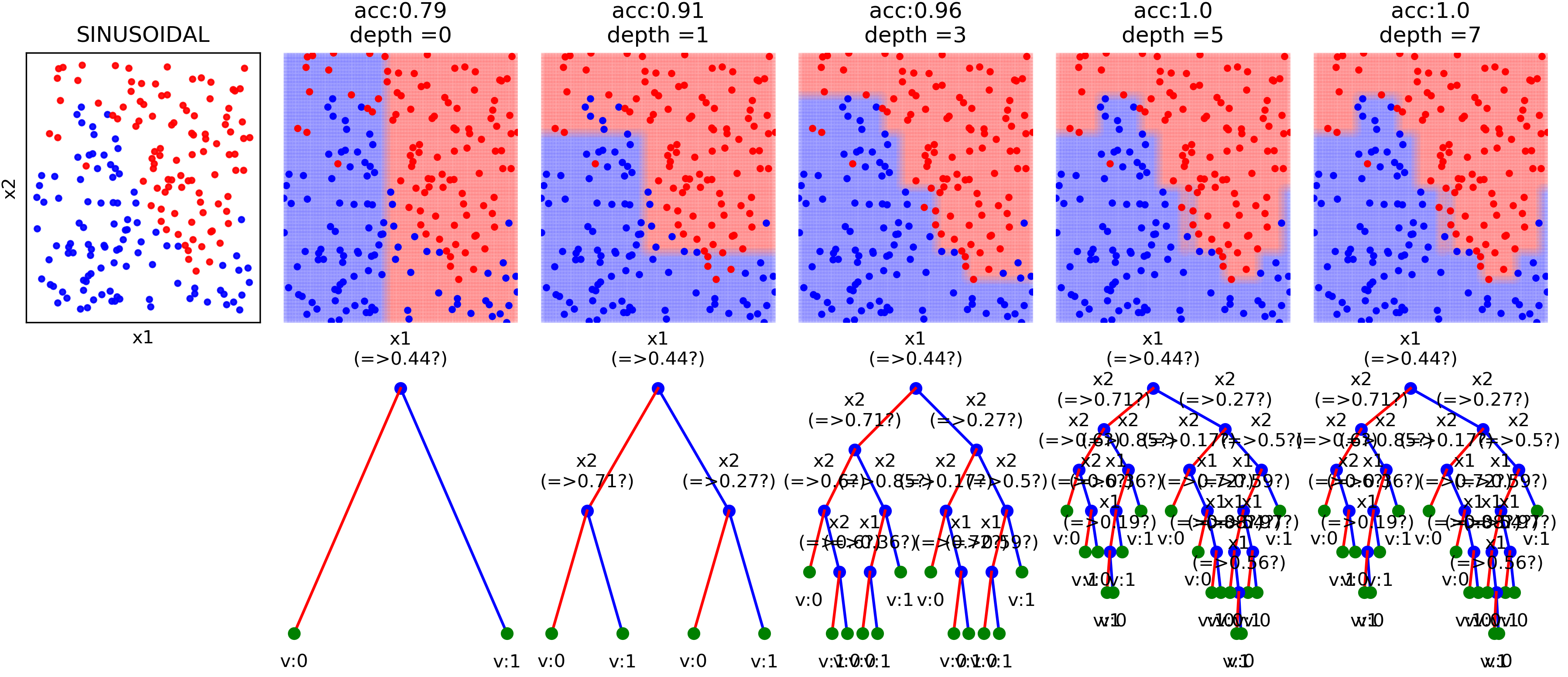 31 |
31 |  ](https://spkit.github.io)
47 |
48 |
49 | ## List of functions [check updated list on homepage]
50 | ## **Information Theory and Signal Processing functions**
51 | **for real valued signals**
52 | * Entropy
53 | * Shannon entropy
54 | * Rényi entropy of order α, Collision entropy,
55 | * Joint entropy
56 | * Conditional entropy
57 | * Mutual Information
58 | * Cross entropy
59 | * Kullback–Leibler divergence
60 | * Spectral Entropy
61 | * Approximate Entropy
62 | * Sample Entropy
63 | * Permutation Entropy
64 | * SVD Entropy
65 |
66 | * **Dispersion Entropy** (Advanced) - for time series signal
67 | * Dispersion Entropy
68 | * Dispersion Entropy - multiscale
69 | * Dispersion Entropy - multiscale - refined
70 | * **Differential Entropy** (Advanced) - for time series signal
71 | * Differential Entropy
72 | * Mutual Information, Conditional, Joint, Entropy
73 | * Transfer Entropy
74 |
75 |
76 | ## **Matrix Decomposition**
77 | * SVD
78 | * ICA using InfoMax, Extended-InfoMax, FastICA & **Picard**
79 |
80 | ## **Continuase Wavelet Transform**
81 | * Gauss wavelet
82 | * Morlet wavelet
83 | * Gabor wavelet
84 | * Poisson wavelet
85 | * Maxican wavelet
86 | * Shannon wavelet
87 |
88 | ## **Discrete Wavelet Transform**
89 | * Wavelet filtering
90 | * Wavelet Packet Analysis and Filtering
91 |
92 | ## **Signal Filtering**
93 | * Removing DC/ Smoothing for multi-channel signals
94 | * Bandpass/Lowpass/Highpass/Bandreject filtering for multi-channel signals
95 |
96 | ## Biomedical Signal Processing
97 | * EEG Signal Processing
98 | * MEA Processing Toolkit
99 |
100 | **Artifact Removal Algorithm**
101 | * **ATAR Algorithm** [Automatic and Tunable Artifact Removal Algorithm for EEG from artical](https://www.sciencedirect.com/science/article/pii/S1746809419302058)
102 | * **ICA based Algorith**
103 |
104 | ## Analysis and Synthesis Models
105 | * **DFT Analysis & Synthesis**
106 | * **STFT Analysis & Synthesis**
107 | * **Sinasodal Model - Analysis & Synthesis**
108 | - to decompose a signal into sinasodal wave tracks
109 | * **f0 detection**
110 |
111 | ## Ramanajum Methods for period estimation
112 | * **Period estimation for a short length sequence using Ramanujam Filters Banks (RFB)**
113 | * **Minizing sparsity of periods**
114 |
115 | ## Fractional Fourier Transform
116 | * **Fractional Fourier Transform**
117 | * **Fast Fractional Fourier Transform**
118 |
119 | ## Machine Learning models - with visualizations
120 | * Logistic Regression
121 | * Naive Bayes
122 | * Decision Trees
123 |
124 |
125 | ## and many more ...
126 |
127 |
128 | # Cite As
129 | ```
130 | @software{nikesh_bajaj_2021_4710694,
131 | author = {Nikesh Bajaj},
132 | title = {Nikeshbajaj/spkit: 0.0.9.4},
133 | month = apr,
134 | year = 2021,
135 | publisher = {Zenodo},
136 | version = {0.0.9.4},
137 | doi = {10.5281/zenodo.4710694},
138 | url = {https://doi.org/10.5281/zenodo.4710694}
139 | }
140 | ```
141 | # Contacts:
142 |
143 | * **Nikesh Bajaj**
144 | * https://nikeshbajaj.in
145 | * n.bajaj[AT]qmul.ac.uk, n.bajaj[AT]imperial[dot]ac[dot]uk
146 | ______________________________________
147 |
--------------------------------------------------------------------------------
/README_copy.md:
--------------------------------------------------------------------------------
1 | # Signal Processing toolkit
2 |
3 | [](https://spkit.readthedocs.io/en/latest/?badge=latest)
4 | [](https://opensource.org/licenses/MIT)
5 | [](https://pypi.org/project/spkit/)
6 | [](https://pypi.python.org/pypi/spkit/)
7 | [](https://GitHub.com/nikeshbajaj/spkit/releases/)
8 | [](https://pypi.python.org/pypi/spkit/)
9 | [](https://pypi.python.org/pypi/spkit/)
10 | [](http://hits.dwyl.io/nikeshbajaj/spkit)
11 | 
12 | [](http://isitmaintained.com/project/nikeshbajaj/spkit "Percentage of issues still open")
13 | [](https://pypi.org/project/spkit/)
14 | [](https://pypi.org/project/spkit/)
15 |
16 |
17 | [](https://pypi.org/project/spkit/)
18 | [](mailto:n.bajaj@qmul.ac.uk)
19 |
20 | 
21 |
22 |
23 |
24 |
25 | ### Links: **[Github](https://github.com/Nikeshbajaj/spkit)** | **[PyPi - project](https://pypi.org/project/spkit/)**
26 | ### Installation: *[pip install spkit](https://pypi.org/project/spkit/)*
27 |
28 | #### Updates:: Decision Tree
29 |
](https://spkit.github.io)
47 |
48 |
49 | ## List of functions [check updated list on homepage]
50 | ## **Information Theory and Signal Processing functions**
51 | **for real valued signals**
52 | * Entropy
53 | * Shannon entropy
54 | * Rényi entropy of order α, Collision entropy,
55 | * Joint entropy
56 | * Conditional entropy
57 | * Mutual Information
58 | * Cross entropy
59 | * Kullback–Leibler divergence
60 | * Spectral Entropy
61 | * Approximate Entropy
62 | * Sample Entropy
63 | * Permutation Entropy
64 | * SVD Entropy
65 |
66 | * **Dispersion Entropy** (Advanced) - for time series signal
67 | * Dispersion Entropy
68 | * Dispersion Entropy - multiscale
69 | * Dispersion Entropy - multiscale - refined
70 | * **Differential Entropy** (Advanced) - for time series signal
71 | * Differential Entropy
72 | * Mutual Information, Conditional, Joint, Entropy
73 | * Transfer Entropy
74 |
75 |
76 | ## **Matrix Decomposition**
77 | * SVD
78 | * ICA using InfoMax, Extended-InfoMax, FastICA & **Picard**
79 |
80 | ## **Continuase Wavelet Transform**
81 | * Gauss wavelet
82 | * Morlet wavelet
83 | * Gabor wavelet
84 | * Poisson wavelet
85 | * Maxican wavelet
86 | * Shannon wavelet
87 |
88 | ## **Discrete Wavelet Transform**
89 | * Wavelet filtering
90 | * Wavelet Packet Analysis and Filtering
91 |
92 | ## **Signal Filtering**
93 | * Removing DC/ Smoothing for multi-channel signals
94 | * Bandpass/Lowpass/Highpass/Bandreject filtering for multi-channel signals
95 |
96 | ## Biomedical Signal Processing
97 | * EEG Signal Processing
98 | * MEA Processing Toolkit
99 |
100 | **Artifact Removal Algorithm**
101 | * **ATAR Algorithm** [Automatic and Tunable Artifact Removal Algorithm for EEG from artical](https://www.sciencedirect.com/science/article/pii/S1746809419302058)
102 | * **ICA based Algorith**
103 |
104 | ## Analysis and Synthesis Models
105 | * **DFT Analysis & Synthesis**
106 | * **STFT Analysis & Synthesis**
107 | * **Sinasodal Model - Analysis & Synthesis**
108 | - to decompose a signal into sinasodal wave tracks
109 | * **f0 detection**
110 |
111 | ## Ramanajum Methods for period estimation
112 | * **Period estimation for a short length sequence using Ramanujam Filters Banks (RFB)**
113 | * **Minizing sparsity of periods**
114 |
115 | ## Fractional Fourier Transform
116 | * **Fractional Fourier Transform**
117 | * **Fast Fractional Fourier Transform**
118 |
119 | ## Machine Learning models - with visualizations
120 | * Logistic Regression
121 | * Naive Bayes
122 | * Decision Trees
123 |
124 |
125 | ## and many more ...
126 |
127 |
128 | # Cite As
129 | ```
130 | @software{nikesh_bajaj_2021_4710694,
131 | author = {Nikesh Bajaj},
132 | title = {Nikeshbajaj/spkit: 0.0.9.4},
133 | month = apr,
134 | year = 2021,
135 | publisher = {Zenodo},
136 | version = {0.0.9.4},
137 | doi = {10.5281/zenodo.4710694},
138 | url = {https://doi.org/10.5281/zenodo.4710694}
139 | }
140 | ```
141 | # Contacts:
142 |
143 | * **Nikesh Bajaj**
144 | * https://nikeshbajaj.in
145 | * n.bajaj[AT]qmul.ac.uk, n.bajaj[AT]imperial[dot]ac[dot]uk
146 | ______________________________________
147 |
--------------------------------------------------------------------------------
/README_copy.md:
--------------------------------------------------------------------------------
1 | # Signal Processing toolkit
2 |
3 | [](https://spkit.readthedocs.io/en/latest/?badge=latest)
4 | [](https://opensource.org/licenses/MIT)
5 | [](https://pypi.org/project/spkit/)
6 | [](https://pypi.python.org/pypi/spkit/)
7 | [](https://GitHub.com/nikeshbajaj/spkit/releases/)
8 | [](https://pypi.python.org/pypi/spkit/)
9 | [](https://pypi.python.org/pypi/spkit/)
10 | [](http://hits.dwyl.io/nikeshbajaj/spkit)
11 | 
12 | [](http://isitmaintained.com/project/nikeshbajaj/spkit "Percentage of issues still open")
13 | [](https://pypi.org/project/spkit/)
14 | [](https://pypi.org/project/spkit/)
15 |
16 |
17 | [](https://pypi.org/project/spkit/)
18 | [](mailto:n.bajaj@qmul.ac.uk)
19 |
20 | 
21 |
22 |
23 |
24 |
25 | ### Links: **[Github](https://github.com/Nikeshbajaj/spkit)** | **[PyPi - project](https://pypi.org/project/spkit/)**
26 | ### Installation: *[pip install spkit](https://pypi.org/project/spkit/)*
27 |
28 | #### Updates:: Decision Tree
29 | 

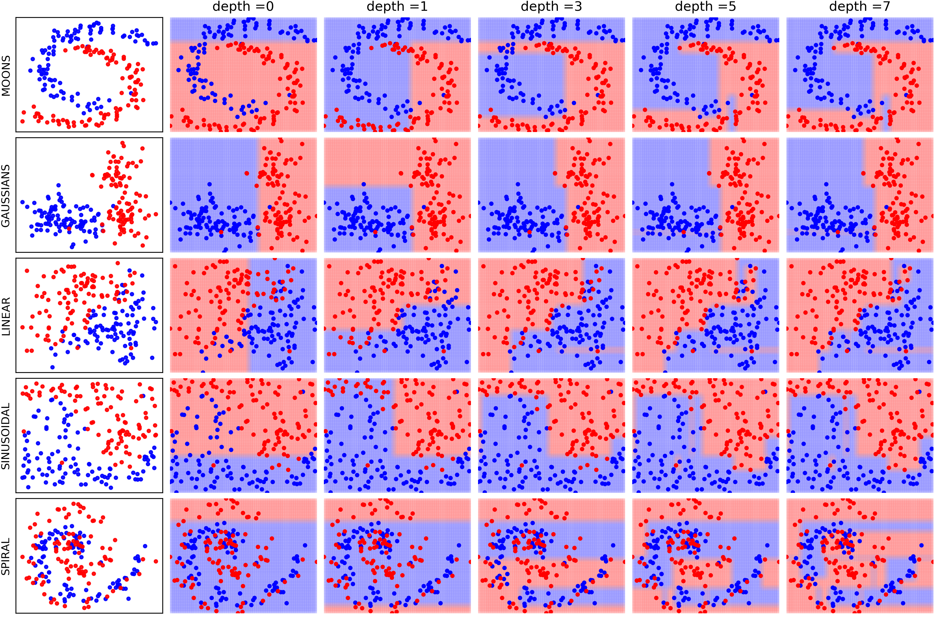 197 |
197 | 
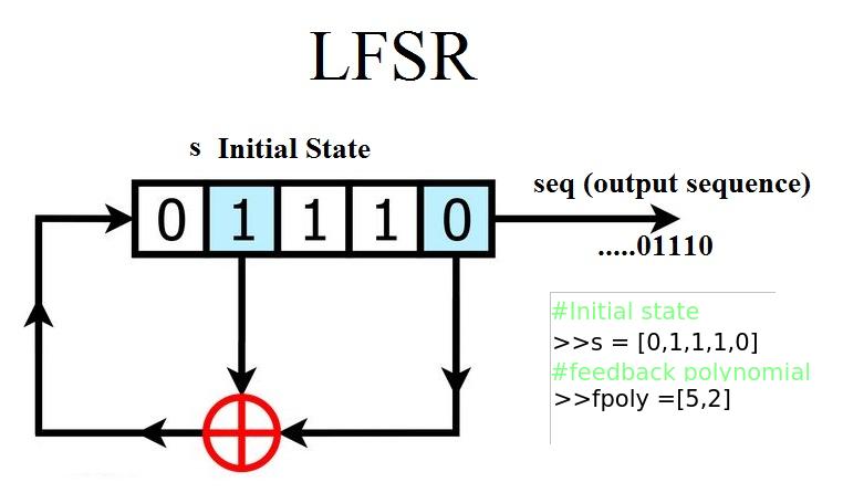 210 |
210 |