Software Engineer, Aeronautical Engineer to be, Straight Outta 256 , I choose Results over Reasons, Passionate Aviator, Show me the code
I share my thoughts majorly here https://nanjekyejoannah.github.io/
9 | 10 | Pypy is an alternate implementation of the python programming language. Pypy started out as a python interpreter written in python. It is aimed at being compatible with cpython and currently with experimental compatibility for CPython C API extensions. 11 | 12 | Pypy originally refered to two things. one the python interpreter and Rpython Translation toolchain but currently pypy is always used to refer to the python interpreter. The translation framework is always refered to as the Rpython Translation Framework. 13 | 14 | It is the distinct features embedded in pypy that give your python programs the magical performance. Lets have a look at some of them. 15 | 16 | # Pypy Distinct Features 17 | 18 | The pypy intepreter offers a couple of distinct features namely; 19 | 20 | * Speed 21 | * Compatibility 22 | * Memory Usage 23 | * Stackless python features 24 | 25 | ##Speed 26 | 27 | Pypy is magically faster due to its high performance Just-in-time compiler and garbage collector. 28 | 29 | It is therefore faster for programs that are JIT susceptible. This means that pypy may not always run faster, it may be for pure python code but actually run slower than Cpython where the JIT cant help. 30 | 31 | pypy may also not be as fast for small scripts that do not give the Just-in-time compiler enough warm up time. 32 | 33 | I ran this [code](https://gist.github.com/mrmoje/30bacf757e400ef28c56fdaecfb0b2a8) on pypy and on normal python and the results show pypy is actually faster. I will go on share the outcomes below; 34 | 35 | 36 |
37 | Alot of benchmarks have shown pypy performing better than Cpython and its not getting slower with time. Each new version of pypy is faster than its predecessor. The pypy team have shared good insight at their [speed center](http://speed.pypy.org/).
38 |
39 |
40 | ##Compatibility
41 |
42 | Good news is pypy is compatible with most of the python Libraries.
43 |
44 | * Django
45 | * Flask
46 | * Bottle
47 | * Pylons
48 | * Pyramid
49 | * Twisted
50 | * lxml
51 | * Beautiful Soup
52 | * Sphinx
53 | * IPyton
54 | * PIL/Pillow
55 | * Psycopg2
56 | * MySQL-Python
57 | * pysqlite
58 | * pymongo
59 | * cx_Oracle
60 | * SQLAlchemy
61 | * Gunicorn
62 | * Requests
63 | * nose
64 | * pytest
65 | * celery
66 | * Pip
67 | * Numpy
68 | * Scipy
69 | * Gevent
70 |
71 | Pypy has Experimental support for Extension modules through cpyext. It can run most C extensions these days.
72 |
73 | ##Memory Usage
74 |
75 | Memory-intensive python programs take lesser space than when running on pypy . However this may not be the case always though due to some details.
76 |
77 | ##Stackless python Features
78 |
79 | Pypy exposes language features similar to the ones present in stackless python.
80 |
81 | #Differences between Cpython and Python
82 |
83 | Lets take a look at pypy and a reference python implementation called cpython.
84 |
85 |
36 |
37 | Alot of benchmarks have shown pypy performing better than Cpython and its not getting slower with time. Each new version of pypy is faster than its predecessor. The pypy team have shared good insight at their [speed center](http://speed.pypy.org/).
38 |
39 |
40 | ##Compatibility
41 |
42 | Good news is pypy is compatible with most of the python Libraries.
43 |
44 | * Django
45 | * Flask
46 | * Bottle
47 | * Pylons
48 | * Pyramid
49 | * Twisted
50 | * lxml
51 | * Beautiful Soup
52 | * Sphinx
53 | * IPyton
54 | * PIL/Pillow
55 | * Psycopg2
56 | * MySQL-Python
57 | * pysqlite
58 | * pymongo
59 | * cx_Oracle
60 | * SQLAlchemy
61 | * Gunicorn
62 | * Requests
63 | * nose
64 | * pytest
65 | * celery
66 | * Pip
67 | * Numpy
68 | * Scipy
69 | * Gevent
70 |
71 | Pypy has Experimental support for Extension modules through cpyext. It can run most C extensions these days.
72 |
73 | ##Memory Usage
74 |
75 | Memory-intensive python programs take lesser space than when running on pypy . However this may not be the case always though due to some details.
76 |
77 | ##Stackless python Features
78 |
79 | Pypy exposes language features similar to the ones present in stackless python.
80 |
81 | #Differences between Cpython and Python
82 |
83 | Lets take a look at pypy and a reference python implementation called cpython.
84 |
85 | 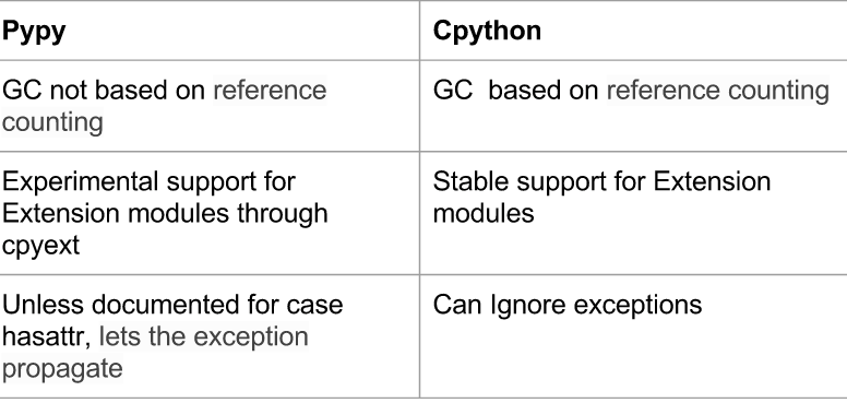 86 |
87 |
88 | # Way Forward
89 |
90 | “If you want your code to run faster, you should probably just use PyPy.” — Guido van Rossum (creator of Python)
91 |
92 | # Installation
93 |
94 | It is easy to install
95 |
96 | ###Linux:-
97 |
98 | `sudo apt-get install pypy`
99 |
100 | ###Mac:-
101 |
102 | `sudo brew install pypy`
103 |
104 | ###Windows:-
105 |
106 | There is rich [Documentation](http://pypy.org/download.html) on installation for windows.
107 |
108 |
109 | # Check these out for more pypy inspiration
110 | *
86 |
87 |
88 | # Way Forward
89 |
90 | “If you want your code to run faster, you should probably just use PyPy.” — Guido van Rossum (creator of Python)
91 |
92 | # Installation
93 |
94 | It is easy to install
95 |
96 | ###Linux:-
97 |
98 | `sudo apt-get install pypy`
99 |
100 | ###Mac:-
101 |
102 | `sudo brew install pypy`
103 |
104 | ###Windows:-
105 |
106 | There is rich [Documentation](http://pypy.org/download.html) on installation for windows.
107 |
108 |
109 | # Check these out for more pypy inspiration
110 | * A computer programmer in Nairobi, and fan of Python. You can check out his homepage here. 9 | 10 | Quicksort is one of the common sorting algorithms taught in computer science. 11 | 12 | Here I shall attempt to give a brief and clear example in Python. 13 | 14 | As a divide end conquer algorithm, three main steps are involved: 15 | 16 | - Pick an element (pivot) in the list 17 | - Partition the list so that all elements smaller than the pivot 18 | come before it and those bigger than the pivot come after it 19 | - Recursively apply the previous steps to the smaller sublists 20 | before and after the pivot 21 | 22 | This should leave you with a fully sorted list at the end. 23 | 24 | Let's define a quicksort function 25 | 26 | :::python 27 | def quicksort(L, lo, hi): 28 | """Sorts elements between indices lo and hi inclusive 29 | 30 | L - a list to sort 31 | lo - index of the lower end in the range 32 | hi - index of the higher end""" 33 | 34 | # Base case: lo and hi are equal, i.e. only one element in sublist 35 | # In this case, nothing is done on the list 36 | 37 | if lo < hi: 38 | # lo is less than hi, i.e. at least two elements in sublist 39 | 40 | # the partitioning step, p is the final position of the 41 | # pivot after partitioning 42 | p = partition(L, lo, hi) 43 | 44 | # Recursively sort the 'less than' partition 45 | quicksort(L, lo, p - 1) 46 | 47 | # Recursively sort the 'greater than' partition 48 | quicksort(L, p + 1, hi) 49 | 50 | # and that's it :-) 51 | 52 | 53 | We then define the partition function that does the actual work. It picks an 54 | element in the list within the given range, and divides the list into segments 55 | less than or equal, and greater than the pivot. 56 | 57 | 58 | :::python 59 | def partition(L, lo, hi): 60 | """Partitions the list within the given range 61 | L - a list to partition 62 | lo - index of the lower end in list to start partitioning from 63 | hi - index of higher end in list to end the partitioning""" 64 | 65 | # There several schemes used to pick the pivot 66 | # Here we shall use a one known as the 'Lomuto partition scheme' 67 | # Where we simply pick the last item in the range as the pivot 68 | 69 | pivot = L[hi] 70 | 71 | # i is the next position in the list where we 72 | # place an element less than or equal to the pivot 73 | 74 | # We begin at the lower end 75 | i = lo 76 | 77 | # We iterate through the list from lo to hi - 1 (the pivot is at hi, remember?) 78 | # separating elements less than or equal to the pivot 79 | # from those greater than the pivot 80 | j = lo 81 | while j < hi: 82 | # if element at j is less than or equal to the pivot 83 | # swap it into location i 84 | if L[j] <= pivot: 85 | L[i], L[j] = L[j], L[i] 86 | i += 1 # and increment i 87 | 88 | # increment j 89 | j += 1 90 | 91 | # When the loop completes, we know that all elements before i are less than 92 | # or equal to the pivot, and all elements from i onwards are greater than 93 | # the pivot 94 | 95 | # swap the pivot into it's correct position, separating these two parts 96 | L[i], L[hi] = L[hi], L[i] 97 | 98 | # Now the pivot is at position i, and all elements after i are greater than 99 | # it 100 | 101 | # return its position 102 | return i 103 | 104 | We can now test our quicksort function. 105 | 106 | :::python 107 | import random 108 | 109 | # Create a list of 10 unsorted integers between 1 and 100 inclusive 110 | list_to_sort = [random.randint(1, 100) for i in range(10)] 111 | print("List before sorting: ", list_to_sort) 112 | 113 | # Now let's sort the list 114 | last_index = len(list_to_sort) - 1 115 | quicksort(list_to_sort, 0, last_index) 116 | 117 | print("List after sorting: ", list_to_sort) 118 | 119 | 120 | You can read more on quicksort in its 121 | [wikipedia page](https://en.wikipedia.org/wiki/Quicksort). 122 | 123 | And [here's](https://www.safaribooksonline.com/library/view/python-cookbook/0596001673/ch02s12.html) 124 | an implementation in only 3 lines of python, if your into that sort of thing. 125 | 126 | [Here's](https://github.com/krmboya/py-examples/blob/master/quicksort.py) the source code. 127 | 128 | Also posted [here](http://www.99nth.com/~krm/blog/quicksort-python.html) 129 | -------------------------------------------------------------------------------- /content/data-vis-brian-suda.md: -------------------------------------------------------------------------------- 1 | Title: Data Vizualization by Brian Suda 2 | Date: 2014-12-16 18:11:00 3 | Tags: data viz, python, deterministic design, iceland, brian suda 4 | Slug: data_viz_by_brian_suda 5 | Author: Brian Suda 6 | Summary: A round up and links from the presentation Brian Suda gave about data vizualizations 7 | email: brian@suda.co.uk 8 | about_author:
Brian Suda is an informatician currently residing in Reykjavík, Iceland. He has spent a good portion of each day connected to Internet after discovering it back in the mid-1990s.
Most recently, he has been focusing more on the mobile space and future predictions, how smaller devices will augment our every day life and what that means to the way we live, work and are entertained.
His own little patch of Internet can be found at http://suda.co.uk where many of his past projects and crazy ideas can be found.
9 | 10 | Thanks to everyone who came on their Saturday to listen to me talk about data visualisations through a computer screen several timezones and many kilometres away. I know sitting through online presentations can be boring, so I hope mine was interesting enough that not many people fell asleep or left. It doesn’t matter, I could only see my slides and hear the shuffling of chairs every once and awhile, so I knew people were still there. 11 | 12 | On Saturday, December 13th, I ran through my presentation about the basics of charts & graphs and how build-up to more complex data visualizations. It was a great group to chat with because it was the a Python meet-up. Most of the event I attend it is a mix of disciplines, so you can never get too technical, or even worse, it is a group of designers who you at you with a blank expression when you start to talk about code and scripts. 13 | 14 | Getting to share some ideas with the folks in Nairobi was an exciting experience, and I know you are the types of people who get it. You’ll take apart the code and understand what’s happening. 15 | 16 | # Deterministic Design 17 | 18 | One of the topics I’m really interested in is this idea of Deterministic Design. 19 | 20 | This is the sort of design that you do once, up front, then feed in the data and see how it looks. Then if you need to update the design, you don’t do it for that particular instance, but back upstream at the source where the code is written. That way, next time the run the code, all future designs will benefit. 21 | 22 | At the moment, I’m calling this Deterministic Design, because if you feed in the same data, you’ll get the same results every time. Much like the color picking example I showed in the presentation. Using the MD5 function, we can get a hex string, which we take the first 6 characters and use that to generate a unique color that is fully reproducible on any system or language. 23 | 24 | :::python 25 | import hashlib 26 | hh = hashlib.md5() 27 | hh.update("Hello World") 28 | hh.hexdigest()[:6] 29 | 30 | I use this equation everywhere. It saves time and thought, but the downside is that you are bound by the color that it returns, even if it isn’t pretty! This little snippet of code needs a friend to help make sure you have the highest color contrast possible. I wrote about this on [24ways Calculating Color Contrast](http://24ways.org/2010/calculating-color-contrast/). You’ll have to port the code to Python yourself. 31 | 32 | I love a lot of these little projects, to convert small ideas into some code that is repeatable over and over again. I also like the UNIX philosophy of small, reusable pieces. This means I tend to write small programs which take a CSV as data and create small SVG files as output. Then I can bring those into more complex programs to edit, annotate and layout the data. If the CSV changes, it is easy for me to reproduce the charts & graphs, because it is all done in code. 33 | 34 | Most of the simple tools that I have written are available on [GitHub](https://github.com/briansuda/Deterministic-Design). There is a lot to wade through and you’ll have to port it to Python, but they are simple, useful utilities. 35 | 36 | # Starting Small and Growing Bigger 37 | When starting off, it is important to just start small. Rather than trying to dig into a massive amount of social media data, why not track your hours each week. How much is spent at work, at home, a sleep. Then try to visualize that in an interesting way. With some practice you’ll figure out what works, what doesn’t and what tools you like to use in your workflow. 38 | 39 | After that you can begin to progress to more complex data sets. Start off with some you like and understand, build-up a small portfolio of interesting examples and then take on bigger and bigger projects. You’ll quickly see that even the biggest project is just a series of smaller ones that you probably have some experience or tools to deal with. 40 | 41 | # Inspiration 42 | To stay fresh, you need to keep an eye on interesting people in the field. There are a lot of resources out there and these are a few to get you started. 43 | 44 | *element without any attribute between them which holds a simple description 165 | # of the post. Basically it makes it hard to extract the description of the post. 166 | # I suggest the developers of the web app should look into it. 167 | # with that issue in mind I did some tweak below in order to get the empty
168 | # tag. 169 | description = header.xpath("p[@class='post-meta']|p/text()").extract()[1] 170 | 171 | # extract post category 172 | category = header.xpath("p[@class='post-meta'] /a/text()").extract_first() 173 | 174 | # extract post date 175 | date = header.xpath("p[@class='post-meta'] /text()")[-1].extract() 176 | 177 | # finally lets return some data 178 | yield { 179 | 'description': description, 'category': category, 'title': title, 'date': date 180 | } 181 | 182 | lets execute our spider 183 | 184 | :::bash 185 | $ scrapy crawl naiblog -o posts.json 186 | 187 | 188 | you will see lots of logs being displayed on your terminal, when there are no more logs displayed navigate to the root of 189 | `naiblog` project and you will see a file named `posts.json`, open it and you will see all the posts in `pynbo blog`. 190 | 191 | Thats all!! 192 | 193 | find the entire project on my git repo [naiblog](https://github.com/gr1d99/naiblog-spider.git). 194 | -------------------------------------------------------------------------------- /content/tracking-vehicles-with-accesskenya-camera.md: -------------------------------------------------------------------------------- 1 | Title: Tracking Vehicles on Access Kenya Cameras 2 | Date: 2016-01-09 18:11:00 3 | Tags: python, image analysis, opencv, access kenya, traffic 4 | Slug: image_analysis_by_chris_orwa 5 | Author: Chris Orwa 6 | Summary: Description of a python API I built to track vehicular movement on Access Kenya cameras 7 | email: chrisorwa@gmail.com 8 | about_author:
Chris Orwa is a Data Scientist currently residing in Nairobi, Kenya. He's main focus is on computational techniques for unstructured data. To that end, he has learned to code in Python and R, and retained both languages as the core-analysis software/language with an occasional dash of C and Java.
His crazy analysis monologues can be found at http://blackorwa.com
9 | 10 | Hello everyone, here's my blog post on how I built an API to return traffic conditions from Access Kenya cameras. The API would work by specifiying a road name at the URL endpoint and a json reponse would have number of cars that moved and the speed of movement. 11 | 12 | #### Data Capture 13 | To begin the process I decided to test if is possible to capture Image from each camera. After exploration of the website I realized each camera had a url with a JPEG file extension at the end. I figured the cameras wrote a new image to the JPEG file on the URL. So, can I captured every new image? Yes - I used the **urllib** library to capture the image and store it on the disk. 14 | 15 | I organized the camera urls into a dict so as to have a means of calling and referencing each road. 16 | 17 | :::python 18 | cameras = dict ( 19 | museum='http://traffic.accesskenya.com/images/traffic/feeds/purshotam.jpg', 20 | ojijo='http://traffic.accesskenya.com/images/traffic/feeds/mhcojijo.jpg', 21 | forest_limuru='http://traffic.accesskenya.com/images/traffic/feeds/forestlimuru.jpg?', 22 | kenyatta_uhuru_valley='http://traffic.accesskenya.com/images/traffic/feeds/barclaysplaza.jpg',) 23 | 24 | After that, I wrote a function that takes a url and extracts three images every 6 seconds. 25 | 26 | :::python 27 | def capture_images(self): 28 | for i in 'abc': 29 | if self.name in way: 30 | urllib.urlretrieve(way[self.name],'img_'+i+'.jpg') 31 | time.sleep(6) 32 | 33 | #### Image Processing 34 | The images captured from the camera are stored on a folder with the name of the road. Next task involves processing the images for analysis. I utlize two libraries for this task; **PIL** for loading the images and **numpy** to convert pixel values to numerical array values. All these are wrapped in a function (shown below) that takes the image folder directory as input then proceeds to load all 3 images, converts them to numpy arrays, deletes the images and returns a python dict holding arrays on all the images. 35 | 36 | :::python 37 | # load images 38 | def load(self): 39 | files = os.listdir(self.path) 40 | a = dict() 41 | b = dict() 42 | k = 0 43 | 44 | while k <= len(files): 45 | for names in files: 46 | if names != '.DS_Store': 47 | a[names] = Image.open(names).convert('L') 48 | a[names].load() 49 | b[names] = np.asarray(a[names]) 50 | k +=1 51 | 52 | # delete image folder 53 | shutil.rmtree(os.getcwd()) 54 | 55 | return b 56 | 57 | #### Motion Detection 58 | The first important step in analysis of the images is checking if there has been movements within the 6 second period. To achieve this, I utilized the concept of differential imaging - a means of measuring motion detection by subtracting the pixel values of subsquent images. In my function, I calculate the number of pixels that have moved, this helps in quantifying the movement (standstill, moderate traffic). 59 | 60 | :::python 61 | # differential imaging 62 | def diffImg(self,img1,img2,img3): 63 | 64 | # calculate absolute difference 65 | d1 = cv2.absdiff(img1,img2) 66 | d2 = cv2.absdiff(img2,img3) 67 | bit = cv2.bitwise_and(d1,d2) 68 | ret,thresh = cv2.threshold(bit,35,255,cv2.THRESH_BINARY) 69 | 70 | #get number of different pixels 71 | moving = list() 72 | for cell in thresh.flat: 73 | if cell == 255: 74 | move = 'True' 75 | moving.append(move) 76 | pixie = len(moving) 77 | 78 | return pixie 79 | 80 | #### Calibrating Movement 81 | Once movement is detected, it is important to then quantify trafficc in km/h. To aid in this calculation is the optical flow algorithm. A concept in computer vision that allow tracking features in an image. I utilized this functionality to find features to track (cars) in the first images, and get their corresponding positions in the second and third image. I then proceeded to calculate the avaerage distance (euclidean distance) that the feature has moved. Dividing the pixel distance by 12 seconds gives me speed at which the objects(cars) are moving. My function returns this value. 82 | 83 | :::python 84 | # calculate optical flow of points on images 85 | def opticalFlow(self,img1,img2,img3): 86 | 87 | #set variables 88 | lk_params = dict(winSize = (10,10), 89 | maxLevel = 5, 90 | criteria = (cv2.TERM_CRITERIA_EPS | cv2.TERM_CRITERIA_COUNT,10,0.03)) 91 | 92 | features_param = dict( maxCorners = 3000, 93 | qualityLevel = 0.5, 94 | minDistance = 3, 95 | blockSize = 3) 96 | 97 | # feature extraction of points to track 98 | pt = cv2.goodFeaturesToTrack(img1,**features_param) 99 | p0 =np.float32(pt).reshape(-1,1,2) 100 | 101 | # calaculate average movement 102 | dist = list() 103 | for loop in p0: 104 | p1,st,err =cv2.calcOpticalFlowPyrLK(img1, img2,loop, 105 | None,**lk_params) 106 | 107 | p0r,st,err =cv2.calcOpticalFlowPyrLK(img2,img1,p1, 108 | None,**lk_params) 109 | 110 | if abs(loop-p0r).reshape(-1, 2).max(-1) < 1: 111 | dst = distance.euclidean(loop,p0r) 112 | dist.append(dst) 113 | 114 | return round(max(dist)*10,2) 115 | 116 | #### The API 117 | The API (underconstruction) is based on flask. By specifying a road name at the HTTP endpoint, the API returns speed of traffic and level of movement (stanstill, moderate rate, no traffic). 118 | 119 | :::python 120 | # load required libraries 121 | import image_processing 122 | import numpy as np 123 | from flask import Flask 124 | import links 125 | import json 126 | import scipy as sp 127 | 128 | # create flask web server 129 | app = Flask(__name__) 130 | 131 | # create HTTP endpoint 132 | @app.route('/ImPro/ 16 |
17 | What do clothes and code (and my jokes) have in common? Answer: They're so
18 | much better when they're dry.
16 |
17 | What do clothes and code (and my jokes) have in common? Answer: They're so
18 | much better when they're dry.  19 |
20 | What does it mean for code to be **DRY**? Simple: **Don't Repeat Yourself**.
21 | The DRY Principle is key when writing efficient code. It helps keep your
22 | codebase smaller and less complex, saves you time, reduces redundancy... it's
23 | basically sugar, spice, and everything nice. :) In this post, I'm going to demonstrate how decorators in Python can help keep
24 | your code DRY.
25 |
26 | Once upon a time, I was building a RESTful API with Flask (which
28 | you can check it out on GitHub
30 | here) for an online bucket list service. Users could:
31 |
32 | 1. Sign up and login
33 | 2. Create, edit, view, and delete bucket lists
34 | 3. Create, edit, view, and delete bucket list items
35 |
36 | Some endpoints were protected and could only be accessed by authorized users.
37 | For instance, only the user who created a bucket list or bucket list item could
38 | edit, view, or delete it.
39 |
40 | Here's how I initially tackled it. First, I created a method to display an
41 | error message, with the default being "Error: You are not authorized to access
42 | this resource."
43 |
44 | ``` python
45 | def unauthorized(message=None):
46 | """
47 | Returns an error message.
48 | """
49 | if not message:
50 | message = "Error: You are not authorized to access this resource."
51 | return jsonify({
52 | "message": message
53 | }), 403
54 | ```
55 |
56 | Then, I went ahead and wrote the methods for the endpoints:
57 |
58 | ``` python
59 | class BucketListAPI(Resource):
60 | """
61 | URL: /api/v1/bucketlists/
19 |
20 | What does it mean for code to be **DRY**? Simple: **Don't Repeat Yourself**.
21 | The DRY Principle is key when writing efficient code. It helps keep your
22 | codebase smaller and less complex, saves you time, reduces redundancy... it's
23 | basically sugar, spice, and everything nice. :) In this post, I'm going to demonstrate how decorators in Python can help keep
24 | your code DRY.
25 |
26 | Once upon a time, I was building a RESTful API with Flask (which
28 | you can check it out on GitHub
30 | here) for an online bucket list service. Users could:
31 |
32 | 1. Sign up and login
33 | 2. Create, edit, view, and delete bucket lists
34 | 3. Create, edit, view, and delete bucket list items
35 |
36 | Some endpoints were protected and could only be accessed by authorized users.
37 | For instance, only the user who created a bucket list or bucket list item could
38 | edit, view, or delete it.
39 |
40 | Here's how I initially tackled it. First, I created a method to display an
41 | error message, with the default being "Error: You are not authorized to access
42 | this resource."
43 |
44 | ``` python
45 | def unauthorized(message=None):
46 | """
47 | Returns an error message.
48 | """
49 | if not message:
50 | message = "Error: You are not authorized to access this resource."
51 | return jsonify({
52 | "message": message
53 | }), 403
54 | ```
55 |
56 | Then, I went ahead and wrote the methods for the endpoints:
57 |
58 | ``` python
59 | class BucketListAPI(Resource):
60 | """
61 | URL: /api/v1/bucketlists/