[1] In fact a major concern with queues is that their length does not explode. This issue cannot be properly explored unless the state space is allowed to be infinite.\n", 679 | "\n", 680 | "
[2] An excellent introduction to operator semigroups, combined with\n", 681 | "applications to PDEs and Markov processes, can be found in [[Applebaum, 2019](https://continuous-time-mcs.quantecon.org/zreferences.html#id5)].\n", 682 | "\n", 683 | "
[3] Convergence of the sum in [(6.3)](#equation-opexpo) follows from boundedness of $ A $ and the fact that $ \\linop $ is a Banach space.\n", 684 | "\n", 685 | "
[4] Be careful: the definition of a UC semigroup requires that\n", 686 | "$ t \\mapsto U_t $ is continuous as a map into $ \\linop $, rather than uniformly\n", 687 | "continuous. The UC terminology comes about because, for a UC semigroup, we\n", 688 | "have, by definition of the operator norm,\n", 689 | "$ \\sup_{\\| g \\| \\leq 1} \\| U_s g - U_t g \\| \\to 0 $ when $ s \\to t $.\n", 690 | "\n", 691 | "
[5] An excellent treatment of the general theory of $ C_0 $ semigroups, can be found in [[Bobrowski, 2005](https://continuous-time-mcs.quantecon.org/zreferences.html#id7)]." 692 | ] 693 | } 694 | ], 695 | "metadata": { 696 | "date": 1763463649.7420359, 697 | "filename": "generators.md", 698 | "kernelspec": { 699 | "display_name": "Python", 700 | "language": "python3", 701 | "name": "python3" 702 | }, 703 | "title": "Semigroups and Generators" 704 | }, 705 | "nbformat": 4, 706 | "nbformat_minor": 5 707 | } -------------------------------------------------------------------------------- /kolmogorov_fwd.ipynb: -------------------------------------------------------------------------------- 1 | { 2 | "cells": [ 3 | { 4 | "cell_type": "markdown", 5 | "id": "2525714d", 6 | "metadata": {}, 7 | "source": [ 8 | "$$\n", 9 | "\\newcommand{\\Exp}{\\operatorname{Exp}}\n", 10 | "\\newcommand{\\Binomial}{\\operatorname{Binomial}}\n", 11 | "\\newcommand{\\Poisson}{\\operatorname{Poisson}}\n", 12 | "\\newcommand{\\BB}{\\mathbb{B}}\n", 13 | "\\newcommand{\\EE}{\\mathbb{E}}\n", 14 | "\\newcommand{\\PP}{\\mathbb{P}}\n", 15 | "\\newcommand{\\RR}{\\mathbb{R}}\n", 16 | "\\newcommand{\\NN}{\\mathbb{N}}\n", 17 | "\\newcommand{\\ZZ}{\\mathbb{Z}}\n", 18 | "\\newcommand{\\dD}{\\mathcal{D}}\n", 19 | "\\newcommand{\\fF}{\\mathcal{F}}\n", 20 | "\\newcommand{\\lL}{\\mathcal{L}}\n", 21 | "\\newcommand{\\linop}{\\mathcal{L}(\\mathbb{B})}\n", 22 | "\\newcommand{\\linopell}{\\mathcal{L}(\\ell_1)}\n", 23 | "$$" 24 | ] 25 | }, 26 | { 27 | "cell_type": "markdown", 28 | "id": "26f9287e", 29 | "metadata": {}, 30 | "source": [ 31 | "# The Kolmogorov Forward Equation\n", 32 | "\n", 33 | "In addition to what’s in Anaconda, this lecture will need the following libraries:" 34 | ] 35 | }, 36 | { 37 | "cell_type": "code", 38 | "execution_count": null, 39 | "id": "338cbb3f", 40 | "metadata": { 41 | "hide-output": false 42 | }, 43 | "outputs": [], 44 | "source": [ 45 | "!pip install quantecon" 46 | ] 47 | }, 48 | { 49 | "cell_type": "markdown", 50 | "id": "d00499f1", 51 | "metadata": {}, 52 | "source": [ 53 | "## Overview\n", 54 | "\n", 55 | "In this lecture we approach continuous time Markov chains from a more\n", 56 | "analytical perspective.\n", 57 | "\n", 58 | "The emphasis will be on describing distribution flows through vector-valued\n", 59 | "differential equations and their solutions.\n", 60 | "\n", 61 | "These distribution flows show how the time $ t $ distribution associated with a\n", 62 | "given Markov chain $ (X_t) $ changes over time.\n", 63 | "\n", 64 | "Distribution flows will be identified with initial value problems generated by autonomous linear ordinary differential equations (ODEs) in vector space.\n", 65 | "\n", 66 | "We will see that the solutions of these flows are described by Markov semigroups.\n", 67 | "\n", 68 | "This leads us back to the theory we have already constructed – some care will\n", 69 | "be taken to clarify all the connections.\n", 70 | "\n", 71 | "In order to avoid being distracted by technicalities, we continue to defer our\n", 72 | "treatment of infinite state spaces, assuming throughout this lecture that $ |S|\n", 73 | "= n $.\n", 74 | "\n", 75 | "As before, $ \\dD $ is the set of all distributions on $ S $.\n", 76 | "\n", 77 | "We will use the following imports" 78 | ] 79 | }, 80 | { 81 | "cell_type": "code", 82 | "execution_count": null, 83 | "id": "55173da0", 84 | "metadata": { 85 | "hide-output": false 86 | }, 87 | "outputs": [], 88 | "source": [ 89 | "import numpy as np\n", 90 | "import scipy as sp\n", 91 | "import matplotlib.pyplot as plt\n", 92 | "import quantecon as qe\n", 93 | "from numba import njit\n", 94 | "from scipy.linalg import expm\n", 95 | "\n", 96 | "from matplotlib import cm\n", 97 | "from mpl_toolkits.mplot3d import Axes3D\n", 98 | "from mpl_toolkits.mplot3d.art3d import Poly3DCollection" 99 | ] 100 | }, 101 | { 102 | "cell_type": "markdown", 103 | "id": "7bbbad6e", 104 | "metadata": {}, 105 | "source": [ 106 | "## From Difference Equations to ODEs\n", 107 | "\n", 108 | "[Previously](https://continuous-time-mcs.quantecon.org/markov_prop.html#invdistflows) we generated this figure, which shows how distributions evolve over time for the inventory model under a certain parameterization:\n", 109 | "\n", 110 | "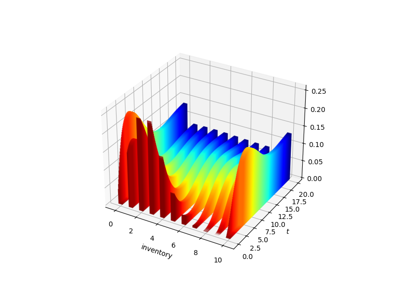\n", 111 | "\n", 112 | "Probability flows for the inventory model. \n", 113 | "(Hot colors indicate early dates and cool colors denote later dates.)\n", 114 | "\n", 115 | "We also learned how this flow is related to\n", 116 | "the Kolmogorov backward equation, which is an ODE.\n", 117 | "\n", 118 | "In this section we examine distribution flows and their connection to\n", 119 | "ODEs and continuous time Markov chains more systematically." 120 | ] 121 | }, 122 | { 123 | "cell_type": "markdown", 124 | "id": "8a3b175d", 125 | "metadata": {}, 126 | "source": [ 127 | "### Review of the Discrete Time Case\n", 128 | "\n", 129 | "Let $ (X_t) $ be a discrete time Markov chain with Markov matrix $ P $.\n", 130 | "\n", 131 | "[Recall that](https://continuous-time-mcs.quantecon.org/markov_prop.html#finstatediscretemc), in the discrete time case, the distribution $ \\psi_t $ of $ X_t $ updates according to\n", 132 | "\n", 133 | "$$\n", 134 | "\\psi_{t+1} = \\psi_t P, \n", 135 | " \\qquad \\psi_0 \\text{ a given element of } \\dD,\n", 136 | "$$\n", 137 | "\n", 138 | "where distributions are understood as row vectors.\n", 139 | "\n", 140 | "Here’s a visualization for the case $ S = \\{0, 1, 2\\} $, so that $ \\dD $ is the [standard\n", 141 | "simplex](https://en.wikipedia.org/wiki/Simplex) in $ \\RR^3 $.\n", 142 | "\n", 143 | "The initial condition is ` (0, 0, 1)` and the Markov matrix is" 144 | ] 145 | }, 146 | { 147 | "cell_type": "code", 148 | "execution_count": null, 149 | "id": "503e86aa", 150 | "metadata": { 151 | "hide-output": false 152 | }, 153 | "outputs": [], 154 | "source": [ 155 | "P = ((0.9, 0.1, 0.0),\n", 156 | " (0.4, 0.4, 0.2),\n", 157 | " (0.1, 0.1, 0.8))" 158 | ] 159 | }, 160 | { 161 | "cell_type": "code", 162 | "execution_count": null, 163 | "id": "7cf5ed90", 164 | "metadata": { 165 | "hide-output": false 166 | }, 167 | "outputs": [], 168 | "source": [ 169 | "def unit_simplex(angle):\n", 170 | " \n", 171 | " fig = plt.figure(figsize=(8, 6))\n", 172 | " ax = fig.add_subplot(111, projection='3d')\n", 173 | "\n", 174 | " vtx = [[0, 0, 1],\n", 175 | " [0, 1, 0], \n", 176 | " [1, 0, 0]]\n", 177 | " \n", 178 | " tri = Poly3DCollection([vtx], color='darkblue', alpha=0.3)\n", 179 | " tri.set_facecolor([0.5, 0.5, 1])\n", 180 | " ax.add_collection3d(tri)\n", 181 | "\n", 182 | " ax.set(xlim=(0, 1), ylim=(0, 1), zlim=(0, 1), \n", 183 | " xticks=(1,), yticks=(1,), zticks=(1,))\n", 184 | "\n", 185 | " ax.set_xticklabels(['$(1, 0, 0)$'], fontsize=12)\n", 186 | " ax.set_yticklabels(['$(0, 1, 0)$'], fontsize=12)\n", 187 | " ax.set_zticklabels(['$(0, 0, 1)$'], fontsize=12)\n", 188 | "\n", 189 | " ax.xaxis.majorTicks[0].set_pad(15)\n", 190 | " ax.yaxis.majorTicks[0].set_pad(15)\n", 191 | " ax.zaxis.majorTicks[0].set_pad(35)\n", 192 | "\n", 193 | " ax.view_init(30, angle)\n", 194 | "\n", 195 | " # Move axis to origin\n", 196 | " ax.xaxis._axinfo['juggled'] = (0, 0, 0)\n", 197 | " ax.yaxis._axinfo['juggled'] = (1, 1, 1)\n", 198 | " ax.zaxis._axinfo['juggled'] = (2, 2, 0)\n", 199 | " \n", 200 | " ax.grid(False)\n", 201 | " \n", 202 | " return ax\n", 203 | "\n", 204 | "\n", 205 | "def convergence_plot(ψ, n=14, angle=50):\n", 206 | "\n", 207 | " ax = unit_simplex(angle)\n", 208 | "\n", 209 | " P = ((0.9, 0.1, 0.0),\n", 210 | " (0.4, 0.4, 0.2),\n", 211 | " (0.1, 0.1, 0.8))\n", 212 | " \n", 213 | " P = np.array(P)\n", 214 | " colors = cm.jet_r(np.linspace(0.0, 1, n))\n", 215 | "\n", 216 | " x_vals, y_vals, z_vals = [], [], []\n", 217 | " for t in range(n):\n", 218 | " x_vals.append(ψ[0])\n", 219 | " y_vals.append(ψ[1])\n", 220 | " z_vals.append(ψ[2])\n", 221 | " ψ = ψ @ P\n", 222 | "\n", 223 | " ax.scatter(x_vals, y_vals, z_vals, c=colors, s=50, alpha=0.7, depthshade=False)\n", 224 | "\n", 225 | " return ψ\n", 226 | "\n", 227 | "ψ = convergence_plot((0, 0, 1))\n", 228 | "\n", 229 | "plt.show()" 230 | ] 231 | }, 232 | { 233 | "cell_type": "markdown", 234 | "id": "8aa54409", 235 | "metadata": {}, 236 | "source": [ 237 | "There’s a sense in which a discrete time Markov chain “is” a homogeneous\n", 238 | "linear difference equation in distribution space.\n", 239 | "\n", 240 | "To clarify this, suppose we\n", 241 | "take $ G $ to be a linear map from $ \\dD $ to itself and\n", 242 | "write down the difference equation\n", 243 | "\n", 244 | "\n", 245 | "\n", 246 | "$$\n", 247 | "\\psi_{t+1} = G(\\psi_t)\n", 248 | " \\quad \\text{with } \\psi_0 \\in \\dD \\text{ given}. \\tag{5.1}\n", 249 | "$$\n", 250 | "\n", 251 | "Because $ G $ is a linear map from a finite dimensional space to itself, it can\n", 252 | "be represented by a matrix.\n", 253 | "\n", 254 | "Moreover, a matrix $ P $ is a Markov matrix if and only if $ \\psi \\mapsto\n", 255 | "\\psi P $ sends $ \\dD $ into itself (check it if you haven’t already).\n", 256 | "\n", 257 | "So, under the stated conditions, our difference equation [(5.1)](#equation-gdiff2) uniquely\n", 258 | "identifies a Markov matrix, along with an initial condition $ \\psi_0 $.\n", 259 | "\n", 260 | "Together, these objects identify the joint distribution of a discrete time Markov chain, as [previously described](https://continuous-time-mcs.quantecon.org/markov_prop.html#jdfin)." 261 | ] 262 | }, 263 | { 264 | "cell_type": "markdown", 265 | "id": "1a7d9df2", 266 | "metadata": {}, 267 | "source": [ 268 | "### Shifting to Continuous Time\n", 269 | "\n", 270 | "We have just argued that a discrete time Markov chain can be identified with a\n", 271 | "linear difference equation evolving in $ \\dD $.\n", 272 | "\n", 273 | "This strongly suggests that a continuous time Markov chain can be identified\n", 274 | "with a linear ODE evolving in $ \\dD $.\n", 275 | "\n", 276 | "This intuition is correct and important.\n", 277 | "\n", 278 | "The rest of the lecture maps out the main ideas." 279 | ] 280 | }, 281 | { 282 | "cell_type": "markdown", 283 | "id": "28684c05", 284 | "metadata": {}, 285 | "source": [ 286 | "## ODEs in Distribution Space\n", 287 | "\n", 288 | "Consider linear differential equation given by\n", 289 | "\n", 290 | "\n", 291 | "\n", 292 | "$$\n", 293 | "\\psi_t' = \\psi_t Q, \n", 294 | " \\qquad \\psi_0 \\text{ a given element of } \\dD, \\tag{5.2}\n", 295 | "$$\n", 296 | "\n", 297 | "where\n", 298 | "\n", 299 | "- $ Q $ is an $ n \\times n $ matrix, \n", 300 | "- distributions are again understood as row vectors, and \n", 301 | "- derivatives are taken element by element, so that \n", 302 | "\n", 303 | "\n", 304 | "$$\n", 305 | "\\psi_t' =\n", 306 | " \\begin{pmatrix}\n", 307 | " \\frac{d}{dt} \\psi_t(x_1) &\n", 308 | " \\cdots &\n", 309 | " \\frac{d}{dt} \\psi_t(x_n)\n", 310 | " \\end{pmatrix}\n", 311 | "$$\n", 312 | "\n", 313 | "\n", 314 | "" 315 | ] 316 | }, 317 | { 318 | "cell_type": "markdown", 319 | "id": "e7be044e", 320 | "metadata": {}, 321 | "source": [ 322 | "### Solutions to Linear Vector ODEs\n", 323 | "\n", 324 | "Using the matrix exponential, the unique solution to the initial value problem\n", 325 | "[(5.2)](#equation-ode-mc) is\n", 326 | "\n", 327 | "\n", 328 | "\n", 329 | "$$\n", 330 | "\\psi_t = \\psi_0 P_t \n", 331 | " \\quad \\text{where } P_t := e^{tQ} \\tag{5.3}\n", 332 | "$$\n", 333 | "\n", 334 | "To check that [(5.3)](#equation-cmc-sol) is a solution, we use [(4.7)](https://continuous-time-mcs.quantecon.org/kolmogorov_bwd.html#equation-expoderiv) again to get\n", 335 | "\n", 336 | "$$\n", 337 | "\\frac{d}{d t} P_t = Q e^{tQ} = e^{tQ} Q\n", 338 | "$$\n", 339 | "\n", 340 | "The first equality can be written as $ P_t' = Q P_t $ and this is just\n", 341 | "the [Kolmogorov backward equation](https://continuous-time-mcs.quantecon.org/kolmogorov_bwd.html).\n", 342 | "\n", 343 | "The second equality can be written as\n", 344 | "\n", 345 | "$$\n", 346 | "P_t' = P_t Q\n", 347 | "$$\n", 348 | "\n", 349 | "and is called the **Kolmogorov forward equation**.\n", 350 | "\n", 351 | "Applying the Kolmogorov forward equation, we obtain\n", 352 | "\n", 353 | "$$\n", 354 | "\\frac{d}{d t} \\psi_t \n", 355 | " = \\frac{d}{d t} \\psi_0 P_t \n", 356 | " = \\psi_0 \\frac{d}{d t} P_t \n", 357 | " = \\psi_0 P_t Q\n", 358 | " = \\psi_t Q\n", 359 | "$$\n", 360 | "\n", 361 | "This confirms that [(5.3)](#equation-cmc-sol) solves [(5.2)](#equation-ode-mc).\n", 362 | "\n", 363 | "Here’s an example of three distribution flows with dynamics generated by [(5.2)](#equation-ode-mc), one starting from each vertex.\n", 364 | "\n", 365 | "The code uses [(5.3)](#equation-cmc-sol) with matrix $ Q $ given by" 366 | ] 367 | }, 368 | { 369 | "cell_type": "code", 370 | "execution_count": null, 371 | "id": "c8917856", 372 | "metadata": { 373 | "hide-output": false 374 | }, 375 | "outputs": [], 376 | "source": [ 377 | "Q = ((-3, 2, 1),\n", 378 | " (3, -5, 2),\n", 379 | " (4, 6, -10))" 380 | ] 381 | }, 382 | { 383 | "cell_type": "code", 384 | "execution_count": null, 385 | "id": "04440d83", 386 | "metadata": { 387 | "hide-output": false 388 | }, 389 | "outputs": [], 390 | "source": [ 391 | "Q = np.array(Q)\n", 392 | "ψ_00 = np.array((0.01, 0.01, 0.99))\n", 393 | "ψ_01 = np.array((0.01, 0.99, 0.01))\n", 394 | "ψ_02 = np.array((0.99, 0.01, 0.01))\n", 395 | "\n", 396 | "ax = unit_simplex(angle=50) \n", 397 | "\n", 398 | "def flow_plot(ψ, h=0.001, n=400, angle=50):\n", 399 | " colors = cm.jet_r(np.linspace(0.0, 1, n))\n", 400 | "\n", 401 | " x_vals, y_vals, z_vals = [], [], []\n", 402 | " for t in range(n):\n", 403 | " x_vals.append(ψ[0])\n", 404 | " y_vals.append(ψ[1])\n", 405 | " z_vals.append(ψ[2])\n", 406 | " ψ = ψ @ expm(h * Q)\n", 407 | "\n", 408 | " ax.scatter(x_vals, y_vals, z_vals, c=colors, s=20, alpha=0.2, depthshade=False)\n", 409 | "\n", 410 | "flow_plot(ψ_00)\n", 411 | "flow_plot(ψ_01)\n", 412 | "flow_plot(ψ_02)\n", 413 | "\n", 414 | "plt.show()" 415 | ] 416 | }, 417 | { 418 | "cell_type": "markdown", 419 | "id": "fc8e8083", 420 | "metadata": {}, 421 | "source": [ 422 | "(Distributions cool over time, so initial conditions are hot colors.)" 423 | ] 424 | }, 425 | { 426 | "cell_type": "markdown", 427 | "id": "1100ffe2", 428 | "metadata": {}, 429 | "source": [ 430 | "### Forwards vs Backwards Equations\n", 431 | "\n", 432 | "As the above discussion shows, we can take the Kolmogorov forward equation\n", 433 | "$ P_t' = P_t Q $ and premultiply by any distribution $ \\psi_0 $ to get the\n", 434 | "distribution ODE $ \\psi'_t = \\psi_t Q $.\n", 435 | "\n", 436 | "In this sense, we can understand the Kolmogorov forward equation as pushing\n", 437 | "distributions forward in time.\n", 438 | "\n", 439 | "Analogously, we can take the Kolmogorov backward equation\n", 440 | "$ P_t' = Q P_t $ and postmultiply by any vector $ h $ to get\n", 441 | "\n", 442 | "$$\n", 443 | "(P_t h)' = Q P_t h\n", 444 | "$$\n", 445 | "\n", 446 | "Recalling that $ (P_t h)(x) = \\EE [ h(X_t) \\,|\\, X_0 = x] $, this vector\n", 447 | "ODE tells us how expectations evolve, conditioning backward to time zero.\n", 448 | "\n", 449 | "Both the forward and the backward equations uniquely pin down the same solution $ P_t = e^{tQ} $ when combined with the initial condition $ P_0 = I $." 450 | ] 451 | }, 452 | { 453 | "cell_type": "markdown", 454 | "id": "ee40ca06", 455 | "metadata": {}, 456 | "source": [ 457 | "### Matrix- vs Vector-Valued ODEs\n", 458 | "\n", 459 | "The ODE $ \\psi'_t = \\psi_t Q $ is sometimes called the\n", 460 | "**Fokker–Planck equation** (although this terminology is most commonly used\n", 461 | "in the context of diffusions).\n", 462 | "\n", 463 | "It is a vector-valued ODE that describes the evolution of a particular\n", 464 | "distribution path.\n", 465 | "\n", 466 | "By comparison, the Kolmogorov forward equation is (like the backward equation)\n", 467 | "a differential equation in matrices.\n", 468 | "\n", 469 | "(And matrices are really maps, which send vectors into vectors.)\n", 470 | "\n", 471 | "Operating at this level is less intuitive and more abstract than working with the\n", 472 | "Fokker–Planck equation.\n", 473 | "\n", 474 | "But, in the end, the object that we want to describe is a Markov\n", 475 | "semigroup.\n", 476 | "\n", 477 | "The Kolmogorov forward and backward equations are the ODEs that define\n", 478 | "this fundamental object." 479 | ] 480 | }, 481 | { 482 | "cell_type": "markdown", 483 | "id": "0fc5d538", 484 | "metadata": {}, 485 | "source": [ 486 | "### Preserving Distributions\n", 487 | "\n", 488 | "In the simulation above, $ Q $ was chosen with some care, so that the flow\n", 489 | "remains in $ \\dD $.\n", 490 | "\n", 491 | "What are the exact properties we require on $ Q $ such that $ \\psi_t $ is always\n", 492 | "in $ \\dD $?\n", 493 | "\n", 494 | "This is an important question, because we are setting up an exact\n", 495 | "correspondence between linear ODEs that evolve in $ \\dD $ and continuous\n", 496 | "time Markov chains.\n", 497 | "\n", 498 | "Recall that the linear update rule $ \\psi \\mapsto \\psi P $ is invariant on\n", 499 | "$ \\dD $ if and only if $ P $ is a Markov matrix.\n", 500 | "\n", 501 | "So now we can rephrase our key question regarding invariance on $ \\dD $:\n", 502 | "\n", 503 | "What properties do we need to impose on $ Q $ so that $ P_t = e^{tQ} $ is a Markov matrix\n", 504 | "for all $ t $?\n", 505 | "\n", 506 | "A square matrix $ Q $ is called an **intensity matrix** if $ Q $ has zero row\n", 507 | "sums and $ Q(x, y) \\geq 0 $ whenever $ x \\not= y $." 508 | ] 509 | }, 510 | { 511 | "cell_type": "markdown", 512 | "id": "22457c27", 513 | "metadata": {}, 514 | "source": [ 515 | "**Theorem 5.1**\n", 516 | "\n", 517 | "If $ Q $ is a matrix on $ S $ and $ P_t := e^{tQ} $, then the following statements\n", 518 | "are equivalent:\n", 519 | "\n", 520 | "1. $ P_t $ is a Markov matrix for all $ t $. \n", 521 | "1. $ Q $ is an intensity matrix. " 522 | ] 523 | }, 524 | { 525 | "cell_type": "markdown", 526 | "id": "226303ab", 527 | "metadata": {}, 528 | "source": [ 529 | "The proof is related to that of [Lemma 4.2](https://continuous-time-mcs.quantecon.org/kolmogorov_bwd.html#jctosg) and is found as\n", 530 | "a solved exercise below." 531 | ] 532 | }, 533 | { 534 | "cell_type": "markdown", 535 | "id": "4f637064", 536 | "metadata": {}, 537 | "source": [ 538 | "**Corollary 5.1**\n", 539 | "\n", 540 | "If $ Q $ is an intensity matrix on finite $ S $ and $ P_t = e^{tQ} $ for all $ t \\geq 0 $,\n", 541 | "then $ (P_t) $ is a Markov semigroup." 542 | ] 543 | }, 544 | { 545 | "cell_type": "markdown", 546 | "id": "9ed5f0c4", 547 | "metadata": {}, 548 | "source": [ 549 | "We call $ (P_t) $ the Markov semigroup **generated** by $ Q $.\n", 550 | "\n", 551 | "Later we will see that this result extends to the case $ |S| = \\infty $ under\n", 552 | "some mild restrictions on $ Q $." 553 | ] 554 | }, 555 | { 556 | "cell_type": "markdown", 557 | "id": "98c16dc7", 558 | "metadata": {}, 559 | "source": [ 560 | "## Jump Chains\n", 561 | "\n", 562 | "Let’s return to the chain $ (X_t) $ created from jump chain pair $ (\\lambda, K) $ in\n", 563 | "[Algorithm 4.1](https://continuous-time-mcs.quantecon.org/kolmogorov_bwd.html#ejc_algo).\n", 564 | "\n", 565 | "We found that the semigroup is given by\n", 566 | "\n", 567 | "$$\n", 568 | "P_t = e^{tQ}\n", 569 | " \\quad \\text{where} \\quad\n", 570 | " Q(x, y) := \\lambda(x) (K(x, y) - I(x, y))\n", 571 | "$$\n", 572 | "\n", 573 | "Using the fact that $ K $ is a Markov matrix and the jump rate function\n", 574 | "$ \\lambda $ is nonnegative, you can easily check that $ Q $ satisfies the\n", 575 | "definition of an intensity matrix.\n", 576 | "\n", 577 | "Hence $ (P_t) $, the Markov semigroup for the jump chain $ (X_t) $, is the\n", 578 | "semigroup generated by the intensity matrix $ Q(x, y) = \\lambda(x) (K(x, y) - I(x, y)) $.\n", 579 | "\n", 580 | "We can differentiate $ P_t = e^{tQ} $ to obtain the Kolmogorov forward equation\n", 581 | "$ P_t' = P_t Q $.\n", 582 | "\n", 583 | "We can then premultiply by $ \\psi_0 \\in \\dD $ to get $ \\psi_t' = \\psi_t\n", 584 | "Q $, which is the Fokker–Planck equation.\n", 585 | "\n", 586 | "More explicitly, for given $ y \\in S $,\n", 587 | "\n", 588 | "$$\n", 589 | "\\psi_t'(y)\n", 590 | " = \\sum_{x \\not= y} \\psi_t(x) \\lambda(x) K(x, y) - \\psi_t(y) \\lambda(y)\n", 591 | "$$\n", 592 | "\n", 593 | "The rate of probability flow into $ y $ is equal to the inflow from other states\n", 594 | "minus the outflow." 595 | ] 596 | }, 597 | { 598 | "cell_type": "markdown", 599 | "id": "4f431a49", 600 | "metadata": {}, 601 | "source": [ 602 | "## Summary\n", 603 | "\n", 604 | "We have seen that any intensity matrix $ Q $ on $ S $ defines a Markov semigroup via $ P_t = e^{tQ} $.\n", 605 | "\n", 606 | "Henceforth, we will say that $ (X_t) $ is **a Markov chain with intensity matrix** $ Q $ if\n", 607 | "$ (X_t) $ is a Markov chain with Markov semigroup $ (e^{tQ}) $.\n", 608 | "\n", 609 | "While our discussion has been in the context of a finite state space, later we\n", 610 | "will see that these ideas carry over to an infinite state setting under mild\n", 611 | "restrictions.\n", 612 | "\n", 613 | "We have also hinted at the fact that *every* continuous time Markov chain\n", 614 | "is a Markov chain with intensity matrix $ Q $ for some suitably chosen $ Q $.\n", 615 | "\n", 616 | "Later we will prove this to be universally true when $ S $ is finite and true\n", 617 | "under mild conditions when $ S $ is countably infinite.\n", 618 | "\n", 619 | "Intensity matrices are important because\n", 620 | "\n", 621 | "1. they are the natural infinitesimal descriptions of Markov semigroups, \n", 622 | "1. they are often easy to write down in applications and \n", 623 | "1. they provide an intuitive description of dynamics. \n", 624 | "\n", 625 | "\n", 626 | "Later, we will see that, for a given intensity matrix $ Q $, the elements are\n", 627 | "understood as follows:\n", 628 | "\n", 629 | "- when $ x \\not= y $, the value $ Q(x, y) $ is the “rate of leaving $ x $ for $ y $” and \n", 630 | "- $ -Q(x, x) \\geq 0 $ is the “rate of leaving $ x $” . " 631 | ] 632 | }, 633 | { 634 | "cell_type": "markdown", 635 | "id": "4c605399", 636 | "metadata": {}, 637 | "source": [ 638 | "## Exercises" 639 | ] 640 | }, 641 | { 642 | "cell_type": "markdown", 643 | "id": "eac307ce", 644 | "metadata": {}, 645 | "source": [ 646 | "## Exercise 5.1\n", 647 | "\n", 648 | "Let $ (P_t) $ be a Markov semigroup such that $ t \\mapsto P_t(x, y) $ is\n", 649 | "differentiable at all $ t \\geq 0 $ and $ (x, y) \\in S \\times S $.\n", 650 | "\n", 651 | "(The derivative at $ t=0 $ is the usual right derivative.)\n", 652 | "\n", 653 | "Define (pointwise, at each $ (x,y) $),\n", 654 | "\n", 655 | "\n", 656 | "\n", 657 | "$$\n", 658 | "Q := P'_0 = \\lim_{h \\downarrow 0} \\frac{P_h - I}{h} \\tag{5.4}\n", 659 | "$$\n", 660 | "\n", 661 | "Assuming that this limit exists, and hence $ Q $ is well-defined, show that\n", 662 | "\n", 663 | "$$\n", 664 | "P'_t = P_t Q\n", 665 | "\\quad \\text{and} \\quad\n", 666 | "P'_t = Q P_t\n", 667 | "$$\n", 668 | "\n", 669 | "both hold. (These are the Kolmogorov forward and backward equations.)" 670 | ] 671 | }, 672 | { 673 | "cell_type": "markdown", 674 | "id": "ebc9dd1e", 675 | "metadata": {}, 676 | "source": [ 677 | "## Solution to[ Exercise 5.1](https://continuous-time-mcs.quantecon.org/#kolmogorov-fwd-1)\n", 678 | "\n", 679 | "Let $ (P_t) $ be a Markov semigroup and let $ Q $ be as defined in the statement\n", 680 | "of the exercise.\n", 681 | "\n", 682 | "Fix $ t \\geq 0 $ and $ h > 0 $.\n", 683 | "\n", 684 | "Combining the semigroup property and linearity with the restriction $ P_0 = I $, we get\n", 685 | "\n", 686 | "$$\n", 687 | "\\frac{P_{t+h} - P_t}{h}\n", 688 | "= \\frac{P_t P_h - P_t}{h}\n", 689 | "= \\frac{P_t (P_h - I)}{h}\n", 690 | "$$\n", 691 | "\n", 692 | "Taking $ h \\downarrow 0 $ and using the definition of $ Q $ give $ P_t' = P_t Q $,\n", 693 | "which is the Kolmogorov forward equation.\n", 694 | "\n", 695 | "For the backward equation we observe that\n", 696 | "\n", 697 | "$$\n", 698 | "\\frac{P_{t+h} - P_t}{h}\n", 699 | "= \\frac{P_h P_t - P_t}{h}\n", 700 | "= \\frac{(P_h - I) P_t}{h}\n", 701 | "$$\n", 702 | "\n", 703 | "also holds. Taking $ h \\downarrow 0 $ gives the Kolmogorov backward equation." 704 | ] 705 | }, 706 | { 707 | "cell_type": "markdown", 708 | "id": "371d696c", 709 | "metadata": {}, 710 | "source": [ 711 | "## Exercise 5.2\n", 712 | "\n", 713 | "Recall [our model](https://continuous-time-mcs.quantecon.org/kolmogorov_bwd.html#sdji) of jump chains with state-dependent jump\n", 714 | "intensities given by rate function $ x \\mapsto \\lambda(x) $.\n", 715 | "\n", 716 | "After a wait time with exponential rate $ \\lambda(x) \\in (0, \\infty) $, the\n", 717 | "state transitions from $ x $ to $ y $ with probability $ K(x,y) $.\n", 718 | "\n", 719 | "We found that the associated semigroup $ (P_t) $ satisfies the Kolmogorov\n", 720 | "backward equation $ P'_t = Q P_t $ with\n", 721 | "\n", 722 | "\n", 723 | "\n", 724 | "$$\n", 725 | "Q(x, y) := \\lambda(x) (K(x, y) - I(x, y)) \\tag{5.5}\n", 726 | "$$\n", 727 | "\n", 728 | "Show that $ Q $ is an intensity matrix and that [(5.4)](#equation-genfl) holds." 729 | ] 730 | }, 731 | { 732 | "cell_type": "markdown", 733 | "id": "9cda6dc9", 734 | "metadata": {}, 735 | "source": [ 736 | "## Solution to[ Exercise 5.2](https://continuous-time-mcs.quantecon.org/#kolmogorov-fwd-2)\n", 737 | "\n", 738 | "Let $ Q $ be as defined in [(5.5)](#equation-qeqagain).\n", 739 | "\n", 740 | "We need to show that $ Q $ is nonnegative off the diagonal and has zero row\n", 741 | "sums.\n", 742 | "\n", 743 | "The first assertion is immediate from nonnegativity of $ K $ and $ \\lambda $.\n", 744 | "\n", 745 | "For the second, we use the fact that $ K $ is a Markov matrix, so that, with $ 1 $\n", 746 | "as a column vector of ones,\n", 747 | "\n", 748 | "$$\n", 749 | "Q 1\n", 750 | "= \\lambda (K 1 - 1)\n", 751 | "= \\lambda (1 - 1)\n", 752 | "= 0\n", 753 | "$$" 754 | ] 755 | }, 756 | { 757 | "cell_type": "markdown", 758 | "id": "21a94fb5", 759 | "metadata": {}, 760 | "source": [ 761 | "## Exercise 5.3\n", 762 | "\n", 763 | "Prove [Theorem 5.1](#intvsmk) by adapting the arguments in [Lemma 4.2](https://continuous-time-mcs.quantecon.org/kolmogorov_bwd.html#jctosg).\n", 764 | "(This is nontrivial but worth at least trying.)\n", 765 | "\n", 766 | "Hint: The constant $ m $ in the proof can be set to $ \\max_x |Q(x, x)| $." 767 | ] 768 | }, 769 | { 770 | "cell_type": "markdown", 771 | "id": "fe6ba2f8", 772 | "metadata": {}, 773 | "source": [ 774 | "## Solution to[ Exercise 5.3](https://continuous-time-mcs.quantecon.org/#kolmogorov-fwd-3)\n", 775 | "\n", 776 | "Suppose that $ Q $ is an intensity matrix, fix $ t \\geq 0 $ and set $ P_t = e^{tQ} $.\n", 777 | "\n", 778 | "The proof from [Lemma 4.2](https://continuous-time-mcs.quantecon.org/kolmogorov_bwd.html#jctosg) that $ P_t $ has unit row sums applies\n", 779 | "directly to the current case.\n", 780 | "\n", 781 | "The proof of nonnegativity of $ P_t $ can be applied after some\n", 782 | "modifications.\n", 783 | "\n", 784 | "To this end, set $ m := \\max_x |Q(x,x)| $ and $ \\hat P := I + Q / m $.\n", 785 | "\n", 786 | "You can check that $ \\hat P $ is a Markov matrix and that $ Q = m( \\hat P - I) $.\n", 787 | "\n", 788 | "The rest of the proof of nonnegativity of $ P_t $ is unchanged and we will not repeat it.\n", 789 | "\n", 790 | "We conclude that $ P_t $ is a Markov matrix.\n", 791 | "\n", 792 | "Regarding the converse implication, suppose that $ P_t = e^{tQ} $ is a Markov\n", 793 | "matrix for all $ t $ and let $ 1 $ be a column vector of ones.\n", 794 | "\n", 795 | "Because $ P_t $ has unit row sums and differentiation is linear,\n", 796 | "we can employ the Kolmogorov backward equation to obtain\n", 797 | "\n", 798 | "$$\n", 799 | "Q 1\n", 800 | " = Q P_t 1\n", 801 | " = \\left( \\frac{d}{d t} P_t \\right) 1\n", 802 | " = \\frac{d}{d t} (P_t 1)\n", 803 | " = \\frac{d}{d t} 1\n", 804 | " = 0\n", 805 | "$$\n", 806 | "\n", 807 | "Hence $ Q $ has zero row sums.\n", 808 | "\n", 809 | "We can use the definition of the matrix exponential to obtain,\n", 810 | "for any $ x, y $ and $ t \\geq 0 $,\n", 811 | "\n", 812 | "\n", 813 | "\n", 814 | "$$\n", 815 | "P_t(x, y) = \\mathbb 1\\{x = y\\} + t Q(x, y) + o(t) \\tag{5.6}\n", 816 | "$$\n", 817 | "\n", 818 | "From this equality and the assumption that $ P_t $ is a Markov matrix for all\n", 819 | "$ t $, we see that the off diagonal elements of $ Q $ must be\n", 820 | "nonnegative.\n", 821 | "\n", 822 | "Hence $ Q $ is an intensity matrix." 823 | ] 824 | } 825 | ], 826 | "metadata": { 827 | "date": 1763463649.8178875, 828 | "filename": "kolmogorov_fwd.md", 829 | "kernelspec": { 830 | "display_name": "Python", 831 | "language": "python3", 832 | "name": "python3" 833 | }, 834 | "title": "The Kolmogorov Forward Equation" 835 | }, 836 | "nbformat": 4, 837 | "nbformat_minor": 5 838 | } -------------------------------------------------------------------------------- /kolmogorov_bwd.ipynb: -------------------------------------------------------------------------------- 1 | { 2 | "cells": [ 3 | { 4 | "cell_type": "markdown", 5 | "id": "a3435ea8", 6 | "metadata": {}, 7 | "source": [ 8 | "$$\n", 9 | "\\newcommand{\\Exp}{\\operatorname{Exp}}\n", 10 | "\\newcommand{\\Binomial}{\\operatorname{Binomial}}\n", 11 | "\\newcommand{\\Poisson}{\\operatorname{Poisson}}\n", 12 | "\\newcommand{\\BB}{\\mathbb{B}}\n", 13 | "\\newcommand{\\EE}{\\mathbb{E}}\n", 14 | "\\newcommand{\\PP}{\\mathbb{P}}\n", 15 | "\\newcommand{\\RR}{\\mathbb{R}}\n", 16 | "\\newcommand{\\NN}{\\mathbb{N}}\n", 17 | "\\newcommand{\\ZZ}{\\mathbb{Z}}\n", 18 | "\\newcommand{\\dD}{\\mathcal{D}}\n", 19 | "\\newcommand{\\fF}{\\mathcal{F}}\n", 20 | "\\newcommand{\\lL}{\\mathcal{L}}\n", 21 | "\\newcommand{\\linop}{\\mathcal{L}(\\mathbb{B})}\n", 22 | "\\newcommand{\\linopell}{\\mathcal{L}(\\ell_1)}\n", 23 | "$$" 24 | ] 25 | }, 26 | { 27 | "cell_type": "markdown", 28 | "id": "787db2c4", 29 | "metadata": {}, 30 | "source": [ 31 | "# The Kolmogorov Backward Equation\n", 32 | "\n", 33 | "In addition to what’s in Anaconda, this lecture will need the following libraries:" 34 | ] 35 | }, 36 | { 37 | "cell_type": "code", 38 | "execution_count": null, 39 | "id": "8e9abfa5", 40 | "metadata": { 41 | "hide-output": false 42 | }, 43 | "outputs": [], 44 | "source": [ 45 | "!pip install quantecon" 46 | ] 47 | }, 48 | { 49 | "cell_type": "markdown", 50 | "id": "e0170ba7", 51 | "metadata": {}, 52 | "source": [ 53 | "## Overview\n", 54 | "\n", 55 | "As models become more complex, deriving analytical representations of the\n", 56 | "Markov semigroup $ (P_t) $ becomes harder.\n", 57 | "\n", 58 | "This is analogous to the idea that solutions to continuous time models often\n", 59 | "lack analytical solutions.\n", 60 | "\n", 61 | "For example, when studying deterministic paths in continuous time,\n", 62 | "infinitesimal descriptions ([ODEs](https://en.wikipedia.org/wiki/Ordinary_differential_equation) and [PDEs](https://en.wikipedia.org/wiki/Partial_differential_equation)) are often more intuitive and easier\n", 63 | "to write down than the associated solutions.\n", 64 | "\n", 65 | "(This is one of the shining insights of mathematics, beginning with the work\n", 66 | "of great scientists such as Isaac Newton.)\n", 67 | "\n", 68 | "We will see in this lecture that the same is true for continuous time Markov\n", 69 | "chains.\n", 70 | "\n", 71 | "To help us focus on intuition in this lecture, rather than technicalities, the state space is assumed to be finite, with $ |S|=n $.\n", 72 | "\n", 73 | "Later we will investigate the case where $ |S| = \\infty $.\n", 74 | "\n", 75 | "We will use the following imports" 76 | ] 77 | }, 78 | { 79 | "cell_type": "code", 80 | "execution_count": null, 81 | "id": "2abf68a1", 82 | "metadata": { 83 | "hide-output": false 84 | }, 85 | "outputs": [], 86 | "source": [ 87 | "import numpy as np\n", 88 | "import scipy as sp\n", 89 | "import matplotlib.pyplot as plt\n", 90 | "import quantecon as qe\n", 91 | "from numba import njit\n", 92 | "\n", 93 | "from scipy.linalg import expm\n", 94 | "from scipy.stats import binom" 95 | ] 96 | }, 97 | { 98 | "cell_type": "markdown", 99 | "id": "0d13c371", 100 | "metadata": {}, 101 | "source": [ 102 | "\n", 103 | "" 104 | ] 105 | }, 106 | { 107 | "cell_type": "markdown", 108 | "id": "14ed9612", 109 | "metadata": {}, 110 | "source": [ 111 | "## State Dependent Jump Intensities\n", 112 | "\n", 113 | "As we have seen, continuous time Markov chains jump between states, and hence can\n", 114 | "have the form\n", 115 | "\n", 116 | "$$\n", 117 | "X_t = \\sum_{k \\geq 0} Y_k \\mathbb 1\\{J_k \\leq t < J_{k+1}\\}\n", 118 | " \\qquad (t \\geq 0)\n", 119 | "$$\n", 120 | "\n", 121 | "where $ (J_k) $ are jump times and $ (Y_k) $ are the states at each jump.\n", 122 | "\n", 123 | "(We are assuming that $ J_k \\to \\infty $ with probability one, so that $ X_t $ is well\n", 124 | "defined for all $ t \\geq 0 $, but this is always true for when holding times are exponential and the state space is finite.)\n", 125 | "\n", 126 | "In the [previous lecture](https://continuous-time-mcs.quantecon.org/markov_prop.html),\n", 127 | "\n", 128 | "- the sequence $ (Y_k) $ was drawn from a Markov matrix $ K $ and called the embedded jump chain, while \n", 129 | "- the holding times $ W_k := J_k - J_{k-1} $ were IID and Exp$ (\\lambda) $ for some\n", 130 | " constant jump intensity $ \\lambda $. \n", 131 | "\n", 132 | "\n", 133 | "In this lecture, we will generalize by allowing the jump intensity to vary\n", 134 | "with the state.\n", 135 | "\n", 136 | "This difference sounds minor but in fact it will allow us to reach full generality\n", 137 | "in our description of continuous time Markov chains, as\n", 138 | "clarified below." 139 | ] 140 | }, 141 | { 142 | "cell_type": "markdown", 143 | "id": "302a36d5", 144 | "metadata": {}, 145 | "source": [ 146 | "### Motivation\n", 147 | "\n", 148 | "As a motivating example, recall [the inventory model](https://continuous-time-mcs.quantecon.org/markov_prop.html#inventory-dynam),\n", 149 | "where we assumed that the wait time for the next customer was equal\n", 150 | "to the wait time for new inventory.\n", 151 | "\n", 152 | "This assumption was made purely for convenience and seems unlikely to hold true.\n", 153 | "\n", 154 | "When we relax it, the jump intensities depend on the state.\n", 155 | "\n", 156 | "\n", 157 | "" 158 | ] 159 | }, 160 | { 161 | "cell_type": "markdown", 162 | "id": "eded02ec", 163 | "metadata": {}, 164 | "source": [ 165 | "### Jump Chain Algorithm\n", 166 | "\n", 167 | "We start with three primitives\n", 168 | "\n", 169 | "1. An initial condition $ \\psi $, \n", 170 | "1. a Markov matrix $ K $ on $ S $ satisfying $ K(x, x) = 0 $ for all $ x \\in S $\n", 171 | " and \n", 172 | "1. a function $ \\lambda $ mapping $ S $ to $ (0, \\infty) $. \n", 173 | "\n", 174 | "\n", 175 | "The process $ (X_t) $\n", 176 | "\n", 177 | "- starts at state $ x $, draw from $ \\psi $, \n", 178 | "- waits there for an exponential time $ W $ with rate $ \\lambda(x) $ and then \n", 179 | "- updates to a new state $ y $ drawn from $ K(x, \\cdot) $. \n", 180 | "\n", 181 | "\n", 182 | "Now we take $ y $ as the new state for the process and repeat.\n", 183 | "\n", 184 | "Here is the same algorithm written more explicitly:" 185 | ] 186 | }, 187 | { 188 | "cell_type": "markdown", 189 | "id": "838eeff6", 190 | "metadata": {}, 191 | "source": [ 192 | "**Algorithm 4.1** (Jump Chain Algorithm)\n", 193 | "\n", 194 | "**Inputs** $ \\psi \\in \\dD $, rate function $ \\lambda $, Markov matrix $ K $\n", 195 | "\n", 196 | "**Outputs** Markov chain $ (X_t) $\n", 197 | "\n", 198 | "1. Draw $ Y_0 $ from $ \\psi $, set $ J_0 = 0 $ and $ k=1 $. \n", 199 | "1. Draw $ W_k $ independently from Exp$ (\\lambda(Y_{k-1})) $. \n", 200 | "1. Set $ J_k = J_{k-1} + W_k $. \n", 201 | "1. Set $ X_t = Y_{k-1} $ for $ t $ in $ [J_{k-1}, J_k) $. \n", 202 | "1. Draw $ Y_k $ from $ K(Y_{k-1}, \\cdot) $. \n", 203 | "1. Set $ k = k+1 $ and go to step 2. " 204 | ] 205 | }, 206 | { 207 | "cell_type": "markdown", 208 | "id": "e960a9d9", 209 | "metadata": {}, 210 | "source": [ 211 | "The sequence $ (W_k) $ is drawn as an IID sequence and $ (W_k) $ and $ (Y_k) $ are\n", 212 | "drawn independently.\n", 213 | "\n", 214 | "The restriction $ K(x,x) = 0 $ for all $ x $ implies that $ (X_t) $ actually jumps at each jump time." 215 | ] 216 | }, 217 | { 218 | "cell_type": "markdown", 219 | "id": "7a6286e6", 220 | "metadata": {}, 221 | "source": [ 222 | "## Computing the Semigroup\n", 223 | "\n", 224 | "For the jump process $ (X_t) $ with time varying intensities described in the\n", 225 | "jump chain algorithm, calculating the Markov semigroup is not a trivial exercise.\n", 226 | "\n", 227 | "The approach we adopt is\n", 228 | "\n", 229 | "1. Use probabilistic reasoning to obtain an integral equation that the\n", 230 | " semigroup must satisfy. \n", 231 | "1. Convert the integral equation into a differential equation that is easier\n", 232 | " to work with. \n", 233 | "1. Solve this differential equation to obtain the Markov semigroup $ (P_t) $. \n", 234 | "\n", 235 | "\n", 236 | "The differential equation in question has a special name: the Kolmogorov backward equation." 237 | ] 238 | }, 239 | { 240 | "cell_type": "markdown", 241 | "id": "4122be41", 242 | "metadata": {}, 243 | "source": [ 244 | "### An Integral Equation\n", 245 | "\n", 246 | "Here is the first step in the sequence listed above." 247 | ] 248 | }, 249 | { 250 | "cell_type": "markdown", 251 | "id": "ea53c03c", 252 | "metadata": {}, 253 | "source": [ 254 | "**Lemma 4.1** (An Integral Equation)\n", 255 | "\n", 256 | "The semigroup $ (P_t) $ of the jump chain with rate function $ \\lambda $ and Markov matrix $ K $ obeys the integral equation\n", 257 | "\n", 258 | "\n", 259 | "\n", 260 | "$$\n", 261 | "P_t(x, y) = e^{-t \\lambda(x)} I(x, y)\n", 262 | " + \\lambda(x) \n", 263 | " \\int_0^t (K P_{t-\\tau})(x, y) e^{- \\tau \\lambda(x)} d \\tau \\tag{4.1}\n", 264 | "$$\n", 265 | "\n", 266 | "for all $ t \\geq 0 $ and $ x, y $ in $ S $." 267 | ] 268 | }, 269 | { 270 | "cell_type": "markdown", 271 | "id": "98390204", 272 | "metadata": {}, 273 | "source": [ 274 | "Here $ (P_t) $ is the Markov semigroup of $ (X_t) $, the process constructed via\n", 275 | "[Algorithm 4.1](#ejc_algo), while $ K P_{t-\\tau} $ is the matrix product of $ K $ and\n", 276 | "$ P_{t-\\tau} $." 277 | ] 278 | }, 279 | { 280 | "cell_type": "markdown", 281 | "id": "a2207c78", 282 | "metadata": {}, 283 | "source": [ 284 | "**Proof.**\n", 285 | "\n", 286 | "Proof. Conditioning implicitly on $ X_0 = x $, the semigroup $ (P_t) $ must satisfy\n", 287 | "\n", 288 | "\n", 289 | "\n", 290 | "$$\n", 291 | "P_t(x, y) \n", 292 | " = \\PP\\{X_t = y\\}\n", 293 | " = \\PP\\{X_t = y, \\; J_1 > t \\}\n", 294 | " + \\PP\\{X_t = y, \\; J_1 \\leq t \\} \\tag{4.2}\n", 295 | "$$\n", 296 | "\n", 297 | "Regarding the first term on the right hand side of [(4.2)](#equation-pt-split), we have\n", 298 | "\n", 299 | "\n", 300 | "\n", 301 | "$$\n", 302 | "\\PP\\{X_t = y, \\; J_1 > t \\}\n", 303 | " = I(x, y) P\\{J_1 > t \\}\n", 304 | " = I(x, y) e^{- t \\lambda(x)} \\tag{4.3}\n", 305 | "$$\n", 306 | "\n", 307 | "where $ I(x, y) = \\mathbb 1\\{x = y\\} $.\n", 308 | "\n", 309 | "For the second term on the right hand side of [(4.2)](#equation-pt-split), we have\n", 310 | "\n", 311 | "$$\n", 312 | "\\PP\\{X_t = y, \\; J_1 \\leq t \\}\n", 313 | " = \\EE \n", 314 | " \\left[\n", 315 | " \\mathbb 1\\{J_1 \\leq t\\} \\PP\\{X_t = y \\,|\\, W_1, Y_1\\}\n", 316 | " \\right]\n", 317 | " = \\EE \n", 318 | " \\left[\n", 319 | " \\mathbb 1\\{J_1 \\leq t\\} P_{t - J_1} (Y_1, y) \n", 320 | " \\right]\n", 321 | "$$\n", 322 | "\n", 323 | "Evaluating the expectation and using the independence of $ J_1 $ and $ Y_1 $, this becomes\n", 324 | "\n", 325 | "$$\n", 326 | "\\begin{aligned}\n", 327 | " \\PP\\{X_t = y, \\; J_1 \\leq t \\}\n", 328 | " & = \\int_0^\\infty\n", 329 | " \\mathbb 1\\{\\tau \\leq t\\}\n", 330 | " \\sum_z K(x, z) P_{t - \\tau} (z, y) \\lambda(x) e^{-\\tau \\lambda(x)} \n", 331 | " d \\tau\n", 332 | " \\\\\n", 333 | " & = \\lambda(x)\n", 334 | " \\int_0^t\n", 335 | " \\sum_z K(x, z) P_{t - \\tau} (z, y) e^{-\\tau \\lambda(x)} \n", 336 | " d \\tau\n", 337 | "\\end{aligned}\n", 338 | "$$\n", 339 | "\n", 340 | "Combining this result with [(4.2)](#equation-pt-split) and [(4.3)](#equation-pt-first) gives\n", 341 | "[(4.1)](#equation-kbinteg)." 342 | ] 343 | }, 344 | { 345 | "cell_type": "markdown", 346 | "id": "e2b9a705", 347 | "metadata": {}, 348 | "source": [ 349 | "### Kolmogorov’s Differential Equation\n", 350 | "\n", 351 | "We have now confirmed that the semigroup $ (P_t) $ associated with the jump\n", 352 | "chain process $ (X_t) $ satisfies [(4.1)](#equation-kbinteg).\n", 353 | "\n", 354 | "Equation [(4.1)](#equation-kbinteg) is important but we can simplify it further without\n", 355 | "losing information by taking the time derivative.\n", 356 | "\n", 357 | "This leads to our main result for the lecture" 358 | ] 359 | }, 360 | { 361 | "cell_type": "markdown", 362 | "id": "0efe2e20", 363 | "metadata": {}, 364 | "source": [ 365 | "**Theorem 4.1** (Kolmogorov Backward Equation)\n", 366 | "\n", 367 | "The semigroup $ (P_t) $ of the jump chain with rate function $ \\lambda $ and Markov matrix $ K $ satisfies the **Kolmogorov backward equation**\n", 368 | "\n", 369 | "\n", 370 | "\n", 371 | "$$\n", 372 | "P'_t = Q P_t \n", 373 | " \\quad \\text{where } \\;\n", 374 | " Q(x, y) := \\lambda(x) (K(x, y) - I(x, y)) \\tag{4.4}\n", 375 | "$$" 376 | ] 377 | }, 378 | { 379 | "cell_type": "markdown", 380 | "id": "152e57b9", 381 | "metadata": {}, 382 | "source": [ 383 | "The derivative on the left hand side of [(4.4)](#equation-kolbackeq) is taken element by\n", 384 | "element, with respect to $ t $, so that\n", 385 | "\n", 386 | "$$\n", 387 | "P'_t(x, y) = \\left( \\frac{d}{dt} P_t(x, y) \\right)\n", 388 | " \\qquad ((x, y) \\in S \\times S)\n", 389 | "$$\n", 390 | "\n", 391 | "The proof that differentiating [(4.1)](#equation-kbinteg) yields [(4.4)](#equation-kolbackeq) is an\n", 392 | "important exercise (see below)." 393 | ] 394 | }, 395 | { 396 | "cell_type": "markdown", 397 | "id": "a5410cc7", 398 | "metadata": {}, 399 | "source": [ 400 | "### Exponential Solution\n", 401 | "\n", 402 | "The Kolmogorov backward equation is a matrix-valued differential equation.\n", 403 | "\n", 404 | "Recall that, for a scalar differential equation $ y'_t = a y_t $ with constant\n", 405 | "$ a $ and initial condition $ y_0 $, the solution is $ y_t = e^{ta} y_0 $.\n", 406 | "\n", 407 | "This, along with $ P_0 = I $, encourages us to guess that the solution to\n", 408 | "Kolmogorov’s backward equation [(4.4)](#equation-kolbackeq) is\n", 409 | "\n", 410 | "\n", 411 | "\n", 412 | "$$\n", 413 | "P_t = e^{t Q} \\tag{4.5}\n", 414 | "$$\n", 415 | "\n", 416 | "where the right hand side is the [matrix exponential](https://en.wikipedia.org/wiki/Matrix_exponential), with definition\n", 417 | "\n", 418 | "\n", 419 | "\n", 420 | "$$\n", 421 | "e^{tQ} \n", 422 | " = \\sum_{k \\geq 0} \\frac{1}{k!} (tQ)^k\n", 423 | " = I + tQ + \\frac{t^2}{2!} Q^2 + \\cdots \\tag{4.6}\n", 424 | "$$\n", 425 | "\n", 426 | "Working element by element, it is not difficult to confirm that\n", 427 | "the derivative of the exponential function $ t \\mapsto e^{tQ} $ is\n", 428 | "\n", 429 | "\n", 430 | "\n", 431 | "$$\n", 432 | "\\frac{d}{dt} e^{t Q} = Q e^{t Q} = e^{t Q} Q \\tag{4.7}\n", 433 | "$$\n", 434 | "\n", 435 | "Hence, differentiating [(4.5)](#equation-expsol) gives $ P'_t = Q e^{t Q} = Q P_t $, which\n", 436 | "convinces us that the exponential solution satisfies [(4.4)](#equation-kolbackeq).\n", 437 | "\n", 438 | "Notice that our solution\n", 439 | "\n", 440 | "\n", 441 | "\n", 442 | "$$\n", 443 | "P_t = e^{t Q} \n", 444 | " \\quad \\text{where } \\;\n", 445 | " Q(x, y) := \\lambda(x) (K(x, y) - I(x, y)) \\tag{4.8}\n", 446 | "$$\n", 447 | "\n", 448 | "for the semigroup of the jump process $ (X_t) $ associated with the jump matrix\n", 449 | "$ K $ and the jump intensity function $ \\lambda \\colon S \\to (0, \\infty) $ is\n", 450 | "consistent with our earlier result.\n", 451 | "\n", 452 | "In particular, we [showed](https://continuous-time-mcs.quantecon.org/markov_prop.html#consjumptransemi) that, for the model with\n", 453 | "constant jump intensity $ \\lambda $, we have $ P_t = e^{t \\lambda (K - I)} $.\n", 454 | "\n", 455 | "This is obviously a special case of [(4.8)](#equation-psolq)." 456 | ] 457 | }, 458 | { 459 | "cell_type": "markdown", 460 | "id": "08997782", 461 | "metadata": {}, 462 | "source": [ 463 | "## Properties of the Solution\n", 464 | "\n", 465 | "Let’s investigate further the properties of the exponential solution." 466 | ] 467 | }, 468 | { 469 | "cell_type": "markdown", 470 | "id": "253a9a7e", 471 | "metadata": {}, 472 | "source": [ 473 | "### Checking the Transition Semigroup Properties\n", 474 | "\n", 475 | "While we have confirmed that $ P_t = e^{t Q} $ solves the Kolmogorov backward\n", 476 | "equation, we still need to check that this solution is a Markov semigroup." 477 | ] 478 | }, 479 | { 480 | "cell_type": "markdown", 481 | "id": "5390ac5a", 482 | "metadata": {}, 483 | "source": [ 484 | "**Lemma 4.2** (From Jump Chain to Semigroup)\n", 485 | "\n", 486 | "Let $ \\lambda $ map $ S $ to $ \\RR_+ $ and let $ K $ be a Markov matrix on $ S $.\n", 487 | "If $ P_t = e^{t Q} $ for all $ t \\geq 0 $, where\n", 488 | "$ Q(x, y) = \\lambda(x) (K(x, y) - I(x, y)) $, then $ (P_t) $ is a Markov\n", 489 | "semigroup on $ S $." 490 | ] 491 | }, 492 | { 493 | "cell_type": "markdown", 494 | "id": "755465cf", 495 | "metadata": {}, 496 | "source": [ 497 | "**Proof.**\n", 498 | "\n", 499 | "Proof. Observe first that $ Q $ has zero row sums, since\n", 500 | "\n", 501 | "$$\n", 502 | "\\sum_y Q(x, y) \n", 503 | " = \\lambda(x) \\sum_y (K(x, y) - I(x, y))\n", 504 | " = 0\n", 505 | "$$\n", 506 | "\n", 507 | "As a small exercise, you can check that, with $ 1 $\n", 508 | "representing a column vector of ones, the following is true\n", 509 | "\n", 510 | "\n", 511 | "\n", 512 | "$$\n", 513 | "Q \\text{ has zero row sums }\n", 514 | " \\iff\n", 515 | " Q^k 1 = 0 \\text{ for all } k \\geq 1 \\tag{4.9}\n", 516 | "$$\n", 517 | "\n", 518 | "This implies that $ Q^k 1 = 0 $ for all $ k $ and, as a result, for any $ t \\geq\n", 519 | "0 $,\n", 520 | "\n", 521 | "$$\n", 522 | "P_t 1\n", 523 | " = e^{tQ} 1\n", 524 | " = I1 + tQ1 + \\frac{t^2}{2!} Q^2 1 + \\cdots\n", 525 | " = I1 = 1\n", 526 | "$$\n", 527 | "\n", 528 | "In other words, each $ P_t $ has unit row sums.\n", 529 | "\n", 530 | "Next we check nonnegativity of all elements of $ P_t $ (which can easily fail for\n", 531 | "matrix exponentials).\n", 532 | "\n", 533 | "To this end, adopting an argument from [[Stroock, 2013](https://continuous-time-mcs.quantecon.org/zreferences.html#id14)], we\n", 534 | "set $ m := \\max_x \\lambda(x) $ and $ \\hat P := I + Q / m $.\n", 535 | "\n", 536 | "It is not difficult to check that $ \\hat P $ is a Markov matrix and $ Q = m( \\hat\n", 537 | "P - I) $.\n", 538 | "\n", 539 | "Recalling that, for matrix exponentials, $ e^{A+B} = e^A e^B $ whenever $ AB =\n", 540 | "BA $, we have\n", 541 | "\n", 542 | "$$\n", 543 | "e^{tQ} \n", 544 | " = e^{tm (\\hat P - I)} \n", 545 | " = e^{-tm I} e^{tm \\hat P}\n", 546 | " = e^{-tm} \n", 547 | " \\left( \n", 548 | " I + tm \\hat P + \\frac{(tm)^2}{2!} \\hat P^2 + \\cdots\n", 549 | " \\right)\n", 550 | "$$\n", 551 | "\n", 552 | "It is clear from this representation that all entries of $ e^{tQ} $ are\n", 553 | "nonnegative.\n", 554 | "\n", 555 | "Finally, we need to check the continuity condition $ P_t(x, y) \\to I(x,y) $ as\n", 556 | "$ t \\to 0 $, which is also part of the definition of a Markov semigroup.\n", 557 | "This is immediate, in the present case, because the exponential function is\n", 558 | "continuous, and hence $ P_t = e^{tQ} \\to e^0 = I $." 559 | ] 560 | }, 561 | { 562 | "cell_type": "markdown", 563 | "id": "8301ff1e", 564 | "metadata": {}, 565 | "source": [ 566 | "We can now be reassured that our solution to the Kolmogorov backward equation\n", 567 | "is indeed a Markov semigroup." 568 | ] 569 | }, 570 | { 571 | "cell_type": "markdown", 572 | "id": "7539220c", 573 | "metadata": {}, 574 | "source": [ 575 | "### Uniqueness\n", 576 | "\n", 577 | "Might there be another, entirely different Markov semigroup that also\n", 578 | "satisfies the Kolmogorov backward equation?\n", 579 | "\n", 580 | "The answer is no: linear ODEs in finite dimensional vector space with\n", 581 | "constant coefficients and fixed initial conditions (in this case $ P_0 = I $)\n", 582 | "have unique solutions.\n", 583 | "\n", 584 | "In fact it’s not hard to supply a proof — see the exercises." 585 | ] 586 | }, 587 | { 588 | "cell_type": "markdown", 589 | "id": "0c6352f1", 590 | "metadata": {}, 591 | "source": [ 592 | "## Application: The Inventory Model\n", 593 | "\n", 594 | "Let us look at a modified version of the inventory model where jump\n", 595 | "intensities depend on the state.\n", 596 | "\n", 597 | "In particular, the wait time for new inventory will now be exponential at rate\n", 598 | "$ \\gamma $.\n", 599 | "\n", 600 | "The arrival rate for customers will still be denoted by $ \\lambda $ and allowed\n", 601 | "to differ from $ \\gamma $.\n", 602 | "\n", 603 | "For parameters we take" 604 | ] 605 | }, 606 | { 607 | "cell_type": "code", 608 | "execution_count": null, 609 | "id": "23c58667", 610 | "metadata": { 611 | "hide-output": false 612 | }, 613 | "outputs": [], 614 | "source": [ 615 | "α = 0.6\n", 616 | "λ = 0.5\n", 617 | "γ = 0.1\n", 618 | "b = 10" 619 | ] 620 | }, 621 | { 622 | "cell_type": "markdown", 623 | "id": "31c0ab0e", 624 | "metadata": {}, 625 | "source": [ 626 | "Our plan is to investigate the distribution $ \\psi_T $ of $ X_T $ at $ T=30 $.\n", 627 | "\n", 628 | "We will do this by simulating many independent draws of $ X_T $ and\n", 629 | "histogramming them.\n", 630 | "\n", 631 | "(In the exercises you are asked to calculate $ \\psi_T $ a different way, via\n", 632 | "[(4.8)](#equation-psolq).)" 633 | ] 634 | }, 635 | { 636 | "cell_type": "code", 637 | "execution_count": null, 638 | "id": "c11eb51d", 639 | "metadata": { 640 | "hide-output": false 641 | }, 642 | "outputs": [], 643 | "source": [ 644 | "@njit\n", 645 | "def draw_X(T, X_0, max_iter=5000):\n", 646 | " \"\"\"\n", 647 | " Generate one draw of X_T given X_0.\n", 648 | " \"\"\"\n", 649 | "\n", 650 | " J, Y = 0, X_0\n", 651 | " m = 0\n", 652 | "\n", 653 | " while m < max_iter:\n", 654 | " s = 1/γ if Y == 0 else 1/λ\n", 655 | " W = np.random.exponential(scale=s) # W ~ E(λ)\n", 656 | " J += W\n", 657 | " if J >= T:\n", 658 | " return Y\n", 659 | " # Otherwise update Y\n", 660 | " if Y == 0:\n", 661 | " Y = b\n", 662 | " else:\n", 663 | " U = np.random.geometric(α)\n", 664 | " Y = Y - min(Y, U)\n", 665 | " m += 1\n", 666 | "\n", 667 | "\n", 668 | "@njit\n", 669 | "def independent_draws(T=10, num_draws=100):\n", 670 | " \"Generate a vector of independent draws of X_T.\"\n", 671 | "\n", 672 | " draws = np.empty(num_draws, dtype=np.int64)\n", 673 | "\n", 674 | " for i in range(num_draws):\n", 675 | " X_0 = np.random.binomial(b+1, 0.25)\n", 676 | " draws[i] = draw_X(T, X_0)\n", 677 | "\n", 678 | " return draws" 679 | ] 680 | }, 681 | { 682 | "cell_type": "code", 683 | "execution_count": null, 684 | "id": "c42d7aa5", 685 | "metadata": { 686 | "hide-output": false 687 | }, 688 | "outputs": [], 689 | "source": [ 690 | "T = 30\n", 691 | "n = b + 1\n", 692 | "draws = independent_draws(T, num_draws=100_000)\n", 693 | "fig, ax = plt.subplots()\n", 694 | "\n", 695 | "ax.bar(range(n), [np.mean(draws == i) for i in range(n)], width=0.8, alpha=0.6)\n", 696 | "ax.set_xlabel(\"inventory\", fontsize=14)\n", 697 | "\n", 698 | "plt.show()" 699 | ] 700 | }, 701 | { 702 | "cell_type": "markdown", 703 | "id": "ec45e8d6", 704 | "metadata": {}, 705 | "source": [ 706 | "If you experiment with the code above, you will see that the large amount of\n", 707 | "mass on zero is due to the low arrival rate $ \\gamma $ for inventory." 708 | ] 709 | }, 710 | { 711 | "cell_type": "markdown", 712 | "id": "7f64003e", 713 | "metadata": {}, 714 | "source": [ 715 | "## Exercises" 716 | ] 717 | }, 718 | { 719 | "cell_type": "markdown", 720 | "id": "01fb9c9f", 721 | "metadata": {}, 722 | "source": [ 723 | "## Exercise 4.1\n", 724 | "\n", 725 | "In the discussion above, we generated an approximation of $ \\psi_T $ when\n", 726 | "$ T=30 $, the initial condition is Binomial$ (n, 0.25) $ and parameters\n", 727 | "are set to" 728 | ] 729 | }, 730 | { 731 | "cell_type": "code", 732 | "execution_count": null, 733 | "id": "2e941573", 734 | "metadata": { 735 | "hide-output": false 736 | }, 737 | "outputs": [], 738 | "source": [ 739 | "α = 0.6\n", 740 | "λ = 0.5\n", 741 | "γ = 0.1\n", 742 | "b = 10" 743 | ] 744 | }, 745 | { 746 | "cell_type": "markdown", 747 | "id": "4c10866b", 748 | "metadata": {}, 749 | "source": [ 750 | "The calculation was done by simulating independent draws and histogramming.\n", 751 | "\n", 752 | "Try to generate the same figure using [(4.8)](#equation-psolq) instead, modifying code from\n", 753 | "[our lecture](https://continuous-time-mcs.quantecon.org/markov_prop.html) on the Markov property." 754 | ] 755 | }, 756 | { 757 | "cell_type": "markdown", 758 | "id": "58820260", 759 | "metadata": {}, 760 | "source": [ 761 | "## Solution to[ Exercise 4.1](https://continuous-time-mcs.quantecon.org/#kolmogorov-bwd-1)\n", 762 | "\n", 763 | "Here is one solution:" 764 | ] 765 | }, 766 | { 767 | "cell_type": "code", 768 | "execution_count": null, 769 | "id": "56d133ad", 770 | "metadata": { 771 | "hide-output": false 772 | }, 773 | "outputs": [], 774 | "source": [ 775 | "α = 0.6\n", 776 | "λ = 0.5\n", 777 | "γ = 0.1\n", 778 | "b = 10\n", 779 | "\n", 780 | "states = np.arange(n)\n", 781 | "I = np.identity(n)\n", 782 | "\n", 783 | "# Embedded jump chain matrix\n", 784 | "K = np.zeros((n, n))\n", 785 | "K[0, -1] = 1\n", 786 | "for i in range(1, n):\n", 787 | " for j in range(0, i):\n", 788 | " if j == 0:\n", 789 | " K[i, j] = (1 - α)**(i-1)\n", 790 | " else:\n", 791 | " K[i, j] = α * (1 - α)**(i-j-1)\n", 792 | "\n", 793 | "# Jump intensities as a function of the state\n", 794 | "r = np.ones(n) * λ\n", 795 | "r[0] = γ\n", 796 | "\n", 797 | "# Q matrix\n", 798 | "Q = np.empty_like(K)\n", 799 | "for i in range(n):\n", 800 | " for j in range(n):\n", 801 | " Q[i, j] = r[i] * (K[i, j] - I[i, j])\n", 802 | "\n", 803 | "def P_t(ψ, t):\n", 804 | " return ψ @ expm(t * Q)\n", 805 | "\n", 806 | "ψ_0 = binom.pmf(states, n, 0.25)\n", 807 | "ψ_T = P_t(ψ_0, T)\n", 808 | "\n", 809 | "fig, ax = plt.subplots()\n", 810 | "\n", 811 | "ax.bar(range(n), ψ_T, width=0.8, alpha=0.6)\n", 812 | "ax.set_xlabel(\"inventory\", fontsize=14)\n", 813 | "\n", 814 | "plt.show()" 815 | ] 816 | }, 817 | { 818 | "cell_type": "markdown", 819 | "id": "097adf33", 820 | "metadata": {}, 821 | "source": [ 822 | "## Exercise 4.2\n", 823 | "\n", 824 | "Prove that differentiating [(4.1)](#equation-kbinteg) at each $ (x, y) $ yields [(4.4)](#equation-kolbackeq)." 825 | ] 826 | }, 827 | { 828 | "cell_type": "markdown", 829 | "id": "f2e976e6", 830 | "metadata": {}, 831 | "source": [ 832 | "## Solution to[ Exercise 4.2](https://continuous-time-mcs.quantecon.org/#kolmogorov-bwd-2)\n", 833 | "\n", 834 | "One can easily verify that, when $ f $ is a differentiable function and $ \\alpha >\n", 835 | "0 $, we have\n", 836 | "\n", 837 | "\n", 838 | "\n", 839 | "$$\n", 840 | "g(t) = e^{- t \\alpha} f(t)\n", 841 | "\\quad \\implies \\quad\n", 842 | "g'(t) = e^{- t \\alpha} f'(t) - \\alpha g(t) \\tag{4.10}\n", 843 | "$$\n", 844 | "\n", 845 | "Note also that, with the change of variable $ s = t - \\tau $, we can rewrite\n", 846 | "[(4.1)](#equation-kbinteg) as\n", 847 | "\n", 848 | "\n", 849 | "\n", 850 | "$$\n", 851 | "P_t(x, y) =\n", 852 | "e^{-t \\lambda(x)}\n", 853 | "\\left\\{\n", 854 | " I(x, y)\n", 855 | " + \\lambda(x)\n", 856 | " \\int_0^t (K P_s)(x, y) e^{s \\lambda(x)} d s\n", 857 | "\\right\\} \\tag{4.11}\n", 858 | "$$\n", 859 | "\n", 860 | "Applying [(4.10)](#equation-gdiff) yields\n", 861 | "\n", 862 | "$$\n", 863 | "P'_t(x, y)\n", 864 | "= e^{-t \\lambda(x)}\n", 865 | " \\left\\{ \n", 866 | " \\lambda(x)\n", 867 | " (K P_t)(x, y) e^{t \\lambda(x)}\n", 868 | " \\right\\}\n", 869 | " - \\lambda(x) P_t(x, y)\n", 870 | "$$\n", 871 | "\n", 872 | "After minor rearrangements this becomes\n", 873 | "\n", 874 | "$$\n", 875 | "P'_t(x, y)\n", 876 | "= \\lambda(x) [ (K - I) P_t](x, y)\n", 877 | "$$\n", 878 | "\n", 879 | "which is identical to [(4.4)](#equation-kolbackeq)." 880 | ] 881 | }, 882 | { 883 | "cell_type": "markdown", 884 | "id": "bde64911", 885 | "metadata": {}, 886 | "source": [ 887 | "## Exercise 4.3\n", 888 | "\n", 889 | "We claimed above that the solution $ P_t = e^{t Q} $ is the unique\n", 890 | "Markov semigroup satisfying the backward equation $ P'_t = Q P_t $.\n", 891 | "\n", 892 | "Try to supply a proof.\n", 893 | "\n", 894 | "(This is not an easy exercise but worth thinking about in any case.)" 895 | ] 896 | }, 897 | { 898 | "cell_type": "markdown", 899 | "id": "8ceb2c9f", 900 | "metadata": {}, 901 | "source": [ 902 | "## Solution to[ Exercise 4.3](https://continuous-time-mcs.quantecon.org/#kolmogorov-bwd-3)\n", 903 | "\n", 904 | "Here is one proof of uniqueness.\n", 905 | "\n", 906 | "Suppose that $ (\\hat P_t) $ is another Markov semigroup satisfying\n", 907 | "$ P'_t = Q P_t $.\n", 908 | "\n", 909 | "Fix $ t > 0 $ and let $ V_s $ be defined by $ V_s = P_s \\hat P_{t-s} $ for all $ s\n", 910 | "\\geq 0 $.\n", 911 | "\n", 912 | "Note that $ V_0 = \\hat P_t $ and $ V_t = P_t $.\n", 913 | "\n", 914 | "Note also that $ s \\mapsto V_s $ is differentiable, with derivative\n", 915 | "\n", 916 | "$$\n", 917 | "V'_s \n", 918 | "= P'_s \\hat P_{t-s} - P_s \\hat P'_{t-s}\n", 919 | "= P_s Q \\hat P_{t-s} - P_s Q \\hat P_{t-s}\n", 920 | "= 0\n", 921 | "$$\n", 922 | "\n", 923 | "where, in the second last equality, we used [(4.7)](#equation-expoderiv).\n", 924 | "\n", 925 | "Hence $ V_s $ is constant, so our previous observations $ V_0 = \\hat P_t $ and $ V_t = P_t $\n", 926 | "now yield $ \\hat P_t = P_t $.\n", 927 | "\n", 928 | "Since $ t $ was arbitrary, the proof is now done." 929 | ] 930 | } 931 | ], 932 | "metadata": { 933 | "date": 1763463649.7927132, 934 | "filename": "kolmogorov_bwd.md", 935 | "kernelspec": { 936 | "display_name": "Python", 937 | "language": "python3", 938 | "name": "python3" 939 | }, 940 | "title": "The Kolmogorov Backward Equation" 941 | }, 942 | "nbformat": 4, 943 | "nbformat_minor": 5 944 | } -------------------------------------------------------------------------------- /uc_mc_semigroups.ipynb: -------------------------------------------------------------------------------- 1 | { 2 | "cells": [ 3 | { 4 | "cell_type": "markdown", 5 | "id": "014a76b5", 6 | "metadata": {}, 7 | "source": [ 8 | "$$\n", 9 | "\\newcommand{\\Exp}{\\operatorname{Exp}}\n", 10 | "\\newcommand{\\Binomial}{\\operatorname{Binomial}}\n", 11 | "\\newcommand{\\Poisson}{\\operatorname{Poisson}}\n", 12 | "\\newcommand{\\BB}{\\mathbb{B}}\n", 13 | "\\newcommand{\\EE}{\\mathbb{E}}\n", 14 | "\\newcommand{\\PP}{\\mathbb{P}}\n", 15 | "\\newcommand{\\RR}{\\mathbb{R}}\n", 16 | "\\newcommand{\\NN}{\\mathbb{N}}\n", 17 | "\\newcommand{\\ZZ}{\\mathbb{Z}}\n", 18 | "\\newcommand{\\dD}{\\mathcal{D}}\n", 19 | "\\newcommand{\\fF}{\\mathcal{F}}\n", 20 | "\\newcommand{\\lL}{\\mathcal{L}}\n", 21 | "\\newcommand{\\linop}{\\mathcal{L}(\\mathbb{B})}\n", 22 | "\\newcommand{\\linopell}{\\mathcal{L}(\\ell_1)}\n", 23 | "$$" 24 | ] 25 | }, 26 | { 27 | "cell_type": "markdown", 28 | "id": "9d00e584", 29 | "metadata": {}, 30 | "source": [ 31 | "# UC Markov Semigroups" 32 | ] 33 | }, 34 | { 35 | "cell_type": "markdown", 36 | "id": "993e290a", 37 | "metadata": {}, 38 | "source": [ 39 | "## Overview\n", 40 | "\n", 41 | "In our previous lecture we covered some of the general theory of operator\n", 42 | "semigroups.\n", 43 | "\n", 44 | "Next we translate these results into the setting of Markov semigroups.\n", 45 | "\n", 46 | "The Markov semigroups are defined on a countable set $ S $.\n", 47 | "\n", 48 | "The main aim is to give an exact one-to-one correspondence between\n", 49 | "\n", 50 | "- UC Markov semigroups \n", 51 | "- “conservative” intensity matrices and \n", 52 | "- jump chains with state dependent jump intensities \n", 53 | "\n", 54 | "\n", 55 | "Conservativeness is defined below and relates to “nonexplosiveness” of the\n", 56 | "associated Markov chain.\n", 57 | "\n", 58 | "We will also give a brief discussion of intensity matrices that do not have\n", 59 | "this property, along with the processes they generate." 60 | ] 61 | }, 62 | { 63 | "cell_type": "markdown", 64 | "id": "ae1d8146", 65 | "metadata": {}, 66 | "source": [ 67 | "## Notation and Terminology\n", 68 | "\n", 69 | "Let $ S $ be an arbitrary countable set.\n", 70 | "\n", 71 | "Let $ \\ell_1 $ be the Banach space of **summable functions** on $ S $; that is, all $ g \\, \\colon S \\to \\RR $ with\n", 72 | "\n", 73 | "$$\n", 74 | "\\| g \\| := \\sum_x |g(x)| < \\infty\n", 75 | "$$\n", 76 | "\n", 77 | "Note that $ \\dD $, the set of all distributions on $ S $, is contained in $ \\ell_1 $.\n", 78 | "\n", 79 | "Each Markov matrix $ P $ on $ S $ can and will be identifed with a linear operator\n", 80 | "$ f \\mapsto fP $ on $ \\ell_1 $ via\n", 81 | "\n", 82 | "\n", 83 | "\n", 84 | "$$\n", 85 | "(fP)(y) = \\sum_x f(x) P(x, y)\n", 86 | " \\qquad (f \\in \\ell_1, \\; y \\in S) \\tag{7.1}\n", 87 | "$$\n", 88 | "\n", 89 | "To be consistent with earlier notation, we are writing the argument of $ P $ to\n", 90 | "the left and applying $ P $ to it as if premultiplying $ P $ by a row vector.\n", 91 | "\n", 92 | "In the exercises you are asked to verify that [(7.1)](#equation-mmismo) defines\n", 93 | "a bounded linear operator on $ \\ell_1 $ such that\n", 94 | "\n", 95 | "\n", 96 | "\n", 97 | "$$\n", 98 | "\\|P\\| = 1 \\text{ and } \\phi P \\in \\dD \\text{ whenever } \\phi \\in \\dD \\tag{7.2}\n", 99 | "$$\n", 100 | "\n", 101 | "Note that composition of $ P $ with itself is equivalent to powers of the matrix\n", 102 | "under matrix multiplication.\n", 103 | "\n", 104 | "For an intensity matrix $ Q $ on $ S $ we can try to introduce the associated\n", 105 | "operator analogously, via\n", 106 | "\n", 107 | "\n", 108 | "\n", 109 | "$$\n", 110 | "(fQ)(y) = \\sum_x f(x) Q(x, y)\n", 111 | " \\qquad (f \\in \\ell_1, \\; y \\in S) \\tag{7.3}\n", 112 | "$$\n", 113 | "\n", 114 | "However, the sum in [(7.3)](#equation-imislo) is not always well defined.[1]\n", 115 | "\n", 116 | "We say that an intensity matrix $ Q $ is **conservative** if the sum in\n", 117 | "[(7.3)](#equation-imislo) is well defined at all $ y $ and, in addition, the mapping $ f\n", 118 | "\\mapsto fQ $ in [(7.3)](#equation-imislo) is a bounded linear operator on $ \\ell_1 $.\n", 119 | "\n", 120 | "Below we show how this property can be checked in applications." 121 | ] 122 | }, 123 | { 124 | "cell_type": "markdown", 125 | "id": "d9c34631", 126 | "metadata": {}, 127 | "source": [ 128 | "## UC Markov Semigroups and their Generators\n", 129 | "\n", 130 | "Let $ Q $ be a conservative intensity matrix on $ S $.\n", 131 | "\n", 132 | "Since $ Q $ is in $ \\linopell $, the operator exponential $ e^{tQ} $ is well defined\n", 133 | "as an element of $ \\linopell $ for all $ t \\geq 0 $.\n", 134 | "\n", 135 | "Moreover, by [Example 6.3](https://continuous-time-mcs.quantecon.org/generators.html#ecuc), the family $ (P_t) $ in $ \\lL(\\ell_1) $ defined by\n", 136 | "$ P_t = e^{tQ} $ defines a UC Markov semigroup on $ \\ell_1 $.\n", 137 | "\n", 138 | "(Here, a Markov semigroup $ (P_t) $ is both a collection of Markov matrices and a\n", 139 | "collection of operators, as in [(7.1)](#equation-mmismo).)\n", 140 | "\n", 141 | "The next theorem says that this is the only way UC Markov semigroups can arise." 142 | ] 143 | }, 144 | { 145 | "cell_type": "markdown", 146 | "id": "eca81345", 147 | "metadata": {}, 148 | "source": [ 149 | "**Theorem 7.1**\n", 150 | "\n", 151 | "If $ (P_t) $ is a UC Markov semigroup on $ \\ell_1 $, then there\n", 152 | "exists a conservative intensity matrix $ Q $ such that $ P_t = e^{tQ} $ for all $ t \\geq 0 $." 153 | ] 154 | }, 155 | { 156 | "cell_type": "markdown", 157 | "id": "9d80dd1d", 158 | "metadata": {}, 159 | "source": [ 160 | "**Proof.**\n", 161 | "\n", 162 | "Proof. Let $ (P_t) $ be a UC Markov semigroup on $ \\ell_1 $.\n", 163 | "\n", 164 | "Since $ (P_t) $ is a UC semigroup on $ \\ell_1 $, it follows from\n", 165 | "[Theorem 6.1](https://continuous-time-mcs.quantecon.org/generators.html#ucsgec) that there exists a $ Q \\in \\lL(\\ell_1) $ such that\n", 166 | "$ P_t = e^{tQ} $ for all $ t \\geq 0 $.\n", 167 | "\n", 168 | "We only need to show that $ Q $ is a conservative intensity matrix.\n", 169 | "\n", 170 | "Because $ (P_t) $ is a Markov semigroup, $ P_t $ is a Markov matrix for all $ t $,\n", 171 | "and, since $ P_t = e^{tQ} $ for all $ t $, it follows that $ Q $ is an intensity\n", 172 | "matrix.\n", 173 | "\n", 174 | "We proved this for the case $ |S| < \\infty $ in [Theorem 5.1](https://continuous-time-mcs.quantecon.org/kolmogorov_fwd.html#intvsmk) and\n", 175 | "one can verify that the same arguments go through when $ |S| = \\infty $.\n", 176 | "\n", 177 | "As $ Q \\in \\lL(\\ell_1) $, we know that $ Q $ is a bounded operator, so $ Q $ is a\n", 178 | "conservative intensity matrix." 179 | ] 180 | }, 181 | { 182 | "cell_type": "markdown", 183 | "id": "3e2215a7", 184 | "metadata": {}, 185 | "source": [ 186 | "From [Theorem 7.1](#usmg) we can easily deduce that\n", 187 | "\n", 188 | "- $ P_t $ is differentiable at every $ t \\geq 0 $, \n", 189 | "- $ Q $ is the generator of $ (P_t) $ and \n", 190 | "- $ P_t' = Q P_t = P_t Q $ for all $ t \\geq 0 $. \n", 191 | "- $ P_0' = Q $ \n", 192 | "\n", 193 | "\n", 194 | "In fact these results are just a special case of the claims in [Theorem 6.1](https://continuous-time-mcs.quantecon.org/generators.html#ucsgec).\n", 195 | "\n", 196 | "The second last of these results is the Kolmogorov forward and backward equations.\n", 197 | "\n", 198 | "The last of these results shows that we can obtain the intensity matrix $ Q $ by differentiating $ P_t $ at $ t=0 $." 199 | ] 200 | }, 201 | { 202 | "cell_type": "markdown", 203 | "id": "a1b56651", 204 | "metadata": {}, 205 | "source": [ 206 | "**Example 7.1**\n", 207 | "\n", 208 | "Let us consider again the Poisson process $ (N_t) $ with rate $ \\lambda > 0 $\n", 209 | "in light of the discussion above.\n", 210 | "\n", 211 | "The corresponding semigroup $ (P_t) $ is UC and hence there exists a\n", 212 | "conservative intensity matrix $ Q $ with $ P_t = e^{tQ} $ for all $ t \\geq 0 $.\n", 213 | "\n", 214 | "This fact can be established by proving UC property and then appealing to\n", 215 | "[Theorem 7.1](#usmg).\n", 216 | "\n", 217 | "Another alternative, easier in this case, is to supply the intensity matrix\n", 218 | "$ Q $ directly and then verify that $ P_t = e^{tQ} $ holds.\n", 219 | "\n", 220 | "The semigroup for a Poisson process with rate $ \\lambda $ was given in\n", 221 | "[(3.9)](https://continuous-time-mcs.quantecon.org/markov_prop.html#equation-poissemi) and is repeated here:\n", 222 | "\n", 223 | "\n", 224 | "\n", 225 | "$$\n", 226 | "P_t(j, k) \n", 227 | " = \n", 228 | " \\begin{cases}\n", 229 | " e^{-\\lambda t} \\frac{ (\\lambda t)^{k-j} }{(k-j)!} \n", 230 | " & \\text{ if } j \\leq k\n", 231 | " \\\\\n", 232 | " 0 & \\text{ otherwise}\n", 233 | " \\end{cases} \\tag{7.4}\n", 234 | "$$\n", 235 | "\n", 236 | "For the intensity matrix we take\n", 237 | "\n", 238 | "\n", 239 | "\n", 240 | "$$\n", 241 | "Q := \n", 242 | " \\begin{pmatrix}\n", 243 | " -\\lambda & \\lambda & 0 & 0 & 0 & \\cdots\n", 244 | " \\\\\n", 245 | " 0 & -\\lambda & \\lambda & 0 & 0 & \\cdots\n", 246 | " \\\\\n", 247 | " 0 & 0 & -\\lambda & \\lambda & 0 & \\cdots\n", 248 | " \\\\\n", 249 | " 0 & 0 & 0 & -\\lambda & \\lambda & \\cdots\n", 250 | " \\\\\n", 251 | " \\vdots & \\vdots & \\vdots & \\vdots & \\vdots \n", 252 | " \\end{pmatrix} \\tag{7.5}\n", 253 | "$$\n", 254 | "\n", 255 | "The form of $ Q $ is intuitive: probability flows out of state $ i $ and into\n", 256 | "state $ i+1 $ at the rate $ \\lambda $.\n", 257 | "\n", 258 | "It is immediate that $ Q $ is an intensity matrix, as claimed.\n", 259 | "\n", 260 | "The exercises ask you to confirm that $ Q $ is in $ \\lL(\\ell_1) $.\n", 261 | "\n", 262 | "To prove that $ P_t = e^{tQ} $ for any $ t \\geq 0 $, we first decompose $ Q $ as $ Q\n", 263 | "= \\lambda (K - I) $, where $ K $ is defined by\n", 264 | "\n", 265 | "$$\n", 266 | "K(i, j) = \\mathbb 1\\{j = i + 1\\}\n", 267 | "$$\n", 268 | "\n", 269 | "For given $ t \\geq 0 $, we then have\n", 270 | "\n", 271 | "$$\n", 272 | "e^{tQ}\n", 273 | " = e^{\\lambda t (K-I)}\n", 274 | " = e^{-\\lambda t} e^{\\lambda t K}\n", 275 | " = e^{-\\lambda t} \n", 276 | " \\sum_{m \\geq 0} \\frac{(\\lambda t K)^m}{m!}\n", 277 | "$$\n", 278 | "\n", 279 | "The exercises ask you to verify that, for the powers of $ K $, we have $ K^m(i,\n", 280 | "j) = \\mathbb 1\\{j = i + m\\} $.\n", 281 | "\n", 282 | "Inserting this expression for $ K^m $ leads to\n", 283 | "\n", 284 | "$$\n", 285 | "e^{tQ}(i, j)\n", 286 | " = e^{-\\lambda t} \n", 287 | " \\sum_{m \\geq 0} \\frac{(\\lambda t )^m}{m!} \\mathbb 1\\{j = i + m\\}\n", 288 | " = e^{-\\lambda t} \n", 289 | " \\sum_{m \\geq 0} \\frac{(\\lambda t )^m}{m!} \\mathbb 1\\{m = j-i\\}\n", 290 | "$$\n", 291 | "\n", 292 | "This is identical to [(7.4)](#equation-poissemi2).\n", 293 | "\n", 294 | "It now follows that $ t \\mapsto P_t \\in \\lL(\\ell_1) $ is differentiable at every\n", 295 | "$ t \\geq 0 $ and $ Q $ is the generator of $ (P_t) $, with $ P_0' = Q $." 296 | ] 297 | }, 298 | { 299 | "cell_type": "markdown", 300 | "id": "5002893a", 301 | "metadata": {}, 302 | "source": [ 303 | "### A Necessary and Sufficient Condition\n", 304 | "\n", 305 | "Our definition of a conservative intensity matrix works for the theory above\n", 306 | "but can be hard to check in appliations and lacks probabilistic intuition.\n", 307 | "\n", 308 | "Fortunately, we have the following simple characterization." 309 | ] 310 | }, 311 | { 312 | "cell_type": "markdown", 313 | "id": "6a624d6e", 314 | "metadata": {}, 315 | "source": [ 316 | "**Lemma 7.1**\n", 317 | "\n", 318 | "An intensity matrix $ Q $ on $ S $ is conservative if and only if $ \\sup_x |Q(x,\n", 319 | "x)| $ is finite." 320 | ] 321 | }, 322 | { 323 | "cell_type": "markdown", 324 | "id": "79a2e5a8", 325 | "metadata": {}, 326 | "source": [ 327 | "The proof is a solved exercise." 328 | ] 329 | }, 330 | { 331 | "cell_type": "markdown", 332 | "id": "92d8817a", 333 | "metadata": {}, 334 | "source": [ 335 | "**Example 7.2**\n", 336 | "\n", 337 | "Recall the jump chain setting where, repeating [(4.4)](https://continuous-time-mcs.quantecon.org/kolmogorov_bwd.html#equation-kolbackeq), we defined $ Q $\n", 338 | "via\n", 339 | "\n", 340 | "\n", 341 | "\n", 342 | "$$\n", 343 | "Q(x, y) := \\lambda(x) (K(x, y) - I(x, y)) \\tag{7.6}\n", 344 | "$$\n", 345 | "\n", 346 | "The function $ \\lambda \\colon S \\to \\RR_+ $ gives the jump rate at each state,\n", 347 | "while $ K $ is the Markov matrix for the embedded discrete time jump chain.\n", 348 | "\n", 349 | "Previously we discussed this in the case where $ S $ is finite but there is no\n", 350 | "need to restrict attention to that case.\n", 351 | "\n", 352 | "For general countable $ S $, the matrix $ Q $ defined in [(7.6)](#equation-kolbackeq-inf) is\n", 353 | "still an intensity matrix.\n", 354 | "\n", 355 | "If we continue to assume that $ K(x,x) = 0 $ for all $ x $, then $ Q(x,x) = -\n", 356 | "\\lambda(x) $.\n", 357 | "\n", 358 | "Hence, $ Q $ is conservative if and only if $ \\sup_x \\lambda(x) $ is finite.\n", 359 | "\n", 360 | "In other words, $ Q $ is conservative if the set of jump rates is bounded." 361 | ] 362 | }, 363 | { 364 | "cell_type": "markdown", 365 | "id": "357ee926", 366 | "metadata": {}, 367 | "source": [ 368 | "This example shows that requiring $ Q $ to be conservative is a relatively mild\n", 369 | "restriction." 370 | ] 371 | }, 372 | { 373 | "cell_type": "markdown", 374 | "id": "790c3095", 375 | "metadata": {}, 376 | "source": [ 377 | "### The Finite State Case\n", 378 | "\n", 379 | "It is immediate from [Lemma 7.1](#scintcon) that every intensity matrix is\n", 380 | "conservative when the state space $ S $ is finite.\n", 381 | "\n", 382 | "Hence, in this setting, every intensity matrix $ Q $ on $ S $ defines a UC Markov\n", 383 | "semigroup $ (P_t) $ via $ P_t = e^{tQ} $.\n", 384 | "\n", 385 | "Conversely, if $ S $ is finite, then any Markov semigroup $ (P_t) $ is a UC Markov\n", 386 | "semigroup.\n", 387 | "\n", 388 | "To see this, recall that, as a Markov semigroup, $ (P_t) $ satisfies\n", 389 | "$ \\lim_{t \\to 0} P_t(x, y) = I(x,y) $ for all $ x,y $ in $ S $.\n", 390 | "\n", 391 | "In any finite dimensional space, pointwise convergence implies norm\n", 392 | "convergence, so $ P_t \\to I $ in operator norm as $ t \\to 0 $ from above.\n", 393 | "\n", 394 | "As we saw previously, this is enough to ensure that $ t \\mapsto P_t $ is norm\n", 395 | "continuous everywhere on $ \\RR_+ $.\n", 396 | "\n", 397 | "Hence $ (P_t) $ is a UC Markov semigroup, as claimed.\n", 398 | "\n", 399 | "Combining these results with [Theorem 7.1](#usmg), we conclude that, when $ S $ is\n", 400 | "finite, there is a one-to-one correspondence between Markov semigroups and\n", 401 | "intensity matrices." 402 | ] 403 | }, 404 | { 405 | "cell_type": "markdown", 406 | "id": "8204add9", 407 | "metadata": {}, 408 | "source": [ 409 | "## From Intensity Matrix to Jump Chain\n", 410 | "\n", 411 | "We now understand that there is a one-to-one pairing between conservative\n", 412 | "intensity matrices and UC Markov semigroups.\n", 413 | "\n", 414 | "These ideas are important from an analytical perspective.\n", 415 | "\n", 416 | "Now we provide another point of view, more connected to probability.\n", 417 | "\n", 418 | "This point of view is important for both theory and computation." 419 | ] 420 | }, 421 | { 422 | "cell_type": "markdown", 423 | "id": "effd8f84", 424 | "metadata": {}, 425 | "source": [ 426 | "### Jump Chain Pairs\n", 427 | "\n", 428 | "Let us agree to call $ (\\lambda, K) $ a **jump chain pair** if $ \\lambda $ is a\n", 429 | "map from $ S $ to $ \\RR_+ $ and $ K $ is a Markov matrix on $ S $.\n", 430 | "\n", 431 | "It is easy to verify that the matrix $ Q $ on $ S $ defined by\n", 432 | "\n", 433 | "\n", 434 | "\n", 435 | "$$\n", 436 | "Q(x, y) := \\lambda(x) (K(x, y) - I(x, y)) \\tag{7.7}\n", 437 | "$$\n", 438 | "\n", 439 | "is an intensity matrix.\n", 440 | "\n", 441 | "(We saw in [an earlier lecture](https://continuous-time-mcs.quantecon.org/kolmogorov_bwd.html) that $ Q $ is the intensity\n", 442 | "matrix for the jump chain $ (X_t) $ built via [Algorithm 4.1](https://continuous-time-mcs.quantecon.org/kolmogorov_bwd.html#ejc_algo) from jump\n", 443 | "chain pair $ (\\lambda, K) $.)\n", 444 | "\n", 445 | "As we now show, every intensity matrix admits the decomposition in\n", 446 | "[(7.7)](#equation-jcinmat) for some jump chain pair." 447 | ] 448 | }, 449 | { 450 | "cell_type": "markdown", 451 | "id": "ed569fa7", 452 | "metadata": {}, 453 | "source": [ 454 | "### Jump Chain Decomposition\n", 455 | "\n", 456 | "Given an intensity matrix $ Q $, set\n", 457 | "\n", 458 | "\n", 459 | "\n", 460 | "$$\n", 461 | "\\lambda(x) := -Q(x, x)\n", 462 | " \\qquad (x \\in S) \\tag{7.8}\n", 463 | "$$\n", 464 | "\n", 465 | "Next we build $ K $, first along the principle diagonal via\n", 466 | "\n", 467 | "\n", 468 | "\n", 469 | "$$\n", 470 | "K(x,x) = \n", 471 | " \\begin{cases}\n", 472 | " 0 & \\text{ if } \\lambda(x) > 0\n", 473 | " \\\\\n", 474 | " 1 & \\text{ otherwise}\n", 475 | " \\end{cases} \\tag{7.9}\n", 476 | "$$\n", 477 | "\n", 478 | "Thus, if the rate of leaving $ x $ is positive, we set $ K(x,x) = 0 $, so that the\n", 479 | "embedded jump chain moves away from $ x $ with probability one when the next\n", 480 | "jump occurs.\n", 481 | "\n", 482 | "Otherwise, when $ Q(x,x) = 0 $, we stay at $ x $ forever, so $ x $ is an **absorbing\n", 483 | "state**.\n", 484 | "\n", 485 | "Off the principle diagonal, where $ x \\not= y $, we set\n", 486 | "\n", 487 | "\n", 488 | "\n", 489 | "$$\n", 490 | "K(x,y) = \n", 491 | " \\begin{cases}\n", 492 | " \\frac{Q(x,y)}{\\lambda(x)} & \\text{ if } \\lambda(x) > 0\n", 493 | " \\\\\n", 494 | " 0 & \\text{ otherwise }\n", 495 | " \\end{cases} \\tag{7.10}\n", 496 | "$$\n", 497 | "\n", 498 | "The exercises below ask you to confirm that, for $ \\lambda $ and $ K $ just defined,\n", 499 | "\n", 500 | "1. $ (\\lambda, K) $ is a jump chain pair and \n", 501 | "1. the intensity matrix $ Q $ satisfies [(7.7)](#equation-jcinmat). \n", 502 | "\n", 503 | "\n", 504 | "We call $ (\\lambda, K) $ the **jump chain decomposition** of $ Q $.\n", 505 | "\n", 506 | "We summarize in a lemma." 507 | ] 508 | }, 509 | { 510 | "cell_type": "markdown", 511 | "id": "437fc031", 512 | "metadata": {}, 513 | "source": [ 514 | "**Lemma 7.2**\n", 515 | "\n", 516 | "A matrix $ Q $ on $ S $ is an intensity matrix if and only if there exists a jump\n", 517 | "chain pair $ (\\lambda, K) $ such that [(7.7)](#equation-jcinmat) holds." 518 | ] 519 | }, 520 | { 521 | "cell_type": "markdown", 522 | "id": "2e85a539", 523 | "metadata": {}, 524 | "source": [ 525 | "### The Conservative Case\n", 526 | "\n", 527 | "We know from [Example 7.2](#jccs) that an intensity matrix $ Q $ is conservative\n", 528 | "if and only if $ \\lambda $ is bounded.\n", 529 | "\n", 530 | "Moreover, we saw in [Theorem 7.1](#usmg) that the pairing between conservative\n", 531 | "intensity matrices and UC Markov semigroups is one-to-one.\n", 532 | "\n", 533 | "This leads to the following result." 534 | ] 535 | }, 536 | { 537 | "cell_type": "markdown", 538 | "id": "17d81319", 539 | "metadata": {}, 540 | "source": [ 541 | "**Theorem 7.2**\n", 542 | "\n", 543 | "On $ S $, there exists a one-to-one correspondence between the following sets of\n", 544 | "objects:\n", 545 | "\n", 546 | "1. The set of all jump chain pairs $ (\\lambda, K) $ such that $ \\lambda $ is bounded. \n", 547 | "1. The set of all conservative intensity matrices. \n", 548 | "1. The set of all UC Markov semigroups. " 549 | ] 550 | }, 551 | { 552 | "cell_type": "markdown", 553 | "id": "7c3ba842", 554 | "metadata": {}, 555 | "source": [ 556 | "### Simulation\n", 557 | "\n", 558 | "In view of the preceding discussion, we have a simple way to simulate a Markov\n", 559 | "chain given any conservative intensity matrix $ Q $.\n", 560 | "\n", 561 | "The steps are\n", 562 | "\n", 563 | "1. Decompose $ Q $ into a jump chain pair $ (\\lambda, K) $. \n", 564 | "1. Simulate via [Algorithm 4.1](https://continuous-time-mcs.quantecon.org/kolmogorov_bwd.html#ejc_algo). \n", 565 | "\n", 566 | "\n", 567 | "Recalling our discussion of the Kolmogorov backward equation, we know that\n", 568 | "this produces a Markov chain with Markov semigroup\n", 569 | "$ (P_t) $ where $ P_t = e^{tQ} $ for $ Q $ satisfying [(7.7)](#equation-jcinmat).\n", 570 | "\n", 571 | "(Although our argument assumed finite $ S $, the proof goes through when\n", 572 | "$ S $ is countably infinite and $ Q $ is conservative with very minor changes.)\n", 573 | "\n", 574 | "In particular, $ (X_t) $ is a continuous time Markov chain with intensity matrix\n", 575 | "$ Q $." 576 | ] 577 | }, 578 | { 579 | "cell_type": "markdown", 580 | "id": "719282b4", 581 | "metadata": {}, 582 | "source": [ 583 | "## Beyond Bounded Intensity Matrices\n", 584 | "\n", 585 | "If we do run into an application where an intensity matrix $ Q $ is not\n", 586 | "conservative, what might we expect?\n", 587 | "\n", 588 | "In this scenario, we can at least hope that $ Q $ is the generator of a $ C_0 $\n", 589 | "semigroup.\n", 590 | "\n", 591 | "Since $ Q $ is an intensity matrix, we can be sure that this semigroup will be a\n", 592 | "Markov semigroup.\n", 593 | "\n", 594 | "To know when $ Q $ will be the generator of a $ C_0 $\n", 595 | "semigroup, we need to look to the [Hille-Yoshida\n", 596 | "Theorem](https://en.wikipedia.org/wiki/Hille%E2%80%93Yosida_theorem) and\n", 597 | "sufficient conditions derived from it.\n", 598 | "\n", 599 | "While we omit a detailed treatment, it is worth noting that the issue is\n", 600 | "linked to explosions.\n", 601 | "\n", 602 | "To see the connection, recall that some initial value problems do not lead to a\n", 603 | "valid solution defined for all $ t \\in \\RR_+ $.\n", 604 | "\n", 605 | "An example is the scalar problem $ x'_t = 1 + x_t^2 $, which has solution $ x_t =\n", 606 | "\\tan (t - c) $ for some constant $ c $.\n", 607 | "\n", 608 | "But this solution equals $ +\\infty $ for $ t \\geq c + \\pi/2 $.\n", 609 | "\n", 610 | "The problem is that the time path explodes to infinity in finite time.\n", 611 | "\n", 612 | "The same issue can occur for Markov processes, if jump rates grow sufficiently\n", 613 | "quickly.\n", 614 | "\n", 615 | "For more discussion, see, for example, Section 2.7 of [[Norris, 1998](https://continuous-time-mcs.quantecon.org/zreferences.html#id12)]." 616 | ] 617 | }, 618 | { 619 | "cell_type": "markdown", 620 | "id": "3b27dcb0", 621 | "metadata": {}, 622 | "source": [ 623 | "## Exercises" 624 | ] 625 | }, 626 | { 627 | "cell_type": "markdown", 628 | "id": "91fabcd9", 629 | "metadata": {}, 630 | "source": [ 631 | "## Exercise 7.1\n", 632 | "\n", 633 | "Let $ P $ be a Markov matrix on $ S $ and identify it with the linear operator in\n", 634 | "[(7.1)](#equation-mmismo). Verify the claims in [(7.2)](#equation-propp)." 635 | ] 636 | }, 637 | { 638 | "cell_type": "markdown", 639 | "id": "f40eeff4", 640 | "metadata": {}, 641 | "source": [ 642 | "## Solution to[ Exercise 7.1](https://continuous-time-mcs.quantecon.org/#uc-mc-semigroups-ex-1)\n", 643 | "\n", 644 | "To determine the norm of $ P $, we use the definition in [(6.2)](https://continuous-time-mcs.quantecon.org/generators.html#equation-norml).\n", 645 | "\n", 646 | "If $ f \\in \\ell_1 $ and $ \\| f \\| \\leq 1 $, then\n", 647 | "\n", 648 | "$$\n", 649 | "\\| f P \\| \n", 650 | "\\leq \\sum_y \\sum_x |f(x)| P(x, y)\n", 651 | "= \\sum_x |f(x)| \\sum_y P(x, y)\n", 652 | "= \\sum_x |f(x)| \n", 653 | "= \\| f \\|\n", 654 | "$$\n", 655 | "\n", 656 | "Hence $ \\| P \\| \\leq 1 $.\n", 657 | "\n", 658 | "To see that equality holds we can repeat this argument with $ f \\geq 0 $,\n", 659 | "obtaining $ \\| fP \\| = \\|f\\| $.\n", 660 | "\n", 661 | "Now pick any $ \\phi \\in \\dD $.\n", 662 | "\n", 663 | "Clearly $ \\phi P \\geq 0 $, and\n", 664 | "\n", 665 | "$$\n", 666 | "\\sum_y (\\phi P)(y)\n", 667 | "=\\sum_y \\sum_x \\phi (x) P(x, y)\n", 668 | "=\\sum_x \\phi (x) \\sum_y P(x, y)\n", 669 | "= 1\n", 670 | "$$\n", 671 | "\n", 672 | "Hence $ \\phi P \\in \\dD $ as claimed." 673 | ] 674 | }, 675 | { 676 | "cell_type": "markdown", 677 | "id": "5e575c06", 678 | "metadata": {}, 679 | "source": [ 680 | "## Exercise 7.2\n", 681 | "\n", 682 | "Prove the claim in [Lemma 7.1](#scintcon)." 683 | ] 684 | }, 685 | { 686 | "cell_type": "markdown", 687 | "id": "4e80ee3a", 688 | "metadata": {}, 689 | "source": [ 690 | "## Solution to[ Exercise 7.2](https://continuous-time-mcs.quantecon.org/#uc-mc-semigroups-ex-2)\n", 691 | "\n", 692 | "Here is one solution.\n", 693 | "\n", 694 | "Let $ Q $ be an intensity matrix on $ S $.\n", 695 | "\n", 696 | "Suppose first that $ m := \\sup_x |Q(x,x)| $ is finite.\n", 697 | "\n", 698 | "Set $ \\hat P := I + Q / m $.\n", 699 | "\n", 700 | "It is not hard to check that $ \\hat P $ is a Markov matrix and that $ Q = m( \\hat\n", 701 | "P - I) $.\n", 702 | "\n", 703 | "Since $ \\hat P $ is a Markov matrix, it induces a bounded linear operator on\n", 704 | "$ \\ell_1 $ via [(7.1)](#equation-mmismo).\n", 705 | "\n", 706 | "As $ \\lL(\\ell_1) $ is a linear space, we see that $ Q $ is likewise in\n", 707 | "$ \\lL(\\ell_1) $.\n", 708 | "\n", 709 | "In particular, $ Q $ is a bounded operator, and hence conservative.\n", 710 | "\n", 711 | "Next, suppose that $ Q $ is conservative and yet $ \\sup_x |Q(x,x)| $ is infinite.\n", 712 | "\n", 713 | "Choose $ x \\in S $ such that $ |Q(x, x)| > \\| Q\\| $\n", 714 | "\n", 715 | "Let $ f \\in \\ell_1 $ be defined by $ f(z) = \\mathbb 1\\{z = x\\} $.\n", 716 | "\n", 717 | "Since $ \\|f\\| = 1 $, we have\n", 718 | "\n", 719 | "$$\n", 720 | "\\| Q \\| \n", 721 | "\\geq \\| f Q \\|\n", 722 | "= \\sum_y \\left| \\sum_z f(z) Q(z, y) \\right|\n", 723 | "= \\sum_y | Q(x, y) |\n", 724 | "\\geq | Q(x, x) |\n", 725 | "$$\n", 726 | "\n", 727 | "Contradiction." 728 | ] 729 | }, 730 | { 731 | "cell_type": "markdown", 732 | "id": "88dfa2a6", 733 | "metadata": {}, 734 | "source": [ 735 | "## Exercise 7.3\n", 736 | "\n", 737 | "Confirm that $ Q $ defined in [(7.5)](#equation-poissonq) induces a bounded linear operator on\n", 738 | "$ \\ell_1 $ via [(7.3)](#equation-imislo)." 739 | ] 740 | }, 741 | { 742 | "cell_type": "markdown", 743 | "id": "332c0eb3", 744 | "metadata": {}, 745 | "source": [ 746 | "## Solution to[ Exercise 7.3](https://continuous-time-mcs.quantecon.org/#uc-mc-semigroups-ex-3)\n", 747 | "\n", 748 | "Linearity is obvious so we focus on boundedness.\n", 749 | "\n", 750 | "For any $ f \\in \\ell_1 $ and this choice of $ Q $, we have\n", 751 | "\n", 752 | "$$\n", 753 | "\\sum_y |(fQ)(y)|\n", 754 | "\\leq \\sum_y \\sum_x |f(x) Q(x, y)|\n", 755 | "\\leq \\lambda \\sum_y \\sum_x |f(y) - f(y+1)|\n", 756 | "$$\n", 757 | "\n", 758 | "Applying the triangle inequality, we see that the right hand side is dominated\n", 759 | "by $ 2 \\lambda \\| f\\| $.\n", 760 | "\n", 761 | "Hence $ \\| fQ \\| \\leq 2 \\lambda \\|f\\| $, which implies that $ Q \\in \\lL(\\ell_1) $\n", 762 | "as required." 763 | ] 764 | }, 765 | { 766 | "cell_type": "markdown", 767 | "id": "683dd7b4", 768 | "metadata": {}, 769 | "source": [ 770 | "## Exercise 7.4\n", 771 | "\n", 772 | "Let $ K $ be defined on $ \\ZZ_+ \\times \\ZZ_+ $ by $ K(i, j) = \\mathbb 1\\{j = i + 1\\} $.\n", 773 | "\n", 774 | "Show that, with $ K^m $ representing the $ m $-th matrix product of $ K $ with itself,\n", 775 | "we have $ K^m(i, j) = \\mathbb 1\\{j = i + m\\} $ for any $ i, j \\in \\ZZ_+ $." 776 | ] 777 | }, 778 | { 779 | "cell_type": "markdown", 780 | "id": "f4f1ea9a", 781 | "metadata": {}, 782 | "source": [ 783 | "## Solution to[ Exercise 7.4](https://continuous-time-mcs.quantecon.org/#uc-mc-semigroups-ex-4)\n", 784 | "\n", 785 | "The statement $ K^m(i, j) = \\mathbb 1\\{j = i + m\\} $ holds by definition when\n", 786 | "$ m=1 $.\n", 787 | "\n", 788 | "Now suppose it holds at arbitrary $ m $.\n", 789 | "\n", 790 | "We then have, by definition of composition (matrix multiplication),\n", 791 | "\n", 792 | "$$\n", 793 | "K^{m+1}(i, j)\n", 794 | " = \\sum_n K(i, n) K^m (n, j)\n", 795 | " = \\sum_n K(i, n) \\mathbb 1\\{j = n + m\\}\n", 796 | " = K(i, j-m)\n", 797 | "$$\n", 798 | "\n", 799 | "Applying the definition $ K(i, j) = \\mathbb 1\\{j = i + 1\\} $ completes verification of the claim." 800 | ] 801 | }, 802 | { 803 | "cell_type": "markdown", 804 | "id": "b09cb1dc", 805 | "metadata": {}, 806 | "source": [ 807 | "## Exercise 7.5\n", 808 | "\n", 809 | "Let $ Q $ be any intensity matrix on $ S $.\n", 810 | "\n", 811 | "Prove that the jump chain decomposition of $ Q $ is in fact a jump chain pair.\n", 812 | "\n", 813 | "Prove that, in addition, this decomposition $ (\\lambda, K) $ satisfies [(7.7)](#equation-jcinmat)." 814 | ] 815 | }, 816 | { 817 | "cell_type": "markdown", 818 | "id": "3d3ec6fe", 819 | "metadata": {}, 820 | "source": [ 821 | "## Solution to[ Exercise 7.5](https://continuous-time-mcs.quantecon.org/#uc-mc-semigroups-ex-5)\n", 822 | "\n", 823 | "Let $ Q $ be an intensity matrix and let $ (\\lambda, K) $ be the jump chain\n", 824 | "decomposition of $ Q $.\n", 825 | "\n", 826 | "Nonnegativity of $ \\lambda $ is immediate from the definition of an intensity\n", 827 | "matrix.\n", 828 | "\n", 829 | "To see that $ K $ is a Markov matrix we fix $ x \\in S $ and suppose first that\n", 830 | "$ \\lambda(x) > 0 $.\n", 831 | "\n", 832 | "Then\n", 833 | "\n", 834 | "$$\n", 835 | "\\sum_y K(x, y) \n", 836 | "= \\sum_{y \\not= x} K(x,y) \n", 837 | "= \\sum_{y \\not= x} \\frac{Q(x,y)}{\\lambda(x)}\n", 838 | "= 1\n", 839 | "$$\n", 840 | "\n", 841 | "If, on the other hand, $ \\lambda(x) = 0 $, then\n", 842 | "$ \\sum_y K(x, y) = 1 $, is immediate from the definition.\n", 843 | "\n", 844 | "As $ K $ is nonnegative, we see that $ K $ is a Markov matrix.\n", 845 | "\n", 846 | "Thus, $ (\\lambda, K) $ is a valid jump chain pair.\n", 847 | "\n", 848 | "The proof that $ Q $ and $ (\\lambda, K) $ satisfy [(7.7)](#equation-jcinmat) is mechanical and\n", 849 | "the details are omitted.\n", 850 | "\n", 851 | "(Try working case-by-case, with $ \\lambda(x) = 0, x=y $, $ \\lambda(x) > 0, x=y $, etc.)\n", 852 | "\n", 853 | "
[1] Previously, we introduced the notion of an intensity matrix when $ S $\n", 854 | "is finite and the definition is essentially unchanged in the current\n", 855 | "setting. In particular, $ Q \\colon S \\times S \\to \\RR $ is called an\n", 856 | "**intensity matrix** if $ Q $ has zero row sums and $ Q(x, y) \\geq 0 $ whenever\n", 857 | "$ x \\not= y $." 858 | ] 859 | } 860 | ], 861 | "metadata": { 862 | "date": 1763463650.0713534, 863 | "filename": "uc_mc_semigroups.md", 864 | "kernelspec": { 865 | "display_name": "Python", 866 | "language": "python3", 867 | "name": "python3" 868 | }, 869 | "title": "UC Markov Semigroups" 870 | }, 871 | "nbformat": 4, 872 | "nbformat_minor": 5 873 | } -------------------------------------------------------------------------------- /ergodicity.ipynb: -------------------------------------------------------------------------------- 1 | { 2 | "cells": [ 3 | { 4 | "cell_type": "markdown", 5 | "id": "b7cd6954", 6 | "metadata": {}, 7 | "source": [ 8 | "$$\n", 9 | "\\newcommand{\\Exp}{\\operatorname{Exp}}\n", 10 | "\\newcommand{\\Binomial}{\\operatorname{Binomial}}\n", 11 | "\\newcommand{\\Poisson}{\\operatorname{Poisson}}\n", 12 | "\\newcommand{\\BB}{\\mathbb{B}}\n", 13 | "\\newcommand{\\EE}{\\mathbb{E}}\n", 14 | "\\newcommand{\\PP}{\\mathbb{P}}\n", 15 | "\\newcommand{\\RR}{\\mathbb{R}}\n", 16 | "\\newcommand{\\NN}{\\mathbb{N}}\n", 17 | "\\newcommand{\\ZZ}{\\mathbb{Z}}\n", 18 | "\\newcommand{\\dD}{\\mathcal{D}}\n", 19 | "\\newcommand{\\fF}{\\mathcal{F}}\n", 20 | "\\newcommand{\\lL}{\\mathcal{L}}\n", 21 | "\\newcommand{\\linop}{\\mathcal{L}(\\mathbb{B})}\n", 22 | "\\newcommand{\\linopell}{\\mathcal{L}(\\ell_1)}\n", 23 | "$$" 24 | ] 25 | }, 26 | { 27 | "cell_type": "markdown", 28 | "id": "31de71ab", 29 | "metadata": {}, 30 | "source": [ 31 | "# Stationarity and Ergodicity\n", 32 | "\n", 33 | "In addition to what’s in Anaconda, this lecture will need the following libraries:" 34 | ] 35 | }, 36 | { 37 | "cell_type": "code", 38 | "execution_count": null, 39 | "id": "79373485", 40 | "metadata": { 41 | "hide-output": false 42 | }, 43 | "outputs": [], 44 | "source": [ 45 | "!pip install quantecon" 46 | ] 47 | }, 48 | { 49 | "cell_type": "markdown", 50 | "id": "1b29116c", 51 | "metadata": {}, 52 | "source": [ 53 | "## Overview\n", 54 | "\n", 55 | "In this lecture we discuss stability and equilibrium behavior for continuous\n", 56 | "time Markov chains.\n", 57 | "\n", 58 | "To give one example of why this theory matters, consider queues, which are\n", 59 | "often modeled as continuous time Markov chains.\n", 60 | "\n", 61 | "Queueing theory is used in applications such as\n", 62 | "\n", 63 | "- treatment of patients arriving at a hospital \n", 64 | "- optimal design of manufacturing processes \n", 65 | "- requests to a file server \n", 66 | "- air traffic \n", 67 | "- customers waiting on a helpline \n", 68 | "\n", 69 | "\n", 70 | "A key topic in queueing theory is average behavior over the long run.\n", 71 | "\n", 72 | "- Will the length of the queue grow without bounds? \n", 73 | "- If not, is there some kind of long run equilibrium? \n", 74 | "- If so, what is the average waiting time in this equilibrium? \n", 75 | "- What is the average length of the queue over a week, or a month? \n", 76 | "\n", 77 | "\n", 78 | "We will use the following imports" 79 | ] 80 | }, 81 | { 82 | "cell_type": "code", 83 | "execution_count": null, 84 | "id": "7de6aa0d", 85 | "metadata": { 86 | "hide-output": false 87 | }, 88 | "outputs": [], 89 | "source": [ 90 | "import numpy as np\n", 91 | "import scipy as sp\n", 92 | "import matplotlib.pyplot as plt\n", 93 | "import quantecon as qe\n", 94 | "from numba import njit\n", 95 | "from scipy.linalg import expm\n", 96 | "\n", 97 | "from matplotlib import cm\n", 98 | "from mpl_toolkits.mplot3d import Axes3D\n", 99 | "from mpl_toolkits.mplot3d.art3d import Poly3DCollection" 100 | ] 101 | }, 102 | { 103 | "cell_type": "markdown", 104 | "id": "27b93ca9", 105 | "metadata": {}, 106 | "source": [ 107 | "## Stationary Distributions" 108 | ] 109 | }, 110 | { 111 | "cell_type": "markdown", 112 | "id": "96a7c81b", 113 | "metadata": {}, 114 | "source": [ 115 | "### Definition\n", 116 | "\n", 117 | "Let $ S $ be countable.\n", 118 | "\n", 119 | "Recall that, for a discrete time Markov chain with Markov matrix $ P $ on $ S $, a\n", 120 | "distribution $ \\psi $ is called stationary for $ P $ if $ \\psi P = \\psi $.\n", 121 | "\n", 122 | "This means that if $ X_t $ has distribution $ \\psi $, then so does $ X_{t+1} $.\n", 123 | "\n", 124 | "For continuous time Markov chains, the definition is analogous.\n", 125 | "\n", 126 | "Given a Markov semigroup $ (P_t) $ on $ S $, a distribution $ \\psi^* \\in \\dD $ is called\n", 127 | "**stationary** for $ (P_t) $ if\n", 128 | "\n", 129 | "$$\n", 130 | "\\psi^* P_t = \\psi^* \n", 131 | " \\text{ for all } t \\geq 0\n", 132 | "$$\n", 133 | "\n", 134 | "As one example, we look [again](https://continuous-time-mcs.quantecon.org/kolmogorov_fwd.html#solvode) at the chain on $ S = \\{0, 1,\n", 135 | "2\\} $ with intensity matrix" 136 | ] 137 | }, 138 | { 139 | "cell_type": "code", 140 | "execution_count": null, 141 | "id": "f30bf8b0", 142 | "metadata": { 143 | "hide-output": false 144 | }, 145 | "outputs": [], 146 | "source": [ 147 | "Q = ((-3, 2, 1),\n", 148 | " (3, -5, 2),\n", 149 | " (4, 6, -10))" 150 | ] 151 | }, 152 | { 153 | "cell_type": "markdown", 154 | "id": "1fdc89e2", 155 | "metadata": {}, 156 | "source": [ 157 | "The following figure was shown before, except that now there is a black dot\n", 158 | "that the three trajectories seem to be converging to.\n", 159 | "\n", 160 | "(Recall that, in the color scheme, trajectories cool as time evolves.)" 161 | ] 162 | }, 163 | { 164 | "cell_type": "code", 165 | "execution_count": null, 166 | "id": "193085a1", 167 | "metadata": { 168 | "hide-output": false 169 | }, 170 | "outputs": [], 171 | "source": [ 172 | "def unit_simplex(angle):\n", 173 | " \n", 174 | " fig = plt.figure(figsize=(8, 6))\n", 175 | " ax = fig.add_subplot(111, projection='3d')\n", 176 | "\n", 177 | " vtx = [[0, 0, 1],\n", 178 | " [0, 1, 0], \n", 179 | " [1, 0, 0]]\n", 180 | " \n", 181 | " tri = Poly3DCollection([vtx], color='darkblue', alpha=0.3)\n", 182 | " tri.set_facecolor([0.5, 0.5, 1])\n", 183 | " ax.add_collection3d(tri)\n", 184 | "\n", 185 | " ax.set(xlim=(0, 1), ylim=(0, 1), zlim=(0, 1), \n", 186 | " xticks=(1,), yticks=(1,), zticks=(1,))\n", 187 | "\n", 188 | " ax.set_xticklabels(['$(1, 0, 0)$'], fontsize=12)\n", 189 | " ax.set_yticklabels(['$(0, 1, 0)$'], fontsize=12)\n", 190 | " ax.set_zticklabels(['$(0, 0, 1)$'], fontsize=12)\n", 191 | "\n", 192 | " ax.xaxis.majorTicks[0].set_pad(15)\n", 193 | " ax.yaxis.majorTicks[0].set_pad(15)\n", 194 | " ax.zaxis.majorTicks[0].set_pad(35)\n", 195 | "\n", 196 | " ax.view_init(30, angle)\n", 197 | "\n", 198 | " # Move axis to origin\n", 199 | " ax.xaxis._axinfo['juggled'] = (0, 0, 0)\n", 200 | " ax.yaxis._axinfo['juggled'] = (1, 1, 1)\n", 201 | " ax.zaxis._axinfo['juggled'] = (2, 2, 0)\n", 202 | " \n", 203 | " ax.grid(False)\n", 204 | " \n", 205 | " return ax\n", 206 | "\n", 207 | "Q = np.array(Q)\n", 208 | "ψ_00 = np.array((0.01, 0.01, 0.99))\n", 209 | "ψ_01 = np.array((0.01, 0.99, 0.01))\n", 210 | "ψ_02 = np.array((0.99, 0.01, 0.01))\n", 211 | "\n", 212 | "ax = unit_simplex(angle=50) \n", 213 | "\n", 214 | "def flow_plot(ψ, h=0.001, n=300, angle=50):\n", 215 | " colors = cm.jet_r(np.linspace(0.0, 1, n))\n", 216 | "\n", 217 | " x_vals, y_vals, z_vals = [], [], []\n", 218 | " for t in range(n):\n", 219 | " x_vals.append(ψ[0])\n", 220 | " y_vals.append(ψ[1])\n", 221 | " z_vals.append(ψ[2])\n", 222 | " ψ = ψ @ expm(h * Q)\n", 223 | "\n", 224 | " ax.scatter(x_vals, y_vals, z_vals, c=colors, s=20, alpha=0.2, depthshade=False)\n", 225 | "\n", 226 | "flow_plot(ψ_00)\n", 227 | "flow_plot(ψ_01)\n", 228 | "flow_plot(ψ_02)\n", 229 | "\n", 230 | "# Add stationary distribution\n", 231 | "P_1 = expm(Q)\n", 232 | "mc = qe.MarkovChain(P_1)\n", 233 | "ψ = mc.stationary_distributions[0]\n", 234 | "ax.scatter(ψ[0], ψ[1], ψ[2], c='k', s=30, depthshade=False)\n", 235 | "\n", 236 | "plt.show()" 237 | ] 238 | }, 239 | { 240 | "cell_type": "markdown", 241 | "id": "0df40267", 242 | "metadata": {}, 243 | "source": [ 244 | "This black dot is the stationary distribution $ \\psi^* $ of the Markov semigroup $ (P_t) $ generated by $ Q $.\n", 245 | "\n", 246 | "It was calculated using the `stationary_distributions` attribute of QuantEcon’s\n", 247 | "[`MarkovChain` class](https://quanteconpy.readthedocs.io/en/latest/markov.html), by arbitrarily setting $ t=1 $ and solving $ \\psi P_1 = \\psi $.\n", 248 | "\n", 249 | "Below we show that, for this choice of $ Q $, the stationary distribution\n", 250 | "$ \\psi^* $ is unique in $ \\dD $, due to irreducibility.\n", 251 | "\n", 252 | "Moreover, $ \\psi P_t \\to \\psi^* $ as $ t \\to \\infty $ for any $ \\psi \\in \\dD $, as\n", 253 | "suggested by the figure." 254 | ] 255 | }, 256 | { 257 | "cell_type": "markdown", 258 | "id": "c31cb4cc", 259 | "metadata": {}, 260 | "source": [ 261 | "### Stationarity via the Generator\n", 262 | "\n", 263 | "In many cases, it is easier to use the generator of the semigroup to identify\n", 264 | "stationary distributions rather than the semigroup itself.\n", 265 | "\n", 266 | "This is analogous to the idea that a point $ \\bar x $ in $ \\RR^d $ is stationary for\n", 267 | "a vector ODE $ x'_t = F(x_t) $ when $ F(\\bar x) = 0 $.\n", 268 | "\n", 269 | "(Here $ F $ is the infinitesimal description, and hence analogous to the generator.)\n", 270 | "\n", 271 | "The next result holds true under weaker conditions but the version stated here\n", 272 | "is easy to prove and sufficient for applications we consider." 273 | ] 274 | }, 275 | { 276 | "cell_type": "markdown", 277 | "id": "e72d2c9a", 278 | "metadata": {}, 279 | "source": [ 280 | "**Theorem 8.1**\n", 281 | "\n", 282 | "Let $ (P_t) $ be a UC Markov semigroup with generator $ Q $. A distribution\n", 283 | "$ \\psi $ on $ S $ is stationary for $ (P_t) $ if and only if $ \\psi Q = 0 $." 284 | ] 285 | }, 286 | { 287 | "cell_type": "markdown", 288 | "id": "a581d899", 289 | "metadata": {}, 290 | "source": [ 291 | "**Proof.**\n", 292 | "\n", 293 | "Proof. Fix $ \\psi \\in \\dD $ and suppose first that $ \\psi Q = 0 $.\n", 294 | "\n", 295 | "Since $ (P_t) $ is a UC Markov semigroup, we have $ P_t = e^{tQ} $ for all $ t $,\n", 296 | "and hence, for any $ t \\geq 0 $,\n", 297 | "\n", 298 | "$$\n", 299 | "\\psi e^{tQ} = \\psi + t \\psi Q + t^2 \\frac{\\psi Q^2}{2!} \n", 300 | " + \\cdots\n", 301 | "$$\n", 302 | "\n", 303 | "From $ \\psi Q = 0 $ we get $ \\psi Q^k = 0 $ for all $ k \\in \\NN $, so the last\n", 304 | "display yields $ \\psi P_t = \\psi $.\n", 305 | "\n", 306 | "Hence $ \\psi $ is stationary for $ (P_t) $.\n", 307 | "\n", 308 | "Now suppose that $ \\psi $ is stationary for $ (P_t) $ and set $ D_t := (1/t) (P_t -\n", 309 | "I) $.\n", 310 | "\n", 311 | "From the triangle inequality and the definition of the operator norm, for any given $ t $,\n", 312 | "\n", 313 | "$$\n", 314 | "\\| \\psi Q \\| \n", 315 | " \\leq \\| \\psi (Q - D_t) \\| + \\| \\psi D_t \\|\n", 316 | " \\leq \\| Q - D_t \\| + \\| \\psi D_t \\|\n", 317 | "$$\n", 318 | "\n", 319 | "Since $ (P_t) $ is UC and $ Q $ is its generator, we have $ \\| D_t - Q \\| \\to 0 $ in\n", 320 | "$ \\lL(\\ell_1) $ as $ t \\to 0^+ $.\n", 321 | "\n", 322 | "Hence $ \\| \\psi Q \\| \\leq \\liminf_{t \\downarrow 0} \\| \\psi D_t \\| $.\n", 323 | "\n", 324 | "As $ \\psi $ is stationary for $ (P_t) $, we have $ \\psi D_t = 0 $ for all $ t $.\n", 325 | "\n", 326 | "Hence $ \\psi Q = 0 $, as was to be shown." 327 | ] 328 | }, 329 | { 330 | "cell_type": "markdown", 331 | "id": "f7f4bbb7", 332 | "metadata": {}, 333 | "source": [ 334 | "## Irreducibility and Uniqueness\n", 335 | "\n", 336 | "Let $ (P_t) $ be a Markov semigroup on $ S $ and consider arbitrary states $ x, y \\in S $.\n", 337 | "\n", 338 | "We say that state $ y $ is **accessible** from state $ x $ if\n", 339 | "there exists a $ t \\geq 0 $ such that $ P_t(x, y) > 0 $.\n", 340 | "\n", 341 | "We say that $ x $ and $ y $ **communicate** if $ x $ is accessible from $ y $ and $ y $\n", 342 | "is accessible from $ x $.\n", 343 | "\n", 344 | "A Markov semigroup $ (P_t) $ on $ S $ is called **irreducible** if\n", 345 | "every pair $ x,y $ in $ S $ communicates.\n", 346 | "\n", 347 | "We seek a characterization of irreducibility of $ (P_t) $ in terms of its\n", 348 | "generator.\n", 349 | "\n", 350 | "As a first step, we will say there is a **$ Q $-positive probability flow** from $ x $\n", 351 | "to $ y $ if there exists a finite sequence $ (z_i)_{i=0}^m $ in $ S $ starting at\n", 352 | "$ x=z_0 $ and ending at $ y=z_m $ such that $ Q(z_i, z_{i+1}) > 0 $ for all $ i $." 353 | ] 354 | }, 355 | { 356 | "cell_type": "markdown", 357 | "id": "4c015f31", 358 | "metadata": {}, 359 | "source": [ 360 | "**Theorem 8.2**\n", 361 | "\n", 362 | "Let $ (P_t) $ be a UC Markov semigroup with generator $ Q $.\n", 363 | "For distinct states $ x $ and $ y $, the following statements are equivalent:\n", 364 | "\n", 365 | "1. The state $ y $ is accessible from $ x $ under $ (P_t) $. \n", 366 | "1. There is a $ Q $-positive probability flow from $ x $ to $ y $. \n", 367 | "1. $ P_t(x, y) > 0 $ for all $ t > 0 $. " 368 | ] 369 | }, 370 | { 371 | "cell_type": "markdown", 372 | "id": "5afbfd5a", 373 | "metadata": {}, 374 | "source": [ 375 | "**Proof.**\n", 376 | "\n", 377 | "Proof. Pick any two distinct states $ x $ and $ y $.\n", 378 | "\n", 379 | "It is obvious that statement 3 implies statement 1, so we need only prove\n", 380 | "(1 $ \\implies $ 2) and (2 $ \\implies $ 3).\n", 381 | "\n", 382 | "Starting with (1 $ \\implies $ 2), recall that\n", 383 | "\n", 384 | "\n", 385 | "\n", 386 | "$$\n", 387 | "P_t(x, y) = t Q(x,y) + \\frac{t^2}{2!} Q^2(x, y) + \\cdots \\tag{8.1}\n", 388 | "$$\n", 389 | "\n", 390 | "If $ x $ is accessible from $ y $, then $ P_t(x, y) > 0 $ for some $ t > 0 $, so\n", 391 | "$ Q^k(x,y) > 0 $ for at least one $ k \\in \\NN $.\n", 392 | "\n", 393 | "Writing out the matrix product as a sum, we now have\n", 394 | "\n", 395 | "\n", 396 | "\n", 397 | "$$\n", 398 | "Q^k(x,y) =\n", 399 | " \\sum_{z_1}\n", 400 | " \\sum_{z_2}\n", 401 | " \\cdots\n", 402 | " \\sum_{z_{k-1}}\n", 403 | " Q(x, z_1) Q(z_1, z_2) \\cdots Q(z_{k-1}, y) \n", 404 | " > 0 \\tag{8.2}\n", 405 | "$$\n", 406 | "\n", 407 | "It follows that at least one element of the sum must be strictly positive.\n", 408 | "\n", 409 | "Therefore, a $ Q $-positive probability flow from $ x $ to $ y $ exists.\n", 410 | "\n", 411 | "Turning to (2 $ \\implies $ 3), first note that, for arbitrary states $ u $ and $ v $, if $ Q(u, v) > 0 $ then $ P_t(u, v) > 0 $ for all $ t > 0 $.\n", 412 | "\n", 413 | "To see this, let $ (\\lambda, K) $ be the jump chain pair constructed from $ Q $ via\n", 414 | "[(7.8)](https://continuous-time-mcs.quantecon.org/uc_mc_semigroups.html#equation-lambdafromq), [(7.9)](https://continuous-time-mcs.quantecon.org/uc_mc_semigroups.html#equation-kfromqxx) and [(7.10)](https://continuous-time-mcs.quantecon.org/uc_mc_semigroups.html#equation-kfromqxy).\n", 415 | "\n", 416 | "Observe that, since $ Q(u, v) > 0 $, we must have $ \\lambda(u) > 0 $.\n", 417 | "\n", 418 | "As a consequence, applying [(7.10)](https://continuous-time-mcs.quantecon.org/uc_mc_semigroups.html#equation-kfromqxy), we have\n", 419 | "\n", 420 | "$$\n", 421 | "K(u, v) = \\frac{Q(u, v)}{\\lambda(u)} > 0\n", 422 | "$$\n", 423 | "\n", 424 | "Let $ (Y_k) $ and $ (J_k) $ be the embedded jump chain and jump sequence generated\n", 425 | "by [Algorithm 4.1](https://continuous-time-mcs.quantecon.org/kolmogorov_bwd.html#ejc_algo), with $ Y_0 = u $.\n", 426 | "\n", 427 | "With $ E_1 \\sim \\Exp(1) $ and $ E_2 \\sim \\Exp(1) $, we have, for any $ t > 0 $,\n", 428 | "\n", 429 | "$$\n", 430 | "\\begin{aligned}\n", 431 | " P_t(u, v) \n", 432 | " & \\geq \\PP \\{J_1 \\leq t, \\, Y_1 = v, \\, J_2 > t \\}\n", 433 | " \\\\\n", 434 | " & \\geq \\PP \\{E_1 \\leq t\\lambda(u), \\, E_2 > t\\lambda(v) \\} \\PP\\{ Y_1 = v \\}\n", 435 | " \\\\\n", 436 | " & = \\PP \\{E_1 \\leq t\\lambda(u)\\} \n", 437 | " \\PP \\{ E_2 > t\\lambda(v) \\} K(u, v) \n", 438 | " \\\\\n", 439 | " & > 0\n", 440 | "\\end{aligned}\n", 441 | "$$\n", 442 | "\n", 443 | "Now suppose there is a $ Q $-positive probability flow $ (z_i)_{i=0}^m $ from $ x $\n", 444 | "to $ y $.\n", 445 | "\n", 446 | "If we fix $ t > 0 $ and repeatedly apply [(3.7)](https://continuous-time-mcs.quantecon.org/markov_prop.html#equation-chapkol-ct2) along with the last\n", 447 | "result, we obtain\n", 448 | "\n", 449 | "$$\n", 450 | "P_t(x, y)\n", 451 | " \\geq\n", 452 | " \\prod_{i=0}^{m-1} P_{t/m} (z_i, z_{i+1}) > 0\n", 453 | "$$" 454 | ] 455 | }, 456 | { 457 | "cell_type": "markdown", 458 | "id": "432b4a05", 459 | "metadata": {}, 460 | "source": [ 461 | "[Theorem 8.2](#equivirr) leads directly to the following strong result." 462 | ] 463 | }, 464 | { 465 | "cell_type": "markdown", 466 | "id": "ead5f1c7", 467 | "metadata": {}, 468 | "source": [ 469 | "**Corollary 8.1**\n", 470 | "\n", 471 | "For a UC Markov semigroup $ (P_t) $, the following statements are\n", 472 | "equivalent:\n", 473 | "\n", 474 | "1. $ (P_t) $ is irreducible. \n", 475 | "1. $ P_t(x,y) > 0 $ for all $ t > 0 $ and all $ (x,y) \\in S \\times S $. " 476 | ] 477 | }, 478 | { 479 | "cell_type": "markdown", 480 | "id": "560a76a5", 481 | "metadata": {}, 482 | "source": [ 483 | ">**Note**\n", 484 | ">\n", 485 | ">To obtain stable long run behavior in discrete time Markov chains, it is\n", 486 | "common to assume that the chain is aperiodic.\n", 487 | "\n", 488 | "This needs to be assumed on top of irreducibility if one wishes to rule out\n", 489 | "all dependence on initial conditions.\n", 490 | "\n", 491 | "[Corollary 8.1](#perimposs) shows that periodicity is not a concern for irreducible\n", 492 | "continuous time Markov chains.\n", 493 | "\n", 494 | "Positive probability flow from $ x $ to $ y $ at some $ t > 0 $ immediately implies\n", 495 | "positive flow for all $ t > 0 $." 496 | ] 497 | }, 498 | { 499 | "cell_type": "markdown", 500 | "id": "cb0bad76", 501 | "metadata": {}, 502 | "source": [ 503 | "## Asymptotic Stabilitiy\n", 504 | "\n", 505 | "We call Markov semigroup $ (P_t) $ **asymptotically stable** if $ (P_t) $ has a\n", 506 | "unique stationary distribution $ \\psi^* $ in $ \\dD $ and\n", 507 | "\n", 508 | "\n", 509 | "\n", 510 | "$$\n", 511 | "\\| \\psi P_t - \\psi^* \\| \\to 0 \\text{ as } t \\to \\infty\n", 512 | " \\text{ for all } \\psi \\in \\dD \\tag{8.3}\n", 513 | "$$\n", 514 | "\n", 515 | "Our aim is to establish conditions for asymptotic stability of Markov\n", 516 | "semigroups." 517 | ] 518 | }, 519 | { 520 | "cell_type": "markdown", 521 | "id": "8d4e4c0e", 522 | "metadata": {}, 523 | "source": [ 524 | "### Contractivity\n", 525 | "\n", 526 | "Let’s recall some useful facts about the discrete time case.\n", 527 | "\n", 528 | "First, if $ P $ is any Markov matrix, we have, in the $ \\ell_1 $ norm,\n", 529 | "\n", 530 | "\n", 531 | "\n", 532 | "$$\n", 533 | "\\| \\psi P \\| \\leq \\| \\psi \\|\n", 534 | " \\text{ for all } \\psi \\in \\dD \\tag{8.4}\n", 535 | "$$\n", 536 | "\n", 537 | "This is because, given $ \\psi \\in \\dD $,\n", 538 | "\n", 539 | "$$\n", 540 | "\\| \\psi P \\|\n", 541 | " = \\sum_y \\left| \\sum_x \\psi(x) P(x, y) \\right|\n", 542 | " \\leq \\sum_y \\sum_x | \\psi(x) | P(x, y)\n", 543 | " = \\| \\psi \\|\n", 544 | "$$\n", 545 | "\n", 546 | "By linearity, for $ \\psi, \\phi \\in \\dD $, we then have\n", 547 | "\n", 548 | "$$\n", 549 | "\\| \\psi P - \\phi P \\| \\leq \\| \\psi - \\phi \\|\n", 550 | "$$\n", 551 | "\n", 552 | "Hence every Markov operator is contracting on $ \\dD $.\n", 553 | "\n", 554 | "Moreover, if $ P $ is everywhere positive, then this inequality is strict:" 555 | ] 556 | }, 557 | { 558 | "cell_type": "markdown", 559 | "id": "9a72ccf4", 560 | "metadata": {}, 561 | "source": [ 562 | "**Lemma 8.1** (Strict Contractivity)\n", 563 | "\n", 564 | "If $ P $ is a Markov matrix and $ P(x, y) > 0 $ for all $ x, y $, then\n", 565 | "\n", 566 | "$$\n", 567 | "\\| \\psi P - \\phi P \\| < \\| \\psi - \\phi \\|\n", 568 | " \\text{ for all } \\psi, \\phi \\in \\dD\n", 569 | " \\text{ with } \\psi \\not= \\phi\n", 570 | "$$" 571 | ] 572 | }, 573 | { 574 | "cell_type": "markdown", 575 | "id": "3c34bd3e", 576 | "metadata": {}, 577 | "source": [ 578 | "The proof follows from the strict triangle inequality, as opposed to the weak\n", 579 | "triangle inequality we used to obtain [(8.4)](#equation-allmocontract).\n", 580 | "\n", 581 | "See, for example, Proposition 3.1.2 of [[Lasota and Mackey, 1994](https://continuous-time-mcs.quantecon.org/zreferences.html#id3)] or Lemma 8.2.3 of [[Stachurski, 2009](https://continuous-time-mcs.quantecon.org/zreferences.html#id4)]." 582 | ] 583 | }, 584 | { 585 | "cell_type": "markdown", 586 | "id": "7654fafc", 587 | "metadata": {}, 588 | "source": [ 589 | "### Uniqueness\n", 590 | "\n", 591 | "Irreducibility of a given Markov chain implies that there are no disjoint\n", 592 | "[absorbing sets](https://en.wikipedia.org/wiki/Absorbing_set).\n", 593 | "\n", 594 | "This in turn leads to uniqueness of stationary distributions:" 595 | ] 596 | }, 597 | { 598 | "cell_type": "markdown", 599 | "id": "8b00db01", 600 | "metadata": {}, 601 | "source": [ 602 | "**Theorem 8.3**\n", 603 | "\n", 604 | "Let $ (P_t) $ be a UC Markov semigroup on $ S $. If $ (P_t) $ is irreducible, then\n", 605 | "$ (P_t) $ has at most one stationary distribution." 606 | ] 607 | }, 608 | { 609 | "cell_type": "markdown", 610 | "id": "b8c15640", 611 | "metadata": {}, 612 | "source": [ 613 | "**Proof.**\n", 614 | "\n", 615 | "Proof. Suppose to the contrary that $ \\psi $ and $ \\phi $ are both stationary for\n", 616 | "$ (P_t) $.\n", 617 | "\n", 618 | "Since $ (P_t) $ is irreducible, we know that $ P_1(x,y) > 0 $ for all $ x,y \\in S $.\n", 619 | "\n", 620 | "If $ \\psi \\not= \\phi $, then, due to positivity of $ P_1 $, the strict inequality\n", 621 | "in [Lemma 8.1](#strictcontract) holds.\n", 622 | "\n", 623 | "At the same time, by stationarity, $ \\| \\psi P - \\phi P \\| = \\| \\psi - \\phi\n", 624 | "\\| $. Contradiction." 625 | ] 626 | }, 627 | { 628 | "cell_type": "markdown", 629 | "id": "d2093570", 630 | "metadata": {}, 631 | "source": [ 632 | "**Example 8.1**\n", 633 | "\n", 634 | "An M/M/1 queue with parameters $ \\mu, \\lambda $ is a continuous time Markov chain $ (X_t) $ on $ S = \\ZZ_+ $ with with intensity matrix\n", 635 | "\n", 636 | "\n", 637 | "\n", 638 | "$$\n", 639 | "Q=\\begin{pmatrix}\n", 640 | " -\\lambda & \\lambda & 0 & 0 & \\cdots \\\\\n", 641 | " \\mu & -(\\mu + \\lambda) & \\lambda & 0 & \\cdots \\\\\n", 642 | " 0 & \\mu & -(\\mu + \\lambda) & \\lambda & \\cdots\\\\\n", 643 | " \\vdots & \\vdots & \\vdots & \\vdots & \\ddots\n", 644 | "\\end{pmatrix} \\tag{8.5}\n", 645 | "$$\n", 646 | "\n", 647 | "The chain $ (X_t) $ records the length of the queue at each moment in time.\n", 648 | "\n", 649 | "The intensity matrix captures the idea that customers flow into the queue at\n", 650 | "rate $ \\lambda $ and are served (and hence leave the queue) at rate $ \\mu $.\n", 651 | "\n", 652 | "If $ \\lambda $ and $ \\mu $ are both positive, then there is a $ Q $-positive\n", 653 | "probability flow between any two states, in both directions, so the\n", 654 | "corresponding semigroup $ (P_t) $ is irreducible.\n", 655 | "\n", 656 | "[Theorem 8.3](#uniirr) now tells us that $ (P_t) $ has at most one stationary\n", 657 | "distribution." 658 | ] 659 | }, 660 | { 661 | "cell_type": "markdown", 662 | "id": "0e0e7351", 663 | "metadata": {}, 664 | "source": [ 665 | "### Stability from the Skeleton\n", 666 | "\n", 667 | "Recall the definition of asymptotic stability given in [(8.3)](#equation-asyms).\n", 668 | "\n", 669 | "Analogously, we call an individual Markov operator $ P $ asymptotically stable if\n", 670 | "$ P $ has a unique stationary distribution $ \\psi^* $ in $ \\dD $ and\n", 671 | "$ \\psi P^n \\to \\psi^* $ as $ n \\to \\infty $ for all $ \\psi \\in \\dD $.\n", 672 | "\n", 673 | "The next result gives a connection between discrete and continuous stability.\n", 674 | "\n", 675 | "The critical ingredient linking these two concepts is the contractivity in\n", 676 | "[(8.4)](#equation-allmocontract)." 677 | ] 678 | }, 679 | { 680 | "cell_type": "markdown", 681 | "id": "26700070", 682 | "metadata": {}, 683 | "source": [ 684 | "**Lemma 8.2**\n", 685 | "\n", 686 | "Let $ (P_t) $ be a Markov semigroup. If there exists an $ s > 0 $ such that the\n", 687 | "Markov matrix $ P_s $ is asymptotically stable, then $ (P_t) $ is asymptotically\n", 688 | "stable with the same stationary distribution." 689 | ] 690 | }, 691 | { 692 | "cell_type": "markdown", 693 | "id": "4866a88c", 694 | "metadata": {}, 695 | "source": [ 696 | "**Proof.**\n", 697 | "\n", 698 | "Proof. Let $ (P_t) $ and $ s $ be as in the statement of [Lemma 8.2](#stabskel).\n", 699 | "\n", 700 | "Let $ \\psi^* $ be the stationary distribution of $ P_s $. Fix $ \\psi \\in \\dD $ and\n", 701 | "$ \\epsilon > 0 $.\n", 702 | "\n", 703 | "By stability of $ P_s $, we can take an $ n \\in \\NN $ such that\n", 704 | "$ \\| \\psi P_s^n - \\psi^* \\| < \\epsilon $.\n", 705 | "\n", 706 | "Pick any $ t > sn $. Set $ h := t - sn $.\n", 707 | "\n", 708 | "By the contractivity in [(8.4)](#equation-allmocontract) and $ P_{sn} = P_s^n $, we have\n", 709 | "\n", 710 | "$$\n", 711 | "\\| \\psi P_t - \\psi^* \\|\n", 712 | " = \\| \\psi P_{sn} P_h - \\psi^* P_h \\|\n", 713 | " \\leq \\| \\psi P_{sn} - \\psi^* \\|\n", 714 | " < \\epsilon\n", 715 | "$$\n", 716 | "\n", 717 | "Hence asymptotic stability holds for $ (P_t) $." 718 | ] 719 | }, 720 | { 721 | "cell_type": "markdown", 722 | "id": "9f3b98ea", 723 | "metadata": {}, 724 | "source": [ 725 | "### Stability via Drift\n", 726 | "\n", 727 | "In this section we address drift conditions, which are a powerful method for\n", 728 | "obtaining asymptotic stability when the state space can be infinite.\n", 729 | "\n", 730 | "The idea is to show that the state tends to drift back to a finite set over\n", 731 | "time.\n", 732 | "\n", 733 | "Such drift, when combined with the contractivity in\n", 734 | "[Lemma 8.1](#strictcontract), is enough to give global stability.\n", 735 | "\n", 736 | "The next theorem gives a useful version of this class of results." 737 | ] 738 | }, 739 | { 740 | "cell_type": "markdown", 741 | "id": "0e7db861", 742 | "metadata": {}, 743 | "source": [ 744 | "**Theorem 8.4**\n", 745 | "\n", 746 | "Let $ (P_t) $ be a UC Markov semigroup with intensity matrix $ Q $. If $ (P_t) $ is\n", 747 | "irreducible and there exists a function $ v \\colon S \\to \\RR_+ $, a finite set\n", 748 | "$ F \\subset S $ and positive constants $ \\epsilon $ and $ M $ such that\n", 749 | "\n", 750 | "$$\n", 751 | "\\sum_y Q(x, y) v(y) \n", 752 | " \\leq \n", 753 | " \\begin{cases}\n", 754 | " M & \\text{ if } x \\in F \\text{ and }\n", 755 | " \\\\\n", 756 | " - \\epsilon & \\text{ otherwise } \n", 757 | " \\end{cases}\n", 758 | "$$\n", 759 | "\n", 760 | "then $ (P_t) $ is asymptotically stable." 761 | ] 762 | }, 763 | { 764 | "cell_type": "markdown", 765 | "id": "2d1a205d", 766 | "metadata": {}, 767 | "source": [ 768 | "The proof of [Theorem 8.4](#sdrift) can be found in [[Pichór *et al.*, 2012](https://continuous-time-mcs.quantecon.org/zreferences.html#id2)]." 769 | ] 770 | }, 771 | { 772 | "cell_type": "markdown", 773 | "id": "b29a27ce", 774 | "metadata": {}, 775 | "source": [ 776 | "**Example 8.2**\n", 777 | "\n", 778 | "Consider again the M/M/1 queue on $ \\ZZ_+ $ with intensity matrix [(8.5)](#equation-mm1q).\n", 779 | "\n", 780 | "Suppose that $ \\lambda < \\mu $.\n", 781 | "\n", 782 | "It is intuitive that, in this case, the queue length will not\n", 783 | "tend to infinity (since the service rate is higher than the arrival rate).\n", 784 | "\n", 785 | "This intuition can be confirmed via [Theorem 8.4](#sdrift), after setting $ v(j) =\n", 786 | "j $.\n", 787 | "\n", 788 | "Indeed, we have, for any $ i \\geq 1 $,\n", 789 | "\n", 790 | "$$\n", 791 | "\\sum_{j \\geq 0} Q(i, j) v(j) \n", 792 | " = (i-1) \\mu - i (\\mu + \\lambda) + (i+1) \\lambda\n", 793 | " = \\lambda - \\mu\n", 794 | "$$\n", 795 | "\n", 796 | "Setting $ F=\\{0\\} $ and $ M = \\lambda - \\mu = - \\epsilon $, we see that the conditions\n", 797 | "of [Theorem 8.4](#sdrift) hold.\n", 798 | "\n", 799 | "Hence the associated semigroup $ (P_t) $ is asymptotically stable." 800 | ] 801 | }, 802 | { 803 | "cell_type": "markdown", 804 | "id": "ef678429", 805 | "metadata": {}, 806 | "source": [ 807 | "**Corollary 8.2**\n", 808 | "\n", 809 | "If $ (P_t) $ is an irreducible UC Markov semigroup and $ S $ is finite, then\n", 810 | "$ (P_t) $ is asymptotically stable." 811 | ] 812 | }, 813 | { 814 | "cell_type": "markdown", 815 | "id": "36a9234d", 816 | "metadata": {}, 817 | "source": [ 818 | "A solved exercise below asks you to confirm this." 819 | ] 820 | }, 821 | { 822 | "cell_type": "markdown", 823 | "id": "14c750a6", 824 | "metadata": {}, 825 | "source": [ 826 | "## Exercises" 827 | ] 828 | }, 829 | { 830 | "cell_type": "markdown", 831 | "id": "18dbcf9b", 832 | "metadata": {}, 833 | "source": [ 834 | "## Exercise 8.1\n", 835 | "\n", 836 | "Let $ (P_t) $ be a Markov semigroup. True or false:\n", 837 | "for this semigroup, every state $ x $ is accessible from itself." 838 | ] 839 | }, 840 | { 841 | "cell_type": "markdown", 842 | "id": "db9d344b", 843 | "metadata": {}, 844 | "source": [ 845 | "## Solution to[ Exercise 8.1](https://continuous-time-mcs.quantecon.org/#ergodicity-ex-1)\n", 846 | "\n", 847 | "The statement is true. With $ t=0 $ we have $ P_t(x,x) = I(x,x) = 1 > 0 $." 848 | ] 849 | }, 850 | { 851 | "cell_type": "markdown", 852 | "id": "fb01a811", 853 | "metadata": {}, 854 | "source": [ 855 | "## Exercise 8.2\n", 856 | "\n", 857 | "Let $ (\\lambda_k) $ be a bounded non-increasing sequence in $ (0, \\infty) $.\n", 858 | "\n", 859 | "A **pure birth process** starting at zero is a continuous time Markov process\n", 860 | "$ (X_t) $ on state space $ \\ZZ_+ $ with intensity matrix\n", 861 | "\n", 862 | "$$\n", 863 | "Q=\\begin{pmatrix}\n", 864 | " -\\lambda_0 & \\lambda_0 & 0 & 0 & \\cdots \\\\\n", 865 | " 0 & -\\lambda_1 & \\lambda_1 & 0 & \\cdots \\\\\n", 866 | " 0 & 0 & -\\lambda_2 & \\lambda_2 & \\cdots\\\\\n", 867 | " \\vdots & \\vdots & \\vdots & \\vdots & \\ddots\n", 868 | "\\end{pmatrix}\n", 869 | "$$\n", 870 | "\n", 871 | "Show that $ (P_t) $, the corresponding Markov semigroup, has no stationary\n", 872 | "distribution." 873 | ] 874 | }, 875 | { 876 | "cell_type": "markdown", 877 | "id": "8510c7e3", 878 | "metadata": {}, 879 | "source": [ 880 | "## Solution to[ Exercise 8.2](https://continuous-time-mcs.quantecon.org/#ergodicity-ex-2)\n", 881 | "\n", 882 | "Suppose to the contrary that $ \\phi \\in \\dD $ and $ \\phi Q = 0 $.\n", 883 | "\n", 884 | "Then, for any $ j \\geq 1 $,\n", 885 | "\n", 886 | "$$\n", 887 | "(\\phi Q)(j) \n", 888 | "= \\sum_{i \\geq 0} \\phi(i) Q(i, j)\n", 889 | "= - \\lambda_j \\phi(j) + \\lambda_{j-1} \\phi(j-1) \n", 890 | "= 0\n", 891 | "$$\n", 892 | "\n", 893 | "Since $ (\\lambda_k) $ is non-increasing, it follows that\n", 894 | "\n", 895 | "$$\n", 896 | "\\frac{\\phi(j)}{\\phi(j-1)} = \\frac{\\lambda_{j-1}}{\\lambda_j} \\geq 1\n", 897 | "$$\n", 898 | "\n", 899 | "Therefore, for any $ j\\geq 1 $, it must be:\n", 900 | "\n", 901 | "$$\n", 902 | "\\phi(j) \\geq \\phi(j-1)\n", 903 | "$$\n", 904 | "\n", 905 | "It follows that $ \\phi $ is non-decreasing on $ \\ZZ_+ $.\n", 906 | "\n", 907 | "But $ \\dD $ contains no non-decreasing functions when the state space is infinite.\n", 908 | "(Why?)\n", 909 | "\n", 910 | "Contradiction." 911 | ] 912 | }, 913 | { 914 | "cell_type": "markdown", 915 | "id": "debc222a", 916 | "metadata": {}, 917 | "source": [ 918 | "## Exercise 8.3\n", 919 | "\n", 920 | "Confirm that [Theorem 8.4](#sdrift) implies [Corollary 8.2](#sfinite)." 921 | ] 922 | }, 923 | { 924 | "cell_type": "markdown", 925 | "id": "ec5f0e2d", 926 | "metadata": {}, 927 | "source": [ 928 | "## Solution to[ Exercise 8.3](https://continuous-time-mcs.quantecon.org/#ergodicity-ex-3)\n", 929 | "\n", 930 | "Let $ (P_t) $ be an irreducible UC Markov semigroup and let $ S $ be finite.\n", 931 | "\n", 932 | "Pick any positive constants $ M, \\epsilon $ and set $ v = M $ and $ F = S $.\n", 933 | "\n", 934 | "We then have\n", 935 | "\n", 936 | "$$\n", 937 | "\\sum_y Q(x, y) v(y)\n", 938 | "= M \\sum_y Q(x, y)\n", 939 | "= 0\n", 940 | "$$\n", 941 | "\n", 942 | "Hence the drift condition in [Theorem 8.4](#sdrift) holds and $ (P_t) $ is\n", 943 | "asymptotically stable." 944 | ] 945 | } 946 | ], 947 | "metadata": { 948 | "date": 1763463649.6541378, 949 | "filename": "ergodicity.md", 950 | "kernelspec": { 951 | "display_name": "Python", 952 | "language": "python3", 953 | "name": "python3" 954 | }, 955 | "title": "Stationarity and Ergodicity" 956 | }, 957 | "nbformat": 4, 958 | "nbformat_minor": 5 959 | } --------------------------------------------------------------------------------