├── README.md
├── applications
├── heterogeneity.ipynb
├── index.ipynb
├── ml_in_economics.ipynb
├── networks.ipynb
├── recidivism.ipynb
└── working_with_text.ipynb
├── index.ipynb
├── introduction
├── cloud_setup.ipynb
├── getting_started.ipynb
├── index.ipynb
├── local_install.ipynb
├── overview.ipynb
└── troubleshooting.ipynb
├── pandas
├── basics.ipynb
├── data_clean.ipynb
├── groupby.ipynb
├── index.ipynb
├── intro.ipynb
├── merge.ipynb
├── reshape.ipynb
├── storage_formats.ipynb
├── the_index.ipynb
└── timeseries.ipynb
├── problem_sets
├── index.ipynb
├── problem_set_1.ipynb
├── problem_set_2.ipynb
├── problem_set_3.ipynb
├── problem_set_4.ipynb
├── problem_set_5.ipynb
├── problem_set_6.ipynb
├── problem_set_7.ipynb
└── problem_set_8.ipynb
├── python_fundamentals
├── basics.ipynb
├── collections.ipynb
├── control_flow.ipynb
├── functions.ipynb
└── index.ipynb
├── scientific
├── applied_linalg.ipynb
├── index.ipynb
├── numpy_arrays.ipynb
├── optimization.ipynb
├── plotting.ipynb
└── randomness.ipynb
├── theme
├── contributors.ipynb
├── projects.ipynb
└── projects_hust.ipynb
└── tools
├── classification.ipynb
├── index.ipynb
├── maps.ipynb
├── matplotlib.ipynb
├── regression.ipynb
└── visualization_rules.ipynb
/README.md:
--------------------------------------------------------------------------------
1 | # lecture-datascience.notebooks
2 |
3 | Notebooks for https://datascience.quantecon.org
4 |
5 | - [Lecture source](https://github.com/QuantEcon/lecture-datascience.myst)
6 | - [README source code](https://github.com/QuantEcon/lecture-datascience.myst/blob/main/_notebook_repo/README.md)
7 |
--------------------------------------------------------------------------------
/applications/index.ipynb:
--------------------------------------------------------------------------------
1 | {
2 | "cells": [
3 | {
4 | "cell_type": "markdown",
5 | "id": "d61da36a",
6 | "metadata": {},
7 | "source": [
8 | "# Applications\n",
9 | "\n",
10 | "In this part of the course, we will begin to apply the skills that you have learned. This\n",
11 | "includes using familiar tools in new applications and learning new tools that can be used for\n",
12 | "special types of analysis."
13 | ]
14 | },
15 | {
16 | "cell_type": "markdown",
17 | "id": "b30ade73",
18 | "metadata": {},
19 | "source": [
20 | "## [Machine Learning in Economics](https://datascience.quantecon.org/ml_in_economics.html)"
21 | ]
22 | },
23 | {
24 | "cell_type": "markdown",
25 | "id": "efa677ef",
26 | "metadata": {},
27 | "source": [
28 | "## [Social and Economic Networks](https://datascience.quantecon.org/networks.html)"
29 | ]
30 | },
31 | {
32 | "cell_type": "markdown",
33 | "id": "2d417f24",
34 | "metadata": {},
35 | "source": [
36 | "## [Case Study: Recidivism](https://datascience.quantecon.org/recidivism.html)"
37 | ]
38 | },
39 | {
40 | "cell_type": "markdown",
41 | "id": "f17a36bd",
42 | "metadata": {},
43 | "source": [
44 | "## [Working with Text](https://datascience.quantecon.org/working_with_text.html)"
45 | ]
46 | },
47 | {
48 | "cell_type": "markdown",
49 | "id": "97c831c3",
50 | "metadata": {},
51 | "source": [
52 | "## [Heterogeneous Effects](https://datascience.quantecon.org/heterogeneity.html)"
53 | ]
54 | }
55 | ],
56 | "metadata": {
57 | "date": 1738727696.6580095,
58 | "filename": "index.md",
59 | "kernelspec": {
60 | "display_name": "Python",
61 | "language": "python3",
62 | "name": "python3"
63 | },
64 | "title": "Applications"
65 | },
66 | "nbformat": 4,
67 | "nbformat_minor": 5
68 | }
--------------------------------------------------------------------------------
/index.ipynb:
--------------------------------------------------------------------------------
1 | {
2 | "cells": [
3 | {
4 | "cell_type": "markdown",
5 | "id": "cd649b89",
6 | "metadata": {},
7 | "source": [
8 | "# Introduction to Economic Modeling and Data Science\n",
9 | "\n",
10 | "This website presents a series of lectures on programming, data science, and economics. The emphasis of these materials is not just the programming and statistics necessary to analyze data, but also on interpreting the results through the lens of economics.\n",
11 | "\n",
12 | "This work was supported in part by the Center for Innovative Data in Economics Research (CIDER) at the [Vancouver School of Economics](https://economics.ubc.ca/), UBC, funded by the Canada Excellence Research Chair grant.\n",
13 | "\n",
14 | "To get an idea of what one can do after taking this course, please take a look at [previous student projects](https://datascience.quantecon.org/theme/projects.html).\n",
15 | "\n",
16 | "[Chase Coleman](http://www.chasegcoleman.com/), [Spencer Lyon](http://spencerlyon.com/), [Jesse Perla](http://jesseperla.com/), [More Contributors](https://datascience.quantecon.org/theme/contributors.html)."
17 | ]
18 | },
19 | {
20 | "cell_type": "markdown",
21 | "id": "e695aea3",
22 | "metadata": {},
23 | "source": [
24 | "# News\n",
25 | "\n",
26 | "[QuantEcon](https://quantecon.org) is moving to the [Jupyter Book](https://jupyterbook.org/intro.html)\n",
27 | "build system for all of its projects. We are a founding member of the\n",
28 | "[Executable Books Project](https://github.com/executablebooks), an international collaboration to\n",
29 | "build open source tools that facilitate publishing using the Jupyter\n",
30 | "ecosystem. Please send feedback to [contact@quantecon.org](mailto:contact@quantecon.org)"
31 | ]
32 | },
33 | {
34 | "cell_type": "markdown",
35 | "id": "c29dc3b9",
36 | "metadata": {},
37 | "source": [
38 | "## [Introduction](https://datascience.quantecon.org/introduction/index.html)\n",
39 | "\n",
40 | "Course description, software installation"
41 | ]
42 | },
43 | {
44 | "cell_type": "markdown",
45 | "id": "3454916a",
46 | "metadata": {},
47 | "source": [
48 | "## [Python Fundamentals](https://datascience.quantecon.org/python_fundamentals/index.html)\n",
49 | "\n",
50 | "Basic Python programming"
51 | ]
52 | },
53 | {
54 | "cell_type": "markdown",
55 | "id": "38828620",
56 | "metadata": {},
57 | "source": [
58 | "## [Scientific Computing](https://datascience.quantecon.org/scientific/index.html)\n",
59 | "\n",
60 | "Numerical and scientific methods"
61 | ]
62 | },
63 | {
64 | "cell_type": "markdown",
65 | "id": "2ec88aa9",
66 | "metadata": {},
67 | "source": [
68 | "## [Working With Data](https://datascience.quantecon.org/pandas/index.html)\n",
69 | "\n",
70 | "The “data” in data science"
71 | ]
72 | },
73 | {
74 | "cell_type": "markdown",
75 | "id": "562d2fbf",
76 | "metadata": {},
77 | "source": [
78 | "## [Data Science Tools](https://datascience.quantecon.org/tools/index.html)\n",
79 | "\n",
80 | "Putting everything together"
81 | ]
82 | },
83 | {
84 | "cell_type": "markdown",
85 | "id": "3165ee4e",
86 | "metadata": {},
87 | "source": [
88 | "## [Applications](https://datascience.quantecon.org/applications/index.html)\n",
89 | "\n",
90 | "Applying our skills to real economic data"
91 | ]
92 | }
93 | ],
94 | "metadata": {
95 | "date": 1738727696.92408,
96 | "filename": "index.md",
97 | "kernelspec": {
98 | "display_name": "Python",
99 | "language": "python3",
100 | "name": "python3"
101 | },
102 | "title": "Introduction to Economic Modeling and Data Science"
103 | },
104 | "nbformat": 4,
105 | "nbformat_minor": 5
106 | }
--------------------------------------------------------------------------------
/introduction/cloud_setup.ipynb:
--------------------------------------------------------------------------------
1 | {
2 | "cells": [
3 | {
4 | "cell_type": "markdown",
5 | "id": "d55042e8",
6 | "metadata": {},
7 | "source": [
8 | "# Cloud Setup"
9 | ]
10 | },
11 | {
12 | "cell_type": "markdown",
13 | "id": "4270e188",
14 | "metadata": {},
15 | "source": [
16 | "## Launch Environments\n",
17 | "\n",
18 | "Various cloud-based Jupyter server environments have been configured to work with [QuantEcon Data Science](https://datascience.quantecon.org/../index.html).\n",
19 | "\n",
20 | "These environments provide a Jupyter interface which displays in your browser, but the code is hosted\n",
21 | "and run on the cloud.\n",
22 | "\n",
23 | "This allows you to interact with this lecture material without requiring you to install Python or\n",
24 | "any other required software on your own computer.\n",
25 | "\n",
26 | "The `Launch Notebook` button opens a new tab in your browser where a Jupyter notebook version of the\n",
27 | "current lecture page will be opened with the selected cloud service.\n",
28 | "\n",
29 | "You can change your cloud environment by selecting another server from the drop down menu (see image):\n",
30 | "\n",
31 | "\n",
32 | "\n",
33 | " \n",
34 | "We discuss each of the options below."
35 | ]
36 | },
37 | {
38 | "cell_type": "markdown",
39 | "id": "ed474e39",
40 | "metadata": {},
41 | "source": [
42 | "### BinderHub"
43 | ]
44 | },
45 | {
46 | "cell_type": "markdown",
47 | "id": "171d206f",
48 | "metadata": {},
49 | "source": [
50 | "#### Launching BinderHub\n",
51 | "\n",
52 | "To launch course material through BinderHub:\n",
53 | "\n",
54 | "**1.** Choose the `BinderHub` under `select a server: public` on the launch bar to change the backend hub.\n",
55 | "\n",
56 | "**2.** Click on the `Launch Notebook` button.\n",
57 | "\n",
58 | "**3.** Wait for `BinderHub` to connect to the repo\n",
59 | "\n",
60 | "\n",
61 | "\n",
62 | " \n",
63 | "**4.** You can use the Jupyter Network interface with `BinderHub`\n",
64 | "\n",
65 | ""
66 | ]
67 | },
68 | {
69 | "cell_type": "markdown",
70 | "id": "8262a72c",
71 | "metadata": {},
72 | "source": [
73 | "### Google Colab\n",
74 | "\n",
75 | "[Google Colab](https://research.google.com/colaboratory/faq.html) is a cloud service hosted by\n",
76 | "Google.\n",
77 | "\n",
78 | "With this environment, you can potentially use GPUs and other specialized\n",
79 | "computational platforms.\n",
80 | "\n",
81 | "This won’t make a difference at first, but having access to a\n",
82 | "GPU or TPU could improve performance.\n",
83 | "\n",
84 | "We recommend starting with the other cloud options because the environment provided isn’t\n",
85 | "quite the same as what you would get on your computer because Google has made their own modifications\n",
86 | "to underlying Jupyter software."
87 | ]
88 | },
89 | {
90 | "cell_type": "markdown",
91 | "id": "1ff16e28",
92 | "metadata": {},
93 | "source": [
94 | "#### Launching Colab\n",
95 | "\n",
96 | "To launch course material through Google Colab:\n",
97 | "\n",
98 | "**1.** Choose the `colab` under `select a server: public` on the launch bar to change the backend hub.\n",
99 | "\n",
100 | "**2.** Click on the `Launch Notebook` button.\n",
101 | "\n",
102 | "**3.** You will be asked to sign in with your Google account and you will see something similar to\n",
103 | "the following picture.\n",
104 | "\n",
105 | "\n",
106 | "\n",
107 | " \n",
108 | "**4.** Once you have launched a Colab notebook, you will need to make sure that any software missing\n",
109 | "from Colab gets installed — this step isn’t required for all notebooks.\n",
110 | "\n",
111 | "For lectures where this step is required, we have provided a script that automatically configures missing\n",
112 | "software.\n",
113 | "\n",
114 | "To run this script, you will need to uncomment the code at the top of the notebook and execute the\n",
115 | "cell — when we say “uncomment”, all we mean is to remove the `#` that precedes the `!` in the\n",
116 | "code that follows.\n",
117 | "\n",
118 | "See the code below to see what we mean:"
119 | ]
120 | },
121 | {
122 | "cell_type": "code",
123 | "execution_count": null,
124 | "id": "3be56327",
125 | "metadata": {
126 | "hide-output": false
127 | },
128 | "outputs": [],
129 | "source": [
130 | "# Uncomment following line to install on colab\n",
131 | "#! pip install "
132 | ]
133 | },
134 | {
135 | "cell_type": "markdown",
136 | "id": "a88af570",
137 | "metadata": {},
138 | "source": [
139 | "**5.** To navigate sections within a Colab notebook, click on the little arrow at the top left corner\n",
140 | "of the page,\n",
141 | "\n",
142 | "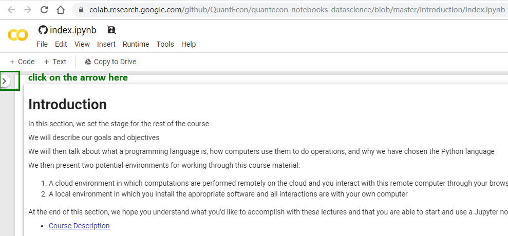\n",
143 | "\n",
144 | " \n",
145 | "Then, “table of contents” will pop up. You can click on sections or subsections for different parts\n",
146 | "of the notebook.\n",
147 | "\n",
148 | "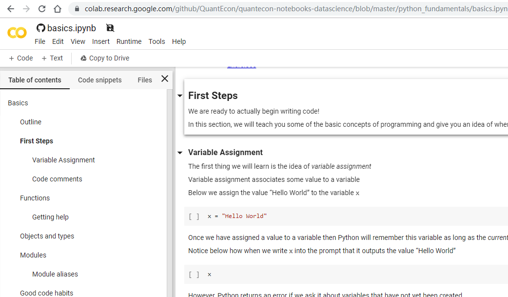"
149 | ]
150 | },
151 | {
152 | "cell_type": "markdown",
153 | "id": "23584db3",
154 | "metadata": {},
155 | "source": [
156 | "#### File Management on Colab\n",
157 | "\n",
158 | "By default, Colab will erase any work that you have done after you have exited a notebook.\n",
159 | "\n",
160 | "If you would like to store your work, you can save it onto your Google Drive by clicking the\n",
161 | "`Copy to Drive` button.\n",
162 | "\n",
163 | "You can create a new notebook by clicking `File` on the menubar and selecting\n",
164 | "`New Python 3 notebook`."
165 | ]
166 | }
167 | ],
168 | "metadata": {
169 | "date": 1738727696.9306712,
170 | "filename": "cloud_setup.md",
171 | "kernelspec": {
172 | "display_name": "Python",
173 | "language": "python3",
174 | "name": "python3"
175 | },
176 | "title": "Cloud Setup"
177 | },
178 | "nbformat": 4,
179 | "nbformat_minor": 5
180 | }
--------------------------------------------------------------------------------
/introduction/getting_started.ipynb:
--------------------------------------------------------------------------------
1 | {
2 | "cells": [
3 | {
4 | "cell_type": "markdown",
5 | "id": "7193abfd",
6 | "metadata": {},
7 | "source": [
8 | "# Getting Started\n",
9 | "\n",
10 | "**Prerequisites**\n",
11 | "\n",
12 | "- Good attitude \n",
13 | "- Good work ethic \n",
14 | "\n",
15 | "\n",
16 | "**Outcomes**\n",
17 | "\n",
18 | "- Understand what a programming language is. \n",
19 | "- Know why we chose Python \n",
20 | "- Know what the Jupyter Notebook is \n",
21 | "- Be able to start JupyterLab in the chosen environment (cloud or personal computer) \n",
22 | "- Be able to open a Jupyter notebook in JupyterLab \n",
23 | "- Know Jupyter Notebook basics: cell modes, editing/evaluating cells "
24 | ]
25 | },
26 | {
27 | "cell_type": "markdown",
28 | "id": "4ca36117",
29 | "metadata": {},
30 | "source": [
31 | "## Welcome\n",
32 | "\n",
33 | "Welcome to the start of your path to learning how to work with data in the\n",
34 | "Python programming language!\n",
35 | "\n",
36 | "A programming language is, loosely speaking, a structured subset of natural\n",
37 | "language (words) and special characters (e.g. `,` or `{`) that allow humans\n",
38 | "to describe operations they would like their computer to perform on their behalf.\n",
39 | "\n",
40 | "The programming language translates these words and\n",
41 | "symbols into instructions the computer can execute."
42 | ]
43 | },
44 | {
45 | "cell_type": "markdown",
46 | "id": "7c0a4bf4",
47 | "metadata": {},
48 | "source": [
49 | "### Why Python?\n",
50 | "\n",
51 | "Among the hundreds of programming languages to choose from, we chose to teach you Python for the\n",
52 | "following reasons:\n",
53 | "\n",
54 | "- Easy to learn and use (relative to other programming languages). \n",
55 | "- Designed with readability in mind. \n",
56 | "- Excellent tools for handling data efficiently and succinctly. \n",
57 | "- Cemented as the world’s [third most popular](https://www.zdnet.com/article/programming-language-of-the-year-python-is-standout-in-latest-rankings/)\n",
58 | " programming language, the most popular scripting language, and an increasing standard for\n",
59 | " [data analysis in industry](https://medium.com/@data_driven/python-vs-r-for-data-science-and-the-winner-is-3ebb1a968197). \n",
60 | "- General purpose: Initially you will learn Python for data analysis, but it\n",
61 | " can also used for websites, database management, web scraping, financial\n",
62 | " modeling, data visualization, etc. In particular, it is the world’s best language for\n",
63 | " [gluing](https://en.wikipedia.org/wiki/Glue_code) those different pieces together. \n",
64 | "\n",
65 | "\n",
66 | "However, the general purpose nature of Python comes at a cost: it is often said that Python is “the\n",
67 | "best language for nothing but the second best language for everything”.\n",
68 | "\n",
69 | "We aren’t sure this is true, but a more optimistic view of that quote is that Python is a great\n",
70 | "language to have in your toolbox to solve all sorts of problems and patch them together.\n",
71 | "\n",
72 | "A versatile “second-best” language might be the best one to learn first.\n",
73 | "\n",
74 | "Some other languages to consider:\n",
75 | "\n",
76 | "- R has an impressive ecosystem of statistical packages, and is defensible as a choice for pure\n",
77 | " data science. It could be a useful second language to learn for projects that are entirely\n",
78 | " statistical. \n",
79 | "- Matlab has much more natural notation for writing linear algebra heavy code. However, it is:\n",
80 | " (a) expensive; (b) poor at dealing with data analysis; (c) grossly inferior to Python as a\n",
81 | " language; and (d) being left behind as Python and Julia ecosystems expand to more packages. \n",
82 | "- Julia is in part a far better version of Matlab, which can be as fast as Fortran or C. However,\n",
83 | " it has a young and immature environment and is currently more appropriate for academics and\n",
84 | " scientific computing specialists. \n",
85 | "\n",
86 | "\n",
87 | "Another consideration for programming language choice is runtime performance. On this dimension,\n",
88 | "Python, R, and Matlab can be slow for certain types of tasks.\n",
89 | "\n",
90 | "Luckily, this will not be an issue for data science and the types of analysis we will do in this\n",
91 | "course, because most of the data analytics packages in Python (and R) rely on high-performance\n",
92 | "code written in other languages in the background.\n",
93 | "\n",
94 | "If you are writing more traditional scientific/technical computing in Python, there are\n",
95 | "[things that can help](http://numba.pydata.org/) make Python faster in some situations,\n",
96 | "but another language like Julia may be a better fit."
97 | ]
98 | },
99 | {
100 | "cell_type": "markdown",
101 | "id": "764ea4e6",
102 | "metadata": {},
103 | "source": [
104 | "### Why Open Source?\n",
105 | "\n",
106 | "Software development has changed radically in the last decade, increasingly becoming a process of\n",
107 | "stitching together both established high quality libraries, and state-of-the-art research projects.\n",
108 | "\n",
109 | "A major disadvantage of Matlab, Stata, and other proprietary languages is that they are not\n",
110 | "open-source, and unable to work within this new paradigm.\n",
111 | "\n",
112 | "Forgetting the cost for a moment, the benefits of using an open-source language are pragmatic rather\n",
113 | "than ideological.\n",
114 | "\n",
115 | "- Open source languages are easier for everyone in the world to write and share packages because\n",
116 | " the code is accessible and available. \n",
117 | "- With the right kinds of open source licenses; academics, businesses, and hobbyists all have\n",
118 | " incentives to contribute. \n",
119 | "- Because open-source languages are managed on publicly accessible sites (e.g. GitHub), it is\n",
120 | " easier to build a community and collaborate. \n",
121 | "- Package management systems (i.e. a way to find, download, install, and upgrade packages) in\n",
122 | " open-source languages can be very open and accessible since they don’t need to deal with\n",
123 | " proprietary software licenses. "
124 | ]
125 | },
126 | {
127 | "cell_type": "markdown",
128 | "id": "a3e664a9",
129 | "metadata": {},
130 | "source": [
131 | "### Computing Environment\n",
132 | "\n",
133 | "These materials are meant to be interacted with, not passively read.\n",
134 | "\n",
135 | "To help you do this, we use a software called [Jupyter](https://jupyter.org/) and files known as\n",
136 | "Jupyter notebooks which allow us to bundle a mixture of text, code, and code output together.\n",
137 | "\n",
138 | "In fact, right now you are either directly reading a Jupyter notebook or a website that was\n",
139 | "generated from a Jupyter notebook."
140 | ]
141 | },
142 | {
143 | "cell_type": "markdown",
144 | "id": "3eab86bb",
145 | "metadata": {},
146 | "source": [
147 | "#### Jupyter\n",
148 | "\n",
149 | "We will refer to two components of Jupyter’s software: JupyterLab and Jupyter Notebook.\n",
150 | "\n",
151 | "**JupyterLab**\n",
152 | "\n",
153 | "JupyterLab is a software that runs in your browser and allows you to do a variety of things such\n",
154 | "as: edit text, view files, and (most importantly) work with Jupyter notebooks.\n",
155 | "\n",
156 | "**Jupyter Notebook**\n",
157 | "\n",
158 | "This is the actual file that allows you to mix code and text.\n",
159 | "\n",
160 | "The content inside a Jupyter notebook is organized into cells.\n",
161 | "\n",
162 | "Cells can have *inputs* and *outputs*.\n",
163 | "\n",
164 | "There are two main types of cells:\n",
165 | "\n",
166 | "1. Markdown cells \n",
167 | " - *Inputs* are written in [markdown](https://github.com/adam-p/markdown-here/wiki/Markdown-Here-Cheatsheet) and can contain formatted text, images, equations, and more. \n",
168 | " - *Outputs* are rendered **in place of the input** when the cell is executed. \n",
169 | "1. Code cells \n",
170 | " - *Inputs* Contain Python code (or code in [another language](https://github.com/jupyter/jupyter/wiki/Jupyter-kernels)). \n",
171 | " - *Outputs* are placed below the input cell and contain the results generated when the input code is executed. \n",
172 | "\n",
173 | "\n",
174 | "Below is an image that demonstrates what a Jupyter Notebook looks like:\n",
175 | "\n",
176 | "\n",
177 | "\n",
178 | " \n",
179 | "Notice a few things about this image:\n",
180 | "\n",
181 | "- Inputs to code cells have a ` [ ]:` to the left of them and have a darker background than the\n",
182 | " surrounding area. \n",
183 | "- Code cells that have not yet been executed do not have a number in the `[ ]:` box and have no\n",
184 | " corresponding output. \n",
185 | "- Executed code cells have a `[#]:` to the left of them (where `#` is a number) and, depending\n",
186 | " on what the code in that cell does, may or may not have an output. \n",
187 | "- Executed markdown cells are displayed as formatted text, rather than the input/output structure. \n",
188 | "\n",
189 | "\n",
190 | "Being able to include both text and code allows us to do interesting computations *and* explain them.\n",
191 | "\n",
192 | "This combination has caused leading companies like [Netflix](https://medium.com/netflix-techblog/notebook-innovation-591ee3221233)\n",
193 | "and [Bloomberg](https://www.techatbloomberg.com/blog/inside-the-collaboration-that-built-the-open-source-jupyterlab-project/)\n",
194 | "to adopt Jupyter as a tool of choice for data analytics and reporting.\n",
195 | "\n",
196 | "We will follow in their path and leverage Jupyter Notebook throughout these materials."
197 | ]
198 | },
199 | {
200 | "cell_type": "markdown",
201 | "id": "e8200a11",
202 | "metadata": {},
203 | "source": [
204 | "#### Running the Lectures\n",
205 | "\n",
206 | "The interactivity of a Jupyter notebook is driven by two main components:\n",
207 | "\n",
208 | "1. Server that is responsible for executing code \n",
209 | "1. GUI that runs in your web browser (what we learned above above) \n",
210 | "\n",
211 | "\n",
212 | "We will edit the content of the notebook and request code execution from the web GUI.\n",
213 | "\n",
214 | "The Jupyter application will then ask the server to execute the code and send the results back to\n",
215 | "the GUI.\n",
216 | "\n",
217 | "You can choose to interact with these materials from two server environments:\n",
218 | "\n",
219 | "1. The cloud \n",
220 | "1. Your own computer \n",
221 | "\n",
222 | "\n",
223 | "**Cloud Computing**\n",
224 | "\n",
225 | "A cloud solution provides a pre-installed environment for you.\n",
226 | "\n",
227 | "As long as you have an internet connection, you will be able to interact with the lectures\n",
228 | "through a few cloud computing options.\n",
229 | "\n",
230 | "We try to ensure that you’ll be able to run any of the lectures from each of the cloud options,\n",
231 | "but because these services are hosted by others, we cannot provide any guarantees.\n",
232 | "\n",
233 | "Using the cloud is a great option if\n",
234 | "\n",
235 | "1. You aren’t sure whether you’d like to learn these skills and just want to test the lectures\n",
236 | " out without any additional commitment. \n",
237 | "1. You are away from your typical work station and would like to spend a few minutes interacting\n",
238 | " with our lectures — we often take this route with our colleagues over coffee (or other\n",
239 | " conversation stimulants). \n",
240 | "\n",
241 | "\n",
242 | "If you would like to work on these lectures from the cloud, please read the instructions for\n",
243 | "getting set up with [cloud computing](https://datascience.quantecon.org/cloud_setup.html).\n",
244 | "\n",
245 | "These instructions describe several of the possible computing environments that you can choose,\n",
246 | "discuss their pros and cons, and explain what JupyterHub is.\n",
247 | "\n",
248 | "After reading the instructions, return to this page and proceed with the Jupyter Basics section.\n",
249 | "\n",
250 | "**Local Installation**\n",
251 | "\n",
252 | "With a local installation, you will install the required software onto your own computer.\n",
253 | "\n",
254 | "This is typically a straightforward task and, once you have done this, you will be able to run the\n",
255 | "lecture code (and any other code you write for your own projects!) on your personal computer.\n",
256 | "\n",
257 | "If you are confident that these are skills you would like to acquire and are willing to have the\n",
258 | "software installed on your computer, then this is a great option.\n",
259 | "\n",
260 | "If you would like to work from a local installation, please read the instructions in\n",
261 | "[local installation instructions](https://datascience.quantecon.org/local_install.html) page.\n",
262 | "\n",
263 | "These instructions will walk you through the installation procedure, help with some basic setup,\n",
264 | "and show you how to open JupyterLab.\n",
265 | "\n",
266 | "Once you have completed installing the software, return to this page and proceed with the Jupyter\n",
267 | "Basics section."
268 | ]
269 | },
270 | {
271 | "cell_type": "markdown",
272 | "id": "2376d931",
273 | "metadata": {},
274 | "source": [
275 | "#### Jupyter Basics\n",
276 | "\n",
277 | "Now that you can open a JupyterLab instance on the cloud or on your own computer, we can talk about\n",
278 | "how you should use them.\n",
279 | "\n",
280 | "Note, not all of this will apply if you are using the Google Colab cloud server since they are\n",
281 | "running a modified version of Jupyter. For more help on using Colab, see their help menu.\n",
282 | "\n",
283 | "**JupyterLab Dashboard**\n",
284 | "\n",
285 | "When you open a new session in Jupyter, you will be taken to the JupyterLab dashboard page.\n",
286 | "\n",
287 | "This page shows the file system of the machine running the Jupyter server and allows you to\n",
288 | "navigate and open particular Jupyter Notebooks (or other types of files!).\n",
289 | "\n",
290 | "The dashboard page is shown below.\n",
291 | "\n",
292 | "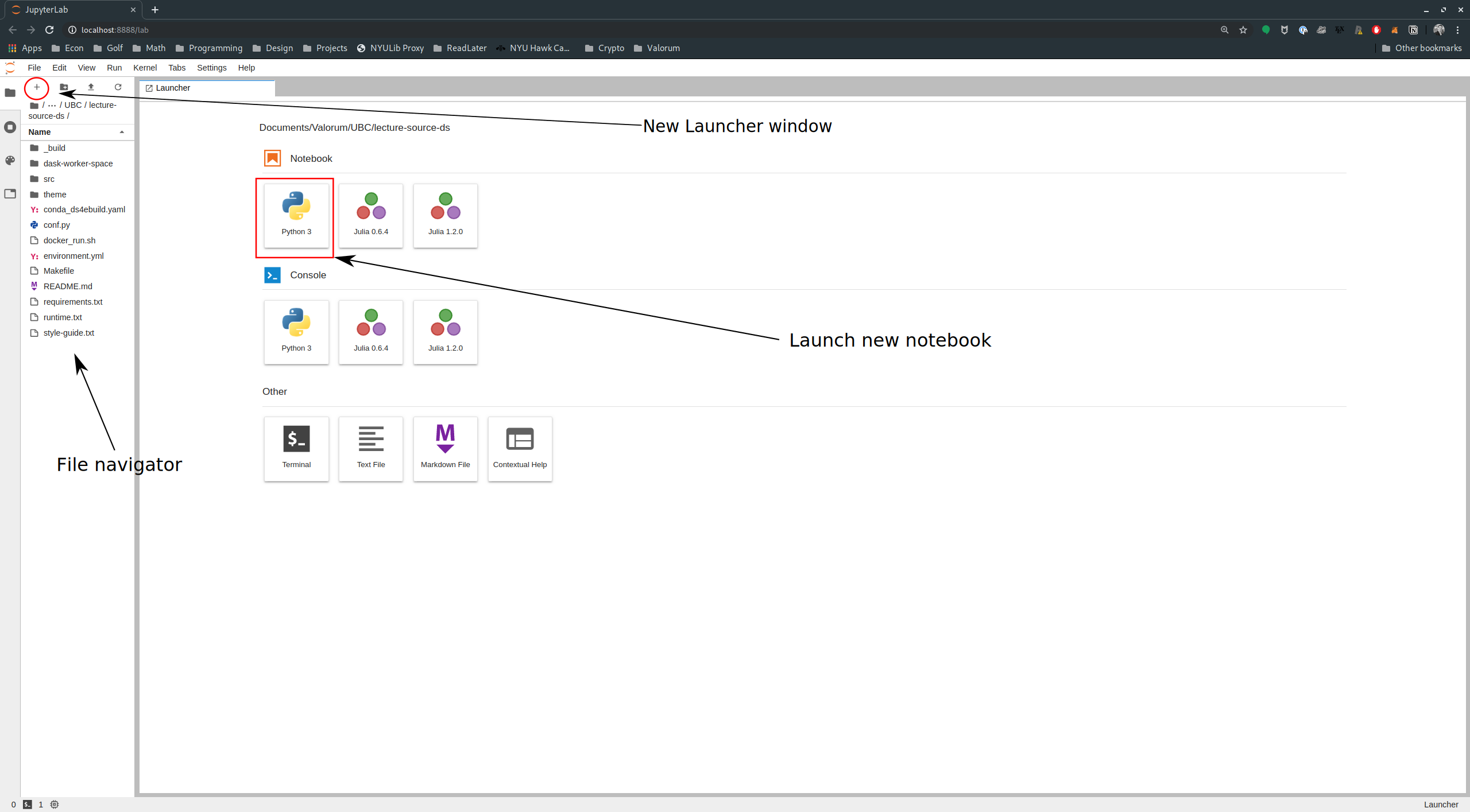\n",
293 | "\n",
294 | " \n",
295 | "You can open existing files or change folders by double clicking on them in the left panel of the\n",
296 | "dashboard (similar to a file explorer you would find on your computer).\n",
297 | "\n",
298 | "You can create new notebooks by clicking `Python 3` in the Launcher (see red square in the image).\n",
299 | "\n",
300 | "If you don’t see the Launcher as one of your tabs, you can open it by clicking the `+` at the top\n",
301 | "of the file explorer section of the JupyterLab dashboard (see the red circle in the image).\n",
302 | "\n",
303 | "**Editing Jupyter Notebooks**\n",
304 | "\n",
305 | "Once you have opened a particular notebook, you can be in one of two “edit modes”.\n",
306 | "\n",
307 | "1. Command mode: This mode is for making high level changes to the notebook\n",
308 | " itself. For example changing the order of cells, creating a new cell, etc… \n",
309 | " - You know you’re in command mode when a blue sidebar appears on the left of the\n",
310 | " cell. \n",
311 | " - Pressing keys tells Jupyter Notebook to run commands. For example, `a`\n",
312 | " adds a new cell above the current cell, `b` adds one below the current\n",
313 | " cell, and `dd` deletes the current cell. \n",
314 | " - up arrow (or `k`) changes the selected cell to the cell above the\n",
315 | " current one and down arrow (or `j`) changes to the cell below. \n",
316 | "1. Edit mode: Used when editing the content inside of cells. \n",
317 | " - When in edit mode, the selected cell displays a green sidebar on left. \n",
318 | " - Can edit the content of a cell. \n",
319 | "\n",
320 | "\n",
321 | "Some useful commands:\n",
322 | "\n",
323 | "- To go from command mode to edit mode, press enter or double click the mouse \n",
324 | "- Go from edit mode to command mode by pressing escape \n",
325 | "- You can evaluate a cell by pressing `Shift + Enter` (meaning `Shift` and `Enter` at\n",
326 | " the same time) "
327 | ]
328 | },
329 | {
330 | "cell_type": "markdown",
331 | "id": "0cd2fd64",
332 | "metadata": {},
333 | "source": [
334 | "#### Exercise\n",
335 | "\n",
336 | "See exercise 1 in the [exercise list](#ex1-1).\n",
337 | "\n",
338 | "**Advanced Usage and Getting Help**\n",
339 | "\n",
340 | "For more help with JupyterLab and Jupyter Notebook, see the user guides:\n",
341 | "\n",
342 | "- [JupyterLab](https://jupyterlab.readthedocs.io/en/latest/user/interface.html) \n",
343 | "- [Jupyter Notebook](https://jupyterlab.readthedocs.io/en/latest/user/notebook.html) \n",
344 | "\n",
345 | "\n",
346 | "\n",
347 | ""
348 | ]
349 | },
350 | {
351 | "cell_type": "markdown",
352 | "id": "990ea73a",
353 | "metadata": {},
354 | "source": [
355 | "## Exercises"
356 | ]
357 | },
358 | {
359 | "cell_type": "markdown",
360 | "id": "b83f8447",
361 | "metadata": {},
362 | "source": [
363 | "### Exercise 1\n",
364 | "\n",
365 | "In the *code* cell below (notice the `[ ]:` to the left) type a quote (`\"`), your name,\n",
366 | "then another quote (`\"`) and evaluate the cell"
367 | ]
368 | },
369 | {
370 | "cell_type": "code",
371 | "execution_count": null,
372 | "id": "ba25ff4d",
373 | "metadata": {
374 | "hide-output": false
375 | },
376 | "outputs": [],
377 | "source": [
378 | "# code here!"
379 | ]
380 | },
381 | {
382 | "cell_type": "markdown",
383 | "id": "3a1b2648",
384 | "metadata": {},
385 | "source": [
386 | "([back to text](#dir1-1-1))"
387 | ]
388 | }
389 | ],
390 | "metadata": {
391 | "date": 1738727696.9452474,
392 | "filename": "getting_started.md",
393 | "kernelspec": {
394 | "display_name": "Python",
395 | "language": "python3",
396 | "name": "python3"
397 | },
398 | "title": "Getting Started"
399 | },
400 | "nbformat": 4,
401 | "nbformat_minor": 5
402 | }
--------------------------------------------------------------------------------
/introduction/index.ipynb:
--------------------------------------------------------------------------------
1 | {
2 | "cells": [
3 | {
4 | "cell_type": "markdown",
5 | "id": "881f39dc",
6 | "metadata": {},
7 | "source": [
8 | "# Introduction\n",
9 | "\n",
10 | "In this section, we set the stage for the rest of the course.\n",
11 | "\n",
12 | "We will describe our goals and objectives.\n",
13 | "\n",
14 | "We will then talk about what a programming language is, how computers use them to do operations, and\n",
15 | "why we have chosen the Python language.\n",
16 | "\n",
17 | "We then present two potential environments for working through this course material:\n",
18 | "\n",
19 | "1. A cloud environment in which computations are performed remotely on the cloud and you interact\n",
20 | " with this remote computer through your browser. \n",
21 | "1. A local environment in which you install the appropriate software and all interactions are with\n",
22 | " your own computer. \n",
23 | "\n",
24 | "\n",
25 | "At the end of this section, we hope you understand what you’d like to accomplish with these lectures\n",
26 | "and that you are able to start and use a Jupyter notebook."
27 | ]
28 | },
29 | {
30 | "cell_type": "markdown",
31 | "id": "4e9e5247",
32 | "metadata": {},
33 | "source": [
34 | "## [Course Description](https://datascience.quantecon.org/overview.html)"
35 | ]
36 | },
37 | {
38 | "cell_type": "markdown",
39 | "id": "43d57cd4",
40 | "metadata": {},
41 | "source": [
42 | "## [Getting Started](https://datascience.quantecon.org/getting_started.html)"
43 | ]
44 | },
45 | {
46 | "cell_type": "markdown",
47 | "id": "bf289199",
48 | "metadata": {},
49 | "source": [
50 | "## [Cloud Setup](https://datascience.quantecon.org/cloud_setup.html)"
51 | ]
52 | },
53 | {
54 | "cell_type": "markdown",
55 | "id": "a651e3b9",
56 | "metadata": {},
57 | "source": [
58 | "## [Local Installation](https://datascience.quantecon.org/local_install.html)"
59 | ]
60 | },
61 | {
62 | "cell_type": "markdown",
63 | "id": "e2ce90a3",
64 | "metadata": {},
65 | "source": [
66 | "## [Troubleshooting](https://datascience.quantecon.org/troubleshooting.html)"
67 | ]
68 | }
69 | ],
70 | "metadata": {
71 | "date": 1738727696.9499226,
72 | "filename": "index.md",
73 | "kernelspec": {
74 | "display_name": "Python",
75 | "language": "python3",
76 | "name": "python3"
77 | },
78 | "title": "Introduction"
79 | },
80 | "nbformat": 4,
81 | "nbformat_minor": 5
82 | }
--------------------------------------------------------------------------------
/introduction/local_install.ipynb:
--------------------------------------------------------------------------------
1 | {
2 | "cells": [
3 | {
4 | "cell_type": "markdown",
5 | "id": "de3648bb",
6 | "metadata": {},
7 | "source": [
8 | "# Local Installation"
9 | ]
10 | },
11 | {
12 | "cell_type": "markdown",
13 | "id": "c295769e",
14 | "metadata": {},
15 | "source": [
16 | "## Installation\n",
17 | "\n",
18 | "Visit [continuum.io](https://www.anaconda.com/download) and download the\n",
19 | "Anaconda Python distribution for your operating system (Windows/Mac OS/Linux).\n",
20 | "\n",
21 | "Be sure to download the Python 3.X (where X is some number greater than or equal to 8) version, not\n",
22 | "the 2.7 version.\n",
23 | "\n",
24 | "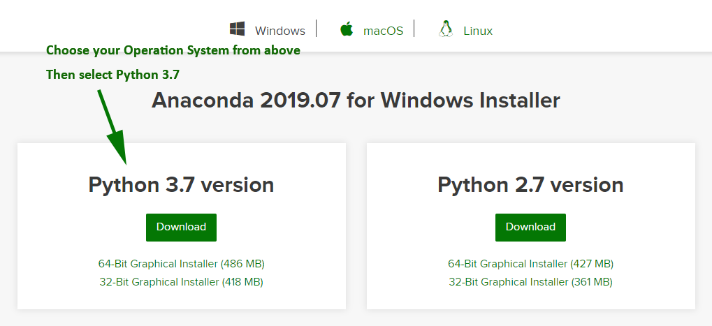\n",
25 | "\n",
26 | " \n",
27 | "Make sure that during the installation [Anaconda](https://www.anaconda.com/distribution/)\n",
28 | "is added to your environment/path.\n",
29 | "\n",
30 | "On Mac OS and Linux, this should happen by default.\n",
31 | "\n",
32 | "For Windows users, we recommend installing for “just me” instead of “all users”. Windows users will need to **check the upper box** when the page shown below appears (disregard the “not recommended” warning from Anaconda).\n",
33 | "\n",
34 | "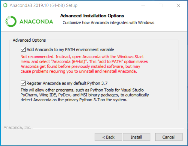"
35 | ]
36 | },
37 | {
38 | "cell_type": "markdown",
39 | "id": "d9dd5346",
40 | "metadata": {},
41 | "source": [
42 | "## Downloading the QuantEcon Data Science Lectures\n",
43 | "\n",
44 | "To download the QuantEcon Data Science lectures, go to its [Github repo](https://github.com/QuantEcon/lecture-datascience.notebooks), click on the\n",
45 | "Code button.\n",
46 | "\n",
47 | "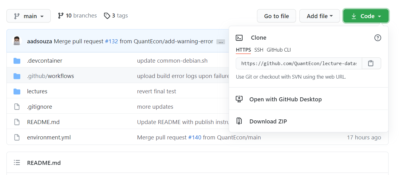\n",
48 | "\n",
49 | " \n",
50 | "You can download the lectures through either **Github Desktop** or **Terminal**:\n",
51 | "\n",
52 | "**Github Desktop** (Mac/Windows only), recommended for most users.\n",
53 | "\n",
54 | "1. Install [Github Desktop](https://desktop.github.com/). \n",
55 | "1. Go to the [Github repo](https://github.com/QuantEcon/lecture-datascience.notebooks). \n",
56 | "1. Click the “Open with Github Desktop” option in the Code button menu. It should open a Github\n",
57 | " Desktop popup that looks like this: \n",
58 | " 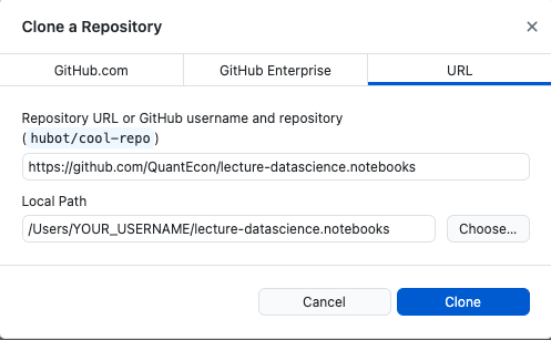\n",
59 | " \n",
60 | " \n",
61 | " You should choose the path (folder) where you would like to download the repository. The default path on\n",
62 | " Windows should be `C:/Users/YOUR_USERNAME/Documents/GitHub`. \n",
63 | "\n",
64 | "\n",
65 | "**Terminal**\n",
66 | "\n",
67 | "1. Make sure that `git` is installed on your computer. (`git` is not installed on Windows by default. You can download and install it from [here](https://git-scm.com/download/win)). \n",
68 | "1. Open a terminal. \n",
69 | "1. Set the path to where you would like to download the lectures. The default one is your home directory. \n",
70 | "1. Run `git clone https://github.com/QuantEcon/lecture-datascience.notebooks.git` which will\n",
71 | " download the repository with notebooks in your working directory. "
72 | ]
73 | },
74 | {
75 | "cell_type": "markdown",
76 | "id": "d0b22327",
77 | "metadata": {},
78 | "source": [
79 | "## Package Management\n",
80 | "\n",
81 | "In addition to Jupyter, the Anaconda Python distribution comes with two package management tools `conda` and `pip`.\n",
82 | "\n",
83 | "These will help you ensure that you have the right packages (think of these as “add-ons” to Python\n",
84 | "that give you additional functionality… We will discuss these more in depth later!) and help you\n",
85 | "keep them all up to date.\n",
86 | "\n",
87 | "We will work through an example below to install some new package functionality needed for some\n",
88 | "later lectures. Generally, packages can be installed by using `conda install ` or\n",
89 | "`pip install `.\n",
90 | "\n",
91 | "Please install the packages you will need later by following the instructions below for your\n",
92 | "computer’s operating system.\n",
93 | "\n",
94 | "**Linux/Mac**\n",
95 | "\n",
96 | "- Open a terminal. \n",
97 | "- Run the following commands: "
98 | ]
99 | },
100 | {
101 | "cell_type": "markdown",
102 | "id": "99b99851",
103 | "metadata": {
104 | "hide-output": false
105 | },
106 | "source": [
107 | "```bash\n",
108 | "# Install Python packages\n",
109 | "conda install python-graphviz\n",
110 | "conda install -c conda-forge \"nodejs>=10.0\" xgboost\n",
111 | "pip install fiona geopandas pyLDAvis gensim folium descartes pyarrow --upgrade\n",
112 | "\n",
113 | "# Activate jlab extensions\n",
114 | "jupyter labextension install @jupyterlab/toc --no-build\n",
115 | "jupyter labextension install @jupyter-widgets/jupyterlab-manager --no-build\n",
116 | "jupyter labextension install plotlywidget --no-build\n",
117 | "jupyter labextension install jupyterlab-plotly --no-build\n",
118 | "jupyter lab build\n",
119 | "```\n"
120 | ]
121 | },
122 | {
123 | "cell_type": "markdown",
124 | "id": "1f579ab6",
125 | "metadata": {},
126 | "source": [
127 | "Press `y` and enter whenever you see `Proceed [y]/n` from your terminal. \n",
128 | "- Close the terminal when the installation finishes. \n",
129 | "\n",
130 | "\n",
131 | "**Windows**\n",
132 | "\n",
133 | "- Open a command prompt by pressing Windows + R to open the `run` box, type `powershell`, and press\n",
134 | " Enter. \n",
135 | "- Run the following commands in order: "
136 | ]
137 | },
138 | {
139 | "cell_type": "markdown",
140 | "id": "6e17a96f",
141 | "metadata": {
142 | "hide-output": false
143 | },
144 | "source": [
145 | "```bash\n",
146 | "# Install Python packages\n",
147 | "conda install geopandas python-graphviz\n",
148 | "conda install -c conda-forge nodejs\n",
149 | "pip install pyLDAvis gensim folium xgboost descartes pyarrow graphviz --upgrade\n",
150 | "\n",
151 | "# Activate jlab extensions\n",
152 | "jupyter labextension install @jupyterlab/toc --no-build\n",
153 | "jupyter labextension install @jupyter-widgets/jupyterlab-manager --no-build\n",
154 | "jupyter labextension install plotlywidget --no-build\n",
155 | "jupyter labextension install jupyterlab-plotly --no-build\n",
156 | "jupyter lab build\n",
157 | "```\n"
158 | ]
159 | },
160 | {
161 | "cell_type": "markdown",
162 | "id": "21b297d8",
163 | "metadata": {},
164 | "source": [
165 | "Press `y` and enter whenever you see `Proceed [y]/n` from your terminal. \n",
166 | "- Close the command window after the installation finishes, log out of Windows, and then log in. \n",
167 | "\n",
168 | "\n",
169 | "If you are told that you are missing a package at any point in time, we recommend trying to install\n",
170 | "the package with `conda` first and, if that doesn’t work, installing with `pip`.\n",
171 | "\n",
172 | "You can update a package by running:\n",
173 | "\n",
174 | "- `conda update ` for conda \n",
175 | "- `pip install --upgrade` for pip \n",
176 | "\n",
177 | "\n",
178 | "**Note:** If you have errors using `graphviz` on Windows, then open a `powershell` terminal and execute the following two lines:"
179 | ]
180 | },
181 | {
182 | "cell_type": "code",
183 | "execution_count": null,
184 | "id": "95c7d4a2",
185 | "metadata": {
186 | "hide-output": false
187 | },
188 | "outputs": [],
189 | "source": [
190 | "$pp = (python -c \"import sys; print(sys.exec_prefix)\")\n",
191 | "\n",
192 | "Set-ItemProperty -path HKCU:\\Environment\\ -Name Path -Value \"$((Get-ItemProperty -path HKCU:\\Environment\\ -Name Path).Path);$($pp)\\Library\\bin\\graphviz\""
193 | ]
194 | },
195 | {
196 | "cell_type": "markdown",
197 | "id": "40f8c2af",
198 | "metadata": {},
199 | "source": [
200 | "## Starting Jupyter\n",
201 | "\n",
202 | "Start JupyterLab by following these steps:\n",
203 | "\n",
204 | "1. Open a new terminal (for Windows, you should use the Powershell: press Win + R and type\n",
205 | " `powershell` in the run box, then hit enter). \n",
206 | "1. Type `jupyter lab` and press Enter. \n",
207 | "\n",
208 | "\n",
209 | "If a web browser doesn’t open by default, look at the terminal text and find something that looks\n",
210 | "like:"
211 | ]
212 | },
213 | {
214 | "cell_type": "markdown",
215 | "id": "40566424",
216 | "metadata": {
217 | "hide-output": false
218 | },
219 | "source": [
220 | "```md\n",
221 | "Copy/paste this URL into your browser when you connect for the first time,\n",
222 | "to login with a token:\n",
223 | " http://localhost:8888/?token=9a39d3741a4f0b200c6e4b07d8e5c04a089899cddc72e7f8\n",
224 | "```\n"
225 | ]
226 | },
227 | {
228 | "cell_type": "markdown",
229 | "id": "2c2c6a43",
230 | "metadata": {},
231 | "source": [
232 | "and copy/paste the line starting with `http://` into your web browser.\n",
233 | "\n",
234 | ">**Note**\n",
235 | ">\n",
236 | ">The terminal you opened must stay open while you are editing the notebooks."
237 | ]
238 | },
239 | {
240 | "cell_type": "markdown",
241 | "id": "1171449f",
242 | "metadata": {},
243 | "source": [
244 | "### Opening a Jupyter Notebook\n",
245 | "\n",
246 | "Once the web browser is open, you should see the JupyterLab dashboard. You can open a new Jupyter\n",
247 | "notebook by clicking Python 3 when you see something like the following image in your browser:\n",
248 | "\n",
249 | "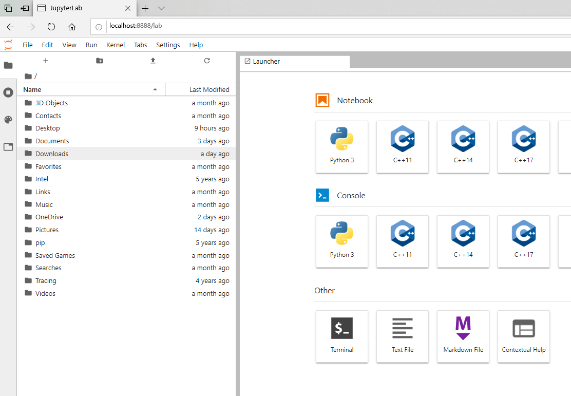\n",
250 | "\n",
251 | " \n",
252 | "Once the notebook is open, you should something similar to the following image:\n",
253 | "\n",
254 | "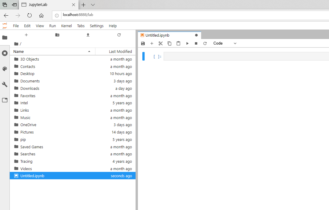\n",
255 | "\n",
256 | " \n",
257 | "Note that:\n",
258 | "\n",
259 | "- The filenames on the left will be different. \n",
260 | "- It *should* list the contents of your personal home directory (folder). "
261 | ]
262 | },
263 | {
264 | "cell_type": "markdown",
265 | "id": "22446b6d",
266 | "metadata": {},
267 | "source": [
268 | "### Exercise\n",
269 | "\n",
270 | "See exercise 1 in the [exercise list](#ex1-2).\n",
271 | "\n",
272 | "\n",
273 | ""
274 | ]
275 | },
276 | {
277 | "cell_type": "markdown",
278 | "id": "c6ee981c",
279 | "metadata": {},
280 | "source": [
281 | "## Exercises"
282 | ]
283 | },
284 | {
285 | "cell_type": "markdown",
286 | "id": "ca88402e",
287 | "metadata": {},
288 | "source": [
289 | "### Exercise 1\n",
290 | "\n",
291 | "Open this file in Jupyter by navigating to the QuantEcon Data Science folder that we downloaded\n",
292 | "earlier, then click on the `introduction` folder, and select the `getting_started.ipynb` file.\n",
293 | "\n",
294 | "([back to text](#dir1-2-1))"
295 | ]
296 | }
297 | ],
298 | "metadata": {
299 | "date": 1738727696.9605854,
300 | "filename": "local_install.md",
301 | "kernelspec": {
302 | "display_name": "Python",
303 | "language": "python3",
304 | "name": "python3"
305 | },
306 | "title": "Local Installation"
307 | },
308 | "nbformat": 4,
309 | "nbformat_minor": 5
310 | }
--------------------------------------------------------------------------------
/introduction/overview.ipynb:
--------------------------------------------------------------------------------
1 | {
2 | "cells": [
3 | {
4 | "cell_type": "markdown",
5 | "id": "2989dc8e",
6 | "metadata": {},
7 | "source": [
8 | "# Course Description"
9 | ]
10 | },
11 | {
12 | "cell_type": "markdown",
13 | "id": "c93a51e7",
14 | "metadata": {},
15 | "source": [
16 | "## Course Objectives and Scope"
17 | ]
18 | },
19 | {
20 | "cell_type": "markdown",
21 | "id": "1f87ab4b",
22 | "metadata": {},
23 | "source": [
24 | "### Scope of Lecture Notes\n",
25 | "\n",
26 | "This course is a lecture series on data science, economics, programming, and how\n",
27 | "they can be used to understand the world around us.\n",
28 | "\n",
29 | "We envision this as a complement to econometrics. We focus on learning practical programming\n",
30 | "skills for the workplace and future studies in economics and finance.\n",
31 | "\n",
32 | "Unlike courses in computer science, data science, or statistics, the emphasis of this course\n",
33 | "includes both the programming and the statistics necessary to analyze data *and* subsequently\n",
34 | "interpret results through the lens of economics.\n",
35 | "\n",
36 | "While anyone with the appropriate prerequisites will benefit from this course, undergraduate\n",
37 | "programs will find the lecture series suitable for 2nd to 3rd year students who have taken two\n",
38 | "calculus classes and their school’s equivalent of Econ 101. No prior programming experience is\n",
39 | "required.\n",
40 | "\n",
41 | "Students who complete this course will be prepared to:\n",
42 | "\n",
43 | "- Work in a data analyst or a data science role with the ability to frame problems in a broader\n",
44 | " economic context and provide unique insights associated with that context, and/or, \n",
45 | "- Continue onto QuantEcon’s “Lectures in Quantitative Economics” in preparation for graduate school\n",
46 | " in economics, policy, or other related fields. \n",
47 | "\n",
48 | "\n",
49 | "To get an idea of what one can do after taking this course, please take a look at [previous student projects](https://datascience.quantecon.org/../theme/projects.html)."
50 | ]
51 | },
52 | {
53 | "cell_type": "markdown",
54 | "id": "4f134296",
55 | "metadata": {},
56 | "source": [
57 | "### Course Outline\n",
58 | "\n",
59 | "The essential outcome of the course is: Students will be able to recognize and understand the\n",
60 | "connections between economic theory and the practice of data science, expanding beyond atheoretical\n",
61 | "statistical approaches.\n",
62 | "\n",
63 | "The course is divided into three segments.\n",
64 | "\n",
65 | "The first segment of this course covers programming and basic scientific computing in Python by\n",
66 | "re-examining basic Econ 101 concepts and models.\n",
67 | "\n",
68 | "This provides a natural introduction to thinking of economics as a quantitative discipline, with\n",
69 | "principles and applications grounded in real world problems.\n",
70 | "\n",
71 | "The second segment dives into data analysis and data science, with the associated data wrangling\n",
72 | "skills, as a way to leverage economic data, tools, and concepts.\n",
73 | "\n",
74 | "The final segment is a sequence of case studies designed to help students answer specific questions\n",
75 | "and recommend solutions.\n",
76 | "\n",
77 | "Students will learn and apply more advanced techniques and models, as well as examine new data sources."
78 | ]
79 | },
80 | {
81 | "cell_type": "markdown",
82 | "id": "eaba0cd1",
83 | "metadata": {},
84 | "source": [
85 | "## Prerequisites\n",
86 | "\n",
87 | "While we have kept the prerequisites to a minimum, some degree of mathematical fluency is required.\n",
88 | "\n",
89 | "Most importantly, while familiarity with computers is expected, **no** programming knowledge is\n",
90 | "required for this course.\n",
91 | "\n",
92 | "To summarize the background we expect that you should have at least: (1) an introductory “ECON 101”\n",
93 | "class; (2) one to two terms of calculus; and (3) either an elementary course in matrix algebra, or a\n",
94 | "willingness to learn the basics on your own."
95 | ]
96 | },
97 | {
98 | "cell_type": "markdown",
99 | "id": "8faa5d2b",
100 | "metadata": {},
101 | "source": [
102 | "### Calculus\n",
103 | "\n",
104 | "You should have one course (and possibly two, depending on your university) in Calculus.\n",
105 | "\n",
106 | "The core concepts used throughout the lectures are\n",
107 | "\n",
108 | "- Basic rules of differentiation of univariate functions (e.g. chain rule, product rule) \n",
109 | "- Exponentials, natural logarithms, and their derivatives \n",
110 | "- Inverse functions and implicit functions \n",
111 | "- Maximization/minimization of univariate functions \n",
112 | "- Sequences, series, and infinite series \n",
113 | "- Partial derivatives and multivariate functions \n",
114 | "- Unconstrained Minimization and maximization of multivariate functions \n",
115 | "- Simple constrained optimization (including Lagrange multipliers) "
116 | ]
117 | },
118 | {
119 | "cell_type": "markdown",
120 | "id": "c394fe00",
121 | "metadata": {},
122 | "source": [
123 | "### Linear Algebra\n",
124 | "\n",
125 | "If you have not taken a first course in applied linear algebra or matrix algebra, you will need to\n",
126 | "learn concepts of\n",
127 | "\n",
128 | "- Vectors and matrices \n",
129 | "- Matrices and systems of linear equations \n",
130 | "- Dimension and rank \n",
131 | "- Matrix operations (e.g. addition, multiplication, inverse) \n",
132 | "- Inner products \n",
133 | "- Least squares "
134 | ]
135 | },
136 | {
137 | "cell_type": "markdown",
138 | "id": "b39051aa",
139 | "metadata": {},
140 | "source": [
141 | "### Probability\n",
142 | "\n",
143 | "Basic probability is sometimes covered in a second calculus course, but if you have never\n",
144 | "encountered the topics, then review\n",
145 | "\n",
146 | "- Basic probability of discrete and continuous distributions \n",
147 | "- Conditional and marginal distributions \n",
148 | "- Expected value, variance, and standard deviation "
149 | ]
150 | },
151 | {
152 | "cell_type": "markdown",
153 | "id": "4586b662",
154 | "metadata": {},
155 | "source": [
156 | "### Economics\n",
157 | "\n",
158 | "While more economics is always better, we will try to assume an “Econ 101” background.\n",
159 | "\n",
160 | "Otherwise, we will try to provide additional background material on the economics topics."
161 | ]
162 | }
163 | ],
164 | "metadata": {
165 | "date": 1738727696.9673533,
166 | "filename": "overview.md",
167 | "kernelspec": {
168 | "display_name": "Python",
169 | "language": "python3",
170 | "name": "python3"
171 | },
172 | "title": "Course Description"
173 | },
174 | "nbformat": 4,
175 | "nbformat_minor": 5
176 | }
--------------------------------------------------------------------------------
/introduction/troubleshooting.ipynb:
--------------------------------------------------------------------------------
1 | {
2 | "cells": [
3 | {
4 | "cell_type": "markdown",
5 | "id": "419ba6d6",
6 | "metadata": {},
7 | "source": [
8 | "\n",
9 | ""
10 | ]
11 | },
12 | {
13 | "cell_type": "markdown",
14 | "id": "f57b6586",
15 | "metadata": {},
16 | "source": [
17 | "# Troubleshooting\n",
18 | "\n",
19 | "This troubleshooting page is to help ensure your environment is setup correctly\n",
20 | "to run this lecture. You can follow [cloud setup instructions](https://datascience.quantecon.org/cloud_setup.html) or [local setup instructions](https://datascience.quantecon.org/local_install.html) to set up a standard environment."
21 | ]
22 | },
23 | {
24 | "cell_type": "markdown",
25 | "id": "da1d7590",
26 | "metadata": {},
27 | "source": [
28 | "## Resetting Lectures\n",
29 | "\n",
30 | "Here are instructions to restore some or all lectures to their original states."
31 | ]
32 | },
33 | {
34 | "cell_type": "markdown",
35 | "id": "736ec918",
36 | "metadata": {},
37 | "source": [
38 | "### Local Machines\n",
39 | "\n",
40 | "The workflow is a bit different on a local machine. We are assuming that you have followed the [local setup instructions](https://datascience.quantecon.org/local_install.html), and have installed GitHub desktop.\n",
41 | "\n",
42 | "1. Open GitHub desktop, and navigate to the repository (you can click “find” under “edit” in the top menu bar, and then type `lecture-datascience.myst`, if you are having trouble.) \n",
43 | "1. To **reset everything**, click “discard all changes” under “branch” in the top menu bar. \n",
44 | "1. To **reset a specific notebook**, right-click the specific file in the changes side tab, and then click “discard changes.” \n",
45 | "1. To **pull the latest from the server**, first make sure you don’t have any conflicting changes (i.e., do step (2) above), and then click “pull” under “repository” in the top menu bar. "
46 | ]
47 | },
48 | {
49 | "cell_type": "markdown",
50 | "id": "183d6966",
51 | "metadata": {},
52 | "source": [
53 | "## Reporting an Issue\n",
54 | "\n",
55 | "One way to give feedback is to raise an issue through our [issue tracker](https://github.com/QuantEcon/lecture-datascience.myst/issues).\n",
56 | "\n",
57 | "Please be as specific as possible. Tell us where the problem is and as much\n",
58 | "detail about your local set up as you can provide.\n",
59 | "\n",
60 | "Another feedback option is to use our [discourse forum](https://discourse.quantecon.org/).\n",
61 | "\n",
62 | "Finally, you can provide direct feedback to [contact@quantecon.org](mailto:contact@quantecon.org)"
63 | ]
64 | }
65 | ],
66 | "metadata": {
67 | "date": 1738727696.9723008,
68 | "filename": "troubleshooting.md",
69 | "kernelspec": {
70 | "display_name": "Python",
71 | "language": "python3",
72 | "name": "python3"
73 | },
74 | "title": "Troubleshooting"
75 | },
76 | "nbformat": 4,
77 | "nbformat_minor": 5
78 | }
--------------------------------------------------------------------------------
/pandas/data_clean.ipynb:
--------------------------------------------------------------------------------
1 | {
2 | "cells": [
3 | {
4 | "cell_type": "markdown",
5 | "id": "6455d19a",
6 | "metadata": {},
7 | "source": [
8 | "# Cleaning Data\n",
9 | "\n",
10 | "**Prerequisites**\n",
11 | "\n",
12 | "- [Intro](https://datascience.quantecon.org/intro.html) \n",
13 | "- [Boolean selection](https://datascience.quantecon.org/basics.html) \n",
14 | "- [Indexing](https://datascience.quantecon.org/the_index.html) \n",
15 | "\n",
16 | "\n",
17 | "**Outcomes**\n",
18 | "\n",
19 | "- Be able to use string methods to clean data that comes as a string \n",
20 | "- Be able to drop missing data \n",
21 | "- Use cleaning methods to prepare and analyze a real dataset \n",
22 | "\n",
23 | "\n",
24 | "**Data**\n",
25 | "\n",
26 | "- Item information from about 3,000 Chipotle meals from about 1,800\n",
27 | " Grubhub orders "
28 | ]
29 | },
30 | {
31 | "cell_type": "code",
32 | "execution_count": null,
33 | "id": "54c269ed",
34 | "metadata": {
35 | "hide-output": false
36 | },
37 | "outputs": [],
38 | "source": [
39 | "# Uncomment following line to install on colab\n",
40 | "#! pip install "
41 | ]
42 | },
43 | {
44 | "cell_type": "code",
45 | "execution_count": null,
46 | "id": "4dcec5d7",
47 | "metadata": {
48 | "hide-output": false
49 | },
50 | "outputs": [],
51 | "source": [
52 | "import pandas as pd\n",
53 | "import numpy as np"
54 | ]
55 | },
56 | {
57 | "cell_type": "markdown",
58 | "id": "c9ef53af",
59 | "metadata": {},
60 | "source": [
61 | "## Cleaning Data\n",
62 | "\n",
63 | "For many data projects, a [significant proportion of\n",
64 | "time](https://www.forbes.com/sites/gilpress/2016/03/23/data-preparation-most-time-consuming-least-enjoyable-data-science-task-survey-says/#74d447456f63)\n",
65 | "is spent collecting and cleaning the data — not performing the analysis.\n",
66 | "\n",
67 | "This non-analysis work is often called “data cleaning”.\n",
68 | "\n",
69 | "pandas provides very powerful data cleaning tools, which we\n",
70 | "will demonstrate using the following dataset."
71 | ]
72 | },
73 | {
74 | "cell_type": "code",
75 | "execution_count": null,
76 | "id": "f540501c",
77 | "metadata": {
78 | "hide-output": false
79 | },
80 | "outputs": [],
81 | "source": [
82 | "df = pd.DataFrame({\"numbers\": [\"#23\", \"#24\", \"#18\", \"#14\", \"#12\", \"#10\", \"#35\"],\n",
83 | " \"nums\": [\"23\", \"24\", \"18\", \"14\", np.nan, \"XYZ\", \"35\"],\n",
84 | " \"colors\": [\"green\", \"red\", \"yellow\", \"orange\", \"purple\", \"blue\", \"pink\"],\n",
85 | " \"other_column\": [0, 1, 0, 2, 1, 0, 2]})\n",
86 | "df"
87 | ]
88 | },
89 | {
90 | "cell_type": "markdown",
91 | "id": "afcf9ffa",
92 | "metadata": {},
93 | "source": [
94 | "What would happen if we wanted to try and compute the mean of\n",
95 | "`numbers`?"
96 | ]
97 | },
98 | {
99 | "cell_type": "code",
100 | "execution_count": null,
101 | "id": "430eabcc",
102 | "metadata": {
103 | "hide-output": false
104 | },
105 | "outputs": [],
106 | "source": [
107 | "df[\"numbers\"].mean()"
108 | ]
109 | },
110 | {
111 | "cell_type": "markdown",
112 | "id": "7bfd0c7e",
113 | "metadata": {},
114 | "source": [
115 | "It throws an error!\n",
116 | "\n",
117 | "Can you figure out why?\n",
118 | "\n",
119 | "When looking at error messages, start at the very bottom.\n",
120 | "\n",
121 | "The final error says, `TypeError: Could not convert #23#24... to numeric`."
122 | ]
123 | },
124 | {
125 | "cell_type": "markdown",
126 | "id": "be3f624a",
127 | "metadata": {},
128 | "source": [
129 | "## Exercise\n",
130 | "\n",
131 | "See exercise 1 in the [exercise list](#pd-cln-ex)."
132 | ]
133 | },
134 | {
135 | "cell_type": "markdown",
136 | "id": "47c5f185",
137 | "metadata": {},
138 | "source": [
139 | "## String Methods\n",
140 | "\n",
141 | "Our solution to the previous exercise was to remove the `#` by using\n",
142 | "the `replace` string method: `int(c2n.replace(\"#\", \"\"))`.\n",
143 | "\n",
144 | "One way to make this change to every element of a column would be to\n",
145 | "loop through all elements of the column and apply the desired string\n",
146 | "methods…"
147 | ]
148 | },
149 | {
150 | "cell_type": "code",
151 | "execution_count": null,
152 | "id": "994bb031",
153 | "metadata": {
154 | "hide-output": false
155 | },
156 | "outputs": [],
157 | "source": [
158 | "%%time\n",
159 | "\n",
160 | "# Iterate over all rows\n",
161 | "for row in df.iterrows():\n",
162 | "\n",
163 | " # `iterrows` method produces a tuple with two elements...\n",
164 | " # The first element is an index and the second is a Series with the data from that row\n",
165 | " index_value, column_values = row\n",
166 | "\n",
167 | " # Apply string method\n",
168 | " clean_number = int(column_values[\"numbers\"].replace(\"#\", \"\"))\n",
169 | "\n",
170 | " # The `at` method is very similar to the `loc` method, but it is specialized\n",
171 | " # for accessing single elements at a time... We wanted to use it here to give\n",
172 | " # the loop the best chance to beat a faster method which we show you next.\n",
173 | " df.at[index_value, \"numbers_loop\"] = clean_number"
174 | ]
175 | },
176 | {
177 | "cell_type": "markdown",
178 | "id": "ae4fc91e",
179 | "metadata": {},
180 | "source": [
181 | "While this is fast for a small dataset like this, this method slows for larger datasets.\n",
182 | "\n",
183 | "One *significantly* faster (and easier) method is to apply a string\n",
184 | "method to an entire column of data.\n",
185 | "\n",
186 | "Most methods that are available to a Python string (we learned a\n",
187 | "few of them in the [strings lecture](https://datascience.quantecon.org/../python_fundamentals/basics.html)) are\n",
188 | "also available to a pandas Series that has `dtype` object.\n",
189 | "\n",
190 | "We access them by doing `s.str.method_name` where `method_name` is\n",
191 | "the name of the method.\n",
192 | "\n",
193 | "When we apply the method to a Series, it is applied to all rows in the\n",
194 | "Series in one shot!\n",
195 | "\n",
196 | "Let’s redo our previous example using a pandas `.str` method."
197 | ]
198 | },
199 | {
200 | "cell_type": "code",
201 | "execution_count": null,
202 | "id": "e347d929",
203 | "metadata": {
204 | "hide-output": false
205 | },
206 | "outputs": [],
207 | "source": [
208 | "%%time\n",
209 | "\n",
210 | "# ~2x faster than loop... However, speed gain increases with size of DataFrame. The\n",
211 | "# speedup can be in the ballpark of ~100-500x faster for big DataFrames.\n",
212 | "# See appendix at the end of the lecture for an application on a larger DataFrame\n",
213 | "df[\"numbers_str\"] = df[\"numbers\"].str.replace(\"#\", \"\")"
214 | ]
215 | },
216 | {
217 | "cell_type": "markdown",
218 | "id": "fd320ce8",
219 | "metadata": {},
220 | "source": [
221 | "We can use `.str` to access almost any string method that works on\n",
222 | "normal strings. (See the [official\n",
223 | "documentation](https://pandas.pydata.org/pandas-docs/stable/text.html)\n",
224 | "for more information.)"
225 | ]
226 | },
227 | {
228 | "cell_type": "code",
229 | "execution_count": null,
230 | "id": "74f3c355",
231 | "metadata": {
232 | "hide-output": false
233 | },
234 | "outputs": [],
235 | "source": [
236 | "df[\"colors\"].str.contains(\"p\")"
237 | ]
238 | },
239 | {
240 | "cell_type": "code",
241 | "execution_count": null,
242 | "id": "74618b7f",
243 | "metadata": {
244 | "hide-output": false
245 | },
246 | "outputs": [],
247 | "source": [
248 | "df[\"colors\"].str.capitalize()"
249 | ]
250 | },
251 | {
252 | "cell_type": "markdown",
253 | "id": "d6e74647",
254 | "metadata": {},
255 | "source": [
256 | "## Exercise\n",
257 | "\n",
258 | "See exercise 2 in the [exercise list](#pd-cln-ex)."
259 | ]
260 | },
261 | {
262 | "cell_type": "markdown",
263 | "id": "b57c07fa",
264 | "metadata": {},
265 | "source": [
266 | "## Type Conversions\n",
267 | "\n",
268 | "In our example above, the `dtype` of the `numbers_str` column shows that pandas still treats\n",
269 | "it as a string even after we have removed the `\"#\"`.\n",
270 | "\n",
271 | "We need to convert this column to numbers.\n",
272 | "\n",
273 | "The best way to do this is using the `pd.to_numeric` function.\n",
274 | "\n",
275 | "This method attempts to convert whatever is stored in a Series into\n",
276 | "numeric values\n",
277 | "\n",
278 | "For example, after the `\"#\"` removed, the numbers of column\n",
279 | "`\"numbers\"` are ready to be converted to actual numbers."
280 | ]
281 | },
282 | {
283 | "cell_type": "code",
284 | "execution_count": null,
285 | "id": "943a1741",
286 | "metadata": {
287 | "hide-output": false
288 | },
289 | "outputs": [],
290 | "source": [
291 | "df[\"numbers_numeric\"] = pd.to_numeric(df[\"numbers_str\"])"
292 | ]
293 | },
294 | {
295 | "cell_type": "code",
296 | "execution_count": null,
297 | "id": "4acacc36",
298 | "metadata": {
299 | "hide-output": false
300 | },
301 | "outputs": [],
302 | "source": [
303 | "df.dtypes"
304 | ]
305 | },
306 | {
307 | "cell_type": "code",
308 | "execution_count": null,
309 | "id": "7fbf6215",
310 | "metadata": {
311 | "hide-output": false
312 | },
313 | "outputs": [],
314 | "source": [
315 | "df.head()"
316 | ]
317 | },
318 | {
319 | "cell_type": "markdown",
320 | "id": "596468d3",
321 | "metadata": {},
322 | "source": [
323 | "We can convert to other types well.\n",
324 | "\n",
325 | "Using the `astype` method, we can convert to any of the supported\n",
326 | "pandas `dtypes` (recall the [intro lecture](https://datascience.quantecon.org/intro.html)).\n",
327 | "\n",
328 | "Below are some examples. (Pay attention to the reported `dtype`)"
329 | ]
330 | },
331 | {
332 | "cell_type": "code",
333 | "execution_count": null,
334 | "id": "f3beb6c8",
335 | "metadata": {
336 | "hide-output": false
337 | },
338 | "outputs": [],
339 | "source": [
340 | "df[\"numbers_numeric\"].astype(str)"
341 | ]
342 | },
343 | {
344 | "cell_type": "code",
345 | "execution_count": null,
346 | "id": "3b525727",
347 | "metadata": {
348 | "hide-output": false
349 | },
350 | "outputs": [],
351 | "source": [
352 | "df[\"numbers_numeric\"].astype(float)"
353 | ]
354 | },
355 | {
356 | "cell_type": "markdown",
357 | "id": "4f23848f",
358 | "metadata": {},
359 | "source": [
360 | "## Exercise\n",
361 | "\n",
362 | "See exercise 3 in the [exercise list](#pd-cln-ex)."
363 | ]
364 | },
365 | {
366 | "cell_type": "markdown",
367 | "id": "94c9c067",
368 | "metadata": {},
369 | "source": [
370 | "## Missing Data\n",
371 | "\n",
372 | "Many datasets have missing data.\n",
373 | "\n",
374 | "In our example, we are missing an element from the `\"nums\"` column."
375 | ]
376 | },
377 | {
378 | "cell_type": "code",
379 | "execution_count": null,
380 | "id": "4089b255",
381 | "metadata": {
382 | "hide-output": false
383 | },
384 | "outputs": [],
385 | "source": [
386 | "df"
387 | ]
388 | },
389 | {
390 | "cell_type": "markdown",
391 | "id": "932d957c",
392 | "metadata": {},
393 | "source": [
394 | "We can find missing data by using the `isnull` method."
395 | ]
396 | },
397 | {
398 | "cell_type": "code",
399 | "execution_count": null,
400 | "id": "8d5ea922",
401 | "metadata": {
402 | "hide-output": false
403 | },
404 | "outputs": [],
405 | "source": [
406 | "df.isnull()"
407 | ]
408 | },
409 | {
410 | "cell_type": "markdown",
411 | "id": "1081a147",
412 | "metadata": {},
413 | "source": [
414 | "We might want to know whether particular rows or columns have any\n",
415 | "missing data.\n",
416 | "\n",
417 | "To do this we can use the `.any` method on the boolean DataFrame\n",
418 | "`df.isnull()`."
419 | ]
420 | },
421 | {
422 | "cell_type": "code",
423 | "execution_count": null,
424 | "id": "b445a42f",
425 | "metadata": {
426 | "hide-output": false
427 | },
428 | "outputs": [],
429 | "source": [
430 | "df.isnull().any(axis=0)"
431 | ]
432 | },
433 | {
434 | "cell_type": "code",
435 | "execution_count": null,
436 | "id": "f7505878",
437 | "metadata": {
438 | "hide-output": false
439 | },
440 | "outputs": [],
441 | "source": [
442 | "df.isnull().any(axis=1)"
443 | ]
444 | },
445 | {
446 | "cell_type": "markdown",
447 | "id": "a25101d9",
448 | "metadata": {},
449 | "source": [
450 | "Many approaches have been developed to deal with missing data, but the two most commonly used (and the corresponding DataFrame method) are:\n",
451 | "\n",
452 | "- Exclusion: Ignore any data that is missing (`.dropna`). \n",
453 | "- Imputation: Compute “predicted” values for the data that is missing\n",
454 | " (`.fillna`). \n",
455 | "\n",
456 | "\n",
457 | "For the advantages and disadvantages of these (and other) approaches,\n",
458 | "consider reading the [Wikipedia\n",
459 | "article](https://en.wikipedia.org/wiki/Missing_data).\n",
460 | "\n",
461 | "For now, let’s see some examples."
462 | ]
463 | },
464 | {
465 | "cell_type": "code",
466 | "execution_count": null,
467 | "id": "026d9d11",
468 | "metadata": {
469 | "hide-output": false
470 | },
471 | "outputs": [],
472 | "source": [
473 | "# drop all rows containing a missing observation\n",
474 | "df.dropna()"
475 | ]
476 | },
477 | {
478 | "cell_type": "code",
479 | "execution_count": null,
480 | "id": "869f738f",
481 | "metadata": {
482 | "hide-output": false
483 | },
484 | "outputs": [],
485 | "source": [
486 | "# fill the missing values with a specific value\n",
487 | "df.fillna(value=100)"
488 | ]
489 | },
490 | {
491 | "cell_type": "code",
492 | "execution_count": null,
493 | "id": "4c5e8655",
494 | "metadata": {
495 | "hide-output": false
496 | },
497 | "outputs": [],
498 | "source": [
499 | "# use the _next_ valid observation to fill the missing data\n",
500 | "df.bfill() # in new versions of pandas, bfill will directly fill missing data"
501 | ]
502 | },
503 | {
504 | "cell_type": "code",
505 | "execution_count": null,
506 | "id": "0133d134",
507 | "metadata": {
508 | "hide-output": false
509 | },
510 | "outputs": [],
511 | "source": [
512 | "# use the _previous_ valid observation to fill missing data\n",
513 | "df.ffill()"
514 | ]
515 | },
516 | {
517 | "cell_type": "markdown",
518 | "id": "31702ffe",
519 | "metadata": {},
520 | "source": [
521 | "We will see more examples of dealing with missing data in future\n",
522 | "chapters."
523 | ]
524 | },
525 | {
526 | "cell_type": "markdown",
527 | "id": "150d7978",
528 | "metadata": {},
529 | "source": [
530 | "## Case Study\n",
531 | "\n",
532 | "We will now use data from an\n",
533 | "[article](https://www.nytimes.com/interactive/2015/02/17/upshot/what-do-people-actually-order-at-chipotle.html)\n",
534 | "written by The Upshot at the NYTimes.\n",
535 | "\n",
536 | "This data has order information from almost 2,000 Chipotle orders and\n",
537 | "includes information on what was ordered and how much it cost."
538 | ]
539 | },
540 | {
541 | "cell_type": "code",
542 | "execution_count": null,
543 | "id": "c6423428",
544 | "metadata": {
545 | "hide-output": false
546 | },
547 | "outputs": [],
548 | "source": [
549 | "url = \"https://datascience.quantecon.org/assets/data/chipotle_raw.csv.zip\"\n",
550 | "chipotle = pd.read_csv(url)\n",
551 | "chipotle.head()"
552 | ]
553 | },
554 | {
555 | "cell_type": "markdown",
556 | "id": "3c25df84",
557 | "metadata": {},
558 | "source": [
559 | "## Exercise\n",
560 | "\n",
561 | "See exercise 4 in the [exercise list](#pd-cln-ex)."
562 | ]
563 | },
564 | {
565 | "cell_type": "markdown",
566 | "id": "3ddf359c",
567 | "metadata": {},
568 | "source": [
569 | "## Appendix: Performance of `.str` Methods\n",
570 | "\n",
571 | "Let’s repeat the “remove the `#`” example from above, but this time on\n",
572 | "a much larger dataset."
573 | ]
574 | },
575 | {
576 | "cell_type": "code",
577 | "execution_count": null,
578 | "id": "e664a198",
579 | "metadata": {
580 | "hide-output": false
581 | },
582 | "outputs": [],
583 | "source": [
584 | "import numpy as np\n",
585 | "test = pd.DataFrame({\"floats\": np.round(100*np.random.rand(100000), 2)})\n",
586 | "test[\"strings\"] = test[\"floats\"].astype(str) + \"%\"\n",
587 | "test.head()"
588 | ]
589 | },
590 | {
591 | "cell_type": "code",
592 | "execution_count": null,
593 | "id": "ce1d64e4",
594 | "metadata": {
595 | "hide-output": false
596 | },
597 | "outputs": [],
598 | "source": [
599 | "%%time\n",
600 | "\n",
601 | "for row in test.iterrows():\n",
602 | " index_value, column_values = row\n",
603 | " clean_number = column_values[\"strings\"].replace(\"%\", \"\")\n",
604 | " test.at[index_value, \"numbers_loop\"] = clean_number"
605 | ]
606 | },
607 | {
608 | "cell_type": "code",
609 | "execution_count": null,
610 | "id": "946a441b",
611 | "metadata": {
612 | "hide-output": false
613 | },
614 | "outputs": [],
615 | "source": [
616 | "%%time\n",
617 | "test[\"numbers_str_method\"] = test[\"strings\"].str.replace(\"%\", \"\")"
618 | ]
619 | },
620 | {
621 | "cell_type": "code",
622 | "execution_count": null,
623 | "id": "c74db45d",
624 | "metadata": {
625 | "hide-output": false
626 | },
627 | "outputs": [],
628 | "source": [
629 | "test[\"numbers_str_method\"].equals(test[\"numbers_loop\"])"
630 | ]
631 | },
632 | {
633 | "cell_type": "markdown",
634 | "id": "c948da26",
635 | "metadata": {},
636 | "source": [
637 | "We got the exact same result in a fraction of the time!\n",
638 | "\n",
639 | "\n",
640 | ""
641 | ]
642 | },
643 | {
644 | "cell_type": "markdown",
645 | "id": "499e4e5f",
646 | "metadata": {},
647 | "source": [
648 | "## Exercises"
649 | ]
650 | },
651 | {
652 | "cell_type": "markdown",
653 | "id": "72d07f4a",
654 | "metadata": {},
655 | "source": [
656 | "### Exercise 1\n",
657 | "\n",
658 | "Convert the string below into a number."
659 | ]
660 | },
661 | {
662 | "cell_type": "code",
663 | "execution_count": null,
664 | "id": "e624e44a",
665 | "metadata": {
666 | "hide-output": false
667 | },
668 | "outputs": [],
669 | "source": [
670 | "c2n = \"#39\""
671 | ]
672 | },
673 | {
674 | "cell_type": "markdown",
675 | "id": "6235c208",
676 | "metadata": {},
677 | "source": [
678 | "([back to text](#pd-cln-dir1))"
679 | ]
680 | },
681 | {
682 | "cell_type": "markdown",
683 | "id": "f0d75589",
684 | "metadata": {},
685 | "source": [
686 | "### Exercise 2\n",
687 | "\n",
688 | "Make a new column called `colors_upper` that contains the elements of\n",
689 | "`colors` with all uppercase letters.\n",
690 | "\n",
691 | "([back to text](#pd-cln-dir2))"
692 | ]
693 | },
694 | {
695 | "cell_type": "markdown",
696 | "id": "a9771b55",
697 | "metadata": {},
698 | "source": [
699 | "### Exercise 3\n",
700 | "\n",
701 | "Convert the column `\"nums\"` to a numeric type using `pd.to_numeric` and\n",
702 | "save it to the DataFrame as `\"nums_tonumeric\"`.\n",
703 | "\n",
704 | "Notice that there is a missing value, and a value that is not a number.\n",
705 | "\n",
706 | "Look at the documentation for `pd.to_numeric` and think about how to\n",
707 | "overcome this.\n",
708 | "\n",
709 | "Think about why this could be a bad idea of used without\n",
710 | "knowing what your data looks like. (Think about what happens when you\n",
711 | "apply it to the `\"numbers\"` column before replacing the `\"#\"`.)\n",
712 | "\n",
713 | "([back to text](#pd-cln-dir3))"
714 | ]
715 | },
716 | {
717 | "cell_type": "markdown",
718 | "id": "7b84d7f1",
719 | "metadata": {},
720 | "source": [
721 | "### Exercise 4\n",
722 | "\n",
723 | "We’d like you to use this data to answer the following questions.\n",
724 | "\n",
725 | "- What is the average price of an item with chicken? \n",
726 | "- What is the average price of an item with steak? \n",
727 | "- Did chicken or steak produce more revenue (total)? \n",
728 | "- How many missing items are there in this dataset? How many missing\n",
729 | " items in each column? \n",
730 | "\n",
731 | "\n",
732 | "Before you will be able to do any of these things you will need to\n",
733 | "make sure the `item_price` column has a numeric `dtype` (probably\n",
734 | "float).\n",
735 | "\n",
736 | "([back to text](#pd-cln-dir4))"
737 | ]
738 | }
739 | ],
740 | "metadata": {
741 | "date": 1738727697.0406766,
742 | "filename": "data_clean.md",
743 | "kernelspec": {
744 | "display_name": "Python",
745 | "language": "python3",
746 | "name": "python3"
747 | },
748 | "title": "Cleaning Data"
749 | },
750 | "nbformat": 4,
751 | "nbformat_minor": 5
752 | }
--------------------------------------------------------------------------------
/pandas/index.ipynb:
--------------------------------------------------------------------------------
1 | {
2 | "cells": [
3 | {
4 | "cell_type": "markdown",
5 | "id": "337e21b2",
6 | "metadata": {},
7 | "source": [
8 | "# DataFrames and Series in Pandas\n",
9 | "\n",
10 | "This section of the workshop covers data ingestion, cleaning,\n",
11 | "manipulation, analysis, and visualization in Python.\n",
12 | "\n",
13 | "We build on the skills learned in the [Python fundamentals](https://datascience.quantecon.org/../python_fundamentals/index.html) section and teach the\n",
14 | "[pandas](https://pandas.pydata.org) library.\n",
15 | "\n",
16 | "At the end of this section, you will be able to:\n",
17 | "\n",
18 | "- Access data stored in a variety of formats \n",
19 | "- Combine multiple datasets based on observations that link them\n",
20 | " together \n",
21 | "- Perform custom operations on tables of data \n",
22 | "- Use the split-apply-combine method for analyzing sub-groups of data \n",
23 | "- Automate static analysis on changing data \n",
24 | "- Produce publication quality visualizations \n",
25 | "\n",
26 | "\n",
27 | "In the end, our goal with this section is to provide you the\n",
28 | "necessary skills to – at a minimum – **immediately** replicate your current\n",
29 | "data analysis workflow in Python with no loss of total (computer +\n",
30 | "human) time.\n",
31 | "\n",
32 | "This is a lower bound on the benefits you should expect to receive by\n",
33 | "studying this section.\n",
34 | "\n",
35 | "The expression “practice makes perfect” is especially true here.\n",
36 | "\n",
37 | "As you work with these tools, both the time to write and the time to run\n",
38 | "your programs will fall dramatically."
39 | ]
40 | },
41 | {
42 | "cell_type": "markdown",
43 | "id": "5d6bdd42",
44 | "metadata": {},
45 | "source": [
46 | "## [Introduction](https://datascience.quantecon.org/intro.html)"
47 | ]
48 | },
49 | {
50 | "cell_type": "markdown",
51 | "id": "6b391528",
52 | "metadata": {},
53 | "source": [
54 | "## [Basic Functionality](https://datascience.quantecon.org/basics.html)"
55 | ]
56 | },
57 | {
58 | "cell_type": "markdown",
59 | "id": "b4802876",
60 | "metadata": {},
61 | "source": [
62 | "## [The Index](https://datascience.quantecon.org/the_index.html)"
63 | ]
64 | },
65 | {
66 | "cell_type": "markdown",
67 | "id": "97f92753",
68 | "metadata": {},
69 | "source": [
70 | "## [Storage Formats](https://datascience.quantecon.org/storage_formats.html)"
71 | ]
72 | },
73 | {
74 | "cell_type": "markdown",
75 | "id": "261b5556",
76 | "metadata": {},
77 | "source": [
78 | "## [Cleaning Data](https://datascience.quantecon.org/data_clean.html)"
79 | ]
80 | },
81 | {
82 | "cell_type": "markdown",
83 | "id": "7e5e9f17",
84 | "metadata": {},
85 | "source": [
86 | "## [Reshape](https://datascience.quantecon.org/reshape.html)"
87 | ]
88 | },
89 | {
90 | "cell_type": "markdown",
91 | "id": "73b78dcb",
92 | "metadata": {},
93 | "source": [
94 | "## [Merge](https://datascience.quantecon.org/merge.html)"
95 | ]
96 | },
97 | {
98 | "cell_type": "markdown",
99 | "id": "14ac7c8f",
100 | "metadata": {},
101 | "source": [
102 | "## [GroupBy](https://datascience.quantecon.org/groupby.html)"
103 | ]
104 | },
105 | {
106 | "cell_type": "markdown",
107 | "id": "6dc9e978",
108 | "metadata": {},
109 | "source": [
110 | "## [Time Series](https://datascience.quantecon.org/timeseries.html)"
111 | ]
112 | }
113 | ],
114 | "metadata": {
115 | "date": 1738727697.093749,
116 | "filename": "index.md",
117 | "kernelspec": {
118 | "display_name": "Python",
119 | "language": "python3",
120 | "name": "python3"
121 | },
122 | "title": "DataFrames and Series in Pandas"
123 | },
124 | "nbformat": 4,
125 | "nbformat_minor": 5
126 | }
--------------------------------------------------------------------------------
/problem_sets/index.ipynb:
--------------------------------------------------------------------------------
1 | {
2 | "cells": [
3 | {
4 | "cell_type": "markdown",
5 | "id": "f1b62563",
6 | "metadata": {},
7 | "source": [
8 | "# Problem Sets\n",
9 | "\n",
10 | "Here are problem sets to check your understanding of the course material."
11 | ]
12 | }
13 | ],
14 | "metadata": {
15 | "date": 1738727697.5839624,
16 | "filename": "index.md",
17 | "kernelspec": {
18 | "display_name": "Python",
19 | "language": "python3",
20 | "name": "python3"
21 | },
22 | "title": "Problem Sets"
23 | },
24 | "nbformat": 4,
25 | "nbformat_minor": 5
26 | }
--------------------------------------------------------------------------------
/problem_sets/problem_set_1.ipynb:
--------------------------------------------------------------------------------
1 | {
2 | "cells": [
3 | {
4 | "cell_type": "markdown",
5 | "id": "31b98063",
6 | "metadata": {},
7 | "source": [
8 | "# Problem Set 1\n",
9 | "\n",
10 | "See “Check Your Understanding” from [Basics](https://datascience.quantecon.org/../python_fundamentals/basics.html) and [Collections](https://datascience.quantecon.org/../python_fundamentals/collections.html)"
11 | ]
12 | },
13 | {
14 | "cell_type": "markdown",
15 | "id": "8101da9e",
16 | "metadata": {},
17 | "source": [
18 | "## Question 1\n",
19 | "\n",
20 | "Below this cell, add\n",
21 | "\n",
22 | "1. A Markdown cell with \n",
23 | " - two levels of headings; \n",
24 | " - a numbered list (We ask for a list in Markdown, not a Python list object); \n",
25 | " - an unnumbered list (again not a Python list object); \n",
26 | " - text with a `*` and a `-` sign (hint: look at this cell and [escape characters](https://www.markdownguide.org/basic-syntax/#characters-you-can-escape)) \n",
27 | " - backticked code (see [https://github.com/adam-p/markdown-here/wiki/Markdown-Cheatsheet](https://github.com/adam-p/markdown-here/wiki/Markdown-Cheatsheet)) \n",
28 | "1. A Markdown cell with \n",
29 | " - the [quadratic formula](https://en.wikipedia.org/wiki/Quadratic_formula) embedded in the cell using [LaTeX](https://jupyter-notebook.readthedocs.io/en/stable/examples/Notebook/Typesetting%20Equations.html) "
30 | ]
31 | },
32 | {
33 | "cell_type": "markdown",
34 | "id": "fa9aa638",
35 | "metadata": {},
36 | "source": [
37 | "## Question 2\n",
38 | "\n",
39 | "Complete the following code, which sets up variables `a, b,` and `c`, to find the roots using the quadratic formula.\n",
40 | "\n",
41 | "$$\n",
42 | "x=\\frac{-b\\pm\\sqrt{b^2-4ac}}{2a}\n",
43 | "$$\n",
44 | "\n",
45 | "Note: because there are two roots, you will need to calculate two values of `x`"
46 | ]
47 | },
48 | {
49 | "cell_type": "code",
50 | "execution_count": null,
51 | "id": "d1703ac9",
52 | "metadata": {
53 | "hide-output": false
54 | },
55 | "outputs": [],
56 | "source": [
57 | "a = 1.0\n",
58 | "b = 2.0\n",
59 | "c = 1.0\n",
60 | "# Your code goes here"
61 | ]
62 | },
63 | {
64 | "cell_type": "markdown",
65 | "id": "676f8d40",
66 | "metadata": {},
67 | "source": [
68 | "## Question 3\n",
69 | "\n",
70 | "In the cell below, use tab completion to find a function from the time\n",
71 | "module that displays the **local** time.\n",
72 | "\n",
73 | "Use `time.FUNC_NAME?` (where `FUNC_NAME` is replaced with the name\n",
74 | "of the function you found) to see information about that function,\n",
75 | "then call the function. (Hint: look for something involving the word\n",
76 | "`local`)."
77 | ]
78 | },
79 | {
80 | "cell_type": "code",
81 | "execution_count": null,
82 | "id": "7c9d67b5",
83 | "metadata": {
84 | "hide-output": false
85 | },
86 | "outputs": [],
87 | "source": [
88 | "import time\n",
89 | "# Your code goes here\n",
90 | "# time. # uncomment and hit to see functions"
91 | ]
92 | },
93 | {
94 | "cell_type": "markdown",
95 | "id": "325f609e",
96 | "metadata": {},
97 | "source": [
98 | "Hint: if you are using an online jupyter server, the time will be based on\n",
99 | "the server settings. If it doesn’t match your location, don’t worry about it."
100 | ]
101 | },
102 | {
103 | "cell_type": "markdown",
104 | "id": "066179ad",
105 | "metadata": {},
106 | "source": [
107 | "## Question 4\n",
108 | "\n",
109 | "Create the following variables:\n",
110 | "\n",
111 | "- `D`: A floating point number with the value 10,000 \n",
112 | "- `r`: A floating point number with the value 0.025 \n",
113 | "- `T`: An integer with the value 30 \n",
114 | "\n",
115 | "\n",
116 | "Compute the present discounted value of a payment (`D`) made\n",
117 | "in `T` years, assuming an interest rate of 2.5%. Save this value to\n",
118 | "a new variable called `PDV` and print your output.\n",
119 | "\n",
120 | "Hint: The formula is\n",
121 | "\n",
122 | "$$\n",
123 | "\\text{PDV} = \\frac{D}{(1 + r)^T}\n",
124 | "$$"
125 | ]
126 | },
127 | {
128 | "cell_type": "code",
129 | "execution_count": null,
130 | "id": "43b446e5",
131 | "metadata": {
132 | "hide-output": false
133 | },
134 | "outputs": [],
135 | "source": [
136 | "# Your code goes here"
137 | ]
138 | },
139 | {
140 | "cell_type": "markdown",
141 | "id": "a3f553fc",
142 | "metadata": {},
143 | "source": [
144 | "## Question 5\n",
145 | "\n",
146 | "How could you use the variables `x` and `y` to create the sentence\n",
147 | "`Hello World` ?\n",
148 | "\n",
149 | "Hint: Think about how to represent a space as a string."
150 | ]
151 | },
152 | {
153 | "cell_type": "code",
154 | "execution_count": null,
155 | "id": "29e44275",
156 | "metadata": {
157 | "hide-output": false
158 | },
159 | "outputs": [],
160 | "source": [
161 | "x = \"Hello\"\n",
162 | "y = \"World\"\n",
163 | "# Your code goes here"
164 | ]
165 | },
166 | {
167 | "cell_type": "markdown",
168 | "id": "5c1c605f",
169 | "metadata": {},
170 | "source": [
171 | "## Question 6\n",
172 | "\n",
173 | "Suppose you are working with price data and come across the value\n",
174 | "`\"€6.50\"`.\n",
175 | "\n",
176 | "When Python tries to interpret this value, it sees the value as the string\n",
177 | "`\"€6.50\"` instead of the number `6.50`. (Quiz: why is this a\n",
178 | "problem? Think about the examples above.)\n",
179 | "\n",
180 | "In this exercise, your task is to convert the variable `price` below\n",
181 | "into a number.\n",
182 | "\n",
183 | "*Hint*: Once the string is in a suitable format, you can call\n",
184 | "`float(clean_price)` to make it a number."
185 | ]
186 | },
187 | {
188 | "cell_type": "code",
189 | "execution_count": null,
190 | "id": "5ac415a0",
191 | "metadata": {
192 | "hide-output": false
193 | },
194 | "outputs": [],
195 | "source": [
196 | "price = \"€6.50\"\n",
197 | "# Your code goes here"
198 | ]
199 | },
200 | {
201 | "cell_type": "markdown",
202 | "id": "0c217e69",
203 | "metadata": {},
204 | "source": [
205 | "## Question 7\n",
206 | "\n",
207 | "Use Python formatting (e.g. `print(f\"text {somecode}\")` where `somecode` is a valid expression or variable name) to produce the following\n",
208 | "output."
209 | ]
210 | },
211 | {
212 | "cell_type": "markdown",
213 | "id": "0baca41e",
214 | "metadata": {
215 | "hide-output": false
216 | },
217 | "source": [
218 | "```text\n",
219 | "The 1st quarter revenue was $110M\n",
220 | "The 2nd quarter revenue was $95M\n",
221 | "The 3rd quarter revenue was $100M\n",
222 | "The 4th quarter revenue was $130M\n",
223 | "```\n"
224 | ]
225 | },
226 | {
227 | "cell_type": "code",
228 | "execution_count": null,
229 | "id": "0b9f86bd",
230 | "metadata": {
231 | "hide-output": false
232 | },
233 | "outputs": [],
234 | "source": [
235 | "# Your code goes here"
236 | ]
237 | },
238 | {
239 | "cell_type": "markdown",
240 | "id": "cea84ecb",
241 | "metadata": {},
242 | "source": [
243 | "## Question 8\n",
244 | "\n",
245 | "Define two lists y and z.\n",
246 | "\n",
247 | "They can contain **anything you want**.\n",
248 | "\n",
249 | "Check what happens when you do y + z.\n",
250 | "When you have finished that, try 2 * x and x * 2 where x represents the object you created from y + z.\n",
251 | "\n",
252 | "Briefly explain."
253 | ]
254 | },
255 | {
256 | "cell_type": "code",
257 | "execution_count": null,
258 | "id": "9c62d4e7",
259 | "metadata": {
260 | "hide-output": false
261 | },
262 | "outputs": [],
263 | "source": [
264 | "y = [] # fill me in!\n",
265 | "z = [] # fill me in!\n",
266 | "# Your code goes here"
267 | ]
268 | }
269 | ],
270 | "metadata": {
271 | "date": 1738727697.593457,
272 | "filename": "problem_set_1.md",
273 | "kernelspec": {
274 | "display_name": "Python",
275 | "language": "python3",
276 | "name": "python3"
277 | },
278 | "title": "Problem Set 1"
279 | },
280 | "nbformat": 4,
281 | "nbformat_minor": 5
282 | }
--------------------------------------------------------------------------------
/problem_sets/problem_set_2.ipynb:
--------------------------------------------------------------------------------
1 | {
2 | "cells": [
3 | {
4 | "cell_type": "markdown",
5 | "id": "9f49504e",
6 | "metadata": {},
7 | "source": [
8 | "# Problem Set 2\n",
9 | "\n",
10 | "See “Check Your Understanding” from [Collections](https://datascience.quantecon.org/../python_fundamentals/collections.html) and [Control Flow](https://datascience.quantecon.org/../python_fundamentals/control_flow.html)\n",
11 | "\n",
12 | "Note: unless stated otherwise, the timing of streams of payoffs is immediately at\n",
13 | "time `0` where appropriate. For example, dividends $ \\{d_1, d_2, \\ldots d_{\\infty}\\} $\n",
14 | "should be valued as $ d_1 + \\beta d_2 + \\beta^2 d_3 \\ldots = \\sum_{j=0}^{\\infty} \\beta^j d_j $.\n",
15 | "\n",
16 | "This timing is consistent with the lectures and most economics, but is different from the timing assumptions\n",
17 | "of some finance models."
18 | ]
19 | },
20 | {
21 | "cell_type": "markdown",
22 | "id": "0449afa7",
23 | "metadata": {},
24 | "source": [
25 | "## Question 1-4\n",
26 | "\n",
27 | "Consider a bond that pays a \\$500 dividend once a quarter.\n",
28 | "\n",
29 | "It pays in the months of March, June, September, and December.\n",
30 | "\n",
31 | "It promises to do so for 10 years after you purchase it (start in January 2019).\n",
32 | "\n",
33 | "You discount the future at rate $ r = 0.005 $ per *month*."
34 | ]
35 | },
36 | {
37 | "cell_type": "markdown",
38 | "id": "73b54603",
39 | "metadata": {},
40 | "source": [
41 | "### Question 1\n",
42 | "\n",
43 | "How much do you value the asset in January 2019?"
44 | ]
45 | },
46 | {
47 | "cell_type": "code",
48 | "execution_count": null,
49 | "id": "90e5e253",
50 | "metadata": {
51 | "hide-output": false
52 | },
53 | "outputs": [],
54 | "source": [
55 | "# Your code goes here"
56 | ]
57 | },
58 | {
59 | "cell_type": "markdown",
60 | "id": "1e9e03a0",
61 | "metadata": {},
62 | "source": [
63 | "### Question 2\n",
64 | "\n",
65 | "Consider a different asset that pays a lump sum at its expiration date rather than a quarterly dividend of \\$500 dollars, how much would this asset need to pay in December 2028 (the final payment date of the quarterly asset) for the two assets to be equally valued?"
66 | ]
67 | },
68 | {
69 | "cell_type": "code",
70 | "execution_count": null,
71 | "id": "9b7f3599",
72 | "metadata": {
73 | "hide-output": false
74 | },
75 | "outputs": [],
76 | "source": [
77 | "# Your code goes here"
78 | ]
79 | },
80 | {
81 | "cell_type": "markdown",
82 | "id": "9e1489b0",
83 | "metadata": {},
84 | "source": [
85 | "### Question 3\n",
86 | "\n",
87 | "How much should you be willing to pay if your friend bought the quarterly asset (from the main text) in January\n",
88 | "2019 but wanted to sell it to you in October 2019?"
89 | ]
90 | },
91 | {
92 | "cell_type": "code",
93 | "execution_count": null,
94 | "id": "7e303633",
95 | "metadata": {
96 | "hide-output": false
97 | },
98 | "outputs": [],
99 | "source": [
100 | "# Your code goes here"
101 | ]
102 | },
103 | {
104 | "cell_type": "markdown",
105 | "id": "e24eca0c",
106 | "metadata": {},
107 | "source": [
108 | "### Question 4\n",
109 | "\n",
110 | "If you already knew that your discount rate would change annually according to the\n",
111 | "table below, at what price would you value the quarterly asset (from the main text) in January 2019?\n",
112 | "\n",
113 | "*Hint*: There are various ways to do this… One way might include a zipped loop for years and a\n",
114 | "second loop for months.\n",
115 | "\n",
116 | "*More Challenging*: Can you create the list of interest rates without calculating each year individually?\n",
117 | "\n",
118 | "|Year|Discount Rate|\n",
119 | "|:------------------------------------------------:|:------------------------------------------------:|\n",
120 | "|2019|0.005|\n",
121 | "|2020|0.00475|\n",
122 | "|2021|0.0045|\n",
123 | "|2022|0.00425|\n",
124 | "|2023|0.004|\n",
125 | "|2024|0.00375|\n",
126 | "|2025|0.0035|\n",
127 | "|2026|0.00325|\n",
128 | "|2027|0.003|\n",
129 | "|2028|0.00275|\n",
130 | "Hint: create appropriate collections typing from the data directly in the code. You cannot parse the\n",
131 | "text table directly."
132 | ]
133 | },
134 | {
135 | "cell_type": "code",
136 | "execution_count": null,
137 | "id": "c51d1a4c",
138 | "metadata": {
139 | "hide-output": false
140 | },
141 | "outputs": [],
142 | "source": [
143 | "# Your code goes here"
144 | ]
145 | },
146 | {
147 | "cell_type": "markdown",
148 | "id": "13e1e7a4",
149 | "metadata": {},
150 | "source": [
151 | "## Questions 5-6\n",
152 | "\n",
153 | "Companies often invest in training their employees to raise their\n",
154 | "productivity. Economists sometimes wonder why companies\n",
155 | "spend money on training employees when this incentivizes other companies to poach\n",
156 | "their employees with higher salaries since the employees gain human capital from training.\n",
157 | "\n",
158 | "Imagine it costs a company 25,000 dollars to teach their employees Python, but\n",
159 | "it also raises their output by 2,500 dollars per month. The company discounts the future\n",
160 | "at rate of $ r = 0.01 $ per month."
161 | ]
162 | },
163 | {
164 | "cell_type": "markdown",
165 | "id": "2dc7d1fa",
166 | "metadata": {},
167 | "source": [
168 | "### Question 5\n",
169 | "\n",
170 | "For how many full months does an employee need to stay at a company for that company to make a profit for\n",
171 | "paying for their employees’ Python training?"
172 | ]
173 | },
174 | {
175 | "cell_type": "code",
176 | "execution_count": null,
177 | "id": "4c2f8056",
178 | "metadata": {
179 | "hide-output": false
180 | },
181 | "outputs": [],
182 | "source": [
183 | "# Your code goes here"
184 | ]
185 | },
186 | {
187 | "cell_type": "markdown",
188 | "id": "7c977982",
189 | "metadata": {},
190 | "source": [
191 | "### Question 6\n",
192 | "\n",
193 | "Imagine that 3/4 of the employees stay for 8 months and 1/4 of the employees stay\n",
194 | "for 24 months. Is it worth it for the company to invest in employee Python training?"
195 | ]
196 | },
197 | {
198 | "cell_type": "code",
199 | "execution_count": null,
200 | "id": "fca3b00f",
201 | "metadata": {
202 | "hide-output": false
203 | },
204 | "outputs": [],
205 | "source": [
206 | "# Your code goes here"
207 | ]
208 | },
209 | {
210 | "cell_type": "markdown",
211 | "id": "ba571e63",
212 | "metadata": {},
213 | "source": [
214 | "## Question 7 and 8\n",
215 | "\n",
216 | "Take the following stock market data, including a stock ticker, price, and company name:\n",
217 | "\n",
218 | "|Ticker|Price|Name|\n",
219 | "|:-------------------------------:|:-------------------------------:|:-------------------------------:|\n",
220 | "|AAPL|175.96|Apple Inc.|\n",
221 | "|GOOGL|0.00475|Alphabet Inc.|\n",
222 | "|TVIX|0.0045|Credit Suisse AG|\n",
223 | "Hint: create appropriate collections typing from the data directly in the code. You cannot parse the table directly."
224 | ]
225 | },
226 | {
227 | "cell_type": "markdown",
228 | "id": "ae34fbdc",
229 | "metadata": {},
230 | "source": [
231 | "### Question 7\n",
232 | "\n",
233 | "- Create a new dict which associates ticker with its price. i.e. the dict key should be a string, the dict value should be a number, and you can ignore the name. \n",
234 | "- Display a list of the underlying stock tickers using the dictionary. Hint:\n",
235 | " use `.` on your dictionary to look for methods to get the list "
236 | ]
237 | },
238 | {
239 | "cell_type": "code",
240 | "execution_count": null,
241 | "id": "b15aac3f",
242 | "metadata": {
243 | "hide-output": false
244 | },
245 | "outputs": [],
246 | "source": [
247 | "# Your code goes here"
248 | ]
249 | },
250 | {
251 | "cell_type": "markdown",
252 | "id": "52e5d064",
253 | "metadata": {},
254 | "source": [
255 | "### Question 8 (More Challenging)\n",
256 | "\n",
257 | "Using the same data,\n",
258 | "\n",
259 | "- Create a new dict, whose values are dictionaries that have a price and name key. These keys should associate the stock tickers with both its stock price and the company name. \n",
260 | "- Display a list of the underlying stock names (i.e. not the ticker symbol) using the dictionary. Hint: use a comprehension. "
261 | ]
262 | },
263 | {
264 | "cell_type": "code",
265 | "execution_count": null,
266 | "id": "b757bff7",
267 | "metadata": {
268 | "hide-output": false
269 | },
270 | "outputs": [],
271 | "source": [
272 | "# Your code goes here"
273 | ]
274 | },
275 | {
276 | "cell_type": "markdown",
277 | "id": "3205d107",
278 | "metadata": {},
279 | "source": [
280 | "## Question 9 (More Challenging)\n",
281 | "\n",
282 | "Imagine that we’d like to invest in a small startup company. We have secret\n",
283 | "information (given to us from a legal source, like statistics, so that we\n",
284 | "aren’t insider trading or anything like that…) that the startup will have\n",
285 | "4,000 dollars of profits for its first 5 years,\n",
286 | "then 20,000 dollars of profits for the next 10 years, and\n",
287 | "then 50,000 dollars of profits for the 10 years after that.\n",
288 | "\n",
289 | "After year 25, the company will go under and pay 0 profits.\n",
290 | "\n",
291 | "The company would like you to buy 50% of its shares, which means that you\n",
292 | "will receive 50% of all of the future profits.\n",
293 | "\n",
294 | "If you discount the future at $ r = 0.05 $, how much would you be willing to pay?\n",
295 | "\n",
296 | "Hint: Think of this in terms of NPV; you should use some conditional\n",
297 | "statements.\n",
298 | "\n",
299 | "*More Challenging*: Can you think of a way to use the summation equations from the lectures\n",
300 | "to check your work!?"
301 | ]
302 | },
303 | {
304 | "cell_type": "code",
305 | "execution_count": null,
306 | "id": "99be73c6",
307 | "metadata": {
308 | "hide-output": false
309 | },
310 | "outputs": [],
311 | "source": [
312 | "profits_0_5 = 4000\n",
313 | "profits_5_15 = 20_000\n",
314 | "profits_15_25 = 50_000\n",
315 | "\n",
316 | "willingness_to_pay = 0.0\n",
317 | "for year in range(25):\n",
318 | " print(\"replace with your code!\")"
319 | ]
320 | },
321 | {
322 | "cell_type": "markdown",
323 | "id": "9349dd06",
324 | "metadata": {},
325 | "source": [
326 | "## Question 10 (More Challenging)\n",
327 | "\n",
328 | "For the tuple `foo` below, use a combination of `zip`, `range`, and `len` to mimic `enumerate(foo)`. Verify that your proposed solution is correct by converting each to a list and checking equality with == HINT: You can see what the answer should look like by starting with `list(enumerate(foo))`."
329 | ]
330 | },
331 | {
332 | "cell_type": "code",
333 | "execution_count": null,
334 | "id": "0b06823f",
335 | "metadata": {
336 | "hide-output": false
337 | },
338 | "outputs": [],
339 | "source": [
340 | "foo = (\"good\", \"luck!\")\n",
341 | "# Your code goes here"
342 | ]
343 | },
344 | {
345 | "cell_type": "markdown",
346 | "id": "2af60dab",
347 | "metadata": {},
348 | "source": [
349 | "## Question 11\n",
350 | "\n",
351 | "In economics, when an individual has knowledge, skills, or education that provides them with a\n",
352 | "source of future income, we call it [human capital](https://en.wikipedia.org/wiki/Human_capital).\n",
353 | "When a student graduating from high school is considering whether to continue with post-secondary\n",
354 | "education, they may consider that it gives them higher-paying jobs in the future, but requires that\n",
355 | "they commence work only after graduation.\n",
356 | "\n",
357 | "Consider the simplified example where a student has perfectly forecastable employment and is given two choices:\n",
358 | "\n",
359 | "1. Begin working immediately and make 40,000 dollars a year until they retire 40 years later. \n",
360 | "1. Pay 5,000 dollars a year for the next 4 years to attend university and then get a job paying\n",
361 | " 50,000 dollars a year until they retire 40 years after making the college attendance decision. \n",
362 | "\n",
363 | "\n",
364 | "Should the student enroll in school if the discount rate is $ r = 0.05 $?"
365 | ]
366 | },
367 | {
368 | "cell_type": "code",
369 | "execution_count": null,
370 | "id": "1f103a34",
371 | "metadata": {
372 | "hide-output": false
373 | },
374 | "outputs": [],
375 | "source": [
376 | "# Discount rate\n",
377 | "r = 0.05\n",
378 | "\n",
379 | "# High school wage\n",
380 | "w_hs = 40_000\n",
381 | "\n",
382 | "# College wage and cost of college\n",
383 | "c_college = 5_000\n",
384 | "w_college = 50_000\n",
385 | "\n",
386 | "# Compute npv of being a hs worker\n",
387 | "\n",
388 | "# Compute npv of attending college\n",
389 | "\n",
390 | "# Compute npv of being a college worker\n",
391 | "\n",
392 | "# Is npv_collegeworker - npv_collegecost > npv_hsworker"
393 | ]
394 | }
395 | ],
396 | "metadata": {
397 | "date": 1738727697.6083486,
398 | "filename": "problem_set_2.md",
399 | "kernelspec": {
400 | "display_name": "Python",
401 | "language": "python3",
402 | "name": "python3"
403 | },
404 | "title": "Problem Set 2"
405 | },
406 | "nbformat": 4,
407 | "nbformat_minor": 5
408 | }
--------------------------------------------------------------------------------
/problem_sets/problem_set_3.ipynb:
--------------------------------------------------------------------------------
1 | {
2 | "cells": [
3 | {
4 | "cell_type": "markdown",
5 | "id": "4f7023ca",
6 | "metadata": {},
7 | "source": [
8 | "# Problem Set 3\n",
9 | "\n",
10 | "See “Check Your Understanding” from [Control Flow](https://datascience.quantecon.org/../python_fundamentals/control_flow.html), [Functions](https://datascience.quantecon.org/../python_fundamentals/functions.html), and [Introduction to Numpy](https://datascience.quantecon.org/../scientific/numpy_arrays.html)"
11 | ]
12 | },
13 | {
14 | "cell_type": "markdown",
15 | "id": "429d7c05",
16 | "metadata": {},
17 | "source": [
18 | "## Question 1\n",
19 | "\n",
20 | "Write a for loop that uses the lists of cities and states to print a message saying `“{city} is in {state}”`, where `{city}` and `{state}` are replaced by different values on each iteration. You are *not* allowed to use `zip`."
21 | ]
22 | },
23 | {
24 | "cell_type": "code",
25 | "execution_count": null,
26 | "id": "4db439b7",
27 | "metadata": {
28 | "hide-output": false
29 | },
30 | "outputs": [],
31 | "source": [
32 | "cities = [\"Phoenix\", \"Austin\", \"San Diego\", \"New York\"]\n",
33 | "states = [\"Arizona\", \"Texas\", \"California\", \"New York\"]\n",
34 | "\n",
35 | "# Your code here"
36 | ]
37 | },
38 | {
39 | "cell_type": "markdown",
40 | "id": "1d99b2d8",
41 | "metadata": {},
42 | "source": [
43 | "Now, do the same thing with a `for` loop using `zip`."
44 | ]
45 | },
46 | {
47 | "cell_type": "code",
48 | "execution_count": null,
49 | "id": "312ff6ae",
50 | "metadata": {
51 | "hide-output": false
52 | },
53 | "outputs": [],
54 | "source": [
55 | "cities = [\"Phoenix\", \"Austin\", \"San Diego\", \"New York\"]\n",
56 | "states = [\"Arizona\", \"Texas\", \"California\", \"New York\"]\n",
57 | "\n",
58 | "# Your code here"
59 | ]
60 | },
61 | {
62 | "cell_type": "markdown",
63 | "id": "c1fd0ced",
64 | "metadata": {},
65 | "source": [
66 | "Write a function that takes in a tuple as `(city, state)` and returns a string `“{city} is in {state}”` with the values substituted."
67 | ]
68 | },
69 | {
70 | "cell_type": "code",
71 | "execution_count": null,
72 | "id": "b4aac11f",
73 | "metadata": {
74 | "hide-output": false
75 | },
76 | "outputs": [],
77 | "source": [
78 | "# Your function here"
79 | ]
80 | },
81 | {
82 | "cell_type": "markdown",
83 | "id": "6f7b3a70",
84 | "metadata": {},
85 | "source": [
86 | "Now, use your function and a `comprehension` to print out `“{city} is in {state}”` as we did above."
87 | ]
88 | },
89 | {
90 | "cell_type": "code",
91 | "execution_count": null,
92 | "id": "dd98c80c",
93 | "metadata": {
94 | "hide-output": false
95 | },
96 | "outputs": [],
97 | "source": [
98 | "cities = [\"Phoenix\", \"Austin\", \"San Diego\", \"New York\"]\n",
99 | "states = [\"Arizona\", \"Texas\", \"California\", \"New York\"]\n",
100 | "\n",
101 | "# Your code here"
102 | ]
103 | },
104 | {
105 | "cell_type": "markdown",
106 | "id": "78ef8683",
107 | "metadata": {},
108 | "source": [
109 | "## Question 2\n",
110 | "\n",
111 | "This exercise explores the concept of higher order functions, or functions\n",
112 | "that can be an input or output of another function.\n",
113 | "\n",
114 | "Below is code that implements a version of the generalized Cobb-Douglas production function which takes the form $ F(K, L) = z K^{\\alpha_1} L^{\\alpha_2} $.\n",
115 | "\n",
116 | "It takes as an argument `alpha_1`, `alpha_2`, and `z` and then\n",
117 | "*returns a function* that implements that parameterization of the\n",
118 | "Cobb-Douglas production function."
119 | ]
120 | },
121 | {
122 | "cell_type": "code",
123 | "execution_count": null,
124 | "id": "8ce7ea6f",
125 | "metadata": {
126 | "hide-output": false
127 | },
128 | "outputs": [],
129 | "source": [
130 | "def cobb_douglas_factory(alpha_1, alpha_2, z=1.0):\n",
131 | " \"\"\"\n",
132 | " Return a function F(K, L) that implements the generalized Cobb-Douglas\n",
133 | " production function with parameters alpha_1, alpha_2, and z\n",
134 | "\n",
135 | " The returned function takes the form F(K, L) = z K^{\\alpha_1} L^{\\alpha_2}\n",
136 | " \"\"\"\n",
137 | " # I'm defining a function inside a function\n",
138 | " def return_func(K, L):\n",
139 | " return z * K**alpha_1 * L**alpha_2\n",
140 | "\n",
141 | " # Notice I'm returning a function! :mind_blown:\n",
142 | " return return_func"
143 | ]
144 | },
145 | {
146 | "cell_type": "markdown",
147 | "id": "66d223e5",
148 | "metadata": {},
149 | "source": [
150 | "We can use this function in two steps:\n",
151 | "\n",
152 | "1. Call it with `alpha_1`, `alpha_2`, and `z` and get a function in return. \n",
153 | "1. Call the returned function with values of `K` and `L`. \n",
154 | "\n",
155 | "\n",
156 | "Here’s how we would repeat the first Cobb-Douglas example from above:"
157 | ]
158 | },
159 | {
160 | "cell_type": "code",
161 | "execution_count": null,
162 | "id": "e6bcb259",
163 | "metadata": {
164 | "hide-output": false
165 | },
166 | "outputs": [],
167 | "source": [
168 | "# step 1\n",
169 | "F2 = cobb_douglas_factory(0.33, 1-0.33)\n",
170 | "\n",
171 | "# step 2\n",
172 | "F2(1.0, 0.5)"
173 | ]
174 | },
175 | {
176 | "cell_type": "markdown",
177 | "id": "1bded126",
178 | "metadata": {},
179 | "source": [
180 | "Now, it is your turn…\n",
181 | "\n",
182 | "Re-write the `returns_to_scale` function above as we had in [Functions](https://datascience.quantecon.org/../python_fundamentals/functions.html) to accept an additional argument\n",
183 | "`F` that represents a production function. The function should take in `K` and `L`\n",
184 | "and return output.\n",
185 | "\n",
186 | "We’ve written some code below to get you started."
187 | ]
188 | },
189 | {
190 | "cell_type": "code",
191 | "execution_count": null,
192 | "id": "1ec4162a",
193 | "metadata": {
194 | "hide-output": false
195 | },
196 | "outputs": [],
197 | "source": [
198 | "def returns_to_scale2(F, K, L, gamma):\n",
199 | " # call F with K and L\n",
200 | "\n",
201 | " # scale K and L by gamma and repeat\n",
202 | "\n",
203 | " # compute returns to scale\n",
204 | "\n",
205 | " # Delete ``pass`` below after you have code\n",
206 | " pass"
207 | ]
208 | },
209 | {
210 | "cell_type": "markdown",
211 | "id": "8ba581e9",
212 | "metadata": {},
213 | "source": [
214 | "Test out your new function using the original `F2` that we defined above and\n",
215 | "using the `cobb_douglas` function defined earlier in the lecture.\n",
216 | "\n",
217 | "Do you get the same answer?"
218 | ]
219 | },
220 | {
221 | "cell_type": "code",
222 | "execution_count": null,
223 | "id": "114f8b88",
224 | "metadata": {
225 | "hide-output": false
226 | },
227 | "outputs": [],
228 | "source": [
229 | "# your code here"
230 | ]
231 | },
232 | {
233 | "cell_type": "markdown",
234 | "id": "d7e4f838",
235 | "metadata": {},
236 | "source": [
237 | "## Question 3\n",
238 | "\n",
239 | "Let’s use our `cobb_douglas_factory` and `returns_to_scale2` functions\n",
240 | "to study returns to scale.\n",
241 | "\n",
242 | "What are the returns to scale when you set `alpha_1 = 0.3` and `alpha_2 = 0.6`?"
243 | ]
244 | },
245 | {
246 | "cell_type": "code",
247 | "execution_count": null,
248 | "id": "ce33a53a",
249 | "metadata": {
250 | "hide-output": false
251 | },
252 | "outputs": [],
253 | "source": [
254 | "# test with alpha_1 = 0.3 and alpha_2 = 0.6"
255 | ]
256 | },
257 | {
258 | "cell_type": "markdown",
259 | "id": "d3f0bd49",
260 | "metadata": {},
261 | "source": [
262 | "What about when you use `alpha_1 = 0.4` and `alpha_2 = 0.65`?"
263 | ]
264 | },
265 | {
266 | "cell_type": "code",
267 | "execution_count": null,
268 | "id": "eae5e0ea",
269 | "metadata": {
270 | "hide-output": false
271 | },
272 | "outputs": [],
273 | "source": [
274 | "# test with alpha_1 = 0.4 and alpha_2 = 0.65"
275 | ]
276 | },
277 | {
278 | "cell_type": "markdown",
279 | "id": "1544659b",
280 | "metadata": {},
281 | "source": [
282 | "What do returns to scale have to do with the quantity $ \\alpha_1 + \\alpha_2 $? When will returns to scale be greater or less than 1?"
283 | ]
284 | },
285 | {
286 | "cell_type": "code",
287 | "execution_count": null,
288 | "id": "0b47bd40",
289 | "metadata": {
290 | "hide-output": false
291 | },
292 | "outputs": [],
293 | "source": [
294 | "# your code here"
295 | ]
296 | },
297 | {
298 | "cell_type": "markdown",
299 | "id": "43771559",
300 | "metadata": {},
301 | "source": [
302 | "## Question 4\n",
303 | "\n",
304 | "Take a production function of only labor, `L`, with the following form\n",
305 | "\n",
306 | "$$\n",
307 | "f(L) = \\begin{cases} L^2 & \\text{ for } L \\in [0, 1)\\\\\n",
308 | " \\sqrt{L} & \\text{ for } L \\in [1, 2]\n",
309 | " \\end{cases}\n",
310 | "$$\n",
311 | "\n",
312 | "Write a function to calculate the marginal product of labor (MPL) numerically by using a method similar to what we did in class."
313 | ]
314 | },
315 | {
316 | "cell_type": "code",
317 | "execution_count": null,
318 | "id": "4c93d72b",
319 | "metadata": {
320 | "hide-output": false
321 | },
322 | "outputs": [],
323 | "source": [
324 | "# your code here"
325 | ]
326 | },
327 | {
328 | "cell_type": "markdown",
329 | "id": "7edbe9b6",
330 | "metadata": {},
331 | "source": [
332 | "Plot the MPL for $ L \\in [0,2] $ (you can choose some sort of grid over those numbers with `np.linspace`)."
333 | ]
334 | },
335 | {
336 | "cell_type": "code",
337 | "execution_count": null,
338 | "id": "5ffaa234",
339 | "metadata": {
340 | "hide-output": false
341 | },
342 | "outputs": [],
343 | "source": [
344 | "# your code here"
345 | ]
346 | },
347 | {
348 | "cell_type": "markdown",
349 | "id": "779aa796",
350 | "metadata": {},
351 | "source": [
352 | "Consider the scenario where you increase the scale of production by a factor of 10 percent more labor. Plot the returns to scale for a grid on $ L \\in [0, 1.5] $.\n",
353 | "*Hint:* For this, you may need to write your own version of the `returns_to_scale` function specific to this production function or carefully use the one above. Either way of implementation is fine."
354 | ]
355 | },
356 | {
357 | "cell_type": "code",
358 | "execution_count": null,
359 | "id": "2ee5e1ec",
360 | "metadata": {
361 | "hide-output": false
362 | },
363 | "outputs": [],
364 | "source": [
365 | "# your code here"
366 | ]
367 | },
368 | {
369 | "cell_type": "markdown",
370 | "id": "b2d8ec8b",
371 | "metadata": {},
372 | "source": [
373 | "Compare these returns to the scale of the Cobb-Douglas functions we have worked with."
374 | ]
375 | },
376 | {
377 | "cell_type": "markdown",
378 | "id": "d725eba6",
379 | "metadata": {},
380 | "source": [
381 | "## Question 5\n",
382 | "\n",
383 | "Take the following definition for `X`. How would you do to extract the array `[[5, 6], [7, 8]]`?"
384 | ]
385 | },
386 | {
387 | "cell_type": "code",
388 | "execution_count": null,
389 | "id": "11685689",
390 | "metadata": {
391 | "hide-output": false
392 | },
393 | "outputs": [],
394 | "source": [
395 | "import numpy as np\n",
396 | "X = np.array([[[1, 2, 3], [3, 4, 5]], [[5, 6, 7], [7, 8, 9]]])\n",
397 | "\n",
398 | "# your code here"
399 | ]
400 | },
401 | {
402 | "cell_type": "markdown",
403 | "id": "ebdb9353",
404 | "metadata": {},
405 | "source": [
406 | "## Question 6\n",
407 | "\n",
408 | "Let’s revisit a bond pricing example we saw in [Control flow](https://datascience.quantecon.org/../python_fundamentals/control_flow.html).\n",
409 | "\n",
410 | "We price the bond today (period 0). Starting from period 1, this bond pays back a coupon $ C $\n",
411 | "every period until maturity $ N $. At the end of maturity, this bond pays principal back as well.\n",
412 | "\n",
413 | "Recall that the equation for pricing a bond with coupon payment $ C $,\n",
414 | "face value $ M $, yield to maturity $ i $, and periods to maturity\n",
415 | "$ N $ is\n",
416 | "\n",
417 | "$$\n",
418 | "\\begin{align*}\n",
419 | " P &= \\left(\\sum_{n=1}^N \\frac{C}{(i+1)^n}\\right) + \\frac{M}{(1+i)^N} \\\\\n",
420 | " &= C \\left(\\frac{1 - (1+i)^{-N}}{i} \\right) + M(1+i)^{-N}\n",
421 | "\\end{align*}\n",
422 | "$$\n",
423 | "\n",
424 | "In the code cell below, we have defined variables for `i`, `M` and `C`.\n",
425 | "\n",
426 | "You have two tasks:\n",
427 | "\n",
428 | "1. Define a numpy array `N` that contains all maturities between 1 and 10. (*Hint:* look at the `np.arange` function) \n",
429 | "1. Using the equation above, determine the price of bonds with all maturity levels in your array. "
430 | ]
431 | },
432 | {
433 | "cell_type": "code",
434 | "execution_count": null,
435 | "id": "7458bb23",
436 | "metadata": {
437 | "hide-output": false
438 | },
439 | "outputs": [],
440 | "source": [
441 | "i = 0.03\n",
442 | "M = 100\n",
443 | "C = 5\n",
444 | "\n",
445 | "# Define array here\n",
446 | "\n",
447 | "# price bonds here"
448 | ]
449 | }
450 | ],
451 | "metadata": {
452 | "date": 1738727697.624105,
453 | "filename": "problem_set_3.md",
454 | "kernelspec": {
455 | "display_name": "Python",
456 | "language": "python3",
457 | "name": "python3"
458 | },
459 | "title": "Problem Set 3"
460 | },
461 | "nbformat": 4,
462 | "nbformat_minor": 5
463 | }
--------------------------------------------------------------------------------
/problem_sets/problem_set_4.ipynb:
--------------------------------------------------------------------------------
1 | {
2 | "cells": [
3 | {
4 | "cell_type": "markdown",
5 | "id": "da1936b3",
6 | "metadata": {},
7 | "source": [
8 | "# Problem Set 4\n",
9 | "\n",
10 | "See “Check Your Understanding” from [Applied Linear Algebra](https://datascience.quantecon.org/../scientific/applied_linalg.html), [Randomness](https://datascience.quantecon.org/../scientific/randomness.html), and [Optimization](https://datascience.quantecon.org/../scientific/optimization.html)"
11 | ]
12 | },
13 | {
14 | "cell_type": "markdown",
15 | "id": "c6d93600",
16 | "metadata": {},
17 | "source": [
18 | "## Question 1\n",
19 | "\n",
20 | "Alice is a stock broker who owns two types of assets: A and B. She owns 100\n",
21 | "units of asset A and 50 units of asset B. The current interest rate is 5%.\n",
22 | "Each of the A assets have a remaining duration of 6 years and pay\n",
23 | "$ 1500 $ dollars each year while each of the B assets have a remaining duration\n",
24 | "of 4 years and pay $ 500 $ dollars each year (assume the first payment starts at the beginning of the\n",
25 | "first year and hence, should not be discounted).\n",
26 | "\n",
27 | "Alice would like to retire if she\n",
28 | "can sell her assets for more than \\$1 million. Use vector addition, scalar\n",
29 | "multiplication, and dot products to determine whether she can retire."
30 | ]
31 | },
32 | {
33 | "cell_type": "code",
34 | "execution_count": null,
35 | "id": "9dd9f91d",
36 | "metadata": {
37 | "hide-output": false
38 | },
39 | "outputs": [],
40 | "source": [
41 | "r = 0.05\n",
42 | "\n",
43 | "# your code here"
44 | ]
45 | },
46 | {
47 | "cell_type": "markdown",
48 | "id": "fa7decbc",
49 | "metadata": {},
50 | "source": [
51 | "## Question 2\n",
52 | "\n",
53 | "As in [Applied Linear Algebra](https://datascience.quantecon.org/../scientific/applied_linalg.html):\n",
54 | "\n",
55 | "Consider an economy where in any given year, $ \\alpha = 3\\% $ of workers lose their jobs and\n",
56 | "$ \\phi = 12\\% $ of unemployed workers find jobs.\n",
57 | "\n",
58 | "Define the vector $ x_0 = \\begin{bmatrix} 600,000 & 200,000 \\end{bmatrix} $ as the number of\n",
59 | "employed and unemployed workers (respectively) at time $ 0 $ in the economy.\n",
60 | "\n",
61 | "Adapting the code from the lecture notes, plot the unemployment rate over time in this economy for $ t = 0, \\ldots 20 $ (i.e. number of unemployed over total number of workers)."
62 | ]
63 | },
64 | {
65 | "cell_type": "code",
66 | "execution_count": null,
67 | "id": "69cf6b3e",
68 | "metadata": {
69 | "hide-output": false
70 | },
71 | "outputs": [],
72 | "source": [
73 | "# your code here"
74 | ]
75 | },
76 | {
77 | "cell_type": "markdown",
78 | "id": "bcbb8c79",
79 | "metadata": {},
80 | "source": [
81 | "Continue the simulation for 1000 periods to find a long-run unemployment rate."
82 | ]
83 | },
84 | {
85 | "cell_type": "code",
86 | "execution_count": null,
87 | "id": "ff734e9c",
88 | "metadata": {
89 | "hide-output": false
90 | },
91 | "outputs": [],
92 | "source": [
93 | "# your code here"
94 | ]
95 | },
96 | {
97 | "cell_type": "markdown",
98 | "id": "1ec22c3d",
99 | "metadata": {},
100 | "source": [
101 | "Adapt the lecture notes code to use the matrix you set up for the evolution equation, and\n",
102 | "find the (left) eigenvector associated with the unit eigenvalue. Rescale this as required (i.e.\n",
103 | "it is only unique up to a scaling parameter) to find the stationary unemployment rate. Compare to the simulated\n",
104 | "one."
105 | ]
106 | },
107 | {
108 | "cell_type": "code",
109 | "execution_count": null,
110 | "id": "a08de624",
111 | "metadata": {
112 | "hide-output": false
113 | },
114 | "outputs": [],
115 | "source": [
116 | "# your code here"
117 | ]
118 | },
119 | {
120 | "cell_type": "markdown",
121 | "id": "b030ae78",
122 | "metadata": {},
123 | "source": [
124 | "## Question 3\n",
125 | "\n",
126 | "Wikipedia and other credible statistics sources tell us that the mean and\n",
127 | "variance of the Uniform(0, 1) distribution are (1/2, 1/12) respectively.\n",
128 | "\n",
129 | "How could we check whether the numpy random numbers approximate these\n",
130 | "values? (*hint*: some functions in [Introduction to Numpy](https://datascience.quantecon.org/../scientific/numpy_arrays.html) and [Randomness](https://datascience.quantecon.org/../scientific/randomness.html) might be useful)"
131 | ]
132 | },
133 | {
134 | "cell_type": "code",
135 | "execution_count": null,
136 | "id": "1dfcd812",
137 | "metadata": {
138 | "hide-output": false
139 | },
140 | "outputs": [],
141 | "source": [
142 | "# your code here"
143 | ]
144 | },
145 | {
146 | "cell_type": "markdown",
147 | "id": "d51b18d5",
148 | "metadata": {},
149 | "source": [
150 | "## Question 4\n",
151 | "\n",
152 | "Assume you have been given the opportunity to choose between one of three financial assets.\n",
153 | "\n",
154 | "You will be given the asset for free, allowed to hold it indefinitely, and will keep all payoffs.\n",
155 | "\n",
156 | "Also assume the assets’ payoffs are distributed as follows (the notations are the same as in “Continuous Distributions” subsection of [Randomness](https://datascience.quantecon.org/../scientific/randomness.html)):\n",
157 | "\n",
158 | "1. Normal with $ \\mu = 10, \\sigma = 5 $ \n",
159 | "1. Gamma with $ k = 5.3, \\theta = 2 $ \n",
160 | "1. Gamma with $ k = 5, \\theta = 2 $ \n",
161 | "\n",
162 | "\n",
163 | "Use `scipy.stats` to answer the following questions:\n",
164 | "\n",
165 | "- Which asset has the highest average returns? \n",
166 | "- Which asset has the highest median returns? \n",
167 | "- Which asset has the lowest coefficient of variation, i.e., standard deviation divided by mean? \n",
168 | "- Which asset would you choose? Why? (There is not a single right answer here. Just be creative and express your preferences.) \n",
169 | "\n",
170 | "\n",
171 | "You can find the official documentation of `scipy.stats` [here](https://docs.scipy.org/doc/scipy/reference/stats.html)"
172 | ]
173 | },
174 | {
175 | "cell_type": "code",
176 | "execution_count": null,
177 | "id": "4dabf5c3",
178 | "metadata": {
179 | "hide-output": false
180 | },
181 | "outputs": [],
182 | "source": [
183 | "# your code here"
184 | ]
185 | },
186 | {
187 | "cell_type": "markdown",
188 | "id": "0f95f0fc",
189 | "metadata": {},
190 | "source": [
191 | "## Question 5\n",
192 | "\n",
193 | "Take the example with preferences over bananas (B) and apples (A) in [Optimization](https://datascience.quantecon.org/../scientific/optimization.html)\n",
194 | "\n",
195 | "The consumer solves the following problem:\n",
196 | "\n",
197 | "$$\n",
198 | "\\begin{aligned}\n",
199 | "\\max_{A, B} & B^{\\alpha}A^{1-\\alpha}\\\\\n",
200 | "\\text{s.t. } & p_A A + B \\leq W\n",
201 | "\\end{aligned}\n",
202 | "$$\n",
203 | "\n",
204 | "Fix $ p_A = 2 $ and $ \\alpha = 0.33 $. Make a grid of `W` between `1` and `3` and then plot the optimal ratio of B to A."
205 | ]
206 | },
207 | {
208 | "cell_type": "code",
209 | "execution_count": null,
210 | "id": "dd1b8e27",
211 | "metadata": {
212 | "hide-output": false
213 | },
214 | "outputs": [],
215 | "source": [
216 | "p_A = 2\n",
217 | "alpha = 0.33\n",
218 | "\n",
219 | "# Your code here"
220 | ]
221 | },
222 | {
223 | "cell_type": "markdown",
224 | "id": "d5d61063",
225 | "metadata": {},
226 | "source": [
227 | "Do the same graph for $ \\alpha = 0.5 $ and compare/interpret."
228 | ]
229 | },
230 | {
231 | "cell_type": "code",
232 | "execution_count": null,
233 | "id": "023639ea",
234 | "metadata": {
235 | "hide-output": false
236 | },
237 | "outputs": [],
238 | "source": [
239 | "# Your code here"
240 | ]
241 | },
242 | {
243 | "cell_type": "markdown",
244 | "id": "350acb19",
245 | "metadata": {},
246 | "source": [
247 | "## Question 6\n",
248 | "\n",
249 | "Normalize the price of potato chips to be $ 1 $ and set the price of chocolate bars to be $ q $.\n",
250 | "\n",
251 | "Using a similar approach as seen in the apples/bananas example above, solve for the optimal\n",
252 | "basket of potato chips and chocolate bars.\n",
253 | "\n",
254 | "$$\n",
255 | "\\begin{aligned}\n",
256 | "\\max_{P, C} & -(P - 20)^2 - 2 * (C - 1)^2\\\\\n",
257 | "\\text{s.t. } & P + q C \\leq W\n",
258 | "\\end{aligned}\n",
259 | "$$\n",
260 | "\n",
261 | "Hint: When analyzing bliss points, as in [Optimization](https://datascience.quantecon.org/../scientific/optimization.html), we need to consider that they may not reach the bliss point. Remember that in the algebra for our problems, we were only able to substitute using the budget constraint if the budget constraint is binding under optimal consumption bundles.\n",
262 | "\n",
263 | "Fix the price for chocolate bars to be $ q = 10 $\n",
264 | "\n",
265 | "Find the optimal quantity of $ C $ and $ P $ for $ W = 20 $"
266 | ]
267 | },
268 | {
269 | "cell_type": "code",
270 | "execution_count": null,
271 | "id": "1bd7f55a",
272 | "metadata": {
273 | "hide-output": false
274 | },
275 | "outputs": [],
276 | "source": [
277 | "W = 20\n",
278 | "q = 10\n",
279 | "\n",
280 | "# Your code here"
281 | ]
282 | },
283 | {
284 | "cell_type": "markdown",
285 | "id": "d894e08a",
286 | "metadata": {},
287 | "source": [
288 | "Now, do the same thing for a grid of $ W $ between $ 20 $ and $ 50 $ and plot the optimal $ C $ and $ P $ in a single graph."
289 | ]
290 | },
291 | {
292 | "cell_type": "code",
293 | "execution_count": null,
294 | "id": "4f6b23dc",
295 | "metadata": {
296 | "hide-output": false
297 | },
298 | "outputs": [],
299 | "source": [
300 | "# Your code here"
301 | ]
302 | },
303 | {
304 | "cell_type": "markdown",
305 | "id": "752aa27e",
306 | "metadata": {},
307 | "source": [
308 | "## Question 7\n",
309 | "\n",
310 | "Let’s revisit the unemployment example from the [Applied Linear Algebra](https://datascience.quantecon.org/../scientific/applied_linalg.html).\n",
311 | "\n",
312 | "We’ll repeat necessary details here.\n",
313 | "\n",
314 | "Consider an economy where in any given year, $ \\alpha = 5\\% $ of workers lose their jobs, and\n",
315 | "$ \\phi = 10\\% $ of unemployed workers find jobs.\n",
316 | "\n",
317 | "Initially, 90% of the 1,000,000 workers are employed.\n",
318 | "\n",
319 | "Suppose that the average employed worker earns 10 dollars while an unemployed worker\n",
320 | "earns 1 dollar per period.\n",
321 | "\n",
322 | "With this, do the following:\n",
323 | "\n",
324 | "- Represent this problem as a Markov chain by defining the three components defined above "
325 | ]
326 | },
327 | {
328 | "cell_type": "code",
329 | "execution_count": null,
330 | "id": "e084269e",
331 | "metadata": {
332 | "hide-output": false
333 | },
334 | "outputs": [],
335 | "source": [
336 | "# define components here"
337 | ]
338 | },
339 | {
340 | "cell_type": "markdown",
341 | "id": "e7db0391",
342 | "metadata": {},
343 | "source": [
344 | "- Construct an instance of the QuantEcon MarkovChain using the objects defined in part 1. "
345 | ]
346 | },
347 | {
348 | "cell_type": "code",
349 | "execution_count": null,
350 | "id": "10aa4f48",
351 | "metadata": {
352 | "hide-output": false
353 | },
354 | "outputs": [],
355 | "source": [
356 | "# construct the Markov chain"
357 | ]
358 | },
359 | {
360 | "cell_type": "markdown",
361 | "id": "90342709",
362 | "metadata": {},
363 | "source": [
364 | "- Simulate the Markov chain 5 times for 50 time periods starting from an employment state and plot the chains over time (see helper code below). "
365 | ]
366 | },
367 | {
368 | "cell_type": "code",
369 | "execution_count": null,
370 | "id": "9bd8f456",
371 | "metadata": {
372 | "hide-output": false
373 | },
374 | "outputs": [],
375 | "source": [
376 | "n = 50\n",
377 | "M = 5\n",
378 | "\n",
379 | "# uncomment the lines below and fill in the blanks\n",
380 | "# sim = XXXXX.simulate(n, init = XXXXX, num_reps = M)\n",
381 | "# fig, ax = plt.subplots(figsize=(10, 8))\n",
382 | "# ax.plot(range(n), sim.T, alpha=0.4)"
383 | ]
384 | },
385 | {
386 | "cell_type": "markdown",
387 | "id": "598c81ca",
388 | "metadata": {},
389 | "source": [
390 | "- Using the approach above, simulate the Markov chain `M=20` times for 50 time periods. Instead of starting from an employment state, start off the `M` in proportion to the initial condition above (i.e. 90% of them in an employment state and 10% in an unemployment state). (Hint: you can pass a list to the `init` parameter in the `simulate` function.) \n",
391 | "\n",
392 | "\n",
393 | "With this simulation, plot the average proportion of `M` agents in the employment state (i.e. it should start at 0.90 from the initial condition)."
394 | ]
395 | },
396 | {
397 | "cell_type": "code",
398 | "execution_count": null,
399 | "id": "1c4032d2",
400 | "metadata": {
401 | "hide-output": false
402 | },
403 | "outputs": [],
404 | "source": [
405 | "# define components here"
406 | ]
407 | },
408 | {
409 | "cell_type": "markdown",
410 | "id": "94c3637f",
411 | "metadata": {},
412 | "source": [
413 | "- Calculate the steady-state of the Markov chain and compare results from this simulation to the steady-state unemployment rate for the Markov chain (on a similar graph). "
414 | ]
415 | },
416 | {
417 | "cell_type": "code",
418 | "execution_count": null,
419 | "id": "9e23e2f2",
420 | "metadata": {
421 | "hide-output": false
422 | },
423 | "outputs": [],
424 | "source": [
425 | "# define components here"
426 | ]
427 | },
428 | {
429 | "cell_type": "markdown",
430 | "id": "3ea7ba63",
431 | "metadata": {},
432 | "source": [
433 | "- Determine the average long-run payment for a worker in this setting. (Hint: Think about the stationary distribution) "
434 | ]
435 | },
436 | {
437 | "cell_type": "code",
438 | "execution_count": null,
439 | "id": "e5ae72a2",
440 | "metadata": {
441 | "hide-output": false
442 | },
443 | "outputs": [],
444 | "source": [
445 | "# define components here\n",
446 | "\n",
447 | "# construct Markov chain\n",
448 | "\n",
449 | "\n",
450 | "# Long-run average payment"
451 | ]
452 | }
453 | ],
454 | "metadata": {
455 | "date": 1738727697.6411872,
456 | "filename": "problem_set_4.md",
457 | "kernelspec": {
458 | "display_name": "Python",
459 | "language": "python3",
460 | "name": "python3"
461 | },
462 | "title": "Problem Set 4"
463 | },
464 | "nbformat": 4,
465 | "nbformat_minor": 5
466 | }
--------------------------------------------------------------------------------
/problem_sets/problem_set_5.ipynb:
--------------------------------------------------------------------------------
1 | {
2 | "cells": [
3 | {
4 | "cell_type": "markdown",
5 | "id": "c69c05c6",
6 | "metadata": {},
7 | "source": [
8 | "# Problem Set 5\n",
9 | "\n",
10 | "See [Optimization](https://datascience.quantecon.org/../scientific/optimization.html), [Introduction](https://datascience.quantecon.org/../pandas/intro.html), and [Basic Functionality](https://datascience.quantecon.org/../pandas/basics.html)"
11 | ]
12 | },
13 | {
14 | "cell_type": "code",
15 | "execution_count": null,
16 | "id": "ac2cb4d7",
17 | "metadata": {
18 | "hide-output": false
19 | },
20 | "outputs": [],
21 | "source": [
22 | "import pandas as pd\n",
23 | "import numpy as np\n",
24 | "\n",
25 | "%matplotlib inline"
26 | ]
27 | },
28 | {
29 | "cell_type": "markdown",
30 | "id": "1d96830f",
31 | "metadata": {},
32 | "source": [
33 | "## Setup for Question 1-5\n",
34 | "\n",
35 | "Load data from the [Basic Functionality](https://datascience.quantecon.org/../pandas/basics.html) lecture."
36 | ]
37 | },
38 | {
39 | "cell_type": "code",
40 | "execution_count": null,
41 | "id": "fffb3a5b",
42 | "metadata": {
43 | "hide-output": false
44 | },
45 | "outputs": [],
46 | "source": [
47 | "url = \"https://datascience.quantecon.org/assets/data/state_unemployment.csv\"\n",
48 | "unemp_raw = pd.read_csv(url, parse_dates=[\"Date\"])"
49 | ]
50 | },
51 | {
52 | "cell_type": "markdown",
53 | "id": "f9d24165",
54 | "metadata": {},
55 | "source": [
56 | "And do the same manipulation as in the pandas basics lecture."
57 | ]
58 | },
59 | {
60 | "cell_type": "code",
61 | "execution_count": null,
62 | "id": "797aba42",
63 | "metadata": {
64 | "hide-output": false
65 | },
66 | "outputs": [],
67 | "source": [
68 | "states = [\n",
69 | " \"Arizona\", \"California\", \"Florida\", \"Illinois\",\n",
70 | " \"Michigan\", \"New York\", \"Texas\"\n",
71 | "]\n",
72 | "\n",
73 | "unemp = (\n",
74 | " unemp_raw\n",
75 | " .reset_index()\n",
76 | " .pivot_table(index=\"Date\", columns=\"state\", values=\"UnemploymentRate\")\n",
77 | " [states]\n",
78 | ")"
79 | ]
80 | },
81 | {
82 | "cell_type": "markdown",
83 | "id": "ef08c995",
84 | "metadata": {},
85 | "source": [
86 | "## Question 1\n",
87 | "\n",
88 | "At each date, what is the minimum unemployment rate across all states\n",
89 | "in our sample?"
90 | ]
91 | },
92 | {
93 | "cell_type": "code",
94 | "execution_count": null,
95 | "id": "81e22c64",
96 | "metadata": {
97 | "hide-output": false
98 | },
99 | "outputs": [],
100 | "source": [
101 | "# Your code here"
102 | ]
103 | },
104 | {
105 | "cell_type": "markdown",
106 | "id": "52df2ffd",
107 | "metadata": {},
108 | "source": [
109 | "What was the median unemployment rate in each state?"
110 | ]
111 | },
112 | {
113 | "cell_type": "code",
114 | "execution_count": null,
115 | "id": "c4a76b55",
116 | "metadata": {
117 | "hide-output": false
118 | },
119 | "outputs": [],
120 | "source": [
121 | "# Your code here"
122 | ]
123 | },
124 | {
125 | "cell_type": "markdown",
126 | "id": "59a3f098",
127 | "metadata": {},
128 | "source": [
129 | "What was the maximum unemployment rate across the states in our\n",
130 | "sample? In what state did it happen? In what month/year was this\n",
131 | "achieved?\n",
132 | "\n",
133 | "- Hint 1: What Python type (not `dtype`) is returned by a reduction? \n",
134 | "- Hint 2: Read documentation for the method `idxmax`. "
135 | ]
136 | },
137 | {
138 | "cell_type": "code",
139 | "execution_count": null,
140 | "id": "05dbc5cf",
141 | "metadata": {
142 | "hide-output": false
143 | },
144 | "outputs": [],
145 | "source": [
146 | "# Your code here"
147 | ]
148 | },
149 | {
150 | "cell_type": "markdown",
151 | "id": "41bf5c64",
152 | "metadata": {},
153 | "source": [
154 | "Classify each state as high or low volatility based on whether the\n",
155 | "variance of their unemployment is above or below 4."
156 | ]
157 | },
158 | {
159 | "cell_type": "code",
160 | "execution_count": null,
161 | "id": "def9f9c2",
162 | "metadata": {
163 | "hide-output": false
164 | },
165 | "outputs": [],
166 | "source": [
167 | "# Your code here"
168 | ]
169 | },
170 | {
171 | "cell_type": "markdown",
172 | "id": "65a4790a",
173 | "metadata": {},
174 | "source": [
175 | "## Question 2\n",
176 | "\n",
177 | "Imagine that we want to determine whether unemployment was high (> 6.5),\n",
178 | "medium (4.5 < x <= 6.5), or low (<= 4.5) for each state and each month.\n",
179 | "\n",
180 | "Write a Python function that takes a single number as an input and\n",
181 | "outputs a single string which notes whether that number is high, medium, or low."
182 | ]
183 | },
184 | {
185 | "cell_type": "code",
186 | "execution_count": null,
187 | "id": "618b9fee",
188 | "metadata": {
189 | "hide-output": false
190 | },
191 | "outputs": [],
192 | "source": [
193 | "# Your code here"
194 | ]
195 | },
196 | {
197 | "cell_type": "markdown",
198 | "id": "095075c8",
199 | "metadata": {},
200 | "source": [
201 | "Pass your function to either `apply` or `applymap` and save the\n",
202 | "result in a new DataFrame called `unemp_bins`."
203 | ]
204 | },
205 | {
206 | "cell_type": "code",
207 | "execution_count": null,
208 | "id": "14bcbd95",
209 | "metadata": {
210 | "hide-output": false
211 | },
212 | "outputs": [],
213 | "source": [
214 | "# Your code here"
215 | ]
216 | },
217 | {
218 | "cell_type": "markdown",
219 | "id": "8a63ec59",
220 | "metadata": {},
221 | "source": [
222 | "## Question 3\n",
223 | "\n",
224 | "This exercise has multiple parts:\n",
225 | "\n",
226 | "Use another transformation on `unemp_bins` to count how many\n",
227 | "times each state had each of the three classifications.\n",
228 | "\n",
229 | "- Hint 1: Will you need to use `apply` or `applymap` for transformation? \n",
230 | "- Hint 2: Try googling “pandas count unique value” or something similar to find the proper transformation. "
231 | ]
232 | },
233 | {
234 | "cell_type": "code",
235 | "execution_count": null,
236 | "id": "917d55e5",
237 | "metadata": {
238 | "hide-output": false
239 | },
240 | "outputs": [],
241 | "source": [
242 | "# Your code here"
243 | ]
244 | },
245 | {
246 | "cell_type": "markdown",
247 | "id": "75661b24",
248 | "metadata": {},
249 | "source": [
250 | "Construct a horizontal bar chart to detail the occurrences of each level.\n",
251 | "Use one bar per state and classification for 21 total bars."
252 | ]
253 | },
254 | {
255 | "cell_type": "code",
256 | "execution_count": null,
257 | "id": "5dbaf48e",
258 | "metadata": {
259 | "hide-output": false
260 | },
261 | "outputs": [],
262 | "source": [
263 | "# Your code here"
264 | ]
265 | },
266 | {
267 | "cell_type": "markdown",
268 | "id": "a8e983e0",
269 | "metadata": {},
270 | "source": [
271 | "## Question 4\n",
272 | "\n",
273 | "Repeat Question 3, but count how many states had\n",
274 | "each classification in each month. Which month had the most states\n",
275 | "with high unemployment? What about medium and low?\n",
276 | "\n",
277 | "Part 1: Write a Python function to classify unemployment levels"
278 | ]
279 | },
280 | {
281 | "cell_type": "code",
282 | "execution_count": null,
283 | "id": "f9761a95",
284 | "metadata": {
285 | "hide-output": false
286 | },
287 | "outputs": [],
288 | "source": [
289 | "# Your code here"
290 | ]
291 | },
292 | {
293 | "cell_type": "markdown",
294 | "id": "6a03dd4b",
295 | "metadata": {},
296 | "source": [
297 | "Part 2: Decide whether you should use `.apply` or `.applymap`.\n",
298 | "\n",
299 | "Part 3: Pass your function from part 1 to the method you determined in Part 2."
300 | ]
301 | },
302 | {
303 | "cell_type": "code",
304 | "execution_count": null,
305 | "id": "4547e1df",
306 | "metadata": {
307 | "hide-output": false
308 | },
309 | "outputs": [],
310 | "source": [
311 | "unemp_bins = unemp#replace this comment with your code!!"
312 | ]
313 | },
314 | {
315 | "cell_type": "markdown",
316 | "id": "7a42db20",
317 | "metadata": {},
318 | "source": [
319 | "Part 4: Count the number of times each state had each classification."
320 | ]
321 | },
322 | {
323 | "cell_type": "code",
324 | "execution_count": null,
325 | "id": "103b636a",
326 | "metadata": {
327 | "hide-output": false
328 | },
329 | "outputs": [],
330 | "source": [
331 | "## then make a horizontal bar chart here"
332 | ]
333 | },
334 | {
335 | "cell_type": "markdown",
336 | "id": "547ff48f",
337 | "metadata": {},
338 | "source": [
339 | "Part 5: Apply the same transformation from Part 4 to each date instead of to each state."
340 | ]
341 | },
342 | {
343 | "cell_type": "code",
344 | "execution_count": null,
345 | "id": "62730e3c",
346 | "metadata": {
347 | "hide-output": false
348 | },
349 | "outputs": [],
350 | "source": [
351 | "# Your code here"
352 | ]
353 | },
354 | {
355 | "cell_type": "markdown",
356 | "id": "e7e5c78d",
357 | "metadata": {},
358 | "source": [
359 | "## Question 5\n",
360 | "\n",
361 | "For a single state of your choice, determine the mean\n",
362 | "unemployment during “Low”, “Medium”, and “High” unemployment times.\n",
363 | "(recall your `unemp_bins` DataFrame from the exercise above)"
364 | ]
365 | },
366 | {
367 | "cell_type": "code",
368 | "execution_count": null,
369 | "id": "e992132f",
370 | "metadata": {
371 | "hide-output": false
372 | },
373 | "outputs": [],
374 | "source": [
375 | "# Your code here"
376 | ]
377 | },
378 | {
379 | "cell_type": "markdown",
380 | "id": "fdffb4c7",
381 | "metadata": {},
382 | "source": [
383 | "Which states in our sample performs the best during “bad times?” To\n",
384 | "determine this, compute each state’s mean unemployment in\n",
385 | "months where the mean unemployment rate is greater than 7."
386 | ]
387 | },
388 | {
389 | "cell_type": "code",
390 | "execution_count": null,
391 | "id": "5df29f16",
392 | "metadata": {
393 | "hide-output": false
394 | },
395 | "outputs": [],
396 | "source": [
397 | "# Your code here"
398 | ]
399 | }
400 | ],
401 | "metadata": {
402 | "date": 1738727697.6551242,
403 | "filename": "problem_set_5.md",
404 | "kernelspec": {
405 | "display_name": "Python",
406 | "language": "python3",
407 | "name": "python3"
408 | },
409 | "title": "Problem Set 5"
410 | },
411 | "nbformat": 4,
412 | "nbformat_minor": 5
413 | }
--------------------------------------------------------------------------------
/problem_sets/problem_set_6.ipynb:
--------------------------------------------------------------------------------
1 | {
2 | "cells": [
3 | {
4 | "cell_type": "markdown",
5 | "id": "b84c59d4",
6 | "metadata": {},
7 | "source": [
8 | "# Problem Set 6\n",
9 | "\n",
10 | "See [Merge](https://datascience.quantecon.org/../pandas/merge.html), [Reshape](https://datascience.quantecon.org/../pandas/reshape.html), and [GroupBy](https://datascience.quantecon.org/../pandas/groupby.html)"
11 | ]
12 | },
13 | {
14 | "cell_type": "code",
15 | "execution_count": null,
16 | "id": "2a7ca394",
17 | "metadata": {
18 | "hide-output": false
19 | },
20 | "outputs": [],
21 | "source": [
22 | "import matplotlib.pyplot as plt\n",
23 | "import numpy as np\n",
24 | "import pandas as pd\n",
25 | "\n",
26 | "%matplotlib inline"
27 | ]
28 | },
29 | {
30 | "cell_type": "markdown",
31 | "id": "c225a967",
32 | "metadata": {},
33 | "source": [
34 | "## Questions 1-7\n",
35 | "\n",
36 | "Lets start with a relatively straightforward exercise before we get to the really fun stuff.\n",
37 | "\n",
38 | "The following code loads a cleaned piece of census data from Statistics Canada."
39 | ]
40 | },
41 | {
42 | "cell_type": "code",
43 | "execution_count": null,
44 | "id": "991b7d48",
45 | "metadata": {
46 | "hide-output": false
47 | },
48 | "outputs": [],
49 | "source": [
50 | "df = pd.read_csv(\"https://datascience.quantecon.org/assets/data/canada_census.csv\", header=0, index_col=False)\n",
51 | "df.head()"
52 | ]
53 | },
54 | {
55 | "cell_type": "markdown",
56 | "id": "b3ef3063",
57 | "metadata": {},
58 | "source": [
59 | "A *census division* is a geographical area, smaller than a Canadian province, that is used to\n",
60 | "organize information at a slightly more granular level than by province or by city. The census\n",
61 | "divisions are shown below.\n",
62 | "\n",
63 | "\n",
64 | "\n",
65 | " \n",
66 | "The data above contains information on the population, percent of population with a college\n",
67 | "degree, percent of population who own their house/apartment, and the median after-tax income at the\n",
68 | "*census division* level.\n",
69 | "\n",
70 | "Hint: The `groupby` is the key here. You will need to practice different split, apply, and combine options."
71 | ]
72 | },
73 | {
74 | "cell_type": "markdown",
75 | "id": "a326bf9f",
76 | "metadata": {},
77 | "source": [
78 | "### Question 1\n",
79 | "\n",
80 | "Assume that you have a separate data source with province codes and names."
81 | ]
82 | },
83 | {
84 | "cell_type": "code",
85 | "execution_count": null,
86 | "id": "af07dac5",
87 | "metadata": {
88 | "hide-output": false
89 | },
90 | "outputs": [],
91 | "source": [
92 | "df_provincecodes = pd.DataFrame({\n",
93 | " \"Pname\" : [ 'Newfoundland and Labrador', 'Prince Edward Island', 'Nova Scotia',\n",
94 | " 'New Brunswick', 'Quebec', 'Ontario', 'Manitoba', 'Saskatchewan',\n",
95 | " 'Alberta', 'British Columbia', 'Yukon', 'Northwest Territories','Nunavut'],\n",
96 | " \"Code\" : ['NL', 'PE', 'NS', 'NB', 'QC', 'ON', 'MB', 'SK', 'AB', 'BC', 'YT', 'NT', 'NU']\n",
97 | " })\n",
98 | "df_provincecodes"
99 | ]
100 | },
101 | {
102 | "cell_type": "markdown",
103 | "id": "d0105f8b",
104 | "metadata": {},
105 | "source": [
106 | "With this,\n",
107 | "\n",
108 | "1. Either merge or join these province codes into the census dataframe to provide province codes for each province\n",
109 | " name. Hint: You need to figure out which “key” matches in the merge, and don’t be afraid to rename columns for convenience. \n",
110 | "1. Drop the province names from the resulting dataframe. \n",
111 | "1. Rename the column with the province codes to “Province”. Hint: `.rename(columns = )` "
112 | ]
113 | },
114 | {
115 | "cell_type": "code",
116 | "execution_count": null,
117 | "id": "1a1f033e",
118 | "metadata": {
119 | "hide-output": false
120 | },
121 | "outputs": [],
122 | "source": [
123 | "# Your code here"
124 | ]
125 | },
126 | {
127 | "cell_type": "markdown",
128 | "id": "6285d7fd",
129 | "metadata": {},
130 | "source": [
131 | "For this particular example, you could have renamed the column using `replace`. This is a good check."
132 | ]
133 | },
134 | {
135 | "cell_type": "code",
136 | "execution_count": null,
137 | "id": "bf7dbf6c",
138 | "metadata": {
139 | "hide-output": false
140 | },
141 | "outputs": [],
142 | "source": [
143 | "(pd.read_csv(\"https://datascience.quantecon.org/assets/data/canada_census.csv\", header=0, index_col=False)\n",
144 | ".replace({\n",
145 | " \"Alberta\": \"AB\", \"British Columbia\": \"BC\", \"Manitoba\": \"MB\", \"New Brunswick\": \"NB\",\n",
146 | " \"Newfoundland and Labrador\": \"NL\", \"Northwest Territories\": \"NT\", \"Nova Scotia\": \"NS\",\n",
147 | " \"Nunavut\": \"NU\", \"Ontario\": \"ON\", \"Prince Edward Island\": \"PE\", \"Quebec\": \"QC\",\n",
148 | " \"Saskatchewan\": \"SK\", \"Yukon\": \"YT\"})\n",
149 | ".rename(columns={\"Pname\" : \"Province\"})\n",
150 | ".head()\n",
151 | ")"
152 | ]
153 | },
154 | {
155 | "cell_type": "markdown",
156 | "id": "2d402816",
157 | "metadata": {},
158 | "source": [
159 | "### Question 2\n",
160 | "\n",
161 | "Which province has the highest population? Which has the lowest?"
162 | ]
163 | },
164 | {
165 | "cell_type": "code",
166 | "execution_count": null,
167 | "id": "4d2b01d9",
168 | "metadata": {
169 | "hide-output": false
170 | },
171 | "outputs": [],
172 | "source": [
173 | "# Your code here"
174 | ]
175 | },
176 | {
177 | "cell_type": "markdown",
178 | "id": "b2fac954",
179 | "metadata": {},
180 | "source": [
181 | "### Question 3\n",
182 | "\n",
183 | "Show a bar plot and a pie plot of the province populations. Hint: After the split-apply-combine, you can use `.plot.bar()` or `.plot.pie()`."
184 | ]
185 | },
186 | {
187 | "cell_type": "code",
188 | "execution_count": null,
189 | "id": "5a19c4a3",
190 | "metadata": {
191 | "hide-output": false
192 | },
193 | "outputs": [],
194 | "source": [
195 | "# Your code here"
196 | ]
197 | },
198 | {
199 | "cell_type": "markdown",
200 | "id": "e9c5c3b5",
201 | "metadata": {},
202 | "source": [
203 | "### Question 3\n",
204 | "\n",
205 | "Which province has the highest percent of individuals with a college education? Which has the\n",
206 | "lowest?\n",
207 | "\n",
208 | "Hint: Remember to weight this calculation by population!"
209 | ]
210 | },
211 | {
212 | "cell_type": "code",
213 | "execution_count": null,
214 | "id": "4ba11895",
215 | "metadata": {
216 | "hide-output": false
217 | },
218 | "outputs": [],
219 | "source": [
220 | "# Your code here"
221 | ]
222 | },
223 | {
224 | "cell_type": "markdown",
225 | "id": "f5dbbeb0",
226 | "metadata": {},
227 | "source": [
228 | "### Question 4\n",
229 | "\n",
230 | "What is the census division with the highest median income in each province?"
231 | ]
232 | },
233 | {
234 | "cell_type": "code",
235 | "execution_count": null,
236 | "id": "24c8bb8d",
237 | "metadata": {
238 | "hide-output": false
239 | },
240 | "outputs": [],
241 | "source": [
242 | "# Your code here"
243 | ]
244 | },
245 | {
246 | "cell_type": "markdown",
247 | "id": "ba869a68",
248 | "metadata": {},
249 | "source": [
250 | "### Question 5\n",
251 | "\n",
252 | "By province, what is the total population of census divisions where more than 80 percent of the population own houses ?"
253 | ]
254 | },
255 | {
256 | "cell_type": "code",
257 | "execution_count": null,
258 | "id": "dadcf1ff",
259 | "metadata": {
260 | "hide-output": false
261 | },
262 | "outputs": [],
263 | "source": [
264 | "# Your code here"
265 | ]
266 | },
267 | {
268 | "cell_type": "markdown",
269 | "id": "441d58be",
270 | "metadata": {},
271 | "source": [
272 | "### Question 6\n",
273 | "\n",
274 | "By province, what is the average proportion of college-educated individuals in census divisions\n",
275 | "where more than 80 percent of the population own houses?"
276 | ]
277 | },
278 | {
279 | "cell_type": "code",
280 | "execution_count": null,
281 | "id": "bcdcd13e",
282 | "metadata": {
283 | "hide-output": false
284 | },
285 | "outputs": [],
286 | "source": [
287 | "# Your code here"
288 | ]
289 | },
290 | {
291 | "cell_type": "markdown",
292 | "id": "5a72a065",
293 | "metadata": {},
294 | "source": [
295 | "### Question 7\n",
296 | "\n",
297 | "Classify the census divisions as low, medium, and highly-educated by using the college-educated proportions,\n",
298 | "where “low” indicates that less than 10 percent of the area is college-educated, “medium” indicates between 10 and 20 percent is college-educated, and “high” indicates more than 20 percent.\n",
299 | "\n",
300 | "Based on that classification, find the average median income across census divisions for each category."
301 | ]
302 | },
303 | {
304 | "cell_type": "code",
305 | "execution_count": null,
306 | "id": "1f2924d4",
307 | "metadata": {
308 | "hide-output": false
309 | },
310 | "outputs": [],
311 | "source": [
312 | "# Your code here"
313 | ]
314 | },
315 | {
316 | "cell_type": "markdown",
317 | "id": "a14de995",
318 | "metadata": {},
319 | "source": [
320 | "## Questions 8-9\n",
321 | "\n",
322 | "Let’s look at another example.\n",
323 | "\n",
324 | "This time, we will use a dataset from the [Bureau of Transportation\n",
325 | "Statistics](https://www.transtats.bts.gov/OT_Delay/OT_DelayCause1.asp)\n",
326 | "that describes the cause for all US domestic flight delays in November 2016:\n",
327 | "\n",
328 | "Loading this dataset the first time will take a minute or two because it is quite hefty… We recommend taking a break to view this [xkcd comic](https://xkcd.com/303/)."
329 | ]
330 | },
331 | {
332 | "cell_type": "code",
333 | "execution_count": null,
334 | "id": "81a4ce18",
335 | "metadata": {
336 | "hide-output": false
337 | },
338 | "outputs": [],
339 | "source": [
340 | "url = \"https://datascience.quantecon.org/assets/data/airline_performance_dec16.csv.zip\"\n",
341 | "air_perf = pd.read_csv(url)[[\"CRSDepTime\", \"Carrier\", \"CarrierDelay\", \"ArrDelay\"]]\n",
342 | "air_perf.info()\n",
343 | "air_perf.head()"
344 | ]
345 | },
346 | {
347 | "cell_type": "markdown",
348 | "id": "55fdb78d",
349 | "metadata": {},
350 | "source": [
351 | "The `Carrier` column identifies the airline while the `CarrierDelay`\n",
352 | "reports the total delay, in minutes, that was the “carrier’s fault”."
353 | ]
354 | },
355 | {
356 | "cell_type": "markdown",
357 | "id": "29c74e1d",
358 | "metadata": {},
359 | "source": [
360 | "### Question 8\n",
361 | "\n",
362 | "Determine the 10 airlines which, on average, contribute most to delays."
363 | ]
364 | },
365 | {
366 | "cell_type": "code",
367 | "execution_count": null,
368 | "id": "0c316ff2",
369 | "metadata": {
370 | "hide-output": false
371 | },
372 | "outputs": [],
373 | "source": [
374 | "# Your code here\n",
375 | "# avg_delays ="
376 | ]
377 | },
378 | {
379 | "cell_type": "markdown",
380 | "id": "f0232bf6",
381 | "metadata": {},
382 | "source": [
383 | "### Question 9\n",
384 | "\n",
385 | "One issue with this dataset is that we might not know what all those two letter carrier codes are!\n",
386 | "\n",
387 | "Thankfully, we have a second dataset that maps two-letter codes\n",
388 | "to full airline names:"
389 | ]
390 | },
391 | {
392 | "cell_type": "code",
393 | "execution_count": null,
394 | "id": "36751a7e",
395 | "metadata": {
396 | "hide-output": false
397 | },
398 | "outputs": [],
399 | "source": [
400 | "url = \"https://datascience.quantecon.org/assets/data/airline_carrier_codes.csv.zip\"\n",
401 | "carrier_code = pd.read_csv(url)\n",
402 | "carrier_code.tail()"
403 | ]
404 | },
405 | {
406 | "cell_type": "markdown",
407 | "id": "037e6001",
408 | "metadata": {},
409 | "source": [
410 | "In this question, you should merge the carrier codes and the previously computed dataframe from Question 9 (the 10 airlines that contribute most to delays)."
411 | ]
412 | },
413 | {
414 | "cell_type": "code",
415 | "execution_count": null,
416 | "id": "600f7e4a",
417 | "metadata": {
418 | "hide-output": false
419 | },
420 | "outputs": [],
421 | "source": [
422 | "# Your code here\n",
423 | "# avg_delays_w_name"
424 | ]
425 | },
426 | {
427 | "cell_type": "markdown",
428 | "id": "df849aee",
429 | "metadata": {},
430 | "source": [
431 | "## Question 10\n",
432 | "\n",
433 | "In this question, we will load data from the World Bank. World Bank data is often stored in formats containing vestigial columns because of their data format standardization.\n",
434 | "\n",
435 | "This particular data contains the world’s age dependency ratios (old) across countries. The ratio is the number of people who are\n",
436 | "above 65 divided by the number of people between 16 and 65 and measures how many working\n",
437 | "individuals exist relative to the number of dependent (retired) individuals."
438 | ]
439 | },
440 | {
441 | "cell_type": "code",
442 | "execution_count": null,
443 | "id": "f97212f1",
444 | "metadata": {
445 | "hide-output": false
446 | },
447 | "outputs": [],
448 | "source": [
449 | "adr = pd.read_csv(\"https://datascience.quantecon.org/assets/data/WorldBank_AgeDependencyRatio.csv\")\n",
450 | "adr.head()"
451 | ]
452 | },
453 | {
454 | "cell_type": "markdown",
455 | "id": "aa1a054d",
456 | "metadata": {},
457 | "source": [
458 | "This data only has a single variable, so you can eliminate the `Series Name` and `Series Code`\n",
459 | "columns. You can also eliminate the `Country Code` or `Country Name` column (but not both),\n",
460 | "since they contain repetitive information.\n",
461 | "\n",
462 | "We can organize this data in a couple of ways.\n",
463 | "\n",
464 | "The first (and the one we’d usually choose) is to place the years and country names on the index and\n",
465 | "have a single column. (If we had more variables, each variable could have its own column.)\n",
466 | "\n",
467 | "Another reasonable organization is to have one country per column and place the years on the index.\n",
468 | "\n",
469 | "Your goal is to reshape the data both ways. Which is easier? Which do you\n",
470 | "think a better organization method?"
471 | ]
472 | },
473 | {
474 | "cell_type": "code",
475 | "execution_count": null,
476 | "id": "52e8a094",
477 | "metadata": {
478 | "hide-output": false
479 | },
480 | "outputs": [],
481 | "source": [
482 | "# Reshape to have years and countries on index"
483 | ]
484 | },
485 | {
486 | "cell_type": "code",
487 | "execution_count": null,
488 | "id": "9ea9ab22",
489 | "metadata": {
490 | "hide-output": false
491 | },
492 | "outputs": [],
493 | "source": [
494 | "# Reshape to have years on index and country identifiers as columns"
495 | ]
496 | }
497 | ],
498 | "metadata": {
499 | "date": 1738727697.6716125,
500 | "filename": "problem_set_6.md",
501 | "kernelspec": {
502 | "display_name": "Python",
503 | "language": "python3",
504 | "name": "python3"
505 | },
506 | "title": "Problem Set 6"
507 | },
508 | "nbformat": 4,
509 | "nbformat_minor": 5
510 | }
--------------------------------------------------------------------------------
/problem_sets/problem_set_7.ipynb:
--------------------------------------------------------------------------------
1 | {
2 | "cells": [
3 | {
4 | "cell_type": "markdown",
5 | "id": "980e8bd1",
6 | "metadata": {},
7 | "source": [
8 | "# Problem Set 7"
9 | ]
10 | },
11 | {
12 | "cell_type": "code",
13 | "execution_count": null,
14 | "id": "36fa42cd",
15 | "metadata": {
16 | "hide-output": false
17 | },
18 | "outputs": [],
19 | "source": [
20 | "import matplotlib.colors as mplc\n",
21 | "import matplotlib.patches as patches\n",
22 | "import matplotlib.pyplot as plt\n",
23 | "import pandas as pd"
24 | ]
25 | },
26 | {
27 | "cell_type": "markdown",
28 | "id": "33d71d9d",
29 | "metadata": {},
30 | "source": [
31 | "## Question 1\n",
32 | "\n",
33 | "From [Data Visualization: Rules and Guidelines](https://datascience.quantecon.org/../tools/visualization_rules.html)\n",
34 | "\n",
35 | "Create a bar chart of the below data on Canadian GDP growth.\n",
36 | "Use a non-red color for the years 2000 to 2008, red for\n",
37 | "2009, and the first color again for 2010 to 2018."
38 | ]
39 | },
40 | {
41 | "cell_type": "code",
42 | "execution_count": null,
43 | "id": "55ae7445",
44 | "metadata": {
45 | "hide-output": false
46 | },
47 | "outputs": [],
48 | "source": [
49 | "ca_gdp = pd.Series(\n",
50 | " [5.2, 1.8, 3.0, 1.9, 3.1, 3.2, 2.8, 2.2, 1.0, -2.8, 3.2, 3.1, 1.7, 2.5, 2.9, 1.0, 1.4, 3.0],\n",
51 | " index=list(range(2000, 2018))\n",
52 | ")\n",
53 | "\n",
54 | "fig, ax = plt.subplots()\n",
55 | "\n",
56 | "for side in [\"right\", \"top\", \"left\", \"bottom\"]:\n",
57 | " ax.spines[side].set_visible(False)"
58 | ]
59 | },
60 | {
61 | "cell_type": "markdown",
62 | "id": "03fec657",
63 | "metadata": {},
64 | "source": [
65 | "## Question 2\n",
66 | "\n",
67 | "From [Data Visualization: Rules and Guidelines](https://datascience.quantecon.org/../tools/visualization_rules.html)\n",
68 | "\n",
69 | "Draft another way to organize time and education by modifying the code below.\n",
70 | "That is, have two subplots (one for each\n",
71 | "education level) and four groups of points (one for each year).\n",
72 | "\n",
73 | "Why do you think they chose to organize the information the way they\n",
74 | "did rather than this way?"
75 | ]
76 | },
77 | {
78 | "cell_type": "code",
79 | "execution_count": null,
80 | "id": "b7edd18a",
81 | "metadata": {
82 | "hide-output": false
83 | },
84 | "outputs": [],
85 | "source": [
86 | "# Read in data\n",
87 | "df = pd.read_csv(\"https://datascience.quantecon.org/assets/data/density_wage_data.csv\")\n",
88 | "df[\"year\"] = df.year.astype(int) # Convert year to int\n",
89 | "\n",
90 | "\n",
91 | "def single_scatter_plot(df, year, educ, ax, color):\n",
92 | " \"\"\"\n",
93 | " This function creates a single year's and education level's\n",
94 | " log density to log wage plot\n",
95 | " \"\"\"\n",
96 | " # Filter data to keep only the data of interest\n",
97 | " _df = df.query(\"(year == @year) & (group == @educ)\")\n",
98 | " _df.plot(\n",
99 | " kind=\"scatter\", x=\"density_log\", y=\"wages_logs\", ax=ax, color=color\n",
100 | " )\n",
101 | "\n",
102 | " return ax\n",
103 | "\n",
104 | "# Create initial plot\n",
105 | "fig, ax = plt.subplots(1, 4, figsize=(16, 6), sharey=True)\n",
106 | "\n",
107 | "for (i, year) in enumerate(df.year.unique()):\n",
108 | " single_scatter_plot(df, year, \"college\", ax[i], \"b\")\n",
109 | " single_scatter_plot(df, year, \"noncollege\", ax[i], \"r\")\n",
110 | " ax[i].set_title(str(year))"
111 | ]
112 | },
113 | {
114 | "cell_type": "markdown",
115 | "id": "33d4de01",
116 | "metadata": {},
117 | "source": [
118 | "## Questions 3-5\n",
119 | "\n",
120 | "These question uses a dataset from the [Bureau of Transportation\n",
121 | "Statistics](https://www.transtats.bts.gov/OT_Delay/OT_DelayCause1.asp)\n",
122 | "that describes the cause for all US domestic flight delays\n",
123 | "in November 2016. We used the same data in the previous problem set."
124 | ]
125 | },
126 | {
127 | "cell_type": "code",
128 | "execution_count": null,
129 | "id": "1fb17607",
130 | "metadata": {
131 | "hide-output": false
132 | },
133 | "outputs": [],
134 | "source": [
135 | "url = \"https://datascience.quantecon.org/assets/data/airline_performance_dec16.csv.zip\"\n",
136 | "air_perf = pd.read_csv(url)[[\"CRSDepTime\", \"Carrier\", \"CarrierDelay\", \"ArrDelay\"]]\n",
137 | "air_perf.info()\n",
138 | "air_perf.head"
139 | ]
140 | },
141 | {
142 | "cell_type": "markdown",
143 | "id": "79578499",
144 | "metadata": {},
145 | "source": [
146 | "The following questions are intentionally somewhat open-ended. For\n",
147 | "each one, carefully choose the type of visualization you’ll create.\n",
148 | "Put some effort into choosing colors, labels, and other\n",
149 | "formatting."
150 | ]
151 | },
152 | {
153 | "cell_type": "markdown",
154 | "id": "4019cdf0",
155 | "metadata": {},
156 | "source": [
157 | "### Question 3\n",
158 | "\n",
159 | "Create a visualization of the relationship between airline (carrier)\n",
160 | "and delays."
161 | ]
162 | },
163 | {
164 | "cell_type": "markdown",
165 | "id": "42adad57",
166 | "metadata": {},
167 | "source": [
168 | "### Question 4\n",
169 | "\n",
170 | "Create a visualization of the relationship between date and delays."
171 | ]
172 | },
173 | {
174 | "cell_type": "markdown",
175 | "id": "9614f9e6",
176 | "metadata": {},
177 | "source": [
178 | "### Question 5\n",
179 | "\n",
180 | "Create a visualization of the relationship between location (origin\n",
181 | "and/or destination) and delays."
182 | ]
183 | }
184 | ],
185 | "metadata": {
186 | "date": 1738727697.6797643,
187 | "filename": "problem_set_7.md",
188 | "kernelspec": {
189 | "display_name": "Python",
190 | "language": "python3",
191 | "name": "python3"
192 | },
193 | "title": "Problem Set 7"
194 | },
195 | "nbformat": 4,
196 | "nbformat_minor": 5
197 | }
--------------------------------------------------------------------------------
/problem_sets/problem_set_8.ipynb:
--------------------------------------------------------------------------------
1 | {
2 | "cells": [
3 | {
4 | "cell_type": "markdown",
5 | "id": "3d33b333",
6 | "metadata": {},
7 | "source": [
8 | "# Problem Set 8\n",
9 | "\n",
10 | "In this problem set, your goal is to train a model to best predict\n",
11 | "log housing values. The criteria for best prediction is mean squared error.\n",
12 | "The file ahs.csv contains data from the [American Housing\n",
13 | "Survey](https://www.census.gov/programs-surveys/ahs.html) . Your predictive model will be\n",
14 | "graded based on another evaluation sample from the same survey.\n",
15 | "You should create a function that returns the predictions of your model\n",
16 | "when given an identically-formatted csv file with all the same variables.\n",
17 | "(Your function should not refit your model on the evaluation sample.)\n",
18 | "In addition, answer the questions below."
19 | ]
20 | },
21 | {
22 | "cell_type": "markdown",
23 | "id": "6dc28b10",
24 | "metadata": {},
25 | "source": [
26 | "## Additional Rules\n",
27 | "\n",
28 | "You may not use additional data from the American Housing Survey to\n",
29 | "fit your model. You may use data from other sources (although this\n",
30 | "is not necessary to receive a good grade). You may use methods not\n",
31 | "covered in this course (although this is also not necessary to receive\n",
32 | "a good grade)."
33 | ]
34 | },
35 | {
36 | "cell_type": "code",
37 | "execution_count": null,
38 | "id": "358c606e",
39 | "metadata": {
40 | "hide-output": false
41 | },
42 | "outputs": [],
43 | "source": [
44 | "import pandas as pd\n",
45 | "import numpy as np\n",
46 | "from sklearn import (\n",
47 | " linear_model, metrics, neural_network, pipeline,\n",
48 | " model_selection, tree\n",
49 | ")\n",
50 | "from sklearn.ensemble import RandomForestRegressor\n",
51 | "# load data\n",
52 | "ahs = pd.read_csv(\"https://datascience.quantecon.org/assets/data/ahs-train.csv\")\n",
53 | "ahs.info()"
54 | ]
55 | },
56 | {
57 | "cell_type": "code",
58 | "execution_count": null,
59 | "id": "1cef0c5a",
60 | "metadata": {
61 | "hide-output": false
62 | },
63 | "outputs": [],
64 | "source": [
65 | "# dataframe of variable descriptions\n",
66 | "ahs_doc = pd.read_csv(\"https://datascience.quantecon.org/assets/data/ahs-doc.csv\", encoding=\"latin1\")\n",
67 | "with pd.option_context('display.max_rows', None, 'display.max_columns', None, 'max_colwidth', None):\n",
68 | " display(ahs_doc[[\"Variable\",\"Question\",\"Description\",\"Associated.Response.Codes\"]])"
69 | ]
70 | },
71 | {
72 | "cell_type": "markdown",
73 | "id": "e8079ce9",
74 | "metadata": {},
75 | "source": [
76 | "### Question 1\n",
77 | "\n",
78 | "Create exploratory table(s) and/or visualization(s) to check the data\n",
79 | "and help make modelling choices. These need not be very polished."
80 | ]
81 | },
82 | {
83 | "cell_type": "markdown",
84 | "id": "eef4e11c",
85 | "metadata": {},
86 | "source": [
87 | "### Question 2\n",
88 | "\n",
89 | "What model will you use for prediction and why you\n",
90 | "did you choose this model?"
91 | ]
92 | },
93 | {
94 | "cell_type": "markdown",
95 | "id": "061051b8",
96 | "metadata": {},
97 | "source": [
98 | "### Question 3\n",
99 | "\n",
100 | "Briefly describe how you chose any regularization and other parameters\n",
101 | "in your model."
102 | ]
103 | },
104 | {
105 | "cell_type": "markdown",
106 | "id": "e9a7bca3",
107 | "metadata": {},
108 | "source": [
109 | "### Question 4\n",
110 | "\n",
111 | "What have you done to avoid overfitting?"
112 | ]
113 | },
114 | {
115 | "cell_type": "markdown",
116 | "id": "91899ab7",
117 | "metadata": {},
118 | "source": [
119 | "### Question 5\n",
120 | "\n",
121 | "Create a visualization to help evaluate of your model. This\n",
122 | "visualization can be part of your answer to questions 2-4 or it\n",
123 | "can simply summarize your model’s predictive accuracy."
124 | ]
125 | },
126 | {
127 | "cell_type": "markdown",
128 | "id": "2bea514e",
129 | "metadata": {},
130 | "source": [
131 | "### Question 6\n",
132 | "\n",
133 | "Create a function that returns the predictions of\n",
134 | "your model when given an identically-formatted pandas DataFrame\n",
135 | "(created from an identically formatted csv file by pd.read_csv)\n",
136 | "with all the same variables. Your function should not refit your model on\n",
137 | "the evaluation sample."
138 | ]
139 | }
140 | ],
141 | "metadata": {
142 | "date": 1738727697.6854188,
143 | "filename": "problem_set_8.md",
144 | "kernelspec": {
145 | "display_name": "Python",
146 | "language": "python3",
147 | "name": "python3"
148 | },
149 | "title": "Problem Set 8"
150 | },
151 | "nbformat": 4,
152 | "nbformat_minor": 5
153 | }
--------------------------------------------------------------------------------
/python_fundamentals/index.ipynb:
--------------------------------------------------------------------------------
1 | {
2 | "cells": [
3 | {
4 | "cell_type": "markdown",
5 | "id": "b24152b1",
6 | "metadata": {},
7 | "source": [
8 | "# Python Fundamentals\n",
9 | "\n",
10 | "In this section, we begin with the basics.\n",
11 | "\n",
12 | "We will talk about what a programming language is and how computers use\n",
13 | "them to perform operations.\n",
14 | "\n",
15 | "We discuss why we chose the Python language for this course.\n",
16 | "\n",
17 | "We learn about core concepts like variables, data-types, and\n",
18 | "functions.\n",
19 | "\n",
20 | "We will become familiar with the core data-types built into Python,\n",
21 | "some standard functions we will frequently use, and learn how to define our own functions.\n",
22 | "\n",
23 | "By the end, you should have a solid grasp on core Python\n",
24 | "concepts, be prepared to study the next sections on numerical programming,\n",
25 | "and feel comfortable handling data."
26 | ]
27 | },
28 | {
29 | "cell_type": "markdown",
30 | "id": "b23d0f86",
31 | "metadata": {},
32 | "source": [
33 | "## [Basics](https://datascience.quantecon.org/basics.html)"
34 | ]
35 | },
36 | {
37 | "cell_type": "markdown",
38 | "id": "82c0dc9c",
39 | "metadata": {},
40 | "source": [
41 | "## [Collections](https://datascience.quantecon.org/collections.html)"
42 | ]
43 | },
44 | {
45 | "cell_type": "markdown",
46 | "id": "82fe1fff",
47 | "metadata": {},
48 | "source": [
49 | "## [Control Flow](https://datascience.quantecon.org/control_flow.html)"
50 | ]
51 | },
52 | {
53 | "cell_type": "markdown",
54 | "id": "1f91a70b",
55 | "metadata": {},
56 | "source": [
57 | "## [Functions](https://datascience.quantecon.org/functions.html)"
58 | ]
59 | }
60 | ],
61 | "metadata": {
62 | "date": 1738727698.0549903,
63 | "filename": "index.md",
64 | "kernelspec": {
65 | "display_name": "Python",
66 | "language": "python3",
67 | "name": "python3"
68 | },
69 | "title": "Python Fundamentals"
70 | },
71 | "nbformat": 4,
72 | "nbformat_minor": 5
73 | }
--------------------------------------------------------------------------------
/scientific/index.ipynb:
--------------------------------------------------------------------------------
1 | {
2 | "cells": [
3 | {
4 | "cell_type": "markdown",
5 | "id": "2bb7b6be",
6 | "metadata": {},
7 | "source": [
8 | "# Scientific Computing\n",
9 | "\n",
10 | "This section discusses several key aspects of scientific computing that enable modern economics, data science, and statistics.\n",
11 | "\n",
12 | "As the size of our data and the complexity of our models have increased (and continue doing so), we have become more reliant on computers to perform computations that we simply cannot do by hand.\n",
13 | "\n",
14 | "In this section, we will cover\n",
15 | "\n",
16 | "- Python’s main numerical library numpy and how to work with its array type. \n",
17 | "- A basic introduction to visualizing data with matplotlib. \n",
18 | "- A refresher on some key linear algebra concepts. \n",
19 | "- A review of basic probability concepts and how to use simulation in learning economics. \n",
20 | "- Using a computer to perform optimization. \n",
21 | "\n",
22 | "\n",
23 | "Many of the tools learned in this section will continue to show up throughout the\n",
24 | "[pandas](https://datascience.quantecon.org/../pandas/index.html) and [applications](https://datascience.quantecon.org/../applications/index.html) sections.\n",
25 | "\n",
26 | "This section has more formal math than the previous material (and there will be more\n",
27 | "math as you cover certain methods).\n",
28 | "\n",
29 | "We expect that students’ mathematical backgrounds will range widely, so for those who have slightly less preparation, please don’t let this scare you.\n",
30 | "\n",
31 | "We have found that although understanding these tools will require some extra effort, it will give you a leg up in almost any career you might consider."
32 | ]
33 | },
34 | {
35 | "cell_type": "markdown",
36 | "id": "3ef62587",
37 | "metadata": {},
38 | "source": [
39 | "## [Introduction to Numpy](https://datascience.quantecon.org/numpy_arrays.html)"
40 | ]
41 | },
42 | {
43 | "cell_type": "markdown",
44 | "id": "630653bd",
45 | "metadata": {},
46 | "source": [
47 | "## [Plotting](https://datascience.quantecon.org/plotting.html)"
48 | ]
49 | },
50 | {
51 | "cell_type": "markdown",
52 | "id": "56610b64",
53 | "metadata": {},
54 | "source": [
55 | "## [Applied Linear Algebra](https://datascience.quantecon.org/applied_linalg.html)"
56 | ]
57 | },
58 | {
59 | "cell_type": "markdown",
60 | "id": "d29484b9",
61 | "metadata": {},
62 | "source": [
63 | "## [Randomness](https://datascience.quantecon.org/randomness.html)"
64 | ]
65 | },
66 | {
67 | "cell_type": "markdown",
68 | "id": "fe59e693",
69 | "metadata": {},
70 | "source": [
71 | "## [Optimization](https://datascience.quantecon.org/optimization.html)"
72 | ]
73 | }
74 | ],
75 | "metadata": {
76 | "date": 1738727698.0970132,
77 | "filename": "index.md",
78 | "kernelspec": {
79 | "display_name": "Python",
80 | "language": "python3",
81 | "name": "python3"
82 | },
83 | "title": "Scientific Computing"
84 | },
85 | "nbformat": 4,
86 | "nbformat_minor": 5
87 | }
--------------------------------------------------------------------------------
/scientific/plotting.ipynb:
--------------------------------------------------------------------------------
1 | {
2 | "cells": [
3 | {
4 | "cell_type": "markdown",
5 | "id": "e58102ce",
6 | "metadata": {},
7 | "source": [
8 | "# Plotting\n",
9 | "\n",
10 | "**Prerequisites**\n",
11 | "\n",
12 | "- [Introduction to Numpy](https://datascience.quantecon.org/numpy_arrays.html) \n",
13 | "\n",
14 | "\n",
15 | "**Outcomes**\n",
16 | "\n",
17 | "- Understand components of matplotlib plots \n",
18 | "- Make basic plots "
19 | ]
20 | },
21 | {
22 | "cell_type": "code",
23 | "execution_count": null,
24 | "id": "a0004998",
25 | "metadata": {
26 | "hide-output": false
27 | },
28 | "outputs": [],
29 | "source": [
30 | "# Uncomment following line to install on colab\n",
31 | "#! pip install "
32 | ]
33 | },
34 | {
35 | "cell_type": "markdown",
36 | "id": "fbd81342",
37 | "metadata": {},
38 | "source": [
39 | "## Visualization\n",
40 | "\n",
41 | "One of the most important outputs of your analysis will be the visualizations that you choose to\n",
42 | "communicate what you’ve discovered.\n",
43 | "\n",
44 | "Here are what some people – whom we think have earned the right to an opinion on this\n",
45 | "material – have said with respect to data visualizations.\n",
46 | "\n",
47 | "> I spend hours thinking about how to get the story across in my visualizations. I don’t mind taking that long because it’s that five minutes of presenting it or someone getting it that can make or break a deal – Goldman Sachs executive\n",
48 | "\n",
49 | "\n",
50 | "We won’t have time to cover “how to make a compelling data visualization” in this lecture.\n",
51 | "\n",
52 | "Instead, we will focus on the basics of creating visualizations in Python.\n",
53 | "\n",
54 | "This will be a fast introduction, but this material appears in almost every\n",
55 | "lecture going forward, which will help the concepts sink in.\n",
56 | "\n",
57 | "In almost any profession that you pursue, much of what you do involves communicating ideas to others.\n",
58 | "\n",
59 | "Data visualization can help you communicate these ideas effectively, and we encourage you to learn\n",
60 | "more about what makes a useful visualization.\n",
61 | "\n",
62 | "We include some references that we have found useful below.\n",
63 | "\n",
64 | "- [The Functional Art: An introduction to information graphics and visualization](https://www.amazon.com/The-Functional-Art-introduction-visualization/dp/0321834739/) by Alberto Cairo \n",
65 | "- [The Visual Display of Quantitative Information](https://www.amazon.com/Visual-Display-Quantitative-Information/dp/1930824130) by Edward Tufte \n",
66 | "- [The Wall Street Journal Guide to Information Graphics: The Dos and Don’ts of Presenting Data, Facts, and Figures](https://www.amazon.com/Street-Journal-Guide-Information-Graphics/dp/0393347281) by Dona M Wong \n",
67 | "- [Introduction to Data Visualization](http://paldhous.github.io/ucb/2016/dataviz/index.html) "
68 | ]
69 | },
70 | {
71 | "cell_type": "markdown",
72 | "id": "bcaa6a2b",
73 | "metadata": {},
74 | "source": [
75 | "## `matplotlib`\n",
76 | "\n",
77 | "The most widely used plotting package in Python is matplotlib.\n",
78 | "\n",
79 | "The standard import alias is"
80 | ]
81 | },
82 | {
83 | "cell_type": "code",
84 | "execution_count": null,
85 | "id": "44764461",
86 | "metadata": {
87 | "hide-output": false
88 | },
89 | "outputs": [],
90 | "source": [
91 | "import matplotlib.pyplot as plt\n",
92 | "import numpy as np"
93 | ]
94 | },
95 | {
96 | "cell_type": "markdown",
97 | "id": "fe00ed1d",
98 | "metadata": {},
99 | "source": [
100 | "Note above that we are using `matplotlib.pyplot` rather than just `matplotlib`.\n",
101 | "\n",
102 | "`pyplot` is a sub-module found in some large packages to further organize functions and types. We are able to give the `plt` alias to this sub-module.\n",
103 | "\n",
104 | "Additionally, when we are working in the notebook, we need tell matplotlib to display our images\n",
105 | "inside of the notebook itself instead of creating new windows with the image.\n",
106 | "\n",
107 | "This is done by"
108 | ]
109 | },
110 | {
111 | "cell_type": "code",
112 | "execution_count": null,
113 | "id": "c85e124c",
114 | "metadata": {
115 | "hide-output": false
116 | },
117 | "outputs": [],
118 | "source": [
119 | "%matplotlib inline"
120 | ]
121 | },
122 | {
123 | "cell_type": "markdown",
124 | "id": "0fbbcf4a",
125 | "metadata": {},
126 | "source": [
127 | "The commands with `%` before them are called [Magics](https://ipython.readthedocs.io/en/stable/interactive/magics.html)."
128 | ]
129 | },
130 | {
131 | "cell_type": "markdown",
132 | "id": "bdbd3fa5",
133 | "metadata": {},
134 | "source": [
135 | "### First Plot\n",
136 | "\n",
137 | "Let’s create our first plot!\n",
138 | "\n",
139 | "After creating it, we will walk through the steps one-by-one to understand what they do."
140 | ]
141 | },
142 | {
143 | "cell_type": "code",
144 | "execution_count": null,
145 | "id": "75e19000",
146 | "metadata": {
147 | "hide-output": false
148 | },
149 | "outputs": [],
150 | "source": [
151 | "# Step 1\n",
152 | "fig, ax = plt.subplots()\n",
153 | "\n",
154 | "# Step 2\n",
155 | "x = np.linspace(0, 2*np.pi, 100)\n",
156 | "y = np.sin(x)\n",
157 | "\n",
158 | "# Step 3\n",
159 | "ax.plot(x, y)"
160 | ]
161 | },
162 | {
163 | "cell_type": "markdown",
164 | "id": "2e77ca52",
165 | "metadata": {},
166 | "source": [
167 | "1. Create a figure and axis object which stores the information from our graph. \n",
168 | "1. Generate data that we will plot. \n",
169 | "1. Use the `x` and `y` data, and make a line plot on our axis, `ax`, by calling the `plot` method. "
170 | ]
171 | },
172 | {
173 | "cell_type": "markdown",
174 | "id": "de8c5232",
175 | "metadata": {},
176 | "source": [
177 | "### Difference between Figure and Axis\n",
178 | "\n",
179 | "We’ve found that the easiest way for us to distinguish between the figure and axis objects is to\n",
180 | "think about them as a framed painting.\n",
181 | "\n",
182 | "The axis is the canvas; it is where we “draw” our plots.\n",
183 | "\n",
184 | "The figure is the entire framed painting (which inclues the axis itself!).\n",
185 | "\n",
186 | "We can also see this by setting certain elements of the figure to different colors."
187 | ]
188 | },
189 | {
190 | "cell_type": "code",
191 | "execution_count": null,
192 | "id": "de7faf34",
193 | "metadata": {
194 | "hide-output": false
195 | },
196 | "outputs": [],
197 | "source": [
198 | "fig, ax = plt.subplots()\n",
199 | "\n",
200 | "fig.set_facecolor(\"red\")\n",
201 | "ax.set_facecolor(\"blue\")"
202 | ]
203 | },
204 | {
205 | "cell_type": "markdown",
206 | "id": "cbe401f9",
207 | "metadata": {},
208 | "source": [
209 | "This difference also means that you can place more than one axis on a figure."
210 | ]
211 | },
212 | {
213 | "cell_type": "code",
214 | "execution_count": null,
215 | "id": "4a6e2d33",
216 | "metadata": {
217 | "hide-output": false
218 | },
219 | "outputs": [],
220 | "source": [
221 | "# We specified the shape of the axes -- It means we will have two rows and three columns\n",
222 | "# of axes on our figure\n",
223 | "fig, axes = plt.subplots(2, 3)\n",
224 | "\n",
225 | "fig.set_facecolor(\"gray\")\n",
226 | "\n",
227 | "# Can choose hex colors\n",
228 | "colors = [\"#065535\", \"#89ecda\", \"#ffd1dc\", \"#ff0000\", \"#6897bb\", \"#9400d3\"]\n",
229 | "\n",
230 | "# axes is a numpy array and we want to iterate over a flat version of it\n",
231 | "for (ax, c) in zip(axes.flat, colors):\n",
232 | " ax.set_facecolor(c)\n",
233 | "\n",
234 | "fig.tight_layout()"
235 | ]
236 | },
237 | {
238 | "cell_type": "markdown",
239 | "id": "b5814499",
240 | "metadata": {},
241 | "source": [
242 | "### Functionality\n",
243 | "\n",
244 | "The matplotlib library is versatile and very flexible.\n",
245 | "\n",
246 | "You can see various examples of what it can do on the\n",
247 | "[matplotlib example gallery](https://matplotlib.org/gallery.html).\n",
248 | "\n",
249 | "We work though a few examples to quickly introduce some possibilities.\n",
250 | "\n",
251 | "**Bar**"
252 | ]
253 | },
254 | {
255 | "cell_type": "code",
256 | "execution_count": null,
257 | "id": "26d05fbf",
258 | "metadata": {
259 | "hide-output": false
260 | },
261 | "outputs": [],
262 | "source": [
263 | "countries = [\"CAN\", \"MEX\", \"USA\"]\n",
264 | "populations = [36.7, 129.2, 325.700]\n",
265 | "land_area = [3.850, 0.761, 3.790]\n",
266 | "\n",
267 | "fig, ax = plt.subplots(2)\n",
268 | "\n",
269 | "ax[0].bar(countries, populations, align=\"center\")\n",
270 | "ax[0].set_title(\"Populations (in millions)\")\n",
271 | "\n",
272 | "ax[1].bar(countries, land_area, align=\"center\")\n",
273 | "ax[1].set_title(\"Land area (in millions miles squared)\")\n",
274 | "\n",
275 | "fig.tight_layout()"
276 | ]
277 | },
278 | {
279 | "cell_type": "markdown",
280 | "id": "90cdf338",
281 | "metadata": {},
282 | "source": [
283 | "**Scatter and annotation**"
284 | ]
285 | },
286 | {
287 | "cell_type": "code",
288 | "execution_count": null,
289 | "id": "cfc667fe",
290 | "metadata": {
291 | "hide-output": false
292 | },
293 | "outputs": [],
294 | "source": [
295 | "N = 50\n",
296 | "\n",
297 | "np.random.seed(42)\n",
298 | "\n",
299 | "x = np.random.rand(N)\n",
300 | "y = np.random.rand(N)\n",
301 | "colors = np.random.rand(N)\n",
302 | "area = np.pi * (15 * np.random.rand(N))**2 # 0 to 15 point radii\n",
303 | "\n",
304 | "fig, ax = plt.subplots()\n",
305 | "\n",
306 | "ax.scatter(x, y, s=area, c=colors, alpha=0.5)\n",
307 | "\n",
308 | "ax.annotate(\n",
309 | " \"First point\", xy=(x[0], y[0]), xycoords=\"data\",\n",
310 | " xytext=(25, -25), textcoords=\"offset points\",\n",
311 | " arrowprops=dict(arrowstyle=\"->\", connectionstyle=\"arc3,rad=0.6\")\n",
312 | ")"
313 | ]
314 | },
315 | {
316 | "cell_type": "markdown",
317 | "id": "81f70ef7",
318 | "metadata": {},
319 | "source": [
320 | "**Fill between**"
321 | ]
322 | },
323 | {
324 | "cell_type": "code",
325 | "execution_count": null,
326 | "id": "6187fc68",
327 | "metadata": {
328 | "hide-output": false
329 | },
330 | "outputs": [],
331 | "source": [
332 | "x = np.linspace(0, 1, 500)\n",
333 | "y = np.sin(4 * np.pi * x) * np.exp(-5 * x)\n",
334 | "\n",
335 | "fig, ax = plt.subplots()\n",
336 | "\n",
337 | "ax.grid(True)\n",
338 | "ax.fill(x, y)"
339 | ]
340 | }
341 | ],
342 | "metadata": {
343 | "date": 1738727698.1680684,
344 | "filename": "plotting.md",
345 | "kernelspec": {
346 | "display_name": "Python",
347 | "language": "python3",
348 | "name": "python3"
349 | },
350 | "title": "Plotting"
351 | },
352 | "nbformat": 4,
353 | "nbformat_minor": 5
354 | }
--------------------------------------------------------------------------------
/theme/contributors.ipynb:
--------------------------------------------------------------------------------
1 | {
2 | "cells": [
3 | {
4 | "cell_type": "markdown",
5 | "id": "d86295d2",
6 | "metadata": {},
7 | "source": [
8 | "# Contributors:\n",
9 | "\n",
10 | "This project would not have been possible without contributions from the people listed\n",
11 | "on this page. They were involved in authoring/editing material, designing the website,\n",
12 | "and providing technological support. We are grateful to each of these individuals for\n",
13 | "their contributions."
14 | ]
15 | },
16 | {
17 | "cell_type": "markdown",
18 | "id": "987f6f47",
19 | "metadata": {},
20 | "source": [
21 | "## [Quentin Batista](https://github.com/QBatista)\n",
22 | "\n",
23 | "- Becker Friedman Institute "
24 | ]
25 | },
26 | {
27 | "cell_type": "markdown",
28 | "id": "244effd2",
29 | "metadata": {},
30 | "source": [
31 | "## [Kim Ruhl](http://kimjruhl.com/)\n",
32 | "\n",
33 | "- UW "
34 | ]
35 | },
36 | {
37 | "cell_type": "markdown",
38 | "id": "6ff8c7b9",
39 | "metadata": {},
40 | "source": [
41 | "## [Thomas Sargent](http://www.tomsargent.com/)\n",
42 | "\n",
43 | "- NYU "
44 | ]
45 | },
46 | {
47 | "cell_type": "markdown",
48 | "id": "d82547c9",
49 | "metadata": {},
50 | "source": [
51 | "## [Paul Schrimpf](https://economics.ubc.ca/faculty-and-staff/paul-schrimpf/)\n",
52 | "\n",
53 | "- UBC "
54 | ]
55 | },
56 | {
57 | "cell_type": "markdown",
58 | "id": "102cb08d",
59 | "metadata": {},
60 | "source": [
61 | "## [Philip Solimine](https://psolimine.net)\n",
62 | "\n",
63 | "- UBC "
64 | ]
65 | },
66 | {
67 | "cell_type": "markdown",
68 | "id": "0ae46e25",
69 | "metadata": {},
70 | "source": [
71 | "## [Arnav Sood](https://arnavsood.com)\n",
72 | "\n",
73 | "- UBC "
74 | ]
75 | },
76 | {
77 | "cell_type": "markdown",
78 | "id": "154aacd7",
79 | "metadata": {},
80 | "source": [
81 | "## [Andrij Stachurski](https://drdrij.com/)\n",
82 | "\n",
83 | "- Web Consultant "
84 | ]
85 | },
86 | {
87 | "cell_type": "markdown",
88 | "id": "b54bff32",
89 | "metadata": {},
90 | "source": [
91 | "## [John Stachurski](http://johnstachurski.net)\n",
92 | "\n",
93 | "- ANU "
94 | ]
95 | },
96 | {
97 | "cell_type": "markdown",
98 | "id": "8ca0a943",
99 | "metadata": {},
100 | "source": [
101 | "## [Natasha Watkins](https://github.com/natashawatkins)\n",
102 | "\n",
103 | "- UCLA "
104 | ]
105 | },
106 | {
107 | "cell_type": "markdown",
108 | "id": "cb749fdf",
109 | "metadata": {},
110 | "source": [
111 | "## [Michael Waugh](http://www.waugheconomics.com/)\n",
112 | "\n",
113 | "- NYU "
114 | ]
115 | },
116 | {
117 | "cell_type": "markdown",
118 | "id": "e4f6c8eb",
119 | "metadata": {},
120 | "source": [
121 | "## [Peifan Wu](https://peifanwu.weebly.com)\n",
122 | "\n",
123 | "- UBC "
124 | ]
125 | }
126 | ],
127 | "metadata": {
128 | "date": 1738727698.2098556,
129 | "filename": "contributors.md",
130 | "kernelspec": {
131 | "display_name": "Python",
132 | "language": "python3",
133 | "name": "python3"
134 | },
135 | "title": "Contributors:"
136 | },
137 | "nbformat": 4,
138 | "nbformat_minor": 5
139 | }
--------------------------------------------------------------------------------
/theme/projects.ipynb:
--------------------------------------------------------------------------------
1 | {
2 | "cells": [
3 | {
4 | "cell_type": "markdown",
5 | "id": "0411ed19",
6 | "metadata": {},
7 | "source": [
8 | "# Previous Projects\n",
9 | "\n",
10 | "This course is taught at UBC under the title Quantitative Economic Modelling and Data Science. This course requires students to submit a final project in which they apply Python programming and data science tools to a topic of their own interest. We are immensely proud of the work that our previous students have produced for this class.\n",
11 | "\n",
12 | "This page contains a selected sample of projects produced by our students, which we share with their permission.\n",
13 | "\n",
14 | "This course is also taught at [Huazhong University of Science and Technology](http://english.hust.edu.cn/). Check out some of their students’ [final projects](https://datascience.quantecon.org/projects_hust.html)."
15 | ]
16 | },
17 | {
18 | "cell_type": "markdown",
19 | "id": "3ccccf41",
20 | "metadata": {},
21 | "source": [
22 | "## 2023\n",
23 | "\n",
24 | "**Section 1**\n",
25 | "\n",
26 | "- [Investigating public health funding discrepancies between counties in Kenya](https://nbviewer.org/github/ubcecon/econ323_projects/blob/main/2023_Spring/decosta_harrop.html) \n",
27 | " - Jesse DeCosta \n",
28 | " - Duncan Harrop \n",
29 | "- [Examining the US/Canada oil price differential](https://nbviewer.org/github/ubcecon/econ323_projects/blob/main/2023_Spring/Hooey_Petroff.ipynb) \n",
30 | " - Nolan Petroff \n",
31 | " - Shaan Hooey \n",
32 | "- **Part I:** [Betting on exchange rates](https://nbviewer.org/github/ubcecon/econ323_projects/blob/main/2023_Spring/Annabella_323_final_project-3.html)\\\\\n",
33 | " \n",
34 | " \n",
35 | " **Part II:** [Theory versus machine learning for exchange rate predictions](https://nbviewer.org/github/ubcecon/econ323_projects/blob/d9696ff285416707bddfa0c45e67c8d1a4830a39/2023_Spring/SD_Kwok.ipynb) \n",
36 | " - Annabella Stoll-Dansereau (Parts I & II) \n",
37 | " - Silas Kwok (Part II) \n",
38 | " - 1 Anonymous student (Part II) \n",
39 | "- [Driving Toward Efficiency: Trends in fuel consumption of Canadian vehicles](https://nbviewer.org/github/kaigg96/Driving-Towards-Efficiency/blob/main/ECON323%20Final%20Project.ipynb) \n",
40 | " - Alexander Proskiw \n",
41 | " - Kai Groden-Gilchrist \n",
42 | "- [Access to legal abortion in Mexico City, 2016 to 2018](https://nbviewer.org/github/ubcecon/econ323_projects/blob/main/2023_Spring/Martinez.ipynb) \n",
43 | " - Julia Martinez \n",
44 | "- [The TikTok effect on an artist’s streaming performance on Spotify](https://nbviewer.org/github/ubcecon/econ323_projects/blob/main/2023_Spring/lucasbruxellasisabela_et_al.ipynb) \n",
45 | " - Isabella Lucas Bruxellas \n",
46 | " - Janvi Singh \n",
47 | " - Evagelos Ifantidis \n",
48 | " - Ameesh Perchani \n",
49 | "\n",
50 | "\n",
51 | "**Section 2**\n",
52 | "\n",
53 | "- [Predicting rice crop yield in Vietnam](https://nbviewer.org/github/ubcecon/econ323_projects/blob/594f7b1532f75dffb4f9760d859fcca5f16e3bb9/2023_Spring/Punjabi_Rohira_Zahir.html)\\\\\n",
54 | " \n",
55 | " \n",
56 | " **PRESS RELEASE:** [EY 2023 Open Science Data Challenge winners help solve world hunger through AI models](https://www.ey.com/en_ps/news/2023/06/ey-2023-open-science-data-challenge-winners-help-solve-world-hunger-through-ai-models) \n",
57 | " - Divyadarshan Punjabi \n",
58 | " - Nirvaan Rohira \n",
59 | " - Yasin Zahir \n",
60 | "- [Spillover effects of mass shootings](https://nbviewer.org/github/ubcecon/econ323_projects/blob/main/2023_Spring/Co_Kaskeyeva_Nainani_Zong.html) \n",
61 | " - William Clinton Co \n",
62 | " - Diana Kaskeyeva \n",
63 | " - Janavi Nainani \n",
64 | " - Hanye Zong \n",
65 | "- [Is ESG dead? Investigating the link between ESG scores and the stock market](https://nbviewer.org/github/ubcecon/econ323_projects/blob/main/2023_Spring/Chan_Du.html) \n",
66 | " - Dalton Du \n",
67 | " - Harvey Chan \n",
68 | "- [Predicting price ranges of AirBnB’s in NYC](https://nbviewer.org/github/ubcecon/econ323_projects/blob/main/2023_Spring/Lu_Anon.html) \n",
69 | " - Joyce Lu \n",
70 | " - 1 Anonymous student "
71 | ]
72 | },
73 | {
74 | "cell_type": "markdown",
75 | "id": "a8093d54",
76 | "metadata": {},
77 | "source": [
78 | "## 2022\n",
79 | "\n",
80 | "- [An analysis of implicit carbon emission between provinces in China with Data Science application](https://nbviewer.jupyter.org/github/Yuetong-Du/projects/blob/main/ECON%20323%20Project%20with%20Elody/323%20project%20Tracy%20Elody%20final_1.ipynb) \n",
81 | " - Tracy Du \n",
82 | " - Elody Alcaraz \n",
83 | "- [NBA Games and LA Car Accidents: Do Sporting Events Lead to More Car Accidents?](https://nbviewer.jupyter.org/github/teenida/econ323-final-project/blob/main/final_project.ipynb) ([Appendix: Data Cleaning](https://nbviewer.jupyter.org/github/teenida/econ323-final-project/blob/main/data_cleaning.ipynb)) \n",
84 | " - Teenida Mea Srisan \n",
85 | "- [Road Surface Temperature Analysis: Influence of weather on road conditions for self driving cars](https://nbviewer.jupyter.org/github/ubcecon/econ323_projects/blob/main/2022_Fall/Project_ChiesaTerpstra-1.ipynb) \n",
86 | " - Martina Chiesa \n",
87 | " - Pascal Terpstra \n",
88 | "- [Personalization of the E-Learning Experience](https://nbviewer.jupyter.org/github/ubcecon/econ323_projects/blob/main/2022_Fall/Alkorey_student_grade_predictions.ipynb) \n",
89 | " - Aziz Alkorey \n",
90 | "- [Predicting House Price in Melbourne City via Machine Learning Model](https://nbviewer.jupyter.org/github/ScottCY/ECON323-Project/blob/main/Qian%20FinalProject%20Econ%20323.ipynb) \n",
91 | " - Chenyue Qian \n",
92 | "- [General Equilibrium with Heterogeneous Agents: A demonstration of the 1st welfare theorem](https://nbviewer.jupyter.org/github/ubcecon/econ323_projects/blob/main/2022_Fall/Znidaric_heterogeneous_agent_Ramsey%E2%80%93Cass%E2%80%93Koopmans.ipynb) \n",
93 | " - [Name redacted by request] \n",
94 | " - Paul Znidaric \n",
95 | "- [Correlation between players’ signing expenditure and the performance of the teams in the Spanish soccer league](https://nbviewer.jupyter.org/github/ubcecon/econ323_projects/blob/main/2022_Fall/Luna_player_signing_expenditure_and_team_performance.ipynb) \n",
96 | " - Sebastian Luna \n",
97 | "- [Using Machine Learning to predict Market Falls with Newspaper Articles](https://nbviewer.jupyter.org/github/jmochoagraciano/UBC_ECON/blob/main/ML_MarketFalls%20%282%29.ipynb) \n",
98 | " - Juan Manuel Ochoa Graciano \n",
99 | "- [Bank Account Fraud Analysis](https://nbviewer.jupyter.org/github/ubcecon/econ323_projects/blob/main/2022_Fall/ECON-323-Project-8-3.ipynb) \n",
100 | " - Steven Mezei \n",
101 | " - Sameer Shankar \n",
102 | "- [Diffusion of political rhetoric: Radio coverage and deforestation rates in Bolsanaro’s Brazil](https://nbviewer.jupyter.org/github/ubcecon/econ323_projects/blob/main/2022_Fall/Harterre%20Zolla%20Final%20Project.ipynb) ([Appendix 1: Deforestation map](https://nbviewer.org/github/ubcecon/econ323_projects/blob/main/2022_Fall/deforestmap.pdf), [Appendix 2: Radio coverage map](https://nbviewer.jupyter.org/github/ubcecon/econ323_projects/blob/main/2022_Fall/radiomap.pdf)) \n",
103 | " - Nicholas Harterre \n",
104 | " - Valeria Zolla "
105 | ]
106 | },
107 | {
108 | "cell_type": "markdown",
109 | "id": "a548732a",
110 | "metadata": {},
111 | "source": [
112 | "## 2021\n",
113 | "\n",
114 | "- [Centrists Win: Evidence from US House Elections](https://nbviewer.jupyter.org/github/HJIzt/Predicting-Election-Wins-in-the-2018-US-Congressional-Midterms---ECON-323-Project/blob/main/ECON%20323%20Final%20Project%20-%20Harry%20Izatt%20Reduced%20Copy.ipynb) \n",
115 | " - Harry Izatt \n",
116 | "- [Factors affecting bike share in San Francisco](https://nbviewer.jupyter.org/github/patkarns/econ-323-final-project/blob/main/final_draft.ipynb) \n",
117 | " - Napat Karnsakultorn \n",
118 | "- [Evolution of NBA Player Salary Determinants](https://nbviewer.jupyter.org/github/silaslm/NBA-Player-Salary-Determinants/blob/main/NBA_Player_Salary_Determinants-2.ipynb) \n",
119 | " - Silas Lee-McNamee \n",
120 | "- [Visualization of Circum-Pacific Belt Earthquakes](https://nbviewer.jupyter.org/github/jessicashi98/ECON323/blob/main/final323.ipynb) \n",
121 | " - Jessica Shi "
122 | ]
123 | },
124 | {
125 | "cell_type": "markdown",
126 | "id": "d857e366",
127 | "metadata": {},
128 | "source": [
129 | "## 2020\n",
130 | "\n",
131 | "- [Machine Learning Models for the Prediction of Obesity](https://nbviewer.jupyter.org/github/ajallow625/ML-models-for-the-Prediction-of-Obesity/blob/master/FINAL%20PROJECT.ipynb) \n",
132 | " - Jallow Abdullah \n",
133 | "- [Effect of Temperature on COVID-19 Transmission](https://nbviewer.jupyter.org/github/Kunal06/COVID-Temperature/blob/master/Code.ipynb) \n",
134 | " - Kunal Aildasani \n",
135 | " - Jenil Doshi \n",
136 | "- [The Effect of Fatalities on the Popularity of Partido Demokratiko Pilipino](https://nbviewer.jupyter.org/github/mattaraneta/Econ-323-final-project/blob/master/final%20project%20CLEAN%202.ipynb) \n",
137 | " - Matthew Araneta \n",
138 | "- [Gendered Language on University Subreddits](https://nbviewer.jupyter.org/github/aadsouza/ubc_econ_323_final_project_submission/blob/master/econ_323_final_project_aa_dsouza_gen_lang.ipynb) \n",
139 | " - Amedeus A. Dsouza \n",
140 | "- [Classification Analysis of Suicide Rates](https://nbviewer.jupyter.org/github/Anahita97/ECON-323-Project/blob/master/ECON%20323%20Project.ipynb) \n",
141 | " - Anahita Einolghozati \n",
142 | "- [Predict Loan Funding with Loan Profile](https://nbviewer.jupyter.org/github/pwesferguson/kiva-visualization-econ-323/blob/master/kiva.ipynb) \n",
143 | " - Wesley Ferguson \n",
144 | "- [Predicting Sovereign Debt Crises](https://nbviewer.jupyter.org/github/rgrach/ECON-323-Final-Project/blob/master/Predicting%20Sovereign%20Debt%20Crises.ipynb) \n",
145 | " - Raphaël Grach \n",
146 | "- [Gentrification and AirBnb in New York: Two sides of the same coin](https://nbviewer.jupyter.org/github/Lubaina97/323-Final-Project/blob/master/Final%20Project-2.ipynb) \n",
147 | " - Lubaina Jaffri \n",
148 | "- [Bitcoin Returns](https://nbviewer.jupyter.org/github/syadk/323-final_project/blob/master/323-final_project.ipynb) \n",
149 | " - Syad Khan \n",
150 | "- [COVID-19 and Resale Price of Luxury Masks](https://nbviewer.jupyter.org/github/statistically/323proj/blob/master/323proj.ipynb) \n",
151 | " - Saeed Khoury \n",
152 | "- [Do New U.S. Permanent Residents Push Up Local Housing Prices](https://nbviewer.jupyter.org/github/RunningMeatball/PR-Housing/blob/master/323Project.ipynb) \n",
153 | " - Yucheng Liu \n",
154 | "- [Loving You is Complicated: Quantifying Musical Sentiment and Success through Data Science](https://nbviewer.jupyter.org/github/jcortesorihuela/ECON323-Final-Project/blob/master/Final%20Project.ipynb) \n",
155 | " - Javier Cortes Orihuela \n",
156 | "- [Effect of Merge and Aquisition on Giant Tech Firms’ Stock Prices](https://nbviewer.jupyter.org/github/mrodrigo1999/ECON-323-Project/blob/master/Final%20Project%20%283%29.ipynb) \n",
157 | " - Rodrigo Martinez Urrutia \n",
158 | "- [Effect of Long-Term Water Boil Advisories on Indigenous Nations](https://nbviewer.jupyter.org/github/noelle-wang/econ323/blob/master/Final%20Project%20%288%29.ipynb) \n",
159 | " - Noelle Wang \n",
160 | "- [Analysis on U.S.-China Trade War](https://nbviewer.jupyter.org/github/roddyzihao/U.S.-China-Trade-War/blob/master/U.S.-China%20Trade%20War%20for%20UBC%20Econ%20323.ipynb) \n",
161 | " - Zihao Wang "
162 | ]
163 | },
164 | {
165 | "cell_type": "markdown",
166 | "id": "ccddae05",
167 | "metadata": {},
168 | "source": [
169 | "## 2019\n",
170 | "\n",
171 | "- [US Courts and Judges](https://nbviewer.jupyter.org/github/isapollnik/uscourts/blob/master/US%20Courts%20and%20Judges%20-%20ECON%20407%20Final%20Project.ipynb) \n",
172 | " - Ian Sapollnik \n",
173 | " - George Radner \n",
174 | "- [Google Trends to Predict Unemployment Rates](https://nbviewer.jupyter.org/github/tudorschlanger/unemp-googleindex/blob/master/code.ipynb) \n",
175 | " - Tudor Schlanger \n",
176 | "- [How Well do FIFA Ratings Predict Match Results?](https://notes.quantecon.org/submission/5cd8a7fab955b800107296ca) \n",
177 | " - Shahzoor Safdar \n",
178 | "- [Firm Level Innovation and CEO Compensation](https://notes.quantecon.org/submission/5cdb1a58b955b800107296cc) \n",
179 | " - Robin Li \n",
180 | "- [Forecasting Inflation Using VAR: Traditional vs ML Approaches](https://notes.quantecon.org/submission/5cc8e7dd4174bb001a39a8ff) \n",
181 | " - Joseph Teh \n",
182 | "- [Machine Learning for Technical Analysis](https://nbviewer.jupyter.org/github/canberk17/Algorithm/blob/master/Clean%20Algorithm%20%281%29.ipynb) \n",
183 | " - Canberk Kandemir \n",
184 | "- [Predicting Financial Success from Reports and Data Breaches](https://nbviewer.jupyter.org/github/e-hall-hoffarth/407_Final_Project/blob/master/financial_predictions.ipynb) \n",
185 | " - Emmet Hall "
186 | ]
187 | }
188 | ],
189 | "metadata": {
190 | "date": 1738727698.2216463,
191 | "filename": "projects.md",
192 | "kernelspec": {
193 | "display_name": "Python",
194 | "language": "python3",
195 | "name": "python3"
196 | },
197 | "title": "Previous Projects"
198 | },
199 | "nbformat": 4,
200 | "nbformat_minor": 5
201 | }
--------------------------------------------------------------------------------
/theme/projects_hust.ipynb:
--------------------------------------------------------------------------------
1 | {
2 | "cells": [
3 | {
4 | "cell_type": "markdown",
5 | "id": "441a2ea2",
6 | "metadata": {},
7 | "source": [
8 | "# Previous Projects:\n",
9 | "\n",
10 | "We are excited that these materials were used to teach students at [Huazhong University of Science and Technology](http://english.hust.edu.cn/).\n",
11 | "\n",
12 | "We were impressed with the work that they produced and, with their permission, we share links to some of their final projects on this page."
13 | ]
14 | },
15 | {
16 | "cell_type": "markdown",
17 | "id": "a6062f64",
18 | "metadata": {},
19 | "source": [
20 | "## 2020\n",
21 | "\n",
22 | "- [Urbanization in China](https://nbviewer.jupyter.org/github/bayeswhu/2020Spring/blob/master/Python/%E8%A6%83%E4%B8%B9/%E8%A6%83%E4%B8%B9U201816119.ipynb) \n",
23 | " - Dan Qin \n",
24 | "- [Analysis on “Pailie 3” Lottery](https://nbviewer.jupyter.org/github/bayeswhu/2020Spring/blob/master/Python/%E9%AD%8F%E5%87%A1%E6%A3%AE/%E9%AD%8F%E5%87%A1%E6%A3%AEU201816089.ipynb) \n",
25 | " - Fansen Wei \n",
26 | "- [Pokémon Stats Analysis](https://nbviewer.jupyter.org/github/bayeswhu/2020Spring/blob/master/Python/%E7%BF%9F%E9%9B%A8%E4%BD%B3/%E7%BF%9F%E9%9B%A8%E4%BD%B3U201816103/%E7%BF%9F%E9%9B%A8%E4%BD%B3U201816103.ipynb) \n",
27 | " - Yujia Zhai \n",
28 | "- [Pokémon Data and Battle Simulation](https://nbviewer.jupyter.org/github/bayeswhu/2020Spring/blob/master/Python/%E5%BC%A0%E6%B3%BD%E6%A5%B7/%E5%BC%A0%E6%B3%BD%E6%A5%B7%20U201816293.ipynb) \n",
29 | " - Zekai Zhang "
30 | ]
31 | }
32 | ],
33 | "metadata": {
34 | "date": 1738727698.2244835,
35 | "filename": "projects_hust.md",
36 | "kernelspec": {
37 | "display_name": "Python",
38 | "language": "python3",
39 | "name": "python3"
40 | },
41 | "title": "Previous Projects:"
42 | },
43 | "nbformat": 4,
44 | "nbformat_minor": 5
45 | }
--------------------------------------------------------------------------------
/tools/index.ipynb:
--------------------------------------------------------------------------------
1 | {
2 | "cells": [
3 | {
4 | "cell_type": "markdown",
5 | "id": "e9332472",
6 | "metadata": {},
7 | "source": [
8 | "# Data Science Tools\n",
9 | "\n",
10 | "In this part of the course we will piece together the skills that we have learned so far, to build a set of tools that we can use to analyze and understand data."
11 | ]
12 | },
13 | {
14 | "cell_type": "markdown",
15 | "id": "e2ce8c7a",
16 | "metadata": {},
17 | "source": [
18 | "## [Intermediate Plotting](https://datascience.quantecon.org/matplotlib.html)"
19 | ]
20 | },
21 | {
22 | "cell_type": "markdown",
23 | "id": "df114c3d",
24 | "metadata": {},
25 | "source": [
26 | "## [Mapping in Python](https://datascience.quantecon.org/maps.html)"
27 | ]
28 | },
29 | {
30 | "cell_type": "markdown",
31 | "id": "c92c53d5",
32 | "metadata": {},
33 | "source": [
34 | "## [Data Visualization: Rules and Guidelines](https://datascience.quantecon.org/visualization_rules.html)"
35 | ]
36 | },
37 | {
38 | "cell_type": "markdown",
39 | "id": "81608b03",
40 | "metadata": {},
41 | "source": [
42 | "## [Regression](https://datascience.quantecon.org/regression.html)"
43 | ]
44 | },
45 | {
46 | "cell_type": "markdown",
47 | "id": "b2aeafda",
48 | "metadata": {},
49 | "source": [
50 | "## [Classification](https://datascience.quantecon.org/classification.html)"
51 | ]
52 | }
53 | ],
54 | "metadata": {
55 | "date": 1738727698.2651472,
56 | "filename": "index.md",
57 | "kernelspec": {
58 | "display_name": "Python",
59 | "language": "python3",
60 | "name": "python3"
61 | },
62 | "title": "Data Science Tools"
63 | },
64 | "nbformat": 4,
65 | "nbformat_minor": 5
66 | }
--------------------------------------------------------------------------------