├── environment.yml
├── README.md
├── troubleshooting.ipynb
├── about.ipynb
├── status.ipynb
├── intro.ipynb
├── zreferences.ipynb
├── commod_price.ipynb
├── supply_demand_heterogeneity.ipynb
├── pv.ipynb
├── schelling.ipynb
├── complex_and_trig.ipynb
├── short_path.ipynb
├── laffer_adaptive.ipynb
└── money_inflation_nonlinear.ipynb


/environment.yml:
--------------------------------------------------------------------------------
1 | name: lecture-python-intro
2 | channels:
3 |   - default
4 | dependencies:
5 |   - python=3.10
6 |   - anaconda=2023.03
7 | 
8 | 


--------------------------------------------------------------------------------
/README.md:
--------------------------------------------------------------------------------
1 | # lecture-python-intro.notebooks
2 | 
3 | [![Binder](https://mybinder.org/badge_logo.svg)](https://mybinder.org/v2/gh/QuantEcon/lecture-python-intro.notebooks/master)
4 | 
5 | <!-- Notebooks for https://python-intro.quantecon.org -->
6 | 
7 | **Note:** This README should be edited [here](https://github.com/quantecon/lecture-python-intro/_notebook_repo)
8 | 


--------------------------------------------------------------------------------
/troubleshooting.ipynb:
--------------------------------------------------------------------------------
 1 | {
 2 |  "cells": [
 3 |   {
 4 |    "cell_type": "markdown",
 5 |    "id": "a4565082",
 6 |    "metadata": {},
 7 |    "source": [
 8 |     "\n",
 9 |     "<a id='troubleshooting'></a>"
10 |    ]
11 |   },
12 |   {
13 |    "cell_type": "markdown",
14 |    "id": "36ebc2d3",
15 |    "metadata": {},
16 |    "source": [
17 |     "# Troubleshooting\n",
18 |     "\n",
19 |     "This page is for readers experiencing errors when running the code from the lectures."
20 |    ]
21 |   },
22 |   {
23 |    "cell_type": "markdown",
24 |    "id": "7606e634",
25 |    "metadata": {},
26 |    "source": [
27 |     "## Fixing your local environment\n",
28 |     "\n",
29 |     "The basic assumption of the lectures is that code in a lecture should execute whenever\n",
30 |     "\n",
31 |     "1. it is executed in a Jupyter notebook and  \n",
32 |     "1. the notebook is running on a machine with the latest version of Anaconda Python.  \n",
33 |     "\n",
34 |     "\n",
35 |     "You have installed Anaconda, haven’t you, following the instructions in [this lecture](https://python-programming.quantecon.org/getting_started.html)?\n",
36 |     "\n",
37 |     "Assuming that you have, the most common source of problems for our readers is that their Anaconda distribution is not up to date.\n",
38 |     "\n",
39 |     "[Here’s a useful article](https://www.anaconda.com/blog/keeping-anaconda-date)\n",
40 |     "on how to update Anaconda.\n",
41 |     "\n",
42 |     "Another option is to simply remove Anaconda and reinstall.\n",
43 |     "\n",
44 |     "You also need to keep the external code libraries, such as [QuantEcon.py](https://quantecon.org/quantecon-py) up to date.\n",
45 |     "\n",
46 |     "For this task you can either\n",
47 |     "\n",
48 |     "- use conda install -y quantecon on the command line, or  \n",
49 |     "- execute !conda install -y quantecon within a Jupyter notebook.  \n",
50 |     "\n",
51 |     "\n",
52 |     "If your local environment is still not working you can do two things.\n",
53 |     "\n",
54 |     "First, you can use a remote machine instead, by clicking on the Launch Notebook icon available for each lecture\n",
55 |     "\n",
56 |     "![https://intro.quantecon.org/_static/lecture_specific/troubleshooting/launch.png](https://intro.quantecon.org/_static/lecture_specific/troubleshooting/launch.png)\n",
57 |     "\n",
58 |     "Second, you can report an issue, so we can try to fix your local set up.\n",
59 |     "\n",
60 |     "We like getting feedback on the lectures so please don’t hesitate to get in\n",
61 |     "touch."
62 |    ]
63 |   },
64 |   {
65 |    "cell_type": "markdown",
66 |    "id": "8c5863aa",
67 |    "metadata": {},
68 |    "source": [
69 |     "## Reporting an issue\n",
70 |     "\n",
71 |     "One way to give feedback is to raise an issue through our [issue tracker](https://github.com/QuantEcon/lecture-python/issues).\n",
72 |     "\n",
73 |     "Please be as specific as possible.  Tell us where the problem is and as much\n",
74 |     "detail about your local set up as you can provide.\n",
75 |     "\n",
76 |     "Finally, you can provide direct feedback to [contact@quantecon.org](mailto:contact@quantecon.org)"
77 |    ]
78 |   }
79 |  ],
80 |  "metadata": {
81 |   "date": 1761795483.069154,
82 |   "filename": "troubleshooting.md",
83 |   "kernelspec": {
84 |    "display_name": "Python",
85 |    "language": "python3",
86 |    "name": "python3"
87 |   },
88 |   "title": "Troubleshooting"
89 |  },
90 |  "nbformat": 4,
91 |  "nbformat_minor": 5
92 | }


--------------------------------------------------------------------------------
/about.ipynb:
--------------------------------------------------------------------------------
  1 | {
  2 |  "cells": [
  3 |   {
  4 |    "cell_type": "markdown",
  5 |    "id": "9acef3ba",
  6 |    "metadata": {},
  7 |    "source": [
  8 |     "# About These Lectures"
  9 |    ]
 10 |   },
 11 |   {
 12 |    "cell_type": "markdown",
 13 |    "id": "27076064",
 14 |    "metadata": {},
 15 |    "source": [
 16 |     "## About\n",
 17 |     "\n",
 18 |     "This lecture series introduces quantitative economics using elementary\n",
 19 |     "mathematics and statistics plus computer code written in\n",
 20 |     "[Python](https://www.python.org/).\n",
 21 |     "\n",
 22 |     "The lectures emphasize simulation and visualization through code as a way to\n",
 23 |     "convey ideas, rather than focusing on mathematical details.\n",
 24 |     "\n",
 25 |     "Although the presentation is quite novel, the ideas are rather foundational.\n",
 26 |     "\n",
 27 |     "We emphasize the deep and fundamental importance of economic theory, as well\n",
 28 |     "as the value of analyzing data and understanding stylized facts.\n",
 29 |     "\n",
 30 |     "The lectures can be used for university courses, self-study, reading groups or\n",
 31 |     "workshops.\n",
 32 |     "\n",
 33 |     "Researchers and policy professionals might also find some parts of the series\n",
 34 |     "valuable for their work.\n",
 35 |     "\n",
 36 |     "We hope the lectures will be of interest to students of economics\n",
 37 |     "who want to learn both economics and computing, as well as students from\n",
 38 |     "fields such as computer science and engineering who are curious about\n",
 39 |     "economics."
 40 |    ]
 41 |   },
 42 |   {
 43 |    "cell_type": "markdown",
 44 |    "id": "fc688311",
 45 |    "metadata": {},
 46 |    "source": [
 47 |     "## Level\n",
 48 |     "\n",
 49 |     "The lecture series is aimed at undergraduate students.\n",
 50 |     "\n",
 51 |     "The level of the lectures varies from truly introductory (suitable for first\n",
 52 |     "year undergraduates or even high school students) to more intermediate.\n",
 53 |     "\n",
 54 |     "The\n",
 55 |     "more intermediate lectures require comfort with linear algebra and some\n",
 56 |     "mathematical maturity (e.g., calmly reading theorems and trying to understand\n",
 57 |     "their meaning).\n",
 58 |     "\n",
 59 |     "In general, easier lectures occur earlier in the lecture\n",
 60 |     "series and harder lectures occur later.\n",
 61 |     "\n",
 62 |     "We assume that readers have covered the easier parts of the QuantEcon lecture\n",
 63 |     "series [on Python\n",
 64 |     "programming](https://python-programming.quantecon.org/intro.html).\n",
 65 |     "\n",
 66 |     "In\n",
 67 |     "particular, readers should be familiar with basic Python syntax including\n",
 68 |     "Python functions. Knowledge of classes and Matplotlib will be beneficial but\n",
 69 |     "not essential."
 70 |    ]
 71 |   },
 72 |   {
 73 |    "cell_type": "markdown",
 74 |    "id": "c8669005",
 75 |    "metadata": {},
 76 |    "source": [
 77 |     "## Credits\n",
 78 |     "\n",
 79 |     "In building this lecture series, we had invaluable assistance from research\n",
 80 |     "assistants at QuantEcon, as well as our QuantEcon colleagues. Without their\n",
 81 |     "help this series would not have been possible.\n",
 82 |     "\n",
 83 |     "In particular, we sincerely thank and give credit to\n",
 84 |     "\n",
 85 |     "- [Aakash Gupta](https://github.com/AakashGfude)  \n",
 86 |     "- [Shu Hu](https://github.com/shlff)  \n",
 87 |     "- Jiacheng Li  \n",
 88 |     "- [Jiarui Zhang](https://github.com/Jiarui-ZH)  \n",
 89 |     "- [Smit Lunagariya](https://github.com/Smit-create)  \n",
 90 |     "- [Maanasee Sharma](https://github.com/maanasee)  \n",
 91 |     "- [Matthew McKay](https://github.com/mmcky)  \n",
 92 |     "- [Margaret Beisenbek](https://github.com/mbek0605)  \n",
 93 |     "- [Phoebe Grosser](https://github.com/pgrosser1)  \n",
 94 |     "- [Longye Tian](https://github.com/longye-tian)  \n",
 95 |     "- [Humphrey Yang](https://github.com/HumphreyYang)  \n",
 96 |     "- [Sylvia Zhao](https://github.com/SylviaZhaooo)  \n",
 97 |     "\n",
 98 |     "\n",
 99 |     "We also thank Noritaka Kudoh for encouraging us to start this project and providing thoughtful suggestions."
100 |    ]
101 |   }
102 |  ],
103 |  "metadata": {
104 |   "date": 1761795479.2084017,
105 |   "filename": "about.md",
106 |   "kernelspec": {
107 |    "display_name": "Python",
108 |    "language": "python3",
109 |    "name": "python3"
110 |   },
111 |   "title": "About These Lectures"
112 |  },
113 |  "nbformat": 4,
114 |  "nbformat_minor": 5
115 | }


--------------------------------------------------------------------------------
/status.ipynb:
--------------------------------------------------------------------------------
  1 | {
  2 |  "cells": [
  3 |   {
  4 |    "cell_type": "markdown",
  5 |    "id": "968bfdfe",
  6 |    "metadata": {},
  7 |    "source": [
  8 |     "# Execution Statistics\n",
  9 |     "\n",
 10 |     "This table contains the latest execution statistics.\n",
 11 |     "\n",
 12 |     "[](https://intro.quantecon.org/ar1_processes.html)[](https://intro.quantecon.org/business_cycle.html)[](https://intro.quantecon.org/cagan_adaptive.html)[](https://intro.quantecon.org/cagan_ree.html)[](https://intro.quantecon.org/cobweb.html)[](https://intro.quantecon.org/commod_price.html)[](https://intro.quantecon.org/complex_and_trig.html)[](https://intro.quantecon.org/cons_smooth.html)[](https://intro.quantecon.org/eigen_I.html)[](https://intro.quantecon.org/eigen_II.html)[](https://intro.quantecon.org/equalizing_difference.html)[](https://intro.quantecon.org/french_rev.html)[](https://intro.quantecon.org/geom_series.html)[](https://intro.quantecon.org/greek_square.html)[](https://intro.quantecon.org/heavy_tails.html)[](https://intro.quantecon.org/inequality.html)[](https://intro.quantecon.org/inflation_history.html)[](https://intro.quantecon.org/input_output.html)[](https://intro.quantecon.org/intro.html)[](https://intro.quantecon.org/intro_supply_demand.html)[](https://intro.quantecon.org/laffer_adaptive.html)[](https://intro.quantecon.org/lake_model.html)[](https://intro.quantecon.org/linear_equations.html)[](https://intro.quantecon.org/lln_clt.html)[](https://intro.quantecon.org/long_run_growth.html)[](https://intro.quantecon.org/lp_intro.html)[](https://intro.quantecon.org/markov_chains_I.html)[](https://intro.quantecon.org/markov_chains_II.html)[](https://intro.quantecon.org/mle.html)[](https://intro.quantecon.org/money_inflation.html)[](https://intro.quantecon.org/money_inflation_nonlinear.html)[](https://intro.quantecon.org/monte_carlo.html)[](https://intro.quantecon.org/networks.html)[](https://intro.quantecon.org/olg.html)[](https://intro.quantecon.org/prob_dist.html)[](https://intro.quantecon.org/pv.html)[](https://intro.quantecon.org/scalar_dynam.html)[](https://intro.quantecon.org/schelling.html)[](https://intro.quantecon.org/short_path.html)[](https://intro.quantecon.org/simple_linear_regression.html)[](https://intro.quantecon.org/solow.html)[](https://intro.quantecon.org/.html)[](https://intro.quantecon.org/supply_demand_heterogeneity.html)[](https://intro.quantecon.org/supply_demand_multiple_goods.html)[](https://intro.quantecon.org/tax_smooth.html)[](https://intro.quantecon.org/time_series_with_matrices.html)[](https://intro.quantecon.org/troubleshooting.html)[](https://intro.quantecon.org/unpleasant.html)[](https://intro.quantecon.org/zreferences.html)|Document|Modified|Method|Run Time (s)|Status|\n",
 13 |     "|:------------------:|:------------------:|:------------------:|:------------------:|:------------------:|\n",
 14 |     "|ar1_processes|2025-10-27 03:36|cache|6.78|✅|\n",
 15 |     "|business_cycle|2025-10-27 03:37|cache|13.5|✅|\n",
 16 |     "|cagan_adaptive|2025-10-27 03:37|cache|2.5|✅|\n",
 17 |     "|cagan_ree|2025-10-27 03:37|cache|3.61|✅|\n",
 18 |     "|cobweb|2025-10-27 03:37|cache|2.66|✅|\n",
 19 |     "|commod_price|2025-10-27 03:37|cache|19.5|✅|\n",
 20 |     "|complex_and_trig|2025-10-27 03:37|cache|2.5|✅|\n",
 21 |     "|cons_smooth|2025-10-27 03:37|cache|3.59|✅|\n",
 22 |     "|eigen_I|2025-10-27 03:37|cache|4.9|✅|\n",
 23 |     "|eigen_II|2025-10-27 03:37|cache|5.81|✅|\n",
 24 |     "|equalizing_difference|2025-10-27 03:37|cache|2.26|✅|\n",
 25 |     "|french_rev|2025-10-27 03:38|cache|7.72|✅|\n",
 26 |     "|geom_series|2025-10-27 03:38|cache|3.18|✅|\n",
 27 |     "|greek_square|2025-10-27 03:38|cache|2.6|✅|\n",
 28 |     "|heavy_tails|2025-10-27 03:38|cache|16.5|✅|\n",
 29 |     "|inequality|2025-10-27 03:39|cache|39.5|✅|\n",
 30 |     "|inflation_history|2025-10-27 03:39|cache|6.91|✅|\n",
 31 |     "|input_output|2025-10-27 03:39|cache|8.84|✅|\n",
 32 |     "|intro|2025-10-27 03:39|cache|0.91|✅|\n",
 33 |     "|intro_supply_demand|2025-10-27 03:39|cache|2.52|✅|\n",
 34 |     "|laffer_adaptive|2025-10-27 03:39|cache|2.49|✅|\n",
 35 |     "|lake_model|2025-10-27 03:39|cache|2.7|✅|\n",
 36 |     "|linear_equations|2025-10-27 03:39|cache|1.84|✅|\n",
 37 |     "|lln_clt|2025-10-27 03:42|cache|151.19|✅|\n",
 38 |     "|long_run_growth|2025-10-27 03:42|cache|7.62|✅|\n",
 39 |     "|lp_intro|2025-10-27 03:42|cache|4.33|✅|\n",
 40 |     "|markov_chains_I|2025-10-27 03:42|cache|15.56|✅|\n",
 41 |     "|markov_chains_II|2025-10-27 03:42|cache|4.87|✅|\n",
 42 |     "|mle|2025-10-27 03:42|cache|6.93|✅|\n",
 43 |     "|money_inflation|2025-10-27 03:42|cache|2.65|✅|\n",
 44 |     "|money_inflation_nonlinear|2025-10-27 03:42|cache|2.19|✅|\n",
 45 |     "|monte_carlo|2025-10-27 03:46|cache|214.89|✅|\n",
 46 |     "|networks|2025-10-27 03:46|cache|7.09|✅|\n",
 47 |     "|olg|2025-10-27 03:46|cache|2.59|✅|\n",
 48 |     "|prob_dist|2025-10-27 03:46|cache|6.56|✅|\n",
 49 |     "|pv|2025-10-27 03:46|cache|1.47|✅|\n",
 50 |     "|scalar_dynam|2025-10-27 03:46|cache|2.8|✅|\n",
 51 |     "|schelling|2025-10-27 03:46|cache|10.43|✅|\n",
 52 |     "|short_path|2025-10-27 03:46|cache|1.01|✅|\n",
 53 |     "|simple_linear_regression|2025-10-27 03:46|cache|3.85|✅|\n",
 54 |     "|solow|2025-10-27 03:47|cache|3.67|✅|\n",
 55 |     "|status|2025-10-27 03:47|cache|4.3|✅|\n",
 56 |     "|supply_demand_heterogeneity|2025-10-27 03:47|cache|1.11|✅|\n",
 57 |     "|supply_demand_multiple_goods|2025-10-27 03:47|cache|1.84|✅|\n",
 58 |     "|tax_smooth|2025-10-27 03:47|cache|3.42|✅|\n",
 59 |     "|time_series_with_matrices|2025-10-27 03:47|cache|2.47|✅|\n",
 60 |     "|troubleshooting|2025-10-27 03:39|cache|0.91|✅|\n",
 61 |     "|unpleasant|2025-10-27 03:47|cache|1.79|✅|\n",
 62 |     "|zreferences|2025-10-27 03:39|cache|0.91|✅|\n",
 63 |     "\n",
 64 |     "<a id='status-machine-details'></a>\n",
 65 |     "These lectures are built on `linux` instances through `github actions`.\n",
 66 |     "\n",
 67 |     "These lectures are using the following python version"
 68 |    ]
 69 |   },
 70 |   {
 71 |    "cell_type": "code",
 72 |    "execution_count": null,
 73 |    "id": "3421a513",
 74 |    "metadata": {
 75 |     "hide-output": false
 76 |    },
 77 |    "outputs": [],
 78 |    "source": [
 79 |     "!python --version"
 80 |    ]
 81 |   },
 82 |   {
 83 |    "cell_type": "markdown",
 84 |    "id": "421ad084",
 85 |    "metadata": {},
 86 |    "source": [
 87 |     "and the following package versions"
 88 |    ]
 89 |   },
 90 |   {
 91 |    "cell_type": "code",
 92 |    "execution_count": null,
 93 |    "id": "6e6900e9",
 94 |    "metadata": {
 95 |     "hide-output": false
 96 |    },
 97 |    "outputs": [],
 98 |    "source": [
 99 |     "!conda list"
100 |    ]
101 |   }
102 |  ],
103 |  "metadata": {
104 |   "date": 1761795482.910614,
105 |   "filename": "status.md",
106 |   "kernelspec": {
107 |    "display_name": "Python",
108 |    "language": "python3",
109 |    "name": "python3"
110 |   },
111 |   "title": "Execution Statistics"
112 |  },
113 |  "nbformat": 4,
114 |  "nbformat_minor": 5
115 | }


--------------------------------------------------------------------------------
/intro.ipynb:
--------------------------------------------------------------------------------
  1 | {
  2 |  "cells": [
  3 |   {
  4 |    "cell_type": "markdown",
  5 |    "id": "d5e5270a",
  6 |    "metadata": {},
  7 |    "source": [
  8 |     "# A First Course in Quantitative Economics with Python\n",
  9 |     "\n",
 10 |     "This lecture series provides an introduction to quantitative economics using Python."
 11 |    ]
 12 |   },
 13 |   {
 14 |    "cell_type": "markdown",
 15 |    "id": "a6650f01",
 16 |    "metadata": {},
 17 |    "source": [
 18 |     "# Introduction\n",
 19 |     "\n",
 20 |     "- [About These Lectures](https://intro.quantecon.org/about.html)"
 21 |    ]
 22 |   },
 23 |   {
 24 |    "cell_type": "markdown",
 25 |    "id": "3b5c17b0",
 26 |    "metadata": {},
 27 |    "source": [
 28 |     "# Economic Data\n",
 29 |     "\n",
 30 |     "- [Long-Run Growth](https://intro.quantecon.org/long_run_growth.html)\n",
 31 |     "- [Business Cycles](https://intro.quantecon.org/business_cycle.html)\n",
 32 |     "- [Price Level Histories](https://intro.quantecon.org/inflation_history.html)\n",
 33 |     "- [Inflation During French Revolution](https://intro.quantecon.org/french_rev.html)\n",
 34 |     "- [Income and Wealth Inequality](https://intro.quantecon.org/inequality.html)"
 35 |    ]
 36 |   },
 37 |   {
 38 |    "cell_type": "markdown",
 39 |    "id": "f24d279d",
 40 |    "metadata": {},
 41 |    "source": [
 42 |     "# Foundations\n",
 43 |     "\n",
 44 |     "- [Introduction to Supply and Demand](https://intro.quantecon.org/intro_supply_demand.html)\n",
 45 |     "- [Linear Equations and Matrix Algebra](https://intro.quantecon.org/linear_equations.html)\n",
 46 |     "- [Complex Numbers and Trigonometry](https://intro.quantecon.org/complex_and_trig.html)\n",
 47 |     "- [Geometric Series for Elementary Economics](https://intro.quantecon.org/geom_series.html)"
 48 |    ]
 49 |   },
 50 |   {
 51 |    "cell_type": "markdown",
 52 |    "id": "b349d6c8",
 53 |    "metadata": {},
 54 |    "source": [
 55 |     "# Linear Dynamics: Finite Horizons\n",
 56 |     "\n",
 57 |     "- [Present Values](https://intro.quantecon.org/pv.html)\n",
 58 |     "- [Consumption Smoothing](https://intro.quantecon.org/cons_smooth.html)\n",
 59 |     "- [Tax Smoothing](https://intro.quantecon.org/tax_smooth.html)\n",
 60 |     "- [Equalizing Difference Model](https://intro.quantecon.org/equalizing_difference.html)\n",
 61 |     "- [A Monetarist Theory of Price Levels](https://intro.quantecon.org/cagan_ree.html)\n",
 62 |     "- [Monetarist Theory of Price Levels with Adaptive Expectations](https://intro.quantecon.org/cagan_adaptive.html)"
 63 |    ]
 64 |   },
 65 |   {
 66 |    "cell_type": "markdown",
 67 |    "id": "4e47eb62",
 68 |    "metadata": {},
 69 |    "source": [
 70 |     "# Linear Dynamics: Infinite Horizons\n",
 71 |     "\n",
 72 |     "- [Eigenvalues and Eigenvectors](https://intro.quantecon.org/eigen_I.html)\n",
 73 |     "- [Computing Square Roots](https://intro.quantecon.org/greek_square.html)"
 74 |    ]
 75 |   },
 76 |   {
 77 |    "cell_type": "markdown",
 78 |    "id": "aa1b0efa",
 79 |    "metadata": {},
 80 |    "source": [
 81 |     "# Probability and Distributions\n",
 82 |     "\n",
 83 |     "- [Distributions and Probabilities](https://intro.quantecon.org/prob_dist.html)\n",
 84 |     "- [LLN and CLT](https://intro.quantecon.org/lln_clt.html)\n",
 85 |     "- [Monte Carlo and Option Pricing](https://intro.quantecon.org/monte_carlo.html)\n",
 86 |     "- [Heavy-Tailed Distributions](https://intro.quantecon.org/heavy_tails.html)\n",
 87 |     "- [Racial Segregation](https://intro.quantecon.org/schelling.html)"
 88 |    ]
 89 |   },
 90 |   {
 91 |    "cell_type": "markdown",
 92 |    "id": "ff6348a1",
 93 |    "metadata": {},
 94 |    "source": [
 95 |     "# Nonlinear Dynamics\n",
 96 |     "\n",
 97 |     "- [Dynamics in One Dimension](https://intro.quantecon.org/scalar_dynam.html)\n",
 98 |     "- [The Solow-Swan Growth Model](https://intro.quantecon.org/solow.html)\n",
 99 |     "- [The Cobweb Model](https://intro.quantecon.org/cobweb.html)\n",
100 |     "- [The Overlapping Generations Model](https://intro.quantecon.org/olg.html)\n",
101 |     "- [Commodity Prices](https://intro.quantecon.org/commod_price.html)"
102 |    ]
103 |   },
104 |   {
105 |    "cell_type": "markdown",
106 |    "id": "bed71875",
107 |    "metadata": {},
108 |    "source": [
109 |     "# Monetary-Fiscal Policy Interactions\n",
110 |     "\n",
111 |     "- [Money Financed Government Deficits and Price Levels](https://intro.quantecon.org/money_inflation.html)\n",
112 |     "- [Some Unpleasant Monetarist Arithmetic](https://intro.quantecon.org/unpleasant.html)\n",
113 |     "- [Inflation Rate Laffer Curves](https://intro.quantecon.org/money_inflation_nonlinear.html)\n",
114 |     "- [Laffer Curves  with Adaptive Expectations](https://intro.quantecon.org/laffer_adaptive.html)"
115 |    ]
116 |   },
117 |   {
118 |    "cell_type": "markdown",
119 |    "id": "5ad248a8",
120 |    "metadata": {},
121 |    "source": [
122 |     "# Stochastic Dynamics\n",
123 |     "\n",
124 |     "- [AR(1) Processes](https://intro.quantecon.org/ar1_processes.html)\n",
125 |     "- [Markov Chains: Basic Concepts](https://intro.quantecon.org/markov_chains_I.html)\n",
126 |     "- [Markov Chains: Irreducibility and Ergodicity](https://intro.quantecon.org/markov_chains_II.html)\n",
127 |     "- [Univariate Time Series with Matrix Algebra](https://intro.quantecon.org/time_series_with_matrices.html)"
128 |    ]
129 |   },
130 |   {
131 |    "cell_type": "markdown",
132 |    "id": "0afbe8e1",
133 |    "metadata": {},
134 |    "source": [
135 |     "# Optimization\n",
136 |     "\n",
137 |     "- [Linear Programming](https://intro.quantecon.org/lp_intro.html)\n",
138 |     "- [Shortest Paths](https://intro.quantecon.org/short_path.html)"
139 |    ]
140 |   },
141 |   {
142 |    "cell_type": "markdown",
143 |    "id": "7df43084",
144 |    "metadata": {},
145 |    "source": [
146 |     "# Modeling in Higher Dimensions\n",
147 |     "\n",
148 |     "- [The Perron-Frobenius Theorem](https://intro.quantecon.org/eigen_II.html)\n",
149 |     "- [Input-Output Models](https://intro.quantecon.org/input_output.html)\n",
150 |     "- [A Lake Model of Employment](https://intro.quantecon.org/lake_model.html)\n",
151 |     "- [Networks](https://intro.quantecon.org/networks.html)"
152 |    ]
153 |   },
154 |   {
155 |    "cell_type": "markdown",
156 |    "id": "1cc19bdd",
157 |    "metadata": {},
158 |    "source": [
159 |     "# Markets and Competitive Equilibrium\n",
160 |     "\n",
161 |     "- [Supply and Demand with Many Goods](https://intro.quantecon.org/supply_demand_multiple_goods.html)\n",
162 |     "- [Market Equilibrium with Heterogeneity](https://intro.quantecon.org/supply_demand_heterogeneity.html)"
163 |    ]
164 |   },
165 |   {
166 |    "cell_type": "markdown",
167 |    "id": "fa29986b",
168 |    "metadata": {},
169 |    "source": [
170 |     "# Estimation\n",
171 |     "\n",
172 |     "- [Simple Linear Regression Model](https://intro.quantecon.org/simple_linear_regression.html)\n",
173 |     "- [Maximum Likelihood Estimation](https://intro.quantecon.org/mle.html)"
174 |    ]
175 |   },
176 |   {
177 |    "cell_type": "markdown",
178 |    "id": "a5be39f5",
179 |    "metadata": {},
180 |    "source": [
181 |     "# Other\n",
182 |     "\n",
183 |     "- [Troubleshooting](https://intro.quantecon.org/troubleshooting.html)\n",
184 |     "- [References](https://intro.quantecon.org/zreferences.html)\n",
185 |     "- [Execution Statistics](https://intro.quantecon.org/status.html)"
186 |    ]
187 |   }
188 |  ],
189 |  "metadata": {
190 |   "date": 1761795481.3237333,
191 |   "filename": "intro.md",
192 |   "kernelspec": {
193 |    "display_name": "Python",
194 |    "language": "python3",
195 |    "name": "python3"
196 |   },
197 |   "title": "A First Course in Quantitative Economics with Python"
198 |  },
199 |  "nbformat": 4,
200 |  "nbformat_minor": 5
201 | }


--------------------------------------------------------------------------------
/zreferences.ipynb:
--------------------------------------------------------------------------------
  1 | {
  2 |  "cells": [
  3 |   {
  4 |    "cell_type": "markdown",
  5 |    "id": "c033b617",
  6 |    "metadata": {},
  7 |    "source": [
  8 |     "\n",
  9 |     "<a id='references'></a>"
 10 |    ]
 11 |   },
 12 |   {
 13 |    "cell_type": "markdown",
 14 |    "id": "e866d120",
 15 |    "metadata": {},
 16 |    "source": [
 17 |     "# References\n",
 18 |     "\n",
 19 |     "<a id='id83'></a>\n",
 20 |     "\\[AR02\\] Daron Acemoglu and James A. Robinson. The political economy of the Kuznets curve. *Review of Development Economics*, 6(2):183–203, 2002.\n",
 21 |     "\n",
 22 |     "<a id='id80'></a>\n",
 23 |     "\\[AKM+18\\] SeHyoun Ahn, Greg Kaplan, Benjamin Moll, Thomas Winberry, and Christian Wolf. When inequality matters for macro and macro matters for inequality. *NBER Macroeconomics Annual*, 32(1):1–75, 2018.\n",
 24 |     "\n",
 25 |     "<a id='id88'></a>\n",
 26 |     "\\[Axt01\\] Robert L Axtell. Zipf distribution of us firm sizes. *science*, 293(5536):1818–1820, 2001.\n",
 27 |     "\n",
 28 |     "<a id='id168'></a>\n",
 29 |     "\\[Bar79\\] Robert J Barro. On the Determination of the Public Debt. *Journal of Political Economy*, 87(5):940–971, 1979.\n",
 30 |     "\n",
 31 |     "<a id='id89'></a>\n",
 32 |     "\\[BB18\\] Jess Benhabib and Alberto Bisin. Skewed wealth distributions: theory and empirics. *Journal of Economic Literature*, 56(4):1261–91, 2018.\n",
 33 |     "\n",
 34 |     "<a id='id278'></a>\n",
 35 |     "\\[BBL19\\] Jess Benhabib, Alberto Bisin, and Mi Luo. Wealth Distribution and Social Mobility in the US: A Quantitative Approach. *American Economic Review*, 109(5):1623–1647, May 2019.\n",
 36 |     "\n",
 37 |     "<a id='id63'></a>\n",
 38 |     "\\[Ber97\\] J. N. Bertsimas, D. & Tsitsiklis. *Introduction to linear optimization*. Athena Scientific, 1997.\n",
 39 |     "\n",
 40 |     "<a id='id81'></a>\n",
 41 |     "\\[BEGS18\\] Anmol Bhandari, David Evans, Mikhail Golosov, and Thomas J Sargent. Inequality, business cycles, and monetary-fiscal policy. Technical Report, National Bureau of Economic Research, 2018.\n",
 42 |     "\n",
 43 |     "<a id='id283'></a>\n",
 44 |     "\\[BEJ18\\] Stephen P Borgatti, Martin G Everett, and Jeffrey C Johnson. *Analyzing social networks*. Sage, 2018.\n",
 45 |     "\n",
 46 |     "<a id='id296'></a>\n",
 47 |     "\\[BF90\\] Michael Bruno and Stanley Fischer. Seigniorage, operating rules, and the high inflation trap. *The Quarterly Journal of Economics*, 105(2):353–374, 1990.\n",
 48 |     "\n",
 49 |     "<a id='id6'></a>\n",
 50 |     "\\[BW84\\] John Bryant and Neil Wallace. A price discrimination analysis of monetary policy. *The Review of Economic Studies*, 51(2):279–288, 1984.\n",
 51 |     "\n",
 52 |     "<a id='id8'></a>\n",
 53 |     "\\[Bur23\\] Jennifer Burns. *Milton Friedman: The Last Conservative by Jennifer Burns*. Farrar, Straus, and Giroux, New York, 2023.\n",
 54 |     "\n",
 55 |     "<a id='id112'></a>\n",
 56 |     "\\[Cag56\\] Philip Cagan. The monetary dynamics of hyperinflation. In Milton Friedman, editor, *Studies in the Quantity Theory of Money*, pages 25–117. University of Chicago Press, Chicago, 1956.\n",
 57 |     "\n",
 58 |     "<a id='id17'></a>\n",
 59 |     "\\[CB96\\] Marcus J Chambers and Roy E Bailey. A theory of commodity price fluctuations. *Journal of Political Economy*, 104(5):924–957, 1996.\n",
 60 |     "\n",
 61 |     "<a id='id14'></a>\n",
 62 |     "\\[Coc23\\] John H Cochrane. *The Fiscal Theory of the Price Level*. Princeton University Press, Princeton, New Jersey, 2023.\n",
 63 |     "\n",
 64 |     "<a id='id288'></a>\n",
 65 |     "\\[Cos21\\] Michele Coscia. The atlas for the aspiring network scientist. *arXiv preprint arXiv:2101.00863*, 2021.\n",
 66 |     "\n",
 67 |     "<a id='id19'></a>\n",
 68 |     "\\[DL92\\] Angus Deaton and Guy Laroque. On the behavior of commodity prices. *The Review of Economic Studies*, 59:1–23, 1992.\n",
 69 |     "\n",
 70 |     "<a id='id18'></a>\n",
 71 |     "\\[DL96\\] Angus Deaton and Guy Laroque. Competitive storage and commodity price dynamics. *Journal of Political Economy*, 104(5):896–923, 1996.\n",
 72 |     "\n",
 73 |     "<a id='id59'></a>\n",
 74 |     "\\[DSS58\\] Robert Dorfman, Paul A. Samuelson, and Robert M. Solow. *Linear Programming and Economic Analysis: Revised Edition*. McGraw Hill, New York, 1958.\n",
 75 |     "\n",
 76 |     "<a id='id282'></a>\n",
 77 |     "\\[EK+10\\] David Easley, Jon Kleinberg, and others. *Networks, crowds, and markets*. Volume 8. Cambridge university press Cambridge, 2010.\n",
 78 |     "\n",
 79 |     "<a id='id183'></a>\n",
 80 |     "\\[Fri56\\] M. Friedman. *A Theory of the Consumption Function*. Princeton University Press, 1956.\n",
 81 |     "\n",
 82 |     "<a id='id10'></a>\n",
 83 |     "\\[FK45\\] Milton Friedman and Simon Kuznets. *Income from Independent Professional Practice*. National Bureau of Economic Research, New York, 1945.\n",
 84 |     "\n",
 85 |     "<a id='id73'></a>\n",
 86 |     "\\[FDGA+04\\] Yoshi Fujiwara, Corrado Di Guilmi, Hideaki Aoyama, Mauro Gallegati, and Wataru Souma. Do pareto–zipf and gibrat laws hold true? an analysis with european firms. *Physica A: Statistical Mechanics and its Applications*, 335(1-2):197–216, 2004.\n",
 87 |     "\n",
 88 |     "<a id='id87'></a>\n",
 89 |     "\\[Gab16\\] Xavier Gabaix. Power laws in economics: an introduction. *Journal of Economic Perspectives*, 30(1):185–206, 2016.\n",
 90 |     "\n",
 91 |     "<a id='id82'></a>\n",
 92 |     "\\[GSS03\\] Edward Glaeser, Jose Scheinkman, and Andrei Shleifer. The injustice of inequality. *Journal of Monetary Economics*, 50(1):199–222, 2003.\n",
 93 |     "\n",
 94 |     "<a id='id285'></a>\n",
 95 |     "\\[Goy23\\] Sanjeev Goyal. *Networks: An economics approach*. MIT Press, 2023.\n",
 96 |     "\n",
 97 |     "<a id='id184'></a>\n",
 98 |     "\\[Hal78\\] Robert E Hall. Stochastic Implications of the Life Cycle-Permanent Income Hypothesis: Theory and Evidence. *Journal of Political Economy*, 86(6):971–987, 1978.\n",
 99 |     "\n",
100 |     "<a id='id187'></a>\n",
101 |     "\\[Ham05\\] James D Hamilton. What's real about the business cycle? *Federal Reserve Bank of St. Louis Review*, pages 435–452, 2005.\n",
102 |     "\n",
103 |     "<a id='id280'></a>\n",
104 |     "\\[Har60\\] Arthur A. Harlow. The hog cycle and the cobweb theorem. *American Journal of Agricultural Economics*, 42(4):842–853, 1960. [doi:https://doi.org/10.2307/1235116](https://doi.org/https://doi.org/10.2307/1235116).\n",
105 |     "\n",
106 |     "<a id='id64'></a>\n",
107 |     "\\[Hu18\\] Y. Hu, Y. & Guo. *Operations research*. Tsinghua University Press, 5th edition, 2018.\n",
108 |     "\n",
109 |     "<a id='id155'></a>\n",
110 |     "\\[Haggstrom02\\] Olle Häggström. *Finite Markov chains and algorithmic applications*. Volume 52. Cambridge University Press, 2002.\n",
111 |     "\n",
112 |     "<a id='id289'></a>\n",
113 |     "\\[IT23\\] Patrick Imam and Jonathan RW Temple. Political institutions and output collapses. *IMF Working Paper*, 2023.\n",
114 |     "\n",
115 |     "<a id='id281'></a>\n",
116 |     "\\[Jac10\\] Matthew O Jackson. *Social and economic networks*. Princeton university press, 2010.\n",
117 |     "\n",
118 |     "<a id='id5'></a>\n",
119 |     "\\[Key40\\] John Maynard Keynes. How to pay for the war. In *Essays in persuasion*, pages 367–439. Springer, 1940.\n",
120 |     "\n",
121 |     "<a id='id71'></a>\n",
122 |     "\\[KLS18\\] Illenin Kondo, Logan T Lewis, and Andrea Stella. On the us firm and establishment size distributions. Technical Report, SSRN, 2018.\n",
123 |     "\n",
124 |     "<a id='id9'></a>\n",
125 |     "\\[KF39\\] Simon Kuznets and Milton Friedman. Incomes from independent professional practice, 1929-1936. *National Bureau of Economic Research Bulletin*, 1939.\n",
126 |     "\n",
127 |     "<a id='id7'></a>\n",
128 |     "\\[Lev19\\] Malcolm Levitt. Why did ancient states collapse?: the dysfunctional state. *Why Did Ancient States Collapse?*, pages 1–56, 2019.\n",
129 |     "\n",
130 |     "<a id='id86'></a>\n",
131 |     "\\[Man63\\] Benoit Mandelbrot. The variation of certain speculative prices. *The Journal of Business*, 36(4):394–419, 1963.\n",
132 |     "\n",
133 |     "<a id='id295'></a>\n",
134 |     "\\[MN03\\] Albert Marcet and Juan P Nicolini. Recurrent hyperinflations and learning. *American Economic Review*, 93(5):1476–1498, 2003.\n",
135 |     "\n",
136 |     "<a id='id297'></a>\n",
137 |     "\\[MS89\\] Albert Marcet and Thomas J Sargent. Least squares learning and the dynamics of hyperinflation. In William Barnett, John Geweke and Karl Shell, editors, *Sunspots, Complexity, and Chaos*. Cambridge University Press, 1989.\n",
138 |     "\n",
139 |     "<a id='id287'></a>\n",
140 |     "\\[MFD20\\] Filippo Menczer, Santo Fortunato, and Clayton A Davis. *A first course in network science*. Cambridge University Press, 2020.\n",
141 |     "\n",
142 |     "<a id='id215'></a>\n",
143 |     "\\[MT09\\] S P Meyn and R L Tweedie. *Markov Chains and Stochastic Stability*. Cambridge University Press, 2009.\n",
144 |     "\n",
145 |     "<a id='id286'></a>\n",
146 |     "\\[New18\\] Mark Newman. *Networks*. Oxford university press, 2018.\n",
147 |     "\n",
148 |     "<a id='id4'></a>\n",
149 |     "\\[NW89\\] Douglass C North and Barry R Weingast. Constitutions and commitment: the evolution of institutions governing public choice in seventeenth-century england. *The journal of economic history*, 49(4):803–832, 1989.\n",
150 |     "\n",
151 |     "<a id='id85'></a>\n",
152 |     "\\[Rac03\\] Svetlozar Todorov Rachev. *Handbook of heavy tailed distributions in finance: Handbooks in finance*. Volume 1. Elsevier, 2003.\n",
153 |     "\n",
154 |     "<a id='id84'></a>\n",
155 |     "\\[RRGM11\\] Hernán D Rozenfeld, Diego Rybski, Xavier Gabaix, and Hernán A Makse. The area and population of cities: new insights from a different perspective on cities. *American Economic Review*, 101(5):2205–25, 2011.\n",
156 |     "\n",
157 |     "<a id='id3'></a>\n",
158 |     "\\[Rus04\\] Bertrand Russell. *History of western philosophy*. Routledge, 2004.\n",
159 |     "\n",
160 |     "<a id='id23'></a>\n",
161 |     "\\[Sam58\\] Paul A Samuelson. An exact consumption-loan model of interest with or without the social contrivance of money. *Journal of political economy*, 66(6):467–482, 1958.\n",
162 |     "\n",
163 |     "<a id='id22'></a>\n",
164 |     "\\[Sam71\\] Paul A Samuelson. Stochastic speculative price. *Proceedings of the National Academy of Sciences*, 68(2):335–337, 1971.\n",
165 |     "\n",
166 |     "<a id='id107'></a>\n",
167 |     "\\[Sam39\\] Paul A. Samuelson. Interactions between the multiplier analysis and the principle of acceleration. *Review of Economic Studies*, 21(2):75–78, 1939.\n",
168 |     "\n",
169 |     "<a id='id294'></a>\n",
170 |     "\\[SWZ09\\] Thomas Sargent, Noah Williams, and Tao Zha. The conquest of south american inflation. *Journal of Political Economy*, 117(2):211–256, 2009.\n",
171 |     "\n",
172 |     "<a id='id15'></a>\n",
173 |     "\\[Sar82\\] Thomas J Sargent. The ends of four big inflations. In Robert E Hall, editor, *Inflation: Causes and effects*, pages 41–98. University of Chicago Press, 1982.\n",
174 |     "\n",
175 |     "<a id='id13'></a>\n",
176 |     "\\[Sar13\\] Thomas J Sargent. *Rational Expectations and Inflation*. Princeton University Press, Princeton, New Jersey, 2013.\n",
177 |     "\n",
178 |     "<a id='id284'></a>\n",
179 |     "\\[SS22\\] Thomas J Sargent and John Stachurski. Economic networks: theory and computation. *arXiv preprint arXiv:2203.11972*, 2022.\n",
180 |     "\n",
181 |     "<a id='id24'></a>\n",
182 |     "\\[SS23\\] Thomas J Sargent and John Stachurski. Economic networks: theory and computation. *arXiv preprint arXiv:2203.11972*, 2023.\n",
183 |     "\n",
184 |     "<a id='id292'></a>\n",
185 |     "\\[SV95\\] Thomas J Sargent and Francois R Velde. Macroeconomic features of the french revolution. *Journal of Political Economy*, 103(3):474–518, 1995.\n",
186 |     "\n",
187 |     "<a id='id12'></a>\n",
188 |     "\\[SV02\\] Thomas J Sargent and François R Velde. *The Big Problem of Small Change*. Princeton University Press, Princeton, New Jersey, 2002.\n",
189 |     "\n",
190 |     "<a id='id293'></a>\n",
191 |     "\\[SW81\\] Thomas J Sargent and Neil Wallace. Some unpleasant monetarist arithmetic. *Federal reserve bank of minneapolis quarterly review*, 5(3):1–17, 1981.\n",
192 |     "\n",
193 |     "<a id='id20'></a>\n",
194 |     "\\[SS83\\] Jose A Scheinkman and Jack Schechtman. A simple competitive model with production and storage. *The Review of Economic Studies*, 50(3):427–441, 1983.\n",
195 |     "\n",
196 |     "<a id='id231'></a>\n",
197 |     "\\[Sch69\\] Thomas C Schelling. Models of Segregation. *American Economic Review*, 59(2):488–493, 1969.\n",
198 |     "\n",
199 |     "<a id='id72'></a>\n",
200 |     "\\[ST19\\] Christian Schluter and Mark Trede. Size distributions reconsidered. *Econometric Reviews*, 38(6):695–710, 2019.\n",
201 |     "\n",
202 |     "<a id='id11'></a>\n",
203 |     "\\[Smi10\\] Adam Smith. *The Wealth of Nations: An inquiry into the nature and causes of the Wealth of Nations*. Harriman House Limited, 2010.\n",
204 |     "\n",
205 |     "<a id='id16'></a>\n",
206 |     "\\[Too14\\] Adam Tooze. The deluge: the great war, america and the remaking of the global order, 1916–1931. 2014.\n",
207 |     "\n",
208 |     "<a id='id90'></a>\n",
209 |     "\\[Vil96\\] Pareto Vilfredo. Cours d'économie politique. *Rouge, Lausanne*, 1896.\n",
210 |     "\n",
211 |     "<a id='id279'></a>\n",
212 |     "\\[Wau64\\] Frederick V. Waugh. Cobweb models. *Journal of Farm Economics*, 46(4):732–750, 1964.\n",
213 |     "\n",
214 |     "<a id='id21'></a>\n",
215 |     "\\[WW82\\] Brian D Wright and Jeffrey C Williams. The economic role of commodity storage. *The Economic Journal*, 92(367):596–614, 1982.\n",
216 |     "\n",
217 |     "<a id='id277'></a>\n",
218 |     "\\[Zha12\\] Dongmei Zhao. *Power Distribution and Performance Analysis for Wireless Communication Networks*. SpringerBriefs in Computer Science. Springer US, Boston, MA, 2012. ISBN 978-1-4614-3283-8 978-1-4614-3284-5. URL: [https://link.springer.com/10.1007/978-1-4614-3284-5](https://link.springer.com/10.1007/978-1-4614-3284-5) (visited on 2023-02-03), [doi:10.1007/978-1-4614-3284-5](https://doi.org/10.1007/978-1-4614-3284-5)."
219 |    ]
220 |   }
221 |  ],
222 |  "metadata": {
223 |   "date": 1761795483.1650424,
224 |   "filename": "zreferences.md",
225 |   "kernelspec": {
226 |    "display_name": "Python",
227 |    "language": "python3",
228 |    "name": "python3"
229 |   },
230 |   "title": "References"
231 |  },
232 |  "nbformat": 4,
233 |  "nbformat_minor": 5
234 | }


--------------------------------------------------------------------------------
/commod_price.ipynb:
--------------------------------------------------------------------------------
  1 | {
  2 |  "cells": [
  3 |   {
  4 |    "cell_type": "markdown",
  5 |    "id": "f090826c",
  6 |    "metadata": {},
  7 |    "source": [
  8 |     "# Commodity Prices"
  9 |    ]
 10 |   },
 11 |   {
 12 |    "cell_type": "markdown",
 13 |    "id": "24d69554",
 14 |    "metadata": {},
 15 |    "source": [
 16 |     "## Outline\n",
 17 |     "\n",
 18 |     "For more than half of all countries around the globe, [commodities](https://en.wikipedia.org/wiki/Commodity) account for [the majority of total exports](https://unctad.org/publication/commodities-and-development-report-2019).\n",
 19 |     "\n",
 20 |     "Examples of commodities include copper, diamonds, iron ore, lithium, cotton\n",
 21 |     "and coffee beans.\n",
 22 |     "\n",
 23 |     "In this lecture we give an introduction to the theory of commodity prices.\n",
 24 |     "\n",
 25 |     "The lecture is quite advanced relative to other lectures in this series.\n",
 26 |     "\n",
 27 |     "We need to compute an equilibrium, and that equilibrium is described by a\n",
 28 |     "price function.\n",
 29 |     "\n",
 30 |     "We will solve an equation where the price function is the unknown.\n",
 31 |     "\n",
 32 |     "This is harder than solving an equation for an unknown number, or vector.\n",
 33 |     "\n",
 34 |     "The lecture will discuss one way to solve a [functional equation](https://en.wikipedia.org/wiki/Functional_equation) (an equation where the unknown object is a function).\n",
 35 |     "\n",
 36 |     "For this lecture we need the `yfinance` library."
 37 |    ]
 38 |   },
 39 |   {
 40 |    "cell_type": "code",
 41 |    "execution_count": null,
 42 |    "id": "d60df7a9",
 43 |    "metadata": {
 44 |     "hide-output": false
 45 |    },
 46 |    "outputs": [],
 47 |    "source": [
 48 |     "!pip install yfinance"
 49 |    ]
 50 |   },
 51 |   {
 52 |    "cell_type": "markdown",
 53 |    "id": "42a5ece7",
 54 |    "metadata": {},
 55 |    "source": [
 56 |     "We will use the following imports"
 57 |    ]
 58 |   },
 59 |   {
 60 |    "cell_type": "code",
 61 |    "execution_count": null,
 62 |    "id": "9f701308",
 63 |    "metadata": {
 64 |     "hide-output": false
 65 |    },
 66 |    "outputs": [],
 67 |    "source": [
 68 |     "import numpy as np\n",
 69 |     "import yfinance as yf\n",
 70 |     "import matplotlib.pyplot as plt\n",
 71 |     "from scipy.interpolate import interp1d\n",
 72 |     "from scipy.optimize import brentq\n",
 73 |     "from scipy.stats import beta"
 74 |    ]
 75 |   },
 76 |   {
 77 |    "cell_type": "markdown",
 78 |    "id": "2a978a71",
 79 |    "metadata": {},
 80 |    "source": [
 81 |     "## Data\n",
 82 |     "\n",
 83 |     "The figure below shows the price of cotton in USD since the start of 2016."
 84 |    ]
 85 |   },
 86 |   {
 87 |    "cell_type": "code",
 88 |    "execution_count": null,
 89 |    "id": "25e461f0",
 90 |    "metadata": {
 91 |     "hide-output": false
 92 |    },
 93 |    "outputs": [],
 94 |    "source": [
 95 |     "s = yf.download('CT=F', '2016-1-1', '2023-4-1')['Close']"
 96 |    ]
 97 |   },
 98 |   {
 99 |    "cell_type": "code",
100 |    "execution_count": null,
101 |    "id": "6e278e6d",
102 |    "metadata": {
103 |     "hide-output": false
104 |    },
105 |    "outputs": [],
106 |    "source": [
107 |     "fig, ax = plt.subplots()\n",
108 |     "\n",
109 |     "ax.plot(s, marker='o', alpha=0.5, ms=1)\n",
110 |     "ax.set_ylabel('cotton price in USD', fontsize=12)\n",
111 |     "ax.set_xlabel('date', fontsize=12)\n",
112 |     "\n",
113 |     "plt.show()"
114 |    ]
115 |   },
116 |   {
117 |    "cell_type": "markdown",
118 |    "id": "69922c22",
119 |    "metadata": {},
120 |    "source": [
121 |     "The figure shows surprisingly large movements in the price of cotton.\n",
122 |     "\n",
123 |     "What causes these movements?\n",
124 |     "\n",
125 |     "In general, prices depend on the choices and actions of\n",
126 |     "\n",
127 |     "1. suppliers,  \n",
128 |     "1. consumers, and  \n",
129 |     "1. speculators.  \n",
130 |     "\n",
131 |     "\n",
132 |     "Our focus will be on the interaction between these parties.\n",
133 |     "\n",
134 |     "We will connect them together in a dynamic model of supply and demand, called\n",
135 |     "the *competitive storage model*.\n",
136 |     "\n",
137 |     "This model was developed by\n",
138 |     "[[Samuelson, 1971](https://intro.quantecon.org/zreferences.html#id22)],\n",
139 |     "[[Wright and Williams, 1982](https://intro.quantecon.org/zreferences.html#id21)], [[Scheinkman and Schechtman, 1983](https://intro.quantecon.org/zreferences.html#id20)],\n",
140 |     "[[Deaton and Laroque, 1992](https://intro.quantecon.org/zreferences.html#id19)], [[Deaton and Laroque, 1996](https://intro.quantecon.org/zreferences.html#id18)], and\n",
141 |     "[[Chambers and Bailey, 1996](https://intro.quantecon.org/zreferences.html#id17)]."
142 |    ]
143 |   },
144 |   {
145 |    "cell_type": "markdown",
146 |    "id": "e08ed4e8",
147 |    "metadata": {},
148 |    "source": [
149 |     "## The competitive storage model\n",
150 |     "\n",
151 |     "In the competitive storage model, commodities are assets that\n",
152 |     "\n",
153 |     "1. can be traded by speculators and  \n",
154 |     "1. have intrinsic value to consumers.  \n",
155 |     "\n",
156 |     "\n",
157 |     "Total demand is the sum of consumer demand and demand by speculators.\n",
158 |     "\n",
159 |     "Supply is exogenous, depending on “harvests”.\n",
160 |     "\n",
161 |     ">**Note**\n",
162 |     ">\n",
163 |     ">These days, goods such as basic computer chips and integrated circuits are\n",
164 |     "often treated as commodities in financial markets, being highly standardized,\n",
165 |     "and, for these kinds of commodities, the word “harvest” is not\n",
166 |     "appropriate.\n",
167 |     "\n",
168 |     "Nonetheless, we maintain it for simplicity.\n",
169 |     "\n",
170 |     "The equilibrium price is determined competitively.\n",
171 |     "\n",
172 |     "It is a function of the current state (which determines\n",
173 |     "current harvests and predicts future harvests)."
174 |    ]
175 |   },
176 |   {
177 |    "cell_type": "markdown",
178 |    "id": "94ed6637",
179 |    "metadata": {},
180 |    "source": [
181 |     "## The model\n",
182 |     "\n",
183 |     "Consider a market for a single commodity, whose price is given at $ t $ by\n",
184 |     "$ p_t $.\n",
185 |     "\n",
186 |     "The harvest of the commodity at time $ t $ is $ Z_t $.\n",
187 |     "\n",
188 |     "We assume that the sequence $ \\{ Z_t \\}_{t \\geq 1} $ is IID with common density function $ \\phi $, where $ \\phi $ is nonnegative.\n",
189 |     "\n",
190 |     "Speculators can store the commodity between periods, with $ I_t $ units\n",
191 |     "purchased in the current period yielding $ \\alpha I_t $ units in the next.\n",
192 |     "\n",
193 |     "Here the parameter $ \\alpha \\in (0,1) $ is a depreciation rate for the commodity.\n",
194 |     "\n",
195 |     "For simplicity, the risk free interest rate is taken to be\n",
196 |     "zero, so expected profit on purchasing $ I_t $ units is\n",
197 |     "\n",
198 |     "$$\n",
199 |     "\\mathbb{E}_t \\, p_{t+1} \\cdot \\alpha I_t - p_t I_t\n",
200 |     "   = (\\alpha \\mathbb{E}_t \\, p_{t+1} - p_t) I_t\n",
201 |     "$$\n",
202 |     "\n",
203 |     "Here $ \\mathbb{E}_t \\, p_{t+1} $ is the expectation of $ p_{t+1} $ taken at time\n",
204 |     "$ t $."
205 |    ]
206 |   },
207 |   {
208 |    "cell_type": "markdown",
209 |    "id": "acd787e4",
210 |    "metadata": {},
211 |    "source": [
212 |     "## Equilibrium\n",
213 |     "\n",
214 |     "In this section we define the equilibrium and discuss how to compute it."
215 |    ]
216 |   },
217 |   {
218 |    "cell_type": "markdown",
219 |    "id": "4f781bd8",
220 |    "metadata": {},
221 |    "source": [
222 |     "### Equilibrium conditions\n",
223 |     "\n",
224 |     "Speculators are assumed to be risk neutral, which means that they buy the\n",
225 |     "commodity whenever expected profits are positive.\n",
226 |     "\n",
227 |     "As a consequence, if expected profits are positive, then the market is not in\n",
228 |     "equilibrium.\n",
229 |     "\n",
230 |     "Hence, to be in equilibrium, prices must satisfy the “no-arbitrage”\n",
231 |     "condition\n",
232 |     "\n",
233 |     "\n",
234 |     "<a id='equation-eq-arbi'></a>\n",
235 |     "$$\n",
236 |     "\\alpha \\mathbb{E}_t \\, p_{t+1}  - p_t \\leq 0 \\tag{28.1}\n",
237 |     "$$\n",
238 |     "\n",
239 |     "This means that if the expected price is lower than the current price, there is no room for arbitrage.\n",
240 |     "\n",
241 |     "Profit maximization gives the additional condition\n",
242 |     "\n",
243 |     "\n",
244 |     "<a id='equation-eq-pmco'></a>\n",
245 |     "$$\n",
246 |     "\\alpha \\mathbb{E}_t \\, p_{t+1}  - p_t  < 0 \\text{ implies } I_t = 0 \\tag{28.2}\n",
247 |     "$$\n",
248 |     "\n",
249 |     "We also require that the market clears, with supply equaling demand in each period.\n",
250 |     "\n",
251 |     "We assume that consumers generate demand quantity $ D(p) $ corresponding to\n",
252 |     "price $ p $.\n",
253 |     "\n",
254 |     "Let $ P := D^{-1} $ be the inverse demand function.\n",
255 |     "\n",
256 |     "Regarding quantities,\n",
257 |     "\n",
258 |     "- supply is the sum of carryover by speculators and the current harvest, and  \n",
259 |     "- demand is the sum of purchases by consumers and purchases by speculators.  \n",
260 |     "\n",
261 |     "\n",
262 |     "Mathematically,\n",
263 |     "\n",
264 |     "- supply is given by $ X_t = \\alpha I_{t-1} + Z_t $, which takes values in $ S := \\mathbb R_+ $, while  \n",
265 |     "- demand $ = D(p_t) + I_t $  \n",
266 |     "\n",
267 |     "\n",
268 |     "Thus, the market equilibrium condition is\n",
269 |     "\n",
270 |     "\n",
271 |     "<a id='equation-eq-mkeq'></a>\n",
272 |     "$$\n",
273 |     "\\alpha I_{t-1} + Z_t =  D(p_t) + I_t \\tag{28.3}\n",
274 |     "$$\n",
275 |     "\n",
276 |     "The initial condition $ X_0 \\in S $ is treated as given."
277 |    ]
278 |   },
279 |   {
280 |    "cell_type": "markdown",
281 |    "id": "af2b95c8",
282 |    "metadata": {},
283 |    "source": [
284 |     "### An equilibrium function\n",
285 |     "\n",
286 |     "How can we find an equilibrium?\n",
287 |     "\n",
288 |     "Our path of attack will be to seek a system of prices that depend only on the\n",
289 |     "current state.\n",
290 |     "\n",
291 |     "(Our solution method involves using an [ansatz](https://en.wikipedia.org/wiki/Ansatz), which is an educated guess — in this case for the price function.)\n",
292 |     "\n",
293 |     "In other words, we take a function $ p $ on $ S $ and set $ p_t = p(X_t) $ for every $ t $.\n",
294 |     "\n",
295 |     "Prices and quantities then follow\n",
296 |     "\n",
297 |     "\n",
298 |     "<a id='equation-eq-eosy'></a>\n",
299 |     "$$\n",
300 |     "p_t = p(X_t), \\quad I_t = X_t - D(p_t), \\quad X_{t+1} = \\alpha I_t + Z_{t+1} \\tag{28.4}\n",
301 |     "$$\n",
302 |     "\n",
303 |     "We choose $ p $ so that these prices and quantities satisfy the equilibrium\n",
304 |     "conditions above.\n",
305 |     "\n",
306 |     "More precisely, we seek a $ p $ such that [(28.1)](#equation-eq-arbi) and [(28.2)](#equation-eq-pmco) hold for\n",
307 |     "the corresponding system [(28.4)](#equation-eq-eosy).\n",
308 |     "\n",
309 |     "\n",
310 |     "<a id='equation-eq-dopf'></a>\n",
311 |     "$$\n",
312 |     "p^*(x) = \\max\n",
313 |     "    \\left\\{\n",
314 |     "    \\alpha \\int_0^\\infty p^*(\\alpha I(x) + z) \\phi(z)dz, P(x)\n",
315 |     "    \\right\\}\n",
316 |     "    \\qquad (x \\in S) \\tag{28.5}\n",
317 |     "$$\n",
318 |     "\n",
319 |     "where\n",
320 |     "\n",
321 |     "\n",
322 |     "<a id='equation-eq-einvf'></a>\n",
323 |     "$$\n",
324 |     "I(x) := x - D(p^*(x))\n",
325 |     "    \\qquad (x \\in S) \\tag{28.6}\n",
326 |     "$$\n",
327 |     "\n",
328 |     "It turns out that such a $ p^* $ will suffice, in the sense that [(28.1)](#equation-eq-arbi)\n",
329 |     "and [(28.2)](#equation-eq-pmco) hold for the corresponding system [(28.4)](#equation-eq-eosy).\n",
330 |     "\n",
331 |     "To see this, observe first that\n",
332 |     "\n",
333 |     "$$\n",
334 |     "\\mathbb{E}_t \\, p_{t+1}\n",
335 |     "   = \\mathbb{E}_t \\, p^*(X_{t+1})\n",
336 |     "   = \\mathbb{E}_t \\, p^*(\\alpha I(X_t) + Z_{t+1})\n",
337 |     "   = \\int_0^\\infty p^*(\\alpha I(X_t) + z) \\phi(z)dz\n",
338 |     "$$\n",
339 |     "\n",
340 |     "Thus [(28.1)](#equation-eq-arbi) requires that\n",
341 |     "\n",
342 |     "$$\n",
343 |     "\\alpha \\int_0^\\infty p^*(\\alpha I(X_t) + z) \\phi(z)dz \\leq p^*(X_t)\n",
344 |     "$$\n",
345 |     "\n",
346 |     "This inequality is immediate from [(28.5)](#equation-eq-dopf).\n",
347 |     "\n",
348 |     "Second, regarding [(28.2)](#equation-eq-pmco), suppose that\n",
349 |     "\n",
350 |     "$$\n",
351 |     "\\alpha \\int_0^\\infty p^*(\\alpha I(X_t) + z) \\phi(z)dz < p^*(X_t)\n",
352 |     "$$\n",
353 |     "\n",
354 |     "Then by [(28.5)](#equation-eq-dopf) we have $ p^*(X_t) = P(X_t) $\n",
355 |     "\n",
356 |     "But then $ D(p^*(X_t)) = X_t $ and $ I_t = I(X_t) = 0 $.\n",
357 |     "\n",
358 |     "As a consequence, both [(28.1)](#equation-eq-arbi) and [(28.2)](#equation-eq-pmco) hold.\n",
359 |     "\n",
360 |     "We have found an equilibrium, which verifies the ansatz."
361 |    ]
362 |   },
363 |   {
364 |    "cell_type": "markdown",
365 |    "id": "26a912b5",
366 |    "metadata": {},
367 |    "source": [
368 |     "### Computing the equilibrium\n",
369 |     "\n",
370 |     "We now know that an equilibrium can be obtained by finding a function $ p^* $\n",
371 |     "that satisfies [(28.5)](#equation-eq-dopf).\n",
372 |     "\n",
373 |     "It can be shown that, under mild conditions there is exactly one function on\n",
374 |     "$ S $ satisfying [(28.5)](#equation-eq-dopf).\n",
375 |     "\n",
376 |     "Moreover, we can compute this function using successive approximation.\n",
377 |     "\n",
378 |     "This means that we start with a guess of the function and then update it using\n",
379 |     "[(28.5)](#equation-eq-dopf).\n",
380 |     "\n",
381 |     "This generates a sequence of functions $ p_1, p_2, \\ldots $\n",
382 |     "\n",
383 |     "We continue until this process converges, in the sense that $ p_k $ and\n",
384 |     "$ p_{k+1} $ are very close together.\n",
385 |     "\n",
386 |     "Then we take the final $ p_k $ that we computed as our approximation of $ p^* $.\n",
387 |     "\n",
388 |     "To implement our update step, it is helpful if we put [(28.5)](#equation-eq-dopf) and\n",
389 |     "[(28.6)](#equation-eq-einvf) together.\n",
390 |     "\n",
391 |     "This leads us to the update rule\n",
392 |     "\n",
393 |     "\n",
394 |     "<a id='equation-eq-dopf2'></a>\n",
395 |     "$$\n",
396 |     "p_{k+1}(x) = \\max\n",
397 |     "    \\left\\{\n",
398 |     "    \\alpha \\int_0^\\infty p_k(\\alpha ( x - D(p_{k+1}(x))) + z) \\phi(z)dz, P(x)\n",
399 |     "    \\right\\} \\tag{28.7}\n",
400 |     "$$\n",
401 |     "\n",
402 |     "In other words, we take $ p_k $ as given and, at each $ x $, solve for $ q $ in\n",
403 |     "\n",
404 |     "\n",
405 |     "<a id='equation-eq-dopf3'></a>\n",
406 |     "$$\n",
407 |     "q = \\max\n",
408 |     "    \\left\\{\n",
409 |     "    \\alpha \\int_0^\\infty p_k(\\alpha ( x - D(q)) + z) \\phi(z)dz, P(x)\n",
410 |     "    \\right\\} \\tag{28.8}\n",
411 |     "$$\n",
412 |     "\n",
413 |     "Actually we can’t do this at every $ x $, so instead we do it on a grid of\n",
414 |     "points $ x_1, \\ldots, x_n $.\n",
415 |     "\n",
416 |     "Then we get the corresponding values $ q_1, \\ldots, q_n $.\n",
417 |     "\n",
418 |     "Then we compute $ p_{k+1} $ as the linear interpolation of\n",
419 |     "the values $ q_1, \\ldots, q_n $ over the grid $ x_1, \\ldots, x_n $.\n",
420 |     "\n",
421 |     "Then we repeat, seeking convergence."
422 |    ]
423 |   },
424 |   {
425 |    "cell_type": "markdown",
426 |    "id": "39ab3815",
427 |    "metadata": {},
428 |    "source": [
429 |     "## Code\n",
430 |     "\n",
431 |     "The code below implements this iterative process, starting from $ p_0 = P $.\n",
432 |     "\n",
433 |     "The distribution $ \\phi $ is set to a shifted Beta distribution (although many\n",
434 |     "other choices are possible).\n",
435 |     "\n",
436 |     "The integral in [(28.8)](#equation-eq-dopf3) is computed via [Monte Carlo](https://intro.quantecon.org/monte_carlo.html#monte-carlo)."
437 |    ]
438 |   },
439 |   {
440 |    "cell_type": "code",
441 |    "execution_count": null,
442 |    "id": "7cd6b909",
443 |    "metadata": {
444 |     "hide-output": false
445 |    },
446 |    "outputs": [],
447 |    "source": [
448 |     "α, a, c = 0.8, 1.0, 2.0\n",
449 |     "beta_a, beta_b = 5, 5\n",
450 |     "mc_draw_size = 250\n",
451 |     "gridsize = 150\n",
452 |     "grid_max = 35\n",
453 |     "grid = np.linspace(a, grid_max, gridsize)\n",
454 |     "\n",
455 |     "beta_dist = beta(5, 5)\n",
456 |     "Z = a + beta_dist.rvs(mc_draw_size) * c    # Shock observations\n",
457 |     "D = P = lambda x: 1.0 / x\n",
458 |     "tol = 1e-4\n",
459 |     "\n",
460 |     "\n",
461 |     "def T(p_array):\n",
462 |     "\n",
463 |     "    new_p = np.empty_like(p_array)\n",
464 |     "\n",
465 |     "    # Interpolate to obtain p as a function.\n",
466 |     "    p = interp1d(grid,\n",
467 |     "                 p_array,\n",
468 |     "                 fill_value=(p_array[0], p_array[-1]),\n",
469 |     "                 bounds_error=False)\n",
470 |     "\n",
471 |     "    # Update\n",
472 |     "    for i, x in enumerate(grid):\n",
473 |     "\n",
474 |     "        h = lambda q: q - max(α * np.mean(p(α * (x - D(q)) + Z)), P(x))\n",
475 |     "        new_p[i] = brentq(h, 1e-8, 100)\n",
476 |     "\n",
477 |     "    return new_p\n",
478 |     "\n",
479 |     "\n",
480 |     "fig, ax = plt.subplots()\n",
481 |     "\n",
482 |     "price = P(grid)\n",
483 |     "ax.plot(grid, price, alpha=0.5, lw=1, label=\"inverse demand curve\")\n",
484 |     "error = tol + 1\n",
485 |     "while error > tol:\n",
486 |     "    new_price = T(price)\n",
487 |     "    error = max(np.abs(new_price - price))\n",
488 |     "    price = new_price\n",
489 |     "\n",
490 |     "ax.plot(grid, price, 'k-', alpha=0.5, lw=2, label=r'$p^*$')\n",
491 |     "ax.legend()\n",
492 |     "ax.set_xlabel('$x$')\n",
493 |     "ax.set_ylabel(\"prices\")\n",
494 |     "\n",
495 |     "plt.show()"
496 |    ]
497 |   },
498 |   {
499 |    "cell_type": "markdown",
500 |    "id": "bfd667f8",
501 |    "metadata": {},
502 |    "source": [
503 |     "The figure above shows the inverse demand curve $ P $, which is also $ p_0 $, as\n",
504 |     "well as our approximation of $ p^* $.\n",
505 |     "\n",
506 |     "Once we have an approximation of $ p^* $, we can simulate a time series of\n",
507 |     "prices."
508 |    ]
509 |   },
510 |   {
511 |    "cell_type": "code",
512 |    "execution_count": null,
513 |    "id": "e774acf9",
514 |    "metadata": {
515 |     "hide-output": false
516 |    },
517 |    "outputs": [],
518 |    "source": [
519 |     "# Turn the price array into a price function\n",
520 |     "p_star = interp1d(grid,\n",
521 |     "                  price,\n",
522 |     "                  fill_value=(price[0], price[-1]),\n",
523 |     "                  bounds_error=False)\n",
524 |     "\n",
525 |     "def carry_over(x):\n",
526 |     "    return α * (x - D(p_star(x)))\n",
527 |     "\n",
528 |     "def generate_cp_ts(init=1, n=50):\n",
529 |     "    X = np.empty(n)\n",
530 |     "    X[0] = init\n",
531 |     "    for t in range(n-1):\n",
532 |     "            Z = a + c * beta_dist.rvs()\n",
533 |     "            X[t+1] = carry_over(X[t]) + Z\n",
534 |     "    return p_star(X)\n",
535 |     "\n",
536 |     "fig, ax = plt.subplots()\n",
537 |     "ax.plot(generate_cp_ts(), label=\"price\")\n",
538 |     "ax.set_xlabel(\"time\")\n",
539 |     "ax.legend()\n",
540 |     "plt.show()"
541 |    ]
542 |   }
543 |  ],
544 |  "metadata": {
545 |   "date": 1761795479.5968633,
546 |   "filename": "commod_price.md",
547 |   "kernelspec": {
548 |    "display_name": "Python",
549 |    "language": "python3",
550 |    "name": "python3"
551 |   },
552 |   "title": "Commodity Prices"
553 |  },
554 |  "nbformat": 4,
555 |  "nbformat_minor": 5
556 | }


--------------------------------------------------------------------------------
/supply_demand_heterogeneity.ipynb:
--------------------------------------------------------------------------------
  1 | {
  2 |  "cells": [
  3 |   {
  4 |    "cell_type": "markdown",
  5 |    "id": "35ea9a3e",
  6 |    "metadata": {},
  7 |    "source": [
  8 |     "\n",
  9 |     "<a id='supply-demand-heterogeneity'></a>"
 10 |    ]
 11 |   },
 12 |   {
 13 |    "cell_type": "markdown",
 14 |    "id": "94a28b57",
 15 |    "metadata": {},
 16 |    "source": [
 17 |     "# Market Equilibrium with Heterogeneity"
 18 |    ]
 19 |   },
 20 |   {
 21 |    "cell_type": "markdown",
 22 |    "id": "6fe55b4f",
 23 |    "metadata": {},
 24 |    "source": [
 25 |     "## Overview\n",
 26 |     "\n",
 27 |     "In the [previous lecture](https://intro.quantecon.org/supply_demand_multiple_goods.html), we studied competitive equilibria in an economy with many goods.\n",
 28 |     "\n",
 29 |     "While the results of the study were informative, we used a strong simplifying assumption: all of the agents in the economy are identical.\n",
 30 |     "\n",
 31 |     "In the real world, households, firms and other economic agents differ from one another along many dimensions.\n",
 32 |     "\n",
 33 |     "In this lecture, we introduce heterogeneity across consumers by allowing their preferences and endowments to differ.\n",
 34 |     "\n",
 35 |     "We will examine competitive equilibrium in this setting.\n",
 36 |     "\n",
 37 |     "We will also show how a “representative consumer” can be constructed.\n",
 38 |     "\n",
 39 |     "Here are some imports:"
 40 |    ]
 41 |   },
 42 |   {
 43 |    "cell_type": "code",
 44 |    "execution_count": null,
 45 |    "id": "c8b34919",
 46 |    "metadata": {
 47 |     "hide-output": false
 48 |    },
 49 |    "outputs": [],
 50 |    "source": [
 51 |     "import numpy as np\n",
 52 |     "from scipy.linalg import inv"
 53 |    ]
 54 |   },
 55 |   {
 56 |    "cell_type": "markdown",
 57 |    "id": "044e5b3a",
 58 |    "metadata": {},
 59 |    "source": [
 60 |     "## An simple example\n",
 61 |     "\n",
 62 |     "Let’s study a simple example of **pure exchange** economy without production.\n",
 63 |     "\n",
 64 |     "There are two consumers who differ in their endowment vectors $ e_i $ and their bliss-point vectors $ b_i $ for $ i=1,2 $.\n",
 65 |     "\n",
 66 |     "The total endowment is $ e_1 + e_2 $.\n",
 67 |     "\n",
 68 |     "A competitive equilibrium requires that\n",
 69 |     "\n",
 70 |     "$$\n",
 71 |     "c_1 + c_2 = e_1 + e_2\n",
 72 |     "$$\n",
 73 |     "\n",
 74 |     "Assume the demand curves\n",
 75 |     "\n",
 76 |     "$$\n",
 77 |     "c_i = (\\Pi^\\top \\Pi )^{-1}(\\Pi^\\top b_i -  \\mu_i p )\n",
 78 |     "$$\n",
 79 |     "\n",
 80 |     "Competitive equilibrium then requires that\n",
 81 |     "\n",
 82 |     "$$\n",
 83 |     "e_1 + e_2 =\n",
 84 |     "    (\\Pi^\\top \\Pi)^{-1}(\\Pi^\\top (b_1 + b_2) - (\\mu_1 + \\mu_2) p )\n",
 85 |     "$$\n",
 86 |     "\n",
 87 |     "which, after a line or two of linear algebra, implies that\n",
 88 |     "\n",
 89 |     "\n",
 90 |     "<a id='equation-eq-old6'></a>\n",
 91 |     "$$\n",
 92 |     "(\\mu_1 + \\mu_2) p = \\Pi^\\top(b_1+ b_2) - \\Pi^\\top \\Pi (e_1 + e_2) \\tag{44.1}\n",
 93 |     "$$\n",
 94 |     "\n",
 95 |     "We can normalize prices by setting $ \\mu_1 + \\mu_2 =1 $ and then solving\n",
 96 |     "\n",
 97 |     "\n",
 98 |     "<a id='equation-eq-old7'></a>\n",
 99 |     "$$\n",
100 |     "\\mu_i(p,e) = \\frac{p^\\top (\\Pi^{-1} b_i - e_i)}{p^\\top (\\Pi^\\top \\Pi )^{-1} p} \\tag{44.2}\n",
101 |     "$$\n",
102 |     "\n",
103 |     "for $ \\mu_i, i = 1,2 $."
104 |    ]
105 |   },
106 |   {
107 |    "cell_type": "markdown",
108 |    "id": "6a27d075",
109 |    "metadata": {},
110 |    "source": [
111 |     "## Exercise 44.1\n",
112 |     "\n",
113 |     "Show that, up to normalization by a positive scalar, the same competitive equilibrium price vector that you computed in the preceding two-consumer economy would prevail in a single-consumer economy in which a single **representative consumer** has utility function\n",
114 |     "\n",
115 |     "$$\n",
116 |     "-.5 (\\Pi c -b) ^\\top (\\Pi c -b )\n",
117 |     "$$\n",
118 |     "\n",
119 |     "and endowment vector $ e $,  where\n",
120 |     "\n",
121 |     "$$\n",
122 |     "b = b_1 + b_2\n",
123 |     "$$\n",
124 |     "\n",
125 |     "and\n",
126 |     "\n",
127 |     "$$\n",
128 |     "e = e_1 + e_2 .\n",
129 |     "$$"
130 |    ]
131 |   },
132 |   {
133 |    "cell_type": "markdown",
134 |    "id": "eb2efcbb",
135 |    "metadata": {},
136 |    "source": [
137 |     "## Pure exchange economy\n",
138 |     "\n",
139 |     "Let’s further explore a pure exchange economy with $ n $ goods and $ m $ people."
140 |    ]
141 |   },
142 |   {
143 |    "cell_type": "markdown",
144 |    "id": "d2a52df6",
145 |    "metadata": {},
146 |    "source": [
147 |     "### Competitive equilibrium\n",
148 |     "\n",
149 |     "We’ll compute a competitive equilibrium.\n",
150 |     "\n",
151 |     "To compute a competitive equilibrium of a pure exchange economy, we use the fact that\n",
152 |     "\n",
153 |     "- Relative prices in a competitive equilibrium are the same as those in a special single person or  representative consumer economy with preference $ \\Pi $ and $ b=\\sum_i b_i $, and endowment $ e = \\sum_i e_{i} $.  \n",
154 |     "\n",
155 |     "\n",
156 |     "We can use the following steps to compute a competitive equilibrium:\n",
157 |     "\n",
158 |     "- First we solve the single representative consumer economy by normalizing $ \\mu = 1 $. Then, we renormalize the price vector by using the first consumption good as a numeraire.  \n",
159 |     "- Next we use the competitive equilibrium prices to compute each consumer’s marginal utility of wealth:  \n",
160 |     "\n",
161 |     "\n",
162 |     "$$\n",
163 |     "\\mu_{i}=\\frac{-W_{i}+p^{\\top}\\left(\\Pi^{-1}b_{i}-e_{i}\\right)}{p^{\\top}(\\Pi^{\\top}\\Pi)^{-1}p}\n",
164 |     "$$\n",
165 |     "\n",
166 |     "- Finally we compute a competitive equilibrium allocation by using the demand curves:  \n",
167 |     "\n",
168 |     "\n",
169 |     "$$\n",
170 |     "c_{i}=\\Pi^{-1}b_{i}-(\\Pi^{\\top}\\Pi)^{-1}\\mu_{i}p\n",
171 |     "$$"
172 |    ]
173 |   },
174 |   {
175 |    "cell_type": "markdown",
176 |    "id": "f092acb7",
177 |    "metadata": {},
178 |    "source": [
179 |     "### Designing some Python code\n",
180 |     "\n",
181 |     "Below we shall construct a Python class with the following attributes:\n",
182 |     "\n",
183 |     "- **Preferences** in the form of  \n",
184 |     "  - an $ n \\times n $  positive definite matrix $ \\Pi $  \n",
185 |     "  - an $ n \\times 1 $ vector of bliss points $ b $  \n",
186 |     "- **Endowments** in the form of  \n",
187 |     "  - an $ n \\times 1 $ vector $ e $  \n",
188 |     "  - a scalar “wealth” $ W $ with default value $ 0 $  \n",
189 |     "\n",
190 |     "\n",
191 |     "The class will include a test to make sure that $ b \\gg \\Pi e $ and raise an exception if it is violated\n",
192 |     "(at some threshold level we’d have to specify).\n",
193 |     "\n",
194 |     "- **A Person** in the form of a pair that consists of  \n",
195 |     "  - **Preferences** and **Endowments**  \n",
196 |     "- **A Pure Exchange Economy** will consist of  \n",
197 |     "  - a collection of $ m $ **persons**  \n",
198 |     "    - $ m=1 $ for our single-agent economy  \n",
199 |     "    - $ m=2 $ for our illustrations of a pure exchange economy  \n",
200 |     "  - an equilibrium price vector $ p $ (normalized somehow)  \n",
201 |     "  - an equilibrium allocation $ c_1, c_2, \\ldots, c_m $ – a collection of $ m $ vectors of dimension $ n \\times 1 $  \n",
202 |     "\n",
203 |     "\n",
204 |     "Now let’s proceed to code."
205 |    ]
206 |   },
207 |   {
208 |    "cell_type": "code",
209 |    "execution_count": null,
210 |    "id": "af230373",
211 |    "metadata": {
212 |     "hide-output": false
213 |    },
214 |    "outputs": [],
215 |    "source": [
216 |     "class ExchangeEconomy:\n",
217 |     "    def __init__(self, \n",
218 |     "                 Π, \n",
219 |     "                 bs, \n",
220 |     "                 es, \n",
221 |     "                 Ws=None, \n",
222 |     "                 thres=1.5):\n",
223 |     "        \"\"\"\n",
224 |     "        Set up the environment for an exchange economy\n",
225 |     "\n",
226 |     "        Args:\n",
227 |     "            Π (np.array): shared matrix of substitution\n",
228 |     "            bs (list): all consumers' bliss points\n",
229 |     "            es (list): all consumers' endowments\n",
230 |     "            Ws (list): all consumers' wealth\n",
231 |     "            thres (float): a threshold set to test b >> Pi e violated\n",
232 |     "        \"\"\"\n",
233 |     "        n, m = Π.shape[0], len(bs)\n",
234 |     "\n",
235 |     "        # check non-satiation\n",
236 |     "        for b, e in zip(bs, es):\n",
237 |     "            if np.min(b / np.max(Π @ e)) <= thres:\n",
238 |     "                raise Exception('set bliss points further away')\n",
239 |     "\n",
240 |     "        if Ws == None:\n",
241 |     "            Ws = np.zeros(m)\n",
242 |     "        else:\n",
243 |     "            if sum(Ws) != 0:\n",
244 |     "                raise Exception('invalid wealth distribution')\n",
245 |     "\n",
246 |     "        self.Π, self.bs, self.es, self.Ws, self.n, self.m = Π, bs, es, Ws, n, m\n",
247 |     "\n",
248 |     "    def competitive_equilibrium(self):\n",
249 |     "        \"\"\"\n",
250 |     "        Compute the competitive equilibrium prices and allocation\n",
251 |     "        \"\"\"\n",
252 |     "        Π, bs, es, Ws = self.Π, self.bs, self.es, self.Ws\n",
253 |     "        n, m = self.n, self.m\n",
254 |     "        slope_dc = inv(Π.T @ Π)\n",
255 |     "        Π_inv = inv(Π)\n",
256 |     "\n",
257 |     "        # aggregate\n",
258 |     "        b = sum(bs)\n",
259 |     "        e = sum(es)\n",
260 |     "\n",
261 |     "        # compute price vector with mu=1 and renormalize\n",
262 |     "        p = Π.T @ b - Π.T @ Π @ e\n",
263 |     "        p = p / p[0]\n",
264 |     "\n",
265 |     "        # compute marginal utility of wealth\n",
266 |     "        μ_s = []\n",
267 |     "        c_s = []\n",
268 |     "        A = p.T @ slope_dc @ p\n",
269 |     "\n",
270 |     "        for i in range(m):\n",
271 |     "            μ_i = (-Ws[i] + p.T @ (Π_inv @ bs[i] - es[i])) / A\n",
272 |     "            c_i = Π_inv @ bs[i] - μ_i * slope_dc @ p\n",
273 |     "            μ_s.append(μ_i)\n",
274 |     "            c_s.append(c_i)\n",
275 |     "\n",
276 |     "        for c_i in c_s:\n",
277 |     "            if any(c_i < 0):\n",
278 |     "                print('allocation: ', c_s)\n",
279 |     "                raise Exception('negative allocation: equilibrium does not exist')\n",
280 |     "\n",
281 |     "        return p, c_s, μ_s"
282 |    ]
283 |   },
284 |   {
285 |    "cell_type": "markdown",
286 |    "id": "d9930bd9",
287 |    "metadata": {},
288 |    "source": [
289 |     "## Implementation\n",
290 |     "\n",
291 |     "Next we use the class `ExchangeEconomy` defined above to study\n",
292 |     "\n",
293 |     "- a two-person economy without production,  \n",
294 |     "- a dynamic economy, and  \n",
295 |     "- an economy with risk and arrow securities.  "
296 |    ]
297 |   },
298 |   {
299 |    "cell_type": "markdown",
300 |    "id": "6d43ac23",
301 |    "metadata": {},
302 |    "source": [
303 |     "### Two-person economy without production\n",
304 |     "\n",
305 |     "Here we study how competitive equilibrium $ p, c_1, c_2 $ respond to different $ b_i $ and $ e_i $, $ i \\in \\{1, 2\\} $."
306 |    ]
307 |   },
308 |   {
309 |    "cell_type": "code",
310 |    "execution_count": null,
311 |    "id": "660a03aa",
312 |    "metadata": {
313 |     "hide-output": false
314 |    },
315 |    "outputs": [],
316 |    "source": [
317 |     "Π = np.array([[1, 0],\n",
318 |     "              [0, 1]])\n",
319 |     "\n",
320 |     "bs = [np.array([5, 5]),  # first consumer's bliss points\n",
321 |     "      np.array([5, 5])]  # second consumer's bliss points\n",
322 |     "\n",
323 |     "es = [np.array([0, 2]),  # first consumer's endowment\n",
324 |     "      np.array([2, 0])]  # second consumer's endowment\n",
325 |     "\n",
326 |     "EE = ExchangeEconomy(Π, bs, es)\n",
327 |     "p, c_s, μ_s = EE.competitive_equilibrium()\n",
328 |     "\n",
329 |     "print('Competitive equilibrium price vector:', p)\n",
330 |     "print('Competitive equilibrium allocation:', c_s)"
331 |    ]
332 |   },
333 |   {
334 |    "cell_type": "markdown",
335 |    "id": "e8005ab6",
336 |    "metadata": {},
337 |    "source": [
338 |     "What happens if the first consumer likes the first good more and the second consumer likes the second good more?"
339 |    ]
340 |   },
341 |   {
342 |    "cell_type": "code",
343 |    "execution_count": null,
344 |    "id": "abd1f71d",
345 |    "metadata": {
346 |     "hide-output": false
347 |    },
348 |    "outputs": [],
349 |    "source": [
350 |     "EE.bs = [np.array([6, 5]),  # first consumer's bliss points\n",
351 |     "         np.array([5, 6])]  # second consumer's bliss points\n",
352 |     "\n",
353 |     "p, c_s, μ_s = EE.competitive_equilibrium()\n",
354 |     "\n",
355 |     "print('Competitive equilibrium price vector:', p)\n",
356 |     "print('Competitive equilibrium allocation:', c_s)"
357 |    ]
358 |   },
359 |   {
360 |    "cell_type": "markdown",
361 |    "id": "aaca23aa",
362 |    "metadata": {},
363 |    "source": [
364 |     "Let the first consumer be poorer."
365 |    ]
366 |   },
367 |   {
368 |    "cell_type": "code",
369 |    "execution_count": null,
370 |    "id": "866d576b",
371 |    "metadata": {
372 |     "hide-output": false
373 |    },
374 |    "outputs": [],
375 |    "source": [
376 |     "EE.es = [np.array([0.5, 0.5]),  # first consumer's endowment\n",
377 |     "         np.array([1, 1])]  # second consumer's endowment\n",
378 |     "\n",
379 |     "p, c_s, μ_s = EE.competitive_equilibrium()\n",
380 |     "\n",
381 |     "print('Competitive equilibrium price vector:', p)\n",
382 |     "print('Competitive equilibrium allocation:', c_s)"
383 |    ]
384 |   },
385 |   {
386 |    "cell_type": "markdown",
387 |    "id": "4ebd38ab",
388 |    "metadata": {},
389 |    "source": [
390 |     "Now let’s construct an autarky (i.e., no-trade) equilibrium."
391 |    ]
392 |   },
393 |   {
394 |    "cell_type": "code",
395 |    "execution_count": null,
396 |    "id": "faa618dd",
397 |    "metadata": {
398 |     "hide-output": false
399 |    },
400 |    "outputs": [],
401 |    "source": [
402 |     "EE.bs = [np.array([4, 6]),  # first consumer's bliss points\n",
403 |     "      np.array([6, 4])]  # second consumer's bliss points\n",
404 |     "\n",
405 |     "EE.es = [np.array([0, 2]),  # first consumer's endowment\n",
406 |     "      np.array([2, 0])]  # second consumer's endowment\n",
407 |     "\n",
408 |     "p, c_s, μ_s = EE.competitive_equilibrium()\n",
409 |     "\n",
410 |     "print('Competitive equilibrium price vector:', p)\n",
411 |     "print('Competitive equilibrium allocation:', c_s)"
412 |    ]
413 |   },
414 |   {
415 |    "cell_type": "markdown",
416 |    "id": "0a934750",
417 |    "metadata": {},
418 |    "source": [
419 |     "Now let’s redistribute endowments before trade."
420 |    ]
421 |   },
422 |   {
423 |    "cell_type": "code",
424 |    "execution_count": null,
425 |    "id": "187a88ad",
426 |    "metadata": {
427 |     "hide-output": false
428 |    },
429 |    "outputs": [],
430 |    "source": [
431 |     "bs = [np.array([5, 5]),  # first consumer's bliss points\n",
432 |     "      np.array([5, 5])]  # second consumer's bliss points\n",
433 |     "\n",
434 |     "es = [np.array([1, 1]),  # first consumer's endowment\n",
435 |     "      np.array([1, 1])]  # second consumer's endowment\n",
436 |     "\n",
437 |     "Ws = [0.5, -0.5]\n",
438 |     "EE_new = ExchangeEconomy(Π, bs, es, Ws)\n",
439 |     "p, c_s, μ_s = EE_new.competitive_equilibrium()\n",
440 |     "\n",
441 |     "print('Competitive equilibrium price vector:', p)\n",
442 |     "print('Competitive equilibrium allocation:', c_s)"
443 |    ]
444 |   },
445 |   {
446 |    "cell_type": "markdown",
447 |    "id": "ca0647c5",
448 |    "metadata": {},
449 |    "source": [
450 |     "### A dynamic economy\n",
451 |     "\n",
452 |     "Now let’s use the tricks described above to study a dynamic economy, one with two periods."
453 |    ]
454 |   },
455 |   {
456 |    "cell_type": "code",
457 |    "execution_count": null,
458 |    "id": "f56406fc",
459 |    "metadata": {
460 |     "hide-output": false
461 |    },
462 |    "outputs": [],
463 |    "source": [
464 |     "beta = 0.95\n",
465 |     "\n",
466 |     "Π = np.array([[1, 0],\n",
467 |     "              [0, np.sqrt(beta)]])\n",
468 |     "\n",
469 |     "bs = [np.array([5, np.sqrt(beta) * 5])]\n",
470 |     "\n",
471 |     "es = [np.array([1, 1])]\n",
472 |     "\n",
473 |     "EE_DE = ExchangeEconomy(Π, bs, es)\n",
474 |     "p, c_s, μ_s = EE_DE.competitive_equilibrium()\n",
475 |     "\n",
476 |     "print('Competitive equilibrium price vector:', p)\n",
477 |     "print('Competitive equilibrium allocation:', c_s)"
478 |    ]
479 |   },
480 |   {
481 |    "cell_type": "markdown",
482 |    "id": "e9ff6958",
483 |    "metadata": {},
484 |    "source": [
485 |     "### Risk economy with arrow securities\n",
486 |     "\n",
487 |     "We use the tricks described above to interpret  $ c_1, c_2 $ as “Arrow securities” that are state-contingent claims to consumption goods."
488 |    ]
489 |   },
490 |   {
491 |    "cell_type": "code",
492 |    "execution_count": null,
493 |    "id": "d4ccd181",
494 |    "metadata": {
495 |     "hide-output": false
496 |    },
497 |    "outputs": [],
498 |    "source": [
499 |     "prob = 0.7\n",
500 |     "\n",
501 |     "Π = np.array([[np.sqrt(prob), 0],\n",
502 |     "              [0, np.sqrt(1 - prob)]])\n",
503 |     "\n",
504 |     "bs = [np.array([np.sqrt(prob) * 5, np.sqrt(1 - prob) * 5]),\n",
505 |     "      np.array([np.sqrt(prob) * 5, np.sqrt(1 - prob) * 5])]\n",
506 |     "\n",
507 |     "es = [np.array([1, 0]),\n",
508 |     "      np.array([0, 1])]\n",
509 |     "\n",
510 |     "EE_AS = ExchangeEconomy(Π, bs, es)\n",
511 |     "p, c_s, μ_s = EE_AS.competitive_equilibrium()\n",
512 |     "\n",
513 |     "print('Competitive equilibrium price vector:', p)\n",
514 |     "print('Competitive equilibrium allocation:', c_s)"
515 |    ]
516 |   },
517 |   {
518 |    "cell_type": "markdown",
519 |    "id": "2b7a754f",
520 |    "metadata": {},
521 |    "source": [
522 |     "## Deducing a representative consumer\n",
523 |     "\n",
524 |     "In the class of multiple consumer economies that we are studying here, it turns out that there\n",
525 |     "exists a single **representative consumer** whose preferences and endowments can be deduced from lists of preferences and endowments for separate individual consumers.\n",
526 |     "\n",
527 |     "Consider a multiple consumer economy with initial distribution of wealth $ W_i $ satisfying $ \\sum_i W_{i}=0 $\n",
528 |     "\n",
529 |     "We allow an initial redistribution of wealth.\n",
530 |     "\n",
531 |     "We have the following objects\n",
532 |     "\n",
533 |     "- The demand curve:  \n",
534 |     "\n",
535 |     "\n",
536 |     "$$\n",
537 |     "c_{i}=\\Pi^{-1}b_{i}-(\\Pi^{\\top}\\Pi)^{-1}\\mu_{i}p\n",
538 |     "$$\n",
539 |     "\n",
540 |     "- The marginal utility of wealth:  \n",
541 |     "\n",
542 |     "\n",
543 |     "$$\n",
544 |     "\\mu_{i}=\\frac{-W_{i}+p^{\\top}\\left(\\Pi^{-1}b_{i}-e_{i}\\right)}{p^{\\top}(\\Pi^{\\top}\\Pi)^{-1}p}\n",
545 |     "$$\n",
546 |     "\n",
547 |     "- Market clearing:  \n",
548 |     "\n",
549 |     "\n",
550 |     "$$\n",
551 |     "\\sum c_{i}=\\sum e_{i}\n",
552 |     "$$\n",
553 |     "\n",
554 |     "Denote aggregate consumption $ \\sum_i c_{i}=c $ and $ \\sum_i \\mu_i = \\mu $.\n",
555 |     "\n",
556 |     "Market clearing requires\n",
557 |     "\n",
558 |     "$$\n",
559 |     "\\Pi^{-1}\\left(\\sum_{i}b_{i}\\right)-(\\Pi^{\\top}\\Pi)^{-1}p\\left(\\sum_{i}\\mu_{i}\\right)=\\sum_{i}e_{i}\n",
560 |     "$$\n",
561 |     "\n",
562 |     "which, after a few steps, leads to\n",
563 |     "\n",
564 |     "$$\n",
565 |     "p=\\mu^{-1}\\left(\\Pi^{\\top}b-\\Pi^{\\top}\\Pi e\\right)\n",
566 |     "$$\n",
567 |     "\n",
568 |     "where\n",
569 |     "\n",
570 |     "$$\n",
571 |     "\\mu = \\sum_i\\mu_{i}=\\frac{0 + p^{\\top}\\left(\\Pi^{-1}b-e\\right)}{p^{\\top}(\\Pi^{\\top}\\Pi)^{-1}p}.\n",
572 |     "$$\n",
573 |     "\n",
574 |     "Now consider the representative consumer economy specified above.\n",
575 |     "\n",
576 |     "Denote the marginal utility of wealth of the representative consumer by $ \\tilde{\\mu} $.\n",
577 |     "\n",
578 |     "The demand function is\n",
579 |     "\n",
580 |     "$$\n",
581 |     "c=\\Pi^{-1}b-(\\Pi^{\\top}\\Pi)^{-1}\\tilde{\\mu} p\n",
582 |     "$$\n",
583 |     "\n",
584 |     "Substituting this into the budget constraint gives\n",
585 |     "\n",
586 |     "$$\n",
587 |     "\\tilde{\\mu}=\\frac{p^{\\top}\\left(\\Pi^{-1}b-e\\right)}{p^{\\top}(\\Pi^{\\top}\\Pi)^{-1}p}\n",
588 |     "$$\n",
589 |     "\n",
590 |     "In an equilibrium $ c=e $, so\n",
591 |     "\n",
592 |     "$$\n",
593 |     "p=\\tilde{\\mu}^{-1}(\\Pi^{\\top}b-\\Pi^{\\top}\\Pi e)\n",
594 |     "$$\n",
595 |     "\n",
596 |     "Thus, we have  verified that, up to the choice of a numeraire in which to express absolute prices, the price\n",
597 |     "vector in our representative consumer economy is the same as that in an underlying  economy with multiple consumers."
598 |    ]
599 |   }
600 |  ],
601 |  "metadata": {
602 |   "date": 1761795482.9245288,
603 |   "filename": "supply_demand_heterogeneity.md",
604 |   "kernelspec": {
605 |    "display_name": "Python",
606 |    "language": "python3",
607 |    "name": "python3"
608 |   },
609 |   "title": "Market Equilibrium with Heterogeneity"
610 |  },
611 |  "nbformat": 4,
612 |  "nbformat_minor": 5
613 | }


--------------------------------------------------------------------------------
/pv.ipynb:
--------------------------------------------------------------------------------
  1 | {
  2 |  "cells": [
  3 |   {
  4 |    "cell_type": "markdown",
  5 |    "id": "2f626bb0",
  6 |    "metadata": {},
  7 |    "source": [
  8 |     "# Present Values"
  9 |    ]
 10 |   },
 11 |   {
 12 |    "cell_type": "markdown",
 13 |    "id": "025584b1",
 14 |    "metadata": {},
 15 |    "source": [
 16 |     "## Overview\n",
 17 |     "\n",
 18 |     "This lecture describes the  **present value model** that is a starting point\n",
 19 |     "of much asset pricing theory.\n",
 20 |     "\n",
 21 |     "Asset pricing theory is a component of theories about many economic decisions including\n",
 22 |     "\n",
 23 |     "- consumption  \n",
 24 |     "- labor supply  \n",
 25 |     "- education choice  \n",
 26 |     "- demand for money  \n",
 27 |     "\n",
 28 |     "\n",
 29 |     "In asset pricing theory, and in economic dynamics more generally, a basic topic is the relationship\n",
 30 |     "among different **time series**.\n",
 31 |     "\n",
 32 |     "A **time series** is a **sequence** indexed by time.\n",
 33 |     "\n",
 34 |     "In this lecture, we’ll represent  a sequence as a vector.\n",
 35 |     "\n",
 36 |     "So our analysis will typically boil down to studying relationships among vectors.\n",
 37 |     "\n",
 38 |     "Our main  tools in this lecture will be\n",
 39 |     "\n",
 40 |     "- matrix multiplication,  and  \n",
 41 |     "- matrix inversion.  \n",
 42 |     "\n",
 43 |     "\n",
 44 |     "We’ll use the calculations described here in  subsequent lectures, including [consumption smoothing](https://intro.quantecon.org/cons_smooth.html), [equalizing difference model](https://intro.quantecon.org/equalizing_difference.html), and\n",
 45 |     "[monetarist theory of price levels](https://intro.quantecon.org/cagan_ree.html).\n",
 46 |     "\n",
 47 |     "Let’s dive in."
 48 |    ]
 49 |   },
 50 |   {
 51 |    "cell_type": "markdown",
 52 |    "id": "72482fe9",
 53 |    "metadata": {},
 54 |    "source": [
 55 |     "## Analysis\n",
 56 |     "\n",
 57 |     "Let\n",
 58 |     "\n",
 59 |     "- $ \\{d_t\\}_{t=0}^T $ be a sequence of dividends or “payouts”  \n",
 60 |     "- $ \\{p_t\\}_{t=0}^T $ be a sequence of prices of a claim on the continuation of\n",
 61 |     "  the asset’s payout  stream from date $ t $ on, namely, $ \\{d_s\\}_{s=t}^T $  \n",
 62 |     "- $ \\delta  \\in (0,1) $ be a one-period “discount factor”  \n",
 63 |     "- $ p_{T+1}^* $ be a terminal price of the asset at time $ T+1 $  \n",
 64 |     "\n",
 65 |     "\n",
 66 |     "We  assume that the dividend stream $ \\{d_t\\}_{t=0}^T $ and the terminal price\n",
 67 |     "$ p_{T+1}^* $ are both exogenous.\n",
 68 |     "\n",
 69 |     "This means that they are determined outside the model.\n",
 70 |     "\n",
 71 |     "Assume the sequence of asset pricing equations\n",
 72 |     "\n",
 73 |     "\n",
 74 |     "<a id='equation-eq-euler1'></a>\n",
 75 |     "$$\n",
 76 |     "p_t = d_t + \\delta p_{t+1}, \\quad t = 0, 1, \\ldots , T \\tag{11.1}\n",
 77 |     "$$\n",
 78 |     "\n",
 79 |     "We say equation**s**, plural, because there are $ T+1 $ equations, one for each $ t =0, 1, \\ldots, T $.\n",
 80 |     "\n",
 81 |     "Equations [(11.1)](#equation-eq-euler1) assert that price paid to purchase  the asset at time $ t $  equals the payout $ d_t $  plus the price at time  $ t+1 $ multiplied by a time discount factor $ \\delta $.\n",
 82 |     "\n",
 83 |     "Discounting tomorrow’s price  by multiplying it by  $ \\delta $ accounts for the “value of waiting one period”.\n",
 84 |     "\n",
 85 |     "We want to solve the system of $ T+1 $ equations [(11.1)](#equation-eq-euler1) for the asset price sequence  $ \\{p_t\\}_{t=0}^T $ as a function of the dividend sequence $ \\{d_t\\}_{t=0}^T $ and the exogenous terminal\n",
 86 |     "price  $ p_{T+1}^* $.\n",
 87 |     "\n",
 88 |     "A system of equations like [(11.1)](#equation-eq-euler1) is an example of a linear  **difference equation**.\n",
 89 |     "\n",
 90 |     "There are powerful mathematical  methods available for solving such systems and they are well worth\n",
 91 |     "studying in their own right, being the foundation for the analysis of many interesting economic models.\n",
 92 |     "\n",
 93 |     "For an example, see [Samuelson multiplier-accelerator](https://dynamics.quantecon.org/samuelson.html)\n",
 94 |     "\n",
 95 |     "In this lecture, we’ll  solve system [(11.1)](#equation-eq-euler1) using matrix multiplication and matrix inversion, basic tools from linear algebra introduced in  [linear equations and matrix algebra](https://intro.quantecon.org/linear_equations.html).\n",
 96 |     "\n",
 97 |     "We will use the following imports"
 98 |    ]
 99 |   },
100 |   {
101 |    "cell_type": "code",
102 |    "execution_count": null,
103 |    "id": "b4276876",
104 |    "metadata": {
105 |     "hide-output": false
106 |    },
107 |    "outputs": [],
108 |    "source": [
109 |     "import numpy as np\n",
110 |     "import matplotlib.pyplot as plt"
111 |    ]
112 |   },
113 |   {
114 |    "cell_type": "markdown",
115 |    "id": "87ba7012",
116 |    "metadata": {},
117 |    "source": [
118 |     "## Representing sequences as vectors\n",
119 |     "\n",
120 |     "The equations in system [(11.1)](#equation-eq-euler1) can be arranged as follows:\n",
121 |     "\n",
122 |     "\n",
123 |     "<a id='equation-eq-euler-stack'></a>\n",
124 |     "$$\n",
125 |     "\\begin{aligned}\n",
126 |     "    p_0 & = d_0 + \\delta p_1 \\\\\n",
127 |     "    p_1 & = d_1 + \\delta p_2 \\\\\n",
128 |     "    \\vdots \\\\\n",
129 |     "    p_{T-1} & = d_{T-1} + \\delta p_T \\\\\n",
130 |     "    p_T & = d_T + \\delta p^*_{T+1}\n",
131 |     "\\end{aligned} \\tag{11.2}\n",
132 |     "$$\n",
133 |     "\n",
134 |     "Write the system [(11.2)](#equation-eq-euler-stack) of $ T+1 $ asset pricing  equations as the single matrix equation\n",
135 |     "\n",
136 |     "\n",
137 |     "<a id='equation-eq-pvpieq'></a>\n",
138 |     "$$\n",
139 |     "\\begin{bmatrix} 1 & -\\delta & 0 & 0 & \\cdots & 0 & 0 \\cr\n",
140 |     "                    0 & 1 & -\\delta & 0 & \\cdots & 0 & 0 \\cr\n",
141 |     "                    0 & 0 & 1 & -\\delta & \\cdots & 0 & 0 \\cr\n",
142 |     "                    \\vdots & \\vdots & \\vdots & \\vdots & \\vdots & 0 & 0 \\cr\n",
143 |     "                    0 & 0 & 0 & 0 & \\cdots & 1 & -\\delta \\cr\n",
144 |     "                    0 & 0 & 0 & 0 & \\cdots & 0 & 1 \\end{bmatrix}\n",
145 |     "    \\begin{bmatrix} p_0 \\cr p_1 \\cr p_2 \\cr \\vdots \\cr p_{T-1} \\cr p_T \n",
146 |     "    \\end{bmatrix} \n",
147 |     "    =  \\begin{bmatrix}  \n",
148 |     "    d_0 \\cr d_1 \\cr d_2 \\cr \\vdots \\cr d_{T-1} \\cr d_T\n",
149 |     "    \\end{bmatrix}\n",
150 |     "    + \\begin{bmatrix} \n",
151 |     "    0 \\cr 0 \\cr 0 \\cr \\vdots \\cr 0 \\cr \\delta p_{T+1}^*\n",
152 |     "    \\end{bmatrix} \\tag{11.3}\n",
153 |     "$$"
154 |    ]
155 |   },
156 |   {
157 |    "cell_type": "markdown",
158 |    "id": "0e86d3ef",
159 |    "metadata": {},
160 |    "source": [
161 |     "## Exercise 11.1\n",
162 |     "\n",
163 |     "Carry out the matrix multiplication in [(11.3)](#equation-eq-pvpieq) by hand and confirm that you\n",
164 |     "recover the equations in [(11.2)](#equation-eq-euler-stack).\n",
165 |     "\n",
166 |     "In vector-matrix notation, we can write  system [(11.3)](#equation-eq-pvpieq) as\n",
167 |     "\n",
168 |     "\n",
169 |     "<a id='equation-eq-apdb'></a>\n",
170 |     "$$\n",
171 |     "A p = d + b \\tag{11.4}\n",
172 |     "$$\n",
173 |     "\n",
174 |     "Here $ A $ is the matrix on the left side of equation [(11.3)](#equation-eq-pvpieq), while\n",
175 |     "\n",
176 |     "$$\n",
177 |     "p = \n",
178 |     "    \\begin{bmatrix}\n",
179 |     "        p_0 \\\\\n",
180 |     "        p_1 \\\\\n",
181 |     "        \\vdots \\\\\n",
182 |     "        p_T\n",
183 |     "    \\end{bmatrix},\n",
184 |     "    \\quad\n",
185 |     "    d = \n",
186 |     "    \\begin{bmatrix}\n",
187 |     "        d_0 \\\\\n",
188 |     "        d_1 \\\\\n",
189 |     "        \\vdots \\\\\n",
190 |     "        d_T\n",
191 |     "    \\end{bmatrix},\n",
192 |     "    \\quad \\text{and} \\quad\n",
193 |     "    b = \n",
194 |     "    \\begin{bmatrix}\n",
195 |     "        0 \\\\\n",
196 |     "        0 \\\\\n",
197 |     "        \\vdots \\\\\n",
198 |     "        \\delta p^*_{T+1}\n",
199 |     "    \\end{bmatrix}\n",
200 |     "$$\n",
201 |     "\n",
202 |     "The solution for the vector of  prices is\n",
203 |     "\n",
204 |     "\n",
205 |     "<a id='equation-eq-apdb-sol'></a>\n",
206 |     "$$\n",
207 |     "p = A^{-1}(d + b) \\tag{11.5}\n",
208 |     "$$\n",
209 |     "\n",
210 |     "For example, suppose that  the dividend stream is\n",
211 |     "\n",
212 |     "$$\n",
213 |     "d_{t+1} = 1.05 d_t, \\quad t = 0, 1, \\ldots , T-1.\n",
214 |     "$$\n",
215 |     "\n",
216 |     "Let’s write Python code to compute and plot the dividend stream."
217 |    ]
218 |   },
219 |   {
220 |    "cell_type": "code",
221 |    "execution_count": null,
222 |    "id": "cbc3560b",
223 |    "metadata": {
224 |     "hide-output": false
225 |    },
226 |    "outputs": [],
227 |    "source": [
228 |     "T = 6\n",
229 |     "current_d = 1.0\n",
230 |     "d = []\n",
231 |     "for t in range(T+1):\n",
232 |     "    d.append(current_d)\n",
233 |     "    current_d = current_d * 1.05 \n",
234 |     "\n",
235 |     "fig, ax = plt.subplots()\n",
236 |     "ax.plot(d, 'o', label='dividends')\n",
237 |     "ax.legend()\n",
238 |     "ax.set_xlabel('time')\n",
239 |     "plt.show()"
240 |    ]
241 |   },
242 |   {
243 |    "cell_type": "markdown",
244 |    "id": "73f841f5",
245 |    "metadata": {},
246 |    "source": [
247 |     "Now let’s compute and plot the asset price.\n",
248 |     "\n",
249 |     "We set $ \\delta $ and $ p_{T+1}^* $ to"
250 |    ]
251 |   },
252 |   {
253 |    "cell_type": "code",
254 |    "execution_count": null,
255 |    "id": "0842c1af",
256 |    "metadata": {
257 |     "hide-output": false
258 |    },
259 |    "outputs": [],
260 |    "source": [
261 |     "δ = 0.99\n",
262 |     "p_star = 10.0"
263 |    ]
264 |   },
265 |   {
266 |    "cell_type": "markdown",
267 |    "id": "68d69708",
268 |    "metadata": {},
269 |    "source": [
270 |     "Let’s build the matrix $ A $"
271 |    ]
272 |   },
273 |   {
274 |    "cell_type": "code",
275 |    "execution_count": null,
276 |    "id": "1dc3e063",
277 |    "metadata": {
278 |     "hide-output": false
279 |    },
280 |    "outputs": [],
281 |    "source": [
282 |     "A = np.zeros((T+1, T+1))\n",
283 |     "for i in range(T+1):\n",
284 |     "    for j in range(T+1):\n",
285 |     "        if i == j:\n",
286 |     "            A[i, j] = 1\n",
287 |     "            if j < T:\n",
288 |     "                A[i, j+1] = -δ"
289 |    ]
290 |   },
291 |   {
292 |    "cell_type": "markdown",
293 |    "id": "047955ea",
294 |    "metadata": {},
295 |    "source": [
296 |     "Let’s inspect $ A $"
297 |    ]
298 |   },
299 |   {
300 |    "cell_type": "code",
301 |    "execution_count": null,
302 |    "id": "88f34295",
303 |    "metadata": {
304 |     "hide-output": false
305 |    },
306 |    "outputs": [],
307 |    "source": [
308 |     "A"
309 |    ]
310 |   },
311 |   {
312 |    "cell_type": "markdown",
313 |    "id": "9c37fef3",
314 |    "metadata": {},
315 |    "source": [
316 |     "Now let’s solve for prices using [(11.5)](#equation-eq-apdb-sol)."
317 |    ]
318 |   },
319 |   {
320 |    "cell_type": "code",
321 |    "execution_count": null,
322 |    "id": "b3824488",
323 |    "metadata": {
324 |     "hide-output": false
325 |    },
326 |    "outputs": [],
327 |    "source": [
328 |     "b = np.zeros(T+1)\n",
329 |     "b[-1] = δ * p_star\n",
330 |     "p = np.linalg.solve(A, d + b)\n",
331 |     "fig, ax = plt.subplots()\n",
332 |     "ax.plot(p, 'o', label='asset price')\n",
333 |     "ax.legend()\n",
334 |     "ax.set_xlabel('time')\n",
335 |     "plt.show()"
336 |    ]
337 |   },
338 |   {
339 |    "cell_type": "markdown",
340 |    "id": "d2c79bd6",
341 |    "metadata": {},
342 |    "source": [
343 |     "Now let’s consider  a cyclically growing dividend sequence:\n",
344 |     "\n",
345 |     "$$\n",
346 |     "d_{t+1} = 1.01 d_t + 0.1 \\sin t, \\quad t = 0, 1, \\ldots , T-1.\n",
347 |     "$$"
348 |    ]
349 |   },
350 |   {
351 |    "cell_type": "code",
352 |    "execution_count": null,
353 |    "id": "4ea7f6f0",
354 |    "metadata": {
355 |     "hide-output": false
356 |    },
357 |    "outputs": [],
358 |    "source": [
359 |     "T = 100\n",
360 |     "current_d = 1.0\n",
361 |     "d = []\n",
362 |     "for t in range(T+1):\n",
363 |     "    d.append(current_d)\n",
364 |     "    current_d = current_d * 1.01 + 0.1 * np.sin(t)\n",
365 |     "\n",
366 |     "fig, ax = plt.subplots()\n",
367 |     "ax.plot(d, 'o-', ms=4, alpha=0.8, label='dividends')\n",
368 |     "ax.legend()\n",
369 |     "ax.set_xlabel('time')\n",
370 |     "plt.show()"
371 |    ]
372 |   },
373 |   {
374 |    "cell_type": "markdown",
375 |    "id": "a62f01ca",
376 |    "metadata": {},
377 |    "source": [
378 |     "## Exercise 11.2\n",
379 |     "\n",
380 |     "Compute the corresponding asset price sequence when $ p^*_{T+1} = 0 $ and $ \\delta\n",
381 |     "= 0.98 $."
382 |    ]
383 |   },
384 |   {
385 |    "cell_type": "markdown",
386 |    "id": "a2408d19",
387 |    "metadata": {},
388 |    "source": [
389 |     "## Solution to[ Exercise 11.2](https://intro.quantecon.org/#pv_ex_cyc)\n",
390 |     "\n",
391 |     "We proceed as above after modifying parameters and consequently the matrix $ A $."
392 |    ]
393 |   },
394 |   {
395 |    "cell_type": "code",
396 |    "execution_count": null,
397 |    "id": "df16640e",
398 |    "metadata": {
399 |     "hide-output": false
400 |    },
401 |    "outputs": [],
402 |    "source": [
403 |     "δ = 0.98\n",
404 |     "p_star = 0.0\n",
405 |     "A = np.zeros((T+1, T+1))\n",
406 |     "for i in range(T+1):\n",
407 |     "    for j in range(T+1):\n",
408 |     "        if i == j:\n",
409 |     "            A[i, j] = 1\n",
410 |     "            if j < T:\n",
411 |     "                A[i, j+1] = -δ\n",
412 |     "\n",
413 |     "b = np.zeros(T+1)\n",
414 |     "b[-1] = δ * p_star\n",
415 |     "p = np.linalg.solve(A, d + b)\n",
416 |     "fig, ax = plt.subplots()\n",
417 |     "ax.plot(p, 'o-', ms=4, alpha=0.8, label='asset price')\n",
418 |     "ax.legend()\n",
419 |     "ax.set_xlabel('time')\n",
420 |     "plt.show()"
421 |    ]
422 |   },
423 |   {
424 |    "cell_type": "markdown",
425 |    "id": "b42d6141",
426 |    "metadata": {},
427 |    "source": [
428 |     "The weighted averaging associated with the present value calculation largely\n",
429 |     "eliminates the cycles."
430 |    ]
431 |   },
432 |   {
433 |    "cell_type": "markdown",
434 |    "id": "5dbfeaa9",
435 |    "metadata": {},
436 |    "source": [
437 |     "## Analytical expressions\n",
438 |     "\n",
439 |     "By the [inverse matrix theorem](https://en.wikipedia.org/wiki/Invertible_matrix), a matrix $ B $ is the inverse of $ A $ whenever $ A B $ is the identity.\n",
440 |     "\n",
441 |     "It can be verified that the  inverse of the matrix $ A $ in [(11.3)](#equation-eq-pvpieq) is\n",
442 |     "\n",
443 |     "\n",
444 |     "<a id='equation-eq-ainv'></a>\n",
445 |     "$$\n",
446 |     "A^{-1} = \n",
447 |     "    \\begin{bmatrix}\n",
448 |     "        1 & \\delta & \\delta^2 & \\cdots & \\delta^{T-1} & \\delta^T \\cr\n",
449 |     "        0 & 1 & \\delta & \\cdots & \\delta^{T-2} & \\delta^{T-1} \\cr\n",
450 |     "        \\vdots & \\vdots & \\vdots & \\cdots & \\vdots & \\vdots \\cr\n",
451 |     "        0 & 0 & 0 & \\cdots & 1  & \\delta \\cr\n",
452 |     "        0 & 0 & 0 & \\cdots & 0 & 1 \\cr\n",
453 |     "    \\end{bmatrix} \\tag{11.6}\n",
454 |     "$$"
455 |    ]
456 |   },
457 |   {
458 |    "cell_type": "markdown",
459 |    "id": "f52878ea",
460 |    "metadata": {},
461 |    "source": [
462 |     "## Exercise 11.3\n",
463 |     "\n",
464 |     "Check this by showing that $ A A^{-1} $ is equal to the identity matrix.\n",
465 |     "\n",
466 |     "If we use the expression [(11.6)](#equation-eq-ainv) in [(11.5)](#equation-eq-apdb-sol) and perform the indicated matrix multiplication, we shall find  that\n",
467 |     "\n",
468 |     "\n",
469 |     "<a id='equation-eq-ptpveq'></a>\n",
470 |     "$$\n",
471 |     "p_t =  \\sum_{s=t}^T \\delta^{s-t} d_s +  \\delta^{T+1-t} p_{T+1}^* \\tag{11.7}\n",
472 |     "$$\n",
473 |     "\n",
474 |     "Pricing formula [(11.7)](#equation-eq-ptpveq) asserts that  two components sum to the asset price\n",
475 |     "$ p_t $:\n",
476 |     "\n",
477 |     "- a **fundamental component** $ \\sum_{s=t}^T \\delta^{s-t} d_s $ that equals the **discounted present value** of prospective dividends  \n",
478 |     "- a **bubble component** $ \\delta^{T+1-t} p_{T+1}^* $  \n",
479 |     "\n",
480 |     "\n",
481 |     "The fundamental component is pinned down by the discount factor $ \\delta $ and the\n",
482 |     "payout of the asset (in this case,  dividends).\n",
483 |     "\n",
484 |     "The bubble component is the part of the price that is not pinned down by\n",
485 |     "fundamentals.\n",
486 |     "\n",
487 |     "It is sometimes convenient to rewrite the bubble component as\n",
488 |     "\n",
489 |     "$$\n",
490 |     "c \\delta^{-t}\n",
491 |     "$$\n",
492 |     "\n",
493 |     "where\n",
494 |     "\n",
495 |     "$$\n",
496 |     "c \\equiv \\delta^{T+1}p_{T+1}^*\n",
497 |     "$$"
498 |    ]
499 |   },
500 |   {
501 |    "cell_type": "markdown",
502 |    "id": "78771656",
503 |    "metadata": {},
504 |    "source": [
505 |     "## More about bubbles\n",
506 |     "\n",
507 |     "For a few moments, let’s focus on  the special case of an asset that   never pays dividends, in which case\n",
508 |     "\n",
509 |     "$$\n",
510 |     "\\begin{bmatrix}  \n",
511 |     "d_0 \\cr d_1 \\cr d_2 \\cr \\vdots \\cr d_{T-1} \\cr d_T\n",
512 |     "\\end{bmatrix} = \n",
513 |     "\\begin{bmatrix}  \n",
514 |     "0 \\cr 0 \\cr 0 \\cr \\vdots \\cr 0 \\cr 0\n",
515 |     "\\end{bmatrix}\n",
516 |     "$$\n",
517 |     "\n",
518 |     "In this case  system [(11.1)](#equation-eq-euler1) of our $ T+1 $ asset pricing  equations takes the\n",
519 |     "form of the single matrix equation\n",
520 |     "\n",
521 |     "\n",
522 |     "<a id='equation-eq-pieq2'></a>\n",
523 |     "$$\n",
524 |     "\\begin{bmatrix} 1 & -\\delta & 0 & 0 & \\cdots & 0 & 0 \\cr\n",
525 |     "                0 & 1 & -\\delta & 0 & \\cdots & 0 & 0 \\cr\n",
526 |     "                0 & 0 & 1 & -\\delta & \\cdots & 0 & 0 \\cr\n",
527 |     "                \\vdots & \\vdots & \\vdots & \\vdots & \\vdots & 0 & 0 \\cr\n",
528 |     "                0 & 0 & 0 & 0 & \\cdots & 1 & -\\delta \\cr\n",
529 |     "                0 & 0 & 0 & 0 & \\cdots & 0 & 1 \\end{bmatrix}\n",
530 |     "\\begin{bmatrix} p_0 \\cr p_1 \\cr p_2 \\cr \\vdots \\cr p_{T-1} \\cr p_T \n",
531 |     "\\end{bmatrix}  =\n",
532 |     "\\begin{bmatrix} \n",
533 |     "0 \\cr 0 \\cr 0 \\cr \\vdots \\cr 0 \\cr \\delta p_{T+1}^*\n",
534 |     "\\end{bmatrix} \\tag{11.8}\n",
535 |     "$$\n",
536 |     "\n",
537 |     "Evidently, if $ p_{T+1}^* = 0 $, a price vector $ p $ of all entries zero\n",
538 |     "solves this equation and the only the **fundamental** component of our pricing\n",
539 |     "formula [(11.7)](#equation-eq-ptpveq) is present.\n",
540 |     "\n",
541 |     "But let’s activate the **bubble**  component by setting\n",
542 |     "\n",
543 |     "\n",
544 |     "<a id='equation-eq-eqbubbleterm'></a>\n",
545 |     "$$\n",
546 |     "p_{T+1}^* = c \\delta^{-(T+1)} \\tag{11.9}\n",
547 |     "$$\n",
548 |     "\n",
549 |     "for some positive constant $ c $.\n",
550 |     "\n",
551 |     "In this case,  when we multiply both sides of [(11.8)](#equation-eq-pieq2) by\n",
552 |     "the matrix $ A^{-1} $ presented in equation [(11.6)](#equation-eq-ainv), we\n",
553 |     "find that\n",
554 |     "\n",
555 |     "\n",
556 |     "<a id='equation-eq-bubble'></a>\n",
557 |     "$$\n",
558 |     "p_t = c \\delta^{-t} \\tag{11.10}\n",
559 |     "$$"
560 |    ]
561 |   },
562 |   {
563 |    "cell_type": "markdown",
564 |    "id": "1fe0d8c8",
565 |    "metadata": {},
566 |    "source": [
567 |     "## Gross rate of return\n",
568 |     "\n",
569 |     "Define the gross rate of return on holding the asset from period $ t $ to period $ t+1 $\n",
570 |     "as\n",
571 |     "\n",
572 |     "\n",
573 |     "<a id='equation-eq-rateofreturn'></a>\n",
574 |     "$$\n",
575 |     "R_t = \\frac{p_{t+1}}{p_t} \\tag{11.11}\n",
576 |     "$$\n",
577 |     "\n",
578 |     "Substituting equation [(11.10)](#equation-eq-bubble) into equation [(11.11)](#equation-eq-rateofreturn) confirms that an asset whose  sole source of value is a bubble  earns a  gross rate of return\n",
579 |     "\n",
580 |     "$$\n",
581 |     "R_t = \\delta^{-1} > 1 , t = 0, 1, \\ldots, T\n",
582 |     "$$"
583 |    ]
584 |   },
585 |   {
586 |    "cell_type": "markdown",
587 |    "id": "42945728",
588 |    "metadata": {},
589 |    "source": [
590 |     "## Exercises"
591 |    ]
592 |   },
593 |   {
594 |    "cell_type": "markdown",
595 |    "id": "021a358d",
596 |    "metadata": {},
597 |    "source": [
598 |     "## Exercise 11.4\n",
599 |     "\n",
600 |     "Assume that $ g >1 $ and that $ \\delta g \\in (0,1) $. Give analytical expressions for an asset price $ p_t $ under the\n",
601 |     "following settings for $ d $ and $ p_{T+1}^* $:\n",
602 |     "\n",
603 |     "1. $ p_{T+1}^* = 0, d_t = g^t d_0 $ (a modified version of the Gordon growth formula)  \n",
604 |     "1. $ p_{T+1}^* = \\frac{g^{T+1} d_0}{1- \\delta g},  d_t = g^t d_0 $ (the plain vanilla  Gordon growth formula)  \n",
605 |     "1. $ p_{T+1}^* = 0, d_t = 0 $ (price of a worthless stock)  \n",
606 |     "1. $ p_{T+1}^* = c \\delta^{-(T+1)}, d_t = 0 $ (price of a pure bubble stock)  "
607 |    ]
608 |   },
609 |   {
610 |    "cell_type": "markdown",
611 |    "id": "25e73ddf",
612 |    "metadata": {},
613 |    "source": [
614 |     "## Solution to[ Exercise 11.4](https://intro.quantecon.org/#pv_ex_a)\n",
615 |     "\n",
616 |     "Plugging each of the above $ p_{T+1}^*, d_t $  pairs into Equation [(11.7)](#equation-eq-ptpveq) yields:\n",
617 |     "\n",
618 |     "1. $ p_t = \\sum^T_{s=t} \\delta^{s-t} g^s d_0     = d_t \\frac{1 - (\\delta g)^{T+1-t}}{1 - \\delta g} $  \n",
619 |     "1. $ p_t = \\sum^T_{s=t} \\delta^{s-t} g^s d_0 + \\frac{\\delta^{T+1-t} g^{T+1} d_0}{1 - \\delta g} =  \\frac{d_t}{1 - \\delta g} $  \n",
620 |     "1. $ p_t = 0 $  \n",
621 |     "1. $ p_t = c \\delta^{-t} $  "
622 |    ]
623 |   }
624 |  ],
625 |  "metadata": {
626 |   "date": 1761795482.754465,
627 |   "filename": "pv.md",
628 |   "kernelspec": {
629 |    "display_name": "Python",
630 |    "language": "python3",
631 |    "name": "python3"
632 |   },
633 |   "title": "Present Values"
634 |  },
635 |  "nbformat": 4,
636 |  "nbformat_minor": 5
637 | }


--------------------------------------------------------------------------------
/schelling.ipynb:
--------------------------------------------------------------------------------
  1 | {
  2 |  "cells": [
  3 |   {
  4 |    "cell_type": "markdown",
  5 |    "id": "5f035280",
  6 |    "metadata": {},
  7 |    "source": [
  8 |     "\n",
  9 |     "<a id='schelling'></a>"
 10 |    ]
 11 |   },
 12 |   {
 13 |    "cell_type": "markdown",
 14 |    "id": "bb993c5a",
 15 |    "metadata": {},
 16 |    "source": [
 17 |     "# Racial Segregation\n",
 18 |     "\n",
 19 |     "\n",
 20 |     "<a id='index-0'></a>\n",
 21 |     "\n",
 22 |     "<a id='index-1'></a>"
 23 |    ]
 24 |   },
 25 |   {
 26 |    "cell_type": "markdown",
 27 |    "id": "359f974e",
 28 |    "metadata": {},
 29 |    "source": [
 30 |     "## Outline\n",
 31 |     "\n",
 32 |     "In 1969, Thomas C. Schelling developed a simple but striking model of racial\n",
 33 |     "segregation [[Schelling, 1969](https://intro.quantecon.org/zreferences.html#id231)].\n",
 34 |     "\n",
 35 |     "His model studies the dynamics of racially mixed neighborhoods.\n",
 36 |     "\n",
 37 |     "Like much of Schelling’s work, the model shows how local interactions can lead\n",
 38 |     "to surprising aggregate outcomes.\n",
 39 |     "\n",
 40 |     "It studies a setting where agents (think of households) have relatively mild\n",
 41 |     "preference for neighbors of the same race.\n",
 42 |     "\n",
 43 |     "For example, these agents might be comfortable with a mixed race neighborhood\n",
 44 |     "but uncomfortable when they feel “surrounded” by people from a different race.\n",
 45 |     "\n",
 46 |     "Schelling illustrated the follow surprising result: in such a setting, mixed\n",
 47 |     "race neighborhoods are likely to be unstable, tending to collapse over time.\n",
 48 |     "\n",
 49 |     "In fact the model predicts strongly divided neighborhoods, with high levels of\n",
 50 |     "segregation.\n",
 51 |     "\n",
 52 |     "In other words, extreme segregation outcomes arise even though people’s\n",
 53 |     "preferences are not particularly extreme.\n",
 54 |     "\n",
 55 |     "These extreme outcomes happen because of *interactions* between agents in the\n",
 56 |     "model (e.g., households in a city) that drive self-reinforcing dynamics in the\n",
 57 |     "model.\n",
 58 |     "\n",
 59 |     "These ideas will become clearer as the lecture unfolds.\n",
 60 |     "\n",
 61 |     "In recognition of his work on segregation and other research, Schelling was\n",
 62 |     "awarded the 2005 Nobel Prize in Economic Sciences (joint with Robert Aumann).\n",
 63 |     "\n",
 64 |     "Let’s start with some imports:"
 65 |    ]
 66 |   },
 67 |   {
 68 |    "cell_type": "code",
 69 |    "execution_count": null,
 70 |    "id": "553bba52",
 71 |    "metadata": {
 72 |     "hide-output": false
 73 |    },
 74 |    "outputs": [],
 75 |    "source": [
 76 |     "import matplotlib.pyplot as plt\n",
 77 |     "from random import uniform, seed\n",
 78 |     "from math import sqrt\n",
 79 |     "import numpy as np"
 80 |    ]
 81 |   },
 82 |   {
 83 |    "cell_type": "markdown",
 84 |    "id": "21eb9ca7",
 85 |    "metadata": {},
 86 |    "source": [
 87 |     "## The model\n",
 88 |     "\n",
 89 |     "In this section we will build a version of Schelling’s model."
 90 |    ]
 91 |   },
 92 |   {
 93 |    "cell_type": "markdown",
 94 |    "id": "8db84305",
 95 |    "metadata": {},
 96 |    "source": [
 97 |     "### Set-Up\n",
 98 |     "\n",
 99 |     "We will cover a variation of Schelling’s model that is different from the\n",
100 |     "original but also easy to program and, at the same time, captures his main\n",
101 |     "idea.\n",
102 |     "\n",
103 |     "Suppose we have two types of people: orange people and green people.\n",
104 |     "\n",
105 |     "Assume there are $ n $ of each type.\n",
106 |     "\n",
107 |     "These agents all live on a single unit square.\n",
108 |     "\n",
109 |     "Thus, the location (e.g, address) of an agent is just a point $ (x, y) $,  where\n",
110 |     "$ 0 < x, y < 1 $.\n",
111 |     "\n",
112 |     "- The set of all points $ (x,y) $ satisfying $ 0 < x, y < 1 $ is called the **unit square**  \n",
113 |     "- Below we denote the unit square by $ S $  "
114 |    ]
115 |   },
116 |   {
117 |    "cell_type": "markdown",
118 |    "id": "f7026e7f",
119 |    "metadata": {},
120 |    "source": [
121 |     "### Preferences\n",
122 |     "\n",
123 |     "We will say that an agent is *happy* if 5 or more of her 10 nearest neighbors are of the same type.\n",
124 |     "\n",
125 |     "An agent who is not happy is called *unhappy*.\n",
126 |     "\n",
127 |     "For example,\n",
128 |     "\n",
129 |     "- if an agent is orange and 5 of her 10 nearest neighbors are orange, then she is happy.  \n",
130 |     "- if an agent is green and 8 of her 10 nearest neighbors are orange, then she is unhappy.  \n",
131 |     "\n",
132 |     "\n",
133 |     "‘Nearest’ is in terms of [Euclidean distance](https://en.wikipedia.org/wiki/Euclidean_distance).\n",
134 |     "\n",
135 |     "An important point to note is that agents are **not** averse to living in mixed areas.\n",
136 |     "\n",
137 |     "They are perfectly happy if half of their neighbors are of the other color."
138 |    ]
139 |   },
140 |   {
141 |    "cell_type": "markdown",
142 |    "id": "002857d7",
143 |    "metadata": {},
144 |    "source": [
145 |     "### Behavior\n",
146 |     "\n",
147 |     "Initially, agents are mixed together (integrated).\n",
148 |     "\n",
149 |     "In particular, we assume that the initial location of each agent is an\n",
150 |     "independent draw from a bivariate uniform distribution on the unit square $ S $.\n",
151 |     "\n",
152 |     "- First their $ x $ coordinate is drawn from a uniform distribution on $ (0,1) $  \n",
153 |     "- Then, independently, their $ y $ coordinate is drawn from the same distribution.  \n",
154 |     "\n",
155 |     "\n",
156 |     "Now, cycling through the set of all agents, each agent is now given the chance to stay or move.\n",
157 |     "\n",
158 |     "Each agent stays if they are happy and moves if they are unhappy.\n",
159 |     "\n",
160 |     "The algorithm for moving is as follows"
161 |    ]
162 |   },
163 |   {
164 |    "cell_type": "markdown",
165 |    "id": "eca91ea4",
166 |    "metadata": {},
167 |    "source": [
168 |     "###  (Jump Chain Algorithm)\n",
169 |     "\n",
170 |     "1. Draw a random location in $ S $  \n",
171 |     "1. If happy at new location, move there  \n",
172 |     "1. Otherwise, go to step 1  \n",
173 |     "\n",
174 |     "\n",
175 |     "We cycle continuously through the agents, each time allowing an unhappy agent\n",
176 |     "to move.\n",
177 |     "\n",
178 |     "We continue to cycle until no one wishes to move."
179 |    ]
180 |   },
181 |   {
182 |    "cell_type": "markdown",
183 |    "id": "bcb70d8e",
184 |    "metadata": {},
185 |    "source": [
186 |     "## Results\n",
187 |     "\n",
188 |     "Let’s now implement and run this simulation.\n",
189 |     "\n",
190 |     "In what follows, agents are modeled as [objects](https://python-programming.quantecon.org/python_oop.html).\n",
191 |     "\n",
192 |     "Here’s an indication of their structure:"
193 |    ]
194 |   },
195 |   {
196 |    "cell_type": "markdown",
197 |    "id": "1fbad910",
198 |    "metadata": {
199 |     "hide-output": false
200 |    },
201 |    "source": [
202 |     "```text\n",
203 |     "* Data:\n",
204 |     "\n",
205 |     "    * type (green or orange)\n",
206 |     "    * location\n",
207 |     "\n",
208 |     "* Methods:\n",
209 |     "\n",
210 |     "    * determine whether happy or not given locations of other agents\n",
211 |     "    * If not happy, move\n",
212 |     "        * find a new location where happy\n",
213 |     "```\n"
214 |    ]
215 |   },
216 |   {
217 |    "cell_type": "markdown",
218 |    "id": "a8d3e901",
219 |    "metadata": {},
220 |    "source": [
221 |     "Let’s build them."
222 |    ]
223 |   },
224 |   {
225 |    "cell_type": "code",
226 |    "execution_count": null,
227 |    "id": "56a6a98d",
228 |    "metadata": {
229 |     "hide-output": false
230 |    },
231 |    "outputs": [],
232 |    "source": [
233 |     "class Agent:\n",
234 |     "\n",
235 |     "    def __init__(self, type):\n",
236 |     "        self.type = type\n",
237 |     "        self.draw_location()\n",
238 |     "\n",
239 |     "    def draw_location(self):\n",
240 |     "        self.location = uniform(0, 1), uniform(0, 1)\n",
241 |     "\n",
242 |     "    def get_distance(self, other):\n",
243 |     "        \"Computes the euclidean distance between self and other agent.\"\n",
244 |     "        a = (self.location[0] - other.location[0])**2\n",
245 |     "        b = (self.location[1] - other.location[1])**2\n",
246 |     "        return sqrt(a + b)\n",
247 |     "\n",
248 |     "    def happy(self,\n",
249 |     "                agents,                # List of other agents\n",
250 |     "                num_neighbors=10,      # No. of agents viewed as neighbors\n",
251 |     "                require_same_type=5):  # How many neighbors must be same type\n",
252 |     "        \"\"\"\n",
253 |     "            True if a sufficient number of nearest neighbors are of the same\n",
254 |     "            type.\n",
255 |     "        \"\"\"\n",
256 |     "\n",
257 |     "        distances = []\n",
258 |     "\n",
259 |     "        # Distances is a list of pairs (d, agent), where d is distance from\n",
260 |     "        # agent to self\n",
261 |     "        for agent in agents:\n",
262 |     "            if self != agent:\n",
263 |     "                distance = self.get_distance(agent)\n",
264 |     "                distances.append((distance, agent))\n",
265 |     "\n",
266 |     "        # Sort from smallest to largest, according to distance\n",
267 |     "        distances.sort()\n",
268 |     "\n",
269 |     "        # Extract the neighboring agents\n",
270 |     "        neighbors = [agent for d, agent in distances[:num_neighbors]]\n",
271 |     "\n",
272 |     "        # Count how many neighbors have the same type as self\n",
273 |     "        num_same_type = sum(self.type == agent.type for agent in neighbors)\n",
274 |     "        return num_same_type >= require_same_type\n",
275 |     "\n",
276 |     "    def update(self, agents):\n",
277 |     "        \"If not happy, then randomly choose new locations until happy.\"\n",
278 |     "        while not self.happy(agents):\n",
279 |     "            self.draw_location()"
280 |    ]
281 |   },
282 |   {
283 |    "cell_type": "markdown",
284 |    "id": "39d3daaa",
285 |    "metadata": {},
286 |    "source": [
287 |     "Here’s some code that takes a list of agents and produces a plot showing their\n",
288 |     "locations on the unit square.\n",
289 |     "\n",
290 |     "Orange agents are represented by orange dots and green ones are represented by\n",
291 |     "green dots."
292 |    ]
293 |   },
294 |   {
295 |    "cell_type": "code",
296 |    "execution_count": null,
297 |    "id": "89a34075",
298 |    "metadata": {
299 |     "hide-output": false
300 |    },
301 |    "outputs": [],
302 |    "source": [
303 |     "def plot_distribution(agents, cycle_num):\n",
304 |     "    \"Plot the distribution of agents after cycle_num rounds of the loop.\"\n",
305 |     "    x_values_0, y_values_0 = [], []\n",
306 |     "    x_values_1, y_values_1 = [], []\n",
307 |     "    # == Obtain locations of each type == #\n",
308 |     "    for agent in agents:\n",
309 |     "        x, y = agent.location\n",
310 |     "        if agent.type == 0:\n",
311 |     "            x_values_0.append(x)\n",
312 |     "            y_values_0.append(y)\n",
313 |     "        else:\n",
314 |     "            x_values_1.append(x)\n",
315 |     "            y_values_1.append(y)\n",
316 |     "    fig, ax = plt.subplots()\n",
317 |     "    plot_args = {'markersize': 8, 'alpha': 0.8}\n",
318 |     "    ax.set_facecolor('azure')\n",
319 |     "    ax.plot(x_values_0, y_values_0,\n",
320 |     "        'o', markerfacecolor='orange', **plot_args)\n",
321 |     "    ax.plot(x_values_1, y_values_1,\n",
322 |     "        'o', markerfacecolor='green', **plot_args)\n",
323 |     "    ax.set_title(f'Cycle {cycle_num-1}')\n",
324 |     "    plt.show()"
325 |    ]
326 |   },
327 |   {
328 |    "cell_type": "markdown",
329 |    "id": "bc0f7297",
330 |    "metadata": {},
331 |    "source": [
332 |     "And here’s some pseudocode for the main loop, where we cycle through the\n",
333 |     "agents until no one wishes to move.\n",
334 |     "\n",
335 |     "The pseudocode is"
336 |    ]
337 |   },
338 |   {
339 |    "cell_type": "markdown",
340 |    "id": "306cfecc",
341 |    "metadata": {
342 |     "hide-output": false
343 |    },
344 |    "source": [
345 |     "```text\n",
346 |     "plot the distribution\n",
347 |     "while agents are still moving\n",
348 |     "    for agent in agents\n",
349 |     "        give agent the opportunity to move\n",
350 |     "plot the distribution\n",
351 |     "```\n"
352 |    ]
353 |   },
354 |   {
355 |    "cell_type": "markdown",
356 |    "id": "58a37e32",
357 |    "metadata": {},
358 |    "source": [
359 |     "The real code is below"
360 |    ]
361 |   },
362 |   {
363 |    "cell_type": "code",
364 |    "execution_count": null,
365 |    "id": "0b38f3b7",
366 |    "metadata": {
367 |     "hide-output": false
368 |    },
369 |    "outputs": [],
370 |    "source": [
371 |     "def run_simulation(num_of_type_0=600,\n",
372 |     "                   num_of_type_1=600,\n",
373 |     "                   max_iter=100_000,       # Maximum number of iterations\n",
374 |     "                   set_seed=1234):\n",
375 |     "\n",
376 |     "    # Set the seed for reproducibility\n",
377 |     "    seed(set_seed)\n",
378 |     "\n",
379 |     "    # Create a list of agents of type 0\n",
380 |     "    agents = [Agent(0) for i in range(num_of_type_0)]\n",
381 |     "    # Append a list of agents of type 1\n",
382 |     "    agents.extend(Agent(1) for i in range(num_of_type_1))\n",
383 |     "\n",
384 |     "    # Initialize a counter\n",
385 |     "    count = 1\n",
386 |     "\n",
387 |     "    # Plot the initial distribution\n",
388 |     "    plot_distribution(agents, count)\n",
389 |     "\n",
390 |     "    # Loop until no agent wishes to move\n",
391 |     "    while count < max_iter:\n",
392 |     "        print('Entering loop ', count)\n",
393 |     "        count += 1\n",
394 |     "        no_one_moved = True\n",
395 |     "        for agent in agents:\n",
396 |     "            old_location = agent.location\n",
397 |     "            agent.update(agents)\n",
398 |     "            if agent.location != old_location:\n",
399 |     "                no_one_moved = False\n",
400 |     "        if no_one_moved:\n",
401 |     "            break\n",
402 |     "\n",
403 |     "    # Plot final distribution\n",
404 |     "    plot_distribution(agents, count)\n",
405 |     "\n",
406 |     "    if count < max_iter:\n",
407 |     "        print(f'Converged after {count} iterations.')\n",
408 |     "    else:\n",
409 |     "        print('Hit iteration bound and terminated.')"
410 |    ]
411 |   },
412 |   {
413 |    "cell_type": "markdown",
414 |    "id": "e44f0c73",
415 |    "metadata": {},
416 |    "source": [
417 |     "Let’s have a look at the results."
418 |    ]
419 |   },
420 |   {
421 |    "cell_type": "code",
422 |    "execution_count": null,
423 |    "id": "609d21b5",
424 |    "metadata": {
425 |     "hide-output": false
426 |    },
427 |    "outputs": [],
428 |    "source": [
429 |     "run_simulation()"
430 |    ]
431 |   },
432 |   {
433 |    "cell_type": "markdown",
434 |    "id": "c2d4c389",
435 |    "metadata": {},
436 |    "source": [
437 |     "As discussed above, agents are initially mixed randomly together.\n",
438 |     "\n",
439 |     "But after several cycles, they become segregated into distinct regions.\n",
440 |     "\n",
441 |     "In this instance, the program terminated after a small number of cycles\n",
442 |     "through the set of agents, indicating that all agents had reached a state of\n",
443 |     "happiness.\n",
444 |     "\n",
445 |     "What is striking about the pictures is how rapidly racial integration breaks down.\n",
446 |     "\n",
447 |     "This is despite the fact that people in the model don’t actually mind living mixed with the other type.\n",
448 |     "\n",
449 |     "Even with these preferences, the outcome is a high degree of segregation."
450 |    ]
451 |   },
452 |   {
453 |    "cell_type": "markdown",
454 |    "id": "b2fa23f1",
455 |    "metadata": {},
456 |    "source": [
457 |     "## Exercises"
458 |    ]
459 |   },
460 |   {
461 |    "cell_type": "markdown",
462 |    "id": "a45d0e8c",
463 |    "metadata": {},
464 |    "source": [
465 |     "## Exercise 23.1\n",
466 |     "\n",
467 |     "The object oriented style that we used for coding above is neat but harder to\n",
468 |     "optimize than procedural code (i.e., code based around functions rather than\n",
469 |     "objects and methods).\n",
470 |     "\n",
471 |     "Try writing a new version of the model that stores\n",
472 |     "\n",
473 |     "- the locations of all agents as a 2D NumPy array of floats.  \n",
474 |     "- the types of all agents as a flat NumPy array of integers.  \n",
475 |     "\n",
476 |     "\n",
477 |     "Write functions that act on this data to update the model using the logic\n",
478 |     "similar to that described above.\n",
479 |     "\n",
480 |     "However, implement the following two changes:\n",
481 |     "\n",
482 |     "1. Agents are offered a move at random (i.e., selected randomly and given the\n",
483 |     "  opportunity to move).  \n",
484 |     "1. After an agent has moved, flip their type with probability 0.01  \n",
485 |     "\n",
486 |     "\n",
487 |     "The second change introduces extra randomness into the model.\n",
488 |     "\n",
489 |     "(We can imagine that, every so often, an agent moves to a different city and,\n",
490 |     "with small probability, is replaced by an agent of the other type.)"
491 |    ]
492 |   },
493 |   {
494 |    "cell_type": "markdown",
495 |    "id": "10bf2a62",
496 |    "metadata": {},
497 |    "source": [
498 |     "## Solution to[ Exercise 23.1](https://intro.quantecon.org/#schelling_ex1)\n",
499 |     "\n",
500 |     "solution here"
501 |    ]
502 |   },
503 |   {
504 |    "cell_type": "code",
505 |    "execution_count": null,
506 |    "id": "58d9727a",
507 |    "metadata": {
508 |     "hide-output": false
509 |    },
510 |    "outputs": [],
511 |    "source": [
512 |     "from numpy.random import uniform, randint\n",
513 |     "\n",
514 |     "n = 1000                # number of agents (agents = 0, ..., n-1)\n",
515 |     "k = 10                  # number of agents regarded as neighbors\n",
516 |     "require_same_type = 5   # want >= require_same_type neighbors of the same type\n",
517 |     "\n",
518 |     "def initialize_state():\n",
519 |     "    locations = uniform(size=(n, 2))\n",
520 |     "    types = randint(0, high=2, size=n)   # label zero or one\n",
521 |     "    return locations, types\n",
522 |     "\n",
523 |     "\n",
524 |     "def compute_distances_from_loc(loc, locations):\n",
525 |     "    \"\"\" Compute distance from location loc to all other points. \"\"\"\n",
526 |     "    return np.linalg.norm(loc - locations, axis=1)\n",
527 |     "\n",
528 |     "def get_neighbors(loc, locations):\n",
529 |     "    \" Get all neighbors of a given location. \"\n",
530 |     "    all_distances = compute_distances_from_loc(loc, locations)\n",
531 |     "    indices = np.argsort(all_distances)   # sort agents by distance to loc\n",
532 |     "    neighbors = indices[:k]               # keep the k closest ones\n",
533 |     "    return neighbors\n",
534 |     "\n",
535 |     "def is_happy(i, locations, types):\n",
536 |     "    happy = True\n",
537 |     "    agent_loc = locations[i, :]\n",
538 |     "    agent_type = types[i]\n",
539 |     "    neighbors = get_neighbors(agent_loc, locations)\n",
540 |     "    neighbor_types = types[neighbors]\n",
541 |     "    if sum(neighbor_types == agent_type) < require_same_type:\n",
542 |     "        happy = False\n",
543 |     "    return happy\n",
544 |     "\n",
545 |     "def count_happy(locations, types):\n",
546 |     "    \" Count the number of happy agents. \"\n",
547 |     "    happy_sum = 0\n",
548 |     "    for i in range(n):\n",
549 |     "        happy_sum += is_happy(i, locations, types)\n",
550 |     "    return happy_sum\n",
551 |     "\n",
552 |     "def update_agent(i, locations, types):\n",
553 |     "    \" Move agent if unhappy. \"\n",
554 |     "    moved = False\n",
555 |     "    while not is_happy(i, locations, types):\n",
556 |     "        moved = True\n",
557 |     "        locations[i, :] = uniform(), uniform()\n",
558 |     "    return moved\n",
559 |     "\n",
560 |     "def plot_distribution(locations, types, title, savepdf=False):\n",
561 |     "    \" Plot the distribution of agents after cycle_num rounds of the loop.\"\n",
562 |     "    fig, ax = plt.subplots()\n",
563 |     "    colors = 'orange', 'green'\n",
564 |     "    for agent_type, color in zip((0, 1), colors):\n",
565 |     "        idx = (types == agent_type)\n",
566 |     "        ax.plot(locations[idx, 0],\n",
567 |     "                locations[idx, 1],\n",
568 |     "                'o',\n",
569 |     "                markersize=8,\n",
570 |     "                markerfacecolor=color,\n",
571 |     "                alpha=0.8)\n",
572 |     "    ax.set_title(title)\n",
573 |     "    plt.show()\n",
574 |     "\n",
575 |     "def sim_random_select(max_iter=100_000, flip_prob=0.01, test_freq=10_000):\n",
576 |     "    \"\"\"\n",
577 |     "    Simulate by randomly selecting one household at each update.\n",
578 |     "\n",
579 |     "    Flip the color of the household with probability `flip_prob`.\n",
580 |     "\n",
581 |     "    \"\"\"\n",
582 |     "\n",
583 |     "    locations, types = initialize_state()\n",
584 |     "    current_iter = 0\n",
585 |     "\n",
586 |     "    while current_iter <= max_iter:\n",
587 |     "\n",
588 |     "        # Choose a random agent and update them\n",
589 |     "        i = randint(0, n)\n",
590 |     "        moved = update_agent(i, locations, types)\n",
591 |     "\n",
592 |     "        if flip_prob > 0:\n",
593 |     "            # flip agent i's type with probability epsilon\n",
594 |     "            U = uniform()\n",
595 |     "            if U < flip_prob:\n",
596 |     "                current_type = types[i]\n",
597 |     "                types[i] = 0 if current_type == 1 else 1\n",
598 |     "\n",
599 |     "        # Every so many updates, plot and test for convergence\n",
600 |     "        if current_iter % test_freq == 0:\n",
601 |     "            cycle = current_iter / n\n",
602 |     "            plot_distribution(locations, types, f'iteration {current_iter}')\n",
603 |     "            if count_happy(locations, types) == n:\n",
604 |     "                print(f\"Converged at iteration {current_iter}\")\n",
605 |     "                break\n",
606 |     "\n",
607 |     "        current_iter += 1\n",
608 |     "\n",
609 |     "    if current_iter > max_iter:\n",
610 |     "        print(f\"Terminating at iteration {current_iter}\")"
611 |    ]
612 |   },
613 |   {
614 |    "cell_type": "markdown",
615 |    "id": "277f6e03",
616 |    "metadata": {},
617 |    "source": [
618 |     "When we run this we again find that mixed neighborhoods break down and segregation emerges.\n",
619 |     "\n",
620 |     "Here’s a sample run."
621 |    ]
622 |   },
623 |   {
624 |    "cell_type": "code",
625 |    "execution_count": null,
626 |    "id": "7b92559f",
627 |    "metadata": {
628 |     "hide-output": false
629 |    },
630 |    "outputs": [],
631 |    "source": [
632 |     "sim_random_select(max_iter=50_000, flip_prob=0.01, test_freq=10_000)"
633 |    ]
634 |   }
635 |  ],
636 |  "metadata": {
637 |   "date": 1761795482.8157356,
638 |   "filename": "schelling.md",
639 |   "kernelspec": {
640 |    "display_name": "Python",
641 |    "language": "python3",
642 |    "name": "python3"
643 |   },
644 |   "title": "Racial Segregation"
645 |  },
646 |  "nbformat": 4,
647 |  "nbformat_minor": 5
648 | }


--------------------------------------------------------------------------------
/complex_and_trig.ipynb:
--------------------------------------------------------------------------------
  1 | {
  2 |  "cells": [
  3 |   {
  4 |    "cell_type": "markdown",
  5 |    "id": "be04b8fb",
  6 |    "metadata": {},
  7 |    "source": [
  8 |     "\n",
  9 |     "<a id='complex-and-trig'></a>\n",
 10 |     "\n",
 11 |     "<a id='index-0'></a>"
 12 |    ]
 13 |   },
 14 |   {
 15 |    "cell_type": "markdown",
 16 |    "id": "44b512cf",
 17 |    "metadata": {},
 18 |    "source": [
 19 |     "# Complex Numbers and Trigonometry"
 20 |    ]
 21 |   },
 22 |   {
 23 |    "cell_type": "markdown",
 24 |    "id": "3b1ffaeb",
 25 |    "metadata": {},
 26 |    "source": [
 27 |     "## Overview\n",
 28 |     "\n",
 29 |     "This lecture introduces some elementary mathematics and trigonometry.\n",
 30 |     "\n",
 31 |     "Useful and interesting in its own right, these concepts reap substantial rewards when studying dynamics generated\n",
 32 |     "by linear difference equations or linear differential equations.\n",
 33 |     "\n",
 34 |     "For example, these tools are keys to understanding outcomes attained by Paul\n",
 35 |     "Samuelson (1939) [[Samuelson, 1939](https://intro.quantecon.org/zreferences.html#id107)] in his classic paper on interactions\n",
 36 |     "between the investment accelerator and the Keynesian consumption function, our\n",
 37 |     "topic in the lecture [Samuelson Multiplier Accelerator](https://dynamics.quantecon.org/samuelson.html).\n",
 38 |     "\n",
 39 |     "In addition to providing foundations for Samuelson’s work and extensions of\n",
 40 |     "it, this lecture can be read as a stand-alone quick reminder of key results\n",
 41 |     "from elementary high school trigonometry.\n",
 42 |     "\n",
 43 |     "So let’s dive in."
 44 |    ]
 45 |   },
 46 |   {
 47 |    "cell_type": "markdown",
 48 |    "id": "238df9ec",
 49 |    "metadata": {},
 50 |    "source": [
 51 |     "### Complex Numbers\n",
 52 |     "\n",
 53 |     "A complex number has a **real part** $ x $ and a purely **imaginary part** $ y $.\n",
 54 |     "\n",
 55 |     "The Euclidean, polar, and trigonometric forms of a complex number $ z $ are:\n",
 56 |     "\n",
 57 |     "$$\n",
 58 |     "z = x + iy = re^{i\\theta} = r(\\cos{\\theta} + i \\sin{\\theta})\n",
 59 |     "$$\n",
 60 |     "\n",
 61 |     "The second equality above is known as **Euler’s formula**\n",
 62 |     "\n",
 63 |     "- [Euler](https://en.wikipedia.org/wiki/Leonhard_Euler) contributed many other formulas too!  \n",
 64 |     "\n",
 65 |     "\n",
 66 |     "The complex conjugate $ \\bar z $ of $ z $ is defined as\n",
 67 |     "\n",
 68 |     "$$\n",
 69 |     "\\bar z = x - iy = r e^{-i \\theta} = r (\\cos{\\theta} - i \\sin{\\theta} )\n",
 70 |     "$$\n",
 71 |     "\n",
 72 |     "The value $ x $ is the **real** part of $ z $ and $ y $ is the\n",
 73 |     "**imaginary** part of $ z $.\n",
 74 |     "\n",
 75 |     "The symbol $ | z | $ = $ \\sqrt{\\bar{z}\\cdot z} = r $ represents the **modulus** of $ z $.\n",
 76 |     "\n",
 77 |     "The value $ r $ is the Euclidean distance of vector $ (x,y) $ from the\n",
 78 |     "origin:\n",
 79 |     "\n",
 80 |     "$$\n",
 81 |     "r = |z| = \\sqrt{x^2 + y^2}\n",
 82 |     "$$\n",
 83 |     "\n",
 84 |     "The value $ \\theta $ is the angle of $ (x,y) $ with respect to the real axis.\n",
 85 |     "\n",
 86 |     "Evidently, the tangent of $ \\theta $ is $ \\left(\\frac{y}{x}\\right) $.\n",
 87 |     "\n",
 88 |     "Therefore,\n",
 89 |     "\n",
 90 |     "$$\n",
 91 |     "\\theta = \\tan^{-1} \\Big( \\frac{y}{x} \\Big)\n",
 92 |     "$$\n",
 93 |     "\n",
 94 |     "Three elementary trigonometric functions are\n",
 95 |     "\n",
 96 |     "$$\n",
 97 |     "\\cos{\\theta} = \\frac{x}{r} = \\frac{e^{i\\theta} + e^{-i\\theta}}{2} , \\quad\n",
 98 |     "\\sin{\\theta} = \\frac{y}{r} = \\frac{e^{i\\theta} - e^{-i\\theta}}{2i} , \\quad\n",
 99 |     "\\tan{\\theta} = \\frac{y}{x}\n",
100 |     "$$\n",
101 |     "\n",
102 |     "We’ll need the following imports:"
103 |    ]
104 |   },
105 |   {
106 |    "cell_type": "code",
107 |    "execution_count": null,
108 |    "id": "ed5003e5",
109 |    "metadata": {
110 |     "hide-output": false
111 |    },
112 |    "outputs": [],
113 |    "source": [
114 |     "import matplotlib.pyplot as plt\n",
115 |     "plt.rcParams[\"figure.figsize\"] = (11, 5)  #set default figure size\n",
116 |     "import numpy as np\n",
117 |     "from sympy import (Symbol, symbols, Eq, nsolve, sqrt, cos, sin, simplify,\n",
118 |     "                  init_printing, integrate)"
119 |    ]
120 |   },
121 |   {
122 |    "cell_type": "markdown",
123 |    "id": "706c9c29",
124 |    "metadata": {},
125 |    "source": [
126 |     "### An Example"
127 |    ]
128 |   },
129 |   {
130 |    "cell_type": "markdown",
131 |    "id": "7e7a0b38",
132 |    "metadata": {},
133 |    "source": [
134 |     "### \n",
135 |     "\n",
136 |     "Consider the complex number $ z = 1 + \\sqrt{3} i $.\n",
137 |     "\n",
138 |     "For $ z = 1 + \\sqrt{3} i $, $ x = 1 $, $ y = \\sqrt{3} $.\n",
139 |     "\n",
140 |     "It follows that $ r = 2 $ and\n",
141 |     "$ \\theta = \\tan^{-1}(\\sqrt{3}) = \\frac{\\pi}{3} = 60^o $.\n",
142 |     "\n",
143 |     "Let’s use Python to plot the trigonometric form of the complex number\n",
144 |     "$ z = 1 + \\sqrt{3} i $."
145 |    ]
146 |   },
147 |   {
148 |    "cell_type": "code",
149 |    "execution_count": null,
150 |    "id": "9702c562",
151 |    "metadata": {
152 |     "hide-output": false
153 |    },
154 |    "outputs": [],
155 |    "source": [
156 |     "# Abbreviate useful values and functions\n",
157 |     "π = np.pi\n",
158 |     "\n",
159 |     "\n",
160 |     "# Set parameters\n",
161 |     "r = 2\n",
162 |     "θ = π/3\n",
163 |     "x = r * np.cos(θ)\n",
164 |     "x_range = np.linspace(0, x, 1000)\n",
165 |     "θ_range = np.linspace(0, θ, 1000)\n",
166 |     "\n",
167 |     "# Plot\n",
168 |     "fig = plt.figure(figsize=(8, 8))\n",
169 |     "ax = plt.subplot(111, projection='polar')\n",
170 |     "\n",
171 |     "ax.plot((0, θ), (0, r), marker='o', color='b')          # Plot r\n",
172 |     "ax.plot(np.zeros(x_range.shape), x_range, color='b')       # Plot x\n",
173 |     "ax.plot(θ_range, x / np.cos(θ_range), color='b')        # Plot y\n",
174 |     "ax.plot(θ_range, np.full(θ_range.shape, 0.1), color='r')  # Plot θ\n",
175 |     "\n",
176 |     "ax.margins(0) # Let the plot starts at origin\n",
177 |     "\n",
178 |     "ax.set_title(\"Trigonometry of complex numbers\", va='bottom',\n",
179 |     "    fontsize='x-large')\n",
180 |     "\n",
181 |     "ax.set_rmax(2)\n",
182 |     "ax.set_rticks((0.5, 1, 1.5, 2))  # Less radial ticks\n",
183 |     "ax.set_rlabel_position(-88.5)    # Get radial labels away from plotted line\n",
184 |     "\n",
185 |     "ax.text(θ, r+0.01 , r'$z = x + iy = 1 + \\sqrt{3}\\, i$')   # Label z\n",
186 |     "ax.text(θ+0.2, 1 , '$r = 2$')                             # Label r\n",
187 |     "ax.text(0-0.2, 0.5, '$x = 1$')                            # Label x\n",
188 |     "ax.text(0.5, 1.2, r'$y = \\sqrt{3}$')                      # Label y\n",
189 |     "ax.text(0.25, 0.15, r'$\\theta = 60^o$')                   # Label θ\n",
190 |     "\n",
191 |     "ax.grid(True)\n",
192 |     "plt.show()"
193 |    ]
194 |   },
195 |   {
196 |    "cell_type": "markdown",
197 |    "id": "b4fd96ae",
198 |    "metadata": {},
199 |    "source": [
200 |     "## De Moivre’s Theorem\n",
201 |     "\n",
202 |     "de Moivre’s theorem states that:\n",
203 |     "\n",
204 |     "$$\n",
205 |     "(r(\\cos{\\theta} + i \\sin{\\theta}))^n =\n",
206 |     "r^n e^{in\\theta} =\n",
207 |     "r^n(\\cos{n\\theta} + i \\sin{n\\theta})\n",
208 |     "$$\n",
209 |     "\n",
210 |     "To prove de Moivre’s theorem, note that\n",
211 |     "\n",
212 |     "$$\n",
213 |     "(r(\\cos{\\theta} + i \\sin{\\theta}))^n = \\big( re^{i\\theta} \\big)^n\n",
214 |     "$$\n",
215 |     "\n",
216 |     "and compute."
217 |    ]
218 |   },
219 |   {
220 |    "cell_type": "markdown",
221 |    "id": "ddbb8056",
222 |    "metadata": {},
223 |    "source": [
224 |     "## Applications of de Moivre’s Theorem"
225 |    ]
226 |   },
227 |   {
228 |    "cell_type": "markdown",
229 |    "id": "f0788826",
230 |    "metadata": {},
231 |    "source": [
232 |     "### Example 1\n",
233 |     "\n",
234 |     "We can use de Moivre’s theorem to show that\n",
235 |     "$ r = \\sqrt{x^2 + y^2} $.\n",
236 |     "\n",
237 |     "We have\n",
238 |     "\n",
239 |     "$$\n",
240 |     "\\begin{aligned}\n",
241 |     "1 &= e^{i\\theta} e^{-i\\theta} \\\\\n",
242 |     "&= (\\cos{\\theta} + i \\sin{\\theta})(\\cos{(\\text{-}\\theta)} + i \\sin{(\\text{-}\\theta)}) \\\\\n",
243 |     "&= (\\cos{\\theta} + i \\sin{\\theta})(\\cos{\\theta} - i \\sin{\\theta}) \\\\\n",
244 |     "&= \\cos^2{\\theta} + \\sin^2{\\theta} \\\\\n",
245 |     "&= \\frac{x^2}{r^2} + \\frac{y^2}{r^2}\n",
246 |     "\\end{aligned}\n",
247 |     "$$\n",
248 |     "\n",
249 |     "and thus\n",
250 |     "\n",
251 |     "$$\n",
252 |     "x^2 + y^2 = r^2\n",
253 |     "$$\n",
254 |     "\n",
255 |     "We recognize this as a theorem of **Pythagoras**."
256 |    ]
257 |   },
258 |   {
259 |    "cell_type": "markdown",
260 |    "id": "30b07b45",
261 |    "metadata": {},
262 |    "source": [
263 |     "### Example 2\n",
264 |     "\n",
265 |     "Let $ z = re^{i\\theta} $ and $ \\bar{z} = re^{-i\\theta} $ so that $ \\bar{z} $ is the **complex conjugate** of $ z $.\n",
266 |     "\n",
267 |     "$ (z, \\bar z) $ form a **complex conjugate pair** of complex numbers.\n",
268 |     "\n",
269 |     "Let $ a = pe^{i\\omega} $ and $ \\bar{a} = pe^{-i\\omega} $ be\n",
270 |     "another complex conjugate pair.\n",
271 |     "\n",
272 |     "For each element of a sequence of integers $ n = 0, 1, 2, \\ldots, $.\n",
273 |     "\n",
274 |     "To do so, we can apply de Moivre’s formula.\n",
275 |     "\n",
276 |     "Thus,\n",
277 |     "\n",
278 |     "$$\n",
279 |     "\\begin{aligned}\n",
280 |     "x_n &= az^n + \\bar{a}\\bar{z}^n \\\\\n",
281 |     "&= p e^{i\\omega} (re^{i\\theta})^n + p e^{-i\\omega} (re^{-i\\theta})^n \\\\\n",
282 |     "&= pr^n e^{i (\\omega + n\\theta)} + pr^n e^{-i (\\omega + n\\theta)} \\\\\n",
283 |     "&= pr^n [\\cos{(\\omega + n\\theta)} + i \\sin{(\\omega + n\\theta)} +\n",
284 |     "         \\cos{(\\omega + n\\theta)} - i \\sin{(\\omega + n\\theta)}] \\\\\n",
285 |     "&= 2 pr^n \\cos{(\\omega + n\\theta)}\n",
286 |     "\\end{aligned}\n",
287 |     "$$"
288 |    ]
289 |   },
290 |   {
291 |    "cell_type": "markdown",
292 |    "id": "11c714c1",
293 |    "metadata": {},
294 |    "source": [
295 |     "### Example 3\n",
296 |     "\n",
297 |     "This example provides  machinery that is at the heard of Samuelson’s analysis of his multiplier-accelerator model [[Samuelson, 1939](https://intro.quantecon.org/zreferences.html#id107)].\n",
298 |     "\n",
299 |     "Thus, consider a **second-order linear difference equation**\n",
300 |     "\n",
301 |     "$$\n",
302 |     "x_{n+2} = c_1 x_{n+1} + c_2 x_n\n",
303 |     "$$\n",
304 |     "\n",
305 |     "whose **characteristic polynomial** is\n",
306 |     "\n",
307 |     "$$\n",
308 |     "z^2 - c_1 z - c_2 = 0\n",
309 |     "$$\n",
310 |     "\n",
311 |     "or\n",
312 |     "\n",
313 |     "$$\n",
314 |     "(z^2 - c_1 z - c_2 ) = (z - z_1)(z- z_2) = 0\n",
315 |     "$$\n",
316 |     "\n",
317 |     "has roots $ z_1, z_1 $.\n",
318 |     "\n",
319 |     "A **solution**  is a sequence $ \\{x_n\\}_{n=0}^\\infty $ that satisfies\n",
320 |     "the difference equation.\n",
321 |     "\n",
322 |     "Under the following circumstances, we can apply our example 2 formula to\n",
323 |     "solve the difference equation\n",
324 |     "\n",
325 |     "- the roots $ z_1, z_2 $ of the characteristic polynomial of the\n",
326 |     "  difference equation form a complex conjugate pair  \n",
327 |     "- the values $ x_0, x_1 $ are given initial conditions  \n",
328 |     "\n",
329 |     "\n",
330 |     "To solve the difference equation, recall from example 2 that\n",
331 |     "\n",
332 |     "$$\n",
333 |     "x_n = 2 pr^n \\cos{(\\omega + n\\theta)}\n",
334 |     "$$\n",
335 |     "\n",
336 |     "where $ \\omega, p $ are coefficients to be determined from\n",
337 |     "information encoded in the initial conditions $ x_1, x_0 $.\n",
338 |     "\n",
339 |     "Since\n",
340 |     "$ x_0 = 2 p \\cos{\\omega} $ and $ x_1 = 2 pr \\cos{(\\omega + \\theta)} $\n",
341 |     "the ratio of $ x_1 $ to $ x_0 $ is\n",
342 |     "\n",
343 |     "$$\n",
344 |     "\\frac{x_1}{x_0} = \\frac{r \\cos{(\\omega + \\theta)}}{\\cos{\\omega}}\n",
345 |     "$$\n",
346 |     "\n",
347 |     "We can solve this equation for $ \\omega $ then solve for $ p $ using $ x_0 = 2 pr^0 \\cos{(\\omega + n\\theta)} $.\n",
348 |     "\n",
349 |     "With the `sympy` package in Python, we are able to solve and plot the\n",
350 |     "dynamics of $ x_n $ given different values of $ n $.\n",
351 |     "\n",
352 |     "In this example, we set the initial values: - $ r = 0.9 $ -\n",
353 |     "$ \\theta = \\frac{1}{4}\\pi $ - $ x_0 = 4 $ -\n",
354 |     "$ x_1 = r \\cdot 2\\sqrt{2} = 1.8 \\sqrt{2} $.\n",
355 |     "\n",
356 |     "We first numerically solve for $ \\omega $ and $ p $ using\n",
357 |     "`nsolve` in the `sympy` package based on the above initial\n",
358 |     "condition:"
359 |    ]
360 |   },
361 |   {
362 |    "cell_type": "code",
363 |    "execution_count": null,
364 |    "id": "0ab1642f",
365 |    "metadata": {
366 |     "hide-output": false
367 |    },
368 |    "outputs": [],
369 |    "source": [
370 |     "# Set parameters\n",
371 |     "r = 0.9\n",
372 |     "θ = π/4\n",
373 |     "x0 = 4\n",
374 |     "x1 = 2 * r * sqrt(2)\n",
375 |     "\n",
376 |     "# Define symbols to be calculated\n",
377 |     "ω, p = symbols('ω p', real=True)\n",
378 |     "\n",
379 |     "# Solve for ω\n",
380 |     "## Note: we choose the solution near 0\n",
381 |     "eq1 = Eq(x1/x0 - r * cos(ω+θ) / cos(ω), 0)\n",
382 |     "ω = nsolve(eq1, ω, 0)\n",
383 |     "ω = float(ω)\n",
384 |     "print(f'ω = {ω:1.3f}')\n",
385 |     "\n",
386 |     "# Solve for p\n",
387 |     "eq2 = Eq(x0 - 2 * p * cos(ω), 0)\n",
388 |     "p = nsolve(eq2, p, 0)\n",
389 |     "p = float(p)\n",
390 |     "print(f'p = {p:1.3f}')"
391 |    ]
392 |   },
393 |   {
394 |    "cell_type": "markdown",
395 |    "id": "e2df45c7",
396 |    "metadata": {},
397 |    "source": [
398 |     "Using the code above, we compute that\n",
399 |     "$ \\omega = 0 $ and $ p = 2 $.\n",
400 |     "\n",
401 |     "Then we plug in the values we solve for $ \\omega $ and $ p $\n",
402 |     "and plot the dynamic."
403 |    ]
404 |   },
405 |   {
406 |    "cell_type": "code",
407 |    "execution_count": null,
408 |    "id": "b64c3700",
409 |    "metadata": {
410 |     "hide-output": false
411 |    },
412 |    "outputs": [],
413 |    "source": [
414 |     "# Define range of n\n",
415 |     "max_n = 30\n",
416 |     "n = np.arange(0, max_n+1, 0.01)\n",
417 |     "\n",
418 |     "# Define x_n\n",
419 |     "x = lambda n: 2 * p * r**n * np.cos(ω + n * θ)\n",
420 |     "\n",
421 |     "# Plot\n",
422 |     "fig, ax = plt.subplots(figsize=(12, 8))\n",
423 |     "\n",
424 |     "ax.plot(n, x(n))\n",
425 |     "ax.set(xlim=(0, max_n), ylim=(-5, 5), xlabel='$n$', ylabel='$x_n$')\n",
426 |     "\n",
427 |     "# Set x-axis in the middle of the plot\n",
428 |     "ax.spines['bottom'].set_position('center')\n",
429 |     "ax.spines['right'].set_color('none')\n",
430 |     "ax.spines['top'].set_color('none')\n",
431 |     "ax.xaxis.set_ticks_position('bottom')\n",
432 |     "ax.yaxis.set_ticks_position('left')\n",
433 |     "\n",
434 |     "ticklab = ax.xaxis.get_ticklabels()[0] # Set x-label position\n",
435 |     "trans = ticklab.get_transform()\n",
436 |     "ax.xaxis.set_label_coords(31, 0, transform=trans)\n",
437 |     "\n",
438 |     "ticklab = ax.yaxis.get_ticklabels()[0] # Set y-label position\n",
439 |     "trans = ticklab.get_transform()\n",
440 |     "ax.yaxis.set_label_coords(0, 5, transform=trans)\n",
441 |     "\n",
442 |     "ax.grid()\n",
443 |     "plt.show()"
444 |    ]
445 |   },
446 |   {
447 |    "cell_type": "markdown",
448 |    "id": "f3f08626",
449 |    "metadata": {},
450 |    "source": [
451 |     "### Trigonometric Identities\n",
452 |     "\n",
453 |     "We can obtain a complete suite of trigonometric identities by\n",
454 |     "appropriately manipulating polar forms of complex numbers.\n",
455 |     "\n",
456 |     "We’ll get many of them by deducing implications of the equality\n",
457 |     "\n",
458 |     "$$\n",
459 |     "e^{i(\\omega + \\theta)} = e^{i\\omega} e^{i\\theta}\n",
460 |     "$$\n",
461 |     "\n",
462 |     "For example, we’ll calculate identities for\n",
463 |     "\n",
464 |     "$ \\cos{(\\omega + \\theta)} $ and $ \\sin{(\\omega + \\theta)} $.\n",
465 |     "\n",
466 |     "Using the sine and cosine formulas presented at the beginning of this\n",
467 |     "lecture, we have:\n",
468 |     "\n",
469 |     "$$\n",
470 |     "\\begin{aligned}\n",
471 |     "\\cos{(\\omega + \\theta)} = \\frac{e^{i(\\omega + \\theta)} + e^{-i(\\omega + \\theta)}}{2} \\\\\n",
472 |     "\\sin{(\\omega + \\theta)} = \\frac{e^{i(\\omega + \\theta)} - e^{-i(\\omega + \\theta)}}{2i}\n",
473 |     "\\end{aligned}\n",
474 |     "$$\n",
475 |     "\n",
476 |     "We can also obtain the trigonometric identities as follows:\n",
477 |     "\n",
478 |     "$$\n",
479 |     "\\begin{aligned}\n",
480 |     "\\cos{(\\omega + \\theta)} + i \\sin{(\\omega + \\theta)}\n",
481 |     "&= e^{i(\\omega + \\theta)} \\\\\n",
482 |     "&= e^{i\\omega} e^{i\\theta} \\\\\n",
483 |     "&= (\\cos{\\omega} + i \\sin{\\omega})(\\cos{\\theta} + i \\sin{\\theta}) \\\\\n",
484 |     "&= (\\cos{\\omega}\\cos{\\theta} - \\sin{\\omega}\\sin{\\theta}) +\n",
485 |     "i (\\cos{\\omega}\\sin{\\theta} + \\sin{\\omega}\\cos{\\theta})\n",
486 |     "\\end{aligned}\n",
487 |     "$$\n",
488 |     "\n",
489 |     "Since both real and imaginary parts of the above formula should be\n",
490 |     "equal, we get:\n",
491 |     "\n",
492 |     "$$\n",
493 |     "\\begin{aligned}\n",
494 |     "\\cos{(\\omega + \\theta)} = \\cos{\\omega}\\cos{\\theta} - \\sin{\\omega}\\sin{\\theta} \\\\\n",
495 |     "\\sin{(\\omega + \\theta)} = \\cos{\\omega}\\sin{\\theta} + \\sin{\\omega}\\cos{\\theta}\n",
496 |     "\\end{aligned}\n",
497 |     "$$\n",
498 |     "\n",
499 |     "The equations above are also known as the **angle sum identities**. We\n",
500 |     "can verify the equations using the `simplify` function in the\n",
501 |     "`sympy` package:"
502 |    ]
503 |   },
504 |   {
505 |    "cell_type": "code",
506 |    "execution_count": null,
507 |    "id": "ae999fb2",
508 |    "metadata": {
509 |     "hide-output": false
510 |    },
511 |    "outputs": [],
512 |    "source": [
513 |     "# Define symbols\n",
514 |     "ω, θ = symbols('ω θ', real=True)\n",
515 |     "\n",
516 |     "# Verify\n",
517 |     "print(\"cos(ω)cos(θ) - sin(ω)sin(θ) =\",\n",
518 |     "    simplify(cos(ω)*cos(θ) - sin(ω) * sin(θ)))\n",
519 |     "print(\"cos(ω)sin(θ) + sin(ω)cos(θ) =\",\n",
520 |     "    simplify(cos(ω)*sin(θ) + sin(ω) * cos(θ)))"
521 |    ]
522 |   },
523 |   {
524 |    "cell_type": "markdown",
525 |    "id": "aeeb9b70",
526 |    "metadata": {},
527 |    "source": [
528 |     "### Trigonometric Integrals\n",
529 |     "\n",
530 |     "We can also compute the trigonometric integrals using polar forms of\n",
531 |     "complex numbers.\n",
532 |     "\n",
533 |     "For example, we want to solve the following integral:\n",
534 |     "\n",
535 |     "$$\n",
536 |     "\\int_{-\\pi}^{\\pi} \\cos(\\omega) \\sin(\\omega) \\, d\\omega\n",
537 |     "$$\n",
538 |     "\n",
539 |     "Using Euler’s formula, we have:\n",
540 |     "\n",
541 |     "$$\n",
542 |     "\\begin{aligned}\n",
543 |     "\\int \\cos(\\omega) \\sin(\\omega) \\, d\\omega\n",
544 |     "&=\n",
545 |     "\\int\n",
546 |     "\\frac{(e^{i\\omega} + e^{-i\\omega})}{2}\n",
547 |     "\\frac{(e^{i\\omega} - e^{-i\\omega})}{2i}\n",
548 |     "\\, d\\omega  \\\\\n",
549 |     "&=\n",
550 |     "\\frac{1}{4i}\n",
551 |     "\\int\n",
552 |     "e^{2i\\omega} - e^{-2i\\omega}\n",
553 |     "\\, d\\omega  \\\\\n",
554 |     "&=\n",
555 |     "\\frac{1}{4i}\n",
556 |     "\\bigg( \\frac{-i}{2} e^{2i\\omega} - \\frac{i}{2} e^{-2i\\omega} + C_1 \\bigg) \\\\\n",
557 |     "&=\n",
558 |     "-\\frac{1}{8}\n",
559 |     "\\bigg[ \\bigg(e^{i\\omega}\\bigg)^2 + \\bigg(e^{-i\\omega}\\bigg)^2 - 2 \\bigg] + C_2 \\\\\n",
560 |     "&=\n",
561 |     "-\\frac{1}{8}  (e^{i\\omega} - e^{-i\\omega})^2  + C_2 \\\\\n",
562 |     "&=\n",
563 |     "\\frac{1}{2} \\bigg( \\frac{e^{i\\omega} - e^{-i\\omega}}{2i} \\bigg)^2 + C_2 \\\\\n",
564 |     "&= \\frac{1}{2} \\sin^2(\\omega) + C_2\n",
565 |     "\\end{aligned}\n",
566 |     "$$\n",
567 |     "\n",
568 |     "and thus:\n",
569 |     "\n",
570 |     "$$\n",
571 |     "\\int_{-\\pi}^{\\pi} \\cos(\\omega) \\sin(\\omega) \\, d\\omega =\n",
572 |     "\\frac{1}{2}\\sin^2(\\pi) - \\frac{1}{2}\\sin^2(-\\pi) = 0\n",
573 |     "$$\n",
574 |     "\n",
575 |     "We can verify the analytical as well as numerical results using\n",
576 |     "`integrate` in the `sympy` package:"
577 |    ]
578 |   },
579 |   {
580 |    "cell_type": "code",
581 |    "execution_count": null,
582 |    "id": "fd709bff",
583 |    "metadata": {
584 |     "hide-output": false
585 |    },
586 |    "outputs": [],
587 |    "source": [
588 |     "# Set initial printing\n",
589 |     "init_printing(use_latex=\"mathjax\")\n",
590 |     "\n",
591 |     "ω = Symbol('ω')\n",
592 |     "print('The analytical solution for integral of cos(ω)sin(ω) is:')\n",
593 |     "integrate(cos(ω) * sin(ω), ω)"
594 |    ]
595 |   },
596 |   {
597 |    "cell_type": "code",
598 |    "execution_count": null,
599 |    "id": "acad049b",
600 |    "metadata": {
601 |     "hide-output": false
602 |    },
603 |    "outputs": [],
604 |    "source": [
605 |     "print('The numerical solution for the integral of cos(ω)sin(ω) \\\n",
606 |     "from -π to π is:')\n",
607 |     "integrate(cos(ω) * sin(ω), (ω, -π, π))"
608 |    ]
609 |   },
610 |   {
611 |    "cell_type": "markdown",
612 |    "id": "02deb3d9",
613 |    "metadata": {},
614 |    "source": [
615 |     "### Exercises"
616 |    ]
617 |   },
618 |   {
619 |    "cell_type": "markdown",
620 |    "id": "ff45d51c",
621 |    "metadata": {},
622 |    "source": [
623 |     "### Exercise 9.1\n",
624 |     "\n",
625 |     "We invite the reader to verify analytically and with the `sympy` package the following two equalities:\n",
626 |     "\n",
627 |     "$$\n",
628 |     "\\int_{-\\pi}^{\\pi} \\cos (\\omega)^2 \\, d\\omega = \\pi\n",
629 |     "$$\n",
630 |     "\n",
631 |     "$$\n",
632 |     "\\int_{-\\pi}^{\\pi} \\sin (\\omega)^2 \\, d\\omega = \\pi\n",
633 |     "$$"
634 |    ]
635 |   },
636 |   {
637 |    "cell_type": "markdown",
638 |    "id": "84106b00",
639 |    "metadata": {},
640 |    "source": [
641 |     "### Solution to[ Exercise 9.1](https://intro.quantecon.org/#complex_ex1)\n",
642 |     "\n",
643 |     "Let’s import symbolic $ \\pi $ from `sympy`"
644 |    ]
645 |   },
646 |   {
647 |    "cell_type": "code",
648 |    "execution_count": null,
649 |    "id": "f5c66037",
650 |    "metadata": {
651 |     "hide-output": false
652 |    },
653 |    "outputs": [],
654 |    "source": [
655 |     "# Import symbolic π from sympy\n",
656 |     "from sympy import pi"
657 |    ]
658 |   },
659 |   {
660 |    "cell_type": "code",
661 |    "execution_count": null,
662 |    "id": "36318bf8",
663 |    "metadata": {
664 |     "hide-output": false
665 |    },
666 |    "outputs": [],
667 |    "source": [
668 |     "print('The analytical solution for the integral of cos(ω)**2 \\\n",
669 |     "from -π to π is:')\n",
670 |     "\n",
671 |     "integrate(cos(ω)**2, (ω, -pi, pi))"
672 |    ]
673 |   },
674 |   {
675 |    "cell_type": "code",
676 |    "execution_count": null,
677 |    "id": "2e0f5856",
678 |    "metadata": {
679 |     "hide-output": false
680 |    },
681 |    "outputs": [],
682 |    "source": [
683 |     "print('The analytical solution for the integral of sin(ω)**2 \\\n",
684 |     "from -π to π is:')\n",
685 |     "\n",
686 |     "integrate(sin(ω)**2, (ω, -pi, pi))"
687 |    ]
688 |   }
689 |  ],
690 |  "metadata": {
691 |   "date": 1761795479.6428733,
692 |   "filename": "complex_and_trig.md",
693 |   "kernelspec": {
694 |    "display_name": "Python",
695 |    "language": "python3",
696 |    "name": "python3"
697 |   },
698 |   "title": "Complex Numbers and Trigonometry"
699 |  },
700 |  "nbformat": 4,
701 |  "nbformat_minor": 5
702 | }


--------------------------------------------------------------------------------
/short_path.ipynb:
--------------------------------------------------------------------------------
  1 | {
  2 |  "cells": [
  3 |   {
  4 |    "cell_type": "markdown",
  5 |    "id": "858de3ba",
  6 |    "metadata": {},
  7 |    "source": [
  8 |     "\n",
  9 |     "<a id='short-path'></a>"
 10 |    ]
 11 |   },
 12 |   {
 13 |    "cell_type": "markdown",
 14 |    "id": "0cef4285",
 15 |    "metadata": {},
 16 |    "source": [
 17 |     "# Shortest Paths\n",
 18 |     "\n",
 19 |     "\n",
 20 |     "<a id='index-0'></a>"
 21 |    ]
 22 |   },
 23 |   {
 24 |    "cell_type": "markdown",
 25 |    "id": "dba0db03",
 26 |    "metadata": {},
 27 |    "source": [
 28 |     "## Overview\n",
 29 |     "\n",
 30 |     "The shortest path problem is a [classic problem](https://en.wikipedia.org/wiki/Shortest_path) in mathematics and computer science with applications in\n",
 31 |     "\n",
 32 |     "- Economics (sequential decision making, analysis of social networks, etc.)  \n",
 33 |     "- Operations research and transportation  \n",
 34 |     "- Robotics and artificial intelligence  \n",
 35 |     "- Telecommunication network design and routing  \n",
 36 |     "- etc., etc.  \n",
 37 |     "\n",
 38 |     "\n",
 39 |     "Variations of the methods we discuss in this lecture are used millions of times every day, in applications such as\n",
 40 |     "\n",
 41 |     "- Google Maps  \n",
 42 |     "- routing packets on the internet  \n",
 43 |     "\n",
 44 |     "\n",
 45 |     "For us, the shortest path problem also provides a nice introduction to the logic of **dynamic programming**.\n",
 46 |     "\n",
 47 |     "Dynamic programming is an extremely powerful optimization technique that we apply in many lectures on this site.\n",
 48 |     "\n",
 49 |     "The only scientific library we’ll need in what follows is NumPy:"
 50 |    ]
 51 |   },
 52 |   {
 53 |    "cell_type": "code",
 54 |    "execution_count": null,
 55 |    "id": "f2fdcf2e",
 56 |    "metadata": {
 57 |     "hide-output": false
 58 |    },
 59 |    "outputs": [],
 60 |    "source": [
 61 |     "import numpy as np"
 62 |    ]
 63 |   },
 64 |   {
 65 |    "cell_type": "markdown",
 66 |    "id": "2d6abaa6",
 67 |    "metadata": {},
 68 |    "source": [
 69 |     "## Outline of the problem\n",
 70 |     "\n",
 71 |     "The shortest path problem is one of finding how to traverse a [graph](https://en.wikipedia.org/wiki/Graph_%28mathematics%29) from one specified node to another at minimum cost.\n",
 72 |     "\n",
 73 |     "Consider the following graph\n",
 74 |     "\n",
 75 | 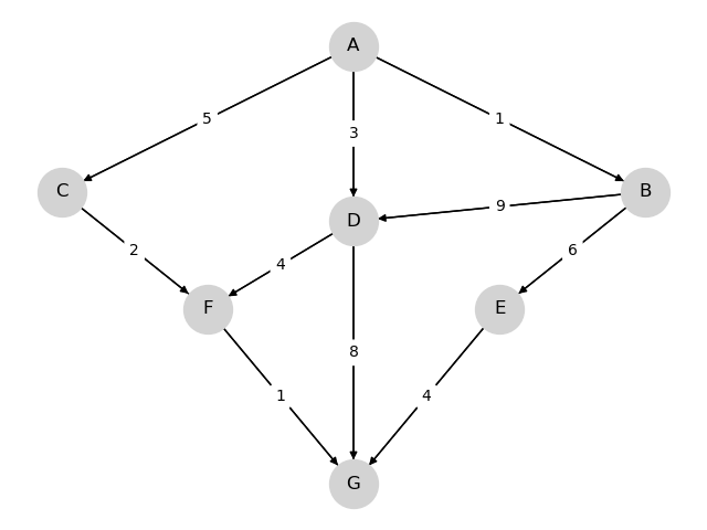    "![https://intro.quantecon.org/_static/lecture_specific/short_path/graph.png](https://intro.quantecon.org/_static/lecture_specific/short_path/graph.png)\n",
 76 |     "\n",
 77 |     "  \n",
 78 |     "We wish to travel from node (vertex) A to node G at minimum cost\n",
 79 |     "\n",
 80 |     "- Arrows (edges) indicate the movements we can take.  \n",
 81 |     "- Numbers on edges indicate the cost of traveling that edge.  \n",
 82 |     "\n",
 83 |     "\n",
 84 |     "(Graphs such as the one above are called weighted [directed graphs](https://en.wikipedia.org/wiki/Directed_graph).)\n",
 85 |     "\n",
 86 |     "Possible interpretations of the graph include\n",
 87 |     "\n",
 88 |     "- Minimum cost for supplier to reach a destination.  \n",
 89 |     "- Routing of packets on the internet (minimize time).  \n",
 90 |     "- etc., etc.  \n",
 91 |     "\n",
 92 |     "\n",
 93 |     "For this simple graph, a quick scan of the edges shows that the optimal paths are\n",
 94 |     "\n",
 95 |     "- A, C, F, G at cost 8  \n",
 96 |     "\n",
 97 |     "\n",
 98 | 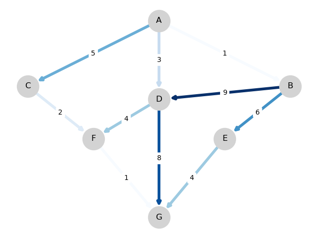    "![https://intro.quantecon.org/_static/lecture_specific/short_path/graph4.png](https://intro.quantecon.org/_static/lecture_specific/short_path/graph4.png)\n",
 99 |     "\n",
100 |     "  \n",
101 |     "- A, D, F, G at cost 8  \n",
102 |     "\n",
103 |     "\n",
104 | 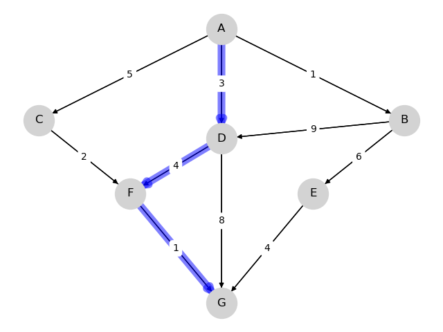    "![https://intro.quantecon.org/_static/lecture_specific/short_path/graph3.png](https://intro.quantecon.org/_static/lecture_specific/short_path/graph3.png)"
105 |    ]
106 |   },
107 |   {
108 |    "cell_type": "markdown",
109 |    "id": "28b4bb48",
110 |    "metadata": {},
111 |    "source": [
112 |     "## Finding least-cost paths\n",
113 |     "\n",
114 |     "For large graphs, we need a systematic solution.\n",
115 |     "\n",
116 |     "Let $ J(v) $ denote the minimum cost-to-go from node $ v $, understood as the total cost from $ v $ if we take the best route.\n",
117 |     "\n",
118 |     "Suppose that we know $ J(v) $ for each node $ v $, as shown below for the graph from the preceding example.\n",
119 |     "\n",
120 | 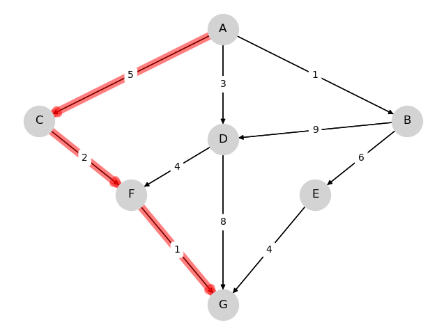    "![https://intro.quantecon.org/_static/lecture_specific/short_path/graph2.png](https://intro.quantecon.org/_static/lecture_specific/short_path/graph2.png)\n",
121 |     "\n",
122 |     "  \n",
123 |     "Note that $ J(G) = 0 $.\n",
124 |     "\n",
125 |     "The best path can now be found as follows\n",
126 |     "\n",
127 |     "1. Start at node $ v = A $  \n",
128 |     "1. From current node $ v $, move to any node that solves  \n",
129 |     "\n",
130 |     "\n",
131 |     "\n",
132 |     "<a id='equation-spprebell'></a>\n",
133 |     "$$\n",
134 |     "\\min_{w \\in F_v} \\{ c(v, w) + J(w) \\} \\tag{38.1}\n",
135 |     "$$\n",
136 |     "\n",
137 |     "where\n",
138 |     "\n",
139 |     "- $ F_v $ is the set of nodes that can be reached from $ v $ in one step.  \n",
140 |     "- $ c(v, w) $ is the cost of traveling from $ v $ to $ w $.  \n",
141 |     "\n",
142 |     "\n",
143 |     "Hence, if we know the function $ J $, then finding the best path is almost trivial.\n",
144 |     "\n",
145 |     "But how can we find the cost-to-go function $ J $?\n",
146 |     "\n",
147 |     "Some thought will convince you that, for every node $ v $,\n",
148 |     "the function $ J $ satisfies\n",
149 |     "\n",
150 |     "\n",
151 |     "<a id='equation-spbell'></a>\n",
152 |     "$$\n",
153 |     "J(v) = \\min_{w \\in F_v} \\{ c(v, w) + J(w) \\} \\tag{38.2}\n",
154 |     "$$\n",
155 |     "\n",
156 |     "This is known as the **Bellman equation**, after the mathematician [Richard Bellman](https://en.wikipedia.org/wiki/Richard_E._Bellman).\n",
157 |     "\n",
158 |     "The Bellman equation can be thought of as a restriction that $ J $ must\n",
159 |     "satisfy.\n",
160 |     "\n",
161 |     "What we want to do now is use this restriction to compute $ J $."
162 |    ]
163 |   },
164 |   {
165 |    "cell_type": "markdown",
166 |    "id": "3f33e9cb",
167 |    "metadata": {},
168 |    "source": [
169 |     "## Solving for minimum cost-to-go\n",
170 |     "\n",
171 |     "Let’s look at an algorithm for computing $ J $ and then think about how to\n",
172 |     "implement it."
173 |    ]
174 |   },
175 |   {
176 |    "cell_type": "markdown",
177 |    "id": "c5097479",
178 |    "metadata": {},
179 |    "source": [
180 |     "### The algorithm\n",
181 |     "\n",
182 |     "The standard algorithm for finding $ J $ is to start an initial guess and then iterate.\n",
183 |     "\n",
184 |     "This is a standard approach to solving nonlinear equations, often called\n",
185 |     "the method of **successive approximations**.\n",
186 |     "\n",
187 |     "Our initial guess will be\n",
188 |     "\n",
189 |     "\n",
190 |     "<a id='equation-spguess'></a>\n",
191 |     "$$\n",
192 |     "J_0(v) = 0 \\text{ for all } v \\tag{38.3}\n",
193 |     "$$\n",
194 |     "\n",
195 |     "Now\n",
196 |     "\n",
197 |     "1. Set $ n = 0 $  \n",
198 |     "1. Set $ J_{n+1} (v) = \\min_{w \\in F_v} \\{ c(v, w) + J_n(w) \\} $ for all $ v $  \n",
199 |     "1. If $ J_{n+1} $ and $ J_n $ are not equal then increment $ n $, go to 2  \n",
200 |     "\n",
201 |     "\n",
202 |     "This sequence converges to $ J $.\n",
203 |     "\n",
204 |     "Although we omit the proof, we’ll prove similar claims in our other lectures\n",
205 |     "on dynamic programming."
206 |    ]
207 |   },
208 |   {
209 |    "cell_type": "markdown",
210 |    "id": "6f99f491",
211 |    "metadata": {},
212 |    "source": [
213 |     "### Implementation\n",
214 |     "\n",
215 |     "Having an algorithm is a good start, but we also need to think about how to\n",
216 |     "implement it on a computer.\n",
217 |     "\n",
218 |     "First, for the cost function $ c $, we’ll implement it as a matrix\n",
219 |     "$ Q $, where a typical element is\n",
220 |     "\n",
221 |     "$$\n",
222 |     "Q(v, w)\n",
223 |     "=\n",
224 |     "\\begin{cases}\n",
225 |     "   & c(v, w) \\text{ if } w \\in F_v \\\\\n",
226 |     "   & +\\infty \\text{ otherwise }\n",
227 |     "\\end{cases}\n",
228 |     "$$\n",
229 |     "\n",
230 |     "In this context $ Q $ is usually called the **distance matrix**.\n",
231 |     "\n",
232 |     "We’re also numbering the nodes now, with $ A = 0 $, so, for example\n",
233 |     "\n",
234 |     "$$\n",
235 |     "Q(1, 2)\n",
236 |     "=\n",
237 |     "\\text{ the cost of traveling from B to C }\n",
238 |     "$$\n",
239 |     "\n",
240 |     "For example, for the simple graph above, we set"
241 |    ]
242 |   },
243 |   {
244 |    "cell_type": "code",
245 |    "execution_count": null,
246 |    "id": "19b8a182",
247 |    "metadata": {
248 |     "hide-output": false
249 |    },
250 |    "outputs": [],
251 |    "source": [
252 |     "from numpy import inf\n",
253 |     "\n",
254 |     "Q = np.array([[inf, 1,   5,   3,   inf, inf, inf],\n",
255 |     "              [inf, inf, inf, 9,   6,   inf, inf],\n",
256 |     "              [inf, inf, inf, inf, inf, 2,   inf],\n",
257 |     "              [inf, inf, inf, inf, inf, 4,   8],\n",
258 |     "              [inf, inf, inf, inf, inf, inf, 4],\n",
259 |     "              [inf, inf, inf, inf, inf, inf, 1],\n",
260 |     "              [inf, inf, inf, inf, inf, inf, 0]])"
261 |    ]
262 |   },
263 |   {
264 |    "cell_type": "markdown",
265 |    "id": "aad0b79e",
266 |    "metadata": {},
267 |    "source": [
268 |     "Notice that the cost of staying still (on the principle diagonal) is set to\n",
269 |     "\n",
270 |     "- `np.inf` for non-destination nodes — moving on is required.  \n",
271 |     "- 0 for the destination node — here is where we stop.  \n",
272 |     "\n",
273 |     "\n",
274 |     "For the sequence of approximations $ \\{J_n\\} $ of the cost-to-go functions, we can use NumPy arrays.\n",
275 |     "\n",
276 |     "Let’s try with this example and see how we go:"
277 |    ]
278 |   },
279 |   {
280 |    "cell_type": "code",
281 |    "execution_count": null,
282 |    "id": "66b8fd0b",
283 |    "metadata": {
284 |     "hide-output": false
285 |    },
286 |    "outputs": [],
287 |    "source": [
288 |     "nodes = range(7)                              # Nodes = 0, 1, ..., 6\n",
289 |     "J = np.zeros_like(nodes, dtype=int)        # Initial guess\n",
290 |     "next_J = np.empty_like(nodes, dtype=int)   # Stores updated guess\n",
291 |     "\n",
292 |     "max_iter = 500\n",
293 |     "i = 0\n",
294 |     "\n",
295 |     "while i < max_iter:\n",
296 |     "    for v in nodes:\n",
297 |     "        # Minimize Q[v, w] + J[w] over all choices of w\n",
298 |     "        next_J[v] = np.min(Q[v, :] + J)\n",
299 |     "    \n",
300 |     "    if np.array_equal(next_J, J):                \n",
301 |     "        break\n",
302 |     "    \n",
303 |     "    J[:] = next_J                                # Copy contents of next_J to J\n",
304 |     "    i += 1\n",
305 |     "\n",
306 |     "print(\"The cost-to-go function is\", J)"
307 |    ]
308 |   },
309 |   {
310 |    "cell_type": "markdown",
311 |    "id": "84ee8d11",
312 |    "metadata": {},
313 |    "source": [
314 |     "This matches with the numbers we obtained by inspection above.\n",
315 |     "\n",
316 |     "But, importantly, we now have a methodology for tackling large graphs."
317 |    ]
318 |   },
319 |   {
320 |    "cell_type": "markdown",
321 |    "id": "aa7ff6e0",
322 |    "metadata": {},
323 |    "source": [
324 |     "## Exercises"
325 |    ]
326 |   },
327 |   {
328 |    "cell_type": "markdown",
329 |    "id": "f97e5eff",
330 |    "metadata": {},
331 |    "source": [
332 |     "## Exercise 38.1\n",
333 |     "\n",
334 |     "The text below describes a weighted directed graph.\n",
335 |     "\n",
336 |     "The line `node0, node1 0.04, node8 11.11, node14 72.21` means that from node0 we can go to\n",
337 |     "\n",
338 |     "- node1 at cost 0.04  \n",
339 |     "- node8 at cost 11.11  \n",
340 |     "- node14 at cost 72.21  \n",
341 |     "\n",
342 |     "\n",
343 |     "No other nodes can be reached directly from node0.\n",
344 |     "\n",
345 |     "Other lines have a similar interpretation.\n",
346 |     "\n",
347 |     "Your task is to use the algorithm given above to find the optimal path and its cost.\n",
348 |     "\n",
349 |     ">**Note**\n",
350 |     ">\n",
351 |     ">You will be dealing with floating point numbers now, rather than\n",
352 |     "integers, so consider replacing `np.equal()` with `np.allclose()`."
353 |    ]
354 |   },
355 |   {
356 |    "cell_type": "code",
357 |    "execution_count": null,
358 |    "id": "2ada8dc7",
359 |    "metadata": {
360 |     "hide-output": false
361 |    },
362 |    "outputs": [],
363 |    "source": [
364 |     "%%file graph.txt\n",
365 |     "node0, node1 0.04, node8 11.11, node14 72.21\n",
366 |     "node1, node46 1247.25, node6 20.59, node13 64.94\n",
367 |     "node2, node66 54.18, node31 166.80, node45 1561.45\n",
368 |     "node3, node20 133.65, node6 2.06, node11 42.43\n",
369 |     "node4, node75 3706.67, node5 0.73, node7 1.02\n",
370 |     "node5, node45 1382.97, node7 3.33, node11 34.54\n",
371 |     "node6, node31 63.17, node9 0.72, node10 13.10\n",
372 |     "node7, node50 478.14, node9 3.15, node10 5.85\n",
373 |     "node8, node69 577.91, node11 7.45, node12 3.18\n",
374 |     "node9, node70 2454.28, node13 4.42, node20 16.53\n",
375 |     "node10, node89 5352.79, node12 1.87, node16 25.16\n",
376 |     "node11, node94 4961.32, node18 37.55, node20 65.08\n",
377 |     "node12, node84 3914.62, node24 34.32, node28 170.04\n",
378 |     "node13, node60 2135.95, node38 236.33, node40 475.33\n",
379 |     "node14, node67 1878.96, node16 2.70, node24 38.65\n",
380 |     "node15, node91 3597.11, node17 1.01, node18 2.57\n",
381 |     "node16, node36 392.92, node19 3.49, node38 278.71\n",
382 |     "node17, node76 783.29, node22 24.78, node23 26.45\n",
383 |     "node18, node91 3363.17, node23 16.23, node28 55.84\n",
384 |     "node19, node26 20.09, node20 0.24, node28 70.54\n",
385 |     "node20, node98 3523.33, node24 9.81, node33 145.80\n",
386 |     "node21, node56 626.04, node28 36.65, node31 27.06\n",
387 |     "node22, node72 1447.22, node39 136.32, node40 124.22\n",
388 |     "node23, node52 336.73, node26 2.66, node33 22.37\n",
389 |     "node24, node66 875.19, node26 1.80, node28 14.25\n",
390 |     "node25, node70 1343.63, node32 36.58, node35 45.55\n",
391 |     "node26, node47 135.78, node27 0.01, node42 122.00\n",
392 |     "node27, node65 480.55, node35 48.10, node43 246.24\n",
393 |     "node28, node82 2538.18, node34 21.79, node36 15.52\n",
394 |     "node29, node64 635.52, node32 4.22, node33 12.61\n",
395 |     "node30, node98 2616.03, node33 5.61, node35 13.95\n",
396 |     "node31, node98 3350.98, node36 20.44, node44 125.88\n",
397 |     "node32, node97 2613.92, node34 3.33, node35 1.46\n",
398 |     "node33, node81 1854.73, node41 3.23, node47 111.54\n",
399 |     "node34, node73 1075.38, node42 51.52, node48 129.45\n",
400 |     "node35, node52 17.57, node41 2.09, node50 78.81\n",
401 |     "node36, node71 1171.60, node54 101.08, node57 260.46\n",
402 |     "node37, node75 269.97, node38 0.36, node46 80.49\n",
403 |     "node38, node93 2767.85, node40 1.79, node42 8.78\n",
404 |     "node39, node50 39.88, node40 0.95, node41 1.34\n",
405 |     "node40, node75 548.68, node47 28.57, node54 53.46\n",
406 |     "node41, node53 18.23, node46 0.28, node54 162.24\n",
407 |     "node42, node59 141.86, node47 10.08, node72 437.49\n",
408 |     "node43, node98 2984.83, node54 95.06, node60 116.23\n",
409 |     "node44, node91 807.39, node46 1.56, node47 2.14\n",
410 |     "node45, node58 79.93, node47 3.68, node49 15.51\n",
411 |     "node46, node52 22.68, node57 27.50, node67 65.48\n",
412 |     "node47, node50 2.82, node56 49.31, node61 172.64\n",
413 |     "node48, node99 2564.12, node59 34.52, node60 66.44\n",
414 |     "node49, node78 53.79, node50 0.51, node56 10.89\n",
415 |     "node50, node85 251.76, node53 1.38, node55 20.10\n",
416 |     "node51, node98 2110.67, node59 23.67, node60 73.79\n",
417 |     "node52, node94 1471.80, node64 102.41, node66 123.03\n",
418 |     "node53, node72 22.85, node56 4.33, node67 88.35\n",
419 |     "node54, node88 967.59, node59 24.30, node73 238.61\n",
420 |     "node55, node84 86.09, node57 2.13, node64 60.80\n",
421 |     "node56, node76 197.03, node57 0.02, node61 11.06\n",
422 |     "node57, node86 701.09, node58 0.46, node60 7.01\n",
423 |     "node58, node83 556.70, node64 29.85, node65 34.32\n",
424 |     "node59, node90 820.66, node60 0.72, node71 0.67\n",
425 |     "node60, node76 48.03, node65 4.76, node67 1.63\n",
426 |     "node61, node98 1057.59, node63 0.95, node64 4.88\n",
427 |     "node62, node91 132.23, node64 2.94, node76 38.43\n",
428 |     "node63, node66 4.43, node72 70.08, node75 56.34\n",
429 |     "node64, node80 47.73, node65 0.30, node76 11.98\n",
430 |     "node65, node94 594.93, node66 0.64, node73 33.23\n",
431 |     "node66, node98 395.63, node68 2.66, node73 37.53\n",
432 |     "node67, node82 153.53, node68 0.09, node70 0.98\n",
433 |     "node68, node94 232.10, node70 3.35, node71 1.66\n",
434 |     "node69, node99 247.80, node70 0.06, node73 8.99\n",
435 |     "node70, node76 27.18, node72 1.50, node73 8.37\n",
436 |     "node71, node89 104.50, node74 8.86, node91 284.64\n",
437 |     "node72, node76 15.32, node84 102.77, node92 133.06\n",
438 |     "node73, node83 52.22, node76 1.40, node90 243.00\n",
439 |     "node74, node81 1.07, node76 0.52, node78 8.08\n",
440 |     "node75, node92 68.53, node76 0.81, node77 1.19\n",
441 |     "node76, node85 13.18, node77 0.45, node78 2.36\n",
442 |     "node77, node80 8.94, node78 0.98, node86 64.32\n",
443 |     "node78, node98 355.90, node81 2.59\n",
444 |     "node79, node81 0.09, node85 1.45, node91 22.35\n",
445 |     "node80, node92 121.87, node88 28.78, node98 264.34\n",
446 |     "node81, node94 99.78, node89 39.52, node92 99.89\n",
447 |     "node82, node91 47.44, node88 28.05, node93 11.99\n",
448 |     "node83, node94 114.95, node86 8.75, node88 5.78\n",
449 |     "node84, node89 19.14, node94 30.41, node98 121.05\n",
450 |     "node85, node97 94.51, node87 2.66, node89 4.90\n",
451 |     "node86, node97 85.09\n",
452 |     "node87, node88 0.21, node91 11.14, node92 21.23\n",
453 |     "node88, node93 1.31, node91 6.83, node98 6.12\n",
454 |     "node89, node97 36.97, node99 82.12\n",
455 |     "node90, node96 23.53, node94 10.47, node99 50.99\n",
456 |     "node91, node97 22.17\n",
457 |     "node92, node96 10.83, node97 11.24, node99 34.68\n",
458 |     "node93, node94 0.19, node97 6.71, node99 32.77\n",
459 |     "node94, node98 5.91, node96 2.03\n",
460 |     "node95, node98 6.17, node99 0.27\n",
461 |     "node96, node98 3.32, node97 0.43, node99 5.87\n",
462 |     "node97, node98 0.30\n",
463 |     "node98, node99 0.33\n",
464 |     "node99,"
465 |    ]
466 |   },
467 |   {
468 |    "cell_type": "markdown",
469 |    "id": "b922cce5",
470 |    "metadata": {},
471 |    "source": [
472 |     "## Solution to[ Exercise 38.1](https://intro.quantecon.org/#short_path_ex1)\n",
473 |     "\n",
474 |     "First let’s write a function that reads in the graph data above and builds a distance matrix."
475 |    ]
476 |   },
477 |   {
478 |    "cell_type": "code",
479 |    "execution_count": null,
480 |    "id": "3030a8ae",
481 |    "metadata": {
482 |     "hide-output": false
483 |    },
484 |    "outputs": [],
485 |    "source": [
486 |     "num_nodes = 100\n",
487 |     "destination_node = 99\n",
488 |     "\n",
489 |     "def map_graph_to_distance_matrix(in_file):\n",
490 |     "\n",
491 |     "    # First let's set of the distance matrix Q with inf everywhere\n",
492 |     "    Q = np.full((num_nodes, num_nodes), np.inf)\n",
493 |     "\n",
494 |     "    # Now we read in the data and modify Q\n",
495 |     "    with open(in_file) as infile:\n",
496 |     "        for line in infile:\n",
497 |     "            elements = line.split(',')\n",
498 |     "            node = elements.pop(0)\n",
499 |     "            node = int(node[4:])    # convert node description to integer\n",
500 |     "            if node != destination_node:\n",
501 |     "                for element in elements:\n",
502 |     "                    destination, cost = element.split()\n",
503 |     "                    destination = int(destination[4:])\n",
504 |     "                    Q[node, destination] = float(cost)\n",
505 |     "            Q[destination_node, destination_node] = 0\n",
506 |     "    return Q"
507 |    ]
508 |   },
509 |   {
510 |    "cell_type": "markdown",
511 |    "id": "e53f82ce",
512 |    "metadata": {},
513 |    "source": [
514 |     "In addition, let’s write\n",
515 |     "\n",
516 |     "1. a “Bellman operator” function that takes a distance matrix and current guess of J and returns an updated guess of J, and  \n",
517 |     "1. a function that takes a distance matrix and returns a cost-to-go function.  \n",
518 |     "\n",
519 |     "\n",
520 |     "We’ll use the algorithm described above.\n",
521 |     "\n",
522 |     "The minimization step is vectorized to make it faster."
523 |    ]
524 |   },
525 |   {
526 |    "cell_type": "code",
527 |    "execution_count": null,
528 |    "id": "6065671e",
529 |    "metadata": {
530 |     "hide-output": false
531 |    },
532 |    "outputs": [],
533 |    "source": [
534 |     "def bellman(J, Q):\n",
535 |     "    return np.min(Q + J, axis=1)\n",
536 |     "\n",
537 |     "\n",
538 |     "def compute_cost_to_go(Q):\n",
539 |     "    num_nodes = Q.shape[0]\n",
540 |     "    J = np.zeros(num_nodes)      # Initial guess\n",
541 |     "    max_iter = 500\n",
542 |     "    i = 0\n",
543 |     "\n",
544 |     "    while i < max_iter:\n",
545 |     "        next_J = bellman(J, Q)\n",
546 |     "        if np.allclose(next_J, J):\n",
547 |     "            break\n",
548 |     "        else:\n",
549 |     "            J[:] = next_J   # Copy contents of next_J to J\n",
550 |     "            i += 1\n",
551 |     "\n",
552 |     "    return(J)"
553 |    ]
554 |   },
555 |   {
556 |    "cell_type": "markdown",
557 |    "id": "54b69dc3",
558 |    "metadata": {},
559 |    "source": [
560 |     "We used np.allclose() rather than testing exact equality because we are\n",
561 |     "dealing with floating point numbers now.\n",
562 |     "\n",
563 |     "Finally, here’s a function that uses the cost-to-go function to obtain the\n",
564 |     "optimal path (and its cost)."
565 |    ]
566 |   },
567 |   {
568 |    "cell_type": "code",
569 |    "execution_count": null,
570 |    "id": "f9af4c08",
571 |    "metadata": {
572 |     "hide-output": false
573 |    },
574 |    "outputs": [],
575 |    "source": [
576 |     "def print_best_path(J, Q):\n",
577 |     "    sum_costs = 0\n",
578 |     "    current_node = 0\n",
579 |     "    while current_node != destination_node:\n",
580 |     "        print(current_node)\n",
581 |     "        # Move to the next node and increment costs\n",
582 |     "        next_node = np.argmin(Q[current_node, :] + J)\n",
583 |     "        sum_costs += Q[current_node, next_node]\n",
584 |     "        current_node = next_node\n",
585 |     "\n",
586 |     "    print(destination_node)\n",
587 |     "    print('Cost: ', sum_costs)"
588 |    ]
589 |   },
590 |   {
591 |    "cell_type": "markdown",
592 |    "id": "741c898b",
593 |    "metadata": {},
594 |    "source": [
595 |     "Okay, now we have the necessary functions, let’s call them to do the job we were assigned."
596 |    ]
597 |   },
598 |   {
599 |    "cell_type": "code",
600 |    "execution_count": null,
601 |    "id": "dad34068",
602 |    "metadata": {
603 |     "hide-output": false
604 |    },
605 |    "outputs": [],
606 |    "source": [
607 |     "Q = map_graph_to_distance_matrix('graph.txt')\n",
608 |     "J = compute_cost_to_go(Q)\n",
609 |     "print_best_path(J, Q)"
610 |    ]
611 |   },
612 |   {
613 |    "cell_type": "markdown",
614 |    "id": "d441a6aa",
615 |    "metadata": {},
616 |    "source": [
617 |     "The total cost of the path should agree with $ J[0] $ so let’s check this."
618 |    ]
619 |   },
620 |   {
621 |    "cell_type": "code",
622 |    "execution_count": null,
623 |    "id": "cd4cd780",
624 |    "metadata": {
625 |     "hide-output": false
626 |    },
627 |    "outputs": [],
628 |    "source": [
629 |     "J[0]"
630 |    ]
631 |   }
632 |  ],
633 |  "metadata": {
634 |   "date": 1761795482.8302946,
635 |   "filename": "short_path.md",
636 |   "kernelspec": {
637 |    "display_name": "Python",
638 |    "language": "python3",
639 |    "name": "python3"
640 |   },
641 |   "title": "Shortest Paths"
642 |  },
643 |  "nbformat": 4,
644 |  "nbformat_minor": 5
645 | }


--------------------------------------------------------------------------------
/laffer_adaptive.ipynb:
--------------------------------------------------------------------------------
  1 | {
  2 |  "cells": [
  3 |   {
  4 |    "cell_type": "markdown",
  5 |    "id": "0b2b61e8",
  6 |    "metadata": {},
  7 |    "source": [
  8 |     "# Laffer Curves  with Adaptive Expectations"
  9 |    ]
 10 |   },
 11 |   {
 12 |    "cell_type": "markdown",
 13 |    "id": "8c70f188",
 14 |    "metadata": {},
 15 |    "source": [
 16 |     "## Overview\n",
 17 |     "\n",
 18 |     "This lecture studies stationary and dynamic **Laffer curves** in the inflation tax rate in a non-linear version of the model studied in this  lecture [Money Financed Government Deficits and Price Levels](https://intro.quantecon.org/money_inflation.html).\n",
 19 |     "\n",
 20 |     "As in the lecture [Money Financed Government Deficits and Price Levels](https://intro.quantecon.org/money_inflation.html), this lecture uses the log-linear version of the demand function for money that  [[Cagan, 1956](https://intro.quantecon.org/zreferences.html#id112)] used in his classic paper in place of the linear demand function used in this  lecture [Money Financed Government Deficits and Price Levels](https://intro.quantecon.org/money_inflation.html).\n",
 21 |     "\n",
 22 |     "But now, instead of assuming  ‘‘rational expectations’’ in the form of ‘‘perfect foresight’’,\n",
 23 |     "we’ll adopt the ‘‘adaptive expectations’’ assumption used by  [[Cagan, 1956](https://intro.quantecon.org/zreferences.html#id112)] and [[Friedman, 1956](https://intro.quantecon.org/zreferences.html#id183)].\n",
 24 |     "\n",
 25 |     "This means that instead of assuming that expected inflation $ \\pi_t^* $ is described by the “perfect foresight” or “rational expectations” hypothesis\n",
 26 |     "\n",
 27 |     "$$\n",
 28 |     "\\pi_t^* = p_{t+1} - p_t\n",
 29 |     "$$\n",
 30 |     "\n",
 31 |     "that we adopted in lectures [Money Financed Government Deficits and Price Levels](https://intro.quantecon.org/money_inflation.html) and lectures [Inflation Rate Laffer Curves](https://intro.quantecon.org/money_inflation_nonlinear.html), we’ll now assume that $ \\pi_t^* $ is determined by the adaptive expectations hypothesis described in equation [(32.4)](#equation-eq-adaptex)  reported below.\n",
 32 |     "\n",
 33 |     "We shall discover that changing our hypothesis about expectations formation in this way will change some our findings and leave others intact.  In particular, we shall discover that\n",
 34 |     "\n",
 35 |     "- replacing rational expectations with adaptive expectations leaves the two stationary inflation rates unchanged, but that $ \\ldots $  \n",
 36 |     "- it reverses the perverse dynamics by making the **lower** stationary inflation rate the one to which the system typically converges  \n",
 37 |     "- a more plausible comparative dynamic outcome emerges in which now inflation can be **reduced** by running **lower**  government deficits  \n",
 38 |     "\n",
 39 |     "\n",
 40 |     "These more plausible comparative dynamics underlie the “old time religion” that states that\n",
 41 |     "“inflation is always and everywhere caused by government deficits”.\n",
 42 |     "\n",
 43 |     "These issues were studied by [[Bruno and Fischer, 1990](https://intro.quantecon.org/zreferences.html#id296)].\n",
 44 |     "\n",
 45 |     "Their purpose was to reverse  what they thought were counter intuitive\n",
 46 |     "predictions of their model under rational expectations (i.e., perfect foresight in this context)\n",
 47 |     "by dropping rational expectations and instead assuming that people form  expectations about future inflation rates according to the “adaptive expectations”  scheme [(32.4)](#equation-eq-adaptex) described below.\n",
 48 |     "\n",
 49 |     ">**Note**\n",
 50 |     ">\n",
 51 |     ">[[Marcet and Sargent, 1989](https://intro.quantecon.org/zreferences.html#id297)]  had studied another way of selecting stationary equilibrium that involved replacing rational expectations with a model of  learning via least squares regression.\\\\\n",
 52 |     "\n",
 53 |     "\n",
 54 |     "[[Marcet and Nicolini, 2003](https://intro.quantecon.org/zreferences.html#id295)] and  [[Sargent *et al.*, 2009](https://intro.quantecon.org/zreferences.html#id294)] extended that work and applied it to study recurrent high-inflation episodes in Latin America."
 55 |    ]
 56 |   },
 57 |   {
 58 |    "cell_type": "markdown",
 59 |    "id": "52118706",
 60 |    "metadata": {},
 61 |    "source": [
 62 |     "## The model\n",
 63 |     "\n",
 64 |     "Let\n",
 65 |     "\n",
 66 |     "- $ m_t $ be the log of the money supply at the beginning of time $ t $  \n",
 67 |     "- $ p_t $ be the log of the price level at time $ t $  \n",
 68 |     "- $ \\pi_t^* $ be the public’s expectation of the rate of inflation between $ t $ and $ t+1 $  \n",
 69 |     "\n",
 70 |     "\n",
 71 |     "The law of motion of the money supply is\n",
 72 |     "\n",
 73 |     "\n",
 74 |     "<a id='equation-eq-ada-msupply'></a>\n",
 75 |     "$$\n",
 76 |     "\\exp(m_{t+1}) - \\exp(m_t) = g \\exp(p_t) \\tag{32.1}\n",
 77 |     "$$\n",
 78 |     "\n",
 79 |     "where $ g $ is the part of government expenditures financed by printing money.\n",
 80 |     "\n",
 81 |     "Notice that equation [(32.1)](#equation-eq-ada-msupply) implies that\n",
 82 |     "\n",
 83 |     "\n",
 84 |     "<a id='equation-eq-ada-msupply2'></a>\n",
 85 |     "$$\n",
 86 |     "m_{t+1} = \\log[ \\exp(m_t) + g \\exp(p_t)] \\tag{32.2}\n",
 87 |     "$$\n",
 88 |     "\n",
 89 |     "The demand function for money is\n",
 90 |     "\n",
 91 |     "\n",
 92 |     "<a id='equation-eq-ada-mdemand'></a>\n",
 93 |     "$$\n",
 94 |     "m_{t+1} - p_t = -\\alpha \\pi_t^* \\tag{32.3}\n",
 95 |     "$$\n",
 96 |     "\n",
 97 |     "where $ \\alpha \\geq 0 $.\n",
 98 |     "\n",
 99 |     "Expectations of inflation are governed by\n",
100 |     "\n",
101 |     "\n",
102 |     "<a id='equation-eq-adaptex'></a>\n",
103 |     "$$\n",
104 |     "\\pi_{t}^* = (1-\\delta) (p_t - p_{t-1}) + \\delta \\pi_{t-1}^* \\tag{32.4}\n",
105 |     "$$\n",
106 |     "\n",
107 |     "where $ \\delta \\in (0,1) $"
108 |    ]
109 |   },
110 |   {
111 |    "cell_type": "markdown",
112 |    "id": "a0e8547f",
113 |    "metadata": {},
114 |    "source": [
115 |     "## Computing an equilibrium sequence\n",
116 |     "\n",
117 |     "Equation the expressions for $ m_{t+1} $ provided  by [(32.3)](#equation-eq-ada-mdemand) and [(32.2)](#equation-eq-ada-msupply2) and use equation [(32.4)](#equation-eq-adaptex) to eliminate $ \\pi_t^* $ to obtain\n",
118 |     "the following equation for $ p_t $:\n",
119 |     "\n",
120 |     "\n",
121 |     "<a id='equation-eq-pequation'></a>\n",
122 |     "$$\n",
123 |     "\\log[ \\exp(m_t) + g \\exp(p_t)] - p_t = -\\alpha [(1-\\delta) (p_t - p_{t-1}) + \\delta \\pi_{t-1}^*] \\tag{32.5}\n",
124 |     "$$\n",
125 |     "\n",
126 |     "**Pseudo-code**\n",
127 |     "\n",
128 |     "Here is the pseudo-code for our algorithm.\n",
129 |     "\n",
130 |     "Starting at time $ 0 $ with initial conditions $ (m_0, \\pi_{-1}^*, p_{-1}) $, for each $ t \\geq 0 $\n",
131 |     "deploy the following steps in order:\n",
132 |     "\n",
133 |     "- solve [(32.5)](#equation-eq-pequation) for $ p_t $  \n",
134 |     "- solve equation [(32.4)](#equation-eq-adaptex) for $ \\pi_t^* $  \n",
135 |     "- solve equation [(32.2)](#equation-eq-ada-msupply2) for $ m_{t+1} $  \n",
136 |     "\n",
137 |     "\n",
138 |     "This completes the algorithm."
139 |    ]
140 |   },
141 |   {
142 |    "cell_type": "markdown",
143 |    "id": "0a33d2ae",
144 |    "metadata": {},
145 |    "source": [
146 |     "## Claims or conjectures\n",
147 |     "\n",
148 |     "It will turn out that\n",
149 |     "\n",
150 |     "- if they exist, limiting values $ \\overline \\pi $ and $ \\overline \\mu $ will be equal  \n",
151 |     "- if  limiting values exist, there are two possible limiting values, one high, one low  \n",
152 |     "- unlike the outcome in lecture [Inflation Rate Laffer Curves](https://intro.quantecon.org/money_inflation_nonlinear.html), for almost all initial log price levels and expected inflation rates $ p_0, \\pi_{t}^* $, the limiting $ \\overline \\pi = \\overline \\mu $ is  the **lower** steady state  value  \n",
153 |     "- for each of the two possible limiting values $ \\bar \\pi $ ,there is a unique initial log price level $ p_0 $ that implies that $ \\pi_t = \\mu_t = \\bar \\mu $ for all  $ t \\geq 0 $  \n",
154 |     "  - this unique initial log price level solves $ \\log(\\exp(m_0) + g \\exp(p_0)) - p_0 = - \\alpha \\bar \\pi $  \n",
155 |     "  - the preceding equation for $ p_0 $ comes from $ m_1 - p_0 = -  \\alpha \\bar \\pi $  "
156 |    ]
157 |   },
158 |   {
159 |    "cell_type": "markdown",
160 |    "id": "f74056f3",
161 |    "metadata": {},
162 |    "source": [
163 |     "## Limiting values of inflation rate\n",
164 |     "\n",
165 |     "As in our earlier lecture [Inflation Rate Laffer Curves](https://intro.quantecon.org/money_inflation_nonlinear.html), we can compute the two prospective limiting values for $ \\bar \\pi $ by studying the steady-state Laffer curve.\n",
166 |     "\n",
167 |     "Thus, in a  **steady state**\n",
168 |     "\n",
169 |     "$$\n",
170 |     "m_{t+1} - m_t = p_{t+1} - p_t =  x \\quad \\forall t ,\n",
171 |     "$$\n",
172 |     "\n",
173 |     "where $ x > 0 $ is a common rate of growth of logarithms of the money supply and price level.\n",
174 |     "\n",
175 |     "A few lines of algebra yields the following equation that $ x $ satisfies\n",
176 |     "\n",
177 |     "\n",
178 |     "<a id='equation-eq-ada-steadypi'></a>\n",
179 |     "$$\n",
180 |     "\\exp(-\\alpha x) - \\exp(-(1 + \\alpha) x) = g \\tag{32.6}\n",
181 |     "$$\n",
182 |     "\n",
183 |     "where we require that\n",
184 |     "\n",
185 |     "\n",
186 |     "<a id='equation-eq-ada-revmax'></a>\n",
187 |     "$$\n",
188 |     "g \\leq \\max_{x: x \\geq 0} \\exp(-\\alpha x) - \\exp(-(1 + \\alpha) x) , \\tag{32.7}\n",
189 |     "$$\n",
190 |     "\n",
191 |     "so that it is feasible to finance $ g $ by printing money.\n",
192 |     "\n",
193 |     "The left side of [(32.6)](#equation-eq-ada-steadypi) is steady state revenue raised by printing money.\n",
194 |     "\n",
195 |     "The right side of [(32.6)](#equation-eq-ada-steadypi) is the quantity  of time $ t $ goods  that the government raises by printing money.\n",
196 |     "\n",
197 |     "Soon  we’ll plot  the left and right sides of equation [(32.6)](#equation-eq-ada-steadypi).\n",
198 |     "\n",
199 |     "But first we’ll write code that computes a steady-state\n",
200 |     "$ \\bar \\pi $.\n",
201 |     "\n",
202 |     "Let’s start by importing some  libraries"
203 |    ]
204 |   },
205 |   {
206 |    "cell_type": "code",
207 |    "execution_count": null,
208 |    "id": "4a282926",
209 |    "metadata": {
210 |     "hide-output": false
211 |    },
212 |    "outputs": [],
213 |    "source": [
214 |     "from collections import namedtuple\n",
215 |     "import numpy as np\n",
216 |     "import matplotlib.pyplot as plt\n",
217 |     "from matplotlib.ticker import MaxNLocator\n",
218 |     "from matplotlib.cm import get_cmap\n",
219 |     "from matplotlib.colors import to_rgba\n",
220 |     "import matplotlib\n",
221 |     "from scipy.optimize import root, fsolve"
222 |    ]
223 |   },
224 |   {
225 |    "cell_type": "markdown",
226 |    "id": "edb3c888",
227 |    "metadata": {},
228 |    "source": [
229 |     "Let’s create a `namedtuple` to store the parameters of the model"
230 |    ]
231 |   },
232 |   {
233 |    "cell_type": "code",
234 |    "execution_count": null,
235 |    "id": "827ab78f",
236 |    "metadata": {
237 |     "hide-output": false
238 |    },
239 |    "outputs": [],
240 |    "source": [
241 |     "LafferAdaptive = namedtuple('LafferAdaptive', \n",
242 |     "                        [\"m0\",  # log of the money supply at t=0\n",
243 |     "                         \"α\",   # sensitivity of money demand\n",
244 |     "                         \"g\",   # government expenditure\n",
245 |     "                         \"δ\"])\n",
246 |     "\n",
247 |     "# Create a Cagan Laffer model\n",
248 |     "def create_model(α=0.5, m0=np.log(100), g=0.35, δ=0.9):\n",
249 |     "    return LafferAdaptive(α=α, m0=m0, g=g, δ=δ)\n",
250 |     "\n",
251 |     "model = create_model()"
252 |    ]
253 |   },
254 |   {
255 |    "cell_type": "markdown",
256 |    "id": "24ad266e",
257 |    "metadata": {},
258 |    "source": [
259 |     "Now we write code that computes steady-state $ \\bar \\pi $s."
260 |    ]
261 |   },
262 |   {
263 |    "cell_type": "code",
264 |    "execution_count": null,
265 |    "id": "c8cbb14b",
266 |    "metadata": {
267 |     "hide-output": false
268 |    },
269 |    "outputs": [],
270 |    "source": [
271 |     "# Define formula for π_bar\n",
272 |     "def solve_π(x, α, g):\n",
273 |     "    return np.exp(-α * x) - np.exp(-(1 + α) * x) - g\n",
274 |     "\n",
275 |     "def solve_π_bar(model, x0):\n",
276 |     "    π_bar = fsolve(solve_π, x0=x0, xtol=1e-10, args=(model.α, model.g))[0]\n",
277 |     "    return π_bar\n",
278 |     "\n",
279 |     "# Solve for the two steady state of π\n",
280 |     "π_l = solve_π_bar(model, x0=0.6)\n",
281 |     "π_u = solve_π_bar(model, x0=3.0)\n",
282 |     "print(f'The two steady state of π are: {π_l, π_u}')"
283 |    ]
284 |   },
285 |   {
286 |    "cell_type": "markdown",
287 |    "id": "f024c361",
288 |    "metadata": {},
289 |    "source": [
290 |     "We find two steady state $ \\bar \\pi $ values"
291 |    ]
292 |   },
293 |   {
294 |    "cell_type": "markdown",
295 |    "id": "f258483d",
296 |    "metadata": {},
297 |    "source": [
298 |     "## Steady-state Laffer curve\n",
299 |     "\n",
300 |     "The following figure plots the steady-state Laffer curve together with the two stationary inflation rates."
301 |    ]
302 |   },
303 |   {
304 |    "cell_type": "code",
305 |    "execution_count": null,
306 |    "id": "a2e8816b",
307 |    "metadata": {
308 |     "hide-output": false
309 |    },
310 |    "outputs": [],
311 |    "source": [
312 |     "def compute_seign(x, α):\n",
313 |     "    return np.exp(-α * x) - np.exp(-(1 + α) * x) \n",
314 |     "\n",
315 |     "def plot_laffer(model, πs):\n",
316 |     "    α, g = model.α, model.g\n",
317 |     "    \n",
318 |     "    # Generate π values\n",
319 |     "    x_values = np.linspace(0, 5, 1000)\n",
320 |     "\n",
321 |     "    # Compute corresponding seigniorage values for the function\n",
322 |     "    y_values = compute_seign(x_values, α)\n",
323 |     "\n",
324 |     "    # Plot the function\n",
325 |     "    plt.plot(x_values, y_values, \n",
326 |     "            label=f'$exp((-{α})x) - exp(- (1- {α}) x)$')\n",
327 |     "    for π, label in zip(πs, ['$\\pi_l$', '$\\pi_u$']):\n",
328 |     "        plt.text(π, plt.gca().get_ylim()[0]*2, \n",
329 |     "                 label, horizontalalignment='center',\n",
330 |     "                 color='brown', size=10)\n",
331 |     "        plt.axvline(π, color='brown', linestyle='--')\n",
332 |     "    plt.axhline(g, color='red', linewidth=0.5, \n",
333 |     "                linestyle='--', label='g')\n",
334 |     "    plt.xlabel('$\\pi$')\n",
335 |     "    plt.ylabel('seigniorage')\n",
336 |     "    plt.legend()\n",
337 |     "    plt.grid(True)\n",
338 |     "    plt.show()\n",
339 |     "\n",
340 |     "# Steady state Laffer curve\n",
341 |     "plot_laffer(model, (π_l, π_u))"
342 |    ]
343 |   },
344 |   {
345 |    "cell_type": "markdown",
346 |    "id": "e16c1481",
347 |    "metadata": {},
348 |    "source": [
349 |     "## Associated initial price levels\n",
350 |     "\n",
351 |     "Now that we have our hands on the two possible steady states, we can compute two initial log price levels $ p_{-1} $, which as initial conditions, imply that $ \\pi_t = \\bar \\pi $ for all $ t \\geq 0 $.\n",
352 |     "\n",
353 |     "In particular, to initiate a fixed point of the dynamic Laffer curve dynamics, we set\n",
354 |     "\n",
355 |     "$$\n",
356 |     "p_{-1} = m_0 + \\alpha \\pi^*\n",
357 |     "$$"
358 |    ]
359 |   },
360 |   {
361 |    "cell_type": "code",
362 |    "execution_count": null,
363 |    "id": "6a417b57",
364 |    "metadata": {
365 |     "hide-output": false
366 |    },
367 |    "outputs": [],
368 |    "source": [
369 |     "def solve_p_init(model, π_star):\n",
370 |     "    m0, α = model.m0, model.α\n",
371 |     "    return m0 + α*π_star\n",
372 |     "\n",
373 |     "\n",
374 |     "# Compute two initial price levels associated with π_l and π_u\n",
375 |     "p_l, p_u = map(lambda π: solve_p_init(model, π), (π_l, π_u))\n",
376 |     "print('Associated initial p_{-1}s', f'are: {p_l, p_u}')"
377 |    ]
378 |   },
379 |   {
380 |    "cell_type": "markdown",
381 |    "id": "bc0ef03f",
382 |    "metadata": {},
383 |    "source": [
384 |     "### Verification\n",
385 |     "\n",
386 |     "To start, let’s write some code to verify that if we initial  $ \\pi_{-1}^*,p_{-1} $ appropriately, the inflation rate $ \\pi_t $ will be constant for all $ t \\geq 0 $ (at either $ \\pi_u $ or $ \\pi_l $ depending on the initial condition)\n",
387 |     "\n",
388 |     "The following code verifies this."
389 |    ]
390 |   },
391 |   {
392 |    "cell_type": "code",
393 |    "execution_count": null,
394 |    "id": "0afbfc06",
395 |    "metadata": {
396 |     "hide-output": false
397 |    },
398 |    "outputs": [],
399 |    "source": [
400 |     "def solve_laffer_adapt(p_init, π_init, model, num_steps):\n",
401 |     "    m0, α, δ, g = model.m0, model.α, model.δ, model.g\n",
402 |     "    \n",
403 |     "    m_seq = np.nan * np.ones(num_steps+1) \n",
404 |     "    π_seq = np.nan * np.ones(num_steps) \n",
405 |     "    p_seq = np.nan * np.ones(num_steps)\n",
406 |     "    μ_seq = np.nan * np.ones(num_steps) \n",
407 |     "    \n",
408 |     "    m_seq[1] = m0\n",
409 |     "    π_seq[0] = π_init\n",
410 |     "    p_seq[0] = p_init\n",
411 |     "        \n",
412 |     "    for t in range(1, num_steps):\n",
413 |     "        # Solve p_t\n",
414 |     "        def p_t(pt):\n",
415 |     "            return np.log(np.exp(m_seq[t]) + g * np.exp(pt)) \\\n",
416 |     "                          - pt + α * ((1-δ)*(pt - p_seq[t-1]) + δ*π_seq[t-1])\n",
417 |     "        \n",
418 |     "        p_seq[t] = root(fun=p_t, x0=p_seq[t-1]).x[0]\n",
419 |     "        \n",
420 |     "        # Solve π_t\n",
421 |     "        π_seq[t] = (1-δ) * (p_seq[t]-p_seq[t-1]) + δ*π_seq[t-1]\n",
422 |     "        \n",
423 |     "        # Solve m_t\n",
424 |     "        m_seq[t+1] = np.log(np.exp(m_seq[t]) + g*np.exp(p_seq[t]))\n",
425 |     "        \n",
426 |     "        # Solve μ_t\n",
427 |     "        μ_seq[t] = m_seq[t+1] - m_seq[t]\n",
428 |     "    \n",
429 |     "    return π_seq, μ_seq, m_seq, p_seq"
430 |    ]
431 |   },
432 |   {
433 |    "cell_type": "markdown",
434 |    "id": "2112e811",
435 |    "metadata": {},
436 |    "source": [
437 |     "Compute limiting values starting from $ p_{-1} $ associated with $ \\pi_l $"
438 |    ]
439 |   },
440 |   {
441 |    "cell_type": "code",
442 |    "execution_count": null,
443 |    "id": "04d37f05",
444 |    "metadata": {
445 |     "hide-output": false
446 |    },
447 |    "outputs": [],
448 |    "source": [
449 |     "π_seq, μ_seq, m_seq, p_seq = solve_laffer_adapt(p_l, π_l, model, 50)\n",
450 |     "\n",
451 |     "# Check steady state m_{t+1} - m_t and p_{t+1} - p_t \n",
452 |     "print('m_{t+1} - m_t:', m_seq[-1] - m_seq[-2])\n",
453 |     "print('p_{t+1} - p_t:', p_seq[-1] - p_seq[-2])\n",
454 |     "\n",
455 |     "# Check if exp(-αx) - exp(-(1 + α)x) = g\n",
456 |     "eq_g = lambda x: np.exp(-model.α * x) - np.exp(-(1 + model.α) * x)\n",
457 |     "\n",
458 |     "print('eq_g == g:', np.isclose(eq_g(m_seq[-1] - m_seq[-2]), model.g))"
459 |    ]
460 |   },
461 |   {
462 |    "cell_type": "markdown",
463 |    "id": "e46d22cb",
464 |    "metadata": {},
465 |    "source": [
466 |     "Compute limiting values starting from $ p_{-1} $ associated with $ \\pi_u $"
467 |    ]
468 |   },
469 |   {
470 |    "cell_type": "code",
471 |    "execution_count": null,
472 |    "id": "394b72a0",
473 |    "metadata": {
474 |     "hide-output": false
475 |    },
476 |    "outputs": [],
477 |    "source": [
478 |     "π_seq, μ_seq, m_seq, p_seq = solve_laffer_adapt(p_u, π_u, model, 50)\n",
479 |     "\n",
480 |     "# Check steady state m_{t+1} - m_t and p_{t+1} - p_t \n",
481 |     "print('m_{t+1} - m_t:', m_seq[-1] - m_seq[-2])\n",
482 |     "print('p_{t+1} - p_t:', p_seq[-1] - p_seq[-2])\n",
483 |     "\n",
484 |     "# Check if exp(-αx) - exp(-(1 + α)x) = g\n",
485 |     "eq_g = lambda x: np.exp(-model.α * x) - np.exp(-(1 + model.α) * x)\n",
486 |     "\n",
487 |     "print('eq_g == g:', np.isclose(eq_g(m_seq[-1] - m_seq[-2]), model.g))"
488 |    ]
489 |   },
490 |   {
491 |    "cell_type": "markdown",
492 |    "id": "27b60780",
493 |    "metadata": {},
494 |    "source": [
495 |     "## Slippery side of Laffer curve dynamics\n",
496 |     "\n",
497 |     "We are now equipped  to compute  time series starting from different $ p_{-1}, \\pi_{-1}^* $ settings, analogous to those in this lecture  [Money Financed Government Deficits and Price Levels](https://intro.quantecon.org/money_inflation.html) and this lecture  [Inflation Rate Laffer Curves](https://intro.quantecon.org/money_inflation_nonlinear.html).\n",
498 |     "\n",
499 |     "Now we’ll study how outcomes unfold when we start $ p_{-1}, \\pi_{-1}^* $ away from a stationary point of the dynamic Laffer curve, i.e., away from either $ \\pi_u $ or $ \\pi_l $.\n",
500 |     "\n",
501 |     "To construct a perturbation pair $ \\check p_{-1}, \\check \\pi_{-1}^* $we’ll implement the following pseudo code:\n",
502 |     "\n",
503 |     "- set $ \\check \\pi_{-1}^* $ not equal to one of the stationary points $ \\pi_u $ or $ \\pi_l $.  \n",
504 |     "- set $ \\check p_{-1} = m_0 + \\alpha \\check \\pi_{-1}^* $  "
505 |    ]
506 |   },
507 |   {
508 |    "cell_type": "code",
509 |    "execution_count": null,
510 |    "id": "c15c8dbd",
511 |    "metadata": {
512 |     "hide-output": false
513 |    },
514 |    "outputs": [],
515 |    "source": [
516 |     "def draw_iterations(π0s, model, line_params, π_bars, num_steps):\n",
517 |     "    fig, axes = plt.subplots(4, 1, figsize=(8, 12), sharex=True)\n",
518 |     "\n",
519 |     "    for ax in axes[:2]:\n",
520 |     "        ax.set_yscale('log')\n",
521 |     "        \n",
522 |     "    for i, π0 in enumerate(π0s):\n",
523 |     "        p0 = model.m0 + model.α*π0\n",
524 |     "        π_seq, μ_seq, m_seq, p_seq = solve_laffer_adapt(p0, π0, model, num_steps)\n",
525 |     "\n",
526 |     "        axes[0].plot(np.arange(num_steps), m_seq[1:], **line_params)\n",
527 |     "        axes[1].plot(np.arange(-1, num_steps-1), p_seq, **line_params)\n",
528 |     "        axes[2].plot(np.arange(-1, num_steps-1), π_seq, **line_params)\n",
529 |     "        axes[3].plot(np.arange(num_steps), μ_seq, **line_params)\n",
530 |     "            \n",
531 |     "    axes[2].axhline(y=π_bars[0], color='grey', linestyle='--', lw=1.5, alpha=0.6)\n",
532 |     "    axes[2].axhline(y=π_bars[1], color='grey', linestyle='--', lw=1.5, alpha=0.6)\n",
533 |     "    axes[2].text(num_steps * 1.07, π_bars[0], r'$\\pi_l$', verticalalignment='center', \n",
534 |     "                     color='grey', size=10)\n",
535 |     "    axes[2].text(num_steps * 1.07, π_bars[1], r'$\\pi_u$', verticalalignment='center', \n",
536 |     "                         color='grey', size=10)\n",
537 |     "\n",
538 |     "    axes[0].set_ylabel('$m_t$')\n",
539 |     "    axes[1].set_ylabel('$p_t$')\n",
540 |     "    axes[2].set_ylabel(r'$\\pi_t$')\n",
541 |     "    axes[3].set_ylabel(r'$\\mu_t$')\n",
542 |     "    axes[3].set_xlabel('timestep')\n",
543 |     "    axes[3].xaxis.set_major_locator(MaxNLocator(integer=True))\n",
544 |     "\n",
545 |     "    plt.tight_layout()\n",
546 |     "    plt.show()"
547 |    ]
548 |   },
549 |   {
550 |    "cell_type": "markdown",
551 |    "id": "d5098827",
552 |    "metadata": {},
553 |    "source": [
554 |     "Let’s simulate the result generated by varying the initial $ \\pi_{-1} $ and corresponding $ p_{-1} $"
555 |    ]
556 |   },
557 |   {
558 |    "cell_type": "code",
559 |    "execution_count": null,
560 |    "id": "d7890899",
561 |    "metadata": {
562 |     "hide-output": false
563 |    },
564 |    "outputs": [],
565 |    "source": [
566 |     "πs = np.linspace(π_l, π_u, 10)\n",
567 |     "\n",
568 |     "line_params = {'lw': 1.5, \n",
569 |     "              'marker': 'o',\n",
570 |     "              'markersize': 3}\n",
571 |     "              \n",
572 |     "π_bars = (π_l, π_u)\n",
573 |     "draw_iterations(πs, model, line_params, π_bars, num_steps=80)"
574 |    ]
575 |   }
576 |  ],
577 |  "metadata": {
578 |   "date": 1761795481.4797766,
579 |   "filename": "laffer_adaptive.md",
580 |   "kernelspec": {
581 |    "display_name": "Python",
582 |    "language": "python3",
583 |    "name": "python3"
584 |   },
585 |   "title": "Laffer Curves  with Adaptive Expectations"
586 |  },
587 |  "nbformat": 4,
588 |  "nbformat_minor": 5
589 | }


--------------------------------------------------------------------------------
/money_inflation_nonlinear.ipynb:
--------------------------------------------------------------------------------
  1 | {
  2 |  "cells": [
  3 |   {
  4 |    "cell_type": "markdown",
  5 |    "id": "a3b54a3d",
  6 |    "metadata": {},
  7 |    "source": [
  8 |     "# Inflation Rate Laffer Curves"
  9 |    ]
 10 |   },
 11 |   {
 12 |    "cell_type": "markdown",
 13 |    "id": "e6dea030",
 14 |    "metadata": {},
 15 |    "source": [
 16 |     "## Overview\n",
 17 |     "\n",
 18 |     "We study stationary and dynamic *Laffer curves* in the inflation tax rate in a non-linear version of the model studied in [Money Financed Government Deficits and Price Levels](https://intro.quantecon.org/money_inflation.html).\n",
 19 |     "\n",
 20 |     "We use the log-linear version of the demand function for money that  [[Cagan, 1956](https://intro.quantecon.org/zreferences.html#id112)]\n",
 21 |     "used in his classic paper in place of the linear demand function used in [Money Financed Government Deficits and Price Levels](https://intro.quantecon.org/money_inflation.html).\n",
 22 |     "\n",
 23 |     "That change requires that we modify parts of our analysis.\n",
 24 |     "\n",
 25 |     "In particular, our dynamic system is no longer linear in state variables.\n",
 26 |     "\n",
 27 |     "Nevertheless, the economic logic underlying an  analysis based on what we called ‘‘method 2’’  remains unchanged.\n",
 28 |     "\n",
 29 |     "We shall discover qualitatively similar outcomes to those that we studied  in [Money Financed Government Deficits and Price Levels](https://intro.quantecon.org/money_inflation.html).\n",
 30 |     "\n",
 31 |     "That lecture presented a linear version of the model in this lecture.\n",
 32 |     "\n",
 33 |     "As in that  lecture,  we discussed these topics:\n",
 34 |     "\n",
 35 |     "- an **inflation tax** that a government gathers by printing paper or electronic money  \n",
 36 |     "- a dynamic **Laffer curve** in the inflation tax rate that has two stationary equilibria  \n",
 37 |     "- perverse dynamics under rational expectations in which the system converges to the higher stationary inflation tax rate  \n",
 38 |     "- a peculiar comparative stationary-state analysis connected with that stationary inflation rate that asserts that inflation can be *reduced* by running *higher*  government deficits  \n",
 39 |     "\n",
 40 |     "\n",
 41 |     "These outcomes will set the stage for the analysis of [Laffer Curves  with Adaptive Expectations](https://intro.quantecon.org/laffer_adaptive.html) that studies a version of the present model that  uses a version of “adaptive expectations” instead of rational expectations.\n",
 42 |     "\n",
 43 |     "That lecture will show that\n",
 44 |     "\n",
 45 |     "- replacing rational expectations with adaptive expectations leaves the two stationary inflation rates unchanged, but that $ \\ldots $  \n",
 46 |     "- it reverses the perverse dynamics by making the *lower* stationary inflation rate the one to which the system typically converges  \n",
 47 |     "- a more plausible comparative dynamic outcome emerges in which now inflation can be *reduced* by running *lower*  government deficits  "
 48 |    ]
 49 |   },
 50 |   {
 51 |    "cell_type": "markdown",
 52 |    "id": "4d602e44",
 53 |    "metadata": {},
 54 |    "source": [
 55 |     "## The Model\n",
 56 |     "\n",
 57 |     "Let\n",
 58 |     "\n",
 59 |     "- $ m_t $ be the log of the money supply at the beginning of time $ t $  \n",
 60 |     "- $ p_t $ be the log of the price level at time $ t $  \n",
 61 |     "\n",
 62 |     "\n",
 63 |     "The demand function for money is\n",
 64 |     "\n",
 65 |     "\n",
 66 |     "<a id='equation-eq-mdemand'></a>\n",
 67 |     "$$\n",
 68 |     "m_{t+1} - p_t = -\\alpha (p_{t+1} - p_t) \\tag{31.1}\n",
 69 |     "$$\n",
 70 |     "\n",
 71 |     "where $ \\alpha \\geq 0 $.\n",
 72 |     "\n",
 73 |     "The law of motion of the money supply is\n",
 74 |     "\n",
 75 |     "\n",
 76 |     "<a id='equation-eq-msupply'></a>\n",
 77 |     "$$\n",
 78 |     "\\exp(m_{t+1}) - \\exp(m_t) = g \\exp(p_t) \\tag{31.2}\n",
 79 |     "$$\n",
 80 |     "\n",
 81 |     "where $ g $ is the part of government expenditures financed by printing money."
 82 |    ]
 83 |   },
 84 |   {
 85 |    "cell_type": "markdown",
 86 |    "id": "aead9353",
 87 |    "metadata": {},
 88 |    "source": [
 89 |     "## \n",
 90 |     "\n",
 91 |     "Please notice that while equation [(31.1)](#equation-eq-mdemand) is linear in logs of the money supply and price level, equation [(31.2)](#equation-eq-msupply) is linear in levels. This will require adapting the equilibrium computation methods that we deployed in [Money Financed Government Deficits and Price Levels](https://intro.quantecon.org/money_inflation.html)."
 92 |    ]
 93 |   },
 94 |   {
 95 |    "cell_type": "markdown",
 96 |    "id": "c862a158",
 97 |    "metadata": {},
 98 |    "source": [
 99 |     "## Limiting Values of Inflation Rate\n",
100 |     "\n",
101 |     "We can compute the two prospective limiting values for $ \\overline \\pi $ by studying the steady-state Laffer curve.\n",
102 |     "\n",
103 |     "Thus, in a  *steady state*\n",
104 |     "\n",
105 |     "$$\n",
106 |     "m_{t+1} - m_t = p_{t+1} - p_t =  x \\quad \\forall t ,\n",
107 |     "$$\n",
108 |     "\n",
109 |     "where $ x > 0 $ is a common rate of growth of logarithms of the money supply and price level.\n",
110 |     "\n",
111 |     "A few lines of algebra yields the following equation that $ x $ satisfies\n",
112 |     "\n",
113 |     "\n",
114 |     "<a id='equation-eq-steadypi'></a>\n",
115 |     "$$\n",
116 |     "\\exp(-\\alpha x) - \\exp(-(1 + \\alpha) x) = g \\tag{31.3}\n",
117 |     "$$\n",
118 |     "\n",
119 |     "where we require that\n",
120 |     "\n",
121 |     "\n",
122 |     "<a id='equation-eq-revmax'></a>\n",
123 |     "$$\n",
124 |     "g \\leq \\max_{x \\geq 0} \\{\\exp(-\\alpha x) - \\exp(-(1 + \\alpha) x) \\}, \\tag{31.4}\n",
125 |     "$$\n",
126 |     "\n",
127 |     "so that it is feasible to finance $ g $ by printing money.\n",
128 |     "\n",
129 |     "The left side of [(31.3)](#equation-eq-steadypi) is steady state revenue raised by printing money.\n",
130 |     "\n",
131 |     "The right side of [(31.3)](#equation-eq-steadypi) is the quantity  of time $ t $ goods  that the government raises by printing money.\n",
132 |     "\n",
133 |     "Soon  we’ll plot  the left and right sides of equation [(31.3)](#equation-eq-steadypi).\n",
134 |     "\n",
135 |     "But first we’ll write code that computes a steady-state\n",
136 |     "$ \\overline \\pi $.\n",
137 |     "\n",
138 |     "Let’s start by importing some  libraries"
139 |    ]
140 |   },
141 |   {
142 |    "cell_type": "code",
143 |    "execution_count": null,
144 |    "id": "dcbd2050",
145 |    "metadata": {
146 |     "hide-output": false
147 |    },
148 |    "outputs": [],
149 |    "source": [
150 |     "from collections import namedtuple\n",
151 |     "import numpy as np\n",
152 |     "import matplotlib.pyplot as plt\n",
153 |     "from matplotlib.ticker import MaxNLocator\n",
154 |     "from scipy.optimize import fsolve "
155 |    ]
156 |   },
157 |   {
158 |    "cell_type": "markdown",
159 |    "id": "43d72a91",
160 |    "metadata": {},
161 |    "source": [
162 |     "Let’s create a `namedtuple` to store the parameters of the model"
163 |    ]
164 |   },
165 |   {
166 |    "cell_type": "code",
167 |    "execution_count": null,
168 |    "id": "4b18ab70",
169 |    "metadata": {
170 |     "hide-output": false
171 |    },
172 |    "outputs": [],
173 |    "source": [
174 |     "CaganLaffer = namedtuple('CaganLaffer', \n",
175 |     "                        [\"m0\",  # log of the money supply at t=0\n",
176 |     "                         \"α\",   # sensitivity of money demand\n",
177 |     "                         \"λ\",\n",
178 |     "                         \"g\" ])\n",
179 |     "\n",
180 |     "# Create a Cagan Laffer model\n",
181 |     "def create_model(α=0.5, m0=np.log(100), g=0.35):\n",
182 |     "    return CaganLaffer(α=α, m0=m0, λ=α/(1+α), g=g)\n",
183 |     "\n",
184 |     "model = create_model()"
185 |    ]
186 |   },
187 |   {
188 |    "cell_type": "markdown",
189 |    "id": "0ed3a056",
190 |    "metadata": {},
191 |    "source": [
192 |     "Now we write code that computes steady-state $ \\overline \\pi $s."
193 |    ]
194 |   },
195 |   {
196 |    "cell_type": "code",
197 |    "execution_count": null,
198 |    "id": "80b79f16",
199 |    "metadata": {
200 |     "hide-output": false
201 |    },
202 |    "outputs": [],
203 |    "source": [
204 |     "# Define formula for π_bar\n",
205 |     "def solve_π(x, α, g):\n",
206 |     "    return np.exp(-α * x) - np.exp(-(1 + α) * x) - g\n",
207 |     "\n",
208 |     "def solve_π_bar(model, x0):\n",
209 |     "    π_bar = fsolve(solve_π, x0=x0, xtol=1e-10, args=(model.α, model.g))[0]\n",
210 |     "    return π_bar\n",
211 |     "\n",
212 |     "# Solve for the two steady state of π\n",
213 |     "π_l = solve_π_bar(model, x0=0.6)\n",
214 |     "π_u = solve_π_bar(model, x0=3.0)\n",
215 |     "print(f'The two steady state of π are: {π_l, π_u}')"
216 |    ]
217 |   },
218 |   {
219 |    "cell_type": "markdown",
220 |    "id": "05844ea1",
221 |    "metadata": {},
222 |    "source": [
223 |     "We find two steady state $ \\overline \\pi $ values."
224 |    ]
225 |   },
226 |   {
227 |    "cell_type": "markdown",
228 |    "id": "538644a0",
229 |    "metadata": {},
230 |    "source": [
231 |     "## Steady State Laffer curve\n",
232 |     "\n",
233 |     "The following figure plots the steady state Laffer curve together with the two stationary inflation rates."
234 |    ]
235 |   },
236 |   {
237 |    "cell_type": "code",
238 |    "execution_count": null,
239 |    "id": "68fbb0b7",
240 |    "metadata": {
241 |     "hide-output": false
242 |    },
243 |    "outputs": [],
244 |    "source": [
245 |     "def compute_seign(x, α):\n",
246 |     "    return np.exp(-α * x) - np.exp(-(1 + α) * x) \n",
247 |     "\n",
248 |     "def plot_laffer(model, πs):\n",
249 |     "    α, g = model.α, model.g\n",
250 |     "    \n",
251 |     "    # Generate π values\n",
252 |     "    x_values = np.linspace(0, 5, 1000)\n",
253 |     "\n",
254 |     "    # Compute corresponding seigniorage values for the function\n",
255 |     "    y_values = compute_seign(x_values, α)\n",
256 |     "\n",
257 |     "    # Plot the function\n",
258 |     "    plt.plot(x_values, y_values, \n",
259 |     "            label=f'Laffer curve')\n",
260 |     "    for π, label in zip(πs, [r'$\\pi_l$', r'$\\pi_u$']):\n",
261 |     "        plt.text(π, plt.gca().get_ylim()[0]*2, \n",
262 |     "                 label, horizontalalignment='center',\n",
263 |     "                 color='brown', size=10)\n",
264 |     "        plt.axvline(π, color='brown', linestyle='--')\n",
265 |     "    plt.axhline(g, color='red', linewidth=0.5, \n",
266 |     "                linestyle='--', label='g')\n",
267 |     "    plt.xlabel(r'$\\pi$')\n",
268 |     "    plt.ylabel('seigniorage')\n",
269 |     "    plt.legend()\n",
270 |     "    plt.show()\n",
271 |     "\n",
272 |     "# Steady state Laffer curve\n",
273 |     "plot_laffer(model, (π_l, π_u))"
274 |    ]
275 |   },
276 |   {
277 |    "cell_type": "markdown",
278 |    "id": "ae682f91",
279 |    "metadata": {},
280 |    "source": [
281 |     "## Initial Price Levels\n",
282 |     "\n",
283 |     "Now that we have our hands on the two possible steady states, we can compute two functions  $ \\underline p(m_0) $ and\n",
284 |     "$ \\overline p(m_0) $, which as initial conditions for $ p_t $ at time $ t $, imply that $ \\pi_t = \\overline \\pi $ for all $ t \\geq 0 $.\n",
285 |     "\n",
286 |     "The function $ \\underline p(m_0) $ will be associated with $ \\pi_l $ the lower steady-state inflation rate.\n",
287 |     "\n",
288 |     "The function $ \\overline p(m_0) $ will be associated with $ \\pi_u $ the lower steady-state inflation rate."
289 |    ]
290 |   },
291 |   {
292 |    "cell_type": "code",
293 |    "execution_count": null,
294 |    "id": "3532a6a5",
295 |    "metadata": {
296 |     "hide-output": false
297 |    },
298 |    "outputs": [],
299 |    "source": [
300 |     "def solve_p0(p0, m0, α, g, π):\n",
301 |     "    return np.log(np.exp(m0) + g * np.exp(p0)) + α * π - p0\n",
302 |     "\n",
303 |     "def solve_p0_bar(model, x0, π_bar):\n",
304 |     "    p0_bar = fsolve(solve_p0, x0=x0, xtol=1e-20, args=(model.m0, \n",
305 |     "                                                       model.α, \n",
306 |     "                                                       model.g, \n",
307 |     "                                                       π_bar))[0]\n",
308 |     "    return p0_bar\n",
309 |     "\n",
310 |     "# Compute two initial price levels associated with π_l and π_u\n",
311 |     "p0_l = solve_p0_bar(model, \n",
312 |     "                    x0=np.log(220), \n",
313 |     "                    π_bar=π_l)\n",
314 |     "p0_u = solve_p0_bar(model, \n",
315 |     "                    x0=np.log(220), \n",
316 |     "                    π_bar=π_u)\n",
317 |     "print(f'Associated initial  p_0s  are: {p0_l, p0_u}')"
318 |    ]
319 |   },
320 |   {
321 |    "cell_type": "markdown",
322 |    "id": "13f5559c",
323 |    "metadata": {},
324 |    "source": [
325 |     "### Verification\n",
326 |     "\n",
327 |     "To start, let’s write some code to verify that if the initial log price level $ p_0 $ takes one\n",
328 |     "of the two values we just calculated, the inflation rate $ \\pi_t $ will be constant for all $ t \\geq 0 $.\n",
329 |     "\n",
330 |     "The following code verifies this."
331 |    ]
332 |   },
333 |   {
334 |    "cell_type": "code",
335 |    "execution_count": null,
336 |    "id": "cedf6c7f",
337 |    "metadata": {
338 |     "hide-output": false
339 |    },
340 |    "outputs": [],
341 |    "source": [
342 |     "# Implement pseudo-code above\n",
343 |     "def simulate_seq(p0, model, num_steps):\n",
344 |     "    λ, g = model.λ, model.g\n",
345 |     "    π_seq, μ_seq, m_seq, p_seq = [], [], [model.m0], [p0]\n",
346 |     "\n",
347 |     "    for t in range(num_steps):\n",
348 |     "        \n",
349 |     "        m_seq.append(np.log(np.exp(m_seq[t]) + g * np.exp(p_seq[t])))\n",
350 |     "        p_seq.append(1/λ * p_seq[t] + (1 - 1/λ) * m_seq[t+1])\n",
351 |     "\n",
352 |     "        μ_seq.append(m_seq[t+1]-m_seq[t])\n",
353 |     "        π_seq.append(p_seq[t+1]-p_seq[t])\n",
354 |     "\n",
355 |     "    return π_seq, μ_seq, m_seq, p_seq"
356 |    ]
357 |   },
358 |   {
359 |    "cell_type": "code",
360 |    "execution_count": null,
361 |    "id": "4179a41e",
362 |    "metadata": {
363 |     "hide-output": false
364 |    },
365 |    "outputs": [],
366 |    "source": [
367 |     "π_seq, μ_seq, m_seq, p_seq = simulate_seq(p0_l, model, 150)\n",
368 |     "\n",
369 |     "# Check π and μ at steady state\n",
370 |     "print('π_bar == μ_bar:', π_seq[-1] == μ_seq[-1])\n",
371 |     "\n",
372 |     "# Check steady state m_{t+1} - m_t and p_{t+1} - p_t \n",
373 |     "print('m_{t+1} - m_t:', m_seq[-1] - m_seq[-2])\n",
374 |     "print('p_{t+1} - p_t:', p_seq[-1] - p_seq[-2])\n",
375 |     "\n",
376 |     "# Check if exp(-αx) - exp(-(1 + α)x) = g\n",
377 |     "eq_g = lambda x: np.exp(-model.α * x) - np.exp(-(1 + model.α) * x)\n",
378 |     "\n",
379 |     "print('eq_g == g:', np.isclose(eq_g(m_seq[-1] - m_seq[-2]), model.g))"
380 |    ]
381 |   },
382 |   {
383 |    "cell_type": "markdown",
384 |    "id": "bc730148",
385 |    "metadata": {},
386 |    "source": [
387 |     "## Computing an Equilibrium Sequence\n",
388 |     "\n",
389 |     "We’ll deploy a method similar to *Method 2* used in [Money Financed Government Deficits and Price Levels](https://intro.quantecon.org/money_inflation.html).\n",
390 |     "\n",
391 |     "We’ll take the time $ t $ state vector to be the pair $ (m_t, p_t) $.\n",
392 |     "\n",
393 |     "We’ll treat $ m_t $ as a `natural state variable` and $ p_t $ as a `jump` variable.\n",
394 |     "\n",
395 |     "Let\n",
396 |     "\n",
397 |     "$$\n",
398 |     "\\lambda \\equiv \\frac{\\alpha}{1+ \\alpha}\n",
399 |     "$$\n",
400 |     "\n",
401 |     "Let’s rewrite equation [(31.1)](#equation-eq-mdemand)  as\n",
402 |     "\n",
403 |     "\n",
404 |     "<a id='equation-eq-mdemand2'></a>\n",
405 |     "$$\n",
406 |     "p_t = (1-\\lambda) m_{t+1} + \\lambda p_{t+1} \\tag{31.5}\n",
407 |     "$$\n",
408 |     "\n",
409 |     "We’ll summarize our algorithm with the following pseudo-code.\n",
410 |     "\n",
411 |     "**Pseudo-code**\n",
412 |     "\n",
413 |     "The heart of the pseudo-code iterates on the following mapping from state vector $ (m_t, p_t) $ at time $ t $\n",
414 |     "to state vector $ (m_{t+1}, p_{t+1}) $ at time $ t+1 $.\n",
415 |     "\n",
416 |     "- starting from a given pair $ (m_t, p_t) $ at time $ t \\geq 0 $  \n",
417 |     "  - solve [(31.2)](#equation-eq-msupply) for $ m_{t+1} $  \n",
418 |     "  - solve [(31.5)](#equation-eq-mdemand2) for $ p_{t+1} = \\lambda^{-1} p_t + (1 - \\lambda^{-1}) m_{t+1} $  \n",
419 |     "  - compute the inflation rate $ \\pi_t = p_{t+1} - p_t $ and growth of money supply $ \\mu_t = m_{t+1} - m_t $  \n",
420 |     "\n",
421 |     "\n",
422 |     "Next,   compute the two functions $ \\underline p(m_0) $ and $ \\overline p(m_0) $ described above\n",
423 |     "\n",
424 |     "Now  initiate the algorithm as follows.\n",
425 |     "\n",
426 |     "- set   $ m_0 >0 $  \n",
427 |     "- set a value of $ p_0 \\in [\\underline p(m_0), \\overline p(m_0)] $  and form the pair  $ (m_0, p_0) $ at time $ t =0 $  \n",
428 |     "\n",
429 |     "\n",
430 |     "Starting from $ (m_0, p_0) $ iterate on $ t $ to convergence of $ \\pi_t \\rightarrow \\overline \\pi $ and $ \\mu_t \\rightarrow \\overline \\mu $\n",
431 |     "\n",
432 |     "It will turn out that\n",
433 |     "\n",
434 |     "- if they exist, limiting values $ \\overline \\pi $ and $ \\overline \\mu $ will be equal  \n",
435 |     "- if  limiting values exist, there are two possible limiting values, one high, one low  \n",
436 |     "- for almost all initial log price levels $ p_0 $, the limiting $ \\overline \\pi = \\overline \\mu $ is\n",
437 |     "  the higher value  \n",
438 |     "- for each of the two possible limiting values $ \\overline \\pi $ ,there is a unique initial log price level $ p_0 $ that implies that $ \\pi_t = \\mu_t = \\overline \\mu $ for all  $ t \\geq 0 $  \n",
439 |     "  - this unique initial log price level solves $ \\log(\\exp(m_0) + g \\exp(p_0)) - p_0 = - \\alpha \\overline \\pi $  \n",
440 |     "  - the preceding equation for $ p_0 $ comes from $ m_1 - p_0 = -  \\alpha \\overline \\pi $  "
441 |    ]
442 |   },
443 |   {
444 |    "cell_type": "markdown",
445 |    "id": "d0da5d12",
446 |    "metadata": {},
447 |    "source": [
448 |     "## Slippery Side of Laffer Curve Dynamics\n",
449 |     "\n",
450 |     "We are now equipped  to compute  time series starting from different $ p_0 $ settings, like those in [Money Financed Government Deficits and Price Levels](https://intro.quantecon.org/money_inflation.html)."
451 |    ]
452 |   },
453 |   {
454 |    "cell_type": "code",
455 |    "execution_count": null,
456 |    "id": "b322998e",
457 |    "metadata": {
458 |     "hide-output": false
459 |    },
460 |    "outputs": [],
461 |    "source": [
462 |     "def draw_iterations(p0s, model, line_params, p0_bars, num_steps):\n",
463 |     "\n",
464 |     "    fig, axes = plt.subplots(4, 1, figsize=(8, 10), sharex=True)\n",
465 |     "    \n",
466 |     "    # Pre-compute time steps\n",
467 |     "    time_steps = np.arange(num_steps) \n",
468 |     "    \n",
469 |     "    # Plot the first two y-axes in log scale\n",
470 |     "    for ax in axes[:2]:\n",
471 |     "        ax.set_yscale('log')\n",
472 |     "\n",
473 |     "    # Iterate over p_0s and calculate a series of y_t\n",
474 |     "    for p0 in p0s:\n",
475 |     "        π_seq, μ_seq, m_seq, p_seq = simulate_seq(p0, model, num_steps)\n",
476 |     "\n",
477 |     "        # Plot m_t\n",
478 |     "        axes[0].plot(time_steps, m_seq[1:], **line_params)\n",
479 |     "\n",
480 |     "        # Plot p_t\n",
481 |     "        axes[1].plot(time_steps, p_seq[1:], **line_params)\n",
482 |     "        \n",
483 |     "        # Plot π_t\n",
484 |     "        axes[2].plot(time_steps, π_seq, **line_params)\n",
485 |     "        \n",
486 |     "        # Plot μ_t\n",
487 |     "        axes[3].plot(time_steps, μ_seq, **line_params)\n",
488 |     "    \n",
489 |     "    # Draw labels\n",
490 |     "    axes[0].set_ylabel('$m_t$')\n",
491 |     "    axes[1].set_ylabel('$p_t$')\n",
492 |     "    axes[2].set_ylabel(r'$\\pi_t$')\n",
493 |     "    axes[3].set_ylabel(r'$\\mu_t$')\n",
494 |     "    axes[3].set_xlabel('timestep')\n",
495 |     "    \n",
496 |     "    for p_0, label in [(p0_bars[0], '$p_0=p_l$'), (p0_bars[1], '$p_0=p_u$')]:\n",
497 |     "        y = simulate_seq(p_0, model, 1)[0]\n",
498 |     "        for ax in axes[2:]:\n",
499 |     "            ax.axhline(y=y[0], color='grey', linestyle='--', lw=1.5, alpha=0.6)\n",
500 |     "            ax.text(num_steps * 1.02, y[0], label, verticalalignment='center', \n",
501 |     "                         color='grey', size=10)\n",
502 |     "    \n",
503 |     "    # Enforce integar axis label\n",
504 |     "    axes[3].xaxis.set_major_locator(MaxNLocator(integer=True))\n",
505 |     "\n",
506 |     "    plt.tight_layout()\n",
507 |     "    plt.show()"
508 |    ]
509 |   },
510 |   {
511 |    "cell_type": "code",
512 |    "execution_count": null,
513 |    "id": "de326783",
514 |    "metadata": {
515 |     "hide-output": false
516 |    },
517 |    "outputs": [],
518 |    "source": [
519 |     "# Generate a sequence from p0_l to p0_u\n",
520 |     "p0s = np.arange(p0_l, p0_u, 0.1) \n",
521 |     "\n",
522 |     "line_params = {'lw': 1.5, \n",
523 |     "              'marker': 'o',\n",
524 |     "              'markersize': 3}\n",
525 |     "\n",
526 |     "p0_bars = (p0_l, p0_u)\n",
527 |     "              \n",
528 |     "draw_iterations(p0s, model, line_params, p0_bars, num_steps=20)"
529 |    ]
530 |   },
531 |   {
532 |    "cell_type": "markdown",
533 |    "id": "432c78ab",
534 |    "metadata": {},
535 |    "source": [
536 |     "Staring at the paths of price levels in  Fig. 31.2 reveals that almost all paths converge to the *higher* inflation tax rate displayed in the stationary state Laffer curve. displayed in figure  Fig. 31.1.\n",
537 |     "\n",
538 |     "Thus, we have reconfirmed  what we have  called the “perverse” dynamics under rational expectations in which the system converges to the higher of two possible stationary inflation tax rates.\n",
539 |     "\n",
540 |     "Those dynamics are “perverse” not only in the sense that they imply that the monetary and fiscal authorities that have chosen to finance government expenditures eventually impose a higher inflation tax than required to finance government expenditures, but because of the following “counterintuitive” situation that we can deduce by staring at the stationary state Laffer curve displayed in figure  Fig. 31.1:\n",
541 |     "\n",
542 |     "- the figure indicates that inflation can be *reduced* by running *higher*  government deficits, i.e., by raising more resources through  printing money.  \n",
543 |     "\n",
544 |     "\n",
545 |     ">**Note**\n",
546 |     ">\n",
547 |     ">The same qualitative outcomes prevail in [Money Financed Government Deficits and Price Levels](https://intro.quantecon.org/money_inflation.html) that studies a linear version of the model in this lecture.\n",
548 |     "\n",
549 |     "We discovered that\n",
550 |     "\n",
551 |     "- all but one of the equilibrium paths converge to limits in which the higher of two possible stationary inflation tax prevails  \n",
552 |     "- there is a unique equilibrium path associated with “plausible” statements about how reductions in government deficits affect a stationary  inflation rate  \n",
553 |     "\n",
554 |     "\n",
555 |     "As in [Money Financed Government Deficits and Price Levels](https://intro.quantecon.org/money_inflation.html),\n",
556 |     "on grounds of plausibility, we  again recommend  selecting the unique equilibrium that converges to the lower stationary inflation tax rate.\n",
557 |     "\n",
558 |     "As we shall see, we  accepting  this recommendation is a key ingredient of outcomes of the “unpleasant arithmetic” that we describe in [Some Unpleasant Monetarist Arithmetic](https://intro.quantecon.org/unpleasant.html).\n",
559 |     "\n",
560 |     "In [Laffer Curves  with Adaptive Expectations](https://intro.quantecon.org/laffer_adaptive.html), we shall explore how  [[Bruno and Fischer, 1990](https://intro.quantecon.org/zreferences.html#id296)] and others justified our equilibrium selection in other ways."
561 |    ]
562 |   }
563 |  ],
564 |  "metadata": {
565 |   "date": 1761795482.1157992,
566 |   "filename": "money_inflation_nonlinear.md",
567 |   "kernelspec": {
568 |    "display_name": "Python",
569 |    "language": "python3",
570 |    "name": "python3"
571 |   },
572 |   "title": "Inflation Rate Laffer Curves"
573 |  },
574 |  "nbformat": 4,
575 |  "nbformat_minor": 5
576 | }


--------------------------------------------------------------------------------