├── environment.yml
├── README.md
├── troubleshooting.ipynb
├── intro.ipynb
├── status.ipynb
├── workspace.ipynb
├── oop_intro.ipynb
├── writing_good_code.ipynb
├── matplotlib.ipynb
├── about_py.ipynb
├── debugging.ipynb
├── need_for_speed.ipynb
└── getting_started.ipynb
/environment.yml:
--------------------------------------------------------------------------------
1 | name: lecture-python-programming
2 | channels:
3 | - default
4 | dependencies:
5 | - python=3.8
6 | - anaconda
7 |
8 |
--------------------------------------------------------------------------------
/README.md:
--------------------------------------------------------------------------------
1 | # lecture-python-programming.notebooks
2 |
3 | [](https://mybinder.org/v2/gh/QuantEcon/lecture-python-programming.notebooks/master)
4 |
5 | Notebooks for https://python-programming.quantecon.org
6 |
7 | **Note:** This README should be edited [here](https://github.com/quantecon/lecture-python-programming.myst/.binder)
8 |
--------------------------------------------------------------------------------
/troubleshooting.ipynb:
--------------------------------------------------------------------------------
1 | {
2 | "cells": [
3 | {
4 | "cell_type": "markdown",
5 | "id": "b1b58586",
6 | "metadata": {},
7 | "source": [
8 | "\n",
9 | "\n",
10 | ""
15 | ]
16 | },
17 | {
18 | "cell_type": "markdown",
19 | "id": "53c39dd4",
20 | "metadata": {},
21 | "source": [
22 | "# Troubleshooting\n",
23 | "\n",
24 | "This page is for readers experiencing errors when running the code from the lectures."
25 | ]
26 | },
27 | {
28 | "cell_type": "markdown",
29 | "id": "0eafd63c",
30 | "metadata": {},
31 | "source": [
32 | "## Fixing Your Local Environment\n",
33 | "\n",
34 | "The basic assumption of the lectures is that code in a lecture should execute whenever\n",
35 | "\n",
36 | "1. it is executed in a Jupyter notebook and \n",
37 | "1. the notebook is running on a machine with the latest version of Anaconda Python. \n",
38 | "\n",
39 | "\n",
40 | "You have installed Anaconda, haven’t you, following the instructions in [this lecture](https://python-programming.quantecon.org/getting_started.html)?\n",
41 | "\n",
42 | "Assuming that you have, the most common source of problems for our readers is that their Anaconda distribution is not up to date.\n",
43 | "\n",
44 | "[Here’s a useful article](https://www.anaconda.com/blog/keeping-anaconda-date)\n",
45 | "on how to update Anaconda.\n",
46 | "\n",
47 | "Another option is to simply remove Anaconda and reinstall.\n",
48 | "\n",
49 | "You also need to keep the external code libraries, such as [QuantEcon.py](https://quantecon.org/quantecon-py/) up to date.\n",
50 | "\n",
51 | "For this task you can either\n",
52 | "\n",
53 | "- use conda upgrade quantecon on the command line, or \n",
54 | "- execute !conda upgrade quantecon within a Jupyter notebook. \n",
55 | "\n",
56 | "\n",
57 | "If your local environment is still not working you can do two things.\n",
58 | "\n",
59 | "First, you can use a remote machine instead, by clicking on the Launch Notebook icon available for each lecture\n",
60 | "\n",
61 | "\n",
62 | "\n",
63 | "Second, you can report an issue, so we can try to fix your local set up.\n",
64 | "\n",
65 | "We like getting feedback on the lectures so please don’t hesitate to get in\n",
66 | "touch."
67 | ]
68 | },
69 | {
70 | "cell_type": "markdown",
71 | "id": "456ec36d",
72 | "metadata": {},
73 | "source": [
74 | "## Reporting an Issue\n",
75 | "\n",
76 | "One way to give feedback is to raise an issue through our [issue tracker](https://github.com/QuantEcon/lecture-python-programming/issues).\n",
77 | "\n",
78 | "Please be as specific as possible. Tell us where the problem is and as much\n",
79 | "detail about your local set up as you can provide.\n",
80 | "\n",
81 | "Finally, you can provide direct feedback to [contact@quantecon.org](mailto:contact@quantecon.org)"
82 | ]
83 | }
84 | ],
85 | "metadata": {
86 | "date": 1764566374.3545406,
87 | "filename": "troubleshooting.md",
88 | "kernelspec": {
89 | "display_name": "Python",
90 | "language": "python3",
91 | "name": "python3"
92 | },
93 | "title": "Troubleshooting"
94 | },
95 | "nbformat": 4,
96 | "nbformat_minor": 5
97 | }
--------------------------------------------------------------------------------
/intro.ipynb:
--------------------------------------------------------------------------------
1 | {
2 | "cells": [
3 | {
4 | "cell_type": "markdown",
5 | "id": "ff47c1fc",
6 | "metadata": {},
7 | "source": [
8 | "# Python Programming for Economics and Finance\n",
9 | "\n",
10 | "These lectures are the first in [the set of lecture series](https://quantecon.org/lectures/) provided by QuantEcon.\n",
11 | "\n",
12 | "They focus on learning to program in Python, with a view to applications in\n",
13 | "economics and finance."
14 | ]
15 | },
16 | {
17 | "cell_type": "markdown",
18 | "id": "60bce1eb",
19 | "metadata": {},
20 | "source": [
21 | "# Introduction to Python\n",
22 | "\n",
23 | "- [About These Lectures](https://python-programming.quantecon.org/about_py.html)\n",
24 | "- [Getting Started](https://python-programming.quantecon.org/getting_started.html)\n",
25 | "- [An Introductory Example](https://python-programming.quantecon.org/python_by_example.html)\n",
26 | "- [Functions](https://python-programming.quantecon.org/functions.html)\n",
27 | "- [Python Essentials](https://python-programming.quantecon.org/python_essentials.html)\n",
28 | "- [OOP I: Objects and Methods](https://python-programming.quantecon.org/oop_intro.html)\n",
29 | "- [Names and Namespaces](https://python-programming.quantecon.org/names.html)\n",
30 | "- [OOP II: Building Classes](https://python-programming.quantecon.org/python_oop.html)"
31 | ]
32 | },
33 | {
34 | "cell_type": "markdown",
35 | "id": "6813ec2d",
36 | "metadata": {},
37 | "source": [
38 | "# Foundations of Scientific Computing\n",
39 | "\n",
40 | "- [Python for Scientific Computing](https://python-programming.quantecon.org/need_for_speed.html)\n",
41 | "- [NumPy](https://python-programming.quantecon.org/numpy.html)\n",
42 | "- [Matplotlib](https://python-programming.quantecon.org/matplotlib.html)\n",
43 | "- [SciPy](https://python-programming.quantecon.org/scipy.html)"
44 | ]
45 | },
46 | {
47 | "cell_type": "markdown",
48 | "id": "e473b98e",
49 | "metadata": {},
50 | "source": [
51 | "# High Performance Computing\n",
52 | "\n",
53 | "- [Numba](https://python-programming.quantecon.org/numba.html)\n",
54 | "- [JAX](https://python-programming.quantecon.org/jax_intro.html)\n",
55 | "- [NumPy vs Numba vs JAX](https://python-programming.quantecon.org/numpy_vs_numba_vs_jax.html)"
56 | ]
57 | },
58 | {
59 | "cell_type": "markdown",
60 | "id": "35ff3e6a",
61 | "metadata": {},
62 | "source": [
63 | "# Working with Data\n",
64 | "\n",
65 | "- [Pandas](https://python-programming.quantecon.org/pandas.html)\n",
66 | "- [Pandas for Panel Data](https://python-programming.quantecon.org/pandas_panel.html)"
67 | ]
68 | },
69 | {
70 | "cell_type": "markdown",
71 | "id": "727f7d8b",
72 | "metadata": {},
73 | "source": [
74 | "# More Python Programming\n",
75 | "\n",
76 | "- [Writing Good Code](https://python-programming.quantecon.org/writing_good_code.html)\n",
77 | "- [Writing Longer Programs](https://python-programming.quantecon.org/workspace.html)\n",
78 | "- [More Language Features](https://python-programming.quantecon.org/python_advanced_features.html)\n",
79 | "- [Debugging and Handling Errors](https://python-programming.quantecon.org/debugging.html)\n",
80 | "- [SymPy](https://python-programming.quantecon.org/sympy.html)"
81 | ]
82 | },
83 | {
84 | "cell_type": "markdown",
85 | "id": "2048f5f9",
86 | "metadata": {},
87 | "source": [
88 | "# Other\n",
89 | "\n",
90 | "- [Troubleshooting](https://python-programming.quantecon.org/troubleshooting.html)\n",
91 | "- [Execution Statistics](https://python-programming.quantecon.org/status.html)"
92 | ]
93 | }
94 | ],
95 | "metadata": {
96 | "date": 1764566373.4921012,
97 | "filename": "intro.md",
98 | "kernelspec": {
99 | "display_name": "Python",
100 | "language": "python3",
101 | "name": "python3"
102 | },
103 | "title": "Python Programming for Economics and Finance"
104 | },
105 | "nbformat": 4,
106 | "nbformat_minor": 5
107 | }
--------------------------------------------------------------------------------
/status.ipynb:
--------------------------------------------------------------------------------
1 | {
2 | "cells": [
3 | {
4 | "cell_type": "markdown",
5 | "id": "e21f7036",
6 | "metadata": {},
7 | "source": [
8 | "# Execution Statistics\n",
9 | "\n",
10 | "This table contains the latest execution statistics.\n",
11 | "\n",
12 | "[](https://python-programming.quantecon.org/about_py.html)[](https://python-programming.quantecon.org/debugging.html)[](https://python-programming.quantecon.org/functions.html)[](https://python-programming.quantecon.org/getting_started.html)[](https://python-programming.quantecon.org/intro.html)[](https://python-programming.quantecon.org/jax_intro.html)[](https://python-programming.quantecon.org/matplotlib.html)[](https://python-programming.quantecon.org/names.html)[](https://python-programming.quantecon.org/need_for_speed.html)[](https://python-programming.quantecon.org/numba.html)[](https://python-programming.quantecon.org/numpy.html)[](https://python-programming.quantecon.org/numpy_vs_numba_vs_jax.html)[](https://python-programming.quantecon.org/oop_intro.html)[](https://python-programming.quantecon.org/pandas.html)[](https://python-programming.quantecon.org/pandas_panel.html)[](https://python-programming.quantecon.org/python_advanced_features.html)[](https://python-programming.quantecon.org/python_by_example.html)[](https://python-programming.quantecon.org/python_essentials.html)[](https://python-programming.quantecon.org/python_oop.html)[](https://python-programming.quantecon.org/scipy.html)[](https://python-programming.quantecon.org/.html)[](https://python-programming.quantecon.org/sympy.html)[](https://python-programming.quantecon.org/troubleshooting.html)[](https://python-programming.quantecon.org/workspace.html)[](https://python-programming.quantecon.org/writing_good_code.html)|Document|Modified|Method|Run Time (s)|Status|\n",
13 | "|:------------------:|:------------------:|:------------------:|:------------------:|:------------------:|\n",
14 | "|about_py|2025-12-01 03:43|cache|6.4|✅|\n",
15 | "|debugging|2025-12-01 03:43|cache|2.47|✅|\n",
16 | "|functions|2025-12-01 03:43|cache|2.15|✅|\n",
17 | "|getting_started|2025-12-01 03:43|cache|1.79|✅|\n",
18 | "|intro|2025-12-01 03:43|cache|0.94|✅|\n",
19 | "|jax_intro|2025-12-01 03:43|cache|20.65|✅|\n",
20 | "|matplotlib|2025-12-01 03:43|cache|5.25|✅|\n",
21 | "|names|2025-12-01 03:43|cache|1.3|✅|\n",
22 | "|need_for_speed|2025-12-01 03:43|cache|4.12|✅|\n",
23 | "|numba|2025-12-01 03:44|cache|20.67|✅|\n",
24 | "|numpy|2025-12-01 03:44|cache|25.29|✅|\n",
25 | "|numpy_vs_numba_vs_jax|2025-12-01 03:44|cache|9.18|✅|\n",
26 | "|oop_intro|2025-12-01 03:44|cache|3.5|✅|\n",
27 | "|pandas|2025-12-01 03:45|cache|32.09|✅|\n",
28 | "|pandas_panel|2025-12-01 03:45|cache|5.79|✅|\n",
29 | "|python_advanced_features|2025-12-01 03:45|cache|27.69|✅|\n",
30 | "|python_by_example|2025-12-01 03:46|cache|8.9|✅|\n",
31 | "|python_essentials|2025-12-01 03:46|cache|1.73|✅|\n",
32 | "|python_oop|2025-12-01 03:46|cache|2.65|✅|\n",
33 | "|scipy|2025-12-01 03:46|cache|5.34|✅|\n",
34 | "|status|2025-12-01 03:46|cache|7.38|✅|\n",
35 | "|sympy|2025-12-01 03:46|cache|9.05|✅|\n",
36 | "|troubleshooting|2025-12-01 03:43|cache|0.94|✅|\n",
37 | "|workspace|2025-12-01 03:46|cache|1.66|✅|\n",
38 | "|writing_good_code|2025-12-01 03:46|cache|3.13|✅|\n",
39 | "\n",
40 | "\n",
41 | "These lectures are built on `linux` instances through `github actions`.\n",
42 | "\n",
43 | "These lectures are using the following python version"
44 | ]
45 | },
46 | {
47 | "cell_type": "code",
48 | "execution_count": null,
49 | "id": "b15c1834",
50 | "metadata": {
51 | "hide-output": false
52 | },
53 | "outputs": [],
54 | "source": [
55 | "!python --version"
56 | ]
57 | },
58 | {
59 | "cell_type": "markdown",
60 | "id": "d1480142",
61 | "metadata": {},
62 | "source": [
63 | "and the following package versions"
64 | ]
65 | },
66 | {
67 | "cell_type": "code",
68 | "execution_count": null,
69 | "id": "740b4c78",
70 | "metadata": {
71 | "hide-output": false
72 | },
73 | "outputs": [],
74 | "source": [
75 | "!conda list"
76 | ]
77 | },
78 | {
79 | "cell_type": "markdown",
80 | "id": "6262451f",
81 | "metadata": {},
82 | "source": [
83 | "This lecture series has access to the following GPU"
84 | ]
85 | },
86 | {
87 | "cell_type": "code",
88 | "execution_count": null,
89 | "id": "3af492f6",
90 | "metadata": {
91 | "hide-output": false
92 | },
93 | "outputs": [],
94 | "source": [
95 | "!nvidia-smi"
96 | ]
97 | },
98 | {
99 | "cell_type": "markdown",
100 | "id": "f54cbf0d",
101 | "metadata": {},
102 | "source": [
103 | "You can check the backend used by JAX using:"
104 | ]
105 | },
106 | {
107 | "cell_type": "code",
108 | "execution_count": null,
109 | "id": "bcd416b4",
110 | "metadata": {
111 | "hide-output": false
112 | },
113 | "outputs": [],
114 | "source": [
115 | "import jax\n",
116 | "# Check if JAX is using GPU\n",
117 | "print(f\"JAX backend: {jax.devices()[0].platform}\")"
118 | ]
119 | }
120 | ],
121 | "metadata": {
122 | "date": 1764566374.2917209,
123 | "filename": "status.md",
124 | "kernelspec": {
125 | "display_name": "Python",
126 | "language": "python3",
127 | "name": "python3"
128 | },
129 | "title": "Execution Statistics"
130 | },
131 | "nbformat": 4,
132 | "nbformat_minor": 5
133 | }
--------------------------------------------------------------------------------
/workspace.ipynb:
--------------------------------------------------------------------------------
1 | {
2 | "cells": [
3 | {
4 | "cell_type": "markdown",
5 | "id": "b5977316",
6 | "metadata": {},
7 | "source": [
8 | "\n",
9 | "\n",
10 | ""
15 | ]
16 | },
17 | {
18 | "cell_type": "markdown",
19 | "id": "69b67cad",
20 | "metadata": {},
21 | "source": [
22 | "# Writing Longer Programs"
23 | ]
24 | },
25 | {
26 | "cell_type": "markdown",
27 | "id": "e9f41395",
28 | "metadata": {},
29 | "source": [
30 | "## Overview\n",
31 | "\n",
32 | "So far, we have explored the use of Jupyter Notebooks in writing and executing Python code.\n",
33 | "\n",
34 | "While they are efficient and adaptable when working with short pieces of code, Notebooks are not the best choice for longer programs and scripts.\n",
35 | "\n",
36 | "Jupyter Notebooks are well suited to interactive computing (i.e. data science workflows) and can help execute chunks of code one at a time.\n",
37 | "\n",
38 | "Text files and scripts allow for long pieces of code to be written and executed in a single go.\n",
39 | "\n",
40 | "We will explore the use of Python scripts as an alternative.\n",
41 | "\n",
42 | "The Jupyter Lab and Visual Studio Code (VS Code) development environments are then introduced along with a primer on version control (Git).\n",
43 | "\n",
44 | "In this lecture, you will learn to\n",
45 | "\n",
46 | "- work with Python scripts \n",
47 | "- set up various development environments \n",
48 | "- get started with GitHub \n",
49 | "\n",
50 | "\n",
51 | ">**Note**\n",
52 | ">\n",
53 | ">Going forward, it is assumed that you have an Anaconda environment up and running.\n",
54 | "\n",
55 | "You may want to [create a new conda environment](https://docs.conda.io/projects/conda/en/latest/user-guide/tasks/manage-environments.html#creating-an-environment-with-commands) if you haven’t done so already."
56 | ]
57 | },
58 | {
59 | "cell_type": "markdown",
60 | "id": "653eb9cf",
61 | "metadata": {},
62 | "source": [
63 | "## Working with Python files\n",
64 | "\n",
65 | "Python files are used when writing long, reusable blocks of code - by convention, they have a `.py` suffix.\n",
66 | "\n",
67 | "Let us begin by working with the following example."
68 | ]
69 | },
70 | {
71 | "cell_type": "code",
72 | "execution_count": null,
73 | "id": "01181a29",
74 | "metadata": {
75 | "hide-output": false
76 | },
77 | "outputs": [],
78 | "source": [
79 | "import matplotlib.pyplot as plt\n",
80 | "import numpy as np\n",
81 | "\n",
82 | "x = np.linspace(0, 10, 100)\n",
83 | "y = np.sin(x)\n",
84 | "\n",
85 | "plt.plot(x, y)\n",
86 | "plt.xlabel('x')\n",
87 | "plt.ylabel('y')\n",
88 | "plt.title('Sine Wave')\n",
89 | "plt.show()"
90 | ]
91 | },
92 | {
93 | "cell_type": "markdown",
94 | "id": "ae283e79",
95 | "metadata": {},
96 | "source": [
97 | "As there are various ways to execute the code, we will explore them in the context of different development environments.\n",
98 | "\n",
99 | "One major advantage of using Python scripts lies in the fact that you can “import” functionality from other scripts into your current script or Jupyter Notebook.\n",
100 | "\n",
101 | "Let’s rewrite the earlier code into a function and write to to a file called `sine_wave.py`."
102 | ]
103 | },
104 | {
105 | "cell_type": "code",
106 | "execution_count": null,
107 | "id": "aafb8cf8",
108 | "metadata": {
109 | "hide-output": false
110 | },
111 | "outputs": [],
112 | "source": [
113 | "%%writefile sine_wave.py\n",
114 | "\n",
115 | "import matplotlib.pyplot as plt\n",
116 | "import numpy as np\n",
117 | "\n",
118 | "# Define the plot_wave function.\n",
119 | "def plot_wave(title : str = 'Sine Wave'):\n",
120 | " x = np.linspace(0, 10, 100)\n",
121 | " y = np.sin(x)\n",
122 | "\n",
123 | " plt.plot(x, y)\n",
124 | " plt.xlabel('x')\n",
125 | " plt.ylabel('y')\n",
126 | " plt.title(title)\n",
127 | " plt.show()"
128 | ]
129 | },
130 | {
131 | "cell_type": "code",
132 | "execution_count": null,
133 | "id": "5ee82f82",
134 | "metadata": {
135 | "hide-output": false
136 | },
137 | "outputs": [],
138 | "source": [
139 | "import sine_wave # Import the sine_wave script\n",
140 | " \n",
141 | "# Call the plot_wave function.\n",
142 | "sine_wave.plot_wave(\"Sine Wave - Called from the Second Script\")"
143 | ]
144 | },
145 | {
146 | "cell_type": "markdown",
147 | "id": "9a6bb4a1",
148 | "metadata": {},
149 | "source": [
150 | "This allows you to split your code into chunks and structure your codebase better.\n",
151 | "\n",
152 | "Look into the use of [modules](https://docs.python.org/3/tutorial/modules.html) and [packages](https://docs.python.org/3/tutorial/modules.html#packages) for more information on importing functionality."
153 | ]
154 | },
155 | {
156 | "cell_type": "markdown",
157 | "id": "85ddf2ba",
158 | "metadata": {},
159 | "source": [
160 | "## Development environments\n",
161 | "\n",
162 | "A development environment is a one stop workspace where you can\n",
163 | "\n",
164 | "- edit and run your code \n",
165 | "- test and debug \n",
166 | "- manage project files \n",
167 | "\n",
168 | "\n",
169 | "This lecture takes you through the workings of two development environments."
170 | ]
171 | },
172 | {
173 | "cell_type": "markdown",
174 | "id": "45d35108",
175 | "metadata": {},
176 | "source": [
177 | "## A step forward from Jupyter Notebooks: JupyterLab\n",
178 | "\n",
179 | "JupyterLab is a browser based development environment for Jupyter Notebooks, code scripts, and data files.\n",
180 | "\n",
181 | "You can [try JupyterLab in the browser](https://jupyter.org/try-jupyter/lab/) if you want to test it out before installing it locally.\n",
182 | "\n",
183 | "You can install JupyterLab using pip"
184 | ]
185 | },
186 | {
187 | "cell_type": "code",
188 | "execution_count": null,
189 | "id": "c7fa999a",
190 | "metadata": {
191 | "hide-output": false
192 | },
193 | "outputs": [],
194 | "source": [
195 | "> pip install jupyterlab"
196 | ]
197 | },
198 | {
199 | "cell_type": "markdown",
200 | "id": "1fd46261",
201 | "metadata": {},
202 | "source": [
203 | "and launch it in the browser, similar to Jupyter Notebooks."
204 | ]
205 | },
206 | {
207 | "cell_type": "code",
208 | "execution_count": null,
209 | "id": "6ea0a930",
210 | "metadata": {
211 | "hide-output": false
212 | },
213 | "outputs": [],
214 | "source": [
215 | "> jupyter-lab"
216 | ]
217 | },
218 | {
219 | "cell_type": "markdown",
220 | "id": "03e35ac1",
221 | "metadata": {},
222 | "source": [
223 | "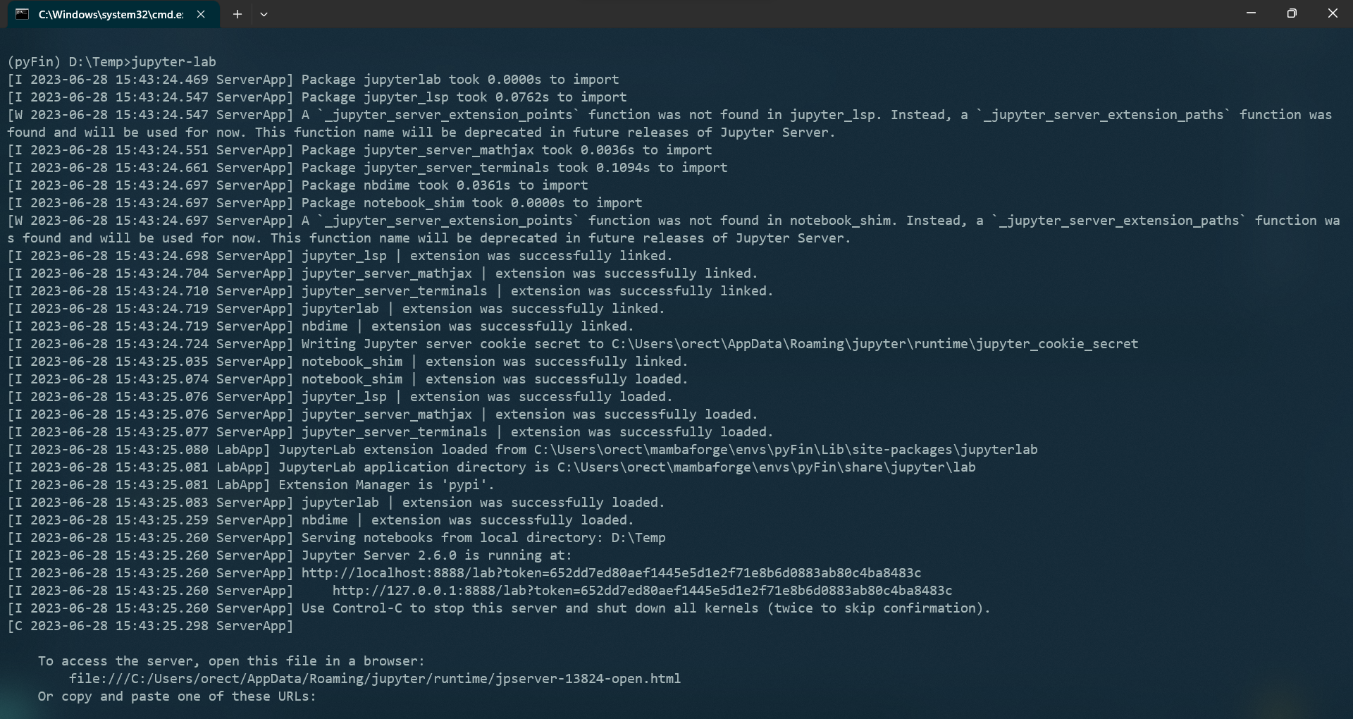\n",
224 | "\n",
225 | " \n",
226 | "You can see that the Jupyter Server is running on port 8888 on the localhost.\n",
227 | "\n",
228 | "The following interface should open up on your default browser automatically - if not, CTRL + Click the server URL.\n",
229 | "\n",
230 | "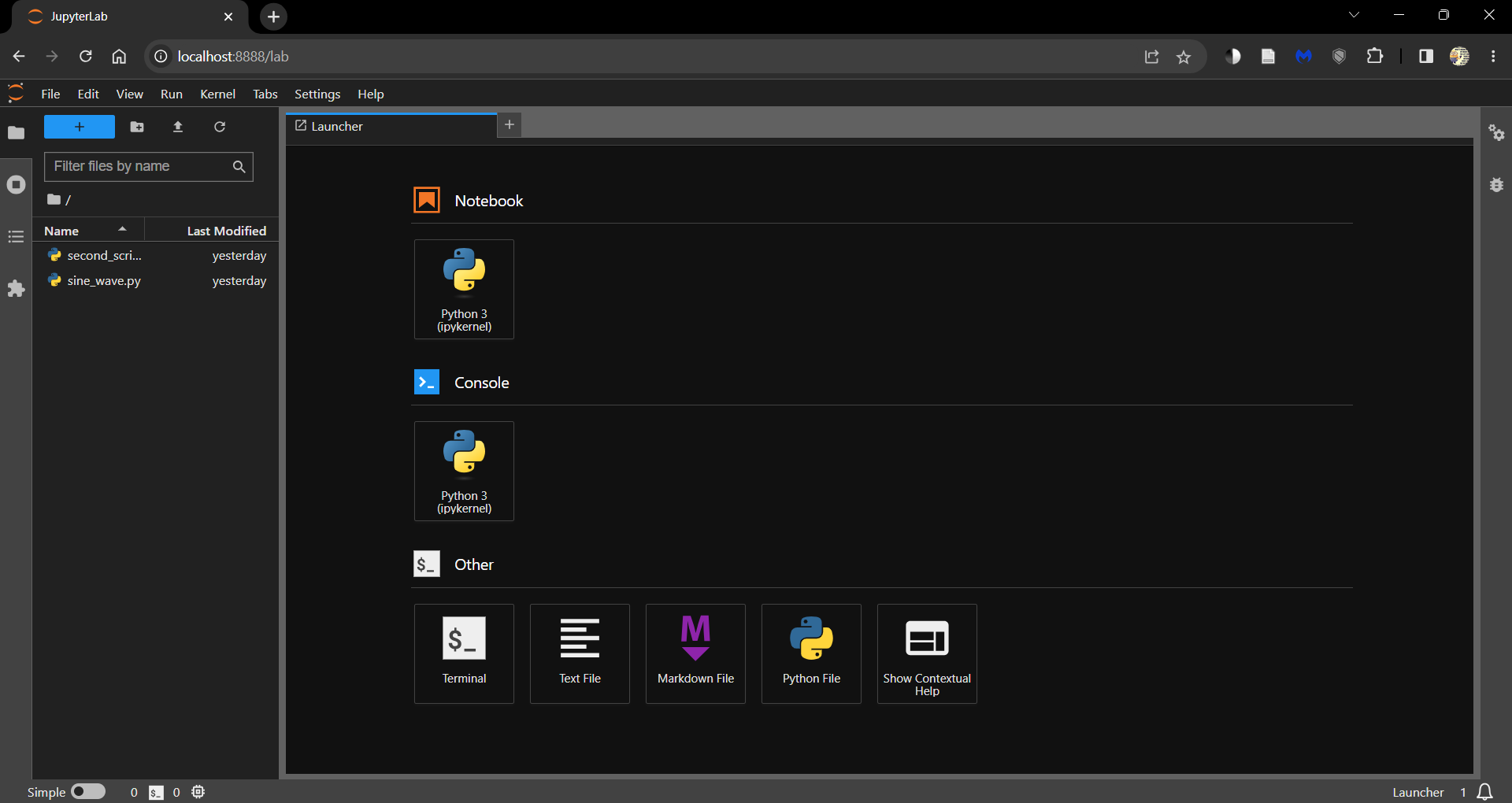\n",
231 | "\n",
232 | " \n",
233 | "Click on\n",
234 | "\n",
235 | "- the Python 3 (ipykernel) button under Notebooks to open a new Jupyter Notebook \n",
236 | "- the Python File button to open a new Python script (.py) \n",
237 | "\n",
238 | "\n",
239 | "You can always open this launcher tab by clicking the ‘+’ button on the top.\n",
240 | "\n",
241 | "All the files and folders in your working directory can be found in the File Browser (tab on the left).\n",
242 | "\n",
243 | "You can create new files and folders using the buttons available at the top of the File Browser tab.\n",
244 | "\n",
245 | "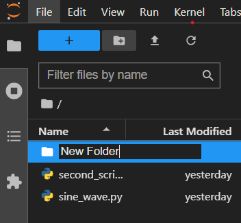\n",
246 | "\n",
247 | " \n",
248 | "You can install extensions that increase the functionality of JupyterLab by visiting the Extensions tab.\n",
249 | "\n",
250 | "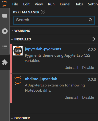\n",
251 | "\n",
252 | " \n",
253 | "Coming back to the example scripts from earlier, there are two ways to work with them in JupyterLab.\n",
254 | "\n",
255 | "- Using magic commands \n",
256 | "- Using the terminal "
257 | ]
258 | },
259 | {
260 | "cell_type": "markdown",
261 | "id": "29d79853",
262 | "metadata": {},
263 | "source": [
264 | "### Using magic commands\n",
265 | "\n",
266 | "Jupyter Notebooks and JupyterLab support the use of [magic commands](https://ipython.readthedocs.io/en/stable/interactive/magics.html) - commands that extend the capabilities of a standard Jupyter Notebook.\n",
267 | "\n",
268 | "The `%run` magic command allows you to run a Python script from within a Notebook.\n",
269 | "\n",
270 | "This is a convenient way to run scripts that you are working on in the same directory as your Notebook and present the outputs within the Notebook.\n",
271 | "\n",
272 | "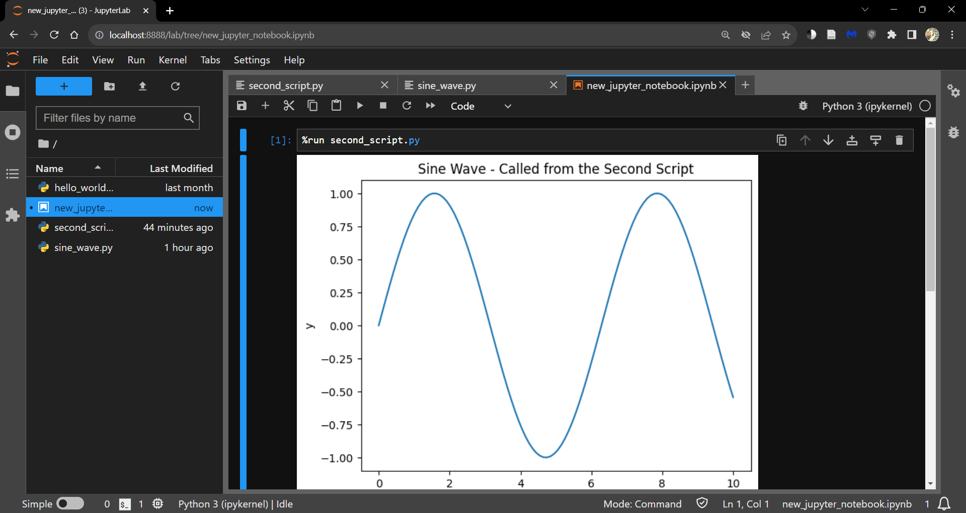"
273 | ]
274 | },
275 | {
276 | "cell_type": "markdown",
277 | "id": "c3ce2771",
278 | "metadata": {},
279 | "source": [
280 | "### Using the terminal\n",
281 | "\n",
282 | "However, if you are looking into just running the `.py` file, it is sometimes easier to use the terminal.\n",
283 | "\n",
284 | "Open a terminal from the launcher and run the following command."
285 | ]
286 | },
287 | {
288 | "cell_type": "code",
289 | "execution_count": null,
290 | "id": "9ad92ae8",
291 | "metadata": {
292 | "hide-output": false
293 | },
294 | "outputs": [],
295 | "source": [
296 | "> python "
297 | ]
298 | },
299 | {
300 | "cell_type": "markdown",
301 | "id": "566d3dc7",
302 | "metadata": {},
303 | "source": [
304 | "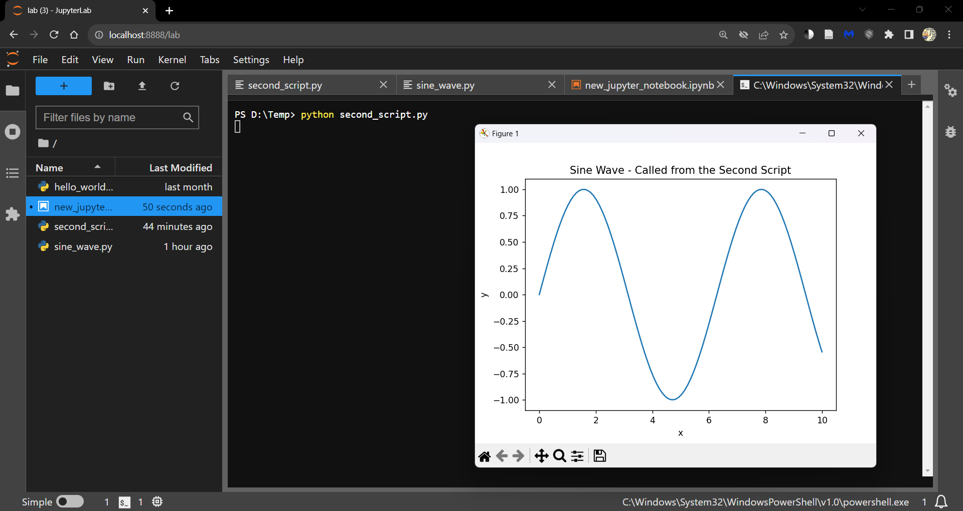\n",
305 | "\n",
306 | " \n",
307 | ">**Note**\n",
308 | ">\n",
309 | ">You can also run the script line by line by opening an ipykernel console either\n",
310 | "\n",
311 | "- from the launcher \n",
312 | "- by right clicking within the Notebook and selecting Create Console for Editor \n",
313 | "\n",
314 | "\n",
315 | "Use Shift + Enter to run a line of code."
316 | ]
317 | },
318 | {
319 | "cell_type": "markdown",
320 | "id": "a650257b",
321 | "metadata": {},
322 | "source": [
323 | "## A walk through Visual Studio Code\n",
324 | "\n",
325 | "Visual Studio Code (VS Code) is a code editor and development workspace that can run\n",
326 | "\n",
327 | "- in the [browser](https://vscode.dev/). \n",
328 | "- as a local [installation](https://code.visualstudio.com/docs/?dv=win). \n",
329 | "\n",
330 | "\n",
331 | "Both interfaces are identical.\n",
332 | "\n",
333 | "When you launch VS Code, you will see the following interface.\n",
334 | "\n",
335 | "\n",
336 | "\n",
337 | " \n",
338 | "Explore how to customize VS Code to your liking through the guided walkthroughs.\n",
339 | "\n",
340 | "\n",
341 | "\n",
342 | " \n",
343 | "When presented with the following prompt, go ahead an install all recommended extensions.\n",
344 | "\n",
345 | "\n",
346 | "\n",
347 | " \n",
348 | "You can also install extensions from the Extensions tab.\n",
349 | "\n",
350 | "\n",
351 | "\n",
352 | " \n",
353 | "Jupyter Notebooks (`.ipynb` files) can be worked on in VS Code.\n",
354 | "\n",
355 | "Make sure to install the Jupyter extension from the Extensions tab before you try to open a Jupyter Notebook.\n",
356 | "\n",
357 | "Create a new file (in the file Explorer tab) and save it with the `.ipynb` extension.\n",
358 | "\n",
359 | "Choose a kernel/environment to run the Notebook in by clicking on the Select Kernel button on the top right corner of the editor.\n",
360 | "\n",
361 | "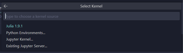\n",
362 | "\n",
363 | " \n",
364 | "VS Code also has excellent version control functionality through the Source Control tab.\n",
365 | "\n",
366 | "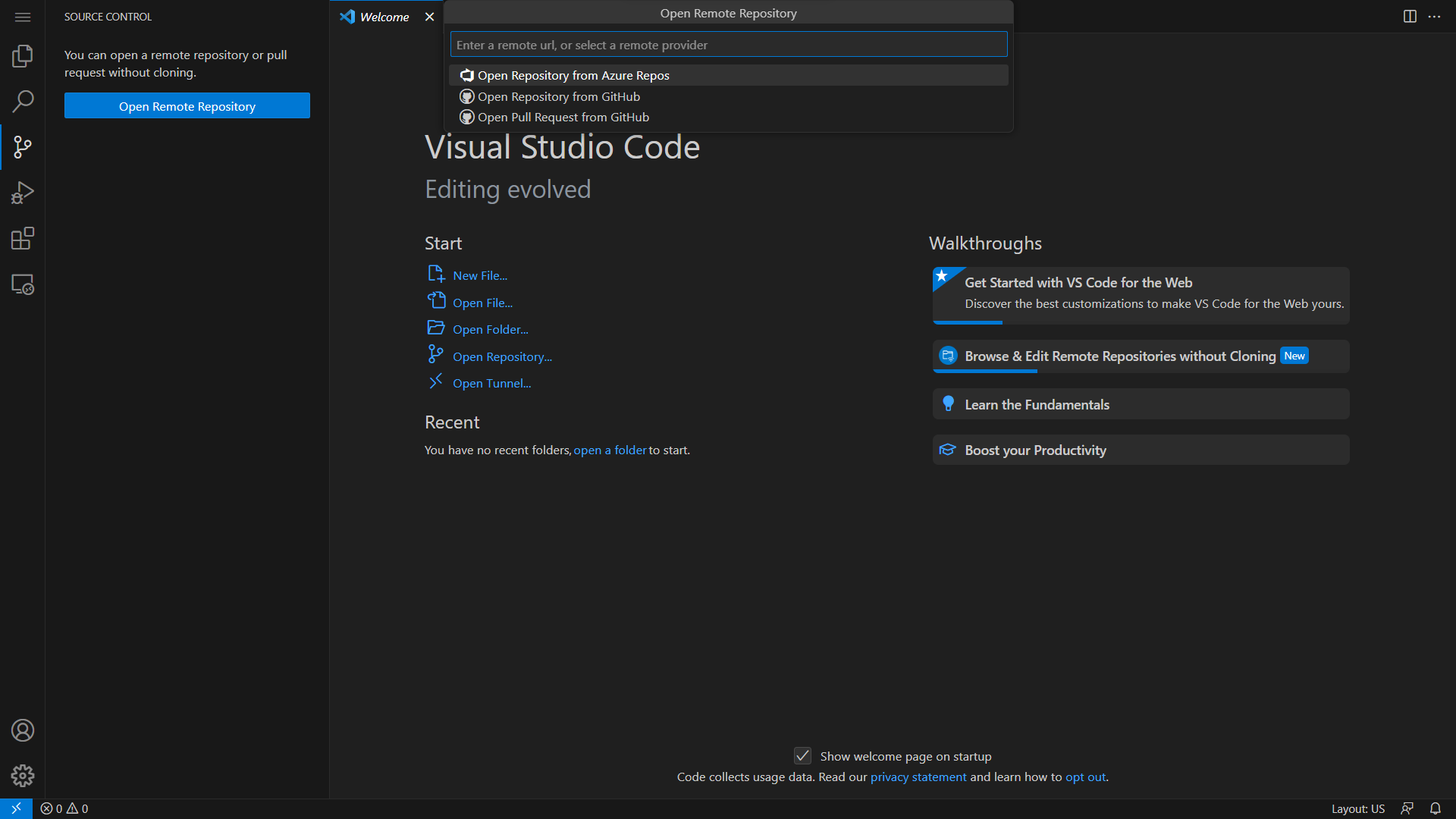\n",
367 | "\n",
368 | " \n",
369 | "Link your GitHub account to VS Code to push and pull changes to and from your repositories.\n",
370 | "\n",
371 | "Further discussions about version control can be found in the next section.\n",
372 | "\n",
373 | "To open a new Terminal in VS Code, click on the Terminal tab and select New Terminal.\n",
374 | "\n",
375 | "VS Code opens a new Terminal in the same directory you are working in - a PowerShell in Windows and a Bash in Linux.\n",
376 | "\n",
377 | "You can change the shell or open a new instance through the dropdown menu on the right end of the terminal tab.\n",
378 | "\n",
379 | "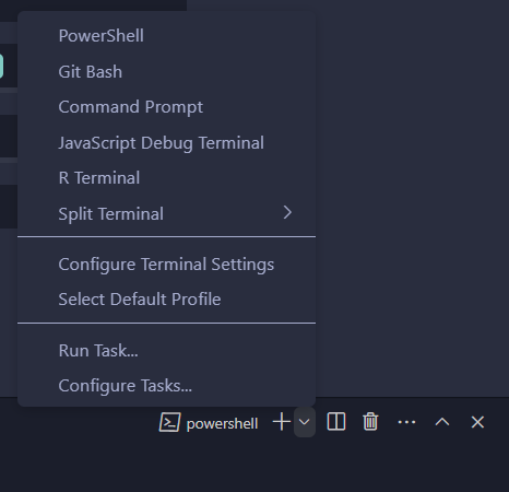\n",
380 | "\n",
381 | " \n",
382 | "VS Code helps you manage conda environments without using the command line.\n",
383 | "\n",
384 | "Open the Command Palette (CTRL + SHIFT + P or from the dropdown menu under View tab) and search for `Python: Select Interpreter`.\n",
385 | "\n",
386 | "This loads existing environments.\n",
387 | "\n",
388 | "You can also create new environments using `Python: Create Environment` in the Command Palette.\n",
389 | "\n",
390 | "A new environment (.conda folder) is created in the the current working directory.\n",
391 | "\n",
392 | "Coming to the example scripts from earlier, there are again two ways to work with them in VS Code.\n",
393 | "\n",
394 | "- Using the run button \n",
395 | "- Using the terminal "
396 | ]
397 | },
398 | {
399 | "cell_type": "markdown",
400 | "id": "4eb5fa87",
401 | "metadata": {},
402 | "source": [
403 | "### Using the run button\n",
404 | "\n",
405 | "You can run the script by clicking on the run button on the top right corner of the editor.\n",
406 | "\n",
407 | "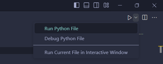\n",
408 | "\n",
409 | " \n",
410 | "You can also run the script interactively by selecting the **Run Current File in Interactive Window** option from the dropdown.\n",
411 | "\n",
412 | "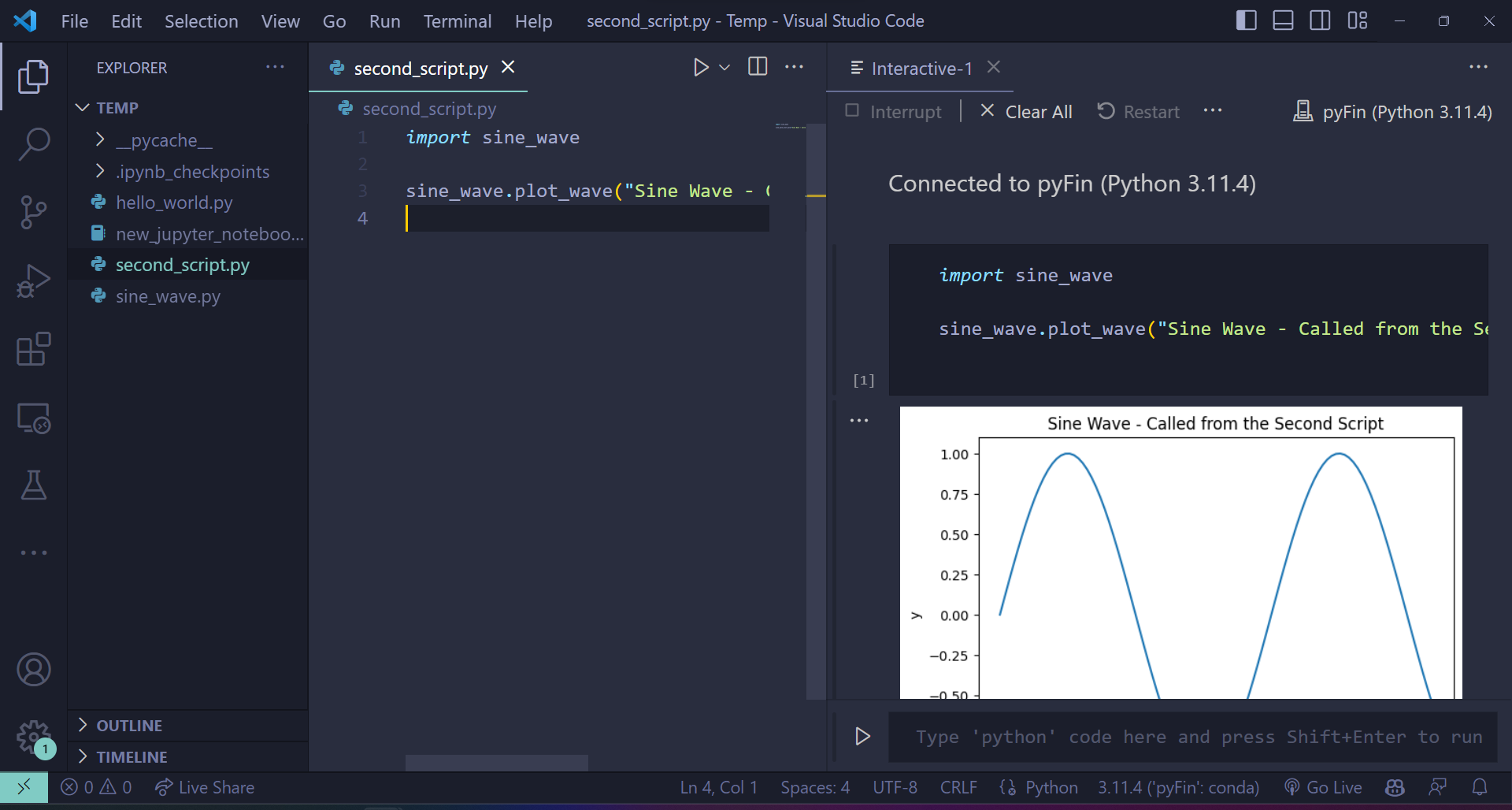\n",
413 | "\n",
414 | " \n",
415 | "This creates an ipykernel console and runs the script."
416 | ]
417 | },
418 | {
419 | "cell_type": "markdown",
420 | "id": "d17e4260",
421 | "metadata": {},
422 | "source": [
423 | "### Using the terminal\n",
424 | "\n",
425 | "The command `python ` is executed on the console of your choice.\n",
426 | "\n",
427 | "If you are using a Windows machine, you can either use the Anaconda Prompt or the Command Prompt - but, generally not the PowerShell.\n",
428 | "\n",
429 | "Here’s an execution of the earlier code.\n",
430 | "\n",
431 | "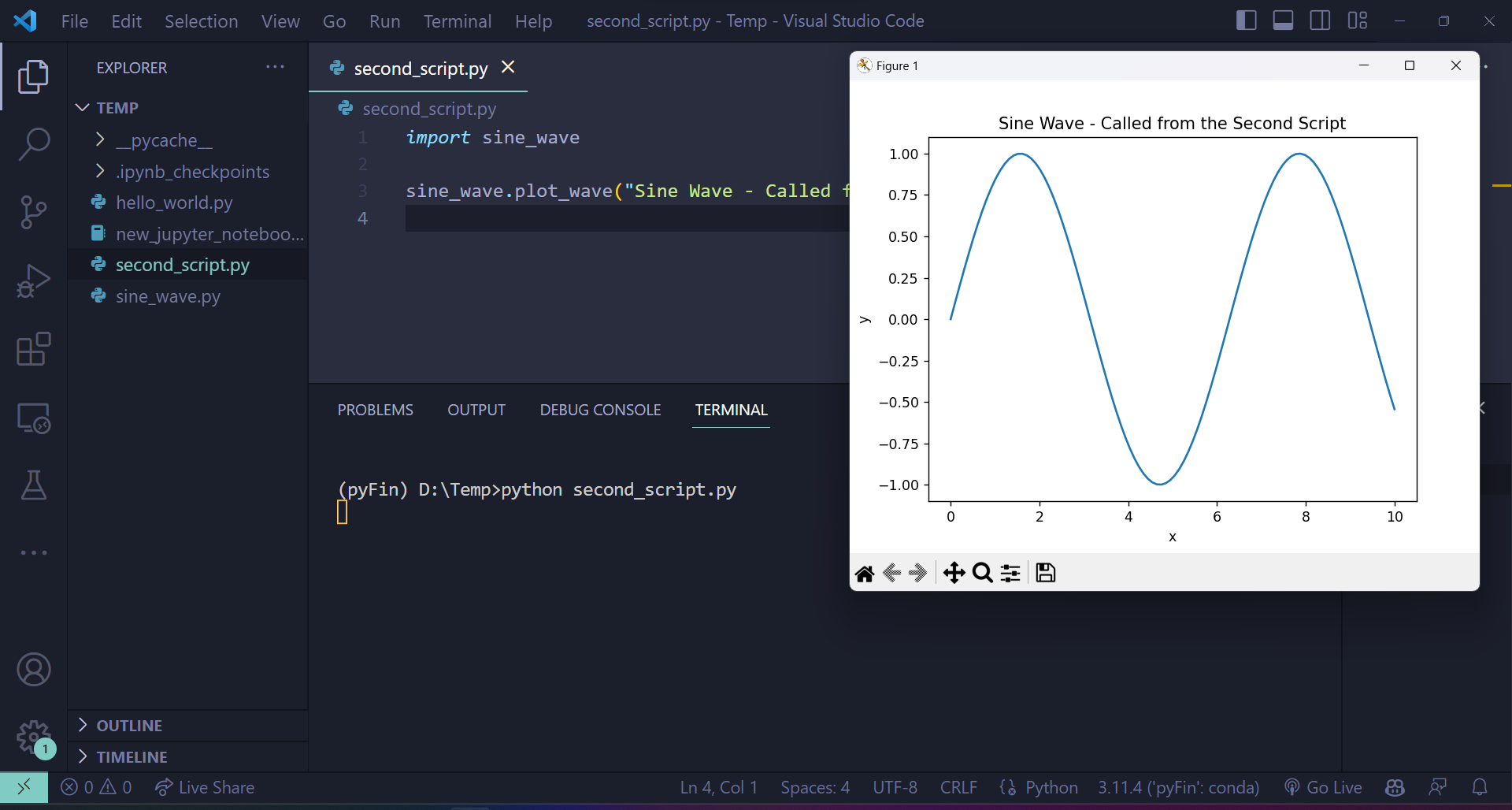\n",
432 | "\n",
433 | " \n",
434 | ">**Note**\n",
435 | ">\n",
436 | ">If you would like to develop packages and build tools using Python, you may want to look into [the use of Docker containers and VS Code](https://github.com/RamiKrispin/vscode-python).\n",
437 | "\n",
438 | "However, this is outside the focus of these lectures."
439 | ]
440 | },
441 | {
442 | "cell_type": "markdown",
443 | "id": "dd0ae1a4",
444 | "metadata": {},
445 | "source": [
446 | "## Git your hands dirty\n",
447 | "\n",
448 | "This section will familiarize you with git and GitHub.\n",
449 | "\n",
450 | "[Git](https://git-scm.com/) is a *version control system* — a piece of software used to manage digital projects such as code libraries.\n",
451 | "\n",
452 | "In many cases, the associated collections of files — called *repositories* — are stored on [GitHub](https://github.com/).\n",
453 | "\n",
454 | "GitHub is a wonderland of collaborative coding projects.\n",
455 | "\n",
456 | "For example, it hosts many of the scientific libraries we’ll be using later\n",
457 | "on, such as [this one](https://github.com/pandas-dev/pandas).\n",
458 | "\n",
459 | "Git is the underlying software used to manage these projects.\n",
460 | "\n",
461 | "Git is an extremely powerful tool for distributed collaboration — for\n",
462 | "example, we use it to share and synchronize all the source files for these\n",
463 | "lectures.\n",
464 | "\n",
465 | "There are two main flavors of Git\n",
466 | "\n",
467 | "1. the plain vanilla [command line Git](https://git-scm.com/downloads) version \n",
468 | "1. the various point-and-click GUI versions \n",
469 | " - See, for example, the [GitHub version](https://github.com/apps/desktop) or Git GUI integrated into your IDE. \n",
470 | "\n",
471 | "\n",
472 | "In case you already haven’t, try\n",
473 | "\n",
474 | "1. Installing Git. \n",
475 | "1. Getting a copy of [QuantEcon.py](https://github.com/QuantEcon/QuantEcon.py) using Git. \n",
476 | "\n",
477 | "\n",
478 | "For example, if you’ve installed the command line version, open up a terminal and enter."
479 | ]
480 | },
481 | {
482 | "cell_type": "markdown",
483 | "id": "39e61fc2",
484 | "metadata": {
485 | "hide-output": false
486 | },
487 | "source": [
488 | "```bash\n",
489 | "git clone https://github.com/QuantEcon/QuantEcon.py\n",
490 | "```\n"
491 | ]
492 | },
493 | {
494 | "cell_type": "markdown",
495 | "id": "650f03a6",
496 | "metadata": {},
497 | "source": [
498 | "(This is just `git clone` in front of the URL for the repository)\n",
499 | "\n",
500 | "This command will download all necessary components to rebuild the lecture you are reading now.\n",
501 | "\n",
502 | "As the 2nd task,\n",
503 | "\n",
504 | "1. Sign up to [GitHub](https://github.com/). \n",
505 | "1. Look into ‘forking’ GitHub repositories (forking means making your own copy of a GitHub repository, stored on GitHub). \n",
506 | "1. Fork [QuantEcon.py](https://github.com/QuantEcon/QuantEcon.py). \n",
507 | "1. Clone your fork to some local directory, make edits, commit them, and push them back up to your forked GitHub repo. \n",
508 | "1. If you made a valuable improvement, send us a [pull request](https://docs.github.com/en/pull-requests/collaborating-with-pull-requests/proposing-changes-to-your-work-with-pull-requests/about-pull-requests)! \n",
509 | "\n",
510 | "\n",
511 | "For reading on these and other topics, try\n",
512 | "\n",
513 | "- [The official Git documentation](https://git-scm.com/doc). \n",
514 | "- Reading through the docs on [GitHub](https://docs.github.com/en). \n",
515 | "- [Pro Git Book](https://git-scm.com/book) by Scott Chacon and Ben Straub. \n",
516 | "- One of the thousands of Git tutorials on the Net. "
517 | ]
518 | }
519 | ],
520 | "metadata": {
521 | "date": 1764566374.3706856,
522 | "filename": "workspace.md",
523 | "kernelspec": {
524 | "display_name": "Python",
525 | "language": "python3",
526 | "name": "python3"
527 | },
528 | "title": "Writing Longer Programs"
529 | },
530 | "nbformat": 4,
531 | "nbformat_minor": 5
532 | }
--------------------------------------------------------------------------------
/oop_intro.ipynb:
--------------------------------------------------------------------------------
1 | {
2 | "cells": [
3 | {
4 | "cell_type": "markdown",
5 | "id": "b9def808",
6 | "metadata": {},
7 | "source": [
8 | "\n",
9 | "\n",
10 | ""
15 | ]
16 | },
17 | {
18 | "cell_type": "markdown",
19 | "id": "85c09796",
20 | "metadata": {},
21 | "source": [
22 | "# OOP I: Objects and Methods"
23 | ]
24 | },
25 | {
26 | "cell_type": "markdown",
27 | "id": "b41963ec",
28 | "metadata": {},
29 | "source": [
30 | "## Overview\n",
31 | "\n",
32 | "The traditional programming paradigm (think Fortran, C, MATLAB, etc.) is called [procedural](https://en.wikipedia.org/wiki/Procedural_programming).\n",
33 | "\n",
34 | "It works as follows\n",
35 | "\n",
36 | "- The program has a state corresponding to the values of its variables. \n",
37 | "- Functions are called to act on and transform the state. \n",
38 | "- Final outputs are produced via a sequence of function calls. \n",
39 | "\n",
40 | "\n",
41 | "Two other important paradigms are [object-oriented programming](https://en.wikipedia.org/wiki/Object-oriented_programming) (OOP) and [functional programming](https://en.wikipedia.org/wiki/Functional_programming).\n",
42 | "\n",
43 | "In the OOP paradigm, data and functions are bundled together into “objects” — and functions in this context are referred to as **methods**.\n",
44 | "\n",
45 | "Methods are called on to transform the data contained in the object.\n",
46 | "\n",
47 | "- Think of a Python list that contains data and has methods such as `append()` and `pop()` that transform the data. \n",
48 | "\n",
49 | "\n",
50 | "Functional programming languages are built on the idea of composing functions.\n",
51 | "\n",
52 | "- Influential examples include [Lisp](https://en.wikipedia.org/wiki/Common_Lisp), [Haskell](https://en.wikipedia.org/wiki/Haskell) and [Elixir](https://en.wikipedia.org/wiki/Elixir_%28programming_language%29). \n",
53 | "\n",
54 | "\n",
55 | "So which of these categories does Python fit into?\n",
56 | "\n",
57 | "Actually Python is a pragmatic language that blends object-oriented, functional and procedural styles, rather than taking a purist approach.\n",
58 | "\n",
59 | "On one hand, this allows Python and its users to cherry pick nice aspects of different paradigms.\n",
60 | "\n",
61 | "On the other hand, the lack of purity might at times lead to some confusion.\n",
62 | "\n",
63 | "Fortunately this confusion is minimized if you understand that, at a foundational level, Python *is* object-oriented.\n",
64 | "\n",
65 | "By this we mean that, in Python, *everything is an object*.\n",
66 | "\n",
67 | "In this lecture, we explain what that statement means and why it matters.\n",
68 | "\n",
69 | "We’ll make use of the following third party library"
70 | ]
71 | },
72 | {
73 | "cell_type": "code",
74 | "execution_count": null,
75 | "id": "667955f4",
76 | "metadata": {
77 | "hide-output": false
78 | },
79 | "outputs": [],
80 | "source": [
81 | "!pip install rich"
82 | ]
83 | },
84 | {
85 | "cell_type": "markdown",
86 | "id": "f25728d7",
87 | "metadata": {},
88 | "source": [
89 | "## Objects\n",
90 | "\n",
91 | "\n",
92 | "\n",
93 | "In Python, an *object* is a collection of data and instructions held in computer memory that consists of\n",
94 | "\n",
95 | "1. a type \n",
96 | "1. a unique identity \n",
97 | "1. data (i.e., content) \n",
98 | "1. methods \n",
99 | "\n",
100 | "\n",
101 | "These concepts are defined and discussed sequentially below.\n",
102 | "\n",
103 | "\n",
104 | ""
105 | ]
106 | },
107 | {
108 | "cell_type": "markdown",
109 | "id": "a69f598e",
110 | "metadata": {},
111 | "source": [
112 | "### Type\n",
113 | "\n",
114 | "\n",
115 | "\n",
116 | "Python provides for different types of objects, to accommodate different categories of data.\n",
117 | "\n",
118 | "For example"
119 | ]
120 | },
121 | {
122 | "cell_type": "code",
123 | "execution_count": null,
124 | "id": "64f8ec51",
125 | "metadata": {
126 | "hide-output": false
127 | },
128 | "outputs": [],
129 | "source": [
130 | "s = 'This is a string'\n",
131 | "type(s)"
132 | ]
133 | },
134 | {
135 | "cell_type": "code",
136 | "execution_count": null,
137 | "id": "5fbeec58",
138 | "metadata": {
139 | "hide-output": false
140 | },
141 | "outputs": [],
142 | "source": [
143 | "x = 42 # Now let's create an integer\n",
144 | "type(x)"
145 | ]
146 | },
147 | {
148 | "cell_type": "markdown",
149 | "id": "422beec5",
150 | "metadata": {},
151 | "source": [
152 | "The type of an object matters for many expressions.\n",
153 | "\n",
154 | "For example, the addition operator between two strings means concatenation"
155 | ]
156 | },
157 | {
158 | "cell_type": "code",
159 | "execution_count": null,
160 | "id": "49f34d0f",
161 | "metadata": {
162 | "hide-output": false
163 | },
164 | "outputs": [],
165 | "source": [
166 | "'300' + 'cc'"
167 | ]
168 | },
169 | {
170 | "cell_type": "markdown",
171 | "id": "5ed2632e",
172 | "metadata": {},
173 | "source": [
174 | "On the other hand, between two numbers it means ordinary addition"
175 | ]
176 | },
177 | {
178 | "cell_type": "code",
179 | "execution_count": null,
180 | "id": "3fe3d860",
181 | "metadata": {
182 | "hide-output": false
183 | },
184 | "outputs": [],
185 | "source": [
186 | "300 + 400"
187 | ]
188 | },
189 | {
190 | "cell_type": "markdown",
191 | "id": "5e8fe20f",
192 | "metadata": {},
193 | "source": [
194 | "Consider the following expression"
195 | ]
196 | },
197 | {
198 | "cell_type": "code",
199 | "execution_count": null,
200 | "id": "bb70b1ff",
201 | "metadata": {
202 | "hide-output": false
203 | },
204 | "outputs": [],
205 | "source": [
206 | "'300' + 400"
207 | ]
208 | },
209 | {
210 | "cell_type": "markdown",
211 | "id": "2f228993",
212 | "metadata": {},
213 | "source": [
214 | "Here we are mixing types, and it’s unclear to Python whether the user wants to\n",
215 | "\n",
216 | "- convert `'300'` to an integer and then add it to `400`, or \n",
217 | "- convert `400` to string and then concatenate it with `'300'` \n",
218 | "\n",
219 | "\n",
220 | "Some languages might try to guess but Python is *strongly typed*\n",
221 | "\n",
222 | "- Type is important, and implicit type conversion is rare. \n",
223 | "- Python will respond instead by raising a `TypeError`. \n",
224 | "\n",
225 | "\n",
226 | "To avoid the error, you need to clarify by changing the relevant type.\n",
227 | "\n",
228 | "For example,"
229 | ]
230 | },
231 | {
232 | "cell_type": "code",
233 | "execution_count": null,
234 | "id": "a9583d8d",
235 | "metadata": {
236 | "hide-output": false
237 | },
238 | "outputs": [],
239 | "source": [
240 | "int('300') + 400 # To add as numbers, change the string to an integer"
241 | ]
242 | },
243 | {
244 | "cell_type": "markdown",
245 | "id": "f57e5972",
246 | "metadata": {},
247 | "source": [
248 | "\n",
249 | ""
250 | ]
251 | },
252 | {
253 | "cell_type": "markdown",
254 | "id": "58c13baf",
255 | "metadata": {},
256 | "source": [
257 | "### Identity\n",
258 | "\n",
259 | "\n",
260 | "\n",
261 | "In Python, each object has a unique identifier, which helps Python (and us) keep track of the object.\n",
262 | "\n",
263 | "The identity of an object can be obtained via the `id()` function"
264 | ]
265 | },
266 | {
267 | "cell_type": "code",
268 | "execution_count": null,
269 | "id": "8777544f",
270 | "metadata": {
271 | "hide-output": false
272 | },
273 | "outputs": [],
274 | "source": [
275 | "y = 2.5\n",
276 | "z = 2.5\n",
277 | "id(y)"
278 | ]
279 | },
280 | {
281 | "cell_type": "code",
282 | "execution_count": null,
283 | "id": "62a1f16b",
284 | "metadata": {
285 | "hide-output": false
286 | },
287 | "outputs": [],
288 | "source": [
289 | "id(z)"
290 | ]
291 | },
292 | {
293 | "cell_type": "markdown",
294 | "id": "5c71ca78",
295 | "metadata": {},
296 | "source": [
297 | "In this example, `y` and `z` happen to have the same value (i.e., `2.5`), but they are not the same object.\n",
298 | "\n",
299 | "The identity of an object is in fact just the address of the object in memory."
300 | ]
301 | },
302 | {
303 | "cell_type": "markdown",
304 | "id": "c73661bd",
305 | "metadata": {},
306 | "source": [
307 | "### Object Content: Data and Attributes\n",
308 | "\n",
309 | "\n",
310 | "\n",
311 | "If we set `x = 42` then we create an object of type `int` that contains\n",
312 | "the data `42`.\n",
313 | "\n",
314 | "In fact, it contains more, as the following example shows"
315 | ]
316 | },
317 | {
318 | "cell_type": "code",
319 | "execution_count": null,
320 | "id": "dcbabcba",
321 | "metadata": {
322 | "hide-output": false
323 | },
324 | "outputs": [],
325 | "source": [
326 | "x = 42\n",
327 | "x"
328 | ]
329 | },
330 | {
331 | "cell_type": "code",
332 | "execution_count": null,
333 | "id": "8594d178",
334 | "metadata": {
335 | "hide-output": false
336 | },
337 | "outputs": [],
338 | "source": [
339 | "x.imag"
340 | ]
341 | },
342 | {
343 | "cell_type": "code",
344 | "execution_count": null,
345 | "id": "009d09ab",
346 | "metadata": {
347 | "hide-output": false
348 | },
349 | "outputs": [],
350 | "source": [
351 | "x.__class__"
352 | ]
353 | },
354 | {
355 | "cell_type": "markdown",
356 | "id": "a9472f2d",
357 | "metadata": {},
358 | "source": [
359 | "When Python creates this integer object, it stores with it various auxiliary information, such as the imaginary part, and the type.\n",
360 | "\n",
361 | "Any name following a dot is called an *attribute* of the object to the left of the dot.\n",
362 | "\n",
363 | "- e.g.,`imag` and `__class__` are attributes of `x`. \n",
364 | "\n",
365 | "\n",
366 | "We see from this example that objects have attributes that contain auxiliary information.\n",
367 | "\n",
368 | "They also have attributes that act like functions, called *methods*.\n",
369 | "\n",
370 | "These attributes are important, so let’s discuss them in-depth.\n",
371 | "\n",
372 | "\n",
373 | ""
374 | ]
375 | },
376 | {
377 | "cell_type": "markdown",
378 | "id": "cd343283",
379 | "metadata": {},
380 | "source": [
381 | "### Methods\n",
382 | "\n",
383 | "\n",
384 | "\n",
385 | "Methods are *functions that are bundled with objects*.\n",
386 | "\n",
387 | "Formally, methods are attributes of objects that are **callable** – i.e., attributes that can be called as functions"
388 | ]
389 | },
390 | {
391 | "cell_type": "code",
392 | "execution_count": null,
393 | "id": "cac3c0e4",
394 | "metadata": {
395 | "hide-output": false
396 | },
397 | "outputs": [],
398 | "source": [
399 | "x = ['foo', 'bar']\n",
400 | "callable(x.append)"
401 | ]
402 | },
403 | {
404 | "cell_type": "code",
405 | "execution_count": null,
406 | "id": "e2470975",
407 | "metadata": {
408 | "hide-output": false
409 | },
410 | "outputs": [],
411 | "source": [
412 | "callable(x.__doc__)"
413 | ]
414 | },
415 | {
416 | "cell_type": "markdown",
417 | "id": "c7aa4470",
418 | "metadata": {},
419 | "source": [
420 | "Methods typically act on the data contained in the object they belong to, or combine that data with other data"
421 | ]
422 | },
423 | {
424 | "cell_type": "code",
425 | "execution_count": null,
426 | "id": "399e482f",
427 | "metadata": {
428 | "hide-output": false
429 | },
430 | "outputs": [],
431 | "source": [
432 | "x = ['a', 'b']\n",
433 | "x.append('c')\n",
434 | "s = 'This is a string'\n",
435 | "s.upper()"
436 | ]
437 | },
438 | {
439 | "cell_type": "code",
440 | "execution_count": null,
441 | "id": "448b3366",
442 | "metadata": {
443 | "hide-output": false
444 | },
445 | "outputs": [],
446 | "source": [
447 | "s.lower()"
448 | ]
449 | },
450 | {
451 | "cell_type": "code",
452 | "execution_count": null,
453 | "id": "2417a99a",
454 | "metadata": {
455 | "hide-output": false
456 | },
457 | "outputs": [],
458 | "source": [
459 | "s.replace('This', 'That')"
460 | ]
461 | },
462 | {
463 | "cell_type": "markdown",
464 | "id": "e98de1c3",
465 | "metadata": {},
466 | "source": [
467 | "A great deal of Python functionality is organized around method calls.\n",
468 | "\n",
469 | "For example, consider the following piece of code"
470 | ]
471 | },
472 | {
473 | "cell_type": "code",
474 | "execution_count": null,
475 | "id": "8916fff5",
476 | "metadata": {
477 | "hide-output": false
478 | },
479 | "outputs": [],
480 | "source": [
481 | "x = ['a', 'b']\n",
482 | "x[0] = 'aa' # Item assignment using square bracket notation\n",
483 | "x"
484 | ]
485 | },
486 | {
487 | "cell_type": "markdown",
488 | "id": "d90e1346",
489 | "metadata": {},
490 | "source": [
491 | "It doesn’t look like there are any methods used here, but in fact the square bracket assignment notation is just a convenient interface to a method call.\n",
492 | "\n",
493 | "What actually happens is that Python calls the `__setitem__` method, as follows"
494 | ]
495 | },
496 | {
497 | "cell_type": "code",
498 | "execution_count": null,
499 | "id": "3eb7665d",
500 | "metadata": {
501 | "hide-output": false
502 | },
503 | "outputs": [],
504 | "source": [
505 | "x = ['a', 'b']\n",
506 | "x.__setitem__(0, 'aa') # Equivalent to x[0] = 'aa'\n",
507 | "x"
508 | ]
509 | },
510 | {
511 | "cell_type": "markdown",
512 | "id": "b3b0af0c",
513 | "metadata": {},
514 | "source": [
515 | "(If you wanted to you could modify the `__setitem__` method, so that square bracket assignment does something totally different)"
516 | ]
517 | },
518 | {
519 | "cell_type": "markdown",
520 | "id": "cc4fd3fc",
521 | "metadata": {},
522 | "source": [
523 | "## Inspection Using Rich\n",
524 | "\n",
525 | "There’s a nice package called [rich](https://github.com/Textualize/rich) that\n",
526 | "helps us view the contents of an object.\n",
527 | "\n",
528 | "For example,"
529 | ]
530 | },
531 | {
532 | "cell_type": "code",
533 | "execution_count": null,
534 | "id": "015f2862",
535 | "metadata": {
536 | "hide-output": false
537 | },
538 | "outputs": [],
539 | "source": [
540 | "from rich import inspect\n",
541 | "x = 10\n",
542 | "inspect(10)"
543 | ]
544 | },
545 | {
546 | "cell_type": "markdown",
547 | "id": "dec532ee",
548 | "metadata": {},
549 | "source": [
550 | "If we want to see the methods as well, we can use"
551 | ]
552 | },
553 | {
554 | "cell_type": "code",
555 | "execution_count": null,
556 | "id": "f06bbea3",
557 | "metadata": {
558 | "hide-output": false
559 | },
560 | "outputs": [],
561 | "source": [
562 | "inspect(10, methods=True)"
563 | ]
564 | },
565 | {
566 | "cell_type": "markdown",
567 | "id": "2f51d1b7",
568 | "metadata": {},
569 | "source": [
570 | "In fact there are still more methods, as you can see if you execute `inspect(10, all=True)`."
571 | ]
572 | },
573 | {
574 | "cell_type": "markdown",
575 | "id": "42fbc10d",
576 | "metadata": {},
577 | "source": [
578 | "## A Little Mystery\n",
579 | "\n",
580 | "In this lecture we claimed that Python is, at heart, an object oriented language.\n",
581 | "\n",
582 | "But here’s an example that looks more procedural."
583 | ]
584 | },
585 | {
586 | "cell_type": "code",
587 | "execution_count": null,
588 | "id": "bd26d130",
589 | "metadata": {
590 | "hide-output": false
591 | },
592 | "outputs": [],
593 | "source": [
594 | "x = ['a', 'b']\n",
595 | "m = len(x)\n",
596 | "m"
597 | ]
598 | },
599 | {
600 | "cell_type": "markdown",
601 | "id": "be4ad353",
602 | "metadata": {},
603 | "source": [
604 | "If Python is object oriented, why don’t we use `x.len()`?\n",
605 | "\n",
606 | "The answer is related to the fact that Python aims for readability and consistent style.\n",
607 | "\n",
608 | "In Python, it is common for users to build custom objects — we discuss how to\n",
609 | "do this [later](https://python-programming.quantecon.org/python_oop.html).\n",
610 | "\n",
611 | "It’s quite common for users to add methods to their that measure the length of\n",
612 | "the object, suitably defined.\n",
613 | "\n",
614 | "When naming such a method, natural choices are `len()` and `length()`.\n",
615 | "\n",
616 | "If some users choose `len()` and others choose `length()`, then the style will\n",
617 | "be inconsistent and harder to remember.\n",
618 | "\n",
619 | "To avoid this, the creator of Python chose to add\n",
620 | "`len()` as a built-in function, to help emphasize that `len()` is the convention.\n",
621 | "\n",
622 | "Now, having said all of this, Python *is* still object oriented under the hood.\n",
623 | "\n",
624 | "In fact, the list `x` discussed above has a method called `__len__()`.\n",
625 | "\n",
626 | "All that the function `len()` does is call this method.\n",
627 | "\n",
628 | "In other words, the following code is equivalent:"
629 | ]
630 | },
631 | {
632 | "cell_type": "code",
633 | "execution_count": null,
634 | "id": "bcbfe534",
635 | "metadata": {
636 | "hide-output": false
637 | },
638 | "outputs": [],
639 | "source": [
640 | "x = ['a', 'b']\n",
641 | "len(x)"
642 | ]
643 | },
644 | {
645 | "cell_type": "markdown",
646 | "id": "be40441a",
647 | "metadata": {},
648 | "source": [
649 | "and"
650 | ]
651 | },
652 | {
653 | "cell_type": "code",
654 | "execution_count": null,
655 | "id": "b45310b6",
656 | "metadata": {
657 | "hide-output": false
658 | },
659 | "outputs": [],
660 | "source": [
661 | "x = ['a', 'b']\n",
662 | "x.__len__()"
663 | ]
664 | },
665 | {
666 | "cell_type": "markdown",
667 | "id": "7e66d981",
668 | "metadata": {},
669 | "source": [
670 | "## Summary\n",
671 | "\n",
672 | "The message in this lecture is clear:\n",
673 | "\n",
674 | "- In Python, *everything in memory is treated as an object*. \n",
675 | "\n",
676 | "\n",
677 | "This includes not just lists, strings, etc., but also less obvious things, such as\n",
678 | "\n",
679 | "- functions (once they have been read into memory) \n",
680 | "- modules (ditto) \n",
681 | "- files opened for reading or writing \n",
682 | "- integers, etc. \n",
683 | "\n",
684 | "\n",
685 | "Remember that everything is an object will help you interact with your programs\n",
686 | "and write clear Pythonic code."
687 | ]
688 | },
689 | {
690 | "cell_type": "markdown",
691 | "id": "4bd388c2",
692 | "metadata": {},
693 | "source": [
694 | "## Exercises"
695 | ]
696 | },
697 | {
698 | "cell_type": "markdown",
699 | "id": "c2ccbd42",
700 | "metadata": {},
701 | "source": [
702 | "## Exercise 6.1\n",
703 | "\n",
704 | "We have met the [boolean data type](https://python-programming.quantecon.org/python_essentials.html#boolean) previously.\n",
705 | "\n",
706 | "Using what we have learnt in this lecture, print a list of methods of the\n",
707 | "boolean object `True`.\n",
708 | "\n",
709 | "You can use `callable()` to test whether an attribute of an object can be called as a function"
710 | ]
711 | },
712 | {
713 | "cell_type": "markdown",
714 | "id": "4d3c5ed9",
715 | "metadata": {},
716 | "source": [
717 | "## Solution to[ Exercise 6.1](https://python-programming.quantecon.org/#oop_intro_ex1)\n",
718 | "\n",
719 | "Firstly, we need to find all attributes of `True`, which can be done via"
720 | ]
721 | },
722 | {
723 | "cell_type": "code",
724 | "execution_count": null,
725 | "id": "2891090e",
726 | "metadata": {
727 | "hide-output": false
728 | },
729 | "outputs": [],
730 | "source": [
731 | "print(sorted(True.__dir__()))"
732 | ]
733 | },
734 | {
735 | "cell_type": "markdown",
736 | "id": "0be38d0e",
737 | "metadata": {},
738 | "source": [
739 | "or"
740 | ]
741 | },
742 | {
743 | "cell_type": "code",
744 | "execution_count": null,
745 | "id": "e0877b02",
746 | "metadata": {
747 | "hide-output": false
748 | },
749 | "outputs": [],
750 | "source": [
751 | "print(sorted(dir(True)))"
752 | ]
753 | },
754 | {
755 | "cell_type": "markdown",
756 | "id": "3310a013",
757 | "metadata": {},
758 | "source": [
759 | "Since the boolean data type is a primitive type, you can also find it in the built-in namespace"
760 | ]
761 | },
762 | {
763 | "cell_type": "code",
764 | "execution_count": null,
765 | "id": "69e1ec73",
766 | "metadata": {
767 | "hide-output": false
768 | },
769 | "outputs": [],
770 | "source": [
771 | "print(dir(__builtins__.bool))"
772 | ]
773 | },
774 | {
775 | "cell_type": "markdown",
776 | "id": "240ea856",
777 | "metadata": {},
778 | "source": [
779 | "Here we use a `for` loop to filter out attributes that are callable"
780 | ]
781 | },
782 | {
783 | "cell_type": "code",
784 | "execution_count": null,
785 | "id": "cca3c61d",
786 | "metadata": {
787 | "hide-output": false
788 | },
789 | "outputs": [],
790 | "source": [
791 | "attributes = dir(__builtins__.bool)\n",
792 | "callablels = []\n",
793 | "\n",
794 | "for attribute in attributes:\n",
795 | " # Use eval() to evaluate a string as an expression\n",
796 | " if callable(eval(f'True.{attribute}')):\n",
797 | " callablels.append(attribute)\n",
798 | "print(callablels)"
799 | ]
800 | }
801 | ],
802 | "metadata": {
803 | "date": 1764566373.860232,
804 | "filename": "oop_intro.md",
805 | "kernelspec": {
806 | "display_name": "Python",
807 | "language": "python3",
808 | "name": "python3"
809 | },
810 | "title": "OOP I: Objects and Methods"
811 | },
812 | "nbformat": 4,
813 | "nbformat_minor": 5
814 | }
--------------------------------------------------------------------------------
/writing_good_code.ipynb:
--------------------------------------------------------------------------------
1 | {
2 | "cells": [
3 | {
4 | "cell_type": "markdown",
5 | "id": "3b93846a",
6 | "metadata": {},
7 | "source": [
8 | "\n",
9 | "\n",
10 | ""
15 | ]
16 | },
17 | {
18 | "cell_type": "markdown",
19 | "id": "93a239a7",
20 | "metadata": {},
21 | "source": [
22 | "# Writing Good Code\n",
23 | "\n",
24 | "\n",
25 | "\n",
26 | "> “Any fool can write code that a computer can understand. Good programmers write code that humans can understand.” – Martin Fowler"
27 | ]
28 | },
29 | {
30 | "cell_type": "markdown",
31 | "id": "c596c42c",
32 | "metadata": {},
33 | "source": [
34 | "## Overview\n",
35 | "\n",
36 | "When computer programs are small, poorly written code is not overly costly.\n",
37 | "\n",
38 | "But more data, more sophisticated models, and more computer power are enabling us to take on more challenging problems that involve writing longer programs.\n",
39 | "\n",
40 | "For such programs, investment in good coding practices will pay high returns.\n",
41 | "\n",
42 | "The main payoffs are higher productivity and faster code.\n",
43 | "\n",
44 | "In this lecture, we review some elements of good coding practice.\n",
45 | "\n",
46 | "We also touch on modern developments in scientific computing — such as just in time compilation — and how they affect good program design."
47 | ]
48 | },
49 | {
50 | "cell_type": "markdown",
51 | "id": "f12ecb22",
52 | "metadata": {},
53 | "source": [
54 | "## An Example of Poor Code\n",
55 | "\n",
56 | "Let’s have a look at some poorly written code.\n",
57 | "\n",
58 | "The job of the code is to generate and plot time series of the simplified Solow model\n",
59 | "\n",
60 | "\n",
61 | "\n",
62 | "$$\n",
63 | "k_{t+1} = s k_t^{\\alpha} + (1 - \\delta) k_t,\n",
64 | "\\quad t = 0, 1, 2, \\ldots \\tag{18.1}\n",
65 | "$$\n",
66 | "\n",
67 | "Here\n",
68 | "\n",
69 | "- $ k_t $ is capital at time $ t $ and \n",
70 | "- $ s, \\alpha, \\delta $ are parameters (savings, a productivity parameter and depreciation) \n",
71 | "\n",
72 | "\n",
73 | "For each parameterization, the code\n",
74 | "\n",
75 | "1. sets $ k_0 = 1 $ \n",
76 | "1. iterates using [(18.1)](#equation-gc-solmod) to produce a sequence $ k_0, k_1, k_2 \\ldots , k_T $ \n",
77 | "1. plots the sequence \n",
78 | "\n",
79 | "\n",
80 | "The plots will be grouped into three subfigures.\n",
81 | "\n",
82 | "In each subfigure, two parameters are held fixed while another varies"
83 | ]
84 | },
85 | {
86 | "cell_type": "code",
87 | "execution_count": null,
88 | "id": "144ede3e",
89 | "metadata": {
90 | "hide-output": false
91 | },
92 | "outputs": [],
93 | "source": [
94 | "import numpy as np\n",
95 | "import matplotlib.pyplot as plt\n",
96 | "\n",
97 | "# Allocate memory for time series\n",
98 | "k = np.empty(50)\n",
99 | "\n",
100 | "fig, axes = plt.subplots(3, 1, figsize=(8, 16))\n",
101 | "\n",
102 | "# Trajectories with different α\n",
103 | "δ = 0.1\n",
104 | "s = 0.4\n",
105 | "α = (0.25, 0.33, 0.45)\n",
106 | "\n",
107 | "for j in range(3):\n",
108 | " k[0] = 1\n",
109 | " for t in range(49):\n",
110 | " k[t+1] = s * k[t]**α[j] + (1 - δ) * k[t]\n",
111 | " axes[0].plot(k, 'o-', label=rf\"$\\alpha = {α[j]},\\; s = {s},\\; \\delta={δ}$\")\n",
112 | "\n",
113 | "axes[0].grid(lw=0.2)\n",
114 | "axes[0].set_ylim(0, 18)\n",
115 | "axes[0].set_xlabel('time')\n",
116 | "axes[0].set_ylabel('capital')\n",
117 | "axes[0].legend(loc='upper left', frameon=True)\n",
118 | "\n",
119 | "# Trajectories with different s\n",
120 | "δ = 0.1\n",
121 | "α = 0.33\n",
122 | "s = (0.3, 0.4, 0.5)\n",
123 | "\n",
124 | "for j in range(3):\n",
125 | " k[0] = 1\n",
126 | " for t in range(49):\n",
127 | " k[t+1] = s[j] * k[t]**α + (1 - δ) * k[t]\n",
128 | " axes[1].plot(k, 'o-', label=rf\"$\\alpha = {α},\\; s = {s[j]},\\; \\delta={δ}$\")\n",
129 | "\n",
130 | "axes[1].grid(lw=0.2)\n",
131 | "axes[1].set_xlabel('time')\n",
132 | "axes[1].set_ylabel('capital')\n",
133 | "axes[1].set_ylim(0, 18)\n",
134 | "axes[1].legend(loc='upper left', frameon=True)\n",
135 | "\n",
136 | "# Trajectories with different δ\n",
137 | "δ = (0.05, 0.1, 0.15)\n",
138 | "α = 0.33\n",
139 | "s = 0.4\n",
140 | "\n",
141 | "for j in range(3):\n",
142 | " k[0] = 1\n",
143 | " for t in range(49):\n",
144 | " k[t+1] = s * k[t]**α + (1 - δ[j]) * k[t]\n",
145 | " axes[2].plot(k, 'o-', label=rf\"$\\alpha = {α},\\; s = {s},\\; \\delta={δ[j]}$\")\n",
146 | "\n",
147 | "axes[2].set_ylim(0, 18)\n",
148 | "axes[2].set_xlabel('time')\n",
149 | "axes[2].set_ylabel('capital')\n",
150 | "axes[2].grid(lw=0.2)\n",
151 | "axes[2].legend(loc='upper left', frameon=True)\n",
152 | "\n",
153 | "plt.show()"
154 | ]
155 | },
156 | {
157 | "cell_type": "markdown",
158 | "id": "c445feb2",
159 | "metadata": {},
160 | "source": [
161 | "True, the code more or less follows [PEP8](https://peps.python.org/pep-0008/).\n",
162 | "\n",
163 | "At the same time, it’s very poorly structured.\n",
164 | "\n",
165 | "Let’s talk about why that’s the case, and what we can do about it."
166 | ]
167 | },
168 | {
169 | "cell_type": "markdown",
170 | "id": "954cfe1a",
171 | "metadata": {},
172 | "source": [
173 | "## Good Coding Practice\n",
174 | "\n",
175 | "There are usually many different ways to write a program that accomplishes a given task.\n",
176 | "\n",
177 | "For small programs, like the one above, the way you write code doesn’t matter too much.\n",
178 | "\n",
179 | "But if you are ambitious and want to produce useful things, you’ll write medium to large programs too.\n",
180 | "\n",
181 | "In those settings, coding style matters **a great deal**.\n",
182 | "\n",
183 | "Fortunately, lots of smart people have thought about the best way to write code.\n",
184 | "\n",
185 | "Here are some basic precepts."
186 | ]
187 | },
188 | {
189 | "cell_type": "markdown",
190 | "id": "59bcb176",
191 | "metadata": {},
192 | "source": [
193 | "### Don’t Use Magic Numbers\n",
194 | "\n",
195 | "If you look at the code above, you’ll see numbers like `50` and `49` and `3` scattered through the code.\n",
196 | "\n",
197 | "These kinds of numeric literals in the body of your code are sometimes called “magic numbers”.\n",
198 | "\n",
199 | "This is not a compliment.\n",
200 | "\n",
201 | "While numeric literals are not all evil, the numbers shown in the program above\n",
202 | "should certainly be replaced by named constants.\n",
203 | "\n",
204 | "For example, the code above could declare the variable `time_series_length = 50`.\n",
205 | "\n",
206 | "Then in the loops, `49` should be replaced by `time_series_length - 1`.\n",
207 | "\n",
208 | "The advantages are:\n",
209 | "\n",
210 | "- the meaning is much clearer throughout \n",
211 | "- to alter the time series length, you only need to change one value "
212 | ]
213 | },
214 | {
215 | "cell_type": "markdown",
216 | "id": "cbe2cf4d",
217 | "metadata": {},
218 | "source": [
219 | "### Don’t Repeat Yourself\n",
220 | "\n",
221 | "The other mortal sin in the code snippet above is repetition.\n",
222 | "\n",
223 | "Blocks of logic (such as the loop to generate time series) are repeated with only minor changes.\n",
224 | "\n",
225 | "This violates a fundamental tenet of programming: Don’t repeat yourself (DRY).\n",
226 | "\n",
227 | "- Also called DIE (duplication is evil). \n",
228 | "\n",
229 | "\n",
230 | "Yes, we realize that you can just cut and paste and change a few symbols.\n",
231 | "\n",
232 | "But as a programmer, your aim should be to **automate** repetition, **not** do it yourself.\n",
233 | "\n",
234 | "More importantly, repeating the same logic in different places means that eventually one of them will likely be wrong.\n",
235 | "\n",
236 | "If you want to know more, read the excellent summary found on [this page](https://code.tutsplus.com/3-key-software-principles-you-must-understand--net-25161t).\n",
237 | "\n",
238 | "We’ll talk about how to avoid repetition below."
239 | ]
240 | },
241 | {
242 | "cell_type": "markdown",
243 | "id": "203b5829",
244 | "metadata": {},
245 | "source": [
246 | "### Minimize Global Variables\n",
247 | "\n",
248 | "Sure, global variables (i.e., names assigned to values outside of any function or class) are convenient.\n",
249 | "\n",
250 | "Rookie programmers typically use global variables with abandon — as we once did ourselves.\n",
251 | "\n",
252 | "But global variables are dangerous, especially in medium to large size programs, since\n",
253 | "\n",
254 | "- they can affect what happens in any part of your program \n",
255 | "- they can be changed by any function \n",
256 | "\n",
257 | "\n",
258 | "This makes it much harder to be certain about what some small part of a given piece of code actually commands.\n",
259 | "\n",
260 | "Here’s a [useful discussion on the topic](https://wiki.c2.com/?GlobalVariablesAreBad).\n",
261 | "\n",
262 | "While the odd global in small scripts is no big deal, we recommend that you teach yourself to avoid them.\n",
263 | "\n",
264 | "(We’ll discuss how just below)."
265 | ]
266 | },
267 | {
268 | "cell_type": "markdown",
269 | "id": "68fe04c7",
270 | "metadata": {},
271 | "source": [
272 | "#### JIT Compilation\n",
273 | "\n",
274 | "For scientific computing, there is another good reason to avoid global variables.\n",
275 | "\n",
276 | "As [we’ve seen in previous lectures](https://python-programming.quantecon.org/numba.html), JIT compilation can generate excellent performance for scripting languages like Python.\n",
277 | "\n",
278 | "But the task of the compiler used for JIT compilation becomes harder when global variables are present.\n",
279 | "\n",
280 | "Put differently, the type inference required for JIT compilation is safer and\n",
281 | "more effective when variables are sandboxed inside a function."
282 | ]
283 | },
284 | {
285 | "cell_type": "markdown",
286 | "id": "1b3b6231",
287 | "metadata": {},
288 | "source": [
289 | "### Use Functions or Classes\n",
290 | "\n",
291 | "Fortunately, we can easily avoid the evils of global variables and WET code.\n",
292 | "\n",
293 | "- WET stands for “we enjoy typing” and is the opposite of DRY. \n",
294 | "\n",
295 | "\n",
296 | "We can do this by making frequent use of functions or classes.\n",
297 | "\n",
298 | "In fact, functions and classes are designed specifically to help us avoid shaming ourselves by repeating code or excessive use of global variables."
299 | ]
300 | },
301 | {
302 | "cell_type": "markdown",
303 | "id": "a44bca98",
304 | "metadata": {},
305 | "source": [
306 | "#### Which One, Functions or Classes?\n",
307 | "\n",
308 | "Both can be useful, and in fact they work well with each other.\n",
309 | "\n",
310 | "We’ll learn more about these topics over time.\n",
311 | "\n",
312 | "(Personal preference is part of the story too)\n",
313 | "\n",
314 | "What’s really important is that you use one or the other or both."
315 | ]
316 | },
317 | {
318 | "cell_type": "markdown",
319 | "id": "f2e3f879",
320 | "metadata": {},
321 | "source": [
322 | "## Revisiting the Example\n",
323 | "\n",
324 | "Here’s some code that reproduces the plot above with better coding style."
325 | ]
326 | },
327 | {
328 | "cell_type": "code",
329 | "execution_count": null,
330 | "id": "3090caec",
331 | "metadata": {
332 | "hide-output": false
333 | },
334 | "outputs": [],
335 | "source": [
336 | "from itertools import product\n",
337 | "\n",
338 | "def plot_path(ax, αs, s_vals, δs, time_series_length=50):\n",
339 | " \"\"\"\n",
340 | " Add a time series plot to the axes ax for all given parameters.\n",
341 | " \"\"\"\n",
342 | " k = np.empty(time_series_length)\n",
343 | "\n",
344 | " for (α, s, δ) in product(αs, s_vals, δs):\n",
345 | " k[0] = 1\n",
346 | " for t in range(time_series_length-1):\n",
347 | " k[t+1] = s * k[t]**α + (1 - δ) * k[t]\n",
348 | " ax.plot(k, 'o-', label=rf\"$\\alpha = {α},\\; s = {s},\\; \\delta = {δ}$\")\n",
349 | "\n",
350 | " ax.set_xlabel('time')\n",
351 | " ax.set_ylabel('capital')\n",
352 | " ax.set_ylim(0, 18)\n",
353 | " ax.legend(loc='upper left', frameon=True)\n",
354 | "\n",
355 | "fig, axes = plt.subplots(3, 1, figsize=(8, 16))\n",
356 | "\n",
357 | "# Parameters (αs, s_vals, δs)\n",
358 | "set_one = ([0.25, 0.33, 0.45], [0.4], [0.1])\n",
359 | "set_two = ([0.33], [0.3, 0.4, 0.5], [0.1])\n",
360 | "set_three = ([0.33], [0.4], [0.05, 0.1, 0.15])\n",
361 | "\n",
362 | "for (ax, params) in zip(axes, (set_one, set_two, set_three)):\n",
363 | " αs, s_vals, δs = params\n",
364 | " plot_path(ax, αs, s_vals, δs)\n",
365 | "\n",
366 | "plt.show()"
367 | ]
368 | },
369 | {
370 | "cell_type": "markdown",
371 | "id": "17e9c735",
372 | "metadata": {},
373 | "source": [
374 | "If you inspect this code, you will see that\n",
375 | "\n",
376 | "- it uses a function to avoid repetition. \n",
377 | "- Global variables are quarantined by collecting them together at the end, not the start of the program. \n",
378 | "- Magic numbers are avoided. \n",
379 | "- The loop at the end where the actual work is done is short and relatively simple. "
380 | ]
381 | },
382 | {
383 | "cell_type": "markdown",
384 | "id": "17906054",
385 | "metadata": {},
386 | "source": [
387 | "## Exercises"
388 | ]
389 | },
390 | {
391 | "cell_type": "markdown",
392 | "id": "8ede213d",
393 | "metadata": {},
394 | "source": [
395 | "## Exercise 18.1\n",
396 | "\n",
397 | "Here is some code that needs improving.\n",
398 | "\n",
399 | "It involves a basic supply and demand problem.\n",
400 | "\n",
401 | "Supply is given by\n",
402 | "\n",
403 | "$$\n",
404 | "q_s(p) = \\exp(\\alpha p) - \\beta.\n",
405 | "$$\n",
406 | "\n",
407 | "The demand curve is\n",
408 | "\n",
409 | "$$\n",
410 | "q_d(p) = \\gamma p^{-\\delta}.\n",
411 | "$$\n",
412 | "\n",
413 | "The values $ \\alpha $, $ \\beta $, $ \\gamma $ and\n",
414 | "$ \\delta $ are **parameters**\n",
415 | "\n",
416 | "The equilibrium $ p^* $ is the price such that\n",
417 | "$ q_d(p) = q_s(p) $.\n",
418 | "\n",
419 | "We can solve for this equilibrium using a root finding algorithm.\n",
420 | "Specifically, we will find the $ p $ such that $ h(p) = 0 $,\n",
421 | "where\n",
422 | "\n",
423 | "$$\n",
424 | "h(p) := q_d(p) - q_s(p)\n",
425 | "$$\n",
426 | "\n",
427 | "This yields the equilibrium price $ p^* $. From this we get the\n",
428 | "equilibrium quantity by $ q^* = q_s(p^*) $\n",
429 | "\n",
430 | "The parameter values will be\n",
431 | "\n",
432 | "- $ \\alpha = 0.1 $ \n",
433 | "- $ \\beta = 1 $ \n",
434 | "- $ \\gamma = 1 $ \n",
435 | "- $ \\delta = 1 $ "
436 | ]
437 | },
438 | {
439 | "cell_type": "code",
440 | "execution_count": null,
441 | "id": "aa2b0e74",
442 | "metadata": {
443 | "hide-output": false
444 | },
445 | "outputs": [],
446 | "source": [
447 | "from scipy.optimize import brentq\n",
448 | "\n",
449 | "# Compute equilibrium\n",
450 | "def h(p):\n",
451 | " return p**(-1) - (np.exp(0.1 * p) - 1) # demand - supply\n",
452 | "\n",
453 | "p_star = brentq(h, 2, 4)\n",
454 | "q_star = np.exp(0.1 * p_star) - 1\n",
455 | "\n",
456 | "print(f'Equilibrium price is {p_star: .2f}')\n",
457 | "print(f'Equilibrium quantity is {q_star: .2f}')"
458 | ]
459 | },
460 | {
461 | "cell_type": "markdown",
462 | "id": "1a9294d0",
463 | "metadata": {},
464 | "source": [
465 | "Let’s also plot our results."
466 | ]
467 | },
468 | {
469 | "cell_type": "code",
470 | "execution_count": null,
471 | "id": "3ecee3ff",
472 | "metadata": {
473 | "hide-output": false
474 | },
475 | "outputs": [],
476 | "source": [
477 | "# Now plot\n",
478 | "grid = np.linspace(2, 4, 100)\n",
479 | "fig, ax = plt.subplots()\n",
480 | "\n",
481 | "qs = np.exp(0.1 * grid) - 1\n",
482 | "qd = grid**(-1)\n",
483 | "\n",
484 | "\n",
485 | "ax.plot(grid, qd, 'b-', lw=2, label='demand')\n",
486 | "ax.plot(grid, qs, 'g-', lw=2, label='supply')\n",
487 | "\n",
488 | "ax.set_xlabel('price')\n",
489 | "ax.set_ylabel('quantity')\n",
490 | "ax.legend(loc='upper center')\n",
491 | "\n",
492 | "plt.show()"
493 | ]
494 | },
495 | {
496 | "cell_type": "markdown",
497 | "id": "717156e7",
498 | "metadata": {},
499 | "source": [
500 | "We also want to consider supply and demand shifts.\n",
501 | "\n",
502 | "For example, let’s see what happens when demand shifts up, with $ \\gamma $ increasing to $ 1.25 $:"
503 | ]
504 | },
505 | {
506 | "cell_type": "code",
507 | "execution_count": null,
508 | "id": "01558ad9",
509 | "metadata": {
510 | "hide-output": false
511 | },
512 | "outputs": [],
513 | "source": [
514 | "# Compute equilibrium\n",
515 | "def h(p):\n",
516 | " return 1.25 * p**(-1) - (np.exp(0.1 * p) - 1)\n",
517 | "\n",
518 | "p_star = brentq(h, 2, 4)\n",
519 | "q_star = np.exp(0.1 * p_star) - 1\n",
520 | "\n",
521 | "print(f'Equilibrium price is {p_star: .2f}')\n",
522 | "print(f'Equilibrium quantity is {q_star: .2f}')"
523 | ]
524 | },
525 | {
526 | "cell_type": "code",
527 | "execution_count": null,
528 | "id": "df612d06",
529 | "metadata": {
530 | "hide-output": false
531 | },
532 | "outputs": [],
533 | "source": [
534 | "# Now plot\n",
535 | "p_grid = np.linspace(2, 4, 100)\n",
536 | "fig, ax = plt.subplots()\n",
537 | "\n",
538 | "qs = np.exp(0.1 * p_grid) - 1\n",
539 | "qd = 1.25 * p_grid**(-1)\n",
540 | "\n",
541 | "\n",
542 | "ax.plot(grid, qd, 'b-', lw=2, label='demand')\n",
543 | "ax.plot(grid, qs, 'g-', lw=2, label='supply')\n",
544 | "\n",
545 | "ax.set_xlabel('price')\n",
546 | "ax.set_ylabel('quantity')\n",
547 | "ax.legend(loc='upper center')\n",
548 | "\n",
549 | "plt.show()"
550 | ]
551 | },
552 | {
553 | "cell_type": "markdown",
554 | "id": "2988bb17",
555 | "metadata": {},
556 | "source": [
557 | "Now we might consider supply shifts, but you already get the idea that there’s\n",
558 | "a lot of repeated code here.\n",
559 | "\n",
560 | "Refactor and improve clarity in the code above using the principles discussed\n",
561 | "in this lecture."
562 | ]
563 | },
564 | {
565 | "cell_type": "markdown",
566 | "id": "7760b82b",
567 | "metadata": {},
568 | "source": [
569 | "## Solution to[ Exercise 18.1](https://python-programming.quantecon.org/#wgc-exercise-1)\n",
570 | "\n",
571 | "Here’s one solution, that uses a class:"
572 | ]
573 | },
574 | {
575 | "cell_type": "code",
576 | "execution_count": null,
577 | "id": "df5a27a8",
578 | "metadata": {
579 | "hide-output": false
580 | },
581 | "outputs": [],
582 | "source": [
583 | "class Equilibrium:\n",
584 | "\n",
585 | " def __init__(self, α=0.1, β=1, γ=1, δ=1):\n",
586 | " self.α, self.β, self.γ, self.δ = α, β, γ, δ\n",
587 | "\n",
588 | " def qs(self, p):\n",
589 | " return np.exp(self.α * p) - self.β\n",
590 | "\n",
591 | " def qd(self, p):\n",
592 | " return self.γ * p**(-self.δ)\n",
593 | "\n",
594 | " def compute_equilibrium(self):\n",
595 | " def h(p):\n",
596 | " return self.qd(p) - self.qs(p)\n",
597 | " p_star = brentq(h, 2, 4)\n",
598 | " q_star = np.exp(self.α * p_star) - self.β\n",
599 | "\n",
600 | " print(f'Equilibrium price is {p_star: .2f}')\n",
601 | " print(f'Equilibrium quantity is {q_star: .2f}')\n",
602 | "\n",
603 | " def plot_equilibrium(self):\n",
604 | " # Now plot\n",
605 | " grid = np.linspace(2, 4, 100)\n",
606 | " fig, ax = plt.subplots()\n",
607 | "\n",
608 | " ax.plot(grid, self.qd(grid), 'b-', lw=2, label='demand')\n",
609 | " ax.plot(grid, self.qs(grid), 'g-', lw=2, label='supply')\n",
610 | "\n",
611 | " ax.set_xlabel('price')\n",
612 | " ax.set_ylabel('quantity')\n",
613 | " ax.legend(loc='upper center')\n",
614 | "\n",
615 | " plt.show()"
616 | ]
617 | },
618 | {
619 | "cell_type": "markdown",
620 | "id": "137355ee",
621 | "metadata": {},
622 | "source": [
623 | "Let’s create an instance at the default parameter values."
624 | ]
625 | },
626 | {
627 | "cell_type": "code",
628 | "execution_count": null,
629 | "id": "bbfc7177",
630 | "metadata": {
631 | "hide-output": false
632 | },
633 | "outputs": [],
634 | "source": [
635 | "eq = Equilibrium()"
636 | ]
637 | },
638 | {
639 | "cell_type": "markdown",
640 | "id": "3f7e2637",
641 | "metadata": {},
642 | "source": [
643 | "Now we’ll compute the equilibrium and plot it."
644 | ]
645 | },
646 | {
647 | "cell_type": "code",
648 | "execution_count": null,
649 | "id": "5e5b1d10",
650 | "metadata": {
651 | "hide-output": false
652 | },
653 | "outputs": [],
654 | "source": [
655 | "eq.compute_equilibrium()"
656 | ]
657 | },
658 | {
659 | "cell_type": "code",
660 | "execution_count": null,
661 | "id": "1cde196e",
662 | "metadata": {
663 | "hide-output": false
664 | },
665 | "outputs": [],
666 | "source": [
667 | "eq.plot_equilibrium()"
668 | ]
669 | },
670 | {
671 | "cell_type": "markdown",
672 | "id": "6532b9c9",
673 | "metadata": {},
674 | "source": [
675 | "One of the nice things about our refactored code is that, when we change\n",
676 | "parameters, we don’t need to repeat ourselves:"
677 | ]
678 | },
679 | {
680 | "cell_type": "code",
681 | "execution_count": null,
682 | "id": "4773ad60",
683 | "metadata": {
684 | "hide-output": false
685 | },
686 | "outputs": [],
687 | "source": [
688 | "eq.γ = 1.25"
689 | ]
690 | },
691 | {
692 | "cell_type": "code",
693 | "execution_count": null,
694 | "id": "5470e7a8",
695 | "metadata": {
696 | "hide-output": false
697 | },
698 | "outputs": [],
699 | "source": [
700 | "eq.compute_equilibrium()"
701 | ]
702 | },
703 | {
704 | "cell_type": "code",
705 | "execution_count": null,
706 | "id": "79db44a1",
707 | "metadata": {
708 | "hide-output": false
709 | },
710 | "outputs": [],
711 | "source": [
712 | "eq.plot_equilibrium()"
713 | ]
714 | }
715 | ],
716 | "metadata": {
717 | "date": 1764566374.3911028,
718 | "filename": "writing_good_code.md",
719 | "kernelspec": {
720 | "display_name": "Python",
721 | "language": "python3",
722 | "name": "python3"
723 | },
724 | "title": "Writing Good Code"
725 | },
726 | "nbformat": 4,
727 | "nbformat_minor": 5
728 | }
--------------------------------------------------------------------------------
/matplotlib.ipynb:
--------------------------------------------------------------------------------
1 | {
2 | "cells": [
3 | {
4 | "cell_type": "markdown",
5 | "id": "533eb3af",
6 | "metadata": {},
7 | "source": [
8 | "\n",
9 | "\n",
10 | ""
15 | ]
16 | },
17 | {
18 | "cell_type": "markdown",
19 | "id": "63e8c2d5",
20 | "metadata": {},
21 | "source": [
22 | "# Matplotlib\n",
23 | "\n",
24 | "\n",
25 | ""
26 | ]
27 | },
28 | {
29 | "cell_type": "markdown",
30 | "id": "c012206a",
31 | "metadata": {},
32 | "source": [
33 | "## Overview\n",
34 | "\n",
35 | "We’ve already generated quite a few figures in these lectures using [Matplotlib](https://matplotlib.org/).\n",
36 | "\n",
37 | "Matplotlib is an outstanding graphics library, designed for scientific computing, with\n",
38 | "\n",
39 | "- high-quality 2D and 3D plots \n",
40 | "- output in all the usual formats (PDF, PNG, etc.) \n",
41 | "- LaTeX integration \n",
42 | "- fine-grained control over all aspects of presentation \n",
43 | "- animation, etc. "
44 | ]
45 | },
46 | {
47 | "cell_type": "markdown",
48 | "id": "5dff8eff",
49 | "metadata": {},
50 | "source": [
51 | "### Matplotlib’s Split Personality\n",
52 | "\n",
53 | "Matplotlib is unusual in that it offers two different interfaces to plotting.\n",
54 | "\n",
55 | "One is a simple MATLAB-style API (Application Programming Interface) that was written to help MATLAB refugees find a ready home.\n",
56 | "\n",
57 | "The other is a more “Pythonic” object-oriented API.\n",
58 | "\n",
59 | "For reasons described below, we recommend that you use the second API.\n",
60 | "\n",
61 | "But first, let’s discuss the difference."
62 | ]
63 | },
64 | {
65 | "cell_type": "markdown",
66 | "id": "74122efd",
67 | "metadata": {},
68 | "source": [
69 | "## The APIs\n",
70 | "\n",
71 | "\n",
72 | ""
73 | ]
74 | },
75 | {
76 | "cell_type": "markdown",
77 | "id": "adfadc3f",
78 | "metadata": {},
79 | "source": [
80 | "### The MATLAB-style API\n",
81 | "\n",
82 | "Here’s the kind of easy example you might find in introductory treatments"
83 | ]
84 | },
85 | {
86 | "cell_type": "code",
87 | "execution_count": null,
88 | "id": "7e2cf30d",
89 | "metadata": {
90 | "hide-output": false
91 | },
92 | "outputs": [],
93 | "source": [
94 | "import matplotlib.pyplot as plt\n",
95 | "import numpy as np\n",
96 | "\n",
97 | "x = np.linspace(0, 10, 200)\n",
98 | "y = np.sin(x)\n",
99 | "\n",
100 | "plt.plot(x, y, 'b-', linewidth=2)\n",
101 | "plt.show()"
102 | ]
103 | },
104 | {
105 | "cell_type": "markdown",
106 | "id": "c1d837a5",
107 | "metadata": {},
108 | "source": [
109 | "This is simple and convenient, but also somewhat limited and un-Pythonic.\n",
110 | "\n",
111 | "For example, in the function calls, a lot of objects get created and passed around without making themselves known to the programmer.\n",
112 | "\n",
113 | "Python programmers tend to prefer a more explicit style of programming (run `import this` in a code block and look at the second line).\n",
114 | "\n",
115 | "This leads us to the alternative, object-oriented Matplotlib API."
116 | ]
117 | },
118 | {
119 | "cell_type": "markdown",
120 | "id": "dccdd85c",
121 | "metadata": {},
122 | "source": [
123 | "### The Object-Oriented API\n",
124 | "\n",
125 | "Here’s the code corresponding to the preceding figure using the object-oriented API"
126 | ]
127 | },
128 | {
129 | "cell_type": "code",
130 | "execution_count": null,
131 | "id": "bdf70346",
132 | "metadata": {
133 | "hide-output": false
134 | },
135 | "outputs": [],
136 | "source": [
137 | "fig, ax = plt.subplots()\n",
138 | "ax.plot(x, y, 'b-', linewidth=2)\n",
139 | "plt.show()"
140 | ]
141 | },
142 | {
143 | "cell_type": "markdown",
144 | "id": "14dc5538",
145 | "metadata": {},
146 | "source": [
147 | "Here the call `fig, ax = plt.subplots()` returns a pair, where\n",
148 | "\n",
149 | "- `fig` is a `Figure` instance—like a blank canvas. \n",
150 | "- `ax` is an `AxesSubplot` instance—think of a frame for plotting in. \n",
151 | "\n",
152 | "\n",
153 | "The `plot()` function is actually a method of `ax`.\n",
154 | "\n",
155 | "While there’s a bit more typing, the more explicit use of objects gives us better control.\n",
156 | "\n",
157 | "This will become more clear as we go along."
158 | ]
159 | },
160 | {
161 | "cell_type": "markdown",
162 | "id": "56074f0a",
163 | "metadata": {},
164 | "source": [
165 | "### Tweaks\n",
166 | "\n",
167 | "Here we’ve changed the line to red and added a legend"
168 | ]
169 | },
170 | {
171 | "cell_type": "code",
172 | "execution_count": null,
173 | "id": "c0b2573c",
174 | "metadata": {
175 | "hide-output": false
176 | },
177 | "outputs": [],
178 | "source": [
179 | "fig, ax = plt.subplots()\n",
180 | "ax.plot(x, y, 'r-', linewidth=2, label='sine function', alpha=0.6)\n",
181 | "ax.legend()\n",
182 | "plt.show()"
183 | ]
184 | },
185 | {
186 | "cell_type": "markdown",
187 | "id": "080c5294",
188 | "metadata": {},
189 | "source": [
190 | "We’ve also used `alpha` to make the line slightly transparent—which makes it look smoother.\n",
191 | "\n",
192 | "The location of the legend can be changed by replacing `ax.legend()` with `ax.legend(loc='upper center')`."
193 | ]
194 | },
195 | {
196 | "cell_type": "code",
197 | "execution_count": null,
198 | "id": "a066ec66",
199 | "metadata": {
200 | "hide-output": false
201 | },
202 | "outputs": [],
203 | "source": [
204 | "fig, ax = plt.subplots()\n",
205 | "ax.plot(x, y, 'r-', linewidth=2, label='sine function', alpha=0.6)\n",
206 | "ax.legend(loc='upper center')\n",
207 | "plt.show()"
208 | ]
209 | },
210 | {
211 | "cell_type": "markdown",
212 | "id": "bba67725",
213 | "metadata": {},
214 | "source": [
215 | "If everything is properly configured, then adding LaTeX is trivial"
216 | ]
217 | },
218 | {
219 | "cell_type": "code",
220 | "execution_count": null,
221 | "id": "2bde4e4f",
222 | "metadata": {
223 | "hide-output": false
224 | },
225 | "outputs": [],
226 | "source": [
227 | "fig, ax = plt.subplots()\n",
228 | "ax.plot(x, y, 'r-', linewidth=2, label=r'$y=\\sin(x)$', alpha=0.6)\n",
229 | "ax.legend(loc='upper center')\n",
230 | "plt.show()"
231 | ]
232 | },
233 | {
234 | "cell_type": "markdown",
235 | "id": "2b45e2c4",
236 | "metadata": {},
237 | "source": [
238 | "Controlling the ticks, adding titles and so on is also straightforward"
239 | ]
240 | },
241 | {
242 | "cell_type": "code",
243 | "execution_count": null,
244 | "id": "1f84fdb2",
245 | "metadata": {
246 | "hide-output": false
247 | },
248 | "outputs": [],
249 | "source": [
250 | "fig, ax = plt.subplots()\n",
251 | "ax.plot(x, y, 'r-', linewidth=2, label=r'$y=\\sin(x)$', alpha=0.6)\n",
252 | "ax.legend(loc='upper center')\n",
253 | "ax.set_yticks([-1, 0, 1])\n",
254 | "ax.set_title('Test plot')\n",
255 | "plt.show()"
256 | ]
257 | },
258 | {
259 | "cell_type": "markdown",
260 | "id": "2f5f26d8",
261 | "metadata": {},
262 | "source": [
263 | "## More Features\n",
264 | "\n",
265 | "Matplotlib has a huge array of functions and features, which you can discover\n",
266 | "over time as you have need for them.\n",
267 | "\n",
268 | "We mention just a few."
269 | ]
270 | },
271 | {
272 | "cell_type": "markdown",
273 | "id": "8e911e28",
274 | "metadata": {},
275 | "source": [
276 | "### Multiple Plots on One Axis\n",
277 | "\n",
278 | "\n",
279 | "\n",
280 | "It’s straightforward to generate multiple plots on the same axes.\n",
281 | "\n",
282 | "Here’s an example that randomly generates three normal densities and adds a label with their mean"
283 | ]
284 | },
285 | {
286 | "cell_type": "code",
287 | "execution_count": null,
288 | "id": "9960bd41",
289 | "metadata": {
290 | "hide-output": false
291 | },
292 | "outputs": [],
293 | "source": [
294 | "from scipy.stats import norm\n",
295 | "from random import uniform\n",
296 | "\n",
297 | "fig, ax = plt.subplots()\n",
298 | "x = np.linspace(-4, 4, 150)\n",
299 | "for i in range(3):\n",
300 | " m, s = uniform(-1, 1), uniform(1, 2)\n",
301 | " y = norm.pdf(x, loc=m, scale=s)\n",
302 | " current_label = rf'$\\mu = {m:.2}$'\n",
303 | " ax.plot(x, y, linewidth=2, alpha=0.6, label=current_label)\n",
304 | "ax.legend()\n",
305 | "plt.show()"
306 | ]
307 | },
308 | {
309 | "cell_type": "markdown",
310 | "id": "7703e75c",
311 | "metadata": {},
312 | "source": [
313 | "### Multiple Subplots\n",
314 | "\n",
315 | "\n",
316 | "\n",
317 | "Sometimes we want multiple subplots in one figure.\n",
318 | "\n",
319 | "Here’s an example that generates 6 histograms"
320 | ]
321 | },
322 | {
323 | "cell_type": "code",
324 | "execution_count": null,
325 | "id": "80477b34",
326 | "metadata": {
327 | "hide-output": false
328 | },
329 | "outputs": [],
330 | "source": [
331 | "num_rows, num_cols = 3, 2\n",
332 | "fig, axes = plt.subplots(num_rows, num_cols, figsize=(10, 12))\n",
333 | "for i in range(num_rows):\n",
334 | " for j in range(num_cols):\n",
335 | " m, s = uniform(-1, 1), uniform(1, 2)\n",
336 | " x = norm.rvs(loc=m, scale=s, size=100)\n",
337 | " axes[i, j].hist(x, alpha=0.6, bins=20)\n",
338 | " t = rf'$\\mu = {m:.2}, \\quad \\sigma = {s:.2}$'\n",
339 | " axes[i, j].set(title=t, xticks=[-4, 0, 4], yticks=[])\n",
340 | "plt.show()"
341 | ]
342 | },
343 | {
344 | "cell_type": "markdown",
345 | "id": "c3ec4fad",
346 | "metadata": {},
347 | "source": [
348 | "### 3D Plots\n",
349 | "\n",
350 | "\n",
351 | "\n",
352 | "Matplotlib does a nice job of 3D plots — here is one example"
353 | ]
354 | },
355 | {
356 | "cell_type": "code",
357 | "execution_count": null,
358 | "id": "a52e7754",
359 | "metadata": {
360 | "hide-output": false
361 | },
362 | "outputs": [],
363 | "source": [
364 | "from mpl_toolkits.mplot3d.axes3d import Axes3D\n",
365 | "from matplotlib import cm\n",
366 | "\n",
367 | "\n",
368 | "def f(x, y):\n",
369 | " return np.cos(x**2 + y**2) / (1 + x**2 + y**2)\n",
370 | "\n",
371 | "xgrid = np.linspace(-3, 3, 50)\n",
372 | "ygrid = xgrid\n",
373 | "x, y = np.meshgrid(xgrid, ygrid)\n",
374 | "\n",
375 | "fig = plt.figure(figsize=(10, 6))\n",
376 | "ax = fig.add_subplot(111, projection='3d')\n",
377 | "ax.plot_surface(x,\n",
378 | " y,\n",
379 | " f(x, y),\n",
380 | " rstride=2, cstride=2,\n",
381 | " cmap=cm.jet,\n",
382 | " alpha=0.7,\n",
383 | " linewidth=0.25)\n",
384 | "ax.set_zlim(-0.5, 1.0)\n",
385 | "plt.show()"
386 | ]
387 | },
388 | {
389 | "cell_type": "markdown",
390 | "id": "37a20a72",
391 | "metadata": {},
392 | "source": [
393 | "### A Customizing Function\n",
394 | "\n",
395 | "Perhaps you will find a set of customizations that you regularly use.\n",
396 | "\n",
397 | "Suppose we usually prefer our axes to go through the origin, and to have a grid.\n",
398 | "\n",
399 | "Here’s a nice example from [Matthew Doty](https://github.com/xcthulhu) of how the object-oriented API can be used to build a custom `subplots` function that implements these changes.\n",
400 | "\n",
401 | "Read carefully through the code and see if you can follow what’s going on"
402 | ]
403 | },
404 | {
405 | "cell_type": "code",
406 | "execution_count": null,
407 | "id": "6ddab9bc",
408 | "metadata": {
409 | "hide-output": false
410 | },
411 | "outputs": [],
412 | "source": [
413 | "def subplots():\n",
414 | " \"Custom subplots with axes through the origin\"\n",
415 | " fig, ax = plt.subplots()\n",
416 | "\n",
417 | " # Set the axes through the origin\n",
418 | " for spine in ['left', 'bottom']:\n",
419 | " ax.spines[spine].set_position('zero')\n",
420 | " for spine in ['right', 'top']:\n",
421 | " ax.spines[spine].set_color('none')\n",
422 | "\n",
423 | " ax.grid()\n",
424 | " return fig, ax\n",
425 | "\n",
426 | "\n",
427 | "fig, ax = subplots() # Call the local version, not plt.subplots()\n",
428 | "x = np.linspace(-2, 10, 200)\n",
429 | "y = np.sin(x)\n",
430 | "ax.plot(x, y, 'r-', linewidth=2, label='sine function', alpha=0.6)\n",
431 | "ax.legend(loc='lower right')\n",
432 | "plt.show()"
433 | ]
434 | },
435 | {
436 | "cell_type": "markdown",
437 | "id": "172e96f6",
438 | "metadata": {},
439 | "source": [
440 | "The custom `subplots` function\n",
441 | "\n",
442 | "1. calls the standard `plt.subplots` function internally to generate the `fig, ax` pair, \n",
443 | "1. makes the desired customizations to `ax`, and \n",
444 | "1. passes the `fig, ax` pair back to the calling code. "
445 | ]
446 | },
447 | {
448 | "cell_type": "markdown",
449 | "id": "04b1de83",
450 | "metadata": {},
451 | "source": [
452 | "### Style Sheets\n",
453 | "\n",
454 | "Another useful feature in Matplotlib is [style sheets](https://matplotlib.org/stable/gallery/style_sheets/style_sheets_reference.html).\n",
455 | "\n",
456 | "We can use style sheets to create plots with uniform styles.\n",
457 | "\n",
458 | "We can find a list of available styles by printing the attribute `plt.style.available`"
459 | ]
460 | },
461 | {
462 | "cell_type": "code",
463 | "execution_count": null,
464 | "id": "16991941",
465 | "metadata": {
466 | "hide-output": false
467 | },
468 | "outputs": [],
469 | "source": [
470 | "print(plt.style.available)"
471 | ]
472 | },
473 | {
474 | "cell_type": "markdown",
475 | "id": "707f3f6f",
476 | "metadata": {},
477 | "source": [
478 | "We can now use the `plt.style.use()` method to set the style sheet.\n",
479 | "\n",
480 | "Let’s write a function that takes the name of a style sheet and draws different plots with the style"
481 | ]
482 | },
483 | {
484 | "cell_type": "code",
485 | "execution_count": null,
486 | "id": "eaf7ee86",
487 | "metadata": {
488 | "hide-output": false
489 | },
490 | "outputs": [],
491 | "source": [
492 | "def draw_graphs(style='default'):\n",
493 | "\n",
494 | " # Setting a style sheet\n",
495 | " plt.style.use(style)\n",
496 | "\n",
497 | " fig, axes = plt.subplots(nrows=1, ncols=4, figsize=(10, 3))\n",
498 | " x = np.linspace(-13, 13, 150)\n",
499 | "\n",
500 | " # Set seed values to replicate results of random draws\n",
501 | " np.random.seed(9)\n",
502 | "\n",
503 | " for i in range(3):\n",
504 | "\n",
505 | " # Draw mean and standard deviation from uniform distributions\n",
506 | " m, s = np.random.uniform(-8, 8), np.random.uniform(2, 2.5)\n",
507 | "\n",
508 | " # Generate a normal density plot\n",
509 | " y = norm.pdf(x, loc=m, scale=s)\n",
510 | " axes[0].plot(x, y, linewidth=3, alpha=0.7)\n",
511 | "\n",
512 | " # Create a scatter plot with random X and Y values \n",
513 | " # from normal distributions\n",
514 | " rnormX = norm.rvs(loc=m, scale=s, size=150)\n",
515 | " rnormY = norm.rvs(loc=m, scale=s, size=150)\n",
516 | " axes[1].plot(rnormX, rnormY, ls='none', marker='o', alpha=0.7)\n",
517 | "\n",
518 | " # Create a histogram with random X values\n",
519 | " axes[2].hist(rnormX, alpha=0.7)\n",
520 | "\n",
521 | " # and a line graph with random Y values\n",
522 | " axes[3].plot(x, rnormY, linewidth=2, alpha=0.7)\n",
523 | "\n",
524 | " style_name = style.split('-')[0]\n",
525 | " plt.suptitle(f'Style: {style_name}', fontsize=13)\n",
526 | " plt.show()"
527 | ]
528 | },
529 | {
530 | "cell_type": "markdown",
531 | "id": "17f9ed89",
532 | "metadata": {},
533 | "source": [
534 | "Let’s see what some of the styles look like.\n",
535 | "\n",
536 | "First, we draw graphs with the style sheet `seaborn`"
537 | ]
538 | },
539 | {
540 | "cell_type": "code",
541 | "execution_count": null,
542 | "id": "0fda9e37",
543 | "metadata": {
544 | "hide-output": false
545 | },
546 | "outputs": [],
547 | "source": [
548 | "draw_graphs(style='seaborn-v0_8')"
549 | ]
550 | },
551 | {
552 | "cell_type": "markdown",
553 | "id": "b79b2095",
554 | "metadata": {},
555 | "source": [
556 | "We can use `grayscale` to remove colors in plots"
557 | ]
558 | },
559 | {
560 | "cell_type": "code",
561 | "execution_count": null,
562 | "id": "aae9a843",
563 | "metadata": {
564 | "hide-output": false
565 | },
566 | "outputs": [],
567 | "source": [
568 | "draw_graphs(style='grayscale')"
569 | ]
570 | },
571 | {
572 | "cell_type": "markdown",
573 | "id": "02123323",
574 | "metadata": {},
575 | "source": [
576 | "Here is what `ggplot` looks like"
577 | ]
578 | },
579 | {
580 | "cell_type": "code",
581 | "execution_count": null,
582 | "id": "ade3884b",
583 | "metadata": {
584 | "hide-output": false
585 | },
586 | "outputs": [],
587 | "source": [
588 | "draw_graphs(style='ggplot')"
589 | ]
590 | },
591 | {
592 | "cell_type": "markdown",
593 | "id": "604283cf",
594 | "metadata": {},
595 | "source": [
596 | "We can also use the style `dark_background`"
597 | ]
598 | },
599 | {
600 | "cell_type": "code",
601 | "execution_count": null,
602 | "id": "aa764047",
603 | "metadata": {
604 | "hide-output": false
605 | },
606 | "outputs": [],
607 | "source": [
608 | "draw_graphs(style='dark_background')"
609 | ]
610 | },
611 | {
612 | "cell_type": "markdown",
613 | "id": "5aba7c5b",
614 | "metadata": {},
615 | "source": [
616 | "You can use the function to experiment with other styles in the list.\n",
617 | "\n",
618 | "If you are interested, you can even create your own style sheets.\n",
619 | "\n",
620 | "Parameters for your style sheets are stored in a dictionary-like variable `plt.rcParams`"
621 | ]
622 | },
623 | {
624 | "cell_type": "code",
625 | "execution_count": null,
626 | "id": "236d5d8a",
627 | "metadata": {
628 | "hide-output": false
629 | },
630 | "outputs": [],
631 | "source": [
632 | "print(plt.rcParams.keys())"
633 | ]
634 | },
635 | {
636 | "cell_type": "markdown",
637 | "id": "806e3859",
638 | "metadata": {},
639 | "source": [
640 | "There are many parameters you could set for your style sheets.\n",
641 | "\n",
642 | "Set parameters for your style sheet by:\n",
643 | "\n",
644 | "1. creating your own [`matplotlibrc` file](https://matplotlib.org/stable/users/explain/customizing.html), or \n",
645 | "1. updating values stored in the dictionary-like variable `plt.rcParams` \n",
646 | "\n",
647 | "\n",
648 | "Let’s change the style of our overlaid density lines using the second method"
649 | ]
650 | },
651 | {
652 | "cell_type": "code",
653 | "execution_count": null,
654 | "id": "233bf122",
655 | "metadata": {
656 | "hide-output": false
657 | },
658 | "outputs": [],
659 | "source": [
660 | "from cycler import cycler\n",
661 | "\n",
662 | "# set to the default style sheet\n",
663 | "plt.style.use('default')\n",
664 | "\n",
665 | "# You can update single values using keys:\n",
666 | "\n",
667 | "# Set the font style to italic\n",
668 | "plt.rcParams['font.style'] = 'italic'\n",
669 | "\n",
670 | "# Update linewidth\n",
671 | "plt.rcParams['lines.linewidth'] = 2\n",
672 | "\n",
673 | "\n",
674 | "# You can also update many values at once using the update() method:\n",
675 | "\n",
676 | "parameters = {\n",
677 | "\n",
678 | " # Change default figure size\n",
679 | " 'figure.figsize': (5, 4),\n",
680 | "\n",
681 | " # Add horizontal grid lines\n",
682 | " 'axes.grid': True,\n",
683 | " 'axes.grid.axis': 'y',\n",
684 | "\n",
685 | " # Update colors for density lines\n",
686 | " 'axes.prop_cycle': cycler('color', \n",
687 | " ['dimgray', 'slategrey', 'darkgray'])\n",
688 | "}\n",
689 | "\n",
690 | "plt.rcParams.update(parameters)"
691 | ]
692 | },
693 | {
694 | "cell_type": "markdown",
695 | "id": "338d014b",
696 | "metadata": {},
697 | "source": [
698 | ">**Note**\n",
699 | ">\n",
700 | ">These settings are `global`.\n",
701 | "\n",
702 | "Any plot generated after changing parameters in `.rcParams` will be affected by the setting."
703 | ]
704 | },
705 | {
706 | "cell_type": "code",
707 | "execution_count": null,
708 | "id": "57020215",
709 | "metadata": {
710 | "hide-output": false
711 | },
712 | "outputs": [],
713 | "source": [
714 | "fig, ax = plt.subplots()\n",
715 | "x = np.linspace(-4, 4, 150)\n",
716 | "for i in range(3):\n",
717 | " m, s = uniform(-1, 1), uniform(1, 2)\n",
718 | " y = norm.pdf(x, loc=m, scale=s)\n",
719 | " current_label = rf'$\\mu = {m:.2}$'\n",
720 | " ax.plot(x, y, linewidth=2, alpha=0.6, label=current_label)\n",
721 | "ax.legend()\n",
722 | "plt.show()"
723 | ]
724 | },
725 | {
726 | "cell_type": "markdown",
727 | "id": "48a40e4d",
728 | "metadata": {},
729 | "source": [
730 | "Apply the `default` style sheet again to change your style back to default"
731 | ]
732 | },
733 | {
734 | "cell_type": "code",
735 | "execution_count": null,
736 | "id": "fe8661e7",
737 | "metadata": {
738 | "hide-output": false
739 | },
740 | "outputs": [],
741 | "source": [
742 | "plt.style.use('default')\n",
743 | "\n",
744 | "# Reset default figure size\n",
745 | "plt.rcParams['figure.figsize'] = (10, 6)"
746 | ]
747 | },
748 | {
749 | "cell_type": "markdown",
750 | "id": "cef74940",
751 | "metadata": {},
752 | "source": [
753 | "## Further Reading\n",
754 | "\n",
755 | "- The [Matplotlib gallery](https://matplotlib.org/stable/gallery/index.html) provides many examples. \n",
756 | "- A nice [Matplotlib tutorial](https://scipy-lectures.org/intro/matplotlib/index.html) by Nicolas Rougier, Mike Muller and Gael Varoquaux. \n",
757 | "- [mpltools](https://tonysyu.github.io/mpltools/index.html) allows easy\n",
758 | " switching between plot styles. \n",
759 | "- [Seaborn](https://github.com/mwaskom/seaborn) facilitates common statistics plots in Matplotlib. "
760 | ]
761 | },
762 | {
763 | "cell_type": "markdown",
764 | "id": "8a4a8b0a",
765 | "metadata": {},
766 | "source": [
767 | "## Exercises"
768 | ]
769 | },
770 | {
771 | "cell_type": "markdown",
772 | "id": "271307d0",
773 | "metadata": {},
774 | "source": [
775 | "## Exercise 11.1\n",
776 | "\n",
777 | "Plot the function\n",
778 | "\n",
779 | "$$\n",
780 | "f(x) = \\cos(\\pi \\theta x) \\exp(-x)\n",
781 | "$$\n",
782 | "\n",
783 | "over the interval $ [0, 5] $ for each $ \\theta $ in `np.linspace(0, 2, 10)`.\n",
784 | "\n",
785 | "Place all the curves in the same figure.\n",
786 | "\n",
787 | "The output should look like this\n",
788 | "\n",
789 | "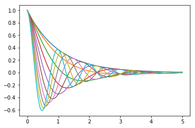"
790 | ]
791 | },
792 | {
793 | "cell_type": "markdown",
794 | "id": "6851914a",
795 | "metadata": {},
796 | "source": [
797 | "## Solution to[ Exercise 11.1](https://python-programming.quantecon.org/#mpl_ex1)\n",
798 | "\n",
799 | "Here’s one solution"
800 | ]
801 | },
802 | {
803 | "cell_type": "code",
804 | "execution_count": null,
805 | "id": "b9e21adc",
806 | "metadata": {
807 | "hide-output": false
808 | },
809 | "outputs": [],
810 | "source": [
811 | "def f(x, θ):\n",
812 | " return np.cos(np.pi * θ * x ) * np.exp(- x)\n",
813 | "\n",
814 | "θ_vals = np.linspace(0, 2, 10)\n",
815 | "x = np.linspace(0, 5, 200)\n",
816 | "fig, ax = plt.subplots()\n",
817 | "\n",
818 | "for θ in θ_vals:\n",
819 | " ax.plot(x, f(x, θ))\n",
820 | "\n",
821 | "plt.show()"
822 | ]
823 | }
824 | ],
825 | "metadata": {
826 | "date": 1764566373.580638,
827 | "filename": "matplotlib.md",
828 | "kernelspec": {
829 | "display_name": "Python",
830 | "language": "python3",
831 | "name": "python3"
832 | },
833 | "title": "Matplotlib"
834 | },
835 | "nbformat": 4,
836 | "nbformat_minor": 5
837 | }
--------------------------------------------------------------------------------
/about_py.ipynb:
--------------------------------------------------------------------------------
1 | {
2 | "cells": [
3 | {
4 | "cell_type": "markdown",
5 | "id": "009ff8e4",
6 | "metadata": {},
7 | "source": [
8 | "\n",
9 | "\n",
10 | "\n",
15 | "\n",
16 | "\n",
17 | ""
18 | ]
19 | },
20 | {
21 | "cell_type": "markdown",
22 | "id": "d710d9b4",
23 | "metadata": {},
24 | "source": [
25 | "# About These Lectures\n",
26 | "\n",
27 | "> “Python has gotten sufficiently weapons grade that we don’t descend into R\n",
28 | "> anymore. Sorry, R people. I used to be one of you but we no longer descend\n",
29 | "> into R.” – Chris Wiggins"
30 | ]
31 | },
32 | {
33 | "cell_type": "markdown",
34 | "id": "e0577b25",
35 | "metadata": {},
36 | "source": [
37 | "## Overview\n",
38 | "\n",
39 | "This lecture series will teach you to use Python for scientific computing, with\n",
40 | "a focus on economics and finance.\n",
41 | "\n",
42 | "The series is aimed at Python novices, although experienced users will also find\n",
43 | "useful content in later lectures.\n",
44 | "\n",
45 | "In this lecture we will\n",
46 | "\n",
47 | "- introduce Python, \n",
48 | "- showcase some of its abilities, \n",
49 | "- explain why Python is our favorite language for scientific computing, and \n",
50 | "- point you to the next steps. \n",
51 | "\n",
52 | "\n",
53 | "You do **not** need to understand everything you see in this lecture – we will work through the details slowly later in the lecture series."
54 | ]
55 | },
56 | {
57 | "cell_type": "markdown",
58 | "id": "351a5ce0",
59 | "metadata": {},
60 | "source": [
61 | "### Can’t I Just Use LLMs?\n",
62 | "\n",
63 | "No!\n",
64 | "\n",
65 | "Of course it’s tempting to think that in the age of AI we don’t need to learn how to code.\n",
66 | "\n",
67 | "And yes, we like to be lazy too sometimes.\n",
68 | "\n",
69 | "In addition, we agree that AIs are outstanding productivity tools for coders.\n",
70 | "\n",
71 | "But AIs cannot reliably solve new problems that they haven’t seen before.\n",
72 | "\n",
73 | "You will need to be the architect and the supervisor – and for these tasks you need to\n",
74 | "be able to read, write, and understand computer code.\n",
75 | "\n",
76 | "Having said that, a good LLM is a useful companion for these lectures – try copy-pasting some\n",
77 | "code from this series and asking for an explanation."
78 | ]
79 | },
80 | {
81 | "cell_type": "markdown",
82 | "id": "9e1aff47",
83 | "metadata": {},
84 | "source": [
85 | "### Isn’t MATLAB Better?\n",
86 | "\n",
87 | "No, no, and one hundred times no.\n",
88 | "\n",
89 | "Nirvana was great (and Soundgarden [was better](https://www.youtube.com/watch?v=3mbBbFH9fAg&list=RD3mbBbFH9fAg)) but\n",
90 | "it’s time to move on from the ’90s.\n",
91 | "\n",
92 | "For most modern problems, Python’s scientific libraries are now far in advance of MATLAB’s capabilities.\n",
93 | "\n",
94 | "This is particularly the case in fast-growing fields such as deep learning and reinforcement learning.\n",
95 | "\n",
96 | "Moreover, all major LLMs are more proficient at writing Python code than MATLAB\n",
97 | "code.\n",
98 | "\n",
99 | "We will discuss relative merits of Python’s libraries throughout this lecture\n",
100 | "series, as well as in our later series on [JAX](https://jax.quantecon.org/intro.html)."
101 | ]
102 | },
103 | {
104 | "cell_type": "markdown",
105 | "id": "95ce9fe1",
106 | "metadata": {},
107 | "source": [
108 | "## Introducing Python\n",
109 | "\n",
110 | "[Python](https://www.python.org) is a general-purpose programming language conceived in 1989 by [Guido van Rossum](https://en.wikipedia.org/wiki/Guido_van_Rossum).\n",
111 | "\n",
112 | "Python is free and [open source](https://en.wikipedia.org/wiki/Open_source), with development coordinated through the [Python Software Foundation](https://www.python.org/psf-landing/).\n",
113 | "\n",
114 | "This is important because it\n",
115 | "\n",
116 | "- saves us money, \n",
117 | "- means that Python is controlled by the community of users rather than a for-profit corporation, and \n",
118 | "- encourages reproducibility and [open science](https://en.wikipedia.org/wiki/Open_science). "
119 | ]
120 | },
121 | {
122 | "cell_type": "markdown",
123 | "id": "9e05fdc4",
124 | "metadata": {},
125 | "source": [
126 | "### Common Uses\n",
127 | "\n",
128 | "Python is a general-purpose language used\n",
129 | "in almost all application domains, including\n",
130 | "\n",
131 | "- AI and computer science \n",
132 | "- other scientific computing \n",
133 | "- communication \n",
134 | "- web development \n",
135 | "- CGI and graphical user interfaces \n",
136 | "- game development \n",
137 | "- resource planning \n",
138 | "- multimedia \n",
139 | "- etc. \n",
140 | "\n",
141 | "\n",
142 | "It is used and supported extensively by large tech firms including\n",
143 | "\n",
144 | "- [Google](https://www.google.com/) \n",
145 | "- [OpenAI](https://openai.com/) \n",
146 | "- [Netflix](https://www.netflix.com/) \n",
147 | "- [Meta](https://opensource.fb.com/) \n",
148 | "- [Amazon](https://www.amazon.com/) \n",
149 | "- [Reddit](https://www.reddit.com/) \n",
150 | "- etc. "
151 | ]
152 | },
153 | {
154 | "cell_type": "markdown",
155 | "id": "6494dd04",
156 | "metadata": {},
157 | "source": [
158 | "### Relative Popularity\n",
159 | "\n",
160 | "Python is one of the most – if not the most – [popular programming languages](https://www.tiobe.com/tiobe-index/).\n",
161 | "\n",
162 | "Python libraries like [pandas](https://pandas.pydata.org/) and [Polars](https://pola.rs/) are replacing familiar tools like Excel and VBA as an essential skill in the fields of finance and banking.\n",
163 | "\n",
164 | "Moreover, Python is extremely popular within the scientific community – especially those connected to AI\n",
165 | "\n",
166 | "For example, the following chart from Stack Overflow Trends shows how the\n",
167 | "popularity of a single Python deep learning library\n",
168 | "([PyTorch](https://pytorch.org/)) has grown over the last few years.\n",
169 | "\n",
170 | "\n",
171 | "\n",
172 | " \n",
173 | "Pytorch is just one of several Python libraries for deep learning and AI."
174 | ]
175 | },
176 | {
177 | "cell_type": "markdown",
178 | "id": "4ec07a27",
179 | "metadata": {},
180 | "source": [
181 | "### Features\n",
182 | "\n",
183 | "Python is a [high-level\n",
184 | "language](https://en.wikipedia.org/wiki/High-level_programming_language), which\n",
185 | "means it is relatively easy to read, write and debug.\n",
186 | "\n",
187 | "It has a relatively small core language that is easy to learn.\n",
188 | "\n",
189 | "This core is supported by many libraries, which can be studied as required.\n",
190 | "\n",
191 | "Python is flexible and pragmatic, supporting multiple programming styles (procedural, object-oriented, functional, etc.)."
192 | ]
193 | },
194 | {
195 | "cell_type": "markdown",
196 | "id": "2f8162d4",
197 | "metadata": {},
198 | "source": [
199 | "### Syntax and Design\n",
200 | "\n",
201 | "\n",
202 | "\n",
203 | "One reason for Python’s popularity is its simple and elegant design.\n",
204 | "\n",
205 | "To get a feeling for this, let’s look at an example.\n",
206 | "\n",
207 | "The code below is written in [Java](https://en.wikipedia.org/wiki/Java_%28programming_language%29) rather than Python.\n",
208 | "\n",
209 | "You do **not** need to read and understand this code!"
210 | ]
211 | },
212 | {
213 | "cell_type": "markdown",
214 | "id": "e212d381",
215 | "metadata": {
216 | "hide-output": false
217 | },
218 | "source": [
219 | "```java\n",
220 | "import java.io.BufferedReader;\n",
221 | "import java.io.FileReader;\n",
222 | "import java.io.IOException;\n",
223 | "\n",
224 | "public class CSVReader {\n",
225 | " public static void main(String[] args) {\n",
226 | " String filePath = \"data.csv\"; \n",
227 | " String line;\n",
228 | " String splitBy = \",\";\n",
229 | " int columnIndex = 1; \n",
230 | " double sum = 0;\n",
231 | " int count = 0;\n",
232 | "\n",
233 | " try (BufferedReader br = new BufferedReader(new FileReader(filePath))) {\n",
234 | " while ((line = br.readLine()) != null) {\n",
235 | " String[] values = line.split(splitBy);\n",
236 | " if (values.length > columnIndex) {\n",
237 | " try {\n",
238 | " double value = Double.parseDouble(\n",
239 | " values[columnIndex]\n",
240 | " );\n",
241 | " sum += value;\n",
242 | " count++;\n",
243 | " } catch (NumberFormatException e) {\n",
244 | " System.out.println(\n",
245 | " \"Skipping non-numeric value: \" + \n",
246 | " values[columnIndex]\n",
247 | " );\n",
248 | " }\n",
249 | " }\n",
250 | " }\n",
251 | " } catch (IOException e) {\n",
252 | " e.printStackTrace();\n",
253 | " }\n",
254 | "\n",
255 | " if (count > 0) {\n",
256 | " double average = sum / count;\n",
257 | " System.out.println(\n",
258 | " \"Average of the second column: \" + average\n",
259 | " );\n",
260 | " } else {\n",
261 | " System.out.println(\n",
262 | " \"No valid numeric data found in the second column.\"\n",
263 | " );\n",
264 | " }\n",
265 | " }\n",
266 | "}\n",
267 | "```\n"
268 | ]
269 | },
270 | {
271 | "cell_type": "markdown",
272 | "id": "1b76b9bd",
273 | "metadata": {},
274 | "source": [
275 | "This Java code opens an imaginary file called `data.csv` and computes the mean\n",
276 | "of the values in the second column.\n",
277 | "\n",
278 | "Here’s Python code that does the same thing.\n",
279 | "\n",
280 | "Even if you don’t yet know Python, you can see that the code is far simpler and easier to read."
281 | ]
282 | },
283 | {
284 | "cell_type": "code",
285 | "execution_count": null,
286 | "id": "846426c7",
287 | "metadata": {
288 | "hide-output": false
289 | },
290 | "outputs": [],
291 | "source": [
292 | "import csv\n",
293 | "\n",
294 | "total, count = 0, 0\n",
295 | "with open('data.csv', mode='r') as file:\n",
296 | " reader = csv.reader(file)\n",
297 | " for row in reader:\n",
298 | " try:\n",
299 | " total += float(row[1])\n",
300 | " count += 1\n",
301 | " except (ValueError, IndexError):\n",
302 | " pass\n",
303 | "print(f\"Average: {total / count if count else 'No valid data'}\")"
304 | ]
305 | },
306 | {
307 | "cell_type": "markdown",
308 | "id": "d8f89822",
309 | "metadata": {},
310 | "source": [
311 | "### The AI Connection\n",
312 | "\n",
313 | "AI is in the process of taking over many tasks currently performed by humans,\n",
314 | "just as other forms of machinery have done over the past few centuries.\n",
315 | "\n",
316 | "Moreover, Python is playing a huge role in the advance of AI and machine learning.\n",
317 | "\n",
318 | "This means that tech firms are pouring money into development of extremely\n",
319 | "powerful Python libraries.\n",
320 | "\n",
321 | "Even if you don’t plan to work on AI and machine learning, you can benefit from\n",
322 | "learning to use some of these libraries for your own projects in economics,\n",
323 | "finance and other fields of science.\n",
324 | "\n",
325 | "These lectures will explain how."
326 | ]
327 | },
328 | {
329 | "cell_type": "markdown",
330 | "id": "5f8d0557",
331 | "metadata": {},
332 | "source": [
333 | "## Scientific Programming with Python\n",
334 | "\n",
335 | "\n",
336 | "\n",
337 | "We have already discussed the importance of Python for AI, machine learning and data science\n",
338 | "\n",
339 | "Python is also one of the dominant players in\n",
340 | "\n",
341 | "- astronomy \n",
342 | "- chemistry \n",
343 | "- computational biology \n",
344 | "- meteorology \n",
345 | "- natural language processing \n",
346 | "- etc. \n",
347 | "\n",
348 | "\n",
349 | "Use of Python is also rising in economics, finance, and adjacent fields like\n",
350 | "operations research – which were previously dominated by MATLAB / Excel / STATA / C / Fortran.\n",
351 | "\n",
352 | "This section briefly showcases some examples of Python for general scientific programming."
353 | ]
354 | },
355 | {
356 | "cell_type": "markdown",
357 | "id": "fafb7017",
358 | "metadata": {},
359 | "source": [
360 | "### NumPy\n",
361 | "\n",
362 | "\n",
363 | "\n",
364 | "One of the most important parts of scientific computing is working with data.\n",
365 | "\n",
366 | "Data is often stored in matrices, vectors and arrays.\n",
367 | "\n",
368 | "We can create a simple array of numbers with pure Python as follows:"
369 | ]
370 | },
371 | {
372 | "cell_type": "code",
373 | "execution_count": null,
374 | "id": "d439910a",
375 | "metadata": {
376 | "hide-output": false
377 | },
378 | "outputs": [],
379 | "source": [
380 | "a = [-3.14, 0, 3.14] # A Python list\n",
381 | "a"
382 | ]
383 | },
384 | {
385 | "cell_type": "markdown",
386 | "id": "350f1a2e",
387 | "metadata": {},
388 | "source": [
389 | "This array is very small so it’s fine to work with pure Python.\n",
390 | "\n",
391 | "But when we want to work with larger arrays in real programs we need more efficiency and more tools.\n",
392 | "\n",
393 | "For this we need to use libraries for working with arrays.\n",
394 | "\n",
395 | "For Python, the most important matrix and array processing library is\n",
396 | "[NumPy](https://numpy.org/) library.\n",
397 | "\n",
398 | "For example, let’s build a NumPy array with 100 elements"
399 | ]
400 | },
401 | {
402 | "cell_type": "code",
403 | "execution_count": null,
404 | "id": "3ec2ca21",
405 | "metadata": {
406 | "hide-output": false
407 | },
408 | "outputs": [],
409 | "source": [
410 | "import numpy as np # Load the library\n",
411 | "\n",
412 | "a = np.linspace(-np.pi, np.pi, 100) # Create even grid from -π to π\n",
413 | "a"
414 | ]
415 | },
416 | {
417 | "cell_type": "markdown",
418 | "id": "eaabd50c",
419 | "metadata": {},
420 | "source": [
421 | "Now let’s transform this array by applying functions to it."
422 | ]
423 | },
424 | {
425 | "cell_type": "code",
426 | "execution_count": null,
427 | "id": "84676785",
428 | "metadata": {
429 | "hide-output": false
430 | },
431 | "outputs": [],
432 | "source": [
433 | "b = np.cos(a) # Apply cosine to each element of a\n",
434 | "c = np.sin(a) # Apply sin to each element of a"
435 | ]
436 | },
437 | {
438 | "cell_type": "markdown",
439 | "id": "b399fc5e",
440 | "metadata": {},
441 | "source": [
442 | "Now we can easily take the inner product of `b` and `c`."
443 | ]
444 | },
445 | {
446 | "cell_type": "code",
447 | "execution_count": null,
448 | "id": "d05cd409",
449 | "metadata": {
450 | "hide-output": false
451 | },
452 | "outputs": [],
453 | "source": [
454 | "b @ c"
455 | ]
456 | },
457 | {
458 | "cell_type": "markdown",
459 | "id": "61409a28",
460 | "metadata": {},
461 | "source": [
462 | "We can also do many other tasks, like\n",
463 | "\n",
464 | "- compute the mean and variance of arrays \n",
465 | "- build matrices and solve linear systems \n",
466 | "- generate random arrays for simulation, etc. \n",
467 | "\n",
468 | "\n",
469 | "We will discuss the details later in the lecture series, where we cover NumPy in depth."
470 | ]
471 | },
472 | {
473 | "cell_type": "markdown",
474 | "id": "48e66b7c",
475 | "metadata": {},
476 | "source": [
477 | "### NumPy Alternatives\n",
478 | "\n",
479 | "While NumPy is still the king of array processing in Python, there are now\n",
480 | "important competitors.\n",
481 | "\n",
482 | "Libraries such as [JAX](https://github.com/jax-ml/jax), [Pytorch](https://pytorch.org/), and [CuPy](https://cupy.dev/) also have\n",
483 | "built in array types and array operations that can be very fast and efficient.\n",
484 | "\n",
485 | "In fact these libraries are better at exploiting parallelization and fast hardware, as\n",
486 | "we’ll explain later in this series.\n",
487 | "\n",
488 | "However, you should still learn NumPy first because\n",
489 | "\n",
490 | "- NumPy is simpler and provides a strong foundation, and \n",
491 | "- libraries like JAX directly extend NumPy functionality and hence are easier to\n",
492 | " learn when you already know NumPy. \n",
493 | "\n",
494 | "\n",
495 | "This lecture series will provide you with extensive background in NumPy."
496 | ]
497 | },
498 | {
499 | "cell_type": "markdown",
500 | "id": "02854a98",
501 | "metadata": {},
502 | "source": [
503 | "### SciPy\n",
504 | "\n",
505 | "The [SciPy](https://scipy.org/) library is built on top of NumPy and provides additional functionality.\n",
506 | "\n",
507 | "\n",
508 | "\n",
509 | "For example, let’s calculate $ \\int_{-2}^2 \\phi(z) dz $ where $ \\phi $ is the standard normal density."
510 | ]
511 | },
512 | {
513 | "cell_type": "code",
514 | "execution_count": null,
515 | "id": "26b39772",
516 | "metadata": {
517 | "hide-output": false
518 | },
519 | "outputs": [],
520 | "source": [
521 | "from scipy.stats import norm\n",
522 | "from scipy.integrate import quad\n",
523 | "\n",
524 | "ϕ = norm()\n",
525 | "value, error = quad(ϕ.pdf, -2, 2) # Integrate using Gaussian quadrature\n",
526 | "value"
527 | ]
528 | },
529 | {
530 | "cell_type": "markdown",
531 | "id": "9bd140c2",
532 | "metadata": {},
533 | "source": [
534 | "SciPy includes many of the standard routines used in\n",
535 | "\n",
536 | "- [linear algebra](https://docs.scipy.org/doc/scipy/reference/linalg.html) \n",
537 | "- [integration](https://docs.scipy.org/doc/scipy/reference/integrate.html) \n",
538 | "- [interpolation](https://docs.scipy.org/doc/scipy/reference/interpolate.html) \n",
539 | "- [optimization](https://docs.scipy.org/doc/scipy/reference/optimize.html) \n",
540 | "- [distributions and statistical techniques](https://docs.scipy.org/doc/scipy/reference/stats.html) \n",
541 | "- [signal processing](https://docs.scipy.org/doc/scipy/reference/signal.html) \n",
542 | "\n",
543 | "\n",
544 | "See them all [here](https://docs.scipy.org/doc/scipy/reference/index.html).\n",
545 | "\n",
546 | "Later we’ll discuss SciPy in more detail."
547 | ]
548 | },
549 | {
550 | "cell_type": "markdown",
551 | "id": "36501eeb",
552 | "metadata": {},
553 | "source": [
554 | "### Graphics\n",
555 | "\n",
556 | "\n",
557 | "\n",
558 | "A major strength of Python is data visualization.\n",
559 | "\n",
560 | "The most popular and comprehensive Python library for creating figures and graphs is [Matplotlib](https://matplotlib.org/), with functionality including\n",
561 | "\n",
562 | "- plots, histograms, contour images, 3D graphs, bar charts etc. \n",
563 | "- output in many formats (PDF, PNG, EPS, etc.) \n",
564 | "- LaTeX integration \n",
565 | "\n",
566 | "\n",
567 | "Example 2D plot with embedded LaTeX annotations\n",
568 | "\n",
569 | "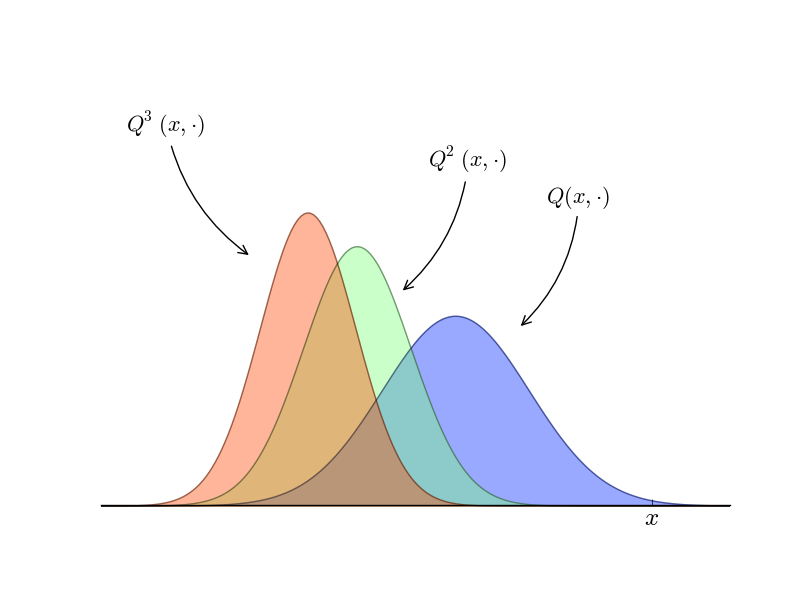\n",
570 | "\n",
571 | " \n",
572 | "Example contour plot\n",
573 | "\n",
574 | "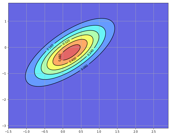\n",
575 | "\n",
576 | " \n",
577 | "Example 3D plot\n",
578 | "\n",
579 | "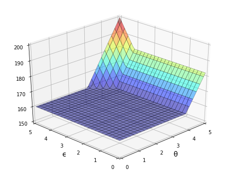\n",
580 | "\n",
581 | " \n",
582 | "More examples can be found in the [Matplotlib thumbnail gallery](https://matplotlib.org/stable/gallery/index.html).\n",
583 | "\n",
584 | "Other graphics libraries include\n",
585 | "\n",
586 | "- [Plotly](https://plotly.com/python/) \n",
587 | "- [seaborn](https://seaborn.pydata.org/) — a high-level interface for matplotlib \n",
588 | "- [Altair](https://altair-viz.github.io/) \n",
589 | "- [Bokeh](https://docs.bokeh.org/en/latest/) \n",
590 | "\n",
591 | "\n",
592 | "You can visit the [Python Graph Gallery](https://python-graph-gallery.com/) for more example plots drawn using a variety of libraries."
593 | ]
594 | },
595 | {
596 | "cell_type": "markdown",
597 | "id": "61b4e05f",
598 | "metadata": {},
599 | "source": [
600 | "### Networks and Graphs\n",
601 | "\n",
602 | "The study of [networks](https://networks.quantecon.org/) is becoming an important part of scientific work\n",
603 | "in economics, finance and other fields.\n",
604 | "\n",
605 | "For example, we are interesting in studying\n",
606 | "\n",
607 | "- production networks \n",
608 | "- networks of banks and financial institutions \n",
609 | "- friendship and social networks \n",
610 | "- etc. \n",
611 | "\n",
612 | "\n",
613 | "Python has many libraries for studying networks and graphs.\n",
614 | "\n",
615 | "\n",
616 | "\n",
617 | "One well-known example is [NetworkX](https://networkx.org/).\n",
618 | "\n",
619 | "Its features include, among many other things:\n",
620 | "\n",
621 | "- standard graph algorithms for analyzing networks \n",
622 | "- plotting routines \n",
623 | "\n",
624 | "\n",
625 | "Here’s some example code that generates and plots a random graph, with node color determined by the shortest path length from a central node."
626 | ]
627 | },
628 | {
629 | "cell_type": "code",
630 | "execution_count": null,
631 | "id": "5a4fb1c7",
632 | "metadata": {
633 | "hide-output": false
634 | },
635 | "outputs": [],
636 | "source": [
637 | "import networkx as nx\n",
638 | "import matplotlib.pyplot as plt\n",
639 | "np.random.seed(1234)\n",
640 | "\n",
641 | "# Generate a random graph\n",
642 | "p = dict((i, (np.random.uniform(0, 1), np.random.uniform(0, 1)))\n",
643 | " for i in range(200))\n",
644 | "g = nx.random_geometric_graph(200, 0.12, pos=p)\n",
645 | "pos = nx.get_node_attributes(g, 'pos')\n",
646 | "\n",
647 | "# Find node nearest the center point (0.5, 0.5)\n",
648 | "dists = [(x - 0.5)**2 + (y - 0.5)**2 for x, y in list(pos.values())]\n",
649 | "ncenter = np.argmin(dists)\n",
650 | "\n",
651 | "# Plot graph, coloring by path length from central node\n",
652 | "p = nx.single_source_shortest_path_length(g, ncenter)\n",
653 | "plt.figure()\n",
654 | "nx.draw_networkx_edges(g, pos, alpha=0.4)\n",
655 | "nx.draw_networkx_nodes(g,\n",
656 | " pos,\n",
657 | " nodelist=list(p.keys()),\n",
658 | " node_size=120, alpha=0.5,\n",
659 | " node_color=list(p.values()),\n",
660 | " cmap=plt.cm.jet_r)\n",
661 | "plt.show()"
662 | ]
663 | },
664 | {
665 | "cell_type": "markdown",
666 | "id": "dcaeb36c",
667 | "metadata": {},
668 | "source": [
669 | "### Other Scientific Libraries\n",
670 | "\n",
671 | "As discussed above, there are literally thousands of scientific libraries for\n",
672 | "Python.\n",
673 | "\n",
674 | "Some are small and do very specific tasks.\n",
675 | "\n",
676 | "Others are huge in terms of lines of code and investment from coders and tech\n",
677 | "firms.\n",
678 | "\n",
679 | "Here’s a short list of some important scientific libraries for Python not\n",
680 | "mentioned above.\n",
681 | "\n",
682 | "- [SymPy](https://www.sympy.org/) for symbolic algebra, including limits, derivatives and integrals \n",
683 | "- [statsmodels](https://www.statsmodels.org/) for statistical routines \n",
684 | "- [scikit-learn](https://scikit-learn.org/) for machine learning \n",
685 | "- [Keras](https://keras.io/) for machine learning \n",
686 | "- [Pyro](https://pyro.ai/) and [PyStan](https://pystan.readthedocs.io/en/latest/) for Bayesian data analysis \n",
687 | "- [GeoPandas](https://geopandas.org/en/stable/) for spatial data analysis \n",
688 | "- [Dask](https://docs.dask.org/en/stable/) for parallelization \n",
689 | "- [Numba](https://numba.pydata.org/) for making Python run at the same speed as native machine code \n",
690 | "- [CVXPY](https://www.cvxpy.org/) for convex optimization \n",
691 | "- [scikit-image](https://scikit-image.org/) and [OpenCV](https://opencv.org/) for processing and analyzing image data \n",
692 | "- [BeautifulSoup](https://www.crummy.com/software/BeautifulSoup/bs4/doc/) for extracting data from HTML and XML files \n",
693 | "\n",
694 | "\n",
695 | "In this lecture series we will learn how to use many of these libraries for\n",
696 | "scientific computing tasks in economics and finance."
697 | ]
698 | }
699 | ],
700 | "metadata": {
701 | "date": 1764566373.3676527,
702 | "filename": "about_py.md",
703 | "kernelspec": {
704 | "display_name": "Python",
705 | "language": "python3",
706 | "name": "python3"
707 | },
708 | "title": "About These Lectures"
709 | },
710 | "nbformat": 4,
711 | "nbformat_minor": 5
712 | }
--------------------------------------------------------------------------------
/debugging.ipynb:
--------------------------------------------------------------------------------
1 | {
2 | "cells": [
3 | {
4 | "cell_type": "markdown",
5 | "id": "0c53dfaa",
6 | "metadata": {},
7 | "source": [
8 | "\n",
9 | "\n",
10 | ""
15 | ]
16 | },
17 | {
18 | "cell_type": "markdown",
19 | "id": "d8fe6fd3",
20 | "metadata": {},
21 | "source": [
22 | "# Debugging and Handling Errors\n",
23 | "\n",
24 | "\n",
25 | "\n",
26 | "> “Debugging is twice as hard as writing the code in the first place.\n",
27 | "> Therefore, if you write the code as cleverly as possible, you are, by definition,\n",
28 | "> not smart enough to debug it.” – Brian Kernighan"
29 | ]
30 | },
31 | {
32 | "cell_type": "markdown",
33 | "id": "394055fc",
34 | "metadata": {},
35 | "source": [
36 | "## Overview\n",
37 | "\n",
38 | "Are you one of those programmers who fills their code with `print` statements when trying to debug their programs?\n",
39 | "\n",
40 | "Hey, we all used to do that.\n",
41 | "\n",
42 | "(OK, sometimes we still do that…)\n",
43 | "\n",
44 | "But once you start writing larger programs you’ll need a better system.\n",
45 | "\n",
46 | "You may also want to handle potential errors in your code as they occur.\n",
47 | "\n",
48 | "In this lecture, we will discuss how to debug our programs and improve error handling."
49 | ]
50 | },
51 | {
52 | "cell_type": "markdown",
53 | "id": "8e0597c5",
54 | "metadata": {},
55 | "source": [
56 | "## Debugging\n",
57 | "\n",
58 | "\n",
59 | "\n",
60 | "Debugging tools for Python vary across platforms, IDEs and editors.\n",
61 | "\n",
62 | "For example, a [visual debugger](https://jupyterlab.readthedocs.io/en/stable/user/debugger.html) is available in JupyterLab.\n",
63 | "\n",
64 | "Here we’ll focus on Jupyter Notebook and leave you to explore other settings.\n",
65 | "\n",
66 | "We’ll need the following imports"
67 | ]
68 | },
69 | {
70 | "cell_type": "code",
71 | "execution_count": null,
72 | "id": "ed089c3f",
73 | "metadata": {
74 | "hide-output": false
75 | },
76 | "outputs": [],
77 | "source": [
78 | "import numpy as np\n",
79 | "import matplotlib.pyplot as plt"
80 | ]
81 | },
82 | {
83 | "cell_type": "markdown",
84 | "id": "a5be54e2",
85 | "metadata": {},
86 | "source": [
87 | "\n",
88 | ""
89 | ]
90 | },
91 | {
92 | "cell_type": "markdown",
93 | "id": "40df3272",
94 | "metadata": {},
95 | "source": [
96 | "### The `debug` Magic\n",
97 | "\n",
98 | "Let’s consider a simple (and rather contrived) example"
99 | ]
100 | },
101 | {
102 | "cell_type": "code",
103 | "execution_count": null,
104 | "id": "03e7fea7",
105 | "metadata": {
106 | "hide-output": false
107 | },
108 | "outputs": [],
109 | "source": [
110 | "def plot_log():\n",
111 | " fig, ax = plt.subplots(2, 1)\n",
112 | " x = np.linspace(1, 2, 10)\n",
113 | " ax.plot(x, np.log(x))\n",
114 | " plt.show()\n",
115 | "\n",
116 | "plot_log() # Call the function, generate plot"
117 | ]
118 | },
119 | {
120 | "cell_type": "markdown",
121 | "id": "c3eae6ca",
122 | "metadata": {},
123 | "source": [
124 | "This code is intended to plot the `log` function over the interval $ [1, 2] $.\n",
125 | "\n",
126 | "But there’s an error here: `plt.subplots(2, 1)` should be just `plt.subplots()`.\n",
127 | "\n",
128 | "(The call `plt.subplots(2, 1)` returns a NumPy array containing two axes objects, suitable for having two subplots on the same figure)\n",
129 | "\n",
130 | "The traceback shows that the error occurs at the method call `ax.plot(x, np.log(x))`.\n",
131 | "\n",
132 | "The error occurs because we have mistakenly made `ax` a NumPy array, and a NumPy array has no `plot` method.\n",
133 | "\n",
134 | "But let’s pretend that we don’t understand this for the moment.\n",
135 | "\n",
136 | "We might suspect there’s something wrong with `ax` but when we try to investigate this object, we get the following exception:"
137 | ]
138 | },
139 | {
140 | "cell_type": "code",
141 | "execution_count": null,
142 | "id": "cf4fb695",
143 | "metadata": {
144 | "hide-output": false
145 | },
146 | "outputs": [],
147 | "source": [
148 | "ax"
149 | ]
150 | },
151 | {
152 | "cell_type": "markdown",
153 | "id": "6f1351a3",
154 | "metadata": {},
155 | "source": [
156 | "The problem is that `ax` was defined inside `plot_log()`, and the name is\n",
157 | "lost once that function terminates.\n",
158 | "\n",
159 | "Let’s try doing it a different way.\n",
160 | "\n",
161 | "We run the first cell block again, generating the same error"
162 | ]
163 | },
164 | {
165 | "cell_type": "code",
166 | "execution_count": null,
167 | "id": "6520ea5a",
168 | "metadata": {
169 | "hide-output": false
170 | },
171 | "outputs": [],
172 | "source": [
173 | "def plot_log():\n",
174 | " fig, ax = plt.subplots(2, 1)\n",
175 | " x = np.linspace(1, 2, 10)\n",
176 | " ax.plot(x, np.log(x))\n",
177 | " plt.show()\n",
178 | "\n",
179 | "plot_log() # Call the function, generate plot"
180 | ]
181 | },
182 | {
183 | "cell_type": "markdown",
184 | "id": "f053bd83",
185 | "metadata": {},
186 | "source": [
187 | "But this time we type in the following cell block"
188 | ]
189 | },
190 | {
191 | "cell_type": "markdown",
192 | "id": "271f1c91",
193 | "metadata": {
194 | "hide-output": false
195 | },
196 | "source": [
197 | "```ipython\n",
198 | "%debug\n",
199 | "```\n"
200 | ]
201 | },
202 | {
203 | "cell_type": "markdown",
204 | "id": "86d54518",
205 | "metadata": {},
206 | "source": [
207 | "You should be dropped into a new prompt that looks something like this"
208 | ]
209 | },
210 | {
211 | "cell_type": "markdown",
212 | "id": "aedae9d6",
213 | "metadata": {
214 | "hide-output": false
215 | },
216 | "source": [
217 | "```ipython\n",
218 | "ipdb>\n",
219 | "```\n"
220 | ]
221 | },
222 | {
223 | "cell_type": "markdown",
224 | "id": "0ffffcf6",
225 | "metadata": {},
226 | "source": [
227 | "(You might see pdb> instead)\n",
228 | "\n",
229 | "Now we can investigate the value of our variables at this point in the program, step forward through the code, etc.\n",
230 | "\n",
231 | "For example, here we simply type the name `ax` to see what’s happening with\n",
232 | "this object:"
233 | ]
234 | },
235 | {
236 | "cell_type": "markdown",
237 | "id": "f1b7a777",
238 | "metadata": {
239 | "hide-output": false
240 | },
241 | "source": [
242 | "```ipython\n",
243 | "ipdb> ax\n",
244 | "array([,\n",
245 | " ], dtype=object)\n",
246 | "```\n"
247 | ]
248 | },
249 | {
250 | "cell_type": "markdown",
251 | "id": "02221f5b",
252 | "metadata": {},
253 | "source": [
254 | "It’s now very clear that `ax` is an array, which clarifies the source of the\n",
255 | "problem.\n",
256 | "\n",
257 | "To find out what else you can do from inside `ipdb` (or `pdb`), use the\n",
258 | "online help"
259 | ]
260 | },
261 | {
262 | "cell_type": "markdown",
263 | "id": "5faf4657",
264 | "metadata": {
265 | "hide-output": false
266 | },
267 | "source": [
268 | "```ipython\n",
269 | "ipdb> h\n",
270 | "\n",
271 | "Documented commands (type help ):\n",
272 | "========================================\n",
273 | "EOF bt cont enable jump pdef r tbreak w\n",
274 | "a c continue exit l pdoc restart u whatis\n",
275 | "alias cl d h list pinfo return unalias where\n",
276 | "args clear debug help n pp run unt\n",
277 | "b commands disable ignore next q s until\n",
278 | "break condition down j p quit step up\n",
279 | "\n",
280 | "Miscellaneous help topics:\n",
281 | "==========================\n",
282 | "exec pdb\n",
283 | "\n",
284 | "Undocumented commands:\n",
285 | "======================\n",
286 | "retval rv\n",
287 | "\n",
288 | "ipdb> h c\n",
289 | "c(ont(inue))\n",
290 | "Continue execution, only stop when a breakpoint is encountered.\n",
291 | "```\n"
292 | ]
293 | },
294 | {
295 | "cell_type": "markdown",
296 | "id": "437d0dc9",
297 | "metadata": {},
298 | "source": [
299 | "### Setting a Break Point\n",
300 | "\n",
301 | "The preceding approach is handy but sometimes insufficient.\n",
302 | "\n",
303 | "Consider the following modified version of our function above"
304 | ]
305 | },
306 | {
307 | "cell_type": "code",
308 | "execution_count": null,
309 | "id": "c0c70f94",
310 | "metadata": {
311 | "hide-output": false
312 | },
313 | "outputs": [],
314 | "source": [
315 | "def plot_log():\n",
316 | " fig, ax = plt.subplots()\n",
317 | " x = np.logspace(1, 2, 10)\n",
318 | " ax.plot(x, np.log(x))\n",
319 | " plt.show()\n",
320 | "\n",
321 | "plot_log()"
322 | ]
323 | },
324 | {
325 | "cell_type": "markdown",
326 | "id": "4d8a2201",
327 | "metadata": {},
328 | "source": [
329 | "Here the original problem is fixed, but we’ve accidentally written\n",
330 | "`np.logspace(1, 2, 10)` instead of `np.linspace(1, 2, 10)`.\n",
331 | "\n",
332 | "Now there won’t be any exception, but the plot won’t look right.\n",
333 | "\n",
334 | "To investigate, it would be helpful if we could inspect variables like `x` during execution of the function.\n",
335 | "\n",
336 | "To this end, we add a “break point” by inserting `breakpoint()` inside the function code block"
337 | ]
338 | },
339 | {
340 | "cell_type": "markdown",
341 | "id": "a0125f13",
342 | "metadata": {
343 | "hide-output": false
344 | },
345 | "source": [
346 | "```python3\n",
347 | "def plot_log():\n",
348 | " breakpoint()\n",
349 | " fig, ax = plt.subplots()\n",
350 | " x = np.logspace(1, 2, 10)\n",
351 | " ax.plot(x, np.log(x))\n",
352 | " plt.show()\n",
353 | "\n",
354 | "plot_log()\n",
355 | "```\n"
356 | ]
357 | },
358 | {
359 | "cell_type": "markdown",
360 | "id": "f96f411e",
361 | "metadata": {},
362 | "source": [
363 | "Now let’s run the script, and investigate via the debugger"
364 | ]
365 | },
366 | {
367 | "cell_type": "markdown",
368 | "id": "95b5001e",
369 | "metadata": {
370 | "hide-output": false
371 | },
372 | "source": [
373 | "```ipython\n",
374 | "> (6)plot_log()\n",
375 | "-> fig, ax = plt.subplots()\n",
376 | "(Pdb) n\n",
377 | "> (7)plot_log()\n",
378 | "-> x = np.logspace(1, 2, 10)\n",
379 | "(Pdb) n\n",
380 | "> (8)plot_log()\n",
381 | "-> ax.plot(x, np.log(x))\n",
382 | "(Pdb) x\n",
383 | "array([ 10. , 12.91549665, 16.68100537, 21.5443469 ,\n",
384 | " 27.82559402, 35.93813664, 46.41588834, 59.94842503,\n",
385 | " 77.42636827, 100. ])\n",
386 | "```\n"
387 | ]
388 | },
389 | {
390 | "cell_type": "markdown",
391 | "id": "0a8a22e7",
392 | "metadata": {},
393 | "source": [
394 | "We used `n` twice to step forward through the code (one line at a time).\n",
395 | "\n",
396 | "Then we printed the value of `x` to see what was happening with that variable.\n",
397 | "\n",
398 | "To exit from the debugger, use `q`."
399 | ]
400 | },
401 | {
402 | "cell_type": "markdown",
403 | "id": "b1670916",
404 | "metadata": {},
405 | "source": [
406 | "### Other Useful Magics\n",
407 | "\n",
408 | "In this lecture, we used the `%debug` IPython magic.\n",
409 | "\n",
410 | "There are many other useful magics:\n",
411 | "\n",
412 | "- `%precision 4` sets printed precision for floats to 4 decimal places \n",
413 | "- `%whos` gives a list of variables and their values \n",
414 | "- `%quickref` gives a list of magics \n",
415 | "\n",
416 | "\n",
417 | "The full list of magics is [here](https://ipython.readthedocs.io/en/stable/interactive/magics.html)."
418 | ]
419 | },
420 | {
421 | "cell_type": "markdown",
422 | "id": "25e1fc32",
423 | "metadata": {},
424 | "source": [
425 | "## Handling Errors\n",
426 | "\n",
427 | "\n",
428 | "\n",
429 | "Sometimes it’s possible to anticipate bugs and errors as we’re writing code.\n",
430 | "\n",
431 | "For example, the unbiased sample variance of sample $ y_1, \\ldots, y_n $\n",
432 | "is defined as\n",
433 | "\n",
434 | "$$\n",
435 | "s^2 := \\frac{1}{n-1} \\sum_{i=1}^n (y_i - \\bar y)^2\n",
436 | "\\qquad \\bar y = \\text{ sample mean}\n",
437 | "$$\n",
438 | "\n",
439 | "This can be calculated in NumPy using `np.var`.\n",
440 | "\n",
441 | "But if you were writing a function to handle such a calculation, you might\n",
442 | "anticipate a divide-by-zero error when the sample size is one.\n",
443 | "\n",
444 | "One possible action is to do nothing — the program will just crash, and spit out an error message.\n",
445 | "\n",
446 | "But sometimes it’s worth writing your code in a way that anticipates and deals with runtime errors that you think might arise.\n",
447 | "\n",
448 | "Why?\n",
449 | "\n",
450 | "- Because the debugging information provided by the interpreter is often less useful than what can be provided by a well written error message. \n",
451 | "- Because errors that cause execution to stop interrupt workflows. \n",
452 | "- Because it reduces confidence in your code on the part of your users (if you are writing for others). \n",
453 | "\n",
454 | "\n",
455 | "In this section, we’ll discuss different types of errors in Python and techniques to handle potential errors in our programs."
456 | ]
457 | },
458 | {
459 | "cell_type": "markdown",
460 | "id": "791b0f5b",
461 | "metadata": {},
462 | "source": [
463 | "### Errors in Python\n",
464 | "\n",
465 | "We have seen `AttributeError` and `NameError` in [our previous examples](#debug-magic).\n",
466 | "\n",
467 | "In Python, there are two types of errors – syntax errors and exceptions.\n",
468 | "\n",
469 | "\n",
470 | "\n",
471 | "Here’s an example of a common error type"
472 | ]
473 | },
474 | {
475 | "cell_type": "code",
476 | "execution_count": null,
477 | "id": "27111380",
478 | "metadata": {
479 | "hide-output": false
480 | },
481 | "outputs": [],
482 | "source": [
483 | "def f:"
484 | ]
485 | },
486 | {
487 | "cell_type": "markdown",
488 | "id": "3e22a4e8",
489 | "metadata": {},
490 | "source": [
491 | "Since illegal syntax cannot be executed, a syntax error terminates execution of the program.\n",
492 | "\n",
493 | "Here’s a different kind of error, unrelated to syntax"
494 | ]
495 | },
496 | {
497 | "cell_type": "code",
498 | "execution_count": null,
499 | "id": "63cf0945",
500 | "metadata": {
501 | "hide-output": false
502 | },
503 | "outputs": [],
504 | "source": [
505 | "1 / 0"
506 | ]
507 | },
508 | {
509 | "cell_type": "markdown",
510 | "id": "140d6a3c",
511 | "metadata": {},
512 | "source": [
513 | "Here’s another"
514 | ]
515 | },
516 | {
517 | "cell_type": "code",
518 | "execution_count": null,
519 | "id": "82f68f56",
520 | "metadata": {
521 | "hide-output": false
522 | },
523 | "outputs": [],
524 | "source": [
525 | "x1 = y1"
526 | ]
527 | },
528 | {
529 | "cell_type": "markdown",
530 | "id": "6aa0aeca",
531 | "metadata": {},
532 | "source": [
533 | "And another"
534 | ]
535 | },
536 | {
537 | "cell_type": "code",
538 | "execution_count": null,
539 | "id": "2bd2ea5c",
540 | "metadata": {
541 | "hide-output": false
542 | },
543 | "outputs": [],
544 | "source": [
545 | "'foo' + 6"
546 | ]
547 | },
548 | {
549 | "cell_type": "markdown",
550 | "id": "0193898a",
551 | "metadata": {},
552 | "source": [
553 | "And another"
554 | ]
555 | },
556 | {
557 | "cell_type": "code",
558 | "execution_count": null,
559 | "id": "5fa80eb5",
560 | "metadata": {
561 | "hide-output": false
562 | },
563 | "outputs": [],
564 | "source": [
565 | "X = []\n",
566 | "x = X[0]"
567 | ]
568 | },
569 | {
570 | "cell_type": "markdown",
571 | "id": "811b2ba0",
572 | "metadata": {},
573 | "source": [
574 | "On each occasion, the interpreter informs us of the error type\n",
575 | "\n",
576 | "- `NameError`, `TypeError`, `IndexError`, `ZeroDivisionError`, etc. \n",
577 | "\n",
578 | "\n",
579 | "In Python, these errors are called *exceptions*."
580 | ]
581 | },
582 | {
583 | "cell_type": "markdown",
584 | "id": "73d468b7",
585 | "metadata": {},
586 | "source": [
587 | "### Assertions\n",
588 | "\n",
589 | "\n",
590 | "\n",
591 | "Sometimes errors can be avoided by checking whether your program runs as expected.\n",
592 | "\n",
593 | "A relatively easy way to handle checks is with the `assert` keyword.\n",
594 | "\n",
595 | "For example, pretend for a moment that the `np.var` function doesn’t\n",
596 | "exist and we need to write our own"
597 | ]
598 | },
599 | {
600 | "cell_type": "code",
601 | "execution_count": null,
602 | "id": "aae85245",
603 | "metadata": {
604 | "hide-output": false
605 | },
606 | "outputs": [],
607 | "source": [
608 | "def var(y):\n",
609 | " n = len(y)\n",
610 | " assert n > 1, 'Sample size must be greater than one.'\n",
611 | " return np.sum((y - y.mean())**2) / float(n-1)"
612 | ]
613 | },
614 | {
615 | "cell_type": "markdown",
616 | "id": "a34a36ae",
617 | "metadata": {},
618 | "source": [
619 | "If we run this with an array of length one, the program will terminate and\n",
620 | "print our error message"
621 | ]
622 | },
623 | {
624 | "cell_type": "code",
625 | "execution_count": null,
626 | "id": "9d9be328",
627 | "metadata": {
628 | "hide-output": false
629 | },
630 | "outputs": [],
631 | "source": [
632 | "var([1])"
633 | ]
634 | },
635 | {
636 | "cell_type": "markdown",
637 | "id": "6673536e",
638 | "metadata": {},
639 | "source": [
640 | "The advantage is that we can\n",
641 | "\n",
642 | "- fail early, as soon as we know there will be a problem \n",
643 | "- supply specific information on why a program is failing "
644 | ]
645 | },
646 | {
647 | "cell_type": "markdown",
648 | "id": "515507a8",
649 | "metadata": {},
650 | "source": [
651 | "### Handling Errors During Runtime\n",
652 | "\n",
653 | "\n",
654 | "\n",
655 | "The approach used above is a bit limited, because it always leads to\n",
656 | "termination.\n",
657 | "\n",
658 | "Sometimes we can handle errors more gracefully, by treating special cases.\n",
659 | "\n",
660 | "Let’s look at how this is done."
661 | ]
662 | },
663 | {
664 | "cell_type": "markdown",
665 | "id": "fae1d8ff",
666 | "metadata": {},
667 | "source": [
668 | "#### Catching Exceptions\n",
669 | "\n",
670 | "We can catch and deal with exceptions using `try` – `except` blocks.\n",
671 | "\n",
672 | "Here’s a simple example"
673 | ]
674 | },
675 | {
676 | "cell_type": "code",
677 | "execution_count": null,
678 | "id": "75322803",
679 | "metadata": {
680 | "hide-output": false
681 | },
682 | "outputs": [],
683 | "source": [
684 | "def f(x):\n",
685 | " try:\n",
686 | " return 1.0 / x\n",
687 | " except ZeroDivisionError:\n",
688 | " print('Error: division by zero. Returned None')\n",
689 | " return None"
690 | ]
691 | },
692 | {
693 | "cell_type": "markdown",
694 | "id": "629a7fe0",
695 | "metadata": {},
696 | "source": [
697 | "When we call `f` we get the following output"
698 | ]
699 | },
700 | {
701 | "cell_type": "code",
702 | "execution_count": null,
703 | "id": "75456262",
704 | "metadata": {
705 | "hide-output": false
706 | },
707 | "outputs": [],
708 | "source": [
709 | "f(2)"
710 | ]
711 | },
712 | {
713 | "cell_type": "code",
714 | "execution_count": null,
715 | "id": "d32b5176",
716 | "metadata": {
717 | "hide-output": false
718 | },
719 | "outputs": [],
720 | "source": [
721 | "f(0)"
722 | ]
723 | },
724 | {
725 | "cell_type": "code",
726 | "execution_count": null,
727 | "id": "8a449e11",
728 | "metadata": {
729 | "hide-output": false
730 | },
731 | "outputs": [],
732 | "source": [
733 | "f(0.0)"
734 | ]
735 | },
736 | {
737 | "cell_type": "markdown",
738 | "id": "3aec217a",
739 | "metadata": {},
740 | "source": [
741 | "The error is caught and execution of the program is not terminated.\n",
742 | "\n",
743 | "Note that other error types are not caught.\n",
744 | "\n",
745 | "If we are worried the user might pass in a string, we can catch that error too"
746 | ]
747 | },
748 | {
749 | "cell_type": "code",
750 | "execution_count": null,
751 | "id": "1f93189a",
752 | "metadata": {
753 | "hide-output": false
754 | },
755 | "outputs": [],
756 | "source": [
757 | "def f(x):\n",
758 | " try:\n",
759 | " return 1.0 / x\n",
760 | " except ZeroDivisionError:\n",
761 | " print('Error: Division by zero. Returned None')\n",
762 | " except TypeError:\n",
763 | " print(f'Error: x cannot be of type {type(x)}. Returned None')\n",
764 | " return None"
765 | ]
766 | },
767 | {
768 | "cell_type": "markdown",
769 | "id": "6df400a4",
770 | "metadata": {},
771 | "source": [
772 | "Here’s what happens"
773 | ]
774 | },
775 | {
776 | "cell_type": "code",
777 | "execution_count": null,
778 | "id": "b76c0ec1",
779 | "metadata": {
780 | "hide-output": false
781 | },
782 | "outputs": [],
783 | "source": [
784 | "f(2)"
785 | ]
786 | },
787 | {
788 | "cell_type": "code",
789 | "execution_count": null,
790 | "id": "aac43b08",
791 | "metadata": {
792 | "hide-output": false
793 | },
794 | "outputs": [],
795 | "source": [
796 | "f(0)"
797 | ]
798 | },
799 | {
800 | "cell_type": "code",
801 | "execution_count": null,
802 | "id": "795d9755",
803 | "metadata": {
804 | "hide-output": false
805 | },
806 | "outputs": [],
807 | "source": [
808 | "f('foo')"
809 | ]
810 | },
811 | {
812 | "cell_type": "markdown",
813 | "id": "c906eb12",
814 | "metadata": {},
815 | "source": [
816 | "If we feel lazy we can catch these errors together"
817 | ]
818 | },
819 | {
820 | "cell_type": "code",
821 | "execution_count": null,
822 | "id": "3f2bd060",
823 | "metadata": {
824 | "hide-output": false
825 | },
826 | "outputs": [],
827 | "source": [
828 | "def f(x):\n",
829 | " try:\n",
830 | " return 1.0 / x\n",
831 | " except:\n",
832 | " print(f'Error. An issue has occurred with x = {x} of type: {type(x)}')\n",
833 | " return None"
834 | ]
835 | },
836 | {
837 | "cell_type": "markdown",
838 | "id": "8c23a97e",
839 | "metadata": {},
840 | "source": [
841 | "Here’s what happens"
842 | ]
843 | },
844 | {
845 | "cell_type": "code",
846 | "execution_count": null,
847 | "id": "a7265526",
848 | "metadata": {
849 | "hide-output": false
850 | },
851 | "outputs": [],
852 | "source": [
853 | "f(2)"
854 | ]
855 | },
856 | {
857 | "cell_type": "code",
858 | "execution_count": null,
859 | "id": "88621234",
860 | "metadata": {
861 | "hide-output": false
862 | },
863 | "outputs": [],
864 | "source": [
865 | "f(0)"
866 | ]
867 | },
868 | {
869 | "cell_type": "code",
870 | "execution_count": null,
871 | "id": "f00a8ee9",
872 | "metadata": {
873 | "hide-output": false
874 | },
875 | "outputs": [],
876 | "source": [
877 | "f('foo')"
878 | ]
879 | },
880 | {
881 | "cell_type": "markdown",
882 | "id": "6b3355d4",
883 | "metadata": {},
884 | "source": [
885 | "In general it’s better to be specific."
886 | ]
887 | },
888 | {
889 | "cell_type": "markdown",
890 | "id": "09798913",
891 | "metadata": {},
892 | "source": [
893 | "## Exercises"
894 | ]
895 | },
896 | {
897 | "cell_type": "markdown",
898 | "id": "b9754fc6",
899 | "metadata": {},
900 | "source": [
901 | "## Exercise 21.1\n",
902 | "\n",
903 | "Suppose we have a text file `numbers.txt` containing the following lines"
904 | ]
905 | },
906 | {
907 | "cell_type": "markdown",
908 | "id": "f49f96ac",
909 | "metadata": {
910 | "hide-output": false
911 | },
912 | "source": [
913 | "```text\n",
914 | "prices\n",
915 | "3\n",
916 | "8\n",
917 | "\n",
918 | "7\n",
919 | "21\n",
920 | "```\n"
921 | ]
922 | },
923 | {
924 | "cell_type": "markdown",
925 | "id": "b74a96f3",
926 | "metadata": {},
927 | "source": [
928 | "Using `try` – `except`, write a program to read in the contents of the file and sum the numbers, ignoring lines without numbers.\n",
929 | "\n",
930 | "You can use the `open()` function we learnt [before](https://python-programming.quantecon.org/python_advanced_features.html#iterators) to open `numbers.txt`."
931 | ]
932 | },
933 | {
934 | "cell_type": "markdown",
935 | "id": "b991f735",
936 | "metadata": {},
937 | "source": [
938 | "## Solution to[ Exercise 21.1](https://python-programming.quantecon.org/#debug_ex1)\n",
939 | "\n",
940 | "Let’s save the data first"
941 | ]
942 | },
943 | {
944 | "cell_type": "code",
945 | "execution_count": null,
946 | "id": "19e3e991",
947 | "metadata": {
948 | "hide-output": false
949 | },
950 | "outputs": [],
951 | "source": [
952 | "%%file numbers.txt\n",
953 | "prices\n",
954 | "3\n",
955 | "8\n",
956 | "\n",
957 | "7\n",
958 | "21"
959 | ]
960 | },
961 | {
962 | "cell_type": "code",
963 | "execution_count": null,
964 | "id": "d5721700",
965 | "metadata": {
966 | "hide-output": false
967 | },
968 | "outputs": [],
969 | "source": [
970 | "f = open('numbers.txt')\n",
971 | "\n",
972 | "total = 0.0\n",
973 | "for line in f:\n",
974 | " try:\n",
975 | " total += float(line)\n",
976 | " except ValueError:\n",
977 | " pass\n",
978 | "\n",
979 | "f.close()\n",
980 | "\n",
981 | "print(total)"
982 | ]
983 | }
984 | ],
985 | "metadata": {
986 | "date": 1764566373.399651,
987 | "filename": "debugging.md",
988 | "kernelspec": {
989 | "display_name": "Python",
990 | "language": "python3",
991 | "name": "python3"
992 | },
993 | "title": "Debugging and Handling Errors"
994 | },
995 | "nbformat": 4,
996 | "nbformat_minor": 5
997 | }
--------------------------------------------------------------------------------
/need_for_speed.ipynb:
--------------------------------------------------------------------------------
1 | {
2 | "cells": [
3 | {
4 | "cell_type": "markdown",
5 | "id": "c96be631",
6 | "metadata": {},
7 | "source": [
8 | "\n",
9 | "\n",
10 | ""
15 | ]
16 | },
17 | {
18 | "cell_type": "markdown",
19 | "id": "f1b5ad46",
20 | "metadata": {},
21 | "source": [
22 | "# Python for Scientific Computing\n",
23 | "\n",
24 | "> “We should forget about small efficiencies, say about 97% of the time:\n",
25 | "> premature optimization is the root of all evil.” – Donald Knuth"
26 | ]
27 | },
28 | {
29 | "cell_type": "markdown",
30 | "id": "46ebe2c6",
31 | "metadata": {},
32 | "source": [
33 | "## Overview\n",
34 | "\n",
35 | "It’s probably safe to say that Python is the most popular language for scientific computing.\n",
36 | "\n",
37 | "This is due to\n",
38 | "\n",
39 | "- the accessible and expressive nature of the language itself, \n",
40 | "- the huge range of high quality scientific libraries, \n",
41 | "- the fact that the language and libraries are open source, \n",
42 | "- the central role that Python plays in data science, machine learning and AI. \n",
43 | "\n",
44 | "\n",
45 | "In previous lectures, we used some scientific Python libraries, including NumPy and Matplotlib.\n",
46 | "\n",
47 | "However, our main focus was the core Python language, rather than the libraries.\n",
48 | "\n",
49 | "Now we turn to the scientific libraries and give them our full attention.\n",
50 | "\n",
51 | "In this introductory lecture, we’ll discuss the following topics:\n",
52 | "\n",
53 | "1. What are the main elements of the scientific Python ecosystem? \n",
54 | "1. How do they fit together? \n",
55 | "1. How is the situation changing over time? \n",
56 | "\n",
57 | "\n",
58 | "In addition to what’s in Anaconda, this lecture will need"
59 | ]
60 | },
61 | {
62 | "cell_type": "code",
63 | "execution_count": null,
64 | "id": "773165ca",
65 | "metadata": {
66 | "hide-output": false
67 | },
68 | "outputs": [],
69 | "source": [
70 | "!pip install quantecon"
71 | ]
72 | },
73 | {
74 | "cell_type": "markdown",
75 | "id": "a38cf882",
76 | "metadata": {},
77 | "source": [
78 | "Let’s start with some imports:"
79 | ]
80 | },
81 | {
82 | "cell_type": "code",
83 | "execution_count": null,
84 | "id": "cb90c358",
85 | "metadata": {
86 | "hide-output": false
87 | },
88 | "outputs": [],
89 | "source": [
90 | "import numpy as np\n",
91 | "import quantecon as qe\n",
92 | "import matplotlib.pyplot as plt\n",
93 | "import random"
94 | ]
95 | },
96 | {
97 | "cell_type": "markdown",
98 | "id": "2d005240",
99 | "metadata": {},
100 | "source": [
101 | "## Major Scientific Libraries\n",
102 | "\n",
103 | "Let’s briefly review Python’s scientific libraries."
104 | ]
105 | },
106 | {
107 | "cell_type": "markdown",
108 | "id": "61340771",
109 | "metadata": {},
110 | "source": [
111 | "### Why do we need them?\n",
112 | "\n",
113 | "One reason we use scientific libraries is because they implement routines we want to use.\n",
114 | "\n",
115 | "- numerical integration, interpolation, linear algebra, root finding, etc. \n",
116 | "\n",
117 | "\n",
118 | "For example, it’s usually better to use an existing routine for root finding than to write a new one from scratch.\n",
119 | "\n",
120 | "(For standard algorithms, efficiency is maximized if the community can\n",
121 | "coordinate on a common set of implementations, written by experts and tuned by\n",
122 | "users to be as fast and robust as possible!)\n",
123 | "\n",
124 | "But this is not the only reason that we use Python’s scientific libraries.\n",
125 | "\n",
126 | "Another is that pure Python is not fast.\n",
127 | "\n",
128 | "So we need libraries that are designed to accelerate execution of Python code.\n",
129 | "\n",
130 | "They do this using two strategies:\n",
131 | "\n",
132 | "1. using compilers that convert Python-like statements into fast machine code for individual threads of logic and \n",
133 | "1. parallelizing tasks across multiple “workers” (e.g., CPUs, individual threads inside GPUs). \n",
134 | "\n",
135 | "\n",
136 | "We will discuss these ideas extensively in this and the remaining lectures from\n",
137 | "this series."
138 | ]
139 | },
140 | {
141 | "cell_type": "markdown",
142 | "id": "f84c2707",
143 | "metadata": {},
144 | "source": [
145 | "### Python’s Scientific Ecosystem\n",
146 | "\n",
147 | "At QuantEcon, the scientific libraries we use most often are\n",
148 | "\n",
149 | "- [NumPy](https://numpy.org/) \n",
150 | "- [SciPy](https://scipy.org/) \n",
151 | "- [Matplotlib](https://matplotlib.org/) \n",
152 | "- [JAX](https://github.com/jax-ml/jax) \n",
153 | "- [Pandas](https://pandas.pydata.org/) \n",
154 | "- [Numba](https://numba.pydata.org/) \n",
155 | "\n",
156 | "\n",
157 | "Here’s how they fit together:\n",
158 | "\n",
159 | "- NumPy forms foundations by providing a basic array data type (think of\n",
160 | " vectors and matrices) and functions for acting on these arrays (e.g., matrix\n",
161 | " multiplication). \n",
162 | "- SciPy builds on NumPy by adding numerical methods routinely used in science (interpolation, optimization, root finding, etc.). \n",
163 | "- Matplotlib is used to generate figures, with a focus on plotting data stored in NumPy arrays. \n",
164 | "- JAX includes array processing operations similar to NumPy, automatic\n",
165 | " differentiation, a parallelization-centric just-in-time compiler, and automated integration with hardware accelerators such as\n",
166 | " GPUs. \n",
167 | "- Pandas provides types and functions for manipulating data. \n",
168 | "- Numba provides a just-in-time compiler that plays well with NumPy and helps accelerate Python code. \n",
169 | "\n",
170 | "\n",
171 | "We will discuss all of these libraries extensively in this lecture series."
172 | ]
173 | },
174 | {
175 | "cell_type": "markdown",
176 | "id": "e45a1420",
177 | "metadata": {},
178 | "source": [
179 | "## Pure Python is slow\n",
180 | "\n",
181 | "As mentioned above, one major attraction of the scientific libraries is greater execution speeds.\n",
182 | "\n",
183 | "We will discuss how scientific libraries can help us accelerate code.\n",
184 | "\n",
185 | "For this topic, it will be helpful if we understand what’s driving slow execution speeds."
186 | ]
187 | },
188 | {
189 | "cell_type": "markdown",
190 | "id": "7f1182c4",
191 | "metadata": {},
192 | "source": [
193 | "### High vs low level code\n",
194 | "\n",
195 | "Higher-level languages like Python are optimized for humans.\n",
196 | "\n",
197 | "This means that the programmer can leave many details to the runtime environment\n",
198 | "\n",
199 | "- specifying variable types \n",
200 | "- memory allocation/deallocation \n",
201 | "- etc. \n",
202 | "\n",
203 | "\n",
204 | "In addition, pure Python is run by an [interpreter](https://en.wikipedia.org/wiki/Interpreter_%28computing%29), which executes code statement-by-statement.\n",
205 | "\n",
206 | "This makes Python flexible, interactive, easy to write, easy to read, and relatively easy to debug.\n",
207 | "\n",
208 | "On the other hand, the standard implementation of Python (called CPython) cannot\n",
209 | "match the speed of compiled languages such as C or Fortran."
210 | ]
211 | },
212 | {
213 | "cell_type": "markdown",
214 | "id": "c87f6528",
215 | "metadata": {},
216 | "source": [
217 | "### Where are the bottlenecks?\n",
218 | "\n",
219 | "Why is this the case?"
220 | ]
221 | },
222 | {
223 | "cell_type": "markdown",
224 | "id": "9eab9a68",
225 | "metadata": {},
226 | "source": [
227 | "#### Dynamic typing\n",
228 | "\n",
229 | "\n",
230 | "\n",
231 | "Consider this Python operation"
232 | ]
233 | },
234 | {
235 | "cell_type": "code",
236 | "execution_count": null,
237 | "id": "95453570",
238 | "metadata": {
239 | "hide-output": false
240 | },
241 | "outputs": [],
242 | "source": [
243 | "a, b = 10, 10\n",
244 | "a + b"
245 | ]
246 | },
247 | {
248 | "cell_type": "markdown",
249 | "id": "3d282fa2",
250 | "metadata": {},
251 | "source": [
252 | "Even for this simple operation, the Python interpreter has a fair bit of work to do.\n",
253 | "\n",
254 | "For example, in the statement `a + b`, the interpreter has to know which\n",
255 | "operation to invoke.\n",
256 | "\n",
257 | "If `a` and `b` are strings, then `a + b` requires string concatenation"
258 | ]
259 | },
260 | {
261 | "cell_type": "code",
262 | "execution_count": null,
263 | "id": "667a771b",
264 | "metadata": {
265 | "hide-output": false
266 | },
267 | "outputs": [],
268 | "source": [
269 | "a, b = 'foo', 'bar'\n",
270 | "a + b"
271 | ]
272 | },
273 | {
274 | "cell_type": "markdown",
275 | "id": "dc8c56bc",
276 | "metadata": {},
277 | "source": [
278 | "If `a` and `b` are lists, then `a + b` requires list concatenation"
279 | ]
280 | },
281 | {
282 | "cell_type": "code",
283 | "execution_count": null,
284 | "id": "e1e86a86",
285 | "metadata": {
286 | "hide-output": false
287 | },
288 | "outputs": [],
289 | "source": [
290 | "a, b = ['foo'], ['bar']\n",
291 | "a + b"
292 | ]
293 | },
294 | {
295 | "cell_type": "markdown",
296 | "id": "4774f74e",
297 | "metadata": {},
298 | "source": [
299 | "(We say that the operator `+` is *overloaded* — its action depends on the\n",
300 | "type of the objects on which it acts)\n",
301 | "\n",
302 | "As a result, when executing `a + b`, Python must first check the type of the objects and then call the correct operation.\n",
303 | "\n",
304 | "This involves a nontrivial overhead.\n",
305 | "\n",
306 | "If we repeatedly execute this expression in a tight loop, the nontrivial\n",
307 | "overhead becomes a large overhead."
308 | ]
309 | },
310 | {
311 | "cell_type": "markdown",
312 | "id": "02dccfe8",
313 | "metadata": {},
314 | "source": [
315 | "#### Static types\n",
316 | "\n",
317 | "\n",
318 | "\n",
319 | "Compiled languages avoid these overheads with explicit, static types.\n",
320 | "\n",
321 | "For example, consider the following C code, which sums the integers from 1 to 10"
322 | ]
323 | },
324 | {
325 | "cell_type": "markdown",
326 | "id": "0fb5d610",
327 | "metadata": {
328 | "hide-output": false
329 | },
330 | "source": [
331 | "```c\n",
332 | "#include \n",
333 | "\n",
334 | "int main(void) {\n",
335 | " int i;\n",
336 | " int sum = 0;\n",
337 | " for (i = 1; i <= 10; i++) {\n",
338 | " sum = sum + i;\n",
339 | " }\n",
340 | " printf(\"sum = %d\\n\", sum);\n",
341 | " return 0;\n",
342 | "}\n",
343 | "```\n"
344 | ]
345 | },
346 | {
347 | "cell_type": "markdown",
348 | "id": "32f59a80",
349 | "metadata": {},
350 | "source": [
351 | "The variables `i` and `sum` are explicitly declared to be integers.\n",
352 | "\n",
353 | "Moreover, when we make a statement such as `int i`, we are making a promise to the compiler\n",
354 | "that `i` will *always* be an integer, throughout execution of the program.\n",
355 | "\n",
356 | "As such, the meaning of addition in the expression `sum + i` is completely unambiguous.\n",
357 | "\n",
358 | "There is no need for type-checking and hence no overhead."
359 | ]
360 | },
361 | {
362 | "cell_type": "markdown",
363 | "id": "b0527c18",
364 | "metadata": {},
365 | "source": [
366 | "### Data Access\n",
367 | "\n",
368 | "Another drag on speed for high-level languages is data access.\n",
369 | "\n",
370 | "To illustrate, let’s consider the problem of summing some data — say, a collection of integers."
371 | ]
372 | },
373 | {
374 | "cell_type": "markdown",
375 | "id": "2caf9d06",
376 | "metadata": {},
377 | "source": [
378 | "#### Summing with Compiled Code\n",
379 | "\n",
380 | "In C or Fortran, these integers would typically be stored in an array, which\n",
381 | "is a simple data structure for storing homogeneous data.\n",
382 | "\n",
383 | "Such an array is stored in a single contiguous block of memory\n",
384 | "\n",
385 | "- In modern computers, memory addresses are allocated to each byte (one byte = 8 bits). \n",
386 | "- For example, a 64 bit integer is stored in 8 bytes of memory. \n",
387 | "- An array of $ n $ such integers occupies $ 8n $ *consecutive* memory slots. \n",
388 | "\n",
389 | "\n",
390 | "Moreover, the compiler is made aware of the data type by the programmer.\n",
391 | "\n",
392 | "- In this case 64 bit integers \n",
393 | "\n",
394 | "\n",
395 | "Hence, each successive data point can be accessed by shifting forward in memory\n",
396 | "space by a known and fixed amount.\n",
397 | "\n",
398 | "- In this case 8 bytes "
399 | ]
400 | },
401 | {
402 | "cell_type": "markdown",
403 | "id": "e79d9d8e",
404 | "metadata": {},
405 | "source": [
406 | "#### Summing in Pure Python\n",
407 | "\n",
408 | "Python tries to replicate these ideas to some degree.\n",
409 | "\n",
410 | "For example, in the standard Python implementation (CPython), list elements are placed in memory locations that are in a sense contiguous.\n",
411 | "\n",
412 | "However, these list elements are more like pointers to data rather than actual data.\n",
413 | "\n",
414 | "Hence, there is still overhead involved in accessing the data values themselves.\n",
415 | "\n",
416 | "This is a considerable drag on speed.\n",
417 | "\n",
418 | "In fact, it’s generally true that memory traffic is a major culprit when it comes to slow execution."
419 | ]
420 | },
421 | {
422 | "cell_type": "markdown",
423 | "id": "5026413d",
424 | "metadata": {},
425 | "source": [
426 | "### Summary\n",
427 | "\n",
428 | "Does the discussion above mean that we should just switch to C or Fortran for everything?\n",
429 | "\n",
430 | "The answer is: Definitely not!\n",
431 | "\n",
432 | "For any given program, relatively few lines are ever going to be time-critical.\n",
433 | "\n",
434 | "Hence it is far more efficient to write most of our code in a high productivity language like Python.\n",
435 | "\n",
436 | "Moreover, even for those lines of code that *are* time-critical, we can now\n",
437 | "equal or outpace binaries compiled from C or Fortran by using Python’s scientific libraries.\n",
438 | "\n",
439 | "On that note, we emphasize that, in the last few years, accelerating code has become essentially\n",
440 | "synonymous with parallelization.\n",
441 | "\n",
442 | "This task is best left to specialized compilers!\n",
443 | "\n",
444 | "Certain Python libraries have outstanding capabilities for parallelizing scientific code – we’ll discuss this more as we go along."
445 | ]
446 | },
447 | {
448 | "cell_type": "markdown",
449 | "id": "1f48dc86",
450 | "metadata": {},
451 | "source": [
452 | "## Accelerating Python\n",
453 | "\n",
454 | "In this section we look at three related techniques for accelerating Python\n",
455 | "code.\n",
456 | "\n",
457 | "Here we’ll focus on the fundamental ideas.\n",
458 | "\n",
459 | "Later we’ll look at specific libraries and how they implement these ideas."
460 | ]
461 | },
462 | {
463 | "cell_type": "markdown",
464 | "id": "a832f48d",
465 | "metadata": {},
466 | "source": [
467 | "### Vectorization\n",
468 | "\n",
469 | "\n",
470 | "\n",
471 | "One method for avoiding memory traffic and type checking is [array\n",
472 | "programming](https://en.wikipedia.org/wiki/Array_programming).\n",
473 | "\n",
474 | "Many economists usually refer to array programming as “vectorization.”\n",
475 | "\n",
476 | ">**Note**\n",
477 | ">\n",
478 | ">In computer science, this term has [a slightly different meaning](https://en.wikipedia.org/wiki/Automatic_vectorization).\n",
479 | "\n",
480 | "The key idea is to send array processing operations in batch to pre-compiled\n",
481 | "and efficient native machine code.\n",
482 | "\n",
483 | "The machine code itself is typically compiled from carefully optimized C or Fortran.\n",
484 | "\n",
485 | "For example, when working in a high level language, the operation of inverting a\n",
486 | "large matrix can be subcontracted to efficient machine code that is pre-compiled\n",
487 | "for this purpose and supplied to users as part of a package.\n",
488 | "\n",
489 | "The core benefits are\n",
490 | "\n",
491 | "1. type-checking is paid *per array*, rather than per element, and \n",
492 | "1. arrays containing elements with the same data type are efficient in terms of\n",
493 | " memory access. \n",
494 | "\n",
495 | "\n",
496 | "The idea of vectorization dates back to MATLAB, which uses vectorization extensively.\n",
497 | "\n",
498 | "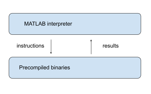"
499 | ]
500 | },
501 | {
502 | "cell_type": "markdown",
503 | "id": "5ff8e300",
504 | "metadata": {},
505 | "source": [
506 | "### Vectorization vs for pure Python loops\n",
507 | "\n",
508 | "Let’s try a quick speed comparison to illustrate how vectorization can\n",
509 | "accelerate code.\n",
510 | "\n",
511 | "Here’s some non-vectorized code, which uses a native Python loop to generate,\n",
512 | "square and then sum a large number of random variables:"
513 | ]
514 | },
515 | {
516 | "cell_type": "code",
517 | "execution_count": null,
518 | "id": "e3f810eb",
519 | "metadata": {
520 | "hide-output": false
521 | },
522 | "outputs": [],
523 | "source": [
524 | "n = 1_000_000"
525 | ]
526 | },
527 | {
528 | "cell_type": "code",
529 | "execution_count": null,
530 | "id": "38c0dc0e",
531 | "metadata": {
532 | "hide-output": false
533 | },
534 | "outputs": [],
535 | "source": [
536 | "with qe.Timer():\n",
537 | " y = 0 # Will accumulate and store sum\n",
538 | " for i in range(n):\n",
539 | " x = random.uniform(0, 1)\n",
540 | " y += x**2"
541 | ]
542 | },
543 | {
544 | "cell_type": "markdown",
545 | "id": "33757495",
546 | "metadata": {},
547 | "source": [
548 | "The following vectorized code uses NumPy, which we’ll soon investigate in depth,\n",
549 | "to achieve the same thing."
550 | ]
551 | },
552 | {
553 | "cell_type": "code",
554 | "execution_count": null,
555 | "id": "c35c0025",
556 | "metadata": {
557 | "hide-output": false
558 | },
559 | "outputs": [],
560 | "source": [
561 | "with qe.Timer():\n",
562 | " x = np.random.uniform(0, 1, n)\n",
563 | " y = np.sum(x**2)"
564 | ]
565 | },
566 | {
567 | "cell_type": "markdown",
568 | "id": "c617ed8f",
569 | "metadata": {},
570 | "source": [
571 | "As you can see, the second code block runs much faster.\n",
572 | "\n",
573 | "It breaks the loop down into three basic operations\n",
574 | "\n",
575 | "1. draw `n` uniforms \n",
576 | "1. square them \n",
577 | "1. sum them \n",
578 | "\n",
579 | "\n",
580 | "These are sent as batch operators to optimized machine code.\n",
581 | "\n",
582 | "\n",
583 | ""
584 | ]
585 | },
586 | {
587 | "cell_type": "markdown",
588 | "id": "ebd28718",
589 | "metadata": {},
590 | "source": [
591 | "### JIT compilers\n",
592 | "\n",
593 | "At best, vectorization yields fast, simple code.\n",
594 | "\n",
595 | "However, it’s not without disadvantages.\n",
596 | "\n",
597 | "One issue is that it can be highly memory-intensive.\n",
598 | "\n",
599 | "This is because vectorization tends to create many intermediate arrays before\n",
600 | "producing the final calculation.\n",
601 | "\n",
602 | "Another issue is that not all algorithms can be vectorized.\n",
603 | "\n",
604 | "Because of these issues, most high performance computing is moving away from\n",
605 | "traditional vectorization and towards the use of [just-in-time\n",
606 | "compilers](https://en.wikipedia.org/wiki/Just-in-time_compilation).\n",
607 | "\n",
608 | "In later lectures in this series, we will learn about how modern Python\n",
609 | "libraries exploit just-in-time compilers to generate fast, efficient,\n",
610 | "parallelized machine code."
611 | ]
612 | },
613 | {
614 | "cell_type": "markdown",
615 | "id": "50a3be7a",
616 | "metadata": {},
617 | "source": [
618 | "## Parallelization\n",
619 | "\n",
620 | "The growth of CPU clock speed (i.e., the speed at which a single chain of logic\n",
621 | "can be run) has slowed dramatically in recent years.\n",
622 | "\n",
623 | "Chip designers and computer programmers have responded to the slowdown by\n",
624 | "seeking a different path to fast execution: parallelization.\n",
625 | "\n",
626 | "Hardware makers have increased the number of cores (physical CPUs) embedded in each machine.\n",
627 | "\n",
628 | "For programmers, the challenge has been to exploit these multiple CPUs by\n",
629 | "running many processes in parallel (i.e., simultaneously).\n",
630 | "\n",
631 | "This is particularly important in scientific programming, which requires handling\n",
632 | "\n",
633 | "- large amounts of data and \n",
634 | "- CPU intensive simulations and other calculations. \n",
635 | "\n",
636 | "\n",
637 | "Below we discuss parallelization for scientific computing, with a focus on\n",
638 | "\n",
639 | "1. the best tools for parallelization in Python and \n",
640 | "1. how these tools can be applied to quantitative economic problems. "
641 | ]
642 | },
643 | {
644 | "cell_type": "markdown",
645 | "id": "82c3cd59",
646 | "metadata": {},
647 | "source": [
648 | "### Parallelization on CPUs\n",
649 | "\n",
650 | "Let’s review the two main kinds of CPU-based parallelization commonly used in\n",
651 | "scientific computing and discuss their pros and cons."
652 | ]
653 | },
654 | {
655 | "cell_type": "markdown",
656 | "id": "b541a5f4",
657 | "metadata": {},
658 | "source": [
659 | "#### Multiprocessing\n",
660 | "\n",
661 | "Multiprocessing means concurrent execution of multiple processes using more than one processor.\n",
662 | "\n",
663 | "In this context, a **process** is a chain of instructions (i.e., a program).\n",
664 | "\n",
665 | "Multiprocessing can be carried out on one machine with multiple CPUs or on a\n",
666 | "collection of machines connected by a network.\n",
667 | "\n",
668 | "In the latter case, the collection of machines is usually called a\n",
669 | "**cluster**.\n",
670 | "\n",
671 | "With multiprocessing, each process has its own memory space, although the\n",
672 | "physical memory chip might be shared."
673 | ]
674 | },
675 | {
676 | "cell_type": "markdown",
677 | "id": "d6570ac9",
678 | "metadata": {},
679 | "source": [
680 | "#### Multithreading\n",
681 | "\n",
682 | "Multithreading is similar to multiprocessing, except that, during execution, the threads all share the same memory space.\n",
683 | "\n",
684 | "Native Python struggles to implement multithreading due to some [legacy design\n",
685 | "features](https://wiki.python.org/moin/GlobalInterpreterLock).\n",
686 | "\n",
687 | "But this is not a restriction for scientific libraries like NumPy and Numba.\n",
688 | "\n",
689 | "Functions imported from these libraries and JIT-compiled code run in low level\n",
690 | "execution environments where Python’s legacy restrictions don’t apply."
691 | ]
692 | },
693 | {
694 | "cell_type": "markdown",
695 | "id": "51031514",
696 | "metadata": {},
697 | "source": [
698 | "#### Advantages and Disadvantages\n",
699 | "\n",
700 | "Multithreading is more lightweight because most system and memory resources\n",
701 | "are shared by the threads.\n",
702 | "\n",
703 | "In addition, the fact that multiple threads all access a shared pool of memory\n",
704 | "is extremely convenient for numerical programming.\n",
705 | "\n",
706 | "On the other hand, multiprocessing is more flexible and can be distributed\n",
707 | "across clusters.\n",
708 | "\n",
709 | "For the great majority of what we do in these lectures, multithreading will\n",
710 | "suffice."
711 | ]
712 | },
713 | {
714 | "cell_type": "markdown",
715 | "id": "43384a4c",
716 | "metadata": {},
717 | "source": [
718 | "### Hardware Accelerators\n",
719 | "\n",
720 | "While CPUs with multiple cores have become standard for parallel computing, a\n",
721 | "more dramatic shift has occurred with the rise of specialized hardware\n",
722 | "accelerators.\n",
723 | "\n",
724 | "These accelerators are designed specifically for the kinds of highly parallel\n",
725 | "computations that arise in scientific computing, machine learning, and data\n",
726 | "science."
727 | ]
728 | },
729 | {
730 | "cell_type": "markdown",
731 | "id": "02a1f1f9",
732 | "metadata": {},
733 | "source": [
734 | "#### GPUs and TPUs\n",
735 | "\n",
736 | "The two most important types of hardware accelerators are\n",
737 | "\n",
738 | "- **GPUs** (Graphics Processing Units) and \n",
739 | "- **TPUs** (Tensor Processing Units). \n",
740 | "\n",
741 | "\n",
742 | "GPUs were originally designed for rendering graphics, which requires performing\n",
743 | "the same operation on many pixels simultaneously.\n",
744 | "\n",
745 | "\n",
746 | "\n",
747 | " \n",
748 | "Scientists and engineers realized that this same architecture — many simple\n",
749 | "processors working in parallel — is ideal for scientific computing tasks\n",
750 | "\n",
751 | "TPUs are a more recent development, designed by Google specifically for machine learning workloads.\n",
752 | "\n",
753 | "Like GPUs, TPUs excel at performing massive numbers of matrix operations in parallel."
754 | ]
755 | },
756 | {
757 | "cell_type": "markdown",
758 | "id": "95051a87",
759 | "metadata": {},
760 | "source": [
761 | "#### Why TPUs/GPUs Matter\n",
762 | "\n",
763 | "The performance gains from using hardware accelerators can be dramatic.\n",
764 | "\n",
765 | "For example, a modern GPU can contain thousands of small processing cores,\n",
766 | "compared to the 8-64 cores typically found in CPUs.\n",
767 | "\n",
768 | "When a problem can be expressed as many independent operations on arrays of\n",
769 | "data, GPUs can be orders of magnitude faster than CPUs.\n",
770 | "\n",
771 | "This is particularly relevant for scientific computing because many algorithms\n",
772 | "naturally map onto the parallel architecture of GPUs."
773 | ]
774 | },
775 | {
776 | "cell_type": "markdown",
777 | "id": "2252e4be",
778 | "metadata": {},
779 | "source": [
780 | "### Single GPUs vs GPU Servers\n",
781 | "\n",
782 | "There are two common ways to access GPU resources:"
783 | ]
784 | },
785 | {
786 | "cell_type": "markdown",
787 | "id": "38b9f991",
788 | "metadata": {},
789 | "source": [
790 | "#### Single GPU Systems\n",
791 | "\n",
792 | "Many workstations and laptops now come with capable GPUs, or can be equipped with them.\n",
793 | "\n",
794 | "A single modern GPU can dramatically accelerate many scientific computing tasks.\n",
795 | "\n",
796 | "For individual researchers and small projects, a single GPU is often sufficient.\n",
797 | "\n",
798 | "Modern Python libraries like JAX, discussed extensively in this lecture series,\n",
799 | "automatically detect and use available GPUs with minimal code changes."
800 | ]
801 | },
802 | {
803 | "cell_type": "markdown",
804 | "id": "25adf4d2",
805 | "metadata": {},
806 | "source": [
807 | "#### Multi-GPU Servers\n",
808 | "\n",
809 | "For larger-scale problems, servers containing multiple GPUs (often 4-8 GPUs per server) are increasingly common.\n",
810 | "\n",
811 | "\n",
812 | "\n",
813 | " \n",
814 | "With appropriate software, computations can be distributed across multiple GPUs, either within a single server or across multiple servers.\n",
815 | "\n",
816 | "This enables researchers to tackle problems that would be infeasible on a single GPU or CPU."
817 | ]
818 | },
819 | {
820 | "cell_type": "markdown",
821 | "id": "e69f5630",
822 | "metadata": {},
823 | "source": [
824 | "### Summary\n",
825 | "\n",
826 | "GPU computing is becoming far more accessible, particularly from within Python.\n",
827 | "\n",
828 | "Some Python scientific libraries, like JAX, now support GPU acceleration with minimal changes to existing code.\n",
829 | "\n",
830 | "We will explore GPU computing in more detail in later lectures, applying it to a\n",
831 | "range of economic applications."
832 | ]
833 | }
834 | ],
835 | "metadata": {
836 | "date": 1764566373.6494503,
837 | "filename": "need_for_speed.md",
838 | "kernelspec": {
839 | "display_name": "Python",
840 | "language": "python3",
841 | "name": "python3"
842 | },
843 | "title": "Python for Scientific Computing"
844 | },
845 | "nbformat": 4,
846 | "nbformat_minor": 5
847 | }
--------------------------------------------------------------------------------
/getting_started.ipynb:
--------------------------------------------------------------------------------
1 | {
2 | "cells": [
3 | {
4 | "cell_type": "markdown",
5 | "id": "ac8e9024",
6 | "metadata": {},
7 | "source": [
8 | "\n",
9 | "\n",
10 | ""
15 | ]
16 | },
17 | {
18 | "cell_type": "markdown",
19 | "id": "671bc87d",
20 | "metadata": {},
21 | "source": [
22 | "# Getting Started\n",
23 | "\n",
24 | "\n",
25 | ""
26 | ]
27 | },
28 | {
29 | "cell_type": "markdown",
30 | "id": "e639d1c8",
31 | "metadata": {},
32 | "source": [
33 | "## Overview\n",
34 | "\n",
35 | "In this lecture, you will learn how to\n",
36 | "\n",
37 | "1. use Python in the cloud \n",
38 | "1. get a local Python environment up and running \n",
39 | "1. execute simple Python commands \n",
40 | "1. run a sample program \n",
41 | "1. install the code libraries that underpin these lectures "
42 | ]
43 | },
44 | {
45 | "cell_type": "markdown",
46 | "id": "5453a941",
47 | "metadata": {},
48 | "source": [
49 | "## Python in the Cloud\n",
50 | "\n",
51 | "The easiest way to get started coding in Python is by running it in the cloud.\n",
52 | "\n",
53 | "(That is, by using a remote server that already has Python installed.)\n",
54 | "\n",
55 | "One option that’s both free and reliable is [Google Colab](https://colab.research.google.com/).\n",
56 | "\n",
57 | "Colab also has the advantage of providing GPUs, which we will make use of in\n",
58 | "more advanced lectures.\n",
59 | "\n",
60 | "Tutorials on how to get started with Google Colab can be found by web and video searches.\n",
61 | "\n",
62 | "Most of our lectures include a “Launch notebook” button (with a play icon) on the top\n",
63 | "right connects you to an executable version on Colab."
64 | ]
65 | },
66 | {
67 | "cell_type": "markdown",
68 | "id": "75238e1e",
69 | "metadata": {},
70 | "source": [
71 | "## Local Install\n",
72 | "\n",
73 | "Local installs are preferable if you have access to a suitable machine and\n",
74 | "plan to do a substantial amount of Python programming.\n",
75 | "\n",
76 | "At the same time, local installs require more work than a cloud option like Colab.\n",
77 | "\n",
78 | "The rest of this lecture runs you through the some details associated with local installs."
79 | ]
80 | },
81 | {
82 | "cell_type": "markdown",
83 | "id": "bb21461c",
84 | "metadata": {},
85 | "source": [
86 | "### The Anaconda Distribution\n",
87 | "\n",
88 | "The [core Python package](https://www.python.org/downloads/) is easy to install but *not* what you should choose for these lectures.\n",
89 | "\n",
90 | "These lectures require the entire scientific programming ecosystem, which\n",
91 | "\n",
92 | "- the core installation doesn’t provide \n",
93 | "- is painful to install one piece at a time. \n",
94 | "\n",
95 | "\n",
96 | "Hence the best approach for our purposes is to install a Python distribution that contains\n",
97 | "\n",
98 | "1. the core Python language **and** \n",
99 | "1. compatible versions of the most popular scientific libraries. \n",
100 | "\n",
101 | "\n",
102 | "The best such distribution is [Anaconda Python](https://www.anaconda.com/).\n",
103 | "\n",
104 | "Anaconda is\n",
105 | "\n",
106 | "- very popular \n",
107 | "- cross-platform \n",
108 | "- comprehensive \n",
109 | "- completely unrelated to the [Nicki Minaj song of the same name](https://www.youtube.com/watch?v=LDZX4ooRsWs) \n",
110 | "\n",
111 | "\n",
112 | "Anaconda also comes with a package management system to organize your code libraries.\n",
113 | "\n",
114 | "**All of what follows assumes that you adopt this recommendation!**\n",
115 | "\n",
116 | "\n",
117 | ""
118 | ]
119 | },
120 | {
121 | "cell_type": "markdown",
122 | "id": "cd641504",
123 | "metadata": {},
124 | "source": [
125 | "### Installing Anaconda\n",
126 | "\n",
127 | "\n",
128 | "\n",
129 | "To install Anaconda, [download](https://www.anaconda.com/download) the binary and follow the instructions.\n",
130 | "\n",
131 | "Important points:\n",
132 | "\n",
133 | "- Make sure you install the correct version for your OS. \n",
134 | "- If you are asked during the installation process whether you’d like to make Anaconda your default Python installation, say yes. "
135 | ]
136 | },
137 | {
138 | "cell_type": "markdown",
139 | "id": "eebb136b",
140 | "metadata": {},
141 | "source": [
142 | "### Updating `conda`\n",
143 | "\n",
144 | "Anaconda supplies a tool called `conda` to manage and upgrade your Anaconda packages.\n",
145 | "\n",
146 | "One `conda` command you should execute regularly is the one that updates the whole Anaconda distribution.\n",
147 | "\n",
148 | "As a practice run, please execute the following\n",
149 | "\n",
150 | "1. Open up a terminal \n",
151 | "1. Type `conda update conda` \n",
152 | "\n",
153 | "\n",
154 | "For more information on conda, type conda help in a terminal.\n",
155 | "\n",
156 | "\n",
157 | ""
158 | ]
159 | },
160 | {
161 | "cell_type": "markdown",
162 | "id": "8c0b025d",
163 | "metadata": {},
164 | "source": [
165 | "## Jupyter Notebooks\n",
166 | "\n",
167 | "\n",
168 | "\n",
169 | "\n",
170 | "\n",
171 | "\n",
172 | "\n",
173 | "[Jupyter](https://jupyter.org/) notebooks are one of the many possible ways to interact with Python and the scientific libraries.\n",
174 | "\n",
175 | "They use a *browser-based* interface to Python with\n",
176 | "\n",
177 | "- The ability to write and execute Python commands. \n",
178 | "- Formatted output in the browser, including tables, figures, animation, etc. \n",
179 | "- The option to mix in formatted text and mathematical expressions. \n",
180 | "\n",
181 | "\n",
182 | "Because of these features, Jupyter is now a major player in the scientific computing ecosystem.\n",
183 | "\n",
184 | "Here’s an image showing execution of some code (borrowed from [here](https://matplotlib.org/stable/gallery/statistics/hexbin_demo.html)) in a Jupyter notebook\n",
185 | "\n",
186 | "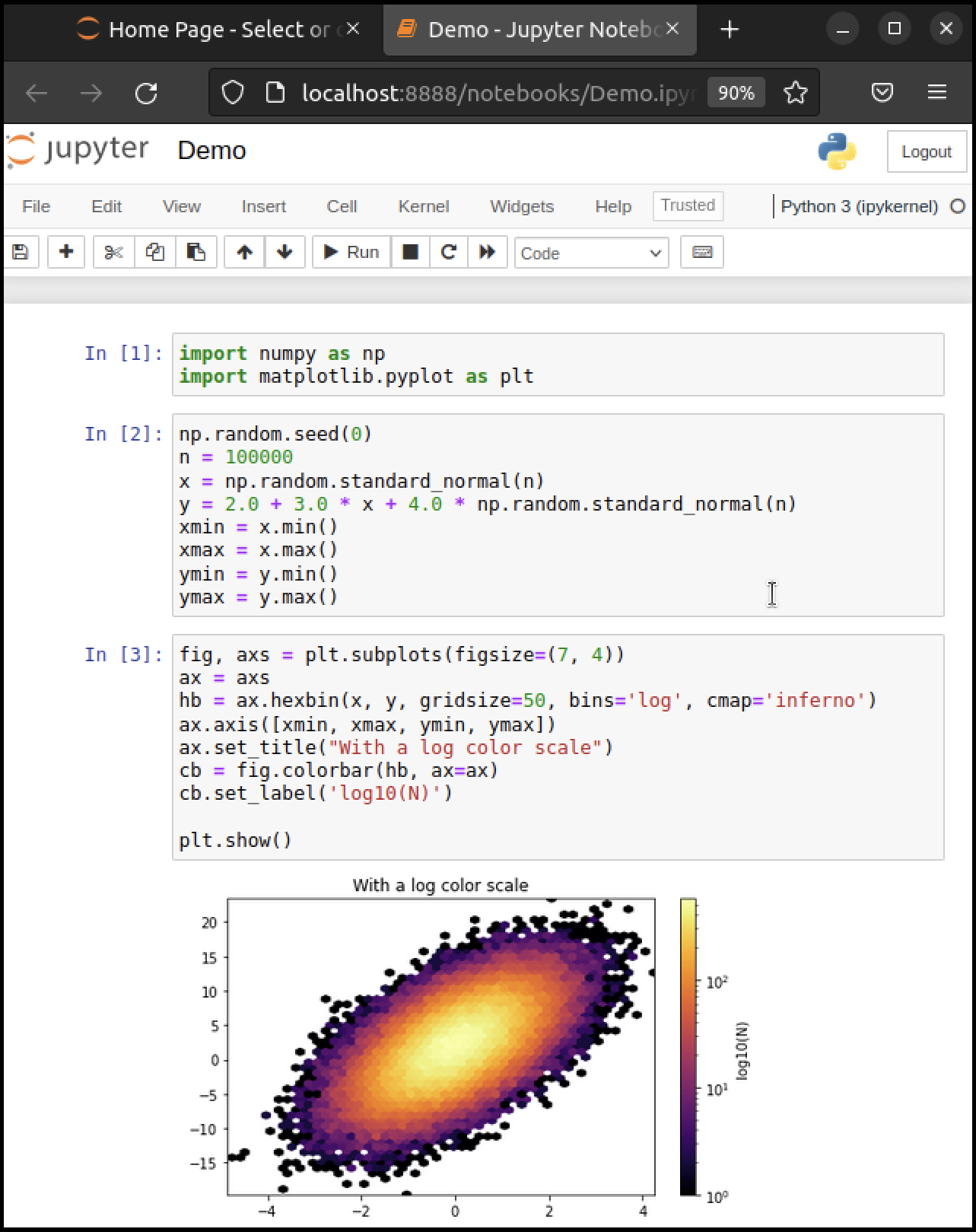\n",
187 | "\n",
188 | " \n",
189 | "While Jupyter isn’t the only way to code in Python, it’s great for when you wish to\n",
190 | "\n",
191 | "- start coding in Python \n",
192 | "- test new ideas or interact with small pieces of code \n",
193 | "- use powerful online interactive environments such as [Google Colab](https://research.google.com/colaboratory/) \n",
194 | "- share or collaborate scientific ideas with students or colleagues \n",
195 | "\n",
196 | "\n",
197 | "These lectures are designed for executing in Jupyter notebooks."
198 | ]
199 | },
200 | {
201 | "cell_type": "markdown",
202 | "id": "906305d0",
203 | "metadata": {},
204 | "source": [
205 | "### Starting the Jupyter Notebook\n",
206 | "\n",
207 | "\n",
208 | "\n",
209 | "Once you have installed Anaconda, you can start the Jupyter notebook.\n",
210 | "\n",
211 | "Either\n",
212 | "\n",
213 | "- search for Jupyter in your applications menu, or \n",
214 | "- open up a terminal and type `jupyter notebook` \n",
215 | " - Windows users should substitute “Anaconda command prompt” for “terminal” in the previous line. \n",
216 | "\n",
217 | "\n",
218 | "If you use the second option, you will see something like this\n",
219 | "\n",
220 | "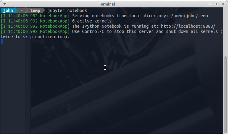\n",
221 | "\n",
222 | " \n",
223 | "The output tells us the notebook is running at `http://localhost:8888/`\n",
224 | "\n",
225 | "- `localhost` is the name of the local machine \n",
226 | "- `8888` refers to [port number](https://en.wikipedia.org/wiki/Port_%28computer_networking%29) 8888 on your computer \n",
227 | "\n",
228 | "\n",
229 | "Thus, the Jupyter kernel is listening for Python commands on port 8888 of our local machine.\n",
230 | "\n",
231 | "Hopefully, your default browser has also opened up with a web page that looks something like this\n",
232 | "\n",
233 | "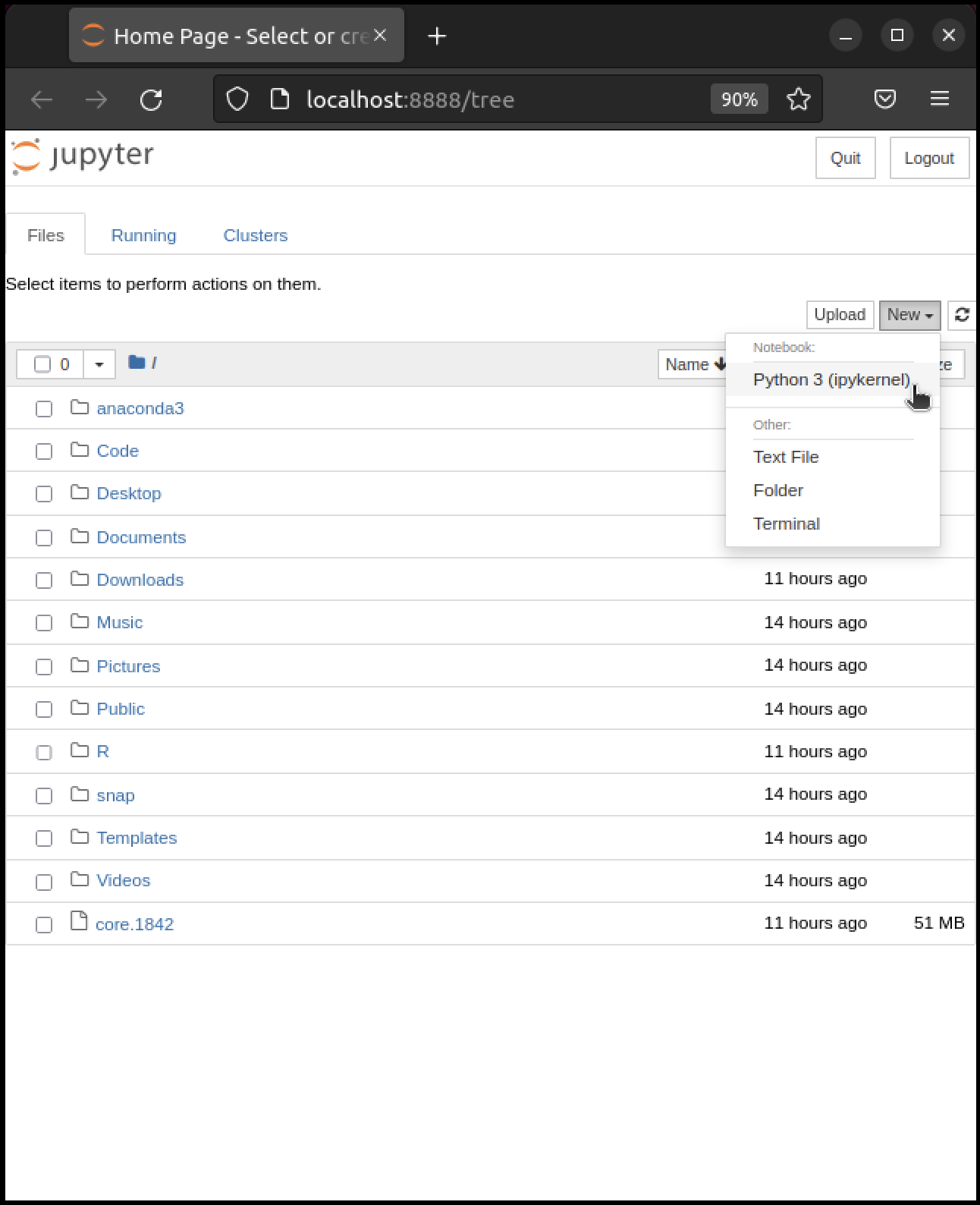\n",
234 | "\n",
235 | " \n",
236 | "What you see here is called the Jupyter *dashboard*.\n",
237 | "\n",
238 | "If you look at the URL at the top, it should be `localhost:8888` or similar, matching the message above.\n",
239 | "\n",
240 | "Assuming all this has worked OK, you can now click on `New` at the top right and select `Python 3` or similar.\n",
241 | "\n",
242 | "Here’s what shows up on our machine:\n",
243 | "\n",
244 | "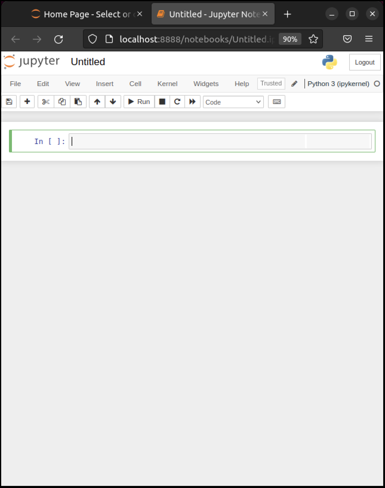\n",
245 | "\n",
246 | " \n",
247 | "The notebook displays an *active cell*, into which you can type Python commands."
248 | ]
249 | },
250 | {
251 | "cell_type": "markdown",
252 | "id": "79a2fb79",
253 | "metadata": {},
254 | "source": [
255 | "### Notebook Basics\n",
256 | "\n",
257 | "\n",
258 | "\n",
259 | "Let’s start with how to edit code and run simple programs."
260 | ]
261 | },
262 | {
263 | "cell_type": "markdown",
264 | "id": "4c3ef9e3",
265 | "metadata": {},
266 | "source": [
267 | "#### Running Cells\n",
268 | "\n",
269 | "Notice that, in the previous figure, the cell is surrounded by a green border.\n",
270 | "\n",
271 | "This means that the cell is in *edit mode*.\n",
272 | "\n",
273 | "In this mode, whatever you type will appear in the cell with the flashing cursor.\n",
274 | "\n",
275 | "When you’re ready to execute the code in a cell, hit `Shift-Enter` instead of the usual `Enter`.\n",
276 | "\n",
277 | "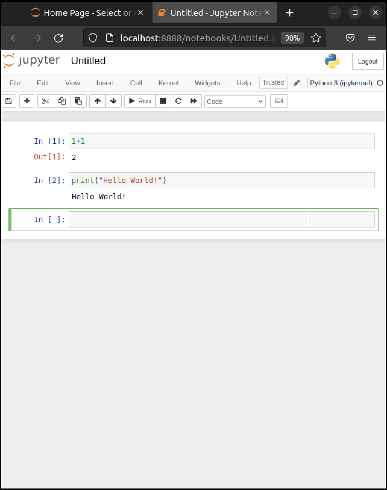\n",
278 | "\n",
279 | " \n",
280 | ">**Note**\n",
281 | ">\n",
282 | ">There are also menu and button options for running code in a cell that you can find by exploring."
283 | ]
284 | },
285 | {
286 | "cell_type": "markdown",
287 | "id": "eeb26544",
288 | "metadata": {},
289 | "source": [
290 | "#### Modal Editing\n",
291 | "\n",
292 | "The next thing to understand about the Jupyter notebook is that it uses a *modal* editing system.\n",
293 | "\n",
294 | "This means that the effect of typing at the keyboard **depends on which mode you are in**.\n",
295 | "\n",
296 | "The two modes are\n",
297 | "\n",
298 | "1. Edit mode \n",
299 | " - Indicated by a green border around one cell, plus a blinking cursor \n",
300 | " - Whatever you type appears as is in that cell \n",
301 | "1. Command mode \n",
302 | " - The green border is replaced by a blue border \n",
303 | " - Keystrokes are interpreted as commands — for example, typing `b` adds a new cell below the current one \n",
304 | "\n",
305 | "\n",
306 | "To switch to\n",
307 | "\n",
308 | "- command mode from edit mode, hit the `Esc` key or `Ctrl-M` \n",
309 | "- edit mode from command mode, hit `Enter` or click in a cell \n",
310 | "\n",
311 | "\n",
312 | "The modal behavior of the Jupyter notebook is very efficient when you get used to it."
313 | ]
314 | },
315 | {
316 | "cell_type": "markdown",
317 | "id": "748bd183",
318 | "metadata": {},
319 | "source": [
320 | "#### Inserting Unicode (e.g., Greek Letters)\n",
321 | "\n",
322 | "Python supports [unicode](https://docs.python.org/3/howto/unicode.html), allowing the use of characters such as $ \\alpha $ and $ \\beta $ as names in your code.\n",
323 | "\n",
324 | "In a code cell, try typing `\\alpha` and then hitting the tab key on your keyboard.\n",
325 | "\n",
326 | "\n",
327 | ""
328 | ]
329 | },
330 | {
331 | "cell_type": "markdown",
332 | "id": "c55aaf33",
333 | "metadata": {},
334 | "source": [
335 | "#### A Test Program\n",
336 | "\n",
337 | "Let’s run a test program.\n",
338 | "\n",
339 | "Here’s an arbitrary program we can use: [https://matplotlib.org/stable/gallery/pie_and_polar_charts/polar_bar.html](https://matplotlib.org/stable/gallery/pie_and_polar_charts/polar_bar.html).\n",
340 | "\n",
341 | "On that page, you’ll see the following code"
342 | ]
343 | },
344 | {
345 | "cell_type": "code",
346 | "execution_count": null,
347 | "id": "0f19774f",
348 | "metadata": {
349 | "hide-output": false
350 | },
351 | "outputs": [],
352 | "source": [
353 | "import numpy as np\n",
354 | "import matplotlib.pyplot as plt\n",
355 | "\n",
356 | "# Fixing random state for reproducibility\n",
357 | "np.random.seed(19680801)\n",
358 | "\n",
359 | "# Compute pie slices\n",
360 | "N = 20\n",
361 | "θ = np.linspace(0.0, 2 * np.pi, N, endpoint=False)\n",
362 | "radii = 10 * np.random.rand(N)\n",
363 | "width = np.pi / 4 * np.random.rand(N)\n",
364 | "colors = plt.cm.viridis(radii / 10.)\n",
365 | "\n",
366 | "ax = plt.subplot(111, projection='polar')\n",
367 | "ax.bar(θ, radii, width=width, bottom=0.0, color=colors, alpha=0.5)\n",
368 | "\n",
369 | "plt.show()"
370 | ]
371 | },
372 | {
373 | "cell_type": "markdown",
374 | "id": "b60e0349",
375 | "metadata": {},
376 | "source": [
377 | "Don’t worry about the details for now — let’s just run it and see what happens.\n",
378 | "\n",
379 | "The easiest way to run this code is to copy and paste it into a cell in the notebook.\n",
380 | "\n",
381 | "Hopefully you will get a similar plot."
382 | ]
383 | },
384 | {
385 | "cell_type": "markdown",
386 | "id": "d6bce68c",
387 | "metadata": {},
388 | "source": [
389 | "### Working with the Notebook\n",
390 | "\n",
391 | "Here are a few more tips on working with Jupyter notebooks."
392 | ]
393 | },
394 | {
395 | "cell_type": "markdown",
396 | "id": "28011d9d",
397 | "metadata": {},
398 | "source": [
399 | "#### Tab Completion\n",
400 | "\n",
401 | "In the previous program, we executed the line `import numpy as np`\n",
402 | "\n",
403 | "- NumPy is a numerical library we’ll work with in depth. \n",
404 | "\n",
405 | "\n",
406 | "After this import command, functions in NumPy can be accessed with `np.function_name` type syntax.\n",
407 | "\n",
408 | "- For example, try `np.random.randn(3)`. \n",
409 | "\n",
410 | "\n",
411 | "We can explore these attributes of `np` using the `Tab` key.\n",
412 | "\n",
413 | "For example, here we type `np.random.r` and hit Tab\n",
414 | "\n",
415 | "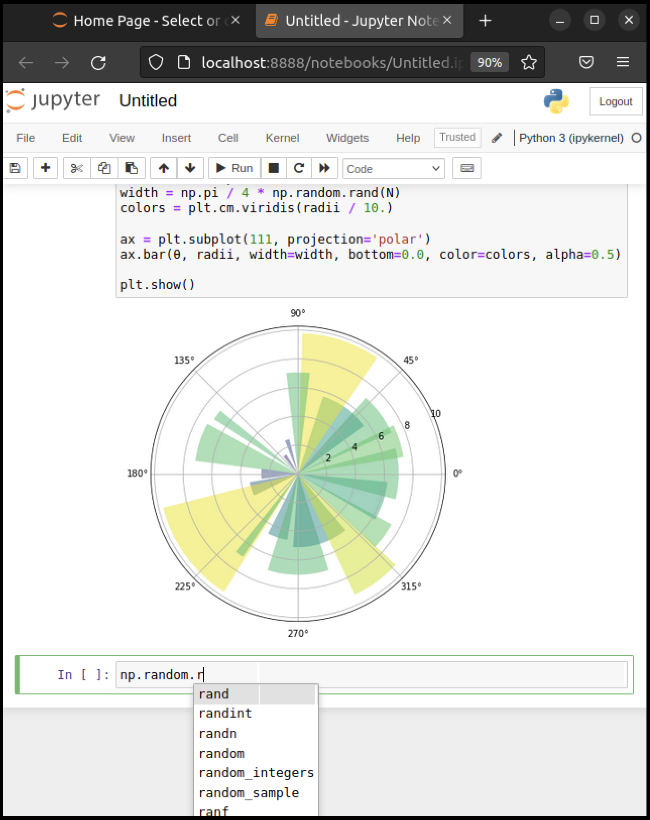\n",
416 | "\n",
417 | " \n",
418 | "Jupyter offers several possible completions for you to choose from.\n",
419 | "\n",
420 | "In this way, the Tab key helps remind you of what’s available and also saves you typing.\n",
421 | "\n",
422 | "\n",
423 | ""
424 | ]
425 | },
426 | {
427 | "cell_type": "markdown",
428 | "id": "a6d364bc",
429 | "metadata": {},
430 | "source": [
431 | "#### On-Line Help\n",
432 | "\n",
433 | "\n",
434 | "\n",
435 | "To get help on `np.random.randn`, we can execute `np.random.randn?`.\n",
436 | "\n",
437 | "Documentation appears in a split window of the browser, like so\n",
438 | "\n",
439 | "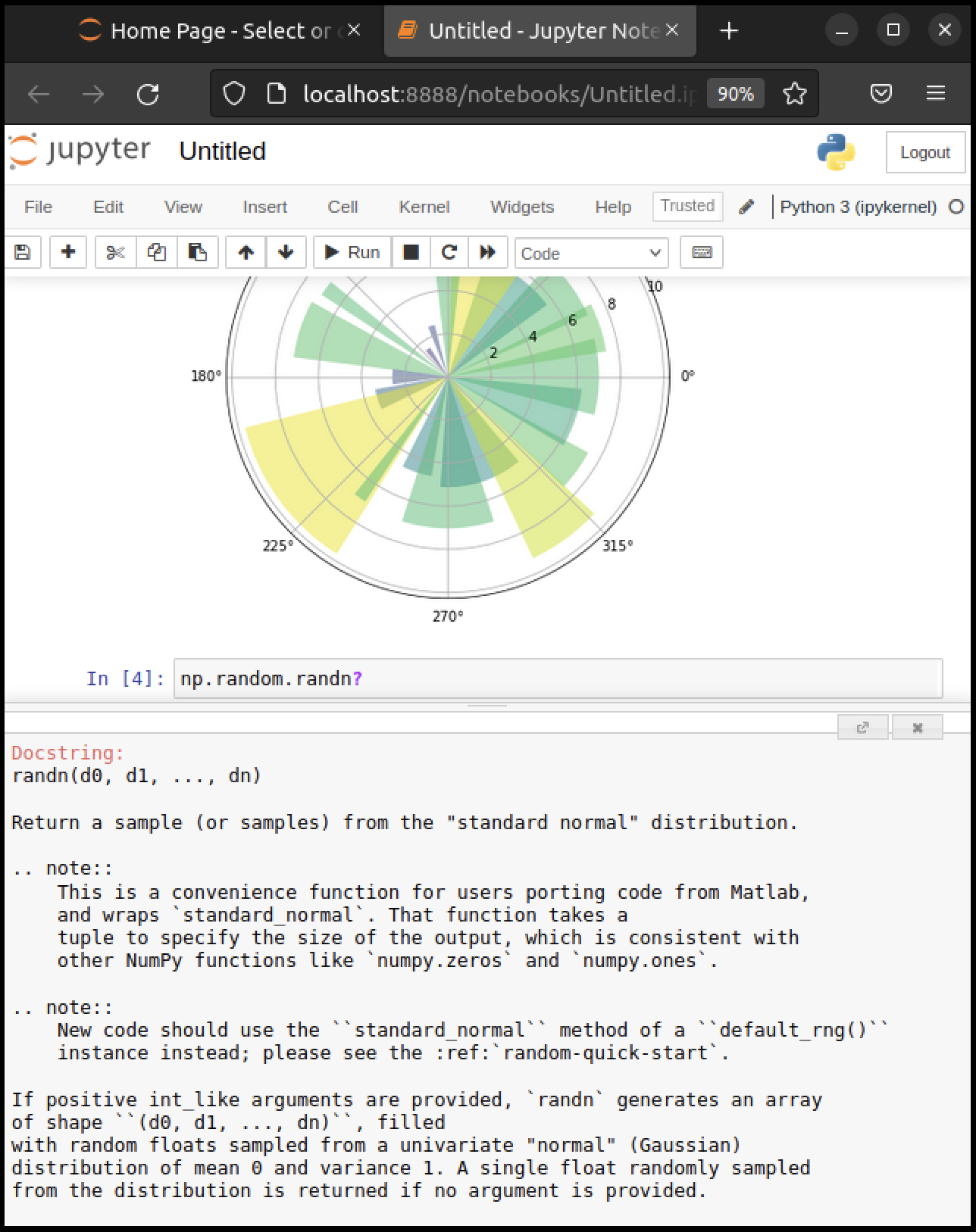\n",
440 | "\n",
441 | " \n",
442 | "Clicking on the top right of the lower split closes the on-line help.\n",
443 | "\n",
444 | "We will learn more about how to create documentation like this [later](https://python-programming.quantecon.org/python_essentials.html#docstrings)!"
445 | ]
446 | },
447 | {
448 | "cell_type": "markdown",
449 | "id": "ff48edc7",
450 | "metadata": {},
451 | "source": [
452 | "#### Other Content\n",
453 | "\n",
454 | "In addition to executing code, the Jupyter notebook allows you to embed text, equations, figures and even videos in the page.\n",
455 | "\n",
456 | "For example, we can enter a mixture of plain text and LaTeX instead of code.\n",
457 | "\n",
458 | "Next we `Esc` to enter command mode and then type `m` to indicate that we\n",
459 | "are writing [Markdown](https://daringfireball.net/projects/markdown/), a mark-up language similar to (but simpler than) LaTeX.\n",
460 | "\n",
461 | "(You can also use your mouse to select `Markdown` from the `Code` drop-down box just below the list of menu items)\n",
462 | "\n",
463 | "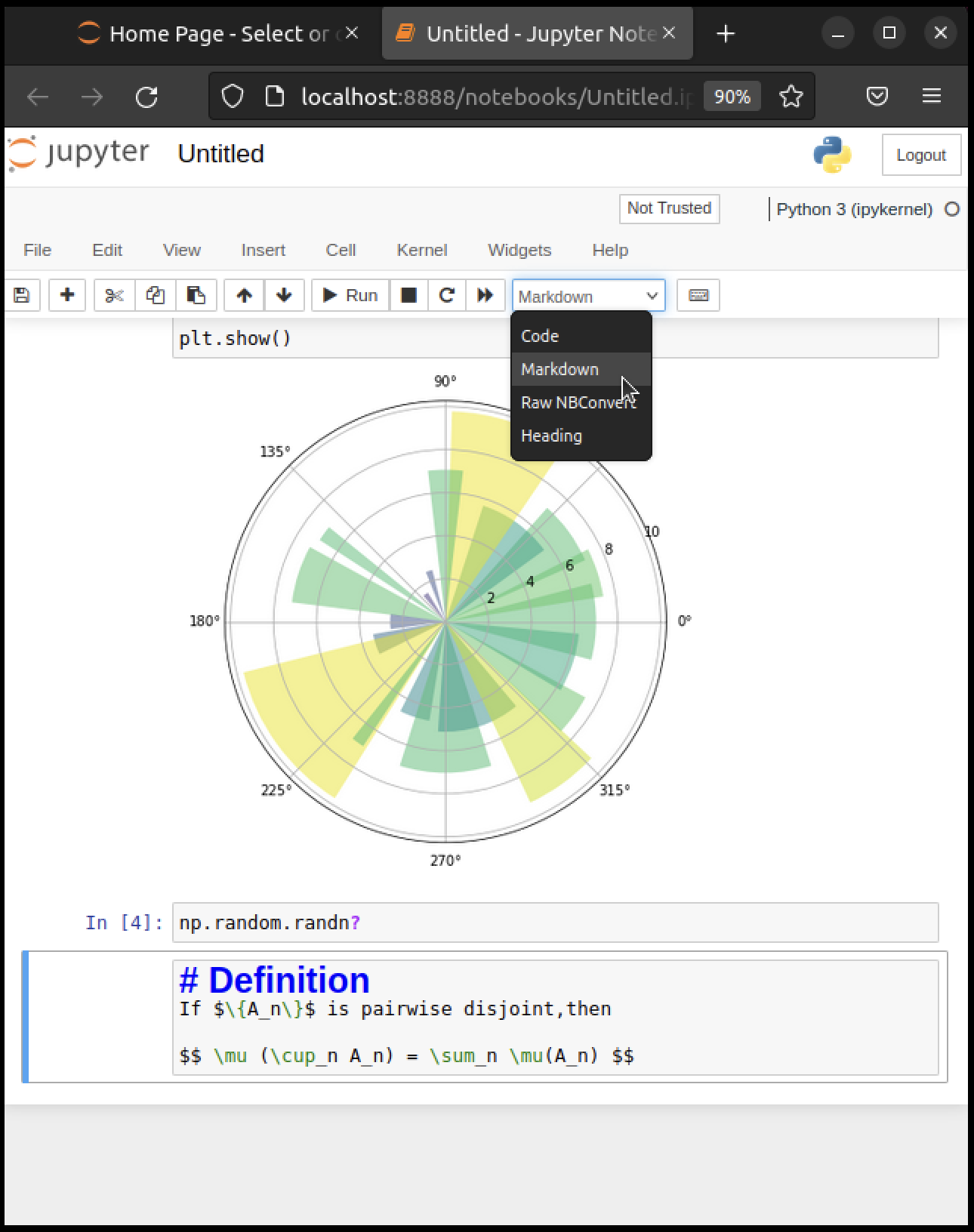\n",
464 | "\n",
465 | " \n",
466 | "Now we `Shift+Enter` to produce this\n",
467 | "\n",
468 | "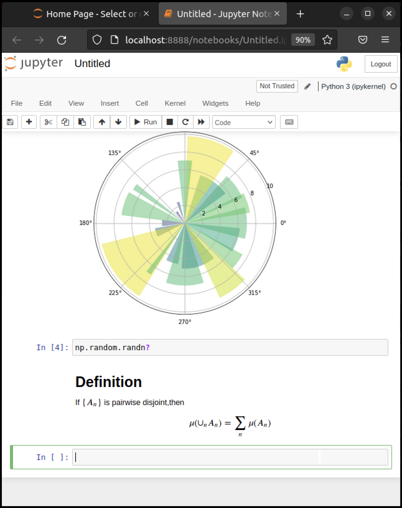"
469 | ]
470 | },
471 | {
472 | "cell_type": "markdown",
473 | "id": "08b2f8bc",
474 | "metadata": {},
475 | "source": [
476 | "### Debugging Code\n",
477 | "\n",
478 | "\n",
479 | "\n",
480 | "Debugging is the process of identifying and removing errors from a program.\n",
481 | "\n",
482 | "You will spend a lot of time debugging code, so it is important to [learn how to do it effectively](https://www.freecodecamp.org/news/what-is-debugging-how-to-debug-code/).\n",
483 | "\n",
484 | "If you are using a newer version of Jupyter, you should see a bug icon on the right end of the toolbar.\n",
485 | "\n",
486 | "\n",
487 | "\n",
488 | " \n",
489 | "Clicking this icon will enable the Jupyter debugger.\n",
490 | "\n",
491 | ">**Note**\n",
492 | ">\n",
493 | ">You may also need to open the Debugger Panel (View -> Debugger Panel).\n",
494 | "\n",
495 | "You can set breakpoints by clicking on the line number of the cell you want to debug.\n",
496 | "\n",
497 | "When you run the cell, the debugger will stop at the breakpoint.\n",
498 | "\n",
499 | "You can then step through the code line by line using the buttons on the “Next” button on the CALLSTACK toolbar (located in the right hand window).\n",
500 | "\n",
501 | "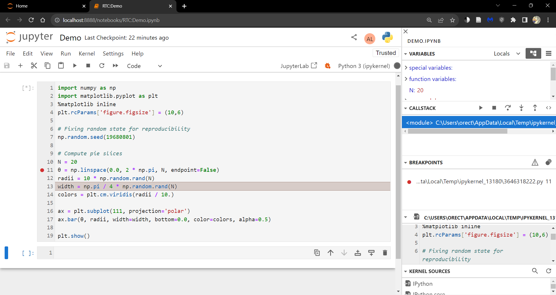\n",
502 | "\n",
503 | " \n",
504 | "You can explore more functionality of the debugger in the [Jupyter documentation](https://jupyterlab.readthedocs.io/en/latest/user/debugger.html)."
505 | ]
506 | },
507 | {
508 | "cell_type": "markdown",
509 | "id": "2465e9e3",
510 | "metadata": {},
511 | "source": [
512 | "### Sharing Notebooks\n",
513 | "\n",
514 | "\n",
515 | "\n",
516 | "\n",
517 | "\n",
518 | "Notebook files are just text files structured in [JSON](https://en.wikipedia.org/wiki/JSON) and typically ending with `.ipynb`.\n",
519 | "\n",
520 | "You can share them in the usual way that you share files — or by using web services such as [nbviewer](https://nbviewer.org/).\n",
521 | "\n",
522 | "The notebooks you see on that site are **static** html representations.\n",
523 | "\n",
524 | "To run one, download it as an `ipynb` file by clicking on the download icon at the top right.\n",
525 | "\n",
526 | "Save it somewhere, navigate to it from the Jupyter dashboard and then run as discussed above.\n",
527 | "\n",
528 | ">**Note**\n",
529 | ">\n",
530 | ">If you are interested in sharing notebooks containing interactive content, you might want to check out [Binder](https://mybinder.org/).\n",
531 | "\n",
532 | "To collaborate with other people on notebooks, you might want to take a look at\n",
533 | "\n",
534 | "- [Google Colab](https://colab.research.google.com/) \n",
535 | "- [Kaggle](https://www.kaggle.com/code) \n",
536 | "\n",
537 | "\n",
538 | "To keep the code private and to use the familiar JupyterLab and Notebook interface, look into the [JupyterLab Real-Time Collaboration extension](https://jupyterlab-realtime-collaboration.readthedocs.io/en/latest/)."
539 | ]
540 | },
541 | {
542 | "cell_type": "markdown",
543 | "id": "15854903",
544 | "metadata": {},
545 | "source": [
546 | "### QuantEcon Notes\n",
547 | "\n",
548 | "QuantEcon has its own site for sharing Jupyter notebooks related\n",
549 | "to economics – [QuantEcon Notes](http://notes.quantecon.org/).\n",
550 | "\n",
551 | "Notebooks submitted to QuantEcon Notes can be shared with a link, and are open\n",
552 | "to comments and votes by the community."
553 | ]
554 | },
555 | {
556 | "cell_type": "markdown",
557 | "id": "efd67ebb",
558 | "metadata": {},
559 | "source": [
560 | "## Installing Libraries\n",
561 | "\n",
562 | "\n",
563 | "\n",
564 | "\n",
565 | "\n",
566 | "Most of the libraries we need come in Anaconda.\n",
567 | "\n",
568 | "Other libraries can be installed with `pip` or `conda`.\n",
569 | "\n",
570 | "One library we’ll be using is [QuantEcon.py](https://quantecon.org/quantecon-py/).\n",
571 | "\n",
572 | "\n",
573 | "\n",
574 | "You can install [QuantEcon.py](https://quantecon.org/quantecon-py/) by\n",
575 | "starting Jupyter and typing"
576 | ]
577 | },
578 | {
579 | "cell_type": "markdown",
580 | "id": "d804012c",
581 | "metadata": {
582 | "hide-output": false
583 | },
584 | "source": [
585 | "```ipython3\n",
586 | "!conda install quantecon\n",
587 | "```\n"
588 | ]
589 | },
590 | {
591 | "cell_type": "markdown",
592 | "id": "5e2815ed",
593 | "metadata": {},
594 | "source": [
595 | "into a cell.\n",
596 | "\n",
597 | "Alternatively, you can type the following into a terminal"
598 | ]
599 | },
600 | {
601 | "cell_type": "markdown",
602 | "id": "1c298663",
603 | "metadata": {
604 | "hide-output": false
605 | },
606 | "source": [
607 | "```bash\n",
608 | "conda install quantecon\n",
609 | "```\n"
610 | ]
611 | },
612 | {
613 | "cell_type": "markdown",
614 | "id": "e14beb62",
615 | "metadata": {},
616 | "source": [
617 | "More instructions can be found on the [library page](https://quantecon.org/quantecon-py/).\n",
618 | "\n",
619 | "To upgrade to the latest version, which you should do regularly, use"
620 | ]
621 | },
622 | {
623 | "cell_type": "markdown",
624 | "id": "a354b73a",
625 | "metadata": {
626 | "hide-output": false
627 | },
628 | "source": [
629 | "```bash\n",
630 | "conda upgrade quantecon\n",
631 | "```\n"
632 | ]
633 | },
634 | {
635 | "cell_type": "markdown",
636 | "id": "972ba520",
637 | "metadata": {},
638 | "source": [
639 | "Another library we will be using is [interpolation.py](https://github.com/EconForge/interpolation.py).\n",
640 | "\n",
641 | "This can be installed by typing in Jupyter"
642 | ]
643 | },
644 | {
645 | "cell_type": "markdown",
646 | "id": "08b6e98f",
647 | "metadata": {
648 | "hide-output": false
649 | },
650 | "source": [
651 | "```ipython3\n",
652 | "!conda install -c conda-forge interpolation\n",
653 | "```\n"
654 | ]
655 | },
656 | {
657 | "cell_type": "markdown",
658 | "id": "2d79cae2",
659 | "metadata": {},
660 | "source": [
661 | "## Working with Python Files\n",
662 | "\n",
663 | "So far we’ve focused on executing Python code entered into a Jupyter notebook\n",
664 | "cell.\n",
665 | "\n",
666 | "Traditionally most Python code has been run in a different way.\n",
667 | "\n",
668 | "Code is first saved in a text file on a local machine\n",
669 | "\n",
670 | "By convention, these text files have a `.py` extension.\n",
671 | "\n",
672 | "We can create an example of such a file as follows:"
673 | ]
674 | },
675 | {
676 | "cell_type": "code",
677 | "execution_count": null,
678 | "id": "315ae3d0",
679 | "metadata": {
680 | "hide-output": false
681 | },
682 | "outputs": [],
683 | "source": [
684 | "%%writefile foo.py\n",
685 | "\n",
686 | "print(\"foobar\")"
687 | ]
688 | },
689 | {
690 | "cell_type": "markdown",
691 | "id": "7490060b",
692 | "metadata": {},
693 | "source": [
694 | "This writes the line `print(\"foobar\")` into a file called `foo.py` in the local directory.\n",
695 | "\n",
696 | "Here `%%writefile` is an example of a [cell magic](https://ipython.readthedocs.io/en/stable/interactive/magics.html#cell-magics)."
697 | ]
698 | },
699 | {
700 | "cell_type": "markdown",
701 | "id": "7a6e3f23",
702 | "metadata": {},
703 | "source": [
704 | "### Editing and Execution\n",
705 | "\n",
706 | "If you come across code saved in a `*.py` file, you’ll need to consider the\n",
707 | "following questions:\n",
708 | "\n",
709 | "1. how should you execute it? \n",
710 | "1. How should you modify or edit it? "
711 | ]
712 | },
713 | {
714 | "cell_type": "markdown",
715 | "id": "147ec901",
716 | "metadata": {},
717 | "source": [
718 | "#### Option 1: JupyterLab\n",
719 | "\n",
720 | "\n",
721 | "\n",
722 | "[JupyterLab](https://github.com/jupyterlab/jupyterlab) is an integrated development environment built on top of Jupyter notebooks.\n",
723 | "\n",
724 | "With JupyterLab you can edit and run `*.py` files as well as Jupyter notebooks.\n",
725 | "\n",
726 | "To start JupyterLab, search for it in the applications menu or type `jupyter-lab` in a terminal.\n",
727 | "\n",
728 | "Now you should be able to open, edit and run the file `foo.py` created above by opening it in JupyterLab.\n",
729 | "\n",
730 | "Read the docs or search for a recent YouTube video to find more information."
731 | ]
732 | },
733 | {
734 | "cell_type": "markdown",
735 | "id": "13b752a6",
736 | "metadata": {},
737 | "source": [
738 | "#### Option 2: Using a Text Editor\n",
739 | "\n",
740 | "One can also edit files using a text editor and then run them from within\n",
741 | "Jupyter notebooks.\n",
742 | "\n",
743 | "A text editor is an application that is specifically designed to work with text files — such as Python programs.\n",
744 | "\n",
745 | "Nothing beats the power and efficiency of a good text editor for working with program text.\n",
746 | "\n",
747 | "A good text editor will provide\n",
748 | "\n",
749 | "- efficient text editing commands (e.g., copy, paste, search and replace) \n",
750 | "- syntax highlighting, etc. \n",
751 | "\n",
752 | "\n",
753 | "Right now, an extremely popular text editor for coding is [VS Code](https://code.visualstudio.com/).\n",
754 | "\n",
755 | "VS Code is easy to use out of the box and has many high quality extensions.\n",
756 | "\n",
757 | "Alternatively, if you want an outstanding free text editor and don’t mind a seemingly vertical learning curve plus long days of pain and suffering while all your neural pathways are rewired, try [Vim](https://www.vim.org/)."
758 | ]
759 | },
760 | {
761 | "cell_type": "markdown",
762 | "id": "c6ec6fd4",
763 | "metadata": {},
764 | "source": [
765 | "## Exercises"
766 | ]
767 | },
768 | {
769 | "cell_type": "markdown",
770 | "id": "e1e4ee32",
771 | "metadata": {},
772 | "source": [
773 | "## Exercise 2.1\n",
774 | "\n",
775 | "If Jupyter is still running, quit by using `Ctrl-C` at the terminal where\n",
776 | "you started it.\n",
777 | "\n",
778 | "Now launch again, but this time using `jupyter notebook --no-browser`.\n",
779 | "\n",
780 | "This should start the kernel without launching the browser.\n",
781 | "\n",
782 | "Note also the startup message: It should give you a URL such as `http://localhost:8888` where the notebook is running.\n",
783 | "\n",
784 | "Now\n",
785 | "\n",
786 | "1. Start your browser — or open a new tab if it’s already running. \n",
787 | "1. Enter the URL from above (e.g. `http://localhost:8888`) in the address bar at the top. \n",
788 | "\n",
789 | "\n",
790 | "You should now be able to run a standard Jupyter notebook session.\n",
791 | "\n",
792 | "This is an alternative way to start the notebook that can also be handy.\n",
793 | "\n",
794 | "This can also work when you accidentally close the webpage as long as the kernel is still running."
795 | ]
796 | }
797 | ],
798 | "metadata": {
799 | "date": 1764566373.4769256,
800 | "filename": "getting_started.md",
801 | "kernelspec": {
802 | "display_name": "Python",
803 | "language": "python3",
804 | "name": "python3"
805 | },
806 | "title": "Getting Started"
807 | },
808 | "nbformat": 4,
809 | "nbformat_minor": 5
810 | }
--------------------------------------------------------------------------------