├── environment.yml
├── README.md
├── heavy_tails.ipynb
├── troubleshooting.ipynb
├── cross_product_trick.ipynb
├── intro.ipynb
├── status.ipynb
├── schelling.ipynb
├── egm_policy_iter.ipynb
├── rand_resp.ipynb
├── os_egm.ipynb
├── cake_eating_egm.ipynb
├── inventory_dynamics.ipynb
├── cake_eating_egm_jax.ipynb
├── os_egm_jax.ipynb
└── mccall_correlated.ipynb


/environment.yml:
--------------------------------------------------------------------------------
1 | name: lecture-python
2 | channels:
3 |   - default
4 | dependencies:
5 |   - python=3.8
6 |   - anaconda
7 | 
8 | 


--------------------------------------------------------------------------------
/README.md:
--------------------------------------------------------------------------------
1 | # lecture-python.notebooks
2 | 
3 | [![Binder](https://mybinder.org/badge_logo.svg)](https://mybinder.org/v2/gh/QuantEcon/lecture-python.notebooks/master)
4 | 
5 | Notebooks for https://python.quantecon.org
6 | 
7 | **Note:** This README should be edited [here](https://github.com/quantecon/lecture-python.myst/_notebook_repo)
8 | 


--------------------------------------------------------------------------------
/heavy_tails.ipynb:
--------------------------------------------------------------------------------
 1 | {
 2 |  "cells": [
 3 |   {
 4 |    "cell_type": "markdown",
 5 |    "id": "3b1e3870",
 6 |    "metadata": {},
 7 |    "source": [
 8 |     "# Heavy-Tailed Distributions"
 9 |    ]
10 |   },
11 |   {
12 |    "cell_type": "markdown",
13 |    "id": "c7252f5d",
14 |    "metadata": {},
15 |    "source": [
16 |     "# New website\n",
17 |     "\n",
18 |     "We have moved this lecture to a new lecture series.\n",
19 |     "\n",
20 |     "See [An Undergraduate Lecture Series for the Foundations of Computational Economics](https://intro.quantecon.org)"
21 |    ]
22 |   }
23 |  ],
24 |  "metadata": {
25 |   "date": 1710733971.7124138,
26 |   "filename": "heavy_tails.md",
27 |   "kernelspec": {
28 |    "display_name": "Python",
29 |    "language": "python3",
30 |    "name": "python3"
31 |   },
32 |   "title": "Heavy-Tailed Distributions"
33 |  },
34 |  "nbformat": 4,
35 |  "nbformat_minor": 5
36 | }


--------------------------------------------------------------------------------
/troubleshooting.ipynb:
--------------------------------------------------------------------------------
  1 | {
  2 |  "cells": [
  3 |   {
  4 |    "cell_type": "markdown",
  5 |    "id": "304b7787",
  6 |    "metadata": {},
  7 |    "source": [
  8 |     "\n",
  9 |     "<a id='troubleshooting'></a>\n",
 10 |     "<div id=\"qe-notebook-header\" align=\"right\" style=\"text-align:right;\">\n",
 11 |     "        <a href=\"https://quantecon.org/\" title=\"quantecon.org\">\n",
 12 |     "                <img style=\"width:250px;display:inline;\" width=\"250px\" src=\"https://assets.quantecon.org/img/qe-menubar-logo.svg\" alt=\"QuantEcon\">\n",
 13 |     "        </a>\n",
 14 |     "</div>"
 15 |    ]
 16 |   },
 17 |   {
 18 |    "cell_type": "markdown",
 19 |    "id": "a813234b",
 20 |    "metadata": {},
 21 |    "source": [
 22 |     "# Troubleshooting"
 23 |    ]
 24 |   },
 25 |   {
 26 |    "cell_type": "markdown",
 27 |    "id": "18baae65",
 28 |    "metadata": {},
 29 |    "source": [
 30 |     "## Contents\n",
 31 |     "\n",
 32 |     "- [Troubleshooting](#Troubleshooting)  \n",
 33 |     "  - [Fixing Your Local Environment](#Fixing-Your-Local-Environment)  \n",
 34 |     "  - [Reporting an Issue](#Reporting-an-Issue)  "
 35 |    ]
 36 |   },
 37 |   {
 38 |    "cell_type": "markdown",
 39 |    "id": "78617204",
 40 |    "metadata": {},
 41 |    "source": [
 42 |     "This page is for readers experiencing errors when running the code from the lectures."
 43 |    ]
 44 |   },
 45 |   {
 46 |    "cell_type": "markdown",
 47 |    "id": "a1af96ae",
 48 |    "metadata": {},
 49 |    "source": [
 50 |     "## Fixing Your Local Environment\n",
 51 |     "\n",
 52 |     "The basic assumption of the lectures is that code in a lecture should execute whenever\n",
 53 |     "\n",
 54 |     "1. it is executed in a Jupyter notebook and  \n",
 55 |     "1. the notebook is running on a machine with the latest version of Anaconda Python.  \n",
 56 |     "\n",
 57 |     "\n",
 58 |     "You have installed Anaconda, haven’t you, following the instructions in [this lecture](https://python-programming.quantecon.org/getting_started.html)?\n",
 59 |     "\n",
 60 |     "Assuming that you have, the most common source of problems for our readers is that their Anaconda distribution is not up to date.\n",
 61 |     "\n",
 62 |     "[Here’s a useful article](https://www.anaconda.com/blog/keeping-anaconda-date)\n",
 63 |     "on how to update Anaconda.\n",
 64 |     "\n",
 65 |     "Another option is to simply remove Anaconda and reinstall.\n",
 66 |     "\n",
 67 |     "You also need to keep the external code libraries, such as [QuantEcon.py](https://quantecon.org/quantecon-py/) up to date.\n",
 68 |     "\n",
 69 |     "For this task you can either\n",
 70 |     "\n",
 71 |     "- use `pip install --upgrade quantecon` on the command line, or  \n",
 72 |     "- execute `!pip install --upgrade quantecon` within a Jupyter notebook.  \n",
 73 |     "\n",
 74 |     "\n",
 75 |     "If your local environment is still not working you can do two things.\n",
 76 |     "\n",
 77 |     "First, you can use a remote machine instead, by clicking on the Launch Notebook icon available for each lecture\n",
 78 |     "\n",
 79 |     "![https://python.quantecon.org/_static/lecture_specific/troubleshooting/launch.png](https://python.quantecon.org/_static/lecture_specific/troubleshooting/launch.png)\n",
 80 |     "\n",
 81 |     "Second, you can report an issue, so we can try to fix your local set up.\n",
 82 |     "\n",
 83 |     "We like getting feedback on the lectures so please don’t hesitate to get in\n",
 84 |     "touch."
 85 |    ]
 86 |   },
 87 |   {
 88 |    "cell_type": "markdown",
 89 |    "id": "c4058ffd",
 90 |    "metadata": {},
 91 |    "source": [
 92 |     "## Reporting an Issue\n",
 93 |     "\n",
 94 |     "One way to give feedback is to raise an issue through our [issue tracker](https://github.com/QuantEcon/lecture-python/issues).\n",
 95 |     "\n",
 96 |     "Please be as specific as possible.  Tell us where the problem is and as much\n",
 97 |     "detail about your local set up as you can provide.\n",
 98 |     "\n",
 99 |     "Finally, you can provide direct feedback to [contact@quantecon.org](mailto:contact@quantecon.org)"
100 |    ]
101 |   }
102 |  ],
103 |  "metadata": {
104 |   "date": 1764675755.943279,
105 |   "filename": "troubleshooting.md",
106 |   "kernelspec": {
107 |    "display_name": "Python",
108 |    "language": "python3",
109 |    "name": "python3"
110 |   },
111 |   "title": "Troubleshooting"
112 |  },
113 |  "nbformat": 4,
114 |  "nbformat_minor": 5
115 | }


--------------------------------------------------------------------------------
/cross_product_trick.ipynb:
--------------------------------------------------------------------------------
  1 | {
  2 |  "cells": [
  3 |   {
  4 |    "cell_type": "markdown",
  5 |    "id": "88bc9b49",
  6 |    "metadata": {},
  7 |    "source": [
  8 |     "# Eliminating Cross Products"
  9 |    ]
 10 |   },
 11 |   {
 12 |    "cell_type": "markdown",
 13 |    "id": "36ea6247",
 14 |    "metadata": {},
 15 |    "source": [
 16 |     "## Overview\n",
 17 |     "\n",
 18 |     "This lecture describes formulas for eliminating\n",
 19 |     "\n",
 20 |     "- cross products between states and control in linear-quadratic dynamic programming  problems  \n",
 21 |     "- covariances between state and measurement noises in  Kalman filtering  problems  \n",
 22 |     "\n",
 23 |     "\n",
 24 |     "For a linear-quadratic dynamic programming problem, the idea involves these steps\n",
 25 |     "\n",
 26 |     "- transform  states and controls in a way that leads to an equivalent problem with no cross-products between transformed states and controls  \n",
 27 |     "- solve the transformed problem using standard formulas for problems with no cross-products between states and controls  presented in this lecture [Linear Control: Foundations](https://python.quantecon.org/lqcontrol.html)  \n",
 28 |     "- transform the optimal decision rule for the altered problem into the optimal decision rule for the original problem with cross-products between states and controls  "
 29 |    ]
 30 |   },
 31 |   {
 32 |    "cell_type": "markdown",
 33 |    "id": "a35f2a1c",
 34 |    "metadata": {},
 35 |    "source": [
 36 |     "## Undiscounted Dynamic Programming Problem\n",
 37 |     "\n",
 38 |     "Here is a nonstochastic undiscounted LQ dynamic programming with cross products between\n",
 39 |     "states and controls in the objective function.\n",
 40 |     "\n",
 41 |     "The problem is defined by the 5-tuple of matrices $ (A, B, R, Q, H) $\n",
 42 |     "where  $ R $ and $ Q $ are positive definite symmetric matrices and\n",
 43 |     "$ A \\sim m \\times m, B \\sim m \\times k,  Q \\sim k \\times k, R \\sim m \\times m $ and $ H \\sim k \\times m $.\n",
 44 |     "\n",
 45 |     "The problem is to choose $ \\{x_{t+1}, u_t\\}_{t=0}^\\infty $ to maximize\n",
 46 |     "\n",
 47 |     "$$\n",
 48 |     "- \\sum_{t=0}^\\infty (x_t' R x_t + u_t' Q u_t + 2 u_t H x_t)\n",
 49 |     "$$\n",
 50 |     "\n",
 51 |     "subject to the linear constraints\n",
 52 |     "\n",
 53 |     "$$\n",
 54 |     "x_{t+1} = A x_t + B u_t,  \\quad t \\geq 0\n",
 55 |     "$$\n",
 56 |     "\n",
 57 |     "where $ x_0 $ is a given initial condition.\n",
 58 |     "\n",
 59 |     "The solution to this undiscounted infinite-horizon problem is a time-invariant feedback rule\n",
 60 |     "\n",
 61 |     "$$\n",
 62 |     "u_t  = -F x_t\n",
 63 |     "$$\n",
 64 |     "\n",
 65 |     "where\n",
 66 |     "\n",
 67 |     "$$\n",
 68 |     "F = -(Q + B'PB)^{-1} B'PA\n",
 69 |     "$$\n",
 70 |     "\n",
 71 |     "and  $ P \\sim m \\times m $ is a positive definite solution of the algebraic matrix Riccati equation\n",
 72 |     "\n",
 73 |     "$$\n",
 74 |     "P = R + A'PA - (A'PB + H')(Q + B'PB)^{-1}(B'PA + H).\n",
 75 |     "$$\n",
 76 |     "\n",
 77 |     "It can be verified that an **equivalent** problem without cross-products between states and controls\n",
 78 |     "is  defined by  a 4-tuple of matrices : $ (A^*, B, R^*, Q) $.\n",
 79 |     "\n",
 80 |     "That the omitted matrix $ H=0 $ indicates that there are no cross products between states and controls\n",
 81 |     "in the equivalent problem.\n",
 82 |     "\n",
 83 |     "The matrices $ (A^*, B, R^*, Q) $ defining the  equivalent problem and the value function, policy function matrices $ P, F^* $ that solve it are  related to the matrices $ (A, B, R, Q, H) $ defining the original problem  and the  value function, policy function matrices $ P, F $ that solve the original problem by\n",
 84 |     "\n",
 85 |     "$$\n",
 86 |     "\\begin{align*}\n",
 87 |     "A^* & = A - B Q^{-1} H, \\\\\n",
 88 |     "R^* & = R - H'Q^{-1} H, \\\\\n",
 89 |     "P & = R^* + {A^*}' P A - ({A^*}' P B) (Q + B' P B)^{-1} B' P A^*, \\\\\n",
 90 |     "F^* & = (Q + B' P B)^{-1} B' P A^*, \\\\\n",
 91 |     "F & = F^* + Q^{-1} H.\n",
 92 |     "\\end{align*}\n",
 93 |     "$$"
 94 |    ]
 95 |   },
 96 |   {
 97 |    "cell_type": "markdown",
 98 |    "id": "192a70b8",
 99 |    "metadata": {},
100 |    "source": [
101 |     "## Kalman Filter\n",
102 |     "\n",
103 |     "The **duality** that prevails  between a linear-quadratic optimal control and a Kalman filtering problem means that there is an analogous transformation that allows us to transform a Kalman filtering problem\n",
104 |     "with non-zero covariance matrix  between between shocks to states and shocks to measurements to an equivalent Kalman filtering problem with zero covariance between shocks to states and measurments.\n",
105 |     "\n",
106 |     "Let’s look at the appropriate transformations.\n",
107 |     "\n",
108 |     "First, let’s recall the Kalman filter with covariance between noises to states and measurements.\n",
109 |     "\n",
110 |     "The hidden Markov model is\n",
111 |     "\n",
112 |     "$$\n",
113 |     "\\begin{align*}\n",
114 |     "x_{t+1} & = A x_t + B w_{t+1},  \\\\\n",
115 |     "z_{t+1} & = D x_t + F w_{t+1},  \n",
116 |     "\\end{align*}\n",
117 |     "$$\n",
118 |     "\n",
119 |     "where $ A \\sim m \\times m, B \\sim m \\times p $ and $ D \\sim k \\times m, F \\sim k \\times p $,\n",
120 |     "and $ w_{t+1} $ is the time $ t+1 $ component of a sequence of i.i.d. $ p \\times 1 $ normally distibuted\n",
121 |     "random vectors with mean vector zero and covariance matrix equal to a $ p \\times p $ identity matrix.\n",
122 |     "\n",
123 |     "Thus, $ x_t $ is $ m \\times 1 $ and $ z_t $ is $ k \\times 1 $.\n",
124 |     "\n",
125 |     "The Kalman  filtering formulas are\n",
126 |     "\n",
127 |     "$$\n",
128 |     "\\begin{align*}\n",
129 |     "K(\\Sigma_t) & = (A \\Sigma_t D' + BF')(D \\Sigma_t D' + FF')^{-1}, \\\\\n",
130 |     "\\Sigma_{t+1}&  = A \\Sigma_t A' + BB' - (A \\Sigma_t D' + BF')(D \\Sigma_t D' + FF')^{-1} (D \\Sigma_t A' + FB').\n",
131 |     "\\end{align*} (eq:Kalman102)\n",
132 |     " \n",
133 |     "\n",
134 |     "Define   tranformed matrices\n",
135 |     "\n",
136 |     "\\begin{align*}\n",
137 |     "A^* & = A - BF' (FF')^{-1} D, \\\\\n",
138 |     "B^* {B^*}' & = BB' - BF' (FF')^{-1} FB'.\n",
139 |     "\\end{align*}\n",
140 |     "$$"
141 |    ]
142 |   },
143 |   {
144 |    "cell_type": "markdown",
145 |    "id": "5f2c5180",
146 |    "metadata": {},
147 |    "source": [
148 |     "### Algorithm\n",
149 |     "\n",
150 |     "A consequence of  formulas {eq}`eq:Kalman102} is that we can use the following algorithm to solve Kalman filtering problems that involve  non zero covariances between state and signal noises.\n",
151 |     "\n",
152 |     "First, compute $ \\Sigma, K^* $ using the ordinary Kalman filtering  formula with $ BF' = 0 $, i.e.,\n",
153 |     "with zero covariance matrix between random shocks to  states and  random shocks to measurements.\n",
154 |     "\n",
155 |     "That is, compute  $ K^* $ and $ \\Sigma $ that  satisfy\n",
156 |     "\n",
157 |     "$$\n",
158 |     "\\begin{align*}\n",
159 |     "K^* & = (A^* \\Sigma D')(D \\Sigma D' + FF')^{-1} \\\\\n",
160 |     "\\Sigma & = A^* \\Sigma {A^*}' + B^* {B^*}' - (A^* \\Sigma D')(D \\Sigma D' + FF')^{-1} (D \\Sigma {A^*}').\n",
161 |     "\\end{align*}\n",
162 |     "$$\n",
163 |     "\n",
164 |     "The Kalman gain for the original problem **with non-zero covariance** between shocks to states and measurements is then\n",
165 |     "\n",
166 |     "$$\n",
167 |     "K = K^* + BF' (FF')^{-1},\n",
168 |     "$$\n",
169 |     "\n",
170 |     "The state reconstruction covariance matrix $ \\Sigma $ for the original problem equals the state reconstrution covariance matrix for the transformed problem."
171 |    ]
172 |   },
173 |   {
174 |    "cell_type": "markdown",
175 |    "id": "352edf14",
176 |    "metadata": {},
177 |    "source": [
178 |     "## Duality table\n",
179 |     "\n",
180 |     "Here is a handy table to remember how the Kalman filter and dynamic program are related.\n",
181 |     "\n",
182 |     "|Dynamic Program|Kalman Filter|\n",
183 |     "|:------------------------------------------------:|:------------------------------------------------:|\n",
184 |     "|$ A $|$ A' $|\n",
185 |     "|$ B $|$ D' $|\n",
186 |     "|$ H $|$ FB' $|\n",
187 |     "|$ Q $|$ FF' $|\n",
188 |     "|$ R $|$ BB' $|\n",
189 |     "|$ F $|$ K' $|\n",
190 |     "|$ P $|$ \\Sigma $|"
191 |    ]
192 |   }
193 |  ],
194 |  "metadata": {
195 |   "date": 1764675748.3485882,
196 |   "filename": "cross_product_trick.md",
197 |   "kernelspec": {
198 |    "display_name": "Python",
199 |    "language": "python3",
200 |    "name": "python3"
201 |   },
202 |   "title": "Eliminating Cross Products"
203 |  },
204 |  "nbformat": 4,
205 |  "nbformat_minor": 5
206 | }


--------------------------------------------------------------------------------
/intro.ipynb:
--------------------------------------------------------------------------------
  1 | {
  2 |  "cells": [
  3 |   {
  4 |    "cell_type": "markdown",
  5 |    "id": "d6f6477b",
  6 |    "metadata": {},
  7 |    "source": [
  8 |     "# Intermediate Quantitative Economics with Python\n",
  9 |     "\n",
 10 |     "This website presents a set of lectures on quantitative economic modeling."
 11 |    ]
 12 |   },
 13 |   {
 14 |    "cell_type": "markdown",
 15 |    "id": "f9c963b1",
 16 |    "metadata": {},
 17 |    "source": [
 18 |     "# Tools and Techniques\n",
 19 |     "\n",
 20 |     "- [Modeling COVID 19](https://python.quantecon.org/sir_model.html)\n",
 21 |     "- [Linear Algebra](https://python.quantecon.org/linear_algebra.html)\n",
 22 |     "- [QR Decomposition](https://python.quantecon.org/qr_decomp.html)\n",
 23 |     "- [Circulant Matrices](https://python.quantecon.org/eig_circulant.html)\n",
 24 |     "- [Singular Value Decomposition (SVD)](https://python.quantecon.org/svd_intro.html)\n",
 25 |     "- [VARs and DMDs](https://python.quantecon.org/var_dmd.html)\n",
 26 |     "- [Using Newton’s Method to Solve Economic Models](https://python.quantecon.org/newton_method.html)"
 27 |    ]
 28 |   },
 29 |   {
 30 |    "cell_type": "markdown",
 31 |    "id": "811f0143",
 32 |    "metadata": {},
 33 |    "source": [
 34 |     "# Elementary Statistics\n",
 35 |     "\n",
 36 |     "- [Elementary Probability with Matrices](https://python.quantecon.org/prob_matrix.html)\n",
 37 |     "- [Some Probability Distributions](https://python.quantecon.org/stats_examples.html)\n",
 38 |     "- [LLN and CLT](https://python.quantecon.org/lln_clt.html)\n",
 39 |     "- [Two Meanings of Probability](https://python.quantecon.org/prob_meaning.html)\n",
 40 |     "- [Multivariate Hypergeometric Distribution](https://python.quantecon.org/multi_hyper.html)\n",
 41 |     "- [Multivariate Normal Distribution](https://python.quantecon.org/multivariate_normal.html)\n",
 42 |     "- [Fault Tree Uncertainties](https://python.quantecon.org/hoist_failure.html)\n",
 43 |     "- [Introduction to Artificial Neural Networks](https://python.quantecon.org/back_prop.html)\n",
 44 |     "- [Randomized Response Surveys](https://python.quantecon.org/rand_resp.html)\n",
 45 |     "- [Expected Utilities of Random Responses](https://python.quantecon.org/util_rand_resp.html)"
 46 |    ]
 47 |   },
 48 |   {
 49 |    "cell_type": "markdown",
 50 |    "id": "d731ce95",
 51 |    "metadata": {},
 52 |    "source": [
 53 |     "# Bayes Law\n",
 54 |     "\n",
 55 |     "- [Non-Conjugate Priors](https://python.quantecon.org/bayes_nonconj.html)\n",
 56 |     "- [Posterior Distributions for  AR(1) Parameters](https://python.quantecon.org/ar1_bayes.html)\n",
 57 |     "- [Forecasting  an AR(1) Process](https://python.quantecon.org/ar1_turningpts.html)"
 58 |    ]
 59 |   },
 60 |   {
 61 |    "cell_type": "markdown",
 62 |    "id": "2771f4fa",
 63 |    "metadata": {},
 64 |    "source": [
 65 |     "# Statistics and Information\n",
 66 |     "\n",
 67 |     "- [Statistical Divergence Measures](https://python.quantecon.org/divergence_measures.html)\n",
 68 |     "- [Likelihood Ratio Processes](https://python.quantecon.org/likelihood_ratio_process.html)\n",
 69 |     "- [Heterogeneous Beliefs and Financial Markets](https://python.quantecon.org/likelihood_ratio_process_2.html)\n",
 70 |     "- [Likelihood Processes For VAR Models](https://python.quantecon.org/likelihood_var.html)\n",
 71 |     "- [Mean of a Likelihood Ratio Process](https://python.quantecon.org/imp_sample.html)\n",
 72 |     "- [A Problem that Stumped Milton Friedman](https://python.quantecon.org/wald_friedman.html)\n",
 73 |     "- [A Bayesian Formulation of Friedman and Wald’s Problem](https://python.quantecon.org/wald_friedman_2.html)\n",
 74 |     "- [Exchangeability and Bayesian Updating](https://python.quantecon.org/exchangeable.html)\n",
 75 |     "- [Likelihood Ratio Processes and Bayesian Learning](https://python.quantecon.org/likelihood_bayes.html)\n",
 76 |     "- [Incorrect Models](https://python.quantecon.org/mix_model.html)\n",
 77 |     "- [Bayesian versus Frequentist Decision Rules](https://python.quantecon.org/navy_captain.html)"
 78 |    ]
 79 |   },
 80 |   {
 81 |    "cell_type": "markdown",
 82 |    "id": "36bd9b3e",
 83 |    "metadata": {},
 84 |    "source": [
 85 |     "# Linear Programming\n",
 86 |     "\n",
 87 |     "- [Optimal Transport](https://python.quantecon.org/opt_transport.html)\n",
 88 |     "- [Von Neumann Growth Model (and a Generalization)](https://python.quantecon.org/von_neumann_model.html)"
 89 |    ]
 90 |   },
 91 |   {
 92 |    "cell_type": "markdown",
 93 |    "id": "aea428e3",
 94 |    "metadata": {},
 95 |    "source": [
 96 |     "# Introduction to Dynamics\n",
 97 |     "\n",
 98 |     "- [Finite Markov Chains](https://python.quantecon.org/finite_markov.html)\n",
 99 |     "- [Inventory Dynamics](https://python.quantecon.org/inventory_dynamics.html)\n",
100 |     "- [Linear State Space Models](https://python.quantecon.org/linear_models.html)\n",
101 |     "- [Samuelson Multiplier-Accelerator](https://python.quantecon.org/samuelson.html)\n",
102 |     "- [Kesten Processes and Firm Dynamics](https://python.quantecon.org/kesten_processes.html)\n",
103 |     "- [Wealth Distribution Dynamics](https://python.quantecon.org/wealth_dynamics.html)\n",
104 |     "- [A First Look at the Kalman Filter](https://python.quantecon.org/kalman.html)\n",
105 |     "- [Another Look at the Kalman Filter](https://python.quantecon.org/kalman_2.html)"
106 |    ]
107 |   },
108 |   {
109 |    "cell_type": "markdown",
110 |    "id": "da56d2f9",
111 |    "metadata": {},
112 |    "source": [
113 |     "# Search\n",
114 |     "\n",
115 |     "- [Job Search I: The McCall Search Model](https://python.quantecon.org/mccall_model.html)\n",
116 |     "- [Job Search II: Search and Separation](https://python.quantecon.org/mccall_model_with_separation.html)\n",
117 |     "- [Job Search III: Search with Separation and Markov Wages](https://python.quantecon.org/mccall_model_with_sep_markov.html)\n",
118 |     "- [Job Search IV: Fitted Value Function Iteration](https://python.quantecon.org/mccall_fitted_vfi.html)\n",
119 |     "- [Job Search V: Persistent and Transitory Wage Shocks](https://python.quantecon.org/mccall_persist_trans.html)\n",
120 |     "- [Job Search VI: Modeling Career Choice](https://python.quantecon.org/career.html)\n",
121 |     "- [Job Search VII: On-the-Job Search](https://python.quantecon.org/jv.html)\n",
122 |     "- [Job Search VIII: Search with Learning](https://python.quantecon.org/odu.html)\n",
123 |     "- [Job Search IX: Search with Q-Learning](https://python.quantecon.org/mccall_q.html)"
124 |    ]
125 |   },
126 |   {
127 |    "cell_type": "markdown",
128 |    "id": "8858aa3f",
129 |    "metadata": {},
130 |    "source": [
131 |     "# Introduction to Optimal Savings\n",
132 |     "\n",
133 |     "- [Optimal Savings I: Cake Eating](https://python.quantecon.org/os.html)\n",
134 |     "- [Optimal Savings II: Numerical Cake Eating](https://python.quantecon.org/os_numerical.html)\n",
135 |     "- [Optimal Savings III: Stochastic Returns](https://python.quantecon.org/os_stochastic.html)\n",
136 |     "- [Optimal Savings IV: Time Iteration](https://python.quantecon.org/os_time_iter.html)\n",
137 |     "- [Optimal Savings V: The Endogenous Grid Method](https://python.quantecon.org/os_egm.html)\n",
138 |     "- [Optimal Savings VI: EGM with JAX](https://python.quantecon.org/os_egm_jax.html)"
139 |    ]
140 |   },
141 |   {
142 |    "cell_type": "markdown",
143 |    "id": "c506a3db",
144 |    "metadata": {},
145 |    "source": [
146 |     "# Household Problems\n",
147 |     "\n",
148 |     "- [The Income Fluctuation Problem I: Discretization and VFI](https://python.quantecon.org/ifp_discrete.html)\n",
149 |     "- [The Income Fluctuation Problem II: Optimistic Policy Iteration](https://python.quantecon.org/ifp_opi.html)\n",
150 |     "- [The Income Fluctuation Problem III: The Endogenous Grid Method](https://python.quantecon.org/ifp_egm.html)\n",
151 |     "- [The Income Fluctuation Problem IV: Transient Income Shocks](https://python.quantecon.org/ifp_egm_transient_shocks.html)\n",
152 |     "- [The Income Fluctuation Problem V: Stochastic Returns on Assets](https://python.quantecon.org/ifp_advanced.html)"
153 |    ]
154 |   },
155 |   {
156 |    "cell_type": "markdown",
157 |    "id": "83e4bde8",
158 |    "metadata": {},
159 |    "source": [
160 |     "# LQ Control\n",
161 |     "\n",
162 |     "- [LQ Control: Foundations](https://python.quantecon.org/lqcontrol.html)\n",
163 |     "- [Lagrangian for LQ Control](https://python.quantecon.org/lagrangian_lqdp.html)\n",
164 |     "- [Eliminating Cross Products](https://python.quantecon.org/cross_product_trick.html)\n",
165 |     "- [The Permanent Income Model](https://python.quantecon.org/perm_income.html)\n",
166 |     "- [Permanent Income II: LQ Techniques](https://python.quantecon.org/perm_income_cons.html)\n",
167 |     "- [Production Smoothing via Inventories](https://python.quantecon.org/lq_inventories.html)"
168 |    ]
169 |   },
170 |   {
171 |    "cell_type": "markdown",
172 |    "id": "19452c8c",
173 |    "metadata": {},
174 |    "source": [
175 |     "# Optimal Growth\n",
176 |     "\n",
177 |     "- [Cass-Koopmans Model](https://python.quantecon.org/cass_koopmans_1.html)\n",
178 |     "- [Cass-Koopmans Competitive Equilibrium](https://python.quantecon.org/cass_koopmans_2.html)\n",
179 |     "- [Cass-Koopmans Model with Distorting Taxes](https://python.quantecon.org/cass_fiscal.html)\n",
180 |     "- [Two-Country Model with Distorting Taxes](https://python.quantecon.org/cass_fiscal_2.html)\n",
181 |     "- [Transitions in an Overlapping Generations Model](https://python.quantecon.org/ak2.html)"
182 |    ]
183 |   },
184 |   {
185 |    "cell_type": "markdown",
186 |    "id": "f5d387f9",
187 |    "metadata": {},
188 |    "source": [
189 |     "# Multiple Agent Models\n",
190 |     "\n",
191 |     "- [A Lake Model of Employment and Unemployment](https://python.quantecon.org/lake_model.html)\n",
192 |     "- [Lake Model with an Endogenous Job Finding Rate](https://python.quantecon.org/endogenous_lake.html)\n",
193 |     "- [Rational Expectations Equilibrium](https://python.quantecon.org/rational_expectations.html)\n",
194 |     "- [Stability in Linear Rational Expectations Models](https://python.quantecon.org/re_with_feedback.html)\n",
195 |     "- [Markov Perfect Equilibrium](https://python.quantecon.org/markov_perf.html)\n",
196 |     "- [Uncertainty Traps](https://python.quantecon.org/uncertainty_traps.html)\n",
197 |     "- [The Aiyagari Model](https://python.quantecon.org/aiyagari.html)\n",
198 |     "- [A Long-Lived, Heterogeneous Agent, Overlapping Generations Model](https://python.quantecon.org/ak_aiyagari.html)"
199 |    ]
200 |   },
201 |   {
202 |    "cell_type": "markdown",
203 |    "id": "4e55c1e4",
204 |    "metadata": {},
205 |    "source": [
206 |     "# Asset Pricing and Finance\n",
207 |     "\n",
208 |     "- [Asset Pricing: Finite State Models](https://python.quantecon.org/markov_asset.html)\n",
209 |     "- [Competitive Equilibria with Arrow Securities](https://python.quantecon.org/ge_arrow.html)\n",
210 |     "- [Heterogeneous Beliefs and Bubbles](https://python.quantecon.org/harrison_kreps.html)\n",
211 |     "- [Speculative Behavior with Bayesian Learning](https://python.quantecon.org/morris_learn.html)"
212 |    ]
213 |   },
214 |   {
215 |    "cell_type": "markdown",
216 |    "id": "a639d899",
217 |    "metadata": {},
218 |    "source": [
219 |     "# Data and Empirics\n",
220 |     "\n",
221 |     "- [Pandas for Panel Data](https://python.quantecon.org/pandas_panel.html)\n",
222 |     "- [Linear Regression in Python](https://python.quantecon.org/ols.html)\n",
223 |     "- [Maximum Likelihood Estimation](https://python.quantecon.org/mle.html)"
224 |    ]
225 |   },
226 |   {
227 |    "cell_type": "markdown",
228 |    "id": "fed79450",
229 |    "metadata": {},
230 |    "source": [
231 |     "# Auctions\n",
232 |     "\n",
233 |     "- [First-Price and Second-Price Auctions](https://python.quantecon.org/two_auctions.html)\n",
234 |     "- [Multiple Good Allocation Mechanisms](https://python.quantecon.org/house_auction.html)"
235 |    ]
236 |   },
237 |   {
238 |    "cell_type": "markdown",
239 |    "id": "d4734599",
240 |    "metadata": {},
241 |    "source": [
242 |     "# Other\n",
243 |     "\n",
244 |     "- [Troubleshooting](https://python.quantecon.org/troubleshooting.html)\n",
245 |     "- [References](https://python.quantecon.org/zreferences.html)\n",
246 |     "- [Execution Statistics](https://python.quantecon.org/status.html)"
247 |    ]
248 |   }
249 |  ],
250 |  "metadata": {
251 |   "date": 1764675750.4240167,
252 |   "filename": "intro.md",
253 |   "kernelspec": {
254 |    "display_name": "Python",
255 |    "language": "python3",
256 |    "name": "python3"
257 |   },
258 |   "title": "Intermediate Quantitative Economics with Python"
259 |  },
260 |  "nbformat": 4,
261 |  "nbformat_minor": 5
262 | }


--------------------------------------------------------------------------------
/status.ipynb:
--------------------------------------------------------------------------------
  1 | {
  2 |  "cells": [
  3 |   {
  4 |    "cell_type": "markdown",
  5 |    "id": "1335d5ad",
  6 |    "metadata": {},
  7 |    "source": [
  8 |     "# Execution Statistics\n",
  9 |     "\n",
 10 |     "This table contains the latest execution statistics.\n",
 11 |     "\n",
 12 |     "[](https://python.quantecon.org/aiyagari.html)[](https://python.quantecon.org/ak2.html)[](https://python.quantecon.org/ak_aiyagari.html)[](https://python.quantecon.org/ar1_bayes.html)[](https://python.quantecon.org/ar1_turningpts.html)[](https://python.quantecon.org/back_prop.html)[](https://python.quantecon.org/bayes_nonconj.html)[](https://python.quantecon.org/career.html)[](https://python.quantecon.org/cass_fiscal.html)[](https://python.quantecon.org/cass_fiscal_2.html)[](https://python.quantecon.org/cass_koopmans_1.html)[](https://python.quantecon.org/cass_koopmans_2.html)[](https://python.quantecon.org/cross_product_trick.html)[](https://python.quantecon.org/divergence_measures.html)[](https://python.quantecon.org/eig_circulant.html)[](https://python.quantecon.org/endogenous_lake.html)[](https://python.quantecon.org/exchangeable.html)[](https://python.quantecon.org/finite_markov.html)[](https://python.quantecon.org/ge_arrow.html)[](https://python.quantecon.org/harrison_kreps.html)[](https://python.quantecon.org/hoist_failure.html)[](https://python.quantecon.org/house_auction.html)[](https://python.quantecon.org/ifp_advanced.html)[](https://python.quantecon.org/ifp_discrete.html)[](https://python.quantecon.org/ifp_egm.html)[](https://python.quantecon.org/ifp_egm_transient_shocks.html)[](https://python.quantecon.org/ifp_opi.html)[](https://python.quantecon.org/imp_sample.html)[](https://python.quantecon.org/intro.html)[](https://python.quantecon.org/inventory_dynamics.html)[](https://python.quantecon.org/jv.html)[](https://python.quantecon.org/kalman.html)[](https://python.quantecon.org/kalman_2.html)[](https://python.quantecon.org/kesten_processes.html)[](https://python.quantecon.org/lagrangian_lqdp.html)[](https://python.quantecon.org/lake_model.html)[](https://python.quantecon.org/likelihood_bayes.html)[](https://python.quantecon.org/likelihood_ratio_process.html)[](https://python.quantecon.org/likelihood_ratio_process_2.html)[](https://python.quantecon.org/likelihood_var.html)[](https://python.quantecon.org/linear_algebra.html)[](https://python.quantecon.org/linear_models.html)[](https://python.quantecon.org/lln_clt.html)[](https://python.quantecon.org/lq_inventories.html)[](https://python.quantecon.org/lqcontrol.html)[](https://python.quantecon.org/markov_asset.html)[](https://python.quantecon.org/markov_perf.html)[](https://python.quantecon.org/mccall_fitted_vfi.html)[](https://python.quantecon.org/mccall_model.html)[](https://python.quantecon.org/mccall_model_with_sep_markov.html)[](https://python.quantecon.org/mccall_model_with_separation.html)[](https://python.quantecon.org/mccall_persist_trans.html)[](https://python.quantecon.org/mccall_q.html)[](https://python.quantecon.org/mix_model.html)[](https://python.quantecon.org/mle.html)[](https://python.quantecon.org/morris_learn.html)[](https://python.quantecon.org/multi_hyper.html)[](https://python.quantecon.org/multivariate_normal.html)[](https://python.quantecon.org/navy_captain.html)[](https://python.quantecon.org/newton_method.html)[](https://python.quantecon.org/odu.html)[](https://python.quantecon.org/ols.html)[](https://python.quantecon.org/opt_transport.html)[](https://python.quantecon.org/os.html)[](https://python.quantecon.org/os_egm.html)[](https://python.quantecon.org/os_egm_jax.html)[](https://python.quantecon.org/os_numerical.html)[](https://python.quantecon.org/os_stochastic.html)[](https://python.quantecon.org/os_time_iter.html)[](https://python.quantecon.org/pandas_panel.html)[](https://python.quantecon.org/perm_income.html)[](https://python.quantecon.org/perm_income_cons.html)[](https://python.quantecon.org/prob_matrix.html)[](https://python.quantecon.org/prob_meaning.html)[](https://python.quantecon.org/qr_decomp.html)[](https://python.quantecon.org/rand_resp.html)[](https://python.quantecon.org/rational_expectations.html)[](https://python.quantecon.org/re_with_feedback.html)[](https://python.quantecon.org/samuelson.html)[](https://python.quantecon.org/sir_model.html)[](https://python.quantecon.org/stats_examples.html)[](https://python.quantecon.org/.html)[](https://python.quantecon.org/svd_intro.html)[](https://python.quantecon.org/troubleshooting.html)[](https://python.quantecon.org/two_auctions.html)[](https://python.quantecon.org/uncertainty_traps.html)[](https://python.quantecon.org/util_rand_resp.html)[](https://python.quantecon.org/var_dmd.html)[](https://python.quantecon.org/von_neumann_model.html)[](https://python.quantecon.org/wald_friedman.html)[](https://python.quantecon.org/wald_friedman_2.html)[](https://python.quantecon.org/wealth_dynamics.html)[](https://python.quantecon.org/zreferences.html)|Document|Modified|Method|Run Time (s)|Status|\n",
 13 |     "|:------------------:|:------------------:|:------------------:|:------------------:|:------------------:|\n",
 14 |     "|aiyagari|2025-12-01 05:34|cache|23.44|✅|\n",
 15 |     "|ak2|2025-12-01 05:34|cache|11.49|✅|\n",
 16 |     "|ak_aiyagari|2025-12-01 05:34|cache|29.35|✅|\n",
 17 |     "|ar1_bayes|2025-12-01 05:40|cache|319.49|✅|\n",
 18 |     "|ar1_turningpts|2025-12-01 05:40|cache|35.86|✅|\n",
 19 |     "|back_prop|2025-12-01 05:42|cache|92.74|✅|\n",
 20 |     "|bayes_nonconj|2025-12-01 05:59|cache|1059.73|✅|\n",
 21 |     "|career|2025-12-01 06:00|cache|11.41|✅|\n",
 22 |     "|cass_fiscal|2025-12-01 06:00|cache|16.91|✅|\n",
 23 |     "|cass_fiscal_2|2025-12-01 06:00|cache|5.57|✅|\n",
 24 |     "|cass_koopmans_1|2025-12-01 06:00|cache|12.55|✅|\n",
 25 |     "|cass_koopmans_2|2025-12-01 06:00|cache|6.48|✅|\n",
 26 |     "|cross_product_trick|2025-12-01 06:00|cache|0.91|✅|\n",
 27 |     "|divergence_measures|2025-12-01 06:01|cache|12.16|✅|\n",
 28 |     "|eig_circulant|2025-12-01 06:01|cache|6.19|✅|\n",
 29 |     "|endogenous_lake|2025-12-01 06:09|cache|475.98|✅|\n",
 30 |     "|exchangeable|2025-12-01 06:09|cache|7.31|✅|\n",
 31 |     "|finite_markov|2025-12-01 06:09|cache|5.94|✅|\n",
 32 |     "|ge_arrow|2025-12-01 06:09|cache|1.92|✅|\n",
 33 |     "|harrison_kreps|2025-12-01 06:09|cache|3.46|✅|\n",
 34 |     "|hoist_failure|2025-12-01 06:10|cache|45.62|✅|\n",
 35 |     "|house_auction|2025-12-01 06:10|cache|3.02|✅|\n",
 36 |     "|ifp_advanced|2025-12-02 11:35|cache|36.51|✅|\n",
 37 |     "|ifp_discrete|2025-12-01 06:10|cache|13.09|✅|\n",
 38 |     "|ifp_egm|2025-12-01 06:10|cache|9.69|✅|\n",
 39 |     "|ifp_egm_transient_shocks|2025-12-02 11:35|cache|17.18|✅|\n",
 40 |     "|ifp_opi|2025-12-01 06:11|cache|8.76|✅|\n",
 41 |     "|imp_sample|2025-12-01 06:15|cache|243.23|✅|\n",
 42 |     "|intro|2025-12-01 06:15|cache|0.97|✅|\n",
 43 |     "|inventory_dynamics|2025-12-01 06:15|cache|9.39|✅|\n",
 44 |     "|jv|2025-12-01 06:15|cache|14.64|✅|\n",
 45 |     "|kalman|2025-12-01 06:16|cache|8.14|✅|\n",
 46 |     "|kalman_2|2025-12-01 06:16|cache|42.85|✅|\n",
 47 |     "|kesten_processes|2025-12-01 06:17|cache|29.92|✅|\n",
 48 |     "|lagrangian_lqdp|2025-12-01 06:17|cache|24.68|✅|\n",
 49 |     "|lake_model|2025-12-01 06:17|cache|10.2|✅|\n",
 50 |     "|likelihood_bayes|2025-12-01 06:18|cache|41.78|✅|\n",
 51 |     "|likelihood_ratio_process|2025-12-01 06:18|cache|20.94|✅|\n",
 52 |     "|likelihood_ratio_process_2|2025-12-01 06:19|cache|28.17|✅|\n",
 53 |     "|likelihood_var|2025-12-01 06:19|cache|18.38|✅|\n",
 54 |     "|linear_algebra|2025-12-01 06:19|cache|2.37|✅|\n",
 55 |     "|linear_models|2025-12-01 06:19|cache|8.21|✅|\n",
 56 |     "|lln_clt|2025-12-01 06:20|cache|9.63|✅|\n",
 57 |     "|lq_inventories|2025-12-01 06:20|cache|11.4|✅|\n",
 58 |     "|lqcontrol|2025-12-01 06:20|cache|4.58|✅|\n",
 59 |     "|markov_asset|2025-12-01 06:20|cache|4.88|✅|\n",
 60 |     "|markov_perf|2025-12-01 06:20|cache|4.32|✅|\n",
 61 |     "|mccall_fitted_vfi|2025-12-01 06:21|cache|42.15|✅|\n",
 62 |     "|mccall_model|2025-12-01 06:21|cache|14.16|✅|\n",
 63 |     "|mccall_model_with_sep_markov|2025-12-01 06:21|cache|23.66|✅|\n",
 64 |     "|mccall_model_with_separation|2025-12-01 06:22|cache|13.02|✅|\n",
 65 |     "|mccall_persist_trans|2025-12-01 06:22|cache|11.04|✅|\n",
 66 |     "|mccall_q|2025-12-01 06:22|cache|17.26|✅|\n",
 67 |     "|mix_model|2025-12-01 06:23|cache|73.37|✅|\n",
 68 |     "|mle|2025-12-01 06:23|cache|10.68|✅|\n",
 69 |     "|morris_learn|2025-12-01 06:24|cache|15.54|✅|\n",
 70 |     "|multi_hyper|2025-12-01 06:24|cache|16.81|✅|\n",
 71 |     "|multivariate_normal|2025-12-01 06:24|cache|4.05|✅|\n",
 72 |     "|navy_captain|2025-12-01 06:24|cache|28.09|✅|\n",
 73 |     "|newton_method|2025-12-01 06:25|cache|55.42|✅|\n",
 74 |     "|odu|2025-12-01 06:26|cache|47.01|✅|\n",
 75 |     "|ols|2025-12-01 06:26|cache|8.04|✅|\n",
 76 |     "|opt_transport|2025-12-01 06:27|cache|11.95|✅|\n",
 77 |     "|os|2025-12-01 06:27|cache|1.75|✅|\n",
 78 |     "|os_egm|2025-12-02 11:35|cache|2.54|✅|\n",
 79 |     "|os_egm_jax|2025-12-02 11:35|cache|5.3|✅|\n",
 80 |     "|os_numerical|2025-12-02 11:36|cache|20.37|✅|\n",
 81 |     "|os_stochastic|2025-12-02 11:37|cache|56.18|✅|\n",
 82 |     "|os_time_iter|2025-12-01 06:28|cache|4.72|✅|\n",
 83 |     "|pandas_panel|2025-12-01 06:28|cache|4.45|✅|\n",
 84 |     "|perm_income|2025-12-01 06:28|cache|3.54|✅|\n",
 85 |     "|perm_income_cons|2025-12-01 06:28|cache|8.07|✅|\n",
 86 |     "|prob_matrix|2025-12-01 06:28|cache|9.35|✅|\n",
 87 |     "|prob_meaning|2025-12-01 06:29|cache|52.7|✅|\n",
 88 |     "|qr_decomp|2025-12-01 06:29|cache|1.28|✅|\n",
 89 |     "|rand_resp|2025-12-01 06:29|cache|2.5|✅|\n",
 90 |     "|rational_expectations|2025-12-01 06:29|cache|3.79|✅|\n",
 91 |     "|re_with_feedback|2025-12-01 06:30|cache|10.74|✅|\n",
 92 |     "|samuelson|2025-12-01 06:30|cache|11.15|✅|\n",
 93 |     "|sir_model|2025-12-01 06:30|cache|2.84|✅|\n",
 94 |     "|stats_examples|2025-12-01 06:30|cache|4.13|✅|\n",
 95 |     "|status|2025-12-01 06:30|cache|6.83|✅|\n",
 96 |     "|svd_intro|2025-12-01 06:30|cache|1.54|✅|\n",
 97 |     "|troubleshooting|2025-12-01 06:15|cache|0.97|✅|\n",
 98 |     "|two_auctions|2025-12-01 06:31|cache|23.77|✅|\n",
 99 |     "|uncertainty_traps|2025-12-01 06:31|cache|2.55|✅|\n",
100 |     "|util_rand_resp|2025-12-01 06:31|cache|2.79|✅|\n",
101 |     "|var_dmd|2025-12-01 06:15|cache|0.97|✅|\n",
102 |     "|von_neumann_model|2025-12-01 06:31|cache|2.69|✅|\n",
103 |     "|wald_friedman|2025-12-01 06:31|cache|19.07|✅|\n",
104 |     "|wald_friedman_2|2025-12-01 06:31|cache|13.27|✅|\n",
105 |     "|wealth_dynamics|2025-12-01 06:32|cache|30.76|✅|\n",
106 |     "|zreferences|2025-12-01 06:15|cache|0.97|✅|\n",
107 |     "\n",
108 |     "<a id='status-machine-details'></a>\n",
109 |     "These lectures are built on `linux` instances through `github actions`.\n",
110 |     "\n",
111 |     "These lectures are using the following python version"
112 |    ]
113 |   },
114 |   {
115 |    "cell_type": "code",
116 |    "execution_count": null,
117 |    "id": "4624dee6",
118 |    "metadata": {
119 |     "hide-output": false
120 |    },
121 |    "outputs": [],
122 |    "source": [
123 |     "!python --version"
124 |    ]
125 |   },
126 |   {
127 |    "cell_type": "markdown",
128 |    "id": "28a623f4",
129 |    "metadata": {},
130 |    "source": [
131 |     "and the following package versions"
132 |    ]
133 |   },
134 |   {
135 |    "cell_type": "code",
136 |    "execution_count": null,
137 |    "id": "63a716a3",
138 |    "metadata": {
139 |     "hide-output": false
140 |    },
141 |    "outputs": [],
142 |    "source": [
143 |     "!conda list"
144 |    ]
145 |   },
146 |   {
147 |    "cell_type": "markdown",
148 |    "id": "5f14acc4",
149 |    "metadata": {},
150 |    "source": [
151 |     "This lecture series has access to the following GPU"
152 |    ]
153 |   },
154 |   {
155 |    "cell_type": "code",
156 |    "execution_count": null,
157 |    "id": "f97d09f8",
158 |    "metadata": {
159 |     "hide-output": false
160 |    },
161 |    "outputs": [],
162 |    "source": [
163 |     "!nvidia-smi"
164 |    ]
165 |   },
166 |   {
167 |    "cell_type": "markdown",
168 |    "id": "4b7599b7",
169 |    "metadata": {},
170 |    "source": [
171 |     "You can check the backend used by JAX using:"
172 |    ]
173 |   },
174 |   {
175 |    "cell_type": "code",
176 |    "execution_count": null,
177 |    "id": "59c95a5d",
178 |    "metadata": {
179 |     "hide-output": false
180 |    },
181 |    "outputs": [],
182 |    "source": [
183 |     "import jax\n",
184 |     "# Check if JAX is using GPU\n",
185 |     "print(f\"JAX backend: {jax.devices()[0].platform}\")"
186 |    ]
187 |   }
188 |  ],
189 |  "metadata": {
190 |   "date": 1764675755.8923905,
191 |   "filename": "status.md",
192 |   "kernelspec": {
193 |    "display_name": "Python",
194 |    "language": "python3",
195 |    "name": "python3"
196 |   },
197 |   "title": "Execution Statistics"
198 |  },
199 |  "nbformat": 4,
200 |  "nbformat_minor": 5
201 | }


--------------------------------------------------------------------------------
/schelling.ipynb:
--------------------------------------------------------------------------------
  1 | {
  2 |  "cells": [
  3 |   {
  4 |    "cell_type": "markdown",
  5 |    "id": "cac95f22",
  6 |    "metadata": {},
  7 |    "source": [
  8 |     "\n",
  9 |     "<a id='schelling'></a>"
 10 |    ]
 11 |   },
 12 |   {
 13 |    "cell_type": "markdown",
 14 |    "id": "3b7537f0",
 15 |    "metadata": {},
 16 |    "source": [
 17 |     "# Schelling’s Segregation Model\n",
 18 |     "\n",
 19 |     "\n",
 20 |     "<a id='index-1'></a>"
 21 |    ]
 22 |   },
 23 |   {
 24 |    "cell_type": "markdown",
 25 |    "id": "b8369ce6",
 26 |    "metadata": {},
 27 |    "source": [
 28 |     "## Contents\n",
 29 |     "\n",
 30 |     "- [Schelling’s Segregation Model](#Schelling’s-Segregation-Model)  \n",
 31 |     "  - [Outline](#Outline)  \n",
 32 |     "  - [The Model](#The-Model)  \n",
 33 |     "  - [Results](#Results)  \n",
 34 |     "  - [Exercises](#Exercises)  "
 35 |    ]
 36 |   },
 37 |   {
 38 |    "cell_type": "markdown",
 39 |    "id": "55c28a5d",
 40 |    "metadata": {},
 41 |    "source": [
 42 |     "## Outline\n",
 43 |     "\n",
 44 |     "In 1969, Thomas C. Schelling developed a simple but striking model of racial segregation [[Schelling, 1969](https://python.quantecon.org/zreferences.html#id211)].\n",
 45 |     "\n",
 46 |     "His model studies the dynamics of racially mixed neighborhoods.\n",
 47 |     "\n",
 48 |     "Like much of Schelling’s work, the model shows how local interactions can lead to surprising aggregate structure.\n",
 49 |     "\n",
 50 |     "In particular, it shows that relatively mild preference for neighbors of similar race can lead in aggregate to the collapse of mixed neighborhoods, and high levels of segregation.\n",
 51 |     "\n",
 52 |     "In recognition of this and other research, Schelling was awarded the 2005 Nobel Prize in Economic Sciences (joint with Robert Aumann).\n",
 53 |     "\n",
 54 |     "In this lecture, we (in fact you) will build and run a version of Schelling’s model.\n",
 55 |     "\n",
 56 |     "Let’s start with some imports:"
 57 |    ]
 58 |   },
 59 |   {
 60 |    "cell_type": "code",
 61 |    "execution_count": null,
 62 |    "id": "f3a1e4c5",
 63 |    "metadata": {
 64 |     "hide-output": false
 65 |    },
 66 |    "outputs": [],
 67 |    "source": [
 68 |     "import matplotlib.pyplot as plt\n",
 69 |     "plt.rcParams[\"figure.figsize\"] = (11, 5)  #set default figure size\n",
 70 |     "from random import uniform, seed\n",
 71 |     "from math import sqrt"
 72 |    ]
 73 |   },
 74 |   {
 75 |    "cell_type": "markdown",
 76 |    "id": "78e2f822",
 77 |    "metadata": {},
 78 |    "source": [
 79 |     "## The Model\n",
 80 |     "\n",
 81 |     "We will cover a variation of Schelling’s model that is easy to program and captures the main idea."
 82 |    ]
 83 |   },
 84 |   {
 85 |    "cell_type": "markdown",
 86 |    "id": "9f330ebb",
 87 |    "metadata": {},
 88 |    "source": [
 89 |     "### Set-Up\n",
 90 |     "\n",
 91 |     "Suppose we have two types of people: orange people and green people.\n",
 92 |     "\n",
 93 |     "For the purpose of this lecture, we will assume there are 250 of each type.\n",
 94 |     "\n",
 95 |     "These agents all live on a single unit square.\n",
 96 |     "\n",
 97 |     "The location of an agent is just a point $ (x, y) $,  where $ 0 < x, y < 1 $."
 98 |    ]
 99 |   },
100 |   {
101 |    "cell_type": "markdown",
102 |    "id": "7a4d81df",
103 |    "metadata": {},
104 |    "source": [
105 |     "### Preferences\n",
106 |     "\n",
107 |     "We will say that an agent is *happy* if half or more of her 10 nearest neighbors are of the same type.\n",
108 |     "\n",
109 |     "Here ‘nearest’ is in terms of [Euclidean distance](https://en.wikipedia.org/wiki/Euclidean_distance).\n",
110 |     "\n",
111 |     "An agent who is not happy is called *unhappy*.\n",
112 |     "\n",
113 |     "An important point here is that agents are not averse to living in mixed areas.\n",
114 |     "\n",
115 |     "They are perfectly happy if half their neighbors are of the other color."
116 |    ]
117 |   },
118 |   {
119 |    "cell_type": "markdown",
120 |    "id": "7a0d8c73",
121 |    "metadata": {},
122 |    "source": [
123 |     "### Behavior\n",
124 |     "\n",
125 |     "Initially, agents are mixed together (integrated).\n",
126 |     "\n",
127 |     "In particular, the initial location of each agent is an independent draw from a bivariate uniform distribution on $ S = (0, 1)^2 $.\n",
128 |     "\n",
129 |     "Now, cycling through the set of all agents, each agent is now given the chance to stay or move.\n",
130 |     "\n",
131 |     "We assume that each agent will stay put if they are happy and move if unhappy.\n",
132 |     "\n",
133 |     "The algorithm for moving is as follows\n",
134 |     "\n",
135 |     "1. Draw a random location in $ S $  \n",
136 |     "1. If happy at new location, move there  \n",
137 |     "1. Else, go to step 1  \n",
138 |     "\n",
139 |     "\n",
140 |     "In this way, we cycle continuously through the agents, moving as required.\n",
141 |     "\n",
142 |     "We continue to cycle until no one wishes to move."
143 |    ]
144 |   },
145 |   {
146 |    "cell_type": "markdown",
147 |    "id": "7683cf27",
148 |    "metadata": {},
149 |    "source": [
150 |     "## Results\n",
151 |     "\n",
152 |     "Let’s have a look at the results we got when we coded and ran this model.\n",
153 |     "\n",
154 |     "As discussed above, agents are initially mixed randomly together.\n",
155 |     "\n",
156 | 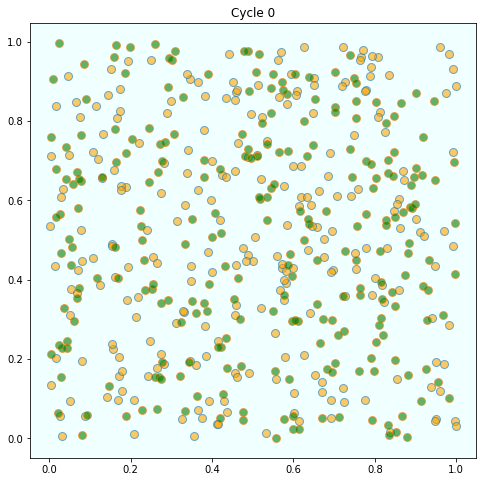    "![https://python.quantecon.org/_static/lecture_specific/schelling/schelling_fig1.png](https://python.quantecon.org/_static/lecture_specific/schelling/schelling_fig1.png)\n",
157 |     "\n",
158 |     "  \n",
159 |     "But after several cycles, they become segregated into distinct regions.\n",
160 |     "\n",
161 | 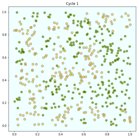    "![https://python.quantecon.org/_static/lecture_specific/schelling/schelling_fig2.png](https://python.quantecon.org/_static/lecture_specific/schelling/schelling_fig2.png)\n",
162 |     "\n",
163 |     "  \n",
164 | 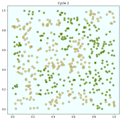    "![https://python.quantecon.org/_static/lecture_specific/schelling/schelling_fig3.png](https://python.quantecon.org/_static/lecture_specific/schelling/schelling_fig3.png)\n",
165 |     "\n",
166 |     "  \n",
167 | 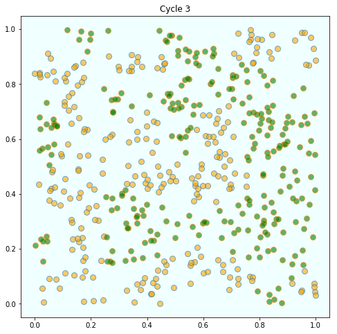    "![https://python.quantecon.org/_static/lecture_specific/schelling/schelling_fig4.png](https://python.quantecon.org/_static/lecture_specific/schelling/schelling_fig4.png)\n",
168 |     "\n",
169 |     "  \n",
170 |     "In this instance, the program terminated after 4 cycles through the set of\n",
171 |     "agents, indicating that all agents had reached a state of happiness.\n",
172 |     "\n",
173 |     "What is striking about the pictures is how rapidly racial integration breaks down.\n",
174 |     "\n",
175 |     "This is despite the fact that people in the model don’t actually mind living mixed with the other type.\n",
176 |     "\n",
177 |     "Even with these preferences, the outcome is a high degree of segregation."
178 |    ]
179 |   },
180 |   {
181 |    "cell_type": "markdown",
182 |    "id": "377ec057",
183 |    "metadata": {},
184 |    "source": [
185 |     "## Exercises"
186 |    ]
187 |   },
188 |   {
189 |    "cell_type": "markdown",
190 |    "id": "62072708",
191 |    "metadata": {},
192 |    "source": [
193 |     "## Exercise 67.1\n",
194 |     "\n",
195 |     "Implement and run this simulation for yourself.\n",
196 |     "\n",
197 |     "Consider the following structure for your program.\n",
198 |     "\n",
199 |     "Agents can be modeled as [objects](https://python-programming.quantecon.org/python_oop.html).\n",
200 |     "\n",
201 |     "Here’s an indication of how they might look"
202 |    ]
203 |   },
204 |   {
205 |    "cell_type": "markdown",
206 |    "id": "0b06bc85",
207 |    "metadata": {
208 |     "hide-output": false
209 |    },
210 |    "source": [
211 |     "```text\n",
212 |     "* Data:\n",
213 |     "\n",
214 |     "    * type (green or orange)\n",
215 |     "    * location\n",
216 |     "\n",
217 |     "* Methods:\n",
218 |     "\n",
219 |     "    * determine whether happy or not given locations of other agents\n",
220 |     "\n",
221 |     "    * If not happy, move\n",
222 |     "\n",
223 |     "        * find a new location where happy\n",
224 |     "```\n"
225 |    ]
226 |   },
227 |   {
228 |    "cell_type": "markdown",
229 |    "id": "e526860e",
230 |    "metadata": {},
231 |    "source": [
232 |     "And here’s some pseudocode for the main loop"
233 |    ]
234 |   },
235 |   {
236 |    "cell_type": "markdown",
237 |    "id": "cf798afd",
238 |    "metadata": {
239 |     "hide-output": false
240 |    },
241 |    "source": [
242 |     "```text\n",
243 |     "while agents are still moving\n",
244 |     "    for agent in agents\n",
245 |     "        give agent the opportunity to move\n",
246 |     "```\n"
247 |    ]
248 |   },
249 |   {
250 |    "cell_type": "markdown",
251 |    "id": "41df4768",
252 |    "metadata": {},
253 |    "source": [
254 |     "Use 250 agents of each type."
255 |    ]
256 |   },
257 |   {
258 |    "cell_type": "markdown",
259 |    "id": "c9d8a1d1",
260 |    "metadata": {},
261 |    "source": [
262 |     "## Solution to[ Exercise 67.1](https://python.quantecon.org/#schelling_ex1)\n",
263 |     "\n",
264 |     "Here’s one solution that does the job we want.\n",
265 |     "\n",
266 |     "If you feel like a further exercise, you can probably speed up some of the computations and\n",
267 |     "then increase the number of agents."
268 |    ]
269 |   },
270 |   {
271 |    "cell_type": "code",
272 |    "execution_count": null,
273 |    "id": "1e6fc12a",
274 |    "metadata": {
275 |     "hide-output": false
276 |    },
277 |    "outputs": [],
278 |    "source": [
279 |     "seed(10)  # For reproducible random numbers\n",
280 |     "\n",
281 |     "class Agent:\n",
282 |     "\n",
283 |     "    def __init__(self, type):\n",
284 |     "        self.type = type\n",
285 |     "        self.draw_location()\n",
286 |     "\n",
287 |     "    def draw_location(self):\n",
288 |     "        self.location = uniform(0, 1), uniform(0, 1)\n",
289 |     "\n",
290 |     "    def get_distance(self, other):\n",
291 |     "        \"Computes the euclidean distance between self and other agent.\"\n",
292 |     "        a = (self.location[0] - other.location[0])**2\n",
293 |     "        b = (self.location[1] - other.location[1])**2\n",
294 |     "        return sqrt(a + b)\n",
295 |     "\n",
296 |     "    def happy(self, agents):\n",
297 |     "        \"True if sufficient number of nearest neighbors are of the same type.\"\n",
298 |     "        distances = []\n",
299 |     "        # distances is a list of pairs (d, agent), where d is distance from\n",
300 |     "        # agent to self\n",
301 |     "        for agent in agents:\n",
302 |     "            if self != agent:\n",
303 |     "                distance = self.get_distance(agent)\n",
304 |     "                distances.append((distance, agent))\n",
305 |     "        # == Sort from smallest to largest, according to distance == #\n",
306 |     "        distances.sort()\n",
307 |     "        # == Extract the neighboring agents == #\n",
308 |     "        neighbors = [agent for d, agent in distances[:num_neighbors]]\n",
309 |     "        # == Count how many neighbors have the same type as self == #\n",
310 |     "        num_same_type = sum(self.type == agent.type for agent in neighbors)\n",
311 |     "        return num_same_type >= require_same_type\n",
312 |     "\n",
313 |     "    def update(self, agents):\n",
314 |     "        \"If not happy, then randomly choose new locations until happy.\"\n",
315 |     "        while not self.happy(agents):\n",
316 |     "            self.draw_location()\n",
317 |     "\n",
318 |     "\n",
319 |     "def plot_distribution(agents, cycle_num):\n",
320 |     "    \"Plot the distribution of agents after cycle_num rounds of the loop.\"\n",
321 |     "    x_values_0, y_values_0 = [], []\n",
322 |     "    x_values_1, y_values_1 = [], []\n",
323 |     "    # == Obtain locations of each type == #\n",
324 |     "    for agent in agents:\n",
325 |     "        x, y = agent.location\n",
326 |     "        if agent.type == 0:\n",
327 |     "            x_values_0.append(x)\n",
328 |     "            y_values_0.append(y)\n",
329 |     "        else:\n",
330 |     "            x_values_1.append(x)\n",
331 |     "            y_values_1.append(y)\n",
332 |     "    fig, ax = plt.subplots(figsize=(8, 8))\n",
333 |     "    plot_args = {'markersize': 8, 'alpha': 0.6}\n",
334 |     "    ax.set_facecolor('azure')\n",
335 |     "    ax.plot(x_values_0, y_values_0, 'o', markerfacecolor='orange', **plot_args)\n",
336 |     "    ax.plot(x_values_1, y_values_1, 'o', markerfacecolor='green', **plot_args)\n",
337 |     "    ax.set_title(f'Cycle {cycle_num-1}')\n",
338 |     "    plt.show()\n",
339 |     "\n",
340 |     "# == Main == #\n",
341 |     "\n",
342 |     "num_of_type_0 = 250\n",
343 |     "num_of_type_1 = 250\n",
344 |     "num_neighbors = 10      # Number of agents regarded as neighbors\n",
345 |     "require_same_type = 5   # Want at least this many neighbors to be same type\n",
346 |     "\n",
347 |     "# == Create a list of agents == #\n",
348 |     "agents = [Agent(0) for i in range(num_of_type_0)]\n",
349 |     "agents.extend(Agent(1) for i in range(num_of_type_1))\n",
350 |     "\n",
351 |     "\n",
352 |     "count = 1\n",
353 |     "# ==  Loop until none wishes to move == #\n",
354 |     "while True:\n",
355 |     "    print('Entering loop ', count)\n",
356 |     "    plot_distribution(agents, count)\n",
357 |     "    count += 1\n",
358 |     "    no_one_moved = True\n",
359 |     "    for agent in agents:\n",
360 |     "        old_location = agent.location\n",
361 |     "        agent.update(agents)\n",
362 |     "        if agent.location != old_location:\n",
363 |     "            no_one_moved = False\n",
364 |     "    if no_one_moved:\n",
365 |     "        break\n",
366 |     "\n",
367 |     "print('Converged, terminating.')"
368 |    ]
369 |   }
370 |  ],
371 |  "metadata": {
372 |   "date": 1710733976.466355,
373 |   "filename": "schelling.md",
374 |   "kernelspec": {
375 |    "display_name": "Python",
376 |    "language": "python3",
377 |    "name": "python3"
378 |   },
379 |   "title": "Schelling’s Segregation Model"
380 |  },
381 |  "nbformat": 4,
382 |  "nbformat_minor": 5
383 | }


--------------------------------------------------------------------------------
/egm_policy_iter.ipynb:
--------------------------------------------------------------------------------
  1 | {
  2 |  "cells": [
  3 |   {
  4 |    "cell_type": "markdown",
  5 |    "id": "642a6393",
  6 |    "metadata": {},
  7 |    "source": [
  8 |     "<div id=\"qe-notebook-header\" align=\"right\" style=\"text-align:right;\">\n",
  9 |     "        <a href=\"https://quantecon.org/\" title=\"quantecon.org\">\n",
 10 |     "                <img style=\"width:250px;display:inline;\" width=\"250px\" src=\"https://assets.quantecon.org/img/qe-menubar-logo.svg\" alt=\"QuantEcon\">\n",
 11 |     "        </a>\n",
 12 |     "</div>"
 13 |    ]
 14 |   },
 15 |   {
 16 |    "cell_type": "markdown",
 17 |    "id": "0c3facee",
 18 |    "metadata": {},
 19 |    "source": [
 20 |     "# Optimal Growth IV: The Endogenous Grid Method"
 21 |    ]
 22 |   },
 23 |   {
 24 |    "cell_type": "markdown",
 25 |    "id": "3641e019",
 26 |    "metadata": {},
 27 |    "source": [
 28 |     "## Contents\n",
 29 |     "\n",
 30 |     "- [Optimal Growth IV: The Endogenous Grid Method](#Optimal-Growth-IV:-The-Endogenous-Grid-Method)  \n",
 31 |     "  - [Overview](#Overview)  \n",
 32 |     "  - [Key Idea](#Key-Idea)  \n",
 33 |     "  - [Implementation](#Implementation)  "
 34 |    ]
 35 |   },
 36 |   {
 37 |    "cell_type": "markdown",
 38 |    "id": "d17745a8",
 39 |    "metadata": {},
 40 |    "source": [
 41 |     "## Overview\n",
 42 |     "\n",
 43 |     "Previously, we solved the stochastic optimal growth model using\n",
 44 |     "\n",
 45 |     "1. [value function iteration](https://python.quantecon.org/optgrowth_fast.html)  \n",
 46 |     "1. [Euler equation based time iteration](https://python.quantecon.org/coleman_policy_iter.html)  \n",
 47 |     "\n",
 48 |     "\n",
 49 |     "We found time iteration to be significantly more accurate and efficient.\n",
 50 |     "\n",
 51 |     "In this lecture, we’ll look at a clever twist on time iteration called the **endogenous grid method** (EGM).\n",
 52 |     "\n",
 53 |     "EGM is a numerical method for implementing policy iteration invented by [Chris Carroll](https://econ.jhu.edu/directory/christopher-carroll/).\n",
 54 |     "\n",
 55 |     "The original reference is [[Carroll, 2006](https://python.quantecon.org/zreferences.html#id168)].\n",
 56 |     "\n",
 57 |     "Let’s start with some standard imports:"
 58 |    ]
 59 |   },
 60 |   {
 61 |    "cell_type": "code",
 62 |    "execution_count": null,
 63 |    "id": "7572e2f1",
 64 |    "metadata": {
 65 |     "hide-output": false
 66 |    },
 67 |    "outputs": [],
 68 |    "source": [
 69 |     "import matplotlib.pyplot as plt\n",
 70 |     "import numpy as np\n",
 71 |     "from numba import jit"
 72 |    ]
 73 |   },
 74 |   {
 75 |    "cell_type": "markdown",
 76 |    "id": "cb928760",
 77 |    "metadata": {},
 78 |    "source": [
 79 |     "## Key Idea\n",
 80 |     "\n",
 81 |     "Let’s start by reminding ourselves of the theory and then see how the numerics fit in."
 82 |    ]
 83 |   },
 84 |   {
 85 |    "cell_type": "markdown",
 86 |    "id": "204b45cd",
 87 |    "metadata": {},
 88 |    "source": [
 89 |     "### Theory\n",
 90 |     "\n",
 91 |     "Take the model set out in [the time iteration lecture](https://python.quantecon.org/coleman_policy_iter.html), following the same terminology and notation.\n",
 92 |     "\n",
 93 |     "The Euler equation is\n",
 94 |     "\n",
 95 |     "\n",
 96 |     "<a id='equation-egm-euler'></a>\n",
 97 |     "$$\n",
 98 |     "(u'\\circ \\sigma^*)(y)\n",
 99 |     "= \\beta \\int (u'\\circ \\sigma^*)(f(y - \\sigma^*(y)) z) f'(y - \\sigma^*(y)) z \\phi(dz) \\tag{61.1}\n",
100 |     "$$\n",
101 |     "\n",
102 |     "As we saw, the Coleman-Reffett operator is a nonlinear operator $ K $ engineered so that $ \\sigma^* $ is a fixed point of $ K $.\n",
103 |     "\n",
104 |     "It takes as its argument a continuous strictly increasing consumption policy $ \\sigma \\in \\Sigma $.\n",
105 |     "\n",
106 |     "It returns a new function $ K \\sigma $,  where $ (K \\sigma)(y) $ is the $ c \\in (0, \\infty) $ that solves\n",
107 |     "\n",
108 |     "\n",
109 |     "<a id='equation-egm-coledef'></a>\n",
110 |     "$$\n",
111 |     "u'(c)\n",
112 |     "= \\beta \\int (u' \\circ \\sigma) (f(y - c) z ) f'(y - c) z \\phi(dz) \\tag{61.2}\n",
113 |     "$$"
114 |    ]
115 |   },
116 |   {
117 |    "cell_type": "markdown",
118 |    "id": "d0ffc4a6",
119 |    "metadata": {},
120 |    "source": [
121 |     "### Exogenous Grid\n",
122 |     "\n",
123 |     "As discussed in [the lecture on time iteration](https://python.quantecon.org/coleman_policy_iter.html), to implement the method on a computer, we need a numerical approximation.\n",
124 |     "\n",
125 |     "In particular, we represent a policy function by a set of values on a finite grid.\n",
126 |     "\n",
127 |     "The function itself is reconstructed from this representation when necessary, using interpolation or some other method.\n",
128 |     "\n",
129 |     "[Previously](https://python.quantecon.org/coleman_policy_iter.html), to obtain a finite representation of an updated consumption policy, we\n",
130 |     "\n",
131 |     "- fixed a grid of income points $ \\{y_i\\} $  \n",
132 |     "- calculated the consumption value $ c_i $ corresponding to each\n",
133 |     "  $ y_i $ using [(61.2)](#equation-egm-coledef) and a root-finding routine  \n",
134 |     "\n",
135 |     "\n",
136 |     "Each $ c_i $ is then interpreted as the value of the function $ K \\sigma $ at $ y_i $.\n",
137 |     "\n",
138 |     "Thus, with the points $ \\{y_i, c_i\\} $ in hand, we can reconstruct $ K \\sigma $ via approximation.\n",
139 |     "\n",
140 |     "Iteration then continues…"
141 |    ]
142 |   },
143 |   {
144 |    "cell_type": "markdown",
145 |    "id": "4f264951",
146 |    "metadata": {},
147 |    "source": [
148 |     "### Endogenous Grid\n",
149 |     "\n",
150 |     "The method discussed above requires a root-finding routine to find the\n",
151 |     "$ c_i $ corresponding to a given income value $ y_i $.\n",
152 |     "\n",
153 |     "Root-finding is costly because it typically involves a significant number of\n",
154 |     "function evaluations.\n",
155 |     "\n",
156 |     "As pointed out by Carroll [[Carroll, 2006](https://python.quantecon.org/zreferences.html#id168)], we can avoid this if\n",
157 |     "$ y_i $ is chosen endogenously.\n",
158 |     "\n",
159 |     "The only assumption required is that $ u' $ is invertible on $ (0, \\infty) $.\n",
160 |     "\n",
161 |     "Let $ (u')^{-1} $ be the inverse function of $ u' $.\n",
162 |     "\n",
163 |     "The idea is this:\n",
164 |     "\n",
165 |     "- First, we fix an *exogenous* grid $ \\{k_i\\} $ for capital ($ k = y - c $).  \n",
166 |     "- Then we obtain  $ c_i $ via  \n",
167 |     "\n",
168 |     "\n",
169 |     "\n",
170 |     "<a id='equation-egm-getc'></a>\n",
171 |     "$$\n",
172 |     "c_i =\n",
173 |     "(u')^{-1}\n",
174 |     "\\left\\{\n",
175 |     "    \\beta \\int (u' \\circ \\sigma) (f(k_i) z ) \\, f'(k_i) \\, z \\, \\phi(dz)\n",
176 |     "\\right\\} \\tag{61.3}\n",
177 |     "$$\n",
178 |     "\n",
179 |     "- Finally, for each $ c_i $ we set $ y_i = c_i + k_i $.  \n",
180 |     "\n",
181 |     "\n",
182 |     "It is clear that each $ (y_i, c_i) $ pair constructed in this manner satisfies [(61.2)](#equation-egm-coledef).\n",
183 |     "\n",
184 |     "With the points $ \\{y_i, c_i\\} $ in hand, we can reconstruct $ K \\sigma $ via approximation as before.\n",
185 |     "\n",
186 |     "The name EGM comes from the fact that the grid $ \\{y_i\\} $ is  determined **endogenously**."
187 |    ]
188 |   },
189 |   {
190 |    "cell_type": "markdown",
191 |    "id": "19b1c2bb",
192 |    "metadata": {},
193 |    "source": [
194 |     "## Implementation\n",
195 |     "\n",
196 |     "As [before](https://python.quantecon.org/coleman_policy_iter.html), we will start with a simple setting\n",
197 |     "where\n",
198 |     "\n",
199 |     "- $ u(c) = \\ln c $,  \n",
200 |     "- production is Cobb-Douglas, and  \n",
201 |     "- the shocks are lognormal.  \n",
202 |     "\n",
203 |     "\n",
204 |     "This will allow us to make comparisons with the analytical solutions"
205 |    ]
206 |   },
207 |   {
208 |    "cell_type": "code",
209 |    "execution_count": null,
210 |    "id": "c78a7db9",
211 |    "metadata": {
212 |     "hide-output": false
213 |    },
214 |    "outputs": [],
215 |    "source": [
216 |     "\n",
217 |     "def v_star(y, α, β, μ):\n",
218 |     "    \"\"\"\n",
219 |     "    True value function\n",
220 |     "    \"\"\"\n",
221 |     "    c1 = np.log(1 - α * β) / (1 - β)\n",
222 |     "    c2 = (μ + α * np.log(α * β)) / (1 - α)\n",
223 |     "    c3 = 1 / (1 - β)\n",
224 |     "    c4 = 1 / (1 - α * β)\n",
225 |     "    return c1 + c2 * (c3 - c4) + c4 * np.log(y)\n",
226 |     "\n",
227 |     "def σ_star(y, α, β):\n",
228 |     "    \"\"\"\n",
229 |     "    True optimal policy\n",
230 |     "    \"\"\"\n",
231 |     "    return (1 - α * β) * y"
232 |    ]
233 |   },
234 |   {
235 |    "cell_type": "markdown",
236 |    "id": "caa68a7c",
237 |    "metadata": {},
238 |    "source": [
239 |     "We reuse the `OptimalGrowthModel` class"
240 |    ]
241 |   },
242 |   {
243 |    "cell_type": "code",
244 |    "execution_count": null,
245 |    "id": "71a74289",
246 |    "metadata": {
247 |     "hide-output": false
248 |    },
249 |    "outputs": [],
250 |    "source": [
251 |     "from numba import float64\n",
252 |     "from numba.experimental import jitclass\n",
253 |     "\n",
254 |     "opt_growth_data = [\n",
255 |     "    ('α', float64),          # Production parameter\n",
256 |     "    ('β', float64),          # Discount factor\n",
257 |     "    ('μ', float64),          # Shock location parameter\n",
258 |     "    ('s', float64),          # Shock scale parameter\n",
259 |     "    ('grid', float64[:]),    # Grid (array)\n",
260 |     "    ('shocks', float64[:])   # Shock draws (array)\n",
261 |     "]\n",
262 |     "\n",
263 |     "@jitclass(opt_growth_data)\n",
264 |     "class OptimalGrowthModel:\n",
265 |     "\n",
266 |     "    def __init__(self,\n",
267 |     "                α=0.4,\n",
268 |     "                β=0.96,\n",
269 |     "                μ=0,\n",
270 |     "                s=0.1,\n",
271 |     "                grid_max=4,\n",
272 |     "                grid_size=120,\n",
273 |     "                shock_size=250,\n",
274 |     "                seed=1234):\n",
275 |     "\n",
276 |     "        self.α, self.β, self.μ, self.s = α, β, μ, s\n",
277 |     "\n",
278 |     "        # Set up grid\n",
279 |     "        self.grid = np.linspace(1e-5, grid_max, grid_size)\n",
280 |     "\n",
281 |     "        # Store shocks (with a seed, so results are reproducible)\n",
282 |     "        np.random.seed(seed)\n",
283 |     "        self.shocks = np.exp(μ + s * np.random.randn(shock_size))\n",
284 |     "\n",
285 |     "\n",
286 |     "    def f(self, k):\n",
287 |     "        \"The production function\"\n",
288 |     "        return k**self.α\n",
289 |     "\n",
290 |     "\n",
291 |     "    def u(self, c):\n",
292 |     "        \"The utility function\"\n",
293 |     "        return np.log(c)\n",
294 |     "\n",
295 |     "    def f_prime(self, k):\n",
296 |     "        \"Derivative of f\"\n",
297 |     "        return self.α * (k**(self.α - 1))\n",
298 |     "\n",
299 |     "\n",
300 |     "    def u_prime(self, c):\n",
301 |     "        \"Derivative of u\"\n",
302 |     "        return 1/c\n",
303 |     "\n",
304 |     "    def u_prime_inv(self, c):\n",
305 |     "        \"Inverse of u'\"\n",
306 |     "        return 1/c"
307 |    ]
308 |   },
309 |   {
310 |    "cell_type": "markdown",
311 |    "id": "ccf7221c",
312 |    "metadata": {},
313 |    "source": [
314 |     "### The Operator\n",
315 |     "\n",
316 |     "Here’s an implementation of $ K $ using EGM as described above."
317 |    ]
318 |   },
319 |   {
320 |    "cell_type": "code",
321 |    "execution_count": null,
322 |    "id": "d6e7ffd9",
323 |    "metadata": {
324 |     "hide-output": false
325 |    },
326 |    "outputs": [],
327 |    "source": [
328 |     "@jit\n",
329 |     "def K(σ_array, og):\n",
330 |     "    \"\"\"\n",
331 |     "    The Coleman-Reffett operator using EGM\n",
332 |     "\n",
333 |     "    \"\"\"\n",
334 |     "\n",
335 |     "    # Simplify names\n",
336 |     "    f, β = og.f, og.β\n",
337 |     "    f_prime, u_prime = og.f_prime, og.u_prime\n",
338 |     "    u_prime_inv = og.u_prime_inv\n",
339 |     "    grid, shocks = og.grid, og.shocks\n",
340 |     "\n",
341 |     "    # Determine endogenous grid\n",
342 |     "    y = grid + σ_array  # y_i = k_i + c_i\n",
343 |     "\n",
344 |     "    # Linear interpolation of policy using endogenous grid\n",
345 |     "    σ = lambda x: np.interp(x, y, σ_array)\n",
346 |     "\n",
347 |     "    # Allocate memory for new consumption array\n",
348 |     "    c = np.empty_like(grid)\n",
349 |     "\n",
350 |     "    # Solve for updated consumption value\n",
351 |     "    for i, k in enumerate(grid):\n",
352 |     "        vals = u_prime(σ(f(k) * shocks)) * f_prime(k) * shocks\n",
353 |     "        c[i] = u_prime_inv(β * np.mean(vals))\n",
354 |     "\n",
355 |     "    return c"
356 |    ]
357 |   },
358 |   {
359 |    "cell_type": "markdown",
360 |    "id": "9ccb0190",
361 |    "metadata": {},
362 |    "source": [
363 |     "Note the lack of any root-finding algorithm."
364 |    ]
365 |   },
366 |   {
367 |    "cell_type": "markdown",
368 |    "id": "af7a6400",
369 |    "metadata": {},
370 |    "source": [
371 |     "### Testing\n",
372 |     "\n",
373 |     "First we create an instance."
374 |    ]
375 |   },
376 |   {
377 |    "cell_type": "code",
378 |    "execution_count": null,
379 |    "id": "ac8b5e4d",
380 |    "metadata": {
381 |     "hide-output": false
382 |    },
383 |    "outputs": [],
384 |    "source": [
385 |     "og = OptimalGrowthModel()\n",
386 |     "grid = og.grid"
387 |    ]
388 |   },
389 |   {
390 |    "cell_type": "markdown",
391 |    "id": "8d5adc39",
392 |    "metadata": {},
393 |    "source": [
394 |     "Here’s our solver routine:"
395 |    ]
396 |   },
397 |   {
398 |    "cell_type": "code",
399 |    "execution_count": null,
400 |    "id": "1749f58a",
401 |    "metadata": {
402 |     "hide-output": false
403 |    },
404 |    "outputs": [],
405 |    "source": [
406 |     "def solve_model_time_iter(model,    # Class with model information\n",
407 |     "                          σ,        # Initial condition\n",
408 |     "                          tol=1e-4,\n",
409 |     "                          max_iter=1000,\n",
410 |     "                          verbose=True,\n",
411 |     "                          print_skip=25):\n",
412 |     "\n",
413 |     "    # Set up loop\n",
414 |     "    i = 0\n",
415 |     "    error = tol + 1\n",
416 |     "\n",
417 |     "    while i < max_iter and error > tol:\n",
418 |     "        σ_new = K(σ, model)\n",
419 |     "        error = np.max(np.abs(σ - σ_new))\n",
420 |     "        i += 1\n",
421 |     "        if verbose and i % print_skip == 0:\n",
422 |     "            print(f\"Error at iteration {i} is {error}.\")\n",
423 |     "        σ = σ_new\n",
424 |     "\n",
425 |     "    if error > tol:\n",
426 |     "        print(\"Failed to converge!\")\n",
427 |     "    elif verbose:\n",
428 |     "        print(f\"\\nConverged in {i} iterations.\")\n",
429 |     "\n",
430 |     "    return σ_new"
431 |    ]
432 |   },
433 |   {
434 |    "cell_type": "markdown",
435 |    "id": "8bf3c238",
436 |    "metadata": {},
437 |    "source": [
438 |     "Let’s call it:"
439 |    ]
440 |   },
441 |   {
442 |    "cell_type": "code",
443 |    "execution_count": null,
444 |    "id": "8393528f",
445 |    "metadata": {
446 |     "hide-output": false
447 |    },
448 |    "outputs": [],
449 |    "source": [
450 |     "σ_init = np.copy(grid)\n",
451 |     "σ = solve_model_time_iter(og, σ_init)"
452 |    ]
453 |   },
454 |   {
455 |    "cell_type": "markdown",
456 |    "id": "fdfc5ff4",
457 |    "metadata": {},
458 |    "source": [
459 |     "Here is a plot of the resulting policy, compared with the true policy:"
460 |    ]
461 |   },
462 |   {
463 |    "cell_type": "code",
464 |    "execution_count": null,
465 |    "id": "b65bfdb1",
466 |    "metadata": {
467 |     "hide-output": false
468 |    },
469 |    "outputs": [],
470 |    "source": [
471 |     "y = grid + σ  # y_i = k_i + c_i\n",
472 |     "\n",
473 |     "fig, ax = plt.subplots()\n",
474 |     "\n",
475 |     "ax.plot(y, σ, lw=2,\n",
476 |     "        alpha=0.8, label='approximate policy function')\n",
477 |     "\n",
478 |     "ax.plot(y, σ_star(y, og.α, og.β), 'k--',\n",
479 |     "        lw=2, alpha=0.8, label='true policy function')\n",
480 |     "\n",
481 |     "ax.legend()\n",
482 |     "plt.show()"
483 |    ]
484 |   },
485 |   {
486 |    "cell_type": "markdown",
487 |    "id": "3e13fe87",
488 |    "metadata": {},
489 |    "source": [
490 |     "The maximal absolute deviation between the two policies is"
491 |    ]
492 |   },
493 |   {
494 |    "cell_type": "code",
495 |    "execution_count": null,
496 |    "id": "50c18390",
497 |    "metadata": {
498 |     "hide-output": false
499 |    },
500 |    "outputs": [],
501 |    "source": [
502 |     "np.max(np.abs(σ - σ_star(y, og.α, og.β)))"
503 |    ]
504 |   },
505 |   {
506 |    "cell_type": "markdown",
507 |    "id": "adce2673",
508 |    "metadata": {},
509 |    "source": [
510 |     "How long does it take to converge?"
511 |    ]
512 |   },
513 |   {
514 |    "cell_type": "code",
515 |    "execution_count": null,
516 |    "id": "49b2ab11",
517 |    "metadata": {
518 |     "hide-output": false
519 |    },
520 |    "outputs": [],
521 |    "source": [
522 |     "%%timeit -n 3 -r 1\n",
523 |     "σ = solve_model_time_iter(og, σ_init, verbose=False)"
524 |    ]
525 |   },
526 |   {
527 |    "cell_type": "markdown",
528 |    "id": "8f210ca1",
529 |    "metadata": {},
530 |    "source": [
531 |     "Relative to time iteration, which as already found to be highly efficient, EGM\n",
532 |     "has managed to shave off still more run time without compromising accuracy.\n",
533 |     "\n",
534 |     "This is due to the lack of a numerical root-finding step.\n",
535 |     "\n",
536 |     "We can now solve the optimal growth model at given parameters extremely fast."
537 |    ]
538 |   }
539 |  ],
540 |  "metadata": {
541 |   "date": 1762377773.044283,
542 |   "filename": "egm_policy_iter.md",
543 |   "kernelspec": {
544 |    "display_name": "Python",
545 |    "language": "python3",
546 |    "name": "python3"
547 |   },
548 |   "title": "Optimal Growth IV: The Endogenous Grid Method"
549 |  },
550 |  "nbformat": 4,
551 |  "nbformat_minor": 5
552 | }


--------------------------------------------------------------------------------
/rand_resp.ipynb:
--------------------------------------------------------------------------------
  1 | {
  2 |  "cells": [
  3 |   {
  4 |    "cell_type": "markdown",
  5 |    "id": "fac619a9",
  6 |    "metadata": {},
  7 |    "source": [
  8 |     "# Randomized Response Surveys"
  9 |    ]
 10 |   },
 11 |   {
 12 |    "cell_type": "markdown",
 13 |    "id": "678daa6d",
 14 |    "metadata": {},
 15 |    "source": [
 16 |     "## Overview\n",
 17 |     "\n",
 18 |     "Social stigmas can inhibit people from confessing potentially embarrassing activities or opinions.\n",
 19 |     "\n",
 20 |     "When people are reluctant to participate a sample survey about personally  sensitive issues, they  might decline  to participate, and even if they do participate, they might choose to provide incorrect answers to  sensitive questions.\n",
 21 |     "\n",
 22 |     "These problems induce  **selection**  biases that present challenges to interpreting and designing surveys.\n",
 23 |     "\n",
 24 |     "To illustrate how social scientists have thought about estimating the prevalence of such embarrassing activities and opinions, this lecture describes a classic approach  of S. L. Warner [[Warner, 1965](https://python.quantecon.org/zreferences.html#id23)].\n",
 25 |     "\n",
 26 |     "Warner  used elementary  probability to construct a  way to protect the privacy  of **individual** respondents to surveys while still    estimating  the fraction of a **collection** of individuals   who have a socially stigmatized characteristic or who engage in  a socially stigmatized activity.\n",
 27 |     "\n",
 28 |     "Warner’s idea was to  add **noise** between the respondent’s answer and the **signal** about that answer that the  survey maker ultimately receives.\n",
 29 |     "\n",
 30 |     "Knowing about the structure of the noise assures the respondent that the survey maker does not observe his answer.\n",
 31 |     "\n",
 32 |     "Statistical properties of the  noise injection procedure provide the respondent  **plausible deniability**.\n",
 33 |     "\n",
 34 |     "Related ideas underlie  modern **differential privacy** systems.\n",
 35 |     "\n",
 36 |     "(See [https://en.wikipedia.org/wiki/Differential_privacy](https://en.wikipedia.org/wiki/Differential_privacy))"
 37 |    ]
 38 |   },
 39 |   {
 40 |    "cell_type": "markdown",
 41 |    "id": "e4bf65aa",
 42 |    "metadata": {},
 43 |    "source": [
 44 |     "## Warner’s Strategy\n",
 45 |     "\n",
 46 |     "As usual, let’s bring in the Python modules we’ll be using."
 47 |    ]
 48 |   },
 49 |   {
 50 |    "cell_type": "code",
 51 |    "execution_count": null,
 52 |    "id": "bde1ce1c",
 53 |    "metadata": {
 54 |     "hide-output": false
 55 |    },
 56 |    "outputs": [],
 57 |    "source": [
 58 |     "import numpy as np\n",
 59 |     "import pandas as pd"
 60 |    ]
 61 |   },
 62 |   {
 63 |    "cell_type": "markdown",
 64 |    "id": "1297d5e4",
 65 |    "metadata": {},
 66 |    "source": [
 67 |     "Suppose that every person in population either belongs to Group A or Group B.\n",
 68 |     "\n",
 69 |     "We want to estimate the proportion $ \\pi $ who belong to Group A while protecting individual respondents’ privacy.\n",
 70 |     "\n",
 71 |     "Warner [[Warner, 1965](https://python.quantecon.org/zreferences.html#id23)] proposed and analyzed the following procedure.\n",
 72 |     "\n",
 73 |     "- A  random sample of $ n $ people is drawn with replacement from the population and  each person is interviewed.  \n",
 74 |     "- Draw $ n $ random samples from the population with replacement and interview each person.  \n",
 75 |     "- Prepare a **random spinner** that with $ p $ probability points to the Letter A and with $ (1-p) $ probability points to the Letter B.  \n",
 76 |     "- Each subject spins a random spinner and sees an outcome (A or B)  that the interviewer  does **not observe**.  \n",
 77 |     "- The subject   states whether he belongs to the group to which the spinner points.  \n",
 78 |     "- If the spinner points to the group that the spinner belongs, the subject reports “yes”; otherwise he reports “no”.  \n",
 79 |     "- The  subject answers the question truthfully.  \n",
 80 |     "\n",
 81 |     "\n",
 82 |     "Warner constructed a maximum  likelihood estimators of the proportion of the population in set A.\n",
 83 |     "\n",
 84 |     "Let\n",
 85 |     "\n",
 86 |     "- $ \\pi $ : True probability of A in the population  \n",
 87 |     "- $ p $ : Probability that the spinner points to A  \n",
 88 |     "- $ X_{i}=\\begin{cases}1,\\text{ if the } i\\text{th} \\ \\text{ subject  says yes}\\\\0,\\text{ if the } i\\text{th} \\ \\text{  subject  says no}\\end{cases} $  \n",
 89 |     "\n",
 90 |     "\n",
 91 |     "Index the sample set so that  the first $ n_1 $ report “yes”, while the second $ n-n_1 $ report “no”.\n",
 92 |     "\n",
 93 |     "The likelihood function of a sample set is\n",
 94 |     "\n",
 95 |     "\n",
 96 |     "<a id='equation-eq-one'></a>\n",
 97 |     "$$\n",
 98 |     "L=\\left[\\pi p + (1-\\pi)(1-p)\\right]^{n_{1}}\\left[(1-\\pi) p +\\pi (1-p)\\right]^{n-n_{1}} \\tag{16.1}\n",
 99 |     "$$\n",
100 |     "\n",
101 |     "The log of the likelihood function is:\n",
102 |     "\n",
103 |     "\n",
104 |     "<a id='equation-eq-two'></a>\n",
105 |     "$$\n",
106 |     "\\log(L)= n_1 \\log \\left[\\pi p + (1-\\pi)(1-p)\\right] + (n-n_{1}) \\log \\left[(1-\\pi) p +\\pi (1-p)\\right] \\tag{16.2}\n",
107 |     "$$\n",
108 |     "\n",
109 |     "The first-order necessary condition for maximizing the log likelihood function with respect to  $ \\pi $ is:\n",
110 |     "\n",
111 |     "$$\n",
112 |     "\\frac{(n-n_1)(2p-1)}{(1-\\pi) p +\\pi (1-p)}=\\frac{n_1 (2p-1)}{\\pi p + (1-\\pi)(1-p)}\n",
113 |     "$$\n",
114 |     "\n",
115 |     "or\n",
116 |     "\n",
117 |     "\n",
118 |     "<a id='equation-eq-3'></a>\n",
119 |     "$$\n",
120 |     "\\pi p + (1-\\pi)(1-p)=\\frac{n_1}{n} \\tag{16.3}\n",
121 |     "$$\n",
122 |     "\n",
123 |     "If  $ p \\neq \\frac{1}{2} $, then the maximum likelihood estimator (MLE) of $ \\pi $ is:\n",
124 |     "\n",
125 |     "\n",
126 |     "<a id='equation-eq-four'></a>\n",
127 |     "$$\n",
128 |     "\\hat{\\pi}=\\frac{p-1}{2p-1}+\\frac{n_1}{(2p-1)n} \\tag{16.4}\n",
129 |     "$$\n",
130 |     "\n",
131 |     "We compute the mean and variance of the MLE estimator $ \\hat \\pi $ to be:\n",
132 |     "\n",
133 |     "\n",
134 |     "<a id='equation-eq-five'></a>\n",
135 |     "$$\n",
136 |     "\\begin{aligned}\n",
137 |     "\\mathbb{E}(\\hat{\\pi})&= \\frac{1}{2 p-1}\\left[p-1+\\frac{1}{n} \\sum_{i=1}^{n} \\mathbb{E} X_i \\right] \\\\\n",
138 |     "&=\\frac{1}{2 p-1} \\left[ p -1 + \\pi p + (1-\\pi)(1-p)\\right] \\\\\n",
139 |     "&=\\pi\n",
140 |     "\\end{aligned} \\tag{16.5}\n",
141 |     "$$\n",
142 |     "\n",
143 |     "and\n",
144 |     "\n",
145 |     "\n",
146 |     "<a id='equation-eq-six'></a>\n",
147 |     "$$\n",
148 |     "\\begin{aligned}\n",
149 |     "Var(\\hat{\\pi})&=\\frac{n Var(X_i)}{(2p - 1 )^2 n^2} \\\\\n",
150 |     "&= \\frac{\\left[\\pi p + (1-\\pi)(1-p)\\right]\\left[(1-\\pi) p +\\pi (1-p)\\right]}{(2p - 1 )^2 n^2}\\\\\n",
151 |     "&=\\frac{\\frac{1}{4}+(2 p^2 - 2 p +\\frac{1}{2})(- 2 \\pi^2 + 2 \\pi -\\frac{1}{2})}{(2p - 1 )^2 n^2}\\\\\n",
152 |     "&=\\frac{1}{n}\\left[\\frac{1}{16(p-\\frac{1}{2})^2}-(\\pi-\\frac{1}{2})^2 \\right]\n",
153 |     "\\end{aligned} \\tag{16.6}\n",
154 |     "$$\n",
155 |     "\n",
156 |     "Equation [(16.5)](#equation-eq-five) indicates  that $ \\hat{\\pi} $ is an **unbiased estimator** of $ \\pi $ while equation [(16.6)](#equation-eq-six) tell us the variance of the estimator.\n",
157 |     "\n",
158 |     "To compute a  confidence interval, first  rewrite [(16.6)](#equation-eq-six) as:\n",
159 |     "\n",
160 |     "\n",
161 |     "<a id='equation-eq-seven'></a>\n",
162 |     "$$\n",
163 |     "Var(\\hat{\\pi})=\\frac{\\frac{1}{4}-(\\pi-\\frac{1}{2})^2}{n}+\\frac{\\frac{1}{16(p-\\frac{1}{2})^2}-\\frac{1}{4}}{n} \\tag{16.7}\n",
164 |     "$$\n",
165 |     "\n",
166 |     "This equation indicates that the variance of $ \\hat{\\pi} $ can be represented as a sum of the variance due to sampling plus the variance due to the random device.\n",
167 |     "\n",
168 |     "From the expressions above we can find that:\n",
169 |     "\n",
170 |     "- When $ p $ is $ \\frac{1}{2} $, expression [(16.1)](#equation-eq-one) degenerates to a constant.  \n",
171 |     "- When $ p $ is $ 1 $ or $ 0 $, the randomized estimate degenerates to an estimator without randomized sampling.  \n",
172 |     "\n",
173 |     "\n",
174 |     "We shall only discuss  situations in which $ p \\in (\\frac{1}{2},1) $\n",
175 |     "\n",
176 |     "(a situation in which $ p \\in (0,\\frac{1}{2}) $ is symmetric).\n",
177 |     "\n",
178 |     "From expressions [(16.5)](#equation-eq-five) and [(16.7)](#equation-eq-seven) we can deduce that:\n",
179 |     "\n",
180 |     "- The MSE of $ \\hat{\\pi} $  decreases as $ p $ increases.  "
181 |    ]
182 |   },
183 |   {
184 |    "cell_type": "markdown",
185 |    "id": "a8aad786",
186 |    "metadata": {},
187 |    "source": [
188 |     "## Comparing Two Survey Designs\n",
189 |     "\n",
190 |     "Let’s compare the preceding randomized-response method with a stylized non-randomized response method.\n",
191 |     "\n",
192 |     "In our non-randomized response method, we suppose that:\n",
193 |     "\n",
194 |     "- Members of Group A tells the truth with probability  $ T_a $ while the members of Group B tells the truth with probability $ T_b $  \n",
195 |     "- $ Y_i $ is $ 1 $ or $ 0 $ according to whether the sample’s $ i\\text{th} $ member’s report is in Group A or not.  \n",
196 |     "\n",
197 |     "\n",
198 |     "Then we can estimate $ \\pi $ as:\n",
199 |     "\n",
200 |     "\n",
201 |     "<a id='equation-eq-eight'></a>\n",
202 |     "$$\n",
203 |     "\\hat{\\pi}=\\frac{\\sum_{i=1}^{n}Y_i}{n} \\tag{16.8}\n",
204 |     "$$\n",
205 |     "\n",
206 |     "We calculate the expectation, bias, and variance of the estimator to be:\n",
207 |     "\n",
208 |     "\n",
209 |     "<a id='equation-eq-nine'></a>\n",
210 |     "$$\n",
211 |     "\\begin{aligned}\n",
212 |     "\\mathbb{E}(\\hat{\\pi})&=\\pi T_a + \\left[ (1-\\pi)(1-T_b)\\right]\\\\\n",
213 |     "\\end{aligned} \\tag{16.9}\n",
214 |     "$$\n",
215 |     "\n",
216 |     "\n",
217 |     "<a id='equation-eq-ten'></a>\n",
218 |     "$$\n",
219 |     "\\begin{aligned}\n",
220 |     "Bias(\\hat{\\pi})&=\\mathbb{E}(\\hat{\\pi}-\\pi)\\\\\n",
221 |     "&=\\pi [T_a + T_b -2 ] + [1- T_b] \\\\\n",
222 |     "\\end{aligned} \\tag{16.10}\n",
223 |     "$$\n",
224 |     "\n",
225 |     "\n",
226 |     "<a id='equation-eq-eleven'></a>\n",
227 |     "$$\n",
228 |     "\\begin{aligned}\n",
229 |     "Var(\\hat{\\pi})&=\\frac{ \\left[ \\pi T_a + (1-\\pi)(1-T_b)\\right]  \\left[1- \\pi T_a -(1-\\pi)(1-T_b)\\right] }{n}\n",
230 |     "\\end{aligned} \\tag{16.11}\n",
231 |     "$$\n",
232 |     "\n",
233 |     "It is useful to define a\n",
234 |     "\n",
235 |     "$$\n",
236 |     "\\text{MSE Ratio}=\\frac{\\text{Mean Square Error Randomized}}{\\text{Mean Square Error Regular}}\n",
237 |     "$$\n",
238 |     "\n",
239 |     "We can compute  MSE Ratios for different survey designs associated with different parameter values.\n",
240 |     "\n",
241 |     "The following Python code computes  objects we want to stare at in order to make comparisons\n",
242 |     "under  different values of $ \\pi_A $ and $ n $:"
243 |    ]
244 |   },
245 |   {
246 |    "cell_type": "code",
247 |    "execution_count": null,
248 |    "id": "2e443e87",
249 |    "metadata": {
250 |     "hide-output": false
251 |    },
252 |    "outputs": [],
253 |    "source": [
254 |     "class Comparison:\n",
255 |     "    def __init__(self, A, n):\n",
256 |     "        self.A = A\n",
257 |     "        self.n = n\n",
258 |     "        TaTb = np.array([[0.95,  1], [0.9,   1], [0.7,    1], \n",
259 |     "                         [0.5,   1], [1,  0.95], [1,    0.9], \n",
260 |     "                         [1,   0.7], [1,   0.5], [0.95, 0.95], \n",
261 |     "                         [0.9, 0.9], [0.7, 0.7], [0.5,  0.5]])\n",
262 |     "        self.p_arr = np.array([0.6, 0.7, 0.8, 0.9])\n",
263 |     "        self.p_map = dict(zip(self.p_arr, [f\"MSE Ratio: p = {x}\" for x in self.p_arr]))\n",
264 |     "        self.template = pd.DataFrame(columns=self.p_arr)\n",
265 |     "        self.template[['T_a','T_b']] = TaTb\n",
266 |     "        self.template['Bias'] = None\n",
267 |     "    \n",
268 |     "    def theoretical(self):\n",
269 |     "        A = self.A\n",
270 |     "        n = self.n\n",
271 |     "        df = self.template.copy()\n",
272 |     "        df['Bias'] = A * (df['T_a'] + df['T_b'] - 2) + (1 - df['T_b'])\n",
273 |     "        for p in self.p_arr:\n",
274 |     "            df[p] = (1 / (16 * (p - 1/2)**2) - (A - 1/2)**2) / n / \\\n",
275 |     "                    (df['Bias']**2 + ((A * df['T_a'] + (1 - A) * (1 - df['T_b'])) * (1 - A * df['T_a'] - (1 - A) * (1 - df['T_b'])) / n))\n",
276 |     "            df[p] = df[p].round(2)\n",
277 |     "        df = df.set_index([\"T_a\", \"T_b\", \"Bias\"]).rename(columns=self.p_map)\n",
278 |     "        return df\n",
279 |     "        \n",
280 |     "    def MCsimulation(self, size=1000, seed=123456):\n",
281 |     "        A = self.A\n",
282 |     "        n = self.n\n",
283 |     "        df = self.template.copy()\n",
284 |     "        np.random.seed(seed)\n",
285 |     "        sample = np.random.rand(size, self.n) <= A\n",
286 |     "        random_device = np.random.rand(size, n)\n",
287 |     "        mse_rd = {}\n",
288 |     "        for p in self.p_arr:\n",
289 |     "            spinner = random_device <= p\n",
290 |     "            rd_answer = sample * spinner + (1 - sample) * (1 - spinner)\n",
291 |     "            n1 = rd_answer.sum(axis=1)\n",
292 |     "            pi_hat = (p - 1) / (2 * p - 1) + n1 / n / (2 * p - 1)\n",
293 |     "            mse_rd[p] = np.sum((pi_hat - A)**2)\n",
294 |     "        for inum, irow in df.iterrows():\n",
295 |     "            truth_a = np.random.rand(size, self.n) <= irow.T_a\n",
296 |     "            truth_b = np.random.rand(size, self.n) <= irow.T_b\n",
297 |     "            trad_answer = sample * truth_a + (1 - sample) * (1 - truth_b)\n",
298 |     "            pi_trad = trad_answer.sum(axis=1) / n\n",
299 |     "            df.loc[inum, 'Bias'] = pi_trad.mean() - A\n",
300 |     "            mse_trad = np.sum((pi_trad - A)**2)\n",
301 |     "            for p in self.p_arr:\n",
302 |     "                df.loc[inum, p] = (mse_rd[p] / mse_trad).round(2)\n",
303 |     "        df = df.set_index([\"T_a\", \"T_b\", \"Bias\"]).rename(columns=self.p_map)\n",
304 |     "        return df"
305 |    ]
306 |   },
307 |   {
308 |    "cell_type": "markdown",
309 |    "id": "d20ebbf7",
310 |    "metadata": {},
311 |    "source": [
312 |     "Let’s put the code to work for parameter values\n",
313 |     "\n",
314 |     "- $ \\pi_A=0.6 $  \n",
315 |     "- $ n=1000 $  \n",
316 |     "\n",
317 |     "\n",
318 |     "We can generate MSE Ratios theoretically using the above formulas.\n",
319 |     "\n",
320 |     "We can also perform   Monte Carlo simulations  of a MSE Ratio."
321 |    ]
322 |   },
323 |   {
324 |    "cell_type": "code",
325 |    "execution_count": null,
326 |    "id": "43919ceb",
327 |    "metadata": {
328 |     "hide-output": false
329 |    },
330 |    "outputs": [],
331 |    "source": [
332 |     "cp1 = Comparison(0.6, 1000)\n",
333 |     "df1_theoretical = cp1.theoretical()\n",
334 |     "df1_theoretical"
335 |    ]
336 |   },
337 |   {
338 |    "cell_type": "code",
339 |    "execution_count": null,
340 |    "id": "6e667ab7",
341 |    "metadata": {
342 |     "hide-output": false
343 |    },
344 |    "outputs": [],
345 |    "source": [
346 |     "df1_mc = cp1.MCsimulation()\n",
347 |     "df1_mc"
348 |    ]
349 |   },
350 |   {
351 |    "cell_type": "markdown",
352 |    "id": "21f90a01",
353 |    "metadata": {},
354 |    "source": [
355 |     "The theoretical calculations  do a good job of predicting  Monte Carlo results.\n",
356 |     "\n",
357 |     "We see that in many situations, especially when the bias is not small, the MSE of the randomized-sampling  methods is smaller than that of the non-randomized sampling method.\n",
358 |     "\n",
359 |     "These differences become larger as  $ p $ increases.\n",
360 |     "\n",
361 |     "By adjusting  parameters $ \\pi_A $ and $ n $, we can study outcomes in different situations.\n",
362 |     "\n",
363 |     "For example, for another situation described in Warner [[Warner, 1965](https://python.quantecon.org/zreferences.html#id23)]:\n",
364 |     "\n",
365 |     "- $ \\pi_A=0.5 $  \n",
366 |     "- $ n=1000 $  \n",
367 |     "\n",
368 |     "\n",
369 |     "we can use the code"
370 |    ]
371 |   },
372 |   {
373 |    "cell_type": "code",
374 |    "execution_count": null,
375 |    "id": "d8df2645",
376 |    "metadata": {
377 |     "hide-output": false
378 |    },
379 |    "outputs": [],
380 |    "source": [
381 |     "cp2 = Comparison(0.5, 1000)\n",
382 |     "df2_theoretical = cp2.theoretical()\n",
383 |     "df2_theoretical"
384 |    ]
385 |   },
386 |   {
387 |    "cell_type": "code",
388 |    "execution_count": null,
389 |    "id": "b584197a",
390 |    "metadata": {
391 |     "hide-output": false
392 |    },
393 |    "outputs": [],
394 |    "source": [
395 |     "df2_mc = cp2.MCsimulation()\n",
396 |     "df2_mc"
397 |    ]
398 |   },
399 |   {
400 |    "cell_type": "markdown",
401 |    "id": "3a287372",
402 |    "metadata": {},
403 |    "source": [
404 |     "We can also revisit a calculation in the  concluding section of Warner [[Warner, 1965](https://python.quantecon.org/zreferences.html#id23)] in which\n",
405 |     "\n",
406 |     "- $ \\pi_A=0.6 $  \n",
407 |     "- $ n=2000 $  \n",
408 |     "\n",
409 |     "\n",
410 |     "We use the code"
411 |    ]
412 |   },
413 |   {
414 |    "cell_type": "code",
415 |    "execution_count": null,
416 |    "id": "d463eae5",
417 |    "metadata": {
418 |     "hide-output": false
419 |    },
420 |    "outputs": [],
421 |    "source": [
422 |     "cp3 = Comparison(0.6, 2000)\n",
423 |     "df3_theoretical = cp3.theoretical()\n",
424 |     "df3_theoretical"
425 |    ]
426 |   },
427 |   {
428 |    "cell_type": "code",
429 |    "execution_count": null,
430 |    "id": "d06079cc",
431 |    "metadata": {
432 |     "hide-output": false
433 |    },
434 |    "outputs": [],
435 |    "source": [
436 |     "df3_mc = cp3.MCsimulation()\n",
437 |     "df3_mc"
438 |    ]
439 |   },
440 |   {
441 |    "cell_type": "markdown",
442 |    "id": "d4ff40b7",
443 |    "metadata": {},
444 |    "source": [
445 |     "Evidently, as $ n $ increases, the randomized response method does  better performance in more situations."
446 |    ]
447 |   },
448 |   {
449 |    "cell_type": "markdown",
450 |    "id": "f1cd5db0",
451 |    "metadata": {},
452 |    "source": [
453 |     "## Concluding Remarks\n",
454 |     "\n",
455 |     "[This QuantEcon lecture](https://python.quantecon.org/util_rand_resp.html)  describes some alternative randomized response surveys.\n",
456 |     "\n",
457 |     "That lecture presents a utilitarian analysis of those alternatives conducted by Lars Ljungqvist\n",
458 |     "[[Ljungqvist, 1993](https://python.quantecon.org/zreferences.html#id24)]."
459 |    ]
460 |   }
461 |  ],
462 |  "metadata": {
463 |   "date": 1764675755.2406225,
464 |   "filename": "rand_resp.md",
465 |   "kernelspec": {
466 |    "display_name": "Python",
467 |    "language": "python3",
468 |    "name": "python3"
469 |   },
470 |   "title": "Randomized Response Surveys"
471 |  },
472 |  "nbformat": 4,
473 |  "nbformat_minor": 5
474 | }


--------------------------------------------------------------------------------
/os_egm.ipynb:
--------------------------------------------------------------------------------
  1 | {
  2 |  "cells": [
  3 |   {
  4 |    "cell_type": "markdown",
  5 |    "id": "41902a14",
  6 |    "metadata": {},
  7 |    "source": [
  8 |     "<div id=\"qe-notebook-header\" align=\"right\" style=\"text-align:right;\">\n",
  9 |     "        <a href=\"https://quantecon.org/\" title=\"quantecon.org\">\n",
 10 |     "                <img style=\"width:250px;display:inline;\" width=\"250px\" src=\"https://assets.quantecon.org/img/qe-menubar-logo.svg\" alt=\"QuantEcon\">\n",
 11 |     "        </a>\n",
 12 |     "</div>"
 13 |    ]
 14 |   },
 15 |   {
 16 |    "cell_type": "markdown",
 17 |    "id": "50125c8a",
 18 |    "metadata": {},
 19 |    "source": [
 20 |     "# Optimal Savings V: The Endogenous Grid Method"
 21 |    ]
 22 |   },
 23 |   {
 24 |    "cell_type": "markdown",
 25 |    "id": "87178c86",
 26 |    "metadata": {},
 27 |    "source": [
 28 |     "## Contents\n",
 29 |     "\n",
 30 |     "- [Optimal Savings V: The Endogenous Grid Method](#Optimal-Savings-V:-The-Endogenous-Grid-Method)  \n",
 31 |     "  - [Overview](#Overview)  \n",
 32 |     "  - [Key Idea](#Key-Idea)  \n",
 33 |     "  - [Implementation](#Implementation)  "
 34 |    ]
 35 |   },
 36 |   {
 37 |    "cell_type": "markdown",
 38 |    "id": "60437ce1",
 39 |    "metadata": {},
 40 |    "source": [
 41 |     "## Overview\n",
 42 |     "\n",
 43 |     "Previously, we solved the optimal savings problem using\n",
 44 |     "\n",
 45 |     "1. [value function iteration](https://python.quantecon.org/os_stochastic.html)  \n",
 46 |     "1. [Euler equation based time iteration](https://python.quantecon.org/os_time_iter.html)  \n",
 47 |     "\n",
 48 |     "\n",
 49 |     "We found time iteration to be significantly more accurate and efficient.\n",
 50 |     "\n",
 51 |     "In this lecture, we’ll look at a clever twist on time iteration called the **endogenous grid method** (EGM).\n",
 52 |     "\n",
 53 |     "EGM is a numerical method for implementing policy iteration invented by [Chris Carroll](https://econ.jhu.edu/directory/christopher-carroll/).\n",
 54 |     "\n",
 55 |     "The original reference is [[Carroll, 2006](https://python.quantecon.org/zreferences.html#id168)].\n",
 56 |     "\n",
 57 |     "For now we will focus on a clean and simple implementation of EGM that stays\n",
 58 |     "close to the underlying mathematics.\n",
 59 |     "\n",
 60 |     "Then, in [Optimal Savings VI: EGM with JAX](https://python.quantecon.org/os_egm_jax.html), we will construct a fully vectorized and parallelized version of EGM based on JAX.\n",
 61 |     "\n",
 62 |     "Let’s start with some standard imports:"
 63 |    ]
 64 |   },
 65 |   {
 66 |    "cell_type": "code",
 67 |    "execution_count": null,
 68 |    "id": "6caf91d9",
 69 |    "metadata": {
 70 |     "hide-output": false
 71 |    },
 72 |    "outputs": [],
 73 |    "source": [
 74 |     "import matplotlib.pyplot as plt\n",
 75 |     "import numpy as np\n",
 76 |     "import quantecon as qe"
 77 |    ]
 78 |   },
 79 |   {
 80 |    "cell_type": "markdown",
 81 |    "id": "9b24e1ce",
 82 |    "metadata": {},
 83 |    "source": [
 84 |     "## Key Idea\n",
 85 |     "\n",
 86 |     "First we remind ourselves of the theory and then we turn to numerical methods."
 87 |    ]
 88 |   },
 89 |   {
 90 |    "cell_type": "markdown",
 91 |    "id": "59263de4",
 92 |    "metadata": {},
 93 |    "source": [
 94 |     "### Theory\n",
 95 |     "\n",
 96 |     "We work with the model set out in [Optimal Savings IV: Time Iteration](https://python.quantecon.org/os_time_iter.html), following the same terminology and notation.\n",
 97 |     "\n",
 98 |     "As we saw, the Coleman-Reffett operator is a nonlinear operator $ K $ engineered so that the optimal policy\n",
 99 |     "$ \\sigma^* $ is a fixed point of $ K $.\n",
100 |     "\n",
101 |     "It takes as its argument a continuous strictly increasing consumption policy $ \\sigma \\in \\Sigma $.\n",
102 |     "\n",
103 |     "It returns a new function $ K \\sigma $,  where $ (K \\sigma)(x) $ is the $ c \\in (0, \\infty) $ that solves\n",
104 |     "\n",
105 |     "\n",
106 |     "<a id='equation-egm-coledef'></a>\n",
107 |     "$$\n",
108 |     "u'(c)\n",
109 |     "= \\beta \\int (u' \\circ \\sigma) (f(x - c) z ) f'(x - c) z \\phi(dz) \\tag{55.1}\n",
110 |     "$$"
111 |    ]
112 |   },
113 |   {
114 |    "cell_type": "markdown",
115 |    "id": "f30f4a25",
116 |    "metadata": {},
117 |    "source": [
118 |     "### Exogenous Grid\n",
119 |     "\n",
120 |     "As discussed in [Optimal Savings IV: Time Iteration](https://python.quantecon.org/os_time_iter.html), to implement the method on a\n",
121 |     "computer, we represent a policy function by a set of values on a finite grid.\n",
122 |     "\n",
123 |     "The function itself is reconstructed from this representation when necessary,\n",
124 |     "using interpolation or some other method.\n",
125 |     "\n",
126 |     "Our previous strategy in [Optimal Savings IV: Time Iteration](https://python.quantecon.org/os_time_iter.html) for obtaining a finite representation of an updated consumption policy was to\n",
127 |     "\n",
128 |     "- fix a grid of income points $ \\{x_i\\} $  \n",
129 |     "- calculate the consumption value $ c_i $ corresponding to each $ x_i $ using\n",
130 |     "  [(55.1)](#equation-egm-coledef) and a root-finding routine  \n",
131 |     "\n",
132 |     "\n",
133 |     "Each $ c_i $ is then interpreted as the value of the function $ K \\sigma $ at $ x_i $.\n",
134 |     "\n",
135 |     "Thus, with the pairs $ \\{(x_i, c_i)\\} $ in hand, we can reconstruct $ K \\sigma $ via approximation.\n",
136 |     "\n",
137 |     "Iteration then continues…"
138 |    ]
139 |   },
140 |   {
141 |    "cell_type": "markdown",
142 |    "id": "38760d3b",
143 |    "metadata": {},
144 |    "source": [
145 |     "### Endogenous Grid\n",
146 |     "\n",
147 |     "The method discussed above requires a root-finding routine to find the\n",
148 |     "$ c_i $ corresponding to a given income value $ x_i $.\n",
149 |     "\n",
150 |     "Root-finding is costly because it typically involves a significant number of\n",
151 |     "function evaluations.\n",
152 |     "\n",
153 |     "As pointed out by Carroll [[Carroll, 2006](https://python.quantecon.org/zreferences.html#id168)], we can avoid this step if\n",
154 |     "$ x_i $ is chosen endogenously.\n",
155 |     "\n",
156 |     "The only assumption required is that $ u' $ is invertible on $ (0, \\infty) $.\n",
157 |     "\n",
158 |     "Let $ (u')^{-1} $ be the inverse function of $ u' $.\n",
159 |     "\n",
160 |     "The idea is this:\n",
161 |     "\n",
162 |     "- First, we fix an *exogenous* grid $ \\{s_i\\} $ for savings ($ s = x - c $).  \n",
163 |     "- Then we obtain  $ c_i $ via  \n",
164 |     "\n",
165 |     "\n",
166 |     "\n",
167 |     "<a id='equation-egm-getc'></a>\n",
168 |     "$$\n",
169 |     "c_i =\n",
170 |     "(u')^{-1}\n",
171 |     "\\left\\{\n",
172 |     "    \\beta \\int (u' \\circ \\sigma) (f(s_i) z ) \\, f'(s_i) \\, z \\, \\phi(dz)\n",
173 |     "\\right\\} \\tag{55.2}\n",
174 |     "$$\n",
175 |     "\n",
176 |     "- Finally, for each $ c_i $ we set $ x_i = c_i + s_i $.  \n",
177 |     "\n",
178 |     "\n",
179 |     "Importantly, each $ (x_i, c_i) $ pair constructed in this manner satisfies [(55.1)](#equation-egm-coledef).\n",
180 |     "\n",
181 |     "With the points $ \\{x_i, c_i\\} $ in hand, we can reconstruct $ K \\sigma $ via approximation as before.\n",
182 |     "\n",
183 |     "The name EGM comes from the fact that the grid $ \\{x_i\\} $ is determined **endogenously**."
184 |    ]
185 |   },
186 |   {
187 |    "cell_type": "markdown",
188 |    "id": "82cee3fb",
189 |    "metadata": {},
190 |    "source": [
191 |     "## Implementation\n",
192 |     "\n",
193 |     "As in [Optimal Savings IV: Time Iteration](https://python.quantecon.org/os_time_iter.html), we will start with a simple setting where\n",
194 |     "\n",
195 |     "- $ u(c) = \\ln c $,  \n",
196 |     "- the function $ f $ has a Cobb-Douglas specification, and  \n",
197 |     "- the shocks are lognormal.  \n",
198 |     "\n",
199 |     "\n",
200 |     "This will allow us to make comparisons with the analytical solutions."
201 |    ]
202 |   },
203 |   {
204 |    "cell_type": "code",
205 |    "execution_count": null,
206 |    "id": "15b09ea0",
207 |    "metadata": {
208 |     "hide-output": false
209 |    },
210 |    "outputs": [],
211 |    "source": [
212 |     "def v_star(x, α, β, μ):\n",
213 |     "    \"\"\"\n",
214 |     "    True value function\n",
215 |     "    \"\"\"\n",
216 |     "    c1 = np.log(1 - α * β) / (1 - β)\n",
217 |     "    c2 = (μ + α * np.log(α * β)) / (1 - α)\n",
218 |     "    c3 = 1 / (1 - β)\n",
219 |     "    c4 = 1 / (1 - α * β)\n",
220 |     "    return c1 + c2 * (c3 - c4) + c4 * np.log(x)\n",
221 |     "\n",
222 |     "def σ_star(x, α, β):\n",
223 |     "    \"\"\"\n",
224 |     "    True optimal policy\n",
225 |     "    \"\"\"\n",
226 |     "    return (1 - α * β) * x"
227 |    ]
228 |   },
229 |   {
230 |    "cell_type": "markdown",
231 |    "id": "c9e9de05",
232 |    "metadata": {},
233 |    "source": [
234 |     "We reuse the `Model` structure from [Optimal Savings IV: Time Iteration](https://python.quantecon.org/os_time_iter.html)."
235 |    ]
236 |   },
237 |   {
238 |    "cell_type": "code",
239 |    "execution_count": null,
240 |    "id": "0638ae53",
241 |    "metadata": {
242 |     "hide-output": false
243 |    },
244 |    "outputs": [],
245 |    "source": [
246 |     "from typing import NamedTuple, Callable\n",
247 |     "\n",
248 |     "class Model(NamedTuple):\n",
249 |     "    u: Callable           # utility function\n",
250 |     "    f: Callable           # production function\n",
251 |     "    β: float              # discount factor\n",
252 |     "    μ: float              # shock location parameter\n",
253 |     "    ν: float              # shock scale parameter\n",
254 |     "    s_grid: np.ndarray    # exogenous savings grid\n",
255 |     "    shocks: np.ndarray    # shock draws\n",
256 |     "    α: float              # production function parameter\n",
257 |     "    u_prime: Callable     # derivative of utility\n",
258 |     "    f_prime: Callable     # derivative of production\n",
259 |     "    u_prime_inv: Callable # inverse of u_prime\n",
260 |     "\n",
261 |     "\n",
262 |     "def create_model(\n",
263 |     "        u: Callable,\n",
264 |     "        f: Callable,\n",
265 |     "        β: float = 0.96,\n",
266 |     "        μ: float = 0.0,\n",
267 |     "        ν: float = 0.1,\n",
268 |     "        grid_max: float = 4.0,\n",
269 |     "        grid_size: int = 120,\n",
270 |     "        shock_size: int = 250,\n",
271 |     "        seed: int = 1234,\n",
272 |     "        α: float = 0.4,\n",
273 |     "        u_prime: Callable = None,\n",
274 |     "        f_prime: Callable = None,\n",
275 |     "        u_prime_inv: Callable = None\n",
276 |     "    ) -> Model:\n",
277 |     "    \"\"\"\n",
278 |     "    Creates an instance of the optimal savings model.\n",
279 |     "    \"\"\"\n",
280 |     "    # Set up exogenous savings grid\n",
281 |     "    s_grid = np.linspace(1e-4, grid_max, grid_size)\n",
282 |     "\n",
283 |     "    # Store shocks (with a seed, so results are reproducible)\n",
284 |     "    np.random.seed(seed)\n",
285 |     "    shocks = np.exp(μ + ν * np.random.randn(shock_size))\n",
286 |     "\n",
287 |     "    return Model(\n",
288 |     "        u, f, β, μ, ν, s_grid, shocks, α, u_prime, f_prime, u_prime_inv\n",
289 |     "    )"
290 |    ]
291 |   },
292 |   {
293 |    "cell_type": "markdown",
294 |    "id": "35fea9e0",
295 |    "metadata": {},
296 |    "source": [
297 |     "### The Operator\n",
298 |     "\n",
299 |     "Here’s an implementation of $ K $ using EGM as described above."
300 |    ]
301 |   },
302 |   {
303 |    "cell_type": "code",
304 |    "execution_count": null,
305 |    "id": "c7ebc38f",
306 |    "metadata": {
307 |     "hide-output": false
308 |    },
309 |    "outputs": [],
310 |    "source": [
311 |     "def K(\n",
312 |     "        c_in: np.ndarray,   # Consumption values on the endogenous grid\n",
313 |     "        x_in: np.ndarray,   # Current endogenous grid\n",
314 |     "        model: Model        # Model specification\n",
315 |     "    ):\n",
316 |     "    \"\"\"\n",
317 |     "    An implementation of the Coleman-Reffett operator using EGM.\n",
318 |     "\n",
319 |     "    \"\"\"\n",
320 |     "\n",
321 |     "    # Simplify names\n",
322 |     "    u, f, β, μ, ν, s_grid, shocks, α, u_prime, f_prime, u_prime_inv = model\n",
323 |     "\n",
324 |     "    # Linear interpolation of policy on the endogenous grid\n",
325 |     "    σ = lambda x: np.interp(x, x_in, c_in)\n",
326 |     "\n",
327 |     "    # Allocate memory for new consumption array\n",
328 |     "    c_out = np.empty_like(s_grid)\n",
329 |     "\n",
330 |     "    for i, s in enumerate(s_grid):\n",
331 |     "        # Approximate marginal utility ∫ u'(σ(f(s, α)z)) f'(s, α) z ϕ(z)dz\n",
332 |     "        vals = u_prime(σ(f(s, α) * shocks)) * f_prime(s, α) * shocks\n",
333 |     "        mu = np.mean(vals)\n",
334 |     "        # Compute consumption\n",
335 |     "        c_out[i] = u_prime_inv(β * mu)\n",
336 |     "\n",
337 |     "    # Determine corresponding endogenous grid\n",
338 |     "    x_out = s_grid + c_out        # x_i = s_i + c_i\n",
339 |     "\n",
340 |     "    return c_out, x_out"
341 |    ]
342 |   },
343 |   {
344 |    "cell_type": "markdown",
345 |    "id": "fe466432",
346 |    "metadata": {},
347 |    "source": [
348 |     "Note the lack of any root-finding algorithm.\n",
349 |     "\n",
350 |     ">**Note**\n",
351 |     ">\n",
352 |     ">The routine is still not particularly fast because we are using pure Python loops.\n",
353 |     "\n",
354 |     "But in the next lecture ([Optimal Savings VI: EGM with JAX](https://python.quantecon.org/os_egm_jax.html)) we will use a fully vectorized and efficient solution."
355 |    ]
356 |   },
357 |   {
358 |    "cell_type": "markdown",
359 |    "id": "579858ec",
360 |    "metadata": {},
361 |    "source": [
362 |     "### Testing\n",
363 |     "\n",
364 |     "First we create an instance."
365 |    ]
366 |   },
367 |   {
368 |    "cell_type": "code",
369 |    "execution_count": null,
370 |    "id": "9cbed337",
371 |    "metadata": {
372 |     "hide-output": false
373 |    },
374 |    "outputs": [],
375 |    "source": [
376 |     "# Define utility and production functions with derivatives\n",
377 |     "u = lambda c: np.log(c)\n",
378 |     "u_prime = lambda c: 1 / c\n",
379 |     "u_prime_inv = lambda x: 1 / x\n",
380 |     "f = lambda k, α: k**α\n",
381 |     "f_prime = lambda k, α: α * k**(α - 1)\n",
382 |     "\n",
383 |     "model = create_model(u=u, f=f, u_prime=u_prime,\n",
384 |     "                     f_prime=f_prime, u_prime_inv=u_prime_inv)\n",
385 |     "s_grid = model.s_grid"
386 |    ]
387 |   },
388 |   {
389 |    "cell_type": "markdown",
390 |    "id": "1a533fa4",
391 |    "metadata": {},
392 |    "source": [
393 |     "Here’s our solver routine:"
394 |    ]
395 |   },
396 |   {
397 |    "cell_type": "code",
398 |    "execution_count": null,
399 |    "id": "768c1d30",
400 |    "metadata": {
401 |     "hide-output": false
402 |    },
403 |    "outputs": [],
404 |    "source": [
405 |     "def solve_model_time_iter(\n",
406 |     "        model: Model,             # Model details\n",
407 |     "        c_init: np.ndarray,       # initial guess of consumption on EG\n",
408 |     "        x_init: np.ndarray,       # initial guess of endogenous grid\n",
409 |     "        tol: float = 1e-5,        # Error tolerance\n",
410 |     "        max_iter: int = 1000,     # Max number of iterations of K\n",
411 |     "        verbose: bool = True      # If true print output\n",
412 |     "    ):\n",
413 |     "    \"\"\"\n",
414 |     "    Solve the model using time iteration with EGM.\n",
415 |     "    \"\"\"\n",
416 |     "    c, x = c_init, x_init\n",
417 |     "    error = tol + 1\n",
418 |     "    i = 0\n",
419 |     "\n",
420 |     "    while error > tol and i < max_iter:\n",
421 |     "        c_new, x_new = K(c, x, model)\n",
422 |     "        error = np.max(np.abs(c_new - c))\n",
423 |     "        c, x = c_new, x_new\n",
424 |     "        i += 1\n",
425 |     "        if verbose:\n",
426 |     "            print(f\"Iteration {i}, error = {error}\")\n",
427 |     "\n",
428 |     "    if i == max_iter:\n",
429 |     "        print(\"Warning: maximum iterations reached\")\n",
430 |     "\n",
431 |     "    return c, x"
432 |    ]
433 |   },
434 |   {
435 |    "cell_type": "markdown",
436 |    "id": "be639860",
437 |    "metadata": {},
438 |    "source": [
439 |     "Let’s call it:"
440 |    ]
441 |   },
442 |   {
443 |    "cell_type": "code",
444 |    "execution_count": null,
445 |    "id": "c65496c4",
446 |    "metadata": {
447 |     "hide-output": false
448 |    },
449 |    "outputs": [],
450 |    "source": [
451 |     "c_init = np.copy(s_grid)\n",
452 |     "x_init = s_grid + c_init\n",
453 |     "c, x = solve_model_time_iter(model, c_init, x_init)"
454 |    ]
455 |   },
456 |   {
457 |    "cell_type": "markdown",
458 |    "id": "28cf7fad",
459 |    "metadata": {},
460 |    "source": [
461 |     "Here is a plot of the resulting policy, compared with the true policy:"
462 |    ]
463 |   },
464 |   {
465 |    "cell_type": "code",
466 |    "execution_count": null,
467 |    "id": "eeb252ab",
468 |    "metadata": {
469 |     "hide-output": false
470 |    },
471 |    "outputs": [],
472 |    "source": [
473 |     "fig, ax = plt.subplots()\n",
474 |     "\n",
475 |     "ax.plot(x, c, lw=2,\n",
476 |     "        alpha=0.8, label='approximate policy function')\n",
477 |     "\n",
478 |     "ax.plot(x, σ_star(x, model.α, model.β), 'k--',\n",
479 |     "        lw=2, alpha=0.8, label='true policy function')\n",
480 |     "\n",
481 |     "ax.legend()\n",
482 |     "plt.show()"
483 |    ]
484 |   },
485 |   {
486 |    "cell_type": "markdown",
487 |    "id": "be9d513f",
488 |    "metadata": {},
489 |    "source": [
490 |     "The maximal absolute deviation between the two policies is"
491 |    ]
492 |   },
493 |   {
494 |    "cell_type": "code",
495 |    "execution_count": null,
496 |    "id": "0504eb26",
497 |    "metadata": {
498 |     "hide-output": false
499 |    },
500 |    "outputs": [],
501 |    "source": [
502 |     "np.max(np.abs(c - σ_star(x, model.α, model.β)))"
503 |    ]
504 |   },
505 |   {
506 |    "cell_type": "markdown",
507 |    "id": "3efe5a26",
508 |    "metadata": {},
509 |    "source": [
510 |     "Here’s the execution time:"
511 |    ]
512 |   },
513 |   {
514 |    "cell_type": "code",
515 |    "execution_count": null,
516 |    "id": "41a56e6b",
517 |    "metadata": {
518 |     "hide-output": false
519 |    },
520 |    "outputs": [],
521 |    "source": [
522 |     "with qe.Timer():\n",
523 |     "    c, x = solve_model_time_iter(model, c_init, x_init, verbose=False)"
524 |    ]
525 |   },
526 |   {
527 |    "cell_type": "markdown",
528 |    "id": "f5535410",
529 |    "metadata": {},
530 |    "source": [
531 |     "EGM is faster than time iteration because it avoids numerical root-finding.\n",
532 |     "\n",
533 |     "Instead, we invert the marginal utility function directly, which is much more efficient.\n",
534 |     "\n",
535 |     "In [Optimal Savings VI: EGM with JAX](https://python.quantecon.org/os_egm_jax.html), we will use a fully vectorized\n",
536 |     "and efficient version of EGM that is also parallelized using JAX.\n",
537 |     "\n",
538 |     "This provides an extremely fast way to solve the optimal consumption problem we\n",
539 |     "have been studying for the last few lectures."
540 |    ]
541 |   }
542 |  ],
543 |  "metadata": {
544 |   "date": 1764675754.2812982,
545 |   "filename": "os_egm.md",
546 |   "kernelspec": {
547 |    "display_name": "Python",
548 |    "language": "python3",
549 |    "name": "python3"
550 |   },
551 |   "title": "Optimal Savings V: The Endogenous Grid Method"
552 |  },
553 |  "nbformat": 4,
554 |  "nbformat_minor": 5
555 | }


--------------------------------------------------------------------------------
/cake_eating_egm.ipynb:
--------------------------------------------------------------------------------
  1 | {
  2 |  "cells": [
  3 |   {
  4 |    "cell_type": "markdown",
  5 |    "id": "86543124",
  6 |    "metadata": {},
  7 |    "source": [
  8 |     "<div id=\"qe-notebook-header\" align=\"right\" style=\"text-align:right;\">\n",
  9 |     "        <a href=\"https://quantecon.org/\" title=\"quantecon.org\">\n",
 10 |     "                <img style=\"width:250px;display:inline;\" width=\"250px\" src=\"https://assets.quantecon.org/img/qe-menubar-logo.svg\" alt=\"QuantEcon\">\n",
 11 |     "        </a>\n",
 12 |     "</div>"
 13 |    ]
 14 |   },
 15 |   {
 16 |    "cell_type": "markdown",
 17 |    "id": "1544e567",
 18 |    "metadata": {},
 19 |    "source": [
 20 |     "# Cake Eating V: The Endogenous Grid Method"
 21 |    ]
 22 |   },
 23 |   {
 24 |    "cell_type": "markdown",
 25 |    "id": "b6bbcdf7",
 26 |    "metadata": {},
 27 |    "source": [
 28 |     "## Contents\n",
 29 |     "\n",
 30 |     "- [Cake Eating V: The Endogenous Grid Method](#Cake-Eating-V:-The-Endogenous-Grid-Method)  \n",
 31 |     "  - [Overview](#Overview)  \n",
 32 |     "  - [Key Idea](#Key-Idea)  \n",
 33 |     "  - [Implementation](#Implementation)  "
 34 |    ]
 35 |   },
 36 |   {
 37 |    "cell_type": "markdown",
 38 |    "id": "af7db430",
 39 |    "metadata": {},
 40 |    "source": [
 41 |     "## Overview\n",
 42 |     "\n",
 43 |     "Previously, we solved the stochastic cake eating problem using\n",
 44 |     "\n",
 45 |     "1. [value function iteration](https://python.quantecon.org/cake_eating_stochastic.html)  \n",
 46 |     "1. [Euler equation based time iteration](https://python.quantecon.org/cake_eating_time_iter.html)  \n",
 47 |     "\n",
 48 |     "\n",
 49 |     "We found time iteration to be significantly more accurate and efficient.\n",
 50 |     "\n",
 51 |     "In this lecture, we’ll look at a clever twist on time iteration called the **endogenous grid method** (EGM).\n",
 52 |     "\n",
 53 |     "EGM is a numerical method for implementing policy iteration invented by [Chris Carroll](https://econ.jhu.edu/directory/christopher-carroll/).\n",
 54 |     "\n",
 55 |     "The original reference is [[Carroll, 2006](https://python.quantecon.org/zreferences.html#id168)].\n",
 56 |     "\n",
 57 |     "For now we will focus on a clean and simple implementation of EGM that stays\n",
 58 |     "close to the underlying mathematics.\n",
 59 |     "\n",
 60 |     "Then, in [the next lecture](https://python.quantecon.org/cake_eating_egm_jax.html), we will construct a fully vectorized and parallelized version of EGM based on JAX.\n",
 61 |     "\n",
 62 |     "Let’s start with some standard imports:"
 63 |    ]
 64 |   },
 65 |   {
 66 |    "cell_type": "code",
 67 |    "execution_count": null,
 68 |    "id": "cc2f79ed",
 69 |    "metadata": {
 70 |     "hide-output": false
 71 |    },
 72 |    "outputs": [],
 73 |    "source": [
 74 |     "import matplotlib.pyplot as plt\n",
 75 |     "import numpy as np\n",
 76 |     "import quantecon as qe"
 77 |    ]
 78 |   },
 79 |   {
 80 |    "cell_type": "markdown",
 81 |    "id": "e88c2593",
 82 |    "metadata": {},
 83 |    "source": [
 84 |     "## Key Idea\n",
 85 |     "\n",
 86 |     "First we remind ourselves of the theory and then we turn to numerical methods."
 87 |    ]
 88 |   },
 89 |   {
 90 |    "cell_type": "markdown",
 91 |    "id": "06deb55b",
 92 |    "metadata": {},
 93 |    "source": [
 94 |     "### Theory\n",
 95 |     "\n",
 96 |     "We work with the model set out in [Cake Eating IV: Time Iteration](https://python.quantecon.org/cake_eating_time_iter.html), following the same terminology and notation.\n",
 97 |     "\n",
 98 |     "The Euler equation is\n",
 99 |     "\n",
100 |     "\n",
101 |     "<a id='equation-egm-euler'></a>\n",
102 |     "$$\n",
103 |     "(u'\\circ \\sigma^*)(x)\n",
104 |     "= \\beta \\int (u'\\circ \\sigma^*)(f(x - \\sigma^*(x)) z) f'(x - \\sigma^*(x)) z \\phi(dz) \\tag{55.1}\n",
105 |     "$$\n",
106 |     "\n",
107 |     "As we saw, the Coleman-Reffett operator is a nonlinear operator $ K $ engineered so that $ \\sigma^* $ is a fixed point of $ K $.\n",
108 |     "\n",
109 |     "It takes as its argument a continuous strictly increasing consumption policy $ \\sigma \\in \\Sigma $.\n",
110 |     "\n",
111 |     "It returns a new function $ K \\sigma $,  where $ (K \\sigma)(x) $ is the $ c \\in (0, \\infty) $ that solves\n",
112 |     "\n",
113 |     "\n",
114 |     "<a id='equation-egm-coledef'></a>\n",
115 |     "$$\n",
116 |     "u'(c)\n",
117 |     "= \\beta \\int (u' \\circ \\sigma) (f(x - c) z ) f'(x - c) z \\phi(dz) \\tag{55.2}\n",
118 |     "$$"
119 |    ]
120 |   },
121 |   {
122 |    "cell_type": "markdown",
123 |    "id": "c1df4345",
124 |    "metadata": {},
125 |    "source": [
126 |     "### Exogenous Grid\n",
127 |     "\n",
128 |     "As discussed in [Cake Eating IV: Time Iteration](https://python.quantecon.org/cake_eating_time_iter.html), to implement the method on a\n",
129 |     "computer, we need numerical approximation.\n",
130 |     "\n",
131 |     "In particular, we represent a policy function by a set of values on a finite grid.\n",
132 |     "\n",
133 |     "The function itself is reconstructed from this representation when necessary,\n",
134 |     "using interpolation or some other method.\n",
135 |     "\n",
136 |     "Our [previous strategy](https://python.quantecon.org/cake_eating_time_iter.html) for obtaining a finite representation of an updated consumption policy was to\n",
137 |     "\n",
138 |     "- fix a grid of income points $ \\{x_i\\} $  \n",
139 |     "- calculate the consumption value $ c_i $ corresponding to each $ x_i $ using\n",
140 |     "  [(55.2)](#equation-egm-coledef) and a root-finding routine  \n",
141 |     "\n",
142 |     "\n",
143 |     "Each $ c_i $ is then interpreted as the value of the function $ K \\sigma $ at $ x_i $.\n",
144 |     "\n",
145 |     "Thus, with the pairs $ \\{(x_i, c_i)\\} $ in hand, we can reconstruct $ K \\sigma $ via approximation.\n",
146 |     "\n",
147 |     "Iteration then continues…"
148 |    ]
149 |   },
150 |   {
151 |    "cell_type": "markdown",
152 |    "id": "7729d35f",
153 |    "metadata": {},
154 |    "source": [
155 |     "### Endogenous Grid\n",
156 |     "\n",
157 |     "The method discussed above requires a root-finding routine to find the\n",
158 |     "$ c_i $ corresponding to a given income value $ x_i $.\n",
159 |     "\n",
160 |     "Root-finding is costly because it typically involves a significant number of\n",
161 |     "function evaluations.\n",
162 |     "\n",
163 |     "As pointed out by Carroll [[Carroll, 2006](https://python.quantecon.org/zreferences.html#id168)], we can avoid this step if\n",
164 |     "$ x_i $ is chosen endogenously.\n",
165 |     "\n",
166 |     "The only assumption required is that $ u' $ is invertible on $ (0, \\infty) $.\n",
167 |     "\n",
168 |     "Let $ (u')^{-1} $ be the inverse function of $ u' $.\n",
169 |     "\n",
170 |     "The idea is this:\n",
171 |     "\n",
172 |     "- First, we fix an *exogenous* grid $ \\{s_i\\} $ for savings ($ s = x - c $).  \n",
173 |     "- Then we obtain  $ c_i $ via  \n",
174 |     "\n",
175 |     "\n",
176 |     "\n",
177 |     "<a id='equation-egm-getc'></a>\n",
178 |     "$$\n",
179 |     "c_i =\n",
180 |     "(u')^{-1}\n",
181 |     "\\left\\{\n",
182 |     "    \\beta \\int (u' \\circ \\sigma) (f(s_i) z ) \\, f'(s_i) \\, z \\, \\phi(dz)\n",
183 |     "\\right\\} \\tag{55.3}\n",
184 |     "$$\n",
185 |     "\n",
186 |     "- Finally, for each $ c_i $ we set $ x_i = c_i + s_i $.  \n",
187 |     "\n",
188 |     "\n",
189 |     "Importantly, each $ (x_i, c_i) $ pair constructed in this manner satisfies [(55.2)](#equation-egm-coledef).\n",
190 |     "\n",
191 |     "With the points $ \\{x_i, c_i\\} $ in hand, we can reconstruct $ K \\sigma $ via approximation as before.\n",
192 |     "\n",
193 |     "The name EGM comes from the fact that the grid $ \\{x_i\\} $ is determined **endogenously**."
194 |    ]
195 |   },
196 |   {
197 |    "cell_type": "markdown",
198 |    "id": "5a379f63",
199 |    "metadata": {},
200 |    "source": [
201 |     "## Implementation\n",
202 |     "\n",
203 |     "As in [Cake Eating IV: Time Iteration](https://python.quantecon.org/cake_eating_time_iter.html), we will start with a simple setting where\n",
204 |     "\n",
205 |     "- $ u(c) = \\ln c $,  \n",
206 |     "- the function $ f $ has a Cobb-Douglas specification, and  \n",
207 |     "- the shocks are lognormal.  \n",
208 |     "\n",
209 |     "\n",
210 |     "This will allow us to make comparisons with the analytical solutions."
211 |    ]
212 |   },
213 |   {
214 |    "cell_type": "code",
215 |    "execution_count": null,
216 |    "id": "90243391",
217 |    "metadata": {
218 |     "hide-output": false
219 |    },
220 |    "outputs": [],
221 |    "source": [
222 |     "def v_star(x, α, β, μ):\n",
223 |     "    \"\"\"\n",
224 |     "    True value function\n",
225 |     "    \"\"\"\n",
226 |     "    c1 = np.log(1 - α * β) / (1 - β)\n",
227 |     "    c2 = (μ + α * np.log(α * β)) / (1 - α)\n",
228 |     "    c3 = 1 / (1 - β)\n",
229 |     "    c4 = 1 / (1 - α * β)\n",
230 |     "    return c1 + c2 * (c3 - c4) + c4 * np.log(x)\n",
231 |     "\n",
232 |     "def σ_star(x, α, β):\n",
233 |     "    \"\"\"\n",
234 |     "    True optimal policy\n",
235 |     "    \"\"\"\n",
236 |     "    return (1 - α * β) * x"
237 |    ]
238 |   },
239 |   {
240 |    "cell_type": "markdown",
241 |    "id": "d85312db",
242 |    "metadata": {},
243 |    "source": [
244 |     "We reuse the `Model` structure from [Cake Eating IV: Time Iteration](https://python.quantecon.org/cake_eating_time_iter.html)."
245 |    ]
246 |   },
247 |   {
248 |    "cell_type": "code",
249 |    "execution_count": null,
250 |    "id": "1e20c204",
251 |    "metadata": {
252 |     "hide-output": false
253 |    },
254 |    "outputs": [],
255 |    "source": [
256 |     "from typing import NamedTuple, Callable\n",
257 |     "\n",
258 |     "class Model(NamedTuple):\n",
259 |     "    u: Callable           # utility function\n",
260 |     "    f: Callable           # production function\n",
261 |     "    β: float              # discount factor\n",
262 |     "    μ: float              # shock location parameter\n",
263 |     "    ν: float              # shock scale parameter\n",
264 |     "    s_grid: np.ndarray    # exogenous savings grid\n",
265 |     "    shocks: np.ndarray    # shock draws\n",
266 |     "    α: float              # production function parameter\n",
267 |     "    u_prime: Callable     # derivative of utility\n",
268 |     "    f_prime: Callable     # derivative of production\n",
269 |     "    u_prime_inv: Callable # inverse of u_prime\n",
270 |     "\n",
271 |     "\n",
272 |     "def create_model(u: Callable,\n",
273 |     "                 f: Callable,\n",
274 |     "                 β: float = 0.96,\n",
275 |     "                 μ: float = 0.0,\n",
276 |     "                 ν: float = 0.1,\n",
277 |     "                 grid_max: float = 4.0,\n",
278 |     "                 grid_size: int = 120,\n",
279 |     "                 shock_size: int = 250,\n",
280 |     "                 seed: int = 1234,\n",
281 |     "                 α: float = 0.4,\n",
282 |     "                 u_prime: Callable = None,\n",
283 |     "                 f_prime: Callable = None,\n",
284 |     "                 u_prime_inv: Callable = None) -> Model:\n",
285 |     "    \"\"\"\n",
286 |     "    Creates an instance of the cake eating model.\n",
287 |     "    \"\"\"\n",
288 |     "    # Set up exogenous savings grid\n",
289 |     "    s_grid = np.linspace(1e-4, grid_max, grid_size)\n",
290 |     "\n",
291 |     "    # Store shocks (with a seed, so results are reproducible)\n",
292 |     "    np.random.seed(seed)\n",
293 |     "    shocks = np.exp(μ + ν * np.random.randn(shock_size))\n",
294 |     "\n",
295 |     "    return Model(u, f, β, μ, ν, s_grid, shocks, α, u_prime, f_prime, u_prime_inv)"
296 |    ]
297 |   },
298 |   {
299 |    "cell_type": "markdown",
300 |    "id": "c7adeccf",
301 |    "metadata": {},
302 |    "source": [
303 |     "### The Operator\n",
304 |     "\n",
305 |     "Here’s an implementation of $ K $ using EGM as described above."
306 |    ]
307 |   },
308 |   {
309 |    "cell_type": "code",
310 |    "execution_count": null,
311 |    "id": "51b0e534",
312 |    "metadata": {
313 |     "hide-output": false
314 |    },
315 |    "outputs": [],
316 |    "source": [
317 |     "def K(\n",
318 |     "        c_in: np.ndarray,   # Consumption values on the endogenous grid\n",
319 |     "        x_in: np.ndarray,   # Current endogenous grid\n",
320 |     "        model: Model        # Model specification\n",
321 |     "    ):\n",
322 |     "    \"\"\"\n",
323 |     "    An implementation of the Coleman-Reffett operator using EGM.\n",
324 |     "\n",
325 |     "    \"\"\"\n",
326 |     "\n",
327 |     "    # Simplify names\n",
328 |     "    u, f, β, μ, ν, s_grid, shocks, α, u_prime, f_prime, u_prime_inv = model\n",
329 |     "\n",
330 |     "    # Linear interpolation of policy on the endogenous grid\n",
331 |     "    σ = lambda x: np.interp(x, x_in, c_in)\n",
332 |     "\n",
333 |     "    # Allocate memory for new consumption array\n",
334 |     "    c_out = np.empty_like(s_grid)\n",
335 |     "\n",
336 |     "    # Solve for updated consumption value\n",
337 |     "    for i, s in enumerate(s_grid):\n",
338 |     "        vals = u_prime(σ(f(s, α) * shocks)) * f_prime(s, α) * shocks\n",
339 |     "        c_out[i] = u_prime_inv(β * np.mean(vals))\n",
340 |     "\n",
341 |     "    # Determine corresponding endogenous grid\n",
342 |     "    x_out = s_grid + c_out        # x_i = s_i + c_i\n",
343 |     "\n",
344 |     "    return c_out, x_out"
345 |    ]
346 |   },
347 |   {
348 |    "cell_type": "markdown",
349 |    "id": "7bfee776",
350 |    "metadata": {},
351 |    "source": [
352 |     "Note the lack of any root-finding algorithm.\n",
353 |     "\n",
354 |     ">**Note**\n",
355 |     ">\n",
356 |     ">The routine is still not particularly fast because we are using pure Python loops.\n",
357 |     "\n",
358 |     "But in the next lecture ([Cake Eating VI: EGM with JAX](https://python.quantecon.org/cake_eating_egm_jax.html)) we will use a fully vectorized and efficient solution."
359 |    ]
360 |   },
361 |   {
362 |    "cell_type": "markdown",
363 |    "id": "e4ce3f23",
364 |    "metadata": {},
365 |    "source": [
366 |     "### Testing\n",
367 |     "\n",
368 |     "First we create an instance."
369 |    ]
370 |   },
371 |   {
372 |    "cell_type": "code",
373 |    "execution_count": null,
374 |    "id": "028d9089",
375 |    "metadata": {
376 |     "hide-output": false
377 |    },
378 |    "outputs": [],
379 |    "source": [
380 |     "# Define utility and production functions with derivatives\n",
381 |     "u = lambda c: np.log(c)\n",
382 |     "u_prime = lambda c: 1 / c\n",
383 |     "u_prime_inv = lambda x: 1 / x\n",
384 |     "f = lambda k, α: k**α\n",
385 |     "f_prime = lambda k, α: α * k**(α - 1)\n",
386 |     "\n",
387 |     "model = create_model(u=u, f=f, u_prime=u_prime,\n",
388 |     "                     f_prime=f_prime, u_prime_inv=u_prime_inv)\n",
389 |     "s_grid = model.s_grid"
390 |    ]
391 |   },
392 |   {
393 |    "cell_type": "markdown",
394 |    "id": "0879fad0",
395 |    "metadata": {},
396 |    "source": [
397 |     "Here’s our solver routine:"
398 |    ]
399 |   },
400 |   {
401 |    "cell_type": "code",
402 |    "execution_count": null,
403 |    "id": "04fe6dbf",
404 |    "metadata": {
405 |     "hide-output": false
406 |    },
407 |    "outputs": [],
408 |    "source": [
409 |     "def solve_model_time_iter(model: Model,\n",
410 |     "                          c_init: np.ndarray,\n",
411 |     "                          x_init: np.ndarray,\n",
412 |     "                          tol: float = 1e-5,\n",
413 |     "                          max_iter: int = 1000,\n",
414 |     "                          verbose: bool = True):\n",
415 |     "    \"\"\"\n",
416 |     "    Solve the model using time iteration with EGM.\n",
417 |     "    \"\"\"\n",
418 |     "    c, x = c_init, x_init\n",
419 |     "    error = tol + 1\n",
420 |     "    i = 0\n",
421 |     "\n",
422 |     "    while error > tol and i < max_iter:\n",
423 |     "        c_new, x_new = K(c, x, model)\n",
424 |     "        error = np.max(np.abs(c_new - c))\n",
425 |     "        c, x = c_new, x_new\n",
426 |     "        i += 1\n",
427 |     "        if verbose:\n",
428 |     "            print(f\"Iteration {i}, error = {error}\")\n",
429 |     "\n",
430 |     "    if i == max_iter:\n",
431 |     "        print(\"Warning: maximum iterations reached\")\n",
432 |     "\n",
433 |     "    return c, x"
434 |    ]
435 |   },
436 |   {
437 |    "cell_type": "markdown",
438 |    "id": "b5374a17",
439 |    "metadata": {},
440 |    "source": [
441 |     "Let’s call it:"
442 |    ]
443 |   },
444 |   {
445 |    "cell_type": "code",
446 |    "execution_count": null,
447 |    "id": "4e1af54e",
448 |    "metadata": {
449 |     "hide-output": false
450 |    },
451 |    "outputs": [],
452 |    "source": [
453 |     "c_init = np.copy(s_grid)\n",
454 |     "x_init = s_grid + c_init\n",
455 |     "c, x = solve_model_time_iter(model, c_init, x_init)"
456 |    ]
457 |   },
458 |   {
459 |    "cell_type": "markdown",
460 |    "id": "e4d02cb9",
461 |    "metadata": {},
462 |    "source": [
463 |     "Here is a plot of the resulting policy, compared with the true policy:"
464 |    ]
465 |   },
466 |   {
467 |    "cell_type": "code",
468 |    "execution_count": null,
469 |    "id": "6cc997fd",
470 |    "metadata": {
471 |     "hide-output": false
472 |    },
473 |    "outputs": [],
474 |    "source": [
475 |     "fig, ax = plt.subplots()\n",
476 |     "\n",
477 |     "ax.plot(x, c, lw=2,\n",
478 |     "        alpha=0.8, label='approximate policy function')\n",
479 |     "\n",
480 |     "ax.plot(x, σ_star(x, model.α, model.β), 'k--',\n",
481 |     "        lw=2, alpha=0.8, label='true policy function')\n",
482 |     "\n",
483 |     "ax.legend()\n",
484 |     "plt.show()"
485 |    ]
486 |   },
487 |   {
488 |    "cell_type": "markdown",
489 |    "id": "1ce11600",
490 |    "metadata": {},
491 |    "source": [
492 |     "The maximal absolute deviation between the two policies is"
493 |    ]
494 |   },
495 |   {
496 |    "cell_type": "code",
497 |    "execution_count": null,
498 |    "id": "a42290df",
499 |    "metadata": {
500 |     "hide-output": false
501 |    },
502 |    "outputs": [],
503 |    "source": [
504 |     "np.max(np.abs(c - σ_star(x, model.α, model.β)))"
505 |    ]
506 |   },
507 |   {
508 |    "cell_type": "markdown",
509 |    "id": "bb4764eb",
510 |    "metadata": {},
511 |    "source": [
512 |     "Here’s the execution time:"
513 |    ]
514 |   },
515 |   {
516 |    "cell_type": "code",
517 |    "execution_count": null,
518 |    "id": "2b09a1fc",
519 |    "metadata": {
520 |     "hide-output": false
521 |    },
522 |    "outputs": [],
523 |    "source": [
524 |     "with qe.Timer():\n",
525 |     "    c, x = solve_model_time_iter(model, c_init, x_init, verbose=False)"
526 |    ]
527 |   },
528 |   {
529 |    "cell_type": "markdown",
530 |    "id": "092040d6",
531 |    "metadata": {},
532 |    "source": [
533 |     "EGM is faster than time iteration because it avoids numerical root-finding.\n",
534 |     "\n",
535 |     "Instead, we invert the marginal utility function directly, which is much more efficient.\n",
536 |     "\n",
537 |     "In the [next lecture](https://python.quantecon.org/cake_eating_egm_jax.html), we will use a fully vectorized\n",
538 |     "and efficient version of EGM that is also parallelized using JAX.\n",
539 |     "\n",
540 |     "This provides an extremely fast way to solve the optimal consumption problem we\n",
541 |     "have been studying for the last few lectures."
542 |    ]
543 |   }
544 |  ],
545 |  "metadata": {
546 |   "date": 1763963171.0992913,
547 |   "filename": "cake_eating_egm.md",
548 |   "kernelspec": {
549 |    "display_name": "Python",
550 |    "language": "python3",
551 |    "name": "python3"
552 |   },
553 |   "title": "Cake Eating V: The Endogenous Grid Method"
554 |  },
555 |  "nbformat": 4,
556 |  "nbformat_minor": 5
557 | }


--------------------------------------------------------------------------------
/inventory_dynamics.ipynb:
--------------------------------------------------------------------------------
  1 | {
  2 |  "cells": [
  3 |   {
  4 |    "cell_type": "markdown",
  5 |    "id": "8b2e20dc",
  6 |    "metadata": {},
  7 |    "source": [
  8 |     "<div id=\"qe-notebook-header\" align=\"right\" style=\"text-align:right;\">\n",
  9 |     "        <a href=\"https://quantecon.org/\" title=\"quantecon.org\">\n",
 10 |     "                <img style=\"width:250px;display:inline;\" width=\"250px\" src=\"https://assets.quantecon.org/img/qe-menubar-logo.svg\" alt=\"QuantEcon\">\n",
 11 |     "        </a>\n",
 12 |     "</div>"
 13 |    ]
 14 |   },
 15 |   {
 16 |    "cell_type": "markdown",
 17 |    "id": "6879e1c7",
 18 |    "metadata": {},
 19 |    "source": [
 20 |     "# Inventory Dynamics\n",
 21 |     "\n",
 22 |     "\n",
 23 |     "<a id='index-0'></a>"
 24 |    ]
 25 |   },
 26 |   {
 27 |    "cell_type": "markdown",
 28 |    "id": "ba406dfc",
 29 |    "metadata": {},
 30 |    "source": [
 31 |     "## Contents\n",
 32 |     "\n",
 33 |     "- [Inventory Dynamics](#Inventory-Dynamics)  \n",
 34 |     "  - [Overview](#Overview)  \n",
 35 |     "  - [Sample Paths](#Sample-Paths)  \n",
 36 |     "  - [Marginal Distributions](#Marginal-Distributions)  \n",
 37 |     "  - [Exercises](#Exercises)  "
 38 |    ]
 39 |   },
 40 |   {
 41 |    "cell_type": "markdown",
 42 |    "id": "6b4878ba",
 43 |    "metadata": {},
 44 |    "source": [
 45 |     "## Overview\n",
 46 |     "\n",
 47 |     "In this lecture we will study the time path of inventories for firms that\n",
 48 |     "follow so-called s-S inventory dynamics.\n",
 49 |     "\n",
 50 |     "Such firms\n",
 51 |     "\n",
 52 |     "1. wait until inventory falls below some level $ s $ and then  \n",
 53 |     "1. order sufficient quantities to bring their inventory back up to capacity $ S $.  \n",
 54 |     "\n",
 55 |     "\n",
 56 |     "These kinds of policies are common in practice and also optimal in certain circumstances.\n",
 57 |     "\n",
 58 |     "A review of early literature and some macroeconomic implications can be found in [[Caplin, 1985](https://python.quantecon.org/zreferences.html#id64)].\n",
 59 |     "\n",
 60 |     "Here our main aim is to learn more about simulation, time series and Markov dynamics.\n",
 61 |     "\n",
 62 |     "While our Markov environment and many of the concepts we consider are related to those found in our [lecture on finite Markov chains](https://python.quantecon.org/finite_markov.html), the state space is a continuum in the current application.\n",
 63 |     "\n",
 64 |     "Let’s start with some imports"
 65 |    ]
 66 |   },
 67 |   {
 68 |    "cell_type": "code",
 69 |    "execution_count": null,
 70 |    "id": "3fbddfab",
 71 |    "metadata": {
 72 |     "hide-output": false
 73 |    },
 74 |    "outputs": [],
 75 |    "source": [
 76 |     "import matplotlib.pyplot as plt\n",
 77 |     "import numpy as np\n",
 78 |     "from numba import jit, float64, prange\n",
 79 |     "from numba.experimental import jitclass"
 80 |    ]
 81 |   },
 82 |   {
 83 |    "cell_type": "markdown",
 84 |    "id": "34bf5ce6",
 85 |    "metadata": {},
 86 |    "source": [
 87 |     "## Sample Paths\n",
 88 |     "\n",
 89 |     "Consider a firm with inventory $ X_t $.\n",
 90 |     "\n",
 91 |     "The firm waits until $ X_t \\leq s $ and then restocks up to $ S $ units.\n",
 92 |     "\n",
 93 |     "It faces stochastic demand $ \\{ D_t \\} $, which we assume is IID.\n",
 94 |     "\n",
 95 |     "With notation $ a^+ := \\max\\{a, 0\\} $, inventory dynamics can be written\n",
 96 |     "as\n",
 97 |     "\n",
 98 |     "$$\n",
 99 |     "X_{t+1} =\n",
100 |     "    \\begin{cases}\n",
101 |     "      ( S - D_{t+1})^+ & \\quad \\text{if } X_t \\leq s \\\\\n",
102 |     "      ( X_t - D_{t+1} )^+ &  \\quad \\text{if } X_t > s\n",
103 |     "    \\end{cases}\n",
104 |     "$$\n",
105 |     "\n",
106 |     "In what follows, we will assume that each $ D_t $ is lognormal, so that\n",
107 |     "\n",
108 |     "$$\n",
109 |     "D_t = \\exp(\\mu + \\sigma Z_t)\n",
110 |     "$$\n",
111 |     "\n",
112 |     "where $ \\mu $ and $ \\sigma $ are parameters and $ \\{Z_t\\} $ is IID\n",
113 |     "and standard normal.\n",
114 |     "\n",
115 |     "Here’s a class that stores parameters and generates time paths for inventory."
116 |    ]
117 |   },
118 |   {
119 |    "cell_type": "code",
120 |    "execution_count": null,
121 |    "id": "38741e53",
122 |    "metadata": {
123 |     "hide-output": false
124 |    },
125 |    "outputs": [],
126 |    "source": [
127 |     "firm_data = [\n",
128 |     "   ('s', float64),          # restock trigger level\n",
129 |     "   ('S', float64),          # capacity\n",
130 |     "   ('mu', float64),         # shock location parameter\n",
131 |     "   ('sigma', float64)       # shock scale parameter\n",
132 |     "]\n",
133 |     "\n",
134 |     "\n",
135 |     "@jitclass(firm_data)\n",
136 |     "class Firm:\n",
137 |     "\n",
138 |     "    def __init__(self, s=10, S=100, mu=1.0, sigma=0.5):\n",
139 |     "\n",
140 |     "        self.s, self.S, self.mu, self.sigma = s, S, mu, sigma\n",
141 |     "\n",
142 |     "    def update(self, x):\n",
143 |     "        \"Update the state from t to t+1 given current state x.\"\n",
144 |     "\n",
145 |     "        Z = np.random.randn()\n",
146 |     "        D = np.exp(self.mu + self.sigma * Z)\n",
147 |     "        if x <= self.s:\n",
148 |     "            return max(self.S - D, 0)\n",
149 |     "        else:\n",
150 |     "            return max(x - D, 0)\n",
151 |     "\n",
152 |     "    def sim_inventory_path(self, x_init, sim_length):\n",
153 |     "\n",
154 |     "        X = np.empty(sim_length)\n",
155 |     "        X[0] = x_init\n",
156 |     "\n",
157 |     "        for t in range(sim_length-1):\n",
158 |     "            X[t+1] = self.update(X[t])\n",
159 |     "        return X"
160 |    ]
161 |   },
162 |   {
163 |    "cell_type": "markdown",
164 |    "id": "52ce9ff3",
165 |    "metadata": {},
166 |    "source": [
167 |     "Let’s run a first simulation, of a single path:"
168 |    ]
169 |   },
170 |   {
171 |    "cell_type": "code",
172 |    "execution_count": null,
173 |    "id": "986aff6a",
174 |    "metadata": {
175 |     "hide-output": false
176 |    },
177 |    "outputs": [],
178 |    "source": [
179 |     "firm = Firm()\n",
180 |     "\n",
181 |     "s, S = firm.s, firm.S\n",
182 |     "sim_length = 100\n",
183 |     "x_init = 50\n",
184 |     "\n",
185 |     "X = firm.sim_inventory_path(x_init, sim_length)\n",
186 |     "\n",
187 |     "fig, ax = plt.subplots()\n",
188 |     "bbox = (0., 1.02, 1., .102)\n",
189 |     "legend_args = {'ncol': 3,\n",
190 |     "               'bbox_to_anchor': bbox,\n",
191 |     "               'loc': 3,\n",
192 |     "               'mode': 'expand'}\n",
193 |     "\n",
194 |     "ax.plot(X, label=\"inventory\")\n",
195 |     "ax.plot(np.full(sim_length, s), 'k--', label=\"$s$\")\n",
196 |     "ax.plot(np.full(sim_length, S), 'k-', label=\"$S$\")\n",
197 |     "ax.set_ylim(0, S+10)\n",
198 |     "ax.set_xlabel(\"time\")\n",
199 |     "ax.legend(**legend_args)\n",
200 |     "\n",
201 |     "plt.show()"
202 |    ]
203 |   },
204 |   {
205 |    "cell_type": "markdown",
206 |    "id": "a719a238",
207 |    "metadata": {},
208 |    "source": [
209 |     "Now let’s simulate multiple paths in order to build a more complete picture of\n",
210 |     "the probabilities of different outcomes:"
211 |    ]
212 |   },
213 |   {
214 |    "cell_type": "code",
215 |    "execution_count": null,
216 |    "id": "b68bb674",
217 |    "metadata": {
218 |     "hide-output": false
219 |    },
220 |    "outputs": [],
221 |    "source": [
222 |     "sim_length=200\n",
223 |     "fig, ax = plt.subplots()\n",
224 |     "\n",
225 |     "ax.plot(np.full(sim_length, s), 'k--', label=\"$s$\")\n",
226 |     "ax.plot(np.full(sim_length, S), 'k-', label=\"$S$\")\n",
227 |     "ax.set_ylim(0, S+10)\n",
228 |     "ax.legend(**legend_args)\n",
229 |     "\n",
230 |     "for i in range(400):\n",
231 |     "    X = firm.sim_inventory_path(x_init, sim_length)\n",
232 |     "    ax.plot(X, 'b', alpha=0.2, lw=0.5)\n",
233 |     "\n",
234 |     "plt.show()"
235 |    ]
236 |   },
237 |   {
238 |    "cell_type": "markdown",
239 |    "id": "01140646",
240 |    "metadata": {},
241 |    "source": [
242 |     "## Marginal Distributions\n",
243 |     "\n",
244 |     "Now let’s look at the marginal distribution $ \\psi_T $ of $ X_T $ for some\n",
245 |     "fixed $ T $.\n",
246 |     "\n",
247 |     "We will do this by generating many draws of $ X_T $ given initial\n",
248 |     "condition $ X_0 $.\n",
249 |     "\n",
250 |     "With these draws of $ X_T $ we can build up a picture of its distribution $ \\psi_T $.\n",
251 |     "\n",
252 |     "Here’s one visualization, with $ T=50 $."
253 |    ]
254 |   },
255 |   {
256 |    "cell_type": "code",
257 |    "execution_count": null,
258 |    "id": "21fc5128",
259 |    "metadata": {
260 |     "hide-output": false
261 |    },
262 |    "outputs": [],
263 |    "source": [
264 |     "T = 50\n",
265 |     "M = 200  # Number of draws\n",
266 |     "\n",
267 |     "ymin, ymax = 0, S + 10\n",
268 |     "\n",
269 |     "fig, axes = plt.subplots(1, 2, figsize=(11, 6))\n",
270 |     "\n",
271 |     "for ax in axes:\n",
272 |     "    ax.grid(alpha=0.4)\n",
273 |     "\n",
274 |     "ax = axes[0]\n",
275 |     "\n",
276 |     "ax.set_ylim(ymin, ymax)\n",
277 |     "ax.set_ylabel('$X_t$', fontsize=16)\n",
278 |     "ax.vlines((T,), -1.5, 1.5)\n",
279 |     "\n",
280 |     "ax.set_xticks((T,))\n",
281 |     "ax.set_xticklabels((r'$T$',))\n",
282 |     "\n",
283 |     "sample = np.empty(M)\n",
284 |     "for m in range(M):\n",
285 |     "    X = firm.sim_inventory_path(x_init, 2 * T)\n",
286 |     "    ax.plot(X, 'b-', lw=1, alpha=0.5)\n",
287 |     "    ax.plot((T,), (X[T+1],), 'ko', alpha=0.5)\n",
288 |     "    sample[m] = X[T+1]\n",
289 |     "\n",
290 |     "axes[1].set_ylim(ymin, ymax)\n",
291 |     "\n",
292 |     "axes[1].hist(sample,\n",
293 |     "             bins=16,\n",
294 |     "             density=True,\n",
295 |     "             orientation='horizontal',\n",
296 |     "             histtype='bar',\n",
297 |     "             alpha=0.5)\n",
298 |     "\n",
299 |     "plt.show()"
300 |    ]
301 |   },
302 |   {
303 |    "cell_type": "markdown",
304 |    "id": "dfb59769",
305 |    "metadata": {},
306 |    "source": [
307 |     "We can build up a clearer picture by drawing more samples"
308 |    ]
309 |   },
310 |   {
311 |    "cell_type": "code",
312 |    "execution_count": null,
313 |    "id": "451da43a",
314 |    "metadata": {
315 |     "hide-output": false
316 |    },
317 |    "outputs": [],
318 |    "source": [
319 |     "T = 50\n",
320 |     "M = 50_000\n",
321 |     "\n",
322 |     "fig, ax = plt.subplots()\n",
323 |     "\n",
324 |     "sample = np.empty(M)\n",
325 |     "for m in range(M):\n",
326 |     "    X = firm.sim_inventory_path(x_init, T+1)\n",
327 |     "    sample[m] = X[T]\n",
328 |     "\n",
329 |     "ax.hist(sample,\n",
330 |     "         bins=36,\n",
331 |     "         density=True,\n",
332 |     "         histtype='bar',\n",
333 |     "         alpha=0.75)\n",
334 |     "\n",
335 |     "plt.show()"
336 |    ]
337 |   },
338 |   {
339 |    "cell_type": "markdown",
340 |    "id": "107eba01",
341 |    "metadata": {},
342 |    "source": [
343 |     "Note that the distribution is bimodal\n",
344 |     "\n",
345 |     "- Most firms have restocked twice but a few have restocked only once (see figure with paths above).  \n",
346 |     "- Firms in the second category have lower inventory.  \n",
347 |     "\n",
348 |     "\n",
349 |     "We can also approximate the distribution using a [kernel density estimator](https://en.wikipedia.org/wiki/Kernel_density_estimation).\n",
350 |     "\n",
351 |     "Kernel density estimators can be thought of as smoothed histograms.\n",
352 |     "\n",
353 |     "They are preferable to histograms when the distribution being estimated is likely to be smooth.\n",
354 |     "\n",
355 |     "We will use a kernel density estimator from [scikit-learn](https://scikit-learn.org/stable/)"
356 |    ]
357 |   },
358 |   {
359 |    "cell_type": "code",
360 |    "execution_count": null,
361 |    "id": "7a49179f",
362 |    "metadata": {
363 |     "hide-output": false
364 |    },
365 |    "outputs": [],
366 |    "source": [
367 |     "from sklearn.neighbors import KernelDensity\n",
368 |     "\n",
369 |     "def plot_kde(sample, ax, label=''):\n",
370 |     "\n",
371 |     "    xmin, xmax = 0.9 * min(sample), 1.1 * max(sample)\n",
372 |     "    xgrid = np.linspace(xmin, xmax, 200)\n",
373 |     "    kde = KernelDensity(kernel='gaussian').fit(sample[:, None])\n",
374 |     "    log_dens = kde.score_samples(xgrid[:, None])\n",
375 |     "\n",
376 |     "    ax.plot(xgrid, np.exp(log_dens), label=label)"
377 |    ]
378 |   },
379 |   {
380 |    "cell_type": "code",
381 |    "execution_count": null,
382 |    "id": "76b6d9c3",
383 |    "metadata": {
384 |     "hide-output": false
385 |    },
386 |    "outputs": [],
387 |    "source": [
388 |     "fig, ax = plt.subplots()\n",
389 |     "plot_kde(sample, ax)\n",
390 |     "plt.show()"
391 |    ]
392 |   },
393 |   {
394 |    "cell_type": "markdown",
395 |    "id": "42ac5b97",
396 |    "metadata": {},
397 |    "source": [
398 |     "The allocation of probability mass is similar to what was shown by the\n",
399 |     "histogram just above."
400 |    ]
401 |   },
402 |   {
403 |    "cell_type": "markdown",
404 |    "id": "7d4567ba",
405 |    "metadata": {},
406 |    "source": [
407 |     "## Exercises"
408 |    ]
409 |   },
410 |   {
411 |    "cell_type": "markdown",
412 |    "id": "288e4001",
413 |    "metadata": {},
414 |    "source": [
415 |     "## Exercise 35.1\n",
416 |     "\n",
417 |     "This model is asymptotically stationary, with a unique stationary\n",
418 |     "distribution.\n",
419 |     "\n",
420 |     "(See the discussion of stationarity in [our lecture on AR(1) processes](https://intro.quantecon.org/ar1_processes.html) for background — the fundamental concepts are the same.)\n",
421 |     "\n",
422 |     "In particular, the sequence of marginal distributions $ \\{\\psi_t\\} $\n",
423 |     "is converging to a unique limiting distribution that does not depend on\n",
424 |     "initial conditions.\n",
425 |     "\n",
426 |     "Although we will not prove this here, we can investigate it using simulation.\n",
427 |     "\n",
428 |     "Your task is to generate and plot the sequence $ \\{\\psi_t\\} $ at times\n",
429 |     "$ t = 10, 50, 250, 500, 750 $ based on the discussion above.\n",
430 |     "\n",
431 |     "(The kernel density estimator is probably the best way to present each\n",
432 |     "distribution.)\n",
433 |     "\n",
434 |     "You should see convergence, in the sense that differences between successive distributions are getting smaller.\n",
435 |     "\n",
436 |     "Try different initial conditions to verify that, in the long run, the distribution is invariant across initial conditions."
437 |    ]
438 |   },
439 |   {
440 |    "cell_type": "markdown",
441 |    "id": "2ac93f09",
442 |    "metadata": {},
443 |    "source": [
444 |     "## Solution\n",
445 |     "\n",
446 |     "Below is one possible solution:\n",
447 |     "\n",
448 |     "The computations involve a lot of CPU cycles so we have tried to write the\n",
449 |     "code efficiently.\n",
450 |     "\n",
451 |     "This meant writing a specialized function rather than using the class above."
452 |    ]
453 |   },
454 |   {
455 |    "cell_type": "code",
456 |    "execution_count": null,
457 |    "id": "0202c935",
458 |    "metadata": {
459 |     "hide-output": false
460 |    },
461 |    "outputs": [],
462 |    "source": [
463 |     "s, S, mu, sigma = firm.s, firm.S, firm.mu, firm.sigma\n",
464 |     "\n",
465 |     "@jit(parallel=True)\n",
466 |     "def shift_firms_forward(current_inventory_levels, num_periods):\n",
467 |     "\n",
468 |     "    num_firms = len(current_inventory_levels)\n",
469 |     "    new_inventory_levels = np.empty(num_firms)\n",
470 |     "\n",
471 |     "    for f in prange(num_firms):\n",
472 |     "        x = current_inventory_levels[f]\n",
473 |     "        for t in range(num_periods):\n",
474 |     "            Z = np.random.randn()\n",
475 |     "            D = np.exp(mu + sigma * Z)\n",
476 |     "            if x <= s:\n",
477 |     "                x = max(S - D, 0)\n",
478 |     "            else:\n",
479 |     "                x = max(x - D, 0)\n",
480 |     "        new_inventory_levels[f] = x\n",
481 |     "\n",
482 |     "    return new_inventory_levels"
483 |    ]
484 |   },
485 |   {
486 |    "cell_type": "code",
487 |    "execution_count": null,
488 |    "id": "aff4aa7a",
489 |    "metadata": {
490 |     "hide-output": false
491 |    },
492 |    "outputs": [],
493 |    "source": [
494 |     "x_init = 50\n",
495 |     "num_firms = 50_000\n",
496 |     "\n",
497 |     "sample_dates = 0, 10, 50, 250, 500, 750\n",
498 |     "\n",
499 |     "first_diffs = np.diff(sample_dates)\n",
500 |     "\n",
501 |     "fig, ax = plt.subplots()\n",
502 |     "\n",
503 |     "X = np.full(num_firms, x_init)\n",
504 |     "\n",
505 |     "current_date = 0\n",
506 |     "for d in first_diffs:\n",
507 |     "    X = shift_firms_forward(X, d)\n",
508 |     "    current_date += d\n",
509 |     "    plot_kde(X, ax, label=f't = {current_date}')\n",
510 |     "\n",
511 |     "ax.set_xlabel('inventory')\n",
512 |     "ax.set_ylabel('probability')\n",
513 |     "ax.legend()\n",
514 |     "plt.show()"
515 |    ]
516 |   },
517 |   {
518 |    "cell_type": "markdown",
519 |    "id": "1b857ce1",
520 |    "metadata": {},
521 |    "source": [
522 |     "Notice that by $ t=500 $ or $ t=750 $ the densities are barely\n",
523 |     "changing.\n",
524 |     "\n",
525 |     "We have reached a reasonable approximation of the stationary density.\n",
526 |     "\n",
527 |     "You can convince yourself that initial conditions don’t matter by\n",
528 |     "testing a few of them.\n",
529 |     "\n",
530 |     "For example, try rerunning the code above with all firms starting at\n",
531 |     "$ X_0 = 20 $ or $ X_0 = 80 $."
532 |    ]
533 |   },
534 |   {
535 |    "cell_type": "markdown",
536 |    "id": "eafdb95a",
537 |    "metadata": {},
538 |    "source": [
539 |     "## Exercise 35.2\n",
540 |     "\n",
541 |     "Using simulation, calculate the probability that firms that start with\n",
542 |     "$ X_0 = 70 $ need to order twice or more in the first 50 periods.\n",
543 |     "\n",
544 |     "You will need a large sample size to get an accurate reading."
545 |    ]
546 |   },
547 |   {
548 |    "cell_type": "markdown",
549 |    "id": "49bd44b3",
550 |    "metadata": {},
551 |    "source": [
552 |     "## Solution\n",
553 |     "\n",
554 |     "Here is one solution.\n",
555 |     "\n",
556 |     "Again, the computations are relatively intensive so we have written a a\n",
557 |     "specialized function rather than using the class above.\n",
558 |     "\n",
559 |     "We will also use parallelization across firms."
560 |    ]
561 |   },
562 |   {
563 |    "cell_type": "code",
564 |    "execution_count": null,
565 |    "id": "69bdd3ec",
566 |    "metadata": {
567 |     "hide-output": false
568 |    },
569 |    "outputs": [],
570 |    "source": [
571 |     "@jit(parallel=True)\n",
572 |     "def compute_freq(sim_length=50, x_init=70, num_firms=1_000_000):\n",
573 |     "\n",
574 |     "    firm_counter = 0  # Records number of firms that restock 2x or more\n",
575 |     "    for m in prange(num_firms):\n",
576 |     "        x = x_init\n",
577 |     "        restock_counter = 0  # Will record number of restocks for firm m\n",
578 |     "\n",
579 |     "        for t in range(sim_length):\n",
580 |     "            Z = np.random.randn()\n",
581 |     "            D = np.exp(mu + sigma * Z)\n",
582 |     "            if x <= s:\n",
583 |     "                x = max(S - D, 0)\n",
584 |     "                restock_counter += 1\n",
585 |     "            else:\n",
586 |     "                x = max(x - D, 0)\n",
587 |     "\n",
588 |     "        if restock_counter > 1:\n",
589 |     "            firm_counter += 1\n",
590 |     "\n",
591 |     "    return firm_counter / num_firms"
592 |    ]
593 |   },
594 |   {
595 |    "cell_type": "markdown",
596 |    "id": "828dfa0a",
597 |    "metadata": {},
598 |    "source": [
599 |     "Note the time the routine takes to run, as well as the output."
600 |    ]
601 |   },
602 |   {
603 |    "cell_type": "code",
604 |    "execution_count": null,
605 |    "id": "c329548b",
606 |    "metadata": {
607 |     "hide-output": false
608 |    },
609 |    "outputs": [],
610 |    "source": [
611 |     "%%time\n",
612 |     "\n",
613 |     "freq = compute_freq()\n",
614 |     "print(f\"Frequency of at least two stock outs = {freq}\")"
615 |    ]
616 |   },
617 |   {
618 |    "cell_type": "markdown",
619 |    "id": "0edec990",
620 |    "metadata": {},
621 |    "source": [
622 |     "Try switching the `parallel` flag to `False` in the jitted function\n",
623 |     "above.\n",
624 |     "\n",
625 |     "Depending on your system, the difference can be substantial.\n",
626 |     "\n",
627 |     "(On our desktop machine, the speed up is by a factor of 5.)"
628 |    ]
629 |   }
630 |  ],
631 |  "metadata": {
632 |   "date": 1764675750.4582036,
633 |   "filename": "inventory_dynamics.md",
634 |   "kernelspec": {
635 |    "display_name": "Python",
636 |    "language": "python3",
637 |    "name": "python3"
638 |   },
639 |   "title": "Inventory Dynamics"
640 |  },
641 |  "nbformat": 4,
642 |  "nbformat_minor": 5
643 | }


--------------------------------------------------------------------------------
/cake_eating_egm_jax.ipynb:
--------------------------------------------------------------------------------
  1 | {
  2 |  "cells": [
  3 |   {
  4 |    "cell_type": "markdown",
  5 |    "id": "cde8d038",
  6 |    "metadata": {},
  7 |    "source": [
  8 |     "<div id=\"qe-notebook-header\" align=\"right\" style=\"text-align:right;\">\n",
  9 |     "        <a href=\"https://quantecon.org/\" title=\"quantecon.org\">\n",
 10 |     "                <img style=\"width:250px;display:inline;\" width=\"250px\" src=\"https://assets.quantecon.org/img/qe-menubar-logo.svg\" alt=\"QuantEcon\">\n",
 11 |     "        </a>\n",
 12 |     "</div>"
 13 |    ]
 14 |   },
 15 |   {
 16 |    "cell_type": "markdown",
 17 |    "id": "4e934218",
 18 |    "metadata": {},
 19 |    "source": [
 20 |     "# Cake Eating VI: EGM with JAX"
 21 |    ]
 22 |   },
 23 |   {
 24 |    "cell_type": "markdown",
 25 |    "id": "6878f849",
 26 |    "metadata": {},
 27 |    "source": [
 28 |     "## Contents\n",
 29 |     "\n",
 30 |     "- [Cake Eating VI: EGM with JAX](#Cake-Eating-VI:-EGM-with-JAX)  \n",
 31 |     "  - [Overview](#Overview)  \n",
 32 |     "  - [Implementation](#Implementation)  \n",
 33 |     "  - [Exercises](#Exercises)  "
 34 |    ]
 35 |   },
 36 |   {
 37 |    "cell_type": "markdown",
 38 |    "id": "98abb649",
 39 |    "metadata": {},
 40 |    "source": [
 41 |     "## Overview\n",
 42 |     "\n",
 43 |     "In this lecture, we’ll implement the endogenous grid method (EGM) using JAX.\n",
 44 |     "\n",
 45 |     "This lecture builds on [Cake Eating V: The Endogenous Grid Method](https://python.quantecon.org/cake_eating_egm.html), which introduced EGM using NumPy.\n",
 46 |     "\n",
 47 |     "By converting to JAX, we can leverage fast linear algebra, hardware accelerators, and JIT compilation for improved performance.\n",
 48 |     "\n",
 49 |     "We’ll also use JAX’s `vmap` function to fully vectorize the Coleman-Reffett operator.\n",
 50 |     "\n",
 51 |     "Let’s start with some standard imports:"
 52 |    ]
 53 |   },
 54 |   {
 55 |    "cell_type": "code",
 56 |    "execution_count": null,
 57 |    "id": "72275424",
 58 |    "metadata": {
 59 |     "hide-output": false
 60 |    },
 61 |    "outputs": [],
 62 |    "source": [
 63 |     "import matplotlib.pyplot as plt\n",
 64 |     "import jax\n",
 65 |     "import jax.numpy as jnp\n",
 66 |     "import quantecon as qe\n",
 67 |     "from typing import NamedTuple"
 68 |    ]
 69 |   },
 70 |   {
 71 |    "cell_type": "markdown",
 72 |    "id": "719b4392",
 73 |    "metadata": {},
 74 |    "source": [
 75 |     "## Implementation\n",
 76 |     "\n",
 77 |     "For details on the savings problem and the endogenous grid method (EGM), please see [Cake Eating V: The Endogenous Grid Method](https://python.quantecon.org/cake_eating_egm.html).\n",
 78 |     "\n",
 79 |     "Here we focus on the JAX implementation of EGM.\n",
 80 |     "\n",
 81 |     "We use the same setting as in [Cake Eating V: The Endogenous Grid Method](https://python.quantecon.org/cake_eating_egm.html):\n",
 82 |     "\n",
 83 |     "- $ u(c) = \\ln c $,  \n",
 84 |     "- production is Cobb-Douglas, and  \n",
 85 |     "- the shocks are lognormal.  \n",
 86 |     "\n",
 87 |     "\n",
 88 |     "Here are the analytical solutions for comparison."
 89 |    ]
 90 |   },
 91 |   {
 92 |    "cell_type": "code",
 93 |    "execution_count": null,
 94 |    "id": "979cce3c",
 95 |    "metadata": {
 96 |     "hide-output": false
 97 |    },
 98 |    "outputs": [],
 99 |    "source": [
100 |     "def v_star(x, α, β, μ):\n",
101 |     "    \"\"\"\n",
102 |     "    True value function\n",
103 |     "    \"\"\"\n",
104 |     "    c1 = jnp.log(1 - α * β) / (1 - β)\n",
105 |     "    c2 = (μ + α * jnp.log(α * β)) / (1 - α)\n",
106 |     "    c3 = 1 / (1 - β)\n",
107 |     "    c4 = 1 / (1 - α * β)\n",
108 |     "    return c1 + c2 * (c3 - c4) + c4 * jnp.log(x)\n",
109 |     "\n",
110 |     "def σ_star(x, α, β):\n",
111 |     "    \"\"\"\n",
112 |     "    True optimal policy\n",
113 |     "    \"\"\"\n",
114 |     "    return (1 - α * β) * x"
115 |    ]
116 |   },
117 |   {
118 |    "cell_type": "markdown",
119 |    "id": "e3f3a354",
120 |    "metadata": {},
121 |    "source": [
122 |     "The `Model` class stores only the data (grids, shocks, and parameters).\n",
123 |     "\n",
124 |     "Utility and production functions will be defined globally to work with JAX’s JIT compiler."
125 |    ]
126 |   },
127 |   {
128 |    "cell_type": "code",
129 |    "execution_count": null,
130 |    "id": "5eac5b66",
131 |    "metadata": {
132 |     "hide-output": false
133 |    },
134 |    "outputs": [],
135 |    "source": [
136 |     "class Model(NamedTuple):\n",
137 |     "    β: float              # discount factor\n",
138 |     "    μ: float              # shock location parameter\n",
139 |     "    s: float              # shock scale parameter\n",
140 |     "    s_grid: jnp.ndarray   # exogenous savings grid\n",
141 |     "    shocks: jnp.ndarray   # shock draws\n",
142 |     "    α: float              # production function parameter\n",
143 |     "\n",
144 |     "\n",
145 |     "def create_model(β: float = 0.96,\n",
146 |     "                 μ: float = 0.0,\n",
147 |     "                 s: float = 0.1,\n",
148 |     "                 grid_max: float = 4.0,\n",
149 |     "                 grid_size: int = 120,\n",
150 |     "                 shock_size: int = 250,\n",
151 |     "                 seed: int = 1234,\n",
152 |     "                 α: float = 0.4) -> Model:\n",
153 |     "    \"\"\"\n",
154 |     "    Creates an instance of the cake eating model.\n",
155 |     "    \"\"\"\n",
156 |     "    # Set up exogenous savings grid\n",
157 |     "    s_grid = jnp.linspace(1e-4, grid_max, grid_size)\n",
158 |     "\n",
159 |     "    # Store shocks (with a seed, so results are reproducible)\n",
160 |     "    key = jax.random.PRNGKey(seed)\n",
161 |     "    shocks = jnp.exp(μ + s * jax.random.normal(key, shape=(shock_size,)))\n",
162 |     "\n",
163 |     "    return Model(β=β, μ=μ, s=s, s_grid=s_grid, shocks=shocks, α=α)"
164 |    ]
165 |   },
166 |   {
167 |    "cell_type": "markdown",
168 |    "id": "e051404e",
169 |    "metadata": {},
170 |    "source": [
171 |     "Here’s the Coleman-Reffett operator using EGM.\n",
172 |     "\n",
173 |     "The key JAX feature here is `vmap`, which vectorizes the computation over the grid points."
174 |    ]
175 |   },
176 |   {
177 |    "cell_type": "code",
178 |    "execution_count": null,
179 |    "id": "0e7192a5",
180 |    "metadata": {
181 |     "hide-output": false
182 |    },
183 |    "outputs": [],
184 |    "source": [
185 |     "def K(\n",
186 |     "        c_in: jnp.ndarray,  # Consumption values on the endogenous grid\n",
187 |     "        x_in: jnp.ndarray,  # Current endogenous grid\n",
188 |     "        model: Model        # Model specification\n",
189 |     "    ):\n",
190 |     "    \"\"\"\n",
191 |     "    The Coleman-Reffett operator using EGM\n",
192 |     "\n",
193 |     "    \"\"\"\n",
194 |     "\n",
195 |     "    # Simplify names\n",
196 |     "    β, α = model.β, model.α\n",
197 |     "    s_grid, shocks = model.s_grid, model.shocks\n",
198 |     "\n",
199 |     "    # Linear interpolation of policy using endogenous grid\n",
200 |     "    σ = lambda x_val: jnp.interp(x_val, x_in, c_in)\n",
201 |     "\n",
202 |     "    # Define function to compute consumption at a single grid point\n",
203 |     "    def compute_c(s):\n",
204 |     "        vals = u_prime(σ(f(s, α) * shocks)) * f_prime(s, α) * shocks\n",
205 |     "        return u_prime_inv(β * jnp.mean(vals))\n",
206 |     "\n",
207 |     "    # Vectorize over grid using vmap\n",
208 |     "    compute_c_vectorized = jax.vmap(compute_c)\n",
209 |     "    c_out = compute_c_vectorized(s_grid)\n",
210 |     "\n",
211 |     "    # Determine corresponding endogenous grid\n",
212 |     "    x_out = s_grid + c_out  # x_i = s_i + c_i\n",
213 |     "\n",
214 |     "    return c_out, x_out"
215 |    ]
216 |   },
217 |   {
218 |    "cell_type": "markdown",
219 |    "id": "667a9cbd",
220 |    "metadata": {},
221 |    "source": [
222 |     "We define utility and production functions globally.\n",
223 |     "\n",
224 |     "Note that `f` and `f_prime` take `α` as an explicit argument, allowing them to work with JAX’s functional programming model."
225 |    ]
226 |   },
227 |   {
228 |    "cell_type": "code",
229 |    "execution_count": null,
230 |    "id": "a91333a8",
231 |    "metadata": {
232 |     "hide-output": false
233 |    },
234 |    "outputs": [],
235 |    "source": [
236 |     "# Define utility and production functions with derivatives\n",
237 |     "u = lambda c: jnp.log(c)\n",
238 |     "u_prime = lambda c: 1 / c\n",
239 |     "u_prime_inv = lambda x: 1 / x\n",
240 |     "f = lambda k, α: k**α\n",
241 |     "f_prime = lambda k, α: α * k**(α - 1)"
242 |    ]
243 |   },
244 |   {
245 |    "cell_type": "markdown",
246 |    "id": "073ab406",
247 |    "metadata": {},
248 |    "source": [
249 |     "Now we create a model instance."
250 |    ]
251 |   },
252 |   {
253 |    "cell_type": "code",
254 |    "execution_count": null,
255 |    "id": "f5d37ec2",
256 |    "metadata": {
257 |     "hide-output": false
258 |    },
259 |    "outputs": [],
260 |    "source": [
261 |     "model = create_model()\n",
262 |     "s_grid = model.s_grid"
263 |    ]
264 |   },
265 |   {
266 |    "cell_type": "markdown",
267 |    "id": "45bb8379",
268 |    "metadata": {},
269 |    "source": [
270 |     "The solver uses JAX’s `jax.lax.while_loop` for the iteration and is JIT-compiled for speed."
271 |    ]
272 |   },
273 |   {
274 |    "cell_type": "code",
275 |    "execution_count": null,
276 |    "id": "1b9e5e28",
277 |    "metadata": {
278 |     "hide-output": false
279 |    },
280 |    "outputs": [],
281 |    "source": [
282 |     "@jax.jit\n",
283 |     "def solve_model_time_iter(model: Model,\n",
284 |     "                          c_init: jnp.ndarray,\n",
285 |     "                          x_init: jnp.ndarray,\n",
286 |     "                          tol: float = 1e-5,\n",
287 |     "                          max_iter: int = 1000):\n",
288 |     "    \"\"\"\n",
289 |     "    Solve the model using time iteration with EGM.\n",
290 |     "    \"\"\"\n",
291 |     "\n",
292 |     "    def condition(loop_state):\n",
293 |     "        i, c, x, error = loop_state\n",
294 |     "        return (error > tol) & (i < max_iter)\n",
295 |     "\n",
296 |     "    def body(loop_state):\n",
297 |     "        i, c, x, error = loop_state\n",
298 |     "        c_new, x_new = K(c, x, model)\n",
299 |     "        error = jnp.max(jnp.abs(c_new - c))\n",
300 |     "        return i + 1, c_new, x_new, error\n",
301 |     "\n",
302 |     "    # Initialize loop state\n",
303 |     "    initial_state = (0, c_init, x_init, tol + 1)\n",
304 |     "\n",
305 |     "    # Run the loop\n",
306 |     "    i, c, x, error = jax.lax.while_loop(condition, body, initial_state)\n",
307 |     "\n",
308 |     "    return c, x"
309 |    ]
310 |   },
311 |   {
312 |    "cell_type": "markdown",
313 |    "id": "029c3e00",
314 |    "metadata": {},
315 |    "source": [
316 |     "We solve the model starting from an initial guess."
317 |    ]
318 |   },
319 |   {
320 |    "cell_type": "code",
321 |    "execution_count": null,
322 |    "id": "8dafc613",
323 |    "metadata": {
324 |     "hide-output": false
325 |    },
326 |    "outputs": [],
327 |    "source": [
328 |     "c_init = jnp.copy(s_grid)\n",
329 |     "x_init = s_grid + c_init\n",
330 |     "c, x = solve_model_time_iter(model, c_init, x_init)"
331 |    ]
332 |   },
333 |   {
334 |    "cell_type": "markdown",
335 |    "id": "0bb4b8a5",
336 |    "metadata": {},
337 |    "source": [
338 |     "Let’s plot the resulting policy against the analytical solution."
339 |    ]
340 |   },
341 |   {
342 |    "cell_type": "code",
343 |    "execution_count": null,
344 |    "id": "21447c6d",
345 |    "metadata": {
346 |     "hide-output": false
347 |    },
348 |    "outputs": [],
349 |    "source": [
350 |     "fig, ax = plt.subplots()\n",
351 |     "\n",
352 |     "ax.plot(x, c, lw=2,\n",
353 |     "        alpha=0.8, label='approximate policy function')\n",
354 |     "\n",
355 |     "ax.plot(x, σ_star(x, model.α, model.β), 'k--',\n",
356 |     "        lw=2, alpha=0.8, label='true policy function')\n",
357 |     "\n",
358 |     "ax.legend()\n",
359 |     "plt.show()"
360 |    ]
361 |   },
362 |   {
363 |    "cell_type": "markdown",
364 |    "id": "d3ce908a",
365 |    "metadata": {},
366 |    "source": [
367 |     "The fit is very good."
368 |    ]
369 |   },
370 |   {
371 |    "cell_type": "code",
372 |    "execution_count": null,
373 |    "id": "bc759dc8",
374 |    "metadata": {
375 |     "hide-output": false
376 |    },
377 |    "outputs": [],
378 |    "source": [
379 |     "max_dev = jnp.max(jnp.abs(c - σ_star(x, model.α, model.β)))\n",
380 |     "print(f\"Maximum absolute deviation: {max_dev:.7}\")"
381 |    ]
382 |   },
383 |   {
384 |    "cell_type": "markdown",
385 |    "id": "0a0ea980",
386 |    "metadata": {},
387 |    "source": [
388 |     "The JAX implementation is very fast thanks to JIT compilation and vectorization."
389 |    ]
390 |   },
391 |   {
392 |    "cell_type": "code",
393 |    "execution_count": null,
394 |    "id": "86e34557",
395 |    "metadata": {
396 |     "hide-output": false
397 |    },
398 |    "outputs": [],
399 |    "source": [
400 |     "with qe.Timer(precision=8):\n",
401 |     "    c, x = solve_model_time_iter(model, c_init, x_init)\n",
402 |     "    jax.block_until_ready(c)"
403 |    ]
404 |   },
405 |   {
406 |    "cell_type": "markdown",
407 |    "id": "b6ebb1a2",
408 |    "metadata": {},
409 |    "source": [
410 |     "This speed comes from:\n",
411 |     "\n",
412 |     "- JIT compilation of the entire solver  \n",
413 |     "- Vectorization via `vmap` in the Coleman-Reffett operator  \n",
414 |     "- Use of `jax.lax.while_loop` instead of a Python loop  \n",
415 |     "- Efficient JAX array operations throughout  "
416 |    ]
417 |   },
418 |   {
419 |    "cell_type": "markdown",
420 |    "id": "c83b0f22",
421 |    "metadata": {},
422 |    "source": [
423 |     "## Exercises"
424 |    ]
425 |   },
426 |   {
427 |    "cell_type": "markdown",
428 |    "id": "7bba0afb",
429 |    "metadata": {},
430 |    "source": [
431 |     "## Exercise 56.1\n",
432 |     "\n",
433 |     "Solve the stochastic cake eating problem with CRRA utility\n",
434 |     "\n",
435 |     "$$\n",
436 |     "u(c) = \\frac{c^{1 - \\gamma} - 1}{1 - \\gamma}\n",
437 |     "$$\n",
438 |     "\n",
439 |     "Compare the optimal policies for values of $ \\gamma $ approaching 1 from above (e.g., 1.05, 1.1, 1.2).\n",
440 |     "\n",
441 |     "Show that as $ \\gamma \\to 1 $, the optimal policy converges to the policy obtained with log utility ($ \\gamma = 1 $).\n",
442 |     "\n",
443 |     "Hint: Use values of $ \\gamma $ close to 1 to ensure the endogenous grids have similar coverage and make visual comparison easier."
444 |    ]
445 |   },
446 |   {
447 |    "cell_type": "markdown",
448 |    "id": "162e018c",
449 |    "metadata": {},
450 |    "source": [
451 |     "## Solution\n",
452 |     "\n",
453 |     "We need to create a version of the Coleman-Reffett operator and solver that work with CRRA utility.\n",
454 |     "\n",
455 |     "The key is to parameterize the utility functions by $ \\gamma $."
456 |    ]
457 |   },
458 |   {
459 |    "cell_type": "code",
460 |    "execution_count": null,
461 |    "id": "e0541215",
462 |    "metadata": {
463 |     "hide-output": false
464 |    },
465 |    "outputs": [],
466 |    "source": [
467 |     "def u_crra(c, γ):\n",
468 |     "    return (c**(1 - γ) - 1) / (1 - γ)\n",
469 |     "\n",
470 |     "def u_prime_crra(c, γ):\n",
471 |     "    return c**(-γ)\n",
472 |     "\n",
473 |     "def u_prime_inv_crra(x, γ):\n",
474 |     "    return x**(-1/γ)"
475 |    ]
476 |   },
477 |   {
478 |    "cell_type": "markdown",
479 |    "id": "a96c8d41",
480 |    "metadata": {},
481 |    "source": [
482 |     "Now we create a version of the Coleman-Reffett operator that takes $ \\gamma $ as a parameter."
483 |    ]
484 |   },
485 |   {
486 |    "cell_type": "code",
487 |    "execution_count": null,
488 |    "id": "733a63a8",
489 |    "metadata": {
490 |     "hide-output": false
491 |    },
492 |    "outputs": [],
493 |    "source": [
494 |     "def K_crra(\n",
495 |     "        c_in: jnp.ndarray,  # Consumption values on the endogenous grid\n",
496 |     "        x_in: jnp.ndarray,  # Current endogenous grid\n",
497 |     "        model: Model,       # Model specification\n",
498 |     "        γ: float            # CRRA parameter\n",
499 |     "    ):\n",
500 |     "    \"\"\"\n",
501 |     "    The Coleman-Reffett operator using EGM with CRRA utility\n",
502 |     "    \"\"\"\n",
503 |     "    # Simplify names\n",
504 |     "    β, α = model.β, model.α\n",
505 |     "    s_grid, shocks = model.s_grid, model.shocks\n",
506 |     "\n",
507 |     "    # Linear interpolation of policy using endogenous grid\n",
508 |     "    σ = lambda x_val: jnp.interp(x_val, x_in, c_in)\n",
509 |     "\n",
510 |     "    # Define function to compute consumption at a single grid point\n",
511 |     "    def compute_c(s):\n",
512 |     "        vals = u_prime_crra(σ(f(s, α) * shocks), γ) * f_prime(s, α) * shocks\n",
513 |     "        return u_prime_inv_crra(β * jnp.mean(vals), γ)\n",
514 |     "\n",
515 |     "    # Vectorize over grid using vmap\n",
516 |     "    compute_c_vectorized = jax.vmap(compute_c)\n",
517 |     "    c_out = compute_c_vectorized(s_grid)\n",
518 |     "\n",
519 |     "    # Determine corresponding endogenous grid\n",
520 |     "    x_out = s_grid + c_out  # x_i = s_i + c_i\n",
521 |     "\n",
522 |     "    return c_out, x_out"
523 |    ]
524 |   },
525 |   {
526 |    "cell_type": "markdown",
527 |    "id": "f2b7f7dd",
528 |    "metadata": {},
529 |    "source": [
530 |     "We also need a solver that uses this operator."
531 |    ]
532 |   },
533 |   {
534 |    "cell_type": "code",
535 |    "execution_count": null,
536 |    "id": "5e4b985b",
537 |    "metadata": {
538 |     "hide-output": false
539 |    },
540 |    "outputs": [],
541 |    "source": [
542 |     "@jax.jit\n",
543 |     "def solve_model_crra(model: Model,\n",
544 |     "                     c_init: jnp.ndarray,\n",
545 |     "                     x_init: jnp.ndarray,\n",
546 |     "                     γ: float,\n",
547 |     "                     tol: float = 1e-5,\n",
548 |     "                     max_iter: int = 1000):\n",
549 |     "    \"\"\"\n",
550 |     "    Solve the model using time iteration with EGM and CRRA utility.\n",
551 |     "    \"\"\"\n",
552 |     "\n",
553 |     "    def condition(loop_state):\n",
554 |     "        i, c, x, error = loop_state\n",
555 |     "        return (error > tol) & (i < max_iter)\n",
556 |     "\n",
557 |     "    def body(loop_state):\n",
558 |     "        i, c, x, error = loop_state\n",
559 |     "        c_new, x_new = K_crra(c, x, model, γ)\n",
560 |     "        error = jnp.max(jnp.abs(c_new - c))\n",
561 |     "        return i + 1, c_new, x_new, error\n",
562 |     "\n",
563 |     "    # Initialize loop state\n",
564 |     "    initial_state = (0, c_init, x_init, tol + 1)\n",
565 |     "\n",
566 |     "    # Run the loop\n",
567 |     "    i, c, x, error = jax.lax.while_loop(condition, body, initial_state)\n",
568 |     "\n",
569 |     "    return c, x"
570 |    ]
571 |   },
572 |   {
573 |    "cell_type": "markdown",
574 |    "id": "235f8548",
575 |    "metadata": {},
576 |    "source": [
577 |     "Now we solve for $ \\gamma = 1 $ (log utility) and values approaching 1 from above."
578 |    ]
579 |   },
580 |   {
581 |    "cell_type": "code",
582 |    "execution_count": null,
583 |    "id": "320ec3f0",
584 |    "metadata": {
585 |     "hide-output": false
586 |    },
587 |    "outputs": [],
588 |    "source": [
589 |     "γ_values = [1.0, 1.05, 1.1, 1.2]\n",
590 |     "policies = {}\n",
591 |     "endogenous_grids = {}\n",
592 |     "\n",
593 |     "model_crra = create_model()\n",
594 |     "\n",
595 |     "for γ in γ_values:\n",
596 |     "    c_init = jnp.copy(model_crra.s_grid)\n",
597 |     "    x_init = model_crra.s_grid + c_init\n",
598 |     "    c_gamma, x_gamma = solve_model_crra(model_crra, c_init, x_init, γ)\n",
599 |     "    jax.block_until_ready(c_gamma)\n",
600 |     "    policies[γ] = c_gamma\n",
601 |     "    endogenous_grids[γ] = x_gamma\n",
602 |     "    print(f\"Solved for γ = {γ}\")"
603 |    ]
604 |   },
605 |   {
606 |    "cell_type": "markdown",
607 |    "id": "255aa755",
608 |    "metadata": {},
609 |    "source": [
610 |     "Plot the policies on their endogenous grids."
611 |    ]
612 |   },
613 |   {
614 |    "cell_type": "code",
615 |    "execution_count": null,
616 |    "id": "14775f57",
617 |    "metadata": {
618 |     "hide-output": false
619 |    },
620 |    "outputs": [],
621 |    "source": [
622 |     "fig, ax = plt.subplots()\n",
623 |     "\n",
624 |     "for γ in γ_values:\n",
625 |     "    x = endogenous_grids[γ]\n",
626 |     "    if γ == 1.0:\n",
627 |     "        ax.plot(x, policies[γ], 'k-', linewidth=2,\n",
628 |     "                label=f'γ = {γ:.2f} (log utility)', alpha=0.8)\n",
629 |     "    else:\n",
630 |     "        ax.plot(x, policies[γ], label=f'γ = {γ:.2f}', alpha=0.8)\n",
631 |     "\n",
632 |     "ax.set_xlabel('State x')\n",
633 |     "ax.set_ylabel('Consumption σ(x)')\n",
634 |     "ax.legend()\n",
635 |     "ax.set_title('Optimal policies: CRRA utility approaching log case')\n",
636 |     "plt.show()"
637 |    ]
638 |   },
639 |   {
640 |    "cell_type": "markdown",
641 |    "id": "cbcc4633",
642 |    "metadata": {},
643 |    "source": [
644 |     "Note that the plots for $ \\gamma > 1 $ do not cover the entire x-axis range shown.\n",
645 |     "\n",
646 |     "This is because the endogenous grid $ x = s + \\sigma(s) $ depends on the consumption policy, which varies with $ \\gamma $.\n",
647 |     "\n",
648 |     "Let’s check the maximum deviation between the log utility case ($ \\gamma = 1.0 $) and values approaching from above."
649 |    ]
650 |   },
651 |   {
652 |    "cell_type": "code",
653 |    "execution_count": null,
654 |    "id": "de415b12",
655 |    "metadata": {
656 |     "hide-output": false
657 |    },
658 |    "outputs": [],
659 |    "source": [
660 |     "for γ in [1.05, 1.1, 1.2]:\n",
661 |     "    max_diff = jnp.max(jnp.abs(policies[1.0] - policies[γ]))\n",
662 |     "    print(f\"Max difference between γ=1.0 and γ={γ}: {max_diff:.6}\")"
663 |    ]
664 |   },
665 |   {
666 |    "cell_type": "markdown",
667 |    "id": "ea493d6a",
668 |    "metadata": {},
669 |    "source": [
670 |     "As expected, the differences decrease as $ \\gamma $ approaches 1 from above, confirming convergence."
671 |    ]
672 |   }
673 |  ],
674 |  "metadata": {
675 |   "date": 1763963171.1191554,
676 |   "filename": "cake_eating_egm_jax.md",
677 |   "kernelspec": {
678 |    "display_name": "Python",
679 |    "language": "python3",
680 |    "name": "python3"
681 |   },
682 |   "title": "Cake Eating VI: EGM with JAX"
683 |  },
684 |  "nbformat": 4,
685 |  "nbformat_minor": 5
686 | }


--------------------------------------------------------------------------------
/os_egm_jax.ipynb:
--------------------------------------------------------------------------------
  1 | {
  2 |  "cells": [
  3 |   {
  4 |    "cell_type": "markdown",
  5 |    "id": "128799aa",
  6 |    "metadata": {},
  7 |    "source": [
  8 |     "<div id=\"qe-notebook-header\" align=\"right\" style=\"text-align:right;\">\n",
  9 |     "        <a href=\"https://quantecon.org/\" title=\"quantecon.org\">\n",
 10 |     "                <img style=\"width:250px;display:inline;\" width=\"250px\" src=\"https://assets.quantecon.org/img/qe-menubar-logo.svg\" alt=\"QuantEcon\">\n",
 11 |     "        </a>\n",
 12 |     "</div>"
 13 |    ]
 14 |   },
 15 |   {
 16 |    "cell_type": "markdown",
 17 |    "id": "6f11b0a1",
 18 |    "metadata": {},
 19 |    "source": [
 20 |     "# Optimal Savings VI: EGM with JAX"
 21 |    ]
 22 |   },
 23 |   {
 24 |    "cell_type": "markdown",
 25 |    "id": "003ec561",
 26 |    "metadata": {},
 27 |    "source": [
 28 |     "# GPU\n",
 29 |     "\n",
 30 |     "This lecture was built using a machine with access to a GPU.\n",
 31 |     "\n",
 32 |     "[Google Colab](https://colab.research.google.com/) has a free tier with GPUs\n",
 33 |     "that you can access as follows:\n",
 34 |     "\n",
 35 |     "1. Click on the “play” icon top right  \n",
 36 |     "1. Select Colab  \n",
 37 |     "1. Set the runtime environment to include a GPU  "
 38 |    ]
 39 |   },
 40 |   {
 41 |    "cell_type": "markdown",
 42 |    "id": "ee2ba702",
 43 |    "metadata": {},
 44 |    "source": [
 45 |     "## Contents\n",
 46 |     "\n",
 47 |     "- [Optimal Savings VI: EGM with JAX](#Optimal-Savings-VI:-EGM-with-JAX)  \n",
 48 |     "  - [Overview](#Overview)  \n",
 49 |     "  - [Implementation](#Implementation)  \n",
 50 |     "  - [Exercises](#Exercises)  "
 51 |    ]
 52 |   },
 53 |   {
 54 |    "cell_type": "markdown",
 55 |    "id": "07a90732",
 56 |    "metadata": {},
 57 |    "source": [
 58 |     "## Overview\n",
 59 |     "\n",
 60 |     "In this lecture, we’ll implement the endogenous grid method (EGM) using JAX.\n",
 61 |     "\n",
 62 |     "This lecture builds on [Optimal Savings V: The Endogenous Grid Method](https://python.quantecon.org/os_egm.html), which introduced EGM using NumPy.\n",
 63 |     "\n",
 64 |     "By converting to JAX, we can leverage fast linear algebra, hardware accelerators, and JIT compilation for improved performance.\n",
 65 |     "\n",
 66 |     "We’ll also use JAX’s `vmap` function to fully vectorize the Coleman-Reffett operator.\n",
 67 |     "\n",
 68 |     "Let’s start with some standard imports:"
 69 |    ]
 70 |   },
 71 |   {
 72 |    "cell_type": "code",
 73 |    "execution_count": null,
 74 |    "id": "7c9cfe71",
 75 |    "metadata": {
 76 |     "hide-output": false
 77 |    },
 78 |    "outputs": [],
 79 |    "source": [
 80 |     "import matplotlib.pyplot as plt\n",
 81 |     "import jax\n",
 82 |     "import jax.numpy as jnp\n",
 83 |     "import quantecon as qe\n",
 84 |     "from typing import NamedTuple"
 85 |    ]
 86 |   },
 87 |   {
 88 |    "cell_type": "markdown",
 89 |    "id": "8846ad8f",
 90 |    "metadata": {},
 91 |    "source": [
 92 |     "## Implementation\n",
 93 |     "\n",
 94 |     "For details on the savings problem and the endogenous grid method (EGM), please see [Optimal Savings V: The Endogenous Grid Method](https://python.quantecon.org/os_egm.html).\n",
 95 |     "\n",
 96 |     "Here we focus on the JAX implementation of EGM.\n",
 97 |     "\n",
 98 |     "We use the same setting as in [Optimal Savings V: The Endogenous Grid Method](https://python.quantecon.org/os_egm.html):\n",
 99 |     "\n",
100 |     "- $ u(c) = \\ln c $,  \n",
101 |     "- production is Cobb-Douglas, and  \n",
102 |     "- the shocks are lognormal.  \n",
103 |     "\n",
104 |     "\n",
105 |     "Here are the analytical solutions for comparison."
106 |    ]
107 |   },
108 |   {
109 |    "cell_type": "code",
110 |    "execution_count": null,
111 |    "id": "c3ed6941",
112 |    "metadata": {
113 |     "hide-output": false
114 |    },
115 |    "outputs": [],
116 |    "source": [
117 |     "def v_star(x, α, β, μ):\n",
118 |     "    \"\"\"\n",
119 |     "    True value function\n",
120 |     "    \"\"\"\n",
121 |     "    c1 = jnp.log(1 - α * β) / (1 - β)\n",
122 |     "    c2 = (μ + α * jnp.log(α * β)) / (1 - α)\n",
123 |     "    c3 = 1 / (1 - β)\n",
124 |     "    c4 = 1 / (1 - α * β)\n",
125 |     "    return c1 + c2 * (c3 - c4) + c4 * jnp.log(x)\n",
126 |     "\n",
127 |     "def σ_star(x, α, β):\n",
128 |     "    \"\"\"\n",
129 |     "    True optimal policy\n",
130 |     "    \"\"\"\n",
131 |     "    return (1 - α * β) * x"
132 |    ]
133 |   },
134 |   {
135 |    "cell_type": "markdown",
136 |    "id": "54754d85",
137 |    "metadata": {},
138 |    "source": [
139 |     "The `Model` class stores only the data (grids, shocks, and parameters).\n",
140 |     "\n",
141 |     "Utility and production functions will be defined globally to work with JAX’s JIT compiler."
142 |    ]
143 |   },
144 |   {
145 |    "cell_type": "code",
146 |    "execution_count": null,
147 |    "id": "6e731a7f",
148 |    "metadata": {
149 |     "hide-output": false
150 |    },
151 |    "outputs": [],
152 |    "source": [
153 |     "class Model(NamedTuple):\n",
154 |     "    β: float              # discount factor\n",
155 |     "    μ: float              # shock location parameter\n",
156 |     "    s: float              # shock scale parameter\n",
157 |     "    s_grid: jnp.ndarray   # exogenous savings grid\n",
158 |     "    shocks: jnp.ndarray   # shock draws\n",
159 |     "    α: float              # production function parameter\n",
160 |     "\n",
161 |     "\n",
162 |     "def create_model(\n",
163 |     "        β: float = 0.96,\n",
164 |     "        μ: float = 0.0,\n",
165 |     "        s: float = 0.1,\n",
166 |     "        grid_max: float = 4.0,\n",
167 |     "        grid_size: int = 120,\n",
168 |     "        shock_size: int = 250,\n",
169 |     "        seed: int = 1234,\n",
170 |     "        α: float = 0.4\n",
171 |     "    ) -> Model:\n",
172 |     "    \"\"\"\n",
173 |     "    Creates an instance of the optimal savings model.\n",
174 |     "    \"\"\"\n",
175 |     "    # Set up exogenous savings grid\n",
176 |     "    s_grid = jnp.linspace(1e-4, grid_max, grid_size)\n",
177 |     "\n",
178 |     "    # Store shocks (with a seed, so results are reproducible)\n",
179 |     "    key = jax.random.PRNGKey(seed)\n",
180 |     "    shocks = jnp.exp(μ + s * jax.random.normal(key, shape=(shock_size,)))\n",
181 |     "\n",
182 |     "    return Model(β, μ, s, s_grid, shocks, α)"
183 |    ]
184 |   },
185 |   {
186 |    "cell_type": "markdown",
187 |    "id": "38ceb134",
188 |    "metadata": {},
189 |    "source": [
190 |     "We define utility and production functions globally."
191 |    ]
192 |   },
193 |   {
194 |    "cell_type": "code",
195 |    "execution_count": null,
196 |    "id": "ffe1c6f6",
197 |    "metadata": {
198 |     "hide-output": false
199 |    },
200 |    "outputs": [],
201 |    "source": [
202 |     "# Define utility and production functions with derivatives\n",
203 |     "u = lambda c: jnp.log(c)\n",
204 |     "u_prime = lambda c: 1 / c\n",
205 |     "u_prime_inv = lambda x: 1 / x\n",
206 |     "f = lambda k, α: k**α\n",
207 |     "f_prime = lambda k, α: α * k**(α - 1)"
208 |    ]
209 |   },
210 |   {
211 |    "cell_type": "markdown",
212 |    "id": "6f03ac1a",
213 |    "metadata": {},
214 |    "source": [
215 |     "Here’s the Coleman-Reffett operator using EGM.\n",
216 |     "\n",
217 |     "The key JAX feature here is `vmap`, which vectorizes the computation over the grid points."
218 |    ]
219 |   },
220 |   {
221 |    "cell_type": "code",
222 |    "execution_count": null,
223 |    "id": "91cedbe0",
224 |    "metadata": {
225 |     "hide-output": false
226 |    },
227 |    "outputs": [],
228 |    "source": [
229 |     "def K(\n",
230 |     "        c_in: jnp.ndarray,  # Consumption values on the endogenous grid\n",
231 |     "        x_in: jnp.ndarray,  # Current endogenous grid\n",
232 |     "        model: Model        # Model specification\n",
233 |     "    ):\n",
234 |     "    \"\"\"\n",
235 |     "    The Coleman-Reffett operator using EGM\n",
236 |     "\n",
237 |     "    \"\"\"\n",
238 |     "    β, μ, s, s_grid, shocks, α = model\n",
239 |     "    σ = lambda x_val: jnp.interp(x_val, x_in, c_in)\n",
240 |     "\n",
241 |     "    # Define function to compute consumption at a single grid point\n",
242 |     "    def compute_c(s):\n",
243 |     "        # Approximate marginal utility ∫ u'(σ(f(s, α)z)) f'(s, α) z ϕ(z)dz\n",
244 |     "        vals = u_prime(σ(f(s, α) * shocks)) * f_prime(s, α) * shocks\n",
245 |     "        mu = jnp.mean(vals)\n",
246 |     "        # Calculate consumption\n",
247 |     "        return u_prime_inv(β * mu)\n",
248 |     "\n",
249 |     "    # Vectorize and calculate on all exogenous grid points\n",
250 |     "    compute_c_vectorized = jax.vmap(compute_c)\n",
251 |     "    c_out = compute_c_vectorized(s_grid)\n",
252 |     "\n",
253 |     "    # Determine corresponding endogenous grid\n",
254 |     "    x_out = s_grid + c_out  # x_i = s_i + c_i\n",
255 |     "\n",
256 |     "    return c_out, x_out"
257 |    ]
258 |   },
259 |   {
260 |    "cell_type": "markdown",
261 |    "id": "e8852d94",
262 |    "metadata": {},
263 |    "source": [
264 |     "Now we create a model instance."
265 |    ]
266 |   },
267 |   {
268 |    "cell_type": "code",
269 |    "execution_count": null,
270 |    "id": "46ca8824",
271 |    "metadata": {
272 |     "hide-output": false
273 |    },
274 |    "outputs": [],
275 |    "source": [
276 |     "model = create_model()\n",
277 |     "s_grid = model.s_grid"
278 |    ]
279 |   },
280 |   {
281 |    "cell_type": "markdown",
282 |    "id": "a4fc8c2d",
283 |    "metadata": {},
284 |    "source": [
285 |     "The solver uses JAX’s `jax.lax.while_loop` for the iteration and is JIT-compiled for speed."
286 |    ]
287 |   },
288 |   {
289 |    "cell_type": "code",
290 |    "execution_count": null,
291 |    "id": "65d038be",
292 |    "metadata": {
293 |     "hide-output": false
294 |    },
295 |    "outputs": [],
296 |    "source": [
297 |     "@jax.jit\n",
298 |     "def solve_model_time_iter(\n",
299 |     "        model: Model,\n",
300 |     "        c_init: jnp.ndarray,\n",
301 |     "        x_init: jnp.ndarray,\n",
302 |     "        tol: float = 1e-5,\n",
303 |     "        max_iter: int = 1000\n",
304 |     "    ):\n",
305 |     "    \"\"\"\n",
306 |     "    Solve the model using time iteration with EGM.\n",
307 |     "    \"\"\"\n",
308 |     "\n",
309 |     "    def condition(loop_state):\n",
310 |     "        i, c, x, error = loop_state\n",
311 |     "        return (error > tol) & (i < max_iter)\n",
312 |     "\n",
313 |     "    def body(loop_state):\n",
314 |     "        i, c, x, error = loop_state\n",
315 |     "        c_new, x_new = K(c, x, model)\n",
316 |     "        error = jnp.max(jnp.abs(c_new - c))\n",
317 |     "        return i + 1, c_new, x_new, error\n",
318 |     "\n",
319 |     "    # Initialize loop state\n",
320 |     "    initial_state = (0, c_init, x_init, tol + 1)\n",
321 |     "\n",
322 |     "    # Run the loop\n",
323 |     "    i, c, x, error = jax.lax.while_loop(condition, body, initial_state)\n",
324 |     "\n",
325 |     "    return c, x"
326 |    ]
327 |   },
328 |   {
329 |    "cell_type": "markdown",
330 |    "id": "1173e31c",
331 |    "metadata": {},
332 |    "source": [
333 |     "We solve the model starting from an initial guess."
334 |    ]
335 |   },
336 |   {
337 |    "cell_type": "code",
338 |    "execution_count": null,
339 |    "id": "954092f3",
340 |    "metadata": {
341 |     "hide-output": false
342 |    },
343 |    "outputs": [],
344 |    "source": [
345 |     "c_init = jnp.copy(s_grid)\n",
346 |     "x_init = s_grid + c_init\n",
347 |     "c, x = solve_model_time_iter(model, c_init, x_init)"
348 |    ]
349 |   },
350 |   {
351 |    "cell_type": "markdown",
352 |    "id": "5b891aa5",
353 |    "metadata": {},
354 |    "source": [
355 |     "Let’s plot the resulting policy against the analytical solution."
356 |    ]
357 |   },
358 |   {
359 |    "cell_type": "code",
360 |    "execution_count": null,
361 |    "id": "c6a370ec",
362 |    "metadata": {
363 |     "hide-output": false
364 |    },
365 |    "outputs": [],
366 |    "source": [
367 |     "fig, ax = plt.subplots()\n",
368 |     "\n",
369 |     "ax.plot(x, c, lw=2,\n",
370 |     "        alpha=0.8, label='approximate policy function')\n",
371 |     "\n",
372 |     "ax.plot(x, σ_star(x, model.α, model.β), 'k--',\n",
373 |     "        lw=2, alpha=0.8, label='true policy function')\n",
374 |     "\n",
375 |     "ax.legend()\n",
376 |     "plt.show()"
377 |    ]
378 |   },
379 |   {
380 |    "cell_type": "markdown",
381 |    "id": "cb6c7c65",
382 |    "metadata": {},
383 |    "source": [
384 |     "The fit is very good."
385 |    ]
386 |   },
387 |   {
388 |    "cell_type": "code",
389 |    "execution_count": null,
390 |    "id": "2272a9b2",
391 |    "metadata": {
392 |     "hide-output": false
393 |    },
394 |    "outputs": [],
395 |    "source": [
396 |     "max_dev = jnp.max(jnp.abs(c - σ_star(x, model.α, model.β)))\n",
397 |     "print(f\"Maximum absolute deviation: {max_dev:.7}\")"
398 |    ]
399 |   },
400 |   {
401 |    "cell_type": "markdown",
402 |    "id": "d733991f",
403 |    "metadata": {},
404 |    "source": [
405 |     "The JAX implementation is very fast thanks to JIT compilation and vectorization."
406 |    ]
407 |   },
408 |   {
409 |    "cell_type": "code",
410 |    "execution_count": null,
411 |    "id": "5a7e4995",
412 |    "metadata": {
413 |     "hide-output": false
414 |    },
415 |    "outputs": [],
416 |    "source": [
417 |     "with qe.Timer(precision=8):\n",
418 |     "    c, x = solve_model_time_iter(model, c_init, x_init)\n",
419 |     "    jax.block_until_ready(c)"
420 |    ]
421 |   },
422 |   {
423 |    "cell_type": "markdown",
424 |    "id": "af0550b9",
425 |    "metadata": {},
426 |    "source": [
427 |     "This speed comes from:\n",
428 |     "\n",
429 |     "- JIT compilation of the entire solver  \n",
430 |     "- Vectorization via `vmap` in the Coleman-Reffett operator  \n",
431 |     "- Use of `jax.lax.while_loop` instead of a Python loop  \n",
432 |     "- Efficient JAX array operations throughout  "
433 |    ]
434 |   },
435 |   {
436 |    "cell_type": "markdown",
437 |    "id": "cd9ba9ae",
438 |    "metadata": {},
439 |    "source": [
440 |     "## Exercises"
441 |    ]
442 |   },
443 |   {
444 |    "cell_type": "markdown",
445 |    "id": "93b14b9c",
446 |    "metadata": {},
447 |    "source": [
448 |     "## Exercise 56.1\n",
449 |     "\n",
450 |     "Solve the optimal savings problem with CRRA utility\n",
451 |     "\n",
452 |     "$$\n",
453 |     "u(c) = \\frac{c^{1 - \\gamma} - 1}{1 - \\gamma}\n",
454 |     "$$\n",
455 |     "\n",
456 |     "Compare the optimal policies for values of $ \\gamma $ approaching 1 from above (e.g., 1.05, 1.1, 1.2).\n",
457 |     "\n",
458 |     "Show that as $ \\gamma \\to 1 $, the optimal policy converges to the policy obtained with log utility ($ \\gamma = 1 $).\n",
459 |     "\n",
460 |     "Hint: Use values of $ \\gamma $ close to 1 to ensure the endogenous grids have similar coverage and make visual comparison easier."
461 |    ]
462 |   },
463 |   {
464 |    "cell_type": "markdown",
465 |    "id": "8167e530",
466 |    "metadata": {},
467 |    "source": [
468 |     "## Solution\n",
469 |     "\n",
470 |     "We need to create a version of the Coleman-Reffett operator and solver that work with CRRA utility.\n",
471 |     "\n",
472 |     "The key is to parameterize the utility functions by $ \\gamma $."
473 |    ]
474 |   },
475 |   {
476 |    "cell_type": "code",
477 |    "execution_count": null,
478 |    "id": "64e65ff2",
479 |    "metadata": {
480 |     "hide-output": false
481 |    },
482 |    "outputs": [],
483 |    "source": [
484 |     "def u_crra(c, γ):\n",
485 |     "    return (c**(1 - γ) - 1) / (1 - γ)\n",
486 |     "\n",
487 |     "def u_prime_crra(c, γ):\n",
488 |     "    return c**(-γ)\n",
489 |     "\n",
490 |     "def u_prime_inv_crra(x, γ):\n",
491 |     "    return x**(-1/γ)"
492 |    ]
493 |   },
494 |   {
495 |    "cell_type": "markdown",
496 |    "id": "a45b41ca",
497 |    "metadata": {},
498 |    "source": [
499 |     "Now we create a version of the Coleman-Reffett operator that takes $ \\gamma $ as a parameter."
500 |    ]
501 |   },
502 |   {
503 |    "cell_type": "code",
504 |    "execution_count": null,
505 |    "id": "3d03abc0",
506 |    "metadata": {
507 |     "hide-output": false
508 |    },
509 |    "outputs": [],
510 |    "source": [
511 |     "def K_crra(\n",
512 |     "        c_in: jnp.ndarray,  # Consumption values on the endogenous grid\n",
513 |     "        x_in: jnp.ndarray,  # Current endogenous grid\n",
514 |     "        model: Model,       # Model specification\n",
515 |     "        γ: float            # CRRA parameter\n",
516 |     "    ):\n",
517 |     "    \"\"\"\n",
518 |     "    The Coleman-Reffett operator using EGM with CRRA utility\n",
519 |     "    \"\"\"\n",
520 |     "    # Simplify names\n",
521 |     "    β, α = model.β, model.α\n",
522 |     "    s_grid, shocks = model.s_grid, model.shocks\n",
523 |     "\n",
524 |     "    # Linear interpolation of policy using endogenous grid\n",
525 |     "    σ = lambda x_val: jnp.interp(x_val, x_in, c_in)\n",
526 |     "\n",
527 |     "    # Define function to compute consumption at a single grid point\n",
528 |     "    def compute_c(s):\n",
529 |     "        vals = u_prime_crra(σ(f(s, α) * shocks), γ) * f_prime(s, α) * shocks\n",
530 |     "        return u_prime_inv_crra(β * jnp.mean(vals), γ)\n",
531 |     "\n",
532 |     "    # Vectorize over grid using vmap\n",
533 |     "    compute_c_vectorized = jax.vmap(compute_c)\n",
534 |     "    c_out = compute_c_vectorized(s_grid)\n",
535 |     "\n",
536 |     "    # Determine corresponding endogenous grid\n",
537 |     "    x_out = s_grid + c_out  # x_i = s_i + c_i\n",
538 |     "\n",
539 |     "    return c_out, x_out"
540 |    ]
541 |   },
542 |   {
543 |    "cell_type": "markdown",
544 |    "id": "35edb324",
545 |    "metadata": {},
546 |    "source": [
547 |     "We also need a solver that uses this operator."
548 |    ]
549 |   },
550 |   {
551 |    "cell_type": "code",
552 |    "execution_count": null,
553 |    "id": "a4772d4d",
554 |    "metadata": {
555 |     "hide-output": false
556 |    },
557 |    "outputs": [],
558 |    "source": [
559 |     "@jax.jit\n",
560 |     "def solve_model_crra(model: Model,\n",
561 |     "                     c_init: jnp.ndarray,\n",
562 |     "                     x_init: jnp.ndarray,\n",
563 |     "                     γ: float,\n",
564 |     "                     tol: float = 1e-5,\n",
565 |     "                     max_iter: int = 1000):\n",
566 |     "    \"\"\"\n",
567 |     "    Solve the model using time iteration with EGM and CRRA utility.\n",
568 |     "    \"\"\"\n",
569 |     "\n",
570 |     "    def condition(loop_state):\n",
571 |     "        i, c, x, error = loop_state\n",
572 |     "        return (error > tol) & (i < max_iter)\n",
573 |     "\n",
574 |     "    def body(loop_state):\n",
575 |     "        i, c, x, error = loop_state\n",
576 |     "        c_new, x_new = K_crra(c, x, model, γ)\n",
577 |     "        error = jnp.max(jnp.abs(c_new - c))\n",
578 |     "        return i + 1, c_new, x_new, error\n",
579 |     "\n",
580 |     "    # Initialize loop state\n",
581 |     "    initial_state = (0, c_init, x_init, tol + 1)\n",
582 |     "\n",
583 |     "    # Run the loop\n",
584 |     "    i, c, x, error = jax.lax.while_loop(condition, body, initial_state)\n",
585 |     "\n",
586 |     "    return c, x"
587 |    ]
588 |   },
589 |   {
590 |    "cell_type": "markdown",
591 |    "id": "bacfbfe9",
592 |    "metadata": {},
593 |    "source": [
594 |     "Now we solve for $ \\gamma = 1 $ (log utility) and values approaching 1 from above."
595 |    ]
596 |   },
597 |   {
598 |    "cell_type": "code",
599 |    "execution_count": null,
600 |    "id": "74549fda",
601 |    "metadata": {
602 |     "hide-output": false
603 |    },
604 |    "outputs": [],
605 |    "source": [
606 |     "γ_values = [1.0, 1.05, 1.1, 1.2]\n",
607 |     "policies = {}\n",
608 |     "endogenous_grids = {}\n",
609 |     "\n",
610 |     "model_crra = create_model()\n",
611 |     "\n",
612 |     "for γ in γ_values:\n",
613 |     "    c_init = jnp.copy(model_crra.s_grid)\n",
614 |     "    x_init = model_crra.s_grid + c_init\n",
615 |     "    c_gamma, x_gamma = solve_model_crra(model_crra, c_init, x_init, γ)\n",
616 |     "    jax.block_until_ready(c_gamma)\n",
617 |     "    policies[γ] = c_gamma\n",
618 |     "    endogenous_grids[γ] = x_gamma\n",
619 |     "    print(f\"Solved for γ = {γ}\")"
620 |    ]
621 |   },
622 |   {
623 |    "cell_type": "markdown",
624 |    "id": "400ddf6f",
625 |    "metadata": {},
626 |    "source": [
627 |     "Plot the policies on their endogenous grids."
628 |    ]
629 |   },
630 |   {
631 |    "cell_type": "code",
632 |    "execution_count": null,
633 |    "id": "1abe54d1",
634 |    "metadata": {
635 |     "hide-output": false
636 |    },
637 |    "outputs": [],
638 |    "source": [
639 |     "fig, ax = plt.subplots()\n",
640 |     "\n",
641 |     "for γ in γ_values:\n",
642 |     "    x = endogenous_grids[γ]\n",
643 |     "    if γ == 1.0:\n",
644 |     "        ax.plot(x, policies[γ], 'k-', linewidth=2,\n",
645 |     "                label=f'γ = {γ:.2f} (log utility)', alpha=0.8)\n",
646 |     "    else:\n",
647 |     "        ax.plot(x, policies[γ], label=f'γ = {γ:.2f}', alpha=0.8)\n",
648 |     "\n",
649 |     "ax.set_xlabel('State x')\n",
650 |     "ax.set_ylabel('Consumption σ(x)')\n",
651 |     "ax.legend()\n",
652 |     "ax.set_title('Optimal policies: CRRA utility approaching log case')\n",
653 |     "plt.show()"
654 |    ]
655 |   },
656 |   {
657 |    "cell_type": "markdown",
658 |    "id": "4a47b7ae",
659 |    "metadata": {},
660 |    "source": [
661 |     "Note that the plots for $ \\gamma > 1 $ do not cover the entire x-axis range shown.\n",
662 |     "\n",
663 |     "This is because the endogenous grid $ x = s + \\sigma(s) $ depends on the consumption policy, which varies with $ \\gamma $.\n",
664 |     "\n",
665 |     "Let’s check the maximum deviation between the log utility case ($ \\gamma = 1.0 $) and values approaching from above."
666 |    ]
667 |   },
668 |   {
669 |    "cell_type": "code",
670 |    "execution_count": null,
671 |    "id": "630ab927",
672 |    "metadata": {
673 |     "hide-output": false
674 |    },
675 |    "outputs": [],
676 |    "source": [
677 |     "for γ in [1.05, 1.1, 1.2]:\n",
678 |     "    max_diff = jnp.max(jnp.abs(policies[1.0] - policies[γ]))\n",
679 |     "    print(f\"Max difference between γ=1.0 and γ={γ}: {max_diff:.6}\")"
680 |    ]
681 |   },
682 |   {
683 |    "cell_type": "markdown",
684 |    "id": "e16d27c8",
685 |    "metadata": {},
686 |    "source": [
687 |     "As expected, the differences decrease as $ \\gamma $ approaches 1 from above, confirming convergence."
688 |    ]
689 |   }
690 |  ],
691 |  "metadata": {
692 |   "date": 1764675754.3008704,
693 |   "filename": "os_egm_jax.md",
694 |   "kernelspec": {
695 |    "display_name": "Python",
696 |    "language": "python3",
697 |    "name": "python3"
698 |   },
699 |   "title": "Optimal Savings VI: EGM with JAX"
700 |  },
701 |  "nbformat": 4,
702 |  "nbformat_minor": 5
703 | }


--------------------------------------------------------------------------------
/mccall_correlated.ipynb:
--------------------------------------------------------------------------------
  1 | {
  2 |  "cells": [
  3 |   {
  4 |    "cell_type": "markdown",
  5 |    "id": "763ea35c",
  6 |    "metadata": {},
  7 |    "source": [
  8 |     "<div id=\"qe-notebook-header\" align=\"right\" style=\"text-align:right;\">\n",
  9 |     "        <a href=\"https://quantecon.org/\" title=\"quantecon.org\">\n",
 10 |     "                <img style=\"width:250px;display:inline;\" width=\"250px\" src=\"https://assets.quantecon.org/img/qe-menubar-logo.svg\" alt=\"QuantEcon\">\n",
 11 |     "        </a>\n",
 12 |     "</div>"
 13 |    ]
 14 |   },
 15 |   {
 16 |    "cell_type": "markdown",
 17 |    "id": "d7849f88",
 18 |    "metadata": {},
 19 |    "source": [
 20 |     "# Job Search V: Correlated Wage Offers"
 21 |    ]
 22 |   },
 23 |   {
 24 |    "cell_type": "markdown",
 25 |    "id": "16b3863a",
 26 |    "metadata": {},
 27 |    "source": [
 28 |     "## Contents\n",
 29 |     "\n",
 30 |     "- [Job Search V: Correlated Wage Offers](#Job-Search-V:-Correlated-Wage-Offers)  \n",
 31 |     "  - [Overview](#Overview)  \n",
 32 |     "  - [The model](#The-model)  \n",
 33 |     "  - [Implementation](#Implementation)  \n",
 34 |     "  - [Unemployment duration](#Unemployment-duration)  \n",
 35 |     "  - [Exercises](#Exercises)  "
 36 |    ]
 37 |   },
 38 |   {
 39 |    "cell_type": "markdown",
 40 |    "id": "8fcf1ea9",
 41 |    "metadata": {},
 42 |    "source": [
 43 |     "In addition to what’s in Anaconda, this lecture will need the following libraries:"
 44 |    ]
 45 |   },
 46 |   {
 47 |    "cell_type": "code",
 48 |    "execution_count": null,
 49 |    "id": "92e3dcdf",
 50 |    "metadata": {
 51 |     "hide-output": false
 52 |    },
 53 |    "outputs": [],
 54 |    "source": [
 55 |     "!pip install quantecon jax"
 56 |    ]
 57 |   },
 58 |   {
 59 |    "cell_type": "markdown",
 60 |    "id": "0e3572b2",
 61 |    "metadata": {},
 62 |    "source": [
 63 |     "## Overview\n",
 64 |     "\n",
 65 |     "In this lecture we solve a [McCall style job search model](https://python.quantecon.org/mccall_model.html) with persistent and\n",
 66 |     "transitory components to wages.\n",
 67 |     "\n",
 68 |     "In other words, we relax the unrealistic assumption that randomness in wages is independent over time.\n",
 69 |     "\n",
 70 |     "At the same time, we will go back to assuming that jobs are permanent and no separation occurs.\n",
 71 |     "\n",
 72 |     "This is to keep the model relatively simple as we study the impact of correlation.\n",
 73 |     "\n",
 74 |     "We will use the following imports:"
 75 |    ]
 76 |   },
 77 |   {
 78 |    "cell_type": "code",
 79 |    "execution_count": null,
 80 |    "id": "18609166",
 81 |    "metadata": {
 82 |     "hide-output": false
 83 |    },
 84 |    "outputs": [],
 85 |    "source": [
 86 |     "import matplotlib.pyplot as plt\n",
 87 |     "import jax\n",
 88 |     "import jax.numpy as jnp\n",
 89 |     "import jax.random as jr\n",
 90 |     "import quantecon as qe\n",
 91 |     "from typing import NamedTuple"
 92 |    ]
 93 |   },
 94 |   {
 95 |    "cell_type": "markdown",
 96 |    "id": "8cdccf84",
 97 |    "metadata": {},
 98 |    "source": [
 99 |     "## The model\n",
100 |     "\n",
101 |     "Wages at each point in time are given by\n",
102 |     "\n",
103 |     "$$\n",
104 |     "w_t = \\exp(z_t) + y_t\n",
105 |     "$$\n",
106 |     "\n",
107 |     "where\n",
108 |     "\n",
109 |     "$$\n",
110 |     "y_t \\sim \\exp(\\mu + s \\zeta_t)\n",
111 |     "\\quad \\text{and} \\quad\n",
112 |     "z_{t+1} = d + \\rho z_t + \\sigma \\epsilon_{t+1}\n",
113 |     "$$\n",
114 |     "\n",
115 |     "Here $ \\{ \\zeta_t \\} $ and $ \\{ \\epsilon_t \\} $ are both IID and standard normal.\n",
116 |     "\n",
117 |     "Here $ \\{y_t\\} $ is a transitory component and $ \\{z_t\\} $ is persistent.\n",
118 |     "\n",
119 |     "As before, the worker can either\n",
120 |     "\n",
121 |     "1. accept an offer and work permanently at that wage, or  \n",
122 |     "1. take unemployment compensation $ c $ and wait till next period.  \n",
123 |     "\n",
124 |     "\n",
125 |     "The value function satisfies the Bellman equation\n",
126 |     "\n",
127 |     "$$\n",
128 |     "v^*(w, z) =\n",
129 |     "    \\max\n",
130 |     "    \\left\\{\n",
131 |     "        \\frac{u(w)}{1-\\beta}, u(c) + \\beta \\, \\mathbb E_z v^*(w', z')\n",
132 |     "    \\right\\}\n",
133 |     "$$\n",
134 |     "\n",
135 |     "In this expression, $ u $ is a utility function and $ \\mathbb E_z $ is expectation of next period variables given current $ z $.\n",
136 |     "\n",
137 |     "The variable $ z $ enters as a state in the Bellman equation because its current value helps predict future wages."
138 |    ]
139 |   },
140 |   {
141 |    "cell_type": "markdown",
142 |    "id": "5d210e88",
143 |    "metadata": {},
144 |    "source": [
145 |     "### A simplification\n",
146 |     "\n",
147 |     "There is a way that we can reduce dimensionality in this problem, which greatly accelerates computation.\n",
148 |     "\n",
149 |     "To start, let $ f^* $ be the continuation value function, defined\n",
150 |     "by\n",
151 |     "\n",
152 |     "$$\n",
153 |     "f^*(z) := u(c) + \\beta \\, \\mathbb E_z v^*(w', z')\n",
154 |     "$$\n",
155 |     "\n",
156 |     "The Bellman equation can now be written\n",
157 |     "\n",
158 |     "$$\n",
159 |     "v^*(w, z) = \\max \\left\\{ \\frac{u(w)}{1-\\beta}, \\, f^*(z) \\right\\}\n",
160 |     "$$\n",
161 |     "\n",
162 |     "Combining the last two expressions, we see that the continuation value\n",
163 |     "function satisfies\n",
164 |     "\n",
165 |     "$$\n",
166 |     "f^*(z) = u(c) + \\beta \\, \\mathbb E_z \\max \\left\\{ \\frac{u(w')}{1-\\beta}, f^*(z') \\right\\}\n",
167 |     "$$\n",
168 |     "\n",
169 |     "We’ll solve this functional equation for $ f^* $ by introducing the\n",
170 |     "operator\n",
171 |     "\n",
172 |     "$$\n",
173 |     "Qf(z) = u(c) + \\beta \\, \\mathbb E_z \\max \\left\\{ \\frac{u(w')}{1-\\beta}, f(z') \\right\\}\n",
174 |     "$$\n",
175 |     "\n",
176 |     "By construction, $ f^* $ is a fixed point of $ Q $, in the sense that\n",
177 |     "$ Q f^* = f^* $.\n",
178 |     "\n",
179 |     "Under mild assumptions, it can be shown that $ Q $ is a [contraction mapping](https://en.wikipedia.org/wiki/Contraction_mapping) over a suitable space of continuous functions on $ \\mathbb R $.\n",
180 |     "\n",
181 |     "By Banach’s contraction mapping theorem, this means that $ f^* $ is the unique fixed point and we can calculate it by iterating with $ Q $ from any reasonable initial condition.\n",
182 |     "\n",
183 |     "Once we have $ f^* $, we can solve the search problem by stopping when the reward for accepting exceeds the continuation value, or\n",
184 |     "\n",
185 |     "$$\n",
186 |     "\\frac{u(w)}{1-\\beta} \\geq f^*(z)\n",
187 |     "$$\n",
188 |     "\n",
189 |     "For utility we take $ u(c) = \\ln(c) $.\n",
190 |     "\n",
191 |     "The reservation wage is the wage where equality holds in the last expression.\n",
192 |     "\n",
193 |     "That is,\n",
194 |     "\n",
195 |     "\n",
196 |     "<a id='equation-corr-mcm-barw'></a>\n",
197 |     "$$\n",
198 |     "\\bar w (z) := \\exp(f^*(z) (1-\\beta)) \\tag{46.1}\n",
199 |     "$$\n",
200 |     "\n",
201 |     "Our main aim is to solve for the reservation rule and study its properties and implications."
202 |    ]
203 |   },
204 |   {
205 |    "cell_type": "markdown",
206 |    "id": "9e97a4d5",
207 |    "metadata": {},
208 |    "source": [
209 |     "## Implementation\n",
210 |     "\n",
211 |     "Let $ f $ be our initial guess of $ f^* $.\n",
212 |     "\n",
213 |     "When we iterate, we use the [fitted value function iteration](https://python.quantecon.org/mccall_fitted_vfi.html) algorithm.\n",
214 |     "\n",
215 |     "In particular, $ f $ and all subsequent iterates are stored as a vector of values on a grid.\n",
216 |     "\n",
217 |     "These points are interpolated into a function as required, using piecewise linear interpolation.\n",
218 |     "\n",
219 |     "The integral in the definition of $ Qf $ is calculated by Monte Carlo.\n",
220 |     "\n",
221 |     "Here’s a `NamedTuple` that stores the model parameters and data.\n",
222 |     "\n",
223 |     "Default parameter values are embedded in the model."
224 |    ]
225 |   },
226 |   {
227 |    "cell_type": "code",
228 |    "execution_count": null,
229 |    "id": "399b8249",
230 |    "metadata": {
231 |     "hide-output": false
232 |    },
233 |    "outputs": [],
234 |    "source": [
235 |     "class JobSearchModel(NamedTuple):\n",
236 |     "    μ: float     # transient shock log mean\n",
237 |     "    s: float     # transient shock log variance  \n",
238 |     "    d: float     # shift coefficient of persistent state\n",
239 |     "    ρ: float     # correlation coefficient of persistent state\n",
240 |     "    σ: float     # state volatility\n",
241 |     "    β: float     # discount factor\n",
242 |     "    c: float     # unemployment compensation\n",
243 |     "    z_grid: jnp.ndarray \n",
244 |     "    e_draws: jnp.ndarray\n",
245 |     "\n",
246 |     "def create_job_search_model(μ=0.0, s=1.0, d=0.0, ρ=0.9, σ=0.1, β=0.98, c=5.0, \n",
247 |     "                           mc_size=1000, grid_size=100, key=jr.PRNGKey(1234)):\n",
248 |     "    \"\"\"\n",
249 |     "    Create a JobSearchModel with computed grid and draws.\n",
250 |     "    \"\"\"\n",
251 |     "    # Set up grid\n",
252 |     "    z_mean = d / (1 - ρ)\n",
253 |     "    z_sd = σ / jnp.sqrt(1 - ρ**2)\n",
254 |     "    k = 3  # std devs from mean\n",
255 |     "    a, b = z_mean - k * z_sd, z_mean + k * z_sd\n",
256 |     "    z_grid = jnp.linspace(a, b, grid_size)\n",
257 |     "\n",
258 |     "    # Draw and store shocks\n",
259 |     "    e_draws = jr.normal(key, (2, mc_size))\n",
260 |     "\n",
261 |     "    return JobSearchModel(μ=μ, s=s, d=d, ρ=ρ, σ=σ, β=β, c=c, \n",
262 |     "                         z_grid=z_grid, e_draws=e_draws)"
263 |    ]
264 |   },
265 |   {
266 |    "cell_type": "markdown",
267 |    "id": "37bc5561",
268 |    "metadata": {},
269 |    "source": [
270 |     "Next we implement the $ Q $ operator."
271 |    ]
272 |   },
273 |   {
274 |    "cell_type": "code",
275 |    "execution_count": null,
276 |    "id": "4b4cf20d",
277 |    "metadata": {
278 |     "hide-output": false
279 |    },
280 |    "outputs": [],
281 |    "source": [
282 |     "def Q(model, f_in):\n",
283 |     "    \"\"\"\n",
284 |     "    Apply the operator Q.\n",
285 |     "\n",
286 |     "        * model is an instance of JobSearchModel\n",
287 |     "        * f_in is an array that represents f\n",
288 |     "        * returns Qf\n",
289 |     "\n",
290 |     "    \"\"\"\n",
291 |     "    μ, s, d = model.μ, model.s, model.d\n",
292 |     "    ρ, σ, β, c = model.ρ, model.σ, model.β, model.c\n",
293 |     "    z_grid, e_draws = model.z_grid, model.e_draws\n",
294 |     "    M = e_draws.shape[1]\n",
295 |     "\n",
296 |     "    def compute_expectation(z):\n",
297 |     "        def evaluate_shock(e):\n",
298 |     "            e1, e2 = e[0], e[1]\n",
299 |     "            z_next = d + ρ * z + σ * e1\n",
300 |     "            go_val = jnp.interp(z_next, z_grid, f_in)  # f(z')\n",
301 |     "            y_next = jnp.exp(μ + s * e2)               # y' draw\n",
302 |     "            w_next = jnp.exp(z_next) + y_next          # w' draw\n",
303 |     "            stop_val = jnp.log(w_next) / (1 - β)\n",
304 |     "            return jnp.maximum(stop_val, go_val)\n",
305 |     "        \n",
306 |     "        expectations = jax.vmap(evaluate_shock)(e_draws.T)\n",
307 |     "        return jnp.mean(expectations)\n",
308 |     "\n",
309 |     "    expectations = jax.vmap(compute_expectation)(z_grid)\n",
310 |     "    f_out = jnp.log(c) + β * expectations\n",
311 |     "    return f_out"
312 |    ]
313 |   },
314 |   {
315 |    "cell_type": "markdown",
316 |    "id": "c11d8409",
317 |    "metadata": {},
318 |    "source": [
319 |     "Here’s a function to compute an approximation to the fixed point of $ Q $."
320 |    ]
321 |   },
322 |   {
323 |    "cell_type": "code",
324 |    "execution_count": null,
325 |    "id": "5c8e6340",
326 |    "metadata": {
327 |     "hide-output": false
328 |    },
329 |    "outputs": [],
330 |    "source": [
331 |     "@jax.jit  \n",
332 |     "def compute_fixed_point(model, tol=1e-4, max_iter=1000):\n",
333 |     "    \"\"\"\n",
334 |     "    Compute an approximation to the fixed point of Q.\n",
335 |     "    \"\"\"\n",
336 |     "    \n",
337 |     "    def cond_fun(loop_state):\n",
338 |     "        f, i, error = loop_state\n",
339 |     "        return jnp.logical_and(error > tol, i < max_iter)\n",
340 |     "    \n",
341 |     "    def body_fun(loop_state):\n",
342 |     "        f, i, error = loop_state\n",
343 |     "        f_new = Q(model, f)\n",
344 |     "        error_new = jnp.max(jnp.abs(f_new - f))\n",
345 |     "        return f_new, i + 1, error_new\n",
346 |     "    \n",
347 |     "    # Initial state\n",
348 |     "    f_init = jnp.full(len(model.z_grid), jnp.log(model.c))\n",
349 |     "    init_state = (f_init, 0, tol + 1)\n",
350 |     "    \n",
351 |     "    # Run iteration\n",
352 |     "    f_final, iterations, final_error = jax.lax.while_loop(\n",
353 |     "        cond_fun, body_fun, init_state\n",
354 |     "    )\n",
355 |     "    \n",
356 |     "    return f_final"
357 |    ]
358 |   },
359 |   {
360 |    "cell_type": "markdown",
361 |    "id": "8d282aa0",
362 |    "metadata": {},
363 |    "source": [
364 |     "Let’s try generating an instance and solving the model."
365 |    ]
366 |   },
367 |   {
368 |    "cell_type": "code",
369 |    "execution_count": null,
370 |    "id": "3eda10f6",
371 |    "metadata": {
372 |     "hide-output": false
373 |    },
374 |    "outputs": [],
375 |    "source": [
376 |     "model = create_job_search_model()\n",
377 |     "\n",
378 |     "with qe.Timer():\n",
379 |     "    f_star = compute_fixed_point(model).block_until_ready()"
380 |    ]
381 |   },
382 |   {
383 |    "cell_type": "markdown",
384 |    "id": "394335fa",
385 |    "metadata": {},
386 |    "source": [
387 |     "Next we will compute and plot the reservation wage function defined in [(46.1)](#equation-corr-mcm-barw)."
388 |    ]
389 |   },
390 |   {
391 |    "cell_type": "code",
392 |    "execution_count": null,
393 |    "id": "2f2b05c8",
394 |    "metadata": {
395 |     "hide-output": false
396 |    },
397 |    "outputs": [],
398 |    "source": [
399 |     "res_wage_function = jnp.exp(f_star * (1 - model.β))\n",
400 |     "\n",
401 |     "fig, ax = plt.subplots()\n",
402 |     "ax.plot(\n",
403 |     "    model.z_grid, res_wage_function, label=\"reservation wage given $z$\"\n",
404 |     ")\n",
405 |     "ax.set(xlabel=\"$z$\", ylabel=\"wage\")\n",
406 |     "ax.legend()\n",
407 |     "plt.show()"
408 |    ]
409 |   },
410 |   {
411 |    "cell_type": "markdown",
412 |    "id": "28284895",
413 |    "metadata": {},
414 |    "source": [
415 |     "Notice that the reservation wage is increasing in the current state $ z $.\n",
416 |     "\n",
417 |     "This is because a higher state leads the agent to predict higher future wages,\n",
418 |     "increasing the option value of waiting.\n",
419 |     "\n",
420 |     "Let’s try changing unemployment compensation and look at its impact on the\n",
421 |     "reservation wage:"
422 |    ]
423 |   },
424 |   {
425 |    "cell_type": "code",
426 |    "execution_count": null,
427 |    "id": "5d55d336",
428 |    "metadata": {
429 |     "hide-output": false
430 |    },
431 |    "outputs": [],
432 |    "source": [
433 |     "c_vals = 1, 2, 3\n",
434 |     "\n",
435 |     "fig, ax = plt.subplots()\n",
436 |     "\n",
437 |     "for c in c_vals:\n",
438 |     "    model = create_job_search_model(c=c)\n",
439 |     "    f_star = compute_fixed_point(model)\n",
440 |     "    res_wage_function = jnp.exp(f_star * (1 - model.β))\n",
441 |     "    ax.plot(model.z_grid, res_wage_function, \n",
442 |     "                label=rf\"$\\bar w$ at $c = {c}$\")\n",
443 |     "\n",
444 |     "ax.set(xlabel=\"$z$\", ylabel=\"wage\")\n",
445 |     "ax.legend()\n",
446 |     "plt.show()"
447 |    ]
448 |   },
449 |   {
450 |    "cell_type": "markdown",
451 |    "id": "947a6849",
452 |    "metadata": {},
453 |    "source": [
454 |     "As expected, higher unemployment compensation shifts the reservation wage up\n",
455 |     "at all state values."
456 |    ]
457 |   },
458 |   {
459 |    "cell_type": "markdown",
460 |    "id": "4c76203e",
461 |    "metadata": {},
462 |    "source": [
463 |     "## Unemployment duration\n",
464 |     "\n",
465 |     "Next we study how mean unemployment duration varies with unemployment compensation.\n",
466 |     "\n",
467 |     "For simplicity we’ll fix the initial state at $ z_t = 0 $."
468 |    ]
469 |   },
470 |   {
471 |    "cell_type": "code",
472 |    "execution_count": null,
473 |    "id": "5728e50b",
474 |    "metadata": {
475 |     "hide-output": false
476 |    },
477 |    "outputs": [],
478 |    "source": [
479 |     "def compute_unemployment_duration(\n",
480 |     "        model, key=jr.PRNGKey(1234), num_reps=100_000\n",
481 |     "    ):\n",
482 |     "    \"\"\"\n",
483 |     "    Compute expected unemployment duration.\n",
484 |     "\n",
485 |     "    \"\"\"\n",
486 |     "    f_star = compute_fixed_point(model)\n",
487 |     "    μ, s, d = model.μ, model.s, model.d\n",
488 |     "    ρ, σ, β, c = model.ρ, model.σ, model.β, model.c\n",
489 |     "    z_grid = model.z_grid\n",
490 |     "\n",
491 |     "    @jax.jit\n",
492 |     "    def f_star_function(z):\n",
493 |     "        return jnp.interp(z, z_grid, f_star)\n",
494 |     "\n",
495 |     "    @jax.jit\n",
496 |     "    def draw_τ(key, t_max=10_000):\n",
497 |     "        def cond_fun(loop_state):\n",
498 |     "            z, t, unemployed, key = loop_state\n",
499 |     "            return jnp.logical_and(unemployed, t < t_max)\n",
500 |     "        \n",
501 |     "        def body_fun(loop_state):\n",
502 |     "            z, t, unemployed, key = loop_state\n",
503 |     "            key1, key2, key = jr.split(key, 3)\n",
504 |     "            \n",
505 |     "            # Draw current wage\n",
506 |     "            y = jnp.exp(μ + s * jr.normal(key1))\n",
507 |     "            w = jnp.exp(z) + y\n",
508 |     "            res_wage = jnp.exp(f_star_function(z) * (1 - β))\n",
509 |     "            \n",
510 |     "            # Check if optimal to stop\n",
511 |     "            accept = w >= res_wage\n",
512 |     "            τ = jnp.where(accept, t, t_max)\n",
513 |     "            \n",
514 |     "            # Update state if not accepting\n",
515 |     "            z_new = jnp.where(accept, z, \n",
516 |     "                                ρ * z + d + σ * jr.normal(key2))\n",
517 |     "            t_new = t + 1\n",
518 |     "            unemployed_new = jnp.logical_not(accept)\n",
519 |     "            \n",
520 |     "            return z_new, t_new, unemployed_new, key\n",
521 |     "        \n",
522 |     "        # Initial loop_state: (z, t, unemployed, key)\n",
523 |     "        init_state = (0.0, 0, True, key)\n",
524 |     "        z_final, t_final, unemployed_final, _ = jax.lax.while_loop(\n",
525 |     "            cond_fun, body_fun, init_state)\n",
526 |     "        \n",
527 |     "        # Return final time if job found, otherwise t_max\n",
528 |     "        return jnp.where(unemployed_final, t_max, t_final)\n",
529 |     "\n",
530 |     "    # Generate keys for all simulations\n",
531 |     "    keys = jr.split(key, num_reps)\n",
532 |     "    \n",
533 |     "    # Vectorize over simulations\n",
534 |     "    τ_vals = jax.vmap(draw_τ)(keys)\n",
535 |     "    \n",
536 |     "    return jnp.mean(τ_vals)"
537 |    ]
538 |   },
539 |   {
540 |    "cell_type": "markdown",
541 |    "id": "be1b0865",
542 |    "metadata": {},
543 |    "source": [
544 |     "Let’s test this out with some possible values for unemployment compensation."
545 |    ]
546 |   },
547 |   {
548 |    "cell_type": "code",
549 |    "execution_count": null,
550 |    "id": "c9c1449d",
551 |    "metadata": {
552 |     "hide-output": false
553 |    },
554 |    "outputs": [],
555 |    "source": [
556 |     "c_vals = jnp.linspace(1.0, 10.0, 8)\n",
557 |     "durations = []\n",
558 |     "for i, c in enumerate(c_vals):\n",
559 |     "    model = create_job_search_model(c=c)\n",
560 |     "    τ = compute_unemployment_duration(model, num_reps=10_000)\n",
561 |     "    durations.append(τ)\n",
562 |     "durations = jnp.array(durations)"
563 |    ]
564 |   },
565 |   {
566 |    "cell_type": "markdown",
567 |    "id": "761c6a82",
568 |    "metadata": {},
569 |    "source": [
570 |     "Here is a plot of the results."
571 |    ]
572 |   },
573 |   {
574 |    "cell_type": "code",
575 |    "execution_count": null,
576 |    "id": "6c0f7602",
577 |    "metadata": {
578 |     "hide-output": false
579 |    },
580 |    "outputs": [],
581 |    "source": [
582 |     "fig, ax = plt.subplots()\n",
583 |     "ax.plot(c_vals, durations)\n",
584 |     "ax.set_xlabel(\"unemployment compensation\")\n",
585 |     "ax.set_ylabel(\"mean unemployment duration\")\n",
586 |     "plt.show()"
587 |    ]
588 |   },
589 |   {
590 |    "cell_type": "markdown",
591 |    "id": "f8b0bffc",
592 |    "metadata": {},
593 |    "source": [
594 |     "Not surprisingly, unemployment duration increases when unemployment compensation is higher.\n",
595 |     "\n",
596 |     "This is because the value of waiting increases with unemployment compensation."
597 |    ]
598 |   },
599 |   {
600 |    "cell_type": "markdown",
601 |    "id": "4b0d41f7",
602 |    "metadata": {},
603 |    "source": [
604 |     "## Exercises"
605 |    ]
606 |   },
607 |   {
608 |    "cell_type": "markdown",
609 |    "id": "287c75a0",
610 |    "metadata": {},
611 |    "source": [
612 |     "## Exercise 46.1\n",
613 |     "\n",
614 |     "Investigate how mean unemployment duration varies with the discount factor $ \\beta $.\n",
615 |     "\n",
616 |     "- What is your prior expectation?  \n",
617 |     "- Do your results match up?  "
618 |    ]
619 |   },
620 |   {
621 |    "cell_type": "markdown",
622 |    "id": "7a1d64c3",
623 |    "metadata": {},
624 |    "source": [
625 |     "## Solution\n",
626 |     "\n",
627 |     "Here is one solution"
628 |    ]
629 |   },
630 |   {
631 |    "cell_type": "code",
632 |    "execution_count": null,
633 |    "id": "60572711",
634 |    "metadata": {
635 |     "hide-output": false
636 |    },
637 |    "outputs": [],
638 |    "source": [
639 |     "beta_vals = jnp.linspace(0.94, 0.99, 8)\n",
640 |     "durations = []\n",
641 |     "for i, β in enumerate(beta_vals):\n",
642 |     "    model = create_job_search_model(β=β)\n",
643 |     "    τ = compute_unemployment_duration(model, num_reps=10_000)\n",
644 |     "    durations.append(τ)\n",
645 |     "durations = jnp.array(durations)"
646 |    ]
647 |   },
648 |   {
649 |    "cell_type": "code",
650 |    "execution_count": null,
651 |    "id": "fc905921",
652 |    "metadata": {
653 |     "hide-output": false
654 |    },
655 |    "outputs": [],
656 |    "source": [
657 |     "fig, ax = plt.subplots()\n",
658 |     "ax.plot(beta_vals, durations)\n",
659 |     "ax.set_xlabel(r\"$\\beta$\")\n",
660 |     "ax.set_ylabel(\"mean unemployment duration\")\n",
661 |     "plt.show()"
662 |    ]
663 |   },
664 |   {
665 |    "cell_type": "markdown",
666 |    "id": "0c35262b",
667 |    "metadata": {},
668 |    "source": [
669 |     "The figure shows that more patient individuals tend to wait longer before accepting an offer."
670 |    ]
671 |   }
672 |  ],
673 |  "metadata": {
674 |   "date": 1762637654.2854698,
675 |   "filename": "mccall_correlated.md",
676 |   "kernelspec": {
677 |    "display_name": "Python",
678 |    "language": "python3",
679 |    "name": "python3"
680 |   },
681 |   "title": "Job Search V: Correlated Wage Offers"
682 |  },
683 |  "nbformat": 4,
684 |  "nbformat_minor": 5
685 | }


--------------------------------------------------------------------------------