├── examples
├── README.rst
├── plot_dc_street_network.py
├── plot_nyc_collisions_quadtree.py
├── plot_ny_state_demographics.py
├── plot_boston_airbnb_kde.py
├── plot_melbourne_schools.py
├── plot_san_francisco_trees.py
├── plot_largest_cities_usa.py
├── plot_obesity.py
├── plot_minard_napoleon_russia.py
├── plot_nyc_collision_factors.py
├── plot_nyc_collisions_map.py
├── plot_los_angeles_flights.py
├── plot_nyc_parking_tickets.py
├── plot_california_districts.py
└── plot_usa_city_elevations.py
├── figures
├── dc-street-network.png
├── los-angeles-flights.png
├── nyc-collision-factors.png
├── nyc-parking-tickets.png
└── usa-city-elevations.png
├── environment.yml
├── .gitignore
├── docs
├── installation.rst
├── Makefile
├── api_reference.rst
├── index.rst
├── conf.py
└── plot_references
│ └── plot_reference.rst
├── geoplot
├── __init__.py
├── datasets.py
├── utils.py
├── crs.py
└── ops.py
├── LICENSE.md
├── setup.py
├── README.md
├── CONTRIBUTING.md
└── tests
├── environment.yml
├── proj_tests.py
├── viz_tests.py
└── mixin_tests.py
/examples/README.rst:
--------------------------------------------------------------------------------
1 | Gallery
2 | =======
--------------------------------------------------------------------------------
/figures/dc-street-network.png:
--------------------------------------------------------------------------------
https://raw.githubusercontent.com/ResidentMario/geoplot/HEAD/figures/dc-street-network.png
--------------------------------------------------------------------------------
/figures/los-angeles-flights.png:
--------------------------------------------------------------------------------
https://raw.githubusercontent.com/ResidentMario/geoplot/HEAD/figures/los-angeles-flights.png
--------------------------------------------------------------------------------
/figures/nyc-collision-factors.png:
--------------------------------------------------------------------------------
https://raw.githubusercontent.com/ResidentMario/geoplot/HEAD/figures/nyc-collision-factors.png
--------------------------------------------------------------------------------
/figures/nyc-parking-tickets.png:
--------------------------------------------------------------------------------
https://raw.githubusercontent.com/ResidentMario/geoplot/HEAD/figures/nyc-parking-tickets.png
--------------------------------------------------------------------------------
/figures/usa-city-elevations.png:
--------------------------------------------------------------------------------
https://raw.githubusercontent.com/ResidentMario/geoplot/HEAD/figures/usa-city-elevations.png
--------------------------------------------------------------------------------
/environment.yml:
--------------------------------------------------------------------------------
1 | name: geoplot-dev
2 |
3 | channels:
4 | - conda-forge
5 |
6 | dependencies:
7 | - python==3.8
8 | - geopandas
9 | - mapclassify
10 | - matplotlib
11 | - seaborn
12 | - cartopy
13 |
--------------------------------------------------------------------------------
/.gitignore:
--------------------------------------------------------------------------------
1 | .vscode/
2 | .cache/
3 | .DS_Store
4 | *.pyc
5 | __pycache__/
6 | build/
7 | docs/_build/
8 | _build/
9 | bin/
10 | dist/
11 | geoplot.egg-info/
12 | tests/baseline/
13 | .pytest_cache/
14 |
15 | # sphinx-gallery
16 | *.md5
17 | docs/gallery/
18 | *.zip
19 | examples/*.png
20 | _downloads
21 |
--------------------------------------------------------------------------------
/docs/installation.rst:
--------------------------------------------------------------------------------
1 | ============
2 | Installation
3 | ============
4 |
5 | ``geoplot`` supports Python 3.7 and higher.
6 |
7 | With Conda (Recommended)
8 | ------------------------
9 |
10 | If you haven't already, `install conda `_. Then run
11 | ``conda install geoplot -c conda-forge`` and you're done. This works on all platforms (Linux, macOS, and Windows).
12 |
13 | Without Conda
14 | -------------
15 |
16 | You can install ``geoplot`` using ``pip install geoplot``. Use caution however, as this probably will not work on
17 | Windows, and possibly will not work on macOS and Linux.
18 |
--------------------------------------------------------------------------------
/docs/Makefile:
--------------------------------------------------------------------------------
1 | # Minimal makefile for Sphinx documentation
2 | #
3 |
4 | # You can set these variables from the command line.
5 | SPHINXOPTS =
6 | SPHINXBUILD = sphinx-build
7 | SOURCEDIR = .
8 | BUILDDIR = _build
9 |
10 | # Put it first so that "make" without argument is like "make help".
11 | help:
12 | @$(SPHINXBUILD) -M help "$(SOURCEDIR)" "$(BUILDDIR)" $(SPHINXOPTS) $(O)
13 |
14 | .PHONY: help Makefile
15 |
16 | # Catch-all target: route all unknown targets to Sphinx using the new
17 | # "make mode" option. $(O) is meant as a shortcut for $(SPHINXOPTS).
18 | %: Makefile
19 | @$(SPHINXBUILD) -M $@ "$(SOURCEDIR)" "$(BUILDDIR)" $(SPHINXOPTS) $(O)
20 |
--------------------------------------------------------------------------------
/geoplot/__init__.py:
--------------------------------------------------------------------------------
1 | from .geoplot import (
2 | pointplot, polyplot, choropleth, cartogram, kdeplot, sankey, voronoi, quadtree, webmap,
3 | __version__
4 | )
5 | from .crs import (
6 | PlateCarree, LambertCylindrical, Mercator, WebMercator, Miller, Mollweide, Robinson,
7 | Sinusoidal, InterruptedGoodeHomolosine, Geostationary, NorthPolarStereo, SouthPolarStereo,
8 | Gnomonic, AlbersEqualArea, AzimuthalEquidistant, LambertConformal, Orthographic,
9 | Stereographic, TransverseMercator, LambertAzimuthalEqualArea, OSGB, EuroPP, OSNI,
10 | EckertI, EckertII, EckertIII, EckertIV, EckertV, EckertVI, NearsidePerspective
11 | )
12 | from .datasets import get_path
13 |
--------------------------------------------------------------------------------
/examples/plot_dc_street_network.py:
--------------------------------------------------------------------------------
1 | """
2 | Sankey of traffic volumes in Washington DC
3 | ==========================================
4 |
5 | This example plots
6 | `annual average daily traffic volume `_
7 | in Washington DC.
8 | """
9 |
10 | import geopandas as gpd
11 | import geoplot as gplt
12 | import geoplot.crs as gcrs
13 | import matplotlib.pyplot as plt
14 |
15 | dc_roads = gpd.read_file(gplt.datasets.get_path('dc_roads'))
16 |
17 | gplt.sankey(
18 | dc_roads, projection=gcrs.AlbersEqualArea(),
19 | scale='aadt', limits=(0.1, 10), color='black'
20 | )
21 |
22 | plt.title("Streets in Washington DC by Average Daily Traffic, 2015")
23 |
--------------------------------------------------------------------------------
/examples/plot_nyc_collisions_quadtree.py:
--------------------------------------------------------------------------------
1 | """
2 | Quadtree of NYC traffic collisions
3 | ==================================
4 |
5 | This example plots traffic collisions in New York City. Overlaying a ``pointplot`` on a
6 | ``quadtree`` like this communicates information on two visual channels, position and texture,
7 | simultaneously.
8 | """
9 |
10 |
11 | import geopandas as gpd
12 | import geoplot as gplt
13 | import geoplot.crs as gcrs
14 | import matplotlib.pyplot as plt
15 |
16 | nyc_boroughs = gpd.read_file(gplt.datasets.get_path('nyc_boroughs'))
17 | collisions = gpd.read_file(gplt.datasets.get_path('nyc_collision_factors'))
18 |
19 | ax = gplt.quadtree(
20 | collisions, nmax=1,
21 | projection=gcrs.AlbersEqualArea(), clip=nyc_boroughs,
22 | facecolor='lightgray', edgecolor='white', zorder=0
23 | )
24 | gplt.pointplot(collisions, s=1, ax=ax)
25 |
26 | plt.title("New York Ciy Traffic Collisions, 2016")
27 |
--------------------------------------------------------------------------------
/examples/plot_ny_state_demographics.py:
--------------------------------------------------------------------------------
1 | """
2 | Choropleth of New York State population demographics
3 | ====================================================
4 |
5 | This example plots the percentage of residents in New York State by county who self-identified as
6 | "white" in the 2000 census. New York City is far more ethnically diversity than the rest of the
7 | state.
8 | """
9 |
10 |
11 | import geopandas as gpd
12 | import geoplot as gplt
13 | import geoplot.crs as gcrs
14 | import matplotlib.pyplot as plt
15 |
16 | ny_census_tracts = gpd.read_file(gplt.datasets.get_path('ny_census'))
17 | ny_census_tracts = ny_census_tracts.assign(
18 | percent_white=ny_census_tracts['WHITE'] / ny_census_tracts['POP2000']
19 | )
20 |
21 | gplt.choropleth(
22 | ny_census_tracts,
23 | hue='percent_white',
24 | cmap='Purples', linewidth=0.5,
25 | edgecolor='white',
26 | legend=True,
27 | projection=gcrs.AlbersEqualArea()
28 | )
29 | plt.title("Percentage White Residents, 2000")
30 |
--------------------------------------------------------------------------------
/LICENSE.md:
--------------------------------------------------------------------------------
1 | The MIT License
2 |
3 | Copyright (c) 2016 Aleksey Bilogur
4 |
5 | Permission is hereby granted, free of charge, to any person obtaining a copy
6 | of this software and associated documentation files (the "Software"), to deal
7 | in the Software without restriction, including without limitation the rights
8 | to use, copy, modify, merge, publish, distribute, sublicense, and/or sell
9 | copies of the Software, and to permit persons to whom the Software is
10 | furnished to do so, subject to the following conditions:
11 |
12 | The above copyright notice and this permission notice shall be included in
13 | all copies or substantial portions of the Software.
14 |
15 | THE SOFTWARE IS PROVIDED "AS IS", WITHOUT WARRANTY OF ANY KIND, EXPRESS OR
16 | IMPLIED, INCLUDING BUT NOT LIMITED TO THE WARRANTIES OF MERCHANTABILITY,
17 | FITNESS FOR A PARTICULAR PURPOSE AND NONINFRINGEMENT. IN NO EVENT SHALL THE
18 | AUTHORS OR COPYRIGHT HOLDERS BE LIABLE FOR ANY CLAIM, DAMAGES OR OTHER
19 | LIABILITY, WHETHER IN AN ACTION OF CONTRACT, TORT OR OTHERWISE, ARISING FROM,
20 | OUT OF OR IN CONNECTION WITH THE SOFTWARE OR THE USE OR OTHER DEALINGS IN
--------------------------------------------------------------------------------
/examples/plot_boston_airbnb_kde.py:
--------------------------------------------------------------------------------
1 | """
2 | KDEPlot of Boston AirBnB Locations
3 | ==================================
4 |
5 | This example demonstrates a combined application of ``kdeplot`` and ``pointplot`` to a
6 | dataset of AirBnB locations in Boston. The result is outputted to a webmap using the nifty
7 | ``mplleaflet`` library. We sample just 1000 points, which captures the overall trend without
8 | overwhelming the renderer.
9 |
10 | `Click here to see this plot as an interactive webmap.
11 | `_
12 | """
13 |
14 | import geopandas as gpd
15 | import geoplot as gplt
16 | import geoplot.crs as gcrs
17 | import matplotlib.pyplot as plt
18 |
19 | boston_airbnb_listings = gpd.read_file(gplt.datasets.get_path('boston_airbnb_listings'))
20 |
21 | ax = gplt.kdeplot(
22 | boston_airbnb_listings, cmap='viridis', projection=gcrs.WebMercator(), figsize=(12, 12),
23 | shade=True
24 | )
25 | gplt.pointplot(boston_airbnb_listings, s=1, color='black', ax=ax)
26 | gplt.webmap(boston_airbnb_listings, ax=ax)
27 | plt.title('Boston AirBnB Locations, 2016', fontsize=18)
28 |
--------------------------------------------------------------------------------
/examples/plot_melbourne_schools.py:
--------------------------------------------------------------------------------
1 | """
2 | Voronoi of Melbourne primary schools
3 | ====================================
4 |
5 | This example shows a ``pointplot`` combined with a ``voronoi`` mapping primary schools in
6 | Melbourne. Schools in outlying, less densely populated areas serve larger zones than those in
7 | central Melbourne.
8 |
9 | This example inspired by the `Melbourne Schools Zones Webmap `_.
10 | """
11 |
12 | import geopandas as gpd
13 | import geoplot as gplt
14 | import geoplot.crs as gcrs
15 | import matplotlib.pyplot as plt
16 |
17 | melbourne = gpd.read_file(gplt.datasets.get_path('melbourne'))
18 | melbourne_primary_schools = gpd.read_file(gplt.datasets.get_path('melbourne_schools'))\
19 | .query('School_Type == "Primary"')
20 |
21 |
22 | ax = gplt.voronoi(
23 | melbourne_primary_schools, clip=melbourne, linewidth=0.5, edgecolor='white',
24 | projection=gcrs.Mercator()
25 | )
26 | gplt.polyplot(melbourne, edgecolor='None', facecolor='lightgray', ax=ax)
27 | gplt.pointplot(melbourne_primary_schools, color='black', ax=ax, s=1, extent=melbourne.total_bounds)
28 | plt.title('Primary Schools in Greater Melbourne, 2018')
29 |
--------------------------------------------------------------------------------
/examples/plot_san_francisco_trees.py:
--------------------------------------------------------------------------------
1 | """
2 | Quadtree of San Francisco street trees
3 | ======================================
4 |
5 | This example shows the geospatial nullity pattern (whether records are more or less likely to be
6 | null in one region versus another) of a dataset on city-maintained street trees by species in San
7 | Francisco.
8 |
9 | In this case we see that there is small but significant amount of variation in the percentage
10 | of trees classified per area, which ranges from 88% to 98%.
11 |
12 | For more tools for visualizing data nullity, `check out the ``missingno`` library
13 | `_.
14 | """
15 |
16 | import geopandas as gpd
17 | import geoplot as gplt
18 | import geoplot.crs as gcrs
19 |
20 |
21 | trees = gpd.read_file(gplt.datasets.get_path('san_francisco_street_trees_sample'))
22 | sf = gpd.read_file(gplt.datasets.get_path('san_francisco'))
23 |
24 |
25 | ax = gplt.quadtree(
26 | trees.assign(nullity=trees['Species'].notnull().astype(int)),
27 | projection=gcrs.AlbersEqualArea(),
28 | hue='nullity', nmax=1, cmap='Greens', scheme='Quantiles', legend=True,
29 | clip=sf, edgecolor='white', linewidth=1
30 | )
31 | gplt.polyplot(sf, facecolor='None', edgecolor='gray', linewidth=1, zorder=2, ax=ax)
32 |
--------------------------------------------------------------------------------
/setup.py:
--------------------------------------------------------------------------------
1 | from setuptools import setup
2 |
3 |
4 | doc_requires = [
5 | 'sphinx', 'sphinx-gallery', 'sphinx_rtd_theme', 'nbsphinx', 'ipython',
6 | 'mplleaflet', 'scipy',
7 | ]
8 | test_requires = ['pytest', 'pytest-mpl', 'scipy']
9 |
10 | setup(
11 | name='geoplot',
12 | packages=['geoplot'],
13 | install_requires=[
14 | 'matplotlib>=3.1.2', # seaborn GH#1773
15 | 'seaborn', 'pandas', 'geopandas>=0.9.0', 'cartopy', 'mapclassify>=2.1',
16 | 'contextily>=1.0.0'
17 | ],
18 | extras_require={
19 | 'doc': doc_requires,
20 | 'test': test_requires,
21 | 'develop': [*doc_requires, *test_requires, 'pylint'],
22 | },
23 | py_modules=['geoplot', 'crs', 'utils', 'ops'],
24 | version='0.5.1',
25 | python_requires='>=3.7.0',
26 | description='High-level geospatial plotting for Python.',
27 | author='Aleksey Bilogur',
28 | author_email='aleksey.bilogur@gmail.com',
29 | url='https://github.com/ResidentMario/geoplot',
30 | download_url='https://github.com/ResidentMario/geoplot/tarball/0.5.1',
31 | keywords=[
32 | 'data', 'data visualization', 'data analysis', 'data science', 'pandas', 'geospatial data',
33 | 'geospatial analytics'
34 | ],
35 | classifiers=['Framework :: Matplotlib'],
36 | )
37 |
--------------------------------------------------------------------------------
/examples/plot_largest_cities_usa.py:
--------------------------------------------------------------------------------
1 | """
2 | Pointplot of US cities by population
3 | ====================================
4 |
5 | This example, taken from the User Guide, plots cities in the contiguous United States by their
6 | population. It demonstrates some of the range of styling options available in ``geoplot``.
7 | """
8 |
9 |
10 | import geopandas as gpd
11 | import geoplot as gplt
12 | import geoplot.crs as gcrs
13 | import matplotlib.pyplot as plt
14 | import mapclassify as mc
15 |
16 | continental_usa_cities = gpd.read_file(gplt.datasets.get_path('usa_cities'))
17 | continental_usa_cities = continental_usa_cities.query('STATE not in ["AK", "HI", "PR"]')
18 | contiguous_usa = gpd.read_file(gplt.datasets.get_path('contiguous_usa'))
19 | scheme = mc.Quantiles(continental_usa_cities['POP_2010'], k=5)
20 |
21 | ax = gplt.polyplot(
22 | contiguous_usa,
23 | zorder=-1,
24 | linewidth=1,
25 | projection=gcrs.AlbersEqualArea(),
26 | edgecolor='white',
27 | facecolor='lightgray',
28 | figsize=(12, 7)
29 | )
30 | gplt.pointplot(
31 | continental_usa_cities,
32 | scale='POP_2010',
33 | limits=(2, 30),
34 | hue='POP_2010',
35 | cmap='Blues',
36 | scheme=scheme,
37 | legend=True,
38 | legend_var='scale',
39 | legend_values=[8000000, 2000000, 1000000, 100000],
40 | legend_labels=['8 million', '2 million', '1 million', '100 thousand'],
41 | legend_kwargs={'frameon': False, 'loc': 'lower right'},
42 | ax=ax
43 | )
44 |
45 | plt.title("Large cities in the contiguous United States, 2010")
46 |
--------------------------------------------------------------------------------
/examples/plot_obesity.py:
--------------------------------------------------------------------------------
1 | """
2 | Cartogram of US states by obesity rate
3 | ======================================
4 |
5 | This example ``cartogram`` showcases regional trends for obesity in the United States. Rugged
6 | mountain states are the healthiest; the deep South, the unhealthiest.
7 |
8 | This example inspired by the `"Non-Contiguous Cartogram" `_
9 | example in the D3.JS example gallery.
10 | """
11 |
12 |
13 | import pandas as pd
14 | import geopandas as gpd
15 | import geoplot as gplt
16 | import geoplot.crs as gcrs
17 | import matplotlib.pyplot as plt
18 | import mapclassify as mc
19 |
20 | # load the data
21 | obesity_by_state = pd.read_csv(gplt.datasets.get_path('obesity_by_state'), sep='\t')
22 | contiguous_usa = gpd.read_file(gplt.datasets.get_path('contiguous_usa'))
23 | contiguous_usa['Obesity Rate'] = contiguous_usa['state'].map(
24 | lambda state: obesity_by_state.query("State == @state").iloc[0]['Percent']
25 | )
26 | scheme = mc.Quantiles(contiguous_usa['Obesity Rate'], k=5)
27 |
28 |
29 | ax = gplt.cartogram(
30 | contiguous_usa,
31 | scale='Obesity Rate', limits=(0.75, 1),
32 | projection=gcrs.AlbersEqualArea(central_longitude=-98, central_latitude=39.5),
33 | hue='Obesity Rate', cmap='Reds', scheme=scheme,
34 | linewidth=0.5,
35 | legend=True, legend_kwargs={'loc': 'lower right'}, legend_var='hue',
36 | figsize=(12, 7)
37 | )
38 | gplt.polyplot(contiguous_usa, facecolor='lightgray', edgecolor='None', ax=ax)
39 |
40 | plt.title("Adult Obesity Rate by State, 2013")
41 |
--------------------------------------------------------------------------------
/examples/plot_minard_napoleon_russia.py:
--------------------------------------------------------------------------------
1 | """
2 | Sankey of Napoleon's march on Moscow with custom colormap
3 | =========================================================
4 |
5 | This example reproduces a famous historical flow map: Charles Joseph Minard's map depicting
6 | Napoleon's disastrously costly 1812 march on Russia during the Napoleonic Wars.
7 |
8 | This plot demonstrates building and using a custom ``matplotlib`` colormap. To learn more refer to
9 | `the matplotlib documentation
10 | `_.
11 |
12 | `Click here `_ to see an
13 | interactive scrolly-panny version of this webmap built with ``mplleaflet``. To learn more about
14 | ``mplleaflet``, refer to `the mplleaflet GitHub repo `_.
15 | """
16 |
17 | import geopandas as gpd
18 | import geoplot as gplt
19 | from matplotlib.colors import LinearSegmentedColormap
20 |
21 | napoleon_troop_movements = gpd.read_file(gplt.datasets.get_path('napoleon_troop_movements'))
22 |
23 | colors = [(215 / 255, 193 / 255, 126 / 255), (37 / 255, 37 / 255, 37 / 255)]
24 | cm = LinearSegmentedColormap.from_list('minard', colors)
25 |
26 | gplt.sankey(
27 | napoleon_troop_movements,
28 | scale='survivors', limits=(0.5, 45),
29 | hue='direction',
30 | cmap=cm
31 | )
32 |
33 | # Uncomment and run the following lines of code to save as an interactive webmap.
34 | # import matplotlib.pyplot as plt
35 | # import mplleaflet
36 | # fig = plt.gcf()
37 | # mplleaflet.save_html(fig, fileobj='minard-napoleon-russia.html')
38 |
--------------------------------------------------------------------------------
/examples/plot_nyc_collision_factors.py:
--------------------------------------------------------------------------------
1 | """
2 | KDEPlot of two NYC traffic accident contributing factors
3 | ========================================================
4 |
5 | This example shows traffic accident densities for two common contributing factors: loss of
6 | consciousness and failure to yield right-of-way. These factors have very different geospatial
7 | distributions: loss of consciousness crashes are more localized to Manhattan.
8 | """
9 |
10 |
11 | import geopandas as gpd
12 | import geoplot as gplt
13 | import geoplot.crs as gcrs
14 | import matplotlib.pyplot as plt
15 |
16 | nyc_boroughs = gpd.read_file(gplt.datasets.get_path('nyc_boroughs'))
17 | nyc_collision_factors = gpd.read_file(gplt.datasets.get_path('nyc_collision_factors'))
18 |
19 |
20 | proj = gcrs.AlbersEqualArea(central_latitude=40.7128, central_longitude=-74.0059)
21 | fig = plt.figure(figsize=(10, 5))
22 | ax1 = plt.subplot(121, projection=proj)
23 | ax2 = plt.subplot(122, projection=proj)
24 |
25 | gplt.kdeplot(
26 | nyc_collision_factors[
27 | nyc_collision_factors['CONTRIBUTING FACTOR VEHICLE 1'] == "Failure to Yield Right-of-Way"
28 | ],
29 | cmap='Reds',
30 | projection=proj,
31 | shade=True, thresh=0.05,
32 | clip=nyc_boroughs.geometry,
33 | ax=ax1
34 | )
35 | gplt.polyplot(nyc_boroughs, zorder=1, ax=ax1)
36 | ax1.set_title("Failure to Yield Right-of-Way Crashes, 2016")
37 |
38 | gplt.kdeplot(
39 | nyc_collision_factors[
40 | nyc_collision_factors['CONTRIBUTING FACTOR VEHICLE 1'] == "Lost Consciousness"
41 | ],
42 | cmap='Reds',
43 | projection=proj,
44 | shade=True, thresh=0.05,
45 | clip=nyc_boroughs.geometry,
46 | ax=ax2
47 | )
48 | gplt.polyplot(nyc_boroughs, zorder=1, ax=ax2)
49 | ax2.set_title("Loss of Consciousness Crashes, 2016")
50 |
--------------------------------------------------------------------------------
/examples/plot_nyc_collisions_map.py:
--------------------------------------------------------------------------------
1 | """
2 | Pointplot of NYC fatal and injurious traffic collisions
3 | =======================================================
4 |
5 | The example plots fatal (>=1 fatality) and injurious (>=1 injury requiring hospitalization)
6 | vehicle collisions in New York City. Injuries are far more common than fatalities.
7 | """
8 |
9 |
10 | import geopandas as gpd
11 | import geoplot as gplt
12 | import geoplot.crs as gcrs
13 | import matplotlib.pyplot as plt
14 |
15 | # load the data
16 | nyc_boroughs = gpd.read_file(gplt.datasets.get_path('nyc_boroughs'))
17 | nyc_fatal_collisions = gpd.read_file(gplt.datasets.get_path('nyc_fatal_collisions'))
18 | nyc_injurious_collisions = gpd.read_file(gplt.datasets.get_path('nyc_injurious_collisions'))
19 |
20 |
21 | fig = plt.figure(figsize=(10, 5))
22 | proj = gcrs.AlbersEqualArea(central_latitude=40.7128, central_longitude=-74.0059)
23 | ax1 = plt.subplot(121, projection=proj)
24 | ax2 = plt.subplot(122, projection=proj)
25 |
26 | ax1 = gplt.pointplot(
27 | nyc_fatal_collisions, projection=proj,
28 | hue='BOROUGH', cmap='Set1',
29 | edgecolor='white', linewidth=0.5,
30 | scale='NUMBER OF PERSONS KILLED', limits=(8, 24),
31 | legend=True, legend_var='scale',
32 | legend_kwargs={'loc': 'upper left', 'markeredgecolor': 'black'},
33 | legend_values=[2, 1], legend_labels=['2 Fatalities', '1 Fatality'],
34 | ax=ax1
35 | )
36 | gplt.polyplot(nyc_boroughs, ax=ax1)
37 | ax1.set_title("Fatal Crashes in New York City, 2016")
38 |
39 | gplt.pointplot(
40 | nyc_injurious_collisions, projection=proj,
41 | hue='BOROUGH', cmap='Set1',
42 | edgecolor='white', linewidth=0.5,
43 | scale='NUMBER OF PERSONS INJURED', limits=(4, 20),
44 | legend=True, legend_var='scale',
45 | legend_kwargs={'loc': 'upper left', 'markeredgecolor': 'black'},
46 | legend_values=[20, 15, 10, 5, 1],
47 | legend_labels=['20 Injuries', '15 Injuries', '10 Injuries', '5 Injuries', '1 Injury'],
48 | ax=ax2
49 | )
50 | gplt.polyplot(nyc_boroughs, ax=ax2, projection=proj)
51 | ax2.set_title("Injurious Crashes in New York City, 2016")
52 |
--------------------------------------------------------------------------------
/docs/api_reference.rst:
--------------------------------------------------------------------------------
1 | =============
2 | API Reference
3 | =============
4 |
5 | Plots
6 | -----
7 |
8 | .. currentmodule:: geoplot
9 |
10 | .. automethod:: geoplot.pointplot
11 |
12 | .. automethod:: geoplot.polyplot
13 |
14 | .. automethod:: geoplot.webmap
15 |
16 | .. automethod:: geoplot.choropleth
17 |
18 | .. automethod:: geoplot.kdeplot
19 |
20 | .. automethod:: geoplot.cartogram
21 |
22 | .. automethod:: geoplot.sankey
23 |
24 | .. automethod:: geoplot.quadtree
25 |
26 | .. automethod:: geoplot.voronoi
27 |
28 | Projections
29 | -----------
30 |
31 | .. automethod:: geoplot.crs.PlateCarree
32 |
33 | .. automethod:: geoplot.crs.LambertCylindrical
34 |
35 | .. automethod:: geoplot.crs.Mercator
36 |
37 | .. automethod:: geoplot.crs.WebMercator
38 |
39 | .. automethod:: geoplot.crs.Miller
40 |
41 | .. automethod:: geoplot.crs.Mollweide
42 |
43 | .. automethod:: geoplot.crs.Robinson
44 |
45 | .. automethod:: geoplot.crs.Sinusoidal
46 |
47 | .. automethod:: geoplot.crs.InterruptedGoodeHomolosine
48 |
49 | .. automethod:: geoplot.crs.Geostationary
50 |
51 | .. automethod:: geoplot.crs.NorthPolarStereo
52 |
53 | .. automethod:: geoplot.crs.SouthPolarStereo
54 |
55 | .. automethod:: geoplot.crs.Gnomonic
56 |
57 | .. automethod:: geoplot.crs.AlbersEqualArea
58 |
59 | .. automethod:: geoplot.crs.AzimuthalEquidistant
60 |
61 | .. automethod:: geoplot.crs.LambertConformal
62 |
63 | .. automethod:: geoplot.crs.Orthographic
64 |
65 | .. automethod:: geoplot.crs.Stereographic
66 |
67 | .. automethod:: geoplot.crs.TransverseMercator
68 |
69 | .. automethod:: geoplot.crs.LambertAzimuthalEqualArea
70 |
71 | .. automethod:: geoplot.crs.OSGB
72 |
73 | .. automethod:: geoplot.crs.EuroPP
74 |
75 | .. automethod:: geoplot.crs.OSNI
76 |
77 | .. automethod:: geoplot.crs.EckertI
78 |
79 | .. automethod:: geoplot.crs.EckertII
80 |
81 | .. automethod:: geoplot.crs.EckertIII
82 |
83 | .. automethod:: geoplot.crs.EckertIV
84 |
85 | .. automethod:: geoplot.crs.EckertV
86 |
87 | .. automethod:: geoplot.crs.EckertVI
88 |
89 | .. automethod:: geoplot.crs.NearsidePerspective
90 |
91 | Utilities
92 | ---------
93 |
94 | .. automethod:: geoplot.datasets.get_path
--------------------------------------------------------------------------------
/examples/plot_los_angeles_flights.py:
--------------------------------------------------------------------------------
1 | """
2 | Sankey of Los Angeles flight volumes with Cartopy globes
3 | ========================================================
4 |
5 | This example plots passenger volumes for commercial flights out of Los Angeles International
6 | Airport. Some globe-modification options available in ``cartopy`` are demonstrated. Visit
7 | `the cartopy docs `_
8 | for more information.
9 | """
10 |
11 | import geopandas as gpd
12 | import geoplot as gplt
13 | import geoplot.crs as gcrs
14 | import matplotlib.pyplot as plt
15 | import cartopy
16 | import mapclassify as mc
17 |
18 | la_flights = gpd.read_file(gplt.datasets.get_path('la_flights'))
19 | scheme = mc.Quantiles(la_flights['Passengers'], k=5)
20 |
21 | f, axarr = plt.subplots(2, 2, figsize=(12, 12), subplot_kw={
22 | 'projection': gcrs.Orthographic(central_latitude=40.7128, central_longitude=-74.0059)
23 | })
24 | plt.suptitle('Popular Flights out of Los Angeles, 2016', fontsize=16)
25 | plt.subplots_adjust(top=0.95)
26 |
27 | ax = gplt.sankey(
28 | la_flights, scale='Passengers', hue='Passengers', cmap='Purples', scheme=scheme, ax=axarr[0][0]
29 | )
30 | ax.set_global()
31 | ax.outline_patch.set_visible(True)
32 | ax.coastlines()
33 |
34 | ax = gplt.sankey(
35 | la_flights, scale='Passengers', hue='Passengers', cmap='Purples', scheme=scheme, ax=axarr[0][1]
36 | )
37 | ax.set_global()
38 | ax.outline_patch.set_visible(True)
39 | ax.stock_img()
40 |
41 | ax = gplt.sankey(
42 | la_flights, scale='Passengers', hue='Passengers', cmap='Purples', scheme=scheme, ax=axarr[1][0]
43 | )
44 | ax.set_global()
45 | ax.outline_patch.set_visible(True)
46 | ax.gridlines()
47 | ax.coastlines()
48 | ax.add_feature(cartopy.feature.BORDERS)
49 |
50 | ax = gplt.sankey(
51 | la_flights, scale='Passengers', hue='Passengers', cmap='Purples', scheme=scheme, ax=axarr[1][1]
52 | )
53 | ax.set_global()
54 | ax.outline_patch.set_visible(True)
55 | ax.coastlines()
56 | ax.add_feature(cartopy.feature.LAND)
57 | ax.add_feature(cartopy.feature.OCEAN)
58 | ax.add_feature(cartopy.feature.LAKES)
59 | ax.add_feature(cartopy.feature.RIVERS)
60 |
--------------------------------------------------------------------------------
/examples/plot_nyc_parking_tickets.py:
--------------------------------------------------------------------------------
1 | """
2 | Choropleth of parking tickets issued to state by precinct in NYC
3 | ================================================================
4 |
5 | This example plots a subset of parking tickets issued to drivers in New York City.
6 | Specifically, it plots the subset of tickets issued in the city which are more common than average
7 | for that state than the average. This difference between "expected tickets issued" and "actual
8 | tickets issued" is interesting because it shows which areas visitors driving into the city
9 | from a specific state are more likely visit than their peers from other states.
10 |
11 | Observations that can be made based on this plot include:
12 |
13 | * Only New Yorkers visit Staten Island.
14 | * Drivers from New Jersey, many of whom likely work in New York City, bias towards Manhattan.
15 | * Drivers from Pennsylvania and Connecticut bias towards the borough closest to their state:
16 | The Bronx for Connecticut, Brooklyn for Pennsylvania.
17 |
18 | This example was inspired by the blog post `"Californians love Brooklyn, New Jerseyans love
19 | Midtown: Mapping NYC’s Visitors Through Parking Tickets"
20 | `_.
21 | """
22 |
23 |
24 | import geopandas as gpd
25 | import geoplot as gplt
26 | import geoplot.crs as gcrs
27 | import matplotlib.pyplot as plt
28 |
29 | # load the data
30 | nyc_boroughs = gpd.read_file(gplt.datasets.get_path('nyc_boroughs'))
31 | tickets = gpd.read_file(gplt.datasets.get_path('nyc_parking_tickets'))
32 |
33 | proj = gcrs.AlbersEqualArea(central_latitude=40.7128, central_longitude=-74.0059)
34 |
35 |
36 | def plot_state_to_ax(state, ax):
37 | gplt.choropleth(
38 | tickets.set_index('id').loc[:, [state, 'geometry']],
39 | hue=state, cmap='Blues',
40 | linewidth=0.0, ax=ax
41 | )
42 | gplt.polyplot(
43 | nyc_boroughs, edgecolor='black', linewidth=0.5, ax=ax
44 | )
45 |
46 |
47 | f, axarr = plt.subplots(2, 2, figsize=(12, 13), subplot_kw={'projection': proj})
48 |
49 | plt.suptitle('Parking Tickets Issued to State by Precinct, 2016', fontsize=16)
50 | plt.subplots_adjust(top=0.95)
51 |
52 | plot_state_to_ax('ny', axarr[0][0])
53 | axarr[0][0].set_title('New York (n=6,679,268)')
54 |
55 | plot_state_to_ax('nj', axarr[0][1])
56 | axarr[0][1].set_title('New Jersey (n=854,647)')
57 |
58 | plot_state_to_ax('pa', axarr[1][0])
59 | axarr[1][0].set_title('Pennsylvania (n=215,065)')
60 |
61 | plot_state_to_ax('ct', axarr[1][1])
62 | axarr[1][1].set_title('Connecticut (n=126,661)')
63 |
--------------------------------------------------------------------------------
/examples/plot_california_districts.py:
--------------------------------------------------------------------------------
1 | """
2 | Choropleth of California districts with alternative binning schemes
3 | ===================================================================
4 |
5 | This example demonstrates the continuous and categorical binning schemes available in ``geoplot``
6 | on a sample dataset of California congressional districts. A binning scheme (or classifier) is a
7 | methodology for splitting a sequence of observations into some number of bins (classes). It is also
8 | possible to have no binning scheme, in which case the data is passed through to ``cmap`` as-is.
9 |
10 | The options demonstrated are:
11 |
12 | * scheme=None—A continuous colormap.
13 | * scheme="Quantiles"—Bins the data such that the bins contain equal numbers of samples.
14 | * scheme="EqualInterval"—Bins the data such that bins are of equal length.
15 | * scheme="FisherJenks"—Bins the data using the Fisher natural breaks optimization
16 | procedure.
17 |
18 | To learn more about colormaps in general, refer to the
19 | :ref:`/user_guide/Customizing_Plots.ipynb#hue` reference in the documentation.
20 |
21 | This demo showcases a small subset of the classifiers available in ``mapclassify``, the library
22 | that ``geoplot`` relies on for this feature. To learn more about ``mapclassify``, including how
23 | you can build your own custom ``UserDefined`` classifier, refer to `the mapclassify docs
24 | `_.
25 | """
26 |
27 |
28 | import geopandas as gpd
29 | import geoplot as gplt
30 | import geoplot.crs as gcrs
31 | import mapclassify as mc
32 | import matplotlib.pyplot as plt
33 |
34 | cali = gpd.read_file(gplt.datasets.get_path('california_congressional_districts'))
35 | cali = cali.assign(area=cali.geometry.area)
36 |
37 |
38 | proj = gcrs.AlbersEqualArea(central_latitude=37.16611, central_longitude=-119.44944)
39 | fig, axarr = plt.subplots(2, 2, figsize=(12, 12), subplot_kw={'projection': proj})
40 |
41 | gplt.choropleth(
42 | cali, hue='area', linewidth=0, scheme=None, ax=axarr[0][0]
43 | )
44 | axarr[0][0].set_title('scheme=None', fontsize=18)
45 |
46 | scheme = mc.Quantiles(cali.area, k=5)
47 | gplt.choropleth(
48 | cali, hue='area', linewidth=0, scheme=scheme, ax=axarr[0][1]
49 | )
50 | axarr[0][1].set_title('scheme="Quantiles"', fontsize=18)
51 |
52 | scheme = mc.EqualInterval(cali.area, k=5)
53 | gplt.choropleth(
54 | cali, hue='area', linewidth=0, scheme=scheme, ax=axarr[1][0]
55 | )
56 | axarr[1][0].set_title('scheme="EqualInterval"', fontsize=18)
57 |
58 | scheme = mc.FisherJenks(cali.area, k=5)
59 | gplt.choropleth(
60 | cali, hue='area', linewidth=0, scheme=scheme, ax=axarr[1][1]
61 | )
62 | axarr[1][1].set_title('scheme="FisherJenks"', fontsize=18)
63 |
64 | plt.subplots_adjust(top=0.92)
65 | plt.suptitle('California State Districts by Area, 2010', fontsize=18)
66 |
--------------------------------------------------------------------------------
/geoplot/datasets.py:
--------------------------------------------------------------------------------
1 | """
2 | Example dataset fetching utility. Used in docs.
3 | """
4 |
5 | src = 'https://raw.githubusercontent.com/ResidentMario/geoplot-data/master'
6 |
7 |
8 | def get_path(dataset_name):
9 | """
10 | Returns the URL path to an example dataset suitable for reading into ``geopandas``.
11 | """
12 | if dataset_name == 'usa_cities':
13 | return f'{src}/usa-cities.geojson'
14 | elif dataset_name == 'contiguous_usa':
15 | return f'{src}/contiguous-usa.geojson'
16 | elif dataset_name == 'nyc_collision_factors':
17 | return f'{src}/nyc-collision-factors.geojson'
18 | elif dataset_name == 'nyc_boroughs':
19 | return f'{src}/nyc-boroughs.geojson'
20 | elif dataset_name == 'ny_census':
21 | return f'{src}/ny-census-partial.geojson'
22 | elif dataset_name == 'obesity_by_state':
23 | return f'{src}/obesity-by-state.tsv'
24 | elif dataset_name == 'la_flights':
25 | return f'{src}/la-flights.geojson'
26 | elif dataset_name == 'dc_roads':
27 | return f'{src}/dc-roads.geojson'
28 | elif dataset_name == 'nyc_map_pluto_sample':
29 | return f'{src}/nyc-map-pluto-sample.geojson'
30 | elif dataset_name == 'nyc_collisions_sample':
31 | return f'{src}/nyc-collisions-sample.csv'
32 | elif dataset_name == 'boston_zip_codes':
33 | return f'{src}/boston-zip-codes.geojson'
34 | elif dataset_name == 'boston_airbnb_listings':
35 | return f'{src}/boston-airbnb-listings.geojson'
36 | elif dataset_name == 'napoleon_troop_movements':
37 | return f'{src}/napoleon-troop-movements.geojson'
38 | elif dataset_name == 'nyc_fatal_collisions':
39 | return f'{src}/nyc-fatal-collisions.geojson'
40 | elif dataset_name == 'nyc_injurious_collisions':
41 | return f'{src}/nyc-injurious-collisions.geojson'
42 | elif dataset_name == 'nyc_police_precincts':
43 | return f'{src}/nyc-police-precincts.geojson'
44 | elif dataset_name == 'nyc_parking_tickets':
45 | return f'{src}/nyc-parking-tickets-sample.geojson'
46 | elif dataset_name == 'world':
47 | return f'{src}/world.geojson'
48 | elif dataset_name == 'melbourne':
49 | return f'{src}/melbourne.geojson'
50 | elif dataset_name == 'melbourne_schools':
51 | return f'{src}/melbourne-schools.geojson'
52 | elif dataset_name == 'san_francisco':
53 | return f'{src}/san-francisco.geojson'
54 | elif dataset_name == 'san_francisco_street_trees_sample':
55 | return f'{src}/san-francisco-street-trees-sample.geojson'
56 | elif dataset_name == 'california_congressional_districts':
57 | return f'{src}/california-congressional-districts.geojson'
58 | else:
59 | raise ValueError(
60 | f'The dataset_name value {dataset_name!r} is not in the list of valid names.'
61 | )
62 |
--------------------------------------------------------------------------------
/README.md:
--------------------------------------------------------------------------------
1 | # geoplot: geospatial data visualization
2 |
3 | [](https://github.com/conda-forge/geoplot-feedstock)    [](https://zenodo.org/record/3475569)
4 |
5 |
6 | 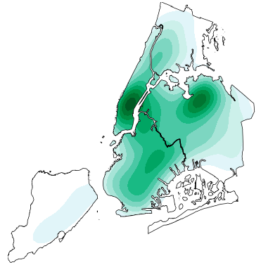 7 |
8 |
9 |
10 |
7 |
8 |
9 |
10 | 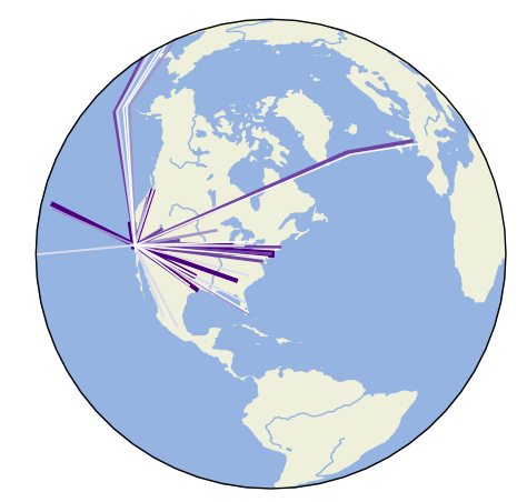 11 |
12 |
13 |
14 |
11 |
12 |
13 |
14 | 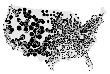 15 |
16 |
17 |
18 |
15 |
16 |
17 |
18 | 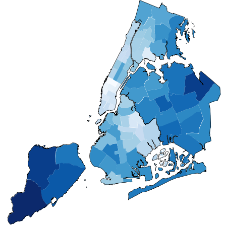 19 |
20 |
21 |
22 |
19 |
20 |
21 |
22 | 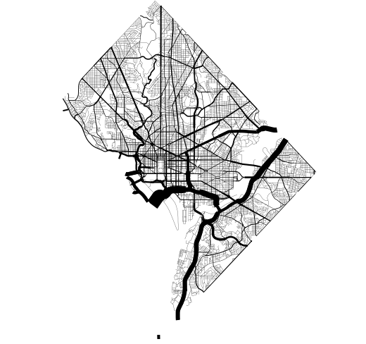 23 |
24 |
25 | `geoplot` is a high-level Python geospatial plotting library. It's an extension to `cartopy` and `matplotlib` which makes mapping easy: like `seaborn` for geospatial. It comes with the following features:
26 |
27 | * **High-level plotting API**: geoplot is cartographic plotting for the 90% of use cases. All of the standard-bearermaps that you’ve probably seen in your geography textbook are easily accessible.
28 | * **Native projection support**: The most fundamental peculiarity of geospatial plotting is projection: how do you unroll a sphere onto a flat surface (a map) in an accurate way? The answer depends on what you’re trying to depict. `geoplot` provides these options.
29 | * **Compatibility with `matplotlib`**: While `matplotlib` is not a good fit for working with geospatial data directly, it’s a format that’s well-incorporated by other tools.
30 |
31 | Installation is simple with `conda install geoplot -c conda-forge`. [See the documentation for help getting started](https://residentmario.github.io/geoplot/index.html).
32 |
33 | ----
34 |
35 | Author note: `geoplot` is currently in a **maintenence** state. I will continue to provide bugfixes and investigate user-reported issues on a best-effort basis, but do not expect to see any new library features anytime soon.
36 |
--------------------------------------------------------------------------------
/CONTRIBUTING.md:
--------------------------------------------------------------------------------
1 | # Contributing
2 |
3 | ## Cloning
4 |
5 | To work on `geoplot` locally, you will need to clone it.
6 |
7 | ```git
8 | git clone https://github.com/ResidentMario/geoplot.git
9 | ```
10 |
11 | You can then set up your own branch version of the code, and work on your changes for a pull request from there.
12 |
13 | ```bash
14 | cd geoplot
15 | git checkout -B new-branch-name
16 | ```
17 |
18 | ## Environment
19 |
20 | To install the `geoplot` development environment run the following in the root directory:
21 |
22 | ```bash
23 | conda env create -f environment.yml
24 | conda activate geoplot-dev
25 | pip install -e .[develop]
26 | ```
27 |
28 | ## Testing
29 |
30 | `geoplot` tests are located in the `tests` folder. Any PRs you submit should eventually pass all of the tests located in this folder.
31 |
32 | `mixin_tests.py` are static unit tests which can be run via `pytest` the usual way (by running `pytest mixin_tests.py` from the command line).
33 |
34 | `proj_tests.py` and `viz_tests.py` are visual tests run via the `pytest-mpl` plugin to be run: [see here](https://github.com/matplotlib/pytest-mpl#using) for instructions on how it's used. These tests are passed by visual inspection: e.g. does the output figure look the way it _should_ look, given the inputs?
35 |
36 | ## Documentation
37 |
38 | Documentation is provided via `sphinx`. To regenerate the documentation from the current source in one shot, navigate to the `docs` folder and run `make html`. Alternatively, to regenerate a single specific section, see the following section.
39 |
40 | ### Static example images
41 |
42 | The static example images on the repo and documentation homepages are located in the `figures/` folder.
43 |
44 | ### Gallery
45 |
46 | The gallery is generated using `sphinx-gallery`, and use the `examples/` folder as their source. The webmap examples are hosted on [bl.ocks.org](https://bl.ocks.org/) and linked to from their gallery landing pages.
47 |
48 | ### Quickstart
49 |
50 | The Quickstart is a Jupyter notebook in the `docs/quickstart/` directory. To rebuild the quickstart, edit the notebook, then run `make html` again.
51 |
52 | ### Tutorials
53 |
54 | The tutorials are Jupyter notebooks in the `docs/user_guide/` directory. To rebuild the tutorials, edit the notebook(s), then run `make html` again.
55 |
56 | ### Example data
57 |
58 | Most of the image resources in the documentation use real-world example data that is packaged as an accessory to this library. The home repo for these datasets is the [`geoplot-data`](https://github.com/ResidentMario/geoplot-data) repository. Use the `geoplot.datasets.get_path` function to get a path to a specific dataset readable by `geopandas`.
59 |
60 | ### Everything else
61 |
62 | The remaining pages are all written as `rst` files accessible from the top level of the `docs` folder.
63 |
64 | ### Serving
65 |
66 | The documentation is served at [residentmario.github.io](https://residentmario.github.io/geoplot/index.html) via GitHub's site export feature, served out of the `gh-pages` branch. To export a new version of the documentation to the website, run the following:
67 |
68 | ```bash
69 | git checkout gh-pages
70 | rm -rf *
71 | git checkout master -- docs/ examples/ geoplot/ .gitignore
72 | cd docs
73 | make html
74 | cd ..
75 | mv docs/_build/html/* ./
76 | rm -rf docs/ examples/ geoplot/
77 | git add .
78 | git commit -m "Publishing update docs..."
79 | git push origin gh-pages
80 | git checkout master
81 | ```
82 |
--------------------------------------------------------------------------------
/docs/index.rst:
--------------------------------------------------------------------------------
1 | geoplot: geospatial data visualization
2 | ======================================
3 |
4 | .. raw:: html
5 |
6 |
23 |
24 |
25 | `geoplot` is a high-level Python geospatial plotting library. It's an extension to `cartopy` and `matplotlib` which makes mapping easy: like `seaborn` for geospatial. It comes with the following features:
26 |
27 | * **High-level plotting API**: geoplot is cartographic plotting for the 90% of use cases. All of the standard-bearermaps that you’ve probably seen in your geography textbook are easily accessible.
28 | * **Native projection support**: The most fundamental peculiarity of geospatial plotting is projection: how do you unroll a sphere onto a flat surface (a map) in an accurate way? The answer depends on what you’re trying to depict. `geoplot` provides these options.
29 | * **Compatibility with `matplotlib`**: While `matplotlib` is not a good fit for working with geospatial data directly, it’s a format that’s well-incorporated by other tools.
30 |
31 | Installation is simple with `conda install geoplot -c conda-forge`. [See the documentation for help getting started](https://residentmario.github.io/geoplot/index.html).
32 |
33 | ----
34 |
35 | Author note: `geoplot` is currently in a **maintenence** state. I will continue to provide bugfixes and investigate user-reported issues on a best-effort basis, but do not expect to see any new library features anytime soon.
36 |
--------------------------------------------------------------------------------
/CONTRIBUTING.md:
--------------------------------------------------------------------------------
1 | # Contributing
2 |
3 | ## Cloning
4 |
5 | To work on `geoplot` locally, you will need to clone it.
6 |
7 | ```git
8 | git clone https://github.com/ResidentMario/geoplot.git
9 | ```
10 |
11 | You can then set up your own branch version of the code, and work on your changes for a pull request from there.
12 |
13 | ```bash
14 | cd geoplot
15 | git checkout -B new-branch-name
16 | ```
17 |
18 | ## Environment
19 |
20 | To install the `geoplot` development environment run the following in the root directory:
21 |
22 | ```bash
23 | conda env create -f environment.yml
24 | conda activate geoplot-dev
25 | pip install -e .[develop]
26 | ```
27 |
28 | ## Testing
29 |
30 | `geoplot` tests are located in the `tests` folder. Any PRs you submit should eventually pass all of the tests located in this folder.
31 |
32 | `mixin_tests.py` are static unit tests which can be run via `pytest` the usual way (by running `pytest mixin_tests.py` from the command line).
33 |
34 | `proj_tests.py` and `viz_tests.py` are visual tests run via the `pytest-mpl` plugin to be run: [see here](https://github.com/matplotlib/pytest-mpl#using) for instructions on how it's used. These tests are passed by visual inspection: e.g. does the output figure look the way it _should_ look, given the inputs?
35 |
36 | ## Documentation
37 |
38 | Documentation is provided via `sphinx`. To regenerate the documentation from the current source in one shot, navigate to the `docs` folder and run `make html`. Alternatively, to regenerate a single specific section, see the following section.
39 |
40 | ### Static example images
41 |
42 | The static example images on the repo and documentation homepages are located in the `figures/` folder.
43 |
44 | ### Gallery
45 |
46 | The gallery is generated using `sphinx-gallery`, and use the `examples/` folder as their source. The webmap examples are hosted on [bl.ocks.org](https://bl.ocks.org/) and linked to from their gallery landing pages.
47 |
48 | ### Quickstart
49 |
50 | The Quickstart is a Jupyter notebook in the `docs/quickstart/` directory. To rebuild the quickstart, edit the notebook, then run `make html` again.
51 |
52 | ### Tutorials
53 |
54 | The tutorials are Jupyter notebooks in the `docs/user_guide/` directory. To rebuild the tutorials, edit the notebook(s), then run `make html` again.
55 |
56 | ### Example data
57 |
58 | Most of the image resources in the documentation use real-world example data that is packaged as an accessory to this library. The home repo for these datasets is the [`geoplot-data`](https://github.com/ResidentMario/geoplot-data) repository. Use the `geoplot.datasets.get_path` function to get a path to a specific dataset readable by `geopandas`.
59 |
60 | ### Everything else
61 |
62 | The remaining pages are all written as `rst` files accessible from the top level of the `docs` folder.
63 |
64 | ### Serving
65 |
66 | The documentation is served at [residentmario.github.io](https://residentmario.github.io/geoplot/index.html) via GitHub's site export feature, served out of the `gh-pages` branch. To export a new version of the documentation to the website, run the following:
67 |
68 | ```bash
69 | git checkout gh-pages
70 | rm -rf *
71 | git checkout master -- docs/ examples/ geoplot/ .gitignore
72 | cd docs
73 | make html
74 | cd ..
75 | mv docs/_build/html/* ./
76 | rm -rf docs/ examples/ geoplot/
77 | git add .
78 | git commit -m "Publishing update docs..."
79 | git push origin gh-pages
80 | git checkout master
81 | ```
82 |
--------------------------------------------------------------------------------
/docs/index.rst:
--------------------------------------------------------------------------------
1 | geoplot: geospatial data visualization
2 | ======================================
3 |
4 | .. raw:: html
5 |
6 |
7 |
13 |
14 |
20 |
21 |
27 |
28 |
34 |
35 |
41 |
42 |