├── .Rbuildignore
├── .github
└── workflows
│ └── CI.yml
├── .gitignore
├── CRAN-RELEASE
├── CRAN-SUBMISSION
├── DESCRIPTION
├── LICENSE
├── NAMESPACE
├── NEWS.md
├── R
└── diffeqr.R
├── README.md
├── cran-comments.md
├── diffeqr.Rproj
├── inst
└── CITATION
├── man
├── diffeq_setup.Rd
├── diffeqgpu_setup.Rd
├── jitoptimize_ode.Rd
└── jitoptimize_sde.Rd
├── tests
├── testthat.R
└── testthat
│ ├── test_dae.R
│ ├── test_dde.R
│ ├── test_ode.R
│ └── test_sde.R
└── vignettes
├── dae.Rmd
├── dde.Rmd
├── gpu.Rmd
├── ode.Rmd
└── sde.Rmd
/.Rbuildignore:
--------------------------------------------------------------------------------
1 | ^.*\.Rproj$
2 | ^\.Rproj\.user$
3 | ^\.travis\.yml$
4 | ^appveyor\.yml$
5 | ^cran-comments\.md$
6 | ^CRAN-RELEASE$
7 | ^doc$
8 | ^Meta$
9 | ^\.github$
10 | ^CRAN-SUBMISSION$
11 |
--------------------------------------------------------------------------------
/.github/workflows/CI.yml:
--------------------------------------------------------------------------------
1 | # For help debugging build failures open an issue on the RStudio community with the 'github-actions' tag.
2 | # https://community.rstudio.com/new-topic?category=Package%20development&tags=github-actions
3 | on: push
4 | name: R-CMD-check
5 |
6 | jobs:
7 | R-CMD-check:
8 | runs-on: ${{ matrix.config.os }}
9 |
10 | name: ${{ matrix.config.os }} (${{ matrix.config.r }})
11 |
12 | strategy:
13 | fail-fast: false
14 | matrix:
15 | config:
16 | - {os: windows-latest, r: 'release'}
17 | - {os: macOS-latest, r: 'release'}
18 | - {os: ubuntu-20.04, r: 'release', rspm: "https://packagemanager.rstudio.com/cran/__linux__/focal/latest"}
19 | - {os: ubuntu-20.04, r: 'devel', rspm: "https://packagemanager.rstudio.com/cran/__linux__/focal/latest"}
20 |
21 | env:
22 | R_REMOTES_NO_ERRORS_FROM_WARNINGS: true
23 | RSPM: ${{ matrix.config.rspm }}
24 |
25 | steps:
26 | - uses: actions/checkout@v4
27 |
28 | - uses: r-lib/actions/setup-r@v2
29 | with:
30 | r-version: ${{ matrix.config.r }}
31 |
32 | - uses: r-lib/actions/setup-pandoc@v2
33 |
34 | - name: Query dependencies
35 | run: |
36 | install.packages('remotes')
37 | saveRDS(remotes::dev_package_deps(dependencies = TRUE), ".github/depends.Rds", version = 2)
38 | writeLines(sprintf("R-%i.%i", getRversion()$major, getRversion()$minor), ".github/R-version")
39 | shell: Rscript {0}
40 |
41 | - name: Cache R packages
42 | if: runner.os != 'Windows'
43 | uses: actions/cache@v4
44 | with:
45 | path: ${{ env.R_LIBS_USER }}
46 | key: ${{ runner.os }}-${{ hashFiles('.github/R-version') }}-1-${{ hashFiles('.github/depends.Rds') }}
47 | restore-keys: ${{ runner.os }}-${{ hashFiles('.github/R-version') }}-1-
48 |
49 | - name: Install system dependencies
50 | if: runner.os == 'Linux'
51 | run: |
52 | while read -r cmd
53 | do
54 | eval sudo $cmd
55 | done < <(Rscript -e 'writeLines(remotes::system_requirements("ubuntu", "20.04"))')
56 | - name: Install dependencies
57 | run: |
58 | remotes::install_deps(dependencies = TRUE)
59 | remotes::install_cran("rcmdcheck")
60 | shell: Rscript {0}
61 |
62 | - name: Check
63 | env:
64 | _R_CHECK_CRAN_INCOMING_REMOTE_: false
65 | run: rcmdcheck::rcmdcheck(args = c("--no-manual", "--as-cran", "--no-multiarch"), error_on = "warning", check_dir = "check")
66 | shell: Rscript {0}
67 |
68 | - name: Upload check results
69 | if: failure()
70 | uses: actions/upload-artifact@v4
71 | with:
72 | name: ${{ runner.os }}-r${{ matrix.config.r }}-results
73 | path: check
74 |
--------------------------------------------------------------------------------
/.gitignore:
--------------------------------------------------------------------------------
1 | .Rproj.user
2 | .Rhistory
3 | .RData
4 | inst/doc
5 | doc
6 | Meta
7 |
--------------------------------------------------------------------------------
/CRAN-RELEASE:
--------------------------------------------------------------------------------
1 | This package was submitted to CRAN on 2021-06-23.
2 | Once it is accepted, delete this file and tag the release (commit 01ae045).
3 |
--------------------------------------------------------------------------------
/CRAN-SUBMISSION:
--------------------------------------------------------------------------------
1 | Version: 2.1.0
2 | Date: 2024-12-04 18:14:02 UTC
3 | SHA: 569e58441b84d7323e1edb27395d1a96631fc7f4
4 |
--------------------------------------------------------------------------------
/DESCRIPTION:
--------------------------------------------------------------------------------
1 | Package: diffeqr
2 | Type: Package
3 | Title: Solving Differential Equations (ODEs, SDEs, DDEs, DAEs)
4 | Version: 2.1.0
5 | Authors@R: person("Christopher", "Rackauckas", email = "me@chrisrackauckas.com", role = c("aut", "cre", "cph"))
6 | Description: An interface to 'DifferentialEquations.jl' from the R programming language.
7 | It has unique high performance methods for solving ordinary differential equations (ODE), stochastic differential equations (SDE),
8 | delay differential equations (DDE), differential-algebraic equations (DAE), and more. Much of the functionality,
9 | including features like adaptive time stepping in SDEs, are unique and allow for multiple orders of magnitude speedup over more common methods.
10 | Supports GPUs, with support for CUDA (NVIDIA), AMD GPUs, Intel oneAPI GPUs, and Apple's Metal (M-series chip GPUs).
11 | 'diffeqr' attaches an R interface onto the package, allowing seamless use of this tooling by R users. For more information,
12 | see Rackauckas and Nie (2017) .
13 | Depends: R (>= 3.4.0)
14 | Encoding: UTF-8
15 | License: MIT + file LICENSE
16 | URL: https://github.com/SciML/diffeqr
17 | SystemRequirements: Julia (>= 1.6), DifferentialEquations.jl, ModelingToolkit.jl
18 | Imports:
19 | JuliaCall
20 | RoxygenNote: 7.1.1
21 | Suggests: testthat,
22 | knitr,
23 | rmarkdown
24 | VignetteBuilder: knitr
25 |
--------------------------------------------------------------------------------
/LICENSE:
--------------------------------------------------------------------------------
1 | YEAR: 2020
2 | COPYRIGHT HOLDER: SciML
3 |
--------------------------------------------------------------------------------
/NAMESPACE:
--------------------------------------------------------------------------------
1 | # Generated by roxygen2: do not edit by hand
2 |
3 | export(diffeq_setup)
4 | export(diffeqgpu_setup)
5 | export(jitoptimize_ode)
6 | export(jitoptimize_sde)
7 |
--------------------------------------------------------------------------------
/NEWS.md:
--------------------------------------------------------------------------------
1 | ## Release v2.1.0
2 |
3 | Better support for ModelingToolkit JIT tracing on SDEs.
4 |
5 | ## Release v2.0.1
6 |
7 | Updated to support ModelingToolkit v9 from the Julia side with the JIT compilation.
8 |
9 | ## Release v2.0.0
10 |
11 | Support new DiffEqGPU syntax. This requires passing a backend. Supports NVIDIA CUDA, Intel OneAPI,
12 | AMD GPUs, and Apple Metal GPUs. Also much faster GPU compilation and runtime performance.
13 |
14 | ## Release v1.1.2
15 |
16 | Bugfixes for newer Julia versions.
17 |
18 | ## Release v1.1.1
19 |
20 | This package now ensures that the tests are not run on build so that
21 | installation of Julia will not occur unless the user specifically asks for it
22 | via diffeqr::diffeq_setup()
23 |
24 | ## Release v1.0.0
25 |
26 | Full recreation of the package. This provides a new simplified interface over
27 | DifferentialEquations.jl that matches the Julia interface almost 1-1.
28 |
29 | ## Release v0.1.1
30 |
31 | This is a quick patch to fix the vignettes of the v0.1.0 release.
32 |
33 | ## Release v0.1.0
34 |
35 | This is the initial release of the package. It provides a simplified interface over DifferentialEquations.jl. Currently it's interfaced via 5 functions:
36 |
37 | - diffeq_setup
38 | - ode.solve
39 | - sde.solve
40 | - dae.solve
41 | - dde.solve
42 |
43 | The return is a list with sol$u and sol$t. In future updates this will be backwards compatibly updated to be a full solution object with the interpolation.
44 |
--------------------------------------------------------------------------------
/R/diffeqr.R:
--------------------------------------------------------------------------------
1 | #' Setup diffeqr
2 | #'
3 | #' This function initializes Julia and the DifferentialEquations.jl package.
4 | #' The first time will be long since it includes precompilation.
5 | #' Additionally, this will install Julia and the required packages
6 | #' if they are missing.
7 | #'
8 | #' @param pkg_check logical, check for DifferentialEquations.jl package and install if necessary
9 | #' @param ... Parameters are passed down to JuliaCall::julia_setup
10 | #'
11 | #' @examples
12 | #'
13 | #' \dontrun{ ## diffeq_setup() is time-consuming and requires Julia+DifferentialEquations.jl
14 | #'
15 | #' diffeqr::diffeq_setup()
16 | #'
17 | #' }
18 | #'
19 | #' @export
20 | diffeq_setup <- function (pkg_check=TRUE,...){
21 | julia <- JuliaCall::julia_setup(installJulia=TRUE,...)
22 | if(pkg_check) JuliaCall::julia_install_package_if_needed("DifferentialEquations")
23 | JuliaCall::julia_library("DifferentialEquations")
24 |
25 | functions <- JuliaCall::julia_eval("filter(isascii, replace.(string.(propertynames(DifferentialEquations)),\"!\"=>\"_bang\"))")
26 | de <- julia_pkg_import("DifferentialEquations",functions)
27 | JuliaCall::autowrap("DiffEqBase.AbstractODESolution", fields = c("t","u"))
28 | JuliaCall::autowrap("DiffEqBase.AbstractRODESolution", fields = c("t","u"))
29 | JuliaCall::autowrap("DiffEqBase.AbstractDDESolution", fields = c("t","u"))
30 | JuliaCall::autowrap("DiffEqBase.AbstractDAESolution", fields = c("t","u"))
31 | JuliaCall::autowrap("DiffEqBase.EnsembleSolution", fields = c("t","u"))
32 | de
33 | }
34 |
35 | julia_locate <- do.call(":::", list("JuliaCall", quote(julia_locate)))
36 |
37 | #' Jit Optimize an ODEProblem
38 | #'
39 | #' This function JIT Optimizes and ODEProblem utilizing the Julia ModelingToolkit
40 | #' and JIT compiler.
41 | #'
42 | #' @param de the current diffeqr environment
43 | #' @param prob an ODEProblem
44 | #'
45 | #' @examples
46 | #'
47 | #' \dontrun{ ## diffeq_setup() is time-consuming and requires Julia+DifferentialEquations.jl
48 | #' de <- diffeqr::diffeq_setup()
49 | #' f <- function(u,p,t) {
50 | #' du1 = p[1]*(u[2]-u[1])
51 | #' du2 = u[1]*(p[2]-u[3]) - u[2]
52 | #' du3 = u[1]*u[2] - p[3]*u[3]
53 | #' return(c(du1,du2,du3))
54 | #' }
55 | #' u0 <- c(1.0,0.0,0.0)
56 | #' tspan <- c(0.0,100.0)
57 | #' p <- c(10.0,28.0,8/3)
58 | #' prob <- de$ODEProblem(f, u0, tspan, p)
59 | #' fastprob <- diffeqr::jitoptimize_ode(de,prob)
60 | #' sol <- de$solve(fastprob,de$Tsit5())
61 | #' }
62 | #'
63 | #' @export
64 | jitoptimize_ode <- function (de,prob){
65 | JuliaCall::julia_install_package_if_needed("ModelingToolkit")
66 | JuliaCall::julia_library("ModelingToolkit")
67 | functions <- JuliaCall::julia_eval("filter(isascii, replace.(string.(propertynames(ModelingToolkit)),\"!\"=>\"_bang\"))")
68 |
69 | # Can remove the de argument when breaking, but kept for backwards compat
70 | mtk <- julia_pkg_import("ModelingToolkit",functions)
71 |
72 | odesys = mtk$modelingtoolkitize(prob)
73 |
74 | JuliaCall::julia_assign("odesys", odesys)
75 | JuliaCall::julia_assign("tspan", prob$tspan)
76 | new_prob <- JuliaCall::julia_eval("ODEProblem(complete(odesys, split=false), [], tspan; jac=true)")
77 | }
78 |
79 | #' Jit Optimize an SDEProblem
80 | #'
81 | #' This function JIT Optimizes and SDEProblem utilizing the Julia ModelingToolkit
82 | #' and JIT compiler.
83 | #'
84 | #' @param de the current diffeqr environment
85 | #' @param prob an SDEProblem
86 | #'
87 | #' @examples
88 | #'
89 | #' \dontrun{ ## diffeq_setup() is time-consuming and requires Julia+DifferentialEquations.jl
90 | #'
91 | #' diffeqr::diffeq_setup()
92 | #'
93 | #' }
94 | #'
95 | #' @export
96 | jitoptimize_sde <- function (de,prob){
97 | JuliaCall::julia_install_package_if_needed("ModelingToolkit")
98 | JuliaCall::julia_library("ModelingToolkit")
99 | functions <- JuliaCall::julia_eval("filter(isascii, replace.(string.(propertynames(ModelingToolkit)),\"!\"=>\"_bang\"))")
100 |
101 | # Can remove the de argument when breaking, but kept for backwards compat
102 | mtk <- julia_pkg_import("ModelingToolkit",functions)
103 |
104 | sdesys = mtk$modelingtoolkitize(prob)
105 | JuliaCall::julia_assign("sdesys", sdesys)
106 | JuliaCall::julia_assign("tspan", prob$tspan)
107 | new_prob <- JuliaCall::julia_eval("SDEProblem(complete(sdesys, split=false), [], tspan; jac=true)")
108 | }
109 |
110 | #' Setup DiffEqGPU
111 | #'
112 | #' This function initializes the DiffEqGPU package for GPU-parallelized ensembles.
113 | #' The first time will be long since it includes precompilation.
114 | #'
115 | #' @param backend the backend for the GPU computation. Choices are "CUDA", "AMDGPU", "Metal", or "oneAPI"
116 | #'
117 | #' @examples
118 | #'
119 | #' \dontrun{ ## diffeq_setup() is time-consuming and requires Julia+DifferentialEquations.jl
120 | #'
121 | #' degpu <- diffeqr::diffeqgpu_setup(backend="CUDA")
122 | #'
123 | #' }
124 | #'
125 | #' @export
126 | diffeqgpu_setup <- function (backend){
127 | JuliaCall::julia_install_package_if_needed("DiffEqGPU")
128 | JuliaCall::julia_library("DiffEqGPU")
129 | functions <- JuliaCall::julia_eval("filter(isascii, replace.(string.(propertynames(DiffEqGPU)),\"!\"=>\"_bang\"))")
130 | degpu <- julia_pkg_import("DiffEqGPU",functions)
131 |
132 | if (backend == "CUDA") {
133 | JuliaCall::julia_install_package_if_needed("CUDA")
134 | JuliaCall::julia_library("CUDA")
135 | backend <- julia_pkg_import("CUDA",c("CUDABackend"))
136 | degpu$CUDABackend <- backend$CUDABackend
137 | } else if (backend == "AMDGPU") {
138 | JuliaCall::julia_install_package_if_needed("AMDGPU")
139 | JuliaCall::julia_library("AMDGPU")
140 | backend <- julia_pkg_import("AMDGPU",c("AMDGPUBackend"))
141 | degpu$AMDGPUBackend <- backend$AMDGPUBackend
142 | } else if (backend == "Metal") {
143 | JuliaCall::julia_install_package_if_needed("Metal")
144 | JuliaCall::julia_library("Metal")
145 | backend <- julia_pkg_import("Metal",c("MetalBackend"))
146 | degpu$MetalBackend <- backend$MetalBackend
147 | } else if (backend == "oneAPI") {
148 | JuliaCall::julia_install_package_if_needed("oneAPI")
149 | JuliaCall::julia_library("oneAPI")
150 | backend <- julia_pkg_import("oneAPI",c("oneAPIBackend"))
151 | degpu$oneAPIBackend <- backend$oneAPIBackend
152 | } else {
153 | stop(paste("Illegal backend choice found. Allowed choices: CUDA, AMDGPU, Metal, and oneAPI. Chosen backend: ", backend))
154 | }
155 | degpu
156 | }
157 |
158 | julia_function <- function(func_name, pkg_name = "Main",
159 | env = emptyenv()){
160 | fname <- paste0(pkg_name, ".", func_name)
161 | force(fname)
162 | f <- function(...,
163 | need_return = c("R", "Julia", "None"),
164 | show_value = FALSE){
165 | if (!isTRUE(env$initialized)) {
166 | env$setup()
167 | }
168 | JuliaCall::julia_do.call(func_name = fname, list(...),
169 | need_return = match.arg(need_return),
170 | show_value = show_value)
171 | }
172 | force(f)
173 | env[[func_name]] <- f
174 | }
175 |
176 | julia_pkg_import <- function(pkg_name, func_list){
177 | env <- new.env(parent = emptyenv())
178 | env$setup <- function(...){
179 | JuliaCall::julia_setup(...)
180 | JuliaCall::julia_library(pkg_name)
181 | env$initialized <- TRUE
182 | }
183 | for (fname in func_list) {
184 | julia_function(func_name = fname,
185 | pkg_name = pkg_name,
186 | env = env)
187 | }
188 | env
189 | }
190 |
--------------------------------------------------------------------------------
/README.md:
--------------------------------------------------------------------------------
1 | # diffeqr
2 |
3 | [](https://cran.r-project.org/package=diffeqr)
4 | [](https://github.com/SciML/diffeqr/actions)
6 |
7 | diffeqr is a package for solving differential equations in R. It utilizes
8 | [DifferentialEquations.jl](https://diffeq.sciml.ai/dev/) for its core routines
9 | to give high performance solving of ordinary differential equations (ODEs),
10 | stochastic differential equations (SDEs), delay differential equations (DDEs), and
11 | differential-algebraic equations (DAEs) directly in R.
12 |
13 | If you have any questions, or just want to chat about solvers/using the package,
14 | please feel free to chat in the [Zulip channel](https://julialang.zulipchat.com/#narrow/stream/279055-sciml-bridged). For bug reports, feature requests, etc., please submit an issue.
15 |
16 | ## Installation
17 |
18 | [diffeqr is registered into CRAN](https://CRAN.R-project.org/package=diffeqr). Thus to add the package, use:
19 |
20 | ```R
21 | install.packages("diffeqr")
22 | ```
23 |
24 | To install the master branch of the package (for developers), use:
25 |
26 | ```R
27 | devtools::install_github('SciML/diffeqr', build_vignettes=T)
28 | ```
29 |
30 | Note that the first invocation of
31 | `diffeqr::diffeq_setup()` will install both Julia
32 | and the required packages if they are missing.
33 | If you wish to have it use an existing Julia binary,
34 | make sure that `julia` is found in the path. For more
35 | information see the `julia_setup()` function from
36 | [JuliaCall](https://github.com/JuliaInterop/JuliaCall).
37 |
38 | ## Google Collab Notebooks
39 |
40 | As a demonstration, check out the following notebooks:
41 |
42 | - [Solving Ordinary Differential Equations Fast in R with diffeqr](https://colab.research.google.com/drive/1p7djwRMfeExVapAN8WPxZZhLnGxy4_Jl?usp=sharing)
43 | - [Solving ODEs on GPUs Fast in R with diffeqr](https://colab.research.google.com/drive/1XGfp30AhuHA7HQHglzVQ6zoweZdZQE6g#scrollTo=U_5yw0iFFt6f)
44 |
45 | ## Usage
46 |
47 | diffeqr provides a direct wrapper over [DifferentialEquations.jl](https://diffeq.sciml.ai).
48 | The namespace is setup so that the standard syntax of Julia translates directly
49 | over to the R environment. There are two things to keep in mind:
50 |
51 | 1. All DifferentialEquations.jl commands are prefaced by `de$`
52 | 2. All commands with a `!` are replaced with `_bang`, for example `solve!` becomes `solve_bang`.
53 |
54 | ## Ordinary Differential Equation (ODE) Examples
55 |
56 | ### 1D Linear ODEs
57 |
58 | Let's solve the linear ODE `u'=1.01u`. First setup the package:
59 |
60 | ```R
61 | de <- diffeqr::diffeq_setup()
62 | ```
63 |
64 | Define the derivative function `f(u,p,t)`.
65 |
66 | ```R
67 | f <- function(u,p,t) {
68 | return(1.01*u)
69 | }
70 | ```
71 |
72 | Then we give it an initial condition and a time span to solve over:
73 |
74 | ```R
75 | u0 <- 1/2
76 | tspan <- c(0., 1.)
77 | ```
78 |
79 | With those pieces we define the `ODEProblem` and `solve` the ODE:
80 |
81 | ```R
82 | prob = de$ODEProblem(f, u0, tspan)
83 | sol = de$solve(prob)
84 | ```
85 |
86 | This gives back a solution object for which `sol$t` are the time points
87 | and `sol$u` are the values. We can treat the solution as a continuous object
88 | in time via
89 |
90 | ```R
91 | sol$.(0.2)
92 | ```
93 |
94 | and a high order interpolation will compute the value at `t=0.2`. We can check
95 | the solution by plotting it:
96 |
97 | ```R
98 | plot(sol$t,sol$u,"l")
99 | ```
100 |
101 | 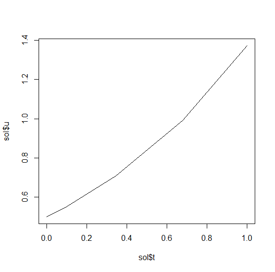
102 |
103 | ### Systems of ODEs
104 |
105 | Now let's solve the Lorenz equations. In this case, our initial condition is a vector and our derivative functions
106 | takes in the vector to return a vector (note: arbitrary dimensional arrays are allowed). We would define this as:
107 |
108 | ```R
109 | f <- function(u,p,t) {
110 | du1 = p[1]*(u[2]-u[1])
111 | du2 = u[1]*(p[2]-u[3]) - u[2]
112 | du3 = u[1]*u[2] - p[3]*u[3]
113 | return(c(du1,du2,du3))
114 | }
115 | ```
116 |
117 | Here we utilized the parameter array `p`. Thus we use `diffeqr::ode.solve` like before, but also pass in parameters this time:
118 |
119 | ```R
120 | u0 <- c(1.0,0.0,0.0)
121 | tspan <- c(0.0,100.0)
122 | p <- c(10.0,28.0,8/3)
123 | prob <- de$ODEProblem(f, u0, tspan, p)
124 | sol <- de$solve(prob)
125 | ```
126 |
127 | The returned solution is like before except now `sol$u` is an array of arrays,
128 | where `sol$u[i]` is the full system at time `sol$t[i]`. It can be convenient to
129 | turn this into an R matrix through `sapply`:
130 |
131 | ```R
132 | mat <- sapply(sol$u,identity)
133 | ```
134 |
135 | This has each row as a time series. `t(mat)` makes each column a time series.
136 | It is sometimes convenient to turn the output into a `data.frame` which is done
137 | via:
138 |
139 | ```R
140 | udf <- as.data.frame(t(mat))
141 | ```
142 |
143 | Now we can use `matplot` to plot the timeseries together:
144 |
145 | ```R
146 | matplot(sol$t,udf,"l",col=1:3)
147 | ```
148 |
149 | 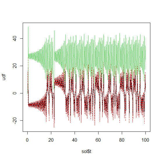
150 |
151 | Now we can use the Plotly package to draw a phase plot:
152 |
153 | ```R
154 | plotly::plot_ly(udf, x = ~V1, y = ~V2, z = ~V3, type = 'scatter3d', mode = 'lines')
155 | ```
156 |
157 | 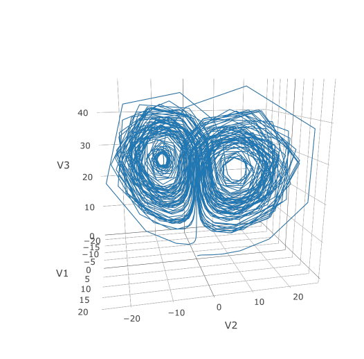
158 |
159 | Plotly is much prettier!
160 |
161 | ### Option Handling
162 |
163 | If we want to have a more accurate solution, we can send `abstol` and `reltol`. Defaults are `1e-6` and `1e-3` respectively.
164 | Generally you can think of the digits of accuracy as related to 1 plus the exponent of the relative tolerance, so the default is
165 | two digits of accuracy. Absolute tolernace is the accuracy near 0.
166 |
167 | In addition, we may want to choose to save at more time points. We do this by giving an array of values to save at as `saveat`.
168 | Together, this looks like:
169 |
170 | ```R
171 | abstol <- 1e-8
172 | reltol <- 1e-8
173 | saveat <- 0:10000/100
174 | sol <- de$solve(prob,abstol=abstol,reltol=reltol,saveat=saveat)
175 | udf <- as.data.frame(t(sapply(sol$u,identity)))
176 | plotly::plot_ly(udf, x = ~V1, y = ~V2, z = ~V3, type = 'scatter3d', mode = 'lines')
177 | ```
178 |
179 | 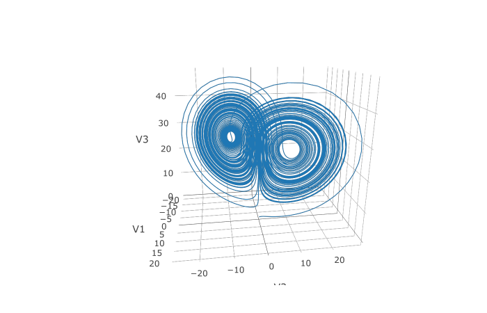
180 |
181 | We can also choose to use a different algorithm. The choice is done using a string that matches the Julia syntax. See
182 | [the ODE tutorial for details](https://diffeq.sciml.ai/dev/tutorials/ode_example/#Choosing-a-Solver-Algorithm-1).
183 | The list of choices for ODEs can be found at the [ODE Solvers page](https://diffeq.sciml.ai/dev/solvers/ode_solve/).
184 | For example, let's use a 9th order method due to Verner:
185 |
186 | ```R
187 | sol <- de$solve(prob,de$Vern9(),abstol=abstol,reltol=reltol,saveat=saveat)
188 | ```
189 |
190 | Note that each algorithm choice will cause a JIT compilation.
191 |
192 | ## Performance Enhancements
193 |
194 | One way to enhance the performance of your code is to define the function in Julia
195 | so that way it is JIT compiled. diffeqr is built using
196 | [the JuliaCall package](https://github.com/JuliaInterop/JuliaCall), and so
197 | you can utilize the Julia JIT compiler. We expose this automatically over ODE
198 | functions via `jitoptimize_ode`, like in the following example:
199 |
200 | ```R
201 | f <- function(u,p,t) {
202 | du1 = p[1]*(u[2]-u[1])
203 | du2 = u[1]*(p[2]-u[3]) - u[2]
204 | du3 = u[1]*u[2] - p[3]*u[3]
205 | return(c(du1,du2,du3))
206 | }
207 | u0 <- c(1.0,0.0,0.0)
208 | tspan <- c(0.0,100.0)
209 | p <- c(10.0,28.0,8/3)
210 | prob <- de$ODEProblem(f, u0, tspan, p)
211 | fastprob <- diffeqr::jitoptimize_ode(de,prob)
212 | sol <- de$solve(fastprob,de$Tsit5())
213 | ```
214 |
215 | Note that the first evaluation of the function will have an ~2 second lag since
216 | the compiler will run, and all subsequent runs will be orders of magnitude faster
217 | than the pure R function. This means it's great for expensive functions (ex. large
218 | PDEs) or functions called repeatedly, like during optimization of parameters.
219 |
220 | We can also use the JuliaCall functions to directly define the function in Julia
221 | to eliminate the R interpreter overhead and get full JIT compilation:
222 |
223 | ```R
224 | julf <- JuliaCall::julia_eval("
225 | function julf(du,u,p,t)
226 | du[1] = 10.0*(u[2]-u[1])
227 | du[2] = u[1]*(28.0-u[3]) - u[2]
228 | du[3] = u[1]*u[2] - (8/3)*u[3]
229 | end")
230 | JuliaCall::julia_assign("u0", u0)
231 | JuliaCall::julia_assign("p", p)
232 | JuliaCall::julia_assign("tspan", tspan)
233 | prob3 = JuliaCall::julia_eval("ODEProblem(julf, u0, tspan, p)")
234 | sol = de$solve(prob3,de$Tsit5())
235 | ```
236 |
237 | To demonstrate the performance advantage, let's time them all:
238 |
239 | ```R
240 | > system.time({ for (i in 1:100){ de$solve(prob ,de$Tsit5()) }})
241 | user system elapsed
242 | 6.69 0.06 6.78
243 | > system.time({ for (i in 1:100){ de$solve(fastprob,de$Tsit5()) }})
244 | user system elapsed
245 | 0.11 0.03 0.14
246 | > system.time({ for (i in 1:100){ de$solve(prob3 ,de$Tsit5()) }})
247 | user system elapsed
248 | 0.14 0.02 0.15
249 | ```
250 |
251 | This is about a 50x improvement!
252 |
253 | #### Limitations of the JIT Compilation
254 |
255 | Using Julia's [ModelingToolkit](https://github.com/SciML/ModelingToolkit.jl)
256 | for tracing to JIT compile via Julia has a few known limitations:
257 |
258 | - It requires that all of the function calls are tracable. Scalar functions
259 | like `cos` and `sin` all fall into this category. Notably, matrix multiplication
260 | is not supported.
261 | - It will have a compilation lag on the first call.
262 |
263 | ## Stochastic Differential Equation (SDE) Examples
264 |
265 | ### 1D SDEs
266 |
267 | Solving stochastic differential equations (SDEs) is the similar to ODEs. To solve an SDE, you use `diffeqr::sde.solve` and give
268 | two functions: `f` and `g`, where `du = f(u,t)dt + g(u,t)dW_t`
269 |
270 | ```r
271 | de <- diffeqr::diffeq_setup()
272 | f <- function(u,p,t) {
273 | return(1.01*u)
274 | }
275 | g <- function(u,p,t) {
276 | return(0.87*u)
277 | }
278 | u0 <- 1/2
279 | tspan <- c(0.0,1.0)
280 | prob <- de$SDEProblem(f,g,u0,tspan)
281 | sol <- de$solve(prob)
282 | udf <- as.data.frame(t(sapply(sol$u,identity)))
283 | plotly::plot_ly(udf, x = sol$t, y = sol$u, type = 'scatter', mode = 'lines')
284 | ```
285 |
286 | 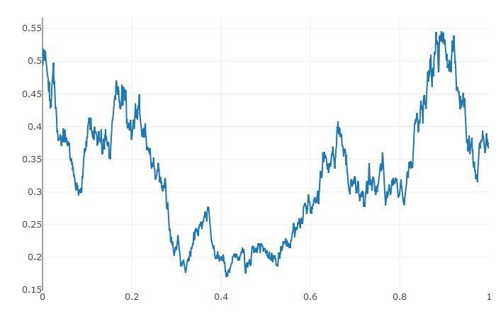
287 |
288 | ### Systems of Diagonal Noise SDEs
289 |
290 | Let's add diagonal multiplicative noise to the Lorenz attractor. diffeqr defaults to diagonal noise when a system of
291 | equations is given. This is a unique noise term per system variable. Thus we generalize our previous functions as
292 | follows:
293 |
294 | ```R
295 | f <- function(u,p,t) {
296 | du1 = p[1]*(u[2]-u[1])
297 | du2 = u[1]*(p[2]-u[3]) - u[2]
298 | du3 = u[1]*u[2] - p[3]*u[3]
299 | return(c(du1,du2,du3))
300 | }
301 | g <- function(u,p,t) {
302 | return(c(0.3*u[1],0.3*u[2],0.3*u[3]))
303 | }
304 | u0 <- c(1.0,0.0,0.0)
305 | tspan <- c(0.0,1.0)
306 | p <- c(10.0,28.0,8/3)
307 | prob <- de$SDEProblem(f,g,u0,tspan,p)
308 | sol <- de$solve(prob,saveat=0.005)
309 | udf <- as.data.frame(t(sapply(sol$u,identity)))
310 | plotly::plot_ly(udf, x = ~V1, y = ~V2, z = ~V3, type = 'scatter3d', mode = 'lines')
311 | ```
312 |
313 | Using a JIT compiled function for the drift and diffusion functions can greatly enhance the speed here.
314 | With the speed increase we can comfortably solve over long time spans:
315 |
316 | ```R
317 | tspan <- c(0.0,100.0)
318 | prob <- de$SDEProblem(f,g,u0,tspan,p)
319 | fastprob <- diffeqr::jitoptimize_sde(de,prob)
320 | sol <- de$solve(fastprob,saveat=0.005)
321 | udf <- as.data.frame(t(sapply(sol$u,identity)))
322 | plotly::plot_ly(udf, x = ~V1, y = ~V2, z = ~V3, type = 'scatter3d', mode = 'lines')
323 | ```
324 |
325 | 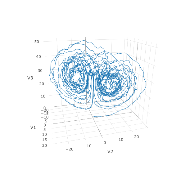
326 |
327 | Let's see how much faster the JIT-compiled version was:
328 |
329 | ```R
330 | > system.time({ for (i in 1:5){ de$solve(prob ) }})
331 | user system elapsed
332 | 146.40 0.75 147.22
333 | > system.time({ for (i in 1:5){ de$solve(fastprob) }})
334 | user system elapsed
335 | 1.07 0.10 1.17
336 | ```
337 |
338 | Holy Monster's Inc. that's about 145x faster.
339 |
340 | ### Systems of SDEs with Non-Diagonal Noise
341 |
342 | In many cases you may want to share noise terms across the system. This is known as non-diagonal noise. The
343 | [DifferentialEquations.jl SDE Tutorial](https://diffeq.sciml.ai/dev/tutorials/sde_example/#Example-4:-Systems-of-SDEs-with-Non-Diagonal-Noise-1)
344 | explains how the matrix form of the diffusion term corresponds to the summation style of multiple Wiener processes. Essentially,
345 | the row corresponds to which system the term is applied to, and the column is which noise term. So `du[i,j]` is the amount of
346 | noise due to the `j`th Wiener process that's applied to `u[i]`. We solve the Lorenz system with correlated noise as follows:
347 |
348 | ```R
349 | f <- JuliaCall::julia_eval("
350 | function f(du,u,p,t)
351 | du[1] = 10.0*(u[2]-u[1])
352 | du[2] = u[1]*(28.0-u[3]) - u[2]
353 | du[3] = u[1]*u[2] - (8/3)*u[3]
354 | end")
355 | g <- JuliaCall::julia_eval("
356 | function g(du,u,p,t)
357 | du[1,1] = 0.3u[1]
358 | du[2,1] = 0.6u[1]
359 | du[3,1] = 0.2u[1]
360 | du[1,2] = 1.2u[2]
361 | du[2,2] = 0.2u[2]
362 | du[3,2] = 0.3u[2]
363 | end")
364 | u0 <- c(1.0,0.0,0.0)
365 | tspan <- c(0.0,100.0)
366 | noise_rate_prototype <- matrix(c(0.0,0.0,0.0,0.0,0.0,0.0), nrow = 3, ncol = 2)
367 |
368 | JuliaCall::julia_assign("u0", u0)
369 | JuliaCall::julia_assign("tspan", tspan)
370 | JuliaCall::julia_assign("noise_rate_prototype", noise_rate_prototype)
371 | prob <- JuliaCall::julia_eval("SDEProblem(f, g, u0, tspan, p, noise_rate_prototype=noise_rate_prototype)")
372 | sol <- de$solve(prob)
373 | udf <- as.data.frame(t(sapply(sol$u,identity)))
374 | plotly::plot_ly(udf, x = ~V1, y = ~V2, z = ~V3, type = 'scatter3d', mode = 'lines')
375 | ```
376 |
377 | 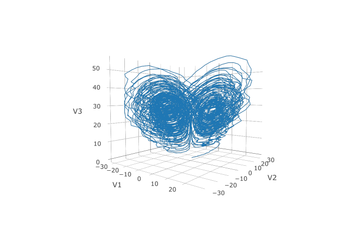
378 |
379 | Here you can see that the warping effect of the noise correlations is quite visible!
380 | Note that we applied JIT compilation since it's quite necessary for any difficult
381 | stochastic example.
382 |
383 | ## Differential-Algebraic Equation (DAE) Examples
384 |
385 | A differential-algebraic equation is defined by an implicit function `f(du,u,p,t)=0`. All of the controls are the
386 | same as the other examples, except here you define a function which returns the residuals for each part of the equation
387 | to define the DAE. The initial value `u0` and the initial derivative `du0` are required, though they do not necessarily
388 | have to satisfy `f` (known as inconsistent initial conditions). The methods will automatically find consistent initial
389 | conditions. In order for this to occur, `differential_vars` must be set. This vector states which of the variables are
390 | differential (have a derivative term), with `false` meaning that the variable is purely algebraic.
391 |
392 | This example shows how to solve the Robertson equation:
393 |
394 | ```R
395 | f <- function (du,u,p,t) {
396 | resid1 = - 0.04*u[1] + 1e4*u[2]*u[3] - du[1]
397 | resid2 = + 0.04*u[1] - 3e7*u[2]^2 - 1e4*u[2]*u[3] - du[2]
398 | resid3 = u[1] + u[2] + u[3] - 1.0
399 | c(resid1,resid2,resid3)
400 | }
401 | u0 <- c(1.0, 0, 0)
402 | du0 <- c(-0.04, 0.04, 0.0)
403 | tspan <- c(0.0,100000.0)
404 | differential_vars <- c(TRUE,TRUE,FALSE)
405 | prob <- de$DAEProblem(f,du0,u0,tspan,differential_vars=differential_vars)
406 | sol <- de$solve(prob)
407 | udf <- as.data.frame(t(sapply(sol$u,identity)))
408 | plotly::plot_ly(udf, x = sol$t, y = ~V1, type = 'scatter', mode = 'lines') |>
409 | plotly::add_trace(y = ~V2) |>
410 | plotly::add_trace(y = ~V3)
411 | ```
412 |
413 | Additionally, an in-place JIT compiled form for `f` can be used to enhance the speed:
414 |
415 | ```R
416 | f = JuliaCall::julia_eval("function f(out,du,u,p,t)
417 | out[1] = - 0.04u[1] + 1e4*u[2]*u[3] - du[1]
418 | out[2] = + 0.04u[1] - 3e7*u[2]^2 - 1e4*u[2]*u[3] - du[2]
419 | out[3] = u[1] + u[2] + u[3] - 1.0
420 | end")
421 | u0 <- c(1.0, 0, 0)
422 | du0 <- c(-0.04, 0.04, 0.0)
423 | tspan <- c(0.0,100000.0)
424 | differential_vars <- c(TRUE,TRUE,FALSE)
425 | JuliaCall::julia_assign("du0", du0)
426 | JuliaCall::julia_assign("u0", u0)
427 | JuliaCall::julia_assign("p", p)
428 | JuliaCall::julia_assign("tspan", tspan)
429 | JuliaCall::julia_assign("differential_vars", differential_vars)
430 | prob = JuliaCall::julia_eval("DAEProblem(f, du0, u0, tspan, p, differential_vars=differential_vars)")
431 | sol = de$solve(prob)
432 | ```
433 |
434 | 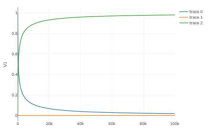
435 |
436 | ## Delay Differential Equation (DDE) Examples
437 |
438 | A delay differential equation is an ODE which allows the use of previous values. In this case, the function
439 | needs to be a JIT compiled Julia function. It looks just like the ODE, except in this case there is a function
440 | `h(p,t)` which allows you to interpolate and grab previous values.
441 |
442 | We must provide a history function `h(p,t)` that gives values for `u` before
443 | `t0`. Here we assume that the solution was constant before the initial time point. Additionally, we pass
444 | `constant_lags = c(20.0)` to tell the solver that only constant-time lags were used and what the lag length
445 | was. This helps improve the solver accuracy by accurately stepping at the points of discontinuity. Together
446 | this is:
447 |
448 | ```R
449 | f <- JuliaCall::julia_eval("function f(du, u, h, p, t)
450 | du[1] = 1.1/(1 + sqrt(10)*(h(p, t-20)[1])^(5/4)) - 10*u[1]/(1 + 40*u[2])
451 | du[2] = 100*u[1]/(1 + 40*u[2]) - 2.43*u[2]
452 | end")
453 | h <- JuliaCall::julia_eval("function h(p, t)
454 | [1.05767027/3, 1.030713491/3]
455 | end")
456 | u0 <- c(1.05767027/3, 1.030713491/3)
457 | tspan <- c(0.0, 100.0)
458 | constant_lags <- c(20.0)
459 | JuliaCall::julia_assign("u0", u0)
460 | JuliaCall::julia_assign("tspan", tspan)
461 | JuliaCall::julia_assign("constant_lags", tspan)
462 | prob <- JuliaCall::julia_eval("DDEProblem(f, u0, h, tspan, constant_lags = constant_lags)")
463 | sol <- de$solve(prob,de$MethodOfSteps(de$Tsit5()))
464 | udf <- as.data.frame(t(sapply(sol$u,identity)))
465 | plotly::plot_ly(udf, x = sol$t, y = ~V1, type = 'scatter', mode = 'lines') |> plotly::add_trace(y = ~V2)
466 | ```
467 |
468 | 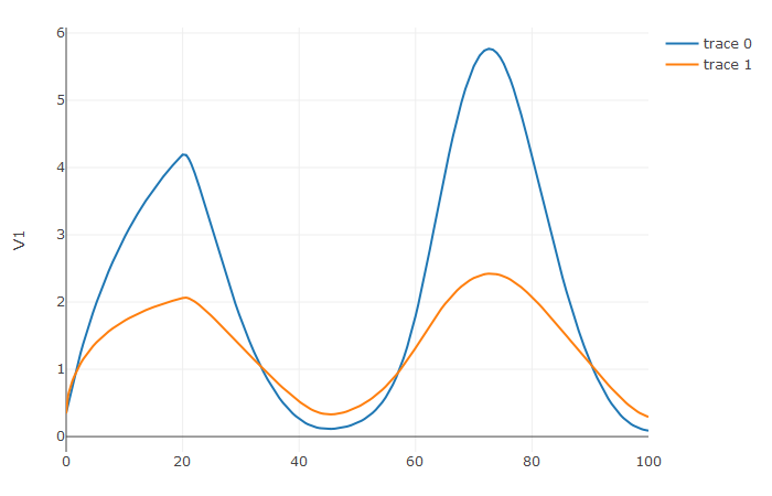
469 |
470 | Notice that the solver accurately is able to simulate the kink (discontinuity) at `t=20` due to the discontinuity
471 | of the derivative at the initial time point! This is why declaring discontinuities can enhance the solver accuracy.
472 |
473 | ## GPU-Accelerated ODE Solving of Ensembles
474 |
475 | In many cases one is interested in solving the same ODE many times over many
476 | different initial conditions and parameters. In diffeqr parlance this is called
477 | an ensemble solve. diffeqr inherits the parallelism tools of the
478 | [SciML ecosystem](https://sciml.ai/) that are used for things like
479 | [automated equation discovery and acceleration](https://arxiv.org/abs/2001.04385).
480 | Here we will demonstrate using these parallel tools to accelerate the solving
481 | of an ensemble.
482 |
483 | First, let's define the JIT-accelerated Lorenz equation like before:
484 |
485 | ```R
486 | de <- diffeqr::diffeq_setup()
487 | lorenz <- function (u,p,t){
488 | du1 = p[1]*(u[2]-u[1])
489 | du2 = u[1]*(p[2]-u[3]) - u[2]
490 | du3 = u[1]*u[2] - p[3]*u[3]
491 | c(du1,du2,du3)
492 | }
493 | u0 <- c(1.0,1.0,1.0)
494 | tspan <- c(0.0,100.0)
495 | p <- c(10.0,28.0,8/3)
496 | prob <- de$ODEProblem(lorenz,u0,tspan,p)
497 | fastprob <- diffeqr::jitoptimize_ode(de,prob)
498 | ```
499 |
500 | Now we use the `EnsembleProblem` as defined on the
501 | [ensemble parallelism page of the documentation](https://diffeq.sciml.ai/stable/features/ensemble/):
502 | Let's build an ensemble by utilizing uniform random numbers to randomize the
503 | initial conditions and parameters:
504 |
505 | ```R
506 | prob_func <- function (prob,i,rep){
507 | de$remake(prob,u0=runif(3)*u0,p=runif(3)*p)
508 | }
509 | ensembleprob = de$EnsembleProblem(fastprob, prob_func = prob_func, safetycopy=FALSE)
510 | ```
511 |
512 | Now we solve the ensemble in serial:
513 |
514 | ```R
515 | sol = de$solve(ensembleprob,de$Tsit5(),de$EnsembleSerial(),trajectories=10000,saveat=0.01)
516 | ```
517 |
518 | To add GPUs to the mix, we need to bring in [DiffEqGPU](https://github.com/SciML/DiffEqGPU.jl).
519 | The `diffeqr::diffeqgpu_setup()` helper function will install CUDA for you and
520 | bring all of the bindings into the returned object:
521 |
522 | ```R
523 | degpu <- diffeqr::diffeqgpu_setup("CUDA")
524 | ```
525 |
526 | #### Note: `diffeqr::diffeqgpu_setup` can take awhile to run the first time as it installs the drivers!
527 |
528 | Now we simply use `EnsembleGPUKernel(degpu$CUDABackend())` with a
529 | GPU-specialized ODE solver `GPUTsit5()` to solve 10,000 ODEs on the GPU in
530 | parallel:
531 |
532 | ```R
533 | sol <- de$solve(ensembleprob,degpu$GPUTsit5(),degpu$EnsembleGPUKernel(degpu$CUDABackend()),trajectories=10000,saveat=0.01)
534 | ```
535 |
536 | For the full list of choices for specialized GPU solvers, see
537 | [the DiffEqGPU.jl documentation](https://docs.sciml.ai/DiffEqGPU/stable/manual/ensemblegpukernel/).
538 |
539 | Note that `EnsembleGPUArray` can be used as well, like:
540 |
541 | ```R
542 | sol <- de$solve(ensembleprob,de$Tsit5(),degpu$EnsembleGPUArray(degpu$CUDABackend()),trajectories=10000,saveat=0.01)
543 | ```
544 |
545 | though we highly recommend the `EnsembleGPUKernel` methods for more speed. Given
546 | the way the JIT compilation performed will also ensure that the faster kernel
547 | generation methods work, `EnsembleGPUKernel` is almost certainly the
548 | better choice in most applications.
549 |
550 | ### Benchmark
551 |
552 | To see how much of an effect the parallelism has, let's test this against R's
553 | deSolve package. This is exactly the same problem as the documentation example
554 | for deSolve, so let's copy that verbatim and then add a function to do the
555 | ensemble generation:
556 |
557 | ```R
558 | library(deSolve)
559 | Lorenz <- function(t, state, parameters) {
560 | with(as.list(c(state, parameters)), {
561 | dX <- a * X + Y * Z
562 | dY <- b * (Y - Z)
563 | dZ <- -X * Y + c * Y - Z
564 | list(c(dX, dY, dZ))
565 | })
566 | }
567 |
568 | parameters <- c(a = -8/3, b = -10, c = 28)
569 | state <- c(X = 1, Y = 1, Z = 1)
570 | times <- seq(0, 100, by = 0.01)
571 | out <- ode(y = state, times = times, func = Lorenz, parms = parameters)
572 |
573 | lorenz_solve <- function (i){
574 | state <- c(X = runif(1), Y = runif(1), Z = runif(1))
575 | parameters <- c(a = -8/3 * runif(1), b = -10 * runif(1), c = 28 * runif(1))
576 | out <- ode(y = state, times = times, func = Lorenz, parms = parameters)
577 | }
578 | ```
579 |
580 | Using `lapply` to generate the ensemble we get:
581 |
582 | ```
583 | > system.time({ lapply(1:1000,lorenz_solve) })
584 | user system elapsed
585 | 225.81 0.46 226.63
586 | ```
587 |
588 | Now let's see how the JIT-accelerated serial Julia version stacks up against that:
589 |
590 | ```
591 | > system.time({ de$solve(ensembleprob,de$Tsit5(),de$EnsembleSerial(),trajectories=1000,saveat=0.01) })
592 | user system elapsed
593 | 2.75 0.30 3.08
594 | ```
595 |
596 | Julia is already about 73x faster than the pure R solvers here! Now let's add
597 | GPU-acceleration to the mix:
598 |
599 | ```
600 | > system.time({ de$solve(ensembleprob,degpu$GPUTsit5(),degpu$EnsembleGPUKernel(degpu$CUDABackend()),trajectories=1000,saveat=0.01) })
601 | user system elapsed
602 | 0.11 0.00 0.12
603 | ```
604 |
605 | Already 26x times faster! But the GPU acceleration is made for massively
606 | parallel problems, so let's up the trajectories a bit. We will not use more
607 | trajectories from R because that would take too much computing power, so let's
608 | see what happens to the Julia serial and GPU at 10,000 trajectories:
609 |
610 | ```
611 | > system.time({ de$solve(ensembleprob,de$Tsit5(),de$EnsembleSerial(),trajectories=10000,saveat=0.01) })
612 | user system elapsed
613 | 35.02 4.19 39.25
614 | ```
615 |
616 | ```
617 | > system.time({ de$solve(ensembleprob,degpu$GPUTsit5(),degpu$EnsembleGPUKernel(degpu$CUDABackend()),trajectories=10000,saveat=0.01) })
618 | user system elapsed
619 | 1.22 0.23 1.50
620 | ```
621 |
622 | To compare this to the pure Julia code:
623 |
624 | ```julia
625 | using OrdinaryDiffEq, DiffEqGPU, CUDA, StaticArrays
626 | function lorenz(u, p, t)
627 | σ = p[1]
628 | ρ = p[2]
629 | β = p[3]
630 | du1 = σ * (u[2] - u[1])
631 | du2 = u[1] * (ρ - u[3]) - u[2]
632 | du3 = u[1] * u[2] - β * u[3]
633 | return SVector{3}(du1, du2, du3)
634 | end
635 |
636 | u0 = SA[1.0f0; 0.0f0; 0.0f0]
637 | tspan = (0.0f0, 10.0f0)
638 | p = SA[10.0f0, 28.0f0, 8 / 3.0f0]
639 | prob = ODEProblem{false}(lorenz, u0, tspan, p)
640 | prob_func = (prob, i, repeat) -> remake(prob, p = (@SVector rand(Float32, 3)) .* p)
641 | monteprob = EnsembleProblem(prob, prob_func = prob_func, safetycopy = false)
642 | @time sol = solve(monteprob, GPUTsit5(), EnsembleGPUKernel(CUDA.CUDABackend()),
643 | trajectories = 10_000,
644 | saveat = 1.0f0);
645 |
646 | # 0.015064 seconds (257.68 k allocations: 13.132 MiB)
647 | ```
648 |
649 | which is about two orders of magnitude faster for computing 10,000 trajectories,
650 | note that the major factors are that we cannot define 32-bit floating point values
651 | from R and the `prob_func` for generating the initial conditions and parameters
652 | is a major bottleneck since this function is written in R.
653 |
654 | To see how this scales in Julia, let's take it to insane heights. First, let's
655 | reduce the amount we're saving:
656 |
657 | ```julia
658 | @time sol = solve(monteprob,GPUTsit5(),EnsembleGPUKernel(CUDA.CUDABackend()),trajectories=10_000,saveat=1.0f0)
659 | 0.015040 seconds (257.64 k allocations: 13.130 MiB)
660 | ```
661 |
662 | This highlights that controlling memory pressure is key with GPU usage: you will
663 | get much better performance when requiring less saved points on the GPU.
664 |
665 | ```julia
666 | @time sol = solve(monteprob,GPUTsit5(),EnsembleGPUKernel(CUDA.CUDABackend()),trajectories=100_000,saveat=1.0f0)
667 | # 0.150901 seconds (2.60 M allocations: 131.576 MiB)
668 | ```
669 |
670 | compared to serial:
671 |
672 | ```julia
673 | @time sol = solve(monteprob,Tsit5(),EnsembleSerial(),trajectories=100_000,saveat=1.0f0)
674 | # 22.136743 seconds (16.40 M allocations: 1.628 GiB, 42.98% gc time)
675 | ```
676 |
677 | And now we start to see that scaling power! Let's solve 1 million trajectories:
678 |
679 | ```julia
680 | @time sol = solve(monteprob,GPUTsit5(),EnsembleGPUKernel(CUDA.CUDABackend()),trajectories=1_000_000,saveat=1.0f0)
681 | # 1.031295 seconds (3.40 M allocations: 241.075 MiB)
682 | ```
683 |
684 | For reference, let's look at deSolve with the change to only save that much:
685 |
686 | ```R
687 | times <- seq(0, 100, by = 1.0)
688 | lorenz_solve <- function (i){
689 | state <- c(X = runif(1), Y = runif(1), Z = runif(1))
690 | parameters <- c(a = -8/3 * runif(1), b = -10 * runif(1), c = 28 * runif(1))
691 | out <- ode(y = state, times = times, func = Lorenz, parms = parameters)
692 | }
693 |
694 | system.time({ lapply(1:1000,lorenz_solve) })
695 | ```
696 |
697 | ```
698 | user system elapsed
699 | 49.69 3.36 53.42
700 | ```
701 |
702 | The GPU version is solving 1000x as many trajectories, 50x as fast! So conclusion,
703 | if you need the most speed, you may want to move to the Julia version to get the
704 | most out of your GPU due to Float32's, and when using GPUs make sure it's a problem
705 | with a relatively average or low memory pressure, and these methods will give
706 | orders of magnitude acceleration compared to what you might be used to.
707 |
--------------------------------------------------------------------------------
/cran-comments.md:
--------------------------------------------------------------------------------
1 | ## Test Environments
2 |
3 | * local Windows 10 install, R 4.2
4 | * local CentOS 7 install, R 4.2
5 | * Windows-latest (on GitHub action), R-release
6 | * Ubuntu 20.04 (on GitHub action), R-release and R-devel
7 |
8 | ## CRAN Test Information
9 |
10 | Proper use of this package requires a Julia and DifferentialEquations.jl installation.
11 | This is noted in the installation guide. The Github Actions tests show that on
12 | the major operating systems, if this is installed, then the package will successfully
13 | pass its tests. However, since these softwares are not available on all of the CRAN
14 | computers the tests fail as expected there, and are thus skipped. Uwe had suggested
15 | updating the CRAN Julia installation, but this will still require a
16 | DifferentialEquations.jl installation, which itself will pull in other binaries,
17 | will be something we will want to be frequently updated, etc. which I can
18 | foresee leading to its own set of issues. Thus we believe the best approach is
19 | to simply \dontrun on CRAN and use our own CI for handling the various
20 | operating systems and binary installations.
21 |
22 | ## R CMD check results
23 |
24 | I would like to keep the CITATION.bib file to conform to the standard format
25 | so that way it can get indexed by non-R tools. The R standard citation is
26 | also included in inst.
27 |
28 | ## Downstream Dependencies
29 |
30 | N/A
31 |
32 | ## Authors and Copyright
33 |
34 | The copyright is held by the SciML organization, which the sole author Chris
35 | Rackauckas is on the steering committee. The other contributions were deemed to
36 | not substantial to merit authorship, being at most ~40 characters total.
37 |
--------------------------------------------------------------------------------
/diffeqr.Rproj:
--------------------------------------------------------------------------------
1 | Version: 1.0
2 |
3 | RestoreWorkspace: No
4 | SaveWorkspace: No
5 | AlwaysSaveHistory: Default
6 |
7 | EnableCodeIndexing: Yes
8 | UseSpacesForTab: Yes
9 | NumSpacesForTab: 2
10 | Encoding: UTF-8
11 |
12 | RnwWeave: Sweave
13 | LaTeX: pdfLaTeX
14 |
15 | AutoAppendNewline: Yes
16 | StripTrailingWhitespace: Yes
17 |
18 | BuildType: Package
19 | PackageUseDevtools: Yes
20 | PackageInstallArgs: --no-multiarch --with-keep.source
21 | PackageRoxygenize: rd,collate,namespace
22 |
--------------------------------------------------------------------------------
/inst/CITATION:
--------------------------------------------------------------------------------
1 | note <- sprintf("R package version %s", meta$Version)
2 |
3 | bibentry(bibtype = "Article",
4 | doi = "10.5334/jors.151",
5 | journal = "The Journal of Open Source Software",
6 | title = "DifferentialEquations.jl – A Performant and Feature-Rich Ecosystem for Solving Differential Equations in Julia",
7 | author = c(person("Chris", "Rackauckas"),
8 | person("Qing", "Nie")),
9 | year = 2017,
10 | volume = 5,
11 | number = 1,
12 | url = "https://openresearchsoftware.metajnl.com/articles/10.5334/jors.151/",
13 | note = note)
14 |
--------------------------------------------------------------------------------
/man/diffeq_setup.Rd:
--------------------------------------------------------------------------------
1 | % Generated by roxygen2: do not edit by hand
2 | % Please edit documentation in R/diffeqr.R
3 | \name{diffeq_setup}
4 | \alias{diffeq_setup}
5 | \title{Setup diffeqr}
6 | \usage{
7 | diffeq_setup(pkg_check = TRUE, ...)
8 | }
9 | \arguments{
10 | \item{pkg_check}{logical, check for DifferentialEquations.jl package and install if necessary}
11 |
12 | \item{...}{Parameters are passed down to JuliaCall::julia_setup}
13 | }
14 | \description{
15 | This function initializes Julia and the DifferentialEquations.jl package.
16 | The first time will be long since it includes precompilation.
17 | Additionally, this will install Julia and the required packages
18 | if they are missing.
19 | }
20 | \value{Returns the de object which gives R-side calls to DifferentialEquations.jl's
21 | functions. For example, de$solve calls the DifferentialEquations.solve function,
22 | and de$ODEProblem calls the DifferentialEquations.}
23 | \examples{
24 |
25 | \dontrun{ ## diffeq_setup() is time-consuming and requires Julia+DifferentialEquations.jl
26 |
27 | diffeqr::diffeq_setup()
28 |
29 | }
30 |
31 | }
32 |
--------------------------------------------------------------------------------
/man/diffeqgpu_setup.Rd:
--------------------------------------------------------------------------------
1 | % Generated by roxygen2: do not edit by hand
2 | % Please edit documentation in R/diffeqr.R
3 | \name{diffeqgpu_setup}
4 | \alias{diffeqgpu_setup}
5 | \title{Setup DiffEqGPU}
6 | \usage{
7 | diffeqgpu_setup(backend)
8 | }
9 | \arguments{
10 | \item{backend}{the backend for the GPU computation. Choices are "CUDA", "AMDGPU", "Metal", or "oneAPI"}
11 | }
12 | \description{
13 | This function initializes the DiffEqGPU package for GPU-parallelized ensembles.
14 | The first time will be long since it includes precompilation.
15 | }
16 | \value{
17 | Returns a degpu object which holds the module state of the Julia-side DiffEqGPU
18 | package. The core use is to use degpu$EnsembleGPUKernel() for choosing the GPU
19 | dispatch in the solve.
20 | }
21 | \examples{
22 |
23 | \dontrun{ ## diffeqgpu_setup() is time-consuming and requires Julia+DifferentialEquations.jl
24 |
25 | degpu <- diffeqr::diffeqgpu_setup(backend)
26 |
27 | }
28 |
29 | }
30 |
--------------------------------------------------------------------------------
/man/jitoptimize_ode.Rd:
--------------------------------------------------------------------------------
1 | % Generated by roxygen2: do not edit by hand
2 | % Please edit documentation in R/diffeqr.R
3 | \name{jitoptimize_ode}
4 | \alias{jitoptimize_ode}
5 | \title{Jit Optimize an ODEProblem}
6 | \usage{
7 | jitoptimize_ode(de, prob)
8 | }
9 | \arguments{
10 | \item{de}{the current diffeqr environment}
11 |
12 | \item{prob}{an ODEProblem}
13 | }
14 | \description{
15 | This function JIT Optimizes and ODEProblem utilizing the Julia ModelingToolkit
16 | and JIT compiler.
17 | }
18 | \value{
19 | Returns an ODEProblem which has been JIT-optimized by Julia.
20 | }
21 | \examples{
22 |
23 | \dontrun{ ## diffeq_setup() is time-consuming and requires Julia+DifferentialEquations.jl
24 | de <- diffeqr::diffeq_setup()
25 | f <- function(u,p,t) {
26 | du1 = p[1]*(u[2]-u[1])
27 | du2 = u[1]*(p[2]-u[3]) - u[2]
28 | du3 = u[1]*u[2] - p[3]*u[3]
29 | return(c(du1,du2,du3))
30 | }
31 | u0 <- c(1.0,0.0,0.0)
32 | tspan <- c(0.0,100.0)
33 | p <- c(10.0,28.0,8/3)
34 | prob <- de$ODEProblem(f, u0, tspan, p)
35 | fastprob <- diffeqr::jitoptimize_ode(de,prob)
36 | sol <- de$solve(fastprob,de$Tsit5())
37 | }
38 |
39 | }
40 |
--------------------------------------------------------------------------------
/man/jitoptimize_sde.Rd:
--------------------------------------------------------------------------------
1 | % Generated by roxygen2: do not edit by hand
2 | % Please edit documentation in R/diffeqr.R
3 | \name{jitoptimize_sde}
4 | \alias{jitoptimize_sde}
5 | \title{Jit Optimize an SDEProblem}
6 | \usage{
7 | jitoptimize_sde(de, prob)
8 | }
9 | \arguments{
10 | \item{de}{the current diffeqr environment}
11 |
12 | \item{prob}{an SDEProblem}
13 | }
14 | \description{
15 | This function JIT Optimizes and SDEProblem utilizing the Julia ModelingToolkit
16 | and JIT compiler.
17 | }
18 | \value{
19 | Returns an SDEProblem which has been JIT-optimized by Julia.
20 | }
21 | \examples{
22 |
23 | \dontrun{ ## diffeq_setup() is time-consuming and requires Julia+DifferentialEquations.jl
24 |
25 | diffeqr::diffeq_setup()
26 |
27 | }
28 |
29 | }
30 |
--------------------------------------------------------------------------------
/tests/testthat.R:
--------------------------------------------------------------------------------
1 | library(testthat)
2 | test_check("diffeqr")
3 |
--------------------------------------------------------------------------------
/tests/testthat/test_dae.R:
--------------------------------------------------------------------------------
1 | context("DAEs")
2 |
3 | test_that('DAEs work',{
4 |
5 | skip_on_cran()
6 |
7 | de <- diffeqr::diffeq_setup()
8 | f <- function (du,u,p,t) {
9 | resid1 = - 0.04*u[1] + 1e4*u[2]*u[3] - du[1]
10 | resid2 = + 0.04*u[1] - 3e7*u[2]^2 - 1e4*u[2]*u[3] - du[2]
11 | resid3 = u[1] + u[2] + u[3] - 1.0
12 | c(resid1,resid2,resid3)
13 | }
14 | u0 <- c(1.0, 0, 0)
15 | du0 <- c(-0.04, 0.04, 0.0)
16 | tspan <- c(0.0,100000.0)
17 | differential_vars <- c(TRUE,TRUE,FALSE)
18 | prob <- de$DAEProblem(f,du0,u0,tspan,differential_vars=differential_vars)
19 | sol <- de$solve(prob)
20 | udf <- as.data.frame(t(sapply(sol$u,identity)))
21 | expect_true(length(sol$t)<200)
22 | })
23 |
--------------------------------------------------------------------------------
/tests/testthat/test_dde.R:
--------------------------------------------------------------------------------
1 | context("DDEs")
2 |
3 | test_that('DDEs work',{
4 |
5 | skip_on_cran()
6 |
7 | de <- diffeqr::diffeq_setup()
8 | f <- JuliaCall::julia_eval("function f(du, u, h, p, t)
9 | du[1] = 1.1/(1 + sqrt(10)*(h(p, t-20)[1])^(5/4)) - 10*u[1]/(1 + 40*u[2])
10 | du[2] = 100*u[1]/(1 + 40*u[2]) - 2.43*u[2]
11 | end")
12 | h <- JuliaCall::julia_eval("function h(p, t)
13 | [1.05767027/3, 1.030713491/3]
14 | end")
15 | u0 <- c(1.05767027/3, 1.030713491/3)
16 | tspan <- c(0.0, 100.0)
17 | constant_lags <- c(20.0)
18 | JuliaCall::julia_assign("u0", u0)
19 | JuliaCall::julia_assign("tspan", tspan)
20 | JuliaCall::julia_assign("constant_lags", tspan)
21 | prob <- JuliaCall::julia_eval("DDEProblem(f, u0, h, tspan, constant_lags = constant_lags)")
22 | sol <- de$solve(prob,de$MethodOfSteps(de$Tsit5()))
23 | udf <- as.data.frame(t(sapply(sol$u,identity)))
24 | expect_true(length(sol$t)<200)
25 | #plotly::plot_ly(udf, x = sol$t, y = ~V1, type = 'scatter', mode = 'lines') %>% plotly::add_trace(y = ~V2)
26 | })
27 |
--------------------------------------------------------------------------------
/tests/testthat/test_ode.R:
--------------------------------------------------------------------------------
1 | context("ODEs")
2 |
3 | test_that('1D works',{
4 | skip_on_cran()
5 | de <- diffeqr::diffeq_setup()
6 | f <- function(u,p,t) {
7 | return(1.01*u)
8 | }
9 | u0 <- 1/2
10 | tspan <- c(0., 1.)
11 | prob = de$ODEProblem(f, u0, tspan)
12 | sol = de$solve(prob)
13 | sol$.(0.2)
14 | expect_true(length(sol$t)<200)
15 | })
16 |
17 | test_that('ODE system works',{
18 |
19 | skip_on_cran()
20 | de <- diffeqr::diffeq_setup()
21 | f <- function(u,p,t) {
22 | du1 = p[1]*(u[2]-u[1])
23 | du2 = u[1]*(p[2]-u[3]) - u[2]
24 | du3 = u[1]*u[2] - p[3]*u[3]
25 | return(c(du1,du2,du3))
26 | }
27 | u0 <- c(1.0,0.0,0.0)
28 | tspan <- list(0.0,100.0)
29 | p <- c(10.0,28.0,8/3)
30 | prob <- de$ODEProblem(f, u0, tspan, p)
31 | sol <- de$solve(prob)
32 | mat <- sapply(sol$u,identity)
33 | udf <- as.data.frame(t(mat))
34 |
35 | abstol <- 1e-8
36 | reltol <- 1e-8
37 | saveat <- 0:10000/100
38 | sol <- de$solve(prob,abstol=abstol,reltol=reltol,saveat=saveat)
39 | udf <- as.data.frame(t(sapply(sol$u,identity)))
40 | expect_true(length(sol$t)>200)
41 | })
42 |
43 | test_that('ODE JIT works',{
44 |
45 | skip_on_cran()
46 | de <- diffeqr::diffeq_setup()
47 | ff <- function(u,p,t) {
48 | du1 = p[1]*(u[2]-u[1])
49 | du2 = u[1]*(p[2]-u[3]) - u[2]
50 | du3 = u[1]*u[2] - p[3]*u[3]
51 | return(c(du1,du2,du3))
52 | }
53 | u0 <- c(1.0,0.0,0.0)
54 | tspan <- c(0.0,100.0)
55 | p <- c(10.0,28.0,8/3)
56 | prob <- de$ODEProblem(ff, u0, tspan, p)
57 | fastprob <- diffeqr::jitoptimize_ode(de,prob)
58 | sol <- de$solve(fastprob,de$Tsit5())
59 | expect_true(length(sol$t)>200)
60 | })
61 |
--------------------------------------------------------------------------------
/tests/testthat/test_sde.R:
--------------------------------------------------------------------------------
1 | context("SDEs")
2 |
3 | test_that('1D works',{
4 |
5 | skip_on_cran()
6 |
7 | de <- diffeqr::diffeq_setup()
8 | f <- function(u,p,t) {
9 | return(1.01*u)
10 | }
11 | g <- function(u,p,t) {
12 | return(0.87*u)
13 | }
14 | u0 <- 1/2
15 | tspan <- list(0.0,1.0)
16 | prob <- de$SDEProblem(f,g,u0,tspan)
17 | sol <- de$solve(prob)
18 | udf <- as.data.frame(t(sapply(sol$u,identity)))
19 |
20 | expect_true(length(sol$t) > 10)
21 | })
22 |
23 | test_that('diagonal noise works',{
24 |
25 | skip_on_cran()
26 | de <- diffeqr::diffeq_setup()
27 | f <- function(u,p,t) {
28 | du1 = p[1]*(u[2]-u[1])
29 | du2 = u[1]*(p[2]-u[3]) - u[2]
30 | du3 = u[1]*u[2] - p[3]*u[3]
31 | return(c(du1,du2,du3))
32 | }
33 | g <- function(u,p,t) {
34 | return(c(0.3*u[1],0.3*u[2],0.3*u[3]))
35 | }
36 | u0 <- c(1.0,0.0,0.0)
37 | tspan <- c(0.0,1.0)
38 | p <- c(10.0,28.0,8/3)
39 | prob <- de$SDEProblem(f,g,u0,tspan,p)
40 | sol <- de$solve(prob,saveat=0.005)
41 | udf <- as.data.frame(t(sapply(sol$u,identity)))
42 | expect_true(length(sol$t)>10)
43 | })
44 |
45 | test_that('diagonal noise JIT works',{
46 |
47 | skip_on_cran()
48 | de <- diffeqr::diffeq_setup()
49 | f <- function(u,p,t) {
50 | du1 = p[1]*(u[2]-u[1])
51 | du2 = u[1]*(p[2]-u[3]) - u[2]
52 | du3 = u[1]*u[2] - p[3]*u[3]
53 | return(c(du1,du2,du3))
54 | }
55 | g <- function(u,p,t) {
56 | return(c(0.3*u[1],0.3*u[2],0.3*u[3]))
57 | }
58 | u0 <- c(1.0,0.0,0.0)
59 | tspan <- c(0.0,1.0)
60 | p <- c(10.0,28.0,8/3)
61 | prob <- de$SDEProblem(f,g,u0,tspan,p)
62 | fastprob <- diffeqr::jitoptimize_sde(de,prob)
63 | sol <- de$solve(fastprob,saveat=0.005)
64 | udf <- as.data.frame(t(sapply(sol$u,identity)))
65 | expect_true(length(sol$t)>10)
66 | })
67 |
68 | test_that('non-diagonal noise works',{
69 |
70 | skip_on_cran()
71 | de <- diffeqr::diffeq_setup()
72 | f <- JuliaCall::julia_eval("
73 | function f(du,u,p,t)
74 | du[1] = 10.0*(u[2]-u[1])
75 | du[2] = u[1]*(28.0-u[3]) - u[2]
76 | du[3] = u[1]*u[2] - (8/3)*u[3]
77 | end")
78 | g <- JuliaCall::julia_eval("
79 | function g(du,u,p,t)
80 | du[1,1] = 0.3u[1]
81 | du[2,1] = 0.6u[1]
82 | du[3,1] = 0.2u[1]
83 | du[1,2] = 1.2u[2]
84 | du[2,2] = 0.2u[2]
85 | du[3,2] = 0.3u[2]
86 | end")
87 | u0 <- c(1.0,0.0,0.0)
88 | tspan <- c(0.0,100.0)
89 | noise_rate_prototype <- matrix(c(0.0,0.0,0.0,0.0,0.0,0.0), nrow = 3, ncol = 2)
90 |
91 | JuliaCall::julia_assign("u0", u0)
92 | JuliaCall::julia_assign("tspan", tspan)
93 | JuliaCall::julia_assign("noise_rate_prototype", noise_rate_prototype)
94 | prob <- JuliaCall::julia_eval("SDEProblem(f, g, u0, tspan, p, noise_rate_prototype=noise_rate_prototype)")
95 | sol <- de$solve(prob)
96 | udf <- as.data.frame(t(sapply(sol$u,identity)))
97 | expect_true(length(sol$t)>10)
98 | })
99 |
--------------------------------------------------------------------------------
/vignettes/dae.Rmd:
--------------------------------------------------------------------------------
1 | ---
2 | title: "Solving Differential-Algebraic Equations (DAE) in R with diffeqr"
3 | author: "Chris Rackauckas"
4 | date: "`r Sys.Date()`"
5 | output: rmarkdown::html_vignette
6 | vignette: >
7 | %\VignetteIndexEntry{Solving Differential-Algebraic Equations (DAE) in R with diffeqr}
8 | %\VignetteEngine{knitr::rmarkdown}
9 | %\VignetteEncoding{UTF-8}
10 | ---
11 |
12 | ```{r setup, include = FALSE}
13 | knitr::opts_chunk$set(
14 | collapse = TRUE,
15 | comment = "#>"
16 | )
17 | ```
18 |
19 | A differential-algebraic equation is defined by an implicit function `f(du,u,p,t)=0`. All of the controls are the
20 | same as the other examples, except here you define a function which returns the residuals for each part of the equation
21 | to define the DAE. The initial value `u0` and the initial derivative `du0` are required, though they do not necessarily
22 | have to satisfy `f` (known as inconsistent initial conditions). The methods will automatically find consistent initial
23 | conditions. In order for this to occur, `differential_vars` must be set. This vector states which of the variables are
24 | differential (have a derivative term), with `false` meaning that the variable is purely algebraic.
25 |
26 | This example shows how to solve the Robertson equation:
27 |
28 | ```R
29 | f <- function (du,u,p,t) {
30 | resid1 = - 0.04*u[1] + 1e4*u[2]*u[3] - du[1]
31 | resid2 = + 0.04*u[1] - 3e7*u[2]^2 - 1e4*u[2]*u[3] - du[2]
32 | resid3 = u[1] + u[2] + u[3] - 1.0
33 | c(resid1,resid2,resid3)
34 | }
35 | u0 <- c(1.0, 0, 0)
36 | du0 <- c(-0.04, 0.04, 0.0)
37 | tspan <- c(0.0,100000.0)
38 | differential_vars <- c(TRUE,TRUE,FALSE)
39 | prob <- de$DAEProblem(f,du0,u0,tspan,differential_vars=differential_vars)
40 | sol <- de$solve(prob)
41 | udf <- as.data.frame(t(sapply(sol$u,identity)))
42 | plotly::plot_ly(udf, x = sol$t, y = ~V1, type = 'scatter', mode = 'lines') %>%
43 | plotly::add_trace(y = ~V2) %>%
44 | plotly::add_trace(y = ~V3)
45 | ```
46 |
47 | 
48 |
49 | Additionally, an in-place JIT compiled form for `f` can be used to enhance the speed:
50 |
51 | ```R
52 | f = JuliaCall::julia_eval("function f(out,du,u,p,t)
53 | out[1] = - 0.04u[1] + 1e4*u[2]*u[3] - du[1]
54 | out[2] = + 0.04u[1] - 3e7*u[2]^2 - 1e4*u[2]*u[3] - du[2]
55 | out[3] = u[1] + u[2] + u[3] - 1.0
56 | end")
57 | u0 <- c(1.0, 0, 0)
58 | du0 <- c(-0.04, 0.04, 0.0)
59 | tspan <- c(0.0,100000.0)
60 | differential_vars <- c(TRUE,TRUE,FALSE)
61 | JuliaCall::julia_assign("du0", du0)
62 | JuliaCall::julia_assign("u0", u0)
63 | JuliaCall::julia_assign("p", p)
64 | JuliaCall::julia_assign("tspan", tspan)
65 | JuliaCall::julia_assign("differential_vars", differential_vars)
66 | prob = JuliaCall::julia_eval("DAEProblem(f, du0, u0, tspan, p, differential_vars=differential_vars)")
67 | sol = de$solve(prob)
68 | ```
69 |
--------------------------------------------------------------------------------
/vignettes/dde.Rmd:
--------------------------------------------------------------------------------
1 | ---
2 | title: "Solving Delay Differential Equations (DDE) in R with diffeqr"
3 | author: "Chris Rackauckas"
4 | date: "`r Sys.Date()`"
5 | output: rmarkdown::html_vignette
6 | vignette: >
7 | %\VignetteIndexEntry{Solving Delay Differential Equations (DDE) in R with diffeqr}
8 | %\VignetteEngine{knitr::rmarkdown}
9 | %\VignetteEncoding{UTF-8}
10 | ---
11 |
12 | ```{r setup, include = FALSE}
13 | knitr::opts_chunk$set(
14 | collapse = TRUE,
15 | comment = "#>"
16 | )
17 | ```
18 |
19 | A delay differential equation is an ODE which allows the use of previous values. In this case, the function
20 | needs to be a JIT compiled Julia function. It looks just like the ODE, except in this case there is a function
21 | `h(p,t)` which allows you to interpolate and grab previous values.
22 |
23 | We must provide a history function `h(p,t)` that gives values for `u` before
24 | `t0`. Here we assume that the solution was constant before the initial time point. Additionally, we pass
25 | `constant_lags = c(20.0)` to tell the solver that only constant-time lags were used and what the lag length
26 | was. This helps improve the solver accuracy by accurately stepping at the points of discontinuity. Together
27 | this is:
28 |
29 | ```R
30 | f <- JuliaCall::julia_eval("function f(du, u, h, p, t)
31 | du[1] = 1.1/(1 + sqrt(10)*(h(p, t-20)[1])^(5/4)) - 10*u[1]/(1 + 40*u[2])
32 | du[2] = 100*u[1]/(1 + 40*u[2]) - 2.43*u[2]
33 | end")
34 | h <- JuliaCall::julia_eval("function h(p, t)
35 | [1.05767027/3, 1.030713491/3]
36 | end")
37 | u0 <- c(1.05767027/3, 1.030713491/3)
38 | tspan <- c(0.0, 100.0)
39 | constant_lags <- c(20.0)
40 | JuliaCall::julia_assign("u0", u0)
41 | JuliaCall::julia_assign("tspan", tspan)
42 | JuliaCall::julia_assign("constant_lags", tspan)
43 | prob <- JuliaCall::julia_eval("DDEProblem(f, u0, h, tspan, constant_lags = constant_lags)")
44 | sol <- de$solve(prob,de$MethodOfSteps(de$Tsit5()))
45 | udf <- as.data.frame(t(sapply(sol$u,identity)))
46 | plotly::plot_ly(udf, x = sol$t, y = ~V1, type = 'scatter', mode = 'lines') %>% plotly::add_trace(y = ~V2)
47 | ```
48 |
49 | 
50 |
51 | Notice that the solver accurately is able to simulate the kink (discontinuity) at `t=20` due to the discontinuity
52 | of the derivative at the initial time point! This is why declaring discontinuities can enhance the solver accuracy.
53 |
--------------------------------------------------------------------------------
/vignettes/gpu.Rmd:
--------------------------------------------------------------------------------
1 | ---
2 | title: "GPU-Accelerated Ordinary Differential Equations (ODE) in R with diffeqr"
3 | author: "Chris Rackauckas"
4 | date: "`r Sys.Date()`"
5 | output: rmarkdown::html_vignette
6 | vignette: >
7 | %\VignetteIndexEntry{GPU-Accelerated Ordinary Differential Equations (ODE) in R with diffeqr}
8 | %\VignetteEngine{knitr::rmarkdown}
9 | %\VignetteEncoding{UTF-8}
10 | ---
11 |
12 | ```{r setup, include = FALSE}
13 | knitr::opts_chunk$set(
14 | collapse = TRUE,
15 | comment = "#>"
16 | )
17 | ```
18 |
19 | In many cases one is interested in solving the same ODE many times over many
20 | different initial conditions and parameters. In diffeqr parlance this is called
21 | an ensemble solve. diffeqr inherits the parallelism tools of the
22 | [SciML ecosystem](https://sciml.ai/) that are used for things like
23 | [automated equation discovery and acceleration](https://arxiv.org/abs/2001.04385).
24 | Here we will demonstrate using these parallel tools to accelerate the solving
25 | of an ensemble.
26 |
27 | First, let's define the JIT-accelerated Lorenz equation like before:
28 |
29 | ```R
30 | de <- diffeqr::diffeq_setup()
31 | lorenz <- function (u,p,t){
32 | du1 = p[1]*(u[2]-u[1])
33 | du2 = u[1]*(p[2]-u[3]) - u[2]
34 | du3 = u[1]*u[2] - p[3]*u[3]
35 | c(du1,du2,du3)
36 | }
37 | u0 <- c(1.0,1.0,1.0)
38 | tspan <- c(0.0,100.0)
39 | p <- c(10.0,28.0,8/3)
40 | prob <- de$ODEProblem(lorenz,u0,tspan,p)
41 | fastprob <- diffeqr::jitoptimize_ode(de,prob)
42 | ```
43 |
44 | Now we use the `EnsembleProblem` as defined on the
45 | [ensemble parallelism page of the documentation](https://diffeq.sciml.ai/stable/features/ensemble/):
46 | Let's build an ensemble by utilizing uniform random numbers to randomize the
47 | initial conditions and parameters:
48 |
49 | ```R
50 | prob_func <- function (prob,i,rep){
51 | de$remake(prob,u0=runif(3)*u0,p=runif(3)*p)
52 | }
53 | ensembleprob = de$EnsembleProblem(fastprob, prob_func = prob_func, safetycopy=FALSE)
54 | ```
55 |
56 | Now we solve the ensemble in serial:
57 |
58 | ```R
59 | sol = de$solve(ensembleprob,de$Tsit5(),de$EnsembleSerial(),trajectories=10000,saveat=0.01)
60 | ```
61 |
62 | To add GPUs to the mix, we need to bring in [DiffEqGPU](https://github.com/SciML/DiffEqGPU.jl).
63 | The `diffeqr::diffeqgpu_setup()` helper function will install CUDA for you and
64 | bring all of the bindings into the returned object:
65 |
66 | ```R
67 | degpu <- diffeqr::diffeqgpu_setup("CUDA")
68 | ```
69 |
70 | #### Note: `diffeqr::diffeqgpu_setup` can take awhile to run the first time as it installs the drivers!
71 |
72 | Now we simply use `EnsembleGPUKernel(degpu$CUDABackend())` with a
73 | GPU-specialized ODE solver `GPUTsit5()` to solve 10,000 ODEs on the GPU in
74 | parallel:
75 |
76 | ```R
77 | sol <- de$solve(ensembleprob,degpu$GPUTsit5(),degpu$EnsembleGPUKernel(degpu$CUDABackend()),trajectories=10000,saveat=0.01)
78 | ```
79 |
80 | For the full list of choices for specialized GPU solvers, see
81 | [the DiffEqGPU.jl documentation](https://docs.sciml.ai/DiffEqGPU/stable/manual/ensemblegpukernel/).
82 |
83 | Note that `EnsembleGPUArray` can be used as well, like:
84 |
85 | ```R
86 | sol <- de$solve(ensembleprob,de$Tsit5(),degpu$EnsembleGPUArray(degpu$CUDABackend()),trajectories=10000,saveat=0.01)
87 | ```
88 |
89 | though we highly recommend the `EnsembleGPUKernel` methods for more speed. Given
90 | the way the JIT compilation performed will also ensure that the faster kernel
91 | generation methods work, `EnsembleGPUKernel` is almost certainly the
92 | better choice in most applications.
93 |
94 | ### Benchmark
95 |
96 | To see how much of an effect the parallelism has, let's test this against R's
97 | deSolve package. This is exactly the same problem as the documentation example
98 | for deSolve, so let's copy that verbatim and then add a function to do the
99 | ensemble generation:
100 |
101 | ```R
102 | library(deSolve)
103 | Lorenz <- function(t, state, parameters) {
104 | with(as.list(c(state, parameters)), {
105 | dX <- a * X + Y * Z
106 | dY <- b * (Y - Z)
107 | dZ <- -X * Y + c * Y - Z
108 | list(c(dX, dY, dZ))
109 | })
110 | }
111 |
112 | parameters <- c(a = -8/3, b = -10, c = 28)
113 | state <- c(X = 1, Y = 1, Z = 1)
114 | times <- seq(0, 100, by = 0.01)
115 | out <- ode(y = state, times = times, func = Lorenz, parms = parameters)
116 |
117 | lorenz_solve <- function (i){
118 | state <- c(X = runif(1), Y = runif(1), Z = runif(1))
119 | parameters <- c(a = -8/3 * runif(1), b = -10 * runif(1), c = 28 * runif(1))
120 | out <- ode(y = state, times = times, func = Lorenz, parms = parameters)
121 | }
122 | ```
123 |
124 | Using `lapply` to generate the ensemble we get:
125 |
126 | ```
127 | > system.time({ lapply(1:1000,lorenz_solve) })
128 | user system elapsed
129 | 225.81 0.46 226.63
130 | ```
131 |
132 | Now let's see how the JIT-accelerated serial Julia version stacks up against that:
133 |
134 | ```
135 | > system.time({ de$solve(ensembleprob,de$Tsit5(),de$EnsembleSerial(),trajectories=1000,saveat=0.01) })
136 | user system elapsed
137 | 2.75 0.30 3.08
138 | ```
139 |
140 | Julia is already about 73x faster than the pure R solvers here! Now let's add
141 | GPU-acceleration to the mix:
142 |
143 | ```
144 | > system.time({ de$solve(ensembleprob,degpu$GPUTsit5(),degpu$EnsembleGPUKernel(degpu$CUDABackend()),trajectories=1000,saveat=0.01) })
145 | user system elapsed
146 | 0.11 0.00 0.12
147 | ```
148 |
149 | Already 26x times faster! But the GPU acceleration is made for massively
150 | parallel problems, so let's up the trajectories a bit. We will not use more
151 | trajectories from R because that would take too much computing power, so let's
152 | see what happens to the Julia serial and GPU at 10,000 trajectories:
153 |
154 | ```
155 | > system.time({ de$solve(ensembleprob,de$Tsit5(),de$EnsembleSerial(),trajectories=10000,saveat=0.01) })
156 | user system elapsed
157 | 35.02 4.19 39.25
158 | ```
159 |
160 | ```
161 | > system.time({ de$solve(ensembleprob,degpu$GPUTsit5(),degpu$EnsembleGPUKernel(degpu$CUDABackend()),trajectories=10000,saveat=0.01) })
162 | user system elapsed
163 | 1.22 0.23 1.50
164 | ```
165 |
166 | To compare this to the pure Julia code:
167 |
168 | ```julia
169 | using OrdinaryDiffEq, DiffEqGPU, CUDA, StaticArrays
170 | function lorenz(u, p, t)
171 | σ = p[1]
172 | ρ = p[2]
173 | β = p[3]
174 | du1 = σ * (u[2] - u[1])
175 | du2 = u[1] * (ρ - u[3]) - u[2]
176 | du3 = u[1] * u[2] - β * u[3]
177 | return SVector{3}(du1, du2, du3)
178 | end
179 |
180 | u0 = SA[1.0f0; 0.0f0; 0.0f0]
181 | tspan = (0.0f0, 10.0f0)
182 | p = SA[10.0f0, 28.0f0, 8 / 3.0f0]
183 | prob = ODEProblem{false}(lorenz, u0, tspan, p)
184 | prob_func = (prob, i, repeat) -> remake(prob, p = (@SVector rand(Float32, 3)) .* p)
185 | monteprob = EnsembleProblem(prob, prob_func = prob_func, safetycopy = false)
186 | @time sol = solve(monteprob, GPUTsit5(), EnsembleGPUKernel(CUDA.CUDABackend()),
187 | trajectories = 10_000,
188 | saveat = 1.0f0);
189 |
190 | # 0.015064 seconds (257.68 k allocations: 13.132 MiB)
191 | ```
192 |
193 | which is about two orders of magnitude faster for computing 10,000 trajectories,
194 | note that the major factors are that we cannot define 32-bit floating point values
195 | from R and the `prob_func` for generating the initial conditions and parameters
196 | is a major bottleneck since this function is written in R.
197 |
198 | To see how this scales in Julia, let's take it to insane heights. First, let's
199 | reduce the amount we're saving:
200 |
201 | ```julia
202 | @time sol = solve(monteprob,GPUTsit5(),EnsembleGPUKernel(CUDA.CUDABackend()),trajectories=10_000,saveat=1.0f0)
203 | 0.015040 seconds (257.64 k allocations: 13.130 MiB)
204 | ```
205 |
206 | This highlights that controlling memory pressure is key with GPU usage: you will
207 | get much better performance when requiring less saved points on the GPU.
208 |
209 | ```julia
210 | @time sol = solve(monteprob,GPUTsit5(),EnsembleGPUKernel(CUDA.CUDABackend()),trajectories=100_000,saveat=1.0f0)
211 | # 0.150901 seconds (2.60 M allocations: 131.576 MiB)
212 | ```
213 |
214 | compared to serial:
215 |
216 | ```julia
217 | @time sol = solve(monteprob,Tsit5(),EnsembleSerial(),trajectories=100_000,saveat=1.0f0)
218 | # 22.136743 seconds (16.40 M allocations: 1.628 GiB, 42.98% gc time)
219 | ```
220 |
221 | And now we start to see that scaling power! Let's solve 1 million trajectories:
222 |
223 | ```julia
224 | @time sol = solve(monteprob,GPUTsit5(),EnsembleGPUKernel(CUDA.CUDABackend()),trajectories=1_000_000,saveat=1.0f0)
225 | # 1.031295 seconds (3.40 M allocations: 241.075 MiB)
226 | ```
227 |
228 | For reference, let's look at deSolve with the change to only save that much:
229 |
230 | ```R
231 | times <- seq(0, 100, by = 1.0)
232 | lorenz_solve <- function (i){
233 | state <- c(X = runif(1), Y = runif(1), Z = runif(1))
234 | parameters <- c(a = -8/3 * runif(1), b = -10 * runif(1), c = 28 * runif(1))
235 | out <- ode(y = state, times = times, func = Lorenz, parms = parameters)
236 | }
237 |
238 | system.time({ lapply(1:1000,lorenz_solve) })
239 | ```
240 |
241 | ```
242 | user system elapsed
243 | 49.69 3.36 53.42
244 | ```
245 |
246 | The GPU version is solving 1000x as many trajectories, 50x as fast! So conclusion,
247 | if you need the most speed, you may want to move to the Julia version to get the
248 | most out of your GPU due to Float32's, and when using GPUs make sure it's a problem
249 | with a relatively average or low memory pressure, and these methods will give
250 | orders of magnitude acceleration compared to what you might be used to.
251 |
--------------------------------------------------------------------------------
/vignettes/ode.Rmd:
--------------------------------------------------------------------------------
1 | ---
2 | title: "Solving Ordinary Differential Equations (ODE) in R with diffeqr"
3 | author: "Chris Rackauckas"
4 | date: "`r Sys.Date()`"
5 | output: rmarkdown::html_vignette
6 | vignette: >
7 | %\VignetteIndexEntry{Solving Ordinary Differential Equations (ODE) in R with diffeqr}
8 | %\VignetteEngine{knitr::rmarkdown}
9 | %\VignetteEncoding{UTF-8}
10 | ---
11 |
12 | ```{r setup, include = FALSE}
13 | knitr::opts_chunk$set(
14 | collapse = TRUE,
15 | comment = "#>"
16 | )
17 | ```
18 |
19 | ### 1D Linear ODEs
20 |
21 | Let's solve the linear ODE `u'=1.01u`. First setup the package:
22 |
23 | ```R
24 | de <- diffeqr::diffeq_setup()
25 | ```
26 |
27 | Define the derivative function `f(u,p,t)`.
28 |
29 | ```R
30 | f <- function(u,p,t) {
31 | return(1.01*u)
32 | }
33 | ```
34 |
35 | Then we give it an initial condition and a time span to solve over:
36 |
37 | ```R
38 | u0 <- 1/2
39 | tspan <- c(0., 1.)
40 | ```
41 |
42 | With those pieces we define the `ODEProblem` and `solve` the ODE:
43 |
44 | ```R
45 | prob = de$ODEProblem(f, u0, tspan)
46 | sol = de$solve(prob)
47 | ```
48 |
49 | This gives back a solution object for which `sol$t` are the time points
50 | and `sol$u` are the values. We can treat the solution as a continuous object
51 | in time via
52 |
53 | and a high order interpolation will compute the value at `t=0.2`. We can check
54 | the solution by plotting it:
55 |
56 | ```R
57 | plot(sol$t,sol$u,"l")
58 | ```
59 |
60 | 
61 |
62 | ### Systems of ODEs
63 |
64 | Now let's solve the Lorenz equations. In this case, our initial condition is a vector and our derivative functions
65 | takes in the vector to return a vector (note: arbitrary dimensional arrays are allowed). We would define this as:
66 |
67 | ```R
68 | f <- function(u,p,t) {
69 | du1 = p[1]*(u[2]-u[1])
70 | du2 = u[1]*(p[2]-u[3]) - u[2]
71 | du3 = u[1]*u[2] - p[3]*u[3]
72 | return(c(du1,du2,du3))
73 | }
74 | ```
75 |
76 | Here we utilized the parameter array `p`. Thus we use `diffeqr::ode.solve` like before, but also pass in parameters this time:
77 |
78 | ```R
79 | u0 <- c(1.0,0.0,0.0)
80 | tspan <- list(0.0,100.0)
81 | p <- c(10.0,28.0,8/3)
82 | prob <- de$ODEProblem(f, u0, tspan, p)
83 | sol <- de$solve(prob)
84 | ```
85 |
86 | The returned solution is like before except now `sol$u` is an array of arrays,
87 | where `sol$u[i]` is the full system at time `sol$t[i]`. It can be convenient to
88 | turn this into an R matrix through `sapply`:
89 |
90 | ```R
91 | mat <- sapply(sol$u,identity)
92 | ```
93 |
94 | This has each row as a time series. `t(mat)` makes each column a time series.
95 | It is sometimes convenient to turn the output into a `data.frame` which is done
96 | via:
97 |
98 | ```R
99 | udf <- as.data.frame(t(mat))
100 | ```
101 |
102 | Now we can use `matplot` to plot the timeseries together:
103 |
104 | ```R
105 | matplot(sol$t,udf,"l",col=1:3)
106 | ```
107 |
108 | 
109 |
110 | Now we can use the Plotly package to draw a phase plot:
111 |
112 | ```R
113 | plotly::plot_ly(udf, x = ~V1, y = ~V2, z = ~V3, type = 'scatter3d', mode = 'lines')
114 | ```
115 |
116 | 
117 |
118 | Plotly is much prettier!
119 |
120 | ### Option Handling
121 |
122 | If we want to have a more accurate solution, we can send `abstol` and `reltol`. Defaults are `1e-6` and `1e-3` respectively.
123 | Generally you can think of the digits of accuracy as related to 1 plus the exponent of the relative tolerance, so the default is
124 | two digits of accuracy. Absolute tolernace is the accuracy near 0.
125 |
126 | In addition, we may want to choose to save at more time points. We do this by giving an array of values to save at as `saveat`.
127 | Together, this looks like:
128 |
129 | ```R
130 | abstol <- 1e-8
131 | reltol <- 1e-8
132 | saveat <- 0:10000/100
133 | sol <- de$solve(prob,abstol=abstol,reltol=reltol,saveat=saveat)
134 | udf <- as.data.frame(t(sapply(sol$u,identity)))
135 | plotly::plot_ly(udf, x = ~V1, y = ~V2, z = ~V3, type = 'scatter3d', mode = 'lines')
136 | ```
137 |
138 | 
139 |
140 | We can also choose to use a different algorithm. The choice is done using a string that matches the Julia syntax. See
141 | [the ODE tutorial for details](https://diffeq.sciml.ai/dev/tutorials/ode_example/#Choosing-a-Solver-Algorithm-1).
142 | The list of choices for ODEs can be found at the [ODE Solvers page](https://diffeq.sciml.ai/dev/solvers/ode_solve/).
143 | For example, let's use a 9th order method due to Verner:
144 |
145 | ```R
146 | sol <- de$solve(prob,de$Vern9(),abstol=abstol,reltol=reltol,saveat=saveat)
147 | ```
148 |
149 | Note that each algorithm choice will cause a JIT compilation
150 |
151 | ## Performance Enhancements
152 |
153 | One way to enhance the performance of your code is to define the function in Julia
154 | so that way it is JIT compiled. diffeqr is built using
155 | [the JuliaCall package](https://github.com/JuliaInterop/JuliaCall), and so
156 | you can utilize the Julia JIT compiler. We expose this automatically over ODE
157 | functions via `jitoptimize_ode`, like in the following example:
158 |
159 | ```R
160 | f <- function(u,p,t) {
161 | du1 = p[1]*(u[2]-u[1])
162 | du2 = u[1]*(p[2]-u[3]) - u[2]
163 | du3 = u[1]*u[2] - p[3]*u[3]
164 | return(c(du1,du2,du3))
165 | }
166 | u0 <- c(1.0,0.0,0.0)
167 | tspan <- c(0.0,100.0)
168 | p <- c(10.0,28.0,8/3)
169 | prob <- de$ODEProblem(f, u0, tspan, p)
170 | fastprob <- diffeqr::jitoptimize_ode(de,prob)
171 | sol <- de$solve(fastprob,de$Tsit5())
172 | ```
173 |
174 | Note that the first evaluation of the function will have an ~2 second lag since
175 | the compiler will run, and all subsequent runs will be orders of magnitude faster
176 | than the pure R function. This means it's great for expensive functions (ex. large
177 | PDEs) or functions called repeatedly, like during optimization of parameters.
178 |
179 | We can also use the JuliaCall functions to directly define the function in Julia
180 | to eliminate the R interpreter overhead and get full JIT compilation:
181 |
182 | ```R
183 | julf <- JuliaCall::julia_eval("
184 | function julf(du,u,p,t)
185 | du[1] = 10.0*(u[2]-u[1])
186 | du[2] = u[1]*(28.0-u[3]) - u[2]
187 | du[3] = u[1]*u[2] - (8/3)*u[3]
188 | end")
189 | JuliaCall::julia_assign("u0", u0)
190 | JuliaCall::julia_assign("p", p)
191 | JuliaCall::julia_assign("tspan", tspan)
192 | prob3 = JuliaCall::julia_eval("ODEProblem(julf, u0, tspan, p)")
193 | sol = de$solve(prob3,de$Tsit5())
194 | ```
195 |
196 | To demonstrate the performance advantage, let's time them all:
197 |
198 | ```R
199 | > system.time({ for (i in 1:100){ de$solve(prob ,de$Tsit5()) }})
200 | user system elapsed
201 | 6.69 0.06 6.78
202 | > system.time({ for (i in 1:100){ de$solve(fastprob,de$Tsit5()) }})
203 | user system elapsed
204 | 0.11 0.03 0.14
205 | > system.time({ for (i in 1:100){ de$solve(prob3 ,de$Tsit5()) }})
206 | user system elapsed
207 | 0.14 0.02 0.15
208 | ```
209 |
210 | This is about a 50x improvement!
211 |
--------------------------------------------------------------------------------
/vignettes/sde.Rmd:
--------------------------------------------------------------------------------
1 | ---
2 | title: "Solving Stochastic Differential Equations (SDE) in R with diffeqr"
3 | author: "Chris Rackauckas"
4 | date: "`r Sys.Date()`"
5 | output: rmarkdown::html_vignette
6 | vignette: >
7 | %\VignetteIndexEntry{Solving Stochastic Differential Equations (SDE) in R with diffeqr}
8 | %\VignetteEngine{knitr::rmarkdown}
9 | %\VignetteEncoding{UTF-8}
10 | ---
11 |
12 | ```{r setup, include = FALSE}
13 | knitr::opts_chunk$set(
14 | collapse = TRUE,
15 | comment = "#>"
16 | )
17 | ```
18 |
19 | ### 1D SDEs
20 |
21 | Solving stochastic differential equations (SDEs) is the similar to ODEs. To solve an SDE, you use `diffeqr::sde.solve` and give
22 | two functions: `f` and `g`, where `du = f(u,t)dt + g(u,t)dW_t`
23 |
24 | ```r
25 | de <- diffeqr::diffeq_setup()
26 | f <- function(u,p,t) {
27 | return(1.01*u)
28 | }
29 | g <- function(u,p,t) {
30 | return(0.87*u)
31 | }
32 | u0 <- 1/2
33 | tspan <- list(0.0,1.0)
34 | prob <- de$SDEProblem(f,g,u0,tspan)
35 | sol <- de$solve(prob)
36 | udf <- as.data.frame(t(sapply(sol$u,identity)))
37 | plotly::plot_ly(udf, x = sol$t, y = sol$u, type = 'scatter', mode = 'lines')
38 | ```
39 |
40 | 
41 |
42 | ### Systems of Diagonal Noise SDEs
43 |
44 | Let's add diagonal multiplicative noise to the Lorenz attractor. diffeqr defaults to diagonal noise when a system of
45 | equations is given. This is a unique noise term per system variable. Thus we generalize our previous functions as
46 | follows:
47 |
48 | ```R
49 | f <- function(u,p,t) {
50 | du1 = p[1]*(u[2]-u[1])
51 | du2 = u[1]*(p[2]-u[3]) - u[2]
52 | du3 = u[1]*u[2] - p[3]*u[3]
53 | return(c(du1,du2,du3))
54 | }
55 | g <- function(u,p,t) {
56 | return(c(0.3*u[1],0.3*u[2],0.3*u[3]))
57 | }
58 | u0 <- c(1.0,0.0,0.0)
59 | tspan <- c(0.0,1.0)
60 | p <- c(10.0,28.0,8/3)
61 | prob <- de$SDEProblem(f,g,u0,tspan,p)
62 | sol <- de$solve(prob,saveat=0.005)
63 | udf <- as.data.frame(t(sapply(sol$u,identity)))
64 | plotly::plot_ly(udf, x = ~V1, y = ~V2, z = ~V3, type = 'scatter3d', mode = 'lines')
65 | ```
66 |
67 | Using a JIT compiled function for the drift and diffusion functions can greatly enhance the speed here.
68 | With the speed increase we can comfortably solve over long time spans:
69 |
70 | ```R
71 | tspan <- c(0.0,100.0)
72 | prob <- de$SDEProblem(f,g,u0,tspan,p)
73 | fastprob <- diffeqr::jitoptimize_sde(de,prob)
74 | sol <- de$solve(fastprob,saveat=0.005)
75 | udf <- as.data.frame(t(sapply(sol$u,identity)))
76 | plotly::plot_ly(udf, x = ~V1, y = ~V2, z = ~V3, type = 'scatter3d', mode = 'lines')
77 | ```
78 |
79 | 
80 | Let's see how much faster the JIT-compiled version was:
81 |
82 | ```R
83 | > system.time({ for (i in 1:5){ de$solve(prob ) }})
84 | user system elapsed
85 | 146.40 0.75 147.22
86 | > system.time({ for (i in 1:5){ de$solve(fastprob) }})
87 | user system elapsed
88 | 1.07 0.10 1.17
89 | ```
90 |
91 | Holy Monster's Inc. that's about 145x faster.
92 |
93 | ### Systems of SDEs with Non-Diagonal Noise
94 |
95 | In many cases you may want to share noise terms across the system. This is known as non-diagonal noise. The
96 | [DifferentialEquations.jl SDE Tutorial](https://diffeq.sciml.ai/dev/tutorials/sde_example/#Example-4:-Systems-of-SDEs-with-Non-Diagonal-Noise-1)
97 | explains how the matrix form of the diffusion term corresponds to the summation style of multiple Wiener processes. Essentially,
98 | the row corresponds to which system the term is applied to, and the column is which noise term. So `du[i,j]` is the amount of
99 | noise due to the `j`th Wiener process that's applied to `u[i]`. We solve the Lorenz system with correlated noise as follows:
100 |
101 | ```R
102 | f <- JuliaCall::julia_eval("
103 | function f(du,u,p,t)
104 | du[1] = 10.0*(u[2]-u[1])
105 | du[2] = u[1]*(28.0-u[3]) - u[2]
106 | du[3] = u[1]*u[2] - (8/3)*u[3]
107 | end")
108 | g <- JuliaCall::julia_eval("
109 | function g(du,u,p,t)
110 | du[1,1] = 0.3u[1]
111 | du[2,1] = 0.6u[1]
112 | du[3,1] = 0.2u[1]
113 | du[1,2] = 1.2u[2]
114 | du[2,2] = 0.2u[2]
115 | du[3,2] = 0.3u[2]
116 | end")
117 | u0 <- c(1.0,0.0,0.0)
118 | tspan <- c(0.0,100.0)
119 | noise_rate_prototype <- matrix(c(0.0,0.0,0.0,0.0,0.0,0.0), nrow = 3, ncol = 2)
120 |
121 | JuliaCall::julia_assign("u0", u0)
122 | JuliaCall::julia_assign("tspan", tspan)
123 | JuliaCall::julia_assign("noise_rate_prototype", noise_rate_prototype)
124 | prob <- JuliaCall::julia_eval("SDEProblem(f, g, u0, tspan, p, noise_rate_prototype=noise_rate_prototype)")
125 | sol <- de$solve(prob)
126 | udf <- as.data.frame(t(sapply(sol$u,identity)))
127 | plotly::plot_ly(udf, x = ~V1, y = ~V2, z = ~V3, type = 'scatter3d', mode = 'lines')
128 | ```
129 |
130 | 
131 |
132 | Here you can see that the warping effect of the noise correlations is quite visible!
133 | Note that we applied JIT compilation since it's quite necessary for any difficult
134 | stochastic example.
135 |
--------------------------------------------------------------------------------