├── CaseAnalyse.md
├── DatasetUrl.md
├── Images
├── 0004.png
├── 0005.png
├── 0006.png
├── 0007.png
├── 0008.png
├── 0009.png
├── 001.png
├── 0010.png
├── 0011.png
├── 0012.png
├── 0013.png
├── 0014.png
├── 0015.png
├── 0016.png
├── 0017.png
├── 0018.png
├── 0019.png
├── 002.png
├── 0020.png
├── 0021.png
├── 0022.png
├── 0023.png
├── 0024.png
├── 0025.png
├── 0026.png
└── 003.png
├── Knowledge.md
├── Lecture_00
└── README.md
├── Lecture_01
├── LinearRegression.md
├── LinearRegression.py
└── README.md
├── Lecture_02
├── LogisticRegression.py
├── README.md
├── data
│ ├── 01.png
│ ├── 02.png
│ └── LogiReg_data.txt
├── e2.py
└── e3.py
├── Lecture_03
├── README.md
├── data
│ ├── 04.png
│ └── README.md
├── ex1.py
└── ex2.py
├── Lecture_04
├── README.md
├── allElectronicsData.dot
├── data
│ └── 01.PNG
└── ex1.py
├── Lecture_05
├── README.md
├── data
│ └── README.md
├── ex1.py
├── ex2.py
└── ex3.py
├── Lecture_06
├── README.md
├── data
│ ├── Figure_1.png
│ ├── README.md
│ ├── p18.png
│ └── simhei.ttf
├── ex1.py
├── ex2.py
├── ex3.py
└── word_cloud.py
├── Lecture_07
├── README.md
├── ex1.py
└── maping.py
├── Lecture_08
├── DBSCAN.md
├── Kmeans.md
├── README.md
├── data
│ └── README.md
└── ex1.py
├── Lecture_09
├── README.md
├── data
│ └── README.md
├── ex1.py
└── ex2.py
├── Lecture_10
├── README.md
└── 初探神经网络.pdf
├── Lecture_11
├── README.md
├── data
│ └── README.md
└── ex1.py
├── Lecture_12
├── README.md
├── data
│ └── README.md
├── ex1.py
├── ex2.py
├── ex3.py
├── ex4.py
└── ex5.py
├── Lecture_13
├── README.md
├── data
│ └── README.md
└── ex1.py
├── Lecture_14
├── README.md
└── data
│ └── README.md
├── Lecture_15
├── README.md
└── data
│ └── README.md
├── Others
├── Anaconda.md
├── EnvironmentSetting.md
├── InstallCUDA.md
├── InstallPytorch.md
├── InstallTensorflow.md
└── Xshell2Service.md
├── README.md
├── RecommendBook.md
└── tools
├── README.md
├── accFscore.py
├── pieChart.py
├── plot001.py
├── plot002.py
├── plot003.py
├── plot004.py
└── visiualImage.py
/CaseAnalyse.md:
--------------------------------------------------------------------------------
1 | # 实战案例分析集合
2 | ## 1.回归
3 | - [1001 波士顿房价预测](./Lecture_01/README.md)
4 |
5 | - [1002 基于Tensorflow的波士顿房价预测](./Lecture_12/README.md)
6 | - [1003 Tensorflow实现两层全连接神经网络拟合正弦函数](./Lecture_12/README.md)
7 |
8 | ## 2.分类
9 | - [2001 是否患癌预测](./Lecture_02/README.md)
10 |
11 | - [2002 是否录取预测](./Lecture_02/README.md)
12 | - [2003 信用卡通过预测](./Lecture_03/README.md)
13 | - [2004 基于决策树的iris预测](./Lecture_04/README.md)
14 | - [2005 是否患有糖尿病预测](./Lecture_05/README.md)
15 | - [2006 泰坦尼克号人员生还预测](./Lecture_05/README.md)
16 | - [2007 基于贝叶斯算法和编辑距离的单词拼写纠正](./Lecture_06/README.md)
17 | - [2008 基于贝叶斯算法和TF-IDF的中文垃圾邮件分类](./Lecture_06/README.md)
18 | - [2009 基于贝叶斯算法和TF-IDF的中文新闻分类](./Lecture_06/README.md)
19 | - [2010 基于SVM的人脸识别](./Lecture_07/README.md)
20 | - [2011 基于决策树和词向量表示的中文垃圾邮件分类](./Lecture_09/README.md)
21 | - [2012 三层神经网络手写体识别](./Lecture_11/README.md)
22 | - [2013 基于Softmax分类器的MNIST手写体识别](./Lecture_12/README.md)
23 | - [2014 基于多层全连接神经网络的MNIST手写体识别](./Lecture_12/README.md)
24 |
25 | ## 3.聚类
26 | - [3001 基于Kmeans的手写体聚类分析](Lecture_08/README.md)
27 | ### [<主页>](./README.md)
28 |
--------------------------------------------------------------------------------
/DatasetUrl.md:
--------------------------------------------------------------------------------
1 | # 数据集下载地址集合
2 | ### 如链接失效,请联系 wangchengo@126.com
3 |
4 | ### 1.分类
5 | - [1001-印度人糖尿病预测(pima-indians-diabetes)](https://pan.baidu.com/s/1Z2JtgJBafytuMRzPDU8Ncw) 提取码:hfb3
6 |
7 | - [1002-泰坦尼克号获救预测](https://pan.baidu.com/s/1Nbd29zac79SHV43oMVDV9A) 提取码: wvmf
8 |
9 | - [1003-单词拼写纠正](https://pan.baidu.com/s/1EPz-Z7WKVPAULGmZ8K6UWQ ) 提取码:zw1s
10 |
11 | - [1004-中文垃圾邮件分类](https://pan.baidu.com/s/10hGDFL9t58o0Moq6BcbotA) 提取码:dyxr
12 |
13 | - [1005-搜狗新闻分类(搜狗实验室)](https://pan.baidu.com/s/1CVLWjTmKht8bQHeep7NSJw) 提取码:44t6
14 |
15 | - [1006-手写体识别5000by10](https://pan.baidu.com/s/1zgOpwZSJMNJ4JP5cbZxMKA) 提取码:wt5f
16 |
17 | - [1007-英文新闻分类数据集AG_news](https://pan.baidu.com/s/19sXx0xnol8c9L0wse_OAMw) 提取码:xvqr
18 |
19 | 训练集120K=4*20K,测试集7.6K,类别数4
20 |
21 | - [1008-DBPedia ontology](https://pan.baidu.com/s/18Uy8uJCAr0uoM0v3uu0yWw) 提取码:nn97
22 |
23 | 来自 DBpedia 2014 的 14 个不重叠的分类的 40,000 个训练样本和 5,000 个测试样本,即训练集560K,测试集70K
24 |
25 | - [1009-Yelp review Full](https://pan.baidu.com/s/1OoJ387QsY7aGgdEPPMKjBw) 提取码:0k94
26 |
27 | 5分类,每个评级分别包含 130,000 个训练样本和 10,000 个 测试样本,即训练集650K,测试集50K
28 |
29 | - [1010-Yelp reviews Polarity](https://pan.baidu.com/s/1oT6du2rLQDCWhPxXtbIyjw) 提取码:do3p
30 |
31 | 2分类,不同极性分别包含 280,000 个训练样本和 19,000 个测试样,即训练集560K,测试集38K
32 |
33 |
34 |
35 | ### 2.回归
36 |
37 | ### 3.中英文语料库
38 | - [3001-常用中文停用词表](https://pan.baidu.com/s/1ovGC1RrIOioMNALjsXu9Ow) 提取码: 9jff
39 |
40 | - [3002-常用词向量](https://github.com/Embedding/Chinese-Word-Vectors)
41 | ### [<主页>](./README.md)
42 |
43 |
--------------------------------------------------------------------------------
/Images/0004.png:
--------------------------------------------------------------------------------
https://raw.githubusercontent.com/TolicWang/MachineLearningWithMe/11d3bc63acc4a40947856e9cdabd47ab6c40793d/Images/0004.png
--------------------------------------------------------------------------------
/Images/0005.png:
--------------------------------------------------------------------------------
https://raw.githubusercontent.com/TolicWang/MachineLearningWithMe/11d3bc63acc4a40947856e9cdabd47ab6c40793d/Images/0005.png
--------------------------------------------------------------------------------
/Images/0006.png:
--------------------------------------------------------------------------------
https://raw.githubusercontent.com/TolicWang/MachineLearningWithMe/11d3bc63acc4a40947856e9cdabd47ab6c40793d/Images/0006.png
--------------------------------------------------------------------------------
/Images/0007.png:
--------------------------------------------------------------------------------
https://raw.githubusercontent.com/TolicWang/MachineLearningWithMe/11d3bc63acc4a40947856e9cdabd47ab6c40793d/Images/0007.png
--------------------------------------------------------------------------------
/Images/0008.png:
--------------------------------------------------------------------------------
https://raw.githubusercontent.com/TolicWang/MachineLearningWithMe/11d3bc63acc4a40947856e9cdabd47ab6c40793d/Images/0008.png
--------------------------------------------------------------------------------
/Images/0009.png:
--------------------------------------------------------------------------------
https://raw.githubusercontent.com/TolicWang/MachineLearningWithMe/11d3bc63acc4a40947856e9cdabd47ab6c40793d/Images/0009.png
--------------------------------------------------------------------------------
/Images/001.png:
--------------------------------------------------------------------------------
https://raw.githubusercontent.com/TolicWang/MachineLearningWithMe/11d3bc63acc4a40947856e9cdabd47ab6c40793d/Images/001.png
--------------------------------------------------------------------------------
/Images/0010.png:
--------------------------------------------------------------------------------
https://raw.githubusercontent.com/TolicWang/MachineLearningWithMe/11d3bc63acc4a40947856e9cdabd47ab6c40793d/Images/0010.png
--------------------------------------------------------------------------------
/Images/0011.png:
--------------------------------------------------------------------------------
https://raw.githubusercontent.com/TolicWang/MachineLearningWithMe/11d3bc63acc4a40947856e9cdabd47ab6c40793d/Images/0011.png
--------------------------------------------------------------------------------
/Images/0012.png:
--------------------------------------------------------------------------------
https://raw.githubusercontent.com/TolicWang/MachineLearningWithMe/11d3bc63acc4a40947856e9cdabd47ab6c40793d/Images/0012.png
--------------------------------------------------------------------------------
/Images/0013.png:
--------------------------------------------------------------------------------
https://raw.githubusercontent.com/TolicWang/MachineLearningWithMe/11d3bc63acc4a40947856e9cdabd47ab6c40793d/Images/0013.png
--------------------------------------------------------------------------------
/Images/0014.png:
--------------------------------------------------------------------------------
https://raw.githubusercontent.com/TolicWang/MachineLearningWithMe/11d3bc63acc4a40947856e9cdabd47ab6c40793d/Images/0014.png
--------------------------------------------------------------------------------
/Images/0015.png:
--------------------------------------------------------------------------------
https://raw.githubusercontent.com/TolicWang/MachineLearningWithMe/11d3bc63acc4a40947856e9cdabd47ab6c40793d/Images/0015.png
--------------------------------------------------------------------------------
/Images/0016.png:
--------------------------------------------------------------------------------
https://raw.githubusercontent.com/TolicWang/MachineLearningWithMe/11d3bc63acc4a40947856e9cdabd47ab6c40793d/Images/0016.png
--------------------------------------------------------------------------------
/Images/0017.png:
--------------------------------------------------------------------------------
https://raw.githubusercontent.com/TolicWang/MachineLearningWithMe/11d3bc63acc4a40947856e9cdabd47ab6c40793d/Images/0017.png
--------------------------------------------------------------------------------
/Images/0018.png:
--------------------------------------------------------------------------------
https://raw.githubusercontent.com/TolicWang/MachineLearningWithMe/11d3bc63acc4a40947856e9cdabd47ab6c40793d/Images/0018.png
--------------------------------------------------------------------------------
/Images/0019.png:
--------------------------------------------------------------------------------
https://raw.githubusercontent.com/TolicWang/MachineLearningWithMe/11d3bc63acc4a40947856e9cdabd47ab6c40793d/Images/0019.png
--------------------------------------------------------------------------------
/Images/002.png:
--------------------------------------------------------------------------------
https://raw.githubusercontent.com/TolicWang/MachineLearningWithMe/11d3bc63acc4a40947856e9cdabd47ab6c40793d/Images/002.png
--------------------------------------------------------------------------------
/Images/0020.png:
--------------------------------------------------------------------------------
https://raw.githubusercontent.com/TolicWang/MachineLearningWithMe/11d3bc63acc4a40947856e9cdabd47ab6c40793d/Images/0020.png
--------------------------------------------------------------------------------
/Images/0021.png:
--------------------------------------------------------------------------------
https://raw.githubusercontent.com/TolicWang/MachineLearningWithMe/11d3bc63acc4a40947856e9cdabd47ab6c40793d/Images/0021.png
--------------------------------------------------------------------------------
/Images/0022.png:
--------------------------------------------------------------------------------
https://raw.githubusercontent.com/TolicWang/MachineLearningWithMe/11d3bc63acc4a40947856e9cdabd47ab6c40793d/Images/0022.png
--------------------------------------------------------------------------------
/Images/0023.png:
--------------------------------------------------------------------------------
https://raw.githubusercontent.com/TolicWang/MachineLearningWithMe/11d3bc63acc4a40947856e9cdabd47ab6c40793d/Images/0023.png
--------------------------------------------------------------------------------
/Images/0024.png:
--------------------------------------------------------------------------------
https://raw.githubusercontent.com/TolicWang/MachineLearningWithMe/11d3bc63acc4a40947856e9cdabd47ab6c40793d/Images/0024.png
--------------------------------------------------------------------------------
/Images/0025.png:
--------------------------------------------------------------------------------
https://raw.githubusercontent.com/TolicWang/MachineLearningWithMe/11d3bc63acc4a40947856e9cdabd47ab6c40793d/Images/0025.png
--------------------------------------------------------------------------------
/Images/0026.png:
--------------------------------------------------------------------------------
https://raw.githubusercontent.com/TolicWang/MachineLearningWithMe/11d3bc63acc4a40947856e9cdabd47ab6c40793d/Images/0026.png
--------------------------------------------------------------------------------
/Images/003.png:
--------------------------------------------------------------------------------
https://raw.githubusercontent.com/TolicWang/MachineLearningWithMe/11d3bc63acc4a40947856e9cdabd47ab6c40793d/Images/003.png
--------------------------------------------------------------------------------
/Knowledge.md:
--------------------------------------------------------------------------------
1 | ## 章节知识点预览目录
2 | - 第零讲 [预备](Lecture_00/README.md)
3 | - 0.1 最小二乘法与正态分布
4 | - 第一讲 [线性回归](Lecture_01/README.md)
5 | - 1.1 最小二乘法
6 | - 1.2 似然函数
7 | - 1.3 梯度下降算法与学习率
8 | - 1.4 特征缩放
9 | - 第二讲 [逻辑回归](Lecture_02/README.md)
10 | - 2.1 Matplotlib作图库介绍
11 | - 2.2 sklearn库介绍
12 | - 第三讲 [案例分析](Lecture_03/README.md)
13 | - 3.1 过拟合、欠拟合与恰拟合
14 | - 3.2 准确率与混淆矩阵
15 | - 3.3 超参数与k-flod交叉验证
16 | - 3.4 超参数的并行搜索
17 | - 3.5 样本重采样
18 | - 3.6 Pandas库介绍
19 | - 第四讲 [决策树算法](Lecture_04/README.md)
20 | - 4.1 决策树的构造及剪枝
21 | - 4.2 决策树的可视化
22 | - 第五讲 [集成算法](Lecture_05/README.md)
23 | - 5.1 Bagging: 随机森林
24 | - 5.2 Boosting: Xgboost,AdaBoost
25 | - 5.3 Stacking
26 | - 5.4 数据缺失值的处理
27 | - 5.5 特征筛选及特征转换
28 | - 第六讲 [贝叶斯算法](Lecture_06/README.md)
29 | - 6.1 贝叶斯算法和平滑处理
30 | - 6.2 中文分词
31 | - 6.3 词集模型与词袋模型
32 | - 6.4 TF-IDF
33 | - 6.5 相似度衡量(欧氏距离与余弦距离)
34 | - 第七讲 [支持向量机](Lecture_07/README.md)
35 | - 7.1 支持向量机与核函数
36 | - 7.2 PCA的使用
37 | - 7.3 RGB图片的介绍
38 | - 7.4 pipeline的使用
39 | - 第八讲 [聚类算法](Lecture_08/README.md)
40 | - 8.1 聚类与无监督算法
41 | - 8.2 聚类与分类的区别
42 | - 8.3 基于距离的聚类算法(Kmeans)
43 | - 8.4 基于密度的聚类算法(DBSCAN)
44 | - 8.5 聚类算法的评估标准(准确率与召回率)
45 | - 第九讲 [语言模型于词向量](Lecture_09/README.md)
46 | - 9.1 词向量模型简介
47 | - 9.2 Gensim库的使用
48 | - 9.3 第三方词向量使用
49 | - 第十讲 [初探神经网络](Lecture_10/README.md)
50 | - 10.1 什么是神经网络? 怎么理解
51 | - 10.2 神经网络的前向传播过程
52 | - 第十一讲 [反向传播算法](Lecture_11/README.md)
53 | - 11.1 神经网络的求解
54 | - 11.2 反向传播算法
55 | - 11.3 如何用Pickle保存变量
56 | - 第十二讲 [Tensorflow的使用](Lecture_12/README.md)
57 | - 12.1 Tensorflow框架简介与安装
58 | - 12.2 Tensorflow的运行模式
59 | - 12.3 Softmax分类器与交叉熵(Cross entropy)
60 | - 12.4 `tf.add_to_collection`与`tf.nn.in_top_k`
61 | - 第十三讲 [卷积神经网络](./Lecture_13/README.md)
62 | - 2.1 卷积的思想与特点
63 | - 2.2 卷积的过程
64 | - 2.3 `Tensorflow`中卷积的使用方法
65 | - 2.4 `Tensorflow`中的padding操作
66 | ### [<主页>](./README.md)
67 |
--------------------------------------------------------------------------------
/Lecture_00/README.md:
--------------------------------------------------------------------------------
1 | 1. **工欲善其事必先利其器**
2 | 1. **系统选择**
3 | 对于操作系统,如果之前有学过各种Linux发行版操作系统的,可以继续使用;如果没接触过的那就先使用windows,等到后面再教如何使用。
4 | 2. **笔记整理**
5 | 记住,**一定要做笔记**、**一定要做笔记**、**一定要做笔记**,重要的话说三遍,并且尽量是电子笔记,不做笔记你会后悔的!
6 | 推荐大家尽量使用支持[Markdown](https://baike.baidu.com/item/markdown/3245829?fr=aladdin)和[LaTex](https://baike.baidu.com/item/LaTeX/1212106?fr=aladdin)的博客平台,例如[CSDN](https://blog.csdn.net/)、[作业部落](https://www.zybuluo.com/mdeditor)等;
7 | - [Markdown 语法手册](https://www.zybuluo.com/EncyKe/note/120103)
8 | - [LaTeX公式指导手册](https://www.zybuluo.com/codeep/note/163962#2%E6%B7%BB%E5%8A%A0%E6%B3%A8%E9%87%8A%E6%96%87%E5%AD%97-text)
9 | 3. **代码托管**
10 | 对于代码的维护也是一个重要的工作,需要我们尽量学习掌握如何用第三方工具来有效的管理。因为即使你不用,比你厉害的人也在用,你要用到别人的代码就要先接触这个平台。对于常用的代码托管平台国外有有[Github](https://github.com/)、[Gitlab](https://about.gitlab.com/)等,国内有[码云](https://gitee.com/)等,推荐使用github
11 | - [Github入门](https://blog.csdn.net/The_lastest/article/details/70001156)
12 | - [Git教程](https://www.liaoxuefeng.com/wiki/0013739516305929606dd18361248578c67b8067c8c017b000/)
13 |
14 | 对于上面提到的这三点,大家之前有没接触到都无所谓;先去大致了解一下他们分别都是干什么的,脑子有个印象就好,不用一头钻进去学。说白了这些都只是工具,完全可以在我们需要用到那个部分那个点的时候再去看。包括Python语言也一样,我不建议大家一门心思的去学Python,这样真的没多大用,在实践中学习就好。
15 | 2. **对于大家的学习方法**
16 | 你们先按照我的说明来看视频,然后我再总的来讲解一下一些常见的问题,以及带着大家做一些动手的实例来理解算法的原理。对于接下来的第一讲,线性回归,大家可以先去看一下这篇文章[最小二乘法与正态分布](https://blog.csdn.net/The_lastest/article/details/82413772)
17 |
18 | 3. **本节视频1,2**
19 | 练习:
20 |
21 | - [这100道练习,带你玩转Numpy](https://www.kesci.com/home/project/59f29f67c5f3f5119527a2cc)
22 | 大家只需要完成中100个练习,就不用再去刻意学numpy了,遵循遇到一个掌握一个即可!对于这100个练习,也只需有个印象就行,不要去刻意花时间去记。
23 | ### [<主页>](../README.md) [<下一讲>](../Lecture_01/README.md)
--------------------------------------------------------------------------------
/Lecture_01/LinearRegression.md:
--------------------------------------------------------------------------------
1 | #### 1.为什么说线性回归中误差是服从均值为0的方差为$\color{red}{\sigma^2}$的正态(高斯)分布,不是0均值行不行?
2 |
3 | 正态分布:
4 | $$
5 | f(x)=\frac{1}{\sqrt{2\pi}\sigma}\exp{\left(-\frac{(x-\mu)^2}{2\sigma^2}\right)}
6 | $$
7 | 对于为什么服从正态分布,参见[最小二乘法与正态分布](https://blog.csdn.net/The_lastest/article/details/82413772);对于“不是0均值行不行”,答案是行。因为在线性回归中即使均值不为0,我们也可以通过最终通过调节偏置来使得均值为0。
8 |
9 | #### 2.什么是最小二乘法?
10 |
11 | 预测值与真实值的算术平均值
12 |
13 | #### 3.为什么要用最小二乘法而不是最小四乘法,六乘法?
14 |
15 | 因为最小二乘法的优化结果,同高斯分布下的极大似然估计结果一样;即最小二乘法是根据基于高斯分布下的极大似然估计推导出来的,而最小四乘法等不能保证这一点。
16 |
17 | #### 4.怎么理解似然函数(likelihood function)
18 |
19 | 统计学中,似然函数是一种关于统计模型参数的函数。给定输出$X$时,关于参数$\theta$的似然函数$L(\theta|x)$(在数值上)等于给定参数$\theta$后变量$x$的概率:$L(\theta|x)=P(X=x|\theta)$。
20 |
21 | 统计学的观点始终是认为样本的出现是基于一个分布的。那么我们去假设这个分布为$f$,里面有参数$\theta$。对于不同的$\theta$,样本的分布不一样(例如,质地不同的硬币,即使在大样本下也不可能得出正面朝上的概率相同)。$P(X=x|θ)$表示的就是在给定参数$\theta$的情况下,$x$出现的可能性多大。$L(θ|x)$表示的是在给定样本$x$的时候,哪个参数$\theta$使得$x$出现的可能性多大。所以其实这个等式要表示的核心意思都是在给一个$\theta$和一个样本$x$的时候,整个事件发生的可能性多大。
22 |
23 | 一句话,对于似然函数就是已知观测结果,但对于不同的分布(不同的参数$\theta$),将使得出现这一结果的概率不同;
24 |
25 | 举例:
26 |
27 | 小明从兜里掏出一枚硬币(质地不均)向上抛了10次,其中正面朝上7次,正面朝下3次;但并不知道在大样本下随机一次正面朝上的概率$\theta$。问:出现这一结果的概率?
28 | $$
29 | P=C_{10}^{7}\theta^{7}(1-\theta)^{3}=120\cdot\theta^{7}(1-\theta)^{3}
30 | $$
31 |
32 | ```
33 | import matplotlib.pyplot as plt
34 | import numpy as np
35 | x = np.linspace(0,1,500)
36 | y=120*np.power(x,7)*np.power((1-x),3)
37 | plt.scatter(x,y,color='r',linestyle='-',linewidth=0.1)
38 | plt.xlabel(r'$\theta$',fontsize=20)
39 | plt.ylabel('p',fontsize=20)
40 | plt.show()
41 | ```
42 |
43 | 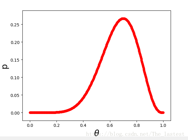
44 |
45 |
46 |
47 | 如图,我们可以发现当且仅当$\theta=0.7$ 时,似然函数取得最大值,即此时情况下事件“正面朝上7次,正面朝下3次”发生的可能性最大,而$\theta=0.7$也就是最大似然估计的结果。
48 |
49 | ------
50 |
51 | **线性回归推导:**
52 |
53 | 记样本为$(x^{(i)},y^{(i)})$,对样本的观测(预测)值记为$\hat{y}^{(i)}=\theta^Tx^{(i)}+\epsilon^{(i)}$,则有:
54 | $$
55 | y^{(i)}=\theta^Tx^{(i)}+\epsilon^{(i)}\tag{01}
56 | $$
57 | 其中$\epsilon^{(i)}$表示第$i$个预测值与真实值之间的误差,同时由于误差$\epsilon^{(i)}$服从均值为0的高斯分布,于是有:
58 | $$
59 | p(\epsilon^{(i)})=\frac{1}{\sqrt{2\pi}\sigma}\exp{\left(-\frac{(\epsilon^{(i)})^2}{2\sigma^2}\right)}\tag{02}
60 | $$
61 | 其中,$p(\epsilon^{(i)})$是概率密度函数
62 |
63 | 于是将$(1)$带入$(2)$有:
64 | $$
65 | p(\epsilon^{(i)})=\frac{1}{\sqrt{2\pi}\sigma}\exp{\left(-\frac{(y^{(i)}-\theta^Tx^{(i)})^2}{2\sigma^2}\right)}\tag{03}
66 | $$
67 | 此时请注意看等式$(3)$的右边部分,显然是随机变量$y^{(i)}$,服从以$\theta^Tx^{(i)}$为均值的正态分布(想想正态分布的表达式),又由于该密度函数与参数$\theta,x$有关(即随机变量$(y^{i})$是$x^{(i)},\theta$下的条件分布),于是有:
68 | $$
69 | p(y^{(i)}|x^{(i)};\theta)=\frac{1}{\sqrt{2\pi}\sigma}\exp{\left(-\frac{(y^{(i)}-\theta^Tx^{(i)})^2}{2\sigma^2}\right)}\tag{04}
70 | $$
71 | 到目前为止,也就是说此时真实值$y^{(i)}$服从均值为$\theta^Tx^{(i)}$,方差为$\sigma^2$的正态分布。同时,由于$\theta^Tx^{(i)}$是依赖于参数$\theta$的变量,那么什么样的一组参数$\theta$能够使得已知的观测值最容易发生呢?此时就要用到极大似然估计来进行参数估计(似然函数的作用就是找到一组参数能够使得随机变量(此处就是$y^{(i)}$)出现的可能性最大):
72 | $$
73 | L(\theta)=\prod_{i=1}^m p(y^{(i)}|x^{(i)};\theta)=\prod_{i=1}^m\frac{1}{\sqrt{2\pi}\sigma}\exp\left(-\frac{(y^{(i)}-\theta^Tx^{(i)})^2}{2\sigma^2}\right)\tag{05}
74 | $$
75 | 为了便于求解,在等式$(05)$的两边同时取自然对数:
76 | $$
77 | \begin{aligned}
78 | \log L(\theta)&=\log\left\{ \prod_{i=1}^m\frac{1}{\sqrt{2\pi}\sigma}\exp\left(-\frac{(y^{(i)}-\theta^Tx^{(i)})^2}{2\sigma^2}\right)\right\}\\[3ex]
79 | &=\sum_{i=1}^m\log\left\{\frac{1}{\sqrt{2\pi}\sigma}\exp\left(-\frac{(y^{(i)}-\theta^Tx^{(i)})^2}{2\sigma^2}\right)\right\}\\[3ex]
80 | &=\sum_{i=1}^m\left\{\log\frac{1}{\sqrt{2\pi}\sigma}-\frac{(y^{(i)}-\theta^Tx^{(i)})^2}{2\sigma^2}\right\}\\[3ex]
81 | &=m\cdot\log\frac{1}{\sqrt{2\pi}\sigma}-\frac{1}{\sigma^2}\frac{1}{2}\sum_{i=1}^m\left(y^{(i)}-\theta^Tx^{(i)}\right)^2
82 | \end{aligned}
83 | $$
84 | 由于$\max L(\theta)\iff\max\log L(\theta)$,所以:
85 | $$
86 | \max\log L(\theta)\iff\min \frac{1}{\sigma^2}\frac{1}{2}\sum_{i=1}^m\left(y^{(i)}-\theta^Tx^{(i)}\right)^2\iff\min\frac{1}{2}\sum_{i=1}^m\left(y^{(i)}-\theta^Tx^{(i)}\right)^2
87 | $$
88 | 于是得目标函数:
89 | $$
90 | \begin{aligned}
91 | J(\theta)&=\frac{1}{2m}\sum_{i=1}^m\left(y^{(i)}-\theta^Tx^{(i)}\right)^2\\[3ex]
92 | &=\frac{1}{2m}\sum_{i=1}^m\left(y^{(i)}-Wx^{(i)}\right)^2
93 | \end{aligned}
94 | $$
95 | 矢量化:
96 | $$
97 | J = 0.5 * (1 / m) * np.sum((y - np.dot(X, w) - b) ** 2)
98 | $$
99 | **求解梯度**
100 |
101 | 符号说明:
102 | $y^{(i)}$表示第$i$个样本的真实值;
103 | $\hat{y}^{(i)}$表示第$i$个样本的预测值;
104 | $W$表示权重(列)向量,$W_j$表示其中一个分量;
105 | $X$表示数据集,形状为$m\times n$,$m$为样本个数,$n$为特征维度;
106 | $x^{(i)}$为一个(列)向量,表示第$i$个样本,$x^{(i)}_j$为第$j$维特征
107 | $$
108 | \begin{aligned}
109 | J(W,b)&=\frac{1}{2m}\sum_{i=1}^m\left(y^{(i)}-\hat{y}^{(i)}\right)^2=\frac{1}{2m}\sum_{i=1}^m\left(y^{(i)}-(W^Tx^{(i)}+b)\right)^2\\[4ex]
110 | \frac{\partial J}{\partial W_j}&=\frac{\partial }{\partial W_j}\frac{1}{2m}\sum_{i=1}^m\left(y^{(i)}-(W_1x^{(i)}_1+W_2x^{(i)}_2\cdots W_nx^{(i)}_n+b)\right)^2\\[3ex]
111 | &=\frac{1}{m}\sum_{i=1}^m\left(y^{(i)}-(W_1x^{(i)}_1+W_2x^{(i)}_2\cdots W_nx^{(i)}_n+b)\right)\cdot(-x_j^{(i)})\\[3ex]
112 | &=\frac{1}{m}\sum_{i=1}^m\left(y^{(i)}-(W^Tx^{(i)}+b)\right)\cdot(-x_j^{(i)})\\[4ex]
113 | \frac{\partial J}{\partial b}&=\frac{\partial }{\partial W_j}\frac{1}{2m}\sum_{i=1}^m\left(y^{(i)}-(W^Tx^{(i)}+b)\right)^2\\[3ex]
114 | &=-\frac{1}{m}\sum_{i=1}^m\left(y^{(i)}-(W^Tx^{(i)}+b)\right)\\[3ex]
115 | \frac{\partial J}{\partial W}&=-\frac{1}{m} np.dot(x.T,(y-\hat{y}))\\[3ex]
116 | \frac{\partial J}{\partial b}&=-\frac{1}{m} np.sum(y-\hat{y})\\[3ex]
117 | \end{aligned}
118 | $$
119 |
120 | ------
121 |
122 | #### 5.怎么理解梯度(Gradient and learning rate),为什么沿着梯度的方向就能保证函数的变化率最大?
123 |
124 | 首先需要明白梯度是一个向量;其次是函数在任意一点,只有沿着梯度的方向才能保证函数值的变化率最大。
125 |
126 | 我们知道函数$f(x)$在某点($x_0$)的导数值决定了其在该点的变化率,也就是说$|f'(x_0)|$越大,则函数$f(x)$在$x=x_0$处的变化速度越快。同时对于高维空间(以三维空间为例)来说,函数$f(x,y)$在某点$(x_0,y_0)$的方向导数值$|\frac{\partial f}{\partial\vec{l}}|$ 的大小还取决于沿着哪个方向求导,也就是说沿着不同的方向,函数$f(x,y)$在$(x_0,y_0)$处的变化率不同。又由于:
127 | $$
128 | \begin{align*}
129 | \frac{\partial f}{\partial\vec{l}}&=\{\frac{\partial f}{\partial x},\frac{\partial f}{\partial y}\} \cdot\{cos\alpha,cos\beta\}\\
130 | &=gradf\cdot\vec{l^0}\\
131 | &=|gradf|\cdot|\vec{l^0}|\cdot cos\theta\\
132 | &=|gradf|\cdot1\cdot cos\theta\\
133 | &=|gradf|\cdot cos\theta
134 | \end{align*}
135 | $$
136 | 因此,当$\theta=0$是,即$\vec{l}$与向量(梯度)$\{\frac{\partial f}{\partial x},\frac{\partial f}{\partial y}\}$同向时方向导数取到最大值:
137 | $$\color{red}{\frac{\partial f}{\partial\vec{l}}=|gradf|=\sqrt{(\frac{\partial f}{\partial x})^2+(\frac{\partial f}{\partial y})^2}}$$
138 |
139 | 故,沿着梯度的方向才能保证函数值的变化率最大。
140 | 参见:[方向导数(Directional derivatives)](https://blog.csdn.net/The_lastest/article/details/77898799)、[梯度(Gradient vectors)](https://blog.csdn.net/The_lastest/article/details/77899206)
141 |
142 | 函数$f(\cdot)$的(方向)导数反映的是函数$f(\cdot)$在点$P$处的变化率的大小,即$|f'(\cdot)|_P|$越大,函数$f(\cdot)$在该点的变化率越大。为了更快的优化目标函数,我们需要找到满足$|f'(\cdot)|_P|$最大时的情况,由梯度计算公式可知,当且仅当方向导数的方向与梯度的方向一致时,$|f'(\cdot)|_P|$能取得最大值。——2019年10月5日更新
143 |
144 | #### 6.怎么理解梯度下降算法与学习率(Gradient Descent)?
145 |
146 | $$w=w-\alpha\frac{\partial J}{\partial w}$$
147 | 梯度下降算法可以看成是空间中的某个点$w$,每次沿着梯度的反方向走一小步,然后更新$w$,然后再走一小步,如此往复直到$J(w)$收敛。而学习率$\alpha$决定的就是在确定方向后每次走多大的“步子”。
148 |
149 | #### 7.学习率过大或者过小将会对目标函数产生什么样的影响?
150 |
151 | $\alpha$过大可能会导致目标函数震荡不能收敛,太小则可能需要大量的迭代才能收敛,耗费时间。
152 |
153 | #### 8.运用梯度下降算法的前提是什么?
154 |
155 | 目标函数为凸函数(形如$y=x^2$)
156 |
157 | #### 9.梯度下降算法是否一定能找到最优解?
158 |
159 | 对于凸函数而言一定等。对于非凸函数来说,能找到局部最优。
160 |
161 |
--------------------------------------------------------------------------------
/Lecture_01/LinearRegression.py:
--------------------------------------------------------------------------------
1 | from sklearn.datasets import load_boston
2 | import numpy as np
3 | import matplotlib.pyplot as plt
4 |
5 |
6 | def feature_scalling(X):
7 | mean = X.mean(axis=0)
8 | std = X.std(axis=0)
9 | return (X - mean) / std
10 |
11 |
12 | def load_data(shuffled=False):
13 | data = load_boston()
14 | # print(data.DESCR)# 数据集描述
15 | X = data.data
16 | y = data.target
17 | X = feature_scalling(X)
18 | y = np.reshape(y, (len(y), 1))
19 | if shuffled:
20 | shuffle_index = np.random.permutation(y.shape[0])
21 | X = X[shuffle_index]
22 | y = y[shuffle_index] # 打乱数据
23 | return X, y
24 |
25 |
26 | def costJ(X, y, w, b):
27 | m, n = X.shape
28 | J = 0.5 * (1 / m) * np.sum((y - np.dot(X, w) - b) ** 2)
29 | return J
30 |
31 |
32 | X, y = load_data()
33 | m, n = X.shape # 506,13
34 | w = np.random.randn(13, 1)
35 | b = 0.1
36 | alpha = 0.01
37 | cost_history = []
38 | for i in range(5000):
39 | y_hat = np.dot(X, w) + b
40 | grad_w = -(1 / m) * np.dot(X.T, (y - y_hat))
41 | grad_b = -(1 / m) * np.sum(y - y_hat)
42 | w = w - alpha * grad_w
43 | b = b - alpha * grad_b
44 | if i % 100 == 0:
45 | cost_history.append(costJ(X, y, w, b))
46 |
47 | # plt.plot(np.arange(len(cost_history)),cost_history)
48 | # plt.show()
49 | # print(cost_history)
50 |
51 | y_pre = np.dot(X, w) + b
52 | numerator = np.sum((y - y_pre) ** 2)
53 | denominator= np.sum((y - y.mean()) ** 2)
54 | print(1 - (numerator / denominator))
55 |
--------------------------------------------------------------------------------
/Lecture_01/README.md:
--------------------------------------------------------------------------------
1 | ### 1. 本节视频6,7
2 | ### 2. 思考问题:
3 | 1. 为什么说线性回归中误差是服从均值为0的方差为sigma^2的正态(高斯)分布,不是0均值行不行?
4 |
5 | 2. 什么是最小二乘法?
6 | 3. 为什么要用最小二乘法而不是最小四乘法,六乘法?
7 | 4. 怎么理解似然函数(likelihood function)
8 | 5. 怎么理解梯度与学习率(Gradient and learning rate)?
9 | 6. 怎么理解梯度下降算法(Gradient Descent)?
10 | 7. 运用梯度下降算法的前提是什么?
11 | 8. 梯度下降算法是否一定能找到最优解?
12 | 9. 学习率过大或者过小将会对目标函数产生什么样的影响?
13 | 10. 什么是feature scalling
14 |
15 | 参考 [线性回归 地址一](https://blog.csdn.net/The_lastest/article/details/82556307) [地址二](./LinearRegression.md)
16 |
17 | ### 3. 算法示例:
18 | - 示例1[波士顿房价预测](LinearRegression.py)
19 | 涉及知识点:
20 | 1. 数据归一化(feature scalling)
21 | 2. 数据打乱(shuffle)
22 | 3. 实现梯度下降
23 | ### [<主页>](../README.md) [<下一讲>](../Lecture_02/README.md)
--------------------------------------------------------------------------------
/Lecture_02/LogisticRegression.py:
--------------------------------------------------------------------------------
1 | import numpy as np
2 | from sklearn.datasets import load_breast_cancer
3 |
4 |
5 | def feature_scalling(X):
6 | mean = X.mean(axis=0)
7 | std = X.std(axis=0)
8 | return (X - mean) / std
9 |
10 |
11 | def load_data(shuffled=False):
12 | data_cancer = load_breast_cancer()
13 | x = data_cancer.data
14 | y = data_cancer.target
15 | x = feature_scalling(x)
16 | y = np.reshape(y, (len(y), 1))
17 | if shuffled:
18 | shuffled_index = np.random.permutation(y.shape[0])
19 | x = x[shuffled_index]
20 | y = y[shuffled_index]
21 | return x, y
22 |
23 |
24 | def sigmoid(z):
25 | gz = 1 / (1 + np.exp(-z))
26 | return gz
27 |
28 |
29 | def gradDescent(X, y, W, b, alpha, maxIt):
30 | cost_history = []
31 | maxIteration = maxIt
32 | m, n = X.shape
33 | for i in range(maxIteration):
34 | z = np.dot(X, W) + b
35 | error = sigmoid(z) - y
36 | W = W - (1 / m) * alpha * np.dot(X.T, error)
37 | b = b - (1.0 / m) * alpha * np.sum(error)
38 | cost_history.append(cost_function(X, y, W, b))
39 | return W, b, cost_history
40 |
41 |
42 | def accuracy(X, y, W, b):
43 | m, n = np.shape(X)
44 | z = np.dot(X, W) + b
45 | y_hat = sigmoid(z)
46 | predictioin = np.ones((m, 1), dtype=float)
47 | for i in range(m):
48 | if y_hat[i, 0] < 0.5:
49 | predictioin[i] = 0.0
50 | return 1 - np.sum(np.abs(y - predictioin)) / m
51 |
52 |
53 | def cost_function(X, y, W, b):
54 | m, n = X.shape
55 | z = np.dot(X, W) + b
56 | y_hat = sigmoid(z)
57 | J = (-1 / m) * np.sum(y * np.log(y_hat) + (1 - y) * np.log(1 - y_hat))
58 | return J
59 |
60 | if __name__ == '__main__':
61 | X, y = load_data()
62 | m, n = X.shape
63 | alpha = 0.1
64 | W = np.random.randn(n, 1)
65 | b = 0.1
66 | maxIt = 200
67 | W, b, cost_history = gradDescent(X, y, W, b, alpha, maxIt)
68 | print("******************")
69 | print("W is : ")
70 | print(W)
71 | print("accuracy is : " + str(accuracy(X, y, W, b)))
72 | print("******************")
73 |
--------------------------------------------------------------------------------
/Lecture_02/README.md:
--------------------------------------------------------------------------------
1 | ### 1. 本节视频3,4,8,9
2 | ### 2. 知识点
3 | - 利用 `Matplotlib`画图
4 | - [Matplotlib画图系列(一)简易线形图及散点图](https://blog.csdn.net/The_lastest/article/details/79828638)
5 | - [Matplotlib画图系列(二)误差曲线(errorbar) ](https://blog.csdn.net/The_lastest/article/details/79829046)
6 | - 逻辑回归代价函数的由来
7 | - [Logistic回归代价函数的数学推导及实现](https://blog.csdn.net/The_lastest/article/details/78761577)
8 | - 利用sklearn库来实现逻辑回归
9 | - 见示例3
10 | ### 3. 算法示例:
11 | - 示例1[breast_cancer分类](LogisticRegression.py)
12 | - 示例2[是否录取分类](e2.py)
13 | - 可视化
14 | 
15 | - 损失图
16 | 
17 | - 示例3[用sklearn库实现示例2](e3.py)
18 | ### [<主页>](../README.md) [<下一讲>](../Lecture_03/README.md)
--------------------------------------------------------------------------------
/Lecture_02/data/01.png:
--------------------------------------------------------------------------------
https://raw.githubusercontent.com/TolicWang/MachineLearningWithMe/11d3bc63acc4a40947856e9cdabd47ab6c40793d/Lecture_02/data/01.png
--------------------------------------------------------------------------------
/Lecture_02/data/02.png:
--------------------------------------------------------------------------------
https://raw.githubusercontent.com/TolicWang/MachineLearningWithMe/11d3bc63acc4a40947856e9cdabd47ab6c40793d/Lecture_02/data/02.png
--------------------------------------------------------------------------------
/Lecture_02/data/LogiReg_data.txt:
--------------------------------------------------------------------------------
1 | 34.62365962451697,78.0246928153624,0
2 | 30.28671076822607,43.89499752400101,0
3 | 35.84740876993872,72.90219802708364,0
4 | 60.18259938620976,86.30855209546826,1
5 | 79.0327360507101,75.3443764369103,1
6 | 45.08327747668339,56.3163717815305,0
7 | 61.10666453684766,96.51142588489624,1
8 | 75.02474556738889,46.55401354116538,1
9 | 76.09878670226257,87.42056971926803,1
10 | 84.43281996120035,43.53339331072109,1
11 | 95.86155507093572,38.22527805795094,0
12 | 75.01365838958247,30.60326323428011,0
13 | 82.30705337399482,76.48196330235604,1
14 | 69.36458875970939,97.71869196188608,1
15 | 39.53833914367223,76.03681085115882,0
16 | 53.9710521485623,89.20735013750205,1
17 | 69.07014406283025,52.74046973016765,1
18 | 67.94685547711617,46.67857410673128,0
19 | 70.66150955499435,92.92713789364831,1
20 | 76.97878372747498,47.57596364975532,1
21 | 67.37202754570876,42.83843832029179,0
22 | 89.67677575072079,65.79936592745237,1
23 | 50.534788289883,48.85581152764205,0
24 | 34.21206097786789,44.20952859866288,0
25 | 77.9240914545704,68.9723599933059,1
26 | 62.27101367004632,69.95445795447587,1
27 | 80.1901807509566,44.82162893218353,1
28 | 93.114388797442,38.80067033713209,0
29 | 61.83020602312595,50.25610789244621,0
30 | 38.78580379679423,64.99568095539578,0
31 | 61.379289447425,72.80788731317097,1
32 | 85.40451939411645,57.05198397627122,1
33 | 52.10797973193984,63.12762376881715,0
34 | 52.04540476831827,69.43286012045222,1
35 | 40.23689373545111,71.16774802184875,0
36 | 54.63510555424817,52.21388588061123,0
37 | 33.91550010906887,98.86943574220611,0
38 | 64.17698887494485,80.90806058670817,1
39 | 74.78925295941542,41.57341522824434,0
40 | 34.1836400264419,75.2377203360134,0
41 | 83.90239366249155,56.30804621605327,1
42 | 51.54772026906181,46.85629026349976,0
43 | 94.44336776917852,65.56892160559052,1
44 | 82.36875375713919,40.61825515970618,0
45 | 51.04775177128865,45.82270145776001,0
46 | 62.22267576120188,52.06099194836679,0
47 | 77.19303492601364,70.45820000180959,1
48 | 97.77159928000232,86.7278223300282,1
49 | 62.07306379667647,96.76882412413983,1
50 | 91.56497449807442,88.69629254546599,1
51 | 79.94481794066932,74.16311935043758,1
52 | 99.2725269292572,60.99903099844988,1
53 | 90.54671411399852,43.39060180650027,1
54 | 34.52451385320009,60.39634245837173,0
55 | 50.2864961189907,49.80453881323059,0
56 | 49.58667721632031,59.80895099453265,0
57 | 97.64563396007767,68.86157272420604,1
58 | 32.57720016809309,95.59854761387875,0
59 | 74.24869136721598,69.82457122657193,1
60 | 71.79646205863379,78.45356224515052,1
61 | 75.3956114656803,85.75993667331619,1
62 | 35.28611281526193,47.02051394723416,0
63 | 56.25381749711624,39.26147251058019,0
64 | 30.05882244669796,49.59297386723685,0
65 | 44.66826172480893,66.45008614558913,0
66 | 66.56089447242954,41.09209807936973,0
67 | 40.45755098375164,97.53518548909936,1
68 | 49.07256321908844,51.88321182073966,0
69 | 80.27957401466998,92.11606081344084,1
70 | 66.74671856944039,60.99139402740988,1
71 | 32.72283304060323,43.30717306430063,0
72 | 64.0393204150601,78.03168802018232,1
73 | 72.34649422579923,96.22759296761404,1
74 | 60.45788573918959,73.09499809758037,1
75 | 58.84095621726802,75.85844831279042,1
76 | 99.82785779692128,72.36925193383885,1
77 | 47.26426910848174,88.47586499559782,1
78 | 50.45815980285988,75.80985952982456,1
79 | 60.45555629271532,42.50840943572217,0
80 | 82.22666157785568,42.71987853716458,0
81 | 88.9138964166533,69.80378889835472,1
82 | 94.83450672430196,45.69430680250754,1
83 | 67.31925746917527,66.58935317747915,1
84 | 57.23870631569862,59.51428198012956,1
85 | 80.36675600171273,90.96014789746954,1
86 | 68.46852178591112,85.59430710452014,1
87 | 42.0754545384731,78.84478600148043,0
88 | 75.47770200533905,90.42453899753964,1
89 | 78.63542434898018,96.64742716885644,1
90 | 52.34800398794107,60.76950525602592,0
91 | 94.09433112516793,77.15910509073893,1
92 | 90.44855097096364,87.50879176484702,1
93 | 55.48216114069585,35.57070347228866,0
94 | 74.49269241843041,84.84513684930135,1
95 | 89.84580670720979,45.35828361091658,1
96 | 83.48916274498238,48.38028579728175,1
97 | 42.2617008099817,87.10385094025457,1
98 | 99.31500880510394,68.77540947206617,1
99 | 55.34001756003703,64.9319380069486,1
100 | 74.77589300092767,89.52981289513276,1
101 |
--------------------------------------------------------------------------------
/Lecture_02/e2.py:
--------------------------------------------------------------------------------
1 | import pandas as pd
2 | import matplotlib.pyplot as plt
3 | import pandas as pd
4 | import numpy as np
5 | from LogisticRegression import gradDescent,cost_function,accuracy,feature_scalling
6 |
7 |
8 | def load_data():
9 | data = pd.read_csv('./data/LogiReg_data.txt', names=['exam1', 'exam2', 'label']).as_matrix()
10 | X = data[:, :-1] # 取前两列
11 | y = data[:, -1:] # 取最后一列
12 | shuffle_index = np.random.permutation(X.shape[0])
13 | X = X[shuffle_index]
14 | y = y[shuffle_index]
15 | return X, y
16 |
17 |
18 | def visualize_data(X, y):
19 | positive = np.where(y == 1)[0]
20 | negative = np.where(y == 0)[0]
21 | plt.scatter(X[positive,0],X[positive,1],s=30,c='b',marker='o',label='Admitted')
22 | plt.scatter(X[negative,0],X[negative,1],s=30,c='r',marker='o',label='Not Admitted')
23 | plt.legend()
24 | plt.show()
25 |
26 | def visualize_cost(ite,cost):
27 | plt.plot(np.linspace(0,ite,ite),cost,linewidth=1)
28 | plt.title('cost history',color='r')
29 | plt.xlabel('iterations')
30 | plt.ylabel('cost J')
31 | plt.show()
32 |
33 |
34 | if __name__ == '__main__':
35 | # Step 1. Load data
36 | X, y = load_data()
37 | # Step 2. Visualize data
38 | visualize_data(X, y)
39 | #
40 | m, n = X.shape
41 | X = feature_scalling(X)
42 | alpha = 0.1
43 | W = np.random.randn(n, 1)
44 | b = 0.1
45 | maxIt = 10000
46 | W, b, cost_history = gradDescent(X, y, W, b, alpha, maxIt)
47 | print("******************")
48 | print(cost_history[:20])
49 | visualize_cost(maxIt,cost_history)
50 | print("accuracys is : " + str(accuracy(X, y, W, b)))
51 | print("W:",W)
52 | print("b: ",b)
53 | print("******************")
54 |
--------------------------------------------------------------------------------
/Lecture_02/e3.py:
--------------------------------------------------------------------------------
1 | import matplotlib.pyplot as plt
2 | import pandas as pd
3 | import numpy as np
4 | from LogisticRegression import feature_scalling
5 | from sklearn.linear_model import LogisticRegression
6 |
7 | def load_data():
8 | data = pd.read_csv('./data/LogiReg_data.txt', names=['exam1', 'exam2', 'label']).as_matrix()
9 | X = data[:, :-1] # 取前两列
10 | y = data[:, -1:] # 取最后一列
11 | shuffle_index = np.random.permutation(X.shape[0])
12 | X = X[shuffle_index]
13 | y = y[shuffle_index]
14 | return X, y
15 |
16 |
17 | def visualize_cost(ite,cost):
18 | plt.plot(np.linspace(0,ite,ite),cost,linewidth=1)
19 | plt.title('cost history',color='r')
20 | plt.xlabel('iterations')
21 | plt.ylabel('cost J')
22 | plt.show()
23 |
24 |
25 | if __name__ == '__main__':
26 | X, y = load_data()
27 | X = feature_scalling(X)
28 | lr = LogisticRegression()
29 | lr.fit(X,y)
30 | print("******************")
31 | print("accuracys is :" ,lr.score(X,y))
32 | print("W:{},b:{}".format(lr.coef_,lr.intercept_))
33 | print("******************")
--------------------------------------------------------------------------------
/Lecture_03/README.md:
--------------------------------------------------------------------------------
1 | ### 1. 本节视频10
2 | 本节视频中讲到的内容比较多也比较杂,但却**非常重要**。有一点不好的就是视频中的代码稍微有点乱,我会用一些其它方式来实现视频中代码(自己能看下去也行)。大家只要掌握好我列出的知识点即可。
3 | ### 2. 知识点
4 | - 2.1 过拟合(over fitting)和欠拟合(under fitting)具体是指什么?常用的解决方法是什么?
5 | - [斯坦福机器学习-第三周(分类,逻辑回归,过度拟合及解决方法)](https://blog.csdn.net/The_lastest/article/details/73349592)
6 | - [机器学习中正则化项L1和L2的直观理解](https://blog.csdn.net/jinping_shi/article/details/52433975)
7 | - 2.2 什么就超参数(hyper parameter)? 如何对模型进行评估?
8 | - 混淆矩阵(confusion matrix)
9 | 
10 | - 准确性(accuracy)
11 | - 精确率(precision)
12 | - 召回率(recall)
13 | - F1-score(**精确率和召回率的调和平均**)
14 | - 2.3 如何对模型进行筛选?
15 | - K折交叉验证(K-fold cross validation)
16 | - 并行参数搜索
17 | - 2.2 如何解决样本分布不均?
18 | - 下采样(down sampling)示例1:以样本数少的类别为标准,去掉样本数多的类别中多余的样本;
19 | - 过采样(over sampling)示例2:以样本数多的类别为标准,对样本数少的类别再生成若干个样本,使两个类别中的样本一致;
20 | ### 3. 示例
21 | - 3.1 示例1 [下采样](ex1.py)
22 | - 3.2 示例2 [过采样](ex2.py)
23 | ### [<主页>](../README.md) [<下一讲>](../Lecture_04/README.md)
--------------------------------------------------------------------------------
/Lecture_03/data/04.png:
--------------------------------------------------------------------------------
https://raw.githubusercontent.com/TolicWang/MachineLearningWithMe/11d3bc63acc4a40947856e9cdabd47ab6c40793d/Lecture_03/data/04.png
--------------------------------------------------------------------------------
/Lecture_03/data/README.md:
--------------------------------------------------------------------------------
1 | 下载好后放入data目录下即可
2 |
3 | ### 数据集下载地址:
4 | 链接: https://pan.baidu.com/s/1OlZ-nkS4sbjSgoaetqqOGg 提取码: ggr8
--------------------------------------------------------------------------------
/Lecture_03/ex1.py:
--------------------------------------------------------------------------------
1 | import pandas as pd
2 | import matplotlib.pyplot as plt
3 | import numpy as np
4 | from sklearn.preprocessing import StandardScaler
5 | from sklearn.cross_validation import train_test_split
6 | from sklearn.grid_search import GridSearchCV
7 | from sklearn.linear_model import LogisticRegression
8 | from sklearn.metrics import classification_report
9 |
10 |
11 | def load_and_analyse_data():
12 | data = pd.read_csv('./data/creditcard.csv')
13 |
14 | # ----------------------查看样本分布情况----------------------------------
15 | # count_classes = pd.value_counts(data['Class'],sort=True).sort_index()
16 | # print(count_classes)# negative 0 :284315 positive 1 :492
17 | # count_classes.plot(kind='bar')
18 | # plt.title('Fraud class histogram')
19 | # plt.xlabel('Class')
20 | # plt.ylabel('Frequency')
21 | # plt.show()
22 | # --------------------------------------------------------------------------
23 |
24 | # ----------------------预处理---------------------------------------------
25 |
26 | # ----------------------标准化Amount列---------
27 | data['normAmout'] = StandardScaler().fit_transform(data['Amount'].values.reshape(-1, 1))
28 | data = data.drop(['Time', 'Amount'], axis=1)
29 | # ----------------------------------------------
30 |
31 | X = data.ix[:, data.columns != 'Class']
32 | y = data.ix[:, data.columns == 'Class']
33 | positive_number = len(y[y.Class == 1]) # 492
34 | negative_number = len(y[y.Class == 0]) # 284315
35 | positive_indices = np.array(y[y.Class == 1].index)
36 | negative_indices = np.array(y[y.Class == 0].index)
37 |
38 | # ----------------------采样-------------------
39 | random_negative_indices = np.random.choice(negative_indices, positive_number, replace=False)
40 | random_negative_indices = np.array(random_negative_indices)
41 | under_sample_indices = np.concatenate([positive_indices, random_negative_indices])
42 | under_sample_data = data.iloc[under_sample_indices, :]
43 | X_sample = under_sample_data.ix[:, under_sample_data.columns != 'Class']
44 | y_sample = under_sample_data.ix[:, under_sample_data.columns == 'Class']
45 | return np.array(X), np.array(y).reshape(len(y)), np.array(X_sample), np.array(y_sample).reshape(len(y_sample))
46 |
47 |
48 | if __name__ == '__main__':
49 | X, y, X_sample, y_sample = load_and_analyse_data()
50 | _, X_test, _, y_test = train_test_split(X, y, test_size=0.3, random_state=30)
51 | X_train, X_dev, y_train, y_dev = train_test_split(X_sample, y_sample, test_size=0.3,
52 | random_state=1)
53 |
54 | print("X_train:{} X_dev:{} X_test:{}".format(len(y_train),len(y_dev),len(y_test)))
55 | model = LogisticRegression()
56 | parameters = {'C': [0.001, 0.003, 0.01, 0.03, 0.1, 0.3, 1, 3, 10]}
57 | gs = GridSearchCV(model, parameters, verbose=5, cv=5)
58 | gs.fit(X_train, y_train)
59 | print('最佳模型:', gs.best_params_, gs.best_score_)
60 | print('在采样数据上的性能表现:')
61 | print(gs.score(X_dev, y_dev))
62 | y_dev_pre = gs.predict(X_dev)
63 | print(classification_report(y_dev, y_dev_pre))
64 | print('在原始数据上的性能表现:')
65 | print(gs.score(X_test, y_test))
66 | y_pre = gs.predict(X_test)
67 | print(classification_report(y_test, y_pre))
68 |
--------------------------------------------------------------------------------
/Lecture_03/ex2.py:
--------------------------------------------------------------------------------
1 | import pandas as pd
2 | import matplotlib.pyplot as plt
3 | import numpy as np
4 | from sklearn.preprocessing import StandardScaler
5 | from sklearn.cross_validation import train_test_split
6 | from sklearn.grid_search import GridSearchCV
7 | from sklearn.linear_model import LogisticRegression
8 | from sklearn.metrics import classification_report
9 | from imblearn.over_sampling import SMOTE
10 |
11 | def load_and_analyse_data():
12 | data = pd.read_csv('./data/creditcard.csv')
13 | # ----------------------预处理---------------------------------------------
14 |
15 | # ----------------------标准化Amount列---------
16 | data['normAmout'] = StandardScaler().fit_transform(data['Amount'].values.reshape(-1, 1))
17 | data = data.drop(['Time', 'Amount'], axis=1)
18 | # ----------------------------------------------
19 |
20 | X = data.ix[:, data.columns != 'Class']
21 | y = data.ix[:, data.columns == 'Class']
22 | X_train,X_test,y_train,y_test = train_test_split(X,y,test_size=0.3,random_state=0)
23 | # ----------------------采样-------------------
24 | sample_solver = SMOTE(random_state=0)
25 | X_sample ,y_sample = sample_solver.fit_sample(X_train,y_train)
26 | return np.array(X_test),np.array(y_test).reshape(len(y_test)),np.array(X_sample),np.array(y_sample).reshape(len(y_sample))
27 |
28 | if __name__ == '__main__':
29 | X_test, y_test, X_sample, y_sample = load_and_analyse_data()
30 | X_train,X_dev,y_train,y_dev = train_test_split(X_sample,y_sample,test_size=0.3,random_state=1)
31 |
32 | print("X_train:{} X_dev:{} X_test:{}".format(len(y_train), len(y_dev), len(y_test)))
33 | model = LogisticRegression()
34 | parameters = {'C':[0.001,0.003,0.01,0.03,0.1,0.3,1,3,10]}
35 | gs = GridSearchCV(model,parameters,verbose=5,cv=5)
36 | gs.fit(X_train,y_train)
37 | print('最佳模型:',gs.best_params_,gs.best_score_)
38 | print('在采样数据上的性能表现:')
39 | print(gs.score(X_dev,y_dev))
40 | y_dev_pre = gs.predict(X_dev)
41 | print(classification_report(y_dev,y_dev_pre))
42 | print('在原始数据上的性能表现:')
43 | print(gs.score(X_test,y_test))
44 | y_pre = gs.predict(X_test)
45 | print(classification_report(y_test,y_pre))
46 |
--------------------------------------------------------------------------------
/Lecture_04/README.md:
--------------------------------------------------------------------------------
1 | ### 1. 本节视频
2 | - 本节视频11,12
3 | ### 2. 知识点
4 | - 2.1 什么是决策树(decision tree)?什么是信息熵?
5 | - [决策树——(一)决策树的思想](https://blog.csdn.net/The_lastest/article/details/78906751)
6 | - 2.2 决策树的构造与剪枝?
7 | - [决策树——(二)决策树的生成与剪枝ID3,C4.5](https://blog.csdn.net/The_lastest/article/details/78915862)
8 | - [决策树——(三)决策树的生成与剪枝CART](https://blog.csdn.net/The_lastest/article/details/78975439)
9 | - 2.3 决策树的可视化
10 | - [Graphviz](https://graphviz.gitlab.io/_pages/Download/Download_windows.html)
11 | - [机器学习笔记——决策数实现及使用Graphviz查看](https://blog.csdn.net/akadiao/article/details/77800909)
12 |
13 | 
14 | ### 3. 示例
15 | - 示例1[ iris分类](ex1.py)
16 | ### 4. 任务
17 | - 4.1 熟悉查看[scikit-learn API](http://scikit-learn.org/stable/modules/classes.html)
18 | ### [<主页>](../README.md) [<下一讲>](../Lecture_05/README.md)
--------------------------------------------------------------------------------
/Lecture_04/allElectronicsData.dot:
--------------------------------------------------------------------------------
1 | digraph Tree {
2 | node [shape=box] ;
3 | 0 [label="petal width (cm) <= -0.526\ngini = 0.665\nsamples = 105\nvalue = [36, 32, 37]\nclass = C"] ;
4 | 1 [label="gini = 0.0\nsamples = 36\nvalue = [36, 0, 0]\nclass = A"] ;
5 | 0 -> 1 [labeldistance=2.5, labelangle=45, headlabel="True"] ;
6 | 2 [label="petal width (cm) <= 0.593\ngini = 0.497\nsamples = 69\nvalue = [0, 32, 37]\nclass = C"] ;
7 | 0 -> 2 [labeldistance=2.5, labelangle=-45, headlabel="False"] ;
8 | 3 [label="petal length (cm) <= 0.706\ngini = 0.161\nsamples = 34\nvalue = [0, 31, 3]\nclass = B"] ;
9 | 2 -> 3 ;
10 | 4 [label="gini = 0.0\nsamples = 30\nvalue = [0, 30, 0]\nclass = B"] ;
11 | 3 -> 4 ;
12 | 5 [label="gini = 0.375\nsamples = 4\nvalue = [0, 1, 3]\nclass = C"] ;
13 | 3 -> 5 ;
14 | 6 [label="petal length (cm) <= 0.621\ngini = 0.056\nsamples = 35\nvalue = [0, 1, 34]\nclass = C"] ;
15 | 2 -> 6 ;
16 | 7 [label="gini = 0.375\nsamples = 4\nvalue = [0, 1, 3]\nclass = C"] ;
17 | 6 -> 7 ;
18 | 8 [label="gini = 0.0\nsamples = 31\nvalue = [0, 0, 31]\nclass = C"] ;
19 | 6 -> 8 ;
20 | }
--------------------------------------------------------------------------------
/Lecture_04/data/01.PNG:
--------------------------------------------------------------------------------
https://raw.githubusercontent.com/TolicWang/MachineLearningWithMe/11d3bc63acc4a40947856e9cdabd47ab6c40793d/Lecture_04/data/01.PNG
--------------------------------------------------------------------------------
/Lecture_04/ex1.py:
--------------------------------------------------------------------------------
1 | import numpy as np
2 | from sklearn.tree import DecisionTreeClassifier
3 | from sklearn.metrics import classification_report
4 |
5 |
6 | def load_data():
7 | from sklearn.datasets import load_iris
8 | from sklearn.preprocessing import StandardScaler
9 | from sklearn.model_selection import train_test_split
10 | data = load_iris()
11 | X = data.data
12 | y = data.target
13 | ss = StandardScaler()
14 | X = ss.fit_transform(X)
15 | x_train, x_test, y_train, y_test = train_test_split(X, y, test_size=0.3, random_state=1)
16 | return x_train, y_train, x_test, y_test, data.feature_names
17 |
18 |
19 | def train():
20 | x_train, y_train, x_test, y_test, _ = load_data()
21 | model = DecisionTreeClassifier()
22 | model.fit(x_train, y_train)
23 | y_pre = model.predict(x_test)
24 | print(model.score(x_test, y_test))
25 | print(classification_report(y_test, y_pre))
26 |
27 |
28 | def grid_search():
29 | from sklearn.model_selection import GridSearchCV
30 | x_train, y_train, x_test, y_test, _ = load_data()
31 | model = DecisionTreeClassifier()
32 | parameters = {'max_depth': np.arange(1, 50, 2)}
33 | gs = GridSearchCV(model, parameters, verbose=5, cv=5)
34 | gs.fit(x_train, y_train)
35 | print('最佳模型:', gs.best_params_, gs.best_score_)
36 | y_pre = gs.predict(x_test)
37 | print(classification_report(y_test, y_pre))
38 |
39 |
40 | def tree_visilize():
41 | from sklearn import tree
42 | x_train, y_train, x_test, y_test, feature_names = load_data()
43 | print('类标:', np.unique(y_train))
44 | print('特征名称:', feature_names)
45 | model = DecisionTreeClassifier(max_depth=3)
46 | model.fit(x_train, y_train)
47 | print(model.score(x_test, y_test))
48 | with open("allElectronicsData.dot", "w") as f:
49 | tree.export_graphviz(model, feature_names=feature_names, class_names=['A', 'B', 'C'], out_file=f)
50 |
51 |
52 | if __name__ == '__main__':
53 | train()
54 | # grid_search()
55 | # tree_visilize()
56 |
--------------------------------------------------------------------------------
/Lecture_05/README.md:
--------------------------------------------------------------------------------
1 | ### 1. 本节视频
2 | - 本节视频13,14,24
3 | ### 2. 知识点
4 | - 2.1 算法原理理解
5 | - Bagging:并行构造n个模型,每个模型彼此独立;如,RandomForest
6 | - Boosting:串行构造模型,下一个模型的提升依赖于训练好的上以个模型;如,AdaBoost,Xgboost
7 | - Stacking:第一阶段得出各自结果,第二阶段再用前一阶段结果训练
8 | - 2.2 数据预处理
9 | - 分析筛选数据特征
10 | - 缺失值补充(均值,最值)
11 | - 特征转换
12 | [用pandas处理缺失值补全及DictVectorizer特征转换](https://blog.csdn.net/The_lastest/article/details/79103386)
13 | [利用随机森林对特征重要性进行评估](https://blog.csdn.net/The_lastest/article/details/81151986)
14 | - 2.3 Xgboost
15 | - 安装
16 | - 方法一:在线安装
17 | ```python
18 | pip install -i https://pypi.tuna.tsinghua.edu.cn/simple/ xgboost
19 | ```
20 | - 方法二:本地安装
21 | 首先去[戳此处](https://www.lfd.uci.edu/~gohlke/pythonlibs/#xgboost)搜索并下载xboost对应安装包
22 | (cp27表示python2.7,win32表示32位,amd64表示64位)
23 | ```python
24 | pip install xgboost-0.80-cp36-cp36m-win_amd64.whl
25 | ```
26 | - 大致原理
27 | ### 3. 示例
28 | - 3.1 本示例先对特征进行人工分析,然后选择其中7个进行训练
29 | - [示例1](ex1.py)
30 | - 3.2 本示例先对特征进行评估,然后选择其中3个进行训练
31 | - [示例2](ex2.py)
32 | - 3.3 本示例是以stacking的思想进行训练
33 | - [示例3](ex3.py)
34 | ### 4. 任务
35 | - 4.1 根据所给[数据集1001](../DatasetUrl.md),预测某人是否患有糖尿病;
36 | - 4.2 根据所给[数据集1002](../DatasetUrl.md),预测泰坦尼克号人员生还情况;
37 |
38 | 要求:
39 | - 要求模型预测的准确率尽可能高;
40 | - 分模块书写代码(比如数据预处理,不同模型的训练要抽象成函数,具体可参见前面例子);
41 | ### [<主页>](../README.md) [<下一讲>](../Lecture_06/README.md)
--------------------------------------------------------------------------------
/Lecture_05/data/README.md:
--------------------------------------------------------------------------------
1 | 下载好后放入data目录下即可
2 |
3 | ### 数据集下载地址:
4 |
5 | [数据集1002](../../DatasetUrl.md)
--------------------------------------------------------------------------------
/Lecture_05/ex1.py:
--------------------------------------------------------------------------------
1 | import pandas as pd
2 | from sklearn.model_selection import GridSearchCV
3 | import numpy as np
4 |
5 |
6 | def load_data_and_preprocessing():
7 | train = pd.read_csv('./data/titanic_train.csv')
8 | test = pd.read_csv('./data/test.csv')
9 | # print(train['Name'])
10 | # print(titannic_train.describe())
11 | # print(train.info())
12 | train_y = train['Survived']
13 | selected_features = ['Pclass', 'Sex', 'Age', 'SibSp', 'Parch', 'Fare', 'Embarked']
14 | train_x = train[selected_features]
15 | train_x['Age'].fillna(train_x['Age'].mean(), inplace=True) # 以均值填充
16 | # print(train_x['Embarked'].value_counts())
17 | train_x['Embarked'].fillna('S', inplace=True)
18 | # print(train_x.info())
19 |
20 | test_x = test[selected_features]
21 | test_x['Age'].fillna(test_x['Age'].mean(), inplace=True)
22 | test_x['Fare'].fillna(test_x['Fare'].mean(), inplace=True)
23 | # print(test_x.info())
24 |
25 | train_x.loc[train_x['Embarked'] == 'S', 'Embarked'] = 0
26 | train_x.loc[train_x['Embarked'] == 'C', 'Embarked'] = 1
27 | train_x.loc[train_x['Embarked'] == 'Q', 'Embarked'] = 2
28 | train_x.loc[train_x['Sex'] == 'male', 'Sex'] = 0
29 | train_x.loc[train_x['Sex'] == 'female', 'Sex'] = 1
30 | x_train = train_x.as_matrix()
31 | y_train = train_y.as_matrix()
32 |
33 | test_x.loc[test_x['Embarked'] == 'S', 'Embarked'] = 0
34 | test_x.loc[test_x['Embarked'] == 'C', 'Embarked'] = 1
35 | test_x.loc[test_x['Embarked'] == 'Q', 'Embarked'] = 2
36 | test_x.loc[test_x['Sex'] == 'male', 'Sex'] = 0
37 | test_x.loc[test_x['Sex'] == 'female', 'Sex'] = 1
38 | x_test = test_x
39 | return x_train, y_train, x_test
40 |
41 |
42 | def logistic_regression():
43 | from sklearn.linear_model import LogisticRegression
44 | x_train, y_train, x_test = load_data_and_preprocessing()
45 | model = LogisticRegression()
46 | paras = {'C': np.linspace(0.1, 10, 50)}
47 | gs = GridSearchCV(model, paras, cv=5, verbose=3)
48 | gs.fit(x_train, y_train)
49 | print('best score:', gs.best_score_)
50 | print('best parameters:', gs.best_params_)
51 |
52 |
53 | def decision_tree():
54 | from sklearn.tree import DecisionTreeClassifier
55 | x_train, y_train, x_test = load_data_and_preprocessing()
56 | model = DecisionTreeClassifier()
57 | paras = {'criterion': ['gini', 'entropy'], 'max_depth': np.arange(5, 50, 5)}
58 | gs = GridSearchCV(model, paras, cv=5, verbose=3)
59 | gs.fit(x_train, y_train)
60 | print('best score:', gs.best_score_)
61 | print('best parameters:', gs.best_params_)
62 |
63 |
64 | def random_forest():
65 | from sklearn.ensemble import RandomForestClassifier
66 | x_train, y_train, x_test = load_data_and_preprocessing()
67 | model = RandomForestClassifier()
68 | paras = {'n_estimators': np.arange(10, 100, 10), 'criterion': ['gini', 'entropy'], 'max_depth': np.arange(5, 50, 5)}
69 | gs = GridSearchCV(model, paras, cv=5, verbose=3)
70 | gs.fit(x_train, y_train)
71 | print('best score:', gs.best_score_)
72 | print('best parameters:', gs.best_params_)
73 |
74 |
75 | def gradient_boosting():
76 | from sklearn.ensemble import GradientBoostingClassifier
77 | x_train, y_train, x_test = load_data_and_preprocessing()
78 | model = GradientBoostingClassifier()
79 | paras = {'learning_rate': np.arange(0.1, 1, 0.1), 'n_estimators': range(80, 120, 10), 'max_depth': range(5, 10, 1)}
80 | gs = GridSearchCV(model, paras, cv=5, verbose=3,n_jobs=2)
81 | gs.fit(x_train, y_train)
82 | print('best score:', gs.best_score_)
83 | print('best parameters:', gs.best_params_)
84 |
85 |
86 | if __name__ == '__main__':
87 | # logistic_regression() # 0.7979
88 | # decision_tree()#0.813
89 | # random_forest() # 0.836 {'criterion': 'entropy', 'max_depth': 10, 'n_estimators': 60}
90 | gradient_boosting()#0.830 {'learning_rate': 0.1, 'max_depth': 5, 'n_estimators': 90}
91 |
--------------------------------------------------------------------------------
/Lecture_05/ex2.py:
--------------------------------------------------------------------------------
1 | import pandas as pd
2 | import numpy as np
3 | from sklearn.model_selection import GridSearchCV
4 |
5 | def feature_selection():
6 | from sklearn.feature_selection import SelectKBest, f_classif
7 | import matplotlib.pyplot as plt
8 | train = pd.read_csv('./data/titanic_train.csv')
9 | selected_features = ['Pclass', 'Sex', 'Age', 'SibSp', 'Parch', 'Fare', 'Embarked']
10 | train_x = train[selected_features]
11 | train_y = train['Survived']
12 | train_x['Age'].fillna(train_x['Age'].mean(), inplace=True) # 以均值填充
13 | train_x['Embarked'].fillna('S', inplace=True)
14 | train_x.loc[train_x['Embarked'] == 'S', 'Embarked'] = 0
15 | train_x.loc[train_x['Embarked'] == 'C', 'Embarked'] = 1
16 | train_x.loc[train_x['Embarked'] == 'Q', 'Embarked'] = 2
17 | train_x.loc[train_x['Sex'] == 'male', 'Sex'] = 0
18 | train_x.loc[train_x['Sex'] == 'female', 'Sex'] = 1
19 |
20 | selector = SelectKBest(f_classif, k=5)
21 | selector.fit(train_x, train_y)
22 | scores = selector.scores_
23 | plt.bar(range(len(selected_features)), scores)
24 | plt.xticks(range(len(selected_features)), selected_features, rotation='vertical')
25 | plt.show()
26 |
27 | x_train = train_x[['Pclass', 'Sex', 'Fare']]
28 | y_train = train_y.as_matrix()
29 | return x_train, y_train
30 | def logistic_regression():
31 | from sklearn.linear_model import LogisticRegression
32 | x_train, y_train= feature_selection()
33 | model = LogisticRegression()
34 | paras = {'C': np.linspace(0.1, 10, 50)}
35 | gs = GridSearchCV(model, paras, cv=5, verbose=3)
36 | gs.fit(x_train, y_train)
37 | print('best score:', gs.best_score_)
38 | print('best parameters:', gs.best_params_)
39 |
40 |
41 | def decision_tree():
42 | from sklearn.tree import DecisionTreeClassifier
43 | x_train, y_train = feature_selection()
44 | model = DecisionTreeClassifier()
45 | paras = {'criterion': ['gini', 'entropy'], 'max_depth': np.arange(5, 50, 5)}
46 | gs = GridSearchCV(model, paras, cv=5, verbose=3)
47 | gs.fit(x_train, y_train)
48 | print('best score:', gs.best_score_)
49 | print('best parameters:', gs.best_params_)
50 |
51 |
52 | def random_forest():
53 | from sklearn.ensemble import RandomForestClassifier
54 | x_train, y_train = feature_selection()
55 | model = RandomForestClassifier()
56 | paras = {'n_estimators': np.arange(10, 100, 10), 'criterion': ['gini', 'entropy'], 'max_depth': np.arange(5, 50, 5)}
57 | gs = GridSearchCV(model, paras, cv=5, verbose=3)
58 | gs.fit(x_train, y_train)
59 | print('best score:', gs.best_score_)
60 | print('best parameters:', gs.best_params_)
61 |
62 | if __name__ == '__main__':
63 | # feature_selection()
64 | # logistic_regression()#0.783
65 | # decision_tree()#0.814
66 | random_forest()# 0.814
--------------------------------------------------------------------------------
/Lecture_05/ex3.py:
--------------------------------------------------------------------------------
1 | from ex1 import load_data_and_preprocessing
2 | from sklearn.model_selection import KFold
3 | from sklearn.ensemble import RandomForestClassifier, GradientBoostingClassifier
4 |
5 |
6 | def stacking():
7 | s = 0
8 | x_train, y_train, x_test = load_data_and_preprocessing()
9 | kf = KFold(n_splits=5)
10 | rfc = RandomForestClassifier(criterion='entropy', max_depth=10, n_estimators=60)
11 | gbc = GradientBoostingClassifier(learning_rate=0.1, max_depth=5, n_estimators=90)
12 | for train_index, test_index in kf.split(x_train):
13 | train_x, test_x = x_train[train_index], x_train[test_index]
14 | train_y, test_y = y_train[train_index], y_train[test_index]
15 | rfc.fit(train_x, train_y)
16 | rfc_pre = rfc.predict_proba(test_x)[:,1]
17 | gbc.fit(train_x, train_y)
18 | gbc_pre = gbc.predict_proba(test_x)[:,1]
19 | y_pre = ((rfc_pre+gbc_pre)/2 >= 0.5)*1
20 | acc = sum((test_y == y_pre)*1)/len(y_pre)
21 | s += acc
22 | print(acc)
23 | print('Accuracy: ',s/5)# 0.823
24 |
25 |
26 | if __name__ == '__main__':
27 | stacking()
28 |
--------------------------------------------------------------------------------
/Lecture_06/README.md:
--------------------------------------------------------------------------------
1 | ### 1. 本节视频
2 | - 本节视频15,16
3 | ### 2. 知识点
4 | - 2.1 贝叶斯算法和贝叶斯估计
5 | - [朴素贝叶斯算法与贝叶斯估计](https://blog.csdn.net/The_lastest/article/details/78807198)
6 | - 平滑处理(拉普拉斯平滑)
7 | - 2.2 特征提取
8 | - 分词处理
9 | - [利用jieba进行中文分词并进行词频统计](https://blog.csdn.net/The_lastest/article/details/81027387)
10 | - 词集模型
11 | - 词袋模型
12 | - TF-IDF
13 | - [Scikit-learn CountVectorizer与TfidfVectorizer](https://blog.csdn.net/The_lastest/article/details/79093407)
14 | - 2.3 相似度计算
15 | - 欧氏距离
16 | - cos距离
17 | 
18 | ### 3. 示例
19 | - [3.1 基于贝叶斯算法的中文垃圾邮件分类](ex1.py)
20 | - [3.2 词云图](word_cloud.py)
21 | 
22 | ### 4. 任务
23 | - [4.1 在3.1的基础上,完成选取所有词中前5000个出现频率最高的词为字典构造TF-IDF特征矩阵,然后训练模型]()
24 | - [4.2 基于贝叶斯算法和编辑距离的单词拼写纠正](ex2.py)
25 | - [4.3 基于贝叶斯算法的中文新闻分类](ex3.py)
26 | ### [<主页>](../README.md) [<下一讲>](../Lecture_07/README.md)
--------------------------------------------------------------------------------
/Lecture_06/data/Figure_1.png:
--------------------------------------------------------------------------------
https://raw.githubusercontent.com/TolicWang/MachineLearningWithMe/11d3bc63acc4a40947856e9cdabd47ab6c40793d/Lecture_06/data/Figure_1.png
--------------------------------------------------------------------------------
/Lecture_06/data/README.md:
--------------------------------------------------------------------------------
1 | 下载好后放入data目录下即可
2 |
3 | ### 数据集下载地址:
4 |
5 | 数据集编号: 1003,1004,1005
6 |
7 | 停用词:3001
8 |
9 | [数据集下载地址集合](../../DatasetUrl.md)
10 |
11 |
--------------------------------------------------------------------------------
/Lecture_06/data/p18.png:
--------------------------------------------------------------------------------
https://raw.githubusercontent.com/TolicWang/MachineLearningWithMe/11d3bc63acc4a40947856e9cdabd47ab6c40793d/Lecture_06/data/p18.png
--------------------------------------------------------------------------------
/Lecture_06/data/simhei.ttf:
--------------------------------------------------------------------------------
https://raw.githubusercontent.com/TolicWang/MachineLearningWithMe/11d3bc63acc4a40947856e9cdabd47ab6c40793d/Lecture_06/data/simhei.ttf
--------------------------------------------------------------------------------
/Lecture_06/ex1.py:
--------------------------------------------------------------------------------
1 | import re
2 | import jieba
3 | import numpy as np
4 | from sklearn.feature_extraction.text import TfidfVectorizer
5 | from sklearn.model_selection import train_test_split
6 | import sys
7 | from sklearn.naive_bayes import MultinomialNB
8 |
9 |
10 | def clean_str(string, sep=" "):
11 | """
12 | 该函数的作用是去掉一个字符串中的所有非中文字符
13 | :param string: 输入必须是字符串类型
14 | :param sep: 表示去掉的部分用什么填充,默认为一个空格
15 | :return: 返回处理后的字符串
16 |
17 | example:
18 | s = "祝你2018000国庆快乐!"
19 | print(clean_str(s))# 祝你 国庆快乐
20 | print(clean_str(s,sep=""))# 祝你国庆快乐
21 | """
22 | string = re.sub(r"[^\u4e00-\u9fff]", sep, string)
23 | string = re.sub(r"\s{2,}", sep, string) # 若有空格,则最多只保留2个宽度
24 | return string.strip()
25 |
26 |
27 | def cut_line(line):
28 | """
29 | 该函数的作用是 先清洗字符串,然后分词
30 | :param line: 输入必须是字符串类型
31 | :return: 分词后的结果
32 |
33 | example:
34 | s ='我今天很高兴'
35 | print(cut_line(s))# 我 今天 很 高兴
36 | """
37 | line = clean_str(line)
38 | seg_list = jieba.cut(line)
39 | cut_words = " ".join(seg_list)
40 | return cut_words
41 |
42 |
43 | def load_data_and_labels(positive_data_file, negative_data_file):
44 | """
45 | 该函数的作用是按行载入数据,然后分词。同时给每个样本构造构造标签
46 | :param positive_data_file: txt文本格式,其中每一行为一个样本
47 | :param negative_data_file: txt文本格式,其中每一行为一个样本
48 | :return: 分词后的结果和标签
49 | example:
50 | positive_data_file:
51 | 今天我很高兴,你吃饭了吗?
52 | 这个怎么这么不正式啊?还上进青年
53 | 我觉得这个不错!
54 | return:
55 | x_text: ['今天 我 很 高兴 你 吃饭 了 吗', '这个 怎么 这么 不 正式 啊 还 上 进 青年', '我 觉得 这个 不错']
56 | y: [1,1,1]
57 | """
58 | print("================Processing in function: %s() !=================" % sys._getframe().f_code.co_name)
59 | positive = []
60 | negative = []
61 | for line in open(positive_data_file, encoding='utf-8'):
62 | positive.append(cut_line(line))
63 | for line in open(negative_data_file, encoding='utf-8'):
64 | negative.append(cut_line(line))
65 | x_text = positive + negative
66 |
67 | positive_label = [1 for _ in positive] # 构造标签
68 | negative_label = [0 for _ in negative]
69 |
70 | y = np.concatenate([positive_label, negative_label], axis=0)
71 |
72 | return x_text, y
73 |
74 |
75 | def get_tf_idf(features,top_k=None):
76 | print()
77 | """
78 | 该函数的作用是得到tfidf特征矩阵
79 | :param features:
80 | :param top_k: 取出现频率最高的前top_k个词为特征向量,默认取全部(即字典长度)
81 | :return:
82 |
83 | example:
84 | X_test = ['没有 你 的 地方 都是 他乡', '没有 你 的 旅行 都是 流浪 较之']
85 | IFIDF词频矩阵:
86 | [[0.57615236 0.57615236 0. 0.40993715 0. 0.40993715]
87 | [0. 0. 0.57615236 0.40993715 0.57615236 0.40993715]]
88 | """
89 | print("================Processing in function: %s() !=================" % sys._getframe().f_code.co_name)
90 | stopwors_dir = './data/stopwords/chinaStopwords.txt'
91 | stopwords = open(stopwors_dir, encoding='utf-8').read().replace('\n', ' ').split()
92 | tfidf = TfidfVectorizer(token_pattern=r"(?u)\b\w\w+\b", stop_words=stopwords)
93 | weight = tfidf.fit_transform(features).toarray()
94 | word = tfidf.get_feature_names()
95 | print('字典长度为:', len(word))
96 | return weight
97 |
98 |
99 | def get_train_test(positive_file, negative_file):
100 | """
101 | 该函数的作用是打乱并划分数据集
102 | :param positive_file:
103 | :param negative_file:
104 | :return:
105 | """
106 | print("================Processing in function: %s() !=================" % sys._getframe().f_code.co_name)
107 | x_text, y = load_data_and_labels(positive_file, negative_file)
108 | x = get_tf_idf(x_text)
109 | X_train, X_test, y_train, y_test = train_test_split(x, y, shuffle=True, test_size=0.3)
110 | return X_train, X_test, y_train, y_test
111 |
112 |
113 | def train(positive_file, negative_file):
114 | print("================Processing in function: %s() !=================" % sys._getframe().f_code.co_name)
115 | X_train, X_test, y_train, y_test = get_train_test(positive_file, negative_file)
116 | model = MultinomialNB()
117 | model.fit(X_train, y_train)
118 | print(model.score(X_test, y_test))
119 |
120 |
121 | if __name__ == "__main__":
122 | positive_file = './data/email/ham_5000.utf8'
123 | negative_file = './data/email/spam_5000.utf8'
124 | train(positive_file, negative_file)
125 |
--------------------------------------------------------------------------------
/Lecture_06/ex2.py:
--------------------------------------------------------------------------------
1 | import re
2 | from collections import Counter
3 | import pickle
4 | import sys, os
5 |
6 |
7 | def load_all_words(data_dir):
8 | """
9 | 该函数的作用是返回数据集中所有的单词
10 | :param data_dir:
11 | :return:
12 |
13 | example:
14 | (#15 in our series by
15 | all_words =['in','our','series','by']
16 | """
17 | text = open(data_dir).read().replace('\n', '').lower()
18 | all_words = re.findall('[a-z]+', text)
19 | return all_words
20 |
21 |
22 | def get_edit_one_distance(word='at'):
23 | """
24 | 该函数的作用是得到一个单词,编辑距离为1情况下的所有可能单词(不一定是正确单词)
25 | :param word:
26 | :return:
27 | example:
28 |
29 | word = 'at'
30 | edit_one={'att', 'aa', 'am', 'ati', 't', 'abt', 'mt', 'aot', 'atu', 'ay', 'aft', 'ac', 'dat', 'ato', 'ft', 'lat',.......}
31 | """
32 | n = len(word)
33 | alphabet = 'abcdefghijklmnopqrstuvwxyz'
34 | edit_one = set([word[0:i] + word[i + 1:] for i in range(n)] + # deletion
35 | [word[0:i] + word[i + 1] + word[i] + word[i + 2:] for i in range(n - 1)] + # transposition
36 | [word[0:i] + c + word[i + 1:] for i in range(n) for c in alphabet] + # alteration
37 | [word[0:i] + c + word[i:] for i in range(n + 1) for c in alphabet]) # insertion
38 | return edit_one
39 |
40 |
41 | def save_model(model_dir='./', para=None):
42 | """
43 | 该函数的作用是保存传进来的参数para
44 | :param model_dir: 保存路径
45 | :param para:
46 | :return:
47 | """
48 | p = {'model': para}
49 | temp = open(model_dir, 'wb')
50 | pickle.dump(p, temp)
51 |
52 |
53 | def load_model(model_dir='./'):
54 | """
55 | 该函数的作用是载入训练好的模型,如果不存在则训练
56 | :param model_dir:
57 | :return:
58 | """
59 | if os.path.exists(model_dir):
60 | p = open(model_dir, 'rb')
61 | data = pickle.load(p)
62 | model = data['model']
63 | else:
64 | model = train()
65 | save_model(model_dir, model)
66 | return model
67 |
68 |
69 | def train():
70 | """
71 | 该函数的作用是训练模型,并且保存
72 | :return:
73 | """
74 | data_dir = './data/spellcheck/big.txt'
75 | all_words = load_all_words(data_dir=data_dir)
76 | c = Counter()
77 | for word in all_words: # 统计词频
78 | c[word] += 1
79 | return c
80 |
81 |
82 | def predict(word):
83 | """
84 | 该函数的作用是,当用户输入单词不在预料库中是,然后根据预料库预测某个可能词
85 | :param word: 输入的单词
86 | :return:
87 |
88 | example:
89 | word = 'tha'
90 | the
91 | """
92 | model_dir = './data/spellcheck/model.dic'
93 | model = load_model(model_dir)
94 | all_words = [w for w in model]
95 | if word in all_words:
96 | correct_word = word
97 | else:
98 | all_candidates = get_edit_one_distance(word)
99 | correct_candidates = []
100 | unique_words = set(all_words)
101 | max_fre = 0
102 | correct_word = ""
103 | for word in all_candidates:
104 | if word in unique_words:
105 | correct_candidates.append(word)
106 | for word in correct_candidates:
107 | freq = model.get(word)
108 | if freq > max_fre:
109 | max_fre = freq
110 | correct_word = word
111 | print("所有的候选词:", correct_candidates)
112 | print("推断词为:", correct_word)
113 |
114 |
115 | if __name__ == "__main__":
116 | while True:
117 | word = input()
118 | print("输入词为:", word)
119 | predict(word)
120 |
--------------------------------------------------------------------------------
/Lecture_06/ex3.py:
--------------------------------------------------------------------------------
1 | import pandas as pd
2 | import re
3 | import jieba
4 | from sklearn.feature_extraction.text import TfidfVectorizer
5 | import sys, os
6 | import numpy as np
7 | from sklearn.model_selection import train_test_split
8 | from sklearn.naive_bayes import MultinomialNB
9 | from datetime import datetime
10 | import pickle
11 |
12 |
13 | def clean_str(string, sep=" "):
14 | """
15 | 该函数的作用是去掉一个字符串中的所有非中文字符
16 | :param string: 输入必须是字符串类型
17 | :param sep: 表示去掉的部分用什么填充,默认为一个空格
18 | :return: 返回处理后的字符串
19 |
20 | example:
21 | s = "祝你2018000国庆快乐!"
22 | print(clean_str(s))# 祝你 国庆快乐
23 | print(clean_str(s,sep=""))# 祝你国庆快乐
24 | """
25 | string = re.sub(r"[^\u4e00-\u9fff]", sep, string)
26 | string = re.sub(r"\s{2,}", sep, string) # 若有空格,则最多只保留2个宽度
27 | return string.strip()
28 |
29 |
30 | def cut_line(line):
31 | """
32 | 该函数的作用是 先清洗字符串,然后分词
33 | :param line: 输入必须是字符串类型
34 | :return: 分词后的结果
35 |
36 | example:
37 | s ='我今天很高兴'
38 | print(cut_line(s))# 我 今天 很 高兴
39 | """
40 | line = clean_str(line)
41 | seg_list = jieba.cut(line)
42 | cut_words = " ".join(seg_list)
43 | return cut_words
44 |
45 |
46 | def get_tf_idf(features, top_k=None):
47 | """
48 | 该函数的作用是得到tfidf特征矩阵
49 | :param features:
50 | :param top_k: 取出现频率最高的前top_k个词为特征向量,默认取全部(即字典长度)
51 | :return:
52 |
53 | example:
54 | X_test = ['没有 你 的 地方 都是 他乡', '没有 你 的 旅行 都是 流浪 较之']
55 | IFIDF词频矩阵:
56 | [[0.57615236 0.57615236 0. 0.40993715 0. 0.40993715]
57 | [0. 0. 0.57615236 0.40993715 0.57615236 0.40993715]]
58 | """
59 | print("================Processing in function: %s()! %s=================" %
60 | (sys._getframe().f_code.co_name, str(datetime.now())[:19]))
61 | tfidf_model_dir = './data/sougounews/tfidf.mode'
62 | if os.path.exists(tfidf_model_dir):
63 | tfidf = load_model(tfidf_model_dir)
64 | weight = tfidf.transform(features).toarray()
65 | else:
66 | stopwors_dir = './data/stopwords/chinaStopwords.txt'
67 | stopwords = open(stopwors_dir, encoding='utf-8').read().replace('\n', ' ').split()
68 | tfidf = TfidfVectorizer(token_pattern=r"(?u)\b\w\w+\b", stop_words=stopwords, max_features=top_k)
69 | weight = tfidf.fit_transform(features).toarray()
70 | save_model(tfidf_model_dir, tfidf)
71 | del features
72 | word = tfidf.get_feature_names()
73 | print('字典长度为:', len(word))
74 | return weight
75 |
76 |
77 | def load_and_cut(data_dir=None):
78 | """
79 | 该函数的作用是载入原始数据,然后返回处理后的数据
80 | :param data_dir:
81 | :return:
82 | content_seg=['经销商 电话 试驾 订车 憬 杭州 滨江区 江陵','计 有 日间 行 车灯 与 运动 保护 型']
83 | y = [1,1]
84 | """
85 | print("================Processing in function: %s()! %s=================" %
86 | (sys._getframe().f_code.co_name, str(datetime.now())[:19]))
87 | names = ['category', 'theme', 'URL', 'content']
88 | data = pd.read_csv(data_dir, names=names, encoding='utf8', sep='\t')
89 | data = data.dropna() # 去掉所有含有缺失值的样本(行)
90 | content = data.content.values.tolist()
91 | content_seg = []
92 | for item in content:
93 | content_seg.append(cut_line(clean_str(item)))
94 | # labels = data.category.unique()
95 | label_mapping = {'汽车': 1, '财经': 2, '科技': 3, '健康': 4, '体育': 5, '教育': 6, '文化': 7, '军事': 8, '娱乐': 9, '时尚': 10}
96 | data['category'] = data['category'].map(label_mapping)
97 | y = np.array(data['category'])
98 | del data,content
99 | return content_seg, y
100 |
101 |
102 | def get_train_test(data_dir=None, top_k=None):
103 | """
104 | 该函数的作用是打乱并划分数据集
105 | :param data_dir:
106 | :return:
107 | """
108 | print("================Processing in function: %s()! %s=================" %
109 | (sys._getframe().f_code.co_name, str(datetime.now())[:19]))
110 | x_train, y_train = load_and_cut(data_dir + 'train.txt')
111 | x_train = get_tf_idf(x_train, top_k=top_k)
112 | x_train, x_dev, y_train, y_dev = train_test_split(x_train, y_train, shuffle=True, test_size=0.3)
113 | return x_train, x_dev, y_train, y_dev
114 |
115 |
116 | def save_model(model_dir='./', para=None):
117 | """
118 | 该函数的作用是保存传进来的参数para
119 | :param model_dir: 保存路径
120 | :param para:
121 | :return:
122 | """
123 | p = {'model': para}
124 | temp = open(model_dir, 'wb')
125 | pickle.dump(p, temp)
126 |
127 |
128 | def load_model(model_dir='./'):
129 | """
130 | 该函数的作用是载入训练好的模型,如果不存在则训练
131 | :param model_dir:
132 | :return:
133 | """
134 | if os.path.exists(model_dir):
135 | p = open(model_dir, 'rb')
136 | data = pickle.load(p)
137 | model = data['model']
138 | else:
139 | model = train()
140 | save_model(model_dir, model)
141 | return model
142 |
143 |
144 | def train(data_dir, top_k=None):
145 | print("================Processing in function: %s()! %s=================" %
146 | (sys._getframe().f_code.co_name, str(datetime.now())[:19]))
147 | x_train, x_dev, y_train, y_dev = get_train_test(data_dir, top_k)
148 | model = MultinomialNB()
149 | model.fit(x_train, y_train)
150 | score = model.score(x_dev, y_dev)
151 | save_model('./data/sougounews/model.m',model)
152 | print("模型已训练成功,准确率为%s,并已保存!" % str(score))
153 |
154 |
155 | def eval(data_dir):
156 | x, y = load_and_cut(data_dir + 'test.txt')
157 | x_test = get_tf_idf(x)
158 | model = load_model('./data/sougounews/model.m')
159 | print("在测试集上的准确率为:%s" % model.score(x_test, y))
160 |
161 |
162 | if __name__ == "__main__":
163 | data_dir = './data/sougounews/'
164 | train(data_dir, top_k=30000)#0.8206
165 | eval(data_dir)# 0.7872
166 |
--------------------------------------------------------------------------------
/Lecture_06/word_cloud.py:
--------------------------------------------------------------------------------
1 | def clean_str(string, sep=" "):
2 | import re
3 | """
4 | 该函数的作用是去掉一个字符串中的所有非中文字符
5 | :param string: 输入必须是字符串类型
6 | :param sep: 表示去掉的部分用什么填充,默认为一个空格
7 | :return: 返回处理后的字符串
8 |
9 | example:
10 | s = "祝你2018000国庆快乐!"
11 | print(clean_str(s))# 祝你 国庆快乐
12 | print(clean_str(s,sep=""))# 祝你国庆快乐
13 | """
14 | string = re.sub(r"[^\u4e00-\u9fff]", sep, string)
15 | string = re.sub(r"\s{2,}", sep, string) # 若有空格,则最多只保留2个宽度
16 | return string.strip()
17 |
18 |
19 | def cut_line(line):
20 | import jieba
21 | """
22 | 该函数的作用是 先清洗字符串,然后分词
23 | :param line: 输入必须是字符串类型
24 | :return: 分词后的结果
25 |
26 | example:
27 | s ='我今天很高兴'
28 | print(cut_line(s))# 我 今天 很 高兴
29 | """
30 | line = clean_str(line)
31 | # seg_list = jieba.cut(line)
32 | # cut_words = " ".join(seg_list)
33 | cut_words = jieba.lcut(line)
34 | return cut_words
35 |
36 |
37 | def drop_stopwords(line, lenth=1):
38 | return [word for word in line if len(word) > lenth]
39 |
40 |
41 | def read_data(data_dir=None):
42 | all_words = []
43 | for line in open(data_dir, encoding='utf-8'):
44 | line = cut_line(clean_str(line))
45 | line = drop_stopwords(line)
46 | all_words += line
47 | return all_words
48 |
49 |
50 | def show_word_cloud(data_dir=None, top_k=None):
51 | from wordcloud import WordCloud
52 | import matplotlib.pyplot as plt
53 | import matplotlib
54 | all_words = read_data(data_dir)
55 | from collections import Counter
56 | c = Counter()
57 | for word in all_words:
58 | c[word] += 1
59 | top_k_words = {}
60 | if top_k:
61 | for k, v in c.most_common(top_k):
62 | top_k_words[k] = v
63 | else:
64 | top_k_words = c
65 | matplotlib.rcParams['figure.figsize'] = (10, 5)
66 | word_cloud = WordCloud(font_path='./data/simhei.ttf', background_color='white', max_font_size=70)
67 | word_cloud = word_cloud.fit_words(top_k_words)
68 | plt.imshow(word_cloud)
69 | plt.show()
70 |
71 |
72 | if __name__ == "__main__":
73 | data_dir = './data/email/ham_100.utf8'
74 | show_word_cloud(data_dir,top_k=200)
75 |
--------------------------------------------------------------------------------
/Lecture_07/README.md:
--------------------------------------------------------------------------------
1 | ### 1. 本节视频
2 | - 本节视频17,18
3 | ### 2. 知识点
4 | - 2.1 从决策面的角度建模支持向量机
5 | - [SVM——(一)线性可分之目标函数推导方法1](https://blog.csdn.net/The_lastest/article/details/78513158)
6 | - [零基础学SVM—Support Vector Machine(一)](https://zhuanlan.zhihu.com/p/24638007)
7 | - 2.2 从间隔度量的角度建模支持向量机
8 | - [SVM——(二)线性可分之目标函数推导方法2](https://blog.csdn.net/the_lastest/article/details/78513834)
9 | - [Andrew Ng. CS229. Note3](http://cs229.stanford.edu/notes/cs229-notes3.pdf)
10 | - [学习July博文总结——支持向量机(SVM)的深入理解(上)](https://blog.csdn.net/ajianyingxiaoqinghan/article/details/72897399)
11 | - [支持向量机通俗导论(理解SVM的三层境界)](https://blog.csdn.net/v_july_v/article/details/7624837)
12 | - 《机器学习》周志华
13 | - 《统计学习方法》李航
14 | - 2.3 模型求解方法
15 | - [SVM——(三)对偶性和KKT条件(Lagrange duality and KKT condition)](https://blog.csdn.net/the_lastest/article/details/78461566)
16 | - 2.4 目标函数求解
17 | - [SVM——(四)目标函数求解](https://blog.csdn.net/the_lastest/article/details/78569092)
18 | - 2.5 核函数
19 | 
20 | - [线性不可分之核函数](https://blog.csdn.net/the_lastest/article/details/78569217)
21 | - 2.6 软间隔
22 | - [SVM——(六)软间隔目标函数求解](https://blog.csdn.net/the_lastest/article/details/78574813)
23 | - 2.7 求解目标函数
24 | - [SVM——(七)SMO(序列最小最优算法)](https://blog.csdn.net/the_lastest/article/details/78637565)
25 | - [The Simplified SMO Algorithm ](http://cs229.stanford.edu/materials/smo.pdf)
26 | - 2.8 pipeline
27 | ### 3. 示例
28 | [基于SVM的人脸识别](./ex1.py)
29 | 
30 | ### [<主页>](../README.md) [<下一讲>](../Lecture_08/README.md)
--------------------------------------------------------------------------------
/Lecture_07/ex1.py:
--------------------------------------------------------------------------------
1 | from sklearn.svm import SVC
2 | from sklearn.decomposition import PCA
3 | from sklearn.datasets import fetch_lfw_people
4 | from sklearn.pipeline import make_pipeline
5 | from sklearn.model_selection import train_test_split,GridSearchCV
6 | import numpy as np
7 | import os
8 |
9 |
10 | def visiualization(color=False):
11 | """
12 | 可视化
13 | :param color: 是否彩色
14 | :return:
15 | """
16 | from PIL import Image
17 | import matplotlib.pyplot as plt
18 | faces = fetch_lfw_people(min_faces_per_person=60, color=color)
19 | fig, ax = plt.subplots(3, 5) # 15张图
20 | for i, axi in enumerate(ax.flat):
21 | image = faces.images[i]
22 | if color:
23 | image = image.transpose(2, 0, 1)
24 | r = Image.fromarray(image[0]).convert('L')
25 | g = Image.fromarray(image[1]).convert('L')
26 | b = Image.fromarray(image[2]).convert('L')
27 | image = Image.merge("RGB", (r, g, b))
28 | axi.imshow(image, cmap='bone')
29 | axi.set(xticks=[], yticks=[], xlabel=faces.target_names[faces.target[i]])
30 | plt.show()
31 |
32 |
33 | def load_data():
34 |
35 | faces = fetch_lfw_people(min_faces_per_person=60)
36 | x = faces.images
37 | x = x.reshape(len(x), -1)
38 | y = faces.target
39 | x_train, x_test, y_train, y_test = train_test_split(x, y, random_state=10)
40 | return x_train, x_test, y_train, y_test
41 |
42 |
43 | def model_select():
44 |
45 | x_train, x_test, y_train, y_test = load_data()
46 | svc = SVC()
47 | pca = PCA(n_components=20, whiten=True, random_state=42)
48 | paras = {'svc__C': np.linspace(1, 5, 10), 'svc__gamma': [0.0001, 0.0005, 0.001, 0.005],
49 | 'pca__n_components': np.arange(10, 200, 20)}
50 | model = make_pipeline(pca, svc)
51 | gs = GridSearchCV(model,paras,n_jobs=-1,verbose=2)
52 | gs.fit(x_train, y_train)
53 | print(gs.best_score_)
54 | print(gs.best_params_)
55 | print(gs.best_estimator_)
56 | print(gs.score(x_test, y_test))
57 | """
58 | [Parallel(n_jobs=-1)]: Done 1200 out of 1200 | elapsed: 4.5min finished
59 | 0.8348170128585559
60 | {'pca__n_components': 90, 'svc__C': 3.2222222222222223, 'svc__gamma': 0.005}
61 | Pipeline(memory=None,
62 | steps=[('pca', PCA(copy=True, iterated_power='auto', n_components=90, random_state=42,
63 | svd_solver='auto', tol=0.0, whiten=True)), ('svc', SVC(C=3.2222222222222223, cache_size=200, class_weight=None, coef0=0.0,
64 | decision_function_shape='ovr', degree=3, gamma=0.005, kernel='rbf',
65 | max_iter=-1, probability=False, random_state=None, shrinking=True,
66 | tol=0.001, verbose=False))])
67 | 0.8605341246290801
68 |
69 | """
70 |
71 | if __name__ == "__main__":
72 | model_select()
73 |
--------------------------------------------------------------------------------
/Lecture_07/maping.py:
--------------------------------------------------------------------------------
1 | import numpy as np
2 | import matplotlib.pyplot as plt
3 |
4 | x1 = np.random.rand(100) * 5
5 | y1 = np.array([1 for _ in x1])
6 | color = [1 if i > 1.25 and i < 3.75 else 0 for i in x1]
7 | x2 = x1
8 | y2 = (x2 - 2.5) ** 2
9 | plt.scatter(x1,y1,c = color)
10 | plt.scatter(x2, y2, c=color)
11 | plt.show()
12 |
--------------------------------------------------------------------------------
/Lecture_08/DBSCAN.md:
--------------------------------------------------------------------------------
1 | ## Density-Based Spatial Clustering of Applications with Noise
2 | ## 基于密度的聚类算法
3 |
4 | **基本概念:**
5 |
6 | 1.核心对象:若某个点的密度达到算法设定的阈值则其为核心点(即r邻域内点的数量>=minPts);
7 | 2.epsilon-邻域的距离阈值:半径r;
8 | 3.直接密度可达:若点p在点q的r邻域内,且q是核心点则称p-q直接密度可达;
9 | 
10 | 4.密度可达:若有一个点的序列$q_0,q_1,q_2...q_k$,对任意$q_i,q_{i-1}$是直接密度可达的,则称从$q_0$到$q_k$密度可达(可以理解为具有传递性);
11 | 
12 | 5.密度相连:若从某核心点p出发,点q和点k;
13 | 
14 | 6.边界点:属于一个类的非核心点;
15 | 
16 | 7.噪音点:不属于任何一个类的点;
17 |
18 | **算法步骤:**
19 | ```python
20 | step1: 标记所有对象为unvisited;
21 | step2: Do
22 | step3: 随机选择一个unvisited对象p;
23 | step4: 标记p为visited
24 | step5: if p 的epsilon-邻域至少又MinPts个对象
25 | step6: 创建一个新簇C,并把p添加到C中
26 | step7: 令N为p的epsilon邻域中的对象集合
27 | step8: for N中每个点p
28 | step9: if p 是unvisited:
29 | step10: 标记p为visited
30 | step11: if p是核心对象,则把p的epsilon邻域的这些点都添加到N
31 | step12: 如果p还不是任何簇的成员,把p添加到C
32 | step13: End for
33 | step14: 输出C
34 | step15: else 标记p为噪声
35 | step16: Until所有对象都为visited
36 | ```
37 |
38 |
39 |
40 |
--------------------------------------------------------------------------------
/Lecture_08/Kmeans.md:
--------------------------------------------------------------------------------
1 | 
--------------------------------------------------------------------------------
/Lecture_08/README.md:
--------------------------------------------------------------------------------
1 | ### 1. 本节视频
2 | - 本节视频19,20,21
3 | ### 2. 知识点
4 | - 2.1 聚类与无监督算法
5 | - 2.2 聚类与分类的区别
6 | - 2.3 基于距离的聚类算法(Kmeans)
7 | - [K-Means算法(思想)](https://blog.csdn.net/The_lastest/article/details/78120185)
8 | - [K-Means算法迭代步骤](Kmeans.md)
9 | - K值不好确定,且对结果影响较大
10 | - 初始点的选择对结果影响较大
11 | - [K-means++算法思想](https://blog.csdn.net/The_lastest/article/details/78288955)
12 | - 局限性较大,不易发现带有畸形分布簇样本
13 | - 速度较快
14 | - Kmeans可视化
15 | - [Visualizing K-Means Clustering](https://www.naftaliharris.com/blog/visualizing-k-means-clustering/)
16 | 
17 | 
18 | - 2.4 基于密度的聚类算法(DBSCAN)
19 | - [DBSCAN算法思想](DBSCAN.md)
20 | - 不需要指定簇个数
21 | - 可以发现任意形状的簇
22 | - 擅长找到离群点(异常点检测)
23 | - 参数少(但对结果影响大)
24 | - 数据大时效率低,耗内存
25 | - DBSCAN可视化
26 | - [Visualizing DBSCAN Clustering](https://www.naftaliharris.com/blog/visualizing-dbscan-clustering/)
27 | 
28 | - 2.5 聚类算法的评估标准
29 | - 轮廓系数
30 | - 准确率、召回率
31 | ### 3. 示例
32 | - [手写体聚类分析](ex1.py)
33 | - [Kmean代码](https://github.com/TolicWang/MachineLearning/blob/master/Cluster/KMeans/Kmeans.py)
34 |
35 | ### [<主页>](../README.md) [<下一讲>](../Lecture_09/README.md)
--------------------------------------------------------------------------------
/Lecture_08/data/README.md:
--------------------------------------------------------------------------------
1 | 下载好后放入data目录下即可
2 |
3 | ### 数据集下载地址:
4 |
5 | 数据集编号:
6 |
7 |
8 | [数据集下载地址集合](../../DatasetUrl.md)
9 |
10 |
--------------------------------------------------------------------------------
/Lecture_08/ex1.py:
--------------------------------------------------------------------------------
1 | # @Time : 2018/11/22 8:17
2 | # @Email : wangchengo@126.com
3 | # @File : as.py
4 | # package info:
5 | # python 3.6
6 | # sklearn 0.20.0
7 | # numpy 1.15.2
8 |
9 | from sklearn.cluster import DBSCAN, KMeans
10 | from sklearn.metrics import silhouette_score
11 | from sklearn.datasets import load_digits
12 | import numpy as np
13 | from tools.accFscore import get_acc_fscore
14 |
15 |
16 | def load_data():
17 | from sklearn.preprocessing import StandardScaler
18 | data = load_digits()
19 | x = data.data
20 | y = data.target
21 | ss = StandardScaler()
22 | x = ss.fit_transform(x)
23 | shuffle_index = np.random.permutation(x.shape[0])
24 | return x[shuffle_index], y[shuffle_index]
25 |
26 |
27 | def visilize():
28 | from tools.visiualImage import visiualization
29 | digits = load_digits()
30 | visiualization(digits.images, label=digits.target, label_name=digits.target_names)
31 |
32 |
33 | def Kmeans_model():
34 | x_train, y_train, = load_data()
35 | model = KMeans(n_clusters=10)
36 | model.fit(x_train)
37 | y_label = model.labels_
38 | print("------------kmeans聚类结果------------")
39 | print("轮廓系数", silhouette_score(x_train, y_label))
40 | print("召回率:%f,准确率: %f"%(get_acc_fscore(y_train, y_label)))
41 |
42 | def DBSCAN_model():
43 | x_train, y_train, = load_data()
44 | model = DBSCAN(eps=3, min_samples=5)
45 | model.fit(x_train)
46 | y_label = model.labels_
47 | print("------------DBSCAN聚类结果------------")
48 | print("轮廓系数", silhouette_score(x_train, y_label))
49 | print("召回率:%f,准确率: %f" % (get_acc_fscore(y_train, y_label)))
50 |
51 |
52 | if __name__ == "__main__":
53 | visilize()
54 | Kmeans_model()
55 | DBSCAN_model()
56 |
57 |
--------------------------------------------------------------------------------
/Lecture_09/README.md:
--------------------------------------------------------------------------------
1 | ### 1. 本节视频
2 | - 本节视频25,26
3 | ### 2. 知识点
4 | - 2.1 词向量模型简介
5 | 
6 | - 2.2 Gensim库的使用
7 | [Gensim之Word2Vec使用手册](https://blog.csdn.net/The_lastest/article/details/81734980)
8 | - 2.3 第三方词向量使用
9 | ### 3. 示例
10 | - [基于决策树和词向量表示的中文垃圾邮件分类](./ex1.py)
11 | ### [<主页>](../README.md) [<下一讲>](../Lecture_10/README.md)
--------------------------------------------------------------------------------
/Lecture_09/data/README.md:
--------------------------------------------------------------------------------
1 | 下载好后放入data目录下即可
2 |
3 | ### 数据集下载地址:
4 |
5 | 数据集编号:
6 |
7 |
8 | [数据集下载地址集合](../../DatasetUrl.md)
9 |
10 |
--------------------------------------------------------------------------------
/Lecture_09/ex1.py:
--------------------------------------------------------------------------------
1 | # @Time : 2018/11/29 15:42
2 | # @Email : wangchengo@126.com
3 | # @File : ex1.py
4 | # package version:
5 | # python 3.6
6 | # sklearn 0.20.0
7 | # numpy 1.15.2
8 | # tensorflow 1.5.0
9 |
10 |
11 | import sys
12 |
13 | sys.path.append('../')
14 | from lib.libstring import cut_line
15 | import numpy as np
16 |
17 |
18 | def load_data_and_labels(positive_data_file, negative_data_file):
19 | """
20 | 该函数的作用是按行载入数据,然后分词。同时给每个样本构造构造标签
21 | :param positive_data_file: txt文本格式,其中每一行为一个样本
22 | :param negative_data_file: txt文本格式,其中每一行为一个样本
23 | :return: 分词后的结果和标签
24 | example:
25 | positive_data_file:
26 | 今天我很高兴,你吃饭了吗?
27 | 这个怎么这么不正式啊?还上进青年
28 | 我觉得这个不错!
29 | return:
30 | x_text: [['今天', '我', '很', '高兴'], ['你', '吃饭', '了', '吗'], ['这个', '怎么', '这么', '不', '正式', '啊', '还', '上进', '青年']]
31 | y: [1,1,1]
32 | """
33 | import logging
34 | logger = logging.getLogger(__name__)
35 | logger.debug("载入原始数据......")
36 | logger.debug("开始清洗数据......")
37 | positive = []
38 | negative = []
39 | for line in open(positive_data_file, encoding='utf-8'):
40 | positive.append(cut_line(line).split())
41 | for line in open(negative_data_file, encoding='utf-8'):
42 | negative.append(cut_line(line).split())
43 | x_text = positive + negative
44 | logger.debug("开始构造标签")
45 | positive_label = [1 for _ in positive] # 构造标签
46 | negative_label = [0 for _ in negative]
47 | y = np.concatenate([positive_label, negative_label], axis=0)
48 |
49 | return x_text, y
50 |
51 |
52 | def load_word2vec_model(corpus, vector_dir=None, embedding_dim=50, min_count=5, window=7):
53 | """
54 | 本函数的作用是训练(载入)词向量模型
55 | :param corpus: 语料,格式为[['A','B','C'],['D','E']] (两个样本)
56 | :param vector_dir: 路径
57 | :param embedding_dim: 词向量维度
58 | :param min_count: 最小词频数
59 | :param window: 滑动窗口大小
60 | :return: 训练好的词向量
61 | """
62 | import os
63 | import gensim
64 | from gensim.models.word2vec import Word2Vec
65 | import logging
66 | logger = logging.getLogger(__name__)
67 | logger.debug("载入词向量模型......")
68 | if os.path.exists(vector_dir):
69 | logger.debug("载入已有词向量模型......")
70 | model = gensim.models.KeyedVectors.load_word2vec_format(vector_dir)
71 | return model
72 | logger.debug("开始训练词向量......")
73 | model = Word2Vec(sentences=corpus, size=embedding_dim, min_count=min_count, window=window)
74 | model.wv.save_word2vec_format(vector_dir, binary=False)
75 | return model
76 |
77 |
78 | def convert_to_vec(sentences, model):
79 | import logging
80 | logger = logging.getLogger(__name__)
81 | logger.debug("转换成词向量......")
82 | x = np.zeros((len(sentences), model.vector_size))
83 | for i, item in enumerate(sentences):
84 | temp_vec = np.zeros((model.vector_size))
85 | for word in item:
86 | if word in model.wv.vocab:
87 | temp_vec += model[word]
88 | x[i, :] = temp_vec
89 | return x
90 |
91 |
92 | def load_dataset(positive_data, negative_data, vec_dir):
93 | """
94 | 载入数据集
95 | :param positive_data:
96 | :param negative_data:
97 | :param vec_dir:
98 | :return:
99 | """
100 | from sklearn.model_selection import train_test_split
101 | import logging
102 | logger = logging.getLogger(__name__)
103 | logger.info("载入数据集")
104 | x_text, y = load_data_and_labels(positive_data, negative_data)
105 | word2vec_model = load_word2vec_model(x_text, vec_dir)
106 | x = convert_to_vec(x_text, word2vec_model)
107 | X_train, X_test, y_train, y_test = train_test_split(x, y, test_size=0.3, random_state=20, shuffle=True)
108 | return X_train, X_test, y_train, y_test
109 |
110 |
111 | def train():
112 | from sklearn.tree import DecisionTreeClassifier
113 | positive_data = './data/email/ham_5000.utf8'
114 | negative_data = './data/email/spam_5000.utf8'
115 | vec_dir = './data/vec.model'
116 | import logging
117 | logger = logging.getLogger(__name__)
118 | logger.info("准备中......")
119 | X_train, X_test, y_train, y_test = load_dataset(positive_data, negative_data, vec_dir)
120 | model = DecisionTreeClassifier()
121 | logger.info("开始训练......")
122 | model.fit(X_train, y_train)
123 | print(model.score(X_test, y_test))
124 |
125 |
126 | if __name__ == "__main__":
127 | import logging
128 |
129 | logging.basicConfig(level=logging.INFO, format='%(asctime)s - %(name)s - %(levelname)s - %(message)s')
130 | train()
131 |
--------------------------------------------------------------------------------
/Lecture_09/ex2.py:
--------------------------------------------------------------------------------
1 | # @Time : 2018/11/30 13:30
2 | # @Email : wangchengo@126.com
3 | # @File : ex2.py
4 | # package version:
5 | # python 3.6
6 | # sklearn 0.20.0
7 | # numpy 1.15.2
8 | # tensorflow 1.5.0
9 |
10 | if __name__ == "__main__":
11 | import gensim
12 |
13 | model = gensim.models.KeyedVectors.load_word2vec_format('./data/sgns.wiki.word.bz2')
14 | print('词表长度:', len(model.wv.vocab))
15 | print('爱 对应的词向量为:', model['爱'])
16 | print('喜欢 对应的词向量为:', model['喜欢'])
17 | print('爱 和 喜欢的距离(余弦距离)',model.wv.similarity('爱','喜欢'))
18 | print('爱 和 喜欢的距离(欧式距离)',model.wv.distance('爱','喜欢'))
19 | print(model.wv.most_similar(['人类'], topn=3))# 取与给定词最相近的topn个词
20 | print('爱,喜欢,恨 中最与众不同的是:', model.wv.doesnt_match(['爱', '喜欢', '恨']))
21 | print(model.wv.doesnt_match(['你','我','他']))#找出与其他词差异最大的词
22 |
23 |
--------------------------------------------------------------------------------
/Lecture_10/README.md:
--------------------------------------------------------------------------------
1 | ### 1. 本节视频
2 | - 无
3 | ### 2. 知识点
4 | - 2.1 什么是神经网络? 怎么理解
5 | - 2.2 神经网络的前向传播过程
6 | - 2.3 [初探神经网络](./初探神经网络.pdf)
7 | ### 3. 示例
8 | - 无
9 |
10 | ### [<主页>](../README.md) [<下一讲>](../Lecture_11/README.md)
--------------------------------------------------------------------------------
/Lecture_10/初探神经网络.pdf:
--------------------------------------------------------------------------------
https://raw.githubusercontent.com/TolicWang/MachineLearningWithMe/11d3bc63acc4a40947856e9cdabd47ab6c40793d/Lecture_10/初探神经网络.pdf
--------------------------------------------------------------------------------
/Lecture_11/README.md:
--------------------------------------------------------------------------------
1 | ### 1. 本节视频
2 | - 无
3 | ### 2. 知识点
4 | - 2.1 神经网络的求解
5 | - 2.2 反向传播算法
6 | - [再探反向传播算法(推导)](https://blog.csdn.net/The_lastest/article/details/80778385)
7 | ### 3. 示例
8 | - [三层神经网络手写体识别](ex1.py)
9 | 
10 | ### [<主页>](../README.md) [<下一讲>](../Lecture_12/README.md)
--------------------------------------------------------------------------------
/Lecture_11/data/README.md:
--------------------------------------------------------------------------------
1 | 下载好后放入data目录下即可
2 |
3 | ### 数据集下载地址:
4 |
5 | 数据集编号:1006
6 |
7 |
8 | [数据集下载地址集合](../../DatasetUrl.md)
9 |
10 |
--------------------------------------------------------------------------------
/Lecture_11/ex1.py:
--------------------------------------------------------------------------------
1 | # @Time : 2018/12/13 10:26
2 | # @Email : wangchengo@126.com
3 | # @File : ex1.py
4 | # package version:
5 | # python 3.6
6 | # sklearn 0.20.0
7 | # numpy 1.15.2
8 | # tensorflow 1.5.0
9 |
10 | import numpy as np
11 | import pandas as pd
12 | import scipy.io as load
13 | import matplotlib.pyplot as plt
14 | import pickle
15 | from sklearn.preprocessing import StandardScaler
16 | from sklearn.metrics import accuracy_score
17 |
18 |
19 | def sigmoid(z):
20 | return 1 / (1 + np.exp(-z))
21 |
22 |
23 | def sigmoidGradient(z):
24 | return sigmoid(z) * (1 - sigmoid(z))
25 |
26 |
27 | def costFandGradient(X, y_label, W1, b1, W2, b2, lambd):
28 | # ============ forward propogation
29 | m, n = np.shape(X) # m:samples, n: dimensions
30 | a1 = X # 5000 by 400
31 | z2 = np.dot(a1, W1) + b1 # 5000 by 400 dot 400 by 25 + 25 by 1= 5000 by 25
32 | a2 = sigmoid(z2) # 5000 by 25
33 | z3 = np.dot(a2, W2) + b2 # 5000 by 25 dot 25 by 10 + 10 by 1= 5000 by 10
34 | a3 = sigmoid(z3) # 5000 by 10
35 | cost = (1 / m) * np.sum((a3 - y_label) ** 2) + (lambd / 2) * (np.sum(W1 ** 2) + np.sum(W2 ** 2))
36 |
37 | # =========== back propogation
38 | delta3 = -(y_label - a3) * sigmoidGradient(z3) # 5000 by 10
39 | df_w2 = np.dot(a2.T, delta3) # 25 by 5000 dot 5000 by 10 = 25 by 10
40 | df_w2 = (1 / m) * df_w2 + lambd * W2
41 |
42 | delta2 = np.dot(delta3, W2.T) * sigmoidGradient(z2) # =5000 by 10 dot 10 by 25 = 5000 by 25
43 | df_w1 = np.dot(a1.T, delta2) # 400 by 5000 dot 5000 by 25 = 400 by 25
44 | df_w1 = (1 / m) * df_w1 + lambd * W1
45 |
46 | df_b1 = (1 / m) * np.sum(delta2, axis=0)
47 | df_b2 = (1 / m) * np.sum(delta3, axis=0)
48 | return cost, df_w1, df_w2, df_b1, df_b2
49 |
50 |
51 | def gradientDescent(learn_rate, W1, b1, W2, b2, df_w1, df_w2, df_b1, df_b2):
52 | W1 = W1 - learn_rate * df_w1 # 400,25
53 | W2 = W2 - learn_rate * df_w2 # 25,10
54 | b1 = b1 - learn_rate * df_b1 # 25 by 1
55 | b2 = b2 - learn_rate * df_b2 # 10 by 1
56 | return W1, b1, W2, b2
57 |
58 |
59 | def load_data():
60 | data = load.loadmat('./data/ex4data1.mat')
61 | X = data['X'] # 5000 by 400 samples by dimensions
62 | y = data['y'].reshape(5000)
63 | eye = np.eye(10)
64 | y_label = eye[y - 1, :] # 10 by 5000
65 | ss = StandardScaler()
66 | X = ss.fit_transform(X)
67 | return X, y, y_label
68 |
69 |
70 | def train():
71 | X, y, y_label = load_data()
72 | input_layer_size = 400
73 | hidden_layer_size = 25
74 | output_layer_size = 10
75 | epsilong_init = 0.15
76 | W1 = np.random.rand(input_layer_size, hidden_layer_size) * 2 * epsilong_init - epsilong_init
77 | W2 = np.random.rand(hidden_layer_size, output_layer_size) * 2 * epsilong_init - epsilong_init
78 | b1 = np.random.rand(hidden_layer_size) * 2 * epsilong_init - epsilong_init
79 | b2 = np.random.rand(output_layer_size) * 2 * epsilong_init - epsilong_init
80 |
81 | lambd = 0.0
82 | iteration = 5000
83 | cost = []
84 | learn_rate = 0.7
85 | for i in range(iteration):
86 | c, df_w1, df_w2, df_b1, df_b2 = costFandGradient(X, y_label, W1, b1, W2, b2, lambd)
87 | cost.append(round(c, 4))
88 | W1, b1, W2, b2 = gradientDescent(learn_rate, W1, b1, W2, b2, df_w1, df_w2, df_b1, df_b2)
89 | print('loss--------------', c)
90 | p = {'W1': W1, 'b1': b1, 'W2': W2, 'b2': b2}
91 | temp = open('./data/para.pkl', 'wb')
92 | pickle.dump(p, temp)
93 |
94 | x = np.arange(1, iteration + 1)
95 | plt.plot(x, cost)
96 | plt.show()
97 |
98 |
99 | def prediction():
100 | X, y, y_label = load_data()
101 | p = open('./data/para.pkl', 'rb')
102 | data = pickle.load(p)
103 | W1 = data['W1']
104 | W2 = data['W2']
105 | b1 = data['b1']
106 | b2 = data['b2']
107 | a1 = X # 5000 by 400
108 | z2 = np.dot(a1, W1) + b1 # 5000 by 400 dot 400 by 25 + 25 by 1= 5000 by 25
109 | a2 = sigmoid(z2) # 5000 by 25
110 | z3 = np.dot(a2, W2) + b2 # 5000 by 25 dot 25 by 10 + 10 by 1= 5000 by 10
111 | a3 = sigmoid(z3) # 5000 by 10
112 | y_pre = np.zeros(a3.shape[0], dtype=int)
113 | for i in range(a3.shape[0]):
114 | col = a3[i,:]
115 | index = np.where(col == np.max(col))[0][0] + 1
116 | y_pre[i] = index
117 | print(accuracy_score(y, y_pre))
118 |
119 |
120 | if __name__ == '__main__':
121 | # load_data()
122 | train()
123 | prediction()
124 |
--------------------------------------------------------------------------------
/Lecture_12/README.md:
--------------------------------------------------------------------------------
1 | ### 1. 本节参考
2 | - 1.1 《21项目玩转深度学习》P1-P13
3 | - 1.2 《白话深度学习与Tensorflow》第三章
4 | ### 2. 知识点
5 | - 2.1 Tensorflow框架简介与安装
6 | - 2.2 Tensorflow的运行模式
7 | - [Tensorflow的大致运行模式(思想)和占位符](https://blog.csdn.net/The_lastest/article/details/81052658)
8 | 
9 | - 2.3 Softmax分类器与交叉熵(Cross entropy)
10 | - 2.4 `tf.add_to_collection`与`tf.nn.in_top_k`
11 | - 2.5 [tf.cast\tf.argmax\tf.argmin](https://blog.csdn.net/The_lastest/article/details/81050778)
12 | - 2.6 [softmax_cross_entropy_with_logits & sparse_softmax_cross_entropy_with_logit区别](https://blog.csdn.net/The_lastest/article/details/80994456)
13 | ### 3. 示例
14 | - [Tensorflow简单示例](./ex1.py)
15 | - [基于Tensorflow的波士顿房价预测](./ex2.py)
16 | - [Tensorflow 两层全连接神经网络拟合正弦函数](./ex3.py)
17 | 
18 | 
19 | - [Tensorflow 两层全连接神经网络拟合正弦函数](https://blog.csdn.net/The_lastest/article/details/82848257)
20 | - [基于Softmax的MNIST手写体识别](./ex4.py)
21 |
22 | ### 4. 作业
23 | - 基于Tensorflow实现一个深层神经网络分类器
24 | - [参考:TensoFlow全连接网络MNIST数字识别与计算图](https://blog.csdn.net/The_lastest/article/details/81054417)
25 |
26 |
27 | ### 5. 总结
28 | - 对于一般的深度学习任务,常见为如下步骤(套路):
29 | - (1) 选定模型
30 | - (2) 定义占位符写出前向传播过程
31 | - (3) 选定优化方法
32 | - (4) 定义好回话开始训练
33 |
34 |
35 | ### [<主页>](../README.md) [<下一讲>](../Lecture_13/README.md)
--------------------------------------------------------------------------------
/Lecture_12/data/README.md:
--------------------------------------------------------------------------------
1 | 下载好后放入data目录下即可
2 |
3 | ### 数据集下载地址:
4 |
5 | 数据集编号:
6 |
7 |
8 | [数据集下载地址集合](../../DatasetUrl.md)
9 |
10 |
--------------------------------------------------------------------------------
/Lecture_12/ex1.py:
--------------------------------------------------------------------------------
1 | # @Time : 2018/12/20 13:17
2 | # @Email : wangchengo@126.com
3 | # @File : ex1.py
4 | # package version:
5 | # python 3.6
6 | # sklearn 0.20.0
7 | # numpy 1.15.2
8 | # tensorflow 1.5.0
9 |
10 | import tensorflow as tf
11 |
12 | a = tf.constant(value=5, dtype=tf.float32)
13 | b = tf.constant(value=6,dtype=tf.float32)
14 | c = a + b
15 | print(c)
16 | with tf.Session() as sess:
17 | print(sess.run(c))
18 |
--------------------------------------------------------------------------------
/Lecture_12/ex2.py:
--------------------------------------------------------------------------------
1 | # @Time : 2018/12/20 13:20
2 | # @Email : wangchengo@126.com
3 | # @File : ex2.py
4 | # package version:
5 | # python 3.6
6 | # sklearn 0.20.0
7 | # numpy 1.15.2
8 | # tensorflow 1.5.0
9 |
10 | import tensorflow as tf
11 |
12 |
13 | def load_data():
14 | from sklearn.datasets import load_boston
15 | from sklearn.preprocessing import StandardScaler
16 | from sklearn.model_selection import train_test_split
17 | import numpy as np
18 | data = load_boston()
19 | # print(data.DESCR)# 数据集描述
20 | X = data.data
21 | y = data.target
22 | ss = StandardScaler()
23 | X = ss.fit_transform(X)
24 | y = np.reshape(y, (len(y), 1))
25 | X_train, X_test, y_train, y_test = train_test_split(X, y, test_size=0.3, shuffle=True, random_state=3)
26 | return X_train, X_test, y_train, y_test
27 |
28 |
29 | def linear_regression():
30 | X_train, X_test, y_train, y_test = load_data()
31 | x = tf.placeholder(dtype=tf.float32, shape=[None, 13], name='input_x')
32 | y_ = tf.placeholder(dtype=tf.float32, shape=[None,1], name='input_y')
33 | w = tf.Variable(tf.truncated_normal(shape=[13, 1], stddev=0.1, dtype=tf.float32, name='weight'))
34 | b = tf.Variable(tf.constant(value=0, dtype=tf.float32, shape=[1]), name='bias')
35 |
36 | y = tf.matmul(x, w) + b# 预测函数(前向传播)
37 | loss = 0.5 * tf.reduce_mean(tf.square(y - y_))# 损失函数表达式
38 |
39 | rmse = tf.sqrt(tf.reduce_mean(tf.square(y - y_)))
40 |
41 | train_op = tf.train.GradientDescentOptimizer(learning_rate=0.01).minimize(loss)
42 |
43 | with tf.Session() as sess:
44 | sess.run(tf.global_variables_initializer())
45 | for i in range(1000):
46 | feed = {x: X_train, y_: y_train}
47 | l, r, _ = sess.run([loss, rmse, train_op], feed_dict=feed)
48 | if i % 20 == 0:
49 | print("## loss on train: {},rms on train: {}".format(l, r))
50 | feed = {x: X_test, y_: y_test}
51 | r = sess.run(rmse, feed_dict=feed)
52 | print("## RMSE on test:", r)
53 |
54 |
55 | if __name__ == '__main__':
56 | linear_regression()
57 | # X_train, X_test, y_train, y_test = load_data()
58 | # print(X_test.shape)
59 | # print(y_test.shape)
--------------------------------------------------------------------------------
/Lecture_12/ex3.py:
--------------------------------------------------------------------------------
1 | # @Time : 2018/12/20 13:47
2 | # @Email : wangchengo@126.com
3 | # @File : ex3.py
4 | # package version:
5 | # python 3.6
6 | # sklearn 0.20.0
7 | # numpy 1.15.2
8 | # tensorflow 1.5.0
9 |
10 | import tensorflow as tf
11 | import numpy as np
12 | import matplotlib.pyplot as plt
13 |
14 |
15 | def gen_data():
16 | x = np.linspace(-np.pi, np.pi, 100)
17 | x = np.reshape(x, (len(x), 1))
18 | y = np.sin(x)
19 | return x, y
20 |
21 |
22 | def inference(x):
23 | w1 = tf.Variable(tf.truncated_normal(shape=[INPUT_NODE, HIDDEN_NODE], stddev=0.1, dtype=tf.float32), name='w1')
24 | b1 = tf.Variable(tf.constant(0, dtype=tf.float32, shape=[HIDDEN_NODE]))
25 | a1 = tf.nn.sigmoid(tf.matmul(x, w1) + b1)
26 | w2 = tf.Variable(tf.truncated_normal(shape=[HIDDEN_NODE, OUTPUT_NODE], stddev=0.1, dtype=tf.float32), name='w2')
27 | b2 = tf.Variable(tf.constant(0, dtype=tf.float32, shape=[OUTPUT_NODE]))
28 | y = tf.matmul(a1, w2) + b2
29 | return y
30 |
31 |
32 | def train():
33 | x = tf.placeholder(dtype=tf.float32, shape=[None, INPUT_NODE], name='x-input')
34 | y_ = tf.placeholder(dtype=tf.float32, shape=[None, OUTPUT_NODE], name='y-input')
35 | y = inference(x)
36 | loss = tf.reduce_mean(tf.square(y_ - y)) # 均方误差
37 | train_step = tf.train.GradientDescentOptimizer(LEARNING_RATE).minimize(loss)
38 | train_x, train_y = gen_data()
39 | np.random.seed(200)
40 | shuffle_index = np.random.permutation(train_x.shape[0]) #
41 | shuffled_X = train_x[shuffle_index]
42 | shuffle_y = train_y[shuffle_index]
43 |
44 | fig = plt.figure()
45 | ax = fig.add_subplot(1, 1, 1)
46 | ax.plot(train_x, train_y, lw=5, c='r')
47 | plt.ion()
48 | plt.show()
49 | with tf.Session() as sess:
50 | sess.run(tf.global_variables_initializer())
51 | for i in range(50000):
52 | feed_dic = {x: shuffled_X, y_: shuffle_y}
53 | _, l = sess.run([train_step, loss], feed_dict=feed_dic)
54 | if (i + 1) % 50 == 0:
55 | print("### loss on train: ", l)
56 | try:
57 | ax.lines.remove(lines[0])
58 | except Exception:
59 | pass
60 | y_pre = sess.run(y, feed_dict={x: train_x})
61 | lines = ax.plot(train_x, y_pre, c='black')
62 | plt.pause(0.1)
63 |
64 |
65 | if __name__ == '__main__':
66 | INPUT_NODE = 1
67 | HIDDEN_NODE = 50
68 | OUTPUT_NODE = 1
69 | LEARNING_RATE = 0.1
70 | train()
71 |
72 | # x, y = gen_data()
73 | # print(x.shape)
74 | # print(y.shape)
75 |
--------------------------------------------------------------------------------
/Lecture_12/ex4.py:
--------------------------------------------------------------------------------
1 | # @Time : 2018/12/20 15:05
2 | # @Email : wangchengo@126.com
3 | # @File : ex4.py
4 | # package version:
5 | # python 3.6
6 | # sklearn 0.20.0
7 | # numpy 1.15.2
8 | # tensorflow 1.5.0
9 |
10 | import tensorflow as tf
11 | from tensorflow.examples.tutorials.mnist import input_data
12 |
13 |
14 | def load_data():
15 | mnist = input_data.read_data_sets("MNIST_data", one_hot=True)
16 | print(mnist.train.labels[0])
17 | print(mnist.validation.images[0])
18 |
19 |
20 | def inference(x):
21 | w = tf.Variable(tf.truncated_normal(shape=[INPUT_NODE, OUTPUT_NODE], stddev=0.1, dtype=tf.float32, name='weight'))
22 | b = tf.Variable(tf.constant(value=0, dtype=tf.float32, shape=[OUTPUT_NODE]), name='bias')
23 | y = tf.nn.softmax(tf.matmul(x, w) + b)
24 | return y
25 |
26 |
27 | def train():
28 | mnist = input_data.read_data_sets("MNIST_data", one_hot=True)
29 | x = tf.placeholder(dtype=tf.float32, shape=[None, INPUT_NODE], name='input_x')
30 | y_ = tf.placeholder(dtype=tf.float32, shape=[None, OUTPUT_NODE], name='input_y')
31 | logit = inference(x)
32 | loss = tf.reduce_mean(-tf.reduce_sum(y_ * tf.log(logit)))
33 | train_op = tf.train.GradientDescentOptimizer(LEARNING_RATE).minimize(loss)
34 | correct_prediciotn = tf.equal(tf.argmax(logit, 1), tf.argmax(y_, 1))
35 | accuracy = tf.reduce_mean(tf.cast(correct_prediciotn, tf.float32))
36 | with tf.Session() as sess:
37 | sess.run(tf.global_variables_initializer())
38 | for i in range(50000):
39 | batch_xs, batch_ys = mnist.train.next_batch(100)
40 | feed = {x: batch_xs, y_: batch_ys}
41 | _, l, acc = sess.run([train_op, loss, accuracy], feed_dict=feed)
42 | if i % 550 == 0:
43 | print("Loss on train {},accuracy {}".format(l, acc))
44 | if i % 5500 == 0:
45 | feed = {x: mnist.test.images, y_: mnist.test.labels}
46 | acc = sess.run(accuracy, feed_dict=feed)
47 | print("accuracy on test ", acc)
48 |
49 |
50 | if __name__ == '__main__':
51 | INPUT_NODE = 784
52 | OUTPUT_NODE = 10
53 | LEARNING_RATE = 0.01
54 | train()
--------------------------------------------------------------------------------
/Lecture_12/ex5.py:
--------------------------------------------------------------------------------
1 | # @Time : 2018/12/28 8:37
2 | # @Email : wangchengo@126.com
3 | # @File : ex5.py
4 | # package version:
5 | # python 3.6
6 | # sklearn 0.20.0
7 | # numpy 1.15.2
8 | # tensorflow 1.5.0
9 | import tensorflow as tf
10 | from tensorflow.examples.tutorials.mnist import input_data
11 |
12 | INPUT_NODE = 784 # 输入层
13 | OUTPUT_NODE = 10 # 输出层
14 | HIDDEN1_NODE = 512 # 隐藏层
15 | HIDDEN2_NODE = 512 # 隐藏层
16 | BATCH_SIZE = 64
17 | LEARNING_RATE_BASE = 0.6 # 基础学习率
18 | REGULARIZATION_RATE = 0.0001 # 惩罚率
19 | EPOCHES = 50
20 |
21 |
22 | def inference(input_tensorf):
23 | w1 = tf.Variable(tf.truncated_normal(shape=[INPUT_NODE, HIDDEN1_NODE], stddev=0.1), dtype=tf.float32, name='w1')
24 | b1 = tf.Variable(tf.constant(0.0, shape=[HIDDEN1_NODE]), dtype=tf.float32, name='b1')
25 | a1 = tf.nn.relu(tf.nn.xw_plus_b(input_tensorf, w1, b1))
26 | tf.add_to_collection('loss', tf.nn.l2_loss(w1))
27 | w2 = tf.Variable(tf.truncated_normal(shape=[HIDDEN1_NODE, HIDDEN2_NODE], stddev=0.1), dtype=tf.float32, name='w2')
28 | b2 = tf.Variable(tf.constant(0.0, shape=[HIDDEN2_NODE]), dtype=tf.float32, name='b2')
29 | a2 = tf.nn.relu(tf.nn.xw_plus_b(a1, w2, b2))
30 | tf.add_to_collection('loss', tf.nn.l2_loss(w2))
31 | w3 = tf.Variable(tf.truncated_normal(shape=[HIDDEN2_NODE, OUTPUT_NODE], stddev=0.1), dtype=tf.float32, name='w3')
32 | b3 = tf.Variable(tf.constant(0.0, shape=[OUTPUT_NODE], dtype=tf.float32, name='b3'))
33 | a3 = tf.nn.xw_plus_b(a2, w3, b3)
34 | tf.add_to_collection('loss', tf.nn.l2_loss(w3))
35 | return a3
36 |
37 |
38 | def train():
39 | mnist = input_data.read_data_sets("MNIST_data", one_hot=True)
40 | x = tf.placeholder(dtype=tf.float32, shape=[None, INPUT_NODE], name='x_input')
41 | y_ = tf.placeholder(dtype=tf.int32, shape=[None, OUTPUT_NODE], name='y_input')
42 | y = inference(x)
43 |
44 | cross_entropy = tf.nn.sparse_softmax_cross_entropy_with_logits(logits=y, labels=tf.argmax(y_, 1))
45 | cross_entropy_mean = tf.reduce_mean(cross_entropy)
46 | l2_loss = tf.add_n(tf.get_collection('loss'))
47 | loss = cross_entropy_mean + REGULARIZATION_RATE*l2_loss
48 |
49 | train_op = tf.train.GradientDescentOptimizer(learning_rate=LEARNING_RATE_BASE).minimize(loss=loss)
50 |
51 | prediction = tf.nn.in_top_k(predictions=y, targets=tf.argmax(y_, 1), k=1)
52 | accuracy = tf.reduce_mean(tf.cast(prediction, tf.float32))
53 |
54 | n_chunk = len(mnist.train.images) // BATCH_SIZE
55 | with tf.Session() as sess:
56 | sess.run(tf.global_variables_initializer())
57 | for epoch in range(EPOCHES):
58 | for batch in range(n_chunk):
59 | batch_xs, batch_ys = mnist.train.next_batch(BATCH_SIZE)
60 | feed = {x: batch_xs, y_: batch_ys}
61 | _, acc, l = sess.run([train_op, accuracy, loss], feed_dict=feed)
62 | if batch % 50 == 0:
63 | print("### Epoch:%d, batch:%d,loss:%.3f, acc on train:%.3f" % (epoch, batch, l, acc))
64 | if epoch % 5 == 0:
65 | feed = {x: mnist.test.images, y_: mnist.test.labels}
66 | acc = sess.run(accuracy, feed_dict=feed)
67 | print("#### Acc on test:%.3f" % (acc))
68 |
69 |
70 | if __name__ == '__main__':
71 | train()
72 |
--------------------------------------------------------------------------------
/Lecture_13/README.md:
--------------------------------------------------------------------------------
1 | ### 1. 本节参考
2 | - 1.1 《21项目玩转深度学习》第一章
3 | - 1.2 《白话深度学习与Tensorflow》第六章
4 | - 1.3 《TensorFlow 实战Google深度学习框架》第六章
5 | - 1.4 [YJango的卷积神经网络——介绍(**强烈推荐**)](https://zhuanlan.zhihu.com/p/27642620)
6 | - 1.5 [卷积过程的可视化展示](http://scs.ryerson.ca/~aharley/vis/conv/)
7 | ### 2. 知识点
8 | - 2.1 卷积的思想与特点
9 | 
10 | - 2.2 卷积的过程
11 |  12 |
12 | 
13 | - 2.3[Tensorflow中卷积的使用方法](https://blog.csdn.net/The_lastest/article/details/85269027)
14 | - 2.4[Tensorflow中的padding操作](https://blog.csdn.net/The_lastest/article/details/82188187)
15 |
16 | ### 3. 示例
17 | - [一次卷积操作](./ex1.py)
18 | - [基于LeNet5的手写体识别](./)
19 | 
20 |
21 | ### 4. 作业
22 | - [基于卷积的中文垃圾邮件分类](./)
23 | 
24 |
25 | ### 5. 总结
26 | - 卷积操作就是通过以共享权重(卷积核)的方式,来提取具有相同空间结构的事物的特征。
27 |
28 |
29 | ### [<主页>](../README.md) [<下一讲>](../Lecture_14/README.md)
--------------------------------------------------------------------------------
/Lecture_13/data/README.md:
--------------------------------------------------------------------------------
1 | 下载好后放入data目录下即可
2 |
3 | ### 数据集下载地址:
4 |
5 | 数据集编号:
6 |
7 |
8 | [数据集下载地址集合](../../DatasetUrl.md)
9 |
10 |
--------------------------------------------------------------------------------
/Lecture_13/ex1.py:
--------------------------------------------------------------------------------
1 | # @Time : 2018/12/28 12:14
2 | # @Email : wangchengo@126.com
3 | # @File : ex1.py
4 | # package version:
5 | # python 3.6
6 | # sklearn 0.20.0
7 | # numpy 1.15.2
8 | # tensorflow 1.5.0
9 |
10 | import tensorflow as tf
11 | import numpy as np
12 |
13 | image_in_man = np.linspace(1, 50, 50).reshape(1, 2, 5, 5)
14 | image_in_tf = image_in_man.transpose(0, 2, 3, 1)
15 | #
16 | weight_in_man = np.array([1, 0, 0, 0, 1, 0, 1, 0, 0, 0, 1, 0, 0, 0, 1, 0, 0, 0]).reshape(1, 2, 3, 3)
17 | weight_in_tf = weight_in_man.transpose(2, 3, 1, 0)
18 | print('image in man:')
19 | print(image_in_man)
20 | # print(image_in_tf)
21 | print('weight in man:')
22 | print(weight_in_man)
23 | # #
24 | x = tf.placeholder(dtype=tf.float32, shape=[1, 5, 5, 2], name='x')
25 | w = tf.placeholder(dtype=tf.float32, shape=[3, 3, 2, 1], name='w')
26 | conv = tf.nn.conv2d(x, w, strides=[1, 1, 1, 1], padding='VALID')
27 | with tf.Session() as sess:
28 | r_in_tf = sess.run(conv, feed_dict={x: image_in_tf, w: weight_in_tf})
29 | r_in_man = r_in_tf.transpose(0, 3, 1, 2)
30 | print(r_in_man)
31 |
--------------------------------------------------------------------------------
/Lecture_14/README.md:
--------------------------------------------------------------------------------
1 | ### 1. 本节参考
2 |
3 | ### 2. 知识点
4 |
5 | ### 3. 示例
6 |
7 |
8 | ### 4. 作业
9 |
10 |
11 | ### 5. 总结
12 |
13 |
14 |
15 | ### [<主页>](../README.md) [<下一讲>](../Lecture_15/README.md)
--------------------------------------------------------------------------------
/Lecture_14/data/README.md:
--------------------------------------------------------------------------------
1 | 下载好后放入data目录下即可
2 |
3 | ### 数据集下载地址:
4 |
5 | 数据集编号:
6 |
7 |
8 | [数据集下载地址集合](../../DatasetUrl.md)
9 |
10 |
--------------------------------------------------------------------------------
/Lecture_15/README.md:
--------------------------------------------------------------------------------
1 | ### 1. 本节参考
2 |
3 | ### 2. 知识点
4 |
5 | ### 3. 示例
6 |
7 |
8 | ### 4. 作业
9 |
10 |
11 | ### 5. 总结
12 |
13 |
14 |
15 | ### [<主页>](../README.md) [<下一讲>](../Lecture_16/README.md)
--------------------------------------------------------------------------------
/Lecture_15/data/README.md:
--------------------------------------------------------------------------------
1 | 下载好后放入data目录下即可
2 |
3 | ### 数据集下载地址:
4 |
5 | 数据集编号:
6 |
7 |
8 | [数据集下载地址集合](../../DatasetUrl.md)
9 |
10 |
--------------------------------------------------------------------------------
/Others/Anaconda.md:
--------------------------------------------------------------------------------
1 | ## 一、安装Anaconda
2 |
3 | ### 1.1 Windows环境下:
4 |
5 | #### 1.1.1 下载Anaconda
6 |
7 | 在[官网](https://www.anaconda.com/distribution/)下载最新版Windows平台下的Anaconda3安装包
8 |
9 | #### 1.1.2 双击安装
10 |
11 | - (1)如无特殊说明,保持默认点直接击下一步
12 |
13 | 
14 |
15 | - (2)指定安装目录
16 |
17 | 
18 |
19 | - (3)添加到环境变量
20 |
21 | 
22 |
23 | - (4)安装完成
24 |
25 | 
26 |
27 | - (5)测试是否安装成功(如果出现以下版本信息则说明安装成功)
28 |
29 | 
30 |
31 | ### 1.2 Linux环境下:
32 |
33 | #### 1.2.1 下载Miniconda
34 |
35 | Anaconda和Miniconda本质上都一样,Anaconda是拓展自Miniconda,里面包含了更多包比较大,由于我们需要创建自己的虚拟环境,所有可以下载更加小巧的Miniconda,两者用法一模一样。
36 |
37 | - (1) 在`https://mirrors.tuna.tsinghua.edu.cn/anaconda/archive/`找到对应的anaconda版本并复制链接地址
38 |
39 | - 例如:`https://mirrors.tuna.tsinghua.edu.cn/anaconda/archive/Anaconda3-5.3.1-Linux-x86_64.sh`
40 |
41 | 
42 |
43 | - (2) 利用`wget`命令下载anaconda或者minicaonda
44 |
45 | - `wget https://mirrors.tuna.tsinghua.edu.cn/anaconda/archive/Anaconda3-5.3.1-Linux-x86_64.sh`
46 | - `wget https://repo.anaconda.com/miniconda/Miniconda3-latest-Linux-x86_64.sh`
47 |
48 | #### 1.2.2 赋权限并安装
49 |
50 | - 赋权限 `chmod +x Anaconda3-5.3.1-Linux-x86_64.sh`
51 |
52 | - 安装`bash Anaconda3-5.3.1-Linux-x86_64.sh`
53 |
54 | 安装时一路按回车健即可,这一步选择yes添加到环境变量
55 |
56 | 
57 |
58 | 如果没有这一步,也无妨继续。
59 |
60 | 上面的命令要灵活改变,比如用户名和anaconda3这两个部分不同的人不一样
61 |
62 | 
63 |
64 | - 检查是否安装成功
65 |
66 | `conda --version`
67 |
68 | 如果提示没有找到`conda`命令,则执行`source ~/.bashrc`,再检查是否安装成功,依旧提示没有找到`conda`命令,则手动添加环境变量:
69 |
70 | - `echo 'export PATH="/home/userneme/anaconda3/bin:$PATH"' >> ~/.bashrc`
71 | - 激活 `source ~/.bashrc`
72 |
73 | 如果输入以上命令能正确显示Anaconda版本号则安装成功。
74 |
75 | ### 1.3 换掉默认anaconda源地址(可选,最好替换掉)
76 |
77 | ```shell
78 | conda config --add channels https://mirrors.tuna.tsinghua.edu.cn/anaconda/pkgs/free/
79 | conda config --add channels https://mirrors.tuna.tsinghua.edu.cn/anaconda/pkgs/main/
80 | conda config --set show_channel_urls yes
81 | ```
82 |
83 | ## 二、Anaconda 环境管理
84 |
85 | ### 2.1 创建环境
86 |
87 | - 安装好`Anaconda`后在终端种使用`conda create -n env_name`(`env_name`表示指定虚拟环境的名称)
88 |
89 | - 同时指定虚拟环境的`Python`版本号 `conda create -n env_name python=3.5`
90 |
91 | - 在创建环境时就安装指定的`Python`包 `conda create -n env_name numpy`
92 |
93 | 注:以上三条命令选择其中之一即可
94 |
95 | ### 2.2 管理环境
96 |
97 | - 创建环境后使用`conda activate env_name`进入该环境,Windows上使用`activate env_name`
98 |
99 | - 安装新的`python`包使用`conda install package_name`,删除`conda uninstall package_name`
100 |
101 | (使用`pip install package_name`也可以,安装好也能用)
102 |
103 | - 退出环境`conda deactivate`,Windows上使用`source deactivate`
104 |
105 | ### 2.3 保存和加载环境
106 |
107 | - 使用`conda env export > environment.yaml`可将现有的环境配置导出
108 | - 使用`conda env create -f environment.yaml`可以创建一个和`environment.yaml`配置一样的虚拟环境
109 | - 使用`conda env list`列出所有的虚拟环境
110 | - 使用`conda env remove -n env_name`删除环境
111 |
112 |
--------------------------------------------------------------------------------
/Others/EnvironmentSetting.md:
--------------------------------------------------------------------------------
1 | ## DL(ML)相关开发环境配置及操作
2 |
3 |
4 |
5 | ### 一、IDE安装及配置
6 |
7 | #### [01. Xshell 连接服务器](./Xshell2Service.md)
8 |
9 | #### [02. Pycharm 配置(待完成)]()
10 |
11 | #### [03. 远程连接Jupyter Notebook(待完成)]()
12 |
13 | ### 二、Linux下环境配置
14 |
15 | #### [01. Linux环境常用命令]()
16 |
17 | #### [02. Anaconda环境配置](./Anaconda.md)
18 |
19 | ### 三、深度学习环境配置
20 |
21 | #### [00. GPU环境配置](./InstallCUDA.md)
22 |
23 | #### [01. Pytorch安装](./InstallPytorch.md)
24 |
25 | #### [02. Tensorflow安装](./InstallTensorflow.md)
26 |
27 |
28 |
29 |
30 |
31 |
32 |
33 |
34 |
35 |
--------------------------------------------------------------------------------
/Others/InstallCUDA.md:
--------------------------------------------------------------------------------
1 | # CUDA及cuDNN安装方式
2 |
3 | 首先说明一下CUDA,CUDA Toolkit,cuDNN三者的关系,这样也便于理解。
4 |
5 | - CUDA就是CUDA Toolkit,两者值的是同一个东西,CUDA Toolkit里面就包含了较新的显卡驱动,安装了CUDA Toolkit后不用人为安装驱动;
6 | - cuDNN是英伟达专门为深度学习所开发的用于深度神经网络的GPU加速库。
7 |
8 | ### 1. 选择CUDA版本
9 |
10 | 点击链接进入下载CUDA下载页面:`https://developer.nvidia.com/cuda-toolkit-archive`
11 |
12 | 
13 |
14 | 可以看到最新的为10.2版本的,最老的有7.0版本的。对于到底选择哪个版本,可以视以下情况而定:
15 |
16 | - 根据你所需要的Pytorch或者Tesorflow的版本而定,也就是说CUDA的版本和这两个框架的版本是有绑定关系的,如果你装了较新的CUDA,老版本的Pytorch或者Tensorflow肯定是用不了的,如下图:
17 |
18 | 
19 |
20 | 如果想要安装Pytorch1.3版本,那么就必须安装9.2或者10.1版本的CUDA。
21 |
22 | - 根据安装系统的版本来,如下图所示:
23 |
24 | 
25 |
26 | 
27 |
28 | 可以看到,10.0版本和9.2版本所支持的Ubuntu的系统不一样,9.2只支持到17.10,而10.0能支持到18.04。
29 |
30 | 如果你前面安装的是18.04版本的Ubuntu那么这儿就只能安装10.0以上的CUDA。
31 |
32 | 总结起来就是,如果你一定要安装特定版本的Pytorch或者Tensorflow,那么你可以根据Pytorch或者Tensorflow来反推CUDA和Ubuntu的版本;如果没有特定版本需要,那么你可以选择一个较新版本的Ubuntu,然后再正推后面CUDA和tensorflow的版本。
33 |
34 | **注意,在选择系统的时候,一般机房里面的主机都只支持服务器版本的系统,例如Ubuntu就是server版本的而非Desktop版本的。具体表现就是如果在不支持Desktop版本的机子上安装Desktop版本的系统,能正常安装但是开机后会花屏无法显示。**
35 |
36 | ### 2.安装CUDA
37 |
38 | 由于这次安装时并没事先考虑到深度学习框架版本的问题,所有就安装了Ubuntu 18.04的版本。于是也就对应下载了10.0版本的CUDA。下载方式点击下图中的Download即可,对于后续版本,对应这个页面可能会有改变,但是都会有提示。
39 |
40 | 
41 |
42 | 下载完成后我们会得到一个类似如下名字的文件:
43 |
44 | `cuda-repo-ubuntu1804-10-0-local-10.0.105-418.39_1.0-1_amd64.deb`
45 |
46 | 将文件通过xshell或者其它方式上传到服务器即可,然后通过上面的4条命令安装。
47 |
48 |
49 |
50 | 当时在进行完这一步的时候以为大功告成了,但重启时发现系统在某个界面卡住了,进不去。于是我又重新安装了一次系统,再次安装10.0的CUDA然后重启,发现依旧是同样的问题。于是就开始想到底是哪儿处了问题,下面是想到的可能性:
51 |
52 | - (1)在选择CUDA版本时,第二个选项`x86_64`,`ppc64le`,这两个到底该选哪个?点击Architecture上的感叹号后发现一般英特尔处理器或者amd64架构的服务器都选择`x86_64`,戴尔服务器一般选择后者。于是排除掉这个问题,因为我看到机子上贴了一个Intel的标签,其次我发现安装系统时下载的镜像名称为`ubuntu-18.04.3-live-server-amd64.iso`,且系统能安装成功,这就更加肯定是选择`x86_64`这个选项;
53 | - (2)会不会是机子有点老,不支持Ubuntu 18.04,进而导致不支持CUDA 10.0;但是按理说18.04的Ubuntu都安装成功了,是这个问题的可能性较小,但也可能有;
54 | - (3)会不会是较新的Ubuntu 18.04不支持CUDA 10.0,应该下载低版本的Ubuntu? 但是上面CUDA 10.0的下载页面明显显示支持18.04,所以这个问题的可能性也比较小,但也可能有;
55 | - (4)保持Ubuntu 18.04,换成其它支持18.04的CUDA试试,比如10.1,10.2也支持Ubuntu 18.04
56 |
57 | 经过上面的分析于是做了如下准备进行尝试:
58 |
59 | 首先下载了CUDA 10.1,CUDA 9.2,以及又制作了一个Ubuntu 16.04安装盘;然后尝试以下方案:
60 |
61 | - 方案一:CUDA 10.1+Ubuntu 18.04
62 | - 方案二:CUDA 10.0+Ubuntu 16.04
63 | - 方案三:CUDA 9.2+Ubuntu 16.04
64 |
65 | 幸运的是,当尝试方案一的时候就成功了,也就没有再试后面的方案了。
66 |
67 | ### 3.安装cuDNN
68 |
69 | 安装好CUDA后下一步就该安装cuDNN了。首先进入Nvidia官网,然后找到对应匹配CUDA版本的cuDNN下载链接:
70 |
71 | `https://developer.nvidia.com/rdp/cudnn-archive`
72 |
73 |  74 |
75 | 但是由于首先要注册才能下载,并且要选择正确的版本,稍微有点麻烦。所以这里就暂时提供另外一种更方便的安装方式,即通过Pytorch来安装,[点击此处跳转](./InstallPytorch.md)。
--------------------------------------------------------------------------------
/Others/InstallPytorch.md:
--------------------------------------------------------------------------------
1 | # Pytorch 安装
2 |
3 | Pytorch的安装比起Tensorflow来说简直是太友好了,尤其是GPU版本的安装。
4 |
5 | ## 1. Pytorch CPU版本安装
6 |
7 | - 点击下面链接进入官网:
8 |
9 | `https://pytorch.org/get-started/locally/`
10 |
11 | - 选择对应版本:
12 |
13 | 
14 |
15 | - 运行命令`pip3 install torch==1.3.1+cpu torchvision==0.4.2+cpu -f https://download.pytorch.org/whl/torch_stable.html`
16 |
17 | 在自己的电脑上也有可能是`pip install ......`,取决于`pip`的默认设置
18 |
19 | ## 2. Pytorch GPU版本安装
20 |
21 | 在前面[安装完成CUDA后](./InstallCUDA.md),选择如下对应CUDA版本的Pytorch即可。
22 |
23 | 
24 |
25 | 如图所示,通过`pip3 install torch torchvision`命令即可安装完成,同时还会帮你自动匹配好cuDNN的版本并进行安装。
26 |
27 | ```python
28 | >>> import torch
29 | >>> print(torch.cuda.is_available())
30 | True
31 | ```
32 |
33 | 如果输出为True的话,则表示安装成功。
34 |
35 |
--------------------------------------------------------------------------------
/Others/InstallTensorflow.md:
--------------------------------------------------------------------------------
1 | # Tensorflow 安装
2 |
3 |
4 |
5 | ## 1. Tensorflow CPU版本安装
6 |
7 | 此处我们通过之前安装好的`Anaconda`来管理环境,所以不用区分Linux还是Windows,安装方式都是一样的。
8 |
9 | #### 1.1 激活之前用`Anaconda`建立的虚拟环境
10 |
11 | `conda activate py36` (py36是你自己虚拟环境的名称)
12 |
13 | 如果出现类似如下报错,可先用`source deactivate`命令,然后再使用`conda activate py36`命令。
14 |
15 | ```shell
16 | CommandNotFoundError: Your shell has not been properly configured to use 'conda activate'.
17 | If your shell is Bash or a Bourne variant, enable conda for the current user with
18 | $ echo ". /home/xxxxx/anaconda3/etc/profile.d/conda.sh" >> ~/.bashrc
19 | ```
20 | #### 1.2 安装CPU版本的Tensorflow
21 |
22 | 安装cpu版本的Tensorflow较为简单,也没有版本匹配的问题,指定对应版本下面一条命令解决即可:
23 |
24 | ```python
25 | pip install tensorflow=1.5.0
26 | ```
27 |
28 |
29 |
30 | ## 2. Tensorflow GPU版本安装
31 |
32 | 此处我们通过之前安装好的`Anaconda`来管理环境,所以不用区分Linux还是Windows,安装方式都是一样的。
33 |
34 | #### 2.1 激活之前用`Anaconda`建立的虚拟环境
35 |
36 | `conda activate py36` (py36是你自己虚拟环境的名称)
37 |
38 | 如果出现类似如下报错,可先用`source deactivate`命令,然后再使用`conda activate py36`命令。
39 |
40 | ```shell
41 | CommandNotFoundError: Your shell has not been properly configured to use 'conda activate'.
42 | If your shell is Bash or a Bourne variant, enable conda for the current user with
43 |
44 | $ echo ". /home/xxxxx/anaconda3/etc/profile.d/conda.sh" >> ~/.bashrc
45 |
46 | ```
47 |
48 | #### 2.2 安装GPU版本的Tensorflow
49 |
50 | - (1)查看对应关系
51 |
52 | 由于GPU版本的Tensorflow与显卡的版本号有着极强的依赖关系,所以需要安装对应版本的Tensorflow和显卡驱动。查找方法直接搜索Tensorflow与CUDA版本对应关系即可找到类似如下表格:
53 |
54 | 
55 |
56 | - (2)查看本地CUDA和cuDNN版本
57 |
58 | ```shell
59 | ~$ cat /usr/local/cuda/version.txt
60 | CUDA Version 10.0.130
61 |
62 | ~$ cat /usr/local/cuda/include/cudnn.h | grep CUDNN_MAJOR -A 2
63 | #define CUDNN_MAJOR 7
64 | #define CUDNN_MINOR 6
65 | #define CUDNN_PATCHLEVEL 0
66 | --
67 | #define CUDNN_VERSION (CUDNN_MAJOR * 1000 + CUDNN_MINOR * 100 + CUDNN_PATCHLEVEL)
68 |
69 | #include "driver_types.h"
70 | ```
71 |
72 | 由此我们可以看到,CUDA的版本号为:10.0.130,CUDNN版本号:7.6.0
73 |
74 | - (3)安装gpu版Tensor flow
75 |
76 | 搜索得知,该CUDA版本下的环境支持Tensorflow gpu1.14.0版本,因此在安装时要指定特定版本号
77 |
78 | `pip install tensorflow-gpu==1.14.0` (可指定版本号)
79 |
80 |
74 |
75 | 但是由于首先要注册才能下载,并且要选择正确的版本,稍微有点麻烦。所以这里就暂时提供另外一种更方便的安装方式,即通过Pytorch来安装,[点击此处跳转](./InstallPytorch.md)。
--------------------------------------------------------------------------------
/Others/InstallPytorch.md:
--------------------------------------------------------------------------------
1 | # Pytorch 安装
2 |
3 | Pytorch的安装比起Tensorflow来说简直是太友好了,尤其是GPU版本的安装。
4 |
5 | ## 1. Pytorch CPU版本安装
6 |
7 | - 点击下面链接进入官网:
8 |
9 | `https://pytorch.org/get-started/locally/`
10 |
11 | - 选择对应版本:
12 |
13 | 
14 |
15 | - 运行命令`pip3 install torch==1.3.1+cpu torchvision==0.4.2+cpu -f https://download.pytorch.org/whl/torch_stable.html`
16 |
17 | 在自己的电脑上也有可能是`pip install ......`,取决于`pip`的默认设置
18 |
19 | ## 2. Pytorch GPU版本安装
20 |
21 | 在前面[安装完成CUDA后](./InstallCUDA.md),选择如下对应CUDA版本的Pytorch即可。
22 |
23 | 
24 |
25 | 如图所示,通过`pip3 install torch torchvision`命令即可安装完成,同时还会帮你自动匹配好cuDNN的版本并进行安装。
26 |
27 | ```python
28 | >>> import torch
29 | >>> print(torch.cuda.is_available())
30 | True
31 | ```
32 |
33 | 如果输出为True的话,则表示安装成功。
34 |
35 |
--------------------------------------------------------------------------------
/Others/InstallTensorflow.md:
--------------------------------------------------------------------------------
1 | # Tensorflow 安装
2 |
3 |
4 |
5 | ## 1. Tensorflow CPU版本安装
6 |
7 | 此处我们通过之前安装好的`Anaconda`来管理环境,所以不用区分Linux还是Windows,安装方式都是一样的。
8 |
9 | #### 1.1 激活之前用`Anaconda`建立的虚拟环境
10 |
11 | `conda activate py36` (py36是你自己虚拟环境的名称)
12 |
13 | 如果出现类似如下报错,可先用`source deactivate`命令,然后再使用`conda activate py36`命令。
14 |
15 | ```shell
16 | CommandNotFoundError: Your shell has not been properly configured to use 'conda activate'.
17 | If your shell is Bash or a Bourne variant, enable conda for the current user with
18 | $ echo ". /home/xxxxx/anaconda3/etc/profile.d/conda.sh" >> ~/.bashrc
19 | ```
20 | #### 1.2 安装CPU版本的Tensorflow
21 |
22 | 安装cpu版本的Tensorflow较为简单,也没有版本匹配的问题,指定对应版本下面一条命令解决即可:
23 |
24 | ```python
25 | pip install tensorflow=1.5.0
26 | ```
27 |
28 |
29 |
30 | ## 2. Tensorflow GPU版本安装
31 |
32 | 此处我们通过之前安装好的`Anaconda`来管理环境,所以不用区分Linux还是Windows,安装方式都是一样的。
33 |
34 | #### 2.1 激活之前用`Anaconda`建立的虚拟环境
35 |
36 | `conda activate py36` (py36是你自己虚拟环境的名称)
37 |
38 | 如果出现类似如下报错,可先用`source deactivate`命令,然后再使用`conda activate py36`命令。
39 |
40 | ```shell
41 | CommandNotFoundError: Your shell has not been properly configured to use 'conda activate'.
42 | If your shell is Bash or a Bourne variant, enable conda for the current user with
43 |
44 | $ echo ". /home/xxxxx/anaconda3/etc/profile.d/conda.sh" >> ~/.bashrc
45 |
46 | ```
47 |
48 | #### 2.2 安装GPU版本的Tensorflow
49 |
50 | - (1)查看对应关系
51 |
52 | 由于GPU版本的Tensorflow与显卡的版本号有着极强的依赖关系,所以需要安装对应版本的Tensorflow和显卡驱动。查找方法直接搜索Tensorflow与CUDA版本对应关系即可找到类似如下表格:
53 |
54 | 
55 |
56 | - (2)查看本地CUDA和cuDNN版本
57 |
58 | ```shell
59 | ~$ cat /usr/local/cuda/version.txt
60 | CUDA Version 10.0.130
61 |
62 | ~$ cat /usr/local/cuda/include/cudnn.h | grep CUDNN_MAJOR -A 2
63 | #define CUDNN_MAJOR 7
64 | #define CUDNN_MINOR 6
65 | #define CUDNN_PATCHLEVEL 0
66 | --
67 | #define CUDNN_VERSION (CUDNN_MAJOR * 1000 + CUDNN_MINOR * 100 + CUDNN_PATCHLEVEL)
68 |
69 | #include "driver_types.h"
70 | ```
71 |
72 | 由此我们可以看到,CUDA的版本号为:10.0.130,CUDNN版本号:7.6.0
73 |
74 | - (3)安装gpu版Tensor flow
75 |
76 | 搜索得知,该CUDA版本下的环境支持Tensorflow gpu1.14.0版本,因此在安装时要指定特定版本号
77 |
78 | `pip install tensorflow-gpu==1.14.0` (可指定版本号)
79 |
80 |  81 |
82 | 如果`pip install` 安装时,提示找不到对应版本,则可以使用`conda install`来进行安装;若还是找不 到,则需要使用其它的源来进行安装。
83 |
84 | [参见此处](https://mirrors.tuna.tsinghua.edu.cn/help/pypi/)
85 |
86 | #### 2.3 检查是否安装成功
87 |
88 | - 可以通过`pip list`(如果是用`conda install`安装的则使用`conda list`)来查看。
89 |
90 |
91 |
81 |
82 | 如果`pip install` 安装时,提示找不到对应版本,则可以使用`conda install`来进行安装;若还是找不 到,则需要使用其它的源来进行安装。
83 |
84 | [参见此处](https://mirrors.tuna.tsinghua.edu.cn/help/pypi/)
85 |
86 | #### 2.3 检查是否安装成功
87 |
88 | - 可以通过`pip list`(如果是用`conda install`安装的则使用`conda list`)来查看。
89 |
90 |
91 |  92 |
93 |
94 |
95 | - 通过一段示例代码来检测
96 |
97 | ```python
98 | import tensorflow as tf
99 | a = tf.constant(dtype = tf.float32,value=[5,6,7,8])
100 | b = tf.constant(dtype = tf.float32,value=[1,2,3,4])
101 | with tf.device('/gpu:0'):
102 | c = a+b
103 | with tf.Session() as sess:
104 | print(sess.run(c))
105 |
106 | ```
107 |
108 | 
109 |
110 | 如果能运行结果如上所示则安装成功!否则检查对应版本是否匹配,以及搜索提示的错误。
--------------------------------------------------------------------------------
/Others/Xshell2Service.md:
--------------------------------------------------------------------------------
1 | ## 将IDE与服务器进行连接
2 |
3 | [TOC]
4 |
5 | 通常情况下我们都是在服务器上运行程序,下面介绍一下Xshell工具的使用
6 |
7 | ### 1.首先安装好破解版的Xmanger Enterprise 5
8 |
9 | 这个工具主要是用来登录连接服务器的,可以实现记住账号和密码,方便下次登陆。安装完成后桌面上会多出一个文件夹,如下:
10 |
11 | 
12 |
13 | ### 2.在Shell中配置账号信息
14 |
15 | #### 2.1 安装好之后我们打开里面的Xshell工具:
16 |
17 | 
18 |
19 | #### 2.2 新建
20 |
21 | 
22 |
23 | #### 2.3 填入账号信息
24 |
25 | 
26 |
27 |
28 |
29 | 
30 |
31 | #### 2.4 输入用户名并保存
32 |
33 | 
34 |
35 | 
36 |
37 | 这样就完成了注册和登陆的部分,之后就可以用Linux命令在你的账号下创建文件夹等等操作。
38 |
39 | ### 后续:
40 |
41 | 将IDE与服务器进行连接所要解决的痛点就是,当你的代码发生更改时不需要频繁的进行拖拽上传到服务器,仅仅只用一个快捷键`ctrl+s`就能解决。
42 |
43 |
--------------------------------------------------------------------------------
/README.md:
--------------------------------------------------------------------------------
1 | # MachineLearningWithMe
2 |
3 | ## 基础篇
4 |
5 | - 跟我一起机器学习
92 |
93 |
94 |
95 | - 通过一段示例代码来检测
96 |
97 | ```python
98 | import tensorflow as tf
99 | a = tf.constant(dtype = tf.float32,value=[5,6,7,8])
100 | b = tf.constant(dtype = tf.float32,value=[1,2,3,4])
101 | with tf.device('/gpu:0'):
102 | c = a+b
103 | with tf.Session() as sess:
104 | print(sess.run(c))
105 |
106 | ```
107 |
108 | 
109 |
110 | 如果能运行结果如上所示则安装成功!否则检查对应版本是否匹配,以及搜索提示的错误。
--------------------------------------------------------------------------------
/Others/Xshell2Service.md:
--------------------------------------------------------------------------------
1 | ## 将IDE与服务器进行连接
2 |
3 | [TOC]
4 |
5 | 通常情况下我们都是在服务器上运行程序,下面介绍一下Xshell工具的使用
6 |
7 | ### 1.首先安装好破解版的Xmanger Enterprise 5
8 |
9 | 这个工具主要是用来登录连接服务器的,可以实现记住账号和密码,方便下次登陆。安装完成后桌面上会多出一个文件夹,如下:
10 |
11 | 
12 |
13 | ### 2.在Shell中配置账号信息
14 |
15 | #### 2.1 安装好之后我们打开里面的Xshell工具:
16 |
17 | 
18 |
19 | #### 2.2 新建
20 |
21 | 
22 |
23 | #### 2.3 填入账号信息
24 |
25 | 
26 |
27 |
28 |
29 | 
30 |
31 | #### 2.4 输入用户名并保存
32 |
33 | 
34 |
35 | 
36 |
37 | 这样就完成了注册和登陆的部分,之后就可以用Linux命令在你的账号下创建文件夹等等操作。
38 |
39 | ### 后续:
40 |
41 | 将IDE与服务器进行连接所要解决的痛点就是,当你的代码发生更改时不需要频繁的进行拖拽上传到服务器,仅仅只用一个快捷键`ctrl+s`就能解决。
42 |
43 |
--------------------------------------------------------------------------------
/README.md:
--------------------------------------------------------------------------------
1 | # MachineLearningWithMe
2 |
3 | ## 基础篇
4 |
5 | - 跟我一起机器学习
6 |
7 | - [x] 第零讲:[预备](./Lecture_00)
8 | - [x] 第一讲:[线性回归](./Lecture_01)
9 | - [x] 第二讲:[逻辑回归](./Lecture_02)
10 | - [x] 第三讲:[案例分析](./Lecture_03)
11 | - [x] 第四讲:[决策树算法](./Lecture_04)
12 | - [x] 第五讲:[集成算法](./Lecture_05)
13 | - [x] 第六讲:[贝叶斯算法](./Lecture_06)
14 | - [x] 第七讲:[支持向量机](./Lecture_07)
15 | - [x] 第八讲:[聚类算法](./Lecture_08)
16 | - [x] 第九讲:[数据预处理与词向量](./Lecture_09)
17 | - [x] 第十讲:[初探神经网络](./Lecture_10)
18 | - [x] 第十一讲:[反向传播算法](./Lecture_11)
19 | - [x] 第十二讲:[Tensorflow的使用](./Lecture_12)
20 | - [x] 第十三讲:[卷积神经网络](./Lecture_13)
21 | - [ ] 第十四讲:[残差网络](./Lecture_14)
22 | - [ ] 第十五讲:[循环神经网络](./Lecture_15)
23 | ## 进阶篇
24 | - 深度学习到底要多深
25 | - [ ] 建设中……
26 |
27 | ## 索引
28 |
29 | - [在线书籍](./RecommendBook.md)
30 | - [章节知识点检索](./Knowledge.md)
31 | - [数据集集合](./DatasetUrl.md)
32 | - [案例分析集合](./CaseAnalyse.md)
33 | - [数据集可视化集合](./tools/README.md)
34 | - [环境配置](./Others/EnvironmentSetting.md)
35 |
36 |
37 |
38 |
--------------------------------------------------------------------------------
/RecommendBook.md:
--------------------------------------------------------------------------------
1 | ## 在线书籍
2 | - [001-《南瓜书》:周志华《机器学习](https://datawhalechina.github.io/)
3 | - [github](https://github.com/datawhalechina/pumpkin-book)
4 | - [002-《神经网络与深度学习》:复旦大学邱锡鹏教授发布教科书](https://nndl.github.io/)
--------------------------------------------------------------------------------
/tools/README.md:
--------------------------------------------------------------------------------
1 | # 函数集合
2 | [1.如何画饼状图](./pieChart.py)
3 | 
4 | [2.如何画词云图](../Lecture_06/word_cloud.py)
5 | 
6 | [3.如何可视化图片](visiualImage.py)
7 | 
8 | [4.簇分布图](./plot001.py)
9 | 
10 | [5.簇分布图](./plot002.py)
11 | 
12 | [6.簇分布图](./plot003.py)
13 | 
14 | [7.簇分布图](./plot004.py)
15 | 
16 |
17 |
18 | ### [<主页>](../README.md)
--------------------------------------------------------------------------------
/tools/accFscore.py:
--------------------------------------------------------------------------------
1 | # @Time : 2018/11/22 9:01
2 | # @Email : wangchengo@126.com
3 | # @File : accFscore.py
4 | # package info:
5 | # python 3.6
6 | # sklearn 0.20.0
7 | # numpy 1.15.2
8 |
9 | from sklearn.metrics import accuracy_score
10 |
11 |
12 | def get_acc_fscore(y, y_pre):
13 | import numpy as np
14 |
15 | n = len(y_pre)
16 | p = np.unique(y)
17 | c = np.unique(y_pre)
18 | p_size = len(p)
19 | c_size = len(c)
20 |
21 | a = np.ones((p_size, 1), dtype=int) * y # p_size by 1 * 1 by n ==> p_size by n
22 | b = p.reshape(p_size, 1) * np.ones((1, n), dtype=int) # p_size by 1 * 1 by n ==> p_size by n
23 | pid = (a == b) * 1 # p_size by n
24 |
25 | a = np.ones((c_size, 1), dtype=int) * y_pre # c_size by 1 * 1 by n ==> c_size by n
26 | b = c.reshape(c_size, 1) * np.ones((1, n))
27 | cid = (a == b) * 1 # c_size by n
28 |
29 | cp = np.dot(cid, pid.T)
30 | pj = np.sum(cp, axis=0)
31 | ci = np.sum(cp, axis=1)
32 |
33 | precision = cp / (ci.reshape(len(ci), 1) * np.ones((1, p_size), dtype=float))
34 | recall = cp / (np.ones((c_size, 1), dtype=float) * pj.reshape(1, len(pj)))
35 |
36 | F = (2 * precision * recall) / (precision + recall)
37 |
38 | F = np.nan_to_num(F)
39 |
40 | temp = (pj / float(pj.sum())) * np.max(F, axis=0)
41 | Fscore = np.sum(temp, axis=0)
42 |
43 | temp = np.max(cp, axis=1)
44 | Accuracy = np.sum(temp, axis=0) / float(n)
45 |
46 | return (Fscore, Accuracy)
47 |
48 |
49 | if __name__ == "__main__":
50 | y1 = [1, 1, 1, 1, 1, 0, 0, 0, 0, 0]
51 | y2 = [0, 0, 0, 0, 0, 1, 1, 1, 0, 1]
52 | print(accuracy_score(y1, y2))
53 | print(get_acc_fscore(y1, y2))
54 |
--------------------------------------------------------------------------------
/tools/pieChart.py:
--------------------------------------------------------------------------------
1 | def pie_chart(data = {'第一部分': 55, '第二部分': 35, '第三部分': 10}):
2 | """
3 | 本函数的作用是绘制饼状图
4 | :param data: 接受的输入data必须为字典类型,如 data={'第一部分':55, '第二部分':35, '第三部分':10}
5 | :return:
6 | """
7 | import matplotlib.pyplot as plt
8 | import matplotlib
9 |
10 | matplotlib.rcParams['font.sans-serif'] = ['SimHei']
11 | matplotlib.rcParams['axes.unicode_minus'] = False
12 | label_list = list(data.keys()) # 各部分标签
13 | size = list(data.values())# 各部分大小
14 | # color = ["red", "green", "blue"] # 各部分颜色
15 | explode = [0]*len(size)
16 | explode[size.index(max(size))] = 0.05# 值最大的部分突出
17 | # """
18 | # 绘制饼图
19 | # explode:设置各部分突出
20 | # label: 设置各部分标签
21 | # labeldistance: 设置标签文本距圆心位置,1.1表示1.1倍半径
22 | # autopct:设置圆里面文本
23 | # shadow:设置是否有阴影
24 | # startangle:起始角度,默认从0开始逆时针转
25 | # pctdistance:设置圆内文本距圆心距离
26 | #
27 | # 返回值
28 | # l_text:圆内部文本,matplotlib.text.Text
29 | # object
30 | # p_text:圆外部文本
31 | # """
32 | patches, l_text, p_text = plt.pie(size, explode=explode, labels=label_list,
33 | labeldistance=1.1, autopct="%1.1f%%", shadow=False, startangle=90,
34 | pctdistance=0.8)# color
35 |
36 | plt.axis("equal") # 设置横轴和纵轴大小相等,这样饼才是圆的
37 | plt.legend(loc='lower left')# 标签显示角落
38 | plt.show()
39 | if __name__ =="__main__":
40 | pie_chart()
--------------------------------------------------------------------------------
/tools/plot001.py:
--------------------------------------------------------------------------------
1 | # @Time : 2019/3/6 14:28
2 | # @Email : wangchengo@126.com
3 | # @File : plot001.py
4 | # package version:
5 | # python 3.6
6 | # sklearn 0.20.0
7 | # numpy 1.15.2
8 | # tensorflow 1.5.0
9 |
10 | import matplotlib.pyplot as plt
11 | import numpy as np
12 |
13 |
14 | rng1=np.random.RandomState(1)
15 | rng2=np.random.RandomState(11)
16 | rng3=np.random.RandomState(21)
17 | x1=rng1.rand(200)*2+1
18 | y1=rng1.rand(200)*10
19 | v1x=np.mean(x1)
20 | v1y=np.mean(y1)
21 |
22 |
23 | x2=rng2.rand(400)*10+5
24 | y2=rng2.rand(400)*4
25 | v2x=np.mean(x2)
26 | v2y=np.mean(y2)
27 |
28 | x3=rng3.rand(600)*10+5
29 | y3=rng2.rand(600)*4+6
30 | v3x=np.mean(x3)
31 | v3y=np.mean(y3)
32 |
33 | v0x=(x1.sum()+x2.sum()+x3.sum())/(x1.size+x2.size+x3.size)
34 | v0y=(y1.sum()+y2.sum()+y3.sum())/(y1.size+y2.size+y3.size)
35 | size=20
36 | plt.scatter(x1,y1,c='orange',alpha=0.83,cmap='hsv',s=size)# alpha 控制透明度
37 | plt.scatter(v1x,v1y,c='black',alpha=0.83,cmap='hsv',s=70)
38 |
39 | plt.scatter(x2,y2,c='green',alpha=0.83,cmap='hsv',s=size)# alpha 控制透明度
40 | plt.scatter(v2x,v2y,c='black',alpha=0.83,cmap='hsv',s=70)
41 |
42 |
43 | plt.scatter(x3,y3,c='blue',alpha=0.83,cmap='hsv',s=size)# alpha 控制透明度
44 | plt.scatter(v3x,v3y,c='black',alpha=0.83,cmap='hsv',s=70)
45 |
46 | plt.scatter(v0x,v0y,c='black',alpha=0.83,cmap='hsv',s=70)
47 |
48 | plt.annotate(r'$z_0=(7.83,5.01)$',xy=(v0x,v0y),fontsize=13,color='black',
49 | xytext=(v0x+1, v0y), arrowprops=dict(arrowstyle="<-", connectionstyle="arc3"))
50 | plt.annotate(r'$z_1=(2.01,5.01)$',xy=(v1x,v1y),fontsize=13,color='black',
51 | xytext=(v1x-1, v1y+6), arrowprops=dict(arrowstyle="<-", connectionstyle="arc3"))
52 | plt.annotate(r'$z_2=(10.07,2.03)$',xy=(v2x,v2y),fontsize=13,color='black',
53 | xytext=(v2x, v2y -3), arrowprops=dict(arrowstyle="<-", connectionstyle="arc3"))
54 | plt.annotate(r'$z_3=(10.07,7.99)$',xy=(v3x,v3y),fontsize=13,color='black',
55 | xytext=(v3x,v3y+3),arrowprops=dict(arrowstyle="<-", connectionstyle="arc3"))
56 | plt.xlim(0,16)
57 | plt.ylim(-2,13)
58 | print('V0',v0x,v0y)
59 | print('V1',v1x,v1y)
60 | print('V2',v2x,v2y)
61 | print('V3',v3x,v3y)
62 | plt.show()
63 |
64 |
--------------------------------------------------------------------------------
/tools/plot002.py:
--------------------------------------------------------------------------------
1 | # @Time : 2019/3/6 14:36
2 | # @Email : wangchengo@126.com
3 | # @File : plot002.py
4 | # package version:
5 | # python 3.6
6 | # sklearn 0.20.0
7 | # numpy 1.15.2
8 | # tensorflow 1.5.0
9 | import matplotlib.pyplot as plt
10 | import numpy as np
11 | from sklearn.datasets.samples_generator import make_blobs
12 |
13 | centers = [[1, 1], [5, 1]] # 指定簇中心
14 | x, y = make_blobs(n_samples=400, centers=centers, cluster_std=1.2, random_state=np.random.seed(100))
15 | size = 35
16 | for i in range(400):
17 | color = 'orange' if y[i] == 0 else 'red'
18 | mark = 'o' if y[i] == 0 else 's' # 形状
19 | plt.scatter(x[i, 0], x[i, 1], c=color, marker=mark, alpha=0.83, cmap='hsv', s=size, ) # alpha 控制透明度
20 |
21 | plt.scatter(centers[0][0], centers[0][1], c='black', alpha=0.83, cmap='hsv', s=70) # 簇中心点
22 | plt.scatter(centers[1][0], centers[1][1], c='black', alpha=0.83, cmap='hsv', s=70) # 簇中心点
23 |
24 | plt.annotate(r'$V_1$', xy=(5, 1), fontsize=13, color='black',
25 | xytext=(7, 1.5), arrowprops=dict(arrowstyle="<-", connectionstyle="arc3"))
26 | plt.annotate(r'$V_2$', xy=(1, 1), fontsize=13, color='black',
27 | xytext=(-0.4, 2.4), arrowprops=dict(arrowstyle="<-", connectionstyle="arc3"))
28 | plt.annotate(r'$\;$', xy=(1, 1), fontsize=13, color='red',
29 | xytext=(3.8, 0.75), arrowprops=dict(arrowstyle="<->", connectionstyle="arc3", color='blue'))
30 | plt.annotate(r'$\;$', xy=(5, 1), fontsize=13, color='red',
31 | xytext=(3.7, 0.74), arrowprops=dict(arrowstyle="<->", connectionstyle="arc3", color='green'))
32 | plt.annotate(r'$d$', xy=(1, 1), fontsize=22, color='blue',
33 | xytext=(2.1, 0.38))
34 | plt.annotate(r'$D$', xy=(1, 1), fontsize=20, color='green',
35 | xytext=(4.3, 0.3))
36 | plt.show()
37 |
--------------------------------------------------------------------------------
/tools/plot003.py:
--------------------------------------------------------------------------------
1 | # @Time : 2019/3/3 14:46
2 | # @Email : wangchengo@126.com
3 | # @File : noise.py
4 | # package version:
5 | # python 3.6
6 | # sklearn 0.20.0
7 | # numpy 1.15.2
8 | # tensorflow 1.5.0
9 |
10 | from sklearn.datasets import load_iris
11 | import matplotlib.pyplot as plt
12 |
13 | data = load_iris()
14 | x = data.data
15 | y = data.target
16 |
17 | s = 1
18 | for i in range(x.shape[1]):
19 | for j in range(i + 1, x.shape[1], 1):
20 | plt.subplot(3, 2, s)
21 | plt.scatter(x[:, i], x[:, j],c=y)
22 | s+=1
23 | plt.show()
24 |
--------------------------------------------------------------------------------
/tools/plot004.py:
--------------------------------------------------------------------------------
1 | # @Time : 2019/3/6 14:36
2 | # @Email : wangchengo@126.com
3 | # @File : plot002.py
4 | # package version:
5 | # python 3.6
6 | # sklearn 0.20.0
7 | # numpy 1.15.2
8 | # tensorflow 1.5.0
9 | import matplotlib.pyplot as plt
10 | import numpy as np
11 | from sklearn.datasets.samples_generator import make_blobs, make_circles
12 |
13 | centers = [[0, 1], [5, 1], [2.5, 4.5], [8, 8]] # 指定簇中心
14 |
15 | x, y = make_blobs(n_samples=1500, centers=centers, cluster_std=1.0, random_state=np.random.seed(100))
16 |
17 | global_center = np.mean(x, axis=0)
18 | size = 35
19 |
20 | k = np.unique(y)
21 |
22 | markers = ['o', 's', 'd', 'h', '*', '>', '<']
23 | for i in k:
24 | index = np.where(y == i)[0]
25 | plt.scatter(x[index, 0], x[index, 1], marker=markers[i], alpha=0.83, s=size, ) # alpha 控制透明度
26 |
27 | for center in centers:
28 | plt.scatter(center[0], center[1], c='black', alpha=0.83, cmap='hsv', s=70) # 簇中心点
29 |
30 | plt.scatter(global_center[0], global_center[1], c='black', s=120)
31 | plt.scatter(4.6, 0.2, c='black', s=50)#v'
32 | plt.annotate(r'$global\_center$', xy=(global_center[0], global_center[1]), fontsize=15, color='black',
33 | xytext=(global_center[0]+0.5, global_center[1]-0.2) )
34 |
35 |
36 | plt.annotate(r'$V_1$', xy=(0, 1), fontsize=15, color='black',
37 | xytext=(0, 2), )
38 | plt.annotate(r'$\;$', xy=(0, 1), fontsize=13, color='red',
39 | xytext=(3.9, 3.6), arrowprops=dict(arrowstyle="<->", connectionstyle="arc3", color='black'))
40 |
41 | plt.annotate(r'$V_2$', xy=(5, 1), fontsize=15, color='black',
42 | xytext=(5, 1.5))
43 | plt.annotate(r'$\;$', xy=(5, 1), fontsize=13, color='red',
44 | xytext=(3.9, 3.6), arrowprops=dict(arrowstyle="<->", connectionstyle="arc3", color='black'))
45 |
46 | plt.annotate(r'$V_2^{\prime}$', xy=(2, 1), fontsize=13, color='red',
47 | xytext=(4.5, -1))
48 | plt.annotate(r'$\;$', xy=(4.6, 0.2), fontsize=13, color='red',
49 | xytext=(3.9, 3.6), arrowprops=dict(arrowstyle="<->", connectionstyle="arc3", color='red'))
50 |
51 | plt.annotate(r'$V_3$', xy=(2.5, 4.5), fontsize=15, color='black',
52 | xytext=(2.5, 5.5), )
53 | plt.annotate(r'$\;$', xy=(2.5, 4.5), fontsize=13, color='red',
54 | xytext=(3.9, 3.6), arrowprops=dict(arrowstyle="<->", connectionstyle="arc3", color='black'))
55 |
56 | plt.annotate(r'$V_4$', xy=(8, 8), fontsize=15, color='black',
57 | xytext=(8, 9))
58 | plt.annotate(r'$\;$', xy=(8, 8), fontsize=13, color='red',
59 | xytext=(3.9, 3.6), arrowprops=dict(arrowstyle="<->", connectionstyle="arc3", color='black'))
60 | plt.show()
61 |
--------------------------------------------------------------------------------
/tools/visiualImage.py:
--------------------------------------------------------------------------------
1 | def visiualization(images, label=[], label_name=[], color=False, row=3, col=5):
2 | """
3 | 可视化
4 | :param color: 是否彩色
5 | :return:
6 | """
7 | from PIL import Image
8 | import matplotlib.pyplot as plt
9 | fig, ax = plt.subplots(row, col) # 15张图
10 | for i, axi in enumerate(ax.flat):
11 | image = images[i]
12 | if color:
13 | image = image.transpose(2, 0, 1)
14 | r = Image.fromarray(image[0]).convert('L')
15 | g = Image.fromarray(image[1]).convert('L')
16 | b = Image.fromarray(image[2]).convert('L')
17 | image = Image.merge("RGB", (r, g, b))
18 | axi.imshow(image, cmap='bone')
19 | if len(label_name) > 0:
20 | axi.set(xticks=[], yticks=[], xlabel=label_name[label[i]])
21 | plt.show()
22 |
23 |
24 | if __name__ == '__main__':
25 | from sklearn.datasets import fetch_lfw_people,load_digits
26 |
27 | faces = fetch_lfw_people(min_faces_per_person=60, color=True)
28 | visiualization(faces.images, label=faces.target, label_name=faces.target_names, color=True)
29 |
30 | digits = load_digits()
31 | visiualization(digits.images,label=digits.target, label_name=digits.target_names)
32 |
--------------------------------------------------------------------------------