├── .gitattributes
├── .gitignore
├── AgeOfBarbarians
├── analyse.sql
├── etl.py
├── visualize.py
└── 野蛮时代数据分析.md
├── AmoyJob
├── 2021厦门招聘数据分析.md
├── analyse.hql
├── etl.py
├── table.sql
├── train.py
└── visualize.py
├── COVID-19
└── 新冠疫情数据分析.ipynb
├── DeathCompany
└── 倒闭企业数据分析.ipynb
├── LICENSE
├── OrderFromTmall
└── 电商订单分析.ipynb
├── README.md
├── RentFromDanke
├── analyse.sql
├── etl.py
├── visualize.py
└── 租房数据分析.md
├── SZTcard
├── analyse.sql
├── etl.py
├── table.sql
└── 深圳通刷卡数据分析.md
├── UserBehaviorFromTaobao_Batch
├── analyse.hql
├── table.hql
└── 用户行为数据分析.md
└── UserBehaviorFromTaobao_Stream
├── category.sql
├── datagen.py
├── flink-user_behavior.sql
└── 用户行为数据实时分析.md
/.gitattributes:
--------------------------------------------------------------------------------
1 | *.ipynb linguist-vendored
--------------------------------------------------------------------------------
/.gitignore:
--------------------------------------------------------------------------------
1 | /.idea/
2 | /rent.db
3 | *csv
4 | */.ipynb_checkpoints/
5 | *html
6 | /test.py
7 | *xls
8 | *xlsx
--------------------------------------------------------------------------------
/AgeOfBarbarians/analyse.sql:
--------------------------------------------------------------------------------
1 | -- 修改字段类型
2 | alter table age_of_barbarians modify register_time timestamp(0);
3 | alter table age_of_barbarians modify avg_online_minutes float(10, 2);
4 | alter table age_of_barbarians modify pay_price float(10, 2);
5 |
6 | -- 1.用户分析
7 |
8 | -- 用户总量
9 | select count(1) as total, count(distinct user_id) as users
10 | from age_of_barbarians
11 |
12 | -- PU ( Paying Users):付费用户总量
13 | select sum(case when pay_price > 0 then 1 else 0 end) as `付费用户`,
14 | sum(case when pay_price > 0 then 0 else 1 end) as `非付费用户`
15 | from age_of_barbarians
16 |
17 | -- DNU(Daily New Users): 每日游戏中的新登入用户数量,即每日新用户数。
18 | ```
19 | 点击:点击广告页或者点击广告链接数
20 | 下载:点击后成功下载用户数
21 | 安装:下载程序并成功安装用户数
22 | 激活:成功安装并首次激活应用程序
23 | 注册:产生user_id
24 | DNU:产生user_id并且首次登陆
25 | ```
26 | select cast(register_time as date) as day,
27 | count(1) as dnu
28 | from age_of_barbarians
29 | group by cast(register_time as date)
30 | order by day;
31 |
32 | -- 每小时的新登入用户数量
33 | select hour(cast(register_time as datetime)) as hour,
34 | count(1) as dnu
35 | from age_of_barbarians
36 | group by hour(cast(register_time as datetime))
37 | order by hour;
38 |
39 |
40 | --2.用户活跃度分析
41 |
42 | -- DAU、WAU、MAU(Daily Active Users、Weekly Active Users、Monthly Active Users):每日、每周、每月登陆游戏的用户数,一般为自然周与自然月。
43 |
44 | -- 平均在线时长
45 | select avg(avg_online_minutes) as `平均在线时长`,
46 | sum(case when pay_price > 0 then avg_online_minutes else 0 end) / sum(case when pay_price > 0 then 1 else 0 end) as `付费用户在线时长`,
47 | sum(case when pay_price > 0 then 0 else avg_online_minutes end) / sum(case when pay_price > 0 then 0 else 1 end) as `非付费用户在线时长`
48 | from age_of_barbarians;
49 |
50 |
51 |
52 | --3.用户付费情况分析
53 |
54 | -- APA(Active Payment Account):活跃付费用户数。
55 | select count(1) as APA from age_of_barbarians where pay_price > 0 and avg_online_minutes > 0; -- 60987
56 |
57 | -- ARPU(Average Revenue Per User) :平均每用户收入。
58 | select sum(pay_price)/sum(case when avg_online_minutes > 0 then 1 else 0 end) from age_of_barbarians; -- 0.582407
59 |
60 | -- ARPPU (Average Revenue Per Paying User): 平均每付费用户收入。
61 | select sum(pay_price)/sum(case when avg_online_minutes > 0 and pay_price > 0 then 1 else 0 end) from age_of_barbarians; -- 29.190265
62 |
63 | -- PUR(Pay User Rate):付费比率,可通过 APA/AU 计算得出。
64 | select sum(case when avg_online_minutes > 0 and pay_price > 0 then 1 else 0 end) / sum(case when avg_online_minutes > 0 then 1 else 0 end)
65 | from age_of_barbarians; -- 0.02
66 |
67 | -- 付费用户人数,付费总额,付费总次数,平均每人付费,平均每人付费次数,平均每次付费
68 | select count(1) as pu, -- 60988
69 | sum(pay_price) as sum_pay_price, -- 1780226.7
70 | avg(pay_price) as avg_pay_price, -- 29.189786
71 | sum(pay_count) as sum_pay_count, -- 193030
72 | avg(pay_count) as avg_pay_count, -- 3.165
73 | sum(pay_price) / sum(pay_count) as each_pay_price -- 9.222539
74 | from age_of_barbarians
75 | where pay_price > 0;
76 |
77 |
78 | --4.用户习惯分析
79 |
80 | --胜率
81 | select 'PVP' as `游戏类型`,
82 | sum(pvp_win_count) / sum(pvp_battle_count) as `平均胜率`,
83 | sum(case when pay_price > 0 then pvp_win_count else 0 end) / sum(case when pay_price > 0 then pvp_battle_count else 0 end) as `付费用户胜率`,
84 | sum(case when pay_price = 0 then pvp_win_count else 0 end) / sum(case when pay_price = 0 then pvp_battle_count else 0 end) as `非付费用户胜率`
85 | from age_of_barbarians
86 | union all
87 | select 'PVE' as `游戏类型`,
88 | sum(pve_win_count) / sum(pve_battle_count) as `平均胜率`,
89 | sum(case when pay_price > 0 then pve_win_count else 0 end) / sum(case when pay_price > 0 then pve_battle_count else 0 end) as `付费用户胜率`,
90 | sum(case when pay_price = 0 then pve_win_count else 0 end) / sum(case when pay_price = 0 then pve_battle_count else 0 end) as `非付费用户胜率`
91 | from age_of_barbarians
92 |
93 | --pvp场次
94 | select 'PVP' as `游戏类型`,
95 | avg(pvp_battle_count) as `平均场次`,
96 | sum(case when pay_price > 0 then pvp_battle_count else 0 end) / sum(case when pay_price > 0 then 1 else 0 end) as `付费用户平均场次`,
97 | sum(case when pay_price = 0 then pvp_battle_count else 0 end) / sum(case when pay_price = 0 then 1 else 0 end) as `非付费用户平均场次`
98 | from age_of_barbarians
99 | union all
100 | select 'PVE' as `游戏类型`,
101 | avg(pve_battle_count) as `均场次`,
102 | sum(case when pay_price > 0 then pve_battle_count else 0 end) / sum(case when pay_price > 0 then 1 else 0 end) as `付费用户平均场次`,
103 | sum(case when pay_price = 0 then pve_battle_count else 0 end) / sum(case when pay_price = 0 then 1 else 0 end) as `非付费用户平均场次`
104 | from age_of_barbarians
105 |
106 |
--------------------------------------------------------------------------------
/AgeOfBarbarians/etl.py:
--------------------------------------------------------------------------------
1 | #!/usr/bin/env python3
2 | # -*- coding: utf-8 -*-
3 | # @Time : 2020/12/30 14:40
4 | # @Author : way
5 | # @Site :
6 | # @Describe: 数据处理
7 |
8 | import os
9 | import pandas as pd
10 | import numpy as np
11 | from sqlalchemy import create_engine
12 |
13 | ############################################# 合并数据文件 ##########################################################
14 | # 只取用于分析的字段,因为字段数太多,去掉没用的字段可以极大的节省内存和提高效率
15 | dir = r"C:\Users\Administrator\Desktop\AgeOfBarbarians"
16 | data_list = []
17 | for path in os.listdir(dir):
18 | path = os.path.join(dir, path)
19 | data = pd.read_csv(path)
20 | data = data[
21 | ['user_id', 'register_time', 'pvp_battle_count', 'pvp_lanch_count', 'pvp_win_count', 'pve_battle_count',
22 | 'pve_lanch_count', 'pve_win_count', 'avg_online_minutes', 'pay_price', 'pay_count']
23 | ]
24 | data_list.append(data)
25 | data = pd.concat(data_list)
26 |
27 | ############################################# 输出处理 ##########################################################
28 | # 没有重复值
29 | # print(data[data.duplicated()])
30 |
31 | # 没有缺失值
32 | # print(data.isnull().sum())
33 |
34 | ############################################# 数据保存 ##########################################################
35 | # 保存清洗后的数据 mysql
36 | engine = create_engine('mysql://root:root@172.16.122.25:3306/test?charset=utf8')
37 | data.to_sql('age_of_barbarians', con=engine, index=False, if_exists='append')
38 |
--------------------------------------------------------------------------------
/AgeOfBarbarians/visualize.py:
--------------------------------------------------------------------------------
1 | #!/usr/bin/env python3
2 | # -*- coding: utf-8 -*-
3 | # @Time : 2020/12/30 15:46
4 | # @Author : way
5 | # @Site :
6 | # @Describe:
7 |
8 | import os
9 | import pandas as pd
10 | from sqlalchemy import create_engine
11 | from pyecharts import options as opts
12 | from pyecharts.charts import Pie, Line, Bar, Liquid
13 |
14 | engine = create_engine('mysql://root:root@172.16.122.25:3306/test?charset=utf8')
15 |
16 | # PU 占比
17 | sql = """
18 | select sum(case when pay_price > 0 then 1 else 0 end) as `付费用户`,
19 | sum(case when pay_price > 0 then 0 else 1 end) as `非付费用户`
20 | from age_of_barbarians
21 | """
22 | data = pd.read_sql(con=engine, sql=sql)
23 | c1 = (
24 | Pie()
25 | .add(
26 | "",
27 | [list(z) for z in zip(data.columns, data.values[0])],
28 | )
29 | .set_series_opts(label_opts=opts.LabelOpts(formatter="{b}: {c} 占比: {d}%"))
30 | .render("pie_pu.html")
31 | )
32 | os.system("pie_pu.html")
33 |
34 | # DNU 柱形图
35 | sql = """
36 | select cast(register_time as date) as day,
37 | count(1) as dnu
38 | from age_of_barbarians
39 | group by cast(register_time as date)
40 | order by day;
41 | """
42 | data = pd.read_sql(con=engine, sql=sql)
43 |
44 | c2 = (
45 | Bar()
46 | .add_xaxis(list(data['day']))
47 | .add_yaxis("新增用户数", list(data['dnu']))
48 | .set_global_opts(title_opts=opts.TitleOpts(title="每日新增用户数量"))
49 | .render("bar_dnu.html")
50 | )
51 | os.system("bar_dnu.html")
52 |
53 | # 每小时注册情况
54 | sql = """
55 | select hour(cast(register_time as datetime)) as hour,
56 | count(1) as dnu
57 | from age_of_barbarians
58 | group by hour(cast(register_time as datetime))
59 | order by hour;
60 | """
61 | data = pd.read_sql(con=engine, sql=sql)
62 | c3 = (
63 | Line()
64 | .add_xaxis(list(data['hour']))
65 | .add_yaxis("新增用户数", list(data['dnu']))
66 | .set_global_opts(title_opts=opts.TitleOpts(title="每小时新增用户数量"))
67 | .render("line_dnu.html")
68 | )
69 | os.system("line_dnu.html")
70 |
71 | # 每小时注册情况
72 | sql = """
73 | select avg(avg_online_minutes) as `平均在线时长`,
74 | sum(case when pay_price > 0 then avg_online_minutes else 0 end) / sum(case when pay_price > 0 then 1 else 0 end) as `付费玩家在线时长`,
75 | sum(case when pay_price > 0 then 0 else avg_online_minutes end) / sum(case when pay_price > 0 then 0 else 1 end) as `非付费玩家在线时长`
76 | from age_of_barbarians;
77 | """
78 | data = pd.read_sql(con=engine, sql=sql)
79 | c4 = (
80 | Bar()
81 | .add_xaxis(list(data.columns))
82 | .add_yaxis("平均在线时长(单位:分钟)", list(data.values[0]))
83 | .set_global_opts(title_opts=opts.TitleOpts(title="平均在线时长"))
84 | .render("bar_online.html")
85 | )
86 | os.system("bar_online.html")
87 |
88 | # 付费比率
89 | sql = """
90 | select sum(case when avg_online_minutes > 0 and pay_price > 0 then 1 else 0 end) / sum(case when avg_online_minutes > 0 then 1 else 0 end) as `rate`
91 | from age_of_barbarians;
92 | """
93 | data = pd.read_sql(con=engine, sql=sql)
94 | c5 = (
95 | Liquid()
96 | .add("lq", [data['rate'][0], data['rate'][0]])
97 | .set_global_opts(title_opts=opts.TitleOpts(title="付费比率"))
98 | .render("liquid_base.html")
99 | )
100 | os.system("liquid_base.html")
101 |
102 | # 用户游戏胜率
103 | sql = """
104 | select 'PVP' as `游戏类型`,
105 | sum(pvp_win_count) / sum(pvp_battle_count) as `平均胜率`,
106 | sum(case when pay_price > 0 then pvp_win_count else 0 end) / sum(case when pay_price > 0 then pvp_battle_count else 0 end) as `付费用户胜率`,
107 | sum(case when pay_price = 0 then pvp_win_count else 0 end) / sum(case when pay_price = 0 then pvp_battle_count else 0 end) as `非付费用户胜率`
108 | from age_of_barbarians
109 | union all
110 | select 'PVE' as `游戏类型`,
111 | sum(pve_win_count) / sum(pve_battle_count) as `平均胜率`,
112 | sum(case when pay_price > 0 then pve_win_count else 0 end) / sum(case when pay_price > 0 then pve_battle_count else 0 end) as `付费用户胜率`,
113 | sum(case when pay_price = 0 then pve_win_count else 0 end) / sum(case when pay_price = 0 then pve_battle_count else 0 end) as `非付费用户胜率`
114 | from age_of_barbarians
115 | """
116 | data = pd.read_sql(con=engine, sql=sql)
117 | c6 = (
118 | Bar()
119 | .add_dataset(
120 | source=[data.columns.tolist()] + data.values.tolist()
121 | )
122 | .add_yaxis(series_name="平均胜率", y_axis=[])
123 | .add_yaxis(series_name="付费用户胜率", y_axis=[])
124 | .add_yaxis(series_name="非付费用户胜率", y_axis=[])
125 | .set_global_opts(
126 | title_opts=opts.TitleOpts(title="游戏胜率"),
127 | xaxis_opts=opts.AxisOpts(type_="category"),
128 | )
129 | .render("dataset_bar_rate.html")
130 | )
131 | os.system("dataset_bar_rate.html")
132 |
133 | # 用户游戏场次
134 | sql = """
135 | select 'PVP' as `游戏类型`,
136 | avg(pvp_battle_count) as `平均场次`,
137 | sum(case when pay_price > 0 then pvp_battle_count else 0 end) / sum(case when pay_price > 0 then 1 else 0 end) as `付费用户平均场次`,
138 | sum(case when pay_price = 0 then pvp_battle_count else 0 end) / sum(case when pay_price = 0 then 1 else 0 end) as `非付费用户平均场次`
139 | from age_of_barbarians
140 | union all
141 | select 'PVE' as `游戏类型`,
142 | avg(pve_battle_count) as `均场次`,
143 | sum(case when pay_price > 0 then pve_battle_count else 0 end) / sum(case when pay_price > 0 then 1 else 0 end) as `付费用户平均场次`,
144 | sum(case when pay_price = 0 then pve_battle_count else 0 end) / sum(case when pay_price = 0 then 1 else 0 end) as `非付费用户平均场次`
145 | from age_of_barbarians
146 | """
147 | data = pd.read_sql(con=engine, sql=sql)
148 | c7 = (
149 | Bar()
150 | .add_dataset(
151 | source=[data.columns.tolist()] + data.values.tolist()
152 | )
153 | .add_yaxis(series_name="平均场次", y_axis=[])
154 | .add_yaxis(series_name="付费用户平均场次", y_axis=[])
155 | .add_yaxis(series_name="非付费用户平均场次", y_axis=[])
156 | .set_global_opts(
157 | title_opts=opts.TitleOpts(title="游戏场次"),
158 | xaxis_opts=opts.AxisOpts(type_="category"),
159 | )
160 | .render("dataset_bar_times.html")
161 | )
162 | os.system("dataset_bar_times.html")
--------------------------------------------------------------------------------
/AgeOfBarbarians/野蛮时代数据分析.md:
--------------------------------------------------------------------------------
1 | [TOC]
2 |
3 | # 1. 数据集说明
4 |
5 | 这是一份手游《野蛮时代》的用户数据,共有训练集和测试集两个数据文件。二者之间数据无交集,合计大小 861 M,总记录数 3,116,941,包含字段 109 个。
6 |
7 | # 2. 数据处理
8 |
9 | 数据处理:将两个数据文件合并,只取分析要用的字段。然后把数据写到 mysql。
10 | >只取用于分析的字段,因为字段数太多,去掉没用的字段可以极大的节省内存和提高效率
11 | ```python
12 | ## 合并数据文件
13 | dir = r"C:\Users\Administrator\Desktop\AgeOfBarbarians"
14 | data_list = []
15 | for path in os.listdir(dir):
16 | path = os.path.join(dir, path)
17 | data = pd.read_csv(path)
18 | data = data[
19 | ['user_id', 'register_time', 'pvp_battle_count', 'pvp_lanch_count', 'pvp_win_count', 'pve_battle_count',
20 | 'pve_lanch_count', 'pve_win_count', 'avg_online_minutes', 'pay_price', 'pay_count']
21 | ]
22 | data_list.append(data)
23 | data = pd.concat(data_list)
24 |
25 | ## 输出处理
26 | # 没有重复值
27 | # print(data[data.duplicated()])
28 |
29 | # 没有缺失值
30 | # print(data.isnull().sum())
31 |
32 | ## 数据保存
33 | # 保存清洗后的数据 mysql
34 | engine = create_engine('mysql://root:root@172.16.122.25:3306/test?charset=utf8')
35 | data.to_sql('age_of_barbarians', con=engine, index=False, if_exists='append')
36 |
37 | ```
38 |
39 | 
40 |
41 | 导进数据库后,在修改下字段类型以解决精度问题。
42 | ```sql
43 | alter table age_of_barbarians modify register_time timestamp(0);
44 | alter table age_of_barbarians modify avg_online_minutes float(10, 2);
45 | alter table age_of_barbarians modify pay_price float(10, 2);
46 | ```
47 |
48 | 
49 |
50 | # 3. 数据分析可视化
51 |
52 | ## 3.1 新增用户
53 |
54 | 总的用户数为 3,116,941。
55 | > 总的记录数与用户数据一致,说明 use_id 可以作为唯一 ID。所以后续对用户的统计,可以不用加 distinct
56 |
57 | 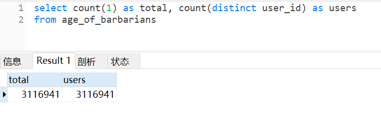
58 |
59 | 其中 PU 为 60,988 人, 占比 1.96 %
60 |
61 | >PU ( Paying Users):付费用户总量
62 |
63 | 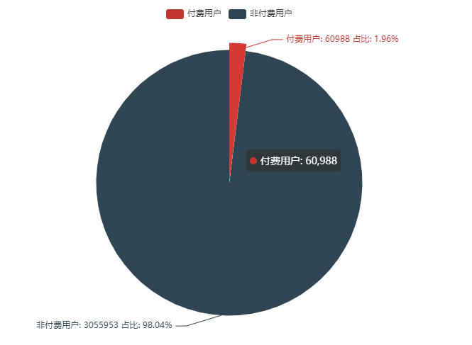
64 |
65 | DNU 的情况如下图,可以看到有两个注册高峰,应该是这款游戏做了什么活动引流产生。
66 |
67 | >DNU(Daily New Users): 每日游戏中的新登入用户数量,即每日新用户数。
68 |
69 | 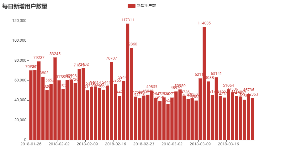
70 |
71 | 每小时注册的用户情况如下,可以看到新用户的注册高峰是在晚间的 21 点。
72 |
73 | 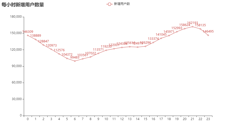
74 |
75 | ## 3.2 用户活跃度
76 |
77 | 从平均在线时间来看,付费用户的平均在线时间高达 2 个小时,远大于整体的平均在线时间。
78 |
79 | 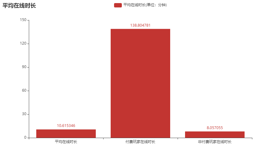
80 |
81 | ## 3.3 用户消费情况
82 |
83 | APA(Active Payment Account):活跃付费用户数。
84 |
85 | ARPU(Average Revenue Per User) :平均每用户收入。
86 |
87 | ARPPU (Average Revenue Per Paying User): 平均每付费用户收入。
88 |
89 | PUR(Pay User Rate):付费比率,可通过 APA/AU 计算得出。
90 |
91 | ```sql
92 | -- APA(Active Payment Account):活跃付费用户数。
93 | select count(1) as APA from age_of_barbarians where pay_price > 0 and avg_online_minutes > 0; -- 60987
94 |
95 | -- ARPU(Average Revenue Per User) :平均每用户收入。
96 | select sum(pay_price)/sum(case when avg_online_minutes > 0 then 1 else 0 end) from age_of_barbarians; -- 0.582407
97 |
98 | -- ARPPU (Average Revenue Per Paying User): 平均每付费用户收入。
99 | select sum(pay_price)/sum(case when avg_online_minutes > 0 and pay_price > 0 then 1 else 0 end) from age_of_barbarians; -- 29.190265
100 |
101 | -- PUR(Pay User Rate):付费比率,可通过 APA/AU 计算得出。
102 | select sum(case when avg_online_minutes > 0 and pay_price > 0 then 1 else 0 end) / sum(case when avg_online_minutes > 0 then 1 else 0 end)
103 | from age_of_barbarians; -- 0.02
104 |
105 | -- 付费用户人数,付费总额,付费总次数,平均每人付费,平均每人付费次数,平均每次付费
106 | select count(1) as pu, -- 60988
107 | sum(pay_price) as sum_pay_price, -- 1780226.7
108 | avg(pay_price) as avg_pay_price, -- 29.189786
109 | sum(pay_count) as sum_pay_count, -- 193030
110 | avg(pay_count) as avg_pay_count, -- 3.165
111 | sum(pay_price) / sum(pay_count) as each_pay_price -- 9.222539
112 | from age_of_barbarians
113 | where pay_price > 0;
114 | ```
115 |
116 | 从上方的统计结果可以知道,这 6 万多的付费用户,一共消费了 178 万元,平均每人消费 29 元。
117 |
118 | 平均每用户收入 0.58 元,平均每付费用户收入 29.19 元,付费比率为 2% 。
119 |
120 | > 这个付费比率应该是比较低的,可以通过一些首冲活动来提高新用户的付费意愿。
121 |
122 | 
123 |
124 |
125 |
126 | ## 3.4 用户游戏情况
127 |
128 | 从胜率和场次来看,氪金确实可以让你变强,付费用户的平均胜率为 71.13 %,远大于非付费用户的 38.03 %,当然也是因为付费用户的平均游戏场次要远大于一般用户,毕竟越肝越强。
129 |
130 | 从游戏类型来看,PVE 的平均胜率达到 90.1 %,说明难度还是比较低的,游戏体验还是很好的,适合符合入门级难度设定。
131 |
132 | 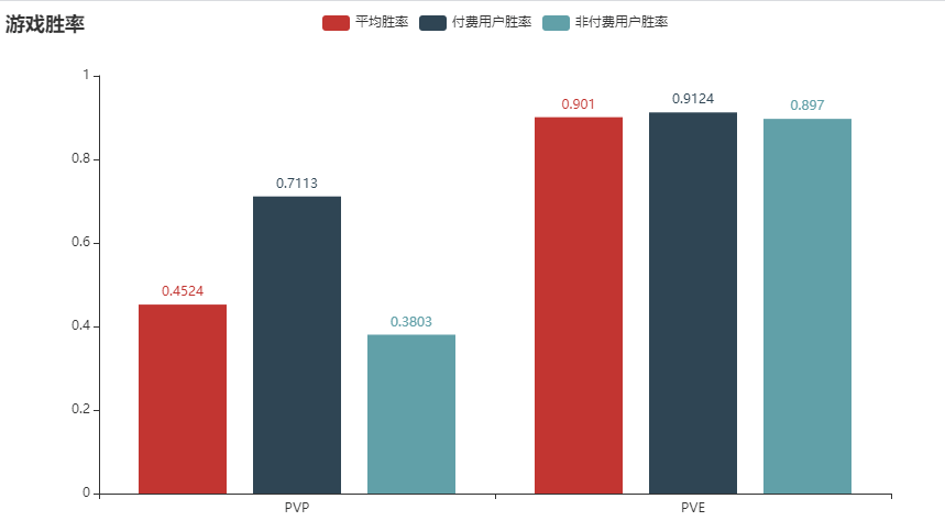
133 |
134 | 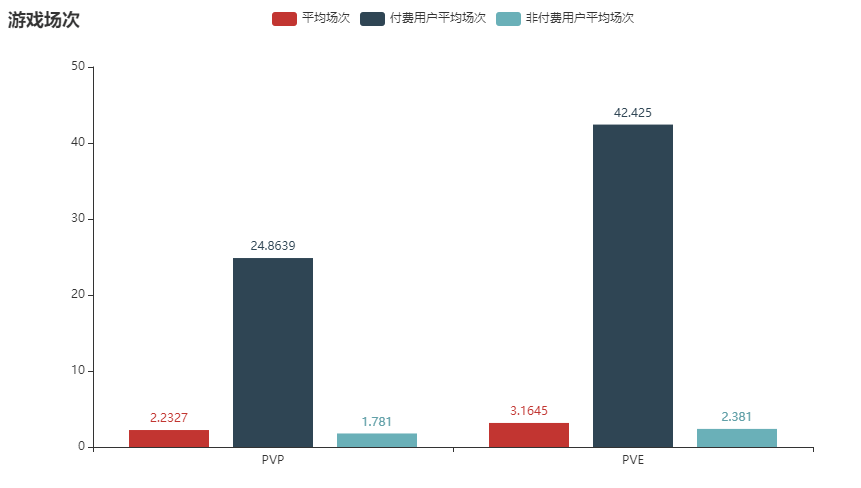
135 |
136 |
--------------------------------------------------------------------------------
/AmoyJob/2021厦门招聘数据分析.md:
--------------------------------------------------------------------------------
1 | [TOC]
2 |
3 | # 1. 数据集说明
4 |
5 | 这是一份来自厦门人才网的企业招聘数据,采集日期为 2021-01-14,总计 100,077 条记录,大小为 122 M,包含 19 个字段。
6 |
7 | # 2. 数据处理
8 |
9 | ## 2.1 数据清洗
10 | 使用 pandas 对数据进行清洗,主要包括:去重、缺失值填充、格式化、计算冗余字段。
11 |
12 | ```python
13 | # 数据重复处理: 删除重复值
14 | # print(data[data.duplicated()])
15 | data.drop_duplicates(inplace=True)
16 | data.reset_index(drop=True, inplace=True)
17 |
18 | # 缺失值查看、处理:
19 | data.isnull().sum()
20 |
21 | # 招聘人数处理:缺失值填 1 ,一般是一人; 若干人当成 3人
22 | data['num'].unique()
23 | data['num'].fillna(1, inplace=True)
24 | data['num'].replace('若干', 3, inplace=True)
25 |
26 | # 年龄要求:缺失值填 无限;格式化
27 | data['age'].unique()
28 | data['age'].fillna('不限', inplace=True)
29 | data['age'] = data['age'].apply(lambda x: x.replace('岁至', '-').replace('岁', ''))
30 |
31 | # 语言要求: 忽视精通程度,格式化
32 | data['lang'].unique()
33 | data['lang'].fillna('不限', inplace=True)
34 | data['lang'] = data['lang'].apply(lambda x: x.split('水平')[0] )
35 | data['lang'].replace('其他', '不限', inplace=True)
36 |
37 | # 月薪: 格式化。根据一般经验取低值,比如 5000-6000, 取 5000
38 | data['salary'].unique()
39 | data['salary'] = data['salary'].apply(lambda x: x.replace('参考月薪: ', '') if '参考月薪: ' in str(x) else x)
40 | data['salary'] = data['salary'].apply(lambda x: x.split('-', 1)[0] if '-' in str(x) else x )
41 | data['salary'].fillna('0', inplace=True)
42 |
43 | # 其它岗位说明:缺失值填无
44 | data.fillna('其他', inplace=True)
45 |
46 | # 工作年限格式化
47 | def jobage_clean(x):
48 | if x in ['应届生', '不限']:
49 | return x
50 | elif re.findall('\d+年', x):
51 | return re.findall('(\d+)年', x)[0]
52 | elif '年' in x:
53 | x = re.findall('\S{1,2}年', x)[0]
54 | x = re.sub('厂|验|年|,', '', x)
55 | digit_map = {
56 | '一': 1, '二': 2, '三': 3, '四': 4, '五': 5, '六': 6, '七': 7, '八': 8, '九': 9, '十':10,
57 | '十一': 11, '十二': 12, '十三': 13, '十四': 14, '十五': 15, '十六': 16, '两':2
58 | }
59 | return digit_map.get(x, x)
60 | return '其它工作经验'
61 |
62 | data['jobage'].unique()
63 | data['jobage'] = data['jobage'].apply(jobage_clean)
64 |
65 | # 性别格式化
66 | data['sex'].unique()
67 | data['sex'].replace('无', '不限', inplace=True)
68 |
69 | # 工作类型格式化
70 | data['job_type'].unique()
71 | data['job_type'].replace('毕业生见习', '实习', inplace=True)
72 |
73 | # 学历格式化
74 | data['education'].unique()
75 | data['education'] = data['education'].apply(lambda x: x[:2])
76 |
77 | # 公司类型 格式化
78 | def company_type_clean(x):
79 | if len(x) > 100 or '其他' in x:
80 | return '其他'
81 | elif re.findall('私营|民营', x):
82 | return '民营/私营'
83 | elif re.findall('外资|外企代表处', x):
84 | return '外资'
85 | elif re.findall('合资', x):
86 | return '合资'
87 | return x
88 |
89 | data['company_type'].unique()
90 | data['company_type'] = data['company_type'].apply(company_type_clean)
91 |
92 | # 行业 格式化。多个行业,取第一个并简单归类
93 | def industry_clean(x):
94 | if len(x) > 100 or '其他' in x:
95 | return '其他'
96 | industry_map = {
97 | 'IT互联网': '互联网|计算机|网络游戏', '房地产': '房地产', '电子技术': '电子技术', '建筑': '建筑|装潢',
98 | '教育培训': '教育|培训', '批发零售': '批发|零售', '金融': '金融|银行|保险', '住宿餐饮': '餐饮|酒店|食品',
99 | '农林牧渔': '农|林|牧|渔', '影视文娱': '影视|媒体|艺术|广告|公关|办公|娱乐', '医疗保健': '医疗|美容|制药',
100 | '物流运输': '物流|运输', '电信通信': '电信|通信', '生活服务': '人力|中介'
101 | }
102 | for industry, keyword in industry_map.items():
103 | if re.findall(keyword, x):
104 | return industry
105 | return x.split('、')[0].replace('/', '')
106 |
107 | data['industry'].unique()
108 | data['industry'] = data['industry'].apply(industry_clean)
109 |
110 | # 工作时间格式化
111 | data['worktime'].unique()
112 | data['worktime_day'] = data['worktime'].apply(lambda x: x.split('小时')[0] if '小时' in x else 0)
113 | data['worktime_week'] = data['worktime'].apply(lambda x: re.findall('\S*周', x)[0] if '周' in x else 0)
114 |
115 | # 从工作要求中正则解析出:技能要求
116 | data['skill'] = data['require'].apply(lambda x: '、'.join(re.findall('[a-zA-Z]+', x)))
117 | ```
118 |
119 | ## 2.2 数据导入
120 | 将清洗后的数据导入到 hive
121 |
122 | ```sql
123 | CREATE TABLE `job`(
124 | `position` string COMMENT '职位',
125 | `num` string COMMENT '招聘人数',
126 | `company` string COMMENT '公司',
127 | `job_type` string COMMENT '职位类型',
128 | `jobage` string COMMENT '工作年限',
129 | `lang` string COMMENT '语言',
130 | `age` string COMMENT '年龄',
131 | `sex` string COMMENT '性别',
132 | `education` string COMMENT '学历',
133 | `workplace` string COMMENT '工作地点',
134 | `worktime` string COMMENT '工作时间',
135 | `salary` string COMMENT '薪资',
136 | `welfare` string COMMENT '福利待遇',
137 | `hr` string COMMENT '招聘人',
138 | `phone` string COMMENT '联系电话',
139 | `address` string COMMENT '联系地址',
140 | `company_type` string COMMENT '公司类型',
141 | `industry` string COMMENT '行业',
142 | `require` string COMMENT '岗位要求',
143 | `worktime_day` string COMMENT '工作时间(每天)',
144 | `worktime_week` string COMMENT '工作时间(每周)',
145 | `skill` string COMMENT '技能要求'
146 | )
147 | row format delimited
148 | fields terminated by ','
149 | lines terminated by '\n';
150 |
151 | -- 加载数据
152 | LOAD DATA INPATH '/tmp/job.csv' OVERWRITE INTO TABLE job;
153 | ```
154 |
155 | 通过 hue 查看一下数据
156 |
157 | 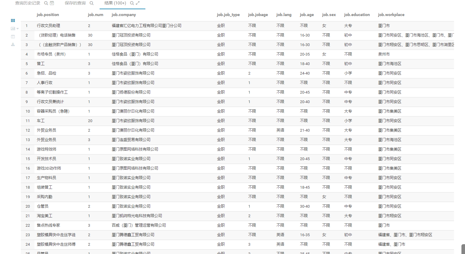
158 |
159 | 然后随便点击一条数据,可以看到,经过前面的清洗,现在的字段已经很好看了,后续的分析也会变得简单许多。
160 |
161 | 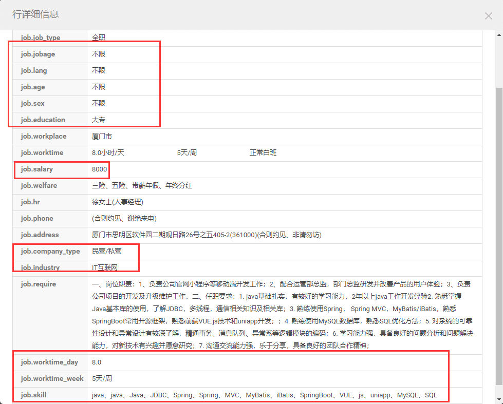
162 |
163 | # 3. 数据分析可视化
164 |
165 | ## 3.1 整体情况(招聘企业数、岗位数、招聘人数、平均工资)
166 |
167 | 招聘企业数为 10093,在招的岗位数有 10 万个,总的招聘人数为 26 万人,平均工资为 5576 元。
168 |
169 | 
170 |
171 | ## 3.2 企业主题
172 |
173 | ### 行业情况
174 |
175 | 各行业的招聘人数排行 TOP10 如下,可以看到 IT 互联网最缺人。
176 |
177 | > 由于数据源的行业分类比较草率,很多公司的分类其实并不是很准确,所以这个结果仅供参考。
178 |
179 | 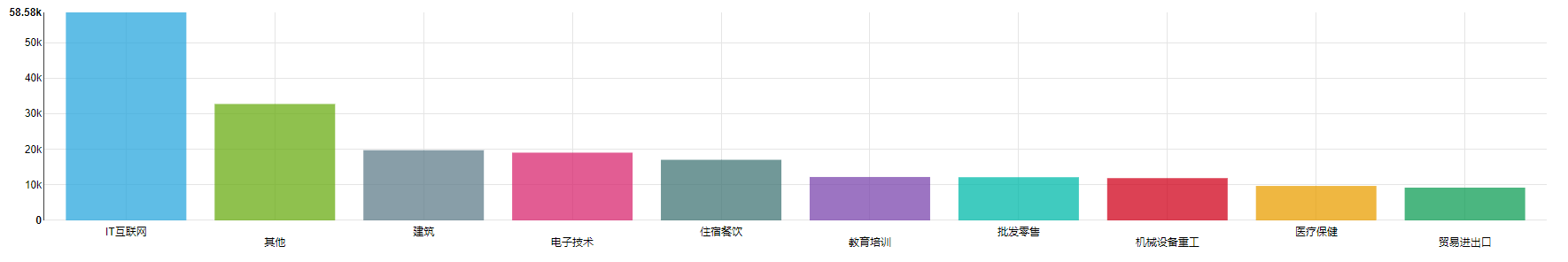
180 |
181 | ### 公司类型
182 |
183 | 从招聘人数上来看,民营/私营的企业最缺人,事业单位的招聘人数最少。
184 |
185 | 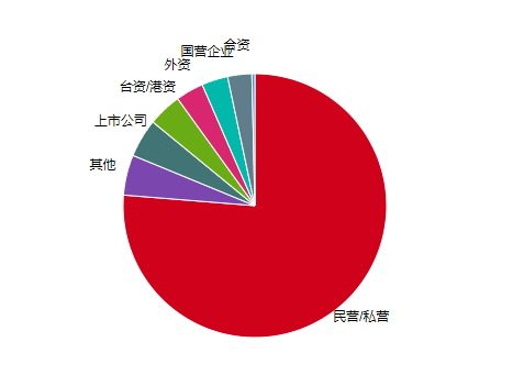
186 |
187 | 从薪资待遇来看,上市公司平均薪资最高 5983 元,而台资/港资则最少 4723 元。
188 |
189 | 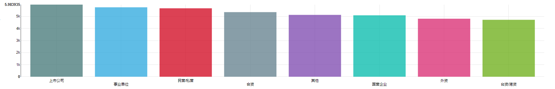
190 |
191 | ### 最缺人的公司 TOP
192 |
193 | 最缺人的公司果然是人力资源公司,总的要招聘 2000 多个人,从详情来看,大多是代招一些流水线岗位。
194 |
195 | 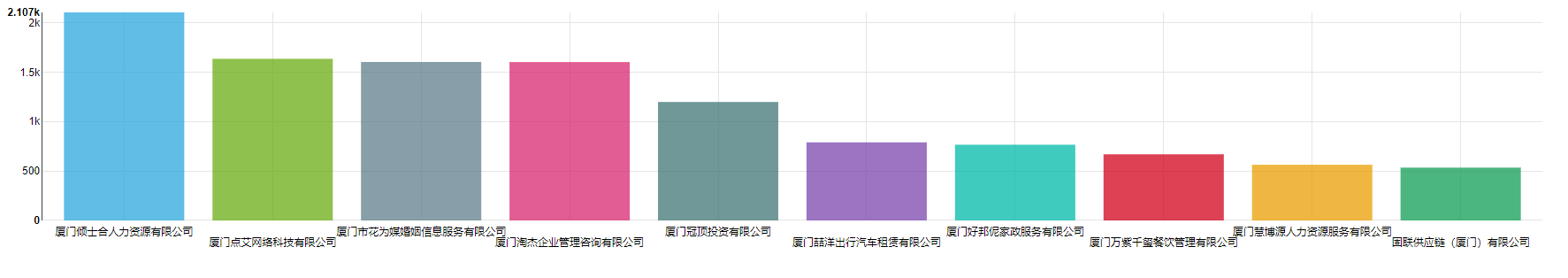
196 |
197 | 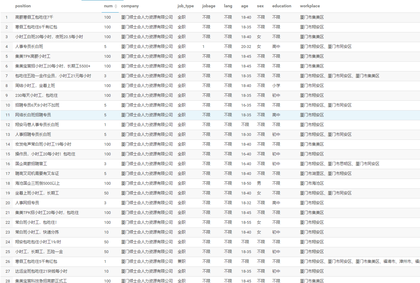
198 |
199 | ### 平均薪资最高的公司 TOP
200 |
201 | 平均薪资最高的公司 **上海美莱投资管理有限公司** 居然有 5 万多,一惊之下,查了下这家公司的招聘信息,可以看到该公司在招的都是高级岗,比如 集团片区总经理(副总裁级),这个岗位人数达到 20 人,岗位月薪 6 万,所以直接把平均薪资拉高了,而且工作地点也不在厦门。
202 |
203 | > 由以上分析,可以得知根据招聘信息来推算平均工资,其实误差还是比较大的,仅供参考。
204 |
205 |
206 | 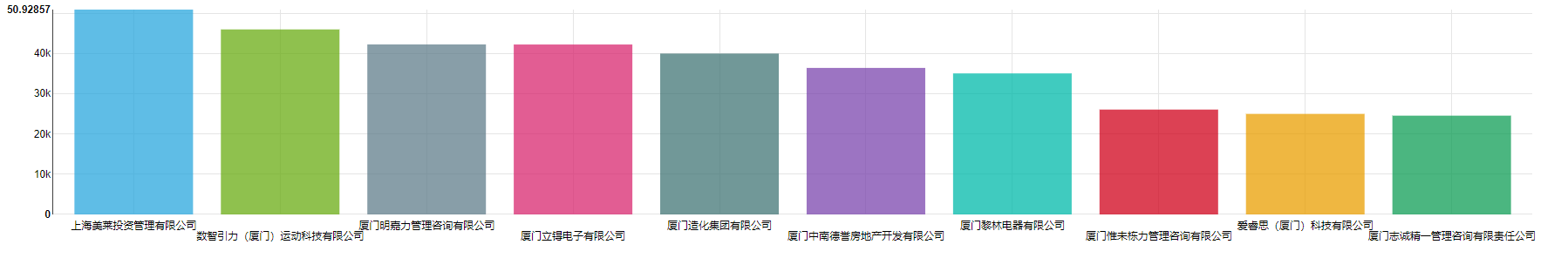
207 |
208 | 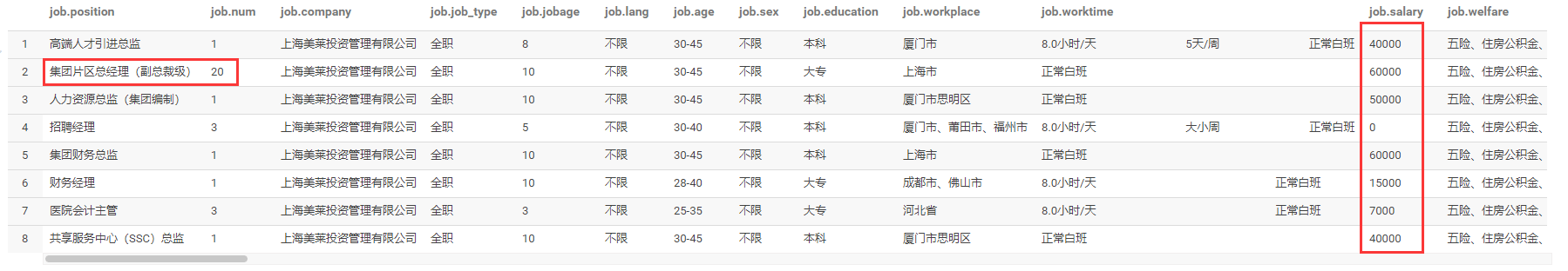
209 |
210 | ### 工作时间
211 |
212 | 从每天工作时间占比 TOP 10 来看,大部分职位是 8 小时工作制,紧接着是 7.5 小时 和 7小时。还有一些每天上班时间要达到 12 小时,主要是 保安 和 普工 这类岗位。
213 |
214 | 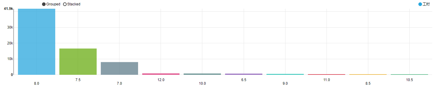
215 |
216 | 每周工作天数占比来看,大部分还是 5天/周的双休制,不过 6 天/周、5.5 天/周、大小周的占比也是相当高。
217 |
218 | 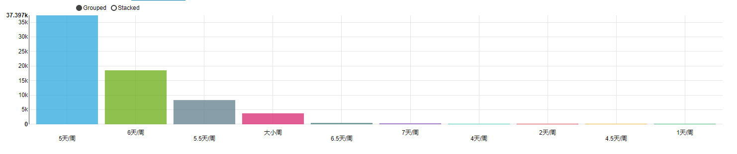
219 |
220 | ### 工作地点
221 |
222 | 岗位数量的分布图,颜色越深代表数量越大,可以看到思明区的工作机会最多,其次是湖里、集美、同安、海沧、翔安。
223 |
224 | 
225 |
226 |
227 | ### 福利词云
228 |
229 | 
230 |
231 | ## 3.3 岗位主题
232 |
233 | ### 工作经验要求
234 |
235 | 从岗位数量来看,一半以上的岗位对工作经验是没有要求的。在有经验要求的岗位里面,1-3 年工作经验的市场需求是最大的。
236 |
237 | 
238 |
239 | 从平均工资来看,符合一般认知。工作经验越多,工资也越高,10 年以上的工作经验最高,平均工资为 13666 元;应届生最低,平均工资为 4587 元。
240 |
241 | 
242 |
243 | ### 学历要求
244 |
245 | 从岗位数来看,大部分岗位的学历要求为大专以上,换言之,在厦门,只要大专学历,就很好找工作了。
246 |
247 | 
248 |
249 | 从平均工资来看,学历越高,工资越高,这也符合一般认知,谁说的读书无用论来着。
250 |
251 | 有趣的是,不限学历的平均工资居然排在了高中的前面,或许这是 九年义务教育的普及与大学扩招带来的内卷,在招聘方眼里,只有两大类:上过大学和没上过大学,从而导致大专以下的学历优势不再明显。
252 |
253 | 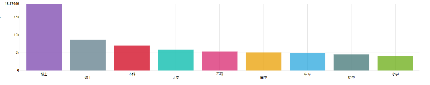
254 |
255 | ### 性别要求
256 |
257 | 岗位数方面,有 6974 个岗位,明确要求性别为 女,仅有 575 个岗位要求性别为 男。
258 |
259 | 平均工资方面,女性岗位的平均工资为 5246 元,而男性则为 4454 元。
260 |
261 | 虽然绝大多数岗位都是不限制性别的,但是,不管是从岗位数量还是平均工资来看,在厦门,女性比男性似乎有更多的职场优势。
262 |
263 | 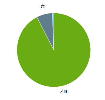
264 |
265 | 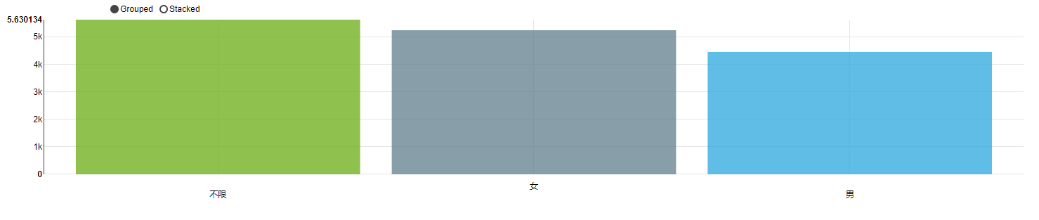
266 |
267 | ### 年龄要求
268 |
269 | 年龄要求一般有一个上限和下限,现在只考虑上限,并通过上限来分析一下,所谓 35 岁的危机。
270 |
271 | 岗位数量上来看,大多数岗位是不限制年龄的,有限制年龄的岗位里面,35 岁以后的岗位有 7327 个,35 岁及以下的岗位有 32967 个,
272 |
273 | 岗位数量上确实少了非常多。
274 |
275 | 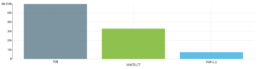
276 |
277 | 从平均工资来看,35 岁以后的岗位 5095 元,35岁及以下的岗位 5489 元,薪资上少了 394 元。
278 |
279 | 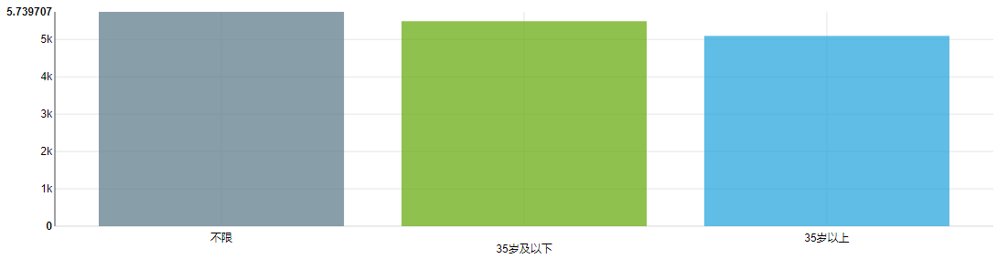
280 |
281 | 所以,单单考虑岗位的年龄上限,那么 35 岁以后的市场需求确实会变少。
282 |
283 | 但是,为什么会是这样的情况呢,个人认为,有可能是 35 岁 以后的职场人士,沉淀更多,进入了更高级的职位,更稳定,所以流动性比较低,自然市场上空出来的需求也会变少了,更不用说还有一部分人变成了创业者。
284 |
285 | ### 语言要求
286 |
287 | 大部分岗位没有语言要求,在有语言要求的岗位里面,英语妥妥的是第一位。
288 |
289 | 值得一提的是,这边还有个闽南语,因为厦门地处闽南,本地的方言就是闽南语。
290 |
291 | 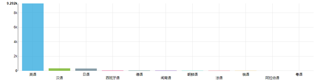
292 |
293 | ### 编程语言要求
294 |
295 | 比较流行的编程语言里面,被岗位要求提到的次数排行如下 。可以看到,C 语言被提及的次数远大于其它语言,不亏是排行榜常年第一的语言。比较惊讶的是如今大火的 python 被提及的次数却很少,排在倒二。
296 |
297 | 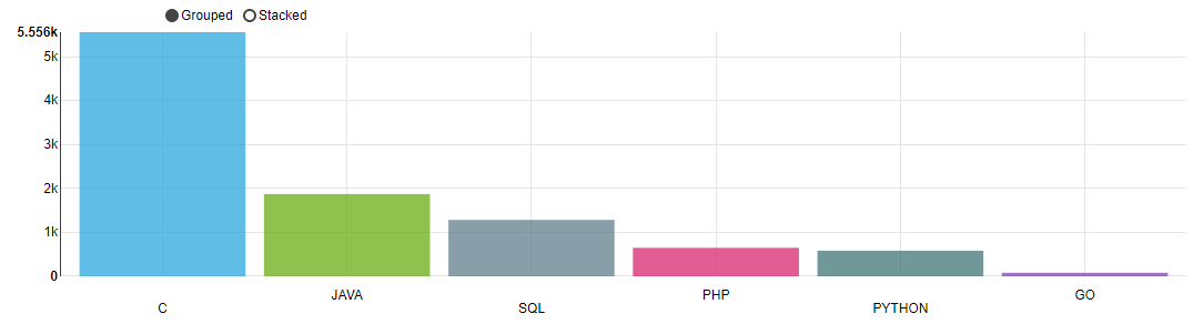
298 |
299 | 这些语言的平均薪资排行,Python 最高为 8732 元。
300 |
301 | 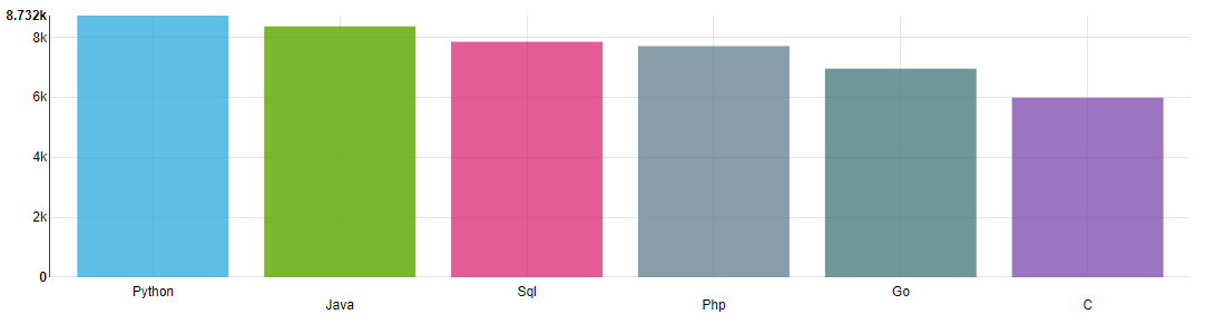
302 |
303 | # 4. 模型预测
304 |
305 | 我们知道影响工资待遇的因素有很多:学历、工作经验、年龄、招聘方的紧急程度、技能的稀缺性、行业的发展情况。。。等等。
306 |
307 | 所以,为了简化模型,就学历和工作经验两个维度进行模型训练,尝试做工资预测。
308 |
309 | ```python
310 | import pandas as pd
311 | from sklearn.linear_model import LinearRegression
312 |
313 | def predict(data, education):
314 | """
315 | :param data: 训练数据
316 | :param education: 学历
317 | :return: 模型得分,10年工作预测
318 | """
319 | train = data[data['education'] == education].to_numpy()
320 | x = train[:, 1:2]
321 | y = train[:, 2]
322 |
323 | # model 训练
324 | model = LinearRegression()
325 | model.fit(x, y)
326 |
327 | # model 预测
328 | X = [[i] for i in range(11)]
329 | return model.score(x, y), model.predict(X)
330 |
331 | education_list = ['小学', '初中', '中专', '高中', '大专', '本科', '硕士', '博士']
332 | data = pd.read_csv('train.csv')
333 |
334 | scores, values = [], []
335 | for education in education_list:
336 | score, y = predict(data, education)
337 | scores.append(score)
338 | values.append(y)
339 |
340 | result = pd.DataFrame()
341 | result['学历'] = education_list
342 | result['模型得分'] = scores
343 | result['(1年经验)平均工资'] = [value[1] for value in values]
344 | result['(3年经验)平均工资'] = [value[2] for value in values]
345 | result['(5年经验)平均工资'] = [value[4] for value in values]
346 | result['(10年经验)平均工资'] = [value[10] for value in values]
347 | print(result)
348 | ```
349 |
350 | 使用线性回归模型分学历进行预测,预测结果如下。
351 |
352 | 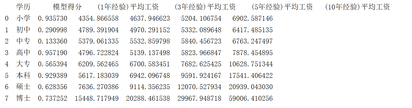
353 |
354 |
355 |
356 |
--------------------------------------------------------------------------------
/AmoyJob/analyse.hql:
--------------------------------------------------------------------------------
1 | -- 启用本地模式
2 | set hive.exec.mode.local.auto=true;
3 | set hive.exec.mode.local.auto.inputbytes.max=52428800;
4 | set hive.exec.mode.local.auto.input.files.max=10;
5 |
6 | -- 整体情况(招聘企业数、岗位数、招聘人数、平均薪资)
7 | select count(distinct company) as `企业数`,
8 | count(1) as `岗位数`,
9 | sum(num) as `招聘人数`,
10 | sum(salary * num) / sum(case when salary > 0 then num else 0 end) as `平均工资`
11 | from job;
12 |
13 | -- 最缺人的行业 TOP 10
14 | select industry, sum(num) as workers
15 | from job
16 | group by industry
17 | order by workers desc
18 | limit 10;
19 |
20 | -- 公司类型情况
21 | select company_type,
22 | sum(num) as workers,
23 | sum(salary * num) / sum(case when salary > 0 then num else 0 end) as avg_salary
24 | from job
25 | group by company_type;
26 |
27 | -- 最缺人的公司 TOP 10
28 | select company, sum(num) as workers
29 | from job
30 | group by company
31 | order by workers desc
32 | limit 10;
33 |
34 | -- 平均薪资最高的公司 TOP 10
35 | select company, sum(salary * num) / sum(num) as avg_salary
36 | from job
37 | where salary > 0
38 | group by company
39 | order by avg_salary desc
40 | limit 10;
41 |
42 | -- 工作时间
43 | select worktime_day, count(1) cn
44 | from job
45 | where worktime_day < 24
46 | and worktime_day > 0
47 | group by worktime_day
48 | order by cn desc
49 | limit 10;
50 |
51 | select worktime_week, count(1) cn
52 | from job
53 | where worktime_week <> '0'
54 | group by worktime_week
55 | order by cn desc
56 | limit 10;
57 |
58 | -- 工作地点(导出为 workplace.csv)
59 | select workplace, count(1) as cn
60 | from(
61 | select regexp_replace(b.workplace, '厦门市', '') as workplace
62 | from job
63 | lateral view explode(split(workplace, '、|,')) b AS workplace
64 | ) as a
65 | where workplace rlike '湖里|海沧|思明|集美|同安|翔安'
66 | group by workplace;
67 |
68 | -- 福利词云(导出为 welfare.csv)
69 | select fl, count(1)
70 | from(
71 | select b.fl
72 | from job
73 | lateral view explode(split(welfare,'、')) b AS fl
74 | ) as a
75 | where fl <> '其他'
76 | group by fl;
77 |
78 | -- 工作经验
79 | select case when jobage in ('其它工作经验', '不限', '应届生') then jobage
80 | when jobage between 1 and 3 then '1-3 年'
81 | when jobage between 3 and 5 then '3-5 年'
82 | when jobage between 5 and 10 then '5-10 年'
83 | when jobage >= 10 then '10 年以上'
84 | else jobage end as jobage,
85 | count(1) as `岗位数量`,
86 | sum(salary * num) / sum(case when salary > 0 then num else 0 end) as `平均工资`
87 | from job
88 | group by case when jobage in ('其它工作经验', '不限', '应届生') then jobage
89 | when jobage between 1 and 3 then '1-3 年'
90 | when jobage between 3 and 5 then '3-5 年'
91 | when jobage between 5 and 10 then '5-10 年'
92 | when jobage >= 10 then '10 年以上'
93 | else jobage end;
94 |
95 | -- 学历
96 | select education,
97 | count(1) as `岗位数量`,
98 | sum(salary * num) / sum(case when salary > 0 then num else 0 end) as `平均工资`
99 | from job
100 | group by education;
101 |
102 | -- 性别
103 | select sex,
104 | count(1) as `岗位数量`,
105 | sum(salary * num) / sum(case when salary > 0 then num else 0 end) as `平均工资`
106 | from job
107 | group by sex;
108 |
109 | -- 年龄
110 | select case when age = '不限' then '不限'
111 | when split(age, '-')[1] >= 35 then '35岁及以下'
112 | else '35岁以上' end as age,
113 | count(1) as `岗位数量`,
114 | sum(salary * num) / sum(case when salary > 0 then num else 0 end) as `平均工资`
115 | from job
116 | group by case when age = '不限' then '不限'
117 | when split(age, '-')[1] >= 35 then '35岁及以下'
118 | else '35岁以上' end
119 | -- 语言
120 | select lang, count(1) as cn
121 | from job
122 | where lang <> '不限'
123 | group by lang
124 | order by cn desc;
125 |
126 | -- 技能
127 | select sk, count(1) as cn
128 | from(
129 | select upper(b.sk) as sk
130 | from job
131 | lateral view explode(split(skill,'、')) b AS sk
132 | ) as a
133 | where sk in ('C', 'JAVA', 'PYTHON', 'PHP', 'SQL', 'GO')
134 | group by sk
135 | order by cn desc;
136 |
137 | select 'Java' as lang, sum(salary * num) / sum(case when salary > 0 then num else 0 end) as `平均工资`
138 | from job
139 | where lower(skill) rlike 'java'
140 | union all
141 | select 'Python' as lang, sum(salary * num) / sum(case when salary > 0 then num else 0 end) as `平均工资`
142 | from job
143 | where lower(skill) rlike 'python'
144 | union all
145 | select 'Php' as lang, sum(salary * num) / sum(case when salary > 0 then num else 0 end) as `平均工资`
146 | from job
147 | where lower(skill) rlike 'php'
148 | union all
149 | select 'Sql' as lang, sum(salary * num) / sum(case when salary > 0 then num else 0 end) as `平均工资`
150 | from job
151 | where lower(skill) rlike 'sql'
152 | union all
153 | select 'Go' as lang, sum(salary * num) / sum(case when salary > 0 then num else 0 end) as `平均工资`
154 | from job
155 | where lower(skill) rlike 'go'
156 | union all
157 | select 'C' as lang, sum(salary * num) / sum(case when salary > 0 then num else 0 end) as `平均工资`
158 | from job
159 | where lower(skill) rlike 'c';
160 |
161 | -- 模型训练(导出为 train.csv)
162 | select education, case when jobage = '应届生' then 0 else jobage end as jobage, avg(salary) as avg_salary
163 | from job
164 | where salary > '0'
165 | and education <> '不限'
166 | and jobage not in ('不限', '其它工作经验')
167 | group by education, case when jobage = '应届生' then 0 else jobage end
--------------------------------------------------------------------------------
/AmoyJob/etl.py:
--------------------------------------------------------------------------------
1 | #!/usr/bin/env python3
2 | # -*- coding: utf-8 -*-
3 | # @Time : 2021/1/21 21:06
4 | # @Author : way
5 | # @Site :
6 | # @Describe: 数据处理
7 |
8 | import re
9 | import pandas as pd
10 |
11 | path = 'job.csv'
12 | data = pd.read_csv(path, header=None)
13 | data.columns = [
14 | 'position', 'num', 'company', 'job_type', 'jobage', 'lang', 'age', 'sex', 'education', 'workplace', 'worktime',
15 | 'salary', 'welfare', 'hr', 'phone', 'address', 'company_type', 'industry', 'require'
16 | ]
17 |
18 | ############################################### 数据清洗 #############################################################
19 | # 数据重复处理: 删除重复值
20 | # print(data[data.duplicated()])
21 | data.drop_duplicates(inplace=True)
22 | data.reset_index(drop=True, inplace=True)
23 |
24 | # 缺失值查看、处理:
25 | data.isnull().sum()
26 |
27 | # 招聘人数处理:缺失值填 1 ,一般是一人; 若干人当成 3人
28 | data['num'].unique()
29 | data['num'].fillna(1, inplace=True)
30 | data['num'].replace('若干', 3, inplace=True)
31 |
32 | # 年龄要求:缺失值填 无限;格式化
33 | data['age'].unique()
34 | data['age'].fillna('不限', inplace=True)
35 | data['age'] = data['age'].apply(lambda x: x.replace('岁至', '-').replace('岁', ''))
36 |
37 | # 语言要求: 忽视精通程度,格式化
38 | data['lang'].unique()
39 | data['lang'].fillna('不限', inplace=True)
40 | data['lang'] = data['lang'].apply(lambda x: x.split('水平')[0])
41 | data['lang'].replace('其他', '不限', inplace=True)
42 |
43 | # 月薪: 格式化。根据一般经验取低值,比如 5000-6000, 取 5000
44 | data['salary'].unique()
45 | data['salary'] = data['salary'].apply(lambda x: x.replace('参考月薪: ', '') if '参考月薪: ' in str(x) else x)
46 | data['salary'] = data['salary'].apply(lambda x: x.split('-', 1)[0] if '-' in str(x) else x)
47 | data['salary'].fillna('0', inplace=True)
48 |
49 | # 其它岗位说明:缺失值填无
50 | data.fillna('其他', inplace=True)
51 |
52 |
53 | # 工作年限格式化
54 | def jobage_clean(x):
55 | if x in ['应届生', '不限']:
56 | return x
57 | elif re.findall('\d+年', x):
58 | return re.findall('(\d+)年', x)[0]
59 | elif '年' in x:
60 | x = re.findall('\S{1,2}年', x)[0]
61 | x = re.sub('厂|验|年|,', '', x)
62 | digit_map = {
63 | '一': 1, '二': 2, '三': 3, '四': 4, '五': 5, '六': 6, '七': 7, '八': 8, '九': 9, '十': 10,
64 | '十一': 11, '十二': 12, '十三': 13, '十四': 14, '十五': 15, '十六': 16, '两': 2
65 | }
66 | return digit_map.get(x, x)
67 | return '其它工作经验'
68 |
69 |
70 | data['jobage'].unique()
71 | data['jobage'] = data['jobage'].apply(jobage_clean)
72 |
73 | # 性别格式化
74 | data['sex'].unique()
75 | data['sex'].replace('无', '不限', inplace=True)
76 |
77 | # 工作类型格式
78 | data['job_type'].unique()
79 | data['job_type'].replace('毕业生见习', '实习', inplace=True)
80 |
81 | # 学历格式化
82 | data['education'].unique()
83 | data['education'] = data['education'].apply(lambda x: x[:2])
84 |
85 |
86 | # 公司类型 格式化
87 | def company_type_clean(x):
88 | if len(x) > 100 or '其他' in x:
89 | return '其他'
90 | elif re.findall('私营|民营', x):
91 | return '民营/私营'
92 | elif re.findall('外资|外企代表处', x):
93 | return '外资'
94 | elif re.findall('合资', x):
95 | return '合资'
96 | return x
97 |
98 |
99 | data['company_type'].unique()
100 | data['company_type'] = data['company_type'].apply(company_type_clean)
101 |
102 |
103 | # 行业 格式化。多个行业,取第一个并简单归类
104 | def industry_clean(x):
105 | if len(x) > 100 or '其他' in x:
106 | return '其他'
107 | industry_map = {
108 | 'IT互联网': '互联网|计算机|网络游戏', '房地产': '房地产', '电子技术': '电子技术', '建筑': '建筑|装潢',
109 | '教育培训': '教育|培训', '批发零售': '批发|零售', '金融': '金融|银行|保险', '住宿餐饮': '餐饮|酒店|食品',
110 | '农林牧渔': '农|林|牧|渔', '影视文娱': '影视|媒体|艺术|广告|公关|办公|娱乐', '医疗保健': '医疗|美容|制药',
111 | '物流运输': '物流|运输', '电信通信': '电信|通信', '生活服务': '人力|中介'
112 | }
113 | for industry, keyword in industry_map.items():
114 | if re.findall(keyword, x):
115 | return industry
116 | return x.split('、')[0].replace('/', '')
117 |
118 |
119 | data['industry'].unique()
120 | data['industry'] = data['industry'].apply(industry_clean)
121 |
122 | # 工作时间格式化
123 | data['worktime'].unique()
124 | data['worktime_day'] = data['worktime'].apply(lambda x: x.split('小时')[0] if '小时' in x else 0)
125 | data['worktime_week'] = data['worktime'].apply(lambda x: re.findall('\S*周', x)[0] if '周' in x else 0)
126 |
127 | # 从工作要求中正则解析出:技能要求
128 | data['skill'] = data['require'].apply(lambda x: '、'.join(re.findall('[a-zA-Z]+', x)))
129 |
130 | ################################################## 数据保存 #########################################################
131 | # 查看保存的数据
132 | print(data.info)
133 |
134 | # 保存清洗后的数据 job_clean.csv
135 | data.to_csv('job_clean.csv', index=False, header=None, encoding='utf-8-sig')
136 |
137 | # 取学历、年龄段、薪资作预测,保存为 train.csv
138 | train_data = data[['education', 'jobage', 'salary']][data['job_type']=='全职']
139 | train_data['jobage'] = train_data['jobage'].apply(lambda x: x if x not in ['应届生', '不限', '其它工作经验'] else '0')
140 | train_data['salary'] = train_data['salary'].astype('int')
141 | train_data = train_data[(train_data['salary'] > 1000)]
142 | train_data = train_data.to_csv('train.csv', index=False, encoding='utf-8-sig')
143 |
--------------------------------------------------------------------------------
/AmoyJob/table.sql:
--------------------------------------------------------------------------------
1 | -- 建表
2 | CREATE TABLE `job`(
3 | `position` string COMMENT '职位',
4 | `num` string COMMENT '招聘人数',
5 | `company` string COMMENT '公司',
6 | `job_type` string COMMENT '职位类型',
7 | `jobage` string COMMENT '工作年限',
8 | `lang` string COMMENT '语言',
9 | `age` string COMMENT '年龄',
10 | `sex` string COMMENT '性别',
11 | `education` string COMMENT '学历',
12 | `workplace` string COMMENT '工作地点',
13 | `worktime` string COMMENT '工作时间',
14 | `salary` string COMMENT '薪资',
15 | `welfare` string COMMENT '福利待遇',
16 | `hr` string COMMENT '招聘人',
17 | `phone` string COMMENT '联系电话',
18 | `address` string COMMENT '联系地址',
19 | `company_type` string COMMENT '公司类型',
20 | `industry` string COMMENT '行业',
21 | `require` string COMMENT '岗位要求',
22 | `worktime_day` string COMMENT '工作时间(每天)',
23 | `worktime_week` string COMMENT '工作时间(每周)',
24 | `skill` string COMMENT '技能要求'
25 | )
26 | row format delimited
27 | fields terminated by ','
28 | lines terminated by '\n';
29 |
30 | -- 加载数据
31 | LOAD DATA INPATH '/tmp/job_clean.csv' OVERWRITE INTO TABLE job;
32 |
--------------------------------------------------------------------------------
/AmoyJob/train.py:
--------------------------------------------------------------------------------
1 | #!/usr/bin/env python3
2 | # -*- coding: utf-8 -*-
3 | # @Time : 2021/1/23 13:16
4 | # @Author : way
5 | # @Site :
6 | # @Describe: 模型预测
7 |
8 | import pandas as pd
9 | from sklearn.linear_model import LinearRegression
10 |
11 | def predict(data, education):
12 | """
13 | :param data: 训练数据
14 | :param education: 学历
15 | :return: 模型得分,10年工资预测
16 | """
17 | train = data[data['education'] == education].to_numpy()
18 | x = train[:, 1:2]
19 | y = train[:, 2]
20 |
21 | # model 训练
22 | model = LinearRegression()
23 | model.fit(x, y)
24 |
25 | # model 预测
26 | X = [[i] for i in range(11)]
27 | return model.score(x, y), model.predict(X)
28 |
29 | education_list = ['小学', '初中', '中专', '高中', '大专', '本科', '硕士', '博士']
30 | data = pd.read_csv('train.csv')
31 |
32 | scores, values = [], []
33 | for education in education_list:
34 | score, y = predict(data, education)
35 | scores.append(score)
36 | values.append(y)
37 |
38 | result = pd.DataFrame()
39 | result['学历'] = education_list
40 | result['模型得分'] = scores
41 | result['(1年经验)平均工资'] = [value[1] for value in values]
42 | result['(3年经验)平均工资'] = [value[2] for value in values]
43 | result['(5年经验)平均工资'] = [value[4] for value in values]
44 | result['(10年经验)平均工资'] = [value[10] for value in values]
45 | print(result)
--------------------------------------------------------------------------------
/AmoyJob/visualize.py:
--------------------------------------------------------------------------------
1 | #!/usr/bin/env python3
2 | # -*- coding: utf-8 -*-
3 | # @Time : 2021/01/22 21:36
4 | # @Author : way
5 | # @Site :
6 | # @Describe: 数据可视化
7 |
8 | import os
9 | import pandas as pd
10 | from pyecharts import options as opts
11 | from pyecharts.charts import WordCloud, Map
12 | from pyecharts.globals import SymbolType
13 |
14 | # 福利词云
15 | data = pd.read_csv('welfare.csv')
16 |
17 | c = (
18 | WordCloud()
19 | .add("", data.values, word_size_range=[20, 100], shape=SymbolType.DIAMOND)
20 | .set_global_opts(title_opts=opts.TitleOpts())
21 | .render("wordcloud.html")
22 | )
23 | os.system("wordcloud.html")
24 |
25 | # 岗位分布
26 | data = pd.read_csv('workplace.csv')
27 |
28 | c1 = (
29 | Map()
30 | .add("岗位数", data.values, "厦门")
31 | .set_global_opts(
32 | title_opts=opts.TitleOpts(title="厦门岗位分布图"),
33 | visualmap_opts=opts.VisualMapOpts(max_=20000, min_=5000)
34 | )
35 | .render("workplace.html")
36 | )
37 | os.system("workplace.html")
38 |
--------------------------------------------------------------------------------
/LICENSE:
--------------------------------------------------------------------------------
1 | MIT License
2 |
3 | Copyright (c) 2020 Way
4 |
5 | Permission is hereby granted, free of charge, to any person obtaining a copy
6 | of this software and associated documentation files (the "Software"), to deal
7 | in the Software without restriction, including without limitation the rights
8 | to use, copy, modify, merge, publish, distribute, sublicense, and/or sell
9 | copies of the Software, and to permit persons to whom the Software is
10 | furnished to do so, subject to the following conditions:
11 |
12 | The above copyright notice and this permission notice shall be included in all
13 | copies or substantial portions of the Software.
14 |
15 | THE SOFTWARE IS PROVIDED "AS IS", WITHOUT WARRANTY OF ANY KIND, EXPRESS OR
16 | IMPLIED, INCLUDING BUT NOT LIMITED TO THE WARRANTIES OF MERCHANTABILITY,
17 | FITNESS FOR A PARTICULAR PURPOSE AND NONINFRINGEMENT. IN NO EVENT SHALL THE
18 | AUTHORS OR COPYRIGHT HOLDERS BE LIABLE FOR ANY CLAIM, DAMAGES OR OTHER
19 | LIABILITY, WHETHER IN AN ACTION OF CONTRACT, TORT OR OTHERWISE, ARISING FROM,
20 | OUT OF OR IN CONNECTION WITH THE SOFTWARE OR THE USE OR OTHER DEALINGS IN THE
21 | SOFTWARE.
22 |
--------------------------------------------------------------------------------
/README.md:
--------------------------------------------------------------------------------
1 | # bigdata_analyse
2 | 该 repo 是本人实践过的数据分析项目集合,每个项目都会包含一个友好的说明文档,用来阐述和展示整个开发流程,同时也会提供相关的数据集,以供下载练习。
3 |
4 | ## wish
5 |
6 | 采用不同的技术栈,通过对不同行业的数据集进行分析,期望达到以下目的:
7 |
8 | - 了解不同领域的业务分析指标
9 | - 深化数据处理、数据分析、数据可视化能力
10 | - 增加大数据批处理、流处理的实践经验
11 | - 增加数据挖掘的实践经验
12 |
13 | ## tip
14 |
15 | - 项目主要使用的编程语言是 python、sql、hql
16 | - .ipynb 可以用 jupyter notebook 打开,如何安装, 可以参考 [jupyter notebook](http://blog.turboway.top/article/jupyter/)
17 | >jupyter notebook 是一种网页交互形式的 python 编辑器,直接通过 pip 安装,也支持 markdown,很适合用来做数据分析可视化以及写文章、写示例代码等。
18 |
19 | ## list
20 |
21 | | 主题 | 处理方式 | 技术栈 | 数据集下载 |
22 | | ------------ | ------------ | ------------ | ------------ |
23 | | [1 亿条淘宝用户行为数据分析](https://github.com/TurboWay/bigdata_analyse/blob/main/UserBehaviorFromTaobao_Batch/用户行为数据分析.md) | 离线处理 | 清洗 hive + 分析 hive + 可视化 echarts | [阿里云](https://tianchi.aliyun.com/dataset/dataDetail?dataId=649&userId=1) 或者 [百度网盘](https://pan.baidu.com/s/15Ss-nDMA120EHhuwpzYm0g) 提取码:5ipq |
24 | | [1000 万条淘宝用户行为数据实时分析](https://github.com/TurboWay/bigdata_analyse/blob/main/UserBehaviorFromTaobao_Stream/用户行为数据实时分析.md) | 实时处理 | 数据源 kafka + 实时分析 flink + 可视化(es + kibana) | [百度网盘](https://pan.baidu.com/s/1CPD5jpmvOUvg1LETAVETGw) 提取码:m4mc|
25 | | [300 万条《野蛮时代》的玩家数据分析](https://github.com/TurboWay/bigdata_analyse/blob/main/AgeOfBarbarians/野蛮时代数据分析.md) | 离线处理 | 清洗 pandas + 分析 mysql + 可视化 pyecharts | [百度网盘](https://pan.baidu.com/s/1Mi5lvGDF405Nk8Y2BZDzdQ) 提取码:paq4 |
26 | | [130 万条深圳通刷卡数据分析](https://github.com/TurboWay/bigdata_analyse/blob/main/SZTcard/深圳通刷卡数据分析.md) | 离线处理 | 清洗 pandas + 分析 impala + 可视化 dbeaver | [百度网盘](https://pan.baidu.com/s/1WslwKXKhVH1q_6u4SvuKkQ) 提取码:t561 |
27 | | [10 万条厦门招聘数据分析](https://github.com/TurboWay/bigdata_analyse/blob/main/AmoyJob/2021厦门招聘数据分析.md) | 离线处理 | 清洗 pandas + 分析 hive + 可视化 ( hue + pyecharts ) + 预测 sklearn | [百度网盘](https://pan.baidu.com/s/1mco8dKb5o0qPd2kqsj7bNg) 提取码:9wx0|
28 | | [7000 条租房数据分析](https://github.com/TurboWay/bigdata_analyse/blob/main/RentFromDanke/租房数据分析.md) | 离线处理 | 清洗 pandas + 分析 sqlite + 可视化 matplotlib | [百度网盘](https://pan.baidu.com/s/1l1x5qurJdkyUxAuhknj_Qw) 提取码:9en3 |
29 | | [6000 条倒闭企业数据分析](https://nbviewer.jupyter.org/github/TurboWay/bigdata_analyse/blob/main/DeathCompany/倒闭企业数据分析.ipynb) | 离线处理 | 清洗 pandas + 分析 pandas + 可视化 (jupyter notebook + pyecharts) | [百度网盘](https://pan.baidu.com/s/1I6E6i4ZadxE9IlVPe3Bqwg) 提取码:xvgm |
30 | | [COVID-19 疫情数据分析](https://nbviewer.jupyter.org/github/TurboWay/bigdata_analyse/blob/main/COVID-19/新冠疫情数据分析.ipynb) | 离线处理 | 清洗 pandas + 分析 pandas + 可视化 (jupyter notebook + pyecharts) | [COVID-19](https://github.com/CSSEGISandData/COVID-19/tree/master/csse_covid_19_data/csse_covid_19_time_series) 或者 [百度网盘](https://pan.baidu.com/s/1b45MqPwjEWPoTOuEXquVcw) 提取码:wgmg |
31 | | [7 万条天猫订单数据分析](https://nbviewer.jupyter.org/github/TurboWay/bigdata_analyse/blob/main/OrderFromTmall/电商订单分析.ipynb) | 离线处理 | 清洗 pandas + 分析 pandas + 可视化 (jupyter notebook + pyecharts) | [百度网盘](https://pan.baidu.com/s/1psK07rkNU0_OdOXG4u1VDw) 提取码:27nr |
32 |
33 | ## refer
34 |
35 | > 1. [https://tianchi.aliyun.com/dataset/](https://tianchi.aliyun.com/dataset/)
36 | > 2. [https://opendata.sz.gov.cn/data/api/toApiDetails/29200_00403601](https://opendata.sz.gov.cn/data/api/toApiDetails/29200_00403601)
37 | > 3. [https://www.kesci.com/home/dataset](https://www.kesci.com/home/dataset)
38 | > 4. [https://github.com/CSSEGISandData/COVID-19](https://github.com/CSSEGISandData/COVID-19)
39 |
--------------------------------------------------------------------------------
/RentFromDanke/analyse.sql:
--------------------------------------------------------------------------------
1 | -- 1.整体情况(出租房数量,每平米租金)
2 | select count(1) as total, -- 出租房总数量
3 | sum(价格)/sum(面积) as per, -- 平均每平米租金
4 | avg(面积) as avg_area -- 每套房源的平均出租面积
5 | from rent
6 |
7 |
8 | -- 2.地区分析
9 | select 位置1, count(1) as total, count(distinct 小区) as com, sum(价格)/sum(面积) as per
10 | from rent
11 | group by 位置1
12 | order by total desc
13 |
14 | -- 3.小区分析
15 | select 小区, 位置1, count(1) as total, sum(价格)/sum(面积) as per
16 | from rent
17 | group by 小区, 位置1
18 | order by total desc
19 |
20 |
21 | -- 4.户型楼层分析
22 | --户型
23 | select 户型, count(1) as total, sum(价格)/sum(面积) as per
24 | from rent
25 | group by 户型
26 | order by total desc
27 |
28 | select substr(户型, 0, 3) as 户型, count(1) as total, sum(价格)/sum(面积) as per
29 | from rent
30 | group by substr(户型, 0, 3)
31 | order by 1
32 |
33 | --电梯
34 | select case when 总楼层 > 7 then '电梯房' else '非电梯房' end as tp, count(1) as total, sum(价格)/sum(面积) as per
35 | from rent
36 | group by case when 总楼层 > 7 then '电梯房' else '非电梯房' end
37 | order by total desc
38 |
39 | -- 所在楼层
40 | select case when 1.0 * 所在楼层/总楼层 > 0.66 then '高层'
41 | when 1.0 * 所在楼层/总楼层 > 0.33 then '中层'
42 | else '底层' end as tp,
43 | count(1) as total, sum(价格)/sum(面积) as per
44 | from rent
45 | group by case when 1.0 * 所在楼层/总楼层 > 0.66 then '高层'
46 | when 1.0 * 所在楼层/总楼层 > 0.33 then '中层'
47 | else '底层' end
48 | order by total desc
49 |
50 | -- 电梯&所在楼层
51 | select case when 总楼层 > 7 then '电梯房'
52 | else '非电梯房' end as tp1,
53 | case when 1.0 * 所在楼层/总楼层 > 0.66 then '高层'
54 | when 1.0 * 所在楼层/总楼层 > 0.33 then '中层'
55 | else '低层' end as tp2,
56 | count(1) as total, sum(价格)/sum(面积) as per
57 | from rent
58 | group by case when 总楼层 > 7 then '电梯房'
59 | else '非电梯房' end,
60 | case when 1.0 * 所在楼层/总楼层 > 0.66 then '高层'
61 | when 1.0 * 所在楼层/总楼层 > 0.33 then '中层'
62 | else '低层' end
63 | order by 1, 2 desc
64 |
65 | -- 5.交通分析
66 |
67 | --地铁数
68 | select 地铁数, count(1) as total, sum(价格)/sum(面积) as per
69 | from rent
70 | group by 地铁数
71 | order by 1
72 |
73 | --距离地铁距离
74 | select case when 距离地铁距离 between 0 and 500 then '500米以内'
75 | when 距离地铁距离 between 501 and 1000 then '1公里以内'
76 | when 距离地铁距离 between 1001 and 1500 then '1.5公里以内'
77 | else '1.5公里以外' end as ds,
78 | count(1) as total, sum(价格)/sum(面积) as per
79 | from rent
80 | group by case when 距离地铁距离 between 0 and 500 then '500米以内'
81 | when 距离地铁距离 between 501 and 1000 then '1公里以内'
82 | when 距离地铁距离 between 1001 and 1500 then '1.5公里以内'
83 | else '1.5公里以外' end
84 | order by 1
--------------------------------------------------------------------------------
/RentFromDanke/etl.py:
--------------------------------------------------------------------------------
1 | #!/usr/bin/env python3
2 | # -*- coding: utf-8 -*-
3 | # @Time : 2020/12/25 13:49
4 | # @Author : way
5 | # @Site :
6 | # @Describe: 数据处理
7 |
8 | import re
9 | import pandas as pd
10 | import numpy as np
11 | from sqlalchemy import create_engine
12 |
13 | ############################################# 合并数据文件 ##########################################################
14 | dir = r"C:\Users\Administrator\Desktop\RentFromDanke"
15 | data_list = []
16 | for i in range(1, 9):
17 | path = f"{dir}\\bj_danke_{i}.csv"
18 | data = pd.read_csv(path)
19 | data_list.append(data)
20 | data = pd.concat(data_list)
21 |
22 | ############################################### 数据清洗 #############################################################
23 | # 数据重复处理: 删除重复值
24 | # print(data[data.duplicated()])
25 | data.drop_duplicates(inplace=True)
26 | data.reset_index(drop=True, inplace=True)
27 |
28 | # 缺失值处理:直接删除缺失值所在行,并重置索引
29 | # print(data.isnull().sum())
30 | data.dropna(axis=0, inplace=True)
31 | data.reset_index(drop=True, inplace=True)
32 |
33 | # 异常值清洗
34 | data['户型'].unique()
35 | # print(data[data['户型'] == '户型'])
36 | data = data[data['户型'] != '户型']
37 |
38 | # 清洗,列替换
39 | data.loc[:, '地铁'] = data['地铁'].apply(lambda x: x.replace('地铁:', ''))
40 |
41 | # 增加列
42 | data.loc[:, '所在楼层'] = data['楼层'].apply(lambda x: int(x.split('/')[0]))
43 | data.loc[:, '总楼层'] = data['楼层'].apply(lambda x: int(x.replace('层', '').split('/')[-1]))
44 | data.loc[:, '地铁数'] = data['地铁'].apply(lambda x: len(re.findall('线', x)))
45 | data.loc[:, '距离地铁距离'] = data['地铁'].apply(lambda x: int(re.findall('(\d+)米', x)[-1]) if re.findall('(\d+)米', x) else -1)
46 |
47 | # 数据类型转换
48 | data['价格'] = data['价格'].astype(np.int64)
49 | data['面积'] = data['面积'].astype(np.int64)
50 | data['距离地铁距离'] = data['距离地铁距离'].astype(np.int64)
51 |
52 | ################################################## 数据保存 #########################################################
53 | # 查看保存的数据
54 | print(data.info)
55 |
56 | # 保存清洗后的数据 csv
57 | # data.to_csv('D:/GitHub/bigdata_analyse/rent.csv', index=False)
58 |
59 | # 保存清洗后的数据 sqlite
60 | engine = create_engine('sqlite:///D:/GitHub/bigdata_analyse/rent.db')
61 | data.to_sql('rent', con=engine, index=False, if_exists='append')
62 |
--------------------------------------------------------------------------------
/RentFromDanke/visualize.py:
--------------------------------------------------------------------------------
1 | #!/usr/bin/env python3
2 | # -*- coding: utf-8 -*-
3 | # @Time : 2020/12/29 13:36
4 | # @Author : way
5 | # @Site :
6 | # @Describe: 数据可视化
7 |
8 | # 解决中文字体问题
9 | import matplotlib as mpl
10 |
11 | mpl.rcParams['font.sans-serif'] = ['KaiTi']
12 | mpl.rcParams['font.serif'] = ['KaiTi']
13 |
14 | import matplotlib.pyplot as plt
15 | import pandas as pd
16 | import numpy as np
17 | from sqlalchemy import create_engine
18 |
19 | engine = create_engine('sqlite:///D:/GitHub/bigdata_analyse/rent.db')
20 |
21 | # 地区-房源
22 | sql = """
23 | select 位置1, count(1) as total, count(distinct 小区) as com, sum(价格)/sum(面积) as per
24 | from rent
25 | group by 位置1
26 | """
27 | data = pd.read_sql(con=engine, sql=sql)
28 | data = data.sort_values(by='total', ascending=False)
29 | plt.bar(data['位置1'], data['total'], label='房源数量')
30 | for x, y in zip(data['位置1'], data['total']):
31 | plt.text(x, y, y, ha='center', va='bottom', fontsize=11)
32 | plt.legend()
33 | plt.show()
34 |
35 | # 小区-租金/平米
36 | sql = """
37 | select 小区, 位置1, count(1) as total, sum(价格)/sum(面积) as per
38 | from rent
39 | group by 小区, 位置1
40 | order by per desc
41 | limit 10
42 | """
43 | data = pd.read_sql(con=engine, sql=sql)
44 | data = data.sort_values(by='per')
45 | plt.barh(data['小区'], data['per'], label='租金(元/平米)', color='g')
46 | for x, y in zip(data['小区'], data['per']):
47 | plt.text(y, x, y, ha='left', va='center', fontsize=11)
48 | plt.legend()
49 | plt.show()
50 |
51 | # 户型-房源数量
52 | sql = """
53 | select substr(户型, 0, 3) as 户型, count(1) as total, sum(价格)/sum(面积) as per
54 | from rent
55 | group by substr(户型, 0, 3)
56 | order by 1
57 | """
58 | data = pd.read_sql(con=engine, sql=sql)
59 | plt.bar(data['户型'], data['total'], label='房源数量')
60 | for x, y in zip(data['户型'], data['total']):
61 | plt.text(x, y, y, ha='center', va='bottom', fontsize=11)
62 | plt.legend()
63 | plt.show()
64 |
65 | # 电梯房-房源数量
66 | sql = """
67 | select case when 总楼层 > 7 then '电梯房' else '非电梯房' end as tp, count(1) as total, sum(价格)/sum(面积) as per
68 | from rent
69 | group by case when 总楼层 > 7 then '电梯房' else '非电梯房' end
70 | order by total desc
71 | """
72 | data = pd.read_sql(con=engine, sql=sql)
73 | plt.pie(data['total'],
74 | labels=data['tp'],
75 | colors=['m','g'],
76 | startangle=90,
77 | shadow= True,
78 | explode=(0,0.1),
79 | autopct='%1.1f%%')
80 | plt.title('房源数量占比')
81 | plt.show()
82 |
83 | plt.bar(data['tp'], data['per'], label='租金(元/平米)')
84 | for x, y in zip(data['tp'], data['per']):
85 | plt.text(x, y, y, ha='center', va='bottom', fontsize=11)
86 | plt.legend()
87 | plt.show()
88 |
89 | # 电梯楼层-价格
90 | sql = """
91 | select case when 总楼层 > 7 then '电梯房'
92 | else '非电梯房' end as tp1,
93 | case when 1.0 * 所在楼层/总楼层 > 0.66 then '高层'
94 | when 1.0 * 所在楼层/总楼层 > 0.33 then '中层'
95 | else '低层' end as tp2,
96 | count(1) as total, sum(价格)/sum(面积) as per
97 | from rent
98 | group by case when 总楼层 > 7 then '电梯房'
99 | else '非电梯房' end,
100 | case when 1.0 * 所在楼层/总楼层 > 0.66 then '高层'
101 | when 1.0 * 所在楼层/总楼层 > 0.33 then '中层'
102 | else '低层' end
103 | order by 1, 2 desc
104 | """
105 | data = pd.read_sql(con=engine, sql=sql)
106 | data['floor'] = data['tp1'] + '(' + data['tp2'] + ')'
107 | plt.plot(data['floor'], data['total'], label='房源数量')
108 | for x, y in zip(data['floor'], data['total']):
109 | plt.text(x, y, y, ha='center', va='bottom', fontsize=11)
110 | plt.plot(data['floor'], data['per'], label='租金(元/平米)')
111 | for x, y in zip(data['floor'], data['per']):
112 | plt.text(x, y, y, ha='center', va='bottom', fontsize=11)
113 | plt.legend()
114 | plt.show()
115 |
116 | # 地铁数-租金
117 | sql = """
118 | select 地铁数, count(1) as total, sum(价格)/sum(面积) as per
119 | from rent
120 | group by 地铁数
121 | order by 1
122 | """
123 | data = pd.read_sql(con=engine, sql=sql)
124 | data['地铁数'] = data['地铁数'].astype(np.str)
125 | plt.plot(data['地铁数'], data['per'], label='租金(元/平米)')
126 | for x, y in zip(data['地铁数'], data['per']):
127 | plt.text(x, y, y, ha='center', va='bottom', fontsize=11)
128 | plt.legend()
129 | plt.xlabel('地铁数')
130 | plt.show()
131 |
132 | # 地铁距离-租金
133 | sql = """
134 | select case when 距离地铁距离 between 0 and 500 then '500米以内'
135 | when 距离地铁距离 between 501 and 1000 then '1公里以内'
136 | when 距离地铁距离 between 1001 and 1500 then '1.5公里以内'
137 | else '1.5公里以外' end as ds,
138 | count(1) as total, sum(价格)/sum(面积) as per
139 | from rent
140 | group by case when 距离地铁距离 between 0 and 500 then '500米以内'
141 | when 距离地铁距离 between 501 and 1000 then '1公里以内'
142 | when 距离地铁距离 between 1001 and 1500 then '1.5公里以内'
143 | else '1.5公里以外' end
144 | order by 1
145 | """
146 | data = pd.read_sql(con=engine, sql=sql)
147 | map_dt = {
148 | '1.5公里以外': 4,
149 | '1.5公里以内': 3,
150 | '1公里以内': 2,
151 | '500米以内': 1
152 | }
153 | data['st'] = data['ds'].apply(lambda x: map_dt[x])
154 | data.sort_values(by='st', inplace=True)
155 | plt.plot(data['ds'], data['per'], label='租金(元/平米)')
156 | for x, y in zip(data['ds'], data['per']):
157 | plt.text(x, y, y, ha='center', va='bottom', fontsize=11)
158 | plt.legend()
159 | plt.xlabel('距离地铁距离')
160 | plt.show()
161 |
--------------------------------------------------------------------------------
/RentFromDanke/租房数据分析.md:
--------------------------------------------------------------------------------
1 | [TOC]
2 |
3 | # 1. 数据集说明
4 |
5 | 这是一份北京的租房数据,总计7000 多 条记录,分为 8 个同样结构的 CSV 数据文件。
6 |
7 | # 2. 数据处理
8 |
9 | 首先通过 pandas 将这些数据文件合并到一起,然后进行数据处理,最后将清洗好的数据写到 sqlite 。
10 |
11 | ```python
12 | # 合并数据文件
13 | dir = r"C:\Users\Administrator\Desktop\RentFromDanke"
14 | data_list = []
15 | for i in range(1, 9):
16 | path = f"{dir}\\bj_danke_{i}.csv"
17 | data = pd.read_csv(path)
18 | data_list.append(data)
19 | data = pd.concat(data_list)
20 |
21 | ## 数据清洗
22 | # 数据重复处理: 删除重复值
23 | # print(data[data.duplicated()])
24 | data.drop_duplicates(inplace=True)
25 | data.reset_index(drop=True, inplace=True)
26 |
27 | # 缺失值处理:直接删除缺失值所在行,并重置索引
28 | # print(data.isnull().sum())
29 | data.dropna(axis=0, inplace=True)
30 | data.reset_index(drop=True, inplace=True)
31 |
32 | # 异常值清洗
33 | data['户型'].unique()
34 | # print(data[data['户型'] == '户型'])
35 | data = data[data['户型'] != '户型']
36 |
37 | # 清洗,列替换
38 | data.loc[:, '地铁'] = data['地铁'].apply(lambda x: x.replace('地铁:', ''))
39 |
40 | # 增加列
41 | data.loc[:, '所在楼层'] = data['楼层'].apply(lambda x: int(x.split('/')[0]))
42 | data.loc[:, '总楼层'] = data['楼层'].apply(lambda x: int(x.replace('层', '').split('/')[-1]))
43 | data.loc[:, '地铁数'] = data['地铁'].apply(lambda x: len(re.findall('线', x)))
44 | data.loc[:, '距离地铁距离'] = data['地铁'].apply(lambda x: int(re.findall('(\d+)米', x)[-1]) if re.findall('(\d+)米', x) else -1)
45 |
46 | # 数据类型转换
47 | data['价格'] = data['价格'].astype(np.int64)
48 | data['面积'] = data['面积'].astype(np.int64)
49 | data['距离地铁距离'] = data['距离地铁距离'].astype(np.int64)
50 |
51 | #数据保存
52 | # 查看保存的数据
53 | print(data.info)
54 |
55 | # 保存清洗后的数据 sqlite
56 | engine = create_engine('sqlite:///D:/GitHub/bigdata_analyse/rent.db')
57 | data.to_sql('rent', con=engine, index=False, if_exists='append')
58 | ```
59 |
60 | 清洗后的数据:
61 |
62 | 
63 |
64 | # 3.数据分析可视化
65 |
66 | ## 3.1 整体情况
67 |
68 | 该数据集总共有 6024 个房源信息,平均每平米的租金为 169 元,每套房源的平均出租面积为 15.68 平米。
69 |
70 | 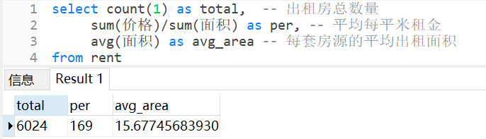
71 |
72 | ## 3.2 地区分析
73 |
74 | 房源数量分布情况如下,可以看到朝阳和通州这两个地区的房源数量要远大于其它区,说明这两个地方的租赁市场比较活跃,人员流动和人口密度可能也比较大。
75 |
76 | 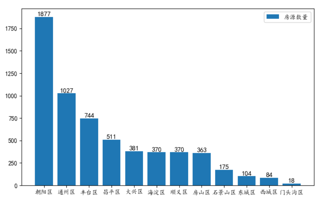
77 |
78 | ## 3.3 小区分析
79 |
80 | 房租最贵的小区 TOP 10。半壁街南路 1 号院的房租最高,达到 596 元/平米,是平均值 169 元/平米的 **3** 倍。
81 |
82 | 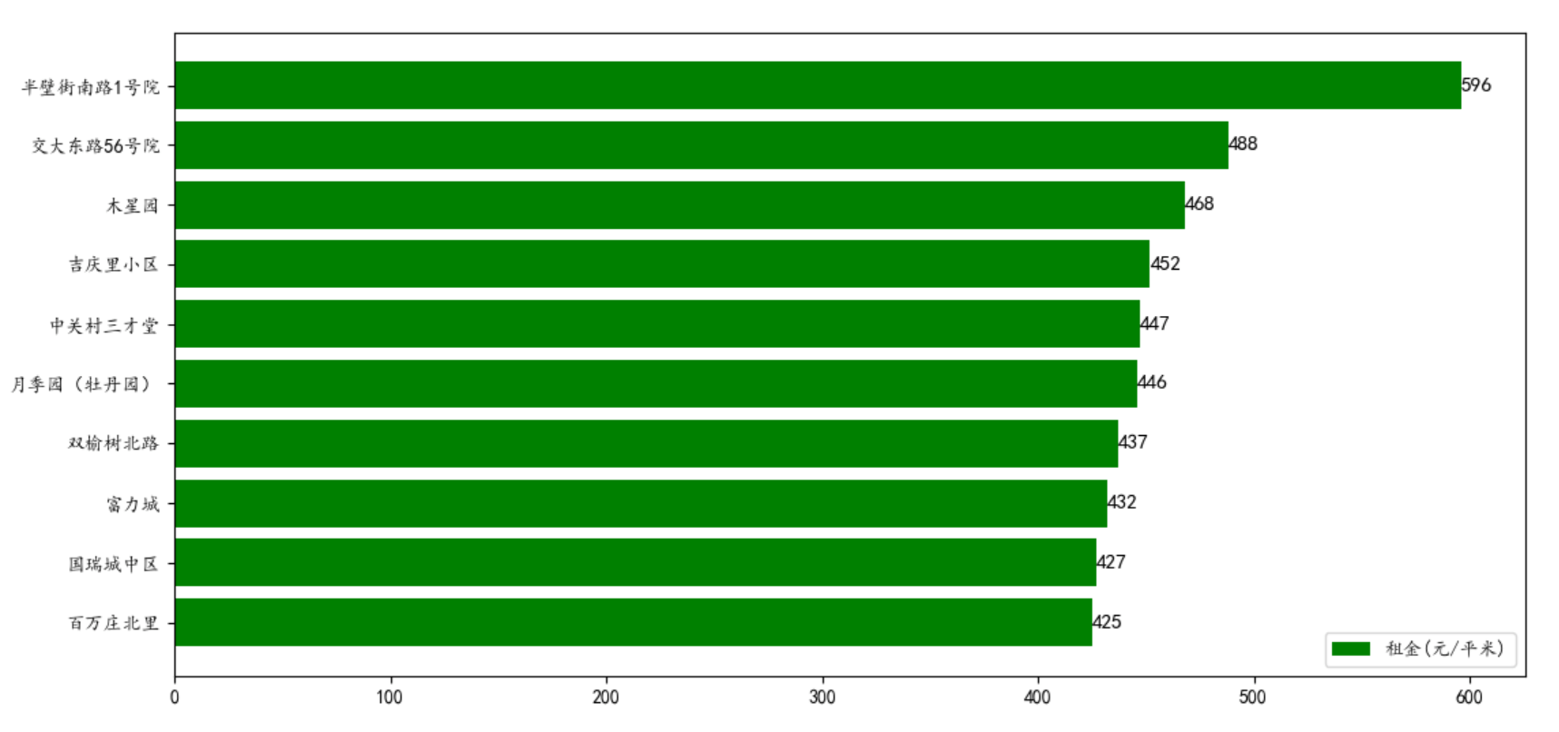
83 |
84 | ## 3.4 户型楼层分析
85 |
86 | 从户型的房源数量分布来看,主要集中在 2-4 室的户型。之前也分析了,每套房源的平均出租面积为 15.68 平米,可见大部分房源都是合租,毕竟房租那么贵,生活成本太高了。
87 |
88 | 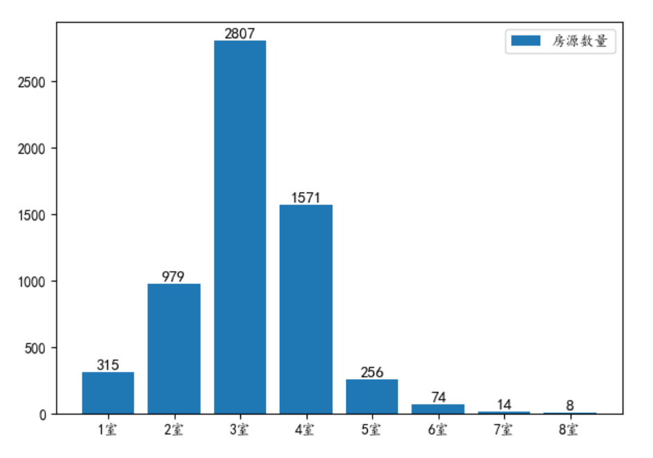
89 |
90 | 国家规定楼层 7 层以上需要装电梯,依据这个规定,我们根据楼层数来判断房源是否有电梯。
91 |
92 | 从下图可以看到,电梯房的房源数量比较多,毕竟楼层高,建的房子多,此外,电梯房平均每平米的租金也要比非电梯房贵 10 块钱。
93 |
94 | 
95 |
96 | 
97 |
98 | 在区分出电梯房之后,我们再引入楼层的纬度进行分析。
99 |
100 | 从租金上看,不管是电梯房还是非电梯房,低楼层的租金都会比较贵一些。因为北京地处北方,天气较干燥,不会有回南天,而且低楼层出行较为方便。电梯房的高楼层,租金也会比较贵,这大概是因为高楼层的风景较好。
101 |
102 | > 南方天气潮湿,在春天的时候,有时会出现 回南天 这一气象,导致低楼层会出现地板、墙壁渗水,所以在南方一般都不爱租低层。
103 |
104 | 从房源数量上看,非电梯房的高层房源最多,低层房源最少。说明非电梯房的高层房源不容易租出去,这点在租金上也有所体现。
105 |
106 | 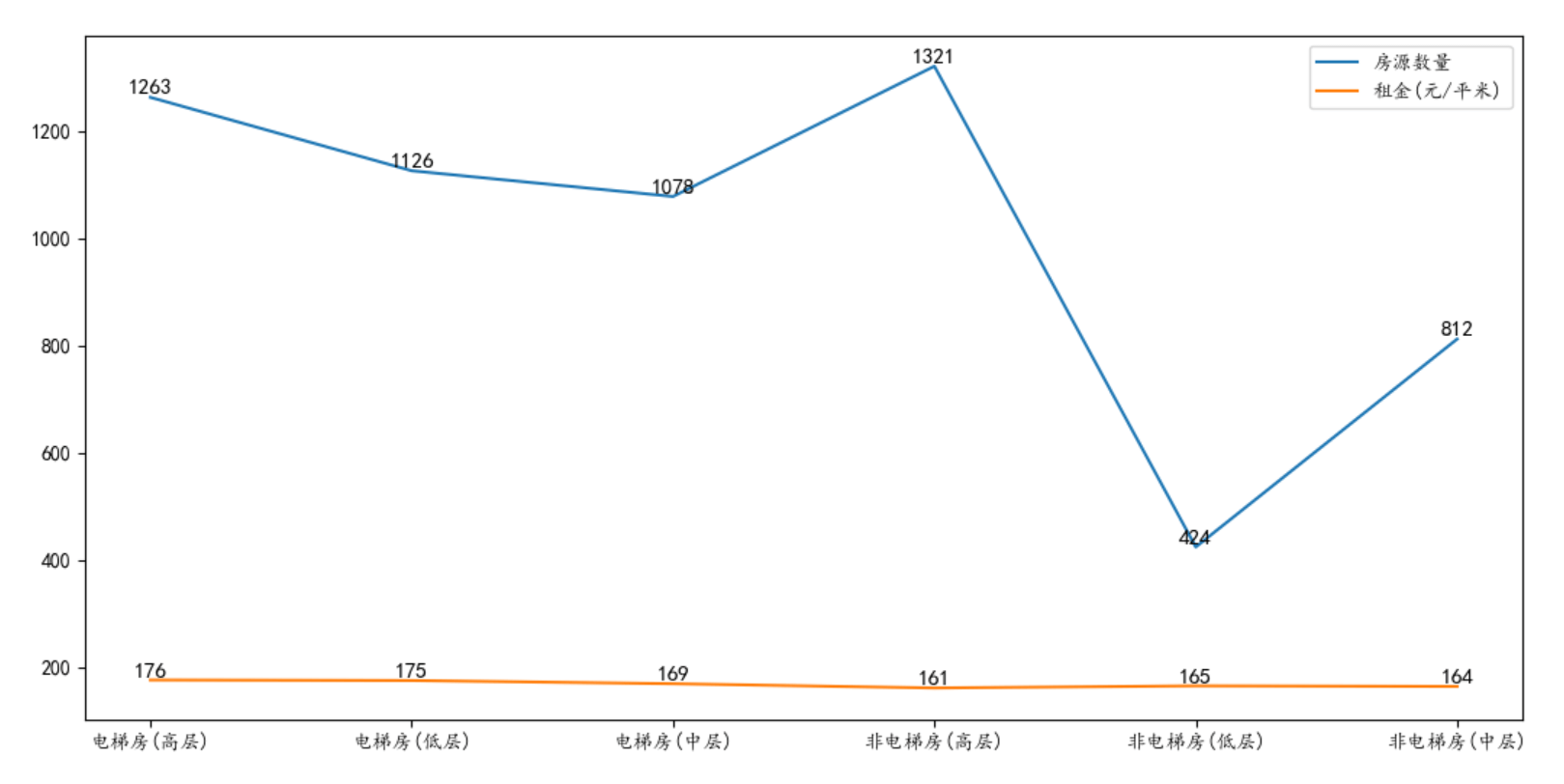
107 |
108 | ## 3.5 交通分析
109 |
110 | 从地理位置上来看,交通越便利,租金也越贵,这个符合一般认知。
111 |
112 | 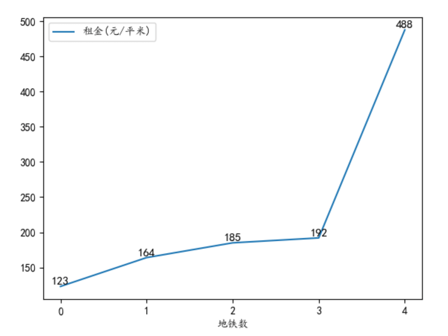
113 |
114 | 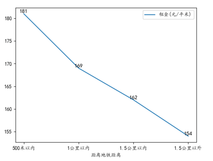
115 |
--------------------------------------------------------------------------------
/SZTcard/analyse.sql:
--------------------------------------------------------------------------------
1 | -- 乘客主题
2 |
3 | -- (整体) 通勤费用
4 | select '整体' deal_type,
5 | count(1) as cnt,
6 | sum(deal_money) / 100 as total,
7 | avg(deal_money) / 100 as per
8 | from sztcard
9 | where deal_type in ('地铁出站', '巴士')
10 | union all
11 | select deal_type,
12 | count(1) as cnt,
13 | sum(deal_money) / 100 as total,
14 | avg(deal_money) / 100 as per
15 | from sztcard
16 | where deal_type in ('地铁出站', '巴士')
17 | group by deal_type;
18 |
19 | -- 优惠情况
20 | select case when a.distinct_count = 1 then '全票'
21 | when a.distinct_count = 0.95 then '9.5 折'
22 | when a.distinct_count >= 0.9 then '9 折'
23 | when a.distinct_count >= 0.85 then '8.5 折'
24 | when a.distinct_count >= 0.75 then '7.5 折'
25 | when a.distinct_count >= 0.5 then '半票'
26 | when a.distinct_count = 0 then '免票'
27 | end as distinct_count_range,
28 | sum(cn) as cn
29 | from(
30 | select deal_money / deal_value as distinct_count, count(1) as cn
31 | from sztcard
32 | where deal_value > 0
33 | group by deal_money / deal_value
34 | ) as a
35 | group by case when a.distinct_count = 1 then '全票'
36 | when a.distinct_count = 0.95 then '9.5 折'
37 | when a.distinct_count >= 0.9 then '9 折'
38 | when a.distinct_count >= 0.85 then '8.5 折'
39 | when a.distinct_count >= 0.75 then '7.5 折'
40 | when a.distinct_count >= 0.5 then '半票'
41 | when a.distinct_count = 0 then '免票'
42 | end;
43 |
44 | -- (整体) 出行时间分布
45 | select hour(deal_date) as h, count(1) as ct
46 | from sztcard
47 | where deal_type in ('地铁入站', '巴士')
48 | group by hour(deal_date)
49 | order by h;
50 |
51 | -- (地铁) 通勤时间
52 | with tt as(
53 | select *, row_number() over( partition by card_no order by deal_date) as px
54 | from sztcard
55 | where deal_type rlike '地铁'
56 | ),
57 | tt2 as(
58 | select t1.card_no,
59 | t1.deal_type as in_type, t1.company_name as in_company, t1.station as in_station, t1.deal_date as in_date,
60 | t2.deal_type as out_type, t2.company_name as out_company, t2.station as out_station, t2.deal_date as out_date,
61 | unix_timestamp(t2.deal_date) - unix_timestamp(t1.deal_date) as diff_sec
62 | from tt as t1
63 | inner join tt as t2 on t1.card_no = t2.card_no and t1.px = t2.px - 1
64 | where t2.deal_type = '地铁出站'
65 | and t1.deal_type = '地铁入站'
66 | and t1.station <> t2.station
67 | and substring(t1.deal_date, 1, 10) = '2018-09-01'
68 | and substring(t2.deal_date, 1, 10) = '2018-09-01'
69 | )
70 |
71 | select avg(diff_sec)/60 from tt2;
72 |
73 |
74 | -- 地铁主题
75 |
76 | -- (基于站点) 进站 top
77 | select station, count(1) as cn
78 | from sztcard
79 | where deal_type = '地铁入站'
80 | and station > ''
81 | group by station
82 | order by cn desc
83 | limit 10;
84 |
85 | -- (基于站点) 出站 top
86 | select station, count(1) as cn
87 | from sztcard
88 | where deal_type = '地铁出站'
89 | and station > ''
90 | group by station
91 | order by cn desc
92 | limit 10;
93 |
94 | -- (基于站点) 进出站 top
95 | select station, count(1) as cn
96 | from sztcard
97 | where deal_type in ('地铁出站', '地铁入站')
98 | and station > ''
99 | group by station
100 | order by cn desc
101 | limit 10;
102 |
103 | -- (基于站点) 站点收入 top
104 | select station, sum(deal_money) / 100 as sm
105 | from sztcard
106 | where deal_type in ('地铁出站', '地铁入站')
107 | and station > ''
108 | group by station
109 | order by sm desc
110 | limit 10;
111 |
112 | -- (基于线路) 运输贡献度 top
113 | -- 进站算一次,出站并且联程算一次
114 | select company_name, count(1) as cn
115 | from sztcard
116 | where company_name rlike '地铁'
117 | and (deal_type = '地铁出站' and conn_mark = '1' or deal_type = '地铁入站')
118 | group by company_name
119 | order by cn desc;
120 |
121 | -- (基于线路) 运输效率 top
122 | -- 每条线路单程直达乘客耗时平均值排行榜
123 | with tt as(
124 | select *, row_number() over( partition by card_no order by deal_date) as px
125 | from sztcard
126 | where deal_type rlike '地铁'
127 | ),
128 | tt2 as(
129 | select t1.card_no,
130 | t1.deal_type as in_type, t1.company_name as in_company, t1.station as in_station, t1.deal_date as in_date,
131 | t2.deal_type as out_type, t2.company_name as out_company, t2.station as out_station, t2.deal_date as out_date,
132 | unix_timestamp(t2.deal_date) - unix_timestamp(t1.deal_date) as diff_sec
133 | from tt as t1
134 | inner join tt as t2 on t1.card_no = t2.card_no and t1.px = t2.px - 1
135 | where t2.deal_type = '地铁出站'
136 | and t1.deal_type = '地铁入站'
137 | and t1.station <> t2.station
138 | and substring(t1.deal_date, 1, 10) = '2018-09-01'
139 | and substring(t2.deal_date, 1, 10) = '2018-09-01'
140 | )
141 |
142 | select in_company, avg(diff_sec) / 60 avg_min
143 | from tt2
144 | where in_company = out_company
145 | group by in_company
146 | order by avg_min;
147 |
148 | -- (基于线路) 换乘比例 top
149 | -- 每线路换乘出站乘客百分比排行榜
150 | with tt as(
151 | select *, row_number() over( partition by card_no order by deal_date) as px
152 | from sztcard
153 | where deal_type rlike '地铁'
154 | ),
155 | tt2 as(
156 | select t1.card_no,
157 | t1.deal_type as in_type, t1.company_name as in_company, t1.station as in_station, t1.deal_date as in_date,
158 | t2.deal_type as out_type, t2.company_name as out_company, t2.station as out_station, t2.deal_date as out_date,
159 | t2.conn_mark,
160 | unix_timestamp(t2.deal_date) - unix_timestamp(t1.deal_date) as diff_sec
161 | from tt as t1
162 | inner join tt as t2 on t1.card_no = t2.card_no and t1.px = t2.px - 1
163 | where t2.deal_type = '地铁出站'
164 | and t1.deal_type = '地铁入站'
165 | and t1.station <> t2.station
166 | and substring(t1.deal_date, 1, 10) = '2018-09-01'
167 | and substring(t2.deal_date, 1, 10) = '2018-09-01'
168 | )
169 |
170 | select out_company, sum(case when conn_mark = '1' then 1 else 0 end) / count(1) as per
171 | from tt2
172 | group by out_company
173 | order by per desc;
174 |
175 | -- (基于线路) 线路收入 top
176 | select company_name, sum(deal_money) / 100 as sm
177 | from sztcard
178 | where deal_type rlike '地铁'
179 | group by company_name
180 | order by sm desc;
181 |
182 | -- 巴士主题
183 |
184 | -- (基于公司) 巴士公司收入 top
185 | select company_name, sum(deal_money) / 100 as sm
186 | from sztcard
187 | where deal_type not rlike '地铁'
188 | group by company_name
189 | order by sm desc;
190 |
191 | -- (基于公司) 巴士公司贡献度 top
192 | select company_name, count(1) as cn
193 | from sztcard
194 | where deal_type not rlike '地铁'
195 | group by company_name
196 | order by cn desc;
--------------------------------------------------------------------------------
/SZTcard/etl.py:
--------------------------------------------------------------------------------
1 | #!/usr/bin/env python3
2 | # -*- coding: utf-8 -*-
3 | # @Time : 2021/1/8 20:03
4 | # @Author : way
5 | # @Site :
6 | # @Describe: 数据处理 https://opendata.sz.gov.cn/data/dataSet/toDataDetails/29200_00403601
7 |
8 | import json
9 | import pandas as pd
10 |
11 | ############################################# 解析 json 数据文件 ##########################################################
12 | path = r"C:\Users\Administrator\Desktop\2018record3.jsons"
13 | data = []
14 | with open(path, 'r', encoding='utf-8') as f:
15 | for line in f.readlines():
16 | data += json.loads(line)['data']
17 | data = pd.DataFrame(data)
18 | columns = ['card_no', 'deal_date', 'deal_type', 'deal_money', 'deal_value', 'equ_no', 'company_name', 'station', 'car_no', 'conn_mark', 'close_date']
19 | data = data[columns] # 调整字段顺序
20 | data.info()
21 |
22 | ############################################# 输出处理 ##########################################################
23 | # 全部都是 交通运输 的刷卡数据
24 | print(data['company_name'].unique())
25 |
26 | # 删除重复值
27 | # print(data[data.duplicated()])
28 | data.drop_duplicates(inplace=True)
29 | data.reset_index(drop=True, inplace=True)
30 |
31 | # 缺失值
32 | # 只有线路站点和车牌号两个字段存在为空,不做处理
33 | # print(data.isnull().sum())
34 |
35 | # 去掉脏数据
36 | data = data[data['deal_date'] > '2018-08-31']
37 | ############################################# 数据保存 ##########################################################
38 | print(data.info)
39 |
40 | # 数据保存为 csv
41 | data.to_csv('SZTcard.csv', index=False, header=None)
42 |
--------------------------------------------------------------------------------
/SZTcard/table.sql:
--------------------------------------------------------------------------------
1 | -- 建表
2 | CREATE TABLE `sztcard`(
3 | `card_no` string COMMENT '卡号',
4 | `deal_date` string COMMENT '交易日期时间',
5 | `deal_type` string COMMENT '交易类型',
6 | `deal_money` float COMMENT '交易金额',
7 | `deal_value` float COMMENT '交易值',
8 | `equ_no` string COMMENT '设备编码',
9 | `company_name` string COMMENT '公司名称',
10 | `station` string COMMENT '线路站点',
11 | `car_no` string COMMENT '车牌号',
12 | `conn_mark` string COMMENT '联程标记',
13 | `close_date` string COMMENT '结算日期'
14 | )
15 | row format delimited
16 | fields terminated by ','
17 | lines terminated by '\n';
18 |
19 | -- 加载数据
20 | LOAD DATA INPATH '/tmp/SZTcard.csv' OVERWRITE INTO TABLE sztcard;
--------------------------------------------------------------------------------
/SZTcard/深圳通刷卡数据分析.md:
--------------------------------------------------------------------------------
1 | [TOC]
2 |
3 | # 1. 数据集说明
4 |
5 | 这是一份来自深圳市政府数据开放平台的深圳通刷卡数据,时间区间为 2018-08-31 到 2018-09-01,总计 1,337,000 条记录,大小为 335 M,包含 11 个字段。
6 |
7 | > 深圳通是由深圳市运输局监制、深圳市公共交通结算管理中心发行的一款即可优惠乘坐深圳市公交车,深圳地铁和商店消费的一种储值卡。
8 |
9 | # 2. 数据处理
10 |
11 | ## 2.1 数据处理
12 | 源数据存的是 json 格式的数据,先使用 python 对数据做一下清洗,然后保存为 csv 数据文件。
13 |
14 | ```python
15 | ### 解析 json 数据文件
16 | path = r"C:\Users\Administrator\Desktop\2018record3.jsons"
17 | data = []
18 | with open(path, 'r', encoding='utf-8') as f:
19 | for line in f.readlines():
20 | data += json.loads(line)['data']
21 | data = pd.DataFrame(data)
22 | columns = ['card_no', 'deal_date', 'deal_type', 'deal_money', 'deal_value', 'equ_no', 'company_name', 'station', 'car_no', 'conn_mark', 'close_date']
23 | data = data[columns] # 调整字段顺序
24 | data.info()
25 |
26 | ### 输出处理
27 | # 全部都是 交通运输 的刷卡数据
28 | print(data['company_name'].unique())
29 |
30 | # 删除重复值
31 | # print(data[data.duplicated()])
32 | data.drop_duplicates(inplace=True)
33 | data.reset_index(drop=True, inplace=True)
34 |
35 | # 缺失值
36 | # 只有线路站点和车牌号两个字段存在为空,不做处理
37 | # print(data.isnull().sum())
38 |
39 | # 去掉脏数据
40 | data = data[data['deal_date'] > '2018-08-31']
41 |
42 | ### 数据保存
43 | print(data.info)
44 |
45 | # 数据保存为 csv
46 | data.to_csv('SZTcard.csv', index=False, header=None)
47 | ```
48 |
49 | ## 2.2 数据加载
50 |
51 | 把清洗好的数据文件上传到 hdfs ,然后加载到 impala,后续就可以直接用 impala 进行数据分析。
52 |
53 | > 与 hive 不同,impala 不支持加载本地数据文件,只能加载 hdfs 数据文件,所以需要先把数据文件上传到 hdfs。
54 |
55 | ```shell
56 | # csv 上传到 hdfs
57 | hdfs dfs -put SZTcard.csv /tmp/
58 | ```
59 |
60 | ```sql
61 | -- 建表
62 | CREATE TABLE `sztcard`(
63 | `card_no` string COMMENT '卡号',
64 | `deal_date` string COMMENT '交易日期时间',
65 | `deal_type` string COMMENT '交易类型',
66 | `deal_money` float COMMENT '交易金额',
67 | `deal_value` float COMMENT '交易值',
68 | `equ_no` string COMMENT '设备编码',
69 | `company_name` string COMMENT '公司名称',
70 | `station` string COMMENT '线路站点',
71 | `car_no` string COMMENT '车牌号',
72 | `conn_mark` string COMMENT '联程标记',
73 | `close_date` string COMMENT '结算日期'
74 | )
75 | row format delimited
76 | fields terminated by ','
77 | lines terminated by '\n';
78 |
79 | -- 加载数据
80 | LOAD DATA INPATH '/tmp/SZTcard.csv' OVERWRITE INTO TABLE sztcard;
81 | ```
82 |
83 | ## 2.3 数据预览
84 |
85 | 数据加载完成后,查看一下数据情况,发现有两个金额字段,但是没有给出数值单位。通过红色框框出来的这个旅途(卡号AEAAAACHG ,草铺>>少年宫),到网上 [搜一下](https://dt.8684.cn/so.php?dtcity=sz&k=p2p&q=%E8%8D%89%E5%9F%94&q1=%E5%B0%91%E5%B9%B4%E5%AE%AB) ,可以看到票价是 4 元,可见这两个字段都是单位都是 分。并且,deal_value 就是票价,而 deal_money 就是实际的消费金额,所以本次是半价,结合目的地,AEAAAACHG 可能是一张学生卡。
86 |
87 | 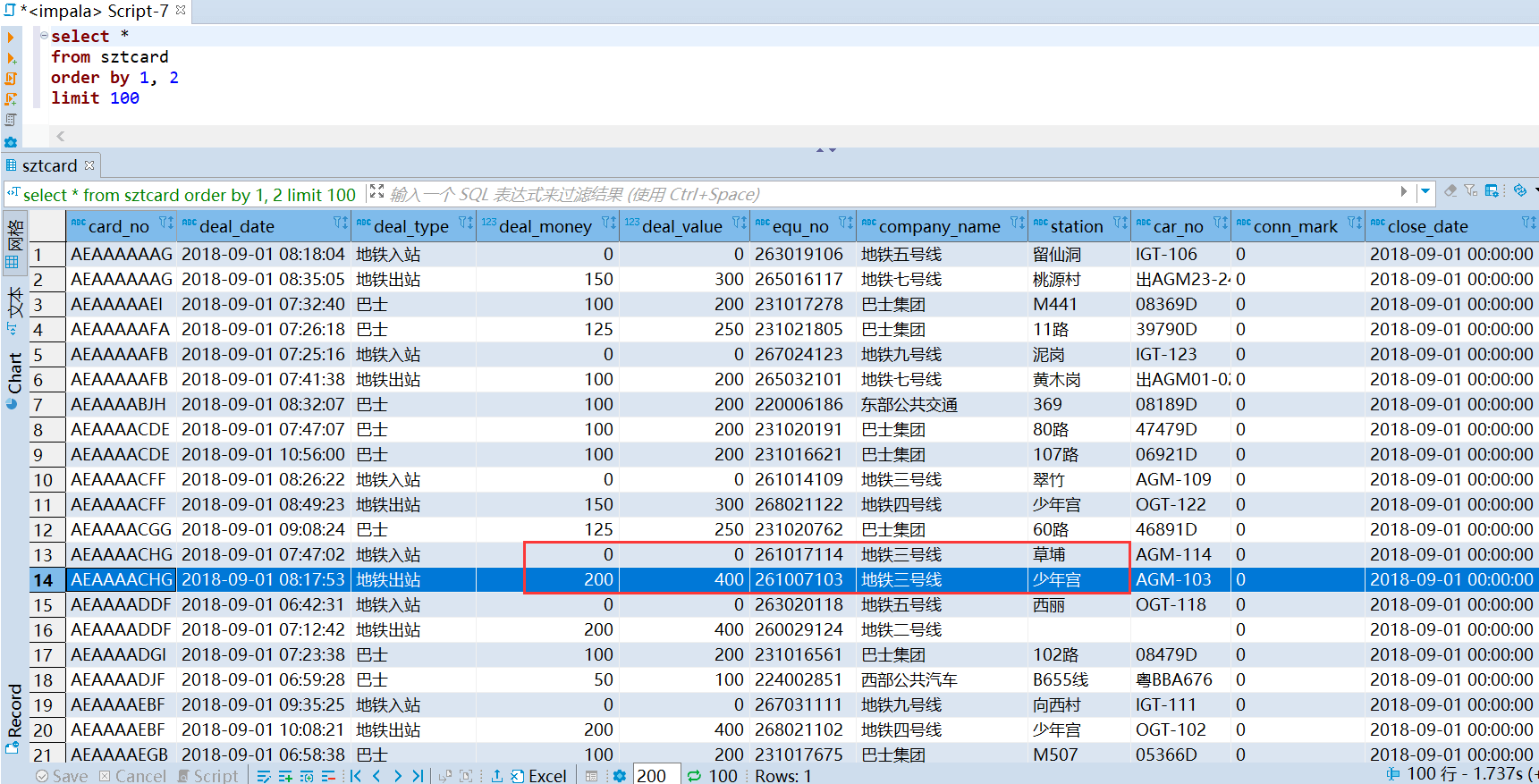
88 |
89 | 
90 |
91 | 然后再查看一下数据集的日期分布,可以看到 2018-09-01 数据量比较大,但是时间范围只有半天。而 2018-08-31 相比之下数据量非常少,但是时间范围是一整天,后续在做一些时间上的分析,应该注意到这点。
92 |
93 | 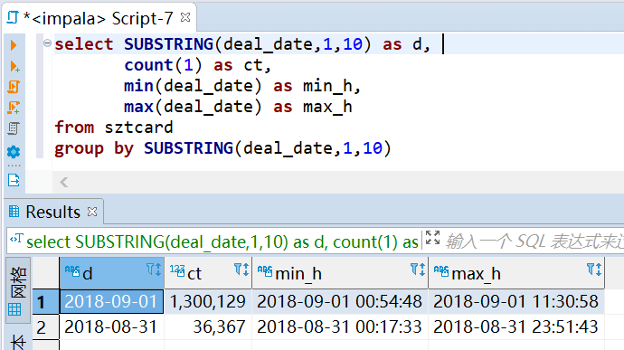
94 |
95 | 最后在看下公司名称分布情况,没有看到什么 某某便利店之类的名称,可见该数据集并没有商店消费的数据,全部都是交通出行的数据。
96 |
97 | 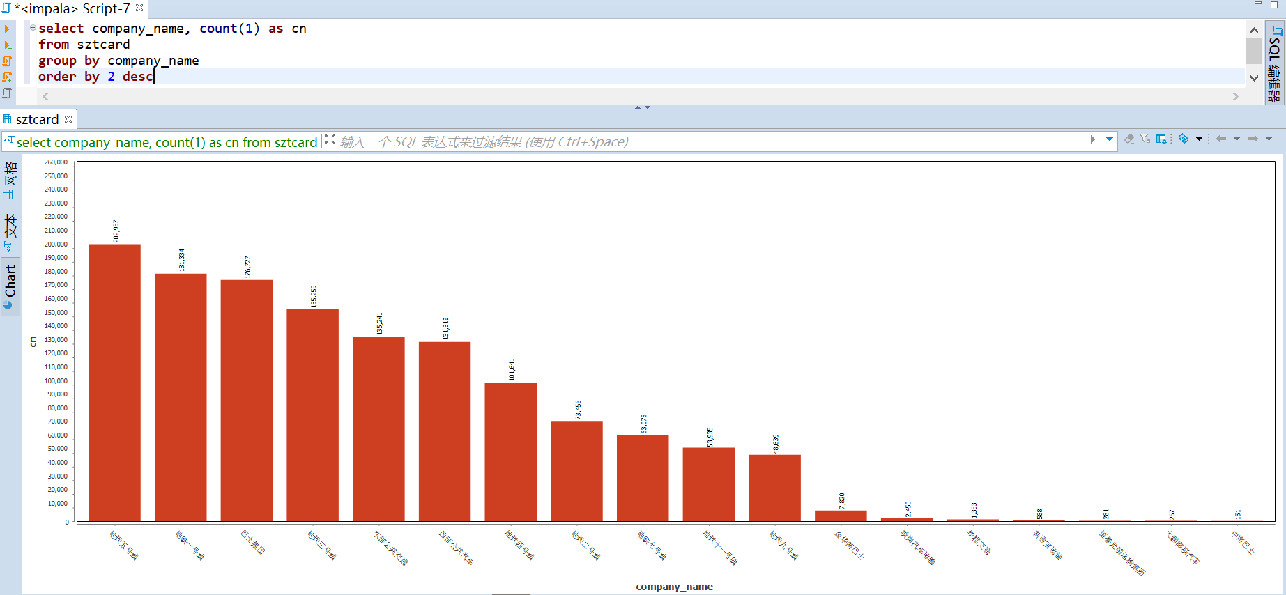
98 |
99 |
100 | # 3. 数据分析可视化
101 |
102 | ## 3.1 乘客主题
103 |
104 | ### (整体) 通勤费用
105 |
106 | 整体的通勤次数为 872,761 人次,总费用为 2,414,023 元,平均每次出行花费 2.76 元。
107 |
108 | 交通工具上来看,坐巴士平均每次为 1.7 元,坐地铁则要 3.9 元。
109 |
110 | 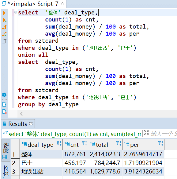
111 |
112 | 从交通优惠的普及情况来看,受众还是非常广的,只有 1,235 人次是购买的全票,占比仅为千分之一(1,235 / 872,761)。
113 |
114 | 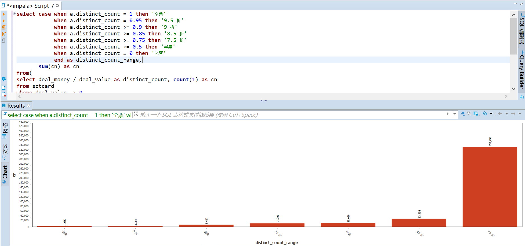
115 |
116 |
117 | ### (整体) 出行时间分布
118 |
119 | 2018-08-31 每小时的出行人次,从中可以看到晚高峰是在 18-19 点之间,早高峰在 8-9 点之间,可能由于数据集本身的不完整,所以早高峰看起来不是很明显。
120 |
121 | 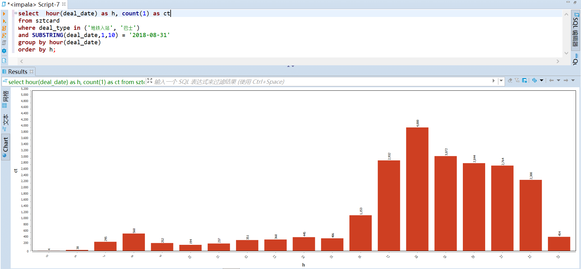
122 |
123 | 2018-09-01 每小时的出行人次,从中可以看到早高峰在 8-9 点之间,由于只有半天的数据,所以看不到晚高峰。
124 |
125 | 
126 |
127 | ### (地铁) 通勤时间
128 |
129 | 由于地铁是进出站都要刷卡,所以可以通过二者之差来计算地铁的通勤时间。平均通勤时间为 29.6 分钟。
130 |
131 | 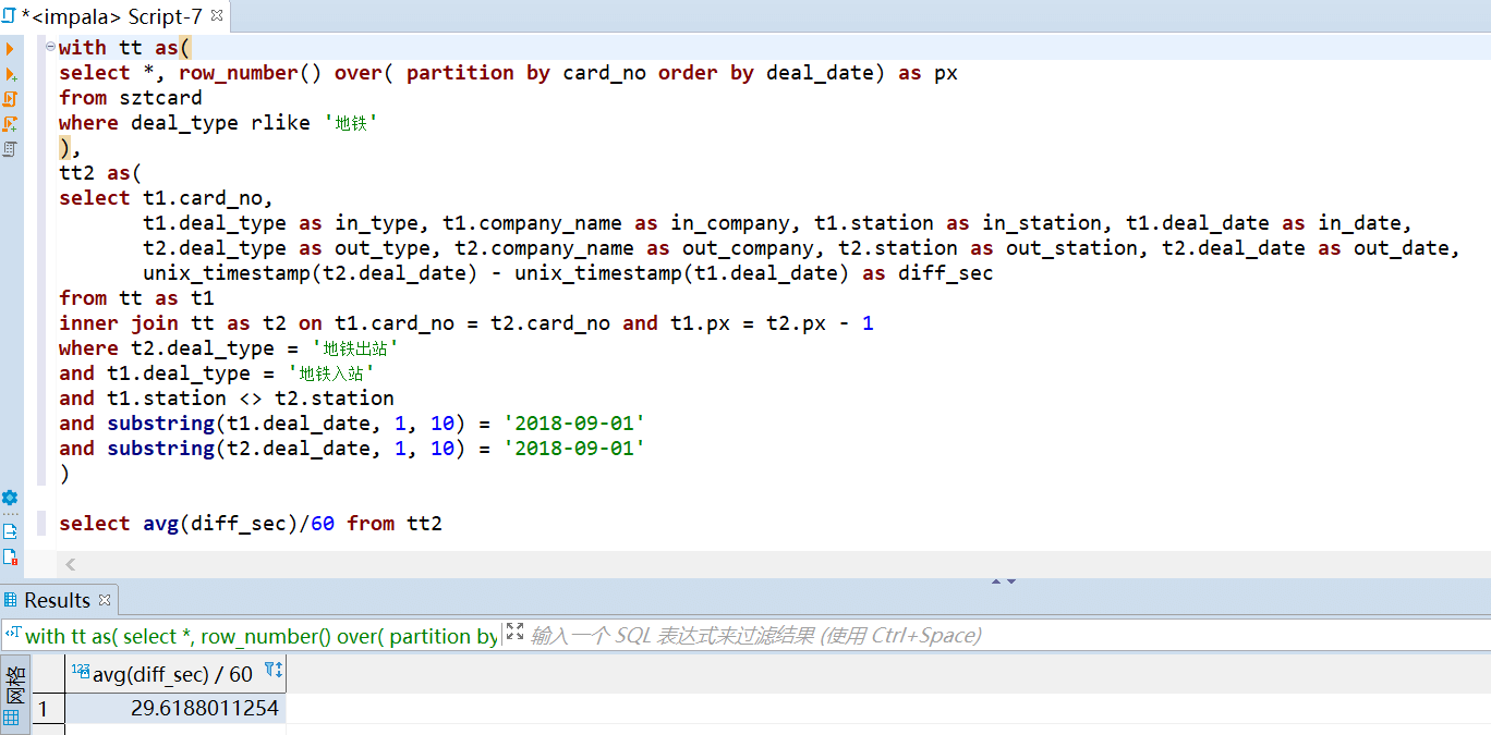
132 |
133 |
134 |
135 | ## 3.2 地铁主题
136 |
137 | ### (基于站点) 进站人流量 top
138 |
139 | 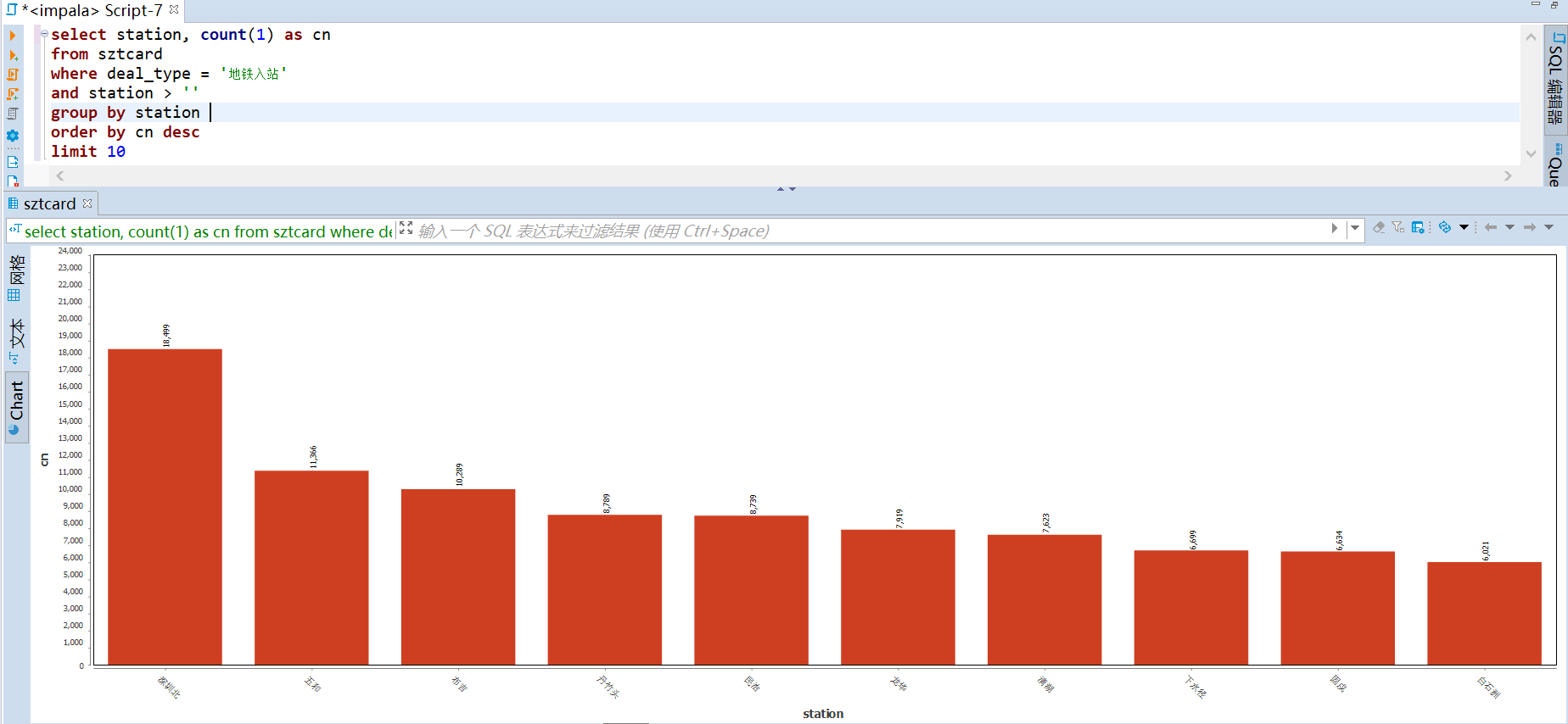
140 |
141 | ### (基于站点) 出站人流量 top
142 |
143 | 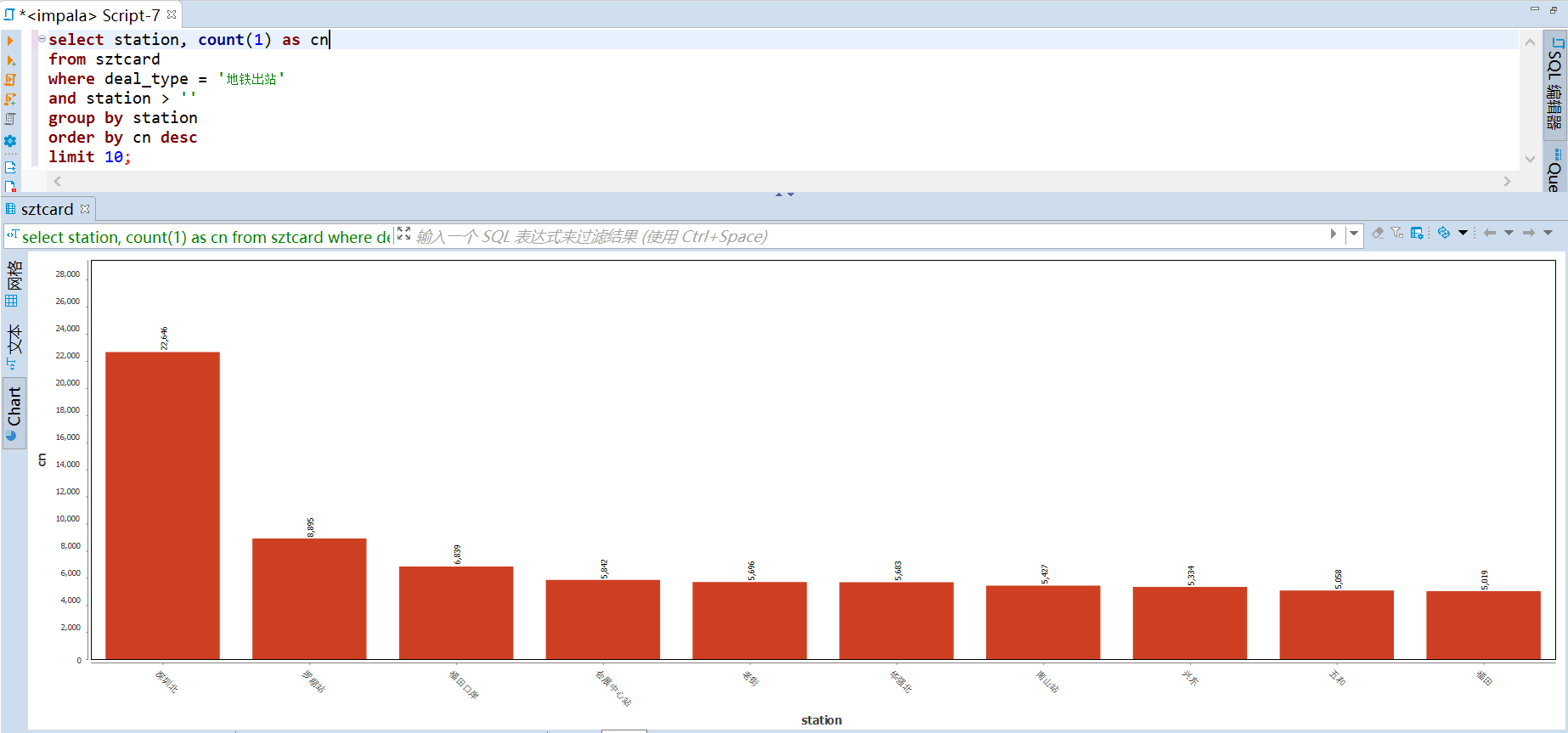
144 |
145 | ### (基于站点) 进出站人流量 top
146 |
147 | 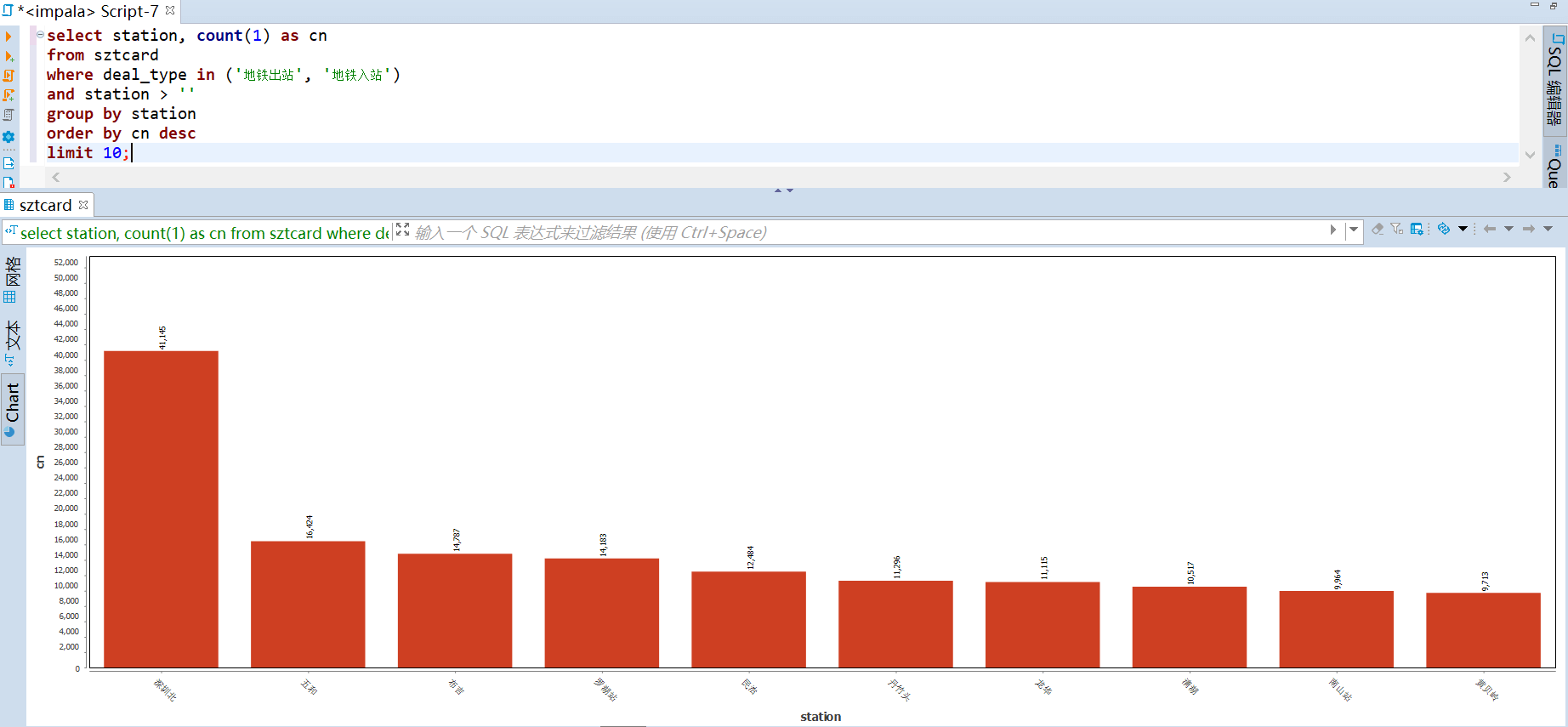
148 |
149 | ### (基于站点) 站点收入 top
150 |
151 | 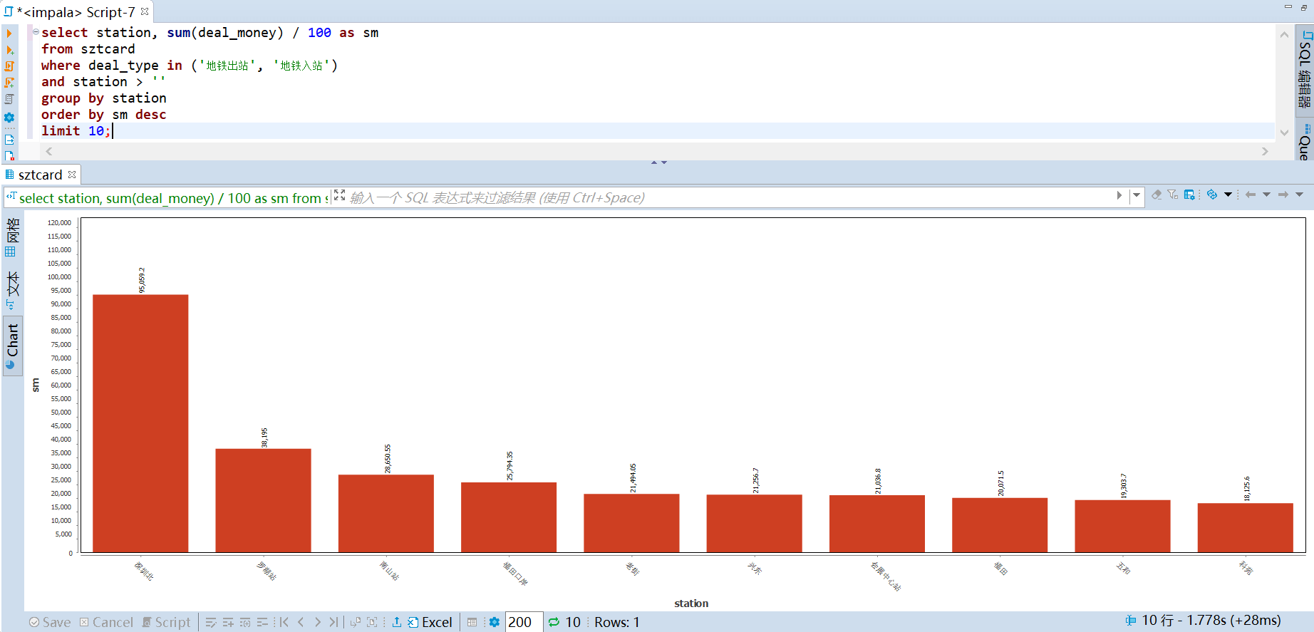
152 |
153 | ### (基于线路) 运输贡献度 top
154 |
155 | 运输贡献度计算规则:进站算一次,出站并且联程算一次。从下图可以看到 五号线的运输贡献度最高,九号线的贡献度最低。
156 |
157 | 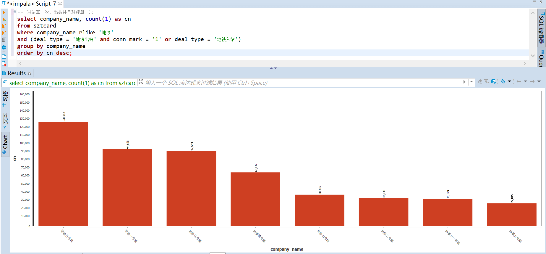
158 |
159 | ### (基于线路) 运输效率 top
160 |
161 | 单程直达每乘客的平均通勤时间可以体现运输效率,从下图可以看到,地铁 9 号线的运输效率最高,平均为 15.81 分钟/人次。
162 |
163 | 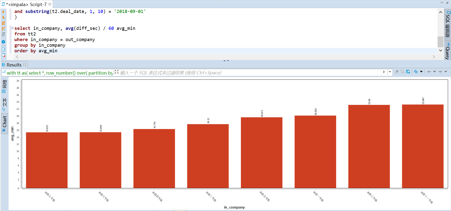
164 |
165 | ### (基于线路) 换乘比例 top
166 |
167 | 从地铁出来后还需要换乘的乘客占比,可以看到 五号线 的换乘比例最高 15.7 %,九号线 换乘比例最低 9.4 %
168 |
169 | 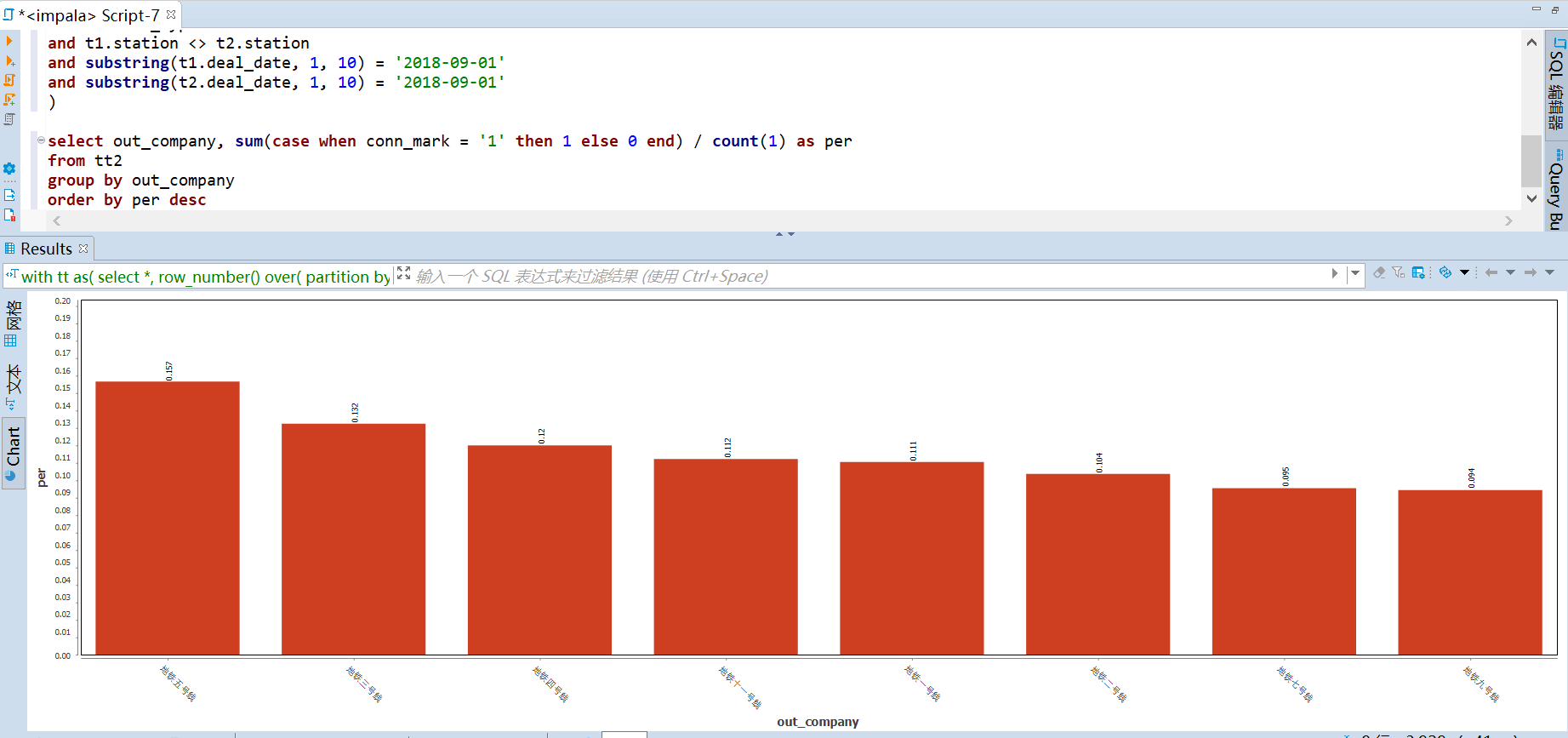
170 |
171 | ### (基于线路) 线路收入 top
172 |
173 | 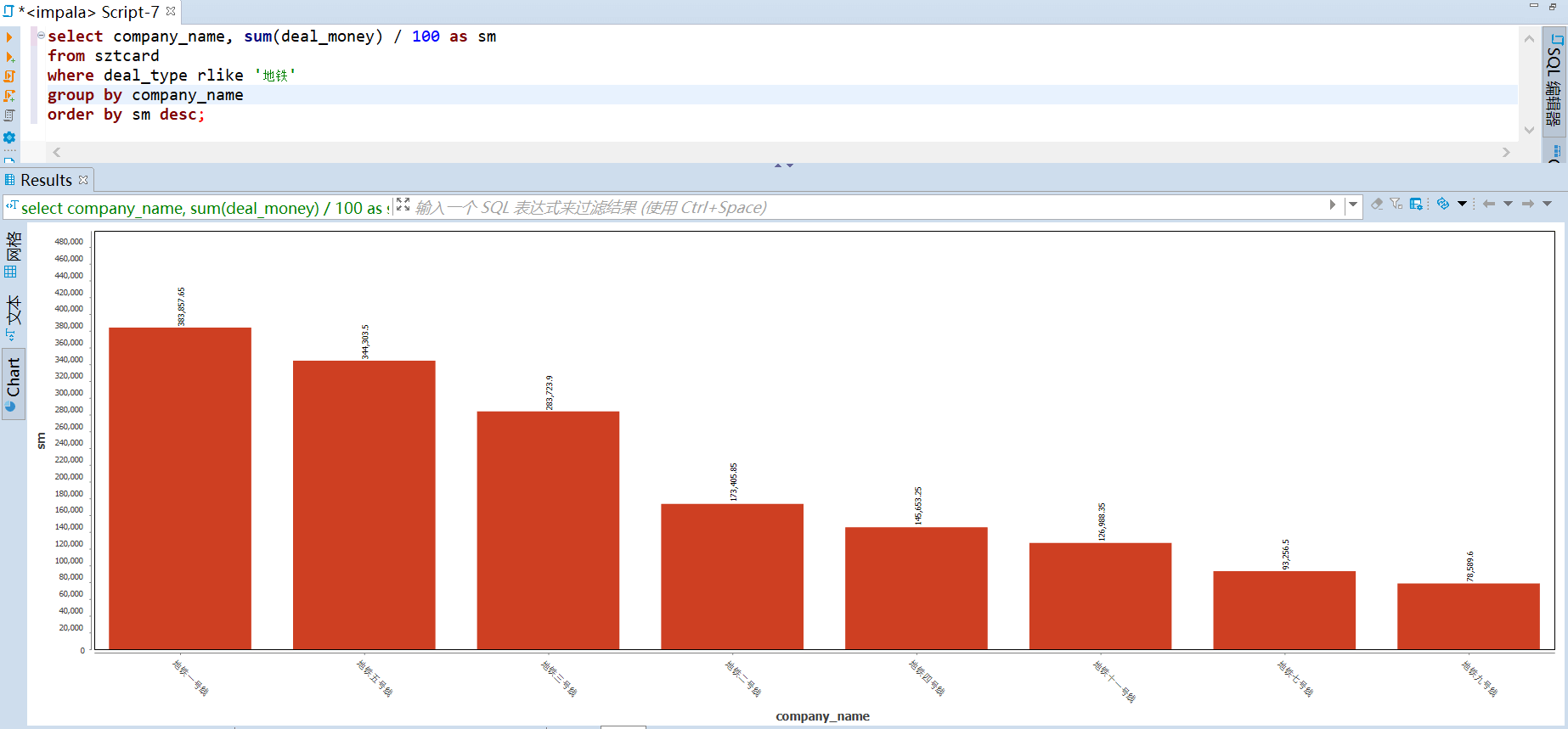
174 |
175 |
176 |
177 | ## 3.3 巴士主题
178 |
179 | ### (基于公司) 巴士公司收入 top
180 |
181 | 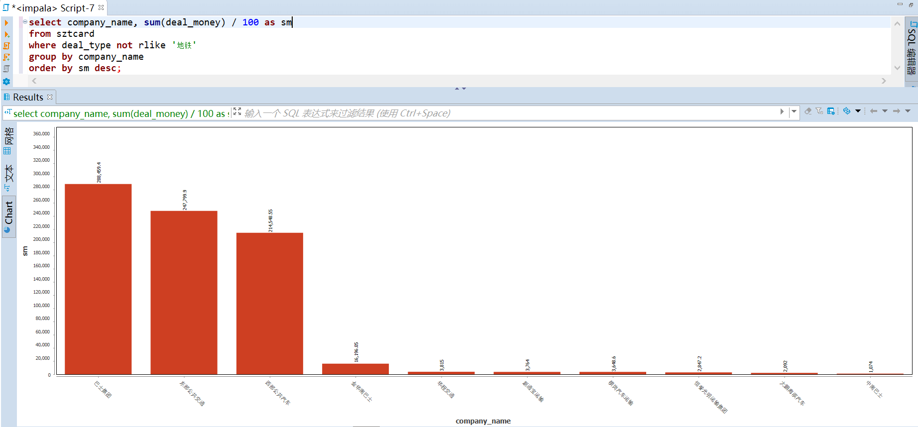
182 |
183 | ### (基于公司) 巴士公司运输贡献度 top
184 |
185 | 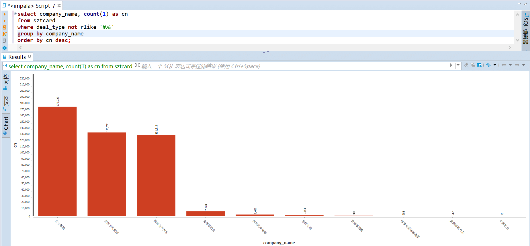
186 |
187 |
188 | # 参考
189 | [https://github.com/geekyouth/SZT-bigdata](https://github.com/geekyouth/SZT-bigdata)
--------------------------------------------------------------------------------
/UserBehaviorFromTaobao_Batch/analyse.hql:
--------------------------------------------------------------------------------
1 | --1、用户流量及购物情况
2 |
3 | --总访问量PV,总用户量UV
4 | select sum(case when behavior_type = 'pv' then 1 else 0 end) as pv,
5 | count(distinct user_id) as uv
6 | from user_behavior;
7 |
8 | --日均访问量,日均用户量
9 | select date(datetime) as day,
10 | sum(case when behavior_type = 'pv' then 1 else 0 end) as pv,
11 | count(distinct user_id) as uv
12 | from user_behavior
13 | group by date(datetime)
14 | order by day;
15 |
16 | --每个用户的购物情况,加工到 user_behavior_count
17 | create table user_behavior_count as
18 | select user_id,
19 | sum(case when behavior_type = 'pv' then 1 else 0 end) as pv, --点击数
20 | sum(case when behavior_type = 'fav' then 1 else 0 end) as fav, --收藏数
21 | sum(case when behavior_type = 'cart' then 1 else 0 end) as cart, --加购物车数
22 | sum(case when behavior_type = 'buy' then 1 else 0 end) as buy --购买数
23 | from user_behavior
24 | group by user_id;
25 |
26 | --点击数最多的用户前十
27 | select * from user_behavior_count order by pv desc limit 10;
28 |
29 | --复购率:产生两次或两次以上购买的用户占购买用户的比例
30 | select sum(case when buy > 1 then 1 else 0 end) / sum(case when buy > 0 then 1 else 0 end)
31 | from user_behavior_count;
32 |
33 |
34 | --2、用户行为转化漏斗
35 |
36 | --点击/(加购物车+收藏)/购买 , 各环节转化率
37 | select a.pv,
38 | a.fav,
39 | a.cart,
40 | a.fav + a.cart as `fav+cart`,
41 | a.buy,
42 | round((a.fav + a.cart) / a.pv, 4) as pv2favcart,
43 | round(a.buy / (a.fav + a.cart), 4) as favcart2buy,
44 | round(a.buy / a.pv, 4) as pv2buy
45 | from(
46 | select sum(pv) as pv, --点击数
47 | sum(fav) as fav, --收藏数
48 | sum(cart) as cart, --加购物车数
49 | sum(buy) as buy --购买数
50 | from user_behavior_count
51 | ) as a;
52 |
53 | --3、用户行为习惯与人群特征
54 |
55 | -- 一天的活跃时段分布
56 | select hour(datetime) as hour,
57 | sum(case when behavior_type = 'pv' then 1 else 0 end) as pv, --点击数
58 | sum(case when behavior_type = 'fav' then 1 else 0 end) as fav, --收藏数
59 | sum(case when behavior_type = 'cart' then 1 else 0 end) as cart, --加购物车数
60 | sum(case when behavior_type = 'buy' then 1 else 0 end) as buy --购买数
61 | from user_behavior
62 | group by hour(datetime)
63 | order by hour;
64 |
65 | --一周用户的活跃分布
66 | select pmod(datediff(datetime, '1920-01-01') - 3, 7) as weekday,
67 | sum(case when behavior_type = 'pv' then 1 else 0 end) as pv, --点击数
68 | sum(case when behavior_type = 'fav' then 1 else 0 end) as fav, --收藏数
69 | sum(case when behavior_type = 'cart' then 1 else 0 end) as cart, --加购物车数
70 | sum(case when behavior_type = 'buy' then 1 else 0 end) as buy --购买数
71 | from user_behavior
72 | where date(datetime) between '2017-11-27' and '2017-12-03'
73 | group by pmod(datediff(datetime, '1920-01-01') - 3, 7)
74 | order by weekday;
75 |
76 | --购买率高
77 | select *, buy / pv as buy_rate
78 | from user_behavior_count
79 | where buy > 0 and pv > 0
80 | order by buy_rate desc
81 | limit 10;
82 |
83 | --购买率低
84 | select *, buy / pv as buy_rate
85 | from user_behavior_count
86 | where buy > 0 and pv > 0
87 | order by buy_rate
88 | limit 10;
89 |
90 | --5、基于RFM模型找出有价值的用户
91 |
92 | /*
93 | RFM模型是衡量客户价值和客户创利能力的重要工具和手段,其中由3个要素构成了数据分析最好的指标,分别是:
94 | R-Recency(最近一次购买时间)
95 | F-Frequency(消费频率)
96 | M-Money(消费金额)
97 | */
98 |
99 | --R-Recency(最近一次购买时间), R值越高,一般说明用户比较活跃
100 | select user_id,
101 | datediff('2017-12-04', max(datetime)) as R,
102 | dense_rank() over(order by datediff('2017-12-04', max(datetime))) as R_rank
103 | from user_behavior
104 | where behavior_type = 'buy'
105 | group by user_id
106 | limit 10;
107 |
108 | --F-Frequency(消费频率), F值越高,说明用户越忠诚
109 | select user_id,
110 | count(1) as F,
111 | dense_rank() over(order by count(1) desc) as F_rank
112 | from user_behavior
113 | where behavior_type = 'buy'
114 | group by user_id
115 | limit 10;
116 |
117 | --对用户进行评分
118 | /*
119 | 对有购买行为的用户按照排名进行分组,共划分为5组,
120 | 前 - 1/5 的用户打5分
121 | 前 1/5 - 2/5 的用户打4分
122 | 前 2/5 - 3/5 的用户打3分
123 | 前 3/5 - 4/5 的用户打2分
124 | 前 4/5 - 的用户打1分
125 | 按照这个规则分别对用户时间间隔排名打分和购买频率排名打分,最后把两个分数合并在一起作为该名用户的最终评分。
126 | */
127 | with cte as(
128 | select user_id,
129 | datediff('2017-12-04', max(datetime)) as R,
130 | dense_rank() over(order by datediff('2017-12-04', max(datetime))) as R_rank,
131 | count(1) as F,
132 | dense_rank() over(order by count(1) desc) as F_rank
133 | from user_behavior
134 | where behavior_type = 'buy'
135 | group by user_id)
136 |
137 | select user_id, R, R_rank, R_score, F, F_rank, F_score, R_score + F_score AS score
138 | from(
139 | select *,
140 | case ntile(5) over(order by R_rank) when 1 then 5
141 | when 2 then 4
142 | when 3 then 3
143 | when 4 then 2
144 | when 5 then 1
145 | end as R_score,
146 | case ntile(5) over(order by F_rank) when 1 then 5
147 | when 2 then 4
148 | when 3 then 3
149 | when 4 then 2
150 | when 5 then 1
151 | end as F_score
152 | from cte
153 | ) as a
154 | order by score desc
155 | limit 20;
156 |
157 |
158 | --6、商品维度的分析
159 |
160 | --销量最高的商品
161 | select item_id ,
162 | sum(case when behavior_type = 'pv' then 1 else 0 end) as pv, --点击数
163 | sum(case when behavior_type = 'fav' then 1 else 0 end) as fav, --收藏数
164 | sum(case when behavior_type = 'cart' then 1 else 0 end) as cart, --加购物车数
165 | sum(case when behavior_type = 'buy' then 1 else 0 end) as buy --购买数
166 | from user_behavior
167 | group by item_id
168 | order by buy desc
169 | limit 10;
170 |
171 | --销量最高的商品大类
172 | select category_id ,
173 | sum(case when behavior_type = 'pv' then 1 else 0 end) as pv, --点击数
174 | sum(case when behavior_type = 'fav' then 1 else 0 end) as fav, --收藏数
175 | sum(case when behavior_type = 'cart' then 1 else 0 end) as cart, --加购物车数
176 | sum(case when behavior_type = 'buy' then 1 else 0 end) as buy --购买数
177 | from user_behavior
178 | group by category_id
179 | order by buy desc
180 | limit 10;
--------------------------------------------------------------------------------
/UserBehaviorFromTaobao_Batch/table.hql:
--------------------------------------------------------------------------------
1 | /*
2 | 说明:淘宝用户行为数据
3 | 来源:https://tianchi.aliyun.com/dataset/dataDetail?dataId=649&userId=1
4 | 大小:3.5 G
5 | 记录数:100,150,807
6 | 字段数:5
7 | */
8 |
9 | -- 建表
10 | drop table if exists user_behavior;
11 | create table user_behavior (
12 | `user_id` string comment '用户ID',
13 | `item_id` string comment '商品ID',
14 | `category_id` string comment '商品类目ID',
15 | `behavior_type` string comment '行为类型,枚举类型,包括(pv, buy, cart, fav)',
16 | `timestamp` int comment '行为时间戳',
17 | `datetime` string comment '行为时间')
18 | row format delimited
19 | fields terminated by ','
20 | lines terminated by '\n';
21 |
22 | -- 加载数据
23 | LOAD DATA LOCAL INPATH '/home/getway/UserBehavior.csv'
24 | OVERWRITE INTO TABLE user_behavior ;
25 |
26 | --查看数据
27 | select * from user_behavior limit 10;
28 |
29 | --数据清洗,去掉完全重复的数据
30 | insert overwrite table user_behavior
31 | select user_id, item_id, category_id, behavior_type, timestamp, datetime
32 | from user_behavior
33 | group by user_id, item_id, category_id, behavior_type, timestamp, datetime;
34 |
35 | --数据清洗,时间戳格式化成 datetime
36 | insert overwrite table user_behavior
37 | select user_id, item_id, category_id, behavior_type, timestamp, from_unixtime(timestamp, 'yyyy-MM-dd HH:mm:ss')
38 | from user_behavior;
39 |
40 | --查看时间是否有异常值
41 | select date(datetime) as day from user_behavior group by date(datetime) order by day;
42 |
43 | --数据清洗,去掉时间异常的数据
44 | insert overwrite table user_behavior
45 | select user_id, item_id, category_id, behavior_type, timestamp, datetime
46 | from user_behavior
47 | where cast(datetime as date) between '2017-11-25' and '2017-12-03';
48 |
49 | --查看 behavior_type 是否有异常值
50 | select behavior_type from user_behavior group by behavior_type;
51 |
52 | --清洗后的数据量
53 | select count(1) from user_behavior;
--------------------------------------------------------------------------------
/UserBehaviorFromTaobao_Batch/用户行为数据分析.md:
--------------------------------------------------------------------------------
1 | [TOC]
2 |
3 | # 1. 数据集说明
4 |
5 | 这是一份来自淘宝的用户行为数据,时间区间为 2017-11-25 到 2017-12-03,总计 100,150,807 条记录,大小为 3.5 G,包含 5 个字段。
6 |
7 | # 2. 数据处理
8 |
9 | ## 2.1 数据导入
10 | 将数据加载到 hive, 然后通过 hive 对数据进行数据处理。
11 |
12 | ```sql
13 | -- 建表
14 | drop table if exists user_behavior;
15 | create table user_behavior (
16 | `user_id` string comment '用户ID',
17 | `item_id` string comment '商品ID',
18 | `category_id` string comment '商品类目ID',
19 | `behavior_type` string comment '行为类型,枚举类型,包括(pv, buy, cart, fav)',
20 | `timestamp` int comment '行为时间戳',
21 | `datetime` string comment '行为时间')
22 | row format delimited
23 | fields terminated by ','
24 | lines terminated by '\n';
25 |
26 | -- 加载数据
27 | LOAD DATA LOCAL INPATH '/home/getway/UserBehavior.csv'
28 | OVERWRITE INTO TABLE user_behavior ;
29 | ```
30 |
31 | ## 2.2 数据清洗
32 | 数据处理主要包括:删除重复值,时间戳格式化,删除异常值。
33 |
34 | ```sql
35 | --数据清洗,去掉完全重复的数据
36 | insert overwrite table user_behavior
37 | select user_id, item_id, category_id, behavior_type, timestamp, datetime
38 | from user_behavior
39 | group by user_id, item_id, category_id, behavior_type, timestamp, datetime;
40 |
41 | --数据清洗,时间戳格式化成 datetime
42 | insert overwrite table user_behavior
43 | select user_id, item_id, category_id, behavior_type, timestamp, from_unixtime(timestamp, 'yyyy-MM-dd HH:mm:ss')
44 | from user_behavior;
45 |
46 | --查看时间是否有异常值
47 | select date(datetime) as day from user_behavior group by date(datetime) order by day;
48 |
49 | --数据清洗,去掉时间异常的数据
50 | insert overwrite table user_behavior
51 | select user_id, item_id, category_id, behavior_type, timestamp, datetime
52 | from user_behavior
53 | where cast(datetime as date) between '2017-11-25' and '2017-12-03';
54 |
55 | --查看 behavior_type 是否有异常值
56 | select behavior_type from user_behavior group by behavior_type;
57 | ```
58 |
59 | # 3.数据分析可视化
60 |
61 | ## 3.1 用户流量及购物情况
62 |
63 | ```sql
64 | --总访问量PV,总用户量UV
65 | select sum(case when behavior_type = 'pv' then 1 else 0 end) as pv,
66 | count(distinct user_id) as uv
67 | from user_behavior;
68 | ```
69 |
70 | 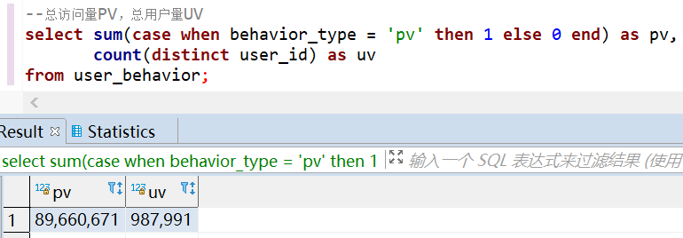
71 |
72 | ```sql
73 | --日均访问量,日均用户量
74 | select cast(datetime as date) as day,
75 | sum(case when behavior_type = 'pv' then 1 else 0 end) as pv,
76 | count(distinct user_id) as uv
77 | from user_behavior
78 | group by cast(datetime as date)
79 | order by day;
80 | ```
81 |
82 | 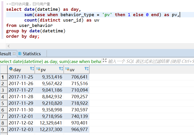
83 |
84 | 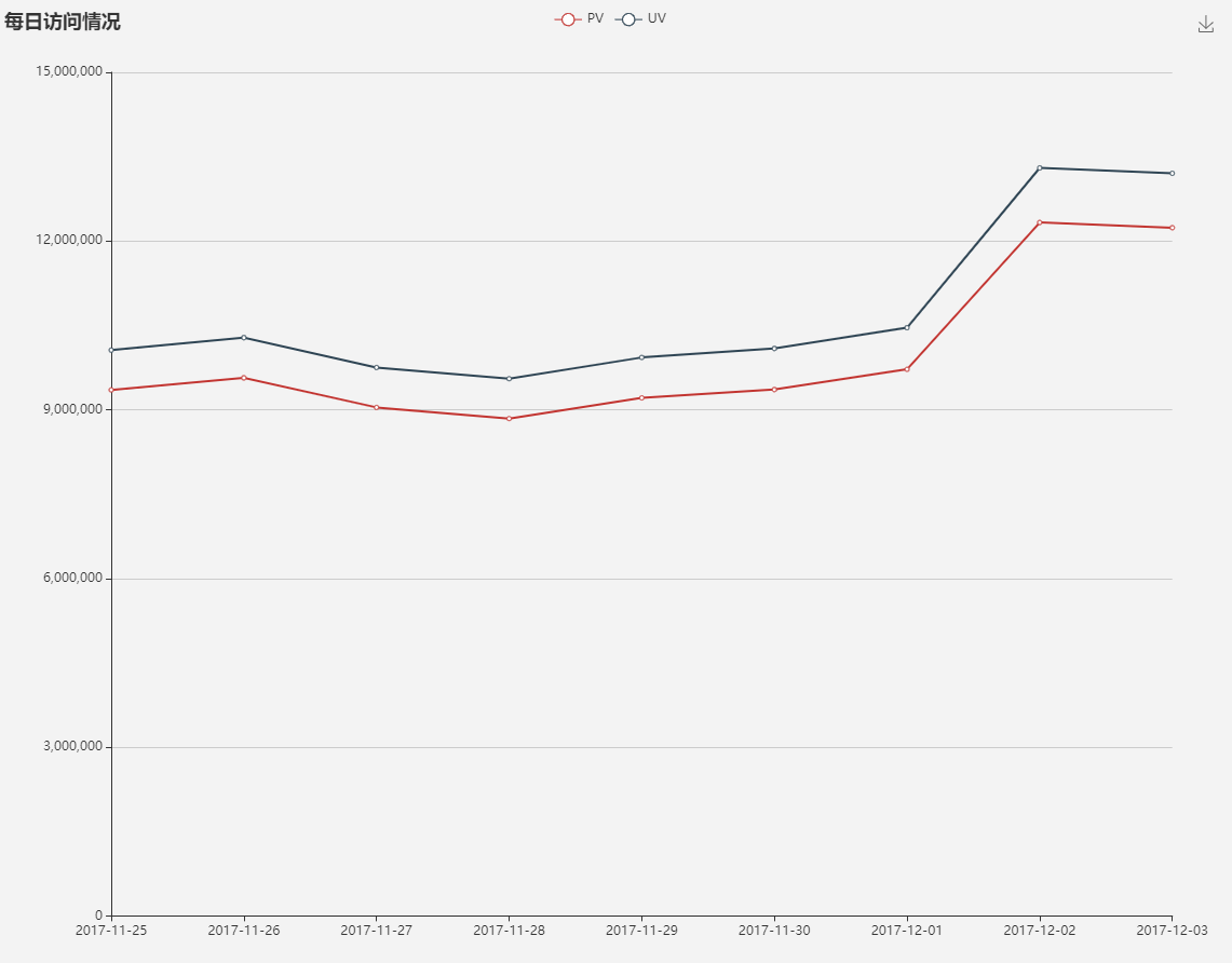
85 |
86 |
87 | ```sql
88 | --每个用户的购物情况,加工到 user_behavior_count
89 | create table user_behavior_count as
90 | select user_id,
91 | sum(case when behavior_type = 'pv' then 1 else 0 end) as pv, --点击数
92 | sum(case when behavior_type = 'fav' then 1 else 0 end) as fav, --收藏数
93 | sum(case when behavior_type = 'cart' then 1 else 0 end) as cart, --加购物车数
94 | sum(case when behavior_type = 'buy' then 1 else 0 end) as buy --购买数
95 | from user_behavior
96 | group by user_id;
97 |
98 | --复购率:产生两次或两次以上购买的用户占购买用户的比例
99 | select sum(case when buy > 1 then 1 else 0 end) / sum(case when buy > 0 then 1 else 0 end)
100 | from user_behavior_count;
101 | ```
102 |
103 | 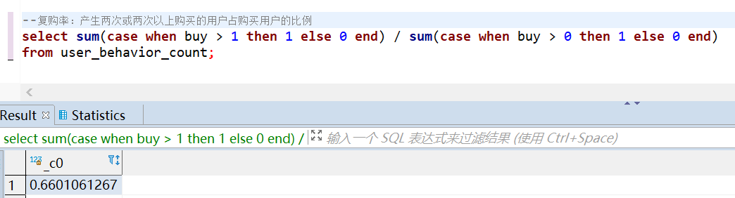
104 |
105 | * 小结:2017-11-25 到 2017-12-03 这段时间,PV 总数为 89,660,671 ,UV 总数为 987,991。从日均访问量趋势来看,进入 12 月份之后有一个比较明显的增长,猜测可能是因为临近双 12 ,电商活动引流产生,另外,2017-12-02 和 2017-12-03 刚好是周末,也可能是周末的用户活跃度本来就比平常高。总体的复购率为 66.01%,说明用户的忠诚度比较高。
106 |
107 | ## 3.2 用户行为转换率
108 |
109 | ```sql
110 | --点击/(加购物车+收藏)/购买 , 各环节转化率
111 | select a.pv,
112 | a.fav,
113 | a.cart,
114 | a.fav + a.cart as `fav+cart`,
115 | a.buy,
116 | round((a.fav + a.cart) / a.pv, 4) as pv2favcart,
117 | round(a.buy / (a.fav + a.cart), 4) as favcart2buy,
118 | round(a.buy / a.pv, 4) as pv2buy
119 | from(
120 | select sum(pv) as pv, --点击数
121 | sum(fav) as fav, --收藏数
122 | sum(cart) as cart, --加购物车数
123 | sum(buy) as buy --购买数
124 | from user_behavior_count
125 | ) as a;
126 | ```
127 |
128 | 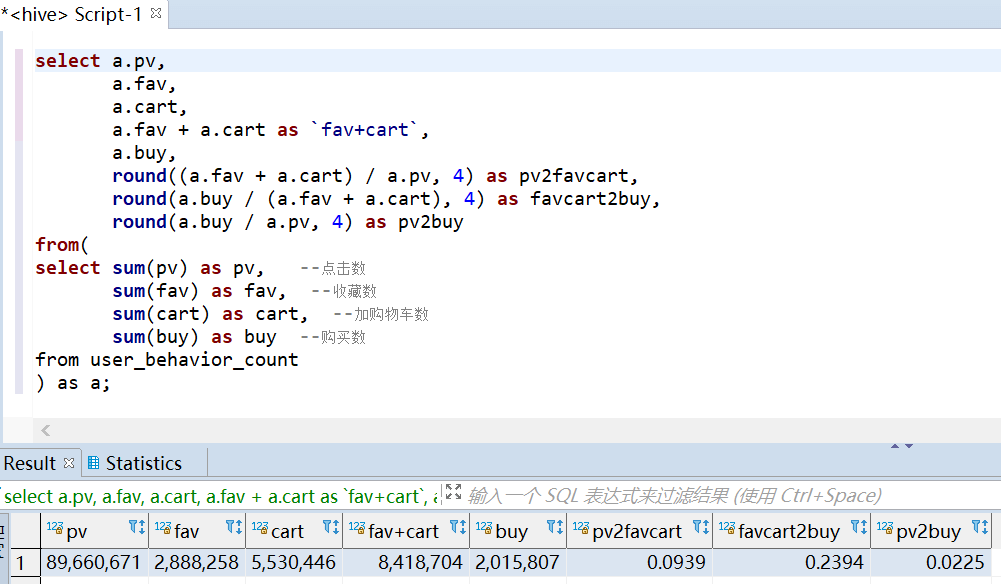
129 |
130 | 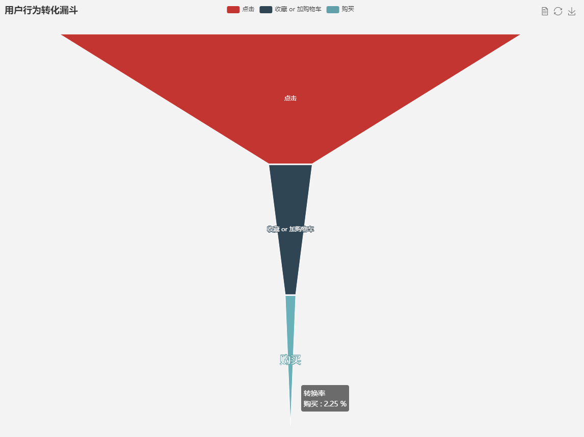
131 |
132 | * 小结:2017-11-25 到 2017-12-03 这段时间,点击数为 89,660,671 ,收藏数为 2,888,258,加购物车数为5,530,446,购买数为 2,015,807。总体的转化率为 2.25%,这个值可能是比较低的,从加到购物车数来看,有可能部分用户是准备等到电商节日活动才进行购买。所以合理推断:一般电商节前一段时间的转化率会比平常低。
133 |
134 | ## 3.3 用户行为习惯
135 |
136 | ```sql
137 | -- 一天的活跃时段分布
138 | select hour(datetime) as hour,
139 | sum(case when behavior_type = 'pv' then 1 else 0 end) as pv, --点击数
140 | sum(case when behavior_type = 'fav' then 1 else 0 end) as fav, --收藏数
141 | sum(case when behavior_type = 'cart' then 1 else 0 end) as cart, --加购物车数
142 | sum(case when behavior_type = 'buy' then 1 else 0 end) as buy --购买数
143 | from user_behavior
144 | group by hour(datetime)
145 | order by hour;
146 | ```
147 |
148 | 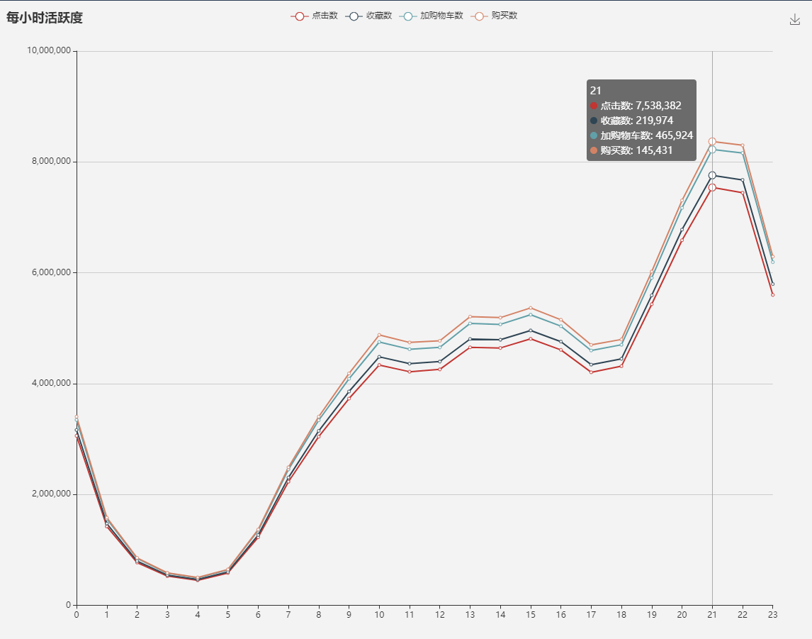
149 |
150 | ```sql
151 | --一周用户的活跃分布
152 | select pmod(datediff(datetime, '1920-01-01') - 3, 7) as weekday,
153 | sum(case when behavior_type = 'pv' then 1 else 0 end) as pv, --点击数
154 | sum(case when behavior_type = 'fav' then 1 else 0 end) as fav, --收藏数
155 | sum(case when behavior_type = 'cart' then 1 else 0 end) as cart, --加购物车数
156 | sum(case when behavior_type = 'buy' then 1 else 0 end) as buy --购买数
157 | from user_behavior
158 | where date(datetime) between '2017-11-27' and '2017-12-03'
159 | group by pmod(datediff(datetime, '1920-01-01') - 3, 7)
160 | order by weekday;
161 | ```
162 |
163 | 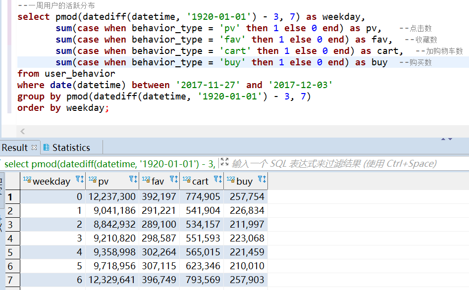
164 |
165 | 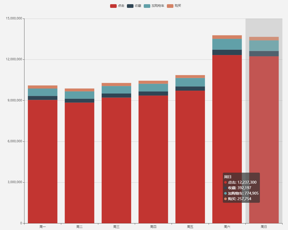
166 |
167 | * 小结:晚上21点-22点之间是用户一天中最活跃的时候,凌晨 4 点,则是活跃度最低的时候。一周中,工作日活跃度都差不多,到了周末活跃度有明显提高。
168 |
169 | ## 3.4 基于 RFM 模型找出有价值的用户
170 |
171 | RFM 模型是衡量客户价值和客户创利能力的重要工具和手段,其中由3个要素构成了数据分析最好的指标,分别是:
172 | * R-Recency(最近一次购买时间)
173 | * F-Frequency(消费频率)
174 | * M-Money(消费金额)
175 |
176 | ```sql
177 | --R-Recency(最近一次购买时间), R值越高,一般说明用户比较活跃
178 | select user_id,
179 | datediff('2017-12-04', max(datetime)) as R,
180 | dense_rank() over(order by datediff('2017-12-04', max(datetime))) as R_rank
181 | from user_behavior
182 | where behavior_type = 'buy'
183 | group by user_id
184 | limit 10;
185 |
186 | --F-Frequency(消费频率), F值越高,说明用户越忠诚
187 | select user_id,
188 | count(1) as F,
189 | dense_rank() over(order by count(1) desc) as F_rank
190 | from user_behavior
191 | where behavior_type = 'buy'
192 | group by user_id
193 | limit 10;
194 |
195 | --M-Money(消费金额),数据集无金额,所以就不分析这一项
196 | ```
197 |
198 | 对有购买行为的用户按照排名进行分组,共划分为5组,
199 | 前 - 1/5 的用户打5分
200 | 前 1/5 - 2/5 的用户打4分
201 | 前 2/5 - 3/5 的用户打3分
202 | 前 3/5 - 4/5 的用户打2分
203 | 前 4/5 - 的用户打1分
204 | 按照这个规则分别对用户时间间隔排名打分和购买频率排名打分,最后把两个分数合并在一起作为该名用户的最终评分
205 |
206 | ```sql
207 | with cte as(
208 | select user_id,
209 | datediff('2017-12-04', max(datetime)) as R,
210 | dense_rank() over(order by datediff('2017-12-04', max(datetime))) as R_rank,
211 | count(1) as F,
212 | dense_rank() over(order by count(1) desc) as F_rank
213 | from user_behavior
214 | where behavior_type = 'buy'
215 | group by user_id)
216 |
217 | select user_id, R, R_rank, R_score, F, F_rank, F_score, R_score + F_score AS score
218 | from(
219 | select *,
220 | case ntile(5) over(order by R_rank) when 1 then 5
221 | when 2 then 4
222 | when 3 then 3
223 | when 4 then 2
224 | when 5 then 1
225 | end as R_score,
226 | case ntile(5) over(order by F_rank) when 1 then 5
227 | when 2 then 4
228 | when 3 then 3
229 | when 4 then 2
230 | when 5 then 1
231 | end as F_score
232 | from cte
233 | ) as a
234 | order by score desc
235 | limit 20;
236 | ```
237 |
238 | 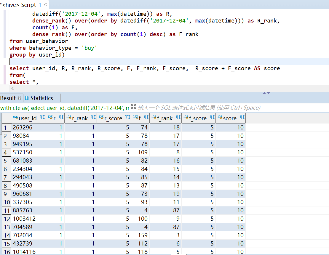
239 |
240 | * 小结:可以根据用户的价值得分,进行个性化的营销推荐。
241 |
242 | ## 3.5 商品维度的分析
243 |
244 | ```sql
245 | --销量最高的商品
246 | select item_id ,
247 | sum(case when behavior_type = 'pv' then 1 else 0 end) as pv, --点击数
248 | sum(case when behavior_type = 'fav' then 1 else 0 end) as fav, --收藏数
249 | sum(case when behavior_type = 'cart' then 1 else 0 end) as cart, --加购物车数
250 | sum(case when behavior_type = 'buy' then 1 else 0 end) as buy --购买数
251 | from user_behavior
252 | group by item_id
253 | order by buy desc
254 | limit 10;
255 |
256 | --销量最高的商品大类
257 | select category_id ,
258 | sum(case when behavior_type = 'pv' then 1 else 0 end) as pv, --点击数
259 | sum(case when behavior_type = 'fav' then 1 else 0 end) as fav, --收藏数
260 | sum(case when behavior_type = 'cart' then 1 else 0 end) as cart, --加购物车数
261 | sum(case when behavior_type = 'buy' then 1 else 0 end) as buy --购买数
262 | from user_behavior
263 | group by category_id
264 | order by buy desc
265 | limit 10;
266 | ```
267 |
268 | * 小结:缺失商品维表,所以没有太多分析价值。假如有商品维表,可以再展开,以商品纬度进行分析,比如不同行业、不同产品的转化率,还有竞品分析等等。
--------------------------------------------------------------------------------
/UserBehaviorFromTaobao_Stream/datagen.py:
--------------------------------------------------------------------------------
1 | #!/usr/bin/env python3
2 | # -*- coding: utf-8 -*-
3 | # @Time : 2020/5/27 14:24
4 | # @Author : way
5 | # @Site :
6 | # @Describe:
7 |
8 | import sys
9 | import time
10 | import json
11 | import queue
12 | from kafka import KafkaProducer
13 | from concurrent.futures import ThreadPoolExecutor
14 |
15 | servers = ['172.16.122.17:9092', ]
16 | topic = 'user_behavior'
17 | path = 'user_behavior.log'
18 |
19 | producer = KafkaProducer(bootstrap_servers=servers, value_serializer=lambda m: json.dumps(m).encode('utf-8'))
20 |
21 |
22 | def send(line):
23 | cols = line.strip('\n').split(',')
24 | ts = time.strftime("%Y-%m-%dT%H:%M:%SZ", time.localtime(int(cols[4])))
25 | value = {"user_id": cols[0], "item_id": cols[1], "category_id": cols[2], "behavior": cols[3], "ts": ts}
26 | producer.send(topic=topic, value=value).get(timeout=10)
27 |
28 |
29 | if __name__ == "__main__":
30 | num = 2000
31 |
32 | if len(sys.argv) > 1:
33 | num = int(sys.argv[1])
34 |
35 |
36 | class BoundThreadPoolExecutor(ThreadPoolExecutor):
37 |
38 | def __init__(self, *args, **kwargs):
39 | super(BoundThreadPoolExecutor, self).__init__(*args, **kwargs)
40 | self._work_queue = queue.Queue(num * 2)
41 |
42 |
43 | with open(path, 'r', encoding='utf-8') as f:
44 | pool = BoundThreadPoolExecutor(max_workers=num)
45 | # for result in pool.map(send, f):
46 | # ...
47 | for arg in f:
48 | pool.submit(send, arg)
49 | pool.shutdown(wait=True)
50 |
--------------------------------------------------------------------------------
/UserBehaviorFromTaobao_Stream/flink-user_behavior.sql:
--------------------------------------------------------------------------------
1 | -- 创建 kafka 表, 读取 kafka 数据
2 | CREATE TABLE user_behavior (
3 | user_id BIGINT,
4 | item_id BIGINT,
5 | category_id BIGINT,
6 | behavior STRING,
7 | ts TIMESTAMP(3),
8 | proctime as PROCTIME(),
9 | WATERMARK FOR ts as ts - INTERVAL '5' SECOND
10 | ) WITH (
11 | 'connector.type' = 'kafka',
12 | 'connector.version' = 'universal',
13 | 'connector.topic' = 'user_behavior',
14 | 'connector.startup-mode' = 'earliest-offset',
15 | 'connector.properties.zookeeper.connect' = '172.16.122.24:2181',
16 | 'connector.properties.bootstrap.servers' = '172.16.122.17:9092',
17 | 'format.type' = 'json'
18 | );
19 | --SELECT * FROM user_behavior;
20 |
21 | -- 每小时的成交量
22 | CREATE TABLE buy_cnt_per_hour (
23 | hour_of_day BIGINT,
24 | buy_cnt BIGINT
25 | ) WITH (
26 | 'connector.type' = 'elasticsearch',
27 | 'connector.version' = '7',
28 | 'connector.hosts' = 'http://172.16.122.13:9200',
29 | 'connector.index' = 'buy_cnt_per_hour',
30 | 'connector.document-type' = 'user_behavior',
31 | 'connector.bulk-flush.max-actions' = '1',
32 | 'update-mode' = 'append',
33 | 'format.type' = 'json'
34 | );
35 |
36 | -- 统计每小时的成交量
37 | INSERT INTO buy_cnt_per_hour
38 | SELECT HOUR(TUMBLE_START(ts, INTERVAL '1' HOUR)), COUNT(*)
39 | FROM user_behavior
40 | WHERE behavior = 'buy'
41 | GROUP BY TUMBLE(ts, INTERVAL '1' HOUR);
42 |
43 | --存放每10分钟累计独立用户数
44 | CREATE TABLE cumulative_uv (
45 | time_str STRING,
46 | uv BIGINT
47 | ) WITH (
48 | 'connector.type' = 'elasticsearch',
49 | 'connector.version' = '7',
50 | 'connector.hosts' = 'http://172.16.122.13:9200',
51 | 'connector.index' = 'cumulative_uv',
52 | 'connector.document-type' = 'user_behavior',
53 | 'update-mode' = 'upsert',
54 | 'format.type' = 'json'
55 | );
56 |
57 | -- 累计独立用户数统计视图
58 | CREATE VIEW uv_per_10min AS
59 | SELECT
60 | MAX(SUBSTR(DATE_FORMAT(ts, 'HH:mm'),1,4) || '0') OVER w AS time_str,
61 | COUNT(DISTINCT user_id) OVER w AS uv
62 | FROM user_behavior
63 | WINDOW w AS (ORDER BY proctime ROWS BETWEEN UNBOUNDED PRECEDING AND CURRENT ROW);
64 |
65 |
66 | -- 统计每10分钟的累计独立用户数
67 | INSERT INTO cumulative_uv
68 | SELECT time_str, MAX(uv)
69 | FROM uv_per_10min
70 | GROUP BY time_str;
71 |
72 | -- 创建商品类目维表
73 | CREATE TABLE category_dim (
74 | sub_category_id BIGINT,
75 | parent_category_name STRING
76 | ) WITH (
77 | 'connector.type' = 'jdbc',
78 | 'connector.url' = 'jdbc:mysql://172.16.122.25:3306/flink',
79 | 'connector.table' = 'category',
80 | 'connector.driver' = 'com.mysql.jdbc.Driver',
81 | 'connector.username' = 'root',
82 | 'connector.password' = 'root',
83 | 'connector.lookup.cache.max-rows' = '5000',
84 | 'connector.lookup.cache.ttl' = '10min'
85 | );
86 |
87 | -- 存放商品类目排行表
88 | CREATE TABLE top_category (
89 | category_name STRING,
90 | buy_cnt BIGINT
91 | ) WITH (
92 | 'connector.type' = 'elasticsearch',
93 | 'connector.version' = '7',
94 | 'connector.hosts' = 'http://172.16.122.13:9200',
95 | 'connector.index' = 'top_category',
96 | 'connector.document-type' = 'user_behavior',
97 | 'update-mode' = 'upsert',
98 | 'format.type' = 'json'
99 | );
100 |
101 | --商品类目销量视图
102 | CREATE VIEW rich_user_behavior AS
103 | SELECT U.user_id, U.item_id, U.behavior, C.parent_category_name as category_name
104 | FROM user_behavior AS U LEFT JOIN category_dim FOR SYSTEM_TIME AS OF U.proctime AS C
105 | ON U.category_id = C.sub_category_id;
106 |
107 |
108 | --统计商品类目销量排行
109 | INSERT INTO top_category
110 | SELECT category_name, COUNT(*) buy_cnt
111 | FROM rich_user_behavior
112 | WHERE behavior = 'buy'
113 | GROUP BY category_name;
--------------------------------------------------------------------------------
/UserBehaviorFromTaobao_Stream/用户行为数据实时分析.md:
--------------------------------------------------------------------------------
1 | [TOC]
2 |
3 | # 1、环境准备
4 |
5 | ## 1.1 flink 下载相关 jar 包
6 |
7 | flink-sql 连接外部系统时,需要依赖特定的 jar 包,所以需要事先把这些 jar 包准备好。[说明与下载入口](https://ci.apache.org/projects/flink/flink-docs-release-1.10/dev/table/connect.html)
8 |
9 | 本项目使用到了以下的 jar 包 ,下载后直接放在了 flink/lib 里面。
10 |
11 | > 需要注意的是 flink-sql 执行时,是转化为 flink-job 提交到集群执行的,所以 flink 集群的每一台机器都要添加以下的 jar 包。
12 |
13 | | 外部 | 版本 | jar |
14 | | ------------- | ---- | ------------------------------------------------------------ |
15 | | kafka | 4.1 | flink-sql-connector-kafka_2.11-1.10.2.jar
flink-json-1.10.2-sql-jar.jar |
16 | | elasticsearch | 7.6 | flink-sql-connector-elasticsearch7_2.11-1.10.2.jar |
17 | | mysql | 5.7 | flink-jdbc_2.11-1.10.2.jar
mysql-connector-java-8.0.11.jar |
18 |
19 |
20 | ## 1.2 生成 kafka 数据
21 |
22 | 用户行为数据来源: [阿里云天池公开数据集](https://tianchi.aliyun.com/dataset/dataDetail?dataId=649)
23 |
24 | > 网盘:https://pan.baidu.com/s/1CPD5jpmvOUvg1LETAVETGw 提取码:m4mc
25 |
26 |
27 | 商品类目纬度数据来源: [category.sql](https://github.com/TurboWay/bigdata_analyse/blob/main/UserBehaviorFromTaobao_Stream/category.sql)
28 |
29 | 数据生成器:[datagen.py](https://github.com/TurboWay/bigdata_analyse/blob/main/UserBehaviorFromTaobao_Stream/datagen.py)
30 |
31 | > 有了数据文件之后,使用 python 读取文件数据,然后并发写入到 kafka。
32 |
33 | > 修改生成器中的 kafka 地址配置,然后运行 以下命令,开始不断往 kafka 写数据
34 |
35 | ```shell
36 | # 5000 并发
37 | nohup python3 datagen.py 5000 &
38 | ```
39 |
40 | ## 1.3 开发前的三个小 tip
41 |
42 | * 生成器往 kafka 写数据,会自动创建主题,无需事先创建
43 |
44 | * flink 往 elasticsearch 写数据,会自动创建索引,无需事先创建
45 |
46 | * Kibana 使用索引模式从 Elasticsearch 索引中检索数据,以实现诸如可视化等功能。
47 | > 使用的逻辑为:创建索引模式 》Discover (发现) 查看索引数据 》visualize(可视化)创建可视化图表》dashboards(仪表板)创建大屏,即汇总多个可视化的图表
48 |
49 |
50 |
51 | # 2、flink-sql 客户端编写运行 sql
52 |
53 | ```shell
54 | # 进入 flink-sql 客户端, 需要指定刚刚下载的 jar 包目录
55 | ./bin/sql-client.sh embedded -l lib
56 | ```
57 |
58 | ## 2.1 创建 kafka 数据源表
59 |
60 | ```sql
61 | -- 创建 kafka 表, 读取 kafka 数据
62 | CREATE TABLE user_behavior (
63 | user_id BIGINT,
64 | item_id BIGINT,
65 | category_id BIGINT,
66 | behavior STRING,
67 | ts TIMESTAMP(3),
68 | proctime as PROCTIME(),
69 | WATERMARK FOR ts as ts - INTERVAL '5' SECOND
70 | ) WITH (
71 | 'connector.type' = 'kafka',
72 | 'connector.version' = 'universal',
73 | 'connector.topic' = 'user_behavior',
74 | 'connector.startup-mode' = 'earliest-offset',
75 | 'connector.properties.zookeeper.connect' = '172.16.122.24:2181',
76 | 'connector.properties.bootstrap.servers' = '172.16.122.17:9092',
77 | 'format.type' = 'json'
78 | );
79 | SELECT * FROM user_behavior;
80 | ```
81 |
82 | ## 2.2 指标统计:每小时成交量
83 |
84 | ### 2.2.1 创建 es 结果表, 存放每小时的成交量
85 |
86 | ```sql
87 | CREATE TABLE buy_cnt_per_hour (
88 | hour_of_day BIGINT,
89 | buy_cnt BIGINT
90 | ) WITH (
91 | 'connector.type' = 'elasticsearch',
92 | 'connector.version' = '7',
93 | 'connector.hosts' = 'http://172.16.122.13:9200',
94 | 'connector.index' = 'buy_cnt_per_hour',
95 | 'connector.document-type' = 'user_behavior',
96 | 'connector.bulk-flush.max-actions' = '1',
97 | 'update-mode' = 'append',
98 | 'format.type' = 'json'
99 | );
100 | ```
101 |
102 | ### 2.2.2 执行 sql ,统计每小时的成交量
103 |
104 | ```sql
105 | INSERT INTO buy_cnt_per_hour
106 | SELECT HOUR(TUMBLE_START(ts, INTERVAL '1' HOUR)), COUNT(*)
107 | FROM user_behavior
108 | WHERE behavior = 'buy'
109 | GROUP BY TUMBLE(ts, INTERVAL '1' HOUR);
110 | ```
111 |
112 | ## 2.3 指标统计:每10分钟累计独立用户数
113 |
114 | ### 2.3.1 创建 es 结果表,存放每10分钟累计独立用户数
115 |
116 | ```sql
117 | CREATE TABLE cumulative_uv (
118 | time_str STRING,
119 | uv BIGINT
120 | ) WITH (
121 | 'connector.type' = 'elasticsearch',
122 | 'connector.version' = '7',
123 | 'connector.hosts' = 'http://172.16.122.13:9200',
124 | 'connector.index' = 'cumulative_uv',
125 | 'connector.document-type' = 'user_behavior',
126 | 'update-mode' = 'upsert',
127 | 'format.type' = 'json'
128 | );
129 | ```
130 |
131 | ### 2.3.2 创建视图
132 |
133 | ```sql
134 | CREATE VIEW uv_per_10min AS
135 | SELECT
136 | MAX(SUBSTR(DATE_FORMAT(ts, 'HH:mm'),1,4) || '0') OVER w AS time_str,
137 | COUNT(DISTINCT user_id) OVER w AS uv
138 | FROM user_behavior
139 | WINDOW w AS (ORDER BY proctime ROWS BETWEEN UNBOUNDED PRECEDING AND CURRENT ROW);
140 | ```
141 |
142 | ### 2.3.3 执行 sql ,统计每10分钟的累计独立用户数
143 | ```sql
144 | INSERT INTO cumulative_uv
145 | SELECT time_str, MAX(uv)
146 | FROM uv_per_10min
147 | GROUP BY time_str;
148 | ```
149 |
150 | ## 2.4 指标统计:商品类目销量排行
151 |
152 | ### 2.4.1 创建商品类目维表
153 |
154 | 先在 mysql 创建一张商品类目的维表,然后配置 flink 读取 mysql。
155 |
156 | ```sql
157 | CREATE TABLE category_dim (
158 | sub_category_id BIGINT,
159 | parent_category_name STRING
160 | ) WITH (
161 | 'connector.type' = 'jdbc',
162 | 'connector.url' = 'jdbc:mysql://172.16.122.25:3306/flink',
163 | 'connector.table' = 'category',
164 | 'connector.driver' = 'com.mysql.jdbc.Driver',
165 | 'connector.username' = 'root',
166 | 'connector.password' = 'root',
167 | 'connector.lookup.cache.max-rows' = '5000',
168 | 'connector.lookup.cache.ttl' = '10min'
169 | );
170 | ```
171 |
172 | ### 2.4.1 创建 es 结果表,存放商品类目排行表
173 |
174 | ```sql
175 | CREATE TABLE top_category (
176 | category_name STRING,
177 | buy_cnt BIGINT
178 | ) WITH (
179 | 'connector.type' = 'elasticsearch',
180 | 'connector.version' = '7',
181 | 'connector.hosts' = 'http://172.16.122.13:9200',
182 | 'connector.index' = 'top_category',
183 | 'connector.document-type' = 'user_behavior',
184 | 'update-mode' = 'upsert',
185 | 'format.type' = 'json'
186 | );
187 | ```
188 |
189 | ### 2.4.2 创建视图
190 |
191 | ```sql
192 | CREATE VIEW rich_user_behavior AS
193 | SELECT U.user_id, U.item_id, U.behavior, C.parent_category_name as category_name
194 | FROM user_behavior AS U LEFT JOIN category_dim FOR SYSTEM_TIME AS OF U.proctime AS C
195 | ON U.category_id = C.sub_category_id;
196 | ```
197 |
198 | ### 2.4.3 执行 sql , 统计商品类目销量排行
199 |
200 | ```sql
201 | INSERT INTO top_category
202 | SELECT category_name, COUNT(*) buy_cnt
203 | FROM rich_user_behavior
204 | WHERE behavior = 'buy'
205 | GROUP BY category_name;
206 | ```
207 |
208 | # 3、最终效果与体验心得
209 |
210 | ## 3.1 最终效果
211 |
212 | 整个开发过程,只用到了 flink-sql ,无需写 java 或者其它代码,就完成了这样一个实时报表。
213 |
214 | 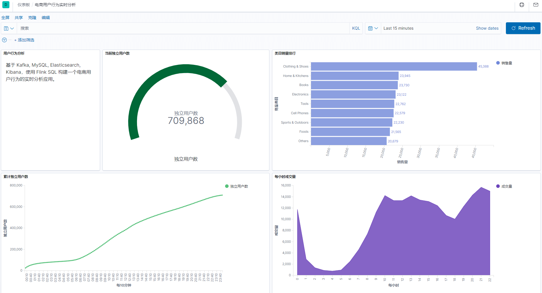
215 |
216 | ## 3.2 体验心得
217 |
218 | ### 3.2.1 执行
219 |
220 | * flink-sql 的 ddl 语句不会触发 flink-job , 同时创建的表、视图仅在会话级别有效。
221 |
222 | * 对于连接表的 insert、select 等操作,则会触发相应的流 job, 并自动提交到 flink 集群,无限地运行下去,直到主动取消或者 job 报错。
223 |
224 | * flink-sql 客户端关闭后,对于已经提交到 flink 集群的 job 不会有任何影响。
225 |
226 | >本次开发,执行了 3 个 insert , 因此打开 flink 集群面板,可以看到有 3 个无限的流 job 。即使 kafka 数据全部写入完毕,关闭 flink-sql 客户端,这个 3 个 job 都不会停止。
227 | 
228 |
229 | ### 3.2.2 存储
230 |
231 | * flnik 本身不存储业务数据,只作为流批一体的引擎存在,所以主要的用法为读取外部系统的数据,处理后,再写到外部系统。
232 |
233 | * flink 本身的元数据,包括表、函数等,默认情况下只是存放在内存里面,所以仅会话级别有效。但是,似乎可以存储到 Hive Metastore 中,关于这一点就留到以后再实践。
234 |
235 | # 4、开源地址
236 |
237 | GitHub 地址:[https://github.com/TurboWay/bigdata_analyse/blob/main/UserBehaviorFromTaobao_Stream/](https://github.com/TurboWay/bigdata_analyse/blob/main/UserBehaviorFromTaobao_Stream/)
238 |
239 | # 5、参考
240 |
241 | - https://blog.csdn.net/ytp552200ytp/article/details/107508373?utm_medium=distribute.pc_relevant.none-task-blog-title-6&spm=1001.2101.3001.4242
242 |
243 | - https://www.cnblogs.com/qiu-hua/p/13940560.html
244 |
--------------------------------------------------------------------------------