├── test
├── __init__.py
└── test_vevesta.py
├── vevestaX
└── __init__.py
├── sampleCode
├── data.csv
├── pysparktest.py
├── sampleExperiment.py
└── sampleExperiment.ipynb
├── requirements.txt
├── setup.py
├── tutorials
├── Overfitting in Shallow and Deep Neural Network.md
├── Do_you_really_need_a_feature_store.md
├── Deep Neural Network with Skip Connections.md
├── ImageAugmentation
│ └── imageAugmentation-tutorial.md
├── Dropout Layer.md
├── Plateau_Problem.md
├── Clustering
│ ├── Kmeans
│ │ └── tutorial_kmeans.md
│ ├── affinityPropagation
│ │ └── affinityPropagationTutorial.md
│ └── DBScan
│ │ └── DBScan tutorial.md
├── classification_featureSelectionByFRUPS
│ ├── FRUFS_tutorial.md.md
│ └── wine.csv
├── LIME
│ ├── Tabular
│ │ └── LIME_Tabular_Tutorial.md
│ └── NLP
│ │ └── Tutorial_LIME_NLP.md
├── FTRL.md
├── CLR_convergence.md
├── Attention Network.md
├── Predicting Future Weights of Neural Network.md
├── Lottery Ticket Hypothesis.md
├── Diffusion Models.md
├── Distributed Training.md
├── Noisy Labels with Deep Neural Networks.md
├── ZIP_models
│ └── ZIP_tutorial.md
└── AI-Fairness-Bias
│ └── AI Fairness Bias - tutorial.md
├── README.md
└── LICENSE
/test/__init__.py:
--------------------------------------------------------------------------------
1 |
--------------------------------------------------------------------------------
/vevestaX/__init__.py:
--------------------------------------------------------------------------------
1 | __version__ = '6.8.1'
2 |
--------------------------------------------------------------------------------
/test/test_vevesta.py:
--------------------------------------------------------------------------------
1 | from vevestaX import vevestaX
2 | def test_test():
3 | print(vevestaX.test())
4 | obj = vevestaX.V()
5 |
6 |
--------------------------------------------------------------------------------
/sampleCode/data.csv:
--------------------------------------------------------------------------------
1 | Gender,Age,Months_Count,Salary,Expenditure,House_Price
2 | 1,2,3,1,34,9884
3 | 1,2,34,0,56,2442
4 | 1,111,231,1,56,2421
5 | 0,49,65,0,156,6767
6 | 0,439,625,20,1256,452555
7 |
--------------------------------------------------------------------------------
/requirements.txt:
--------------------------------------------------------------------------------
1 | ipynbname==2021.3.2
2 | Jinja2==3.1.2
3 | matplotlib==3.5.2
4 | numpy==1.22.3
5 | openpyxl==3.0.9
6 | pandas==1.4.2
7 | pyspark==3.2.1
8 | requests==2.27.1
9 | scipy==1.8.0
10 |
11 | setuptools~=60.2.0
12 | PyGithub~=1.55
13 | img2pdf==0.4.4
--------------------------------------------------------------------------------
/setup.py:
--------------------------------------------------------------------------------
1 | from setuptools import find_packages, setup
2 | from vevestaX import __version__
3 |
4 | setup(
5 |
6 | name='vevestaX',
7 | packages=find_packages(include=['vevestaX']),
8 | version=__version__,
9 | description='Stupidly simple library to track machine learning experiments as well as features',
10 | author='Vevesta Labs',
11 | license='Apache 2.0',
12 | install_requires=['pandas','Jinja2','ipynbname','datetime','openpyxl','xlrd','requests','matplotlib','pyspark','numpy','scipy','statistics', 'PyGithub','img2pdf'],
13 | setup_requires=['pytest-runner'],
14 | tests_require=['pytest==4.4.1'],
15 | test_suite='tests',
16 |
17 | )
18 |
--------------------------------------------------------------------------------
/sampleCode/pysparktest.py:
--------------------------------------------------------------------------------
1 | from vevestaX import vevesta
2 | from pyspark.sql import SparkSession
3 | # import pandas as pd
4 |
5 | import os
6 | import sys
7 |
8 | os.environ['PYSPARK_PYTHON'] = sys.executable
9 | os.environ['PYSPARK_DRIVER_PYTHON'] = sys.executable
10 |
11 | V = vevesta.Experiment()
12 |
13 |
14 | spark = SparkSession.builder.appName("vevesta").getOrCreate()
15 | df_pyspark = spark.read.format("csv").option("header", "true").load("data.csv")
16 |
17 |
18 | sc = spark.sparkContext
19 | sc.setLogLevel("OFF")
20 |
21 | # df_pyspark = pd.read_csv("data.csv")
22 |
23 | V.dataSourcing = df_pyspark
24 | print(V.ds)
25 |
26 | # Do some feature engineering
27 | # df_pyspark["salary_feature"]= df_pyspark["Salary"] * 100/ df_pyspark["House_Price"]
28 | # df_pyspark['salary_ratio1']=df_pyspark["Salary"] * 100 / df_pyspark["Months_Count"] * 100
29 |
30 |
31 | # performing column operation on pyspark dataframe
32 | df_pyspark = df_pyspark.withColumn("salary_feature", df_pyspark.Salary*100 / df_pyspark.House_Price)
33 | df_pyspark = df_pyspark.withColumn("salary_ratio1", df_pyspark.Salary*100 / df_pyspark.Months_Count * 100)
34 |
35 | #Extract features engineered
36 | V.fe=df_pyspark
37 |
38 | #Print the features engineered
39 | print(V.fe)
40 |
41 | V.dump(techniqueUsed='XGBoost', filename="../vevestaX/vevestaDump.xlsx", message="precision is tracked", version=1)
42 | V.commit(techniqueUsed = "XGBoost", message="increased accuracy", version=1, projectId=122, attachmentFlag=True)
43 |
44 |
--------------------------------------------------------------------------------
/sampleCode/sampleExperiment.py:
--------------------------------------------------------------------------------
1 | #!/usr/bin/env python
2 | # coding: utf-8
3 |
4 | #import the vevesta Library
5 | from vevestaX import vevesta as v
6 |
7 | #create a vevestaX object
8 | V=v.Experiment()
9 |
10 | #read the dataset
11 | import pandas as pd
12 | df=pd.read_csv("data.csv")
13 |
14 | print(df.head(2))
15 |
16 | #Extract the columns names for features
17 | V.ds=df
18 | #you can also use:
19 | #V.dataSourcing = df
20 |
21 | #Print the feature being used
22 | print(V.ds)
23 |
24 | # Do some feature engineering
25 | df["salary_feature"]= df["Salary"] * 100/ df["House_Price"]
26 | df['salary_ratio1']=df["Salary"] * 100 / df["Months_Count"] * 100
27 |
28 | #Extract features engineered
29 | V.fe=df
30 |
31 | #you can also use:
32 | #V.featureEngineering = df
33 |
34 |
35 | #Print the features engineered
36 | print(V.fe)
37 |
38 | #Track variables which have been used for modelling
39 | V.start()
40 |
41 | #you can also use:
42 | #V.startModelling()
43 |
44 | #All the varibales mentioned here will be tracked
45 | epochs=1500
46 | seed=2000
47 | loss='rmse'
48 | accuracy= 91.2
49 |
50 | #end tracking of variables
51 | V.end()
52 | #you can also use V.endModelling()
53 |
54 |
55 | V.start()
56 | recall = 95
57 | precision = 87
58 | V.end()
59 |
60 | # Dump the datasourcing, features engineered and the variables tracked in a xlsx file
61 | V.dump(techniqueUsed='XGBoost',filename="vevestaDump.xlsx",message="precision is tracked",version=1)
62 |
63 | #if filename is not mentioned, then by default the data will be dumped to vevesta.xlsx file
64 | #V.dump(techniqueUsed='XGBoost')
65 |
66 |
--------------------------------------------------------------------------------
/tutorials/Overfitting in Shallow and Deep Neural Network.md:
--------------------------------------------------------------------------------
1 |
2 | # Quick overview of methods used to handle overfitting in Shallow and Deep Neural Network
3 |
4 | Overfitting is due to the fact that the model is complex, only memorizes the training data with limited generalizability and cannot correctly recognize different unseen data.
5 |
6 | 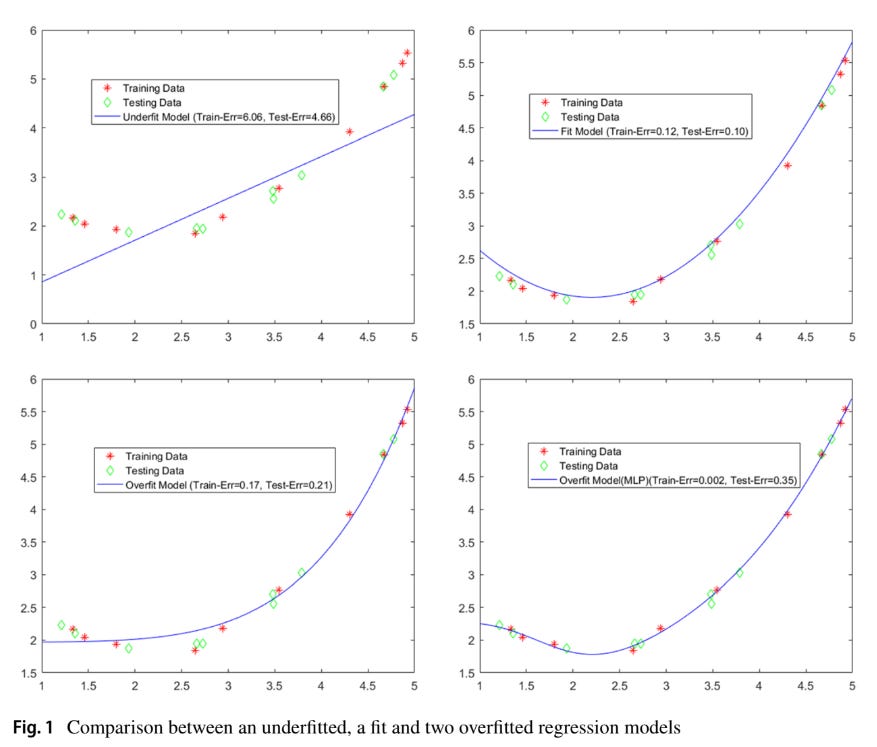
7 |
8 | According to [authors](https://link.springer.com/article/10.1007/s10462-021-09975-1), reasons for overfitting are as follows:
9 |
10 | 1. Noise of the training samples,
11 | 2. Lack of training samples (under-sampled training data),
12 | 3. Biased or disproportionate training samples,
13 | 4. Non-negligible variance of the estimation errors,
14 | 5. Multiple patterns with different non-linearity levels that need different learning models,
15 | 6. Biased predictions using different selections of variables,
16 | 7. Stopping training procedure before convergence or dropping in a local minimum,
17 | 8. Different distributions for training and testing samples.
18 |
19 | ## Methods to handle overfitting:
20 |
21 | 1. Passive Schemes: Methods meant to search for suitable configuration of the model/network and are some times called as Model selection techniques or hyper-parameter optimization techniques.
22 | 2. Active Schemes: Also, referred as regularization techniques, this method introduces dynamic noise during model training time.
23 | 3. Semi - Active Schemes: In this methodology, the network is changed during the training time. The same is achieved either by network pruning during training or addition of hidden units during the training.
24 |
25 | 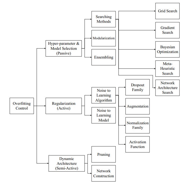
26 |
27 | ## References:
28 |
29 | 1. [A systematic review on overftting control in shallow and deep neural networks](https://link.springer.com/article/10.1007/s10462-021-09975-1)
30 | 2. [Overfitting in Shallow and Deep Neural Network on Vevesta](https://www.vevesta.com/blog/25-Handling-overfitting-in-Shallow-and-Deep-Neural-Network)
31 | 3. [Overfitting in Shallow and Deep Neural Network on Substack](https://vevesta.substack.com/p/deep-dive-in-causes-of-overfitting)
32 |
33 | ## Credits
34 |
35 | The above article is sponsored by [vevesta](https://www.vevesta.com/).
36 |
37 | [Vevesta](https://www.vevesta.com/): Your Machine Learning Team’s Feature and Technique Dictionary: Accelerate your Machine learning project by using features, techniques and projects used by your peers. Explore [Vevesta](https://www.vevesta.com/) for free. For more such stories, follow us on twitter at [@vevesta_labs](https://twitter.com/vevesta_labs).
--------------------------------------------------------------------------------
/tutorials/Do_you_really_need_a_feature_store.md:
--------------------------------------------------------------------------------
1 | # Do you really need a Feature Store ?
2 |
3 | 
4 |
5 | Photo by [Compare Fibre](https://unsplash.com/@comparefibre?utm_source=medium&utm_medium=referral) on [Unsplash](https://unsplash.com/?utm_source=medium&utm_medium=referral)
6 |
7 | Feature store’s strength lies predominantly in the fact that it brings data from disparate sources especially, time-stamped clickstream data and provides them to data scientists as and when needed. But a deeper dive reveals a lot of use cases that are dominant in the data science community and are in fact overlooked by feature stores.
8 |
9 | ## When are Feature Stores useful :
10 | Feature stores are useful since they enable data scientists to compute features on the server, say number of clicks. The alternative to this is computing features in the model itself or/and compute in a transform function in SQL.
11 |
12 | ## Where Feature Stores fail ?
13 | 1. **Steep learning curve:** The code that is required to integrate features with the feature store is not simple for a data scientist from non-programming backgrounds. Data Scientists are in general exposed to Pandas and SQL type of syntax. The learning curve required to work feature stores is by no means small.
14 |
15 | 2. **Little overlap in features being used:** Feature stores enables you to reuse features. In data science, features require some pre-processing, so either values are imputed in the features or some aggregation of features is done, say value of feature in the last 24 hours or last week. For feature stores to be of real use, not only do these features need to be computationally expensive, they also require reuse of features by multiple data science teams. But, this is generally not the case, each project will use its own data imputation and aggregation, depending on the problem at hand.
16 |
17 | 3. **Risk of change is pipelines:** Feature stores enable extensive collaboration between data scientists. But the implicit requirement is that data scientists for a particular project might use, say, imputation of mode during pre-processing, but then they later decide to change it to, say, mean. This will require the data scientist to create a new feature in the feature store and change his complete pipeline or change the definition of feature in feature store which in turn would require other data scientists dependent on the feature to change their pipelines, neither is a comfortable option.
18 | In short, feature stores are clearly suited for the narrow use case of creation of features from time series data that are extensively computationally expensive features. Most organizations don’t have this use case in place.
19 |
20 | ## Credits:
21 | The above article is sponsored by [***Vevesta.***](http://www.vevesta.com/?utm_source=Github_VevestaX_FeatureStore)
22 |
23 | [***Vevesta:***](http://www.vevesta.com/?utm_source=Github_VevestaX_FeatureStore) Your Machine Learning Team’s Collective Wiki: Save and Share your features and techniques.
24 |
25 | For more such stories, follow us on twitter at [@vevesta1](http://twitter.com/vevesta1).
26 |
27 | ## Author
28 | Priyanka
29 |
--------------------------------------------------------------------------------
/tutorials/Deep Neural Network with Skip Connections.md:
--------------------------------------------------------------------------------
1 |
2 | # Why is Everyone Training Very Deep Neural Network with Skip Connections?
3 |
4 | Deep neural networks (DNNs) have are a powerful means to train models on various learning tasks, with the capability to automatically learn relevant features. According to empirical studies, there seem to be positive correlation between model depth and generalization performance.
5 |
6 | Generally, training PlainNets (Neural networks without Skip Connections) with few number of layers (i.e. typically one to ten layers) is not problematic. But when model depth is increased beyond 10 layers, training difficulty can experienced. Training difficulty typically worsens with increase in depth, and sometimes even the training set cannot be fitted. For example, when training from scratch there was optimization failure for the VGG-13 model with 13 layers and VGG-16 model with 16 layers. Hence, VGG-13 model was trained by initializing its first 11 layers with the weights of the already trained VGG-11 model. Similar was the case with VGG-16. Currently, there is proliferation of networks, such as Resnet, FractalNet, etc which use skip connections.
7 |
8 | ## What are skip connections?
9 |
10 | Skip connections are where the outputs of preceding layers are connected (e.g. via summation or concatenation) to later layers. Architectures with more than 15 layers have increasingly turned to skip connections. According to empirical studies, skip connections alleviate training problems and improve model generalization. Although multiple weights initialization schemes and batch normalization can alleviate the training problems, optimizing PlainNets becomes absolutely impossible beyond a certain depth.
11 |
12 | ## Experimental Results
13 |
14 | Experiments were done on MNIST, CIFAR-10 and CIFAR-100 datasets using PlainNet, ResNet and ResNeXt, each having 164 layers.
15 |
16 | 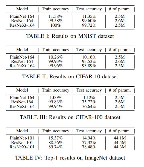
17 |
18 | Tables 1, 2, 3 and 4 show the obtained accuracies on the different datasets. Clearly it can be seen, as in figure 3 and figure 4, that PlainNets perform worser than networks with skip connections and are essentially untrainable. PlainNets failure to learn, given the very poor accuracies on the training sets.
19 |
20 | 
21 |
22 | ## Discussion and Observations:
23 |
24 | The plot of PlainNets activations and weights given below in Figure 5 and Figure 6.
25 |
26 | 
27 |
28 |
29 | 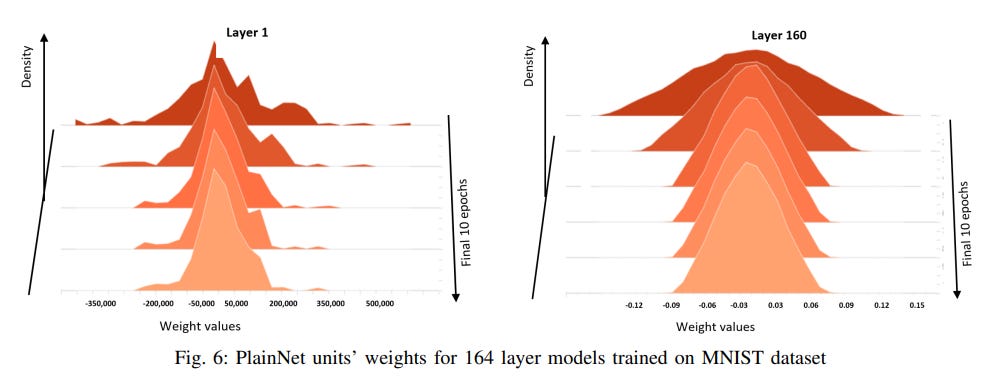
30 | The plot of ResNet unit’s activations and weights given below in Figure 7 and Figure 8.
31 |
32 | 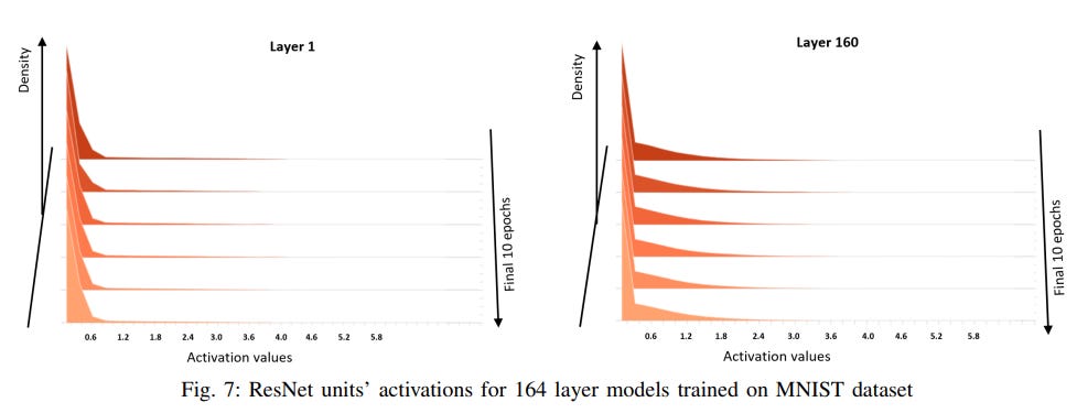
33 |
34 | 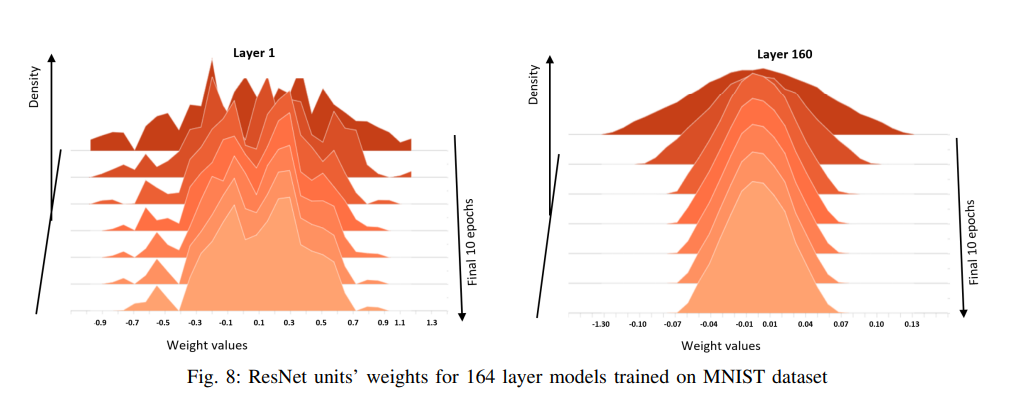
35 |
36 | According to authors of the [paper](https://orbilu.uni.lu/bitstream/10993/48927/1/TNNLS-2020-P-13752.pdf), the PlainNet trained on CIFAR10 dataset, starting from the eightieth layer, have hidden representations with infinite condition numbers; on CIFAR100 dataset, starting from the hundredth layer, the PlainNet’s hidden representations have infinite condition numbers. This observation depicts the worst scenario of the singularity problem for optimization such that model generalization is impossible as given in Remark 8. In contrast, the hidden representations of the ResNet never have infinite condition numbers; the condition numbers, which are high in the early layers quickly reduce to reasonable values so that optimization converges successfully.
37 |
38 | ## Conclusion
39 |
40 | Skip connections are a powerful means to train Deep Neural Networks.
41 |
42 | ## Credits
43 |
44 | The above article is sponsored by [Vevesta](https://www.vevesta.com/).
45 |
46 | [Vevesta](https://www.vevesta.com/): Your Machine Learning Team’s Feature and Technique Dictionary: Accelerate your Machine learning project by using features, techniques and projects used by your peers. Explore [Vevesta](https://www.vevesta.com/) for free. For more such stories, follow us on twitter at [@vevesta_labs](https://twitter.com/vevesta_labs).
47 |
48 | 100 early birds who login into [Vevesta](https://www.vevesta.com/) will get free subscription for 3 months
49 |
50 | Subscribe to receive a copy of our newsletter directly delivered to your inbox.
--------------------------------------------------------------------------------
/tutorials/ImageAugmentation/imageAugmentation-tutorial.md:
--------------------------------------------------------------------------------
1 | # Image Augmentation
2 | ## Introduction
3 |
4 | A deep learning model generally works well when it has a huge amount of data. In general, the more data we have better will be the performance of the model.
5 |
6 | 
7 | *Img Source: [Cousins of Artificial Intelligence | Seema Singh](https://towardsdatascience.com/cousins-of-artificial-intelligence-dda4edc27b55)*
8 |
9 | From the graph above, we can notice that as the amount of data increases the performance of the deep learning model also improves. But acquiring a massive amount of data is itself a major challenge. Every time it is not possible to have a large amount of data to feed the deep learning network.
10 |
11 | The problem with the lack of a good amount of data is that the deep learning model might not learn the patterns or the functions from the data and hence it might not perform well.
12 |
13 | So in order to deal with this and spending days manually collecting the data, we make use of Image Augmentation techniques.
14 |
15 | ## Image Data Augmentation
16 |
17 | Image data augmentation is a method that can be used to increase the size of a training database by creating modified versions of images in the database.
18 |
19 | It is a process of taking the images that are already present in the training dataset and manipulating them to create many altered versions. This not only provides more images to train on, but also help our classifier to expose a wider variety of lighting and coloring situations thus making it a more skillful model.
20 |
21 | 
22 |
23 | In the above figure, since all these images are generated from training data itself we don’t have to collect them manually. This increases the training sample without going out and collecting this data. Note that, the label for all the images will be the same and that is of the original image which is used to generate them.
24 |
25 | Point to be noted is that Image data augmentation is typically only applied to the training dataset, and not to the validation or test dataset. This is different from data preparation such as image resizing and pixel scaling; they must be performed consistently across all datasets that interact with the model.
26 |
27 | ## Image Augmentation With ImageDataGenerator
28 |
29 | The Keras deep learning library provides the ability to use data augmentation automatically when training a model.
30 |
31 | A range of techniques are supported, as well as pixel scaling methods. Few of them are:
32 |
33 | * Image shifts via the width_shift_range and height_shift_range arguments.
34 | * Image flips via the horizontal_flip and vertical_flip arguments.
35 | * Image rotations via the rotation_range argument
36 | * Image brightness via the brightness_range argument.
37 | * Image zoom via the zoom_range argument.
38 | Here in this article we will be restricting ourselves to the image augmentation by shifting the width range only, further augmentation like flipping the images, brightness and contrast, rotation etc. can be done by slight modification in the Hyper Parameters.
39 |
40 | Let us take the following image for augmentation purpose.
41 |
42 | 
43 |
44 | * Importing Libraries
45 | ```
46 | from numpy import expand_dims
47 | from keras.preprocessing.image import load_img
48 | from keras.preprocessing.image import img_to_array
49 | from keras.preprocessing.image import ImageDataGenerator
50 | from matplotlib import pyplot
51 | ```
52 | * Loading the image and preprocessing it.
53 | ```
54 | # load the image
55 | img = load_img('bird.jpg')
56 | # convert to numpy array
57 | data = img_to_array(img)
58 | # it is a function of numpy which expand dimension to one sample in specified axis here 0 that is horizontal
59 | samples = expand_dims(data, 0)
60 | ```
61 | * Creating image data augmentation generator and preparing iterator.
62 | ```
63 | # create image data augmentation generator
64 | datagen = ImageDataGenerator(width_shift_range=[-200,200])
65 | #the width_shift_range and height_shift_range arguments to the ImageDataGenerator constructor control the amount of horizontal and vertical shift respectively.
66 | # prepare iterator
67 | it = datagen.flow(samples, batch_size=1)
68 | ```
69 | * Plotting the augmented images
70 | ```
71 | # generate samples and plot
72 | for i in range(9):
73 | # define subplot
74 | pyplot.subplot(330 + 1 + i)
75 |
76 | # generate batch of images
77 | batch = it.next()
78 |
79 | # convert to unsigned integers for viewing
80 | image = batch[0].astype('uint8')
81 |
82 | # plot raw pixel data
83 | pyplot.imshow(image)
84 | # show the figure
85 | pyplot.show()
86 | ```
87 | 
88 |
89 | ## End Notes
90 |
91 | To summarize, If we are aiming to develop a robust and generalized deep learning model but do not have a large dataset, In such cases, image augmentation techniques come as a savior, as they allow us to generate a wide range of new data without much effort.
92 |
93 | ## References
94 |
95 | * [Machine Learning Mastery](https://machinelearningmastery.com/how-to-configure-image-data-augmentation-when-training-deep-learning-neural-networks/)
96 | * [Analytics Vidhya](https://www.analyticsvidhya.com/blog/2021/03/image-augmentation-techniques-for-training-deep-learning-models/)
97 |
98 |
--------------------------------------------------------------------------------
/tutorials/Dropout Layer.md:
--------------------------------------------------------------------------------
1 |
2 | # Uncovering Hidden Insights into Dropout Layer
3 |
4 | Problem faced in training deep neural networks
5 |
6 | Deep neural networks with a large number of parameters suffer from overfitting and are also slow to use.
7 |
8 |
9 | ## What is Dropout, in short?
10 |
11 | According to the authors, the key idea of dropout is based on randomly droping units (along with their connections) from the neural network during training. This stops units from “co-adapting too much”. During training, exponential number of different “thinned” networks are sampled. “At test time, it is easy to approximate the effect of averaging the predictions of all these thinned networks by simply using a single unthinned network that has smaller weights. This significantly reduces overfitting and gives major improvements over other regularization methods”. Also, dropout layer avoids co-adaptation of neurons by making it impossible for two subsequent neurons to rely solely on each other.
12 |
13 | Using dropout can be viewed as training a huge number of neural networks with shared parameters and applying bagging at test time for better generalization.
14 |
15 | 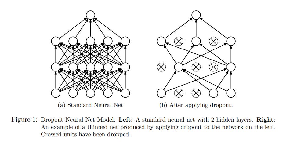
16 |
17 | ## Deep Dive into Dropout
18 |
19 | The term “dropout” refers to dropping out units, both hidden and visible, in a neural network. Dropping a neuron/unit out means temporarily removing it from the network along with all its incoming and outgoing connections. The choice of which units to drop is random. In the simplest case, each unit is retained with a fixed probability p independent of other units, where p can be chosen using a validation set.
20 |
21 | ### Things to keep in mind while using Dropout in experiments
22 |
23 | 1. For a wide variety of networks and tasks, dropout should be set to 0.5.
24 | 2. For input units, the optimal dropout is usually closer to 0 than 0.5, or alternatively, optimal probability of retention should be closer to 1.
25 | 3. Note that p is 1- (dropout probability) and dropout probability is what we set in neural network while coding in keras or Tensorflow.
26 | 4. While training network with SGD, dropout layer along with maxnorm regularization, large decaying learning rates and high momentum provides a significant boost over just using dropout.
27 |
28 | ### How does Dropout work?
29 |
30 | 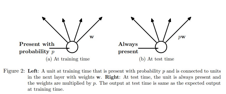
31 |
32 | As shown in Figure 2, during training, the unit/neuron is present with probability p and is connected with units in the next layer with weights, w. During testing phase, the unit is always present and its weights are multiplied by p.
33 |
34 | Dropout is applied to the neural network of n units and 2^n possible thinned neural networks are generated. A thinned neural network is a neural network which has dropped some units and their corresponding connections, as shown in figure 1b. The interesting part is that despite thinning, these networks all share weights so that the total number of parameters is still O(n^2), or less. During training phase for each data point, a certain permutation of units are switched off and a new thinned network is sampled and trained. Each thinned network gets trained very rarely, if at all.
35 |
36 | At test time, since it’s not feasible to explicitly average the predictions from exponentially many thinned models. The idea is that the full neural net is used at test time without dropout. Inorder to compensate for dropout being applied during training phase, if a neuron is retained with probability p during training, the outgoing weights of that neuron are multiplied by p at test time, as can be seen in Figure 2. By using this methodology, during the testing phase, 2^n networks with shared weights can be combined into a single neural network. According to [authors](http://cs.toronto.edu/~rsalakhu/papers/srivastava14a.pdf), it was noticed using this methodology leads to significantly lower generalization error on a wide variety of classification problems compared to training with other regularization methods.
37 |
38 | ## Applications of Dropout layer
39 |
40 | Few examples of domains where dropout is finding extensive use are as follows:
41 |
42 | 1. According to Merity et al., dropout is the norm for NLP problems as it is much more effective than methods such as L2 regularization
43 | 2. In vision, dropout is often used to train extremely large models such as EfficientNet-B7.
44 |
45 | ## References:
46 |
47 | 1. [Regularizing and Optimizing LSTM Language Models](https://arxiv.org/abs/1708.02182)
48 | 2. [EfficientNet: Rethinking Model Scaling for Convolutional Neural Networks](http://proceedings.mlr.press/v97/tan19a/tan19a.pdf)
49 | 3. [Dropout: A Simple Way to Prevent Neural Networks from Overfitting](https://www.cs.toronto.edu/~rsalakhu/papers/srivastava14a.pdf)
50 | 4. [Dropout as data augmentation](https://arxiv.org/pdf/1506.08700.pdf)
51 | 5. [Dropout Layer Article on Substack](https://vevesta.substack.com/p/uncovering-hidden-insights-into-dropout)
52 | 6. [Dropout Layer Article on Vevesta](https://www.vevesta.com/blog/21-Dropout-Layer)
53 |
54 | ## Credits:
55 |
56 | The above article is sponsored by [vevesta.](https://www.vevesta.com/)
57 |
58 | [Vevesta](https://www.vevesta.com/): Your Machine Learning Team’s Feature and Technique Dictionary: Accelerate your Machine learning project by using features, techniques and projects used by your peers. Explore [Vevesta](https://www.vevesta.com/) for free. For more such stories, follow us on twitter at [@vevesta_labs](https://twitter.com/vevesta_labs).
--------------------------------------------------------------------------------
/tutorials/Plateau_Problem.md:
--------------------------------------------------------------------------------
1 | # Pitfalls of early stopping neural network
2 | We've all noticed that after a certain number of training steps, the loss starts to slow significantly. After a long period of steady loss, the loss may abruptly resume dropping rapidly for no apparent reason, and this process will continue until we run out of steps.
3 |
4 | 
5 | [Image Credits](https://cdn-images-1.medium.com/max/900/0*rA05n6siCddLinjn.png).
6 |
7 | The loss falls rapidly for the first ten epochs, but thereafter tends to remain constant for a long time, as seen in Figure (a). Following that, the loss tends to reduce substantially, as illustrated in figure (b), before becoming practically constant.
8 |
9 | Many of us may base our decision on the curve depicted in fig (a), however the fact is that if we train our network for additional epochs, there is a probability that the model will converge at a better position.
10 |
11 | These plateaus complicate our judgement on when to stop the gradient drop and also slow down convergence because traversing a plateau in the expectation of minimising the loss demands more iterations.
12 |
13 | ## Cause of Plateau
14 | The formation of a plateau is caused primarily by two factors, which are as follows:
15 | * Saddle Point
16 | * Local Minima
17 |
18 | 
19 | [Image Credits](https://medium.com/r/?url=https%3A%2F%2Fwww.researchgate.net%2Ffigure%2FDefinition-of-grey-level-blobs-from-local-minima-and-saddle-points-2D-case_fig1_10651758).
20 |
21 | ## Saddle Point
22 |
23 | 
24 | [Image Credits](https://medium.com/r/?url=https%3A%2F%2Fen.wikipedia.org%2Fwiki%2FSaddle_point)
25 |
26 | The fundamental problem with saddle points is that the gradient of a function is zero at the saddle point, which does not reflect the greatest and minimum value. The gradient value optimises the machine learning and optimization algorithms in a neural network, and if the gradient is zero, the model becomes stalled.
27 |
28 | ## Local Minima
29 |
30 | 
31 | [Image Credits](https://www.researchgate.net/figure/1st-order-saddle-point-in-the-3-dimensional-surface-Surface-is-described-by-the_fig7_280804948)
32 |
33 | In this scenario, the point is an extremum, which is good, but the gradient is zero. We may not be able to escape the local minimum if our learning rate is too low. The loss value in our hypothetical training environment began balancing around some constant number, as shown in fig(a); one major explanation for this is the establishment of these types of local minimums.
34 |
35 | ## Effect of Learning Rate
36 | The learning rate hyperparameter determines how quickly the model learns. A higher learning rate allows the model to learn faster, but it may result in a less-than-ideal final set of weights. A slower learning rate, on the other hand, may allow the model to acquire a more optimal, or possibly a globally ideal, set of weights, but training will be much more time consuming. A sluggish learning rate has the disadvantage of never convergent or becoming stuck on a suboptimal solution.
37 |
38 | Thus, learning rate is important in overcoming the plateau problem; strategies such as scheduling the learning rate or cyclical learning rate are employed for this.
39 |
40 | ## Methods to Overcome a Plateau Problem
41 | Following are the approaches which might be used to tweak the learning rates in order to overcome the plateau problem:
42 |
43 | ## Scheduling the Learning Rate
44 | The most frequent method is to plan the learning rate, which suggests beginning with a reasonably high learning rate and gradually decreasing it over training. The concept is that we want to get from the initial parameters to a range of excellent parameter values as rapidly as possible, but we also want a low enough learning rate to explore the deeper, but narrower, regions of the loss function.
45 |
46 | 
47 | [Image Credits](https://medium.com/r/?url=https%3A%2F%2Fwww.researchgate.net%2Ffigure%2FStep-Decay-Learning-Rate_fig3_337159046)
48 |
49 | An example of this is Step decay in which the learning rate is lowered by a certain percentage after a certain number of training epochs.
50 |
51 | ## Cyclical Learning Rate
52 | Leslie Smith provided a cyclical learning rate scheduling approach with two bound values that fluctuate.
53 |
54 | Cyclical learning scheme displays a sublime balance between passing over local minima while still allowing us to look around in detail.
55 |
56 | 
57 |
58 | [Image Credits](https://medium.com/r/?url=https%3A%2F%2Farxiv.org%2Fpdf%2F1506.01186.pdf)
59 |
60 | Thus, scheduling the learning rate aids us in overcoming the plateau issues encountered while optimising neural networks
61 | ## References
62 | * [Analytics Vidhya](https://medium.com/r/?url=https%3A%2F%2Fanalyticsindiamag.com%2Fwhat-is-the-plateau-problem-in-neural-networks-and-how-to-fix-it%2F)
63 | * [Plateau Phenomenon by Mark Ainsworth](https://medium.com/r/?url=https%3A%2F%2Farxiv.org%2Fpdf%2F2007.07213.pdf)
64 | * [Cyclical Learning Rate](https://medium.com/r/?url=https%3A%2F%2Farxiv.org%2Fpdf%2F1506.01186.pdf)
65 | * [Find best learning rate on Plateau](https://medium.com/r/?url=https%3A%2F%2Fgithub.com%2FJonnoFTW%2Fkeras_find_lr_on_plateau)
66 | * [Original Article on Plateau](https://www.vevesta.com/blog/13-Early-stopping-of-neural-network-might-not-be-optimal-decision-Plateau-problem?utm_source=GitHub_VevestaX_plateauProblem)
67 |
68 | ## Credits
69 | [Vevesta](https://www.vevesta.com?utm_source=Github_VevestaX_Plateau) is Your Machine Learning Team's Collective Wiki: Save and Share your features and techniques. Explore [Vevesta](https://www.vevesta.com?utm_source=Github_VevestaX_Plateau) for free. For more such stories, follow us on twitter at [@vevesta1](http://twitter.com/vevesta1).
70 |
71 | ## Author
72 | Sarthak Kedia
73 |
--------------------------------------------------------------------------------
/tutorials/Clustering/Kmeans/tutorial_kmeans.md:
--------------------------------------------------------------------------------
1 |
2 | # Classification with K-Means and VevestaX library.
3 |
4 | In this article we will be focusing on a very well-known unsupervised machine learning technique 'K-Means' and will be using a very efficient python package known as 'VevestaX' in order to perform Exploratory Data Analysis and Experiment Tracking.
5 |
6 | ## Table of Contents
7 | 1. [K-Mean Clustering](https://github.com/Vevesta/VevestaX/blob/main/tutorials/Kmeans/tutorial_kmeans.md#k-mean-clustering)
8 | 2. [How the K-means algorithm works?](https://github.com/Vevesta/VevestaX/blob/main/tutorials/Kmeans/tutorial_kmeans.md#how-the-k-means-algorithm-works)
9 | 3. [VevestaX](https://github.com/Vevesta/VevestaX/blob/main/tutorials/Kmeans/tutorial_kmeans.md#vevestax)
10 | 4. [How To Use VevestaX?](https://github.com/Vevesta/VevestaX/blob/main/tutorials/Kmeans/tutorial_kmeans.md#how-to-use-vevestax)
11 | 5. [How to perform clustering using K Means and VevestaX?](https://github.com/Vevesta/VevestaX/blob/main/tutorials/Kmeans/tutorial_kmeans.md#how-to-perform-clustering-using-k-means-and-vevestax)
12 | 6. [References](https://github.com/Vevesta/VevestaX/blob/main/tutorials/Kmeans/tutorial_kmeans.md#references)
13 |
14 | ## K-Mean Clustering
15 | K-means clustering is one of the easiest and most popular unsupervised machine learning algorithms. Clustering algorithms are used to cluster similar data points, each based on their own definition of similarity. The K-means algorithm identifies the number of clusters, k and then assigns each data point to the nearest cluster.
16 |
17 | ## How the K-means algorithm works?
18 | While learning from the data, the K-means algorithm starts with a first group of randomly selected centroids. These centroids are used as the initial points assigned to every cluster. K-means performs iterative (repetitive) calculations to optimize the positions of the centroids. It does this by minimizing the distance of points from the centroid.
19 |
20 | It stops creating and optimizing the clusters when either:
21 |
22 | * There is no change in the values of the centroid because the clustering has been successful.
23 | * The defined number of iterations has been achieved.
24 |
25 | ## VevestaX
26 | VevestaX is an open source Python package which includes a variety of features that makes the work of a Data Scientist pretty much easier especially when it comes to analyses and getting the insights from the data.
27 |
28 | The package can be used to extract the features from the datasets and can track all the variables used in code.
29 |
30 | The best part of this package is about its output. The output file of the VevestaX provides us with numerous EDA tools like histograms, performance plots, correlation matrix and much more without writing the actual code for each of them separately.
31 |
32 | ## How To Use VevestaX?
33 | Install the package as follows:
34 |
35 | ```
36 | pip install vevestaX
37 | ```
38 |
39 | Import and create a vevesta object as follows:
40 |
41 | ```
42 | from vevestaX import vevesta as v
43 | V=v.Experiment()
44 | ```
45 |
46 | To track the feature used:
47 |
48 | ```
49 | V.ds = df
50 | ```
51 |
52 | where df is the pandas dataframe with the input features
53 |
54 | 
55 |
56 | To track features engineered
57 |
58 | ```
59 | V.fe = df
60 | ```
61 |
62 | Finally in order to dump the features and variables used into an excel file and to see the insights what the data carries use:
63 |
64 | ```
65 | V.dump(techniqueUsed="Model_Name",filename="vevestaDump.xlsx",message="precision is tracked",version=1)
66 | ```
67 |
68 |
69 | Following are the insights we received after dumping the features:
70 |
71 | 
72 |
73 | 
74 |
75 | 
76 |
77 | 
78 |
79 | 
80 |
81 | ## How to perform clustering using K Means and VevestaX?
82 |
83 | So what we have basically done is, firstly we have imported the necessary libraries and loaded the dataset.
84 |
85 | 
86 |
87 | Thereafter we had performed the train_test _split in order to get the train and test dataset.
88 |
89 | 
90 |
91 | Next, we cluster the data using K-Means. The number of clusters to be formed will be same as the classes in the data. The K-Means model is fitted on the train data and then the labels for test data are predicted. Finally, we calculate the baseline NMI score for the model.
92 |
93 | 
94 |
95 | Next in order to get the centroids of the clusters we used:
96 |
97 | ```
98 | model_kmeans.cluster_centers_
99 | ```
100 |
101 |
102 | 
103 |
104 | Finally we have dumped the data into Excel File using VevestaX.
105 |
106 | 
107 |
108 | [*For Source Code Click Here*](https://gist.github.com/sarthakkedia123/bd77515160a0b2d953266e0302268fd2)
109 |
110 | ## References
111 |
112 | 1. [VevestaX article](https://medium.com/@priyanka_60446/vevestax-open-source-library-to-track-failed-and-successful-machine-learning-experiments-and-data-8deb76254b9c)
113 | 2. [VevestaX GitHub Link](https://github.com/Vevesta/VevestaX)
114 | 3. [Article](https://www.vevesta.com/blog/4_Classification_with_K-Means_and_Vevestax_library?utm_source=Github_VevestaX_Kmeans)
115 |
116 | ## Credits
117 | [Vevesta](https://www.vevesta.com?utm_source=Github_VevestaX_Kmeans) is Your Machine Learning Team's Collective Wiki: Save and Share your features and techniques. Explore [Vevesta](https://www.vevesta.com?utm_source=Github_VevestaX_Kmeans) for free. For more such stories, follow us on twitter at [@vevesta1](http://twitter.com/vevesta1).
118 |
119 | ## Author
120 | Sarthak Kedia
121 |
--------------------------------------------------------------------------------
/tutorials/classification_featureSelectionByFRUPS/FRUFS_tutorial.md.md:
--------------------------------------------------------------------------------
1 |
2 | # Feature selection using FRUFS and VevestaX
3 |
4 | In machine learning problems, feature selection helps in reducing overfitting, removes noisy variables, reduces memory footprint, etc. In this article we present a new technique, namely FRUFS. The algorithm is based on the idea that the most important feature is the one that can largely represent all other features. Similarly, the second most important feature can approximate all other remaining features but not as well as the most important one and so on.
5 |
6 | FRUFS is model agnostic and is unsupervised, which means that Y does not have a role to play in identifying the features importance. Hence in the first step we remove Y from the data. We then take a single feature j as the target and try to predict it with any model f using the remaining features. In this technique, the target is X[j] and the features are X[~j], where X is the data. All the features (except feature j) are used to predict feature j. The technique is model agnostic, meaning that any model right from linear regression to XGBoost can be used to predict the target feature j. In each iteration of identifying the target j using model m, the feature importance is calculated for all the remaining features. This process is repeated for all the features i.e 1<= j <= n and finally, feature importance is averaged. Note, sampling of data is applied to increase the speed of convergence of the algorithm
7 |
8 | In summary, we can say that this algorithm depends on a feature’s ability to predict other features. If feature 1 can be predicted by feature 2, 3 and 4. We can easily drop features 2, 3 and 4. Based on this idea, FRUFS (Feature Relevance based Unsupervised Feature Selection) has been defined. The authors have described FRUFS as an unsupervised feature selection technique that uses supervised algorithms such as XGBoost to rank features based on their importance.
9 |
10 | ## How To Use VevestaX
11 | To track experiments — features, features engineered and parameters you can use VevestaX library. Install VevestaX as follows:
12 |
13 | * *pip install vevestaX*
14 |
15 | Import and create a vevesta object as follows
16 |
17 | * *from vevestaX import vevesta as v*
18 |
19 | * *V=v.Experiment()*
20 |
21 | To track feature used
22 |
23 | * *V.ds = data*
24 |
25 | where data is the pandas dataframe with the input features
26 |
27 | To track features engineered
28 |
29 | * *V.fe = data*
30 |
31 | Finally, if you want to track specific variables used in the code, enclose with V.start() at the start of the code block and V.end() at the end of the code block. By default, VevestaX tracks all the variables used in the code. Finally, use V.dump to dump features and variables used into an excel file. Example
32 |
33 | * *V.dump(techniqueUsed = “XGBoost”)*
34 |
35 | If you are working on kaggle or colab or don’t want to use V.start() and V.end(), by default, VevestaX will track all the variables (of primitive data types) used in the code for you.
36 |
37 | ## How to Use Frufs
38 | You can install this library with
39 |
40 | * *pip install FRUFS*
41 |
42 | Start by importing the library
43 |
44 | * *from FRUFS import FRUFS*
45 |
46 | Call the FRUFS object as follows:
47 |
48 | * *model = FRUFS(model_r, model_c, k, n_jobs, verbose, categorical_features, random_state)*
49 |
50 | Example:
51 |
52 | * *model = FRUFS(model_r=DecisionTreeRegressor(random_state=27),k=5, n_jobs=-1, verbose=0, random_state=1)*
53 |
54 | Now Train the FRUFS model and use it to downsize your data
55 |
56 | * *x = model.fit_transform(x)*
57 |
58 | Finally, to get a plot of the feature importance scores
59 |
60 | * *model.feature_importance()*
61 |
62 | ## Sample output of the VevestaX library:
63 | Data Sourcing tab details the features used in the experiment with 1 indicating feature present and 0 indicating its absence in the experiment.
64 |
65 | 
66 |
67 | Feature Engineering tab details the features created in the experiments such that 1 means feature was engineered in that experiment and 0 means it was not.
68 |
69 | 
70 |
71 | Modeling tab gives the details of features used in the experiment along with variables used in the code such as average Accuracy, shuffle Flag, etc.
72 |
73 | 
74 |
75 | Messages tab gives the details of file used to do the experiment along with version, technique used in the experiment and timestamp of the experiment.
76 |
77 | 
78 |
79 | EDA-correlation as the name suggests gives the correlation between the features.
80 |
81 | 
82 |
83 | EDA-scatterplot as the name suggests gives the scatterplot of the features.
84 |
85 | 
86 |
87 | EDA-performance plot plots the values of variables used in the code with the experiment timestamps
88 |
89 | 
90 |
91 |
92 | ## Credits
93 |
94 | [Vevesta](https://www.vevesta.com?utm_source=Github_VevestaX_FRUFS) is Your Machine Learning Team's Collective Wiki: Save and Share your features and techniques. Explore [Vevesta](https://www.vevesta.com?utm_source=Github_VevestaX_FRUFS) for free. For more such stories, follow us on twitter at [@vevesta1](http://twitter.com/vevesta1).
95 |
96 |
97 | ## References
98 |
99 | 1. [FRUFS’s Github](https://github.com/atif-hassan/FRUFS)
100 | 2. [FRUFS Author’s article](https://www.deepwizai.com/projects/how-to-perform-unsupervised-feature-selection-using-supervised-algorithms)
101 | 3. [FRUFS article](https://www.vevesta.com/blog/1-Feature-selection-FRUFS?utm_source=Github_VevestaX_FRUFS)
102 | 4. [VevestaX article](https://medium.com/@priyanka_60446/vevestax-open-source-library-to-track-failed-and-successful-machine-learning-experiments-and-data-8deb76254b9c)
103 | 5. [VevestaX GitHub Link](https://github.com/Vevesta/VevestaX)
104 | 6. [MachineLearningPlus Article](https://www.machinelearningplus.com/deployment/feature-selection-using-frufs-and-vevestax/)
105 |
--------------------------------------------------------------------------------
/tutorials/Clustering/affinityPropagation/affinityPropagationTutorial.md:
--------------------------------------------------------------------------------
1 | ## Affinity Propagation Clustering
2 | In statistics and data mining, Affinity Propagation is a clustering technique based on the concept of “message passing” between data points.
3 |
4 | The algorithm creates clusters by sending messages between data points until convergence. It takes as input the similarities between the data points and identifies exemplars based on certain criteria. Messages are exchanged between the data points until a high-quality set of exemplars are obtained.
5 |
6 | Unlike clustering algorithms such as k-means or k-medoids, affinity propagation does not require the number of clusters to be determined or estimated before running the algorithm.
7 |
8 | Lets have a deeper dig into the topic.
9 |
10 | ## Dataset
11 |
12 | Let us consider the following dataset in order to understand the working of the Algorithm.
13 |
14 | 
15 |
16 | ## Similarity Matrix
17 |
18 | Every cell in the similarity matrix is calculated by negating the sum of the squares of the differences between participants.
19 |
20 | For example, the similarity between Alice and Bob, the sum of the squares of the differences is (3–4)² + (4–3)² + (3–5)² + (2–1)² + (1–1)² = 7. Thus, the similarity value of Alice and Bob is -(7).
21 |
22 | 
23 |
24 | The algorithm will converge around a small number of clusters if a smaller value is chosen for the diagonal, and vice versa. Therefore, we fill in the diagonal elements of the similarity matrix with -22, the lowest number from among the different cells.
25 |
26 | 
27 |
28 | ## Responsibility Matrix
29 |
30 | We will start by constructing an availability matrix with all elements set to zero. Then, we will be calculating every cell in the responsibility matrix using the following formula:
31 |
32 | 
33 |
34 | Here i refers to the row and k refers to the column of the associated matrix.
35 |
36 | For example, the responsibility of Bob (column) to Alice (row) is -1, which is calculated by subtracting the maximum of the similarities of Alice’s row except similarity of Bob to Alice (-6) from similarity of Bob to Alice(-7).
37 |
38 | 
39 |
40 | After calculating the responsibilities for the rest of the pairs of participants, we end up with the following matrix.
41 |
42 | 
43 |
44 | ## Availability Matrix
45 |
46 | In order to construct an Availability Matrix we will be using two separate equations for on diagonal and off diagonal elements and will be applying them on our responsibility matrix.
47 |
48 | For the Diagonal elements the below mentioned formula will be used.
49 |
50 | 
51 |
52 | Here i refers to the row and k the column of the associated matrix.
53 |
54 | In essence, the equation is telling us to calculate the sum all the values above 0 along the column except for the row whose value is equal to the column in question. For example, the on diagonal elemental value of Alice will be the sum of the positive values of Alice’s column excluding Alice’s self-value which will be then equal to 21(10 + 11 + 0 + 0).
55 |
56 | 
57 |
58 | After Partial Modification our Availability Matrix would look like this:
59 |
60 | 
61 |
62 | Now for the off diagonal elements the following equation will be used to update their values.
63 |
64 | 
65 |
66 | Lets try to understand the above equation with a help of an example. Suppose we need to find the availability of Bob (column) to Alice (row) then it would be the summation of Bob’s self-responsibility(on diagonal values) and the sum of the remaining positive responsibilities of Bob’s column excluding the responsibility of Bob to Alice (-15 + 0 + 0 + 0 = -15).
67 |
68 | After calculating the rest, we wind up with the following availability matrix.
69 |
70 | 
71 |
72 | ## Criterion Matrix
73 |
74 | Each cell in the criterion matrix is simply the sum of the availability matrix and responsibility matrix at that location.
75 |
76 | 
77 |
78 | 
79 |
80 |
81 | The column that has the highest criterion value of each row is designated as the exemplar. Rows that share the same exemplar are in the same cluster. Thus, in our example. Alice, Bob, Cary Doug and Edna all belongs to the same cluster.
82 |
83 | If in case the situation might go somewhat like this:
84 |
85 | 
86 |
87 | then Alice, Bob, and Cary form one cluster whereas Doug and Edna constitute the second.
88 |
89 | ## Code
90 | * Import the libraries
91 | ```
92 | import numpy as np
93 | from matplotlib import pyplot as plt
94 | import seaborn as sns
95 | sns.set()
96 | from sklearn.datasets import make_blobs
97 | from sklearn.cluster import AffinityPropagation
98 | ```
99 | * Generating Clustered Data From Sklearn
100 | ```
101 | X, clusters = make_blobs(n_samples=1000, centers=5, cluster_std=0.8, random_state=0)
102 | plt.scatter(X[:,0], X[:,1], alpha=0.7, edgecolors='b')
103 | ```
104 | 
105 |
106 | * Initialization and Fitting the model.
107 | ```
108 | af = AffinityPropagation(preference=-50)
109 | clustering = af.fit(X)
110 | ```
111 | * Plotting the Data points
112 | ```
113 | plt.scatter(X[:,0], X[:,1], c=clustering.labels_, cmap='rainbow', alpha=0.7, edgecolors='b')
114 | ```
115 | 
116 |
117 | ## Conclusion
118 |
119 | Affinity Propagation is an unsupervised machine learning technique that is particularly used where we don’t know the optimal number of clusters.
120 |
121 | ## Credits
122 | [Vevesta](https://www.vevesta.com?utm_source=Github_VevestaX_AffinityPropogation) is Your Machine Learning Team's Collective Wiki: Save and Share your features and techniques. Explore [Vevesta](https://www.vevesta.com?utm_source=Github_VevestaX_AffinityPropogation) for free. For more such stories, follow us on twitter at [@vevesta1](http://twitter.com/vevesta1).
123 |
124 | ## References
125 |
126 | * [Precha Thavikulwat](http://citeseerx.ist.psu.edu/viewdoc/download?doi=10.1.1.490.7628&rep=rep1&type=pdf)
127 | * [Cory Maklin (Towards Data Science)](https://towardsdatascience.com/unsupervised-machine-learning-affinity-propagation-algorithm-explained-d1fef85f22c8)
128 | * [Original Article on Affinity Propogation](https://www.vevesta.com/blog/10_Affinity_Propagation_Clustering?utm_source=Github_VevestaX_AffinityPropogation)
129 |
130 | ## Author
131 | Sarthak Kedia
132 |
--------------------------------------------------------------------------------
/tutorials/Clustering/DBScan/DBScan tutorial.md:
--------------------------------------------------------------------------------
1 | ## DBSCAN Clustering
2 | Clustering is the technique of dividing the population or data points into a number of groups such that data points in the same groups are more similar to other data points in the same group than those in other groups. In simple words, the aim is to segregate groups with similar traits and assign them into clusters.
3 |
4 | It is an unsupervised learning method so there is no label associated with data points. The algorithm tries to find the underlying structure of the data. It comprises of many different methods, few of which are: K-Means (distance between points), Affinity propagation (graph distance), Mean-shift (distance between points), DBSCAN (distance between nearest points), Gaussian mixtures, etc.
5 |
6 | In this article we will be focusing on the detailed study of DB Scan Algorithm, so let’s begin.
7 |
8 | Partition-based or hierarchical clustering techniques are highly efficient with normal shaped clusters. However, when it comes to arbitrary shaped clusters or detecting outliers, density-based techniques are more efficient.
9 |
10 | Lets consider the following figures..
11 |
12 | 
13 | 
14 | 
15 | The above images are taken from the [article](https://towardsdatascience.com/dbscan-clustering-explained-97556a2ad556) published in Towards Data Science.
16 |
17 |
18 | The data points in these figures are grouped in arbitrary shapes or include outliers. Thus Density-based clustering algorithms are very efficient in finding high-density regions and outliers when compared with Normal K-Means or Hierarchical Clustering Algorithms.
19 |
20 | **DBSCAN**
21 |
22 | The DBSCAN algorithm stands for Density-Based Spatial Clustering of Applications with Noise. It is capable to find arbitrary shaped clusters and clusters with noise (i.e. outliers).
23 |
24 | The main idea behind the DBSCAN Algorithm is that a point belongs to a cluster if it is close to several points from that cluster.
25 |
26 | There are two key parameters of DBSCAN:
27 |
28 | * **eps(Epsilon)**: The distance that defines the neighborhoods. Two points are considered to be neighbors if the distance between them is less than or equal to eps.
29 | * **minPts(minPoints)**: Minimum number of data points that are required to define a cluster.
30 | Based on these two parameters, points are classified as core point, border point, or outlier:
31 |
32 | * **Core point:** A point is said to be a core point if there are at least minPts number of points (including the point itself) in its surrounding area with radius eps.
33 | * **Border point:** A point is a border point if it is reachable from a core point and there are less than minPts number of points within its surrounding area.
34 | * **Outlier:** A point is an outlier if it is not a core point and not reachable from any core points.
35 | The following figure has eps=1 and minPts=5 and is taken from [researchgate.net](https://www.researchgate.net/publication/334809161_ANOMALOUS_ACTIVITY_DETECTION_FROM_DAILY_SOCIAL_MEDIA_USER_MOBILITY_DATA).
36 |
37 | 
38 |
39 | **How does the DBSCAN Algorithm create Clusters?**
40 |
41 | The DBSCAN algorithm starts by picking a point(one record) x from the dataset at random and assign it to a cluster 1. Then it counts how many points are located within the ε (epsilon) distance from x. If this quantity is greater than or equal to minPoints (n), then considers it as core point, then it will pull out all these ε-neighbors to the same cluster 1. It will then examine each member of cluster 1 and find their respective ε -neighbors. If some member of cluster 1 has n or more ε-neighbors, it will expand cluster 1 by putting those ε-neighbors to the cluster. It will continue expanding cluster 1 until there are no more data points to put in it.
42 |
43 | In the latter case, it will pick another point from the dataset not belonging to any cluster and put it to cluster 2. It will continue like this until all data points either belong to some cluster or are marked as outliers.
44 |
45 | **DBSCAN Parameter Selection**
46 |
47 | DBSCAN is extremely sensitive to the values of epsilon and minPoints. A slight variation in these values can significantly change the results produced by the DBSCAN algorithm. Therefore, it is important to understand how to select the values of epsilon and minPoints.
48 |
49 | * **minPoints(n):**
50 | As a starting point, a minimum n can be derived from the number of dimensions D in the data set, as n ≥ D + 1. For data sets with noise, larger values are usually better and will yield more significant clusters. Hence, n = 2·D can be a suggested valued, however this is not a hard and fast rule and should be checked for multiple values of n.
51 |
52 | * **Epsilon(ε):**
53 | If a small epsilon is chosen, a large part of the data will not be clustered whereas, for a too high value of ε, clusters will merge and the majority of objects will be in the same cluster. Hence, the value for ε can then be chosen by using a [k-graph](https://en.wikipedia.org/wiki/Nearest_neighbor_graph). Good values of ε are where this plot shows an “elbow”.
54 |
55 | **Code**
56 |
57 | *Importing the Libraries*
58 | ```
59 | import numpy as np
60 | import pandas as pd
61 | from sklearn.datasets import make_blobs
62 | from sklearn.preprocessing import StandardScaler
63 | import matplotlib.pyplot as plt
64 | %matplotlib inline
65 | ```
66 | *Generating Clustered Data From Sklearn*
67 | ```
68 | X, y = make_blobs(n_samples=1000,cluster_std=0.5, random_state=0)
69 | plt.figure(figsize=(8,6))
70 | plt.scatter(X[:,0], X[:,1], c=y)
71 | plt.show()
72 | ```
73 | 
74 |
75 | *Initialization and Fitting the model.*
76 | ```
77 | from sklearn.cluster import DBSCAN
78 | db = DBSCAN(eps=0.4, min_samples=20)
79 | db.fit(X)
80 | y_pred = db.fit_predict(X)
81 | ```
82 |
83 | *Plotting the clustered data points*
84 | ```
85 | plt.figure(figsize=(8,6))
86 | plt.scatter(X[:,0], X[:,1],c=y_pred)
87 | plt.title("Clusters determined by DBSCAN")
88 | plt.show()
89 | ```
90 | 
91 |
92 | The clusters in this sample dataset do not have arbitrary shapes but here we see that DBSCAN performed really good at detecting outliers which would not be easy with partition-based (e.g. k-means) or hierarchical (e.g. agglomerative) clustering techniques. If we would have applied DBSCAN to a dataset with arbitrary shaped clusters, DBSCAN would still outperform the rest of the two clustering techniques mentioned above.
93 |
94 | **References**
95 |
96 | * [MyGreatLearning](https://www.mygreatlearning.com/blog/dbscan-algorithm/)
97 | * [Soner Yıldırım](https://towardsdatascience.com/dbscan-clustering-explained-97556a2ad556)
98 | * [DBscan Original article](https://www.vevesta.com/blog/11-DBSCAN-Clustering?utm_source=GitHub_VevestaX_DBScan)
99 |
100 | ## Credits
101 | [Vevesta](https://www.vevesta.com?utm_source=GitHub_VevestaX_DBScan) is Your Machine Learning Team's Collective Wiki: Save and Share your features and techniques. Explore [Vevesta](https://www.vevesta.com?utm_source=GitHub_VevestaX_DBScan) for free. For more such stories, follow us on twitter at [@vevesta1](http://twitter.com/vevesta1).
102 |
103 | **Author:** Sarthak Kedia
104 |
--------------------------------------------------------------------------------
/tutorials/LIME/Tabular/LIME_Tabular_Tutorial.md:
--------------------------------------------------------------------------------
1 | # LIME
2 | Data Science is a fast evolving field where most of the ML models are still treated as black boxes. Understanding the reason behind the predictions is one of the most important task one needs to perform in order to assess the trust if one plans to take action based on the predictions provided by the machine learning models.
3 |
4 | This article deals with a novel explanation technique known as LIME that explains the predictions of any classifier in an interpretable and faithful manner.
5 |
6 | ## What is LIME?
7 |
8 | LIME, or Local Interpretable Model-Agnostic Explanations, is an algorithm which explains the prediction of classifier or regressor by approximating it locally with an interpretable model. It modifies a single data sample by tweaking the feature values and observes the resulting impact on the output. It performs the role of an “explainer” to explain predictions from each data sample. The output of LIME is a set of explanations representing the contribution of each feature to a prediction for a single sample, which is a form of local interpretability.
9 |
10 | ## Why LIME?
11 |
12 | LIME explains a prediction so that even the non-experts could compare and improve on an untrustworthy model through feature engineering. An ideal model explainer should contain the following desirable properties:
13 |
14 | * Interpretable
15 | LIME provides a qualitative understanding between the input variables and the response which makes it easy to understand.
16 | * Local Fidelity
17 | It might not be possible for an explanation to be completely faithful unless it is the complete description of the model itself. Having said that it should be at least locally faithful i.e. it must replicate the model’s behavior in the vicinity of the instance being predicted and here too LIME doesn’t disappoints us.
18 | * Model Agnostic
19 | LIME can explain any model without making any prior assumptions about the model.
20 | * Global perspective
21 | The LIME explains a representative set to the user so that the user can have a global intuition of the model.
22 | Let’s have a quick look on a practical example of using LIME on a classification problem.
23 |
24 | ## Importing the libraries
25 | ```
26 | import numpy as np
27 | import matplotlib.pyplot as plt
28 | import pandas as pd
29 | from vevestaX import vevesta as v
30 | Loading the Dataset
31 | ```
32 |
33 | ## Importing the dataset
34 | ```
35 | dataset = pd.read_csv('Churn_Modelling.csv')
36 | dataset.head()
37 | ```
38 | 
39 | ## Data Preprocessing and Train-Test-Split
40 | ```
41 | x = dataset.iloc[:, 3:13]
42 | y = dataset.iloc[:, 13]
43 |
44 | #Create dummy variables
45 | geography=pd.get_dummies(x["Geography"],drop_first=True)
46 | gender=pd.get_dummies(x['Gender'],drop_first=True)
47 |
48 | ## Concatenate the Data Frames
49 | x=pd.concat([x,geography,gender],axis=1)
50 |
51 | ## Drop Unnecessary columns
52 | x=x.drop(['Geography','Gender'],axis=1)
53 |
54 | # Splitting the dataset into the Training set and Test set
55 | from sklearn.model_selection import train_test_split
56 | x_train, x_test, y_train, y_test = train_test_split(x, y, test_size = 0.2, random_state = 0)
57 | ```
58 | ## Model Training
59 | ```
60 | from sklearn.ensemble import RandomForestClassifier
61 | classifier=RandomForestClassifier()
62 | classifier.fit(x_train,y_train)
63 | ```
64 | ## Introducing LIME
65 | ```
66 | import lime
67 | from lime import lime_tabular
68 | interpretor = lime_tabular.LimeTabularExplainer(
69 | training_data=np.array(x_train),
70 | feature_names=x_train.columns,
71 | mode='classification'
72 | )
73 | exp = interpretor.explain_instance(
74 | data_row=x_test.iloc[5], ##new data
75 | predict_fn=classifier.predict_proba
76 | )
77 | exp.show_in_notebook(show_table=True)
78 | ```
79 | This is how the explanations look for the index 5 of test data.
80 |
81 | Note that LIME takes individual record as an input and then gives Explanation as the output.
82 |
83 | 
84 |
85 | There are three parts to the explanation :
86 |
87 | 1. The left most section displays prediction probabilities, here in our case probability of being 0 comes out to be 0.33 whereas 0.67 for 1.
88 | 2. The middle section returns the most important features. For the binary classification task, it would be in 2 colors orange/blue. Attributes in orange support class 1 and those in blue support class 0. Age >44.00 supports class 1. Float point numbers on the horizontal bars represent the relative importance of these features.
89 | 3. The color-coding is consistent across sections. It contains the actual values of the variables.
90 |
91 | ## Dumping the Experiment
92 | ```
93 | V.dump(techniqueUsed='LIME',filename="LIME.xlsx",message="LIME was used",version=1)
94 | ```
95 | ## Brief Intro about VevestaX
96 | VevestaX is an open source Python package which includes a variety of features that makes the work of a Data Scientist pretty much easier especially when it comes to analyses and getting the insights from the data.
97 |
98 | The package can be used to extract the features from the datasets and can track all the variables used in code.
99 |
100 | The best part of this package is about its output. The output file of the VevestaX provides us with numerous EDA tools like histograms, performance plots, correlation matrix and much more without writing the actual code for each of them separately.
101 |
102 | ## How to Use VevestaX?
103 |
104 | * Install the package using:
105 | ```
106 | pip install vevestaX
107 | ```
108 | * Import the library in your kernel as:
109 | ```
110 | from vevestaX import vevesta as v
111 | V=v.Experiment()
112 | ```
113 | * To track the feature used:
114 | ```
115 | V.ds = dataframe
116 | ```
117 | * To track features engineered
118 | ```
119 | V.fe = dataframe
120 | ```
121 | * Finally in order to dump the features and variables used into an excel file and to see the insights what the data carries use:
122 | ```
123 | V.dump(techniqueUsed='LIME',filename="LIME.xlsx",message="AIF 360 was used",version=1)
124 | ```
125 | Following are the insights we received after dumping the experiment:
126 |
127 | 
128 |
129 | 
130 |
131 | 
132 |
133 | 
134 |
135 | 
136 |
137 | 
138 |
139 | 
140 |
141 | 
142 |
143 | Here ends our look at using the LIME Package in Machine Learning Models.
144 |
145 | For Source Code [Click Here](https://gist.github.com/sarthakkedia123/7f305ade7478779838f844e3b787011d#file-lime-ipynb)
146 |
147 | ## References
148 |
149 | * [Towards DataScience](https://towardsdatascience.com/decrypting-your-machine-learning-model-using-lime-5adc035109b5)
150 | * [Papers with Code](https://paperswithcode.com/method/lime)
151 | * [VevestaX GitHub Link](https://github.com/Vevesta/VevestaX)
152 | * [Original LIME Tabular Tutorial](https://www.vevesta.com/blog/8_Using_LIME_to_understand_NLP_Models?utm_source=Github_VevestaX_LIME_Tabular)
153 |
154 | ## Credits
155 | [Vevesta](https://www.vevesta.com?utm_source=Github_VevestaX_LIME_Tabular) is Your Machine Learning Team's Collective Wiki: Save and Share your features and techniques. Explore [Vevesta](https://www.vevesta.com?utm_source=Github_VevestaX_LIME_Tabular) for free. For more such stories, follow us on twitter at [@vevesta1](http://twitter.com/vevesta1).
156 |
157 | ## Author
158 | Sarthak Kedia
159 |
--------------------------------------------------------------------------------
/tutorials/FTRL.md:
--------------------------------------------------------------------------------
1 |
2 | # A look into little known but powerful optimizer by Google, FTRL
3 |
4 | ### A look into little known but powerful optimizer by Google, FTRL
5 |
6 | When training a neural network, its weights are initially initialized randomly and then they are updated in each epoch in a manner such that they reduce the overall loss of the network. In each epoch, the output of the training data is compared to actual data with the help of the loss function to calculate the error and then the weight is updated accordingly. But how do we know how to update the weight such that it reduce the loss?
7 |
8 | This is essentially an optimization problem where the goal is to optimize the loss function and arrive at ideal weights. The method used for optimization is known as Optimizer.
9 |
10 | Optimizers are techniques or algorithms used to decrease loss (an error) by tuning various parameters and weights, hence minimizing the loss function, providing better accuracy of model faster.
11 |
12 | Follow The Regularized Leader (FTRL) is an optimization algorithm developed at Google for click-through rate prediction in the early 2010s. It is best suited for shallow models having sparse and large feature spaces. The algorithm is described by [McMahan et al., 2013.](https://research.google.com/pubs/archive/41159.pdf) This version supports both shrinkage-type L2 regularization (summation of L2 penalty and loss function) and online L2 regularization.
13 |
14 | The Ftrl-proximal algorithm, abbreviated for Follow-the-regularized-leader (FTRL) can give a good performance vs. sparsity tradeoff.
15 |
16 | Ftrl-proximal uses its own global base learning rate and can behave like Adagrad with learning_rate_power=-0.5, or like gradient descent with learning_rate_power=0.0.
17 |
18 | ```
19 | tf.keras.optimizers.Ftrl(
20 | learning_rate=0.001,
21 | learning_rate_power=-0.5,
22 | initial_accumulator_value=0.1,
23 | l1_regularization_strength=0.0,
24 | l2_regularization_strength=0.0,
25 | name="Ftrl",
26 | l2_shrinkage_regularization_strength=0.0,
27 | beta=0.0,
28 | **kwargs
29 | )
30 | ```
31 |
32 | ## Initialization
33 |
34 | ```
35 | n = 0
36 | sigma = 0
37 | z = 0
38 | ```
39 |
40 | #### Notation
41 |
42 | * lr is the learning rate
43 | * g is the gradient for the variable
44 | * lambda_1 is the L1 regularization strength
45 | * lambda_2 is the L2 regularization strength
46 |
47 | #### Update rule for one variable w
48 |
49 | ```
50 | prev_n = n
51 | n = n + g ** 2
52 | sigma = (sqrt(n) - sqrt(prev_n)) / lr
53 | z = z + g - sigma * w
54 | if abs(z) < lambda_1:
55 | w = 0
56 | else:
57 | w = (sgn(z) * lambda_1 - z) / ((beta + sqrt(n)) / alpha + lambda_2)
58 | ```
59 |
60 | #### Arguments
61 |
62 | 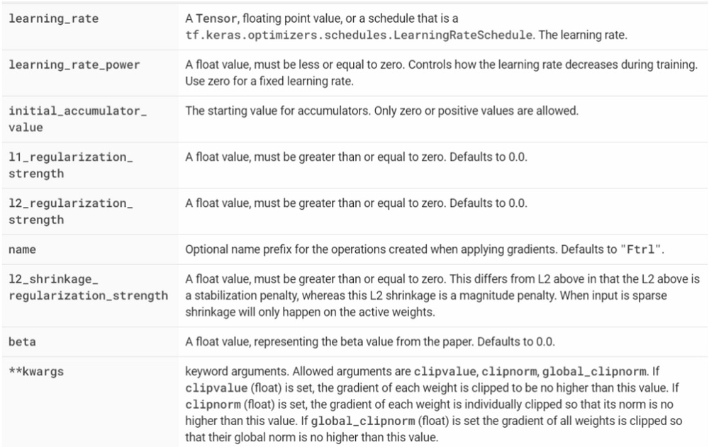
63 |
64 | ## Uses of FTRL optimizer
65 |
66 | #### 1. Ranking Documents
67 | Ranking means sorting documents by relevance to find contents of interest with respect to a query. Ranking models typically work by predicting a relevance score s = f(x) for each input x = (q, d) where q is a query and d is a document. Once we have the relevance of each document, we can sort (i.e. rank) the documents according to those scores.
68 |
69 | #### 2. Multi-Armed Bandit (MAB) problem
70 | In this problem, as mentioned in [Towards an Optimization Perspective for Bandits Problem](https://cseweb.ucsd.edu/classes/wi22/cse203B-a/proj22/17.pdf), a decision-maker is faced with a fixed arm set and needs to design a strategy to pull an arm to minimize the cumulative loss, termed regret. At each round, the decision-maker adapts the pulling strategy by solving an optimization problem (OP), and the solution of OP is a probability distribution over all arms. FTRL-based algorithm is one of the methods achieve the best of both worlds, i.e., stochastic and adversarial setting, in bandit problem with graph feedback.
71 |
72 | #### 3. Document Retrieval, Recommendation Systems, and Disease Diagnosis
73 | [A mini-batch stochastic gradient method for sparse learning to rank](http://www.ijicic.org/ijicic-140403.pdf) states that the algorithm for rank learning begins with formulating sparse learning to rank as a mini-batch based convex optimization problem with L1 regularization. Then for the problem that simple adding L1 term does not necessarily induce the sparsity, FTRL method is adopted for inner optimization, which can obtain good solution with high sparsity.
74 |
75 | #### 4. Online Advertising
76 | The underlying driving technology for online advertising is Click-Through Rates (CTR) estimation, in which the task is to predict the click probability of the browsers for some commodities in certain scenarios. Accurate prediction of CTR will not only benefit advertisers’ promotion of products but also ensure users’ good experiences and interests. The FTRL model combined the power of forward backward splitting algorithm (FOBOS) and regularized dual averaging algorithm (RDA) and has been successfully be used for online optimization of logistic regression model. It uses both L1 and L2 regularization terms in the iterative process, which greatly improves the prediction of the model. This was deduced by [A New Click-Through Rates Prediction Model Based on Deep & Cross Network.](https://www.mdpi.com/1999-4893/13/12/342/htm)
77 |
78 | #### 5. High-Dimensional Sparse Streaming Data Analysis
79 | An algorithm based on FTRL, FTRL-AUC, as proposed by [Online AUC Optimization for Sparse High-Dimensional Datasets](https://arxiv.org/pdf/2009.10867.pdf). can process data in an online fashion with a much cheaper per-iteration cost O(k), making it amenable for high-dimensional sparse streaming data analysis. It significantly improves both run time and model sparsity while achieving competitive Area Under the ROC Curve (AUC) scores compared with the state-of-the-art methods. Comparison with the online learning method for logistic loss demonstrates that FTRL-AUC achieves higher AUC scores especially when datasets are imbalanced.
80 |
81 | ## Advantages
82 | 1. Can minimize loss function better.
83 |
84 | ## Disadvantages
85 | 1. Cannot achieve adequate stability if the range of the regulariser is insufficient.
86 | 2. If the range of the regulariser is huge, then it’s far away from the optimal decision.
87 |
88 | ## References:
89 |
90 | 1. [Ftrl (keras.io)](https://keras.io/api/optimizers/ftrl/)
91 | 2. [tf.keras.optimizers.Ftrl | TensorFlow v2.9.1](https://www.tensorflow.org/api_docs/python/tf/keras/optimizers/Ftrl)
92 | 3. [Optimizers in Tensorflow-GeeksforGeeks](https://www.geeksforgeeks.org/optimizers-in-tensorflow/)
93 | 4. [McMahan et al., 2013.](https://research.google.com/pubs/archive/41159.pdf)
94 | 5. [Towards an Optimization Perspective for Bandits Problem.](https://cseweb.ucsd.edu/classes/wi22/cse203B-a/proj22/17.pdf)
95 | 6. [A mini-batch stochastic gradient method for sparse learning to rank.](http://www.ijicic.org/ijicic-140403.pdf)
96 | 7. [A New Click-Through Rates Prediction Model Based on Deep & Cross Network.](https://www.mdpi.com/1999-4893/13/12/342/htm)
97 | 8. [Online AUC Optimization for Sparse High-Dimensional Datasets.](https://www.vevesta.com/blog/Online%20AUC%20Optimization%20for%20Sparse%20High-Dimensional%20Datasets.)
98 | 9. [FTRL article on Vevesta](https://www.vevesta.com/blog/23-FTRL)
99 | 10. [FTRL article on Substack](https://vevesta.substack.com/p/a-look-into-little-known-but-powerful)
100 | ## Credits
101 |
102 | The above article is sponsored by [vevesta](https://www.vevesta.com/).
103 |
104 | [Vevesta](https://www.vevesta.com/): Your Machine Learning Team’s Feature and Technique Dictionary: Accelerate your Machine learning project by using features, techniques and projects used by your peers. Explore [Vevesta](https://www.vevesta.com/) for free. For more such stories, follow us on twitter at [@vevesta_labs](https://twitter.com/vevesta_labs).
--------------------------------------------------------------------------------
/tutorials/CLR_convergence.md:
--------------------------------------------------------------------------------
1 |
2 | # How to use Cyclical Learning Rate to get quick convergence for your Neural Network?
3 |
4 | Achieve higher accuracy for your machine learning model in lesser iterations.
5 |
6 | 
7 |
8 | The learning rate is a hyper-parameter that determines the pace at which an algorithm updates or learns the values of a parameter estimate. It regulates the amount of allocated error with which the model’s weights are updated each time they are updated, such as at the end of each batch of training instances.
9 |
10 | If the learning rate used is low, the number of iterations/epochs required to minimize the cost function is high (takes longer time). If the learning rate is high, the cost function could saturate at a value higher than the minimum value. An optimal learning rate can cause our model to converge faster.
11 |
12 | 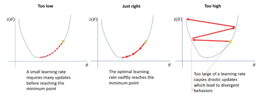
13 |
14 | 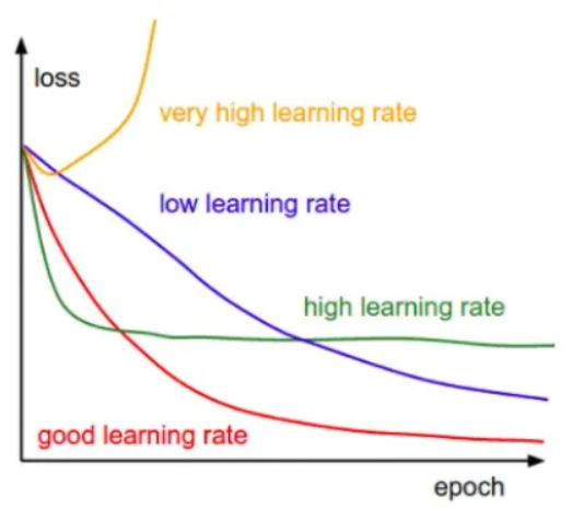
15 |
16 | There are various sorts of learning rate approaches but here we will talk about Cyclical Learning Rate.
17 |
18 | Cyclical Learning Rate is one of the approaches to achieve Optimal Learning Rates. The learning rate cyclically changes between a base minimum rate and a maximum rate in this methodology. The learning rate changes are cyclic, always returning to the learning rate's initial value.
19 |
20 | A very high learning rate causes the model to fluctuate more or to diverge from the minima, while a lower learning rate can cause the model to converge very slowly or to converge to the local minima. Cyclical learning rate (CLR) allows keeping the learning rate high and low, causing the model not to diverge along with jumping from the local minima.
21 |
22 | # How Cyclic Learning Rate improves speed of convergence?
23 |
24 | In CLR, we vary the Learning Rates between a lower and higher threshold. In other words, learning rate oscillates between base (minimum) learning rate and maximum learning rate. This helps as follows:
25 |
26 | 1. Periodic higher learning rates within each epoch helps to come out of any saddle points or local minima if it encounters into one. Saddle points have small gradients that slow the learning process.
27 |
28 | 2. According to [authors](https://arxiv.org/pdf/1506.01186.pdf), when using CLR it is likely the optimum learning rate will be between the bounds and near optimal learning rates will be used throughout training.
29 |
30 | In the figure below, Classification accuracy has been plotted with multiple learning rates while training on CIFAR-10. The red curve shows the result of training with one of the CLR (Cyclic Learning rate) policy. The implication is clear: The baseline (blue curve) reaches a final accuracy of 81.4 % after 70, 000 iterations. In contrast, with CLR, it is possible to fully train the network (red curve) within 25,000 iterations and attain the same accuracy.
31 |
32 | 
33 |
34 | # Types of Cyclic Learning Rates
35 |
36 | At a constant frequency, the learning rate varies in a triangular pattern between the maximum and base rates. The oscillation of learning rate can be based on various function-triangular (linear), Welch window (parabolic), or Hann window (sinusoidal).
37 |
38 | ## The Triangular Window
39 |
40 | The triangular window is a simpler way of changing the learning rate that is linearly increasing with some constant from min learning rate to max learning rate then linearly decreasing with the same constant from max learning rate to minimum learning rate.
41 |
42 | 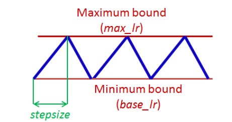
43 |
44 | The idea is to divide the training process into cycles determined by a stepsize parameter. This code varies the learning rate linearly between the minimum (base LR) and the maximum (max LR)
45 |
46 | 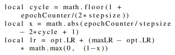
47 |
48 | - LR: the computed learning rate
49 | - opt.LR: the specified lower (base) learning rate
50 | - maxLR: Maximum learning rate boundary
51 | - epochCounter: the number of epochs of training
52 | - cycle length: Number of iterations until the learning rate returns to the initial value.
53 | - stepsize: the number of iterations in half a cycle
54 |
55 | # Implementation Nuggets
56 |
57 | According to [authors](https://arxiv.org/pdf/1506.01186.pdf), following needs to be kept in mind while training with CLR:
58 |
59 | 1. stepsize should be equal to 2-10 times the number of iterations in an epoch. We can calculate iterations present in an epoch using dataset size and batch size. If the dataset comprises 50,000 data entries and the batch size is 100, then the number of iterations in an epoch will be 500 (50,000/100).
60 | 2. Experiments show that replacing each step of a constant learning rate with at least 3 cycles trains the network weights most of the way and running for 4 or more cycles will achieve even better performance.
61 | 3. Also, it is best to stop training at the end of a cycle, which is when the learning rate is at the minimum value and the accuracy peaks.
62 | 4. Set base learning rate (or opt.LR) to 1/3 or 1/4 of maximum learning rate. Alternatively, run the model for few epochs when given a new architecture or dataset. Plot learning rate and accuracy as shown in the figure below. Note the learning rate value when the accuracy starts to increase, set this learning rate as base learning rate. And when the accuracy drops or slows or becomes ragged, set it to maximum learning rate. Example: from the plot, it can be seen that we can set base lr = 0.001 because the model starts converging right away. Furthermore, above a learning rate of 0.006 the accuracy rise gets rough and eventually begins to drop so it is reasonable to set max lr = 0.006.
63 |
64 | 
65 |
66 | # Conclusion:
67 |
68 | - Only a few epochs where the learning rate linearly increases is sufficient to estimate boundary learning rates for CLR.
69 | - Use of cyclic functions as a learning rate policy leads to substantial improvements in performance for a range of architectures.
70 | - The cyclic nature of CLR guides when to drop the learning rate values (after 3 - 5 cycles) a2d when to stop the training.
71 |
72 | # References:
73 |
74 | 1. [Cyclical Learning Rates](https://medium.com/analytics-vidhya/cyclical-learning-rates-a922a60e8c04#:~:text=Cyclical%20learning%20rate%20%28CLR%29%20allows%20keeping%20the%20learning,between%20base%20learning%20rate%20and%20max%20learning%20rate.)
75 | 2. [Cyclical Learning Rates for Training Neural Networks](https://arxiv.org/pdf/1506.01186.pdf)
76 |
77 | # Credits
78 |
79 | The above article is sponsored by [vevesta](https://www.vevesta.com/).
80 |
81 | [Vevesta](https://www.vevesta.com/): Your Machine Learning Team’s feature and Technique Dictionary: Accelerate your Machine learning project by using features, techniques and projects used by your peers. Explore Vevesta for free. For more such stories, follow us on twitter at [@vevesta_labs](https://twitter.com/vevesta_labs).
--------------------------------------------------------------------------------
/sampleCode/sampleExperiment.ipynb:
--------------------------------------------------------------------------------
1 | {
2 | "cells": [
3 | {
4 | "cell_type": "code",
5 | "execution_count": 1,
6 | "metadata": {},
7 | "outputs": [],
8 | "source": [
9 | "#import the vevesta Library\n",
10 | "from vevestaX import vevesta as v\n",
11 | "\n",
12 | "#create a vevestaX object\n",
13 | "V=v.Experiment()"
14 | ]
15 | },
16 | {
17 | "cell_type": "code",
18 | "execution_count": 2,
19 | "metadata": {
20 | "scrolled": true
21 | },
22 | "outputs": [
23 | {
24 | "data": {
25 | "text/html": [
26 | "\n",
27 | "\n",
40 | "
\n",
41 | " \n",
42 | " \n",
43 | " | \n",
44 | " Gender | \n",
45 | " Age | \n",
46 | " Months_Count | \n",
47 | " Salary | \n",
48 | " Expenditure | \n",
49 | " House_Price | \n",
50 | "
\n",
51 | " \n",
52 | " \n",
53 | " \n",
54 | " | 0 | \n",
55 | " 1 | \n",
56 | " 2 | \n",
57 | " 3 | \n",
58 | " 1 | \n",
59 | " 34 | \n",
60 | " 9884 | \n",
61 | "
\n",
62 | " \n",
63 | " | 1 | \n",
64 | " 1 | \n",
65 | " 2 | \n",
66 | " 34 | \n",
67 | " 0 | \n",
68 | " 56 | \n",
69 | " 2442 | \n",
70 | "
\n",
71 | " \n",
72 | "
\n",
73 | "