├── .gitignore
├── AI.jpg
├── _layouts
├── home.html
├── category.html
├── tag.html
├── collection.html
├── archive-taxonomy.html
├── posts.html
├── splash.html
├── tags.html
├── default.html
├── categories.html
├── archive.html
├── search.html
├── compress.html
└── single.html
├── Gemfile
├── _includes
├── footer
│ └── custom.html
├── analytics-providers
│ ├── custom.html
│ ├── google-gtag.html
│ ├── google-universal.html
│ └── google.html
├── comments-providers
│ ├── custom.html
│ ├── google-plus.html
│ ├── facebook.html
│ ├── scripts.html
│ ├── disqus.html
│ ├── discourse.html
│ ├── staticman.html
│ └── staticman_v2.html
├── posts-tag.html
├── posts-category.html
├── head
│ └── custom.html
├── page__hero_video.html
├── page__taxonomy.html
├── author-profile-custom-links.html
├── browser-upgrade.html
├── toc
├── figure
├── search
│ ├── lunr-search-scripts.html
│ ├── search_form.html
│ ├── google-search-scripts.html
│ └── algolia-search-scripts.html
├── analytics.html
├── mathjax.html
├── video
├── documents-collection.html
├── disqus.html
├── read-time.html
├── sidebar.html
├── post_pagination.html
├── scripts.html
├── footer.html
├── comment.html
├── tag-list.html
├── group-by-array
├── head.html
├── category-list.html
├── archive-single.html
├── gallery
├── masthead.html
├── breadcrumbs.html
├── feature_row
├── nav_list
├── social-share.html
├── paginator.html
├── page__hero.html
├── toc.html
├── seo.html
├── author-profile.html
└── comments.html
├── machine-learning
├── images
│ ├── svm_gm.png
│ ├── err_ana.png
│ ├── svm_bound.png
│ ├── err_ana_cn.png
│ ├── svm_outlier.png
│ ├── ablative_ana.png
│ ├── cs229_boost_1.png
│ ├── cs229_lec1_bgd.png
│ ├── cs229_trees_1.png
│ ├── cs229_trees_10.png
│ ├── cs229_trees_11.png
│ ├── cs229_trees_12.png
│ ├── cs229_trees_13.png
│ ├── cs229_trees_14.png
│ ├── cs229_trees_15.png
│ ├── cs229_trees_16.png
│ ├── cs229_trees_17.png
│ ├── cs229_trees_18.png
│ ├── cs229_trees_19.png
│ ├── cs229_trees_2.png
│ ├── cs229_trees_20.png
│ ├── cs229_trees_3.png
│ ├── cs229_trees_4.png
│ ├── cs229_trees_5.png
│ ├── cs229_trees_6.png
│ ├── cs229_trees_7.png
│ ├── cs229_trees_8.png
│ ├── cs229_trees_9.png
│ ├── svm_coordinate.png
│ ├── svm_intuition.png
│ ├── svm_two_coord.png
│ ├── ablative_ana_cn.png
│ ├── cs229_usv_keams.png
│ ├── cs229_gen_gda_learn.png
│ ├── cs229_gen_mul_gau.png
│ ├── cs229_lec1_intuit.png
│ ├── cs229_lec1_logistic.png
│ ├── cs229_lec1_newton.png
│ ├── cs229_usv_em_jensen.png
│ ├── cs229_deeplearning_nn.png
│ ├── cs229_em_missingdata.png
│ ├── cs229_deeplearning_bp_1.png
│ ├── cs229_deeplearning_bp_2.png
│ ├── cs229_deeplearning_cnn_1.png
│ ├── cs229_deeplearning_cnn_2.png
│ ├── cs229_deeplearning_link.png
│ ├── cs229_learningtheory_vc1.png
│ ├── cs229_learningtheory_vc2.png
│ ├── cs229_learningtheory_vc3.png
│ └── cs229_deeplearning_neuron.png
├── english-version
│ ├── dl_propagation.md
│ ├── usv_factor_analysis.md
│ ├── rl.md
│ ├── sv_bias_variance_tradeoff.md
│ ├── sv_online_learning_perceptron.md
│ ├── sv_regularization_model_selection.md
│ └── usv_kmeans.md
└── chinese-version
│ ├── sv_bias_variance_tradeoff_ch.md
│ ├── sv_regularization_model_selection_ch.md
│ ├── sv_tree_ch.md
│ └── sv_boost_ch.md
├── LICENSE
├── package.json
├── Rakefile
├── staticman.yml
├── README.md
├── Gemfile.lock
└── _config.yml
/.gitignore:
--------------------------------------------------------------------------------
1 | _site/*
2 | test
3 |
--------------------------------------------------------------------------------
/AI.jpg:
--------------------------------------------------------------------------------
https://raw.githubusercontent.com/Wei2624/AI_Learning_Hub/HEAD/AI.jpg
--------------------------------------------------------------------------------
/_layouts/home.html:
--------------------------------------------------------------------------------
1 | ---
2 | layout: archive
3 | ---
4 |
5 | {{ content }}
6 |
--------------------------------------------------------------------------------
/Gemfile:
--------------------------------------------------------------------------------
1 | source "https://rubygems.org"
2 | gem 'github-pages', group: :jekyll_plugins
--------------------------------------------------------------------------------
/_includes/footer/custom.html:
--------------------------------------------------------------------------------
1 |
2 |
3 |
--------------------------------------------------------------------------------
/_includes/analytics-providers/custom.html:
--------------------------------------------------------------------------------
1 |
2 |
3 |
--------------------------------------------------------------------------------
/_includes/comments-providers/custom.html:
--------------------------------------------------------------------------------
1 |
2 |
3 |
--------------------------------------------------------------------------------
/machine-learning/images/svm_gm.png:
--------------------------------------------------------------------------------
https://raw.githubusercontent.com/Wei2624/AI_Learning_Hub/HEAD/machine-learning/images/svm_gm.png
--------------------------------------------------------------------------------
/machine-learning/images/err_ana.png:
--------------------------------------------------------------------------------
https://raw.githubusercontent.com/Wei2624/AI_Learning_Hub/HEAD/machine-learning/images/err_ana.png
--------------------------------------------------------------------------------
/machine-learning/images/svm_bound.png:
--------------------------------------------------------------------------------
https://raw.githubusercontent.com/Wei2624/AI_Learning_Hub/HEAD/machine-learning/images/svm_bound.png
--------------------------------------------------------------------------------
/_includes/posts-tag.html:
--------------------------------------------------------------------------------
1 | {%- for post in site.tags[include.taxonomy] -%}
2 | {% include archive-single.html %}
3 | {%- endfor -%}
4 |
--------------------------------------------------------------------------------
/machine-learning/images/err_ana_cn.png:
--------------------------------------------------------------------------------
https://raw.githubusercontent.com/Wei2624/AI_Learning_Hub/HEAD/machine-learning/images/err_ana_cn.png
--------------------------------------------------------------------------------
/machine-learning/images/svm_outlier.png:
--------------------------------------------------------------------------------
https://raw.githubusercontent.com/Wei2624/AI_Learning_Hub/HEAD/machine-learning/images/svm_outlier.png
--------------------------------------------------------------------------------
/machine-learning/images/ablative_ana.png:
--------------------------------------------------------------------------------
https://raw.githubusercontent.com/Wei2624/AI_Learning_Hub/HEAD/machine-learning/images/ablative_ana.png
--------------------------------------------------------------------------------
/machine-learning/images/cs229_boost_1.png:
--------------------------------------------------------------------------------
https://raw.githubusercontent.com/Wei2624/AI_Learning_Hub/HEAD/machine-learning/images/cs229_boost_1.png
--------------------------------------------------------------------------------
/machine-learning/images/cs229_lec1_bgd.png:
--------------------------------------------------------------------------------
https://raw.githubusercontent.com/Wei2624/AI_Learning_Hub/HEAD/machine-learning/images/cs229_lec1_bgd.png
--------------------------------------------------------------------------------
/machine-learning/images/cs229_trees_1.png:
--------------------------------------------------------------------------------
https://raw.githubusercontent.com/Wei2624/AI_Learning_Hub/HEAD/machine-learning/images/cs229_trees_1.png
--------------------------------------------------------------------------------
/machine-learning/images/cs229_trees_10.png:
--------------------------------------------------------------------------------
https://raw.githubusercontent.com/Wei2624/AI_Learning_Hub/HEAD/machine-learning/images/cs229_trees_10.png
--------------------------------------------------------------------------------
/machine-learning/images/cs229_trees_11.png:
--------------------------------------------------------------------------------
https://raw.githubusercontent.com/Wei2624/AI_Learning_Hub/HEAD/machine-learning/images/cs229_trees_11.png
--------------------------------------------------------------------------------
/machine-learning/images/cs229_trees_12.png:
--------------------------------------------------------------------------------
https://raw.githubusercontent.com/Wei2624/AI_Learning_Hub/HEAD/machine-learning/images/cs229_trees_12.png
--------------------------------------------------------------------------------
/machine-learning/images/cs229_trees_13.png:
--------------------------------------------------------------------------------
https://raw.githubusercontent.com/Wei2624/AI_Learning_Hub/HEAD/machine-learning/images/cs229_trees_13.png
--------------------------------------------------------------------------------
/machine-learning/images/cs229_trees_14.png:
--------------------------------------------------------------------------------
https://raw.githubusercontent.com/Wei2624/AI_Learning_Hub/HEAD/machine-learning/images/cs229_trees_14.png
--------------------------------------------------------------------------------
/machine-learning/images/cs229_trees_15.png:
--------------------------------------------------------------------------------
https://raw.githubusercontent.com/Wei2624/AI_Learning_Hub/HEAD/machine-learning/images/cs229_trees_15.png
--------------------------------------------------------------------------------
/machine-learning/images/cs229_trees_16.png:
--------------------------------------------------------------------------------
https://raw.githubusercontent.com/Wei2624/AI_Learning_Hub/HEAD/machine-learning/images/cs229_trees_16.png
--------------------------------------------------------------------------------
/machine-learning/images/cs229_trees_17.png:
--------------------------------------------------------------------------------
https://raw.githubusercontent.com/Wei2624/AI_Learning_Hub/HEAD/machine-learning/images/cs229_trees_17.png
--------------------------------------------------------------------------------
/machine-learning/images/cs229_trees_18.png:
--------------------------------------------------------------------------------
https://raw.githubusercontent.com/Wei2624/AI_Learning_Hub/HEAD/machine-learning/images/cs229_trees_18.png
--------------------------------------------------------------------------------
/machine-learning/images/cs229_trees_19.png:
--------------------------------------------------------------------------------
https://raw.githubusercontent.com/Wei2624/AI_Learning_Hub/HEAD/machine-learning/images/cs229_trees_19.png
--------------------------------------------------------------------------------
/machine-learning/images/cs229_trees_2.png:
--------------------------------------------------------------------------------
https://raw.githubusercontent.com/Wei2624/AI_Learning_Hub/HEAD/machine-learning/images/cs229_trees_2.png
--------------------------------------------------------------------------------
/machine-learning/images/cs229_trees_20.png:
--------------------------------------------------------------------------------
https://raw.githubusercontent.com/Wei2624/AI_Learning_Hub/HEAD/machine-learning/images/cs229_trees_20.png
--------------------------------------------------------------------------------
/machine-learning/images/cs229_trees_3.png:
--------------------------------------------------------------------------------
https://raw.githubusercontent.com/Wei2624/AI_Learning_Hub/HEAD/machine-learning/images/cs229_trees_3.png
--------------------------------------------------------------------------------
/machine-learning/images/cs229_trees_4.png:
--------------------------------------------------------------------------------
https://raw.githubusercontent.com/Wei2624/AI_Learning_Hub/HEAD/machine-learning/images/cs229_trees_4.png
--------------------------------------------------------------------------------
/machine-learning/images/cs229_trees_5.png:
--------------------------------------------------------------------------------
https://raw.githubusercontent.com/Wei2624/AI_Learning_Hub/HEAD/machine-learning/images/cs229_trees_5.png
--------------------------------------------------------------------------------
/machine-learning/images/cs229_trees_6.png:
--------------------------------------------------------------------------------
https://raw.githubusercontent.com/Wei2624/AI_Learning_Hub/HEAD/machine-learning/images/cs229_trees_6.png
--------------------------------------------------------------------------------
/machine-learning/images/cs229_trees_7.png:
--------------------------------------------------------------------------------
https://raw.githubusercontent.com/Wei2624/AI_Learning_Hub/HEAD/machine-learning/images/cs229_trees_7.png
--------------------------------------------------------------------------------
/machine-learning/images/cs229_trees_8.png:
--------------------------------------------------------------------------------
https://raw.githubusercontent.com/Wei2624/AI_Learning_Hub/HEAD/machine-learning/images/cs229_trees_8.png
--------------------------------------------------------------------------------
/machine-learning/images/cs229_trees_9.png:
--------------------------------------------------------------------------------
https://raw.githubusercontent.com/Wei2624/AI_Learning_Hub/HEAD/machine-learning/images/cs229_trees_9.png
--------------------------------------------------------------------------------
/machine-learning/images/svm_coordinate.png:
--------------------------------------------------------------------------------
https://raw.githubusercontent.com/Wei2624/AI_Learning_Hub/HEAD/machine-learning/images/svm_coordinate.png
--------------------------------------------------------------------------------
/machine-learning/images/svm_intuition.png:
--------------------------------------------------------------------------------
https://raw.githubusercontent.com/Wei2624/AI_Learning_Hub/HEAD/machine-learning/images/svm_intuition.png
--------------------------------------------------------------------------------
/machine-learning/images/svm_two_coord.png:
--------------------------------------------------------------------------------
https://raw.githubusercontent.com/Wei2624/AI_Learning_Hub/HEAD/machine-learning/images/svm_two_coord.png
--------------------------------------------------------------------------------
/_includes/posts-category.html:
--------------------------------------------------------------------------------
1 | {%- for post in site.categories[include.taxonomy] -%}
2 | {% include archive-single.html %}
3 | {%- endfor -%}
4 |
--------------------------------------------------------------------------------
/machine-learning/images/ablative_ana_cn.png:
--------------------------------------------------------------------------------
https://raw.githubusercontent.com/Wei2624/AI_Learning_Hub/HEAD/machine-learning/images/ablative_ana_cn.png
--------------------------------------------------------------------------------
/machine-learning/images/cs229_usv_keams.png:
--------------------------------------------------------------------------------
https://raw.githubusercontent.com/Wei2624/AI_Learning_Hub/HEAD/machine-learning/images/cs229_usv_keams.png
--------------------------------------------------------------------------------
/machine-learning/images/cs229_gen_gda_learn.png:
--------------------------------------------------------------------------------
https://raw.githubusercontent.com/Wei2624/AI_Learning_Hub/HEAD/machine-learning/images/cs229_gen_gda_learn.png
--------------------------------------------------------------------------------
/machine-learning/images/cs229_gen_mul_gau.png:
--------------------------------------------------------------------------------
https://raw.githubusercontent.com/Wei2624/AI_Learning_Hub/HEAD/machine-learning/images/cs229_gen_mul_gau.png
--------------------------------------------------------------------------------
/machine-learning/images/cs229_lec1_intuit.png:
--------------------------------------------------------------------------------
https://raw.githubusercontent.com/Wei2624/AI_Learning_Hub/HEAD/machine-learning/images/cs229_lec1_intuit.png
--------------------------------------------------------------------------------
/machine-learning/images/cs229_lec1_logistic.png:
--------------------------------------------------------------------------------
https://raw.githubusercontent.com/Wei2624/AI_Learning_Hub/HEAD/machine-learning/images/cs229_lec1_logistic.png
--------------------------------------------------------------------------------
/machine-learning/images/cs229_lec1_newton.png:
--------------------------------------------------------------------------------
https://raw.githubusercontent.com/Wei2624/AI_Learning_Hub/HEAD/machine-learning/images/cs229_lec1_newton.png
--------------------------------------------------------------------------------
/machine-learning/images/cs229_usv_em_jensen.png:
--------------------------------------------------------------------------------
https://raw.githubusercontent.com/Wei2624/AI_Learning_Hub/HEAD/machine-learning/images/cs229_usv_em_jensen.png
--------------------------------------------------------------------------------
/machine-learning/images/cs229_deeplearning_nn.png:
--------------------------------------------------------------------------------
https://raw.githubusercontent.com/Wei2624/AI_Learning_Hub/HEAD/machine-learning/images/cs229_deeplearning_nn.png
--------------------------------------------------------------------------------
/machine-learning/images/cs229_em_missingdata.png:
--------------------------------------------------------------------------------
https://raw.githubusercontent.com/Wei2624/AI_Learning_Hub/HEAD/machine-learning/images/cs229_em_missingdata.png
--------------------------------------------------------------------------------
/machine-learning/images/cs229_deeplearning_bp_1.png:
--------------------------------------------------------------------------------
https://raw.githubusercontent.com/Wei2624/AI_Learning_Hub/HEAD/machine-learning/images/cs229_deeplearning_bp_1.png
--------------------------------------------------------------------------------
/machine-learning/images/cs229_deeplearning_bp_2.png:
--------------------------------------------------------------------------------
https://raw.githubusercontent.com/Wei2624/AI_Learning_Hub/HEAD/machine-learning/images/cs229_deeplearning_bp_2.png
--------------------------------------------------------------------------------
/machine-learning/images/cs229_deeplearning_cnn_1.png:
--------------------------------------------------------------------------------
https://raw.githubusercontent.com/Wei2624/AI_Learning_Hub/HEAD/machine-learning/images/cs229_deeplearning_cnn_1.png
--------------------------------------------------------------------------------
/machine-learning/images/cs229_deeplearning_cnn_2.png:
--------------------------------------------------------------------------------
https://raw.githubusercontent.com/Wei2624/AI_Learning_Hub/HEAD/machine-learning/images/cs229_deeplearning_cnn_2.png
--------------------------------------------------------------------------------
/machine-learning/images/cs229_deeplearning_link.png:
--------------------------------------------------------------------------------
https://raw.githubusercontent.com/Wei2624/AI_Learning_Hub/HEAD/machine-learning/images/cs229_deeplearning_link.png
--------------------------------------------------------------------------------
/machine-learning/images/cs229_learningtheory_vc1.png:
--------------------------------------------------------------------------------
https://raw.githubusercontent.com/Wei2624/AI_Learning_Hub/HEAD/machine-learning/images/cs229_learningtheory_vc1.png
--------------------------------------------------------------------------------
/machine-learning/images/cs229_learningtheory_vc2.png:
--------------------------------------------------------------------------------
https://raw.githubusercontent.com/Wei2624/AI_Learning_Hub/HEAD/machine-learning/images/cs229_learningtheory_vc2.png
--------------------------------------------------------------------------------
/machine-learning/images/cs229_learningtheory_vc3.png:
--------------------------------------------------------------------------------
https://raw.githubusercontent.com/Wei2624/AI_Learning_Hub/HEAD/machine-learning/images/cs229_learningtheory_vc3.png
--------------------------------------------------------------------------------
/machine-learning/images/cs229_deeplearning_neuron.png:
--------------------------------------------------------------------------------
https://raw.githubusercontent.com/Wei2624/AI_Learning_Hub/HEAD/machine-learning/images/cs229_deeplearning_neuron.png
--------------------------------------------------------------------------------
/_includes/head/custom.html:
--------------------------------------------------------------------------------
1 |
2 |
3 |
4 |
5 |
6 |
--------------------------------------------------------------------------------
/_includes/page__hero_video.html:
--------------------------------------------------------------------------------
1 | {% capture video_id %}{{ page.header.video.id }}{% endcapture %}
2 | {% capture video_provider %}{{ page.header.video.provider }}{% endcapture %}
3 |
4 | {% include video id=video_id provider=video_provider %}
5 |
--------------------------------------------------------------------------------
/_layouts/category.html:
--------------------------------------------------------------------------------
1 | ---
2 | layout: archive
3 | ---
4 |
5 | {{ content }}
6 |
7 |
8 | {% include posts-category.html taxonomy=page.taxonomy type=page.entries_layout %}
9 |
10 |
--------------------------------------------------------------------------------
/_includes/page__taxonomy.html:
--------------------------------------------------------------------------------
1 | {% if site.tag_archive.type and page.tags[0] %}
2 | {% include tag-list.html %}
3 | {% endif %}
4 |
5 | {% if site.category_archive.type and page.categories[0] %}
6 | {% include category-list.html %}
7 | {% endif %}
--------------------------------------------------------------------------------
/_includes/author-profile-custom-links.html:
--------------------------------------------------------------------------------
1 |
--------------------------------------------------------------------------------
/_layouts/tag.html:
--------------------------------------------------------------------------------
1 | ---
2 | layout: archive
3 | ---
4 |
5 | {{ content }}
6 |
7 |
8 | {% include posts-tag.html taxonomy=page.taxonomy type=page.entries_layout %}
9 |
10 |
--------------------------------------------------------------------------------
/_includes/comments-providers/google-plus.html:
--------------------------------------------------------------------------------
1 |
2 |
--------------------------------------------------------------------------------
/_includes/browser-upgrade.html:
--------------------------------------------------------------------------------
1 |
4 |
--------------------------------------------------------------------------------
/_layouts/collection.html:
--------------------------------------------------------------------------------
1 | ---
2 | layout: archive
3 | ---
4 |
5 | {{ content }}
6 |
7 |
8 | {% include documents-collection.html collection=page.collection sort_by=page.sort_by sort_order=page.sort_order type=page.entries_layout %}
9 |
10 |
--------------------------------------------------------------------------------
/_includes/toc:
--------------------------------------------------------------------------------
1 |
--------------------------------------------------------------------------------
/_layouts/archive-taxonomy.html:
--------------------------------------------------------------------------------
1 | ---
2 | layout: default
3 | author_profile: false
4 | ---
5 |
6 |
7 | {% include sidebar.html %}
8 |
9 |
10 |
{{ page.title }}
11 | {% for post in page.posts %}
12 | {% include archive-single.html %}
13 | {% endfor %}
14 |
15 |
 9 | {% if include.caption %}
10 | {{ include.caption | markdownify | remove: "
9 | {% if include.caption %}
10 | {{ include.caption | markdownify | remove: "" | remove: "
" }}
11 | {% endif %}
12 |
13 |
--------------------------------------------------------------------------------
/_includes/search/lunr-search-scripts.html:
--------------------------------------------------------------------------------
1 | {% assign lang = site.locale | slice: 0,2 | default: "en" %}
2 | {% case lang %}
3 | {% when "gr" %}
4 | {% assign lang = "gr" %}
5 | {% else %}
6 | {% assign lang = "en" %}
7 | {% endcase %}
8 |
9 |
10 |
--------------------------------------------------------------------------------
/_includes/analytics-providers/google-gtag.html:
--------------------------------------------------------------------------------
1 |
2 |
3 |
10 |
--------------------------------------------------------------------------------
/_includes/analytics.html:
--------------------------------------------------------------------------------
1 | {% if jekyll.environment == 'production' and site.analytics.provider and page.analytics != false %}
2 |
3 | {% case site.analytics.provider %}
4 | {% when "google" %}
5 | {% include /analytics-providers/google.html %}
6 | {% when "google-universal" %}
7 | {% include /analytics-providers/google-universal.html %}
8 | {% when "google-gtag" %}
9 | {% include /analytics-providers/google-gtag.html %}
10 | {% when "custom" %}
11 | {% include /analytics-providers/custom.html %}
12 | {% endcase %}
13 |
14 | {% endif %}
--------------------------------------------------------------------------------
/_includes/mathjax.html:
--------------------------------------------------------------------------------
1 | {% if page.mathjax %}
2 |
10 |
16 |
22 | {% endif %}
23 |
--------------------------------------------------------------------------------
/_includes/video:
--------------------------------------------------------------------------------
1 | {% capture video_id %}{{ include.id }}{% endcapture %}
2 | {% capture video_provider %}{{ include.provider }}{% endcapture %}
3 |
4 |
5 |
6 | {% if video_provider == "vimeo" %}
7 |
8 | {% elsif video_provider == "youtube" %}
9 |
10 | {% endif %}
11 |
12 |
--------------------------------------------------------------------------------
/_includes/analytics-providers/google-universal.html:
--------------------------------------------------------------------------------
1 |
11 |
--------------------------------------------------------------------------------
/_includes/documents-collection.html:
--------------------------------------------------------------------------------
1 | {% assign entries = site[include.collection] %}
2 |
3 | {% if include.sort_by == 'title' %}
4 | {% if include.sort_order == 'reverse' %}
5 | {% assign entries = entries | sort: 'title' | reverse %}
6 | {% else %}
7 | {% assign entries = entries | sort: 'title' %}
8 | {% endif %}
9 | {% elsif include.sort_by == 'date' %}
10 | {% if include.sort_order == 'reverse' %}
11 | {% assign entries = entries | sort: 'date' | reverse %}
12 | {% else %}
13 | {% assign entries = entries | sort: 'date' %}
14 | {% endif %}
15 | {% endif %}
16 |
17 | {%- for post in entries -%}
18 | {% include archive-single.html %}
19 | {%- endfor -%}
20 |
--------------------------------------------------------------------------------
/_includes/analytics-providers/google.html:
--------------------------------------------------------------------------------
1 |
--------------------------------------------------------------------------------
/_includes/disqus.html:
--------------------------------------------------------------------------------
1 | {% if site.disqus %}
2 |
17 | {% endif %}
18 |
--------------------------------------------------------------------------------
/_includes/comments-providers/scripts.html:
--------------------------------------------------------------------------------
1 | {% if site.comments.provider and page.comments %}
2 | {% case site.comments.provider %}
3 | {% when "disqus" %}
4 | {% include /comments-providers/disqus.html %}
5 | {% when "discourse" %}
6 | {% include /comments-providers/discourse.html %}
7 | {% when "facebook" %}
8 | {% include /comments-providers/facebook.html %}
9 | {% when "google-plus" %}
10 | {% include /comments-providers/google-plus.html %}
11 | {% when "staticman" %}
12 | {% include /comments-providers/staticman.html %}
13 | {% when "staticman_v2" %}
14 | {% include /comments-providers/staticman_v2.html %}
15 | {% when "custom" %}
16 | {% include /comments-providers/custom.html %}
17 | {% endcase %}
18 | {% endif %}
--------------------------------------------------------------------------------
/_includes/read-time.html:
--------------------------------------------------------------------------------
1 | {% assign words_per_minute = site.words_per_minute | default: 200 %}
2 |
3 | {% if post.read_time %}
4 | {% assign words = post.content | strip_html | number_of_words %}
5 | {% elsif page.read_time %}
6 | {% assign words = page.content | strip_html | number_of_words %}
7 | {% endif %}
8 |
9 | {% if words < words_per_minute %}
10 | {{ site.data.ui-text[site.locale].less_than | default: "less than" }} 1 {{ site.data.ui-text[site.locale].minute_read | default: "minute read" }}
11 | {% elsif words == words_per_minute %}
12 | 1 {{ site.data.ui-text[site.locale].minute_read | default: "minute read" }}
13 | {% else %}
14 | {{ words | divided_by:words_per_minute }} {{ site.data.ui-text[site.locale].minute_read | default: "minute read" }}
15 | {% endif %}
--------------------------------------------------------------------------------
/_includes/comments-providers/disqus.html:
--------------------------------------------------------------------------------
1 | {% if site.comments.disqus.shortname %}
2 |
14 |
15 | {% endif %}
16 |
--------------------------------------------------------------------------------
/_includes/comments-providers/discourse.html:
--------------------------------------------------------------------------------
1 | {% if site.comments.discourse.server %}
2 | {% capture canonical %}{% if site.permalink contains '.html' %}{{ page.url | absolute_url }}{% else %}{{ page.url | absolute_url | remove:'index.html' | strip_slash }}{% endif %}{% endcapture %}
3 |
12 |
13 | {% endif %}
14 |
--------------------------------------------------------------------------------
/_includes/sidebar.html:
--------------------------------------------------------------------------------
1 | {% if page.author_profile or layout.author_profile or page.sidebar %}
2 |
23 | {% endif %}
24 |
--------------------------------------------------------------------------------
/_includes/post_pagination.html:
--------------------------------------------------------------------------------
1 | {% if page.previous or page.next %}
2 |
14 | {% endif %}
--------------------------------------------------------------------------------
/_includes/search/search_form.html:
--------------------------------------------------------------------------------
1 |
2 | {%- assign search_provider = site.search_provider | default: "lunr" -%}
3 | {%- case search_provider -%}
4 | {%- when "lunr" -%}
5 |
6 |
7 | {%- when "google" -%}
8 |
11 |
12 |
13 |
14 | {%- when "algolia" -%}
15 |
16 |
17 | {%- endcase -%}
18 |
12 |
13 | {% if page.title %}{% endif %}
14 | {% if page.excerpt %}{% endif %}
15 | {% if page.date %}{% endif %}
16 | {% if page.last_modified_at %}{% endif %}
17 |
18 |
21 |
22 |
17 | {{ site.data.ui-text[site.locale].tags_label | default: "Tags:" }}
18 |
19 | {% for hash in tag_hashes %}
20 | {% assign keyValue = hash | split: '#' %}
21 | {% capture tag_word %}{{ keyValue[1] | strip_newlines }}{% endcapture %}
22 | {{ tag_word }}{% unless forloop.last %}, {% endunless %}
23 | {% endfor %}
24 |
25 |
26 | {% endif %}
--------------------------------------------------------------------------------
/_includes/group-by-array:
--------------------------------------------------------------------------------
1 |
7 |
8 |
9 | {% assign __empty_array = '' | split: ',' %}
10 | {% assign group_names = __empty_array %}
11 | {% assign group_items = __empty_array %}
12 |
13 |
14 | {% assign __names = include.collection | map: include.field %}
15 |
16 |
17 | {% assign __names = __names | join: ',' | join: ',' | split: ',' %}
18 |
19 |
20 | {% assign __names = __names | sort %}
21 | {% for name in __names %}
22 |
23 |
24 | {% unless name == previous %}
25 |
26 |
27 | {% assign group_names = group_names | push: name %}
28 | {% endunless %}
29 |
30 | {% assign previous = name %}
31 | {% endfor %}
32 |
33 |
34 |
35 | {% for name in group_names %}
36 |
37 |
38 | {% assign __item = __empty_array %}
39 | {% for __element in include.collection %}
40 | {% if __element[include.field] contains name %}
41 | {% assign __item = __item | push: __element %}
42 | {% endif %}
43 | {% endfor %}
44 |
45 |
46 | {% assign group_items = group_items | push: __item %}
47 | {% endfor %}
--------------------------------------------------------------------------------
/_includes/head.html:
--------------------------------------------------------------------------------
1 |
2 |
3 | {% include seo.html %}
4 |
5 |
6 |
7 |
8 |
9 |
10 |
13 |
14 |
15 |
16 |
17 |
31 |
32 | {% if site.head_scripts %}
33 | {% for script in site.head_scripts %}
34 | {% if script contains "://" %}
35 | {% capture script_path %}{{ script }}{% endcapture %}
36 | {% else %}
37 | {% capture script_path %}{{ script | relative_url }}{% endcapture %}
38 | {% endif %}
39 |
40 | {% endfor %}
41 | {% endif %}
42 |
--------------------------------------------------------------------------------
/_layouts/tags.html:
--------------------------------------------------------------------------------
1 | ---
2 | layout: archive
3 | ---
4 |
5 | {{ content }}
6 |
7 | {% assign tags_max = 0 %}
8 | {% for tag in site.tags %}
9 | {% if tag[1].size > tags_max %}
10 | {% assign tags_max = tag[1].size %}
11 | {% endif %}
12 | {% endfor %}
13 |
14 |
15 | {% for i in (1..tags_max) reversed %}
16 | {% for tag in site.tags %}
17 | {% if tag[1].size == i %}
18 | -
19 |
20 | {{ tag[0] }} {{ i }}
21 |
22 |
23 | {% endif %}
24 | {% endfor %}
25 | {% endfor %}
26 |
27 |
28 | {% for i in (1..tags_max) reversed %}
29 | {% for tag in site.tags %}
30 | {% if tag[1].size == i %}
31 |
40 | {% endif %}
41 | {% endfor %}
42 | {% endfor %}
43 |
--------------------------------------------------------------------------------
/_includes/category-list.html:
--------------------------------------------------------------------------------
1 | {% case site.category_archive.type %}
2 | {% when "liquid" %}
3 | {% assign path_type = "#" %}
4 | {% when "jekyll-archives" %}
5 | {% assign path_type = nil %}
6 | {% endcase %}
7 |
8 | {% if site.category_archive.path %}
9 | {% comment %}
10 |
11 |
12 | {% endcomment %}
13 | {% capture page_categories %}{% for category in page.categories %}{{ category | downcase }}#{{ category }}{% unless forloop.last %},{% endunless %}{% endfor %}{% endcapture %}
14 | {% assign category_hashes = page_categories | split: ',' | sort %}
15 |
16 |
17 | {{ site.data.ui-text[site.locale].categories_label | default: "Categories:" }}
18 |
19 | {% for hash in category_hashes %}
20 | {% assign keyValue = hash | split: '#' %}
21 | {% capture category_word %}{{ keyValue[1] | strip_newlines }}{% endcapture %}
22 | {{ category_word }}{% unless forloop.last %}, {% endunless %}
23 | {% endfor %}
24 |
25 |
26 | {% endif %}
--------------------------------------------------------------------------------
/_layouts/default.html:
--------------------------------------------------------------------------------
1 | ---
2 | ---
3 |
4 |
5 |
11 |
12 |
13 | {% include head.html %}
14 | {% include head/custom.html %}
15 | {% include analytics.html %}
16 |
17 |
18 |
19 |
20 |
21 | {% include browser-upgrade.html %}
22 | {% include masthead.html %}
23 |
24 |
25 | {{ content }}
26 |
27 |
28 | {% if site.search == true %}
29 |
30 | {% include search/search_form.html %}
31 |
32 | {% endif %}
33 |
34 |
40 |
41 | {% include scripts.html %}
42 |
43 |
44 |
45 |
--------------------------------------------------------------------------------
/_layouts/categories.html:
--------------------------------------------------------------------------------
1 | ---
2 | layout: archive
3 | ---
4 |
5 | {{ content }}
6 |
7 | {% assign categories_max = 0 %}
8 | {% for category in site.categories %}
9 | {% if category[1].size > categories_max %}
10 | {% assign categories_max = category[1].size %}
11 | {% endif %}
12 | {% endfor %}
13 |
14 |
15 | {% for i in (1..categories_max) reversed %}
16 | {% for category in site.categories %}
17 | {% if category[1].size == i %}
18 | -
19 |
20 | {{ category[0] }} {{ i }}
21 |
22 |
23 | {% endif %}
24 | {% endfor %}
25 | {% endfor %}
26 |
27 |
28 | {% for i in (1..categories_max) reversed %}
29 | {% for category in site.categories %}
30 | {% if category[1].size == i %}
31 |
40 | {% endif %}
41 | {% endfor %}
42 | {% endfor %}
43 |
--------------------------------------------------------------------------------
/_layouts/archive.html:
--------------------------------------------------------------------------------
1 | ---
2 | layout: default
3 | ---
4 |
5 | {% if page.header.overlay_color or page.header.overlay_image or page.header.image %}
6 | {% include page__hero.html %}
7 | {% elsif page.header.video.id and page.header.video.provider %}
8 | {% include page__hero_video.html %}
9 | {% endif %}
10 |
11 | {% if page.url != "/" and site.breadcrumbs %}
12 | {% unless paginator %}
13 | {% include breadcrumbs.html %}
14 | {% endunless %}
15 | {% endif %}
16 |
17 |
18 | {% include sidebar.html %}
19 |
20 |
21 | {% unless page.header.overlay_color or page.header.overlay_image %}
22 |
{{ page.title }}
23 | {% endunless %}
24 |
25 | {% if page.toc %}
26 |
32 | {% endif %}
33 | {{ content }}
34 | {% if page.link %}{% endif %}
35 |
36 |
37 |
" | remove: "
" %}
9 | {% else %}
10 | {% assign title = post.title %}
11 | {% endif %}
12 |
13 |
14 |
15 | {% if include.type == "grid" and teaser %}
16 |
17 |

24 |
27 | {% if post.link %}
28 | {{ title }} Permalink
29 | {% else %}
30 | {{ title }}
31 | {% endif %}
32 |
33 | {% if post.read_time %}
34 | {% include read-time.html %}
35 | {% endif %}
36 | {% if post.excerpt %}{{ post.excerpt | markdownify | strip_html | truncate: 160 }}
{% endif %}
37 |
38 |
 37 |
38 | {% else %}
39 |
37 |
38 | {% else %}
39 |  46 | {% endif %}
47 | {% endfor %}
48 | {% if include.caption %}
49 | {{ include.caption | markdownify | remove: "
46 | {% endif %}
47 | {% endfor %}
48 | {% if include.caption %}
49 | {{ include.caption | markdownify | remove: "" | remove: "
" }}
50 | {% endif %}
51 |
--------------------------------------------------------------------------------
/_layouts/search.html:
--------------------------------------------------------------------------------
1 | ---
2 | layout: default
3 | ---
4 |
5 | {% if page.header.overlay_color or page.header.overlay_image or page.header.image %}
6 | {% include page__hero.html %}
7 | {% endif %}
8 |
9 | {% if page.url != "/" and site.breadcrumbs %}
10 | {% unless paginator %}
11 | {% include breadcrumbs.html %}
12 | {% endunless %}
13 | {% endif %}
14 |
15 |
16 | {% include sidebar.html %}
17 |
18 |
19 | {% unless page.header.overlay_color or page.header.overlay_image %}
20 |
{{ page.title }}
21 | {% endunless %}
22 |
23 | {{ content }}
24 |
25 | {%- assign search_provider = site.search_provider | default: "lunr" -%}
26 | {%- case search_provider -%}
27 | {%- when "lunr" -%}
28 |
29 |
30 | {%- when "google" -%}
31 |
34 |
35 |
36 |
37 | {%- when "algolia" -%}
38 |
39 |
40 | {%- endcase -%}
41 |
42 |
8 |
9 | {% for f in feature_row %}
10 |
11 | {% if f.url contains "://" %}
12 | {% capture f_url %}{{ f.url }}{% endcapture %}
13 | {% else %}
14 | {% capture f_url %}{{ f.url | relative_url }}{% endcapture %}
15 | {% endif %}
16 |
17 |
18 |
19 | {% if f.image_path %}
20 |
21 |

28 | {% if f.image_caption %}
29 |
{{ f.image_caption | markdownify | remove: "" | remove: "
" }}
30 | {% endif %}
31 |
32 | {% endif %}
33 |
34 |
35 | {% if f.title %}
36 |
{{ f.title }}
37 | {% endif %}
38 |
39 | {% if f.excerpt %}
40 |
41 | {{ f.excerpt | markdownify }}
42 |
43 | {% endif %}
44 |
45 | {% if f.url %}
46 |
{{ f.btn_label | default: site.data.ui-text[site.locale].more_label | default: "Learn More" }}
47 | {% endif %}
48 |
49 |
50 |
51 | {% endfor %}
52 |
53 |
{{ site.data.ui-text[site.locale].share_on_label | default: "Share on" }}
4 | {% endif %}
5 |
6 |
7 |
8 | Facebook
9 |
10 | Google+
11 |
12 | QR Code
13 |
14 |
--------------------------------------------------------------------------------
/_includes/search/algolia-search-scripts.html:
--------------------------------------------------------------------------------
1 |
2 |
3 |
4 |
5 |
6 |
55 |
--------------------------------------------------------------------------------
/_includes/comments-providers/staticman.html:
--------------------------------------------------------------------------------
1 | {% if site.repository and site.staticman.branch %}
2 |
42 | {% endif %}
--------------------------------------------------------------------------------
/_includes/comments-providers/staticman_v2.html:
--------------------------------------------------------------------------------
1 | {% if site.repository and site.staticman.branch %}
2 |
42 | {% endif %}
--------------------------------------------------------------------------------
/Rakefile:
--------------------------------------------------------------------------------
1 | require "bundler/gem_tasks"
2 | require "jekyll"
3 | require "listen"
4 |
5 | def listen_ignore_paths(base, options)
6 | [
7 | /_config\.ya?ml/,
8 | /_site/,
9 | /\.jekyll-metadata/
10 | ]
11 | end
12 |
13 | def listen_handler(base, options)
14 | site = Jekyll::Site.new(options)
15 | Jekyll::Command.process_site(site)
16 | proc do |modified, added, removed|
17 | t = Time.now
18 | c = modified + added + removed
19 | n = c.length
20 | relative_paths = c.map{ |p| Pathname.new(p).relative_path_from(base).to_s }
21 | print Jekyll.logger.message("Regenerating:", "#{relative_paths.join(", ")} changed... ")
22 | begin
23 | Jekyll::Command.process_site(site)
24 | puts "regenerated in #{Time.now - t} seconds."
25 | rescue => e
26 | puts "error:"
27 | Jekyll.logger.warn "Error:", e.message
28 | Jekyll.logger.warn "Error:", "Run jekyll build --trace for more information."
29 | end
30 | end
31 | end
32 |
33 | task :preview do
34 | base = Pathname.new('.').expand_path
35 | options = {
36 | "source" => base.join('test').to_s,
37 | "destination" => base.join('test/_site').to_s,
38 | "force_polling" => false,
39 | "serving" => true,
40 | "theme" => "minimal-mistakes-jekyll"
41 | }
42 |
43 | options = Jekyll.configuration(options)
44 |
45 | ENV["LISTEN_GEM_DEBUGGING"] = "1"
46 | listener = Listen.to(
47 | base.join("_data"),
48 | base.join("_includes"),
49 | base.join("_layouts"),
50 | base.join("_sass"),
51 | base.join("assets"),
52 | options["source"],
53 | :ignore => listen_ignore_paths(base, options),
54 | :force_polling => options['force_polling'],
55 | &(listen_handler(base, options))
56 | )
57 |
58 | begin
59 | listener.start
60 | Jekyll.logger.info "Auto-regeneration:", "enabled for '#{options["source"]}'"
61 |
62 | unless options['serving']
63 | trap("INT") do
64 | listener.stop
65 | puts " Halting auto-regeneration."
66 | exit 0
67 | end
68 |
69 | loop { sleep 1000 }
70 | end
71 | rescue ThreadError
72 | # You pressed Ctrl-C, oh my!
73 | end
74 |
75 | Jekyll::Commands::Serve.process(options)
76 | end
77 |
--------------------------------------------------------------------------------
/machine-learning/english-version/dl_propagation.md:
--------------------------------------------------------------------------------
1 | ---
2 | layout: single
3 | mathjax: true
4 | toc: true
5 | toc_sticky: true
6 | category: Machine Learning
7 | tags: [notes]
8 | qr: machine_learning_notes.png
9 | title: Backpropagation
10 | share: true
11 | permalink: /MachineLearning/dl_propagtion/
12 | sidebar:
13 | nav: "MachineLearning"
14 | ---
15 |
16 | # 1 Forward Propagation
17 |
18 | This is more like a summary section.
19 |
20 | We set $a^{[0]} = x$ for our input to the network and $\ell = 1,2,\dots,N$ where N is the number of layers of network. Then, we have
21 |
22 | $$z^{[\ell]} = W^{[\ell]}a^{[\ell-1]} + b^{[\ell]}$$
23 |
24 | $$a^{[\ell]} = g^{[\ell]}(z^{[\ell]})$$
25 |
26 | where $g^{[\ell]}$ is the same for all the layers except for last layer. For the last layer, we can do:
27 |
28 | 1 regression then $g(x) = x$
29 |
30 | 2 binary then $g(x) = sigmoid(x)$
31 |
32 | 3 multi-class then $g(x) = softmax(x)$
33 |
34 | Finally, we can have the output of the network $a^{[N]}$ and compute its loss.
35 |
36 | For regression, we have:
37 |
38 | $$\mathcal{L}(\hat{y},y) = \frac{1}{2}(\hat{y} - y)^2$$
39 |
40 | For binary classification, we have:
41 |
42 | $$\mathcal{L}(\hat{y},y) = -\bigg(y\log\hat{y} + (1-y)\log (1-\hat{y})\bigg)$$
43 |
44 | For multi-classification, we have:
45 |
46 | $$\mathcal{L}(\hat{y},y) = -\sum\limits_{j=1}^k\mathbb{1}\{y=j\}\log\hat{y}_j$$
47 |
48 |
49 | Note that for multi-class, if we have $\hat{y}$ as a k-dimensional vector, we can calculate its cross-entropy for its loss:
50 |
51 | $$\mathcal{L}(\hat{y},y) = -\sum\limits_{j=1}^ky_j\log\hat{y}_j$$
52 |
53 | # 2 Backpropagation
54 |
55 | We define that:
56 |
57 | $$\delta^{[\ell]} = \triangledown_{z^{[\ell]}}\mathcal{L}(\hat{y},y)$$
58 |
59 | So we have three steps for computing the gradient for any layer:
60 |
61 | 1 For output layer N, we have:
62 |
63 | $$\delta^{[N]} = \triangledown_{z^{[N]}}\mathcal{L}(\hat{y},y)$$
64 |
65 | For softmax function, since it is not performed element-wise, so you can directly caculate it as a whole. For sigmoid, it is applied element-wise, so we need to:
66 |
67 | $$\triangledown_{z^{[N]}}\mathcal{L}(\hat{y},y) = \triangledown_{\hat{y}}\mathcal{L}(\hat{y},y)\circ (g^{[N]})^{\prime}(z^{[N]})$$
68 |
69 | Note this is element-wise operation.
70 |
71 | 2 For $\ell = N-1,N-2,\dots,1$, we have:
72 |
73 | $$\delta^{[\ell]} = (W^{[\ell+1]T}\delta^{[\ell+1]})\circ g^{\prime}(z^{[\ell]})$$
74 |
75 | 3 For each layer, we have:
76 |
77 | $$\triangle_{W^{[\ell]}}J(W,b) = \delta^{[\ell]}a^{[\ell]T}$$
78 |
79 | $$\triangle_{b^{[\ell]}}J(W,b) = \delta^{[\ell]}$$
80 |
81 | This can be directly used in coding, which acts like a formula.
82 |
--------------------------------------------------------------------------------
/machine-learning/chinese-version/sv_bias_variance_tradeoff_ch.md:
--------------------------------------------------------------------------------
1 | ---
2 | published: true
3 | layout: single
4 | mathjax: true
5 | toc: true
6 | toc_sticky: true
7 | category: Machine Learning
8 | tags: [notes,chinese]
9 | excerpt: "This post is a translation for one of Wei's posts in his machine learning notes."
10 | title: Bias Varicne Tradeoff Chinese Version
11 | share: true
12 | author_profile: true
13 | permalink: /MachineLearning/sv_bias_variance_tradeoff_ch/
14 | ---
15 |
16 | This Article is a Chinese translation of a study note by Wei. Click [here](https://wei2624.github.io/MachineLearning/sv_bias_varience_tradeoff/) to see the original English version in Wei's homepage. I will continue to update Chinese translation to sync with Wei's notes.
17 |
18 | 请注意: 本文是我翻译的一份学习资料,英文原版请点击[Wei的学习笔记](https://wei2624.github.io/MachineLearning/sv_bias_varience_tradeoff/)。我将不断和原作者的英文笔记同步内容,定期更新和维护。
19 |
20 | 在这一节中,我们重点讨论偏差和误差之间是如何相互关联的。我们总想拥有0偏差和0方差,然而在实际中这是不可能的。因此,它们之间总会有权衡,一者多,另一者少。
21 |
22 | # 1 偏差-方差间权衡 (Bias Variance Tradeoff)
23 |
24 | 我们将基于一些样本训练好的模型定义为$\overset{\wedge}{f}$,并且$y$ 为事实标签。因此,**均方差(mean squared error(MSE))**可以定义为:
25 |
26 | $$\mathbb{E}_{(x,y)\sim \text{test set}} \lvert \overset{\wedge}{f}(x) - y \rvert^2$$
27 |
28 | 对于很高的均方差,我们有以下3种解释:
29 |
30 | **过渡拟合(overfitting)**: 模型只在训练样本中表现良好,但是并不能很好地推广适用到测试数据上。
31 |
32 | **欠拟合(underfitting)**: 模型训练还不够,或者没有足够的训练数据,以至于模型不能很好的表示训练数据的情况。
33 |
34 | **两者都不**: 数据的**噪音(noise)**太大。
35 |
36 | 我们将这些情况归纳为**偏差-方差权衡(Bias-Variance Tradeoff)**。
37 |
38 | 假设所有数据都来自于以下定义的相似的分布:$y_i = f(x_i) + \epsilon_i$ 其中噪音 $\mathbb{E}[\epsilon] = 0$ and $Var(\epsilon) = \sigma^2$。
39 |
40 | 尽管我们的目标是计算f,但我们只能通过从以上分布所产生的样本中训练得到一个估值。因此,$\overset{\wedge}{f}(x_i)$ 是随机的,因为它取决于随机的$\epsilon_i$,并且它也是$y = f(x_i) + \epsilon_i$的预测值。因此,得出$\mathbb{E}(\overset{\wedge}{f}(x)-y)$是很合理的。
41 |
42 | 我们也可以计算MSE的期望:
43 |
44 | $$\begin{align}
45 | \mathbb{E}[(y-\overset{\wedge}{f}(x))^2] &= \mathbb{E}[y^2 + (\overset{\wedge}{f})^2 - 2y\overset{\wedge}{f}]\\
46 | &= \mathbb{E}{y^2} + E[(\overset{\wedge}{f})^2] - \mathbb{E}[2y\overset{\wedge}{f}] \\
47 | &= Var(y) + Var(\overset{\wedge}{f}) + (f^2 - 2f\mathbb{E}[\overset{\wedge}{f}] + (\mathbb{E}[\overset{\wedge}{f}])^2\\
48 | &= Var(y) + Var(\overset{\wedge}{f}) + (f - \mathbb{E}[\overset{\wedge}{f}])^2\\
49 | &=\sigma^2 + \text{Bias}(f)^2+ Var(\overset{\wedge}{f})
50 | \end{align}$$
51 |
52 | 第一项是我们无法处理的噪声。高偏差意味着模型的学习效率很低,并且欠拟合。一个高度的方差代表着模型不能很好的概括更多普通的情况,同时代表过渡拟合。
53 |
54 | # 2 误差分析 (Error Aanalysis)
55 |
56 | 为了分析一个模型,我们应该首先将模型模块化。然后我们将每个模块的事实标签代入到每一模块中,观察每一个变化会如何影响整体模型的精确度。我们试图观察事实标签中的哪个模块对模型系统的影响最大。以下是一个例子
57 |
58 | 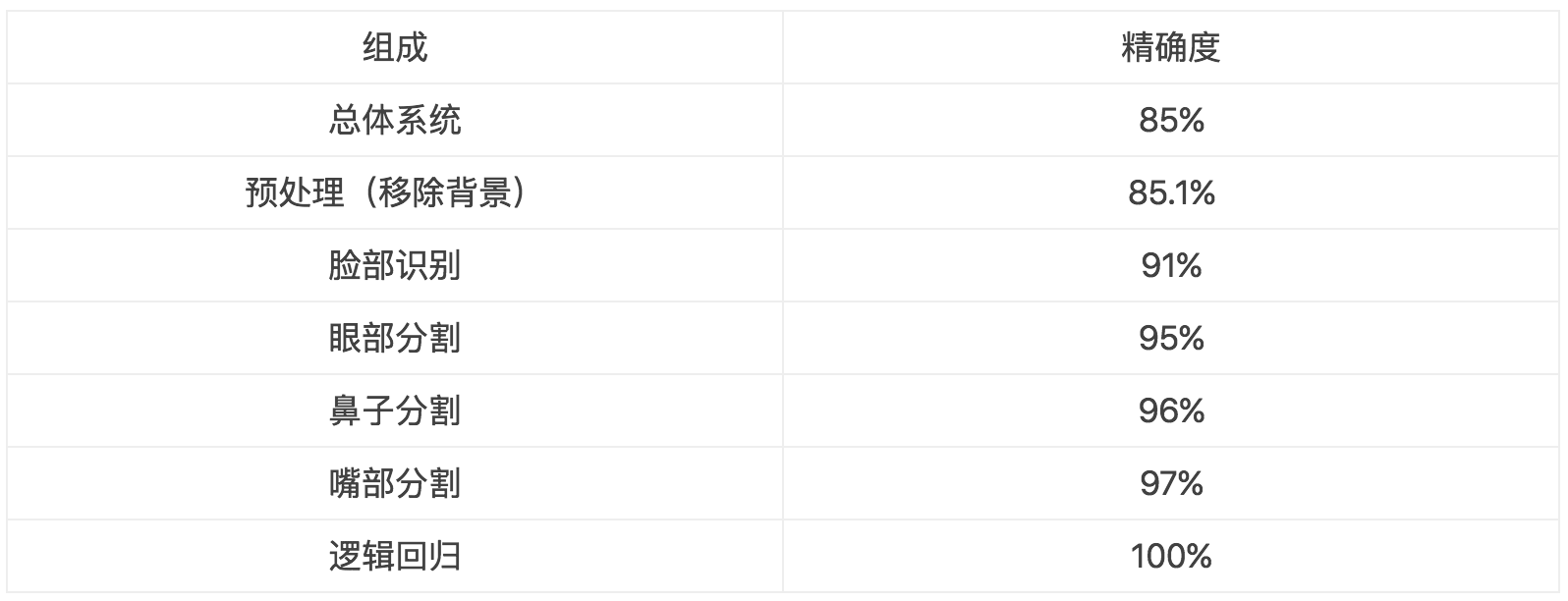
59 |
60 | 表1:这个表给出了模块化对应的准确度
61 |
62 | # 3 去除分析 (Ablative Analysis)
63 |
64 | 误差分析试图识别模型当前表现与完美表现之前的区别,而去除分析试图识别基准线与当前模型之前的区别。去除分析非常重要,很多研究论文因为丢失了这部分而被拒绝。这个分析可以告诉我们模型的哪个部分是最具影响力的。
65 | 例如,假设我们有更多附加的特征可以让模型表现更好。我们想观察通过每一次减少一个附加的特征,模型的表现会减少多少。下面是一个例子
66 |
67 | 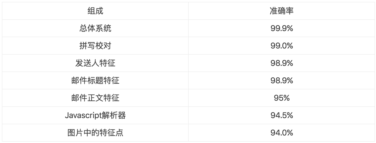
68 |
69 | 表2:从逻辑回归移除特征的精确度
70 |
71 |
--------------------------------------------------------------------------------
/machine-learning/english-version/usv_factor_analysis.md:
--------------------------------------------------------------------------------
1 | ---
2 | layout: single
3 | mathjax: true
4 | toc: true
5 | toc_sticky: true
6 | category: Machine Learning
7 | tags: [notes]
8 | qr: machine_learning_notes.png
9 | title: Factor Analysis
10 | share: true
11 | permalink: /MachineLearning/usv_factor_analysis/
12 | sidebar:
13 | nav: "MachineLearning"
14 | ---
15 |
16 | # Introduction
17 |
18 | Recall that when we have the data $x^i\in \mathbb{R}^n$ for mixture of Gaussian, we usually assume that the number of samples m is larger than the sample dimension n. Then, EM algorithm can be applied to fit the data. However, EM algorithm will fail if data dimension is larger than the number of sample.
19 |
20 | For example, if $n \gg m$, in such case, it might be difficult to model the data with even a single Gaussian. This is because m data points can only span a subspace of feature space$\mathbb{R}^n$. If we model such a dataset using maximum likelihood estimator, we should have:
21 |
22 | $$\begin{align}
23 | \mu &= \frac{1}{m}\sum\limits_{i=1}^m x^i \\
24 | \Sigma &= \frac{1}{m} \sum\limits_{i=1}^m (x^i-\mu)((x^i-\mu)^T)
25 | \end{align}$$
26 |
27 | Each $(x^i-\mu)((x^i-\mu)^T)$ produces a matrix with rank 1. The rank of the sum of all the matrices is the sum of the rank of each matrix. Thus, the final $\Sigma$ has the most rank m. If $n \gg m$, $\Sigma$ is a singular matrix, and its inverse does not exist. Furthermore, $1/\lvert \Sigma \rvert^{1/2} = 1/0$, which is invalid. This cannot be used to define the density of Gaussian distribution.
28 |
29 | Thus, we will talk about how to find the best fit of model given the few amount of data.
30 |
31 |
32 | # Restrictions of $\Sigma$
33 |
34 | If we do not have sufficient data to fit a model, we might want to place some restrictions on $\Sigma$ so that it can be a valid covariance matrix.
35 |
36 | The first restriction is to force the covariance matrix to be diagonal. In this setting, we should have our covariance matrix as:
37 |
38 | $$\Sigma_{jj} = \frac{1}{m} \sum\limits_{i=1}^m (x_j^i - \mu_j)^2$$
39 |
40 | Off-diagonals are just zero.
41 |
42 | The second type of restriction is to further force the covariance matrix to the diagonal matrix where all the diagonals are equal. In general, we have $\Sigma = \sigma^2 I$ where $\sigma^2$ is the control parameter.
43 |
44 | It can also be found using maximum likelihood as:
45 |
46 | $$\sigma^2 = \frac{1}{mn} \sum\limits_{j=1}^n\sum\limits_{i=1}^m (x_j^i - \mu_j)^2$$
47 |
48 | If we have a 2D Gaussian and plot it, we should see a contours that are circles.
49 |
50 | To see why this helps, if we model a full, unconstrained covariance matrix, it was necessary (not sufficient) that $m\geq n$ in order to make $\Sigma$ non-singular. On the other hand, either of the two restriction above will produce a non-singular matrix $\Sigma$ when $m\geq 2$.
51 |
52 | However, both restrictions have the same issue. That is, we cannot model the correlation and dependence between any pair of features in the covariance matrix because they are forced to be zero. So We cannot capture any correlation between any pair of features, which is bad.
53 |
54 | # Marginals and Conditions of Gaussian
55 |
56 | Before talking about factor analysis, we want to talk about how to find conditional and marginal distributions of multivariate Gaussian variables.
57 |
58 | Suppose we have a vector-valued random variable:
59 |
60 | $$x = \begin{bmatrix} x_1 \\ x_2 \end{bmatrix}$$
61 |
62 | where $x_1\in \mathbb{R}^r, x_2\in$
63 |
--------------------------------------------------------------------------------
/_includes/paginator.html:
--------------------------------------------------------------------------------
1 | {% if paginator.total_pages > 1 %}
2 |
69 | {% endif %}
70 |
--------------------------------------------------------------------------------
/machine-learning/english-version/rl.md:
--------------------------------------------------------------------------------
1 | ---
2 | layout: single
3 | mathjax: true
4 | toc: true
5 | toc_sticky: true
6 | category: Machine Learning
7 | tags: [notes]
8 | qr: machine_learning_notes.png
9 | title: Reinforcement Learning
10 | share: true
11 | permalink: /MachineLearning/rl/
12 | sidebar:
13 | nav: "MachineLearning"
14 | ---
15 |
16 |
17 | # 1 Introduction
18 |
19 | In supervised learning scheme, we have labels for each data sample, which sorts of represents the "right answer" for each sample. In reinforcement learning (RL), we have no such labels at all because it might not be appropriate to define the "right answer" in some scenario. For example, it is hard to label the correct movement for game Go to achieve a higher score given a current state. Unlike unsupervised learning either where no metric evalution is given for a new prediction, RL has the reward function to evluate the proposed action. The goal is to maximize the reward.
20 |
21 |
22 | # 2 Markov Decision Processes (MDP)
23 |
24 | MDP has been the foundation of RL. MDP typically contains a typle $(S, A, \{P_{sa}\}, \gamma, R$ where:
25 |
26 | - S is the set of states.
27 |
28 | - A is the set of actions that an agent can take.
29 |
30 | - $P_{sa}$ is the transition probability vector of taking action $a\in A$ at the state $s \in S$.
31 |
32 | - $\gamma$ is the discount factor
33 |
34 | - $R: S\times A \rightarrow \mathbb{R}$ is the reward function.
35 |
36 | A typical MDP starts from an intial state $s_0$ and $a_o \in A$. Then we trainsit to $s_1 \sim P_{s_0 a_0}$. This process will continue as:
37 |
38 | $$s_0 \rightarrow{a_0} s_1 \rightarrow{a_1} s_2 \rightarrow{a_2} \dots$$
39 |
40 | The **reward** for such a sequence can be defined as:
41 |
42 | $$R(s_0,a_0) + \gamma R(s_1,a_1) + \gamma^2 R(s_2, a_2) + \dots$$
43 |
44 | Or without the loss of generality:
45 |
46 | $$R(s_0) + \gamma R(s_1) + \gamma^2 R(s_2) + \dots$$
47 |
48 | Our goal is to maxmize:
49 |
50 | $$\mathbb{E}[R(s_0) + \gamma R(s_1) + \gamma^2 R(s_2) + \dots]$$
51 |
52 | One key note here is to notice the discount factor which is compounded over time. This simply means that to maximize the total reward, we want to get the largest reward as soon as possible and postpone negative rewards as long as possible.
53 |
54 | To make an action at a given state, we also have the **policy** $\pi: S\rightarrow A$ mapping from the states to the actions, namely $a=\pi(s)$. In addition, we also define the **value function** with the fixed policy as:
55 |
56 | $$V^{\pi}(s) = R(s) + \gamma \sum\limits_{s^{\prime}\in S} P_{s\pi(s)}(s^{\prime})V^{\pi}(s^{\prime})$$
57 |
58 | which is also called **Bellman equation**. The first term is the immediate reward of a state s. The second term is the expected sum of discount rewards for starting in state $s^{\prime}$. Basically, it is $\mathbb{E}_{s^{\prime}\sim P_{s\pi(s)}}[V^{\pi}(s^{\prime})]$. Bellman equations enable us to solve a finite-state MDP problem ($\| S \| < \infty$). We can write dowm $\| S \|$ equations with one for each state with $\| S \|$ variables.
59 |
60 | The **optimal value function** is defined as:
61 |
62 | $$V^{\ast}(s) = \max_{\pi}V^{\pi}(s)$$
63 |
64 | We can also write it in Bellman's form:
65 |
66 | $$V^{\ast}(s) = R(s) + \max_{a\in A} \gamma \sum\limits_{s^{\prime}\in S} P_{sa}(s^{\prime})V^{\ast}(s^{\prime})$$
67 |
68 | Similarily, we can have:
69 |
70 | $$\pi^{\ast}(s) = \arg\max_{a\in A} \sum\limits_{s^{\prime}\in S} P_{sa}(s^{\prime})V^{\ast}(s^{\prime})$$
71 |
72 | Then, we can conlcude that:
73 |
74 | $$V^{\ast}(s) = V^{\pi^{\ast}}(s) \geq V^{\pi}(s)$$
75 |
76 | One thing to notice is that $\pi^{\ast}$ is optimal for all the states regardless of what current state it is.
77 |
78 |
79 |
80 |
--------------------------------------------------------------------------------
/staticman.yml:
--------------------------------------------------------------------------------
1 | comments:
2 | # (*) REQUIRED
3 | #
4 | # Names of the fields the form is allowed to submit. If a field that is
5 | # not here is part of the request, an error will be thrown.
6 | allowedFields: ["name", "email", "url", "message"]
7 |
8 | # (*) REQUIRED WHEN USING NOTIFICATIONS
9 | #
10 | # When allowedOrigins is defined, only requests sent from one of the domains
11 | # listed will be accepted. The origin is sent as part as the `options` object
12 | # (e.g.
36 | {% if page.header.overlay_color or page.header.overlay_image %}
37 |
38 |
39 | {% if paginator and site.paginate_show_page_num %}
40 | {{ site.title }}{% unless paginator.page == 1 %} {{ site.data.ui-text[site.locale].page | default: "Page" }} {{ paginator.page }}{% endunless %}
41 | {% else %}
42 | {{ page.title | default: site.title | markdownify | remove: "
" | remove: "
" }}
43 | {% endif %}
44 |
45 | {% if page.header.show_overlay_excerpt != false and page.excerpt %}
46 |
{{ page.excerpt | markdownify | remove: "
" | remove: "
" }}
47 | {% endif %}
48 | {% if page.read_time %}
49 |
{% include read-time.html %}
50 | {% endif %}
51 | {% if page.header.cta_url %}
52 |
{{ page.header.cta_label | default: site.data.ui-text[site.locale].more_label | default: "Learn More" }}
53 | {% endif %}
54 | {% if page.header.actions %}
55 |
56 | {% for action in page.header.actions %}
57 | {% if action.url contains "://" %}
58 | {% assign url = action.url %}
59 | {% else %}
60 | {% assign url = action.url | relative_url %}
61 | {% endif %}
62 | {{ action.label | default: site.data.ui-text[site.locale].more_label | default: "Learn More" }}
63 | {% endfor %}
64 | {% endif %}
65 |
 68 | {% endif %}
69 | {% if page.header.caption %}
70 | {{ page.header.caption | markdownify | remove: "
68 | {% endif %}
69 | {% if page.header.caption %}
70 | {{ page.header.caption | markdownify | remove: "" | remove: "
" }}
71 | {% endif %}
72 |
73 |
--------------------------------------------------------------------------------
/machine-learning/english-version/sv_bias_variance_tradeoff.md:
--------------------------------------------------------------------------------
1 | ---
2 | layout: single
3 | mathjax: true
4 | toc: true
5 | toc_sticky: true
6 | category: Machine Learning
7 | tags: [notes]
8 | qr: machine_learning_notes.png
9 | title: Bias-Varaince and Error Analysis
10 | share: true
11 | permalink: /MachineLearning/sv_bias_variance_tradeoff/
12 | sidebar:
13 | nav: "MachineLearning"
14 | ---
15 |
16 | A Chinese version of this section is available. It can be found [here](https://dark417.github.io/MachineLearning/sv_bias_variance_tradeoff_ch/). The Chinese version will be synced periodically with English version. If the page is not working, you can check out a back-up link [here](https://wei2624.github.io/MachineLearning/sv_bias_variance_tradeoff_ch/).
17 |
18 | ---
19 |
20 | In this section, we focus on how bias and varaince are correlated. We always want to have zero bias and zero variance. However, this is practically impossible. So there is tradeoff in between.
21 |
22 | # 1 The Bias-Varaince Tradeoff
23 |
24 | Let's denote $\overset{\wedge}{f}$ be the model that is trained on some dataset and $y$ be the ground truth. Then, the mean squared error(MSE) is defined:
25 |
26 | $$\mathbb{E}_{(x,y)\sim \text{test set}} \lvert \overset{\wedge}{f}(x) - y \rvert^2$$
27 |
28 | We have three explanation for a high MSE:
29 |
30 | **Overfitting:** The model does not generalize well and probably only works well in training dataset.
31 |
32 | **Underfitting:** The model does not train enough or have enough data for training so does not learn a good representation.
33 |
34 | **Neither:** The noise of data is too high.
35 |
36 | We formulate these into **Bias-Varaince Tradeoff**.
37 |
38 | Assume that samples are sampled from similar distribution which can be defined as:
39 |
40 | $y_i = f(x_i) + \epsilon_i$ where the noise $\mathbb{E}[\epsilon] = 0$ and $Var(\epsilon) = \sigma^2$.
41 |
42 | Whereas our goal is to compute f, we can only obtain an estimate by looking at training samples generated from above distribution. Thus, $\overset{\wedge}{f}(x_i)$ is random since it depends on $\epsilon_i$ which is random and it is also the prediction of $y = f(x_i) + \epsilon_i$. Thus, it makes sense to get $\mathbb{E}(\overset{\wedge}{f}(x)-y)$.
43 |
44 | We can now calculate the expected MSE:
45 |
46 | $$\begin{align}
47 | \mathbb{E}[(y-\overset{\wedge}{f}(x))^2] &= \mathbb{E}[y^2 + (\overset{\wedge}{f})^2 - 2y\overset{\wedge}{f}]\\
48 | &= \mathbb{E}{y^2} + E[(\overset{\wedge}{f})^2] - \mathbb{E}[2y\overset{\wedge}{f}] \\
49 | &= Var(y) + Var(\overset{\wedge}{f}) + (f^2 - 2f\mathbb{E}[\overset{\wedge}{f}] + (\mathbb{E}[\overset{\wedge}{f}])^2\\
50 | &= Var(y) + Var(\overset{\wedge}{f}) + (f - \mathbb{E}[\overset{\wedge}{f}])^2\\
51 | &=\sigma^2 + \text{Bias}(f)^2+ Var(\overset{\wedge}{f})
52 | \end{align}$$
53 |
54 | The fisrt term is data noise which we cannot do anything. A high bias term means the model does not learn efficiently and is underfitting. A high variance means that the model does not generalize well and is overfitting.
55 |
56 | # 2 Error Analysis
57 |
58 | To analyze a model, we should first build a pipeline of the interests. Then, we start from plugging ground truth for each component and see how much accuracy that change makes on the model. We always try to see which componenet in ground truth is affect the most when adding to the system. An example can be seen below.
59 |
60 | 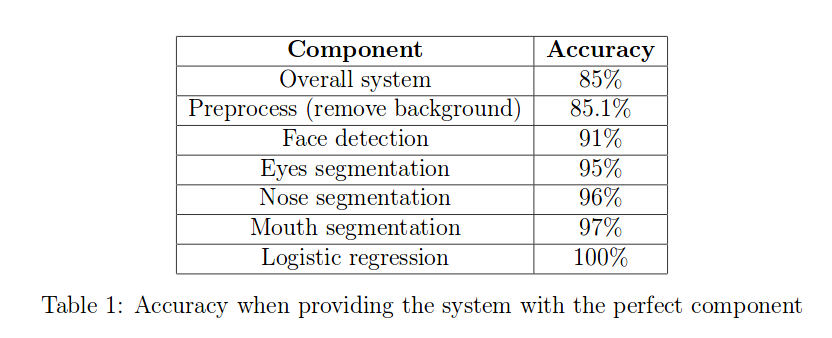
61 |
62 | # 3 Ablative Analysis
63 |
64 | Whereas error analysis tries to recognize the difference between current performance and perfect performance, Ablative Analysis tries to recognize that between baseline and current model. Ablation analysis is quite important, many research papers are rejected because of the missing of this part. This analysis can tell us which part of the model affects the most.
65 |
66 |
67 | For example, assume that we have more add-on features that makes the model perform better. We want to see how much performance it will be reduced by eliminating one add-on feature at a time. An example can be shown below.
68 |
69 | 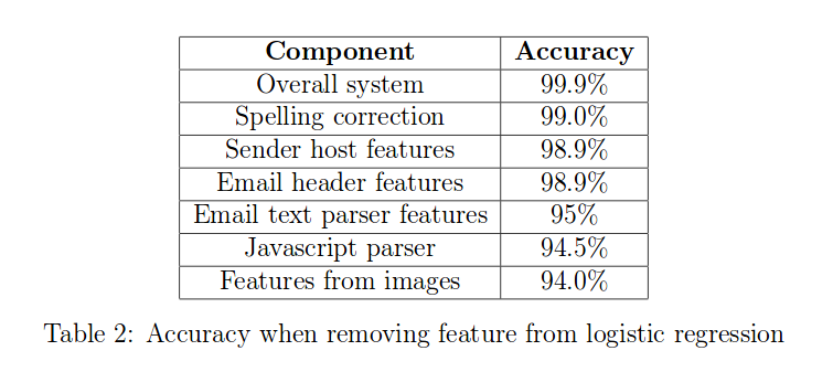
--------------------------------------------------------------------------------
/machine-learning/chinese-version/sv_regularization_model_selection_ch.md:
--------------------------------------------------------------------------------
1 | ---
2 | published: true
3 | layout: single
4 | mathjax: true
5 | toc: true
6 | toc_sticky: true
7 | category: Machine Learning
8 | tags: [notes,chinese]
9 | excerpt: "This post is a translation for one of Wei's posts in his machine learning notes."
10 | title: Regularization and Model Selection Chinese Version
11 | share: true
12 | author_profile: true
13 | permalink: /MachineLearning/sv_regularization_model_selection_ch/
14 | ---
15 |
16 | This Article is a Chinese translation of a study note by Wei. Click [here](https://wei2624.github.io/MachineLearning/sv_regularization_model_selection/) to see the original English version in Wei's homepage. I will continue to update Chinese translation to sync with Wei's notes.
17 |
18 | 请注意: 本文是我翻译的一份学习资料,英文原版请点击[Wei的学习笔记](https://wei2624.github.io/MachineLearning/sv_regularization_model_selection/)。我将不断和原作者的英文笔记同步内容,定期更新和维护。
19 |
20 | 正则化与模型选择
21 | 在选择模型时,如果我们在一个模型中有k个参数,那么问题就是这k个参数应该是什么值?哪些值可以给出最佳偏差-方差权衡呢。其中,我们从有限集合的模型 $\mathcal{M} = \{M_1,M_2,\dots,M_d\}$ 中来选取最佳模型。在集合中,我们有不同的模型,或者不同的参数。
22 |
23 | # 1 交叉验证(Cross Validation)
24 |
25 | 想象一下,给定数据集S与一系列的模型,我们很容易想到通过以下方式来选择模型:
26 |
27 | 1 从S集合训练每个模型$M_i$ ,并得到相应的假设$h_i$
28 |
29 | 2 选取最小训练误差的模型
30 |
31 | 这个想法不能达到目的因为当我们选择的多项数阶数越高时,模型会更好的拟合训练数据集。然而,这个模型将会在新的数据集中有很高的统一化误差,也就是高方差。
32 |
33 | 在这个情况中,**保留交叉验证(hold-out cross validation)**将会做得更好:
34 |
35 | 1 以70%和30%的比例将S随机分成训练数据集$S_{tr}$和验证数据集$S_{cv}$
36 |
37 | 2 在$S_{tr}$在中训练每一个 $M_i$ 以学习假设 $h_i$
38 |
39 | 3 选择拥有最小**经验误差(empirical error)**的模型 $S_{cv}$,我们将它标记为
40 | $\hat{\varepsilon}\_{S_{cv}}(h_i)$
41 |
42 | 通过以上几步,我们试图通过测试模型在验证集上的表现以估计真实统一化误差。在第3步中,在选择最优模型后,我们可以用整个数据集来重复训练模型来得到最佳假设模型。然而,即使我们可以这样做,我们仍然选择的是基于70%数据集来训练模型。当数据少的时候这是很糟糕的。
43 |
44 | 因此,我们引出**K折交叉验证(K-fold cross validation)**:
45 |
46 | 1 随机将S分成k个分离的子集,每个子集有m/k个样本,记为$S_1,S_2,\dots,S_k$
47 |
48 | 2 对于每个模型$M_i$,我们排除一个子集并标记为j,然后我们用其余的样本训练模型以得到$H_{ij}$。我们在$S_j$上测试模型,并且得到 $\varepsilon_{S_j}(h_{ij})$。我们这样遍历每一个j。最后,我们获取统一化误差除以j的平均。
49 |
50 | 3 我们选择有最小平均统一误差的模型
51 |
52 | 通常我们取k为10。虽然这样计算上很复杂,但是它会给我们很好的结果。如果数据很少,我们也可能设k=m。在这种情况下,我们每一次除去一个样本,这种方法叫**除一交叉验证(leave-one-out cross validation)**。
53 |
54 | # 2 特征选择(Feature Selection)
55 |
56 | 如果我们有n个特征,m个样本,其中$n \gg m$ (VC 维度is O(n)),我们可能会过度拟合。在这种情况下,你想选择最重要的特征来训练。在暴力算法中,我们会有用$2^n$ 个特征组合,我们会有$2^n$ 个可能的模型,这处理起来会很费力。因此我们可以选择用**向前搜索算法(forward search algorithm)**:
57 |
58 | 1 我们初始化为$\mathcal{F} = \emptyset$
59 |
60 | 2 重复:(a)for $i =1,\dots,n$ 如果$i\notin\mathcal{F}$, 让$\mathcal{F}_i = \mathcal{F}\cup\{i\}$ 并且使用交叉验证算法来估计$\mathcal{F}_i$. (b)设置$\mathcal{F}$作为(a)中的最佳特征子集
61 |
62 | 3 从以上选择最佳特征子集。
63 |
64 | 你可以通过设置目标特征数量来终止循环。相反地,在特征选择中我们也可以使用**向后搜索算法(backward search)**,这于去除算法类似。然而,因为这两种算法的时间复杂度都是$O(n^2)$ ,它们训练起来都会比较慢。
65 |
66 | 然而,我们也可以使用**过滤特征选择(filter feature selection)**。它的概念是对于标签y,我们会根据每一个特征提供了多少信息来给它打分,然后挑选出最佳者。
67 | 一个容易想到的方法是根据每个$x_i$和标签y的相关性打分。实际中,我们将分数设为**相互信息(mutual information)**:
68 |
69 | $$MI(x_i,y) = \sum\limits_{x_i\in\{0,1\}}\sum\limits_{y\in\{0,1\}} p(x_i,y)\log\frac{p(x_i,y)}{p(x_i)p(y)}$$
70 |
71 | 其中我们假设每个特征和标签都是二元值,并且求和覆盖整个变量域。每一个可能性都会从训练数据集中计算。为了进一步理解,我们知道:
72 |
73 | $$MI(x_i,y) = KL(p(x_i,y)\lvert\lvert p(x_i)p(y))$$
74 |
75 | 其中KL是**相对熵(Kullback-Leibler divergence)**。它计算了竖线两边变量分布的差异。如果$x_i$和 $y$ 是独立的,那么 KL 是0。这代表着特征和标签直接没有任何关系。然而如果MI很高,那么这个特征和标签有强相关性。
76 |
77 | # 3 贝叶斯统计与正则化(Bayesian Statistics and regularization)
78 |
79 | 在前面一章我们讨论了**最大似然法(maximum likelihood (ML) algorithm)**是如何训练模型参数的:
80 |
81 | $$\theta_{ML} = \arg\max\prod_{i=1}^m p(y^{(i)}\lvert x^{(i)},\theta)$$
82 |
83 | 在这种情况下,我们视$\theta$ 为未知参数,它已经存在但是未知。我们的任务是找到未知参数并计算它的值。
84 | 同时$\theta$也是随机的,因此我们设置一个先验值,称它为**先验分布(prior distribution)**。基于先验分布,我们可以用S数据集来计算后验分布:
85 |
86 | $$p(\theta\lvert S) = \frac{p(S\lvert\theta)p(\theta)}{p(S)} = \frac{\prod_{i=1}^m p(y^{(i)}\lvert x^{(i)},\theta)(p(\theta)}{\int_{\theta}\prod_{i=1}^m p(y^{(i)}\lvert x^{(i)},\theta)(p(\theta)d\theta}$$
87 |
88 | 使用后验分布来预测推断,我们有:
89 |
90 | $$p(y\lvert x,S) = \int_{\theta}p(y\lvert x,\theta)p(\theta\lvert S)d\theta$$
91 |
92 | 现在,我们可以计算条件期望值y。然而计算后验值的完全解是很难的,因为分母中的积分很难得到完全解。因此,我们用另一种方式来计算,我们找到一个后验值的点估计,在这个点上我们获得后验值的最佳 $\theta$。**最大后验MAP(maximum a posteriori)** 可以用以下方法计算:
93 |
94 | $$\theta_{MAP} = \arg\max_{\theta} = \prod_{i=1}^m p(y^{(i)}\lvert x^{(i)},\theta)p(\theta)$$
95 |
96 | 通常来讲,先验分布有0均值,单位方差。这会使MAP 比ML 更不容易过度拟合。
97 |
98 |
--------------------------------------------------------------------------------
/_includes/toc.html:
--------------------------------------------------------------------------------
1 | {% capture tocWorkspace %}
2 | {% comment %}
3 | Version 1.0.5
4 | https://github.com/allejo/jekyll-toc
5 |
6 | "...like all things liquid - where there's a will, and ~36 hours to spare, there's usually a/some way" ~jaybe
7 |
8 | Usage:
9 | {% include toc.html html=content sanitize=true class="inline_toc" id="my_toc" h_min=2 h_max=3 %}
10 |
11 | Parameters:
12 | * html (string) - the HTML of compiled markdown generated by kramdown in Jekyll
13 |
14 | Optional Parameters:
15 | * sanitize (bool) : false - when set to true, the headers will be stripped of any HTML in the TOC
16 | * class (string) : '' - a CSS class assigned to the TOC
17 | * id (string) : '' - an ID to assigned to the TOC
18 | * h_min (int) : 1 - the minimum TOC header level to use; any header lower than this value will be ignored
19 | * h_max (int) : 6 - the maximum TOC header level to use; any header greater than this value will be ignored
20 | * ordered (bool) : false - when set to true, an ordered list will be outputted instead of an unordered list
21 | * item_class (string) : '' - add custom class for each list item; has support for '%level%' placeholder, which is the current heading level
22 | * baseurl (string) : '' - add a base url to the TOC links for when your TOC is on another page than the actual content
23 |
24 | Output:
25 | An ordered or unordered list representing the table of contents of a markdown block. This snippet will only generate the table of contents and will NOT output the markdown given to it
26 | {% endcomment %}
27 |
28 | {% capture my_toc %}{% endcapture %}
29 | {% assign orderedList = include.ordered | default: false %}
30 | {% assign minHeader = include.h_min | default: 1 %}
31 | {% assign maxHeader = include.h_max | default: 6 %}
32 | {% assign nodes = include.html | split: ' maxHeader %}
45 | {% continue %}
46 | {% endif %}
47 |
48 | {% if firstHeader %}
49 | {% assign firstHeader = false %}
50 | {% assign minHeader = headerLevel %}
51 | {% endif %}
52 |
53 | {% assign indentAmount = headerLevel | minus: minHeader | add: 1 %}
54 | {% assign _workspace = node | split: '' | first }}>{% endcapture %}
61 | {% assign header = _workspace[0] | replace: _hAttrToStrip, '' %}
62 |
63 | {% assign space = '' %}
64 | {% for i in (1..indentAmount) %}
65 | {% assign space = space | prepend: ' ' %}
66 | {% endfor %}
67 |
68 | {% unless include.item_class == blank %}
69 | {% capture listItemClass %}{:.{{ include.item_class | replace: '%level%', headerLevel }}}{% endcapture %}
70 | {% endunless %}
71 |
72 | {% capture my_toc %}{{ my_toc }}
73 | {{ space }}{{ listModifier }} {{ listItemClass }} [{% if include.sanitize %}{{ header | strip_html }}{% else %}{{ header }}{% endif %}]({% if include.baseurl %}{{ include.baseurl }}{% endif %}#{{ html_id }}){% endcapture %}
74 | {% endfor %}
75 |
76 | {% if include.class %}
77 | {% capture my_toc %}{:.{{ include.class }}}
78 | {{ my_toc | lstrip }}{% endcapture %}
79 | {% endif %}
80 |
81 | {% if include.id %}
82 | {% capture my_toc %}{: #{{ include.id }}}
83 | {{ my_toc | lstrip }}{% endcapture %}
84 | {% endif %}
85 | {% endcapture %}{% assign tocWorkspace = '' %}{{ my_toc | markdownify | strip }}
--------------------------------------------------------------------------------
/_layouts/compress.html:
--------------------------------------------------------------------------------
1 | ---
2 | # Jekyll layout that compresses HTML
3 | # v3.0.2
4 | # http://jch.penibelst.de/
5 | # © 2014–2015 Anatol Broder
6 | # MIT License
7 | ---
8 |
9 | {% capture _LINE_FEED %}
10 | {% endcapture %}{% if site.compress_html.ignore.envs contains jekyll.environment %}{{ content }}{% else %}{% capture _content %}{{ content }}{% endcapture %}{% assign _profile = site.compress_html.profile %}{% if site.compress_html.endings == "all" %}{% assign _endings = "html head body li dt dd p rt rp optgroup option colgroup caption thead tbody tfoot tr td th" | split: " " %}{% else %}{% assign _endings = site.compress_html.endings %}{% endif %}{% for _element in _endings %}{% capture _end %}{% endcapture %}{% assign _content = _content | remove: _end %}{% endfor %}{% if _profile and _endings %}{% assign _profile_endings = _content | size | plus: 1 %}{% endif %}{% for _element in site.compress_html.startings %}{% capture _start %}<{{ _element }}>{% endcapture %}{% assign _content = _content | remove: _start %}{% endfor %}{% if _profile and site.compress_html.startings %}{% assign _profile_startings = _content | size | plus: 1 %}{% endif %}{% if site.compress_html.comments == "all" %}{% assign _comments = "" | split: " " %}{% else %}{% assign _comments = site.compress_html.comments %}{% endif %}{% if _comments.size == 2 %}{% capture _comment_befores %}.{{ _content }}{% endcapture %}{% assign _comment_befores = _comment_befores | split: _comments.first %}{% for _comment_before in _comment_befores %}{% if forloop.first %}{% continue %}{% endif %}{% capture _comment_outside %}{% if _carry %}{{ _comments.first }}{% endif %}{{ _comment_before }}{% endcapture %}{% capture _comment %}{% unless _carry %}{{ _comments.first }}{% endunless %}{{ _comment_outside | split: _comments.last | first }}{% if _comment_outside contains _comments.last %}{{ _comments.last }}{% assign _carry = false %}{% else %}{% assign _carry = true %}{% endif %}{% endcapture %}{% assign _content = _content | remove_first: _comment %}{% endfor %}{% if _profile %}{% assign _profile_comments = _content | size | plus: 1 %}{% endif %}{% endif %}{% assign _pre_befores = _content | split: "" %}{% assign _pres_after = "" %}{% if _pres.size != 0 %}{% if site.compress_html.blanklines %}{% assign _lines = _pres.last | split: _LINE_FEED %}{% capture _pres_after %}{% for _line in _lines %}{% assign _trimmed = _line | split: " " | join: " " %}{% if _trimmed != empty or forloop.last %}{% unless forloop.first %}{{ _LINE_FEED }}{% endunless %}{{ _line }}{% endif %}{% endfor %}{% endcapture %}{% else %}{% assign _pres_after = _pres.last | split: " " | join: " " %}{% endif %}{% endif %}{% capture _content %}{{ _content }}{% if _pre_before contains "" %}{% endif %}{% unless _pre_before contains "" and _pres.size == 1 %}{{ _pres_after }}{% endunless %}{% endcapture %}{% endfor %}{% if _profile %}{% assign _profile_collapse = _content | size | plus: 1 %}{% endif %}{% if site.compress_html.clippings == "all" %}{% assign _clippings = "html head title base link meta style body article section nav aside h1 h2 h3 h4 h5 h6 hgroup header footer address p hr blockquote ol ul li dl dt dd figure figcaption main div table caption colgroup col tbody thead tfoot tr td th" | split: " " %}{% else %}{% assign _clippings = site.compress_html.clippings %}{% endif %}{% for _element in _clippings %}{% assign _edges = " ;; ;" | replace: "e", _element | split: ";" %}{% assign _content = _content | replace: _edges[0], _edges[1] | replace: _edges[2], _edges[3] | replace: _edges[4], _edges[5] %}{% endfor %}{% if _profile and _clippings %}{% assign _profile_clippings = _content | size | plus: 1 %}{% endif %}{{ _content }}{% if _profile %} | Step | Bytes |
| raw | {{ content | size }}{% if _profile_endings %} |
| endings | {{ _profile_endings }}{% endif %}{% if _profile_startings %} |
| startings | {{ _profile_startings }}{% endif %}{% if _profile_comments %} |
| comments | {{ _profile_comments }}{% endif %}{% if _profile_collapse %} |
| collapse | {{ _profile_collapse }}{% endif %}{% if _profile_clippings %} |
| clippings | {{ _profile_clippings }}{% endif %} |
{% endif %}{% endif %}
--------------------------------------------------------------------------------
/machine-learning/english-version/sv_online_learning_perceptron.md:
--------------------------------------------------------------------------------
1 | ---
2 | layout: single
3 | mathjax: true
4 | toc: true
5 | toc_sticky: true
6 | category: Machine Learning
7 | tags: [notes]
8 | qr: machine_learning_notes.png
9 | title: Online Learning and Perceptron Algorithm
10 | share: true
11 | permalink: /MachineLearning/sv_online_learning_perceptron/
12 | sidebar:
13 | nav: "MachineLearning"
14 | ---
15 |
16 | We have talked about the learning paradigm where we feed a batch of training data to train a model. This is called **batch learning**. In this section, we think about the scenario where the model has to make prediction while it is continously learning on the go. This is called **online learning**.
17 |
18 | In this scenario, we have a sequnce of examples $(x^{(1)},y^{(1)}),(x^{(2)},y^{(2)}),\dots,(x^{(n)},y^{(n)})$. What online learning does is to first feed $x^{(1)}$ to the model and ask model to predict, and then show $y^{(1)}$ to the model to let the model perform learning process on it. We do this for one pair of training samples at a time. Eventually, we can come up with a model which has gone through the training dataset. What we are interested in is how many errors this model makes while in online learning process. This is heavily related to the knowledge from learning theory we have discussed before.
19 |
20 | Now, we can take perceptron algorithm as an example. We define $y\in\\{-1,1\\}$ for the label classes. Perceptron algorithm makes prediction based on:
21 |
22 | $$h_{\theta}(x) = g(\theta^{T}x)$$
23 |
24 | where:
25 |
26 | $$g(z) = \begin{cases} 1 \text{, if } z \geq 0 \\ -1 \text{, otherwise} \\ \end{cases}$$
27 |
28 | Then the model makes the update to its parameters as:
29 |
30 | $$\theta_t = \theta_{t-1} + (h_{\theta}-y)x$$
31 |
32 | We can see that if the prediction is correct, we make no change to the parameters. Then, we have the following theorem for the bound on the number of errors made in the online process.
33 |
34 | **Theorem** Let a sequence of examples $(x^{(1)},y^{(1)}),(x^{(2)},y^{(2)}),\dots,(x^{(n)},y^{(n)})$ be given. Suppose that $\lvert\lvert x^{(i)}\rvert\rvert\leq D$ for all i, and further that there exists a unit-length vector u ($\lvert\lvert u\rvert\rvert_2=2$) such that $y^{(i)}(u^Tx^{(i)}\geq \gamma$ for all examples in the sequence(i.e., $u^Tx^{(i)}\geq \gamma$ if $y^{(i)}=1$ and $u^Tx^{(i)}\leq -\gamma$ if $y^{(i)}=-1$ so that u separates the data with the margin at least $\gamma$). Then the total number of mistakes that the perceptron algorithm makes on this sequnece is at most $O(D/\gamma)^2$.
35 |
36 | **Proof**. Perceptron is an online learning algorithm. That means it will feed one pair of samples at a time. We also know that perceptron algorithm only updates its parameters when it makes a mistake. Thus, let $\theta^k$ be the weights that were being used for k-th mistake. We initialize from zero vector. Thus, $\theta^1 = \overrightarrow{0}$. In addition, when we make a mistake on i-th iteration, then $g((x^{(i)})^T\theta^k)\neq y^{(i)}$. This is saying:
37 |
38 | $$(x^{(i)})^T\theta^k y^{(i)} \leq 0$$
39 |
40 | The update rule is $\theta^{k+1} = \theta^k + y^{(i)}x^{(i)}$. We can multiply it by u to have:
41 |
42 | $$(\theta^{k+1})^Tu = (\theta^k)^Tu + y^{(i)}(x^{(i)})^Tu \geq (\theta^k)^Tu + \gamma$$
43 |
44 | This triggers inductive calculation, which says:
45 |
46 | $$(\theta^{k+1})^Tu \geq k\gamma$$
47 |
48 | On the other hand, we have:
49 |
50 | $$\begin{align}
51 | \lvert\lvert \theta^{k+1}\rvert\rvert^2 &= \lvert\lvert \theta^k + y^{(i)}x^{(i)}\rvert\rvert^2\\
52 | &= \lvert\lvert\theta^k\rvert\rvert^2 + 2y^{(i)}(x^{(i)})^T\theta^k + \lvert\lvert x^{(i)}\rvert\rvert^2\\
53 | &\leq \lvert\lvert\theta^k\rvert\rvert^2 + \lvert\lvert x^{(i)}\rvert\rvert^2 \\
54 | &\leq \lvert\lvert\theta^k\rvert\rvert^2 + D^2
55 | \end{align}$$
56 |
57 | The third step is because last term in step 2 is a negative. Similarly, we can apply induction here to get:
58 |
59 | $$\lvert\lvert \theta^{k+1}\rvert\rvert^2 \leq kD^2$$
60 |
61 | Now, we combine everything to get:
62 |
63 | $$\begin{align}
64 | \sqrt{k}D &\geq \lvert\lvert \theta^{k+1}\rvert\rvert\\
65 | &\geq (\theta^{k+1})^Tu\\
66 | &\leq k\gamma
67 | \end{align}$$
68 |
69 | We have second step because u is unit length vector so the product of the norms is greater than the dot product of the two. This means $k\leq (\frac{D}{\gamma})^2$. Note that this bound does not involve in the number of training samples. So the number of mistakes perceptron made is only bounded by D and $\gamma$.
--------------------------------------------------------------------------------
/_layouts/single.html:
--------------------------------------------------------------------------------
1 | ---
2 | layout: default
3 | ---
4 |
5 | {% if page.header.overlay_color or page.header.overlay_image or page.header.image %}
6 | {% include page__hero.html %}
7 | {% elsif page.header.video.id and page.header.video.provider %}
8 | {% include page__hero_video.html %}
9 | {% endif %}
10 |
11 | {% if page.url != "/" and site.breadcrumbs %}
12 | {% unless paginator %}
13 | {% include breadcrumbs.html %}
14 | {% endunless %}
15 | {% endif %}
16 |
17 |
18 | {% include sidebar.html %}
19 | {% include analytics.html %}
20 | {% include disqus.html %}
21 | {% include mathjax.html %}
22 |
23 |
24 | {% if page.title %}{% endif %}
25 | {% if page.excerpt %}{% endif %}
26 | {% if page.date %}{% endif %}
27 | {% if page.last_modified_at %}{% endif %}
28 |
29 |
30 | {% unless page.header.overlay_color or page.header.overlay_image %}
31 |
37 | {% endunless %}
38 |
39 |
40 | {% if page.toc %}
41 |
47 | {% endif %}
48 | {{ content }}
49 | {% if page.link %}{% endif %}
50 |
51 |
52 |
63 |
64 |
81 |
82 |
83 | {% if page.share %}{% include social-share.html %}{% endif %}
84 |
85 | {% include post_pagination.html %}
86 |
92 |
93 | {% comment %}{% endcomment %}
94 | {% if page.id and page.related and site.related_posts.size > 0 %}
95 |
96 |
{{ site.data.ui-text[site.locale].related_label | default: "You May Also Enjoy" }}
97 |
98 | {% for post in site.related_posts limit:4 %}
99 | {% include archive-single.html type="grid" %}
100 | {% endfor %}
101 |
102 |
103 | {% comment %}{% endcomment %}
104 | {% elsif page.id and page.related %}
105 |
106 |
{{ site.data.ui-text[site.locale].related_label | default: "You May Also Enjoy" }}
107 |
108 | {% for post in site.posts limit:4 %}
109 | {% include archive-single.html type="grid" %}
110 | {% endfor %}
111 |
112 |
113 | {% endif %}
114 |
 6 |
7 |
6 |
7 |
8 |
9 |
10 | Photo Credit: [Liam Kay](https://www.thirdsector.co.uk/author/4626/Liam-Kay)
11 |
12 |
13 | AI Learning Hub is an open-sourced machine learning handbook. We contribute to this repo by summarizing interesting blog, course and/or notes of machine learning, deep learning, computer vision, robotics and/or statistics. We also intend to provide each post with Chinese version.
14 |
15 | We do this because we love AI and sharing. Excellent materials are the step stone for learning AI. We think everyone is deserved a chance to study AI with excellent materials. We welcome anyone to join us to make it better!
16 |
17 | And you own whatever you write here!
18 |
19 | ## What notes are/can be posted here?
20 |
21 | We are looking for any related notes that are genuinely created by your own. By genuinity, we mean one of the following:
22 |
23 | 1. You create and write the contents of notes from scratch. Everything is original.
24 |
25 | 2. You summarize contents from related course(s), book(s) and note(s). You can merge contents from multiple sources. Although this is expected to be a summary, your summary should be original.
26 |
27 | 3. You translate one of the notes in THIS repo.
28 |
29 | ## View Contents
30 |
31 | We provide with two ways to view and learn the blogs.
32 |
33 | ### View author's homepage (Highly Recommended!)
34 |
35 | The best way to view the contents of any blog is to view the homepage of the author of that blog that especially interests you. The information of author's homepage of each blog is listed in this README and will be updated as any changes happen.
36 |
37 | We highly recommend this way to view the contents of any blog.
38 |
39 | ### Use Jekyll and Ruby to view locally (Not Recommended)
40 |
41 | 1. Install Ruby environment. Instructions can be found [here](https://jekyllrb.com/docs/installation/).
42 |
43 | 2. Run
44 |
45 | ```
46 | gem install jekyll bundler
47 | ```
48 |
49 | 3. Run
50 |
51 | ```
52 | git clone https://github.com/Wei2624/AI_Learning_Hub.git
53 | cd AI_Learning_Hub
54 | bundle install
55 | bundle exec jekyll build
56 | ```
57 |
58 | 4. In `_site` directory, you can find `.html` file. Then, you are able to view them locally.
59 |
60 | ## Join us
61 |
62 | You are very welcome to join us to improve this repo more!
63 |
64 | ### Write Blog
65 |
66 | The easiest way to contribute is to [fork](https://help.github.com/articles/fork-a-repo/) this project and write your own contents. Remember that you own whatever you write.
67 |
68 | To unify the style of each blog, you should use `markdown` as the syntax with `mathjax` as a plugin for math. Of course, you can insert `html` code whenever you want. An example of header of a blog can be as below:
69 |
70 | ```
71 | ---
72 | layout: single
73 | mathjax: true
74 | title: Regularization and Model Selection
75 | share: true
76 | permalink: /MachineLearning/sv_regularization_model_selection/
77 | ---
78 | ```
79 |
80 | For `layout`, you better either choose `single` where comments are enabled or `archive` where comments are disabled. For more layout options, you can view [here](https://mmistakes.github.io/minimal-mistakes/docs/layouts/).
81 |
82 | `permalink` is a slef-defined relative url path. If you want to host up your blog, you can append `permalink` to your `site-url`.
83 |
84 | **You better follow this procedure so that people can run `ruby` command to generate local page for view.**
85 |
86 |
87 | ### Host Blog
88 |
89 | You can put up your own blog. The easiest way to do this is to use [submodule](https://git-scm.com/book/en/v2/Git-Tools-Submodules) from git.
90 |
91 | Essentially, you have your own repo. Then you can run `git submodule` command to add this repo as a subdirectory to your original repo. This repo will just become one of the folders in your repo. You can access whatever you write here.
92 |
93 |
94 | ## Distribution of contents
95 |
96 | **Distribution of contents without author's permission is strictly prohibited.**
97 |
98 | Please respect the authorship of each blog there. If you want to distribute them, you can ask the author for permission. Every author here has all the rights to their written blog and is fully responsible for their written blogs.
99 |
100 |
101 | # Blog Information
102 |
103 | ## Blogs in English
104 |
105 | | Module | Blog Title | Lang | Author | Contact |
106 | |:--------:|:------------:|:------:|:--------:|:---------:|
107 | |ML|[Generative Algorithm](https://wei2624.github.io/MachineLearning/sv_generative_model/)|EN|[Wei Zhang](https://wei2624.github.io/)|weiuw2624@gmail.com|
108 | |ML|[Discriminative Algorithm](https://wei2624.github.io/MachineLearning/sv_discriminative_model/)|EN|[Wei Zhang](https://wei2624.github.io/)|weiuw2624@gmail.com|
109 | |ML|[Support Vector Machine](https://wei2624.github.io/MachineLearning/sv_svm/)|EN|[Wei Zhang](https://wei2624.github.io/)|weiuw2624@gmail.com|
110 | |ML|[Bias-Varaince and Error Analysis](https://wei2624.github.io/MachineLearning/sv_bias_variance_tradeoff/)|EN|[Wei Zhang](https://wei2624.github.io/)|weiuw2624@gmail.com|
111 | |ML|[Learning Theory ](https://wei2624.github.io/MachineLearning/sv_learning_theory/)|EN|[Wei Zhang](https://wei2624.github.io/)|weiuw2624@gmail.com|
112 | |ML|[Regularization and Model Selection](https://wei2624.github.io/MachineLearning/sv_regularization_model_selection/)|EN|[Wei Zhang](https://wei2624.github.io/)|weiuw2624@gmail.com|
113 | |ML|[Online Learning and Perceptron Algorithm](https://wei2624.github.io/MachineLearning/sv_online_learning_perceptron/)|EN|[Wei Zhang](https://wei2624.github.io/)|weiuw2624@gmail.com|
114 | |ML|[K-Means](https://wei2624.github.io/MachineLearning/usv_kmeans/)|EN|[Wei Zhang](https://wei2624.github.io/)|weiuw2624@gmail.com|
115 | |ML|[EM Algorithm](https://wei2624.github.io/MachineLearning/usv_em/)|EN|[Wei Zhang](https://wei2624.github.io/)|weiuw2624@gmail.com|
116 | |ML|[Variational Inference](https://wei2624.github.io/MachineLearning/bayes_vi/)|EN|[Wei Zhang](https://wei2624.github.io/)|weiuw2624@gmail.com|
117 | |DL|[Nerual Networks ](https://wei2624.github.io/MachineLearning/dl_neural_network/)|EN|[Wei Zhang](https://wei2624.github.io/)|weiuw2624@gmail.com|
118 | |DL|[Backpropagation](https://wei2624.github.io/MachineLearning/dl_propagtion/)|EN|[Wei Zhang](https://wei2624.github.io/)|weiuw2624@gmail.com|
119 |
120 | ## Blogs in Chinese
121 |
122 | | Module | Blog Title | Lang | Author | Contact |
123 | |:--------:|:------------:|:------:|:--------:|:---------:|
124 | |ML|[Generative Algorithm](https://air-yan.github.io/machine%20learning/Generative-Learning-Algorithm/)|CH|[Zishi Yan](https://air-yan.github.io/)|WeChat:air-sowhat|
125 | |ML|[Discriminative Algorithm](https://dark417.github.io/MachineLearning/sv_discriminative_model_ch/)|CH|[Xiaoxiao Lei](https://dark417.github.io/)|WeChat: Dark417|
126 | |ML|[Support Vector Machine](https://air-yan.github.io//MachineLearning/sv_svm_ch/)|CH|[Zishi Yan](https://air-yan.github.io/)|WeChat:air-sowhat|
127 | |ML|[Bias-Varaince and Error Analysis](https://dark417.github.io/MachineLearning/sv_bias_variance_tradeoff_ch/)|CH|[Xiaoxiao Lei](https://dark417.github.io/)|WeChat: Dark417|
128 | |ML|[Regularization and Model Selection](https://dark417.github.io/MachineLearning/sv_regularization_model_selection_ch/)|CH|[Xiaoxiao Lei](https://dark417.github.io/)|WeChat: Dark417|
129 |
--------------------------------------------------------------------------------
/Gemfile.lock:
--------------------------------------------------------------------------------
1 | GEM
2 | remote: https://rubygems.org/
3 | specs:
4 | activesupport (4.2.10)
5 | i18n (~> 0.7)
6 | minitest (~> 5.1)
7 | thread_safe (~> 0.3, >= 0.3.4)
8 | tzinfo (~> 1.1)
9 | addressable (2.5.2)
10 | public_suffix (>= 2.0.2, < 4.0)
11 | coffee-script (2.4.1)
12 | coffee-script-source
13 | execjs
14 | coffee-script-source (1.11.1)
15 | colorator (1.1.0)
16 | commonmarker (0.17.13)
17 | ruby-enum (~> 0.5)
18 | concurrent-ruby (1.1.4)
19 | dnsruby (1.61.2)
20 | addressable (~> 2.5)
21 | em-websocket (0.5.1)
22 | eventmachine (>= 0.12.9)
23 | http_parser.rb (~> 0.6.0)
24 | ethon (0.11.0)
25 | ffi (>= 1.3.0)
26 | eventmachine (1.2.7)
27 | execjs (2.7.0)
28 | faraday (0.15.4)
29 | multipart-post (>= 1.2, < 3)
30 | ffi (1.9.25)
31 | forwardable-extended (2.6.0)
32 | gemoji (3.0.0)
33 | github-pages (193)
34 | activesupport (= 4.2.10)
35 | github-pages-health-check (= 1.8.1)
36 | jekyll (= 3.7.4)
37 | jekyll-avatar (= 0.6.0)
38 | jekyll-coffeescript (= 1.1.1)
39 | jekyll-commonmark-ghpages (= 0.1.5)
40 | jekyll-default-layout (= 0.1.4)
41 | jekyll-feed (= 0.11.0)
42 | jekyll-gist (= 1.5.0)
43 | jekyll-github-metadata (= 2.9.4)
44 | jekyll-mentions (= 1.4.1)
45 | jekyll-optional-front-matter (= 0.3.0)
46 | jekyll-paginate (= 1.1.0)
47 | jekyll-readme-index (= 0.2.0)
48 | jekyll-redirect-from (= 0.14.0)
49 | jekyll-relative-links (= 0.5.3)
50 | jekyll-remote-theme (= 0.3.1)
51 | jekyll-sass-converter (= 1.5.2)
52 | jekyll-seo-tag (= 2.5.0)
53 | jekyll-sitemap (= 1.2.0)
54 | jekyll-swiss (= 0.4.0)
55 | jekyll-theme-architect (= 0.1.1)
56 | jekyll-theme-cayman (= 0.1.1)
57 | jekyll-theme-dinky (= 0.1.1)
58 | jekyll-theme-hacker (= 0.1.1)
59 | jekyll-theme-leap-day (= 0.1.1)
60 | jekyll-theme-merlot (= 0.1.1)
61 | jekyll-theme-midnight (= 0.1.1)
62 | jekyll-theme-minimal (= 0.1.1)
63 | jekyll-theme-modernist (= 0.1.1)
64 | jekyll-theme-primer (= 0.5.3)
65 | jekyll-theme-slate (= 0.1.1)
66 | jekyll-theme-tactile (= 0.1.1)
67 | jekyll-theme-time-machine (= 0.1.1)
68 | jekyll-titles-from-headings (= 0.5.1)
69 | jemoji (= 0.10.1)
70 | kramdown (= 1.17.0)
71 | liquid (= 4.0.0)
72 | listen (= 3.1.5)
73 | mercenary (~> 0.3)
74 | minima (= 2.5.0)
75 | nokogiri (>= 1.8.2, < 2.0)
76 | rouge (= 2.2.1)
77 | terminal-table (~> 1.4)
78 | github-pages-health-check (1.8.1)
79 | addressable (~> 2.3)
80 | dnsruby (~> 1.60)
81 | octokit (~> 4.0)
82 | public_suffix (~> 2.0)
83 | typhoeus (~> 1.3)
84 | html-pipeline (2.9.1)
85 | activesupport (>= 2)
86 | nokogiri (>= 1.4)
87 | http_parser.rb (0.6.0)
88 | i18n (0.9.5)
89 | concurrent-ruby (~> 1.0)
90 | jekyll (3.7.4)
91 | addressable (~> 2.4)
92 | colorator (~> 1.0)
93 | em-websocket (~> 0.5)
94 | i18n (~> 0.7)
95 | jekyll-sass-converter (~> 1.0)
96 | jekyll-watch (~> 2.0)
97 | kramdown (~> 1.14)
98 | liquid (~> 4.0)
99 | mercenary (~> 0.3.3)
100 | pathutil (~> 0.9)
101 | rouge (>= 1.7, < 4)
102 | safe_yaml (~> 1.0)
103 | jekyll-avatar (0.6.0)
104 | jekyll (~> 3.0)
105 | jekyll-coffeescript (1.1.1)
106 | coffee-script (~> 2.2)
107 | coffee-script-source (~> 1.11.1)
108 | jekyll-commonmark (1.2.0)
109 | commonmarker (~> 0.14)
110 | jekyll (>= 3.0, < 4.0)
111 | jekyll-commonmark-ghpages (0.1.5)
112 | commonmarker (~> 0.17.6)
113 | jekyll-commonmark (~> 1)
114 | rouge (~> 2)
115 | jekyll-default-layout (0.1.4)
116 | jekyll (~> 3.0)
117 | jekyll-feed (0.11.0)
118 | jekyll (~> 3.3)
119 | jekyll-gist (1.5.0)
120 | octokit (~> 4.2)
121 | jekyll-github-metadata (2.9.4)
122 | jekyll (~> 3.1)
123 | octokit (~> 4.0, != 4.4.0)
124 | jekyll-mentions (1.4.1)
125 | html-pipeline (~> 2.3)
126 | jekyll (~> 3.0)
127 | jekyll-optional-front-matter (0.3.0)
128 | jekyll (~> 3.0)
129 | jekyll-paginate (1.1.0)
130 | jekyll-readme-index (0.2.0)
131 | jekyll (~> 3.0)
132 | jekyll-redirect-from (0.14.0)
133 | jekyll (~> 3.3)
134 | jekyll-relative-links (0.5.3)
135 | jekyll (~> 3.3)
136 | jekyll-remote-theme (0.3.1)
137 | jekyll (~> 3.5)
138 | rubyzip (>= 1.2.1, < 3.0)
139 | jekyll-sass-converter (1.5.2)
140 | sass (~> 3.4)
141 | jekyll-seo-tag (2.5.0)
142 | jekyll (~> 3.3)
143 | jekyll-sitemap (1.2.0)
144 | jekyll (~> 3.3)
145 | jekyll-swiss (0.4.0)
146 | jekyll-theme-architect (0.1.1)
147 | jekyll (~> 3.5)
148 | jekyll-seo-tag (~> 2.0)
149 | jekyll-theme-cayman (0.1.1)
150 | jekyll (~> 3.5)
151 | jekyll-seo-tag (~> 2.0)
152 | jekyll-theme-dinky (0.1.1)
153 | jekyll (~> 3.5)
154 | jekyll-seo-tag (~> 2.0)
155 | jekyll-theme-hacker (0.1.1)
156 | jekyll (~> 3.5)
157 | jekyll-seo-tag (~> 2.0)
158 | jekyll-theme-leap-day (0.1.1)
159 | jekyll (~> 3.5)
160 | jekyll-seo-tag (~> 2.0)
161 | jekyll-theme-merlot (0.1.1)
162 | jekyll (~> 3.5)
163 | jekyll-seo-tag (~> 2.0)
164 | jekyll-theme-midnight (0.1.1)
165 | jekyll (~> 3.5)
166 | jekyll-seo-tag (~> 2.0)
167 | jekyll-theme-minimal (0.1.1)
168 | jekyll (~> 3.5)
169 | jekyll-seo-tag (~> 2.0)
170 | jekyll-theme-modernist (0.1.1)
171 | jekyll (~> 3.5)
172 | jekyll-seo-tag (~> 2.0)
173 | jekyll-theme-primer (0.5.3)
174 | jekyll (~> 3.5)
175 | jekyll-github-metadata (~> 2.9)
176 | jekyll-seo-tag (~> 2.0)
177 | jekyll-theme-slate (0.1.1)
178 | jekyll (~> 3.5)
179 | jekyll-seo-tag (~> 2.0)
180 | jekyll-theme-tactile (0.1.1)
181 | jekyll (~> 3.5)
182 | jekyll-seo-tag (~> 2.0)
183 | jekyll-theme-time-machine (0.1.1)
184 | jekyll (~> 3.5)
185 | jekyll-seo-tag (~> 2.0)
186 | jekyll-titles-from-headings (0.5.1)
187 | jekyll (~> 3.3)
188 | jekyll-watch (2.1.2)
189 | listen (~> 3.0)
190 | jemoji (0.10.1)
191 | gemoji (~> 3.0)
192 | html-pipeline (~> 2.2)
193 | jekyll (~> 3.0)
194 | kramdown (1.17.0)
195 | liquid (4.0.0)
196 | listen (3.1.5)
197 | rb-fsevent (~> 0.9, >= 0.9.4)
198 | rb-inotify (~> 0.9, >= 0.9.7)
199 | ruby_dep (~> 1.2)
200 | mercenary (0.3.6)
201 | mini_portile2 (2.4.0)
202 | minima (2.5.0)
203 | jekyll (~> 3.5)
204 | jekyll-feed (~> 0.9)
205 | jekyll-seo-tag (~> 2.1)
206 | minitest (5.11.3)
207 | multipart-post (2.0.0)
208 | nokogiri (1.9.1)
209 | mini_portile2 (~> 2.4.0)
210 | octokit (4.13.0)
211 | sawyer (~> 0.8.0, >= 0.5.3)
212 | pathutil (0.16.2)
213 | forwardable-extended (~> 2.6)
214 | public_suffix (2.0.5)
215 | rb-fsevent (0.10.3)
216 | rb-inotify (0.10.0)
217 | ffi (~> 1.0)
218 | rouge (2.2.1)
219 | ruby-enum (0.7.2)
220 | i18n
221 | ruby_dep (1.5.0)
222 | rubyzip (1.2.2)
223 | safe_yaml (1.0.4)
224 | sass (3.7.2)
225 | sass-listen (~> 4.0.0)
226 | sass-listen (4.0.0)
227 | rb-fsevent (~> 0.9, >= 0.9.4)
228 | rb-inotify (~> 0.9, >= 0.9.7)
229 | sawyer (0.8.1)
230 | addressable (>= 2.3.5, < 2.6)
231 | faraday (~> 0.8, < 1.0)
232 | terminal-table (1.8.0)
233 | unicode-display_width (~> 1.1, >= 1.1.1)
234 | thread_safe (0.3.6)
235 | typhoeus (1.3.1)
236 | ethon (>= 0.9.0)
237 | tzinfo (1.2.5)
238 | thread_safe (~> 0.1)
239 | unicode-display_width (1.4.1)
240 |
241 | PLATFORMS
242 | ruby
243 |
244 | DEPENDENCIES
245 | github-pages
246 |
247 | BUNDLED WITH
248 | 1.17.3
249 |
--------------------------------------------------------------------------------
/machine-learning/english-version/usv_kmeans.md:
--------------------------------------------------------------------------------
1 | ---
2 | layout: single
3 | mathjax: true
4 | toc: true
5 | toc_sticky: true
6 | category: Machine Learning
7 | tags: [notes]
8 | qr: machine_learning_notes.png
9 | title: K-Means
10 | share: true
11 | permalink: /MachineLearning/usv_kmeans/
12 | sidebar:
13 | nav: "MachineLearning"
14 | ---
15 |
16 | # Introduction
17 |
18 | In supervised learning, we are always given all the labels/ground truth in training phase. This makes it supervised property. Note that in general that supervised learning assumes that each sample is i.i.d. in the training and testing samples.
19 |
20 | In unsupervised learning, we are not given any labels or ground truth for training. We are simply taking input into training model. We call it **unsupervised learning**.
21 |
22 | # K-means Clustering Algorithm
23 |
24 | K-means clustering algorithm is a standard unsupervised learning algorithm for clustering. K-means will usually generate K clusters based on the distance of data point and cluster mean. On the other hand, **knn clustering algorithm** usually will return clusters with k samples for each cluster. Keep in mind that there is no label or ground truth required.
25 |
26 | We are given a training set $\{x^{(1)},x^{(2)},\dots,x^{(m)}\}$ where $x^{(i)}\in \mathbb{R}^n$. These are our training samples. The output should be a vector **c** of cluster assignment for each sample and K mean vectors $\mu$. Formally,
27 |
28 | **Input:** $\mathcal{X}\in \mathbb{R}^n$
29 |
30 | **Output:**
31 |
32 | $c=(c_1,c_2,\dots,c_m)$ where $c_i\in\{1,\dots,K\}$
33 |
34 | $\mu=(\mu_1,\mu_2,\dots,\mu_k)$ where $\mu_k\in\mathbb{R}^n$
35 |
36 | Then, we need to define an objective function that will give us good c and $\mu$ and is easy to optimize.
37 |
38 | An intuitive way is to use Euclidean distance as a measurement. The goal is just to find good centroids with corresponding assignments for each sample. Formally, we want:
39 |
40 | $$\mu^{\ast},c^{\ast} = \arg\min_{\mu,c}\sum\limits_{i=1}^m\sum\limits_{k=1}^K \mathbb{1}\{c_i=k\} \lvert\lvert x_i-\mu_k\rvert\rvert^2$$
41 |
42 | Thus, our loss function can be defined as:
43 |
44 | $$\begin{align}
45 | \mathcal{L} &= \sum\limits_{i=1}^m\sum\limits_{k=1}^K \mathbb{1}\{c_i=k\} \lvert\lvert x_i-\mu_k\rvert\rvert^2 \\
46 | &= \sum\limits_{i=1}^m\lvert\lvert x^i - \mu_{c^i}\rvert\rvert^2
47 | \end{align}$$
48 |
49 | By looking at this function, we can realize that this is a non-convex function. That means we cannot find the global optimal $\mu$ and c. We can only find a local optimum of them.
50 |
51 | ## Gradient-based optimization
52 |
53 | So the frist try is to use gradient-based algorithm to optimize.
54 |
55 | Since we cannot take derivative of the loss function w.r.t. c, so we have to use iterative algorithm. Recall:
56 |
57 | $$w^{t+1} = w^t - \eta\triangledown_w\mathcal{L}$$
58 |
59 | However, it is easily realized that this is hard because:
60 |
61 | First, w needs to be continuous-valued. The vector c is not in this case.
62 |
63 | Second, it will not go to a better value if step size is too big.
64 |
65 | So we seek for an alternative way to this loss function, which is coordinate descent algorithm
66 |
67 | ## Coordinate Descent Algorithm
68 |
69 | So the loss function is:
70 |
71 | $$\mathcal{L} = \sum\limits_{i=1}^m\sum\limits_{k=1}^K \mathbb{1}\{c_i=k\} \lvert\lvert x_i-\mu_k\rvert\rvert^2$$
72 |
73 | Although we cannot find the best $\mu$ and c at the same time, we can:
74 |
75 | (1) fix $\mu$, we find the best c exactly.
76 |
77 | (2) fix c, we find the best $\mu$ exactly.
78 |
79 | The next step is to come up with a formula for updating each parameter.
80 |
81 | **For updating c:**
82 |
83 | We rewrite the loss function as:
84 |
85 | $$\mathcal{L} = \underbrace{\bigg(\sum\limits_{k=1}^K\mathbb{1}[c_1=k]\lvert\lvert x_1-\mu_k\rvert\rvert^2\bigg)}_{\text{distance of }x_1\text{to its assigned centroid}} + \dots + \underbrace{\bigg(\sum\limits_{k=1}^K\mathbb{1}[c_1=k]\lvert\lvert x_m-\mu_k\rvert\rvert^2\bigg)}_{\text{distance of }x_m\text{to its assigned centroid}}$$
86 |
87 | We can minimize this function w.r.t. each $c_i$ by minimizing each term above individually. This solution is:
88 |
89 | $$c^i = \arg\min_j\lvert\lvert x^i - \mu_j\rvert\rvert^2$$
90 |
91 | Because c is discrete, there is no derivative. We simply calculate all the possible values for $c_i$ and pick the smallest.
92 |
93 | **For updating $\mu$:**
94 |
95 | This time, we rewrite the loss function as:
96 |
97 | $$\mathcal{L} = \underbrace{\bigg(\sum\limits_{i=1}^m\mathbb{1}[c_i=1]\lvert\lvert x_i-\mu_1\rvert\rvert^2\bigg)}_{sum squared distance of data in cluster 1} + \dots + \underbrace{\bigg(\sum\limits_{i=1}^m\mathbb{1}[c_i=K]\lvert\lvert x_i-\mu_K\rvert\rvert^2\bigg)}_{sum squared distance of data in cluster K}$$
98 |
99 | For each k, let $n_k = \sum_{i=1}^m\mathbb{1}[c_i=k]$. Then,
100 |
101 | $$\mu_k = \arg\min_{\mu}\sum\limits_{i=1}^m\mathbb{1}[c_i=k]\lvert\lvert x_i-\mu_k\rvert\rvert^2$$
102 |
103 | $$\mu_k = \frac{1}{n_k} \sum\limits_{i=1}^m x_i\mathbb{1}[c_i=k]$$
104 |
105 | Then we can formally define K-means clustering algorithm as:
106 |
107 | 1 Initialize **cluster centroids** $\mu_1,\mu_2,\dots,\mu_k\in \mathbb{R}^n$ randomly
108 |
109 | 2 Repeat until convergence:
110 |
111 | For every i, set $c^i = \arg\min_j\lvert\lvert x^i - \mu_j\rvert\rvert^2$
112 |
113 | For each j, set $\mu_j = \frac{\sum_{i=1}^m\mathbb{1}[c^i=j]x^i}{\sum_{i=1}^m\mathbb{1}[c^i=j]}$
114 |
115 | Intuitively, we can think it this way: given a particular $\mu$, we are able to find the best c but once c is changed we can probably find a better $\mu$. We do this in a cycled way to optimize loss function.
116 |
117 | K is the parameter that we need to pre-define. This is called **parametric laerning**. After selecting K, we can ramdomly pick up K samples to be our K centroids. Surly, we can use some other way to initialize them.
118 |
119 | The figure of learning process can show this process.
120 |
121 | 
122 |
123 | Plot (a) is the plot of samples. Plot (b) is samples with centroids. The rest plots show the training process.
124 |
125 | A natural question to ask is: Is the k-means algorithm guaranteed to converge?
126 |
127 | The answer is yes.
128 |
129 | We have shown that k-means algorithm is exactly coordinate descent on $\mathcal{L}$. Remember that coordinate descent is to minimize the cost function with respect to one of the variables while holding the others static. Every update to c and $\mu$ decreases the loss function to the previous value. Thus, we can always find out that $\mathcal{L}$, c and $\mu$ will always converge.
130 |
131 | Since J is non-convex function, coordinate descent is not guaranteed to converge to the global minimum. Rather, it will always converge to local mimimum. Intuitively, we can see that when c stops changing, the algorithm has converged to a local ooptimal solution. There might be other solutions of c where we can get the same loss function and even better. This is the reault of not being convex.
132 |
133 | To avoid this, we can run k-means several times with different initilizations and choose the best in terms of J.
134 |
135 | # How to select K
136 |
137 | Recall that K-means is a parameteric learning algorithm. That means we need to manually set up a K for the algorithm to work. So how do we select a good K?
138 |
139 | The K-means objective function decreases as K increases. This is no magic. Some simple methods to choose K are that:
140 |
141 | 1 Using advanced information, if you split a set of things among K people, you know K.
142 |
143 | 2 Looking at the relative decrease in loss function. If $K^{\ast}$ is the best, then increasing K when $KK^{\ast}$.
144 |
145 | 3 Seeking for non-parameteric learning. I will talk about that later.
146 |
147 |
148 |
--------------------------------------------------------------------------------
/machine-learning/chinese-version/sv_tree_ch.md:
--------------------------------------------------------------------------------
1 | ---
2 | published: true
3 | layout: single
4 | mathjax: true
5 | toc: true
6 | toc_sticky: true
7 | category: Machine Learning
8 | tags: [notes]
9 | excerpt: "This post is a translation for one of Wei's posts in his machine learning notes."
10 | title: Decision Trees Chinese Version
11 | share: true
12 | author_profile: true
13 | permalink: /MachineLearning/sv_trees_ch/
14 | ---
15 |
16 | 请注意: 本文是我翻译的一份学习资料,英文原版请点击Wei的学习笔记:[Decision Trees](https://wei2624.github.io/MachineLearning/sv_trees/) 我将不断和原作者的英文笔记同步内容,定期更新和维护。
17 |
18 | # 简介
19 |
20 | 决策树是当下使用的最流行的非线性框架之一。目前为止,我们学过的支持向量机和广义线性都是线性模型的例子,内核化则是通过映射特征$\phi(x)$得出非线性假设函数。决策树因其对噪声的鲁棒性和学习析取表达式的能力而闻名。实际上,决策树已被广泛运用于贷款申请人的信用风险测评中。
21 |
22 | 决策树使用二进制规则将输入$x\in \mathbb{R}^d$映射到输出y。从自上而下的角度,树中的每个节点都有一个拆分规则。在最底部,每个叶节点输出一个值或一个类。注意,输出可以重复。每个拆分规则可以表征为:
23 |
24 | $$h(x) = \mathbb{1}[x_j > t]$$
25 |
26 | 对于某些维度j和$t\in \mathbb{R}$,我们可以从叶节点了解到预测结果。以下是一个决策树的例子:
27 |
28 | 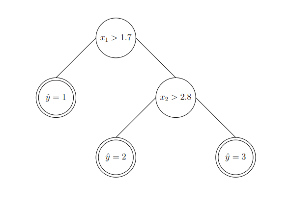
29 |
30 | # 决策树种类
31 |
32 | 与传统预测模型类似,决策树可以分为分类树和回归树。分类树用于对输入进行分类,而回归树通过回归输出真实数值作为预测结果。
33 |
34 | ## 回归树
35 |
36 | 在这种情况下,决策树的运行就像是对空间进行分割,并以此对结果进行预测。例如,我们有一个二维输入空间,在这个空间内我们可以单独对每个维度进行划分,并为某个区域提供回归值。具体可以参考下图的左侧。
37 |
38 | 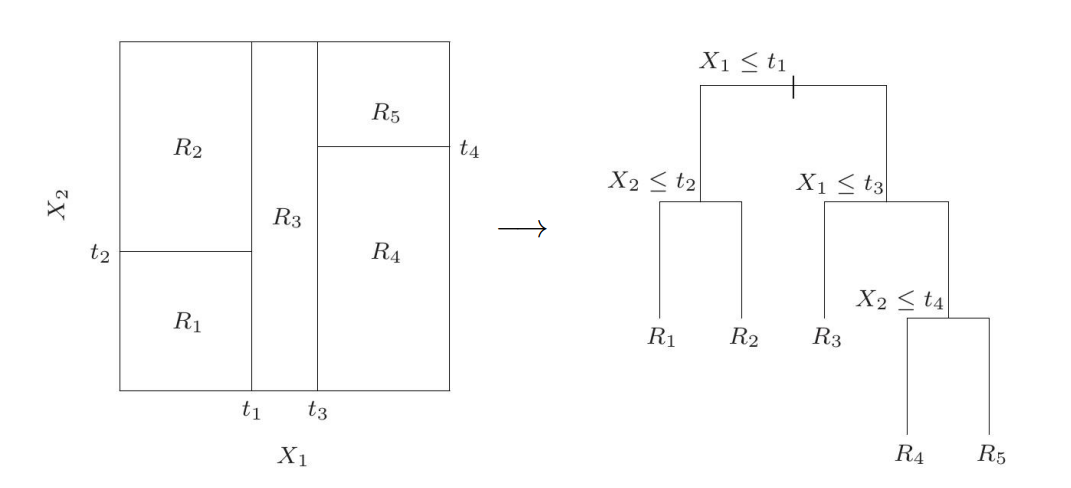
39 |
40 | 回归树事实上是一个如上图中的右侧的树形结构。为了预测,我们将$R_1,R_2,R_3,R_4,R_5$分配给它们的相应路径。在3D空间中,上面的回归树在3D空间中的分割是阶梯式的,如下图所示。
41 |
42 | 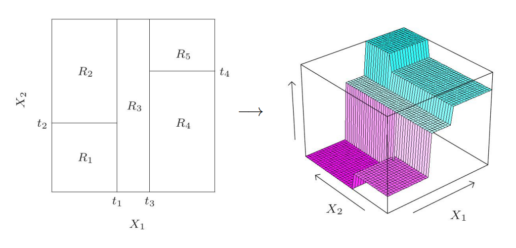
43 |
44 | ## 分类树
45 |
46 | 让我们看一下分类决策树的例子。假设我们有两个特征$x_1,x_2$作为输入,三个类标签作为输出,定义上也就是说$x \in \mathbb{R}^2$ and $y \in \{1,2,3\}$,在图中我们可以看到:
47 |
48 | 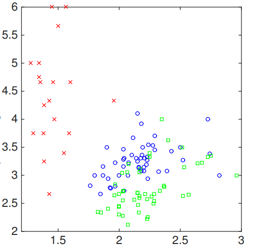
49 |
50 | 现在,我们可以从第一个特征开始下手。那么我们选择1.7作为要分割的阈值。因此,我们可以:
51 |
52 | 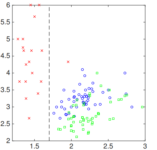
53 |
54 | 输出的决策树可以描述为:
55 |
56 | 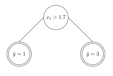
57 |
58 | 我们可以对输入的第二个特征执行类似的操作。我们在第二特征空间选择另一个阈值,其结果是:
59 |
60 | 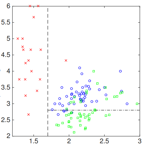
61 |
62 | 生成的决策树可以显示为:
63 |
64 | 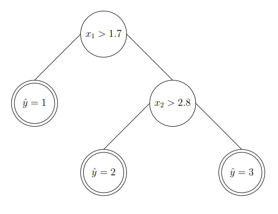
65 |
66 | 上述步骤显示了从输入空间构建分类决策树的流程。
67 |
68 | # 决策树学习算法
69 |
70 | 在本节中,我们将讨论这两种类型决策树的学习算法。通常,学习树使用自上而下的贪婪算法。在此算法中,我们从单个节点开始,找出可以最大程度上降低不确定性的阈值。我们重复这一过程,直到找到所有的阈值。
71 |
72 | ## 回归树学习算法
73 |
74 | 回到例子中:
75 |
76 | 
77 |
78 | 在左图中,我们有五个区域,两个输入特征和四个阈值。让我们推广到M个区域$R_1,\dots,R_M$。那么我们的预测公式可以是:
79 |
80 | $$f(x) = \sum\limits_{m=1}^M c_m \mathbb{1} \{x\in R_m \}$$
81 |
82 | 其中$R_m$是x所属的区域,$c_m$是预测值。
83 |
84 | 目标是尽量减少:
85 |
86 | $$\sum\limits_i (y_i - f(x_i))^2$$
87 |
88 | 我们先来看看定义。这里我们有两个变量需要确定,$c_m, R_m$,其中$c_m$为预测结果。那么如果基于给定的$R_m$,我们是否可以更容易地预测$c_m$呢?答案是肯定的。我们可以简单地求出将该区域所有样本的平均值,作为$c_m$。现在的问题是:我们如何找出这些区域?
89 |
90 | 初始区域通常是整个数据集,首先我们在维度j的阈值s处分割一个区域R。我们可以定义$R^{-}(j,s) = \{ x_i\in\mathbb{R}^d\lvert x_i(j) \leq s \}$ and $R^{+}(j,s) = \{ x_i\in\mathbb{R}^d\lvert x_i(j) \geq s \}$。那么,对于每个维度j,我们计算并找到最佳分裂点s。我们应该为每个现有的区域(叶节点)执行此操作,并根据定义好的度量标准选择出最佳区域分割。
91 |
92 | **简而言之,我们需要选择一个区域(叶节点),然后选择一个特征,再之后选择一个阈值来形成一个新的分割。**
93 |
94 | ## 分类树学习算法
95 |
96 | 在回归树任务中,我们使用了平方误差来确定分割规则的质量。在分类任务中,我们则有更多的选择来评估分割质量。
97 |
98 | 总的来说,在决策树生长中有三种常见的分类测量方法。
99 |
100 | 1, 分类误差: $1 - \max_k p_k$
101 |
102 | 2, 基尼指数: $1 - \sum_k p_k^2$
103 |
104 | 3, 信息熵:$-\sum_k p_k \ln p_k$
105 |
106 | 其中$p_k$代表每个类的经验概率(empirical portion),k表示类索引。对于二元分类,如果我们绘制出每次评估相对于$p_k$的值,我们可以看到:
107 |
108 | 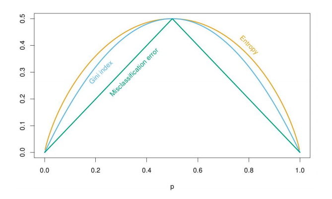
109 |
110 | 这证明了:
111 |
112 | 1, 当$p_k$在$R_m$中的K类上是均匀分布时,所有评估都是最大化的
113 |
114 | 2, 当$p_k = 1$或 0 时,所有评估都被最小化
115 |
116 | 一般而言,我们希望最大化**原始损失**与**分割区域的基数加权损**之差。定义上讲,
117 |
118 | $$L(R_p) = \frac{\lvert R_1\rvert L(R_1) + \lvert R_2\lvert L(R_2)}{\lvert R_1\lvert +\lvert R_2\lvert}$$
119 |
120 | 然而,不同的损失函数各有利弊。对于分类误差类型,它的问题是对分割区域的变化不敏感。例如,如果我们组成一个父区域$R_p$,请看下图:
121 |
122 | 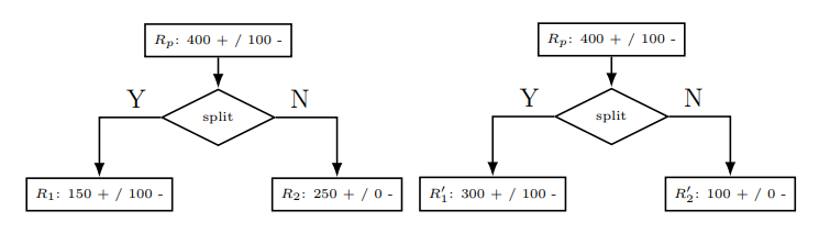
123 |
124 | 虽然以上两个分割是不同的,不过我们可以发现:
125 |
126 | $$L(R_p) = \frac{\lvert R_1\rvert L(R_1) + \lvert R_2\lvert L(R_2)}{\lvert R_1\lvert +\lvert R_2\lvert} = \frac{\lvert R_1^{\prime}\rvert L(R_1^{\prime}) + \lvert R_2^{\prime}\lvert L(R_2^{\prime})}{\lvert R_1^{\prime}\lvert +\lvert R_2^{\prime}\lvert} =100$$
127 |
128 | 我们注意到,如果我们使用分类误差类型,不同的拆分结果也会计算出相同的损失值。此外,我们还看到新的分割区域不会减少原始损失。这是因为,严格上来讲,分类误差损失并非凹函数(concave function)。因此,如果我们绘制上面的分割示例,我们可以看到:
129 |
130 | 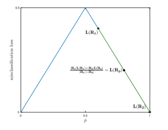
131 |
132 | 从上图中,我们看出分类误差损失对我们并没有多大的帮助。另一方面,如果我们使用信息熵损失,在图中的显示则与其不同。
133 |
134 | 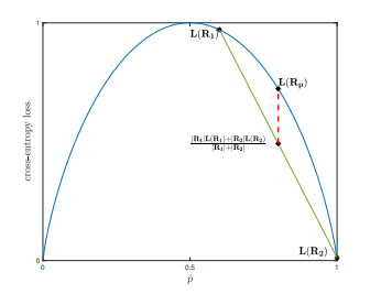
135 |
136 | 从图中可以看出,我们使用信息熵损失方法分割父区域后,得到的损失将减少。这是因为熵函数是凹函数。
137 |
138 | 让我们看一个示例,这个示例将使用Gini索引作为损失函数来生成分类树。让我们假设我们有一个2D空间,空间中绘制了一些分类点。图像如下面所示:
139 |
140 | 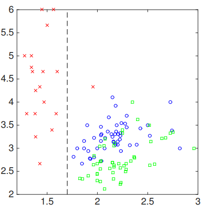
141 |
142 | 在这种情况下,左边$R_1$区域被分类为标签1。我们可以看到它被近似完美地分类,那么我们可以确定对该区域的测量应该是不错的。
143 |
144 | 区域2的话,由于基尼指数并不为零,我们需要下更多功夫。如果我们计算基尼指数,我们可以:
145 |
146 | $$G(R_2) = 1 - (\frac{1}{101})^2 - (\frac{50}{101})^2 - (\frac{50}{101})^2 = 0.5089$$
147 |
148 | 接下来,我们希望看到不同轴上不同位置的分割点如何根据某些评估函数影响该区域的基尼指数。这样的评估函数,即不确定性函数,可以是:
149 |
150 | $$G(R_m) - (p_{r_m^-}G(R_m^-) + p_{r_m^+}G(R_m^+))$$
151 |
152 | 其中$p_{R_m^+}$是$R_m$中的$R_m^+$的占比,$G(R_m^+)$是新区域$R_m^+$的基尼指数。那么,我们希望新的分割区域的基尼指数为零。因此,我们希望最大化**原始区域的基尼指数**与**新区域基尼指数的加权和**之差。因此,我们希望将基尼指数上的减少量设为y,不同的分裂点设为x,并绘制出函数。
153 |
154 | 对于上面的例子,首先我们沿着水平轴来查看不同的分裂点。
155 |
156 | 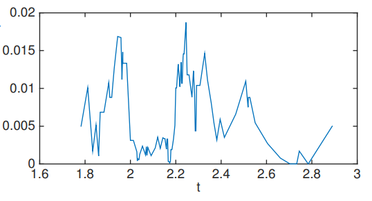
157 |
158 | 你可以看到图的两侧有两个明显的切口,这是因为小于大约1.7左右的点属于标签1,大约在2.9之后就没有任何点了。我们还可以尝试通过沿另一个轴(即垂直轴)滑动来观察结果。
159 |
160 | 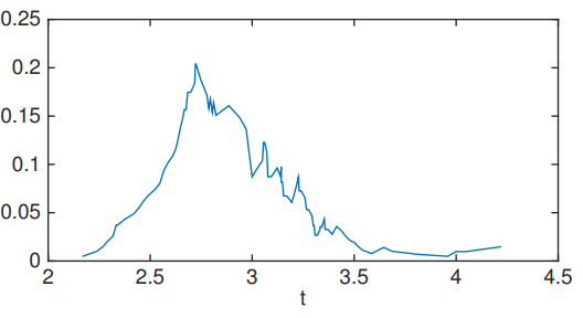
161 |
162 | 从图中可以看出,垂直分裂点在值为2.7附近有最大的改进。那么,我们可以将数据样本拆分为:
163 |
164 | 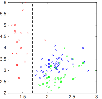
165 |
166 | 最终的决策树:
167 |
168 | 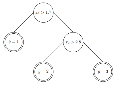
169 |
170 | ## 正规化
171 |
172 | 那么问题来了,我们什么时候选择停止决策树的生长呢?当然,你可以说当叶子只包含一种标签时,我们就停止训练。然而,这将导致高方差和低偏差问题,也就是说过度拟合。一些现有的解决方式如下所示:
173 |
174 | 1,**最小叶子结点大小**:我们可以设置最小叶子结点大小。
175 |
176 | 2,**最大深度**:我们还可以在树深度上设置阈值。
177 |
178 | 3,**最大节点数**:当树中的节点数达到叶节点的阈值时,我们可以停止训练。
179 |
180 | 然而,即便我们可以使用这些方法以避免过度拟合,仍然很难训练一个在一般情况下表现良好的决策树。因此,我们将在另一部分笔记中讲解一种称为**集成方法**的训练技术。
181 |
182 | ## 缺少累加结构
183 |
184 | 在每个决策树节点的决策阶段,决策规则只能有一个,且规则只能基于某一个特征而制定。这个特征只能从现有的两个特征($x_1$ 或 $x_2$)中选择,而不能用另一个新建的特征。这将会为决策树带来一些问题。如下图所示,我们必须在每个轴上设置多个分裂点以保证准确性,因为每次只允许分割一个特征空间。这就是为什么下图中总是出现平行线的原因。
185 |
186 | 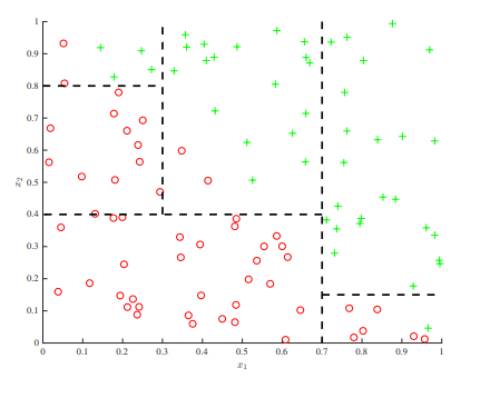
187 |
188 | 但是,通过累加结构,我们可以很容易地绘制出此图的线性边界。
189 |
190 | 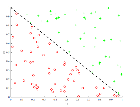
191 |
--------------------------------------------------------------------------------
/_config.yml:
--------------------------------------------------------------------------------
1 | # Theme Settings
2 | #
3 | # Review documentation to determine if you should use `theme` or `remote_theme`
4 | # https://mmistakes.github.io/minimal-mistakes/docs/quick-start-guide/#installing-the-theme
5 |
6 | # theme : "minimal-mistakes-jekyll"
7 | remote_theme : "mmistakes/minimal-mistakes"
8 | minimal_mistakes_skin : "default" # "air", "aqua", "contrast", "dark", "dirt", "neon", "mint", "plum", "sunrise"
9 |
10 | # Site Settings
11 | locale : "en-US"
12 | title : ""
13 | title_separator : "-"
14 | name : ""
15 | description : ""
16 | url : ""
17 | baseurl : #"https://wei2624.github.io"
18 | repository : # GitHub username/repo-name e.g. "mmistakes/minimal-mistakes"
19 | teaser : # path of fallback teaser image, e.g. "/assets/images/500x300.png"
20 | # breadcrumbs : false # true, false (default)
21 | words_per_minute : 100
22 | comments:
23 | provider : # false (default), "disqus", "discourse", "facebook", "google-plus", "staticman", "staticman_v2" "custom"
24 | disqus:
25 | shortname : # https://help.disqus.com/customer/portal/articles/466208-what-s-a-shortname-
26 | discourse:
27 | server : # https://meta.discourse.org/t/embedding-discourse-comments-via-javascript/31963 , e.g.: meta.discourse.org
28 | facebook:
29 | # https://developers.facebook.com/docs/plugins/comments
30 | appid :
31 | num_posts : # 5 (default)
32 | colorscheme : # "light" (default), "dark"
33 | staticman:
34 | allowedFields : # ['name', 'email', 'url', 'message']
35 | branch : # "master"
36 | commitMessage : # "New comment by {fields.name}"
37 | filename : # comment-{@timestamp}
38 | format : # "yml"
39 | moderation : # true
40 | path : # "/_data/comments/{options.slug}" (default)
41 | requiredFields : # ['name', 'email', 'message']
42 | transforms:
43 | email : # "md5"
44 | generatedFields:
45 | date:
46 | type : # "date"
47 | options:
48 | format : # "iso8601" (default), "timestamp-seconds", "timestamp-milliseconds"
49 | reCaptcha:
50 | siteKey :
51 | secret :
52 | atom_feed:
53 | path : # blank (default) uses feed.xml
54 | search : # true, false (default)
55 | search_full_content : # true, false (default)
56 | search_provider : # lunr (default), algolia, google
57 | algolia:
58 | application_id : # YOUR_APPLICATION_ID
59 | index_name : # YOUR_INDEX_NAME
60 | search_only_api_key : # YOUR_SEARCH_ONLY_API_KEY
61 | powered_by : # true (default), false
62 | google:
63 | search_engine_id : # YOUR_SEARCH_ENGINE_ID
64 | instant_search : # false (default), true
65 | # SEO Related
66 | google_site_verification :
67 | bing_site_verification :
68 | yandex_site_verification :
69 | naver_site_verification :
70 |
71 | # Social Sharing
72 | twitter:
73 | username :
74 | facebook:
75 | username :
76 | app_id :
77 | publisher :
78 | og_image : # Open Graph/Twitter default site image
79 | # For specifying social profiles
80 | # - https://developers.google.com/structured-data/customize/social-profiles
81 | social:
82 | type : # Person or Organization (defaults to Person)
83 | name : # If the user or organization name differs from the site's name
84 | links: # An array of links to social media profiles
85 |
86 | # Analytics
87 | analytics:
88 | provider : # false (default), "google", "google-universal", "custom"
89 | google:
90 | tracking_id :
91 | anonymize_ip : # true, false (default)
92 |
93 |
94 | # Site Author
95 | author:
96 | name : ""
97 | avatar : ""
98 | bio : ""
99 | location : ""
100 | email : #"wz2363@columbia.edu"
101 | links:
102 | # - label: "Email"
103 | # icon: "fas fa-fw fa-envelope-square"
104 | # url: mailto:wz2363@columbia.edu
105 |
106 | # Site Footer
107 | footer:
108 | links:
109 | - label: "Twitter"
110 | icon: "fab fa-fw fa-twitter-square"
111 | # url:
112 | - label: "Facebook"
113 | icon: "fab fa-fw fa-facebook-square"
114 | # url:
115 | - label: "GitHub"
116 | icon: "fab fa-fw fa-github"
117 | # url:
118 | - label: "GitLab"
119 | icon: "fab fa-fw fa-gitlab"
120 | # url:
121 | - label: "Bitbucket"
122 | icon: "fab fa-fw fa-bitbucket"
123 | # url:
124 | - label: "Instagram"
125 | icon: "fab fa-fw fa-instagram"
126 | # url:
127 |
128 |
129 | # Reading Files
130 | include:
131 | - .htaccess
132 | - _pages
133 | - _MachineLearning
134 | - _MachineLearning/chinese_version
135 | exclude:
136 | - "*.sublime-project"
137 | - "*.sublime-workspace"
138 | - vendor
139 | - .asset-cache
140 | - .bundle
141 | - .jekyll-assets-cache
142 | - .sass-cache
143 | - assets/js/plugins
144 | - assets/js/_main.js
145 | - assets/js/vendor
146 | - Capfile
147 | - CHANGELOG
148 | - config
149 | - googlea7995681fcbbb1c5
150 | - Gemfile
151 | - Gruntfile.js
152 | - gulpfile.js
153 | - LICENSE
154 | - log
155 | - node_modules
156 | - package.json
157 | - Rakefile
158 | - README
159 | - tmp
160 | keep_files:
161 | - .git
162 | - .svn
163 | encoding: "utf-8"
164 | markdown_ext: "markdown,mkdown,mkdn,mkd,md"
165 |
166 |
167 | # Conversion
168 | markdown: kramdown
169 | highlighter: rouge
170 | lsi: false
171 | excerpt_separator: "\n\n"
172 | incremental: false
173 |
174 |
175 | # Markdown Processing
176 | kramdown:
177 | input: GFM
178 | hard_wrap: false
179 | auto_ids: true
180 | footnote_nr: 1
181 | entity_output: as_char
182 | toc_levels: 1..6
183 | smart_quotes: lsquo,rsquo,ldquo,rdquo
184 | enable_coderay: false
185 |
186 |
187 | # Sass/SCSS
188 | sass:
189 | sass_dir: _sass
190 | style: compressed # http://sass-lang.com/documentation/file.SASS_REFERENCE.html#output_style
191 |
192 |
193 | # Outputting
194 | permalink: /:categories/:title/
195 | paginate: 10 # amount of posts to show
196 | paginate_path: /page:num/
197 | timezone: # https://en.wikipedia.org/wiki/List_of_tz_database_time_zones
198 |
199 |
200 | # Plugins (previously gems:)
201 | plugins:
202 | - jekyll-paginate
203 | - jekyll-sitemap
204 | - jekyll-gist
205 | - jekyll-feed
206 | - jekyll-google_cse
207 | - jemoji
208 |
209 | # mimic GitHub Pages with --safe
210 | whitelist:
211 | - jekyll-paginate
212 | - jekyll-sitemap
213 | - jekyll-gist
214 | - jekyll-feed
215 | - jemoji
216 |
217 |
218 | # Archives
219 | # Type
220 | # - GitHub Pages compatible archive pages built with Liquid ~> type: liquid (default)
221 | # - Jekyll Archives plugin archive pages ~> type: jekyll-archives
222 | # Path (examples)
223 | # - Archive page should exist at path when using Liquid method or you can
224 | # expect broken links (especially with breadcrumbs enabled)
225 | # - /tags/my-awesome-tag/index.html ~> path: /tags/
226 | # - path: /categories/
227 | # - path: /
228 | category_archive:
229 | type: liquid
230 | path: /categories/
231 | tag_archive:
232 | type: liquid
233 | path: /tags/
234 | # https://github.com/jekyll/jekyll-archives
235 | # jekyll-archives:
236 | # enabled:
237 | # - categories
238 | # - tags
239 | # layouts:
240 | # category: archive-taxonomy
241 | # tag: archive-taxonomy
242 | # permalinks:
243 | # category: /categories/:name/
244 | # tag: /tags/:name/
245 |
246 |
247 | # HTML Compression
248 | # - http://jch.penibelst.de/
249 | compress_html:
250 | clippings: all
251 | ignore:
252 | envs: development
253 |
254 |
255 | # Defaults
256 | defaults:
257 | # _posts
258 | - scope:
259 | path: ""
260 | type: posts
261 | values:
262 | layout: single
263 | author_profile: true
264 | read_time: true
265 | comments: # true
266 | share: true
267 | related: true
--------------------------------------------------------------------------------
/_includes/author-profile.html:
--------------------------------------------------------------------------------
1 | {% assign author = page.author | default: page.authors[0] | default: site.author %}
2 | {% assign author = site.data.authors[author] | default: author %}
3 |
4 |
5 |
6 | {% if author.avatar %}
7 |
8 | {% if author.avatar contains "://" %}
9 | {% assign author_src = author.avatar %}
10 | {% else %}
11 | {% assign author_src = author.avatar | relative_url %}
12 | {% endif %}
13 |
14 | {% if author.home %}
15 | {% if author.home contains "://" %}
16 | {% assign author_link = author.home %}
17 | {% else %}
18 | {% assign author_link = author.home | relative_url %}
19 | {% endif %}
20 |
21 |  22 |
22 |
23 | {% else %}
24 |
25 | {% endif %}
26 |
27 | {% endif %}
28 |
29 |
30 | {% if author.home %}
31 |
{{ author.name }}
32 | {% else %}
33 |
{{ author.name }}
34 | {% endif %}
35 | {% if author.bio %}
36 |
37 | {{ author.bio }}
38 |
39 | {% endif %}
40 |
41 |
42 |
43 |
44 |
270 |
271 |
 4 |
4 |