0]
2403 | P.values=P.values[P.values<1]
2404 | N=length(P.values)
2405 | P.values=P.values[order(P.values)]
2406 | }else{
2407 | N=length(P.values)
2408 | P.values=P.values[order(P.values,decreasing=TRUE)]
2409 | }
2410 | p_value_quantiles=(1:length(P.values))/(length(P.values)+1)
2411 | log.Quantiles <- -log10(p_value_quantiles)
2412 | if(LOG10){
2413 | log.P.values <- -log10(P.values)
2414 | }else{
2415 | log.P.values <- P.values
2416 | }
2417 |
2418 | #calculate the confidence interval of QQ-plot
2419 | if(conf.int){
2420 | N1=length(log.Quantiles)
2421 | c95 <- rep(NA,N1)
2422 | c05 <- rep(NA,N1)
2423 | for(j in 1:N1){
2424 | xi=ceiling((10^-log.Quantiles[j])*N)
2425 | if(xi==0)xi=1
2426 | c95[j] <- qbeta(0.95,xi,N-xi+1)
2427 | c05[j] <- qbeta(0.05,xi,N-xi+1)
2428 | }
2429 | index=length(c95):1
2430 | }else{
2431 | c05 <- 1
2432 | c95 <- 1
2433 | }
2434 | if(is.null(ylim)){
2435 | YlimMax <- max_no_na(c(floor(max_no_na(c(max_no_na(-log10(c05)), max_no_na(-log10(c95))))+1), floor(max_no_na(log.P.values)+1)))
2436 | plot(NULL, xlim=c(0,floor(max_no_na(log.Quantiles)+1)), axes=FALSE, cex.axis=axis.cex, cex.lab=lab.cex,ylim=c(0,YlimMax),xlab="",ylab="")
2437 | }else{
2438 | plot(NULL, xlim=c(0,floor(max_no_na(log.Quantiles)+1)), axes=FALSE, cex.axis=axis.cex, cex.lab=lab.cex,ylim=c(0,max(ylim[[i]])),xlab="",ylab="")
2439 | }
2440 | axis(1, mgp=c(3,xticks.pos,0),at=seq(0,floor(max_no_na(log.Quantiles)+1),ceiling((max_no_na(log.Quantiles)+1)/10)), lwd=axis.lwd,labels=seq(0,floor(max_no_na(log.Quantiles)+1),ceiling((max_no_na(log.Quantiles)+1)/10)), cex.axis=axis.cex)
2441 | axis(2, las=1,lwd=axis.lwd,cex.axis=axis.cex)
2442 | axis(2, at=c(0, ifelse(is.null(ylim), YlimMax, max(ylim[[i]]))), labels=c("",""), tcl=0, lwd=axis.lwd)
2443 |
2444 | mtext(side=1, text=expression(Expected~~-log[10](italic(p))), line=ylab.pos+1, cex=lab.cex, font=lab.font, xpd=TRUE)
2445 | mtext(side=2, text=expression(Observed~~-log[10](italic(p))), line=ylab.pos, cex=lab.cex, font=lab.font, xpd=TRUE)
2446 |
2447 | #plot the confidence interval of QQ-plot
2448 | if(conf.int){
2449 | if(is.null(conf.int.col)){
2450 | polygon(c(log.Quantiles[index],log.Quantiles),c(-log10(c05)[index],-log10(c95)),col=rgb(t(col2rgb(t(col)[i])), alpha=points.alpha, maxColorValue=255),border=rgb(t(col2rgb(t(col)[i])), alpha=points.alpha, maxColorValue=255))
2451 | }else{
2452 | polygon(c(log.Quantiles[index],log.Quantiles),c(-log10(c05)[index],-log10(c95)),col=rgb(t(col2rgb(conf.int.col[i])), alpha=points.alpha, maxColorValue=255),border=rgb(t(col2rgb(conf.int.col[i])), alpha=points.alpha, maxColorValue=255))
2453 | }
2454 | }
2455 |
2456 | if(!is.null(threshold.col)){par(xpd=FALSE); abline(a=0, b=1,lwd=threshold.lty[1], lty=threshold.lty[1], col=threshold.col[1]); par(xpd=TRUE)}
2457 | # points(log.Quantiles, log.P.values, col=t(col)[i],pch=19,cex=cex[3])
2458 | is_visable <- filter.points(log.Quantiles, log.P.values, wh, ht, dpi=dpi)
2459 | if(!is.null(threshold[[i]])){
2460 | # if(sum(threshold!=0)==length(threshold)){
2461 | thre.line=-log10(min_no_na(threshold[[i]]))
2462 | if(amplify==TRUE){
2463 | thre.index <- log.P.values
3 |
4 | ## A high-quality drawing tool designed for Manhattan plot of genomic analysis
5 |
6 | ### :toolbox: Relevant software tools for genetic analyses and genomic breeding
7 |
8 |
9 | | 📫 HIBLUP: Versatile and easy-to-use GS toolbox. |
10 | 🍀 SIMER: data simulation for life science and breeding. |
11 |
12 |
13 | | 🚴♂️ KAML: Advanced GS method for complex traits. |
14 | 🏔️ IAnimal: an omics knowledgebase for animals. |
15 |
16 |
17 | | 🏊 hibayes: A Bayesian-based GWAS and GS tool. |
18 | 📮 rMVP: Efficient and easy-to-use GWAS tool. |
19 |
20 |
21 |
22 | ### Installation
23 |
24 | **CMplot** is available on CRAN, so it can be installed with the following R code:
25 |
26 | ```r
27 | > install.packages("CMplot")
28 | > library("CMplot")
29 |
30 | # if you want to use the latest version on GitHub:
31 | > source("https://raw.githubusercontent.com/YinLiLin/CMplot/master/R/CMplot.r")
32 | ```
33 |
34 | ---
35 |
36 | There are two example datasets attached in **CMplot**, users can export and view the details by following R code:
37 |
38 | ```r
39 | > data(pig60K) #calculated p-values by MLM
40 | > data(cattle50K) #calculated SNP effects by rrblup
41 | > head(pig60K)
42 |
43 | SNP Chromosome Position trait1 trait2 trait3
44 | 1 ALGA0000009 1 52297 0.7738187 0.51194318 0.51194318
45 | 2 ALGA0000014 1 79763 0.7738187 0.51194318 0.51194318
46 | 3 ALGA0000021 1 209568 0.7583016 0.98405289 0.98405289
47 | 4 ALGA0000022 1 292758 0.7200305 0.48887140 0.48887140
48 | 5 ALGA0000046 1 747831 0.9736840 0.22096836 0.22096836
49 | 6 ALGA0000047 1 761957 0.9174565 0.05753712 0.05753712
50 |
51 | > head(cattle50K)
52 |
53 | SNP chr pos Somatic cell score Milk yield Fat percentage
54 | 1 SNP1 1 59082 0.000244361 0.000484255 0.001379210
55 | 2 SNP2 1 118164 0.000532272 0.000039800 0.000598951
56 | 3 SNP3 1 177246 0.001633058 0.000311645 0.000279427
57 | 4 SNP4 1 236328 0.001412865 0.000909370 0.001040161
58 | 5 SNP5 1 295410 0.000090700 0.002202973 0.000351394
59 | 6 SNP6 1 354493 0.000110681 0.000342628 0.000105792
60 |
61 | ```
62 | As the example datasets, the first three columns are names, chromosome, position of SNPs respectively, the rest of columns are the pvalues of GWAS or effects of GS/GP for traits, the number of traits is unlimited.
63 | Note: if plotting SNP_Density, only the first three columns are needed.
64 |
65 | Now **CMplot** could handle not only Genome-wide association study results, but also SNP effects, Fst, tajima's D and so on.
66 |
67 | ---
68 |
69 | Total 50~ parameters are available in **CMplot**, typing ```?CMplot``` can get the detail function of all parameters.
70 |
71 | ---
72 | ### Citation
73 | CMplot has been integrated into our developed GWAS package ```rMVP```, please cite the following paper:
74 | Yin, L. et al. [rMVP: A Memory-efficient, Visualization-enhanced, and Parallel-accelerated tool for Genome-Wide Association Study](https://doi.org/10.1016/j.gpb.2020.10.007), ***Genomics, Proteomics & Bioinformatics*** (2021), doi: 10.1016/j.gpb.2020.10.007.
75 |
76 | ---
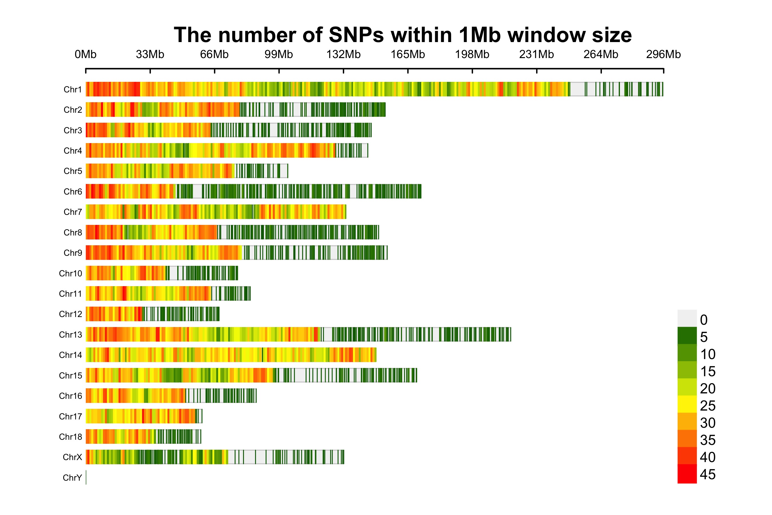
77 | ### SNP-density plot
78 |
79 | ```r
80 | > CMplot(pig60K,plot.type="d",bin.size=1e6,chr.den.col=c("darkgreen", "yellow", "red"),file="jpg",file.name=NULL,dpi=300,
81 | main="illumilla_60K",file.output=TRUE,verbose=TRUE,width=9,height=6)
82 | # set the window size: bin.size=1e6
83 | # set the legend breaks by: bin.breaks=seq(min, max, step), e.g., bin.breaks=seq(0, 50, 10), the windows out of the breaks will be plotted in the same color as min or max.
84 | # get the detailed information of all windows: "windinfo <- CMplot(pig60K, plot.type="d", ...)"
85 | # file: the format of the output file, if file="png", CMplot will output a transparent background file
86 | # file.name: specify the output file name, the default is corresponding column name when setting file.name=NULL
87 | # chr.labels: change the chromosome names
88 | # main: change the title of the plots
89 | # NOTE: to show the full length of each chromosome, users can manually add every chromosome with one SNP, whose
90 | # position equals to the length of corresponding chromosome, then specify the parameter: CMplot(..., chr.pos.max=TRUE).
91 | ```
92 |
93 |
94 |
95 |  96 |
97 |
96 |
97 |
98 |
99 | ---
100 |
101 | ### Circular-Manhattan plot
102 |
103 | #### (1) Genome-wide association study(GWAS)
104 |
105 | ```r
106 | > CMplot(pig60K,type="p",plot.type="c",chr.labels=paste("Chr",c(1:18,"X","Y"),sep=""),r=0.4,cir.axis=TRUE,
107 | outward=FALSE,cir.axis.col="black",cir.chr.h=1.3,chr.den.col="black",file="jpg",
108 | file.name=NULL,dpi=300,file.output=TRUE,verbose=TRUE,width=10,height=10)
109 | # to remove the grid line in circles, add parameter cir.axis.grid=FALSE
110 | # file.name: specify the output file name, the default is corresponding column name
111 | ```
112 |
113 |
114 |  115 |
116 |
115 |
116 |
117 |
118 | ```r
119 | > CMplot(pig60K,type="p",plot.type="c",r=0.4,col=c("grey30","grey60"),chr.labels=paste("Chr",c(1:18,"X","Y"),sep=""),
120 | threshold=c(1e-6,1e-4),cir.chr.h=1.5,amplify=TRUE,threshold.lty=c(1,2),threshold.col=c("red",
121 | "blue"),signal.line=1,signal.col=c("red","green"),chr.den.col=c("darkgreen","yellow","red"),
122 | bin.size=1e6,outward=FALSE,file="jpg",file.name=NULL,dpi=300,file.output=TRUE,verbose=TRUE,width=10,height=10)
123 |
124 | #Note:
125 | 1. if signal.line=NULL, the lines that crosse circles won't be added.
126 | 2. if the length of parameter 'chr.den.col' is not equal to 1, SNP density that counts
127 | the number of SNP within given size('bin.size') will be plotted around the circle.
128 | ```
129 |
130 |
131 |
132 |  133 |
134 |
133 |
134 |
135 |
136 |
137 | #### (2) Genomic Selection/Prediction(GS/GP)
138 |
139 | ```r
140 | > CMplot(cattle50K,type="p",plot.type="c",LOG10=FALSE,outward=TRUE,col=matrix(c("#4DAF4A",NA,NA,"dodgerblue4",
141 | "deepskyblue",NA,"dodgerblue1", "olivedrab3", "darkgoldenrod1"), nrow=3, byrow=TRUE),
142 | chr.labels=paste("Chr",c(1:29),sep=""),threshold=NULL,r=1.2,cir.chr.h=1.5,axis.cex=1,
143 | cir.band=1,file="jpg", file.name=NULL,dpi=300,chr.den.col="black",file.output=TRUE,verbose=TRUE,
144 | width=10,height=10)
145 |
146 | # parameter 'col' can be either vector or matrix, if a matrix, each trait can be plotted in different colors.
147 | # file.name: specify the output file name, the default is corresponding column name when setting ' file.name=NULL '
148 | ```
149 |
150 |
151 |
152 |  153 |
154 |
153 |
154 |
155 |
156 | ---
157 |
158 | ### Rectangular-Manhattan plot
159 |
160 | #### Genome-wide association study(GWAS)
161 |
162 | ```r
163 | > CMplot(pig60K,type="p",plot.type="m",LOG10=TRUE,threshold=NULL,file="jpg",file.name=NULL,dpi=300,
164 | file.output=TRUE,verbose=TRUE,width=14,height=6,chr.labels.angle=45)
165 | # 'chr.labels.angle': adjust the angle of labels of x-axis (-90 < chr.labels.angle < 90).
166 | # file.name: specify the output file name, the default is corresponding column name when setting ' file.name=NULL '.
167 | ```
168 |
169 |
170 |
171 |  172 |
173 |
172 |
173 |
174 |
175 | #### Amplify signals on pch, cex and col
176 |
177 | ```r
178 | > CMplot(pig60K, plot.type="m", col=c("grey30","grey60"), LOG10=TRUE, ylim=c(2,12), threshold=c(1e-6,1e-4),
179 | threshold.lty=c(1,2), threshold.lwd=c(1,1), threshold.col=c("black","grey"), amplify=TRUE,
180 | chr.den.col=NULL, signal.col=c("red","green"), signal.cex=c(1.5,1.5),signal.pch=c(19,19),
181 | file="jpg",file.name=NULL,dpi=300,file.output=TRUE,verbose=TRUE,width=14,height=6)
182 |
183 | #Note: if the ylim is setted, then CMplot will only plot the points among this interval,
184 | # ylim can be vector or list, if it is a list, different traits can be assigned with
185 | # different range at y-axis.
186 | # 'threshold' can be set for different traits, for example: threshold=list(c(1e-6,1e-4), NULL, 1e-5),
187 | # each list contains a vector of thresholds for each trait, NULL means no threshold for corresponding trait.
188 | ```
189 |
190 |
191 |
192 |  193 |
194 |
193 |
194 |
195 |
196 | #### Attach chromosome density on the bottom of Manhattan plot
197 |
198 | ```r
199 | > CMplot(pig60K, plot.type="m", LOG10=TRUE, ylim=NULL, threshold=c(1e-6,1e-4),threshold.lty=c(1,2),
200 | threshold.lwd=c(1,1), threshold.col=c("black","grey"), amplify=TRUE,bin.size=1e6,
201 | chr.den.col=c("darkgreen", "yellow", "red"),signal.col=c("red","green"),signal.cex=c(1.5,1.5),
202 | signal.pch=c(19,19),file="jpg",file.name=NULL,dpi=300,file.output=TRUE,verbose=TRUE,
203 | width=14,height=6)
204 |
205 | # Note: if the length of parameter 'chr.den.col' is bigger than 1, SNP density that counts
206 | # the number of SNP within given size('bin.size') will be plotted.
207 | # file.name: specify the output file name, the default is corresponding column name when setting file.name=NULL
208 | ```
209 |
210 |
211 |
212 |
213 |  214 |
215 |
216 | #### Highlight a group of SNPs on pch, cex, type, and col
217 |
218 | ```r
219 | > signal <- pig60K$Position[which.min(pig60K$trait2)]
220 | > SNPs <- pig60K$SNP[pig60K$Chromosome==13 &
221 | pig60K$Position<(signal+1000000)&pig60K$Position>(signal-1000000)]
222 | > CMplot(pig60K, plot.type="m",LOG10=TRUE,col=c("grey30","grey60"),highlight=SNPs,
223 | highlight.col="green",highlight.cex=1,highlight.pch=19,file="jpg",file.name=NULL,
224 | chr.border=TRUE,dpi=300,file.output=TRUE,verbose=TRUE,width=14,height=6)
225 | # Note:
226 | # 'highlight' could be vector or list, if it is a vector, all traits will use the same highlighted SNPs index,
227 | # if it is a list, the length of the list should equal to the number of traits.
228 | # highlight.col, highlight.cex, highlight.pch can be value or vector, if its length equals to the length of highlighted SNPs,
229 | # each SNPs have its special colour, size and shape.
230 | ```
231 |
232 |
214 |
215 |
216 | #### Highlight a group of SNPs on pch, cex, type, and col
217 |
218 | ```r
219 | > signal <- pig60K$Position[which.min(pig60K$trait2)]
220 | > SNPs <- pig60K$SNP[pig60K$Chromosome==13 &
221 | pig60K$Position<(signal+1000000)&pig60K$Position>(signal-1000000)]
222 | > CMplot(pig60K, plot.type="m",LOG10=TRUE,col=c("grey30","grey60"),highlight=SNPs,
223 | highlight.col="green",highlight.cex=1,highlight.pch=19,file="jpg",file.name=NULL,
224 | chr.border=TRUE,dpi=300,file.output=TRUE,verbose=TRUE,width=14,height=6)
225 | # Note:
226 | # 'highlight' could be vector or list, if it is a vector, all traits will use the same highlighted SNPs index,
227 | # if it is a list, the length of the list should equal to the number of traits.
228 | # highlight.col, highlight.cex, highlight.pch can be value or vector, if its length equals to the length of highlighted SNPs,
229 | # each SNPs have its special colour, size and shape.
230 | ```
231 |
232 |
233 |
234 |
235 |  236 |
237 |
238 | ```r
239 | > SNPs <- pig60K[pig60K$trait2 < 1e-4, 1]
240 | > CMplot(pig60K,type="h",plot.type="m",LOG10=TRUE,highlight=SNPs,highlight.type="p",
241 | highlight.col=NULL,highlight.cex=1.2,highlight.pch=19,file="jpg",file.name=NULL,
242 | dpi=300,file.output=TRUE,verbose=TRUE,width=14,height=6,band=0.6)
243 | ```
244 |
245 |
236 |
237 |
238 | ```r
239 | > SNPs <- pig60K[pig60K$trait2 < 1e-4, 1]
240 | > CMplot(pig60K,type="h",plot.type="m",LOG10=TRUE,highlight=SNPs,highlight.type="p",
241 | highlight.col=NULL,highlight.cex=1.2,highlight.pch=19,file="jpg",file.name=NULL,
242 | dpi=300,file.output=TRUE,verbose=TRUE,width=14,height=6,band=0.6)
243 | ```
244 |
245 |
246 |
247 |
248 |  249 |
250 |
251 | ```r
252 | > SNPs <- pig60K[pig60K$trait2 < 1e-4, 1]
253 | > CMplot(pig60K,type="p",plot.type="m",LOG10=TRUE,highlight=SNPs,highlight.type="h",
254 | col=c("grey30","grey60"),highlight.col="darkgreen",highlight.cex=1.2,highlight.pch=19,
255 | file="jpg",dpi=300,file.output=TRUE,verbose=TRUE,width=14,height=6)
256 | ```
257 |
258 |
249 |
250 |
251 | ```r
252 | > SNPs <- pig60K[pig60K$trait2 < 1e-4, 1]
253 | > CMplot(pig60K,type="p",plot.type="m",LOG10=TRUE,highlight=SNPs,highlight.type="h",
254 | col=c("grey30","grey60"),highlight.col="darkgreen",highlight.cex=1.2,highlight.pch=19,
255 | file="jpg",dpi=300,file.output=TRUE,verbose=TRUE,width=14,height=6)
256 | ```
257 |
258 |
259 |
260 |
261 |  262 |
263 |
264 | ```r
265 | > SNPs <- pig60K[
266 | pig60K$trait1 < 1e-4 |
267 | pig60K$trait2 < 1e-4 |
268 | pig60K$trait3 < 1e-4, 1]
269 | > CMplot(pig60K,type="p",plot.type="m",LOG10=TRUE,highlight=SNPs,highlight.type="l",
270 | threshold=1e-4,threshold.col="black",threshold.lty=1,col=c("grey60","#4197d8"),
271 | signal.cex=1.2, signal.col="red", highlight.col="grey",highlight.cex=0.7,
272 | file="jpg",dpi=300,file.output=TRUE,verbose=TRUE,multracks=TRUE)
273 |
274 | ```
275 |
276 |
262 |
263 |
264 | ```r
265 | > SNPs <- pig60K[
266 | pig60K$trait1 < 1e-4 |
267 | pig60K$trait2 < 1e-4 |
268 | pig60K$trait3 < 1e-4, 1]
269 | > CMplot(pig60K,type="p",plot.type="m",LOG10=TRUE,highlight=SNPs,highlight.type="l",
270 | threshold=1e-4,threshold.col="black",threshold.lty=1,col=c("grey60","#4197d8"),
271 | signal.cex=1.2, signal.col="red", highlight.col="grey",highlight.cex=0.7,
272 | file="jpg",dpi=300,file.output=TRUE,verbose=TRUE,multracks=TRUE)
273 |
274 | ```
275 |
276 |
277 |
278 |
279 |  280 |
281 |
282 | #### Visualize only one chromosome
283 |
284 | ```r
285 | > CMplot(pig60K[pig60K$Chromosome==13, ], plot.type="m",LOG10=TRUE,col=c("grey60"),highlight=SNPs,
286 | highlight.col="green",highlight.cex=1,highlight.pch=19,file="jpg",file.name=NULL,
287 | threshold=c(1e-6,1e-4),threshold.lty=c(1,2),threshold.lwd=c(1,2), width=9,height=6,
288 | threshold.col=c("red","blue"),amplify=FALSE,dpi=300,file.output=TRUE,verbose=TRUE)
289 | ```
290 |
291 |
280 |
281 |
282 | #### Visualize only one chromosome
283 |
284 | ```r
285 | > CMplot(pig60K[pig60K$Chromosome==13, ], plot.type="m",LOG10=TRUE,col=c("grey60"),highlight=SNPs,
286 | highlight.col="green",highlight.cex=1,highlight.pch=19,file="jpg",file.name=NULL,
287 | threshold=c(1e-6,1e-4),threshold.lty=c(1,2),threshold.lwd=c(1,2), width=9,height=6,
288 | threshold.col=c("red","blue"),amplify=FALSE,dpi=300,file.output=TRUE,verbose=TRUE)
289 | ```
290 |
291 |
292 |
293 |
294 |  295 |
296 |
297 | #### add genes or SNP names around the highlighted SNPs
298 |
299 | ```r
300 | > SNPs <- pig60K[pig60K[,5] < (0.05 / nrow(pig60K)), 1]
301 | > genes <- paste("GENE", 1:length(SNPs), sep="_")
302 | > set.seed(666666)
303 | > CMplot(pig60K[,c(1:3,5)], plot.type="m",LOG10=TRUE,col=c("grey30","grey60"),highlight=SNPs,
304 | highlight.col=rep(c("green","blue"),length=length(SNPs)),highlight.cex=1, highlight.text=genes,
305 | highlight.text.col=rep("red",length(SNPs)),threshold=0.05/nrow(pig60K),threshold.lty=2,
306 | amplify=FALSE,file="jpg",file.name=NULL,dpi=300,file.output=TRUE,verbose=TRUE,width=14,height=6)
307 | # Note:
308 | # 'highlight', 'highlight.text' could be vector or list, if it is a vector, all traits will
309 | # use the same highlighted SNPs index and text, if it is a list, the length of the list should equal to the number of traits.
310 | # the order of 'highlight.text' must be consistent with 'highlight'
311 | # highlight.text.cex: value or vecter, control the size of added text
312 | # highlight.text.font: value or vecter, control the font of added text
313 | ```
314 |
315 |
295 |
296 |
297 | #### add genes or SNP names around the highlighted SNPs
298 |
299 | ```r
300 | > SNPs <- pig60K[pig60K[,5] < (0.05 / nrow(pig60K)), 1]
301 | > genes <- paste("GENE", 1:length(SNPs), sep="_")
302 | > set.seed(666666)
303 | > CMplot(pig60K[,c(1:3,5)], plot.type="m",LOG10=TRUE,col=c("grey30","grey60"),highlight=SNPs,
304 | highlight.col=rep(c("green","blue"),length=length(SNPs)),highlight.cex=1, highlight.text=genes,
305 | highlight.text.col=rep("red",length(SNPs)),threshold=0.05/nrow(pig60K),threshold.lty=2,
306 | amplify=FALSE,file="jpg",file.name=NULL,dpi=300,file.output=TRUE,verbose=TRUE,width=14,height=6)
307 | # Note:
308 | # 'highlight', 'highlight.text' could be vector or list, if it is a vector, all traits will
309 | # use the same highlighted SNPs index and text, if it is a list, the length of the list should equal to the number of traits.
310 | # the order of 'highlight.text' must be consistent with 'highlight'
311 | # highlight.text.cex: value or vecter, control the size of added text
312 | # highlight.text.font: value or vecter, control the font of added text
313 | ```
314 |
315 |
316 |
317 |
318 |  319 |
320 |
321 | #### Genomic Selection/Prediction(GS/GP) or other none p-values
322 |
323 | ```r
324 | > CMplot(cattle50K, plot.type="m", band=0.5, LOG10=FALSE, ylab="SNP effect",threshold=0.015,
325 | threshold.lty=2, threshold.lwd=1, threshold.col="red", amplify=TRUE, width=14,height=6,
326 | signal.col=NULL, chr.den.col=NULL, file="jpg",file.name=NULL,dpi=300,file.output=TRUE,
327 | verbose=TRUE,cex=0.8)
328 | #Note: if signal.col=NULL, the significant SNPs will be plotted with original colors.
329 | ```
330 |
331 |
319 |
320 |
321 | #### Genomic Selection/Prediction(GS/GP) or other none p-values
322 |
323 | ```r
324 | > CMplot(cattle50K, plot.type="m", band=0.5, LOG10=FALSE, ylab="SNP effect",threshold=0.015,
325 | threshold.lty=2, threshold.lwd=1, threshold.col="red", amplify=TRUE, width=14,height=6,
326 | signal.col=NULL, chr.den.col=NULL, file="jpg",file.name=NULL,dpi=300,file.output=TRUE,
327 | verbose=TRUE,cex=0.8)
328 | #Note: if signal.col=NULL, the significant SNPs will be plotted with original colors.
329 | ```
330 |
331 |
332 |
333 |  334 |
335 |
334 |
335 |
336 |
337 | ```r
338 | > cattle50K[,4:ncol(cattle50K)] <- apply(cattle50K[,4:ncol(cattle50K)], 2,
339 | function(x) x*sample(c(1,-1), length(x), rep=TRUE))
340 | > CMplot(cattle50K, type="h",plot.type="m", band=0.5, LOG10=FALSE, ylab="SNP effect",ylim=c(-0.02,0.02),
341 | threshold.lty=2, threshold.lwd=1, threshold.col="red", amplify=FALSE,cex=0.6,
342 | chr.den.col=NULL, file="jpg",file.name=NULL,dpi=300,file.output=TRUE,verbose=TRUE)
343 | #Note: Positive and negative values are acceptable.
344 | ```
345 |
346 |
347 |
348 |  349 |
350 |
349 |
350 |
351 |
352 | ### Multiple tracks Rectangular-Manhattan plot
353 |
354 | ```r
355 | > SNPs <- list(
356 | pig60K$SNP[pig60K$trait1<1e-6],
357 | pig60K$SNP[pig60K$trait2<1e-6],
358 | pig60K$SNP[pig60K$trait3<1e-6]
359 | )
360 | > CMplot(pig60K, plot.type="m",multracks=TRUE,threshold=c(1e-6,1e-4),threshold.lty=c(1,2),
361 | threshold.lwd=c(1,1), threshold.col=c("black","grey"), amplify=TRUE, signal.col=
362 | c("red","green"), signal.cex=1, file="jpg",file.name=NULL,dpi=300,file.output=TRUE,
363 | verbose=TRUE, highlight=SNPs, highlight.text=SNPs, highlight.text.cex=1.4)
364 | #Note: if you are not supposed to change the color of signal,
365 | # please set signal.col=NULL and highlight.col=NULL.
366 | ```
367 |
368 |
369 |
370 |  371 |
372 |
371 |
372 |
373 |
374 | ### Multiple traits Rectangular-Manhattan plot
375 | ```r
376 | > CMplot(pig60K, plot.type="m",multraits=TRUE,threshold=c(1e-6,1e-4),threshold.lty=c(1,2),
377 | threshold.lwd=c(1,1), threshold.col=c("black","grey"), amplify=TRUE,bin.size=1e6,
378 | chr.den.col=c("darkgreen", "yellow", "red"), signal.col=c("red","green"),
379 | signal.cex=1, file="jpg",file.name=NULL,dpi=300,file.output=TRUE,verbose=TRUE,
380 | points.alpha=100,legend.ncol=1, legend.pos="left")
381 | ```
382 |
383 |
384 |
385 |  386 |
387 |
386 |
387 |
388 |
389 | ```r
390 | >CMplot(pig60K, plot.type="m",col="grey",multraits=TRUE,threshold=1e-4,threshold.lty=1,
391 | threshold.lwd=c(1,1), threshold.col=c("black","grey"),amplify=TRUE,
392 | chr.den.col=NULL, signal.col=c("red","green","blue"),signal.cex=1,
393 | file="jpg",file.name=NULL,dpi=300,file.output=TRUE,verbose=TRUE,
394 | points.alpha=225,legend.ncol=3, legend.pos="middle")
395 | # note: length of 'col' should be equal to 1 for this case.
396 | ```
397 |
398 |
399 |
400 |  401 |
402 | ---
403 |
404 | ### Q-Q plot
405 |
406 | ```r
407 | > CMplot(pig60K,plot.type="q",box=FALSE,file="jpg",file.name=NULL,dpi=300,
408 | conf.int=TRUE,conf.int.col=NULL,threshold.col="red",threshold.lty=2,
409 | file.output=TRUE,verbose=TRUE,width=5,height=5)
410 | ```
411 |
412 |
401 |
402 | ---
403 |
404 | ### Q-Q plot
405 |
406 | ```r
407 | > CMplot(pig60K,plot.type="q",box=FALSE,file="jpg",file.name=NULL,dpi=300,
408 | conf.int=TRUE,conf.int.col=NULL,threshold.col="red",threshold.lty=2,
409 | file.output=TRUE,verbose=TRUE,width=5,height=5)
410 | ```
411 |
412 |
413 |
414 |  415 |
416 |
415 |
416 |
417 |
418 | ### Multiple tracks Q-Q plot
419 |
420 | ```r
421 | > pig60K$trait1[sample(1:nrow(pig60K), round(nrow(pig60K)*0.80))] <- NA
422 | > pig60K$trait2[sample(1:nrow(pig60K), round(nrow(pig60K)*0.25))] <- NA
423 | > CMplot(pig60K,plot.type="q",col=c("dodgerblue1", "olivedrab3", "darkgoldenrod1"),multracks=TRUE,
424 | threshold=1e-6,ylab.pos=2,signal.pch=c(19,6,4),signal.cex=1.2,signal.col="red",
425 | conf.int=TRUE,box=FALSE,axis.cex=2,file="jpg",file.name=NULL,dpi=300,file.output=TRUE,
426 | verbose=TRUE,ylim=c(0,8),width=5,height=5)
427 | ```
428 |
429 |
430 |
431 |  432 |
433 |
432 |
433 |
434 |
435 | ### Multiple traits Q-Q plot
436 |
437 | ```r
438 | > CMplot(pig60K,plot.type="q",col=c("dodgerblue1", "olivedrab3", "darkgoldenrod1"),multraits=TRUE,
439 | threshold=1e-6,ylab.pos=2,signal.pch=c(19,6,4),signal.cex=1.2,signal.col="red",
440 | conf.int=TRUE,box=FALSE,axis.cex=1,file="jpg",file.name=NULL,dpi=300,file.output=TRUE,
441 | verbose=TRUE,ylim=c(0,8),width=5,height=5)
442 | ```
443 |
444 |
445 |
446 |  447 |
448 |
447 |
448 |
449 |
450 | ---
451 |
452 | ### Contact
453 | Questions, suggestions, and bug reports are welcome and appreciated.
454 | - **Author:** Lilin Yin
455 | - **Contact:** ylilin@163.com
456 | - **QQ group:** 166305848
457 | - **Institution:** [*Huazhong agricultural university*](http://www.hzau.edu.cn/en/HOME.htm)
458 |
--------------------------------------------------------------------------------
/User Manual for CMplot.pdf:
--------------------------------------------------------------------------------
https://raw.githubusercontent.com/YinLiLin/CMplot/a8084aa1bc63d0a366300e61f3be3b79263a6de4/User Manual for CMplot.pdf
--------------------------------------------------------------------------------
 96 |
97 |
96 |
97 | 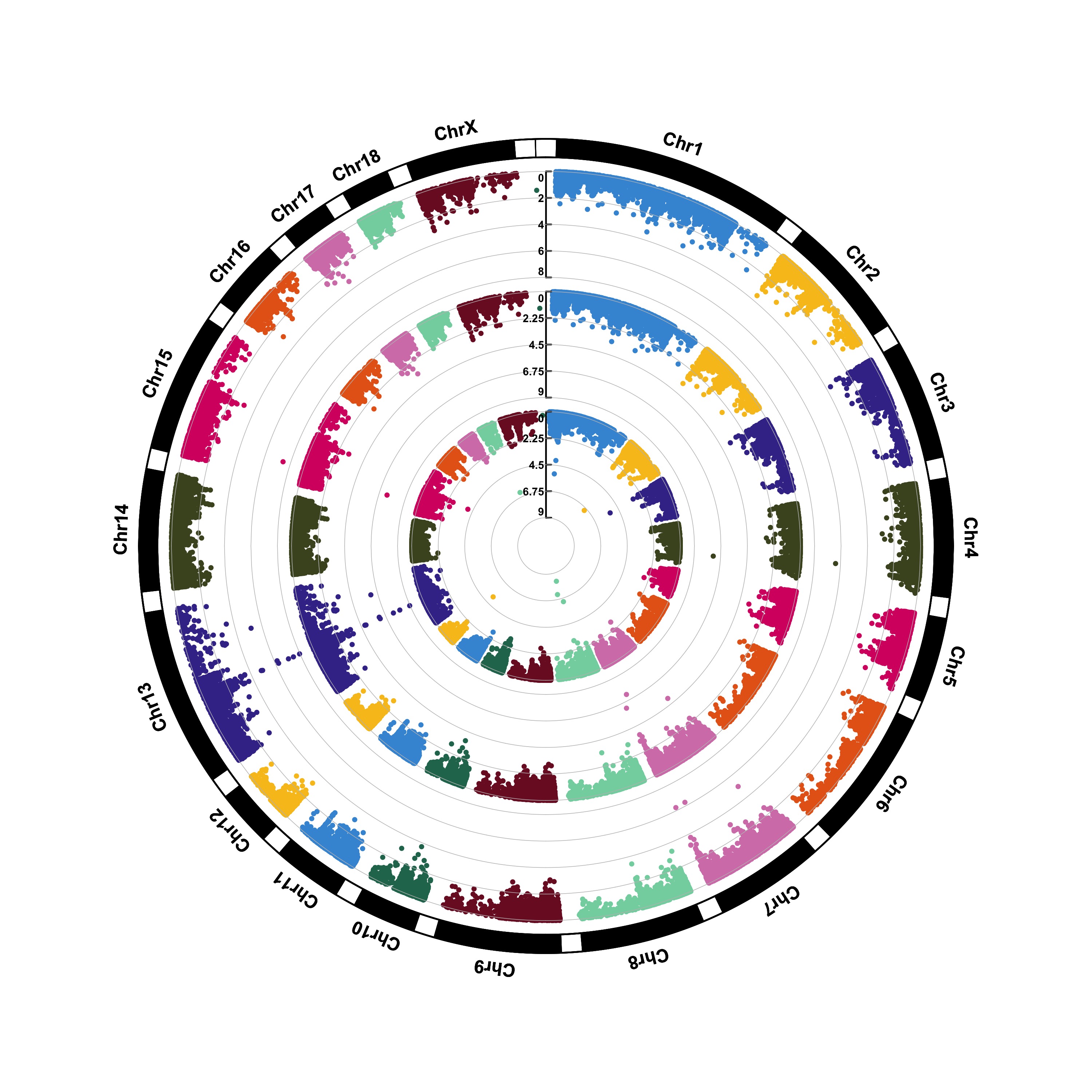 115 |
116 |
115 |
116 | 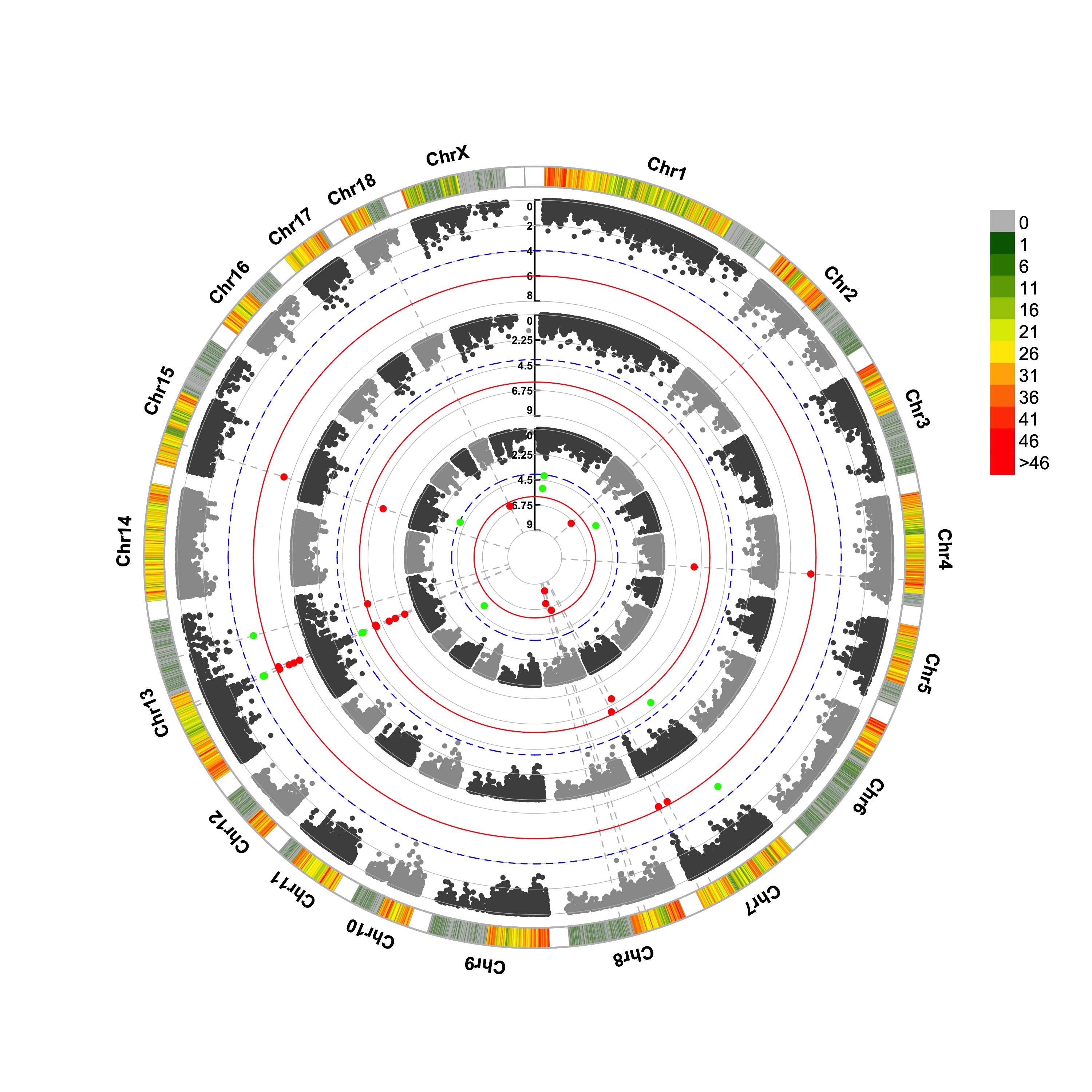 133 |
134 |
133 |
134 |  153 |
154 |
153 |
154 | 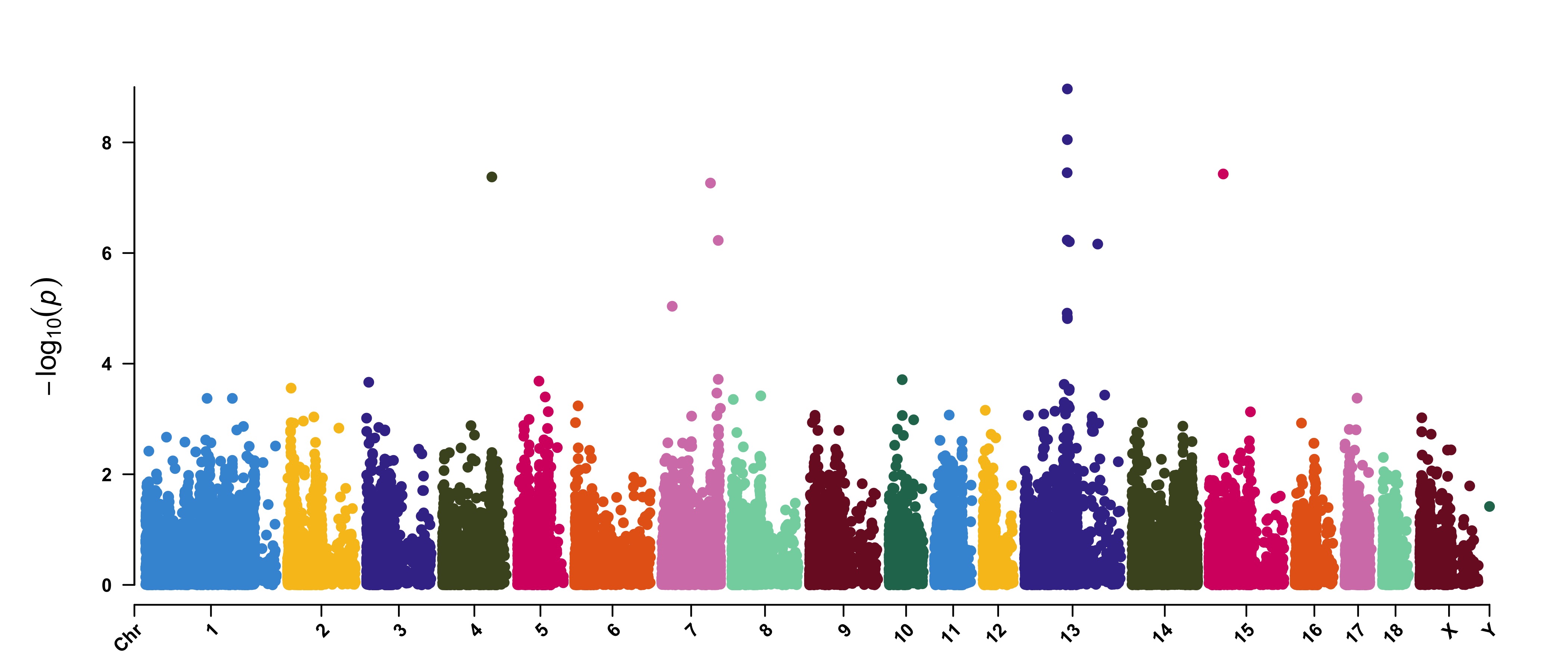 172 |
173 |
172 |
173 |  193 |
194 |
193 |
194 | 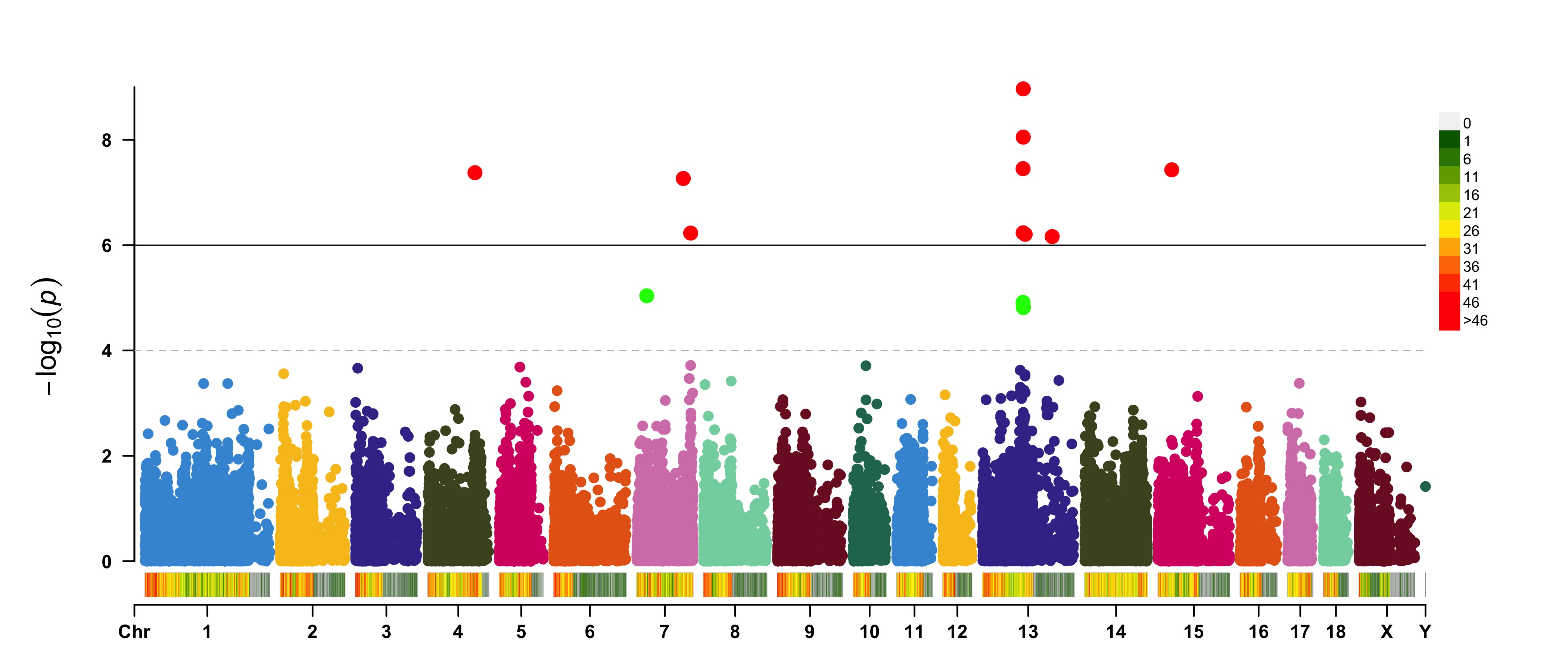 214 |
215 |
216 | #### Highlight a group of SNPs on pch, cex, type, and col
217 |
218 | ```r
219 | > signal <- pig60K$Position[which.min(pig60K$trait2)]
220 | > SNPs <- pig60K$SNP[pig60K$Chromosome==13 &
221 | pig60K$Position<(signal+1000000)&pig60K$Position>(signal-1000000)]
222 | > CMplot(pig60K, plot.type="m",LOG10=TRUE,col=c("grey30","grey60"),highlight=SNPs,
223 | highlight.col="green",highlight.cex=1,highlight.pch=19,file="jpg",file.name=NULL,
224 | chr.border=TRUE,dpi=300,file.output=TRUE,verbose=TRUE,width=14,height=6)
225 | # Note:
226 | # 'highlight' could be vector or list, if it is a vector, all traits will use the same highlighted SNPs index,
227 | # if it is a list, the length of the list should equal to the number of traits.
228 | # highlight.col, highlight.cex, highlight.pch can be value or vector, if its length equals to the length of highlighted SNPs,
229 | # each SNPs have its special colour, size and shape.
230 | ```
231 |
232 |
214 |
215 |
216 | #### Highlight a group of SNPs on pch, cex, type, and col
217 |
218 | ```r
219 | > signal <- pig60K$Position[which.min(pig60K$trait2)]
220 | > SNPs <- pig60K$SNP[pig60K$Chromosome==13 &
221 | pig60K$Position<(signal+1000000)&pig60K$Position>(signal-1000000)]
222 | > CMplot(pig60K, plot.type="m",LOG10=TRUE,col=c("grey30","grey60"),highlight=SNPs,
223 | highlight.col="green",highlight.cex=1,highlight.pch=19,file="jpg",file.name=NULL,
224 | chr.border=TRUE,dpi=300,file.output=TRUE,verbose=TRUE,width=14,height=6)
225 | # Note:
226 | # 'highlight' could be vector or list, if it is a vector, all traits will use the same highlighted SNPs index,
227 | # if it is a list, the length of the list should equal to the number of traits.
228 | # highlight.col, highlight.cex, highlight.pch can be value or vector, if its length equals to the length of highlighted SNPs,
229 | # each SNPs have its special colour, size and shape.
230 | ```
231 |
232 | 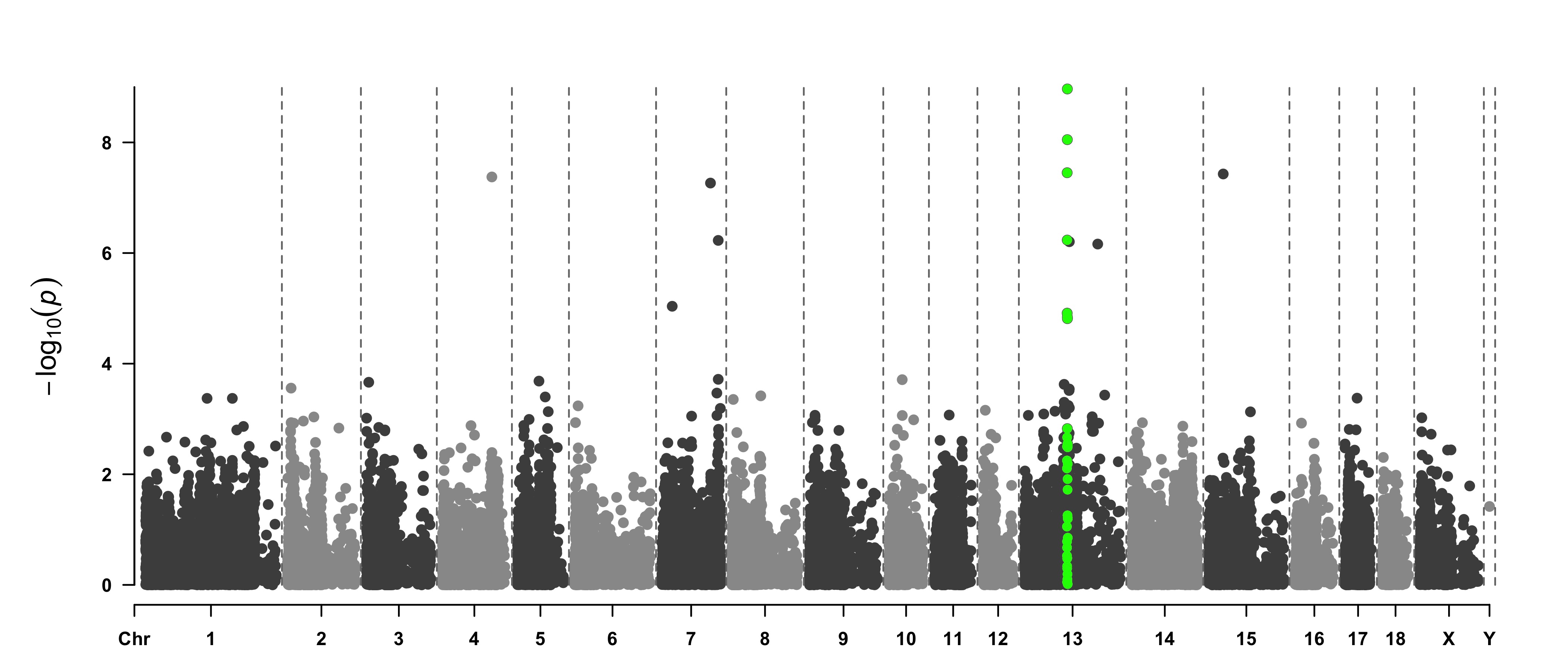 236 |
237 |
238 | ```r
239 | > SNPs <- pig60K[pig60K$trait2 < 1e-4, 1]
240 | > CMplot(pig60K,type="h",plot.type="m",LOG10=TRUE,highlight=SNPs,highlight.type="p",
241 | highlight.col=NULL,highlight.cex=1.2,highlight.pch=19,file="jpg",file.name=NULL,
242 | dpi=300,file.output=TRUE,verbose=TRUE,width=14,height=6,band=0.6)
243 | ```
244 |
245 |
236 |
237 |
238 | ```r
239 | > SNPs <- pig60K[pig60K$trait2 < 1e-4, 1]
240 | > CMplot(pig60K,type="h",plot.type="m",LOG10=TRUE,highlight=SNPs,highlight.type="p",
241 | highlight.col=NULL,highlight.cex=1.2,highlight.pch=19,file="jpg",file.name=NULL,
242 | dpi=300,file.output=TRUE,verbose=TRUE,width=14,height=6,band=0.6)
243 | ```
244 |
245 | 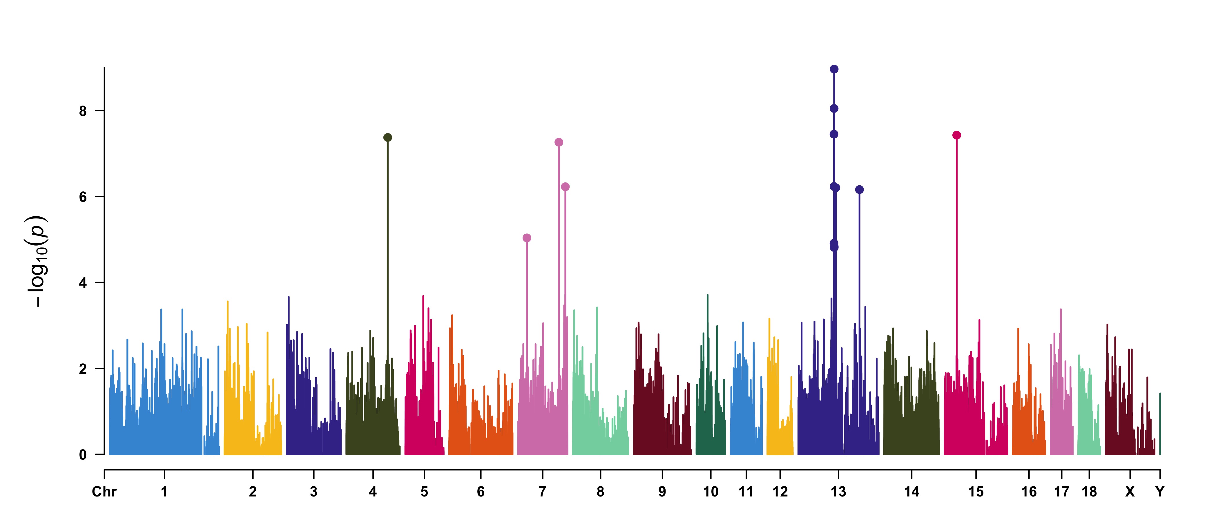 249 |
250 |
251 | ```r
252 | > SNPs <- pig60K[pig60K$trait2 < 1e-4, 1]
253 | > CMplot(pig60K,type="p",plot.type="m",LOG10=TRUE,highlight=SNPs,highlight.type="h",
254 | col=c("grey30","grey60"),highlight.col="darkgreen",highlight.cex=1.2,highlight.pch=19,
255 | file="jpg",dpi=300,file.output=TRUE,verbose=TRUE,width=14,height=6)
256 | ```
257 |
258 |
249 |
250 |
251 | ```r
252 | > SNPs <- pig60K[pig60K$trait2 < 1e-4, 1]
253 | > CMplot(pig60K,type="p",plot.type="m",LOG10=TRUE,highlight=SNPs,highlight.type="h",
254 | col=c("grey30","grey60"),highlight.col="darkgreen",highlight.cex=1.2,highlight.pch=19,
255 | file="jpg",dpi=300,file.output=TRUE,verbose=TRUE,width=14,height=6)
256 | ```
257 |
258 | 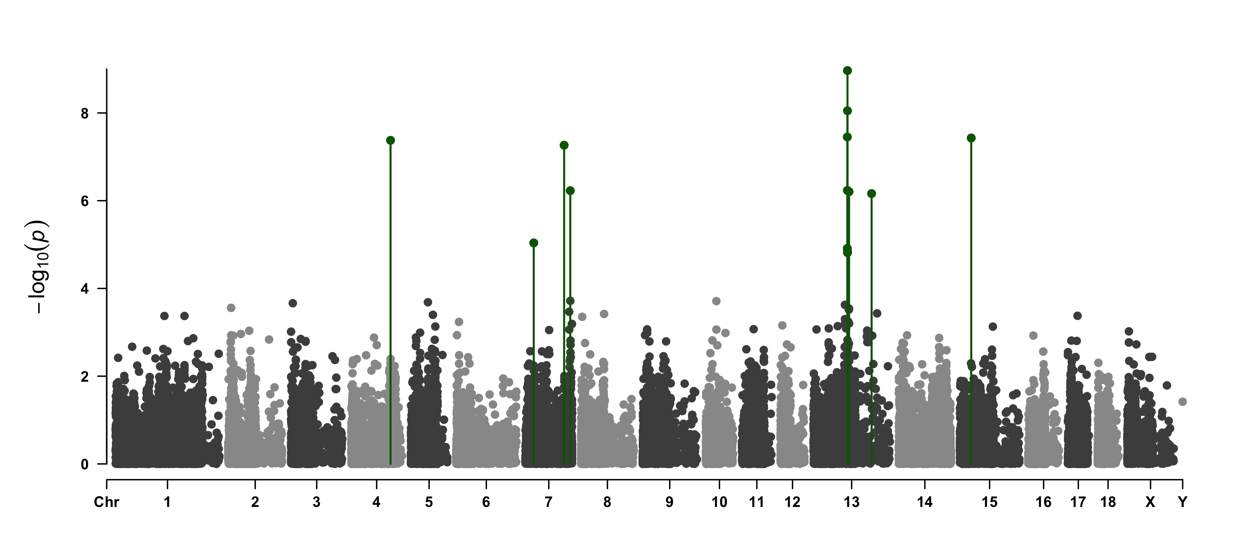 262 |
263 |
264 | ```r
265 | > SNPs <- pig60K[
266 | pig60K$trait1 < 1e-4 |
267 | pig60K$trait2 < 1e-4 |
268 | pig60K$trait3 < 1e-4, 1]
269 | > CMplot(pig60K,type="p",plot.type="m",LOG10=TRUE,highlight=SNPs,highlight.type="l",
270 | threshold=1e-4,threshold.col="black",threshold.lty=1,col=c("grey60","#4197d8"),
271 | signal.cex=1.2, signal.col="red", highlight.col="grey",highlight.cex=0.7,
272 | file="jpg",dpi=300,file.output=TRUE,verbose=TRUE,multracks=TRUE)
273 |
274 | ```
275 |
276 |
262 |
263 |
264 | ```r
265 | > SNPs <- pig60K[
266 | pig60K$trait1 < 1e-4 |
267 | pig60K$trait2 < 1e-4 |
268 | pig60K$trait3 < 1e-4, 1]
269 | > CMplot(pig60K,type="p",plot.type="m",LOG10=TRUE,highlight=SNPs,highlight.type="l",
270 | threshold=1e-4,threshold.col="black",threshold.lty=1,col=c("grey60","#4197d8"),
271 | signal.cex=1.2, signal.col="red", highlight.col="grey",highlight.cex=0.7,
272 | file="jpg",dpi=300,file.output=TRUE,verbose=TRUE,multracks=TRUE)
273 |
274 | ```
275 |
276 | 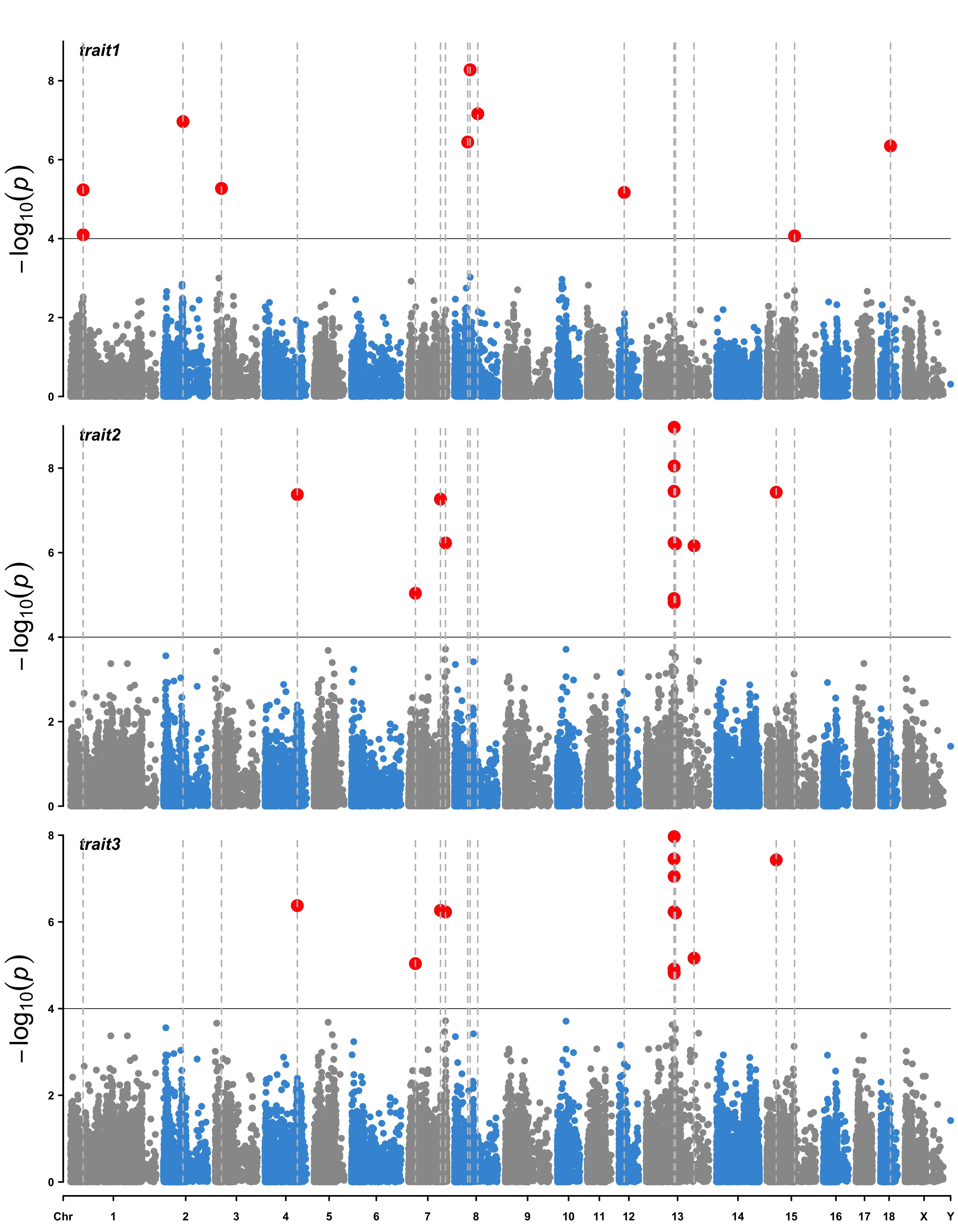 280 |
281 |
282 | #### Visualize only one chromosome
283 |
284 | ```r
285 | > CMplot(pig60K[pig60K$Chromosome==13, ], plot.type="m",LOG10=TRUE,col=c("grey60"),highlight=SNPs,
286 | highlight.col="green",highlight.cex=1,highlight.pch=19,file="jpg",file.name=NULL,
287 | threshold=c(1e-6,1e-4),threshold.lty=c(1,2),threshold.lwd=c(1,2), width=9,height=6,
288 | threshold.col=c("red","blue"),amplify=FALSE,dpi=300,file.output=TRUE,verbose=TRUE)
289 | ```
290 |
291 |
280 |
281 |
282 | #### Visualize only one chromosome
283 |
284 | ```r
285 | > CMplot(pig60K[pig60K$Chromosome==13, ], plot.type="m",LOG10=TRUE,col=c("grey60"),highlight=SNPs,
286 | highlight.col="green",highlight.cex=1,highlight.pch=19,file="jpg",file.name=NULL,
287 | threshold=c(1e-6,1e-4),threshold.lty=c(1,2),threshold.lwd=c(1,2), width=9,height=6,
288 | threshold.col=c("red","blue"),amplify=FALSE,dpi=300,file.output=TRUE,verbose=TRUE)
289 | ```
290 |
291 | 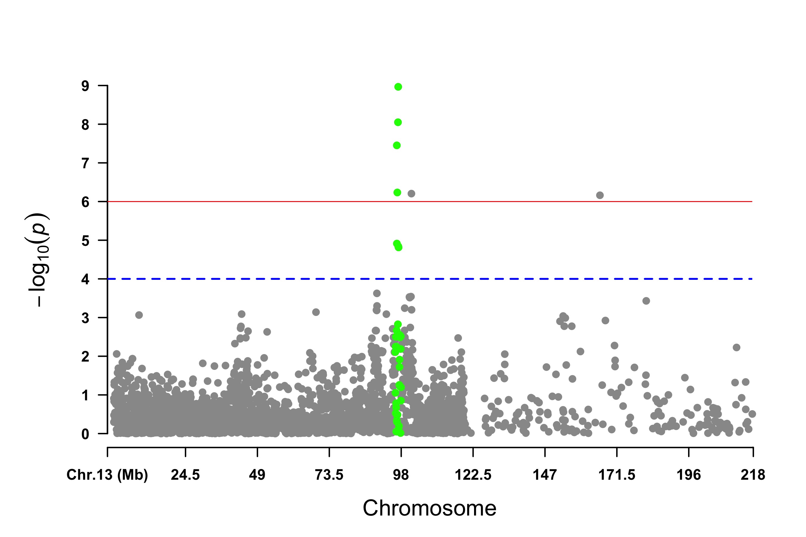 295 |
296 |
297 | #### add genes or SNP names around the highlighted SNPs
298 |
299 | ```r
300 | > SNPs <- pig60K[pig60K[,5] < (0.05 / nrow(pig60K)), 1]
301 | > genes <- paste("GENE", 1:length(SNPs), sep="_")
302 | > set.seed(666666)
303 | > CMplot(pig60K[,c(1:3,5)], plot.type="m",LOG10=TRUE,col=c("grey30","grey60"),highlight=SNPs,
304 | highlight.col=rep(c("green","blue"),length=length(SNPs)),highlight.cex=1, highlight.text=genes,
305 | highlight.text.col=rep("red",length(SNPs)),threshold=0.05/nrow(pig60K),threshold.lty=2,
306 | amplify=FALSE,file="jpg",file.name=NULL,dpi=300,file.output=TRUE,verbose=TRUE,width=14,height=6)
307 | # Note:
308 | # 'highlight', 'highlight.text' could be vector or list, if it is a vector, all traits will
309 | # use the same highlighted SNPs index and text, if it is a list, the length of the list should equal to the number of traits.
310 | # the order of 'highlight.text' must be consistent with 'highlight'
311 | # highlight.text.cex: value or vecter, control the size of added text
312 | # highlight.text.font: value or vecter, control the font of added text
313 | ```
314 |
315 |
295 |
296 |
297 | #### add genes or SNP names around the highlighted SNPs
298 |
299 | ```r
300 | > SNPs <- pig60K[pig60K[,5] < (0.05 / nrow(pig60K)), 1]
301 | > genes <- paste("GENE", 1:length(SNPs), sep="_")
302 | > set.seed(666666)
303 | > CMplot(pig60K[,c(1:3,5)], plot.type="m",LOG10=TRUE,col=c("grey30","grey60"),highlight=SNPs,
304 | highlight.col=rep(c("green","blue"),length=length(SNPs)),highlight.cex=1, highlight.text=genes,
305 | highlight.text.col=rep("red",length(SNPs)),threshold=0.05/nrow(pig60K),threshold.lty=2,
306 | amplify=FALSE,file="jpg",file.name=NULL,dpi=300,file.output=TRUE,verbose=TRUE,width=14,height=6)
307 | # Note:
308 | # 'highlight', 'highlight.text' could be vector or list, if it is a vector, all traits will
309 | # use the same highlighted SNPs index and text, if it is a list, the length of the list should equal to the number of traits.
310 | # the order of 'highlight.text' must be consistent with 'highlight'
311 | # highlight.text.cex: value or vecter, control the size of added text
312 | # highlight.text.font: value or vecter, control the font of added text
313 | ```
314 |
315 | 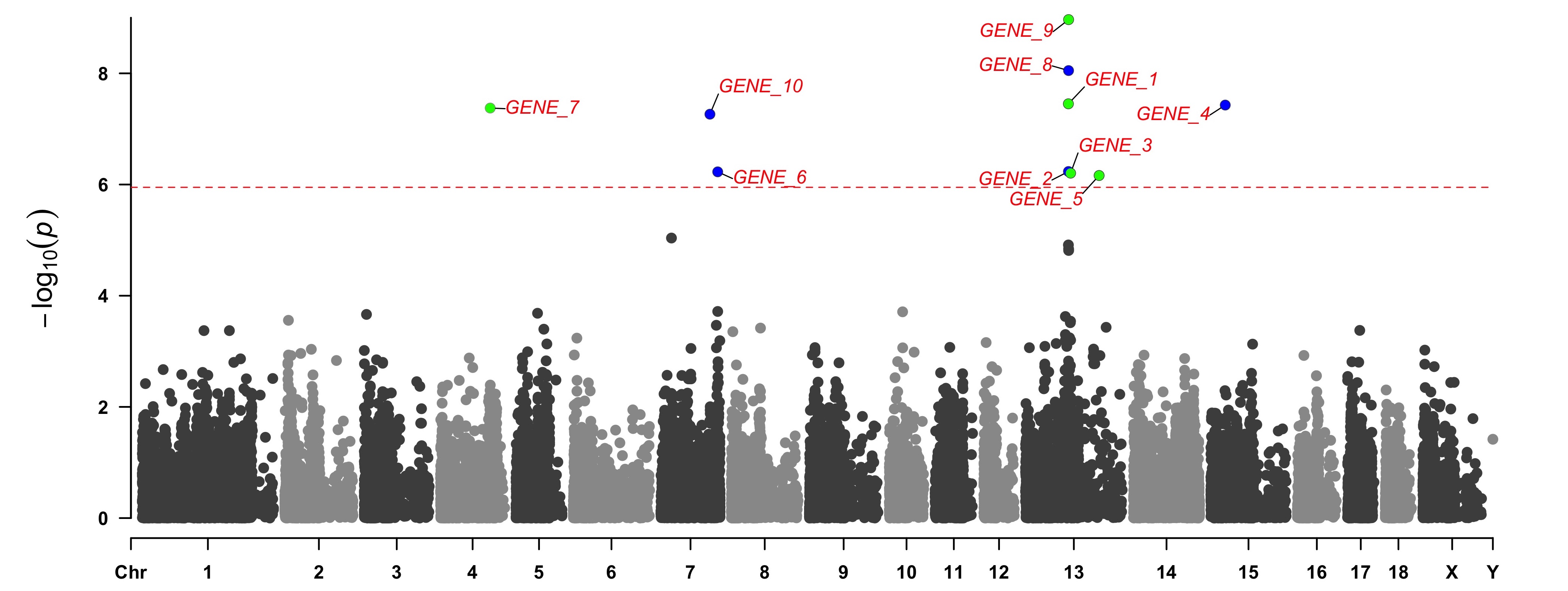 319 |
320 |
321 | #### Genomic Selection/Prediction(GS/GP) or other none p-values
322 |
323 | ```r
324 | > CMplot(cattle50K, plot.type="m", band=0.5, LOG10=FALSE, ylab="SNP effect",threshold=0.015,
325 | threshold.lty=2, threshold.lwd=1, threshold.col="red", amplify=TRUE, width=14,height=6,
326 | signal.col=NULL, chr.den.col=NULL, file="jpg",file.name=NULL,dpi=300,file.output=TRUE,
327 | verbose=TRUE,cex=0.8)
328 | #Note: if signal.col=NULL, the significant SNPs will be plotted with original colors.
329 | ```
330 |
331 |
319 |
320 |
321 | #### Genomic Selection/Prediction(GS/GP) or other none p-values
322 |
323 | ```r
324 | > CMplot(cattle50K, plot.type="m", band=0.5, LOG10=FALSE, ylab="SNP effect",threshold=0.015,
325 | threshold.lty=2, threshold.lwd=1, threshold.col="red", amplify=TRUE, width=14,height=6,
326 | signal.col=NULL, chr.den.col=NULL, file="jpg",file.name=NULL,dpi=300,file.output=TRUE,
327 | verbose=TRUE,cex=0.8)
328 | #Note: if signal.col=NULL, the significant SNPs will be plotted with original colors.
329 | ```
330 |
331 | 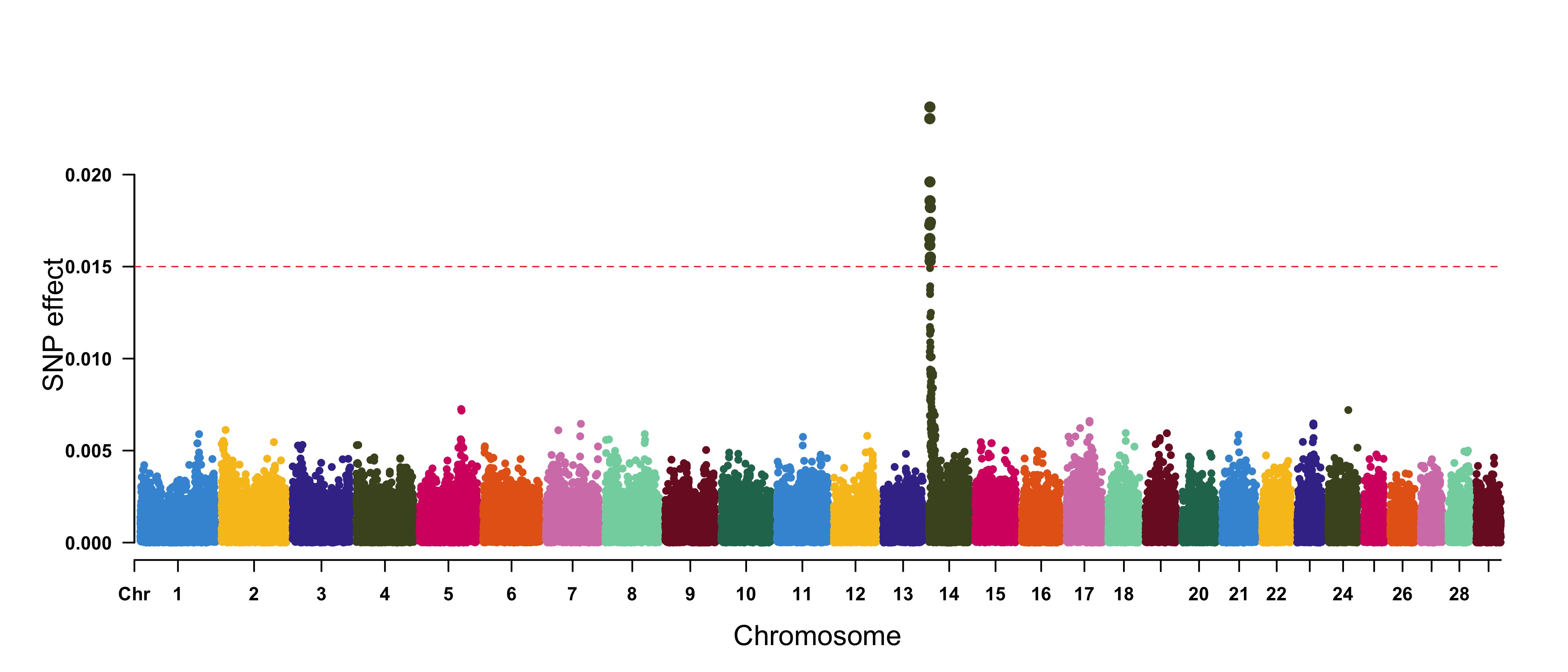 334 |
335 |
334 |
335 | 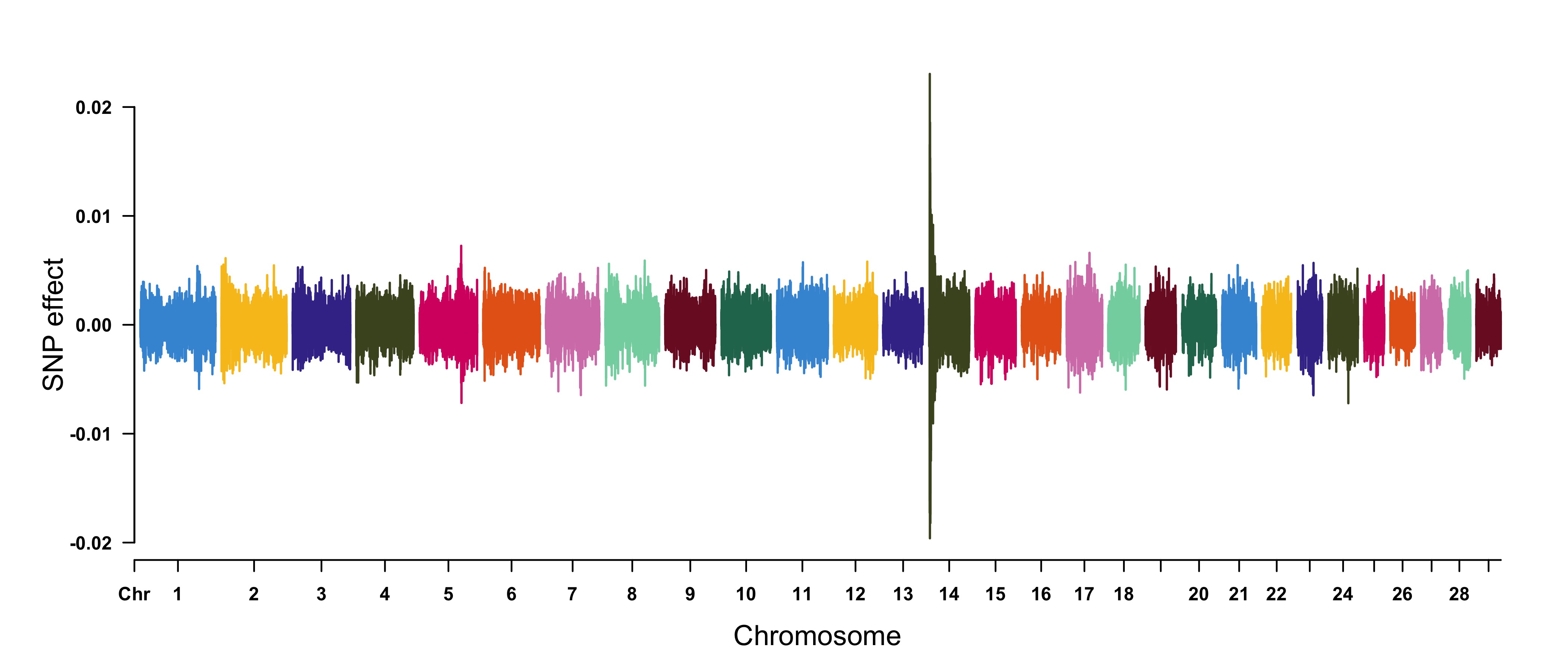 349 |
350 |
349 |
350 | 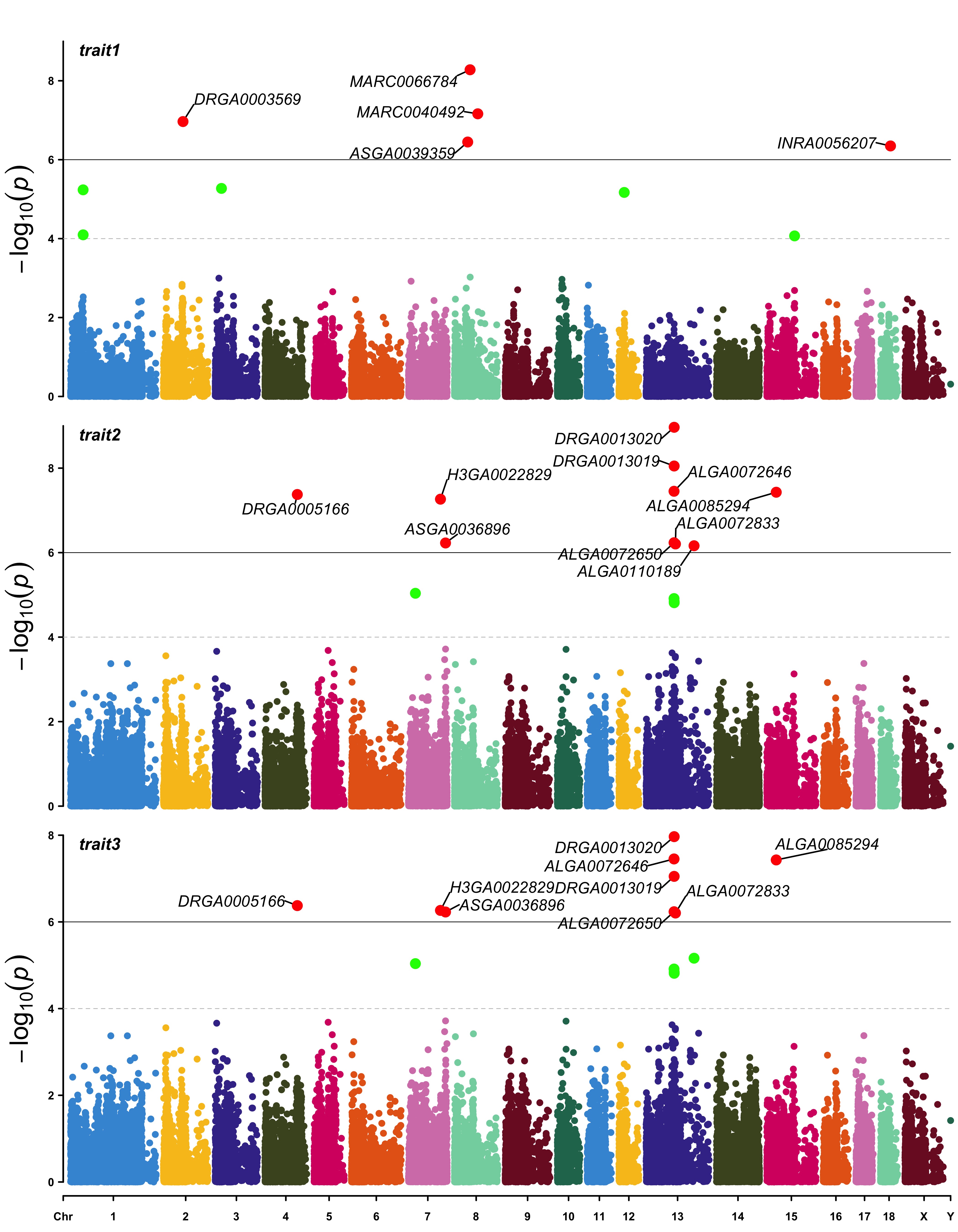 371 |
372 |
371 |
372 | 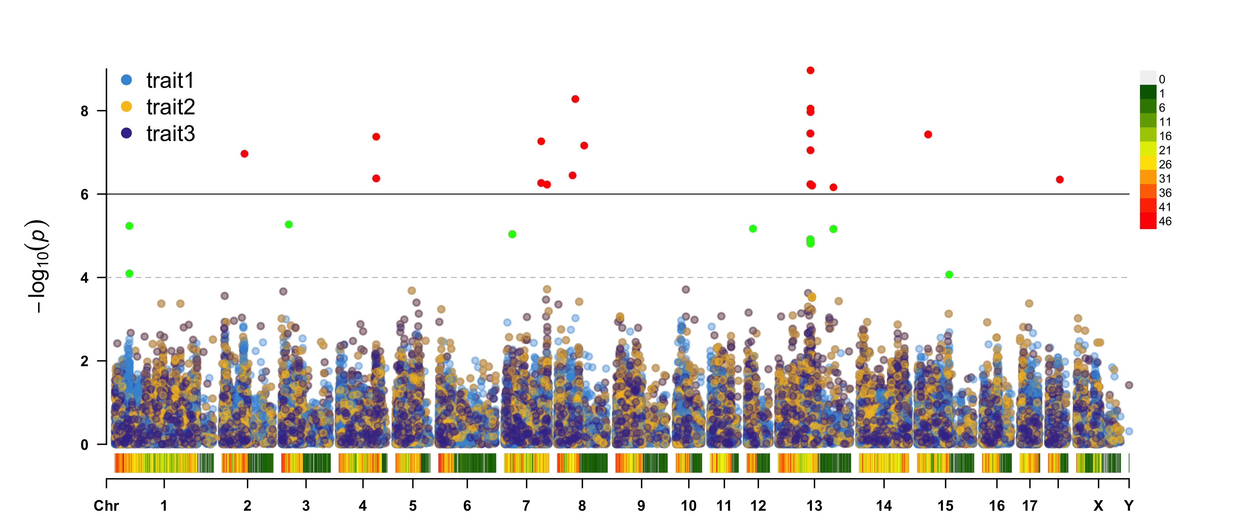 386 |
387 |
386 |
387 | 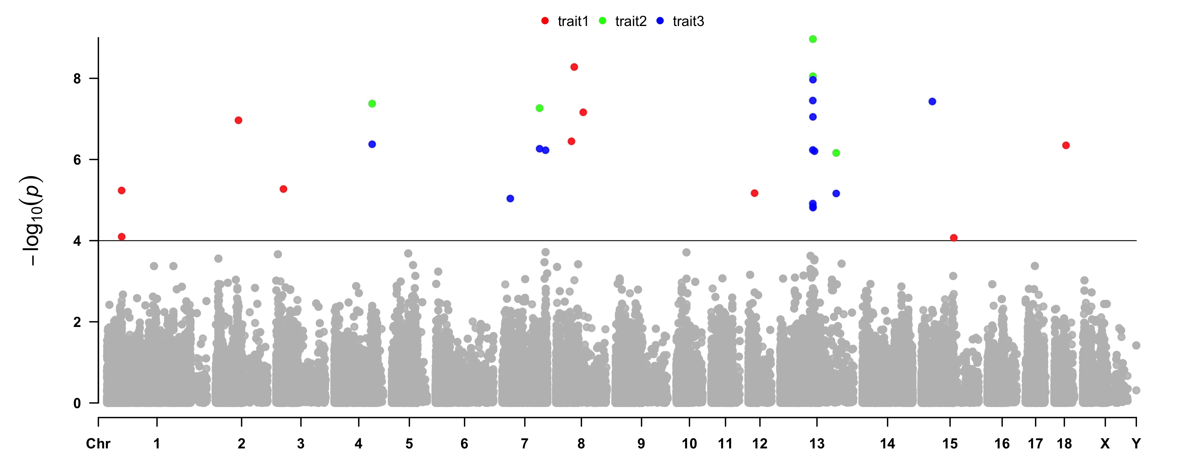 401 |
402 | ---
403 |
404 | ### Q-Q plot
405 |
406 | ```r
407 | > CMplot(pig60K,plot.type="q",box=FALSE,file="jpg",file.name=NULL,dpi=300,
408 | conf.int=TRUE,conf.int.col=NULL,threshold.col="red",threshold.lty=2,
409 | file.output=TRUE,verbose=TRUE,width=5,height=5)
410 | ```
411 |
412 |
401 |
402 | ---
403 |
404 | ### Q-Q plot
405 |
406 | ```r
407 | > CMplot(pig60K,plot.type="q",box=FALSE,file="jpg",file.name=NULL,dpi=300,
408 | conf.int=TRUE,conf.int.col=NULL,threshold.col="red",threshold.lty=2,
409 | file.output=TRUE,verbose=TRUE,width=5,height=5)
410 | ```
411 |
412 | 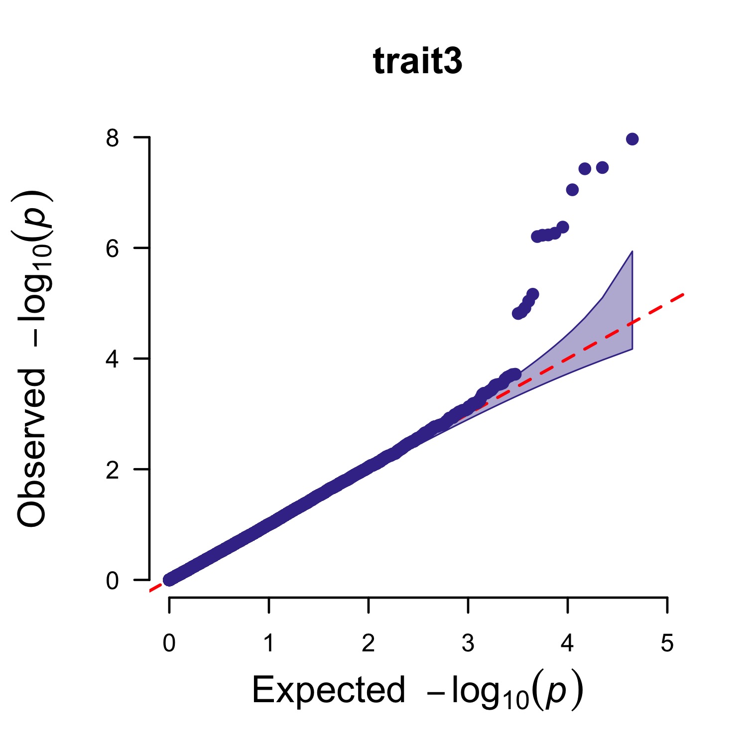 415 |
416 |
415 |
416 | 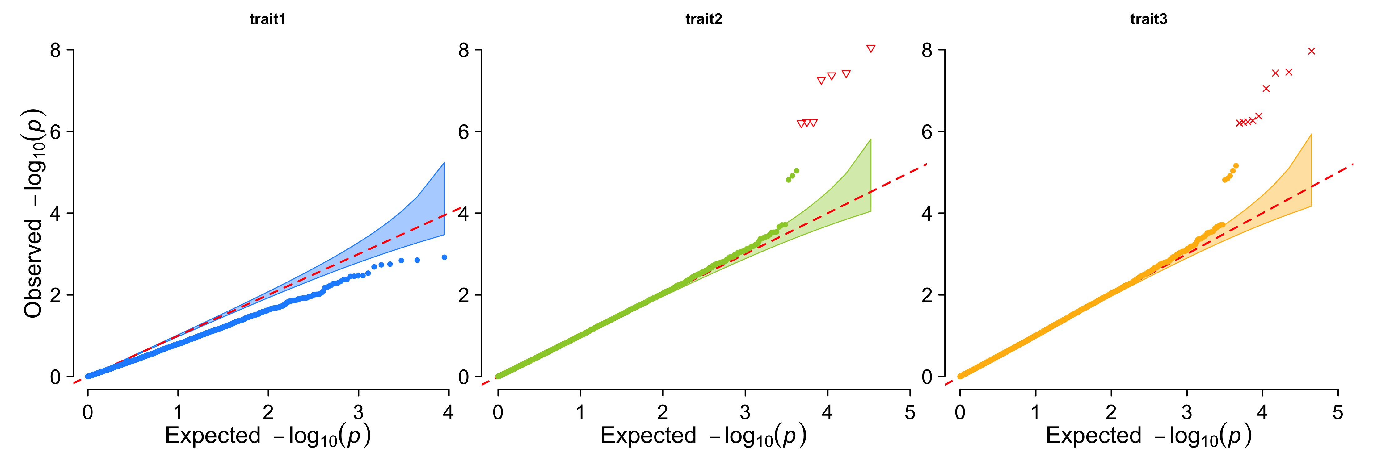 432 |
433 |
432 |
433 | 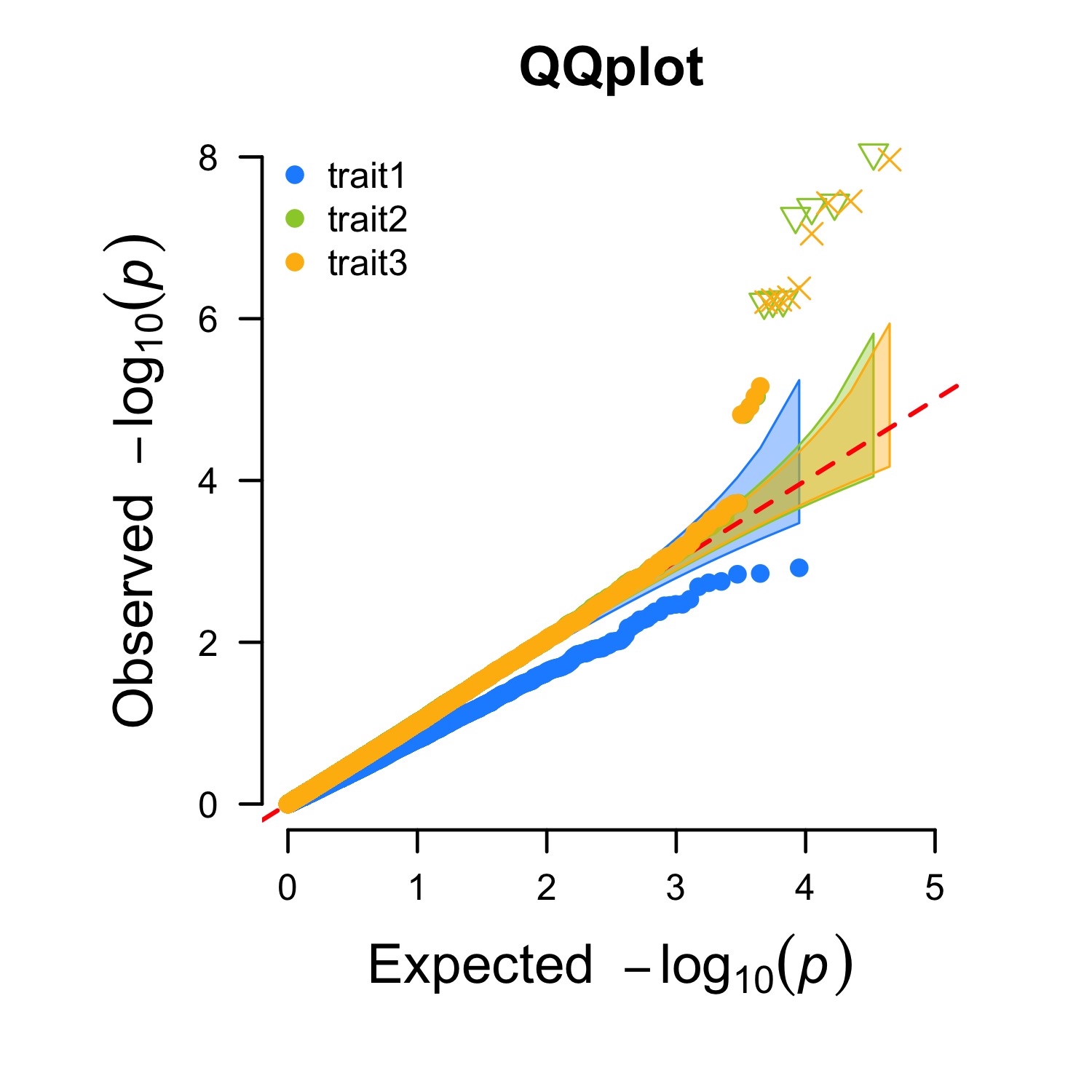 447 |
448 |
447 |
448 |