├── Nov-2017
├── array_archive.npz
├── array_ex.txt
├── numpy-1-student.ipynb
├── numpy-1.ipynb
├── numpy-2-student.ipynb
├── numpy-2.ipynb
└── some_array.npy
├── README.md
├── array_archive.npz
├── array_ex.txt
├── numpy-tutorial-student.ipynb
├── proj
├── .ipynb_checkpoints
│ └── Untitled-checkpoint.ipynb
├── Untitled.ipynb
├── dict.pkl
├── embed.npy
├── p_vector.npy
└── senti.binary.test.txt
├── python-numpy-tutorial.ipynb
└── some_array.npy
/Nov-2017/array_archive.npz:
--------------------------------------------------------------------------------
https://raw.githubusercontent.com/ZeweiChu/numpy-tutorial/bcda441bee52af9ff392f58f688ec7f5cc57d8d5/Nov-2017/array_archive.npz
--------------------------------------------------------------------------------
/Nov-2017/array_ex.txt:
--------------------------------------------------------------------------------
1 | 0.580052,0.186730,1.040717,1.134411
2 | 0.194163,-0.636917,-0.938659,0.124094
3 | -0.126410,0.268607,-0.695724,0.047428
4 | -1.484413,0.004176,-0.744203,0.005487
5 | 2.302869,0.200131,1.670238,-1.881090
6 | -0.193230,1.047233,0.482803,0.960334
--------------------------------------------------------------------------------
/Nov-2017/numpy-1-student.ipynb:
--------------------------------------------------------------------------------
1 | {
2 | "cells": [
3 | {
4 | "cell_type": "markdown",
5 | "metadata": {},
6 | "source": [
7 | "# numpy基础\n",
8 | "\n",
9 | "### 七月在线python数据分析集训营 julyedu.com\n",
10 | "\n",
11 | "褚则伟 zeweichu@gmail.com"
12 | ]
13 | },
14 | {
15 | "cell_type": "markdown",
16 | "metadata": {},
17 | "source": [
18 | "## Numpy简介\n",
19 | "\n",
20 | "- Numpy是Python语言的一个library [numpy](http://www.numpy.org/)\n",
21 | "- Numpy主要支持矩阵操作和运算\n",
22 | "- Numpy非常高效,core代码由C语言写成\n",
23 | "- 我们第三课要讲的pandas也是基于Numpy构建的一个library\n",
24 | "- 现在比较流行的机器学习框架(例如Tensorflow/PyTorch等等),语法都与Numpy比较接近"
25 | ]
26 | },
27 | {
28 | "cell_type": "markdown",
29 | "metadata": {},
30 | "source": [
31 | "## 目录\n",
32 | "- 数组简介和数组的构造(ndarray)\n",
33 | "- 数组取值和赋值\n",
34 | "- 数学运算\n",
35 | "- broadcasting广播"
36 | ]
37 | },
38 | {
39 | "cell_type": "markdown",
40 | "metadata": {},
41 | "source": [
42 | "python里面调用一个包,用import对吧, 所以我们import `numpy` 包:\n",
43 | "\n",
44 | "如果还没有安装的话,你可以在command line界面使用`pip install numpy`"
45 | ]
46 | },
47 | {
48 | "cell_type": "markdown",
49 | "metadata": {},
50 | "source": [
51 | "## Arrays/数组\n",
52 | "\n",
53 | "### 七月在线python数据分析集训营 julyedu.com"
54 | ]
55 | },
56 | {
57 | "cell_type": "markdown",
58 | "metadata": {},
59 | "source": [
60 | "看你数组的维度啦,我自己的话比较简单粗暴,一般直接把1维数组就看做向量/vector,2维数组看做2维矩阵,3维数组看做3维矩阵..."
61 | ]
62 | },
63 | {
64 | "cell_type": "markdown",
65 | "metadata": {},
66 | "source": [
67 | "可以调用np.array去从list初始化一个数组:"
68 | ]
69 | },
70 | {
71 | "cell_type": "markdown",
72 | "metadata": {},
73 | "source": [
74 | "查看每个element的大小"
75 | ]
76 | },
77 | {
78 | "cell_type": "markdown",
79 | "metadata": {},
80 | "source": [
81 | "有一些内置的创建数组的函数:"
82 | ]
83 | },
84 | {
85 | "cell_type": "markdown",
86 | "metadata": {},
87 | "source": [
88 | "linspace也是一个很常用的初始化数据的手段,它可以帮我们产生一连串等间距的数组"
89 | ]
90 | },
91 | {
92 | "cell_type": "markdown",
93 | "metadata": {},
94 | "source": [
95 | "## 使用reshape来改变tensor的形状\n",
96 | "### 七月在线python数据分析集训营 julyedu.com"
97 | ]
98 | },
99 | {
100 | "cell_type": "markdown",
101 | "metadata": {},
102 | "source": [
103 | "numpy可以很容易地把一维数组转成二维数组,三维数组。"
104 | ]
105 | },
106 | {
107 | "cell_type": "markdown",
108 | "metadata": {},
109 | "source": [
110 | "直接把shape给重新定义了其实也可以"
111 | ]
112 | },
113 | {
114 | "cell_type": "markdown",
115 | "metadata": {},
116 | "source": [
117 | "如果我们在某一个维度上写上-1,numpy会帮我们自动推导出正确的维度"
118 | ]
119 | },
120 | {
121 | "cell_type": "markdown",
122 | "metadata": {},
123 | "source": [
124 | "还可以从其他的ndarray中获取shape信息然后reshape"
125 | ]
126 | },
127 | {
128 | "cell_type": "markdown",
129 | "metadata": {},
130 | "source": [
131 | "高维数组可以用ravel来拉平"
132 | ]
133 | },
134 | {
135 | "cell_type": "markdown",
136 | "metadata": {},
137 | "source": [
138 | "### 数组的数据类型 dtype\n",
139 | "\n",
140 | "数组可以有不同的数据类型"
141 | ]
142 | },
143 | {
144 | "cell_type": "markdown",
145 | "metadata": {},
146 | "source": [
147 | "生成数组时可以指定数据类型,如果不指定numpy会自动匹配合适的类型"
148 | ]
149 | },
150 | {
151 | "cell_type": "markdown",
152 | "metadata": {},
153 | "source": [
154 | "有时候如果我们需要ndarray是一个特定的数据类型,可以使用astype复制数组并转换数据类型"
155 | ]
156 | },
157 | {
158 | "cell_type": "markdown",
159 | "metadata": {},
160 | "source": [
161 | "使用astype将float转换为int时小数部分被舍弃"
162 | ]
163 | },
164 | {
165 | "cell_type": "markdown",
166 | "metadata": {},
167 | "source": [
168 | "使用astype把字符串转换为数组,如果失败抛出异常。"
169 | ]
170 | },
171 | {
172 | "cell_type": "markdown",
173 | "metadata": {},
174 | "source": [
175 | "astype使用其它数组的数据类型作为参数"
176 | ]
177 | },
178 | {
179 | "cell_type": "markdown",
180 | "metadata": {},
181 | "source": [
182 | "更多的内容可以读读[文档](http://docs.scipy.org/doc/numpy/reference/arrays.dtypes.html)."
183 | ]
184 | },
185 | {
186 | "cell_type": "markdown",
187 | "metadata": {},
188 | "source": [
189 | "## Array indexing/数组取值和赋值\n",
190 | "\n",
191 | "### 七月在线python数据分析集训营 julyedu.com"
192 | ]
193 | },
194 | {
195 | "cell_type": "markdown",
196 | "metadata": {},
197 | "source": [
198 | "Numpy提供了蛮多种取值的方式的."
199 | ]
200 | },
201 | {
202 | "cell_type": "markdown",
203 | "metadata": {},
204 | "source": [
205 | "可以像list一样切片(多维数组可以从各个维度同时切片):"
206 | ]
207 | },
208 | {
209 | "cell_type": "markdown",
210 | "metadata": {},
211 | "source": [
212 | "虽然,怎么说呢,不建议你这样去赋值,但是你确实可以修改切片出来的对象,然后完成对原数组的赋值."
213 | ]
214 | },
215 | {
216 | "cell_type": "markdown",
217 | "metadata": {},
218 | "source": [
219 | "关于Copy和View的关系\n",
220 | "- 简单的数组赋值,切片,包括作为函数的参数传递一个数组--并不会复制出一个新的数组,只是制造了一个新的reference。所以如果我们在新赋值的变量上改变数组的内容,原来的那个数组内容也会发生改变。这一点千万要注意哦!"
221 | ]
222 | },
223 | {
224 | "cell_type": "markdown",
225 | "metadata": {},
226 | "source": [
227 | "- 使用`view`方法,我们可以拿到数组的一部分或者全部,但是在view上面修改内容还是会把原来的数组给更改了"
228 | ]
229 | },
230 | {
231 | "cell_type": "markdown",
232 | "metadata": {},
233 | "source": [
234 | "使用`base`方法可以查看一个数组的owner是谁,也就是说这个数组是由谁制造产生的。"
235 | ]
236 | },
237 | {
238 | "cell_type": "markdown",
239 | "metadata": {},
240 | "source": [
241 | "其实使用切片方法我们拿到的也是一个view"
242 | ]
243 | },
244 | {
245 | "cell_type": "markdown",
246 | "metadata": {},
247 | "source": [
248 | "所以更改切片上的内容之后,原来数组的内容也被更改了"
249 | ]
250 | },
251 | {
252 | "cell_type": "markdown",
253 | "metadata": {},
254 | "source": [
255 | "如果要复制出一个新的数组,我们就需要使用`copy()`这个方法了"
256 | ]
257 | },
258 | {
259 | "cell_type": "markdown",
260 | "metadata": {},
261 | "source": [
262 | "下面我们继续回到数组切片的问题上\n",
263 | "\n",
264 | "创建3x4的2维数组/矩阵"
265 | ]
266 | },
267 | {
268 | "cell_type": "markdown",
269 | "metadata": {},
270 | "source": [
271 | "你就放心大胆地去取你想要的数咯:"
272 | ]
273 | },
274 | {
275 | "cell_type": "markdown",
276 | "metadata": {},
277 | "source": [
278 | "试试在第2个维度上切片也一样的:"
279 | ]
280 | },
281 | {
282 | "cell_type": "markdown",
283 | "metadata": {},
284 | "source": [
285 | "dots(...)"
286 | ]
287 | },
288 | {
289 | "cell_type": "markdown",
290 | "metadata": {},
291 | "source": [
292 | "下面这个高级了,更自由地取值和组合,但是要看清楚一点:"
293 | ]
294 | },
295 | {
296 | "cell_type": "markdown",
297 | "metadata": {},
298 | "source": [
299 | "再来熟悉一下\n",
300 | "\n",
301 | "先创建一个2维数组"
302 | ]
303 | },
304 | {
305 | "cell_type": "markdown",
306 | "metadata": {},
307 | "source": [
308 | "用下标生成一个向量"
309 | ]
310 | },
311 | {
312 | "cell_type": "markdown",
313 | "metadata": {},
314 | "source": [
315 | "你能看明白下面做的事情吗?"
316 | ]
317 | },
318 | {
319 | "cell_type": "markdown",
320 | "metadata": {},
321 | "source": [
322 | "既然可以取出来,我们当然也可以对这些元素操作咯"
323 | ]
324 | },
325 | {
326 | "cell_type": "markdown",
327 | "metadata": {},
328 | "source": [
329 | "### numpy的条件判断\n",
330 | "\n",
331 | "比较fashion的取法之一,用条件判定去取(但是很好用):"
332 | ]
333 | },
334 | {
335 | "cell_type": "markdown",
336 | "metadata": {},
337 | "source": [
338 | "用刚才的布尔型数组作为下标就可以去除符合条件的元素啦"
339 | ]
340 | },
341 | {
342 | "cell_type": "markdown",
343 | "metadata": {},
344 | "source": [
345 | "其实一句话也可以完成是不是?"
346 | ]
347 | },
348 | {
349 | "cell_type": "markdown",
350 | "metadata": {},
351 | "source": [
352 | "那个,真的,其实还有很多细节,其他的方式去取值,你可以看看官方文档。"
353 | ]
354 | },
355 | {
356 | "cell_type": "markdown",
357 | "metadata": {},
358 | "source": [
359 | "我们一起来来总结一下,看下面切片取值方式(对应颜色是取出来的结果):"
360 | ]
361 | },
362 | {
363 | "cell_type": "markdown",
364 | "metadata": {},
365 | "source": [
366 | "\n",
367 | ""
368 | ]
369 | },
370 | {
371 | "cell_type": "markdown",
372 | "metadata": {},
373 | "source": [
374 | "## 简单数学运算\n",
375 | "### 七月在线python数据分析集训营 julyedu.com"
376 | ]
377 | },
378 | {
379 | "cell_type": "markdown",
380 | "metadata": {},
381 | "source": [
382 | "下面这些运算是你在科学运算中经常经常会用到的,比如逐个元素的运算如下:"
383 | ]
384 | },
385 | {
386 | "cell_type": "markdown",
387 | "metadata": {},
388 | "source": [
389 | "逐元素求和有下面2种方式"
390 | ]
391 | },
392 | {
393 | "cell_type": "markdown",
394 | "metadata": {},
395 | "source": [
396 | "逐元素作差"
397 | ]
398 | },
399 | {
400 | "cell_type": "markdown",
401 | "metadata": {},
402 | "source": [
403 | "逐元素相乘"
404 | ]
405 | },
406 | {
407 | "cell_type": "markdown",
408 | "metadata": {},
409 | "source": [
410 | "逐元素相除"
411 | ]
412 | },
413 | {
414 | "cell_type": "markdown",
415 | "metadata": {},
416 | "source": [
417 | "逐元素求平方根!!!"
418 | ]
419 | },
420 | {
421 | "cell_type": "markdown",
422 | "metadata": {},
423 | "source": [
424 | "当然还可以逐个元素求平方"
425 | ]
426 | },
427 | {
428 | "cell_type": "markdown",
429 | "metadata": {},
430 | "source": [
431 | "你猜你做科学运算会最常用到的矩阵内元素的运算是什么?对啦,是求和,用 `sum`可以完成:"
432 | ]
433 | },
434 | {
435 | "cell_type": "markdown",
436 | "metadata": {},
437 | "source": [
438 | "还有一些其他我们可以想到的运算,比如求和,求平均,求cumulative sum,sumulative product用numpy都可以做到"
439 | ]
440 | },
441 | {
442 | "cell_type": "markdown",
443 | "metadata": {},
444 | "source": [
445 | "我想说最基本的运算就是上面这个样子,更多的运算可能得查查[文档](http://docs.scipy.org/doc/numpy/reference/routines.math.html).\n",
446 | "\n",
447 | "其实除掉基本运算,我们经常还需要做一些操作,比如矩阵的变形,转置和重排等等:"
448 | ]
449 | },
450 | {
451 | "cell_type": "markdown",
452 | "metadata": {},
453 | "source": [
454 | "一维数组的排序"
455 | ]
456 | },
457 | {
458 | "cell_type": "markdown",
459 | "metadata": {},
460 | "source": [
461 | "二维数组也可以在某些维度上排序"
462 | ]
463 | },
464 | {
465 | "cell_type": "markdown",
466 | "metadata": {},
467 | "source": [
468 | "下面我们做一个小案例,找出排序后位置在5%的数字"
469 | ]
470 | },
471 | {
472 | "cell_type": "markdown",
473 | "metadata": {},
474 | "source": [
475 | "## Broadcasting\n",
476 | "### 七月在线python数据分析集训营 julyedu.com"
477 | ]
478 | },
479 | {
480 | "cell_type": "markdown",
481 | "metadata": {},
482 | "source": [
483 | "这个没想好哪个中文词最贴切,我们暂且叫它“传播吧”:
\n",
484 | "作用是什么呢,我们设想一个场景,如果要用小的矩阵去和大的矩阵做一些操作,但是希望小矩阵能循环和大矩阵的那些块做一样的操作,那急需要Broadcasting啦"
485 | ]
486 | },
487 | {
488 | "cell_type": "markdown",
489 | "metadata": {},
490 | "source": [
491 | "我们要做一件事情,给x的每一行都逐元素加上一个向量,然后生成y"
492 | ]
493 | },
494 | {
495 | "cell_type": "markdown",
496 | "metadata": {},
497 | "source": [
498 | "比较粗暴的方式是,用for循环逐个相加"
499 | ]
500 | },
501 | {
502 | "cell_type": "markdown",
503 | "metadata": {},
504 | "source": [
505 | "这种方法当然可以啦,问题是不高效嘛,如果你的x矩阵行数非常多,那就很慢的咯:"
506 | ]
507 | },
508 | {
509 | "cell_type": "markdown",
510 | "metadata": {},
511 | "source": [
512 | "Numpy broadcasting allows us to perform this computation without actually creating multiple copies of v. Consider this version, using broadcasting:"
513 | ]
514 | },
515 | {
516 | "cell_type": "markdown",
517 | "metadata": {},
518 | "source": [
519 | "因为broadcasting的存在,你上面的操作可以简单地汇总成一个求和操作"
520 | ]
521 | },
522 | {
523 | "cell_type": "markdown",
524 | "metadata": {},
525 | "source": [
526 | "当操作两个array时,numpy会逐个比较它们的shape,在下述情况下,两arrays会兼容和输出broadcasting结果:
\n",
527 | "\n",
528 | "1. 相等\n",
529 | "2. 其中一个为1,(进而可进行拷贝拓展已至,shape匹配)\n",
530 | "3. 当两个ndarray的维度不完全相同的时候,rank较小的那个ndarray会被自动在前面加上一个一维维度,直到与另一个ndaary rank相同再检查是否匹配\n",
531 | "\n",
532 | "比如求和的时候有:\n",
533 | "```python\n",
534 | "Image (3d array): 256 x 256 x 3\n",
535 | "Scale (1d array): 3\n",
536 | "Result (3d array): 256 x 256 x 3\n",
537 | "\n",
538 | "A (4d array): 8 x 1 x 6 x 1\n",
539 | "B (3d array): 7 x 1 x 5\n",
540 | "Result (4d array): 8 x 7 x 6 x 5\n",
541 | "\n",
542 | "A (2d array): 5 x 4\n",
543 | "B (1d array): 1\n",
544 | "Result (2d array): 5 x 4\n",
545 | "\n",
546 | "A (2d array): 15 x 3 x 5\n",
547 | "B (1d array): 15 x 1 x 5\n",
548 | "Result (2d array): 15 x 3 x 5\n",
549 | "```\n",
550 | "\n",
551 | "下面是一些 broadcasting 的例子:"
552 | ]
553 | },
554 | {
555 | "cell_type": "markdown",
556 | "metadata": {},
557 | "source": [
558 | "我们来理解一下broadcasting的这种用法\n",
559 | "\n",
560 | "先把v变形成3x1的数组/矩阵,然后就可以broadcasting加在w上了:"
561 | ]
562 | },
563 | {
564 | "cell_type": "markdown",
565 | "metadata": {},
566 | "source": [
567 | "那如果要把一个矩阵的每一行都加上一个向量呢"
568 | ]
569 | },
570 | {
571 | "cell_type": "markdown",
572 | "metadata": {},
573 | "source": [
574 | "上面那个操作太复杂了,其实我们可以直接这么做嘛"
575 | ]
576 | },
577 | {
578 | "cell_type": "markdown",
579 | "metadata": {},
580 | "source": [
581 | "broadcasting当然可以逐元素运算了"
582 | ]
583 | },
584 | {
585 | "cell_type": "markdown",
586 | "metadata": {},
587 | "source": [
588 | "总结一下broadcasting,可以看看下面的图:
\n",
589 | "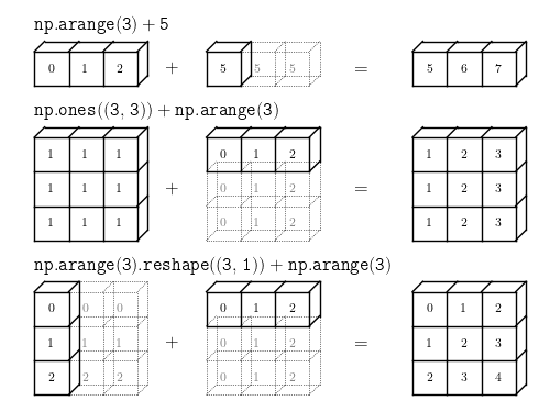"
590 | ]
591 | },
592 | {
593 | "cell_type": "markdown",
594 | "metadata": {},
595 | "source": [
596 | "## 逻辑运算\n",
597 | "### 七月在线python数据分析班 2017升级版 julyedu.com"
598 | ]
599 | },
600 | {
601 | "cell_type": "markdown",
602 | "metadata": {},
603 | "source": [
604 | "where可以帮我们选择是取第一个ndarray的元素还是第二个的"
605 | ]
606 | },
607 | {
608 | "cell_type": "markdown",
609 | "metadata": {},
610 | "source": [
611 | "## 连接两个二维数组\n",
612 | "### 七月在线python数据分析集训营 julyedu.com"
613 | ]
614 | },
615 | {
616 | "cell_type": "markdown",
617 | "metadata": {},
618 | "source": [
619 | "所谓堆叠,参考叠盘子。。。连接的另一种表述\n",
620 | "垂直stack与水平stack"
621 | ]
622 | },
623 | {
624 | "cell_type": "markdown",
625 | "metadata": {},
626 | "source": [
627 | "拆分数组, 我们使用[split方法](https://docs.scipy.org/doc/numpy-1.13.0/reference/generated/numpy.split.html)。\n",
628 | "\n",
629 | "split(array, indices_or_sections, axis=0)\n",
630 | "\n",
631 | "第一个参数array没有什么疑问,第二个参数可以是切断的index,也可以是切分的个数,第三个参数是我们切块的维度"
632 | ]
633 | },
634 | {
635 | "cell_type": "markdown",
636 | "metadata": {},
637 | "source": [
638 | "如果我们想要直接平均切分成三块呢?"
639 | ]
640 | },
641 | {
642 | "cell_type": "markdown",
643 | "metadata": {},
644 | "source": [
645 | "堆叠辅助"
646 | ]
647 | },
648 | {
649 | "cell_type": "markdown",
650 | "metadata": {},
651 | "source": [
652 | "r_用于按行堆叠"
653 | ]
654 | },
655 | {
656 | "cell_type": "markdown",
657 | "metadata": {},
658 | "source": [
659 | "c_用于按列堆叠"
660 | ]
661 | },
662 | {
663 | "cell_type": "markdown",
664 | "metadata": {},
665 | "source": [
666 | "切片直接转为数组"
667 | ]
668 | },
669 | {
670 | "cell_type": "markdown",
671 | "metadata": {},
672 | "source": [
673 | "使用repeat来重复ndarry中的元素"
674 | ]
675 | },
676 | {
677 | "cell_type": "markdown",
678 | "metadata": {},
679 | "source": [
680 | "按元素重复"
681 | ]
682 | },
683 | {
684 | "cell_type": "markdown",
685 | "metadata": {},
686 | "source": [
687 | "指定axis来重复"
688 | ]
689 | },
690 | {
691 | "cell_type": "markdown",
692 | "metadata": {},
693 | "source": [
694 | "Tile: 参考贴瓷砖\n",
695 | "[numpy tile](https://docs.scipy.org/doc/numpy/reference/generated/numpy.tile.html)"
696 | ]
697 | }
698 | ],
699 | "metadata": {
700 | "kernelspec": {
701 | "display_name": "Python 3",
702 | "language": "python",
703 | "name": "python3"
704 | },
705 | "language_info": {
706 | "codemirror_mode": {
707 | "name": "ipython",
708 | "version": 3
709 | },
710 | "file_extension": ".py",
711 | "mimetype": "text/x-python",
712 | "name": "python",
713 | "nbconvert_exporter": "python",
714 | "pygments_lexer": "ipython3",
715 | "version": "3.6.1"
716 | }
717 | },
718 | "nbformat": 4,
719 | "nbformat_minor": 1
720 | }
721 |
--------------------------------------------------------------------------------
/Nov-2017/numpy-1.ipynb:
--------------------------------------------------------------------------------
1 | {
2 | "cells": [
3 | {
4 | "cell_type": "markdown",
5 | "metadata": {},
6 | "source": [
7 | "# numpy基础\n",
8 | "\n",
9 | "### 七月在线python数据分析集训营 julyedu.com\n",
10 | "\n",
11 | "褚则伟 zeweichu@gmail.com"
12 | ]
13 | },
14 | {
15 | "cell_type": "markdown",
16 | "metadata": {},
17 | "source": [
18 | "## Numpy简介\n",
19 | "\n",
20 | "- Numpy是Python语言的一个library [numpy](http://www.numpy.org/)\n",
21 | "- Numpy主要支持矩阵操作和运算\n",
22 | "- Numpy非常高效,core代码由C语言写成\n",
23 | "- 我们第三课要讲的pandas也是基于Numpy构建的一个library\n",
24 | "- 现在比较流行的机器学习框架(例如Tensorflow/PyTorch等等),语法都与Numpy比较接近"
25 | ]
26 | },
27 | {
28 | "cell_type": "markdown",
29 | "metadata": {},
30 | "source": [
31 | "## 目录\n",
32 | "- 数组简介和数组的构造(ndarray)\n",
33 | "- 数组取值和赋值\n",
34 | "- 数学运算"
35 | ]
36 | },
37 | {
38 | "cell_type": "markdown",
39 | "metadata": {},
40 | "source": [
41 | "python里面调用一个包,用import对吧, 所以我们import `numpy` 包:\n",
42 | "\n",
43 | "如果还没有安装的话,你可以在command line界面使用`pip install numpy`"
44 | ]
45 | },
46 | {
47 | "cell_type": "code",
48 | "execution_count": 1,
49 | "metadata": {
50 | "collapsed": true
51 | },
52 | "outputs": [],
53 | "source": [
54 | "import numpy as np"
55 | ]
56 | },
57 | {
58 | "cell_type": "markdown",
59 | "metadata": {},
60 | "source": [
61 | "## Arrays/数组\n",
62 | "\n",
63 | "### 七月在线python数据分析集训营 julyedu.com"
64 | ]
65 | },
66 | {
67 | "cell_type": "markdown",
68 | "metadata": {},
69 | "source": [
70 | "看你数组的维度啦,我自己的话比较简单粗暴,一般直接把1维数组就看做向量/vector,2维数组看做2维矩阵,3维数组看做3维矩阵..."
71 | ]
72 | },
73 | {
74 | "cell_type": "markdown",
75 | "metadata": {},
76 | "source": [
77 | "可以调用np.array去从list初始化一个数组:"
78 | ]
79 | },
80 | {
81 | "cell_type": "code",
82 | "execution_count": 2,
83 | "metadata": {},
84 | "outputs": [
85 | {
86 | "name": "stdout",
87 | "output_type": "stream",
88 | "text": [
89 | " (3,) 1 2 3\n",
90 | "[5 2 3]\n"
91 | ]
92 | }
93 | ],
94 | "source": [
95 | "a = np.array([1, 2, 3]) # 1维数组\n",
96 | "print(type(a), a.shape, a[0], a[1], a[2])\n",
97 | "a[0] = 5 # 重新赋值\n",
98 | "print(a) "
99 | ]
100 | },
101 | {
102 | "cell_type": "code",
103 | "execution_count": 3,
104 | "metadata": {},
105 | "outputs": [
106 | {
107 | "name": "stdout",
108 | "output_type": "stream",
109 | "text": [
110 | "[[1 2 3]\n",
111 | " [4 5 6]]\n"
112 | ]
113 | }
114 | ],
115 | "source": [
116 | "b = np.array([[1,2,3],[4,5,6]]) # 2维数组\n",
117 | "print(b)"
118 | ]
119 | },
120 | {
121 | "cell_type": "code",
122 | "execution_count": 4,
123 | "metadata": {},
124 | "outputs": [
125 | {
126 | "name": "stdout",
127 | "output_type": "stream",
128 | "text": [
129 | "(2, 3)\n",
130 | "1 2 4\n"
131 | ]
132 | }
133 | ],
134 | "source": [
135 | "print(b.shape) #可以看形状的(非常常用!!!) \n",
136 | "print(b[0, 0], b[0, 1], b[1, 0])"
137 | ]
138 | },
139 | {
140 | "cell_type": "code",
141 | "execution_count": 5,
142 | "metadata": {},
143 | "outputs": [
144 | {
145 | "name": "stdout",
146 | "output_type": "stream",
147 | "text": [
148 | "6\n"
149 | ]
150 | }
151 | ],
152 | "source": [
153 | "print(b.size)"
154 | ]
155 | },
156 | {
157 | "cell_type": "code",
158 | "execution_count": 6,
159 | "metadata": {},
160 | "outputs": [
161 | {
162 | "name": "stdout",
163 | "output_type": "stream",
164 | "text": [
165 | "int64\n"
166 | ]
167 | }
168 | ],
169 | "source": [
170 | "print(b.dtype)"
171 | ]
172 | },
173 | {
174 | "cell_type": "markdown",
175 | "metadata": {},
176 | "source": [
177 | "查看每个element的大小"
178 | ]
179 | },
180 | {
181 | "cell_type": "code",
182 | "execution_count": 7,
183 | "metadata": {
184 | "scrolled": true
185 | },
186 | "outputs": [
187 | {
188 | "name": "stdout",
189 | "output_type": "stream",
190 | "text": [
191 | "8\n"
192 | ]
193 | }
194 | ],
195 | "source": [
196 | "print(b.itemsize)"
197 | ]
198 | },
199 | {
200 | "cell_type": "markdown",
201 | "metadata": {},
202 | "source": [
203 | "有一些内置的创建数组的函数:"
204 | ]
205 | },
206 | {
207 | "cell_type": "code",
208 | "execution_count": 8,
209 | "metadata": {},
210 | "outputs": [
211 | {
212 | "name": "stdout",
213 | "output_type": "stream",
214 | "text": [
215 | "[[ 0. 0.]\n",
216 | " [ 0. 0.]]\n"
217 | ]
218 | }
219 | ],
220 | "source": [
221 | "a = np.zeros((2,2)) # 创建2x2的全0数组\n",
222 | "print(a)"
223 | ]
224 | },
225 | {
226 | "cell_type": "code",
227 | "execution_count": 9,
228 | "metadata": {},
229 | "outputs": [
230 | {
231 | "name": "stdout",
232 | "output_type": "stream",
233 | "text": [
234 | "[[ 1. 1.]]\n"
235 | ]
236 | }
237 | ],
238 | "source": [
239 | "b = np.ones((1,2)) # 创建1x2的全1数组\n",
240 | "print(b)"
241 | ]
242 | },
243 | {
244 | "cell_type": "code",
245 | "execution_count": 10,
246 | "metadata": {},
247 | "outputs": [
248 | {
249 | "name": "stdout",
250 | "output_type": "stream",
251 | "text": [
252 | "[[7 7]\n",
253 | " [7 7]]\n"
254 | ]
255 | }
256 | ],
257 | "source": [
258 | "c = np.full((2,2), 7) # 定值数组\n",
259 | "print(c) "
260 | ]
261 | },
262 | {
263 | "cell_type": "code",
264 | "execution_count": 11,
265 | "metadata": {},
266 | "outputs": [
267 | {
268 | "name": "stdout",
269 | "output_type": "stream",
270 | "text": [
271 | "[[ 1. 0.]\n",
272 | " [ 0. 1.]]\n"
273 | ]
274 | }
275 | ],
276 | "source": [
277 | "d = np.eye(2) # 对角矩阵(对角元素为1)\n",
278 | "print(d)"
279 | ]
280 | },
281 | {
282 | "cell_type": "code",
283 | "execution_count": 12,
284 | "metadata": {},
285 | "outputs": [
286 | {
287 | "name": "stdout",
288 | "output_type": "stream",
289 | "text": [
290 | "[[ 0.18371333 0.67849295]\n",
291 | " [ 0.56642033 0.87021502]]\n"
292 | ]
293 | }
294 | ],
295 | "source": [
296 | "e = np.random.random((2,2)) # 2x2的随机数组(矩阵)\n",
297 | "print(e)"
298 | ]
299 | },
300 | {
301 | "cell_type": "code",
302 | "execution_count": 13,
303 | "metadata": {},
304 | "outputs": [
305 | {
306 | "name": "stdout",
307 | "output_type": "stream",
308 | "text": [
309 | "[[[ 0.00000000e+000 3.11108892e+231]\n",
310 | " [ 2.96439388e-323 0.00000000e+000]\n",
311 | " [ 2.12199579e-314 1.58817677e-052]]\n",
312 | "\n",
313 | " [[ 5.20845631e-090 1.69175720e-052]\n",
314 | " [ 3.61111103e+174 4.79126305e-037]\n",
315 | " [ 3.99910963e+252 8.34404912e-309]]]\n",
316 | "(2, 3, 2)\n"
317 | ]
318 | }
319 | ],
320 | "source": [
321 | "f = np.empty((2,3,2)) # empty是未初始化的数据\n",
322 | "print(f)\n",
323 | "print(f.shape)"
324 | ]
325 | },
326 | {
327 | "cell_type": "code",
328 | "execution_count": 14,
329 | "metadata": {},
330 | "outputs": [
331 | {
332 | "name": "stdout",
333 | "output_type": "stream",
334 | "text": [
335 | "[ 0 1 2 3 4 5 6 7 8 9 10 11 12 13 14]\n",
336 | "(15,)\n"
337 | ]
338 | }
339 | ],
340 | "source": [
341 | "g = np.arange(15) # 用arange可以生成连续的一串元素\n",
342 | "print(g)\n",
343 | "print(g.shape)"
344 | ]
345 | },
346 | {
347 | "cell_type": "markdown",
348 | "metadata": {},
349 | "source": [
350 | "linspace也是一个很常用的初始化数据的手段,它可以帮我们产生一连串等间距的数组"
351 | ]
352 | },
353 | {
354 | "cell_type": "code",
355 | "execution_count": 15,
356 | "metadata": {},
357 | "outputs": [
358 | {
359 | "data": {
360 | "text/plain": [
361 | "array([ 2. , 2.25, 2.5 , 2.75, 3. ])"
362 | ]
363 | },
364 | "execution_count": 15,
365 | "metadata": {},
366 | "output_type": "execute_result"
367 | }
368 | ],
369 | "source": [
370 | "np.linspace(2.0, 3.0, 5)"
371 | ]
372 | },
373 | {
374 | "cell_type": "markdown",
375 | "metadata": {},
376 | "source": [
377 | "## 使用reshape来改变tensor的形状\n",
378 | "### 七月在线python数据分析集训营 julyedu.com"
379 | ]
380 | },
381 | {
382 | "cell_type": "markdown",
383 | "metadata": {},
384 | "source": [
385 | "numpy可以很容易地把一维数组转成二维数组,三维数组。"
386 | ]
387 | },
388 | {
389 | "cell_type": "code",
390 | "execution_count": 16,
391 | "metadata": {},
392 | "outputs": [
393 | {
394 | "name": "stdout",
395 | "output_type": "stream",
396 | "text": [
397 | "(4,2): [[0 1]\n",
398 | " [2 3]\n",
399 | " [4 5]\n",
400 | " [6 7]]\n",
401 | "\n",
402 | "(2,2,2): [[[0 1]\n",
403 | " [2 3]]\n",
404 | "\n",
405 | " [[4 5]\n",
406 | " [6 7]]]\n"
407 | ]
408 | }
409 | ],
410 | "source": [
411 | "import numpy as np\n",
412 | "\n",
413 | "arr = np.arange(8)\n",
414 | "print(\"(4,2):\", arr.reshape((4,2)))\n",
415 | "print()\n",
416 | "print(\"(2,2,2):\", arr.reshape((2,2,2)))"
417 | ]
418 | },
419 | {
420 | "cell_type": "markdown",
421 | "metadata": {},
422 | "source": [
423 | "直接把shape给重新定义了其实也可以"
424 | ]
425 | },
426 | {
427 | "cell_type": "code",
428 | "execution_count": 17,
429 | "metadata": {},
430 | "outputs": [
431 | {
432 | "data": {
433 | "text/plain": [
434 | "array([[0, 1, 2, 3],\n",
435 | " [4, 5, 6, 7]])"
436 | ]
437 | },
438 | "execution_count": 17,
439 | "metadata": {},
440 | "output_type": "execute_result"
441 | }
442 | ],
443 | "source": [
444 | "arr = np.arange(8)\n",
445 | "arr.shape = 2,4\n",
446 | "arr"
447 | ]
448 | },
449 | {
450 | "cell_type": "markdown",
451 | "metadata": {},
452 | "source": [
453 | "如果我们在某一个维度上写上-1,numpy会帮我们自动推导出正确的维度"
454 | ]
455 | },
456 | {
457 | "cell_type": "code",
458 | "execution_count": 18,
459 | "metadata": {},
460 | "outputs": [
461 | {
462 | "name": "stdout",
463 | "output_type": "stream",
464 | "text": [
465 | "[[ 0 1 2]\n",
466 | " [ 3 4 5]\n",
467 | " [ 6 7 8]\n",
468 | " [ 9 10 11]\n",
469 | " [12 13 14]]\n",
470 | "(5, 3)\n"
471 | ]
472 | }
473 | ],
474 | "source": [
475 | "arr = np.arange(15)\n",
476 | "print(arr.reshape((5,-1)))\n",
477 | "print(arr.reshape((5,-1)).shape)"
478 | ]
479 | },
480 | {
481 | "cell_type": "markdown",
482 | "metadata": {},
483 | "source": [
484 | "还可以从其他的ndarray中获取shape信息然后reshape"
485 | ]
486 | },
487 | {
488 | "cell_type": "code",
489 | "execution_count": 19,
490 | "metadata": {},
491 | "outputs": [
492 | {
493 | "name": "stdout",
494 | "output_type": "stream",
495 | "text": [
496 | "(3, 5)\n",
497 | "[[ 0 1 2 3 4]\n",
498 | " [ 5 6 7 8 9]\n",
499 | " [10 11 12 13 14]]\n"
500 | ]
501 | }
502 | ],
503 | "source": [
504 | "other_arr = np.ones((3,5))\n",
505 | "print(other_arr.shape)\n",
506 | "print(arr.reshape(other_arr.shape))"
507 | ]
508 | },
509 | {
510 | "cell_type": "markdown",
511 | "metadata": {},
512 | "source": [
513 | "高维数组可以用ravel来拉平"
514 | ]
515 | },
516 | {
517 | "cell_type": "code",
518 | "execution_count": 20,
519 | "metadata": {},
520 | "outputs": [
521 | {
522 | "name": "stdout",
523 | "output_type": "stream",
524 | "text": [
525 | "[ 0 1 2 3 4 5 6 7 8 9 10 11 12 13 14]\n"
526 | ]
527 | }
528 | ],
529 | "source": [
530 | "print(arr.ravel())"
531 | ]
532 | },
533 | {
534 | "cell_type": "markdown",
535 | "metadata": {},
536 | "source": [
537 | "### 数组的数据类型 dtype\n",
538 | "\n",
539 | "数组可以有不同的数据类型"
540 | ]
541 | },
542 | {
543 | "cell_type": "markdown",
544 | "metadata": {},
545 | "source": [
546 | "生成数组时可以指定数据类型,如果不指定numpy会自动匹配合适的类型"
547 | ]
548 | },
549 | {
550 | "cell_type": "code",
551 | "execution_count": 21,
552 | "metadata": {},
553 | "outputs": [
554 | {
555 | "name": "stdout",
556 | "output_type": "stream",
557 | "text": [
558 | "float64\n"
559 | ]
560 | }
561 | ],
562 | "source": [
563 | "arr = np.array([1,2,3], dtype=np.float64)\n",
564 | "print(arr.dtype)"
565 | ]
566 | },
567 | {
568 | "cell_type": "code",
569 | "execution_count": 22,
570 | "metadata": {},
571 | "outputs": [
572 | {
573 | "name": "stdout",
574 | "output_type": "stream",
575 | "text": [
576 | "int32\n"
577 | ]
578 | }
579 | ],
580 | "source": [
581 | "arr = np.array([1,2,3], dtype=np.int32)\n",
582 | "print(arr.dtype)"
583 | ]
584 | },
585 | {
586 | "cell_type": "markdown",
587 | "metadata": {},
588 | "source": [
589 | "有时候如果我们需要ndarray是一个特定的数据类型,可以使用astype复制数组并转换数据类型"
590 | ]
591 | },
592 | {
593 | "cell_type": "code",
594 | "execution_count": 23,
595 | "metadata": {},
596 | "outputs": [
597 | {
598 | "name": "stdout",
599 | "output_type": "stream",
600 | "text": [
601 | "int64\n",
602 | "float64\n"
603 | ]
604 | }
605 | ],
606 | "source": [
607 | "int_arr = np.array([1,2,3,4,5])\n",
608 | "float_arr = int_arr.astype(np.float)\n",
609 | "print(int_arr.dtype)\n",
610 | "print(float_arr.dtype)"
611 | ]
612 | },
613 | {
614 | "cell_type": "markdown",
615 | "metadata": {},
616 | "source": [
617 | "使用astype将float转换为int时小数部分被舍弃"
618 | ]
619 | },
620 | {
621 | "cell_type": "code",
622 | "execution_count": 24,
623 | "metadata": {},
624 | "outputs": [
625 | {
626 | "name": "stdout",
627 | "output_type": "stream",
628 | "text": [
629 | "[ 3 -1 -2 0 12 10]\n"
630 | ]
631 | }
632 | ],
633 | "source": [
634 | "float_arr = np.array([3.7, -1.2, -2.6, 0.5, 12.9, 10.1])\n",
635 | "int_arr = float_arr.astype(dtype = np.int)\n",
636 | "print(int_arr)"
637 | ]
638 | },
639 | {
640 | "cell_type": "markdown",
641 | "metadata": {},
642 | "source": [
643 | "使用astype把字符串转换为数组,如果失败抛出异常。"
644 | ]
645 | },
646 | {
647 | "cell_type": "code",
648 | "execution_count": 25,
649 | "metadata": {},
650 | "outputs": [
651 | {
652 | "name": "stdout",
653 | "output_type": "stream",
654 | "text": [
655 | "[ 1.25 -9.6 42. ]\n"
656 | ]
657 | }
658 | ],
659 | "source": [
660 | "str_arr = np.array(['1.25', '-9.6', '42'], dtype = np.string_)\n",
661 | "float_arr = str_arr.astype(dtype = np.float)\n",
662 | "print(float_arr)"
663 | ]
664 | },
665 | {
666 | "cell_type": "markdown",
667 | "metadata": {},
668 | "source": [
669 | "astype使用其它数组的数据类型作为参数"
670 | ]
671 | },
672 | {
673 | "cell_type": "code",
674 | "execution_count": 26,
675 | "metadata": {},
676 | "outputs": [
677 | {
678 | "name": "stdout",
679 | "output_type": "stream",
680 | "text": [
681 | "[ 0. 1. 2. 3. 4. 5. 6. 7. 8. 9.]\n",
682 | "0 1\n"
683 | ]
684 | }
685 | ],
686 | "source": [
687 | "int_arr = np.arange(10)\n",
688 | "float_arr = np.array([.23, 0.270, .357, 0.44, 0.5], dtype = np.float64)\n",
689 | "print(int_arr.astype(float_arr.dtype))\n",
690 | "print(int_arr[0], int_arr[1])"
691 | ]
692 | },
693 | {
694 | "cell_type": "markdown",
695 | "metadata": {},
696 | "source": [
697 | "更多的内容可以读读[文档](http://docs.scipy.org/doc/numpy/reference/arrays.dtypes.html)."
698 | ]
699 | },
700 | {
701 | "cell_type": "markdown",
702 | "metadata": {},
703 | "source": [
704 | "## Array indexing/数组取值和赋值\n",
705 | "\n",
706 | "### 七月在线python数据分析集训营 julyedu.com"
707 | ]
708 | },
709 | {
710 | "cell_type": "markdown",
711 | "metadata": {},
712 | "source": [
713 | "Numpy提供了蛮多种取值的方式的."
714 | ]
715 | },
716 | {
717 | "cell_type": "markdown",
718 | "metadata": {},
719 | "source": [
720 | "可以像list一样切片(多维数组可以从各个维度同时切片):"
721 | ]
722 | },
723 | {
724 | "cell_type": "code",
725 | "execution_count": 27,
726 | "metadata": {},
727 | "outputs": [
728 | {
729 | "name": "stdout",
730 | "output_type": "stream",
731 | "text": [
732 | "[[2 3]\n",
733 | " [6 7]]\n"
734 | ]
735 | }
736 | ],
737 | "source": [
738 | "import numpy as np\n",
739 | "\n",
740 | "# 创建一个如下格式的3x4数组\n",
741 | "# [[ 1 2 3 4]\n",
742 | "# [ 5 6 7 8]\n",
743 | "# [ 9 10 11 12]]\n",
744 | "a = np.array([[1,2,3,4], [5,6,7,8], [9,10,11,12]])\n",
745 | "\n",
746 | "# 在两个维度上分别按照[:2]和[1:3]进行切片,取需要的部分\n",
747 | "# [[2 3]\n",
748 | "# [6 7]]\n",
749 | "b = a[:2, 1:3]\n",
750 | "print(b)"
751 | ]
752 | },
753 | {
754 | "cell_type": "markdown",
755 | "metadata": {},
756 | "source": [
757 | "虽然,怎么说呢,不建议你这样去赋值,但是你确实可以修改切片出来的对象,然后完成对原数组的赋值."
758 | ]
759 | },
760 | {
761 | "cell_type": "code",
762 | "execution_count": 28,
763 | "metadata": {},
764 | "outputs": [
765 | {
766 | "name": "stdout",
767 | "output_type": "stream",
768 | "text": [
769 | "2\n",
770 | "77\n"
771 | ]
772 | }
773 | ],
774 | "source": [
775 | "print(a[0, 1]) \n",
776 | "b[0, 0] = 77 # b[0, 0]改了,很遗憾a[0, 1]也被修改了\n",
777 | "print(a[0, 1])"
778 | ]
779 | },
780 | {
781 | "cell_type": "markdown",
782 | "metadata": {},
783 | "source": [
784 | "关于Copy和View的关系\n",
785 | "- 简单的数组赋值,切片,包括作为函数的参数传递一个数组--并不会复制出一个新的数组,只是制造了一个新的reference。所以如果我们在新赋值的变量上改变数组的内容,原来的那个数组内容也会发生改变。这一点千万要注意哦!"
786 | ]
787 | },
788 | {
789 | "cell_type": "code",
790 | "execution_count": 29,
791 | "metadata": {},
792 | "outputs": [
793 | {
794 | "data": {
795 | "text/plain": [
796 | "True"
797 | ]
798 | },
799 | "execution_count": 29,
800 | "metadata": {},
801 | "output_type": "execute_result"
802 | }
803 | ],
804 | "source": [
805 | "b = a\n",
806 | "b is a"
807 | ]
808 | },
809 | {
810 | "cell_type": "markdown",
811 | "metadata": {},
812 | "source": [
813 | "- 使用`view`方法,我们可以拿到数组的一部分或者全部,但是在view上面修改内容还是会把原来的数组给更改了"
814 | ]
815 | },
816 | {
817 | "cell_type": "code",
818 | "execution_count": 30,
819 | "metadata": {},
820 | "outputs": [
821 | {
822 | "data": {
823 | "text/plain": [
824 | "False"
825 | ]
826 | },
827 | "execution_count": 30,
828 | "metadata": {},
829 | "output_type": "execute_result"
830 | }
831 | ],
832 | "source": [
833 | "c = a.view()\n",
834 | "c is a"
835 | ]
836 | },
837 | {
838 | "cell_type": "markdown",
839 | "metadata": {},
840 | "source": [
841 | "使用`base`方法可以查看一个数组的owner是谁,也就是说这个数组是由谁制造产生的。"
842 | ]
843 | },
844 | {
845 | "cell_type": "code",
846 | "execution_count": 31,
847 | "metadata": {
848 | "scrolled": false
849 | },
850 | "outputs": [
851 | {
852 | "data": {
853 | "text/plain": [
854 | "True"
855 | ]
856 | },
857 | "execution_count": 31,
858 | "metadata": {},
859 | "output_type": "execute_result"
860 | }
861 | ],
862 | "source": [
863 | "c.base is a"
864 | ]
865 | },
866 | {
867 | "cell_type": "markdown",
868 | "metadata": {},
869 | "source": [
870 | "其实使用切片方法我们拿到的也是一个view"
871 | ]
872 | },
873 | {
874 | "cell_type": "code",
875 | "execution_count": 32,
876 | "metadata": {
877 | "scrolled": true
878 | },
879 | "outputs": [
880 | {
881 | "data": {
882 | "text/plain": [
883 | "True"
884 | ]
885 | },
886 | "execution_count": 32,
887 | "metadata": {},
888 | "output_type": "execute_result"
889 | }
890 | ],
891 | "source": [
892 | "s = a[:, 2:]\n",
893 | "s.base is a"
894 | ]
895 | },
896 | {
897 | "cell_type": "markdown",
898 | "metadata": {},
899 | "source": [
900 | "所以更改切片上的内容之后,原来数组的内容也被更改了"
901 | ]
902 | },
903 | {
904 | "cell_type": "code",
905 | "execution_count": 33,
906 | "metadata": {},
907 | "outputs": [
908 | {
909 | "data": {
910 | "text/plain": [
911 | "array([[ 1, 77, 10, 10],\n",
912 | " [ 5, 6, 10, 10],\n",
913 | " [ 9, 10, 10, 10]])"
914 | ]
915 | },
916 | "execution_count": 33,
917 | "metadata": {},
918 | "output_type": "execute_result"
919 | }
920 | ],
921 | "source": [
922 | "s[:] = 10\n",
923 | "a"
924 | ]
925 | },
926 | {
927 | "cell_type": "markdown",
928 | "metadata": {},
929 | "source": [
930 | "如果要复制出一个新的数组,我们就需要使用`copy()`这个方法了"
931 | ]
932 | },
933 | {
934 | "cell_type": "code",
935 | "execution_count": 34,
936 | "metadata": {},
937 | "outputs": [
938 | {
939 | "data": {
940 | "text/plain": [
941 | "False"
942 | ]
943 | },
944 | "execution_count": 34,
945 | "metadata": {},
946 | "output_type": "execute_result"
947 | }
948 | ],
949 | "source": [
950 | "d = a.copy()\n",
951 | "d is a"
952 | ]
953 | },
954 | {
955 | "cell_type": "code",
956 | "execution_count": 35,
957 | "metadata": {
958 | "scrolled": true
959 | },
960 | "outputs": [
961 | {
962 | "data": {
963 | "text/plain": [
964 | "False"
965 | ]
966 | },
967 | "execution_count": 35,
968 | "metadata": {},
969 | "output_type": "execute_result"
970 | }
971 | ],
972 | "source": [
973 | "d.base is a"
974 | ]
975 | },
976 | {
977 | "cell_type": "code",
978 | "execution_count": 36,
979 | "metadata": {},
980 | "outputs": [
981 | {
982 | "data": {
983 | "text/plain": [
984 | "array([[ 1, 77, 10, 10],\n",
985 | " [ 5, 6, 10, 10],\n",
986 | " [ 9, 10, 10, 10]])"
987 | ]
988 | },
989 | "execution_count": 36,
990 | "metadata": {},
991 | "output_type": "execute_result"
992 | }
993 | ],
994 | "source": [
995 | "d[0,0] = 9999\n",
996 | "a"
997 | ]
998 | },
999 | {
1000 | "cell_type": "markdown",
1001 | "metadata": {},
1002 | "source": [
1003 | "下面我们继续回到数组切片的问题上\n",
1004 | "\n",
1005 | "创建3x4的2维数组/矩阵"
1006 | ]
1007 | },
1008 | {
1009 | "cell_type": "code",
1010 | "execution_count": 37,
1011 | "metadata": {},
1012 | "outputs": [
1013 | {
1014 | "name": "stdout",
1015 | "output_type": "stream",
1016 | "text": [
1017 | "[[ 1 2 3 4]\n",
1018 | " [ 5 6 7 8]\n",
1019 | " [ 9 10 11 12]]\n"
1020 | ]
1021 | }
1022 | ],
1023 | "source": [
1024 | "a = np.array([[1,2,3,4], [5,6,7,8], [9,10,11,12]])\n",
1025 | "print(a)"
1026 | ]
1027 | },
1028 | {
1029 | "cell_type": "markdown",
1030 | "metadata": {},
1031 | "source": [
1032 | "你就放心大胆地去取你想要的数咯:"
1033 | ]
1034 | },
1035 | {
1036 | "cell_type": "code",
1037 | "execution_count": 38,
1038 | "metadata": {},
1039 | "outputs": [
1040 | {
1041 | "name": "stdout",
1042 | "output_type": "stream",
1043 | "text": [
1044 | "[5 6 7 8] (4,)\n",
1045 | "[[5 6 7 8]] (1, 4)\n",
1046 | "[[5 6 7 8]] (1, 4)\n"
1047 | ]
1048 | }
1049 | ],
1050 | "source": [
1051 | "row_r1 = a[1, :] # 第2行,但是得到的是1维输出(列向量)\n",
1052 | "row_r2 = a[1:2, :] # 1x2的2维输出\n",
1053 | "row_r3 = a[[1], :] # 同上\n",
1054 | "print(row_r1, row_r1.shape)\n",
1055 | "print(row_r2, row_r2.shape)\n",
1056 | "print(row_r3, row_r3.shape)"
1057 | ]
1058 | },
1059 | {
1060 | "cell_type": "markdown",
1061 | "metadata": {},
1062 | "source": [
1063 | "试试在第2个维度上切片也一样的:"
1064 | ]
1065 | },
1066 | {
1067 | "cell_type": "code",
1068 | "execution_count": 39,
1069 | "metadata": {},
1070 | "outputs": [
1071 | {
1072 | "name": "stdout",
1073 | "output_type": "stream",
1074 | "text": [
1075 | "[ 2 6 10] (3,)\n",
1076 | "\n",
1077 | "[[ 2]\n",
1078 | " [ 6]\n",
1079 | " [10]] (3, 1)\n"
1080 | ]
1081 | }
1082 | ],
1083 | "source": [
1084 | "col_r1 = a[:, 1]\n",
1085 | "col_r2 = a[:, 1:2]\n",
1086 | "print(col_r1, col_r1.shape)\n",
1087 | "print()\n",
1088 | "print(col_r2, col_r2.shape)"
1089 | ]
1090 | },
1091 | {
1092 | "cell_type": "markdown",
1093 | "metadata": {},
1094 | "source": [
1095 | "dots(...)"
1096 | ]
1097 | },
1098 | {
1099 | "cell_type": "code",
1100 | "execution_count": 40,
1101 | "metadata": {},
1102 | "outputs": [
1103 | {
1104 | "data": {
1105 | "text/plain": [
1106 | "array([[ 75, 76, 77, 78, 79],\n",
1107 | " [ 95, 96, 97, 98, 99],\n",
1108 | " [115, 116, 117, 118, 119]])"
1109 | ]
1110 | },
1111 | "execution_count": 40,
1112 | "metadata": {},
1113 | "output_type": "execute_result"
1114 | }
1115 | ],
1116 | "source": [
1117 | "import numpy as np\n",
1118 | "c = np.arange(120).reshape(2,3,4,5)\n",
1119 | "c[1, ..., 3, :]"
1120 | ]
1121 | },
1122 | {
1123 | "cell_type": "markdown",
1124 | "metadata": {},
1125 | "source": [
1126 | "下面这个高级了,更自由地取值和组合,但是要看清楚一点:"
1127 | ]
1128 | },
1129 | {
1130 | "cell_type": "code",
1131 | "execution_count": 41,
1132 | "metadata": {},
1133 | "outputs": [
1134 | {
1135 | "name": "stdout",
1136 | "output_type": "stream",
1137 | "text": [
1138 | "[1 4 5]\n",
1139 | "[1 4 5]\n"
1140 | ]
1141 | }
1142 | ],
1143 | "source": [
1144 | "a = np.array([[1,2], [3, 4], [5, 6]])\n",
1145 | "\n",
1146 | "# 其实意思就是取(0,0),(1,1),(2,0)的元素组起来\n",
1147 | "print(a[[0, 1, 2], [0, 1, 0]])\n",
1148 | "\n",
1149 | "# 下面这个比较直白啦\n",
1150 | "print(np.array([a[0, 0], a[1, 1], a[2, 0]]))"
1151 | ]
1152 | },
1153 | {
1154 | "cell_type": "code",
1155 | "execution_count": 42,
1156 | "metadata": {},
1157 | "outputs": [
1158 | {
1159 | "data": {
1160 | "text/plain": [
1161 | "array([ 1, 39, 77, 110])"
1162 | ]
1163 | },
1164 | "execution_count": 42,
1165 | "metadata": {},
1166 | "output_type": "execute_result"
1167 | }
1168 | ],
1169 | "source": [
1170 | "a = np.arange(4*5*6).reshape(4,5,6)\n",
1171 | "a[np.arange(4), np.arange(4), [1,3,5,2]]"
1172 | ]
1173 | },
1174 | {
1175 | "cell_type": "code",
1176 | "execution_count": 43,
1177 | "metadata": {},
1178 | "outputs": [
1179 | {
1180 | "name": "stdout",
1181 | "output_type": "stream",
1182 | "text": [
1183 | "[[ 6 7 8 9 10 11]\n",
1184 | " [ 6 7 8 9 10 11]]\n",
1185 | "[[ 6 7 8 9 10 11]\n",
1186 | " [ 6 7 8 9 10 11]]\n"
1187 | ]
1188 | }
1189 | ],
1190 | "source": [
1191 | "# 再来试试\n",
1192 | "print(a[[0, 0], [1, 1]])\n",
1193 | "\n",
1194 | "# 还是一样\n",
1195 | "print(np.array([a[0, 1], a[0, 1]]))"
1196 | ]
1197 | },
1198 | {
1199 | "cell_type": "markdown",
1200 | "metadata": {},
1201 | "source": [
1202 | "再来熟悉一下\n",
1203 | "\n",
1204 | "先创建一个2维数组"
1205 | ]
1206 | },
1207 | {
1208 | "cell_type": "code",
1209 | "execution_count": 44,
1210 | "metadata": {},
1211 | "outputs": [
1212 | {
1213 | "name": "stdout",
1214 | "output_type": "stream",
1215 | "text": [
1216 | "[[ 1 2 3]\n",
1217 | " [ 4 5 6]\n",
1218 | " [ 7 8 9]\n",
1219 | " [10 11 12]]\n"
1220 | ]
1221 | }
1222 | ],
1223 | "source": [
1224 | "a = np.array([[1,2,3], [4,5,6], [7,8,9], [10, 11, 12]])\n",
1225 | "print(a)"
1226 | ]
1227 | },
1228 | {
1229 | "cell_type": "markdown",
1230 | "metadata": {},
1231 | "source": [
1232 | "用下标生成一个向量"
1233 | ]
1234 | },
1235 | {
1236 | "cell_type": "code",
1237 | "execution_count": 45,
1238 | "metadata": {
1239 | "collapsed": true
1240 | },
1241 | "outputs": [],
1242 | "source": [
1243 | "b = np.array([0, 2, 0, 1])"
1244 | ]
1245 | },
1246 | {
1247 | "cell_type": "markdown",
1248 | "metadata": {},
1249 | "source": [
1250 | "你能看明白下面做的事情吗?"
1251 | ]
1252 | },
1253 | {
1254 | "cell_type": "code",
1255 | "execution_count": 46,
1256 | "metadata": {},
1257 | "outputs": [
1258 | {
1259 | "name": "stdout",
1260 | "output_type": "stream",
1261 | "text": [
1262 | "[ 1 6 7 11]\n"
1263 | ]
1264 | }
1265 | ],
1266 | "source": [
1267 | "print(a[np.arange(4), b]) "
1268 | ]
1269 | },
1270 | {
1271 | "cell_type": "markdown",
1272 | "metadata": {},
1273 | "source": [
1274 | "既然可以取出来,我们当然也可以对这些元素操作咯"
1275 | ]
1276 | },
1277 | {
1278 | "cell_type": "code",
1279 | "execution_count": 47,
1280 | "metadata": {},
1281 | "outputs": [
1282 | {
1283 | "name": "stdout",
1284 | "output_type": "stream",
1285 | "text": [
1286 | "[[11 2 3]\n",
1287 | " [ 4 5 16]\n",
1288 | " [17 8 9]\n",
1289 | " [10 21 12]]\n"
1290 | ]
1291 | }
1292 | ],
1293 | "source": [
1294 | "a[np.arange(4), b] += 10\n",
1295 | "print(a)"
1296 | ]
1297 | },
1298 | {
1299 | "cell_type": "markdown",
1300 | "metadata": {},
1301 | "source": [
1302 | "### numpy的条件判断\n",
1303 | "\n",
1304 | "比较fashion的取法之一,用条件判定去取(但是很好用):"
1305 | ]
1306 | },
1307 | {
1308 | "cell_type": "code",
1309 | "execution_count": 48,
1310 | "metadata": {},
1311 | "outputs": [
1312 | {
1313 | "name": "stdout",
1314 | "output_type": "stream",
1315 | "text": [
1316 | "[[False False]\n",
1317 | " [ True True]\n",
1318 | " [ True True]]\n"
1319 | ]
1320 | }
1321 | ],
1322 | "source": [
1323 | "a = np.array([[1,2], [3, 4], [5, 6]])\n",
1324 | "\n",
1325 | "bool_idx = (a > 2) # 就是判定一下是否大于2\n",
1326 | "\n",
1327 | "print(bool_idx) # 返回一个布尔型的3x2数组"
1328 | ]
1329 | },
1330 | {
1331 | "cell_type": "markdown",
1332 | "metadata": {},
1333 | "source": [
1334 | "用刚才的布尔型数组作为下标就可以去除符合条件的元素啦"
1335 | ]
1336 | },
1337 | {
1338 | "cell_type": "code",
1339 | "execution_count": 49,
1340 | "metadata": {},
1341 | "outputs": [
1342 | {
1343 | "name": "stdout",
1344 | "output_type": "stream",
1345 | "text": [
1346 | "[3 4 5 6]\n"
1347 | ]
1348 | }
1349 | ],
1350 | "source": [
1351 | "print(a[bool_idx])"
1352 | ]
1353 | },
1354 | {
1355 | "cell_type": "markdown",
1356 | "metadata": {},
1357 | "source": [
1358 | "其实一句话也可以完成是不是?"
1359 | ]
1360 | },
1361 | {
1362 | "cell_type": "code",
1363 | "execution_count": 50,
1364 | "metadata": {},
1365 | "outputs": [
1366 | {
1367 | "name": "stdout",
1368 | "output_type": "stream",
1369 | "text": [
1370 | "[3 4 5 6]\n"
1371 | ]
1372 | }
1373 | ],
1374 | "source": [
1375 | "print(a[a > 2])"
1376 | ]
1377 | },
1378 | {
1379 | "cell_type": "markdown",
1380 | "metadata": {},
1381 | "source": [
1382 | "那个,真的,其实还有很多细节,其他的方式去取值,你可以看看官方文档。"
1383 | ]
1384 | },
1385 | {
1386 | "cell_type": "markdown",
1387 | "metadata": {},
1388 | "source": [
1389 | "我们一起来来总结一下,看下面切片取值方式(对应颜色是取出来的结果):"
1390 | ]
1391 | },
1392 | {
1393 | "cell_type": "markdown",
1394 | "metadata": {},
1395 | "source": [
1396 | "\n",
1397 | ""
1398 | ]
1399 | },
1400 | {
1401 | "cell_type": "markdown",
1402 | "metadata": {},
1403 | "source": [
1404 | "## 简单数学运算\n",
1405 | "### 七月在线python数据分析集训营 julyedu.com"
1406 | ]
1407 | },
1408 | {
1409 | "cell_type": "markdown",
1410 | "metadata": {},
1411 | "source": [
1412 | "下面这些运算是你在科学运算中经常经常会用到的,比如逐个元素的运算如下:"
1413 | ]
1414 | },
1415 | {
1416 | "cell_type": "code",
1417 | "execution_count": 2,
1418 | "metadata": {
1419 | "collapsed": true
1420 | },
1421 | "outputs": [],
1422 | "source": [
1423 | "import numpy as np\n",
1424 | "x = np.array([[1,2],[3,4]], dtype=np.float64)\n",
1425 | "y = np.array([[5,6],[7,8]], dtype=np.float64)"
1426 | ]
1427 | },
1428 | {
1429 | "cell_type": "markdown",
1430 | "metadata": {},
1431 | "source": [
1432 | "逐元素求和有下面2种方式"
1433 | ]
1434 | },
1435 | {
1436 | "cell_type": "code",
1437 | "execution_count": 52,
1438 | "metadata": {},
1439 | "outputs": [
1440 | {
1441 | "name": "stdout",
1442 | "output_type": "stream",
1443 | "text": [
1444 | "[[ 6. 8.]\n",
1445 | " [ 10. 12.]]\n",
1446 | "[[ 6. 8.]\n",
1447 | " [ 10. 12.]]\n"
1448 | ]
1449 | }
1450 | ],
1451 | "source": [
1452 | "print(x + y)\n",
1453 | "print(np.add(x, y))"
1454 | ]
1455 | },
1456 | {
1457 | "cell_type": "markdown",
1458 | "metadata": {},
1459 | "source": [
1460 | "逐元素作差"
1461 | ]
1462 | },
1463 | {
1464 | "cell_type": "code",
1465 | "execution_count": 53,
1466 | "metadata": {},
1467 | "outputs": [
1468 | {
1469 | "name": "stdout",
1470 | "output_type": "stream",
1471 | "text": [
1472 | "[[-4. -4.]\n",
1473 | " [-4. -4.]]\n",
1474 | "[[-4. -4.]\n",
1475 | " [-4. -4.]]\n"
1476 | ]
1477 | }
1478 | ],
1479 | "source": [
1480 | "print(x - y)\n",
1481 | "print(np.subtract(x, y))"
1482 | ]
1483 | },
1484 | {
1485 | "cell_type": "markdown",
1486 | "metadata": {},
1487 | "source": [
1488 | "逐元素相乘"
1489 | ]
1490 | },
1491 | {
1492 | "cell_type": "code",
1493 | "execution_count": 54,
1494 | "metadata": {},
1495 | "outputs": [
1496 | {
1497 | "name": "stdout",
1498 | "output_type": "stream",
1499 | "text": [
1500 | "[[ 5. 12.]\n",
1501 | " [ 21. 32.]]\n",
1502 | "[[ 5. 12.]\n",
1503 | " [ 21. 32.]]\n"
1504 | ]
1505 | }
1506 | ],
1507 | "source": [
1508 | "print(x * y)\n",
1509 | "print(np.multiply(x, y))"
1510 | ]
1511 | },
1512 | {
1513 | "cell_type": "markdown",
1514 | "metadata": {},
1515 | "source": [
1516 | "逐元素相除"
1517 | ]
1518 | },
1519 | {
1520 | "cell_type": "code",
1521 | "execution_count": 55,
1522 | "metadata": {},
1523 | "outputs": [
1524 | {
1525 | "name": "stdout",
1526 | "output_type": "stream",
1527 | "text": [
1528 | "[[ 0.2 0.33333333]\n",
1529 | " [ 0.42857143 0.5 ]]\n",
1530 | "[[ 0.2 0.33333333]\n",
1531 | " [ 0.42857143 0.5 ]]\n"
1532 | ]
1533 | }
1534 | ],
1535 | "source": [
1536 | "print(x / y)\n",
1537 | "print(np.divide(x, y))"
1538 | ]
1539 | },
1540 | {
1541 | "cell_type": "markdown",
1542 | "metadata": {},
1543 | "source": [
1544 | "逐元素求平方根!!!"
1545 | ]
1546 | },
1547 | {
1548 | "cell_type": "code",
1549 | "execution_count": 56,
1550 | "metadata": {},
1551 | "outputs": [
1552 | {
1553 | "name": "stdout",
1554 | "output_type": "stream",
1555 | "text": [
1556 | "[[ 1. 1.41421356]\n",
1557 | " [ 1.73205081 2. ]]\n"
1558 | ]
1559 | }
1560 | ],
1561 | "source": [
1562 | "print(np.sqrt(x))"
1563 | ]
1564 | },
1565 | {
1566 | "cell_type": "markdown",
1567 | "metadata": {},
1568 | "source": [
1569 | "当然还可以逐个元素求平方"
1570 | ]
1571 | },
1572 | {
1573 | "cell_type": "code",
1574 | "execution_count": 57,
1575 | "metadata": {},
1576 | "outputs": [
1577 | {
1578 | "name": "stdout",
1579 | "output_type": "stream",
1580 | "text": [
1581 | "[[ 1. 4.]\n",
1582 | " [ 9. 16.]]\n"
1583 | ]
1584 | }
1585 | ],
1586 | "source": [
1587 | "print(x**2)"
1588 | ]
1589 | },
1590 | {
1591 | "cell_type": "markdown",
1592 | "metadata": {},
1593 | "source": [
1594 | "你猜你做科学运算会最常用到的矩阵内元素的运算是什么?对啦,是求和,用 `sum`可以完成:"
1595 | ]
1596 | },
1597 | {
1598 | "cell_type": "code",
1599 | "execution_count": 58,
1600 | "metadata": {},
1601 | "outputs": [
1602 | {
1603 | "name": "stdout",
1604 | "output_type": "stream",
1605 | "text": [
1606 | "10\n",
1607 | "[4 6]\n",
1608 | "[3 7]\n"
1609 | ]
1610 | }
1611 | ],
1612 | "source": [
1613 | "x = np.array([[1,2],[3,4]])\n",
1614 | "\n",
1615 | "print(np.sum(x)) # 数组/矩阵中所有元素求和; prints \"10\"\n",
1616 | "print(np.sum(x, axis=0)) # 按行去求和; prints \"[4 6]\"\n",
1617 | "print(np.sum(x, axis=1)) # 按列去求和; prints \"[3 7]\""
1618 | ]
1619 | },
1620 | {
1621 | "cell_type": "markdown",
1622 | "metadata": {},
1623 | "source": [
1624 | "还有一些其他我们可以想到的运算,比如求和,求平均,求cumulative sum,sumulative product用numpy都可以做到"
1625 | ]
1626 | },
1627 | {
1628 | "cell_type": "code",
1629 | "execution_count": 59,
1630 | "metadata": {},
1631 | "outputs": [
1632 | {
1633 | "name": "stdout",
1634 | "output_type": "stream",
1635 | "text": [
1636 | "2.5\n",
1637 | "[ 2. 3.]\n",
1638 | "[ 1.5 3.5]\n",
1639 | "[[1 2]\n",
1640 | " [4 6]]\n",
1641 | "[[ 1 2]\n",
1642 | " [ 3 12]]\n"
1643 | ]
1644 | }
1645 | ],
1646 | "source": [
1647 | "print(np.mean(x))\n",
1648 | "print(np.mean(x, axis=0))\n",
1649 | "print(np.mean(x, axis=1))\n",
1650 | "print(x.cumsum(axis=0))\n",
1651 | "print(x.cumprod(axis=1))"
1652 | ]
1653 | },
1654 | {
1655 | "cell_type": "markdown",
1656 | "metadata": {},
1657 | "source": [
1658 | "当我们在某一个维度上对ndarray求和求平均的时候,那一个维度会被自动压缩掉,但是如果我们希望保留这个维度的话,可以使用keepdims这个parameter,这个小技巧有时候很有用"
1659 | ]
1660 | },
1661 | {
1662 | "cell_type": "code",
1663 | "execution_count": 12,
1664 | "metadata": {},
1665 | "outputs": [
1666 | {
1667 | "name": "stdout",
1668 | "output_type": "stream",
1669 | "text": [
1670 | "[[ 1. 2.]\n",
1671 | " [ 3. 4.]]\n"
1672 | ]
1673 | }
1674 | ],
1675 | "source": [
1676 | "print(x)"
1677 | ]
1678 | },
1679 | {
1680 | "cell_type": "code",
1681 | "execution_count": 9,
1682 | "metadata": {},
1683 | "outputs": [
1684 | {
1685 | "name": "stdout",
1686 | "output_type": "stream",
1687 | "text": [
1688 | "(2, 1) \n",
1689 | " [[ 1.5]\n",
1690 | " [ 3.5]]\n"
1691 | ]
1692 | }
1693 | ],
1694 | "source": [
1695 | "x_mean = x.mean(1, keepdims=True)\n",
1696 | "print(x_mean.shape, \"\\n\", x_mean)"
1697 | ]
1698 | },
1699 | {
1700 | "cell_type": "code",
1701 | "execution_count": 10,
1702 | "metadata": {},
1703 | "outputs": [
1704 | {
1705 | "data": {
1706 | "text/plain": [
1707 | "array([[-0.5, -1.5],\n",
1708 | " [ 1.5, 0.5]])"
1709 | ]
1710 | },
1711 | "execution_count": 10,
1712 | "metadata": {},
1713 | "output_type": "execute_result"
1714 | }
1715 | ],
1716 | "source": [
1717 | "x - x.mean(1)"
1718 | ]
1719 | },
1720 | {
1721 | "cell_type": "code",
1722 | "execution_count": 11,
1723 | "metadata": {},
1724 | "outputs": [
1725 | {
1726 | "data": {
1727 | "text/plain": [
1728 | "array([[-0.5, 0.5],\n",
1729 | " [-0.5, 0.5]])"
1730 | ]
1731 | },
1732 | "execution_count": 11,
1733 | "metadata": {},
1734 | "output_type": "execute_result"
1735 | }
1736 | ],
1737 | "source": [
1738 | "x - x.mean(1, keepdims=True)"
1739 | ]
1740 | },
1741 | {
1742 | "cell_type": "markdown",
1743 | "metadata": {},
1744 | "source": [
1745 | "我想说最基本的运算就是上面这个样子,更多的运算可能得查查[文档](http://docs.scipy.org/doc/numpy/reference/routines.math.html)."
1746 | ]
1747 | },
1748 | {
1749 | "cell_type": "markdown",
1750 | "metadata": {},
1751 | "source": [
1752 | "一维数组的排序"
1753 | ]
1754 | },
1755 | {
1756 | "cell_type": "code",
1757 | "execution_count": 60,
1758 | "metadata": {
1759 | "scrolled": true
1760 | },
1761 | "outputs": [
1762 | {
1763 | "name": "stdout",
1764 | "output_type": "stream",
1765 | "text": [
1766 | "[-0.59089959 -0.69464228 0.19764173 1.06542957 -0.93167911 0.72010009\n",
1767 | " 0.98485164 0.64554892]\n",
1768 | "[-0.93167911 -0.69464228 -0.59089959 0.19764173 0.64554892 0.72010009\n",
1769 | " 0.98485164 1.06542957]\n"
1770 | ]
1771 | }
1772 | ],
1773 | "source": [
1774 | "arr = np.random.randn(8)\n",
1775 | "print(arr)\n",
1776 | "arr.sort()\n",
1777 | "print(arr)"
1778 | ]
1779 | },
1780 | {
1781 | "cell_type": "markdown",
1782 | "metadata": {},
1783 | "source": [
1784 | "二维数组也可以在某些维度上排序"
1785 | ]
1786 | },
1787 | {
1788 | "cell_type": "code",
1789 | "execution_count": 61,
1790 | "metadata": {},
1791 | "outputs": [
1792 | {
1793 | "name": "stdout",
1794 | "output_type": "stream",
1795 | "text": [
1796 | "[[ 0.96442199 0.24170399 -0.34868107]\n",
1797 | " [ 0.49019122 -0.44247649 0.26807994]\n",
1798 | " [-0.19606933 0.8373728 -0.42110106]\n",
1799 | " [-1.17488438 -0.01514267 -1.40175246]\n",
1800 | " [ 1.03809644 -0.32226042 1.21621558]]\n",
1801 | "[[-0.34868107 0.24170399 0.96442199]\n",
1802 | " [-0.44247649 0.26807994 0.49019122]\n",
1803 | " [-0.42110106 -0.19606933 0.8373728 ]\n",
1804 | " [-1.40175246 -1.17488438 -0.01514267]\n",
1805 | " [-0.32226042 1.03809644 1.21621558]]\n"
1806 | ]
1807 | }
1808 | ],
1809 | "source": [
1810 | "arr = np.random.randn(5,3)\n",
1811 | "print(arr)\n",
1812 | "arr.sort(1)\n",
1813 | "print(arr)"
1814 | ]
1815 | },
1816 | {
1817 | "cell_type": "markdown",
1818 | "metadata": {},
1819 | "source": [
1820 | "下面我们做一个小案例,找出排序后位置在5%的数字"
1821 | ]
1822 | },
1823 | {
1824 | "cell_type": "code",
1825 | "execution_count": 62,
1826 | "metadata": {},
1827 | "outputs": [
1828 | {
1829 | "name": "stdout",
1830 | "output_type": "stream",
1831 | "text": [
1832 | "-1.69029967076\n"
1833 | ]
1834 | }
1835 | ],
1836 | "source": [
1837 | "large_arr = np.random.randn(1000)\n",
1838 | "large_arr.sort()\n",
1839 | "print(large_arr[int(0.05*len(large_arr))])"
1840 | ]
1841 | },
1842 | {
1843 | "cell_type": "markdown",
1844 | "metadata": {},
1845 | "source": [
1846 | "如果我们想要找出某个dimension上最大的index呢?"
1847 | ]
1848 | },
1849 | {
1850 | "cell_type": "code",
1851 | "execution_count": 16,
1852 | "metadata": {},
1853 | "outputs": [
1854 | {
1855 | "name": "stdout",
1856 | "output_type": "stream",
1857 | "text": [
1858 | "[[ 0.69729261 0.46836516 0.61262327 0.5116643 0.11963729 0.65744612]\n",
1859 | " [ 0.59042301 0.52653756 0.83107804 0.49619956 0.8131979 0.90982086]\n",
1860 | " [ 0.54387051 0.7645951 0.03996066 0.60462687 0.21541442 0.33530842]\n",
1861 | " [ 0.89684909 0.46083355 0.45639174 0.03490184 0.54921917 0.42301243]\n",
1862 | " [ 0.23118945 0.46970828 0.25111209 0.48423839 0.69496104 0.22514291]]\n"
1863 | ]
1864 | }
1865 | ],
1866 | "source": [
1867 | "x = np.random.random((5, 6))\n",
1868 | "print(x)"
1869 | ]
1870 | },
1871 | {
1872 | "cell_type": "code",
1873 | "execution_count": 17,
1874 | "metadata": {
1875 | "scrolled": true
1876 | },
1877 | "outputs": [
1878 | {
1879 | "data": {
1880 | "text/plain": [
1881 | "array([0, 5, 1, 0, 4])"
1882 | ]
1883 | },
1884 | "execution_count": 17,
1885 | "metadata": {},
1886 | "output_type": "execute_result"
1887 | }
1888 | ],
1889 | "source": [
1890 | "np.argmax(x, 1)"
1891 | ]
1892 | },
1893 | {
1894 | "cell_type": "markdown",
1895 | "metadata": {},
1896 | "source": [
1897 | "如果我们想要找出top k个数字呢?"
1898 | ]
1899 | },
1900 | {
1901 | "cell_type": "code",
1902 | "execution_count": 20,
1903 | "metadata": {},
1904 | "outputs": [
1905 | {
1906 | "data": {
1907 | "text/plain": [
1908 | "array([[0, 5, 2],\n",
1909 | " [5, 2, 4],\n",
1910 | " [1, 3, 0],\n",
1911 | " [0, 4, 1],\n",
1912 | " [4, 3, 1]])"
1913 | ]
1914 | },
1915 | "execution_count": 20,
1916 | "metadata": {},
1917 | "output_type": "execute_result"
1918 | }
1919 | ],
1920 | "source": [
1921 | "x.argsort()[:, -3:][:, ::-1]"
1922 | ]
1923 | }
1924 | ],
1925 | "metadata": {
1926 | "kernelspec": {
1927 | "display_name": "Python 3",
1928 | "language": "python",
1929 | "name": "python3"
1930 | },
1931 | "language_info": {
1932 | "codemirror_mode": {
1933 | "name": "ipython",
1934 | "version": 3
1935 | },
1936 | "file_extension": ".py",
1937 | "mimetype": "text/x-python",
1938 | "name": "python",
1939 | "nbconvert_exporter": "python",
1940 | "pygments_lexer": "ipython3",
1941 | "version": "3.6.1"
1942 | }
1943 | },
1944 | "nbformat": 4,
1945 | "nbformat_minor": 1
1946 | }
1947 |
--------------------------------------------------------------------------------
/Nov-2017/numpy-2-student.ipynb:
--------------------------------------------------------------------------------
1 | {
2 | "cells": [
3 | {
4 | "cell_type": "markdown",
5 | "metadata": {},
6 | "source": [
7 | "# numpy基础\n",
8 | "\n",
9 | "### 七月在线python数据分析集训营 julyedu.com\n",
10 | "\n",
11 | "褚则伟 zeweichu@gmail.com"
12 | ]
13 | },
14 | {
15 | "cell_type": "markdown",
16 | "metadata": {},
17 | "source": [
18 | "## 目录\n",
19 | "- broadcasting广播\n",
20 | "- 文件输入输出\n",
21 | "- 线性代数运算\n",
22 | "- 随堂小项目:用Numpy写一个Softmax"
23 | ]
24 | },
25 | {
26 | "cell_type": "markdown",
27 | "metadata": {},
28 | "source": [
29 | "## 复习"
30 | ]
31 | },
32 | {
33 | "cell_type": "markdown",
34 | "metadata": {},
35 | "source": [
36 | "首先复习一下上次讲课的内容,我们首先产生一个随机的numpy ndarray"
37 | ]
38 | },
39 | {
40 | "cell_type": "markdown",
41 | "metadata": {},
42 | "source": [
43 | "## Broadcasting\n",
44 | "### 七月在线python数据分析集训营 julyedu.com"
45 | ]
46 | },
47 | {
48 | "cell_type": "markdown",
49 | "metadata": {},
50 | "source": [
51 | "这个没想好哪个中文词最贴切,我们暂且叫它“传播吧”:
\n",
52 | "作用是什么呢,我们设想一个场景,如果要用小的矩阵去和大的矩阵做一些操作,但是希望小矩阵能循环和大矩阵的那些块做一样的操作,那急需要Broadcasting啦"
53 | ]
54 | },
55 | {
56 | "cell_type": "markdown",
57 | "metadata": {},
58 | "source": [
59 | "我们要做一件事情,给x的每一行都逐元素加上一个向量,然后生成y"
60 | ]
61 | },
62 | {
63 | "cell_type": "markdown",
64 | "metadata": {},
65 | "source": [
66 | "比较粗暴的方式是,用for循环逐个相加"
67 | ]
68 | },
69 | {
70 | "cell_type": "markdown",
71 | "metadata": {},
72 | "source": [
73 | "这种方法当然可以啦,问题是不高效嘛,如果你的x矩阵行数非常多,那就很慢的咯:"
74 | ]
75 | },
76 | {
77 | "cell_type": "markdown",
78 | "metadata": {},
79 | "source": [
80 | "Numpy broadcasting allows us to perform this computation without actually creating multiple copies of v. Consider this version, using broadcasting:"
81 | ]
82 | },
83 | {
84 | "cell_type": "markdown",
85 | "metadata": {},
86 | "source": [
87 | "因为broadcasting的存在,你上面的操作可以简单地汇总成一个求和操作"
88 | ]
89 | },
90 | {
91 | "cell_type": "markdown",
92 | "metadata": {},
93 | "source": [
94 | "当操作两个array时,numpy会逐个比较它们的shape,在下述情况下,两arrays会兼容和输出broadcasting结果:
\n",
95 | "\n",
96 | "1. 相等\n",
97 | "2. 其中一个为1,(进而可进行拷贝拓展已至,shape匹配)\n",
98 | "3. 当两个ndarray的维度不完全相同的时候,rank较小的那个ndarray会被自动在前面加上一个一维维度,直到与另一个ndaary rank相同再检查是否匹配\n",
99 | "\n",
100 | "比如求和的时候有:\n",
101 | "```python\n",
102 | "Image (3d array): 256 x 256 x 3\n",
103 | "Scale (1d array): 3\n",
104 | "Result (3d array): 256 x 256 x 3\n",
105 | "\n",
106 | "A (4d array): 8 x 1 x 6 x 1\n",
107 | "B (3d array): 7 x 1 x 5\n",
108 | "Result (4d array): 8 x 7 x 6 x 5\n",
109 | "\n",
110 | "A (2d array): 5 x 4\n",
111 | "B (1d array): 1\n",
112 | "Result (2d array): 5 x 4\n",
113 | "\n",
114 | "A (2d array): 15 x 3 x 5\n",
115 | "B (1d array): 15 x 1 x 5\n",
116 | "Result (2d array): 15 x 3 x 5\n",
117 | "```\n",
118 | "\n",
119 | "下面是一些 broadcasting 的例子:"
120 | ]
121 | },
122 | {
123 | "cell_type": "markdown",
124 | "metadata": {},
125 | "source": [
126 | "我们来理解一下broadcasting的这种用法\n",
127 | "\n",
128 | "先把v变形成3x1的数组/矩阵,然后就可以broadcasting加在w上了:"
129 | ]
130 | },
131 | {
132 | "cell_type": "markdown",
133 | "metadata": {},
134 | "source": [
135 | "那如果要把一个矩阵的每一行都加上一个向量呢"
136 | ]
137 | },
138 | {
139 | "cell_type": "markdown",
140 | "metadata": {},
141 | "source": [
142 | "上面那个操作太复杂了,其实我们可以直接这么做嘛"
143 | ]
144 | },
145 | {
146 | "cell_type": "markdown",
147 | "metadata": {},
148 | "source": [
149 | "broadcasting当然可以逐元素运算了"
150 | ]
151 | },
152 | {
153 | "cell_type": "markdown",
154 | "metadata": {},
155 | "source": [
156 | "总结一下broadcasting,可以看看下面的图:
\n",
157 | ""
158 | ]
159 | },
160 | {
161 | "cell_type": "markdown",
162 | "metadata": {},
163 | "source": [
164 | "## 逻辑运算\n",
165 | "### 七月在线python数据分析班 2017升级版 julyedu.com"
166 | ]
167 | },
168 | {
169 | "cell_type": "markdown",
170 | "metadata": {},
171 | "source": [
172 | "where可以帮我们选择是取第一个ndarray的元素还是第二个的"
173 | ]
174 | },
175 | {
176 | "cell_type": "markdown",
177 | "metadata": {},
178 | "source": [
179 | "## 连接两个二维数组\n",
180 | "### 七月在线python数据分析集训营 julyedu.com"
181 | ]
182 | },
183 | {
184 | "cell_type": "markdown",
185 | "metadata": {},
186 | "source": [
187 | "所谓堆叠,参考叠盘子。。。连接的另一种表述\n",
188 | "垂直stack与水平stack"
189 | ]
190 | },
191 | {
192 | "cell_type": "markdown",
193 | "metadata": {},
194 | "source": [
195 | "拆分数组, 我们使用[split方法](https://docs.scipy.org/doc/numpy-1.13.0/reference/generated/numpy.split.html)。\n",
196 | "\n",
197 | "split(array, indices_or_sections, axis=0)\n",
198 | "\n",
199 | "第一个参数array没有什么疑问,第二个参数可以是切断的index,也可以是切分的个数,第三个参数是我们切块的维度"
200 | ]
201 | },
202 | {
203 | "cell_type": "markdown",
204 | "metadata": {},
205 | "source": [
206 | "如果我们想要直接平均切分成三块呢?"
207 | ]
208 | },
209 | {
210 | "cell_type": "markdown",
211 | "metadata": {},
212 | "source": [
213 | "堆叠辅助"
214 | ]
215 | },
216 | {
217 | "cell_type": "markdown",
218 | "metadata": {},
219 | "source": [
220 | "r_用于按行堆叠"
221 | ]
222 | },
223 | {
224 | "cell_type": "markdown",
225 | "metadata": {},
226 | "source": [
227 | "c_用于按列堆叠"
228 | ]
229 | },
230 | {
231 | "cell_type": "markdown",
232 | "metadata": {},
233 | "source": [
234 | "切片直接转为数组"
235 | ]
236 | },
237 | {
238 | "cell_type": "markdown",
239 | "metadata": {},
240 | "source": [
241 | "使用repeat来重复ndarry中的元素"
242 | ]
243 | },
244 | {
245 | "cell_type": "markdown",
246 | "metadata": {},
247 | "source": [
248 | "按元素重复"
249 | ]
250 | },
251 | {
252 | "cell_type": "markdown",
253 | "metadata": {},
254 | "source": [
255 | "指定axis来重复"
256 | ]
257 | },
258 | {
259 | "cell_type": "markdown",
260 | "metadata": {},
261 | "source": [
262 | "Tile: 参考贴瓷砖\n",
263 | "[numpy tile](https://docs.scipy.org/doc/numpy/reference/generated/numpy.tile.html)"
264 | ]
265 | },
266 | {
267 | "cell_type": "markdown",
268 | "metadata": {},
269 | "source": [
270 | "## numpy的文件输入输出\n",
271 | "### 七月在线python数据分析集训营 julyedu.com"
272 | ]
273 | },
274 | {
275 | "cell_type": "markdown",
276 | "metadata": {},
277 | "source": [
278 | "读取csv文件作为数组"
279 | ]
280 | },
281 | {
282 | "cell_type": "markdown",
283 | "metadata": {},
284 | "source": [
285 | "还有一个常用的把文本数据转换成ndarray的方法叫做genfromtxt"
286 | ]
287 | },
288 | {
289 | "cell_type": "markdown",
290 | "metadata": {},
291 | "source": [
292 | "数组文件读写"
293 | ]
294 | },
295 | {
296 | "cell_type": "markdown",
297 | "metadata": {},
298 | "source": [
299 | "多个数组可以一起压缩存储"
300 | ]
301 | },
302 | {
303 | "cell_type": "markdown",
304 | "metadata": {},
305 | "source": [
306 | "## numpy和scipy的相关数学运算\n",
307 | "### 七月在线python数据分析集训营 julyedu.com"
308 | ]
309 | },
310 | {
311 | "cell_type": "markdown",
312 | "metadata": {},
313 | "source": [
314 | "那如果我要做矩阵的乘法运算怎么办!!!恩,别着急,照着下面写就可以了:\n",
315 | "\n",
316 | "[matrix multiplication](http://mathworld.wolfram.com/MatrixMultiplication.html)"
317 | ]
318 | },
319 | {
320 | "cell_type": "markdown",
321 | "metadata": {},
322 | "source": [
323 | "求向量内积"
324 | ]
325 | },
326 | {
327 | "cell_type": "markdown",
328 | "metadata": {},
329 | "source": [
330 | "矩阵的乘法"
331 | ]
332 | },
333 | {
334 | "cell_type": "markdown",
335 | "metadata": {},
336 | "source": [
337 | "向量的内积[inner](https://docs.scipy.org/doc/numpy-1.13.0/reference/generated/numpy.inner.html#numpy.inner)"
338 | ]
339 | },
340 | {
341 | "cell_type": "markdown",
342 | "metadata": {
343 | "collapsed": true
344 | },
345 | "source": [
346 | "转置和数学公式一样,简单粗暴"
347 | ]
348 | },
349 | {
350 | "cell_type": "markdown",
351 | "metadata": {},
352 | "source": [
353 | "需要说明一下,1维的vector转置还是自己"
354 | ]
355 | },
356 | {
357 | "cell_type": "markdown",
358 | "metadata": {},
359 | "source": [
360 | "2维的就不一样了"
361 | ]
362 | },
363 | {
364 | "cell_type": "markdown",
365 | "metadata": {},
366 | "source": [
367 | "利用转置矩阵做dot product"
368 | ]
369 | },
370 | {
371 | "cell_type": "markdown",
372 | "metadata": {},
373 | "source": [
374 | "高维的tensor也可以做转置"
375 | ]
376 | },
377 | {
378 | "cell_type": "markdown",
379 | "metadata": {},
380 | "source": [
381 | "### [matmul](https://docs.scipy.org/doc/numpy-1.13.0/reference/generated/numpy.matmul.html#numpy.matmul)\n",
382 | "\n",
383 | "非常常用,用于计算矩阵乘法"
384 | ]
385 | },
386 | {
387 | "cell_type": "markdown",
388 | "metadata": {},
389 | "source": [
390 | "### [outer product](https://docs.scipy.org/doc/numpy-1.13.0/reference/generated/numpy.outer.html)\n",
391 | "\n",
392 | "与数学中的定义一样,outer product就是两个向量酸外积,变成了一个矩阵"
393 | ]
394 | },
395 | {
396 | "cell_type": "markdown",
397 | "metadata": {},
398 | "source": [
399 | "### 一些更高级的线性代数操作"
400 | ]
401 | },
402 | {
403 | "cell_type": "markdown",
404 | "metadata": {},
405 | "source": [
406 | "计算determinant"
407 | ]
408 | },
409 | {
410 | "cell_type": "markdown",
411 | "metadata": {},
412 | "source": [
413 | "计算inverse"
414 | ]
415 | },
416 | {
417 | "cell_type": "markdown",
418 | "metadata": {},
419 | "source": [
420 | "计算pseudo-inverse"
421 | ]
422 | },
423 | {
424 | "cell_type": "markdown",
425 | "metadata": {},
426 | "source": [
427 | "计算Matrix的[norm](https://docs.scipy.org/doc/numpy-1.13.0/reference/generated/numpy.linalg.norm.html#numpy.linalg.norm)"
428 | ]
429 | },
430 | {
431 | "cell_type": "markdown",
432 | "metadata": {},
433 | "source": [
434 | "计算singular value decomposition (SVD)"
435 | ]
436 | },
437 | {
438 | "cell_type": "markdown",
439 | "metadata": {},
440 | "source": [
441 | "\n",
442 | "## 随堂小项目\n",
443 | "\n",
444 | "### 七月在线python数据分析集训营 julyedu.com\n",
445 | "\n",
446 | "用numpy写一个softmax\n",
447 | "\n",
448 | "[什么是softmax?](http://cs231n.github.io/linear-classify/#softmax)"
449 | ]
450 | },
451 | {
452 | "cell_type": "markdown",
453 | "metadata": {},
454 | "source": [
455 | "更多的numpy细节和用法可以查看一下官网[numpy指南](http://docs.scipy.org/doc/numpy/reference/)"
456 | ]
457 | }
458 | ],
459 | "metadata": {
460 | "kernelspec": {
461 | "display_name": "Python 3",
462 | "language": "python",
463 | "name": "python3"
464 | },
465 | "language_info": {
466 | "codemirror_mode": {
467 | "name": "ipython",
468 | "version": 3
469 | },
470 | "file_extension": ".py",
471 | "mimetype": "text/x-python",
472 | "name": "python",
473 | "nbconvert_exporter": "python",
474 | "pygments_lexer": "ipython3",
475 | "version": "3.6.1"
476 | }
477 | },
478 | "nbformat": 4,
479 | "nbformat_minor": 1
480 | }
481 |
--------------------------------------------------------------------------------
/Nov-2017/numpy-2.ipynb:
--------------------------------------------------------------------------------
1 | {
2 | "cells": [
3 | {
4 | "cell_type": "markdown",
5 | "metadata": {},
6 | "source": [
7 | "# numpy基础\n",
8 | "\n",
9 | "### 七月在线python数据分析集训营 julyedu.com\n",
10 | "\n",
11 | "褚则伟 zeweichu@gmail.com"
12 | ]
13 | },
14 | {
15 | "cell_type": "markdown",
16 | "metadata": {},
17 | "source": [
18 | "## 目录\n",
19 | "- broadcasting广播\n",
20 | "- 文件输入输出\n",
21 | "- 线性代数运算\n",
22 | "- 随堂小项目:用Numpy写一个Softmax"
23 | ]
24 | },
25 | {
26 | "cell_type": "markdown",
27 | "metadata": {},
28 | "source": [
29 | "## 复习"
30 | ]
31 | },
32 | {
33 | "cell_type": "markdown",
34 | "metadata": {},
35 | "source": [
36 | "首先复习一下上次讲课的内容,我们首先产生一个随机的numpy ndarray"
37 | ]
38 | },
39 | {
40 | "cell_type": "code",
41 | "execution_count": 1,
42 | "metadata": {},
43 | "outputs": [
44 | {
45 | "name": "stdout",
46 | "output_type": "stream",
47 | "text": [
48 | "(3, 5, 6) (3, 6, 4)\n"
49 | ]
50 | }
51 | ],
52 | "source": [
53 | "import numpy as np\n",
54 | "x = (10 * np.random.random((3, 5, 6)) - 5).astype(np.int32)\n",
55 | "y = (10 * np.random.random((3, 6, 4)) - 5).astype(np.int32)\n",
56 | "print(x.shape, y.shape)"
57 | ]
58 | },
59 | {
60 | "cell_type": "code",
61 | "execution_count": 2,
62 | "metadata": {},
63 | "outputs": [
64 | {
65 | "data": {
66 | "text/plain": [
67 | "array([[ 2, 1, -3, 2, -3, -1],\n",
68 | " [-3, 4, -1, -2, -2, -1],\n",
69 | " [-2, 2, 4, 0, 1, -2]], dtype=int32)"
70 | ]
71 | },
72 | "execution_count": 2,
73 | "metadata": {},
74 | "output_type": "execute_result"
75 | }
76 | ],
77 | "source": [
78 | "x[:, 2, :]"
79 | ]
80 | },
81 | {
82 | "cell_type": "code",
83 | "execution_count": 3,
84 | "metadata": {},
85 | "outputs": [
86 | {
87 | "data": {
88 | "text/plain": [
89 | "array([[-2.5 , 0. , -0.33333333, 0.83333333, -0.66666667],\n",
90 | " [ 0.16666667, 1.83333333, -0.83333333, 1.66666667, 0.5 ],\n",
91 | " [-0.16666667, -0.5 , 0.5 , -1.16666667, 0.5 ]])"
92 | ]
93 | },
94 | "execution_count": 3,
95 | "metadata": {},
96 | "output_type": "execute_result"
97 | }
98 | ],
99 | "source": [
100 | "np.mean(x, -1)"
101 | ]
102 | },
103 | {
104 | "cell_type": "code",
105 | "execution_count": 4,
106 | "metadata": {},
107 | "outputs": [
108 | {
109 | "data": {
110 | "text/plain": [
111 | "array([[[-2.5 ],\n",
112 | " [ 0. ],\n",
113 | " [-0.33333333],\n",
114 | " [ 0.83333333],\n",
115 | " [-0.66666667]],\n",
116 | "\n",
117 | " [[ 0.16666667],\n",
118 | " [ 1.83333333],\n",
119 | " [-0.83333333],\n",
120 | " [ 1.66666667],\n",
121 | " [ 0.5 ]],\n",
122 | "\n",
123 | " [[-0.16666667],\n",
124 | " [-0.5 ],\n",
125 | " [ 0.5 ],\n",
126 | " [-1.16666667],\n",
127 | " [ 0.5 ]]])"
128 | ]
129 | },
130 | "execution_count": 4,
131 | "metadata": {},
132 | "output_type": "execute_result"
133 | }
134 | ],
135 | "source": [
136 | "np.mean(x, -1, keepdims=True)"
137 | ]
138 | },
139 | {
140 | "cell_type": "markdown",
141 | "metadata": {},
142 | "source": [
143 | "## Broadcasting\n",
144 | "### 七月在线python数据分析集训营 julyedu.com"
145 | ]
146 | },
147 | {
148 | "cell_type": "markdown",
149 | "metadata": {},
150 | "source": [
151 | "这个没想好哪个中文词最贴切,我们暂且叫它“传播吧”:
\n",
152 | "作用是什么呢,我们设想一个场景,如果要用小的矩阵去和大的矩阵做一些操作,但是希望小矩阵能循环和大矩阵的那些块做一样的操作,那急需要Broadcasting啦"
153 | ]
154 | },
155 | {
156 | "cell_type": "markdown",
157 | "metadata": {},
158 | "source": [
159 | "我们要做一件事情,给x的每一行都逐元素加上一个向量,然后生成y"
160 | ]
161 | },
162 | {
163 | "cell_type": "code",
164 | "execution_count": 5,
165 | "metadata": {},
166 | "outputs": [
167 | {
168 | "name": "stdout",
169 | "output_type": "stream",
170 | "text": [
171 | "[[0 0 0]\n",
172 | " [0 0 0]\n",
173 | " [0 0 0]\n",
174 | " [0 0 0]]\n"
175 | ]
176 | }
177 | ],
178 | "source": [
179 | "x = np.array([[1,2,3], [4,5,6], [7,8,9], [10, 11, 12]])\n",
180 | "v = np.array([1, 0, 1])\n",
181 | "y = np.zeros_like(x) # 生成一个和x维度一致的空数组/矩阵\n",
182 | "print(y)"
183 | ]
184 | },
185 | {
186 | "cell_type": "markdown",
187 | "metadata": {},
188 | "source": [
189 | "比较粗暴的方式是,用for循环逐个相加"
190 | ]
191 | },
192 | {
193 | "cell_type": "code",
194 | "execution_count": 6,
195 | "metadata": {},
196 | "outputs": [
197 | {
198 | "name": "stdout",
199 | "output_type": "stream",
200 | "text": [
201 | "[[ 2 2 4]\n",
202 | " [ 5 5 7]\n",
203 | " [ 8 8 10]\n",
204 | " [11 11 13]]\n"
205 | ]
206 | }
207 | ],
208 | "source": [
209 | "for i in range(x.shape[0]):\n",
210 | " for j in range(x.shape[1]):\n",
211 | " y[i, j] = x[i, j] + v[j]\n",
212 | "print(y)"
213 | ]
214 | },
215 | {
216 | "cell_type": "markdown",
217 | "metadata": {},
218 | "source": [
219 | "这种方法当然可以啦,问题是不高效嘛,如果你的x矩阵行数非常多,那就很慢的咯:"
220 | ]
221 | },
222 | {
223 | "cell_type": "code",
224 | "execution_count": 7,
225 | "metadata": {
226 | "collapsed": true
227 | },
228 | "outputs": [],
229 | "source": [
230 | "import time"
231 | ]
232 | },
233 | {
234 | "cell_type": "code",
235 | "execution_count": 8,
236 | "metadata": {},
237 | "outputs": [
238 | {
239 | "name": "stdout",
240 | "output_type": "stream",
241 | "text": [
242 | "[[ 500. 500. 500. ..., 500. 500. 500.]\n",
243 | " [ 500. 500. 500. ..., 500. 500. 500.]\n",
244 | " [ 500. 500. 500. ..., 500. 500. 500.]\n",
245 | " ..., \n",
246 | " [ 500. 500. 500. ..., 500. 500. 500.]\n",
247 | " [ 500. 500. 500. ..., 500. 500. 500.]\n",
248 | " [ 500. 500. 500. ..., 500. 500. 500.]]\n",
249 | "It took 18.60887122154236 seconds to finish\n"
250 | ]
251 | }
252 | ],
253 | "source": [
254 | "start = time.time()\n",
255 | "x = 200 * np.ones((5000, 6000))\n",
256 | "v = 300 * np.ones((6000))\n",
257 | "y = np.zeros_like(x)\n",
258 | "for i in range(x.shape[0]):\n",
259 | " for j in range(x.shape[1]):\n",
260 | " y[i, j] = x[i, j] + v[j]\n",
261 | "print(y)\n",
262 | "print(\"It took {} seconds to finish\".format(time.time() - start))"
263 | ]
264 | },
265 | {
266 | "cell_type": "markdown",
267 | "metadata": {},
268 | "source": [
269 | "Numpy broadcasting allows us to perform this computation without actually creating multiple copies of v. Consider this version, using broadcasting:"
270 | ]
271 | },
272 | {
273 | "cell_type": "markdown",
274 | "metadata": {},
275 | "source": [
276 | "因为broadcasting的存在,你上面的操作可以简单地汇总成一个求和操作"
277 | ]
278 | },
279 | {
280 | "cell_type": "code",
281 | "execution_count": 9,
282 | "metadata": {},
283 | "outputs": [
284 | {
285 | "name": "stdout",
286 | "output_type": "stream",
287 | "text": [
288 | "[[ 2 2 4]\n",
289 | " [ 5 5 7]\n",
290 | " [ 8 8 10]\n",
291 | " [11 11 13]]\n"
292 | ]
293 | }
294 | ],
295 | "source": [
296 | "x = np.array([[1,2,3], [4,5,6], [7,8,9], [10, 11, 12]])\n",
297 | "v = np.array([1, 0, 1])\n",
298 | "y = x + v # Add v to each row of x using broadcasting\n",
299 | "print(y)"
300 | ]
301 | },
302 | {
303 | "cell_type": "code",
304 | "execution_count": 10,
305 | "metadata": {},
306 | "outputs": [
307 | {
308 | "name": "stdout",
309 | "output_type": "stream",
310 | "text": [
311 | "It took 0.2812681198120117 seconds to finish\n"
312 | ]
313 | }
314 | ],
315 | "source": [
316 | "start = time.time()\n",
317 | "x = 200 * np.ones((5000, 6000))\n",
318 | "v = 300 * np.array((6000))\n",
319 | "y = x + v\n",
320 | "print(\"It took {} seconds to finish\".format(time.time() - start))"
321 | ]
322 | },
323 | {
324 | "cell_type": "markdown",
325 | "metadata": {},
326 | "source": [
327 | "当操作两个array时,numpy会逐个比较它们的shape,在下述情况下,两arrays会兼容和输出broadcasting结果:
\n",
328 | "\n",
329 | "1. 相等\n",
330 | "2. 其中一个为1,(进而可进行拷贝拓展已至,shape匹配)\n",
331 | "3. 当两个ndarray的维度不完全相同的时候,rank较小的那个ndarray会被自动在前面加上一个一维维度,直到与另一个ndaary rank相同再检查是否匹配\n",
332 | "\n",
333 | "比如求和的时候有:\n",
334 | "```python\n",
335 | "Image (3d array): 256 x 256 x 3\n",
336 | "Scale (1d array): 3\n",
337 | "Result (3d array): 256 x 256 x 3\n",
338 | "\n",
339 | "A (4d array): 8 x 1 x 6 x 1\n",
340 | "B (3d array): 7 x 1 x 5\n",
341 | "Result (4d array): 8 x 7 x 6 x 5\n",
342 | "\n",
343 | "A (2d array): 5 x 4\n",
344 | "B (1d array): 1\n",
345 | "Result (2d array): 5 x 4\n",
346 | "\n",
347 | "A (2d array): 15 x 3 x 5\n",
348 | "B (1d array): 15 x 1 x 5\n",
349 | "Result (2d array): 15 x 3 x 5\n",
350 | "```\n",
351 | "\n",
352 | "下面是一些 broadcasting 的例子:"
353 | ]
354 | },
355 | {
356 | "cell_type": "markdown",
357 | "metadata": {},
358 | "source": [
359 | "我们来理解一下broadcasting的这种用法\n",
360 | "\n",
361 | "先把v变形成3x1的数组/矩阵,然后就可以broadcasting加在w上了:"
362 | ]
363 | },
364 | {
365 | "cell_type": "code",
366 | "execution_count": 11,
367 | "metadata": {},
368 | "outputs": [
369 | {
370 | "name": "stdout",
371 | "output_type": "stream",
372 | "text": [
373 | "[[ 4 5]\n",
374 | " [ 8 10]\n",
375 | " [12 15]]\n"
376 | ]
377 | }
378 | ],
379 | "source": [
380 | "v = np.array([1,2,3]) # v 形状是 (3,)\n",
381 | "w = np.array([4,5]) # w 形状是 (2,)\n",
382 | "\n",
383 | "print(np.reshape(v, (3, 1)) * w) # (3, 1), (2,) -> (3, 1), (1, 2) -> (3, 2)"
384 | ]
385 | },
386 | {
387 | "cell_type": "markdown",
388 | "metadata": {},
389 | "source": [
390 | "那如果要把一个矩阵的每一行都加上一个向量呢"
391 | ]
392 | },
393 | {
394 | "cell_type": "code",
395 | "execution_count": 12,
396 | "metadata": {},
397 | "outputs": [
398 | {
399 | "name": "stdout",
400 | "output_type": "stream",
401 | "text": [
402 | "[[2 4 6]\n",
403 | " [5 7 9]]\n"
404 | ]
405 | }
406 | ],
407 | "source": [
408 | "x = np.array([[1,2,3], [4,5,6]]) # (2,3)\n",
409 | "v = np.array([1,2,3]) # (3,)\n",
410 | "print(x + v) #(2, 3), (3,) -> (2, 3), (1, 3) -> (2, 3)"
411 | ]
412 | },
413 | {
414 | "cell_type": "code",
415 | "execution_count": 13,
416 | "metadata": {
417 | "scrolled": true
418 | },
419 | "outputs": [
420 | {
421 | "ename": "ValueError",
422 | "evalue": "operands could not be broadcast together with shapes (2,3) (2,) ",
423 | "output_type": "error",
424 | "traceback": [
425 | "\u001b[0;31m---------------------------------------------------------------------------\u001b[0m",
426 | "\u001b[0;31mValueError\u001b[0m Traceback (most recent call last)",
427 | "\u001b[0;32m\u001b[0m in \u001b[0;36m\u001b[0;34m()\u001b[0m\n\u001b[1;32m 1\u001b[0m \u001b[0mx\u001b[0m \u001b[0;34m=\u001b[0m \u001b[0mnp\u001b[0m\u001b[0;34m.\u001b[0m\u001b[0marray\u001b[0m\u001b[0;34m(\u001b[0m\u001b[0;34m[\u001b[0m\u001b[0;34m[\u001b[0m\u001b[0;36m1\u001b[0m\u001b[0;34m,\u001b[0m\u001b[0;36m2\u001b[0m\u001b[0;34m,\u001b[0m\u001b[0;36m3\u001b[0m\u001b[0;34m]\u001b[0m\u001b[0;34m,\u001b[0m \u001b[0;34m[\u001b[0m\u001b[0;36m4\u001b[0m\u001b[0;34m,\u001b[0m\u001b[0;36m5\u001b[0m\u001b[0;34m,\u001b[0m\u001b[0;36m6\u001b[0m\u001b[0;34m]\u001b[0m\u001b[0;34m]\u001b[0m\u001b[0;34m)\u001b[0m \u001b[0;31m# 2x3的\u001b[0m\u001b[0;34m\u001b[0m\u001b[0m\n\u001b[1;32m 2\u001b[0m \u001b[0mw\u001b[0m \u001b[0;34m=\u001b[0m \u001b[0mnp\u001b[0m\u001b[0;34m.\u001b[0m\u001b[0marray\u001b[0m\u001b[0;34m(\u001b[0m\u001b[0;34m[\u001b[0m\u001b[0;36m4\u001b[0m\u001b[0;34m,\u001b[0m\u001b[0;36m5\u001b[0m\u001b[0;34m]\u001b[0m\u001b[0;34m)\u001b[0m \u001b[0;31m# w 形状是 (2,)\u001b[0m\u001b[0;34m\u001b[0m\u001b[0m\n\u001b[0;32m----> 3\u001b[0;31m \u001b[0mprint\u001b[0m\u001b[0;34m(\u001b[0m\u001b[0mx\u001b[0m \u001b[0;34m+\u001b[0m \u001b[0mw\u001b[0m\u001b[0;34m)\u001b[0m \u001b[0;31m# (2, 3), (2, ) -> (2, 3), (1, 2) -> not compatible\u001b[0m\u001b[0;34m\u001b[0m\u001b[0m\n\u001b[0m",
428 | "\u001b[0;31mValueError\u001b[0m: operands could not be broadcast together with shapes (2,3) (2,) "
429 | ]
430 | }
431 | ],
432 | "source": [
433 | "x = np.array([[1,2,3], [4,5,6]]) # 2x3的\n",
434 | "w = np.array([4,5]) # w 形状是 (2,)\n",
435 | "print(x + w) # (2, 3), (2, ) -> (2, 3), (1, 2) -> not compatible"
436 | ]
437 | },
438 | {
439 | "cell_type": "code",
440 | "execution_count": null,
441 | "metadata": {
442 | "collapsed": true
443 | },
444 | "outputs": [],
445 | "source": [
446 | "print((x.T + w).T)"
447 | ]
448 | },
449 | {
450 | "cell_type": "markdown",
451 | "metadata": {},
452 | "source": [
453 | "上面那个操作太复杂了,其实我们可以直接这么做嘛"
454 | ]
455 | },
456 | {
457 | "cell_type": "code",
458 | "execution_count": null,
459 | "metadata": {
460 | "collapsed": true
461 | },
462 | "outputs": [],
463 | "source": [
464 | "print(x + np.reshape(w, (2, 1)))"
465 | ]
466 | },
467 | {
468 | "cell_type": "markdown",
469 | "metadata": {},
470 | "source": [
471 | "broadcasting当然可以逐元素运算了"
472 | ]
473 | },
474 | {
475 | "cell_type": "code",
476 | "execution_count": null,
477 | "metadata": {
478 | "collapsed": true
479 | },
480 | "outputs": [],
481 | "source": [
482 | "print(x * 2)"
483 | ]
484 | },
485 | {
486 | "cell_type": "markdown",
487 | "metadata": {},
488 | "source": [
489 | "总结一下broadcasting,可以看看下面的图:
\n",
490 | ""
491 | ]
492 | },
493 | {
494 | "cell_type": "markdown",
495 | "metadata": {},
496 | "source": [
497 | "## 逻辑运算\n",
498 | "### 七月在线python数据分析班 2017升级版 julyedu.com"
499 | ]
500 | },
501 | {
502 | "cell_type": "markdown",
503 | "metadata": {},
504 | "source": [
505 | "where可以帮我们选择是取第一个ndarray的元素还是第二个的"
506 | ]
507 | },
508 | {
509 | "cell_type": "code",
510 | "execution_count": 92,
511 | "metadata": {},
512 | "outputs": [
513 | {
514 | "name": "stdout",
515 | "output_type": "stream",
516 | "text": [
517 | "[ 1.1 2.2 1.3 1.4 2.5]\n"
518 | ]
519 | }
520 | ],
521 | "source": [
522 | "x_arr = np.array([1.1, 1.2, 1.3, 1.4, 1.5])\n",
523 | "y_arr = np.array([2.1, 2.2, 2.3, 2.4, 2.5])\n",
524 | "cond = np.array([True, False, True, True, False])\n",
525 | "print(np.where(cond, x_arr, y_arr))"
526 | ]
527 | },
528 | {
529 | "cell_type": "code",
530 | "execution_count": 93,
531 | "metadata": {},
532 | "outputs": [
533 | {
534 | "name": "stdout",
535 | "output_type": "stream",
536 | "text": [
537 | "[[-0.70291816 -0.48078299 -0.07345543 0.37364768]\n",
538 | " [-2.12054472 0.12560835 0.53658201 -0.34450973]\n",
539 | " [-0.23174391 -0.78220029 -0.34650272 0.16584218]\n",
540 | " [-0.12586755 -0.46684574 -1.76005006 -0.93146404]]\n"
541 | ]
542 | }
543 | ],
544 | "source": [
545 | "arr = np.random.randn(4,4)\n",
546 | "print(arr)"
547 | ]
548 | },
549 | {
550 | "cell_type": "code",
551 | "execution_count": 94,
552 | "metadata": {},
553 | "outputs": [
554 | {
555 | "name": "stdout",
556 | "output_type": "stream",
557 | "text": [
558 | "[[-2 -2 -2 2]\n",
559 | " [-2 2 2 -2]\n",
560 | " [-2 -2 -2 2]\n",
561 | " [-2 -2 -2 -2]]\n"
562 | ]
563 | }
564 | ],
565 | "source": [
566 | "print(np.where(arr > 0, 2, -2))"
567 | ]
568 | },
569 | {
570 | "cell_type": "code",
571 | "execution_count": 95,
572 | "metadata": {},
573 | "outputs": [
574 | {
575 | "name": "stdout",
576 | "output_type": "stream",
577 | "text": [
578 | "[[-0.70291816 -0.48078299 -0.07345543 2. ]\n",
579 | " [-2.12054472 2. 2. -0.34450973]\n",
580 | " [-0.23174391 -0.78220029 -0.34650272 2. ]\n",
581 | " [-0.12586755 -0.46684574 -1.76005006 -0.93146404]]\n"
582 | ]
583 | }
584 | ],
585 | "source": [
586 | "print(np.where(arr > 0, 2, arr))"
587 | ]
588 | },
589 | {
590 | "cell_type": "code",
591 | "execution_count": 96,
592 | "metadata": {},
593 | "outputs": [
594 | {
595 | "name": "stdout",
596 | "output_type": "stream",
597 | "text": [
598 | "[1 2 1 0 3]\n"
599 | ]
600 | }
601 | ],
602 | "source": [
603 | "cond_1 = np.array([True, False, True, True, False])\n",
604 | "cond_2 = np.array([False, True, False, True, False])\n",
605 | "result = np.where(cond_1 & cond_2, 0, \\\n",
606 | " np.where(cond_1, 1, np.where(cond_2, 2, 3)))\n",
607 | "print(result)"
608 | ]
609 | },
610 | {
611 | "cell_type": "code",
612 | "execution_count": 97,
613 | "metadata": {},
614 | "outputs": [
615 | {
616 | "name": "stdout",
617 | "output_type": "stream",
618 | "text": [
619 | "[ 1.84333075 -0.18505244 -0.3696118 1.36176081 1.36693291 0.41808203\n",
620 | " -1.03304133 -0.04080082 0.03553841 -0.29910141]\n",
621 | "5\n"
622 | ]
623 | }
624 | ],
625 | "source": [
626 | "arr = np.random.randn(10)\n",
627 | "print(arr)\n",
628 | "print((arr > 0).sum())"
629 | ]
630 | },
631 | {
632 | "cell_type": "code",
633 | "execution_count": 98,
634 | "metadata": {},
635 | "outputs": [
636 | {
637 | "name": "stdout",
638 | "output_type": "stream",
639 | "text": [
640 | "True\n",
641 | "False\n"
642 | ]
643 | }
644 | ],
645 | "source": [
646 | "bools = np.array([False, False, True, False])\n",
647 | "print(bools.any()) # 有一个为True则返回True\n",
648 | "print(bools.all()) # 有一个为False则返回False"
649 | ]
650 | },
651 | {
652 | "cell_type": "markdown",
653 | "metadata": {},
654 | "source": [
655 | "## 连接两个二维数组\n",
656 | "### 七月在线python数据分析集训营 julyedu.com"
657 | ]
658 | },
659 | {
660 | "cell_type": "code",
661 | "execution_count": null,
662 | "metadata": {
663 | "collapsed": true
664 | },
665 | "outputs": [],
666 | "source": [
667 | "arr1 = np.array([[1, 2, 3], [4, 5, 6]])\n",
668 | "arr2 = np.array([[7, 8, 9], [10, 11, 12]])\n",
669 | "print(np.concatenate([arr1, arr2], axis = 0)) # 按行连接\n",
670 | "print(np.concatenate([arr1, arr2], axis = 1)) # 按列连接"
671 | ]
672 | },
673 | {
674 | "cell_type": "markdown",
675 | "metadata": {},
676 | "source": [
677 | "所谓堆叠,参考叠盘子。。。连接的另一种表述\n",
678 | "垂直stack与水平stack"
679 | ]
680 | },
681 | {
682 | "cell_type": "code",
683 | "execution_count": null,
684 | "metadata": {
685 | "collapsed": true
686 | },
687 | "outputs": [],
688 | "source": [
689 | "print(np.vstack((arr1, arr2))) # 垂直堆叠\n",
690 | "print(np.hstack((arr1, arr2))) # 水平堆叠"
691 | ]
692 | },
693 | {
694 | "cell_type": "markdown",
695 | "metadata": {},
696 | "source": [
697 | "拆分数组, 我们使用[split方法](https://docs.scipy.org/doc/numpy-1.13.0/reference/generated/numpy.split.html)。\n",
698 | "\n",
699 | "split(array, indices_or_sections, axis=0)\n",
700 | "\n",
701 | "第一个参数array没有什么疑问,第二个参数可以是切断的index,也可以是切分的个数,第三个参数是我们切块的维度"
702 | ]
703 | },
704 | {
705 | "cell_type": "code",
706 | "execution_count": 87,
707 | "metadata": {},
708 | "outputs": [
709 | {
710 | "name": "stdout",
711 | "output_type": "stream",
712 | "text": [
713 | "[[ 0.02748613 0.80183338 0.98362064 0.83390233 0.30820675 0.62237232]\n",
714 | " [ 0.24180617 0.50848842 0.11817702 0.63971147 0.95449527 0.77232103]\n",
715 | " [ 0.65504176 0.33856181 0.58431342 0.11515941 0.50000158 0.56214734]\n",
716 | " [ 0.36666571 0.11613323 0.01241145 0.67861831 0.46134197 0.69705024]\n",
717 | " [ 0.68029107 0.12991374 0.98166857 0.5981871 0.80964768 0.44394885]\n",
718 | " [ 0.72437319 0.5260204 0.05226753 0.51586905 0.71076813 0.83842862]]\n"
719 | ]
720 | }
721 | ],
722 | "source": [
723 | "arr = np.random.rand(6,6)\n",
724 | "print(arr)"
725 | ]
726 | },
727 | {
728 | "cell_type": "code",
729 | "execution_count": 88,
730 | "metadata": {},
731 | "outputs": [
732 | {
733 | "name": "stdout",
734 | "output_type": "stream",
735 | "text": [
736 | "[[ 0.02748613 0.80183338 0.98362064 0.83390233 0.30820675 0.62237232]]\n",
737 | "\n",
738 | "[[ 0.24180617 0.50848842 0.11817702 0.63971147 0.95449527 0.77232103]\n",
739 | " [ 0.65504176 0.33856181 0.58431342 0.11515941 0.50000158 0.56214734]]\n",
740 | "\n",
741 | "[[ 0.36666571 0.11613323 0.01241145 0.67861831 0.46134197 0.69705024]\n",
742 | " [ 0.68029107 0.12991374 0.98166857 0.5981871 0.80964768 0.44394885]\n",
743 | " [ 0.72437319 0.5260204 0.05226753 0.51586905 0.71076813 0.83842862]]\n"
744 | ]
745 | }
746 | ],
747 | "source": [
748 | "first, second, third = np.split(arr, [1,3], axis = 0)\n",
749 | "print(first)\n",
750 | "print()\n",
751 | "print(second)\n",
752 | "print()\n",
753 | "print(third)"
754 | ]
755 | },
756 | {
757 | "cell_type": "code",
758 | "execution_count": 89,
759 | "metadata": {
760 | "scrolled": true
761 | },
762 | "outputs": [
763 | {
764 | "name": "stdout",
765 | "output_type": "stream",
766 | "text": [
767 | "[[ 0.02748613]\n",
768 | " [ 0.24180617]\n",
769 | " [ 0.65504176]\n",
770 | " [ 0.36666571]\n",
771 | " [ 0.68029107]\n",
772 | " [ 0.72437319]]\n",
773 | "\n",
774 | "[[ 0.80183338 0.98362064]\n",
775 | " [ 0.50848842 0.11817702]\n",
776 | " [ 0.33856181 0.58431342]\n",
777 | " [ 0.11613323 0.01241145]\n",
778 | " [ 0.12991374 0.98166857]\n",
779 | " [ 0.5260204 0.05226753]]\n",
780 | "\n",
781 | "[[ 0.83390233 0.30820675 0.62237232]\n",
782 | " [ 0.63971147 0.95449527 0.77232103]\n",
783 | " [ 0.11515941 0.50000158 0.56214734]\n",
784 | " [ 0.67861831 0.46134197 0.69705024]\n",
785 | " [ 0.5981871 0.80964768 0.44394885]\n",
786 | " [ 0.51586905 0.71076813 0.83842862]]\n"
787 | ]
788 | }
789 | ],
790 | "source": [
791 | "first, second, third = np.split(arr, [1, 3], axis = 1)\n",
792 | "print(first)\n",
793 | "print()\n",
794 | "print(second)\n",
795 | "print()\n",
796 | "print(third)"
797 | ]
798 | },
799 | {
800 | "cell_type": "markdown",
801 | "metadata": {},
802 | "source": [
803 | "如果我们想要直接平均切分成三块呢?"
804 | ]
805 | },
806 | {
807 | "cell_type": "code",
808 | "execution_count": 90,
809 | "metadata": {},
810 | "outputs": [
811 | {
812 | "name": "stdout",
813 | "output_type": "stream",
814 | "text": [
815 | "\n",
816 | "3\n",
817 | "[array([[ 0.02748613, 0.80183338],\n",
818 | " [ 0.24180617, 0.50848842],\n",
819 | " [ 0.65504176, 0.33856181],\n",
820 | " [ 0.36666571, 0.11613323],\n",
821 | " [ 0.68029107, 0.12991374],\n",
822 | " [ 0.72437319, 0.5260204 ]]), array([[ 0.98362064, 0.83390233],\n",
823 | " [ 0.11817702, 0.63971147],\n",
824 | " [ 0.58431342, 0.11515941],\n",
825 | " [ 0.01241145, 0.67861831],\n",
826 | " [ 0.98166857, 0.5981871 ],\n",
827 | " [ 0.05226753, 0.51586905]]), array([[ 0.30820675, 0.62237232],\n",
828 | " [ 0.95449527, 0.77232103],\n",
829 | " [ 0.50000158, 0.56214734],\n",
830 | " [ 0.46134197, 0.69705024],\n",
831 | " [ 0.80964768, 0.44394885],\n",
832 | " [ 0.71076813, 0.83842862]])]\n"
833 | ]
834 | }
835 | ],
836 | "source": [
837 | "blocks = np.split(arr, 3, axis = 1)\n",
838 | "print(type(blocks)) # 我们会拿到一个list of ndarray\n",
839 | "print(len(blocks))\n",
840 | "print(blocks)"
841 | ]
842 | },
843 | {
844 | "cell_type": "markdown",
845 | "metadata": {},
846 | "source": [
847 | "堆叠辅助"
848 | ]
849 | },
850 | {
851 | "cell_type": "code",
852 | "execution_count": 91,
853 | "metadata": {
854 | "collapsed": true,
855 | "scrolled": true
856 | },
857 | "outputs": [],
858 | "source": [
859 | "arr = np.arange(6)\n",
860 | "arr1 = arr.reshape((3, 2))\n",
861 | "arr2 = np.random.randn(3, 2)"
862 | ]
863 | },
864 | {
865 | "cell_type": "markdown",
866 | "metadata": {},
867 | "source": [
868 | "r_用于按行堆叠"
869 | ]
870 | },
871 | {
872 | "cell_type": "code",
873 | "execution_count": 92,
874 | "metadata": {},
875 | "outputs": [
876 | {
877 | "name": "stdout",
878 | "output_type": "stream",
879 | "text": [
880 | "[[ 0. 1. ]\n",
881 | " [ 2. 3. ]\n",
882 | " [ 4. 5. ]\n",
883 | " [ 1.72687736 1.39613883]\n",
884 | " [-0.48292151 1.21469352]\n",
885 | " [ 0.59093029 1.92159834]]\n",
886 | "\n"
887 | ]
888 | }
889 | ],
890 | "source": [
891 | "print(np.r_[arr1, arr2])\n",
892 | "print()"
893 | ]
894 | },
895 | {
896 | "cell_type": "markdown",
897 | "metadata": {},
898 | "source": [
899 | "c_用于按列堆叠"
900 | ]
901 | },
902 | {
903 | "cell_type": "code",
904 | "execution_count": 93,
905 | "metadata": {},
906 | "outputs": [
907 | {
908 | "name": "stdout",
909 | "output_type": "stream",
910 | "text": [
911 | "[[ 0. 1. 0. ]\n",
912 | " [ 2. 3. 1. ]\n",
913 | " [ 4. 5. 2. ]\n",
914 | " [ 1.72687736 1.39613883 3. ]\n",
915 | " [-0.48292151 1.21469352 4. ]\n",
916 | " [ 0.59093029 1.92159834 5. ]]\n",
917 | "\n"
918 | ]
919 | }
920 | ],
921 | "source": [
922 | "print(np.c_[np.r_[arr1, arr2], arr])\n",
923 | "print()"
924 | ]
925 | },
926 | {
927 | "cell_type": "markdown",
928 | "metadata": {},
929 | "source": [
930 | "切片直接转为数组"
931 | ]
932 | },
933 | {
934 | "cell_type": "code",
935 | "execution_count": 94,
936 | "metadata": {},
937 | "outputs": [
938 | {
939 | "name": "stdout",
940 | "output_type": "stream",
941 | "text": [
942 | "[[ 1 -10]\n",
943 | " [ 2 -9]\n",
944 | " [ 3 -8]\n",
945 | " [ 4 -7]\n",
946 | " [ 5 -6]]\n",
947 | "\n"
948 | ]
949 | }
950 | ],
951 | "source": [
952 | "print(np.c_[1:6, -10:-5])\n",
953 | "print()"
954 | ]
955 | },
956 | {
957 | "cell_type": "markdown",
958 | "metadata": {},
959 | "source": [
960 | "使用repeat来重复ndarry中的元素"
961 | ]
962 | },
963 | {
964 | "cell_type": "markdown",
965 | "metadata": {},
966 | "source": [
967 | "按元素重复"
968 | ]
969 | },
970 | {
971 | "cell_type": "code",
972 | "execution_count": 95,
973 | "metadata": {},
974 | "outputs": [
975 | {
976 | "name": "stdout",
977 | "output_type": "stream",
978 | "text": [
979 | "[0 0 0 1 1 1 2 2 2]\n",
980 | "[0 0 1 1 1 2 2 2 2]\n",
981 | "\n"
982 | ]
983 | }
984 | ],
985 | "source": [
986 | "arr = np.arange(3)\n",
987 | "print(arr.repeat(3))\n",
988 | "print(arr.repeat([2,3,4]))\n",
989 | "print()"
990 | ]
991 | },
992 | {
993 | "cell_type": "markdown",
994 | "metadata": {},
995 | "source": [
996 | "指定axis来重复"
997 | ]
998 | },
999 | {
1000 | "cell_type": "code",
1001 | "execution_count": 72,
1002 | "metadata": {},
1003 | "outputs": [
1004 | {
1005 | "name": "stdout",
1006 | "output_type": "stream",
1007 | "text": [
1008 | "[[ 0.01909565 0.27303844]\n",
1009 | " [ 0.15173119 0.04216735]]\n"
1010 | ]
1011 | }
1012 | ],
1013 | "source": [
1014 | "arr = np.random.rand(2,2)\n",
1015 | "print(arr)"
1016 | ]
1017 | },
1018 | {
1019 | "cell_type": "code",
1020 | "execution_count": 73,
1021 | "metadata": {},
1022 | "outputs": [
1023 | {
1024 | "name": "stdout",
1025 | "output_type": "stream",
1026 | "text": [
1027 | "[[ 0.01909565 0.27303844]\n",
1028 | " [ 0.01909565 0.27303844]\n",
1029 | " [ 0.15173119 0.04216735]\n",
1030 | " [ 0.15173119 0.04216735]]\n",
1031 | "[[ 0.01909565 0.01909565 0.27303844 0.27303844]\n",
1032 | " [ 0.15173119 0.15173119 0.04216735 0.04216735]]\n"
1033 | ]
1034 | }
1035 | ],
1036 | "source": [
1037 | "print(arr.repeat(2, axis=0))\n",
1038 | "print(arr.repeat(2, axis=1))"
1039 | ]
1040 | },
1041 | {
1042 | "cell_type": "markdown",
1043 | "metadata": {},
1044 | "source": [
1045 | "Tile: 参考贴瓷砖\n",
1046 | "[numpy tile](https://docs.scipy.org/doc/numpy/reference/generated/numpy.tile.html)"
1047 | ]
1048 | },
1049 | {
1050 | "cell_type": "code",
1051 | "execution_count": 74,
1052 | "metadata": {},
1053 | "outputs": [
1054 | {
1055 | "name": "stdout",
1056 | "output_type": "stream",
1057 | "text": [
1058 | "[[ 0.01909565 0.27303844 0.01909565 0.27303844]\n",
1059 | " [ 0.15173119 0.04216735 0.15173119 0.04216735]]\n",
1060 | "[[ 0.01909565 0.27303844 0.01909565 0.27303844 0.01909565 0.27303844]\n",
1061 | " [ 0.15173119 0.04216735 0.15173119 0.04216735 0.15173119 0.04216735]\n",
1062 | " [ 0.01909565 0.27303844 0.01909565 0.27303844 0.01909565 0.27303844]\n",
1063 | " [ 0.15173119 0.04216735 0.15173119 0.04216735 0.15173119 0.04216735]]\n"
1064 | ]
1065 | }
1066 | ],
1067 | "source": [
1068 | "print(np.tile(arr, 2))\n",
1069 | "print(np.tile(arr, (2,3)))"
1070 | ]
1071 | },
1072 | {
1073 | "cell_type": "markdown",
1074 | "metadata": {},
1075 | "source": [
1076 | "## numpy的文件输入输出\n",
1077 | "### 七月在线python数据分析集训营 julyedu.com"
1078 | ]
1079 | },
1080 | {
1081 | "cell_type": "markdown",
1082 | "metadata": {},
1083 | "source": [
1084 | "读取csv文件作为数组"
1085 | ]
1086 | },
1087 | {
1088 | "cell_type": "code",
1089 | "execution_count": 1,
1090 | "metadata": {},
1091 | "outputs": [
1092 | {
1093 | "name": "stdout",
1094 | "output_type": "stream",
1095 | "text": [
1096 | "[[ 0.580052 0.18673 1.040717 1.134411]\n",
1097 | " [ 0.194163 -0.636917 -0.938659 0.124094]\n",
1098 | " [-0.12641 0.268607 -0.695724 0.047428]\n",
1099 | " [-1.484413 0.004176 -0.744203 0.005487]\n",
1100 | " [ 2.302869 0.200131 1.670238 -1.88109 ]\n",
1101 | " [-0.19323 1.047233 0.482803 0.960334]]\n"
1102 | ]
1103 | }
1104 | ],
1105 | "source": [
1106 | "import numpy as np\n",
1107 | "arr = np.loadtxt('array_ex.txt', delimiter=',')\n",
1108 | "print(arr)"
1109 | ]
1110 | },
1111 | {
1112 | "cell_type": "markdown",
1113 | "metadata": {},
1114 | "source": [
1115 | "数组文件读写"
1116 | ]
1117 | },
1118 | {
1119 | "cell_type": "code",
1120 | "execution_count": 3,
1121 | "metadata": {
1122 | "collapsed": true
1123 | },
1124 | "outputs": [],
1125 | "source": [
1126 | "arr = np.arange(10)\n",
1127 | "np.save('some_array', arr)"
1128 | ]
1129 | },
1130 | {
1131 | "cell_type": "code",
1132 | "execution_count": 4,
1133 | "metadata": {},
1134 | "outputs": [
1135 | {
1136 | "name": "stdout",
1137 | "output_type": "stream",
1138 | "text": [
1139 | "[0 1 2 3 4 5 6 7 8 9]\n"
1140 | ]
1141 | }
1142 | ],
1143 | "source": [
1144 | "print(np.load('some_array.npy'))"
1145 | ]
1146 | },
1147 | {
1148 | "cell_type": "markdown",
1149 | "metadata": {},
1150 | "source": [
1151 | "多个数组可以一起压缩存储"
1152 | ]
1153 | },
1154 | {
1155 | "cell_type": "code",
1156 | "execution_count": 5,
1157 | "metadata": {
1158 | "collapsed": true
1159 | },
1160 | "outputs": [],
1161 | "source": [
1162 | "arr2 = np.arange(15).reshape(3,5)\n",
1163 | "np.savez('array_archive.npz', a=arr, b=arr2)"
1164 | ]
1165 | },
1166 | {
1167 | "cell_type": "code",
1168 | "execution_count": 6,
1169 | "metadata": {},
1170 | "outputs": [
1171 | {
1172 | "name": "stdout",
1173 | "output_type": "stream",
1174 | "text": [
1175 | "[0 1 2 3 4 5 6 7 8 9]\n",
1176 | "[[ 0 1 2 3 4]\n",
1177 | " [ 5 6 7 8 9]\n",
1178 | " [10 11 12 13 14]]\n"
1179 | ]
1180 | }
1181 | ],
1182 | "source": [
1183 | "arch = np.load('array_archive.npz')\n",
1184 | "print(arch['a'])\n",
1185 | "print(arch['b'])"
1186 | ]
1187 | },
1188 | {
1189 | "cell_type": "markdown",
1190 | "metadata": {},
1191 | "source": [
1192 | "## numpy和scipy的相关数学运算\n",
1193 | "### 七月在线python数据分析集训营 julyedu.com"
1194 | ]
1195 | },
1196 | {
1197 | "cell_type": "code",
1198 | "execution_count": 7,
1199 | "metadata": {
1200 | "collapsed": true
1201 | },
1202 | "outputs": [],
1203 | "source": [
1204 | "import numpy as np"
1205 | ]
1206 | },
1207 | {
1208 | "cell_type": "markdown",
1209 | "metadata": {},
1210 | "source": [
1211 | "那如果我要做矩阵的乘法运算怎么办!!!恩,别着急,照着下面写就可以了:\n",
1212 | "\n",
1213 | "[matrix multiplication](http://mathworld.wolfram.com/MatrixMultiplication.html)"
1214 | ]
1215 | },
1216 | {
1217 | "cell_type": "code",
1218 | "execution_count": 8,
1219 | "metadata": {},
1220 | "outputs": [
1221 | {
1222 | "name": "stdout",
1223 | "output_type": "stream",
1224 | "text": [
1225 | "[[ 1. 2.]\n",
1226 | " [ 3. 4.]]\n",
1227 | "[[ 5. 6.]\n",
1228 | " [ 7. 8.]]\n"
1229 | ]
1230 | }
1231 | ],
1232 | "source": [
1233 | "x = np.array([[1,2],[3,4]], dtype=np.float64)\n",
1234 | "y = np.array([[5,6],[7,8]], dtype=np.float64)\n",
1235 | "v = np.array([9,10])\n",
1236 | "w = np.array([11, 12])\n",
1237 | "print(x)\n",
1238 | "print(y)"
1239 | ]
1240 | },
1241 | {
1242 | "cell_type": "markdown",
1243 | "metadata": {},
1244 | "source": [
1245 | "求向量内积"
1246 | ]
1247 | },
1248 | {
1249 | "cell_type": "code",
1250 | "execution_count": 9,
1251 | "metadata": {},
1252 | "outputs": [
1253 | {
1254 | "name": "stdout",
1255 | "output_type": "stream",
1256 | "text": [
1257 | "219\n",
1258 | "219\n"
1259 | ]
1260 | }
1261 | ],
1262 | "source": [
1263 | "print(v.dot(w))\n",
1264 | "print(np.dot(v, w))"
1265 | ]
1266 | },
1267 | {
1268 | "cell_type": "markdown",
1269 | "metadata": {},
1270 | "source": [
1271 | "矩阵的乘法"
1272 | ]
1273 | },
1274 | {
1275 | "cell_type": "code",
1276 | "execution_count": 10,
1277 | "metadata": {},
1278 | "outputs": [
1279 | {
1280 | "name": "stdout",
1281 | "output_type": "stream",
1282 | "text": [
1283 | "[ 29. 67.]\n",
1284 | "[ 29. 67.]\n"
1285 | ]
1286 | }
1287 | ],
1288 | "source": [
1289 | "print(x.dot(v))\n",
1290 | "print(np.dot(x, v))"
1291 | ]
1292 | },
1293 | {
1294 | "cell_type": "code",
1295 | "execution_count": 11,
1296 | "metadata": {
1297 | "scrolled": true
1298 | },
1299 | "outputs": [
1300 | {
1301 | "name": "stdout",
1302 | "output_type": "stream",
1303 | "text": [
1304 | "[[ 19. 22.]\n",
1305 | " [ 43. 50.]]\n",
1306 | "[[ 19. 22.]\n",
1307 | " [ 43. 50.]]\n"
1308 | ]
1309 | }
1310 | ],
1311 | "source": [
1312 | "print(x.dot(y))\n",
1313 | "print(np.dot(x, y))"
1314 | ]
1315 | },
1316 | {
1317 | "cell_type": "markdown",
1318 | "metadata": {},
1319 | "source": [
1320 | "向量的内积[inner](https://docs.scipy.org/doc/numpy-1.13.0/reference/generated/numpy.inner.html#numpy.inner)"
1321 | ]
1322 | },
1323 | {
1324 | "cell_type": "code",
1325 | "execution_count": 12,
1326 | "metadata": {},
1327 | "outputs": [
1328 | {
1329 | "data": {
1330 | "text/plain": [
1331 | "array([[ 17., 23.],\n",
1332 | " [ 39., 53.]])"
1333 | ]
1334 | },
1335 | "execution_count": 12,
1336 | "metadata": {},
1337 | "output_type": "execute_result"
1338 | }
1339 | ],
1340 | "source": [
1341 | "np.inner(x, y)"
1342 | ]
1343 | },
1344 | {
1345 | "cell_type": "code",
1346 | "execution_count": 13,
1347 | "metadata": {},
1348 | "outputs": [
1349 | {
1350 | "data": {
1351 | "text/plain": [
1352 | "array([[[ 14, 38, 62],\n",
1353 | " [ 38, 126, 214],\n",
1354 | " [ 62, 214, 366]],\n",
1355 | "\n",
1356 | " [[ 86, 302, 518],\n",
1357 | " [110, 390, 670],\n",
1358 | " [134, 478, 822]]])"
1359 | ]
1360 | },
1361 | "execution_count": 13,
1362 | "metadata": {},
1363 | "output_type": "execute_result"
1364 | }
1365 | ],
1366 | "source": [
1367 | "X = np.arange(24).reshape(2,3,4)\n",
1368 | "Y = np.arange(12).reshape(3,4)\n",
1369 | "np.inner(X, Y)"
1370 | ]
1371 | },
1372 | {
1373 | "cell_type": "code",
1374 | "execution_count": 14,
1375 | "metadata": {},
1376 | "outputs": [
1377 | {
1378 | "data": {
1379 | "text/plain": [
1380 | "(2, 3, 4)"
1381 | ]
1382 | },
1383 | "execution_count": 14,
1384 | "metadata": {},
1385 | "output_type": "execute_result"
1386 | }
1387 | ],
1388 | "source": [
1389 | "X = np.arange(24).reshape(2,3,4)\n",
1390 | "Y = np.arange(16).reshape(4,4)\n",
1391 | "np.inner(X, Y).shape"
1392 | ]
1393 | },
1394 | {
1395 | "cell_type": "markdown",
1396 | "metadata": {
1397 | "collapsed": true
1398 | },
1399 | "source": [
1400 | "转置和数学公式一样,简单粗暴"
1401 | ]
1402 | },
1403 | {
1404 | "cell_type": "code",
1405 | "execution_count": 15,
1406 | "metadata": {},
1407 | "outputs": [
1408 | {
1409 | "name": "stdout",
1410 | "output_type": "stream",
1411 | "text": [
1412 | "[[ 1. 2.]\n",
1413 | " [ 3. 4.]]\n",
1414 | "[[ 1. 3.]\n",
1415 | " [ 2. 4.]]\n"
1416 | ]
1417 | }
1418 | ],
1419 | "source": [
1420 | "print(x)\n",
1421 | "print(x.T)"
1422 | ]
1423 | },
1424 | {
1425 | "cell_type": "code",
1426 | "execution_count": 16,
1427 | "metadata": {},
1428 | "outputs": [
1429 | {
1430 | "ename": "SyntaxError",
1431 | "evalue": "invalid character in identifier (, line 1)",
1432 | "output_type": "error",
1433 | "traceback": [
1434 | "\u001b[0;36m File \u001b[0;32m\"\"\u001b[0;36m, line \u001b[0;32m1\u001b[0m\n\u001b[0;31m 需要说明一下,1维的vector转置还是自己\u001b[0m\n\u001b[0m ^\u001b[0m\n\u001b[0;31mSyntaxError\u001b[0m\u001b[0;31m:\u001b[0m invalid character in identifier\n"
1435 | ]
1436 | }
1437 | ],
1438 | "source": [
1439 | "需要说明一下,1维的vector转置还是自己"
1440 | ]
1441 | },
1442 | {
1443 | "cell_type": "code",
1444 | "execution_count": 17,
1445 | "metadata": {},
1446 | "outputs": [
1447 | {
1448 | "name": "stdout",
1449 | "output_type": "stream",
1450 | "text": [
1451 | "[1 2 3]\n",
1452 | "[1 2 3]\n"
1453 | ]
1454 | }
1455 | ],
1456 | "source": [
1457 | "v = np.array([1,2,3])\n",
1458 | "print(v)\n",
1459 | "print(v.T)"
1460 | ]
1461 | },
1462 | {
1463 | "cell_type": "markdown",
1464 | "metadata": {},
1465 | "source": [
1466 | "2维的就不一样了"
1467 | ]
1468 | },
1469 | {
1470 | "cell_type": "code",
1471 | "execution_count": 18,
1472 | "metadata": {},
1473 | "outputs": [
1474 | {
1475 | "name": "stdout",
1476 | "output_type": "stream",
1477 | "text": [
1478 | "[[1 2 3]]\n",
1479 | "[[1]\n",
1480 | " [2]\n",
1481 | " [3]]\n"
1482 | ]
1483 | }
1484 | ],
1485 | "source": [
1486 | "w = np.array([[1,2,3]])\n",
1487 | "print(w)\n",
1488 | "print(w.T)"
1489 | ]
1490 | },
1491 | {
1492 | "cell_type": "markdown",
1493 | "metadata": {},
1494 | "source": [
1495 | "利用转置矩阵做dot product"
1496 | ]
1497 | },
1498 | {
1499 | "cell_type": "code",
1500 | "execution_count": 19,
1501 | "metadata": {},
1502 | "outputs": [
1503 | {
1504 | "name": "stdout",
1505 | "output_type": "stream",
1506 | "text": [
1507 | "[[ 3.25570055 0.34061858 -0.66837506]\n",
1508 | " [ 0.34061858 4.34204493 -0.08812162]\n",
1509 | " [ -0.66837506 -0.08812162 12.28257546]]\n"
1510 | ]
1511 | }
1512 | ],
1513 | "source": [
1514 | "arr = np.random.randn(6,3)\n",
1515 | "print(np.dot(arr.T, arr))"
1516 | ]
1517 | },
1518 | {
1519 | "cell_type": "code",
1520 | "execution_count": 20,
1521 | "metadata": {},
1522 | "outputs": [
1523 | {
1524 | "ename": "ValueError",
1525 | "evalue": "shapes (6,3) and (6,3) not aligned: 3 (dim 1) != 6 (dim 0)",
1526 | "output_type": "error",
1527 | "traceback": [
1528 | "\u001b[0;31m---------------------------------------------------------------------------\u001b[0m",
1529 | "\u001b[0;31mValueError\u001b[0m Traceback (most recent call last)",
1530 | "\u001b[0;32m\u001b[0m in \u001b[0;36m\u001b[0;34m()\u001b[0m\n\u001b[0;32m----> 1\u001b[0;31m \u001b[0mprint\u001b[0m\u001b[0;34m(\u001b[0m\u001b[0mnp\u001b[0m\u001b[0;34m.\u001b[0m\u001b[0mdot\u001b[0m\u001b[0;34m(\u001b[0m\u001b[0marr\u001b[0m\u001b[0;34m,\u001b[0m \u001b[0marr\u001b[0m\u001b[0;34m)\u001b[0m\u001b[0;34m)\u001b[0m\u001b[0;34m\u001b[0m\u001b[0m\n\u001b[0m",
1531 | "\u001b[0;31mValueError\u001b[0m: shapes (6,3) and (6,3) not aligned: 3 (dim 1) != 6 (dim 0)"
1532 | ]
1533 | }
1534 | ],
1535 | "source": [
1536 | "print(np.dot(arr, arr))"
1537 | ]
1538 | },
1539 | {
1540 | "cell_type": "markdown",
1541 | "metadata": {},
1542 | "source": [
1543 | "高维的tensor也可以做转置"
1544 | ]
1545 | },
1546 | {
1547 | "cell_type": "code",
1548 | "execution_count": 21,
1549 | "metadata": {},
1550 | "outputs": [
1551 | {
1552 | "name": "stdout",
1553 | "output_type": "stream",
1554 | "text": [
1555 | "[[[ 0 1 2 3]\n",
1556 | " [ 4 5 6 7]]\n",
1557 | "\n",
1558 | " [[ 8 9 10 11]\n",
1559 | " [12 13 14 15]]]\n"
1560 | ]
1561 | }
1562 | ],
1563 | "source": [
1564 | "arr = np.arange(16).reshape((2, 2, 4))\n",
1565 | "print(arr)"
1566 | ]
1567 | },
1568 | {
1569 | "cell_type": "code",
1570 | "execution_count": 22,
1571 | "metadata": {},
1572 | "outputs": [
1573 | {
1574 | "name": "stdout",
1575 | "output_type": "stream",
1576 | "text": [
1577 | "[[[ 0 1 2 3]\n",
1578 | " [ 8 9 10 11]]\n",
1579 | "\n",
1580 | " [[ 4 5 6 7]\n",
1581 | " [12 13 14 15]]]\n"
1582 | ]
1583 | }
1584 | ],
1585 | "source": [
1586 | "print(arr.transpose((1,0,2)))"
1587 | ]
1588 | },
1589 | {
1590 | "cell_type": "code",
1591 | "execution_count": 23,
1592 | "metadata": {},
1593 | "outputs": [
1594 | {
1595 | "name": "stdout",
1596 | "output_type": "stream",
1597 | "text": [
1598 | "[[[ 0 4]\n",
1599 | " [ 1 5]\n",
1600 | " [ 2 6]\n",
1601 | " [ 3 7]]\n",
1602 | "\n",
1603 | " [[ 8 12]\n",
1604 | " [ 9 13]\n",
1605 | " [10 14]\n",
1606 | " [11 15]]]\n"
1607 | ]
1608 | }
1609 | ],
1610 | "source": [
1611 | "print(arr.swapaxes(1,2))"
1612 | ]
1613 | },
1614 | {
1615 | "cell_type": "markdown",
1616 | "metadata": {},
1617 | "source": [
1618 | "### [matmul](https://docs.scipy.org/doc/numpy-1.13.0/reference/generated/numpy.matmul.html#numpy.matmul)\n",
1619 | "\n",
1620 | "非常常用,用于计算矩阵乘法"
1621 | ]
1622 | },
1623 | {
1624 | "cell_type": "code",
1625 | "execution_count": 24,
1626 | "metadata": {
1627 | "collapsed": true
1628 | },
1629 | "outputs": [],
1630 | "source": [
1631 | "import numpy as np"
1632 | ]
1633 | },
1634 | {
1635 | "cell_type": "code",
1636 | "execution_count": 25,
1637 | "metadata": {},
1638 | "outputs": [
1639 | {
1640 | "name": "stdout",
1641 | "output_type": "stream",
1642 | "text": [
1643 | "[[[ 28 34]\n",
1644 | " [ 76 98]\n",
1645 | " [124 162]]\n",
1646 | "\n",
1647 | " [[172 226]\n",
1648 | " [220 290]\n",
1649 | " [268 354]]]\n"
1650 | ]
1651 | }
1652 | ],
1653 | "source": [
1654 | "x = np.arange(24).reshape(2,3,4)\n",
1655 | "y = np.arange(8).reshape(4,2)\n",
1656 | "print(np.matmul(x,y))"
1657 | ]
1658 | },
1659 | {
1660 | "cell_type": "code",
1661 | "execution_count": 26,
1662 | "metadata": {},
1663 | "outputs": [
1664 | {
1665 | "name": "stdout",
1666 | "output_type": "stream",
1667 | "text": [
1668 | "[[[ 28 34]\n",
1669 | " [ 76 98]\n",
1670 | " [124 162]]\n",
1671 | "\n",
1672 | " [[172 226]\n",
1673 | " [220 290]\n",
1674 | " [268 354]]]\n"
1675 | ]
1676 | }
1677 | ],
1678 | "source": [
1679 | "print(np.dot(x, y))"
1680 | ]
1681 | },
1682 | {
1683 | "cell_type": "code",
1684 | "execution_count": 27,
1685 | "metadata": {},
1686 | "outputs": [
1687 | {
1688 | "name": "stdout",
1689 | "output_type": "stream",
1690 | "text": [
1691 | "[[ 28 34]\n",
1692 | " [ 76 98]\n",
1693 | " [124 162]]\n",
1694 | "[[172 226]\n",
1695 | " [220 290]\n",
1696 | " [268 354]]\n"
1697 | ]
1698 | }
1699 | ],
1700 | "source": [
1701 | "x1 = np.arange(12).reshape(3,4)\n",
1702 | "print(np.matmul(x1, y))\n",
1703 | "x2 = np.arange(12,24).reshape(3,4)\n",
1704 | "print(np.matmul(x2, y))"
1705 | ]
1706 | },
1707 | {
1708 | "cell_type": "code",
1709 | "execution_count": 28,
1710 | "metadata": {},
1711 | "outputs": [
1712 | {
1713 | "name": "stdout",
1714 | "output_type": "stream",
1715 | "text": [
1716 | "(2, 3, 2, 2)\n"
1717 | ]
1718 | }
1719 | ],
1720 | "source": [
1721 | "y = np.arange(16).reshape(2,4,2)\n",
1722 | "print(x.dot(y).shape)"
1723 | ]
1724 | },
1725 | {
1726 | "cell_type": "code",
1727 | "execution_count": 29,
1728 | "metadata": {},
1729 | "outputs": [
1730 | {
1731 | "name": "stdout",
1732 | "output_type": "stream",
1733 | "text": [
1734 | "(2, 3, 2)\n"
1735 | ]
1736 | }
1737 | ],
1738 | "source": [
1739 | "print(np.matmul(x,y).shape)"
1740 | ]
1741 | },
1742 | {
1743 | "cell_type": "code",
1744 | "execution_count": 30,
1745 | "metadata": {},
1746 | "outputs": [
1747 | {
1748 | "name": "stdout",
1749 | "output_type": "stream",
1750 | "text": [
1751 | "[[[ 28 34]\n",
1752 | " [ 76 98]\n",
1753 | " [ 124 162]]\n",
1754 | "\n",
1755 | " [[ 604 658]\n",
1756 | " [ 780 850]\n",
1757 | " [ 956 1042]]]\n"
1758 | ]
1759 | }
1760 | ],
1761 | "source": [
1762 | "x = np.arange(24).reshape(2,3,4)\n",
1763 | "y = np.arange(16).reshape(2,4,2)\n",
1764 | "print(np.matmul(x,y))"
1765 | ]
1766 | },
1767 | {
1768 | "cell_type": "code",
1769 | "execution_count": 31,
1770 | "metadata": {},
1771 | "outputs": [
1772 | {
1773 | "name": "stdout",
1774 | "output_type": "stream",
1775 | "text": [
1776 | "[[[ 28 34]\n",
1777 | " [ 76 98]\n",
1778 | " [124 162]]\n",
1779 | "\n",
1780 | " [[172 226]\n",
1781 | " [220 290]\n",
1782 | " [268 354]]]\n"
1783 | ]
1784 | }
1785 | ],
1786 | "source": [
1787 | "x = np.arange(24).reshape(2,3,4) \n",
1788 | "y = np.arange(8).reshape(1,4,2)\n",
1789 | "print(np.matmul(x,y))"
1790 | ]
1791 | },
1792 | {
1793 | "cell_type": "code",
1794 | "execution_count": 32,
1795 | "metadata": {},
1796 | "outputs": [
1797 | {
1798 | "name": "stdout",
1799 | "output_type": "stream",
1800 | "text": [
1801 | "x [[ 0 1 2 3]\n",
1802 | " [ 4 5 6 7]\n",
1803 | " [ 8 9 10 11]] [[12 13 14 15]\n",
1804 | " [16 17 18 19]\n",
1805 | " [20 21 22 23]]\n",
1806 | "[[[0 1]\n",
1807 | " [2 3]\n",
1808 | " [4 5]\n",
1809 | " [6 7]]]\n"
1810 | ]
1811 | }
1812 | ],
1813 | "source": [
1814 | "print(\"x\", x[0], x[1])\n",
1815 | "print(y)"
1816 | ]
1817 | },
1818 | {
1819 | "cell_type": "markdown",
1820 | "metadata": {},
1821 | "source": [
1822 | "### [outer product](https://docs.scipy.org/doc/numpy-1.13.0/reference/generated/numpy.outer.html)\n",
1823 | "\n",
1824 | "与数学中的定义一样,outer product就是两个向量酸外积,变成了一个矩阵"
1825 | ]
1826 | },
1827 | {
1828 | "cell_type": "code",
1829 | "execution_count": 33,
1830 | "metadata": {},
1831 | "outputs": [
1832 | {
1833 | "data": {
1834 | "text/plain": [
1835 | "array([[-10., -15., -20.],\n",
1836 | " [ 0., 0., 0.],\n",
1837 | " [ 10., 15., 20.]])"
1838 | ]
1839 | },
1840 | "execution_count": 33,
1841 | "metadata": {},
1842 | "output_type": "execute_result"
1843 | }
1844 | ],
1845 | "source": [
1846 | "a = np.linspace(-5,5,3)\n",
1847 | "b = np.arange(2,5)\n",
1848 | "np.outer(a, b)"
1849 | ]
1850 | },
1851 | {
1852 | "cell_type": "code",
1853 | "execution_count": null,
1854 | "metadata": {
1855 | "collapsed": true
1856 | },
1857 | "outputs": [],
1858 | "source": []
1859 | },
1860 | {
1861 | "cell_type": "markdown",
1862 | "metadata": {},
1863 | "source": [
1864 | "### 一些更高级的线性代数操作"
1865 | ]
1866 | },
1867 | {
1868 | "cell_type": "markdown",
1869 | "metadata": {},
1870 | "source": [
1871 | "计算determinant"
1872 | ]
1873 | },
1874 | {
1875 | "cell_type": "code",
1876 | "execution_count": 34,
1877 | "metadata": {},
1878 | "outputs": [
1879 | {
1880 | "data": {
1881 | "text/plain": [
1882 | "-9.0000000000000018"
1883 | ]
1884 | },
1885 | "execution_count": 34,
1886 | "metadata": {},
1887 | "output_type": "execute_result"
1888 | }
1889 | ],
1890 | "source": [
1891 | "x = np.array([[1, 5], [2, 1]])\n",
1892 | "np.linalg.det(x)"
1893 | ]
1894 | },
1895 | {
1896 | "cell_type": "markdown",
1897 | "metadata": {},
1898 | "source": [
1899 | "计算inverse"
1900 | ]
1901 | },
1902 | {
1903 | "cell_type": "code",
1904 | "execution_count": 35,
1905 | "metadata": {},
1906 | "outputs": [
1907 | {
1908 | "name": "stdout",
1909 | "output_type": "stream",
1910 | "text": [
1911 | "x_inv [[-0.11111111 0.55555556]\n",
1912 | " [ 0.22222222 -0.11111111]]\n"
1913 | ]
1914 | },
1915 | {
1916 | "data": {
1917 | "text/plain": [
1918 | "array([[ 1.00000000e+00, 5.55111512e-17],\n",
1919 | " [ 0.00000000e+00, 1.00000000e+00]])"
1920 | ]
1921 | },
1922 | "execution_count": 35,
1923 | "metadata": {},
1924 | "output_type": "execute_result"
1925 | }
1926 | ],
1927 | "source": [
1928 | "x_inv = np.linalg.inv(x)\n",
1929 | "print(\"x_inv\", x_inv)\n",
1930 | "np.dot(x, x_inv)"
1931 | ]
1932 | },
1933 | {
1934 | "cell_type": "markdown",
1935 | "metadata": {},
1936 | "source": [
1937 | "计算pseudo-inverse"
1938 | ]
1939 | },
1940 | {
1941 | "cell_type": "code",
1942 | "execution_count": 36,
1943 | "metadata": {},
1944 | "outputs": [
1945 | {
1946 | "data": {
1947 | "text/plain": [
1948 | "0.0"
1949 | ]
1950 | },
1951 | "execution_count": 36,
1952 | "metadata": {},
1953 | "output_type": "execute_result"
1954 | }
1955 | ],
1956 | "source": [
1957 | "x = np.array([[1,2,3], [2,4,6], [1,3,5]])\n",
1958 | "np.linalg.det(x)"
1959 | ]
1960 | },
1961 | {
1962 | "cell_type": "code",
1963 | "execution_count": 37,
1964 | "metadata": {},
1965 | "outputs": [
1966 | {
1967 | "ename": "LinAlgError",
1968 | "evalue": "Singular matrix",
1969 | "output_type": "error",
1970 | "traceback": [
1971 | "\u001b[0;31m---------------------------------------------------------------------------\u001b[0m",
1972 | "\u001b[0;31mLinAlgError\u001b[0m Traceback (most recent call last)",
1973 | "\u001b[0;32m\u001b[0m in \u001b[0;36m\u001b[0;34m()\u001b[0m\n\u001b[0;32m----> 1\u001b[0;31m \u001b[0mx_inv\u001b[0m \u001b[0;34m=\u001b[0m \u001b[0mnp\u001b[0m\u001b[0;34m.\u001b[0m\u001b[0mlinalg\u001b[0m\u001b[0;34m.\u001b[0m\u001b[0minv\u001b[0m\u001b[0;34m(\u001b[0m\u001b[0mx\u001b[0m\u001b[0;34m)\u001b[0m\u001b[0;34m\u001b[0m\u001b[0m\n\u001b[0m",
1974 | "\u001b[0;32m~/anaconda3/envs/py36/lib/python3.6/site-packages/numpy/linalg/linalg.py\u001b[0m in \u001b[0;36minv\u001b[0;34m(a)\u001b[0m\n\u001b[1;32m 511\u001b[0m \u001b[0msignature\u001b[0m \u001b[0;34m=\u001b[0m \u001b[0;34m'D->D'\u001b[0m \u001b[0;32mif\u001b[0m \u001b[0misComplexType\u001b[0m\u001b[0;34m(\u001b[0m\u001b[0mt\u001b[0m\u001b[0;34m)\u001b[0m \u001b[0;32melse\u001b[0m \u001b[0;34m'd->d'\u001b[0m\u001b[0;34m\u001b[0m\u001b[0m\n\u001b[1;32m 512\u001b[0m \u001b[0mextobj\u001b[0m \u001b[0;34m=\u001b[0m \u001b[0mget_linalg_error_extobj\u001b[0m\u001b[0;34m(\u001b[0m\u001b[0m_raise_linalgerror_singular\u001b[0m\u001b[0;34m)\u001b[0m\u001b[0;34m\u001b[0m\u001b[0m\n\u001b[0;32m--> 513\u001b[0;31m \u001b[0mainv\u001b[0m \u001b[0;34m=\u001b[0m \u001b[0m_umath_linalg\u001b[0m\u001b[0;34m.\u001b[0m\u001b[0minv\u001b[0m\u001b[0;34m(\u001b[0m\u001b[0ma\u001b[0m\u001b[0;34m,\u001b[0m \u001b[0msignature\u001b[0m\u001b[0;34m=\u001b[0m\u001b[0msignature\u001b[0m\u001b[0;34m,\u001b[0m \u001b[0mextobj\u001b[0m\u001b[0;34m=\u001b[0m\u001b[0mextobj\u001b[0m\u001b[0;34m)\u001b[0m\u001b[0;34m\u001b[0m\u001b[0m\n\u001b[0m\u001b[1;32m 514\u001b[0m \u001b[0;32mreturn\u001b[0m \u001b[0mwrap\u001b[0m\u001b[0;34m(\u001b[0m\u001b[0mainv\u001b[0m\u001b[0;34m.\u001b[0m\u001b[0mastype\u001b[0m\u001b[0;34m(\u001b[0m\u001b[0mresult_t\u001b[0m\u001b[0;34m,\u001b[0m \u001b[0mcopy\u001b[0m\u001b[0;34m=\u001b[0m\u001b[0;32mFalse\u001b[0m\u001b[0;34m)\u001b[0m\u001b[0;34m)\u001b[0m\u001b[0;34m\u001b[0m\u001b[0m\n\u001b[1;32m 515\u001b[0m \u001b[0;34m\u001b[0m\u001b[0m\n",
1975 | "\u001b[0;32m~/anaconda3/envs/py36/lib/python3.6/site-packages/numpy/linalg/linalg.py\u001b[0m in \u001b[0;36m_raise_linalgerror_singular\u001b[0;34m(err, flag)\u001b[0m\n\u001b[1;32m 88\u001b[0m \u001b[0;34m\u001b[0m\u001b[0m\n\u001b[1;32m 89\u001b[0m \u001b[0;32mdef\u001b[0m \u001b[0m_raise_linalgerror_singular\u001b[0m\u001b[0;34m(\u001b[0m\u001b[0merr\u001b[0m\u001b[0;34m,\u001b[0m \u001b[0mflag\u001b[0m\u001b[0;34m)\u001b[0m\u001b[0;34m:\u001b[0m\u001b[0;34m\u001b[0m\u001b[0m\n\u001b[0;32m---> 90\u001b[0;31m \u001b[0;32mraise\u001b[0m \u001b[0mLinAlgError\u001b[0m\u001b[0;34m(\u001b[0m\u001b[0;34m\"Singular matrix\"\u001b[0m\u001b[0;34m)\u001b[0m\u001b[0;34m\u001b[0m\u001b[0m\n\u001b[0m\u001b[1;32m 91\u001b[0m \u001b[0;34m\u001b[0m\u001b[0m\n\u001b[1;32m 92\u001b[0m \u001b[0;32mdef\u001b[0m \u001b[0m_raise_linalgerror_nonposdef\u001b[0m\u001b[0;34m(\u001b[0m\u001b[0merr\u001b[0m\u001b[0;34m,\u001b[0m \u001b[0mflag\u001b[0m\u001b[0;34m)\u001b[0m\u001b[0;34m:\u001b[0m\u001b[0;34m\u001b[0m\u001b[0m\n",
1976 | "\u001b[0;31mLinAlgError\u001b[0m: Singular matrix"
1977 | ]
1978 | }
1979 | ],
1980 | "source": [
1981 | "x_inv = np.linalg.inv(x)"
1982 | ]
1983 | },
1984 | {
1985 | "cell_type": "code",
1986 | "execution_count": 38,
1987 | "metadata": {
1988 | "scrolled": true
1989 | },
1990 | "outputs": [
1991 | {
1992 | "name": "stdout",
1993 | "output_type": "stream",
1994 | "text": [
1995 | "x_pinv [[ 0.43333333 0.86666667 -1.33333333]\n",
1996 | " [ 0.13333333 0.26666667 -0.33333333]\n",
1997 | " [-0.16666667 -0.33333333 0.66666667]]\n"
1998 | ]
1999 | }
2000 | ],
2001 | "source": [
2002 | "x_pinv = np.linalg.pinv(x)\n",
2003 | "print(\"x_pinv\", x_pinv)"
2004 | ]
2005 | },
2006 | {
2007 | "cell_type": "code",
2008 | "execution_count": 39,
2009 | "metadata": {},
2010 | "outputs": [
2011 | {
2012 | "data": {
2013 | "text/plain": [
2014 | "array([[ 2.00000000e-01, 4.00000000e-01, 0.00000000e+00],\n",
2015 | " [ 4.00000000e-01, 8.00000000e-01, 0.00000000e+00],\n",
2016 | " [ 1.11022302e-16, 0.00000000e+00, 1.00000000e+00]])"
2017 | ]
2018 | },
2019 | "execution_count": 39,
2020 | "metadata": {},
2021 | "output_type": "execute_result"
2022 | }
2023 | ],
2024 | "source": [
2025 | "np.dot(x, x_pinv)"
2026 | ]
2027 | },
2028 | {
2029 | "cell_type": "markdown",
2030 | "metadata": {},
2031 | "source": [
2032 | "计算Matrix的[norm](https://docs.scipy.org/doc/numpy-1.13.0/reference/generated/numpy.linalg.norm.html#numpy.linalg.norm)"
2033 | ]
2034 | },
2035 | {
2036 | "cell_type": "code",
2037 | "execution_count": 40,
2038 | "metadata": {},
2039 | "outputs": [
2040 | {
2041 | "data": {
2042 | "text/plain": [
2043 | "31.859064644147981"
2044 | ]
2045 | },
2046 | "execution_count": 40,
2047 | "metadata": {},
2048 | "output_type": "execute_result"
2049 | }
2050 | ],
2051 | "source": [
2052 | "x = np.arange(15).reshape(3,5)\n",
2053 | "np.linalg.norm(x, \"fro\")"
2054 | ]
2055 | },
2056 | {
2057 | "cell_type": "code",
2058 | "execution_count": 41,
2059 | "metadata": {},
2060 | "outputs": [
2061 | {
2062 | "data": {
2063 | "text/plain": [
2064 | "31.859064644147981"
2065 | ]
2066 | },
2067 | "execution_count": 41,
2068 | "metadata": {},
2069 | "output_type": "execute_result"
2070 | }
2071 | ],
2072 | "source": [
2073 | "np.sqrt(np.sum(x**2))"
2074 | ]
2075 | },
2076 | {
2077 | "cell_type": "code",
2078 | "execution_count": 42,
2079 | "metadata": {},
2080 | "outputs": [
2081 | {
2082 | "data": {
2083 | "text/plain": [
2084 | "60.0"
2085 | ]
2086 | },
2087 | "execution_count": 42,
2088 | "metadata": {},
2089 | "output_type": "execute_result"
2090 | }
2091 | ],
2092 | "source": [
2093 | "np.linalg.norm(x, np.inf)"
2094 | ]
2095 | },
2096 | {
2097 | "cell_type": "markdown",
2098 | "metadata": {},
2099 | "source": [
2100 | "计算singular value decomposition (SVD)"
2101 | ]
2102 | },
2103 | {
2104 | "cell_type": "code",
2105 | "execution_count": 43,
2106 | "metadata": {
2107 | "collapsed": true
2108 | },
2109 | "outputs": [],
2110 | "source": [
2111 | "U, s, V = np.linalg.svd(x)"
2112 | ]
2113 | },
2114 | {
2115 | "cell_type": "code",
2116 | "execution_count": 44,
2117 | "metadata": {},
2118 | "outputs": [
2119 | {
2120 | "data": {
2121 | "text/plain": [
2122 | "array([[ 1.00000000e+00, 0.00000000e+00, -2.77555756e-17],\n",
2123 | " [ 0.00000000e+00, 1.00000000e+00, -5.55111512e-17],\n",
2124 | " [ -2.77555756e-17, -5.55111512e-17, 1.00000000e+00]])"
2125 | ]
2126 | },
2127 | "execution_count": 44,
2128 | "metadata": {},
2129 | "output_type": "execute_result"
2130 | }
2131 | ],
2132 | "source": [
2133 | "np.dot(U, U.T)"
2134 | ]
2135 | },
2136 | {
2137 | "cell_type": "code",
2138 | "execution_count": 45,
2139 | "metadata": {},
2140 | "outputs": [
2141 | {
2142 | "data": {
2143 | "text/plain": [
2144 | "array([[ 1.00000000e+00, -1.07948583e-16, 5.91865369e-17,\n",
2145 | " -4.17545215e-17, -4.14054997e-17],\n",
2146 | " [ -1.07948583e-16, 1.00000000e+00, -1.25162789e-16,\n",
2147 | " -1.68536677e-17, 5.08778614e-18],\n",
2148 | " [ 5.91865369e-17, -1.25162789e-16, 1.00000000e+00,\n",
2149 | " 4.99764062e-17, -8.35727138e-17],\n",
2150 | " [ -4.17545215e-17, -1.68536677e-17, 4.99764062e-17,\n",
2151 | " 1.00000000e+00, -8.67263621e-17],\n",
2152 | " [ -4.14054997e-17, 5.08778614e-18, -8.35727138e-17,\n",
2153 | " -8.67263621e-17, 1.00000000e+00]])"
2154 | ]
2155 | },
2156 | "execution_count": 45,
2157 | "metadata": {},
2158 | "output_type": "execute_result"
2159 | }
2160 | ],
2161 | "source": [
2162 | "np.dot(V, V.T)"
2163 | ]
2164 | },
2165 | {
2166 | "cell_type": "code",
2167 | "execution_count": 46,
2168 | "metadata": {},
2169 | "outputs": [
2170 | {
2171 | "data": {
2172 | "text/plain": [
2173 | "array([ 3.17420265e+01, 2.72832424e+00, 8.33338143e-16])"
2174 | ]
2175 | },
2176 | "execution_count": 46,
2177 | "metadata": {},
2178 | "output_type": "execute_result"
2179 | }
2180 | ],
2181 | "source": [
2182 | "s"
2183 | ]
2184 | },
2185 | {
2186 | "cell_type": "markdown",
2187 | "metadata": {},
2188 | "source": [
2189 | "\n",
2190 | "## 随堂小项目\n",
2191 | "\n",
2192 | "### 七月在线python数据分析集训营 julyedu.com\n",
2193 | "\n",
2194 | "用numpy写一个softmax\n",
2195 | "\n",
2196 | "[什么是softmax?](http://cs231n.github.io/linear-classify/#softmax)"
2197 | ]
2198 | },
2199 | {
2200 | "cell_type": "markdown",
2201 | "metadata": {},
2202 | "source": [
2203 | "一维softmax"
2204 | ]
2205 | },
2206 | {
2207 | "cell_type": "code",
2208 | "execution_count": 99,
2209 | "metadata": {},
2210 | "outputs": [
2211 | {
2212 | "data": {
2213 | "text/plain": [
2214 | "array([ 0.60621965, 0.30030324, 0.89137532, 0.71493725, 0.13655471,\n",
2215 | " 0.08581598, 0.54112516, 0.4707926 , 0.35316744, 0.35783616])"
2216 | ]
2217 | },
2218 | "execution_count": 99,
2219 | "metadata": {},
2220 | "output_type": "execute_result"
2221 | }
2222 | ],
2223 | "source": [
2224 | "import numpy as np\n",
2225 | "x = np.random.random(10)\n",
2226 | "x"
2227 | ]
2228 | },
2229 | {
2230 | "cell_type": "code",
2231 | "execution_count": 101,
2232 | "metadata": {},
2233 | "outputs": [
2234 | {
2235 | "data": {
2236 | "text/plain": [
2237 | "array([ 1.83348706, 1.3502682 , 2.43848103, 2.04405842, 1.14631759,\n",
2238 | " 1.0896058 , 1.71793872, 1.60126285, 1.42356949, 1.43023128])"
2239 | ]
2240 | },
2241 | "execution_count": 101,
2242 | "metadata": {},
2243 | "output_type": "execute_result"
2244 | }
2245 | ],
2246 | "source": [
2247 | "np.exp(x)"
2248 | ]
2249 | },
2250 | {
2251 | "cell_type": "code",
2252 | "execution_count": 102,
2253 | "metadata": {},
2254 | "outputs": [
2255 | {
2256 | "data": {
2257 | "text/plain": [
2258 | "16.075220445857994"
2259 | ]
2260 | },
2261 | "execution_count": 102,
2262 | "metadata": {},
2263 | "output_type": "execute_result"
2264 | }
2265 | ],
2266 | "source": [
2267 | "np.sum(np.exp(x))"
2268 | ]
2269 | },
2270 | {
2271 | "cell_type": "code",
2272 | "execution_count": 100,
2273 | "metadata": {},
2274 | "outputs": [
2275 | {
2276 | "data": {
2277 | "text/plain": [
2278 | "array([ 0.11405673, 0.08399687, 0.15169192, 0.12715586, 0.0713096 ,\n",
2279 | " 0.0677817 , 0.10686875, 0.09961063, 0.08855676, 0.08897118])"
2280 | ]
2281 | },
2282 | "execution_count": 100,
2283 | "metadata": {},
2284 | "output_type": "execute_result"
2285 | }
2286 | ],
2287 | "source": [
2288 | "np.exp(x) / np.sum(np.exp(x))"
2289 | ]
2290 | },
2291 | {
2292 | "cell_type": "code",
2293 | "execution_count": 48,
2294 | "metadata": {},
2295 | "outputs": [
2296 | {
2297 | "name": "stdout",
2298 | "output_type": "stream",
2299 | "text": [
2300 | "[[ 1009.03960456 1000.28966207 1007.0243779 1005.12220239\n",
2301 | " 1002.88437093 1008.84302621 1009.51564452 1004.52647942\n",
2302 | " 1007.62835009 1008.12790242]\n",
2303 | " [ 1003.55735494 1001.23541286 1007.98665582 1009.49467382\n",
2304 | " 1002.31208185 1007.62423241 1007.39623205 1004.85250709\n",
2305 | " 1008.49656807 1003.80373337]\n",
2306 | " [ 1009.55551008 1001.83598146 1000.82767674 1009.83673379\n",
2307 | " 1000.46585151 1002.29082922 1008.02347323 1001.54300225 1002.5740486\n",
2308 | " 1003.26800962]\n",
2309 | " [ 1003.98037258 1008.25950365 1000.73334725 1006.18337055\n",
2310 | " 1005.91710081 1003.29850781 1009.37108919 1000.71425167\n",
2311 | " 1006.56877464 1004.29557635]\n",
2312 | " [ 1009.52417036 1005.76606876 1001.65168779 1000.34081781\n",
2313 | " 1003.53449811 1002.72862727 1000.80267248 1009.70808009\n",
2314 | " 1007.96610372 1000.50550359]\n",
2315 | " [ 1005.48887008 1002.22319984 1000.76703623 1005.11631226\n",
2316 | " 1006.19447414 1006.16004298 1001.07526485 1005.16117179\n",
2317 | " 1001.39018188 1002.61539398]\n",
2318 | " [ 1004.08661371 1003.84655825 1003.65662011 1000.81745635\n",
2319 | " 1006.05343756 1005.86074863 1009.81171013 1003.1970601 1003.3602387\n",
2320 | " 1007.25948129]\n",
2321 | " [ 1001.52682237 1009.01222274 1005.9308933 1009.42206593\n",
2322 | " 1001.90505273 1001.93671271 1005.26838395 1004.79170226\n",
2323 | " 1003.69677991 1007.48275556]\n",
2324 | " [ 1002.05268084 1007.16277577 1009.38249775 1008.39492843\n",
2325 | " 1003.98635282 1007.43979093 1001.40709911 1002.6240636 1003.62269888\n",
2326 | " 1008.41843796]\n",
2327 | " [ 1007.43767778 1006.55560766 1005.18042169 1005.12971307\n",
2328 | " 1005.62346619 1004.48468658 1005.2506437 1007.44010259\n",
2329 | " 1002.50114765 1003.87657108]]\n"
2330 | ]
2331 | }
2332 | ],
2333 | "source": [
2334 | "import numpy as np\n",
2335 | "m = np.random.rand(10, 10) * 10 + 1000\n",
2336 | "print(m)"
2337 | ]
2338 | },
2339 | {
2340 | "cell_type": "code",
2341 | "execution_count": 49,
2342 | "metadata": {},
2343 | "outputs": [
2344 | {
2345 | "name": "stdout",
2346 | "output_type": "stream",
2347 | "text": [
2348 | "[[ inf inf inf inf inf inf inf inf inf inf]\n",
2349 | " [ inf inf inf inf inf inf inf inf inf inf]\n",
2350 | " [ inf inf inf inf inf inf inf inf inf inf]\n",
2351 | " [ inf inf inf inf inf inf inf inf inf inf]\n",
2352 | " [ inf inf inf inf inf inf inf inf inf inf]\n",
2353 | " [ inf inf inf inf inf inf inf inf inf inf]\n",
2354 | " [ inf inf inf inf inf inf inf inf inf inf]\n",
2355 | " [ inf inf inf inf inf inf inf inf inf inf]\n",
2356 | " [ inf inf inf inf inf inf inf inf inf inf]\n",
2357 | " [ inf inf inf inf inf inf inf inf inf inf]]\n"
2358 | ]
2359 | },
2360 | {
2361 | "name": "stderr",
2362 | "output_type": "stream",
2363 | "text": [
2364 | "/Users/zeweichu/anaconda3/envs/py36/lib/python3.6/site-packages/ipykernel_launcher.py:1: RuntimeWarning: overflow encountered in exp\n",
2365 | " \"\"\"Entry point for launching an IPython kernel.\n"
2366 | ]
2367 | }
2368 | ],
2369 | "source": [
2370 | "print(np.exp(m))"
2371 | ]
2372 | },
2373 | {
2374 | "cell_type": "code",
2375 | "execution_count": 50,
2376 | "metadata": {},
2377 | "outputs": [
2378 | {
2379 | "name": "stdout",
2380 | "output_type": "stream",
2381 | "text": [
2382 | "[ 1009.51564452 1009.49467382 1009.83673379 1009.37108919 1009.70808009\n",
2383 | " 1006.19447414 1009.81171013 1009.42206593 1009.38249775 1007.44010259] (10,)\n"
2384 | ]
2385 | }
2386 | ],
2387 | "source": [
2388 | "m_row_max = m.max(axis=1)\n",
2389 | "print(m_row_max, m_row_max.shape)"
2390 | ]
2391 | },
2392 | {
2393 | "cell_type": "code",
2394 | "execution_count": 51,
2395 | "metadata": {},
2396 | "outputs": [
2397 | {
2398 | "name": "stdout",
2399 | "output_type": "stream",
2400 | "text": [
2401 | "[[ -4.76039960e-01 -9.20501175e+00 -2.81235589e+00 -4.24888680e+00\n",
2402 | " -6.82370916e+00 2.64855206e+00 -2.96065608e-01 -4.89558651e+00\n",
2403 | " -1.75414766e+00 6.87799827e-01]\n",
2404 | " [ -5.95828958e+00 -8.25926095e+00 -1.85007797e+00 1.23584629e-01\n",
2405 | " -7.39599824e+00 1.42975827e+00 -2.41547808e+00 -4.56955883e+00\n",
2406 | " -8.85929673e-01 -3.63636923e+00]\n",
2407 | " [ 3.98655546e-02 -7.65869236e+00 -9.00905705e+00 4.65644603e-01\n",
2408 | " -9.24222857e+00 -3.90364492e+00 -1.78823690e+00 -7.87906367e+00\n",
2409 | " -6.80844914e+00 -4.17209297e+00]\n",
2410 | " [ -5.53527194e+00 -1.23517017e+00 -9.10338654e+00 -3.18771864e+00\n",
2411 | " -3.79097927e+00 -2.89596633e+00 -4.40620942e-01 -8.70781425e+00\n",
2412 | " -2.81372310e+00 -3.14452624e+00]\n",
2413 | " [ 8.52583931e-03 -3.72860506e+00 -8.18504600e+00 -9.03027138e+00\n",
2414 | " -6.17358197e+00 -3.46584687e+00 -9.00903765e+00 2.86014159e-01\n",
2415 | " -1.41639402e+00 -6.93459900e+00]\n",
2416 | " [ -4.02677444e+00 -7.27147398e+00 -9.06969756e+00 -4.25477693e+00\n",
2417 | " -3.51360594e+00 -3.44311628e-02 -8.73644528e+00 -4.26089414e+00\n",
2418 | " -7.99231586e+00 -4.82470861e+00]\n",
2419 | " [ -5.42903082e+00 -5.64811557e+00 -6.18011368e+00 -8.55363284e+00\n",
2420 | " -3.65464253e+00 -3.33725512e-01 0.00000000e+00 -6.22500582e+00\n",
2421 | " -6.02225905e+00 -1.80621301e-01]\n",
2422 | " [ -7.98882216e+00 -4.82451080e-01 -3.90584049e+00 5.09767380e-02\n",
2423 | " -7.80302735e+00 -4.25776143e+00 -4.54332618e+00 -4.63036366e+00\n",
2424 | " -5.68571783e+00 4.26529647e-02]\n",
2425 | " [ -7.46296368e+00 -2.33189805e+00 -4.54236045e-01 -9.76160754e-01\n",
2426 | " -5.72172726e+00 1.24531679e+00 -8.40461102e+00 -6.79800233e+00\n",
2427 | " -5.75979887e+00 9.78335370e-01]\n",
2428 | " [ -2.07796674e+00 -2.93906616e+00 -4.65631210e+00 -4.24137611e+00\n",
2429 | " -4.08461389e+00 -1.70978756e+00 -4.56106643e+00 -1.98196333e+00\n",
2430 | " -6.88135010e+00 -3.56353152e+00]]\n"
2431 | ]
2432 | }
2433 | ],
2434 | "source": [
2435 | "m = m - m_row_max\n",
2436 | "print(m)"
2437 | ]
2438 | },
2439 | {
2440 | "cell_type": "code",
2441 | "execution_count": 52,
2442 | "metadata": {},
2443 | "outputs": [
2444 | {
2445 | "name": "stdout",
2446 | "output_type": "stream",
2447 | "text": [
2448 | "[[ 6.21238657e-01 1.00534285e-04 6.00633229e-02 1.42801218e-02\n",
2449 | " 1.08767906e-03 1.41335593e+01 7.43738631e-01 7.47952116e-03\n",
2450 | " 1.73054682e-01 1.98933384e+00]\n",
2451 | " [ 2.58432847e-03 2.58850223e-04 1.57224907e-01 1.13154576e+00\n",
2452 | " 6.13703750e-04 4.17768918e+00 8.93246242e-02 1.03625303e-02\n",
2453 | " 4.12330662e-01 2.63478335e-02]\n",
2454 | " [ 1.04067085e+00 4.71924116e-04 1.22297121e-04 1.59304074e+00\n",
2455 | " 9.68614866e-05 2.01682655e-02 1.67254797e-01 3.78587373e-04\n",
2456 | " 1.10440435e-03 1.54199529e-02]\n",
2457 | " [ 3.94513565e-03 2.90785275e-01 1.11288288e-04 4.12659061e-02\n",
2458 | " 2.25734854e-02 5.52456136e-02 6.43636636e-01 1.65289140e-04\n",
2459 | " 5.99812597e-02 4.30873321e-02]\n",
2460 | " [ 1.00856229e+00 2.40263278e-02 2.78791604e-04 1.19729997e-04\n",
2461 | " 2.08375865e-03 3.12465324e-02 1.22299494e-04 1.33111130e+00\n",
2462 | " 2.42587206e-01 9.73513369e-04]\n",
2463 | " [ 1.78317546e-02 6.95086697e-04 1.15101344e-04 1.41962572e-02\n",
2464 | " 2.97893021e-02 9.66154845e-01 1.60623848e-04 1.41096808e-02\n",
2465 | " 3.38050298e-04 8.02889305e-03]\n",
2466 | " [ 4.38734589e-03 3.52415153e-03 2.07019250e-03 1.92843258e-04\n",
2467 | " 2.58707439e-02 7.16250357e-01 1.00000000e+00 1.97931229e-03\n",
2468 | " 2.42418705e-03 8.34751418e-01]\n",
2469 | " [ 3.39233412e-04 6.17268561e-01 2.01240333e-02 1.05229841e+00\n",
2470 | " 4.08496442e-04 1.41539515e-02 1.06379639e-02 9.75121230e-03\n",
2471 | " 3.39409598e-03 1.04357567e+00]\n",
2472 | " [ 5.73952636e-04 9.71112500e-02 6.34932843e-01 3.76754780e-01\n",
2473 | " 3.27405087e-03 3.47403515e+00 2.23832843e-04 1.11600233e-03\n",
2474 | " 3.15174546e-03 2.66002460e+00]\n",
2475 | " [ 1.25184486e-01 5.29151200e-02 9.50143822e-03 1.43877790e-02\n",
2476 | " 1.68296361e-02 1.80904219e-01 1.04509078e-02 1.37798427e-01\n",
2477 | " 1.02675689e-03 2.83385696e-02]] (10, 10)\n"
2478 | ]
2479 | }
2480 | ],
2481 | "source": [
2482 | "m_exp = np.exp(m)\n",
2483 | "print(m_exp, m_exp.shape)"
2484 | ]
2485 | },
2486 | {
2487 | "cell_type": "code",
2488 | "execution_count": 53,
2489 | "metadata": {},
2490 | "outputs": [
2491 | {
2492 | "name": "stdout",
2493 | "output_type": "stream",
2494 | "text": [
2495 | "[[ 17.74393632]\n",
2496 | " [ 6.00828239]\n",
2497 | " [ 2.83872868]\n",
2498 | " [ 1.16079722]\n",
2499 | " [ 2.64111175]\n",
2500 | " [ 1.05141959]\n",
2501 | " [ 2.59145055]\n",
2502 | " [ 2.77195164]\n",
2503 | " [ 7.2511982 ]\n",
2504 | " [ 0.57733734]] (10, 1)\n"
2505 | ]
2506 | }
2507 | ],
2508 | "source": [
2509 | "m_exp_row_sum = m_exp.sum(axis = 1).reshape(10,1)\n",
2510 | "print(m_exp_row_sum, m_exp_row_sum.shape)"
2511 | ]
2512 | },
2513 | {
2514 | "cell_type": "code",
2515 | "execution_count": 54,
2516 | "metadata": {},
2517 | "outputs": [
2518 | {
2519 | "name": "stdout",
2520 | "output_type": "stream",
2521 | "text": [
2522 | "[[ 3.50113214e-02 5.66583891e-06 3.38500555e-03 8.04788830e-04\n",
2523 | " 6.12986339e-05 7.96528971e-01 4.19150868e-02 4.21525473e-04\n",
2524 | " 9.75289126e-03 1.12113445e-01]\n",
2525 | " [ 4.30127665e-04 4.30822332e-05 2.61680288e-02 1.88330989e-01\n",
2526 | " 1.02142960e-04 6.95321710e-01 1.48669151e-02 1.72470760e-03\n",
2527 | " 6.86270444e-02 4.38525219e-03]\n",
2528 | " [ 3.66597505e-01 1.66244883e-04 4.30816521e-05 5.61181049e-01\n",
2529 | " 3.41214317e-05 7.10468234e-03 5.89189092e-02 1.33365114e-04\n",
2530 | " 3.89048928e-04 5.43199249e-03]\n",
2531 | " [ 3.39864326e-03 2.50504800e-01 9.58722898e-05 3.55496252e-02\n",
2532 | " 1.94465364e-02 4.75928203e-02 5.54478099e-01 1.42392777e-04\n",
2533 | " 5.16724701e-02 3.71187416e-02]\n",
2534 | " [ 3.81870357e-01 9.09705083e-03 1.05558428e-04 4.53331808e-05\n",
2535 | " 7.88970271e-04 1.18308256e-02 4.63060656e-05 5.03996585e-01\n",
2536 | " 9.18504134e-02 3.68599840e-04]\n",
2537 | " [ 1.69596940e-02 6.61093535e-04 1.09472322e-04 1.35019903e-02\n",
2538 | " 2.83324585e-02 9.18905116e-01 1.52768551e-04 1.34196479e-02\n",
2539 | " 3.21517974e-04 7.63624066e-03]\n",
2540 | " [ 1.69300776e-03 1.35991464e-03 7.98854717e-04 7.44151794e-05\n",
2541 | " 9.98311308e-03 2.76389745e-01 3.85884268e-01 7.63785475e-04\n",
2542 | " 9.35455647e-04 3.22117440e-01]\n",
2543 | " [ 1.22380711e-04 2.22683741e-01 7.25987895e-03 3.79623656e-01\n",
2544 | " 1.47367810e-04 5.10613221e-03 3.83771627e-03 3.51781473e-03\n",
2545 | " 1.22444271e-03 3.76476869e-01]\n",
2546 | " [ 7.91527993e-05 1.33924418e-02 8.75624724e-02 5.19575895e-02\n",
2547 | " 4.51518601e-04 4.79098082e-01 3.08683940e-05 1.53905920e-04\n",
2548 | " 4.34651676e-04 3.66839317e-01]\n",
2549 | " [ 2.16830745e-01 9.16537289e-02 1.64573423e-02 2.49209223e-02\n",
2550 | " 2.91504375e-02 3.13342316e-01 1.81019087e-02 2.38679222e-01\n",
2551 | " 1.77843493e-03 4.90849416e-02]]\n"
2552 | ]
2553 | }
2554 | ],
2555 | "source": [
2556 | "m_softmax = m_exp / m_exp_row_sum\n",
2557 | "print(m_softmax)"
2558 | ]
2559 | },
2560 | {
2561 | "cell_type": "code",
2562 | "execution_count": 55,
2563 | "metadata": {},
2564 | "outputs": [
2565 | {
2566 | "name": "stdout",
2567 | "output_type": "stream",
2568 | "text": [
2569 | "[ 1. 1. 1. 1. 1. 1. 1. 1. 1. 1.]\n"
2570 | ]
2571 | }
2572 | ],
2573 | "source": [
2574 | "print(m_softmax.sum(axis=1))"
2575 | ]
2576 | },
2577 | {
2578 | "cell_type": "markdown",
2579 | "metadata": {},
2580 | "source": [
2581 | "更多的numpy细节和用法可以查看一下官网[numpy指南](http://docs.scipy.org/doc/numpy/reference/)"
2582 | ]
2583 | }
2584 | ],
2585 | "metadata": {
2586 | "kernelspec": {
2587 | "display_name": "Python 3",
2588 | "language": "python",
2589 | "name": "python3"
2590 | },
2591 | "language_info": {
2592 | "codemirror_mode": {
2593 | "name": "ipython",
2594 | "version": 3
2595 | },
2596 | "file_extension": ".py",
2597 | "mimetype": "text/x-python",
2598 | "name": "python",
2599 | "nbconvert_exporter": "python",
2600 | "pygments_lexer": "ipython3",
2601 | "version": "3.6.1"
2602 | }
2603 | },
2604 | "nbformat": 4,
2605 | "nbformat_minor": 1
2606 | }
2607 |
--------------------------------------------------------------------------------
/Nov-2017/some_array.npy:
--------------------------------------------------------------------------------
https://raw.githubusercontent.com/ZeweiChu/numpy-tutorial/bcda441bee52af9ff392f58f688ec7f5cc57d8d5/Nov-2017/some_array.npy
--------------------------------------------------------------------------------
/README.md:
--------------------------------------------------------------------------------
1 | # numpy-tutorial
2 | numpy tutorial for julyedu
3 |
--------------------------------------------------------------------------------
/array_archive.npz:
--------------------------------------------------------------------------------
https://raw.githubusercontent.com/ZeweiChu/numpy-tutorial/bcda441bee52af9ff392f58f688ec7f5cc57d8d5/array_archive.npz
--------------------------------------------------------------------------------
/array_ex.txt:
--------------------------------------------------------------------------------
1 | 0.580052,0.186730,1.040717,1.134411
2 | 0.194163,-0.636917,-0.938659,0.124094
3 | -0.126410,0.268607,-0.695724,0.047428
4 | -1.484413,0.004176,-0.744203,0.005487
5 | 2.302869,0.200131,1.670238,-1.881090
6 | -0.193230,1.047233,0.482803,0.960334
--------------------------------------------------------------------------------
/proj/.ipynb_checkpoints/Untitled-checkpoint.ipynb:
--------------------------------------------------------------------------------
1 | {
2 | "cells": [
3 | {
4 | "cell_type": "code",
5 | "execution_count": 2,
6 | "metadata": {
7 | "collapsed": true
8 | },
9 | "outputs": [],
10 | "source": [
11 | "import numpy as np"
12 | ]
13 | },
14 | {
15 | "cell_type": "code",
16 | "execution_count": 4,
17 | "metadata": {},
18 | "outputs": [
19 | {
20 | "ename": "UnicodeDecodeError",
21 | "evalue": "'charmap' codec can't decode byte 0x90 in position 104: character maps to ",
22 | "output_type": "error",
23 | "traceback": [
24 | "\u001b[1;31m---------------------------------------------------------------------------\u001b[0m",
25 | "\u001b[1;31mUnicodeDecodeError\u001b[0m Traceback (most recent call last)",
26 | "\u001b[1;32m\u001b[0m in \u001b[0;36m\u001b[1;34m()\u001b[0m\n\u001b[1;32m----> 1\u001b[1;33m \u001b[0membed\u001b[0m \u001b[1;33m=\u001b[0m \u001b[0mnp\u001b[0m\u001b[1;33m.\u001b[0m\u001b[0mload\u001b[0m\u001b[1;33m(\u001b[0m\u001b[0mopen\u001b[0m\u001b[1;33m(\u001b[0m\u001b[1;34m\"embed.npy\"\u001b[0m\u001b[1;33m,\u001b[0m \u001b[1;34m\"r\"\u001b[0m\u001b[1;33m)\u001b[0m\u001b[1;33m)\u001b[0m\u001b[1;33m\u001b[0m\u001b[0m\n\u001b[0m\u001b[0;32m 2\u001b[0m \u001b[0mp_vector\u001b[0m \u001b[1;33m=\u001b[0m \u001b[0mnp\u001b[0m\u001b[1;33m.\u001b[0m\u001b[0mload\u001b[0m\u001b[1;33m(\u001b[0m\u001b[0mopen\u001b[0m\u001b[1;33m(\u001b[0m\u001b[1;34m\"p_vector\"\u001b[0m\u001b[1;33m,\u001b[0m \u001b[1;34m\"r\"\u001b[0m\u001b[1;33m)\u001b[0m\u001b[1;33m)\u001b[0m\u001b[1;33m\u001b[0m\u001b[0m\n",
27 | "\u001b[1;32mc:\\users\\jasonchuzewei\\anaconda3\\envs\\julyedu\\lib\\site-packages\\numpy\\lib\\npyio.py\u001b[0m in \u001b[0;36mload\u001b[1;34m(file, mmap_mode, allow_pickle, fix_imports, encoding)\u001b[0m\n\u001b[0;32m 400\u001b[0m \u001b[0m_ZIP_PREFIX\u001b[0m \u001b[1;33m=\u001b[0m \u001b[0masbytes\u001b[0m\u001b[1;33m(\u001b[0m\u001b[1;34m'PK\\x03\\x04'\u001b[0m\u001b[1;33m)\u001b[0m\u001b[1;33m\u001b[0m\u001b[0m\n\u001b[0;32m 401\u001b[0m \u001b[0mN\u001b[0m \u001b[1;33m=\u001b[0m \u001b[0mlen\u001b[0m\u001b[1;33m(\u001b[0m\u001b[0mformat\u001b[0m\u001b[1;33m.\u001b[0m\u001b[0mMAGIC_PREFIX\u001b[0m\u001b[1;33m)\u001b[0m\u001b[1;33m\u001b[0m\u001b[0m\n\u001b[1;32m--> 402\u001b[1;33m \u001b[0mmagic\u001b[0m \u001b[1;33m=\u001b[0m \u001b[0mfid\u001b[0m\u001b[1;33m.\u001b[0m\u001b[0mread\u001b[0m\u001b[1;33m(\u001b[0m\u001b[0mN\u001b[0m\u001b[1;33m)\u001b[0m\u001b[1;33m\u001b[0m\u001b[0m\n\u001b[0m\u001b[0;32m 403\u001b[0m \u001b[1;31m# If the file size is less than N, we need to make sure not\u001b[0m\u001b[1;33m\u001b[0m\u001b[1;33m\u001b[0m\u001b[0m\n\u001b[0;32m 404\u001b[0m \u001b[1;31m# to seek past the beginning of the file\u001b[0m\u001b[1;33m\u001b[0m\u001b[1;33m\u001b[0m\u001b[0m\n",
28 | "\u001b[1;32mc:\\users\\jasonchuzewei\\anaconda3\\envs\\julyedu\\lib\\encodings\\cp1252.py\u001b[0m in \u001b[0;36mdecode\u001b[1;34m(self, input, final)\u001b[0m\n\u001b[0;32m 21\u001b[0m \u001b[1;32mclass\u001b[0m \u001b[0mIncrementalDecoder\u001b[0m\u001b[1;33m(\u001b[0m\u001b[0mcodecs\u001b[0m\u001b[1;33m.\u001b[0m\u001b[0mIncrementalDecoder\u001b[0m\u001b[1;33m)\u001b[0m\u001b[1;33m:\u001b[0m\u001b[1;33m\u001b[0m\u001b[0m\n\u001b[0;32m 22\u001b[0m \u001b[1;32mdef\u001b[0m \u001b[0mdecode\u001b[0m\u001b[1;33m(\u001b[0m\u001b[0mself\u001b[0m\u001b[1;33m,\u001b[0m \u001b[0minput\u001b[0m\u001b[1;33m,\u001b[0m \u001b[0mfinal\u001b[0m\u001b[1;33m=\u001b[0m\u001b[1;32mFalse\u001b[0m\u001b[1;33m)\u001b[0m\u001b[1;33m:\u001b[0m\u001b[1;33m\u001b[0m\u001b[0m\n\u001b[1;32m---> 23\u001b[1;33m \u001b[1;32mreturn\u001b[0m \u001b[0mcodecs\u001b[0m\u001b[1;33m.\u001b[0m\u001b[0mcharmap_decode\u001b[0m\u001b[1;33m(\u001b[0m\u001b[0minput\u001b[0m\u001b[1;33m,\u001b[0m\u001b[0mself\u001b[0m\u001b[1;33m.\u001b[0m\u001b[0merrors\u001b[0m\u001b[1;33m,\u001b[0m\u001b[0mdecoding_table\u001b[0m\u001b[1;33m)\u001b[0m\u001b[1;33m[\u001b[0m\u001b[1;36m0\u001b[0m\u001b[1;33m]\u001b[0m\u001b[1;33m\u001b[0m\u001b[0m\n\u001b[0m\u001b[0;32m 24\u001b[0m \u001b[1;33m\u001b[0m\u001b[0m\n\u001b[0;32m 25\u001b[0m \u001b[1;32mclass\u001b[0m \u001b[0mStreamWriter\u001b[0m\u001b[1;33m(\u001b[0m\u001b[0mCodec\u001b[0m\u001b[1;33m,\u001b[0m\u001b[0mcodecs\u001b[0m\u001b[1;33m.\u001b[0m\u001b[0mStreamWriter\u001b[0m\u001b[1;33m)\u001b[0m\u001b[1;33m:\u001b[0m\u001b[1;33m\u001b[0m\u001b[0m\n",
29 | "\u001b[1;31mUnicodeDecodeError\u001b[0m: 'charmap' codec can't decode byte 0x90 in position 104: character maps to "
30 | ]
31 | }
32 | ],
33 | "source": [
34 | "embed = np.load(open(\"embed.npy\", \"r\"))\n",
35 | "p_vector = np.load(open(\"p_vector\", \"r\"))"
36 | ]
37 | },
38 | {
39 | "cell_type": "code",
40 | "execution_count": 11,
41 | "metadata": {},
42 | "outputs": [],
43 | "source": [
44 | "def load_data(in_file, relabeling=True):\n",
45 | " docs = []\n",
46 | " labels = []\n",
47 | " num_examples = 0\n",
48 | " f = open(in_file, 'r')\n",
49 | " line = f.readline()\n",
50 | " while line != \"\": \n",
51 | " line = line.strip().split(\"\\t\") \n",
52 | " \n",
53 | " if len(line) >= 2:\n",
54 | " docs.append(line[0].split())\n",
55 | " labels.append(line[1])\n",
56 | " num_examples += 1\n",
57 | " else:\n",
58 | " docs.append(line[0].split())\n",
59 | " num_examples += 1\n",
60 | "\n",
61 | " line = f.readline()\n",
62 | " f.close()\n",
63 | " return (docs, labels)\n",
64 | "\n",
65 | "def encode(examples, word_dict, pos_examples=None, pos_dict=None, sort_by_len=True):\n",
66 | " '''\n",
67 | " Encode the sequences. \n",
68 | " '''\n",
69 | " in_doc = []\n",
70 | " in_l = []\n",
71 | " in_pos = []\n",
72 | "\n",
73 | " \n",
74 | " if pos_examples is not None:\n",
75 | " for idx, (d_words, l_words, pos_words) in enumerate(zip(examples[0], examples[1], pos_examples[0])):\n",
76 | " seq1 = [word_dict[w] if w in word_dict else 0 for w in d_words]\n",
77 | " seq2 = [int(w) for w in l_words]\n",
78 | " seq3 = [pos_dict[w] if w in pos_dict else 0 for w in pos_words]\n",
79 | " \n",
80 | " if len(seq1) > 0:\n",
81 | " in_doc.append(seq1)\n",
82 | " in_l.append(seq2)\n",
83 | " in_pos.append(seq3)\n",
84 | " else:\n",
85 | " for idx, (d_words, l_words) in enumerate(zip(examples[0], examples[1])):\n",
86 | " seq1 = [word_dict[w] if w in word_dict else 0 for w in d_words]\n",
87 | " seq2 = [int(w) for w in l_words]\n",
88 | " \n",
89 | " if len(seq1) > 0:\n",
90 | " in_doc.append(seq1)\n",
91 | " in_l.append(seq2)\n",
92 | "\n",
93 | " def len_argsort(seq):\n",
94 | " return sorted(range(len(seq)), key=lambda x: len(seq[x]))\n",
95 | "\n",
96 | " if sort_by_len:\n",
97 | " # sort by the document length\n",
98 | " sorted_index = len_argsort(in_doc)\n",
99 | " in_doc = [in_doc[i] for i in sorted_index]\n",
100 | " in_l = [in_l[i] for i in sorted_index]\n",
101 | " if pos_examples is not None:\n",
102 | " in_pos = [in_pos[i] for i in sorted_index]\n",
103 | "\n",
104 | " if pos_examples is not None:\n",
105 | " return in_doc, in_l, in_pos\n",
106 | " else:\n",
107 | " return in_doc, in_l\n",
108 | "\n",
109 | "def get_minibatches(n, minibatch_size, shuffle=False):\n",
110 | " idx_list = np.arange(0, n, minibatch_size)\n",
111 | " if shuffle:\n",
112 | " np.random.shuffle(idx_list)\n",
113 | " minibatches = []\n",
114 | " for idx in idx_list:\n",
115 | " minibatches.append(np.arange(idx, min(idx + minibatch_size, n)))\n",
116 | " return minibatches\n",
117 | "\n",
118 | "def prepare_data(seqs):\n",
119 | " lengths = [len(seq) for seq in seqs]\n",
120 | " n_samples = len(seqs)\n",
121 | " max_len = np.max(lengths)\n",
122 | " x = np.zeros((n_samples, max_len)).astype('int32')\n",
123 | " x_mask = np.zeros((n_samples, max_len)).astype('float32')\n",
124 | " for idx, seq in enumerate(seqs):\n",
125 | " x[idx, :lengths[idx]] = seq\n",
126 | " x_mask[idx, :lengths[idx]] = 1.0\n",
127 | " return x, x_mask\n",
128 | "\n",
129 | "def gen_examples(d, l, batch_size, pos=None):\n",
130 | "\n",
131 | " minibatches = get_minibatches(len(d), batch_size)\n",
132 | " all_ex = []\n",
133 | " for minibatch in minibatches:\n",
134 | " mb_d = [d[t] for t in minibatch]\n",
135 | " mb_l = [l[t] for t in minibatch]\n",
136 | " mb_d, mb_mask_d = prepare_data(mb_d)\n",
137 | " if pos is not None:\n",
138 | " mb_pos = [pos[t] for t in minibatch]\n",
139 | " mb_pos, mb_mask_pos = prepare_data(mb_pos)\n",
140 | " all_ex.append((mb_d, mb_mask_d, mb_l, mb_pos))\n",
141 | " else:\n",
142 | " all_ex.append((mb_d, mb_mask_d, mb_l))\n",
143 | " return all_ex"
144 | ]
145 | },
146 | {
147 | "cell_type": "code",
148 | "execution_count": null,
149 | "metadata": {
150 | "collapsed": true
151 | },
152 | "outputs": [],
153 | "source": [
154 | "data = load_data(\"senti.binary.test.txt\", \"r\")\n",
155 | "docs, labels = utils.encode(data, word_dict)\n",
156 | "data = utils.gen_examples(d_docs, d_labels, args.batch_size)\n",
157 | "for idx, (mb_d, mb_mask_d, mb_l) in enumerate(data):\n",
158 | " \n",
159 | "\n",
160 | "print()"
161 | ]
162 | },
163 | {
164 | "cell_type": "code",
165 | "execution_count": null,
166 | "metadata": {
167 | "collapsed": true
168 | },
169 | "outputs": [],
170 | "source": []
171 | }
172 | ],
173 | "metadata": {
174 | "kernelspec": {
175 | "display_name": "Python 3",
176 | "language": "python",
177 | "name": "python3"
178 | },
179 | "language_info": {
180 | "codemirror_mode": {
181 | "name": "ipython",
182 | "version": 3
183 | },
184 | "file_extension": ".py",
185 | "mimetype": "text/x-python",
186 | "name": "python",
187 | "nbconvert_exporter": "python",
188 | "pygments_lexer": "ipython3",
189 | "version": "3.6.1"
190 | }
191 | },
192 | "nbformat": 4,
193 | "nbformat_minor": 2
194 | }
195 |
--------------------------------------------------------------------------------
/proj/Untitled.ipynb:
--------------------------------------------------------------------------------
1 | {
2 | "cells": [
3 | {
4 | "cell_type": "code",
5 | "execution_count": 2,
6 | "metadata": {
7 | "collapsed": true
8 | },
9 | "outputs": [],
10 | "source": [
11 | "import numpy as np"
12 | ]
13 | },
14 | {
15 | "cell_type": "code",
16 | "execution_count": 4,
17 | "metadata": {},
18 | "outputs": [
19 | {
20 | "ename": "UnicodeDecodeError",
21 | "evalue": "'charmap' codec can't decode byte 0x90 in position 104: character maps to ",
22 | "output_type": "error",
23 | "traceback": [
24 | "\u001b[1;31m---------------------------------------------------------------------------\u001b[0m",
25 | "\u001b[1;31mUnicodeDecodeError\u001b[0m Traceback (most recent call last)",
26 | "\u001b[1;32m\u001b[0m in \u001b[0;36m\u001b[1;34m()\u001b[0m\n\u001b[1;32m----> 1\u001b[1;33m \u001b[0membed\u001b[0m \u001b[1;33m=\u001b[0m \u001b[0mnp\u001b[0m\u001b[1;33m.\u001b[0m\u001b[0mload\u001b[0m\u001b[1;33m(\u001b[0m\u001b[0mopen\u001b[0m\u001b[1;33m(\u001b[0m\u001b[1;34m\"embed.npy\"\u001b[0m\u001b[1;33m,\u001b[0m \u001b[1;34m\"r\"\u001b[0m\u001b[1;33m)\u001b[0m\u001b[1;33m)\u001b[0m\u001b[1;33m\u001b[0m\u001b[0m\n\u001b[0m\u001b[0;32m 2\u001b[0m \u001b[0mp_vector\u001b[0m \u001b[1;33m=\u001b[0m \u001b[0mnp\u001b[0m\u001b[1;33m.\u001b[0m\u001b[0mload\u001b[0m\u001b[1;33m(\u001b[0m\u001b[0mopen\u001b[0m\u001b[1;33m(\u001b[0m\u001b[1;34m\"p_vector\"\u001b[0m\u001b[1;33m,\u001b[0m \u001b[1;34m\"r\"\u001b[0m\u001b[1;33m)\u001b[0m\u001b[1;33m)\u001b[0m\u001b[1;33m\u001b[0m\u001b[0m\n",
27 | "\u001b[1;32mc:\\users\\jasonchuzewei\\anaconda3\\envs\\julyedu\\lib\\site-packages\\numpy\\lib\\npyio.py\u001b[0m in \u001b[0;36mload\u001b[1;34m(file, mmap_mode, allow_pickle, fix_imports, encoding)\u001b[0m\n\u001b[0;32m 400\u001b[0m \u001b[0m_ZIP_PREFIX\u001b[0m \u001b[1;33m=\u001b[0m \u001b[0masbytes\u001b[0m\u001b[1;33m(\u001b[0m\u001b[1;34m'PK\\x03\\x04'\u001b[0m\u001b[1;33m)\u001b[0m\u001b[1;33m\u001b[0m\u001b[0m\n\u001b[0;32m 401\u001b[0m \u001b[0mN\u001b[0m \u001b[1;33m=\u001b[0m \u001b[0mlen\u001b[0m\u001b[1;33m(\u001b[0m\u001b[0mformat\u001b[0m\u001b[1;33m.\u001b[0m\u001b[0mMAGIC_PREFIX\u001b[0m\u001b[1;33m)\u001b[0m\u001b[1;33m\u001b[0m\u001b[0m\n\u001b[1;32m--> 402\u001b[1;33m \u001b[0mmagic\u001b[0m \u001b[1;33m=\u001b[0m \u001b[0mfid\u001b[0m\u001b[1;33m.\u001b[0m\u001b[0mread\u001b[0m\u001b[1;33m(\u001b[0m\u001b[0mN\u001b[0m\u001b[1;33m)\u001b[0m\u001b[1;33m\u001b[0m\u001b[0m\n\u001b[0m\u001b[0;32m 403\u001b[0m \u001b[1;31m# If the file size is less than N, we need to make sure not\u001b[0m\u001b[1;33m\u001b[0m\u001b[1;33m\u001b[0m\u001b[0m\n\u001b[0;32m 404\u001b[0m \u001b[1;31m# to seek past the beginning of the file\u001b[0m\u001b[1;33m\u001b[0m\u001b[1;33m\u001b[0m\u001b[0m\n",
28 | "\u001b[1;32mc:\\users\\jasonchuzewei\\anaconda3\\envs\\julyedu\\lib\\encodings\\cp1252.py\u001b[0m in \u001b[0;36mdecode\u001b[1;34m(self, input, final)\u001b[0m\n\u001b[0;32m 21\u001b[0m \u001b[1;32mclass\u001b[0m \u001b[0mIncrementalDecoder\u001b[0m\u001b[1;33m(\u001b[0m\u001b[0mcodecs\u001b[0m\u001b[1;33m.\u001b[0m\u001b[0mIncrementalDecoder\u001b[0m\u001b[1;33m)\u001b[0m\u001b[1;33m:\u001b[0m\u001b[1;33m\u001b[0m\u001b[0m\n\u001b[0;32m 22\u001b[0m \u001b[1;32mdef\u001b[0m \u001b[0mdecode\u001b[0m\u001b[1;33m(\u001b[0m\u001b[0mself\u001b[0m\u001b[1;33m,\u001b[0m \u001b[0minput\u001b[0m\u001b[1;33m,\u001b[0m \u001b[0mfinal\u001b[0m\u001b[1;33m=\u001b[0m\u001b[1;32mFalse\u001b[0m\u001b[1;33m)\u001b[0m\u001b[1;33m:\u001b[0m\u001b[1;33m\u001b[0m\u001b[0m\n\u001b[1;32m---> 23\u001b[1;33m \u001b[1;32mreturn\u001b[0m \u001b[0mcodecs\u001b[0m\u001b[1;33m.\u001b[0m\u001b[0mcharmap_decode\u001b[0m\u001b[1;33m(\u001b[0m\u001b[0minput\u001b[0m\u001b[1;33m,\u001b[0m\u001b[0mself\u001b[0m\u001b[1;33m.\u001b[0m\u001b[0merrors\u001b[0m\u001b[1;33m,\u001b[0m\u001b[0mdecoding_table\u001b[0m\u001b[1;33m)\u001b[0m\u001b[1;33m[\u001b[0m\u001b[1;36m0\u001b[0m\u001b[1;33m]\u001b[0m\u001b[1;33m\u001b[0m\u001b[0m\n\u001b[0m\u001b[0;32m 24\u001b[0m \u001b[1;33m\u001b[0m\u001b[0m\n\u001b[0;32m 25\u001b[0m \u001b[1;32mclass\u001b[0m \u001b[0mStreamWriter\u001b[0m\u001b[1;33m(\u001b[0m\u001b[0mCodec\u001b[0m\u001b[1;33m,\u001b[0m\u001b[0mcodecs\u001b[0m\u001b[1;33m.\u001b[0m\u001b[0mStreamWriter\u001b[0m\u001b[1;33m)\u001b[0m\u001b[1;33m:\u001b[0m\u001b[1;33m\u001b[0m\u001b[0m\n",
29 | "\u001b[1;31mUnicodeDecodeError\u001b[0m: 'charmap' codec can't decode byte 0x90 in position 104: character maps to "
30 | ]
31 | }
32 | ],
33 | "source": [
34 | "embed = np.load(open(\"embed.npy\", \"r\"))\n",
35 | "p_vector = np.load(open(\"p_vector\", \"r\"))"
36 | ]
37 | },
38 | {
39 | "cell_type": "code",
40 | "execution_count": 11,
41 | "metadata": {},
42 | "outputs": [],
43 | "source": [
44 | "def load_data(in_file, relabeling=True):\n",
45 | " docs = []\n",
46 | " labels = []\n",
47 | " num_examples = 0\n",
48 | " f = open(in_file, 'r')\n",
49 | " line = f.readline()\n",
50 | " while line != \"\": \n",
51 | " line = line.strip().split(\"\\t\") \n",
52 | " \n",
53 | " if len(line) >= 2:\n",
54 | " docs.append(line[0].split())\n",
55 | " labels.append(line[1])\n",
56 | " num_examples += 1\n",
57 | " else:\n",
58 | " docs.append(line[0].split())\n",
59 | " num_examples += 1\n",
60 | "\n",
61 | " line = f.readline()\n",
62 | " f.close()\n",
63 | " return (docs, labels)\n",
64 | "\n",
65 | "def encode(examples, word_dict, pos_examples=None, pos_dict=None, sort_by_len=True):\n",
66 | " '''\n",
67 | " Encode the sequences. \n",
68 | " '''\n",
69 | " in_doc = []\n",
70 | " in_l = []\n",
71 | " in_pos = []\n",
72 | "\n",
73 | " \n",
74 | " if pos_examples is not None:\n",
75 | " for idx, (d_words, l_words, pos_words) in enumerate(zip(examples[0], examples[1], pos_examples[0])):\n",
76 | " seq1 = [word_dict[w] if w in word_dict else 0 for w in d_words]\n",
77 | " seq2 = [int(w) for w in l_words]\n",
78 | " seq3 = [pos_dict[w] if w in pos_dict else 0 for w in pos_words]\n",
79 | " \n",
80 | " if len(seq1) > 0:\n",
81 | " in_doc.append(seq1)\n",
82 | " in_l.append(seq2)\n",
83 | " in_pos.append(seq3)\n",
84 | " else:\n",
85 | " for idx, (d_words, l_words) in enumerate(zip(examples[0], examples[1])):\n",
86 | " seq1 = [word_dict[w] if w in word_dict else 0 for w in d_words]\n",
87 | " seq2 = [int(w) for w in l_words]\n",
88 | " \n",
89 | " if len(seq1) > 0:\n",
90 | " in_doc.append(seq1)\n",
91 | " in_l.append(seq2)\n",
92 | "\n",
93 | " def len_argsort(seq):\n",
94 | " return sorted(range(len(seq)), key=lambda x: len(seq[x]))\n",
95 | "\n",
96 | " if sort_by_len:\n",
97 | " # sort by the document length\n",
98 | " sorted_index = len_argsort(in_doc)\n",
99 | " in_doc = [in_doc[i] for i in sorted_index]\n",
100 | " in_l = [in_l[i] for i in sorted_index]\n",
101 | " if pos_examples is not None:\n",
102 | " in_pos = [in_pos[i] for i in sorted_index]\n",
103 | "\n",
104 | " if pos_examples is not None:\n",
105 | " return in_doc, in_l, in_pos\n",
106 | " else:\n",
107 | " return in_doc, in_l\n",
108 | "\n",
109 | "def get_minibatches(n, minibatch_size, shuffle=False):\n",
110 | " idx_list = np.arange(0, n, minibatch_size)\n",
111 | " if shuffle:\n",
112 | " np.random.shuffle(idx_list)\n",
113 | " minibatches = []\n",
114 | " for idx in idx_list:\n",
115 | " minibatches.append(np.arange(idx, min(idx + minibatch_size, n)))\n",
116 | " return minibatches\n",
117 | "\n",
118 | "def prepare_data(seqs):\n",
119 | " lengths = [len(seq) for seq in seqs]\n",
120 | " n_samples = len(seqs)\n",
121 | " max_len = np.max(lengths)\n",
122 | " x = np.zeros((n_samples, max_len)).astype('int32')\n",
123 | " x_mask = np.zeros((n_samples, max_len)).astype('float32')\n",
124 | " for idx, seq in enumerate(seqs):\n",
125 | " x[idx, :lengths[idx]] = seq\n",
126 | " x_mask[idx, :lengths[idx]] = 1.0\n",
127 | " return x, x_mask\n",
128 | "\n",
129 | "def gen_examples(d, l, batch_size, pos=None):\n",
130 | "\n",
131 | " minibatches = get_minibatches(len(d), batch_size)\n",
132 | " all_ex = []\n",
133 | " for minibatch in minibatches:\n",
134 | " mb_d = [d[t] for t in minibatch]\n",
135 | " mb_l = [l[t] for t in minibatch]\n",
136 | " mb_d, mb_mask_d = prepare_data(mb_d)\n",
137 | " if pos is not None:\n",
138 | " mb_pos = [pos[t] for t in minibatch]\n",
139 | " mb_pos, mb_mask_pos = prepare_data(mb_pos)\n",
140 | " all_ex.append((mb_d, mb_mask_d, mb_l, mb_pos))\n",
141 | " else:\n",
142 | " all_ex.append((mb_d, mb_mask_d, mb_l))\n",
143 | " return all_ex"
144 | ]
145 | },
146 | {
147 | "cell_type": "code",
148 | "execution_count": null,
149 | "metadata": {
150 | "collapsed": true
151 | },
152 | "outputs": [],
153 | "source": [
154 | "data = load_data(\"senti.binary.test.txt\", \"r\")\n",
155 | "docs, labels = utils.encode(data, word_dict)\n",
156 | "data = utils.gen_examples(d_docs, d_labels, args.batch_size)\n",
157 | "for idx, (mb_d, mb_mask_d, mb_l) in enumerate(data):\n",
158 | " \n",
159 | "\n",
160 | "print()"
161 | ]
162 | },
163 | {
164 | "cell_type": "code",
165 | "execution_count": null,
166 | "metadata": {
167 | "collapsed": true
168 | },
169 | "outputs": [],
170 | "source": []
171 | }
172 | ],
173 | "metadata": {
174 | "kernelspec": {
175 | "display_name": "Python 3",
176 | "language": "python",
177 | "name": "python3"
178 | },
179 | "language_info": {
180 | "codemirror_mode": {
181 | "name": "ipython",
182 | "version": 3
183 | },
184 | "file_extension": ".py",
185 | "mimetype": "text/x-python",
186 | "name": "python",
187 | "nbconvert_exporter": "python",
188 | "pygments_lexer": "ipython3",
189 | "version": "3.6.1"
190 | }
191 | },
192 | "nbformat": 4,
193 | "nbformat_minor": 2
194 | }
195 |
--------------------------------------------------------------------------------
/proj/embed.npy:
--------------------------------------------------------------------------------
https://raw.githubusercontent.com/ZeweiChu/numpy-tutorial/bcda441bee52af9ff392f58f688ec7f5cc57d8d5/proj/embed.npy
--------------------------------------------------------------------------------
/proj/p_vector.npy:
--------------------------------------------------------------------------------
https://raw.githubusercontent.com/ZeweiChu/numpy-tutorial/bcda441bee52af9ff392f58f688ec7f5cc57d8d5/proj/p_vector.npy
--------------------------------------------------------------------------------
/some_array.npy:
--------------------------------------------------------------------------------
https://raw.githubusercontent.com/ZeweiChu/numpy-tutorial/bcda441bee52af9ff392f58f688ec7f5cc57d8d5/some_array.npy
--------------------------------------------------------------------------------