├── 2022
├── readme.md
├── week10handout.pdf
├── week12handout.pdf
├── week13handout.pdf
├── week14handout.pdf
├── week15handout.pdf
├── week1handout.pdf
├── week3handout.pdf
├── week4handout.pdf
├── week5handout.pdf
├── week6handout.pdf
├── week7handout.pdf
└── week8handout.pdf
├── 2024
├── Week 1
│ └── week1handout.pdf
├── Week 10
│ ├── basic LaTeX document.zip
│ ├── week10assignment.md
│ └── week10handout.pdf
├── Week 11
│ ├── week11assignment.md
│ └── week11handout.pdf
├── Week 12
│ ├── big_project.zip
│ ├── week12assignment.md
│ └── week12handout.pdf
├── Week 13
│ ├── big_project_1.zip
│ ├── big_project_2.zip
│ ├── corpus1.TXT
│ ├── corpus2.TXT
│ ├── corpus3.TXT
│ ├── week13assignment.md
│ └── week13upload.pdf
├── Week 14
│ ├── readme-example.md
│ ├── week14assignment.md
│ └── week14handout.pdf
├── Week 15
│ └── week15handout.pdf
├── Week 2
│ ├── .Rhistory
│ ├── code_APR15.r
│ ├── week2assignment.md
│ └── week2handout.pdf
├── Week 3
│ ├── code_APR22.r
│ ├── week3assignment.md
│ └── week3handout.pdf
├── Week 4
│ ├── code_APR29.r
│ ├── week4assignment.md
│ └── week4handout.pdf
├── Week 5
│ ├── code_MAY06.r
│ ├── week5assignment.md
│ └── week5handout.pdf
├── Week 6
│ ├── code_MAY13.r
│ ├── week6assignment.md
│ └── week6handout.pdf
├── Week 8
│ ├── code_MAY27.r
│ ├── week8.pdf
│ ├── week8assignment.md
│ └── week8handout.pdf
├── Week 9
│ ├── quarto-demo.zip
│ ├── week9assignment.md
│ └── week9handout.pdf
└── readme.md
├── 2025
├── Week 1
│ ├── assignment01.md
│ └── week01handout.pdf
├── Week 2
│ ├── assignment02.md
│ ├── week02.R
│ └── week02handout.pdf
├── Week 3
│ ├── assignment03.R
│ ├── assignment03.md
│ ├── week03.R
│ └── week03handout.pdf
├── Week 4
│ ├── assignment04.R
│ ├── assignment04.md
│ ├── week04.R
│ └── week04handout.pdf
├── Week 5
│ ├── assignment05.R
│ ├── assignment05.md
│ ├── week05.R
│ └── week05handout.pdf
├── Week 6
│ ├── assignment06.R
│ └── week06handout.pdf
├── Week 7
│ ├── assignment07.R
│ ├── week07.R
│ └── week07handout.pdf
├── Week 8
│ ├── assignment08.md
│ ├── week08.R
│ └── week08handout.pdf
├── Week 9
│ ├── assignment09.md
│ ├── quarto_demo.zip
│ └── week09handout.pdf
└── readme.md
├── R_tutorial
├── .gitignore
├── R_tutorial.Rproj
├── readme.md
├── rsconnect
│ └── documents
│ │ └── tutorial.Rmd
│ │ └── shinyapps.io
│ │ └── anna-pryslopska
│ │ └── TidyversePractice.dcf
├── tutorial.Rmd
└── tutorial.html
└── readme.md
/2022/readme.md:
--------------------------------------------------------------------------------
1 | # Course description
2 |
3 | This seminar provides a gentle, hands-on introduction to the essential tools for quantitative research for students of the humanities. During the course of the seminar, the students will familiarize themselves with a wide array of software that is rarely taught but is invaluable in developing an efficient, transparent, reusable, and scalable research workflow. From text file, through data visualization, to creating beautiful reports - this course will empower students to improve their skill and help them establish good practices.
4 |
5 | The seminar is targeted at students with little to no experience with programming, who wish to improve their workflow, learn the basics of data handling and document typesetting, prepare for a big project (such as a BA or MA thesis), and learn about scientific project management.
6 |
7 | Materials: laptop with internet access
8 |
9 | ## Syllabus
10 |
11 | | Week | Topic | Description | Slides |
12 | | --:| -- | -- | -- |
13 | | 1 | Introduction, course overview and software installation | Course overview and expectations, classroom management and assignments/grading etc. | [Slides](https://github.com/a-nap/Digital-Research-Toolkit/blob/main/2022/week1handout.pdf) (some pages missing for privacy) |
14 | | 2 | | *no class* | |
15 | | 3 | Looking at data | Data types, encoding, R and RStudio, installing and loading packages, importing data | [Slides](https://github.com/a-nap/Digital-Research-Toolkit/blob/main/2022/week3handout.pdf) |
16 | | 4 | Reading data, data inspection and manipulation | Basic operators, importing, sorting, filtering, subsetting, removing missing data, data maniplation | [Slides](https://github.com/a-nap/Digital-Research-Toolkit/blob/main/2022/week4handout.pdf) |
17 | | 5 | Data manipulation and error handling | Data manipulation (merging, summary statistics, grouping, if ... else ..., etc.), naming variables, pipelines, documentation, tidy code, error handling and getting help | [Slides](https://github.com/a-nap/Digital-Research-Toolkit/blob/main/2022/week5handout.pdf) |
18 | | 6 | Data visualization | Visualizing in R (`ggplot2`, `esquisse`), choice of visualization, plot types, best practices, exporting plots and data | [Slides](https://github.com/a-nap/Digital-Research-Toolkit/blob/main/2022/week6handout.pdf) |
19 | | 7 | Creating reports with RMarkdown and `knitr` | Pandoc, RMarkdown, basic syntax and elements, export, document, and chunk options, documentation | [Slides](https://github.com/a-nap/Digital-Research-Toolkit/blob/main/2022/week7handout.pdf) |
20 | | 8 | Typesetting documents with LaTeX | What is LaTeX, basic document and file structure, advantages and disadvantages, from R to LaTeX | [Slides](https://github.com/a-nap/Digital-Research-Toolkit/blob/main/2022/week8handout.pdf) |
21 | | 9 | | *no class* | |
22 | | 10 | Typesetting documents with LaTeX | Editing text (commands, whitespace, environments, font properties, figures, and tables), glosses, IPA symbols, semantic formulae, syntactic trees | [Slides](https://github.com/a-nap/Digital-Research-Toolkit/blob/main/2022/week10handout.pdf) |
23 | | 11 | | *no class* | |
24 | | 12 | Typesetting documents with LaTeX and bibliography management | Large projects, citations, references, bibliography styles, bib file structure | [Slides](https://github.com/a-nap/Digital-Research-Toolkit/blob/main/2022/week12handout.pdf) |
25 | | 13 | Literature and reference management, common command line commands | Reference managers, looking up literature, text editors, command line commads (grep, diff, ping, cd, etc.) | [Slides](https://github.com/a-nap/Digital-Research-Toolkit/blob/main/2022/week13handout.pdf) (some pages missing for privacy) |
26 | | 14 | Version control and Git | Git, GitHub, version control | [Slides](https://github.com/a-nap/Digital-Research-Toolkit/blob/main/2022/week14handout.pdf) |
27 | | 15| Version control and Git, course wrap-up | Git, GitHub, SSH, reverting to older versions | [Slides](https://github.com/a-nap/Digital-Research-Toolkit/blob/main/2022/week15handout.pdf) |
28 |
--------------------------------------------------------------------------------
/2022/week10handout.pdf:
--------------------------------------------------------------------------------
https://raw.githubusercontent.com/a-nap/Digital-Research-Toolkit/a77600100bb012f00ea4329d576d3e40501eea01/2022/week10handout.pdf
--------------------------------------------------------------------------------
/2022/week12handout.pdf:
--------------------------------------------------------------------------------
https://raw.githubusercontent.com/a-nap/Digital-Research-Toolkit/a77600100bb012f00ea4329d576d3e40501eea01/2022/week12handout.pdf
--------------------------------------------------------------------------------
/2022/week13handout.pdf:
--------------------------------------------------------------------------------
https://raw.githubusercontent.com/a-nap/Digital-Research-Toolkit/a77600100bb012f00ea4329d576d3e40501eea01/2022/week13handout.pdf
--------------------------------------------------------------------------------
/2022/week14handout.pdf:
--------------------------------------------------------------------------------
https://raw.githubusercontent.com/a-nap/Digital-Research-Toolkit/a77600100bb012f00ea4329d576d3e40501eea01/2022/week14handout.pdf
--------------------------------------------------------------------------------
/2022/week15handout.pdf:
--------------------------------------------------------------------------------
https://raw.githubusercontent.com/a-nap/Digital-Research-Toolkit/a77600100bb012f00ea4329d576d3e40501eea01/2022/week15handout.pdf
--------------------------------------------------------------------------------
/2022/week1handout.pdf:
--------------------------------------------------------------------------------
https://raw.githubusercontent.com/a-nap/Digital-Research-Toolkit/a77600100bb012f00ea4329d576d3e40501eea01/2022/week1handout.pdf
--------------------------------------------------------------------------------
/2022/week3handout.pdf:
--------------------------------------------------------------------------------
https://raw.githubusercontent.com/a-nap/Digital-Research-Toolkit/a77600100bb012f00ea4329d576d3e40501eea01/2022/week3handout.pdf
--------------------------------------------------------------------------------
/2022/week4handout.pdf:
--------------------------------------------------------------------------------
https://raw.githubusercontent.com/a-nap/Digital-Research-Toolkit/a77600100bb012f00ea4329d576d3e40501eea01/2022/week4handout.pdf
--------------------------------------------------------------------------------
/2022/week5handout.pdf:
--------------------------------------------------------------------------------
https://raw.githubusercontent.com/a-nap/Digital-Research-Toolkit/a77600100bb012f00ea4329d576d3e40501eea01/2022/week5handout.pdf
--------------------------------------------------------------------------------
/2022/week6handout.pdf:
--------------------------------------------------------------------------------
https://raw.githubusercontent.com/a-nap/Digital-Research-Toolkit/a77600100bb012f00ea4329d576d3e40501eea01/2022/week6handout.pdf
--------------------------------------------------------------------------------
/2022/week7handout.pdf:
--------------------------------------------------------------------------------
https://raw.githubusercontent.com/a-nap/Digital-Research-Toolkit/a77600100bb012f00ea4329d576d3e40501eea01/2022/week7handout.pdf
--------------------------------------------------------------------------------
/2022/week8handout.pdf:
--------------------------------------------------------------------------------
https://raw.githubusercontent.com/a-nap/Digital-Research-Toolkit/a77600100bb012f00ea4329d576d3e40501eea01/2022/week8handout.pdf
--------------------------------------------------------------------------------
/2024/Week 1/week1handout.pdf:
--------------------------------------------------------------------------------
https://raw.githubusercontent.com/a-nap/Digital-Research-Toolkit/a77600100bb012f00ea4329d576d3e40501eea01/2024/Week 1/week1handout.pdf
--------------------------------------------------------------------------------
/2024/Week 10/basic LaTeX document.zip:
--------------------------------------------------------------------------------
https://raw.githubusercontent.com/a-nap/Digital-Research-Toolkit/a77600100bb012f00ea4329d576d3e40501eea01/2024/Week 10/basic LaTeX document.zip
--------------------------------------------------------------------------------
/2024/Week 10/week10assignment.md:
--------------------------------------------------------------------------------
1 | # Assignment Week 10
2 |
3 | Create a basic XeLaTeX document for the Noisy channel experiment (as on page 29 in the handout and the provided LaTeX files). Upload the resulting files to ILIAS. Use the scientific document structure. You DON'T need to include:
4 |
5 | - references,
6 | - abstract,
7 | - tables,
8 | - pictures,
9 | - lists,
10 | - numbered examples,
11 |
12 | You DO need to:
13 |
14 | - describe the experiment in detail,
15 | - include a description of the phenomenon,
16 | - describle the sentences.
17 |
--------------------------------------------------------------------------------
/2024/Week 10/week10handout.pdf:
--------------------------------------------------------------------------------
https://raw.githubusercontent.com/a-nap/Digital-Research-Toolkit/a77600100bb012f00ea4329d576d3e40501eea01/2024/Week 10/week10handout.pdf
--------------------------------------------------------------------------------
/2024/Week 11/week11assignment.md:
--------------------------------------------------------------------------------
1 | # Assignment Week 10
2 |
3 | Re-create the Moses illusion report in LaTeX (don't worry about proper citations). Upload all the files needed for compiling your report (obligatorily the TEX file, but also plots) and the PDF report file.
4 |
5 | - Include at least one table and one figure of the data (with captions).
6 | - Reference and hyperlink the table and figure in the text.
7 | - Create one list (via itemize, enumerate, or exe).
8 | - Make one gloss (e.g. translate a question from the experiment to your native language).
9 | - Make one syntactic tree.
10 | - Make one semantic formula.
11 | - Preserve the scientific article structure (Background, methods, results, etc.).
12 | - Include a table of contents.
13 |
--------------------------------------------------------------------------------
/2024/Week 11/week11handout.pdf:
--------------------------------------------------------------------------------
https://raw.githubusercontent.com/a-nap/Digital-Research-Toolkit/a77600100bb012f00ea4329d576d3e40501eea01/2024/Week 11/week11handout.pdf
--------------------------------------------------------------------------------
/2024/Week 12/big_project.zip:
--------------------------------------------------------------------------------
https://raw.githubusercontent.com/a-nap/Digital-Research-Toolkit/a77600100bb012f00ea4329d576d3e40501eea01/2024/Week 12/big_project.zip
--------------------------------------------------------------------------------
/2024/Week 12/week12assignment.md:
--------------------------------------------------------------------------------
1 | # Assignment Week 12
2 |
3 | Continue writing the Moses illusion report: make a style file and add a reference section. Upload your TEX, PDF, BIB, image, and style files.
4 |
5 | 1. Put all packages you're loading in a separate style file and load it.
6 | 2. Add 10 different but relevant references to your report, among them
7 | - at least one journal `@article`
8 | - at least one book `@book`
9 | - at least one part of a book `@incollection`
10 | - at least one thesis `@thesis`
11 | 3. Reference all the citations in the text, so that there is at least one of each of these:
12 | - as a parenthetical reference
13 | - as a textual reference
14 | - reference only the author
15 | - reference only the publication year
16 | - reference only the title
17 | - reference it without a citation but include in bibliography
18 | 4. Sort the entries by name, year, and title
19 | 5. Use the `authoryear` or `apa` reference style
--------------------------------------------------------------------------------
/2024/Week 12/week12handout.pdf:
--------------------------------------------------------------------------------
https://raw.githubusercontent.com/a-nap/Digital-Research-Toolkit/a77600100bb012f00ea4329d576d3e40501eea01/2024/Week 12/week12handout.pdf
--------------------------------------------------------------------------------
/2024/Week 13/big_project_1.zip:
--------------------------------------------------------------------------------
https://raw.githubusercontent.com/a-nap/Digital-Research-Toolkit/a77600100bb012f00ea4329d576d3e40501eea01/2024/Week 13/big_project_1.zip
--------------------------------------------------------------------------------
/2024/Week 13/big_project_2.zip:
--------------------------------------------------------------------------------
https://raw.githubusercontent.com/a-nap/Digital-Research-Toolkit/a77600100bb012f00ea4329d576d3e40501eea01/2024/Week 13/big_project_2.zip
--------------------------------------------------------------------------------
/2024/Week 13/week13assignment.md:
--------------------------------------------------------------------------------
1 | # Assignment Week 13
2 |
3 | Upload the solution as a single file of your choosing.
4 |
5 | - Find the changes I made in the big project (files: `big_poject1.zip` vs `big_poject2.zip`) → I didn’t compile it so the PDF will look the same.
6 | - How many times does the word "Tagblatt" appear in the files `corpus1.txt`, `corpus2.txt`, and `corpus3.txt`? Count only the lines.
7 | - Count all the lines and instances where the whole article "die" appears in these 3 files. Capitalization is not important, i.e. Die OK, Dieser not OK
8 | - What are the differences between `corpus2.txt` and `corpus3.txt`?
9 |
--------------------------------------------------------------------------------
/2024/Week 13/week13upload.pdf:
--------------------------------------------------------------------------------
https://raw.githubusercontent.com/a-nap/Digital-Research-Toolkit/a77600100bb012f00ea4329d576d3e40501eea01/2024/Week 13/week13upload.pdf
--------------------------------------------------------------------------------
/2024/Week 14/readme-example.md:
--------------------------------------------------------------------------------
1 | # Big project
2 |
3 | What is this? This project is authored by Anna Prysłopska.
4 |
5 | This is my Big Project. This can be my BA thesis, a novel, the next big app that Facebook will buy (I don't subscribe to their rebranding), or anything else.
6 |
7 | ## Table of Contents
8 | - [Installation](#installation)
9 | - [Usage](#usage)
10 | - [Configuration](#configuration)
11 | - [Examples](#examples)
12 | - [Contributing](#contributing)
13 | - [Contact](#contact)
14 |
15 | ## Installation
16 |
17 | You need LaTeX for this.
18 |
19 | ## Usage
20 |
21 | Read it.
22 |
23 | ## Configuration
24 |
25 | Some details.
26 |
27 | ## Examples
28 |
29 | Just read it. If you cannot read, this documentation will not help you.
30 |
31 | ## Contributing
32 |
33 | Pull requests are welcome or not.
34 |
35 | ## Contact
36 |
37 | It's Anna Prysłopska, Wikipedia, and ChatGPT.
--------------------------------------------------------------------------------
/2024/Week 14/week14assignment.md:
--------------------------------------------------------------------------------
1 | # Assignment Week 14
2 |
3 | Upload a plain text file about how far you got with #2.
4 |
5 | 1. Make a new git repository for the project we worked on this semester (Moses illusion, noisy channel, and the related files). Add a readme file, then add the R files, the Quarto files, and the LaTeX files AS INDIVIDUAL COMMITS. Include only the necessary files (omit redundant files). You should have at least 4 commits. Write meaningful commit messages.
6 | 2. Attempt this exercise and report on how far you got with it: [Bandit](https://overthewire.org/wargames/bandit/bandit0.html)
7 |
--------------------------------------------------------------------------------
/2024/Week 14/week14handout.pdf:
--------------------------------------------------------------------------------
https://raw.githubusercontent.com/a-nap/Digital-Research-Toolkit/a77600100bb012f00ea4329d576d3e40501eea01/2024/Week 14/week14handout.pdf
--------------------------------------------------------------------------------
/2024/Week 15/week15handout.pdf:
--------------------------------------------------------------------------------
https://raw.githubusercontent.com/a-nap/Digital-Research-Toolkit/a77600100bb012f00ea4329d576d3e40501eea01/2024/Week 15/week15handout.pdf
--------------------------------------------------------------------------------
/2024/Week 2/.Rhistory:
--------------------------------------------------------------------------------
https://raw.githubusercontent.com/a-nap/Digital-Research-Toolkit/a77600100bb012f00ea4329d576d3e40501eea01/2024/Week 2/.Rhistory
--------------------------------------------------------------------------------
/2024/Week 2/code_APR15.r:
--------------------------------------------------------------------------------
1 | # Lecture 15 APR 2024 -----------------------------------------------------
2 | # Installing and loading packages
3 | install.packages("dplyr")
4 | library(dplyr)
5 |
6 | # Working directory
7 | setwd() # FIXME remember to add your path!
8 | getwd()
9 |
10 | # First function call
11 | print("Hello world!")
12 |
13 | # Assignment
14 | ten <- 10.2 # works
15 | "rose" -> Rose # works
16 | name = "Anna" # works
17 | true <<- FALSE # works
18 | 13/12 ->> n # doesn't work
19 | 13/12 ->> nrs # works
20 |
21 | # Homework
22 | # 1. Change the layout and color theme of RStudio.
23 | # 2. Make and upload a screenshot of your RStudio installation.
24 | # 3. Install and load the packages: tidyverse, knitr, MASS, and psych
25 | # 4. Write a code that prints a long text (~30 words) and save it to a variable.
26 | # 5. Upload your code to ILIAS.
27 |
28 | # Session information
29 | sessionInfo()
30 |
--------------------------------------------------------------------------------
/2024/Week 2/week2assignment.md:
--------------------------------------------------------------------------------
1 | # Assignment Week 2
2 |
3 | Upload 2 files to complete this assignment.
4 |
5 | ## Part 1/file 1 (image)
6 |
7 | - Change the layout and color theme of RStudio.
8 | - Make and upload a screenshot of your RStudio installation.
9 |
10 | ## Part 2/file 2 (r script)
11 |
12 | Upload an R script that does all of the following:
13 |
14 | - Install and load the packages: tidyverse, knitr, MASS, and psych
15 | - Prints a long text (~30 words) and saves it to a variable.
16 |
--------------------------------------------------------------------------------
/2024/Week 2/week2handout.pdf:
--------------------------------------------------------------------------------
https://raw.githubusercontent.com/a-nap/Digital-Research-Toolkit/a77600100bb012f00ea4329d576d3e40501eea01/2024/Week 2/week2handout.pdf
--------------------------------------------------------------------------------
/2024/Week 3/code_APR22.r:
--------------------------------------------------------------------------------
1 | # Lecture 22 APR 2024 -----------------------------------------------------
2 | library(tidyverse)
3 | library(psych)
4 |
5 | # Data types
6 | log <- TRUE
7 | int <- 1L
8 | dbl <- 1.0
9 | cpx <- 1+0i
10 | chr <- "one"
11 | nan <- NaN
12 | inf <- Inf
13 | ninf <- -Inf
14 | mis <- NA
15 | ntype <- NULL
16 |
17 | # Data type exercises
18 | # = is for assignment; == is for equality
19 | log == int
20 | log == 10
21 | int == dbl
22 | dbl == cpx
23 | cpx == chr
24 | chr == nan
25 | nan == inf
26 | inf == ninf
27 | ninf == mis
28 | mis == mis
29 | mis == ntype
30 | ninf == ntype
31 |
32 |
33 | 5L + 2
34 | 3.7 * 3L
35 | 99999.0e-1 - 3.3e+3
36 | 10 / as.complex(2)
37 | as.character(5) / 5
38 |
39 | # Removing from the environment
40 | x <- "bad"
41 | rm(x)
42 |
43 | # Moses illusion data
44 | moses <- read_csv("moses.csv")
45 | moses
46 | print(moses)
47 | print(moses, n=Inf)
48 | View(moses)
49 | head(moses)
50 | head(as.data.frame(moses))
51 | tail(as.data.frame(moses), n = 20)
52 | spec(moses)
53 | summary(moses)
54 | describe(moses)
55 | colnames(moses)
--------------------------------------------------------------------------------
/2024/Week 3/week3assignment.md:
--------------------------------------------------------------------------------
1 | # Assignment Week 3
2 |
3 | Please complete the following tasks. Submit the assignment as a single R script. Use comments and sections to give your file structure.
4 |
5 | ## According to R, what is the type of the following
6 |
7 | "Anna"
8 | -10
9 | FALSE
10 | 3.14
11 | as.logical(1)
12 |
13 | ## According to R, is the following true
14 |
15 | 7+0i == 7
16 | 9 == 9.0
17 | "zero" == 0L
18 | "cat" == "cat"
19 | TRUE == 1
20 |
21 | ## What is the output of the following operations and why?
22 |
23 | 10 < 1
24 | 5 != 4
25 | 5 - FALSE
26 | 1.0 == 1
27 | 4 *9.1
28 | "a" + 1
29 | 0/0
30 | b* 2
31 | (1-2)/0
32 | 10 <- 20
33 | NA == NA
34 | -Inf == NA
35 |
36 | ## Read and inspect the `noisy.csv` data
37 |
38 | What are the meaningful columns? What should be kept and what can be discarded?
39 |
40 | (anonymized data tdb)
41 |
--------------------------------------------------------------------------------
/2024/Week 3/week3handout.pdf:
--------------------------------------------------------------------------------
https://raw.githubusercontent.com/a-nap/Digital-Research-Toolkit/a77600100bb012f00ea4329d576d3e40501eea01/2024/Week 3/week3handout.pdf
--------------------------------------------------------------------------------
/2024/Week 4/code_APR29.r:
--------------------------------------------------------------------------------
1 | # Lecture 29 APR 2024 -----------------------------------------------------
2 | library(tidyverse)
3 | library(psych)
4 |
5 | # Moses illusion data
6 | moses <- read_csv("moses.csv")
7 |
8 | ## Clean up data -----------------------------------------------------------
9 | # Task 1: Rename and drop columns
10 | moses.ren <-
11 | rename(moses,
12 | ID = MD5.hash.of.participant.s.IP.address,
13 | ANSWER = Value)
14 |
15 | moses.sel <-
16 | select(moses.ren, c(ITEM, CONDITION, ANSWER, ID,
17 | Label, Parameter))
18 |
19 | # Task 2: Remove missing values
20 | moses.na <- na.omit(moses.sel)
21 |
22 | # Task 3: Remove unnecessary rows
23 | moses.fil <-
24 | filter(moses.na,
25 | Parameter == "Final",
26 | Label != "instructions",
27 | CONDITION %in% 1:2)
28 |
29 | # Task 4: Sort the values
30 | moses.arr <- arrange(moses.fil, ITEM, CONDITION,
31 | desc(ANSWER))
32 |
33 | # Task 5: Re-code item number
34 | moses.it <- mutate(moses.arr, ITEM = as.numeric(ITEM))
35 | head(moses.it, n=20)
36 |
37 | # Task 6: Look at possible answers
38 | uk <- unique(select(filter(moses.it, ITEM == 2), ANSWER))
39 |
40 | ## Noisy channel data ------------------------------------------------------
41 | noisy <- read_csv("noisy.csv")
42 |
43 | noisy |>
44 | rename(ID = MD5.hash.of.participant.s.IP.address) |>
45 | select(ID,
46 | Label,
47 | PennElementType,
48 | Parameter,
49 | Value,
50 | ITEM,
51 | CONDITION,
52 | Reading.time,
53 | Sentence..or.sentence.MD5.) |>
54 | view()
55 |
56 | # Session information
57 | sessionInfo()
58 |
--------------------------------------------------------------------------------
/2024/Week 4/week4assignment.md:
--------------------------------------------------------------------------------
1 | # Assignment Week 4
2 |
3 | Please complete the following tasks. Submit the assignment as a single R script. Use comments and sections to give your file structure.
4 |
5 | ## What do the following evaluate to and why?
6 |
7 | !TRUE
8 | FALSE + 0
9 | 5 & TRUE
10 | 0 & TRUE
11 | 1 - FALSE
12 | FALSE + 1
13 | 1 | FALSE
14 | FALSE | NA
15 |
16 | ## Have the moses.csv data saved in your environment as "moses". Why do the following fail?
17 |
18 | Summary(moses)
19 | read_csv(moses.csv)
20 | tail(moses, n==10)
21 | describe(Moses)
22 | filter(moses, CONDITION == 102)
23 | arragne(moses, ID)
24 | mutate(moses, ITEMS = as.character("ITEM"))
25 |
26 | ## Clean up the Moses illusion data like we did in the tasks in class and save it to a new data frame. Use pipes instead of saving each step to a new data frame.
27 |
28 | - select relevant columns
29 | - rename mislabeled columns
30 | - remove missing data
31 | - remove unnecessary rows
32 | - change the item column to numeric values
33 | - arrange by item, condition, and answer
34 |
35 | ## From the Moses illusion data, make two new variables (printing and dont.know, respectively) with all answers which are supposed to mean "printing (press) and "don't know".
36 |
37 | ## Preprocess noisy channel data.
38 |
39 | Make two data frames: for reading times and for acceptability judgments.
40 |
41 | ### Acceptability ratings
42 |
43 | - rename the ID column and column with the rating
44 | - only data from the experiment (see `Label`) and where `PennElementType` IS "Scale"
45 | - make sure the column with the rating data is numeric
46 | - select the relevant columns: participant ID, item, condition, rating
47 | - remove missing values
48 |
49 | ### Reading times
50 |
51 | - rename the ID column and column with the full sentence
52 | - only data from the experiment (see `Label`)
53 | - only data where `PennElementType` IS NOT "Scale" or "TextInput"
54 | - only data from where Reading.time is not "NULL" (as a string)
55 | - make a new column with reading times as numeric values
56 | - keep only those rows with realistic reading times (between 80 and 2000 ms)
57 | - select relevant columns: participant ID, item, condition, sentence, reading time, and Parameter
58 | - remove missing values
59 |
60 | ## Solve the logic exercise from the slides.
61 |
--------------------------------------------------------------------------------
/2024/Week 4/week4handout.pdf:
--------------------------------------------------------------------------------
https://raw.githubusercontent.com/a-nap/Digital-Research-Toolkit/a77600100bb012f00ea4329d576d3e40501eea01/2024/Week 4/week4handout.pdf
--------------------------------------------------------------------------------
/2024/Week 5/code_MAY06.r:
--------------------------------------------------------------------------------
1 | # Lecture 6 May 2024 ------------------------------------------------------
2 | library(tidyverse)
3 | library(psych)
4 |
5 | ## Homework ---------------------------------------------------------------
6 |
7 | moses <- read_csv("moses.csv")
8 |
9 | moses <-
10 | moses |>
11 | rename(ID = MD5.hash.of.participant.s.IP.address,
12 | ANSWER = Value) |>
13 | select(ITEM, CONDITION, ANSWER, ID, Label, Parameter) |>
14 | na.omit() |>
15 | filter(Parameter == "Final",
16 | Label != "instructions",
17 | CONDITION%in%1:2) |>
18 | arrange(ITEM, CONDITION, desc(ANSWER)) |>
19 | mutate(ITEM = as.numeric(ITEM))
20 |
21 |
22 |
23 | moses |> select(RESPONSE) |> arrange(RESPONSE) |> unique()
24 | dont.know <- c("Don't Know", "Don't know", "don't knoe", "don't know",
25 | "don`t know", "dont know", "don´t know", "i don't know",
26 | "Not sure", "no idea", "forgotten", "I do not know",
27 | "I don't know")
28 |
29 | moses |> filter(ITEM == 108) |> select(RESPONSE) |> unique()
30 | printing <- c("Print", "printer", "Printing", "Printing books", "printing press",
31 | "press", "Press", "letter press", "letterpress", "Letterpressing",
32 | "inventing printing", "inventing the book press/his bibles",
33 | "finding a way to print books", "for inventing the pressing machine",
34 | "Drucka", "Book print", "book printing", "bookpress", "Buchdruck",
35 | "the book printer")
36 |
37 |
38 |
39 | noisy <- read_csv("noisy.csv")
40 | noisy.rt <-
41 | noisy |>
42 | rename(ID = "MD5.hash.of.participant.s.IP.address",
43 | SENTENCE = "Sentence..or.sentence.MD5.") |>
44 | mutate(RT = as.numeric(Reading.time)) |>
45 | filter(Label == "experiment",
46 | PennElementType != "Scale",
47 | PennElementType != "TextInput",
48 | Reading.time != "NULL",
49 | RT > 80 & RT < 2000) |>
50 | select(ID, ITEM, CONDITION, SENTENCE, RT, Parameter) |>
51 | na.omit()
52 |
53 | noisy.aj <-
54 | noisy |>
55 | filter(Label == "experiment",
56 | PennElementType == "Scale") |>
57 | mutate(RATING = as.numeric(Value),
58 | ID = "MD5.hash.of.participant.s.IP.address") |>
59 | select(ID, ITEM, CONDITION, RATING) |>
60 | na.omit()
61 |
62 |
63 | ## Naming -----------------------------------------------------------------
64 |
65 | ueOd2FNRGAP0dRopq4OqU <- 1:10
66 | ueOd2FNRGAPOdRopq4OqU <- c("Passport", "ID", "Driver's license")
67 | ueOb2FNRGAPOdRopq4OqU <- FALSE
68 | ueOd2FNRGAPOdRopq4OqU <- 5L
69 |
70 | He_just.kept_talking.in.one.long_incredibly.unbroken.sentence.moving_from.topic_to.topic <- 1
71 |
72 | ## Joining, cleaning, grouping, summarizing -------------------------------
73 | moses <- read_csv("moses_clean.csv") # Look, I overwrote the previous 'moses' variable!
74 | questions <- read_csv("questions.csv")
75 |
76 | # Task 1
77 | data_with_answers <-
78 | moses |>
79 | inner_join(questions, by=c("ITEM", "CONDITION", "LIST")) |>
80 | select(ITEM, CONDITION, ID, ANSWER, CORRECT_ANSWER, LIST)
81 |
82 | moses |>
83 | full_join(questions, by=c("ITEM", "CONDITION", "LIST")) |>
84 | select(ITEM, CONDITION, ID, ANSWER, CORRECT_ANSWER, LIST)
85 |
86 | moses |>
87 | merge(questions, by=c("ITEM", "CONDITION", "LIST")) |>
88 | select(ITEM, CONDITION, ID, ANSWER, CORRECT_ANSWER, LIST)
89 |
90 | # Task 2
91 | moses |>
92 | inner_join(questions, by=c("ITEM", "CONDITION", "LIST")) |>
93 | select(ITEM, CONDITION, ID, ANSWER, CORRECT_ANSWER, LIST) |>
94 | mutate(ACCURATE = ANSWER == CORRECT_ANSWER)
95 |
96 | # Task 3
97 | moses |>
98 | inner_join(questions, by=c("ITEM", "CONDITION", "LIST")) |>
99 | select(ITEM, CONDITION, ID, ANSWER, CORRECT_ANSWER, LIST) |>
100 | mutate(ACCURATE = ifelse(CORRECT_ANSWER == ANSWER,
101 | yes = "correct",
102 | no = ifelse(ANSWER == "dont_know",
103 | yes = "dont_know",
104 | no = "incorrect")))
105 |
106 | # Task 4
107 | moses |>
108 | inner_join(questions, by=c("ITEM", "CONDITION", "LIST")) |>
109 | select(ITEM, CONDITION, ID, ANSWER, CORRECT_ANSWER, LIST) |>
110 | mutate(ACCURATE = ifelse(CORRECT_ANSWER == ANSWER,
111 | yes = "correct",
112 | no = ifelse(ANSWER == "dont_know",
113 | yes = "dont_know",
114 | no = "incorrect")),
115 | CONDITION = case_when(CONDITION == '1' ~ 'illusion',
116 | CONDITION == '2' ~ 'no illusion',
117 | CONDITION == '100' ~ 'good filler',
118 | CONDITION == '101' ~ 'bad filler'))
119 |
120 | # Task 5
121 | moses |>
122 | full_join(questions, by=c("ITEM", "CONDITION", "LIST")) |>
123 | select(ITEM, CONDITION, ID, ANSWER, CORRECT_ANSWER, LIST) |>
124 | mutate(ACCURATE = ifelse(CORRECT_ANSWER == ANSWER,
125 | yes = "correct",
126 | no = ifelse(ANSWER == "dont_know",
127 | yes = "dont_know",
128 | no = "incorrect")),
129 | CONDITION = case_when(CONDITION == '1' ~ 'illusion',
130 | CONDITION == '2' ~ 'no illusion',
131 | CONDITION == '100' ~ 'good filler',
132 | CONDITION == '101' ~ 'bad filler')) |>
133 | group_by(ITEM, ACCURATE) |>
134 | summarise(Count = n())
--------------------------------------------------------------------------------
/2024/Week 5/week5assignment.md:
--------------------------------------------------------------------------------
1 | # Assignment Week 5
2 |
3 | ## Read and preprocess the new Moses illusion data (`moses_clean.csv`)
4 |
5 | 1. Calculate the percentage of "correct", "incorrect", and "don't know" answers in the two critical conditions.
6 | 2. Of all the questions in all conditions, which question was the easiest and which was the hardest?
7 | 3. Of the Moses illusion questions, which question fooled most people?
8 | 4. Which participant was the best in answering questions? Who was the worst?
9 |
10 | ## Read and inspect the updated new noisy channel data (`noisy_rt.csv` and `noisy_aj.csv`).
11 |
12 | 1. **Acceptability judgment data:** Calculate the mean rating in each condition. How was the data spread out? Did the participants rate the sentences differently?
13 | 2. **Reading times:** calculate the average length people spent reading each sentence fragment in each condition. Did the participant read the sentences differently in each condition?
14 | 3. Make one data frame out of both data frames. Keep all the information but remove redundancy.
15 |
--------------------------------------------------------------------------------
/2024/Week 5/week5handout.pdf:
--------------------------------------------------------------------------------
https://raw.githubusercontent.com/a-nap/Digital-Research-Toolkit/a77600100bb012f00ea4329d576d3e40501eea01/2024/Week 5/week5handout.pdf
--------------------------------------------------------------------------------
/2024/Week 6/code_MAY13.r:
--------------------------------------------------------------------------------
1 | library(tidyverse)
2 |
3 | # Homework ----------------------------------------------------------------
4 | # Task 1.1: Calculate the percentage of "correct", "incorrect",
5 | # and "don't know" answers in the two critical conditions.
6 |
7 | moses <- read_csv("moses_clean.csv")
8 | questions <- read_csv("questions.csv")
9 |
10 | moses.preprocessed <-
11 | moses |>
12 | inner_join(questions, by=c("ITEM", "CONDITION", "LIST")) |>
13 | select(ID, ITEM, CONDITION, QUESTION, ANSWER, CORRECT_ANSWER) |>
14 | mutate(ACCURATE = ifelse(CORRECT_ANSWER == ANSWER,
15 | yes = "correct",
16 | no = ifelse(ANSWER == "dont_know",
17 | yes = "dont_know",
18 | no = "incorrect")),
19 | CONDITION = case_when(CONDITION == '1' ~ 'illusion',
20 | CONDITION == '2' ~ 'no illusion',
21 | CONDITION == '100' ~ 'good filler',
22 | CONDITION == '101' ~ 'bad filler'))
23 |
24 | moses.preprocessed |>
25 | filter(CONDITION %in% c('illusion', 'no illusion')) |>
26 | group_by(CONDITION, ACCURATE) |>
27 | summarise(count = n()) |>
28 | mutate(percentage = count / sum(count) * 100)
29 |
30 | # Task 1.2: Of all the questions in all conditions, which
31 | # question was the easiest and which was the hardest?
32 |
33 | minmax <-
34 | moses.preprocessed |>
35 | group_by(ITEM, QUESTION, ACCURATE) |>
36 | summarise(count = n()) |>
37 | mutate(CORRECT_ANSWERS = count / sum(count) * 100) |>
38 | arrange(CORRECT_ANSWERS) |>
39 | filter(ACCURATE == "correct")
40 |
41 | head(minmax, 2)
42 | tail(minmax, 2)
43 |
44 | minmax |>
45 | filter(CORRECT_ANSWERS == min(minmax$CORRECT_ANSWERS) |
46 | CORRECT_ANSWERS == max(minmax$CORRECT_ANSWERS))
47 |
48 | # Task 1.3: Of the Moses illusion questions, which question fooled most people?
49 |
50 | moses.preprocessed |>
51 | group_by(ITEM, CONDITION, QUESTION, ACCURATE) |>
52 | summarise(count = n()) |>
53 | mutate(CORRECT_ANSWERS = count / sum(count) * 100) |>
54 | filter(CONDITION == 'illusion',
55 | ACCURATE == "incorrect") |>
56 | arrange(CORRECT_ANSWERS) |>
57 | print(n=Inf)
58 |
59 | # Task 1.4: Which participant was the best in answering questions?
60 | # Who was the worst?
61 |
62 | moses.preprocessed |>
63 | group_by(ID, ACCURATE) |>
64 | summarise(count = n()) |>
65 | mutate(CORRECT_ANSWERS = count / sum(count) * 100) |>
66 | filter(ACCURATE == "correct") |>
67 | arrange(CORRECT_ANSWERS) |>
68 | print(n=Inf)
69 |
70 | # Task 2.1
71 | noisy_aj <- read.csv("noisy_aj.csv")
72 | noisy_aj |>
73 | group_by(CONDITION) |>
74 | summarise(MEAN_RATING = mean(RATING),
75 | SD = sd(RATING))
76 |
77 | # Task 2.2
78 | noisy_rt <- read.csv("noisy_rt.csv")
79 | noisy_rt |>
80 | group_by(IA, CONDITION) |>
81 | summarise(MEAN_RT = mean(RT),
82 | SD = sd(RT))
83 |
84 | # Task 2.3
85 |
86 | noisy <- noisy_aj |>
87 | full_join(noisy_rt)
88 | # full_join(noisy_rt, by=c("ID", "ITEM", "CONDITION")) |> head()
89 |
90 | # Lecture 13 May 2024 ------------------------------------------------------
91 |
92 | # Noisy data preparation
93 | noisy <- read_csv("noisy.csv")
94 | noisy.rt <-
95 | noisy |>
96 | rename(ID = "MD5.hash.of.participant.s.IP.address",
97 | SENTENCE = "Sentence..or.sentence.MD5.") |>
98 | mutate(RT = as.numeric(Reading.time)) |>
99 | filter(Label == "experiment",
100 | PennElementType != "Scale",
101 | PennElementType != "TextInput",
102 | Reading.time != "NULL",
103 | RT > 80 & RT < 2000) |>
104 | select(ID, ITEM, CONDITION, SENTENCE, RT, Parameter) |>
105 | na.omit()
106 |
107 | # Plotting
108 | # Data summary with 1 row per observation
109 | noisy.summary <-
110 | noisy.rt |>
111 | group_by(ITEM, CONDITION, Parameter) |>
112 | summarise(RT = mean(RT)) |>
113 | group_by(CONDITION, Parameter) |>
114 | summarise(MeanRT = mean(RT),
115 | SD = sd(RT)) |>
116 | rename(IA = Parameter)
117 |
118 | # Plot object
119 | noisy.summary |>
120 | ggplot() +
121 | aes(x=as.numeric(IA), y=MeanRT, colour=CONDITION) +
122 | geom_line() +
123 | geom_point() +
124 | facet_wrap(.~CONDITION) +
125 | stat_sum() +
126 | # geom_errorbar(aes(ymin=MeanRT-2*SD, ymax=MeanRT+2*SD)) +
127 | coord_polar() +
128 | theme_classic() +
129 | labs(x = "Interest area",
130 | y = "Mean reading time in ms",
131 | title = "Noisy channel data",
132 | subtitle = "Reading times only",
133 | caption = "Additional caption",
134 | colour="Condition",
135 | size = "Count")
136 |
137 | # Esquisse
138 | library(esquisse)
139 | set_i18n("de") # Set language to German
140 | esquisser()
141 |
--------------------------------------------------------------------------------
/2024/Week 6/week6assignment.md:
--------------------------------------------------------------------------------
1 | # Assignment Week 6
2 |
3 | **Make 10 plots overall.**
4 |
5 | 9 plots should visualize the data from the two in-class experiments. These plots should follow the WCOG guidelines and show different aspects of the data (e.g. only one condition, only one interest area) Do not make 3 plots that show the same thing, e.g. three times the mean acceptability rating between conditions.
6 |
7 | - 3 plots for the Moses illusion data (line, point, and bar),
8 | - 3 plots for the noisy channel reading time data (line, point, and bar), and
9 | - 3 plots for the noisy channel acceptability rating data (line, point, and bar).
10 |
11 | You can use hybrid plots as well.
12 |
13 | The last plot can be based on any dataset you want and be in any shape you want. It has to be ugly, unreadable, and violate as many WCOG guidelines as it can.
14 |
15 | If you use a dataset outside of the two experiments in class, please upload it with your script file.
16 |
--------------------------------------------------------------------------------
/2024/Week 6/week6handout.pdf:
--------------------------------------------------------------------------------
https://raw.githubusercontent.com/a-nap/Digital-Research-Toolkit/a77600100bb012f00ea4329d576d3e40501eea01/2024/Week 6/week6handout.pdf
--------------------------------------------------------------------------------
/2024/Week 8/code_MAY27.r:
--------------------------------------------------------------------------------
1 | # Load necessary packages
2 | library(ggplot2)
3 | library(patchwork)
4 | library(cowplot)
5 |
6 |
7 | # Last homework: minimal and maximal values only --------------------------
8 | minmax <-
9 | moses.preprocessed |>
10 | group_by(ITEM, QUESTION, ACCURATE) |>
11 | summarise(count = n()) |>
12 | mutate(CORRECT_ANSWERS = count / sum(count) * 100) |>
13 | arrange(CORRECT_ANSWERS) |>
14 | filter(ACCURATE == "correct")
15 |
16 | minmax |>
17 | filter(CORRECT_ANSWERS == min(minmax$CORRECT_ANSWERS) |
18 | CORRECT_ANSWERS == max(minmax$CORRECT_ANSWERS))
19 |
20 | # Generate plots from the R base 'iris' dataframe -------------------------
21 | # Find out more abotu the iris dataframe by typing: ?iris
22 | plot1 <-
23 | ggplot(iris) +
24 | aes(x = Sepal.Length,
25 | fill = Species) +
26 | geom_density(alpha = 0.5) +
27 | theme_minimal()
28 |
29 | plot2 <-
30 | ggplot(iris) +
31 | aes(x = Sepal.Length,
32 | y = Sepal.Width,
33 | color = Species) +
34 | geom_point() +
35 | theme_minimal()
36 |
37 | plot3 <-
38 | ggplot(iris) +
39 | aes(x = Species, y = Petal.Width, fill = Species) +
40 | geom_boxplot() +
41 | theme_minimal()
42 |
43 | plot4 <-
44 | ggplot(iris) +
45 | aes(x = Petal.Length,
46 | y = Petal.Width,
47 | colour = Species,
48 | group = Species) +
49 | geom_step() +
50 | theme_minimal()
51 |
52 |
53 | # Patchwork ---------------------------------------------------------------
54 | # Join plots and arrange them in two rows
55 | plots <- (plot1 | plot2 | plot3) / plot4 + plot_layout(nrow = 2)
56 | # Keep all legends together and add annotations
57 | plots + plot_layout(guides = 'collect') + plot_annotation(tag_levels = 'A')
58 |
59 | # Export plots
60 | ggsave("patchwork_plots.png", width=1000, units = "px", dpi=100)
61 | ggsave("patchwork_plots.pdf", dpi=100)
62 |
63 | # Remove last plot
64 | dev.off()
65 |
66 | # Cowplot -----------------------------------------------------------------
67 | # Join plots, remove all legends, add annotations
68 | plots <-
69 | plot_grid(plot1 + theme(legend.position="none"),
70 | plot2 + theme(legend.position="none"),
71 | plot3 + theme(legend.position="none"),
72 | plot4 + theme(legend.position="none"),
73 | labels = c('A', 'B', 'C', 'D'),
74 | label_size = 12)
75 | # Choose one legend to keep
76 | legend <-
77 | get_legend(plot1 +
78 | guides(color = guide_legend(nrow = 1)) +
79 | theme(legend.box.margin = margin(12, 12, 12, 12)))
80 | # Put the plot and legend together
81 | plot_grid(plots, legend, rel_widths = c(3, .4))
82 |
83 | # Export plots
84 | ggsave("cowplot_plots.png", height=8, dpi=100)
85 | ggsave("cowplot_plots.pdf", dpi=100)
86 |
--------------------------------------------------------------------------------
/2024/Week 8/week8.pdf:
--------------------------------------------------------------------------------
https://raw.githubusercontent.com/a-nap/Digital-Research-Toolkit/a77600100bb012f00ea4329d576d3e40501eea01/2024/Week 8/week8.pdf
--------------------------------------------------------------------------------
/2024/Week 8/week8assignment.md:
--------------------------------------------------------------------------------
1 | # Assignment Week 8
2 |
3 | Upload 1 file.
4 |
5 | - Upload one PNG or PDF file with the plots from last week's homework in one picture (**not one picture per plot**). Use the packages `patchwork` or `cowplot`.
6 | - Vote for the ugliest plot
7 | - Install Quarto: https://quarto.org/docs/get-started/
8 | - Watch the introductory video: https://youtu.be/_f3latmOhew?si=xxovQvYkUosC_4uB
9 |
--------------------------------------------------------------------------------
/2024/Week 8/week8handout.pdf:
--------------------------------------------------------------------------------
https://raw.githubusercontent.com/a-nap/Digital-Research-Toolkit/a77600100bb012f00ea4329d576d3e40501eea01/2024/Week 8/week8handout.pdf
--------------------------------------------------------------------------------
/2024/Week 9/quarto-demo.zip:
--------------------------------------------------------------------------------
https://raw.githubusercontent.com/a-nap/Digital-Research-Toolkit/a77600100bb012f00ea4329d576d3e40501eea01/2024/Week 9/quarto-demo.zip
--------------------------------------------------------------------------------
/2024/Week 9/week9assignment.md:
--------------------------------------------------------------------------------
1 | # Assignment Week 9
2 |
3 | Submit two files in which you report on the Moses illusion experiment: a Quarto file (`.qmd`) and an HTML file (`.html`). The Quarto file should have all the code, text, and markup. The HTML file should look like **a beautiful report with no unnecessary code or output.** Treat it like a report or presentation, but be very brief; this is not a term paper.
4 |
5 | - Keep all the code you need for analyzing and visualizing the data.
6 | - Make at least one table.
7 | - Make at least one list.
8 | - Include at least one plot of the data.
9 | - Reference the table, list, and plot in the report text by hyperlinking/cross-referencing.
10 | - Include the session info in full.
11 |
12 | Your Quarto file should include ALL code needed to generate the data. That means you need to include everything from start to finish, so also the code for **loading the packages and data**. Then all the code for preprocessing and generating tables, plots, etc.
13 |
--------------------------------------------------------------------------------
/2024/Week 9/week9handout.pdf:
--------------------------------------------------------------------------------
https://raw.githubusercontent.com/a-nap/Digital-Research-Toolkit/a77600100bb012f00ea4329d576d3e40501eea01/2024/Week 9/week9handout.pdf
--------------------------------------------------------------------------------
/2024/readme.md:
--------------------------------------------------------------------------------
1 | # Digital Research Toolkit for Linguists
2 |
3 | Author: `anna.pryslopska[ AT ]ling.uni-stuttgart.de`
4 |
5 | These are the original materials from the course "Digital Research Toolkit for Linguists taught by me in the Summer Semester 2024 at the University of Stuttgart.
6 |
7 | If you want to replicate this course, you can do so with proper attribution. To replicate the data, follow these links for [Experiment 1](https://farm.pcibex.net/r/CuZHnp/) (full Moses illusion experiment) and [Experiment 2](https://farm.pcibex.net/r/zAxKiw/) (demo of self-paced reading with acceptability judgment).
8 |
9 | ## Schedule and syllabus
10 |
11 | This is a rough overview of the topics discussed every week. These are subject to change, depending on how the class goes.
12 |
13 | | Week | Topic | Description | Assignments | Materials |
14 | | ---- | ----- | ----------- | ----------- | --------- |
15 | | 1 | Introduction & overview | Course overview and expectations, classroom management and assignments/grading etc. Data collection. | Complete [Experiment 1](https://farm.pcibex.net/p/glQRwV/) and [Experiment 2](https://farm.pcibex.net/p/ceZUkj/) and recruit one more person. [Install R](https://www.r-project.org/) and [RStudio](https://posit.co/download/rstudio-desktop/), install [Texmaker](https://www.xm1math.net/texmaker/) or make an [Overleaf](https://www.overleaf.com/) account. | [Slides](https://github.com/a-nap/DRTfL2024/blob/1e3ac235f6957eaaebf8a19f1889d0b6a6f79fb7/Week%201/week1handout.pdf) |
16 | | 2 | Data, R and RStudio | Intro recap, directories, R and RStudio, installing and loading packages, working with scripts | Read chapters 2, 6 and 7 of [R for Data Science](https://r4ds.hadley.nz/), complete [assignment 1](https://github.com/a-nap/DRTfL2024/blob/main/Week%202/week2assignment.md) | [Slides](https://github.com/a-nap/DRTfL2024/blob/main/Week%202/week2handout.pdf), [code](https://github.com/a-nap/DRTfL2024/blob/main/Week%202/code_APR15.r) |
17 | | 3 | Reading data, data inspection and manipulation | Looking at your data, data types, importing, making sense of the data, intro to sorting, filtering, subsetting, removing missing data, data manipulation | Read chapters 3, 4 and 5 of [R for Data Science](https://r4ds.hadley.nz/), complete [assignment 2](https://github.com/a-nap/DRTfL2024/blob/main/Week%203/week3assignment.md). | [Slides](https://github.com/a-nap/DRTfL2024/blob/main/Week%203/week3handout.pdf), [code](https://github.com/a-nap/DRTfL2024/blob/main/Week%203/code_APR22.r), data |
18 | | 4 | Data manipulation | Basic operators, data manipulation (filtering, sorting, subsetting, arranging), pipelines, tidy code, practice. | Compete [assignment 3](https://github.com/a-nap/DRTfL2024/blob/main/Week%204/week4assignment.md) | [Slides](https://github.com/a-nap/DRTfL2024/blob/main/Week%204/week4handout.pdf), [code](https://github.com/a-nap/DRTfL2024/blob/main/Week%204/code_APR29.r), data |
19 | | 5 | Data manipulation and error handling | Summary statistics, grouping, merging, if ... else, naming variables, tidy code, error handling and getting help. | [Assignment 4](https://github.com/a-nap/DRTfL2024/blob/main/Week%205/week5assignment.md), read the slides from the QCBS R Workshop Series [*Workshop 3: Introduction to data visualisation with `ggplot2`*](https://r.qcbs.ca/workshop03/pres-en/workshop03-pres-en.html) | [Slides](https://github.com/a-nap/DRTfL2024/blob/main/Week%205/week5handout.pdf), [code](https://github.com/a-nap/DRTfL2024/blob/main/Week%205/code_MAY06.r) |
20 | | 6 | Data visualization | Communicating with graphics, choice of visualization, plot types, best practices, visualizing in R (`ggplot2`, `esquisse`), exporting plots and data | Complete [assignment 5](https://github.com/a-nap/DRTfL2024/blob/main/Week%206/week6assignment.md). If you haven't yet, install the package `esquisse` | [Slides](https://github.com/a-nap/DRTfL2024/blob/main/Week%206/week6handout.pdf), [code](https://github.com/a-nap/DRTfL2024/blob/main/Week%206/code_MAY13.r) |
21 | | 7 | No class | Holiday | | |
22 | | 8 | Data visualization | Data visualization recap, best practices, lying with plots, practical exercises, exporting/saving plots and data. | Complete [assignment 6](https://github.com/a-nap/DRTfL2024/blob/main/Week%208/week8assignment.md). Install [Quarto](https://quarto.org/docs/get-started/). Watch [the introductory video](https://www.youtube.com/watch?v=_f3latmOhew) | Slides [large](https://github.com/a-nap/DRTfL2024/blob/main/Week%208/week8.pdf) and [compressed](https://github.com/a-nap/DRTfL2024/blob/main/Week%208/week8handout.pdf), [code](https://github.com/a-nap/DRTfL2024/blob/main/Week%208/code_MAY27.r) |
23 | | 9 | Creating reports with Quarto and knitr | Pandoc, markdown, Quarto, basic syntax and elements, export, document, and chunk options, documentation | Complete [assignment 7](https://github.com/a-nap/DRTfL2024/blob/main/Week%209/week9assignment.md). | [Slides](https://github.com/a-nap/DRTfL2024/blob/main/Week%209/week9handout.pdf), [compressed Quarto files](https://github.com/a-nap/DRTfL2024/blob/main/Week%209/quarto-demo.zip) |
24 | | 10 | Typesetting documents with LaTeX | What is LaTeX, basic document and file structure, advantages and disadvantages, from R to LaTeX | Complete [assignment 8](https://github.com/a-nap/DRTfL2024/blob/main/Week%2010/week10assignment.md), read chapter 2 of [*The Not So Short Introduction to LaTeX*](https://tobi.oetiker.ch/lshort/lshort.pdf). | [Slides](https://github.com/a-nap/DRTfL2024/blob/main/Week%2010/week10handout.pdf), [basic LaTeX file (zip)](https://github.com/a-nap/DRTfL2024/blob/main/Week%2010/basic%20LaTeX%20document.zip) |
25 | | 11 | Typesetting documents with LaTeX | Editing text (commands, whitespace, environments, font properties, figures, and tables), glosses, IPA symbols, semantic formulae, syntactic trees | Complete [assignment 9](https://github.com/a-nap/DRTfL2024/blob/main/Week%2011/week11assignment.md), read [*Bibliography management with biblatex*](https://www.overleaf.com/learn/latex/Bibliography_management_with_biblatex) | [Slides](https://github.com/a-nap/DRTfL2024/blob/main/Week%2011/week11handout.pdf) |
26 | | 12 | Typesetting documents with LaTeX and bibliography management | Large projects, citations, references, bibliography styles, bib file structure | Complete [assignment 10](https://github.com/a-nap/DRTfL2024/blob/main/Week%2012/week12assignment.md) | [Slides](https://github.com/a-nap/DRTfL2024/blob/main/Week%2012/week12handout.pdf), [big project files](https://github.com/a-nap/DRTfL2024/blob/main/Week%2012/big_project.zip) |
27 | | 13 | Literature and reference management, common command line commands | Reference managers, looking up literature, command line commands (grep, diff, ping, cd, etc.) | Complete [assignment 11](https://github.com/a-nap/DRTfL2024/blob/main/Week%2013/week13assignment.md) | [Slides](https://github.com/a-nap/DRTfL2024/blob/main/Week%2013/week13upload.pdf), [corpus1.txt](https://github.com/a-nap/DRTfL2024/blob/main/Week%2013/corpus1.TXT), [corpus2.txt](https://github.com/a-nap/DRTfL2024/blob/main/Week%2013/corpus2.TXT), [corpus3.txt](https://github.com/a-nap/DRTfL2024/blob/main/Week%2013/corpus3.TXT), [big project 1](https://github.com/a-nap/DRTfL2024/blob/main/Week%2013/big_project_1.zip), [big project 2](https://github.com/a-nap/DRTfL2024/blob/main/Week%2013/big_project_2.zip) |
28 | | 14 | Text editors, version control and Git | Text editors, Git, GitHub, version control | Complete [assignment 12](https://github.com/a-nap/DRTfL2024/blob/main/Week%2014/week14assignment.md) | [Slides](https://github.com/a-nap/DRTfL2024/blob/main/Week%2014/week14handout.pdf), [example readme file](https://github.com/a-nap/DRTfL2024/blob/main/Week%2014/readme-example.md) |
29 | | 15 | Version control and Git | Git, GitHub, SSH, reverting to older versions | In class assignment | [Slides](https://github.com/a-nap/DRTfL2024/blob/main/Week%2015/week15handout.pdf), [SSH for GitHub video](https://vimeo.com/989393245) |
30 |
31 | ## Recommended reading
32 |
33 | ### Git
34 |
35 | - GitHub Git guide: [`https://github.com/git-guides/`](https://github.com/git-guides/)
36 | - Another git guide: [`http://rogerdudler.github.io/git-guide/`](http://rogerdudler.github.io/git-guide/)
37 | - Git tutorial: [`http://git-scm.com/docs/gittutorial`](http://git-scm.com/docs/gittutorial)
38 | - Another git tutorial: [`https://www.w3schools.com/git/`](https://www.w3schools.com/git/)
39 | - Git cheat sheets: [`https://training.github.com/`](https://training.github.com/)
40 | - Where to ask questions: [Stackoverflow](https://stackoverflow.com)
41 |
42 | ### LaTeX
43 |
44 | - Overleaf (n.d.) *Bibliography management with biblatex*. Accessed: 2024-06-24. URL: [`https://www.overleaf.com/learn/latex/Bibliography_management_with_biblatex`](https://www.overleaf.com/learn/latex/Bibliography_management_with_biblatex)
45 | - Dickinson, Markus and Josh Herring (2008). *LaTeX for Linguists*. Accessed: 2024-06-07. URL:
46 | [`https://cl.indiana.edu/~md7/08/latex/slides.pdf`](https://cl.indiana.edu/~md7/08/latex/slides.pdf).
47 | - LaTeX/Linguistics - Wikibooks (2024). Accessed: 2024-06-07. URL: [`https://en.wikibooks.org/wiki/LaTeX/Linguistics`](https://en.wikibooks.org/wiki/LaTeX/Linguistics).
48 | - Oetiker, Tobias et al. (2023). *The Not So Short Introduction to LATEX*. Accessed: 2024-06-07. URL:
49 | [`https://tobi.oetiker.ch/lshort/lshort.pdf`](https://tobi.oetiker.ch/lshort/lshort.pdf).
50 |
51 | ### Quarto
52 |
53 | - Introductory video: [`https://www.youtube.com/watch?v=_f3latmOhew`](https://www.youtube.com/watch?v=_f3latmOhew)
54 | - Documentation: [`https://quarto.org/docs/get-started/`](https://quarto.org/docs/get-started/)
55 |
56 | ### R
57 |
58 | - QCBS R Workshop Series [`https://r.qcbs.ca/`](https://r.qcbs.ca/)
59 | - Wickham, Hadley, Mine Çetinkaya-Rundel, and Garrett Grolemund (2023). *R for data science: import, tidy, transform, visualize, and model data*. 2nd ed. O’Reilly Media, Inc. URL: [`https://r4ds.hadley.nz/`](https://r4ds.hadley.nz/).
60 |
61 | ### Experiments
62 |
63 | - Free-response: Erickson, Thomas D and Mark E Mattson (1981). “From words to meaning: A semantic illusion”. In: *Journal of Verbal Learning and Verbal Behavior* 20.5, pp. 540–551. DOI: [`10.1016/s0022-5371(81)90165-1`](https://www.sciencedirect.com/science/article/abs/pii/S0022537181901651).
64 | - Self-paced reading with acceptability judgments: Gibson, Edward, Leon Bergen, and Steven T Piantadosi (2013). “Rational integration of noisy evidence and prior semantic expectations in sentence interpretation”. In: *Proceedings of the National Academy of Sciences* 110.20, pp. 8051–8056. DOI: [`10.1073/pnas.1216438110`](https://www.pnas.org/doi/full/10.1073/pnas.1216438110).
65 |
--------------------------------------------------------------------------------
/2025/Week 1/assignment01.md:
--------------------------------------------------------------------------------
1 | # Assignment 01
2 |
3 | Give one answer to each of the three tasks.
4 |
5 | ## Task 1
6 |
7 | 1. Take part in the class experiment: https://farm.pcibex.net/p/glQRwV/
8 | 2. Which question did you like most?
9 |
10 | ## Task 2
11 |
12 | 1. Install R: https://cran.r-project.org/
13 | 2. Install RStudio: https://www.rstudio.com/
14 | 3. Did you successfully install both?
15 |
16 | ## Task 3
17 |
18 | Check if your data is sold: https://netzpolitik.org/2024/databroker-files-jetzt-testen-wurde-mein-handy-standort-verkauft/
19 |
20 | Was your data sold?
--------------------------------------------------------------------------------
/2025/Week 1/week01handout.pdf:
--------------------------------------------------------------------------------
https://raw.githubusercontent.com/a-nap/Digital-Research-Toolkit/a77600100bb012f00ea4329d576d3e40501eea01/2025/Week 1/week01handout.pdf
--------------------------------------------------------------------------------
/2025/Week 2/assignment02.md:
--------------------------------------------------------------------------------
1 | # Assignment 02
2 |
3 | Upload 2 files to complete this assignment.
4 |
5 | ## Part 1/file 1 (image)
6 |
7 | - Change the layout and color theme of RStudio.
8 | - Make and upload a screenshot of your RStudio installation.
9 |
10 | ## Part 2/file 2 (r script)
11 |
12 | Upload an R script that does all of the following:
13 |
14 | - Install and load the packages: tidyverse, knitr, patchwork, and psych
15 | - Prints a long text (30-50 words) and saves it to a variable called "long_text"
16 |
--------------------------------------------------------------------------------
/2025/Week 2/week02.R:
--------------------------------------------------------------------------------
1 | # Week 02 -----------------------------------------------------------------
2 | # April 15th 2025
3 |
4 | # Working directory
5 | setwd("path here") # For me, this is "~/Linguistics toolkit course/2025/Code"
6 | getwd() # Show the working directory
7 |
8 | # Packages
9 | install.packages(c("NAME", "ANOTHER NAME")) # Install packages called NAME and ANOTHER NAME
10 | library(NAME) # Load one package at a time
11 | sessionInfo() # Current R session information
12 | detach("package:NAME", unload = TRUE) # Unload the package called NAME
--------------------------------------------------------------------------------
/2025/Week 2/week02handout.pdf:
--------------------------------------------------------------------------------
https://raw.githubusercontent.com/a-nap/Digital-Research-Toolkit/a77600100bb012f00ea4329d576d3e40501eea01/2025/Week 2/week02handout.pdf
--------------------------------------------------------------------------------
/2025/Week 3/assignment03.R:
--------------------------------------------------------------------------------
1 | # Homework assignment week 3
2 | # AUTOGRADER INFORMATION/CAUTION
3 | # Type your answers in the comments next to the word "ANSWER".
4 | # Do not make new lines, delete code, or change the code. This might make the autograder fail.
5 |
6 | # 1. According to R, what is the type of the following variables:
7 | "R" # ANSWER
8 | -10 # ANSWER
9 | FALSE # ANSWER
10 | 3.14 # ANSWER
11 | as.logical(1) # ANSWER
12 | as.numeric(TRUE) # ANSWER
13 |
14 | # 2. According to R, are the following two variables equivalent (yes/no):
15 | 7+0i == 7 # ANSWER
16 | 9 == 9.0 # ANSWER
17 | "zero" == 0L # ANSWER
18 | "cat" == "cat" # ANSWER
19 | TRUE == 1 # ANSWER
20 |
21 | # 3. What is the output of the following operations? If there is an error, what caused it?
22 | -10 > 1 # ANSWER
23 | 5 != 4 # ANSWER
24 | 5 - FALSE # ANSWER
25 | 17.0 == 7 # ANSWER
26 | 4 = 9.1 # ANSWER
27 | 0/0 # ANSWER
28 | "toolkit" + 1 # ANSWER
29 | toolkit = 2 # ANSWER
30 | toolkit * 2 # ANSWER
31 | (1-2)/0 # ANSWER
32 | 10 -> 20 # ANSWER
33 | NA == NA # ANSWER
34 | NA == Inf # ANSWER
35 |
36 | # 4. Create a long text (30-50 words) and save it to a variable called "long_text".
37 |
--------------------------------------------------------------------------------
/2025/Week 3/assignment03.md:
--------------------------------------------------------------------------------
1 | # Assignment 03
2 |
3 | Upload 1 file to complete this assignment: assignment03.R
4 |
5 | ## AUTOGRADER INFORMATION/CAUTION
6 |
7 | Type your answers in the comments next to the word "ANSWER" for tasks 1-3.
--------------------------------------------------------------------------------
/2025/Week 3/week03.R:
--------------------------------------------------------------------------------
1 | # Week 03 -----------------------------------------------------------------
2 | # April 22nd 2025
3 |
4 | library(tidyverse)
5 | library(psych)
6 |
7 | # Data types
8 | typeof(1L)
9 | is.numeric(1)
10 | as.character(1)
11 |
12 | # Printing and assigning
13 | print("Hello World")
14 | jabberwocky <- print("Twas brillig, and the slithy toves did gyre and gimble in the wabe: all mimsy were the borogoves, and the mome raths outgrabe.")
15 | rm(jabberwocky) # Removes the variable "jabberwocky"
16 |
17 | # This operator can be used anywhere
18 | ten <- 10.2
19 | "rose" -> Rose
20 | mean(number <- 10)
21 |
22 | # This operator can be used only at the top level
23 | name = "Anna"
24 | mean(number = 10) # This will not work and cause an error
25 |
26 | # This operator assigns the value (used mainly in functions)
27 | true <<- FALSE
28 | 13/12 ->> n
29 | mean(number <<- 10)
30 |
31 | # Type coercion
32 | TRUE + 1
33 | 5L + 2
34 | 3.7 * 3L
35 | 99999.0e-1 - 3.3e+3
36 | 10 / as.complex(2)
37 | as.character(5) / 5 # This will not work and will cause an error
38 | paste(5+0i, "five")
39 |
40 | # Loading data
41 | getwd() # Check your working directory!
42 | moses <- read_csv("moses_raw_data.csv")
43 |
44 | # Inspecting data
45 | View(moses)
46 | moses
47 | print(moses, n=Inf)
48 | head(moses)
49 | tail(moses, n=20)
50 | spec(moses)
51 | summary(moses)
52 | describe(moses)
53 | colnames(moses)
54 |
55 | # This function calculates the probability of getting exactly 6 successes
56 | # out of 9 tries in a binomial experiment, where each try has a 50% (0.5)
57 | # chance of success. In other words: What are the chances of a fair coin landing
58 | # on "heads" 6 times out of 9 throws. Returns a probability between 0 and 1.
59 | # You can translate probability to percent by multiplying the result by 100
60 | # (so around 16.4%).
61 | dbinom(x=6, size=9, prob=0.5)
62 |
63 | min(moses$EventTime)
64 | max(moses$EventTime)
65 | quantile(moses$EventTime)
66 | colnames(moses)
67 | mean(moses$EventTime)
68 | median(moses$EventTime)
69 | min(moses$EventTime)
70 | max(moses$EventTime)
71 | range(moses$EventTime)
72 | sd(moses$EventTime)
73 | skew(moses$EventTime)
74 | kurtosis(moses$EventTime) # requires the package "moments", which we won't use
75 | mean_se(moses$EventTime)
76 |
77 | # Data cleanup
78 | select(WHERE, WHAT) # Select columns
79 | na.omit(WHERE) # Remove missing values
80 | filter(WHERE, TRUE CONDITION) # Select rows, based on a condition
81 | arrange(WHERE, HOW) # Reorder data by rows
82 | rename(WHERE, NEW = OLD) # Rename columns
83 | mutate(WHERE, NEW = FUNCTION(OLD)) # Create new values
84 |
85 | # Optional plot: Normal distribution with standard deviation lines.
86 | # Feel free to ignore. This code gives you a small preview of data visualization
87 | # That we'll be doing later in the course.
88 |
89 | # Define custom colors I use for the course
90 | dusk <- "#343643"
91 | pine <- "#476938"
92 | meadow <- "#86B047"
93 | sunshine <- "#DABA2E"
94 |
95 | # Set the mean and standard deviation for the normal distribution
96 | mean_value <- 0
97 | sd_value <- 1
98 |
99 | # Create a sequence of values from -4 to 4 (for plotting the bell curve)
100 | x_values <- seq(-4, 4, length.out = 100)
101 |
102 | # Generate the normal distribution values for those x-values
103 | y_values <- dnorm(x_values, mean = mean_value, sd = sd_value)
104 |
105 | # Create a data frame to use with ggplot
106 | data <- data.frame(x = x_values, y = y_values)
107 |
108 | # Plot the normal distribution curve
109 | ggplot(data, aes(x = x, y = y)) +
110 | geom_line(linewidth=2) + # Line for the bell curve
111 | annotate("text", x = mean_value + sd_value, y = 0.4, label = "68%", color = pine, size = 5) +
112 | annotate("text", x = mean_value + 2*sd_value, y = 0.4, label = "95%", color = meadow, size = 5) +
113 | annotate("text", x = mean_value + 3*sd_value, y = 0.4, label = "99.7%", color = sunshine, size = 5) +
114 | annotate("text", x = mean_value - sd_value, y = 0.4, label = "±1 SD", color = pine, size = 5) +
115 | annotate("text", x = mean_value - 2*sd_value, y = 0.4, label = "±2 SD", color = meadow, size = 5) +
116 | annotate("text", x = mean_value - 3*sd_value, y = 0.4, label = "±3 SD", color = sunshine, size = 5) +
117 | geom_histogram(stat="identity", fill="white", color=dusk)+ # Uncomment this line to see the values
118 | geom_vline(xintercept = mean_value, color = dusk, linetype = "dashed") + # Mean line
119 | geom_vline(xintercept = mean_value + sd_value, color = pine, linetype = "dotted", linewidth=1) + # +1 SD line
120 | geom_vline(xintercept = mean_value - sd_value, color = pine, linetype = "dotted", linewidth=1) + # -1 SD line
121 | geom_vline(xintercept = mean_value + 2*sd_value, color = meadow, linetype = "dashed", linewidth=1) + # +2 SD line
122 | geom_vline(xintercept = mean_value - 2*sd_value, color = meadow, linetype = "dashed", linewidth=1) + # -2 SD line
123 | geom_vline(xintercept = mean_value + 3*sd_value, color = sunshine, linetype = "solid", linewidth=1) + # +3 SD line
124 | geom_vline(xintercept = mean_value - 3*sd_value, color = sunshine, linetype = "solid", linewidth=1) + # -3 SD line
125 | labs(title = "Normal distribution with standard deviation lines", x = "Some variable X",
126 | y = "Density (how much data lies here)",
127 | subtitle="AKA Bell curve with ±1, ±2, ±3 SDs") +
128 | theme_bw() +
129 | theme(panel.grid = element_blank()) # Removes grid lines, because I think they're distracting
130 |
131 |
--------------------------------------------------------------------------------
/2025/Week 3/week03handout.pdf:
--------------------------------------------------------------------------------
https://raw.githubusercontent.com/a-nap/Digital-Research-Toolkit/a77600100bb012f00ea4329d576d3e40501eea01/2025/Week 3/week03handout.pdf
--------------------------------------------------------------------------------
/2025/Week 4/assignment04.R:
--------------------------------------------------------------------------------
1 | ###########################################################################
2 | # Assignment Week 4
3 | ###########################################################################
4 |
5 | # Please complete the following 4 tasks. Submit the assignment as a single R script.
6 | # Use comments and sections to give your file structure. I should be able to run
7 | # your script without errors.
8 |
9 | # Task 1 ------------------------------------------------------------------
10 | # Clean up the Moses illusion data like we did in the tasks in class and save it
11 | # to a new data frame.
12 | # - select relevant columns
13 | # - rename mislabeled columns
14 | # - remove missing data
15 | # - remove unnecessary rows
16 | # - arrange by condition, and answer
17 |
18 |
19 |
20 |
21 |
22 |
23 | # Task 2 ------------------------------------------------------------------
24 | # Have the mosesdata saved in your environment as "moses".
25 | # Why do these functions not work as intended? Fix the code and explain what was
26 | # wrong.
27 | ### IMPORTANT #############################################################
28 | # Type your answers in the comments next to the word "ANSWER".
29 |
30 | read_csv(moses.csv) # ANSWER
31 | tail(moses, n==10) # ANSWER
32 | Summary(moses) # ANSWER
33 | describe(Moses) # ANSWER
34 | filter(moses, CONDITION == 102) # ANSWER
35 | arragne(moses, ID) # ANSWER
36 |
37 |
38 | # Task 3 ------------------------------------------------------------------
39 | # From the Moses illusion data, make two new variables (called 'nobel' and
40 | # 'valentines', respectively) with all answers which are supposed to mean
41 | # "Nobel Prize" and "Valentines Day". You will have to figure out which ITEM ID
42 | # corresponds to the questions asking about Nobel Prize and Valentines Day.
43 | # Tip: The questions always come in pairs, so ITEM ID 1 will be present in
44 | # CONDITION 1 and 2. You want to look at both conditions in this assignment.
45 | # Try to figure out which item IDs you need by previewing the data first.
46 |
47 |
48 |
49 |
50 |
51 |
52 |
53 |
54 | # Task 4 ------------------------------------------------------------------
55 | # Logic exercise from the slides
56 | # Your world has four individuals: octopus, dolphin, llama, and parrot.
57 | # Octopus and dolphin are of the type 'dive', because they can dive.
58 | # Llama and dolphin are of the type 'mammal', because they are mammals.
59 | # Type your answers as a string. For example:
60 |
61 | octopus_dolphin = "dive"
62 | llama_dolphin = "mammal"
63 | octopus_parrot = "!mammal"
64 |
65 | ### IMPORTANT #############################################################
66 | # Write your answers in between the quotation marks, as in the examples above.
67 | octopus = ""
68 | dolphin = ""
69 | llama = ""
70 | parrot = ""
71 | llama_parrot = ""
72 | parrot_dolphin = ""
73 | llama_octopus_parrot = ""
74 | octopus_llama_dolphin = ""
75 | dolphin_parrot_octopus = ""
76 | octopus_dolphin_llama_parrot = ""
77 | exclude_all = ""
78 |
--------------------------------------------------------------------------------
/2025/Week 4/assignment04.md:
--------------------------------------------------------------------------------
1 | # Assignment 04
2 |
3 | Upload 1 file to complete this assignment: assignment04.R
4 |
5 | ## AUTOGRADER INFORMATION/CAUTION
6 |
7 | Please complete the following 4 tasks. Submit the assignment as a single R script. Use comments and sections to give your file structure. I should be able to run your script without errors.
--------------------------------------------------------------------------------
/2025/Week 4/week04.R:
--------------------------------------------------------------------------------
1 | # Week 04 -----------------------------------------------------------------
2 | # April 29th 2025
3 |
4 | # Check your working directory
5 | getwd()
6 |
7 | # Load the necessary packages and data
8 | library(tidyverse)
9 | moses <- read_csv("moses_raw_data.csv")
10 | moses
11 |
12 | # Renaming columns
13 | rename(moses,
14 | ID = MD5.hash.of.participant.s.IP.address,
15 | ANSWER = Value)
16 |
17 | # Selecting columns in 3 ways.
18 | select(moses, ID, ITEM, CONDITION, ANSWER)
19 | select(moses, c(ID, ITEM, CONDITION, ANSWER))
20 | select(moses, c(ID, ITEM:ANSWER))
21 |
22 | # Printing values
23 | 10 < 1
24 | print(10 < 1)
25 | c(10 < 1)
26 | cat(10 < 1)
27 |
28 | # Removing missing values
29 | na.omit(moses)
30 | na.omit(moses$Item)
31 | na.omit(moses[ , "Item"])
32 | na.omit(moses[ , 4])
33 |
34 | # Filtering rows
35 | # Only condition 1
36 | filter(moses, CONDITION == 1)
37 | filter(moses, CONDITION %in% 1)
38 | filter(moses, CONDITION >= 1 & CONDITION < 2) # CONDITION is at least 1 but less than 2
39 | # Conditions 1 and 2
40 | filter(moses, CONDITION == 1 | CONDITION == 2) # CONDITION is either 1 or 2.
41 | filter(moses, CONDITION %in% 1:2) # CONDITION is in the set {1, 2}. Here, the set is a range from 1 to 2.
42 | filter(moses, CONDITION < 100) # CONDITION is less than 100
43 | filter(moses, CONDITION %in% c(1, 2)) # Same syntax as above, but also works for character vectors.
44 | # The next function behaves unexpectedly. R tries to recycle values here. It compares CONDITION[1] == 1, CONDITION[2] == 2, etc.
45 | # So this does not check if CONDITION is 1 or 2, and can lead to confusing or incorrect results.
46 | filter(moses, CONDITION == 1:2)
47 |
48 | # Arranging rows
49 | arrange(moses, ITEM)
50 | arrange(moses, ITEM, CONDITION)
51 | arrange(moses, -ID) # ID is in decreasing order
52 | arrange(moses, desc(is.na(ANSWER))) # ANSWER is in decreasing order
53 |
54 | # Unique values
55 | unique(moses$ANSWER) # Show all the different values in ANSWER without repetitions
56 | unique(select(moses, ANSWER)) # Same as above
57 | print(unique(select(moses, ANSWER)), n=Inf) # Same as above, but print everything (= up to a max. value of infinity)
58 |
59 | # Data cleanup
60 | # To get all these values, I used a combination of selecting columns, filtering rows,
61 | # getting unique values, and arranging them in a reasonable way. For the homework
62 | # assignment, you will need to figure out which ITEM ID
63 | cant_answer <- c("Can't Answer", "Can't answer",
64 | "Can't answer the question", "Can't answrer",
65 | "Can't be answered", "Can´t answer", "i can't answer",
66 | "can't andwer" , "can't answer" ,
67 | "can't answer (Nobel is given by Norway)", "can't asnwer",
68 | "can't know", "can`t answer", "can`t asnwer" ,
69 | "cant answer", "can´t answ", "can´t answer", "no answer")
70 |
--------------------------------------------------------------------------------
/2025/Week 4/week04handout.pdf:
--------------------------------------------------------------------------------
https://raw.githubusercontent.com/a-nap/Digital-Research-Toolkit/a77600100bb012f00ea4329d576d3e40501eea01/2025/Week 4/week04handout.pdf
--------------------------------------------------------------------------------
/2025/Week 5/assignment05.R:
--------------------------------------------------------------------------------
1 | ###########################################################################
2 | # Assignment Week 5
3 | ###########################################################################
4 |
5 | # Please complete the following 3 tasks. Submit the assignment as a single R script.
6 | # Use comments and sections to give your file structure. I should be able to run
7 | # your script without errors.
8 |
9 |
10 | # Task 1 ------------------------------------------------------------------
11 | # Using pipes, clean up the original, Moses illusion raw data like we did in
12 | # the tasks in class and save it to a new data frame.
13 | # - select relevant columns
14 | # - rename mislabeled columns
15 | # - remove missing data
16 | # - remove unnecessary rows
17 | # - arrange by condition, and answer
18 | # - re-code the ITEM column as a number
19 | # For this task 1, use the original, not preprocessed data: moses_raw_data.csv.
20 |
21 |
22 |
23 |
24 |
25 |
26 |
27 |
28 |
29 | # Task 2 ------------------------------------------------------------------
30 | # Using if-else or case_when statements, change the CONDITION column to have
31 | # more descriptive names for conditions instead of numbers.
32 | # Condition 1 are the Moses illusion questions.
33 | # Condition 2 are control questions, which have a single, predefined correct answer.
34 | # Condition 100 are good filler questions, which have a single, predefined correct answer.
35 | # Condition 101 are bad filler questions, which have no correct answer.
36 | # For this task, use the preprocessed data and questions: moses_clean.csv and questions.csv
37 | # If you save the result of this exercise as a new variable, you can use it for
38 | # the next next exercise.
39 |
40 |
41 |
42 |
43 |
44 | # Task 3 ------------------------------------------------------------------
45 | # Calculate the percentage of "correct", "incorrect", and "don't know" answers
46 | # in the two critical conditions (think about which conditions these are).
47 | # Include the code for answering these questions.
48 | # For this task, use the preprocessed data and questions: moses_clean.csv and questions.csv
49 | # (i.e. the data frame you )
50 |
51 | # Task 3A -----------------------------------------------------------------
52 | # Of all the questions in all conditions, which question was the easiest and
53 | # which was the hardest?
54 |
55 |
56 | # Task 3B ------------------------------------------------------------------
57 | # Of the Moses illusion questions, which question fooled most people?
58 |
59 |
60 | # Task 3C ------------------------------------------------------------------
61 | # Which participant was the best in answering questions? Who was the worst?
62 |
--------------------------------------------------------------------------------
/2025/Week 5/assignment05.md:
--------------------------------------------------------------------------------
1 | # Assignment 05
2 |
3 | Complete and upload the file assignment05.R Remember to rename your file with your name and assignment number.
--------------------------------------------------------------------------------
/2025/Week 5/week05.R:
--------------------------------------------------------------------------------
1 | # Week 05 -----------------------------------------------------------------
2 | # May 6th 2025
3 | library(tidyverse)
4 | library(psych)
5 |
6 | moses <- read_csv("moses_raw_data.csv")
7 |
8 | # Mutating ----------------------------------------------------------------
9 | # Note: the code from line 13 will not work, because I didn't assign the mutated
10 | # data frame anywhere.
11 |
12 | mutate(moses, CLASS = TRUE) # Make a new column
13 | mutate(moses, NUMBER = 1:20596) # Make a new column
14 | mutate(moses, NUMBERS = NUMBER + 1) # Calculate a new column from existing one
15 | mutate(moses, NUMBER1 = NUMBER == 1) # Evaluate column
16 | mutate(moses, NUMBER = as.character(NUMBER)) # Overwrite column
17 | mutate(moses, NUMBER1 = NULL) # Remove column
18 |
19 | # Pipes -------------------------------------------------------------------
20 |
21 | moses |>
22 | rename(ANSWER = Value,
23 | ID = MD5.hash.of.participant.s.IP.address) |>
24 | select(ID, ITEM, CONDITION, ANSWER) |>
25 | na.omit() |>
26 | filter(CONDITION != 0) |>
27 | mutate(ITEM = as.numeric(ITEM)) |>
28 | arrange(ITEM, CONDITION) |>
29 | unique()
30 |
31 | # Joins -------------------------------------------------------------------
32 | moses <- read_csv("moses_clean.csv")
33 | questions <- read_csv("questions.csv")
34 |
35 |
36 | # If else statements ------------------------------------------------------
37 |
38 | moses |>
39 | mutate(ACCURATE = ifelse(test = CORRECT_ANSWER ==
40 | ANSWER, yes = TRUE, no = FALSE))
41 |
42 | moses |>
43 | mutate(ACCURATE = ifelse(CORRECT_ANSWER == ANSWER,
44 | "correct", "incorrect"))
45 |
46 |
47 | # Case when ---------------------------------------------------------------
48 |
49 | moses |>
50 | mutate(CONDITION = case_when(
51 | CONDITION == '1' ~ 'illusion',
52 | CONDITION == '2' ~ 'no illusion',
53 | CONDITION == '100' ~ 'good filler',
54 | CONDITION == '101' ~ 'bad filler')
55 | )
56 |
57 |
58 | moses |>
59 | # Code for joins and if-else statements omitted for brevity
60 | mutate(ACCURATE = case_when(
61 | ANSWER == CORRECT_ANSWER ~ "correct",
62 | ANSWER != "dont_know" ~ "incorrect",
63 | TRUE ~ ANSWER))
64 |
65 | # Task 6
66 | moses.clean |>
67 | group_by(ITEM, ACCURATE) |>
68 | summarise(Count = n())
69 |
--------------------------------------------------------------------------------
/2025/Week 5/week05handout.pdf:
--------------------------------------------------------------------------------
https://raw.githubusercontent.com/a-nap/Digital-Research-Toolkit/a77600100bb012f00ea4329d576d3e40501eea01/2025/Week 5/week05handout.pdf
--------------------------------------------------------------------------------
/2025/Week 6/assignment06.R:
--------------------------------------------------------------------------------
1 | ###########################################################################
2 | # Assignment Week 6
3 | ###########################################################################
4 |
5 | # The goal of this homework is to preprocess the noisy illusion data and compute summary statistics.
6 |
7 | # Meet the data -----------------------------------------------------------
8 |
9 | # This is a NEW experiment data that you haven't see yet. It's about the
10 | # noisy channel effect and it was done with the same software that I used
11 | # for the Moses illusion experiment.
12 |
13 | # The noisy channel: Humans understand language even in noisy environments
14 | # and can recover meaning from imperfect utterances.
15 | # Semantic cues can pull a comprehender towards plausible meanings,
16 | # but too much noise makes comprehenders switch to the literal
17 | # interpretation.
18 |
19 | # In this study, participants read sentences bit by bit and the goal was to see
20 | # whether one kind of sentence caused people to read for longer (indicating
21 | # comprehension issues).
22 | # There were two kinds of sentences
23 | # • The cook baked Lucy a cake. = grammatical sentence
24 | # • The cook baked a cake Lucy. = ungrammatical sentence
25 |
26 | # !!!!!!!!!!! The reading time is in milliseconds !!!!!!!!!!!!!!!!!!!
27 |
28 | # You can read more about the effect here:
29 | # Gibson et al. (2013). “Rational integration of noisy evidence and prior semantic
30 | # expectations in sentence interpretation”. In: Proceedings of the
31 | # National Academy of Sciences 110.20, pp. 8051–8056. DOI:
32 | # 10.1073/pnas.1216438110.
33 |
34 | # Task 1 ------------------------------------------------------------------
35 |
36 | # Using pipes, clean up the data like we did in class.
37 | # Save it to a new data frame.
38 | # !!!!!!!!!!! I WAS EVIL AND BROKE THE DATA IN SOME WAYS !!!!!!!!!!!
39 | # You need to think about what kind of data is even possible (e.g. what values
40 | # can reading time even take?).
41 |
42 | # • select relevant columns
43 | # • rename mislabeled columns
44 | # • remove missing data
45 | # • remove unnecessary rows
46 | # • arrange by condition, and reading time
47 | # • re-code the columns to the appropriate types
48 | # • make new columns if needed
49 |
50 | # Hint: Preview the data first in at least 2 or 3 ways to check what nonsense
51 | # I did and what the relevant columns may be.
52 |
53 | # Task 2 ------------------------------------------------------------------
54 |
55 | # Calculate for each sentence type:
56 | # • the average reading time
57 | # • the standard deviation
58 | # • the minimal reading time
59 | # • the maximal reading time
60 |
61 | # Task 3 ------------------------------------------------------------------
62 |
63 | # Calculate for each participant:
64 | # • the average reading time
65 | # • the standard deviation
66 | # • the minimal reading time
67 | # • the maximal deviation
68 |
69 | # Hint: you can reuse the code from Task 2
--------------------------------------------------------------------------------
/2025/Week 6/week06handout.pdf:
--------------------------------------------------------------------------------
https://raw.githubusercontent.com/a-nap/Digital-Research-Toolkit/a77600100bb012f00ea4329d576d3e40501eea01/2025/Week 6/week06handout.pdf
--------------------------------------------------------------------------------
/2025/Week 7/assignment07.R:
--------------------------------------------------------------------------------
1 | ###########################################################################
2 | # Assignment Week 7
3 | ###########################################################################
4 |
5 | # The goal of this homework is to preview and plot the noisy channel and moses illusion data.
6 | # Preprocess the data as in the previous assignments. You can reuse your code
7 | # or use the solution provided in class. You can use the esquisse package for
8 | # creating plots but then you must copy the code to each task.
9 |
10 | # Task 1: NOISY CHANNEL ---------------------------------------------------
11 | # Create a bar plot with all the reading times (histogram).
12 |
13 |
14 | # Task 2: NOISY CHANEL ----------------------------------------------------
15 |
16 | # Create a point plot that shows the mean reading times on each phrase (or interest area).
17 |
18 | # Task 3: NOISY CHANNEL ---------------------------------------------------
19 |
20 | # Create a line plot that shows the mean reading times on each phrase (or interest area)
21 | # for each condition.
22 |
23 | # Task 4: MOSES ILLUSION --------------------------------------------------
24 |
25 | # Create the ugliest plot you can think of of the MOSES ILLUSION data.
26 | # Ensure that it BREAKS all POUR principles.
27 |
28 |
--------------------------------------------------------------------------------
/2025/Week 7/week07.R:
--------------------------------------------------------------------------------
1 | # Week 07 -----------------------------------------------------------------
2 | # May 20th 2025
3 | # Learn more about the datasets used for these expercises:
4 | # https://anna-pryslopska.shinyapps.io/TidyversePractice/#section-introduction
5 |
6 | library(tidyverse)
7 |
8 | # Exercise 1 --------------------------------------------------------------
9 | # Create a ggplot object from the `mtcars` data.
10 |
11 | ggplot(data = mtcars)
12 |
13 | # Exercise 2 --------------------------------------------------------------
14 | # Create a ggplot object from the `iris` data. This time, use the pipe operator.
15 |
16 | iris |>
17 | ggplot()
18 |
19 | # Exercise 3 --------------------------------------------------------------
20 | # Create a ggplot object from the `mtcars` data and put the horsepower on the x axis
21 | # and the miles per gallon on the y axis.
22 |
23 | ggplot(data = mtcars) + aes(x = hp, y = mpg)
24 |
25 | # Exercise 4 --------------------------------------------------------------
26 | # Create a ggplot object from the `iris` data and put the petal length on the x axis
27 | # and petal width y axis. This time, use the pipe operator.
28 |
29 | iris |>
30 | ggplot() +
31 | aes(x = Petal.Length, y = Petal.Width)
32 |
33 | # Exercise 5 --------------------------------------------------------------
34 | # Create a ggplot object from the `mtcars` data and put the horsepower on the x axis
35 | # and the miles per gallon on the y axis.
36 | # Then add the geometry to make it a point plot.
37 |
38 | ggplot(data = mtcars) +
39 | aes(x = hp, y = mpg) +
40 | geom_point()
41 |
42 | # Exercise 6 --------------------------------------------------------------
43 | # Create a ggplot object from the `iris` data and put the petal length on the x axis.
44 | # Then add the geometry to make it a bar plot. This time, use the pipe operator.
45 |
46 | iris |>
47 | ggplot() +
48 | aes(x = Petal.Length) +
49 | geom_bar()
50 |
51 | # Exercise 7 --------------------------------------------------------------
52 | # Create a ggplot object from the `iris` data and put the petal length on the x axis
53 | # and petal width y axis. This time, use the pipe operator and make it a column plot.
54 |
55 | iris |>
56 | ggplot() +
57 | aes(x = Petal.Length, y = Petal.Width) +
58 | geom_col()
59 |
60 | # Exercise 8 --------------------------------------------------------------
61 | # Create a ggplot object from the `airquality` data from May only.
62 | # Put the day of the month on the x axis and the temperature on the y axis.
63 | # Add first a column geometry and then a line geometry. Use the pipe operator.
64 |
65 | airquality |>
66 | filter(Month == 5) |>
67 | ggplot() +
68 | aes(x = Day, y = Temp) +
69 | geom_col() +
70 | geom_line()
71 |
72 | # Exercise 9 --------------------------------------------------------------
73 | # Create a ggplot object from the `airquality`. Change the month column from
74 | # numbers to characters. Put the temperature on the x axis and the ozone values
75 | # on the y axis and create a column plot. Use the pipe operator.
76 |
77 | airquality |>
78 | mutate(Month = as.character(Month)) |>
79 | ggplot() +
80 | aes(x = Temp,
81 | y = Ozone,
82 | fill = Month) +
83 | geom_col()
84 |
85 | # Exercise 10 -------------------------------------------------------------
86 | # Create a bar ggplot from the `iris` data. Put the petal length on the y axis.
87 | # Group the data by petal width. Then change the color of the bars to the default gradient.
88 |
89 | iris |>
90 | ggplot() +
91 | aes(y = Petal.Length,
92 | group = Petal.Width,
93 | fill = Petal.Width) + # Map (or assign) the color of the fill based on Petal.Width
94 | geom_bar() +
95 | scale_fill_gradient()
96 |
97 | # Exercise 11 -------------------------------------------------------------
98 | # Create a point plot with a smoothing line from the `iris` data. Put the petal
99 | # length on the x axis and petal width on the y axis. Group the data by species.
100 | # Then change the color of the points to pink, orchid and purple.
101 |
102 | iris |>
103 | ggplot() +
104 | aes(x = Petal.Length,
105 | y = Petal.Width,
106 | group = Species,
107 | color = Species) + # Map (or assign) the color of the points based on Petal.Width
108 | geom_point() +
109 | scale_color_manual(values = c("pink", "orchid", "purple")) +
110 | geom_smooth()
111 |
112 | # Exercise 12 -------------------------------------------------------------
113 | # Create a point ggplot from the `iris` data. Put the petal length on the x axis
114 | # and petal width on the y axis. Group the data by species. Then change the shape
115 | # (default) AND color of the points (to pink, orchid and purple).
116 |
117 | iris |>
118 | ggplot() +
119 | aes(x = Petal.Length,
120 | y = Petal.Width,
121 | group = Species,
122 | color = Species,
123 | shape = Species) + # Assign the shapes of the point based on the values in Species
124 | geom_point() +
125 | scale_color_manual(values = c("pink", "orchid", "purple"))
126 |
--------------------------------------------------------------------------------
/2025/Week 7/week07handout.pdf:
--------------------------------------------------------------------------------
https://raw.githubusercontent.com/a-nap/Digital-Research-Toolkit/a77600100bb012f00ea4329d576d3e40501eea01/2025/Week 7/week07handout.pdf
--------------------------------------------------------------------------------
/2025/Week 8/assignment08.md:
--------------------------------------------------------------------------------
1 | # Assignment 08
2 |
3 | In this task, you will export data relating to the Moses illusion and the noisy channel data sets. Upload a total of THREE files: PNG, PDF, and CSV.
4 |
5 | Use the packages patchwork or cowplot to export the plots. Each file should consist plots of different kinds (6 plots overall in 2 files; e.g. no two point plots in file 1, no two bar plots in file 2, etc.).
6 |
7 | ## Task 1
8 |
9 | Upload one PNG file with three plots visualizing the Moses illusion data. Use the tree different types of plot we spoke about in week 6 (or hybrid plots).
10 |
11 | 1. Did you fall for the illusion? Show the correct answers per question type (% of correct answers in the illusion, control, and each filler type conditions).
12 | 2. How did you do on the questions? Show the average accuracy per participant ONLY in two conditions: illusion and control (% of correct vs. incorrect answers; exclude don't knows).
13 | 3. Which questions fooled the most people? Show the average accuracy per participant ONLY in two conditions: illusion and control (% of correct vs. incorrect answers; exclude don't knows).
14 |
15 | ## Task 2
16 |
17 | Export the preprocessed noisy channel data to CSV. Only clean the data, do not calculate summary statistics. You should have the preprocessing code already from a previous homework.
18 |
19 | ## Task 3
20 |
21 | Upload one PDF file with three plots visualizing the cleaned and preprocessed noisy channel data. Use the tree different types of plot we spoke about in week 6 (or hybrid plots).
22 |
23 | 1. Were all sentences created equal? Show whether there is difference in the total reading times for the whole sentence between all conditions.
24 | 2. Did readers correct errors on the fly? Show the average reading times per sentence segment (also called interest area or IA) in both conditions.
25 | 3. Were some participants fast or slow readers? Show the total reading time per participant.
26 |
27 | ## Task 4
28 |
29 | Vote for the ugliest and least accessible plot.
30 |
31 | ## Task 5
32 |
33 | - Install Quarto: https://quarto.org/docs/get-started/
34 | - Watch the introductory video: https://youtu.be/_f3latmOhew?si=xxovQvYkUosC_4uB
35 |
--------------------------------------------------------------------------------
/2025/Week 8/week08.R:
--------------------------------------------------------------------------------
1 | # Week 08 -----------------------------------------------------------------
2 | # May 27th 2025
3 |
4 | library(tidyverse)
5 | library(patchwork)
6 |
7 | # Plot 1 ------------------------------------------------------------------
8 | my.plot1 <-
9 | iris |>
10 | ggplot() +
11 | aes(x = Petal.Length,
12 | y = Petal.Width,
13 | group = Species,
14 | color = Species,
15 | shape = Species) +
16 | geom_point() +
17 | scale_color_manual(values = c("pink", "orchid", "purple")) +
18 | theme_light() +
19 | labs(x = "Petal length",
20 | y = "Petal width",
21 | title = "Orchid petal comparison",
22 | subtitle = "Petal length and width in cm")
23 |
24 | # Plot 2 ------------------------------------------------------------------
25 | my.plot2 <-
26 | iris |>
27 | ggplot() +
28 | aes(x = Petal.Length) +
29 | geom_histogram(fill = "#112446") +
30 | theme_light() +
31 | xlim(0, 8) +
32 | labs(x = "Petal length (cm)",
33 | y = "Count",
34 | title = "Petal distribution")
35 |
36 | # Plot 3 ------------------------------------------------------------------
37 | my.plot3 <-
38 | iris |>
39 | ggplot() +
40 | aes(x = Species,
41 | y = Sepal.Width,
42 | group = Species,
43 | fill = Species) +
44 | geom_boxplot() +
45 | scale_fill_manual(values = c("pink", "orchid", "purple")) +
46 | theme_light() +
47 | labs(x = "Sepal length",
48 | y = "Sepal width",
49 | title = "Orchid sepal comparison",
50 | subtitle = "Sepal length and width in cm")
51 |
52 | my.plot1
53 | my.plot2
54 | my.plot3
55 |
56 | # Export data -------------------------------------------------------------
57 | write_csv(iris, "iris.csv")
58 | write_tsv(iris, "learning_data/iris.tsv")
59 | write_delim(iris, "iris.txt", delim=";")
60 |
61 | # Export plots ------------------------------------------------------------
62 | ggsave("iris1.png", width=10, height=10, units = "cm", dpi=150)
63 | ggsave(plot=my.plot2, "iris2.svg", width=10, height=10, units = "cm", dpi=150)
64 |
65 | all.my.plots <-
66 | (my.plot1 + my.plot3) / my.plot2 +
67 | plot_annotation(
68 | tag_levels = 'A',
69 | title = 'All of my orchid plots',
70 | caption = 'Disclaimer: None of these plots are particularly insightful'
71 | ) +
72 | plot_layout(guides = 'collect')
73 |
74 | ggsave("iris3.pdf", width=20, height=15, units = "cm", dpi=150)
75 |
--------------------------------------------------------------------------------
/2025/Week 8/week08handout.pdf:
--------------------------------------------------------------------------------
https://raw.githubusercontent.com/a-nap/Digital-Research-Toolkit/a77600100bb012f00ea4329d576d3e40501eea01/2025/Week 8/week08handout.pdf
--------------------------------------------------------------------------------
/2025/Week 9/assignment09.md:
--------------------------------------------------------------------------------
1 | # Assignment 09
2 |
3 | Create a quarto document with the collected homework assignments from Week 1 to Week 8 (inclusive). Make sections for each week and subsections for each task. Include the figures and print the plots where needed. I should be able to knit aka create the report on my computer.
4 |
5 | Your quarto document should contain:
6 |
7 | 1. The week numbers from Week 1 to Week 8 (inclusive).
8 | 2. The task numbers (if multiple)
9 | 3. The task descriptions (in plain text or as code, as applicable)
10 | 4. The solution code as code
11 | 5. Plots code, where applicable
12 | 6. Images, where applicable
13 | 7. Your session info.
14 |
15 | **Please upload two files: the quarto QMD file and an exported PDF file.** You **don't need** to include external images (e.g. screenshots) and data files, but you **do need** to include code for making plots. I will be able to see them in the PDF report.
16 |
17 | Remember to name your files with your name and assignment number.
18 |
--------------------------------------------------------------------------------
/2025/Week 9/quarto_demo.zip:
--------------------------------------------------------------------------------
https://raw.githubusercontent.com/a-nap/Digital-Research-Toolkit/a77600100bb012f00ea4329d576d3e40501eea01/2025/Week 9/quarto_demo.zip
--------------------------------------------------------------------------------
/2025/Week 9/week09handout.pdf:
--------------------------------------------------------------------------------
https://raw.githubusercontent.com/a-nap/Digital-Research-Toolkit/a77600100bb012f00ea4329d576d3e40501eea01/2025/Week 9/week09handout.pdf
--------------------------------------------------------------------------------
/2025/readme.md:
--------------------------------------------------------------------------------
1 | # Digital Research Toolkit for Linguists
2 |
3 | Author: `anna.pryslopska[ AT ]ling.uni-stuttgart.de`
4 |
5 | These are the original materials from the course "Digital Research Toolkit for Linguists taught by me in the Summer Semester 2025 at the University of Stuttgart.
6 |
7 | If you want to replicate this course, you can do so with proper attribution. To replicate the data, follow [this link for the experiment](https://farm.pcibex.net/r/CuZHnp/) (full Moses illusion experiment).
8 |
9 | ## Schedule and syllabus
10 |
11 | This is a rough overview of the topics discussed every week. These are subject to change, depending on how the class goes.
12 |
13 | | Week | Date | Topic | Description | Assignments | Materials |
14 | | ---- | ----- | ----------- | ----------- | --------- | --------- |
15 | | 1 | 08.04 | Course intro, data | General information, syllabus, data security | [Assignment 1](https://github.com/a-nap/Digital-Research-Toolkit/blob/main/2025/Week%201/assignment01.md) | [Slides](https://github.com/a-nap/Digital-Research-Toolkit/blob/main/2025/Week%201/week01handout.pdf) |
16 | | 2 | 15.04 | Data, R, RStudio | Data sources, directories, R and RStudio, installing and loading packages, working with scripts | [Assignment 2](https://github.com/a-nap/Digital-Research-Toolkit/blob/main/2025/Week%202/assignment02.md) | [Slides](https://github.com/a-nap/Digital-Research-Toolkit/blob/main/2025/Week%202/week02handout.pdf), [code](https://github.com/a-nap/Digital-Research-Toolkit/blob/main/2025/Week%202/week02.R) |
17 | | 3 | 22.04 | Data, R, RStudio | Scripts, data types, encoding, importing and inspecting data | [Assignment 3](https://github.com/a-nap/Digital-Research-Toolkit/blob/main/2025/Week%203/assignment03.md) | [Slides](https://github.com/a-nap/Digital-Research-Toolkit/blob/main/2025/Week%203/week03handout.pdf), [code](https://github.com/a-nap/Digital-Research-Toolkit/blob/main/2025/Week%203/week03.R) |
18 | | 4 | 29.04 | Data cleaning and manipulation | Basic operators, data manipulation (filtering, sorting, subsetting, arranging, renaming), dealing with missing data, sets, logic | [Assignment 4](https://github.com/a-nap/Digital-Research-Toolkit/blob/main/2025/Week%204/assignment04.md) | [Slides](https://github.com/a-nap/Digital-Research-Toolkit/blob/main/2025/Week%204/week04handout.pdf), [code](https://github.com/a-nap/Digital-Research-Toolkit/blob/main/2025/Week%204/week04.R) |
19 | | 5 | 06.05 | Data manipulation | Mutating, pipes, joining data frames, if…else, summary statistics | [Assignment 5](https://github.com/a-nap/Digital-Research-Toolkit/blob/main/2025/Week%205/assignment05.md) | [Slides](https://github.com/a-nap/Digital-Research-Toolkit/blob/main/2025/Week%205/week05handout.pdf), [code](https://github.com/a-nap/Digital-Research-Toolkit/blob/main/2025/Week%205/week05.R) |
20 | | 6 | 13.05 | Debugging, data visualization | Debugging, MRE, data vis goals, accessibility, plot types | [Assignment 6](https://github.com/a-nap/Digital-Research-Toolkit/blob/main/2025/Week%206/assignment06.R) | [Slides](https://github.com/a-nap/Digital-Research-Toolkit/blob/main/2025/Week%206/week06handout.pdf) |
21 | | 7 | 20.05 | Data visualization | Communicating with graphics, accessibility, visualizing in R (`ggplot2`, `esquisse`) | [Assignment 7](https://github.com/a-nap/Digital-Research-Toolkit/blob/main/2025/Week%207/assignment07.R) | [Slides](https://github.com/a-nap/Digital-Research-Toolkit/blob/main/2025/Week%207/week07handout.pdf), [code](https://github.com/a-nap/Digital-Research-Toolkit/blob/main/2025/Week%207/week07.R) |
22 | | 8 | 27.05 | Data visualization | Best practices, lying with plots, in-class exercises, exporting/saving plots and data. | [Assignment 8](https://github.com/a-nap/Digital-Research-Toolkit/blob/main/2025/Week%208/assignment08.md) | [Slides](https://github.com/a-nap/Digital-Research-Toolkit/blob/main/2025/Week%208/week08handout.pdf), [code](https://github.com/a-nap/Digital-Research-Toolkit/blob/main/2025/Week%208/week08.R) |
23 | | 9 | 03.06 | Documentation, Quarto | Pandoc, markdown, Quarto, `knitr`, basic syntax and elements, export, chunk options, documentation | [Assignment 9](https://github.com/a-nap/Digital-Research-Toolkit/blob/main/2025/Week%209/assignment09.md) | [Slides](https://github.com/a-nap/Digital-Research-Toolkit/blob/main/2025/Week%209/week09handout.pdf), [Quarto demo](https://github.com/a-nap/Digital-Research-Toolkit/blob/main/2025/Week%209/quarto_demo.zip) |
24 | | 10 | 10.06 | *no class* | | |
25 | | 11 | 17.06 | Text editors, writing reports | Plain text editors, writing reports | Assignment 10 | Slides |
26 | | 12 | 24.06 | Reference management | Reference managers, literature research, DOIs | Assignment 11 | Slides |
27 | | 13 | 01.07 | LLM, AI | LLM for humanities, effective AI use | Assignment 12 | Slides |
28 | | 14 | 08.07 | Git, GitHub | Version control, Git, GitHub, SSH | Assignment 13 | Slides |
29 | | 15 | 15.07 | Git, GitHub, course outro | Git, GitHub, reverting to older versions, class recap | In class assignment | Slides |
30 |
31 | ## Recommended reading
32 |
33 | ### Git
34 |
35 | - GitHub Git guide: [`https://github.com/git-guides/`](https://github.com/git-guides/)
36 | - Another git guide: [`http://rogerdudler.github.io/git-guide/`](http://rogerdudler.github.io/git-guide/)
37 | - Git tutorial: [`http://git-scm.com/docs/gittutorial`](http://git-scm.com/docs/gittutorial)
38 | - Another git tutorial: [`https://www.w3schools.com/git/`](https://www.w3schools.com/git/)
39 | - Git cheat sheets: [`https://training.github.com/`](https://training.github.com/)
40 | - Where to ask questions: [Stackoverflow](https://stackoverflow.com)
41 |
42 | ### Quarto
43 |
44 | - Introductory video: [`https://www.youtube.com/watch?v=_f3latmOhew`](https://www.youtube.com/watch?v=_f3latmOhew)
45 | - Documentation: [`https://quarto.org/docs/get-started/`](https://quarto.org/docs/get-started/)
46 |
47 | ### R
48 |
49 | - QCBS R Workshop Series [`https://r.qcbs.ca/`](https://r.qcbs.ca/)
50 | - Wickham, Hadley, Mine Çetinkaya-Rundel, and Garrett Grolemund (2023). *R for data science: import, tidy, transform, visualize, and model data*. 2nd ed. O’Reilly Media, Inc. URL: [`https://r4ds.hadley.nz/`](https://r4ds.hadley.nz/).
51 | - [Tidyverse practice tutorial](https://anna-pryslopska.shinyapps.io/TidyversePractice) for this class (selecting, arranging, filtering, grouping, summarizing etc.)
52 | - [Penguin wrangling `dplyr` tutorial](https://allisonhorst.github.io/posts/2021-02-08-dplyr-learnr/) by Allison Horst.
53 |
54 | ### Experiment
55 |
56 | - Erickson, Thomas D and Mark E Mattson (1981). “From words to meaning: A semantic illusion”. In: *Journal of Verbal Learning and Verbal Behavior* 20.5, pp. 540–551. DOI: [`10.1016/s0022-5371(81)90165-1`](https://www.sciencedirect.com/science/article/abs/pii/S0022537181901651).
--------------------------------------------------------------------------------
/R_tutorial/.gitignore:
--------------------------------------------------------------------------------
1 | .Rproj.user
2 | .Rhistory
3 | .RData
4 | .Ruserdata
5 |
--------------------------------------------------------------------------------
/R_tutorial/R_tutorial.Rproj:
--------------------------------------------------------------------------------
1 | Version: 1.0
2 | ProjectId: 11be4ae0-cc5b-49e1-a78b-d1ebb484bc9e
3 |
4 | RestoreWorkspace: Default
5 | SaveWorkspace: Default
6 | AlwaysSaveHistory: Default
7 |
8 | EnableCodeIndexing: Yes
9 | UseSpacesForTab: Yes
10 | NumSpacesForTab: 2
11 | Encoding: UTF-8
12 |
13 | RnwWeave: Sweave
14 | LaTeX: XeLaTeX
15 |
16 | AutoAppendNewline: Yes
17 | StripTrailingWhitespace: Yes
18 |
19 | BuildType: Website
20 |
21 | SpellingDictionary: en_US
22 |
--------------------------------------------------------------------------------
/R_tutorial/readme.md:
--------------------------------------------------------------------------------
1 | # Tidyverse Practice: Digital Research Toolkit for the Humanities (SoSe 2025)
2 |
3 | Welcome to the repository for Tidyverse Practice, an interactive R tutorial developed for the *Digital Research Toolkit for the Humanities* course in the Summer Semester 2025. This tutorial helps students and researchers new to R gain hands-on experience with the tidyverse ecosystem, focusing on data manipulation with real-world datasets.
4 |
5 | Live demo: [LINK](https://anna-pryslopska.shinyapps.io/TidyversePractice/)
6 |
7 | ## About the Project
8 |
9 | This project uses the `learnr` package to provide an interactive and progressive learning environment. The tutorial covers foundational R concepts and `dplyr` functions with exercises that help learners build confidence in working with data.
10 |
11 | ## Key Features
12 |
13 | - Interactive code exercises with hints and solutions
14 | - Custom themed interface
15 | - Real datasets used in the social sciences and humanities
16 | - Focus on reproducible and readable R code
17 |
18 | ## Topics Covered
19 |
20 | The tutorial includes the following modules:
21 |
22 | 1. Navigating working directories and file structure
23 | 2. Installing, loading, and unloading R packages
24 | 3. Previewing and exploring data
25 | 4. Data preprocessing:
26 | - Selecting and renaming columns
27 | - Filtering values (with an introduction to set theory)
28 | - Handling missing values
29 | - Creating new variables
30 | - Sorting rows
31 | - Identifying unique values
32 | 5. Grouping data and summarizing results
33 | 6. Using conditional logic with if-else statements
34 | 7. Assigning values and data input
35 | 8. Creating dataframes, binding rows and columns
36 | 9. Combining data with joins and merges
37 |
38 | Each section includes multiple hands-on exercises designed to reinforce the concepts covered.
39 |
40 | ## Getting Started
41 |
42 | ### Prerequisites
43 |
44 | Ensure you have the following installed:
45 |
46 | - R (>= 4.0)
47 | - RStudio
48 | - The R packages: `learnr`, `tidyverse`, `psych`, `formattable`, `knitr`, `shiny`, `rmarkdown`
49 |
50 | ### Run the Tutorial Locally
51 |
52 | Clone this repository, open the `.Rmd` file in RStudio and click "Run Document".
53 |
54 | Note: Some exercises may not work in online or restricted R environments (e.g., installing packages or setting the working directory).
55 |
--------------------------------------------------------------------------------
/R_tutorial/rsconnect/documents/tutorial.Rmd/shinyapps.io/anna-pryslopska/TidyversePractice.dcf:
--------------------------------------------------------------------------------
1 | name: TidyversePractice
2 | title: TidyversePractice
3 | username:
4 | account: anna-pryslopska
5 | server: shinyapps.io
6 | hostUrl: https://api.shinyapps.io/v1
7 | appId: 14699182
8 | bundleId: 10257058
9 | url: https://anna-pryslopska.shinyapps.io/TidyversePractice/
10 | version: 1
11 | asMultiple: FALSE
12 | asStatic: FALSE
13 | when: 1612315822.30477
14 |
15 |
--------------------------------------------------------------------------------
/R_tutorial/tutorial.Rmd:
--------------------------------------------------------------------------------
1 | ---
2 | title: "Tidyverse Practice"
3 | author: "Anna Pryslopska"
4 | output:
5 | learnr::tutorial:
6 | progressive: TRUE
7 | include_code: FALSE
8 | theme:
9 | bg: "#ffffff"
10 | fg: "#343643"
11 | secondary: "#0A0A1A"
12 | primary: "#000000"
13 | success: "#01AEAD"
14 | info: "#01AEAD"
15 | warning: "#F0AD4E"
16 | danger: "#D9534F"
17 | runtime: shiny_prerendered
18 | ---
19 |
20 | ```{r setup, include=FALSE}
21 | library(shiny)
22 | library(learnr)
23 | library(tidyverse)
24 | # library(fontawesome)
25 | # library(here)
26 |
27 | countries_data <- data.frame(
28 | Country = c("Canada", "Japan", "Brazil", "Egypt", "Germany", "Australia"),
29 | Capital = c("Ottawa", "Tokyo", "Brasília", "Cairo", "Berlin", "Canberra"),
30 | Continent = c("North America", "Asia", "South America", "Africa", "Europe", "Oceania")
31 | )
32 |
33 | school <- data.frame(Age = 1:18,
34 | School = c("Preschool", "Preschool","Preschool","Preschool", "Preschool",
35 | "Primary school", "Primary school","Primary school","Primary school",
36 | "Middle school","Middle school","Middle school","Middle school","Middle school","Middle school", "High school", "High school", "High school"))
37 |
38 | knitr::opts_chunk$set(echo = FALSE)
39 |
40 | ```
41 |
42 | ## Introduction
43 |
44 | This interactive tutorial will guide you through common **dplyr**, **ggplot2** and base R functions for data manipulation.
45 | You will practice with real data sets like `mtcars`, `iris`, `starwars`, and `airquality`.
46 |
47 | ### About this tutorial
48 |
49 | These exercises are meant to be complementary to the *Digital Research Toolkit for Linguists* offered in the summer semester 2025 at the University of Stuttgart.
50 | I reference the materials and examples from the seminar in several places.
51 | The relevant slides and exercises are available from the GitHub repository: [LINK](https://github.com/a-nap/Digital-Research-Toolkit).
52 |
53 | For questions and feedback, please contact Anna Prysłopska at `anna . pryslopska [AT] gmail . com`
54 |
55 | Topics covered include:
56 |
57 | 1. Navigating working directories and file structure
58 | 2. Installing, loading, and unloading R packages
59 | 3. Previewing and exploring data
60 | 4. Data preprocessing:
61 | - Selecting and renaming columns
62 | - Filtering values (with an introduction to set theory)
63 | - Handling missing values
64 | - Creating new variables
65 | - Sorting rows
66 | - Identifying unique values
67 | 5. Grouping data and summarizing results
68 | 6. Using conditional logic with if-else statements
69 | 7. Assigning values and data input
70 | 8. Creating dataframes, binding rows and columns
71 | 9. Combining data with joins and merges
72 | 10. Visualizing data
73 |
74 | #### How to use this tutorial
75 |
76 | This tutorial consists primarily of exercises.
77 | You will read a short description of the task and see a code chunk window, like the one below.
78 |
79 | ```{r intro, exercise=TRUE}
80 | # There is some code here
81 | print("Hello world!")
82 | ```
83 |
84 | ```{r intro-solution}
85 | # You can copy this code and it will print "Hello world!"
86 | print("Hello world!")
87 | ```
88 |
89 | You write your solution in the code window and run it by pressing `shift`+`enter`.The result should appear below the exercise window.
90 |
91 | Unfortunately, the run code button is disabled at the beginning for some reason (probably an error in the package or insufficient memory).
92 |
93 | If you get stuck, you can click on the *Hint* and/or *Solution* button to (incrementally) reveal the solution. You can then copy and paste the solution into the code window. Click on the *Hint* or *Solution* button again to close the popup window and return to the code chunk.
94 |
95 | Your solution is not actually graded in this tutorial, so it does not look to see if your answer matches the solution. Rather, it's a guideline for self-study.
96 |
97 | #### The tidyverse
98 |
99 | In class, we used tidyverse functions over base R.
100 | The [tidyverse](https://www.tidyverse.org/) is a curated set of R packages tailored for data science, all built around a consistent design philosophy, shared grammar, and common structures.
101 | They usually have punny names.
102 |
103 | There is SO MUCH more to both the packages we used in class and the tidyverse overall.
104 |
105 | #### `dplyr`
106 |
107 | [`dplyr`](https://dplyr.tidyverse.org/) is an R package in the tidyverse. It helps you work with data by providing you a set of simple, consistent commands that make it easier to do common tasks like filtering, sorting, and summarizing data.
108 |
109 | #### `ggplot2`
110 |
111 | I class, we have been using the `ggplot2` and `esquisse` packages to visualize data. In this tutorial, you will practice plotting with the former package.
112 |
113 | [`ggplot2`](https://ggplot2.tidyverse.org/) is a tool for making graphs. Its approach to data viz is that of a layered grammar of graphics. You design and construct graphics in
114 | a structured manner from data upwards.
115 | First, you tell it what data to use, how to match data to things like color or position, and what kind of shapes to draw (like bars or lines). Then `ggplot2` builds the graph for you, handling the rest of the work.
116 |
117 | `ggplot2` was created by Hadley Wickham.
118 |
119 | {width="50%"}
120 |
121 | #### `esquisse`
122 |
123 | [`esquisse`](https://dreamrs.github.io/esquisse/) is a package that lets you explore data interactively in a graphical user interface. It uses `ggplot2` for visualization.
124 | You can export the generated graph and save the code to generate it.
125 | It has its limitations but is useful to get a first impression/overview.
126 |
127 | #### `mtcars`
128 |
129 | The **`mtcars`** data set contains car data with fuel consumption and design specs for 32 car models taken from the US magazine *Motor Trend* (1973–74).
130 |
131 | | Column | Explanation |
132 | |--------|------------------------------------------|
133 | | `mpg` | Miles/(US) gallon |
134 | | `cyl` | Number of cylinders |
135 | | `disp` | Displacement (cu.in.) |
136 | | `hp` | Gross horsepower |
137 | | `drat` | Rear axle ratio |
138 | | `wt` | Weight (1000 lbs) |
139 | | `qsec` | 1/4 mile time |
140 | | `vs` | Engine (0 = V-shaped, 1 = straight) |
141 | | `am` | Transmission (0 = automatic, 1 = manual) |
142 | | `gear` | Number of forward gears |
143 |
144 | #### `iris` data set
145 |
146 | The **`iris`** data set contains measurements (sepal/petal) of 150 iris flowers across three species.
147 | Originally published by [the UCI Machine Learning Repository](https://archive.ics.uci.edu/data set/53/iris).
148 |
149 | | Column | Explanation |
150 | |----------------|------------------|
151 | | `Sepal.Length` | Length of sepals |
152 | | `Sepal.Width` | Width of sepals |
153 | | `Petal.Length` | Length of petals |
154 | | `Petal.Width` | Width of petals |
155 | | `Species` | One of 3 species |
156 |
157 | {width="90%"}
158 |
159 | #### `starwars` data set
160 |
161 | The **`starwars`** data set from the `dplyr` package contains [data on characters from the Star Wars universe](https://dplyr.tidyverse.org/reference/starwars.html).
162 |
163 | | Column | Explanation |
164 | |----|----|
165 | | `name` | Name of the character |
166 | | `height` | Height (cm) |
167 | | `mass` | Weight (kg) |
168 | | `hair_color`, `skin_color`, `eye_color` | Hair, skin, and eye colors |
169 | | `birth_year` | Year born (BBY = Before Battle of Yavin) |
170 | | `sex` | The biological sex of the character, namely male, female, hermaphroditic, or none (as in the case for Droids). |
171 | | `gender` | The gender role or gender identity of the character as determined by their personality or the way they were programmed (as in the case for Droids). |
172 | | `homeworld` | Name of homeworld |
173 | | `species` | Name of species |
174 | | `films` | List of films the character appeared in |
175 | | `vehicles` | List of vehicles the character has piloted |
176 | | `starships` | List of starships the character has piloted |
177 |
178 | #### `airquality` data set
179 |
180 | The **`airquality`** data contains daily air quality measurements in New York (May–September 1973).
181 |
182 | | Column | Explanation |
183 | |----|----|
184 | | `Ozone` | Mean ozone in parts per billion from 1300 to 1500 hours at Roosevelt Island |
185 | | `Solar.R` | Solar radiation in Langleys in the frequency band 4000–7700 Angstroms from 0800 to 1200 hours at Central Park |
186 | | `Wind` | Average wind speed in miles per hour at 0700 and 1000 hours at LaGuardia Airport |
187 | | `Temp` | Maximum daily temperature in degrees Fahrenheit at La Guardia Airport. |
188 |
189 |
190 | ------------------------------------------------------------------------
191 |
192 | ## 1. Working directory
193 |
194 | *2 exercises*
195 |
196 | A **directory** or **folder** is a container for storing files or other folders.
197 | **File structure** or **file hierarchy** or **folder organization** is the way these containers are organized.
198 |
199 | The working directory is where R will look for files, where R will save visible and hidden files, and where R will automatically load files from.
200 |
201 | {width="50%"}
202 |
203 | ### Exercise 1.1: Check your working directory
204 |
205 | Check what working directory you are in.
206 |
207 | ```{r directory-ex1, exercise=TRUE}
208 | # Write your code here
209 |
210 | ```
211 |
212 | ```{r directory-ex1-solution}
213 | getwd()
214 | ```
215 |
216 | ### Exercise 1.2: Set your working directory
217 |
218 | Change the working directory to the one you're using in class.
219 | You won't actually manage to change it online, but try to do it anyway.
220 |
221 | ```{r directory-ex2, exercise=TRUE}
222 | # Write your code here
223 |
224 | ```
225 |
226 |
227 | ```{r directory-ex2-hint}
228 | setwd("path/to/your/directory/in quotes")
229 | ```
230 |
231 |
232 | ```{r directory-ex2-solution}
233 | setwd("path/to/your/directory/in quotes")
234 | ```
235 |
236 | ## 2. Packages
237 |
238 | *4 exercises*
239 |
240 | Packages are collections of functions and/or data sets with a common theme (e.g. statistics, spatial analysis, plotting).
241 | Most packages are available through the [Comprehensive R Archive Network (CRAN)](https://cran.r-project.org/) and on GitHub.
242 |
243 | ### Exercise 2.1: Install packages
244 |
245 | Install the packages `ggplot2` and `formattable` using the `install.packages()` function.
246 | You won't be able to do this online (and will get an error like *trying to use CRAN without setting a mirror*), but try anyway.
247 |
248 | ```{r packages-ex1, exercise=TRUE}
249 | # Write your code here
250 |
251 | ```
252 |
253 | ```{r packages-ex1-hint}
254 | install.packages(c())
255 |
256 | ```
257 |
258 | ```{r packages-ex1-solution}
259 | install.packages(c("ggplot2", "formattable"))
260 | ```
261 |
262 | ### Exercise 2.2: Load packages
263 |
264 | Load (aka import or activate) the packages you just installed into the workspace.
265 |
266 | ```{r packages-ex2, exercise=TRUE}
267 | # Write your code here
268 |
269 | ```
270 |
271 | ```{r packages-ex2-hint}
272 | library(ggplot2)
273 | ```
274 |
275 |
276 | ```{r packages-ex2-solution}
277 | library(ggplot2)
278 | library(formattable)
279 | ```
280 |
281 | ### Exercise 2.3: Unload packages
282 |
283 | Sometimes packages will conflict with one another.
284 | Then you might want to "unload" a packages.
285 | Unload the packages you just installed and loaded into the workspace.
286 |
287 | ```{r packages-ex3, exercise=TRUE}
288 | # Write your code here
289 |
290 | ```
291 |
292 | ```{r packages-ex3-hint}
293 | # Option 1:
294 | unloadNamespace("ggplot2")
295 | # Option 2:
296 | detach("package:ggplot2", unload = TRUE)
297 | ```
298 |
299 | ```{r packages-ex3-solution}
300 | # Option 1
301 | unloadNamespace("ggplot2")
302 | unloadNamespace("formattable")
303 | # Option 2
304 | detach("package:ggplot2", unload = TRUE)
305 | detach("package:formattable", unload = TRUE)
306 | ```
307 |
308 | ### Exercise 2.4: Session information
309 |
310 | You should collect information about current R session, so that you can reproduce the analysis, should anything change in R or in the packages you use.
311 |
312 | Check what packages are loaded in
313 |
314 | ```{r packages-ex4, exercise=TRUE}
315 | # Write your code here
316 |
317 | ```
318 |
319 | ```{r packages-ex4-solution}
320 | sessionInfo()
321 | ```
322 |
323 | ------------------------------------------------------------------------
324 |
325 | ## 3. Preview data
326 |
327 | *7 exercises*
328 |
329 | Before starting any kind of analysis, you have to look at what you're dealing with.
330 |
331 | ```{r, include=FALSE}
332 | library(tidyverse)
333 | library(dplyr)
334 | ```
335 |
336 | ### Exercise 3.1: No functions
337 |
338 | Preview the `starwars` data without calling any functions.
339 |
340 | ```{r preview-ex1, exercise=TRUE}
341 | # Write your code here
342 |
343 | ```
344 |
345 | ```{r preview-ex1-solution}
346 | starwars
347 | ```
348 |
349 | ### Exercise 3.2: Preview the columns
350 |
351 | What columns does the `mtcars` dataframe have?
352 |
353 | ```{r preview-ex2, exercise=TRUE}
354 | # Write your code here
355 |
356 | ```
357 |
358 | ```{r preview-ex2-hint}
359 | colnames()
360 | ```
361 |
362 | ```{r preview-ex2-solution}
363 | colnames(mtcars)
364 | ```
365 |
366 | ### Exercise 3.3: Data summary
367 |
368 | Print a summary of the `iris` data set.
369 |
370 | ```{r preview-ex3, exercise=TRUE}
371 | # Write your code here
372 |
373 | ```
374 |
375 | ```{r preview-ex3-hint}
376 | summary()
377 | ```
378 |
379 | ```{r preview-ex3-solution}
380 | summary(iris)
381 | ```
382 |
383 | ### Exercise 3.4: Describing data
384 |
385 | Using the package `psych`, show the description of the `airquality` data.
386 |
387 | ```{r preview-ex4, exercise=TRUE}
388 | # Write your code here
389 |
390 | ```
391 |
392 | ```{r preview-ex4-hint-1}
393 | # Remember to load the package `psych` first.
394 | library(psych)
395 | ```
396 |
397 | ```{r preview-ex4-hint-2}
398 | # Then use the describe function
399 | library(psych)
400 | describe()
401 | ```
402 |
403 | ```{r preview-ex4-solution}
404 | library(psych)
405 | describe(airquality)
406 | ```
407 |
408 | ### Exercise 3.5: Print the whole data
409 |
410 | Print the whole `starwars` data.
411 | All rows and columns.
412 |
413 | ```{r preview-ex5, exercise=TRUE}
414 | # Write your code here
415 |
416 | ```
417 |
418 | ```{r preview-ex5-hint-1}
419 | # Use the print() function
420 | print()
421 | ```
422 |
423 | ```{r preview-ex5-hint-2}
424 | # Specify how many rows to print (an infinite amount!)
425 | print(, n=Inf)
426 | ```
427 |
428 | ```{r preview-ex5-solution}
429 | print(starwars, n=Inf)
430 | ```
431 |
432 | ### Exercise 3.6: Heads
433 |
434 | Print the first 6 rows of the `mtcars` data.
435 |
436 | ```{r preview-ex6, exercise=TRUE}
437 | # Write your code here
438 |
439 | ```
440 |
441 | ```{r preview-ex6-hint}
442 | # The top rows are the head
443 | head()
444 | ```
445 |
446 |
447 | ```{r preview-ex6-solution}
448 | head(mtcars)
449 | ```
450 |
451 | ### Exercise 3.7: Tails
452 |
453 | Print the last 10 rows of the `iris` data.
454 |
455 | ```{r preview-ex7, exercise=TRUE}
456 | # Write your code here
457 |
458 | ```
459 |
460 | ```{r preview-ex7-hint-1}
461 | # The bottom rows are the tail
462 | tail()
463 | ```
464 |
465 | ```{r preview-ex7-hint-2}
466 | # Specify how many rows to show (an infinite amount!)
467 | tail(, n=10)
468 | ```
469 |
470 | ```{r preview-ex7-solution}
471 | tail(iris, n=10)
472 | ```
473 |
474 | ------------------------------------------------------------------------
475 |
476 | ## 4. `select()`
477 |
478 | *4 exercises*
479 |
480 | During data clean up, we selected only those columns that were meaningful for our analysis by using the function `select()`. All the other columns were removed.
481 |
482 | You can use `select()` with operators to select variables, as per the documentation:
483 |
484 | - `:` for selecting a range of consecutive variables.
485 | - `!` for taking the complement of a set of variables.
486 | - `&` and `|` for selecting the intersection or the union of two sets of variables.
487 | - `c()` for combining selections.
488 |
489 | ### Exercise 4.1: Select specific columns
490 |
491 | Use `select()` on `mtcars` data to choose miles per gallon, horse power, and weight columns.
492 |
493 | ```{r select-ex1, exercise=TRUE}
494 | # Write your code here
495 |
496 | ```
497 |
498 | ```{r select-ex1-hint-1}
499 | # The data is the first argument you must give to the function
500 | ```
501 |
502 |
503 | ```{r select-ex1-hint-2}
504 | # The columns you need are: mpg, hp, wt
505 | ```
506 |
507 | ```{r select-ex1-solution}
508 | select(mtcars, mpg, hp, wt)
509 | ```
510 |
511 | ### Exercise 4.2: Exclude columns
512 |
513 | Use `select()` on `starwars` to drop hair color and skin color columns.
514 |
515 | ```{r select-ex2, exercise=TRUE}
516 | # Write your code here
517 |
518 | ```
519 |
520 | ```{r select-ex2-hint}
521 | # The columns you want to remove are hair_color and skin_color
522 | ```
523 |
524 | ```{r select-ex2-solution}
525 | select(starwars, -hair_color, -skin_color)
526 | ```
527 |
528 | ### Exercise 4.3: Select the last columns
529 |
530 | Use `select()` on `iris` to pick the last three columns.
531 |
532 | ```{r select-ex3, exercise=TRUE}
533 | # Write your code here
534 |
535 | ```
536 |
537 | ```{r select-ex3-hint-1}
538 | # Go back to the introduction to check the columns or preview them
539 | colnames(iris)
540 | ```
541 |
542 | ```{r select-ex3-hint-2}
543 | # Now that you know the column names, you have two options to select the final 3.
544 | # Option 1: using c() for concatenation
545 | # Option 2: using : for the range
546 | ```
547 |
548 | ```{r select-ex3-solution}
549 | # Option 1:
550 | select(iris, c(Petal.Length, Petal.Width, Species))
551 | # Option 2:
552 | select(iris, 3:5)
553 | ```
554 |
555 | ### Exercise 4.4: Select a column range
556 |
557 | Use `select()` to select all the columns between "Ozone" and "Temp" in the `airquality` data.
558 |
559 | ```{r select-ex4, exercise=TRUE}
560 | # Write your code here
561 |
562 | ```
563 |
564 | ```{r select-ex4-hint}
565 | # You want to take the range of columns, which should also include the "Ozone" and "Temp" columns.
566 | ```
567 |
568 | ```{r select-ex4-solution}
569 | select(airquality, Ozone:Temp)
570 | ```
571 |
572 | ------------------------------------------------------------------------
573 |
574 | ## 5. `rename()`
575 |
576 | *3 exercises*
577 |
578 | Sometimes, columns are named in a annoying or misleading way.
579 | One of the steps of data analysis is to give columns, data, variables etc. meaningful names.
580 |
581 | ### Exercise 5.1: Rename a single column
582 |
583 | In `mtcars`, rename "mpg" to "miles_per_gallon".
584 |
585 | ```{r rename-ex1, exercise=TRUE}
586 | # Write your code here
587 |
588 | ```
589 |
590 | ```{r rename-ex1-hint}
591 | # The rename() function takes the arguments:
592 | # Data (frame)
593 | # New variable name = Old variable name
594 | ```
595 |
596 | ```{r rename-ex1-solution}
597 | rename(mtcars, miles_per_gallon = mpg)
598 | ```
599 |
600 | ### Exercise 5.2: Rename multiple columns
601 |
602 | In `starwars`, rename "birth_year" to "age" and "mass" to "weight."
603 |
604 | ```{r rename-ex2, exercise=TRUE}
605 | # Write your code here
606 |
607 | ```
608 |
609 | ```{r rename-ex2-hint-1}
610 | # As in the exercise before, you need to specify the data frame and new names for old columns.
611 | # You can simply list the new columns as arguments (comma separated) or use concatenation.
612 | ```
613 |
614 | ```{r rename-ex2-hint-2}
615 | # Option 1:
616 | rename(df,
617 | new1 = old1,
618 | new2 = old2)
619 | ```
620 |
621 | ```{r rename-ex2-hint-3}
622 | # Option 2:
623 | rename(df,
624 | c(new1 = old1,
625 | new2 = old2))
626 | ```
627 |
628 | ```{r rename-ex2-solution}
629 | # Option 1:
630 | rename(starwars,
631 | age = birth_year,
632 | weight = mass)
633 | # Option 2:
634 | rename(starwars,
635 | c(age = birth_year,
636 | weight = mass))
637 | ```
638 |
639 | ### Exercise 5.3: Rename after select
640 |
641 | Select "species" and "homeworld" from `starwars` and rename them to "type" and "planet".
642 | Do this in two steps, assigning the steps to the variables `df1` and `df2` ("dataframe 1" and "dataframe 2" for short).
643 |
644 | ```{r rename-ex3, exercise=TRUE}
645 | # Write your code here
646 |
647 | ```
648 |
649 | ```{r rename-ex3-hint-1}
650 | # Start by creating a new data frame with the selected columns
651 | df1 <- select(df, column1, column2)
652 | ```
653 |
654 | ```{r rename-ex3-hint-2}
655 | # Rename the columns
656 | # Remember to pass the correct variable to the second function.
657 | df2 <- rename(df,
658 | new1 = old1,
659 | new2 = old2)
660 | ```
661 |
662 | ```{r rename-ex3-solution}
663 | df1 <- select(starwars, species, homeworld)
664 | df2 <- rename(df1, type = species, planet = homeworld)
665 | ```
666 |
667 | ------------------------------------------------------------------------
668 |
669 | ## 6. `filter()`
670 |
671 | *7 exercises*
672 |
673 | Filtering rows is analogous to selecting columns.
674 | Some rows are not relevant to us (or maybe at all!) and removing them makes it easier to determine the important information.
675 |
676 | In class, we spoke about using R as a calculator and how it can do basic functions:
677 |
678 | | Function | Symbol |
679 | |:---------------------------------------|---------------------|
680 | | addition | `+` |
681 | | subtraction | `-` |
682 | | division | `/` |
683 | | multiplication | `*` |
684 | | power | `^` |
685 | | equals | `==` |
686 | | does not equal | `!=` |
687 | | greater than | `>` |
688 | | greater than or equal | `>=` |
689 | | less than | `<` |
690 | | less than or equal | `<=` |
691 | | range (from NR1 to NR2) | NR1`:`NR2 |
692 | | identify element (is VALUE in OBJECT?) | VALUE `%in%` OBJECT |
693 |
694 | We also practiced set theory.
695 | **Set theory** is a part of math and a way to thinking about groups of things and how they relate to each other.
696 | These "things" can be anything: numbers, letters, shapes, people, concepts, ideas, etc.
697 | We call these collections sets and each thing inside the set is called an **element**.
698 | Sets are useful because they allow us to analyze arguments using logic and structure, define categories (e.g. all living beings) and compare them ("some living beings are humans").
699 | You can combine and compare sets by using unions ('or' `|`, so everything in A or B) and intersections ('and' `&`, so only what is in *both* A and B).
700 |
701 | 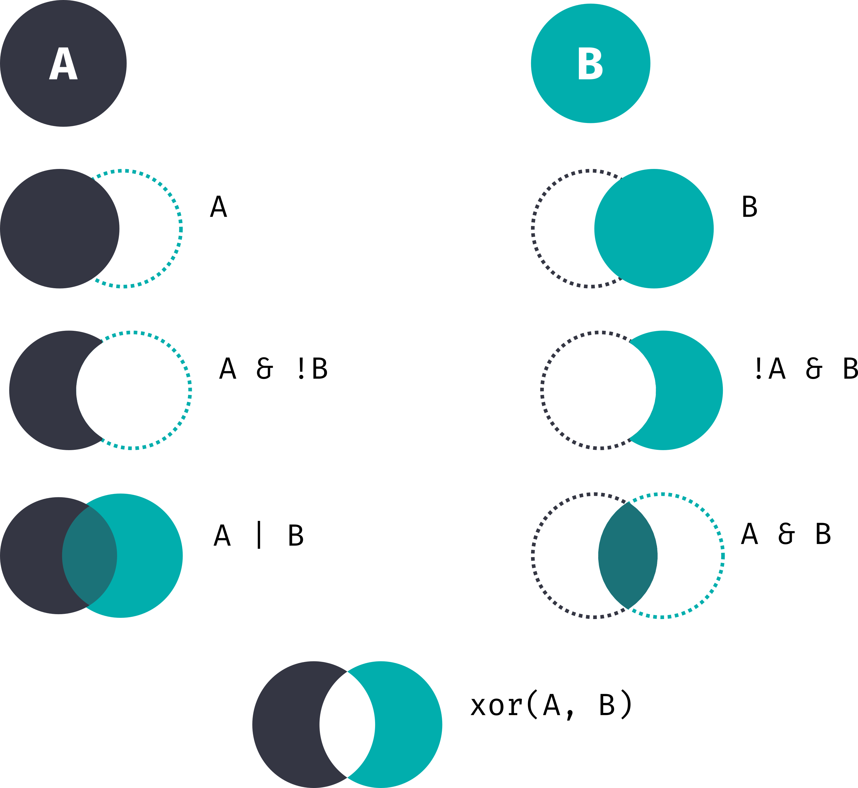{width="50%"}
702 |
703 | ### Exercise 6.1: Basic filtering
704 |
705 | Filter `mtcars` for rows where the miles per gallon are more than 25.
706 |
707 | ```{r filter-ex1, exercise=TRUE}
708 | # Write your code here
709 |
710 | ```
711 |
712 | ```{r filter-ex1-hint}
713 | # Substitute "condition" for a statement that evaluates to TRUE
714 | # In this case, miles per gallon is over 25.
715 | filter(df, condition)
716 | ```
717 |
718 | ```{r filter-ex1-solution}
719 | filter(mtcars, mpg > 25)
720 | ```
721 |
722 | ### Exercise 6.2: Multiple conditions
723 |
724 | From `starwars`, keep only masculine characters which are taller than 180.
725 |
726 | ```{r filter-ex2, exercise=TRUE}
727 | # Write your code here
728 |
729 | ```
730 |
731 | ```{r filter-ex2-hint-1}
732 | # Option 1:
733 | filter(df,
734 | condition1,
735 | condition2)
736 | ```
737 |
738 | ```{r filter-ex2-hint-2}
739 | # Option 2:
740 | filter(df,
741 | condition1 & condition2)
742 | ```
743 |
744 | ```{r filter-ex2-solution}
745 | # Option 1:
746 | filter(starwars,
747 | gender == 'masculine',
748 | height > 180)
749 | # Option 2:
750 | filter(starwars,
751 | gender == 'masculine' &
752 | height > 180)
753 | ```
754 |
755 | ### Exercise 6.3: Filter with %in%
756 |
757 | On `iris`, filter only the setosa and versicolor species.
758 |
759 | ```{r filter-ex3, exercise=TRUE}
760 | # Write your code here
761 |
762 | ```
763 |
764 | ```{r filter-ex3-hint}
765 | # There are multiple ways to solve this exercise:
766 | # Option 1: Using %in%
767 | # Option 2: Using == and |
768 | # Option 3: Using !=
769 | ```
770 |
771 | ```{r filter-ex3-solution}
772 | # Option 1:
773 | filter(iris, Species %in% c('setosa', 'versicolor'))
774 | # Option 2:
775 | filter(iris, Species == 'setosa' | Species == 'versicolor')
776 | # Option 3:
777 | filter(iris, Species != 'virginica')
778 | ```
779 |
780 | ### Exercise 6.4: More filters
781 |
782 | On `iris`, how many flowers of the virginica species have the petal width of at least 2.5 and petal length of 6 or less?
783 |
784 | ```{r filter-ex4, exercise=TRUE}
785 | # Write your code here
786 |
787 | ```
788 |
789 | ```{r filter-ex4-hint-1}
790 | # As a reminder, you can combine the conditions in two ways:
791 | # Option 1: As a comma-separated list
792 | # Option 2: By using &
793 | ```
794 |
795 | ```{r filter-ex4-hint-2}
796 | # Option 1:
797 | filter(df,
798 | condition1,
799 | condition2,
800 | cobndition3)
801 | ```
802 |
803 | ```{r filter-ex4-hint-3}
804 | # Option 2:
805 | filter(df,
806 | condition1 &
807 | condition2 &
808 | condition3)
809 | ```
810 |
811 |
812 | ```{r filter-ex4-solution}
813 | # This is true of only 2 flowers
814 | # Option 1:
815 | filter(iris,
816 | Species == 'virginica',
817 | Petal.Width > 2.4,
818 | Petal.Length <= 6.0)
819 | # Option 2:
820 | filter(iris,
821 | Species == 'virginica' &
822 | Petal.Width > 2.4 &
823 | Petal.Length <= 6.0)
824 | ```
825 |
826 | ### Exercise 6.5: Mixing filters
827 |
828 | Look at the `starwars` data.
829 | What is the name and species of the man who is between 100 and 180 cm tall, has black or blue eyes, weighs 80 kg or less, does not have black hair, and whose homeworld is neither "Sullust" nor "Bespin".
830 |
831 | ```{r filter-ex5, exercise=TRUE}
832 | # Write your code here
833 |
834 | ```
835 |
836 | ```{r filter-ex5-solution}
837 | filter(starwars,
838 | sex == "male",
839 | height %in% 100:180,
840 | eye_color %in% c("black", "blue"),
841 | mass <= 80,
842 | hair_color != "black",
843 | !(homeworld %in% c("Sullust", "Bespin")))
844 | ```
845 |
846 |
847 |
848 | **Hint:** You don't need to select the name and species.
849 | It's enough if you return the row with this individual.
850 |
851 |
852 |
853 | ### Exercise 6.6: More mixing filters
854 |
855 | Look at the `starwars` data.
856 | What is the homeworld of the grey or green-skinned, bald man, who has neither yellow nor gold eyes.
857 | They weigh under 90 kg and don't pilot the Millennium Falcon.
858 | They're either over 230 cm or under 200 cm tall.
859 |
860 | ```{r filter-ex6, exercise=TRUE}
861 | # Write your code here
862 |
863 | ```
864 |
865 | ```{r filter-ex6-solution}
866 | filter(starwars,
867 | skin_color %in% c("grey", "green"),
868 | hair_color == "none",
869 | sex =="male",
870 | !(eye_color %in% c("yellow", "gold")),
871 | mass < 90,
872 | starships != "Millennium Falcon",
873 | (height < 200 | height > 230))
874 | ```
875 |
876 |
877 |
878 | **Hint:** You don't need to select the homeworld.
879 | It's enough if you return the row with this individual.
880 |
881 |
882 |
883 | ### Exercise 6.7: Even more filters
884 |
885 | Look at the `starwars` data.
886 | Find the only woman with a combined height and mass under 200.
887 |
888 | ```{r filter-ex7, exercise=TRUE}
889 | # Write your code here
890 |
891 | ```
892 |
893 | ```{r filter-ex7-solution}
894 | filter(starwars,
895 | sex =="female",
896 | (height + mass) < 200)
897 | ```
898 |
899 | ------------------------------------------------------------------------
900 |
901 | ## 7. `mutate()`
902 |
903 | *3 exercises*
904 |
905 | In R, mutating means adding new columns or changing existing ones in a dataframe.
906 |
907 | ### Exercise 7.1: Create a new column
908 |
909 | In `mtcars`, make a new column called "power_to_weight" which is the ratio of horse power to weight.
910 |
911 | ```{r mutate-ex1, exercise=TRUE}
912 | # Write your code here
913 |
914 |
915 | ```
916 |
917 | ```{r mutate-ex1-solution}
918 | mutate(mtcars, power_to_weight = hp / wt)
919 | ```
920 |
921 |
922 |
923 | **Hint:** To calculate the ratio you need to divide one thing by the other.
924 | Check the column names in the code window or in the introduction to figure out which values you need.
925 |
926 |
927 |
928 | ### Exercise 7.2: Multiple mutations
929 |
930 | In `starwars`, calculate two values:
931 |
932 | - "height_m" each character's height in meters, and
933 | - "bmi" [the body mass index](https://en.wikipedia.org/wiki/Body_mass_index) of each character.
934 |
935 | **Don't use pipes for this exercise.**
936 |
937 | ```{r mutate-ex2, exercise=TRUE}
938 | # Write your code here
939 |
940 |
941 |
942 | ```
943 |
944 |
945 |
946 | **Hint 1:** BMI is measured in kg/m2.
947 | The "height" values in `starwars` are in centimeters.
948 |
949 | **Hint 2:** Since we're not using pipes at this stage yet, you have to proceed in 2 steps.
950 |
951 |
952 |
953 | ```{r mutate-ex2-solution}
954 | starwars <- mutate(starwars, height_m = height / 100)
955 | starwars <- mutate(starwars, bmi = mass / (height_m ^ 2))
956 | ```
957 |
958 | ### Exercise 7.3: More mutations
959 |
960 | Convert temperature from Fahrenheit to Celsius in `airquality` data and save it to a new column "temp_c".
961 |
962 | ```{r mutate-ex3, exercise=TRUE}
963 | # Write your code here
964 |
965 | ```
966 |
967 | ```{r mutate-ex3-solution}
968 | mutate(airquality, temp_c = (Temp - 32) * 5 / 9)
969 | ```
970 |
971 |
972 |
973 | **Hint:** The conversion formula is temperature °C = (temperature °F - 32) \* 5/9
974 |
975 |
976 |
977 | ------------------------------------------------------------------------
978 |
979 | ## 8. `na.omit()`
980 |
981 | *7 exercises*
982 |
983 | There are many ways in which you can deal with missing values, which is what R calls `NA`.
984 | You can remove them (which is what we're doing here), set them to a specific value, or other things.
985 | In class, we simply removed all NAs.
986 | As a rule of thumb, you want to look at what values are missing from your data to see if there is anything amiss with it.
987 |
988 | This function takes only one argument.
989 |
990 | ### Exercise 8.1: Remove rows with any NA
991 |
992 | Apply `na.omit()` to `airquality` and report the number of rows before and after.
993 |
994 | ```{r naomit-ex1, exercise=TRUE}
995 | # Write your code here
996 |
997 | ```
998 |
999 | ```{r naomit-ex1-solution}
1000 | nrow(airquality)
1001 | nrow(na.omit(airquality))
1002 | ```
1003 |
1004 |
1005 |
1006 | **Hint:** Use the function `nrow()` to get the number of rows of a dataframe.
1007 |
1008 |
1009 |
1010 | ### Exercise 8.2: Compare before and after
1011 |
1012 | Report the number of rows of the `starwars` data before and after removing missing values.
1013 |
1014 | ```{r naomit-ex2, exercise=TRUE}
1015 | # Write your code here
1016 |
1017 |
1018 | ```
1019 |
1020 | ```{r naomit-ex2-solution}
1021 | nrow(starwars)
1022 | nrow(na.omit(starwars))
1023 | ```
1024 |
1025 | ### Exercise 8.3: Difference
1026 |
1027 | Subtract the number of rows with missing values from the number of all rows in the `iris` data set.
1028 |
1029 | ```{r naomit-ex3, exercise=TRUE}
1030 | # Write your code here
1031 |
1032 | ```
1033 |
1034 | ```{r naomit-ex3-solution}
1035 | nrow(iris) - nrow(na.omit(iris))
1036 | ```
1037 |
1038 | ### Exercise 8.4: Chain with select
1039 |
1040 | In the `starwars` data, remove NAs then select the name, weight, and birth_year.
1041 | **Do this in two steps.**
1042 |
1043 | ```{r naomit-ex4, exercise=TRUE}
1044 | # Write your code here
1045 |
1046 | ```
1047 |
1048 | ```{r naomit-ex4-solution}
1049 | df1 <- na.omit(starwars)
1050 | select(df1, name, mass, birth_year)
1051 | ```
1052 |
1053 | ### Exercise 8.5: Show all missing values
1054 |
1055 | Using and `filter()`, show all the rows in the `airquality` data set with missing values in the Ozone column.
1056 |
1057 | ```{r naomit-ex5, exercise=TRUE}
1058 | # Write your code here
1059 |
1060 | ```
1061 |
1062 | ```{r naomit-ex5-solution}
1063 | filter(airquality, is.na(Ozone)==TRUE)
1064 | ```
1065 |
1066 |
1067 |
1068 | **Hint:** Use the function `is.na()` to get a logical vector of rows with an `NA` value.
1069 | This is similar to the functions `is.numeric()`, `is.logical()` etc. that we talked out in class.
1070 |
1071 |
1072 |
1073 | ### Exercise 8.6: Chain with select in one line
1074 |
1075 | In the `airquality` data, remove NAs then select the the wind and temperature.
1076 | **Do this in one steps and one line.**
1077 |
1078 | ```{r naomit-ex6, exercise=TRUE}
1079 | # Write your code here
1080 |
1081 | ```
1082 |
1083 | ```{r naomit-ex6-solution}
1084 | select(na.omit(airquality), Wind, Temp)
1085 | ```
1086 |
1087 |
1088 |
1089 | **Hint:** You can nest functions, which means calling one function from inside another function.
1090 |
1091 |
1092 |
1093 | ### Exercise 8.7: Chain multiple functions in one line
1094 |
1095 | In the `airquality` data, remove NAs then select the the wind and temperature, then count the number of rows.
1096 | **Do this in one steps and one line.**
1097 |
1098 | ```{r naomit-ex7, exercise=TRUE}
1099 | # Write your code here
1100 |
1101 | ```
1102 |
1103 | ```{r naomit-ex7-solution}
1104 | nrow(select(na.omit(airquality), Wind, Temp))
1105 | ```
1106 |
1107 |
1108 |
1109 | **Hint:** You can the `nrow()` functions to return the number of rows.
1110 |
1111 |
1112 |
1113 | ------------------------------------------------------------------------
1114 |
1115 | ## 9. `arrange()`
1116 |
1117 | *4 exercises*
1118 |
1119 | Sort the values in a dataframe.
1120 | By default, `arrange()` sorts the values from smallest to largest of alphabetically from A to Z.
1121 |
1122 | ### Exercise 9.1: Ascending order
1123 |
1124 | Arrange `mtcars` by weight and horsepower, both in ascending order.
1125 |
1126 | ```{r arrange-ex1, exercise=TRUE}
1127 | # Write your code here
1128 |
1129 | ```
1130 |
1131 | ```{r arrange-ex1-solution}
1132 | arrange(mtcars, wt, hp)
1133 | ```
1134 |
1135 | ### Exercise 9.2: Descending order of numbers
1136 |
1137 | Arrange `starwars` by height in descending.
1138 |
1139 | ```{r arrange-ex2, exercise=TRUE}
1140 | # Write your code here
1141 |
1142 | ```
1143 |
1144 | ```{r arrange-ex2-solution}
1145 | arrange(starwars, -height)
1146 | ```
1147 |
1148 |
1149 |
1150 | **Hint:** To sort numeric values from largest to smallest, you can use `-` in front of the column name.
1151 |
1152 |
1153 |
1154 | ### Exercise 9.3: Descending order of characters
1155 |
1156 | Arrange `starwars` by species in descending.
1157 |
1158 | ```{r arrange-ex3, exercise=TRUE}
1159 | # Write your code here
1160 |
1161 | ```
1162 |
1163 | ```{r arrange-ex3-solution}
1164 | arrange(starwars, desc(species))
1165 | ```
1166 |
1167 |
1168 |
1169 | **Hint:** To sort characters or strings in descending order, use the function `desc()`.
1170 |
1171 |
1172 |
1173 | ### Exercise 9.4: Multiple variables
1174 |
1175 | Arrange `iris` by species (descending), then by sepal width (ascending), then by sepal length (descending).
1176 |
1177 | ```{r arrange-ex4, exercise=TRUE}
1178 | # Write your code here
1179 |
1180 | ```
1181 |
1182 | ```{r arrange-ex4-solution}
1183 | arrange(iris, desc(Species), Sepal.Width, -Sepal.Length)
1184 | ```
1185 |
1186 | ------------------------------------------------------------------------
1187 |
1188 | ## 10. unique()
1189 |
1190 | *3 exercises*
1191 |
1192 | ### Exercise 10.1: Unique values in a column
1193 |
1194 | Show all unique species in the `iris` data set.
1195 |
1196 | ```{r unique-ex1, exercise=TRUE}
1197 | # Write your code here
1198 |
1199 | ```
1200 |
1201 | ```{r unique-ex1-solution}
1202 | unique(iris$Species)
1203 | ```
1204 |
1205 | ### Exercise 10.2: Count unique car gears
1206 |
1207 | Count how many unique gear values are in `mtcars`.
1208 | Do this in one line.
1209 |
1210 | ```{r unique-ex2, exercise=TRUE}
1211 | # Write your code here
1212 |
1213 | ```
1214 |
1215 | ```{r unique-ex2-solution}
1216 | length(unique(mtcars$gear))
1217 | ```
1218 |
1219 |
1220 |
1221 | **Hint:** To get the number of values, use the `length()` function, which takes only one element.
1222 |
1223 |
1224 |
1225 | ### Exercise 10.3: Multiple unique values
1226 |
1227 | Get the unique eye and skin colors in the `starwars` data set.
1228 |
1229 | ```{r unique-ex3, exercise=TRUE}
1230 | # Write your code here
1231 |
1232 | ```
1233 |
1234 | ```{r unique-ex3-solution}
1235 | unique(c(starwars$skin_color, starwars$eye_color))
1236 | ```
1237 |
1238 | ------------------------------------------------------------------------
1239 |
1240 | ## 11. Pipes
1241 |
1242 | *7 exercises*
1243 |
1244 | A powerful tool for clearly expressing a sequence of multiple operations.
1245 | Passes the output as the new input.
1246 | They can be read as "and then".
1247 |
1248 | The pipe translates `x |> f(y)` into `f(x, y)`.
1249 |
1250 | ### Exercise 11.1: Use \|\> with select
1251 |
1252 | Select name and species from `starwars` using native pipe.
1253 |
1254 | ```{r pipe-ex1, exercise=TRUE}
1255 | # Write your code here
1256 |
1257 | ```
1258 |
1259 | ```{r pipe-ex1-solution}
1260 | starwars |> select(name, species)
1261 | ```
1262 |
1263 | ### Exercise 11.2: Use \|\> with select
1264 |
1265 | Remove only the skin color from `starwars` using native pipe.
1266 |
1267 | ```{r pipe-ex2, exercise=TRUE}
1268 | # Write your code here
1269 |
1270 | ```
1271 |
1272 | ```{r pipe-ex2-solution}
1273 | starwars |> select(-skin_color)
1274 | ```
1275 |
1276 | ### Exercise 11.3: Combine filter and select
1277 |
1278 | Filter only the hermaphroditic characters from `starwars` and select their name, skin color and eye color.
1279 |
1280 | ```{r pipe-ex3, exercise=TRUE}
1281 | # Write your code here
1282 |
1283 | ```
1284 |
1285 | ```{r pipe-ex3-solution}
1286 | starwars |>
1287 | filter(sex == "hermaphroditic") |>
1288 | select(name, skin_color, eye_color)
1289 | ```
1290 |
1291 | ### Exercise 11.4: Pipeline with filter, select and mutate
1292 |
1293 | Filter only the female characters from `starwars` and select all the columns except for their hair color.
1294 | Then change their height to meters.
1295 |
1296 | ```{r pipe-ex4, exercise=TRUE}
1297 | # Write your code here
1298 |
1299 |
1300 | ```
1301 |
1302 | ```{r pipe-ex4-solution}
1303 | starwars |>
1304 | filter(sex == "female") |>
1305 | select(-hair_color) |>
1306 | mutate(height = height/100)
1307 | ```
1308 |
1309 | ### Exercise 11.5: Pipeline with filter, select, remove missing values, and mutate
1310 |
1311 | From the `airquality` data set, filter the data from June, drop the day of the month, remove missing values, and change the temperature from °Fahrenheit to °Celsius.
1312 |
1313 | ```{r pipe-ex5, exercise=TRUE}
1314 | # Write your code here
1315 |
1316 |
1317 |
1318 |
1319 | ```
1320 |
1321 | ```{r pipe-ex5-solution}
1322 | airquality |>
1323 | filter(Month == 6) |>
1324 | select(-Day) |>
1325 | na.omit() |>
1326 | mutate(Temp = (Temp - 32) * 5/9)
1327 | ```
1328 |
1329 |
1330 |
1331 | **Hint:** The conversion formula is temperature °C = (temperature °F - 32) \* 5/9
1332 |
1333 |
1334 |
1335 | ### Exercise 11.6: Pipeline with filter, select, remove missing values, mutate, and arrange
1336 |
1337 | From the `airquality` data set, filter the data from the first three weeks of August, keep only the columns "Ozone", "Solar.R", "Wind", and "Temp", remove missing values, change the temperature from °Fahrenheit to °Celsius, change the wind speed from miles per hour to kilometers per hour, make a new column "Month" with the name of the month in English, and sort the values by ozone (ascending) and solar radiation (descending).
1338 |
1339 | ```{r pipe-ex6, exercise=TRUE}
1340 | # Write your code here
1341 |
1342 |
1343 |
1344 |
1345 | ```
1346 |
1347 | ```{r pipe-ex6-solution}
1348 | airquality |>
1349 | filter(Month == 8,
1350 | Day <22) |>
1351 | select(Ozone, Solar.R, Wind, Temp) |>
1352 | na.omit() |>
1353 | mutate(Temp = (Temp - 32) * 5/9,
1354 | Wind = Wind * 1.609344,
1355 | Month = "August") |>
1356 | arrange(Ozone, -Solar.R)
1357 | ```
1358 |
1359 |
1360 |
1361 | **Hint:** One mile is around 1609.344 meters.
1362 |
1363 |
1364 |
1365 | ### Exercise 11.7: Pipeline with filter, select, remove missing values, and mutate
1366 |
1367 | From the `airquality` data set, filter the data from May, remove missing values, change the temperature from °Fahrenheit to °Celsius, round the resulting temperature to a whole number (no decimal points), and return only the unique temperatures.
1368 | How many unique temperatures were there?
1369 | **Use `mutate()` only once to do the calculation and rounding at the same time.**
1370 |
1371 | ```{r pipe-ex7, exercise=TRUE}
1372 | # Write your code here
1373 |
1374 |
1375 |
1376 |
1377 | ```
1378 |
1379 | ```{r pipe-ex7-solution}
1380 | airquality |>
1381 | filter(Month == 5) |>
1382 | na.omit() |>
1383 | mutate(Temp = round((Temp - 32) * 5/9, 0)) |>
1384 | select(Temp) |>
1385 | unique() |>
1386 | nrow()
1387 | ```
1388 |
1389 |
1390 |
1391 | **Hint 1:** Use the `round()` function to round a number.
1392 | It takes two arguments: values (a number or a numeric vector, like a column) and number of decimal places (default 0).
1393 |
1394 | **Hint 2:** Use `nrow()` to return the number of rows.
1395 |
1396 |
1397 |
1398 | ------------------------------------------------------------------------
1399 |
1400 | ## 12. Grouping and summarizing
1401 |
1402 | *8 + 2 exercises*
1403 |
1404 | When you group data with `group_by()`, you're putting it into categories based on one or more columns (like grouping people by age or cars by number of cylinders).
1405 | Calling the grouping function does not change anything *visibly* but it changes the data "under the hood".
1406 |
1407 | When you summarize with `summarize()`, you calculate some new values for each group—like the average, total, or count.
1408 | `summarize()` calculates a single value (per group) and drops columns which are not grouped by.
1409 | In contrast, `mutate()` changes an existing column or adds a new one, but does not drop columns.
1410 |
1411 | **Use pipes to solve these exercises.**
1412 |
1413 | Recall that in Week 3 of the course we talked about the measures of central tendency (mean, median, standard deviation etc.).
1414 | If you get stuck on these exercises, check the handout for week 3, pages 22-24.
1415 |
1416 | ### Exercise 12.1: Average
1417 |
1418 | Group `mtcars` by number of cylinders and compute average miles per gallon.
1419 |
1420 | ```{r group-ex1, exercise=TRUE}
1421 | # Write your code here
1422 |
1423 | ```
1424 |
1425 | ```{r group-ex1-solution}
1426 | mtcars |>
1427 | group_by(cyl) |>
1428 | summarise(avg_mpg = mean(mpg))
1429 | ```
1430 |
1431 |
1432 |
1433 | **Hint:** Use `mean()` to calculate the mean value.
1434 |
1435 |
1436 |
1437 | ### Exercise 12.2: Count characters by species
1438 |
1439 | Count number of characters per species in `starwars`.
1440 |
1441 | ```{r group-ex2, exercise=TRUE}
1442 | # Write your code here
1443 |
1444 | ```
1445 |
1446 | ```{r group-ex2-solution}
1447 | starwars |>
1448 | group_by(species) |>
1449 | summarise(count = n())
1450 | ```
1451 |
1452 |
1453 |
1454 | **Hint:** Use `n()` to count the number of cases.
1455 |
1456 |
1457 |
1458 | ### Exercise 12.3: Median sepal width by species
1459 |
1460 | Calculate the median sepal width per species in the `iris` data.
1461 |
1462 | ```{r group-ex3, exercise=TRUE}
1463 | # Write your code here
1464 |
1465 | ```
1466 |
1467 | ```{r group-ex3-solution}
1468 | iris |>
1469 | group_by(Species) |>
1470 | summarise(median_width = median(Sepal.Width))
1471 | ```
1472 |
1473 |
1474 |
1475 | **Hint:** Use `median()` to calculate the median.
1476 |
1477 |
1478 |
1479 | ### Exercise 12.4: Max and min horsepower by gear
1480 |
1481 | Calculate the maximal and minimal horsepower by number of forward gears in `mtcars`.
1482 |
1483 | ```{r group-ex4, exercise=TRUE}
1484 | # Write your code here
1485 |
1486 | ```
1487 |
1488 | ```{r group-ex4-solution}
1489 | mtcars |>
1490 | group_by(gear) |>
1491 | summarise(max_hp = max(hp),
1492 | min_hp = min(hp))
1493 | ```
1494 |
1495 | ### Exercise 12.5: Number of days by month
1496 |
1497 | Count number of observations per month in `airquality` data.
1498 |
1499 | ```{r group-ex5, exercise=TRUE}
1500 | # Write your code here
1501 |
1502 | ```
1503 |
1504 | ```{r group-ex5-solution}
1505 | airquality |>
1506 | group_by(Month) |>
1507 | summarise(count = n())
1508 | ```
1509 |
1510 | ### Exercise 12.6: Mean wind speed by month
1511 |
1512 | Calculate the average, maximal, and minimal wind speed per month in `airquality` data.
1513 |
1514 | ```{r group-ex6, exercise=TRUE}
1515 | # Write your code here
1516 |
1517 | ```
1518 |
1519 | ```{r group-ex6-solution}
1520 | airquality |>
1521 | group_by(Month) |>
1522 | na.omit() |>
1523 | summarise(mean_wind = mean(Wind),
1524 | max_wind = max(Wind),
1525 | min_wind = min(Wind))
1526 | ```
1527 |
1528 |
1529 |
1530 | **Hint:** Remove missing values before calculating the mean.
1531 |
1532 |
1533 |
1534 | ### Exercise 12.7: Central tendency of solar radiation by day
1535 |
1536 | Calculate the average, standard deviation solar radiation per day in `airquality` data.
1537 | Round the solar radiation to a full number.
1538 |
1539 | ```{r group-ex7, exercise=TRUE}
1540 | # Write your code here
1541 |
1542 | ```
1543 |
1544 | ```{r group-ex7-solution}
1545 | airquality |>
1546 | group_by(Day) |>
1547 | na.omit() |>
1548 | summarise(mean_sr = mean(Solar.R),
1549 | sd_sr = round(sd(Solar.R)))
1550 | ```
1551 |
1552 | ### Exercise 12.8: Collective mass and height
1553 |
1554 | Count the sum of the weights and heights for all `starwars` characters.
1555 |
1556 | ```{r group-ex8, exercise=TRUE}
1557 | # Write your code here
1558 |
1559 | ```
1560 |
1561 | ```{r group-ex8-solution}
1562 | starwars |>
1563 | summarize(
1564 | total_height = sum(height, na.rm = TRUE),
1565 | total_mass = sum(mass, na.rm = TRUE)
1566 | )
1567 | ```
1568 |
1569 |
1570 |
1571 | **Hint:** You can set the argument `na.rm` i.e. "remove NA" to `TRUE` within the summing function to remove all missing values, or you can use the NA removing function we used so far.
1572 |
1573 |
1574 |
1575 | ### Bonus Exercise 12.9: Tallest character per species
1576 |
1577 | Find the tallest character for each species in `starwars` data.
1578 | **Return not only the number, but the whole row.**
1579 |
1580 | ```{r group-ex9, exercise=TRUE, hint="Use group_by(species) then ."}
1581 | # Write your code here
1582 |
1583 | ```
1584 |
1585 | ```{r group-ex9-solution}
1586 | starwars |>
1587 | group_by(species) |>
1588 | slice_max(height)
1589 | ```
1590 |
1591 |
1592 |
1593 | **Hint:** Use `slice_max()` to return the *row* with the maximal value in a group.
1594 |
1595 |
1596 |
1597 | ### Bonus Exercise 12.10: Number of distinct homeworlds by species
1598 |
1599 | Count the distinct homeworlds per species in `starwars` data.
1600 |
1601 | ```{r group-ex10, exercise=TRUE}
1602 | # Write your code here
1603 |
1604 | ```
1605 |
1606 | ```{r group-ex10-solution}
1607 | starwars |>
1608 | group_by(species) |>
1609 | summarise(n_homeworlds = n_distinct(homeworld))
1610 | ```
1611 |
1612 |
1613 |
1614 | **Hint:** Use `n_distinct()` to count the number of distinct values.
1615 |
1616 |
1617 |
1618 | ------------------------------------------------------------------------
1619 |
1620 | ## 13. If else statements
1621 |
1622 | *8 exercises*
1623 |
1624 | In class, we used `ifelse()` and `case_when()` to recode values for conditions and also validate the answers to the Moses illusion questions.
1625 |
1626 | - Use `ifelse()` when you have one condition (or maybe two). It’s great for simple either/or decisions.
1627 | - Use `case_when()` when you have multiple conditions. It checks several conditions in order, and returns the first one that's true.
1628 |
1629 | **Remember to use pipes to solve these exercises.**
1630 |
1631 | {width="50%"}
1632 |
1633 | ### Exercise 13.1: Flag efficient cars
1634 |
1635 | Create a new column called "efficient" in which you flag `mtcars` cars with mpg \> 20 as efficient.
1636 |
1637 | ```{r ifelse-ex1, exercise=TRUE}
1638 | # Write your code here
1639 |
1640 | ```
1641 |
1642 | ```{r ifelse-ex1-solution}
1643 | mtcars |>
1644 | mutate(efficient = ifelse(mpg > 20, 'Yes', "No"))
1645 | ```
1646 |
1647 | ### Exercise 13.2: Label engine size
1648 |
1649 | Create a column "size" labeling engines as "Large" or "Small" based on displacement with a threshold of 200.
1650 |
1651 | ```{r ifelse-ex2, exercise=TRUE}
1652 | # Write your code here
1653 |
1654 | ```
1655 |
1656 | ```{r ifelse-ex2-solution}
1657 | mtcars |>
1658 | mutate(size = ifelse(disp > 200, 'Large', 'Small'))
1659 | ```
1660 |
1661 | ### Exercise 13.3: Case when for speed class
1662 |
1663 | Label the cars in `mtcars` with a speed class based on horse power: "High" for over 150 horse power, "Medium" for over 100 horse power, and "Low" otherwise.
1664 | Use `case_when()`, because you have 3 options.
1665 |
1666 | ```{r casewhen-ex3, exercise=TRUE}
1667 | # Write your code here
1668 |
1669 | ```
1670 |
1671 | ```{r casewhen-ex3-solution}
1672 | mtcars |>
1673 | mutate(speed_class = case_when(hp > 150 ~ 'High',
1674 | hp > 100 ~ 'Medium',
1675 | TRUE ~ 'Low'))
1676 | ```
1677 |
1678 |
1679 |
1680 | **Hint:** `TRUE` is the final "else" statement.
1681 |
1682 |
1683 |
1684 | ### Exercise 13.4: Categorize characters by height
1685 |
1686 | Categorize characters by height in `starwars`: "Very tall" for 200 cm or more, "Tall" for over 180 cm, "Medium" for 150 cm or more, and "Small" for under 150 cm.
1687 | Show only the name, height, and height class.
1688 |
1689 | ```{r casewhen-ex4, exercise=TRUE}
1690 | # Write your code here
1691 |
1692 | ```
1693 |
1694 | ```{r casewhen-ex4-solution}
1695 | starwars |>
1696 | mutate(height_class = case_when(height >= 200 ~ 'Very Tall',
1697 | height > 180 ~ 'Tall',
1698 | height >= 150 ~ 'Medium',
1699 | TRUE ~ 'Short')) |>
1700 | select(name, height, height_class)
1701 | ```
1702 |
1703 | ### Exercise 13.5: Flag missing birth year
1704 |
1705 | Flag `starwars` rows where "birth_year" is missing.
1706 | Then select only the name, birth year, and the newly created column.
1707 |
1708 | ```{r casewhen-ex5, exercise=TRUE}
1709 | # Write your code here
1710 |
1711 | ```
1712 |
1713 | ```{r casewhen-ex5-solution}
1714 | starwars |>
1715 | mutate(missing_birthyear = ifelse(is.na(birth_year), TRUE, FALSE)) |>
1716 | select(name, birth_year, missing_birthyear)
1717 | ```
1718 |
1719 |
1720 |
1721 | **Hint:** Use `is.na()` inside `ifelse()`.
1722 |
1723 |
1724 |
1725 | ### Exercise 13.6: Label temperature levels
1726 |
1727 | Label `airquality` days as "Hot", "Warm", or "Cool" based on temperature in °Celsius.
1728 |
1729 | ```{r casewhen-ex6, exercise=TRUE, hint="Use Temp thresholds in case_when()."}
1730 | # Write your code here
1731 |
1732 | ```
1733 |
1734 | ```{r casewhen-ex6-solution}
1735 | airquality |>
1736 | mutate(
1737 | Temp_C = (Temp - 32) * 5/9,
1738 | Temp_Label = case_when(
1739 | Temp_C >= 30 ~ "Hot",
1740 | Temp_C >= 20 ~ "Warm",
1741 | TRUE ~ "Cool"
1742 | )
1743 | )
1744 | ```
1745 |
1746 |
1747 |
1748 | **Hint:** Remember to calculate the correct temperature.
1749 |
1750 |
1751 |
1752 | ### Exercise 13.7: Case when for iris petal size
1753 |
1754 | Classify `iris` flowers by petal length using `case_when()`: "small", "medium", "large".
1755 | Base your classification on the quantiles.
1756 |
1757 | ```{r casewhen-ex7, exercise=TRUE}
1758 | # Write your code here
1759 |
1760 | ```
1761 |
1762 | ```{r casewhen-ex7-solution}
1763 | iris |>
1764 | mutate(
1765 | PetalSize = case_when(
1766 | Petal.Length < 1.6 ~ "small",
1767 | Petal.Length < 5.1 ~ "medium",
1768 | TRUE ~ "large"
1769 | )
1770 | )
1771 | ```
1772 |
1773 |
1774 |
1775 | **Hint:** One of the ways of previewing data allowed us to check the quantiles.
1776 | Go back to chapter 3 or the handout for Week 3 if you need a refresher.
1777 |
1778 |
1779 |
1780 | ### Exercise 13.8: Engine performance tier
1781 |
1782 | Add column to `mtcars`: "Economy" (horse power under 100 and more than 25 miles per gallon), "Balanced" (between 100 and 200 horse power and at least 15 miles per gallon), "Performance" (more than 200 horse power) tiers.
1783 | Any remaining cars should be classified as "Other".
1784 | Lastly, count how many cars are in each of these classes.
1785 |
1786 | ```{r casewhen-ex8, exercise=TRUE}
1787 | # Write your code here
1788 |
1789 | ```
1790 |
1791 | ```{r casewhen-ex8-solution}
1792 | mtcars |>
1793 | mutate(
1794 | Tier = case_when(
1795 | hp < 100 & mpg > 25 ~ "Economy",
1796 | hp >= 100 & hp <= 200 & mpg >= 15 ~ "Balanced",
1797 | hp > 200 ~ "Performance",
1798 | TRUE ~ "Other")
1799 | ) |>
1800 | group_by(Tier) |>
1801 | summarise(Count = n())
1802 | ```
1803 |
1804 |
1805 |
1806 | **Hint:** Remember how we combined conditions when filtering and in set theory.
1807 |
1808 |
1809 |
1810 | ------------------------------------------------------------------------
1811 |
1812 | ## 14. Assignment and data input
1813 |
1814 | In R, you can use three operators to assign values to a variable: `->`, `=`, and `->>`.
1815 |
1816 | | Operator | Example | Uses |
1817 | |----|----|----|
1818 | | `<-` and `->` | `x <- 5` | This is the traditional way of assigning values. You can read it as "Put 5 in x". |
1819 | | `=` | `x = 5` | This is similar to the operator above. It works fine in most cases and is usually used inside functions (like `nrow(x = starwars)`). You can read the example as "Set x equal to 5". |
1820 | | `->>` and `<<-` | `x <<- 5` | This is a special kind of `<-` operator: a "global assignment" operator. It assigns 5 to x in the **global environment** (outside the local scope), even if you're inside a function. In lay terms, it makes the variable jump out of its environment and become global. |
1821 |
1822 | In this course, we use the `->` operator for assigning global values (e.g. outside of functions) and the `=` operator for assigning values inside functions.
1823 |
1824 | ```{r, echo=FALSE, include=TRUE}
1825 | starwars_rows <- nrow(x = starwars)
1826 | ```
1827 |
1828 | ### Exercise 14.1: Assign a numeric vector
1829 |
1830 | Create a vector of your favorite number and assign it to `my_number`.
1831 |
1832 | ```{r assign-ex1, exercise=TRUE}
1833 | # Write your code here
1834 |
1835 |
1836 | ```
1837 |
1838 | ```{r assign-ex1-hint}
1839 | # Use <- to assign a vector of your favorite number.
1840 |
1841 | ```
1842 |
1843 | ### Exercise 14.2: Assign a character vector
1844 |
1845 | Assign a vector of 3 fruit names to `fruits`.
1846 |
1847 | ```{r assign-ex2, exercise=TRUE}
1848 | # Write your code here
1849 |
1850 |
1851 | ```
1852 |
1853 | ```{r assign-ex2-hint}
1854 | # Use <- and c() to store fruit names in a vector.
1855 |
1856 | ```
1857 |
1858 | ### Exercise 14.3: Create a logical vector
1859 |
1860 | Imagine you're playing the game "3 truths and a lie".
1861 | Assign a vector of 4 logical values, 3 of which are `TRUE` and one which is not, to the variable `game`.
1862 |
1863 | ```{r assign-ex3, exercise=TRUE}
1864 | # Write your code here
1865 |
1866 |
1867 | ```
1868 |
1869 | ```{r assign-ex3-hint}
1870 | # Use <- and c() to store logical values in a vector.
1871 |
1872 | ```
1873 |
1874 | ### Exercise 14.4: Create a mixed vector
1875 |
1876 | Create a variable called `mix` which contains 3 of your favorite numbers, 3 of your favorite fruits, and one logical vector.
1877 |
1878 | ```{r assign-ex4, exercise=TRUE}
1879 | # Write your code here
1880 |
1881 |
1882 | ```
1883 |
1884 | ```{r assign-ex4-hint}
1885 | # Use <- and c() to store the values in a vector.
1886 |
1887 | ```
1888 |
1889 | ------------------------------------------------------------------------
1890 |
1891 | ## 15. Bonus: Creating dataframes
1892 |
1893 | *6 exercises*
1894 |
1895 | While the toolkit course does not cover creating dataframes, we used joins to add the correct answers to the Moses illusion responses.
1896 | However, sometimes you might want to make data in R instead of importing it from elsewhere.
1897 |
1898 | **You can safely skip this chapter** but working through this examples will give you a better understanding of the structures underlying the tables we're working with in class.
1899 |
1900 | **Note:** The data in this section is either fictional (`children`) or taken from [Wikipedia](https://en.wikipedia.org/) and [WorldoMeter](https://www.worldometers.info/).
1901 | It may be inaccurate.
1902 |
1903 | ### Exercise 15.1: Create a small dataframe
1904 |
1905 | Create a dataframe with names of 3 children (Lila, Kai, and Ezra) and their ages (7, 2, 12), assign it to `children`.
1906 | Then print the dataframe.
1907 |
1908 | ```{r df-ex1, exercise=TRUE, warning=FALSE}
1909 | # Write your code here
1910 |
1911 | ```
1912 |
1913 | ```{r df-ex1-solution, warning=FALSE}
1914 | children <- data.frame(name = c("Lila", "Kai", "Ezra"), age = c(7, 2, 12))
1915 | children
1916 | ```
1917 |
1918 |
1919 |
1920 | **Hint:** You need two different kinds of assignment for this exercise.
1921 |
1922 |
1923 |
1924 | ### Exercise 15.2: Create a country list
1925 |
1926 | Re-create this table as a dataframe, call it `countries`, and print it.
1927 |
1928 | | Country | Capital | Continent |
1929 | |-----------|----------|---------------|
1930 | | Canada | Ottawa | North America |
1931 | | Japan | Tokyo | Asia |
1932 | | Brazil | Brasília | South America |
1933 | | Egypt | Cairo | Africa |
1934 | | Germany | Berlin | Europe |
1935 | | Australia | Canberra | Oceania |
1936 |
1937 | ```{r df-ex2, exercise=TRUE, warning=FALSE}
1938 | # Write your code here
1939 |
1940 | ```
1941 |
1942 | ```{r df-ex2-solution, warning=FALSE}
1943 | countries_data <- data.frame(
1944 | Country = c("Canada", "Japan", "Brazil", "Egypt", "Germany", "Australia"),
1945 | Capital = c("Ottawa", "Tokyo", "Brasília", "Cairo", "Berlin", "Canberra"),
1946 | Continent = c("North America", "Asia", "South America", "Africa", "Europe", "Oceania")
1947 | )
1948 | print(countries_data)
1949 | ```
1950 |
1951 | ### Exercise 15.3: Add another column
1952 |
1953 | Add the estimated population in millions and print the resulting dataframe.
1954 |
1955 | | Country | Capital | Continent | Population |
1956 | |-----------|----------|---------------|------------|
1957 | | Canada | Ottawa | North America | 39.566 |
1958 | | Japan | Tokyo | Asia | 123.199 |
1959 | | Brazil | Brasília | South America | 212.693 |
1960 | | Egypt | Cairo | Africa | 118.084 |
1961 | | Germany | Berlin | Europe | 84.145 |
1962 | | Australia | Canberra | Oceania | 26.934 |
1963 |
1964 | ```{r df-ex3, exercise=TRUE}
1965 | # Write your code here
1966 |
1967 | ```
1968 |
1969 | ```{r df-ex3-solution}
1970 | countries_data <- data.frame(countries_data, Population = c(39.566, 123.199, 212.693, 118.084, 84.145, 26.934))
1971 | print(countries_data)
1972 | ```
1973 |
1974 |
1975 |
1976 | **Hint:** You can reuse the dataframe you created in the previous exercise.
1977 |
1978 |
1979 |
1980 | ### Exercise 15.4: Combining data with `cbind()`
1981 |
1982 | Think of `cbind()` as adding more columns to your data.
1983 | Use it when you're adding new types of information about your existing entries (like currency and timezone).
1984 | It is used to bind any number of dataframes by column.
1985 | The resulting dataframe is wider.
1986 |
1987 | In this exercise, you will create two new variables called `Population` and `Official_Language` with the population and official languages of these countries.
1988 | Then, use `cbind()` to add first "Population" and then "Official_Language" to the dataframe.
1989 | The first part of the code is provided for you.
1990 | Save the resulting the dataframe by overwriting `countries_data` and preview the data.
1991 |
1992 | | Country | Capital | Continent | Population | Official_Language |
1993 | |-----------|----------|---------------|------------|--------------------|
1994 | | Canada | Ottawa | North America | 39.566 | English and French |
1995 | | Japan | Tokyo | Asia | 123.199 | Japanese |
1996 | | Brazil | Brasília | South America | 212.693 | Portuguese |
1997 | | Egypt | Cairo | Africa | 118.084 | Arabic |
1998 | | Germany | Berlin | Europe | 84.145 | German |
1999 | | Australia | Canberra | Oceania | 26.934 | English |
2000 |
2001 | ```{r cbind1, exercise=TRUE}
2002 | countries_data <- data.frame(
2003 | Country = c("Canada", "Japan", "Brazil", "Egypt", "Germany", "Australia"),
2004 | Capital = c("Ottawa", "Tokyo", "Brasília", "Cairo", "Berlin", "Canberra"),
2005 | Continent = c("North America", "Asia", "South America", "Africa", "Europe", "Oceania")
2006 | )
2007 |
2008 | Population = c(39.566, 123.199, 212.693, 118.084, 84.145, 26.934)
2009 | countries_data <- cbind(countries_data, Population)
2010 |
2011 | # Write your code here
2012 |
2013 | ```
2014 |
2015 | ```{r cbind1-solution}
2016 | countries_data <- data.frame(
2017 | Country = c("Canada", "Japan", "Brazil", "Egypt", "Germany", "Australia"),
2018 | Capital = c("Ottawa", "Tokyo", "Brasília", "Cairo", "Berlin", "Canberra"),
2019 | Continent = c("North America", "Asia", "South America", "Africa", "Europe", "Oceania")
2020 | )
2021 | Population = c(39.566, 123.199, 212.693, 118.084, 84.145, 26.934)
2022 | countries_data <- cbind(countries_data, Population)
2023 |
2024 | Official_Language = c("English and French", "Japanese", "Portuguese", "Arabic", "German", "English")
2025 |
2026 | countries_data <- cbind(countries_data, Official_Language)
2027 | print(countries_data)
2028 | ```
2029 |
2030 | ### Exercise 15.5: Combining rows with `rbind()`
2031 |
2032 | Think of `rbind()` (row bind) as adding more rows to your data (in our case, more countries).
2033 | It is used to bind any number of dataframes by row.
2034 | The resulting dataframe is longer.
2035 | Use `rbind()` to add two new countries to the list: Poland and French Polynesia.
2036 | The first part of the code is provided for you.
2037 | Save the resulting the dataframe by overwriting `countries_data` and preview the data.
2038 |
2039 | | Country | Capital | Continent | Population | Official_Language |
2040 | |------------------|---------|-----------|------------|---------------------|
2041 | | Poland | Warsaw | Europe | 37.637 | Polish |
2042 | | French Polynesia | Papeete | Oceania | 0.282 | French and Tahitian |
2043 |
2044 | ```{r rbind1, exercise=TRUE}
2045 | countries_data <- data.frame(
2046 | Country = c("Canada", "Japan", "Brazil", "Egypt", "Germany", "Australia"),
2047 | Capital = c("Ottawa", "Tokyo", "Brasília", "Cairo", "Berlin", "Canberra"),
2048 | Continent = c("North America", "Asia", "South America", "Africa", "Europe", "Oceania"),
2049 | Population = c(39.566, 123.199, 212.693, 118.084, 84.145, 26.934),
2050 | Official_Language = c("English and French", "Japanese", "Portuguese", "Arabic", "German", "English")
2051 | )
2052 |
2053 | poland <- data.frame(
2054 | Country = "Poland",
2055 | Capital = "Warsaw",
2056 | Continent = "Europe",
2057 | Population = 37.637,
2058 | Official_Language = "Polish"
2059 | )
2060 |
2061 | countries_data <- rbind(countries_data, poland)
2062 |
2063 | ###################################
2064 | # Start your code here
2065 | ###################################
2066 |
2067 | ```
2068 |
2069 | ```{r rbind1-solution}
2070 | countries_data <- data.frame(
2071 | Country = c("Canada", "Japan", "Brazil", "Egypt", "Germany", "Australia"),
2072 | Capital = c("Ottawa", "Tokyo", "Brasília", "Cairo", "Berlin", "Canberra"),
2073 | Continent = c("North America", "Asia", "South America", "Africa", "Europe", "Oceania"),
2074 | Population = c(39.566, 123.199, 212.693, 118.084, 84.145, 26.934),
2075 | Official_Language = c("English and French", "Japanese", "Portuguese", "Arabic", "German", "English")
2076 | )
2077 |
2078 | poland <- data.frame(
2079 | Country = "Poland",
2080 | Capital = "Warsaw",
2081 | Continent = "Europe",
2082 | Population = 37.637,
2083 | Official_Language = "Polish"
2084 | )
2085 |
2086 | countries_data <- rbind(countries_data, poland)
2087 |
2088 | french_polynesia <- data.frame(
2089 | Country = "French Polynesia",
2090 | Capital = "Papeete",
2091 | Continent = "Oceania",
2092 | Population = 0.282,
2093 | Official_Language = "French and Tahitian"
2094 | )
2095 |
2096 | countries_data <- rbind(countries_data, french_polynesia)
2097 | print(countries_data)
2098 | ```
2099 |
2100 | ### Exercise 15.6: Combining rows and columns
2101 |
2102 | For this exercise, you will use both `rbind()` and `cbind()`.
2103 | In class, we will use joins for combining dataframes, but if you know you have the same rows and columns everywhere, you can also use `rbind()` and `cbind()` for adding data to your dataframe.
2104 | In this exercise:
2105 |
2106 | 1. Add four new countries to your dataframe (in this order): India, Argentina, Kenya, and Mexico.
2107 | 2. Add three new columns, one by one, to your dataframe: currency, timezone, and calling code.
2108 | 3. Sort the resulting dataframe by the continent, population (descending), and timezone. Save it to `countries_final`.
2109 | 4. Print the `countries_final` data.
2110 |
2111 | The code for the new rows and columns is provided for you.
2112 | Mexico does not have an official language *de jure*, so that data is missing.
2113 |
2114 | ```{r crbind1, exercise=TRUE}
2115 | # Original dataframe with Poland and French Polynesia.
2116 | countries_data <- data.frame(
2117 | Country = c("Canada", "Japan", "Brazil", "Egypt", "Germany", "Australia", "Poland", "French Polynesia"),
2118 | Capital = c("Ottawa", "Tokyo", "Brasília", "Cairo", "Berlin", "Canberra", "Warsaw", "Papeete"),
2119 | Continent = c("North America", "Asia", "South America", "Africa", "Europe", "Oceania", "Europe", "Oceania"),
2120 | Population = c(39.566, 123.199, 212.693, 118.084, 84.145, 26.934, 37.637, 0.282),
2121 | Official_Language = c("English and French", "Japanese", "Portuguese", "Arabic", "German", "English", "Polish", "French and Tahitian")
2122 | )
2123 |
2124 | # New rows
2125 | india <- data.frame(
2126 | Country = "India",
2127 | Capital = "New Delhi",
2128 | Continent = "Asia",
2129 | Population = 1461.987,
2130 | Official_Language = "Hindi, English"
2131 | )
2132 |
2133 | peru <- data.frame(
2134 | Country = "Peru",
2135 | Capital = "Lima",
2136 | Continent = "South America",
2137 | Population = 34.524,
2138 | Official_Language = "Spanish, Quechua, Aymara"
2139 | )
2140 |
2141 | kenya <- data.frame(
2142 | Country = "Kenya",
2143 | Capital = "Nairobi",
2144 | Continent = "Africa",
2145 | Population = 57.372,
2146 | Official_Language = "English, Swahili"
2147 | )
2148 |
2149 | mexico <- data.frame(
2150 | Country = c("Mexico"),
2151 | Capital = c("Mexico City"),
2152 | Continent = c("North America"),
2153 | Population = c(128.932),
2154 | Official_Language = NA)
2155 |
2156 | # New columns
2157 | currency <- c(
2158 | "CAD", "JPY", "BRL", "EGP", "EUR", "AUD", "PLN", "XPF", "INR", "PEN", "KES", "MXN")
2159 |
2160 | timezone <- c(
2161 | "UTC-05:00", # Canada (Ottawa)
2162 | "UTC+09:00", # Japan (Tokyo)
2163 | "UTC-03:00", # Brazil (Brasília)
2164 | "UTC+02:00", # Egypt (Cairo)
2165 | "UTC+01:00", # Germany (Berlin)
2166 | "UTC+10:00", # Australia (Canberra)
2167 | "UTC+01:00", # Poland (Warsaw)
2168 | "UTC-10:00", # French Polynesia (Papeete)
2169 | "UTC+05:30", # India (New Delhi)
2170 | "UTC−05:00", # Peru (Lima)
2171 | "UTC+03:00", # Kenya (Nairobi)
2172 | "UTC-06:00" # Mexico (Mexico City)
2173 | )
2174 |
2175 | calling_code <- c(
2176 | "+1", "+81", "+55", "+20", "+49", "+61", "+48", "+689", "+91", "+51", "+254", "+52")
2177 |
2178 | ###################################
2179 | # Start your code here
2180 | ###################################
2181 |
2182 | ```
2183 |
2184 | ```{r crbind1-solution, exercise=TRUE}
2185 | # Original dataframe with Poland and French Polynesia.
2186 | countries_data <- data.frame(
2187 | Country = c("Canada", "Japan", "Brazil", "Egypt", "Germany", "Australia", "Poland", "French Polynesia"),
2188 | Capital = c("Ottawa", "Tokyo", "Brasília", "Cairo", "Berlin", "Canberra", "Warsaw", "Papeete"),
2189 | Continent = c("North America", "Asia", "South America", "Africa", "Europe", "Oceania", "Europe", "Oceania"),
2190 | Population = c(39.566, 123.199, 212.693, 118.084, 84.145, 26.934, 37.637, 0.282),
2191 | Official_Language = c("English and French", "Japanese", "Portuguese", "Arabic", "German", "English", "Polish", "French and Tahitian")
2192 | )
2193 |
2194 | # New rows
2195 | india <- data.frame(
2196 | Country = "India",
2197 | Capital = "New Delhi",
2198 | Continent = "Asia",
2199 | Population = 1461.987,
2200 | Official_Language = "Hindi, English"
2201 | )
2202 |
2203 | peru <- data.frame(
2204 | Country = "Peru",
2205 | Capital = "Lima",
2206 | Continent = "South America",
2207 | Population = 34.524,
2208 | Official_Language = "Spanish, Quechua, Aymara"
2209 | )
2210 |
2211 | kenya <- data.frame(
2212 | Country = "Kenya",
2213 | Capital = "Nairobi",
2214 | Continent = "Africa",
2215 | Population = 57.372,
2216 | Official_Language = "English, Swahili"
2217 | )
2218 |
2219 | mexico <- data.frame(
2220 | Country = c("Mexico"),
2221 | Capital = c("Mexico City"),
2222 | Continent = c("North America"),
2223 | Population = c(128.932),
2224 | Official_Language = NA)
2225 |
2226 | # New columns
2227 | currency <- c(
2228 | "CAD", "JPY", "BRL", "EGP", "EUR", "AUD", "PLN", "XPF", "INR", "PEN", "KES", "MXN")
2229 |
2230 | timezone <- c(
2231 | "UTC-05:00", # Canada (Ottawa)
2232 | "UTC+09:00", # Japan (Tokyo)
2233 | "UTC-03:00", # Brazil (Brasília)
2234 | "UTC+02:00", # Egypt (Cairo)
2235 | "UTC+01:00", # Germany (Berlin)
2236 | "UTC+10:00", # Australia (Canberra)
2237 | "UTC+01:00", # Poland (Warsaw)
2238 | "UTC-10:00", # French Polynesia (Papeete)
2239 | "UTC+05:30", # India (New Delhi)
2240 | "UTC−05:00", # Peru (Lima)
2241 | "UTC+03:00", # Kenya (Nairobi)
2242 | "UTC-06:00" # Mexico (Mexico City)
2243 | )
2244 |
2245 | calling_code <- c(
2246 | "+1", "+81", "+55", "+20", "+49", "+61", "+48", "+689", "+91", "+51", "+254", "+52")
2247 |
2248 | # Adding the four new countries.
2249 | countries_data <- rbind(countries_data,
2250 | india,
2251 | peru,
2252 | kenya,
2253 | mexico)
2254 |
2255 | # Adding the four new rows.
2256 | countries_data <- cbind(countries_data,
2257 | Currency = currency,
2258 | Timezone = timezone,
2259 | Calling_code = calling_code)
2260 |
2261 |
2262 | countries_final <- arrange(countries_data,
2263 | Continent,
2264 | -Population,
2265 | Timezone)
2266 | countries_final
2267 | ```
2268 |
2269 | This is what you should expect:
2270 |
2271 | | Country | Capital | Continent | Population | Official_Language | Currency | Timezone | Calling_code |
2272 | |---:|---:|---:|:---|---:|---:|---:|---:|
2273 | | Egypt | Cairo | Africa | 118.084 | Arabic | EGP | UTC+02:00 | +20 |
2274 | | Kenya | Nairobi | Africa | 57.372 | English, Swahili | KES | UTC+03:00 | +254 |
2275 | | India | New Delhi | Asia | 1461.987 | Hindi, English | INR | UTC+05:30 | +91 |
2276 | | Japan | Tokyo | Asia | 123.199 | Japanese | JPY | UTC+09:00 | +81 |
2277 | | Germany | Berlin | Europe | 84.145 | German | EUR | UTC+01:00 | +49 |
2278 | | Poland | Warsaw | Europe | 37.637 | Polish | PLN | UTC+01:00 | +48 |
2279 | | Mexico | Mexico City | North America | 128.932 | | MXN | UTC-06:00 | +52 |
2280 | | Canada | Ottawa | North America | 39.566 | English and French | CAD | UTC-05:00 | +1 |
2281 | | Australia | Canberra | Oceania | 26.934 | English | AUD | UTC+10:00 | +61 |
2282 | | French Polynesia | Papeete | Oceania | 0.282 | French and Tahitian | XPF | UTC-10:00 | +689 |
2283 | | Brazil | Brasília | South America | 212.693 | Portuguese | BRL | UTC-03:00 | +55 |
2284 | | Peru | Lima | South America | 34.524 | Spanish, Quechua, Aymara | PEN | UTC−05:00 | +51 |
2285 |
2286 | ------------------------------------------------------------------------
2287 |
2288 | ## 16. Joining data
2289 |
2290 | *10 exercises*
2291 |
2292 | Sometimes, you have two dataframes, and you want to combine them based on something they have in common (e.g. matching people by name, countries by continent, or books by title and author).
2293 | `merge()` is a built-in R function.
2294 | It looks for a common column (like "Country") in two dataframes and joins the rows that match.
2295 | The `dplyr` package gives you more precise control with functions like:
2296 |
2297 | - `left_join()`
2298 | - `right_join()`
2299 | - `inner_join()`
2300 | - `full_join()`
2301 | - `anti_join()`
2302 |
2303 | They all do the same basic thing as `merge()`: combine two dataframes using a shared column.
2304 | But they let you choose what to keep if there's not a perfect match.
2305 |
2306 | {width="50%"}
2307 |
2308 | ### Exercise 16.1: Full join two small dataframes
2309 |
2310 | For this exercise, do the following tasks:
2311 |
2312 | 1. Create a dataframe with names of 10 children **in this order** (Lila, Kai, Ezra, Maya, Ethan, Zoe, Leo, Isla, Raja, Zara) and their ages (7, 2, 12, 4, 3, 2, 10, 13, 6, 7), assign it to `children`.
2313 | 2. Create a second dataframe with the names of the children **in this order** (Zoe, Kai, Lila, Ethan, Leo, Ezra, Isla, Zara, Maya, Raja) and their favorite animals (Clownfish, Panda, Elephant, Penguin, Koala, Tiger, Giraffe, Rabbit, Cat, Fox), assign it to `animals`.
2314 | 3. Use `full_join()` to join these two dataframes by the common identifier column.
2315 |
2316 | ```{r joinpractice-ex1, exercise=TRUE}
2317 | # Write your code here
2318 |
2319 | ```
2320 |
2321 | ```{r joinpractice-ex1-solution}
2322 | children <- data.frame(
2323 | Name = c("Lila", "Kai", "Ezra", "Maya", "Ethan", "Zoe", "Leo", "Isla", "Raja", "Zara"),
2324 | Age = c(7, 2, 12, 4, 3, 2, 10, 13, 6, 7))
2325 |
2326 | animals <- data.frame(
2327 | Name = c("Zoe", "Kai", "Lila", "Ethan", "Leo", "Ezra", "Isla", "Zara", "Maya", "Raja"),
2328 | Animal = c("Clownfish", "Panda", "Elephant", "Penguin", "Koala", "Tiger", "Giraffe", "Rabbit", "Cat", "Fox"))
2329 |
2330 | full_join(children, animals, by="Name")
2331 | ```
2332 |
2333 |
2334 |
2335 | **Hint:** The `full_join()` function takes as argument two dataframes and the common identifier arguments by which to match the rows `by=`.
2336 |
2337 |
2338 |
2339 | ### Exercise 16.2: Inner join two small dataframes
2340 |
2341 | Again, make the same exact dataframes as in the previous exercise, but this time, use `inner_join()`.
2342 | Does the resulting dataframe differ from the previous one?
2343 |
2344 | ```{r joinpractice-ex2, exercise=TRUE}
2345 | # Write your code here
2346 |
2347 | ```
2348 |
2349 | ```{r joinpractice-ex2-solution}
2350 | children <- data.frame(
2351 | Name = c("Lila", "Kai", "Ezra", "Maya", "Ethan", "Zoe", "Leo", "Isla", "Raja", "Zara"),
2352 | Age = c(7, 2, 12, 4, 3, 2, 10, 13, 6, 7))
2353 |
2354 | animals <- data.frame(
2355 | Name = c("Zoe", "Kai", "Lila", "Ethan", "Leo", "Ezra", "Isla", "Zara", "Maya", "Raja"),
2356 | Animal = c("Clownfish", "Panda", "Elephant", "Penguin", "Koala", "Tiger", "Giraffe", "Rabbit", "Cat", "Fox"))
2357 |
2358 | inner_join(children, animals, by="Name")
2359 |
2360 | ```
2361 |
2362 |
2363 |
2364 | **Hint:** The `inner_join()` function takes as argument two dataframes and the common identifier arguments by which to match the rows `by=`, just like `full_join()`.
2365 |
2366 |
2367 |
2368 | ### Exercise 16.3: Inner join on two differently sized dataframes
2369 |
2370 | In the previous two exercises, using both `inner_join()` and `full_join()` resulted in the same dataframe.
2371 | This time, complete the following steps:
2372 |
2373 | 1. Create a dataframe with names of 10 children **in this order** (Lila, Kai, Ezra, Maya, Ethan, Zoe, Leo, Isla, Raja, Zara) and their ages (7, 2, 12, 4, 3, 2, 10, 13, 6, 7), assign it to `children`.
2374 | 2. Create a second dataframe with the names of 15 children **in this order** (Zoe, Kai, Lila, Ethan, Leo, Ezra, Isla, Zara, Maya, Raja, Catherine, Takeshi, Sven, Anouk, Amara) and their favorite animals (Clownfish, Panda, Elephant, Penguin, Koala, Tiger, Giraffe, Rabbit, Cat, Fox, Dog, Otter, Parrot, Owl, Llama), assign it to `animals`.
2375 | 3. Use `inner_join()` to join these two dataframes by the common identifier column.
2376 |
2377 | How does the resulting data differ from the previous exercises?
2378 |
2379 | ```{r joinpractice-ex3, exercise=TRUE}
2380 | # Write your code here
2381 |
2382 | ```
2383 |
2384 | ```{r joinpractice-ex3-solution}
2385 | children <- data.frame(
2386 | Name = c("Lila", "Kai", "Ezra", "Maya", "Ethan", "Zoe", "Leo", "Isla", "Raja", "Zara"),
2387 | Age = c(7, 2, 12, 4, 3, 2, 10, 13, 6, 7))
2388 |
2389 | animals <- data.frame(
2390 | Name = c("Zoe", "Kai", "Lila", "Ethan", "Leo", "Ezra", "Isla", "Zara", "Maya", "Raja", "Catherine", "Takeshi", "Sven", "Anouk", "Amara"),
2391 | Animal = c("Clownfish", "Panda", "Elephant", "Penguin", "Koala", "Tiger", "Giraffe", "Rabbit", "Cat", "Fox", "Dog", "Otter", "Parrot", "Owl", "Llama"))
2392 |
2393 | inner_join(children, animals, by = "Name")
2394 | ```
2395 |
2396 |
2397 |
2398 | **Hint:** You can reuse the code from the previous exercise.
2399 |
2400 |
2401 |
2402 | ### Exercise 16.4: Full join two unequal dataframes
2403 |
2404 | In the last 3 exercises, the dataframes ended up being the same.
2405 | `inner_join()` simply kept the existing children and did not add the newest 5.
2406 | This time, make the same exact dataframes as in the previous exercise (16.3), but this time, use `full_join()`.
2407 | Does the resulting dataframe differ from the previous ones?
2408 |
2409 | ```{r joinpractice-ex4, exercise=TRUE}
2410 | # Write your code here
2411 |
2412 | ```
2413 |
2414 | ```{r joinpractice-ex4-solution}
2415 | children <- data.frame(
2416 | Name = c("Lila", "Kai", "Ezra", "Maya", "Ethan", "Zoe", "Leo", "Isla", "Raja", "Zara"),
2417 | Age = c(7, 2, 12, 4, 3, 2, 10, 13, 6, 7))
2418 |
2419 | animals <- data.frame(
2420 | Name = c("Zoe", "Kai", "Lila", "Ethan", "Leo", "Ezra", "Isla", "Zara", "Maya", "Raja", "Catherine", "Takeshi", "Sven", "Anouk", "Amara"),
2421 | Animal = c("Clownfish", "Panda", "Elephant", "Penguin", "Koala", "Tiger", "Giraffe", "Rabbit", "Cat", "Fox", "Dog", "Otter", "Parrot", "Owl", "Llama"))
2422 |
2423 | full_join(children, animals, by = "Name")
2424 | ```
2425 |
2426 | ### Exercise 16.5: Right join
2427 |
2428 | Make the same exact dataframes as in the previous exercises (this code is provided for you), but this time, use `right_join()`.
2429 | Which other result does this one match: `inner_join()` or `full_join()`?
2430 |
2431 | ```{r joinpractice-ex5, exercise=TRUE}
2432 | children <- data.frame(
2433 | Name = c("Lila", "Kai", "Ezra", "Maya", "Ethan", "Zoe", "Leo", "Isla", "Raja", "Zara"),
2434 | Age = c(7, 2, 12, 4, 3, 2, 10, 13, 6, 7))
2435 |
2436 | animals <- data.frame(
2437 | Name = c("Zoe", "Kai", "Lila", "Ethan", "Leo", "Ezra", "Isla", "Zara", "Maya", "Raja", "Catherine", "Takeshi", "Sven", "Anouk", "Amara"),
2438 | Animal = c("Clownfish", "Panda", "Elephant", "Penguin", "Koala", "Tiger", "Giraffe", "Rabbit", "Cat", "Fox", "Dog", "Otter", "Parrot", "Owl", "Llama"))
2439 |
2440 | ###################################
2441 | # Start your code here
2442 | ###################################
2443 |
2444 |
2445 | ```
2446 |
2447 | ```{r joinpractice-ex5-solution}
2448 | children <- data.frame(
2449 | Name = c("Lila", "Kai", "Ezra", "Maya", "Ethan", "Zoe", "Leo", "Isla", "Raja", "Zara"),
2450 | Age = c(7, 2, 12, 4, 3, 2, 10, 13, 6, 7))
2451 |
2452 | animals <- data.frame(
2453 | Name = c("Zoe", "Kai", "Lila", "Ethan", "Leo", "Ezra", "Isla", "Zara", "Maya", "Raja", "Catherine", "Takeshi", "Sven", "Anouk", "Amara"),
2454 | Animal = c("Clownfish", "Panda", "Elephant", "Penguin", "Koala", "Tiger", "Giraffe", "Rabbit", "Cat", "Fox", "Dog", "Otter", "Parrot", "Owl", "Llama"))
2455 |
2456 | right_join(children, animals, by = "Name")
2457 | ```
2458 |
2459 | ### Exercise 16.6: Left join
2460 |
2461 | Make the same exact dataframes as in the previous exercises (this code is provided for you), but this time, use `left_join()`.
2462 | Which other result does this one match: `inner_join()` or `full_join()`?
2463 |
2464 | ```{r joinpractice-ex6, exercise=TRUE}
2465 | children <- data.frame(
2466 | Name = c("Lila", "Kai", "Ezra", "Maya", "Ethan", "Zoe", "Leo", "Isla", "Raja", "Zara"),
2467 | Age = c(7, 2, 12, 4, 3, 2, 10, 13, 6, 7))
2468 |
2469 | animals <- data.frame(
2470 | Name = c("Zoe", "Kai", "Lila", "Ethan", "Leo", "Ezra", "Isla", "Zara", "Maya", "Raja", "Catherine", "Takeshi", "Sven", "Anouk", "Amara"),
2471 | Animal = c("Clownfish", "Panda", "Elephant", "Penguin", "Koala", "Tiger", "Giraffe", "Rabbit", "Cat", "Fox", "Dog", "Otter", "Parrot", "Owl", "Llama"))
2472 |
2473 | ###################################
2474 | # Start your code here
2475 | ###################################
2476 |
2477 | ```
2478 |
2479 | ```{r joinpractice-ex6-solution}
2480 | children <- data.frame(
2481 | Name = c("Lila", "Kai", "Ezra", "Maya", "Ethan", "Zoe", "Leo", "Isla", "Raja", "Zara"),
2482 | Age = c(7, 2, 12, 4, 3, 2, 10, 13, 6, 7))
2483 |
2484 | animals <- data.frame(
2485 | Name = c("Zoe", "Kai", "Lila", "Ethan", "Leo", "Ezra", "Isla", "Zara", "Maya", "Raja", "Catherine", "Takeshi", "Sven", "Anouk", "Amara"),
2486 | Animal = c("Clownfish", "Panda", "Elephant", "Penguin", "Koala", "Tiger", "Giraffe", "Rabbit", "Cat", "Fox", "Dog", "Otter", "Parrot", "Owl", "Llama"))
2487 |
2488 | left_join(children, animals, by = "Name")
2489 | ```
2490 |
2491 | ### Exercise 16.7: Base R merge
2492 |
2493 | Merge two dataframes in base R using `merge()`.
2494 | Which of the joins does this result resemble?
2495 |
2496 | ```{r joinpractice-ex7, exercise=TRUE}
2497 | children <- data.frame(
2498 | Name = c("Lila", "Kai", "Ezra", "Maya", "Ethan", "Zoe", "Leo", "Isla", "Raja", "Zara"),
2499 | Age = c(7, 2, 12, 4, 3, 2, 10, 13, 6, 7))
2500 |
2501 | animals <- data.frame(
2502 | Name = c("Zoe", "Kai", "Lila", "Ethan", "Leo", "Ezra", "Isla", "Zara", "Maya", "Raja", "Catherine", "Takeshi", "Sven", "Anouk", "Amara"),
2503 | Animal = c("Clownfish", "Panda", "Elephant", "Penguin", "Koala", "Tiger", "Giraffe", "Rabbit", "Cat", "Fox", "Dog", "Otter", "Parrot", "Owl", "Llama"))
2504 |
2505 | ###################################
2506 | # Start your code here
2507 | ###################################
2508 |
2509 | ```
2510 |
2511 | ```{r joinpractice-ex7-solution}
2512 | children <- data.frame(
2513 | Name = c("Lila", "Kai", "Ezra", "Maya", "Ethan", "Zoe", "Leo", "Isla", "Raja", "Zara"),
2514 | Age = c(7, 2, 12, 4, 3, 2, 10, 13, 6, 7))
2515 |
2516 | animals <- data.frame(
2517 | Name = c("Zoe", "Kai", "Lila", "Ethan", "Leo", "Ezra", "Isla", "Zara", "Maya", "Raja", "Catherine", "Takeshi", "Sven", "Anouk", "Amara"),
2518 | Animal = c("Clownfish", "Panda", "Elephant", "Penguin", "Koala", "Tiger", "Giraffe", "Rabbit", "Cat", "Fox", "Dog", "Otter", "Parrot", "Owl", "Llama"))
2519 |
2520 | merge(children, animals, by = "Name")
2521 | ```
2522 |
2523 | ### Exercise 16.8: Add missing ages and schools
2524 |
2525 | When using `full_join()` on the `children` and `animals` dataframes, there were ages missing from a few kids.
2526 | In this exercise you will:
2527 |
2528 | 1. Create a dataframe for children and their favorite animals (this code is provided for you).
2529 | 2. Use `full_join()` to create a combined dataframe of `children` and `animals`.
2530 | 3. Using `case_when()`, add the ages for Catherine (5), Takeshi and Sven (both 8), Anouk (3), and Amara (11).
2531 | 4. Then, create a new column called `School` for the school they go to:
2532 | - 1-5: Preschool
2533 | - 6-9: Primary school
2534 | - 10-15: Middle school
2535 | - 16+: High school
2536 | 5. Calculate the number of children (`N`) and their average age (`Mean_age`) per school.
2537 | 6. Sort the results by number of children.
2538 | 7. Print the resulting dataframe.
2539 |
2540 | **Use pipes to complete steps 2-7.**
2541 |
2542 | ```{r joinpractice-ex8, exercise=TRUE}
2543 | children <- data.frame(
2544 | Name = c("Lila", "Kai", "Ezra", "Maya", "Ethan", "Zoe", "Leo", "Isla", "Raja", "Zara"),
2545 | Age = c(7, 2, 12, 4, 3, 2, 10, 13, 6, 7))
2546 |
2547 | animals <- data.frame(
2548 | Name = c("Zoe", "Kai", "Lila", "Ethan", "Leo", "Ezra", "Isla", "Zara", "Maya", "Raja", "Catherine", "Takeshi", "Sven", "Anouk", "Amara"),
2549 | Animal = c("Clownfish", "Panda", "Elephant", "Penguin", "Koala", "Tiger", "Giraffe", "Rabbit", "Cat", "Fox", "Dog", "Otter", "Parrot", "Owl", "Llama"))
2550 |
2551 | ###################################
2552 | # Start your code here
2553 | ###################################
2554 |
2555 |
2556 | ```
2557 |
2558 | ```{r joinpractice-ex8-solution}
2559 | children <- data.frame(
2560 | Name = c("Lila", "Kai", "Ezra", "Maya", "Ethan", "Zoe", "Leo", "Isla", "Raja", "Zara"),
2561 | Age = c(7, 2, 12, 4, 3, 2, 10, 13, 6, 7))
2562 |
2563 | animals <- data.frame(
2564 | Name = c("Zoe", "Kai", "Lila", "Ethan", "Leo", "Ezra", "Isla", "Zara", "Maya", "Raja", "Catherine", "Takeshi", "Sven", "Anouk", "Amara"),
2565 | Animal = c("Clownfish", "Panda", "Elephant", "Penguin", "Koala", "Tiger", "Giraffe", "Rabbit", "Cat", "Fox", "Dog", "Otter", "Parrot", "Owl", "Llama"))
2566 |
2567 |
2568 | full_join(children, animals, by = "Name") |>
2569 | mutate(
2570 | Age = case_when(
2571 | Name == "Catherine" ~ 5,
2572 | Name == "Takeshi" ~ 8,
2573 | Name == "Sven" ~ 8,
2574 | Name == "Anouk" ~ 3,
2575 | Name == "Amara" ~ 11,
2576 | TRUE ~ Age # Keep everything else as it is.
2577 | ),
2578 | School = case_when(
2579 | Age >= 1 & Age <= 5 ~ "Preschool",
2580 | Age >= 6 & Age <= 9 ~ "Primary school",
2581 | Age >= 10 & Age <= 15 ~ "Middle school",
2582 | TRUE ~ "Highschool"
2583 | )) |>
2584 | group_by(School) |>
2585 | summarise(
2586 | N = n(),
2587 | Mean_Age = mean(Age)
2588 | ) |>
2589 | arrange(N)
2590 |
2591 | ```
2592 |
2593 |
2594 |
2595 | **Hint:** Think about how to handle the cases where you **don't** want to change the age.
2596 |
2597 |
2598 |
2599 | ### Exercise 16.9: More join practice
2600 |
2601 | Unlike with the `children` and `animals`, the data we combined in class did not have one unique identifier column.
2602 | We needed to use the item, condition, list and type columns to match the answers to the answer key.
2603 | For this exercise, keep all the rows.
2604 |
2605 | ```{r joinpractice-ex9, exercise=TRUE}
2606 | children <- data.frame(
2607 | Name = c("Lila", "Kai", "Ezra", "Maya", "Ethan", "Zoe", "Leo", "Isla", "Raja", "Zara", "Catherine", "Takeshi", "Sven", "Anouk", "Amara"),
2608 | Age = c(7, 2, 12, 4, 3, 2, 10, 13, 6, 7, 5, 8, 8, 3, 11),
2609 | Animal = c("Elephant", "Panda", "Tiger", "Cat", "Penguin", "Clownfish", "Koala", "Giraffe", "Fox", "Rabbit", "Dog", "Otter", "Parrot", "Owl", "Llama"))
2610 |
2611 | animals_answers <- data.frame(
2612 | Name = c("Lila", "Kai", "Ezra", "Maya", "Ethan", "Zoe", "Leo", "Isla", "Raja", "Zara", "Catherine", "Takeshi", "Sven", "Anouk", "Amara"),
2613 | Animal = c("Elephant", "Panda", "Tiger", "Cat", "Penguin", "Clownfish", "Koala", "Giraffe", "Fox", "Rabbit", "Dog", "Otter", "Parrot", "Owl", "Llama"),
2614 | Pets = c(F, F, F, T, F, T, F, F, F, T, T, F, T, F, F),
2615 | Type = c("Mammal", "Mammal", "Mammal", "Mammal", "Bird", "Fish", "Mammal", "Mammal", "Mammal", "Mammal", "Mammal", "Mammal", "Bird", "Bird", "Mammal"))
2616 |
2617 | ###################################
2618 | # Start your code here
2619 | ###################################
2620 |
2621 |
2622 | ```
2623 |
2624 | ```{r joinpractice-ex9-solution}
2625 | children <- data.frame(
2626 | Name = c("Lila", "Kai", "Ezra", "Maya", "Ethan", "Zoe", "Leo", "Isla", "Raja", "Zara", "Catherine", "Takeshi", "Sven", "Anouk", "Amara"),
2627 | Age = c(7, 2, 12, 4, 3, 2, 10, 13, 6, 7, 5, 8, 8, 3, 11),
2628 | Animal = c("Elephant", "Panda", "Tiger", "Cat", "Penguin", "Clownfish", "Koala", "Giraffe", "Fox", "Rabbit", "Dog", "Otter", "Parrot", "Owl", "Llama"))
2629 |
2630 | animals_answers <- data.frame(
2631 | Name = c("Lila", "Kai", "Ezra", "Maya", "Ethan", "Zoe", "Leo", "Isla", "Raja", "Zara", "Catherine", "Takeshi", "Sven", "Anouk", "Amara"),
2632 | Animal = c("Elephant", "Panda", "Tiger", "Cat", "Penguin", "Clownfish", "Koala", "Giraffe", "Fox", "Rabbit", "Dog", "Otter", "Parrot", "Owl", "Llama"),
2633 | Pets = c(F, F, F, T, F, T, F, F, F, T, T, F, T, F, F),
2634 | Type = c("Mammal", "Mammal", "Mammal", "Mammal", "Bird", "Fish", "Mammal", "Mammal", "Mammal", "Mammal", "Mammal", "Mammal", "Bird", "Bird", "Mammal"))
2635 |
2636 | full_join(children, animals_answers, by = c("Name", "Animal"))
2637 | ```
2638 |
2639 | ### Exercise 16.10: Even more join practice
2640 |
2641 | The children in our database are going to school.
2642 | The school information is recorded in the `school` dataframe:
2643 |
2644 | ```{r echo=F}
2645 | school
2646 | ```
2647 |
2648 | Use pipes for this exercise.
2649 | Join the `children` dataframe with the `school` to assign the students to their schools.
2650 | **Keep only the values which are in the `children` data.** Arrange the results by age and name, then print the result.
2651 |
2652 | ```{r joinpractice-ex10, exercise=TRUE}
2653 | children <- data.frame(
2654 | Name = c("Lila", "Kai", "Ezra", "Maya", "Ethan", "Zoe", "Leo", "Isla", "Raja", "Zara", "Catherine", "Takeshi", "Sven", "Anouk", "Amara"),
2655 | Age = c(7, 2, 12, 4, 3, 2, 10, 13, 6, 7, 5, 8, 8, 3, 11))
2656 |
2657 | ###################################
2658 | # Start your code here
2659 | ###################################
2660 |
2661 |
2662 | ```
2663 |
2664 | ```{r joinpractice-ex10-solution}
2665 | children <- data.frame(
2666 | Name = c("Lila", "Kai", "Ezra", "Maya", "Ethan", "Zoe", "Leo", "Isla", "Raja", "Zara", "Catherine", "Takeshi", "Sven", "Anouk", "Amara"),
2667 | Age = c(7, 2, 12, 4, 3, 2, 10, 13, 6, 7, 5, 8, 8, 3, 11))
2668 |
2669 | school |>
2670 | inner_join(children, by = join_by(Age)) |> # You can also use right_join()
2671 | arrange(Age, Name)
2672 | ```
2673 |
2674 | ## 17. Plotting
2675 |
2676 | *22 exercises*
2677 |
2678 | ### Exercise 17.1: Create a ggplot object
2679 |
2680 | Using `ggplot()`, create a plot object from the `mtcars` data.
2681 |
2682 | ```{r data-1, exercise=TRUE}
2683 | # Write your code here
2684 |
2685 | ```
2686 |
2687 | ```{r data-1-solution}
2688 | ggplot(data = mtcars)
2689 | ```
2690 |
2691 | ### Exercise 17.2: Create another ggplot object
2692 |
2693 | Create a ggplot object from the `iris` data. This time, use the pipe operator.
2694 |
2695 | ```{r data-2, exercise=TRUE}
2696 | # Write your code here
2697 |
2698 | ```
2699 |
2700 | ```{r data-2-solution}
2701 | iris |>
2702 | ggplot()
2703 | ```
2704 |
2705 | ### Exercise 17.3: Add aesthetics
2706 |
2707 | Create a ggplot object from the `mtcars` data and put the horsepower on the x axis and the miles per gallon on the y axis.
2708 |
2709 | ```{r data-3, exercise=TRUE}
2710 | # Write your code here
2711 |
2712 | ```
2713 |
2714 | ```{r data-3-solution}
2715 | ggplot(data = mtcars) +
2716 | aes(x = hp, y = mpg)
2717 | ```
2718 |
2719 | ### Exercise 17.4: Add aesthetics again
2720 |
2721 | Create a ggplot object from the `iris` data and put the petal length on the x axis and petal width y axis. This time, use the pipe operator.
2722 |
2723 | ```{r data-4, exercise=TRUE}
2724 | # Write your code here
2725 |
2726 | ```
2727 |
2728 | ```{r data-4-solution}
2729 | iris |>
2730 | ggplot() +
2731 | aes(x = Petal.Length, y = Petal.Width)
2732 | ```
2733 |
2734 | ### Exercise 17.5: Add geometries
2735 |
2736 | Create a ggplot object from the `mtcars` data and put the horsepower on the x axis and the miles per gallon on the y axis.
2737 | Then add the geometry to make it a point plot.
2738 |
2739 | ```{r data-5, exercise=TRUE}
2740 | # Write your code here
2741 |
2742 | ```
2743 |
2744 | ```{r data-5-solution}
2745 | ggplot(data = mtcars) +
2746 | aes(x = hp, y = mpg) +
2747 | geom_point()
2748 | ```
2749 |
2750 | ### Exercise 17.6: Add geometries again
2751 |
2752 | Create a ggplot object from the `iris` data and put the petal length on the x axis. Then add the geometry to make it a bar plot.
2753 | This time, use the pipe operator.
2754 |
2755 | ```{r data-6, exercise=TRUE}
2756 | # Write your code here
2757 |
2758 | ```
2759 |
2760 | ```{r data-6-solution}
2761 | iris |>
2762 | ggplot() +
2763 | aes(x = Petal.Length) +
2764 | geom_bar()
2765 | ```
2766 |
2767 | ### Exercise 17.7: Add geometries once more
2768 |
2769 | Create a ggplot object from the `iris` data and put the petal length on the x axis and petal width y axis. This time, use the pipe operator and make it a column plot.
2770 |
2771 | ```{r data-7, exercise=TRUE}
2772 | # Write your code here
2773 |
2774 | ```
2775 |
2776 | ```{r data-7-solution}
2777 | iris |>
2778 | ggplot() +
2779 | aes(x = Petal.Length, y = Petal.Width) +
2780 | geom_col()
2781 | ```
2782 |
2783 | ### Exercise 17.8: Add geometries one last time
2784 |
2785 | Create a ggplot object from the `airquality` data from May only. Put the day of the month on the x axis and the temperature on the y axis. Add first a column geometry and then a line geometry. Use the pipe operator.
2786 |
2787 | ```{r data-8, exercise=TRUE}
2788 | # Write your code here
2789 |
2790 | ```
2791 |
2792 | ```{r data-8-solution}
2793 | airquality |>
2794 | filter(Month == 5) |>
2795 | ggplot() +
2796 | aes(x = Day, y = Temp) +
2797 | geom_col() +
2798 | geom_line()
2799 | ```
2800 |
2801 |
2802 | ### Exercise 17.9: Add scales
2803 |
2804 | Create a ggplot object from the `airquality`. Change the month column from numbers to characters. Put the temperature on the x axis and the ozone values on the y axis and create a column plot. Use the pipe operator.
2805 |
2806 | ```{r data-9, exercise=TRUE}
2807 | # Write your code here
2808 |
2809 | ```
2810 |
2811 | ```{r data-9-solution, warning=FALSE}
2812 | airquality |>
2813 | mutate(Month = as.character(Month)) |>
2814 | ggplot() +
2815 | aes(x = Temp,
2816 | y = Ozone,
2817 | fill = Month) +
2818 | geom_col()
2819 | ```
2820 |
2821 | ### Exercise 17.10: Add scales again
2822 |
2823 | Create a bar ggplot from the `iris` data. Put the petal length on the y axis. Group the data by petal width. Then change the color of the bars to the default gradient.
2824 |
2825 | ```{r data-10, exercise=TRUE}
2826 | # Write your code here
2827 |
2828 | ```
2829 |
2830 | ```{r data-10-solution}
2831 | iris |>
2832 | ggplot() +
2833 | aes(y = Petal.Length,
2834 | group = Petal.Width,
2835 | fill = Petal.Width) +
2836 | geom_bar() +
2837 | scale_fill_gradient()
2838 | ```
2839 |
2840 |
2841 |
2842 | **Hint:** Use `scale_fill_gradient()` to set the gradient
2843 |
2844 |
2845 |
2846 |
2847 | ### Exercise 17.11: Add scales once more
2848 |
2849 |
2850 | Create a point plot with a smoothing line from the `iris` data. Put the petal length on the x axis and petal width on the y axis. Group the data by species. Then change the color of the points to pink, orchid and purple.
2851 |
2852 |
2853 | ```{r data-11, exercise=TRUE}
2854 | # Write your code here
2855 |
2856 | ```
2857 |
2858 | ```{r data-11-solution}
2859 | iris |>
2860 | ggplot() +
2861 | aes(x = Petal.Length,
2862 | y = Petal.Width,
2863 | group = Species,
2864 | color = Species) +
2865 | geom_point() +
2866 | scale_color_manual(values = c("pink", "orchid", "purple")) +
2867 | geom_smooth()
2868 | ```
2869 |
2870 |
2871 |
2872 |
2873 | **Hint 1:** Use `c("pink", "orchid", "purple")` to set the colors.
2874 |
2875 | **Hint 2:** Use `geom_smooth()` to get the smoothing lines.
2876 |
2877 |
2878 |
2879 | ### Exercise 17.12: Add scales and change the shape
2880 |
2881 | Create a point ggplot from the `iris` data. Put the petal length on the x axis and petal width on the y axis. Group the data by species. Then change the shape (default) AND color of the points (to pink, orchid and purple).
2882 |
2883 | ```{r data-12, exercise=TRUE}
2884 | # Write your code here
2885 |
2886 | ```
2887 |
2888 | ```{r data-12-solution}
2889 | iris |>
2890 | ggplot() +
2891 | aes(x = Petal.Length,
2892 | y = Petal.Width,
2893 | group = Species,
2894 | color = Species,
2895 | shape = Species) +
2896 | geom_point() +
2897 | scale_color_manual(values = c("pink", "orchid", "purple"))
2898 | ```
2899 |
2900 | ### Exercise 17.13: Add scales and change them
2901 |
2902 | Create a column plot from the `airquality`. Change the month column from numbers to characters. Put the day on the x axis, the temp on the y axis, and group the data by month (as a character). Transform the y axis using log10 and don't stack the data.
2903 |
2904 | ```{r data-13, exercise=TRUE}
2905 | # Write your code here
2906 |
2907 | ```
2908 |
2909 | ```{r data-13-solution}
2910 | airquality |>
2911 | mutate(Month = as.character(Month)) |>
2912 | ggplot() +
2913 | aes(x = Day,
2914 | y = Temp,
2915 | fill = Month) +
2916 | geom_col(position = "dodge") +
2917 | scale_y_log10()
2918 | ```
2919 |
2920 |
2921 |
2922 | **Hint 1:** Use `scale_y_log10()` to transform the y axis.
2923 |
2924 | **Hint 2:** Use `position = "dodge"` to change the columns from stacked to next to each other.
2925 |
2926 |
2927 |
2928 |
2929 | ### Exercise 17.14: Add coordinates
2930 |
2931 | Create a boxplot of the `iris` data. Plot the species on the x axis and the sepal length on they axis, the flip the coordinates.
2932 |
2933 | ```{r coord-1, exercise=TRUE}
2934 | # Write your code here
2935 |
2936 |
2937 | ```
2938 |
2939 | ```{r coord-1-solution}
2940 | iris |>
2941 | ggplot() +
2942 | aes(x = Species, y = Sepal.Length) +
2943 | geom_boxplot() +
2944 | coord_flip()
2945 | ```
2946 |
2947 |
2948 |
2949 | **Hint:** Use `coord_flip()` to flip the axes.
2950 |
2951 |
2952 |
2953 | ### Exercise 17.15: Add coordinates again
2954 |
2955 | Create a polar bar chart of number of cars by gear.
2956 |
2957 | ```{r coord-2, exercise=TRUE}
2958 | # Write your code here
2959 |
2960 |
2961 | ```
2962 |
2963 | ```{r coord-2-solution}
2964 | mtcars |>
2965 | ggplot() +
2966 | aes(x = factor(gear)) +
2967 | geom_bar() +
2968 | coord_polar()
2969 | ```
2970 |
2971 | ### Exercise 17.16: Add facets
2972 |
2973 | Create a facet wrap by species using the `iris` data set.
2974 |
2975 | ```{r facet-1, exercise=TRUE}
2976 | # Write your code here
2977 |
2978 |
2979 | ```
2980 |
2981 | ```{r facet-1-solution}
2982 | iris |>
2983 | ggplot() +
2984 | aes(x = Petal.Length, y = Petal.Width) +
2985 | geom_point() +
2986 | facet_wrap(~ Species)
2987 | ```
2988 |
2989 | ### Exercise 17.17: Add facets again
2990 |
2991 | Use facet grid to compare data by month and day in the `airquality` data.
2992 |
2993 | ```{r facet-2, exercise=TRUE}
2994 | # Write your code here
2995 |
2996 | ```
2997 |
2998 | ```{r facet-2-solution}
2999 | airquality |>
3000 | mutate(Month = as.factor(Month)) |>
3001 | ggplot() +
3002 | aes(x = Wind, y = Temp) +
3003 | geom_point() +
3004 | facet_grid(Month ~ .)
3005 | ```
3006 |
3007 | ### Exercise 17.18: Add facets yet again
3008 |
3009 | Use `mtcars` data set and facet by number of gears and cylinders.
3010 |
3011 | ```{r facet-3, exercise=TRUE}
3012 | # Write your code here
3013 |
3014 | ```
3015 |
3016 | ```{r facet-3-solution}
3017 | mtcars |>
3018 | ggplot() +
3019 | aes(x = mpg, y = hp) +
3020 | geom_point() +
3021 | facet_grid(gear ~ cyl)
3022 | ```
3023 |
3024 | ### Exercise 17.19: Add a theme
3025 |
3026 | `gglpot2` has multiple integrated themes:
3027 |
3028 | - `theme_gray()` and `theme_grey()`
3029 | - `theme_bw()`
3030 | - `theme_linedraw()`
3031 | - `theme_light()`
3032 | - `theme_dark()`
3033 | - `theme_minimal()`
3034 | - `theme_classic()`
3035 | - and more!
3036 |
3037 | Use a classic theme on an `iris` point plot where you plot the sepal length and sepal width on the x and y axes, respectively.
3038 |
3039 | ```{r theme-1, exercise=TRUE}
3040 | # Write your code here
3041 |
3042 | ```
3043 |
3044 | ```{r theme-1-solution}
3045 | iris |>
3046 | ggplot() +
3047 | aes(x = Sepal.Length, y = Sepal.Width) +
3048 | geom_point() +
3049 | theme_classic()
3050 | ```
3051 |
3052 | ### Exercise 17.20: Add a theme again
3053 |
3054 | Use a void theme on an `starwars` column plot where you plot the hair color and height x and y axes, respectively. Remove the bold characters and the missing values before plotting.
3055 |
3056 | ```{r theme-2, exercise=TRUE}
3057 | # Write your code here
3058 |
3059 | ```
3060 |
3061 | ```{r theme-2-solution}
3062 | starwars |>
3063 | na.omit() |>
3064 | filter(hair_color != "none") |>
3065 | ggplot() +
3066 | aes(x = hair_color, y = height) +
3067 | geom_col() +
3068 | theme_void()
3069 | ```
3070 |
3071 | ### Exercise 17.21: Add labels
3072 |
3073 | You can add labels such as title and subtitle to your plot, as well as rename the x and y axes and color guides by using the `labs()` function.
3074 |
3075 | Create a point ggplot from the `iris` data:
3076 |
3077 | - Put the petal length on the y axis and petal width on the x axis.
3078 | - Group the data by species. Then change the shape (default) AND color of the points (to pink, orchid and purple).
3079 | - Add a black and white theme.
3080 | - Change the labels on the x and y axes to "Petal width" and "Petal length", respectively.
3081 | - Change the color and shape guide to "Species"
3082 |
3083 | ```{r labels-1, exercise=TRUE}
3084 | # Write your code here
3085 |
3086 | ```
3087 |
3088 | ```{r labels-1-solution}
3089 | iris |>
3090 | ggplot() +
3091 | aes(x = Petal.Length,
3092 | y = Petal.Width,
3093 | group = Species,
3094 | color = Species,
3095 | shape = Species) +
3096 | geom_point() +
3097 | scale_color_manual(values = c("pink", "orchid", "purple")) +
3098 | theme_bw() +
3099 | labs(x = "Petal width", y = "Petal length", color = "Species", shape = "Species")
3100 | ```
3101 |
3102 | ### Exercise 17.22: Add labels again
3103 |
3104 | Create a histogram plot from the `starwars` data:
3105 |
3106 | - Remove the missing values.
3107 | - Plot the height on the x axis.
3108 | - Use gender for coloring the bars.
3109 | - Set the number of bins in the geom to 20 and the bar position to dodge.
3110 | - Use the minimal theme.
3111 | - Add a title and a subtitle to the plot.
3112 | - Change the x and y axes labels, as well as the fill.
3113 |
3114 | and the gender on
3115 |
3116 | ```{r labels-2, exercise=TRUE}
3117 | # Write your code here
3118 |
3119 | ```
3120 |
3121 |
3122 | ```{r}
3123 | starwars |>
3124 | filter(!is.na(gender)) |>
3125 | ggplot() +
3126 | aes(x = height,
3127 | group = gender,
3128 | fill = gender) +
3129 | geom_histogram(bins = 20, position = position_dodge()) +
3130 | labs(
3131 | x = "Height (cm)",
3132 | y = "Count",
3133 | title = "Starwars characters",
3134 | subtitle = "Character height distribution by gender",
3135 | fill = "Gender") +
3136 | theme_minimal()
3137 | ```
3138 |
3139 |
3140 |
3141 | **Hint:** You can adjust the bar position within the geom as `position = position_dodge()` if you want the bars to be next to each other (as opposed to stacked).
3142 |
3143 |
3144 |
--------------------------------------------------------------------------------
/readme.md:
--------------------------------------------------------------------------------
1 | # Digital Research Toolkit for Linguists
2 |
3 | Author: `anna.pryslopska[ AT ]ling.uni-stuttgart.de`
4 |
5 | These are the original materials from the course "Digital Research Toolkit for Linguists taught by me in the Summer Semesters 2024 and 2025 at the University of Stuttgart.
6 | The materials will be updated weekly. Identifying information of the in-class participants will be removed, so some slides, data or exercises may be missing.
7 |
8 | You are more than welcome to follow along but I will not be able to grade or evaluate your homework.
9 |
10 | If you want to replicate this course, you can do so with
11 | proper attribution. To replicate the data, follow these links for [Experiment 1](https://farm.pcibex.net/r/CuZHnp/) (full Moses illusion experiment) and [Experiment 2](https://farm.pcibex.net/r/zAxKiw/) (demo of self-paced reading with acceptability judgment).
12 |
13 | ## Course description
14 |
15 | This seminar provides a gentle, hands-on introduction to the essential tools for quantitative research for students of linguistics and the humanities overall. During the course of the seminar, the students will familiarize themselves with software that is rarely taught but is invaluable in developing an efficient, transparent, reusable, and scalable research workflow (e.g. R basics, LaTeX, git). From text file, through data visualization, to creating beautiful reports: this course will empower students to improve their skill and help them establish good practices.
16 |
17 | The seminar is targeted at **students with little to no experience with programming**. It provides key skills that are useful for research and industry jobs.
18 |
19 | There are two versions of this course. The topics are mostly the same, but some topics are new in 2025 and some were omitted.
20 |
21 | ## Course content
22 |
23 | In this course, you'll learn how to make sense of data, communicate your insights clearly, and collaborate with others by sharing your data efficiently. It teaches the following concepts:
24 |
25 | 📂 directories and file hierarchy,
26 | 💻 R programming basics and RStudio IDE,
27 | 📦 installing and loading packages,
28 | 📄 working with scripts,
29 | 💡 data (types, sources and making sense of it),
30 | ⚙ preprocessing,
31 | ✅ logic,
32 | 🛠 data manipulation,
33 | 🌟 best practices,
34 | 📊 data visualization,
35 | 🌍 accessibility and WCOG,
36 | 📝 documentation,
37 | 🔢 LaTeX (2024 version),
38 | 📖 scientific documents 101,
39 | 🔍 literature research,
40 | ⌨️ command line basics,
41 | 🖊️ text editors and their uses,
42 | 🔗 Git, GitHub, and SSH,
43 | 🤖 LLMs (2025 version),
44 | ... and more!
45 |
46 | The course does not cover topics such as:
47 |
48 | ❌ Experiment design
49 | ❌ Inferential statistics
50 | ❌ Cognitive modelling
51 | ❌ Corpus research
52 |
--------------------------------------------------------------------------------