├── Prac_Numpy_Questions.ipynb
├── Prac_Normal_Distribution_Questions.ipynb
├── Prac_Statistical_Inference_Questions.ipynb
├── Prac_Python_Questions.ipynb
├── Prac_SK0_Questions.ipynb
├── Prac_Numpy_Solutions.ipynb
├── Prac_Python_Solutions.ipynb
├── Prac_Linear_Regression_Questions.ipynb
├── Prac_SK3_Questions.ipynb
├── Prac_SK1_Questions.ipynb
├── Prac_SK4_Questions.ipynb
├── Prac_SK5_Questions.ipynb
├── Prac_Descriptive_Stats_Questions.ipynb
├── Prac_SK2_Questions.ipynb
├── Prac_Formatting_Notebooks.ipynb
├── Prac_Pandas_Questions.ipynb
├── Prac_Logistic_Regression_Example_Donner_Party.ipynb
├── Prac_Data_Prep_Questions.ipynb
└── Prac_Logistic_Regression_Example_Income_Status.ipynb
/Prac_Numpy_Questions.ipynb:
--------------------------------------------------------------------------------
1 | {
2 | "cells": [
3 | {
4 | "cell_type": "markdown",
5 | "metadata": {},
6 | "source": [
7 | "# NumPy Exercises"
8 | ]
9 | },
10 | {
11 | "cell_type": "markdown",
12 | "metadata": {},
13 | "source": [
14 | "Reference for some of these exercises is [here](https://www.w3resource.com/python-exercises/)."
15 | ]
16 | },
17 | {
18 | "cell_type": "markdown",
19 | "metadata": {},
20 | "source": [
21 | "## Exercise 1\n",
22 | "\n",
23 | "Write a NumPy program to create a random array with 100 real-valued elements between 1 & 5 and compute the following for this array rounded to 2 decimal places:\n",
24 | "- average (that is, the sample mean)\n",
25 | "- population variance and population standard deviation (default option in NumPy)\n",
26 | "- sample variance and sample standard deviation\n",
27 | "\n",
28 | "**Hint:** For sample variance and sample standard deviation, use the `ddof=1` parameter value."
29 | ]
30 | },
31 | {
32 | "cell_type": "markdown",
33 | "metadata": {},
34 | "source": [
35 | "**Explanations**\n",
36 | "\n",
37 | "Population variance\n",
38 | "\n",
39 | "$$\\text{Population variance} = \\frac{\\sum_{i=1}^{N}(X_i - \\bar{X})^{2}}{N}$$\n",
40 | "\n",
41 | "Sample variance\n",
42 | "\n",
43 | "$$\\text{Sample variance} = \\frac{\\sum_{i=1}^{N}(X_i - \\bar{X})^{2}}{N-1}$$"
44 | ]
45 | },
46 | {
47 | "cell_type": "code",
48 | "execution_count": null,
49 | "metadata": {},
50 | "outputs": [],
51 | "source": []
52 | },
53 | {
54 | "cell_type": "markdown",
55 | "metadata": {},
56 | "source": [
57 | "## Execise 2\n",
58 | "\n",
59 | "Write a NumPy program to get the values and indices of the elements that are bigger than 10 in a given array. "
60 | ]
61 | },
62 | {
63 | "cell_type": "code",
64 | "execution_count": null,
65 | "metadata": {},
66 | "outputs": [],
67 | "source": []
68 | },
69 | {
70 | "cell_type": "markdown",
71 | "metadata": {},
72 | "source": [
73 | "## Exercise 3\n",
74 | "\n",
75 | "Write a NumPy program to find the set difference of two arrays. The set difference will return the sorted, unique values in the first array `array1` that are not in the second one `array2`. **Hint:** This is a one-liner."
76 | ]
77 | },
78 | {
79 | "cell_type": "code",
80 | "execution_count": null,
81 | "metadata": {},
82 | "outputs": [],
83 | "source": []
84 | },
85 | {
86 | "cell_type": "markdown",
87 | "metadata": {},
88 | "source": [
89 | "## Exercise 4\n",
90 | "\n",
91 | "Write a NumPy program to calculate element-wise round, floor, ceiling, and truncated form of an input array."
92 | ]
93 | },
94 | {
95 | "cell_type": "code",
96 | "execution_count": null,
97 | "metadata": {},
98 | "outputs": [],
99 | "source": []
100 | },
101 | {
102 | "cell_type": "markdown",
103 | "metadata": {},
104 | "source": [
105 | "***\n",
106 | "www.featureranking.com"
107 | ]
108 | }
109 | ],
110 | "metadata": {
111 | "hide_input": false,
112 | "kernelspec": {
113 | "display_name": "Python 3 (ipykernel)",
114 | "language": "python",
115 | "name": "python3"
116 | },
117 | "language_info": {
118 | "codemirror_mode": {
119 | "name": "ipython",
120 | "version": 3
121 | },
122 | "file_extension": ".py",
123 | "mimetype": "text/x-python",
124 | "name": "python",
125 | "nbconvert_exporter": "python",
126 | "pygments_lexer": "ipython3",
127 | "version": "3.8.10"
128 | }
129 | },
130 | "nbformat": 4,
131 | "nbformat_minor": 2
132 | }
133 |
--------------------------------------------------------------------------------
/Prac_Normal_Distribution_Questions.ipynb:
--------------------------------------------------------------------------------
1 | {
2 | "cells": [
3 | {
4 | "cell_type": "markdown",
5 | "metadata": {},
6 | "source": [
7 | "# Normal Distribution Exercises"
8 | ]
9 | },
10 | {
11 | "cell_type": "markdown",
12 | "metadata": {},
13 | "source": [
14 | "**For Fun:** Plot normal distribution with Python using its probability density function\n",
15 | "\n",
16 | "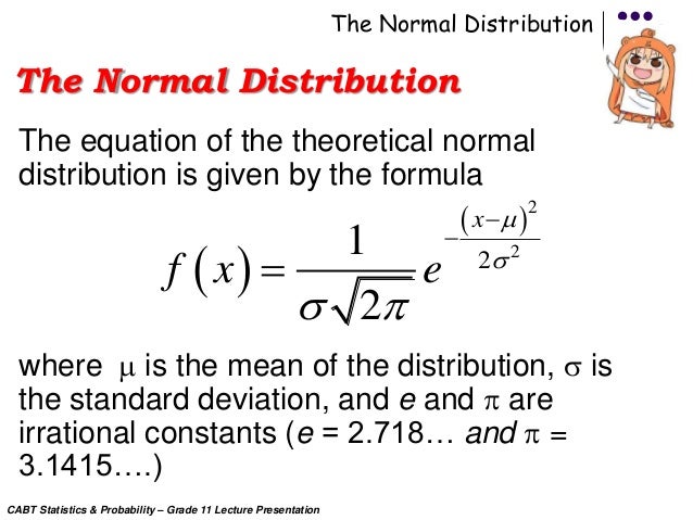 \n"
17 | ]
18 | },
19 | {
20 | "cell_type": "markdown",
21 | "metadata": {},
22 | "source": [
23 | "**Exercise 1:** \n",
24 | "If X is normally distributed with a mean of 4 and and a variance of 16 using python calculate the following probabilities to 3 decimal places:\n",
25 | "- $\\text{Pr}(X < 5.7)$\n",
26 | "- $\\text{Pr}(X > 7)$\n",
27 | "- $\\text{Pr}(2.2 < X < 8)$\n",
28 | "\n"
29 | ]
30 | },
31 | {
32 | "cell_type": "markdown",
33 | "metadata": {},
34 | "source": [
35 | "**Exercise 2:** Calculate the following percentiles of $X$.\n",
36 | "$$ X \\sim (\\mu =5 , \\sigma^2 = 12) $$\n",
37 | "- The 42nd percentile \n",
38 | "- The 88th percentile\n"
39 | ]
40 | },
41 | {
42 | "cell_type": "markdown",
43 | "metadata": {},
44 | "source": [
45 | "**Exercise 3:** Mark and Jane both run in the 1000 metres, a popular track race in the olympics. Mark competed in the Men, Ages 25 - 29 group, while Jane competed in the Women, Ages 20 - 24 group. \n",
46 | "\n",
47 | "Mark completed the race in 221 seconds, while Jane completed the race in 246 seconds. Obviously Mark finished faster, but the question is how well they did within their respective groups. Here is some information on the performance of their groups:\n",
48 | "- The finishing times of the Men, Ages 25 - 29 group has a mean of 181 seconds with a standard deviation of 35 seconds.\n",
49 | "- The finishing times of the Women, Ages 20 - 24 group has a mean of 224 seconds with a standard deviation of 46 seconds.\n",
50 | "- The distributions of finishing times for both groups are approximately Normal. Keep in mind that a better performance corresponds to a faster finish.\n",
51 | "\n",
52 | "\n",
53 | "A) What are the Z-scores for Mark’s and Jane’s finishing times? What do these Z-scores tell you?\n"
54 | ]
55 | },
56 | {
57 | "cell_type": "markdown",
58 | "metadata": {},
59 | "source": [
60 | "B) Did Mark or Jane rank better in their respective groups? Explain your reasoning."
61 | ]
62 | },
63 | {
64 | "cell_type": "markdown",
65 | "metadata": {},
66 | "source": [
67 | "C) What percent of the runners did Mark finish faster than in his group?"
68 | ]
69 | },
70 | {
71 | "cell_type": "markdown",
72 | "metadata": {},
73 | "source": [
74 | "D) What percent of the runners did Jane finish faster than in her group?\n",
75 | "\n"
76 | ]
77 | },
78 | {
79 | "cell_type": "markdown",
80 | "metadata": {},
81 | "source": [
82 | "E) If the distributions of finishing times are not nearly normal, would your answers to parts (A) - (D) change? Explain your reasoning."
83 | ]
84 | },
85 | {
86 | "cell_type": "markdown",
87 | "metadata": {},
88 | "source": [
89 | "**Exercise 4:** Suppose weights of the checked baggage of airline passengers follow a nearly normal distribution with mean 45 pounds and standard deviation 3.2 pounds. Most airlines charge a fee for baggage that weigh in excess of 50 pounds. Determine what percent of airline passengers incur this fee."
90 | ]
91 | },
92 | {
93 | "cell_type": "markdown",
94 | "metadata": {},
95 | "source": [
96 | "**Exercise 5:** A market researcher wants to evaluate car insurance savings at a competing company. Based on past studies he is assuming that the standard deviation of savings is AUD 100. He wants to collect data such that he can get a margin of error of no more than AUD 10 at a 95% confidence level. How large of a sample should he collect?"
97 | ]
98 | },
99 | {
100 | "cell_type": "markdown",
101 | "metadata": {},
102 | "source": [
103 | "***\n",
104 | "www.featureranking.com"
105 | ]
106 | }
107 | ],
108 | "metadata": {
109 | "hide_input": false,
110 | "kernelspec": {
111 | "display_name": "Python 3 (ipykernel)",
112 | "language": "python",
113 | "name": "python3"
114 | },
115 | "language_info": {
116 | "codemirror_mode": {
117 | "name": "ipython",
118 | "version": 3
119 | },
120 | "file_extension": ".py",
121 | "mimetype": "text/x-python",
122 | "name": "python",
123 | "nbconvert_exporter": "python",
124 | "pygments_lexer": "ipython3",
125 | "version": "3.8.10"
126 | }
127 | },
128 | "nbformat": 4,
129 | "nbformat_minor": 2
130 | }
131 |
--------------------------------------------------------------------------------
/Prac_Statistical_Inference_Questions.ipynb:
--------------------------------------------------------------------------------
1 | {
2 | "cells": [
3 | {
4 | "cell_type": "markdown",
5 | "metadata": {},
6 | "source": [
7 | "# Statistical Inference Exercises"
8 | ]
9 | },
10 | {
11 | "cell_type": "markdown",
12 | "metadata": {},
13 | "source": [
14 | "### BDIMS Data Overview\n",
15 | "\n",
16 | "In the following Exercises, you will be working with measurements of body dimensions. This data set contains measurements from 247 men and 260 women, most of whom were considered healthy young adults.\n",
17 | "\n",
18 | "Data source: amstat.org\n",
19 | "\n",
20 | "You will begin by downloading the dataset of around 500 observations from OpenIntro website as below.\n",
21 | "\n",
22 | "[link](https://github.com/akmand/datasets/blob/main/openintro/bdims.csv)\n",
23 | "\n",
24 | "Place the csv in the same directory as this notebook and read in the data."
25 | ]
26 | },
27 | {
28 | "cell_type": "markdown",
29 | "metadata": {},
30 | "source": [
31 | "**Exercise 1:** Make a histogram of men's heights and a histogram of women's heights. How would you compare the various aspects of the two distributions?\n",
32 | "\n",
33 | "**Hint:** `sex = 1` means male, otherwise female."
34 | ]
35 | },
36 | {
37 | "cell_type": "markdown",
38 | "metadata": {},
39 | "source": [
40 | "**Exercise 2:** Make a normal probability plot of men's heights and a normal probability plot of women's heights. Do all of the points fall on the line?\n",
41 | "\n",
42 | "**Hint:** Use `probplot` function from [`scipy.stats`](https://docs.scipy.org/doc/scipy/reference/generated/scipy.stats.probplot.html)."
43 | ]
44 | },
45 | {
46 | "cell_type": "markdown",
47 | "metadata": {},
48 | "source": [
49 | "**Exercise 3:** Now that we have seen that both male and female heights are approximately normally distributed, let's focus on male height. What is the sample mean and standard deviation of `hgt`? "
50 | ]
51 | },
52 | {
53 | "cell_type": "markdown",
54 | "metadata": {},
55 | "source": [
56 | "**Exercise 4:** What is the standard error for male height?"
57 | ]
58 | },
59 | {
60 | "cell_type": "markdown",
61 | "metadata": {},
62 | "source": [
63 | "**Exercise 5:** Calculate the 95% confidence interval for men's height"
64 | ]
65 | },
66 | {
67 | "cell_type": "markdown",
68 | "metadata": {},
69 | "source": [
70 | "**Exercise 6:** Would you expect the 90% confidence interval to be wider or more narrow than the 95% confidence interval? Calculate the 90% Confidence interval for mens height to confirm your answer"
71 | ]
72 | },
73 | {
74 | "cell_type": "markdown",
75 | "metadata": {},
76 | "source": [
77 | "**Exercise 7:** Perform a hypothesis test using a 5% significance test on female height to see whether the mean height is different to 164."
78 | ]
79 | },
80 | {
81 | "cell_type": "markdown",
82 | "metadata": {},
83 | "source": [
84 | "**Question 8:** Would we have reached the same conclusion in the previous question if we were using a 1% significance level?"
85 | ]
86 | },
87 | {
88 | "cell_type": "markdown",
89 | "metadata": {},
90 | "source": [
91 | "**Exercise 9:** We will now shift our attention to t distributions.\n",
92 | "\n",
93 | "We use scipy.stats generate a random sample (seed =11) of 20 centered around 5 and with a standard deviation of 0.9 by running the following code:\n",
94 | "\n",
95 | "```{code}\n",
96 | "np.random.seed(11)\n",
97 | "x = norm.rvs(loc = 5 , scale = 0.9, size =20)\n",
98 | "```\n",
99 | "\n",
100 | "What is the sample mean and standard deviation?\n"
101 | ]
102 | },
103 | {
104 | "cell_type": "markdown",
105 | "metadata": {},
106 | "source": [
107 | "**Exercise 10:** Plot this random sample as a distribution plot in seaborn with kde set to True. How would you describe the distribution?"
108 | ]
109 | },
110 | {
111 | "cell_type": "markdown",
112 | "metadata": {},
113 | "source": [
114 | "**Exercise 11:** Calculate the p_value for the null and alternate hypothesis below on the randomly generated data.\n",
115 | "\n",
116 | "$$H_0: \\mu = 5.22 $$\n",
117 | "$$H_1: \\mu \\neq 5.22$$"
118 | ]
119 | },
120 | {
121 | "cell_type": "markdown",
122 | "metadata": {},
123 | "source": [
124 | "**Exercises 12:**\n",
125 | "How do we interpret the p value? For what conventional significance levels (1%, 5% and 10%) do we reject and fail to reject the hypothesis.\n"
126 | ]
127 | },
128 | {
129 | "cell_type": "markdown",
130 | "metadata": {},
131 | "source": [
132 | "**Exercise 13:** For a different alone variable, you are given the following hypotheses:\n",
133 | "\n",
134 | "$Ho$: $\\mu$ = 60\n",
135 | "\n",
136 | "$Ha$: $\\mu$ != 60\n",
137 | "\n",
138 | "The sample standard deviation is 8 and the sample size is 20. For what sample mean would the p-value be equal to 0.05? Assume that all conditions necessary for inference are satisfied."
139 | ]
140 | },
141 | {
142 | "cell_type": "markdown",
143 | "metadata": {},
144 | "source": [
145 | "***\n",
146 | "www.featureranking.com"
147 | ]
148 | }
149 | ],
150 | "metadata": {
151 | "hide_input": false,
152 | "kernelspec": {
153 | "display_name": "Python 3 (ipykernel)",
154 | "language": "python",
155 | "name": "python3"
156 | },
157 | "language_info": {
158 | "codemirror_mode": {
159 | "name": "ipython",
160 | "version": 3
161 | },
162 | "file_extension": ".py",
163 | "mimetype": "text/x-python",
164 | "name": "python",
165 | "nbconvert_exporter": "python",
166 | "pygments_lexer": "ipython3",
167 | "version": "3.8.10"
168 | }
169 | },
170 | "nbformat": 4,
171 | "nbformat_minor": 2
172 | }
173 |
--------------------------------------------------------------------------------
/Prac_Python_Questions.ipynb:
--------------------------------------------------------------------------------
1 | {
2 | "cells": [
3 | {
4 | "cell_type": "markdown",
5 | "metadata": {},
6 | "source": [
7 | "# Python Programming Exercises"
8 | ]
9 | },
10 | {
11 | "cell_type": "markdown",
12 | "metadata": {},
13 | "source": [
14 | "Reference for some of these exercises is [here](https://www.w3resource.com/python-exercises/)."
15 | ]
16 | },
17 | {
18 | "cell_type": "markdown",
19 | "metadata": {
20 | "heading_collapsed": true
21 | },
22 | "source": [
23 | "## Exercise 1\n",
24 | "\n",
25 | "Write a Python function to check whether a number is divisible by another number. Your function should accept two integers values and return a boolean. "
26 | ]
27 | },
28 | {
29 | "cell_type": "markdown",
30 | "metadata": {
31 | "hidden": true
32 | },
33 | "source": [
34 | "**Examples**\n",
35 | "\n",
36 | "* $23/5 = 4 \\frac{3}{5} \\implies 23$ is not divisible by $5$ as the remainder is not $0 \\implies $ `False`\n",
37 | "* $20/5 = 4 \\frac{0}{5} = 4 \\implies 20$ is divisible by $5$ as the remainder is $0 \\implies $ `True`"
38 | ]
39 | },
40 | {
41 | "cell_type": "code",
42 | "execution_count": null,
43 | "metadata": {
44 | "code_folding": [],
45 | "hidden": true
46 | },
47 | "outputs": [],
48 | "source": []
49 | },
50 | {
51 | "cell_type": "markdown",
52 | "metadata": {
53 | "heading_collapsed": true
54 | },
55 | "source": [
56 | "## Exercise 2 \n",
57 | "\n",
58 | "Fibonacci numbers start with 0, 1 and continues such that the next number is the sum of the previous two numbers. Write a Python function that gives a list of the first $N$ Fibonacci numbers. \n",
59 | "\n",
60 | "**Bonus:** Make the first two numbers optional with default values of 0 and 1. "
61 | ]
62 | },
63 | {
64 | "cell_type": "markdown",
65 | "metadata": {
66 | "hidden": true
67 | },
68 | "source": [
69 | "**Some illustrations**\n",
70 | "\n",
71 | "How does Fibonacci sequence look like?\n",
72 | "\n",
73 | "$$0, 1, 1, 2, 3, 5, 8, 13...$$\n",
74 | "\n",
75 | "In terms of iteration $i$, let $x_{i}$ be the $i^{th}$ number in a Fibonacci sequence, we can break down\n",
76 | "\n",
77 | "\n",
78 | "* $i = 0$, $a = x_0 = 0, b = x_1 = 1$\n",
79 | "* $i = 1$, $x_2 = x_1 + x_0 = 1 + 0 = 1$\n",
80 | "* $i = 2$, $x_3 = x_2 + x_1 = 1 + 1 = 2$\n",
81 | "* $i = 3$, $x_4 = x_3 + x_2 = 2 + 1 = 3$\n",
82 | "* $i = 4$, $x_5 = x_4 + x_3 = 5 + 3 = 8$\n",
83 | "\n",
84 | "* $\\vdots$\n",
85 | "\n",
86 | "In general, $x_{i+1} = x_{i} + x_{i-1}$.\n",
87 | "\n",
88 | "* $x_{i}' \\rightarrow x_{i+1} = x_{i} + x_{i-1}$ after one iteration\n",
89 | "* $x_{i-1}' \\rightarrow x_{i}$ after one iteration"
90 | ]
91 | },
92 | {
93 | "cell_type": "code",
94 | "execution_count": null,
95 | "metadata": {
96 | "hidden": true
97 | },
98 | "outputs": [],
99 | "source": []
100 | },
101 | {
102 | "cell_type": "markdown",
103 | "metadata": {
104 | "heading_collapsed": true
105 | },
106 | "source": [
107 | "## Exercise 3\n",
108 | "\n",
109 | "Write a Python program to count the number of even and odd numbers in a given list of numbers."
110 | ]
111 | },
112 | {
113 | "cell_type": "code",
114 | "execution_count": null,
115 | "metadata": {
116 | "hidden": true
117 | },
118 | "outputs": [],
119 | "source": []
120 | },
121 | {
122 | "cell_type": "markdown",
123 | "metadata": {
124 | "heading_collapsed": true
125 | },
126 | "source": [
127 | "## Exercise 4\n",
128 | "\n",
129 | "Write a Python function that accepts a string and calculates the number of upper case and lower case letters using a dictionary with two keys."
130 | ]
131 | },
132 | {
133 | "cell_type": "markdown",
134 | "metadata": {
135 | "hidden": true
136 | },
137 | "source": [
138 | "**Tricks**\n",
139 | "\n",
140 | "* `.isupper()` and * `.islower()`\n"
141 | ]
142 | },
143 | {
144 | "cell_type": "markdown",
145 | "metadata": {
146 | "hidden": true
147 | },
148 | "source": [
149 | "**Remarks**\n",
150 | "\n",
151 | "* Special characters are not alphabets. So, `'!'.isupper()` or `'!'.isupper()` will return `False`\n",
152 | "* Numeric characters are not alphabets. So, `'2'.isupper()` or `'2'.isupper()` will return `False`"
153 | ]
154 | },
155 | {
156 | "cell_type": "code",
157 | "execution_count": null,
158 | "metadata": {
159 | "hidden": true
160 | },
161 | "outputs": [],
162 | "source": []
163 | },
164 | {
165 | "cell_type": "code",
166 | "execution_count": null,
167 | "metadata": {
168 | "hidden": true
169 | },
170 | "outputs": [],
171 | "source": []
172 | },
173 | {
174 | "cell_type": "markdown",
175 | "metadata": {
176 | "heading_collapsed": true
177 | },
178 | "source": [
179 | "## Exercise 5\n",
180 | "\n",
181 | "Write a Python program to store duplicate elements in a given list."
182 | ]
183 | },
184 | {
185 | "cell_type": "code",
186 | "execution_count": null,
187 | "metadata": {
188 | "hidden": true
189 | },
190 | "outputs": [],
191 | "source": []
192 | },
193 | {
194 | "cell_type": "markdown",
195 | "metadata": {
196 | "heading_collapsed": true
197 | },
198 | "source": [
199 | "## Exercise 6 \n",
200 | "\n",
201 | "Write a Python function that takes two lists and returns `True` if they have at least one common element."
202 | ]
203 | },
204 | {
205 | "cell_type": "code",
206 | "execution_count": null,
207 | "metadata": {
208 | "hidden": true
209 | },
210 | "outputs": [],
211 | "source": []
212 | },
213 | {
214 | "cell_type": "markdown",
215 | "metadata": {
216 | "hidden": true
217 | },
218 | "source": [
219 | "***\n",
220 | "www.featureranking.com"
221 | ]
222 | }
223 | ],
224 | "metadata": {
225 | "hide_input": false,
226 | "kernelspec": {
227 | "display_name": "Python 3 (ipykernel)",
228 | "language": "python",
229 | "name": "python3"
230 | },
231 | "language_info": {
232 | "codemirror_mode": {
233 | "name": "ipython",
234 | "version": 3
235 | },
236 | "file_extension": ".py",
237 | "mimetype": "text/x-python",
238 | "name": "python",
239 | "nbconvert_exporter": "python",
240 | "pygments_lexer": "ipython3",
241 | "version": "3.9.7"
242 | }
243 | },
244 | "nbformat": 4,
245 | "nbformat_minor": 2
246 | }
247 |
--------------------------------------------------------------------------------
/Prac_SK0_Questions.ipynb:
--------------------------------------------------------------------------------
1 | {
2 | "cells": [
3 | {
4 | "cell_type": "markdown",
5 | "metadata": {
6 | "collapsed": true
7 | },
8 | "source": [
9 | "# Practice Exercise: Scikit-Learn 0\n",
10 | "### Introduction to Predictive Modeling with Python and Scikit-Learn"
11 | ]
12 | },
13 | {
14 | "cell_type": "markdown",
15 | "metadata": {
16 | "collapsed": true
17 | },
18 | "source": [
19 | "### Objectives\n",
20 | "\n",
21 | "As in the [SK0 Tutorial](https://www.featureranking.com/tutorials/machine-learning-tutorials/sk-part-0-introduction-to-machine-learning-with-python-and-scikit-learn/), the objective of this practice notebook is to show you a panoramic view of how to build simple machine learning models using the cleaned \"income data\" from previous data preparation practices using a `holdout` approach. In the previous practices, you cleaned and transformed the raw `income data` and renamed the `income` column as `target` which is defined as:\n",
22 | "\n",
23 | "\n",
24 | "$$\\text{target} = \\begin{cases} 1 & \\text{ if the income exceeds USD 50,000} \\\\ 0 & \\text{ otherwise }\\end{cases}$$\n",
25 | "\n",
26 | "Including `target`, the cleaned data consists of 42 columns and 45,222 rows. Each column is numeric and between 0 and 1."
27 | ]
28 | },
29 | {
30 | "cell_type": "markdown",
31 | "metadata": {
32 | "collapsed": true
33 | },
34 | "source": [
35 | "### Exercise 0: Modeling Preparation\n",
36 | "\n",
37 | "- Read the clean data `us_census_income_data_clean_encoded.csv` available [here](https://github.com/akmand/datasets). \n",
38 | "- Randomly sample 5000 rows as it's too big for a short demo (using a random seed of 999).\n",
39 | "- Split the sampled data as 70% training set and the remaining 30% test set using a random seed of 999. \n",
40 | "- Remember to separate `target` during the splitting process. \n",
41 | "- Side question: Why do we need to set a random seed?"
42 | ]
43 | },
44 | {
45 | "cell_type": "markdown",
46 | "metadata": {},
47 | "source": [
48 | "### Exercise 1\n",
49 | "\n",
50 | "Verify whether training and test sets have similar proportion of target labels. Why is this step important?\n"
51 | ]
52 | },
53 | {
54 | "cell_type": "markdown",
55 | "metadata": {},
56 | "source": [
57 | "### Exercise 2\n",
58 | "\n",
59 | "- Fit a nearest neighbor (NN) classifier with $k=5$ neighbors using the Euclidean distance. \n",
60 | "- Fit the model on the train data and evaluate its performance on the test data using accuracy."
61 | ]
62 | },
63 | {
64 | "cell_type": "markdown",
65 | "metadata": {},
66 | "source": [
67 | "### Exercise 3\n",
68 | "\n",
69 | "- Extend the previous question by fitting $k=1, 3, 5, 10, 15, 20$ neighbors using the Manhattan and Euclidean distances respectively. \n",
70 | "- What is the optimal $k$ value for each distance metric? That is, at which $k$, the NN classifier returns the highest accuracy score? **Note:** We will learn later how to perform \"grid search\" to determine the optimal $k$ in later practices.\n",
71 | "- Which distance metric seems to be better? "
72 | ]
73 | },
74 | {
75 | "cell_type": "markdown",
76 | "metadata": {},
77 | "source": [
78 | "### Exercise 4\n",
79 | "\n",
80 | "- Fit a decision tree classifier with the entropy split criterion and a maximum depth of 5 on the train data, and then evaluate its performance on the test data. \n",
81 | "- Does it perform better than the \"best\" KNN model from the previous question?"
82 | ]
83 | },
84 | {
85 | "cell_type": "markdown",
86 | "metadata": {},
87 | "source": [
88 | "### Exercise 5\n",
89 | "\n",
90 | "- Fit a random forest classifier with `n_estimators=100` on train data, and then evaluate its performance on the test data. \n",
91 | "- Does it perform better than the decision tree model in the previous question?"
92 | ]
93 | },
94 | {
95 | "cell_type": "markdown",
96 | "metadata": {},
97 | "source": [
98 | "### Exercise 6\n",
99 | "\n",
100 | "Fit a random forest classifier with `n_estimators=250` on train data, and then evaluate its performance on the test data. Does it return a higher accuracy compared to `n_estimators=100`?"
101 | ]
102 | },
103 | {
104 | "cell_type": "markdown",
105 | "metadata": {},
106 | "source": [
107 | "### Exercise 7\n",
108 | "\n",
109 | "Fit to a Gaussian naive Bayes classifier with a variance smoothing value of $10^{-2}$."
110 | ]
111 | },
112 | {
113 | "cell_type": "markdown",
114 | "metadata": {},
115 | "source": [
116 | "### Exercise 8\n",
117 | "\n",
118 | "Fit to a support vector machine with default values."
119 | ]
120 | },
121 | {
122 | "cell_type": "markdown",
123 | "metadata": {},
124 | "source": [
125 | "### Exercise 9\n",
126 | "\n",
127 | "Predict the first three observations of the full cleaned data using the support vector machine built in the previous question."
128 | ]
129 | },
130 | {
131 | "cell_type": "markdown",
132 | "metadata": {},
133 | "source": [
134 | "### Exercise 10\n",
135 | "\n",
136 | "Use `Pandas` to create a confusion matrix for the SVM model.
\n"
17 | ]
18 | },
19 | {
20 | "cell_type": "markdown",
21 | "metadata": {},
22 | "source": [
23 | "**Exercise 1:** \n",
24 | "If X is normally distributed with a mean of 4 and and a variance of 16 using python calculate the following probabilities to 3 decimal places:\n",
25 | "- $\\text{Pr}(X < 5.7)$\n",
26 | "- $\\text{Pr}(X > 7)$\n",
27 | "- $\\text{Pr}(2.2 < X < 8)$\n",
28 | "\n"
29 | ]
30 | },
31 | {
32 | "cell_type": "markdown",
33 | "metadata": {},
34 | "source": [
35 | "**Exercise 2:** Calculate the following percentiles of $X$.\n",
36 | "$$ X \\sim (\\mu =5 , \\sigma^2 = 12) $$\n",
37 | "- The 42nd percentile \n",
38 | "- The 88th percentile\n"
39 | ]
40 | },
41 | {
42 | "cell_type": "markdown",
43 | "metadata": {},
44 | "source": [
45 | "**Exercise 3:** Mark and Jane both run in the 1000 metres, a popular track race in the olympics. Mark competed in the Men, Ages 25 - 29 group, while Jane competed in the Women, Ages 20 - 24 group. \n",
46 | "\n",
47 | "Mark completed the race in 221 seconds, while Jane completed the race in 246 seconds. Obviously Mark finished faster, but the question is how well they did within their respective groups. Here is some information on the performance of their groups:\n",
48 | "- The finishing times of the Men, Ages 25 - 29 group has a mean of 181 seconds with a standard deviation of 35 seconds.\n",
49 | "- The finishing times of the Women, Ages 20 - 24 group has a mean of 224 seconds with a standard deviation of 46 seconds.\n",
50 | "- The distributions of finishing times for both groups are approximately Normal. Keep in mind that a better performance corresponds to a faster finish.\n",
51 | "\n",
52 | "\n",
53 | "A) What are the Z-scores for Mark’s and Jane’s finishing times? What do these Z-scores tell you?\n"
54 | ]
55 | },
56 | {
57 | "cell_type": "markdown",
58 | "metadata": {},
59 | "source": [
60 | "B) Did Mark or Jane rank better in their respective groups? Explain your reasoning."
61 | ]
62 | },
63 | {
64 | "cell_type": "markdown",
65 | "metadata": {},
66 | "source": [
67 | "C) What percent of the runners did Mark finish faster than in his group?"
68 | ]
69 | },
70 | {
71 | "cell_type": "markdown",
72 | "metadata": {},
73 | "source": [
74 | "D) What percent of the runners did Jane finish faster than in her group?\n",
75 | "\n"
76 | ]
77 | },
78 | {
79 | "cell_type": "markdown",
80 | "metadata": {},
81 | "source": [
82 | "E) If the distributions of finishing times are not nearly normal, would your answers to parts (A) - (D) change? Explain your reasoning."
83 | ]
84 | },
85 | {
86 | "cell_type": "markdown",
87 | "metadata": {},
88 | "source": [
89 | "**Exercise 4:** Suppose weights of the checked baggage of airline passengers follow a nearly normal distribution with mean 45 pounds and standard deviation 3.2 pounds. Most airlines charge a fee for baggage that weigh in excess of 50 pounds. Determine what percent of airline passengers incur this fee."
90 | ]
91 | },
92 | {
93 | "cell_type": "markdown",
94 | "metadata": {},
95 | "source": [
96 | "**Exercise 5:** A market researcher wants to evaluate car insurance savings at a competing company. Based on past studies he is assuming that the standard deviation of savings is AUD 100. He wants to collect data such that he can get a margin of error of no more than AUD 10 at a 95% confidence level. How large of a sample should he collect?"
97 | ]
98 | },
99 | {
100 | "cell_type": "markdown",
101 | "metadata": {},
102 | "source": [
103 | "***\n",
104 | "www.featureranking.com"
105 | ]
106 | }
107 | ],
108 | "metadata": {
109 | "hide_input": false,
110 | "kernelspec": {
111 | "display_name": "Python 3 (ipykernel)",
112 | "language": "python",
113 | "name": "python3"
114 | },
115 | "language_info": {
116 | "codemirror_mode": {
117 | "name": "ipython",
118 | "version": 3
119 | },
120 | "file_extension": ".py",
121 | "mimetype": "text/x-python",
122 | "name": "python",
123 | "nbconvert_exporter": "python",
124 | "pygments_lexer": "ipython3",
125 | "version": "3.8.10"
126 | }
127 | },
128 | "nbformat": 4,
129 | "nbformat_minor": 2
130 | }
131 |
--------------------------------------------------------------------------------
/Prac_Statistical_Inference_Questions.ipynb:
--------------------------------------------------------------------------------
1 | {
2 | "cells": [
3 | {
4 | "cell_type": "markdown",
5 | "metadata": {},
6 | "source": [
7 | "# Statistical Inference Exercises"
8 | ]
9 | },
10 | {
11 | "cell_type": "markdown",
12 | "metadata": {},
13 | "source": [
14 | "### BDIMS Data Overview\n",
15 | "\n",
16 | "In the following Exercises, you will be working with measurements of body dimensions. This data set contains measurements from 247 men and 260 women, most of whom were considered healthy young adults.\n",
17 | "\n",
18 | "Data source: amstat.org\n",
19 | "\n",
20 | "You will begin by downloading the dataset of around 500 observations from OpenIntro website as below.\n",
21 | "\n",
22 | "[link](https://github.com/akmand/datasets/blob/main/openintro/bdims.csv)\n",
23 | "\n",
24 | "Place the csv in the same directory as this notebook and read in the data."
25 | ]
26 | },
27 | {
28 | "cell_type": "markdown",
29 | "metadata": {},
30 | "source": [
31 | "**Exercise 1:** Make a histogram of men's heights and a histogram of women's heights. How would you compare the various aspects of the two distributions?\n",
32 | "\n",
33 | "**Hint:** `sex = 1` means male, otherwise female."
34 | ]
35 | },
36 | {
37 | "cell_type": "markdown",
38 | "metadata": {},
39 | "source": [
40 | "**Exercise 2:** Make a normal probability plot of men's heights and a normal probability plot of women's heights. Do all of the points fall on the line?\n",
41 | "\n",
42 | "**Hint:** Use `probplot` function from [`scipy.stats`](https://docs.scipy.org/doc/scipy/reference/generated/scipy.stats.probplot.html)."
43 | ]
44 | },
45 | {
46 | "cell_type": "markdown",
47 | "metadata": {},
48 | "source": [
49 | "**Exercise 3:** Now that we have seen that both male and female heights are approximately normally distributed, let's focus on male height. What is the sample mean and standard deviation of `hgt`? "
50 | ]
51 | },
52 | {
53 | "cell_type": "markdown",
54 | "metadata": {},
55 | "source": [
56 | "**Exercise 4:** What is the standard error for male height?"
57 | ]
58 | },
59 | {
60 | "cell_type": "markdown",
61 | "metadata": {},
62 | "source": [
63 | "**Exercise 5:** Calculate the 95% confidence interval for men's height"
64 | ]
65 | },
66 | {
67 | "cell_type": "markdown",
68 | "metadata": {},
69 | "source": [
70 | "**Exercise 6:** Would you expect the 90% confidence interval to be wider or more narrow than the 95% confidence interval? Calculate the 90% Confidence interval for mens height to confirm your answer"
71 | ]
72 | },
73 | {
74 | "cell_type": "markdown",
75 | "metadata": {},
76 | "source": [
77 | "**Exercise 7:** Perform a hypothesis test using a 5% significance test on female height to see whether the mean height is different to 164."
78 | ]
79 | },
80 | {
81 | "cell_type": "markdown",
82 | "metadata": {},
83 | "source": [
84 | "**Question 8:** Would we have reached the same conclusion in the previous question if we were using a 1% significance level?"
85 | ]
86 | },
87 | {
88 | "cell_type": "markdown",
89 | "metadata": {},
90 | "source": [
91 | "**Exercise 9:** We will now shift our attention to t distributions.\n",
92 | "\n",
93 | "We use scipy.stats generate a random sample (seed =11) of 20 centered around 5 and with a standard deviation of 0.9 by running the following code:\n",
94 | "\n",
95 | "```{code}\n",
96 | "np.random.seed(11)\n",
97 | "x = norm.rvs(loc = 5 , scale = 0.9, size =20)\n",
98 | "```\n",
99 | "\n",
100 | "What is the sample mean and standard deviation?\n"
101 | ]
102 | },
103 | {
104 | "cell_type": "markdown",
105 | "metadata": {},
106 | "source": [
107 | "**Exercise 10:** Plot this random sample as a distribution plot in seaborn with kde set to True. How would you describe the distribution?"
108 | ]
109 | },
110 | {
111 | "cell_type": "markdown",
112 | "metadata": {},
113 | "source": [
114 | "**Exercise 11:** Calculate the p_value for the null and alternate hypothesis below on the randomly generated data.\n",
115 | "\n",
116 | "$$H_0: \\mu = 5.22 $$\n",
117 | "$$H_1: \\mu \\neq 5.22$$"
118 | ]
119 | },
120 | {
121 | "cell_type": "markdown",
122 | "metadata": {},
123 | "source": [
124 | "**Exercises 12:**\n",
125 | "How do we interpret the p value? For what conventional significance levels (1%, 5% and 10%) do we reject and fail to reject the hypothesis.\n"
126 | ]
127 | },
128 | {
129 | "cell_type": "markdown",
130 | "metadata": {},
131 | "source": [
132 | "**Exercise 13:** For a different alone variable, you are given the following hypotheses:\n",
133 | "\n",
134 | "$Ho$: $\\mu$ = 60\n",
135 | "\n",
136 | "$Ha$: $\\mu$ != 60\n",
137 | "\n",
138 | "The sample standard deviation is 8 and the sample size is 20. For what sample mean would the p-value be equal to 0.05? Assume that all conditions necessary for inference are satisfied."
139 | ]
140 | },
141 | {
142 | "cell_type": "markdown",
143 | "metadata": {},
144 | "source": [
145 | "***\n",
146 | "www.featureranking.com"
147 | ]
148 | }
149 | ],
150 | "metadata": {
151 | "hide_input": false,
152 | "kernelspec": {
153 | "display_name": "Python 3 (ipykernel)",
154 | "language": "python",
155 | "name": "python3"
156 | },
157 | "language_info": {
158 | "codemirror_mode": {
159 | "name": "ipython",
160 | "version": 3
161 | },
162 | "file_extension": ".py",
163 | "mimetype": "text/x-python",
164 | "name": "python",
165 | "nbconvert_exporter": "python",
166 | "pygments_lexer": "ipython3",
167 | "version": "3.8.10"
168 | }
169 | },
170 | "nbformat": 4,
171 | "nbformat_minor": 2
172 | }
173 |
--------------------------------------------------------------------------------
/Prac_Python_Questions.ipynb:
--------------------------------------------------------------------------------
1 | {
2 | "cells": [
3 | {
4 | "cell_type": "markdown",
5 | "metadata": {},
6 | "source": [
7 | "# Python Programming Exercises"
8 | ]
9 | },
10 | {
11 | "cell_type": "markdown",
12 | "metadata": {},
13 | "source": [
14 | "Reference for some of these exercises is [here](https://www.w3resource.com/python-exercises/)."
15 | ]
16 | },
17 | {
18 | "cell_type": "markdown",
19 | "metadata": {
20 | "heading_collapsed": true
21 | },
22 | "source": [
23 | "## Exercise 1\n",
24 | "\n",
25 | "Write a Python function to check whether a number is divisible by another number. Your function should accept two integers values and return a boolean. "
26 | ]
27 | },
28 | {
29 | "cell_type": "markdown",
30 | "metadata": {
31 | "hidden": true
32 | },
33 | "source": [
34 | "**Examples**\n",
35 | "\n",
36 | "* $23/5 = 4 \\frac{3}{5} \\implies 23$ is not divisible by $5$ as the remainder is not $0 \\implies $ `False`\n",
37 | "* $20/5 = 4 \\frac{0}{5} = 4 \\implies 20$ is divisible by $5$ as the remainder is $0 \\implies $ `True`"
38 | ]
39 | },
40 | {
41 | "cell_type": "code",
42 | "execution_count": null,
43 | "metadata": {
44 | "code_folding": [],
45 | "hidden": true
46 | },
47 | "outputs": [],
48 | "source": []
49 | },
50 | {
51 | "cell_type": "markdown",
52 | "metadata": {
53 | "heading_collapsed": true
54 | },
55 | "source": [
56 | "## Exercise 2 \n",
57 | "\n",
58 | "Fibonacci numbers start with 0, 1 and continues such that the next number is the sum of the previous two numbers. Write a Python function that gives a list of the first $N$ Fibonacci numbers. \n",
59 | "\n",
60 | "**Bonus:** Make the first two numbers optional with default values of 0 and 1. "
61 | ]
62 | },
63 | {
64 | "cell_type": "markdown",
65 | "metadata": {
66 | "hidden": true
67 | },
68 | "source": [
69 | "**Some illustrations**\n",
70 | "\n",
71 | "How does Fibonacci sequence look like?\n",
72 | "\n",
73 | "$$0, 1, 1, 2, 3, 5, 8, 13...$$\n",
74 | "\n",
75 | "In terms of iteration $i$, let $x_{i}$ be the $i^{th}$ number in a Fibonacci sequence, we can break down\n",
76 | "\n",
77 | "\n",
78 | "* $i = 0$, $a = x_0 = 0, b = x_1 = 1$\n",
79 | "* $i = 1$, $x_2 = x_1 + x_0 = 1 + 0 = 1$\n",
80 | "* $i = 2$, $x_3 = x_2 + x_1 = 1 + 1 = 2$\n",
81 | "* $i = 3$, $x_4 = x_3 + x_2 = 2 + 1 = 3$\n",
82 | "* $i = 4$, $x_5 = x_4 + x_3 = 5 + 3 = 8$\n",
83 | "\n",
84 | "* $\\vdots$\n",
85 | "\n",
86 | "In general, $x_{i+1} = x_{i} + x_{i-1}$.\n",
87 | "\n",
88 | "* $x_{i}' \\rightarrow x_{i+1} = x_{i} + x_{i-1}$ after one iteration\n",
89 | "* $x_{i-1}' \\rightarrow x_{i}$ after one iteration"
90 | ]
91 | },
92 | {
93 | "cell_type": "code",
94 | "execution_count": null,
95 | "metadata": {
96 | "hidden": true
97 | },
98 | "outputs": [],
99 | "source": []
100 | },
101 | {
102 | "cell_type": "markdown",
103 | "metadata": {
104 | "heading_collapsed": true
105 | },
106 | "source": [
107 | "## Exercise 3\n",
108 | "\n",
109 | "Write a Python program to count the number of even and odd numbers in a given list of numbers."
110 | ]
111 | },
112 | {
113 | "cell_type": "code",
114 | "execution_count": null,
115 | "metadata": {
116 | "hidden": true
117 | },
118 | "outputs": [],
119 | "source": []
120 | },
121 | {
122 | "cell_type": "markdown",
123 | "metadata": {
124 | "heading_collapsed": true
125 | },
126 | "source": [
127 | "## Exercise 4\n",
128 | "\n",
129 | "Write a Python function that accepts a string and calculates the number of upper case and lower case letters using a dictionary with two keys."
130 | ]
131 | },
132 | {
133 | "cell_type": "markdown",
134 | "metadata": {
135 | "hidden": true
136 | },
137 | "source": [
138 | "**Tricks**\n",
139 | "\n",
140 | "* `.isupper()` and * `.islower()`\n"
141 | ]
142 | },
143 | {
144 | "cell_type": "markdown",
145 | "metadata": {
146 | "hidden": true
147 | },
148 | "source": [
149 | "**Remarks**\n",
150 | "\n",
151 | "* Special characters are not alphabets. So, `'!'.isupper()` or `'!'.isupper()` will return `False`\n",
152 | "* Numeric characters are not alphabets. So, `'2'.isupper()` or `'2'.isupper()` will return `False`"
153 | ]
154 | },
155 | {
156 | "cell_type": "code",
157 | "execution_count": null,
158 | "metadata": {
159 | "hidden": true
160 | },
161 | "outputs": [],
162 | "source": []
163 | },
164 | {
165 | "cell_type": "code",
166 | "execution_count": null,
167 | "metadata": {
168 | "hidden": true
169 | },
170 | "outputs": [],
171 | "source": []
172 | },
173 | {
174 | "cell_type": "markdown",
175 | "metadata": {
176 | "heading_collapsed": true
177 | },
178 | "source": [
179 | "## Exercise 5\n",
180 | "\n",
181 | "Write a Python program to store duplicate elements in a given list."
182 | ]
183 | },
184 | {
185 | "cell_type": "code",
186 | "execution_count": null,
187 | "metadata": {
188 | "hidden": true
189 | },
190 | "outputs": [],
191 | "source": []
192 | },
193 | {
194 | "cell_type": "markdown",
195 | "metadata": {
196 | "heading_collapsed": true
197 | },
198 | "source": [
199 | "## Exercise 6 \n",
200 | "\n",
201 | "Write a Python function that takes two lists and returns `True` if they have at least one common element."
202 | ]
203 | },
204 | {
205 | "cell_type": "code",
206 | "execution_count": null,
207 | "metadata": {
208 | "hidden": true
209 | },
210 | "outputs": [],
211 | "source": []
212 | },
213 | {
214 | "cell_type": "markdown",
215 | "metadata": {
216 | "hidden": true
217 | },
218 | "source": [
219 | "***\n",
220 | "www.featureranking.com"
221 | ]
222 | }
223 | ],
224 | "metadata": {
225 | "hide_input": false,
226 | "kernelspec": {
227 | "display_name": "Python 3 (ipykernel)",
228 | "language": "python",
229 | "name": "python3"
230 | },
231 | "language_info": {
232 | "codemirror_mode": {
233 | "name": "ipython",
234 | "version": 3
235 | },
236 | "file_extension": ".py",
237 | "mimetype": "text/x-python",
238 | "name": "python",
239 | "nbconvert_exporter": "python",
240 | "pygments_lexer": "ipython3",
241 | "version": "3.9.7"
242 | }
243 | },
244 | "nbformat": 4,
245 | "nbformat_minor": 2
246 | }
247 |
--------------------------------------------------------------------------------
/Prac_SK0_Questions.ipynb:
--------------------------------------------------------------------------------
1 | {
2 | "cells": [
3 | {
4 | "cell_type": "markdown",
5 | "metadata": {
6 | "collapsed": true
7 | },
8 | "source": [
9 | "# Practice Exercise: Scikit-Learn 0\n",
10 | "### Introduction to Predictive Modeling with Python and Scikit-Learn"
11 | ]
12 | },
13 | {
14 | "cell_type": "markdown",
15 | "metadata": {
16 | "collapsed": true
17 | },
18 | "source": [
19 | "### Objectives\n",
20 | "\n",
21 | "As in the [SK0 Tutorial](https://www.featureranking.com/tutorials/machine-learning-tutorials/sk-part-0-introduction-to-machine-learning-with-python-and-scikit-learn/), the objective of this practice notebook is to show you a panoramic view of how to build simple machine learning models using the cleaned \"income data\" from previous data preparation practices using a `holdout` approach. In the previous practices, you cleaned and transformed the raw `income data` and renamed the `income` column as `target` which is defined as:\n",
22 | "\n",
23 | "\n",
24 | "$$\\text{target} = \\begin{cases} 1 & \\text{ if the income exceeds USD 50,000} \\\\ 0 & \\text{ otherwise }\\end{cases}$$\n",
25 | "\n",
26 | "Including `target`, the cleaned data consists of 42 columns and 45,222 rows. Each column is numeric and between 0 and 1."
27 | ]
28 | },
29 | {
30 | "cell_type": "markdown",
31 | "metadata": {
32 | "collapsed": true
33 | },
34 | "source": [
35 | "### Exercise 0: Modeling Preparation\n",
36 | "\n",
37 | "- Read the clean data `us_census_income_data_clean_encoded.csv` available [here](https://github.com/akmand/datasets). \n",
38 | "- Randomly sample 5000 rows as it's too big for a short demo (using a random seed of 999).\n",
39 | "- Split the sampled data as 70% training set and the remaining 30% test set using a random seed of 999. \n",
40 | "- Remember to separate `target` during the splitting process. \n",
41 | "- Side question: Why do we need to set a random seed?"
42 | ]
43 | },
44 | {
45 | "cell_type": "markdown",
46 | "metadata": {},
47 | "source": [
48 | "### Exercise 1\n",
49 | "\n",
50 | "Verify whether training and test sets have similar proportion of target labels. Why is this step important?\n"
51 | ]
52 | },
53 | {
54 | "cell_type": "markdown",
55 | "metadata": {},
56 | "source": [
57 | "### Exercise 2\n",
58 | "\n",
59 | "- Fit a nearest neighbor (NN) classifier with $k=5$ neighbors using the Euclidean distance. \n",
60 | "- Fit the model on the train data and evaluate its performance on the test data using accuracy."
61 | ]
62 | },
63 | {
64 | "cell_type": "markdown",
65 | "metadata": {},
66 | "source": [
67 | "### Exercise 3\n",
68 | "\n",
69 | "- Extend the previous question by fitting $k=1, 3, 5, 10, 15, 20$ neighbors using the Manhattan and Euclidean distances respectively. \n",
70 | "- What is the optimal $k$ value for each distance metric? That is, at which $k$, the NN classifier returns the highest accuracy score? **Note:** We will learn later how to perform \"grid search\" to determine the optimal $k$ in later practices.\n",
71 | "- Which distance metric seems to be better? "
72 | ]
73 | },
74 | {
75 | "cell_type": "markdown",
76 | "metadata": {},
77 | "source": [
78 | "### Exercise 4\n",
79 | "\n",
80 | "- Fit a decision tree classifier with the entropy split criterion and a maximum depth of 5 on the train data, and then evaluate its performance on the test data. \n",
81 | "- Does it perform better than the \"best\" KNN model from the previous question?"
82 | ]
83 | },
84 | {
85 | "cell_type": "markdown",
86 | "metadata": {},
87 | "source": [
88 | "### Exercise 5\n",
89 | "\n",
90 | "- Fit a random forest classifier with `n_estimators=100` on train data, and then evaluate its performance on the test data. \n",
91 | "- Does it perform better than the decision tree model in the previous question?"
92 | ]
93 | },
94 | {
95 | "cell_type": "markdown",
96 | "metadata": {},
97 | "source": [
98 | "### Exercise 6\n",
99 | "\n",
100 | "Fit a random forest classifier with `n_estimators=250` on train data, and then evaluate its performance on the test data. Does it return a higher accuracy compared to `n_estimators=100`?"
101 | ]
102 | },
103 | {
104 | "cell_type": "markdown",
105 | "metadata": {},
106 | "source": [
107 | "### Exercise 7\n",
108 | "\n",
109 | "Fit to a Gaussian naive Bayes classifier with a variance smoothing value of $10^{-2}$."
110 | ]
111 | },
112 | {
113 | "cell_type": "markdown",
114 | "metadata": {},
115 | "source": [
116 | "### Exercise 8\n",
117 | "\n",
118 | "Fit to a support vector machine with default values."
119 | ]
120 | },
121 | {
122 | "cell_type": "markdown",
123 | "metadata": {},
124 | "source": [
125 | "### Exercise 9\n",
126 | "\n",
127 | "Predict the first three observations of the full cleaned data using the support vector machine built in the previous question."
128 | ]
129 | },
130 | {
131 | "cell_type": "markdown",
132 | "metadata": {},
133 | "source": [
134 | "### Exercise 10\n",
135 | "\n",
136 | "Use `Pandas` to create a confusion matrix for the SVM model.
\n",
137 | "**Hint:** Use pd.crosstab().
\n",
138 | "**Note:** We will learn how to use other performance evaluation measures using `Scikit-Learn` in upcoming practices."
139 | ]
140 | },
141 | {
142 | "cell_type": "markdown",
143 | "metadata": {},
144 | "source": [
145 | "### Exercise 11\n",
146 | "\n",
147 | "- Which cells in the confusion matrix correspond to `TP` and `TN`? \n",
148 | "- Calculate\n",
149 | "> - Accuracy rate\n",
150 | "> - Error rate\n",
151 | "> - Precision (across the \"1\" column)\n",
152 | "> - Recall (across the \"1\" row)"
153 | ]
154 | },
155 | {
156 | "cell_type": "markdown",
157 | "metadata": {},
158 | "source": [
159 | "***\n",
160 | "www.featureranking.com"
161 | ]
162 | }
163 | ],
164 | "metadata": {
165 | "kernelspec": {
166 | "display_name": "Python 3 (ipykernel)",
167 | "language": "python",
168 | "name": "python3"
169 | },
170 | "language_info": {
171 | "codemirror_mode": {
172 | "name": "ipython",
173 | "version": 3
174 | },
175 | "file_extension": ".py",
176 | "mimetype": "text/x-python",
177 | "name": "python",
178 | "nbconvert_exporter": "python",
179 | "pygments_lexer": "ipython3",
180 | "version": "3.8.10"
181 | }
182 | },
183 | "nbformat": 4,
184 | "nbformat_minor": 2
185 | }
186 |
--------------------------------------------------------------------------------
/Prac_Numpy_Solutions.ipynb:
--------------------------------------------------------------------------------
1 | {
2 | "cells": [
3 | {
4 | "cell_type": "markdown",
5 | "metadata": {},
6 | "source": [
7 | "# NumPy Exercises"
8 | ]
9 | },
10 | {
11 | "cell_type": "markdown",
12 | "metadata": {},
13 | "source": [
14 | "Reference for some of these exercises is [here](https://www.w3resource.com/python-exercises/)."
15 | ]
16 | },
17 | {
18 | "cell_type": "markdown",
19 | "metadata": {},
20 | "source": [
21 | "**Exercise 1:** Write a NumPy program to create a random array with 100 real-valued elements between 1 & 5 and compute the following for this array rounded to 2 decimal places:\n",
22 | "- average (that is, the sample mean)\n",
23 | "- population variance and population standard deviation (default option in NumPy)\n",
24 | "- sample variance and sample standard deviation\n",
25 | "\n",
26 | "**Hint:** For sample variance and sample standard deviation, use the `ddof=1` parameter value."
27 | ]
28 | },
29 | {
30 | "cell_type": "code",
31 | "execution_count": 1,
32 | "metadata": {},
33 | "outputs": [
34 | {
35 | "name": "stdout",
36 | "output_type": "stream",
37 | "text": [
38 | "Average: 3.19\n",
39 | "Population variance: 1.3\n",
40 | "Population standard deviation: 1.14\n",
41 | "Sample variance: 1.31\n",
42 | "Sample standard deviation: 1.15\n"
43 | ]
44 | }
45 | ],
46 | "source": [
47 | "import numpy as np\n",
48 | "\n",
49 | "# set the seed here so that the results are repeatable\n",
50 | "np.random.seed(999)\n",
51 | "\n",
52 | "x = 1 + 4*np.random.rand(100)\n",
53 | "\n",
54 | "print('Average:', x.mean().round(2))\n",
55 | "\n",
56 | "print('Population variance:', np.var(x).round(2))\n",
57 | "print('Population standard deviation:', np.std(x).round(2))\n",
58 | "\n",
59 | "print('Sample variance:', np.var(x, ddof=1).round(2))\n",
60 | "print('Sample standard deviation:', np.std(x, ddof=1).round(2))"
61 | ]
62 | },
63 | {
64 | "cell_type": "markdown",
65 | "metadata": {},
66 | "source": [
67 | "**Execise 2:** Write a NumPy program to get the values and indices of the elements that are bigger than 10 in a given array."
68 | ]
69 | },
70 | {
71 | "cell_type": "code",
72 | "execution_count": 2,
73 | "metadata": {},
74 | "outputs": [
75 | {
76 | "name": "stdout",
77 | "output_type": "stream",
78 | "text": [
79 | "Original array: \n",
80 | "[ 5 6 7 8 9 10 11 12 13 14]\n",
81 | "Values bigger than 10: [11 12 13 14]\n",
82 | "Their indices are [6 7 8 9]\n"
83 | ]
84 | }
85 | ],
86 | "source": [
87 | "import numpy as np\n",
88 | "x = 5 + np.arange(10)\n",
89 | "\n",
90 | "print('Original array: ')\n",
91 | "print(x)\n",
92 | "print('Values bigger than 10:', x[x > 10])\n",
93 | "print('Their indices are', np.nonzero(x > 10)[0])"
94 | ]
95 | },
96 | {
97 | "cell_type": "markdown",
98 | "metadata": {},
99 | "source": [
100 | "**Exercise 3:** Write a NumPy program to find the set difference of two arrays. The set difference will return the sorted, unique values in the first array `array1` that are not in the second one `array2`. **Hint:** This is a one-liner."
101 | ]
102 | },
103 | {
104 | "cell_type": "code",
105 | "execution_count": 3,
106 | "metadata": {},
107 | "outputs": [
108 | {
109 | "name": "stdout",
110 | "output_type": "stream",
111 | "text": [
112 | "Array1: [ 0 10 20 40 60 80]\n",
113 | "Array2: [10, 30, 40, 50, 70]\n",
114 | "Unique values in array1 that are not in array2:\n",
115 | "[ 0 20 60 80]\n"
116 | ]
117 | }
118 | ],
119 | "source": [
120 | "import numpy as np\n",
121 | "\n",
122 | "array1 = np.array([0, 10, 20, 40, 60, 80])\n",
123 | "print('Array1: ', array1)\n",
124 | "\n",
125 | "array2 = [10, 30, 40, 50, 70]\n",
126 | "print('Array2: ', array2)\n",
127 | "\n",
128 | "print('Unique values in array1 that are not in array2:')\n",
129 | "print(np.setdiff1d(array1, array2))"
130 | ]
131 | },
132 | {
133 | "cell_type": "markdown",
134 | "metadata": {},
135 | "source": [
136 | "**Exercise 4:** Write a NumPy program to calculate element-wise round, floor, ceiling, and truncated form of an input array."
137 | ]
138 | },
139 | {
140 | "cell_type": "code",
141 | "execution_count": 4,
142 | "metadata": {},
143 | "outputs": [
144 | {
145 | "name": "stdout",
146 | "output_type": "stream",
147 | "text": [
148 | "Original array: [ 3.17 3.5 4.5 2.9 -3.1 -3.5 -5.9 ]\n",
149 | "round with np.round(): [ 3. 4. 4. 3. -3. -4. -6.]\n",
150 | "round with x.round(): [ 3. 4. 4. 3. -3. -4. -6.]\n",
151 | "round to 1 digit: [ 3.2 3.5 4.5 2.9 -3.1 -3.5 -5.9]\n",
152 | "floor: [ 3. 3. 4. 2. -4. -4. -6.]\n",
153 | "ceil: [ 4. 4. 5. 3. -3. -3. -5.]\n",
154 | "truncated: [ 3. 3. 4. 2. -3. -3. -5.]\n"
155 | ]
156 | }
157 | ],
158 | "source": [
159 | "import numpy as np\n",
160 | "\n",
161 | "x = np.array([3.17, 3.5, 4.5, 2.9, -3.1, -3.5, -5.9])\n",
162 | "\n",
163 | "print('Original array:', x)\n",
164 | "\n",
165 | "print('round with np.round():', np.round(x))\n",
166 | "\n",
167 | "# this also works:\n",
168 | "print('round with x.round():', x.round())\n",
169 | "\n",
170 | "print('round to 1 digit:', x.round(1))\n",
171 | "\n",
172 | "print('floor:', np.floor(x))\n",
173 | "\n",
174 | "# this DOES NOT work!\n",
175 | "# it will give attribute error:\n",
176 | "# 'numpy.ndarray' object has no attribute 'floor'\n",
177 | "### print(x.floor())\n",
178 | "\n",
179 | "print('ceil:', np.ceil(x))\n",
180 | "\n",
181 | "print('truncated:', np.trunc(x)) "
182 | ]
183 | },
184 | {
185 | "cell_type": "markdown",
186 | "metadata": {},
187 | "source": [
188 | "***\n",
189 | "www.featureranking.com"
190 | ]
191 | }
192 | ],
193 | "metadata": {
194 | "hide_input": false,
195 | "kernelspec": {
196 | "display_name": "Python 3 (ipykernel)",
197 | "language": "python",
198 | "name": "python3"
199 | },
200 | "language_info": {
201 | "codemirror_mode": {
202 | "name": "ipython",
203 | "version": 3
204 | },
205 | "file_extension": ".py",
206 | "mimetype": "text/x-python",
207 | "name": "python",
208 | "nbconvert_exporter": "python",
209 | "pygments_lexer": "ipython3",
210 | "version": "3.8.10"
211 | }
212 | },
213 | "nbformat": 4,
214 | "nbformat_minor": 2
215 | }
216 |
--------------------------------------------------------------------------------
/Prac_Python_Solutions.ipynb:
--------------------------------------------------------------------------------
1 | {
2 | "cells": [
3 | {
4 | "cell_type": "markdown",
5 | "metadata": {},
6 | "source": [
7 | "# Python Programming Exercises"
8 | ]
9 | },
10 | {
11 | "cell_type": "markdown",
12 | "metadata": {},
13 | "source": [
14 | "Reference for some of these exercises is [here](https://www.w3resource.com/python-exercises/)."
15 | ]
16 | },
17 | {
18 | "cell_type": "markdown",
19 | "metadata": {},
20 | "source": [
21 | "**Exercise 1:** Write a Python function to check whether a number is divisible by another number. Your function should accept two integers values and return a boolean."
22 | ]
23 | },
24 | {
25 | "cell_type": "code",
26 | "execution_count": 1,
27 | "metadata": {},
28 | "outputs": [
29 | {
30 | "name": "stdout",
31 | "output_type": "stream",
32 | "text": [
33 | "True\n",
34 | "False\n"
35 | ]
36 | }
37 | ],
38 | "source": [
39 | "def is_divisible(m, n):\n",
40 | " return True if m % n == 0 else False\n",
41 | "\n",
42 | "print(is_divisible(20, 5))\n",
43 | "print(is_divisible(7, 2))"
44 | ]
45 | },
46 | {
47 | "cell_type": "markdown",
48 | "metadata": {},
49 | "source": [
50 | "**Exercise 2:** Fibonacci numbers start with 0, 1 and continues such that the next number is the sum of the previous two numbers. Write a Python function that gives a list of the first N fibonacci numbers.\n",
51 | "\n",
52 | "**Bonus:** Make the first two numbers optional with default values of 0 and 1."
53 | ]
54 | },
55 | {
56 | "cell_type": "code",
57 | "execution_count": 2,
58 | "metadata": {},
59 | "outputs": [
60 | {
61 | "name": "stdout",
62 | "output_type": "stream",
63 | "text": [
64 | "[0, 1, 1, 2, 3, 5, 8, 13, 21, 34]\n",
65 | "[5, 6, 11, 17, 28, 45, 73, 118, 191, 309]\n"
66 | ]
67 | }
68 | ],
69 | "source": [
70 | "def fibonacci(N, a = 0, b = 1):\n",
71 | " L = []\n",
72 | " L.append(a)\n",
73 | " while len(L) < N:\n",
74 | " a, b = b, a + b\n",
75 | " L.append(a)\n",
76 | " return L\n",
77 | "\n",
78 | "print(fibonacci(10))\n",
79 | "print(fibonacci(10,5,6))"
80 | ]
81 | },
82 | {
83 | "cell_type": "markdown",
84 | "metadata": {},
85 | "source": [
86 | "**Exercise 3:** Write a Python program to count the number of even and odd numbers in a given list of numbers."
87 | ]
88 | },
89 | {
90 | "cell_type": "code",
91 | "execution_count": 3,
92 | "metadata": {},
93 | "outputs": [
94 | {
95 | "name": "stdout",
96 | "output_type": "stream",
97 | "text": [
98 | "Number of even numbers : 51\n",
99 | "Number of odd numbers : 50\n"
100 | ]
101 | }
102 | ],
103 | "source": [
104 | "numbers = list(range(101))\n",
105 | "count_odd = 0\n",
106 | "count_even = 0\n",
107 | "for x in numbers:\n",
108 | " if not x % 2: # Alternatively, you can write \"if x % 2 == 0:\"\n",
109 | " count_even += 1\n",
110 | " else:\n",
111 | " count_odd += 1\n",
112 | "print('Number of even numbers :',count_even)\n",
113 | "print('Number of odd numbers :',count_odd)"
114 | ]
115 | },
116 | {
117 | "cell_type": "markdown",
118 | "metadata": {},
119 | "source": [
120 | "**Exercise 4:** Write a Python function that accepts a string and calculates the number of upper case and lower case letters using a dictionary with two keys."
121 | ]
122 | },
123 | {
124 | "cell_type": "code",
125 | "execution_count": 4,
126 | "metadata": {},
127 | "outputs": [
128 | {
129 | "name": "stdout",
130 | "output_type": "stream",
131 | "text": [
132 | "Input String: Why would anyone not love Python?\n",
133 | "No. of upper case characters : 2\n",
134 | "No. of lower case characters : 25\n"
135 | ]
136 | }
137 | ],
138 | "source": [
139 | "def string_test(s):\n",
140 | " d = {'UPPER_CASE': 0, 'LOWER_CASE': 0}\n",
141 | " for c in s:\n",
142 | " if c.isupper():\n",
143 | " d['UPPER_CASE'] += 1\n",
144 | " elif c.islower():\n",
145 | " d['LOWER_CASE'] += 1\n",
146 | " else:\n",
147 | " pass\n",
148 | " print ('Input String:', s)\n",
149 | " print ('No. of upper case characters : ', d['UPPER_CASE'])\n",
150 | " print ('No. of lower case characters : ', d['LOWER_CASE'])\n",
151 | "\n",
152 | "string_test('Why would anyone not love Python?')"
153 | ]
154 | },
155 | {
156 | "cell_type": "markdown",
157 | "metadata": {},
158 | "source": [
159 | "**Exercise 5:** Write a Python program to store duplicate elements in a given list."
160 | ]
161 | },
162 | {
163 | "cell_type": "code",
164 | "execution_count": 5,
165 | "metadata": {},
166 | "outputs": [
167 | {
168 | "name": "stdout",
169 | "output_type": "stream",
170 | "text": [
171 | "[3, 8, 11]\n"
172 | ]
173 | }
174 | ],
175 | "source": [
176 | "lst = [1, 2, 3, 3, 5, 7, 8, 8, 11, 11, 11, 11]\n",
177 | "\n",
178 | "dup_elements = []\n",
179 | "for x in lst:\n",
180 | " if lst.count(x) > 1:\n",
181 | " if dup_elements.count(x) == 0:\n",
182 | " dup_elements.append(x)\n",
183 | "\n",
184 | "print(dup_elements)"
185 | ]
186 | },
187 | {
188 | "cell_type": "markdown",
189 | "metadata": {},
190 | "source": [
191 | "**Exercise 6:** Write a Python function that takes two lists and returns `True` if they have at least one common element."
192 | ]
193 | },
194 | {
195 | "cell_type": "code",
196 | "execution_count": 6,
197 | "metadata": {},
198 | "outputs": [
199 | {
200 | "name": "stdout",
201 | "output_type": "stream",
202 | "text": [
203 | "True\n",
204 | "False\n"
205 | ]
206 | }
207 | ],
208 | "source": [
209 | "def common_element(list1, list2):\n",
210 | " result = False\n",
211 | " for x in list1:\n",
212 | " for y in list2:\n",
213 | " if x == y:\n",
214 | " result = True\n",
215 | " return result\n",
216 | "\n",
217 | "print(common_element([1,2], [2,3]))\n",
218 | "print(common_element([1,2], [3,4]))"
219 | ]
220 | },
221 | {
222 | "cell_type": "markdown",
223 | "metadata": {},
224 | "source": [
225 | "***\n",
226 | "www.featureranking.com"
227 | ]
228 | }
229 | ],
230 | "metadata": {
231 | "hide_input": false,
232 | "kernelspec": {
233 | "display_name": "Python 3 (ipykernel)",
234 | "language": "python",
235 | "name": "python3"
236 | },
237 | "language_info": {
238 | "codemirror_mode": {
239 | "name": "ipython",
240 | "version": 3
241 | },
242 | "file_extension": ".py",
243 | "mimetype": "text/x-python",
244 | "name": "python",
245 | "nbconvert_exporter": "python",
246 | "pygments_lexer": "ipython3",
247 | "version": "3.8.10"
248 | }
249 | },
250 | "nbformat": 4,
251 | "nbformat_minor": 2
252 | }
253 |
--------------------------------------------------------------------------------
/Prac_Linear_Regression_Questions.ipynb:
--------------------------------------------------------------------------------
1 | {
2 | "cells": [
3 | {
4 | "cell_type": "markdown",
5 | "metadata": {},
6 | "source": [
7 | "# Linear Regression Exercises"
8 | ]
9 | },
10 | {
11 | "cell_type": "markdown",
12 | "metadata": {},
13 | "source": [
14 | "**Exercise 1:** The Child Health and Development Studies investigate a range of topics. One study considered all pregnancies between 1960 and 1967 among women in the Kaiser Foundation Health Plan in the San Francisco East Bay area. Variables in this study are as follows:\n",
15 | "- **response variable:** birth weight in ounces (`bwt`)\n",
16 | "- length of pregnancy in days (`gestation`)\n",
17 | "- mother's age in years (`age`)\n",
18 | "- mother's height in inches (`height`)\n",
19 | "- mother's pregnancy weight in pounds (`weight`)\n",
20 | "- mother's `smoke` status: 1 if the mother is a smoker, 0 otherwise\n",
21 | "- child's `parity` status: 1 if first child, 0 otherwise\n",
22 | "\n",
23 | "Below are three observations from this data set.\n",
24 | "\n",
25 | "| id | bwt | gestation | parity | age | height | weight | smoke |\n",
26 | "|------|------|------|------|------|------|------|------|\n",
27 | "| 1 | 120 | 284 | 0 | 27 | 62 | 100 | 0 |\n",
28 | "| 2 | 113 | 282| 0| 33| 64 | 135 | 0 |\n",
29 | "| . | . | .| . | . | . | . | . |\n",
30 | "| . | . | .| . | . | . | . | . |\n",
31 | "| . | . | .| . | . | . | . | . |\n",
32 | "| 1236 | 117 | 297| 0| 38 | 65 | 129 | 0 |\n",
33 | " \n",
34 | "\n",
35 | "The summary table below shows the results of a regression model for predicting the birth weight of\n",
36 | "babies (`bwt`) based on all of the variables included in the dataset.\n",
37 | "\n",
38 | "| - | Estimate | Std. Error | t value | Pr(>abs(t)) |\n",
39 | "|------|------|------|------|------|\n",
40 | "| (Intercept) | -80.41 | 14.35 | -5.60 | 0.0000 |\n",
41 | "| gestation | 0.44 | 0.03| 15.26 | 0.0000 | \n",
42 | "| parity | -3.33 | 1.13| -2.95 | 0.0033 | \n",
43 | "| age | -0.01 | 0.09| -0.10| 0.9170 | \n",
44 | "| height | 1.15 | 0.21| 5.63 | 0.0000 | \n",
45 | "| weight | 0.05 | 0.03| 1.99 | 0.0471 | \n",
46 | "| smoke | -8.40 | 0.95| -8.81 | 0.0000 | \n",
47 | "\n",
48 | "(A) Write the equation of the regression model that includes all of the variables.\n",
49 | "\n",
50 | "(B) Interpret the slopes of `gestation` and `age` in this context.\n",
51 | "\n",
52 | "(C) Calculate the residual for the first observation in the data set.\n",
53 | "\n",
54 | "(D) Is there a statistically significant relationship between `bwt` and `smoke`?\n",
55 | "\n",
56 | "(E) The variance of the residuals is 249.28 and the variance of the birth weights of all babies in the dataset is 332.57. Calculate the R-squared and the adjusted R-squared values. Note that there are 1,236 observations in the dataset."
57 | ]
58 | },
59 | {
60 | "cell_type": "markdown",
61 | "metadata": {},
62 | "source": [
63 | "## Baseball Player Statistics (MLB11)\n",
64 | "\n",
65 | "The movie [Moneyball](https://www.imdb.com/title/tt1210166/) focuses on the \"quest for the secret of success in baseball\". It follows a low-budget team, the Oakland Athletics, who believed that under-used statistics, such as a player's ability to get on base, better predict the ability to score runs than typical statistics like home runs, RBIs (runs batted in), and batting average. Obtaining players who excelled in these under-used statistics turned out to be much more affordable for the team.\n",
66 | "\n",
67 | "Data Source: www.mlb.com\n",
68 | "\n",
69 | "The data set is available as a CSV file named `mlb11.csv` [here](https://github.com/akmand/datasets/tree/main/openintro)."
70 | ]
71 | },
72 | {
73 | "cell_type": "code",
74 | "execution_count": null,
75 | "metadata": {},
76 | "outputs": [],
77 | "source": [
78 | "import warnings\n",
79 | "warnings.filterwarnings(\"ignore\")\n",
80 | "\n",
81 | "import numpy as np\n",
82 | "import pandas as pd\n",
83 | "import io\n",
84 | "import requests\n",
85 | "\n",
86 | "# so that we can see all the columns\n",
87 | "pd.set_option('display.max_columns', None) \n",
88 | "\n",
89 | "import os, ssl\n",
90 | "if (not os.environ.get('PYTHONHTTPSVERIFY', '') and\n",
91 | " getattr(ssl, '_create_unverified_context', None)): \n",
92 | " ssl._create_default_https_context = ssl._create_unverified_context\n",
93 | "\n",
94 | "df_url = 'https://raw.githubusercontent.com/vaksakalli/datasets/master/mlb11.csv'\n",
95 | "url_content = requests.get(df_url).content\n",
96 | "mlb11 = pd.read_csv(io.StringIO(url_content.decode('utf-8')))\n",
97 | "\n",
98 | "print(f'Data shape = {mlb11.shape}')\n",
99 | "mlb11.head()"
100 | ]
101 | },
102 | {
103 | "cell_type": "markdown",
104 | "metadata": {},
105 | "source": [
106 | "**Exercise 2:** Plot pairwise relationships among `runs`, `hits`, `bat_avg` and `wins`.\n",
107 | "\n",
108 | "**Hint**: Use seaborn's [`pairplot()`](https://seaborn.pydata.org/generated/seaborn.pairplot.html) function."
109 | ]
110 | },
111 | {
112 | "cell_type": "markdown",
113 | "metadata": {},
114 | "source": [
115 | "**Exercise 3:** Construct a multiple regression model for `runs` as the response (dependent) variable and `bat_avg`, `wins`, `strikeouts` as the independent variables. Compute R-squared and Adjusted R-squared values.\n",
116 | "\n",
117 | "**Hint**: Use [`statsmodels.api`](https://www.statsmodels.org/stable/regression.html) to fit the model."
118 | ]
119 | },
120 | {
121 | "cell_type": "markdown",
122 | "metadata": {},
123 | "source": [
124 | "**Exercise 4:** Construct a multiple regression model for `runs` as dependent variable again, but this time include all the independent variables (except `team`) in the model. Compute R-squared and Adjusted R-squared values again."
125 | ]
126 | }
127 | ],
128 | "metadata": {
129 | "hide_input": false,
130 | "kernelspec": {
131 | "display_name": "Python 3 (ipykernel)",
132 | "language": "python",
133 | "name": "python3"
134 | },
135 | "language_info": {
136 | "codemirror_mode": {
137 | "name": "ipython",
138 | "version": 3
139 | },
140 | "file_extension": ".py",
141 | "mimetype": "text/x-python",
142 | "name": "python",
143 | "nbconvert_exporter": "python",
144 | "pygments_lexer": "ipython3",
145 | "version": "3.8.10"
146 | },
147 | "varInspector": {
148 | "cols": {
149 | "lenName": 16,
150 | "lenType": 16,
151 | "lenVar": 40
152 | },
153 | "kernels_config": {
154 | "python": {
155 | "delete_cmd_postfix": "",
156 | "delete_cmd_prefix": "del ",
157 | "library": "var_list.py",
158 | "varRefreshCmd": "print(var_dic_list())"
159 | },
160 | "r": {
161 | "delete_cmd_postfix": ") ",
162 | "delete_cmd_prefix": "rm(",
163 | "library": "var_list.r",
164 | "varRefreshCmd": "cat(var_dic_list()) "
165 | }
166 | },
167 | "types_to_exclude": [
168 | "module",
169 | "function",
170 | "builtin_function_or_method",
171 | "instance",
172 | "_Feature"
173 | ],
174 | "window_display": false
175 | }
176 | },
177 | "nbformat": 4,
178 | "nbformat_minor": 2
179 | }
180 |
--------------------------------------------------------------------------------
/Prac_SK3_Questions.ipynb:
--------------------------------------------------------------------------------
1 | {
2 | "cells": [
3 | {
4 | "cell_type": "markdown",
5 | "metadata": {},
6 | "source": [
7 | "# Practice Exercise: Scikit-Learn 3\n",
8 | "### Model Evaluation"
9 | ]
10 | },
11 | {
12 | "cell_type": "markdown",
13 | "metadata": {},
14 | "source": [
15 | "### Objectives\n",
16 | "\n",
17 | "As in the [SK3 Tutorial](https://www.featureranking.com/tutorials/machine-learning-tutorials/sk-part-3-model-evaluation/), the objective of this practice notebook is to illustrate how you can evaluate machine learning algorithms using various performance metrics. We will show two examples of this: one for classification and one for regression.\n",
18 | "\n",
19 | "You will use **stratified 5-fold cross-validation with 2 repetitions** during training. For testing, you will use the fine-tuned model for prediction **without** any cross-validation for simplicity.\n",
20 | "\n",
21 | "In `GridSearchCV()`, try setting `n_jobs` to -2 for shorter run times with parallel processing. Here, -2 means use all core except 1. See [SK5 Tutorial](https://www.featureranking.com/tutorials/machine-learning-tutorials/sk-part-5-advanced-topics-pipelines-statistical-model-comparison-and-model-deployment/) for more details."
22 | ]
23 | },
24 | {
25 | "cell_type": "markdown",
26 | "metadata": {},
27 | "source": [
28 | "## Part 1: Evaluating Classifiers\n",
29 | "\n",
30 | "In the previous practices, you cleaned and transformed the raw `income data` and renamed the `income` column as `target` (with high income being the positive class). Including `target`, the cleaned data consists of 42 columns and 45,222 rows. Each column is numeric and between 0 and 1."
31 | ]
32 | },
33 | {
34 | "cell_type": "markdown",
35 | "metadata": {},
36 | "source": [
37 | "### Exercise 0: Modeling Preparation\n",
38 | "\n",
39 | "- Read in the clean data `us_census_income_data_clean_encoded.csv` on GitHub [here](https://github.com/akmand/datasets). \n",
40 | "- Randomly sample 5000 rows using a random seed of 999.\n",
41 | "- Split the sampled data as 70% training set and the remaining 30% test set using a random seed of 999. \n",
42 | "- Remember to separate `target` during the splitting process. "
43 | ]
44 | },
45 | {
46 | "cell_type": "markdown",
47 | "metadata": {},
48 | "source": [
49 | "### Exercise 1\n",
50 | "\n",
51 | "Get a value counts of the target feature levels in the sample data. Do you see a class imbalance problem? In this case, which performance metrics would you prefer?\n",
52 | "\n",
53 | "**HINT:**\n",
54 | "\n",
55 | "For a list of scorers as a **string** that you can pass into `cross_val_score()` or `GridSearchCV()` methods, please try this:\n",
56 | "```Python\n",
57 | "from sklearn import metrics \n",
58 | "metrics.SCORERS.keys()\n",
59 | "```\n",
60 | "\n",
61 | "`Scikit-Learn` has a module named `metrics` which contains different performance metrics for classifiers and regressors. For a list of metrics **methods** that you can use, please see official Scikit-Learn documentation on model evaluation [here](https://scikit-learn.org/stable/modules/model_evaluation.html)."
62 | ]
63 | },
64 | {
65 | "cell_type": "markdown",
66 | "metadata": {},
67 | "source": [
68 | "### Exercise 2\n",
69 | "\n",
70 | "Fit and fine-tune a DT model using the **train** data. For fine-tuning, consider max_depth values in {3, 5, 7, 10} and min_samples_split values in {2, 5, 15, 20}. Display the best parameter values and the best estimator found during the grid search."
71 | ]
72 | },
73 | {
74 | "cell_type": "markdown",
75 | "metadata": {},
76 | "source": [
77 | "### Exercise 3\n",
78 | "\n",
79 | "Get the predictions for the test data using the best estimator. You can achieve this via the following:\n",
80 | "```Python\n",
81 | "t_pred = gs_DT.predict(D_test)\n",
82 | "```\n",
83 | "Using the predictions on the **test** data, display the confusion matrix. In addition, compute the following metrics:\n",
84 | "1. Accuracy rate\n",
85 | "2. Error (misclassification) rate\n",
86 | "3. Precision\n",
87 | "4. Recall (TPR)\n",
88 | "5. F1-Score\n",
89 | "6. AUC"
90 | ]
91 | },
92 | {
93 | "cell_type": "markdown",
94 | "metadata": {},
95 | "source": [
96 | "### Exercise 4\n",
97 | "\n",
98 | "Visualize an ROC curve by calculating prediction scores using the `predict_proba` method in `Scikit-learn`."
99 | ]
100 | },
101 | {
102 | "cell_type": "markdown",
103 | "metadata": {},
104 | "source": [
105 | "## Part 2: Evaluating Regressors "
106 | ]
107 | },
108 | {
109 | "cell_type": "markdown",
110 | "metadata": {},
111 | "source": [
112 | "### Exercise 0: Modeling Preparation\n",
113 | " \n",
114 | "For evaluating regressors, we will use the **diamonds** dataset from Prac_SK1. On Canvas, you will see a CSV called 'diamonds_clean_5000.csv'. This is preprocessed diamonds dataset with a random sample of 5000 instances. Read in this dataset and display 5 random instances. Split this data as 70% training set and the remaining 30% test set using a random seed of 999. The target response is the `price`. "
115 | ]
116 | },
117 | {
118 | "cell_type": "markdown",
119 | "metadata": {},
120 | "source": [
121 | "### Exercise 1\n",
122 | "\n",
123 | "Fit and fine-tune a DT regressor model using the **train** data. For fine-tuning, consider max_depth values in {10, 20, 30, 40} and min_samples_split values in {15, 25, 35}. For scoring, use **MSE (mean squared error)**. Display the best parameter values and the best estimator found during the grid search."
124 | ]
125 | },
126 | {
127 | "cell_type": "markdown",
128 | "metadata": {},
129 | "source": [
130 | "### Exercise 2\n",
131 | " \n",
132 | "Get the predictions for the test data using the best estimator. You can achieve this via the following:\n",
133 | "```Python\n",
134 | "t_pred = gs_DT_regressor.predict(D_test)\n",
135 | "```\n",
136 | "Using the predictions on the **test** data, compute the following metrics:\n",
137 | "1. MSE\n",
138 | "2. RMSE\n",
139 | "3. Mean absolute error (MAE)\n",
140 | "4. $R^2$ "
141 | ]
142 | },
143 | {
144 | "cell_type": "markdown",
145 | "metadata": {},
146 | "source": [
147 | "### Exercise 3\n",
148 | "\n",
149 | "Create a histogram of residuals for your DT model. How does it look in terms of shape and spread?"
150 | ]
151 | },
152 | {
153 | "cell_type": "markdown",
154 | "metadata": {},
155 | "source": [
156 | "### Exercise 4 (Optional)\n",
157 | "\n",
158 | "In Exercise 2, we obtain an MSE around 870 USD. Without any domain knowledge on diamond prices, how do we conclude whether the range of prediction errors (i.e., residuals) is \"reasonable\"? Let's use standardised residuals $e$ defined as follows: \n",
159 | "\n",
160 | "$$e = \\frac{\\varepsilon-\\bar{\\varepsilon}}{\\sigma(\\varepsilon)}$$\n",
161 | "\n",
162 | "where residuals are denoted by $\\varepsilon$ with $\\bar{\\varepsilon}$ and $\\sigma$ denoting their mean and standard deviation respectively. \n",
163 | "\n",
164 | "**HINT**\n",
165 | "\n",
166 | "Consider plotting a histogram of standardised errors."
167 | ]
168 | },
169 | {
170 | "cell_type": "markdown",
171 | "metadata": {},
172 | "source": [
173 | "***\n",
174 | "www.featureranking.com"
175 | ]
176 | }
177 | ],
178 | "metadata": {
179 | "kernelspec": {
180 | "display_name": "Python 3 (ipykernel)",
181 | "language": "python",
182 | "name": "python3"
183 | },
184 | "language_info": {
185 | "codemirror_mode": {
186 | "name": "ipython",
187 | "version": 3
188 | },
189 | "file_extension": ".py",
190 | "mimetype": "text/x-python",
191 | "name": "python",
192 | "nbconvert_exporter": "python",
193 | "pygments_lexer": "ipython3",
194 | "version": "3.8.10"
195 | }
196 | },
197 | "nbformat": 4,
198 | "nbformat_minor": 4
199 | }
200 |
--------------------------------------------------------------------------------
/Prac_SK1_Questions.ipynb:
--------------------------------------------------------------------------------
1 | {
2 | "cells": [
3 | {
4 | "cell_type": "markdown",
5 | "metadata": {
6 | "collapsed": true
7 | },
8 | "source": [
9 | "# Practice Exercise: Scikit-Learn 1\n",
10 | "## Basic Modeling"
11 | ]
12 | },
13 | {
14 | "cell_type": "markdown",
15 | "metadata": {
16 | "collapsed": true
17 | },
18 | "source": [
19 | "### Objectives\n",
20 | "\n",
21 | "In line with the [SK1 Tutorial](https://www.featureranking.com/tutorials/machine-learning-tutorials/sk-part-1-basic-modeling/), the objective of this practice notebook is to familiarize you with working with a regression problem using a `holdout` approach. The dataset under consideration is the `diamonds` dataset that comes with the `ggplot2` library in R.\n",
22 | "\n",
23 | "The `diamonds` dataset contains information on diamonds including carat (numeric), clarity (categorical), cut (categorical), and color (categorical). The dataset has 10 features and 53940 instances. The objective is to predict the price of a diamond in USD given its attributes. "
24 | ]
25 | },
26 | {
27 | "cell_type": "markdown",
28 | "metadata": {
29 | "collapsed": true
30 | },
31 | "source": [
32 | "### Exercise 0: Data Preparation\n",
33 | "\n",
34 | "Prepare the dataset for predictive modeling as follows:\n",
35 | "\n",
36 | "0. Refer to our data prep practice solutions on Canvas as well as our data prep script on GitHub [here](https://github.com/akmand/datasets/blob/master/prepare_dataset_for_modeling.py) for some inspiration on preparing this data for predictive modeling.\n",
37 | "1. Set `pd.set_option('display.max_columns', None)`. Read in the raw data `diamonds.csv` on GitHub [here](https://github.com/akmand/datasets). Have a look at the shape and data types of the features. Also have a look at the top 5 rows.\n",
38 | "2. Generate descriptive statistics for categorical and numerical features separately.\n",
39 | "3. Have a look at the unique values for each categorical feature and check whether everything is OK in the sense that there are no unusual values.\n",
40 | "4. Make sure there are no missing values anywhere.\n",
41 | "5. Separate the last column from the dataset and set it to \"target\". Make sure \"target\" is a `Pandas` series at this point, and not a `NumPy` array (which will be necessary for the sampling below). Set all the other columns to be the \"Data\" data frame, which will be the set of descriptive features.\n",
42 | "6. Make sure all categorical descriptive features are encoded via one-hot-encoding. In this particular dataset, some categorical descriptive features are actually ordinal, but we will go ahead and encode them via one-hot-encoding for simplicity.\n",
43 | "7. Make sure all descriptive features are scaled via min-max scaling and the output is a `Pandas` data frame with correct column names. Do **NOT** scale the target feature!\n",
44 | "8. Finally have a look at the top 5 rows of \"target\" and \"Data\" respectively."
45 | ]
46 | },
47 | {
48 | "cell_type": "markdown",
49 | "metadata": {
50 | "collapsed": true
51 | },
52 | "source": [
53 | "### Exercise 1: Modeling Preparation\n",
54 | "\n",
55 | "- Randomly sample 5000 rows as it's too big for a short demo (using a random seed of 999). Make sure to run `reset_index(drop=True)` on the sampled data to reset the indices.\n",
56 | "> - **NOTE:** It's **extremely** important to use the same seed for both Data and target while sampling, otherwise you will happily mix and match different rows without getting any execution errors and all you results will be garbage.\n",
57 | "- Split the sampled data as 70% training set and the remaining 30% test set using a random seed of 999. "
58 | ]
59 | },
60 | {
61 | "cell_type": "markdown",
62 | "metadata": {},
63 | "source": [
64 | "### Exercise 2\n",
65 | "\n",
66 | "- Fit a nearest neighbor (NN) regressor with $k=3$ neighbors using the Euclidean distance. \n",
67 | "- Fit the model on the train data and evaluate its $R^2$ (the default \"score()\" for regressors) performance on the test data. "
68 | ]
69 | },
70 | {
71 | "cell_type": "markdown",
72 | "metadata": {},
73 | "source": [
74 | "### Exercise 3\n",
75 | "\n",
76 | "- Extend Question 2 by fitting $k=1,\\ldots,10$ neighbors using the Manhattan and Euclidean distances respectively.\n",
77 | "- What is the optimal $k$ value for each distance metric? That is, at which $k$, the NN regressor returns the highest $R^2$ score?\n",
78 | "- Which distance metric seems to be better? "
79 | ]
80 | },
81 | {
82 | "cell_type": "markdown",
83 | "metadata": {},
84 | "source": [
85 | "### Exercise 4\n",
86 | "\n",
87 | "- Fit a decision tree regressor with default values on the train data, and then evaluate its performance on the test data. \n",
88 | "- Does it perform better than the best KNN model from the previous question?"
89 | ]
90 | },
91 | {
92 | "cell_type": "markdown",
93 | "metadata": {},
94 | "source": [
95 | "### Exercise 5\n",
96 | "\n",
97 | "- Fit a simple linear regression model on train data, and then evaluate its performance on the test data. **Hint:** Use `LinearRegression()` in `sklearn.linear_model`. \n",
98 | "- How does it compare to the previous models?"
99 | ]
100 | },
101 | {
102 | "cell_type": "markdown",
103 | "metadata": {},
104 | "source": [
105 | "### Exercise 6\n",
106 | "\n",
107 | "- Fit a random forest regressor with `n_estimators=100` on train data, and then evaluate its performance on the test data. \n",
108 | "- How does it compare to the previous models?"
109 | ]
110 | },
111 | {
112 | "cell_type": "markdown",
113 | "metadata": {},
114 | "source": [
115 | "### Exercise 7\n",
116 | "\n",
117 | "- Predict the first 5 observations of the **test** data using the linear regression model you built earlier. \n",
118 | "- Display your results as a data frame with three columns: 'target', 'prediction', 'absolute_diff'.\n",
119 | "- How do the predictions look?"
120 | ]
121 | },
122 | {
123 | "cell_type": "markdown",
124 | "metadata": {},
125 | "source": [
126 | "**Further exposition**\n",
127 | "\n",
128 | "Let's create histograms to visualize the difference between predicted values from the linear regression and target values on both training and test sets. How are the difference values distributed? Are they centered around zero? What are minimum and maximum difference values for training and test sets?"
129 | ]
130 | },
131 | {
132 | "cell_type": "markdown",
133 | "metadata": {},
134 | "source": [
135 | "## Optional: diagnostic of regressors \n",
136 | "\n",
137 | "Relying on $R^{2}$ to evaluate regressor performance is not sufficient. Sometimes, we need to ensure if the regressors generate reasonable predictions. In this case, we have to check if the predicted diamond prices are positive (a negative price would imply you would get the diamond free and some extra cash!) \n",
138 | "\n",
139 | "Let's predict on training set for each model developed in the previous exercises. Create a dataframe, named `pred_result`, which consists of four columns corresponding to their predictions. Then, run `pred_result.describe()` to check if any model has a negative minimum value. Does the result surprise you? Will you get a similar result if you predict on test set?\n"
140 | ]
141 | },
142 | {
143 | "cell_type": "markdown",
144 | "metadata": {},
145 | "source": [
146 | "***\n",
147 | "www.featureranking.com"
148 | ]
149 | }
150 | ],
151 | "metadata": {
152 | "kernelspec": {
153 | "display_name": "Python 3 (ipykernel)",
154 | "language": "python",
155 | "name": "python3"
156 | },
157 | "language_info": {
158 | "codemirror_mode": {
159 | "name": "ipython",
160 | "version": 3
161 | },
162 | "file_extension": ".py",
163 | "mimetype": "text/x-python",
164 | "name": "python",
165 | "nbconvert_exporter": "python",
166 | "pygments_lexer": "ipython3",
167 | "version": "3.8.10"
168 | }
169 | },
170 | "nbformat": 4,
171 | "nbformat_minor": 2
172 | }
173 |
--------------------------------------------------------------------------------
/Prac_SK4_Questions.ipynb:
--------------------------------------------------------------------------------
1 | {
2 | "cells": [
3 | {
4 | "cell_type": "markdown",
5 | "metadata": {
6 | "slideshow": {
7 | "slide_type": "slide"
8 | }
9 | },
10 | "source": [
11 | "# Practice Exercise: Scikit-Learn 4\n",
12 | "### Cross-Validation and Hyper-parameter Tuning¶"
13 | ]
14 | },
15 | {
16 | "cell_type": "markdown",
17 | "metadata": {
18 | "slideshow": {
19 | "slide_type": "slide"
20 | }
21 | },
22 | "source": [
23 | "### Objectives\n",
24 | "\n",
25 | "As in the [SK4 Tutorial](https://www.featureranking.com/tutorials/machine-learning-tutorials/sk-part-4-cross-validation-and-hyperparameter-tuning/), the objective of this practice notebook is to illustrate how you can perform cross-validation and hyper-parameter tuning using `Scikit-Learn`. You will also perform paired t-tests to determine statistically significant performance results, as explained [here](https://www.featureranking.com/tutorials/machine-learning-tutorials/sk-part-5-advanced-topics-pipelines-statistical-model-comparison-and-model-deployment/#4). \n",
26 | "\n",
27 | "You will be using the cleaned \"income data\" dataset. In the previous practices, you cleaned and transformed the raw `income data` and renamed the `income` column as `target` (with high income being the positive class). Including `target`, the cleaned data consists of 42 columns and 45,222 rows. Each column is numeric and between 0 and 1.\n",
28 | "\n",
29 | "In `GridSearchCV()`, try setting `n_jobs` to -2 for shorter run times with parallel processing. Here, -2 means use all core except 1. See [SK5 Tutorial](https://www.featureranking.com/tutorials/machine-learning-tutorials/sk-part-5-advanced-topics-pipelines-statistical-model-comparison-and-model-deployment/) for more details."
30 | ]
31 | },
32 | {
33 | "cell_type": "markdown",
34 | "metadata": {},
35 | "source": [
36 | "### Instructions\n",
37 | "\n",
38 | "- For ease of computation, you will first randomly sample 5,000 rows from this dataset. \n",
39 | "- You will then split this sample into 70% train and 30% test datasets. \n",
40 | "- You will use the first set for **training**: you will fine tune your models using this train data. \n",
41 | "- You will use the second set for **testing**: you will perform cross-validation in a paired fashion using the test data and then you will compare the performance of your tuned models using a paired t-test.\n",
42 | "- You will use **stratified 5-fold cross-validation with no repetitions** during both training and testing.\n",
43 | "- For scoring, you will use AUC, that is, \"area under the ROC curve\". "
44 | ]
45 | },
46 | {
47 | "cell_type": "markdown",
48 | "metadata": {},
49 | "source": [
50 | "### Some Bookkeeping\n",
51 | "\n",
52 | "- Define a variable called `num_samples` and set it to 5000. You will use this variable when sampling a smaller subset of the full set of instances.\n",
53 | "- Define a variable called `num_features` and set it to 10. Prior to fitting any models, you will perform feature selection by making use of this `num_features` variable.\n",
54 | "- Define a variable called `scoring_metric` and set it to to `'roc_auc'`. You will set `scoring` option in all `cross_val_score()` functions to this `scoring_metric` variable.\n",
55 | "\n",
56 | "You can achieve these by running the code chunk below:\n",
57 | "```Python\n",
58 | "import numpy as np\n",
59 | "np.random.seed(999)\n",
60 | "num_samples = 5000\n",
61 | "scoring_metric = 'roc_auc'\n",
62 | "num_features = 10\n",
63 | "```"
64 | ]
65 | },
66 | {
67 | "cell_type": "markdown",
68 | "metadata": {},
69 | "source": [
70 | "### Exercise 0: Modeling Preparation\n",
71 | "\n",
72 | "- Read in the clean data `us_census_income_data_clean_encoded.csv` on GitHub [here](https://github.com/akmand/datasets). \n",
73 | "- Randomly sample 5000 rows using a random seed of 999.\n",
74 | "- Split the sampled data as 70% training set and the remaining 30% test set using a random seed of 999. \n",
75 | "- Remember to separate `target` during the splitting process. "
76 | ]
77 | },
78 | {
79 | "cell_type": "markdown",
80 | "metadata": {},
81 | "source": [
82 | "### Exercise 1\n",
83 | "\n",
84 | "Determine the most important 10 features as selected by Random Forest Importance (RFI) using the **training** data and visualize them.\n",
85 | "\n",
86 | "In the rest of these exercises, you will use these selected features and not the whole set of descriptive features. You can achieve this as below:\n",
87 | "```Python\n",
88 | "D_Train_fs = D_train[:, fs_indices_rfi]\n",
89 | "D_Test_fs = D_test[:, fs_indices_rfi]\n",
90 | "```"
91 | ]
92 | },
93 | {
94 | "cell_type": "markdown",
95 | "metadata": {},
96 | "source": [
97 | "### Exercise 2\n",
98 | "\n",
99 | "Fit and fine-tune a KNN model using the **train** data. For fine-tuning, consider K values in {1, 5, 10, 15, 20} and p values in {1, 2}. Also visualize the tuning results."
100 | ]
101 | },
102 | {
103 | "cell_type": "markdown",
104 | "metadata": {},
105 | "source": [
106 | "### Exercise 3\n",
107 | "\n",
108 | "Fit and fine-tune a DT model using the **train** data. For fine-tuning, consider max_depth values in {3, 5, 7, 10, 12} and min_samples_split values in {2, 5, 15, 20, 25}. Also visualize the tuning results."
109 | ]
110 | },
111 | {
112 | "cell_type": "markdown",
113 | "metadata": {},
114 | "source": [
115 | "### Exercise 4\n",
116 | "\n",
117 | "Fit and fine-tune a NB model using the **train** data. For fine-tuning, consider var_smoothing values in `np.logspace(1,-2, num=50)`. Also visualize the tuning results."
118 | ]
119 | },
120 | {
121 | "cell_type": "markdown",
122 | "metadata": {},
123 | "source": [
124 | "### Exercise 5\n",
125 | "\n",
126 | "Fit and fine-tune a Random Forest model using the **train** data. For fine-tuning, consider n_estimators values in {100, 250, 500} and max_depth values in {3, 5, 7, 10, 12}. Also visualize the tuning results."
127 | ]
128 | },
129 | {
130 | "cell_type": "markdown",
131 | "metadata": {},
132 | "source": [
133 | "### Exercise 6\n",
134 | "\n",
135 | "What we would like to do now is to \"fit\" each tuned classifier (with their best set of hyperparameter values) on the **test** data in a cross-validated fashion to figure out which (tuned) classifier performs the best. This way, we will be measuring performance of the tuned classifiers on data that they did not \"see\" previously.\n",
136 | "\n",
137 | "Since cross validation itself is a random process, we would like to perform pairwise t-tests to determine if any difference between the performance of any two (tuned) classifiers is statistically significant. Specifically, we first perform 5-fold stratified cross-validation (without any repetitions) on each (tuned) classifier where we use the same seed in each of the four cross-validation runs. Second, we conduct a paired t-test for the AUC score between the following (tuned) classifier combinations.\n",
138 | "\n",
139 | "For this question, perform the procedures discussed above and decide if any one the tuned classifiers is statistically better than the rest at a 95% significance level."
140 | ]
141 | },
142 | {
143 | "cell_type": "markdown",
144 | "metadata": {},
145 | "source": [
146 | "### Exercise 7\n",
147 | "\n",
148 | "Rerun your notebook with different number of features (e.g., 5, 15, 20). Also try with no feature selection at all (set num_features=41).\n",
149 | "Comment if your results improve. Which number of features seem to work best?"
150 | ]
151 | },
152 | {
153 | "cell_type": "markdown",
154 | "metadata": {},
155 | "source": [
156 | "***\n",
157 | "www.featureranking.com"
158 | ]
159 | }
160 | ],
161 | "metadata": {
162 | "kernelspec": {
163 | "display_name": "Python 3 (ipykernel)",
164 | "language": "python",
165 | "name": "python3"
166 | },
167 | "language_info": {
168 | "codemirror_mode": {
169 | "name": "ipython",
170 | "version": 3
171 | },
172 | "file_extension": ".py",
173 | "mimetype": "text/x-python",
174 | "name": "python",
175 | "nbconvert_exporter": "python",
176 | "pygments_lexer": "ipython3",
177 | "version": "3.8.10"
178 | }
179 | },
180 | "nbformat": 4,
181 | "nbformat_minor": 4
182 | }
183 |
--------------------------------------------------------------------------------
/Prac_SK5_Questions.ipynb:
--------------------------------------------------------------------------------
1 | {
2 | "cells": [
3 | {
4 | "cell_type": "markdown",
5 | "metadata": {},
6 | "source": [
7 | "# Practice Exercise: Scikit-Learn 5\n",
8 | "### Pipelines"
9 | ]
10 | },
11 | {
12 | "cell_type": "markdown",
13 | "metadata": {},
14 | "source": [
15 | "### Objectives\n",
16 | "\n",
17 | "As part of the [SK5 Tutorial](https://www.featureranking.com/tutorials/machine-learning-tutorials/sk-part-5-advanced-topics-pipelines-statistical-model-comparison-and-model-deployment/), the objective of this practice notebook is to illustrate how you can set up `pipelines` for streamlining your machine learning workflow using `Scikit-Learn`. Pipelines make life easier in relatively large machine learning projects by combining multiple steps in to a single process.\n",
18 | "\n",
19 | "You will be using the cleaned \"income data\" dataset. In the previous practices, you cleaned and transformed the raw `income data` and renamed the `income` column as `target` (with high income being the positive class). Including `target`, the cleaned data consists of 42 columns and 45,222 rows. Each column is numeric and between 0 and 1.\n",
20 | "\n",
21 | "You will use **stratified 5-fold cross-validation with no repetitions** during training. For testing, you will use the fine-tuned model for prediction **without** any cross-validation for simplicity.\n",
22 | "\n",
23 | "In `GridSearchCV()`, try setting `n_jobs` to -2 for shorter run times with parallel processing. Here, -2 means use all core except 1."
24 | ]
25 | },
26 | {
27 | "cell_type": "markdown",
28 | "metadata": {},
29 | "source": [
30 | "### Exercise 0: Modeling Preparation\n",
31 | "\n",
32 | "- Read in the clean data `us_census_income_data_clean_encoded.csv` on GitHub [here](https://github.com/akmand/datasets). \n",
33 | "- Randomly sample 5000 rows using a random seed of 999.\n",
34 | "- Split the sampled data as 70% training set and the remaining 30% test set using a random seed of 999. \n",
35 | "- Remember to separate `target` during the splitting process. "
36 | ]
37 | },
38 | {
39 | "cell_type": "markdown",
40 | "metadata": {},
41 | "source": [
42 | "### Exercise 1: Pipeline Preparation"
43 | ]
44 | },
45 | {
46 | "cell_type": "markdown",
47 | "metadata": {},
48 | "source": [
49 | "For feature selection, you will use the powerful Random Forest Importance (RFI) method with 100 estimators. A trick here is that you will need a bit of coding so that you can make RFI feature selection as part of the pipeline. For this reason, we are providing for you the custom `RFIFeatureSelector()` class below to pass in RFI as a \"step\" to the pipeline.\n",
50 | "```Python\n",
51 | "from sklearn.base import BaseEstimator, TransformerMixin\n",
52 | "# custom function for RFI feature selection inside a pipeline\n",
53 | "# here we use n_estimators=100\n",
54 | "# notice the random_state in RandomForestClassifier()\n",
55 | "# to control randomness\n",
56 | "class RFIFeatureSelector(BaseEstimator, TransformerMixin):\n",
57 | " # class constructor \n",
58 | " # make sure class attributes end with a \"_\"\n",
59 | " # per scikit-learn convention to avoid errors\n",
60 | " def __init__(self, n_features_=10):\n",
61 | " self.n_features_ = n_features_\n",
62 | " self.fs_indices_ = None\n",
63 | " # override the fit function\n",
64 | " def fit(self, X, y):\n",
65 | " from sklearn.ensemble import RandomForestClassifier\n",
66 | " from numpy import argsort\n",
67 | " model_rfi = RandomForestClassifier(n_estimators=100, random_state=999)\n",
68 | " model_rfi.fit(X, y)\n",
69 | " self.fs_indices_ = argsort(model_rfi.feature_importances_)[::-1][0:self.n_features_] \n",
70 | " return self \n",
71 | " # override the transform function\n",
72 | " def transform(self, X, y=None):\n",
73 | " return X[:, self.fs_indices_]\n",
74 | "```\n",
75 | "\n",
76 | "We are also making available the custom function below, called `get_search_results()`, which will format outputs of an input grid search object as a `Pandas` data frame.\n",
77 | "```Python\n",
78 | "# custom function to format the search results as a Pandas data frame\n",
79 | "def get_search_results(gs):\n",
80 | " def model_result(scores, params):\n",
81 | " scores = {'mean_score': np.mean(scores),\n",
82 | " 'std_score': np.std(scores),\n",
83 | " 'min_score': np.min(scores),\n",
84 | " 'max_score': np.max(scores)}\n",
85 | " return pd.Series({**params,**scores})\n",
86 | " models = []\n",
87 | " scores = []\n",
88 | " for i in range(gs.n_splits_):\n",
89 | " key = f\"split{i}_test_score\"\n",
90 | " r = gs.cv_results_[key] \n",
91 | " scores.append(r.reshape(-1,1))\n",
92 | " all_scores = np.hstack(scores)\n",
93 | " for p, s in zip(gs.cv_results_['params'], all_scores):\n",
94 | " models.append((model_result(s, p)))\n",
95 | " pipe_results = pd.concat(models, axis=1).T.sort_values(['mean_score'], ascending=False)\n",
96 | " columns_first = ['mean_score', 'std_score', 'max_score', 'min_score']\n",
97 | " columns = columns_first + [c for c in pipe_results.columns if c not in columns_first]\n",
98 | " return pipe_results[columns]\n",
99 | "```\n",
100 | "\n",
101 | "You will need to copy and paste these two code blocks before you can continue with the next exercise."
102 | ]
103 | },
104 | {
105 | "cell_type": "markdown",
106 | "metadata": {},
107 | "source": [
108 | "### Exercise 2\n",
109 | "\n",
110 | "Using a pipeline, stack Random Forest Importance (RFI) feature selection together with grid search for DT hyperparameter tuning via cross-validation using the **train** data. For scoring, use AUC, that is, \"area under the ROC curve\". \n",
111 | "\n",
112 | "For RFI, consider number of features in {10, 20, full_number_of_descriptive_features}.\n",
113 | "\n",
114 | "For the DT model, aim to determine the optimal combinations of maximum depth (`max_depth`) and minimum sample split (`min_samples_split`) using the **Gini Index** split criterion. In particular, consider max_depth values in {3, 5, 7, 9, 11} and min_samples_split values in {2, 5, 7, 9, 11}."
115 | ]
116 | },
117 | {
118 | "cell_type": "markdown",
119 | "metadata": {},
120 | "source": [
121 | "### Exercise 3\n",
122 | "\n",
123 | "Display the pipeline best parameters, the best score, and the best estimator. "
124 | ]
125 | },
126 | {
127 | "cell_type": "markdown",
128 | "metadata": {},
129 | "source": [
130 | "### Exercise 4\n",
131 | "\n",
132 | "Using the custom `get_search_results()` function, display the top 5 combinations of the pipeline."
133 | ]
134 | },
135 | {
136 | "cell_type": "markdown",
137 | "metadata": {},
138 | "source": [
139 | "### Exercise 5\n",
140 | "\n",
141 | "Visualize DT performance comparison results by filtering the output of the `get_search_results()` function for 10 features. Put minimum samples for split in the x-axis, AUC in the y-axis and break down the plot by maximum depth."
142 | ]
143 | },
144 | {
145 | "cell_type": "markdown",
146 | "metadata": {},
147 | "source": [
148 | "### Exercise 6\n",
149 | "\n",
150 | "Using the best estimator of the pipeline, obtain the predictions on the **test** data. Display the confusion matrix and the AUC score on this test data. \n",
151 | "\n",
152 | "Next, using the best estimator of the pipeline, obtain the predictions on the **train** data. Display the confusion matrix and the AUC score on this train data. \n",
153 | "\n",
154 | "How does the test AUC compare to the train AUC? Why do you think there is difference?"
155 | ]
156 | },
157 | {
158 | "cell_type": "markdown",
159 | "metadata": {},
160 | "source": [
161 | "***\n",
162 | "www.featureranking.com"
163 | ]
164 | }
165 | ],
166 | "metadata": {
167 | "kernelspec": {
168 | "display_name": "Python 3 (ipykernel)",
169 | "language": "python",
170 | "name": "python3"
171 | },
172 | "language_info": {
173 | "codemirror_mode": {
174 | "name": "ipython",
175 | "version": 3
176 | },
177 | "file_extension": ".py",
178 | "mimetype": "text/x-python",
179 | "name": "python",
180 | "nbconvert_exporter": "python",
181 | "pygments_lexer": "ipython3",
182 | "version": "3.8.10"
183 | }
184 | },
185 | "nbformat": 4,
186 | "nbformat_minor": 2
187 | }
188 |
--------------------------------------------------------------------------------
/Prac_Descriptive_Stats_Questions.ipynb:
--------------------------------------------------------------------------------
1 | {
2 | "cells": [
3 | {
4 | "cell_type": "markdown",
5 | "metadata": {},
6 | "source": [
7 | "# Descriptive Statistics Exercises"
8 | ]
9 | },
10 | {
11 | "cell_type": "markdown",
12 | "metadata": {},
13 | "source": [
14 | "## Important Notes\n",
15 | "\n",
16 | "**IMPORTANT NOTE 1:** Please remember to **run your code cells** so that you can see the output of your codes.\n",
17 | "\n",
18 | "**IMPORTANT NOTE 2:** By default, Jupyter Notebook will only display the output of the last command in a Code cell. Thus, if you have multiple commands in a Code cell and you need to print output of a Python command in the middle of the cell, you have two options: \n",
19 | "- Option 1: Break your Code cell into multiple Code cells and place only one command in each cell so that you can display output of each command.\n",
20 | "- Option 2: (**Preferred**) In a Code cell, put print() statements around each Python command whose output you would like to display."
21 | ]
22 | },
23 | {
24 | "cell_type": "markdown",
25 | "metadata": {},
26 | "source": [
27 | "## Tutorial Overview\n",
28 | "\n",
29 | "In this exercise, you will gain insight into public health by generating simple graphical and numerical summaries of a dataset collected by the U.S. Centers for Disease Control and Prevention (CDC).\n",
30 | "\n",
31 | "The Behavioral Risk Factor Surveillance System (BRFSS) is an annual telephone survey of 350,000 people in the United States. As its name implies, the BRFSS is designed to identify risk factors in the adult population and report emerging health trends. For example, respondents are asked about their diet and weekly physical activity, their HIV/AIDS status, possible tobacco use, and even their level of healthcare coverage.\n",
32 | "\n",
33 | "Data source: cdc.gov/brfss\n",
34 | "\n",
35 | "We will focus on a random sample of 60 people from the BRFSS survey conducted in 2000. While there are over 200 variables in this data set, we will work with a small subset. \n",
36 | "\n"
37 | ]
38 | },
39 | {
40 | "cell_type": "markdown",
41 | "metadata": {},
42 | "source": [
43 | "**Exercise 1:** Import the `numpy` and `pandas` modules in as `np` and `pd` respectively. Then place the `cdc_sample.csv` from our dataset GitHub repository into the same directory as this notebook and read in the data as `cdc`. Display the first 5 rows of the data. "
44 | ]
45 | },
46 | {
47 | "cell_type": "markdown",
48 | "metadata": {},
49 | "source": [
50 | "**Exercise 2:** How many variables are there in this dataset? For each variable, identify its data type (e.g., categorical, numerical). If categorical, state the number of levels.\n",
51 | "\n",
52 | "**Hint:** Try using Pandas' `info()` method on your data frame. In the output of this method, `object` data type (\"dtype\") stands for a string type, which usually indicates a categorical variable. On the hand, some numerical variables can actually be categorical in nature (think about hlthplan, for instance). This can be verified when coupled with the `nunique()` function.\n",
53 | "\n"
54 | ]
55 | },
56 | {
57 | "cell_type": "markdown",
58 | "metadata": {},
59 | "source": [
60 | "**Exercise 3:** What are the levels in `genhlth`? and how many people fall under each level?\n",
61 | "\n",
62 | "**Hint:** you can use Pandas' `value_counts()` function."
63 | ]
64 | },
65 | {
66 | "cell_type": "markdown",
67 | "metadata": {},
68 | "source": [
69 | "**Exercise 4:** Import `matplotlib.pyplot` as `plt` and create a scatterplot of `height` and `weight`, ensuring that the plot has an appropriate title and axis labels. What is the association between these two variables? "
70 | ]
71 | },
72 | {
73 | "cell_type": "markdown",
74 | "metadata": {},
75 | "source": [
76 | "**Exercise 5:** Find the mean, sample standard deviation, and median of `weight`."
77 | ]
78 | },
79 | {
80 | "cell_type": "markdown",
81 | "metadata": {},
82 | "source": [
83 | "**Exercise 6:** Find the mean, sample standard deviation, and median of `weight` for respondents who exercised in the past month. Is there any significant difference in the results when compared to the results of Exercise 5?\n",
84 | "\n",
85 | "**Hint:** `exerany` is the variable that is 1 if the respondent exercised in the past month and 0 otherwise."
86 | ]
87 | },
88 | {
89 | "cell_type": "markdown",
90 | "metadata": {},
91 | "source": [
92 | "**Exercise 7:** Create a histogram of `weight` from the data examined in Exercise 5 and 6 on the same plot. Ensuring that your plot has an appropriate title, axis labels and legend. Does this histogram support your answer in question 6? Also comment of the shape of the distribution.\n",
93 | "\n",
94 | "**Hint:** The `alpha` argument of plotting can be used to change the level of transparacy."
95 | ]
96 | },
97 | {
98 | "cell_type": "markdown",
99 | "metadata": {},
100 | "source": [
101 | "**Exercise 8:** Continuing our investigation into the `weight` variable compute the: \n",
102 | "\n",
103 | "- 5-number summary in ascending order (that is, min, Q1, Q2 (median), Q3, and max). \n",
104 | "- interquartile range (IQR) for this variable (which is Q3-Q1). \n",
105 | "- max upper whisker reach and max lower whisker reach. Based on these values, how many outliers are there for `weight`? \n",
106 | "\n",
107 | "Finally, using Matplotlib, create a boxplot for this variable.\n",
108 | "\n",
109 | "**Hint:** For quantiles, you can use `np.quantile()`."
110 | ]
111 | },
112 | {
113 | "cell_type": "markdown",
114 | "metadata": {},
115 | "source": [
116 | "**Exercise 9:** Similarly for the `wtdesire` compute the 5 number summary. Produce a boxplot of both `wtdesire` and `weight`.\n",
117 | "\n",
118 | "Then compare it with the results from Exercise 8 and comment on the boxplot. "
119 | ]
120 | },
121 | {
122 | "cell_type": "markdown",
123 | "metadata": {},
124 | "source": [
125 | "**Exercise 10:** Create a new data subset called `under25_and_overweight` that contains all respondents under the age of 25 who think their actual weights are over their desired weights. \n",
126 | "\n",
127 | "How many rows are there in this dataset? \n",
128 | "\n",
129 | "What percent of respondents under the age 25 think that they are overweight?\n"
130 | ]
131 | },
132 | {
133 | "cell_type": "markdown",
134 | "metadata": {},
135 | "source": [
136 | "**Exercise 11:** Let's consider a new variable: the difference between desired weight (`wtdesire`) and current weight (`weight`). Create this new variable by subtracting the two columns in the cdc data frame and assigning them to a new variable called `wdiff`."
137 | ]
138 | },
139 | {
140 | "cell_type": "markdown",
141 | "metadata": {},
142 | "source": [
143 | "**Exercise 12:** What percent of respondents' `wdiff` is zero? Comment on the result."
144 | ]
145 | },
146 | {
147 | "cell_type": "markdown",
148 | "metadata": {},
149 | "source": [
150 | "**Exercise 13:** What percent of respondents think they are overweight, that is, their `wdiff` value is less than 0? What percent of respondents think they are underweight?"
151 | ]
152 | },
153 | {
154 | "cell_type": "markdown",
155 | "metadata": {},
156 | "source": [
157 | "**Exercise 14:** Make a scatterplot of weight versus desired weight. Set the fill color as blue and alpha level as 0.3. Describe the relationship between these two variables.\n",
158 | "\n",
159 | "**Bonus**: Also fit a red line with a slope of 1 and an intercept value of 0. See [this](https://www.featureranking.com/tutorials/python-tutorials/matplotlib/#Lines) for an example of a line fit. "
160 | ]
161 | },
162 | {
163 | "cell_type": "markdown",
164 | "metadata": {},
165 | "source": [
166 | "**Exercise 15:** Create a side-by-side boxplot to determine if men tend to view their weight differently than women.\n",
167 | "\n",
168 | "**Hint**: For this, you will need to use the [Seaborn module](https://www.featureranking.com/tutorials/python-tutorials/seaborn/#Boxplots)."
169 | ]
170 | },
171 | {
172 | "cell_type": "markdown",
173 | "metadata": {},
174 | "source": [
175 | "***\n",
176 | "www.featureranking.com"
177 | ]
178 | }
179 | ],
180 | "metadata": {
181 | "hide_input": false,
182 | "kernelspec": {
183 | "display_name": "Python 3 (ipykernel)",
184 | "language": "python",
185 | "name": "python3"
186 | },
187 | "language_info": {
188 | "codemirror_mode": {
189 | "name": "ipython",
190 | "version": 3
191 | },
192 | "file_extension": ".py",
193 | "mimetype": "text/x-python",
194 | "name": "python",
195 | "nbconvert_exporter": "python",
196 | "pygments_lexer": "ipython3",
197 | "version": "3.8.10"
198 | }
199 | },
200 | "nbformat": 4,
201 | "nbformat_minor": 2
202 | }
203 |
--------------------------------------------------------------------------------
/Prac_SK2_Questions.ipynb:
--------------------------------------------------------------------------------
1 | {
2 | "cells": [
3 | {
4 | "cell_type": "markdown",
5 | "metadata": {},
6 | "source": [
7 | "# Practice Exercise: Scikit-Learn 2\n",
8 | "### Feature Selection and Ranking"
9 | ]
10 | },
11 | {
12 | "cell_type": "markdown",
13 | "metadata": {},
14 | "source": [
15 | "### Objectives\n",
16 | "\n",
17 | "As in the [SK2 Tutorial](https://www.featureranking.com/tutorials/machine-learning-tutorials/sk-part-2-feature-selection-and-ranking/), the goal of this practice notebook is to illustrate how you can perform feature selection (FS) and ranking using the relevant methods within `Scikit-Learn`. You will be using the cleaned \"income data\" from previous data preparation practices you will take a cross-validation (CV) approach. \n",
18 | "\n",
19 | "In the previous practices, you cleaned and transformed the raw `income data` and renamed the `income` column as `target` (with high income being the positive class). Including `target`, the cleaned data consists of 42 columns and 45,222 rows. Each column is numeric and between 0 and 1.\n",
20 | "\n",
21 | "For FS methods other than the ones illustrated here, please refer to the official `Scikit-Learn` documentation [here](https://scikit-learn.org/stable/modules/generated/sklearn.feature_selection.SelectKBest.html#sklearn.feature_selection.SelectKBest)."
22 | ]
23 | },
24 | {
25 | "cell_type": "markdown",
26 | "metadata": {},
27 | "source": [
28 | "### Machine Learning: The Art and The Science\n",
29 | "\n",
30 | "If you notice things in our practice exercises that are different from those in the corresponding tutorials, it's OK. There are usually multiple ways of doing the right thing in ML, and more importantly, always keep in mind that machine learning is as much **art** as it is **science**!"
31 | ]
32 | },
33 | {
34 | "cell_type": "markdown",
35 | "metadata": {},
36 | "source": [
37 | "### Instructions\n",
38 | "\n",
39 | "- For all the questions below, you will use **stratified 5-fold cross-validation with no repetitions** and set the random state to 999 when applicable. \n",
40 | "- As the wrapper (that is, the intended classifier), you will use a decision tree with a `max_depth` of 5. Don't forget to set the `random_state` so that your results do not change from run to run.\n",
41 | "- For ease of computation, you will first randomly sample 5,000 rows from this dataset. \n",
42 | "- You will then split this sample into two equal-sized datasets.\n",
43 | "- You will use the first set for **training**: you will find the best 10-features using different methods using this train data. \n",
44 | "- You will use the second set for **testing**: you will perform cross-validation in a paired fashion using the test data and then you will compare the results using a paired t-test.\n",
45 | "- For scoring, you will use AUC, that is, \"area under the ROC curve\". \n",
46 | "\n",
47 | "**Hint:** For a list of scorers as a **string** that you can pass into `cross_val_score()` or `GridSearchCV()` methods, please try this:\n",
48 | "```Python\n",
49 | "from sklearn import metrics \n",
50 | "metrics.SCORERS.keys()\n",
51 | "```"
52 | ]
53 | },
54 | {
55 | "cell_type": "markdown",
56 | "metadata": {},
57 | "source": [
58 | "### Some Bookkeeping\n",
59 | "\n",
60 | "- Define a variable called `num_samples` and set it to 5000. You will use this variable when sampling a smaller subset of the full set of instances.\n",
61 | "- Define a variable called `num_features` and set it to 10. You will perform all feature selection tasks by making use of this `num_features` variable.\n",
62 | "- Define a variable called `scoring_metric` and set it to to `'roc_auc'`. You will set `scoring` option in all `cross_val_score()` functions to this `scoring_metric` variable.\n",
63 | "- Define an object called `clf` and set its value to `DecisionTreeClassifier(max_depth=5, random_state=999)`. You will use this classifier as your wrapper when comparing performance of feature selection (FS) methods.\n",
64 | "\n",
65 | "You can achieve these by running the code chunk below:\n",
66 | "```Python\n",
67 | "import numpy as np\n",
68 | "num_samples = 5000\n",
69 | "num_features = 10\n",
70 | "scoring_metric = 'roc_auc'\n",
71 | "from sklearn.tree import DecisionTreeClassifier\n",
72 | "clf = DecisionTreeClassifier(max_depth=5, random_state=999)\n",
73 | "```"
74 | ]
75 | },
76 | {
77 | "cell_type": "markdown",
78 | "metadata": {},
79 | "source": [
80 | "### Exercise 0: Modeling Preparation\n",
81 | "\n",
82 | "- Read in the clean data `us_census_income_data_clean_encoded.csv` on GitHub [here](https://github.com/akmand/datasets). \n",
83 | "- Randomly sample the rows.\n",
84 | "- Split the sampled data as 50% training set and the remaining 50% test set using a random seed of 999. \n",
85 | "- Remember to separate `target` during the splitting process. "
86 | ]
87 | },
88 | {
89 | "cell_type": "markdown",
90 | "metadata": {},
91 | "source": [
92 | "### Exercise 1\n",
93 | "\n",
94 | "Assess the cross-validated performance of your DT classifier using the **test** data with all the features."
95 | ]
96 | },
97 | {
98 | "cell_type": "markdown",
99 | "metadata": {},
100 | "source": [
101 | "### Exercise 2\n",
102 | "\n",
103 | "- Select the top 10 features via the **F-Score** method using the **train** data.\n",
104 | "- Evaluate the cross-validated performance of these features using your DT classifier on the **test** data.\n",
105 | "\n",
106 | "**NOTE:** For this particular dataset, the F-Score will be \"NaN\" for one of the features due to some technical reasons (related to the nature of the F-distribution). For this reason, when you pass the `fs_fit_fscore.scores_` object in to the `np.argsort()` function, you will need to apply the `np.nan_to_num()` function first. This way, you will convert that \"NaN\" value to zero for a correct result. Specifically, you will need the following line:\n",
107 | "```Python\n",
108 | "fs_indices_fscore = np.argsort(np.nan_to_num(fs_fit_fscore.scores_))[::-1][0:num_features]\n",
109 | "\n",
110 | "```"
111 | ]
112 | },
113 | {
114 | "cell_type": "markdown",
115 | "metadata": {},
116 | "source": [
117 | "### Exercise 3\n",
118 | "\n",
119 | "- Select the top 10 features using the **Mutual Information** method using the **train** data.\n",
120 | "- Evaluate the cross-validated performance of these features using your DT classifier on the **test** data."
121 | ]
122 | },
123 | {
124 | "cell_type": "markdown",
125 | "metadata": {},
126 | "source": [
127 | "### Exercise 4\n",
128 | "\n",
129 | "- Select the top 10 features using the **Random Forest Importance** method (with `random_state=999`) with `n_estimators=100` using the **train** data.\n",
130 | "- Evaluate the cross-validated performance of these features using your DT classifier on the **test** data."
131 | ]
132 | },
133 | {
134 | "cell_type": "markdown",
135 | "metadata": {},
136 | "source": [
137 | "### Exercise 5\n",
138 | "\n",
139 | "Conduct 3 paired t-tests at a 95% significance level: the cross-validated performance with full set of features (using the **test** data) vs. each one of the three FS methods (evaluated again on the **test** data). \n",
140 | "\n",
141 | "But first remind yourself the performances of the FS methods by printing the 4 respective `cv_perf_?` variables.\n",
142 | "\n",
143 | "Comment on performance of which FS method(s) is (are) statistically different from that of the full set of features. Does FS seem to result in any meaningful dimensionality reduction in this particular case?\n",
144 | "\n",
145 | "**Hint:** Any p-value smaller than 0.05 indicates a statistically different result."
146 | ]
147 | },
148 | {
149 | "cell_type": "markdown",
150 | "metadata": {},
151 | "source": [
152 | "### Exercise 6\n",
153 | "\n",
154 | "Re-run your entire notebook with different combinations of different settings and see for yourself if FS is still meaningful. Some suggested changes are as follows:\n",
155 | "- Change `num_samples` to 10000 or 20000.\n",
156 | "- Change `num_features` to 5 or 20.\n",
157 | "- Change `scoring_metric` to 'accuracy' or 'f1'.\n",
158 | "- Change `max_depth` in DT to 3 or 10.\n",
159 | "- Try different wrappers, such as KNN with different $k$ and $p$ values."
160 | ]
161 | },
162 | {
163 | "cell_type": "markdown",
164 | "metadata": {},
165 | "source": [
166 | "***\n",
167 | "www.featureranking.com"
168 | ]
169 | }
170 | ],
171 | "metadata": {
172 | "kernelspec": {
173 | "display_name": "Python 3 (ipykernel)",
174 | "language": "python",
175 | "name": "python3"
176 | },
177 | "language_info": {
178 | "codemirror_mode": {
179 | "name": "ipython",
180 | "version": 3
181 | },
182 | "file_extension": ".py",
183 | "mimetype": "text/x-python",
184 | "name": "python",
185 | "nbconvert_exporter": "python",
186 | "pygments_lexer": "ipython3",
187 | "version": "3.8.10"
188 | }
189 | },
190 | "nbformat": 4,
191 | "nbformat_minor": 2
192 | }
193 |
--------------------------------------------------------------------------------
/Prac_Formatting_Notebooks.ipynb:
--------------------------------------------------------------------------------
1 | {
2 | "cells": [
3 | {
4 | "cell_type": "markdown",
5 | "metadata": {},
6 | "source": [
7 | "# Practice Exercise: Formatting Jupyter Notebooks"
8 | ]
9 | },
10 | {
11 | "cell_type": "markdown",
12 | "metadata": {},
13 | "source": [
14 | "## Overview\n",
15 | "For this practice session, your task is to **reverse engineer** this HTML page (starting from the `Credit` section below) back to Jupyter notebook format. That is, you will come up with a Jupyter notebook that, when saved as HTML, it will look like **exactly** this page. In particular, you need to make sure that your website links work correctly and your Table of Contents is clickable.\n",
16 | "\n",
17 | "### Hint\n",
18 | "Github does not play nice with HTML files. In order to display a GitHub-hosted HTML file properly, you need to add this before the address of the file: `https://htmlpreview.github.io/?`. For instance, to properly display the HTML version of this notebook, you will need to visit https://htmlpreview.github.io/?https://github.com/akmand/practice_exercises/blob/main/Prac_Formatting_Notebooks.html\n",
19 | "\n",
20 | "## Purpose\n",
21 | "This practice exercise will help you become familiar and comfortable with Jupyter notebook format. This is a critical skill in this course because you will be submitting *all* of your assessments (other than the online practical assessment) as HTML files converted from Jupyter notebooks. You will also gain experience in embedding mathematical notation inside Jupyter notebooks.\n",
22 | "\n",
23 | "## Instructions\n",
24 | "- Please make sure you reverse engineer the entire document for ensuring sufficient competency in working with Jupyter notebooks.
\n",
25 | "- While working on your solutions, please pay attention to the content as well, which is related to variables and expressions in Python.
\n",
26 | "- Keep in mind that your solutions for practice session exercises will **not** be marked.
\n",
27 | "- Also keep in mind that we will be releasing the solutions one day after the practice sessions.
\n",
28 | "\n",
29 | "## Latex Hints\n",
30 | "- $\\LaTeX$ (pronounced as in `leitek` per [Wikipedia](https://en.wikipedia.org/wiki/LaTeX#Pronouncing_and_writing)) is a language for typesetting beautiful-looking math expressions. You can embed Latex expressions directly inside your notebooks for professional-looking reports.\n",
31 | "- Inline Latex expressions need to be enclosed between single dollar (\\$\\) signs.\n",
32 | "- Latex expressions on their own line need to be enclosed between double dollar signs.\n",
33 | "- Fractions are defined by \\frac{}{} statements. \n",
34 | "- Example 1: \n",
35 | "```latex\n",
36 | "\\alpha = \\frac{\\beta}{\\gamma} \n",
37 | "```\n",
38 | "between single dollar signs will give you $\\alpha = \\frac{\\beta}{\\gamma}$.\n",
39 | "- Example 2: \n",
40 | "```latex\n",
41 | "e^x=\\sum_{i=0}^\\infty \\frac{1}{i!}x^i\n",
42 | "```\n",
43 | "between double dollar signs will give you the expression below:\n",
44 | "$$ e^x=\\sum_{i=0}^\\infty \\frac{1}{i!}x^i$$\n",
45 | "\n",
46 | "- Some Latex expressions you might find useful are \\times, \\dot, \\leftarrow, \\rightarrow, etc.\n",
47 | "- For Latex expressions to work on your local installation, you will need to install either MacTex (Mac) or MikTex (Windows) and also perhaps do some additional Google'ing.\n",
48 | "- For further help, just Google! Like `Greek symbols in Latex`, `Arrows in Latex` etc."
49 | ]
50 | },
51 | {
52 | "cell_type": "markdown",
53 | "metadata": {},
54 | "source": [
55 | "# START FROM BELOW:\n",
56 | "\n",
57 | "***\n",
58 | "\n",
59 | "# Credit\n",
60 | "This page is adapted from University of Cambridge Engineering Department's gitHub page [here](https://github.com/CambridgeEngineering).\n",
61 | "\n",
62 | "\n",
63 | "# Introduction\n",
64 | "\n",
65 | "We begin with assignment to variables and familiar mathematical operations.\n",
66 | "\n",
67 | "\n",
68 | "# Objectives\n",
69 | "\n",
70 | "1. Introduce expressions and basic operators\n",
71 | "2. Introduce operator precedence"
72 | ]
73 | },
74 | {
75 | "cell_type": "markdown",
76 | "metadata": {},
77 | "source": [
78 | "# Table of Contents\n",
79 | "- [Evaluating expressions: simple operators](#evaluation)\n",
80 | "- [Operator precedence](#precedence)"
81 | ]
82 | },
83 | {
84 | "cell_type": "markdown",
85 | "metadata": {},
86 | "source": [
87 | "# Evaluating expressions: simple operators \n",
88 | "\n",
89 | "We can use Python like a **calculator**. Consider the simple expression $3 + 8$. We can evaluate and print this by:"
90 | ]
91 | },
92 | {
93 | "cell_type": "code",
94 | "execution_count": 1,
95 | "metadata": {},
96 | "outputs": [
97 | {
98 | "data": {
99 | "text/plain": [
100 | "11"
101 | ]
102 | },
103 | "execution_count": 1,
104 | "metadata": {},
105 | "output_type": "execute_result"
106 | }
107 | ],
108 | "source": [
109 | "3 + 8"
110 | ]
111 | },
112 | {
113 | "cell_type": "markdown",
114 | "metadata": {},
115 | "source": [
116 | "Another simple calculation is the gravitational potential $V$ of a body of mass $m$ (point mass) at a distance $r_{M}$ from a body of mass $M$, which is given by\n",
117 | "\n",
118 | "$$\n",
119 | "V = \\frac{G M m}{r_{M}}\n",
120 | "$$\n",
121 | "\n",
122 | "where $G$ is the *gravitational constant*. A good approximation is $G = 6.674 \\times 10^{-11}$ N m$^{2}$ kg$^{-2}$.\n",
123 | "\n",
124 | "For the case $M = 1.65 \\times 10^{12}$ kg, $m = 6.1 \\times 10^2$ kg and $r_{M} = 7.0 \\times 10^3$ m, we can easily compute the gravitational potential $V$ using Python.\n",
125 | "\n",
126 | "To display the value of $V$, we will use the **f-strings** functionality first introduced in Python 3.6.\n",
127 | "\n",
128 | "For this to work, **you must make sure that your Python kernel is at least 3.6**: go to *Kernel* $\\rightarrow$ *Change Kernel* $\\rightarrow$ Select *Python 3.6*\n",
129 | "\n",
130 | "Notice below how you can easily round a variable inside an f-string!"
131 | ]
132 | },
133 | {
134 | "cell_type": "code",
135 | "execution_count": 2,
136 | "metadata": {},
137 | "outputs": [
138 | {
139 | "name": "stdout",
140 | "output_type": "stream",
141 | "text": [
142 | "Value of V rounded to 3 decimal places is 9.596\n"
143 | ]
144 | }
145 | ],
146 | "source": [
147 | "V = 6.674e-11*1.65e12*6.1e2/7.0e3\n",
148 | "print(f'Value of V rounded to 3 decimal places is {V:.3f}')"
149 | ]
150 | },
151 | {
152 | "cell_type": "markdown",
153 | "metadata": {},
154 | "source": [
155 | "We have used 'scientific notation' to input the values. For example, the number $8 \\times 10^{-2}$ can be input as `0.08` or `8e-2`. We can easily verify that the two are the same via subtraction:"
156 | ]
157 | },
158 | {
159 | "cell_type": "code",
160 | "execution_count": 3,
161 | "metadata": {},
162 | "outputs": [
163 | {
164 | "data": {
165 | "text/plain": [
166 | "0.0"
167 | ]
168 | },
169 | "execution_count": 3,
170 | "metadata": {},
171 | "output_type": "execute_result"
172 | }
173 | ],
174 | "source": [
175 | "0.08 - 8e-2"
176 | ]
177 | },
178 | {
179 | "cell_type": "markdown",
180 | "metadata": {},
181 | "source": [
182 | "A common operation is raising a number to a power. To compute $3^4$:"
183 | ]
184 | },
185 | {
186 | "cell_type": "code",
187 | "execution_count": 4,
188 | "metadata": {},
189 | "outputs": [
190 | {
191 | "data": {
192 | "text/plain": [
193 | "81"
194 | ]
195 | },
196 | "execution_count": 4,
197 | "metadata": {},
198 | "output_type": "execute_result"
199 | }
200 | ],
201 | "source": [
202 | "3**4"
203 | ]
204 | },
205 | {
206 | "cell_type": "markdown",
207 | "metadata": {},
208 | "source": [
209 | "The remainder is computed using the modulus operator '`%`':"
210 | ]
211 | },
212 | {
213 | "cell_type": "code",
214 | "execution_count": 5,
215 | "metadata": {},
216 | "outputs": [
217 | {
218 | "data": {
219 | "text/plain": [
220 | "2"
221 | ]
222 | },
223 | "execution_count": 5,
224 | "metadata": {},
225 | "output_type": "execute_result"
226 | }
227 | ],
228 | "source": [
229 | "11 % 3"
230 | ]
231 | },
232 | {
233 | "cell_type": "markdown",
234 | "metadata": {},
235 | "source": [
236 | "To get the quotient we use 'floor division', which uses the symbol '`//`':"
237 | ]
238 | },
239 | {
240 | "cell_type": "code",
241 | "execution_count": 6,
242 | "metadata": {},
243 | "outputs": [
244 | {
245 | "data": {
246 | "text/plain": [
247 | "3"
248 | ]
249 | },
250 | "execution_count": 6,
251 | "metadata": {},
252 | "output_type": "execute_result"
253 | }
254 | ],
255 | "source": [
256 | "11 // 3"
257 | ]
258 | },
259 | {
260 | "cell_type": "markdown",
261 | "metadata": {},
262 | "source": [
263 | "# Operator precedence \n",
264 | "\n",
265 | "Operator precedence refers to the order in which operations are performed, e.g. multiplication before addition.
\n",
266 | "Most programming languages, including Python, follow the usual mathematical rules for precedence. We explore this through some examples."
267 | ]
268 | },
269 | {
270 | "cell_type": "markdown",
271 | "metadata": {},
272 | "source": [
273 | "Consider the expression $4 \\cdot (7 - 2) = 20$. If we are careless, "
274 | ]
275 | },
276 | {
277 | "cell_type": "code",
278 | "execution_count": 7,
279 | "metadata": {},
280 | "outputs": [
281 | {
282 | "data": {
283 | "text/plain": [
284 | "26"
285 | ]
286 | },
287 | "execution_count": 7,
288 | "metadata": {},
289 | "output_type": "execute_result"
290 | }
291 | ],
292 | "source": [
293 | "4*7 - 2"
294 | ]
295 | },
296 | {
297 | "cell_type": "markdown",
298 | "metadata": {},
299 | "source": [
300 | "In the above, `4*7` is evaluated first, then `2` is subtracted because multiplication (`*`) comes before subtraction (`-`) in terms of precedence. We can control the order of the operation using brackets, just as we would on paper:"
301 | ]
302 | },
303 | {
304 | "cell_type": "code",
305 | "execution_count": 8,
306 | "metadata": {},
307 | "outputs": [
308 | {
309 | "data": {
310 | "text/plain": [
311 | "20"
312 | ]
313 | },
314 | "execution_count": 8,
315 | "metadata": {},
316 | "output_type": "execute_result"
317 | }
318 | ],
319 | "source": [
320 | "4*(7 - 2)"
321 | ]
322 | },
323 | {
324 | "cell_type": "markdown",
325 | "metadata": {},
326 | "source": [
327 | "A common example where readability is a concern is \n",
328 | "\n",
329 | "$$\n",
330 | "\\frac{10}{2 \\times 50} = 0.1\n",
331 | "$$\n",
332 | "\n",
333 | "The code"
334 | ]
335 | },
336 | {
337 | "cell_type": "code",
338 | "execution_count": 9,
339 | "metadata": {},
340 | "outputs": [
341 | {
342 | "data": {
343 | "text/plain": [
344 | "250.0"
345 | ]
346 | },
347 | "execution_count": 9,
348 | "metadata": {},
349 | "output_type": "execute_result"
350 | }
351 | ],
352 | "source": [
353 | "10/2*50"
354 | ]
355 | },
356 | {
357 | "cell_type": "markdown",
358 | "metadata": {},
359 | "source": [
360 | "is not consistent with what we wish to compute. Multiplication and division have the same precedence, so the expression is evaluated 'left-to-right'. The correct result is computed from "
361 | ]
362 | },
363 | {
364 | "cell_type": "code",
365 | "execution_count": 10,
366 | "metadata": {},
367 | "outputs": [
368 | {
369 | "data": {
370 | "text/plain": [
371 | "0.1"
372 | ]
373 | },
374 | "execution_count": 10,
375 | "metadata": {},
376 | "output_type": "execute_result"
377 | }
378 | ],
379 | "source": [
380 | "10/2/50"
381 | ]
382 | },
383 | {
384 | "cell_type": "markdown",
385 | "metadata": {},
386 | "source": [
387 | "but this is hard to read and could easily lead to errors in a program. Better is to use brackets to make the order clear:"
388 | ]
389 | },
390 | {
391 | "cell_type": "code",
392 | "execution_count": 11,
393 | "metadata": {},
394 | "outputs": [
395 | {
396 | "data": {
397 | "text/plain": [
398 | "0.1"
399 | ]
400 | },
401 | "execution_count": 11,
402 | "metadata": {},
403 | "output_type": "execute_result"
404 | }
405 | ],
406 | "source": [
407 | "10/(2*50)"
408 | ]
409 | },
410 | {
411 | "cell_type": "markdown",
412 | "metadata": {},
413 | "source": [
414 | "***\n",
415 | "www.featureranking.com"
416 | ]
417 | }
418 | ],
419 | "metadata": {
420 | "kernelspec": {
421 | "display_name": "Python 3 (ipykernel)",
422 | "language": "python",
423 | "name": "python3"
424 | },
425 | "language_info": {
426 | "codemirror_mode": {
427 | "name": "ipython",
428 | "version": 3
429 | },
430 | "file_extension": ".py",
431 | "mimetype": "text/x-python",
432 | "name": "python",
433 | "nbconvert_exporter": "python",
434 | "pygments_lexer": "ipython3",
435 | "version": "3.8.10"
436 | }
437 | },
438 | "nbformat": 4,
439 | "nbformat_minor": 4
440 | }
441 |
--------------------------------------------------------------------------------
/Prac_Pandas_Questions.ipynb:
--------------------------------------------------------------------------------
1 | {
2 | "cells": [
3 | {
4 | "cell_type": "markdown",
5 | "metadata": {},
6 | "source": [
7 | "# Pandas Exercises"
8 | ]
9 | },
10 | {
11 | "cell_type": "markdown",
12 | "metadata": {},
13 | "source": [
14 | "This exercise is concerned with baby names in the US between the years 2000 and 2018. The exercise tasks include exploratory data analysis and some data visualization. With these exercises, you will get to practice with some of the most commonly used Pandas features for hand-on data analytics.\n",
15 | "\n",
16 | "Data source: catalog.data.gov\n",
17 | "\n",
18 | "Inspiration for this exercise: PhantomInsights@github"
19 | ]
20 | },
21 | {
22 | "cell_type": "markdown",
23 | "metadata": {
24 | "hide_input": false
25 | },
26 | "source": [
27 | "The data set is available as a CSV file named \"baby_names_2000.csv\" on GitHub [here](https://github.com/akmand/datasets)."
28 | ]
29 | },
30 | {
31 | "cell_type": "markdown",
32 | "metadata": {
33 | "heading_collapsed": true,
34 | "hide_input": false
35 | },
36 | "source": [
37 | "## Exercise 1 \n",
38 | "\n",
39 | "Place this CSV file under the same directory where your Jupyter Notebook file is. \n",
40 | "\n",
41 | "Import Pandas as \"pd\" and NumPy as \"np\". \n",
42 | "\n",
43 | "Read the data into a Pandas data frame called `df`."
44 | ]
45 | },
46 | {
47 | "cell_type": "code",
48 | "execution_count": null,
49 | "metadata": {
50 | "hidden": true
51 | },
52 | "outputs": [],
53 | "source": []
54 | },
55 | {
56 | "cell_type": "markdown",
57 | "metadata": {
58 | "heading_collapsed": true
59 | },
60 | "source": [
61 | "## Exercise 2\n",
62 | "\n",
63 | "How many rows are there in this dataset?"
64 | ]
65 | },
66 | {
67 | "cell_type": "code",
68 | "execution_count": null,
69 | "metadata": {
70 | "hidden": true
71 | },
72 | "outputs": [],
73 | "source": []
74 | },
75 | {
76 | "cell_type": "markdown",
77 | "metadata": {
78 | "heading_collapsed": true
79 | },
80 | "source": [
81 | "## Exercise 3\n",
82 | "\n",
83 | "How many columns does this dataset have?"
84 | ]
85 | },
86 | {
87 | "cell_type": "code",
88 | "execution_count": null,
89 | "metadata": {
90 | "hidden": true
91 | },
92 | "outputs": [],
93 | "source": []
94 | },
95 | {
96 | "cell_type": "markdown",
97 | "metadata": {
98 | "heading_collapsed": true
99 | },
100 | "source": [
101 | "## Exercise 4\n",
102 | "\n",
103 | "What are the names of columns in this dataset? Format the output as a Python list, please.\n",
104 | "\n",
105 | "**Hint:** Use the `columns` attribute of `df` and cast the result to a Python list."
106 | ]
107 | },
108 | {
109 | "cell_type": "code",
110 | "execution_count": null,
111 | "metadata": {
112 | "hidden": true
113 | },
114 | "outputs": [],
115 | "source": []
116 | },
117 | {
118 | "cell_type": "markdown",
119 | "metadata": {
120 | "heading_collapsed": true
121 | },
122 | "source": [
123 | "## Exercise 5\n",
124 | "\n",
125 | "Display the first 10 rows."
126 | ]
127 | },
128 | {
129 | "cell_type": "code",
130 | "execution_count": null,
131 | "metadata": {
132 | "hidden": true
133 | },
134 | "outputs": [],
135 | "source": []
136 | },
137 | {
138 | "cell_type": "markdown",
139 | "metadata": {
140 | "heading_collapsed": true
141 | },
142 | "source": [
143 | "## Exercise 6\n",
144 | "\n",
145 | "Display the last 10 rows."
146 | ]
147 | },
148 | {
149 | "cell_type": "code",
150 | "execution_count": null,
151 | "metadata": {
152 | "hidden": true
153 | },
154 | "outputs": [],
155 | "source": []
156 | },
157 | {
158 | "cell_type": "markdown",
159 | "metadata": {
160 | "heading_collapsed": true
161 | },
162 | "source": [
163 | "## Exercise 7\n",
164 | "\n",
165 | "Replace the gender \"M\" with \"B\" for boy, and \"F\" with \"G\" for girl."
166 | ]
167 | },
168 | {
169 | "cell_type": "code",
170 | "execution_count": null,
171 | "metadata": {
172 | "hidden": true
173 | },
174 | "outputs": [],
175 | "source": []
176 | },
177 | {
178 | "cell_type": "markdown",
179 | "metadata": {
180 | "heading_collapsed": true
181 | },
182 | "source": [
183 | "## Exercise 8 \n",
184 | "What is the earliest year?"
185 | ]
186 | },
187 | {
188 | "cell_type": "code",
189 | "execution_count": null,
190 | "metadata": {
191 | "hidden": true
192 | },
193 | "outputs": [],
194 | "source": []
195 | },
196 | {
197 | "cell_type": "markdown",
198 | "metadata": {},
199 | "source": [
200 | "## Exercise 9\n",
201 | "\n",
202 | "What is the most recent year?"
203 | ]
204 | },
205 | {
206 | "cell_type": "markdown",
207 | "metadata": {
208 | "heading_collapsed": true
209 | },
210 | "source": [
211 | "## Exercise 10\n",
212 | "\n",
213 | "How many unique names are there regardless of gender?\n",
214 | "\n",
215 | "**Hint:** Use the `nunique()` function."
216 | ]
217 | },
218 | {
219 | "cell_type": "code",
220 | "execution_count": null,
221 | "metadata": {
222 | "hidden": true
223 | },
224 | "outputs": [],
225 | "source": []
226 | },
227 | {
228 | "cell_type": "markdown",
229 | "metadata": {
230 | "heading_collapsed": true
231 | },
232 | "source": [
233 | "## Exercise 11\n",
234 | "\n",
235 | "How many unique names for boys?"
236 | ]
237 | },
238 | {
239 | "cell_type": "code",
240 | "execution_count": null,
241 | "metadata": {
242 | "hidden": true
243 | },
244 | "outputs": [],
245 | "source": []
246 | },
247 | {
248 | "cell_type": "markdown",
249 | "metadata": {
250 | "heading_collapsed": true
251 | },
252 | "source": [
253 | "## Exercise 12 \n",
254 | "\n",
255 | "How many unique names for girls?"
256 | ]
257 | },
258 | {
259 | "cell_type": "code",
260 | "execution_count": null,
261 | "metadata": {
262 | "hidden": true
263 | },
264 | "outputs": [],
265 | "source": []
266 | },
267 | {
268 | "cell_type": "markdown",
269 | "metadata": {},
270 | "source": [
271 | "# Optional Exercises"
272 | ]
273 | },
274 | {
275 | "cell_type": "markdown",
276 | "metadata": {
277 | "heading_collapsed": true
278 | },
279 | "source": [
280 | "## Exercise 13\n",
281 | "\n",
282 | "The *gender* variable is categorical with two levels: *B, G*. You will now define a new data frame called `pivot_df` by \"spreading\" these two values into two columns where the cell values will be the sum of all the counts over all the years. You need to have a unique name in each row. To be clear, your new data frame needs to have exactly three columns: *name, B, G*. This is called a **pivot table**. Once you define your new data frame, display the top 5 rows.\n",
283 | "\n",
284 | "**Hint:** For this, you will need to use the `pivot_table()` function with the `np.sum` aggregation. In particular, you will need to run the line below.\n",
285 | "```Python\n",
286 | "pivot_df = df.pivot_table(index = 'name', columns = 'gender', values = 'count', aggfunc = np.sum)\n",
287 | "```\n",
288 | "After that, you will need to run the `dropna()` and `reset_index()` functions.\n",
289 | "\n",
290 | "**Bonus:** Get rid of the columns' name on the top left corner. That is, set the data frame's columns' `name` attribute to \"None\"."
291 | ]
292 | },
293 | {
294 | "cell_type": "markdown",
295 | "metadata": {
296 | "hidden": true
297 | },
298 | "source": [
299 | "**Illustration**\n",
300 | "\n",
301 | "\n",
302 | "| name\t| B\t| G | \n",
303 | "|-------|---|---|\n",
304 | "| Aaden\t|4828.0| 5.0|\n",
305 | "| Aadi |851. |16.0 |"
306 | ]
307 | },
308 | {
309 | "cell_type": "code",
310 | "execution_count": null,
311 | "metadata": {
312 | "hidden": true
313 | },
314 | "outputs": [],
315 | "source": []
316 | },
317 | {
318 | "cell_type": "markdown",
319 | "metadata": {
320 | "heading_collapsed": true
321 | },
322 | "source": [
323 | "## Exercise 14 \n",
324 | "\n",
325 | "How many unique names are there that are gender-neutral (that is, names used for both boys and girls)? For more meaningful results, use names where both boy and girl counts are at least 1000.\n",
326 | "\n",
327 | "**Hint:** Use your new pivot table from above and assign the query result to back to `pivot_df`."
328 | ]
329 | },
330 | {
331 | "cell_type": "code",
332 | "execution_count": null,
333 | "metadata": {
334 | "hidden": true
335 | },
336 | "outputs": [],
337 | "source": []
338 | },
339 | {
340 | "cell_type": "markdown",
341 | "metadata": {
342 | "heading_collapsed": true
343 | },
344 | "source": [
345 | "## Exercise 15\n",
346 | "\n",
347 | "\n",
348 | "For the pivot table, define a new column *Total* which is the sum of boy and girl name counts for each name. Set the new column's data type to an integer using the `astype()` function with the `int` option. Then display 10 randomly selected rows."
349 | ]
350 | },
351 | {
352 | "cell_type": "code",
353 | "execution_count": null,
354 | "metadata": {
355 | "hidden": true
356 | },
357 | "outputs": [],
358 | "source": []
359 | },
360 | {
361 | "cell_type": "markdown",
362 | "metadata": {
363 | "heading_collapsed": true
364 | },
365 | "source": [
366 | "## Exercise 16\n",
367 | "\n",
368 | "What are the top 10 boy names?"
369 | ]
370 | },
371 | {
372 | "cell_type": "markdown",
373 | "metadata": {
374 | "hidden": true
375 | },
376 | "source": [
377 | "**Hint:** First filter for boys in the `df` data frame (not `pivot_df`). Then use the `groupby()` function on the *names* column followed by the `sum()` function. \n",
378 | "\n",
379 | "Keep in mind that when an aggregation function such as `sum()` is called an a `groupby` object, it is applied to each group separately. \n",
380 | "\n",
381 | "Next, sort the resulting data frame by the *count* column in a descending order and finally get the top 10 rows."
382 | ]
383 | },
384 | {
385 | "cell_type": "code",
386 | "execution_count": null,
387 | "metadata": {
388 | "hidden": true
389 | },
390 | "outputs": [],
391 | "source": []
392 | },
393 | {
394 | "cell_type": "markdown",
395 | "metadata": {
396 | "heading_collapsed": true
397 | },
398 | "source": [
399 | "## Exercise 17\n",
400 | "\n",
401 | "How about the top 10 girl names?"
402 | ]
403 | },
404 | {
405 | "cell_type": "code",
406 | "execution_count": null,
407 | "metadata": {
408 | "hidden": true
409 | },
410 | "outputs": [],
411 | "source": []
412 | },
413 | {
414 | "cell_type": "markdown",
415 | "metadata": {
416 | "heading_collapsed": true
417 | },
418 | "source": [
419 | "## Exercise 18\n",
420 | "\n",
421 | "How about the top 10 gender-neutral names (after filtering for low-count names)?\n",
422 | "\n",
423 | "**Hint**: Use the `pivot_df` data frame and sort it."
424 | ]
425 | },
426 | {
427 | "cell_type": "code",
428 | "execution_count": null,
429 | "metadata": {
430 | "hidden": true
431 | },
432 | "outputs": [],
433 | "source": []
434 | },
435 | {
436 | "cell_type": "markdown",
437 | "metadata": {
438 | "heading_collapsed": true
439 | },
440 | "source": [
441 | "## Exercise 19 (Matplotlib)\n",
442 | "\n",
443 | "Plot the number of baby boys and baby girls on the same plot as a function of years. The y-axis should be the number of babies and the x-axis should be the year. Make sure you have a meaningful title, correct x and y axis labels, and also a legend.\n",
444 | "\n",
445 | "**Hint:** Define two new data frames using `df`, one for boys and one for girls. For each data frame, first group by the *year* variable and then use the `sum()` function. This will give you data frames with two columns each: `year` and `count`. You can directly pass these data frames into the `plot()` function. Make sure you define 'Boy' and 'Girl' plot labels for the `plot()` function calls. Use blue color for boys and red color for girls. Use a line width of 2 for both using the `lw` option."
446 | ]
447 | },
448 | {
449 | "cell_type": "code",
450 | "execution_count": null,
451 | "metadata": {
452 | "hidden": true
453 | },
454 | "outputs": [],
455 | "source": []
456 | },
457 | {
458 | "cell_type": "markdown",
459 | "metadata": {
460 | "heading_collapsed": true
461 | },
462 | "source": [
463 | "## Exercise 20 (Matplotlib)\n",
464 | "\n",
465 | "We are now interested in two cute baby names: Emma and Emily. Plot the number of baby girls (that is, boys excluded) with these names on the same plot as a function of time as two separate lines. The y-axis should be the number of babies and the x-axis should be the year. Make sure you have a meaningful title, correct x and y labels, and also a legend.\n",
466 | "\n",
467 | "Which name seems to maintain its popularity over the years and which name seems to lose it?"
468 | ]
469 | },
470 | {
471 | "cell_type": "code",
472 | "execution_count": null,
473 | "metadata": {
474 | "hidden": true
475 | },
476 | "outputs": [],
477 | "source": []
478 | },
479 | {
480 | "cell_type": "markdown",
481 | "metadata": {
482 | "hidden": true
483 | },
484 | "source": [
485 | "***\n",
486 | "www.featureranking.com"
487 | ]
488 | }
489 | ],
490 | "metadata": {
491 | "hide_input": false,
492 | "kernelspec": {
493 | "display_name": "Python 3 (ipykernel)",
494 | "language": "python",
495 | "name": "python3"
496 | },
497 | "language_info": {
498 | "codemirror_mode": {
499 | "name": "ipython",
500 | "version": 3
501 | },
502 | "file_extension": ".py",
503 | "mimetype": "text/x-python",
504 | "name": "python",
505 | "nbconvert_exporter": "python",
506 | "pygments_lexer": "ipython3",
507 | "version": "3.9.7"
508 | }
509 | },
510 | "nbformat": 4,
511 | "nbformat_minor": 2
512 | }
513 |
--------------------------------------------------------------------------------
/Prac_Logistic_Regression_Example_Donner_Party.ipynb:
--------------------------------------------------------------------------------
1 | {
2 | "cells": [
3 | {
4 | "cell_type": "markdown",
5 | "metadata": {},
6 | "source": [
7 | "## Logistic Regression Example: The Donner Party"
8 | ]
9 | },
10 | {
11 | "cell_type": "markdown",
12 | "metadata": {},
13 | "source": [
14 | "### Background \n",
15 | "- **Chapter 9, Section 5:**\n",
16 | "- In 1846, the Donner family left Springfield, Illinois, for California.\n",
17 | "- The group became stranded in the eastern Sierra Nevada mountains when the region was hit by heavy snows in late October.\n",
18 | "- By the time the last survivor was rescued, 40 of the 87 members had died from famine and exposure to extreme cold.\n",
19 | "- How can we predict probability of survival using the `age` and `gender` variables using a logistic regression model?"
20 | ]
21 | },
22 | {
23 | "cell_type": "code",
24 | "execution_count": 1,
25 | "metadata": {},
26 | "outputs": [],
27 | "source": [
28 | "import warnings\n",
29 | "warnings.filterwarnings(\"ignore\")\n",
30 | "\n",
31 | "import numpy as np\n",
32 | "import pandas as pd\n",
33 | "import io\n",
34 | "import requests\n",
35 | "\n",
36 | "# so that we can see all the columns\n",
37 | "pd.set_option('display.max_columns', None) \n",
38 | "\n",
39 | "df_url = 'https://raw.githubusercontent.com/akmand/datasets/master/donner_party.csv'\n",
40 | "url_content = requests.get(df_url, verify=False).content\n",
41 | "df = pd.read_csv(io.StringIO(url_content.decode('utf-8')))"
42 | ]
43 | },
44 | {
45 | "cell_type": "code",
46 | "execution_count": 2,
47 | "metadata": {},
48 | "outputs": [
49 | {
50 | "name": "stdout",
51 | "output_type": "stream",
52 | "text": [
53 | "df shape: (45, 3)\n"
54 | ]
55 | },
56 | {
57 | "data": {
58 | "text/html": [
59 | "\n",
60 | "\n",
73 | "
\n",
74 | " \n",
75 | " \n",
76 | " | \n",
77 | " age | \n",
78 | " gender | \n",
79 | " status | \n",
80 | "
\n",
81 | " \n",
82 | " \n",
83 | " \n",
84 | " | 20 | \n",
85 | " 20 | \n",
86 | " male | \n",
87 | " died | \n",
88 | "
\n",
89 | " \n",
90 | " | 10 | \n",
91 | " 25 | \n",
92 | " male | \n",
93 | " survived | \n",
94 | "
\n",
95 | " \n",
96 | " | 35 | \n",
97 | " 32 | \n",
98 | " male | \n",
99 | " died | \n",
100 | "
\n",
101 | " \n",
102 | " | 1 | \n",
103 | " 40 | \n",
104 | " male | \n",
105 | " died | \n",
106 | "
\n",
107 | " \n",
108 | " | 3 | \n",
109 | " 30 | \n",
110 | " female | \n",
111 | " survived | \n",
112 | "
\n",
113 | " \n",
114 | " | 24 | \n",
115 | " 25 | \n",
116 | " female | \n",
117 | " died | \n",
118 | "
\n",
119 | " \n",
120 | " | 12 | \n",
121 | " 28 | \n",
122 | " female | \n",
123 | " survived | \n",
124 | "
\n",
125 | " \n",
126 | " | 15 | \n",
127 | " 23 | \n",
128 | " male | \n",
129 | " died | \n",
130 | "
\n",
131 | " \n",
132 | " | 42 | \n",
133 | " 23 | \n",
134 | " female | \n",
135 | " died | \n",
136 | "
\n",
137 | " \n",
138 | " | 38 | \n",
139 | " 25 | \n",
140 | " female | \n",
141 | " survived | \n",
142 | "
\n",
143 | " \n",
144 | "
\n",
145 | "
\n",
69 | "\n",
82 | "
\n",
83 | " \n",
84 | " \n",
85 | " | \n",
86 | " age | \n",
87 | " workclass | \n",
88 | " education_num | \n",
89 | " marital_status | \n",
90 | " occupation | \n",
91 | " relationship | \n",
92 | " race | \n",
93 | " gender | \n",
94 | " hours_per_week | \n",
95 | " native_country | \n",
96 | " capital | \n",
97 | " income_status | \n",
98 | "
\n",
99 | " \n",
100 | " \n",
101 | " \n",
102 | " | 0 | \n",
103 | " 39 | \n",
104 | " state_gov | \n",
105 | " 13 | \n",
106 | " never_married | \n",
107 | " adm_clerical | \n",
108 | " not_in_family | \n",
109 | " white | \n",
110 | " male | \n",
111 | " 40 | \n",
112 | " united_states | \n",
113 | " 2174 | \n",
114 | " <=50k | \n",
115 | "
\n",
116 | " \n",
117 | " | 1 | \n",
118 | " 50 | \n",
119 | " self_emp_not_inc | \n",
120 | " 13 | \n",
121 | " married_civ_spouse | \n",
122 | " exec_managerial | \n",
123 | " husband | \n",
124 | " white | \n",
125 | " male | \n",
126 | " 13 | \n",
127 | " united_states | \n",
128 | " 0 | \n",
129 | " <=50k | \n",
130 | "
\n",
131 | " \n",
132 | " | 2 | \n",
133 | " 38 | \n",
134 | " private | \n",
135 | " 9 | \n",
136 | " divorced | \n",
137 | " handlers_cleaners | \n",
138 | " not_in_family | \n",
139 | " white | \n",
140 | " male | \n",
141 | " 40 | \n",
142 | " united_states | \n",
143 | " 0 | \n",
144 | " <=50k | \n",
145 | "
\n",
146 | " \n",
147 | " | 3 | \n",
148 | " 53 | \n",
149 | " private | \n",
150 | " 7 | \n",
151 | " married_civ_spouse | \n",
152 | " handlers_cleaners | \n",
153 | " husband | \n",
154 | " other | \n",
155 | " male | \n",
156 | " 40 | \n",
157 | " united_states | \n",
158 | " 0 | \n",
159 | " <=50k | \n",
160 | "
\n",
161 | " \n",
162 | " | 4 | \n",
163 | " 28 | \n",
164 | " private | \n",
165 | " 13 | \n",
166 | " married_civ_spouse | \n",
167 | " prof_specialty | \n",
168 | " wife | \n",
169 | " other | \n",
170 | " female | \n",
171 | " 40 | \n",
172 | " other | \n",
173 | " 0 | \n",
174 | " <=50k | \n",
175 | "
\n",
176 | " \n",
177 | " | 5 | \n",
178 | " 37 | \n",
179 | " private | \n",
180 | " 14 | \n",
181 | " married_civ_spouse | \n",
182 | " exec_managerial | \n",
183 | " wife | \n",
184 | " white | \n",
185 | " female | \n",
186 | " 40 | \n",
187 | " united_states | \n",
188 | " 0 | \n",
189 | " <=50k | \n",
190 | "
\n",
191 | " \n",
192 | " | 6 | \n",
193 | " 49 | \n",
194 | " private | \n",
195 | " 5 | \n",
196 | " married_spouse_absent | \n",
197 | " other_service | \n",
198 | " not_in_family | \n",
199 | " other | \n",
200 | " female | \n",
201 | " 16 | \n",
202 | " other | \n",
203 | " 0 | \n",
204 | " <=50k | \n",
205 | "
\n",
206 | " \n",
207 | " | 7 | \n",
208 | " 52 | \n",
209 | " self_emp_not_inc | \n",
210 | " 9 | \n",
211 | " married_civ_spouse | \n",
212 | " exec_managerial | \n",
213 | " husband | \n",
214 | " white | \n",
215 | " male | \n",
216 | " 45 | \n",
217 | " united_states | \n",
218 | " 0 | \n",
219 | " >50k | \n",
220 | "
\n",
221 | " \n",
222 | " | 8 | \n",
223 | " 31 | \n",
224 | " private | \n",
225 | " 14 | \n",
226 | " never_married | \n",
227 | " prof_specialty | \n",
228 | " not_in_family | \n",
229 | " white | \n",
230 | " female | \n",
231 | " 50 | \n",
232 | " united_states | \n",
233 | " 14084 | \n",
234 | " >50k | \n",
235 | "
\n",
236 | " \n",
237 | " | 9 | \n",
238 | " 42 | \n",
239 | " private | \n",
240 | " 13 | \n",
241 | " married_civ_spouse | \n",
242 | " exec_managerial | \n",
243 | " husband | \n",
244 | " white | \n",
245 | " male | \n",
246 | " 40 | \n",
247 | " united_states | \n",
248 | " 5178 | \n",
249 | " >50k | \n",
250 | "
\n",
251 | " \n",
252 | "
\n",
253 | "
\n",
581 | "\n",
594 | "
\n",
595 | " \n",
596 | " \n",
597 | " | \n",
598 | " actual | \n",
599 | " predicted_proba | \n",
600 | " predicted_income | \n",
601 | "
\n",
602 | " \n",
603 | " \n",
604 | " \n",
605 | " | 0 | \n",
606 | " 0 | \n",
607 | " 0.862740 | \n",
608 | " 0 | \n",
609 | "
\n",
610 | " \n",
611 | " | 1 | \n",
612 | " 0 | \n",
613 | " 0.718657 | \n",
614 | " 0 | \n",
615 | "
\n",
616 | " \n",
617 | " | 2 | \n",
618 | " 0 | \n",
619 | " 0.971674 | \n",
620 | " 0 | \n",
621 | "
\n",
622 | " \n",
623 | " | 3 | \n",
624 | " 0 | \n",
625 | " 0.888291 | \n",
626 | " 0 | \n",
627 | "
\n",
628 | " \n",
629 | " | 4 | \n",
630 | " 0 | \n",
631 | " 0.365294 | \n",
632 | " 1 | \n",
633 | "
\n",
634 | " \n",
635 | " | 5 | \n",
636 | " 0 | \n",
637 | " 0.167451 | \n",
638 | " 1 | \n",
639 | "
\n",
640 | " \n",
641 | " | 6 | \n",
642 | " 0 | \n",
643 | " 0.998926 | \n",
644 | " 0 | \n",
645 | "
\n",
646 | " \n",
647 | " | 7 | \n",
648 | " 1 | \n",
649 | " 0.537058 | \n",
650 | " 0 | \n",
651 | "
\n",
652 | " \n",
653 | " | 8 | \n",
654 | " 1 | \n",
655 | " 0.157606 | \n",
656 | " 1 | \n",
657 | "
\n",
658 | " \n",
659 | " | 9 | \n",
660 | " 1 | \n",
661 | " 0.096465 | \n",
662 | " 1 | \n",
663 | "
\n",
664 | " \n",
665 | "
\n",
666 | "
\n",
727 | "\n",
740 | "
\n",
741 | " \n",
742 | " \n",
743 | " | \n",
744 | " age | \n",
745 | " workclass | \n",
746 | " education_num | \n",
747 | " marital_status | \n",
748 | " occupation | \n",
749 | " relationship | \n",
750 | " race | \n",
751 | " gender | \n",
752 | " hours_per_week | \n",
753 | " native_country | \n",
754 | " capital | \n",
755 | "
\n",
756 | " \n",
757 | " \n",
758 | " \n",
759 | " | 0 | \n",
760 | " 40 | \n",
761 | " private | \n",
762 | " 15 | \n",
763 | " married_civ_spouse | \n",
764 | " prof_specialty | \n",
765 | " husband | \n",
766 | " white | \n",
767 | " male | \n",
768 | " 40 | \n",
769 | " united_states | \n",
770 | " 10000 | \n",
771 | "
\n",
772 | " \n",
773 | "
\n",
774 | "