├── .gitignore
├── scatter.png
├── scatter_lfit.png
├── LICENSE
├── knitr.do
├── clustered-standard-errors.domd
├── tutorial.domd
├── clustered-standard-errors.md
└── tutorial.md
/.gitignore:
--------------------------------------------------------------------------------
1 | *~
2 | *.md1
3 |
--------------------------------------------------------------------------------
/scatter.png:
--------------------------------------------------------------------------------
https://raw.githubusercontent.com/amarder/stata-tutorial/HEAD/scatter.png
--------------------------------------------------------------------------------
/scatter_lfit.png:
--------------------------------------------------------------------------------
https://raw.githubusercontent.com/amarder/stata-tutorial/HEAD/scatter_lfit.png
--------------------------------------------------------------------------------
/LICENSE:
--------------------------------------------------------------------------------
1 | MIT License
2 |
3 | Copyright (c) 2012 Andrew Marder
4 |
5 | Permission is hereby granted, free of charge, to any person obtaining a copy
6 | of this software and associated documentation files (the "Software"), to deal
7 | in the Software without restriction, including without limitation the rights
8 | to use, copy, modify, merge, publish, distribute, sublicense, and/or sell
9 | copies of the Software, and to permit persons to whom the Software is
10 | furnished to do so, subject to the following conditions:
11 |
12 | The above copyright notice and this permission notice shall be included in all
13 | copies or substantial portions of the Software.
14 |
15 | THE SOFTWARE IS PROVIDED "AS IS", WITHOUT WARRANTY OF ANY KIND, EXPRESS OR
16 | IMPLIED, INCLUDING BUT NOT LIMITED TO THE WARRANTIES OF MERCHANTABILITY,
17 | FITNESS FOR A PARTICULAR PURPOSE AND NONINFRINGEMENT. IN NO EVENT SHALL THE
18 | AUTHORS OR COPYRIGHT HOLDERS BE LIABLE FOR ANY CLAIM, DAMAGES OR OTHER
19 | LIABILITY, WHETHER IN AN ACTION OF CONTRACT, TORT OR OTHERWISE, ARISING FROM,
20 | OUT OF OR IN CONNECTION WITH THE SOFTWARE OR THE USE OR OTHER DEALINGS IN THE
21 | SOFTWARE.
22 |
--------------------------------------------------------------------------------
/knitr.do:
--------------------------------------------------------------------------------
1 | capture program drop knit
2 | program define knit
3 | args in
4 |
5 | _knit_with_code_tags "`in'"
6 | _make_code_blocks "`in'"
7 | end
8 |
9 | capture program drop _knit_with_code_tags
10 | program define _knit_with_code_tags
11 | args in
12 |
13 | set more off
14 |
15 | file open f using "`in'", read
16 |
17 | local out = subinstr("`in'", ".domd", ".md1", 1)
18 | log using "`out'", text replace
19 |
20 | local in_code_block = 0
21 | file read f line
22 | while r(eof) == 0 {
23 | if substr("`line'", 1, 4) == " " {
24 | if !`in_code_block' {
25 | display ""
26 | local in_code_block = 1
27 | }
28 | else {
29 | display ""
30 | }
31 | display ". `=ltrim("`line'")'"
32 | `line'
33 | }
34 | else {
35 | if `in_code_block' {
36 | display ""
37 | local in_code_block = 0
38 | }
39 | display "`line'"
40 | }
41 | file read f line
42 | }
43 |
44 | log close
45 | file close f
46 | end
47 |
48 |
49 | capture program drop _make_code_blocks
50 | program define _make_code_blocks
51 | args in
52 |
53 | local out = subinstr("`in'", ".domd", ".md", 1)
54 | file open f_in using "`out'1", read
55 | file open f_out using "`out'", write replace
56 |
57 | local in_code_block = 0
58 | local footer = 0
59 |
60 | file read f_in line
61 | local line_no = 1
62 | while r(eof) == 0 {
63 | local header = `line_no' <= 5
64 | local footer = ("`line'" == " name: " & !`header') | `footer'
65 | if "`line'" == "" {
66 | local in_code_block = 1
67 | }
68 | else if "`line'" == "" {
69 | local in_code_block = 0
70 | }
71 | else {
72 | if `in_code_block' {
73 | file write f_out " `line'" _n
74 | }
75 | else {
76 | if !`header' & !`footer' {
77 | file write f_out "`line'" _n
78 | }
79 | }
80 | }
81 | file read f_in line
82 | local line_no = `line_no' + 1
83 | }
84 |
85 | file close f_in
86 | file close f_out
87 | end
88 |
89 |
90 | knit "clustered-standard-errors.domd"
91 |
--------------------------------------------------------------------------------
/clustered-standard-errors.domd:
--------------------------------------------------------------------------------
1 | ---
2 | layout: post
3 | title: xtreg fe - Clustered Standard Errors - Use Caution
4 | ---
5 |
6 | I have been implementing a fixed-effects estimator in Python so I can
7 | work with data that is too large to hold in memory. To make sure I
8 | was calculating my coefficients and standard errors correctly I have
9 | been comparing the calculations of my Python code to results from
10 | Stata. This lead me to find a surprising inconsistency in Stata's
11 | calculation of standard errors. I illustrate the issue by comparing
12 | standard errors computed by Stata's `xtreg fe` command to those
13 | computed by the standard `regress` command. To start, I use the first
14 | hundred observations of the `nlswork` dataset:
15 |
16 | webuse nlswork, clear
17 | keep if _n <= 100
18 |
19 | I then estimate a fixed-effects model using regress:
20 |
21 | regress ln_w age tenure i.idcode, vce(cluster idcode)
22 |
23 | For comparison, I estimate the same model using `xtreg fe`:
24 |
25 | xtset idcode
26 | xtreg ln_w age tenure, fe vce(cluster idcode)
27 |
28 | Notice that the coefficients on age and tenure match perfectly across
29 | the two regressions, but the standard errors calculated by `xtreg fe`
30 | are smaller. This is due to a difference in the degrees of freedom
31 | adjustment used. `regress` counts the fixed effects as coefficients
32 | estimated, while `xtreg fe` by default does not. As Kevin Goulding
33 | explains
34 | [here](http://thetarzan.wordpress.com/2011/06/11/clustered-standard-errors-in-r/),
35 | clustered standard errors are generally computed by multiplying the
36 | estimated asymptotic variance by (M / (M - 1)) ((N - 1) / (N - K)). M
37 | is the number of individuals, N is the number of observations, and K
38 | is the number of parameters estimated. The standard `regress` command
39 | correctly sets K = 12, `xtreg fe` sets K = 3. Making the asymptotic
40 | variance (99 - 12) / (99 - 3) = 0.90625 times the correct value.
41 |
42 | To get the correct standard errors from `xtreg fe` use the `dfadj`
43 | option:
44 |
45 | xtreg ln_w age tenure, fe vce(cluster idcode) dfadj
46 |
47 | This seems like an option that could be missed easily.
48 |
--------------------------------------------------------------------------------
/tutorial.domd:
--------------------------------------------------------------------------------
1 | ---
2 | layout: post
3 | title: Stata Tutorial
4 | ---
5 |
6 | Stata is a commonly used tool for empirical research. Stata comes
7 | with an extensive library of statistical methods, and there are
8 | additional user written methods that extend the functionality of Stata
9 | even further.
10 |
11 | Stata stores data in memory as a single matrix. If you are familiar
12 | with Microsoft Excel Workbooks, Stata stores a single Worksheet in
13 | memory where each column has a name and each row is numbered from 1 to
14 | the total number of rows in the dataset.
15 |
16 | This tutorial aims to introduce you to the key features of Stata and
17 | its documentation so you can start your own empirical work.
18 |
19 | Typing Commands
20 | ---------------
21 |
22 | The `display` command is useful for showing values at the command
23 | line.
24 |
25 | display 1 + 2
26 |
27 | Use the `Page Up` key to recall the previous command evaluated. This
28 | is particularly useful if you need to fix a typo.
29 |
30 | Commands can be abbreviated, `di` is equivalent to `display`. I
31 | prefer to use the whole command name because it makes code explicit.
32 |
33 | Getting Help
34 | ------------
35 |
36 | Use the `help` command if you know the name of the function and want
37 | more details. Use the `findit` command if you want to find a
38 | function. I end up using Google more than `findit`, but this may be a
39 | mistake.
40 |
41 | Unfortunately the help command opens a new window each time you use
42 | it, use the `nonew` option to prevent this behavior,
43 | `help help, nonew`.
44 |
45 |
46 | Reading Data Into Stata
47 | -----------------------
48 |
49 | There are many different ways to read data into Stata. To get a good
50 | overview of how to import data into Stata type `help import` in
51 | Stata's Command window. The functions I use most are `import excel`
52 | and `insheet`. `import excel` is great if you are working with an
53 | Excel workbook, while `insheet` is great if you have a comma-separated
54 | values (csv) file.
55 |
56 | Stata datasets are generally stored in files with a `.dta` extension.
57 | To read a Stata dataset use the `use` command. For the purpose of
58 | this tutorial we will use a dataset shipped with Stata about
59 | automobiles. Type in `sysuse auto` to load the dataset into memory.
60 |
61 | sysuse auto, clear
62 |
63 | Descriptive Statistics
64 | ----------------------
65 |
66 | The `describe` command gives useful information about the variables in
67 | the dataset and the number of rows in the dataset.
68 |
69 | describe
70 |
71 | The `summarize` command gives some useful summary statistics for each
72 | variable.
73 |
74 | summarize
75 |
76 | You'll notice that 11 of 12 variables in the auto dataset are numeric
77 | and the `make` variable is a string. To see what the make variable
78 | looks like, we can list the first few observations.
79 |
80 | list make if _n <= 5
81 |
82 | To see if `make` uniquely identifies each row in the dataset we can
83 | use the `isid` function.
84 |
85 | isid make
86 |
87 | When `isid` says nothing the variable list does uniquely identify each
88 | row. Are cars uniquely identified by their weight and length?
89 |
90 | duplicates report make
91 | duplicates report weight length
92 |
93 | Imagine we are interested in looking at how foreign and domestic cars
94 | differ. As a first step, it would be good to examine some summary
95 | statistics for foreign and domestic cars, the `tabstat` command makes
96 | this fairly easy.
97 |
98 | tabstat price mpg weight length, by(foreign) stat(mean sd)
99 |
100 | You may have noticed from the output of the `summarize` command that
101 | `rep78` has 5 missing values. We can look at those observations using
102 | the list command:
103 |
104 | list if missing(rep78)
105 |
106 | Graphs
107 | ------
108 |
109 | There are good graph galleries provided by [StataCorp][graphs1],
110 | [UCLA][graphs2], and [Survey Design and Analysis Services][graphs3].
111 | Below is a simple scatter plot of weight versus length:
112 |
113 | graph twoway scatter weight length
114 | graph export scatter.png, replace
115 |
116 | 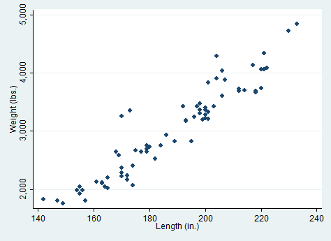
117 |
118 | Creating New Variables
119 | ----------------------
120 |
121 | There are a number of ways to create new variables or modifying
122 | existing variables. The most important command in this section is the
123 | `generate` command. Imagine we are curious about cars that are heavy
124 | for their length we could create a new variable
125 |
126 | generate weight_per_length = weight / length
127 |
128 | This creates a new column in the dataset, for each car we have
129 | calculated the ratio of that car's weight to its length. Let's take a
130 | look at the top five heaviest cars per length.
131 |
132 | gsort -weight_per_length
133 | list make weight_per_length if _n <= 5
134 |
135 | Another very useful command for generating new variables is the `egen`
136 | command. This is particularly useful is you want to merge summary
137 | statistics for groups of cars back into the larger dataset. For
138 | instance, we might be curious to see how a car's price compares to the
139 | average price among foreign or domestic cars. We can find the average
140 | price for foreign and domestic cars using tabstat, but how do we make
141 | a column in the dataset with these values?
142 |
143 | tabstat price, by(foreign)
144 | egen ave_price = mean(price), by(foreign)
145 | list foreign ave_price
146 |
147 | Regressions
148 | -----------
149 |
150 | To further explore the relationship between weight and length we can
151 | run a regression.
152 |
153 | regress weight length
154 |
155 | We see that on average, each additional inch is associated with 33
156 | pounds. We can plot the predicted values from the regression on the
157 | scatter plot from above.
158 |
159 | graph twoway (scatter weight length) (lfit weight length)
160 | graph export scatter_lfit.png, replace
161 |
162 | 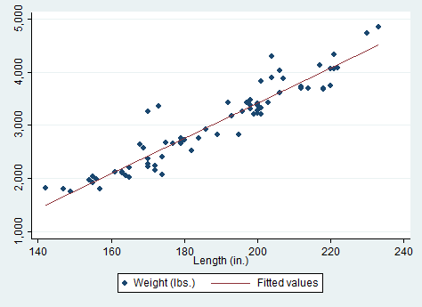
163 |
164 | Further Reading
165 | ---------------
166 |
167 | [Germán Rodríguez's Stata Tutorial][1] is an excellent introduction to
168 | Stata..
169 |
170 | These [notes on writing code][booth] by Matthew Gentzkow and Jesse
171 | Shapiro have excellent suggestions on how to program with Stata.
172 |
173 |
174 | [1]: http://data.princeton.edu/stata/
175 |
176 | [graphs1]: http://www.stata.com/support/faqs/graphics/gph/statagraphs.html
177 | [graphs2]: http://www.ats.ucla.edu/stat/Stata/library/GraphExamples/default.htm
178 | [graphs3]: http://www.survey-design.com.au/Usergraphs.html
179 |
180 | [booth]: http://faculty.chicagobooth.edu/matthew.gentzkow/research/ra_manual_coding.pdf
181 |
--------------------------------------------------------------------------------
/clustered-standard-errors.md:
--------------------------------------------------------------------------------
1 | ---
2 | layout: post
3 | title: xtreg fe - Clustered Standard Errors - Use Caution
4 | ---
5 |
6 | I have been implementing a fixed-effects estimator in Python so I can
7 | work with data that is too large to hold in memory. To make sure I
8 | was calculating my coefficients and standard errors correctly I have
9 | been comparing the calculations of my Python code to results from
10 | Stata. This lead me to find a surprising inconsistency in Stata's
11 | calculation of standard errors. I illustrate the issue by comparing
12 | standard errors computed by Stata's `xtreg fe` command to those
13 | computed by the standard `regress` command. To start, I use the first
14 | hundred observations of the `nlswork` dataset:
15 |
16 | . webuse nlswork, clear
17 | (National Longitudinal Survey. Young Women 14-26 years of age in 1968)
18 |
19 | . keep if _n <= 100
20 | (28434 observations deleted)
21 |
22 | I then estimate a fixed-effects model using regress:
23 |
24 | . regress ln_w age tenure i.idcode, vce(cluster idcode)
25 |
26 | Linear regression Number of obs = 99
27 | F( 1, 8) = .
28 | Prob > F = .
29 | R-squared = 0.5172
30 | Root MSE = .26493
31 |
32 | (Std. Err. adjusted for 9 clusters in idcode)
33 | ------------------------------------------------------------------------------
34 | | Robust
35 | ln_wage | Coef. Std. Err. t P>|t| [95% Conf. Interval]
36 | -------------+----------------------------------------------------------------
37 | age | .0025964 .0159834 0.16 0.875 -.0342613 .0394541
38 | tenure | .0356595 .0165 2.16 0.063 -.0023896 .0737086
39 | |
40 | idcode |
41 | 2 | -.4282753 .0207949 -20.60 0.000 -.4762285 -.3803222
42 | 3 | -.5313624 .0531705 -9.99 0.000 -.6539738 -.408751
43 | 4 | -.1054791 .0862957 -1.22 0.256 -.3044774 .0935192
44 | 5 | -.1976049 .0275788 -7.17 0.000 -.2612016 -.1340081
45 | 6 | -.4590234 .0484582 -9.47 0.000 -.5707681 -.3472787
46 | 7 | -.7201447 .0362701 -19.86 0.000 -.8037837 -.6365058
47 | 9 | -.2538001 .1237821 -2.05 0.074 -.5392421 .031642
48 | 10 | -.5417859 .1337093 -4.05 0.004 -.8501201 -.2334518
49 | |
50 | _cons | 1.922783 .4005497 4.80 0.001 .9991134 2.846452
51 | ------------------------------------------------------------------------------
52 |
53 | For comparison, I estimate the same model using `xtreg fe`:
54 |
55 | . xtset idcode
56 | panel variable: idcode (unbalanced)
57 |
58 | . xtreg ln_w age tenure, fe vce(cluster idcode)
59 |
60 | Fixed-effects (within) regression Number of obs = 99
61 | Group variable: idcode Number of groups = 9
62 |
63 | R-sq: within = 0.2358 Obs per group: min = 3
64 | between = 0.1373 avg = 11.0
65 | overall = 0.1740 max = 15
66 |
67 | F(2,8) = 14.98
68 | corr(u_i, Xb) = -0.0963 Prob > F = 0.0020
69 |
70 | (Std. Err. adjusted for 9 clusters in idcode)
71 | ------------------------------------------------------------------------------
72 | | Robust
73 | ln_wage | Coef. Std. Err. t P>|t| [95% Conf. Interval]
74 | -------------+----------------------------------------------------------------
75 | age | .0025964 .0153029 0.17 0.869 -.0326922 .0378849
76 | tenure | .0356595 .0157976 2.26 0.054 -.0007698 .0720888
77 | _cons | 1.583834 .3793026 4.18 0.003 .7091607 2.458508
78 | -------------+----------------------------------------------------------------
79 | sigma_u | .23415096
80 | sigma_e | .26492811
81 | rho | .43856575 (fraction of variance due to u_i)
82 | ------------------------------------------------------------------------------
83 |
84 | Notice that the coefficients on age and tenure match perfectly across
85 | the two regressions, but the standard errors calculated by `xtreg fe`
86 | are smaller. This is due to a difference in the degrees of freedom
87 | adjustment used. `regress` counts the fixed effects as coefficients
88 | estimated, while `xtreg fe` by default does not. As Kevin Goulding
89 | explains
90 | [here](http://thetarzan.wordpress.com/2011/06/11/clustered-standard-errors-in-r/),
91 | clustered standard errors are generally computed by multiplying the
92 | estimated asymptotic variance by (M / (M - 1)) ((N - 1) / (N - K)). M
93 | is the number of individuals, N is the number of observations, and K
94 | is the number of parameters estimated. The standard `regress` command
95 | correctly sets K = 12, `xtreg fe` sets K = 3. Making the asymptotic
96 | variance (99 - 12) / (99 - 3) = 0.90625 times the correct value.
97 |
98 | To get the correct standard errors from `xtreg fe` use the `dfadj`
99 | option:
100 |
101 | . xtreg ln_w age tenure, fe vce(cluster idcode) dfadj
102 |
103 | Fixed-effects (within) regression Number of obs = 99
104 | Group variable: idcode Number of groups = 9
105 |
106 | R-sq: within = 0.2358 Obs per group: min = 3
107 | between = 0.1373 avg = 11.0
108 | overall = 0.1740 max = 15
109 |
110 | F(2,8) = 13.73
111 | corr(u_i, Xb) = -0.0963 Prob > F = 0.0026
112 |
113 | (Std. Err. adjusted for 9 clusters in idcode)
114 | ------------------------------------------------------------------------------
115 | | Robust
116 | ln_wage | Coef. Std. Err. t P>|t| [95% Conf. Interval]
117 | -------------+----------------------------------------------------------------
118 | age | .0025964 .0159834 0.16 0.875 -.0342613 .0394541
119 | tenure | .0356595 .0165 2.16 0.063 -.0023896 .0737086
120 | _cons | 1.583834 .3961687 4.00 0.004 .6702675 2.497401
121 | -------------+----------------------------------------------------------------
122 | sigma_u | .23415096
123 | sigma_e | .26492811
124 | rho | .43856575 (fraction of variance due to u_i)
125 | ------------------------------------------------------------------------------
126 |
127 | This seems like an option that could be missed easily.
128 |
--------------------------------------------------------------------------------
/tutorial.md:
--------------------------------------------------------------------------------
1 | ---
2 | layout: post
3 | title: Stata Tutorial
4 | ---
5 |
6 |
7 | Stata is a commonly used tool for empirical research. Stata comes
8 | with an extensive library of statistical methods, and there are
9 | additional user written methods that extend the functionality of Stata
10 | even further.
11 |
12 | Stata stores data in memory as a single matrix. If you are familiar
13 | with Microsoft Excel Workbooks, Stata stores a single Worksheet in
14 | memory where each column has a name and each row is numbered from 1 to
15 | the total number of rows in the dataset.
16 |
17 | This tutorial aims to introduce you to the key features of Stata and
18 | its documentation so you can start your own empirical work.
19 |
20 | Typing Commands
21 | ---------------
22 |
23 | The `display` command is useful for showing values at the command
24 | line.
25 |
26 | . display 1 + 2
27 | 3
28 |
29 | Use the `Page Up` key to recall the previous command evaluated. This
30 | is particularly useful if you need to fix a typo.
31 |
32 | Commands can be abbreviated, `di` is equivalent to `display`. I
33 | prefer to use the whole command name because it makes code explicit.
34 |
35 | Getting Help
36 | ------------
37 |
38 | Use the `help` command if you know the name of the function and want
39 | more details. Use the `findit` command if you want to find a
40 | function. I end up using Google more than `findit`, but this may be a
41 | mistake.
42 |
43 | Unfortunately the help command opens a new window each time you use
44 | it, use the `nonew` option to prevent this behavior,
45 | `help help, nonew`.
46 |
47 |
48 | Reading Data Into Stata
49 | -----------------------
50 |
51 | There are many different ways to read data into Stata. To get a good
52 | overview of how to import data into Stata type `help import` in
53 | Stata's Command window. The functions I use most are `import excel`
54 | and `insheet`. `import excel` is great if you are working with an
55 | Excel workbook, while `insheet` is great if you have a comma-separated
56 | values (csv) file.
57 |
58 | Stata datasets are generally stored in files with a `.dta` extension.
59 | To read a Stata dataset use the `use` command. For the purpose of
60 | this tutorial we will use a dataset shipped with Stata about
61 | automobiles. Type in `sysuse auto` to load the dataset into memory.
62 |
63 | . sysuse auto, clear
64 | (1978 Automobile Data)
65 |
66 | Descriptive Statistics
67 | ----------------------
68 |
69 | The `describe` command gives useful information about the variables in
70 | the dataset and the number of rows in the dataset.
71 |
72 | . describe
73 |
74 | Contains data from /Applications/Stata/ado/base/a/auto.dta
75 | obs: 74 1978 Automobile Data
76 | vars: 12 13 Apr 2011 17:45
77 | size: 3,182 (_dta has notes)
78 | --------------------------------------------------------------------------------------------------------
79 | storage display value
80 | variable name type format label variable label
81 | --------------------------------------------------------------------------------------------------------
82 | make str18 %-18s Make and Model
83 | price int %8.0gc Price
84 | mpg int %8.0g Mileage (mpg)
85 | rep78 int %8.0g Repair Record 1978
86 | headroom float %6.1f Headroom (in.)
87 | trunk int %8.0g Trunk space (cu. ft.)
88 | weight int %8.0gc Weight (lbs.)
89 | length int %8.0g Length (in.)
90 | turn int %8.0g Turn Circle (ft.)
91 | displacement int %8.0g Displacement (cu. in.)
92 | gear_ratio float %6.2f Gear Ratio
93 | foreign byte %8.0g origin Car type
94 | --------------------------------------------------------------------------------------------------------
95 | Sorted by: foreign
96 |
97 | The `summarize` command gives some useful summary statistics for each
98 | variable.
99 |
100 | . summarize
101 |
102 | Variable | Obs Mean Std. Dev. Min Max
103 | -------------+--------------------------------------------------------
104 | make | 0
105 | price | 74 6165.257 2949.496 3291 15906
106 | mpg | 74 21.2973 5.785503 12 41
107 | rep78 | 69 3.405797 .9899323 1 5
108 | headroom | 74 2.993243 .8459948 1.5 5
109 | -------------+--------------------------------------------------------
110 | trunk | 74 13.75676 4.277404 5 23
111 | weight | 74 3019.459 777.1936 1760 4840
112 | length | 74 187.9324 22.26634 142 233
113 | turn | 74 39.64865 4.399354 31 51
114 | displacement | 74 197.2973 91.83722 79 425
115 | -------------+--------------------------------------------------------
116 | gear_ratio | 74 3.014865 .4562871 2.19 3.89
117 | foreign | 74 .2972973 .4601885 0 1
118 |
119 | You'll notice that 11 of 12 variables in the auto dataset are numeric
120 | and the `make` variable is a string. To see what the make variable
121 | looks like, we can list the first few observations.
122 |
123 | . list make if _n <= 5
124 |
125 | +---------------+
126 | | make |
127 | |---------------|
128 | 1. | AMC Concord |
129 | 2. | AMC Pacer |
130 | 3. | AMC Spirit |
131 | 4. | Buick Century |
132 | 5. | Buick Electra |
133 | +---------------+
134 |
135 | To see if `make` uniquely identifies each row in the dataset we can
136 | use the `isid` function.
137 |
138 | . isid make
139 |
140 | When `isid` says nothing the variable list does uniquely identify each
141 | row. Are cars uniquely identified by their weight and length?
142 |
143 | . duplicates report make
144 |
145 | Duplicates in terms of make
146 |
147 | --------------------------------------
148 | copies | observations surplus
149 | ----------+---------------------------
150 | 1 | 74 0
151 | --------------------------------------
152 |
153 | . duplicates report weight length
154 |
155 | Duplicates in terms of weight length
156 |
157 | --------------------------------------
158 | copies | observations surplus
159 | ----------+---------------------------
160 | 1 | 70 0
161 | 2 | 4 2
162 | --------------------------------------
163 |
164 | Imagine we are interested in looking at how foreign and domestic cars
165 | differ. As a first step, it would be good to examine some summary
166 | statistics for foreign and domestic cars, the `tabstat` command makes
167 | this fairly easy.
168 |
169 | . tabstat price mpg weight length, by(foreign) stat(mean sd)
170 |
171 | Summary statistics: mean, sd
172 | by categories of: foreign (Car type)
173 |
174 | foreign | price mpg weight length
175 | ---------+----------------------------------------
176 | Domestic | 6072.423 19.82692 3317.115 196.1346
177 | | 3097.104 4.743297 695.3637 20.04605
178 | ---------+----------------------------------------
179 | Foreign | 6384.682 24.77273 2315.909 168.5455
180 | | 2621.915 6.611187 433.0035 13.68255
181 | ---------+----------------------------------------
182 | Total | 6165.257 21.2973 3019.459 187.9324
183 | | 2949.496 5.785503 777.1936 22.26634
184 | --------------------------------------------------
185 |
186 | You may have noticed from the output of the `summarize` command that
187 | `rep78` has 5 missing values. We can look at those observations using
188 | the list command:
189 |
190 | . list if missing(rep78)
191 |
192 | +---------------------------------------------------------------------------------------------+
193 | 3. | make | price | mpg | rep78 | headroom | trunk | weight | length | turn | displa~t |
194 | | AMC Spirit | 3,799 | 22 | . | 3.0 | 12 | 2,640 | 168 | 35 | 121 |
195 | |---------------------------------------------------------------------------------------------|
196 | | gear_r~o | foreign |
197 | | 3.08 | Domestic |
198 | +---------------------------------------------------------------------------------------------+
199 |
200 | +---------------------------------------------------------------------------------------------+
201 | 7. | make | price | mpg | rep78 | headroom | trunk | weight | length | turn | displa~t |
202 | | Buick Opel | 4,453 | 26 | . | 3.0 | 10 | 2,230 | 170 | 34 | 304 |
203 | |---------------------------------------------------------------------------------------------|
204 | | gear_r~o | foreign |
205 | | 2.87 | Domestic |
206 | +---------------------------------------------------------------------------------------------+
207 |
208 | +---------------------------------------------------------------------------------------------+
209 | 45. | make | price | mpg | rep78 | headroom | trunk | weight | length | turn | displa~t |
210 | | Plym. Sapporo | 6,486 | 26 | . | 1.5 | 8 | 2,520 | 182 | 38 | 119 |
211 | |---------------------------------------------------------------------------------------------|
212 | | gear_r~o | foreign |
213 | | 3.54 | Domestic |
214 | +---------------------------------------------------------------------------------------------+
215 |
216 | +---------------------------------------------------------------------------------------------+
217 | 51. | make | price | mpg | rep78 | headroom | trunk | weight | length | turn | displa~t |
218 | | Pont. Phoenix | 4,424 | 19 | . | 3.5 | 13 | 3,420 | 203 | 43 | 231 |
219 | |---------------------------------------------------------------------------------------------|
220 | | gear_r~o | foreign |
221 | | 3.08 | Domestic |
222 | +---------------------------------------------------------------------------------------------+
223 |
224 | +---------------------------------------------------------------------------------------------+
225 | 64. | make | price | mpg | rep78 | headroom | trunk | weight | length | turn | displa~t |
226 | | Peugeot 604 | 12,990 | 14 | . | 3.5 | 14 | 3,420 | 192 | 38 | 163 |
227 | |---------------------------------------------------------------------------------------------|
228 | | gear_r~o | foreign |
229 | | 3.58 | Foreign |
230 | +---------------------------------------------------------------------------------------------+
231 |
232 | Graphs
233 | ------
234 |
235 | There are good graph galleries provided by [StataCorp][graphs1],
236 | [UCLA][graphs2], and [Survey Design and Analysis Services][graphs3].
237 | Below is a simple scatter plot of weight versus length:
238 |
239 | . graph twoway scatter weight length
240 |
241 | . graph export scatter.png, replace
242 | (file scatter.png written in PNG format)
243 |
244 | 
245 |
246 | Creating New Variables
247 | ----------------------
248 |
249 | There are a number of ways to create new variables or modifying
250 | existing variables. The most important command in this section is the
251 | `generate` command. Imagine we are curious about cars that are heavy
252 | for their length we could create a new variable
253 |
254 | . generate weight_per_length = weight / length
255 |
256 | This creates a new column in the dataset, for each car we have
257 | calculated the ratio of that car's weight to its length. Let's take a
258 | look at the top five heaviest cars per length.
259 |
260 | . gsort -weight_per_length
261 |
262 | . list make weight_per_length if _n <= 5
263 |
264 | +------------------------------+
265 | | make weight~h |
266 | |------------------------------|
267 | 1. | Cad. Seville 21.02941 |
268 | 2. | Linc. Continental 20.77253 |
269 | 3. | Linc. Mark V 20.52174 |
270 | 4. | Cad. Deville 19.59276 |
271 | 5. | Olds Toronado 19.56311 |
272 | +------------------------------+
273 |
274 | Another very useful command for generating new variables is the `egen`
275 | command. This is particularly useful is you want to merge summary
276 | statistics for groups of cars back into the larger dataset. For
277 | instance, we might be curious to see how a car's price compares to the
278 | average price among foreign or domestic cars. We can find the average
279 | price for foreign and domestic cars using tabstat, but how do we make
280 | a column in the dataset with these values?
281 |
282 | . tabstat price, by(foreign)
283 |
284 | Summary for variables: price
285 | by categories of: foreign (Car type)
286 |
287 | foreign | mean
288 | ---------+----------
289 | Domestic | 6072.423
290 | Foreign | 6384.682
291 | ---------+----------
292 | Total | 6165.257
293 | --------------------
294 |
295 | . egen ave_price = mean(price), by(foreign)
296 |
297 | . list foreign ave_price
298 |
299 | +---------------------+
300 | | foreign ave_pr~e |
301 | |---------------------|
302 | 1. | Domestic 6072.423 |
303 | 2. | Domestic 6072.423 |
304 | 3. | Domestic 6072.423 |
305 | 4. | Domestic 6072.423 |
306 | 5. | Domestic 6072.423 |
307 | |---------------------|
308 | 6. | Domestic 6072.423 |
309 | 7. | Domestic 6072.423 |
310 | 8. | Domestic 6072.423 |
311 | 9. | Domestic 6072.423 |
312 | 10. | Domestic 6072.423 |
313 | |---------------------|
314 | 11. | Domestic 6072.423 |
315 | 12. | Domestic 6072.423 |
316 | 13. | Domestic 6072.423 |
317 | 14. | Domestic 6072.423 |
318 | 15. | Foreign 6384.682 |
319 | |---------------------|
320 | 16. | Domestic 6072.423 |
321 | 17. | Domestic 6072.423 |
322 | 18. | Domestic 6072.423 |
323 | 19. | Domestic 6072.423 |
324 | 20. | Domestic 6072.423 |
325 | |---------------------|
326 | 21. | Domestic 6072.423 |
327 | 22. | Domestic 6072.423 |
328 | 23. | Domestic 6072.423 |
329 | 24. | Domestic 6072.423 |
330 | 25. | Domestic 6072.423 |
331 | |---------------------|
332 | 26. | Domestic 6072.423 |
333 | 27. | Domestic 6072.423 |
334 | 28. | Domestic 6072.423 |
335 | 29. | Domestic 6072.423 |
336 | 30. | Domestic 6072.423 |
337 | |---------------------|
338 | 31. | Domestic 6072.423 |
339 | 32. | Domestic 6072.423 |
340 | 33. | Domestic 6072.423 |
341 | 34. | Domestic 6072.423 |
342 | 35. | Foreign 6384.682 |
343 | |---------------------|
344 | 36. | Domestic 6072.423 |
345 | 37. | Domestic 6072.423 |
346 | 38. | Domestic 6072.423 |
347 | 39. | Domestic 6072.423 |
348 | 40. | Domestic 6072.423 |
349 | |---------------------|
350 | 41. | Domestic 6072.423 |
351 | 42. | Domestic 6072.423 |
352 | 43. | Domestic 6072.423 |
353 | 44. | Foreign 6384.682 |
354 | 45. | Domestic 6072.423 |
355 | |---------------------|
356 | 46. | Domestic 6072.423 |
357 | 47. | Foreign 6384.682 |
358 | 48. | Foreign 6384.682 |
359 | 49. | Foreign 6384.682 |
360 | 50. | Domestic 6072.423 |
361 | |---------------------|
362 | 51. | Domestic 6072.423 |
363 | 52. | Foreign 6384.682 |
364 | 53. | Foreign 6384.682 |
365 | 54. | Domestic 6072.423 |
366 | 55. | Foreign 6384.682 |
367 | |---------------------|
368 | 56. | Domestic 6072.423 |
369 | 57. | Foreign 6384.682 |
370 | 58. | Foreign 6384.682 |
371 | 59. | Foreign 6384.682 |
372 | 60. | Domestic 6072.423 |
373 | |---------------------|
374 | 61. | Foreign 6384.682 |
375 | 62. | Domestic 6072.423 |
376 | 63. | Domestic 6072.423 |
377 | 64. | Foreign 6384.682 |
378 | 65. | Foreign 6384.682 |
379 | |---------------------|
380 | 66. | Foreign 6384.682 |
381 | 67. | Foreign 6384.682 |
382 | 68. | Foreign 6384.682 |
383 | 69. | Foreign 6384.682 |
384 | 70. | Domestic 6072.423 |
385 | |---------------------|
386 | 71. | Foreign 6384.682 |
387 | 72. | Foreign 6384.682 |
388 | 73. | Foreign 6384.682 |
389 | 74. | Domestic 6072.423 |
390 | +---------------------+
391 |
392 | Regressions
393 | -----------
394 |
395 | To further explore the relationship between weight and length we can
396 | run a regression.
397 |
398 | . regress weight length
399 |
400 | Source | SS df MS Number of obs = 74
401 | -------------+------------------------------ F( 1, 72) = 613.27
402 | Model | 39461306.8 1 39461306.8 Prob > F = 0.0000
403 | Residual | 4632871.55 72 64345.4382 R-squared = 0.8949
404 | -------------+------------------------------ Adj R-squared = 0.8935
405 | Total | 44094178.4 73 604029.841 Root MSE = 253.66
406 |
407 | ------------------------------------------------------------------------------
408 | weight | Coef. Std. Err. t P>|t| [95% Conf. Interval]
409 | -------------+----------------------------------------------------------------
410 | length | 33.01988 1.333364 24.76 0.000 30.36187 35.67789
411 | _cons | -3186.047 252.3113 -12.63 0.000 -3689.02 -2683.073
412 | ------------------------------------------------------------------------------
413 |
414 | We see that on average, each additional inch is associated with 33
415 | pounds. We can plot the predicted values from the regression on the
416 | scatter plot from above.
417 |
418 | . graph twoway (scatter weight length) (lfit weight length)
419 |
420 | . graph export scatter_lfit.png, replace
421 | (file scatter_lfit.png written in PNG format)
422 |
423 | 
424 |
425 | Further Reading
426 | ---------------
427 |
428 | [Germán Rodríguez's Stata Tutorial][1] is an excellent introduction to
429 | Stata..
430 |
431 | These [notes on writing code][booth] by Matthew Gentzkow and Jesse
432 | Shapiro have excellent suggestions on how to program with Stata.
433 |
434 |
435 | [1]: http://data.princeton.edu/stata/
436 |
437 | [graphs1]: http://www.stata.com/support/faqs/graphics/gph/statagraphs.html
438 | [graphs2]: http://www.ats.ucla.edu/stat/Stata/library/GraphExamples/default.htm
439 | [graphs3]: http://www.survey-design.com.au/Usergraphs.html
440 |
441 | [booth]: http://faculty.chicagobooth.edu/matthew.gentzkow/research/ra_manual_coding.pdf
442 |
--------------------------------------------------------------------------------