├── .gitignore
├── .pylintrc
├── .readthedocs.yml
├── CHANGELOG.md
├── LICENSE
├── README.md
├── docs
├── Makefile
├── make.bat
├── quick_start.png
├── quick_start_radar.png
└── source
│ ├── Mplsoccer logo github.jpg
│ ├── api.rst
│ ├── conf.py
│ ├── explain_standardizer.png
│ ├── index.rst
│ ├── installation.rst
│ ├── logo-white.png
│ ├── logo.png
│ ├── mplsoccer.bumpy_chart.rst
│ ├── mplsoccer.grid.rst
│ ├── mplsoccer.linecollection.rst
│ ├── mplsoccer.pitch.rst
│ ├── mplsoccer.py_pizza.rst
│ ├── mplsoccer.quiver.rst
│ ├── mplsoccer.radar_chart.rst
│ ├── mplsoccer.statsbomb.rst
│ └── mplsoccer.utils.rst
├── examples
├── README.rst
├── bumpy_charts
│ ├── README.rst
│ └── plot_bumpy.py
├── pitch_plots
│ ├── README.rst
│ ├── plot_animation.py
│ ├── plot_arrows.py
│ ├── plot_cmap.py
│ ├── plot_convex_hull.py
│ ├── plot_cyberpunk.py
│ ├── plot_delaunay.py
│ ├── plot_fbref.py
│ ├── plot_flow.py
│ ├── plot_formations.py
│ ├── plot_grid.py
│ ├── plot_heatmap.py
│ ├── plot_heatmap_positional.py
│ ├── plot_hexbin.py
│ ├── plot_jointgrid.py
│ ├── plot_kde.py
│ ├── plot_lines.py
│ ├── plot_markers.py
│ ├── plot_pass_network.py
│ ├── plot_photo.py
│ ├── plot_sb360_frame.py
│ ├── plot_scatter.py
│ ├── plot_shot_freeze_frame.py
│ ├── plot_standardize.py
│ ├── plot_textured_background.py
│ ├── plot_twitter_powerpoint.py
│ └── plot_voronoi.py
├── pitch_setup
│ ├── README.rst
│ ├── plot_compare_pitches.py
│ ├── plot_explain_standardizer.py
│ ├── plot_pitch_types.py
│ ├── plot_pitches.py
│ └── plot_quick_start.py
├── pizza_plots
│ ├── README.rst
│ ├── plot_pizza_basic.py
│ ├── plot_pizza_colorful.py
│ ├── plot_pizza_comparison.py
│ ├── plot_pizza_comparison_vary_scales.py
│ ├── plot_pizza_dark_theme.py
│ ├── plot_pizza_different_units.py
│ └── plot_pizza_scales_vary.py
├── radar
│ ├── README.rst
│ ├── plot_radar.py
│ └── plot_turbine.py
├── sonars
│ ├── README.rst
│ ├── plot_bin_statistic_sonar.py
│ ├── plot_sonar.py
│ └── plot_sonar_grid.py
├── statsbomb
│ ├── README.rst
│ └── plot_statsbomb_data.py
└── tutorials
│ ├── README.rst
│ ├── plot_pass_sonar_kde.py
│ ├── plot_wedges.py
│ ├── plot_xt.py
│ └── plot_xt_improvements.py
├── mplsoccer
├── __about__.py
├── __init__.py
├── _pitch_base.py
├── _pitch_plot.py
├── bumpy_chart.py
├── cm.py
├── dimensions.py
├── formations.py
├── grid.py
├── heatmap.py
├── linecollection.py
├── pitch.py
├── py_pizza.py
├── quiver.py
├── radar_chart.py
├── scatterutils.py
├── statsbomb.py
└── utils.py
├── pyproject.toml
└── tests
├── __init__.py
├── test_bin_statistic.py
├── test_grid.py
└── test_standarizer.py
/.gitignore:
--------------------------------------------------------------------------------
1 |
2 | # Created by https://www.toptal.com/developers/gitignore/api/python
3 | # Edit at https://www.toptal.com/developers/gitignore?templates=python
4 |
5 | ### Python ###
6 | # Byte-compiled / optimized / DLL files
7 | __pycache__/
8 | *.py[cod]
9 | *$py.class
10 |
11 | # C extensions
12 | *.so
13 |
14 | # Mac
15 | .DS_Store
16 |
17 | # Distribution / packaging
18 | .Python
19 | build/
20 | develop-eggs/
21 | dist/
22 | downloads/
23 | eggs/
24 | .eggs/
25 | lib/
26 | lib64/
27 | parts/
28 | sdist/
29 | var/
30 | wheels/
31 | pip-wheel-metadata/
32 | share/python-wheels/
33 | *.egg-info/
34 | .installed.cfg
35 | *.egg
36 | MANIFEST
37 |
38 | # PyInstaller
39 | # Usually these files are written by a python script from a template
40 | # before PyInstaller builds the exe, so as to inject date/other infos into it.
41 | *.manifest
42 | *.spec
43 |
44 | # Installer logs
45 | pip-log.txt
46 | pip-delete-this-directory.txt
47 |
48 | # Unit test / coverage reports
49 | htmlcov/
50 | .tox/
51 | .nox/
52 | .coverage
53 | .coverage.*
54 | .cache
55 | nosetests.xml
56 | coverage.xml
57 | *.cover
58 | *.py,cover
59 | .hypothesis/
60 | .pytest_cache/
61 | pytestdebug.log
62 |
63 | # Translations
64 | *.mo
65 | *.pot
66 |
67 | # Django stuff:
68 | *.log
69 | local_settings.py
70 | db.sqlite3
71 | db.sqlite3-journal
72 |
73 | # Flask stuff:
74 | instance/
75 | .webassets-cache
76 |
77 | # Scrapy stuff:
78 | .scrapy
79 |
80 | # Sphinx documentation
81 | docs/_build/
82 | doc/_build/
83 |
84 | # PyBuilder
85 | target/
86 |
87 | # Jupyter Notebook
88 | .ipynb_checkpoints
89 | */.ipynb_checkpoints/*
90 |
91 | # IPython
92 | profile_default/
93 | ipython_config.py
94 |
95 | # pyenv
96 | .python-version
97 |
98 | # pipenv
99 | # According to pypa/pipenv#598, it is recommended to include Pipfile.lock in version control.
100 | # However, in case of collaboration, if having platform-specific dependencies or dependencies
101 | # having no cross-platform support, pipenv may install dependencies that don't work, or not
102 | # install all needed dependencies.
103 | #Pipfile.lock
104 |
105 | # PEP 582; used by e.g. github.com/David-OConnor/pyflow
106 | __pypackages__/
107 |
108 | # Celery stuff
109 | celerybeat-schedule
110 | celerybeat.pid
111 |
112 | # SageMath parsed files
113 | *.sage.py
114 |
115 | # Environments
116 | .env
117 | .venv
118 | env/
119 | venv/
120 | ENV/
121 | env.bak/
122 | venv.bak/
123 |
124 | # Spyder project settings
125 | .spyderproject
126 | .spyproject
127 |
128 | # Rope project settings
129 | .ropeproject
130 |
131 | # mkdocs documentation
132 | /site
133 |
134 | # mypy
135 | .mypy_cache/
136 | .dmypy.json
137 | dmypy.json
138 |
139 | # Pyre type checker
140 | .pyre/
141 |
142 | # pytype static type analyzer
143 | .pytype/
144 |
145 | # End of https://www.toptal.com/developers/gitignore/api/python
146 |
147 | # ignore binaries for programs and plugins
148 | *.exe
149 | *.dll
150 | *.dylib
151 | *.parquet
152 |
153 | # do not version control autogenerated gallery
154 | docs/source/gallery
155 |
156 | # ignore desktop.ini
157 | desktop.ini
158 |
159 | # ignore data directory
160 | data/
161 |
162 | *idea/
--------------------------------------------------------------------------------
/.readthedocs.yml:
--------------------------------------------------------------------------------
1 | # .readthedocs.yml
2 | # Read the Docs configuration file
3 | # See https://docs.readthedocs.io/en/stable/config-file/v2.html for details
4 |
5 | # Required
6 | version: 2
7 |
8 | build:
9 | os: ubuntu-24.04
10 | apt_packages:
11 | - python3-lxml
12 | tools:
13 | python: "3.12"
14 | jobs:
15 | create_environment:
16 | - asdf plugin add uv
17 | - asdf install uv latest
18 | - asdf global uv latest
19 | - UV_PROJECT_ENVIRONMENT=$READTHEDOCS_VIRTUALENV_PATH uv venv --python 3.12
20 | install:
21 | - uv pip install --editable . --group docs
22 |
23 | # Build documentation in the docs/ directory with Sphinx
24 | sphinx:
25 | configuration: docs/source/conf.py
26 |
--------------------------------------------------------------------------------
/LICENSE:
--------------------------------------------------------------------------------
1 | MIT License
2 |
3 | Copyright (c) 2025 Anmol Durgapal, Andrew Rowlinson
4 |
5 | Permission is hereby granted, free of charge, to any person obtaining a copy
6 | of this software and associated documentation files (the "Software"), to deal
7 | in the Software without restriction, including without limitation the rights
8 | to use, copy, modify, merge, publish, distribute, sublicense, and/or sell
9 | copies of the Software, and to permit persons to whom the Software is
10 | furnished to do so, subject to the following conditions:
11 |
12 | The above copyright notice and this permission notice shall be included in all
13 | copies or substantial portions of the Software.
14 |
15 | THE SOFTWARE IS PROVIDED "AS IS", WITHOUT WARRANTY OF ANY KIND, EXPRESS OR
16 | IMPLIED, INCLUDING BUT NOT LIMITED TO THE WARRANTIES OF MERCHANTABILITY,
17 | FITNESS FOR A PARTICULAR PURPOSE AND NONINFRINGEMENT. IN NO EVENT SHALL THE
18 | AUTHORS OR COPYRIGHT HOLDERS BE LIABLE FOR ANY CLAIM, DAMAGES OR OTHER
19 | LIABILITY, WHETHER IN AN ACTION OF CONTRACT, TORT OR OTHERWISE, ARISING FROM,
20 | OUT OF OR IN CONNECTION WITH THE SOFTWARE OR THE USE OR OTHER DEALINGS IN THE
21 | SOFTWARE.
--------------------------------------------------------------------------------
/README.md:
--------------------------------------------------------------------------------
1 | 
2 |
3 | **mplsoccer is a Python library for plotting soccer/football charts in Matplotlib
4 | and loading StatsBomb open-data.**
5 |
6 | ---
7 |
8 | ## Installation
9 |
10 | Use the package manager [pip](https://pip.pypa.io/en/stable/) to install mplsoccer.
11 |
12 | ```bash
13 | pip install mplsoccer
14 | ```
15 |
16 | Or install via [Anaconda](https://docs.anaconda.com/free/anaconda/install/index.html).
17 |
18 | ```bash
19 | conda install -c conda-forge mplsoccer
20 | ```
21 |
22 | ---
23 |
24 | ## Docs
25 |
26 | Read more in the [docs](https://mplsoccer.readthedocs.io/) and see some
27 | examples in our [gallery](https://mplsoccer.readthedocs.io/en/latest/gallery/index.html).
28 |
29 | ---
30 |
31 | ## Quick start
32 |
33 | Plot a StatsBomb pitch
34 |
35 | ```python
36 | from mplsoccer import Pitch
37 | import matplotlib.pyplot as plt
38 | pitch = Pitch(pitch_color='grass', line_color='white', stripe=True)
39 | fig, ax = pitch.draw()
40 | plt.show()
41 | ```
42 | 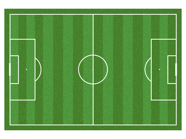
43 |
44 | Plot a Radar
45 | ```python
46 | from mplsoccer import Radar
47 | import matplotlib.pyplot as plt
48 | radar = Radar(params=['Agility', 'Speed', 'Strength'], min_range=[0, 0, 0], max_range=[10, 10, 10])
49 | fig, ax = radar.setup_axis()
50 | rings_inner = radar.draw_circles(ax=ax, facecolor='#ffb2b2', edgecolor='#fc5f5f')
51 | values = [5, 3, 10]
52 | radar_poly, rings, vertices = radar.draw_radar(values, ax=ax,
53 | kwargs_radar={'facecolor': '#00f2c1', 'alpha': 0.6},
54 | kwargs_rings={'facecolor': '#d80499', 'alpha': 0.6})
55 | range_labels = radar.draw_range_labels(ax=ax)
56 | param_labels = radar.draw_param_labels(ax=ax)
57 | plt.show()
58 | ```
59 | 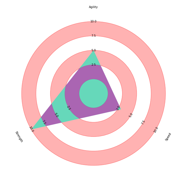
60 |
61 | ---
62 |
63 | ## What is mplsoccer?
64 | In mplsoccer, you can:
65 |
66 | - plot football/soccer pitches on nine different pitch types
67 | - plot radar charts
68 | - plot Nightingale/pizza charts
69 | - plot bumpy charts for showing changes over time
70 | - plot arrows, heatmaps, hexbins, scatter, and (comet) lines
71 | - load StatsBomb data as a tidy dataframe
72 | - standardize pitch coordinates into a single format
73 |
74 | I hope mplsoccer helps you make insightful graphics faster,
75 | so you don't have to build charts from scratch.
76 |
77 | ---
78 |
79 | ## Want to help?
80 | I would love the community to get involved in mplsoccer.
81 | Take a look at our [open-issues](https://github.com/andrewRowlinson/mplsoccer/issues)
82 | for inspiration.
83 | Please get in touch at rowlinsonandy@gmail.com or
84 | [@numberstorm](https://twitter.com/numberstorm) on Twitter to find out more.
85 |
86 | ---
87 |
88 | ## Recent changes
89 |
90 | View the [changelog](https://github.com/andrewRowlinson/mplsoccer/blob/master/CHANGELOG.md)
91 | for a full list of the recent changes to mplsoccer.
92 |
93 | ---
94 |
95 | ## Inspiration
96 |
97 | mplsoccer was inspired by:
98 | - [Peter McKeever](https://petermckeever.com/) heavily inspired the API design
99 | - [ggsoccer](https://github.com/Torvaney/ggsoccer) influenced the design and Standardizer
100 | - [lastrow's](https://twitter.com/lastrowview) legendary animations
101 | - [fcrstats'](https://twitter.com/FC_rstats) tutorials for using football data
102 | - [fcpython's](https://fcpython.com/) Python tutorials for using football data
103 | - [Karun Singh's](https://twitter.com/karun1710) expected threat (xT) visualizations
104 | - [StatsBomb's](https://statsbomb.com/) great visual design and free open-data
105 | - John Burn-Murdoch's [tweet](https://twitter.com/jburnmurdoch/status/1057907312030085120) got me
106 | interested in football analytics
107 |
108 | ---
109 |
110 | ## License
111 |
112 | [MIT](https://choosealicense.com/licenses/mit)
113 |
--------------------------------------------------------------------------------
/docs/Makefile:
--------------------------------------------------------------------------------
1 | # Minimal makefile for Sphinx documentation
2 | #
3 |
4 | # You can set these variables from the command line, and also
5 | # from the environment for the first two.
6 | SPHINXOPTS ?=
7 | SPHINXBUILD ?= sphinx-build
8 | SOURCEDIR = source
9 | BUILDDIR = build
10 |
11 | # Put it first so that "make" without argument is like "make help".
12 | help:
13 | @$(SPHINXBUILD) -M help "$(SOURCEDIR)" "$(BUILDDIR)" $(SPHINXOPTS) $(O)
14 |
15 | .PHONY: help Makefile
16 |
17 | # Catch-all target: route all unknown targets to Sphinx using the new
18 | # "make mode" option. $(O) is meant as a shortcut for $(SPHINXOPTS).
19 | %: Makefile
20 | @$(SPHINXBUILD) -M $@ "$(SOURCEDIR)" "$(BUILDDIR)" $(SPHINXOPTS) $(O)
21 |
--------------------------------------------------------------------------------
/docs/make.bat:
--------------------------------------------------------------------------------
1 | @ECHO OFF
2 |
3 | pushd %~dp0
4 |
5 | REM Command file for Sphinx documentation
6 |
7 | if "%SPHINXBUILD%" == "" (
8 | set SPHINXBUILD=sphinx-build
9 | )
10 | set SOURCEDIR=source
11 | set BUILDDIR=build
12 |
13 | if "%1" == "" goto help
14 |
15 | %SPHINXBUILD% >NUL 2>NUL
16 | if errorlevel 9009 (
17 | echo.
18 | echo.The 'sphinx-build' command was not found. Make sure you have Sphinx
19 | echo.installed, then set the SPHINXBUILD environment variable to point
20 | echo.to the full path of the 'sphinx-build' executable. Alternatively you
21 | echo.may add the Sphinx directory to PATH.
22 | echo.
23 | echo.If you don't have Sphinx installed, grab it from
24 | echo.http://sphinx-doc.org/
25 | exit /b 1
26 | )
27 |
28 | %SPHINXBUILD% -M %1 %SOURCEDIR% %BUILDDIR% %SPHINXOPTS% %O%
29 | goto end
30 |
31 | :help
32 | %SPHINXBUILD% -M help %SOURCEDIR% %BUILDDIR% %SPHINXOPTS% %O%
33 |
34 | :end
35 | popd
36 |
--------------------------------------------------------------------------------
/docs/quick_start.png:
--------------------------------------------------------------------------------
https://raw.githubusercontent.com/andrewRowlinson/mplsoccer/d1965987e410efcc0079ad279cbf43d053430b2d/docs/quick_start.png
--------------------------------------------------------------------------------
/docs/quick_start_radar.png:
--------------------------------------------------------------------------------
https://raw.githubusercontent.com/andrewRowlinson/mplsoccer/d1965987e410efcc0079ad279cbf43d053430b2d/docs/quick_start_radar.png
--------------------------------------------------------------------------------
/docs/source/Mplsoccer logo github.jpg:
--------------------------------------------------------------------------------
https://raw.githubusercontent.com/andrewRowlinson/mplsoccer/d1965987e410efcc0079ad279cbf43d053430b2d/docs/source/Mplsoccer logo github.jpg
--------------------------------------------------------------------------------
/docs/source/api.rst:
--------------------------------------------------------------------------------
1 | API
2 | ===
3 |
4 | .. toctree::
5 | :maxdepth: 2
6 |
7 | mplsoccer.pitch
8 | mplsoccer.radar_chart
9 | mplsoccer.statsbomb
10 | mplsoccer.bumpy_chart
11 | mplsoccer.py_pizza
12 | mplsoccer.utils
13 | mplsoccer.quiver
14 | mplsoccer.linecollection
15 | mplsoccer.grid
16 |
--------------------------------------------------------------------------------
/docs/source/conf.py:
--------------------------------------------------------------------------------
1 | # Configuration file for the Sphinx documentation builder.
2 | #
3 | # This file only contains a selection of the most common options. For a full
4 | # list see the documentation:
5 | # https://www.sphinx-doc.org/en/master/usage/configuration.html
6 |
7 | # -- Path setup --------------------------------------------------------------
8 |
9 | # If extensions (or modules to document with autodoc) are in another directory,
10 | # add these directories to sys.path here. If the directory is relative to the
11 | # documentation root, use os.path.abspath to make it absolute, like shown here.
12 | #
13 | import sphinx_gallery
14 | from sphinx_gallery.sorting import ExplicitOrder
15 | from sphinx_gallery.sorting import ExampleTitleSortKey
16 | import os
17 | import sys
18 | import mplsoccer
19 | import warnings
20 | sys.path.insert(0, os.path.abspath('.'))
21 |
22 | # -- Project information -----------------------------------------------------
23 |
24 | project = 'mplsoccer'
25 | copyright = '2025, Anmol Durgapal & Andrew Rowlinson'
26 | author = 'Anmol Durgapal & Andrew Rowlinson'
27 |
28 | # The full version, including alpha/beta/rc tags
29 | VERSION = mplsoccer.__version__
30 | release = VERSION
31 |
32 |
33 | # -- General configuration ---------------------------------------------------
34 |
35 | # Add any Sphinx extension module names here, as strings. They can be
36 | # extensions coming with Sphinx (named 'sphinx.ext.*') or your custom
37 | # ones.
38 | extensions = ['sphinx.ext.autodoc',
39 | 'sphinx.ext.autosummary',
40 | 'sphinx.ext.imgmath',
41 | 'sphinx.ext.viewcode',
42 | 'sphinx_gallery.gen_gallery',
43 | 'sphinx.ext.autosectionlabel',
44 | 'sphinx.ext.napoleon',
45 | 'numpydoc']
46 |
47 | # https://github.com/readthedocs/readthedocs.org/issues/2569
48 | master_doc = 'index'
49 |
50 | # this is needed for some reason...
51 | # see https://github.com/numpy/numpydoc/issues/69
52 | numpydoc_class_members_toctree = False
53 | napoleon_google_docstring = False
54 | napoleon_use_param = False
55 | napoleon_use_ivar = True
56 | # format examples correctly
57 | napoleon_use_admonition_for_examples = True
58 |
59 | # generate autosummary even if no references
60 | autosummary_generate = True
61 | # order api docs by order they appear in the code
62 | autodoc_member_order = 'bysource'
63 |
64 | # Add any paths that contain templates here, relative to this directory.
65 | templates_path = ['_templates']
66 |
67 | # List of patterns, relative to source directory, that match files and
68 | # directories to ignore when looking for source files.
69 | # This pattern also affects html_static_path and html_extra_path.
70 | exclude_patterns = ['_build']
71 |
72 | # sphinx gallery
73 | sphinx_gallery_conf = {
74 | 'examples_dirs': ['../../examples'],
75 | 'gallery_dirs': ['gallery'],
76 | 'image_scrapers': ('matplotlib'),
77 | 'matplotlib_animations': True,
78 | 'within_subsection_order': ExampleTitleSortKey,
79 | 'subsection_order': ExplicitOrder(['../../examples/radar',
80 | '../../examples/pizza_plots',
81 | '../../examples/bumpy_charts',
82 | '../../examples/pitch_plots',
83 | '../../examples/sonars',
84 | '../../examples/tutorials',
85 | '../../examples/statsbomb',
86 | '../../examples/pitch_setup', ])}
87 |
88 |
89 | # filter warning messages
90 | warnings.filterwarnings("ignore", category=UserWarning,
91 | message='Matplotlib is currently using agg, which is a'
92 | ' non-GUI backend, so cannot show the figure.')
93 |
94 | # -- Options for HTML output -------------------------------------------------
95 |
96 | # The theme to use for HTML and HTML Help pages. See the documentation for
97 | # a list of builtin themes.
98 | #
99 | html_theme = 'sphinx_rtd_theme'
100 |
101 | # Add any paths that contain custom static files (such as style sheets) here,
102 | # relative to this directory. They are copied after the builtin static files,
103 | # so a file named "default.css" will overwrite the builtin "default.css".
104 | html_static_path = []
105 |
106 | # add logo
107 | html_logo = "logo-white.png"
108 | html_theme_options = {'logo_only': True,
109 | 'display_version': False}
110 |
--------------------------------------------------------------------------------
/docs/source/explain_standardizer.png:
--------------------------------------------------------------------------------
https://raw.githubusercontent.com/andrewRowlinson/mplsoccer/d1965987e410efcc0079ad279cbf43d053430b2d/docs/source/explain_standardizer.png
--------------------------------------------------------------------------------
/docs/source/index.rst:
--------------------------------------------------------------------------------
1 | .. image:: logo.png
2 | :width: 157
3 | :align: center
4 |
5 | **mplsoccer is a Python library for plotting soccer/football charts in Matplotlib and
6 | loading StatsBomb open-data.**
7 |
8 | -----------
9 | Quick start
10 | -----------
11 |
12 | Use the package manager `pip `_ to install mplsoccer.
13 |
14 | .. code-block:: bash
15 |
16 | pip install mplsoccer
17 |
18 | Or install via `Anaconda `_
19 |
20 | .. code-block:: bash
21 |
22 | conda install -c conda-forge mplsoccer
23 |
24 | Plot a StatsBomb pitch:
25 |
26 | .. code-block:: python
27 |
28 | from mplsoccer.pitch import Pitch
29 | pitch = Pitch(pitch_color='grass', line_color='white', stripe=True)
30 | fig, ax = pitch.draw()
31 |
32 | .. image:: gallery/pitch_setup/images/sphx_glr_plot_quick_start_001.png
33 |
34 | ------------------
35 | What is mplsoccer?
36 | ------------------
37 |
38 | In mplsoccer, you can:
39 |
40 | - plot football/soccer pitches on nine different pitch types
41 | - plot radar charts
42 | - plot Nightingale/pizza charts
43 | - plot bumpy charts for showing changes over time
44 | - plot arrows, heatmaps, hexbins, scatter, and (comet) lines
45 | - load StatsBomb data as a tidy dataframe
46 | - standardize pitch coordinates into a single format
47 |
48 | I hope mplsoccer helps you make insightful graphics faster,
49 | so you don't have to build charts from scratch.
50 |
51 | -------------
52 | Want to help?
53 | -------------
54 |
55 | I would love the community to get involved in mplsoccer.
56 | Take a look at our `open-issues `_
57 | for inspiration. Please get in touch at rowlinsonandy@gmail.com or on
58 | `Twitter `_ to find out more.
59 |
60 | --------------
61 | Recent changes
62 | --------------
63 |
64 | View the `changelog `_
65 | for a full list of the recent changes to mplsoccer.
66 |
67 | -------
68 | License
69 | -------
70 | `MIT `_
71 |
72 | -----------
73 | Inspiration
74 | -----------
75 |
76 | mplsoccer was inspired by:
77 |
78 | - `Peter McKeever `_ heavily inspired the API design
79 | - `ggsoccer `_ influenced the design and Standardizer
80 | - `lastrow's `_ legendary animations
81 | - `fcrstats' `_ tutorials for using football data
82 | - `fcpython's `_ Python tutorials for using football data
83 | - `Karun Singh's `_ expected threat (xT) visualizations
84 | - `StatsBomb's `_ great visual design and free open-data
85 | - John Burn-Murdoch's `tweet `_
86 | got me interested in football analytics
87 |
88 |
89 | .. _Python: http://www.python.org/
90 |
91 | .. toctree::
92 | :maxdepth: 1
93 | :caption: Contents:
94 |
95 | installation
96 | gallery/pitch_setup/plot_pitches
97 | gallery/pitch_setup/plot_pitch_types
98 | gallery/radar/plot_radar
99 | gallery/bumpy_charts/plot_bumpy
100 | gallery/statsbomb/plot_statsbomb_data
101 | gallery/index
102 | api
103 |
104 | Indices and tables
105 | ==================
106 |
107 | * :ref:`genindex`
108 | * :ref:`modindex`
109 | * :ref:`search`
110 |
--------------------------------------------------------------------------------
/docs/source/installation.rst:
--------------------------------------------------------------------------------
1 | ============
2 | Installation
3 | ============
4 |
5 | The library uses Python 3.6 onwards.
6 |
7 | To install the latest version via ``pip`` ::
8 |
9 | pip install -U mplsoccer
10 |
11 | To install the latest version via ``Anaconda`` ::
12 |
13 | conda install -c conda-forge mplsoccer
14 |
15 | You may also need to upgrade mplsoccer dependencies such as seaborn.
16 |
--------------------------------------------------------------------------------
/docs/source/logo-white.png:
--------------------------------------------------------------------------------
https://raw.githubusercontent.com/andrewRowlinson/mplsoccer/d1965987e410efcc0079ad279cbf43d053430b2d/docs/source/logo-white.png
--------------------------------------------------------------------------------
/docs/source/logo.png:
--------------------------------------------------------------------------------
https://raw.githubusercontent.com/andrewRowlinson/mplsoccer/d1965987e410efcc0079ad279cbf43d053430b2d/docs/source/logo.png
--------------------------------------------------------------------------------
/docs/source/mplsoccer.bumpy_chart.rst:
--------------------------------------------------------------------------------
1 | mplsoccer.bumpy_chart module
2 | ============================
3 |
4 | .. automodule:: mplsoccer.bumpy_chart
5 | :members:
6 | :undoc-members:
7 | :show-inheritance:
8 |
--------------------------------------------------------------------------------
/docs/source/mplsoccer.grid.rst:
--------------------------------------------------------------------------------
1 | mplsoccer.grid module
2 | =========================
3 |
4 | .. automodule:: mplsoccer.grid
5 | :members:
6 | :undoc-members:
7 | :show-inheritance:
8 |
--------------------------------------------------------------------------------
/docs/source/mplsoccer.linecollection.rst:
--------------------------------------------------------------------------------
1 | mplsoccer.linecollection module
2 | ===============================
3 |
4 | .. automodule:: mplsoccer.linecollection
5 | :members:
6 | :undoc-members:
7 | :show-inheritance:
8 |
--------------------------------------------------------------------------------
/docs/source/mplsoccer.pitch.rst:
--------------------------------------------------------------------------------
1 | mplsoccer.pitch module
2 | ======================
3 |
4 | .. automodule:: mplsoccer.pitch
5 | :members:
6 | :undoc-members:
7 | :show-inheritance:
8 | :inherited-members:
9 |
--------------------------------------------------------------------------------
/docs/source/mplsoccer.py_pizza.rst:
--------------------------------------------------------------------------------
1 | mplsoccer.py_pizza module
2 | =========================
3 |
4 | .. automodule:: mplsoccer.py_pizza
5 | :members:
6 | :undoc-members:
7 | :show-inheritance:
8 |
--------------------------------------------------------------------------------
/docs/source/mplsoccer.quiver.rst:
--------------------------------------------------------------------------------
1 | mplsoccer.quiver module
2 | =======================
3 |
4 | .. automodule:: mplsoccer.quiver
5 | :members:
6 | :undoc-members:
7 | :show-inheritance:
8 |
--------------------------------------------------------------------------------
/docs/source/mplsoccer.radar_chart.rst:
--------------------------------------------------------------------------------
1 | mplsoccer.radar_chart module
2 | ============================
3 |
4 | .. automodule:: mplsoccer.radar_chart
5 | :members:
6 | :undoc-members:
7 | :show-inheritance:
8 |
--------------------------------------------------------------------------------
/docs/source/mplsoccer.statsbomb.rst:
--------------------------------------------------------------------------------
1 | mplsoccer.statsbomb module
2 | ==========================
3 |
4 | .. automodule:: mplsoccer.statsbomb
5 | :members:
6 | :undoc-members:
7 | :show-inheritance:
8 |
--------------------------------------------------------------------------------
/docs/source/mplsoccer.utils.rst:
--------------------------------------------------------------------------------
1 | mplsoccer.utils module
2 | ==========================
3 |
4 | .. automodule:: mplsoccer.utils
5 | :members:
6 | :undoc-members:
7 | :show-inheritance:
8 |
--------------------------------------------------------------------------------
/examples/README.rst:
--------------------------------------------------------------------------------
1 | Examples
2 | ========
3 |
4 | This gallery contains a selection of examples of the plots mplsoccer can create.
5 |
6 | All of the examples can be run from `this Anaconda environment `_.
7 |
8 | To install the environment yourself use the `Anaconda `_ Prompt:
9 |
10 | #. Copy the code above into a blank file called ``environment.yml``, then run the following command from the directory containing the file.
11 |
12 | .. code ::
13 |
14 | conda env create -f environment.yml
15 |
16 | #. Activate the new environment:
17 |
18 | .. code ::
19 |
20 | conda activate mplsoccer
21 |
--------------------------------------------------------------------------------
/examples/bumpy_charts/README.rst:
--------------------------------------------------------------------------------
1 | ------------
2 | Bumpy Charts
3 | ------------
4 |
5 | Examples of plotting a bumpy chart using mplsoccer.
6 |
--------------------------------------------------------------------------------
/examples/pitch_plots/README.rst:
--------------------------------------------------------------------------------
1 | -------
2 | Pitches
3 | -------
4 |
5 | Examples of the methods for plotting pitches in mplsoccer.
6 |
--------------------------------------------------------------------------------
/examples/pitch_plots/plot_animation.py:
--------------------------------------------------------------------------------
1 | """
2 | =========
3 | Animation
4 | =========
5 |
6 | This example shows how to animate tracking data from
7 | `metricasports `_.
8 | """
9 |
10 | import numpy as np
11 | import pandas as pd
12 | from matplotlib import animation
13 | from matplotlib import pyplot as plt
14 |
15 | from mplsoccer import Pitch
16 |
17 | ##############################################################################
18 | # Load the data
19 |
20 | # load away data
21 | LINK1 = ('https://raw.githubusercontent.com/metrica-sports/sample-data/master/'
22 | 'data/Sample_Game_1/Sample_Game_1_RawTrackingData_Away_Team.csv')
23 | df_away = pd.read_csv(LINK1, skiprows=2)
24 | df_away.sort_values('Time [s]', inplace=True)
25 |
26 | # load home data
27 | LINK2 = ('https://raw.githubusercontent.com/metrica-sports/sample-data/master/'
28 | 'data/Sample_Game_1/Sample_Game_1_RawTrackingData_Home_Team.csv')
29 | df_home = pd.read_csv(LINK2, skiprows=2)
30 | df_home.sort_values('Time [s]', inplace=True)
31 |
32 | ##############################################################################
33 | # Reset the column names
34 |
35 | # column names aren't great so this sets the player ones with _x and _y suffixes
36 |
37 |
38 | def set_col_names(df):
39 | """ Renames the columns to have x and y suffixes."""
40 | cols = list(np.repeat(df.columns[3::2], 2))
41 | cols = [col+'_x' if i % 2 == 0 else col+'_y' for i, col in enumerate(cols)]
42 | cols = np.concatenate([df.columns[:3], cols])
43 | df.columns = cols
44 |
45 |
46 | set_col_names(df_away)
47 | set_col_names(df_home)
48 |
49 | ##############################################################################
50 | # Subset 2 seconds of data
51 |
52 | # get a subset of the data (10 seconds)
53 | df_away = df_away[(df_away['Time [s]'] >= 815) & (df_away['Time [s]'] < 825)].copy()
54 | df_home = df_home[(df_home['Time [s]'] >= 815) & (df_home['Time [s]'] < 825)].copy()
55 |
56 | ##############################################################################
57 | # Split off the ball data, and drop the ball columns from the df_away/ df_home dataframes
58 |
59 | # split off a df_ball dataframe and drop the ball columns from the player dataframes
60 | df_ball = df_away[['Period', 'Frame', 'Time [s]', 'Ball_x', 'Ball_y']].copy()
61 | df_home.drop(['Ball_x', 'Ball_y'], axis=1, inplace=True)
62 | df_away.drop(['Ball_x', 'Ball_y'], axis=1, inplace=True)
63 | df_ball.rename({'Ball_x': 'x', 'Ball_y': 'y'}, axis=1, inplace=True)
64 |
65 | ##############################################################################
66 | # Convert to long form. So each row is a single player's coordinates for a single frame
67 |
68 |
69 | # convert to long form from wide form
70 | def to_long_form(df):
71 | """ Pivots a dataframe from wide-form (each player as a separate column) to long form (rows)"""
72 | df = pd.melt(df, id_vars=df.columns[:3], value_vars=df.columns[3:], var_name='player')
73 | df.loc[df.player.str.contains('_x'), 'coordinate'] = 'x'
74 | df.loc[df.player.str.contains('_y'), 'coordinate'] = 'y'
75 | df = df.dropna(axis=0, how='any')
76 | df['player'] = df.player.str[6:-2]
77 | df = (df.set_index(['Period', 'Frame', 'Time [s]', 'player', 'coordinate'])['value']
78 | .unstack()
79 | .reset_index()
80 | .rename_axis(None, axis=1))
81 | return df
82 |
83 |
84 | df_away = to_long_form(df_away)
85 | df_home = to_long_form(df_home)
86 |
87 | ##############################################################################
88 | # Show the away data
89 | df_away.head()
90 |
91 | ##############################################################################
92 | # Show the home data
93 | df_home.head()
94 |
95 | ##############################################################################
96 | # Show the ball data
97 | df_ball.head()
98 |
99 | ##############################################################################
100 | # Plot the animation
101 |
102 | # First set up the figure, the axis
103 | pitch = Pitch(pitch_type='metricasports', goal_type='line', pitch_width=68, pitch_length=105)
104 | fig, ax = pitch.draw(figsize=(16, 10.4))
105 |
106 | # then setup the pitch plot markers we want to animate
107 | marker_kwargs = {'marker': 'o', 'markeredgecolor': 'black', 'linestyle': 'None'}
108 | ball, = ax.plot([], [], ms=6, markerfacecolor='w', zorder=3, **marker_kwargs)
109 | away, = ax.plot([], [], ms=10, markerfacecolor='#b94b75', **marker_kwargs) # red/maroon
110 | home, = ax.plot([], [], ms=10, markerfacecolor='#7f63b8', **marker_kwargs) # purple
111 |
112 |
113 | # animation function
114 | def animate(i):
115 | """ Function to animate the data. Each frame it sets the data for the players and the ball."""
116 | # set the ball data with the x and y positions for the ith frame
117 | ball.set_data(df_ball.iloc[i, [3]], df_ball.iloc[i, [4]])
118 | # get the frame id for the ith frame
119 | frame = df_ball.iloc[i, 1]
120 | # set the player data using the frame id
121 | away.set_data(df_away.loc[df_away.Frame == frame, 'x'],
122 | df_away.loc[df_away.Frame == frame, 'y'])
123 | home.set_data(df_home.loc[df_home.Frame == frame, 'x'],
124 | df_home.loc[df_home.Frame == frame, 'y'])
125 | return ball, away, home
126 |
127 |
128 | # call the animator, animate so 25 frames per second
129 | anim = animation.FuncAnimation(fig, animate, frames=len(df_ball), interval=50, blit=True)
130 | plt.show()
131 |
132 | # note that its hard to get the ffmpeg requirements right.
133 | # I installed from conda-forge: see the environment.yml file in the docs folder
134 | # how to save animation - commented out for example
135 | # anim.save('example.mp4', dpi=150, fps=25,
136 | # extra_args=['-vcodec', 'libx264'],
137 | # savefig_kwargs={'pad_inches':0, 'facecolor':'#457E29'})
138 |
--------------------------------------------------------------------------------
/examples/pitch_plots/plot_arrows.py:
--------------------------------------------------------------------------------
1 | """
2 | =======================
3 | Pass plot using arrrows
4 | =======================
5 |
6 | This example shows how to plot all passes from a team in a match as arrows.
7 | """
8 |
9 | from mplsoccer import Pitch, FontManager, Sbopen
10 | from matplotlib import rcParams
11 | import matplotlib.pyplot as plt
12 |
13 | rcParams['text.color'] = '#c7d5cc' # set the default text color
14 |
15 | # get event dataframe for game 7478
16 | parser = Sbopen()
17 | df, related, freeze, tactics = parser.event(7478)
18 |
19 | ##############################################################################
20 | # Boolean mask for filtering the dataset by team
21 |
22 | team1, team2 = df.team_name.unique()
23 | mask_team1 = (df.type_name == 'Pass') & (df.team_name == team1)
24 |
25 | ##############################################################################
26 | # Filter dataset to only include one teams passes and get boolean mask for the completed passes
27 |
28 | df_pass = df.loc[mask_team1, ['x', 'y', 'end_x', 'end_y', 'outcome_name']]
29 | mask_complete = df_pass.outcome_name.isnull()
30 |
31 | ##############################################################################
32 | # View the pass dataframe.
33 |
34 | df_pass.head()
35 |
36 | ##############################################################################
37 | # Plotting
38 |
39 | # Set up the pitch
40 | pitch = Pitch(pitch_type='statsbomb', pitch_color='#22312b', line_color='#c7d5cc')
41 | fig, ax = pitch.draw(figsize=(16, 11), constrained_layout=True, tight_layout=False)
42 | fig.set_facecolor('#22312b')
43 |
44 | # Plot the completed passes
45 | pitch.arrows(df_pass[mask_complete].x, df_pass[mask_complete].y,
46 | df_pass[mask_complete].end_x, df_pass[mask_complete].end_y, width=2,
47 | headwidth=10, headlength=10, color='#ad993c', ax=ax, label='completed passes')
48 |
49 | # Plot the other passes
50 | pitch.arrows(df_pass[~mask_complete].x, df_pass[~mask_complete].y,
51 | df_pass[~mask_complete].end_x, df_pass[~mask_complete].end_y, width=2,
52 | headwidth=6, headlength=5, headaxislength=12,
53 | color='#ba4f45', ax=ax, label='other passes')
54 |
55 | # Set up the legend
56 | ax.legend(facecolor='#22312b', handlelength=5, edgecolor='None', fontsize=20, loc='upper left')
57 |
58 | # Set the title
59 | ax_title = ax.set_title(f'{team1} passes vs {team2}', fontsize=30)
60 |
61 | ##############################################################################
62 | # Plotting with grid.
63 | # We will use mplsoccer's grid function to plot a pitch with a title and endnote axes.
64 | fig, axs = pitch.grid(endnote_height=0.03, endnote_space=0, figheight=12,
65 | title_height=0.06, title_space=0, grid_height=0.86,
66 | # Turn off the endnote/title axis. I usually do this after
67 | # I am happy with the chart layout and text placement
68 | axis=False)
69 | fig.set_facecolor('#22312b')
70 |
71 | # Plot the completed passes
72 | pitch.arrows(df_pass[mask_complete].x, df_pass[mask_complete].y,
73 | df_pass[mask_complete].end_x, df_pass[mask_complete].end_y, width=2, headwidth=10,
74 | headlength=10, color='#ad993c', ax=axs['pitch'], label='completed passes')
75 |
76 | # Plot the other passes
77 | pitch.arrows(df_pass[~mask_complete].x, df_pass[~mask_complete].y,
78 | df_pass[~mask_complete].end_x, df_pass[~mask_complete].end_y, width=2,
79 | headwidth=6, headlength=5, headaxislength=12,
80 | color='#ba4f45', ax=axs['pitch'], label='other passes')
81 |
82 | # fontmanager for Google font (robotto)
83 | robotto_regular = FontManager()
84 |
85 | # Set up the legend
86 | legend = axs['pitch'].legend(facecolor='#22312b', handlelength=5, edgecolor='None',
87 | prop=robotto_regular.prop, loc='upper left')
88 | for text in legend.get_texts():
89 | text.set_fontsize(25)
90 |
91 | # endnote and title
92 | axs['endnote'].text(1, 0.5, '@your_twitter_handle', va='center', ha='right', fontsize=20,
93 | fontproperties=robotto_regular.prop, color='#dee6ea')
94 | axs['title'].text(0.5, 0.5, f'{team1} passes vs {team2}', color='#dee6ea',
95 | va='center', ha='center',
96 | fontproperties=robotto_regular.prop, fontsize=25)
97 |
98 | plt.show() # If you are using a Jupyter notebook you do not need this line
99 |
--------------------------------------------------------------------------------
/examples/pitch_plots/plot_convex_hull.py:
--------------------------------------------------------------------------------
1 | """
2 | ===========
3 | Convex Hull
4 | ===========
5 |
6 | This example shows how to plot a convex hull around a player's events.
7 |
8 | Thanks to `Devin Pleuler `_ for adding this to mplsoccer.
9 | """
10 |
11 | from mplsoccer import Pitch, Sbopen
12 | import matplotlib.pyplot as plt
13 |
14 | # read data
15 | parser = Sbopen()
16 | df, related, freeze, tactics = parser.event(7478)
17 |
18 | ##############################################################################
19 | # Filter passes by Jodie Taylor
20 | df = df[(df.player_name == 'Jodie Taylor') & (df.type_name == 'Pass')].copy()
21 |
22 | ##############################################################################
23 | # Plotting
24 |
25 | pitch = Pitch()
26 | fig, ax = pitch.draw(figsize=(8, 6))
27 | hull = pitch.convexhull(df.x, df.y)
28 | poly = pitch.polygon(hull, ax=ax, edgecolor='cornflowerblue', facecolor='cornflowerblue', alpha=0.3)
29 | scatter = pitch.scatter(df.x, df.y, ax=ax, edgecolor='black', facecolor='cornflowerblue')
30 | plt.show() # if you are not using a Jupyter notebook this is necessary to show the plot
31 |
--------------------------------------------------------------------------------
/examples/pitch_plots/plot_cyberpunk.py:
--------------------------------------------------------------------------------
1 | """
2 | ===============
3 | Cyberpunk theme
4 | ===============
5 |
6 | This example shows how to recreate the
7 | `mplcyberpunk `_ theme in mplsoccer.
8 |
9 | It copies the technique of plotting the line once and adding glow effects.
10 | The glow effects are a loop of transparent lines increasing in linewidth
11 | so the center is more opaque than the outside.
12 | """
13 | from mplsoccer import Pitch, FontManager, Sbopen
14 | import matplotlib.patheffects as path_effects
15 |
16 | # read data
17 | parser = Sbopen()
18 | df, related, freeze, tactics = parser.event(7478)
19 |
20 | # get the team names
21 | team1, team2 = df.team_name.unique()
22 | # filter the dataset to completed passes for team 1
23 | mask_team1 = (df.type_name == 'Pass') & (df.team_name == team1) & (df.outcome_name.isnull())
24 | df_pass = df.loc[mask_team1, ['x', 'y', 'end_x', 'end_y', 'outcome_name']]
25 |
26 | # load a custom font from google fonts
27 | fm = FontManager('https://raw.githubusercontent.com/google/fonts/main/ofl/sedgwickave/'
28 | 'SedgwickAve-Regular.ttf')
29 |
30 | ##############################################################################
31 | # Plotting cybperpunk passes
32 | # --------------------------
33 | LINEWIDTH = 1 # starting linewidth
34 | DIFF_LINEWIDTH = 1.2 # amount the glow linewidth increases each loop
35 | NUM_GLOW_LINES = 10 # the amount of loops, if you increase the glow will be wider
36 |
37 | # in each loop, for the glow, we plot the alpha divided by the num_glow_lines
38 | # I have a lower alpha_pass_line value as there is a slight overlap in
39 | # the pass comet lines when using capstyle='round'
40 | ALPHA_PITCH_LINE = 0.3
41 | ALPHA_PASS_LINE = 0.15
42 |
43 | # The colors are borrowed from mplcyberpunk. Try some of the following alternatives
44 | # '#08F7FE' (teal/cyan), '#FE53BB' (pink), '#F5D300' (yellow),
45 | # '#00ff41' (matrix green), 'r' (red), '#9467bd' (viloet)
46 | BACKGROUND_COLOR = '#212946'
47 | PASS_COLOR = '#FE53BB'
48 | LINE_COLOR = '#08F7FE'
49 |
50 | # plot as initial pitch and the lines with alpha=1
51 | # I have used grid to get a title and endnote axis automatically, but you could you pitch.draw()
52 | pitch = Pitch(line_color=LINE_COLOR, pitch_color=BACKGROUND_COLOR, linewidth=LINEWIDTH,
53 | line_alpha=1, goal_alpha=1, goal_type='box')
54 | fig, ax = pitch.grid(grid_height=0.9, title_height=0.06, axis=False,
55 | endnote_height=0.04, title_space=0, endnote_space=0)
56 | fig.set_facecolor(BACKGROUND_COLOR)
57 | pitch.lines(df_pass.x, df_pass.y,
58 | df_pass.end_x, df_pass.end_y,
59 | capstyle='butt', # cut-off the line at the end-location.
60 | linewidth=LINEWIDTH, color=PASS_COLOR, comet=True, ax=ax['pitch'])
61 |
62 | # plotting the titles and endnote
63 | text_effects = [path_effects.Stroke(linewidth=3, foreground='black'),
64 | path_effects.Normal()]
65 | ax['title'].text(0.5, 0.3, f'{team1} passes versus {team2}',
66 | path_effects=text_effects,
67 | va='center', ha='center', color=LINE_COLOR, fontsize=30, fontproperties=fm.prop)
68 | ax['endnote'].text(1, 0.5, '@numberstorm', va='center', path_effects=text_effects,
69 | ha='right', color=LINE_COLOR, fontsize=30, fontproperties=fm.prop)
70 |
71 | # plotting the glow effect. it is essentially a loop that plots the line with
72 | # a low alpha (transparency) value and gradually increases the linewidth.
73 | # This way the center will have more color than the outer area.
74 | # you could break this up into two loops if you wanted the pitch lines to have wider glow
75 | for i in range(1, NUM_GLOW_LINES + 1):
76 | pitch = Pitch(line_color=LINE_COLOR, pitch_color=BACKGROUND_COLOR,
77 | linewidth=LINEWIDTH + (DIFF_LINEWIDTH * i),
78 | line_alpha=ALPHA_PITCH_LINE / NUM_GLOW_LINES,
79 | goal_alpha=ALPHA_PITCH_LINE / NUM_GLOW_LINES,
80 | goal_type='box')
81 | pitch.draw(ax=ax['pitch']) # we plot on-top of our previous axis from pitch.grid
82 | pitch.lines(df_pass.x, df_pass.y,
83 | df_pass.end_x, df_pass.end_y,
84 | linewidth=LINEWIDTH + (DIFF_LINEWIDTH * i),
85 | capstyle='round', # capstyle round so the glow extends past the line
86 | alpha=ALPHA_PASS_LINE / NUM_GLOW_LINES,
87 | color=PASS_COLOR, comet=True, ax=ax['pitch'])
88 |
--------------------------------------------------------------------------------
/examples/pitch_plots/plot_delaunay.py:
--------------------------------------------------------------------------------
1 | """
2 | ======================================
3 | Plots Delaunay Tessellation of Players
4 | ======================================
5 |
6 | This example shows how to plot the delaunay tesellation for a shot freeze frame
7 |
8 | Added by `Matthew Williamson `_
9 | """
10 |
11 |
12 | import matplotlib.pyplot as plt
13 | import numpy as np
14 | import pandas as pd
15 |
16 | from mplsoccer import VerticalPitch, Sbopen
17 |
18 | # get event and freeze frame data for game 7478
19 | parser = Sbopen()
20 | df_event, related, df_freeze, tactics = parser.event(7478)
21 |
22 | #############################################################################
23 | # Subset a shot
24 |
25 | SHOT_ID = '974211ad-df10-4fac-a61c-6329e0c32af8'
26 | df_freeze_frame = df_freeze[df_freeze.id == SHOT_ID].copy()
27 | df_shot_event = df_event[df_event.id == SHOT_ID].dropna(axis=1, how='all').copy()
28 |
29 | #############################################################################
30 | # Location dataset
31 |
32 | df = pd.concat([df_shot_event[['x', 'y']], df_freeze_frame[['x', 'y']]])
33 |
34 | x = df.x.values
35 | y = df.y.values
36 | teams = np.concatenate([[True], df_freeze_frame.teammate.values])
37 |
38 | #############################################################################
39 | # Plotting
40 |
41 | # draw plot
42 | pitch = VerticalPitch(half=True, pitch_color='w', line_color='k')
43 | fig, ax = pitch.draw(figsize=(8, 6.2))
44 |
45 | # Get positions of Team B - which we'll use for plotting
46 | team_b_x = x[~teams]
47 | team_b_y = y[~teams]
48 |
49 | # Plot triangles
50 | t1 = pitch.triplot(team_b_x, team_b_y, ax=ax, color='dimgrey', linewidth=2)
51 |
52 | # Plot players
53 | sc1 = pitch.scatter(x[teams], y[teams], ax=ax, c='#c34c45', s=150, zorder=10)
54 | sc2 = pitch.scatter(team_b_x, team_b_y, ax=ax, c='#6f63c5', s=150, zorder=10)
55 |
56 | plt.show() # If you are using a Jupyter notebook you do not need this line
57 |
--------------------------------------------------------------------------------
/examples/pitch_plots/plot_fbref.py:
--------------------------------------------------------------------------------
1 | """
2 | ==============
3 | FBRef Touches
4 | ==============
5 |
6 | This example shows how to scrape touches events from FBRef.com and plot them as a heatmap.
7 | """
8 | from urllib.request import urlopen
9 |
10 | import matplotlib.patheffects as path_effects
11 | import matplotlib.pyplot as plt
12 | import pandas as pd
13 | from PIL import Image
14 |
15 | from mplsoccer import Pitch, FontManager, add_image
16 |
17 | ##############################################################################
18 | # Scrape the data via a link to a specific table.
19 | # To get the link for a different league,
20 | # find the table you want from the website. Then click "Share & more" and copy the link from
21 | # the option "Modify & Share Table". Then "click url for sharing" and get the table as a url.
22 | URL = 'https://fbref.com/en/share/LdLSY'
23 | df = pd.read_html(URL)[0]
24 | # select a subset of the columns (Squad and touches columns)
25 | df = df[['Unnamed: 0_level_0', 'Touches']].copy()
26 | df.columns = df.columns.droplevel() # drop the top-level of the multi-index
27 | df = df.drop(["Def Pen", "Att Pen", "Live"], axis = 1) # drop the def pen, att pen, live touches column
28 |
29 | ##############################################################################
30 | # Get the league average percentages
31 | touches_cols = ['Def 3rd', 'Mid 3rd', 'Att 3rd']
32 | df_total = pd.DataFrame(df[touches_cols].sum())
33 | df_total.columns = ['total']
34 | df_total = df_total.T
35 | df_total = df_total.divide(df_total.sum(axis=1), axis=0) * 100
36 |
37 | ##############################################################################
38 | # Calculate the percentages for each team and sort so that the teams make the most touches are last
39 | df[touches_cols] = df[touches_cols].divide(df[touches_cols].sum(axis=1), axis=0) * 100.
40 | df.sort_values(['Att 3rd', 'Def 3rd'], ascending=[True, False], inplace=True)
41 |
42 | ##############################################################################
43 | # Get Stats Perform's logo and Fonts
44 |
45 | SP_LOGO_URL = ('https://upload.wikimedia.org/wikipedia/commons/d/d5/StatsPerform_Logo_Primary_01.png')
46 | sp_logo = Image.open(urlopen(SP_LOGO_URL))
47 |
48 | # a FontManager object for using a google font (default Robotto)
49 | fm = FontManager()
50 | # path effects
51 | path_eff = [path_effects.Stroke(linewidth=3, foreground='black'),
52 | path_effects.Normal()]
53 |
54 | ##############################################################################
55 | # Plot the percentages
56 |
57 | # setup a mplsoccer pitch
58 | pitch = Pitch(line_zorder=2, line_color='black', pad_top=20)
59 |
60 | # mplsoccer calculates the binned statistics usually from raw locations, such as touches events
61 | # for this example we will create a binned statistic dividing
62 | # the pitch into thirds for one point (0, 0)
63 | # we will fill this in a loop later with each team's statistics from the dataframe
64 | bin_statistic = pitch.bin_statistic([0], [0], statistic='count', bins=(3, 1))
65 |
66 | GRID_HEIGHT = 0.8
67 | CBAR_WIDTH = 0.03
68 | fig, axs = pitch.grid(nrows=4, ncols=5, figheight=20,
69 | # leaves some space on the right hand side for the colorbar
70 | grid_width=0.88, left=0.025,
71 | endnote_height=0.03, endnote_space=0,
72 | # Turn off the endnote/title axis. I usually do this after
73 | # I am happy with the chart layout and text placement
74 | axis=False,
75 | title_space=0.02, title_height=0.06, grid_height=GRID_HEIGHT)
76 | fig.set_facecolor('white')
77 |
78 | teams = df['Squad'].values
79 | vmin = df[touches_cols].min().min() # we normalise the heatmaps with the min / max values
80 | vmax = df[touches_cols].max().max()
81 | for i, ax in enumerate(axs['pitch'].flat[:len(teams)]):
82 | # the top of the pitch is zero
83 | # plot the title half way between zero and -20 (the top padding)
84 | ax.text(60, -10, teams[i],
85 | ha='center', va='center', fontsize=50,
86 | fontproperties=fm.prop)
87 |
88 | # fill in the bin statistics from df and plot the heatmap
89 | bin_statistic['statistic'] = df.loc[df.Squad == teams[i], touches_cols].values
90 | heatmap = pitch.heatmap(bin_statistic, ax=ax, cmap='coolwarm', vmin=vmin, vmax=vmax)
91 | annotate = pitch.label_heatmap(bin_statistic, color='white', fontproperties=fm.prop,
92 | path_effects=path_eff, fontsize=50, ax=ax,
93 | str_format='{0:.0f}%', ha='center', va='center')
94 |
95 | # if its the Bundesliga remove the two spare pitches
96 | if len(teams) == 18:
97 | for ax in axs['pitch'][-1, 3:]:
98 | ax.remove()
99 |
100 | # add cbar axes
101 | cbar_bottom = axs['pitch'][-1, 0].get_position().y0
102 | cbar_left = axs['pitch'][0, -1].get_position().x1 + 0.01
103 | ax_cbar = fig.add_axes((cbar_left, cbar_bottom, CBAR_WIDTH,
104 | # take a little bit off the height because of padding
105 | GRID_HEIGHT - 0.036))
106 | cbar = plt.colorbar(heatmap, cax=ax_cbar)
107 | for label in cbar.ax.get_yticklabels():
108 | label.set_fontproperties(fm.prop)
109 | label.set_fontsize(50)
110 |
111 | # title and endnote
112 | add_image(sp_logo, fig,
113 | left=axs['endnote'].get_position().x0,
114 | bottom=axs['endnote'].get_position().y0,
115 | height=axs['endnote'].get_position().height)
116 | title = axs['title'].text(0.5, 0.5, 'Touches events %, Bundesliga, 2022/23',
117 | ha='center', va='center', fontsize=70)
118 |
119 | ##############################################################################
120 | # Plot the percentage point difference
121 |
122 | # Calculate the percentage point difference from the league average
123 | df[touches_cols] = df[touches_cols].values - df_total.values
124 |
125 | GRID_HEIGHT = 0.76
126 | fig, axs = pitch.grid(nrows=4, ncols=5, figheight=20,
127 | # leaves some space on the right hand side for the colorbar
128 | grid_width=0.88, left=0.025,
129 | endnote_height=0.03, endnote_space=0,
130 | # Turn off the endnote/title axis. I usually do this after
131 | # I am happy with the chart layout and text placement
132 | axis=False,
133 | title_space=0.02, title_height=0.1, grid_height=GRID_HEIGHT)
134 | fig.set_facecolor('white')
135 |
136 | teams = df['Squad'].values
137 | vmin = df[touches_cols].min().min() # we normalise the heatmaps with the min / max values
138 | vmax = df[touches_cols].max().max()
139 |
140 | for i, ax in enumerate(axs['pitch'].flat[:len(teams)]):
141 | # the top of the pitch is zero
142 | # plot the title half way between zero and -20 (the top padding)
143 | ax.text(60, -10, teams[i], ha='center', va='center', fontsize=50, fontproperties=fm.prop)
144 |
145 | # fill in the bin statistics from df and plot the heatmap
146 | bin_statistic['statistic'] = df.loc[df.Squad == teams[i], touches_cols].values
147 | heatmap = pitch.heatmap(bin_statistic, ax=ax, cmap='coolwarm', vmin=vmin, vmax=vmax)
148 | annotate = pitch.label_heatmap(bin_statistic, color='white', fontproperties=fm.prop,
149 | path_effects=path_eff, str_format='{0:.0f}%', fontsize=50,
150 | ax=ax, ha='center', va='center')
151 |
152 | # if its the Bundesliga remove the two spare pitches
153 | if len(teams) == 18:
154 | for ax in axs['pitch'][-1, 3:]:
155 | ax.remove()
156 |
157 | # add cbar axes
158 | cbar_bottom = axs['pitch'][-1, 0].get_position().y0
159 | cbar_left = axs['pitch'][0, -1].get_position().x1 + 0.01
160 | ax_cbar = fig.add_axes((cbar_left, cbar_bottom, CBAR_WIDTH,
161 | # take a little bit off the height because of padding
162 | GRID_HEIGHT - 0.035))
163 | cbar = plt.colorbar(heatmap, cax=ax_cbar)
164 | for label in cbar.ax.get_yticklabels():
165 | label.set_fontproperties(fm.prop)
166 | label.set_fontsize(50)
167 |
168 | # title and endnote
169 | add_image(sp_logo, fig,
170 | left=axs['endnote'].get_position().x0,
171 | bottom=axs['endnote'].get_position().y0,
172 | height=axs['endnote'].get_position().height)
173 | TITLE = 'Touches events, percentage point difference\nfrom the Bundesliga average 2022/23'
174 | title = axs['title'].text(0.5, 0.5, TITLE, ha='center', va='center', fontsize=60)
175 |
176 | plt.show() # If you are using a Jupyter notebook you do not need this line
177 |
--------------------------------------------------------------------------------
/examples/pitch_plots/plot_flow.py:
--------------------------------------------------------------------------------
1 | """
2 | ==============
3 | Pass flow plot
4 | ==============
5 |
6 | This example shows how to plot the passes from a team as a pass flow plot.
7 | """
8 |
9 | from matplotlib import rcParams
10 | import matplotlib.pyplot as plt
11 | from matplotlib.colors import LinearSegmentedColormap
12 |
13 | from mplsoccer import Pitch, FontManager, Sbopen
14 |
15 | rcParams['text.color'] = '#c7d5cc' # set the default text color
16 |
17 | # get event dataframe for game 7478
18 | parser = Sbopen()
19 | df, related, freeze, tactics = parser.event(7478)
20 |
21 | ##############################################################################
22 | # Boolean mask for filtering the dataset by team
23 |
24 | team1, team2 = df.team_name.unique()
25 | mask_team1 = (df.type_name == 'Pass') & (df.team_name == team1)
26 |
27 | ##############################################################################
28 | # Filter dataset to only include one teams passes and get boolean mask for the completed passes
29 |
30 | df_pass = df.loc[mask_team1, ['x', 'y', 'end_x', 'end_y', 'outcome_name']]
31 | mask_complete = df_pass.outcome_name.isnull()
32 |
33 | ##############################################################################
34 | # Setup the pitch and number of bins
35 | pitch = Pitch(pitch_type='statsbomb', line_zorder=2, line_color='#c7d5cc', pitch_color='#22312b')
36 | bins = (6, 4)
37 |
38 | ##############################################################################
39 | # Plotting using a single color and length
40 | fig, ax = pitch.draw(figsize=(16, 11), constrained_layout=True, tight_layout=False)
41 | fig.set_facecolor('#22312b')
42 | # plot the heatmap - darker colors = more passes originating from that square
43 | bs_heatmap = pitch.bin_statistic(df_pass.x, df_pass.y, statistic='count', bins=bins)
44 | hm = pitch.heatmap(bs_heatmap, ax=ax, cmap='Blues')
45 | # plot the pass flow map with a single color ('black') and length of the arrow (5)
46 | fm = pitch.flow(df_pass.x, df_pass.y, df_pass.end_x, df_pass.end_y,
47 | color='black', arrow_type='same',
48 | arrow_length=5, bins=bins, ax=ax)
49 | ax_title = ax.set_title(f'{team1} pass flow map vs {team2}', fontsize=30, pad=-20)
50 |
51 | ##############################################################################
52 | # Plotting using a cmap and scaled arrows
53 |
54 | fig, ax = pitch.draw(figsize=(16, 11), constrained_layout=True, tight_layout=False)
55 | fig.set_facecolor('#22312b')
56 | # plot the heatmap - darker colors = more passes originating from that square
57 | bs_heatmap = pitch.bin_statistic(df_pass.x, df_pass.y, statistic='count', bins=bins)
58 | hm = pitch.heatmap(bs_heatmap, ax=ax, cmap='Reds')
59 | # plot the pass flow map with a custom color map and the arrows scaled by the average pass length
60 | # the longer the arrow the greater the average pass length in the cell
61 | grey = LinearSegmentedColormap.from_list('custom cmap', ['#DADADA', 'black'])
62 | fm = pitch.flow(df_pass.x, df_pass.y, df_pass.end_x, df_pass.end_y, cmap=grey,
63 | arrow_type='scale', arrow_length=15, bins=bins, ax=ax)
64 | ax_title = ax.set_title(f'{team1} pass flow map vs {team2}', fontsize=30, pad=-20)
65 |
66 | ##############################################################################
67 | # Plotting with arrow lengths equal to average distance
68 |
69 | fig, ax = pitch.draw(figsize=(16, 11), constrained_layout=True, tight_layout=False)
70 | fig.set_facecolor('#22312b')
71 | # plot the heatmap - darker colors = more passes originating from that square
72 | bs_heatmap = pitch.bin_statistic(df_pass.x, df_pass.y, statistic='count', bins=bins)
73 | hm = pitch.heatmap(bs_heatmap, ax=ax, cmap='Greens')
74 | # plot the pass flow map with a single color and the
75 | # arrow length equal to the average distance in the cell
76 | fm = pitch.flow(df_pass.x, df_pass.y, df_pass.end_x, df_pass.end_y, color='black',
77 | arrow_type='average', bins=bins, ax=ax)
78 | ax_title = ax.set_title(f'{team1} pass flow map vs {team2}', fontsize=30, pad=-20)
79 |
80 | ##############################################################################
81 | # Plotting with an endnote/title
82 |
83 | # We will use mplsoccer's grid function to plot a pitch with a title axis.
84 | pitch = Pitch(pitch_type='statsbomb', pad_bottom=1, pad_top=1,
85 | pad_left=1, pad_right=1,
86 | line_zorder=2, line_color='#c7d5cc', pitch_color='#22312b')
87 | fig, axs = pitch.grid(figheight=8, endnote_height=0.03, endnote_space=0,
88 | title_height=0.1, title_space=0, grid_height=0.82,
89 | # Turn off the endnote/title axis. I usually do this after
90 | # I am happy with the chart layout and text placement
91 | axis=False)
92 | fig.set_facecolor('#22312b')
93 |
94 | # plot the heatmap - darker colors = more passes originating from that square
95 | bs_heatmap = pitch.bin_statistic(df_pass.x, df_pass.y, statistic='count', bins=bins)
96 | hm = pitch.heatmap(bs_heatmap, ax=axs['pitch'], cmap='Blues')
97 | # plot the pass flow map with a single color ('black') and length of the arrow (5)
98 | fm = pitch.flow(df_pass.x, df_pass.y, df_pass.end_x, df_pass.end_y,
99 | color='black', arrow_type='same',
100 | arrow_length=5, bins=bins, ax=axs['pitch'])
101 |
102 | # title / endnote
103 | font = FontManager() # default is loading robotto font from google fonts
104 | axs['title'].text(0.5, 0.5, f'{team1} pass flow map vs {team2}',
105 | fontsize=25, fontproperties=font.prop, va='center', ha='center')
106 | axs['endnote'].text(1, 0.5, '@your_amazing_tag',
107 | fontsize=18, fontproperties=font.prop, va='center', ha='right')
108 |
109 | plt.show() # If you are using a Jupyter notebook you do not need this line
110 |
--------------------------------------------------------------------------------
/examples/pitch_plots/plot_heatmap_positional.py:
--------------------------------------------------------------------------------
1 | """
2 | =========================
3 | Heatmap Juego de Posición
4 | =========================
5 | This example shows how to plot all pressure events from three matches as
6 | a `Juego de Posición
7 | `_ heatmap.
8 | """
9 |
10 | import matplotlib.patheffects as path_effects
11 | import matplotlib.pyplot as plt
12 | import pandas as pd
13 | from matplotlib.colors import LinearSegmentedColormap
14 |
15 | from mplsoccer import VerticalPitch, FontManager, Sbopen
16 |
17 | # get data
18 | parser = Sbopen()
19 | match_files = [19789, 19794, 19805]
20 | df = pd.concat([parser.event(file)[0] for file in match_files]) # 0 index is the event file
21 | # filter chelsea pressure events
22 | mask_chelsea_pressure = (df.team_name == 'Chelsea FCW') & (df.type_name == 'Pressure')
23 | df = df.loc[mask_chelsea_pressure, ['x', 'y']]
24 |
25 | ##############################################################################
26 | # Custom colormap, font, and path effects
27 |
28 | # see the custom colormaps example for more ideas on setting colormaps
29 | pearl_earring_cmap = LinearSegmentedColormap.from_list("Pearl Earring - 10 colors",
30 | ['#15242e', '#4393c4'], N=10)
31 |
32 | # fontmanager for google font (robotto)
33 | robotto_regular = FontManager()
34 |
35 | path_eff = [path_effects.Stroke(linewidth=3, foreground='black'),
36 | path_effects.Normal()]
37 |
38 | ##############################################################################
39 | # Plot positional heatmap
40 | # -----------------------
41 |
42 | # setup pitch
43 | pitch = VerticalPitch(pitch_type='statsbomb', line_zorder=2,
44 | pitch_color='#22312b', line_color='white')
45 | # draw
46 | fig, ax = pitch.draw(figsize=(4.125, 6))
47 | bin_statistic = pitch.bin_statistic_positional(df.x, df.y, statistic='count',
48 | positional='full', normalize=True)
49 | pitch.heatmap_positional(bin_statistic, ax=ax, cmap='coolwarm', edgecolors='#22312b')
50 | pitch.scatter(df.x, df.y, c='white', s=2, ax=ax)
51 | labels = pitch.label_heatmap(bin_statistic, color='#f4edf0', fontsize=18,
52 | ax=ax, ha='center', va='center',
53 | str_format='{:.0%}', path_effects=path_eff)
54 |
55 | ##############################################################################
56 | # Plot the chart again with a title
57 | # ---------------------------------
58 | # We will use mplsoccer's grid function to plot a pitch with a title and endnote axes.
59 | pitch = VerticalPitch(pitch_type='statsbomb', line_zorder=2, pitch_color='#1e4259')
60 | fig, axs = pitch.grid(endnote_height=0.03, endnote_space=0,
61 | title_height=0.08, title_space=0,
62 | # Turn off the endnote/title axis. I usually do this after
63 | # I am happy with the chart layout and text placement
64 | axis=False,
65 | grid_height=0.84)
66 | fig.set_facecolor('#1e4259')
67 |
68 | # heatmap and labels
69 | bin_statistic = pitch.bin_statistic_positional(df.x, df.y, statistic='count',
70 | positional='full', normalize=True)
71 | pitch.heatmap_positional(bin_statistic, ax=axs['pitch'],
72 | cmap=pearl_earring_cmap, edgecolors='#22312b')
73 | labels = pitch.label_heatmap(bin_statistic, color='#f4edf0', fontsize=18,
74 | ax=axs['pitch'], ha='center', va='center',
75 | str_format='{:.0%}', path_effects=path_eff)
76 |
77 | # endnote and title
78 | axs['endnote'].text(1, 0.5, '@your_twitter_handle', va='center', ha='right', fontsize=15,
79 | fontproperties=robotto_regular.prop, color='#dee6ea')
80 | axs['title'].text(0.5, 0.5, "Pressure applied by\n Chelsea FC Women", color='#dee6ea',
81 | va='center', ha='center', path_effects=path_eff,
82 | fontproperties=robotto_regular.prop, fontsize=25)
83 | # sphinx_gallery_thumbnail_path = 'gallery/pitch_plots/images/sphx_glr_plot_heatmap_positional_002.png'
84 |
85 | plt.show() # If you are using a Jupyter notebook you do not need this line
86 |
--------------------------------------------------------------------------------
/examples/pitch_plots/plot_hexbin.py:
--------------------------------------------------------------------------------
1 | """
2 | ===========
3 | Hexbin plot
4 | ===========
5 |
6 | This example shows how to plot the location of events occurring in a match
7 | using hexbins.
8 | """
9 | from urllib.request import urlopen
10 |
11 | from matplotlib.colors import LinearSegmentedColormap
12 | import matplotlib.pyplot as plt
13 | from PIL import Image
14 | from highlight_text import ax_text
15 |
16 | from mplsoccer import VerticalPitch, add_image, FontManager, Sbopen
17 |
18 | ##############################################################################
19 | # Load the first game that Messi played as a false-9 and the match before.
20 | parser = Sbopen()
21 | df_false9 = parser.event(69249)[0] # 0 index is the event file
22 | df_before_false9 = parser.event(69251)[0] # 0 index is the event file
23 | # filter messi's actions (starting positions)
24 | df_false9 = df_false9.loc[df_false9.player_id == 5503, ['x', 'y']]
25 | df_before_false9 = df_before_false9.loc[df_before_false9.player_id == 5503, ['x', 'y']]
26 |
27 | ##############################################################################
28 | # Create a custom colormap.
29 | # Note see the `custom colormaps
30 | # `_
31 | # example for more ideas.
32 | flamingo_cmap = LinearSegmentedColormap.from_list("Flamingo - 10 colors",
33 | ['#e3aca7', '#c03a1d'], N=10)
34 |
35 | ##############################################################################
36 | # Plot Messi's first game as a false-9.
37 | pitch = VerticalPitch(line_color='#000009', line_zorder=2, pitch_color='white')
38 | fig, ax = pitch.draw(figsize=(4.4, 6.4))
39 | hexmap = pitch.hexbin(df_false9.x, df_false9.y, ax=ax, edgecolors='#f4f4f4',
40 | gridsize=(8, 8), cmap=flamingo_cmap)
41 |
42 | ##############################################################################
43 | # Load a custom font.
44 | URL = 'https://raw.githubusercontent.com/googlefonts/roboto/main/src/hinted/Roboto-Regular.ttf'
45 | URL2 = 'https://raw.githubusercontent.com/google/fonts/main/apache/robotoslab/RobotoSlab[wght].ttf'
46 | robotto_regular = FontManager(URL)
47 | robboto_bold = FontManager(URL2)
48 |
49 | ##############################################################################
50 | # Load images.
51 |
52 | # Load the StatsBomb logo and Messi picture
53 | MESSI_URL = 'https://upload.wikimedia.org/wikipedia/commons/b/b8/Messi_vs_Nigeria_2018.jpg'
54 | messi_image = Image.open(urlopen(MESSI_URL))
55 | SB_LOGO_URL = ('https://raw.githubusercontent.com/statsbomb/open-data/'
56 | 'master/img/SB%20-%20Icon%20Lockup%20-%20Colour%20positive.png')
57 | sb_logo = Image.open(urlopen(SB_LOGO_URL))
58 |
59 | ##############################################################################
60 | # Plot the chart again with a title.
61 | # We will use mplsoccer's grid function to plot a pitch with a title and endnote axes.
62 |
63 | fig, axs = pitch.grid(figheight=10, title_height=0.08, endnote_space=0,
64 | title_space=0,
65 | # Turn off the endnote/title axis. I usually do this after
66 | # I am happy with the chart layout and text placement
67 | axis=False,
68 | grid_height=0.82, endnote_height=0.03)
69 | hexmap = pitch.hexbin(df_false9.x, df_false9.y, ax=axs['pitch'], edgecolors='#f4f4f4',
70 | gridsize=(8, 8), cmap=flamingo_cmap)
71 | axs['endnote'].text(1, 0.5, '@your_twitter_handle', va='center', ha='right', fontsize=15,
72 | fontproperties=robotto_regular.prop)
73 | axs['title'].text(0.5, 0.7, "Lionel Messi's Actions", color='#000009',
74 | va='center', ha='center', fontproperties=robotto_regular.prop, fontsize=30)
75 | axs['title'].text(0.5, 0.25, "First game as a false nine", color='#000009',
76 | va='center', ha='center', fontproperties=robotto_regular.prop, fontsize=20)
77 | ax_sb_logo = add_image(sb_logo, fig,
78 | # set the left, bottom and height to align with the endnote
79 | left=axs['endnote'].get_position().x0,
80 | bottom=axs['endnote'].get_position().y0,
81 | height=axs['endnote'].get_position().height)
82 |
83 | ##############################################################################
84 | # Plot Messi's actions in the matches before and after becoming a false-9.
85 | # We will use mplsoccer's grid function, which is a convenient way to plot a grid
86 | # of pitches with a title and endnote axes.
87 |
88 | fig, axs = pitch.grid(ncols=2, axis=False, endnote_height=0.05)
89 | hexmap_before = pitch.hexbin(df_before_false9.x, df_before_false9.y, ax=axs['pitch'][0],
90 | edgecolors='#f4f4f4',
91 | gridsize=(8, 8), cmap='Reds')
92 | hexmap2_after = pitch.hexbin(df_false9.x, df_false9.y, ax=axs['pitch'][1], edgecolors='#f4f4f4',
93 | gridsize=(8, 8), cmap='Blues')
94 | ax_sb_logo = add_image(sb_logo, fig,
95 | # set the left, bottom and height to align with the endnote
96 | left=axs['endnote'].get_position().x0,
97 | bottom=axs['endnote'].get_position().y0,
98 | height=axs['endnote'].get_position().height)
99 | ax_messi = add_image(messi_image, fig, interpolation='hanning',
100 | # set the left, bottom and height to align with the title
101 | left=axs['title'].get_position().x0,
102 | bottom=axs['title'].get_position().y0,
103 | height=axs['title'].get_position().height)
104 |
105 | # titles using highlight_text and a google font (Robotto)
106 |
107 | TITLE_STR1 = 'The Evolution of Lionel Messi'
108 | TITLE_STR2 = 'Actions in the match and\n becoming a False-9'
109 | title1_text = axs['title'].text(0.5, 0.7, TITLE_STR1, fontsize=28, color='#000009',
110 | fontproperties=robotto_regular.prop,
111 | ha='center', va='center')
112 | highlight_text = [{'color': '#800610', 'fontproperties': robboto_bold.prop},
113 | {'color': '#08306b', 'fontproperties': robboto_bold.prop}]
114 | ax_text(0.5, 0.3, TITLE_STR2, ha='center', va='center', fontsize=18, color='#000009',
115 | fontproperties=robotto_regular.prop, highlight_textprops=highlight_text, ax=axs['title'])
116 |
117 | # sphinx_gallery_thumbnail_path = 'gallery/pitch_plots/images/sphx_glr_plot_hexbin_003.png'
118 |
119 | # Messi Photo from: https://en.wikipedia.org/wiki/Lionel_Messi#/media/File:Messi_vs_Nigeria_2018.jpg
120 | # License: https://creativecommons.org/licenses/by-sa/3.0/;
121 | # Creator: Кирилл Венедиктов
122 |
123 | plt.show() # If you are using a Jupyter notebook you do not need this line
124 |
--------------------------------------------------------------------------------
/examples/pitch_plots/plot_kde.py:
--------------------------------------------------------------------------------
1 | """
2 | ================================
3 | Event distribution using kdeplot
4 | ================================
5 |
6 | This example shows how to plot the location of events occurring in a match
7 | using kernel density estimation (KDE).
8 | """
9 |
10 | from urllib.request import urlopen
11 |
12 | from matplotlib.colors import LinearSegmentedColormap
13 | import matplotlib.pyplot as plt
14 | from PIL import Image
15 | from highlight_text import ax_text
16 |
17 | from mplsoccer import VerticalPitch, add_image, FontManager, Sbopen
18 |
19 | ##############################################################################
20 | # Load the first game that Messi played as a false-9 and the match before.
21 | parser = Sbopen()
22 | df_false9 = parser.event(69249)[0] # 0 index is the event file
23 | df_before_false9 = parser.event(69251)[0] # 0 index is the event file
24 | # filter messi's actions (starting positions)
25 | df_false9 = df_false9.loc[df_false9.player_id == 5503, ['x', 'y']]
26 | df_before_false9 = df_before_false9.loc[df_before_false9.player_id == 5503, ['x', 'y']]
27 |
28 | ##############################################################################
29 | # Create a custom colormap.
30 | # Note see the `custom colormaps
31 | # `_
32 | # example for more ideas.
33 | flamingo_cmap = LinearSegmentedColormap.from_list("Flamingo - 100 colors",
34 | ['#e3aca7', '#c03a1d'], N=100)
35 |
36 | ##############################################################################
37 | # Plot Messi's first game as a false-9.
38 | pitch = VerticalPitch(line_color='#000009', line_zorder=2)
39 | fig, ax = pitch.draw(figsize=(4.4, 6.4))
40 | kde = pitch.kdeplot(df_false9.x, df_false9.y, ax=ax,
41 | # fill using 100 levels so it looks smooth
42 | fill=True, levels=100,
43 | # shade the lowest area so it looks smooth
44 | # so even if there are no events it gets some color
45 | thresh=0,
46 | cut=4, # extended the cut so it reaches the bottom edge
47 | cmap=flamingo_cmap)
48 |
49 | ##############################################################################
50 | # Load a custom font.
51 | URL = 'https://raw.githubusercontent.com/googlefonts/roboto/main/src/hinted/Roboto-Regular.ttf'
52 | URL2 = 'https://raw.githubusercontent.com/google/fonts/main/apache/robotoslab/RobotoSlab[wght].ttf'
53 | robotto_regular = FontManager(URL)
54 | robboto_bold = FontManager(URL2)
55 |
56 | ##############################################################################
57 | # Load images.
58 |
59 | # Load the StatsBomb logo and Messi picture
60 | MESSI_URL = 'https://upload.wikimedia.org/wikipedia/commons/b/b8/Messi_vs_Nigeria_2018.jpg'
61 | messi_image = Image.open(urlopen(MESSI_URL))
62 | SB_LOGO_URL = ('https://raw.githubusercontent.com/statsbomb/open-data/'
63 | 'master/img/SB%20-%20Icon%20Lockup%20-%20Colour%20positive.png')
64 | sb_logo = Image.open(urlopen(SB_LOGO_URL))
65 |
66 | ##############################################################################
67 | # Plot the chart again with a title.
68 | # We will use mplsoccer's grid function to plot a pitch with a title and endnote axes.
69 |
70 | fig, axs = pitch.grid(figheight=10, title_height=0.08, endnote_space=0, title_space=0,
71 | # Turn off the endnote/title axis. I usually do this after
72 | # I am happy with the chart layout and text placement
73 | axis=False,
74 | grid_height=0.82, endnote_height=0.03)
75 | kde = pitch.kdeplot(df_false9.x, df_false9.y, ax=axs['pitch'],
76 | # fill using 100 levels so it looks smooth
77 | fill=True, levels=100,
78 | # shade the lowest area so it looks smooth
79 | # so even if there are no events it gets some color
80 | thresh=0,
81 | cut=4, # extended the cut so it reaches the bottom edge
82 | cmap=flamingo_cmap)
83 | axs['endnote'].text(1, 0.5, '@your_twitter_handle', va='center', ha='right', fontsize=15,
84 | fontproperties=robotto_regular.prop)
85 | axs['title'].text(0.5, 0.7, "Lionel Messi's Actions", color='#000009',
86 | va='center', ha='center', fontproperties=robotto_regular.prop, fontsize=30)
87 | axs['title'].text(0.5, 0.25, "First game as a false nine", color='#000009',
88 | va='center', ha='center', fontproperties=robotto_regular.prop, fontsize=20)
89 | ax_sb_logo = add_image(sb_logo, fig,
90 | # set the left, bottom and height to align with the endnote
91 | left=axs['endnote'].get_position().x0,
92 | bottom=axs['endnote'].get_position().y0,
93 | height=axs['endnote'].get_position().height)
94 |
95 | ##############################################################################
96 | # Plot Messi's actions in the matches before and after becoming a false-9.
97 | # We will use mplsoccer's grid function, which is a convenient way to plot a grid
98 | # of pitches with a title and endnote axes.
99 |
100 | fig, axs = pitch.grid(ncols=2, axis=False, endnote_height=0.05)
101 |
102 | kde_before = pitch.kdeplot(df_before_false9.x, df_before_false9.y, ax=axs['pitch'][0],
103 | fill=True, levels=100, thresh=0,
104 | cut=4, cmap='Reds')
105 |
106 | kde_after = pitch.kdeplot(df_false9.x, df_false9.y, ax=axs['pitch'][1],
107 | fill=True, levels=100, thresh=0,
108 | cut=4, cmap='Blues')
109 |
110 | ax_sb_logo = add_image(sb_logo, fig,
111 | # set the left, bottom and height to align with the endnote
112 | left=axs['endnote'].get_position().x0,
113 | bottom=axs['endnote'].get_position().y0,
114 | height=axs['endnote'].get_position().height)
115 | ax_messi = add_image(messi_image, fig, interpolation='hanning',
116 | # set the left, bottom and height to align with the title
117 | left=axs['title'].get_position().x0,
118 | bottom=axs['title'].get_position().y0,
119 | height=axs['title'].get_position().height)
120 |
121 | # titles using highlight_text and a google font (Robotto)
122 |
123 | TITLE_STR1 = 'The Evolution of Lionel Messi'
124 | TITLE_STR2 = 'Actions in the match and\n becoming a False-9'
125 | title1_text = axs['title'].text(0.5, 0.7, TITLE_STR1, fontsize=28, color='#000009',
126 | fontproperties=robotto_regular.prop,
127 | ha='center', va='center')
128 | highlight_text = [{'color': '#800610', 'fontproperties': robboto_bold.prop},
129 | {'color': '#08306b', 'fontproperties': robboto_bold.prop}]
130 | ax_text(0.5, 0.3, TITLE_STR2, ha='center', va='center', fontsize=18, color='#000009',
131 | fontproperties=robotto_regular.prop,
132 | highlight_textprops=highlight_text, ax=axs['title'])
133 |
134 | # sphinx_gallery_thumbnail_path = 'gallery/pitch_plots/images/sphx_glr_plot_kde_003.png'
135 |
136 | # Messi Photo from: https://en.wikipedia.org/wiki/Lionel_Messi#/media/File:Messi_vs_Nigeria_2018.jpg
137 | # License: https://creativecommons.org/licenses/by-sa/3.0/;
138 | # Creator: Кирилл Венедиктов
139 |
140 | plt.show() # If you are using a Jupyter notebook you do not need this line
141 |
--------------------------------------------------------------------------------
/examples/pitch_plots/plot_lines.py:
--------------------------------------------------------------------------------
1 | """
2 | =====================
3 | Pass plot using lines
4 | =====================
5 |
6 | This example shows how to plot all passes from a team in a match as lines.
7 | """
8 |
9 | import matplotlib.pyplot as plt
10 | from matplotlib import rcParams
11 |
12 | from mplsoccer import Pitch, VerticalPitch, FontManager, Sbopen
13 |
14 | rcParams['text.color'] = '#c7d5cc' # set the default text color
15 |
16 | # get event dataframe for game 7478
17 | parser = Sbopen()
18 | df, related, freeze, tactics = parser.event(7478)
19 |
20 | ##############################################################################
21 | # Boolean mask for filtering the dataset by team
22 |
23 | team1, team2 = df.team_name.unique()
24 | mask_team1 = (df.type_name == 'Pass') & (df.team_name == team1)
25 |
26 | ##############################################################################
27 | # Filter dataset to only include one teams passes and get boolean mask for the completed passes
28 |
29 | df_pass = df.loc[mask_team1, ['x', 'y', 'end_x', 'end_y', 'outcome_name']]
30 | mask_complete = df_pass.outcome_name.isnull()
31 |
32 | ##############################################################################
33 | # View the pass dataframe.
34 |
35 | df_pass.head()
36 |
37 | ##############################################################################
38 | # Plotting
39 |
40 | # Setup the pitch
41 | pitch = Pitch(pitch_type='statsbomb', pitch_color='#22312b', line_color='#c7d5cc')
42 | fig, ax = pitch.draw(figsize=(16, 11), constrained_layout=False, tight_layout=True)
43 | fig.set_facecolor('#22312b')
44 |
45 | # Plot the completed passes
46 | lc1 = pitch.lines(df_pass[mask_complete].x, df_pass[mask_complete].y,
47 | df_pass[mask_complete].end_x, df_pass[mask_complete].end_y,
48 | lw=5, transparent=True, comet=True, label='completed passes',
49 | color='#ad993c', ax=ax)
50 |
51 | # Plot the other passes
52 | lc2 = pitch.lines(df_pass[~mask_complete].x, df_pass[~mask_complete].y,
53 | df_pass[~mask_complete].end_x, df_pass[~mask_complete].end_y,
54 | lw=5, transparent=True, comet=True, label='other passes',
55 | color='#ba4f45', ax=ax)
56 |
57 | # Plot the legend
58 | ax.legend(facecolor='#22312b', edgecolor='None', fontsize=20, loc='upper left', handlelength=4)
59 |
60 | # Set the title
61 | ax_title = ax.set_title(f'{team1} passes vs {team2}', fontsize=30)
62 |
63 | ##############################################################################
64 | # Plotting with grid.
65 | # We will use mplsoccer's grid function to plot a pitch with a title and endnote axes.
66 | fig, axs = pitch.grid(endnote_height=0.03, endnote_space=0, figheight=12,
67 | title_height=0.06, title_space=0,
68 | # Turn off the endnote/title axis. I usually do this after
69 | # I am happy with the chart layout and text placement
70 | axis=False,
71 | grid_height=0.86)
72 | fig.set_facecolor('#22312b')
73 |
74 | # Plot the completed passes
75 | lc1 = pitch.lines(df_pass[mask_complete].x, df_pass[mask_complete].y,
76 | df_pass[mask_complete].end_x, df_pass[mask_complete].end_y,
77 | lw=5, transparent=True, comet=True, label='completed passes',
78 | color='#ad993c', ax=axs['pitch'])
79 |
80 | # Plot the other passes
81 | lc2 = pitch.lines(df_pass[~mask_complete].x, df_pass[~mask_complete].y,
82 | df_pass[~mask_complete].end_x, df_pass[~mask_complete].end_y,
83 | lw=5, transparent=True, comet=True, label='other passes',
84 | color='#ba4f45', ax=axs['pitch'])
85 |
86 | # fontmanager for google font (robotto)
87 | robotto_regular = FontManager()
88 |
89 | # setup the legend
90 | legend = axs['pitch'].legend(facecolor='#22312b', handlelength=5, edgecolor='None',
91 | prop=robotto_regular.prop, loc='upper left')
92 | for text in legend.get_texts():
93 | text.set_fontsize(25)
94 |
95 | # endnote and title
96 | axs['endnote'].text(1, 0.5, '@your_twitter_handle', va='center', ha='right', fontsize=20,
97 | fontproperties=robotto_regular.prop, color='#dee6ea')
98 | ax_title = axs['title'].text(0.5, 0.5, f'{team1} passes vs {team2}', color='#dee6ea',
99 | va='center', ha='center',
100 | fontproperties=robotto_regular.prop, fontsize=25)
101 |
102 | ##############################################################################
103 | # Filter datasets to only include passes leading to shots, and goals
104 |
105 | TEAM1 = 'OL Reign'
106 | TEAM2 = 'Houston Dash'
107 | df_pass = df.loc[(df.pass_assisted_shot_id.notnull()) & (df.team_name == TEAM1),
108 | ['x', 'y', 'end_x', 'end_y', 'pass_assisted_shot_id']]
109 |
110 | df_shot = (df.loc[(df.type_name == 'Shot') & (df.team_name == TEAM1),
111 | ['id', 'outcome_name', 'shot_statsbomb_xg']]
112 | .rename({'id': 'pass_assisted_shot_id'}, axis=1))
113 |
114 | df_pass = df_pass.merge(df_shot, how='left').drop('pass_assisted_shot_id', axis=1)
115 |
116 | mask_goal = df_pass.outcome_name == 'Goal'
117 |
118 | ##############################################################################
119 | # This example shows how to plot all passes leading to shots from a team using a colormap (cmap).
120 |
121 | # Setup the pitch
122 | pitch = VerticalPitch(pitch_type='statsbomb', pitch_color='#22312b', line_color='#c7d5cc',
123 | half=True, pad_top=2)
124 | fig, axs = pitch.grid(endnote_height=0.03, endnote_space=0, figheight=12,
125 | title_height=0.08, title_space=0, axis=False,
126 | grid_height=0.82)
127 | fig.set_facecolor('#22312b')
128 |
129 | # Plot the completed passes
130 | pitch.lines(df_pass.x, df_pass.y, df_pass.end_x, df_pass.end_y,
131 | lw=10, transparent=True, comet=True, cmap='jet',
132 | label='pass leading to shot', ax=axs['pitch'])
133 |
134 | # Plot the goals
135 | pitch.scatter(df_pass[mask_goal].end_x, df_pass[mask_goal].end_y, s=700,
136 | marker='football', edgecolors='black', c='white', zorder=2,
137 | label='goal', ax=axs['pitch'])
138 | pitch.scatter(df_pass[~mask_goal].end_x, df_pass[~mask_goal].end_y,
139 | edgecolors='white', c='#22312b', s=700, zorder=2,
140 | label='shot', ax=axs['pitch'])
141 |
142 | # endnote and title
143 | axs['endnote'].text(1, 0.5, '@your_twitter_handle', va='center', ha='right', fontsize=25,
144 | fontproperties=robotto_regular.prop, color='#dee6ea')
145 | axs['title'].text(0.5, 0.5, f'{TEAM1} passes leading to shots \n vs {TEAM2}', color='#dee6ea',
146 | va='center', ha='center',
147 | fontproperties=robotto_regular.prop, fontsize=25)
148 |
149 | # set legend
150 | legend = axs['pitch'].legend(facecolor='#22312b', edgecolor='None',
151 | loc='lower center', handlelength=4)
152 | for text in legend.get_texts():
153 | text.set_fontproperties(robotto_regular.prop)
154 | text.set_fontsize(25)
155 |
156 | plt.show() # If you are using a Jupyter notebook you do not need this line
157 |
--------------------------------------------------------------------------------
/examples/pitch_plots/plot_markers.py:
--------------------------------------------------------------------------------
1 | """
2 | =======
3 | Markers
4 | =======
5 |
6 | This example shows how to plot special football markers
7 | designed by the wonderful Kalle Yrjänä.
8 | """
9 |
10 | import matplotlib.patheffects as path_effects
11 | import matplotlib.pyplot as plt
12 |
13 | from mplsoccer import Pitch, football_left_boot_marker, football_right_boot_marker, \
14 | football_shirt_marker, FontManager, VerticalPitch
15 |
16 | fm_jersey = FontManager('https://raw.githubusercontent.com/google/fonts/main/ofl/'
17 | 'jersey15/Jersey15-Regular.ttf')
18 | path_eff = [path_effects.Stroke(linewidth=2, foreground='black'), path_effects.Normal()]
19 |
20 | ##############################################################################
21 | # Plot football markers on a pitch
22 | pitch = Pitch()
23 | fig, ax = pitch.draw(figsize=(8, 5.5))
24 | pitch.scatter(27.5, 30, marker=football_shirt_marker, s=20000,
25 | ec='black', fc='#DA291C', ax=ax)
26 | pitch.scatter(15, 60, marker=football_left_boot_marker, s=5000,
27 | ec='#f66e90', fc='#2377c0', ax=ax)
28 | pitch.scatter(40, 60, marker=football_right_boot_marker, s=5000,
29 | ec='#f66e90', fc='#2377c0', ax=ax)
30 | pitch.text(27.5, 35, '22', va='center', ha='center', color='white', fontproperties=fm_jersey.prop,
31 | path_effects=path_eff, fontsize=50, ax=ax)
32 |
33 | ##############################################################################
34 | # Plot a formation of football shirts
35 | pitch = VerticalPitch(pitch_type='opta')
36 | fig, ax = pitch.draw(figsize=(9, 6))
37 | sc = pitch.formation('442', kind='scatter', marker=football_shirt_marker, s=5000, ec='black',
38 | fc='#DA291C', ax=ax)
39 | texts = pitch.formation('442', kind='text',
40 | text=[1, 2, 5, 6, 3, 7, 4, 8, 11, 10, 9],
41 | va='center', ha='center', fontproperties=fm_jersey.prop,
42 | path_effects=path_eff, fontsize=32, color='white',
43 | positions=[1, 2, 5, 6, 3, 7, 4, 8, 11, 10, 9],
44 | xoffset=-3, ax=ax)
45 |
46 | plt.show() # If you are using a Jupyter notebook you do not need this line
47 |
--------------------------------------------------------------------------------
/examples/pitch_plots/plot_photo.py:
--------------------------------------------------------------------------------
1 | """
2 | ======
3 | Photos
4 | ======
5 |
6 | This example shows how to plot photos in your charts.
7 | """
8 |
9 | from urllib.request import urlopen
10 |
11 | import matplotlib.pyplot as plt
12 | from PIL import Image
13 |
14 | from mplsoccer import Pitch, add_image
15 |
16 | plt.style.use('dark_background')
17 |
18 | ##############################################################################
19 | # Load an image of Messi
20 | # ######################
21 |
22 | # load the image
23 | IMAGE_URL = 'https://upload.wikimedia.org/wikipedia/commons/b/b8/Messi_vs_Nigeria_2018.jpg'
24 | image = Image.open(urlopen(IMAGE_URL))
25 |
26 | ##############################################################################
27 | # Inset image
28 | # ###########
29 | #
30 | # You can use ``ax_image`` to create an inset_axes on a pitch and then plot an image.
31 | pitch = Pitch(line_zorder=2)
32 | fig, ax = pitch.draw(figsize=(16, 9), tight_layout=False)
33 | ax_image = pitch.inset_image(40, 60, image, height=20, ax=ax)
34 |
35 | ##############################################################################
36 | # Photo from: https://en.wikipedia.org/wiki/Lionel_Messi#/media/File:Messi_vs_Nigeria_2018.jpg;
37 | # License: https://creativecommons.org/licenses/by-sa/3.0/;
38 | # Creator: Кирилл Венедиктов
39 |
40 | ##############################################################################
41 | # Plotting an image over a pitch
42 | # ##############################
43 | #
44 | # You can also use ``add_image``, which uses figure coordinates instead of the pitch coordinates
45 | # for placing the axes.
46 |
47 | # draw the pitch
48 | pitch = Pitch(line_zorder=2)
49 | fig, ax = pitch.draw(figsize=(16, 9), tight_layout=False)
50 |
51 | # add an image
52 | ax_image = add_image(image, fig, left=0.55, bottom=0.2, width=0.2,
53 | alpha=0.9, interpolation='hanning')
54 |
55 | ##############################################################################
56 | # More control over the images and axis
57 | # #####################################
58 | #
59 | # For more control over where the images are placed,
60 | # you can create a blank figure with ``plt.figure()``
61 | # and then use ``Figure.add_axes()`` to add seperate axes for each of the plot elements.
62 |
63 | # setup a blank figure
64 | figsize = (16, 9)
65 | fig_aspect = figsize[0] / figsize[1]
66 | fig = plt.figure(figsize=figsize)
67 |
68 | # setup a Pitch object
69 | pitch = Pitch(pad_bottom=0.5, pad_top=0.5, pad_left=0.5, pad_right=0.5, line_zorder=2)
70 |
71 | # we are going to add an axis for the pitch
72 | # the width will be 65% (0.65) of the total figure
73 | # we then calculate the pitch display height and draw the pitch on the new axis
74 | PITCH_DISPLAY_WIDTH = 0.65
75 | pitch_display_height = PITCH_DISPLAY_WIDTH / pitch.ax_aspect * fig_aspect
76 | ax1 = fig.add_axes((0.05, # 5% in from the left of the image
77 | 0.05, # 5% in from the bottom of the image
78 | PITCH_DISPLAY_WIDTH, pitch_display_height))
79 | pitch.draw(ax=ax1, tight_layout=False)
80 |
81 | # we are also going to add the Messi image to the top of the figure as a new axis
82 | # but this time the width will be 8% of the figure
83 | ax2 = add_image(image, fig, left=0.054, bottom=0.84, width=0.08, interpolation='hanning')
84 |
85 | # and the Messi image to the bottom right of the figure on a new axis
86 | # but this time the width will be 20% of the figure
87 | ax3 = add_image(image, fig, left=0.75, bottom=0.054, width=0.2, interpolation='hanning')
88 |
89 | # add a title
90 | title = fig.suptitle("Messi's greatest hits", x=0.42, y=0.9, va='center', ha='center', fontsize=60)
91 |
92 | ##############################################################################
93 | # Photo from: https://en.wikipedia.org/wiki/Lionel_Messi#/media/File:Messi_vs_Nigeria_2018.jpg;
94 | # License: https://creativecommons.org/licenses/by-sa/3.0/;
95 | # Creator: Кирилл Венедиктов
96 |
97 | plt.show() # If you are using a Jupyter notebook you do not need this line
98 |
--------------------------------------------------------------------------------
/examples/pitch_plots/plot_sb360_frame.py:
--------------------------------------------------------------------------------
1 | """
2 | =============
3 | StatsBomb 360
4 | =============
5 | This example shows how to plot the StatsBomb 360 data.
6 | Code by `@abhisheksh_98 `_
7 | """
8 | import matplotlib.pyplot as plt
9 | from mplsoccer import Pitch, Sbopen
10 | import numpy as np
11 |
12 | ## load in Statsbomb360 data remotely
13 | parser = Sbopen()
14 | frames, visible = parser.frame(3788741)
15 |
16 | ## get plotting data
17 | frame_idx = 50
18 | frame_id = visible.iloc[50].id
19 |
20 | visible_area = np.array(visible.iloc[frame_idx].visible_area).reshape(-1, 2)
21 | player_position_data = frames[frames.id == frame_id]
22 |
23 | teammate_locs = player_position_data[player_position_data.teammate]
24 | opponent_locs = player_position_data[~player_position_data.teammate]
25 |
26 | ## set up pitch
27 | p = Pitch(pitch_type='statsbomb')
28 | fig, ax = p.draw(figsize=(12,8))
29 |
30 | p.scatter(teammate_locs.x, teammate_locs.y, c='orange', s=80, ec='k', ax=ax)
31 | p.scatter(opponent_locs.x, opponent_locs.y, c='dodgerblue', s=80, ec='k', ax=ax)
32 | p.polygon([visible_area], color=(1, 0, 0, 0.3), ax=ax)
33 |
34 | plt.show() ##to see the plot. You don't need this if you're using a jupyter notebook
35 |
--------------------------------------------------------------------------------
/examples/pitch_plots/plot_shot_freeze_frame.py:
--------------------------------------------------------------------------------
1 | """
2 | =================
3 | Shot freeze frame
4 | =================
5 |
6 | This example shows how to plot a shot freeze frame.
7 | """
8 |
9 | import matplotlib.pyplot as plt
10 |
11 | from mplsoccer import VerticalPitch, FontManager, Sbopen
12 |
13 | plt.style.use('ggplot')
14 |
15 | # get event and lineup dataframes for game 7478
16 | # event data
17 | parser = Sbopen()
18 | df_event, df_related, df_freeze, df_tactics = parser.event(7478)
19 |
20 | # lineup data
21 | df_lineup = parser.lineup(7478)
22 | df_lineup = df_lineup[['player_id', 'jersey_number', 'team_name']].copy()
23 |
24 | ##############################################################################
25 | # Subset a shot
26 |
27 | SHOT_ID = '974211ad-df10-4fac-a61c-6329e0c32af8'
28 | df_freeze_frame = df_freeze[df_freeze.id == SHOT_ID].copy()
29 | df_shot_event = df_event[df_event.id == SHOT_ID].dropna(axis=1, how='all').copy()
30 |
31 | # add the jersey number
32 | df_freeze_frame = df_freeze_frame.merge(df_lineup, how='left', on='player_id')
33 |
34 | ##############################################################################
35 | # Subset the teams
36 |
37 | # strings for team names
38 | team1 = df_shot_event.team_name.iloc[0]
39 | team2 = list(set(df_event.team_name.unique()) - {team1})[0]
40 |
41 | # subset the team shooting, and the opposition (goalkeeper/ other)
42 | df_team1 = df_freeze_frame[df_freeze_frame.team_name == team1]
43 | df_team2_goal = df_freeze_frame[(df_freeze_frame.team_name == team2) &
44 | (df_freeze_frame.position_name == 'Goalkeeper')]
45 | df_team2_other = df_freeze_frame[(df_freeze_frame.team_name == team2) &
46 | (df_freeze_frame.position_name != 'Goalkeeper')]
47 |
48 | ##############################################################################
49 | # Plotting
50 |
51 | # Setup the pitch
52 | pitch = VerticalPitch(half=True, goal_type='box', pad_bottom=-20)
53 |
54 | # We will use mplsoccer's grid function to plot a pitch with a title axis.
55 | fig, axs = pitch.grid(figheight=8, endnote_height=0, # no endnote
56 | title_height=0.1, title_space=0.02,
57 | # Turn off the endnote/title axis. I usually do this after
58 | # I am happy with the chart layout and text placement
59 | axis=False,
60 | grid_height=0.83)
61 |
62 | # Plot the players
63 | sc1 = pitch.scatter(df_team1.x, df_team1.y, s=600, c='#727cce', label='Attacker', ax=axs['pitch'])
64 | sc2 = pitch.scatter(df_team2_other.x, df_team2_other.y, s=600,
65 | c='#5ba965', label='Defender', ax=axs['pitch'])
66 | sc4 = pitch.scatter(df_team2_goal.x, df_team2_goal.y, s=600,
67 | ax=axs['pitch'], c='#c15ca5', label='Goalkeeper')
68 |
69 | # plot the shot
70 | sc3 = pitch.scatter(df_shot_event.x, df_shot_event.y, marker='football',
71 | s=600, ax=axs['pitch'], label='Shooter', zorder=1.2)
72 | line = pitch.lines(df_shot_event.x, df_shot_event.y,
73 | df_shot_event.end_x, df_shot_event.end_y, comet=True,
74 | label='shot', color='#cb5a4c', ax=axs['pitch'])
75 |
76 | # plot the angle to the goal
77 | pitch.goal_angle(df_shot_event.x, df_shot_event.y, ax=axs['pitch'], alpha=0.2, zorder=1.1,
78 | color='#cb5a4c', goal='right')
79 |
80 | # fontmanager for google font (robotto)
81 | robotto_regular = FontManager()
82 |
83 | # plot the jersey numbers
84 | for i, label in enumerate(df_freeze_frame.jersey_number):
85 | pitch.annotate(label, (df_freeze_frame.x[i], df_freeze_frame.y[i]),
86 | va='center', ha='center', color='white',
87 | fontproperties=robotto_regular.prop, fontsize=15, ax=axs['pitch'])
88 |
89 | # add a legend and title
90 | legend = axs['pitch'].legend(loc='center left', labelspacing=1.5)
91 | for text in legend.get_texts():
92 | text.set_fontproperties(robotto_regular.prop)
93 | text.set_fontsize(20)
94 | text.set_va('center')
95 |
96 | # title
97 | axs['title'].text(0.5, 0.5, f'{df_shot_event.player_name.iloc[0]}\n{team1} vs. {team2}',
98 | va='center', ha='center', color='black',
99 | fontproperties=robotto_regular.prop, fontsize=25)
100 |
101 | plt.show() # If you are using a Jupyter notebook you do not need this line
102 |
--------------------------------------------------------------------------------
/examples/pitch_plots/plot_textured_background.py:
--------------------------------------------------------------------------------
1 | """
2 | ===================
3 | Textured background
4 | ===================
5 |
6 | This example shows how to plot a pitch with a textured background behind it.
7 | """
8 |
9 | from urllib.request import urlopen
10 |
11 | from PIL import Image
12 | import matplotlib.pyplot as plt
13 |
14 | from mplsoccer.pitch import Pitch
15 | from mplsoccer.utils import add_image
16 |
17 | # opening the background image
18 | # pic by webtreats: https://www.flickr.com/photos/webtreatsetc/
19 | # available at: https://www.flickr.com/photos/webtreatsetc/5756834840
20 | IMAGE_URL = 'https://live.staticflickr.com/5065/5756834840_e31c559b26_c_d.jpg'
21 | image = Image.open(urlopen(IMAGE_URL))
22 |
23 | pitch = Pitch(pitch_color='None')
24 | fig, ax = pitch.draw(tight_layout=False)
25 | # adding the image and the image credits
26 | ax_image = add_image(image, fig, left=0, bottom=0, width=1, height=1)
27 | ax.text(70, 75, 'cloud pic by\nwebtreats (flickr)', color='white')
28 | # set the pitch to be plotted after the image
29 | # note these numbers can be anything like 0.5, 0.2 as long
30 | # as the image zorder is behind the pitch zorder
31 | ax.set_zorder(1)
32 | ax_image.set_zorder(0)
33 | # save with 'tight' and no padding to avoid borders
34 | # fig.savefig('cloud.png', bbox_inches='tight', pad_inches=0)
35 |
36 | plt.show() # If you are using a Jupyter notebook you do not need this line
37 |
--------------------------------------------------------------------------------
/examples/pitch_plots/plot_twitter_powerpoint.py:
--------------------------------------------------------------------------------
1 | """
2 | ===============================
3 | Twitter and Powerpoint friendly
4 | ===============================
5 |
6 | In these examples, we aim to size the pitches so that they are not cropped
7 | by Twitter and fit exactly in a Powerpoint slide (16:9 aspect ratio).
8 |
9 | I am not sure if this is good or bad for increasing your social media reach.
10 | It could increase likes/retweets by making the media more accessible. On
11 | the other hand the algorithms might pick up engagement from people clicking to
12 | enlarge cropped photos.
13 |
14 | For Twitter, the following aspect ratios prevent images getting cropped (width then height):
15 |
16 | * A single image: ``16 by 9``
17 |
18 | * Two images: ``7 by 8``
19 |
20 | * One ``7 by 8`` and two ``7 by 4``
21 |
22 | * Four images: ``7 by 4``
23 |
24 | """
25 | import matplotlib.pyplot as plt
26 |
27 | from mplsoccer import Pitch, VerticalPitch
28 |
29 | ##############################################################################
30 | # 16 by 9 horizontal
31 | # ------------------
32 | # I created a function to calculate the maximum dimensions you can get away with while
33 | # having a set figure size. Let's use this to create the largest pitch possible
34 | # with a 16:9 figure aspect ratio.
35 |
36 | FIGWIDTH = 16
37 | FIGHEIGHT = 9
38 | NROWS = 1
39 | NCOLS = 1
40 | # here we want the maximum side in proportion to the figure dimensions
41 | # (height in this case) to take up all of the image
42 | MAX_GRID = 1
43 |
44 | # pitch with minimal padding (2 each side)
45 | pitch = Pitch(pad_top=2, pad_bottom=2, pad_left=2, pad_right=2, pitch_color='#22312b')
46 |
47 | # calculate the maximum grid_height/ width
48 | GRID_WIDTH, GRID_HEIGHT = pitch.grid_dimensions(figwidth=FIGWIDTH, figheight=FIGHEIGHT,
49 | nrows=NROWS, ncols=NCOLS,
50 | max_grid=MAX_GRID, space=0)
51 |
52 | # plot using the mplsoccer grid function
53 | fig, ax = pitch.grid(figheight=FIGHEIGHT, grid_width=GRID_WIDTH, grid_height=GRID_HEIGHT,
54 | title_height=0, endnote_height=0)
55 | fig.set_facecolor('#22312b')
56 |
57 | ##############################################################################
58 | # 16 by 9 horizontal grass
59 | # ------------------------
60 | # Now let's get the largest pitch possible for a 16:9 figure but with grassy stripes.
61 | # See `Caley Graphics `_ for some inspiration
62 | # on how you might add titles on the pitch.
63 |
64 | FIGWIDTH = 16
65 | FIGHEIGHT = 9
66 | NROWS = 1
67 | NCOLS = 1
68 | MAX_GRID = 1
69 |
70 | # here we setup the padding to get a 16:9 aspect ratio for the axis
71 | # note 80 is the StatsBomb width and 120 is the StatsBomb length
72 | # this will extend the (axis) grassy effect to the figure edges
73 | PAD_TOP = 2
74 | PAD_BOTTOM = 2
75 | PAD_SIDES = (((80 + PAD_BOTTOM + PAD_TOP) * FIGWIDTH / FIGHEIGHT) - 120) / 2
76 | pitch = Pitch(pad_top=PAD_TOP, pad_bottom=PAD_BOTTOM,
77 | pad_left=PAD_SIDES, pad_right=PAD_SIDES,
78 | pitch_color='grass', stripe=True, line_color='white')
79 |
80 | # calculate the maximum grid_height/ width
81 | GRID_WIDTH, GRID_HEIGHT = pitch.grid_dimensions(figwidth=FIGWIDTH, figheight=FIGHEIGHT,
82 | nrows=NROWS, ncols=NCOLS,
83 | max_grid=1, space=0)
84 | # plot
85 | fig, ax = pitch.grid(figheight=FIGHEIGHT, grid_width=GRID_WIDTH, grid_height=GRID_HEIGHT,
86 | title_height=0, endnote_height=0)
87 |
88 | ##############################################################################
89 | # 16 by 9: three vertical pitches
90 | # -------------------------------
91 | # Three vertical pitches fits nicely in the 16:9 aspect ratio.
92 | # Here we plot with a title and endnote axis too.
93 |
94 | FIGWIDTH = 16
95 | FIGHEIGHT = 9
96 | NROWS = 1
97 | NCOLS = 3
98 | SPACE = 0.09
99 | MAX_GRID = 0.95
100 |
101 | pitch = VerticalPitch(pad_top=1, pad_bottom=1,
102 | pad_left=1, pad_right=1,
103 | pitch_color='grass', stripe=True, line_color='white')
104 |
105 | GRID_WIDTH, GRID_HEIGHT = pitch.grid_dimensions(figwidth=FIGWIDTH, figheight=FIGHEIGHT,
106 | nrows=NROWS, ncols=NCOLS,
107 | max_grid=MAX_GRID, space=SPACE)
108 |
109 | TITLE_HEIGHT = 0.1
110 | ENDNOTE_HEIGHT = MAX_GRID - (GRID_HEIGHT + TITLE_HEIGHT)
111 |
112 | fig, ax = pitch.grid(figheight=FIGHEIGHT, grid_width=GRID_WIDTH, grid_height=GRID_HEIGHT,
113 | space=SPACE, ncols=NCOLS, nrows=NROWS, title_height=TITLE_HEIGHT,
114 | endnote_height=ENDNOTE_HEIGHT, axis=True)
115 |
116 | ##############################################################################
117 | # 16 by 9: 2 cropped half-pitches
118 | # -------------------------------
119 | # Here we plot two half pitches side-by-side that are cropped so 15 units are taken
120 | # off each side. This is how I would do game xG comparisons.
121 |
122 | FIGWIDTH = 16
123 | FIGHEIGHT = 9
124 | NROWS = 1
125 | NCOLS = 2
126 | SPACE = 0.05
127 | MAX_GRID = 0.95
128 |
129 | pitch = VerticalPitch(pad_top=3, pad_bottom=-15,
130 | pad_left=-15, pad_right=-15, linewidth=1, half=True,
131 | pitch_color='grass', stripe=True, line_color='white')
132 |
133 | GRID_WIDTH, GRID_HEIGHT = pitch.grid_dimensions(figwidth=FIGWIDTH, figheight=FIGHEIGHT,
134 | nrows=NROWS, ncols=NCOLS,
135 | max_grid=MAX_GRID, space=SPACE)
136 | TITLE_HEIGHT = 0.08
137 | ENDNOTE_HEIGHT = 0.04
138 |
139 | fig, ax = pitch.grid(figheight=FIGHEIGHT, grid_width=GRID_WIDTH, grid_height=GRID_HEIGHT,
140 | space=SPACE, ncols=NCOLS, nrows=NROWS, title_height=TITLE_HEIGHT,
141 | endnote_height=ENDNOTE_HEIGHT, axis=True)
142 |
143 | ##############################################################################
144 | # 16 by 9: team of pitches
145 | # ------------------------
146 | # Here we plot 15 pitches (11 players + 3 subs + 1 pitch for the whole team).
147 |
148 | FIGWIDTH = 16
149 | FIGHEIGHT = 9
150 | NROWS = 3
151 | NCOLS = 5
152 | SPACE = 0.1
153 | MAX_GRID = 0.98
154 |
155 | pitch = Pitch(pad_top=1, pad_bottom=1,
156 | pad_left=1, pad_right=1, linewidth=1,
157 | pitch_color='grass', stripe=True, line_color='white')
158 |
159 | GRID_WIDTH, GRID_HEIGHT = pitch.grid_dimensions(figwidth=FIGWIDTH, figheight=FIGHEIGHT,
160 | nrows=NROWS, ncols=NCOLS,
161 | max_grid=MAX_GRID, space=SPACE)
162 |
163 | TITLE_HEIGHT = 0.15
164 | ENDNOTE_HEIGHT = 0.05
165 |
166 | fig, ax = pitch.grid(figheight=FIGHEIGHT, grid_width=GRID_WIDTH,
167 | grid_height=GRID_HEIGHT, space=SPACE,
168 | ncols=NCOLS, nrows=NROWS, title_height=TITLE_HEIGHT,
169 | endnote_height=ENDNOTE_HEIGHT, axis=True)
170 |
171 | ##############################################################################
172 | # 7 by 8
173 | # ------
174 | # Most of the Twitter aspect ratios are around 1.5 - 1.8 with the exception of
175 | # the 7 by 8 aspect ratio. This isn't a great aspect ratio for pitches, but seems
176 | # to work okay for one vertical pitch (with a bit of extra space either side).
177 |
178 | FIGWIDTH = 7
179 | FIGHEIGHT = 8
180 | NROWS = 1
181 | NCOLS = 1
182 | SPACE = 0
183 | MAX_GRID = 1
184 |
185 | # here we setup the padding to get a 16:9 aspect ratio for the axis
186 | # note 80 is the StatsBomb width and 120 is the StatsBomb length
187 | # this will extend the (axis) grassy effect to the figure edges
188 | PAD_TOP = 2
189 | PAD_BOTTOM = 2
190 | PAD_SIDES = ((120 + PAD_TOP + PAD_BOTTOM) * FIGWIDTH / FIGHEIGHT - 80) / 2
191 | pitch = VerticalPitch(pad_top=PAD_TOP, pad_bottom=PAD_BOTTOM,
192 | pad_left=PAD_SIDES, pad_right=PAD_SIDES,
193 | pitch_color='grass', stripe=True, line_color='white')
194 |
195 | GRID_WIDTH, GRID_HEIGHT = pitch.grid_dimensions(figwidth=FIGWIDTH, figheight=FIGHEIGHT,
196 | nrows=NROWS, ncols=NCOLS,
197 | max_grid=MAX_GRID, space=SPACE)
198 | TITLE_HEIGHT = 0
199 | ENDNOTE_HEIGHT = 0
200 |
201 | fig, ax = pitch.grid(figheight=FIGHEIGHT, grid_width=GRID_WIDTH,
202 | grid_height=GRID_HEIGHT, space=SPACE,
203 | ncols=NCOLS, nrows=NROWS, title_height=TITLE_HEIGHT,
204 | endnote_height=ENDNOTE_HEIGHT, axis=True)
205 |
206 | plt.show() # If you are using a Jupyter notebook you do not need this line
207 |
--------------------------------------------------------------------------------
/examples/pitch_plots/plot_voronoi.py:
--------------------------------------------------------------------------------
1 | """
2 | =======================
3 | Plots a Voronoi diagram
4 | =======================
5 |
6 | This example shows how to plot a Voronoi diagram for a freeze frame.
7 | """
8 | import matplotlib.pyplot as plt
9 | from mplsoccer import Pitch, Sbopen
10 | import numpy as np
11 |
12 | # get freeze frame data for game 3788741
13 | parser = Sbopen()
14 | frames, visible = parser.frame(3788741)
15 |
16 | ##############################################################################
17 | # Subset a shot
18 |
19 | frame_idx = 50
20 | frame_id = visible.iloc[50].id
21 |
22 | visible_area = np.array(visible.iloc[frame_idx].visible_area).reshape(-1, 2)
23 | player_position_data = frames[frames.id == frame_id]
24 |
25 | teammate_locs = player_position_data[player_position_data.teammate]
26 | opponent_locs = player_position_data[~player_position_data.teammate]
27 |
28 | ##############################################################################
29 | # Plotting
30 |
31 | # draw plot
32 | p = Pitch(pitch_type='statsbomb')
33 | fig, ax = p.draw(figsize=(12,8))
34 |
35 | # Plot Voronoi
36 | team1, team2 = p.voronoi(player_position_data.x, player_position_data.y,
37 | player_position_data.teammate)
38 | t1 = p.polygon(team1, ax=ax, fc='orange', ec='white', lw=3, alpha=0.4)
39 | t2 = p.polygon(team2, ax=ax, fc='dodgerblue', ec='white', lw=3, alpha=0.4)
40 |
41 | # Plot players
42 | sc1 = p.scatter(teammate_locs.x, teammate_locs.y, c='orange', s=80, ec='k', ax=ax)
43 | sc2 = p.scatter(opponent_locs.x, opponent_locs.y, c='dodgerblue', s=80, ec='k', ax=ax)
44 |
45 | # Plot the visible area
46 | visible = p.polygon([visible_area], color='None', ec='k', linestyle='--', lw=2, ax=ax)
47 |
48 | # clip each player to the visible area
49 | for p1 in t1:
50 | p1.set_clip_path(visible[0])
51 | for p2 in t2:
52 | p2.set_clip_path(visible[0])
53 |
54 | plt.show() # If you are using a Jupyter notebook you do not need this line
55 |
--------------------------------------------------------------------------------
/examples/pitch_setup/README.rst:
--------------------------------------------------------------------------------
1 | -----------
2 | Pitch setup
3 | -----------
4 |
5 | How drawing the pitch works.
6 |
--------------------------------------------------------------------------------
/examples/pitch_setup/plot_compare_pitches.py:
--------------------------------------------------------------------------------
1 | """
2 | ================
3 | Pitch comparison
4 | ================
5 | """
6 | from mplsoccer import Pitch
7 | import matplotlib.pyplot as plt
8 | plt.style.use('dark_background')
9 |
10 | fig, axes = plt.subplots(4, 2, figsize=(12, 14))
11 | axes = axes.ravel()
12 | pitch_kwargs = {'line_color': '#94A7AE', 'axis': True, 'label': True, 'pad_left': 0,
13 | 'pad_right': 0, 'pad_top': 0, 'pad_bottom': 0, 'linewidth': 1}
14 | pitch_types = ['statsbomb', 'opta', 'tracab', 'skillcorner', 'wyscout',
15 | 'metricasports', 'uefa', 'custom']
16 | FONTCOLOR = '#b6b9ea'
17 | arrowprops = {'arrowstyle': '->', 'lw': 4,
18 | 'connectionstyle': 'angle3,angleA=0,angleB=-90', 'color': FONTCOLOR}
19 | font_kwargs = {'fontsize': 14, 'ha': 'center', 'va': 'bottom', 'fontweight': 'bold',
20 | 'fontstyle': 'italic', 'c': FONTCOLOR}
21 |
22 | for idx, pt in enumerate(pitch_types):
23 | if pt in ['tracab', 'metricasports', 'custom', 'skillcorner']:
24 | pitch = Pitch(pitch_type=pt, pitch_length=105, pitch_width=68, **pitch_kwargs)
25 | else:
26 | pitch = Pitch(pitch_type=pt, **pitch_kwargs)
27 | pitch.draw(axes[idx])
28 | xmin, xmax, ymin, ymax = pitch.extent
29 | if not pitch.dim.aspect_equal:
30 | TEXT = 'data coordinates \n are square (1:1) \n scale up to a real-pitch size'
31 | axes[idx].annotate(TEXT, xy=(xmin, ymin), xytext=(0 + (xmax - xmin)/2, ymin),
32 | **font_kwargs)
33 | axes[idx].xaxis.set_ticks([xmin, xmax])
34 | axes[idx].yaxis.set_ticks([ymin, ymax])
35 | axes[idx].tick_params(labelsize=15)
36 | if pt == 'skillcorner':
37 | axes[idx].set_title('skillcorner / secondspectrum', fontsize=20, c='#9749b9', pad=15)
38 | else:
39 | axes[idx].set_title(pt, fontsize=20, c='#9749b9', pad=15)
40 | if pitch.dim.invert_y:
41 | TEXT = 'inverted y axis'
42 | xytext = (0 + (xmax - xmin)/2, ymin + (ymax - ymin)/2)
43 | axes[idx].annotate(TEXT, xy=(xmin, ymin), xytext=xytext,
44 | arrowprops=arrowprops, **font_kwargs)
45 | axes[idx].annotate(TEXT, xy=(xmin, ymax), xytext=xytext,
46 | alpha=0, arrowprops=arrowprops, **font_kwargs)
47 | if xmin < 0:
48 | TEXT = ('x and y axes are negative \n starts at -len/2 and -width/2'
49 | '\n ends at len/2 and width/2.')
50 | if pt == 'tracab':
51 | xytext = (0, -1000)
52 | TEXT = TEXT + '\n dimensions in centimeters'
53 | else:
54 | xytext = (0, -10)
55 | TEXT = TEXT + '\n dimensions in meters'
56 | axes[idx].annotate(TEXT, xy=(xmin, ymin), xytext=xytext,
57 | arrowprops=arrowprops, **font_kwargs)
58 | axes[idx].annotate(TEXT, xy=(xmax, ymin), xytext=xytext,
59 | alpha=0, arrowprops=arrowprops, **font_kwargs)
60 | axes[idx].annotate(TEXT, xy=(xmin, ymax), xytext=xytext,
61 | alpha=0, arrowprops=arrowprops, **font_kwargs)
62 | if pt == 'custom':
63 | TEXT = 'decide the pitch dimensions\n via pitch_length and pitch_width'
64 | xytext = (0 + (xmax - xmin)/2, ymin + (ymax - ymin)/2)
65 | axes[idx].annotate(TEXT, xy=(xmin, ymax), xytext=xytext,
66 | arrowprops=arrowprops, **font_kwargs)
67 | axes[idx].annotate(TEXT, xy=(xmax, ymin), xytext=xytext,
68 | alpha=0, arrowprops=arrowprops, **font_kwargs)
69 | fig.tight_layout()
70 |
71 | plt.show() # If you are using a Jupyter notebook you do not need this line
72 |
--------------------------------------------------------------------------------
/examples/pitch_setup/plot_pitch_types.py:
--------------------------------------------------------------------------------
1 | """
2 | ===========
3 | Pitch Types
4 | ===========
5 |
6 | A key design principle of mplsoccer is to support
7 | different data providers by changing the ``pitch_type`` argument.
8 |
9 | The current supported pitch types are printed below.
10 | """
11 |
12 | import pprint
13 | import matplotlib.pyplot as plt
14 | from mplsoccer import Pitch
15 | from mplsoccer.dimensions import valid
16 | pprint.pp(valid)
17 |
18 | ##############################################################################
19 | # StatsBomb
20 | # ---------
21 | # The default pitch is `StatsBomb `_
22 | # The xaxis limits are 0 to 120 and the yaxis limits are 80 to 0 (inverted).
23 | pitch = Pitch(pitch_type='statsbomb', axis=True, label=True)
24 | fig, ax = pitch.draw()
25 |
26 | ##############################################################################
27 | # Tracab
28 | # ------
29 | # `Tracab `_ are centered pitches for tracking data.
30 | # The xaxis limits are -pitch_length/2 * 100 to pitch_length/2 * 100.
31 | # The yaxis limits are -pitch_width/2 * 100 to pitch_width/2 * 100.
32 | pitch = Pitch(pitch_type='tracab', pitch_width=68, pitch_length=105,
33 | axis=True, label=True)
34 | fig, ax = pitch.draw()
35 |
36 | ##############################################################################
37 | # Opta
38 | # ----
39 | # `Opta data from Stats Perform `_ has
40 | # both the x and y limits between 0 and 100.
41 | # Opta pitch coordinates are used by
42 | # `Sofascore `_ and
43 | # `WhoScored `_
44 | pitch = Pitch(pitch_type='opta', axis=True, label=True)
45 | fig, ax = pitch.draw()
46 |
47 | ##############################################################################
48 | # Wyscout
49 | # -------
50 | # `Wyscout data from Hudl `_ also has
51 | # both the x and y limits between 0 and 100, but the y-axis is inverted.
52 | pitch = Pitch(pitch_type='wyscout', axis=True, label=True)
53 | fig, ax = pitch.draw()
54 |
55 | ##############################################################################
56 | # Custom
57 | # ------
58 | # The custom pitch allows you to set the limits of the pitch in meters
59 | # by changing the pitch_length and pitch_width.
60 | pitch = Pitch(pitch_type='custom', pitch_width=68, pitch_length=105,
61 | axis=True, label=True)
62 | fig, ax = pitch.draw()
63 |
64 | ##############################################################################
65 | # Uefa
66 | # ----
67 | # The uefa pitch is a special case of the custom pitch with the pitch_length
68 | # and pitch_width set to Uefa's standard (105m * 65m).
69 | pitch = Pitch(pitch_type='uefa', axis=True, label=True)
70 | fig, ax = pitch.draw()
71 |
72 | ##############################################################################
73 | # Metricasports
74 | # -------------
75 | # `Metrica Sports `_ has
76 | # pitch limits are between 0 and 1, but the y-axis is inverted.
77 | pitch = Pitch(pitch_type='metricasports', pitch_length=105, pitch_width=68,
78 | axis=True, label=True)
79 | fig, ax = pitch.draw()
80 |
81 | ##############################################################################
82 | # Skillcorner
83 | # -----------
84 | # `SkillCorner `_ has
85 | # centered pitches from -pitch_width/2 to pitch_width/2 and
86 | # -pitch_length/2 to pitch_length/2.
87 | pitch = Pitch(pitch_type='skillcorner', pitch_length=105, pitch_width=68,
88 | axis=True, label=True)
89 | fig, ax = pitch.draw()
90 |
91 | ##############################################################################
92 | # Second Spectrum
93 | # ---------------
94 | # `Second Spectrum `_ also has
95 | # centered pitches from -pitch_width/2 to pitch_width/2 and
96 | # -pitch_length/2 to pitch_length/2.
97 | pitch = Pitch(pitch_type='secondspectrum', pitch_length=105, pitch_width=68,
98 | axis=True, label=True)
99 | fig, ax = pitch.draw()
100 |
101 | ##############################################################################
102 | # Impect
103 | # ------
104 | # `Impect `_
105 | # has centered pitches from -52.5 to 52.5 (x-axis) and -34 to 34 (y-axis).
106 | pitch = Pitch(pitch_type='impect', axis=True, label=True)
107 | fig, ax = pitch.draw()
108 |
109 | ##############################################################################
110 | # Standardized coordinates
111 | # ------------------------
112 | # Mplsoccer version 1.3.0 onwards also allows custom dimensions
113 | # to be passed to the ``pitch_type`` argument.
114 | # It is common in some machine learning methods to standardize values, e.g. coordinates.
115 | # However, you might still want to plot the standardized coordinates to check your transforms work.
116 | # You can use the center_scale_dims function to create custom centered pitch dimensions
117 | # and pass this to the ``pitch_type`` argument.
118 | # Below we create a pitch with limits between -1 and 1 (``width``/2 and ``length``/2).
119 | # You can also change the ``width`` and ``length`` arguments to get different pitch limits.
120 | # The visual layout of the pitch is controlled by the ``pitch_width`` and ``pitch_length``
121 | # arguments.
122 | from mplsoccer.dimensions import center_scale_dims
123 | from mplsoccer import Pitch
124 | dim = center_scale_dims(pitch_width=68, pitch_length=105,
125 | width=2, length=2, invert_y=False)
126 | pitch = Pitch(pitch_type=dim, label=True, axis=True)
127 | fig, ax = pitch.draw()
128 |
129 | ##############################################################################
130 | # Other custom dimensions
131 | # -----------------------
132 | # Aditionally, you can create your own arbitrary dimensions.
133 | # See the `mplsoccer.dimensions module `_
134 | # for examples of how to define the dimensions.
135 | # The custom dimensions object must be a subclass of ``mplsoccer.dimensions.BaseDims``
136 | # and can then be passed to the ``pitch_type`` argument.
137 |
138 | plt.show() # If you are using a Jupyter notebook you do not need this line
139 |
--------------------------------------------------------------------------------
/examples/pitch_setup/plot_pitches.py:
--------------------------------------------------------------------------------
1 | """
2 | ============
3 | Pitch Basics
4 | ============
5 |
6 | First we import the Pitch classes and matplotlib
7 | """
8 | import matplotlib.pyplot as plt
9 |
10 | from mplsoccer import Pitch, VerticalPitch
11 |
12 | ##############################################################################
13 | # Draw a pitch on a new axis
14 | # --------------------------
15 | # Let's plot on a new axis first.
16 |
17 | pitch = Pitch()
18 | # specifying figure size (width, height)
19 | fig, ax = pitch.draw(figsize=(8, 4))
20 |
21 | ##############################################################################
22 | # Draw on an existing axis
23 | # ------------------------
24 | # mplsoccer also plays nicely with other matplotlib figures. To draw a pitch on an
25 | # existing matplotlib axis specify an ``ax`` in the ``draw`` method.
26 |
27 | fig, axs = plt.subplots(nrows=1, ncols=2)
28 | pitch = Pitch()
29 | pie = axs[0].pie(x=[5, 15])
30 | pitch.draw(ax=axs[1])
31 |
32 | ##############################################################################
33 | # Supported data providers
34 | # ------------------------
35 | # mplsoccer supports 10 pitch types by specifying the ``pitch_type`` argument:
36 | # 'statsbomb', 'opta', 'tracab', 'wyscout', 'uefa', 'metricasports', 'custom',
37 | # 'skillcorner', 'secondspectrum' and 'impect'.
38 | # If you are using tracking data or the custom pitch ('metricasports', 'tracab',
39 | # 'skillcorner', 'secondspectrum' or 'custom'), you also need to specify the
40 | # ``pitch_length`` and ``pitch_width``, which are typically 105 and 68 respectively.
41 |
42 | pitch = Pitch(pitch_type='opta') # example plotting an Opta/ Stats Perform pitch
43 | fig, ax = pitch.draw()
44 |
45 | ##############################################################################
46 |
47 | pitch = Pitch(pitch_type='tracab', # example plotting a tracab pitch
48 | pitch_length=105, pitch_width=68,
49 | axis=True, label=True) # showing axis labels is optional
50 | fig, ax = pitch.draw()
51 |
52 | ##############################################################################
53 | # Adjusting the plot layout
54 | # -------------------------
55 | # mplsoccer also plots on grids by specifying nrows and ncols.
56 | # The default is to use
57 | # tight_layout. See: https://matplotlib.org/stable/tutorials/intermediate/tight_layout_guide.html.
58 |
59 | pitch = Pitch()
60 | fig, axs = pitch.draw(nrows=2, ncols=3)
61 |
62 | ##############################################################################
63 | # But you can also use constrained layout
64 | # by setting ``constrained_layout=True`` and ``tight_layout=False``, which may look better.
65 | # See: https://matplotlib.org/stable/tutorials/intermediate/constrainedlayout_guide.html.
66 |
67 | pitch = Pitch()
68 | fig, axs = pitch.draw(nrows=2, ncols=3, tight_layout=False, constrained_layout=True)
69 |
70 | ##############################################################################
71 | # If you want more control over how pitches are placed
72 | # you can use the grid method. This also works for one pitch (nrows=1 and ncols=1).
73 | # It also plots axes for an endnote and title (see the plot_grid example for more information).
74 |
75 | pitch = Pitch()
76 | fig, axs = pitch.grid(nrows=3, ncols=3, figheight=10,
77 | # the grid takes up 71.5% of the figure height
78 | grid_height=0.715,
79 | # 5% of grid_height is reserved for space between axes
80 | space=0.05,
81 | # centers the grid horizontally / vertically
82 | left=None, bottom=None)
83 |
84 | ##############################################################################
85 | # Pitch orientation
86 | # -----------------
87 | # There are four basic pitch orientations.
88 | # To get vertical pitches use the VerticalPitch class.
89 | # To get half pitches use the half=True argument.
90 | #
91 | # Horizontal full
92 |
93 | pitch = Pitch(half=False)
94 | fig, ax = pitch.draw()
95 |
96 | ##############################################################################
97 | # Vertical full
98 |
99 | pitch = VerticalPitch(half=False)
100 | fig, ax = pitch.draw()
101 |
102 | ##############################################################################
103 | # Horizontal half
104 | pitch = Pitch(half=True)
105 | fig, ax = pitch.draw()
106 |
107 | ##############################################################################
108 | # Vertical half
109 | pitch = VerticalPitch(half=True)
110 | fig, ax = pitch.draw()
111 |
112 | ##############################################################################
113 | # You can also adjust the pitch orientations with the ``pad_left``, ``pad_right``,
114 | # ``pad_bottom`` and ``pad_top`` arguments to make arbitrary pitch shapes.
115 |
116 | pitch = VerticalPitch(half=True,
117 | pad_left=-10, # bring the left axis in 10 data units (reduce the size)
118 | pad_right=-10, # bring the right axis in 10 data units (reduce the size)
119 | pad_top=10, # extend the top axis 10 data units
120 | pad_bottom=20) # extend the bottom axis 20 data units
121 | fig, ax = pitch.draw()
122 |
123 | ##############################################################################
124 | # Pitch appearance
125 | # ----------------
126 | # The pitch appearance is adjustable.
127 | # Use ``pitch_color`` and ``line_color``, and ``stripe_color`` (if ``stripe=True``)
128 | # to adjust the colors.
129 |
130 | pitch = Pitch(pitch_color='#aabb97', line_color='white',
131 | stripe_color='#c2d59d', stripe=True) # optional stripes
132 | fig, ax = pitch.draw()
133 |
134 | ##############################################################################
135 | # Line style
136 | # ----------
137 | # The pitch line style is adjustable.
138 | # Use ``linestyle`` and ``goal_linestyle`` to adjust the colors.
139 |
140 | pitch = Pitch(linestyle='--', linewidth=1, goal_linestyle='-')
141 | fig, ax = pitch.draw()
142 |
143 | ##############################################################################
144 | # Line alpha
145 | # ----------
146 | # The pitch transparency is adjustable.
147 | # Use ``pitch_alpha`` and ``goal_alpha`` to adjust the colors.
148 |
149 | pitch = Pitch(line_alpha=0.5, goal_alpha=0.3)
150 | fig, ax = pitch.draw()
151 |
152 | ##############################################################################
153 | # Corner arcs
154 | # -----------
155 | # You can add corner arcs to the pitch by setting ``corner_arcs`` = True
156 |
157 | pitch = VerticalPitch(corner_arcs=True, half=True)
158 | fig, ax = pitch.draw(figsize=(10, 7.727))
159 |
160 | ##############################################################################
161 | # Juego de Posición
162 | # -----------------
163 | # You can add the Juego de Posición pitch lines and shade the middle third.
164 | # You can also adjust the transparency via ``shade_alpha`` and ``positional_alpha``.
165 |
166 | pitch = Pitch(positional=True, shade_middle=True, positional_color='#eadddd', shade_color='#f2f2f2')
167 | fig, ax = pitch.draw()
168 |
169 | ##############################################################################
170 | # mplsoccer can also plot grass pitches by setting ``pitch_color='grass'``.
171 |
172 | pitch = Pitch(pitch_color='grass', line_color='white',
173 | stripe=True) # optional stripes
174 | fig, ax = pitch.draw()
175 |
176 | ##############################################################################
177 | # Three goal types are included ``goal_type='line'``, ``goal_type='box'``,
178 | # and ``goal_type='circle'``
179 |
180 | fig, axs = plt.subplots(nrows=3, figsize=(10, 18))
181 | pitch = Pitch(goal_type='box', goal_alpha=1) # you can also adjust the transparency (alpha)
182 | pitch.draw(axs[0])
183 | pitch = Pitch(goal_type='line')
184 | pitch.draw(axs[1])
185 | pitch = Pitch(goal_type='circle', linewidth=1)
186 | pitch.draw(axs[2])
187 |
188 | ##############################################################################
189 | # The line markings and spot size can be adjusted via ``linewidth`` and ``spot_scale``.
190 | # Spot scale also adjusts the size of the circle goal posts.
191 |
192 | pitch = Pitch(linewidth=3,
193 | # the size of the penalty and center spots relative to the pitch_length
194 | spot_scale=0.01)
195 | fig, ax = pitch.draw()
196 |
197 | ##############################################################################
198 | # The center and penalty spots can also be changed to a square to avoid clashes with scatter points.
199 |
200 | pitch = Pitch(spot_type='square', spot_scale=0.01)
201 | fig, ax = pitch.draw()
202 |
203 | ##############################################################################
204 | # If you need to lift the pitch markings above other elements of the chart.
205 | # You can do this via ``line_zorder``, ``stripe_zorder``,
206 | # ``positional_zorder``, and ``shade_zorder``.
207 |
208 | pitch = Pitch(line_zorder=2) # e.g. useful if you want to plot pitch lines over heatmaps
209 | fig, ax = pitch.draw()
210 |
211 | ##############################################################################
212 | # Axis
213 | # ----
214 | # By default mplsoccer turns of the axis (border), ticks, and labels.
215 | # You can use them by setting the ``axis``, ``label`` and ``tick`` arguments.
216 |
217 | pitch = Pitch(axis=True, label=True, tick=True)
218 | fig, ax = pitch.draw()
219 |
220 | ##############################################################################
221 | # xkcd
222 | # ----
223 | # Finally let's use matplotlib's xkcd theme.
224 |
225 | plt.xkcd()
226 | pitch = Pitch(pitch_color='grass', stripe=True)
227 | fig, ax = pitch.draw(figsize=(8, 4))
228 | annotation = ax.annotate('Who can resist this?', (60, 10), fontsize=30, ha='center')
229 |
230 | plt.show() # If you are using a Jupyter notebook you do not need this line
231 |
--------------------------------------------------------------------------------
/examples/pitch_setup/plot_quick_start.py:
--------------------------------------------------------------------------------
1 | """
2 | ===========
3 | Quick start
4 | ===========
5 | """
6 | import matplotlib.pyplot as plt
7 | from mplsoccer import Pitch, Radar
8 |
9 | # plot a StatsBomb pitch
10 | pitch = Pitch(pitch_color='grass', line_color='white', stripe=True)
11 | fig, ax = pitch.draw()
12 |
13 | # plot a basic Radar
14 | radar = Radar(params=['Agility', 'Speed', 'Strength'], min_range=[0, 0, 0],
15 | max_range=[10, 10, 10])
16 | fig, ax = radar.setup_axis()
17 | rings_inner = radar.draw_circles(ax=ax, facecolor='#ffb2b2', edgecolor='#fc5f5f')
18 | values = [5, 3, 10]
19 | radar_poly, rings, vertices = radar.draw_radar(values, ax=ax,
20 | kwargs_radar={'facecolor': '#00f2c1', 'alpha': 0.6},
21 | kwargs_rings={'facecolor': '#d80499', 'alpha': 0.6})
22 | range_labels = radar.draw_range_labels(ax=ax)
23 | param_labels = radar.draw_param_labels(ax=ax)
24 |
25 | plt.show() # If you are using a Jupyter notebook you do not need this line
26 |
--------------------------------------------------------------------------------
/examples/pizza_plots/README.rst:
--------------------------------------------------------------------------------
1 | ------------
2 | Pizza Plots
3 | ------------
4 |
5 | Examples of plotting a pizza plot using mplsoccer.
6 |
--------------------------------------------------------------------------------
/examples/pizza_plots/plot_pizza_colorful.py:
--------------------------------------------------------------------------------
1 | """
2 | ============================
3 | Colorful Pizza (Percentiles)
4 | ============================
5 |
6 | * Author: `slothfulwave612 `_
7 |
8 | * ``mplsoccer``, ``py_pizza`` module helps one to plot pizza charts in a few lines of code.
9 |
10 | * The design idea is inspired by `Tom Worville `_, \
11 | `Football Slices `_ and \
12 | `Soma Zero FC `_
13 |
14 | * We have re-written `Soumyajit Bose's `_ pizza chart code \
15 | to enable greater customisation.
16 |
17 | Here we plot a pizza chart with different colors for each slice.
18 | """
19 |
20 | from urllib.request import urlopen
21 |
22 | import matplotlib.pyplot as plt
23 | from PIL import Image
24 |
25 | from mplsoccer import PyPizza, add_image, FontManager
26 |
27 | ##############################################################################
28 | # Load some fonts
29 | # ---------------
30 | # We will use mplsoccer's FontManager to load some fonts from Google Fonts.
31 | # We borrowed the FontManager from the excellent
32 | # `ridge_map library `_.
33 |
34 | font_normal = FontManager('https://raw.githubusercontent.com/googlefonts/roboto/main/'
35 | 'src/hinted/Roboto-Regular.ttf')
36 | font_italic = FontManager('https://raw.githubusercontent.com/googlefonts/roboto/main/'
37 | 'src/hinted/Roboto-Italic.ttf')
38 | font_bold = FontManager('https://raw.githubusercontent.com/google/fonts/main/apache/robotoslab/'
39 | 'RobotoSlab[wght].ttf')
40 |
41 | ##############################################################################
42 | # Load Image
43 | # ----------
44 | # Load a cropped image of Frenkie de Jong.
45 |
46 | URL = "https://raw.githubusercontent.com/andrewRowlinson/mplsoccer-assets/main/fdj_cropped.png"
47 | fdj_cropped = Image.open(urlopen(URL))
48 |
49 | ##############################################################################
50 | # Multiple Slice Colors
51 | # ---------------------
52 | # Here we show an example where the slice colors are set via lists.
53 |
54 | # parameter list
55 | params = [
56 | "Non-Penalty Goals", "npxG", "xA",
57 | "Open Play\nShot Creating Actions", "\nPenalty Area\nEntries",
58 | "Touches\nper Turnover", "Progressive\nPasses", "Progressive\nCarries",
59 | "Final 1/3 Passes", "Final 1/3 Carries",
60 | "pAdj\nPressure Regains", "pAdj\nTackles Made",
61 | "pAdj\nInterceptions", "Recoveries", "Aerial Win %"
62 | ]
63 |
64 | # value list
65 | # The values are taken from the excellent fbref website (supplied by StatsBomb)
66 | values = [
67 | 70, 77, 74, 68, 60,
68 | 96, 89, 97, 92, 94,
69 | 16, 19, 56, 53, 94
70 | ]
71 |
72 | # color for the slices and text
73 | slice_colors = ["#1A78CF"] * 5 + ["#FF9300"] * 5 + ["#D70232"] * 5
74 | text_colors = ["#000000"] * 10 + ["#F2F2F2"] * 5
75 |
76 | # instantiate PyPizza class
77 | baker = PyPizza(
78 | params=params, # list of parameters
79 | background_color="#EBEBE9", # background color
80 | straight_line_color="#EBEBE9", # color for straight lines
81 | straight_line_lw=1, # linewidth for straight lines
82 | last_circle_lw=0, # linewidth of last circle
83 | other_circle_lw=0, # linewidth for other circles
84 | inner_circle_size=20 # size of inner circle
85 | )
86 |
87 | # plot pizza
88 | fig, ax = baker.make_pizza(
89 | values, # list of values
90 | figsize=(8, 8.5), # adjust figsize according to your need
91 | color_blank_space="same", # use same color to fill blank space
92 | slice_colors=slice_colors, # color for individual slices
93 | value_colors=text_colors, # color for the value-text
94 | value_bck_colors=slice_colors, # color for the blank spaces
95 | blank_alpha=0.4, # alpha for blank-space colors
96 | kwargs_slices=dict(
97 | edgecolor="#F2F2F2", zorder=2, linewidth=1
98 | ), # values to be used when plotting slices
99 | kwargs_params=dict(
100 | color="#000000", fontsize=11,
101 | fontproperties=font_normal.prop, va="center"
102 | ), # values to be used when adding parameter
103 | kwargs_values=dict(
104 | color="#000000", fontsize=11,
105 | fontproperties=font_normal.prop, zorder=3,
106 | bbox=dict(
107 | edgecolor="#000000", facecolor="cornflowerblue",
108 | boxstyle="round,pad=0.2", lw=1
109 | )
110 | ) # values to be used when adding parameter-values
111 | )
112 |
113 | # add title
114 | fig.text(
115 | 0.515, 0.975, "Frenkie de Jong - FC Barcelona", size=16,
116 | ha="center", fontproperties=font_bold.prop, color="#000000"
117 | )
118 |
119 | # add subtitle
120 | fig.text(
121 | 0.515, 0.953,
122 | "Percentile Rank vs Top-Five League Midfielders | Season 2020-21",
123 | size=13,
124 | ha="center", fontproperties=font_bold.prop, color="#000000"
125 | )
126 |
127 | # add credits
128 | CREDIT_1 = "data: statsbomb viz fbref"
129 | CREDIT_2 = "inspired by: @Worville, @FootballSlices, @somazerofc & @Soumyaj15209314"
130 |
131 | fig.text(
132 | 0.99, 0.02, f"{CREDIT_1}\n{CREDIT_2}", size=9,
133 | fontproperties=font_italic.prop, color="#000000",
134 | ha="right"
135 | )
136 |
137 | # add text
138 | fig.text(
139 | 0.34, 0.925, "Attacking Possession Defending", size=14,
140 | fontproperties=font_bold.prop, color="#000000"
141 | )
142 |
143 | # add rectangles
144 | fig.patches.extend([
145 | plt.Rectangle(
146 | (0.31, 0.9225), 0.025, 0.021, fill=True, color="#1a78cf",
147 | transform=fig.transFigure, figure=fig
148 | ),
149 | plt.Rectangle(
150 | (0.462, 0.9225), 0.025, 0.021, fill=True, color="#ff9300",
151 | transform=fig.transFigure, figure=fig
152 | ),
153 | plt.Rectangle(
154 | (0.632, 0.9225), 0.025, 0.021, fill=True, color="#d70232",
155 | transform=fig.transFigure, figure=fig
156 | ),
157 | ])
158 |
159 | # add image
160 | ax_image = add_image(
161 | fdj_cropped, fig, left=0.4478, bottom=0.4315, width=0.13, height=0.127
162 | ) # these values might differ when you are plotting
163 |
164 | plt.show()
165 |
--------------------------------------------------------------------------------
/examples/pizza_plots/plot_pizza_comparison.py:
--------------------------------------------------------------------------------
1 | """
2 | ==============================
3 | Comparison Pizza (Percentiles)
4 | ==============================
5 |
6 | * Author: `slothfulwave612 `_
7 |
8 | * ``mplsoccer``, ``py_pizza`` module helps one to plot pizza charts in a few lines of code.
9 |
10 | * The design idea is inspired by `Tom Worville `_, \
11 | `Football Slices `_ and \
12 | `Soma Zero FC `_
13 |
14 | * We have re-written `Soumyajit Bose's `_ pizza chart code \
15 | to enable greater customisation.
16 |
17 | Here we plot a pizza chart for comparing two players.
18 | """
19 |
20 | import matplotlib.pyplot as plt
21 | from highlight_text import fig_text
22 |
23 | from mplsoccer import PyPizza, FontManager
24 |
25 | ##############################################################################
26 | # Load some fonts
27 | # ---------------
28 | # We will use mplsoccer's FontManager to load some fonts from Google Fonts.
29 | # We borrowed the FontManager from the excellent
30 | # `ridge_map library `_.
31 |
32 | font_normal = FontManager('https://raw.githubusercontent.com/googlefonts/roboto/main/'
33 | 'src/hinted/Roboto-Regular.ttf')
34 | font_italic = FontManager('https://raw.githubusercontent.com/googlefonts/roboto/main/'
35 | 'src/hinted/Roboto-Italic.ttf')
36 | font_bold = FontManager('https://raw.githubusercontent.com/google/fonts/main/apache/robotoslab/'
37 | 'RobotoSlab[wght].ttf')
38 |
39 | ##############################################################################
40 | # Comparison Chart
41 | # ----------------
42 | # To plot comparison chart one have to pass list of values to ``compare_values`` argument.
43 |
44 | # parameter and values list
45 | # The values are taken from the excellent fbref website (supplied by StatsBomb)
46 | params = [
47 | "Non-Penalty Goals", "npxG", "npxG per Shot", "xA",
48 | "Open Play\nShot Creating Actions", "\nPenalty Area\nEntries",
49 | "Progressive Passes", "Progressive Carries", "Successful Dribbles",
50 | "\nTouches\nper Turnover", "pAdj\nPress Regains", "Aerials Won"
51 | ]
52 | values = [99, 99, 87, 51, 62, 58, 45, 40, 27, 74, 77, 73] # for Robert Lewandowski
53 | values_2 = [83, 75, 55, 62, 72, 92, 92, 79, 64, 92, 68, 31] # for Mohamed Salah
54 |
55 | # instantiate PyPizza class
56 | baker = PyPizza(
57 | params=params, # list of parameters
58 | background_color="#EBEBE9", # background color
59 | straight_line_color="#222222", # color for straight lines
60 | straight_line_lw=1, # linewidth for straight lines
61 | last_circle_lw=1, # linewidth of last circle
62 | last_circle_color="#222222", # color of last circle
63 | other_circle_ls="-.", # linestyle for other circles
64 | other_circle_lw=1 # linewidth for other circles
65 | )
66 |
67 | # plot pizza
68 | fig, ax = baker.make_pizza(
69 | values, # list of values
70 | compare_values=values_2, # comparison values
71 | figsize=(8, 8), # adjust figsize according to your need
72 | kwargs_slices=dict(
73 | facecolor="#1A78CF", edgecolor="#222222",
74 | zorder=2, linewidth=1
75 | ), # values to be used when plotting slices
76 | kwargs_compare=dict(
77 | facecolor="#FF9300", edgecolor="#222222",
78 | zorder=2, linewidth=1,
79 | ),
80 | kwargs_params=dict(
81 | color="#000000", fontsize=12,
82 | fontproperties=font_normal.prop, va="center"
83 | ), # values to be used when adding parameter
84 | kwargs_values=dict(
85 | color="#000000", fontsize=12,
86 | fontproperties=font_normal.prop, zorder=3,
87 | bbox=dict(
88 | edgecolor="#000000", facecolor="cornflowerblue",
89 | boxstyle="round,pad=0.2", lw=1
90 | )
91 | ), # values to be used when adding parameter-values labels
92 | kwargs_compare_values=dict(
93 | color="#000000", fontsize=12, fontproperties=font_normal.prop, zorder=3,
94 | bbox=dict(edgecolor="#000000", facecolor="#FF9300", boxstyle="round,pad=0.2", lw=1)
95 | ), # values to be used when adding parameter-values labels
96 | )
97 |
98 | # add title
99 | fig_text(
100 | 0.515, 0.99, " vs ", size=17, fig=fig,
101 | highlight_textprops=[{"color": '#1A78CF'}, {"color": '#EE8900'}],
102 | ha="center", fontproperties=font_bold.prop, color="#000000"
103 | )
104 |
105 | # add subtitle
106 | fig.text(
107 | 0.515, 0.942,
108 | "Percentile Rank vs Top-Five League Forwards | Season 2020-21",
109 | size=15,
110 | ha="center", fontproperties=font_bold.prop, color="#000000"
111 | )
112 |
113 | # add credits
114 | CREDIT_1 = "data: statsbomb viz fbref"
115 | CREDIT_2 = "inspired by: @Worville, @FootballSlices, @somazerofc & @Soumyaj15209314"
116 |
117 | fig.text(
118 | 0.99, 0.005, f"{CREDIT_1}\n{CREDIT_2}", size=9,
119 | fontproperties=font_italic.prop, color="#000000",
120 | ha="right"
121 | )
122 |
123 | plt.show()
124 |
125 | ##############################################################################
126 | # Adjust Overlapping Values
127 | # -------------------------
128 | # To adjust overlapping values one can use ``adjust_texts()`` method.
129 | # The user have to pass ``params_offset`` list
130 | # which will contain bool values denoting which parameter's text is to be adjusted,
131 | # an ``offset`` value denoting how much adjustment will be made,
132 | # and if the user wants to adjust the comparison-text then can pass
133 | # ``adj_comp_values=True`` to the ``adjust_texts()`` method. Below is an example code.
134 |
135 | # parameter and values list
136 | params = [
137 | "Non-Penalty Goals", "npxG", "npxG per Shot", "xA",
138 | "Open Play\nShot Creating Actions", "\nPenalty Area\nEntries",
139 | "Progressive Passes", "Progressive Carries", "Successful Dribbles",
140 | "\nTouches\nper Turnover", "pAdj\nPress Regains", "Aerials Won"
141 | ]
142 |
143 | # dummy values
144 | values = [15, 7, 57, 86, 63, 51, 11, 32, 85, 69, 90, 54] # for Player 1
145 | values_2 = [31, 41, 43, 42, 47, 24, 60, 60, 28, 70, 92, 64] # for Player 2
146 |
147 | # pass True in that parameter-index whose values are to be adjusted
148 | # here True values are passed for "\nTouches\nper Turnover" and "pAdj\nPress Regains" params
149 | params_offset = [
150 | False, False, False, False, False, False,
151 | False, False, False, True, True, False
152 | ]
153 |
154 | # instantiate PyPizza class
155 | baker = PyPizza(
156 | params=params, # list of parameters
157 | background_color="#EBEBE9", # background color
158 | straight_line_color="#222222", # color for straight lines
159 | straight_line_lw=1, # linewidth for straight lines
160 | last_circle_lw=1, # linewidth of last circle
161 | last_circle_color="#222222", # color of last circle
162 | other_circle_ls="-.", # linestyle for other circles
163 | other_circle_lw=1 # linewidth for other circles
164 | )
165 |
166 | # plot pizza
167 | fig, ax = baker.make_pizza(
168 | values, # list of values
169 | compare_values=values_2, # comparison values
170 | figsize=(8, 8), # adjust figsize according to your need
171 | kwargs_slices=dict(
172 | facecolor="#1A78CF", edgecolor="#222222",
173 | zorder=2, linewidth=1
174 | ), # values to be used when plotting slices
175 | kwargs_compare=dict(
176 | facecolor="#FF9300", edgecolor="#222222",
177 | zorder=2, linewidth=1,
178 | ),
179 | kwargs_params=dict(
180 | color="#000000", fontsize=12,
181 | fontproperties=font_normal.prop, va="center"
182 | ), # values to be used when adding parameter
183 | kwargs_values=dict(
184 | color="#000000", fontsize=12,
185 | fontproperties=font_normal.prop, zorder=3,
186 | bbox=dict(
187 | edgecolor="#000000", facecolor="cornflowerblue",
188 | boxstyle="round,pad=0.2", lw=1
189 | )
190 | ), # values to be used when adding parameter-values labels
191 | kwargs_compare_values=dict(
192 | color="#000000", fontsize=12, fontproperties=font_normal.prop, zorder=3,
193 | bbox=dict(edgecolor="#000000", facecolor="#FF9300", boxstyle="round,pad=0.2", lw=1)
194 | ), # values to be used when adding parameter-values labels
195 | )
196 |
197 |
198 | # adjust text for comparison-values-text
199 | baker.adjust_texts(params_offset, offset=-0.17, adj_comp_values=True)
200 |
201 | # add title
202 | fig_text(
203 | 0.515, 0.99, " vs ", size=17, fig=fig,
204 | highlight_textprops=[{"color": '#1A78CF'}, {"color": '#EE8900'}],
205 | ha="center", fontproperties=font_bold.prop, color="#000000"
206 | )
207 |
208 | # add subtitle
209 | fig.text(
210 | 0.515, 0.942,
211 | "Percentile Rank Chart",
212 | size=15,
213 | ha="center", fontproperties=font_bold.prop, color="#000000"
214 | )
215 |
216 | # add credits
217 | CREDIT_1 = "dummy-data"
218 | CREDIT_2 = "inspired by: @Worville, @FootballSlices, @somazerofc & @Soumyaj15209314"
219 |
220 | fig.text(
221 | 0.99, 0.005, f"{CREDIT_1}\n{CREDIT_2}", size=9,
222 | fontproperties=font_italic.prop, color="#000000",
223 | ha="right"
224 | )
225 |
226 | plt.show()
227 |
--------------------------------------------------------------------------------
/examples/pizza_plots/plot_pizza_dark_theme.py:
--------------------------------------------------------------------------------
1 | """
2 | ==============================
3 | Dark Theme Pizza (Percentiles)
4 | ==============================
5 |
6 | * Author: `slothfulwave612 `_
7 |
8 | * ``mplsoccer``, ``py_pizza`` module helps one to plot pizza charts in a few lines of code.
9 |
10 | * The design idea is inspired by `Tom Worville `_, \
11 | `Football Slices `_ and \
12 | `Soma Zero FC `_
13 |
14 | * We have re-written `Soumyajit Bose's `_ pizza chart code \
15 | to enable greater customisation.
16 |
17 | Here we plot a pizza chart with a dark theme.
18 | """
19 |
20 | from urllib.request import urlopen
21 |
22 | import matplotlib.pyplot as plt
23 | from PIL import Image
24 |
25 | from mplsoccer import PyPizza, add_image, FontManager
26 |
27 | ##############################################################################
28 | # Load some fonts
29 | # ---------------
30 | # We will use mplsoccer's FontManager to load some fonts from Google Fonts.
31 | # We borrowed the FontManager from the excellent
32 | # `ridge_map library `_.
33 |
34 | font_normal = FontManager('https://raw.githubusercontent.com/googlefonts/roboto/main/'
35 | 'src/hinted/Roboto-Regular.ttf')
36 | font_italic = FontManager('https://raw.githubusercontent.com/googlefonts/roboto/main/'
37 | 'src/hinted/Roboto-Italic.ttf')
38 | font_bold = FontManager('https://raw.githubusercontent.com/google/fonts/main/apache/robotoslab/'
39 | 'RobotoSlab[wght].ttf')
40 |
41 | ##############################################################################
42 | # Load Image
43 | # ----------
44 | # Load a cropped image of Frenkie de Jong.
45 |
46 | URL = "https://raw.githubusercontent.com/andrewRowlinson/mplsoccer-assets/main/fdj_cropped.png"
47 | fdj_cropped = Image.open(urlopen(URL))
48 |
49 | ##############################################################################
50 | # Dark Theme
51 | # ----------
52 | # Below is an example code for dark theme.
53 |
54 | # parameter list
55 | params = ["Non-Penalty Goals", "npxG", "xA", "Open Play\nShot Creating Actions",
56 | "\nPenalty Area\nEntries", "Touches\nper Turnover", "Progressive\nPasses",
57 | "Progressive\nCarries", "Final 1/3 Passes", "Final 1/3 Carries", "pAdj\nPressure Regains",
58 | "pAdj\nTackles Made", "pAdj\nInterceptions", "Recoveries", "Aerial Win %"]
59 |
60 | # value list
61 | # The values are taken from the excellent fbref website (supplied by StatsBomb)
62 | values = [70, 77, 74, 68, 60, 96, 89, 97, 92, 94, 16, 19, 56, 53, 94]
63 |
64 | # color for the slices and text
65 | slice_colors = ["#1A78CF"] * 5 + ["#FF9300"] * 5 + ["#D70232"] * 5
66 | text_colors = ["#000000"] * 10 + ["#F2F2F2"] * 5
67 |
68 | # instantiate PyPizza class
69 | baker = PyPizza(
70 | params=params, # list of parameters
71 | background_color="#222222", # background color
72 | straight_line_color="#000000", # color for straight lines
73 | straight_line_lw=1, # linewidth for straight lines
74 | last_circle_color="#000000", # color for last line
75 | last_circle_lw=1, # linewidth of last circle
76 | other_circle_lw=0, # linewidth for other circles
77 | inner_circle_size=20 # size of inner circle
78 | )
79 |
80 | # plot pizza
81 | fig, ax = baker.make_pizza(
82 | values, # list of values
83 | figsize=(8, 8.5), # adjust the figsize according to your need
84 | color_blank_space="same", # use the same color to fill blank space
85 | slice_colors=slice_colors, # color for individual slices
86 | value_colors=text_colors, # color for the value-text
87 | value_bck_colors=slice_colors, # color for the blank spaces
88 | blank_alpha=0.4, # alpha for blank-space colors
89 | kwargs_slices=dict(
90 | edgecolor="#000000", zorder=2, linewidth=1
91 | ), # values to be used when plotting slices
92 | kwargs_params=dict(
93 | color="#F2F2F2", fontsize=11,
94 | fontproperties=font_normal.prop, va="center"
95 | ), # values to be used when adding parameter labels
96 | kwargs_values=dict(
97 | color="#F2F2F2", fontsize=11,
98 | fontproperties=font_normal.prop, zorder=3,
99 | bbox=dict(
100 | edgecolor="#000000", facecolor="cornflowerblue",
101 | boxstyle="round,pad=0.2", lw=1
102 | )
103 | ) # values to be used when adding parameter-values labels
104 | )
105 |
106 | # add title
107 | fig.text(
108 | 0.515, 0.975, "Frenkie de Jong - FC Barcelona", size=16,
109 | ha="center", fontproperties=font_bold.prop, color="#F2F2F2"
110 | )
111 |
112 | # add subtitle
113 | fig.text(
114 | 0.515, 0.955,
115 | "Percentile Rank vs Top-Five League Midfielders | Season 2020-21",
116 | size=13,
117 | ha="center", fontproperties=font_bold.prop, color="#F2F2F2"
118 | )
119 |
120 | # add credits
121 | CREDIT_1 = "data: statsbomb viz fbref"
122 | CREDIT_2 = "inspired by: @Worville, @FootballSlices, @somazerofc & @Soumyaj15209314"
123 |
124 | fig.text(
125 | 0.99, 0.02, f"{CREDIT_1}\n{CREDIT_2}", size=9,
126 | fontproperties=font_italic.prop, color="#F2F2F2",
127 | ha="right"
128 | )
129 |
130 | # add text
131 | fig.text(
132 | 0.34, 0.93, "Attacking Possession Defending", size=14,
133 | fontproperties=font_bold.prop, color="#F2F2F2"
134 | )
135 |
136 | # add rectangles
137 | fig.patches.extend([
138 | plt.Rectangle(
139 | (0.31, 0.9225), 0.025, 0.021, fill=True, color="#1a78cf",
140 | transform=fig.transFigure, figure=fig
141 | ),
142 | plt.Rectangle(
143 | (0.462, 0.9225), 0.025, 0.021, fill=True, color="#ff9300",
144 | transform=fig.transFigure, figure=fig
145 | ),
146 | plt.Rectangle(
147 | (0.632, 0.9225), 0.025, 0.021, fill=True, color="#d70232",
148 | transform=fig.transFigure, figure=fig
149 | ),
150 | ])
151 |
152 | # add image
153 | ax_image = add_image(
154 | fdj_cropped, fig, left=0.4478, bottom=0.4315, width=0.13, height=0.127
155 | ) # these values might differ when you are plotting
156 |
157 | plt.show()
158 |
--------------------------------------------------------------------------------
/examples/pizza_plots/plot_pizza_different_units.py:
--------------------------------------------------------------------------------
1 | """
2 | =====================
3 | Different Units Pizza
4 | =====================
5 |
6 | * Author: `slothfulwave612 `_
7 |
8 | * ``mplsoccer``, ``py_pizza`` module helps one to plot pizza charts in a few lines of code.
9 |
10 | * The design idea is inspired by `Tom Worville `_, \
11 | `Football Slices `_ and \
12 | `Soma Zero FC `_
13 |
14 | * We have re-written `Soumyajit Bose's `_ pizza chart code \
15 | to enable greater customisation.
16 |
17 | Here we plot a pizza chart where the parameters have the same units, but the maximum
18 | is five instead of 100.
19 | """
20 |
21 | import matplotlib.pyplot as plt
22 |
23 | from mplsoccer import PyPizza, FontManager
24 |
25 | ##############################################################################
26 | # Load some fonts
27 | # ---------------
28 | # We will use mplsoccer's FontManager to load some fonts from Google Fonts.
29 | # We borrowed the FontManager from the excellent
30 | # `ridge_map library `_.
31 |
32 | font_normal = FontManager('https://raw.githubusercontent.com/googlefonts/roboto/main/'
33 | 'src/hinted/Roboto-Regular.ttf')
34 | font_italic = FontManager('https://raw.githubusercontent.com/googlefonts/roboto/main/'
35 | 'src/hinted/Roboto-Italic.ttf')
36 | font_bold = FontManager('https://raw.githubusercontent.com/google/fonts/main/apache/robotoslab/'
37 | 'RobotoSlab[wght].ttf')
38 |
39 | ##############################################################################
40 | # Different Units
41 | # ---------------
42 | # Till now we were plotting a percentile chart where the upper limit was 100.
43 | # Let's take another example where the lower limit is 0 and upper limit is 5.
44 | # The below code shows how to plot pizza-chart for such case.
45 |
46 | # parameter and value list
47 | params = ['Speed', 'Agility', 'Strength', 'Passing', 'Dribbles']
48 | values = [5, 2, 4, 3, 1]
49 |
50 | # instantiate PyPizza class
51 | baker = PyPizza(
52 | params=params, # list of parameters
53 | straight_line_color="#F2F2F2", # color for straight lines
54 | straight_line_lw=1, # linewidth for straight lines
55 | straight_line_limit=5.0, # max limit of straight lines
56 | last_circle_lw=0, # linewidth of last circle
57 | other_circle_lw=0, # linewidth for other circles
58 | inner_circle_size=0.4, # size of inner circle
59 | )
60 |
61 | # plot pizza
62 | fig, ax = baker.make_pizza(
63 | values, # list of values
64 | figsize=(8, 8), # adjust figsize according to your need
65 | color_blank_space="same", # use same color to fill blank space
66 | blank_alpha=0.4, # alpha for blank-space colors
67 | param_location=5.5, # where the parameters will be added
68 | kwargs_slices=dict(
69 | facecolor="cornflowerblue", edgecolor="#F2F2F2",
70 | zorder=2, linewidth=1
71 | ), # values to be used when plotting slices
72 | kwargs_params=dict(
73 | color="#000000", fontsize=12,
74 | fontproperties=font_normal.prop, va="center"
75 | ), # values to be used when adding parameter
76 | kwargs_values=dict(
77 | color="#000000", fontsize=12,
78 | fontproperties=font_normal.prop, zorder=3,
79 | bbox=dict(
80 | edgecolor="#000000", facecolor="cornflowerblue",
81 | boxstyle="round,pad=0.2", lw=1
82 | )
83 | ) # values to be used when adding parameter-values
84 | )
85 |
86 | # add title
87 | fig.text(
88 | 0.515, 0.97, "Player Name - Team Name", size=18,
89 | ha="center", fontproperties=font_bold.prop, color="#000000"
90 | )
91 |
92 | # add subtitle
93 | fig.text(
94 | 0.515, 0.942,
95 | "Rank vs Player's Position | Season Name",
96 | size=15,
97 | ha="center", fontproperties=font_bold.prop, color="#000000"
98 | )
99 |
100 | plt.show()
101 |
--------------------------------------------------------------------------------
/examples/pizza_plots/plot_pizza_scales_vary.py:
--------------------------------------------------------------------------------
1 | """
2 | ======================
3 | Different Scales Pizza
4 | ======================
5 |
6 | * Author: `slothfulwave612 `_
7 |
8 | * ``mplsoccer``, ``py_pizza`` module helps one to plot pizza charts in a few lines of code.
9 |
10 | * The design idea is inspired by `Tom Worville `_, \
11 | `Football Slices `_ and \
12 | `Soma Zero FC `_
13 |
14 | * We have re-written `Soumyajit Bose's `_ pizza chart code \
15 | to enable greater customisation.
16 |
17 | Here we plot a pizza chart where each parameters has a different
18 | maximum and minimum value.
19 | """
20 |
21 | from urllib.request import urlopen
22 |
23 | import matplotlib.pyplot as plt
24 | from PIL import Image
25 |
26 | from mplsoccer import PyPizza, add_image, FontManager
27 |
28 | ##############################################################################
29 | # Load some fonts
30 | # ---------------
31 | # We will use mplsoccer's FontManager to load some fonts from Google Fonts.
32 | # We borrowed the FontManager from the excellent
33 | # `ridge_map library `_.
34 |
35 | font_normal = FontManager('https://raw.githubusercontent.com/googlefonts/roboto/main/'
36 | 'src/hinted/Roboto-Regular.ttf')
37 | font_italic = FontManager('https://raw.githubusercontent.com/googlefonts/roboto/main/'
38 | 'src/hinted/Roboto-Italic.ttf')
39 | font_bold = FontManager('https://raw.githubusercontent.com/google/fonts/main/apache/robotoslab/'
40 | 'RobotoSlab[wght].ttf')
41 |
42 | ##############################################################################
43 | # Load Image
44 | # ----------
45 | # Load a cropped image of Alexia Putellas.
46 |
47 | URL = "https://raw.githubusercontent.com/andrewRowlinson/mplsoccer-assets/main/putellas_cropped.png"
48 | putellas_cropped = Image.open(urlopen(URL))
49 |
50 | ##############################################################################
51 | # Slices With Different Scales
52 | # ----------------------------
53 | # Let's say you want to plot values for parameters with different range,
54 | # e.g. for pass % parameter you have lower limit as 72 and upper limit as 92,
55 | # for npxG you have lower limit as 0.05 and upper limit as 0.25 so on.
56 | # In order to plot parameter and values like this see below example.
57 | # We will pass min-range-value and max-range-value for each parameter.
58 |
59 | # parameter and value list
60 | # The values are taken from the excellent fbref website (supplied by StatsBomb)
61 | params = [
62 | "Passing %", "Deep Progression", "xG Assisted", "xG Buildup",
63 | "Successful Dribbles", "Fouls Won", "Turnovers", "Pressure Regains",
64 | "pAdj Tackles", "pAdj Interceptions"
65 | ]
66 | values = [82, 9.94, 0.22, 1.58, 1.74, 1.97, 2.43, 2.81, 3.04, 0.92]
67 |
68 | # minimum range value and maximum range value for parameters
69 | min_range = [74, 3.3, 0.03, 0.28, 0.4, 0.7, 2.6, 2.4, 1.1, 0.7]
70 | max_range = [90, 9.7, 0.20, 0.89, 2.1, 2.7, 0.4, 5.1, 3.7, 2.5]
71 |
72 | # instantiate PyPizza class
73 | baker = PyPizza(
74 | params=params,
75 | min_range=min_range, # min range values
76 | max_range=max_range, # max range values
77 | background_color="#222222", straight_line_color="#000000",
78 | last_circle_color="#000000", last_circle_lw=2.5, straight_line_lw=1,
79 | other_circle_lw=0, other_circle_color="#000000", inner_circle_size=20,
80 | )
81 |
82 | # plot pizza
83 | fig, ax = baker.make_pizza(
84 | values, # list of values
85 | figsize=(8, 8), # adjust figsize according to your need
86 | color_blank_space="same", # use same color to fill blank space
87 | blank_alpha=0.4, # alpha for blank-space colors
88 | param_location=110, # where the parameters will be added
89 | kwargs_slices=dict(
90 | facecolor="#1A78CF", edgecolor="#000000",
91 | zorder=1, linewidth=1
92 | ), # values to be used when plotting slices
93 | kwargs_params=dict(
94 | color="#F2F2F2", fontsize=12, zorder=5,
95 | fontproperties=font_normal.prop, va="center"
96 | ), # values to be used when adding parameter
97 | kwargs_values=dict(
98 | color="#000000", fontsize=12,
99 | fontproperties=font_normal.prop, zorder=3,
100 | bbox=dict(
101 | edgecolor="#000000", facecolor="#1A78CF",
102 | boxstyle="round,pad=0.2", lw=1
103 | )
104 | ) # values to be used when adding parameter-values
105 | )
106 |
107 | # add title
108 | fig.text(
109 | 0.515, 0.97, "Alexia Putellas - FC Barcelona Femení", size=18,
110 | ha="center", fontproperties=font_bold.prop, color="#F2F2F2"
111 | )
112 |
113 | # add subtitle
114 | fig.text(
115 | 0.515, 0.942,
116 | "Primera División Femenina | Season 2020-21 | 90s Played: 13.2",
117 | size=15,
118 | ha="center", fontproperties=font_bold.prop, color="#F2F2F2"
119 | )
120 |
121 | # add credits
122 | CREDIT_1 = "data: statsbomb viz fbref"
123 | CREDIT_2 = "inspired by: @Worville, @FootballSlices, @somazerofc & @Soumyaj15209314"
124 |
125 | fig.text(
126 | 0.99, 0.005, f"{CREDIT_1}\n{CREDIT_2}", size=9,
127 | fontproperties=font_italic.prop, color="#F2F2F2",
128 | ha="right"
129 | )
130 |
131 | # add image
132 | ax_image = add_image(
133 | putellas_cropped, fig, left=0.4478, bottom=0.4315, width=0.13, height=0.127
134 | ) # these values might differ when you are plotting
135 |
136 | plt.show()
137 |
--------------------------------------------------------------------------------
/examples/radar/README.rst:
--------------------------------------------------------------------------------
1 | ------------
2 | Radar charts
3 | ------------
4 |
5 | Examples of plotting a radar chart using mplsoccer.
6 |
--------------------------------------------------------------------------------
/examples/radar/plot_turbine.py:
--------------------------------------------------------------------------------
1 | """
2 | ==============
3 | Turbine Charts
4 | ==============
5 |
6 | Here we jazz up radar charts by putting the distributions inside the
7 | radar chart. You can mix and match the various elements of the Radar
8 | class to create your own version.
9 |
10 | Each blade of the turbine represents the statistics for the skill.
11 | While the blade is split at the point of the individual player's skill level.
12 |
13 | If you like this idea follow `Soumyajit Bose `_
14 | on Twitter, as I borrowed some of his ideas for this chart.
15 | """
16 | import pandas as pd
17 | from mplsoccer import Radar, FontManager, grid
18 | import numpy as np
19 | import scipy.stats as stats
20 | import matplotlib.pyplot as plt
21 |
22 | ##############################################################################
23 | # Creating some random data
24 | # -------------------------
25 | # Here we create some random data from a truncated normal distribution.
26 | # In real life, the values would be an array or dataframe of
27 | # shape number of players * number of skills
28 | lower, upper, mu, sigma = 0, 1, 0.35, 0.25
29 | X = stats.truncnorm((lower - mu) / sigma, (upper - mu) / sigma, loc=mu, scale=sigma)
30 | # for 1000 people and 11 skills
31 | values = X.rvs((1000, 11))
32 | # the names of the skills
33 | params = ['Expected goals', 'Total shots',
34 | 'Touches in attacking penalty area', 'Pass completion %',
35 | 'Crosses into the 18-yard box (excluding set pieces)',
36 | 'Expected goals assisted', 'Fouls drawn', 'Successful dribbles',
37 | 'Successful pressures', 'Non-penalty expected goals per shot',
38 | 'Miscontrols/ Dispossessed']
39 | # set up a dataframe with the random values
40 | df = pd.DataFrame(values)
41 | df.columns = params
42 | # in real-life you'd probably have a string column for the player name,
43 | # but we will use numbers here
44 | df['player_name'] = np.arange(1000)
45 |
46 | ##############################################################################
47 | # Instantiate the Radar Class
48 | # ---------------------------
49 | # We will instantiate a radar object and set the lower and upper bounds.
50 | # For miscontrols/ dispossessed it is better to have a lower number, so we
51 | # will flip the statistic by adding the parameter to ``lower_is_better``.
52 |
53 | # create the radar object with an upper and lower bound of the 5% and 95% quantiles
54 | low = df[params].quantile(0.05).values
55 | high = df[params].quantile(0.95).values
56 | lower_is_better = ['Miscontrols/ Dispossessed']
57 | radar = Radar(params, low, high, lower_is_better=lower_is_better, num_rings=4)
58 |
59 | ##############################################################################
60 | # Load a font
61 | # -----------
62 | # We will use mplsoccer's FontManager to load the default Robotto font.
63 | fm = FontManager()
64 |
65 | ##############################################################################
66 | # Making a Simple Turbine Chart
67 | # -----------------------------
68 | # Here we will make a very simple turbine chart using the ``radar_chart`` module.
69 |
70 | # get the player's values (usually the 23 would be a string)
71 | # so for example you might put
72 | # df.loc[df.player_name == 'Martin Ødegaard', params].values[0].tolist()
73 | player_values = df.loc[df.player_name == 23, params].values[0]
74 |
75 | # plot the turbine plot
76 | fig, ax = radar.setup_axis() # format axis as a radar
77 | # plot the turbine blades. Here we give the player_Values and the
78 | # value for all players shape=(1000, 11)
79 | turbine_output = radar.turbine(player_values, df[params].values, ax=ax,
80 | kwargs_inner={'edgecolor': 'black'},
81 | kwargs_inner_gradient={'cmap': 'Blues'},
82 | kwargs_outer={'facecolor': '#b2b2b2', 'edgecolor': 'black'})
83 | # plot some dashed rings and the labels for the values and parameter names
84 | rings_inner = radar.draw_circles(ax=ax, facecolor='None', edgecolor='black', linestyle='--')
85 | range_labels = radar.draw_range_labels(ax=ax, fontsize=15, fontproperties=fm.prop, zorder=2)
86 | param_labels = radar.draw_param_labels(ax=ax, fontsize=15, fontproperties=fm.prop, zorder=2)
87 |
88 | ##############################################################################
89 | # Adding a title and endnote
90 | # --------------------------
91 | # Here we will add an endnote and title to the Radar. We will use the ``grid`` function to create
92 | # the figure and pass the axs['radar'] axes to the Radar's methods.
93 |
94 | # creating the figure using the grid function from mplsoccer:
95 | fig, axs = grid(figheight=14, grid_height=0.915, title_height=0.06, endnote_height=0.025,
96 | title_space=0, endnote_space=0, grid_key='radar', axis=False)
97 |
98 | # plot the turbine plot
99 | radar.setup_axis(ax=axs['radar'])
100 | # plot the turbine blades. Here we give the player_Values and
101 | # the value for all players shape=(1000, 11)
102 | turbine_output = radar.turbine(player_values, df[params].values, ax=axs['radar'],
103 | kwargs_inner={'edgecolor': 'black'},
104 | kwargs_inner_gradient={'cmap': 'plasma'},
105 | kwargs_outer={'facecolor': '#b2b2b2', 'edgecolor': 'black'})
106 | # plot some dashed rings and the labels for the values and parameter names
107 | rings_inner = radar.draw_circles(ax=axs['radar'], facecolor='None',
108 | edgecolor='black', linestyle='--')
109 | range_labels = radar.draw_range_labels(ax=axs['radar'], fontsize=15,
110 | fontproperties=fm.prop, zorder=2)
111 | param_labels = radar.draw_param_labels(ax=axs['radar'], fontsize=15,
112 | fontproperties=fm.prop, zorder=2)
113 |
114 | # adding a title and endnote
115 | title1_text = axs['title'].text(0.01, 0.65, 'Random player', fontsize=25,
116 | fontproperties=fm.prop, ha='left', va='center')
117 | title2_text = axs['title'].text(0.01, 0.25, 'Team', fontsize=20,
118 | fontproperties=fm.prop,
119 | ha='left', va='center', color='#B6282F')
120 | title3_text = axs['title'].text(0.99, 0.65, 'Turbine Chart', fontsize=25,
121 | fontproperties=fm.prop, ha='right', va='center')
122 | title4_text = axs['title'].text(0.99, 0.25, 'Position', fontsize=20,
123 | fontproperties=fm.prop,
124 | ha='right', va='center', color='#B6282F')
125 | endnote_text = axs['endnote'].text(0.99, 0.5, 'Inspired By StatsBomb', fontsize=15,
126 | fontproperties=fm.prop, ha='right', va='center')
127 |
128 | ##############################################################################
129 | # Mixing with Radars
130 | # ------------------
131 | # You can also mix and match the different elements of Radars and Turbines.
132 |
133 | # creating the figure using the grid function from mplsoccer:
134 | fig, axs = grid(figheight=14, grid_height=0.915, title_height=0.06, endnote_height=0.025,
135 | title_space=0, endnote_space=0, grid_key='radar', axis=False)
136 |
137 | # plot the turbine plot
138 | radar.setup_axis(ax=axs['radar'])
139 | # plot the turbine blades. Here we give the player_Values and
140 | # the value for all players shape=(1000, 11)
141 | turbine_output = radar.turbine(player_values, df[params].values, ax=axs['radar'],
142 | kwargs_inner={'edgecolor': '#d4d4d4', 'color': '#81b8fb'},
143 | kwargs_outer={'facecolor': '#eeeeee', 'edgecolor': '#d4d4d4'})
144 | # plot some dashed rings and the labels for the values and parameter names
145 | rings_inner = radar.draw_circles(ax=axs['radar'], facecolor='None',
146 | edgecolor='black', linestyle='--')
147 | range_labels = radar.draw_range_labels(ax=axs['radar'], fontsize=15,
148 | fontproperties=fm.prop, zorder=12)
149 | param_labels = radar.draw_param_labels(ax=axs['radar'], fontsize=15,
150 | fontproperties=fm.prop, zorder=2)
151 | # overlay the radar
152 | radar_output = radar.draw_radar(player_values, ax=axs['radar'],
153 | kwargs_radar={'facecolor': '#9dc7ff', 'alpha': 0.7},
154 | kwargs_rings={'facecolor': '#bbd8ff', 'alpha': 0.7})
155 |
156 | # adding a title and endnote
157 | title1_text = axs['title'].text(0.01, 0.65, 'Random player', fontsize=25,
158 | fontproperties=fm.prop, ha='left', va='center')
159 | title2_text = axs['title'].text(0.01, 0.25, 'Team', fontsize=20,
160 | fontproperties=fm.prop,
161 | ha='left', va='center', color='#B6282F')
162 | title3_text = axs['title'].text(0.99, 0.65, 'Turbine Chart', fontsize=25,
163 | fontproperties=fm.prop, ha='right', va='center')
164 | title4_text = axs['title'].text(0.99, 0.25, 'Position', fontsize=20,
165 | fontproperties=fm.prop,
166 | ha='right', va='center', color='#B6282F')
167 | endnote_text = axs['endnote'].text(0.99, 0.5, 'Inspired By StatsBomb', fontsize=15,
168 | fontproperties=fm.prop, ha='right', va='center')
169 |
170 | plt.show() # not needed in Jupyter notebooks
171 |
--------------------------------------------------------------------------------
/examples/sonars/README.rst:
--------------------------------------------------------------------------------
1 | ------
2 | Sonars
3 | ------
4 |
5 | Examples of the methods for plotting sonars in mplsoccer.
6 |
--------------------------------------------------------------------------------
/examples/sonars/plot_bin_statistic_sonar.py:
--------------------------------------------------------------------------------
1 | """
2 | ===================
3 | Bin Statistic Sonar
4 | ===================
5 | StatsBomb has a great
6 | `blog `_
7 | on the history of Sonars. Sonars show more information than heatmaps
8 | by introducing the angle of passes, shots or other events.
9 |
10 | The following examples show how to use the ``bin_statistic_sonar`` method to bin
11 | data by x/y coordinates and angles. More information is available on how to
12 | customize the plotted sonars in :ref:`sphx_glr_gallery_sonars_plot_sonar_grid.py`
13 | and :ref:`sphx_glr_gallery_sonars_plot_sonar.py`.
14 | """
15 | import matplotlib.pyplot as plt
16 | import numpy as np
17 |
18 | from mplsoccer import Pitch, VerticalPitch, Sbopen
19 |
20 | ##############################################################################
21 | # Load the first game that Messi played as a false-9.
22 | parser = Sbopen()
23 | df = parser.event(69249)[0] # 0 index is the event file
24 | df = df[(df.type_name == 'Pass') & (df.team_name == 'Barcelona') &
25 | (~df.sub_type_name.isin(['Free Kick', 'Throw-in',
26 | 'Goal Kick', 'Kick Off', 'Corner']))].copy()
27 |
28 | ##############################################################################
29 | # Plot a Pass Sonar
30 | # -----------------
31 | # Here, we calculate the angle and distance for each pass.
32 | # We then split the data into 6x4 grid cells. Within each grid cell, we
33 | # split the data into four equal segments of 90 degrees (360 / 4).
34 | # The defaults count the number of actions (passes) in each segment.
35 | pitch = Pitch()
36 | angle, distance = pitch.calculate_angle_and_distance(df.x, df.y, df.end_x, df.end_y)
37 | bs = pitch.bin_statistic_sonar(df.x, df.y, angle,
38 | bins=(6, 4, 4), # x, y, angle binning
39 | # center the first angle so it starts
40 | # at -45 degrees (90 / 2) rather than 0 degrees
41 | center=True)
42 | fig, ax = pitch.draw(figsize=(8, 5.5))
43 | axs = pitch.sonar_grid(bs, width=15, fc='cornflowerblue', ec='black', ax=ax)
44 |
45 | ##############################################################################
46 | # Center argument
47 | # ---------------
48 | # You can either center the first slice around zero degrees (``center=True``)
49 | # or start the first segment at zero degrees (``center=False``).
50 | pitch = VerticalPitch()
51 | fig, axs = pitch.draw(figsize=(8, 6), nrows=1, ncols=2)
52 | angle, distance = pitch.calculate_angle_and_distance(df.x, df.y, df.end_x, df.end_y)
53 | bs_center = pitch.bin_statistic_sonar(df.x, df.y, angle, bins=(6, 4, 4), center=True)
54 | bs_not_center = pitch.bin_statistic_sonar(df.x, df.y, angle, bins=(6, 4, 4), center=False)
55 | axs_sonar = pitch.sonar_grid(bs_center, width=15, fc='cornflowerblue', ec='black', ax=axs[0])
56 | axs_sonar = pitch.sonar_grid(bs_not_center, width=15, fc='cornflowerblue', ec='black', ax=axs[1])
57 | text1 = pitch.text(60, 40, 'center=True', va='center', ha='center', fontsize=15, ax=axs[0])
58 | text1 = pitch.text(60, 40, 'center=False', va='center', ha='center', fontsize=15, ax=axs[1])
59 |
60 | ##############################################################################
61 | # Statistic
62 | # ---------
63 | # The default ``statistic='count'`` calculates counts in each segment.
64 | # You can also use the ``statistic`` and ``values`` arguments to calculate
65 | # other statistics. Here, we calculate the average pass distance
66 | # and plot this instead of the count of passes.
67 | # You can also normalize results between 0 to 1 with the ``normalize=True`` argument.
68 | pitch = Pitch()
69 | angle, distance = pitch.calculate_angle_and_distance(df.x, df.y, df.end_x, df.end_y)
70 | bs = pitch.bin_statistic_sonar(df.x, df.y, angle,
71 | # calculate the average distance
72 | # you can also calculate other statistics
73 | # such as std, median, sum, min and the max
74 | values=distance, statistic='mean',
75 | bins=(6, 4, 4), center=True)
76 | fig, ax = pitch.draw(figsize=(8, 5.5))
77 | axs = pitch.sonar_grid(bs, width=15, fc='cornflowerblue', ec='black', ax=ax)
78 |
79 | ##############################################################################
80 | # Bins
81 | # ----
82 | # In addition to integer values for ``bins``, you can use a sequence of angle edges.
83 | # The angle edges should be between zero and 2*pi (~6.283), i.e. the angles
84 | # in radians. You can convert from degrees to radians using numpy.radians.
85 | pitch = Pitch()
86 | angle, distance = pitch.calculate_angle_and_distance(df.x, df.y, df.end_x, df.end_y)
87 | x_bin = 3 # the bin argument can contain a mix of sequences and integers
88 | y_bin = pitch.dim.positional_y
89 | # I use cumsum so I can use widths rather than bin edges.
90 | # I convert to radians using numpy
91 | angle_bin = np.radians(np.array([0, 90, 45, 90, 90, 45])).cumsum()
92 | bs = pitch.bin_statistic_sonar(df.x, df.y, angle,
93 | bins=(x_bin, y_bin, angle_bin), center=True)
94 | fig, ax = pitch.draw(figsize=(8, 5.5))
95 | axs = pitch.sonar_grid(bs, width=15, fc='cornflowerblue', ec='black', ax=ax)
96 |
97 | ##############################################################################
98 | # Binnumber
99 | # ---------
100 | # You can also get the bin numbers from the bin_statistic_sonar result.
101 | # Here, we use the ``binnumber`` to filter for the forward passes in the
102 | # final third and plot them as arrows.
103 | pitch = Pitch()
104 | angle, distance = pitch.calculate_angle_and_distance(df.x, df.y, df.end_x, df.end_y)
105 | bs = pitch.bin_statistic_sonar(df.x, df.y, angle,
106 | bins=(3, 1, 2), center=True)
107 | fig, ax = pitch.draw(figsize=(8, 5.5))
108 | axs = pitch.sonar_grid(bs, width=15, fc='cornflowerblue', ec='black', ax=ax)
109 | mask = np.logical_and(np.logical_and(bs['binnumber'][0] == 2, # x in the final third
110 | bs['binnumber'][1] == 0),
111 | # only one y but here for completeness
112 | bs['binnumber'][2] == 0 # first angle
113 | )
114 | arr = pitch.arrows(df[mask].x, df[mask].y, df[mask].end_x, df[mask].end_y, ax=ax)
115 |
116 | plt.show() # If you are using a Jupyter notebook you do not need this line
117 |
--------------------------------------------------------------------------------
/examples/sonars/plot_sonar.py:
--------------------------------------------------------------------------------
1 | """
2 | =====
3 | Sonar
4 | =====
5 | StatsBomb has a great
6 | `blog `_
7 | on the history of Sonars. Sonars show more information than heatmaps
8 | by introducing the angle of passes, shots or other events.
9 |
10 | The following examples show how to use the ``sonar`` method to plot
11 | a single sonar. I have copied a layout by
12 | `John Muller `_.
13 | However, I encourage you to try out your variations as the API
14 | allows you to mix and match different metrics for setting the slice length
15 | and colors. Given the huge array of possible combinations, you should also
16 | add a key to explain the viz because there isn’t a single standard for Sonars.
17 |
18 | More information is available on how to customize the grid cells and segments in
19 | :ref:`sphx_glr_gallery_sonars_plot_bin_statistic_sonar.py`.
20 | """
21 | import matplotlib.patheffects as path_effects
22 | import matplotlib.pyplot as plt
23 |
24 | from mplsoccer import VerticalPitch, Sbopen, FontManager
25 |
26 | fm_rubik = FontManager('https://raw.githubusercontent.com/google/fonts/main/ofl/'
27 | 'rubikmonoone/RubikMonoOne-Regular.ttf')
28 | path_eff = [path_effects.Stroke(linewidth=1, foreground='white'),
29 | path_effects.Normal()]
30 | bins = (1, 1, 6)
31 |
32 | ##############################################################################
33 | # Load the first game that Messi played as a false-9.
34 | parser = Sbopen()
35 | df_lineup = parser.lineup(69249)
36 | df, _, _, df_tactics = parser.event(69249)
37 |
38 | # get starting XI and formation
39 | mask_start = (df.type_name == 'Starting XI') & (df.team_name == 'Barcelona')
40 | formation = df.loc[mask_start, 'tactics_formation'].iloc[0]
41 | start_id = df.loc[mask_start, 'id']
42 | df_start = df_tactics[df_tactics['id'].isin(start_id)].copy()
43 |
44 | # filter open-play passes
45 | df_pass = df[(df.type_name == 'Pass') & (df.team_name == 'Barcelona') &
46 | (~df.sub_type_name.isin(['Free Kick', 'Throw-in',
47 | 'Goal Kick', 'Kick Off', 'Corner']))].copy()
48 | mask_success = df_pass['outcome_name'].isnull()
49 |
50 | ##############################################################################
51 | # Add on the player short names manually
52 | player_short_names = {'Víctor Valdés Arribas': 'Víctor Valdés',
53 | 'Daniel Alves da Silva': 'Dani Alves',
54 | 'Gerard Piqué Bernabéu': 'Gerard Piqué',
55 | 'Carles Puyol i Saforcada': 'Carles Puyol',
56 | 'Eric-Sylvain Bilal Abidal': 'Eric Abidal',
57 | 'Gnégnéri Yaya Touré': 'Yaya Touré',
58 | 'Andrés Iniesta Luján': 'Andrés Iniesta',
59 | 'Xavier Hernández Creus': 'Xavier Hernández',
60 | 'Lionel Andrés Messi Cuccittini': 'Lionel Messi',
61 | 'Thierry Henry': 'Thierry Henry',
62 | "Samuel Eto''o Fils": "Samuel Eto'o"}
63 | df_start['player_name'] = df_start['player_name'].map(player_short_names).str.replace(' ', '\n')
64 |
65 | ##############################################################################
66 | # Plot the Sonars using average positions
67 | # Here, we plot all attempted passes regardless of whether they were succesful.
68 | pitch = VerticalPitch(line_color='#f0eded', pad_top=-30)
69 | angle, distance = pitch.calculate_angle_and_distance(df_pass.x, df_pass.y, df_pass.end_x,
70 | df_pass.end_y)
71 |
72 | fig, ax = pitch.draw(figsize=(4.8215, 7))
73 | for i, row in df_start.iterrows():
74 | mask = df_pass.player_id == row.player_id
75 | df_player = df_pass[mask]
76 | avg_x, avg_y = df_player.x.mean(), df_player.y.mean()
77 | ax_player = pitch.inset_axes(avg_x, avg_y, height=13, polar=True, zorder=2, ax=ax)
78 | bs_count_all = pitch.bin_statistic_sonar(df_pass[mask].x, df_pass[mask].y, angle[mask],
79 | bins=bins, center=True)
80 | bs_distance = pitch.bin_statistic_sonar(df_pass[mask].x, df_pass[mask].y, angle[mask],
81 | values=distance[mask], statistic='mean',
82 | bins=bins, center=True)
83 | pitch.sonar(bs_count_all, stats_color=bs_distance, vmin=0, vmax=30,
84 | cmap='Blues', ec='#202020', zorder=3, ax=ax_player)
85 | # adjust the text little to avoid overlaps
86 | if row.player_name == 'Andrés\nIniesta':
87 | avg_y = avg_y - 6
88 | elif row.player_name == "Samuel\nEto'o":
89 | avg_y = avg_y + 4
90 | pitch.text(avg_x - 6, avg_y, row.player_name, va='center', ha='center', path_effects=path_eff,
91 | fontproperties=fm_rubik.prop, fontsize=9, color='#353535', zorder=5, ax=ax)
92 |
93 | ##############################################################################
94 | # Plot the Sonars using formations
95 | # Here, we use John Muller's style of also plotting unsuccessful passes.
96 | pitch = VerticalPitch(line_color='#f0eded')
97 | fig, ax = pitch.draw(figsize=(4.8215, 7))
98 | axs = pitch.formation(formation, positions=df_start.position_id, height=15, polar=True, kind='axes',
99 | ax=ax)
100 | player_text = pitch.formation(formation, positions=df_start.position_id,
101 | xoffset=[-6, -6, -6, -6, -6, -6, -10, -10, -10, -10, -10],
102 | text=df_start.player_name.tolist(), va='center', ha='center',
103 | fontproperties=fm_rubik.prop,
104 | fontsize=9, color='#353535', kind='text', ax=ax)
105 |
106 | for key in axs.keys():
107 | player_id = df_start.loc[df_start.position_id == key, 'player_id'].iloc[0]
108 | mask = df_pass.player_id == player_id
109 | bs_count_all = pitch.bin_statistic_sonar(df_pass[mask].x, df_pass[mask].y, angle[mask],
110 | bins=bins, center=True)
111 | bs_count_success = pitch.bin_statistic_sonar(df_pass[mask & mask_success].x,
112 | df_pass[mask & mask_success].y,
113 | angle[mask & mask_success],
114 | bins=bins, center=True)
115 | bs_distance = pitch.bin_statistic_sonar(df_pass[mask].x, df_pass[mask].y, angle[mask],
116 | values=distance[mask], statistic='mean',
117 | bins=bins, center=True)
118 | pitch.sonar(bs_count_success, stats_color=bs_distance, vmin=0, vmax=30,
119 | cmap='Blues', ec='#202020', zorder=3, ax=axs[key])
120 | pitch.sonar(bs_count_all, color='#f2f0f0', zorder=2, ec='#202020', ax=axs[key])
121 |
122 | plt.show() # If you are using a Jupyter notebook you do not need this line
123 |
--------------------------------------------------------------------------------
/examples/sonars/plot_sonar_grid.py:
--------------------------------------------------------------------------------
1 | """
2 | ==========
3 | Sonar Grid
4 | ==========
5 | StatsBomb has a great
6 | `blog `_
7 | on the history of Sonars. Sonars show more information than heatmaps
8 | by introducing the angle of passes, shots or other events.
9 |
10 | The following examples show how to use the ``sonar_grid`` method to plot
11 | a grid of sonars. I have copied a layout by `Ted Knutson `_ the founder
12 | of StatsBomb. However, I encourage you to try out your variations as the API
13 | allows you to mix and match different metrics for setting the slice length
14 | and colors. Given the huge array of possible combinations, you should also
15 | add a key to explain the viz because there isn’t a single standard for Sonars.
16 |
17 | More information is available on how to customize the grid cells and segments in
18 | :ref:`sphx_glr_gallery_sonars_plot_bin_statistic_sonar.py`.
19 | """
20 | import matplotlib.pyplot as plt
21 | import numpy as np
22 |
23 | from mplsoccer import Pitch, Sbopen
24 |
25 | ##############################################################################
26 | # Load the first game that Messi played as a false-9.
27 | parser = Sbopen()
28 | df = parser.event(69249)[0] # 0 index is the event file
29 | df_pass = df[(df.type_name == 'Pass') & (df.team_name == 'Barcelona') &
30 | (~df.sub_type_name.isin(['Free Kick', 'Throw-in',
31 | 'Goal Kick', 'Kick Off', 'Corner']))].copy()
32 | df_pass['success'] = df_pass['outcome_name'].isnull()
33 | # There aren't that many throw-ins in this match so we will plot the data from both teams
34 | df_throw = df[df.sub_type_name == 'Throw-in'].copy()
35 | df_throw['success'] = df_throw['outcome_name'].isnull()
36 |
37 | ##############################################################################
38 | # Calculate the angle and distance and create the binned statistics
39 | pitch = Pitch(line_color='#f0eded')
40 | angle, distance = pitch.calculate_angle_and_distance(df_pass.x, df_pass.y, df_pass.end_x,
41 | df_pass.end_y)
42 | throw_angle, throw_distance = pitch.calculate_angle_and_distance(df_throw.x, df_throw.y,
43 | df_throw.end_x, df_throw.end_y)
44 | # stats for passes
45 | bins = (6, 4, 5)
46 | bs_count_all = pitch.bin_statistic_sonar(df_pass.x, df_pass.y, angle, bins=bins, center=True)
47 | bs_success = pitch.bin_statistic_sonar(df_pass.x, df_pass.y, angle, values=df_pass.success,
48 | statistic='mean', bins=bins, center=True)
49 | bs_distance = pitch.bin_statistic_sonar(df_pass.x, df_pass.y, angle, values=distance,
50 | statistic='mean', bins=bins, center=True)
51 | # note we do not center the throw-in segments as throw-ins generally don't go backwards :D
52 | throw_bins = (6, 5, 12)
53 | bs_throw_success = pitch.bin_statistic_sonar(df_throw.x, df_throw.y, throw_angle,
54 | values=df_throw.success, statistic='mean',
55 | bins=throw_bins, center=False)
56 | bs_throw_distance = pitch.bin_statistic_sonar(df_throw.x, df_throw.y, throw_angle,
57 | values=throw_distance, statistic='mean',
58 | bins=throw_bins, center=False)
59 |
60 | ##############################################################################
61 | # Here, we plot a Sonar grid that copies the style of StatsBomb IQ with
62 | # average distance for the slice length and the success rate of the passes for the color.
63 | fig, ax = pitch.draw(figsize=(8, 5.5))
64 | axs = pitch.sonar_grid(bs_distance,
65 | # here we set the color of the slices based on the % success of the pass
66 | stats_color=bs_success, cmap='viridis', ec='#202020',
67 | # we set the color map to be mapped from 0% to 100%
68 | # rather than the default min/max of the values
69 | vmin=0, vmax=1,
70 | # the axis minimum and maximum are set automatically to the min/max
71 | # here we set it explicity to 0 and 50 units
72 | rmin=0, rmax=50,
73 | zorder=3, # slices appear above the axis lines
74 | width=15,
75 | # the size of the sonar axis in data coordinates. Can use height instead
76 | ax=ax)
77 |
78 | # you can turn on the axis and labels with axis=True and label=True in sonar_grid
79 | # here, we manually make changes so we can change the styling
80 | for ax in axs.flatten():
81 | ax.grid(False, axis='x') # Turn off x-axis spokes
82 | ax.grid(True, axis='y', lw=1, ls='--',
83 | color='#969696') # Turn on y-axis rings and change line style
84 | ax.set_yticks(np.arange(0, 51, 10)) # y-axis rings every 10 distance (0, 10, 20, 30, 40, 50)
85 | ax.spines['polar'].set_visible(True)
86 | ax.spines['polar'].set_color('#202020')
87 |
88 | ##############################################################################
89 | # Another popular variation is to have the number of passes as the slice
90 | # length and another metric as the color (e.g. success rate or pass distance).
91 | fig, ax = pitch.draw(figsize=(8, 5.5))
92 | axs = pitch.sonar_grid(bs_count_all,
93 | stats_color=bs_distance, cmap='Blues', vmin=0, vmax=50,
94 | width=15,
95 | # set the axis to the next multiple of 5
96 | rmin=0, rmax=np.ceil(bs_count_all['statistic'].max() / 5) * 5,
97 | ax=ax)
98 |
99 | ##############################################################################
100 | # Here, we plot a Sonar grid for throw-ins.
101 | # The method's defaults do not plot the Sonar grid cell if all the values are numpy_nan
102 | # (``exclude_nan=True``) or all the values are zero (``exclude_zeros=True``).
103 | fig, ax = pitch.draw(figsize=(8, 5.5))
104 | axs = pitch.sonar_grid(bs_throw_distance,
105 | # here we set the color of the slices based on the % success of the pass
106 | stats_color=bs_throw_success, cmap='viridis', ec='#202020',
107 | exclude_zeros=True,
108 | # we set the color map to be mapped from 0% to 100%
109 | # rather than the default min/max of the values
110 | vmin=0, vmax=1,
111 | # the axis minimum and maximum are set automatically to the min/max
112 | # here we set it explicity to 0 and 50 units
113 | rmin=0, rmax=50,
114 | zorder=3, # slices appear above the axis lines
115 | width=15,
116 | # the size of the sonar axis in data coordinates. Can use height instead
117 | ax=ax)
118 |
119 | # you can turn on the axis and labels with axis=True and label=True in sonar_grid
120 | # here, we manually make changes so we can change the styling
121 | for ax in axs.flatten():
122 | if ax is not None: # a lot of the axis are None as there are no values in the middle of the pitch
123 | ax.grid(True, axis='y', lw=1, ls='--',
124 | color='#969696') # Turn on y-axis rings and change line style
125 | ax.set_yticks(
126 | np.arange(0, 51, 10)) # y-axis rings every 10 distance (0, 10, 20, 30, 40, 50)
127 | ax.spines['polar'].set_visible(True)
128 | ax.spines['polar'].set_color('#202020')
129 |
130 | plt.show() # If you are using a Jupyter notebook you do not need this line
131 |
--------------------------------------------------------------------------------
/examples/statsbomb/README.rst:
--------------------------------------------------------------------------------
1 | ---------
2 | StatsBomb
3 | ---------
4 |
5 | Using real StatsBomb data for plotting.
6 |
--------------------------------------------------------------------------------
/examples/statsbomb/plot_statsbomb_data.py:
--------------------------------------------------------------------------------
1 | """
2 | =========
3 | StatsBomb
4 | =========
5 |
6 | mplsoccer contains functions to return StatsBomb data in a flat, tidy dataframe.
7 | However, if you want to flatten the json into a dictionary you can also set ``dataframe=False``.
8 |
9 | You can read more about the Statsbomb open-data on their
10 | `resource centre `_ page.
11 |
12 | It can be used with the StatBomb `open-data `_
13 | or the StatsBomb API if you are lucky enough to have access:
14 |
15 | StatsBomb API:
16 |
17 | .. code-block:: python
18 |
19 | # this only works if you have access
20 | # to the StatsBomb API and assumes
21 | # you have set the environmental
22 | # variables SB_USERNAME
23 | # and SB_PASSWORD
24 | # otherwise pass the arguments:
25 | # parser = Sbapi(username='changeme',
26 | # password='changeme')
27 | from mplsoccer import Sbapi
28 | parser = Sbapi(dataframe=True)
29 | (events, related,
30 | freeze, tactics) = parser.event(3788741)
31 |
32 | StatsBomb local data:
33 |
34 | .. code-block:: python
35 |
36 | from mplsoccer import Sblocal
37 | parser = Sblocal(dataframe=True)
38 | (events, related,
39 | freeze, tactics) = parser.event(3788741)
40 |
41 | Here are some alternatives to mplsoccer's statsbomb module:
42 |
43 | - `statsbombapi `_
44 | - `statsbombpy `_
45 | - `statsbomb-parser `_
46 | """
47 |
48 | from mplsoccer import Sbopen
49 |
50 | # instantiate a parser object
51 | parser = Sbopen()
52 |
53 | ##############################################################################
54 | # Competition data
55 | # ----------------
56 | # Get the competition data as a dataframe
57 |
58 | df_competition = parser.competition()
59 | df_competition.info()
60 |
61 | ##############################################################################
62 | # Match data
63 | # -----------
64 | # Get the match data as a dataframe.
65 | # Note there is a mismatch between the length of this file
66 | # and the number of event files because some event files don't have match data in the open-data.
67 | df_match = parser.match(competition_id=11, season_id=1)
68 | df_match.info()
69 |
70 | ##############################################################################
71 | # Lineup data
72 | # -----------
73 | df_lineup = parser.lineup(7478)
74 | df_lineup.info()
75 |
76 | ##############################################################################
77 | # Event data
78 | # ----------
79 | df_event, df_related, df_freeze, df_tactics = parser.event(7478)
80 |
81 | # exploring the data
82 | df_event.info()
83 | df_related.info()
84 | df_freeze.info()
85 | df_tactics.info()
86 |
87 | ##############################################################################
88 | # 360 data
89 | # --------
90 | df_frame, df_visible = parser.frame(3788741)
91 |
92 | # exploring the data
93 | df_frame.info()
94 | df_visible.info()
95 |
--------------------------------------------------------------------------------
/examples/tutorials/README.rst:
--------------------------------------------------------------------------------
1 | ---------
2 | Tutorials
3 | ---------
4 |
5 | Tutorials for soccer data.
6 |
--------------------------------------------------------------------------------
/examples/tutorials/plot_pass_sonar_kde.py:
--------------------------------------------------------------------------------
1 | """
2 | ======================
3 | Pass Sonar Alternative
4 | ======================
5 |
6 | This example shows how to make an alternative to the pass sonar. The pass sonar was introduced
7 | by `Eliot McKinley `_. The idea is to use a kernel density
8 | estimator (KDE) instead of a polar bar chart that is used in the usual pass sonar.
9 |
10 | The steps to produce this are:
11 |
12 | * convert the pass start/ end points to angles (radians) and distance
13 |
14 | * convert to Cartesian coordinates so each pass start point is centered at coordinate x=0, y=0
15 |
16 | * plot the kernel density estimate of the new pass end points on a square inset axes
17 |
18 | * draw circles at intervals of ten, which that act as grid lines
19 |
20 | * cut the kernel density estimate contours to the last circle
21 |
22 | I tried a lot of different techniques, but couldn't get it to work plot on polar axes so gave up.
23 | I eventually stumbled on this solution after reading a
24 | `stats stackexchange post `_.
25 | """
26 | import matplotlib.pyplot as plt
27 | import numpy as np
28 | from matplotlib.patches import Circle
29 | from scipy.stats import gaussian_kde
30 |
31 | from mplsoccer import VerticalPitch, Sbopen, FontManager
32 |
33 | # data parser, fonts and path effects for giving the font an edge
34 | parser = Sbopen()
35 | pitch = VerticalPitch(goal_type='box', line_alpha=0.5, goal_alpha=0.5)
36 | fm_rubik = FontManager('https://raw.githubusercontent.com/google/fonts/main/ofl/'
37 | 'rubikmonoone/RubikMonoOne-Regular.ttf')
38 |
39 | ##############################################################################
40 | # Load StatsBomb data
41 | # -------------------
42 | # Load the Starting XI and pass receptions for a Barcelona vs. Real Madrid match for
43 | # plotting Barcelona's starting formation.
44 |
45 | event, related, freeze, tactics = parser.event(69249)
46 | # starting players from Barcelona
47 | starting_xi_event = event.loc[((event['type_name'] == 'Starting XI') &
48 | (event['team_name'] == 'Barcelona')), ['id', 'tactics_formation']]
49 | # joining on the team name and formation to the lineup
50 | starting_xi = tactics.merge(starting_xi_event, on='id')
51 | # replace player names with the shorter version
52 | player_short_names = {'Víctor Valdés Arribas': 'Víctor Valdés',
53 | 'Daniel Alves da Silva': 'Dani Alves',
54 | 'Gerard Piqué Bernabéu': 'Gerard Piqué',
55 | 'Carles Puyol i Saforcada': 'Carles Puyol',
56 | 'Eric-Sylvain Bilal Abidal': 'Eric Abidal',
57 | 'Gnégnéri Yaya Touré': 'Yaya Touré',
58 | 'Andrés Iniesta Luján': 'Andrés Iniesta',
59 | 'Xavier Hernández Creus': 'Xavier Hernández',
60 | 'Lionel Andrés Messi Cuccittini': 'Lionel Messi',
61 | 'Thierry Henry': 'Thierry Henry',
62 | "Samuel Eto''o Fils": "Samuel Eto'o"}
63 | starting_xi['player_name'] = (starting_xi['player_name']
64 | .replace(player_short_names)
65 | .str.replace(' ', '\n')
66 | )
67 | # filter only succesful passes the starting XI
68 | event = event.loc[((event['type_name'] == 'Pass') &
69 | (event['outcome_name'].isnull()) &
70 | (event['player_id'].isin(starting_xi['player_id']))
71 | ), ['player_id', 'x', 'y', 'end_x', 'end_y']]
72 | # merge on the starting positions to the events
73 | event = event.merge(starting_xi, on='player_id')
74 | formation = event['tactics_formation'].iloc[0]
75 |
76 | ##############################################################################
77 | # Plot the data
78 | # -------------
79 |
80 | fig, ax = pitch.grid(endnote_height=0, title_height=0.08, figheight=14, grid_width=0.9,
81 | grid_height=0.9, axis=False)
82 | title = ax['title'].text(0.5, 0.5, 'Passes\nBarcelona vs. Real Madrid', fontsize=25,
83 | va='center',
84 | ha='center', color='#161616', fontproperties=fm_rubik.prop)
85 | player_names = pitch.formation(formation, positions=starting_xi.position_id,
86 | xoffset=[-15, -12, -12, -12, -12, -6, -12, -12, -12, -12, -12],
87 | text=starting_xi['player_name'],
88 | kind='text', va='center', ha='center', fontproperties=fm_rubik.prop,
89 | fontsize=12, ax=ax['pitch'], color='#353535')
90 | axs = pitch.formation(formation, positions=starting_xi.position_id, height=20, aspect=1,
91 | xoffset=[-3, 0, 0, 0, 0, 6, 0, 0, 0, 0, 0],
92 | kind='axes', ax=ax['pitch'])
93 |
94 | # grid for evaluating the kernel density estimator
95 | X, Y = np.mgrid[-50:50:100j, -50:50:100j]
96 | grid = np.vstack([X.ravel(), Y.ravel()])
97 |
98 | for position in axs:
99 |
100 | # set the inset axes to square, here I made the goalkeeper larger as they tend to kick longer
101 | lim = 50 if position == 1 else 40
102 | num_lines = 5 if position == 1 else 4
103 | axs[position].set_xlim(-lim - 1, lim + 1) # added some padding for plotting the last circle
104 | axs[position].set_ylim(-lim - 1, lim + 1)
105 | axs[position].axis('off')
106 |
107 | event_position = event[event.position_id == position].copy()
108 | angle_position, distance_position = pitch.calculate_angle_and_distance(event_position.x,
109 | event_position.y,
110 | event_position.end_x,
111 | event_position.end_y)
112 | x = distance_position * np.cos(angle_position)
113 | y = distance_position * np.sin(angle_position)
114 | xy = np.vstack([y, x])
115 | kde = gaussian_kde(xy)
116 | density = kde(grid).T.reshape(X.shape)
117 |
118 | # note on vertical pitches the kde needs to be rotated and X, Y switched
119 | if pitch.vertical:
120 | contours = axs[position].contourf(Y, X, np.rot90(density, k=3), cmap='viridis', levels=50,
121 | zorder=2) # switch Y and X as plotted on a vertical pitch
122 | else:
123 | contours = axs[position].contourf(X, Y, density, cmap='viridis', levels=50, zorder=2)
124 |
125 | # add circles at intervals of ten
126 | for i in range(num_lines):
127 | lw = 3 if i == num_lines else 1 # make the last circle thicker
128 | circ = Circle((0, 0), (i + 1) * 10, ec='#a19e9d', lw=lw, alpha=0.5, fc='None', zorder=3)
129 | circ_artist = axs[position].add_artist(circ)
130 |
131 | # clip to the last circle
132 | contours.set_clip_path(circ_artist)
133 |
134 | plt.show() # If you are using a Jupyter notebook you do not need this line
135 |
--------------------------------------------------------------------------------
/examples/tutorials/plot_wedges.py:
--------------------------------------------------------------------------------
1 | """
2 | ===========
3 | Plot wedges
4 | ===========
5 |
6 | This example shows how you can plot wedge and comet lines on normal axes.
7 | """
8 | import matplotlib.pyplot as plt
9 | import numpy as np
10 |
11 | ##############################################################################
12 | # Generate random data
13 | # --------------------
14 | # First let's generate some random data
15 | np.random.seed(42)
16 | x = np.random.uniform(0, 120, 10)
17 | y = np.random.uniform(0, 80, 10)
18 | x_end = np.random.uniform(0, 120, 10)
19 | y_end = np.random.uniform(0, 80, 10)
20 |
21 | ##############################################################################
22 | # Plot using wedges
23 | # -----------------
24 | # This shows how to plot the lines using wedges. The code was donated by
25 | # `Jon Ollington `_
26 | fig, ax = plt.subplots()
27 | ax.set_xlim(0, 120)
28 | ax.set_ylim(0, 80)
29 | for i in range(len(x)):
30 | ax.annotate('', xy=(x[i], y[i]), xytext=(x_end[i], y_end[i]), zorder=2,
31 | arrowprops=dict(arrowstyle="wedge,tail_width=1", linewidth=1,
32 | fc='red', ec='black', alpha=0.4),
33 | )
34 |
35 | ##############################################################################
36 | # Plot using lines
37 | # ----------------
38 | # You can also use mplsoccer's lines function on normal axes.
39 | from mplsoccer import lines
40 |
41 | fig, ax = plt.subplots()
42 | ax.set_xlim(0, 120)
43 | ax.set_ylim(0, 80)
44 | lc1 = lines(x, y, x_end, y_end, color='red', comet=True, transparent=True,
45 | alpha_start=0.1, alpha_end=0.4, ax=ax)
46 |
47 | ##############################################################################
48 | # Plot using cmap
49 | # ---------------
50 | # You can also use plot using a color map using mplsoccer's lines function.
51 |
52 | fig, ax = plt.subplots()
53 | ax.set_xlim(0, 120)
54 | ax.set_ylim(0, 80)
55 | lc2 = lines(x, y, x_end, y_end, cmap='viridis', comet=True, transparent=True,
56 | alpha_start=0.1, alpha_end=0.4, ax=ax)
57 |
58 | plt.show() # If you are using a Jupyter notebook you do not need this line
59 |
--------------------------------------------------------------------------------
/mplsoccer/__about__.py:
--------------------------------------------------------------------------------
1 | __version__ = "1.4.0"
2 |
--------------------------------------------------------------------------------
/mplsoccer/__init__.py:
--------------------------------------------------------------------------------
1 | """ This module imports the mplsoccer classes/ functions so that they can be used like
2 | from mplsoccer import Pitch."""
3 |
4 | from .__about__ import __version__
5 | from .statsbomb import Sbopen, Sbapi, Sblocal
6 | from .cm import *
7 | from .linecollection import *
8 | from .pitch import *
9 | from .quiver import *
10 | from .radar_chart import *
11 | from .scatterutils import *
12 | from .utils import *
13 | from .bumpy_chart import *
14 | from .py_pizza import *
15 | from .grid import *
16 |
--------------------------------------------------------------------------------
/mplsoccer/cm.py:
--------------------------------------------------------------------------------
1 | """ Colormap functions."""
2 |
3 | import numpy as np
4 | from matplotlib import colormaps
5 | from matplotlib.colors import LinearSegmentedColormap, ListedColormap, to_rgba
6 |
7 | __all__ = ['create_transparent_cmap', 'grass_cmap']
8 |
9 |
10 | def grass_cmap():
11 | """ Create a grass colormap.
12 |
13 | Returns
14 | -------
15 | cmap : matplotlib.colors.ListedColormap
16 | """
17 | color_from = (0.25, 0.44, 0.12, 1)
18 | color_to = (0.38612245, 0.77142857, 0.3744898, 1.)
19 | cmap = LinearSegmentedColormap.from_list('grass', [color_from, color_to], N=30)
20 | cmap = cmap(np.linspace(0, 1, 30))
21 | cmap = np.concatenate((cmap[:10][::-1], cmap))
22 | return ListedColormap(cmap, name='grass')
23 |
24 |
25 | def create_transparent_cmap(color=None, cmap=None, n_segments=100, alpha_start=0.01, alpha_end=1):
26 | """ Create a colormap where the alpha transparency increases linearly
27 | from alpha_start to alpha_end.
28 |
29 | Parameters
30 | ----------
31 | color : A matplotlib color, default None.
32 | A matplotlib color. Use either cmap or color, not both.
33 | cmap : str, default None
34 | A matplotlib cmap (colormap) name. Use either cmap or color, not both.
35 | n_segments : int, default 100
36 | The number of colors in the cmap.
37 | alpha_start, alpha_end: float, default 0.01, 1
38 | The starting/ ending alpha values for the cmap transparency.
39 | Values between 0 (transparent) and 1 (opaque).
40 |
41 | Returns
42 | -------
43 | cmap : matplotlib.colors.ListedColormap
44 | """
45 | # check one of cmap and color are not None
46 | if color is None and cmap is None:
47 | raise ValueError("Missing 1 required argument: color or cmap")
48 | if color is not None and cmap is not None:
49 | raise ValueError("Use either cmap or color arguments not both.")
50 |
51 | # cmap as an rgba array (n_segments long)
52 | if color is not None:
53 | cmap = to_rgba(color)
54 | cmap = np.tile(np.array(cmap), (n_segments, 1))
55 | else:
56 | if isinstance(cmap, str):
57 | cmap = colormaps.get_cmap(cmap)
58 | if not isinstance(cmap, (ListedColormap, LinearSegmentedColormap)):
59 | raise ValueError("cmap: not a recognised cmap type.")
60 | cmap = cmap(np.linspace(0, 1, n_segments))
61 |
62 | # amend the alpha channel
63 | cmap[:, 3] = np.linspace(alpha_start, alpha_end, n_segments)
64 |
65 | return ListedColormap(cmap, name='transparent cmap')
66 |
--------------------------------------------------------------------------------
/mplsoccer/quiver.py:
--------------------------------------------------------------------------------
1 | """`mplsoccer.quiver` is a python module containing a function to plot arrows in
2 | Matplotlib and a complementary handler for adding the arrows to the legend."""
3 |
4 | import numpy as np
5 | from matplotlib import patches
6 | from matplotlib.legend import Legend
7 | from matplotlib.legend_handler import HandlerLine2D
8 | from matplotlib.quiver import Quiver
9 |
10 | from mplsoccer.utils import validate_ax
11 |
12 | __all__ = ['arrows']
13 |
14 |
15 | def arrows(xstart, ystart, xend, yend, *args, ax=None, vertical=False, **kwargs):
16 | """ Utility wrapper around matplotlib.axes.Axes.quiver.
17 | Quiver uses locations and direction vectors usually.
18 | Here these are instead calculated automatically
19 | from the start and endpoints of the arrow.
20 | The function also automatically flips the x and y coordinates if the pitch is vertical.
21 |
22 | Plot a 2D field of arrows.
23 | See: https://matplotlib.org/stable/api/_as_gen/matplotlib.axes.Axes.quiver.html
24 |
25 | Parameters
26 | ----------
27 | xstart, ystart, xend, yend: array-like or scalar.
28 | Commonly, these parameters are 1D arrays.
29 | These should be the start and end coordinates of the lines.
30 | C: 1D or 2D array-like, optional
31 | Numeric data that defines the arrow colors by colormapping via norm and cmap.
32 | This does not support explicit colors.
33 | If you want to set colors directly, use color instead.
34 | The size of C must match the number of arrow locations.
35 | ax : matplotlib.axes.Axes, default None
36 | The axis to plot on.
37 | vertical : bool, default False
38 | If the orientation is vertical (True), then the code switches the x and y coordinates.
39 | width : float, default 4
40 | Arrow shaft width in points.
41 | headwidth : float, default 3
42 | Head width as a multiple of the arrow shaft width.
43 | headlength : float, default 5
44 | Head length as a multiple of the arrow shaft width.
45 | headaxislength : float, default: 4.5
46 | Head length at the shaft intersection.
47 | If this is equal to the headlength then the arrow will be a triangular shape.
48 | If greater than the headlength then the arrow will be wedge shaped.
49 | If less than the headlength the arrow will be swept back.
50 | color : color or color sequence, optional
51 | Explicit color(s) for the arrows. If C has been set, color has no effect.
52 | linewidth or linewidths or lw : float or sequence of floats
53 | Edgewidth of arrow.
54 | edgecolor or ec or edgecolors : color or sequence of colors or 'face'
55 | alpha : float or None
56 | Transparency of arrows.
57 | **kwargs : All other keyword arguments are passed on to matplotlib.axes.Axes.quiver.
58 |
59 | Returns
60 | -------
61 | PolyCollection : matplotlib.quiver.Quiver
62 |
63 | Examples
64 | --------
65 | >>> from mplsoccer import Pitch
66 | >>> pitch = Pitch()
67 | >>> fig, ax = pitch.draw()
68 | >>> pitch.arrows(20, 20, 45, 80, ax=ax)
69 |
70 | >>> from mplsoccer.quiver import arrows
71 | >>> import matplotlib.pyplot as plt
72 | >>> fig, ax = plt.subplots()
73 | >>> arrows([0.1, 0.4], [0.1, 0.5], [0.9, 0.4], [0.8, 0.8], ax=ax)
74 | >>> ax.set_xlim(0, 1)
75 | >>> ax.set_ylim(0, 1)
76 | """
77 | validate_ax(ax)
78 |
79 | # set so plots in data units
80 | units = kwargs.pop('units', 'inches')
81 | scale_units = kwargs.pop('scale_units', 'xy')
82 | angles = kwargs.pop('angles', 'xy')
83 | scale = kwargs.pop('scale', 1)
84 | width = kwargs.pop('width', 4)
85 | # fixed a bug here. I changed the units to inches and divided by 72
86 | # so the width is in points, i.e. 1/72th of an inch
87 | width = width / 72.
88 |
89 | xstart = np.ravel(xstart)
90 | ystart = np.ravel(ystart)
91 | xend = np.ravel(xend)
92 | yend = np.ravel(yend)
93 |
94 | if xstart.size != ystart.size:
95 | raise ValueError("xstart and ystart must be the same size")
96 | if xstart.size != xend.size:
97 | raise ValueError("xstart and xend must be the same size")
98 | if ystart.size != yend.size:
99 | raise ValueError("ystart and yend must be the same size")
100 |
101 | # vectors for direction
102 | u = xend - xstart
103 | v = yend - ystart
104 |
105 | if vertical:
106 | ystart, xstart = xstart, ystart
107 | v, u = u, v
108 |
109 | q = ax.quiver(xstart, ystart, u, v, *args,
110 | units=units, scale_units=scale_units, angles=angles,
111 | scale=scale, width=width, **kwargs)
112 |
113 | quiver_handler = HandlerQuiver()
114 | Legend.update_default_handler_map({Quiver: quiver_handler})
115 |
116 | return q
117 |
118 |
119 | class HandlerQuiver(HandlerLine2D):
120 | """Automatically generated by mplsoccer's arrows() to allow use of arrows in legend.
121 | """
122 | def create_artists(self, legend, orig_handle, xdescent, ydescent,
123 | width, height, fontsize, trans):
124 | xdata, _ = self.get_xdata(legend, xdescent, ydescent, width, height, fontsize)
125 | ydata = ((height - ydescent) / 2.) * np.ones(len(xdata), float)
126 | # I divide by 72 in the quiver plot so have to multiply
127 | # back here as the legend is in different units
128 | width = orig_handle.width * 72.
129 | head_width = width * orig_handle.headwidth
130 | head_length = width * orig_handle.headlength
131 | overhang = (orig_handle.headlength - orig_handle.headaxislength)/orig_handle.headlength
132 | edgecolor = orig_handle.get_edgecolor()
133 | facecolor = orig_handle.get_facecolor()
134 | edgecolor = None if len(edgecolor) == 0 else edgecolor[0]
135 | facecolor = None if len(facecolor) == 0 else facecolor[0]
136 | legline = patches.FancyArrow(x=xdata[0],
137 | y=ydata[0],
138 | dx=xdata[-1]-xdata[0],
139 | dy=ydata[-1]-ydata[0],
140 | head_width=head_width,
141 | head_length=head_length,
142 | overhang=overhang,
143 | length_includes_head=True,
144 | width=width,
145 | lw=orig_handle.get_linewidths()[0],
146 | edgecolor=edgecolor,
147 | facecolor=facecolor)
148 | legline.set_transform(trans)
149 | return [legline]
150 |
--------------------------------------------------------------------------------
/pyproject.toml:
--------------------------------------------------------------------------------
1 | [build-system]
2 | requires = ["hatchling"]
3 | build-backend = "hatchling.build"
4 |
5 | [project]
6 | name = "mplsoccer"
7 | description = 'Football pitch plotting library for matplotlib'
8 | readme = "README.md"
9 | dynamic = ["version"]
10 | requires-python = ">=3.9"
11 | license = "MIT"
12 | keywords = [
13 | "football",
14 | "soccer",
15 | "matplotlib",
16 | "mplsoccer",
17 | "visualization",
18 | ]
19 | authors = [
20 | { name = "Andrew Rowlinson", email = "rowlinsonandy@gmail.com" },
21 | { name = "Anmol Durgapal", email = "slothfulwave10@gmail.com" },
22 | ]
23 | classifiers = [
24 | "Framework :: Matplotlib",
25 | "License :: OSI Approved :: MIT License",
26 | "Programming Language :: Python",
27 | "Programming Language :: Python :: 3.9",
28 | "Programming Language :: Python :: 3.10",
29 | "Programming Language :: Python :: 3.11",
30 | "Programming Language :: Python :: 3.12",
31 | "Programming Language :: Python :: 3.13",
32 | "Programming Language :: Python :: 3.14",
33 | "Topic :: Scientific/Engineering :: Visualization",
34 | ]
35 | dependencies = ['matplotlib >= 3.6',
36 | 'numpy',
37 | 'pandas',
38 | 'Pillow',
39 | 'requests',
40 | 'scipy',
41 | 'seaborn',
42 | ]
43 |
44 | [project.urls]
45 | Documentation = "https://mplsoccer.readthedocs.io"
46 | Issues = "https://github.com/andrewRowlinson/mplsoccer/issues"
47 | Source = "https://github.com/andrewRowlinson/mplsoccer"
48 |
49 | [tool.hatch.version]
50 | path = "mplsoccer/__about__.py"
51 |
52 | [tool.hatch.envs.default]
53 | installer = "uv"
54 | dependencies = [
55 | "pytest",
56 | "pytest-cov",
57 | ]
58 | [tool.hatch.envs.default.scripts]
59 | cov = "pytest --cov-report=term-missing --cov-config=pyproject.toml --cov=temporary --cov=tests"
60 | no-cov = "cov --no-cov"
61 |
62 | [dependency-groups]
63 | docs = ['adjustText',
64 | 'cmasher',
65 | 'highlight-text',
66 | 'kloppy',
67 | 'lxml',
68 | 'numpydoc',
69 | 'pyarrow',
70 | 'Sphinx',
71 | 'sphinx-gallery',
72 | 'sphinx-rtd-theme',
73 | ]
74 | dev = ['grayskull',
75 | 'hatch',
76 | 'jupyterlab',
77 | 'pylint',
78 | 'pytest',
79 | ]
80 |
81 | [tool.uv]
82 | default-groups = ['docs']
83 |
84 | [[tool.hatch.envs.test.matrix]]
85 | python = ["39", "310", "311", "312", "313", "314"]
86 |
87 | [tool.coverage.run]
88 | branch = true
89 | parallel = true
90 | omit = [
91 | "mplsoccer/__about__.py",
92 | ]
93 |
94 | [tool.coverage.report]
95 | exclude_lines = [
96 | "no cov",
97 | "if __name__ == .__main__.:",
98 | "if TYPE_CHECKING:",
99 | ]
100 |
--------------------------------------------------------------------------------
/tests/__init__.py:
--------------------------------------------------------------------------------
https://raw.githubusercontent.com/andrewRowlinson/mplsoccer/d1965987e410efcc0079ad279cbf43d053430b2d/tests/__init__.py
--------------------------------------------------------------------------------
/tests/test_bin_statistic.py:
--------------------------------------------------------------------------------
1 | """ Test the bin statistic methods for binning data on the pitch."""
2 |
3 | import numpy as np
4 | import pandas as pd
5 |
6 | from mplsoccer import Pitch
7 | from mplsoccer.dimensions import valid, size_varies
8 |
9 |
10 | def test_bin_statistic_points():
11 | """ Test all 10 million points are included in the stats"""
12 | num_points = 10000000
13 | for pitch_type in valid:
14 | if pitch_type in size_varies:
15 | kwargs = {'pitch_length': 105, 'pitch_width': 68}
16 | else:
17 | kwargs = {}
18 | pitch = Pitch(pitch_type=pitch_type, label=True, axis=True, **kwargs)
19 | x = np.random.uniform(low=pitch.dim.pitch_extent[0], high=pitch.dim.pitch_extent[1],
20 | size=num_points)
21 | y = np.random.uniform(low=pitch.dim.pitch_extent[2], high=pitch.dim.pitch_extent[3],
22 | size=num_points)
23 | stats = pitch.bin_statistic(x, y)
24 | assert stats["statistic"].sum() == num_points
25 |
26 |
27 | def test_binnumber_correct():
28 | """ Test that the bin numbers match the statistic grid."""
29 | num_points = 10000000
30 | for pitch_type in valid:
31 | if pitch_type in size_varies:
32 | kwargs = {'pitch_length': 105, 'pitch_width': 68}
33 | else:
34 | kwargs = {}
35 | pitch = Pitch(pitch_type=pitch_type, label=True, axis=True, **kwargs)
36 | x = np.random.uniform(low=pitch.dim.pitch_extent[0], high=pitch.dim.pitch_extent[1],
37 | size=num_points)
38 | y = np.random.uniform(low=pitch.dim.pitch_extent[2], high=pitch.dim.pitch_extent[3],
39 | size=num_points)
40 | stats = pitch.bin_statistic(x, y, bins=(5, 4))
41 | df = pd.DataFrame(stats['binnumber'].T)
42 | df.columns = ['x', 'y']
43 | df = df.value_counts().reset_index(name='bin_counts')
44 |
45 | bin_stats = np.zeros((4, 5)) # note that statistic is transposed
46 | bin_stats[df['y'], df['x']] = df['bin_counts']
47 | assert (bin_stats == stats['statistic']).mean() == 1
48 |
49 |
50 | def test_bin_statistic_positional_points():
51 | """ Test all 10 million points are included in the stats"""
52 | num_points = 10000000
53 | for pitch_type in valid:
54 | if pitch_type in size_varies:
55 | kwargs = {'pitch_length': 105, 'pitch_width': 68}
56 | else:
57 | kwargs = {}
58 | pitch = Pitch(pitch_type=pitch_type, label=True, axis=True, **kwargs)
59 | x = np.random.uniform(low=pitch.dim.pitch_extent[0], high=pitch.dim.pitch_extent[1],
60 | size=num_points)
61 | y = np.random.uniform(low=pitch.dim.pitch_extent[2], high=pitch.dim.pitch_extent[3],
62 | size=num_points)
63 | stats = pitch.bin_statistic_positional(x, y)
64 | assert np.array([stat["statistic"].sum() for stat in stats]).sum() == num_points
65 |
66 |
67 | def test_bin_statistic_positional_yedge():
68 | """ Test all 8 million points (1 million * 8 edges) are included in the stats"""
69 | for pitch_type in valid:
70 | if pitch_type in size_varies:
71 | kwargs = {'pitch_length': 105, 'pitch_width': 68}
72 | else:
73 | kwargs = {}
74 | pitch = Pitch(pitch_type=pitch_type, label=True, axis=True, **kwargs)
75 | y = np.tile(pitch.dim.y_markings_sorted, 1000000)
76 | x = np.random.uniform(low=pitch.dim.pitch_extent[0], high=pitch.dim.pitch_extent[1],
77 | size=y.size)
78 | stats = pitch.bin_statistic_positional(x, y)
79 | assert np.array([stat["statistic"].sum() for stat in stats]).sum() == 8000000
80 |
81 |
82 | def test_bin_statistic_positional_xedge():
83 | """ Test all 9 million points (1 million * 9 edges) are included in the stats"""
84 | for pitch_type in valid:
85 | if pitch_type in size_varies:
86 | kwargs = {'pitch_length': 105, 'pitch_width': 68}
87 | else:
88 | kwargs = {}
89 | pitch = Pitch(pitch_type=pitch_type, label=True, axis=True, **kwargs)
90 | x = np.tile(pitch.dim.x_markings_sorted, 1000000)
91 | y = np.random.uniform(low=pitch.dim.pitch_extent[2], high=pitch.dim.pitch_extent[3],
92 | size=x.size)
93 | stats = pitch.bin_statistic_positional(x, y)
94 | assert np.array([stat["statistic"].sum() for stat in stats]).sum() == 9000000
95 |
--------------------------------------------------------------------------------
/tests/test_grid.py:
--------------------------------------------------------------------------------
1 | """ Test the grid functions, which create a grid of axes."""
2 |
3 | import matplotlib.pyplot as plt
4 | import numpy as np
5 |
6 | from mplsoccer import grid, grid_dimensions
7 |
8 |
9 | def test_figsize():
10 | for i in range(100):
11 | ax_aspect = np.random.uniform(0.3, 2)
12 | nrows = np.random.randint(1, 6)
13 | ncols = np.random.randint(1, 6)
14 | figwidth = np.random.uniform(0.5, 10)
15 | figheight = np.random.uniform(0.5, 10)
16 | max_grid = np.random.uniform(0.5, 1)
17 | space = np.random.uniform(0, 0.2)
18 |
19 | grid_width, grid_height = grid_dimensions(ax_aspect=ax_aspect,
20 | figwidth=figwidth,
21 | figheight=figheight,
22 | nrows=nrows,
23 | ncols=ncols,
24 | max_grid=max_grid,
25 | space=space)
26 | assert np.isclose(grid_height - max_grid, 0) or np.isclose(grid_width - max_grid, 0)
27 |
28 | fig, ax = grid(ax_aspect=ax_aspect,
29 | figheight=figheight,
30 | nrows=nrows,
31 | ncols=ncols,
32 | grid_height=grid_height,
33 | grid_width=grid_width,
34 | space=space,
35 | endnote_height=0,
36 | title_height=0)
37 | check_figwidth, check_figheight = fig.get_size_inches()
38 |
39 | assert np.isclose(check_figwidth - figwidth, 0)
40 | assert np.isclose(check_figheight - figheight, 0)
41 | plt.close(fig)
42 |
--------------------------------------------------------------------------------
/tests/test_standarizer.py:
--------------------------------------------------------------------------------
1 | """ Test the Standardizer, which transforms points between different coordinate systems."""
2 |
3 | import random
4 |
5 | import numpy as np
6 |
7 | from mplsoccer import Standardizer
8 | from mplsoccer.dimensions import valid, size_varies, create_pitch_dims
9 |
10 |
11 | def test_standardizer_multiple():
12 | """Shove 100k points through 1000 pitch transforms (ending at the original)
13 | and check the result approximately equal the original values."""
14 | num_pitches = 1000
15 | num_points = 100000
16 | pitch_types = np.random.choice(valid, size=num_pitches)
17 | pitch_types_shift = np.roll(pitch_types, shift=-1)
18 | pitch_length = random.randint(a=90, b=115)
19 | pitch_width = random.randint(a=55, b=75)
20 | if pitch_types[0] in size_varies:
21 | dims = create_pitch_dims(pitch_types[0], pitch_width=pitch_width, pitch_length=pitch_length)
22 | else:
23 | dims = create_pitch_dims(pitch_types[0])
24 | x = np.random.uniform(low=dims.pitch_extent[0], high=dims.pitch_extent[1], size=num_points)
25 | y = np.random.uniform(low=dims.pitch_extent[2], high=dims.pitch_extent[3], size=num_points)
26 | x_copy = x.copy()
27 | y_copy = y.copy()
28 | # test
29 | kwargs = {'width_from': pitch_width, 'length_from': pitch_length,
30 | 'width_to': pitch_width, 'length_to': pitch_length}
31 | for i in range(num_pitches):
32 | pitch_from = pitch_types[i]
33 | pitch_to = pitch_types_shift[i]
34 | standard = Standardizer(pitch_from=pitch_from, pitch_to=pitch_to, **kwargs)
35 | x, y = standard.transform(x, y)
36 |
37 | assert np.isclose(np.abs(x - x_copy).sum(), 0, atol=1e-05)
38 | assert np.isclose(np.abs(y - y_copy).sum(), 0, atol=1e-05)
39 |
40 |
41 | def test_standardizer_reverse():
42 | """Shove 100k points through a transform and the reverse and check that
43 | the original values approximately match the reversed values (1000 times)."""
44 | num_pitches = 1000
45 | num_points = 100000
46 | for i in range(num_pitches):
47 | # from
48 | pitch_type_from = np.random.choice(valid)
49 | length_from = random.randint(a=90, b=115)
50 | width_from = random.randint(a=55, b=75)
51 | # to
52 | pitch_type_to = np.random.choice(valid)
53 | length_to = random.randint(a=90, b=115)
54 | width_to = random.randint(a=55, b=75)
55 | # pitches
56 | standard = Standardizer(pitch_from=pitch_type_from, pitch_to=pitch_type_to,
57 | length_from=length_from, width_from=width_from,
58 | length_to=length_to, width_to=width_to,)
59 | # random points
60 | x = np.random.uniform(low=standard.dim_from.pitch_extent[0],
61 | high=standard.dim_from.pitch_extent[1],
62 | size=num_points)
63 | y = np.random.uniform(low=standard.dim_from.pitch_extent[2],
64 | high=standard.dim_from.pitch_extent[3],
65 | size=num_points)
66 | x_std, y_std = standard.transform(x, y)
67 | x_reverse, y_reverse = standard.transform(x_std, y_std, reverse=True)
68 | assert np.isclose(np.abs(x - x_reverse).sum(), 0, atol=1e-05)
69 | assert np.isclose(np.abs(y - y_reverse).sum(), 0, atol=1e-05)
70 |
--------------------------------------------------------------------------------