├── docs
├── Statistics For ML.pdf
└── Statistics Resources.pdf
├── Naive Bayes
├── docs
│ └── Naive Bayes.pdf
└── README.md
├── GD Regressor
├── img
│ ├── change_in_cost.gif
│ ├── change_in_slope.gif
│ ├── training_with_gd.gif
│ └── change_in_intercept.gif
└── README.md
├── Probability Distribution Functions
├── docs
│ └── PDF.pdf
└── README.md
├── Descriptive Statistics
├── docs
│ └── Descriptive Statistics.pdf
└── README.md
├── Analysis with Statistics
├── docs
│ └── Analysis with Statistics.pdf
└── README.md
├── .gitignore
├── create_new_folder.py
├── README.md
├── Linear Regression
└── README.md
├── course_parser.py
└── SGD Regressor
└── notebook
└── my-SGD.ipynb
/docs/Statistics For ML.pdf:
--------------------------------------------------------------------------------
https://raw.githubusercontent.com/arv-anshul/campusx-learning/HEAD/docs/Statistics For ML.pdf
--------------------------------------------------------------------------------
/docs/Statistics Resources.pdf:
--------------------------------------------------------------------------------
https://raw.githubusercontent.com/arv-anshul/campusx-learning/HEAD/docs/Statistics Resources.pdf
--------------------------------------------------------------------------------
/Naive Bayes/docs/Naive Bayes.pdf:
--------------------------------------------------------------------------------
https://raw.githubusercontent.com/arv-anshul/campusx-learning/HEAD/Naive Bayes/docs/Naive Bayes.pdf
--------------------------------------------------------------------------------
/GD Regressor/img/change_in_cost.gif:
--------------------------------------------------------------------------------
https://raw.githubusercontent.com/arv-anshul/campusx-learning/HEAD/GD Regressor/img/change_in_cost.gif
--------------------------------------------------------------------------------
/GD Regressor/img/change_in_slope.gif:
--------------------------------------------------------------------------------
https://raw.githubusercontent.com/arv-anshul/campusx-learning/HEAD/GD Regressor/img/change_in_slope.gif
--------------------------------------------------------------------------------
/GD Regressor/img/training_with_gd.gif:
--------------------------------------------------------------------------------
https://raw.githubusercontent.com/arv-anshul/campusx-learning/HEAD/GD Regressor/img/training_with_gd.gif
--------------------------------------------------------------------------------
/GD Regressor/img/change_in_intercept.gif:
--------------------------------------------------------------------------------
https://raw.githubusercontent.com/arv-anshul/campusx-learning/HEAD/GD Regressor/img/change_in_intercept.gif
--------------------------------------------------------------------------------
/Probability Distribution Functions/docs/PDF.pdf:
--------------------------------------------------------------------------------
https://raw.githubusercontent.com/arv-anshul/campusx-learning/HEAD/Probability Distribution Functions/docs/PDF.pdf
--------------------------------------------------------------------------------
/Descriptive Statistics/docs/Descriptive Statistics.pdf:
--------------------------------------------------------------------------------
https://raw.githubusercontent.com/arv-anshul/campusx-learning/HEAD/Descriptive Statistics/docs/Descriptive Statistics.pdf
--------------------------------------------------------------------------------
/Analysis with Statistics/docs/Analysis with Statistics.pdf:
--------------------------------------------------------------------------------
https://raw.githubusercontent.com/arv-anshul/campusx-learning/HEAD/Analysis with Statistics/docs/Analysis with Statistics.pdf
--------------------------------------------------------------------------------
/.gitignore:
--------------------------------------------------------------------------------
1 | # Ignore virtual environments
2 | .venv/
3 |
4 | # Ignore environment variables
5 | .env
6 |
7 | # Ignore files
8 | *__rough__*.*
9 |
10 | # Ignore directories
11 | .vscode/
12 | .DS_Store
13 | __pycache__/
14 | .ipynb_checkpoints/
15 | __rough__/
16 |
17 | raw/
18 |
--------------------------------------------------------------------------------
/Naive Bayes/README.md:
--------------------------------------------------------------------------------
1 | # Naive Bayes
2 |
3 | ## Table of Contents
4 |
5 | 0. [Resources](#resources)
6 |
7 | ## Resources
8 |
9 | - [CampusX Playlist](https://www.youtube.com/watch?v=Ty7knppVo9E&list=PLKnIA16_RmvZ67wQaHoBuzXaDAfPz-a6l)
10 | - [PDF](./docs/Naive%20Bayes.pdf)
11 | - [Online PDF](https://drive.google.com/file/d/1UqadGJVXFZEPD4YOUAZ2t15mJCpJYghS/view?usp=sharing)
12 | - [Session Notebook](https://colab.research.google.com/drive/1lbqkDb-3TQn4xKu3yUzMeS8tjgZLwd4k?usp=sharing)
13 | - [Kaggle Notebook](https://www.kaggle.com/campusx/sentiment-analysis-using-naive-bayes)
14 |
15 | ## Topics
16 |
17 |
--------------------------------------------------------------------------------
/GD Regressor/README.md:
--------------------------------------------------------------------------------
1 | # GD Regressor
2 |
3 | ## Resources
4 |
5 | - [Video](https://youtu.be/ORyfPJypKuU)
6 | - [Session Notebook](https://github.com/campusx-official/100-days-of-machine-learning/tree/main/day51-gradient-descent)
7 | - [Gradient Descent Tool](https://developers.google.com/machine-learning/crash-course/fitter/graph)
8 | - My Notebooks for [Gradient Descent](./notebook)
9 |
10 | ### I created a Gradient Descent class from scratch and train it using artificial dataset created using `sklearn.datasets.make_regression` function.
11 |
12 | ### Also I created a class called `AnimateRegressor` which is used to create some awesome animation like below.
13 |
14 | #### How the regression line gets fit on the data
15 |
16 | 
17 |
18 | ### Below graphs shows that how does the cost/slope/intercept changes w.r.t epochs
19 |
20 | 
21 | 
22 | 
23 |
--------------------------------------------------------------------------------
/create_new_folder.py:
--------------------------------------------------------------------------------
1 | from argparse import ArgumentParser
2 | from pathlib import Path
3 |
4 | readme_txt = """# {name}
5 |
6 | ## Table of Contents
7 |
8 | 0. [Resources](#resources)
9 |
10 | ## Resources
11 |
12 | - [Video]()
13 | - [PDF](./docs/)
14 | - [Online PDF]()
15 | - [Session Notebook]()
16 |
17 | ## Topics
18 | """
19 |
20 |
21 | def create_folder_with_files(name):
22 | # Create the main folder
23 | folder_path = Path(name)
24 |
25 | try:
26 | folder_path.mkdir(parents=True)
27 | except FileExistsError as e:
28 | return print(e)
29 |
30 | # Create empty files
31 | readme_fp = folder_path / 'README.md'
32 | with open(readme_fp, 'w') as f:
33 | f.write(readme_txt.format(name=name))
34 |
35 | # Create folders
36 | (folder_path / 'docs').mkdir(exist_ok=True)
37 | (folder_path / 'notebook').mkdir(exist_ok=True)
38 |
39 | print(f"Folder '{name}' with files and folders created successfully.")
40 |
41 |
42 | if __name__ == '__main__':
43 | parser = ArgumentParser(
44 | description='Create a folder with empty files and folders.'
45 | )
46 | parser.add_argument('-n', '--name', type=str,
47 | help='Name of the folder to create', required=True)
48 | args = parser.parse_args()
49 |
50 | create_folder_with_files(args.name)
51 |
52 | # DEMO
53 | # $ python3 create_new_folder.py -n "Naive Bayes"
54 |
--------------------------------------------------------------------------------
/README.md:
--------------------------------------------------------------------------------
1 | # Learning from CampusX
2 |
3 | This contains all the notes and docs created by [**@arv-anshul**][arv-github] while learning Machine Learning concept by [**CampusX**][campusx-yt].
4 | I am learning from CampusX [**YouTube Channel**][campusx-yt] and its paid course [**Data Science Mentorship Program**][campusx-website] (DSMP).
5 |
6 | ## Topics
7 |
8 | - Statistics
9 | - [Descriptive Statistics](./Descriptive%20Statistics/README.md)
10 | - [Analysis with Statistics](./Analysis%20with%20Statistics/README.md)
11 | - [Probability Distribution Functions](./Probability%20Distribution%20Functions/README.md)
12 |
13 | ## Resources
14 |
15 |
16 |
17 |
18 |
19 | - [CampusX Data Science Mentorship Program 2022-23](https://www.youtube.com/playlist?list=PLKnIA16_RmvbAlyx4_rdtR66B7EHX5k3z)
20 | - [Maths for Machine Learning](https://www.youtube.com/playlist?list=PLKnIA16_RmvbYFaaeLY28cWeqV-3vADST)
21 | - [Maths for ML and DL G-Drive](https://docs.google.com/spreadsheets/d/10spJMs0Zmv5cugfFjJVc4MudyOVjl_16Ef5z54oxqnM/edit#gid=241859416)
22 | - [Statistics For ML](./docs/Statistics%20For%20ML.pdf)
23 | - [Statistics Resources PDF](./docs/Statistics%20Resources.pdf)
24 | - [Statistics Resource G-Drive](https://docs.google.com/document/d/1GDKMZG5es9wkqk3ftiAXeUXKBc5fl0HlFIIKucPgRIs/edit)
25 |
26 | ## Acknowledgement
27 |
28 | 1. **Tutor:** [CampusX][campusx-yt] by [Nitish Sir](mailto:nitish.campusx@gmail.com)
29 | 2. **Github Repo Owner:** [Anshul Raj Verma][arv-github]
30 |
31 |
32 |
33 | [arv-github]: https://github.com/arv-anshul
34 | [campusx-yt]: https://youtube.com/@campusx-official
35 | [campusx-website]: https://learnwith.campusx.in
36 |
--------------------------------------------------------------------------------
/Linear Regression/README.md:
--------------------------------------------------------------------------------
1 | # Linear Regression
2 |
3 | ## Resources
4 |
5 | - [Video](https://youtu.be/aEPoLeS6UMM)
6 | - [Session 49 - PDF](https://drive.google.com/file/d/18oSjN8aEztz_m-_CoKb5i_kGHvKccjdp/view?usp=share_link)
7 | - [Day48 Simple Linear Regression](https://github.com/campusx-official/100-days-of-machine-learning/tree/main/day48-simple-linear-regression)
8 | - [Day49 Regression Metrics](https://github.com/campusx-official/100-days-of-machine-learning/tree/main/day49-regression-metrics)
9 | - [Session 50 Notebook](https://colab.research.google.com/github/campusx-official/100-days-of-machine-learning/blob/main/day50-multiple-linear-regression/multiple_linear_regression.ipynb#scrollTo=NpAvnU-t3yV0)
10 | - [Session 50 Notebook - 2](https://colab.research.google.com/github/campusx-official/100-days-of-machine-learning/blob/main/day50-multiple-linear-regression/code-from-scratch.ipynb#scrollTo=afc9a715)
11 | - [Session 50 - PDF](https://drive.google.com/file/d/1fYGa7wXCirq8Tvo2YqfHsQSlhs1DXXwo/view?usp=share_link)
12 |
13 | ## Topics
14 |
15 | **Practice topics [in Code](./notebook)**
16 |
17 | ### Simple Linear Regression
18 |
19 | Used to create relationship between target feature and only one input feature.
20 |
21 | > [!IMPORTANT]
22 | >
23 | > **For Example,** if have data of college student CGPA and LPA salary after placement of the student as input feature. The Linear Regression model tries to create relationship between these two features by plotting a regression line on the graph which pass through all the points in such a way that **the residuals/error between the line and points is least**.
24 |
25 | | $m = \text{Slope of Regression Line}$ | $b = \text{Intercept of Regression Line}$ |
26 | | ----------------------------------------------------------------------------------------------------------------------------- | ----------------------------------------- |
27 | | $$m = \frac{\displaystyle\sum_{i=1}^{n} {(x_i - \bar{x}) (y_i - \bar{y})}}{\displaystyle\sum_{i=1}^{n} {(x_i - \bar{x})^2}}$$ | $$b = \bar{y} - m \cdot \bar{x}$$ |
28 |
29 | $$f(x) = m \cdot x + b$$
30 |
31 | ### Multiple Linear Regression
32 |
33 | This method used to model the relationship between multiple independent variables (features) and a dependent variable (response) using a linear equation. The general form of a multiple linear regression model with $(p)$ independent variables is:
34 |
35 | $$Y = \beta{_0} + \beta{_1}X_1 + \beta{_2}X_2 + \ldots + \beta{_p}X_p + \varepsilon$$
36 |
37 | Where:
38 |
39 | - $(Y)$ is the dependent variable (response).
40 | - $(X_1, X_2, \ldots, X_p)$ are the independent variables (features).
41 | - $(\beta{_0}, \beta{_1}, \beta{_2}, \ldots, \beta{_p})$ are the coefficients that represent the impact of each independent variable on the dependent variable.
42 | - $(\varepsilon)$ is the error term, representing the unexplained variation in the dependent variable.
43 |
44 | This equation can be expressed in matrix notation as follows:
45 |
46 | $$[ \mathbf{Y} = \mathbf{X} \beta + \mathbf{\varepsilon} ]$$
47 |
48 | **Where:**
49 |
50 | - $(\mathbf{Y})$ is the vector of observed values of the dependent variable.
51 | - $(\mathbf{X})$ is the design matrix containing the observed values of the independent variables.
52 | - $(\beta)$ is the vector of coefficients.
53 | - $(\mathbf{\varepsilon})$ is the vector of error terms.
54 |
55 | In matrix notation, the model is typically written as:
56 |
57 | $$
58 | \begin{bmatrix}
59 | y_1 \\
60 | y_2 \\
61 | \vdots \\
62 | y_n
63 | \end{bmatrix} = \begin{bmatrix}
64 | 1 & x_{11} & x_{12} & \ldots & x_{1p} \\
65 | 1 & x_{21} & x_{22} & \ldots & x_{2p} \\
66 | \vdots & \vdots & \vdots & \ddots & \vdots \\
67 | 1 & x_{n1} & x_{n2} & \ldots & x_{np}
68 | \end{bmatrix} \begin{bmatrix}
69 | \beta{_0} \\
70 | \beta{_1} \\
71 | \beta{_2} \\
72 | \vdots \\
73 | \beta{_p}
74 | \end{bmatrix} + \begin{bmatrix}
75 | \varepsilon{_1} \\
76 | \varepsilon{_2} \\
77 | \vdots \\
78 | \varepsilon{_n}
79 | \end{bmatrix}
80 | $$
81 |
82 | To estimate the coefficients $(\beta)$, the least squares method is commonly used. The goal is to minimize the sum of squared differences between the observed values $(\mathbf{Y})$ and the values predicted by the model $(\mathbf{X} \beta)$:
83 |
84 | $$\text{minimize} |{\mathbf{Y} - \mathbf{X} \beta}|^2$$
85 |
86 | The least squares solution for $(\beta)$ is given by:
87 |
88 | $$\beta = (\mathbf{X}^T \mathbf{X})^{-1} \mathbf{X}^T \mathbf{Y}$$
89 |
90 | **Where:**
91 |
92 | - $((\mathbf{X}^T \mathbf{X})^{-1})$ is the inverse of the matrix $(\mathbf{X}^T \mathbf{X})$.
93 | - $(\mathbf{X}^T)$ is the transpose of the matrix $(\mathbf{X})$.
94 | - $(\mathbf{Y})$ is the vector of observed values of the dependent variable.
95 |
96 | This solution gives us the estimated coefficients $(\beta)$ that best fit the data in a least squares sense.
97 |
98 | In summary, multiple linear regression uses matrices to express the relationships between multiple independent variables and a dependent variable. The goal is to find the coefficients that minimize the sum of squared differences between the observed and predicted values. The least squares method provides a way to estimate these coefficients using matrix operations.
99 |
--------------------------------------------------------------------------------
/Descriptive Statistics/README.md:
--------------------------------------------------------------------------------
1 | # Descriptive Statistics
2 |
3 | ## Table of Contents
4 |
5 | 0. [Resources](#resources)
6 | 1. [What is Statistics?](#what-is-statistics?)
7 | 2. [Types of Statistics](#types-of-statistics)
8 | 3. [Population and Sample](#population-and-sample)
9 | 4. [Types of Data in Statistics](#types-of-data-in-statistics)
10 | 5. [Measure of Central Tendency](#measure-of-central-tendency)
11 | 6. [Measure of Dispersion](#measure-of-dispersion)
12 |
13 | ## Resources
14 |
15 | 1. [Descriptive Statistics](https://www.youtube.com/watch?v=Uv3Blie7F3g&list=PLKnIA16_RmvbYFaaeLY28cWeqV-3vADST&index=1)
16 | 2. [PDF](./docs/Descriptive%20Statistics.pdf)
17 |
18 | ## Topics
19 |
20 | ### What is Statistics?
21 |
22 | - Statistics is a branch of mathematics that involves collecting, analyzing, interpreting and presenting data.
23 | - It provide methods to understand and make sense of large amounts of data and to draw conclusions and make decisions based on the data.
24 | - It is used to conduct research studies, analyze market trends, evaluate the effectiveness of treatments and interventions, and make forecasts and predictions.
25 |
26 | ### Types of Statistics
27 |
28 | 1. **Descriptive Statistics:** It uses to summarize the data using some methods like _mean, median, mode, variance, standard deviation, etc._ It doesn't not depend upon population data.
29 | In simple words, the statistics used to summarize the data to draw some insights from the sample data.
30 |
31 | 2. **Inferential Statistics:** It deals with making conclusions and prediction about a population based on a sample. It uses probability to estimate the predictions.
32 | In simple words, the statistics used for making predictions is known as Inferential Statistics.
33 |
34 | ### Population and Sample
35 |
36 | - **Population:** It is the entire group/sample/data/observations that we want to make inferences about.
37 |
38 | **Example:** We want to calculate the average salary of Indian citizens. Here, all the 100 crore people (except children) of india is the population for this inference.
39 |
40 | - **Sample:** It is the random subset of population which is used to make inference about the population.
41 |
42 | **Example:** According to above population, any random sample size i.e 10,000, 1,00,000 etc. people are sample data to calculate the average salary of Indian citizens.
43 |
44 | ### Types of Data in Statistics
45 |
46 | ```mermaid
47 | graph
48 | A[Types of Data \n in Statistics]
49 | A --> B(Categorical or \n Qualitative Data)
50 | A --> C(Numerical or \n Quantitative Data)
51 | C --> D(Discrete Data)
52 | C --> E(Continuous Data)
53 | B --> F(Nominal Data)
54 | B --> G(Ordinal Data)
55 | ```
56 |
57 | ### Measure of Central Tendency
58 |
59 | It is used to measure the centered value of sample dataset. It shows the summary of data by identifying a single value that is most representative of the dataset as a whole.
60 |
61 | 1. **Mean:** The mean is the sum of all values in the dataset divided by the number of values.
62 |
63 | | Sample Mean | Population Mean |
64 | | :----------------------------------------: | :------------------------------------: |
65 | | $$\bar{x} = \frac{\sum_{i=1}^{n} x_i}{n}$$ | $$\mu = \frac{\sum_{i=1}^{N} x_i}{N}$$ |
66 |
67 | 2. **Median:** The median is the middle value in the dataset when the data is arranged in order.
68 |
69 | 3. **Mode:** The mode is the value that appears most frequently in the dataset.
70 |
71 | 4. **Weighted Mean:** The weighted mean is the sum of the products of each value and its weight, divided by the sum of the weights. It is used to calculate a mean when the values in the dataset have different importance or frequency.
72 |
73 | $$\bar{x}_w = \frac{\sum{i=1}^{n} w_i \cdot x_i}{\sum_{i=1}^{n} w_i}$$
74 |
75 | 5. **Trimmed Mean:** It is calculated by removing a certain percentage of the smallest and largest values from the dataset and then taking the mean of the remaining values. The percentage of values removed is called the trimming percentage.
76 |
77 | ### Measure of Dispersion
78 |
79 | It describes the spread or variability of a dataset. It provides information about how the data is distributed around the central tendency (mean, median or mode) of the dataset.
80 |
81 | 1. **Range:** It is the difference between the maximum and minimum values in the dataset. It can be affected by outliers.
82 |
83 | 2. **Variance:** It measures the average distance of each data point from the mean.
84 |
85 | | Sample Variance | Population Variance |
86 | | :----------------------------------------------------: | :---------------------------------------------------: |
87 | | $$s^2 = \frac{\sum_{i=1}^{n} (x_i - \bar{x})^2}{n-1}$$ | $$\sigma^2 = \frac{\sum_{i=1}^{N} (x_i - \mu)^2}{N}$$ |
88 |
89 | 3. **Standard Deviation:** It is the square root of the variance. And it is useful in describing **the shape of a distribution**.
90 |
91 | | Sample Standard Deviation | Population Standard Deviation |
92 | | :---------------------------------------------------------: | :--------------------------------------------------------: |
93 | | $$s = \sqrt{\frac{\sum_{i=1}^{n} (x_i - \bar{x})^2}{n-1}}$$ | $$\sigma = \sqrt{\frac{\sum_{i=1}^{N} (x_i - \mu)^2}{N}}$$ |
94 |
95 | 4. **Coefficient of Variation (CV):** CV is the ratio of the standard deviation to the mean expressed as a percentage. It is used to compare the variability of datasets with mean.
96 |
97 | $$ \frac{\sigma}{\mu} \cdot 100 = \text{CV} \% $$
98 |
--------------------------------------------------------------------------------
/Analysis with Statistics/README.md:
--------------------------------------------------------------------------------
1 | # Analysis with Statistics
2 |
3 | ## Table of Contents
4 |
5 | 0. [Resources](#resources)
6 |
7 | 1. [Types of Analysis](#types-of-analysis)
8 |
9 | 2. [Univariate Analysis](#univariate-analysis)
10 |
11 | - [Categorical](#categorical)
12 | - [Numerical](#numerical)
13 |
14 | 3. [Bivariate Analysis](#bivariate-analysis)
15 |
16 | - [Categorical - Categorical](#categorical---categorical)
17 | - [Numerical - Numerical](#numerical---numerical)
18 | - [Categorical - Numerical](#categorical---numerical)
19 |
20 | 4. [Multivariate Analysis](#multivariate-analysis)
21 |
22 | ## Resources
23 |
24 | - [Video](https://www.youtube.com/watch?v=1ndVC500-EU&list=PLKnIA16_RmvbYFaaeLY28cWeqV-3vADST&index=2)
25 | - [PDF](./docs/Analysis%20with%20Statistics.pdf)
26 | - [Notebook](https://colab.research.google.com/drive/19YlpW_N7idyQQvmpgrZg8KNSvIjCPk-8?usp=sharing)
27 |
28 | ## Topics
29 |
30 | ### Types of Analysis
31 |
32 | ```mermaid
33 | graph LR
34 | A((Types of Analysis \n in Stats))
35 |
36 | A --> B(Univariate Analysis)
37 | B --> B1(Each Categorical Feature)
38 | B --> B2(Each Numerical Feature)
39 |
40 | A --> C(Bivariate Analysis)
41 | C --> C1(Categorical - Categorical)
42 | C --> C2(Categorical - Numerical)
43 | C --> C3(Numerical - Numerical)
44 |
45 | A --> D(Multivariate Analysis)
46 | D --> D1{{Analysis using more than \n two features}}
47 | ```
48 |
49 | ### Univariate Analysis
50 |
51 | #### Categorical
52 |
53 | 1. **Frequency Distribution Table** is a table that summarizes the number of time (or frequency) that each value occurs in the dataset.
54 |
55 | 2. **Relative frequency** is the proportion or percentage of a category in a dataset or sample.
56 | It is calculated by dividing the frequency of a category by the total number of observations in the dataset or sample.
57 |
58 | 3. **Cumulative frequency** is the running total of frequencies of a variable or category in a dataset or sample. It is calculated by adding up the frequencies of the current category and all previous categories in the dataset or sample.
59 |
60 | #### Numerical
61 |
62 | 1. **Frequency Distribution Table or Histogram** is being made using binning method for numerical data. It calculate the number of data falls in each bins.
63 | Here, every bins works as category of particular data.
64 |
65 | ### Bivariate Analysis
66 |
67 | #### Categorical - Categorical
68 |
69 | 1. **Contingency Table or Cross-Tabulation** is used to summarize the relationship between two categorical variables.
70 | It shows the frequencies or relative frequencies of the observed values of two variables.
71 |
72 | #### Numerical - Numerical
73 |
74 | 1. **Scatter Plot** tells the positive/negative relationship of two numerical datasets.
75 |
76 | 2. **Regression Plot** is a special scatter plot which also draw a line.
77 |
78 | 3. **Jointplot** is display two plots at a time scatter plot and histogram both.
79 |
80 | #### Categorical - Numerical
81 |
82 | 1. **Quantiles** are used to divide the data into equal-sized groups.
83 | Quantiles are important measures of variability and can be use to understand distribution of data, summarize and compare different datasets. They can also be used to identify outliers.
84 |
85 | There are several types of quantiles used in statistics such as **Quartiles, Deciles, Percentiles, Quintiles** but the most important one is **Percentile** because it divides the data into 100 equal parts.
86 |
87 | 2. **Percentile** is a measure that represents the percentage of dataset that falls below a particular value.
88 | _For example,_ the 75th percentile is the value below which 75% of the observations in the dataset fall.
89 |
90 | 3. **Inter Quartile Range (IQR)** is a the difference between the third quartile (Q3) and the first quartile (Q1) of a dataset.
91 |
92 | 4. **Five number summary** represents the Minimum, Q1, Q2 (Median), Q3 and Maximum. Where,
93 | $$ \text{Minimum} = \text{Q1} - (1.5 \ast \text{IQR}) $$
94 | $$ \text{Maximum} = \text{Q1} + (1.5 \ast \text{IQR}) $$
95 |
96 | Five number summary generally visualize using **Box Plot or Whisker Plot,**.
97 |
98 | 
99 |
100 | - **Benefits of a Box Plot:**
101 |
102 | - Easy way to see the **distribution of data**.
103 | - Tells about **skewness of data**.
104 | - Can **identify outliers**.
105 | - **Compare 2 categories** of data.
106 |
107 | 5. **Covariance** describes the degree to which two variables are linearly related. It measures how much two variables change together, such that when one variable increases, does the other variable also increase, or does it decrease?
108 | A covariance of zero indicates that the variables are not linearly related.
109 |
110 | 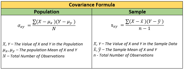
111 |
112 | - **Disadvantages of using Covariance**
113 | One limitation of covariance is that it does not tell us about the **strength of the relationship between two variables**, since the magnitude of **covariance is affected by the scale of the variables**.
114 |
115 | 6. **Correlation** measures the degree to which two variables are related and how they tend to change together.
116 | Correlation is often measured using a statistical tool called the correlation coefficient, which ranges from -1 to 1. A correlation coefficient of -1 indicates a perfect negative correlation, a correlation coefficient of 0 indicates no correlation, and a correlation coefficient of 1 indicates a perfect positive correlation.
117 |
118 | $$ \text{Correlation} = \frac{Cov(x, y)}{\sigma x \ast \sigma y} $$
119 |
120 | > **Note:** Correlation does not imply causation means if two variables are correlated then it does means that other variable is affected by first variable or vice-versa.
121 |
122 | ### Multivariate Analysis
123 |
124 | 1. **3D Scatter Plot**
125 |
126 | 2. **Plots Parameters** are used to display another impact of another categorical or numerical variable in the plot.
127 |
128 | - Hue/Color Parameter
129 | - Size Parameter
130 |
131 | 3. **Facet Grids**
132 |
133 | 4. **Pairplot**
134 |
135 | 5. **Bubble Chart**
136 |
--------------------------------------------------------------------------------
/Probability Distribution Functions/README.md:
--------------------------------------------------------------------------------
1 | # Analysis with Statistics
2 |
3 | ## Table of Contents
4 |
5 | 0. [Resources](#resources)
6 |
7 | 1. [Random Variables](#random-variables)
8 |
9 | 2. [Types of Random Variables](#types-of-random-variables)
10 |
11 | 3. [Probability Distributions](#probability-distributions)
12 |
13 | 4. [What are Probability Distributions?](#what-are-probability-distributions?)
14 |
15 | 5. [Problem with Distribution?](#problem-with-distribution?)
16 |
17 | 6. [Solution: Probability Distribution Functions](#solution:-probability-distribution-functions)
18 |
19 | 7. [Different types of Probability Distributions](#different-types-of-probability-distributions)
20 |
21 | 8. [Why are Probability Distributions important?](#why-are-probability-distributions-important?)
22 |
23 | 9. [A note on Parameters of Probability Distribution Functions](#a-note-on-parameters-of-probability-distribution-functions)
24 |
25 | 10. [Probability Mass Function (PMF)](#probability-mass-function-pmf)
26 |
27 | 11. [Cumulative Distribution Function (CDF) of PMF](#cumulative-distribution-function-cdf-of-pmf)
28 |
29 | 12. [Probability Density Function (PDF)](#probability-density-function-pdf)
30 |
31 | 13. [Questions related to PDFs](#questions-related-to-pdfs)
32 |
33 | 14. [Density Estimation](#density-estimation)
34 |
35 | 15. [Types of Density Estimation](#types-of-density-estimation)
36 |
37 | 16. [Parametric Density Estimation](#parametric-density-estimation)
38 |
39 | 17. [Non-Parametric Density Estimation](#non-parametric-density-estimation)
40 |
41 | 18. [Kernel Density Estimate (KDE)](#kernel-density-estimate-kde)
42 |
43 | 19. [PDF, PMF and CDF](#pdf-pmf-and-cdf)
44 |
45 | ## Resources
46 |
47 | - [Video](https://www.youtube.com/watch?v=C_QAURbgBqY&list=PLKnIA16_RmvbYFaaeLY28cWeqV-3vADST&index=4)
48 | - [PDF](./docs/PDF.pdf)
49 | - [Online PDF](https://drive.google.com/file/d/1FQ65CTmMLK-PYZ6NT9txGcGmJHobtNYl/view)
50 | - [Session Notebook](https://colab.research.google.com/drive/1N_T0_w5vpT1k1Z4pSf4IMhAxYT1nRKLU?usp=sharing)
51 |
52 | ## Topics
53 |
54 | ### Random Variables
55 |
56 | A Random Variable is a set of possible values from a random experiment.
57 |
58 | ### Types of Random Variables
59 |
60 | ```mermaid
61 | graph
62 | A[Types of Random Variable]
63 |
64 | A --> B(Discrete \n Random Variable)
65 | A --> C(Continuous \n Random Variable)
66 | ```
67 |
68 | ### Probability Distributions
69 |
70 | ### What are Probability Distributions?
71 |
72 | A probability distribution is a list of all of the possible outcomes of a random variable along with their corresponding probability values.
73 |
74 | ### Problem with Distribution?
75 |
76 | In many scenarios, the number of outcomes can be much larger and hence a table would be tedious to write down. Worse still, the number of possible outcomes could be infinite, in which case, good luck writing a table for that.
77 |
78 | > **Example:** Height of people, Rolling 10 dice together.
79 |
80 | ### Solution: Probability Distribution Functions
81 |
82 | A probability distribution function is a mathematical function that describes the **probability of obtaining different values of a random variable** in a particular probability distribution.
83 |
84 | ### Different types of Probability Distributions
85 |
86 | 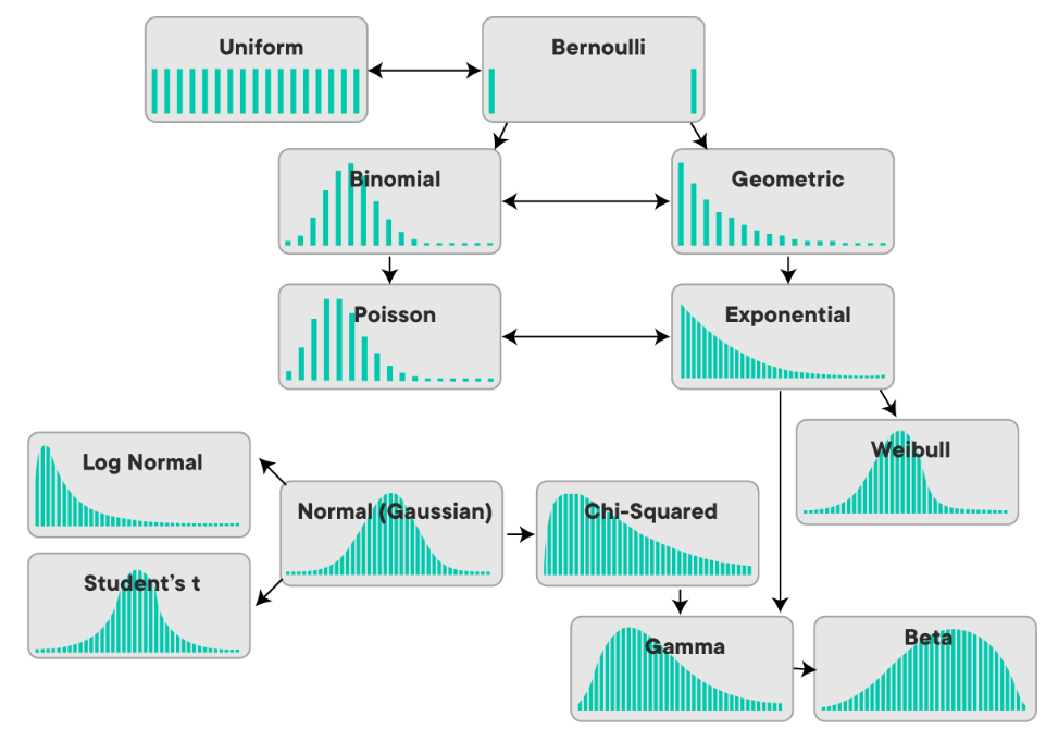
87 |
88 | 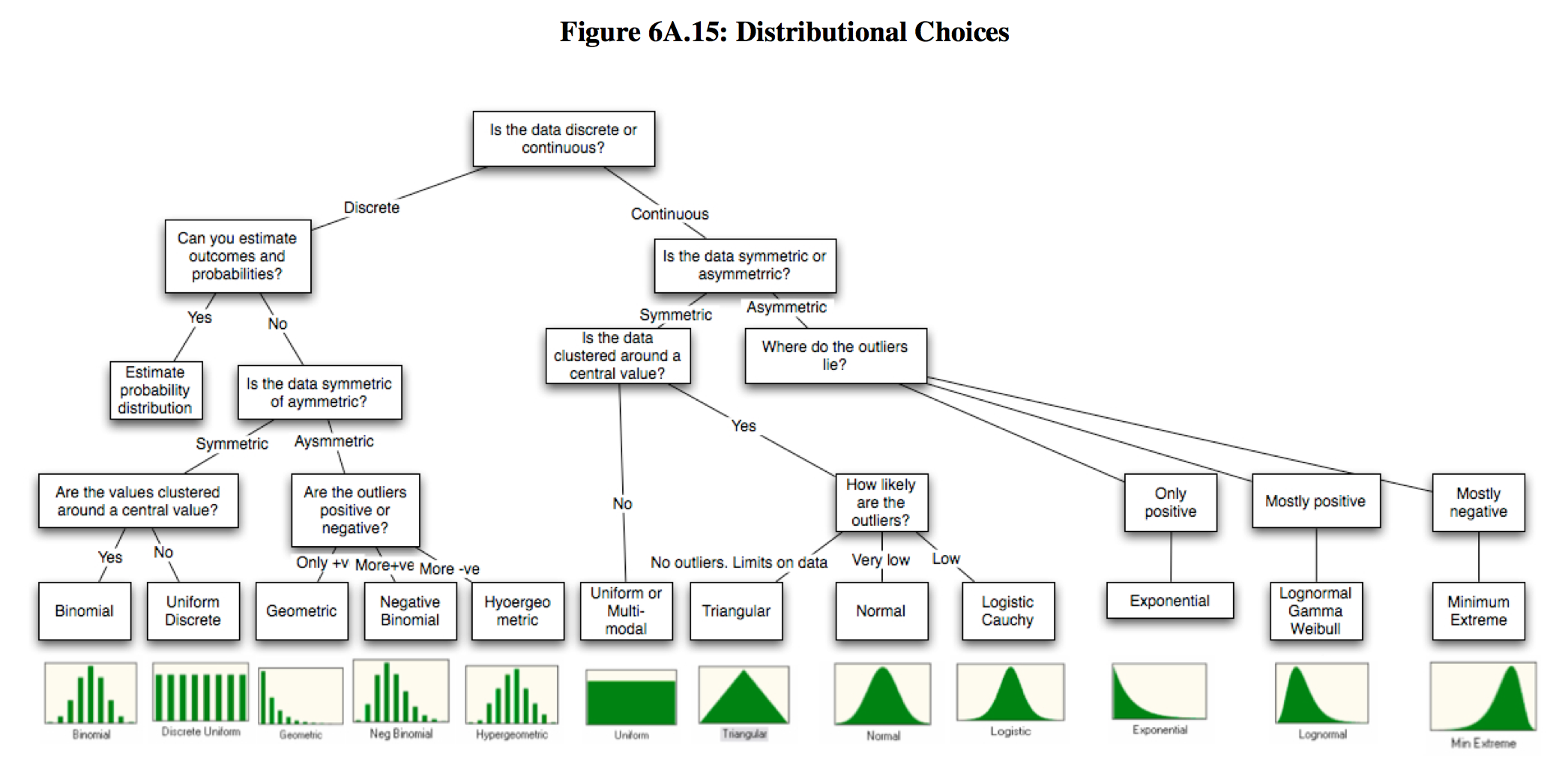
89 |
90 | ### Why are Probability Distributions important?
91 |
92 | - Gives an idea about the shape/distribution of the data.
93 | - And if our data follows a famous distribution then we automatically know a lot about the data.
94 |
95 | ### A note on Parameters of Probability Distribution Functions
96 |
97 | Parameters in probability distributions are numerical values that determine the shape, location, and scale of the distribution.
98 | Different probability distributions have different sets of parameters that determine their shape and characteristics, and understanding these parameters is essential in statistical analysis and inference.
99 |
100 | ### Probability Mass Function (PMF)
101 |
102 | Describes the probability distribution of a **discrete random variable**.
103 |
104 | PMF assign a probability to each value of the random variable. The probabilities assigned by the PMF must satisfy two conditions:
105 |
106 | 1. The probability assigned to each **value must be non-negative** (i.e., greater than or equal to zero).
107 | 2. The **sum** of the probabilities assigned to all possible values must **equal 1**.
108 |
109 | ### Cumulative Distribution Function (CDF) of PMF
110 |
111 | Describes the probability that a random variable X with a given probability distribution will be found at a value less than or equal to x.
112 |
113 | $$ F(x) = P(X \le x) $$
114 |
115 | **Examples:**
116 |
117 | - [Bernoulli Distribution](https://en.wikipedia.org/wiki/Bernoulli_distribution)
118 | - [Binomial Distribution](https://en.wikipedia.org/wiki/Binomial_distribution)
119 |
120 | ### Probability Density Function (PDF)
121 |
122 | Describes the probability distribution of a continuous random variable.
123 |
124 | ### Questions related to PDFs
125 |
126 | 1. Why Probability Density represents the y-axis and why not Probability?
127 |
128 | - Because you have infinite value on the x-axis and you cannot calculate probability of each of the values of a continuous random variable dataset.
129 |
130 | 2. What does the area under the graph represents in PDF?
131 |
132 | - Area under the graph represents the probability of a range (3.0 to 3.1) on x-axis because you have probability density on the y-axis.
133 |
134 | 3. How to calculate Probability from PDF graph?
135 |
136 | - If you reduce the range of two points on x-axis with a very significant amount then you can calculate approx. probability of a point.
137 |
138 | 4. Examples of PDF:
139 |
140 | - [Normal Distribution](https://en.wikipedia.org/wiki/Normal_distribution)
141 | - [Log Normal Distribution](https://en.wikipedia.org/wiki/Log-normal_distribution)
142 | - [Poisson Distribution](https://en.wikipedia.org/wiki/Poisson_distribution)
143 |
144 | 5. How is graph calculated?
145 |
146 | - Using [Density Estimation](#density-estimation)
147 |
148 | ### Density Estimation
149 |
150 | Density estimation is a statistical technique used to estimate the probability density function (PDF) of a random variable.
151 |
152 | It is particularly useful in areas such as machine learning, where it is often used to estimate the probability distribution of input data or to model the likelihood of certain events or outcomes.
153 |
154 | ### Types of Density Estimation
155 |
156 | ```mermaid
157 | graph
158 |
159 | A[Types of \n Density Estimation]
160 |
161 | A --> B(Parametric \n Density Estimation)
162 | A --> C(Non-Parametric \n Density Estimation)
163 | ```
164 |
165 | ### Parametric Density Estimation
166 |
167 | This method estimate probability density by assuming that the random variable is follow some specific distribution such normal, exponential, log normal, or Poisson distributions.
168 | This estimation depends on population mean and standard deviation.
169 |
170 | ### Non-Parametric Density Estimation
171 |
172 | When sometime the distribution of random variable is not clear or it's not one of the famous distributions.
173 |
174 | This method estimate probability density of a random variable without making any assumption about the underlying distribution. This typically done by creating a **kernel density estimate**.
175 |
176 | It has several **advantages over parametric density estimation**.
177 | One of the main advantages is that **it does not require the assumption of a specific distribution**, which allows for more flexible and accurate estimation in situations where the underlying distribution is unknown or complex.
178 | However, non-parametric density estimation **can be computationally intensive and may require more data to achieve accurate estimates** compared to parametric methods.
179 |
180 | ### Kernel Density Estimate (KDE)
181 |
182 | The KDE technique involves using a kernel function to smooth out the data and create a continuous estimate of the underlying density function.
183 |
184 | [**Watch the video for more clarity.**](https://www.youtube.com/watch?v=C_QAURbgBqY&list=PLKnIA16_RmvbYFaaeLY28cWeqV-3vADST&index=4)
185 |
186 | ### PDF, PMF and CDF
187 |
188 | 
189 |
190 | 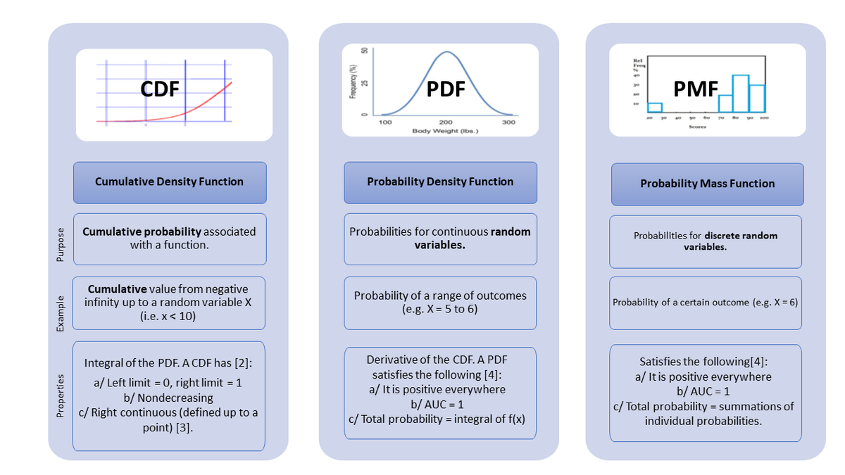
191 |
--------------------------------------------------------------------------------
/course_parser.py:
--------------------------------------------------------------------------------
1 | from __future__ import annotations
2 |
3 | import json
4 | import time
5 | from dataclasses import dataclass, field
6 | from typing import TYPE_CHECKING, Iterable, Literal, Self
7 |
8 | from bs4 import BeautifulSoup, Tag
9 |
10 | if TYPE_CHECKING:
11 | from pathlib import Path
12 |
13 | import httpx
14 |
15 | COURSE_URL = "https://learnwith.campusx.in/s/courses/653f50d1e4b0d2eae855480a/take"
16 | BASE_RESOURCE_URL = "https://learnwith.campusx.in/s/courses/653f50d1e4b0d2eae855480a"
17 | BASE_HEADERS = {
18 | "accept": "application/json, text/javascript, */*; q=0.01",
19 | "referer": COURSE_URL,
20 | "user-agent": (
21 | "Mozilla/5.0 (Macintosh; Intel Mac OS X 10_13_7) AppleWebKit/537.36 (KHTML, "
22 | "like Gecko) Chrome/111.5.0.0 Safari/507.02"
23 | ),
24 | }
25 | ResourceType = Literal[
26 | "article",
27 | "assessment",
28 | "assignment",
29 | "link",
30 | "livetest",
31 | "pdf",
32 | "video",
33 | ]
34 |
35 |
36 | def fetch_sub_topic_resource(
37 | client: httpx.Client,
38 | sub_topic_id: str,
39 | resource_type: ResourceType,
40 | ) -> bytes:
41 | """Fetches the resource data for the given subtopic ID and resource type.
42 |
43 | Args:
44 | client: HTTPX client instance with cookies set.
45 | sub_topic_id: ID of the subtopic to fetch.
46 | resource_type: Type of resource to fetch.
47 |
48 | Returns:
49 | The data as bytes for the requested resource.
50 |
51 | Raises:
52 | ValueError: If client does not have cookies set.
53 | HTTPError: If the API request fails.
54 | """
55 | if not client.cookies:
56 | raise ValueError("Client does not have cookies.")
57 | res = client.get(f"/{resource_type}s/{sub_topic_id}/get")
58 | res.raise_for_status()
59 | return res.content
60 |
61 |
62 | @dataclass(kw_only=True)
63 | class CourseTopic:
64 | title: str
65 | id: str
66 | source: Tag = field(repr=False)
67 |
68 | @staticmethod
69 | def search(html_path: Path) -> Tag:
70 | """
71 | Parses CourseTopic instances from a BeautifulSoup tag.
72 |
73 | Yields CourseTopic instances parsed from the provided BeautifulSoup tag source.
74 | """
75 | soup = BeautifulSoup(html_path.read_bytes(), "html.parser")
76 | course_items_tag = soup.select_one("div.courseItems")
77 | if course_items_tag:
78 | return course_items_tag
79 | raise ValueError("'div.courseItems' css selector not present in source.")
80 |
81 | @classmethod
82 | def parse(cls, source: Tag) -> Iterable[Self]:
83 | """
84 | Parses CourseTopic instances from a BeautifulSoup tag.
85 |
86 | Yields CourseTopic instances parsed from the provided BeautifulSoup tag source.
87 | """
88 | yield from (
89 | cls(
90 | title=tag["data-title"],
91 | id=tag["data-id"],
92 | source=tag,
93 | )
94 | for tag in source.find_all("div", {"data-type": "label"})
95 | )
96 |
97 |
98 | @dataclass(kw_only=True)
99 | class CourseSubTopic:
100 | id: str
101 | topicId: str
102 | title: str
103 | type: ResourceType
104 | source: Tag = field(repr=False)
105 |
106 | @classmethod
107 | def parse(cls, topic: CourseTopic) -> Iterable[Self]:
108 | """
109 | Parses CourseSubTopic instances from a CourseTopic BeautifulSoup tag.
110 |
111 | Yields CourseSubTopic instances parsed from the provided CourseTopic
112 | BeautifulSoup tag source.
113 | """
114 | yield from (
115 | cls(
116 | id=tag["data-id"],
117 | topicId=topic.id,
118 | title=tag["data-title"],
119 | type=tag["data-type"],
120 | source=tag,
121 | )
122 | for tag in topic.source.find_all("div", {"data-type": True})
123 | )
124 |
125 | @classmethod
126 | def parse_many(
127 | cls,
128 | topics: Iterable[CourseTopic],
129 | ) -> Iterable[tuple[CourseTopic, Iterable[Self]]]:
130 | for topic in topics:
131 | yield topic, cls.parse(topic)
132 |
133 | @classmethod
134 | def find(
135 | cls,
136 | course_topics: Iterable[CourseTopic],
137 | *,
138 | id: str | None = None,
139 | title: str | None = None,
140 | ) -> Iterable[Self]:
141 | """
142 | Parses a single CourseSubTopic from the given CourseTopics.
143 |
144 | This allows fetching a specific CourseSubTopic by title or id from the
145 | list of CourseTopics, by searching through their associated subtopics.
146 |
147 | Args:
148 | course_topics: Iterable of CourseTopic instances to search through.
149 | title: Optional title of subtopic to find.
150 | id: Optional id of subtopic to find.
151 |
152 | Returns:
153 | Iterable of matching CourseSubTopic instances.
154 |
155 | Raises:
156 | ValueError: If both title and id are None.
157 | ValueError: If no matching subtopic is found.
158 | """
159 | if id is None and title is None:
160 | raise ValueError("Both 'id' and 'title' must not be None.")
161 |
162 | for topic in course_topics:
163 | if topic.id == id or topic.title == title:
164 | yield from cls.parse(topic)
165 | break
166 | else:
167 | raise ValueError(f"No subtopic found matching id={id} or title={title}")
168 |
169 |
170 | @dataclass(kw_only=True)
171 | class CourseVideoResource:
172 | id: str
173 | topicId: str
174 | title: str
175 | totalTime: str
176 | description: str = field(repr=False)
177 | isDescriptionHtml: bool = field(repr=False)
178 |
179 | @classmethod
180 | def fetch(cls, client: httpx.Client, sub_topic: CourseSubTopic) -> Self:
181 | if sub_topic.type != "video":
182 | raise ValueError(f"sub_topic is not a video resource, got {sub_topic.type}")
183 |
184 | response = fetch_sub_topic_resource(
185 | client=client,
186 | sub_topic_id=sub_topic.id,
187 | resource_type="video",
188 | )
189 | try:
190 | data = json.loads(response)
191 | data = data["spayee:resource"]
192 | except json.JSONDecodeError as e:
193 | raise ValueError("Response could not be parsed as JSON.") from e
194 | except KeyError as e:
195 | raise ValueError("Bad response or missing required fields.") from e
196 | return cls(
197 | id=sub_topic.id,
198 | topicId=sub_topic.topicId,
199 | title=data["spayee:title"],
200 | description=data["spayee:description"],
201 | totalTime=data["spayee:totalTime"],
202 | isDescriptionHtml=data["spayee:isDescriptionHtml"],
203 | )
204 |
205 |
206 | @dataclass(kw_only=True)
207 | class CourseAssignmentResource:
208 | id: str
209 | topicId: str
210 | title: str
211 | assignmentLink: str = field(repr=False)
212 |
213 | @classmethod
214 | def fetch(cls, client: httpx.Client, sub_topic: CourseSubTopic) -> Self:
215 | if sub_topic.type != "assignment":
216 | raise ValueError(
217 | f"sub_topic is not an assignment resource, got {sub_topic.type}"
218 | )
219 |
220 | response = fetch_sub_topic_resource(
221 | client=client,
222 | sub_topic_id=sub_topic.id,
223 | resource_type="assignment",
224 | )
225 |
226 | def parse_assignment_link(source: str | bytes) -> str:
227 | soup = BeautifulSoup(source, "html.parser")
228 | link_tag = soup.select_one("#instructions a")
229 | if link_tag:
230 | return link_tag.get_attribute_list("href", "")[0]
231 | raise ValueError("assignmentLink tag not found in source")
232 |
233 | return cls(
234 | id=sub_topic.id,
235 | topicId=sub_topic.topicId,
236 | title=sub_topic.title,
237 | assignmentLink=parse_assignment_link(response),
238 | )
239 |
240 |
241 | if __name__ == "__main__":
242 | from pathlib import Path
243 |
244 | import httpx
245 | from rich import print
246 |
247 | # campusx.html contains the html content of the website
248 | course_topic_tag = CourseTopic.search(Path("campusx.html"))
249 | course_topics = list(CourseTopic.parse(course_topic_tag))
250 | print(course_topics[-10:])
251 |
252 | sub_topics = list(CourseSubTopic.find(course_topics, id="olh5gfqpjt"))
253 | print(list(sub_topics))
254 |
255 | # Fill cookies from browser's network tab
256 | cookies = {
257 | "c_ujwt": "Your Token",
258 | "SESSIONID": "Your current SESSION ID.",
259 | }
260 |
261 | results: list[CourseVideoResource] = []
262 | with httpx.Client(
263 | base_url=BASE_RESOURCE_URL, headers=BASE_HEADERS, cookies=cookies
264 | ) as client:
265 | for i, sub_topic in enumerate(sub_topics, 1):
266 | if sub_topic.type != "video":
267 | print(f"subtopic id={sub_topic.id} is not a video resource.")
268 | continue
269 | if i % 7 == 0:
270 | print("sleeping for 3 seconds...")
271 | time.sleep(3)
272 | results.append(CourseVideoResource.fetch(client, sub_topic))
273 | if not results:
274 | raise ValueError("No video resources found.")
275 | print(results)
276 |
--------------------------------------------------------------------------------
/SGD Regressor/notebook/my-SGD.ipynb:
--------------------------------------------------------------------------------
1 | {
2 | "cells": [
3 | {
4 | "cell_type": "code",
5 | "execution_count": 28,
6 | "id": "60e43fd7",
7 | "metadata": {},
8 | "outputs": [],
9 | "source": [
10 | "import numpy as np\n",
11 | "import matplotlib.pyplot as plt\n",
12 | "\n",
13 | "from sklearn.linear_model import LinearRegression, SGDRegressor\n",
14 | "from sklearn.metrics import r2_score\n",
15 | "from sklearn.model_selection import train_test_split\n",
16 | "from sklearn.datasets import make_regression"
17 | ]
18 | },
19 | {
20 | "cell_type": "code",
21 | "execution_count": 33,
22 | "id": "a90f5266",
23 | "metadata": {},
24 | "outputs": [
25 | {
26 | "name": "stdout",
27 | "output_type": "stream",
28 | "text": [
29 | "(100, 1) (100,)\n"
30 | ]
31 | },
32 | {
33 | "data": {
34 | "image/png": "iVBORw0KGgoAAAANSUhEUgAAAjMAAAGdCAYAAADnrPLBAAAAOXRFWHRTb2Z0d2FyZQBNYXRwbG90bGliIHZlcnNpb24zLjcuMiwgaHR0cHM6Ly9tYXRwbG90bGliLm9yZy8pXeV/AAAACXBIWXMAAA9hAAAPYQGoP6dpAAA2cklEQVR4nO3df3iU5Z3v8c+EHwkBMjECmUQDRLBKSgXRglHbIzSaWC6qLetVrLqgFlcEXY1WYE8V0XUpWkvXHwtrq2CLP+qe66iLerKlILLYABaa9SDaFRoEIROUyAxESSCZ8wdnxkyYH8/MPDPP88y8X9c1V83Mk8k9aevzyX1/7+/tCgQCAQEAADhUntUDAAAASAVhBgAAOBphBgAAOBphBgAAOBphBgAAOBphBgAAOBphBgAAOBphBgAAOFpfqweQCd3d3Tpw4IAGDx4sl8tl9XAAAIABgUBAR44cUXl5ufLyos+/5ESYOXDggCoqKqweBgAASMK+fft05plnRn09J8LM4MGDJZ38ZRQVFVk8GgAAYITf71dFRUXoPh5NToSZ4NJSUVERYQYAAIeJVyJCATAAAHA0wgwAAHA0wgwAAHA0wgwAAHA0wgwAAHA0wgwAAHA0wgwAAHA0wgwAAHC0nGiaBwAAzNfVHdDW5jYdPHJMwwYXaGJlifrkZf4MRMIMAABIWMOOFi1es1MtvmOh58rcBVo0rUp1Y8syOhaWmQAAQEIadrRozurtYUFGkry+Y5qzersadrRkdDyEGQAAYFhXd0CL1+xUIMJrwecWr9mpru5IV6QHYQYAABi2tbntlBmZngKSWnzHtLW5LWNjIswAAADDDh6JHmSSuc4MhBkAAGDYsMEFpl5nBsIMAAAwbGJlicrcBYq2Adulk7uaJlaWZGxMhBkAAGBYnzyXFk2rkqRTAk3w60XTqjLabyatYWbjxo2aNm2aysvL5XK59Oqrr4a9PmvWLLlcrrBHXV1d2DVtbW267rrrVFRUpOLiYt188806evRoOocNAABiqBtbpuXXT5DHHb6U5HEXaPn1EzLeZyatTfPa29s1btw43XTTTfrBD34Q8Zq6ujqtXLky9HV+fn7Y69ddd51aWlq0du1aHT9+XDfeeKNuueUWvfDCC+kcOgAAiKFubJkur/JkfwfgK6+8UldeeWXMa/Lz8+XxeCK+9sEHH6ihoUHvvvuuLrzwQknSE088oe9+97v6+c9/rvLyctPHDAAAjOmT51L1qNOtHob1NTMbNmzQsGHDdM4552jOnDk6dOhQ6LXGxkYVFxeHgowk1dTUKC8vT1u2bIn6nh0dHfL7/WEPAACQnSwNM3V1dfrNb36jdevWaenSpXr77bd15ZVXqqurS5Lk9Xo1bNiwsO/p27evSkpK5PV6o77vkiVL5Ha7Q4+Kioq0fg4AAGAdSw+anDFjRuifv/GNb+i8887TqFGjtGHDBn3nO99J+n0XLlyo+vr60Nd+v59AAwBAlrJ8mamns846S0OGDNGuXbskSR6PRwcPHgy75sSJE2pra4taZyOdrMMpKioKewAAgOxkqzDzySef6NChQyorO7mlq7q6WocPH9a2bdtC16xfv17d3d2aNGmSVcMEAAA2ktZlpqNHj4ZmWSSpublZTU1NKikpUUlJiRYvXqzp06fL4/Fo9+7duvfeezV69GjV1tZKksaMGaO6ujrNnj1bK1as0PHjxzVv3jzNmDGDnUwAAECS5AoEAmk7o3vDhg2aPHnyKc/PnDlTy5cv19VXX60///nPOnz4sMrLy3XFFVfooYceUmlpaejatrY2zZs3T2vWrFFeXp6mT5+uxx9/XIMGDTI8Dr/fL7fbLZ/Px5ITAAAOYfT+ndYwYxeEGQAAnMfo/dtWNTMAAACJIswAAABHI8wAAABHI8wAAABHI8wAAABHI8wAAABHI8wAAABHI8wAAABHI8wAAABHI8wAAABHI8wAAABHI8wAAABHI8wAAABHI8wAAABHI8wAAABHI8wAAABHI8wAAABHI8wAAABHI8wAAABHI8wAAABHI8wAAABHI8wAAABHI8wAAABHI8wAAABH62v1AAAAgP11dQe0tblNB48c07DBBZpYWaI+eS6rhyWJMAMAAOJo2NGixWt2qsV3LPRcmbtAi6ZVqW5smYUjO4llJgAAEFXDjhbNWb09LMhIktd3THNWb1fDjhaLRvYVwgwAAIioqzugxWt2KhDhteBzi9fsVFd3pCsyhzADAAAi2trcdsqMTE8BSS2+Y9ra3Ja5QUVAmAEAABEdPBI9yCRzXboQZgAAQETDBheYel26EGYAAEBEEytLVOYuULQN2C6d3NU0sbIkk8M6BWEGAABE1CfPpUXTqiTplEAT/HrRtCrL+80QZgAAQFR1Y8u0/PoJ8rjDl5I87gItv36CLfrM0DQPAJCzUu1qa+euuGaqG1umy6s8tv2shBkAQE5Ktaut3bvimq1PnkvVo063ehgRscwEAMg5qXa1dUJX3FxCmAEA5JRUu9o6pStuLiHMAABySqpdbZ3SFTeXEGYAADkl1a62TumKm0sIMwCAnJJqV1undMXNJWkNMxs3btS0adNUXl4ul8ulV199Nez1QCCg+++/X2VlZRowYIBqamr00UcfhV3T1tam6667TkVFRSouLtbNN9+so0ePpnPYAIAslmpXW6d0xc0laQ0z7e3tGjdunJ566qmIrz/yyCN6/PHHtWLFCm3ZskUDBw5UbW2tjh37amruuuuu0/vvv6+1a9fq9ddf18aNG3XLLbekc9gAgCyWaldbp3TFzSWuQCCQkXJrl8ulV155RVdffbWkk7My5eXluvvuu3XPPfdIknw+n0pLS7Vq1SrNmDFDH3zwgaqqqvTuu+/qwgsvlCQ1NDTou9/9rj755BOVl5cb+tl+v19ut1s+n09FRUVp+XwAAGehz4z9Gb1/W9Y0r7m5WV6vVzU1NaHn3G63Jk2apMbGRs2YMUONjY0qLi4OBRlJqqmpUV5enrZs2aLvf//7Ed+7o6NDHR0doa/9fn/6PggAwDF6d+x9+yeTte3jz5Pqamv3rri5xLIw4/V6JUmlpaVhz5eWloZe83q9GjZsWNjrffv2VUlJSeiaSJYsWaLFixebPGIAgJPFmkm5avwZSb2nnbvi5pKs3M20cOFC+Xy+0GPfvn1WDwkAYCE69mY3y8KMx+ORJLW2toY939raGnrN4/Ho4MGDYa+fOHFCbW1toWsiyc/PV1FRUdgDAJCb6Nib/SwLM5WVlfJ4PFq3bl3oOb/fry1btqi6ulqSVF1drcOHD2vbtm2ha9avX6/u7m5NmjQp42MGADgPHXuzX1prZo4ePapdu3aFvm5ublZTU5NKSko0fPhw3XnnnfrHf/xHnX322aqsrNR9992n8vLy0I6nMWPGqK6uTrNnz9aKFSt0/PhxzZs3TzNmzDC8kwkAkNvo2Jv90hpm/vSnP2ny5Mmhr+vr6yVJM2fO1KpVq3Tvvfeqvb1dt9xyiw4fPqxLL71UDQ0NKij4qmvi888/r3nz5uk73/mO8vLyNH36dD3++OPpHDYAIIvQsTf7ZazPjJXoMwMAuaurO6BLl66X13csYt2MS5LHXaBN86ewrdpmjN6/s3I3EwAAQXTszX6EGQBA1qsbW6bl10+Qxx2+lORxF2j59RPo2OtwljXNAwAgk+jYm70IMwCAjOt9rECmQgUde7MTYQYAkFHJHNBoVfiBMxBmAAAZEzxWoPeuouCxApHqVzidGvFQAAwAUFd3QI27D+m1pv1q3H0oLa39kzlWgDOVYAQzMwCQ4zI185HIsQLVo06PG35cOhl+Lq/ysOSU45iZAYAclsmZj0SPFeBMJRhFmAGAHJXp06QTPVaAM5VgFGEGAHJUpmc+JlaWqMxdcEoX3iCXTi5vTawskcSZSjCOMAMAOSrTMx+JHiuQaPgxSyaKoWEuCoABIEdZMfMRPFagd8GxJ0LBcTD8zFm9XS4pbDksXWcqsQ3cmTg1GwBylJWnSSfSBC9TASNaD5zgqIye4USDP/MYvX8TZgAghwVv4FLkmQ+7HMLYeaJbv23co4/bvtCIkkLdUD1S/fueWimRbJAIBrtoNURGgx0zO+YizPRAmAGA6Ox+AzY6vlQ+R+PuQ7r2V5vjjuXF2RdFPdvJrJkdfMXo/ZuaGQDIcXY+Tdro8QfJHJPQU6rF0DT4sxa7mQAAodOkrxp/hqpHnW6LG67RPjidJ7pT7peTajE0Df6sRZgBANiS0YDw28Y9KQeJVLeB0+DPWoQZAIAtGb3xf9z2Rcrvl2gPnN5o8GctwgwAwJaM3vhHlBSa8n7BHjged/h1HndB3Jobqxr84SQKgAEAthQMCPH64NxQPVK/3tQc9zojQSLZYmgrGvzhK8zMAAAMyXSbf6NLP/375qW0RBTp5yZTDJ3KzA5SQ58ZAEBcVvaiyUSfGTPRAdg8NM3rgTADAMmzQzM4owGBIJFdaJoHAEiZXZrBBZd+zLoO2YWaGQBAVDSDgxMwMwMAFrPz0gjN4OAEhBkAsJBdilajMbMZnJ1DG5yNMAMAFkn1cMRMMNrrJV4PFzuENsJU9iLMAIAFjBbWDs7vp8/aOyy7+ZrRDM4Ooc0OYQrpw9ZsALBA4+5DuvZXmxP6HitvvsmGga7ugC5duj5qEXFwZmfT/ClpC2p22FqO5LA1GwBsLJmCWSuXn5Jt85/Ibqh0bKm2y9ZypBdhBgAskMzpyVbffJPp4ZKu3VBG61+sDlPIDMIMAFggXmFtNE67+Zq5GyookSUvtpbnBprmAYAFYh2iaIRTbr7B0BbtM7p0MogYOdFa+qr+pfdsS3AJrmFHS9jz6QhTsB/CDABYJNopy0Y45eZr9ORrI0tm8epfpJNLcD1P8zY7TMGeCDMAYKG6sWXaNH+KXpx9kf55xng9/+NJ8hTlx735XjDiNDXuPqTXmvarcfehsBu43UQLbR53QULFzMkcrWBmmIJ9UTMDABbrXVj7wPe+HrOvy/fGlel/PPqWJT1Tkm08l+xuqJ6SrX8JhqnedTYe+sxkDcIMANhMrJvv98aV6emNzZY0oEu18VyqJ1qnUv9iRpiCfdE0DwBsqvcsyAUjTjtlRqandDags0PjuWADvnhHK6SzAR8yy+j92/KamQceeEAulyvsce6554ZeP3bsmObOnavTTz9dgwYN0vTp09Xa2mrhiAEgM4IzGVeNP0PVo07Xto8/T7hmxAzJFN6mA/UviMbyMCNJX//619XS0hJ6bNq0KfTaXXfdpTVr1ujf/u3f9Pbbb+vAgQP6wQ9+YOFoAcAaVvVMSabwNl3MKiZGdrFFzUzfvn3l8XhOed7n8+mZZ57RCy+8oClTpkiSVq5cqTFjxmjz5s266KKLMj1UALCMVT1T7NZ4zun1L5zebT5bhJmPPvpI5eXlKigoUHV1tZYsWaLhw4dr27ZtOn78uGpqakLXnnvuuRo+fLgaGxujhpmOjg51dHSEvvb7/Wn/DACQbhMrS1Rc2E+Hvzge8fVgzYjZPVPs2Hgu1WJiq3B6d3pYvsw0adIkrVq1Sg0NDVq+fLmam5v1rW99S0eOHJHX61X//v1VXFwc9j2lpaXyer1R33PJkiVyu92hR0VFRZo/BQCk39qd3qhBRjq53DPjm8NN/7k0njNHot2LYZzlYebKK6/UNddco/POO0+1tbV68803dfjwYb388stJv+fChQvl8/lCj3379pk4YgDIvGARbjzL/vDfunTpelNvjBTeps4uRdTZyvIw01txcbG+9rWvadeuXfJ4POrs7NThw4fDrmltbY1YYxOUn5+voqKisAcAOFm8Itye0vGXPoW3qbFTEXU2skXNTE9Hjx7V7t27dcMNN+iCCy5Qv379tG7dOk2fPl2S9Je//EV79+5VdXW1xSMFgMxJpLg2oJMzJovX7NTlVR7TZkycXnhrJbsVUWcby8PMPffco2nTpmnEiBE6cOCAFi1apD59+ujaa6+V2+3WzTffrPr6epWUlKioqEi33367qqur2ckEIKckWlzb8y99MwtlnVp4azU7FlFnE8vDzCeffKJrr71Whw4d0tChQ3XppZdq8+bNGjp0qCRp2bJlysvL0/Tp09XR0aHa2lr9y7/8i8WjBoDMChbhRut+Gw1/6dtDvP/+0rUTLVdwnAEAOERwN4wkw4HmxdkXMZNiE9H++8vkkRBO45jjDAAgW3V1B9S4+5Bea9qvxt2HUt6pEq0INxK2S9sPRdTpw8wMAKRBOpujBTvI/mGnV8+8s+eU13PtL32nddR12nitZPT+TZgBAJNl8oTpXO8om+ufP9sRZnogzADIlK7ugC5duj5qT5Fgoeem+VPC/hpP5a/1XP1LP5OhEdYwev+2fDcTAGSTRJqjBQtzU51dyMXt0vE66qajzw7siwJgADBRos3R0nlej9kFyHZCR130xMwMAJgokeZoqc4uxFpeyvZaEjrqoifCDACYIBgsvP5jKhnYT23tkU+37tkcLZklqaBYYUVSxFqS4GxPNtSS0FEXPRFmACBFkYJFJL1PmE52diFa4WswrLgL+2V9LQkdddETNTMAkIJoNS+R9G6OlszsQrylqYCkw19EnhUKXpMNtSR98lyhWajekax3aET2Y2YGAJIUK1hIJ2+qJQP766dTx8jjHnDKlumJlSUqLuwXM3ycVtgvbHYh3tKUUdlQSxLsqNt7VsyTRbVBMIYwAwBJMlLzcqi9Ux73gKS3TvcOSmaFkGypJakbW6bLqzw52WcHXyHMAECSUt1Rs7W5LeasjHRyyahnAXCqISQba0lysc8OwlEzAwBJSnVHTTJhKFj4msy8A7UkyFaEGQBIUrxgEe/k6mTCUM/C10RxOjOyFWEGAJKU6o6aZMNQ3dgy3VnztYTGOm/yKG2aP4Ugg6xEmAGQk8xq9R/cUeNxh8+yGJkFSSUMjRxSmNA4Lxk9lKUlZC0KgAHkHLNb/aeyoybZ7cWJFALHWuoCsoErEAhkz8ljURg9QhxA9ovWPTcYO6yqKYl1zlK06y9duj5qB9yeVlAnA4cyev9mmQlAzojXPVc62eo/uOSUyVOng9uLrxp/hqpHnR53VifWElVQcWE/ggxyAstMAHJCV3dAq95pNnywo+/LTtufOh1tiaq4sJ9uvLhS86aMjju7E202KNGZIsBKLDMByHpGD4IMuumSkVr5zh7bLUVFk0zwiHfqtt2DHHKD0fs3YQZAVotWIxNLycD+amvvjPhasIPupvlTHDtTEatuKNY5U5L9ghyyGzUzABwv1ZqVeAdB9nbyYMh+UYOM5PxTp43UDUUSqaYIsAtqZgDYkhnbpxM5YTo48/D98WfomXf2xL3eqadOp3Lqds8gx1lIsBNmZgDYTnAZpPdN1+s7pjmrt6thR4uh90kkcASb3NVUeQxd79RTp80IYU4NcshezMwAsJV4yyAunVzquLzKE7dmxWjguG/qGM26pFJ98lzq6g6ozF0QtX+L00+dNiOEOTXIIXsxMwPAVuItgyRSs2L07KNgkJFSP2/J7lI9dZtuwrAjwgwAWzG6hGHkumSDSSrnLdmdkd9JrNecHOSQvVhmAmArRpcwjF6X7NlHqZy3lG6pNrSL9zuRTu0zE+/3BViJPjMAbCXemUPJ9nnJREfbTPwMMw/JpAMw7I6meT0QZgBnCe5mksJ7n9i5cZvZJ3FH+xl2PCQTSBea5gGwrXjN8KyuWUm0WV+iW8mTaQaY6CGZQC6hZgZARhmdwbCqZiXRGZZEt5InO4OTyC4vGtoh1zAzAyBjEp3B6JPnUvWo03XV+DNUPer0jASZRJv1JRIyUmkGaOYuLyDbEGYAZITdl0mSHZ/R8OD1fZnS5ze6e+uj1qNJnWMFOBlhBkBGmNkMLxFG61OSHZ/RkNHW3pnS5zfa7O7Jt3bp2l9t1qVL1xs+9gFwOmpmAGSEFcskidSnGP25/+f/B4Rg/U4wZMTbSl4yKN/Q+0cbR7DZ3ZzV2+VS7BOupa+WrtjhhFzAzAyAjDC7GV480epTWnzHdGuE+hSjP/c3jR+HzXwY7TLsKTL2/ns++yLqa9F2eUVih6U7IFMIMwAywug5SWac+xOr/iVowf/+v2E3+UTPLOpZtGtkK7nR9//lH/475vJQ3dgybZo/RS/OvkjzJo+K+V7pWroD7MYxYeapp57SyJEjVVBQoEmTJmnr1q1WDwlAAjJ5gGO8+hdJOvzFcT25flfE8RnRe+ajZ8j45xnj9eLsi7Rp/pTQEk/w/Y3MkcSbTQnu8jq7dLChsbLDCdnOEWHmd7/7nerr67Vo0SJt375d48aNU21trQ4ePGj10AAkIFPN8IzevJ995696Z9dnoeLg7m7JXdjP8M/pPfMRbyt53dgy3VVzdkLvGUuml+4Au3JEAfAvfvELzZ49WzfeeKMkacWKFXrjjTf07LPPasGCBRaPDkAi6saWacq5pfpt4x593PaFRpQU6obqkerf17y/rYzevH1fntB1v96S8s9LZOZj5JCBpr2n0eJjM5buADuzfZjp7OzUtm3btHDhwtBzeXl5qqmpUWNjo4UjA5CMSDuMfr2p2dQzjD5v7zTlfYxKZObDzNmUWDuczF66A+zM9stMn332mbq6ulRaWhr2fGlpqbxeb8Tv6ejokN/vD3sAsF4qHXCN6uoO6KE3dqb8PkYkU7RsdiG01edYAXZg+5mZZCxZskSLFy+2ehgAekj0DCMj7xfp3CYjxb9mSHbmIx2zKVadYwXYhe3DzJAhQ9SnTx+1traGPd/a2iqPxxPxexYuXKj6+vrQ136/XxUVFWkdJ4DYzDwoMVYzvI4T3WYNOSaPgcMhownOpvT+DKm8Z7D4GMhFtg8z/fv31wUXXKB169bp6quvliR1d3dr3bp1mjdvXsTvyc/PV36+sW6bADLDrA7AwaWq3jM8wWZ4fzPhjCRHGF2wkPbnfzNOn7V3mDLzwWwKYB7bhxlJqq+v18yZM3XhhRdq4sSJ+uUvf6n29vbQ7iYA9mdG4auRZnj/a/t+5bmkWE1v81xSIBD/SAApfOnnkrOHGPgO45hNAczhiDDzwx/+UJ9++qnuv/9+eb1ejR8/Xg0NDacUBQOwr1S3EXd1B7TqnWZD9TDRgkwwmMz+VqWe3ths6IyjVJZ+AGSGKxAIZP2hHX6/X263Wz6fT0VFRVYPB8hZwSUiKXLha7TdN5FqZIzoPUPT85DJaHU3900do9MG5rP0A9iA0fs3YQZARiVyknXw+kg1MkbdN3WMhgzOjxhMou2IAmAPRu/fjlhmApA9Eil8NVIjE8+Qwfm6anzkomBqVoDsQJgBkHFGQ4QZPWM4lwjIfoQZALaVymnPnEsE5A7CDICMSbRGJdlZFc4lAnILYQZARiRa+CsZ287tLuyngr595PWn3kmXgmDAmdjNBCDt3nzvgG574c+nPB9vS7ZkbDu3GZ10kwlbANKLrdk9EGYA67z5Xovmvbg9ZiM7j7tAm+ZPiRpA0h00om3/NhK2AKQPW7MBWK5hR4tue2F7zGuMHDCZznOMzD7NG0DmEWYApEUwJBj1zq5PYwaVdPWEMfM0bwDWIMwASItEe8Q8+dbu0D+ns1ald5Gv1/eloe9LZZs4gPQizABIi1Ru/l7fMc1Zvd30WpVItTclA/sb+l6a7wH2lWf1AABkpyGD8pP+3mD9yuI1O9UVrXI4gq7ugBp3H9JrTfvVuPtQ2PcGi3x7zxZ93t4Z932LC/vRfA+wMWZmAKRHivskE61VibXj6fIqT8wi33gOf3Fca3d62dEE2BQzMwDS4rP2DlPex8hyVbRZl+By1ZPrP0rpjKfgjqZEZokAZA5hBoCk2Es0yTCrxiTe+8TbWi1JK9/Zk9IYes4SAbAflpkApKUpXbyjCIzwFOXHrVUxsrX68JfHkxxBOHY0AfbEzAyQ4+It0TTsaEnqffvkubRoWpWkrzrpJurYiW6t3emNeU2814OKB/RLehxB7GgC7IkwA+QwI0s0qdSK1I0t0/LrJ8jjTi4E+L44HjNQNexo0bMGl5BuvKRSUnLByqWTM1XsaALsiTAD5LBEut8mq25smTbNn6L7po5J+HtjBapEOgyXuQs0b8ropIJVMPwsmlbFcQaATRFmgBxmtAYk1VqRPnkuDRmcXN+ZaIEqkQ7DwSCSTLDyuAs4aBKwOQqAgSzTu11/rAMZjdaAJForEmkMqdab9A5URgPWzZeMDAsiffJcmnVJpX69qTlmcXJxYT89de0EXTTqdGZkAJsjzABZJN6upN4h44IRp8XcceTSyZmJRGpFoo3hvqlVKe1u6h2GjIajmirPKc8Fi5PnrN4ul8Ib5wVjy89+8A1dcvaQJEYKINMIM0CWCO5K6h0UgruSbvl2pf79v1pOCRnfG1empzc2R72pJ1IrEmsMc184OYZIPyuWaIEq3tbveEEsWJzcO3h50njIJYD0cAUCgaxvaen3++V2u+Xz+VRUVGT1cADTdXUHdOnS9Ql3uQ1GlGhBJ5GberwxBMPFfVPH6KE3PjA8VpcUtWYlGJ6kyEHMSK1LIstyADLL6P2bmRkgCyRSDNtTQCdv/P/+Xy16+yeTte3jz5O+qRvdGXXawHxtmj9Fq95p1kNvfBD3fe+s+VrUQGLG7EqfPJehs58A2BdhBsgCqew2CoaMbR9/ntJNPZGdUYnsbho5pDDm63Vjy3R5lYfZFSCHEWaALGBGZ9pUt18nujPKzJ1UzK4AuY0+M0AWCBbDpjIXkWogijeG3l10E70eAKIhzAAOFjzp+vX3DmjGN4dLOrVdf7yAY1ZoiHUWU6SdUYleH2T26d4AnI/dTIBDRernUlzYT5J0+IuvTonuuf1aMrbrJ5UdPomewJ3I9ek43RuAfRm9fxNmAAeK1s8l2L/lrpqzNXLIwLAgYjQImBEYEg1DRq6P9ZklY9uwATgLYaYHwgyyidF+LpvmT4m4RBMrNNg1MKTymQE4l9H7NzUzgMOkctJ1cNfPVePPUHWvM4eCp1BH+usm1unVmZCJ070BOBdhBnCYdJ10befAkKnTvQE4E2EGcJh0nXRt58CQrs8MIDsQZgCHSVd/FqNBYM9nXyT0vmagJw2AWAgzgMMk258lnomVJfIUxT9i4KV392a8biZdnxlAdiDMAA4UPGDR4w6fTfG4C5LecdQnz6VrJw6Pe51VdTPp+MwAsgNnMwEZZLT/ipHr0nHA4sghAw1dZ1WhLYdKAoiEMIOMS6W7rJOlo2md2QcsOqHQlkMlAfRm6TLTyJEj5XK5wh4/+9nPwq5577339K1vfUsFBQWqqKjQI488YtFoYYaGHS26dOl6Xfurzfr7l5p07a8269Kl69Wwo8XqoaVVsBld763PXt8xzVm9PfT5jV6XLhTaAnAiy2tmHnzwQbW0tIQet99+e+g1v9+vK664QiNGjNC2bdv06KOP6oEHHtDTTz9t4YiRLKtv1FYx2oyu80S35U3rKLQF4ESWh5nBgwfL4/GEHgMHfrVm//zzz6uzs1PPPvusvv71r2vGjBm644479Itf/MLCESMZdu4um25Gm9H9tnGPLZrWUWgLwGksr5n52c9+poceekjDhw/Xj370I911113q2/fksBobG/Xtb39b/fv3D11fW1urpUuX6vPPP9dpp50W8T07OjrU0dER+trv96f3QyCuRLrLZls9hNFi2Y/bjPVvyUTxLYW2AJzE0jBzxx13aMKECSopKdEf//hHLVy4UC0tLaGZF6/Xq8rKyrDvKS0tDb0WLcwsWbJEixcvTu/gkRA7d5dNN6PFsiNKCk19v1RRaAvAKUxfZlqwYMEpRb29Hx9++KEkqb6+XpdddpnOO+883XrrrXrsscf0xBNPhM2qJGPhwoXy+Xyhx759+8z4aEiBE3bJpIvRotobqkcaLr7t6g6ocfchvda0X427D2Xl8hwAGGX6zMzdd9+tWbNmxbzmrLPOivj8pEmTdOLECe3Zs0fnnHOOPB6PWltbw64Jfu3xeKK+f35+vvLz43cyReYEb+he37GIdTMunazJyMZdMsGi2jmrt8slhX3+nkW1/fvmGbpu7U6v4a3bAJALTJ+ZGTp0qM4999yYj541MD01NTUpLy9Pw4YNkyRVV1dr48aNOn78eOiatWvX6pxzzom6xAR7yvVdMkaLauNdJyknd4QBQCyuQCBgyfx0Y2OjtmzZosmTJ2vw4MFqbGzUXXfdpSuvvFLPPfecJMnn8+mcc87RFVdcofnz52vHjh266aabtGzZMt1yyy2Gf5bf75fb7ZbP51NRUVG6PhIMSKQhXDZKpQOwJF26dH3UQurg7Nam+VOyNhQCyC1G79+WhZnt27frtttu04cffqiOjg5VVlbqhhtuUH19fdgS0Xvvvae5c+fq3Xff1ZAhQ3T77bdr/vz5Cf0swoy9ZEsH4Ex/jsbdh3TtrzbHve7F2RdRuAsgKxi9f1u2m2nChAnavDn+v5jPO+88/ed//mcGRoRMyYZdMlbMMOXyjjAAiMXypnmA01jVyTiXd4QBQCyEGSABVnYy5twkAIiMMAMkIJFOxmbL9R1hABANYQZIgNV1K/G2bl9e5aGZHoCcY/nZTICTmF23ksyOqGjnJq3d6T1l63YubXsHkLsIM0ACzOxknMqOqN47woJFyb3HFCxK5rRrANmMZSYgAWbVrZi5I8rKomQAsAPCDJAgo0cTRGN2+LCyKBkA7IBlJiAJ0epWjOwkSiR8GGkuaHVRMgBYjTADJCnZTsZmhw87FCUDgJUIM0CGmR0+7FKUDABWoWYGyDCzO/nasSgZADKJMANkWDo6+WaiKPl/vrJDr2z/hGZ8AGzHFQgEsv7fSkaPEAcyKR1LOsnWuzTuPqRrfxX/FHuzxgkARhi9f1MzA1gklR1R0aS7KDmIZnwA7IQwA8i6HTzJhg+zGS02Dgro5JLY4jU7dXmVh91OACxFmEHOYwdP/B1RkSTaDwcA0oUCYOQ0s3fwdHUHHHlqdayi5HhoxgfAaszMIGfF28GT6DKK02d4gjuien+GeBJdogIAszEzg5xl5plG2dKjpW5smTbNn6IXZ1+kZT8cr5KB/aJem2g/HABIF2ZmkLPMOlbA7Bkeq/UsSh7QL09zVm+XpLDPl2w/HABIB8IMcpZZxwoYneHZ/NdDynO50rpjyuxdWdGWnjwOWj4DkP0IM8hZZp1pZHSGZ+7z23X4y+Ohr82up0lXzU46+uEAgJmomUHOMutYAaMzPD2DjGRuPU26a3aCS09XjT9D1aNOJ8gAsBXCDHJOz+3T7gH99dSPkj/TSIp/cGQ0wdmgxWt2prSF28i5Sqn+DACwM5aZkFOiLcXcN3WMThuYn9QySnCGZ87q7XJJhpvOSeY0nktkVxbN7QBkI2ZmkDNiLcXMfeHP8n3ZmfQySrRTq4sLo29t7imVxnNm7coCAKdiZgY5IRPbpyMVynZ3B3TdM1vifm8qjefM2pUFAE5FmEFOyNRSTO+DI7u6A6bsmIrFrF1ZAOBULDMhJ1i1FGPWjimrfwYA2BlhBmljp0MXrVyKiVZPk8iOKTv8DACwK5aZkBZ2O3TR6qWYTDSeo7kdgFzlCgQCWd98wu/3y+12y+fzqaioyOrhZL3grqHe/8MK3lKtmikIjkuKfM4QMxgAYC9G798sM8FUdm7gxlIMAGQnlplgKrs3cGMpBgCyD2EGpnJCA7fe26cBAM7GMhNMRQM3AECmEWZgqniHLrp0clcTDdwAAGYhzMBUTmrgZqc+OACA5FEzA9MFdw317jPjsbDPTG9264MDAEgefWaQNl3dAVvuGrJrHxwAQDjL+8w8/PDDuvjii1VYWKji4uKI1+zdu1dTp05VYWGhhg0bpp/85Cc6ceJE2DUbNmzQhAkTlJ+fr9GjR2vVqlXpGjJMFtw1dNX4M1Q96nRbBBk798EBACQnbWGms7NT11xzjebMmRPx9a6uLk2dOlWdnZ364x//qOeee06rVq3S/fffH7qmublZU6dO1eTJk9XU1KQ777xTP/7xj/Uf//Ef6Ro2slwifXAAAM6QtpqZxYsXS1LUmZTf//732rlzp/7whz+otLRU48eP10MPPaT58+frgQceUP/+/bVixQpVVlbqsccekySNGTNGmzZt0rJly1RbW5uuoSOLOaEPDgAgMZbtZmpsbNQ3vvENlZaWhp6rra2V3+/X+++/H7qmpqYm7Ptqa2vV2NgY8707Ojrk9/vDHoBEHxwAyEaWhRmv1xsWZCSFvvZ6vTGv8fv9+vLLL6O+95IlS+R2u0OPiooKk0cPp6IPDgBkn4TCzIIFC+RyuWI+Pvzww3SN1bCFCxfK5/OFHvv27bN6SDnHrj1cnNQHBwBgTEI1M3fffbdmzZoV85qzzjrL0Ht5PB5t3bo17LnW1tbQa8H/DD7X85qioiINGDAg6nvn5+crPz/f0DhgPrv3cHFCHxwAgHEJhZmhQ4dq6NChpvzg6upqPfzwwzp48KCGDRsmSVq7dq2KiopUVVUVuubNN98M+761a9equrralDHAfNF6uHh9xzRn9Xbb9HDh9GwAyB5p2820d+9etbW1ae/everq6lJTU5MkafTo0Ro0aJCuuOIKVVVV6YYbbtAjjzwir9ern/70p5o7d25oVuXWW2/Vk08+qXvvvVc33XST1q9fr5dffllvvPFGuoaNFMTr4eLSyR4ul1d5bBEaOD0bALJD2gqA77//fp1//vlatGiRjh49qvPPP1/nn3++/vSnP0mS+vTpo9dff119+vRRdXW1rr/+ev3t3/6tHnzwwdB7VFZW6o033tDatWs1btw4PfbYY/r1r3/NtmyboocLAMAKHGeAqBI9juC1pv36+5ea4r7vP88Yr6vGn2HiSAEA2cjo/ZuDJhFRMkW89HABAFjBsj4zsK9gEW/vJaNgEW/DjpaI30cPFwCAFQgzCJPKQYz0cAEAWIEwgzCpFvEGe7h43OFLSR53gW22ZQMAsgs1MwhjxkGM9HABAGQSYQZhzCripYcLACBTWGZCGIp4AQBOQ5hBGIp4AQBOQ5jBKSjiBQA4CTUziCjTRbyJdhsGACCIMIOoMlXEm0y3YQAAglhmgqWS7TYMAEAQYSZHdXUH1Lj7kF5r2q/G3YcidvTNxBiS7TYMAEAQy0w5yC7LOol0G6ZnDQAgGmZmcoydlnXM6DYMAABhJofYbVnHrG7DAIDcRpjJIakeImk2ug0DAMxAmMkhdlvWodswAMAMhJkcYsdlHboNAwBSxW6mHBJc1vH6jkWsm3HpZIjI9LJOprsNAwCyC2EmhwSXdeas3i6XFBZorF7WyVS3YQBA9mGZKcewrAMAyDbMzOQglnUAANmEMJOjWNYBAGQLlpkAAICjMTODqLq6AyxFAQBsjzCDiOxyGCUAAPGwzIRT2OkwSgAA4iHMIIzdDqMEACAewgzC2O0wSgAA4iHMIIzdDqMEACAewgzC2PEwSgAAYmE3k43YYSu0XQ+jBAAgGsKMTdhlK7SdD6MEACASlplswG5boTmMEgDgJMzMWCzeVmiXTm6FvrzKI0kZW4biMEoAgFMQZixmdCv0k+t36aV392Z0GYrDKAEATsAyk8WMbnFe9of/ts0yFAAAdkKYsVgqW5zpyAsAAGHGcsGt0MlWotCRFwCQ6wgzFgtuhZZ0SqBJJODQkRcAkKvSFmYefvhhXXzxxSosLFRxcXHEa1wu1ymPl156KeyaDRs2aMKECcrPz9fo0aO1atWqdA3ZMrG2Qt9Vc7ah96AjLwAgV6VtN1NnZ6euueYaVVdX65lnnol63cqVK1VXVxf6umfwaW5u1tSpU3Xrrbfq+eef17p16/TjH/9YZWVlqq2tTdfQLRFtK7QkvfTuPjryAgAQRdrCzOLFiyUp7kxKcXGxPB5PxNdWrFihyspKPfbYY5KkMWPGaNOmTVq2bFnWhRkp+lZoOvICABCd5TUzc+fO1ZAhQzRx4kQ9++yzCgS+ul03NjaqpqYm7Pra2lo1NjbGfM+Ojg75/f6wh5PRkRcAgOgsbZr34IMPasqUKSosLNTvf/973XbbbTp69KjuuOMOSZLX61VpaWnY95SWlsrv9+vLL7/UgAEDIr7vkiVLQjND2YKOvAAARJZQmFmwYIGWLl0a85oPPvhA5557rqH3u++++0L/fP7556u9vV2PPvpoKMwka+HChaqvrw997ff7VVFRkdJ72gEdeQEAOFVCYebuu+/WrFmzYl5z1llnJT2YSZMm6aGHHlJHR4fy8/Pl8XjU2toadk1ra6uKioqizspIUn5+vvLz85MeBwAAcI6EwszQoUM1dOjQdI1FTU1NOu2000JBpLq6Wm+++WbYNWvXrlV1dXXaxgAAAJwlbTUze/fuVVtbm/bu3auuri41NTVJkkaPHq1BgwZpzZo1am1t1UUXXaSCggKtXbtW//RP/6R77rkn9B633nqrnnzySd1777266aabtH79er388st644030jVsAADgMK5Az+1DJpo1a5aee+65U55/6623dNlll6mhoUELFy7Url27FAgENHr0aM2ZM0ezZ89WXt5Xm6w2bNigu+66Szt37tSZZ56p++67L+5SV29+v19ut1s+n09FRUWpfjQAAJABRu/faQszdkKYAQDAeYzevy3vMwMAAJAKwgwAAHA0wgwAAHA0wgwAAHA0wgwAAHA0S89mcrKu7gDnJAEAYAOEmSQ07GjR4jU71eI7FnquzF2gRdOqOMEaAIAMY5kpQQ07WjRn9fawICNJXt8xzVm9XQ07WiwaGQAAuYkwk4Cu7oAWr9mpSF0Gg88tXrNTXd1Z34cQAADbIMwkYGtz2ykzMj0FJLX4jmlrc1vmBgUAQI4jzCTg4JHoQSaZ6wAAQOoIMwkYNrjA1OsAAEDqCDMJmFhZojJ3gaJtwHbp5K6miZUlmRwWAAA5jTCTgD55Li2aViVJpwSa4NeLplXRbwYAgAwizCSobmyZll8/QR53+FKSx12g5ddPoM8MAAAZRtO8JNSNLdPlVR46AAMAYAOEmST1yXOpetTpVg8DAICcxzITAABwNMIMAABwNMIMAABwNMIMAABwNMIMAABwNMIMAABwNMIMAABwNMIMAABwNMIMAABwtJzoABwIBCRJfr/f4pEAAACjgvft4H08mpwIM0eOHJEkVVRUWDwSAACQqCNHjsjtdkd93RWIF3eyQHd3tw4cOKDBgwfL5eIwyGT5/X5VVFRo3759Kioqsno4WY3fdebwu84sft+Zkw2/60AgoCNHjqi8vFx5edErY3JiZiYvL09nnnmm1cPIGkVFRY79P4bT8LvOHH7XmcXvO3Oc/ruONSMTRAEwAABwNMIMAABwNMIMDMvPz9eiRYuUn59v9VCyHr/rzOF3nVn8vjMnl37XOVEADAAAshczMwAAwNEIMwAAwNEIMwAAwNEIMwAAwNEIM0jKnj17dPPNN6uyslIDBgzQqFGjtGjRInV2dlo9tKz08MMP6+KLL1ZhYaGKi4utHk5WeeqppzRy5EgVFBRo0qRJ2rp1q9VDykobN27UtGnTVF5eLpfLpVdffdXqIWWlJUuW6Jvf/KYGDx6sYcOG6eqrr9Zf/vIXq4eVdoQZJOXDDz9Ud3e3/vVf/1Xvv/++li1bphUrVugf/uEfrB5aVurs7NQ111yjOXPmWD2UrPK73/1O9fX1WrRokbZv365x48aptrZWBw8etHpoWae9vV3jxo3TU089ZfVQstrbb7+tuXPnavPmzVq7dq2OHz+uK664Qu3t7VYPLa3Ymg3TPProo1q+fLn++te/Wj2UrLVq1SrdeeedOnz4sNVDyQqTJk3SN7/5TT355JOSTp7jVlFRodtvv10LFiyweHTZy+Vy6ZVXXtHVV19t9VCy3qeffqphw4bp7bff1re//W2rh5M2zMzAND6fTyUlJVYPAzCks7NT27ZtU01NTei5vLw81dTUqLGx0cKRAebx+XySlPX/bibMwBS7du3SE088ob/7u7+zeiiAIZ999pm6urpUWloa9nxpaam8Xq9FowLM093drTvvvFOXXHKJxo4da/Vw0oowgzALFiyQy+WK+fjwww/Dvmf//v2qq6vTNddco9mzZ1s0cudJ5ncNAEbNnTtXO3bs0EsvvWT1UNKur9UDgL3cfffdmjVrVsxrzjrrrNA/HzhwQJMnT9bFF1+sp59+Os2jyy6J/q5hriFDhqhPnz5qbW0Ne761tVUej8eiUQHmmDdvnl5//XVt3LhRZ555ptXDSTvCDMIMHTpUQ4cONXTt/v37NXnyZF1wwQVauXKl8vKY6EtEIr9rmK9///664IILtG7dulAhand3t9atW6d58+ZZOzggSYFAQLfffrteeeUVbdiwQZWVlVYPKSMIM0jK/v37ddlll2nEiBH6+c9/rk8//TT0Gn/Vmm/v3r1qa2vT3r171dXVpaamJknS6NGjNWjQIGsH52D19fWaOXOmLrzwQk2cOFG//OUv1d7erhtvvNHqoWWdo0ePateuXaGvm5ub1dTUpJKSEg0fPtzCkWWXuXPn6oUXXtBrr72mwYMHh+q/3G63BgwYYPHo0igAJGHlypUBSREfMN/MmTMj/q7feustq4fmeE888URg+PDhgf79+wcmTpwY2Lx5s9VDykpvvfVWxP8Nz5w50+qhZZVo/15euXKl1UNLK/rMAAAAR6PIAQAAOBphBgAAOBphBgAAOBphBgAAOBphBgAAOBphBgAAOBphBgAAOBphBgAAOBphBgAAOBphBgAAOBphBgAAOBphBgAAONr/A4Tk+O+vR6kHAAAAAElFTkSuQmCC",
35 | "text/plain": [
36 | ""
37 | ]
38 | },
39 | "metadata": {},
40 | "output_type": "display_data"
41 | }
42 | ],
43 | "source": [
44 | "random_state = 2\n",
45 | "X, y, *_ = make_regression(\n",
46 | " n_samples=100, n_features=1, n_informative=1, n_targets=1, noise=20, random_state=random_state\n",
47 | ")\n",
48 | "print(X.shape, y.shape)\n",
49 | "\n",
50 | "plt.scatter(X, y)\n",
51 | "plt.show()"
52 | ]
53 | },
54 | {
55 | "cell_type": "code",
56 | "execution_count": 34,
57 | "id": "f6f4edcf",
58 | "metadata": {},
59 | "outputs": [
60 | {
61 | "data": {
62 | "text/plain": [
63 | "((80, 1), (20, 1))"
64 | ]
65 | },
66 | "execution_count": 34,
67 | "metadata": {},
68 | "output_type": "execute_result"
69 | }
70 | ],
71 | "source": [
72 | "X_train, X_test, y_train, y_test = train_test_split(X, y, test_size=0.2, random_state=random_state)\n",
73 | "\n",
74 | "X_train.shape, X_test.shape"
75 | ]
76 | },
77 | {
78 | "cell_type": "markdown",
79 | "id": "b692b6aa",
80 | "metadata": {},
81 | "source": [
82 | "\n",
83 | "---\n",
84 | "\n",
85 | "# LinearRegression"
86 | ]
87 | },
88 | {
89 | "cell_type": "code",
90 | "execution_count": 35,
91 | "id": "eb4d3f4e",
92 | "metadata": {},
93 | "outputs": [
94 | {
95 | "data": {
96 | "text/html": [
97 | "
LinearRegression()
In a Jupyter environment, please rerun this cell to show the HTML representation or trust the notebook. On GitHub, the HTML representation is unable to render, please try loading this page with nbviewer.org.
 17 |
17 |