├── .gitignore
├── .ipynb_checkpoints
└── FFT-Tutorial-checkpoint.ipynb
├── FFT-Tutorial.ipynb
├── FFT-Tutorial.py
├── FFT.png
├── README.md
├── VerticalGridLoadGermany2013-FFT.png
├── VerticalGridLoadGermany2013.png
├── VerticalGridLoadGermany2014-FFT.png
├── VerticalGridLoadGermany2014.png
├── VerticalGridLoadGermany2015-FFT.png
├── VerticalGridLoadGermany2015.png
├── VerticalGridLoadGermany2016-FFT.png
├── VerticalGridLoadGermany2016.png
├── VerticalGridLoadGermany2017-FFT.png
├── VerticalGridLoadGermany2017.png
├── VerticalGridLoadGermany2018-FFT.png
├── VerticalGridLoadGermany2018.png
├── VerticalGridLoadGermany2019-FFT.png
├── VerticalGridLoadGermany2019.png
├── VerticalGridLoadGermany2020-FFT.png
├── VerticalGridLoadGermany2020.png
├── VerticalGridLoadGermany2021-FFT.png
├── VerticalGridLoadGermany2021.png
├── VerticalGridLoadGermany2022-FFT.png
└── VerticalGridLoadGermany2022.png
/.gitignore:
--------------------------------------------------------------------------------
1 | .DS_Store
2 |
--------------------------------------------------------------------------------
/FFT-Tutorial.py:
--------------------------------------------------------------------------------
1 | # -*- coding: utf-8 -*-
2 | # 3.0
3 |
4 | #
5 |
6 | # FFT with Python
7 |
8 | #
9 |
10 | # If you want to know how the FFT Algorithm works, Jake Vanderplas explained it extremely well in his blog: http://jakevdp.github.io/blog/2013/08/28/understanding-the-fft/
11 |
12 | #
13 |
14 | # Here is, how it is applied and how the axis are scaled to real physical values.
15 |
16 | #
17 |
18 | import csv
19 | import pandas as pd
20 | import numpy as np
21 | import matplotlib.pyplot as plt
22 |
23 | #
24 |
25 | %pylab inline --no-import-all
26 |
27 | #
28 |
29 | # First: A synthetic Signal, a simple Sine Wave
30 |
31 | #
32 |
33 | t = np.linspace(0, 2*np.pi, 1000, endpoint=True)
34 | f = 3.0 # Frequency in Hz
35 | A = 100.0 # Amplitude in Unit
36 | s = A * np.sin(2*np.pi*f*t) # Signal
37 |
38 | #
39 |
40 | plt.plot(t,s)
41 | plt.xlabel('Time ($s$)')
42 | plt.ylabel('Amplitude ($Unit$)')
43 |
44 | #
45 |
46 | # Do the Discrete Fourier Transform with the Blazing Fast FFT Algorithm
47 |
48 | #
49 |
50 | Y = np.fft.fft(s)
51 |
52 | #
53 |
54 | # That's it.
55 |
56 | #
57 |
58 | # Let's take a look at the result
59 |
60 | #
61 |
62 | plt.plot(Y)
63 |
64 | #
65 |
66 | # Hm, looks strange. Something, which is mirrored at the half, right?!
67 |
68 | #
69 |
70 | N = len(Y)/2+1
71 | Y[N-4:N+3]
72 |
73 | #
74 |
75 | # Can you see it?
76 | #
77 | # And it is something with imaginary parts (the $j$) in it. So let's just take the real part of it with the `abs` command.
78 |
79 | #
80 |
81 | plt.plot(np.abs(Y))
82 |
83 | #
84 |
85 | # Again, it is perfectly mirrored at the half. So let's just take the first half.
86 |
87 | #
88 |
89 | # Amplitude Spectrum
90 |
91 | #
92 |
93 | # Remember: $N$ is half the length of the output of the FFT.
94 |
95 | #
96 |
97 | plt.plot(np.abs(Y[:N]))
98 |
99 | #
100 |
101 | # That looks pretty good. It is called the **amplitude spectrum** of the time domain signal and was calculated with the Discrete Fourier Transform with the *Chuck-Norris-Fast* FFT algorithm. But how to get the x- and y-axis to real physical scaled values?!
102 |
103 | #
104 |
105 | # Real Physical Values for the Amplitude and Frequency Axes of the FFT
106 |
107 | #
108 |
109 | # x-Axis: The Frequency Axis of the FFT
110 |
111 | #
112 |
113 | # First, let us determine the timestep, which is used to sample the signal. We made it synthetically, but a real signal has a period (measured every second or every day or something similar). If there is no constant frequency, the FFT can not be used! One can interpolate the signal to a new time base, but then the signal spectrum is not the original one. It depends on the case, if the quality is enough or if the information is getting lost with this shift keying. Enough.
114 | #
115 | # We have a good signal:
116 |
117 | #
118 |
119 | dt = t[1] - t[0]
120 | fa = 1.0/dt # scan frequency
121 | print('dt=%.5fs (Sample Time)' % dt)
122 | print('fa=%.2fHz (Frequency)' % fa)
123 |
124 | #
125 |
126 | # Now we need to create a x-Axis vector, which starts from $0.0$ and is filled with $N$ (length of half of the FFT signal) values and going all the way to the maximum frequency, which can be reconstructed. This frequency is half of the maximum sampling frequency ($f_a$) and is called the `Nyquist-Frequency` (see [Nyquist-Shannon Sampling Theorem](http://en.wikipedia.org/wiki/Nyquist%E2%80%93Shannon_sampling_theorem)).
127 |
128 | #
129 |
130 | X = np.linspace(0, fa/2, N, endpoint=True)
131 | X[:4]
132 |
133 | #
134 |
135 | # Now let's plot the amplitude spectrum over the newly created frequency vector $X$
136 |
137 | #
138 |
139 | plt.plot(X, np.abs(Y[:N]))
140 | plt.xlabel('Frequency ($Hz$)')
141 |
142 | #
143 |
144 | # Yeah! The x-Axis is showing us, that we have a peak at exactly these frequencies, from which our synthetically created signal was build of. That was the job.
145 | #
146 | # The sample frequency was $f_a=159Hz$, so the amplitude spectrum is from $0.0$ to $\frac{f_a}{2}=79.5Hz$.
147 |
148 | #
149 |
150 | # y-Axis: The Amplitude of the FFT Signal
151 |
152 | #
153 |
154 | # This task is not this easy, because one have to understand, how the Fourier Transform or the Discrete Fourier Transform works in detail. We need to transform the y-axis value from *something* to a real physical value. Because the power of the signal in time and frequency domain have to be equal, and we just used the left half of the signal (look at $N$), now we need to multiply the amplitude with the factor of **2**. If we inverse the FFT with `IFFT`, the power of the signal is the same.
155 | #
156 | # But that was the easy part. The more complicated one is, if you look at the definition of the Discrete Fourier Transform:
157 | #
158 | # $Y[k]=\frac{1}{N} \underbrace{\sum_{N} x(nT)\cdot e^{-i 2 \pi \frac{k}{N}n}}_{DFT}$
159 | #
160 | # In most implementations, the output $Y$ of the `FFT` is normalized with the number of samples. We have to divide by $N$ to get the real physical value.
161 | #
162 | # The magic factor is $\frac{2}{N}$.
163 |
164 | #
165 |
166 | plt.plot(X, 2.0*np.abs(Y[:N])/N)
167 | plt.xlabel('Frequency ($Hz$)')
168 | plt.ylabel('Amplitude ($Unit$)')
169 |
170 | #
171 |
172 | # Yeah! Job accomplised. Congratulations. But wait...
173 | #
174 | # If you look at the parameters for the original signal ($A$), our signal amplitude was not, what is calculated here. Why??
175 |
176 | #
177 |
178 | # The wrong Amplitude Spectrum because of Leakage Effect
179 |
180 | #
181 |
182 | # Take a look at the original signal.
183 |
184 | #
185 |
186 | plt.plot(t,s)
187 | plt.xlabel('Time ($s$)')
188 | plt.ylabel('Amplitude ($Unit$)')
189 |
190 | #
191 |
192 | # Do you see, that the signal do not end at amplitude zero, where it started? That means, if you add these signals up, it looks like this:
193 |
194 | #
195 |
196 | plt.plot(t, s, label='Signal 1')
197 | plt.plot(t+t[-1], s, label='Signal 1 again')
198 | plt.xlim(t[-1]-1, t[-1]+1)
199 | plt.xlabel('Time ($s$)')
200 | plt.ylabel('Amplitude ($Unit$)')
201 | plt.legend()
202 |
203 | #
204 |
205 | # And the Fourier Transform was originally invented by Mr Fourier for, and only for, periodic signals (see [Fourier Transform](http://en.wikipedia.org/wiki/Fourier_transform)). So the Discrete Fourier Transform does and the Fast Fourier Transform Algorithm does it, too.
206 | #
207 | # The signal has to be strictly periodic, which introduces the so called **windowing** to eliminate the leakage effect.
208 |
209 | #
210 |
211 | # Window Functions to get periodic signals from real data
212 |
213 | #
214 |
215 | # There are a lot of window functions, like the *Hamming*, *Hanning*, *Blackman*, ...
216 |
217 | #
218 |
219 | hann = np.hanning(len(s))
220 | hamm = np.hamming(len(s))
221 | black= np.blackman(len(s))
222 |
223 | plt.figure(figsize=(8,3))
224 | plt.subplot(131)
225 | plt.plot(hann)
226 | plt.title('Hanning')
227 | plt.subplot(132)
228 | plt.plot(hamm)
229 | plt.title('Hamming')
230 | plt.subplot(133)
231 | plt.plot(black)
232 | plt.title('Blackman')
233 | plt.tight_layout()
234 |
235 | #
236 |
237 | # All have different characteristics, which is an [own engineering discipline](http://en.wikipedia.org/wiki/Window_function). Let's take the *Hanning* window function to multiply our signal with.
238 |
239 | #
240 |
241 | plt.plot(t,hann*s)
242 | plt.xlabel('Time ($s$)')
243 | plt.ylabel('Amplitude ($Unit$)')
244 | plt.title('Signal with Hanning Window function applied')
245 |
246 | #
247 |
248 | # FFT with windowed signal
249 |
250 | #
251 |
252 | Yhann = np.fft.fft(hann*s)
253 |
254 | plt.figure(figsize=(7,3))
255 | plt.subplot(121)
256 | plt.plot(t,s)
257 | plt.title('Time Domain Signal')
258 | plt.ylim(np.min(s)*3, np.max(s)*3)
259 | plt.xlabel('Time ($s$)')
260 | plt.ylabel('Amplitude ($Unit$)')
261 |
262 | plt.subplot(122)
263 | plt.plot(X, 2.0*np.abs(Yhann[:N])/N)
264 | plt.title('Frequency Domain Signal')
265 | plt.xlabel('Frequency ($Hz$)')
266 | plt.ylabel('Amplitude ($Unit$)')
267 |
268 | plt.annotate("FFT",
269 | xy=(0.0, 0.1), xycoords='axes fraction',
270 | xytext=(-0.8, 0.2), textcoords='axes fraction',
271 | size=30, va="center", ha="center",
272 | arrowprops=dict(arrowstyle="simple",
273 | connectionstyle="arc3,rad=0.2"))
274 | plt.tight_layout()
275 |
276 | plt.savefig('FFT.png',bbox_inches='tight', dpi=150, transparent=True)
277 |
278 | #
279 |
280 | # This is exactly, what we wanted to see: A beautiful amplitude spectrum of our signal, which was calcualted with the FFT algorithm.
281 | #
282 | # Now let's take a look at some real data!
283 |
284 | #
285 |
286 | # Vertical Grid Load of Germany 2013
287 |
288 | #
289 |
290 | # "The vertical grid load is the sum, positive or negative, of all power transferred from the transmission grid through directly connected transformers and power lines to distribution grids and final consumers."
291 | #
292 | # Download the Data from [50Hertz.com](http://www.50hertz.com/de/1987.htm)
293 |
294 | #
295 |
296 | !wget -O 'Vertikale_Netzlast_2013.csv' 'http://www.50hertz.com/transmission/files/sync/Netzkennzahlen/Netzlast/ArchivCSV/Vertikale_Netzlast_2013.csv'
297 |
298 | #
299 |
300 | df = pd.read_csv('Vertikale_Netzlast_2013.csv', header=6, sep=';', parse_dates=[[0, 1]], index_col=0, na_values=['n.v.'])
301 | df.rename(columns={'Unnamed: 3': 'Load'}, inplace=True)
302 |
303 | #
304 |
305 | # Interpolate the missing data
306 |
307 | #
308 |
309 | df.Load = df.Load.interpolate()
310 |
311 | #
312 |
313 | plt.figure(figsize=(14,5))
314 | df.Load.plot()
315 | plt.title('Vertical Grid Load Germany 2013')
316 | plt.ylabel('Power [$MW$]')
317 | plt.savefig('VerticalGridLoadGermany2013.png',bbox_inches='tight', dpi=150, transparent=True)
318 |
319 | #
320 |
321 | # Do the FFT
322 |
323 | #
324 |
325 | hann = np.hanning(len(df.Load.values))
326 |
327 | #
328 |
329 | Y = np.fft.fft(hann*df.Load.values)
330 |
331 | #
332 |
333 | N = len(Y)/2+1
334 | fa = 1.0/(15.0*60.0) # every 15 minutes
335 | print('fa=%.4fHz (Frequency)' % fa)
336 |
337 | #
338 |
339 | X = np.linspace(0, fa/2, N, endpoint=True)
340 |
341 | #
342 |
343 | plt.plot(X, 2.0*np.abs(Y[:N])/N)
344 | plt.xlabel('Frequency ($Hz$)')
345 | plt.ylabel('vertical powergrid load ($MW$)')
346 |
347 | #
348 |
349 | # Hm. This is not what we expected. For humans, the x-axis is not understandable. What is $0.0002Hz$? Let's convert it to period, which is the reciprocal of the sampling rate.
350 |
351 | #
352 |
353 | # The Rythm of modern Life, seen in the Power Grid
354 |
355 | #
356 |
357 | Xp = 1.0/X # in seconds
358 | Xph= Xp/(60.0*60.0) # in hours
359 |
360 | #
361 |
362 | plt.figure(figsize=(15,6))
363 | plt.plot(Xph, 2.0*np.abs(Y[:N])/N)
364 | plt.xticks([12, 24, 33, 84, 168])
365 | plt.xlim(0, 180)
366 | plt.ylim(0, 1500)
367 | plt.xlabel('Period ($h$)')
368 | plt.savefig('VerticalGridLoadGermany2013-FFT.png',bbox_inches='tight', dpi=150, transparent=True)
369 |
370 | #
371 |
372 | # Aaaaah! Now we see following peaks:
373 | #
374 | # * `12h` day/night rythm
375 | # * `24h` daily rythm
376 | # * `33.6h` something? Any suggestions?
377 | # * `84.2h` something? Any suggestions?
378 | # * `168h` week rythm
379 |
380 |
--------------------------------------------------------------------------------
/FFT.png:
--------------------------------------------------------------------------------
https://raw.githubusercontent.com/balzer82/FFT-Python/2484dd2327739724bdb65747b0a5c29d094df9dc/FFT.png
--------------------------------------------------------------------------------
/README.md:
--------------------------------------------------------------------------------
1 | FFT-Python
2 | ==========
3 |
4 | FFT Examples in Python
5 |
6 | This tutorial covers step by step, how to perform a Fast Fourier Transform with Python.
7 |
8 | 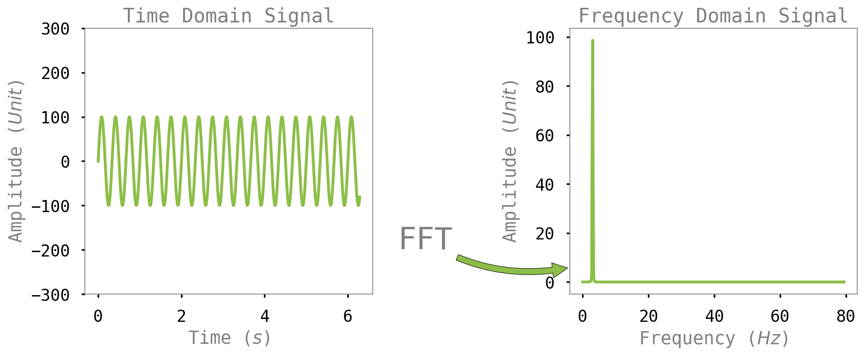
9 |
10 | Including
11 |
12 | * How to scale the x- and y-axis in the amplitude spectrum
13 | * Leakage Effect
14 | * Windowing
15 |
16 | ### [Take a look at the IPython Notebook](http://nbviewer.ipython.org/github/balzer82/FFT-Python/blob/master/FFT-Tutorial.ipynb)
17 |
18 | #### Real World Data Example
19 |
20 | From
21 |
22 | 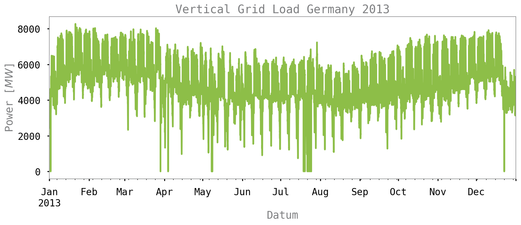
23 |
24 | To
25 |
26 | 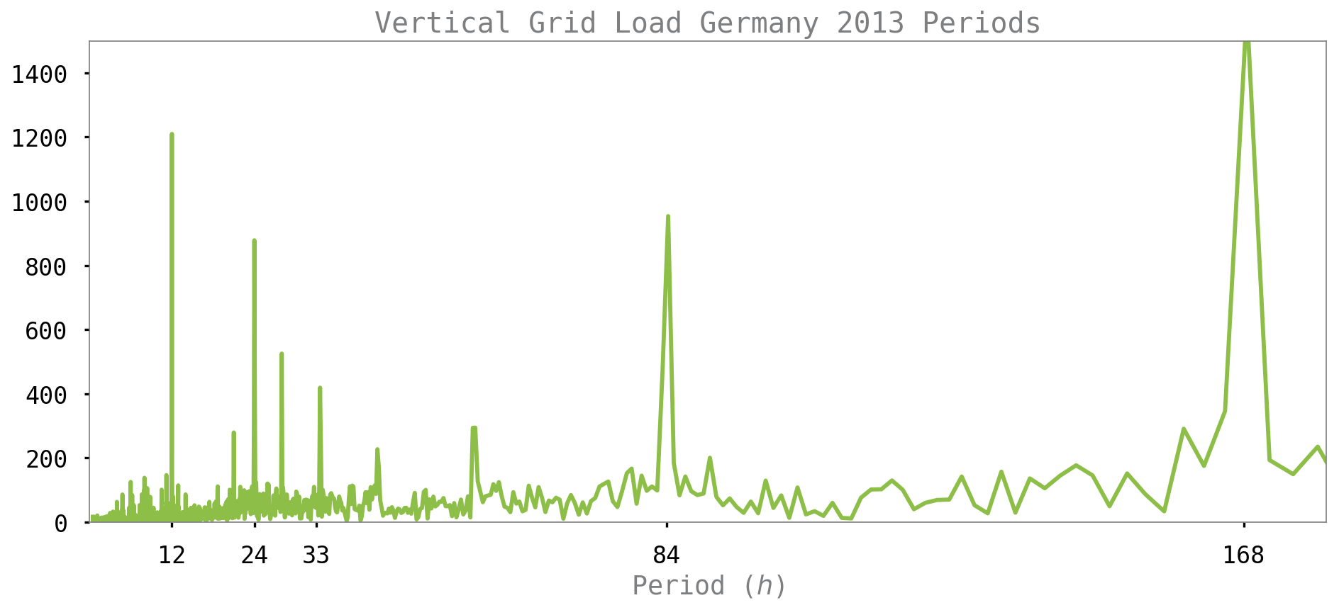
27 |
--------------------------------------------------------------------------------
/VerticalGridLoadGermany2013-FFT.png:
--------------------------------------------------------------------------------
https://raw.githubusercontent.com/balzer82/FFT-Python/2484dd2327739724bdb65747b0a5c29d094df9dc/VerticalGridLoadGermany2013-FFT.png
--------------------------------------------------------------------------------
/VerticalGridLoadGermany2013.png:
--------------------------------------------------------------------------------
https://raw.githubusercontent.com/balzer82/FFT-Python/2484dd2327739724bdb65747b0a5c29d094df9dc/VerticalGridLoadGermany2013.png
--------------------------------------------------------------------------------
/VerticalGridLoadGermany2014-FFT.png:
--------------------------------------------------------------------------------
https://raw.githubusercontent.com/balzer82/FFT-Python/2484dd2327739724bdb65747b0a5c29d094df9dc/VerticalGridLoadGermany2014-FFT.png
--------------------------------------------------------------------------------
/VerticalGridLoadGermany2014.png:
--------------------------------------------------------------------------------
https://raw.githubusercontent.com/balzer82/FFT-Python/2484dd2327739724bdb65747b0a5c29d094df9dc/VerticalGridLoadGermany2014.png
--------------------------------------------------------------------------------
/VerticalGridLoadGermany2015-FFT.png:
--------------------------------------------------------------------------------
https://raw.githubusercontent.com/balzer82/FFT-Python/2484dd2327739724bdb65747b0a5c29d094df9dc/VerticalGridLoadGermany2015-FFT.png
--------------------------------------------------------------------------------
/VerticalGridLoadGermany2015.png:
--------------------------------------------------------------------------------
https://raw.githubusercontent.com/balzer82/FFT-Python/2484dd2327739724bdb65747b0a5c29d094df9dc/VerticalGridLoadGermany2015.png
--------------------------------------------------------------------------------
/VerticalGridLoadGermany2016-FFT.png:
--------------------------------------------------------------------------------
https://raw.githubusercontent.com/balzer82/FFT-Python/2484dd2327739724bdb65747b0a5c29d094df9dc/VerticalGridLoadGermany2016-FFT.png
--------------------------------------------------------------------------------
/VerticalGridLoadGermany2016.png:
--------------------------------------------------------------------------------
https://raw.githubusercontent.com/balzer82/FFT-Python/2484dd2327739724bdb65747b0a5c29d094df9dc/VerticalGridLoadGermany2016.png
--------------------------------------------------------------------------------
/VerticalGridLoadGermany2017-FFT.png:
--------------------------------------------------------------------------------
https://raw.githubusercontent.com/balzer82/FFT-Python/2484dd2327739724bdb65747b0a5c29d094df9dc/VerticalGridLoadGermany2017-FFT.png
--------------------------------------------------------------------------------
/VerticalGridLoadGermany2017.png:
--------------------------------------------------------------------------------
https://raw.githubusercontent.com/balzer82/FFT-Python/2484dd2327739724bdb65747b0a5c29d094df9dc/VerticalGridLoadGermany2017.png
--------------------------------------------------------------------------------
/VerticalGridLoadGermany2018-FFT.png:
--------------------------------------------------------------------------------
https://raw.githubusercontent.com/balzer82/FFT-Python/2484dd2327739724bdb65747b0a5c29d094df9dc/VerticalGridLoadGermany2018-FFT.png
--------------------------------------------------------------------------------
/VerticalGridLoadGermany2018.png:
--------------------------------------------------------------------------------
https://raw.githubusercontent.com/balzer82/FFT-Python/2484dd2327739724bdb65747b0a5c29d094df9dc/VerticalGridLoadGermany2018.png
--------------------------------------------------------------------------------
/VerticalGridLoadGermany2019-FFT.png:
--------------------------------------------------------------------------------
https://raw.githubusercontent.com/balzer82/FFT-Python/2484dd2327739724bdb65747b0a5c29d094df9dc/VerticalGridLoadGermany2019-FFT.png
--------------------------------------------------------------------------------
/VerticalGridLoadGermany2019.png:
--------------------------------------------------------------------------------
https://raw.githubusercontent.com/balzer82/FFT-Python/2484dd2327739724bdb65747b0a5c29d094df9dc/VerticalGridLoadGermany2019.png
--------------------------------------------------------------------------------
/VerticalGridLoadGermany2020-FFT.png:
--------------------------------------------------------------------------------
https://raw.githubusercontent.com/balzer82/FFT-Python/2484dd2327739724bdb65747b0a5c29d094df9dc/VerticalGridLoadGermany2020-FFT.png
--------------------------------------------------------------------------------
/VerticalGridLoadGermany2020.png:
--------------------------------------------------------------------------------
https://raw.githubusercontent.com/balzer82/FFT-Python/2484dd2327739724bdb65747b0a5c29d094df9dc/VerticalGridLoadGermany2020.png
--------------------------------------------------------------------------------
/VerticalGridLoadGermany2021-FFT.png:
--------------------------------------------------------------------------------
https://raw.githubusercontent.com/balzer82/FFT-Python/2484dd2327739724bdb65747b0a5c29d094df9dc/VerticalGridLoadGermany2021-FFT.png
--------------------------------------------------------------------------------
/VerticalGridLoadGermany2021.png:
--------------------------------------------------------------------------------
https://raw.githubusercontent.com/balzer82/FFT-Python/2484dd2327739724bdb65747b0a5c29d094df9dc/VerticalGridLoadGermany2021.png
--------------------------------------------------------------------------------
/VerticalGridLoadGermany2022-FFT.png:
--------------------------------------------------------------------------------
https://raw.githubusercontent.com/balzer82/FFT-Python/2484dd2327739724bdb65747b0a5c29d094df9dc/VerticalGridLoadGermany2022-FFT.png
--------------------------------------------------------------------------------
/VerticalGridLoadGermany2022.png:
--------------------------------------------------------------------------------
https://raw.githubusercontent.com/balzer82/FFT-Python/2484dd2327739724bdb65747b0a5c29d094df9dc/VerticalGridLoadGermany2022.png
--------------------------------------------------------------------------------