├── .gitignore
├── README.md
├── LICENSE
├── World-of-Jupyter.md
├── 1--The Notebook.ipynb
└── 2--The Python world of science and data.ipynb
/.gitignore:
--------------------------------------------------------------------------------
1 |
2 | .ipynb_checkpoints/1--The Notebook-checkpoint.ipynb
3 |
4 | .ipynb_checkpoints/2--The Python world of science and data-checkpoint.ipynb
5 |
6 | .ipynb_checkpoints/3--Jupyter like a pro-checkpoint.ipynb
7 |
--------------------------------------------------------------------------------
/README.md:
--------------------------------------------------------------------------------
1 | # Jupyter Tutorial
2 |
3 | [](http://mybinder.org:/repo/barbagroup/jupyter-tutorial)
4 |
5 | * [**"The world of Jupyter"**](https://github.com/barbagroup/jupyter-tutorial/blob/master/World-of-Jupyter.md)—a tutorial held in Huazhong University of Science and Technology (HUST) in Wuhan, China (June 2016).
6 |
7 | ---
8 |
9 | ### License
10 |
11 | The content of this repository is shared under a Creative Commons Attribution License CC-BY 4.0. All code is under MIT License.
12 |
13 | (c) 2016 Barba group (Lorena A. Barba and co-authors, as indicated)
14 |
--------------------------------------------------------------------------------
/LICENSE:
--------------------------------------------------------------------------------
1 | The MIT License (MIT)
2 |
3 | Copyright (c) 2016 Barba group
4 |
5 | Permission is hereby granted, free of charge, to any person obtaining a copy
6 | of this software and associated documentation files (the "Software"), to deal
7 | in the Software without restriction, including without limitation the rights
8 | to use, copy, modify, merge, publish, distribute, sublicense, and/or sell
9 | copies of the Software, and to permit persons to whom the Software is
10 | furnished to do so, subject to the following conditions:
11 |
12 | The above copyright notice and this permission notice shall be included in all
13 | copies or substantial portions of the Software.
14 |
15 | THE SOFTWARE IS PROVIDED "AS IS", WITHOUT WARRANTY OF ANY KIND, EXPRESS OR
16 | IMPLIED, INCLUDING BUT NOT LIMITED TO THE WARRANTIES OF MERCHANTABILITY,
17 | FITNESS FOR A PARTICULAR PURPOSE AND NONINFRINGEMENT. IN NO EVENT SHALL THE
18 | AUTHORS OR COPYRIGHT HOLDERS BE LIABLE FOR ANY CLAIM, DAMAGES OR OTHER
19 | LIABILITY, WHETHER IN AN ACTION OF CONTRACT, TORT OR OTHERWISE, ARISING FROM,
20 | OUT OF OR IN CONNECTION WITH THE SOFTWARE OR THE USE OR OTHER DEALINGS IN THE
21 | SOFTWARE.
22 |
--------------------------------------------------------------------------------
/World-of-Jupyter.md:
--------------------------------------------------------------------------------
1 | # The world of Jupyter
2 | ## An environment to think, code, explore data and communicate science
3 |
4 | At the center of the Jupyter world are *notebooks*: documents containing a mix of rich text elements—headings, paragraph text, hyperlinks, mathematical symbols and embedded figures—and interactive code elements. The document uses "cells" to divide up the text and code elements: text is formatted using markdown, and code can be executed using the IPython kernel or others (like Julia or R language).
5 |
6 | You can use the notebooks to annotate ideas around code, to explain your thought process, or to report on research process and results. Having interactive code right there in the document empowers you to "think with code," trying things out and exploring data as you go. The notebook has also become a very popular platform for teaching and learning, with a growing community of users publishing lessons, even books, using notebooks.
7 |
8 | To work on notebooks, you run the Jupyter Notebook App and edit them from your favorite browser. The app gives you a dashboard on a new browser window that connects to the computational engine (called kernel) behind the scenes. You can install Jupyter locally on your computer, or use it on the cloud on paid or free services. You can also share your finished notebooks online as a static web page, via the free [`nbviewer`](http://nbviewer.jupyter.org) service.
9 |
10 | Everything in Project Jupyter is free and open source. Via the IPython kernel, you can access the whole ecosystem of Python with its libraries for numerical computing, visualization, data analysis, machine learning and more. Jupyter is a world of sharing code and content, and a productive environment to get things done with code and data.
11 |
12 | Get started with Jupyter in this tutorial, and then follow some of the many more available online.
13 |
14 | You can try Jupyter right now on this free service: [https://try.jupyter.org](https://try.jupyter.org). Click on the "Welcome to Python" link there: this demo is a temporary notebook with a single code cell that reads some data and draws a plot. Or you can instead click on the "New" button (top right) and choose Python 3 from the options, to get a blank notebook (also temporary). To try a notebook that you can save on the cloud, use the new free service by Azure: [https://notebooks.azure.com](https://notebooks.azure.com). If you want everything installed in your own laptop computer, download the Anaconda distribution (free) from: [https://www.continuum.io/downloads](https://www.continuum.io/downloads)
15 |
16 | ### Jupyter tutorial in Wuhan, June 2016
17 |
18 | For the Jupyter tutorial at **Huazhong University of Science and Technology** (Wuhan, China), by Prof. Lorena Barba, students should prepare by doing one of these:
19 |
20 | 1. Create an account on Microsoft **Azure** and test the free cloud notebooks at [https://notebooks.azure.com](https://notebooks.azure.com) — you need an account to be able to save notebooks for later. If you only access the free demos, your work will not be saved.
21 | 2. Install **Anaconda** in your laptop computer. Downloading from the [official website](https://www.continuum.io/downloads) could take a long time, but there is a mirror at Tsinghua University, according to the post in: [http://www.tuicool.com/articles/vyyA7rB](http://www.tuicool.com/articles/vyyA7rB)
22 | We found an error in the URL provided in that post, though. The actual location of the Tsinghua mirror is [https://mirrors.tuna.tsinghua.edu.cn/anaconda/archive/](https://mirrors.tuna.tsinghua.edu.cn/anaconda/archive/)
23 | Download the latest version for your operating system (we'll be using Python 3).
24 | After installing, from a terminal, run `conda update conda` and then run `conda update jupyter numpy sympy scipy matplotlib`
25 | 3. If your internet is slow or you want to save disk space, you can instead install **Miniconda** from the [official site](http://conda.pydata.org/miniconda.html) or from the [mirror](https://mirrors.tuna.tsinghua.edu.cn/anaconda/miniconda/) in Tsinghua University. Then, you should run three commands from the terminal:
26 | `conda update conda`
27 | `conda install jupyter`
28 | `conda install numpy scipy sympy matplotlib`
29 |
30 | ## Contents
31 |
32 | (Links to notebooks rendered by **nbviewer**.)
33 |
34 | 1. [The Notebook](http://nbviewer.jupyter.org/github/barbagroup/jupyter-tutorial/blob/master/1--The%20Notebook.ipynb)
35 | 2. [The Python world of science and data](http://nbviewer.jupyter.org/github/barbagroup/jupyter-tutorial/blob/master/2--The%20Python%20world%20of%20science%20and%20data.ipynb)
36 | 3. [Jupyter like a pro](http://nbviewer.jupyter.org/github/barbagroup/jupyter-tutorial/blob/master/3--Jupyter%20like%20a%20pro.ipynb)
37 |
38 |
39 | ### Interact with the notebooks on Azure cloud:
40 |
41 | You can interact with the notebooks right now, without downloading anything—thanks to the new cloud notebooks by Azure—by following this link:
42 | [https://notebooks.azure.com/library/Jbzl8X0qhHw](https://notebooks.azure.com/library/Jbzl8X0qhHw)
--------------------------------------------------------------------------------
/1--The Notebook.ipynb:
--------------------------------------------------------------------------------
1 | {
2 | "cells": [
3 | {
4 | "cell_type": "markdown",
5 | "metadata": {},
6 | "source": [
7 | "# The Notebook\n",
8 | "\n",
9 | "This is a _notebook_: a document that can contain rich text elements—headings, paragraph text, hyperlinks, mathematical symbols and embedded figures—and interactive code elements. The document uses \"cells\" to divide up the text and code elements: text is formatted using markdown, and code can be executed using the IPython kernel.\n",
10 | "\n",
11 | "[Markdown](https://en.wikipedia.org/wiki/Markdown) is an easy way to format text to be displayed on a browser. You can format headings, bold face, italics, add a horizonal line, hyperlink some text, add bulleted or numbered lists. It's so easy, you can learn it in minutes! The \"Daring Fireball\" (by John Gruber) [markdown syntax](https://daringfireball.net/projects/markdown/syntax) page is a nice starting point or reference."
12 | ]
13 | },
14 | {
15 | "cell_type": "markdown",
16 | "metadata": {},
17 | "source": [
18 | "## Nbviewer\n",
19 | "\n",
20 | "If you came to view this notebook following the link on the tutorial description, [\"The world of Jupyter\"](https://github.com/barbagroup/jupyter-tutorial/blob/master/World-of-Jupyter.md) (itself, a markdown file), then you are seeing it rendered as a static webpage on the free [**nbviewer**](http://nbviewer.jupyter.org) service. It is the simplest way to share a notebook with anyone: just host the notebook file (`.ipynb` extension) online and enter the public URL to the file on the **nbviewer** _Go!_ box. The notebook will be rendered like a static webpage: visitors can read everything, but they cannot interact with the code. \n",
21 | "\n",
22 | "To interact with a notebook, you need the Jupyter Notebook App, either locally installed on your computer or on some cloud service."
23 | ]
24 | },
25 | {
26 | "cell_type": "markdown",
27 | "metadata": {},
28 | "source": [
29 | "## Jupyter Notebook App\n",
30 | "\n",
31 | "If you want to see what the Jupyter Notebook App looks like, you can try it right now on this free service: [https://try.jupyter.org](https://try.jupyter.org). You should see the _Dashboard_, which shows a list of available files, like this:\n",
32 | "\n",
33 | "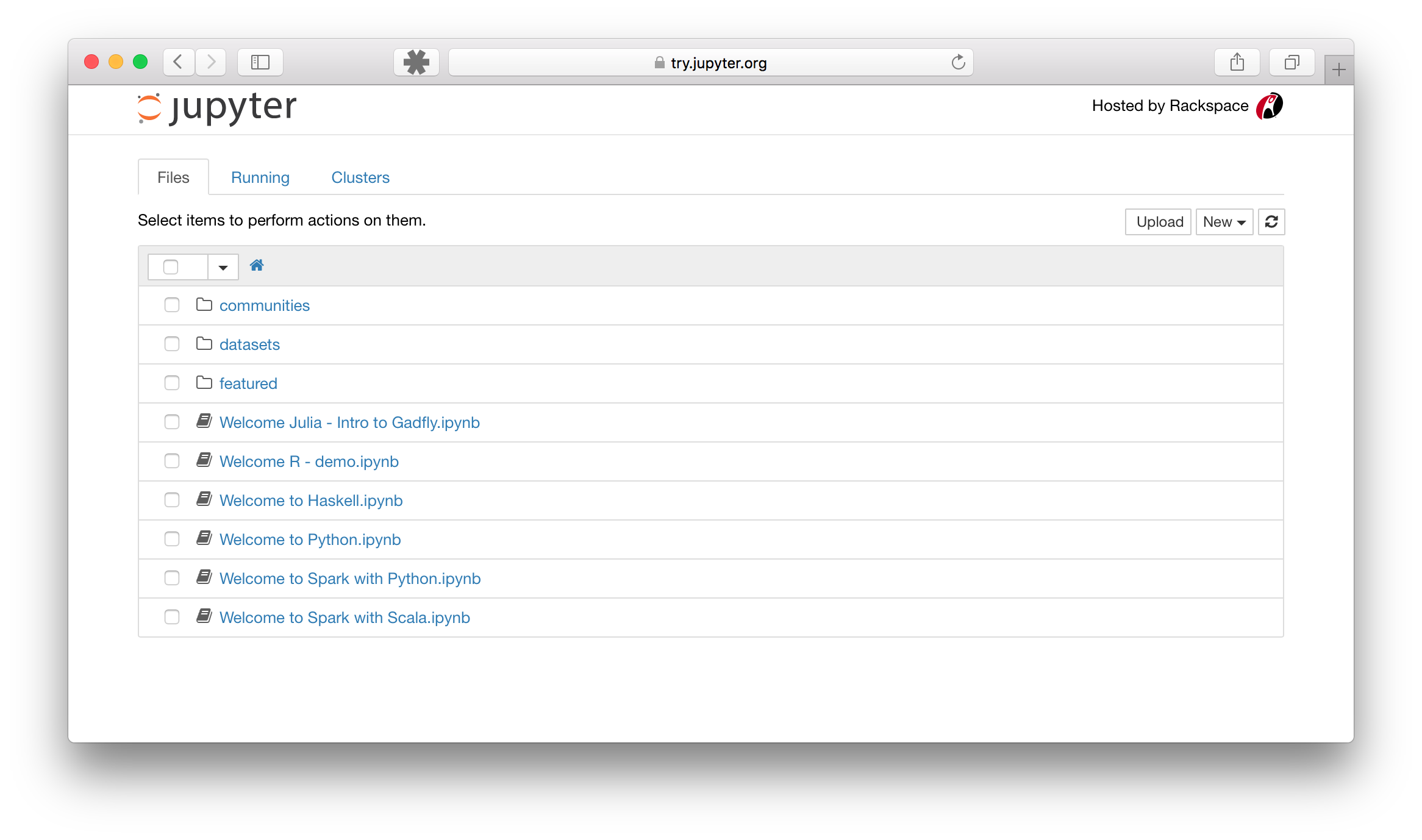\n",
34 | "\n",
35 | "Click on the _New_ button on the top right, and choose \"Python 3\" from the pull-down options to get a notebook that is connected to the IPython kernel. You should get an empty notebook with a single empty code cell labeled `In[ ]`, with a flashing cursor inside. This is a code cell. You can start by trying any simple mathematical operation (like a calculator), and type `[shift] + [enter]` to execute it.\n",
36 | "\n",
37 | "You can try any of the arithmetic operators in Python:\n",
38 | "```python\n",
39 | " + - * / ** % //\n",
40 | "```\n",
41 | "The last three operators above are _exponent_ (raise to the power of), _modulo_ (divide and return remainder) and _floor division_. Be careful that the division operator behaves differently in legacy Python 2: it rounds to an integer when the operands are integers. We use Python 3 and don't worry about this, because it gives the expected result, e.g., `1/2` gives `0.5` (not zero!).\n",
42 | "\n",
43 | "Here's a simple example calculation in a code cell:"
44 | ]
45 | },
46 | {
47 | "cell_type": "code",
48 | "execution_count": 1,
49 | "metadata": {
50 | "collapsed": false
51 | },
52 | "outputs": [
53 | {
54 | "data": {
55 | "text/plain": [
56 | "24"
57 | ]
58 | },
59 | "execution_count": 1,
60 | "metadata": {},
61 | "output_type": "execute_result"
62 | }
63 | ],
64 | "source": [
65 | "2 * 12"
66 | ]
67 | },
68 | {
69 | "cell_type": "markdown",
70 | "metadata": {},
71 | "source": [
72 | "Typing `[shift] + [enter]` will execute the cell and give you the output in a new line, labeled `Out[1]` (the numbering increases each time you execute a cell). If you're at the end of the notebook, you will also get a new blank cell, where you can try more arithmetic operations, if you want. Or, you can change the type of cell from _Code_ to _Markdown_ with the button on the menu bar. See if you find that now, and then type some text into a markdwon cell. Try some [markdown syntax](https://daringfireball.net/projects/markdown/syntax)!\n",
73 | "\n",
74 | "In a code cell, you can enter any valid Python code, and type `[shift] + [enter]` to execute it. For example, the simplest code example just prints the message _Hello World!_, like this:"
75 | ]
76 | },
77 | {
78 | "cell_type": "code",
79 | "execution_count": 2,
80 | "metadata": {
81 | "collapsed": false
82 | },
83 | "outputs": [
84 | {
85 | "name": "stdout",
86 | "output_type": "stream",
87 | "text": [
88 | "Hello World!\n"
89 | ]
90 | }
91 | ],
92 | "source": [
93 | "print(\"Hello World!\")"
94 | ]
95 | },
96 | {
97 | "cell_type": "markdown",
98 | "metadata": {},
99 | "source": [
100 | "You can also define a variable (say `x`) and assign it a value (say, 2), then use that variable in some code:"
101 | ]
102 | },
103 | {
104 | "cell_type": "code",
105 | "execution_count": 3,
106 | "metadata": {
107 | "collapsed": true
108 | },
109 | "outputs": [],
110 | "source": [
111 | "x = 2"
112 | ]
113 | },
114 | {
115 | "cell_type": "code",
116 | "execution_count": 4,
117 | "metadata": {
118 | "collapsed": false
119 | },
120 | "outputs": [
121 | {
122 | "name": "stdout",
123 | "output_type": "stream",
124 | "text": [
125 | "Hello World!Hello World!\n"
126 | ]
127 | }
128 | ],
129 | "source": [
130 | "print(x * \"Hello World!\")"
131 | ]
132 | },
133 | {
134 | "cell_type": "code",
135 | "execution_count": 5,
136 | "metadata": {
137 | "collapsed": false
138 | },
139 | "outputs": [
140 | {
141 | "data": {
142 | "text/plain": [
143 | "24"
144 | ]
145 | },
146 | "execution_count": 5,
147 | "metadata": {},
148 | "output_type": "execute_result"
149 | }
150 | ],
151 | "source": [
152 | "x * 12"
153 | ]
154 | },
155 | {
156 | "cell_type": "markdown",
157 | "metadata": {},
158 | "source": [
159 | "## More Jupyter cloud services\n",
160 | "\n",
161 | "If you followed the instructions above, you launched the Jupyter Notebook App on a cloud service called **`tmpnb`**. As the prefix `tmp` indicates, it gives you a temporary demo: as soon as you close the browser tab (or after a few minutes of inactivity), the kernel dies and the content you wrote is not saved anywhere. This is a free service, sponsored by the company Rackspace, just for trying something out.\n",
162 | "\n",
163 | "You can work on notebooks and save your work using other cloud services. A long-running cloud offering is [SageMathCloud](https://cloud.sagemath.com). And most recently (in June 2016), Microsoft announced [notebooks hosted on Azure](https://notebooks.azure.com) cloud. In both cases, you need to create a free account to be able to save your work."
164 | ]
165 | },
166 | {
167 | "cell_type": "markdown",
168 | "metadata": {},
169 | "source": [
170 | "## The world of Jupyter, so far\n",
171 | "\n",
172 | "You learned about: \n",
173 | "\n",
174 | "* the notebook, \n",
175 | "* code cells and markdown cells, \n",
176 | "* **nbviewer**, \n",
177 | "* the Jupyter Notebook App, \n",
178 | "* `[shift] + [enter]` to execute, \n",
179 | "* **`tmpnb`**, and\n",
180 | "* cloud notebook services."
181 | ]
182 | },
183 | {
184 | "cell_type": "markdown",
185 | "metadata": {},
186 | "source": [
187 | "## Optional next step: local installation\n",
188 | "\n",
189 | "Cloud notebook services (especially free ones!) have their limitations. As you start using notebooks more, you'll want to **install Jupyter** on your personal computer. For that, we recommend the free [Anaconda](https://www.continuum.io/downloads) distribution, which includes _all_ the Python packages you may need (more than 700 packages are included!).\n",
190 | "\n",
191 | "If you prefer a light installation (e.g., if your internet is slow), we can recommend [Miniconda](http://conda.pydata.org/miniconda.html). This will include only `conda` (the package manager) and its dependencies, and Python. You will have to install Jupyter separately, and also other basic Python libraries for numerical mathematics and data analysis, using the `conda install` command.\n",
192 | "\n",
193 | "We also recommend that you start with Python 3 right away—Python 2.7 is the _legacy_ Python, and you should only need to use it if you have a lot of code written in the past that you need to work with.\n"
194 | ]
195 | },
196 | {
197 | "cell_type": "markdown",
198 | "metadata": {},
199 | "source": [
200 | "# Next\n",
201 | "\n",
202 | "* Get started with a foundation on Python for numerical mathematics and data analysis: [The Python world of science and data](http://nbviewer.jupyter.org/github/barbagroup/jupyter-tutorial/blob/master/2--The%20Python%20world%20of%20science%20and%20data.ipynb)"
203 | ]
204 | },
205 | {
206 | "cell_type": "markdown",
207 | "metadata": {},
208 | "source": [
209 | "---\n",
210 | "\n",
211 | "(c) 2016 Lorena A. Barba. Free to use under Creative Commons Attribution CC-BY 4.0 License. This notebook was written for the tutorial \"The world of Jupyter\" at the Huazhong University of Science and Technology (HUST), Wuhan, China.\n",
212 | "
"
213 | ]
214 | }
215 | ],
216 | "metadata": {
217 | "kernelspec": {
218 | "display_name": "Python 3",
219 | "language": "python",
220 | "name": "python3"
221 | },
222 | "language_info": {
223 | "codemirror_mode": {
224 | "name": "ipython",
225 | "version": 3
226 | },
227 | "file_extension": ".py",
228 | "mimetype": "text/x-python",
229 | "name": "python",
230 | "nbconvert_exporter": "python",
231 | "pygments_lexer": "ipython3",
232 | "version": "3.5.1"
233 | }
234 | },
235 | "nbformat": 4,
236 | "nbformat_minor": 0
237 | }
238 |
--------------------------------------------------------------------------------
/2--The Python world of science and data.ipynb:
--------------------------------------------------------------------------------
1 | {
2 | "cells": [
3 | {
4 | "cell_type": "markdown",
5 | "metadata": {},
6 | "source": [
7 | "# The Python world of science and data\n",
8 | "\n",
9 | "The [Jupyter notebook](http://nbviewer.jupyter.org/github/barbagroup/jupyter-tutorial/blob/master/1--The%20Notebook.ipynb) is a nice way to write and share some content online, but you'll get superpowers from Python libraries for science and data!\n",
10 | "\n",
11 | "We already used code cells to do simple calculations via the arithmetic operators in Python:\n",
12 | "```python\n",
13 | " + - * / ** % //\n",
14 | "```\n",
15 | "\n",
16 | "\n",
17 | "\n",
18 | "In addition to arithmetics, you can do comparisons with operators that return Boolean values (`True` or `False`). These are:\n",
19 | "```python\n",
20 | " == != < > <= >=\n",
21 | "```\n",
22 | "\n",
23 | "On top of those, you have assignment operators, bitwise operators, logical operators, membership operators, and identity operators. You can find online several \"cheat sheets\" for Python operators. For example: [\"Operators and expressions\"](http://pymbook.readthedocs.io/en/latest/operatorsexpressions.html) in the online book _\"Python for You and Me.\"_\n",
24 | "\n",
25 | "Go ahead and experiment with various Python operators until you're satisfied. You can open a new, empty notebook and experiment in code cells, taking notes of the things that you find interesting in markdown cells. Or, if you have _this_ notebook open in the Jupyter Notebook App, you can add a new cell by clicking the plus button: , and work right here. Remember to type `[shift] + [enter]` to exectue any cell.\n",
26 | "\n",
27 | "Next, let's learn about the Python world of science and data."
28 | ]
29 | },
30 | {
31 | "cell_type": "markdown",
32 | "metadata": {},
33 | "source": [
34 | "## Two libraries that made Python useful for science: NumPy and Matplotlib\n",
35 | "\n",
36 | "Python is a general-purpose language: you can use it to create websites, to write programs that crawl the web, to support you in scientific research or data analysis, etc. Because it can be used in so many fields, the core language is supported by many libraries (not everyone needs to have every functionality). In science, two libraries made Python really useful: [**NumPy**](http://www.numpy.org) and [**Matplotlib**](http://matplotlib.org).\n",
37 | "\n",
38 | "**NumPy** gives you access to numerical mathematics on arrays (like vectors and matrices). **Matplotlib** gives you a catalog of plotting functions for visualizing data."
39 | ]
40 | },
41 | {
42 | "cell_type": "code",
43 | "execution_count": 1,
44 | "metadata": {
45 | "collapsed": true
46 | },
47 | "outputs": [],
48 | "source": [
49 | "import numpy"
50 | ]
51 | },
52 | {
53 | "cell_type": "markdown",
54 | "metadata": {},
55 | "source": [
56 | "The command `import` followed by the name of a library will extend your Python session with all of the functions in that library. After executing the code cell above, we have all of **NumPy** available to us. If you have this notebook open in the Jupyter Notebook App, make sure to execute the cell above by clicking on it and typing ``[shift] + [enter]``.\n",
57 | "\n",
58 | "Now, to use one of **NumPy**'s functions, we prepend `numpy.` (with the dot) to the function name. For example:"
59 | ]
60 | },
61 | {
62 | "cell_type": "code",
63 | "execution_count": 2,
64 | "metadata": {
65 | "collapsed": false
66 | },
67 | "outputs": [
68 | {
69 | "data": {
70 | "text/plain": [
71 | "array([ 0. , 0.55555556, 1.11111111, 1.66666667, 2.22222222,\n",
72 | " 2.77777778, 3.33333333, 3.88888889, 4.44444444, 5. ])"
73 | ]
74 | },
75 | "execution_count": 2,
76 | "metadata": {},
77 | "output_type": "execute_result"
78 | }
79 | ],
80 | "source": [
81 | "numpy.linspace(0, 5, 10)"
82 | ]
83 | },
84 | {
85 | "cell_type": "markdown",
86 | "metadata": {},
87 | "source": [
88 | "The **NumPy** function [`linspace()`](http://docs.scipy.org/doc/numpy/reference/generated/numpy.linspace.html) creates an array with equally spaced numbers between a start and end. It's a very useful function! In the code cell above, we create an array of 10 numbers from 0 to 5. Go ahead and try it with different argument values.\n",
89 | "\n",
90 | "To be able to do something with this array later, we normally want to give it a name. Like,"
91 | ]
92 | },
93 | {
94 | "cell_type": "code",
95 | "execution_count": 3,
96 | "metadata": {
97 | "collapsed": true
98 | },
99 | "outputs": [],
100 | "source": [
101 | "xarray = numpy.linspace(0, 5, 10)"
102 | ]
103 | },
104 | {
105 | "cell_type": "markdown",
106 | "metadata": {},
107 | "source": [
108 | "Now, we can use **NumPy** to do computations with the array. Like take its square:"
109 | ]
110 | },
111 | {
112 | "cell_type": "code",
113 | "execution_count": 4,
114 | "metadata": {
115 | "collapsed": false
116 | },
117 | "outputs": [
118 | {
119 | "data": {
120 | "text/plain": [
121 | "array([ 0. , 0.30864198, 1.2345679 , 2.77777778,\n",
122 | " 4.9382716 , 7.71604938, 11.11111111, 15.12345679,\n",
123 | " 19.75308642, 25. ])"
124 | ]
125 | },
126 | "execution_count": 4,
127 | "metadata": {},
128 | "output_type": "execute_result"
129 | }
130 | ],
131 | "source": [
132 | "xarray ** 2"
133 | ]
134 | },
135 | {
136 | "cell_type": "markdown",
137 | "metadata": {},
138 | "source": [
139 | "In **NumPy**, the square of an array of numbers takes the square of each element. You will likely want to give your result a name, too. So let's do this again, and also take the cube, and the square root of the array at the same time."
140 | ]
141 | },
142 | {
143 | "cell_type": "code",
144 | "execution_count": 5,
145 | "metadata": {
146 | "collapsed": true
147 | },
148 | "outputs": [],
149 | "source": [
150 | "yarray = xarray ** 2\n",
151 | "zarray = xarray ** 3\n",
152 | "warray = numpy.sqrt(xarray)"
153 | ]
154 | },
155 | {
156 | "cell_type": "markdown",
157 | "metadata": {},
158 | "source": [
159 | "You notice that **NumPy** knows how to take the power of an array, and it has a built-in function for the square-root. Now, you may want to draw a plot of these results with the original array on the x-axis. For that we need the module `pyplot` from **Matplotlib**."
160 | ]
161 | },
162 | {
163 | "cell_type": "code",
164 | "execution_count": 6,
165 | "metadata": {
166 | "collapsed": true
167 | },
168 | "outputs": [],
169 | "source": [
170 | "from matplotlib import pyplot\n",
171 | "%matplotlib notebook"
172 | ]
173 | },
174 | {
175 | "cell_type": "markdown",
176 | "metadata": {},
177 | "source": [
178 | "The command `%matplotlib notebook` is there to get our plots inside the notebook (instead of a pop-up window, which is the default behavior of `pyplot`). Let's try a line plot now! We use the `pyplot.plot()` function, specifying the line color (`'k'` for black) and line style (`'-'`, `'--'` and `':'` for continuous, dashed and dotted line), and giving each line a label. Note that the values for `color`, `linestyle` and `label` are given in quotes."
179 | ]
180 | },
181 | {
182 | "cell_type": "code",
183 | "execution_count": 7,
184 | "metadata": {
185 | "collapsed": false
186 | },
187 | "outputs": [
188 | {
189 | "data": {
190 | "application/javascript": [
191 | "/* Put everything inside the global mpl namespace */\n",
192 | "window.mpl = {};\n",
193 | "\n",
194 | "mpl.get_websocket_type = function() {\n",
195 | " if (typeof(WebSocket) !== 'undefined') {\n",
196 | " return WebSocket;\n",
197 | " } else if (typeof(MozWebSocket) !== 'undefined') {\n",
198 | " return MozWebSocket;\n",
199 | " } else {\n",
200 | " alert('Your browser does not have WebSocket support.' +\n",
201 | " 'Please try Chrome, Safari or Firefox ≥ 6. ' +\n",
202 | " 'Firefox 4 and 5 are also supported but you ' +\n",
203 | " 'have to enable WebSockets in about:config.');\n",
204 | " };\n",
205 | "}\n",
206 | "\n",
207 | "mpl.figure = function(figure_id, websocket, ondownload, parent_element) {\n",
208 | " this.id = figure_id;\n",
209 | "\n",
210 | " this.ws = websocket;\n",
211 | "\n",
212 | " this.supports_binary = (this.ws.binaryType != undefined);\n",
213 | "\n",
214 | " if (!this.supports_binary) {\n",
215 | " var warnings = document.getElementById(\"mpl-warnings\");\n",
216 | " if (warnings) {\n",
217 | " warnings.style.display = 'block';\n",
218 | " warnings.textContent = (\n",
219 | " \"This browser does not support binary websocket messages. \" +\n",
220 | " \"Performance may be slow.\");\n",
221 | " }\n",
222 | " }\n",
223 | "\n",
224 | " this.imageObj = new Image();\n",
225 | "\n",
226 | " this.context = undefined;\n",
227 | " this.message = undefined;\n",
228 | " this.canvas = undefined;\n",
229 | " this.rubberband_canvas = undefined;\n",
230 | " this.rubberband_context = undefined;\n",
231 | " this.format_dropdown = undefined;\n",
232 | "\n",
233 | " this.image_mode = 'full';\n",
234 | "\n",
235 | " this.root = $('');\n",
236 | " this._root_extra_style(this.root)\n",
237 | " this.root.attr('style', 'display: inline-block');\n",
238 | "\n",
239 | " $(parent_element).append(this.root);\n",
240 | "\n",
241 | " this._init_header(this);\n",
242 | " this._init_canvas(this);\n",
243 | " this._init_toolbar(this);\n",
244 | "\n",
245 | " var fig = this;\n",
246 | "\n",
247 | " this.waiting = false;\n",
248 | "\n",
249 | " this.ws.onopen = function () {\n",
250 | " fig.send_message(\"supports_binary\", {value: fig.supports_binary});\n",
251 | " fig.send_message(\"send_image_mode\", {});\n",
252 | " fig.send_message(\"refresh\", {});\n",
253 | " }\n",
254 | "\n",
255 | " this.imageObj.onload = function() {\n",
256 | " if (fig.image_mode == 'full') {\n",
257 | " // Full images could contain transparency (where diff images\n",
258 | " // almost always do), so we need to clear the canvas so that\n",
259 | " // there is no ghosting.\n",
260 | " fig.context.clearRect(0, 0, fig.canvas.width, fig.canvas.height);\n",
261 | " }\n",
262 | " fig.context.drawImage(fig.imageObj, 0, 0);\n",
263 | " };\n",
264 | "\n",
265 | " this.imageObj.onunload = function() {\n",
266 | " this.ws.close();\n",
267 | " }\n",
268 | "\n",
269 | " this.ws.onmessage = this._make_on_message_function(this);\n",
270 | "\n",
271 | " this.ondownload = ondownload;\n",
272 | "}\n",
273 | "\n",
274 | "mpl.figure.prototype._init_header = function() {\n",
275 | " var titlebar = $(\n",
276 | " '');\n",
278 | " var titletext = $(\n",
279 | " '');\n",
281 | " titlebar.append(titletext)\n",
282 | " this.root.append(titlebar);\n",
283 | " this.header = titletext[0];\n",
284 | "}\n",
285 | "\n",
286 | "\n",
287 | "\n",
288 | "mpl.figure.prototype._canvas_extra_style = function(canvas_div) {\n",
289 | "\n",
290 | "}\n",
291 | "\n",
292 | "\n",
293 | "mpl.figure.prototype._root_extra_style = function(canvas_div) {\n",
294 | "\n",
295 | "}\n",
296 | "\n",
297 | "mpl.figure.prototype._init_canvas = function() {\n",
298 | " var fig = this;\n",
299 | "\n",
300 | " var canvas_div = $('');\n",
301 | "\n",
302 | " canvas_div.attr('style', 'position: relative; clear: both; outline: 0');\n",
303 | "\n",
304 | " function canvas_keyboard_event(event) {\n",
305 | " return fig.key_event(event, event['data']);\n",
306 | " }\n",
307 | "\n",
308 | " canvas_div.keydown('key_press', canvas_keyboard_event);\n",
309 | " canvas_div.keyup('key_release', canvas_keyboard_event);\n",
310 | " this.canvas_div = canvas_div\n",
311 | " this._canvas_extra_style(canvas_div)\n",
312 | " this.root.append(canvas_div);\n",
313 | "\n",
314 | " var canvas = $('');\n",
315 | " canvas.addClass('mpl-canvas');\n",
316 | " canvas.attr('style', \"left: 0; top: 0; z-index: 0; outline: 0\")\n",
317 | "\n",
318 | " this.canvas = canvas[0];\n",
319 | " this.context = canvas[0].getContext(\"2d\");\n",
320 | "\n",
321 | " var rubberband = $('');\n",
322 | " rubberband.attr('style', \"position: absolute; left: 0; top: 0; z-index: 1;\")\n",
323 | "\n",
324 | " var pass_mouse_events = true;\n",
325 | "\n",
326 | " canvas_div.resizable({\n",
327 | " start: function(event, ui) {\n",
328 | " pass_mouse_events = false;\n",
329 | " },\n",
330 | " resize: function(event, ui) {\n",
331 | " fig.request_resize(ui.size.width, ui.size.height);\n",
332 | " },\n",
333 | " stop: function(event, ui) {\n",
334 | " pass_mouse_events = true;\n",
335 | " fig.request_resize(ui.size.width, ui.size.height);\n",
336 | " },\n",
337 | " });\n",
338 | "\n",
339 | " function mouse_event_fn(event) {\n",
340 | " if (pass_mouse_events)\n",
341 | " return fig.mouse_event(event, event['data']);\n",
342 | " }\n",
343 | "\n",
344 | " rubberband.mousedown('button_press', mouse_event_fn);\n",
345 | " rubberband.mouseup('button_release', mouse_event_fn);\n",
346 | " // Throttle sequential mouse events to 1 every 20ms.\n",
347 | " rubberband.mousemove('motion_notify', mouse_event_fn);\n",
348 | "\n",
349 | " rubberband.mouseenter('figure_enter', mouse_event_fn);\n",
350 | " rubberband.mouseleave('figure_leave', mouse_event_fn);\n",
351 | "\n",
352 | " canvas_div.on(\"wheel\", function (event) {\n",
353 | " event = event.originalEvent;\n",
354 | " event['data'] = 'scroll'\n",
355 | " if (event.deltaY < 0) {\n",
356 | " event.step = 1;\n",
357 | " } else {\n",
358 | " event.step = -1;\n",
359 | " }\n",
360 | " mouse_event_fn(event);\n",
361 | " });\n",
362 | "\n",
363 | " canvas_div.append(canvas);\n",
364 | " canvas_div.append(rubberband);\n",
365 | "\n",
366 | " this.rubberband = rubberband;\n",
367 | " this.rubberband_canvas = rubberband[0];\n",
368 | " this.rubberband_context = rubberband[0].getContext(\"2d\");\n",
369 | " this.rubberband_context.strokeStyle = \"#000000\";\n",
370 | "\n",
371 | " this._resize_canvas = function(width, height) {\n",
372 | " // Keep the size of the canvas, canvas container, and rubber band\n",
373 | " // canvas in synch.\n",
374 | " canvas_div.css('width', width)\n",
375 | " canvas_div.css('height', height)\n",
376 | "\n",
377 | " canvas.attr('width', width);\n",
378 | " canvas.attr('height', height);\n",
379 | "\n",
380 | " rubberband.attr('width', width);\n",
381 | " rubberband.attr('height', height);\n",
382 | " }\n",
383 | "\n",
384 | " // Set the figure to an initial 600x600px, this will subsequently be updated\n",
385 | " // upon first draw.\n",
386 | " this._resize_canvas(600, 600);\n",
387 | "\n",
388 | " // Disable right mouse context menu.\n",
389 | " $(this.rubberband_canvas).bind(\"contextmenu\",function(e){\n",
390 | " return false;\n",
391 | " });\n",
392 | "\n",
393 | " function set_focus () {\n",
394 | " canvas.focus();\n",
395 | " canvas_div.focus();\n",
396 | " }\n",
397 | "\n",
398 | " window.setTimeout(set_focus, 100);\n",
399 | "}\n",
400 | "\n",
401 | "mpl.figure.prototype._init_toolbar = function() {\n",
402 | " var fig = this;\n",
403 | "\n",
404 | " var nav_element = $('')\n",
405 | " nav_element.attr('style', 'width: 100%');\n",
406 | " this.root.append(nav_element);\n",
407 | "\n",
408 | " // Define a callback function for later on.\n",
409 | " function toolbar_event(event) {\n",
410 | " return fig.toolbar_button_onclick(event['data']);\n",
411 | " }\n",
412 | " function toolbar_mouse_event(event) {\n",
413 | " return fig.toolbar_button_onmouseover(event['data']);\n",
414 | " }\n",
415 | "\n",
416 | " for(var toolbar_ind in mpl.toolbar_items) {\n",
417 | " var name = mpl.toolbar_items[toolbar_ind][0];\n",
418 | " var tooltip = mpl.toolbar_items[toolbar_ind][1];\n",
419 | " var image = mpl.toolbar_items[toolbar_ind][2];\n",
420 | " var method_name = mpl.toolbar_items[toolbar_ind][3];\n",
421 | "\n",
422 | " if (!name) {\n",
423 | " // put a spacer in here.\n",
424 | " continue;\n",
425 | " }\n",
426 | " var button = $('');\n",
427 | " button.addClass('ui-button ui-widget ui-state-default ui-corner-all ' +\n",
428 | " 'ui-button-icon-only');\n",
429 | " button.attr('role', 'button');\n",
430 | " button.attr('aria-disabled', 'false');\n",
431 | " button.click(method_name, toolbar_event);\n",
432 | " button.mouseover(tooltip, toolbar_mouse_event);\n",
433 | "\n",
434 | " var icon_img = $('');\n",
435 | " icon_img.addClass('ui-button-icon-primary ui-icon');\n",
436 | " icon_img.addClass(image);\n",
437 | " icon_img.addClass('ui-corner-all');\n",
438 | "\n",
439 | " var tooltip_span = $('');\n",
440 | " tooltip_span.addClass('ui-button-text');\n",
441 | " tooltip_span.html(tooltip);\n",
442 | "\n",
443 | " button.append(icon_img);\n",
444 | " button.append(tooltip_span);\n",
445 | "\n",
446 | " nav_element.append(button);\n",
447 | " }\n",
448 | "\n",
449 | " var fmt_picker_span = $('');\n",
450 | "\n",
451 | " var fmt_picker = $('');\n",
452 | " fmt_picker.addClass('mpl-toolbar-option ui-widget ui-widget-content');\n",
453 | " fmt_picker_span.append(fmt_picker);\n",
454 | " nav_element.append(fmt_picker_span);\n",
455 | " this.format_dropdown = fmt_picker[0];\n",
456 | "\n",
457 | " for (var ind in mpl.extensions) {\n",
458 | " var fmt = mpl.extensions[ind];\n",
459 | " var option = $(\n",
460 | " '', {selected: fmt === mpl.default_extension}).html(fmt);\n",
461 | " fmt_picker.append(option)\n",
462 | " }\n",
463 | "\n",
464 | " // Add hover states to the ui-buttons\n",
465 | " $( \".ui-button\" ).hover(\n",
466 | " function() { $(this).addClass(\"ui-state-hover\");},\n",
467 | " function() { $(this).removeClass(\"ui-state-hover\");}\n",
468 | " );\n",
469 | "\n",
470 | " var status_bar = $('');\n",
471 | " nav_element.append(status_bar);\n",
472 | " this.message = status_bar[0];\n",
473 | "}\n",
474 | "\n",
475 | "mpl.figure.prototype.request_resize = function(x_pixels, y_pixels) {\n",
476 | " // Request matplotlib to resize the figure. Matplotlib will then trigger a resize in the client,\n",
477 | " // which will in turn request a refresh of the image.\n",
478 | " this.send_message('resize', {'width': x_pixels, 'height': y_pixels});\n",
479 | "}\n",
480 | "\n",
481 | "mpl.figure.prototype.send_message = function(type, properties) {\n",
482 | " properties['type'] = type;\n",
483 | " properties['figure_id'] = this.id;\n",
484 | " this.ws.send(JSON.stringify(properties));\n",
485 | "}\n",
486 | "\n",
487 | "mpl.figure.prototype.send_draw_message = function() {\n",
488 | " if (!this.waiting) {\n",
489 | " this.waiting = true;\n",
490 | " this.ws.send(JSON.stringify({type: \"draw\", figure_id: this.id}));\n",
491 | " }\n",
492 | "}\n",
493 | "\n",
494 | "\n",
495 | "mpl.figure.prototype.handle_save = function(fig, msg) {\n",
496 | " var format_dropdown = fig.format_dropdown;\n",
497 | " var format = format_dropdown.options[format_dropdown.selectedIndex].value;\n",
498 | " fig.ondownload(fig, format);\n",
499 | "}\n",
500 | "\n",
501 | "\n",
502 | "mpl.figure.prototype.handle_resize = function(fig, msg) {\n",
503 | " var size = msg['size'];\n",
504 | " if (size[0] != fig.canvas.width || size[1] != fig.canvas.height) {\n",
505 | " fig._resize_canvas(size[0], size[1]);\n",
506 | " fig.send_message(\"refresh\", {});\n",
507 | " };\n",
508 | "}\n",
509 | "\n",
510 | "mpl.figure.prototype.handle_rubberband = function(fig, msg) {\n",
511 | " var x0 = msg['x0'];\n",
512 | " var y0 = fig.canvas.height - msg['y0'];\n",
513 | " var x1 = msg['x1'];\n",
514 | " var y1 = fig.canvas.height - msg['y1'];\n",
515 | " x0 = Math.floor(x0) + 0.5;\n",
516 | " y0 = Math.floor(y0) + 0.5;\n",
517 | " x1 = Math.floor(x1) + 0.5;\n",
518 | " y1 = Math.floor(y1) + 0.5;\n",
519 | " var min_x = Math.min(x0, x1);\n",
520 | " var min_y = Math.min(y0, y1);\n",
521 | " var width = Math.abs(x1 - x0);\n",
522 | " var height = Math.abs(y1 - y0);\n",
523 | "\n",
524 | " fig.rubberband_context.clearRect(\n",
525 | " 0, 0, fig.canvas.width, fig.canvas.height);\n",
526 | "\n",
527 | " fig.rubberband_context.strokeRect(min_x, min_y, width, height);\n",
528 | "}\n",
529 | "\n",
530 | "mpl.figure.prototype.handle_figure_label = function(fig, msg) {\n",
531 | " // Updates the figure title.\n",
532 | " fig.header.textContent = msg['label'];\n",
533 | "}\n",
534 | "\n",
535 | "mpl.figure.prototype.handle_cursor = function(fig, msg) {\n",
536 | " var cursor = msg['cursor'];\n",
537 | " switch(cursor)\n",
538 | " {\n",
539 | " case 0:\n",
540 | " cursor = 'pointer';\n",
541 | " break;\n",
542 | " case 1:\n",
543 | " cursor = 'default';\n",
544 | " break;\n",
545 | " case 2:\n",
546 | " cursor = 'crosshair';\n",
547 | " break;\n",
548 | " case 3:\n",
549 | " cursor = 'move';\n",
550 | " break;\n",
551 | " }\n",
552 | " fig.rubberband_canvas.style.cursor = cursor;\n",
553 | "}\n",
554 | "\n",
555 | "mpl.figure.prototype.handle_message = function(fig, msg) {\n",
556 | " fig.message.textContent = msg['message'];\n",
557 | "}\n",
558 | "\n",
559 | "mpl.figure.prototype.handle_draw = function(fig, msg) {\n",
560 | " // Request the server to send over a new figure.\n",
561 | " fig.send_draw_message();\n",
562 | "}\n",
563 | "\n",
564 | "mpl.figure.prototype.handle_image_mode = function(fig, msg) {\n",
565 | " fig.image_mode = msg['mode'];\n",
566 | "}\n",
567 | "\n",
568 | "mpl.figure.prototype.updated_canvas_event = function() {\n",
569 | " // Called whenever the canvas gets updated.\n",
570 | " this.send_message(\"ack\", {});\n",
571 | "}\n",
572 | "\n",
573 | "// A function to construct a web socket function for onmessage handling.\n",
574 | "// Called in the figure constructor.\n",
575 | "mpl.figure.prototype._make_on_message_function = function(fig) {\n",
576 | " return function socket_on_message(evt) {\n",
577 | " if (evt.data instanceof Blob) {\n",
578 | " /* FIXME: We get \"Resource interpreted as Image but\n",
579 | " * transferred with MIME type text/plain:\" errors on\n",
580 | " * Chrome. But how to set the MIME type? It doesn't seem\n",
581 | " * to be part of the websocket stream */\n",
582 | " evt.data.type = \"image/png\";\n",
583 | "\n",
584 | " /* Free the memory for the previous frames */\n",
585 | " if (fig.imageObj.src) {\n",
586 | " (window.URL || window.webkitURL).revokeObjectURL(\n",
587 | " fig.imageObj.src);\n",
588 | " }\n",
589 | "\n",
590 | " fig.imageObj.src = (window.URL || window.webkitURL).createObjectURL(\n",
591 | " evt.data);\n",
592 | " fig.updated_canvas_event();\n",
593 | " fig.waiting = false;\n",
594 | " return;\n",
595 | " }\n",
596 | " else if (typeof evt.data === 'string' && evt.data.slice(0, 21) == \"data:image/png;base64\") {\n",
597 | " fig.imageObj.src = evt.data;\n",
598 | " fig.updated_canvas_event();\n",
599 | " fig.waiting = false;\n",
600 | " return;\n",
601 | " }\n",
602 | "\n",
603 | " var msg = JSON.parse(evt.data);\n",
604 | " var msg_type = msg['type'];\n",
605 | "\n",
606 | " // Call the \"handle_{type}\" callback, which takes\n",
607 | " // the figure and JSON message as its only arguments.\n",
608 | " try {\n",
609 | " var callback = fig[\"handle_\" + msg_type];\n",
610 | " } catch (e) {\n",
611 | " console.log(\"No handler for the '\" + msg_type + \"' message type: \", msg);\n",
612 | " return;\n",
613 | " }\n",
614 | "\n",
615 | " if (callback) {\n",
616 | " try {\n",
617 | " // console.log(\"Handling '\" + msg_type + \"' message: \", msg);\n",
618 | " callback(fig, msg);\n",
619 | " } catch (e) {\n",
620 | " console.log(\"Exception inside the 'handler_\" + msg_type + \"' callback:\", e, e.stack, msg);\n",
621 | " }\n",
622 | " }\n",
623 | " };\n",
624 | "}\n",
625 | "\n",
626 | "// from http://stackoverflow.com/questions/1114465/getting-mouse-location-in-canvas\n",
627 | "mpl.findpos = function(e) {\n",
628 | " //this section is from http://www.quirksmode.org/js/events_properties.html\n",
629 | " var targ;\n",
630 | " if (!e)\n",
631 | " e = window.event;\n",
632 | " if (e.target)\n",
633 | " targ = e.target;\n",
634 | " else if (e.srcElement)\n",
635 | " targ = e.srcElement;\n",
636 | " if (targ.nodeType == 3) // defeat Safari bug\n",
637 | " targ = targ.parentNode;\n",
638 | "\n",
639 | " // jQuery normalizes the pageX and pageY\n",
640 | " // pageX,Y are the mouse positions relative to the document\n",
641 | " // offset() returns the position of the element relative to the document\n",
642 | " var x = e.pageX - $(targ).offset().left;\n",
643 | " var y = e.pageY - $(targ).offset().top;\n",
644 | "\n",
645 | " return {\"x\": x, \"y\": y};\n",
646 | "};\n",
647 | "\n",
648 | "/*\n",
649 | " * return a copy of an object with only non-object keys\n",
650 | " * we need this to avoid circular references\n",
651 | " * http://stackoverflow.com/a/24161582/3208463\n",
652 | " */\n",
653 | "function simpleKeys (original) {\n",
654 | " return Object.keys(original).reduce(function (obj, key) {\n",
655 | " if (typeof original[key] !== 'object')\n",
656 | " obj[key] = original[key]\n",
657 | " return obj;\n",
658 | " }, {});\n",
659 | "}\n",
660 | "\n",
661 | "mpl.figure.prototype.mouse_event = function(event, name) {\n",
662 | " var canvas_pos = mpl.findpos(event)\n",
663 | "\n",
664 | " if (name === 'button_press')\n",
665 | " {\n",
666 | " this.canvas.focus();\n",
667 | " this.canvas_div.focus();\n",
668 | " }\n",
669 | "\n",
670 | " var x = canvas_pos.x;\n",
671 | " var y = canvas_pos.y;\n",
672 | "\n",
673 | " this.send_message(name, {x: x, y: y, button: event.button,\n",
674 | " step: event.step,\n",
675 | " guiEvent: simpleKeys(event)});\n",
676 | "\n",
677 | " /* This prevents the web browser from automatically changing to\n",
678 | " * the text insertion cursor when the button is pressed. We want\n",
679 | " * to control all of the cursor setting manually through the\n",
680 | " * 'cursor' event from matplotlib */\n",
681 | " event.preventDefault();\n",
682 | " return false;\n",
683 | "}\n",
684 | "\n",
685 | "mpl.figure.prototype._key_event_extra = function(event, name) {\n",
686 | " // Handle any extra behaviour associated with a key event\n",
687 | "}\n",
688 | "\n",
689 | "mpl.figure.prototype.key_event = function(event, name) {\n",
690 | "\n",
691 | " // Prevent repeat events\n",
692 | " if (name == 'key_press')\n",
693 | " {\n",
694 | " if (event.which === this._key)\n",
695 | " return;\n",
696 | " else\n",
697 | " this._key = event.which;\n",
698 | " }\n",
699 | " if (name == 'key_release')\n",
700 | " this._key = null;\n",
701 | "\n",
702 | " var value = '';\n",
703 | " if (event.ctrlKey && event.which != 17)\n",
704 | " value += \"ctrl+\";\n",
705 | " if (event.altKey && event.which != 18)\n",
706 | " value += \"alt+\";\n",
707 | " if (event.shiftKey && event.which != 16)\n",
708 | " value += \"shift+\";\n",
709 | "\n",
710 | " value += 'k';\n",
711 | " value += event.which.toString();\n",
712 | "\n",
713 | " this._key_event_extra(event, name);\n",
714 | "\n",
715 | " this.send_message(name, {key: value,\n",
716 | " guiEvent: simpleKeys(event)});\n",
717 | " return false;\n",
718 | "}\n",
719 | "\n",
720 | "mpl.figure.prototype.toolbar_button_onclick = function(name) {\n",
721 | " if (name == 'download') {\n",
722 | " this.handle_save(this, null);\n",
723 | " } else {\n",
724 | " this.send_message(\"toolbar_button\", {name: name});\n",
725 | " }\n",
726 | "};\n",
727 | "\n",
728 | "mpl.figure.prototype.toolbar_button_onmouseover = function(tooltip) {\n",
729 | " this.message.textContent = tooltip;\n",
730 | "};\n",
731 | "mpl.toolbar_items = [[\"Home\", \"Reset original view\", \"fa fa-home icon-home\", \"home\"], [\"Back\", \"Back to previous view\", \"fa fa-arrow-left icon-arrow-left\", \"back\"], [\"Forward\", \"Forward to next view\", \"fa fa-arrow-right icon-arrow-right\", \"forward\"], [\"\", \"\", \"\", \"\"], [\"Pan\", \"Pan axes with left mouse, zoom with right\", \"fa fa-arrows icon-move\", \"pan\"], [\"Zoom\", \"Zoom to rectangle\", \"fa fa-square-o icon-check-empty\", \"zoom\"], [\"\", \"\", \"\", \"\"], [\"Download\", \"Download plot\", \"fa fa-floppy-o icon-save\", \"download\"]];\n",
732 | "\n",
733 | "mpl.extensions = [\"eps\", \"pdf\", \"png\", \"ps\", \"raw\", \"svg\"];\n",
734 | "\n",
735 | "mpl.default_extension = \"png\";var comm_websocket_adapter = function(comm) {\n",
736 | " // Create a \"websocket\"-like object which calls the given IPython comm\n",
737 | " // object with the appropriate methods. Currently this is a non binary\n",
738 | " // socket, so there is still some room for performance tuning.\n",
739 | " var ws = {};\n",
740 | "\n",
741 | " ws.close = function() {\n",
742 | " comm.close()\n",
743 | " };\n",
744 | " ws.send = function(m) {\n",
745 | " //console.log('sending', m);\n",
746 | " comm.send(m);\n",
747 | " };\n",
748 | " // Register the callback with on_msg.\n",
749 | " comm.on_msg(function(msg) {\n",
750 | " //console.log('receiving', msg['content']['data'], msg);\n",
751 | " // Pass the mpl event to the overriden (by mpl) onmessage function.\n",
752 | " ws.onmessage(msg['content']['data'])\n",
753 | " });\n",
754 | " return ws;\n",
755 | "}\n",
756 | "\n",
757 | "mpl.mpl_figure_comm = function(comm, msg) {\n",
758 | " // This is the function which gets called when the mpl process\n",
759 | " // starts-up an IPython Comm through the \"matplotlib\" channel.\n",
760 | "\n",
761 | " var id = msg.content.data.id;\n",
762 | " // Get hold of the div created by the display call when the Comm\n",
763 | " // socket was opened in Python.\n",
764 | " var element = $(\"#\" + id);\n",
765 | " var ws_proxy = comm_websocket_adapter(comm)\n",
766 | "\n",
767 | " function ondownload(figure, format) {\n",
768 | " window.open(figure.imageObj.src);\n",
769 | " }\n",
770 | "\n",
771 | " var fig = new mpl.figure(id, ws_proxy,\n",
772 | " ondownload,\n",
773 | " element.get(0));\n",
774 | "\n",
775 | " // Call onopen now - mpl needs it, as it is assuming we've passed it a real\n",
776 | " // web socket which is closed, not our websocket->open comm proxy.\n",
777 | " ws_proxy.onopen();\n",
778 | "\n",
779 | " fig.parent_element = element.get(0);\n",
780 | " fig.cell_info = mpl.find_output_cell(\"\");\n",
781 | " if (!fig.cell_info) {\n",
782 | " console.error(\"Failed to find cell for figure\", id, fig);\n",
783 | " return;\n",
784 | " }\n",
785 | "\n",
786 | " var output_index = fig.cell_info[2]\n",
787 | " var cell = fig.cell_info[0];\n",
788 | "\n",
789 | "};\n",
790 | "\n",
791 | "mpl.figure.prototype.handle_close = function(fig, msg) {\n",
792 | " fig.root.unbind('remove')\n",
793 | "\n",
794 | " // Update the output cell to use the data from the current canvas.\n",
795 | " fig.push_to_output();\n",
796 | " var dataURL = fig.canvas.toDataURL();\n",
797 | " // Re-enable the keyboard manager in IPython - without this line, in FF,\n",
798 | " // the notebook keyboard shortcuts fail.\n",
799 | " IPython.keyboard_manager.enable()\n",
800 | " $(fig.parent_element).html(' ');\n",
801 | " fig.close_ws(fig, msg);\n",
802 | "}\n",
803 | "\n",
804 | "mpl.figure.prototype.close_ws = function(fig, msg){\n",
805 | " fig.send_message('closing', msg);\n",
806 | " // fig.ws.close()\n",
807 | "}\n",
808 | "\n",
809 | "mpl.figure.prototype.push_to_output = function(remove_interactive) {\n",
810 | " // Turn the data on the canvas into data in the output cell.\n",
811 | " var dataURL = this.canvas.toDataURL();\n",
812 | " this.cell_info[1]['text/html'] = '';\n",
813 | "}\n",
814 | "\n",
815 | "mpl.figure.prototype.updated_canvas_event = function() {\n",
816 | " // Tell IPython that the notebook contents must change.\n",
817 | " IPython.notebook.set_dirty(true);\n",
818 | " this.send_message(\"ack\", {});\n",
819 | " var fig = this;\n",
820 | " // Wait a second, then push the new image to the DOM so\n",
821 | " // that it is saved nicely (might be nice to debounce this).\n",
822 | " setTimeout(function () { fig.push_to_output() }, 1000);\n",
823 | "}\n",
824 | "\n",
825 | "mpl.figure.prototype._init_toolbar = function() {\n",
826 | " var fig = this;\n",
827 | "\n",
828 | " var nav_element = $('')\n",
829 | " nav_element.attr('style', 'width: 100%');\n",
830 | " this.root.append(nav_element);\n",
831 | "\n",
832 | " // Define a callback function for later on.\n",
833 | " function toolbar_event(event) {\n",
834 | " return fig.toolbar_button_onclick(event['data']);\n",
835 | " }\n",
836 | " function toolbar_mouse_event(event) {\n",
837 | " return fig.toolbar_button_onmouseover(event['data']);\n",
838 | " }\n",
839 | "\n",
840 | " for(var toolbar_ind in mpl.toolbar_items){\n",
841 | " var name = mpl.toolbar_items[toolbar_ind][0];\n",
842 | " var tooltip = mpl.toolbar_items[toolbar_ind][1];\n",
843 | " var image = mpl.toolbar_items[toolbar_ind][2];\n",
844 | " var method_name = mpl.toolbar_items[toolbar_ind][3];\n",
845 | "\n",
846 | " if (!name) { continue; };\n",
847 | "\n",
848 | " var button = $('');\n",
849 | " button.click(method_name, toolbar_event);\n",
850 | " button.mouseover(tooltip, toolbar_mouse_event);\n",
851 | " nav_element.append(button);\n",
852 | " }\n",
853 | "\n",
854 | " // Add the status bar.\n",
855 | " var status_bar = $('');\n",
856 | " nav_element.append(status_bar);\n",
857 | " this.message = status_bar[0];\n",
858 | "\n",
859 | " // Add the close button to the window.\n",
860 | " var buttongrp = $('');\n",
861 | " var button = $('');\n",
862 | " button.click(function (evt) { fig.handle_close(fig, {}); } );\n",
863 | " button.mouseover('Stop Interaction', toolbar_mouse_event);\n",
864 | " buttongrp.append(button);\n",
865 | " var titlebar = this.root.find($('.ui-dialog-titlebar'));\n",
866 | " titlebar.prepend(buttongrp);\n",
867 | "}\n",
868 | "\n",
869 | "mpl.figure.prototype._root_extra_style = function(el){\n",
870 | " var fig = this\n",
871 | " el.on(\"remove\", function(){\n",
872 | "\tfig.close_ws(fig, {});\n",
873 | " });\n",
874 | "}\n",
875 | "\n",
876 | "mpl.figure.prototype._canvas_extra_style = function(el){\n",
877 | " // this is important to make the div 'focusable\n",
878 | " el.attr('tabindex', 0)\n",
879 | " // reach out to IPython and tell the keyboard manager to turn it's self\n",
880 | " // off when our div gets focus\n",
881 | "\n",
882 | " // location in version 3\n",
883 | " if (IPython.notebook.keyboard_manager) {\n",
884 | " IPython.notebook.keyboard_manager.register_events(el);\n",
885 | " }\n",
886 | " else {\n",
887 | " // location in version 2\n",
888 | " IPython.keyboard_manager.register_events(el);\n",
889 | " }\n",
890 | "\n",
891 | "}\n",
892 | "\n",
893 | "mpl.figure.prototype._key_event_extra = function(event, name) {\n",
894 | " var manager = IPython.notebook.keyboard_manager;\n",
895 | " if (!manager)\n",
896 | " manager = IPython.keyboard_manager;\n",
897 | "\n",
898 | " // Check for shift+enter\n",
899 | " if (event.shiftKey && event.which == 13) {\n",
900 | " this.canvas_div.blur();\n",
901 | " event.shiftKey = false;\n",
902 | " // Send a \"J\" for go to next cell\n",
903 | " event.which = 74;\n",
904 | " event.keyCode = 74;\n",
905 | " manager.command_mode();\n",
906 | " manager.handle_keydown(event);\n",
907 | " }\n",
908 | "}\n",
909 | "\n",
910 | "mpl.figure.prototype.handle_save = function(fig, msg) {\n",
911 | " fig.ondownload(fig, null);\n",
912 | "}\n",
913 | "\n",
914 | "\n",
915 | "mpl.find_output_cell = function(html_output) {\n",
916 | " // Return the cell and output element which can be found *uniquely* in the notebook.\n",
917 | " // Note - this is a bit hacky, but it is done because the \"notebook_saving.Notebook\"\n",
918 | " // IPython event is triggered only after the cells have been serialised, which for\n",
919 | " // our purposes (turning an active figure into a static one), is too late.\n",
920 | " var cells = IPython.notebook.get_cells();\n",
921 | " var ncells = cells.length;\n",
922 | " for (var i=0; i= 3 moved mimebundle to data attribute of output\n",
929 | " data = data.data;\n",
930 | " }\n",
931 | " if (data['text/html'] == html_output) {\n",
932 | " return [cell, data, j];\n",
933 | " }\n",
934 | " }\n",
935 | " }\n",
936 | " }\n",
937 | "}\n",
938 | "\n",
939 | "// Register the function which deals with the matplotlib target/channel.\n",
940 | "// The kernel may be null if the page has been refreshed.\n",
941 | "if (IPython.notebook.kernel != null) {\n",
942 | " IPython.notebook.kernel.comm_manager.register_target('matplotlib', mpl.mpl_figure_comm);\n",
943 | "}\n"
944 | ],
945 | "text/plain": [
946 | ""
947 | ]
948 | },
949 | "metadata": {},
950 | "output_type": "display_data"
951 | },
952 | {
953 | "data": {
954 | "text/html": [
955 | "
');\n",
801 | " fig.close_ws(fig, msg);\n",
802 | "}\n",
803 | "\n",
804 | "mpl.figure.prototype.close_ws = function(fig, msg){\n",
805 | " fig.send_message('closing', msg);\n",
806 | " // fig.ws.close()\n",
807 | "}\n",
808 | "\n",
809 | "mpl.figure.prototype.push_to_output = function(remove_interactive) {\n",
810 | " // Turn the data on the canvas into data in the output cell.\n",
811 | " var dataURL = this.canvas.toDataURL();\n",
812 | " this.cell_info[1]['text/html'] = '';\n",
813 | "}\n",
814 | "\n",
815 | "mpl.figure.prototype.updated_canvas_event = function() {\n",
816 | " // Tell IPython that the notebook contents must change.\n",
817 | " IPython.notebook.set_dirty(true);\n",
818 | " this.send_message(\"ack\", {});\n",
819 | " var fig = this;\n",
820 | " // Wait a second, then push the new image to the DOM so\n",
821 | " // that it is saved nicely (might be nice to debounce this).\n",
822 | " setTimeout(function () { fig.push_to_output() }, 1000);\n",
823 | "}\n",
824 | "\n",
825 | "mpl.figure.prototype._init_toolbar = function() {\n",
826 | " var fig = this;\n",
827 | "\n",
828 | " var nav_element = $('')\n",
829 | " nav_element.attr('style', 'width: 100%');\n",
830 | " this.root.append(nav_element);\n",
831 | "\n",
832 | " // Define a callback function for later on.\n",
833 | " function toolbar_event(event) {\n",
834 | " return fig.toolbar_button_onclick(event['data']);\n",
835 | " }\n",
836 | " function toolbar_mouse_event(event) {\n",
837 | " return fig.toolbar_button_onmouseover(event['data']);\n",
838 | " }\n",
839 | "\n",
840 | " for(var toolbar_ind in mpl.toolbar_items){\n",
841 | " var name = mpl.toolbar_items[toolbar_ind][0];\n",
842 | " var tooltip = mpl.toolbar_items[toolbar_ind][1];\n",
843 | " var image = mpl.toolbar_items[toolbar_ind][2];\n",
844 | " var method_name = mpl.toolbar_items[toolbar_ind][3];\n",
845 | "\n",
846 | " if (!name) { continue; };\n",
847 | "\n",
848 | " var button = $('');\n",
849 | " button.click(method_name, toolbar_event);\n",
850 | " button.mouseover(tooltip, toolbar_mouse_event);\n",
851 | " nav_element.append(button);\n",
852 | " }\n",
853 | "\n",
854 | " // Add the status bar.\n",
855 | " var status_bar = $('');\n",
856 | " nav_element.append(status_bar);\n",
857 | " this.message = status_bar[0];\n",
858 | "\n",
859 | " // Add the close button to the window.\n",
860 | " var buttongrp = $('');\n",
861 | " var button = $('');\n",
862 | " button.click(function (evt) { fig.handle_close(fig, {}); } );\n",
863 | " button.mouseover('Stop Interaction', toolbar_mouse_event);\n",
864 | " buttongrp.append(button);\n",
865 | " var titlebar = this.root.find($('.ui-dialog-titlebar'));\n",
866 | " titlebar.prepend(buttongrp);\n",
867 | "}\n",
868 | "\n",
869 | "mpl.figure.prototype._root_extra_style = function(el){\n",
870 | " var fig = this\n",
871 | " el.on(\"remove\", function(){\n",
872 | "\tfig.close_ws(fig, {});\n",
873 | " });\n",
874 | "}\n",
875 | "\n",
876 | "mpl.figure.prototype._canvas_extra_style = function(el){\n",
877 | " // this is important to make the div 'focusable\n",
878 | " el.attr('tabindex', 0)\n",
879 | " // reach out to IPython and tell the keyboard manager to turn it's self\n",
880 | " // off when our div gets focus\n",
881 | "\n",
882 | " // location in version 3\n",
883 | " if (IPython.notebook.keyboard_manager) {\n",
884 | " IPython.notebook.keyboard_manager.register_events(el);\n",
885 | " }\n",
886 | " else {\n",
887 | " // location in version 2\n",
888 | " IPython.keyboard_manager.register_events(el);\n",
889 | " }\n",
890 | "\n",
891 | "}\n",
892 | "\n",
893 | "mpl.figure.prototype._key_event_extra = function(event, name) {\n",
894 | " var manager = IPython.notebook.keyboard_manager;\n",
895 | " if (!manager)\n",
896 | " manager = IPython.keyboard_manager;\n",
897 | "\n",
898 | " // Check for shift+enter\n",
899 | " if (event.shiftKey && event.which == 13) {\n",
900 | " this.canvas_div.blur();\n",
901 | " event.shiftKey = false;\n",
902 | " // Send a \"J\" for go to next cell\n",
903 | " event.which = 74;\n",
904 | " event.keyCode = 74;\n",
905 | " manager.command_mode();\n",
906 | " manager.handle_keydown(event);\n",
907 | " }\n",
908 | "}\n",
909 | "\n",
910 | "mpl.figure.prototype.handle_save = function(fig, msg) {\n",
911 | " fig.ondownload(fig, null);\n",
912 | "}\n",
913 | "\n",
914 | "\n",
915 | "mpl.find_output_cell = function(html_output) {\n",
916 | " // Return the cell and output element which can be found *uniquely* in the notebook.\n",
917 | " // Note - this is a bit hacky, but it is done because the \"notebook_saving.Notebook\"\n",
918 | " // IPython event is triggered only after the cells have been serialised, which for\n",
919 | " // our purposes (turning an active figure into a static one), is too late.\n",
920 | " var cells = IPython.notebook.get_cells();\n",
921 | " var ncells = cells.length;\n",
922 | " for (var i=0; i= 3 moved mimebundle to data attribute of output\n",
929 | " data = data.data;\n",
930 | " }\n",
931 | " if (data['text/html'] == html_output) {\n",
932 | " return [cell, data, j];\n",
933 | " }\n",
934 | " }\n",
935 | " }\n",
936 | " }\n",
937 | "}\n",
938 | "\n",
939 | "// Register the function which deals with the matplotlib target/channel.\n",
940 | "// The kernel may be null if the page has been refreshed.\n",
941 | "if (IPython.notebook.kernel != null) {\n",
942 | " IPython.notebook.kernel.comm_manager.register_target('matplotlib', mpl.mpl_figure_comm);\n",
943 | "}\n"
944 | ],
945 | "text/plain": [
946 | ""
947 | ]
948 | },
949 | "metadata": {},
950 | "output_type": "display_data"
951 | },
952 | {
953 | "data": {
954 | "text/html": [
955 | " "
956 | ],
957 | "text/plain": [
958 | ""
959 | ]
960 | },
961 | "metadata": {},
962 | "output_type": "display_data"
963 | }
964 | ],
965 | "source": [
966 | "pyplot.plot(xarray,yarray,color='k',linestyle='-', label='square')\n",
967 | "pyplot.plot(xarray,zarray,color='k',linestyle='--', label='cube')\n",
968 | "pyplot.plot(xarray,warray,color='k',linestyle=':', label='square root')\n",
969 | "pyplot.legend(loc='best')\n",
970 | "pyplot.show()"
971 | ]
972 | },
973 | {
974 | "cell_type": "markdown",
975 | "metadata": {},
976 | "source": [
977 | "That's very nice! By now, you are probably imagining all the great stuff you can do with Jupyter notebooks, Python and its scientific libraries **NumPy** and **Matplotlib**. Explore all the beautiful plots you can make by browsing the [Matplotlib gallery](http://matplotlib.org/gallery.html).\n",
978 | "\n",
979 | "Today, the world of Pyhon for science and data includes several other amazing libraries. For data analysis and modeling, you have [**pandas**](http://pandas.pydata.org). For symbolic mathematics, [**SymPy**](http://www.sympy.org/) gives you a Python-powered computer algebra system. You can draw beautiful 3D visualizations thanks to the [**Mayavi**](http://code.enthought.com/projects/mayavi/) project. And there are many more!"
980 | ]
981 | },
982 | {
983 | "cell_type": "markdown",
984 | "metadata": {},
985 | "source": [
986 | "## The world of Python, so far\n",
987 | "\n",
988 | "You learned about:\n",
989 | "\n",
990 | "* Python operators\n",
991 | "* the `import` statement\n",
992 | "* the **NumPy** library for array mathematics\n",
993 | "* the **Matplotlib** library for plotting\n",
994 | "* calling library functions by prepending the library name with a dot, e.g., `numpy.linspace()`\n",
995 | "* making a line plot\n",
996 | "* there's a world of Python libraries for science and data"
997 | ]
998 | },
999 | {
1000 | "cell_type": "markdown",
1001 | "metadata": {},
1002 | "source": [
1003 | "## Optional next step: explore published notebooks\n",
1004 | "\n",
1005 | "There are many ways you can go from here. To whet your appetite, you could browse for a bit on the [Gallery of Interesting IPython Notebooks](https://github.com/ipython/ipython/wiki/A-gallery-of-interesting-IPython-Notebooks). Find a topic that interests you and see if there is a notebook that someone has shared; study the code examples and see if you can replicate some of it on your own fresh notebook.\n",
1006 | "\n",
1007 | "If you would like to follow a step-by-step tutorial that teaches a foundation in computational fluid dynamics, let me introduce you to our very own [**\"CFD Python. 12 steps to Navier-Stokes\"**](https://github.com/barbagroup/CFDPython) — you can follow this 12-step program to build a solution to the Navier-Stokes equations for 2D cavity flow and 2D channel flow, using the finite-difference method."
1008 | ]
1009 | },
1010 | {
1011 | "cell_type": "markdown",
1012 | "metadata": {},
1013 | "source": [
1014 | "# Next\n",
1015 | "\n",
1016 | "* Get things done in [Jupyter like a pro](http://nbviewer.jupyter.org/github/barbagroup/jupyter-tutorial/blob/master/3--Jupyter%20like%20a%20pro.ipynb)!"
1017 | ]
1018 | },
1019 | {
1020 | "cell_type": "markdown",
1021 | "metadata": {},
1022 | "source": [
1023 | "---\n",
1024 | "\n",
1025 | "
"
956 | ],
957 | "text/plain": [
958 | ""
959 | ]
960 | },
961 | "metadata": {},
962 | "output_type": "display_data"
963 | }
964 | ],
965 | "source": [
966 | "pyplot.plot(xarray,yarray,color='k',linestyle='-', label='square')\n",
967 | "pyplot.plot(xarray,zarray,color='k',linestyle='--', label='cube')\n",
968 | "pyplot.plot(xarray,warray,color='k',linestyle=':', label='square root')\n",
969 | "pyplot.legend(loc='best')\n",
970 | "pyplot.show()"
971 | ]
972 | },
973 | {
974 | "cell_type": "markdown",
975 | "metadata": {},
976 | "source": [
977 | "That's very nice! By now, you are probably imagining all the great stuff you can do with Jupyter notebooks, Python and its scientific libraries **NumPy** and **Matplotlib**. Explore all the beautiful plots you can make by browsing the [Matplotlib gallery](http://matplotlib.org/gallery.html).\n",
978 | "\n",
979 | "Today, the world of Pyhon for science and data includes several other amazing libraries. For data analysis and modeling, you have [**pandas**](http://pandas.pydata.org). For symbolic mathematics, [**SymPy**](http://www.sympy.org/) gives you a Python-powered computer algebra system. You can draw beautiful 3D visualizations thanks to the [**Mayavi**](http://code.enthought.com/projects/mayavi/) project. And there are many more!"
980 | ]
981 | },
982 | {
983 | "cell_type": "markdown",
984 | "metadata": {},
985 | "source": [
986 | "## The world of Python, so far\n",
987 | "\n",
988 | "You learned about:\n",
989 | "\n",
990 | "* Python operators\n",
991 | "* the `import` statement\n",
992 | "* the **NumPy** library for array mathematics\n",
993 | "* the **Matplotlib** library for plotting\n",
994 | "* calling library functions by prepending the library name with a dot, e.g., `numpy.linspace()`\n",
995 | "* making a line plot\n",
996 | "* there's a world of Python libraries for science and data"
997 | ]
998 | },
999 | {
1000 | "cell_type": "markdown",
1001 | "metadata": {},
1002 | "source": [
1003 | "## Optional next step: explore published notebooks\n",
1004 | "\n",
1005 | "There are many ways you can go from here. To whet your appetite, you could browse for a bit on the [Gallery of Interesting IPython Notebooks](https://github.com/ipython/ipython/wiki/A-gallery-of-interesting-IPython-Notebooks). Find a topic that interests you and see if there is a notebook that someone has shared; study the code examples and see if you can replicate some of it on your own fresh notebook.\n",
1006 | "\n",
1007 | "If you would like to follow a step-by-step tutorial that teaches a foundation in computational fluid dynamics, let me introduce you to our very own [**\"CFD Python. 12 steps to Navier-Stokes\"**](https://github.com/barbagroup/CFDPython) — you can follow this 12-step program to build a solution to the Navier-Stokes equations for 2D cavity flow and 2D channel flow, using the finite-difference method."
1008 | ]
1009 | },
1010 | {
1011 | "cell_type": "markdown",
1012 | "metadata": {},
1013 | "source": [
1014 | "# Next\n",
1015 | "\n",
1016 | "* Get things done in [Jupyter like a pro](http://nbviewer.jupyter.org/github/barbagroup/jupyter-tutorial/blob/master/3--Jupyter%20like%20a%20pro.ipynb)!"
1017 | ]
1018 | },
1019 | {
1020 | "cell_type": "markdown",
1021 | "metadata": {},
1022 | "source": [
1023 | "---\n",
1024 | "\n",
1025 | "(c) 2016 Lorena A. Barba. Free to use under Creative Commons Attribution CC-BY 4.0 License. This notebook was written for the tutorial \"The world of Jupyter\" at the Huazhong University of Science and Technology (HUST), Wuhan, China.\n",
1026 | "
"
1027 | ]
1028 | }
1029 | ],
1030 | "metadata": {
1031 | "kernelspec": {
1032 | "display_name": "Python 3",
1033 | "language": "python",
1034 | "name": "python3"
1035 | },
1036 | "language_info": {
1037 | "codemirror_mode": {
1038 | "name": "ipython",
1039 | "version": 3
1040 | },
1041 | "file_extension": ".py",
1042 | "mimetype": "text/x-python",
1043 | "name": "python",
1044 | "nbconvert_exporter": "python",
1045 | "pygments_lexer": "ipython3",
1046 | "version": "3.5.1"
1047 | }
1048 | },
1049 | "nbformat": 4,
1050 | "nbformat_minor": 0
1051 | }
1052 |
--------------------------------------------------------------------------------