├── btc_mp_v1.bat
├── btc_mp_v1.sh
├── LICENSE
├── README.md
├── btc_mp_v1.py
└── MP.py
/btc_mp_v1.bat:
--------------------------------------------------------------------------------
1 | start "" http://127.0.0.1:8000/ & python.exe C:\anaconda\Scripts\dash_2\BTC_mp_v2.py
2 |
--------------------------------------------------------------------------------
/btc_mp_v1.sh:
--------------------------------------------------------------------------------
1 | #!/bin/sh
2 | xdg-open http://127.0.0.1:8000/ & python3.8 /home/alex2/scripts/dash_2/btc_mp_v1.py
3 |
--------------------------------------------------------------------------------
/LICENSE:
--------------------------------------------------------------------------------
1 | MIT License
2 |
3 | Copyright (c) 2021 beinghorizontal
4 |
5 | Permission is hereby granted, free of charge, to any person obtaining a copy
6 | of this software and associated documentation files (the "Software"), to deal
7 | in the Software without restriction, including without limitation the rights
8 | to use, copy, modify, merge, publish, distribute, sublicense, and/or sell
9 | copies of the Software, and to permit persons to whom the Software is
10 | furnished to do so, subject to the following conditions:
11 |
12 | The above copyright notice and this permission notice shall be included in all
13 | copies or substantial portions of the Software.
14 |
15 | THE SOFTWARE IS PROVIDED "AS IS", WITHOUT WARRANTY OF ANY KIND, EXPRESS OR
16 | IMPLIED, INCLUDING BUT NOT LIMITED TO THE WARRANTIES OF MERCHANTABILITY,
17 | FITNESS FOR A PARTICULAR PURPOSE AND NONINFRINGEMENT. IN NO EVENT SHALL THE
18 | AUTHORS OR COPYRIGHT HOLDERS BE LIABLE FOR ANY CLAIM, DAMAGES OR OTHER
19 | LIABILITY, WHETHER IN AN ACTION OF CONTRACT, TORT OR OTHERWISE, ARISING FROM,
20 | OUT OF OR IN CONNECTION WITH THE SOFTWARE OR THE USE OR OTHER DEALINGS IN THE
21 | SOFTWARE.
22 |
--------------------------------------------------------------------------------
/README.md:
--------------------------------------------------------------------------------
1 | # tpo_btc
2 | This is a Python visualization code. It fetches BTC data from Binance servers and streams live market profile chart using Dash. This code is the modification of my existing old code posted here https://github.com/beinghorizontal/tpo_project/
3 |
4 | ## Dependencies
5 | pip install plotly (update if previously installed)
6 |
7 | pip install dash (update if previously installed)
8 |
9 | pip install pandas
10 |
11 | pip install requests
12 |
13 | ## Steps for live chat
14 |
15 | Download all the files or clone this repo as a zip and extract it in a local folder.
16 |
17 | In Windows: a) Edit btc_mp_v2.bat file (right-click, open in notepad) and change the URL where you saved btc_mp_v2.py and save it
18 | eg. start "" http://127.0.0.1:8000/ & python.exe C:\here_i_saved_the_file\btc_mp_v2.py
19 | b) Double click the .bat file and a new tab will open in your default browser, wait for few seconds as it takes time to fetch the data from the servers and finish the one-time calculations for the context (this delay is only when you first run the batch script) and live chat will get automatically updated. That's it.
20 |
21 | In Linux: a) Edit btc_mp_v2.sh and change the URL where you saved btc_mp_v2.py and save it.
22 | b) You have to make this shell script executable. Open the command prompt, cd to where you saved the python file and type chmod +x btc_mp_v2.py
23 | c) Double click the .sh file and a new tab will open in your default browser, wait for few seconds as it takes time to fetch the data from the servers and finish the one-time calculations for the context (this delay is only when you first run the shell script) and live chat will get automatically updated. That's it.
24 |
25 | By default only the current day is displayed, if you want to see more than one day then adjust the slider at the bottom (see the 1st image below)
26 |
27 | If you want to use volume profile instead of TPO profile (based on price), then edit the code btc_mp_v1.py and go to the line 55 and replace mode ='tpo' by mode ='vol'. You don't need to close the live chart if it is open, chart will automatically refresh (Unless you executed the code from ipython console) and the code will use volume for all market profile related calculations.
28 |
29 | ## What is new
30 |
31 | The old code was for the local data while this one fetches the live data for BTC-USD directly from Binance servers in 30 minute format for last 10 days (binance limitation) You can use it for any other pair supported by Binance. Fetching the data part is actually very small. Any URL that supports 30-minute data with a minimum history of 10 days will work with this code.
32 |
33 | Wrote one big class for all market profile and day ranking related calculations instead of functions which is the heart of the code. It also means no repeat calculations and more readable code
34 |
35 | Added volume bars at the bottom
36 |
37 | Removed Initial Balance (Opening range) related calculations as it was impacting the stability of the code and also it doesn't make sense to use the initial balance for 24-hour scrips like bitcoin-USD pair or any other Forex pair.
38 |
39 | Insights and strength breakdown for the current day are displayed to the right and will get updated live. You can also hover the mouse over circles on top of market profile chart to see the insights (Those who are new to the plotly ecosystem, hover text is supported by plotly by default and Dash is the extension of Plotly).
40 |
41 | Factors that are not contributing to the strength (where value = 0 in breakdown part) will get dynamically omitted to reduce the clutter and increase the readability. Also, when these factors are in play they will get automatically added in breakdown commentary (where breakdown value != 0).
42 |
43 | ## This is how the chart looks like in the new version
44 | 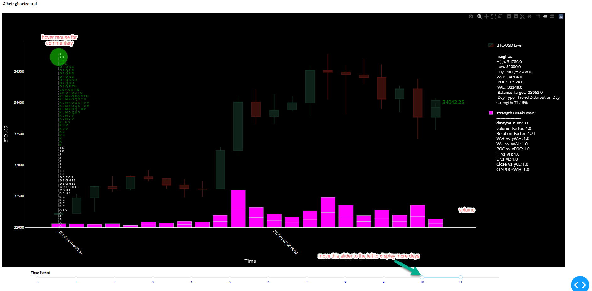
45 |
46 |
47 | ## General overview of the TPO chart produced by the algo (ignore the price as I copied this from readme section of the old versionThe)
48 | 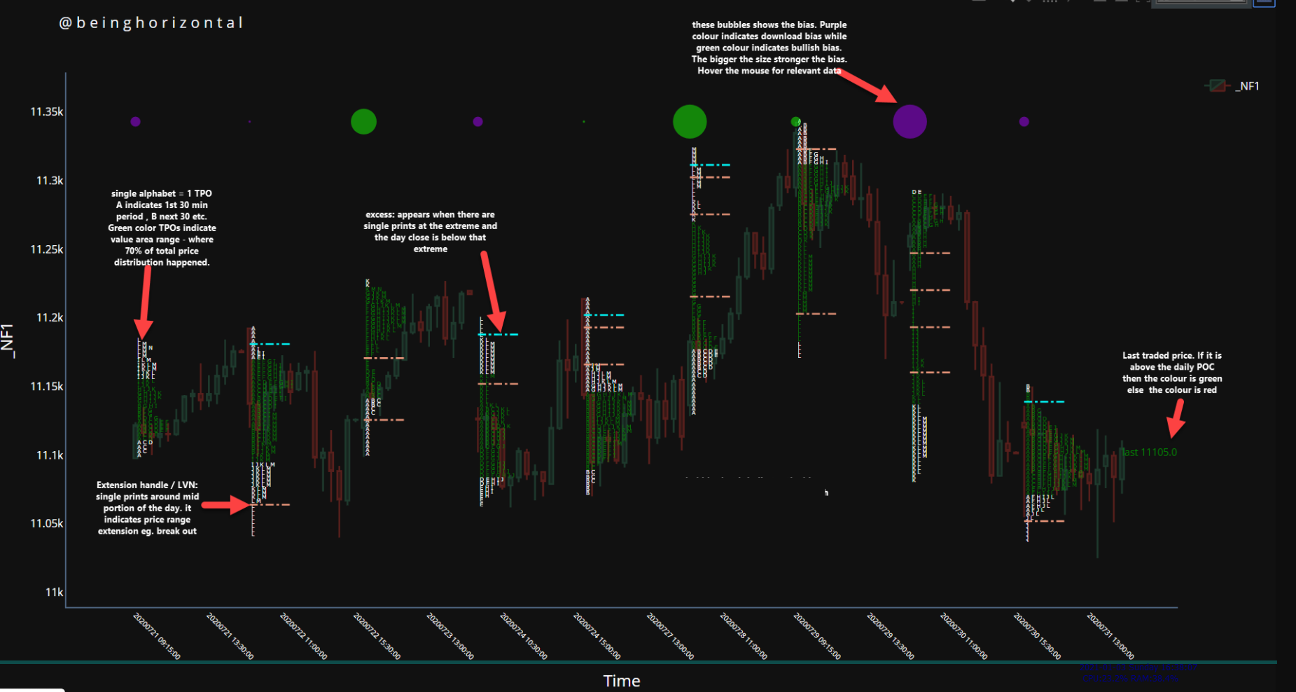
49 |
50 |
51 | ## Bubbles at the top:
52 | 
53 |
54 | # Disclaimer about balanced target
55 | if you read the insights and it's breakdown carefully there is a one line called a balanced target. So what is it and how important it is? well, I don't believe in using market profile as an indicator but thought to add this line as it indicates where the mean reversion target will be. This will be highly dangerous to use in scrips like Bitcoin or in general when the market is in strong trend.
56 |
57 | In the simplest form this is how it works. If there is an imbalance between POC -VAL and VAH-POC ( when price excessively moves to one direction) then it assumes that price will revert back and then it updates the balanced target. Don't take it too seriously, back then it used to work well in E-mini.
58 |
59 | # Final thoughts
60 |
61 | If you don't know anything about Market Profile (TM) then you might not understand the whole concept completely. If you're interested then do read the small handbook on Auction Market Theory(direct link below). Don't get confused by the name, AMT and Market Profile is the same thing. In short, the concept is based on how Auctions work. Of course the concept is not as deep as that 2020 Nobel Prize winner in Economics and quite frankly this one is quite usable. Usable in the sense most of the part is quantifiable. At the end of day it is a visual tool to assist the decision process and not an execution tool. In other words market profile is not an indicator or any kind of signal.
62 | # Link
63 | CBOT Market Profile handbook (13 mb pdf) https://t.co/L8DfNkLNi5?amp=1
64 |
--------------------------------------------------------------------------------
/btc_mp_v1.py:
--------------------------------------------------------------------------------
1 | from MP import MpFunctions
2 | import requests
3 | import dash
4 | import dash_core_components as dcc
5 | import dash_html_components as html
6 | from dash.dependencies import Input, Output
7 | import pandas as pd
8 | import plotly.graph_objs as go
9 | import datetime as dt
10 | import numpy as np
11 | import warnings
12 |
13 | warnings.filterwarnings('ignore')
14 |
15 | app = dash.Dash(__name__)
16 |
17 | def get_ticksize(data, freq=30):
18 | # data = dflive30
19 | numlen = int(len(data) / 2)
20 | # sample size for calculating ticksize = 50% of most recent data
21 | tztail = data.tail(numlen).copy()
22 | tztail['tz'] = tztail.Close.rolling(freq).std() # std. dev of 30 period rolling
23 | tztail = tztail.dropna()
24 | ticksize = np.ceil(tztail['tz'].mean() * 0.25) # 1/4 th of mean std. dev is our ticksize
25 |
26 | if ticksize < 0.2:
27 | ticksize = 0.2 # minimum ticksize limit
28 |
29 | return int(ticksize)
30 |
31 | def get_data(url):
32 | """
33 | :param url: binance url
34 | :return: ohlcv dataframe
35 | """
36 | response = requests.get(url)
37 | data = response.json()
38 | df = pd.DataFrame(data)
39 | df = df.apply(pd.to_numeric)
40 | df[0] = pd.to_datetime(df[0], unit='ms')
41 | df = df[[0, 1, 2, 3, 4, 5]]
42 | df.columns = ['datetime', 'Open', 'High', 'Low', 'Close', 'volume']
43 | df = df.set_index('datetime', inplace=False, drop=False)
44 | return df
45 |
46 |
47 | url_30m = "https://www.binance.com/api/v1/klines?symbol=BTCBUSD&interval=30m" # 10 days history 30 min ohlcv
48 | df = get_data(url_30m)
49 | df.to_csv('btcusd30m.csv', index=False)
50 |
51 | # params
52 | context_days = len([group[1] for group in df.groupby(df.index.date)]) # Number of days used for context
53 | freq = 2 # for 1 min bar use 30 min frequency for each TPO, here we fetch default 30 min bars server
54 | avglen = context_days - 2 # num days to calculate average values
55 | mode = 'tpo' # for volume --> 'vol'
56 | trading_hr = 24 # Default for BTC USD or Forex
57 | day_back = 0 # -1 While testing sometimes maybe you don't want current days data then use -1
58 | # ticksz = 28 # If you want to use manual tick size then uncomment this. Really small number means convoluted alphabets (TPO)
59 | ticksz = (get_ticksize(df.copy(), freq=freq))*2 # Algorithm will calculate the optimal tick size based on volatility
60 | textsize = 10
61 |
62 | if day_back != 0:
63 | symbol = 'Historical Mode'
64 | else:
65 | symbol = 'BTC-USD Live'
66 |
67 | dfnflist = [group[1] for group in df.groupby(df.index.date)] #
68 |
69 | dates = []
70 | for d in range(0, len(dfnflist)):
71 | dates.append(dfnflist[d].index[0])
72 |
73 | date_time_close = dt.datetime.today().strftime('%Y-%m-%d') + ' ' + '23:59:59'
74 | append_dt = pd.Timestamp(date_time_close)
75 | dates.append(append_dt)
76 | date_mark = {str(h): {'label': str(h), 'style': {'color': 'blue', 'fontsize': '4',
77 | 'text-orientation': 'upright'}} for h in range(0, len(dates))}
78 |
79 | mp = MpFunctions(data=df.copy(), freq=freq, style=mode, avglen=avglen, ticksize=ticksz, session_hr=trading_hr)
80 | mplist = mp.get_context()
81 |
82 | app.layout = html.Div(
83 | html.Div([
84 | dcc.Location(id='url', refresh=False),
85 | dcc.Link('Twitter', href='https://twitter.com/beinghorizontal'),
86 | html.Br(),
87 | dcc.Link('python source code', href='http://www.github.com/beinghorizontal'),
88 | html.H4('@beinghorizontal'),
89 | dcc.Graph(id='beinghorizontal'),
90 | dcc.Interval(
91 | id='interval-component',
92 | interval=5 * 1000, # Reduce the time if you want frequent updates 5000 = 5 sec
93 | n_intervals=0
94 | ),
95 | html.P([
96 | html.Label("Time Period"),
97 | dcc.RangeSlider(id='slider',
98 | pushable=1,
99 | marks=date_mark,
100 | min=0,
101 | max=len(dates),
102 | step=None,
103 | value=[len(dates) - 2, len(dates) - 1])
104 | ], style={'width': '80%',
105 | 'fontSize': '14px',
106 | 'padding-left': '100px',
107 | 'display': 'inline-block'})
108 | ])
109 | )
110 |
111 |
112 | @app.callback(Output(component_id='beinghorizontal', component_property='figure'),
113 | [Input('interval-component', 'n_intervals'),
114 | Input('slider', 'value')
115 | ])
116 | def update_graph(n, value):
117 | listmp_hist = mplist[0]
118 | distribution_hist = mplist[1]
119 |
120 | url_1m = "https://www.binance.com/api/v1/klines?symbol=BTCBUSD&interval=1m"
121 |
122 | df_live1 = get_data(url_1m) # this line fetches new data for current day
123 | df_live1 = df_live1.dropna()
124 |
125 | dflive30 = df_live1.resample('30min').agg({'datetime': 'last', 'Open': 'first', 'High': 'max', 'Low': 'min',
126 | 'Close': 'last', 'volume': 'sum'})
127 | df2 = pd.concat([df, dflive30])
128 | df2 = df2.drop_duplicates('datetime')
129 |
130 | ticksz_live = (get_ticksize(dflive30.copy(), freq=2))
131 | mplive = MpFunctions(data=dflive30.copy(), freq=freq, style=mode, avglen=avglen, ticksize=ticksz_live,
132 | session_hr=trading_hr)
133 | mplist_live = mplive.get_context()
134 | listmp_live = mplist_live[0] # it will be in list format so take [0] slice for current day MP data frame
135 | df_distribution_live = mplist_live[1]
136 | df_distribution_concat = pd.concat([distribution_hist, df_distribution_live], axis=0)
137 | df_distribution_concat = df_distribution_concat.reset_index(inplace=False, drop=True)
138 |
139 | df_updated_rank = mp.get_dayrank()
140 | ranking = df_updated_rank[0]
141 | power1 = ranking.power1 # Non-normalised IB strength
142 | power = ranking.power # Normalised IB strength for dynamic shape size for markers at bottom
143 | breakdown = df_updated_rank[1]
144 | dh_list = ranking.highd
145 | dl_list = ranking.lowd
146 |
147 | listmp = listmp_hist + listmp_live
148 |
149 | df3 = df2[(df2.index >= dates[value[0]]) & (df2.index <= dates[value[1]])]
150 | DFList = [group[1] for group in df2.groupby(df2.index.date)]
151 |
152 | fig = go.Figure(data=[go.Candlestick(x=df3.index,
153 |
154 | open=df3['Open'],
155 | high=df3['High'],
156 | low=df3['Low'],
157 | close=df3['Close'],
158 | showlegend=True,
159 | name=symbol,
160 | opacity=0.3)]) # To make candlesticks more prominent increase the opacity
161 |
162 | for inc in range(value[1] - value[0]):
163 | i = value[0]
164 | # inc = 0 # for debug
165 | # i = value[0]
166 |
167 | i += inc
168 | df1 = DFList[i].copy()
169 | df_mp = listmp[i]
170 | irank = ranking.iloc[i] # select single row from ranking df
171 | df_mp['i_date'] = df1['datetime'][0]
172 | # # @todo: background color for text
173 | df_mp['color'] = np.where(np.logical_and(
174 | df_mp['close'] > irank.vallist, df_mp['close'] < irank.vahlist), 'green', 'white')
175 |
176 | df_mp = df_mp.set_index('i_date', inplace=False)
177 |
178 | # print(df_mp.index)
179 | fig.add_trace(
180 | go.Scattergl(x=df_mp.index, y=df_mp.close, mode="text", text=df_mp.alphabets,
181 | showlegend=False, textposition="top right",
182 | textfont=dict(family="verdana", size=textsize, color=df_mp.color)))
183 |
184 | if power1[i] < 0:
185 | my_rgb = 'rgba({power}, 3, 252, 0.5)'.format(power=abs(165))
186 | else:
187 | my_rgb = 'rgba(23, {power}, 3, 0.5)'.format(power=abs(252))
188 |
189 | brk_f_list_maj = []
190 | f = 0
191 | for f in range(len(breakdown.columns)):
192 | brk_f_list_min = []
193 | for index, rows in breakdown.iterrows():
194 | if rows[f] != 0:
195 | brk_f_list_min.append(index + str(': ') + str(rows[f]) + '
')
196 | brk_f_list_maj.append(brk_f_list_min)
197 |
198 | breakdown_values = '' # for bubble callouts
199 | for st in brk_f_list_maj[i]:
200 | breakdown_values += st
201 | commentary_text = (
202 | '
Insights:
High: {}
Low: {}
Day_Range: {}
VAH: {}
POC: {}
VAL: {}
Balance Target: '
203 | '{}
Day Type: {}
strength: {}%
strength BreakDown: {}
{}
{}'.format(
204 | dh_list[i], dl_list[i],round(dh_list[i]- dl_list[i],2),
205 | irank.vahlist,
206 | irank.poclist, irank.vallist, irank.btlist, irank.daytype, irank.power, '',
207 | '-------------------', breakdown_values))
208 |
209 |
210 | fig.add_trace(go.Scattergl(
211 | x=[irank.date],
212 | y=[df3['High'].max() - (ticksz)],
213 | mode="markers",
214 | marker=dict(color=my_rgb, size=0.90 * power[i],
215 | line=dict(color='rgb(17, 17, 17)', width=2)),
216 | # marker_symbol='square',
217 | hovertext=commentary_text, showlegend=False))
218 |
219 | lvns = irank.lvnlist
220 |
221 | for lvn in lvns:
222 | if lvn > irank.vallist and lvn < irank.vahlist:
223 | fig.add_shape(
224 | # Line Horizontal
225 | type="line",
226 | x0=df_mp.index[0],
227 | y0=lvn,
228 | x1=df_mp.index[0] + dt.timedelta(hours=1),
229 | y1=lvn,
230 | line=dict(
231 | color="darksalmon",
232 | width=2,
233 | dash="dashdot", ), )
234 |
235 | fig.add_shape(
236 | type="line",
237 | x0=df_mp.index[0],
238 | y0=dl_list[i],
239 | x1=df_mp.index[0],
240 | y1=dh_list[i],
241 | line=dict(
242 | color="gray",
243 | width=1,
244 | dash="dashdot", ), )
245 |
246 | fig.layout.xaxis.type = 'category' # This line will omit annoying weekends on the plotly graph
247 |
248 | ltp = df1.iloc[-1]['Close']
249 | if ltp >= irank.poclist:
250 | ltp_color = 'green'
251 | else:
252 | ltp_color = 'red'
253 |
254 | fig.add_trace(go.Bar(x=df3.index, y=df3['volume'], marker=dict(color='magenta'), yaxis='y3', name=str(commentary_text)))
255 |
256 | fig.add_trace(go.Scattergl(
257 | x=[df3.iloc[-1]['datetime']],
258 | y=[df3.iloc[-1]['Close']],
259 | mode="text",
260 | name="last traded price",
261 | text=[str(df3.iloc[-1]['Close'])],
262 | textposition="bottom center",
263 | textfont=dict(size=18, color=ltp_color),
264 | showlegend=False
265 | ))
266 | # to make x-axis less crowded
267 | if value[1] - value[0] > 4:
268 | dticksv = 30
269 | else:
270 | dticksv = len(dates)
271 | y3min = df3['volume'].min()
272 | y3max = df3['volume'].max() * 10
273 | ymin = df3['Low'].min()
274 | ymax = df3['High'].max() + (4 * ticksz)
275 |
276 | # Adjust height & width according to your monitor size & orientation.
277 | fig.update_layout(paper_bgcolor='black', plot_bgcolor='black', height=900, width=1990,
278 | xaxis=dict(showline=True, color='white', type='category', title_text='Time', tickangle=45,
279 | dtick=dticksv, title_font=dict(size=18, color='white')),
280 | yaxis=dict(showline=True, color='white', range=[ymin, ymax], showgrid=False,
281 | title_text='BTC/USD'),
282 | yaxis2=dict(showgrid=False),
283 | yaxis3=dict(range=[y3min, y3max], overlaying="y",
284 | side="right",
285 | color='black',
286 | showgrid=False),
287 | legend=dict(font=dict(color='White',size=14)))
288 |
289 | fig.update_layout(yaxis_tickformat='d')
290 | fig["layout"]["xaxis"]["rangeslider"]["visible"] = False
291 | fig["layout"]["xaxis"]["tickformat"] = "%H:%M:%S"
292 |
293 | # plot(fig, auto_open=True) # For debugging
294 | return (fig)
295 |
296 |
297 | if __name__ == '__main__':
298 | app.run_server(port=8000, host='127.0.0.1',
299 | debug=True) # debug=False if executing from ipython(vscode/Pycharm/Spyder)
300 |
--------------------------------------------------------------------------------
/MP.py:
--------------------------------------------------------------------------------
1 | # -*- coding: utf-8 -*-
2 | """
3 | Created on Mon Jul 27 13:26:04 2020
4 |
5 | @author: alex1
6 | """
7 | import math
8 | import numpy as np
9 | import pandas as pd
10 |
11 |
12 | # # debug
13 | # mp = MpFunctions(data=df, freq=2, style='tpo', avglen=8, ticksize=24, session_hr=24)
14 | # mplist = mp.get_context()
15 | # #mplist[1]
16 | # meandict = mp.get_mean()
17 | # #meandict['volume_mean']
18 |
19 |
20 | class MpFunctions():
21 | def __init__(self, data, freq=30, style='tpo', avglen=8, ticksize=8, session_hr=8):
22 | self.data = data
23 | self.freq = freq
24 | self.style = style
25 | self.avglen = avglen
26 | self.ticksize = ticksize
27 | self.session_hr = session_hr
28 |
29 | def get_ticksize(self):
30 | # data = df
31 | numlen = int(len(self.data) / 2)
32 | # sample size for calculating ticksize = 50% of most recent data
33 | tztail = self.data.tail(numlen).copy()
34 | tztail['tz'] = tztail.Close.rolling(self.freq).std() # std. dev of 30 period rolling
35 | tztail = tztail.dropna()
36 | ticksize = np.ceil(tztail['tz'].mean() * 0.25) # 1/4 th of mean std. dev is our ticksize
37 |
38 | if ticksize < 0.2:
39 | ticksize = 0.2 # minimum ticksize limit
40 |
41 | return int(ticksize)
42 |
43 | def abc(self):
44 | caps = [' A', ' B', ' C', ' D', ' E', ' F', ' G', ' H', ' I', ' J', ' K', ' L', ' M',
45 | ' N', ' O', ' P', ' Q', ' R', ' S', ' T', ' U', ' V', ' W', ' X', ' Y', ' Z']
46 | abc_lw = [x.lower() for x in caps]
47 | Aa = caps + abc_lw
48 | alimit = math.ceil(self.session_hr * (60 / self.freq)) + 3
49 | if alimit > 52:
50 | alphabets = Aa * int(
51 | (np.ceil((alimit - 52) / 52)) + 1) # if bar frequency is less than 30 minutes then multiply list
52 | else:
53 | alphabets = Aa[0:alimit]
54 | bk = [28, 31, 35, 40, 33, 34, 41, 44, 35, 52, 41, 40, 46, 27, 38]
55 | ti = []
56 | for s1 in bk:
57 | ti.append(Aa[s1 - 1])
58 | tt = (''.join(ti))
59 |
60 | return alphabets, tt
61 |
62 | def get_rf(self):
63 | self.data['cup'] = np.where(self.data['Close'] >= self.data['Close'].shift(), 1, -1)
64 | self.data['hup'] = np.where(self.data['High'] >= self.data['High'].shift(), 1, -1)
65 | self.data['lup'] = np.where(self.data['Low'] >= self.data['Low'].shift(), 1, -1)
66 |
67 | self.data['rf'] = self.data['cup'] + self.data['hup'] + self.data['lup']
68 | dataf = self.data.drop(['cup', 'lup', 'hup'], axis=1)
69 | return dataf
70 |
71 | def get_mean(self):
72 | """
73 | dfhist: pandas dataframe 1 min frequency
74 | avglen: Length for mean values
75 | freq: timeframe for the candlestick & TPOs
76 |
77 | return: a) daily mean for volume, rotational factor (absolute value), IB volume, IB RF b) session length
78 | dfhist = df.copy()
79 | """
80 | dfhist = self.get_rf()
81 | # dfhist = get_rf(dfhist.copy())
82 | dfhistd = dfhist.resample("D").agg(
83 | {'Open': 'first', 'High': 'max', 'Low': 'min', 'Close': 'last', 'volume': 'sum',
84 | 'rf': 'sum', })
85 | dfhistd = dfhistd.dropna()
86 | comp_days = len(dfhistd)
87 |
88 | vm30 = dfhistd['volume'].rolling(self.avglen).mean()
89 | volume_mean = vm30[len(vm30) - 1]
90 | rf30 = abs((dfhistd['rf'])).rolling(
91 | self.avglen).mean() # it is abs mean to get meaningful value to compare daily values
92 | rf_mean = rf30[len(rf30) - 1]
93 |
94 | date2 = dfhistd.index[1].date()
95 | mask = dfhist.index.date < date2
96 | dfsession = dfhist.loc[mask]
97 | session_hr = math.ceil(len(dfsession) / 60)
98 |
99 | all_val = dict(volume_mean=volume_mean, rf_mean=rf_mean, session_hr=session_hr)
100 |
101 | return all_val
102 |
103 | def tpo(self, dft_rs):
104 | # dft_rs = dfc1.copy()
105 | # if len(dft_rs) > int(60 / freq):
106 | if len(dft_rs) > int(0):
107 | dft_rs = dft_rs.drop_duplicates('datetime')
108 | dft_rs = dft_rs.reset_index(inplace=False, drop=True)
109 | dft_rs['rol_mx'] = dft_rs['High'].cummax()
110 | dft_rs['rol_mn'] = dft_rs['Low'].cummin()
111 | dft_rs['ext_up'] = dft_rs['rol_mn'] > dft_rs['rol_mx'].shift(2)
112 | dft_rs['ext_dn'] = dft_rs['rol_mx'] < dft_rs['rol_mn'].shift(2)
113 | alphabets = self.abc()[0]
114 | # alphabets = abc(session_hr, freq)[0]
115 | alphabets = alphabets[0:len(dft_rs)]
116 | hh = dft_rs['High'].max()
117 | ll = dft_rs['Low'].min()
118 | day_range = hh - ll
119 | dft_rs['abc'] = alphabets
120 | # place represents total number of steps to take to compare the TPO count
121 | place = int(np.ceil((hh - ll) / self.ticksize))
122 | # kk = 0
123 | abl_bg = []
124 | tpo_countbg = []
125 | pricel = []
126 | volcountbg = []
127 | # datel = []
128 | for u in range(place):
129 | abl = []
130 | tpoc = []
131 | volcount = []
132 | p = ll + (u * self.ticksize)
133 | for lenrs in range(len(dft_rs)):
134 | if p >= dft_rs['Low'][lenrs] and p < dft_rs['High'][lenrs]:
135 | abl.append(dft_rs['abc'][lenrs])
136 | tpoc.append(1)
137 | volcount.append((dft_rs['volume'][lenrs]) / self.freq)
138 | abl_bg.append(''.join(abl))
139 | tpo_countbg.append(sum(tpoc))
140 | volcountbg.append(sum(volcount))
141 | pricel.append(p)
142 |
143 | dftpo = pd.DataFrame({'close': pricel, 'alphabets': abl_bg,
144 | 'tpocount': tpo_countbg, 'volsum': volcountbg})
145 | # drop empty rows
146 | dftpo['alphabets'].replace('', np.nan, inplace=True)
147 | dftpo = dftpo.dropna()
148 | dftpo = dftpo.reset_index(inplace=False, drop=True)
149 | dftpo = dftpo.sort_index(ascending=False)
150 | dftpo = dftpo.reset_index(inplace=False, drop=True)
151 |
152 | if self.style == 'tpo':
153 | column = 'tpocount'
154 | else:
155 | column = 'volsum'
156 |
157 | dfmx = dftpo[dftpo[column] == dftpo[column].max()]
158 |
159 | mid = ll + ((hh - ll) / 2)
160 | dfmax = dfmx.copy()
161 | dfmax['poc-mid'] = abs(dfmax['close'] - mid)
162 | pocidx = dfmax['poc-mid'].idxmin()
163 | poc = dfmax['close'][pocidx]
164 | poctpo = dftpo[column].max()
165 | tpo_updf = dftpo[dftpo['close'] > poc]
166 | tpo_updf = tpo_updf.sort_index(ascending=False)
167 | tpo_updf = tpo_updf.reset_index(inplace=False, drop=True)
168 |
169 | tpo_dndf = dftpo[dftpo['close'] < poc]
170 | tpo_dndf = tpo_dndf.reset_index(inplace=False, drop=True)
171 |
172 | valtpo = (dftpo[column].sum()) * 0.70
173 |
174 | abovepoc = tpo_updf[column].to_list()
175 | belowpoc = tpo_dndf[column].to_list()
176 |
177 | if (len(abovepoc) / 2).is_integer() is False:
178 | abovepoc = abovepoc + [0]
179 |
180 | if (len(belowpoc) / 2).is_integer() is False:
181 | belowpoc = belowpoc + [0]
182 |
183 | bel2 = np.array(belowpoc).reshape(-1, 2)
184 | bel3 = bel2.sum(axis=1)
185 | bel4 = list(bel3)
186 | abv2 = np.array(abovepoc).reshape(-1, 2)
187 | abv3 = abv2.sum(axis=1)
188 | abv4 = list(abv3)
189 | # cum = poctpo
190 | # up_i = 0
191 | # dn_i = 0
192 | df_va = pd.DataFrame({'abv': pd.Series(abv4), 'bel': pd.Series(bel4)})
193 | df_va = df_va.fillna(0)
194 | df_va['abv_idx'] = np.where(df_va.abv > df_va.bel, 1, 0)
195 | df_va['bel_idx'] = np.where(df_va.bel > df_va.abv, 1, 0)
196 | df_va['cum_tpo'] = np.where(df_va.abv > df_va.bel, df_va.abv, 0)
197 | df_va['cum_tpo'] = np.where(df_va.bel > df_va.abv, df_va.bel, df_va.cum_tpo)
198 |
199 | df_va['cum_tpo'] = np.where(df_va.abv == df_va.bel, df_va.abv + df_va.bel, df_va.cum_tpo)
200 | df_va['abv_idx'] = np.where(df_va.abv == df_va.bel, 1, df_va.abv_idx)
201 | df_va['bel_idx'] = np.where(df_va.abv == df_va.bel, 1, df_va.bel_idx)
202 | df_va['cum_tpo_cumsum'] = df_va.cum_tpo.cumsum()
203 | # haven't add poc tpo because loop cuts off way before 70% so it gives same effect
204 | df_va_cut = df_va[df_va.cum_tpo_cumsum + poctpo <= valtpo]
205 | vah_idx = (df_va_cut.abv_idx.sum()) * 2
206 | val_idx = (df_va_cut.bel_idx.sum()) * 2
207 |
208 | if vah_idx >= len(tpo_updf) and vah_idx != 0:
209 | vah_idx = vah_idx - 2
210 |
211 | if val_idx >= len(tpo_dndf) and val_idx != 0:
212 | val_idx = val_idx - 2
213 |
214 | vah = tpo_updf.close[vah_idx]
215 | val = tpo_dndf.close[val_idx]
216 |
217 | tpoval = dftpo[self.ticksize:-(self.ticksize)]['tpocount'] # take mid section
218 | exhandle_index = np.where(tpoval <= 2, tpoval.index, None) # get index where TPOs are 2
219 | exhandle_index = list(filter(None, exhandle_index))
220 | distance = self.ticksize * 3 # distance b/w two ex handles / lvn
221 | lvn_list = []
222 | for ex in exhandle_index[0:-1:distance]:
223 | lvn_list.append(dftpo['close'][ex])
224 |
225 | area_above_poc = dft_rs.High.max() - poc
226 | area_below_poc = poc - dft_rs.Low.min()
227 | if area_above_poc == 0:
228 | area_above_poc = 1
229 | if area_below_poc == 0:
230 | area_below_poc = 1
231 | balance = area_above_poc / area_below_poc
232 |
233 | if balance >= 0:
234 | bal_target = poc - area_above_poc
235 | else:
236 | bal_target = poc + area_below_poc
237 |
238 | mp = {'df': dftpo, 'vah': round(vah, 2), 'poc': round(poc, 2), 'val': round(val, 2), 'lvn': lvn_list,
239 | 'bal_target': round(bal_target, 2)}
240 |
241 | else:
242 | print('not enough bars for date {}'.format(dft_rs['datetime'][0]))
243 | mp = {}
244 |
245 | return mp
246 |
247 | # !!! fetch all MP derived results here with date and do extra context analysis
248 |
249 | def get_context(self):
250 | df_hi = self.get_rf()
251 | try:
252 | # df_hi = dflive30.copy() # testing
253 | DFcontext = [group[1] for group in df_hi.groupby(df_hi.index.date)]
254 | dfmp_l = []
255 | i_poctpo_l = []
256 | i_tposum = []
257 | vah_l = []
258 | poc_l = []
259 | val_l = []
260 | bt_l = []
261 | lvn_l = []
262 | # excess_l = []
263 | date_l = []
264 | volume_l = []
265 | rf_l = []
266 | # ibv_l = []
267 | # ibrf_l = []
268 | # ibh_l = []
269 | # ib_l = []
270 | close_l = []
271 | hh_l = []
272 | ll_l = []
273 | range_l = []
274 |
275 | for c in range(len(DFcontext)): # c=0 for testing
276 | dfc1 = DFcontext[c].copy()
277 | # dfc1.iloc[:, 2:6] = dfc1.iloc[:, 2:6].apply(pd.to_numeric)
278 |
279 | dfc1 = dfc1.reset_index(inplace=False, drop=True)
280 | mpc = self.tpo(dfc1)
281 | dftmp = mpc['df']
282 | dfmp_l.append(dftmp)
283 | # for day types
284 | i_poctpo_l.append(dftmp['tpocount'].max())
285 | i_tposum.append(dftmp['tpocount'].sum())
286 | # !!! get value areas
287 | vah_l.append(mpc['vah'])
288 | poc_l.append(mpc['poc'])
289 | val_l.append(mpc['val'])
290 |
291 | bt_l.append(mpc['bal_target'])
292 | lvn_l.append(mpc['lvn'])
293 | # excess_l.append(mpc['excess'])
294 |
295 | # !!! operatio of non profile stats
296 | date_l.append(dfc1.datetime[0])
297 | close_l.append(dfc1.iloc[-1]['Close'])
298 | hh_l.append(dfc1.High.max())
299 | ll_l.append(dfc1.Low.min())
300 | range_l.append(dfc1.High.max() - dfc1.Low.min())
301 |
302 | volume_l.append(dfc1.volume.sum())
303 | rf_l.append(dfc1.rf.sum())
304 | # !!! get IB
305 | dfc1['cumsumvol'] = dfc1.volume.cumsum()
306 | dfc1['cumsumrf'] = dfc1.rf.cumsum()
307 | dfc1['cumsumhigh'] = dfc1.High.cummax()
308 | dfc1['cumsummin'] = dfc1.Low.cummin()
309 |
310 | dist_df = pd.DataFrame({'date': date_l, 'maxtpo': i_poctpo_l, 'tpocount': i_tposum, 'vahlist': vah_l,
311 | 'poclist': poc_l, 'vallist': val_l, 'btlist': bt_l, 'lvnlist': lvn_l,
312 | 'volumed': volume_l, 'rfd': rf_l, 'highd': hh_l, 'lowd': ll_l, 'ranged': range_l,
313 | 'close': close_l})
314 |
315 | except Exception as e:
316 | print(str(e))
317 | ranking_df = []
318 | dfmp_l = []
319 | dist_df = []
320 |
321 | return (dfmp_l, dist_df)
322 |
323 | def get_dayrank(self):
324 | # dist_df = df_distribution_concat.copy()
325 | # LVNs
326 | dist_df = self.get_context()[1]
327 | lvnlist = dist_df['lvnlist'].to_list()
328 | cllist = dist_df['close'].to_list()
329 | lvn_powerlist = []
330 | total_lvns = 0
331 | for c, llist in zip(cllist, lvnlist):
332 | if len(llist) == 0:
333 | delta_lvn = 0
334 | total_lvns = 0
335 | lvn_powerlist.append(total_lvns)
336 | else:
337 | for l in llist:
338 | delta_lvn = c - l
339 | if delta_lvn >= 0:
340 | lvn_i = 1
341 | else:
342 | lvn_i = -1
343 | total_lvns = total_lvns + lvn_i
344 | lvn_powerlist.append(total_lvns)
345 | total_lvns = 0
346 |
347 | dist_df['Single_Prints'] = lvn_powerlist
348 |
349 | dist_df['distr'] = dist_df.tpocount / dist_df.maxtpo
350 | dismean = math.floor(dist_df.distr.mean())
351 | dissig = math.floor(dist_df.distr.std())
352 |
353 | # Assign day types based on TPO distribution and give numerical value for each day types for calculating total strength at the end
354 |
355 | dist_df['daytype'] = np.where(np.logical_and(dist_df.distr >= dismean,
356 | dist_df.distr < dismean + dissig), 'Trend Distribution Day', '')
357 |
358 | dist_df['daytype_num'] = np.where(np.logical_and(dist_df.distr >= dismean,
359 | dist_df.distr < dismean + dissig), 3, 0)
360 |
361 | dist_df['daytype'] = np.where(np.logical_and(dist_df.distr < dismean,
362 | dist_df.distr >= dismean - dissig), 'Normal Variation Day',
363 | dist_df['daytype'])
364 |
365 | dist_df['daytype_num'] = np.where(np.logical_and(dist_df.distr < dismean,
366 | dist_df.distr >= dismean - dissig), 2, dist_df['daytype_num'])
367 |
368 | dist_df['daytype'] = np.where(dist_df.distr < dismean - dissig,
369 | 'Neutral Day', dist_df['daytype'])
370 |
371 | dist_df['daytype_num'] = np.where(dist_df.distr < dismean - dissig,
372 | 1, dist_df['daytype_num'])
373 |
374 | dist_df['daytype'] = np.where(dist_df.distr > dismean + dissig,
375 | 'Trend Day', dist_df['daytype'])
376 | dist_df['daytype_num'] = np.where(dist_df.distr > dismean + dissig,
377 | 4, dist_df['daytype_num'])
378 | dist_df['daytype_num'] = np.where(dist_df.close >= dist_df.poclist, dist_df.daytype_num * 1,
379 | dist_df.daytype_num * -1) # assign signs as per bias
380 |
381 | daytypes = dist_df['daytype'].to_list()
382 |
383 | # volume comparison with mean
384 | mean_val = self.get_mean()
385 | rf_mean = mean_val['rf_mean']
386 | vol_mean = mean_val['volume_mean']
387 |
388 | dist_df['vold_zscore'] = (dist_df.volumed - vol_mean) / dist_df.volumed.std(ddof=0)
389 | dist_df['rfd_zscore'] = (abs(dist_df.rfd) - rf_mean) / abs(dist_df.rfd).std(ddof=0)
390 | a, b = 1, 4
391 | x, y = dist_df.rfd_zscore.min(), dist_df.rfd_zscore.max()
392 | dist_df['norm_rf'] = (dist_df.rfd_zscore - x) / (y - x) * (b - a) + a
393 |
394 | p, q = dist_df.vold_zscore.min(), dist_df.vold_zscore.max()
395 | dist_df['norm_volume'] = (dist_df.vold_zscore - p) / (q - p) * (b - a) + a
396 |
397 | dist_df['volume_Factor'] = np.where(dist_df.close >= dist_df.poclist, dist_df.norm_volume * 1,
398 | dist_df.norm_volume * -1)
399 | dist_df['Rotation_Factor'] = np.where(dist_df.rfd >= 0, dist_df.norm_rf * 1, dist_df.norm_rf * -1)
400 |
401 | # !!! get ranking based on distribution data frame aka dist_df
402 | ranking_df = dist_df.copy()
403 | ranking_df['VAH_vs_yVAH'] = np.where(ranking_df.vahlist >= ranking_df.vahlist.shift(), 1, -1)
404 | ranking_df['VAL_vs_yVAL'] = np.where(ranking_df.vallist >= ranking_df.vallist.shift(), 1, -1)
405 | ranking_df['POC_vs_yPOC'] = np.where(ranking_df.poclist >= ranking_df.poclist.shift(), 1, -1)
406 | ranking_df['H_vs_yH'] = np.where(ranking_df.highd >= ranking_df.highd.shift(), 1, -1)
407 | ranking_df['L_vs_yL'] = np.where(ranking_df.lowd >= ranking_df.lowd.shift(), 1, -1)
408 | ranking_df['Close_vs_yCL'] = np.where(ranking_df.close >= ranking_df.close.shift(), 1, -1)
409 | ranking_df['CL>POC= ranking_df.poclist, ranking_df.close < ranking_df.vahlist), 1, 0)
411 | ranking_df['CLval'] = np.where(
412 | np.logical_and(ranking_df.close < ranking_df.poclist, ranking_df.close >= ranking_df.vallist), -1,
413 | 0) # Max is 2
414 | ranking_df['CL=VAH'] = np.where(ranking_df.close >= ranking_df.vahlist, 2, 0)
416 |
417 | ranking_df['power1'] = 100 * (
418 | (ranking_df.VAH_vs_yVAH + ranking_df.VAL_vs_yVAL + ranking_df.POC_vs_yPOC + ranking_df.H_vs_yH +
419 | ranking_df.L_vs_yL + ranking_df['Close_vs_yCL'] + ranking_df['CL>POCval'] + ranking_df.Single_Prints +
421 | ranking_df['CL=VAH'] + ranking_df.volume_Factor + ranking_df.Rotation_Factor + ranking_df.daytype_num) / 14)
423 |
424 | c, d = 25, 100
425 | r, s = abs(ranking_df.power1).min(), abs(ranking_df.power1).max()
426 | ranking_df['power'] = (abs(ranking_df.power1) - r) / (s - r) * (d - c) + c
427 | ranking_df = ranking_df.round(2)
428 | # ranking_df['power'] = abs(ranking_df['power1'])
429 |
430 | breakdown_df = ranking_df[
431 | ['Single_Prints', 'daytype_num', 'volume_Factor', 'Rotation_Factor', 'VAH_vs_yVAH', 'VAL_vs_yVAL',
432 | 'POC_vs_yPOC', 'H_vs_yH',
433 | 'L_vs_yL', 'Close_vs_yCL', 'CL>POCval', 'CL=VAH']].transpose()
434 |
435 | breakdown_df = breakdown_df.round(2)
436 |
437 | return (ranking_df, breakdown_df)
438 |
--------------------------------------------------------------------------------