├── .gitignore
├── LICENSE
├── README.md
├── html
├── 01-setup.html
├── 02-data-handling.html
├── 03-classification.html
├── 04-dimensionality-reduction.html
├── 05-classifier-optimization.html
├── 06-rsa.html
├── 07-searchlight.html
├── 08-connectivity.html
├── 09-fcma.html
├── 10-isc.html
├── 11-srm.html
├── 12-hmm.html
├── 13-real-time.html
└── imgs
│ ├── lab11
│ └── srm_time_segment_matching.png
│ ├── lab12
│ └── hmm_schematics.png
│ └── lab7
│ ├── mpi_openmp.jpg
│ └── nodes_process.jpg
└── tutorials
├── 00-all-imports-test.ipynb
├── 01-setup.ipynb
├── 02-data-handling.ipynb
├── 03-classification.ipynb
├── 04-dimensionality-reduction.ipynb
├── 05-classifier-optimization.ipynb
├── 06-rsa.ipynb
├── 07-searchlight.ipynb
├── 07-searchlight
├── avg18_whole_brain_SL.nii.gz
├── avg3_whole_brain_SL.nii.gz
├── rank_whole_brain_SL.nii.gz
├── run_searchlight.sh
├── searchlight.py
├── searchlight_rank.py
└── searchlight_single_subject.py
├── 08-connectivity.ipynb
├── 09-fcma.ipynb
├── 09-fcma
├── fcma_classify.py
├── fcma_voxel_selection_cv.py
├── make_top_voxel_mask.sh
├── run_fcma_classify.sh
└── run_fcma_voxel_selection_cv.sh
├── 10-isc.ipynb
├── 11-srm.ipynb
├── 12-hmm.ipynb
├── 13-real-time.ipynb
├── 13-real-time
├── fmrisim
│ ├── ROI_A.nii.gz
│ ├── ROI_B.nii.gz
│ ├── mask.npy
│ ├── sub_noise_dict.txt
│ └── sub_template.nii.gz
├── generate_data.py
└── run_generate_data.sh
├── colab-env-setup.ipynb
├── imgs
├── lab11
│ └── srm_time_segment_matching.png
├── lab12
│ └── hmm_schematics.png
└── lab7
│ ├── mpi_openmp.jpg
│ └── nodes_process.jpg
├── logs
└── .gitkeep
├── requirements.txt
├── run_jupyter.sh
├── run_jupyter_docker.sh
├── run_jupyter_remote_cluster.sh
├── run_jupyter_remote_server.sh
├── setup_environment.sh
└── utils.py
/.gitignore:
--------------------------------------------------------------------------------
1 | # To be ignored
2 | .DS_Store
3 | .ipynb_checkpoints
4 | __MACOSX
5 | __pycache__
6 | *.swp
7 | tutorials/logs/*
8 | tutorials/__pycache__
9 | brainiak
10 |
11 | # To be excepted
12 | !tutorials/logs/.gitkeep
13 |
--------------------------------------------------------------------------------
/LICENSE:
--------------------------------------------------------------------------------
1 |
2 | Apache License
3 | Version 2.0, January 2004
4 | http://www.apache.org/licenses/
5 |
6 | TERMS AND CONDITIONS FOR USE, REPRODUCTION, AND DISTRIBUTION
7 |
8 | 1. Definitions.
9 |
10 | "License" shall mean the terms and conditions for use, reproduction,
11 | and distribution as defined by Sections 1 through 9 of this document.
12 |
13 | "Licensor" shall mean the copyright owner or entity authorized by
14 | the copyright owner that is granting the License.
15 |
16 | "Legal Entity" shall mean the union of the acting entity and all
17 | other entities that control, are controlled by, or are under common
18 | control with that entity. For the purposes of this definition,
19 | "control" means (i) the power, direct or indirect, to cause the
20 | direction or management of such entity, whether by contract or
21 | otherwise, or (ii) ownership of fifty percent (50%) or more of the
22 | outstanding shares, or (iii) beneficial ownership of such entity.
23 |
24 | "You" (or "Your") shall mean an individual or Legal Entity
25 | exercising permissions granted by this License.
26 |
27 | "Source" form shall mean the preferred form for making modifications,
28 | including but not limited to software source code, documentation
29 | source, and configuration files.
30 |
31 | "Object" form shall mean any form resulting from mechanical
32 | transformation or translation of a Source form, including but
33 | not limited to compiled object code, generated documentation,
34 | and conversions to other media types.
35 |
36 | "Work" shall mean the work of authorship, whether in Source or
37 | Object form, made available under the License, as indicated by a
38 | copyright notice that is included in or attached to the work
39 | (an example is provided in the Appendix below).
40 |
41 | "Derivative Works" shall mean any work, whether in Source or Object
42 | form, that is based on (or derived from) the Work and for which the
43 | editorial revisions, annotations, elaborations, or other modifications
44 | represent, as a whole, an original work of authorship. For the purposes
45 | of this License, Derivative Works shall not include works that remain
46 | separable from, or merely link (or bind by name) to the interfaces of,
47 | the Work and Derivative Works thereof.
48 |
49 | "Contribution" shall mean any work of authorship, including
50 | the original version of the Work and any modifications or additions
51 | to that Work or Derivative Works thereof, that is intentionally
52 | submitted to Licensor for inclusion in the Work by the copyright owner
53 | or by an individual or Legal Entity authorized to submit on behalf of
54 | the copyright owner. For the purposes of this definition, "submitted"
55 | means any form of electronic, verbal, or written communication sent
56 | to the Licensor or its representatives, including but not limited to
57 | communication on electronic mailing lists, source code control systems,
58 | and issue tracking systems that are managed by, or on behalf of, the
59 | Licensor for the purpose of discussing and improving the Work, but
60 | excluding communication that is conspicuously marked or otherwise
61 | designated in writing by the copyright owner as "Not a Contribution."
62 |
63 | "Contributor" shall mean Licensor and any individual or Legal Entity
64 | on behalf of whom a Contribution has been received by Licensor and
65 | subsequently incorporated within the Work.
66 |
67 | 2. Grant of Copyright License. Subject to the terms and conditions of
68 | this License, each Contributor hereby grants to You a perpetual,
69 | worldwide, non-exclusive, no-charge, royalty-free, irrevocable
70 | copyright license to reproduce, prepare Derivative Works of,
71 | publicly display, publicly perform, sublicense, and distribute the
72 | Work and such Derivative Works in Source or Object form.
73 |
74 | 3. Grant of Patent License. Subject to the terms and conditions of
75 | this License, each Contributor hereby grants to You a perpetual,
76 | worldwide, non-exclusive, no-charge, royalty-free, irrevocable
77 | (except as stated in this section) patent license to make, have made,
78 | use, offer to sell, sell, import, and otherwise transfer the Work,
79 | where such license applies only to those patent claims licensable
80 | by such Contributor that are necessarily infringed by their
81 | Contribution(s) alone or by combination of their Contribution(s)
82 | with the Work to which such Contribution(s) was submitted. If You
83 | institute patent litigation against any entity (including a
84 | cross-claim or counterclaim in a lawsuit) alleging that the Work
85 | or a Contribution incorporated within the Work constitutes direct
86 | or contributory patent infringement, then any patent licenses
87 | granted to You under this License for that Work shall terminate
88 | as of the date such litigation is filed.
89 |
90 | 4. Redistribution. You may reproduce and distribute copies of the
91 | Work or Derivative Works thereof in any medium, with or without
92 | modifications, and in Source or Object form, provided that You
93 | meet the following conditions:
94 |
95 | (a) You must give any other recipients of the Work or
96 | Derivative Works a copy of this License; and
97 |
98 | (b) You must cause any modified files to carry prominent notices
99 | stating that You changed the files; and
100 |
101 | (c) You must retain, in the Source form of any Derivative Works
102 | that You distribute, all copyright, patent, trademark, and
103 | attribution notices from the Source form of the Work,
104 | excluding those notices that do not pertain to any part of
105 | the Derivative Works; and
106 |
107 | (d) If the Work includes a "NOTICE" text file as part of its
108 | distribution, then any Derivative Works that You distribute must
109 | include a readable copy of the attribution notices contained
110 | within such NOTICE file, excluding those notices that do not
111 | pertain to any part of the Derivative Works, in at least one
112 | of the following places: within a NOTICE text file distributed
113 | as part of the Derivative Works; within the Source form or
114 | documentation, if provided along with the Derivative Works; or,
115 | within a display generated by the Derivative Works, if and
116 | wherever such third-party notices normally appear. The contents
117 | of the NOTICE file are for informational purposes only and
118 | do not modify the License. You may add Your own attribution
119 | notices within Derivative Works that You distribute, alongside
120 | or as an addendum to the NOTICE text from the Work, provided
121 | that such additional attribution notices cannot be construed
122 | as modifying the License.
123 |
124 | You may add Your own copyright statement to Your modifications and
125 | may provide additional or different license terms and conditions
126 | for use, reproduction, or distribution of Your modifications, or
127 | for any such Derivative Works as a whole, provided Your use,
128 | reproduction, and distribution of the Work otherwise complies with
129 | the conditions stated in this License.
130 |
131 | 5. Submission of Contributions. Unless You explicitly state otherwise,
132 | any Contribution intentionally submitted for inclusion in the Work
133 | by You to the Licensor shall be under the terms and conditions of
134 | this License, without any additional terms or conditions.
135 | Notwithstanding the above, nothing herein shall supersede or modify
136 | the terms of any separate license agreement you may have executed
137 | with Licensor regarding such Contributions.
138 |
139 | 6. Trademarks. This License does not grant permission to use the trade
140 | names, trademarks, service marks, or product names of the Licensor,
141 | except as required for reasonable and customary use in describing the
142 | origin of the Work and reproducing the content of the NOTICE file.
143 |
144 | 7. Disclaimer of Warranty. Unless required by applicable law or
145 | agreed to in writing, Licensor provides the Work (and each
146 | Contributor provides its Contributions) on an "AS IS" BASIS,
147 | WITHOUT WARRANTIES OR CONDITIONS OF ANY KIND, either express or
148 | implied, including, without limitation, any warranties or conditions
149 | of TITLE, NON-INFRINGEMENT, MERCHANTABILITY, or FITNESS FOR A
150 | PARTICULAR PURPOSE. You are solely responsible for determining the
151 | appropriateness of using or redistributing the Work and assume any
152 | risks associated with Your exercise of permissions under this License.
153 |
154 | 8. Limitation of Liability. In no event and under no legal theory,
155 | whether in tort (including negligence), contract, or otherwise,
156 | unless required by applicable law (such as deliberate and grossly
157 | negligent acts) or agreed to in writing, shall any Contributor be
158 | liable to You for damages, including any direct, indirect, special,
159 | incidental, or consequential damages of any character arising as a
160 | result of this License or out of the use or inability to use the
161 | Work (including but not limited to damages for loss of goodwill,
162 | work stoppage, computer failure or malfunction, or any and all
163 | other commercial damages or losses), even if such Contributor
164 | has been advised of the possibility of such damages.
165 |
166 | 9. Accepting Warranty or Additional Liability. While redistributing
167 | the Work or Derivative Works thereof, You may choose to offer,
168 | and charge a fee for, acceptance of support, warranty, indemnity,
169 | or other liability obligations and/or rights consistent with this
170 | License. However, in accepting such obligations, You may act only
171 | on Your own behalf and on Your sole responsibility, not on behalf
172 | of any other Contributor, and only if You agree to indemnify,
173 | defend, and hold each Contributor harmless for any liability
174 | incurred by, or claims asserted against, such Contributor by reason
175 | of your accepting any such warranty or additional liability.
176 |
177 | END OF TERMS AND CONDITIONS
178 |
179 | APPENDIX: How to apply the Apache License to your work.
180 |
181 | To apply the Apache License to your work, attach the following
182 | boilerplate notice, with the fields enclosed by brackets "[]"
183 | replaced with your own identifying information. (Don't include
184 | the brackets!) The text should be enclosed in the appropriate
185 | comment syntax for the file format. We also recommend that a
186 | file or class name and description of purpose be included on the
187 | same "printed page" as the copyright notice for easier
188 | identification within third-party archives.
189 |
190 | Copyright [yyyy] [name of copyright owner]
191 |
192 | Licensed under the Apache License, Version 2.0 (the "License");
193 | you may not use this file except in compliance with the License.
194 | You may obtain a copy of the License at
195 |
196 | http://www.apache.org/licenses/LICENSE-2.0
197 |
198 | Unless required by applicable law or agreed to in writing, software
199 | distributed under the License is distributed on an "AS IS" BASIS,
200 | WITHOUT WARRANTIES OR CONDITIONS OF ANY KIND, either express or implied.
201 | See the License for the specific language governing permissions and
202 | limitations under the License.
203 |
--------------------------------------------------------------------------------
/README.md:
--------------------------------------------------------------------------------
1 | # Tutorials
2 |
3 | Welcome to the BrainIAK tutorial repository.
4 |
5 | Advanced fMRI analyses have the potential to answer questions that mainstream methods cannot. BrainIAK aims to integrate these cutting-edge techniques into a single, accessible Python environment. To help users get started, we have created the following set of tutorials based on courses taught at Princeton and Yale Universities.
6 |
7 | Detailed information is available here: https://brainiak.org/tutorials
8 |
9 | If you are an instructor interested in using these materials for a course, we would be happy to share our experiences from teaching these materials. You may contact any of the creators directly or via the [BrainIAK chat room on Gitter](https://gitter.im/brainiak/brainiak) or the [BrainIAK email list](mailto:brainiak@googlegroups.com).
10 |
--------------------------------------------------------------------------------
/html/imgs/lab11/srm_time_segment_matching.png:
--------------------------------------------------------------------------------
https://raw.githubusercontent.com/brainiak/brainiak-tutorials/fb62ede943d9694fe703aee0df5f43ecf5558415/html/imgs/lab11/srm_time_segment_matching.png
--------------------------------------------------------------------------------
/html/imgs/lab12/hmm_schematics.png:
--------------------------------------------------------------------------------
https://raw.githubusercontent.com/brainiak/brainiak-tutorials/fb62ede943d9694fe703aee0df5f43ecf5558415/html/imgs/lab12/hmm_schematics.png
--------------------------------------------------------------------------------
/html/imgs/lab7/mpi_openmp.jpg:
--------------------------------------------------------------------------------
https://raw.githubusercontent.com/brainiak/brainiak-tutorials/fb62ede943d9694fe703aee0df5f43ecf5558415/html/imgs/lab7/mpi_openmp.jpg
--------------------------------------------------------------------------------
/html/imgs/lab7/nodes_process.jpg:
--------------------------------------------------------------------------------
https://raw.githubusercontent.com/brainiak/brainiak-tutorials/fb62ede943d9694fe703aee0df5f43ecf5558415/html/imgs/lab7/nodes_process.jpg
--------------------------------------------------------------------------------
/tutorials/00-all-imports-test.ipynb:
--------------------------------------------------------------------------------
1 | {
2 | "cells": [
3 | {
4 | "cell_type": "markdown",
5 | "metadata": {},
6 | "source": [
7 | "### Test All Imports"
8 | ]
9 | },
10 | {
11 | "cell_type": "code",
12 | "execution_count": null,
13 | "metadata": {
14 | "scrolled": true
15 | },
16 | "outputs": [],
17 | "source": [
18 | "import warnings\n",
19 | "import sys \n",
20 | "if not sys.warnoptions:\n",
21 | " warnings.simplefilter(\"ignore\")\n",
22 | "\n",
23 | "# The plotting tool we will be using in this course\n",
24 | "import matplotlib.pyplot as plt\n",
25 | "\n",
26 | "# Module essential for data organization and manipulation\n",
27 | "import numpy as np #numpy's \"nickname\" is np\n",
28 | "\n",
29 | "# Import a function from BrainIAK to simulate fMRI data\n",
30 | "import brainiak.utils.fmrisim as sim \n",
31 | "\n",
32 | "import numpy as np\n",
33 | "import nibabel as nib\n",
34 | "from nilearn.input_data import NiftiMasker, MultiNiftiMasker\n",
35 | "from scipy import stats\n",
36 | "from sklearn import preprocessing\n",
37 | "import matplotlib.pyplot as plt \n",
38 | "import seaborn as sns \n",
39 | "\n",
40 | "import os \n",
41 | "import nibabel as nib\n",
42 | "import numpy as np\n",
43 | "from nilearn.input_data import NiftiMasker\n",
44 | "import scipy.io\n",
45 | "from scipy import stats\n",
46 | "import matplotlib.pyplot as plt\n",
47 | "import seaborn as sns \n",
48 | "\n",
49 | "from sklearn.svm import LinearSVC\n",
50 | "from sklearn.model_selection import PredefinedSplit\n",
51 | "from sklearn.preprocessing import StandardScaler\n",
52 | "from brainiak.utils.fmrisim import _double_gamma_hrf as hrf_func\n",
53 | "from brainiak.utils import fmrisim as sim\n",
54 | "\n",
55 | "# Import neuroimaging, analysis and general libraries\n",
56 | "import numpy as np\n",
57 | "from time import time\n",
58 | "import pandas as pd\n",
59 | "\n",
60 | "# Import plotting libraries\n",
61 | "import matplotlib.pyplot as plt\n",
62 | "import seaborn as sns\n",
63 | "\n",
64 | "# Machine learning libraries\n",
65 | "from sklearn.model_selection import cross_val_score, cross_validate, PredefinedSplit\n",
66 | "from sklearn.svm import SVC\n",
67 | "from sklearn.decomposition import PCA\n",
68 | "from sklearn.feature_selection import SelectKBest, RFECV, f_classif\n",
69 | "from sklearn.pipeline import Pipeline\n",
70 | "\n",
71 | "import nibabel as nib\n",
72 | "import numpy as np\n",
73 | "import scipy.io\n",
74 | "from scipy import stats\n",
75 | "import pandas as pd\n",
76 | "\n",
77 | "# Import plotting library\n",
78 | "import matplotlib.pyplot as plt\n",
79 | "import seaborn as sns \n",
80 | "# %matplotlib notebook\n",
81 | "\n",
82 | "# Import machine learning libraries\n",
83 | "from nilearn.input_data import NiftiMasker\n",
84 | "from sklearn import preprocessing\n",
85 | "from sklearn.model_selection import GridSearchCV, PredefinedSplit\n",
86 | "from sklearn.svm import SVC\n",
87 | "from sklearn.decomposition import PCA\n",
88 | "from sklearn.feature_selection import VarianceThreshold, f_classif, SelectKBest\n",
89 | "from sklearn.pipeline import Pipeline\n",
90 | "from sklearn.linear_model import LogisticRegression\n",
91 | "from scipy.stats import sem\n",
92 | "from copy import deepcopy\n",
93 | "\n",
94 | "import os\n",
95 | "import numpy as np\n",
96 | "import pandas as pd\n",
97 | "import scipy.io\n",
98 | "from scipy import stats\n",
99 | "from sklearn.manifold import MDS\n",
100 | "import scipy.spatial.distance as sp_distance\n",
101 | "\n",
102 | "import matplotlib.pyplot as plt\n",
103 | "import seaborn as sns \n",
104 | "from mpl_toolkits.mplot3d import Axes3D\n",
105 | "\n",
106 | "import nibabel as nib\n",
107 | "import numpy as np\n",
108 | "import os \n",
109 | "import time\n",
110 | "from nilearn import plotting\n",
111 | "from brainiak.searchlight.searchlight import Searchlight\n",
112 | "from brainiak.fcma.preprocessing import prepare_searchlight_mvpa_data\n",
113 | "from brainiak import io\n",
114 | "from pathlib import Path\n",
115 | "from shutil import copyfile\n",
116 | "\n",
117 | "# Import machine learning libraries\n",
118 | "from sklearn.model_selection import StratifiedKFold, GridSearchCV, cross_val_score\n",
119 | "from sklearn.svm import SVC\n",
120 | "\n",
121 | "import matplotlib.pyplot as plt\n",
122 | "import seaborn as sns \n",
123 | "\n",
124 | "import numpy as np\n",
125 | "import os \n",
126 | "import nibabel as nib\n",
127 | "from nilearn.input_data import NiftiMasker, NiftiLabelsMasker\n",
128 | "from nilearn import plotting\n",
129 | "from nilearn import datasets\n",
130 | "from nilearn.connectome import ConnectivityMeasure\n",
131 | "from scipy import stats\n",
132 | "from scipy.ndimage.measurements import center_of_mass\n",
133 | "import matplotlib.pyplot as plt\n",
134 | "import seaborn as sns \n",
135 | "import pandas as pd\n",
136 | "import brainiak.utils.fmrisim as sim\n",
137 | "from brainiak.fcma.util import compute_correlation\n",
138 | "from nilearn import input_data\n",
139 | "import time\n",
140 | "from utils import shift_timing\n",
141 | "\n",
142 | "import nibabel as nib\n",
143 | "import numpy as np\n",
144 | "import time\n",
145 | "import os\n",
146 | "from scipy.stats import sem\n",
147 | "\n",
148 | "from nilearn import plotting\n",
149 | "from nilearn.image import coord_transform\n",
150 | "\n",
151 | "import brainiak.utils.fmrisim as sim\n",
152 | "from brainiak.fcma.voxelselector import VoxelSelector\n",
153 | "from brainiak.fcma.preprocessing import prepare_fcma_data\n",
154 | "from brainiak.fcma.preprocessing import RandomType\n",
155 | "from brainiak.fcma.util import compute_correlation\n",
156 | "from brainiak import io\n",
157 | "\n",
158 | "import networkx as nx\n",
159 | "from nxviz.plots import CircosPlot\n",
160 | "\n",
161 | "import matplotlib.pyplot as plt\n",
162 | "import seaborn as sns \n",
163 | "\n",
164 | "import os \n",
165 | "import glob\n",
166 | "import time\n",
167 | "from copy import deepcopy\n",
168 | "import numpy as np\n",
169 | "import pandas as pd \n",
170 | "\n",
171 | "from nilearn import datasets\n",
172 | "from nilearn import surface\n",
173 | "from nilearn import plotting\n",
174 | "from nilearn.input_data import NiftiMasker, NiftiLabelsMasker\n",
175 | "import nibabel as nib\n",
176 | "\n",
177 | "from brainiak import image, io\n",
178 | "from brainiak.isc import isc, isfc\n",
179 | "\n",
180 | "import matplotlib.pyplot as plt\n",
181 | "import seaborn as sns \n",
182 | "\n",
183 | "import os \n",
184 | "\n",
185 | "import numpy as np\n",
186 | "from scipy import stats\n",
187 | "import scipy.spatial.distance as sp_distance\n",
188 | "from sklearn.svm import NuSVC\n",
189 | "\n",
190 | "import brainiak.isc\n",
191 | "from brainiak.fcma.util import compute_correlation\n",
192 | "import brainiak.funcalign.srm\n",
193 | "\n",
194 | "import matplotlib.pyplot as plt\n",
195 | "\n",
196 | "import deepdish as dd\n",
197 | "import numpy as np\n",
198 | "\n",
199 | "import brainiak.eventseg.event\n",
200 | "import nibabel as nib\n",
201 | "from nilearn.input_data import NiftiMasker\n",
202 | "\n",
203 | "import scipy.io\n",
204 | "from scipy import stats\n",
205 | "from scipy.stats import norm, zscore, pearsonr\n",
206 | "from scipy.signal import gaussian, convolve\n",
207 | "from sklearn import decomposition\n",
208 | "from sklearn.model_selection import LeaveOneOut, KFold\n",
209 | "\n",
210 | "from matplotlib import pyplot as plt\n",
211 | "from mpl_toolkits.mplot3d import Axes3D\n",
212 | "import matplotlib.patches as patches\n",
213 | "import seaborn as sns \n",
214 | "\n",
215 | "import os\n",
216 | "import time\n",
217 | "import numpy as np # type: ignore\n",
218 | "import matplotlib.pyplot as plt\n",
219 | "%matplotlib inline\n",
220 | "from sklearn.linear_model import LogisticRegression # type: ignore\n",
221 | "from watchdog.events import PatternMatchingEventHandler # type: ignore\n",
222 | "from watchdog.observers import Observer # type: ignore\n",
223 | "from queue import Queue\n",
224 | "from sklearn import svm\n",
225 | "from sklearn import linear_model\n",
226 | "import scipy.stats\n",
227 | "from IPython import display"
228 | ]
229 | }
230 | ],
231 | "metadata": {
232 | "kernelspec": {
233 | "display_name": "Python 3",
234 | "language": "python",
235 | "name": "python3"
236 | },
237 | "language_info": {
238 | "codemirror_mode": {
239 | "name": "ipython",
240 | "version": 3
241 | },
242 | "file_extension": ".py",
243 | "mimetype": "text/x-python",
244 | "name": "python",
245 | "nbconvert_exporter": "python",
246 | "pygments_lexer": "ipython3",
247 | "version": "3.6.4"
248 | }
249 | },
250 | "nbformat": 4,
251 | "nbformat_minor": 2
252 | }
253 |
--------------------------------------------------------------------------------
/tutorials/01-setup.ipynb:
--------------------------------------------------------------------------------
1 | {
2 | "cells": [
3 | {
4 | "cell_type": "markdown",
5 | "metadata": {},
6 | "source": [
7 | "# Introduction to BrainIAK tutorials\n",
8 | "\n",
9 | "\n",
10 | "Congratulations, if you are viewing this Jupyter notebook, you have already acquired many of the skills necessary to excel in this course and you are well on your way to learning cutting-edge methods for cognitive neuroscience!\n",
11 | "\n",
12 | "For users on NeuroLibre, you are seeing a ready to run version of these tutorials that needed no installation or configuration on your part. If you would like to install and use these tutorials on your own machines, follow the instructions on [brainiak tutorials](http://brainiak.org/tutorials).\n",
13 | "\n",
14 | "In this course we will use a variety of tools, many of which will likely be new to you. Don't worry if you are having trouble wrapping your head around them now: by the end of this course you will be proficient in not only these useful skills but also the exciting analyses that use them. \n",
15 | "\n",
16 | "## Goal of this notebook\n",
17 | " 1. Familiarize yourself with the tools that will be used in these notebooks. \n",
18 | "\n",
19 | "\n",
20 | "## Table of Contents\n",
21 | "\n",
22 | "Exercises\n",
23 | ">[Exercise 1](#ex1) \n",
24 | "\n",
25 | "[Contributions](#contributions)"
26 | ]
27 | },
28 | {
29 | "cell_type": "markdown",
30 | "metadata": {},
31 | "source": [
32 | "## Resources \n",
33 | "\n",
34 | "Here are some resources (Python, fMRI and machine learning, etc.): \n",
35 | "BrainIAK tutorials resource page"
36 | ]
37 | },
38 | {
39 | "cell_type": "markdown",
40 | "metadata": {},
41 | "source": [
42 | "## Import necessary packages\n",
43 | "\n",
44 | "While importing packages, you may see warning messages. It is safe to ignore these warnings as they will not impact your execution of the tutorials. "
45 | ]
46 | },
47 | {
48 | "cell_type": "code",
49 | "execution_count": null,
50 | "metadata": {},
51 | "outputs": [],
52 | "source": [
53 | "# suppress warnings\n",
54 | "import warnings\n",
55 | "import sys \n",
56 | "if not sys.warnoptions:\n",
57 | " warnings.simplefilter(\"ignore\")\n",
58 | "\n",
59 | "# The plotting tool we will be using in this course\n",
60 | "import matplotlib.pyplot as plt\n",
61 | "\n",
62 | "# Module essential for data organization and manipulation\n",
63 | "import numpy as np #numpy's \"nickname\" is np\n",
64 | "\n",
65 | "# Import a function from BrainIAK to simulate fMRI data\n",
66 | "import brainiak.utils.fmrisim as sim \n",
67 | "\n",
68 | "# display the plots inline \n",
69 | "%matplotlib inline \n",
70 | "# autosave for every 5 secs\n",
71 | "%autosave 5"
72 | ]
73 | },
74 | {
75 | "cell_type": "markdown",
76 | "metadata": {},
77 | "source": [
78 | "### Brain template \n",
79 | "\n",
80 | "We are now going to use some of the tools we just loaded. First we'll call a function from `brainiak` to load a gray matter mask from the MNI152 standard brain. Here's an article talking about different anatomical standards, including MNI152: [Structural Brain Atlases: Design, Rationale, and Applications in Normal and Pathological Cohorts](https://www.ncbi.nlm.nih.gov/pmc/articles/PMC4324755/)"
81 | ]
82 | },
83 | {
84 | "cell_type": "code",
85 | "execution_count": null,
86 | "metadata": {},
87 | "outputs": [],
88 | "source": [
89 | "# Set the size (in terms of X, Y, Z) of the volume we want to create\n",
90 | "dimensions = np.asarray([64, 64, 64])\n",
91 | "\n",
92 | "# Generate an anatomical image with the size above of brain voxels in gray matter\n",
93 | "# This outputs variables for two versions of the image, binary (mask) and probabilistic (template)\n",
94 | "mask, template = sim.mask_brain(dimensions, mask_self=False)"
95 | ]
96 | },
97 | {
98 | "cell_type": "markdown",
99 | "metadata": {},
100 | "source": [
101 | "Congrats, you just ran a command from BrainIAK!!\n",
102 | "\n",
103 | "We are now going to take a slice from that template and display it."
104 | ]
105 | },
106 | {
107 | "cell_type": "code",
108 | "execution_count": null,
109 | "metadata": {},
110 | "outputs": [],
111 | "source": [
112 | "# Get an axial (a.k.a. transverse or horizontal) slice halfway through the brain\n",
113 | "mid_idx = dimensions[2] // 2\n",
114 | "axial_slice = template[:, :, mid_idx]\n",
115 | "\n",
116 | "# imshow can visualize a 2d array \n",
117 | "plt.imshow(axial_slice)\n",
118 | "plt.title('An axial brain slice');"
119 | ]
120 | },
121 | {
122 | "cell_type": "markdown",
123 | "metadata": {},
124 | "source": [
125 | "There are great tools in Python for exploring brains in notebooks. One such tool is [niwidgets](http://nipy.org/niwidgets/examples.html). Below we use that tool to look at the brain interactively. If you cannot install it, there are other options to consider, like [nibabel.viewers.OrthoSlicer3D](https://nipy.org/nibabel/reference/nibabel.viewers.html#nibabel.viewers.OrthoSlicer3D)"
126 | ]
127 | },
128 | {
129 | "cell_type": "code",
130 | "execution_count": null,
131 | "metadata": {},
132 | "outputs": [],
133 | "source": [
134 | "try:\n",
135 | " # Load in the new variable\n",
136 | " from niwidgets import NiftiWidget\n",
137 | "\n",
138 | " template_nii = nib.Nifti1Image(template, np.eye(4))\n",
139 | " viewer = NiftiWidget(template_nii)\n",
140 | " viewer.nifti_plotter();\n",
141 | "\n",
142 | "except:\n",
143 | " print('niwidgets cannot run, try installing it or some other viewing tool')"
144 | ]
145 | },
146 | {
147 | "cell_type": "markdown",
148 | "metadata": {},
149 | "source": [
150 | "### \"help()\"\n",
151 | "\n",
152 | "`help` is a very useful function in Python. If you type `help(function_name)` in Python, you will get some basic infomation about how to use this function. If you run the following line, you will see that `sim.mask_brain` takes the dimension of x, y, and z, and then output a MNI152 template with the specified dimensions. Note, you can also do this by typing [SHIFT] + [TAB] while the cursor is hovering over a function name. \n",
153 | "\n",
154 | "**Note:** The [SHIFT] + [TAB] works in Jupyter environments, but you will see small differences in this functionality when these notebooks are are used in other environments such as NeuroLibre that use Binder."
155 | ]
156 | },
157 | {
158 | "cell_type": "code",
159 | "execution_count": null,
160 | "metadata": {},
161 | "outputs": [],
162 | "source": [
163 | "help(sim.mask_brain)"
164 | ]
165 | },
166 | {
167 | "cell_type": "markdown",
168 | "metadata": {},
169 | "source": [
170 | "### Look at the source code\n",
171 | "If you want to see the source code, you can use the `getsource` function from the `inspect` package. \n",
172 | "\n",
173 | "Run the following code to see the source code of `sim.mask_brain`. "
174 | ]
175 | },
176 | {
177 | "cell_type": "code",
178 | "execution_count": null,
179 | "metadata": {},
180 | "outputs": [],
181 | "source": [
182 | "import inspect # this \"inspect\" package can let you peek what's inside a function\n",
183 | "source_code = inspect.getsource(sim.mask_brain)\n",
184 | "print(source_code)"
185 | ]
186 | },
187 | {
188 | "cell_type": "markdown",
189 | "metadata": {},
190 | "source": [
191 | "#### Creating a Python function\n",
192 | "\n",
193 | "`sim.mask_brain()` is a Python \"function\". In general, a Python function has the following structure: \n",
194 | "\n",
195 | " def function_name(input_1, input_2, ..., input_m):\n",
196 | " some code \n",
197 | " some code\n",
198 | " ...\n",
199 | " some code\n",
200 | " return output1, output2, ... output_n"
201 | ]
202 | },
203 | {
204 | "cell_type": "markdown",
205 | "metadata": {},
206 | "source": [
207 | "**Exercise 1:** Change the above script in at least 3 ways (examples: add a subplot of different slices, change the colors, show a histogram of values, etc.):"
208 | ]
209 | },
210 | {
211 | "cell_type": "markdown",
212 | "metadata": {},
213 | "source": [
214 | "## Contributions\n",
215 | " \n",
216 | "M. Kumar, C. Ellis and N. Turk-Browne produced the initial notebook 01/2018 \n",
217 | "T. Meissner minor edits \n",
218 | "Q. Lu: switch to matplotlib, fix dead links, add resources, encapsulate brainiak fmrisim \n",
219 | "C. Ellis updated with comments from cmhn-s19"
220 | ]
221 | }
222 | ],
223 | "metadata": {
224 | "anaconda-cloud": {},
225 | "kernelspec": {
226 | "display_name": "Python 3",
227 | "language": "python",
228 | "name": "python3"
229 | },
230 | "language_info": {
231 | "codemirror_mode": {
232 | "name": "ipython",
233 | "version": 3
234 | },
235 | "file_extension": ".py",
236 | "mimetype": "text/x-python",
237 | "name": "python",
238 | "nbconvert_exporter": "python",
239 | "pygments_lexer": "ipython3",
240 | "version": "3.7.4"
241 | }
242 | },
243 | "nbformat": 4,
244 | "nbformat_minor": 2
245 | }
246 |
--------------------------------------------------------------------------------
/tutorials/02-data-handling.ipynb:
--------------------------------------------------------------------------------
1 | {
2 | "cells": [
3 | {
4 | "cell_type": "markdown",
5 | "metadata": {},
6 | "source": [
7 | "# fMRI Data Loading and Normalization in Python \n",
8 | "\n",
9 | "In cognitive neuroscience, what was considered impossible a few decades ago is now doable. Today, we can infer certain aspects of a person's cognitive processes from measurements of brain activity. This progress has come about due to a confluence of improvements in three different areas: computing speeds, brain imaging methods, and efficient machine learning algorithms. To use all three of these aspects for our data analysis, in an optimal manner, involves learning a complex sequence of steps. Our overarching goal for these exercises is to provide a step-by-step walk-through on how to execute these analysis steps and infer cognitive states from brain activity.\n",
10 | "\n",
11 | "This process begins with running experiments and collecting fMRI data. Then, collected data undergo preprocessing, which involves corrections, transformations, and alignments. Only after these steps have been completed are the data ready for analysis by machine learning algorithms. Preprocessed fMRI data are commonly stored in the NIfTI format, the starting point for our analyses.\n",
12 | "\n",
13 | "In this notebook, our aim is to cover the very first step in the analysis: the extraction and normalization of pre-processed fMRI data. We will use a localizer dataset from [Kim et al. (2017)](https://doi.org/10.1523/JNEUROSCI.3272-16.2017). This dataset will heretofore be referred to as the \"vdc\" dataset. For the localizer, subjects were shown blocks of faces, scenes and objects in 3 separate runs.\n",
14 | "\n",
15 | "**Note:** If you need help understanding terms such as \"localizer\", \"blocks\", \"runs\", please read the glossary below and also do some self-study on fMRI terminology. This [talk series](https://cbmm.mit.edu/fmri-bootcamp) is a great starting place. If you would like to learn more about fMRI preprocessing, you can find some useful lecture material here: https://fsl.fmrib.ox.ac.uk/fslcourse/ (scroll down to 'Lecture slides & Practical Data').\n",
16 | "\n",
17 | "### Goal of this notebook\n",
18 | "This notebook will teach you how to visualize and normalize your data. Specifically, you will learn how to do the following:\n",
19 | " 1. Load fMRI data into Python.\n",
20 | " 2. Plot the timeseries for a voxel.\n",
21 | " 3. Normalize the data with z-scoring.\n",
22 | "\n",
23 | "## Table of Contents\n",
24 | "[1. Import necessary packages](#import) \n",
25 | "\n",
26 | "[2. Load in timing files](#load_timing) \n",
27 | ">[2.1 Timing file description](#load_timing_describe) \n",
28 | ">[2.2 Plot stimulus presentation](#plot) \n",
29 | "\n",
30 | "[3. Load fMRI](#load_fmri) \n",
31 | ">[3.1 Plot voxel time series](#plot_voxel) \n",
32 | "\n",
33 | "[4. Normalization](#zscore) \n",
34 | ">[4.1 Check the z scoring](#zscore_check) \n",
35 | ">[4.2 Exploring a new dataset](#zscore_test)\n",
36 | "\n",
37 | "[5. BIDS Formatted Data](#bids)\n",
38 | "\n",
39 | "\n",
40 | "\n",
41 | "Exercises\n",
42 | ">[Exercise 1](#ex1) [2](#ex2) [3](#ex3) [4](#ex4) [5](#ex5) [6](#ex6) [7](#ex7) [8](#ex8) [9](#ex9) \n",
43 | "\n",
44 | ">[Novel contribution](#novel) \n",
45 | "\n",
46 | "[Contributions](#contributions)\n"
47 | ]
48 | },
49 | {
50 | "cell_type": "markdown",
51 | "metadata": {},
52 | "source": [
53 | "## 1. Import necessary packages \n",
54 | "The following packages will be used: \n",
55 | ">nibabel: Read fMRI data into Python arrays. \n",
56 | ">numpy: Perform numerical operations in Python. \n",
57 | ">scipy: Scientific computing methods. \n",
58 | ">nilearn: Used to extract masked fMRI data from a NIfTI file. \n",
59 | ">sklearn: Machine learning methods. \n",
60 | ">matplotlib, sns: Plotting libraries. "
61 | ]
62 | },
63 | {
64 | "cell_type": "code",
65 | "execution_count": null,
66 | "metadata": {},
67 | "outputs": [],
68 | "source": [
69 | "import warnings\n",
70 | "import sys \n",
71 | "if not sys.warnoptions:\n",
72 | " warnings.simplefilter(\"ignore\")\n",
73 | "import numpy as np\n",
74 | "import nibabel as nib\n",
75 | "from nilearn.input_data import NiftiMasker, MultiNiftiMasker\n",
76 | "from scipy import stats\n",
77 | "from sklearn import preprocessing\n",
78 | "import matplotlib.pyplot as plt \n",
79 | "import seaborn as sns \n",
80 | "import os\n",
81 | "%matplotlib inline \n",
82 | "%autosave 5\n",
83 | "sns.set(style = 'white', context='poster', rc={\"lines.linewidth\": 2.5})\n",
84 | "sns.set(palette=\"colorblind\")"
85 | ]
86 | },
87 | {
88 | "cell_type": "markdown",
89 | "metadata": {},
90 | "source": [
91 | "### 1.1 Helper Functions\n",
92 | "\n",
93 | "To make it easier for you to achieve the goals of this notebook, we have created helper functions that do the heavy lifting in terms of data extraction. Thus, a complex set of steps to load data, across NIfTI and MATLAB file formats, from multiple runs, is executed in few lines of code in this notebook. In future notebooks, you will be exposed to more details of data extraction. The helper functions are all in the `utils.py` script in this folder."
94 | ]
95 | },
96 | {
97 | "cell_type": "code",
98 | "execution_count": null,
99 | "metadata": {},
100 | "outputs": [],
101 | "source": [
102 | "# Load some helper functions\n",
103 | "from utils import load_vdc_stim_labels, load_vdc_mask, load_vdc_epi_data\n",
104 | "\n",
105 | "# Load some constants\n",
106 | "from utils import vdc_data_dir, vdc_all_ROIs, vdc_label_dict, vdc_n_runs, nb2_simulated_data\n",
107 | "\n",
108 | "print('Data dir = %s' % (vdc_data_dir))\n",
109 | "print('Regions of interest = %s' % (vdc_all_ROIs))\n",
110 | "print('Labels = %s' % (vdc_label_dict))\n",
111 | "print('Number of runs = %d' % (vdc_n_runs))"
112 | ]
113 | },
114 | {
115 | "cell_type": "markdown",
116 | "metadata": {},
117 | "source": [
118 | "\n",
119 | " Note on data file paths: If you are running this notebook on your local machines you will need to pay attention to the data directory path. The data directory path variable points to a specific location. You will need to make a change to the data file path variable `vdc_data_dir` in `utils.py` based on where you download the dataset on your computer. \n",
120 | "
\n",
121 | " No changes to the data path are needed if you are running on NeuroLibre or Google Colaboratory. \n",
122 | "
"
123 | ]
124 | },
125 | {
126 | "cell_type": "markdown",
127 | "metadata": {},
128 | "source": [
129 | "**Exercise 1:** Describe the difference in functionality between 'import numpy' and 'from numpy import zeros':"
130 | ]
131 | },
132 | {
133 | "cell_type": "markdown",
134 | "metadata": {},
135 | "source": [
136 | "**A:**"
137 | ]
138 | },
139 | {
140 | "cell_type": "markdown",
141 | "metadata": {},
142 | "source": [
143 | "## 2. Load in timing files\n",
144 | "\n",
145 | "The first way we are going to examine the vdc dataset is by looking at the timing of events in the experiment. The labels for each run of the experiment are stored in the localizer MATLAB file (e.g., `sub-01_localizer_01.mat`). We will read and plot the data that show which stimulus was presented at what time during the experiment. The columns in the localizer MATLAB file represent time in the experiment."
146 | ]
147 | },
148 | {
149 | "cell_type": "markdown",
150 | "metadata": {},
151 | "source": [
152 | "\n",
153 | "Throughout these notebooks there will be self-study questions/suggestions. You are encouraged to explore these topics in order to expand your understanding of these topics and tools.
"
154 | ]
155 | },
156 | {
157 | "cell_type": "markdown",
158 | "metadata": {},
159 | "source": [
160 | "**Self-study:** Navigate through the folder that contains these data (defined in `vdc_data_dir`) to get an understanding of the file structure. Open up the files and look at their contents. Be an explorer!\n",
161 | "\n",
162 | "**If you are using the NeuroLibre binder to run these tutorials, you will not have easy access to view and open the files. You can download the vdc dataset from here: https://brainiak.org/tutorials/, onto your local machine, to view the files.**"
163 | ]
164 | },
165 | {
166 | "cell_type": "markdown",
167 | "metadata": {},
168 | "source": [
169 | "**Glossary of common terms used to describe experiments**\n",
170 | ">*stimulus*: The item that we wish to present to the participant in an experiment. Typically a picture or a sound. In the 'vdc' study, pictures of faces, places, and objects are shown to the participant. \n",
171 | ">*trial*: One presentation of the stimulus. \n",
172 | ">*block*: A sequence of trials of the same category. In the 'vdc' study, e.g. a block would consist of all face trials. Usually, multiple blocks are presented to the participant. \n",
173 | ">*run*: A sequence of blocks presented to the participant. Typically an experiment will have multiple runs. There are a few reasons for this:\n",
174 | ">> *counter balancing*: If we started an experiment with faces, we want to also start with other categories to ensure there is no effect of the order of the category. This can be accomplished by having multiple runs, and manipulating the order of categories within runs. \n",
175 | ">> *rest time*: Continuously performing a task can lead to fatigue. In fMRI studies, participants get to relax between runs. \n",
176 | "\n",
177 | ">*TR*: Also known as Repetition Time. It is the time interval at which pulses occur and signal is collected. It can thus be considered as the sampling period of the BOLD signal. More details can be found here: https://mriquestions.com/tr-and-te.html\n",
178 | "\n",
179 | ">*Localizers*: Every person has a unique brain anatomy. Thus, it becomes difficult to pinpoint an exact location in an individual that would be preferential to a stimulus e.g. faces, based on a study with other individuals. We could make an approximate guess of the location, but that would only be approximate. To get the precise location of a brain region in an individual that is sensitive to faces, we need to measure brain activity in that person when he/she is viewing faces. This helps localize the face preferred region in the brain of this individual and such experiments are called localizers. They are often used in conjunction with a main study to help localize a brain region preferential to a stimulus, in an individual, and this region is then used for further analysis in the main study. Localizers are typically block design experiments and are analyzed by contrasting the preferred stimuli with other stimuli. They are also used as independent determiners of the preferred stimulus to avoid circular inferences (more details will be covered in later notebooks). You can learn more about localizers here: \n",
180 | "Saxe, R., Brett, M., & Kanwisher, N. (2006). Divide and conquer: A defense of functional localizers. NeuroImage, 30(4), 1088–1096. https://doi.org/10.1016/j.neuroimage.2005.12.062\n"
181 | ]
182 | },
183 | {
184 | "cell_type": "markdown",
185 | "metadata": {},
186 | "source": [
187 | "### 2.1 Timing file description \n",
188 | "The localizer task consists of 3 runs. Each run contained 15 blocks, with 5 blocks from each of 3 stimulus categories: faces, scenes and objects. There were 10 trials per block. Within a block, a stimulus was presented every 1.5s (1 TR). Between blocks, there were 15s (10 TRs) of fixation. Each run was approximately 310 TRs. \n",
189 | "\n",
190 | "There is a bunch of information about each run in the MATLAB stimulus file that we are about to load. Each row contains a different type of information (e.g., stimulus type, reaction time, etc.) and each column represents a different trial. \n",
191 | "\n",
192 | "Of most importance to us, the first row has the stimulus labels for the localizer runs; whereas the third row contains the time in seconds when the stimulus was presented (relative to the start of each run). The data were loaded in such a way that the three runs were concatenated in time, i.e., columns were added for each run.\n",
193 | "\n",
194 | "The stimulus labels used in row 1 and their corresponding categories are as follows: \n",
195 | "1= Faces \n",
196 | "2= Scenes \n",
197 | "3= Objects \n",
198 | "\n",
199 | "\n",
200 | " Reminder: Python row and column indexing-- everything begins at [0], not [1].\n",
201 | "
\n",
202 | "When we refer to the first line of a file, and we call it row 1, it is indexed as row [0] in Python. Subsequently, each line number in a file (e.g., row n) will be indexed in Python as [n-1].\n",
203 | "
"
204 | ]
205 | },
206 | {
207 | "cell_type": "code",
208 | "execution_count": null,
209 | "metadata": {},
210 | "outputs": [],
211 | "source": [
212 | "sub = 'sub-01'\n",
213 | "stim_label_allruns = load_vdc_stim_labels(sub)\n",
214 | "print('stim_label_allruns has shape: ', np.shape(stim_label_allruns))"
215 | ]
216 | },
217 | {
218 | "cell_type": "markdown",
219 | "metadata": {},
220 | "source": [
221 | "\n",
222 | " Recommendation: Because Python suppresses output (when there is no error), you may want to include print statements at the end of cells to indicate to you when a cell has executed all lines of code. This also is a useful technique to debug your programs. In Jupyter, there is an indicator to show that a cell is running - the asterisk '*' on the left hand side of the cell. Once the cell execution is complete, this changes to a number.\n",
223 | "
"
224 | ]
225 | },
226 | {
227 | "cell_type": "markdown",
228 | "metadata": {},
229 | "source": [
230 | "When analyzing data it is important to keep checking whether the code you wrote actually does what you intend it to do. For example, one possible thing to check is whether the created output variable stim_label_allruns indeed contains the expected number of rows and columns. We use a function from the imported numpy package for this purpose: np.shape(stim_label_allruns). Of course, there are plenty of other ways to check whether your code works the way you want it to work."
231 | ]
232 | },
233 | {
234 | "cell_type": "markdown",
235 | "metadata": {},
236 | "source": [
237 | "**Exercise 2:** How big is the dataset in terms of number of subjects?\n",
238 | "\n"
239 | ]
240 | },
241 | {
242 | "cell_type": "markdown",
243 | "metadata": {},
244 | "source": [
245 | "**A:**"
246 | ]
247 | },
248 | {
249 | "cell_type": "markdown",
250 | "metadata": {},
251 | "source": [
252 | "### 2.2 Plot stimulus presentation \n",
253 | "\n",
254 | "We want to look at the sequence of stimulus presentations. Of course, you can look at the timeline of the stimulus presentation by selecting these rows and output them as an array of values (stim_label_allruns[0,:] and stim_label_allruns[2,:])."
255 | ]
256 | },
257 | {
258 | "cell_type": "markdown",
259 | "metadata": {},
260 | "source": [
261 | "**Self-study:** Don't know what a Python dictionary is? Look it up!\n"
262 | ]
263 | },
264 | {
265 | "cell_type": "code",
266 | "execution_count": null,
267 | "metadata": {},
268 | "outputs": [],
269 | "source": [
270 | "# choose a run \n",
271 | "run_id = 1\n",
272 | "\n",
273 | "# select the corresponding time points for a given run\n",
274 | "# The 6th row is the run identifier for a particular run.\n",
275 | "time_points_mask = stim_label_allruns[5,:] == run_id\n",
276 | "\n",
277 | "# the 1st row (index =0) is the labels of the stimuli \n",
278 | "labels = stim_label_allruns[0, time_points_mask]\n",
279 | "\n",
280 | "# the 3rd row (index =2) is time in secs \n",
281 | "time_secs = stim_label_allruns[2, time_points_mask]\n",
282 | "\n",
283 | "print('labels:\\n\\n %s \\n\\n' % labels)\n",
284 | "print('time_secs:\\n\\n%s' % time_secs)"
285 | ]
286 | },
287 | {
288 | "cell_type": "markdown",
289 | "metadata": {},
290 | "source": [
291 | "However, a better way of visualizing the timeline of the stimulus presentation is by creating a plot, which we will now teach you by using the plotting package matplotlib (that you have imported earlier in this script). Here is one way to set up a plot:"
292 | ]
293 | },
294 | {
295 | "cell_type": "code",
296 | "execution_count": null,
297 | "metadata": {},
298 | "outputs": [],
299 | "source": [
300 | "# Make an empty plot\n",
301 | "plt.figure()\n",
302 | "\n",
303 | "# Plot the data\n",
304 | "plt.plot(time_secs, labels)\n",
305 | "\n",
306 | "# you can add plot title like this\n",
307 | "plt.title('stimulus presentation')\n",
308 | "\n",
309 | "# you can set xlabel like this\n",
310 | "plt.xlabel('time in secs');"
311 | ]
312 | },
313 | {
314 | "cell_type": "markdown",
315 | "metadata": {},
316 | "source": [
317 | "We can set this up in a way that is a little more controllable (by capturing the figure and axis handles)"
318 | ]
319 | },
320 | {
321 | "cell_type": "code",
322 | "execution_count": null,
323 | "metadata": {},
324 | "outputs": [],
325 | "source": [
326 | "n_conditions = len(vdc_label_dict)\n",
327 | "cur_pals = sns.color_palette('colorblind', n_colors=n_conditions)\n",
328 | "\n",
329 | "# create a plotting panel \n",
330 | "f, ax = plt.subplots(1,1, figsize = (14, 5))\n",
331 | "\n",
332 | "# plot the label for each condition\n",
333 | "for i_cond in range(n_conditions): \n",
334 | " label = list(vdc_label_dict.keys())[i_cond]\n",
335 | " temp_mask = label == labels\n",
336 | " ax.scatter(time_secs[temp_mask], labels[temp_mask], \n",
337 | " color = cur_pals[i_cond], marker = 'o')\n",
338 | "ax.legend(vdc_label_dict.values())\n",
339 | "\n",
340 | "# connect the dots \n",
341 | "ax.plot(time_secs, labels, color = 'black', alpha = .5)\n",
342 | "\n",
343 | "# mark the plot\n",
344 | "ax.set_title('Stimulus Presentation for Run %d' % (run_id))\n",
345 | "ax.set_yticks(list(vdc_label_dict.keys()))\n",
346 | "ax.set_yticklabels(vdc_label_dict.values())\n",
347 | "ax.set_xlabel('Time (seconds)');"
348 | ]
349 | },
350 | {
351 | "cell_type": "markdown",
352 | "metadata": {},
353 | "source": [
354 | "**Exercise 3:** Plot the stimulus presentation for runs 2 and 3 for this subject."
355 | ]
356 | },
357 | {
358 | "cell_type": "code",
359 | "execution_count": null,
360 | "metadata": {},
361 | "outputs": [],
362 | "source": [
363 | "# Insert code here"
364 | ]
365 | },
366 | {
367 | "cell_type": "markdown",
368 | "metadata": {},
369 | "source": [
370 | "**Exercise 4:** Is the stimulus presented in the same order for all the three runs?"
371 | ]
372 | },
373 | {
374 | "cell_type": "markdown",
375 | "metadata": {},
376 | "source": [
377 | "**A:**"
378 | ]
379 | },
380 | {
381 | "cell_type": "markdown",
382 | "metadata": {},
383 | "source": [
384 | "## 3. Load fMRI data \n",
385 | "\n",
386 | "We'll load the data for one run. We will also extract a subset of the signal from the whole-brain data by using a mask for the \"fusiform face area\" ('FFA')."
387 | ]
388 | },
389 | {
390 | "cell_type": "code",
391 | "execution_count": null,
392 | "metadata": {},
393 | "outputs": [],
394 | "source": [
395 | "print('Here\\'re the available ROIs: ', vdc_all_ROIs)"
396 | ]
397 | },
398 | {
399 | "cell_type": "markdown",
400 | "metadata": {},
401 | "source": [
402 | "#### Get voxels from an ROI\n",
403 | "\n",
404 | "We will extract BOLD data, only for voxels in a mask, by executing the following sequence of steps: \n",
405 | "1. Load whole brain fMRI data (for a given subject and a given run)\n",
406 | "2. Load the mask of FFA \n",
407 | "3. Use `NiftiMasker` to sub-select FFA voxels from the whole brain data. This is a function from nilearn. Here's an [example](https://nilearn.github.io/auto_examples/04_manipulating_images/plot_mask_computation.html) about how to use it, and here's the official [documentation](https://nilearn.github.io/modules/generated/nilearn.input_data.NiftiMasker.html)."
408 | ]
409 | },
410 | {
411 | "cell_type": "code",
412 | "execution_count": null,
413 | "metadata": {},
414 | "outputs": [],
415 | "source": [
416 | "# choose FFA\n",
417 | "ROI_name = 'FFA'\n",
418 | "\n",
419 | "# 1. Load the fMRI data \n",
420 | "epi_data = load_vdc_epi_data(sub, run_id)\n",
421 | "\n",
422 | "# 2. Load the mask file \n",
423 | "mask = load_vdc_mask(ROI_name, sub)\n",
424 | "\n",
425 | "# 3. Apply ROI mask\n",
426 | "nifti_masker = NiftiMasker(mask_img=mask)\n",
427 | "maskedData = nifti_masker.fit_transform(epi_data)\n",
428 | "\n",
429 | "print('Data shape - before masking: ', epi_data.shape)\n",
430 | "print('Data shape - after masking: ', maskedData.shape)\n",
431 | "print('Mask name: ', ROI_name)"
432 | ]
433 | },
434 | {
435 | "cell_type": "markdown",
436 | "metadata": {},
437 | "source": [
438 | "**Self-study:** Not quite sure how the process of applying the mask worked in detail? Check out the documentation of the function we used (nilearn.input_data.NiftiMasker).\n",
439 | "\n",
440 | "**Self-study:** The PPA is listed as an ROI in vdc_all_ROIs. What is the parahippocampal place area (PPA)?"
441 | ]
442 | },
443 | {
444 | "cell_type": "markdown",
445 | "metadata": {},
446 | "source": [
447 | "### 3.1. Plot a voxel time-series \n",
448 | "\n",
449 | "After masking, the fMRI dataset at this stage (found in the variable epi_mask_data that was created in the cell above) is in the format rows=time (i.e. 310 rows referring to 310 TRs) and columns=voxels (i.e. the number of voxels in your mask, FFA in this example)."
450 | ]
451 | },
452 | {
453 | "cell_type": "code",
454 | "execution_count": null,
455 | "metadata": {},
456 | "outputs": [],
457 | "source": [
458 | "# Plot a voxel value (in this example of voxel 100) through time\n",
459 | "voxel_id = 100\n",
460 | "\n",
461 | "f, ax = plt.subplots(1,1, figsize=(14,5))\n",
462 | "ax.plot(maskedData[:, voxel_id])\n",
463 | "\n",
464 | "ax.set_title('Voxel time series, voxel id = %d' % voxel_id)\n",
465 | "ax.set_xlabel('TR')\n",
466 | "ax.set_ylabel('Voxel Intensity');"
467 | ]
468 | },
469 | {
470 | "cell_type": "markdown",
471 | "metadata": {},
472 | "source": [
473 | "## 4. Normalization \n",
474 | "\n",
475 | "Sometimes it is necessary to rescale data in order to make different sets of data more comparable. In machine learning, normalization is a standard preprocessing step, as described in [scikit-learn](http://scikit-learn.org/stable/modules/preprocessing.html). In fMRI, we often normalize in order to remove differences that may exist between runs or subjects for uninteresting reasons, such as scanner drift and to account for differences in variance.\n",
476 | "\n",
477 | "There are many ways to normalize data. Z-scoring is one of the most common approaches: we center the data to mean of zero and a standard deviation of one ($\\mu=0, \\sigma = 1$). \n",
478 | "\n",
479 | "We will use the StandardScaler method for normalization. "
480 | ]
481 | },
482 | {
483 | "cell_type": "markdown",
484 | "metadata": {},
485 | "source": [
486 | "**Self-study:** Explore other normalization techniques in `scikit-learn` using the link above."
487 | ]
488 | },
489 | {
490 | "cell_type": "markdown",
491 | "metadata": {},
492 | "source": [
493 | "`StandardScaler` is a function from `sklearn.preprocessing`. `sklearn` functions tend to have the following generate usage: \n",
494 | "\n",
495 | "- Step 1: `sklearn_function.fit(some_data)`, which returns as fitted model\n",
496 | "- Step 2: `sklearn_function.transform(some_data)`, which returns the transformed data \n",
497 | " "
498 | ]
499 | },
500 | {
501 | "cell_type": "code",
502 | "execution_count": null,
503 | "metadata": {},
504 | "outputs": [],
505 | "source": [
506 | "# The following procedure normalizes the response within voxels over time\n",
507 | "scaler = preprocessing.StandardScaler().fit(maskedData)\n",
508 | "maskedData_zscore = scaler.transform(maskedData)\n",
509 | "\n",
510 | "#another way\n",
511 | "scaler = preprocessing.StandardScaler()\n",
512 | "scaler.fit(maskedData)\n",
513 | "maskedData_zscore = scaler.transform(maskedData)\n",
514 | "\n",
515 | "#yet another way\n",
516 | "maskedData_zscore = preprocessing.StandardScaler().fit_transform(maskedData)\n"
517 | ]
518 | },
519 | {
520 | "cell_type": "markdown",
521 | "metadata": {},
522 | "source": [
523 | "### 4.1 Check the z scoring \n",
524 | "\n",
525 | "The mean values never equal exactly zero, and the standard deviation is never exactly 1. This happens because of rounding and precision limitations. These small values are considered zero for most practical purposes. Below we print out the mean and standard deviation of individual voxels. "
526 | ]
527 | },
528 | {
529 | "cell_type": "code",
530 | "execution_count": null,
531 | "metadata": {},
532 | "outputs": [],
533 | "source": [
534 | "voxel_mean = np.mean(maskedData_zscore, axis=0)\n",
535 | "voxel_std = np.std(maskedData_zscore, axis=0)\n",
536 | "print('The number of voxels in the mask is %d' % len(voxel_mean));\n",
537 | "print('The mean of the first few voxels:\\n', voxel_mean[0:4])\n",
538 | "print('The std of the first few voxels:\\n', voxel_std[0:4])"
539 | ]
540 | },
541 | {
542 | "cell_type": "markdown",
543 | "metadata": {},
544 | "source": [
545 | "**Exercise 5:** Compare the raw data vs. the z-scored data"
546 | ]
547 | },
548 | {
549 | "cell_type": "code",
550 | "execution_count": null,
551 | "metadata": {},
552 | "outputs": [],
553 | "source": [
554 | "# Insert code here"
555 | ]
556 | },
557 | {
558 | "cell_type": "markdown",
559 | "metadata": {},
560 | "source": [
561 | "**Exercise 6:** Plot the distribution of values for a z-scored voxel as a histogram. Sample histogram code can be found [here.](https://matplotlib.org/examples/statistics/histogram_demo_histtypes.html)"
562 | ]
563 | },
564 | {
565 | "cell_type": "code",
566 | "execution_count": null,
567 | "metadata": {},
568 | "outputs": [],
569 | "source": [
570 | "# Insert code here"
571 | ]
572 | },
573 | {
574 | "cell_type": "markdown",
575 | "metadata": {},
576 | "source": [
577 | "**Exercise 7:** Z-score the data by writing your own code instead of using the StandardScaler() method.\n",
578 | "\n",
579 | "Assign the Z-score data to `maskedData_normalized` \n"
580 | ]
581 | },
582 | {
583 | "cell_type": "code",
584 | "execution_count": null,
585 | "metadata": {},
586 | "outputs": [],
587 | "source": [
588 | "# Insert code here\n",
589 | "maskedData_normalized =None # modify this to compute the z-score."
590 | ]
591 | },
592 | {
593 | "cell_type": "code",
594 | "execution_count": null,
595 | "metadata": {},
596 | "outputs": [],
597 | "source": [
598 | "if maskedData_normalized is not None:\n",
599 | " f, axes = plt.subplots(2,1,figsize = (14,9))\n",
600 | " v = 0\n",
601 | " t = 0 \n",
602 | "\n",
603 | " # Plot the results for the a feature vector at one time-point\n",
604 | " axes[0].plot(maskedData_normalized[:, v])\n",
605 | " axes[0].set_title('voxel-wise normalized BOLD time course (voxel id = %d)' % (v))\n",
606 | " axes[0].set_xlabel('TR')\n",
607 | "\n",
608 | " # Plot the time-series for one voxel\n",
609 | " axes[1].plot(maskedData_normalized[t, :])\n",
610 | " axes[1].set_title('voxel-wise normalized BOLD whole brain patttern (time = %d)' % (t))\n",
611 | " axes[1].set_xlabel('Voxel index')\n",
612 | "\n",
613 | " f.tight_layout()\n",
614 | "else:\n",
615 | " print('Please assign Z-score values in the previous step to maskedData_normalized.')"
616 | ]
617 | },
618 | {
619 | "cell_type": "markdown",
620 | "metadata": {},
621 | "source": [
622 | "### 4.2 Exploring a new dataset\n",
623 | "\n",
624 | "We have a new dataset that needs some investigating. In this dataset, found in the **'lab1'** folder of the dataset repository, we have two conditions (Face, Scene) of a single participant's data while they viewed short blocks of faces and scenes, respectively (well actually, this is simulated data to prove an analytic point, but the point is an important one!). Four runs of data were simulated. We extracted data for the two conditions from the PPA and averaged the activity of all the voxels in that ROI. In an initial analysis we looked at the mean PPA activity of both conditions after subtracting the baseline (activity when nothing was on screen) and found that the Face condition had greater activation than the Scene condition in this participant. We did this by taking the time point labels and averaging all time points belonging to each condition.\n",
625 | "\n",
626 | "The variables that loaded in are: \n",
627 | "`activity`: the average activity of an ROI, stored time point by time point, and concatenated across runs \n",
628 | "`cond_labels`: which condition does this time point belong to (1 means Face condition, 2 means Scene condition, 0 means neither [baseline])? \n",
629 | "`run_labels`: what run does this time point belong to? "
630 | ]
631 | },
632 | {
633 | "cell_type": "code",
634 | "execution_count": null,
635 | "metadata": {},
636 | "outputs": [],
637 | "source": [
638 | "# Load in the data\n",
639 | "activity = np.load(os.path.join(nb2_simulated_data, 'activity.npy'))\n",
640 | "cond_labels = np.load(os.path.join(nb2_simulated_data,'cond_labels.npy'))\n",
641 | "run_labels = np.load(os.path.join(nb2_simulated_data,'run_labels.npy'))\n",
642 | "\n",
643 | "# When are the face, scene and baseline time points?\n",
644 | "time_shift = 2 # We perform time shifting to account for the hemodynamic lag. This will explained in a future notebook\n",
645 | "face_labels = np.where(cond_labels == 1)[0] + time_shift \n",
646 | "scene_labels = np.where(cond_labels == 2)[0] + time_shift\n",
647 | "baseline_labels = np.where(cond_labels == 0)[0] + time_shift \n",
648 | "\n",
649 | "# Make sure the baseline labels don't exceed the maximum allowed (because of shifting)\n",
650 | "baseline_labels = baseline_labels[baseline_labels < len(activity)]\n",
651 | "\n",
652 | "# Pull out the time points corresponding to the block onset\n",
653 | "face_activity = activity[face_labels]\n",
654 | "scene_activity = activity[scene_labels]\n",
655 | "baseline_activity = activity[baseline_labels]\n",
656 | "\n",
657 | "# Get the difference from baseline for the two conditions\n",
658 | "face_diff = face_activity - np.mean(baseline_activity)\n",
659 | "scene_diff = scene_activity - np.mean(baseline_activity)\n",
660 | "\n",
661 | "# Plot the data\n",
662 | "plt.figure()\n",
663 | "plt.errorbar([1, 2], [np.mean(face_diff), np.mean(scene_diff)], [np.std(face_diff), np.std(scene_diff)]);\n",
664 | "plt.title('Averaged evoked response')\n",
665 | "plt.xticks(labels=['Face', 'Scene'], ticks = [1, 2])\n",
666 | "plt.ylabel('Average Y value')\n",
667 | "plt.xlabel('Condition')\n",
668 | "plt.xlim([0.5, 2.5]);"
669 | ]
670 | },
671 | {
672 | "cell_type": "markdown",
673 | "metadata": {},
674 | "source": [
675 | "**Exercise 8:** However, there is a problem: There is a quirk in this design that makes z-scoring a necessary step. If you were designing the study from scratch it could be avoided with a better experimental design, but we can use normalization to correct the problem. Search through the labels and data to identify the problem. Then use z-scoring to fix the problem and re-plot the result above, describing what has changed.\n",
676 | "\n",
677 | "**Hint:** We *strongly* recommend that you plot the condition labels and the activity across the four runs."
678 | ]
679 | },
680 | {
681 | "cell_type": "code",
682 | "execution_count": null,
683 | "metadata": {},
684 | "outputs": [],
685 | "source": [
686 | "# Put your code here for showing your working"
687 | ]
688 | },
689 | {
690 | "cell_type": "markdown",
691 | "metadata": {},
692 | "source": [
693 | "**A**:"
694 | ]
695 | },
696 | {
697 | "cell_type": "markdown",
698 | "metadata": {},
699 | "source": [
700 | "### 5. BIDS Formatted Data \n",
701 | "\n",
702 | "The BIDS standard for neuroimaging data is being increasingly used to share data across laboratories. It enables open science practices and reproducibility. Instead of using arbitrary names for files, the BIDS format enforces a file naming structure, making it easy for other people to understand the various files. Detailed information on BIDS can be found here: https://bids.neuroimaging.io\n",
703 | "\n",
704 | "Below, we show how to read in files written in the BIDS format. There are a few key elements in the file naming:\n",
705 | ">`root folder`: This is where the data for all subjects is stored. \n",
706 | ">`func`: This folder is where all the functional neuroimaging data (epi) is stored. The `anat` folder stores the structural data. \n",
707 | "\n",
708 | "Keywords that are part of the file name:\n",
709 | ">`ses`: The session that the data was acquired. Typically data acquired when a subject enters and leaves the scanner is counted as one session. Some studies could have participants return on other days and these would be counted as new sessions e.g ses-01, ses-02 etc. This keyword is used in the naming sub folders within a subject, as well as in the file name within a session. \n",
710 | ">`task`: This label typically describes what the experiment was about. \n",
711 | ">`space`: The orientation of the dataset. This could be T1w or MNI depending on the data. \n",
712 | ">`run`: The run id in which the volumes were acquired. \n",
713 | ">`bold`: This suffix denotes the type of data that is contained in the file. For fmri data it is 'bold'. \n",
714 | "The above keywords are always separated by underscores.\n",
715 | "\n",
716 | "\n",
717 | "Using the above elements we can construct the file name. Note you will first need to download BIDS formatted data into an accessible folder and specify the path in `bids_folder` below. Once you have generated the file name, you can use Nilearn's data loading functions to read in the data.\n"
718 | ]
719 | },
720 | {
721 | "cell_type": "code",
722 | "execution_count": null,
723 | "metadata": {},
724 | "outputs": [],
725 | "source": [
726 | "bids_folder= 'bids_root_directory/' #specify path to BIDS folder\n",
727 | "subj_bids='sub-01' # the subject id of the subject\n",
728 | "ses_bids='ses-01' # the session information\n",
729 | "#Using the above information, we can get the fMRI data file location.\n",
730 | "file_loc= os.path.join(bids_folder,subj_bids,ses_bids,'func')\n",
731 | "print('Directory where files are stored: %s' % file_loc)\n",
732 | "\n",
733 | "#To get a specific file, we will need to add the following.\n",
734 | "task_bids='faceplace' # the task name. change this for the specific dataset that you are using.\n",
735 | "space_bids='T1w' # space of the dataset\n",
736 | "run_bids='01' # the run id.\n",
737 | "bids_file_name= '%s_task-%s' % (subj_bids,task_bids) + '_space-%s' % space_bids + \\\n",
738 | " '_run-%s' % run_bids +'_bold.nii.gz'\n",
739 | "print('BIDS file name: %s' % bids_file_name)\n",
740 | "bids_full_path_to_file= os.path.join(file_loc,bids_file_name)\n",
741 | "\n",
742 | "print('Full path to file: %s' % bids_full_path_to_file)\n"
743 | ]
744 | },
745 | {
746 | "cell_type": "markdown",
747 | "metadata": {},
748 | "source": [
749 | "**Novel contribution:** Be creative and make one new discovery by adding an analysis, visualization, or optimization."
750 | ]
751 | },
752 | {
753 | "cell_type": "code",
754 | "execution_count": null,
755 | "metadata": {},
756 | "outputs": [],
757 | "source": [
758 | "# Put novel contribution here"
759 | ]
760 | },
761 | {
762 | "cell_type": "markdown",
763 | "metadata": {},
764 | "source": [
765 | "## Contributions \n",
766 | "\n",
767 | "M. Kumar, C. Ellis and N. Turk-Browne produced the initial notebook 01/2018 \n",
768 | "T. Meissner minor edits \n",
769 | "Q. Lu switch to matplotlib, color blind friendly colors, encapsulate helper functions, del ex.3 (loop) \n",
770 | "M. Kumar: Added Exercise 10, deleted masking exercise. \n",
771 | "K.A. Norman provided suggestions on the overall content and made edits to this notebook. \n",
772 | "C. Ellis: Incorporated comments from cmhn-s19. \n",
773 | "A.K. Sahoo made minor edits to the notebook."
774 | ]
775 | }
776 | ],
777 | "metadata": {
778 | "anaconda-cloud": {},
779 | "kernelspec": {
780 | "display_name": "Python 3",
781 | "language": "python",
782 | "name": "python3"
783 | },
784 | "language_info": {
785 | "codemirror_mode": {
786 | "name": "ipython",
787 | "version": 3
788 | },
789 | "file_extension": ".py",
790 | "mimetype": "text/x-python",
791 | "name": "python",
792 | "nbconvert_exporter": "python",
793 | "pygments_lexer": "ipython3",
794 | "version": "3.6.8"
795 | }
796 | },
797 | "nbformat": 4,
798 | "nbformat_minor": 2
799 | }
800 |
--------------------------------------------------------------------------------
/tutorials/04-dimensionality-reduction.ipynb:
--------------------------------------------------------------------------------
1 | {
2 | "cells": [
3 | {
4 | "cell_type": "markdown",
5 | "metadata": {},
6 | "source": [
7 | "# Dimensionality reduction\n",
8 | "[Contributions](#contributions)\n",
9 | "\n",
10 | "fMRI analysis often has a dimensionality problem: we get approximately 100,000 voxels (i.e., features) per volume, but only 100s of time points or trials (i.e., examples). This makes it very hard for machine learning algorithms to model how each voxel contributes. For more general information on this problem, also dubbed the [curse of dimensionality](https://en.wikipedia.org/wiki/Curse_of_dimensionality), see [these slides from the Texas A&M University Computer Science and Engineering Department](http://courses.cs.tamu.edu/choe/11spring/633/lectures/slide08.pdf). For a neuroimaging-specific view on the curse of dimensionality, you might want to take a look at [Mwangi et al.'s Neuroinformatics review from 2014](https://www.ncbi.nlm.nih.gov/pmc/articles/PMC4040248/).\n",
11 | "\n",
12 | "In this notebook we are going to learn various methods that can help us reduce the dimensionality of fMRI data.\n",
13 | "\n",
14 | "## Goal of this script\n",
15 | "1. Learn to compute the covariance of a dataset. \n",
16 | "2. Reduce the feature space using principal component analysis (PCA). \n",
17 | "3. Interpret the meaning of PCA components. \n",
18 | "4. Perform feature selection using cross-validation. \n",
19 | "\n",
20 | "## Pre-requisites\n",
21 | "You should be familiar with the functions in the data loading and classification notebooks.\n",
22 | "\n",
23 | "## Table of Contents\n",
24 | "[1. Load the data](#load-data) \n",
25 | "\n",
26 | "[2. Covariance](#covariance) \n",
27 | "\n",
28 | "[3. PCA](#pca) \n",
29 | ">[3.1 Plot PCA](#plot_pca) \n",
30 | ">[3.2 Scree Plots](#scree) \n",
31 | ">[3.3 Interpreting Components](#cog-relevance) \n",
32 | ">[3.4 Normalization](#pca-norm) \n",
33 | ">[3.5 PCA dimensionality reduction and classification](#wb-pca-class) \n",
34 | "\n",
35 | "[4. Feature Selection](#feat) \n",
36 | ">[4.1 Feature Selection: Pipelines](#pipeline) \n",
37 | ">[4.2 Feature Selection: Univariate](#univariate) \n",
38 | "\n",
39 | "Exercises\n",
40 | ">[Exercise 1](#ex1) [2](#ex2) [3](#ex3) [4](#ex4) [5](#ex5) [6](#ex6) [7](#ex7) [8](#ex8) [9](#ex9)\n"
41 | ]
42 | },
43 | {
44 | "cell_type": "markdown",
45 | "metadata": {},
46 | "source": [
47 | "**Dataset:** For this script we will use a localizer dataset from [Kim et al. (2017)](https://doi.org/10.1523/JNEUROSCI.3272-16.2017) again. Just to recap: The localizer consisted of 3 runs with 5 blocks of each category (faces, scenes and objects) per run. Each block was presented for 15s. Within a block, a stimulus was presented every 1.5s (1 TR). Between blocks, there was 15s (10 TRs) of fixation. Each run was 310 TRs. In the matlab stimulus file, the first row codes for the stimulus category for each trial (1 = Faces, 2 = Scenes, 3 = Objects). The 3rd row contains the time (in seconds, relative to the start of the run) when the stimulus was presented for each trial.\n",
48 | "\n"
49 | ]
50 | },
51 | {
52 | "cell_type": "code",
53 | "execution_count": null,
54 | "metadata": {},
55 | "outputs": [],
56 | "source": [
57 | "import warnings\n",
58 | "import sys\n",
59 | "if not sys.warnoptions:\n",
60 | " warnings.simplefilter('ignore')\n",
61 | "\n",
62 | "# Import neuroimaging, analysis and general libraries\n",
63 | "import numpy as np\n",
64 | "from time import time\n",
65 | "import pandas as pd\n",
66 | "\n",
67 | "# Import plotting libraries\n",
68 | "import matplotlib.pyplot as plt\n",
69 | "import seaborn as sns\n",
70 | "\n",
71 | "# Machine learning libraries\n",
72 | "from sklearn.model_selection import cross_val_score, cross_validate, PredefinedSplit\n",
73 | "from sklearn.svm import SVC\n",
74 | "from sklearn.decomposition import PCA\n",
75 | "from sklearn.feature_selection import SelectKBest, RFECV, f_classif\n",
76 | "from sklearn.pipeline import Pipeline\n",
77 | "\n",
78 | "%matplotlib inline\n",
79 | "%autosave 5\n",
80 | "sns.set(style = 'white', context='poster', rc={'lines.linewidth': 2.5})\n",
81 | "sns.set(palette=\"colorblind\")"
82 | ]
83 | },
84 | {
85 | "cell_type": "code",
86 | "execution_count": null,
87 | "metadata": {},
88 | "outputs": [],
89 | "source": [
90 | "# load some helper functions\n",
91 | "from utils import load_labels, load_data, blockwise_sampling, label2TR, shift_timing, reshape_data\n",
92 | "from utils import normalize, decode\n",
93 | "# load some constants\n",
94 | "from utils import vdc_data_dir, vdc_all_ROIs, vdc_label_dict, vdc_n_runs, vdc_hrf_lag, vdc_TR, vdc_TRs_run\n",
95 | "\n",
96 | "print('Here\\'re some constants, which is specific for VDC data:')\n",
97 | "print('data dir = %s' % (vdc_data_dir))\n",
98 | "print('ROIs = %s' % (vdc_all_ROIs))\n",
99 | "print('Labels = %s' % (vdc_label_dict))\n",
100 | "print('number of runs = %s' % (vdc_n_runs))\n",
101 | "print('1 TR = %.2f sec' % (vdc_TR))\n",
102 | "print('HRF lag = %.2f sec' % (vdc_hrf_lag))\n",
103 | "print('num TRs per run = %d' % (vdc_TRs_run))"
104 | ]
105 | },
106 | {
107 | "cell_type": "markdown",
108 | "metadata": {},
109 | "source": [
110 | "## 1. Load the data \n",
111 | "\n",
112 | "Load the data for one participant using these helper functions."
113 | ]
114 | },
115 | {
116 | "cell_type": "code",
117 | "execution_count": null,
118 | "metadata": {},
119 | "outputs": [],
120 | "source": [
121 | "sub_id = 1\n",
122 | "mask_name = 'FFA' # This is set in order to reduce memory demands in order to run within 4Gb, however, if you want to make this run on whole brain, then set this to ''"
123 | ]
124 | },
125 | {
126 | "cell_type": "code",
127 | "execution_count": null,
128 | "metadata": {},
129 | "outputs": [],
130 | "source": [
131 | "# Specify the subject name\n",
132 | "sub = 'sub-%.2d' % (sub_id)\n",
133 | "# Convert the shift into TRs\n",
134 | "shift_size = int(vdc_hrf_lag / vdc_TR) \n",
135 | "\n",
136 | "# Load subject labels\n",
137 | "stim_label_allruns = load_labels(vdc_data_dir, sub)\n",
138 | "\n",
139 | "# Load run_ids\n",
140 | "run_ids_raw = stim_label_allruns[5,:] - 1 \n",
141 | "\n",
142 | "# Load the fMRI data using a mask\n",
143 | "epi_mask_data_all = load_data(vdc_data_dir, sub, mask_name=mask_name)[0]\n",
144 | "\n",
145 | "# This can differ per participant\n",
146 | "print(sub, '= TRs: ', epi_mask_data_all.shape[1], '; Voxels: ', epi_mask_data_all.shape[0])\n",
147 | "TRs_run = int(epi_mask_data_all.shape[1] / vdc_n_runs)\n",
148 | "\n",
149 | "# Convert the timing into TR indexes\n",
150 | "stim_label_TR = label2TR(stim_label_allruns, vdc_n_runs, vdc_TR, TRs_run)\n",
151 | "\n",
152 | "# Shift the data some amount\n",
153 | "stim_label_TR_shifted = shift_timing(stim_label_TR, shift_size)\n",
154 | "\n",
155 | "# Perform the reshaping of the data\n",
156 | "bold_data_raw, labels_raw = reshape_data(stim_label_TR_shifted, epi_mask_data_all)\n",
157 | "\n",
158 | "# Normalize raw data within each run\n",
159 | "bold_normalized_raw = normalize(bold_data_raw, run_ids_raw)\n",
160 | "\n",
161 | "# Down sample the data to be blockwise rather than trialwise. \n",
162 | "#We'll use the blockwise data for all the \n",
163 | "bold_data, labels, run_ids = blockwise_sampling(bold_data_raw, labels_raw, run_ids_raw)\n",
164 | "\n",
165 | "# Normalize blockwise data within each run\n",
166 | "bold_normalized = normalize(bold_data, run_ids)"
167 | ]
168 | },
169 | {
170 | "cell_type": "markdown",
171 | "metadata": {},
172 | "source": [
173 | "\n",
174 | "Block Averaging\n",
175 | "
\n",
176 | "Previously, we have been using data from each trial. Within each block, the voxel activity is correlated across trials. Thus, it is common (and probably better) to take the average value of the activity within a block as your observation in decoding analyses in order to avoid concerns about non-independence. Mean values of activity or beta coefficients (from GLM) are commonly used in the literature.\n",
177 | "
"
178 | ]
179 | },
180 | {
181 | "cell_type": "markdown",
182 | "metadata": {},
183 | "source": [
184 | "**Self-study:** We introduce a simple kind of debugging here, as we print both the number of expected and resampled blocks (resampled refers to the conversion from trialwise data to blockwise data). Thus, if something went wrong, we would be able to spot it the output. Learn about more ways of debugging your code by using assertions [here](https://wiki.python.org/moin/UsingAssertionsEffectively)."
185 | ]
186 | },
187 | {
188 | "cell_type": "markdown",
189 | "metadata": {},
190 | "source": [
191 | "## 2. Covariance \n",
192 | "\n",
193 | "As a precursor to understanding dimensionality reduction techniques, we need to learn how to compute the covariance matrix because it is often used in these methods. \n",
194 | "\n",
195 | "By default, we used an FFA mask to reduce the memory demands in this notebook, but if possible we recommend that you use no mask in order to grapple with the memory issues of working with wholebrain data. There are nearly 1 million voxels in every volume we acquire, of which about 15% are in the brain. The data matrix of >100,000 voxels and <1000 time points is very large, making any computations on all of this data very intensive."
196 | ]
197 | },
198 | {
199 | "cell_type": "markdown",
200 | "metadata": {},
201 | "source": [
202 | "The covariance of two variables is calculated as follows: $$ Cov(X,Y) = \\frac{\\sum_{1}^{N}(X-\\bar{X})(Y-\\bar{Y})}{(N-1)}$$\n",
203 | "where $\\mbox{ } \\bar{X} = mean(X), \\mbox{ } \\bar{Y} = mean(Y), \\mbox{ } N = \\mbox{number of samples } $\n",
204 | "\n",
205 | "In fMRI, X and Y could be time-series data for two voxels (two columns in our time by voxels data matrix) or the pattern across voxels for two different time points (two rows in the data matrix). The choice of vectors depends on the application.\n",
206 | "\n",
207 | "**Exercise 1:** Compute the covariance between two blocks (i.e., their averaged patterns across voxels). The steps to do this are outlined below. You could just use a function but we want you to code the individual steps as described (refer [here]( https://docs.scipy.org/doc/numpy-1.13.0/reference/generated/numpy.cov.html) for additional help)\n"
208 | ]
209 | },
210 | {
211 | "cell_type": "code",
212 | "execution_count": null,
213 | "metadata": {},
214 | "outputs": [],
215 | "source": [
216 | "# Enter your code here\n",
217 | "\n",
218 | "# Compute the mean of one row of the block-averaged bold data called: X\n",
219 | "\n",
220 | "# Compute the mean of any other row of the block-averaged bold data called: Y\n",
221 | "\n",
222 | "# Compute the differences of individual voxel values in these rows from the corresponding mean for X or Y.\n",
223 | "\n",
224 | "# Compute the pointwise product of the difference vectors across the two rows.\n",
225 | "\n",
226 | "# Sum over the products of the differences.\n",
227 | "\n",
228 | "# Complete the covariance calculation with these values.\n",
229 | "\n",
230 | "# Compare your result to the answer obtained with np.cov(X,Y)\n"
231 | ]
232 | },
233 | {
234 | "cell_type": "markdown",
235 | "metadata": {},
236 | "source": [
237 | "Covariance is dependent on the unit and scale of the measurement. Its value is thus not easily interpretable or comparable across datasets -- e.g. is there a strong relationship between X and Y if the covariance is 200 as compared to 2 or 2000?\n",
238 | "\n",
239 | "Correlation solves this problem by normalizing the range of the covariance from -1 to +1.\n",
240 | "\n",
241 | "$$ Corr(X,Y) = \\frac{Cov(X,Y)}{\\sqrt{\\frac{\\sum_{1}^{N}(X-\\bar{X})^2}{(N-1)}}\\sqrt{\\frac{\\sum_{1}^{N}(Y-\\bar{Y})^2}{(N-1)}}}$$\n",
242 | "\n",
243 | "**Exercise 2:** Compute the correlation between all pairs of blocks manually (one pair at a time) and compare the result with a numpy function that calculates the block-by-block correlation matrix in one step."
244 | ]
245 | },
246 | {
247 | "cell_type": "code",
248 | "execution_count": null,
249 | "metadata": {},
250 | "outputs": [],
251 | "source": [
252 | "# Compute the correlation manually\n",
253 | "\n",
254 | "# Now with a function \n"
255 | ]
256 | },
257 | {
258 | "cell_type": "markdown",
259 | "metadata": {},
260 | "source": [
261 | "**Exercise 3**: Now compute the covariance between time-series across pairs of voxels (using the np.cov). Perform this compution on a group of 100 voxels in order to make a voxel-by-voxel covariance matrix in one step (no `for` loops allowed). Make sure the output is the correct shape (100, 100). "
262 | ]
263 | },
264 | {
265 | "cell_type": "code",
266 | "execution_count": null,
267 | "metadata": {},
268 | "outputs": [],
269 | "source": [
270 | "# Insert your code here.\n",
271 | "\n",
272 | "# Subselect 100 voxels from bold_data into a matrix.\n",
273 | "\n",
274 | "# Use np.cov() to compute the covariance of this matrix."
275 | ]
276 | },
277 | {
278 | "cell_type": "markdown",
279 | "metadata": {},
280 | "source": [
281 | "## 3. PCA \n",
282 | "\n",
283 | "We will use principal component analysis (PCA) to **reduce the dimensionality** of the data. Some voxels may contain correlated information or no information and so the original voxel-dimensional data matrix (time-by-voxels) can be projected into a lower-dimensional \"component\" matrix space (time-by-component) without losing much information.\n",
284 | "\n",
285 | "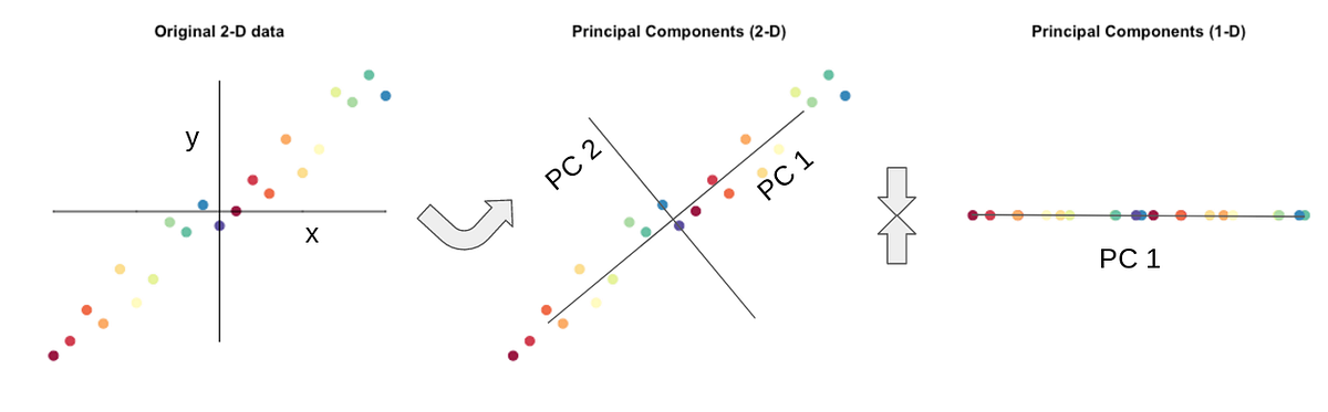"
286 | ]
287 | },
288 | {
289 | "cell_type": "code",
290 | "execution_count": null,
291 | "metadata": {},
292 | "outputs": [],
293 | "source": [
294 | "# We now use the PCA function in scikit-learn to reduce the dimensionality of the data\n",
295 | "# The number of components was chosen arbitrarily.\n",
296 | "pca = PCA(n_components=20)\n",
297 | "bold_pca = pca.fit_transform(bold_data)\n",
298 | "\n",
299 | "print('Original data shape:', bold_data.shape)\n",
300 | "print('PCA data shape:', bold_pca.shape)"
301 | ]
302 | },
303 | {
304 | "cell_type": "markdown",
305 | "metadata": {},
306 | "source": [
307 | "### 3.1 Plot PCA \n",
308 | "\n",
309 | "Let's visualize the variance in the data along different component dimensions."
310 | ]
311 | },
312 | {
313 | "cell_type": "code",
314 | "execution_count": null,
315 | "metadata": {},
316 | "outputs": [],
317 | "source": [
318 | "# Setting plotting parameter\n",
319 | "n_bins=75\n",
320 | "\n",
321 | "# Plot\n",
322 | "n_plots = 4\n",
323 | "components_to_plot = [0,1,2,19]\n",
324 | "f, axes = plt.subplots(1, n_plots, figsize=(14, 14/n_plots))\n",
325 | "st=f.suptitle(\"Figure 3.1. Histogram of values for each PC dimension \", fontsize=\"x-large\")\n",
326 | "\n",
327 | "for i in range(n_plots): \n",
328 | " axes[i].hist(bold_pca[:, components_to_plot[i]], \n",
329 | " bins=n_bins)\n",
330 | " # mark the plots \n",
331 | " axes[i].set_title('PC Dimension %d'%(components_to_plot[i]+1))\n",
332 | " axes[i].set_ylabel('Frequency')\n",
333 | " axes[i].set_xlabel('Value') \n",
334 | " axes[i].set_xticks([])\n",
335 | " axes[i].set_yticks([]) \n",
336 | "\n",
337 | "f.tight_layout()\n",
338 | "st.set_y(0.95)\n",
339 | "f.subplots_adjust(top=0.75)\n"
340 | ]
341 | },
342 | {
343 | "cell_type": "markdown",
344 | "metadata": {},
345 | "source": [
346 | "Let's visualize the relationship between variances across pairs of components."
347 | ]
348 | },
349 | {
350 | "cell_type": "code",
351 | "execution_count": null,
352 | "metadata": {},
353 | "outputs": [],
354 | "source": [
355 | "\"\"\"\n",
356 | "Plot the low dim representation of the bold data\n",
357 | "\"\"\"\n",
358 | "# Setting plotting parameters\n",
359 | "alpha_val = .8\n",
360 | "cur_pals = sns.color_palette('colorblind', n_colors=vdc_n_runs)\n",
361 | "\n",
362 | "# Plot\n",
363 | "n_plots = 3 \n",
364 | "f, axes = plt.subplots(1, n_plots, figsize=(14,5))\n",
365 | "st=f.suptitle(\"Figure 3.2. Scatter plots comparing PCA dimensions \", fontsize=\"x-large\")\n",
366 | "\n",
367 | "# plot data\n",
368 | "axes[0].scatter(bold_pca[:, 0], bold_pca[:, 1], \n",
369 | " alpha=alpha_val, marker='.', color = 'k')\n",
370 | "axes[1].scatter(bold_pca[:, 2], bold_pca[:, 3], \n",
371 | " alpha=alpha_val, marker='.', color = 'k')\n",
372 | "axes[2].scatter(bold_pca[:, 18], bold_pca[:, 19], \n",
373 | " alpha=alpha_val, marker='.', color = 'k')\n",
374 | "\n",
375 | "axes[0].set_title('PCA Dimensions\\n1 x 2')\n",
376 | "axes[1].set_title('PCA Dimensions\\n3 x 4')\n",
377 | "axes[2].set_title('PCA Dimensions\\n18 x 19')\n",
378 | "\n",
379 | "# modifications that are common to all plots \n",
380 | "for i in range(n_plots): \n",
381 | " axes[i].axis('equal')\n",
382 | " axes[i].set_xticks([])\n",
383 | " axes[i].set_yticks([])\n",
384 | "\n",
385 | "f.tight_layout()\n",
386 | "st.set_y(0.95)\n",
387 | "f.subplots_adjust(top=0.75)\n"
388 | ]
389 | },
390 | {
391 | "cell_type": "markdown",
392 | "metadata": {},
393 | "source": [
394 | "### 3.2 Scree plots \n",
395 | "\n",
396 | "A [\"scree\" plot](https://www.theanalysisfactor.com/factor-analysis-how-many-factors/) can depict the amount of variance in the original data that is explained by each component.\n",
397 | "\n",
398 | "**Exercise 4:** Make a scree plot for the PCA above. How many components would be sufficient to account for most of the variance?"
399 | ]
400 | },
401 | {
402 | "cell_type": "code",
403 | "execution_count": null,
404 | "metadata": {},
405 | "outputs": [],
406 | "source": [
407 | "# Plot the scree plot"
408 | ]
409 | },
410 | {
411 | "cell_type": "markdown",
412 | "metadata": {},
413 | "source": [
414 | "**A:**"
415 | ]
416 | },
417 | {
418 | "cell_type": "markdown",
419 | "metadata": {},
420 | "source": [
421 | "### 3.3 Interpreting Components \n",
422 | "\n",
423 | "From the previous plot of the first and second PCA dimension, you can see you have three clusters. You might assume that they correspond to faces, scenes, and objects."
424 | ]
425 | },
426 | {
427 | "cell_type": "markdown",
428 | "metadata": {},
429 | "source": [
430 | "**Exercise 5:** Determine what the three clusters correspond to. First, create a new scatter plot of these two components and mark (e.g., in different symbols or colors) each point on the plot by visual category. Then, create a second scatter plot with points labeled in a way that better corresponds to the clusters (complete this exercise before reading further). (Hint: What else was there three of?)"
431 | ]
432 | },
433 | {
434 | "cell_type": "code",
435 | "execution_count": null,
436 | "metadata": {},
437 | "outputs": [],
438 | "source": [
439 | "# Put answer\n",
440 | "\n",
441 | "\n",
442 | "\n",
443 | "\n",
444 | "\n",
445 | "\n",
446 | "\n",
447 | "\n",
448 | "\n",
449 | "\n",
450 | " "
451 | ]
452 | },
453 | {
454 | "cell_type": "markdown",
455 | "metadata": {},
456 | "source": [
457 | "### 3.4 Normalization \n",
458 | "\n",
459 | "We ran the PCA analysis without normalizing the data.\n",
460 | "\n",
461 | "**Exercise 6:** Using the variable `bold_normalized` re-compute the PCA (components=20). Plot the results with a scatter plot like **Figure 3.2**. What was the effect of normalization and why is this useful?"
462 | ]
463 | },
464 | {
465 | "cell_type": "code",
466 | "execution_count": null,
467 | "metadata": {},
468 | "outputs": [],
469 | "source": [
470 | "# Insert code here"
471 | ]
472 | },
473 | {
474 | "cell_type": "markdown",
475 | "metadata": {},
476 | "source": [
477 | "### 3.5 PCA dimensionality reduction and classification \n",
478 | "As mentioned earlier, we use PCA to reduce the dimensionality of the data and thus minimize the 'curse of dimensionality'. Below we explore how PCA affects classification accuracy."
479 | ]
480 | },
481 | {
482 | "cell_type": "code",
483 | "execution_count": null,
484 | "metadata": {},
485 | "outputs": [],
486 | "source": [
487 | "# Run a basic n-fold classification\n",
488 | "\n",
489 | "# Get baseline, whole-brain decoding accuracy without PCA\n",
490 | "print('Baseline classification')\n",
491 | "print('Original size: ', bold_normalized.shape)\n",
492 | "svc = SVC(kernel=\"linear\", C=1)\n",
493 | "\n",
494 | "start = time()\n",
495 | "models, scores = decode(bold_normalized, labels, run_ids, svc)\n",
496 | "end = time()\n",
497 | "print('Accuracy: ', scores)\n",
498 | "print('Run time: %0.4fs' %(end - start))"
499 | ]
500 | },
501 | {
502 | "cell_type": "code",
503 | "execution_count": null,
504 | "metadata": {},
505 | "outputs": [],
506 | "source": [
507 | "# Run the classifier on data in component space \n",
508 | "pca = PCA(n_components=20)\n",
509 | "bold_pca_normalized = pca.fit_transform(bold_normalized)\n",
510 | "print('PCA (c=%d) classification' % bold_pca_normalized.shape[1])\n",
511 | "print('New size after PCA: ', bold_pca_normalized.shape)\n",
512 | "\n",
513 | "start = time()\n",
514 | "models_pca, scores_pca = decode(bold_pca_normalized, labels, run_ids, svc)\n",
515 | "end = time()\n",
516 | "print('Accuracy: ', scores_pca)\n",
517 | "print('Run time: %0.4fs' %(end - start))"
518 | ]
519 | },
520 | {
521 | "cell_type": "markdown",
522 | "metadata": {},
523 | "source": [
524 | "In this case PCA does not improve decoding accuracy. However, note that similar performance was achieved with 20 vs. 177,314 features, that the analysis ran 500x faster, and that the resulting model is likely to generalize better to new data (e.g., from a different subject)."
525 | ]
526 | },
527 | {
528 | "cell_type": "markdown",
529 | "metadata": {},
530 | "source": [
531 | "**Exercise 7:** We used an arbitrary number of components. How does decoding accuracy change with more or less components?"
532 | ]
533 | },
534 | {
535 | "cell_type": "code",
536 | "execution_count": null,
537 | "metadata": {},
538 | "outputs": [],
539 | "source": [
540 | "# Insert code"
541 | ]
542 | },
543 | {
544 | "cell_type": "markdown",
545 | "metadata": {},
546 | "source": [
547 | "### 3.5.1 The PCA Challenge \n",
548 | "\n",
549 | "**Exercise 8:** Given that some of the early PCA dimensions may not be cognitively relevant, determine the smallest number of PCA components from which you can get the highest decoding accuracy. \n",
550 | "\n"
551 | ]
552 | },
553 | {
554 | "cell_type": "markdown",
555 | "metadata": {},
556 | "source": [
557 | "## 4. Feature selection using cross-validation \n",
558 | "\n",
559 | "When we took a few PCA components instead of all voxels, we were performing feature selection. Feature selection is used to reduce noise and increase computational speed. However, a problem with the approach above is that feature selection is applied to all data (prior to division into training and test sets) and is thus a kind of double dipping.\n",
560 | "\n",
561 | "A better way to select features is during cross-validation. In this case, feature selection is only performed on the training set, and the same features are used on the test data. This way the classifier never sees the test data during training.\n",
562 | "\n",
563 | "\n",
564 | "Aside: While doing PCA on the whole dataset violates the principle of “never touch your test data during training”, researchers have sometimes used this approach, justifying it on the grounds that — while PCA is using the fMRI data from the test set — it is not peeking at the class labels from the test set, and thus it will not bias classification accuracy. Is this OK? It’s difficult to say *a priori*. It is always safer to completely avoid touching the test data during training, so you should do this if at all possible. If you aren’t sure what problems might emerge from a particular analysis method, a good check of your method is to test on random noise; when you do this, classification should not exceed chance (if it does, you have a problem…)\n",
565 | "
\n",
566 | "\n",
567 | "We will perform feature selection during cross-validation in this section. The `Pipelines` method in scikit-learn provides an easy interface to perform these steps and we will use it extensively.\n"
568 | ]
569 | },
570 | {
571 | "cell_type": "markdown",
572 | "metadata": {},
573 | "source": [
574 | "\n",
575 | "### 4.1 Pipelines: Feature selection with cross-validation \n",
576 | "\n",
577 | "The scikit-learn has a method, [Pipeline](http://scikit-learn.org/stable/modules/generated/sklearn.pipeline.Pipeline.html#sklearn.pipeline.Pipeline), that simplifies running a sequence of steps in an automated fashion. Below we create a pipeline with the following steps:\n",
578 | " \n",
579 | ">Perform dimensionality reduction. \n",
580 | ">Run an SVM.\n",
581 | "\n",
582 | "To do this systematically during cross-validation, we will embed `Pipeline` in the `cross_validate` method in scikit-learn.\n",
583 | "\n",
584 | "The steps below are based on [this example in scikit-learn](https://scikit-learn.org/stable/auto_examples/compose/plot_compare_reduction.html#illustration-of-pipeline-and-gridsearchcv)."
585 | ]
586 | },
587 | {
588 | "cell_type": "code",
589 | "execution_count": null,
590 | "metadata": {},
591 | "outputs": [],
592 | "source": [
593 | "# Example: \n",
594 | "# Set up the pipeline\n",
595 | "pipe = Pipeline([\n",
596 | " ('reduce_dim', PCA(n_components=20)),\n",
597 | " ('classify', SVC(kernel=\"linear\", C=1)),\n",
598 | "])\n",
599 | "\n",
600 | "# Run the pipeline with cross-validation\n",
601 | "ps = PredefinedSplit(run_ids) # Provides train/test indices to split data in train/test sets\n",
602 | "clf_pipe = cross_validate(\n",
603 | " pipe,bold_normalized,labels,cv=ps,\n",
604 | " return_train_score=True\n",
605 | ")\n",
606 | "\n",
607 | "# Print results from this dimensionality reduction technique\n",
608 | "print(clf_pipe)\n",
609 | "print (\"Average Testing Accuracy: %0.2f\" % (np.mean(clf_pipe['test_score'])))"
610 | ]
611 | },
612 | {
613 | "cell_type": "markdown",
614 | "metadata": {},
615 | "source": [
616 | "Print out the data indices that were used for training and testing. Ensure that they are different for each fold. "
617 | ]
618 | },
619 | {
620 | "cell_type": "code",
621 | "execution_count": null,
622 | "metadata": {},
623 | "outputs": [],
624 | "source": [
625 | "# Print train/test split\n",
626 | "for cv_idx ,(train_index, test_index) in enumerate(ps.split(bold_normalized, labels)):\n",
627 | " print('CV iteration: %s' % cv_idx)\n",
628 | " print('Train_index: ')\n",
629 | " print(train_index)\n",
630 | " print('Test_index: ')\n",
631 | " print(test_index)\n",
632 | "\n",
633 | "# Print results from this dimensionality reduction technique\n",
634 | "print(clf_pipe)\n",
635 | "print (\"Average Testing Accuracy: %0.2f\" % (np.mean(clf_pipe['test_score'])))"
636 | ]
637 | },
638 | {
639 | "cell_type": "markdown",
640 | "metadata": {},
641 | "source": [
642 | "### 4.2 Feature selection: Univariate \n",
643 | "\n",
644 | "We can also use a variety of univariate methods to do feature selection in scikit-learn. One commonly used technique is to compute an ANOVA on the data and pick voxels with large F values. The F value measures the ratio of the variance between conditions (signal) to the variance within condition (noise). You can learn more about the ANOVA here: [ANOVA F-value](http://scikit-learn.org/stable/modules/generated/sklearn.feature_selection.f_classif.html). Note that implementing this completely different feature selection approach requires changing only one line in the pipeline, demonstrating the usefulness of this framework."
645 | ]
646 | },
647 | {
648 | "cell_type": "markdown",
649 | "metadata": {},
650 | "source": [
651 | "**Exercise 9:** Implement the pipeline using ANOVA F-value (imported as `f_classif`) and the [`SelectKBest` method](http://scikit-learn.org/stable/modules/feature_selection.html#univariate-feature-selection) pick the top 100 voxels with the highest F values."
652 | ]
653 | },
654 | {
655 | "cell_type": "code",
656 | "execution_count": null,
657 | "metadata": {},
658 | "outputs": [],
659 | "source": [
660 | "# Insert code"
661 | ]
662 | },
663 | {
664 | "cell_type": "markdown",
665 | "metadata": {},
666 | "source": [
667 | "**Novel contribution:** be creative and make one new discovery by adding an analysis, visualization, or optimization. This week we encourage you to implement a different feature selection [approach](https://scikit-learn.org/stable/modules/classes.html#module-sklearn.feature_selection)."
668 | ]
669 | },
670 | {
671 | "cell_type": "markdown",
672 | "metadata": {},
673 | "source": [
674 | "## Contributions \n",
675 | "\n",
676 | "M. Kumar, C. Ellis and N. Turk-Browne produced the initial notebook 02/2018 \n",
677 | "T. Meissner minor edits and added the ICA section \n",
678 | "Q. Lu revise PCA plots, cb colors, code style improvement, leverage exisiting funcs \n",
679 | "H. Zhang added pipeline section, use blockwise normalized data, other edits \n",
680 | "M. Kumar enhanced section introductions. \n",
681 | "K.A. Norman provided suggestions on the overall content and made edits to this notebook. \n",
682 | "C. Ellis implemented comments from cmhn-s19 \n",
683 | "A.K. Sahoo fixed broken links and did minor edits."
684 | ]
685 | },
686 | {
687 | "cell_type": "code",
688 | "execution_count": null,
689 | "metadata": {},
690 | "outputs": [],
691 | "source": []
692 | }
693 | ],
694 | "metadata": {
695 | "anaconda-cloud": {},
696 | "kernelspec": {
697 | "display_name": "Python 3",
698 | "language": "python",
699 | "name": "python3"
700 | },
701 | "language_info": {
702 | "codemirror_mode": {
703 | "name": "ipython",
704 | "version": 3
705 | },
706 | "file_extension": ".py",
707 | "mimetype": "text/x-python",
708 | "name": "python",
709 | "nbconvert_exporter": "python",
710 | "pygments_lexer": "ipython3",
711 | "version": "3.7.4"
712 | }
713 | },
714 | "nbformat": 4,
715 | "nbformat_minor": 2
716 | }
717 |
--------------------------------------------------------------------------------
/tutorials/06-rsa.ipynb:
--------------------------------------------------------------------------------
1 | {
2 | "cells": [
3 | {
4 | "cell_type": "markdown",
5 | "metadata": {},
6 | "source": [
7 | "# Representational Similarity Analysis\n",
8 | "[Contributions](#contributions)\n",
9 | "\n",
10 | "Oranges and orange ping-pong balls are not kept next to each other in the grocery store. The oranges are usually placed with other fruits and ping-pong balls with other sport equipment. This helps us shop easily, as we usually group our shopping by categories: fruits and vegetables, meat and dairy, frozen foods, and, somewhere far away, kitchen supplies, toys and sports. Beyond grocery stores, are these meaningful conceptual groupings in the brain? Are patterns of neural activity for oranges and apples more similar to each other as compared to the patterns for oranges and ping-pong balls?\n",
11 | "\n",
12 | "One could conceivably group items based on other attributes such as shape and color. This would make the neural representations of oranges and orange colored ping-pong balls very similar to each other. In a brain region that cares about color, the neural similarity would be greater for oranges and orange ping-pong balls, compared to oranges and red apples. How can we determine the similarity between neural representations and which attributes are driving this similarity?\n",
13 | "\n",
14 | "Representational similarity analysis (RSA) is a way to compare and contrast different brain states and the stimuli that elicited them. In RSA, we compute a similarity measure (often a correlation) between patterns of neural activity for all items being compared. Then, to examine whether neural patterns in a brain region are grouped by color, shape, or category, we can order the similarity measure based on a model that groups by these attributes.\n",
15 | "\n",
16 | "RSA is a highly versatile tool: it can be used to compare brain activity to models, compare data across brain imaging techniques, and even to make cross-species comparisons. You can learn more about the RSA method [here](https://doi.org/10.3389/neuro.06.004.2008) and [here](https://doi.org/10.1016/j.tics.2013.06.007).\n",
17 | " \n",
18 | "## Goal of this script\n",
19 | "\n",
20 | ">1. Learn how to perform RSA on a dataset\n",
21 | " >> Calculate and plot Pearson and Spearman correlations in ROIs \n",
22 | " >> Order these similarity matrices in a meaningful way \n",
23 | " >> Interpret a (dis)similarity matrix \n",
24 | ">2. Visualize similarity with multi dimensional scaling (MDS)\n",
25 | "\n",
26 | "## Table of Contents \n",
27 | "[1. Prepare for RSA](#preprocessing)\n",
28 | ">[1.1 Load the data for one subject](#load_data) \n",
29 | ">[1.2 Helper Functions ](#helper) \n",
30 | ">[1.3 Visualize the data](#visualize_data) \n",
31 | "\n",
32 | "[2. Create a similarity matrix](#sim_mat) \n",
33 | ">[2.1 Reorder data into categories](#reorder) \n",
34 | ">[2.2 How to read a similarity matrix](#read_sim_mat) \n",
35 | ">[2.3 Representational dissimilarity](#read_dsim_mat) \n",
36 | ">[2.4 Comparison of representations in monkeys and humans](#rdm-monkey-human) \n",
37 | "\n",
38 | "[3. Manifolds and multi-dimensional scaling (MDS)](#mds) \n",
39 | ">[3.1 Plotting RDM in 2d](#plot_2d) \n",
40 | ">[3.2 Plotting RDM in 3d](#plot_3d) \n",
41 | "\n",
42 | "\n",
43 | "Exercises\n",
44 | ">[Exercise 1](#ex1) [2](#ex2) [3](#ex3) [4](#ex4) [5](#ex5) [6](#ex6) [7](#ex7) [8](#ex8) [9](#ex9) [10](#ex10)\n",
45 | "\n",
46 | "[Novel contribution](#novel) "
47 | ]
48 | },
49 | {
50 | "cell_type": "markdown",
51 | "metadata": {},
52 | "source": [
53 | "### Dataset \n",
54 | "\n",
55 | "The dataset we will be using for this exercise is from [Kriegeskorte et al. (2008)](https://www.sciencedirect.com/science/article/pii/S0896627308009434), called 'Ninetysix' in the `datasets` folder. 96 visual stimuli, from the 6 categories listed below, were presented to participants. The image stimuli are stored in the subfolder `Stimuli`.\n",
56 | "\n",
57 | "The data have 6 categories: \n",
58 | " 1. artificial inanimate (object/scene)\n",
59 | " 2. human bodypart \n",
60 | " 3. human face \n",
61 | " 4. natural inanimate (object/scene)\n",
62 | " 5. nonhuman bodypart\n",
63 | " 6. nonhuman face\n",
64 | "\n",
65 | "**Self-study:** Explore the data"
66 | ]
67 | },
68 | {
69 | "cell_type": "code",
70 | "execution_count": null,
71 | "metadata": {},
72 | "outputs": [],
73 | "source": [
74 | "import warnings\n",
75 | "import sys \n",
76 | "if not sys.warnoptions:\n",
77 | " warnings.simplefilter(\"ignore\")\n",
78 | "\n",
79 | "import os\n",
80 | "import numpy as np\n",
81 | "import pandas as pd\n",
82 | "import scipy.io\n",
83 | "from scipy import stats\n",
84 | "from sklearn.manifold import MDS\n",
85 | "import scipy.spatial.distance as sp_distance\n",
86 | "\n",
87 | "import matplotlib.pyplot as plt\n",
88 | "import seaborn as sns \n",
89 | "from mpl_toolkits.mplot3d import Axes3D\n",
90 | "\n",
91 | "# %matplotlib notebook\n",
92 | "%matplotlib inline\n",
93 | "%autosave 5\n",
94 | "sns.set(style = 'white', context='poster', rc={\"lines.linewidth\": 2.5})\n",
95 | "sns.set(palette=\"colorblind\")"
96 | ]
97 | },
98 | {
99 | "cell_type": "markdown",
100 | "metadata": {},
101 | "source": [
102 | "### 1.1 Load the data for one subject\n",
103 | "\n",
104 | "The data for these participants are stored as a matlab file (it was 2008 after all...). Python is able to load matlab files using a scipy utility. However, the file formats can be tricky and may require transformations to make compatible with typical Python organization. \n",
105 | "\n",
106 | "The data from matlab are stored as a dictionary where the variables in the matlab files are keys in the dictionary:\n",
107 | "\n",
108 | ">The ROI names are listed in **roinames**. \n",
109 | ">The category label indices for each condition are listed in **labels**. \n",
110 | ">The label indices correspond to entries in **categoryNames**. \n",
111 | ">The data for each ROI, in the order of roinames, is stored in **roi_data**. \n",
112 | "\n",
113 | "Each row of roi_data represents a stimulus (as defined in labels) and each column represents a voxel (there will be different numbers of voxels in different ROIs). These data have been preprocessed and each entry is stored in terms of t-values. There is no time information and no baseline signal to be used for reference.\n",
114 | "\n",
115 | "**Self-study:** What do you think these t-values reflect?\n",
116 | "\n",
117 | "The last 4 rows of the dataset have unknown labels (dun dun dunnnnn!). We'll use only the first 92 rows for analysis, for now.\n",
118 | "\n",
119 | "In the analyses that follow we are going to explore the data of subject 'BE'."
120 | ]
121 | },
122 | {
123 | "cell_type": "markdown",
124 | "metadata": {},
125 | "source": [
126 | "### 1.2 Helper Functions \n",
127 | "\n",
128 | "To make it easy for you to achieve the main goals of this notebook, we have created helper functions that extract data from matlab files and convert into numpy arrays."
129 | ]
130 | },
131 | {
132 | "cell_type": "code",
133 | "execution_count": null,
134 | "metadata": {},
135 | "outputs": [],
136 | "source": [
137 | "from utils import load_data_for_a_subj, digitize_rdm, ns_data_dir"
138 | ]
139 | },
140 | {
141 | "cell_type": "code",
142 | "execution_count": null,
143 | "metadata": {},
144 | "outputs": [],
145 | "source": [
146 | "# Load the data for one subject\n",
147 | "subj_initials = 'BE'\n",
148 | "data_pack = load_data_for_a_subj(subj_initials)\n",
149 | "images, roi_data, roi_names, n_rois, categories, n_categories, labels, label_dict = data_pack\n",
150 | "n_stimuli = len(images)"
151 | ]
152 | },
153 | {
154 | "cell_type": "markdown",
155 | "metadata": {},
156 | "source": [
157 | "**Exercise 1:** Inspect the data. \n",
158 | "- Print the name of each category.\n",
159 | "- Report the shape of the data for each ROI and what each dimension means"
160 | ]
161 | },
162 | {
163 | "cell_type": "code",
164 | "execution_count": null,
165 | "metadata": {},
166 | "outputs": [],
167 | "source": [
168 | "# Insert code here"
169 | ]
170 | },
171 | {
172 | "cell_type": "markdown",
173 | "metadata": {},
174 | "source": [
175 | "### 1.3 Visualize the data \n",
176 | "\n",
177 | "It is always a good idea to plot data as a sanity check before starting analysis. \n",
178 | "\n",
179 | "We also want to see the corresponding labels. Notice the category order is random."
180 | ]
181 | },
182 | {
183 | "cell_type": "code",
184 | "execution_count": null,
185 | "metadata": {},
186 | "outputs": [],
187 | "source": [
188 | "plt.figure()\n",
189 | "\n",
190 | "# Label plot\n",
191 | "plt.subplot(2,1,2)\n",
192 | "plt.plot(labels,'.-')\n",
193 | "plt.xlabel('Stimuli', fontsize=16)\n",
194 | "plt.ylabel('Category', fontsize=16)"
195 | ]
196 | },
197 | {
198 | "cell_type": "markdown",
199 | "metadata": {},
200 | "source": [
201 | "\n",
202 | "Notice that the category order is random i.e. the stimuli at every point are from a different category compared to the neighbors.\n",
203 | "
"
204 | ]
205 | },
206 | {
207 | "cell_type": "markdown",
208 | "metadata": {},
209 | "source": [
210 | "## 2. Create a similarity matrix \n",
211 | "\n",
212 | "Let's examine the similarity of the neural representations of each image with the neural patterns of every other image in the dataset. If the neural patterns are similar between images, we will see high values of similarity, but if the neural patterns are dissimilar, we will see low values of similarity. \n",
213 | "\n",
214 | "There are many ways to compute similarity. We start with one of the most common measures of similarity that you are already familiar with: Pearson correlation (see notebook-04). We compute the Pearson correlation on the neural pattern for each image with every other image. We can compute this on data for each of the ROIs that we have just loaded (left and right FFA, and left and right PPA). For each ROI, our computation will result in a 92 x 92 matrix (we only have labels for 92 images). This resulting matrix shows how similar the neural patterns of activity are between images and is called the representational **similarity** matrix (RSM)."
215 | ]
216 | },
217 | {
218 | "cell_type": "code",
219 | "execution_count": null,
220 | "metadata": {},
221 | "outputs": [],
222 | "source": [
223 | "print('ROI names: ', roi_names)"
224 | ]
225 | },
226 | {
227 | "cell_type": "code",
228 | "execution_count": null,
229 | "metadata": {},
230 | "outputs": [],
231 | "source": [
232 | "# Choose your ROI here!\n",
233 | "roi_id = 1\n",
234 | "\n",
235 | "# Plot figure of these correlations\n",
236 | "f, ax = plt.subplots(1,1, figsize=(8, 7))\n",
237 | "\n",
238 | "plt.imshow(\n",
239 | " np.corrcoef(roi_data[roi_id]), \n",
240 | " cmap='bwr', \n",
241 | " vmin=-1,\n",
242 | " vmax=1,\n",
243 | ")\n",
244 | "plt.colorbar()\n",
245 | "ax.set_title('RSM, unsorted, %s' % (roi_names[roi_id])) \n",
246 | "ax.set_xlabel('stimuli id')\n",
247 | "ax.set_ylabel('stimuli id')"
248 | ]
249 | },
250 | {
251 | "cell_type": "markdown",
252 | "metadata": {},
253 | "source": [
254 | "**Exercise 2:** In the plot above you used Pearson correlation to compute similarity. An alternative metric is a Spearman correlation. \n",
255 | "\n",
256 | "- Explain the difference between Pearson and Spearman correlation. \n",
257 | "- Redo the analysis above with Spearman correlation. \n",
258 | "- Visualize the RSM based on Spearman correlation. "
259 | ]
260 | },
261 | {
262 | "cell_type": "markdown",
263 | "metadata": {},
264 | "source": [
265 | "**A:**"
266 | ]
267 | },
268 | {
269 | "cell_type": "code",
270 | "execution_count": null,
271 | "metadata": {},
272 | "outputs": [],
273 | "source": [
274 | "# Insert code here"
275 | ]
276 | },
277 | {
278 | "cell_type": "markdown",
279 | "metadata": {},
280 | "source": [
281 | "### 2.1 Reorder data into categories \n",
282 | "\n",
283 | "Although the plot above is useful, it is hard to observe any structure because the order of the stimuli is random. To simplify, let's reorganize into label groups."
284 | ]
285 | },
286 | {
287 | "cell_type": "code",
288 | "execution_count": null,
289 | "metadata": {},
290 | "outputs": [],
291 | "source": [
292 | "# Add the stimulus condition labels so that we can sort the data, collecting rows from the same condition together.\n",
293 | "sort_ids = labels.argsort()\n",
294 | "lffa_sorted = roi_data[0][sort_ids, :]\n",
295 | "\n",
296 | "plt.figure(figsize=(9,7))\n",
297 | "\n",
298 | "# Plot the new sorted results\n",
299 | "plt.subplot(2,1,1)\n",
300 | "plt.plot(lffa_sorted[:,0])\n",
301 | "plt.ylabel('t-Value', fontsize=16)\n",
302 | "plt.xlim(0, 96)\n",
303 | "\n",
304 | "plt.subplot(2,1,2)\n",
305 | "plt.plot(labels[sort_ids],'.')\n",
306 | "plt.xlabel('Stimuli', fontsize=16)\n",
307 | "plt.ylabel('Category', fontsize=16)\n",
308 | "plt.show()"
309 | ]
310 | },
311 | {
312 | "cell_type": "code",
313 | "execution_count": null,
314 | "metadata": {},
315 | "outputs": [],
316 | "source": [
317 | "# Choose your ROI here! \n",
318 | "roi_id = 1\n",
319 | "\n",
320 | "# Calculate the RSM\n",
321 | "rsm = np.corrcoef(roi_data[roi_id][sort_ids, :][:92,])\n",
322 | "\n",
323 | "# Plot \n",
324 | "f, ax = plt.subplots(1,1, figsize=(10, 8))\n",
325 | "plt.imshow(\n",
326 | " rsm, \n",
327 | " cmap='bwr', \n",
328 | " vmin=-1,\n",
329 | " vmax=1,\n",
330 | ")\n",
331 | "plt.colorbar()\n",
332 | "\n",
333 | "# Pull out the bin edges between the different categories\n",
334 | "binsize = np.histogram(labels[:92,], 6)[0]\n",
335 | "edges = np.concatenate([np.asarray([0]), np.cumsum(binsize)])[:-1]\n",
336 | "ax.set_xticks(list(np.array(edges)+8))\n",
337 | "ax.set_xticklabels(categories, rotation = 30)\n",
338 | "ax.set_yticks(list(np.array(edges)+8))\n",
339 | "ax.set_yticklabels(categories)\n",
340 | "ax.vlines(edges,0,92)\n",
341 | "ax.hlines(edges,0,92)\n",
342 | "ax.set_title('RSM, sorted, %s' % roi_names[roi_id])"
343 | ]
344 | },
345 | {
346 | "cell_type": "markdown",
347 | "metadata": {},
348 | "source": [
349 | "\n",
350 | "Binning the data: In Figure 1 of Kriegeskorte et al. (2008), the raw correlation values were binned into ten bins based on the percentile score of the dissimilarity value, and the percentile value was plotted. We have created a function `digitize_rdm` to perform the same calculation here and make the plots similar to Figure 1 in Kriegeskorte et al. (2008). \n",
351 | "
\n",
352 | "
\n",
353 | "Note that Figure 1 was using dissimilarity rather than similarity and that the data were from a different ROI (inferior temporal cortex, or IT). However, we can apply the same function to our RSM, the only difference being that the percentile will be based on similarity. \n",
354 | "
\n",
355 | "
\n",
356 | "The `digitize_rdm` functions works in the following manner: \n",
357 | "
\n",
358 | "
\n",
359 | "1. Create `n_bins` of percentile values.
\n",
360 | "2. Take in the matrix of correlations and reshape it into a single row.
\n",
361 | "3. Determine the percentile value of every correlation point and assign it to a bin (`np.digitize` does this).
\n",
362 | "4. Reshape the assigned percentile values into the original correlation matrix shape.
\n",
363 | "5. Finally, plot the percentile values.
\n",
364 | "
\n",
365 | "
"
366 | ]
367 | },
368 | {
369 | "cell_type": "code",
370 | "execution_count": null,
371 | "metadata": {},
372 | "outputs": [],
373 | "source": [
374 | "# Plot the RSM\n",
375 | "f, ax = plt.subplots(1,1, figsize=(10, 8))\n",
376 | "plt.imshow(\n",
377 | " digitize_rdm(rsm), cmap='jet', \n",
378 | ")\n",
379 | "plt.colorbar()\n",
380 | "\n",
381 | "# Pull out the bin edges between the different categories\n",
382 | "binsize = np.histogram(labels[:92,], 6)[0]\n",
383 | "edges = np.concatenate([np.asarray([0]), np.cumsum(binsize)])[:-1]\n",
384 | "ax.set_xticks(list(np.array(edges)+8))\n",
385 | "ax.set_xticklabels(categories, rotation = 30)\n",
386 | "ax.set_yticks(list(np.array(edges)+8))\n",
387 | "ax.set_yticklabels(categories)\n",
388 | "ax.vlines(edges,0,92)\n",
389 | "ax.hlines(edges,0,92)\n",
390 | "ax.set_title('RSM digitized %s' % roi_names[roi_id])"
391 | ]
392 | },
393 | {
394 | "cell_type": "markdown",
395 | "metadata": {},
396 | "source": [
397 | "**Exercise 3:** This new organization is helpful but could be improved (based on our knowledge of the brain). Order the datapoints so that the categories are as follows: human face, human body part, non-human face, non-human body part, natural inanimate and artificial inanimate. This will make for a nicer looking correlation matrix and will help you see any structure within and between categories. \n",
398 | "\n",
399 | "- Write a function to re-order the data. \n",
400 | "- Recompute the RSM based on the re-ordered data and visualize it.\n",
401 | "- Visualize the digitized RSM using the digitization function provided earlier. "
402 | ]
403 | },
404 | {
405 | "cell_type": "code",
406 | "execution_count": null,
407 | "metadata": {},
408 | "outputs": [],
409 | "source": [
410 | "# Insert code here"
411 | ]
412 | },
413 | {
414 | "cell_type": "markdown",
415 | "metadata": {},
416 | "source": [
417 | "### 2.2 How to read a similarity matrix \n",
418 | "\n",
419 | "It is important to be able to read a similarity matrix at a glance. There are couple features to look out for and we will highlight these with some toy data.\n",
420 | "\n",
421 | "Imagine a scenario where we have 12 trial types (e.g., images) grouped into 4 categories (e.g., faces, objects, body parts, and scenes). We are going to simulate some data that has similar activity within category but different activity between categories."
422 | ]
423 | },
424 | {
425 | "cell_type": "markdown",
426 | "metadata": {},
427 | "source": [
428 | "#### 2.2.1. Create simulated data. "
429 | ]
430 | },
431 | {
432 | "cell_type": "code",
433 | "execution_count": null,
434 | "metadata": {},
435 | "outputs": [],
436 | "source": [
437 | "trial_types = 12\n",
438 | "n_sim_categories = 4\n",
439 | "repetitions_per_trial = 24\n",
440 | "trial_noise = 0.5 # multiplying factor for the noise for each trial.\n",
441 | "trials_per_category = int(trial_types / n_sim_categories)\n",
442 | "\n",
443 | "# The template per category. One common signal per category. \n",
444 | "# This will be the similarity within category.\n",
445 | "category_templates = np.random.randn(n_sim_categories, repetitions_per_trial)\n",
446 | "\n",
447 | "# Add some noise to each trial and add the category template to each trial.\n",
448 | "# This will create the trial activity.\n",
449 | "trials = np.zeros((trial_types, repetitions_per_trial))\n",
450 | "for category_counter in range(n_sim_categories):\n",
451 | " category_trials = np.random.randn(trials_per_category, repetitions_per_trial) * trial_noise\n",
452 | " for trial_counter in range(trials_per_category):\n",
453 | " trials[(trials_per_category * category_counter) + trial_counter, :] = category_templates[category_counter, :] + category_trials[trial_counter, :]\n",
454 | "\n"
455 | ]
456 | },
457 | {
458 | "cell_type": "markdown",
459 | "metadata": {},
460 | "source": [
461 | "#### 2.2.2. Compute correlation and plot the result"
462 | ]
463 | },
464 | {
465 | "cell_type": "code",
466 | "execution_count": null,
467 | "metadata": {},
468 | "outputs": [],
469 | "source": [
470 | "# Create the correlation matrix \n",
471 | "sim_r1 = np.corrcoef(trials)\n",
472 | "plt.figure(figsize=(8, 8))\n",
473 | "plt.imshow(sim_r1, \n",
474 | " interpolation='none',\n",
475 | " cmap='bwr', \n",
476 | " vmin=-1,\n",
477 | " vmax=1,\n",
478 | " )\n",
479 | "plt.colorbar()"
480 | ]
481 | },
482 | {
483 | "cell_type": "markdown",
484 | "metadata": {},
485 | "source": [
486 | "In the above plot you should see some clear blocking structure along the diagonal: items within a category are more similar to one another than they are to items in different categories."
487 | ]
488 | },
489 | {
490 | "cell_type": "markdown",
491 | "metadata": {},
492 | "source": [
493 | "#### 2.2.3. Make two categories similar and observe changes in the similarity matrix \n",
494 | "\n",
495 | "Below we create a plot where there is off-diagonal structure. High similarity in off-diagonal parts of a similarity matrix means that elements that are far apart in the ordering have similar structure. In this toy simulation we create an example where the first and third categories are similar to one another (i.e., faces and body parts)."
496 | ]
497 | },
498 | {
499 | "cell_type": "code",
500 | "execution_count": null,
501 | "metadata": {},
502 | "outputs": [],
503 | "source": [
504 | "# Overwrite the template for the 3rd category with the template for 1st category. \n",
505 | "# Python indexing begins at [0].\n",
506 | "category_templates[2, :] = category_templates[0, :]\n",
507 | "\n",
508 | "# Create the trial activity\n",
509 | "trials = np.zeros((trial_types, repetitions_per_trial))\n",
510 | "for category_counter in range(n_sim_categories):\n",
511 | " category_trials = np.random.randn(trials_per_category, repetitions_per_trial) * trial_noise\n",
512 | " for trial_counter in range(trials_per_category):\n",
513 | " trials[(trials_per_category * category_counter) + trial_counter, :] = category_templates[category_counter, :] + category_trials[trial_counter, :]\n",
514 | "\n",
515 | "# Create the correlation matrix \n",
516 | "sim_r2 = np.corrcoef(trials)\n",
517 | "plt.figure(figsize=(8, 8))\n",
518 | "plt.imshow(sim_r2, \n",
519 | " interpolation='none',\n",
520 | " cmap='bwr', \n",
521 | " vmin=-1,\n",
522 | " vmax=1,\n",
523 | " )\n",
524 | "plt.colorbar()"
525 | ]
526 | },
527 | {
528 | "cell_type": "markdown",
529 | "metadata": {},
530 | "source": [
531 | "**Exercise 4:** Now use your new knowledge about reading a similarity matrix to interpret the matrix you created for the real data [Exercise 3](#ex3)."
532 | ]
533 | },
534 | {
535 | "cell_type": "markdown",
536 | "metadata": {},
537 | "source": [
538 | "**A:**"
539 | ]
540 | },
541 | {
542 | "cell_type": "markdown",
543 | "metadata": {},
544 | "source": [
545 | "### 2.3 Representational dissimilarity \n",
546 | "\n",
547 | "The previous analyses framed everything in terms of similarity between the items. However people sometimes prefer to consider this type of data in terms of dissimilarity. This close cousin of the similarity matrix is called the representational dissimilarity matrix (RDM). The dissimilarity matrix is computed simply as 1 - correlation. "
548 | ]
549 | },
550 | {
551 | "cell_type": "markdown",
552 | "metadata": {},
553 | "source": [
554 | "**Exercise 5:** Plot the RDM for the right FFA ROI using the new order as you created in [Exercise 3](#ex3)."
555 | ]
556 | },
557 | {
558 | "cell_type": "code",
559 | "execution_count": null,
560 | "metadata": {},
561 | "outputs": [],
562 | "source": [
563 | "# Insert code here"
564 | ]
565 | },
566 | {
567 | "cell_type": "markdown",
568 | "metadata": {},
569 | "source": [
570 | "**Exercise 6:** For RDM plots based on correlation values, what does an RDM value greater than 1 correspond to in terms of a correlation?"
571 | ]
572 | },
573 | {
574 | "cell_type": "markdown",
575 | "metadata": {},
576 | "source": [
577 | "**A:**"
578 | ]
579 | },
580 | {
581 | "cell_type": "markdown",
582 | "metadata": {},
583 | "source": [
584 | "### 2.4 Comparison of representations in monkeys and humans \n",
585 | "\n",
586 | "The RSA can be used to compare information not just in humans, but across species too. Below is comparison of the RDM for monkeys and humans, in the inferior temporal cortex (Color map altered to match Figure 1 in Kriegeskorte et al. (2008))."
587 | ]
588 | },
589 | {
590 | "cell_type": "code",
591 | "execution_count": null,
592 | "metadata": {},
593 | "outputs": [],
594 | "source": [
595 | "# Load the data, and bin to percentile\n",
596 | "monkeyRDM = pd.read_csv(os.path.join(ns_data_dir, 'RDM_mIT_fig1.txt'), header=None)\n",
597 | "humanRDM = pd.read_csv(os.path.join(ns_data_dir, 'RDM_hIT_fig1.txt'), header=None)\n",
598 | "\n",
599 | "monkey_rdm_digitized = digitize_rdm(monkeyRDM)\n",
600 | "human_rdm_digitized = digitize_rdm(humanRDM)\n",
601 | "\n",
602 | "f, axes = plt.subplots(1,2, figsize = (14, 6))\n",
603 | "axes[0].imshow(\n",
604 | " monkey_rdm_digitized, \n",
605 | " cmap='jet', \n",
606 | ")\n",
607 | "axes[1].imshow(\n",
608 | " human_rdm_digitized, \n",
609 | " cmap='jet', \n",
610 | ")\n",
611 | "# plt.colorbar()\n",
612 | "axes[0].set_title('Monkey RDM')\n",
613 | "axes[1].set_title('Human RDM')\n",
614 | "\n",
615 | "#for i in range(2): \n",
616 | "# axes[i].set_xlabel('stimuli id')\n",
617 | "# axes[i].set_ylabel('stimuli id')"
618 | ]
619 | },
620 | {
621 | "cell_type": "markdown",
622 | "metadata": {},
623 | "source": [
624 | "## 3. Multi-dimensional scaling (MDS) \n",
625 | "\n",
626 | "The correlation matrix for the 92 images describes how similar each item is to each other item. This means that if two items have a high positive correlation then they can be thought of as eliciting a very similar activation pattern across voxels. We can reframe this to be thought of as a distance in a high-dimensional space. From this perspective, items that are similar to one another will be grouped close together and far away from points that they are dissimilar to. \n",
627 | "\n",
628 | "MDS allows us to visualize the similarity of our data in a different way than plotting the matrices above. Specifically, it allows to generate a lower-dimensional image (e.g., 2-D or 3-D) in which the distances between points approximate the distances in the original high-dimensional data. There is an MDS [method](https://homepages.uni-tuebingen.de/florian.wickelmaier/pubs/Wickelmaier2003SQRU.pdf) built into [scikit-learn](http://scikit-learn.org/stable/modules/manifold.html#multidimensional-scaling)."
629 | ]
630 | },
631 | {
632 | "cell_type": "code",
633 | "execution_count": null,
634 | "metadata": {},
635 | "outputs": [],
636 | "source": [
637 | "# Create a 2-D MDS\n",
638 | "mds = MDS(n_components=2, dissimilarity=\"precomputed\", random_state=0) # Create the MDS object\n",
639 | "results = mds.fit(digitize_rdm(1 - rsm)) # Use the dissimilarity matrix"
640 | ]
641 | },
642 | {
643 | "cell_type": "markdown",
644 | "metadata": {},
645 | "source": [
646 | "**Exercise 7:** How does changing the order of the data (e.g., shuffling the rows/columns) in your RDM affect the distance between points calculated by MDS? "
647 | ]
648 | },
649 | {
650 | "cell_type": "markdown",
651 | "metadata": {},
652 | "source": [
653 | "**A:**"
654 | ]
655 | },
656 | {
657 | "cell_type": "markdown",
658 | "metadata": {},
659 | "source": [
660 | "### 3.1 Plot the 2D structure of the RDM \n",
661 | "\n",
662 | "We'll plot the 92 images on a \"map\" signifying how close or far apart images are to each other. We use different colors for the 6 categories of images."
663 | ]
664 | },
665 | {
666 | "cell_type": "code",
667 | "execution_count": null,
668 | "metadata": {},
669 | "outputs": [],
670 | "source": [
671 | "coords = results.embedding_\n",
672 | "\n",
673 | "plt.figure(figsize=(10, 7))\n",
674 | "for label_counter in np.unique(labels[:92]):\n",
675 | " label_idxs = (labels[:92] == label_counter)[:]\n",
676 | " plt.scatter(\n",
677 | " coords[label_idxs, 0], coords[label_idxs, 1], \n",
678 | " marker = 'o', s = 50\n",
679 | " )\n",
680 | "plt.legend(categories, bbox_to_anchor=(1, .8), loc=\"upper left\")\n",
681 | "plt.title('MDS, 2D');"
682 | ]
683 | },
684 | {
685 | "cell_type": "markdown",
686 | "metadata": {},
687 | "source": [
688 | "**Self-study**: On the MDS plot you are currently plotting each item as a point. You could instead load in each image and plot that image on the MDS plot directly to get a feel for which stimuli are being grouped."
689 | ]
690 | },
691 | {
692 | "cell_type": "markdown",
693 | "metadata": {},
694 | "source": [
695 | "### 3.2 Plot the 3D structure of the RDM \n",
696 | "\n",
697 | "MDS is just trying to find a k-dimensional embedding that minimizes the stress (something akin to the goodness of fit). This means we can actually plot it in arbitrarily high dimensions to try and capture the data structure. Below we make a 3D plot, given that the 2D plot."
698 | ]
699 | },
700 | {
701 | "cell_type": "code",
702 | "execution_count": null,
703 | "metadata": {},
704 | "outputs": [],
705 | "source": [
706 | "# Multi-dimensional scaling\n",
707 | "mds = MDS(n_components=3, dissimilarity=\"precomputed\", random_state=0)\n",
708 | "results = mds.fit(digitize_rdm(1 - rsm))\n",
709 | "\n",
710 | "coords = results.embedding_\n",
711 | "\n",
712 | "fig = plt.figure(figsize=(10, 7))\n",
713 | "ax = fig.add_subplot(111, projection='3d')\n",
714 | "for label_counter in np.unique(labels[:92]):\n",
715 | " label_idxs = (labels[:92] == label_counter)[:]\n",
716 | " ax.scatter(\n",
717 | " coords[label_idxs, 0], coords[label_idxs, 1], coords[label_idxs, 2], \n",
718 | " marker = 'o', s = 50\n",
719 | " )\n",
720 | " \n",
721 | "plt.legend(categories, bbox_to_anchor=(1,.7), loc=\"upper left\")\n",
722 | "plt.title('MDS, 3D')\n",
723 | "plt.tight_layout()"
724 | ]
725 | },
726 | {
727 | "cell_type": "markdown",
728 | "metadata": {},
729 | "source": [
730 | "There are tools available to us to evaluate what is the appropriate dimensionality for visualization of our data (i.e. what dimensionality has sufficiently low stress). We can look at the stress of the MDS with different numbers of components (i.e. different dimensionality) and determine what dimensionality of the data is appropriate.\n",
731 | "\n",
732 | "Let's make a toy problem to start off with in order to get a handle on what this should look like. We are going to make points that lie on a line in 3D space. Because a line has only one dimension of information (along its length) the data ought to be able to be reduced in dimensionality to a single dimension. We will run MDS on this data to see if that is the case."
733 | ]
734 | },
735 | {
736 | "cell_type": "code",
737 | "execution_count": null,
738 | "metadata": {},
739 | "outputs": [],
740 | "source": [
741 | "coords = np.linspace(1, 30, 30)\n",
742 | "coords = np.vstack((coords, coords, coords)).T\n",
743 | "\n",
744 | "fig = plt.figure()\n",
745 | "ax = fig.add_subplot(111, projection='3d')\n",
746 | "ax.scatter(coords[:, 0], coords[:, 1], coords[:, 2])"
747 | ]
748 | },
749 | {
750 | "cell_type": "code",
751 | "execution_count": null,
752 | "metadata": {},
753 | "outputs": [],
754 | "source": [
755 | "# Calculate the euclidean distance of every point from every other point\n",
756 | "dist = sp_distance.squareform(sp_distance.pdist(coords))\n",
757 | "\n",
758 | "# Iterate through different numbers of components\n",
759 | "stress = []\n",
760 | "for components in range(1, 6):\n",
761 | " mds = MDS(n_components=components, dissimilarity=\"precomputed\", random_state=0)\n",
762 | " # Pull out the stress of the MDS fit\n",
763 | " stress.append(mds.fit(dist).stress_)\n",
764 | "\n",
765 | "# Plot the stress\n",
766 | "plt.figure()\n",
767 | "plt.plot(range(1, 6), stress)\n",
768 | "plt.ylabel('Stress')\n",
769 | "plt.xlabel('Dimensionality')"
770 | ]
771 | },
772 | {
773 | "cell_type": "markdown",
774 | "metadata": {},
775 | "source": [
776 | "**Exercise 8:** It is not typical for data to be able to be described accurately in low dimensionality: stress generally decreases with the number of components. Perform a similar analysis below to estimate the appropriate dimensionality to visualize the RDM of the right FFA data from this participant. What is the appropriate lower dimensional representation of the data? Note: Make sure you don't calculate the stress metric from the MDS embedding, calculate the MDS fit from the RDM.\n",
777 | "\n",
778 | "MDS documentation: https://scikit-learn.org/stable/modules/generated/sklearn.manifold.MDS.html \n",
779 | "\n",
780 | "Here's the list of arguments for MDS: \n",
781 | "```\n",
782 | "MDS(n_components=2, metric=True, n_init=4, max_iter=300, verbose=0, eps=0.001, n_jobs=None, random_state=None, dissimilarity=’euclidean’)\n",
783 | "```\n",
784 | "\n",
785 | "Empirically, more stringent convergence criteria (i.e. large `n_init` and `max_iter`, small `eps`) will lead to more stable results. "
786 | ]
787 | },
788 | {
789 | "cell_type": "markdown",
790 | "metadata": {},
791 | "source": [
792 | "**A:**"
793 | ]
794 | },
795 | {
796 | "cell_type": "code",
797 | "execution_count": null,
798 | "metadata": {},
799 | "outputs": [],
800 | "source": [
801 | "# Insert code here"
802 | ]
803 | },
804 | {
805 | "cell_type": "markdown",
806 | "metadata": {},
807 | "source": [
808 | "**Exercise 9:** Compute RDMs and create MDS plots for the left PPA and right PPA using the reordering you created above."
809 | ]
810 | },
811 | {
812 | "cell_type": "code",
813 | "execution_count": null,
814 | "metadata": {},
815 | "outputs": [],
816 | "source": [
817 | "# Insert code here"
818 | ]
819 | },
820 | {
821 | "cell_type": "markdown",
822 | "metadata": {},
823 | "source": [
824 | "**Exercise 10:** The last four rows in the dataset for subject BE have unmarked labels. One of them is a human face. Using the techniques outlined here and your knowledge of the category preference of each ROI, analyze the data to make a best guess of which one of the 4 missing labels is a human face. Show your work and reasoning that led you to this conclusion. Hint: It will help to visualize these 4 points amongst the points you already have. It would also help to compare the response of each of the missing data points with a 'canonical' face response."
825 | ]
826 | },
827 | {
828 | "cell_type": "code",
829 | "execution_count": null,
830 | "metadata": {},
831 | "outputs": [],
832 | "source": [
833 | "# Insert code here"
834 | ]
835 | },
836 | {
837 | "cell_type": "markdown",
838 | "metadata": {},
839 | "source": [
840 | "**Novel contribution:** be creative and make one new discovery by adding an analysis, visualization, or optimization.\n",
841 | "\n",
842 | "Some examples: \n",
843 | "\n",
844 | "- visualize the average RDM across subjects\n",
845 | "- compare the empirical RDM to some theoretical RDM\n",
846 | "- check the consistency between hierarchical clustering vs. ground truth label ordering \n",
847 | "- use other dimensionality reduction methods to visualize the data (PCA, tSNE, etc.)\n",
848 | "- perform some classification on this data set\n",
849 | "- apply RSA on previous datasets (e.g. VDC, the simulated dataset used in the 1st notebook)\n",
850 | "- apply RSA on previous datasets (e.g., VDC)\n",
851 | "- even better, your own ambitious ideas! "
852 | ]
853 | },
854 | {
855 | "cell_type": "markdown",
856 | "metadata": {},
857 | "source": [
858 | "## Contributions \n",
859 | "\n",
860 | "M. Kumar, C. Ellis and N. Turk-Browne produced the initial notebook. 02/2018 \n",
861 | "The mystery label exercise was borrowed from a matlab version created by F. Pereira. \n",
862 | "T. Meissner minor edits. \n",
863 | "Q. Lu plot aesthetics, digitization func, modularize funcs, re-ordering, replicate the original paper. \n",
864 | "K.A. Norman provided suggestions on the overall content and made edits to this notebook. \n",
865 | "C. Ellis implemented updates from cmhn-s19.
\n",
866 | "X. Li edited stimuli from continuous line to discrete dots in section 1.3 and 2.1"
867 | ]
868 | }
869 | ],
870 | "metadata": {
871 | "anaconda-cloud": {},
872 | "kernelspec": {
873 | "display_name": "Python 3",
874 | "language": "python",
875 | "name": "python3"
876 | },
877 | "language_info": {
878 | "codemirror_mode": {
879 | "name": "ipython",
880 | "version": 3
881 | },
882 | "file_extension": ".py",
883 | "mimetype": "text/x-python",
884 | "name": "python",
885 | "nbconvert_exporter": "python",
886 | "pygments_lexer": "ipython3",
887 | "version": "3.7.4"
888 | }
889 | },
890 | "nbformat": 4,
891 | "nbformat_minor": 2
892 | }
--------------------------------------------------------------------------------
/tutorials/07-searchlight/avg18_whole_brain_SL.nii.gz:
--------------------------------------------------------------------------------
https://raw.githubusercontent.com/brainiak/brainiak-tutorials/fb62ede943d9694fe703aee0df5f43ecf5558415/tutorials/07-searchlight/avg18_whole_brain_SL.nii.gz
--------------------------------------------------------------------------------
/tutorials/07-searchlight/avg3_whole_brain_SL.nii.gz:
--------------------------------------------------------------------------------
https://raw.githubusercontent.com/brainiak/brainiak-tutorials/fb62ede943d9694fe703aee0df5f43ecf5558415/tutorials/07-searchlight/avg3_whole_brain_SL.nii.gz
--------------------------------------------------------------------------------
/tutorials/07-searchlight/rank_whole_brain_SL.nii.gz:
--------------------------------------------------------------------------------
https://raw.githubusercontent.com/brainiak/brainiak-tutorials/fb62ede943d9694fe703aee0df5f43ecf5558415/tutorials/07-searchlight/rank_whole_brain_SL.nii.gz
--------------------------------------------------------------------------------
/tutorials/07-searchlight/run_searchlight.sh:
--------------------------------------------------------------------------------
1 | #!/bin/bash -i
2 | # Input python command to be submitted as a job
3 |
4 | #SBATCH --output=../logs/searchlight-%j.out
5 | #SBATCH --job-name searchlight
6 | #SBATCH -t 30 # time limit: how many minutes
7 | #SBATCH --mem=4G # memory limit
8 | #SBATCH -n 2 # how many cores to use
9 |
10 | # Set up the environment
11 | source ../setup_environment.sh
12 |
13 | # Run the python script (use mpi if running on the cluster)
14 | if [ $configuration == "cluster" ]
15 | then
16 | srun --mpi=pmi2 python ./searchlight.py
17 | else
18 | python ./searchlight.py
19 | fi
20 |
--------------------------------------------------------------------------------
/tutorials/07-searchlight/searchlight.py:
--------------------------------------------------------------------------------
1 | # Run a whole brain searchlight
2 |
3 | # Import libraries
4 | import nibabel as nib
5 | import numpy as np
6 | from mpi4py import MPI
7 | from brainiak.searchlight.searchlight import Searchlight
8 | from sklearn.model_selection import StratifiedShuffleSplit, GridSearchCV
9 | from sklearn.svm import SVC
10 | from scipy.spatial.distance import euclidean
11 | import os
12 | import pickle
13 | from utils import results_path
14 |
15 | # Import additional libraries you need
16 | fs_data_dir = os.path.expanduser(results_path + '/searchlight_data')
17 |
18 | num_subj = 3
19 |
20 | # Load and perpare data for one subject
21 | def load_fs_data(sub_id, mask=''):
22 | # find file path
23 | sub = 'sub-%.2d' % (sub_id)
24 | input_dir = os.path.join(fs_data_dir, sub)
25 | data_file = os.path.join(input_dir, 'data.nii.gz')
26 |
27 | if mask == '':
28 | mask_file = os.path.join(fs_data_dir, 'wb_mask.nii.gz')
29 | else:
30 | mask_file = os.path.join(fs_data_dir, '{}_mask.nii.gz'.format(mask))
31 |
32 | # load bold data and some header information so that we can save searchlight results later
33 | data_file = nib.load(data_file)
34 | bold_data = data_file.get_data()
35 | affine_mat = data_file.affine
36 | dimsize = data_file.header.get_zooms()
37 |
38 | # load mask
39 | brain_mask = nib.load(mask_file)
40 | brain_mask = brain_mask.get_data()
41 |
42 | return bold_data, brain_mask, affine_mat, dimsize
43 |
44 | def load_fs_label(sub_id, mask=''):
45 | # find file path
46 | sub = 'sub-%.2d' % (sub_id)
47 | input_dir = os.path.join(fs_data_dir, sub)
48 | label_file = os.path.join(input_dir, 'label.npz')
49 | # load label
50 | label = np.load(label_file)
51 | label = label['label']
52 | return label
53 |
54 | # Data Path
55 | data_path = os.path.expanduser(results_path + '/searchlight_results')
56 | # if not os.path.exists(data_path):
57 | # os.makedirs(data_path)
58 |
59 | # Pull out the MPI information
60 | comm = MPI.COMM_WORLD
61 | rank = comm.rank
62 | size = comm.size
63 |
64 | # load mask
65 | mask_file = os.path.join(fs_data_dir, 'wb_mask.nii.gz')
66 | mask = nib.load(mask_file)
67 | mask = mask.get_data()
68 |
69 | # Loop over subjects
70 | data = []
71 | bcvar = []
72 | for sub_id in range(1,num_subj+1):
73 | if rank == 0:
74 | data_i, mask, affine_mat, dimsize = load_fs_data(sub_id)
75 | data.append(data_i)
76 | else:
77 | data.append(None)
78 | bcvar_i = load_fs_label(sub_id)
79 | bcvar.append(bcvar_i)
80 |
81 | sl_rad = 1
82 | max_blk_edge = 5
83 | pool_size = 1
84 |
85 | coords = np.where(mask)
86 |
87 |
88 | # Create the searchlight object
89 | sl = Searchlight(sl_rad=sl_rad,max_blk_edge=max_blk_edge)
90 | # print("Setup searchlight inputs")
91 | # print("Number of subjects: " + str(len(data)))
92 | # print("Input data shape: " + str(data[0].shape))
93 | # print("Input mask shape: " + str(mask.shape) + "\n")
94 |
95 | # Distribute the information to the searchlights (preparing it to run)
96 | sl.distribute(data, mask)
97 |
98 | # Broadcast variables
99 | sl.broadcast(bcvar)
100 |
101 | # Set up the kernel function, in this case an SVM
102 | def calc_svm(data, sl_mask, myrad, bcvar):
103 | accuracy = []
104 | sl_num_vx = sl_mask.shape[0] * sl_mask.shape[1] * sl_mask.shape[2]
105 | num_epoch = data[0].shape[3]
106 | # Loop over subjects to leave each subject out once:
107 | for idx in range(len(data)):
108 | # Pull out the data
109 | # Testing data
110 | data4D_test = data[idx]
111 | labels_test = bcvar[idx]
112 | bolddata_sl_test = data4D_test.reshape(sl_num_vx, num_epoch).T
113 |
114 | # Training data
115 | labels_train = []
116 | bolddata_sl_train = np.empty((0, sl_num_vx))
117 | for train_id in range(len(data)):
118 | if train_id != idx:
119 | labels_train.extend(list(bcvar[train_id]))
120 | bolddata_sl_train = np.concatenate((bolddata_sl_train, data[train_id].reshape(sl_num_vx, num_epoch).T))
121 | labels_train = np.array(labels_train)
122 |
123 | # Train classifier
124 | clf = SVC(kernel='linear', C=1)
125 | clf.fit(bolddata_sl_train, labels_train)
126 |
127 | # Test classifier
128 | score = clf.score(bolddata_sl_test, labels_test)
129 | accuracy.append(score)
130 |
131 | return accuracy
132 |
133 | # Run the searchlight analysis
134 | print("Begin SearchLight in rank %s\n" % rank)
135 | all_sl_result = sl.run_searchlight(calc_svm, pool_size=pool_size)
136 | print("End SearchLight in rank %s\n" % rank)
137 |
138 | # Only save the data if this is the first core
139 | if rank == 0:
140 | all_sl_result = all_sl_result[mask==1]
141 | all_sl_result = [num_subj*[0] if not n else n for n in all_sl_result] # replace all None
142 | # The average result
143 | avg_vol = np.zeros((mask.shape[0], mask.shape[1], mask.shape[2]))
144 |
145 | # Loop over subjects
146 | for sub_id in range(1,num_subj+1):
147 | sl_result = [r[sub_id-1] for r in all_sl_result]
148 | # reshape
149 | result_vol = np.zeros((mask.shape[0], mask.shape[1], mask.shape[2]))
150 | result_vol[coords[0], coords[1], coords[2]] = sl_result
151 | # Convert the output into what can be used
152 | result_vol = result_vol.astype('double')
153 | result_vol[np.isnan(result_vol)] = 0 # If there are nans we want this
154 | # Add the processed result_vol into avg_vol
155 | avg_vol += result_vol
156 | # Save the volume
157 | output_name = os.path.join(data_path, 'subj%s_whole_brain_SL.nii.gz' % (sub_id))
158 | sl_nii = nib.Nifti1Image(result_vol, affine_mat)
159 | hdr = sl_nii.header
160 | hdr.set_zooms((dimsize[0], dimsize[1], dimsize[2]))
161 | nib.save(sl_nii, output_name) # Save
162 |
163 | # Save the average result
164 | output_name = os.path.join(data_path, 'avg%s_whole_brain_SL.nii.gz' % (num_subj))
165 | sl_nii = nib.Nifti1Image(avg_vol/num_subj, affine_mat)
166 | hdr = sl_nii.header
167 | hdr.set_zooms((dimsize[0], dimsize[1], dimsize[2]))
168 | nib.save(sl_nii, output_name) # Save
169 |
170 | print('Finished searchlight')
--------------------------------------------------------------------------------
/tutorials/07-searchlight/searchlight_rank.py:
--------------------------------------------------------------------------------
1 | # Run a whole brain searchlight
2 |
3 | # Import libraries
4 | import nibabel as nib
5 | import numpy as np
6 | from mpi4py import MPI
7 | from brainiak.searchlight.searchlight import Searchlight
8 | from sklearn.model_selection import StratifiedShuffleSplit, GridSearchCV
9 | from sklearn.svm import SVC
10 | from scipy.spatial.distance import euclidean
11 | import os
12 | import pickle
13 |
14 | # Import additional libraries you need
15 | fs_data_dir = os.path.expanduser('~/searchlight_data')
16 |
17 | num_subj = 1
18 |
19 | # Load and perpare data for one subject
20 | def load_fs_data(sub_id, mask=''):
21 | # find file path
22 | sub = 'sub-%.2d' % (sub_id)
23 | input_dir = os.path.join(fs_data_dir, sub)
24 | data_file = os.path.join(input_dir, 'data.nii.gz')
25 | label_file = os.path.join(input_dir, 'label.npz')
26 | if mask == '':
27 | mask_file = os.path.join(fs_data_dir, 'wb_mask.nii.gz')
28 | else:
29 | mask_file = os.path.join(fs_data_dir, '{}_mask.nii.gz'.format(mask))
30 |
31 | # load bold data and some header information so that we can save searchlight results later
32 | data_file = nib.load(data_file)
33 | bold_data = data_file.get_data()
34 | affine_mat = data_file.affine
35 | dimsize = data_file.header.get_zooms()
36 |
37 | # load label
38 | label = np.load(label_file)
39 | label = label['label']
40 |
41 | # load mask
42 | brain_mask = nib.load(mask_file)
43 | brain_mask = brain_mask.get_data()
44 |
45 | return bold_data, label, brain_mask, affine_mat, dimsize
46 |
47 | # Data Path
48 | data_path = os.path.expanduser('~/searchlight_results')
49 | # if not os.path.exists(data_path):
50 | # os.makedirs(data_path)
51 |
52 | # Loop over subjects
53 | data = []
54 | bcvar = []
55 | for sub_id in range(1,num_subj+1):
56 | data_i, bcvar_i, mask, affine_mat, dimsize = load_fs_data(sub_id)
57 | data.append(data_i)
58 | bcvar.append(bcvar_i)
59 |
60 | sl_rad = 1
61 | max_blk_edge = 5
62 | pool_size = 1
63 |
64 | coords = np.where(mask)
65 |
66 | # Pull out the MPI information
67 | comm = MPI.COMM_WORLD
68 | rank = comm.rank
69 | size = comm.size
70 |
71 | # Create the searchlight object
72 | sl = Searchlight(sl_rad=sl_rad,max_blk_edge=max_blk_edge)
73 | print("Setup searchlight inputs")
74 | print("Number of subjects: " + str(len(data)))
75 | print("Input data shape: " + str(data[0].shape))
76 | print("Input mask shape: " + str(mask.shape) + "\n")
77 |
78 | # Distribute the information to the searchlights (preparing it to run)
79 | sl.distribute(data, mask)
80 |
81 | # Broadcast variables
82 | sl.broadcast(bcvar)
83 |
84 | # Set up the kernel function, in this case an SVM
85 | def calc_rank(data, sl_mask, myrad, bcvar):
86 | # Pull out the MPI information
87 | comm = MPI.COMM_WORLD
88 | rank = comm.rank
89 | size = comm.size
90 | return [rank]
91 |
92 | # Run the searchlight analysis
93 | print("Begin SearchLight in rank %s\n" % rank)
94 | all_sl_result = sl.run_searchlight(calc_rank, pool_size=pool_size)
95 | print("End SearchLight in rank %s\n" % rank)
96 |
97 | # Only save the data if this is the first core
98 | if rank == 0:
99 | all_sl_result = all_sl_result[mask==1]
100 | all_sl_result = [num_subj*[0] if not n else n for n in all_sl_result] # replace all None
101 |
102 | # Loop over subjects
103 | for sub_id in range(1,num_subj+1):
104 | sl_result = [r[sub_id-1] for r in all_sl_result]
105 | # reshape
106 | result_vol = np.zeros((mask.shape[0], mask.shape[1], mask.shape[2]))
107 | result_vol[coords[0], coords[1], coords[2]] = sl_result
108 | # Convert the output into what can be used
109 | result_vol = result_vol.astype('double')
110 | result_vol[np.isnan(result_vol)] = 0 # If there are nans we want this
111 | # Save the volume
112 | output_name = os.path.join(data_path, 'rank_whole_brain_SL.nii.gz' )
113 | sl_nii = nib.Nifti1Image(result_vol, affine_mat)
114 | hdr = sl_nii.header
115 | hdr.set_zooms((dimsize[0], dimsize[1], dimsize[2]))
116 | nib.save(sl_nii, output_name) # Save
117 |
118 | print('Finished searchlight')
--------------------------------------------------------------------------------
/tutorials/07-searchlight/searchlight_single_subject.py:
--------------------------------------------------------------------------------
1 | # Run a whole brain searchlight on a single subject in the VDC dataset
2 |
3 | # Import libraries
4 | import nibabel as nib
5 | import numpy as np
6 | from mpi4py import MPI
7 | from brainiak.searchlight.searchlight import Searchlight
8 | from sklearn.model_selection import PredefinedSplit
9 | from sklearn.svm import LinearSVC
10 | from scipy.stats import zscore
11 | import os, sys
12 |
13 | # Import additional libraries you need
14 | sys.path.append('../')
15 | # load some helper functions
16 | from utils import load_vdc_mask, load_vdc_epi_data, load_vdc_stim_labels, label2TR, shift_timing
17 | # load some constants
18 | from utils import vdc_data_dir, results_path,vdc_all_ROIs, vdc_label_dict, vdc_n_runs, vdc_hrf_lag, vdc_TR, vdc_TRs_run
19 |
20 | # parameters
21 | sub = 'sub-01'
22 | roi_name = 'FFA'
23 |
24 | # Pull out the MPI information
25 | comm = MPI.COMM_WORLD
26 | rank = comm.rank
27 | size = comm.size
28 |
29 | # Output data Path
30 | output_path = os.path.join(results_path,'searchlight_results')
31 | if rank == 0:
32 | if not os.path.exists(output_path):
33 | os.makedirs(output_path)
34 |
35 | # load mask of the subject
36 | mask = load_vdc_mask(roi_name, sub)
37 | mask = mask.get_data()
38 | coords = np.where(mask)
39 |
40 | # load labels of the subject in all ranks
41 | stim_label_allruns = load_vdc_stim_labels(sub)
42 | stim_label_TR = label2TR(stim_label_allruns, vdc_n_runs, vdc_TR, vdc_TRs_run)
43 | shift_size = int(vdc_hrf_lag / vdc_TR)
44 | label = shift_timing(stim_label_TR, shift_size)
45 | # extract non-zero labels
46 | label_index = np.squeeze(np.nonzero(label))
47 | # Pull out the indexes
48 | labels = label[label_index]
49 |
50 | # get run ids (works similarity to cv_ids)
51 | run_ids = stim_label_allruns[5,:] - 1
52 | # split data according to run ids
53 | ps = PredefinedSplit(run_ids)
54 |
55 | # Same them as the broadcast variables
56 | bcvar = [labels, ps]
57 |
58 | # load the data in rank 0
59 | if rank == 0:
60 | # Make a function to load the data
61 | def load_data(directory, subject_name):
62 | # Cycle through the runs
63 | for run in range(1, vdc_n_runs + 1):
64 | epi_data = load_vdc_epi_data(subject_name, run)
65 | bold_data = epi_data.get_data()
66 | affine_mat = epi_data.affine
67 | dimsize = epi_data.header.get_zooms()
68 | # Concatenate the data
69 | if run == 1:
70 | concatenated_data = bold_data
71 | else:
72 | concatenated_data = np.concatenate((concatenated_data, bold_data), axis=-1)
73 | return concatenated_data, affine_mat, dimsize
74 |
75 | data, affine_mat, dimsize = load_data(vdc_data_dir, sub)
76 | # extract bold data for non-zero labels
77 | data = data[:, :, :, label_index]
78 | # normalize the data within each run
79 | for r in range(vdc_n_runs):
80 | data[:, :, :, run_ids==r] = np.nan_to_num(zscore(data[:, :, :, run_ids==r], axis=3))
81 | else:
82 | data = None
83 |
84 | # Set parameters
85 | sl_rad = 1
86 | max_blk_edge = 5
87 | pool_size = 1
88 |
89 | # Create the searchlight object
90 | sl = Searchlight(sl_rad=sl_rad,max_blk_edge=max_blk_edge)
91 |
92 | # Distribute the information to the searchlights (preparing it to run)
93 | sl.distribute([data], mask)
94 |
95 | # Broadcast variables
96 | sl.broadcast(bcvar)
97 |
98 | # Set up the kernel function, in this case an SVM
99 | def calc_svm(data, sl_mask, myrad, bcvar):
100 | if np.sum(sl_mask) < 14:
101 | return -1
102 | scores = []
103 | labels, ps = bcvar[0], bcvar[1]
104 |
105 | # Reshape the data
106 | sl_num_vx = sl_mask.shape[0] * sl_mask.shape[1] * sl_mask.shape[2]
107 | num_epoch = data[0].shape[3]
108 | data_sl = data[0].reshape(sl_num_vx, num_epoch).T
109 |
110 | # Classifier: loop over all runs to leave each run out once
111 | model = LinearSVC()
112 | for train_index, test_index in ps.split():
113 | X_train, X_test = data_sl[train_index], data_sl[test_index]
114 | y_train, y_test = labels[train_index], labels[test_index]
115 | # Fit a svm
116 | model.fit(X_train, y_train)
117 | # Calculate the accuracy for the hold out run
118 | score = model.score(X_test, y_test)
119 | scores.append(score)
120 |
121 | return np.mean(scores)
122 |
123 | # Run the searchlight analysis
124 | print("Begin SearchLight in rank %s\n" % rank)
125 | sl_result = sl.run_searchlight(calc_svm, pool_size=pool_size)
126 | print("End SearchLight in rank %s\n" % rank)
127 |
128 | # Only save the data if this is the first core
129 | if rank == 0:
130 | # Convert NaN to 0 in the output
131 | sl_result = np.nan_to_num(sl_result[mask==1])
132 | # Reshape
133 | result_vol = np.zeros((mask.shape[0], mask.shape[1], mask.shape[2]))
134 | result_vol[coords[0], coords[1], coords[2]] = sl_result
135 | # Convert the output into what can be used
136 | result_vol = result_vol.astype('double')
137 | # Save the average result
138 | output_name = os.path.join(output_path, '%s_%s_SL.nii.gz' % (sub, roi_name))
139 | sl_nii = nib.Nifti1Image(result_vol, affine_mat)
140 | hdr = sl_nii.header
141 | hdr.set_zooms((dimsize[0], dimsize[1], dimsize[2]))
142 | nib.save(sl_nii, output_name) # Save
143 |
144 | print('Finished searchlight')
145 |
--------------------------------------------------------------------------------
/tutorials/09-fcma/fcma_classify.py:
--------------------------------------------------------------------------------
1 | # Copyright 2016 Intel Corporation
2 | #
3 | # Licensed under the Apache License, Version 2.0 (the "License");
4 | # you may not use this file except in compliance with the License.
5 | # You may obtain a copy of the License at
6 | #
7 | # http://www.apache.org/licenses/LICENSE-2.0
8 | #
9 | # Unless required by applicable law or agreed to in writing, software
10 | # distributed under the License is distributed on an "AS IS" BASIS,
11 | # WITHOUT WARRANTIES OR CONDITIONS OF ANY KIND, either express or implied.
12 | # See the License for the specific language governing permissions and
13 | # limitations under the License.
14 |
15 | from brainiak.fcma.classifier import Classifier
16 | from brainiak.fcma.preprocessing import prepare_fcma_data
17 | from brainiak import io
18 |
19 | from sklearn.svm import SVC
20 | import sys
21 | import logging
22 | import numpy as np
23 | from sklearn import model_selection
24 | from mpi4py import MPI
25 | import os
26 | from utils import results_path
27 |
28 | format = '%(asctime)s - %(name)s - %(levelname)s - %(message)s'
29 | # if want to output log to a file instead of outputting log to the console,
30 | # replace "stream=sys.stdout" with "filename='fcma.log'"
31 | logging.basicConfig(level=logging.INFO, format=format, stream=sys.stdout)
32 | logger = logging.getLogger(__name__)
33 |
34 | data_dir = sys.argv[1]
35 | suffix = sys.argv[2]
36 | top_n_mask_file = sys.argv[3] # This is not the whole brain mask! This is the voxel selection mask
37 | epoch_file = sys.argv[4]
38 | left_out_subj = sys.argv[5]
39 | if len(sys.argv)==7:
40 | second_mask = sys.argv[6] # Do you want to supply a second mask (for extrinsic analysis)
41 | else:
42 | second_mask = "None"
43 |
44 | # Where do you want to output the classification results?
45 | output_file = results_path + '/classify_result.txt'
46 |
47 | # Do you want to compute this in an easily understood way (0) or a memory efficient way (1)?
48 | is_memory_efficient = 1
49 |
50 | # If a second mask was supplied then this is an extrinsic analysis and treat it as such
51 | if second_mask == "None":
52 | is_extrinsic = 0
53 | else:
54 | is_extrinsic = 1
55 |
56 | if __name__ == '__main__':
57 |
58 | # Send a message on the first node
59 | if MPI.COMM_WORLD.Get_rank()==0:
60 | logger.info(
61 | 'Testing for participant %d.\nProgramming starts in %d process(es)' %
62 | (int(left_out_subj), MPI.COMM_WORLD.Get_size())
63 | )
64 |
65 | # Load in the volumes, mask and labels
66 | images = io.load_images_from_dir(data_dir, suffix=suffix)
67 | top_n_mask = io.load_boolean_mask(top_n_mask_file)
68 | epoch_list = io.load_labels(epoch_file)
69 |
70 | # Parse the epoch data for useful dimensions
71 | epochs_per_subj = epoch_list[0].shape[1]
72 | num_subjs = len(epoch_list)
73 |
74 | # Prepare the data
75 | int_data, _, labels = prepare_fcma_data(images, epoch_list, top_n_mask)
76 |
77 | # What indexes pick out the left out participant?
78 | start_idx = int(int(left_out_subj) * epochs_per_subj)
79 | end_idx = int(start_idx + epochs_per_subj)
80 |
81 | # Take out the idxs corresponding to all participants but this one
82 | training_idx = list(set(range(len(labels))) - set(range(start_idx, end_idx)))
83 | testing_idx = list(range(start_idx, end_idx))
84 |
85 | # Pull out the data
86 | int_data_training = [int_data[i] for i in training_idx]
87 | int_data_testing = [int_data[i] for i in testing_idx]
88 |
89 | # Pull out the labels
90 | labels_training = [labels[i] for i in training_idx]
91 | labels_testing = [labels[i] for i in testing_idx]
92 |
93 | # Prepare the data to be processed efficiently (albeit in a less easy to follow way)
94 | if is_memory_efficient == 1:
95 | rearranged_int_data = int_data_training + int_data_testing
96 | rearranged_labels = labels_training + labels_testing
97 | num_training_samples = epochs_per_subj * (num_subjs - 1)
98 |
99 | # Do you want to perform an intrinsic vs extrinsic analysis
100 | if is_extrinsic > 0 and is_memory_efficient == 1:
101 |
102 | # This needs to be reloaded every time you call prepare_fcma_data
103 | images = io.load_images_from_dir(data_dir, suffix=suffix)
104 |
105 | # Multiply the inverse of the top n mask by the whole brain mask to bound it
106 | second_mask = io.load_boolean_mask(second_mask)
107 | extrinsic_mask = ((top_n_mask == 0) * second_mask)==1
108 |
109 | # Prepare the data using the extrinsic data
110 | ext_data, _, _ = prepare_fcma_data(images, epoch_list, extrinsic_mask)
111 |
112 | # Pull out the appropriate extrinsic data
113 | ext_data_training = [ext_data[i] for i in training_idx]
114 | ext_data_testing = [ext_data[i] for i in testing_idx]
115 |
116 | # Set up data so that the internal mask is correlated with the extrinsic mask
117 | rearranged_ext_data = ext_data_training + ext_data_testing
118 | corr_obj = list(zip(rearranged_ext_data, rearranged_int_data))
119 | else:
120 |
121 | # Set up data so that the internal mask is correlated with the internal mask
122 | if is_memory_efficient == 1:
123 | corr_obj = list(zip(rearranged_int_data, rearranged_int_data))
124 | else:
125 | training_obj = list(zip(int_data_training, int_data_training))
126 | testing_obj = list(zip(int_data_testing, int_data_testing))
127 |
128 | # no shrinking, set C=1
129 | svm_clf = SVC(kernel='precomputed', shrinking=False, C=1)
130 |
131 | clf = Classifier(svm_clf, epochs_per_subj=epochs_per_subj)
132 |
133 | # Train the model on the training data
134 | if is_memory_efficient == 1:
135 | clf.fit(corr_obj, rearranged_labels, num_training_samples)
136 | else:
137 | clf.fit(training_obj, labels_training)
138 |
139 | # What is the cv accuracy?
140 | if is_memory_efficient == 0:
141 | cv_prediction = clf.predict(training_obj)
142 |
143 | # Test on the testing data
144 | if is_memory_efficient == 1:
145 | predict = clf.predict()
146 | else:
147 | predict = clf.predict(testing_obj)
148 |
149 | # Report results on the first rank core
150 | if MPI.COMM_WORLD.Get_rank()==0:
151 | print('--RESULTS--')
152 | print(clf.decision_function())
153 |
154 | # How often does the prediction match the target
155 | num_correct = (np.asanyarray(predict) == np.asanyarray(labels_testing)).sum()
156 |
157 | # Print the CV accuracy
158 | if is_memory_efficient == 0:
159 | cv_accuracy = (np.asanyarray(cv_prediction) == np.asanyarray(labels_training)).sum() / len(labels_training)
160 | print('CV accuracy: %0.5f' % (cv_accuracy))
161 |
162 | intrinsic_vs_extrinsic = ['intrinsic', 'extrinsic']
163 |
164 | # Report accuracy
165 | logger.info(
166 | 'When leaving subject %d out for testing using the %s mask for an %s correlation, the accuracy is %d / %d = %.2f' %
167 | (int(left_out_subj), top_n_mask_file, intrinsic_vs_extrinsic[int(is_extrinsic)], num_correct, epochs_per_subj, num_correct / epochs_per_subj)
168 | )
169 |
170 | # Append this accuracy on to a score sheet
171 | with open(output_file, 'a') as fp:
172 | fp.write(top_n_mask_file + ', ' + str(intrinsic_vs_extrinsic[int(is_extrinsic)]) + ': ' + str(num_correct / epochs_per_subj) + '\n')
173 |
--------------------------------------------------------------------------------
/tutorials/09-fcma/fcma_voxel_selection_cv.py:
--------------------------------------------------------------------------------
1 | # Copyright 2016 Intel Corporation
2 | #
3 | # Licensed under the Apache License, Version 2.0 (the "License");
4 | # you may not use this file except in compliance with the License.
5 | # You may obtain a copy of the License at
6 | #
7 | # http://www.apache.org/licenses/LICENSE-2.0
8 | #
9 | # Unless required by applicable law or agreed to in writing, software
10 | # distributed under the License is distributed on an "AS IS" BASIS,
11 | # WITHOUT WARRANTIES OR CONDITIONS OF ANY KIND, either express or implied.
12 | # See the License for the specific language governing permissions and
13 | # limitations under the License.
14 |
15 | from brainiak.fcma.voxelselector import VoxelSelector
16 | from brainiak.fcma.preprocessing import prepare_fcma_data
17 | from brainiak.fcma.preprocessing import RandomType
18 | from brainiak import io
19 | from sklearn.svm import SVC
20 | import sys
21 | from mpi4py import MPI
22 | import logging
23 | import numpy as np
24 | import nibabel as nib
25 | import os
26 |
27 | format = '%(asctime)s - %(name)s - %(levelname)s - %(message)s'
28 | # if want to output log to a file instead of outputting log to the console,
29 | # replace "stream=sys.stdout" with "filename='fcma.log'"
30 | logging.basicConfig(level=logging.INFO, format=format, stream=sys.stdout)
31 | logger = logging.getLogger(__name__)
32 |
33 | """
34 | Perform leave one participant out voxel selection with FCMA
35 | """
36 |
37 | data_dir = sys.argv[1] # What is the directory containing data?
38 | suffix = sys.argv[2] # What is the extension of the data you're loading
39 | mask_file = sys.argv[3] # What is the path to the whole brain mask
40 | epoch_file = sys.argv[4] # What is the path to the epoch file
41 | left_out_subj = sys.argv[5] # Which participant (as an integer) are you leaving out for this cv?
42 | output_dir = sys.argv[6] # What is the path to the folder you want to save this data in
43 |
44 | # Only run the following from the controller core
45 | if __name__ == '__main__':
46 | if MPI.COMM_WORLD.Get_rank()==0:
47 | logger.info(
48 | 'Testing for participant %d.\nProgramming starts in %d process(es)' %
49 | (int(left_out_subj), MPI.COMM_WORLD.Get_size())
50 | )
51 | # create output_dir
52 | if not os.path.exists(output_dir):
53 | os.makedirs(output_dir)
54 |
55 | # Load in the volumes, mask and labels
56 | images = io.load_images_from_dir(data_dir, suffix=suffix)
57 | mask = io.load_boolean_mask(mask_file)
58 | epoch_list = io.load_labels(epoch_file)
59 |
60 | # Parse the epoch data for useful dimensions
61 | epochs_per_subj = epoch_list[0].shape[1]
62 | num_subjs = len(epoch_list)
63 |
64 | # Preprocess the data and prepare for FCMA
65 | raw_data, _, labels = prepare_fcma_data(images, epoch_list, mask)
66 |
67 | # enforce left one out
68 | file_str = output_dir + '/fc_no' + str(left_out_subj) + '_'
69 | start_idx = int(int(left_out_subj) * epochs_per_subj)
70 | end_idx = int(start_idx + epochs_per_subj)
71 |
72 | # Take out the idxs corresponding to all participants but this one
73 | subsampled_idx = list(set(range(len(labels))) - set(range(start_idx, end_idx)))
74 | labels_subsampled = [labels[i] for i in subsampled_idx]
75 | raw_data_subsampled = [raw_data[i] for i in subsampled_idx]
76 |
77 | # Set up the voxel selection object for fcma
78 | vs = VoxelSelector(labels_subsampled, epochs_per_subj, num_subjs - 1, raw_data_subsampled)
79 |
80 | # for cross validation, use SVM with precomputed kernel
81 | clf = SVC(kernel='precomputed', shrinking=False, C=1)
82 | results = vs.run(clf)
83 |
84 | # this output is just for result checking
85 | if MPI.COMM_WORLD.Get_rank()==0:
86 | logger.info(
87 | 'correlation-based voxel selection is done'
88 | )
89 |
90 | # Load in the mask with nibabel
91 | mask_img = nib.load(mask_file)
92 | mask = mask_img.get_data().astype(np.bool)
93 |
94 | # Preset the volumes
95 | score_volume = np.zeros(mask.shape, dtype=np.float32)
96 | score = np.zeros(len(results), dtype=np.float32)
97 | seq_volume = np.zeros(mask.shape, dtype=np.int)
98 | seq = np.zeros(len(results), dtype=np.int)
99 |
100 | # Write a text document of the voxel selection results
101 | with open(file_str + 'result_list.txt', 'w') as fp:
102 | for idx, tuple in enumerate(results):
103 | fp.write(str(tuple[0]) + ' ' + str(tuple[1]) + '\n')
104 |
105 | # Store the score for each voxel
106 | score[tuple[0]] = tuple[1]
107 | seq[tuple[0]] = idx
108 |
109 | # Convert the list into a volume
110 | score_volume[mask] = score
111 | seq_volume[mask] = seq
112 |
113 | # Save volume
114 | io.save_as_nifti_file(score_volume, mask_img.affine,
115 | file_str + 'result_score.nii.gz')
116 | io.save_as_nifti_file(seq_volume, mask_img.affine,
117 | file_str + 'result_seq.nii.gz')
118 |
--------------------------------------------------------------------------------
/tutorials/09-fcma/make_top_voxel_mask.sh:
--------------------------------------------------------------------------------
1 | #!/bin/bash -i
2 | #
3 | # Takes in a results directory from fcma analysis and a certain number of voxels to threshold for a mask as input
4 |
5 | #You will need to load fsl module/conda for your cluster
6 | source ../setup_environment.sh
7 |
8 |
9 | # Take inputs
10 | input_dir=$1 # What is the path to thedata?
11 | voxel_number=$2 # What voxel threshold would you like to set
12 | output_dir=$3 # Where do you want to put the data
13 |
14 | # Create output_dir
15 | if [ ! -d ${output_dir} ]; then
16 | mkdir ${output_dir}
17 | fi
18 |
19 | # Iterate through each volume in the fcma directory
20 | for file in ${input_dir}/*_seq.nii.gz
21 | do
22 | # Preprocess the file name
23 | fbase=$(basename "$file")
24 | pref="${fbase%%.*}"
25 |
26 | # Create the voxel mask
27 | fslmaths $file -uthr $voxel_number -bin ${output_dir}/${pref}_top${voxel_number}.nii.gz
28 |
29 | done
30 |
31 | # Concatenate all of the masks from each volume
32 | fslmerge -t ${output_dir}/all_top${voxel_number} ${output_dir}/fc_no*top${voxel_number}.nii.gz
33 |
34 | # Create a probability map of each voxel being included across participants
35 | fslmaths ${output_dir}/all_top${voxel_number} -Tmean ${output_dir}/prop_top${voxel_number} -odt float
36 |
--------------------------------------------------------------------------------
/tutorials/09-fcma/run_fcma_classify.sh:
--------------------------------------------------------------------------------
1 | #!/bin/bash -i
2 | #SBATCH -t 15
3 | #SBATCH --mem-per-cpu=12G
4 | #SBATCH -n 2
5 | #SBATCH --job-name fcma_classify
6 | #SBATCH --output=../logs/fcma_classify-%j.out
7 |
8 | # Set up the environment. You will need to modify the module for your cluster.
9 | source ../setup_environment.sh
10 |
11 | # How many threads can you make
12 | export OMP_NUM_THREADS=32
13 |
14 | # set the current dir
15 | currentdir=`pwd`
16 |
17 | # Prepare inputs to voxel selection function
18 | data_dir=$1 # What is the directory containing data?
19 | suffix=$2 # What is the extension of the data you're loading
20 | mask_file=$3 #What is the path to the top N mask file (THIS IS NOT THE WHOLE BRAIN MASK)
21 | epoch_file=$4 # What is the path to the epoch file
22 | left_out_subj=$5 #Which participant (as an integer) are you using for testing?
23 | second_mask=$6 # Do you want to use a second mask to compare the data with? Necessary for extrinsic analyses. Otherwise ignore this input or set to None
24 |
25 | # Run the script
26 | # Run the python script (use mpi if running on the cluster)
27 | if [ $configuration == "cluster" ]
28 | then
29 | srun --mpi=pmi2 python ./fcma_classify.py $data_dir $suffix $mask_file $epoch_file $left_out_subj $second_mask
30 | else
31 | mpirun -np 2 python ./fcma_classify.py $data_dir $suffix $mask_file $epoch_file $left_out_subj $second_mask
32 | fi
33 |
--------------------------------------------------------------------------------
/tutorials/09-fcma/run_fcma_voxel_selection_cv.sh:
--------------------------------------------------------------------------------
1 | #!/bin/bash -i
2 | #SBATCH -t 20
3 | #SBATCH --mem-per-cpu=8G
4 | #SBATCH -n 2
5 | #SBATCH --job-name fcma_voxel_select_cv
6 | #SBATCH --output=../logs/fcma_voxel_select_cv-%j.out
7 |
8 | # Set up the environment. You will need to modify the module for your cluster.
9 | source ../setup_environment.sh
10 |
11 | # How many threads can you make
12 | export OMP_NUM_THREADS=32
13 |
14 | # set the current dir
15 | currentdir=`pwd`
16 |
17 | # Prepare inputs to voxel selection function
18 | data_dir=$1 # What is the directory containing data?
19 | suffix=$2 # What is the extension of the data you're loading
20 | mask_file=$3 # What is the path to the whole brain mask
21 | epoch_file=$4 # What is the path to the epoch file
22 | left_out_subj=$5 # Which participant (as an integer) are you leaving out for this cv?
23 | output_dir=$6 # Where do you want to save the data
24 |
25 | # Run the script
26 | if [ $configuration == "cluster" ]
27 | then
28 | srun --mpi=pmi2 python ./fcma_voxel_selection_cv.py $data_dir $suffix $mask_file $epoch_file $left_out_subj $output_dir
29 | else
30 | mpirun -np 2 python ./fcma_voxel_selection_cv.py $data_dir $suffix $mask_file $epoch_file $left_out_subj $output_dir
31 | fi
32 |
--------------------------------------------------------------------------------
/tutorials/13-real-time/fmrisim/ROI_A.nii.gz:
--------------------------------------------------------------------------------
https://raw.githubusercontent.com/brainiak/brainiak-tutorials/fb62ede943d9694fe703aee0df5f43ecf5558415/tutorials/13-real-time/fmrisim/ROI_A.nii.gz
--------------------------------------------------------------------------------
/tutorials/13-real-time/fmrisim/ROI_B.nii.gz:
--------------------------------------------------------------------------------
https://raw.githubusercontent.com/brainiak/brainiak-tutorials/fb62ede943d9694fe703aee0df5f43ecf5558415/tutorials/13-real-time/fmrisim/ROI_B.nii.gz
--------------------------------------------------------------------------------
/tutorials/13-real-time/fmrisim/mask.npy:
--------------------------------------------------------------------------------
https://raw.githubusercontent.com/brainiak/brainiak-tutorials/fb62ede943d9694fe703aee0df5f43ecf5558415/tutorials/13-real-time/fmrisim/mask.npy
--------------------------------------------------------------------------------
/tutorials/13-real-time/fmrisim/sub_noise_dict.txt:
--------------------------------------------------------------------------------
1 | {'voxel_size': [3.0, 3.0, 3.5000014], 'max_activity': 1624.0952380952381, 'sfnr': 70.7171164884859, 'fwhm': 5.6615986148452109, 'snr': 69.511670001526468, 'auto_reg_sigma': 0.3953408689278336, 'drift_sigma': 0.6046591310721664}
--------------------------------------------------------------------------------
/tutorials/13-real-time/fmrisim/sub_template.nii.gz:
--------------------------------------------------------------------------------
https://raw.githubusercontent.com/brainiak/brainiak-tutorials/fb62ede943d9694fe703aee0df5f43ecf5558415/tutorials/13-real-time/fmrisim/sub_template.nii.gz
--------------------------------------------------------------------------------
/tutorials/13-real-time/generate_data.py:
--------------------------------------------------------------------------------
1 | # Generate a noise volume given a set of parameters
2 |
3 | import os
4 | import glob
5 | import time
6 | import random
7 | import inspect
8 | import typing
9 | import nibabel # type: ignore
10 | import numpy as np # type: ignore
11 | from brainiak.utils import fmrisim as sim # type: ignore
12 | import sys
13 | sys.path.append(os.getcwd())
14 | import utils
15 |
16 | # Template input directory
17 | frame = inspect.currentframe()
18 | moduleFile = typing.cast(str, frame.f_code.co_filename)
19 | moduleDir = os.path.dirname(moduleFile)
20 | fmrisim_dir = os.path.join(moduleDir, "fmrisim/")
21 |
22 | # Data output directory
23 | data_dir = os.path.join(utils.results_path, "13-real-time/data/")
24 |
25 | # If the folder doesn't exist then make it
26 | if os.path.isdir(data_dir) is False:
27 | os.makedirs(data_dir, exist_ok=True)
28 |
29 | # Specify the volume parameters
30 | trDuration = 2 # seconds
31 | numTRs = 200 # How many TRs will you generate?
32 |
33 | # Set up stimulus event time course parameters
34 | event_duration = 10 # How long is each event
35 | isi = 0 # What is the time between each event
36 | burn_in = 0 # How long before the first event
37 |
38 | # Specify signal magnitude parameters
39 | signal_change = 10 # How much change is there in intensity for the max of the patterns across participants
40 | multivariate_pattern = 0 # Do you want the signal to be a z scored pattern across voxels (1) or a univariate increase (0)
41 | switch_ROI = 0 # Do you want to switch the ROIs over part way through and if so, specify the proportion of TRs before this happens
42 |
43 | print('Load template of average voxel value')
44 | template_nii = nibabel.load(fmrisim_dir + 'sub_template.nii.gz')
45 | template = template_nii.get_data()
46 |
47 | dimensions = np.array(template.shape[0:3])
48 |
49 | print('Create binary mask and normalize the template range')
50 | mask, template = sim.mask_brain(volume=template,
51 | mask_self=True,
52 | )
53 |
54 | # Write out the mask as a numpy file
55 | np.save(data_dir + 'mask.npy', mask.astype(np.uint8))
56 |
57 | # Load the noise dictionary
58 | print('Loading noise parameters')
59 | with open(fmrisim_dir + 'sub_noise_dict.txt', 'r') as f:
60 | noise_dict = f.read()
61 | noise_dict = eval(noise_dict)
62 | noise_dict['matched'] = 0
63 |
64 | print('Generating noise')
65 | noise = sim.generate_noise(dimensions=dimensions,
66 | stimfunction_tr=np.zeros((numTRs, 1)),
67 | tr_duration=int(trDuration),
68 | template=template,
69 | mask=mask,
70 | noise_dict=noise_dict,
71 | )
72 |
73 | # Create the stimulus time course of the conditions
74 | total_time = int(numTRs * trDuration)
75 | events = int(total_time / event_duration)
76 | onsets_A = []
77 | onsets_B = []
78 | for event_counter in range(events):
79 |
80 | # Flip a coin for each epoch to determine whether it is A or B
81 | if np.random.randint(0, 2) == 1:
82 | onsets_A.append(event_counter * event_duration)
83 | else:
84 | onsets_B.append(event_counter * event_duration)
85 |
86 | temporal_res = 0.5 # How many timepoints per second of the stim function are to be generated?
87 |
88 | # Create a time course of events
89 | stimfunc_A = sim.generate_stimfunction(onsets=onsets_A,
90 | event_durations=[event_duration],
91 | total_time=total_time,
92 | temporal_resolution=temporal_res,
93 | )
94 |
95 | stimfunc_B = sim.generate_stimfunction(onsets=onsets_B,
96 | event_durations=[event_duration],
97 | total_time=total_time,
98 | temporal_resolution=temporal_res,
99 | )
100 |
101 | # Create a labels timecourse
102 | np.save(data_dir + 'labels.npy', (stimfunc_A + (stimfunc_B * 2)))
103 |
104 |
105 | print('Load ROIs')
106 | nii_A = nibabel.load(fmrisim_dir + 'ROI_A.nii.gz')
107 | nii_B = nibabel.load(fmrisim_dir + 'ROI_B.nii.gz')
108 | ROI_A = nii_A.get_data()
109 | ROI_B = nii_B.get_data()
110 |
111 | # How many voxels per ROI
112 | voxels_A = int(ROI_A.sum())
113 | voxels_B = int(ROI_B.sum())
114 |
115 | # Create a pattern of activity across the two voxels
116 | print('Creating signal pattern')
117 | if multivariate_pattern == 1:
118 | pattern_A = np.random.rand(voxels_A).reshape((voxels_A, 1))
119 | pattern_B = np.random.rand(voxels_B).reshape((voxels_B, 1))
120 | else: # Just make a univariate increase
121 | pattern_A = np.tile(1, voxels_A).reshape((voxels_A, 1))
122 | pattern_B = np.tile(1, voxels_B).reshape((voxels_B, 1))
123 |
124 | # Multiply each pattern by each voxel time course
125 | weights_A = np.tile(stimfunc_A, voxels_A) * pattern_A.T
126 | weights_B = np.tile(stimfunc_B, voxels_B) * pattern_B.T
127 |
128 | # Convolve the onsets with the HRF
129 | print('Creating signal time course')
130 | signal_func_A = sim.convolve_hrf(stimfunction=weights_A,
131 | tr_duration=trDuration,
132 | temporal_resolution=temporal_res,
133 | scale_function=1,
134 | )
135 |
136 | signal_func_B = sim.convolve_hrf(stimfunction=weights_B,
137 | tr_duration=trDuration,
138 | temporal_resolution=temporal_res,
139 | scale_function=1,
140 | )
141 |
142 | # Multiply the signal by the signal change
143 | signal_func_A *= signal_change
144 | signal_func_B *= signal_change
145 |
146 | # Combine the signal time course with the signal volume
147 | print('Creating signal volumes')
148 | signal_A = sim.apply_signal(signal_func_A,
149 | ROI_A,
150 | )
151 |
152 | signal_B = sim.apply_signal(signal_func_B,
153 | ROI_B,
154 | )
155 |
156 | # Do you want to switch the location of the signal 75% of the way through through?
157 | if switch_ROI > 0:
158 |
159 | # When does the switch occur?
160 | switch_point = int(numTRs * switch_ROI)
161 |
162 | part_1_A = sim.apply_signal(signal_func_A[:switch_point, :],
163 | ROI_A,
164 | )
165 |
166 | part_2_A = sim.apply_signal(signal_func_A[switch_point:, :],
167 | ROI_B,
168 | )
169 |
170 | part_1_B = sim.apply_signal(signal_func_B[:switch_point, :],
171 | ROI_B,
172 | )
173 |
174 | part_2_B = sim.apply_signal(signal_func_B[switch_point:, :],
175 | ROI_A,
176 | )
177 |
178 | # Concatenate the new volumes
179 | signal_A = np.concatenate((part_1_A, part_2_A), axis=3)
180 | signal_B = np.concatenate((part_1_B, part_2_B), axis=3)
181 |
182 | # # What will you name this file as?
183 | # data_dir = fmrisim_dir + 'data_switched'
184 |
185 | # Combine the two signal timecourses
186 | signal = signal_A + signal_B
187 |
188 | print('Generating TRs in real time')
189 | for idx in range(numTRs):
190 |
191 | # Create the brain volume on this TR
192 | brain = noise[:, :, :, idx] + signal[:, :, :, idx]
193 |
194 | # Save the volume as a numpy file, with each TR as its own file
195 | output_file = data_dir + 'rt_' + format(idx, '03d') + '.npy'
196 |
197 | # Save file
198 | brain_float32 = brain.astype(np.float32)
199 | print("Generate {}".format(output_file))
200 | np.save(output_file, brain_float32)
201 |
202 | # Sleep until next TR
203 | time.sleep(trDuration)
204 |
--------------------------------------------------------------------------------
/tutorials/13-real-time/run_generate_data.sh:
--------------------------------------------------------------------------------
1 | #!/bin/bash
2 | # Input python command to be submitted as a job
3 |
4 | #SBATCH --output=generate_data-%j.out
5 | #SBATCH --job-name generate_data
6 | #SBATCH -t 30
7 | #SBATCH --mem=4G
8 | #SBATCH -n 1
9 |
10 | # Check you are in the correct directory
11 | if [ ${PWD##*/} == '13-real-time' ]
12 | then
13 | cd ..
14 | echo "Changing to the tutorials directory"
15 | fi
16 |
17 |
18 | # Set up the environment
19 | source ./setup_environment.sh
20 |
21 | # Run the python script
22 | python ./13-real-time/generate_data.py
23 |
--------------------------------------------------------------------------------
/tutorials/colab-env-setup.ipynb:
--------------------------------------------------------------------------------
1 | {
2 | "cells": [
3 | {
4 | "cell_type": "markdown",
5 | "metadata": {
6 | "colab_type": "text",
7 | "id": "yb-sHbwR4QO2"
8 | },
9 | "source": [
10 | "# Brainiak Tutorials Environment Setup for Google CoLab"
11 | ]
12 | },
13 | {
14 | "cell_type": "markdown",
15 | "metadata": {
16 | "colab_type": "text",
17 | "id": "dyFoGtMhg_kC"
18 | },
19 | "source": [
20 | "## Install Brainiak and code dependencies (Approx install time 1 minute)"
21 | ]
22 | },
23 | {
24 | "cell_type": "code",
25 | "execution_count": 0,
26 | "metadata": {
27 | "colab": {},
28 | "colab_type": "code",
29 | "collapsed": true,
30 | "id": "DZ_oWJwO2392"
31 | },
32 | "outputs": [],
33 | "source": [
34 | "!pip install deepdish ipython matplotlib nilearn notebook pandas seaborn watchdog\n",
35 | "!pip install pip\\<10\n",
36 | "!pip install git+https://github.com/brainiak/brainiak"
37 | ]
38 | },
39 | {
40 | "cell_type": "markdown",
41 | "metadata": {
42 | "colab_type": "text",
43 | "id": "327lTJCnhQyY"
44 | },
45 | "source": [
46 | "## Git-clone helper files for tutorials"
47 | ]
48 | },
49 | {
50 | "cell_type": "code",
51 | "execution_count": 0,
52 | "metadata": {
53 | "colab": {},
54 | "colab_type": "code",
55 | "collapsed": true,
56 | "id": "7sfzHEQA4GJ-"
57 | },
58 | "outputs": [],
59 | "source": [
60 | "!git clone https://github.com/brainiak/brainiak-tutorials.git\n",
61 | "!cd brainiak-tutorials/tutorials/; cp -r 07-searchlight 09-fcma 13-real-time utils.py setup_environment.sh /content/\n",
62 | "# Make brainiak_datasets sub-directory in home directory\n",
63 | "!mkdir /root/brainiak_datasets"
64 | ]
65 | },
66 | {
67 | "cell_type": "markdown",
68 | "metadata": {
69 | "colab_type": "text",
70 | "id": "6yLqGuNihci9"
71 | },
72 | "source": [
73 | "## Download datasets for tutorials\n",
74 | "Pick one of the following datasets to download for the appropriate tutorial you will work on"
75 | ]
76 | },
77 | {
78 | "cell_type": "code",
79 | "execution_count": null,
80 | "metadata": {},
81 | "outputs": [],
82 | "source": [
83 | "!mkdir -p /root/brainiak_datasets"
84 | ]
85 | },
86 | {
87 | "cell_type": "markdown",
88 | "metadata": {
89 | "colab_type": "text",
90 | "id": "20dULqJi1rPL"
91 | },
92 | "source": [
93 | "### Download VDC dataset - (tutorial notebooks 02-05) (Approx runtime 8 minutes)\n",
94 | "Dataset size: 5.3 GB, Estimated download time: 2.5 minutes, Estimated unzip time 6 minutes"
95 | ]
96 | },
97 | {
98 | "cell_type": "code",
99 | "execution_count": 0,
100 | "metadata": {
101 | "colab": {},
102 | "colab_type": "code",
103 | "collapsed": true,
104 | "id": "iASMWeOdFxjI"
105 | },
106 | "outputs": [],
107 | "source": [
108 | "!cd /root/brainiak_datasets; wget -q --show-progress --no-check-certificate -r 'https://drive.google.com/uc?id=1tiEjtp96zwIdnl3p726llj5KMETnNJ4A&export=download' -O '02-data-handling-simulated-dataset.zip'\n",
109 | "!cd /root/brainiak_datasets; unzip 02-data-handling-simulated-dataset.zip\n",
110 | "!cd /root/brainiak_datasets; wget -q --show-progress --no-check-certificate -r 'https://drive.google.com/uc?export=download&confirm=KlKd&id=1PrnucQ4hXqUY8gl6ysGJJiTreYu7KOLz' -O 'vdc.zip'\n",
111 | "!cd /root/brainiak_datasets; unzip vdc.zip"
112 | ]
113 | },
114 | {
115 | "cell_type": "markdown",
116 | "metadata": {
117 | "colab_type": "text",
118 | "id": "e23rxU432dms"
119 | },
120 | "source": [
121 | "### Download NinetySix dataset - (tutorial notebook 06-rsa) (Approx runtime 10 sec)\n",
122 | "Dataset size: 150 MB"
123 | ]
124 | },
125 | {
126 | "cell_type": "code",
127 | "execution_count": 0,
128 | "metadata": {
129 | "colab": {},
130 | "colab_type": "code",
131 | "collapsed": true,
132 | "id": "1FFAkp5hJrNr"
133 | },
134 | "outputs": [],
135 | "source": [
136 | "!cd /root/brainiak_datasets; wget -q --show-progress --no-check-certificate -r 'https://drive.google.com/uc?export=download&confirm=Yqoe&id=14m-YY-N3mCjCdHGkeVlTS4uA7WJzbQS0' -O 'NinetySix.zip'\n",
137 | "!cd /root/brainiak_datasets/; unzip NinetySix.zip"
138 | ]
139 | },
140 | {
141 | "cell_type": "markdown",
142 | "metadata": {
143 | "colab_type": "text",
144 | "id": "ZXJvLs028xnW"
145 | },
146 | "source": [
147 | "### Download Face-scene dataset - (tutorial notebooks 07-searchlights, 09-fcma*) (Approx runtime 10 sec)\n",
148 | "*09-fcma is not supported on CoLab
\n",
149 | "Dataset size: 255 MB"
150 | ]
151 | },
152 | {
153 | "cell_type": "code",
154 | "execution_count": 0,
155 | "metadata": {
156 | "colab": {},
157 | "colab_type": "code",
158 | "collapsed": true,
159 | "id": "5M8ulqZb9-H_"
160 | },
161 | "outputs": [],
162 | "source": [
163 | "!cd /root/brainiak_datasets; wget -q --show-progress --no-check-certificate -r 'https://drive.google.com/uc?export=download&confirm=GYuk&id=1LBhKWx5NSlndUlBev3jP997wNiM6HA9N' -O 'face_scene.zip'\n",
164 | "!cd /root/brainiak_datasets/; unzip face_scene.zip"
165 | ]
166 | },
167 | {
168 | "cell_type": "markdown",
169 | "metadata": {
170 | "colab_type": "text",
171 | "id": "3f77ezxd9WOl"
172 | },
173 | "source": [
174 | "### Download Latatt dataset - (tutorial notebook 08-connectivity) (Approx runtime 15 sec)\n",
175 | "Dataset size: 584 MB"
176 | ]
177 | },
178 | {
179 | "cell_type": "code",
180 | "execution_count": 0,
181 | "metadata": {
182 | "colab": {},
183 | "colab_type": "code",
184 | "collapsed": true,
185 | "id": "p1mHpAbK-P0j"
186 | },
187 | "outputs": [],
188 | "source": [
189 | "!cd /root/brainiak_datasets; wget -q --show-progress --no-check-certificate -r 'https://drive.google.com/uc?export=download&confirm=jj9P&id=1iX5nLZvQsWuM5AmKeiBNoP8QkZjlOY7T' -O 'latatt.zip'\n",
190 | "!cd /root/brainiak_datasets/; unzip latatt.zip"
191 | ]
192 | },
193 | {
194 | "cell_type": "markdown",
195 | "metadata": {
196 | "colab_type": "text",
197 | "id": "vh5emd9j9hsH"
198 | },
199 | "source": [
200 | "### Download Pieman2 dataset - (tutorial notebook 10-isc, 11-srm) (Approx runtime 3 minutes)\n",
201 | "Dataset size: 2.65 GB, Estimated download time: 1 minute, Estimated unzip time: 2 minutes"
202 | ]
203 | },
204 | {
205 | "cell_type": "code",
206 | "execution_count": 0,
207 | "metadata": {
208 | "colab": {},
209 | "colab_type": "code",
210 | "collapsed": true,
211 | "id": "V9HuQQHm-fdf"
212 | },
213 | "outputs": [],
214 | "source": [
215 | "!cd /root/brainiak_datasets; wget -q --show-progress --no-check-certificate -r 'https://drive.google.com/uc?export=download&confirm=5QPf&id=1IBA39ZZjeGS1u_DvZdiw1AZZQMS3K5q0' -O 'Pieman2.zip'\n",
216 | "!cd /root/brainiak_datasets/; unzip Pieman2.zip"
217 | ]
218 | },
219 | {
220 | "cell_type": "markdown",
221 | "metadata": {
222 | "colab_type": "text",
223 | "id": "3tmyB5aw9rgW"
224 | },
225 | "source": [
226 | "### Download Raider dataset - (tutorial notebook 11-srm) (Approx runtime 5 sec)\n",
227 | "Dataset size: 31 MB"
228 | ]
229 | },
230 | {
231 | "cell_type": "code",
232 | "execution_count": 0,
233 | "metadata": {
234 | "colab": {},
235 | "colab_type": "code",
236 | "collapsed": true,
237 | "id": "p22qFy0n-tPW"
238 | },
239 | "outputs": [],
240 | "source": [
241 | "!cd /root/brainiak_datasets; wget -q --show-progress --no-check-certificate -r 'https://drive.google.com/uc?export=download&confirm=SE4m&id=1zCQoulK_rlzzRb4n6YMVp2cI8vZpxnwx' -O 'raider.zip'\n",
242 | "!cd /root/brainiak_datasets/; unzip raider.zip"
243 | ]
244 | },
245 | {
246 | "cell_type": "markdown",
247 | "metadata": {
248 | "colab_type": "text",
249 | "id": "YK8ZESol9wME"
250 | },
251 | "source": [
252 | "### Download Sherlock_processed dataset - (tutorial notebook 12-hmm) (Approx runtime 10 sec)\n",
253 | "Dataset size: 255 MB"
254 | ]
255 | },
256 | {
257 | "cell_type": "code",
258 | "execution_count": 0,
259 | "metadata": {
260 | "colab": {},
261 | "colab_type": "code",
262 | "collapsed": true,
263 | "id": "oAJrPZhP_B88"
264 | },
265 | "outputs": [],
266 | "source": [
267 | "!cd /root/brainiak_datasets; wget -q --show-progress --no-check-certificate -r 'https://drive.google.com/uc?export=download&confirm=wZk0&id=11y9iQUoNVyVLANllKebFUrqdvQt-vsXm' -O 'Sherlock_processed.zip'\n",
268 | "!cd /root/brainiak_datasets/; unzip Sherlock_processed.zip"
269 | ]
270 | },
271 | {
272 | "cell_type": "markdown",
273 | "metadata": {
274 | "colab_type": "text",
275 | "id": "moZ9nTzt4Ce3"
276 | },
277 | "source": [
278 | "### Download all datasets - (uncomment to run) (Approx runtime 14 minutes)\n",
279 | "Dataset size: 9.2 GB, Estimated download time: 5 minutes, Estimated unzip time: 9 minutes"
280 | ]
281 | },
282 | {
283 | "cell_type": "code",
284 | "execution_count": 0,
285 | "metadata": {
286 | "colab": {},
287 | "colab_type": "code",
288 | "collapsed": true,
289 | "id": "k--4ayA25Uxa"
290 | },
291 | "outputs": [],
292 | "source": [
293 | "#!cd /root; wget -q --show-progress --no-check-certificate -r 'https://docs.google.com/uc?export=download&id=1ZglrmkYw8isBAfsL53n9JgHEucmrnm4E' -O 'tutorials.zip'\n",
294 | "#!cd /root; unzip tutorials.zip"
295 | ]
296 | },
297 | {
298 | "cell_type": "markdown",
299 | "metadata": {
300 | "colab_type": "text",
301 | "id": "aFpm6-Hbfg9L"
302 | },
303 | "source": [
304 | "### Remove downloaded zip files - (uncomment to run)"
305 | ]
306 | },
307 | {
308 | "cell_type": "code",
309 | "execution_count": 0,
310 | "metadata": {
311 | "colab": {},
312 | "colab_type": "code",
313 | "collapsed": true,
314 | "id": "E0kSNsP8fkUe"
315 | },
316 | "outputs": [],
317 | "source": [
318 | "#!cd /root/brainiak_datasets; rm *.zip"
319 | ]
320 | }
321 | ],
322 | "metadata": {
323 | "colab": {
324 | "collapsed_sections": [],
325 | "name": "Google CoLab Brainiak Tutorial Setup",
326 | "provenance": [],
327 | "toc_visible": true,
328 | "version": "0.3.2"
329 | },
330 | "kernelspec": {
331 | "display_name": "Python 3",
332 | "language": "python",
333 | "name": "python3"
334 | },
335 | "language_info": {
336 | "codemirror_mode": {
337 | "name": "ipython",
338 | "version": 3
339 | },
340 | "file_extension": ".py",
341 | "mimetype": "text/x-python",
342 | "name": "python",
343 | "nbconvert_exporter": "python",
344 | "pygments_lexer": "ipython3",
345 | "version": "3.6.6"
346 | }
347 | },
348 | "nbformat": 4,
349 | "nbformat_minor": 1
350 | }
351 |
--------------------------------------------------------------------------------
/tutorials/imgs/lab11/srm_time_segment_matching.png:
--------------------------------------------------------------------------------
https://raw.githubusercontent.com/brainiak/brainiak-tutorials/fb62ede943d9694fe703aee0df5f43ecf5558415/tutorials/imgs/lab11/srm_time_segment_matching.png
--------------------------------------------------------------------------------
/tutorials/imgs/lab12/hmm_schematics.png:
--------------------------------------------------------------------------------
https://raw.githubusercontent.com/brainiak/brainiak-tutorials/fb62ede943d9694fe703aee0df5f43ecf5558415/tutorials/imgs/lab12/hmm_schematics.png
--------------------------------------------------------------------------------
/tutorials/imgs/lab7/mpi_openmp.jpg:
--------------------------------------------------------------------------------
https://raw.githubusercontent.com/brainiak/brainiak-tutorials/fb62ede943d9694fe703aee0df5f43ecf5558415/tutorials/imgs/lab7/mpi_openmp.jpg
--------------------------------------------------------------------------------
/tutorials/imgs/lab7/nodes_process.jpg:
--------------------------------------------------------------------------------
https://raw.githubusercontent.com/brainiak/brainiak-tutorials/fb62ede943d9694fe703aee0df5f43ecf5558415/tutorials/imgs/lab7/nodes_process.jpg
--------------------------------------------------------------------------------
/tutorials/logs/.gitkeep:
--------------------------------------------------------------------------------
https://raw.githubusercontent.com/brainiak/brainiak-tutorials/fb62ede943d9694fe703aee0df5f43ecf5558415/tutorials/logs/.gitkeep
--------------------------------------------------------------------------------
/tutorials/requirements.txt:
--------------------------------------------------------------------------------
1 | deepdish
2 | ipython
3 | matplotlib
4 | networkx
5 | nilearn
6 | notebook
7 | nxviz
8 | pandas
9 | seaborn
10 | watchdog
11 | niwidgets
12 |
--------------------------------------------------------------------------------
/tutorials/run_jupyter.sh:
--------------------------------------------------------------------------------
1 | #!/bin/bash -i
2 |
3 | source ~/.bashrc
4 |
5 | # Setup the environment
6 | source setup_environment.sh
7 |
8 | # Launch a jupyter notebook
9 | jupyter notebook
10 |
--------------------------------------------------------------------------------
/tutorials/run_jupyter_docker.sh:
--------------------------------------------------------------------------------
1 | #!/bin/bash
2 | python3 -m notebook --allow-root --no-browser --ip=0.0.0.0 --port 8899
3 |
--------------------------------------------------------------------------------
/tutorials/run_jupyter_remote_cluster.sh:
--------------------------------------------------------------------------------
1 | #!/bin/bash -i
2 | #SBATCH --partition short
3 | #SBATCH --nodes 1
4 | #SBATCH --time 4:00:00
5 | #SBATCH --mem-per-cpu 12G
6 | #SBATCH --job-name tunnel
7 | #SBATCH --output logs/jupyter-log-%J.txt
8 |
9 | # setup the environment
10 | source setup_environment.sh
11 |
12 | ## get tunneling info
13 | XDG_RUNTIME_DIR=""
14 | ipnport=$(shuf -i8000-9999 -n1)
15 | ipnip=$(hostname -i)
16 | ## print tunneling instructions to jupyter-log-{jobid}.txt
17 | echo -e "
18 | Copy/Paste this in your local terminal to ssh tunnel with remote
19 | -----------------------------------------------------------------
20 | ssh -N -L $ipnport:$ipnip:$ipnport $USER@${server}
21 | -----------------------------------------------------------------
22 |
23 | Then open a browser on your local machine to the following address
24 | ------------------------------------------------------------------
25 | localhost:$ipnport (prefix w/ https:// if using password)
26 | ------------------------------------------------------------------
27 | "
28 |
29 | ## start an ipcluster instance and launch jupyter
30 | mpirun -n 1 jupyter-notebook --no-browser --port=$ipnport --ip=$ipnip
31 |
--------------------------------------------------------------------------------
/tutorials/run_jupyter_remote_server.sh:
--------------------------------------------------------------------------------
1 | #!/bin/bash -i
2 | XDG_RUNTIME_DIR=""
3 | ipnport=$(shuf -i8000-9999 -n1)
4 | ipnip=$(hostname -i)
5 | server=$(hostname)
6 |
7 | echo -e "
8 | Copy/Paste this in your local terminal to ssh tunnel with remote
9 | -----------------------------------------------------------------
10 | ssh -N -L $ipnport:$ipnip:$ipnport $USER@${server}
11 | -----------------------------------------------------------------
12 |
13 | Then open a browser on your local machine to the following address
14 | ------------------------------------------------------------------
15 | localhost:$ipnport (prefix w/ https:// if using password)
16 | ------------------------------------------------------------------
17 | "
18 |
19 | ## start an ip instance and launch jupyter server
20 |
21 | # Setup environment
22 | source setup_environment.sh
23 |
24 | jupyter notebook --no-browser --port=$ipnport --ip=$ipnip
25 |
26 | # (prefix w/ https:// if using password)
27 |
--------------------------------------------------------------------------------
/tutorials/setup_environment.sh:
--------------------------------------------------------------------------------
1 | #!/bin/bash -i
2 |
3 | # Specify the code necessary to setup your environment to run BrainIAK on a Jupyter notebook. This could involve activating a conda environment (like below) or importing modules.
4 | CONDA_ENV=mybrainiak
5 |
6 | # How are you interacting with the notebooks? On a cluster, locally on a laptop, using docker, etc.? This will determine how some functions are launched, such as jupyter and some jobs
7 | configuration='server' # includes 'cluster' or 'local' or 'docker'
8 |
9 | # Also setup the environment to use some simple visualization tools, like FSL
10 | #module load FSL
11 |
12 | # If on a cluster, specify the server name you are going to use. This might be the address you use for your SSH key to log in to the cluster. The default is to use the host name that may be appropriate
13 | server=$(hostname)
14 |
15 | if [[ -n $CONDA_ENV ]]; then
16 | # Start the conda environment
17 | conda activate &> /dev/null
18 | if [[ $? -eq 0 ]]; then
19 | # conda activate command is present
20 | conda activate $CONDA_ENV
21 | else
22 | # older versions of conda use source activate instead
23 | source activate $CONDA_ENV
24 | fi
25 |
26 | # Check if the conda command succeeded
27 | if [[ $? -ne 0 ]]; then
28 | echo "Conda not initialized properly, check your conda environment"
29 | exit -1
30 | fi
31 | fi
32 |
33 |
--------------------------------------------------------------------------------
/tutorials/utils.py:
--------------------------------------------------------------------------------
1 | import numpy as np
2 | import os
3 | import scipy.io
4 | import nibabel as nib
5 | from nilearn.input_data import NiftiMasker
6 | from nilearn.masking import compute_epi_mask
7 | from sklearn import preprocessing
8 | from sklearn.preprocessing import StandardScaler
9 | from sklearn.model_selection import PredefinedSplit
10 | from copy import deepcopy
11 |
12 | # Data path: Where the data for the tutorials is stored.
13 | # Change this path only if you have saved the data to a different folder.
14 | data_path = os.path.join(os.path.expanduser('~'), 'brainiak_datasets')
15 |
16 | # Results path: Where the results and intermediate analyses of the tutorials are stored.
17 | # Change this path only if you wish to save your outputs to a different folder.
18 | results_path = os.path.join(os.path.expanduser('~'), 'brainiak_results')
19 |
20 | # Data path VDC dataset
21 | vdc_data_dir = os.path.join(data_path, 'vdc')
22 |
23 | # constants for the VDC dataset
24 | vdc_label_dict = {1: "Faces", 2: "Scenes", 3: "Objects"}
25 | vdc_all_ROIs = ['FFA', 'PPA']
26 | vdc_n_runs = 3
27 | vdc_TR = 1.5
28 | vdc_hrf_lag = 4.5 # In seconds what is the lag between a stimulus onset and the peak bold response
29 | vdc_TRs_run = 310
30 |
31 | #constants for the simulated data in notebook 02-data-handling
32 | nb2_simulated_data = os.path.join(data_path, '02-data-handling-simulated-dataset')
33 |
34 | #constants for ninety six dataset
35 | ns_data_dir = os.path.join(data_path, 'NinetySix')
36 |
37 | all_subj_initials = {'BE', 'KO', 'SN', 'TI'}
38 | rois_to_remove = ['lLO', 'rLO']
39 | rois_to_keep = ['lFFA', 'rFFA', 'lPPA', 'rPPA']
40 |
41 | #constants for latatt dataset
42 | latatt_dir = os.path.join(data_path, 'latatt')
43 |
44 | # constants for the FCMA (face-scene) dataset
45 | fs_data_dir = os.path.join(data_path, 'face_scene')
46 |
47 | # for Pieman2 dataset
48 | pieman2_dir = os.path.join(data_path, 'Pieman2')
49 |
50 | # for Raider dataset
51 | raider_data_dir = os.path.join(data_path, 'raider')
52 |
53 | # for Sherlock dataset
54 | sherlock_h5_data = os.path.join(data_path, 'sherlock_h5')
55 | sherlock_dir = os.path.join(data_path, 'Sherlock_processed')
56 |
57 |
58 |
59 | def get_MNI152_template(dim_x, dim_y, dim_z):
60 | """get MNI152 template used in fmrisim
61 | Parameters
62 | ----------
63 | dim_x: int
64 | dim_y: int
65 | dim_z: int
66 | - dims set the size of the volume we want to create
67 |
68 | Return
69 | -------
70 | MNI_152_template: 3d array (dim_x, dim_y, dim_z)
71 | """
72 | # Import the fmrisim from BrainIAK
73 | import brainiak.utils.fmrisim as sim
74 | # Make a grey matter mask into a 3d volume of a given size
75 | dimensions = np.asarray([dim_x, dim_y, dim_z])
76 | _, MNI_152_template = sim.mask_brain(dimensions)
77 | return MNI_152_template
78 |
79 |
80 | def load_vdc_stim_labels(sub):
81 | """load the stimulus labels for the VDC data
82 | Parameters
83 | ----------
84 | sub: string, subject id
85 |
86 | Return
87 | ----------
88 | Stimulus labels for all runs
89 | """
90 | stim_label = [];
91 | stim_label_allruns = [];
92 | for run in range(1, vdc_n_runs + 1):
93 | in_file = os.path.join(vdc_data_dir, sub ,'ses-day2','design_matrix','%s_localizer_0%d.mat' % (sub, run))
94 | # Load in data from matlab
95 | stim_label = scipy.io.loadmat(in_file);
96 | stim_label = np.array(stim_label['data']);
97 | # Store the data
98 | if run == 1:
99 | stim_label_allruns = stim_label;
100 | else:
101 | stim_label_allruns = np.hstack((stim_label_allruns, stim_label))
102 | return stim_label_allruns
103 |
104 |
105 | def load_vdc_mask(ROI_name, sub):
106 | """Load the mask for the VDC data
107 | Parameters
108 | ----------
109 | ROI_name: string
110 | sub: string
111 |
112 | Return
113 | ----------
114 | the requested mask
115 | """
116 | assert ROI_name in vdc_all_ROIs
117 | maskdir = os.path.join(vdc_data_dir,sub,'preprocessed','masks')
118 | # load the mask
119 | maskfile = os.path.join(maskdir, sub + "_ventral_%s_locColl_to_epi1.nii.gz" % (ROI_name))
120 | mask = nib.load(maskfile)
121 | print("Loaded %s mask" % (ROI_name))
122 | return mask
123 |
124 |
125 | def load_vdc_epi_data(sub, run):
126 | # Load MRI file (in Nifti format) of one localizer run
127 | epi_in = os.path.join(vdc_data_dir, sub,
128 | "preprocessed","loc","%s_filtered2_d1_firstExampleFunc_r%d.nii" % (sub, run))
129 | epi_data = nib.load(epi_in)
130 | print("Loading data from %s" % (epi_in))
131 | return epi_data
132 |
133 |
134 | def mask_data(epi_data, mask):
135 | """mask the input data with the input mask
136 | Parameters
137 | ----------
138 | epi_data
139 | mask
140 |
141 | Return
142 | ----------
143 | masked data
144 | """
145 | nifti_masker = NiftiMasker(mask_img=mask)
146 | epi_masked_data = nifti_masker.fit_transform(epi_data);
147 | return epi_masked_data
148 |
149 |
150 | def scale_data(data):
151 | data_scaled = preprocessing.StandardScaler().fit_transform(data)
152 | return data_scaled
153 |
154 |
155 | # Make a function to load the mask data
156 | def load_vdc_masked_data(directory, subject_name, mask_list):
157 | masked_data_all = [0] * len(mask_list)
158 |
159 | # Cycle through the masks
160 | for mask_counter in range(len(mask_list)):
161 | # load the mask for the corresponding ROI
162 | mask = load_vdc_mask(mask_list[mask_counter], subject_name)
163 |
164 | # Cycle through the runs
165 | for run in range(1, vdc_n_runs + 1):
166 | # load fMRI data
167 | epi_data = load_vdc_epi_data(subject_name, run)
168 | # mask the data
169 | epi_masked_data = mask_data(epi_data, mask)
170 | epi_masked_data = np.transpose(epi_masked_data)
171 |
172 | # concatenate data
173 | if run == 1:
174 | masked_data_all[mask_counter] = epi_masked_data
175 | else:
176 | masked_data_all[mask_counter] = np.hstack(
177 | (masked_data_all[mask_counter], epi_masked_data)
178 | )
179 | return masked_data_all
180 |
181 |
182 |
183 | """"""
184 |
185 |
186 | # Make a function to load the mask data
187 | def load_data(directory, subject_name, mask_name='', num_runs=3, zscore_data=False):
188 |
189 | # Cycle through the masks
190 | print ("Processing Start ...")
191 |
192 | # If there is a mask supplied then load it now
193 | if mask_name is '':
194 | mask = None
195 | else:
196 | mask = load_vdc_mask(mask_name, subject_name)
197 |
198 | # Cycle through the runs
199 | for run in range(1, num_runs + 1):
200 | epi_data = load_vdc_epi_data(subject_name, run)
201 |
202 | # Mask the data if necessary
203 | if mask_name is not '':
204 | epi_mask_data = mask_data(epi_data, mask).T
205 | else:
206 | # Do a whole brain mask
207 | if run == 1:
208 | # Compute mask from epi
209 | mask = compute_epi_mask(epi_data).get_data()
210 | else:
211 | # Get the intersection mask
212 | # (set voxels that are within the mask on all runs to 1, set all other voxels to 0)
213 | mask *= compute_epi_mask(epi_data).get_data()
214 |
215 | # Reshape all of the data from 4D (X*Y*Z*time) to 2D (voxel*time): not great for memory
216 | epi_mask_data = epi_data.get_data().reshape(
217 | mask.shape[0] * mask.shape[1] * mask.shape[2],
218 | epi_data.shape[3]
219 | )
220 |
221 | # Transpose and z-score (standardize) the data
222 | if zscore_data == True:
223 | scaler = preprocessing.StandardScaler().fit(epi_mask_data)
224 | preprocessed_data = scaler.transform(epi_mask_data)
225 | else:
226 | preprocessed_data = epi_mask_data
227 |
228 | # Concatenate the data
229 | if run == 1:
230 | concatenated_data = preprocessed_data
231 | else:
232 | concatenated_data = np.hstack((concatenated_data, preprocessed_data))
233 |
234 | # Apply the whole-brain masking: First, reshape the mask from 3D (X*Y*Z) to 1D (voxel).
235 | # Second, get indices of non-zero voxels, i.e. voxels inside the mask.
236 | # Third, zero out all of the voxels outside of the mask.
237 | if mask_name is '':
238 | mask_vector = np.nonzero(mask.reshape(mask.shape[0] * mask.shape[1] * mask.shape[2], ))[0]
239 | concatenated_data = concatenated_data[mask_vector, :]
240 |
241 | # Return the list of mask data
242 | return concatenated_data, mask
243 |
244 |
245 | # Make a function for loading in the labels
246 | def load_labels(directory, subject_name):
247 | stim_label = [];
248 | stim_label_concatenated = [];
249 | for run in range(1,4):
250 | in_file= os.path.join(directory, subject_name, 'ses-day2','design_matrix' ,"%s_localizer_0%d.mat" % (subject_name, run))
251 |
252 | # Load in data from matlab
253 | stim_label = scipy.io.loadmat(in_file);
254 | stim_label = np.array(stim_label['data']);
255 |
256 | # Store the data
257 | if run == 1:
258 | stim_label_concatenated = stim_label;
259 | else:
260 | stim_label_concatenated = np.hstack((stim_label_concatenated, stim_label))
261 |
262 | print("Loaded ", subject_name)
263 | return stim_label_concatenated
264 |
265 |
266 | # Convert the TR
267 | def label2TR(stim_label, num_runs, TR, TRs_run):
268 |
269 | # Calculate the number of events/run
270 | _, events = stim_label.shape
271 | events_run = int(events / num_runs)
272 |
273 | # Preset the array with zeros
274 | stim_label_TR = np.zeros((TRs_run * 3, 1))
275 |
276 | # Cycle through the runs
277 | for run in range(0, num_runs):
278 |
279 | # Cycle through each element in a run
280 | for i in range(events_run):
281 |
282 | # What element in the concatenated timing file are we accessing
283 | time_idx = run * (events_run) + i
284 |
285 | # What is the time stamp
286 | time = stim_label[2, time_idx]
287 |
288 | # What TR does this timepoint refer to?
289 | TR_idx = int(time / TR) + (run * (TRs_run - 1))
290 |
291 | # Add the condition label to this timepoint
292 | stim_label_TR[TR_idx]=stim_label[0, time_idx]
293 |
294 | return stim_label_TR
295 |
296 | # Create a function to shift the size
297 | def shift_timing(label_TR, TR_shift_size):
298 |
299 | # Create a short vector of extra zeros
300 | zero_shift = np.zeros((TR_shift_size, 1))
301 |
302 | # Zero pad the column from the top.
303 | label_TR_shifted = np.vstack((zero_shift, label_TR))
304 |
305 | # Don't include the last rows that have been shifted out of the time line.
306 | label_TR_shifted = label_TR_shifted[0:label_TR.shape[0],0]
307 |
308 | return label_TR_shifted
309 |
310 |
311 | # Extract bold data for non-zero labels.
312 | def reshape_data(label_TR_shifted, masked_data_all):
313 | label_index = np.nonzero(label_TR_shifted)
314 | label_index = np.squeeze(label_index)
315 |
316 | # Pull out the indexes
317 | indexed_data = np.transpose(masked_data_all[:,label_index])
318 | nonzero_labels = label_TR_shifted[label_index]
319 |
320 | return indexed_data, nonzero_labels
321 |
322 | # Take in a brain volume and label vector that is the length of the event number and convert it into a list the length of the block number
323 | def blockwise_sampling(eventwise_data, eventwise_labels, eventwise_run_ids, events_per_block=10):
324 |
325 | # How many events are expected
326 | expected_blocks = int(eventwise_data.shape[0] / events_per_block)
327 |
328 | # Average the BOLD data for each block of trials into blockwise_data
329 | blockwise_data = np.zeros((expected_blocks, eventwise_data.shape[1]))
330 | blockwise_labels = np.zeros(expected_blocks)
331 | blockwise_run_ids = np.zeros(expected_blocks)
332 |
333 | for i in range(0, expected_blocks):
334 | start_row = i * events_per_block
335 | end_row = start_row + events_per_block - 1
336 |
337 | blockwise_data[i,:] = np.mean(eventwise_data[start_row:end_row,:], axis = 0)
338 | blockwise_labels[i] = np.mean(eventwise_labels[start_row:end_row])
339 | blockwise_run_ids[i] = np.mean(eventwise_run_ids[start_row:end_row])
340 |
341 | # Report the new variable sizes
342 | print('Expected blocks: %d; Resampled blocks: %d' % (expected_blocks, blockwise_data.shape[0]))
343 |
344 | # Return the variables downsampled_data and downsampled_labels
345 | return blockwise_data, blockwise_labels, blockwise_run_ids
346 |
347 |
348 |
349 |
350 | def normalize(bold_data_, run_ids):
351 | """normalized the data within each run
352 |
353 | Parameters
354 | --------------
355 | bold_data_: np.array, n_stimuli x n_voxels
356 | run_ids: np.array or a list
357 |
358 | Return
359 | --------------
360 | normalized_data
361 | """
362 | scaler = StandardScaler()
363 | data = []
364 | for r in range(vdc_n_runs):
365 | data.append(scaler.fit_transform(bold_data_[run_ids == r, :]))
366 | normalized_data = np.vstack(data)
367 | return normalized_data
368 |
369 |
370 | def decode(X, y, cv_ids, model):
371 | """
372 | Parameters
373 | --------------
374 | X: np.array, n_stimuli x n_voxels
375 | y: np.array, n_stimuli,
376 | cv_ids: np.array - n_stimuli,
377 |
378 | Return
379 | --------------
380 | models, scores
381 | """
382 | scores = []
383 | models = []
384 | ps = PredefinedSplit(cv_ids)
385 | for train_index, test_index in ps.split():
386 | # split the data
387 | X_train, X_test = X[train_index], X[test_index]
388 | y_train, y_test = y[train_index], y[test_index]
389 | # fit the model on the training set
390 | model.fit(X_train, y_train)
391 | # calculate the accuracy for the hold out run
392 | score = model.score(X_test, y_test)
393 | # save stuff
394 | models.append(deepcopy(model))
395 | scores.append(score)
396 | return models, scores
397 |
398 | """helper funcs
399 | """
400 |
401 | def load_data_for_a_subj(subj_initials):
402 | assert subj_initials in all_subj_initials
403 | images = scipy.io.loadmat(
404 | os.path.join(ns_data_dir, '%s_images.mat' % (subj_initials))
405 | )['images']
406 | data = scipy.io.loadmat(
407 | os.path.join(ns_data_dir, '%s_roi_data.mat' % (subj_initials))
408 | )
409 |
410 | # Unpack metadata
411 | roi_data_all = data['roi_data']
412 | roi_names = data['roinames']
413 | labels = np.array(data['labels'])
414 | categoryNames = data['categoryNames']
415 |
416 | # Re-format metadata labels and ROIs
417 | n_categories = categoryNames.shape[1]
418 | n_rois = roi_names.shape[1]
419 | categories = [categoryNames[0, i][0] for i in range(n_categories)]
420 | roi_names = [roi_names[0, i][0] for i in range(n_rois)]
421 | labels = np.squeeze(labels)
422 | label_dict = {categories[i]: i+1 for i in range(len(categories))}
423 |
424 | # Remove r/lLO
425 | roi_data = []
426 | for r in range(n_rois):
427 | if roi_names[r] in rois_to_keep:
428 | roi_data.append(roi_data_all[0, r])
429 | roi_names = rois_to_keep
430 | n_rois = len(rois_to_keep)
431 | return images, roi_data, roi_names, n_rois, categories, n_categories, labels, label_dict
432 |
433 |
434 | def digitize_rdm(rdm_raw, n_bins = 10):
435 | """Digitize an input matrix to n bins (10 bins by default)
436 | rdm_raw: a square matrix
437 | """
438 | # compute the bins
439 |
440 | rdm_bins = [np.percentile(np.ravel(rdm_raw), 100/n_bins * i) for i in range(n_bins)]
441 | # Compute the vectorized digitized value
442 | rdm_vec_digitized = np.digitize(np.ravel(rdm_raw), bins = rdm_bins) * (100 // n_bins)
443 |
444 | # Reshape to matrix
445 | rdm_digitized = np.reshape(rdm_vec_digitized, np.shape(rdm_raw))
446 |
447 | # Force symmetry in the plot
448 | rdm_digitized = (rdm_digitized + rdm_digitized.T) / 2
449 |
450 | return rdm_digitized
451 |
--------------------------------------------------------------------------------