├── DOUblet_Cluster_Labeling.ipynb
├── DeepTree_algorithm_demo.ipynb
├── Human_fetal_lung_cell_atlas_2022
├── MarkerGenes.md
└── README.md
├── LICENSE
├── Pythonplus.py
├── README.md
├── Scanpyplus.py
├── Soft_integration_limb.ipynb
├── Soft_integration_pancreas.ipynb
└── pandasPlus.py
/Human_fetal_lung_cell_atlas_2022/MarkerGenes.md:
--------------------------------------------------------------------------------
1 | |name|index|big_cluster|pan-group marker|In-group marker|Known markers|Literature justification|cell_number|Proximal/Distal|P/D significance|
2 | |:---:|:---:|:---:|:---:|:---:|:---:|:---:|:---:|:---:|:---:|
3 | |Mid fibro|1|C0|COL1A2|GNAO1, PCLAF|-| |10505|1.07734901|0.04857607|
4 | |Alveolar fibro|2|C0|COL1A2|CFD, VEGFD, AFDN, FAM155A, GABRD|FGFR4, CFD|Travaglini et al. 2020; Madissoon et al. 2021|8289|1.07161335|0.00015867|
5 | |Early fibro|3|C0|COL1A2|HMGA1, SNCG, HIST3H2A|-| |4928|NA|NA|
6 | |Interm fibro|4|C0|COL1A2|CNTNAP2, ALDH1A1, FMO1, CA3, GGT5|-| |3156|0.73322326|1.77E-18|
7 | |Adventitial fibro|5|C0|COL1A2|SERPINF1, ENTPD2, RCN3, COL12A1, PDGFRL, IGFBP6|SERPINF1|Travaglini et al. 2020; Madissoon et al. 2021|2403|0.83861085|0.000036|
8 | |Pericyte|6|C0|COL1A2|NDUFA4L2, TRPC6, RFTN1|PDGFRB, COX4I2|Crapo et al. 1982; Travaglini et al. 2020|2161|1.44470911|1.49E-13|
9 | |Late airway SMC|7|C0|COL1A2|HHIP, MYH11, ACTG2, CNN1, PLP1, CD9, RAMP1|LGR6, ACTG2|Travaglini et al. 2020|1855|1.38415687|5.9E-12|
10 | |Mid airway SMC 2|8|C0|COL1A2|HHIP, MYH11, ACTG2, MYL4, ARL4A, RAMP1, CD9|ACTG2|Travaglini et al. 2020|871|1.75181483|0.13338706|
11 | |MYL4+ SMC|9|C0|COL1A2|MYL4, IL17B, CHCHD7|-| |465|NA|NA|
12 | |Myofibro 1|10|C0|COL1A2|CT45A1, CT45A2, CT45A3, KCNK17|-| |415|1.62240515|0.00050008|
13 | |Vascular SMC 1|11|C0|COL1A2|OLFML2B, NTRK3, NTN4|-| |371|1.02246753|0.07369706|
14 | |Myofibro 2|12|C0|COL1A2|KCNK17, THBD, NOTUM, STC1, TPST2|-| |335|1.32952127|0.00705873|
15 | |Airway fibro|13|C0|COL1A2|SERPINF1, S100A4, FGF7, TNC, CRYM|-| |309|3.3874159|1.23E-20|
16 | |Vascular SMC 2|14|C0|COL1A2|NET1, PLN, PDLIM5, FRZB, KCNA5|-| |276|1.06452317|0.08653233|
17 | |Early mesothelial|15|C0|COL1A2|WT1, TNNT1, UPK3B, PODXL|WT1, PDPN|Buechler et al. 2019|211|NA|NA|
18 | |Mid airway SMC 1|16|C0|COL1A2|MYH11, ACTG2, HTRA1, RHCG, ADAMTSL2|ACTG2|Travaglini et al. 2020|177|0.50427617|0.38307309|
19 | |Mesenchymal 3|17|C0|COL1A2|PITX2, GATA4, TECRL, RPRM, CA10, RELN|-| |158|NA|NA|
20 | |Late mesothelial|18|C0|COL1A2|WT1, TNNT1, UPK3B, PODXL, TM4SF1|WT1, PDPN|Buechler et al. 2019|120|0.36313702|0.00000155|
21 | |Myofibro 3|19|C0|COL1A2|KCNK17, STC1, SYT1, ETV5|-| |98|1.39484778|0.05453932|
22 | |Mesenchymal 2|20|C0|COL1A2|PITX2, LINC01082, PITX1, C8orf34, CHST9|-| |97|NA|NA|
23 | |ACTC+ SMC|21|C0|COL1A2|ACTC1, TES|-| |84|NA|NA|
24 | |Mid mesothelial|22|C0|COL1A2|WT1, TNNT1, UPK3B, PODXL, TM4SF1|WT1, PDPN|Buechler et al. 2019|73|0.25828779|0.17459369|
25 | |Mesenchymal 1|23|C0|COL1A2|PITX2, EDN3, PDE1A, KIT, TLL1, ALDH1A3|-| |69|NA|NA|
26 | |Interm chondrocyte|24|C0|COL1A2|COL9A2, HAPLN1, WFDC2, EPYC, CNMD|SOX9, COL9A2, HAPLN1|Gan et al. 2021; Madissoon et al. 2021|51|2.71308915|0.27972473|
27 | |ASPN+ chondrocyte|25|C0|COL1A2|COL9A2, HAPLN1, NPPC, RBP4, CLIP2, MIA|SOX9, COL9A2, HAPLN1|Gan et al. 2021; Madissoon et al. 2021|33|49.0981617|0.06404166|
28 | |Resting chondrocyte|26|C0|COL1A2|COL9A2, HAPLN1, EPYC, CNMD, UCMA, S100A1|SOX9, COL9A2, HAPLN1|Gan et al. 2021; Madissoon et al. 2021|19|20.2168901|0.27972473|
29 | |Late tip|27|C1|KRT19|SFTPA1, RASGRF1, TNC, PPP1R1B|SOX9, ETV5, ETV4|Nikolić et al. 2017; Miller et al. 2018|2127|0.89795088|0.00350518|
30 | |Mid tip|28|C1|KRT19|TTYH1, SHISAL2B, LEF1, TTN|SOX9, ETV5, ETV4|Nikolić et al. 2017; Miller et al. 2018|1393|0.96270905|0.50386152|
31 | |Mid stalk|29|C1|KRT19|LRRC3B|-| |1380|1.8378991|0.39138911|
32 | |Mid airway progenitor|30|C1|KRT19|CYTL1, COL6A2, CDH2, FAM129A, FRMD3, RP1, MTTP|-| |798|0.96270905|0.216647|
33 | |Late stalk|31|C1|KRT19|FILIP1|-| |670|1.34903443|0.00013479|
34 | |Early airway progenitor|32|C1|KRT19|CYTL1, ADM, CRH, MITF, ZMAT4|-| |432|NA|NA|
35 | |AT2|33|C1|KRT19|LRRK2, ABCA3|SFPTC, CD36, NAPSA, ETV5, SLC34A2, HOPX, LAMP3, ABCA3|Travaglini et al. 2020; Barkauskas et al. 2013; Wang et al. 2020|382|0.89467308|0.05533309|
36 | |AT1|34|C1|KRT19|ADIRF, MSLN, ICAM1, UPK3B, CAV2, MMP28|HOPX, AQP4, AQP5, CAV1, AGER, RAGE, SPOCK2|Travaglini et al. 2020; Wang et al. 2020|283|1.60693471|0.00015515|
37 | |Early tip|35|C1|KRT19|TTYH1|SOX9, ETV5, ETV4, TPPP3, TESC, CA2, MFSD2A| |252|NA|NA|
38 | |Club|36|C1|KRT19|AGR3, FMO2, STEAP4, KDR, SCGB1A1|SCGB1A1, SCGB3A2|Lambrechts et al. 2018; Travaglini et al. 2020; Wang et al. 2020; Carraro et al. 2021; Miller et al., 2020|208|1.01032078|0.08653233|
39 | |Late airway progenitor|37|C1|KRT19|PCP4, CYTL1, RP1|-| |193|0.93326841|0.08313327|
40 | |Mid basal|38|C1|KRT19|COL14A1, DLK1, ABI3BP|TP63, KRT5, F3|Miller et al. 2020; Wang et al. 2020; Deprez et al. 2020; Carraro et al. 2021; Travaglini et al. 2020; Rock et al. 2009|143|58.7252522|0.04857607|
41 | |Early stalk|39|C1|KRT19|MAD2L1, UBE2T, BIRC5, CDC20, CCNB2, ORC6|-| |95|NA|NA|
42 | |GHRL+ NE precursor|40|C1|KRT19|GHRL[+/low], CFC1[low], NEUROD1[low] ACSL1[low]|-| |94|1.27326036|0.29238481|
43 | |GHRL+ neuroendocrine|41|C1|KRT19|GHRL, NEUROD1, CFC1, RFX6|GHRL|Cao et al., 2020; Santos et al. 2006; Volante et al. 2002|77|1.0494396|0.18594646|
44 | |Late basal|42|C1|KRT19|IL33, TP63, KRT15, KRT5[low/-], KRT13[-]|TP63, IL33|Miller et al. 2020; Carraro et al. 2021; Rock et al. 2009|63|5.7084579|0.00000363|
45 | |Pulmonary NE precursor|43|C1|KRT19|GRP[+/low], ASCL1[low], DPYSL3[low], DDC[low], DLL3[low]|-| |61|3.25487346|0.1048676|
46 | |Proximal basal|44|C1|KRT19|TP63, KRT15, KRT5[high/+], F3, KRT13[+], IGFBP3, IL33|TP63, KRT5, F3|Miller et al. 2020; Carraro et al. 2021; Travaglini et al. 2020; Rock et al. 2009|57|549.706869|6.13E-16|
47 | |Proximal secretory 1|45|C1|KRT19|SCGB1A1[low/-]SCGB3A2[+]SCGB3A1[+]|-| |55|39.4710711|0.096808|
48 | |Intermediate neuroendocrine|46|C1|KRT19|NEUROG3|-| |50|1.8378991|0.39138911|
49 | |Proximal secretory progenitors|47|C1|KRT19|SCGB3A2, MXPH4, KIAA1324, NDUFA4L2|SCGB3A2|Miller et al. 2020|39|10.5897996|0.50949987|
50 | |Proximal secretory 2|48|C1|KRT19|SCGB1A1[+]SCGB3A2[+]SCGB3A1[+]|-| |26|58.7252522|0.04857607|
51 | |MUC5AC+ ASCL1+ progenitor|49|C1|KRT19|MUC5AC, ASCL1|-| |19|NA|NA|
52 | |SMG basal|50|C1|KRT19|TP63[low/+], KRT15, KRT5[+], KRT13[-/low], SOX9, IL33[-], ACTA2|TP63, ACTA2, SOX9, KRT5|Miller et al. 2020; Yu et al. 2021|15|4.63017211|0.04975534|
53 | |Squamous|51|C1|KRT19|PSCA, KRT80, CDKN1A, RNF39, SPRR1B, SCEL|SPRR1B, SCEL|Deprez et al. 2020|11|1.66713031|0.19172599|
54 | |Proximal secretory 3|52|C1|KRT19|SCGB1A1[high/+]SCGB3A2[low/-]SCGB3A1[+]|-| |8|68.3523427|0.03009688|
55 | |SMG|53|C1|KRT19|LTF[+]SCGB3A2[-]SCGB3A1[+]|LTF|Miller et al. 2020; Yu et al. 2021; Deprez et al., 2020|7|5.33865929|0.09044083|
56 | |SPP1+ MΦ|54|C2|AIF1/SPI1|RNASE1, SELENOP, LYVE1, LILRB5, CCL2|SPP1, C1QA|Popescu D et al. 2019|2345|0.74024643|9.89E-12|
57 | |DC2|55|C2|AIF1/SPI1|CD1C, FCER1A, HLA-DOA, PKIB, S100B, CD1E|CD1C, FCER1A, CLEC10A|Villani et al. 2017|1048|0.76120794|0.0000146|
58 | |S100A12-hi cla. mono.|56|C2|AIF1/SPI1|HLA-DPB1, S100A8, VCAN, FCN1, S100A12, RBP7, SLC11A1, CDA|-| |931|0.86787081|0.01094967|
59 | |CX3CR1+ MΦ|57|C2|AIF1/SPI1|OLFML2B, METTL27, IGSF21, P2RY12|CXCR1, C1QA|Popescu D et al. 2019|480|0.6443674|0.0000121|
60 | |Non-cla. mono.|58|C2|AIF1/SPI1|FCGR3A, CD300E, GCH1, GBP2|FCGR3A|Schyns et al. 2019|403|1.05434714|0.06439059|
61 | |S100A12-lo cla. mono.|59|C2|AIF1/SPI1|FCGBP|-| |327|0.54084246|0.000000364|
62 | |DC1|60|C2|AIF1/SPI1|C1orf54, CLEC9A, S100B, RGCC, CLNK, RAB7B, CADM1|CLEC9A, XCR1|Villani et al. 2017|323|0.93895312|0.06905945|
63 | |DC3|61|C2|AIF1/SPI1|S100A8, RNASE2, UPK3A, CES1, MTMR11|CD88-, CD1C, CD163|Bourdely et al. 2020|198|0.84131994|0.06279591|
64 | |Neutrophil|62|C2|AIF1/SPI1|S100A12, S100A8, CDA, RBP7, PADI4, SLC11A1, VNN2, S100P, FCGR3B, ORM1, G0S2, MCEMP1|ITGAM, ORM1|Borregard N et al. 2007|141|0.71929336|0.03496351|
65 | |pDC|63|C2|AIF1/SPI1|JCHAIN, GZMB, FAM129C, SERPINF1, MZB1, TPM2, UGCG, LTB, IGKC, CLIC3|GZMB, JCHAIN, SERPINF1|Villani et al. 2017|125|0.70901319|0.03679162|
66 | |Promonocyte-like|64|C2|AIF1/SPI1|RNASE2, MKI67, NKG7, SMC4, S100A12, MPO|MPO, VCAN, S100A8|Jardine et al. 2021|124|1.048512|0.09912555|
67 | |Cycling DC|65|C2|AIF1/SPI1|TYMS, LMNB1, CD1C|-| |84|0.91469364|0.11210663|
68 | |Megakaryocyte|66|C2|AIF1/SPI1|GP9, CAVIN2, GP1BA, CLEC1B, TUBB1, PF4, ITGA2B, PPBP, STOM, RAB27B, LAT, ESAM, GATA1, MYLK|PF4, MYL9|Popescu D et al|61|1.26954859|0.09798098|
69 | |pre-pDC/DC5|67|C2|AIF1/SPI1|CLEC4C, LILRA4, SIGLEC6, SPI1,S100B, CLEC10A|SIGLEC6, IRF8|Villani et al. 2017, Collin et al. 2018|37|1.14209583|0.15555671|
70 | |Promyelocyte-like|68|C2|AIF1/SPI1|S100A8, AZU1, MPO, PRTN3, RNASE2, CLEC11A, MS4A3, RNASE3|MPO, CTSG, PRTN3, AZU1|Borregard N et al. 2007|36|0.59770088|0.07682246|
71 | |Myelocyte-like|69|C2|AIF1/SPI1|PGLYRP1, LCN2, CAMP, S100A12, LTF, CDA, CHI3L1, CD177, S100P, CRISP3, DEFA3, DEFA1B |LCN2, CAMP, LTF|Borregard N et al. 2007|36|0.4835326|0.04932522|
72 | |aDC 1|70|C2|AIF1/SPI1|CCR7, LAMP3, IL32, BIRC3, TRAF1, ESPTI1, CCL19, ARHGAP22, TFPI2, NCCRP1, IL7R, IDO1|CCR7, CCL19, LAMP3|Zhang et al. 2019; Madissoon et al. 2021|29|0.50907651|0.06404166|
73 | |GMP|71|C2|AIF1/SPI1|PRSS57, AZU1, PRTN3, MPO, MS4A3, CLEC11A, RNASE2, RNASE3, CTSG, SERPINB10, ELANE, DEFA4|PRSS57, CALR, AZU1,ELANE|Pellin D et al, Kwok I et al|29|1.03098629|0.17459369|
74 | |HSC|72|C2|AIF1/SPI1|SMIM24, C1QTNF4, CD34, AC084033.3, PRSS57, SPINK2, ANGPT1|MLLT3, HLF, SPINK2, CD34, PRSS57|Popescu D et al. 2019, Calvanese V et al. 2019|29|1.8205686|0.0743501|
75 | |MEP|73|C2|AIF1/SPI1|AC084033.3, GATA2, PRSS57, GATA1|GATA1, GATA2, KLF1|Popescu D et al. 2019|28|1.03619829|0.17712315|
76 | |CXCL9+ MΦ|74|C2|AIF1/SPI1|CXCL10, GBP4, GBP1, STAT1, APOL3, CXCL11, GBP5|-| |23|0.88314632|0.18065129|
77 | |Platelet|75|C2|AIF1/SPI1|HIST1H4H, SOCS2, KEL, GADD45A, HIST1H2AK, HIST1H4B|CLK1, CLCN7|Schwertz et al. 2006, Lewandrowski et al. 2009|21|1.20041499|0.19291972|
78 | |HSC/ELP|76|C2|AIF1/SPI1|SPINK2, HOPX, PRSS57, PTPRCAP, CD34, SMIM24, MZB1, C1QTNF4, IGHM|CD34|Pellin et al. 2019|21|2.38309946|0.06404166|
79 | |aDC 2|77|C2|AIF1/SPI1|LAMP3, CD1C, CD1E, TRAF1, CCL22, IL4I1, CXCL9|-| |14|2.37155157|0.09699879|
80 | |APOE+ MΦ2|78|C2|AIF1/SPI1|ACP2, PLA2G7, CD82, APOE, GPNMB, LMNA, APOC1, KCNMA1, NR1H3|TREM2, APOE|Cochain et al. 2018, Williams et al. 2020, Evren et al. 2021|13|2.20491428|0.15555671|
81 | |Eosinophil|79|C2|AIF1/SPI1|HDC, GATA2, SLC45A3[high], AC084033.3, CD82, PRSS57, CNRIP1, NFE2, CPA3, GFI1B, RHEX|CLC, IL5RA|Lee et al. 2012|13|0.60615014|0.17459369|
82 | |APOE+ MΦ1|80|C2|AIF1/SPI1|APOE, APOC1, MMP9, TIMD4, CETP, PLA2G2D, PLA2G7, PTGDS, NR1H3|TREM2, APOE|Cochain et al. 2018, Williams et al. 2020, Evren et al. 2021|10|1.27326036|0.29238481|
83 | |CMP|81|C2|AIF1/SPI1|DLK1, C1QTNF4, TRH, IGLL1, SMIM24, PRSS57, MPO, CPA3, CD34, SPINK2, ANGPT1, PTPRCAP|SPINK2, CD34, CTSG, PRTN3|Kwok I et al. 2020, Smith SL et al. 2020, Pellin D et al. 2019, Velten L et al. 2017|7|0.39640961|0.17913329|
84 | |Basophil|82|C2|AIF1/SPI1|CLC, CPA3, HDC, MS4A3, CA8, S100P, HCAR3, IL5RA, GCSAML, GATA2, RHEX|CCR3, IL3RA|Santos et al. 2016|7|1.27326036|0.29238481|
85 | |Mid cap|83|C3|CDH5|FAM84A, TIAM1, MYOC, DIXDC1, LIMD1|CA4|Schupp et al. 2021; Wang et al. 2020; Travaglini et al. 2020; Gillich et al. 2020|1020|1.04155278|0.05986836|
86 | |Definitive erythrocyte|84|C3|CDH5|HBB, HBG2, HBG1, ALAS2|HBB| |897|0.75543211|0.0000561|
87 | |Lymphatic endo|85|C3|CDH5|PTX3, PRSS23, STAB2, RELN, LOX, CYTL1, PDE2A|PDPN, PROX1|Lambrechts et al. 2018; Schupp et al. 2021|812|0.8063696|0.00243739|
88 | |Late cap|86|C3|CDH5|IL7R|CA4|Schupp et al. 2021; Wang et al. 2020; Travaglini et al. 2020; Gillich et al. 2020|804|0.98480643|0.06279591|
89 | |Venous endo|87|C3|CDH5|ACKR1, NUAK1, CDH11, PTGDS, SELP, FAM84B, HDAC9, DUSP23, CHODL|ACKR1|Travaglini et al. 2020; Schupp et al. 2021|324|0.95037454|0.07129931|
90 | |Definitive reticulocyte|88|C3|CDH5|TSPO2, ACSL6, MOSPD1, RSAD2, CHST2, ARG1|UCP2|Flachs et al. 2007|300|0.81470347|0.03837112|
91 | |Early cap|89|C3|CDH5|TUBB2B, TPM2, THY1, CD24, HAPLN1|CA4|Schupp et al. 2021; Wang et al. 2020; Travaglini et al. 2020; Gillich et al. 2020|265|NA|NA|
92 | |Primitive erythrocyte|90|C3|CDH5|MT1G, MT1F, MT1E, CTSE, BEX1, SOD3, MAP1A|-| |223|NA|NA|
93 | |GRIA2+ arterial endo|91|C3|CDH5|GRIA2, ATP13A3, APOA1, AIF1L, DUSP4|GJA5|Travaglini et al. 2020; Schupp et al. 2021|170|1.3381806|0.03985821|
94 | |Intermediate lymphatic endo|92|C3|CDH5|HS3ST1, KLHL4, LYPD6, AL583785.1, MFAP4, GUCY1A1|-| |134|0.76782868|0.05453932|
95 | |Aerocyte|93|C3|CDH5|TBX2, S100A3, SPON2, RGS9, GRID1|EDNRB, APLN|Gillich et al. 2020; Travaglini et al. 2020|128|1.9008478|0.00084655|
96 | |SCG3+ lymphatic endothelial|94|C3|CDH5|SCG3, SBSPON, TCTN3, ABCA4, GJD3, CCDC3, NEO1|SCG3+|Takeda et al. 2019|93|0.70888746|0.05453932|
97 | |HMOX1+ primitive erythroblast|95|C3|CDH5|HMOX1, UCA1, CDKN1A, FDXR, GDF15|-| |82|NA|NA|
98 | |Cycling definitive erythroblast|96|C3|CDH5|HEMGN, GATA1, MKI67|-| |80|0.73457894|0.11253951|
99 | |Definitive erythroblast|97|C3|CDH5|CPEB4, LPIN2, TRAK2, FHDC1, RIPOR3, ATG4D|XPO7, USP7|Hattangadi et al. 2014; Liang et al. 2019|43|1.01311267|0.15555671|
100 | |Arterial endo|98|C3|CDH5|SERPINE2, DKK2, NSG1, RNLS, LINC00440|GJA5|Travaglini et al. 2020; Schupp et al. 2021|42|1.50086939|0.08653233|
101 | |OMD+ endo|99|C3|CDH5|OMD, CXCL2, ITPR2, HEY2, SFRP4, FBN2, BMP4|-| |27|2.72541577|0.03006071|
102 | |Pulmonary venous endo|100|C3|CDH5|PTHLH, RSPO3, FBLN2, CDH23, CDH11, CYP1B1|PTGS1|Schupp et al. 2021|13|10.5897996|0.00840089|
103 | |Intermediate NK|101|C4|CD247|GZMK, GZMB, GNLY, S1PR5, CD52|-| |1080|0.9095305|0.02791797|
104 | |CD56bright NK|102|C4|CD247|GZMK, TOX2, CCL3L1, CXCR6, KRT86, ITM2C,|GZMK, XCL1, NKG7|Bratke et al. 2005, Smith SL et al. 2020|752|0.87409354|0.02070128|
105 | |CD16+ NK|103|C4|CD247|SPON2, FGFBP2, GZMB, GZMH, ADGRG1, CX3CR1, GNLY, S1PR5, LAIR2, MYOM2, PRSS23, KIR2DL3, FCRL6, KIR3DL1, KIR2DL1|PRF1, GZMH, FCGR3A, NKG7|Smith SL et al. 2020|687|1.00280999|0.06404166|
106 | |CD4 T|104|C4|CD247|CD4, CCR7, LRRN3, CD40LG, CHI3L2, ARMH1, BACH2, CSGALNACT1, PASK|CD40LG|Park JE et al. 2020|638|1.21524528|0.00699579|
107 | |CD8 T|105|C4|CD247|CD8B, CCR7, LINC02446, CPNE2, A1BG, FBLN2, S100B, NT5E|CD8A, CD8B|Park JE et al. 2020|405|1.33058729|0.00350518|
108 | |Treg|106|C4|CD247|CTLA4, FOXP3, NCF4, RTKN2, IL2RA, DUSP4, AC133644.2, RGPD2, RGPD1, CCR4, TNFRSF4|TIGIT, FOXP3|Park JE et al. 2020|253|1.08395704|0.07129931|
109 | |Th17|107|C4|CD247|LST1, CCR6, BLK, SLAMF1, GPR25, IL4I1, RORC, IL23R, TRDV2, SCART1, ADAM19, IL23A|IL4I1, CCR6|Santarlasci et al. 2014; Wang et al. 2009|167|1.30121434|0.04410283|
110 | |ILC2|108|C4|CD247|HPGDS, PTGDR2, KRT1, TMEM273, IL9R, BACE2, TNFRSF18, IL2RA, IL1RL1, CD84, PLAGL1|GATA3, MAF, PTGDR2, HPGDS|Mazzurana et al. 2021|149|0.7944453|0.05986836|
111 | |NKT2|109|C4|CD247|CXCR3, SIRPG, ZNF683, IFNG-AS1, TRDV2, DBN1, CPNE2, PDCD1, TRG-AS1, AC004585.1|KLRC2|Cohen et al. 2013|147|0.81665964|0.06404166|
112 | |ILC3|110|C4|CD247|CCR6, IL4I1, LST1, RORC, IL23R, KIT, CA2, SLC16A3, SCART1, GPR25, ADAM12, TNFSF13B, TTC39C-AS1, TOX2|IL17A, RORC, ZBTB16|Zhong et al. 2016, Cumano A et al 2019|135|1.45254145|0.0294878|
113 | |NKT1|111|C4|CD247|IL23R, SLC4A10, TRDV2, CXCR6, RORC, BLK, CCR6|KLRB1|Liao et al. 2013|123|0.51801199|0.00078683|
114 | |ILCP|112|C4|CD247|LINC00299, IL4I1, RORC, HPN, KIT, SCN1B, JAG1, IL1R1, PEG10, CXCR5, ADAM12, BCAS1|SCN1B, HPN|Elmentaite et al. 2021|80|0.92962627|0.13198559|
115 | |Cycling NK|113|C4|CD247|TYMS, MKI67, CDK1, TOP2A, NKG7|-| |64|1.42296836|0.07085423|
116 | |Cycling T|114|C4|CD247|TYMS, MKI67, CDK1, TOP2A, CD52|-| |46|1.14521314|0.13472932|
117 | |Activated NK|115|C4|CD247|TNFRSF9, CRTAM, TNFRSF18, RAMP1, CD82|TNFRSF9|Marvel et al. 2010|40|0.96270905|0.15555671|
118 | |Tαβ_Entry|116|C4|CD247|CD1E, ARPP21, CD1B, MZB1, RAG1, CCR9, RAG2, AL138899.1, AL365440.2, CD1A, CD1C, TSHR, GALNT7|CCR9, RAG1, RAG2|Park JE et al. 2020|12|2.82601689|0.09044083|
119 | |Late pre-B|117|C5|VPREB3|IGLV1-40, BACH2, IGLL5|CD19, IGLL5, VPREB1|Burrows et al 2020, Clark et al. 2013, Matthias et al. 2005, Rickert et al. 2013|594|0.87606214|0.03009688|
120 | |CD5- Mature B|118|C5|VPREB3|SLC2A3, MYC, LINC00926, CD83, SELL, GPR183, TRBC2, CD1C, DUSP2, NR4A2, CXCR5|CD19, MS4A1, IGHM, IGHD|Burrows et al 2020, Clark et al. 2013, Matthias et al. 2005, Rickert et al. 2013|555|0.99808976|0.06404166|
121 | |Large pre-B|119|C5|VPREB3|IGLL5, LMNB1, TYMS, TCL1A, PTPN6|CD19, MS4A1, IL7R, SPIB|Burrows et al 2020, Clark et al. 2013, Matthias et al. 2005, Rickert et al. 2013|546|1.03276448|0.06404166|
122 | |λ small pre-B|120|C5|VPREB3|ACSM3, AMN, DEPP1, BMP3, IGF2-1, CEBPD, LINC00472, AC108879.1, RAG1, VPREB1|CD19, RAG1, VPREB1|Burrows et al 2020, Clark et al. 2013, Matthias et al. 2005, Rickert et al. 2013|542|0.98066334|0.06404166|
123 | |Immature B|121|C5|VPREB3|LTB, MS4A1, IGHD, LTB, LIMS2, TNFRSF18|CD19, MS4A1, IGHM|Burrows et al 2020, Clark et al. 2013, Matthias et al. 2005, Rickert et al. 2013|526|0.981287|0.06404166|
124 | |κ small pre-B|122|C5|VPREB3|TNFRSF17, AL133467.1, CDHR3, RAG1, VPREB1|CD19, RAG1, IGLL5, VPREB1|Burrows et al 2020, Clark et al. 2013, Matthias et al. 2005, Rickert et al. 2013|453|1.05180753|0.06404166|
125 | |Late pro-B|123|C5|VPREB3|TYMS[-], CD9, NEIL1, FCMR, RUBCNL, TRGV9, H1F0, DEPP1, SMAD1, CD27|CD19, IL7R, CD34, DNTT|Burrows et al 2020, Clark et al. 2013, Matthias et al. 2005, Rickert et al. 2013|452|0.76481239|0.00350518|
126 | |CD5+ CCL22- mature B|124|C5|VPREB3|ISG20, BANK1, JCHAIN, FCRL1, CLECL1, TRAC, CCL22[-]|CD19, MS4A1, IGHM, IGHD, CD5,|Burrows et al 2020, Clark et al. 2013, Matthias et al. 2005, Rickert et al. 2013|218|1.16879356|0.06279591|
127 | |Pro-B|125|C5|VPREB3|DNTT, SOCS2, LMNB1, TYMS, EGFL7, ERG, LINC01013|CD19, IL7R, CD34, DNTT, MKI67|Burrows et al 2020, Clark et al. 2013, Matthias et al. 2005, Rickert et al. 2013|135|0.93443566|0.09379346|
128 | |CD5+ CCL22+ mature B|126|C5|VPREB3|CCND2, TYW3, CCL22, MIR155HG, CCR10|-| |61|1.29467769|0.09224432|
129 | |Pro-B/Pre-B transition|127|C5|VPREB3|LTB, LINC01013, LINC01781, CDC25B, CCDC191, IGLL5|CD19, MS4A1 low, RAG1, IGLL5, VPREB1|Burrows et al 2020, Clark et al. 2013, Matthias et al. 2005, Rickert et al. 2013|56|1.19283871|0.11297547|
130 | |Ciliated|128|C6|DNAH12|FOXJ1, ALOX15|FOXJ1, MYB|Deprez et al. 2020; A. Wang et al. 2020; Carraro et al. 2021|1339|1.11510041|0.01168299|
131 | |MUC16+ ciliated|129|C6|DNAH12|MUC16, FOXJ1[low/+]|-| |218|8.54240928|4.69E-33|
132 | |Deuterosomal|130|C6|DNAH12|MCIDAS, CDC20B|MCIDAS, HES6, CDC20B|Deprez et al. 2020|84|1.14938394|0.10192084|
133 | |Schwann precursor|131|C7|DLX1|POSTN, HEYL, TYMS, LINC01198, INSC, SLC15A3, CTH, NOTCH1|MPZ, PLP1, S100B (low)|Woodhoo et al. 2008|192|NA|NA|
134 | |MFNG+ DBH+ neuron|132|C7|DLX1|DBH, SRRM4, MFNG, DDC, IGFBPL1, ENO3, NFASC, VWDE, SEZ6, IL17B, THBS4, FNDC5, PIPOX|-| |70|NA|NA|
135 | |TM4SF4+ CHODL+ neuron|133|C7|DLX1|TAC3, NRSN1, TM4SF4, AKAP6, NDUFA4L2, MAB21L2, CHODL, NXPH4 |-| |58|NA|NA|
136 | |TM4SF4+ PENK+ neuron|134|C7|DLX1|PENK, TMOD1, ISL1, MAPT, PTGER3, TAC3, TTC9B, PLPPR5, SLC5A7, ENTPD3, PLPP4, MIR7-3HG, CELF4|-| |49|NA|NA|
137 | |Late Schwann|135|C7|DLX1|TMEM176A, TMEM176B, OLFML2A, EGFL8, AHNAK, ENTPD2, COL4A1, LAMB1, SCN7A, TSPAN11, GFRA3, MATN2, RXRG, FST, HSPG2, COL5A3, PLEKHA4, MIA, MAL|-| |47|7.06769328|0.000039|
138 | |Mid Schwann|136|C7|DLX1|APOA1, MBP, FAM198B, RELN, ITIH5, FAM19A5, SEMA3B, EGFL8, LAMA2, GFRA3, HSPG2, LAMB1, MATN2, COL14A1, OLFML2B, PLEKHA4, MAL, ABCA8|-| |46|49.0981617|0.06404166|
139 | |COL20A1+ Schwann|137|C7|DLX1|COL20A1, ITM2A, ACTC1, KLF4, CYTL1, P3H2, ANGPT1, FRAS1, ALDH1A3, TGFBI, TFAP2C, GRID2|COL20A1|Castro et al. 2020|39|39.4710711|0.096808|
140 | |SST+ neuron|138|C7|DLX1|DPYS,LY6H, SYT4, NRCAM, PPP2R2B, SST, ACHE, SNCG, VAT1L, ARHGDIG|-| |36|NA|NA|
141 | |Early Schwann|139|C7|DLX1|ASCL1, HAND2-AS1, ALDH1A1, OLFML2A|-| |33|NA|NA|
142 | |KCNIP4+ neuron|140|C7|DLX1|PTPRR, KCNIP4, MAP7, TSPAN7, AC092691.1, PCBP3, PLPPR2, CNGB1, DLX3, CHRM2, AK1, NWD2, PDE2A|KCNIP4|Pruunsild et al. 2005|30|20.2168901|0.27972473|
143 | |PCP4+ neuron|141|C7|DLX1|PCP4, ACHE, LY6H, TMEM130, SST, SV2C, SYT4, NTNG1, AC073050.1, FRY, HOXD1|-| |27|NA|NA|
144 | |FGFBP2+ Neural progenitor|142|C7|DLX1|ADM, FGFBP2, RAPSN, METTL7A, BCL11A, EPAS1, DOK4, DGKB, DDC, SYN2, CCSER1, VWDE, PLCD4|NFIX|Heng et al. 2014|15|0.96270905|0.50386152|
145 | |Proliferating Schwann|143|C7|DLX1|APOA1, MIA, MAL, PLEKHA4, CENPM, GFRA3, KIFC1, CDK1, COL5A3|-| |7|NA|NA|
146 | |Mast|144|C8|TPSD1|TPSB2, TPSAB1, AL157895.1, CPA3, HDC, TPSD1, SLC18A2, VWA5A, SLC45A3|KIT, TPSAB1, HPGDS, HDC|Popescu D et al. 2019|22|2.04745165|0.07751663|
147 |
--------------------------------------------------------------------------------
/Human_fetal_lung_cell_atlas_2022/README.md:
--------------------------------------------------------------------------------
1 | # ⚠️⚠️Repo MOVED to [HERE](https://github.com/Peng-He-Lab/Human_fetal_lung_cell_atlas_2022) ⚠️⚠️!
2 | # ⚠️⚠️Updated Folder [HERE](https://github.com/Peng-He-Lab/Human_fetal_lung_cell_atlas_2022)⚠️⚠️!
3 | # ⚠️⚠️Newer version [HERE](https://github.com/Peng-He-Lab/Human_fetal_lung_cell_atlas_2022) ⚠️⚠️!
4 |
5 | 
6 | # Processed data
7 | ## [Human lung cell atlases](https://www.lungcellatlas.org/)
8 | ### [Human fetal lung cell atlas](https://fetal-lung.cellgeni.sanger.ac.uk/) ([Tutorial](https://youtu.be/3BZdofyr6us?feature=shared))
9 | #### [scRNA-seq](https://fetal-lung.cellgeni.sanger.ac.uk/scRNA.html)
10 | #### [scATAC-seq](https://fetal-lung.cellgeni.sanger.ac.uk/atac)
11 | [cellranger-atac output files](https://urldefense.proofpoint.com/v2/url?u=https-3A__drive.google.com_drive_folders_1AOfYN7fl31XzxVqDjMA0OAE9PpVMtOa4-3Fusp-3Dsharing&d=DwMFaQ&c=D7ByGjS34AllFgecYw0iC6Zq7qlm8uclZFI0SqQnqBo&r=jnOclbqDO8gTjG2ALkLiP8QIqLRquEVwWdtJRbxgXwQ&m=CrCPk7IFAhbpTuzwLiJOGATAuwNr00RsDhlXZQYUwp0PZkwrkNp6IzSs3bGi_-WT&s=GQoOWAXqOaG0J66pOVnkjM0-TOuGj3Hr5bR6OLbRwkc&e=)
12 |
13 | [ATAC-seq tracks](https://genome.ucsc.edu/s/brianpenghe/scATAC_fetal_lung20211206)
14 | #### [*in situ* staining Images](https://fetal-lung.cellgeni.sanger.ac.uk/figures.html)
15 | #### [Visium spatial transcriptomics](https://fetal-lung.cellgeni.sanger.ac.uk/visium.html)
16 | Alternatively, you can find our scRNA-seq data on [cellxgene.cziscience](https://cellxgene.cziscience.com/collections/2d2e2acd-dade-489f-a2da-6c11aa654028)
17 |
18 | # Our marker gene table
19 | ### [Marker genes for 144 cell states](https://github.com/brianpenghe/python-genomics/blob/master/Human_fetal_lung_cell_atlas_2022/MarkerGenes.md)
20 |
21 | # Raw data (fastq)
22 | ## [BioStudies/ArrayExpress](https://www.ebi.ac.uk/biostudies/arrayexpress/studies?query=high-resolution%2Bsingle-cell%2Bmultiomic%2Batlas%2Bof%2Bthe%2Bhuman%2Bfetal%2Blung)
23 | #### [Fetal lung scRNA-seq and scVDJ](https://www.ebi.ac.uk/biostudies/arrayexpress/studies/E-MTAB-11278?accession=E-MTAB-11278)
24 | #### [Organoid scRNA-seq](https://www.ebi.ac.uk/biostudies/arrayexpress/studies/E-MTAB-11267?accession=E-MTAB-11267)
25 | #### [Fetal lung Visium scRNA-seq](https://www.ebi.ac.uk/biostudies/arrayexpress/studies/E-MTAB-11265?accession=E-MTAB-11265)
26 | #### [Fetal lung scATAC-seq](https://www.ebi.ac.uk/biostudies/arrayexpress/studies/E-MTAB-11266?accession=E-MTAB-11266)
27 | ## [ENA](https://www.ebi.ac.uk/ena/browser/text-search?query=high-resolution%20single-cell%20multiomic%20atlas%20of%20the%20human%20fetal%20lung)
28 |
29 | # Citation
30 | 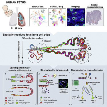
31 | #### [link to the paper](https://www.cell.com/cell/fulltext/S0092-8674(22)01415-5)
32 |
33 |
34 |
--------------------------------------------------------------------------------
/LICENSE:
--------------------------------------------------------------------------------
1 | BSD 2-Clause License
2 |
3 | Copyright (c) 2021, brianpenghe
4 | All rights reserved.
5 |
6 | Redistribution and use in source and binary forms, with or without
7 | modification, are permitted provided that the following conditions are met:
8 |
9 | 1. Redistributions of source code must retain the above copyright notice, this
10 | list of conditions and the following disclaimer.
11 |
12 | 2. Redistributions in binary form must reproduce the above copyright notice,
13 | this list of conditions and the following disclaimer in the documentation
14 | and/or other materials provided with the distribution.
15 |
16 | THIS SOFTWARE IS PROVIDED BY THE COPYRIGHT HOLDERS AND CONTRIBUTORS "AS IS"
17 | AND ANY EXPRESS OR IMPLIED WARRANTIES, INCLUDING, BUT NOT LIMITED TO, THE
18 | IMPLIED WARRANTIES OF MERCHANTABILITY AND FITNESS FOR A PARTICULAR PURPOSE ARE
19 | DISCLAIMED. IN NO EVENT SHALL THE COPYRIGHT HOLDER OR CONTRIBUTORS BE LIABLE
20 | FOR ANY DIRECT, INDIRECT, INCIDENTAL, SPECIAL, EXEMPLARY, OR CONSEQUENTIAL
21 | DAMAGES (INCLUDING, BUT NOT LIMITED TO, PROCUREMENT OF SUBSTITUTE GOODS OR
22 | SERVICES; LOSS OF USE, DATA, OR PROFITS; OR BUSINESS INTERRUPTION) HOWEVER
23 | CAUSED AND ON ANY THEORY OF LIABILITY, WHETHER IN CONTRACT, STRICT LIABILITY,
24 | OR TORT (INCLUDING NEGLIGENCE OR OTHERWISE) ARISING IN ANY WAY OUT OF THE USE
25 | OF THIS SOFTWARE, EVEN IF ADVISED OF THE POSSIBILITY OF SUCH DAMAGE.
26 |
--------------------------------------------------------------------------------
/Pythonplus.py:
--------------------------------------------------------------------------------
1 | import inspect
2 |
3 | def CheckSource(Function2Check):
4 | print( "".join(inspect.getsourcelines(Function2Check)[0]))
5 |
--------------------------------------------------------------------------------
/README.md:
--------------------------------------------------------------------------------
1 | # ⚠️⚠️Repo MOVED to [HERE](https://github.com/Peng-He-Lab/ScanpyPlus) ⚠️⚠️!
2 | # ⚠️⚠️Updated Folder [HERE](https://github.com/Peng-He-Lab/ScanpyPlus)⚠️⚠️!
3 | # ⚠️⚠️Newer version [HERE](https://github.com/Peng-He-Lab/ScanpyPlus) ⚠️⚠️!
4 |
5 | # python-genomics
6 | A set of files to do genomics analysis in python
7 |
8 | To use any of these script collections, just run these two lines in your *python kernel / Jupyter notebook*:
9 | ```
10 | sys.path.append('/home/ubuntu/tools/python-genomics')
11 | import Scanpyplus
12 | ```
13 | ## Citation:
14 | [He, Lim and Sun et al.](https://www.cell.com/cell/fulltext/S0092-8674(22)01415-5)
15 | A human fetal lung cell atlas uncovers proximal-distal gradients of differentiation and key regulators of epithelial fates
16 |
17 | ## DeepTree feature selection
18 | 
19 |
20 |
21 | Among the functions in *Scanpyplus*, there's also a function to do feature gene selection (*DeepTree* algorithm). It removes garbage among highly variable genes, mitigate batch effect if you remove garbage batch by batch, and increases signal-to-noise ratio of the top PCs to promote rare cell type discovery.
22 |
23 | [Here](https://nbviewer.jupyter.org/github/brianpenghe/python-genomics/blob/master/DeepTree_algorithm_demo.ipynb) is a [notebook](https://github.com/brianpenghe/python-genomics/blob/master/DeepTree_algorithm_demo.ipynb) to use DeepTree algorithm to "de-noise" highly-variable genes and improve initial clustering.
24 |
25 | A *MATLAB* implementation can be found [here](https://github.com/brianpenghe/Matlab-genomics).
26 |
27 | This algorithm can be potentially used to reduce batch effect when fearing overcorrection, especially comparing conditions or time points. Two notebooks are provided showing "soft integration" of [fetal limb](https://nbviewer.jupyter.org/github/brianpenghe/python-genomics/blob/master/Soft_integration_limb.ipynb) and [pancreas](https://nbviewer.jupyter.org/github/brianpenghe/python-genomics/blob/master/Soft_integration_pancreas.ipynb) data.
28 |
29 | ## Doublet Cluster Labeling (DouCLing)
30 | 
31 |
32 | There are 4 types of doublets:
33 |
34 | 
35 |
36 | Cross-sample doublets can usually be identified by hastags or genetic backgrounds. Theoretically, (n-1)/n of doublets can be identified as cross-sample doublets when n samples with different hashtags/genetics are pooled equally.
37 |
38 | Heterotypic doublets can sometimes trick data scientists into thinking they are a new type of dual-feature cell type like NKT cells etc.
39 | Heterotypic doublets are usually identified by matching individual cells to synthetic doublets regardless of manually curated clusters. Algorithms like Scrublet can remove a substantial part of doublet cells but not all of them. The survivor doublets can still aggregate into tiny clusters picked up by the annotaters when doing subclustering. Doublets of rarer cell types are also often missed, which obscures the discoveries of new cell types and states.
40 | To leverage the input from biologists' manual parsing and the increased sensitivity of cluster-average signatures, I introduce here an alternative approach to facilitate heterotypic doublet cluster identification. This approach scans through individual tiny clusters and look for its "Parent 2" that gives it a unique feature that's different from its sibling subclusters sharing the same "Parent 1".
41 | [A notebook using published PBMC data](https://nbviewer.jupyter.org/github/brianpenghe/python-genomics/blob/master/DOUblet_Cluster_Labeling.ipynb) is provided.
42 |
43 |
44 | Other functions in Scanpyplus:
45 |
46 | ### An alternative way to call doublet subclusters based on *Scrublet* and [the gastrulation paper](https://www.nature.com/articles/s41586-019-0933-9)
47 | `Bertie(adata,Resln=1,batch_key='batch')` was written with the help from [K. Polanski](https://github.com/ktpolanski). This script aggregates *Scrublet* scores from subclusters and makes threshold cuts based on subcluster p-values. And this is done batch by batch.
48 |
49 | A variant version `Bertie_preclustered` allows users to use user-defined clusters to calculate p-values. This is also done batch by batch.
50 |
51 | ### Manipulating colors:
52 | You can extract the color dict of a variable from an anndata object using `ExtractColor(adata,obsKey='louvain',keytype=int)`,
53 |
54 | and manipulate the color dict using `UpdateUnsColor`.
55 |
56 | You can also cherry pick a value of a variable and make it white using `MakeWhite`.
57 |
58 | ### Manipulating obs (observation) names and metadata:
59 | You can plot sankey graph between two variables of an anndata object using `ScanpySankey`.
60 |
61 | Re-ordering the cluster IDs based on relationship rather than size can be done by `orderGroups`.
62 |
63 | `remove_barcode_suffix` removes the suffix after the '-' in the cell (barcode) name.
64 |
65 | `CopyMeta` copies the metadata (both obs and var) from one object to another.
66 |
67 | `AddMeta` stores a dataframe of obs values per each cell into an object.
68 |
69 | `AddMetaBatch` reads a dataframe of obs values per batch into an object. This format of metadata (rows are batch names, columns are obs categories) is more common, compact and human readable that is usually stored in *Excel* spreadsheets.
70 |
71 | ### Manipulating var (variable) names metadata:
72 | `OrthoTranslate` translates mouse genes to human orthologs and filter out poorly conserved genes, based on ortholog table that can be derived from Biomart etc.
73 |
74 | ### Converting file types:
75 | `file2gz` creates .gz files which is useful for creating artificial 10X files.
76 |
77 | `Scanpy2MM` saves an *anndata* into *MatrixMarket* form.
78 |
79 | `mtx2df` reads *MatrixMarket* files into a dataframe.
80 |
81 | ### Manipulating matrix:
82 | Transfer the raw layer to the default layer by `GetRaw` and calculate integer raw counts based on `n_counts`
83 |
84 | and log-transformed counts using `CalculateRaw`.
85 |
86 | For large matrices, cells can be `DownSample`d based on labels such as cell types.
87 |
88 | Sometimes `PseudoBulk` profiles are also useful to generate, whether it's the mean, median or max.
89 |
90 | ### Manipulating obsm embedding coordinates:
91 | `ShiftEmbedding` creates a platter that juxtaposes subsets of the data (batches, stages etc.) to visualize side by side.
92 |
93 | `CopyEmbedding` copies the embedding of one object to another.
94 |
95 | ### Plotting stacked barplots of cell-type/condition proportions:
96 | `celltype_per_stage_plot` and `stage_per_celltype_plot` plot horizontal and vertical bar plots respectively based on two metadata variables (cell type and stage, for example).
97 |
98 | ### Plot 3D UMAP:
99 | `Plot3DimUMAP` generates a 3D plot (by *plotly*) of the UMAP after sc.tl.umap produces the 3D coordinates.
100 |
101 |
102 | ### Gene-level calculation and plotting:
103 | `DEmarkers` calculates, filteres and plots differentially expressed genes between two populations.
104 |
105 | `GlobalMarkers` calculates marker genes for every cell cluster and filters them.
106 |
107 | `ClusterGenes` transposes a log-transformed *adata* object and performs clustering and dimension reduction to classify genes.
108 |
109 | `Dotplot2D` plots the expression levels of a gene across two metadata categories (e.g. samples and cell types). It can be used to trace maternal contimation by plotting XIST and check a key gene's expression patterns against cell types and age etc.
110 |
111 | ### Plotting Seaborn plots:
112 | `snsSplitViolin` plots splitviolin plots for two populations.
113 |
114 | `snsCluster` plots clustermaps using an *anndata object* as input. This has been helped by Bao Zhang from [Zhang lab](https://github.com/ZhangHongbo-Lab)
115 |
116 | `markSeaborn` marks specific genes on a *Seaborn* plot.
117 |
118 | `extractSeabornRows` extracts the rowlabels of a *Seaborn object* and saves into a *Series*.
119 |
120 | ### Plotting Venn diagram:
121 | `Venn_Upset` can be used to directly plot upset plots (bar plots of each category of intersections).
122 |
123 | ### Label transfer:
124 | `LogisticRegressionCellType` can learn the defining features of a variable (such as cell type) of the reference object and predict the corresponding labels of a query object.
125 |
126 | The saved model files and also be re-used to predict a new query object in future by `LogisticPrediction`.
127 |
128 |
129 |
130 | Functions in pandasPlus:
131 |
132 | `DF2Ann` converts a dataframe into an *anndata* object.
133 |
134 | `UpSetFromLists` plots an upset plot (barplot of Venn diagram intersections) based on lists of lists.
135 |
136 | `show_graph_with_labels` plots an interaction graph using edges to represent connection strength (max at 1, at least 0.9 to be shown).
137 |
138 | Dataframe values can also be used to calculate `zscore` and `Ginni` coefficients.
139 |
140 | `cellphonedb_n_interaction_Mat` and `cellphonedb_mat_per_interaction` are useful to reformat cellphonedb outputs.
141 |
142 |
--------------------------------------------------------------------------------
/Scanpyplus.py:
--------------------------------------------------------------------------------
1 | import gc
2 | #import scrublet as scr
3 | import scipy.io
4 | from scipy import sparse
5 | import matplotlib.pyplot as plt
6 | from matplotlib import rcParams
7 | import seaborn as sns
8 | import numpy as np
9 | import random
10 | import sys
11 | from sklearn.manifold import TSNE
12 | from sklearn.preprocessing import scale
13 | from sklearn.decomposition import TruncatedSVD
14 | from sklearn.cluster import SpectralClustering
15 | from sklearn.model_selection import cross_val_score, StratifiedKFold
16 | from sklearn.linear_model import LogisticRegression
17 | from sklearn.feature_extraction.text import TfidfTransformer
18 | import joblib
19 |
20 | import numpy as np
21 | import pandas as pd
22 | import scanpy as sc
23 | import anndata
24 | import os
25 | from scipy import sparse
26 | from scipy import cluster
27 | from glob import iglob
28 | import gzip
29 |
30 | def ExtractColor(adata,obsKey='louvain',keytype=int):
31 | # labels=sorted(adata.obs[obsKey].unique().to_list(),key=keytype)
32 | labels=adata.obs[obsKey].cat.categories
33 | colors=adata.uns[obsKey+'_colors']
34 | return dict(zip(labels,colors))
35 |
36 | def UpdateUnsColor(adata,ColorDict,obsKey='louvain'):
37 | #ColorDict is like {'Secretory 3 C1': '#c0c0c5','Secretory 4 C1': '#87ceee'}
38 | ColorUns=ExtractColor(adata,obsKey,keytype=str)
39 | ColorUns.update(ColorDict)
40 | adata.uns[obsKey+'_colors']=list(ColorUns.values())
41 | return adata
42 |
43 | def Plot3DimUMAP(adata,obsKey='leiden',obsmKey='X_umap'):
44 | #Make sure adata.obsm['X_umap'] contains three columns
45 | #The obsKey must points to a str/categorical variable
46 | import plotly.express as px
47 | ThreeDdata=pd.DataFrame(adata.obsm[obsmKey],index=adata.obs_names,columns=['x','y','z'])
48 | ThreeDdata[obsKey]=adata.obs[obsKey]
49 | fig=px.scatter_3d(ThreeDdata,x='x',y='y',z='z',color=obsKey,opacity=1,
50 | color_discrete_map=ExtractColor(adata,obsKey,str))
51 | fig.update_traces(marker=dict(size=2,
52 | line=dict(width=0,
53 | color='black')))
54 | return fig
55 |
56 | def ScanpySankey(adata,var1,var2,aspect=20,
57 | fontsize=12, figureName="cell type", leftLabels=['Default'],
58 | rightLabels=['Default']):
59 | from pysankey import sankey
60 | colordict={**ExtractColor(adata,var1,str),
61 | **ExtractColor(adata,var2,str)}
62 | if 'Default' in leftLabels:
63 | leftLabels=sorted(adata.obs[var1].unique().tolist())
64 | if 'Default' in rightLabels:
65 | rightLabels=sorted(adata.obs[var2].unique().tolist())
66 | return sankey(adata.obs[var1],adata.obs[var2],aspect=aspect,colorDict=colordict,
67 | fontsize=fontsize,figureName=figureName,leftLabels=leftLabels,rightLabels=rightLabels)
68 |
69 | def iRODS_stats_starsolo(samples):
70 | #samples should be a list of library IDs
71 | qc = pd.DataFrame(0, index=samples, columns=['n_cells', 'median_n_counts'])
72 | for sample in samples:
73 | #download and import data
74 | os.system('iget -Kr /archive/HCA/10X/'+sample+'/starsolo/counts/Gene/cr3')
75 | adata = sc.read_10x_mtx('cr3')
76 | #this gets .obs['n_counts'] computed
77 | sc.pp.filter_cells(adata, min_counts=1)
78 | #compute the qc metrics and store them
79 | qc.loc[sample, 'n_cells'] = adata.shape[0]
80 | qc.loc[sample, 'median_n_counts'] = np.median(adata.obs['n_counts']).astype(float)
81 | #delete downloaded count matrix
82 | os.system('rm -r cr3')
83 | return qc
84 |
85 | def orderGroups(adata,groupby='leiden'):
86 | #this returns a list of group names
87 | sc.tl.dendrogram(adata,groupby=groupby)
88 | return adata.uns[f'dendrogram_'+groupby]['dendrogram_info']['ivl']
89 |
90 | def MakeWhite(adata,obsKey='louvain',whiteCat='nan',type=str):
91 | temp=ExtractColor(adata,obsKey,type)
92 | temp[whiteCat]='#FFFFFF'
93 | UpdateUnsColor(adata,temp,obsKey)
94 | return adata
95 |
96 | def GetRaw(adata_all):
97 | adata=anndata.AnnData(X=adata_all.raw.X,obs=adata_all.obs,var=adata_all.raw.var,\
98 | obsm=adata_all.obsm,uns=adata_all.uns,obsp=adata_all.obsp)
99 | adata.raw=adata
100 | return adata
101 |
102 | def CalculateRaw(adata,scaling_factor=10000):
103 | #update by Polanski in Feb 2022
104 | #The object must contain a log-transformed matrix
105 | #This function returns an integer-count object
106 | #The normalization constant is assumed to be 10000
107 | #return anndata.AnnData(X=sparse.csr_matrix(np.rint(np.array(np.expm1(adata.X).todense().transpose())*(adata.obs['n_counts'].values).transpose() / scaling_factor).transpose()),\
108 | # obs=adata.obs,var=adata.var,obsm=adata.obsm,varm=adata.varm)
109 | adata.X=adata.X.tocsr() #this step makes sure the datamatrix is in csr not csc
110 | X = np.expm1(adata.X)
111 | scaling_vector = adata.obs['n_counts'].values / scaling_factor
112 | #.indptr[i]:.indptr[i+1] provides the .data coordinates where the i'th row of the data resides in CSR
113 | #which happens to be a cell, which happens to be what we have a unique entry in scaling_vector for
114 | for i in np.arange(X.shape[0]):
115 | X.data[X.indptr[i]:X.indptr[i+1]] = X.data[X.indptr[i]:X.indptr[i+1]] * scaling_vector[i]
116 | return anndata.AnnData(X=np.rint(X),obs=adata.obs,var=adata.var,obsm=adata.obsm,varm=adata.varm)
117 |
118 |
119 | def CalculateRawAuto(adata):
120 | X = np.expm1(adata.X)
121 | #.indptr[i]:.indptr[i+1] provides the .data coordinates where the i'th row of the data resides in CSR
122 | #which happens to be a cell, which happens to be what we need to reverse
123 | for i in np.arange(X.shape[0]):
124 | #the object is cursed, locate lowest count for each cell. treat that as 1
125 | #divide other counts by it. don't round for post-fact checks
126 | norm_one = np.min(X.data[X.indptr[i]:X.indptr[i+1]])
127 | X.data[X.indptr[i]:X.indptr[i+1]] = X.data[X.indptr[i]:X.indptr[i+1]] / norm_one
128 | #originally this had X=np.rint(X) but we actually want the full value space here
129 | return anndata.AnnData(X=X,obs=adata.obs,var=adata.var,obsm=adata.obsm,varm=adata.varm)
130 |
131 | def CheckGAPDH(adata,sparse=True,gene='GAPDH'):
132 | if sparse==True:
133 | return adata[:,gene].X[0:5].todense()
134 | else:
135 | return adata[:,gene].X[0:5]
136 |
137 | def FindSimilarGenes(adata,genename='GAPDH'):
138 | #This function finds the most correlated genes for a given gene
139 | temp=adata.to_df()
140 | corr_temp=np.corrcoef(temp,rowvar=False)
141 | corr_temp_series=pd.Series(corr_temp[:,temp.columns.get_loc(genename)],
142 | index=temp.columns)
143 | return corr_temp_series.sort_values(ascending=False)
144 |
145 | def OrthoTranslate(adata,\
146 | oTable='~/refseq/Mouse-Human_orthologs_only.csv'):
147 | adata.var_names_make_unique(join='-')
148 | OrthologTable = pd.read_csv(oTable).dropna()
149 | MouseGenes=OrthologTable.loc[:,'Gene name'].drop_duplicates(keep=False)
150 | HumanGenes=OrthologTable.loc[:,'Human gene name'].drop_duplicates(keep=False)
151 | FilteredTable=OrthologTable.loc[((OrthologTable.loc[:,'Gene name'].isin(MouseGenes)) &\
152 | (OrthologTable.loc[:,'Human gene name'].isin(HumanGenes))),:]
153 | bdata=adata[:,adata.var_names.isin(FilteredTable.loc[:,'Gene name'])]
154 | FilteredTable.set_index('Gene name',inplace=True,drop=False)
155 | bdata.var_names=FilteredTable.loc[bdata.var_names,'Human gene name']
156 | return bdata
157 |
158 | def remove_barcode_suffix(adata):
159 | bdata=adata.copy()
160 | bdata.obs_names=pd.Index([i[0] for i in bdata.obs_names.str.split('-',expand=True)])
161 | return bdata
162 |
163 | def file2gz(file,delete_original=True):
164 | with open(file,'rb') as src, gzip.open(file+'.gz','wb') as dst:
165 | dst.writelines(src)
166 | if delete_original==True:
167 | os.remove(file)
168 |
169 | def Scanpy2MM(adata,prefix='temp',write2Dobsm=['No']):
170 | #Scanpy2MM(adata,"./")
171 | #please make sure the object contains raw counts (using our CalculateRaw function)
172 | adata.var['feature_types']='Gene Expression'
173 | scipy.io.mmwrite(prefix+'matrix.mtx',adata.X.transpose(),field='integer')
174 | if 'gene_ids' not in adata.var.columns.unique():
175 | adata.var['gene_ids']=adata.var_names
176 | adata.var[['gene_ids','feature_types']].reset_index().set_index(keys='gene_ids').to_csv(prefix+"features.tsv", \
177 | sep = "\t", index= True,header=False)
178 | if 'No' in write2Dobsm:
179 | print('No embeddings written')
180 | else:
181 | for basis in write2Dobsm: #save embeddings in obs
182 | adata.obs[basis+'_x']=adata.obsm[basis][:,0]
183 | adata.obs[basis+'_y']=adata.obsm[basis][:,1]
184 | adata.obs.to_csv(prefix+"barcodes.tsv", sep = "\t", columns=[],header= False)
185 | adata.obs.to_csv(prefix+"metadata.tsv", sep = "\t", index= True)
186 | if 'No' in write2Dobsm:
187 | print('No embeddings written')
188 | else:
189 | for basis in write2Dobsm: #delete obsm->obs
190 | del adata.obs[basis+'_x']
191 | del adata.obs[basis+'_y']
192 | file2gz(prefix+"matrix.mtx")
193 | file2gz(prefix+"barcodes.tsv")
194 | ##file2gz(prefix+"metadata.tsv")
195 | file2gz(prefix+"features.tsv")
196 |
197 | def ShiftEmbedding(adata,domain_key='batch',embedding='X_umap',nrows=3,alpha=0.9):
198 | from sklearn import preprocessing
199 | scaler = preprocessing.MinMaxScaler()
200 | adata.obs[embedding+'0']=adata.obsm[embedding][:,0]
201 | adata.obs[embedding+'1']=adata.obsm[embedding][:,1]
202 | X=adata.obs[embedding+'0']
203 | Y=adata.obs[embedding+'1']
204 | batch_categories=adata.obs[domain_key].unique()
205 | for i in list(range(len(batch_categories))):
206 | temp=adata[adata.obs[domain_key]==batch_categories[i]].obsm[embedding]
207 | scaler.fit(temp)
208 | X.loc[adata.obs[domain_key]==batch_categories[i]]=(scaler.transform(temp)*alpha+ [int(i/nrows),i%nrows])[:,0]
209 | Y.loc[adata.obs[domain_key]==batch_categories[i]]=(scaler.transform(temp)*alpha+ [i/nrows,i%nrows])[:,1]
210 | adata.obsm[embedding]=np.vstack((X.values,Y.values)).T
211 | del adata.obs[embedding+'0']
212 | del adata.obs[embedding+'1']
213 | return adata
214 |
215 | def CopyEmbedding(aFrom,aTo,embedding='X_umap'):
216 | aFrom.obs['temp0']=aFrom.obsm[embedding][:,0]
217 | aFrom.obs['temp1']=aFrom.obsm[embedding][:,1]
218 | aTo.obs['temp0']=''
219 | aTo.obs['temp1']=''
220 | aTo.obs.loc[aFrom.obs_names,'temp0']=aFrom.obs['temp0']
221 | aTo.obs.loc[aFrom.obs_names,'temp1']=aFrom.obs['temp1']
222 | aTo.obsm[embedding]=np.vstack((aTo.obs['temp0'],aTo.obs['temp1'])).T
223 | del aFrom.obs['temp0']
224 | del aFrom.obs['temp1']
225 | del aTo.obs['temp0']
226 | del aTo.obs['temp1']
227 | return aTo
228 |
229 | def CopyMeta(aFro,aTo,overwrite=False):
230 | #This function copies the metadata of one object to another
231 | aFrom=aFro[aFro.obs_names.isin(aTo.obs_names)][:,
232 | aFro.var_names.isin(aTo.var_names)]
233 | aFrom
234 | if overwrite==True:
235 | obs_items=aFrom.obs.columns
236 | var_items=aFrom.var.columns
237 | else:
238 | obs_items=aFrom.obs.columns[~aFrom.obs.columns.isin(aTo.obs.columns)]
239 | var_items=aFrom.var.columns[~aFrom.var.columns.isin(aTo.var.columns)]
240 | aTo.obs[obs_items]=np.nan
241 | aTo.var[var_items]=np.nan
242 | aTo.obs.loc[aFrom.obs_names,obs_items]=aFrom.obs.loc[:,obs_items]
243 | aTo.var.loc[aFrom.var_names,var_items]=aFrom.var.loc[:,var_items]
244 | return aTo
245 |
246 | def AddMeta(adata,meta):
247 | meta_df=meta.loc[meta.index.isin(adata.obs_names),:]
248 | meta_df=meta_df.loc[meta_df.index.drop_duplicates(keep=False),:]
249 | temp=adata.copy()
250 | # temp.obs=temp.obs.combine_first(meta_df) #it has barcode sliding problem!
251 | for i in meta_df.columns:
252 | print("copying "+i+"\n")
253 | temp.obs[i]=np.nan
254 | temp.obs.loc[meta_df.index,i]=meta_df.loc[:,i]
255 | return temp
256 |
257 | def AddMetaBatch(adata,meta_compact,batch_key='batch'):
258 | #import your csv file into a df. The index should be batch IDs
259 | temp=adata.copy()
260 | for i in meta_compact.columns:
261 | temp.obs[i]=temp.obs[batch_key].replace(to_replace=meta_compact.loc[:,i].to_dict())
262 | return temp
263 |
264 | def ExtractMetaBatch(adata,batch_key='batch'):
265 | #return a dataframe of the most frequent value for each variable per batch key
266 | #This can be regarded as the reverse of AddMetaBatch except for numeric variables
267 | return adata.obs.groupby(batch_key).agg(pd.Series.mode)
268 |
269 | def celltype_per_stage_plot(adata,celltypekey='louvain',stagekey='batch',plotlabel=True,\
270 | celltypelist=['default'],stagelist=['default'],celltypekeytype=int,stagekeytype=str,
271 | fontsize='x-small',yfontsize='x-small',legend_pos=(1,0.5),savefig=None):
272 | # this is a function for horizonal bar plots
273 | if 'default' in celltypelist:
274 | celltypelist = sorted(adata.obs[celltypekey].unique().tolist(),key=celltypekeytype)
275 | if 'default' in stagelist:
276 | stagelist = sorted(adata.obs[stagekey].unique().tolist(),key=stagekeytype)
277 | celltypelist=[i for i in celltypelist if i in adata.obs[celltypekey].unique()]
278 | stagelist=[i for i in stagelist if i in adata.obs[stagekey].unique()]
279 | colors=ExtractColor(adata,celltypekey,keytype=str)
280 | count_array=np.array(pd.crosstab(adata.obs[celltypekey],adata.obs[stagekey]).loc[celltypelist,stagelist])
281 | count_ratio_array=count_array / np.sum(count_array,axis=0)
282 | for i in range(len(celltypelist)):
283 | plt.barh(stagelist[::-1],count_ratio_array[i,::-1],
284 | left=np.sum(count_ratio_array[0:i,::-1],axis=0),color=colors[celltypelist[i]],label=celltypelist[i])
285 | plt.yticks(fontsize=yfontsize)
286 | plt.grid(b=False)
287 | if plotlabel:
288 | plt.legend(celltypelist,fontsize=fontsize,bbox_to_anchor=legend_pos)
289 | if savefig is not None:
290 | plt.savefig(savefig+'.pdf',bbox_inches='tight')
291 |
292 | def stage_per_celltype_plot(adata,celltypekey='louvain',stagekey='batch',plotlabel=True,\
293 | # this is a function for vertical bar plots
294 | # please remember to run pl.umap to assign colors
295 | celltypelist=['default'],stagelist=['default'],celltypekeytype=int,stagekeytype=str,
296 | fontsize='x-small',xfontsize='x-small',legend_pos=(1,1),savefig=None):
297 | if 'default' in celltypelist:
298 | celltypelist = sorted(adata.obs[celltypekey].unique().tolist(),key=celltypekeytype)
299 | if 'default' in stagelist:
300 | stagelist = sorted(adata.obs[stagekey].unique().tolist(),key=stagekeytype)
301 | celltypelist=[i for i in celltypelist if i in adata.obs[celltypekey].unique()]
302 | stagelist=[i for i in stagelist if i in adata.obs[stagekey].unique()]
303 | colors=ExtractColor(adata,stagekey,keytype=str)
304 | count_array=np.array(pd.crosstab(adata.obs[celltypekey],adata.obs[stagekey]).loc[celltypelist,stagelist])
305 | count_ratio_array=count_array.transpose() / np.sum(count_array,axis=1)
306 | for i in range(len(stagelist)):
307 | plt.bar(celltypelist,count_ratio_array[i,:],
308 | bottom=1-np.sum(count_ratio_array[0:i+1,:],axis=0),
309 | color=colors[stagelist[i]],label=stagelist[i])
310 | plt.xticks(fontsize=xfontsize)
311 | plt.grid(b=False)
312 | plt.legend(stagelist,fontsize=fontsize,bbox_to_anchor=legend_pos)
313 | plt.xticks(rotation=90)
314 | if savefig is not None:
315 | plt.savefig(savefig+'.pdf',bbox_inches='tight')
316 |
317 | def mtx2df(mtx,idx,col):
318 | #mtx is the name/location of the matrix.mtx file
319 | #idx is the index file (rownames)
320 | #col is the colnames file
321 | count = scipy.io.mmread(mtx)
322 | idxs = [i.strip() for i in open(idx)]
323 | cols = [i.strip() for i in open(col)]
324 | sc_count = pd.DataFrame(data=count.toarray(),
325 | index=idxs,
326 | columns=cols)
327 | return sc_count
328 |
329 | def returnDEres(adata, column = None, key= None, remove_mito_ribo = True):
330 | import functools
331 | if key is None:
332 | key = 'rank_genes_groups'
333 | else:
334 | key = key
335 |
336 | if column is None:
337 | column = list(adata.uns[key]['scores'].dtype.fields.keys())[0]
338 | else:
339 | column = column
340 |
341 | scores = pd.DataFrame(data = adata.uns[key]['scores'][column], index = adata.uns[key]['names'][column])
342 | lfc = pd.DataFrame(data = adata.uns[key]['logfoldchanges'][column], index = adata.uns[key]['names'][column])
343 | pvals = pd.DataFrame(data = adata.uns[key]['pvals'][column], index = adata.uns[key]['names'][column])
344 | padj = pd.DataFrame(data = adata.uns[key]['pvals_adj'][column], index = adata.uns[key]['names'][column])
345 | try:
346 | pts = pd.DataFrame(data = adata.uns[key]['pts'][column], index = adata.uns[key]['names'][column])
347 | except:
348 | pass
349 | scores = scores.loc[scores.index.dropna()]
350 | lfc = lfc.loc[lfc.index.dropna()]
351 | pvals = pvals.loc[pvals.index.dropna()]
352 | padj = padj.loc[padj.index.dropna()]
353 | try:
354 | pts = pts.loc[pts.index.dropna()]
355 | except:
356 | pass
357 | try:
358 | dfs = [scores, lfc, pvals, padj, pts]
359 | except:
360 | dfs = [scores, lfc, pvals, padj]
361 | df_final = functools.reduce(lambda left, right: pd.merge(left, right, left_index = True, right_index = True), dfs)
362 | try:
363 | df_final.columns = ['scores', 'logfoldchanges', 'pvals', 'pvals_adj', 'pts']
364 | except:
365 | df_final.columns = ['scores', 'logfoldchanges', 'pvals', 'pvals_adj']
366 | if remove_mito_ribo:
367 | df_final = df_final[~df_final.index.isin(list(df_final.filter(regex='^RPL|^RPS|^MRPS|^MRPL|^MT-', axis = 0).index))]
368 | df_final = df_final[~df_final.index.isin(list(df_final.filter(regex='^Rpl|^Rps|^Mrps|^Mrpl|^mt-', axis = 0).index))]
369 | return(df_final)
370 |
371 | def DEmarkers(adata,celltype,reference,obs,max_out_group_fraction=0.25,\
372 | use_raw=False,length=100,obslist=['percent_mito','n_genes','batch'],\
373 | min_fold_change=2,min_in_group_fraction=0.25,log=True,method='wilcoxon',
374 | embedding='X_umap'):
375 | celltype=celltype
376 | sc.tl.rank_genes_groups(adata, obs, groups=[celltype],n_genes=length,
377 | reference=reference,method=method,log=log,pts=True)
378 | # temp=returnDEres(adata,key='rank_genes_groups',column=celltype)
379 | sc.tl.filter_rank_genes_groups(adata, groupby=obs,\
380 | max_out_group_fraction=max_out_group_fraction,
381 | min_fold_change=min_fold_change,use_raw=use_raw,
382 | min_in_group_fraction=min_in_group_fraction)
383 | GeneList=pd.DataFrame(adata.uns['rank_genes_groups_filtered']['names']).loc[:,celltype].dropna().head(length).transpose().tolist()
384 | # temp1=pd.concat([temp,
385 | # (adata[:,temp.index][adata.obs[obs]==celltype].to_df()>0).mean(axis=0).rename('pct1'),
386 | # (adata[:,temp.index][adata.obs[obs]==reference].to_df()>0).mean(axis=0).rename('pct2')],
387 | # axis=1)
388 | import math
389 | # GeneList=temp1.loc[(temp1.pvals < 0.05) & (temp1.pct1 >= min_in_group_fraction) & \
390 | #(temp1.logfoldchanges > math.log(min_fold_change)) & (temp1.pct2 <= max_out_group_fraction),:].index.tolist()
391 | sc.pl.embedding(adata,basis=embedding,color=GeneList+obslist,
392 | color_map = 'jet',use_raw=use_raw)
393 | sc.pl.dotplot(adata,var_names=GeneList,
394 | groupby=obs,use_raw=use_raw,standard_scale='var')
395 | sc.pl.stacked_violin(adata[adata.obs[obs].isin([celltype,reference]),:],var_names=GeneList,groupby=obs,
396 | swap_axes=True)
397 | del adata.uns['rank_genes_groups']
398 | del adata.uns['rank_genes_groups_filtered']
399 | return GeneList
400 |
401 | def GlobalMarkers(adata,obs,max_out_group_fraction=0.25,min_fold_change=2,\
402 | min_in_group_fraction=0.25,use_raw=False,method='wilcoxon'):
403 | sc.tl.rank_genes_groups(adata,groupby=obs,n_genes=len(adata.var_names),
404 | method=method)
405 | sc.tl.filter_rank_genes_groups(adata,groupby=obs,
406 | max_out_group_fraction=max_out_group_fraction,
407 | min_fold_change=min_fold_change,use_raw=use_raw,
408 | min_in_group_fraction=min_in_group_fraction)
409 | Markers=pd.DataFrame(adata.uns['rank_genes_groups_filtered']['names'])
410 | return Markers.apply(lambda x: pd.Series(x.dropna().values))
411 |
412 | def HVGbyBatch(adata,batch_key='batch',min_mean=0.0125, max_mean=3, min_disp=0.5,\
413 | min_clustersize=100,genenames=['default']):
414 | if 'default' in genenames:
415 | genenames = adata.var_names
416 | sc.settings.verbosity=0
417 | batchlist=adata.obs[batch_key].value_counts()
418 | for key in batchlist[batchlist>min_clustersize].index:
419 | adata_sample = adata[adata.obs[batch_key]==key,:][:,genenames]
420 | print(key)
421 | sc.pp.highly_variable_genes(adata_sample, min_mean=min_mean, max_mean=max_mean, min_disp=min_disp)
422 | adata.var['highly_variable'+key]=pd.Series(adata.var_names,\
423 | index=adata.var_names).isin(adata_sample.var_names[adata_sample.var['highly_variable']])
424 | sc.settings.verbosity=3
425 | adata.var['highly_variable_n']=0
426 | temp=adata.var['highly_variable_n'].astype('int32')
427 | for key in batchlist[batchlist>min_clustersize].index:
428 | temp=temp+adata.var['highly_variable'+key].astype('int32')
429 | adata.var['highly_variable_n']=temp
430 | return adata
431 |
432 | def HVG_cutoff(adata,range_int=10,cutoff=5000,HVG_var='highly_variable_n',fig_size=(8,6)):
433 | if range_int>max(adata.var[HVG_var]):
434 | range_int=max(adata.var[HVG_var])
435 | HVG_list=[]
436 | for i in list(range(range_int)):
437 | HVG_list.append((adata.var[HVG_var]>i).value_counts()[True])
438 | plt.figure(figsize=fig_size)
439 | plt.plot(list(range(range_int)),HVG_list)
440 | plt.axhline(y=cutoff, color='r', linestyle='--')
441 | HVG_n=next((x for x in reversed(HVG_list) if x >= cutoff), HVG_list[0])
442 | HVG_i=len(HVG_list) - 1 - next((i for i, x in enumerate(reversed(HVG_list)) if x >= cutoff), len(HVG_list)-1)
443 | print("The smallest i for intersection to achieve more than "+str(cutoff)+" HVGs is "+str(HVG_i)+" , yielding "+str(HVG_n)+" genes")
444 | return HVG_i
445 |
446 | def Bertie(adata,Resln=1,batch_key='batch'):
447 | import scrublet as scr
448 | scorenames = ['scrublet_score','scrublet_cluster_score','bh_pval']
449 | adata.obs['doublet_scores']=0
450 | def bh(pvalues):
451 | '''
452 | Computes the Benjamini-Hochberg FDR correction.
453 |
454 | Input:
455 | * pvals - vector of p-values to correct
456 | '''
457 | n = int(pvalues.shape[0])
458 | new_pvalues = np.empty(n)
459 | values = [ (pvalue, i) for i, pvalue in enumerate(pvalues) ]
460 | values.sort()
461 | values.reverse()
462 | new_values = []
463 | for i, vals in enumerate(values):
464 | rank = n - i
465 | pvalue, index = vals
466 | new_values.append((n/rank) * pvalue)
467 | for i in range(0, int(n)-1):
468 | if new_values[i] < new_values[i+1]:
469 | new_values[i+1] = new_values[i]
470 | for i, vals in enumerate(values):
471 | pvalue, index = vals
472 | new_pvalues[index] = new_values[i]
473 | return new_pvalues
474 |
475 | for i in np.unique(adata.obs[batch_key]):
476 | print(i)
477 | adata_sample = adata[adata.obs[batch_key]==i,:]
478 | scrub = scr.Scrublet(adata_sample.X)
479 | doublet_scores, predicted_doublets = scrub.scrub_doublets(verbose=False)
480 | adata_sample.obs['scrublet_score'] = doublet_scores
481 | adata_sample=adata_sample.copy()
482 | sc.pp.filter_genes(adata_sample, min_cells=3)
483 | sc.pp.normalize_per_cell(adata_sample, counts_per_cell_after=1e4)
484 | sc.pp.log1p(adata_sample)
485 | sc.pp.highly_variable_genes(adata_sample, min_mean=0.0125, max_mean=3, min_disp=0.5)
486 | adata_sample = adata_sample[:, adata_sample.var['highly_variable']]
487 | sc.pp.scale(adata_sample, max_value=10)
488 | sc.tl.pca(adata_sample, svd_solver='arpack')
489 | adata_sample = adata_sample.copy()
490 | # del adata_sample.obsm['X_diffmap']
491 | sc.pp.neighbors(adata_sample)
492 | #eoverclustering proper - do basic clustering first, then cluster each cluster
493 | sc.tl.louvain(adata_sample)
494 | for clus in np.unique(adata_sample.obs['louvain']):
495 | sc.tl.louvain(adata_sample, restrict_to=('louvain',[clus]),resolution=Resln)
496 | adata_sample.obs['louvain'] = adata_sample.obs['louvain_R']
497 | #compute the cluster scores - the median of Scrublet scores per overclustered cluster
498 | for clus in np.unique(adata_sample.obs['louvain']):
499 | adata_sample.obs.loc[adata_sample.obs['louvain']==clus, 'scrublet_cluster_score'] = \
500 | np.median(adata_sample.obs.loc[adata_sample.obs['louvain']==clus, 'scrublet_score'])
501 | #now compute doublet p-values. figure out the median and mad (from above-median values) for the distribution
502 | med = np.median(adata_sample.obs['scrublet_cluster_score'])
503 | mask = adata_sample.obs['scrublet_cluster_score']>med
504 | mad = np.median(adata_sample.obs['scrublet_cluster_score'][mask]-med)
505 | #let's do a one-sided test. the Bertie write-up does not address this but it makes sense
506 | pvals = 1-scipy.stats.norm.cdf(adata_sample.obs['scrublet_cluster_score'], loc=med, scale=1.4826*mad)
507 | adata_sample.obs['bh_pval'] = bh(pvals)
508 | #create results data frame for single sample and copy stuff over from the adata object
509 | scrublet_sample = pd.DataFrame(0, index=adata_sample.obs_names, columns=scorenames)
510 | for meta in scorenames:
511 | scrublet_sample[meta] = adata_sample.obs[meta]
512 | #write out complete sample scores
513 | #scrublet_sample.to_csv('scrublet-scores/'+i+'.csv')
514 |
515 | #scrub.plot_histogram();
516 | #plt.savefig('limb/sample_'+i+'_doulet_histogram.pdf')
517 | adata.obs.loc[adata.obs[batch_key]==i,'doublet_scores']=doublet_scores
518 | adata.obs.loc[adata.obs[batch_key]==i,'bh_pval'] = bh(pvals)
519 | del adata_sample
520 | return adata
521 |
522 | def Bertie_preclustered(adata,batch_key='batch',cluster_key='louvain'):
523 | import scrublet as scr
524 | scorenames = ['scrublet_score','scrublet_cluster_score','bh_pval']
525 | adata.obs['doublet_scores']=0
526 | def bh(pvalues):
527 | '''
528 | Computes the Benjamini-Hochberg FDR correction.
529 |
530 | Input:
531 | * pvals - vector of p-values to correct
532 | '''
533 | n = int(pvalues.shape[0])
534 | new_pvalues = np.empty(n)
535 | values = [ (pvalue, i) for i, pvalue in enumerate(pvalues) ]
536 | values.sort()
537 | values.reverse()
538 | new_values = []
539 | for i, vals in enumerate(values):
540 | rank = n - i
541 | pvalue, index = vals
542 | new_values.append((n/rank) * pvalue)
543 | for i in range(0, int(n)-1):
544 | if new_values[i] < new_values[i+1]:
545 | new_values[i+1] = new_values[i]
546 | for i, vals in enumerate(values):
547 | pvalue, index = vals
548 | new_pvalues[index] = new_values[i]
549 | return new_pvalues
550 |
551 | for i in np.unique(adata.obs[batch_key]):
552 | adata_sample = adata[adata.obs[batch_key]==i,:]
553 | scrub = scr.Scrublet(adata_sample.X)
554 | doublet_scores, predicted_doublets = scrub.scrub_doublets(verbose=False)
555 | adata_sample.obs['scrublet_score'] = doublet_scores
556 | adata_sample=adata_sample.copy()
557 |
558 | for clus in np.unique(adata_sample.obs[cluster_key]):
559 | adata_sample.obs.loc[adata_sample.obs[cluster_key]==clus, 'scrublet_cluster_score'] = \
560 | np.median(adata_sample.obs.loc[adata_sample.obs[cluster_key]==clus, 'scrublet_score'])
561 |
562 | med = np.median(adata_sample.obs['scrublet_cluster_score'])
563 | mask = adata_sample.obs['scrublet_cluster_score']>med
564 | mad = np.median(adata_sample.obs['scrublet_cluster_score'][mask]-med)
565 | #let's do a one-sided test. the Bertie write-up does not address this but it makes sense
566 | pvals = 1-scipy.stats.norm.cdf(adata_sample.obs['scrublet_cluster_score'], loc=med, scale=1.4826*mad)
567 | adata_sample.obs['bh_pval'] = bh(pvals)
568 | #create results data frame for single sample and copy stuff over from the adata object
569 | scrublet_sample = pd.DataFrame(0, index=adata_sample.obs_names, columns=scorenames)
570 | for meta in scorenames:
571 | scrublet_sample[meta] = adata_sample.obs[meta]
572 | #write out complete sample scores
573 | #scrublet_sample.to_csv('scrublet-scores/'+i+'.csv')
574 |
575 | #scrub.plot_histogram();
576 | #plt.savefig('limb/sample_'+i+'_doulet_histogram.pdf')
577 | adata.obs.loc[adata.obs[batch_key]==i,'doublet_scores']=doublet_scores
578 | adata.obs.loc[adata.obs[batch_key]==i,'bh_pval'] = bh(pvals)
579 | del adata_sample
580 | return adata
581 |
582 |
583 | def snsSplitViolin(adata,genelist,celltype='leiden',celltypelist=['0','1']):
584 | df=sc.get.obs_df(adata[adata.obs[celltype].isin(celltypelist)],genelist+[celltype])
585 | df = df.set_index(celltype).stack().reset_index()
586 | df.columns=[celltype,'gene','value']
587 | sns.violinplot(data=df, x='gene', y='value', hue=celltype,
588 | split=True, inner="quart", linewidth=1)
589 |
590 | def DownSample(MouseC1data,cell_type='leiden',downsampleTo=10):
591 | NewIndex3=[]
592 | if ( downsampleTo > 0 ) & (isinstance(downsampleTo, int)):
593 | for i in MouseC1data.obs[cell_type].sort_values().unique():
594 | NewIndex3=NewIndex3+random.sample(\
595 | population=MouseC1data[MouseC1data.obs[cell_type]==i].obs_names.tolist(),
596 | k=min(downsampleTo,len(MouseC1data[MouseC1data.obs[cell_type]==i\
597 | ].obs_names.tolist())))
598 | return MouseC1data[NewIndex3]
599 |
600 | def snsCluster(MouseC1data,MouseC1ColorDict2={False:'#000000',True:'#00FFFF'},cell_type='louvain',gene_type='highly_variable',\
601 | cellnames=['default'],genenames=['default'],figsize=(10,7),row_cluster=False,col_cluster=False,\
602 | robust=True,xticklabels=False,yticklabels=False,method='complete',metric='correlation',cmap='jet',\
603 | downsampleTo=0):
604 | if 'default' in cellnames:
605 | cellnames = MouseC1data.obs_names
606 | if ( downsampleTo > 0 ) & (isinstance(downsampleTo, int)):
607 | cellnames = DownSample(MouseC1data,cell_type,downsampleTo).obs_names
608 | if 'default' in genenames:
609 | genenames = MouseC1data.var_names
610 | genenames = [i for i in genenames if i in MouseC1data.var_names]
611 | cellnames = [i for i in cellnames if i in MouseC1data.obs_names]
612 | cell_types=cell_type
613 | gene_types=gene_type
614 | if type(cell_type) == str:
615 | cell_types=[cell_type]
616 | if type(gene_type) == str:
617 | gene_types=[gene_type]
618 | louvain_col_colors=[]
619 | for key in cell_types:
620 | MouseC1data_df = MouseC1data[MouseC1data.obs_names][:,genenames].to_df()
621 | MouseC1data_df[key] = MouseC1data[MouseC1data.obs_names].obs[key]
622 | MouseC1data_df = MouseC1data_df.sort_values(by=key)
623 | MouseC1data_df3 = MouseC1data_df.loc[pd.Series(cellnames,index=cellnames).index,:]
624 | cluster_names=MouseC1data_df3.pop(key)
625 | louvain_col_colors.append(cluster_names.map(ExtractColor(MouseC1data,obsKey=key,keytype=str)).astype(str))
626 | adata_for_plotting = MouseC1data_df.loc[cellnames,MouseC1data_df.columns.isin(genenames)]
627 | adata_for_plotting = adata_for_plotting.reindex(columns=genenames)
628 | if len(louvain_col_colors) > 1:
629 | louvain_col_colors=pd.concat(louvain_col_colors,axis=1)
630 | else:
631 | louvain_col_colors=louvain_col_colors[0]
632 | if 'null' in gene_types:
633 | cg1_0point2=sns.clustermap(adata_for_plotting.transpose(),metric=metric,cmap=cmap,\
634 | figsize=figsize,row_cluster=row_cluster,col_cluster=col_cluster,robust=robust,xticklabels=xticklabels,\
635 | yticklabels=yticklabels,z_score=0,vmin=-2.5,vmax=2.5,col_colors=louvain_col_colors,method=method)
636 | else:
637 | celltype_row_colors=[]
638 | for key in gene_types:
639 | genegroup_names=MouseC1data[:,genenames].var[key]
640 | celltype_row_colors.append(genegroup_names.map(MouseC1ColorDict2).astype(str))
641 | if len(celltype_row_colors) > 1:
642 | celltype_row_colors=pd.concat(celltype_row_colors,axis=1)
643 | else:
644 | celltype_row_colors=celltype_row_colors[0]
645 | cg1_0point2=sns.clustermap(adata_for_plotting.transpose(),metric=metric,cmap=cmap,\
646 | figsize=figsize,row_cluster=row_cluster,col_cluster=col_cluster,robust=robust,xticklabels=xticklabels,\
647 | yticklabels=yticklabels,z_score=0,vmin=-2.5,vmax=2.5,col_colors=louvain_col_colors,row_colors=celltype_row_colors,method=method)
648 |
649 | return cg1_0point2
650 |
651 | def extractSeabornRows(snsObj):
652 | #This function returns a Series containing row labels
653 | NewIndex=pd.DataFrame(np.asarray([snsObj.data.index[i] for i in snsObj.dendrogram_row.reordered_ind])).iloc[:,0]
654 | return NewIndex
655 |
656 | def markSeaborn(snsObj,genes,clustermap=True):
657 | if clustermap == True:
658 | NewIndex=pd.DataFrame(np.asarray([snsObj.data.index[i] for i in snsObj.dendrogram_row.reordered_ind])).iloc[:,0]
659 | NewIndex2=NewIndex.isin(genes)
660 | snsObj.ax_heatmap.set_yticks(NewIndex[NewIndex2].index.values.tolist())
661 | snsObj.ax_heatmap.set_yticklabels(NewIndex[NewIndex2].values.tolist())
662 | else:
663 | NewIndex=pd.DataFrame(np.asarray(snsObj.data.index))
664 | NewIndex2=snsObj.data.index.isin(genes)
665 | snsObj.ax_heatmap.set_yticks(NewIndex[NewIndex2].index.values)
666 | snsObj.ax_heatmap.set_yticklabels(NewIndex[NewIndex2].values[:,0])
667 | #snsObj.fig
668 | return snsObj.fig
669 |
670 | def PseudoBulk(adata, group_key, layer=None, gene_symbols=None):
671 | #This function was written by ivirshup
672 | #https://github.com/scverse/scanpy/issues/181#issuecomment-534867254
673 | if layer is not None:
674 | getX = lambda x: x.layers[layer]
675 | else:
676 | getX = lambda x: x.X
677 | if gene_symbols is not None:
678 | new_idx = adata.var[idx]
679 | else:
680 | new_idx = adata.var_names
681 |
682 | grouped = adata.obs.groupby(group_key)
683 | out = pd.DataFrame(
684 | np.zeros((adata.shape[1], len(grouped)), dtype=np.float64),
685 | columns=list(grouped.groups.keys()),
686 | index=adata.var_names
687 | )
688 |
689 | for group, idx in grouped.indices.items():
690 | X = getX(adata[idx])
691 | out[group] = np.ravel(X.mean(axis=0, dtype=np.float64))
692 | return out
693 |
694 | def Dotplot2D(adata,obs1,obs2,gene,cmap='OrRd', min_count=1):
695 | #This function was modified from K Polanski's codes. It can plot a gene such as XIST across samples and cell types
696 | #require at least these many cells in a batch+celltype intersection to process it
697 |
698 | #extract a simpler form of all the needed data - the gene's expression and the two obs columns
699 | #this way things run way quicker downstream
700 | expression = np.array(adata[:,gene].X)
701 | batches = adata.obs[obs1].values
702 | celltypes = adata.obs[obs2].values
703 |
704 | dot_size_df = pd.DataFrame(0.0, index=np.unique(batches), columns=np.unique(celltypes))
705 | dot_color_df = pd.DataFrame(0.0, index=np.unique(batches), columns=np.unique(celltypes))
706 |
707 | for batch in np.unique(batches):
708 | mask_batch = (batches == batch)
709 | for celltype in np.unique(celltypes):
710 | mask_celltype = (celltypes == celltype)
711 | #skip if there's not enough data for spot
712 | if np.sum(mask_batch & mask_celltype) >= min_count:
713 | sub = expression[mask_batch & mask_celltype]
714 | #color is mean expression
715 | dot_color_df.loc[batch, celltype] = np.mean(sub)
716 | #fraction expressed can be easily computed
717 | #by making all expressed cells be 1, and then doing a mean again
718 | sub[sub>0] = 1
719 | dot_size_df.loc[batch, celltype] = np.mean(sub)
720 |
721 | #reduce dimensions - no need for all-zero rows/cols
722 | dot_size_df = dot_size_df.loc[(dot_size_df.sum(axis=1) != 0), (dot_size_df.sum(axis=0) != 0)]
723 | dot_color_df = dot_color_df.loc[(dot_color_df.sum(axis=1) != 0), (dot_color_df.sum(axis=0) != 0)]
724 |
725 | import anndata
726 | from scanpy.pl import DotPlot
727 |
728 | bdata = anndata.AnnData(np.zeros(dot_size_df.shape))
729 | bdata.var_names = dot_size_df.columns
730 | bdata.obs_names = list(dot_size_df.index)
731 | bdata.obs[obs1] = dot_size_df.index
732 | bdp = DotPlot(bdata, dot_size_df.columns, obs1, dot_size_df=dot_size_df, dot_color_df=dot_color_df)
733 | bdp = bdp.style(cmap=cmap)
734 | bdp.make_figure()
735 |
736 |
737 | def DeepTree(adata,MouseC1ColorDict2,cell_type='louvain',gene_type='highly_variable',\
738 | cellnames=['default'],genenames=['default'],figsize=(10,7),row_cluster=True,col_cluster=True,\
739 | method='complete',metric='correlation',Cutoff=0.8,CladeSize=2):
740 | if 'default' in cellnames:
741 | cellnames = adata.obs_names
742 | if 'default' in genenames:
743 | genenames = adata.var_names
744 | test=snsCluster(adata,\
745 | MouseC1ColorDict2=MouseC1ColorDict2,\
746 | genenames=genenames, cellnames=cellnames,\
747 | gene_type=gene_type, cell_type=cell_type,method=method,\
748 | figsize=figsize,row_cluster=row_cluster,col_cluster=col_cluster,metric=metric)
749 | cutree = cluster.hierarchy.cut_tree(test.dendrogram_row.linkage,height=Cutoff)
750 | TreeDict=dict(zip(*np.unique(cutree, return_counts=True)))
751 | TreeDF=pd.DataFrame(TreeDict,index=[0])
752 | DeepIndex=[i in TreeDF.loc[:,TreeDF.iloc[0,:] > CladeSize].columns.values for i in cutree]
753 | bdata=adata[:,test.data.index][cellnames]
754 | bdata.var['Deep']=DeepIndex
755 | test1=snsCluster(bdata,\
756 | MouseC1ColorDict2=MouseC1ColorDict2,\
757 | cellnames=cellnames,gene_type='Deep',cell_type=cell_type,method=method,\
758 | figsize=figsize,row_cluster=True,col_cluster=True,metric=metric)
759 | test2=snsCluster(bdata[:,DeepIndex],\
760 | MouseC1ColorDict2=MouseC1ColorDict2,\
761 | cellnames=cellnames,gene_type='null',cell_type=cell_type,method=method,\
762 | figsize=figsize,row_cluster=True,col_cluster=True,metric=metric)
763 | return [bdata,test,test1,test2]
764 |
765 | def DeepTree_per_batch(adata,batch_key='batch',obslist=['batch'],min_clustersize=100,Cutoff=0.8,CladeSize=2):
766 | batchlist=adata.obs[batch_key].value_counts()
767 | for key in batchlist[batchlist>min_clustersize].index:
768 | print(key)
769 | bdata=adata[:,adata.var['highly_variable'+key]][adata.obs[batch_key]==key,:]
770 | sc.pp.filter_genes(bdata,min_cells=3)
771 | sc.pl.umap(bdata,color=obslist)
772 | [bdata,test, test1, test2]=DeepTree(bdata,
773 | MouseC1ColorDict2={False:'#000000',True:'#00FFFF'},
774 | cell_type=obslist,
775 | cellnames=adata[adata.obs[batch_key]==key,:].obs_names.tolist(),
776 | genenames=adata[:,adata.var['highly_variable'+key]].var_names.tolist(),
777 | row_cluster=True,col_cluster=True,Cutoff=Cutoff,CladeSize=CladeSize)
778 | adata.var['Deep_'+key]=pd.Series(adata.var_names,index=adata.var_names).isin((bdata)[:,bdata.var['Deep']].var_names)
779 | # sc.pl.umap(adata,color=obslist)
780 | adata.var['Deep_n']=0
781 | temp=adata.var['Deep_n'].astype('int32')
782 | for key in batchlist[batchlist>min_clustersize].index:
783 | temp=temp+adata.var['Deep_'+key].astype('int32')
784 | adata.var['Deep_n']=temp
785 | return adata
786 |
787 | def Venn_Upset(adata,genelists,size_height=3):
788 | from upsetplot import UpSet
789 | from upsetplot import plot
790 | #gene lists can be ['Deep_1','Deep_2']
791 | deepgenes=pd.DataFrame(adata.var[genelists+['highly_variable']])
792 | deepgenes=deepgenes.set_index(genelists)
793 | upset = UpSet(deepgenes, subset_size='count', intersection_plot_elements=size_height)
794 | upset.plot()
795 | return upset
796 |
797 | def Treemap(adata,output="temp",branchlist=['project','batch'],width=1000,height=700,title='title'):
798 | import pandas as pd
799 | import numpy as np
800 | temp=adata.obs.groupby(by=branchlist).size()
801 | temp=temp[temp>0]
802 | import plotly.express as px
803 | fig = px.treemap(temp.reset_index(),
804 | path=branchlist,values=0)
805 | fig.update_layout(title=title,
806 | width=width, height=height)
807 | fig.write_image(output+'.pdf')
808 | temp.to_csv(output+'.csv')
809 | return fig
810 |
811 | def DeepTree2(adata,method='complete',metric='correlation',cellnames=['default'],genenames=['default'],\
812 | Cutoff=0.8,CladeSize=2):
813 | if 'default' in cellnames:
814 | cellnames = adata.obs_names
815 | if 'default' in genenames:
816 | genenames = adata.var_names
817 | adata_df=adata[cellnames,:][:,genenames].to_df()
818 | testscipy=scipy.cluster.hierarchy.fclusterdata(adata_df.transpose(),\
819 | metric=metric,method=method,t=Cutoff,criterion="distance")
820 | TreeDict=dict(zip(*np.unique(testscipy, return_counts=True)))
821 | TreeDF=pd.DataFrame(TreeDict,index=[0])
822 | DeepIndex=[i in TreeDF.loc[:,TreeDF.iloc[0,:] > CladeSize].columns.values for i in testscipy]
823 | bdata=adata[cellnames,:][:,genenames]
824 | bdata.var['Deep']=DeepIndex
825 | return bdata
826 |
827 | def LoadLogitModel(model_addr):
828 | import joblib
829 | lr = joblib.load(open(model_addr,'rb'))
830 | return lr
831 |
832 | def LoadLogitGenes(genecsv):
833 | CT_genes=pd.read_csv(genecsv,header=None)
834 | CT_genes['idx'] = CT_genes.index
835 | CT_genes.columns = ['symbol', 'idx']
836 | CT_genes = np.array(CT_genes['symbol'])
837 | return CT_genes
838 |
839 | def ExtractLogitScores(adata,model,CT_genes):
840 | P=model.predict_proba(adata[:,CT_genes].X)
841 | df=pd.DataFrame(P,index=adata.obs_names,columns=model.classes_+'_prob')
842 | df['lr_score']=df.max(axis=1)
843 | return df
844 |
845 | def Model2Coeff(model_pkl,genelistcsv):
846 | lr = LoadLogitModel(model_pkl)
847 | CT_genes = LoadLogitGenes(genelistcsv)
848 | return pd.DataFrame(lr.coef_,columns=CT_genes,index=lr.classes_)
849 |
850 | from datetime import date
851 | def LogisticRegressionCellType(Reference, Query, Category = 'louvain', DoValidate = False,\
852 | multi_class='ovr',n_jobs=15,max_iter=1000,tol=1e-4,keyword=''):
853 | #This function doesn't do normalization or scaling
854 | #The logistic regression function returns the updated Query object with predicted info stored
855 | Reference.var_names_make_unique()
856 | Query.var_names_make_unique()
857 | IntersectGenes = np.intersect1d(Reference.var_names,Query.var_names)
858 | Reference2 = Reference[:,IntersectGenes]
859 | Query2 = Query[:,IntersectGenes]
860 | X = Reference2.X
861 | y = Reference2.obs[Category].replace(np.nan,'None',regex=True)
862 | x = Query2.X
863 | cv = StratifiedKFold(n_splits=5, random_state=None, shuffle=False)
864 | logit = LogisticRegression(penalty='l2',
865 | random_state=42,
866 | C=0.2,
867 | tol=tol,
868 | n_jobs=n_jobs,
869 | solver='sag',
870 | multi_class=multi_class,
871 | max_iter=max_iter,
872 | verbose=10
873 | )
874 | result=logit.fit(X, y)
875 | y_predict=result.predict(x)
876 | today = date.today()
877 | if DoValidate is True:
878 | scores = cross_val_score(logit, X, y, cv=cv)
879 | print(scores)
880 | _ = joblib.dump(result,str(today)+'Sklearn.result.'+keyword+'.pkl',compress=9)
881 | np.savetxt(str(today)+'Sklearn.result.'+keyword+'.csv',IntersectGenes,fmt='%s',delimiter=',')
882 | Query.obs['Predicted'] = y_predict
883 | return Query
884 |
885 | def LogisticPrediction(adata,model_pkl,genelistcsv,scores=True):
886 | #This function imports saved logistic model and gene list csv to predict cell types for adata
887 | #adata has better been scaled if you trained a model using scaled AnnData
888 | CT_genes = LoadLogitGenes(genelistcsv)
889 | lr = LoadLogitModel(model_pkl)
890 | lr.features = CT_genes
891 | features = adata.var_names
892 | k_x = features.isin(list(CT_genes))
893 | print(f'{k_x.sum()} features used for prediction', file=sys.stderr)
894 | k_x_idx = np.where(k_x)[0]
895 | temp=adata
896 | X = temp.X[:, k_x_idx]
897 | features = features[k_x]
898 | ad_ft = pd.DataFrame(features.values, columns=['ad_features']).reset_index().rename(columns={'index': 'ad_idx'})
899 | lr_ft = pd.DataFrame(lr.features, columns=['lr_features']).reset_index().rename(columns={'index': 'lr_idx'})
900 | lr_idx = lr_ft.merge(ad_ft, left_on='lr_features', right_on='ad_features').sort_values(by='ad_idx').lr_idx.values
901 |
902 | lr.n_features_in_ = lr_idx.size
903 | lr.features = lr.features[lr_idx]
904 | lr.coef_ = lr.coef_[:, lr_idx]
905 | predicted_hi = lr.predict(X)
906 | adata.obs['Predicted'] = predicted_hi
907 | if scores:
908 | return AddMeta(adata,ExtractLogitScores(adata,lr,CT_genes))
909 | else:
910 | return adata
911 |
912 | def DouCLing(adata,hi_type,lo_type,rm_genes=[],print_marker_genes=False, fraction_threshold=0.6):
913 | DoubletScores=pd.DataFrame(0,index=adata.obs[hi_type].unique(),
914 | columns=['Parent1','Parent2','Parent1_count','Parent2_count','All_count','p_value'])
915 | #Dou(blet)C(luster)L(abe)ling method
916 | #hi_type='leiden_R' is the key for high-resolution cell types that main include doublet clusters
917 | #lo_type='leiden' is the key for low-resolution cell types that represent compartments
918 | #this function aims to identify cross-compartment doublet clusters. Same-compartment doublet clusters
919 | # look more like transitional cell types closer to homotypic doublets which are difficult to catch
920 | #rm_genes=['TYMS','MKI67'] is a list of genes you don't want to include, such as cell-cycle genes
921 | import time
922 | import scipy.stats as ss
923 | start_time = time.time()
924 | alpha=adata.obs[lo_type].value_counts()
925 | for j in adata.obs[lo_type].sort_values().unique():
926 | temp=adata[adata.obs[lo_type]==j][:,~adata.var_names.isin(rm_genes)]
927 | if len(temp.obs[hi_type].value_counts())==1:
928 | continue
929 | sc.tl.rank_genes_groups(temp,groupby=hi_type,n_genes=50)
930 | Markers=pd.DataFrame(temp.uns['rank_genes_groups']['names'])
931 | for i in pd.DataFrame(temp.uns['rank_genes_groups']['names']).columns:
932 | scoring_genes=Markers.loc[~(Markers.loc[:,i].isin(rm_genes)),i]
933 | if print_marker_genes:
934 | print(scoring_genes)
935 | if len(scoring_genes)<20:
936 | continue
937 | sc.tl.score_genes(adata,gene_list=scoring_genes,score_name=i+'_score')
938 | DoubletScores.loc[i,'Parent1']=adata[adata.obs[hi_type]==i\
939 | ].obs[lo_type].value_counts().index[0]
940 | cutoff=adata[adata.obs[hi_type]==i].obs[i+'_score'].quantile(q=0.75)
941 |
942 | beta=adata.obs.loc[adata.obs.loc[:,i+'_score'\
943 | ]>cutoff,lo_type].value_counts()
944 | DoubletScores.loc[i,'Parent2']=beta.index[0]
945 | # if DoubletScores.loc[i,'Parent1']==DoubletScores.loc[i,'Parent2']:
946 | # pass
947 | # else:
948 | DoubletScores.loc[i,'Parent2_count']=beta[0]
949 | DoubletScores.loc[i,'Parent1_count']=beta.loc[DoubletScores.loc[i,'Parent1']]
950 | DoubletScores.loc[i,'All_count']=beta.sum()
951 | hpd=ss.hypergeom(alpha.sum()-alpha.loc[DoubletScores.loc[i,'Parent1']],
952 | alpha.loc[DoubletScores.loc[i,'Parent2']],
953 | beta.sum()-beta.loc[DoubletScores.loc[i,'Parent1']])
954 | DoubletScores.loc[i,'p_value']=hpd.pmf(DoubletScores.loc[i,'Parent2_count'])
955 | print("--- %s seconds ---" % (time.time() - start_time))
956 | DoubletScores.loc[:,'Is_doublet_cluster']=(DoubletScores.loc[:,'Parent2_count'] / DoubletScores.loc[:,'All_count'] > fraction_threshold) & \
957 | ~(DoubletScores.loc[:,'Parent1'] == DoubletScores.loc[:,'Parent2'])
958 | return DoubletScores
959 |
960 | def ClusterGenes(adata,num_pcs=50,embedding='tsne'):
961 | #adata is already log-transformed
962 | bdata = adata.copy()
963 | sc.pp.scale(bdata)
964 | bdata = bdata.T
965 | sc.tl.pca(bdata,n_comps=num_pcs)
966 | sc.pl.pca_variance_ratio(bdata, log=True,n_pcs=50)
967 | sc.pp.neighbors(bdata,n_pcs=num_pcs)
968 | if embedding=='umap':
969 | sc.tl.umap(bdata)
970 | if embedding=='tsne':
971 | sc.tl.tsne(bdata)
972 | sc.tl.leiden(bdata,resolution=0.5)
973 | #bdata.obs['s_genes'] = [i in s_genes for i in bdata.obs_names]
974 | #bdata.obs['g2m_genes'] = [i in g2m_genes for i in bdata.obs_names]
975 | return bdata
976 |
--------------------------------------------------------------------------------
/pandasPlus.py:
--------------------------------------------------------------------------------
1 | import gc
2 | #import scrublet as scr
3 | import scipy.io
4 | #import scvelo as scv
5 | import matplotlib.pyplot as plt
6 | import networkx as nx
7 | from matplotlib import rcParams
8 | import seaborn as sns
9 | import numpy as np
10 | import random
11 | import sys
12 | from sklearn.manifold import TSNE
13 | from sklearn.preprocessing import scale
14 | from sklearn.decomposition import TruncatedSVD
15 | from sklearn.cluster import SpectralClustering
16 | from sklearn.model_selection import cross_val_score, StratifiedKFold
17 | from sklearn.linear_model import LogisticRegression
18 | from sklearn.feature_extraction.text import TfidfTransformer
19 | import joblib
20 | #not that it used to be called pySankey with uppercase "s"
21 | import scipy.stats
22 | import numpy as np
23 | import pandas as pd
24 | #import scanpy.api as sc
25 | import anndata
26 | #import bbknn
27 | import os
28 | from scipy import sparse
29 | from scipy import cluster
30 | from glob import iglob
31 |
32 | def show_graph_with_labels(adjacency_matrix):
33 | rows, cols = np.where(adjacency_matrix.values >= 0.9)
34 | edges = zip(rows.tolist(), cols.tolist())
35 | gr = nx.Graph()
36 | gr.add_edges_from(edges)
37 | nx.draw(gr, node_size=100,
38 | labels={i : adjacency_matrix.index.values.tolist()[i] for i in range(0, len(adjacency_matrix.index.values) ) },
39 | with_labels=True)
40 | plt.show()
41 |
42 | def DF2Ann(DF):
43 | #This function converts a dataframe to AnnData
44 | #Make sure to transpose if needed
45 | return(anndata.AnnData(DF))
46 |
47 | def UpSetFromLists(listOflist,labels,size_height=3,showplot=True):
48 | from upsetplot import UpSet
49 | listall=list(set([j for i in listOflist for j in i]))
50 | temp=pd.Series(listall,index=listall)
51 | temp2=pd.concat([temp.isin(i) for i in listOflist+[temp]],axis=1)
52 | temp2.columns=labels+['all']
53 | temp2=temp2.set_index(labels)
54 | upset = UpSet(temp2,subset_size='count', intersection_plot_elements=3)
55 | if showplot is True:
56 | upset.plot()
57 | return upset
58 |
59 | def zscore(DF,dropna=True,axis=1):
60 | output=pd.DataFrame(scipy.stats.zscore(DF.values,axis=1),
61 | index=DF.index,
62 | columns=DF.columns)
63 | if dropna==True:
64 | return output.dropna(axis=1-axis)
65 | return output
66 |
67 | def Ginni(beta):
68 | #beta is a DataFrame with columns of distributions
69 | beta.loc['Ginni']=[np.abs(np.subtract.outer(beta.loc[:,i].values,\
70 | beta.loc[:,i].values)).mean()/np.mean(beta.loc[:,i].values)*0.5 for i in beta.columns]
71 | return beta
72 |
73 | def cellphonedb_p2adjMat(cpdb_p_loc='pvalues.txt',pval=0.05):
74 | #this function reads the p_value file from cellphonedb output and generates a matrix file
75 | #with significant pairs only
76 | cpdb_p=pd.read_csv(cpdb_p_loc,sep='\t')
77 | cellpairs=pd.Series(cpdb_p.iloc[0,11:].index).str.split('|',expand=True)
78 | cell0=cellpairs.loc[:,0].unique()
79 | cell1=cellpairs.loc[:,1].unique()
80 | InterMat=pd.DataFrame('',index=cell0,columns=cell1)
81 | for i in cell0:
82 | for j in cell1:
83 | InterMat.loc[i,j]= '|'.join(cpdb_p.loc[cpdb_p.loc[:,i+'|'+j]