├── CS110x Big Data Analysis with Apache Spark
└── cs110_lab1_power_plant_ml_pipeline.ipynb
├── README.md
├── .gitignore
├── CS105x Introduction to Apache Spark
├── cs105_lab1b_word_count.ipynb
├── cs105_lab1b_word_count.py
├── cs105_lab1a_spark_tutorial.ipynb
└── cs105_lab2_apache_log.ipynb
└── CS120x Distributed Machine Learning with Apache Spark
├── cs120_lab1b_word_count_rdd.ipynb
└── cs120_lab1a_math_review.ipynb
/CS110x Big Data Analysis with Apache Spark/cs110_lab1_power_plant_ml_pipeline.ipynb:
--------------------------------------------------------------------------------
https://raw.githubusercontent.com/burun/BerkeleyX-Apache-Spark-Labs/HEAD/CS110x Big Data Analysis with Apache Spark/cs110_lab1_power_plant_ml_pipeline.ipynb
--------------------------------------------------------------------------------
/README.md:
--------------------------------------------------------------------------------
1 | # Labs from BerkeleyX Apache Spark
2 |
3 | ## [CS105x Introduction to Apache Spark](https://courses.edx.org/courses/course-v1:BerkeleyX+CS105x+1T2016/info)
4 |
5 | - cs105_lab1a_spark_tutorial
6 | - cs105_lab1b_word_count
7 | - cs105_lab2_apache_log
8 |
9 | ## [CS110x Big Data Analysis with Apache Spark](https://courses.edx.org/courses/course-v1:BerkeleyX+CS110x+2T2016/info)
10 |
11 | - cs110_lab1_power_plant_ml_pipeline
12 |
13 |
14 | ## [CS120x Distributed Machine Learning with Apache Spark](https://courses.edx.org/courses/course-v1:BerkeleyX+CS120x+2T2016/info)
15 |
16 | - cs120_lab1a_math_review
17 | - cs120_lab1b_word_count_rdd
18 |
--------------------------------------------------------------------------------
/.gitignore:
--------------------------------------------------------------------------------
1 | # Byte-compiled / optimized / DLL files
2 | __pycache__/
3 | *.py[cod]
4 | *$py.class
5 |
6 | # C extensions
7 | *.so
8 |
9 | # Distribution / packaging
10 | .Python
11 | env/
12 | build/
13 | develop-eggs/
14 | dist/
15 | downloads/
16 | eggs/
17 | .eggs/
18 | lib/
19 | lib64/
20 | parts/
21 | sdist/
22 | var/
23 | *.egg-info/
24 | .installed.cfg
25 | *.egg
26 |
27 | # PyInstaller
28 | # Usually these files are written by a python script from a template
29 | # before PyInstaller builds the exe, so as to inject date/other infos into it.
30 | *.manifest
31 | *.spec
32 |
33 | # Installer logs
34 | pip-log.txt
35 | pip-delete-this-directory.txt
36 |
37 | # Unit test / coverage reports
38 | htmlcov/
39 | .tox/
40 | .coverage
41 | .coverage.*
42 | .cache
43 | nosetests.xml
44 | coverage.xml
45 | *,cover
46 | .hypothesis/
47 |
48 | # Translations
49 | *.mo
50 | *.pot
51 |
52 | # Django stuff:
53 | *.log
54 | local_settings.py
55 |
56 | # Flask stuff:
57 | instance/
58 | .webassets-cache
59 |
60 | # Scrapy stuff:
61 | .scrapy
62 |
63 | # Sphinx documentation
64 | docs/_build/
65 |
66 | # PyBuilder
67 | target/
68 |
69 | # IPython Notebook
70 | .ipynb_checkpoints
71 |
72 | # pyenv
73 | .python-version
74 |
75 | # celery beat schedule file
76 | celerybeat-schedule
77 |
78 | # dotenv
79 | .env
80 |
81 | # virtualenv
82 | venv/
83 | ENV/
84 |
85 | # Spyder project settings
86 | .spyderproject
87 |
88 | # Rope project settings
89 | .ropeproject
90 |
--------------------------------------------------------------------------------
/CS105x Introduction to Apache Spark/cs105_lab1b_word_count.ipynb:
--------------------------------------------------------------------------------
1 | {"cells":[{"cell_type":"markdown","source":["
This work is licensed under a Creative Commons Attribution-NonCommercial-NoDerivatives 4.0 International License."],"metadata":{}},{"cell_type":"markdown","source":["# + \n# **Word Count Lab: Building a word count application**\n\nThis lab will build on the techniques covered in the Spark tutorial to develop a simple word count application. The volume of unstructured text in existence is growing dramatically, and Spark is an excellent tool for analyzing this type of data. In this lab, we will write code that calculates the most common words in the [Complete Works of William Shakespeare](http://www.gutenberg.org/ebooks/100) retrieved from [Project Gutenberg](http://www.gutenberg.org/wiki/Main_Page). This could also be scaled to larger applications, such as finding the most common words in Wikipedia.\n\n** During this lab we will cover: **\n* *Part 1:* Creating a base DataFrame and performing operations\n* *Part 2:* Counting with Spark SQL and DataFrames\n* *Part 3:* Finding unique words and a mean value\n* *Part 4:* Apply word count to a file\n\nNote that for reference, you can look up the details of the relevant methods in [Spark's Python API](https://spark.apache.org/docs/latest/api/python/pyspark.html#pyspark.sql)."],"metadata":{}},{"cell_type":"code","source":["labVersion = 'cs105x-word-count-df-0.1.0'"],"metadata":{},"outputs":[],"execution_count":3},{"cell_type":"markdown","source":["#### ** Part 1: Creating a base DataFrame and performing operations **"],"metadata":{}},{"cell_type":"markdown","source":["In this part of the lab, we will explore creating a base DataFrame with `sqlContext.createDataFrame` and using DataFrame operations to count words."],"metadata":{}},{"cell_type":"markdown","source":["** (1a) Create a DataFrame **\n\nWe'll start by generating a base DataFrame by using a Python list of tuples and the `sqlContext.createDataFrame` method. Then we'll print out the type and schema of the DataFrame. The Python API has several examples for using the [`createDataFrame` method](http://spark.apache.org/docs/latest/api/python/pyspark.sql.html#pyspark.sql.SQLContext.createDataFrame)."],"metadata":{}},{"cell_type":"code","source":["wordsDF = sqlContext.createDataFrame([('cat',), ('elephant',), ('rat',), ('rat',), ('cat', )], ['word'])\nwordsDF.show()\nprint type(wordsDF)\nwordsDF.printSchema()"],"metadata":{},"outputs":[],"execution_count":7},{"cell_type":"markdown","source":["** (1b) Using DataFrame functions to add an 's' **\n\nLet's create a new DataFrame from `wordsDF` by performing an operation that adds an 's' to each word. To do this, we'll call the [`select` DataFrame function](http://spark.apache.org/docs/latest/api/python/pyspark.sql.html#pyspark.sql.DataFrame.select) and pass in a column that has the recipe for adding an 's' to our existing column. To generate this `Column` object you should use the [`concat` function](http://spark.apache.org/docs/latest/api/python/pyspark.sql.html#pyspark.sql.functions.concat) found in the [`pyspark.sql.functions` module](http://spark.apache.org/docs/latest/api/python/pyspark.sql.html#module-pyspark.sql.functions). Note that `concat` takes in two or more string columns and returns a single string column. In order to pass in a constant or literal value like 's', you'll need to wrap that value with the [`lit` column function](http://spark.apache.org/docs/latest/api/python/pyspark.sql.html#pyspark.sql.functions.lit).\n\nPlease replace `` with your solution. After you have created `pluralDF` you can run the next cell which contains two tests. If you implementation is correct it will print `1 test passed` for each test.\n\nThis is the general form that exercises will take. Exercises will include an explanation of what is expected, followed by code cells where one cell will have one or more `` sections. The cell that needs to be modified will have `# TODO: Replace with appropriate code` on its first line. Once the `` sections are updated and the code is run, the test cell can then be run to verify the correctness of your solution. The last code cell before the next markdown section will contain the tests.\n\n> Note:\n> Make sure that the resulting DataFrame has one column which is named 'word'."],"metadata":{}},{"cell_type":"code","source":["# TODO: Replace with appropriate code\nfrom pyspark.sql.functions import lit, concat\n\npluralDF = wordsDF.select(concat(wordsDF[\"word\"], lit(\"s\")).alias(\"word\"))\npluralDF.show()"],"metadata":{},"outputs":[],"execution_count":9},{"cell_type":"code","source":["# Load in the testing code and check to see if your answer is correct\n# If incorrect it will report back '1 test failed' for each failed test\n# Make sure to rerun any cell you change before trying the test again\nfrom databricks_test_helper import Test\n# TEST Using DataFrame functions to add an 's' (1b)\nTest.assertEquals(pluralDF.first()[0], 'cats', 'incorrect result: you need to add an s')\nTest.assertEquals(pluralDF.columns, ['word'], \"there should be one column named 'word'\")"],"metadata":{},"outputs":[],"execution_count":10},{"cell_type":"markdown","source":["** (1c) Length of each word **\n\nNow use the SQL `length` function to find the number of characters in each word. The [`length` function](http://spark.apache.org/docs/latest/api/python/pyspark.sql.html#pyspark.sql.functions.length) is found in the `pyspark.sql.functions` module."],"metadata":{}},{"cell_type":"code","source":["# TODO: Replace with appropriate code\nfrom pyspark.sql.functions import length\npluralLengthsDF = pluralDF.select(length('word').alias('length'))\npluralLengthsDF.show()"],"metadata":{},"outputs":[],"execution_count":12},{"cell_type":"code","source":["# TEST Length of each word (1e)\nfrom collections import Iterable\nasSelf = lambda v: map(lambda r: r[0] if isinstance(r, Iterable) and len(r) == 1 else r, v)\n\nTest.assertEquals(asSelf(pluralLengthsDF.collect()), [4, 9, 4, 4, 4],\n 'incorrect values for pluralLengths')"],"metadata":{},"outputs":[],"execution_count":13},{"cell_type":"markdown","source":["#### ** Part 2: Counting with Spark SQL and DataFrames **"],"metadata":{}},{"cell_type":"markdown","source":["Now, let's count the number of times a particular word appears in the 'word' column. There are multiple ways to perform the counting, but some are much less efficient than others.\n\nA naive approach would be to call `collect` on all of the elements and count them in the driver program. While this approach could work for small datasets, we want an approach that will work for any size dataset including terabyte- or petabyte-sized datasets. In addition, performing all of the work in the driver program is slower than performing it in parallel in the workers. For these reasons, we will use data parallel operations."],"metadata":{}},{"cell_type":"markdown","source":["** (2a) Using `groupBy` and `count` **\n\nUsing DataFrames, we can preform aggregations by grouping the data using the [`groupBy` function](http://spark.apache.org/docs/latest/api/python/pyspark.sql.html#pyspark.sql.DataFrame.groupBy) on the DataFrame. Using `groupBy` returns a [`GroupedData` object](http://spark.apache.org/docs/latest/api/python/pyspark.sql.html#pyspark.sql.GroupedData) and we can use the functions available for `GroupedData` to aggregate the groups. For example, we can call `avg` or `count` on a `GroupedData` object to obtain the average of the values in the groups or the number of occurrences in the groups, respectively.\n\nTo find the counts of words, group by the words and then use the [`count` function](http://spark.apache.org/docs/latest/api/python/pyspark.sql.html#pyspark.sql.GroupedData.count) to find the number of times that words occur."],"metadata":{}},{"cell_type":"code","source":["# TODO: Replace with appropriate code\nwordCountsDF = (wordsDF\n .groupby('word')\n .count())\nwordCountsDF.show()"],"metadata":{},"outputs":[],"execution_count":17},{"cell_type":"code","source":["# TEST groupBy and count (2a)\nTest.assertEquals(wordCountsDF.collect(), [('cat', 2), ('rat', 2), ('elephant', 1)],\n 'incorrect counts for wordCountsDF')"],"metadata":{},"outputs":[],"execution_count":18},{"cell_type":"markdown","source":["#### ** Part 3: Finding unique words and a mean value **"],"metadata":{}},{"cell_type":"markdown","source":["** (3a) Unique words **\n\nCalculate the number of unique words in `wordsDF`. You can use other DataFrames that you have already created to make this easier."],"metadata":{}},{"cell_type":"code","source":["from spark_notebook_helpers import printDataFrames\n\n#This function returns all the DataFrames in the notebook and their corresponding column names.\nprintDataFrames(True)"],"metadata":{},"outputs":[],"execution_count":21},{"cell_type":"code","source":["# TODO: Replace with appropriate code\nuniqueWordsCount = wordsDF.distinct().count()\nprint uniqueWordsCount"],"metadata":{},"outputs":[],"execution_count":22},{"cell_type":"code","source":["# TEST Unique words (3a)\nTest.assertEquals(uniqueWordsCount, 3, 'incorrect count of unique words')"],"metadata":{},"outputs":[],"execution_count":23},{"cell_type":"markdown","source":["** (3b) Means of groups using DataFrames **\n\nFind the mean number of occurrences of words in `wordCountsDF`.\n\nYou should use the [`mean` GroupedData method](http://spark.apache.org/docs/latest/api/python/pyspark.sql.html#pyspark.sql.GroupedData.mean) to accomplish this. Note that when you use `groupBy` you don't need to pass in any columns. A call without columns just prepares the DataFrame so that aggregation functions like `mean` can be applied."],"metadata":{}},{"cell_type":"code","source":["# TODO: Replace with appropriate code\naverageCount = (wordCountsDF\n .groupby()\n .mean()\n .collect())[0][0]\n\nprint averageCount"],"metadata":{},"outputs":[],"execution_count":25},{"cell_type":"code","source":["# TEST Means of groups using DataFrames (3b)\nTest.assertEquals(round(averageCount, 2), 1.67, 'incorrect value of averageCount')"],"metadata":{},"outputs":[],"execution_count":26},{"cell_type":"markdown","source":["#### ** Part 4: Apply word count to a file **"],"metadata":{}},{"cell_type":"markdown","source":["In this section we will finish developing our word count application. We'll have to build the `wordCount` function, deal with real world problems like capitalization and punctuation, load in our data source, and compute the word count on the new data."],"metadata":{}},{"cell_type":"markdown","source":["** (4a) The `wordCount` function **\n\nFirst, define a function for word counting. You should reuse the techniques that have been covered in earlier parts of this lab. This function should take in a DataFrame that is a list of words like `wordsDF` and return a DataFrame that has all of the words and their associated counts."],"metadata":{}},{"cell_type":"code","source":["# TODO: Replace with appropriate code\ndef wordCount(wordListDF):\n \"\"\"Creates a DataFrame with word counts.\n\n Args:\n wordListDF (DataFrame of str): A DataFrame consisting of one string column called 'word'.\n\n Returns:\n DataFrame of (str, int): A DataFrame containing 'word' and 'count' columns.\n \"\"\"\n return wordListDF.groupby('word').count()\n\nwordCount(wordsDF).show()"],"metadata":{},"outputs":[],"execution_count":30},{"cell_type":"code","source":["# TEST wordCount function (4a)\nTest.assertEquals(sorted(wordCount(wordsDF).collect()),\n [('cat', 2), ('elephant', 1), ('rat', 2)],\n 'incorrect definition for wordCountDF function')"],"metadata":{},"outputs":[],"execution_count":31},{"cell_type":"markdown","source":["** (4b) Capitalization and punctuation **\n\nReal world files are more complicated than the data we have been using in this lab. Some of the issues we have to address are:\n + Words should be counted independent of their capitialization (e.g., Spark and spark should be counted as the same word).\n + All punctuation should be removed.\n + Any leading or trailing spaces on a line should be removed.\n\nDefine the function `removePunctuation` that converts all text to lower case, removes any punctuation, and removes leading and trailing spaces. Use the Python [regexp_replace](http://spark.apache.org/docs/latest/api/python/pyspark.sql.html#pyspark.sql.functions.regexp_replace) module to remove any text that is not a letter, number, or space. If you are unfamiliar with regular expressions, you may want to review [this tutorial](https://developers.google.com/edu/python/regular-expressions) from Google. Also, [this website](https://regex101.com/#python) is a great resource for debugging your regular expression.\n\nYou should also use the `trim` and `lower` functions found in [pyspark.sql.functions](http://spark.apache.org/docs/latest/api/python/pyspark.sql.html#pyspark.sql.functions).\n\n> Note that you shouldn't use any RDD operations or need to create custom user defined functions (udfs) to accomplish this task"],"metadata":{}},{"cell_type":"code","source":["# TODO: Replace with appropriate code\nfrom pyspark.sql.functions import regexp_replace, trim, col, lower\ndef removePunctuation(column):\n \"\"\"Removes punctuation, changes to lower case, and strips leading and trailing spaces.\n\n Note:\n Only spaces, letters, and numbers should be retained. Other characters should should be\n eliminated (e.g. it's becomes its). Leading and trailing spaces should be removed after\n punctuation is removed.\n\n Args:\n column (Column): A Column containing a sentence.\n\n Returns:\n Column: A Column named 'sentence' with clean-up operations applied.\n \"\"\"\n return lower(trim(regexp_replace(column, '[^A-Za-z0-9 ]', ''))).alias('sentence')\n\nsentenceDF = sqlContext.createDataFrame([('Hi, you!',),\n (' No under_score!',),\n (' * Remove punctuation then spaces * ',)], ['sentence'])\nsentenceDF.show(truncate=False)\n(sentenceDF\n .select(removePunctuation(col('sentence')))\n .show(truncate=False))"],"metadata":{},"outputs":[],"execution_count":33},{"cell_type":"code","source":["# TEST Capitalization and punctuation (4b)\ntestPunctDF = sqlContext.createDataFrame([(\" The Elephant's 4 cats. \",)])\nTest.assertEquals(testPunctDF.select(removePunctuation(col('_1'))).first()[0],\n 'the elephants 4 cats',\n 'incorrect definition for removePunctuation function')"],"metadata":{},"outputs":[],"execution_count":34},{"cell_type":"markdown","source":["** (4c) Load a text file **\n\nFor the next part of this lab, we will use the [Complete Works of William Shakespeare](http://www.gutenberg.org/ebooks/100) from [Project Gutenberg](http://www.gutenberg.org/wiki/Main_Page). To convert a text file into a DataFrame, we use the `sqlContext.read.text()` method. We also apply the recently defined `removePunctuation()` function using a `select()` transformation to strip out the punctuation and change all text to lower case. Since the file is large we use `show(15)`, so that we only print 15 lines."],"metadata":{}},{"cell_type":"code","source":["fileName = \"dbfs:/databricks-datasets/cs100/lab1/data-001/shakespeare.txt\"\n\nshakespeareDF = sqlContext.read.text(fileName).select(removePunctuation(col('value')))\nshakespeareDF.show(15, truncate=False)"],"metadata":{},"outputs":[],"execution_count":36},{"cell_type":"markdown","source":["** (4d) Words from lines **\n\nBefore we can use the `wordcount()` function, we have to address two issues with the format of the DataFrame:\n + The first issue is that that we need to split each line by its spaces.\n + The second issue is we need to filter out empty lines or words.\n\nApply a transformation that will split each 'sentence' in the DataFrame by its spaces, and then transform from a DataFrame that contains lists of words into a DataFrame with each word in its own row. To accomplish these two tasks you can use the `split` and `explode` functions found in [pyspark.sql.functions](http://spark.apache.org/docs/latest/api/python/pyspark.sql.html#pyspark.sql.functions).\n\nOnce you have a DataFrame with one word per row you can apply the [DataFrame operation `where`](http://spark.apache.org/docs/latest/api/python/pyspark.sql.html#pyspark.sql.DataFrame.where) to remove the rows that contain ''.\n\n> Note that `shakeWordsDF` should be a DataFrame with one column named `word`."],"metadata":{}},{"cell_type":"code","source":["# TODO: Replace with appropriate code\nfrom pyspark.sql.functions import split, explode\nshakeWordsDF = (shakespeareDF\n .select(explode(split(shakespeareDF.sentence, ' '))\n .alias(\"word\"))\n .where(\"word != ''\"))\n\nshakeWordsDF.show(truncate=False)\nshakeWordsDFCount = shakeWordsDF.count()\nprint shakeWordsDFCount\n"],"metadata":{},"outputs":[],"execution_count":38},{"cell_type":"code","source":["# TEST Remove empty elements (4d)\nTest.assertEquals(shakeWordsDF.count(), 882996, 'incorrect value for shakeWordCount')\nTest.assertEquals(shakeWordsDF.columns, ['word'], \"shakeWordsDF should only contain the Column 'word'\")"],"metadata":{},"outputs":[],"execution_count":39},{"cell_type":"markdown","source":["** (4e) Count the words **\n\nWe now have a DataFrame that is only words. Next, let's apply the `wordCount()` function to produce a list of word counts. We can view the first 20 words by using the `show()` action; however, we'd like to see the words in descending order of count, so we'll need to apply the [`orderBy` DataFrame method](http://spark.apache.org/docs/latest/api/python/pyspark.sql.html#pyspark.sql.DataFrame.orderBy) to first sort the DataFrame that is returned from `wordCount()`.\n\nYou'll notice that many of the words are common English words. These are called stopwords. In a later lab, we will see how to eliminate them from the results."],"metadata":{}},{"cell_type":"code","source":["# TODO: Replace with appropriate code\nfrom pyspark.sql.functions import desc\ntopWordsAndCountsDF = wordCount(shakeWordsDF).orderBy(desc('count'))\ntopWordsAndCountsDF.show()"],"metadata":{},"outputs":[],"execution_count":41},{"cell_type":"code","source":["# TEST Count the words (4e)\nTest.assertEquals(topWordsAndCountsDF.take(15),\n [(u'the', 27361), (u'and', 26028), (u'i', 20681), (u'to', 19150), (u'of', 17463),\n (u'a', 14593), (u'you', 13615), (u'my', 12481), (u'in', 10956), (u'that', 10890),\n (u'is', 9134), (u'not', 8497), (u'with', 7771), (u'me', 7769), (u'it', 7678)],\n 'incorrect value for top15WordsAndCountsDF')"],"metadata":{},"outputs":[],"execution_count":42},{"cell_type":"markdown","source":["#### ** Prepare to the course autograder **\nOnce you confirm that your lab notebook is passing all tests, you can submit it first to the course autograder and then second to the edX website to receive a grade.\n \n\n** Note that you can only submit to the course autograder once every 1 minute. **"],"metadata":{}},{"cell_type":"markdown","source":["** (a) Restart your cluster by clicking on the dropdown next to your cluster name and selecting \"Restart Cluster\".**\n\nYou can do this step in either notebook, since there is one cluster for your notebooks.\n\n
 "],"metadata":{}},{"cell_type":"markdown","source":["** (b) _IN THIS NOTEBOOK_, click on \"Run All\" to run all of the cells. **\n\n
 \n\nThis step will take some time. While the cluster is running all the cells in your lab notebook, you will see the \"Stop Execution\" button.\n\n
  \n\nWait for your cluster to finish running the cells in your lab notebook before proceeding."],"metadata":{}},{"cell_type":"markdown","source":["** (c) Verify that your LAB notebook passes as many tests as you can. **\n\nMost computations should complete within a few seconds unless stated otherwise. As soon as the expression of a cell have been successfully evaluated, you will see one or more \"test passed\" messages if the cell includes test expressions:\n\n
 \n\nor just execution time otherwise:\n
  "],"metadata":{}},{"cell_type":"markdown","source":["** (d) Publish your LAB notebook(this notebook) by clicking on the \"Publish\" button at the top of your LAB notebook. **\n\n
 \n\nWhen you click on the button, you will see the following popup.\n\n
 \n\nWhen you click on \"Publish\", you will see a popup with your notebook's public link. __Copy the link and set the notebook_URL variable in the AUTOGRADER notebook(not this notebook).__\n\n
 "],"metadata":{}}],"metadata":{"name":"cs105_lab1b_word_count","notebookId":3854889752546080},"nbformat":4,"nbformat_minor":0}
2 |
--------------------------------------------------------------------------------
/CS105x Introduction to Apache Spark/cs105_lab1b_word_count.py:
--------------------------------------------------------------------------------
1 | # Databricks notebook source exported at Sat, 25 Jun 2016 14:14:27 UTC
2 | # MAGIC %md
3 | # MAGIC
"],"metadata":{}}],"metadata":{"name":"cs105_lab1b_word_count","notebookId":3854889752546080},"nbformat":4,"nbformat_minor":0}
2 |
--------------------------------------------------------------------------------
/CS105x Introduction to Apache Spark/cs105_lab1b_word_count.py:
--------------------------------------------------------------------------------
1 | # Databricks notebook source exported at Sat, 25 Jun 2016 14:14:27 UTC
2 | # MAGIC %md
3 | # MAGIC 
This work is licensed under a Creative Commons Attribution-NonCommercial-NoDerivatives 4.0 International License.
4 |
5 | # COMMAND ----------
6 |
7 | # MAGIC %md
8 | # MAGIC # + 
9 | # MAGIC # **Word Count Lab: Building a word count application**
10 | # MAGIC
11 | # MAGIC This lab will build on the techniques covered in the Spark tutorial to develop a simple word count application. The volume of unstructured text in existence is growing dramatically, and Spark is an excellent tool for analyzing this type of data. In this lab, we will write code that calculates the most common words in the [Complete Works of William Shakespeare](http://www.gutenberg.org/ebooks/100) retrieved from [Project Gutenberg](http://www.gutenberg.org/wiki/Main_Page). This could also be scaled to larger applications, such as finding the most common words in Wikipedia.
12 | # MAGIC
13 | # MAGIC ** During this lab we will cover: **
14 | # MAGIC * *Part 1:* Creating a base DataFrame and performing operations
15 | # MAGIC * *Part 2:* Counting with Spark SQL and DataFrames
16 | # MAGIC * *Part 3:* Finding unique words and a mean value
17 | # MAGIC * *Part 4:* Apply word count to a file
18 | # MAGIC
19 | # MAGIC Note that for reference, you can look up the details of the relevant methods in [Spark's Python API](https://spark.apache.org/docs/latest/api/python/pyspark.html#pyspark.sql).
20 |
21 | # COMMAND ----------
22 |
23 | labVersion = 'cs105x-word-count-df-0.1.0'
24 |
25 | # COMMAND ----------
26 |
27 | # MAGIC %md
28 | # MAGIC #### ** Part 1: Creating a base DataFrame and performing operations **
29 |
30 | # COMMAND ----------
31 |
32 | # MAGIC %md
33 | # MAGIC In this part of the lab, we will explore creating a base DataFrame with `sqlContext.createDataFrame` and using DataFrame operations to count words.
34 |
35 | # COMMAND ----------
36 |
37 | # MAGIC %md
38 | # MAGIC ** (1a) Create a DataFrame **
39 | # MAGIC
40 | # MAGIC We'll start by generating a base DataFrame by using a Python list of tuples and the `sqlContext.createDataFrame` method. Then we'll print out the type and schema of the DataFrame. The Python API has several examples for using the [`createDataFrame` method](http://spark.apache.org/docs/latest/api/python/pyspark.sql.html#pyspark.sql.SQLContext.createDataFrame).
41 |
42 | # COMMAND ----------
43 |
44 | wordsDF = sqlContext.createDataFrame([('cat',), ('elephant',), ('rat',), ('rat',), ('cat', )], ['word'])
45 | wordsDF.show()
46 | print type(wordsDF)
47 | wordsDF.printSchema()
48 |
49 | # COMMAND ----------
50 |
51 | # MAGIC %md
52 | # MAGIC ** (1b) Using DataFrame functions to add an 's' **
53 | # MAGIC
54 | # MAGIC Let's create a new DataFrame from `wordsDF` by performing an operation that adds an 's' to each word. To do this, we'll call the [`select` DataFrame function](http://spark.apache.org/docs/latest/api/python/pyspark.sql.html#pyspark.sql.DataFrame.select) and pass in a column that has the recipe for adding an 's' to our existing column. To generate this `Column` object you should use the [`concat` function](http://spark.apache.org/docs/latest/api/python/pyspark.sql.html#pyspark.sql.functions.concat) found in the [`pyspark.sql.functions` module](http://spark.apache.org/docs/latest/api/python/pyspark.sql.html#module-pyspark.sql.functions). Note that `concat` takes in two or more string columns and returns a single string column. In order to pass in a constant or literal value like 's', you'll need to wrap that value with the [`lit` column function](http://spark.apache.org/docs/latest/api/python/pyspark.sql.html#pyspark.sql.functions.lit).
55 | # MAGIC
56 | # MAGIC Please replace `` with your solution. After you have created `pluralDF` you can run the next cell which contains two tests. If you implementation is correct it will print `1 test passed` for each test.
57 | # MAGIC
58 | # MAGIC This is the general form that exercises will take. Exercises will include an explanation of what is expected, followed by code cells where one cell will have one or more `` sections. The cell that needs to be modified will have `# TODO: Replace with appropriate code` on its first line. Once the `` sections are updated and the code is run, the test cell can then be run to verify the correctness of your solution. The last code cell before the next markdown section will contain the tests.
59 | # MAGIC
60 | # MAGIC > Note:
61 | # MAGIC > Make sure that the resulting DataFrame has one column which is named 'word'.
62 |
63 | # COMMAND ----------
64 |
65 | # TODO: Replace with appropriate code
66 | from pyspark.sql.functions import lit, concat
67 |
68 | pluralDF = wordsDF.select(concat(wordsDF["word"], lit("s")).alias("word"))
69 | pluralDF.show()
70 |
71 | # COMMAND ----------
72 |
73 | # Load in the testing code and check to see if your answer is correct
74 | # If incorrect it will report back '1 test failed' for each failed test
75 | # Make sure to rerun any cell you change before trying the test again
76 | from databricks_test_helper import Test
77 | # TEST Using DataFrame functions to add an 's' (1b)
78 | Test.assertEquals(pluralDF.first()[0], 'cats', 'incorrect result: you need to add an s')
79 | Test.assertEquals(pluralDF.columns, ['word'], "there should be one column named 'word'")
80 |
81 | # COMMAND ----------
82 |
83 | # MAGIC %md
84 | # MAGIC ** (1c) Length of each word **
85 | # MAGIC
86 | # MAGIC Now use the SQL `length` function to find the number of characters in each word. The [`length` function](http://spark.apache.org/docs/latest/api/python/pyspark.sql.html#pyspark.sql.functions.length) is found in the `pyspark.sql.functions` module.
87 |
88 | # COMMAND ----------
89 |
90 | # TODO: Replace with appropriate code
91 | from pyspark.sql.functions import length
92 | pluralLengthsDF = pluralDF.select(length('word').alias('length'))
93 | pluralLengthsDF.show()
94 |
95 | # COMMAND ----------
96 |
97 | # TEST Length of each word (1e)
98 | from collections import Iterable
99 | asSelf = lambda v: map(lambda r: r[0] if isinstance(r, Iterable) and len(r) == 1 else r, v)
100 |
101 | Test.assertEquals(asSelf(pluralLengthsDF.collect()), [4, 9, 4, 4, 4],
102 | 'incorrect values for pluralLengths')
103 |
104 | # COMMAND ----------
105 |
106 | # MAGIC %md
107 | # MAGIC #### ** Part 2: Counting with Spark SQL and DataFrames **
108 |
109 | # COMMAND ----------
110 |
111 | # MAGIC %md
112 | # MAGIC Now, let's count the number of times a particular word appears in the 'word' column. There are multiple ways to perform the counting, but some are much less efficient than others.
113 | # MAGIC
114 | # MAGIC A naive approach would be to call `collect` on all of the elements and count them in the driver program. While this approach could work for small datasets, we want an approach that will work for any size dataset including terabyte- or petabyte-sized datasets. In addition, performing all of the work in the driver program is slower than performing it in parallel in the workers. For these reasons, we will use data parallel operations.
115 |
116 | # COMMAND ----------
117 |
118 | # MAGIC %md
119 | # MAGIC ** (2a) Using `groupBy` and `count` **
120 | # MAGIC
121 | # MAGIC Using DataFrames, we can preform aggregations by grouping the data using the [`groupBy` function](http://spark.apache.org/docs/latest/api/python/pyspark.sql.html#pyspark.sql.DataFrame.groupBy) on the DataFrame. Using `groupBy` returns a [`GroupedData` object](http://spark.apache.org/docs/latest/api/python/pyspark.sql.html#pyspark.sql.GroupedData) and we can use the functions available for `GroupedData` to aggregate the groups. For example, we can call `avg` or `count` on a `GroupedData` object to obtain the average of the values in the groups or the number of occurrences in the groups, respectively.
122 | # MAGIC
123 | # MAGIC To find the counts of words, group by the words and then use the [`count` function](http://spark.apache.org/docs/latest/api/python/pyspark.sql.html#pyspark.sql.GroupedData.count) to find the number of times that words occur.
124 |
125 | # COMMAND ----------
126 |
127 | # TODO: Replace with appropriate code
128 | wordCountsDF = (wordsDF
129 | .groupby('word')
130 | .count())
131 | wordCountsDF.show()
132 |
133 | # COMMAND ----------
134 |
135 | # TEST groupBy and count (2a)
136 | Test.assertEquals(wordCountsDF.collect(), [('cat', 2), ('rat', 2), ('elephant', 1)],
137 | 'incorrect counts for wordCountsDF')
138 |
139 | # COMMAND ----------
140 |
141 | # MAGIC %md
142 | # MAGIC #### ** Part 3: Finding unique words and a mean value **
143 |
144 | # COMMAND ----------
145 |
146 | # MAGIC %md
147 | # MAGIC ** (3a) Unique words **
148 | # MAGIC
149 | # MAGIC Calculate the number of unique words in `wordsDF`. You can use other DataFrames that you have already created to make this easier.
150 |
151 | # COMMAND ----------
152 |
153 | from spark_notebook_helpers import printDataFrames
154 |
155 | #This function returns all the DataFrames in the notebook and their corresponding column names.
156 | printDataFrames(True)
157 |
158 | # COMMAND ----------
159 |
160 | # TODO: Replace with appropriate code
161 | uniqueWordsCount = wordsDF.distinct().count()
162 | print uniqueWordsCount
163 |
164 | # COMMAND ----------
165 |
166 | # TEST Unique words (3a)
167 | Test.assertEquals(uniqueWordsCount, 3, 'incorrect count of unique words')
168 |
169 | # COMMAND ----------
170 |
171 | # MAGIC %md
172 | # MAGIC ** (3b) Means of groups using DataFrames **
173 | # MAGIC
174 | # MAGIC Find the mean number of occurrences of words in `wordCountsDF`.
175 | # MAGIC
176 | # MAGIC You should use the [`mean` GroupedData method](http://spark.apache.org/docs/latest/api/python/pyspark.sql.html#pyspark.sql.GroupedData.mean) to accomplish this. Note that when you use `groupBy` you don't need to pass in any columns. A call without columns just prepares the DataFrame so that aggregation functions like `mean` can be applied.
177 |
178 | # COMMAND ----------
179 |
180 | # TODO: Replace with appropriate code
181 | averageCount = (wordCountsDF
182 | .groupby()
183 | .mean()
184 | .collect())[0][0]
185 |
186 | print averageCount
187 |
188 | # COMMAND ----------
189 |
190 | # TEST Means of groups using DataFrames (3b)
191 | Test.assertEquals(round(averageCount, 2), 1.67, 'incorrect value of averageCount')
192 |
193 | # COMMAND ----------
194 |
195 | # MAGIC %md
196 | # MAGIC #### ** Part 4: Apply word count to a file **
197 |
198 | # COMMAND ----------
199 |
200 | # MAGIC %md
201 | # MAGIC In this section we will finish developing our word count application. We'll have to build the `wordCount` function, deal with real world problems like capitalization and punctuation, load in our data source, and compute the word count on the new data.
202 |
203 | # COMMAND ----------
204 |
205 | # MAGIC %md
206 | # MAGIC ** (4a) The `wordCount` function **
207 | # MAGIC
208 | # MAGIC First, define a function for word counting. You should reuse the techniques that have been covered in earlier parts of this lab. This function should take in a DataFrame that is a list of words like `wordsDF` and return a DataFrame that has all of the words and their associated counts.
209 |
210 | # COMMAND ----------
211 |
212 | # TODO: Replace with appropriate code
213 | def wordCount(wordListDF):
214 | """Creates a DataFrame with word counts.
215 |
216 | Args:
217 | wordListDF (DataFrame of str): A DataFrame consisting of one string column called 'word'.
218 |
219 | Returns:
220 | DataFrame of (str, int): A DataFrame containing 'word' and 'count' columns.
221 | """
222 | return wordListDF.groupby('word').count()
223 |
224 | wordCount(wordsDF).show()
225 |
226 | # COMMAND ----------
227 |
228 | # TEST wordCount function (4a)
229 | Test.assertEquals(sorted(wordCount(wordsDF).collect()),
230 | [('cat', 2), ('elephant', 1), ('rat', 2)],
231 | 'incorrect definition for wordCountDF function')
232 |
233 | # COMMAND ----------
234 |
235 | # MAGIC %md
236 | # MAGIC ** (4b) Capitalization and punctuation **
237 | # MAGIC
238 | # MAGIC Real world files are more complicated than the data we have been using in this lab. Some of the issues we have to address are:
239 | # MAGIC + Words should be counted independent of their capitialization (e.g., Spark and spark should be counted as the same word).
240 | # MAGIC + All punctuation should be removed.
241 | # MAGIC + Any leading or trailing spaces on a line should be removed.
242 | # MAGIC
243 | # MAGIC Define the function `removePunctuation` that converts all text to lower case, removes any punctuation, and removes leading and trailing spaces. Use the Python [regexp_replace](http://spark.apache.org/docs/latest/api/python/pyspark.sql.html#pyspark.sql.functions.regexp_replace) module to remove any text that is not a letter, number, or space. If you are unfamiliar with regular expressions, you may want to review [this tutorial](https://developers.google.com/edu/python/regular-expressions) from Google. Also, [this website](https://regex101.com/#python) is a great resource for debugging your regular expression.
244 | # MAGIC
245 | # MAGIC You should also use the `trim` and `lower` functions found in [pyspark.sql.functions](http://spark.apache.org/docs/latest/api/python/pyspark.sql.html#pyspark.sql.functions).
246 | # MAGIC
247 | # MAGIC > Note that you shouldn't use any RDD operations or need to create custom user defined functions (udfs) to accomplish this task
248 |
249 | # COMMAND ----------
250 |
251 | # TODO: Replace with appropriate code
252 | from pyspark.sql.functions import regexp_replace, trim, col, lower
253 | def removePunctuation(column):
254 | """Removes punctuation, changes to lower case, and strips leading and trailing spaces.
255 |
256 | Note:
257 | Only spaces, letters, and numbers should be retained. Other characters should should be
258 | eliminated (e.g. it's becomes its). Leading and trailing spaces should be removed after
259 | punctuation is removed.
260 |
261 | Args:
262 | column (Column): A Column containing a sentence.
263 |
264 | Returns:
265 | Column: A Column named 'sentence' with clean-up operations applied.
266 | """
267 | return lower(trim(regexp_replace(column, '[^A-Za-z0-9 ]', ''))).alias('sentence')
268 |
269 | sentenceDF = sqlContext.createDataFrame([('Hi, you!',),
270 | (' No under_score!',),
271 | (' * Remove punctuation then spaces * ',)], ['sentence'])
272 | sentenceDF.show(truncate=False)
273 | (sentenceDF
274 | .select(removePunctuation(col('sentence')))
275 | .show(truncate=False))
276 |
277 | # COMMAND ----------
278 |
279 | # TEST Capitalization and punctuation (4b)
280 | testPunctDF = sqlContext.createDataFrame([(" The Elephant's 4 cats. ",)])
281 | Test.assertEquals(testPunctDF.select(removePunctuation(col('_1'))).first()[0],
282 | 'the elephants 4 cats',
283 | 'incorrect definition for removePunctuation function')
284 |
285 | # COMMAND ----------
286 |
287 | # MAGIC %md
288 | # MAGIC ** (4c) Load a text file **
289 | # MAGIC
290 | # MAGIC For the next part of this lab, we will use the [Complete Works of William Shakespeare](http://www.gutenberg.org/ebooks/100) from [Project Gutenberg](http://www.gutenberg.org/wiki/Main_Page). To convert a text file into a DataFrame, we use the `sqlContext.read.text()` method. We also apply the recently defined `removePunctuation()` function using a `select()` transformation to strip out the punctuation and change all text to lower case. Since the file is large we use `show(15)`, so that we only print 15 lines.
291 |
292 | # COMMAND ----------
293 |
294 | fileName = "dbfs:/databricks-datasets/cs100/lab1/data-001/shakespeare.txt"
295 |
296 | shakespeareDF = sqlContext.read.text(fileName).select(removePunctuation(col('value')))
297 | shakespeareDF.show(15, truncate=False)
298 |
299 | # COMMAND ----------
300 |
301 | # MAGIC %md
302 | # MAGIC ** (4d) Words from lines **
303 | # MAGIC
304 | # MAGIC Before we can use the `wordcount()` function, we have to address two issues with the format of the DataFrame:
305 | # MAGIC + The first issue is that that we need to split each line by its spaces.
306 | # MAGIC + The second issue is we need to filter out empty lines or words.
307 | # MAGIC
308 | # MAGIC Apply a transformation that will split each 'sentence' in the DataFrame by its spaces, and then transform from a DataFrame that contains lists of words into a DataFrame with each word in its own row. To accomplish these two tasks you can use the `split` and `explode` functions found in [pyspark.sql.functions](http://spark.apache.org/docs/latest/api/python/pyspark.sql.html#pyspark.sql.functions).
309 | # MAGIC
310 | # MAGIC Once you have a DataFrame with one word per row you can apply the [DataFrame operation `where`](http://spark.apache.org/docs/latest/api/python/pyspark.sql.html#pyspark.sql.DataFrame.where) to remove the rows that contain ''.
311 | # MAGIC
312 | # MAGIC > Note that `shakeWordsDF` should be a DataFrame with one column named `word`.
313 |
314 | # COMMAND ----------
315 |
316 | # TODO: Replace with appropriate code
317 | from pyspark.sql.functions import split, explode
318 | shakeWordsDF = (shakespeareDF
319 | .select(explode(split(shakespeareDF.sentence, ' '))
320 | .alias("word"))
321 | .where("word != ''"))
322 |
323 | shakeWordsDF.show(truncate=False)
324 | shakeWordsDFCount = shakeWordsDF.count()
325 | print shakeWordsDFCount
326 |
327 |
328 | # COMMAND ----------
329 |
330 | # TEST Remove empty elements (4d)
331 | Test.assertEquals(shakeWordsDF.count(), 882996, 'incorrect value for shakeWordCount')
332 | Test.assertEquals(shakeWordsDF.columns, ['word'], "shakeWordsDF should only contain the Column 'word'")
333 |
334 | # COMMAND ----------
335 |
336 | # MAGIC %md
337 | # MAGIC ** (4e) Count the words **
338 | # MAGIC
339 | # MAGIC We now have a DataFrame that is only words. Next, let's apply the `wordCount()` function to produce a list of word counts. We can view the first 20 words by using the `show()` action; however, we'd like to see the words in descending order of count, so we'll need to apply the [`orderBy` DataFrame method](http://spark.apache.org/docs/latest/api/python/pyspark.sql.html#pyspark.sql.DataFrame.orderBy) to first sort the DataFrame that is returned from `wordCount()`.
340 | # MAGIC
341 | # MAGIC You'll notice that many of the words are common English words. These are called stopwords. In a later lab, we will see how to eliminate them from the results.
342 |
343 | # COMMAND ----------
344 |
345 | # TODO: Replace with appropriate code
346 | from pyspark.sql.functions import desc
347 | topWordsAndCountsDF = wordCount(shakeWordsDF).orderBy(desc('count'))
348 | topWordsAndCountsDF.show()
349 |
350 | # COMMAND ----------
351 |
352 | # TEST Count the words (4e)
353 | Test.assertEquals(topWordsAndCountsDF.take(15),
354 | [(u'the', 27361), (u'and', 26028), (u'i', 20681), (u'to', 19150), (u'of', 17463),
355 | (u'a', 14593), (u'you', 13615), (u'my', 12481), (u'in', 10956), (u'that', 10890),
356 | (u'is', 9134), (u'not', 8497), (u'with', 7771), (u'me', 7769), (u'it', 7678)],
357 | 'incorrect value for top15WordsAndCountsDF')
358 |
359 | # COMMAND ----------
360 |
361 | # MAGIC %md
362 | # MAGIC #### ** Prepare to the course autograder **
363 | # MAGIC Once you confirm that your lab notebook is passing all tests, you can submit it first to the course autograder and then second to the edX website to receive a grade.
364 | # MAGIC  365 | # MAGIC
366 | # MAGIC ** Note that you can only submit to the course autograder once every 1 minute. **
367 |
368 | # COMMAND ----------
369 |
370 | # MAGIC %md
371 | # MAGIC ** (a) Restart your cluster by clicking on the dropdown next to your cluster name and selecting "Restart Cluster".**
372 | # MAGIC
373 | # MAGIC You can do this step in either notebook, since there is one cluster for your notebooks.
374 | # MAGIC
375 | # MAGIC
365 | # MAGIC
366 | # MAGIC ** Note that you can only submit to the course autograder once every 1 minute. **
367 |
368 | # COMMAND ----------
369 |
370 | # MAGIC %md
371 | # MAGIC ** (a) Restart your cluster by clicking on the dropdown next to your cluster name and selecting "Restart Cluster".**
372 | # MAGIC
373 | # MAGIC You can do this step in either notebook, since there is one cluster for your notebooks.
374 | # MAGIC
375 | # MAGIC  376 |
377 | # COMMAND ----------
378 |
379 | # MAGIC %md
380 | # MAGIC ** (b) _IN THIS NOTEBOOK_, click on "Run All" to run all of the cells. **
381 | # MAGIC
382 | # MAGIC
376 |
377 | # COMMAND ----------
378 |
379 | # MAGIC %md
380 | # MAGIC ** (b) _IN THIS NOTEBOOK_, click on "Run All" to run all of the cells. **
381 | # MAGIC
382 | # MAGIC  383 | # MAGIC
384 | # MAGIC This step will take some time. While the cluster is running all the cells in your lab notebook, you will see the "Stop Execution" button.
385 | # MAGIC
386 | # MAGIC
383 | # MAGIC
384 | # MAGIC This step will take some time. While the cluster is running all the cells in your lab notebook, you will see the "Stop Execution" button.
385 | # MAGIC
386 | # MAGIC  387 | # MAGIC
388 | # MAGIC Wait for your cluster to finish running the cells in your lab notebook before proceeding.
389 |
390 | # COMMAND ----------
391 |
392 | # MAGIC %md
393 | # MAGIC ** (c) Verify that your LAB notebook passes as many tests as you can. **
394 | # MAGIC
395 | # MAGIC Most computations should complete within a few seconds unless stated otherwise. As soon as the expression of a cell have been successfully evaluated, you will see one or more "test passed" messages if the cell includes test expressions:
396 | # MAGIC
397 | # MAGIC
387 | # MAGIC
388 | # MAGIC Wait for your cluster to finish running the cells in your lab notebook before proceeding.
389 |
390 | # COMMAND ----------
391 |
392 | # MAGIC %md
393 | # MAGIC ** (c) Verify that your LAB notebook passes as many tests as you can. **
394 | # MAGIC
395 | # MAGIC Most computations should complete within a few seconds unless stated otherwise. As soon as the expression of a cell have been successfully evaluated, you will see one or more "test passed" messages if the cell includes test expressions:
396 | # MAGIC
397 | # MAGIC  398 | # MAGIC
399 | # MAGIC or just execution time otherwise:
400 | # MAGIC
398 | # MAGIC
399 | # MAGIC or just execution time otherwise:
400 | # MAGIC  401 |
402 | # COMMAND ----------
403 |
404 | # MAGIC %md
405 | # MAGIC ** (d) Publish your LAB notebook(this notebook) by clicking on the "Publish" button at the top of your LAB notebook. **
406 | # MAGIC
407 | # MAGIC
401 |
402 | # COMMAND ----------
403 |
404 | # MAGIC %md
405 | # MAGIC ** (d) Publish your LAB notebook(this notebook) by clicking on the "Publish" button at the top of your LAB notebook. **
406 | # MAGIC
407 | # MAGIC 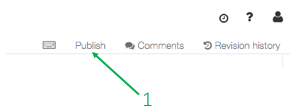 408 | # MAGIC
409 | # MAGIC When you click on the button, you will see the following popup.
410 | # MAGIC
411 | # MAGIC
408 | # MAGIC
409 | # MAGIC When you click on the button, you will see the following popup.
410 | # MAGIC
411 | # MAGIC 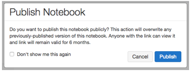 412 | # MAGIC
413 | # MAGIC When you click on "Publish", you will see a popup with your notebook's public link. __Copy the link and set the notebook_URL variable in the AUTOGRADER notebook(not this notebook).__
414 | # MAGIC
415 | # MAGIC
412 | # MAGIC
413 | # MAGIC When you click on "Publish", you will see a popup with your notebook's public link. __Copy the link and set the notebook_URL variable in the AUTOGRADER notebook(not this notebook).__
414 | # MAGIC
415 | # MAGIC 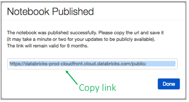 416 |
--------------------------------------------------------------------------------
/CS120x Distributed Machine Learning with Apache Spark/cs120_lab1b_word_count_rdd.ipynb:
--------------------------------------------------------------------------------
1 | {"cells":[{"cell_type":"markdown","source":["
416 |
--------------------------------------------------------------------------------
/CS120x Distributed Machine Learning with Apache Spark/cs120_lab1b_word_count_rdd.ipynb:
--------------------------------------------------------------------------------
1 | {"cells":[{"cell_type":"markdown","source":[" 
This work is licensed under a Creative Commons Attribution-NonCommercial-NoDerivatives 4.0 International License. "],"metadata":{}},{"cell_type":"markdown","source":["# + \n# Word Count Lab: Building a word count application\n\nThis lab will build on the techniques covered in the Spark tutorial to develop a simple word count application. The volume of unstructured text in existence is growing dramatically, and Spark is an excellent tool for analyzing this type of data. In this lab, we will write code that calculates the most common words in the [Complete Works of William Shakespeare](http://www.gutenberg.org/ebooks/100) retrieved from [Project Gutenberg](http://www.gutenberg.org/wiki/Main_Page).\n\nThis could also be scaled to find the most common words in Wikipedia.\n\n## During this lab we will cover:\n* *Part 1:* Creating a base RDD and pair RDDs\n* *Part 2:* Counting with pair RDDs\n* *Part 3:* Finding unique words and a mean value\n* *Part 4:* Apply word count to a file\n* *Appendix A:* Submitting your exercises to the Autograder\n\n> Note that for reference, you can look up the details of the relevant methods in:\n> * [Spark's Python API](https://spark.apache.org/docs/latest/api/python/pyspark.html#pyspark.RDD)"],"metadata":{}},{"cell_type":"code","source":["labVersion = 'cs120x-lab1b-1.0.0'"],"metadata":{},"outputs":[],"execution_count":3},{"cell_type":"markdown","source":["## Part 1: Creating a base RDD and pair RDDs"],"metadata":{}},{"cell_type":"markdown","source":["In this part of the lab, we will explore creating a base RDD with `parallelize` and using pair RDDs to count words."],"metadata":{}},{"cell_type":"markdown","source":["### (1a) Create a base RDD\nWe'll start by generating a base RDD by using a Python list and the `sc.parallelize` method. Then we'll print out the type of the base RDD."],"metadata":{}},{"cell_type":"code","source":["wordsList = ['cat', 'elephant', 'rat', 'rat', 'cat']\nwordsRDD = sc.parallelize(wordsList, 4)\n# Print out the type of wordsRDD\nprint type(wordsRDD)"],"metadata":{},"outputs":[],"execution_count":7},{"cell_type":"markdown","source":["### (1b) Pluralize and test\n\nLet's use a `map()` transformation to add the letter 's' to each string in the base RDD we just created. We'll define a Python function that returns the word with an 's' at the end of the word. Please replace `` with your solution. If you have trouble, the next cell has the solution. After you have defined `makePlural` you can run the third cell which contains a test. If you implementation is correct it will print `1 test passed`.\n\nThis is the general form that exercises will take, except that no example solution will be provided. Exercises will include an explanation of what is expected, followed by code cells where one cell will have one or more `` sections. The cell that needs to be modified will have `# TODO: Replace with appropriate code` on its first line. Once the `` sections are updated and the code is run, the test cell can then be run to verify the correctness of your solution. The last code cell before the next markdown section will contain the tests."],"metadata":{}},{"cell_type":"code","source":["# TODO: Replace with appropriate code\ndef makePlural(word):\n \"\"\"Adds an 's' to `word`.\n\n Note:\n This is a simple function that only adds an 's'. No attempt is made to follow proper\n pluralization rules.\n\n Args:\n word (str): A string.\n\n Returns:\n str: A string with 's' added to it.\n \"\"\"\n return word + 's'\n\nprint makePlural('cat')"],"metadata":{},"outputs":[],"execution_count":9},{"cell_type":"code","source":["# One way of completing the function\ndef makePlural(word):\n return word + 's'\n\nprint makePlural('cat')"],"metadata":{},"outputs":[],"execution_count":10},{"cell_type":"code","source":["# Load in the testing code and check to see if your answer is correct\n# If incorrect it will report back '1 test failed' for each failed test\n# Make sure to rerun any cell you change before trying the test again\nfrom databricks_test_helper import Test\n# TEST Pluralize and test (1b)\nTest.assertEquals(makePlural('rat'), 'rats', 'incorrect result: makePlural does not add an s')"],"metadata":{},"outputs":[],"execution_count":11},{"cell_type":"markdown","source":["### (1c) Apply `makePlural` to the base RDD\n\nNow pass each item in the base RDD into a [map()](http://spark.apache.org/docs/latest/api/python/pyspark.html#pyspark.RDD.map) transformation that applies the `makePlural()` function to each element. And then call the [collect()](http://spark.apache.org/docs/latest/api/python/pyspark.html#pyspark.RDD.collect) action to see the transformed RDD."],"metadata":{}},{"cell_type":"code","source":["# TODO: Replace with appropriate code\npluralRDD = wordsRDD.map(makePlural)\nprint pluralRDD.collect()"],"metadata":{},"outputs":[],"execution_count":13},{"cell_type":"code","source":["# TEST Apply makePlural to the base RDD(1c)\nTest.assertEquals(pluralRDD.collect(), ['cats', 'elephants', 'rats', 'rats', 'cats'],\n 'incorrect values for pluralRDD')"],"metadata":{},"outputs":[],"execution_count":14},{"cell_type":"markdown","source":["### (1d) Pass a `lambda` function to `map`\n\nLet's create the same RDD using a `lambda` function."],"metadata":{}},{"cell_type":"code","source":["# TODO: Replace with appropriate code\npluralLambdaRDD = wordsRDD.map(lambda x: x + 's')\nprint pluralLambdaRDD.collect()"],"metadata":{},"outputs":[],"execution_count":16},{"cell_type":"code","source":["# TEST Pass a lambda function to map (1d)\nTest.assertEquals(pluralLambdaRDD.collect(), ['cats', 'elephants', 'rats', 'rats', 'cats'],\n 'incorrect values for pluralLambdaRDD (1d)')"],"metadata":{},"outputs":[],"execution_count":17},{"cell_type":"markdown","source":["### (1e) Length of each word\n\nNow use `map()` and a `lambda` function to return the number of characters in each word. We'll `collect` this result directly into a variable."],"metadata":{}},{"cell_type":"code","source":["# TODO: Replace with appropriate code\npluralLengths = (pluralRDD\n .map(lambda x: len(x))\n .collect())\nprint pluralLengths"],"metadata":{},"outputs":[],"execution_count":19},{"cell_type":"code","source":["# TEST Length of each word (1e)\nTest.assertEquals(pluralLengths, [4, 9, 4, 4, 4],\n 'incorrect values for pluralLengths')"],"metadata":{},"outputs":[],"execution_count":20},{"cell_type":"markdown","source":["### (1f) Pair RDDs\n\nThe next step in writing our word counting program is to create a new type of RDD, called a pair RDD. A pair RDD is an RDD where each element is a pair tuple `(k, v)` where `k` is the key and `v` is the value. In this example, we will create a pair consisting of `('', 1)` for each word element in the RDD.\nWe can create the pair RDD using the `map()` transformation with a `lambda()` function to create a new RDD."],"metadata":{}},{"cell_type":"code","source":["# TODO: Replace with appropriate code\nwordPairs = wordsRDD.map(lambda x: (x, 1))\nprint wordPairs.collect()"],"metadata":{},"outputs":[],"execution_count":22},{"cell_type":"code","source":["# TEST Pair RDDs (1f)\nTest.assertEquals(wordPairs.collect(),\n [('cat', 1), ('elephant', 1), ('rat', 1), ('rat', 1), ('cat', 1)],\n 'incorrect value for wordPairs')"],"metadata":{},"outputs":[],"execution_count":23},{"cell_type":"markdown","source":["## Part 2: Counting with pair RDDs"],"metadata":{}},{"cell_type":"markdown","source":["Now, let's count the number of times a particular word appears in the RDD. There are multiple ways to perform the counting, but some are much less efficient than others.\n\nA naive approach would be to `collect()` all of the elements and count them in the driver program. While this approach could work for small datasets, we want an approach that will work for any size dataset including terabyte- or petabyte-sized datasets. In addition, performing all of the work in the driver program is slower than performing it in parallel in the workers. For these reasons, we will use data parallel operations."],"metadata":{}},{"cell_type":"markdown","source":["### (2a) `groupByKey()` approach\nAn approach you might first consider (we'll see shortly that there are better ways) is based on using the [groupByKey()](http://spark.apache.org/docs/latest/api/python/pyspark.html#pyspark.RDD.groupByKey) transformation. As the name implies, the `groupByKey()` transformation groups all the elements of the RDD with the same key into a single list in one of the partitions.\n\nThere are two problems with using `groupByKey()`:\n + The operation requires a lot of data movement to move all the values into the appropriate partitions.\n + The lists can be very large. Consider a word count of English Wikipedia: the lists for common words (e.g., the, a, etc.) would be huge and could exhaust the available memory in a worker.\n\nUse `groupByKey()` to generate a pair RDD of type `('word', iterator)`."],"metadata":{}},{"cell_type":"code","source":["# TODO: Replace with appropriate code\n# Note that groupByKey requires no parameters\nwordsGrouped = wordPairs.groupByKey()\nfor key, value in wordsGrouped.collect():\n print '{0}: {1}'.format(key, list(value))"],"metadata":{},"outputs":[],"execution_count":27},{"cell_type":"code","source":["# TEST groupByKey() approach (2a)\nTest.assertEquals(sorted(wordsGrouped.mapValues(lambda x: list(x)).collect()),\n [('cat', [1, 1]), ('elephant', [1]), ('rat', [1, 1])],\n 'incorrect value for wordsGrouped')"],"metadata":{},"outputs":[],"execution_count":28},{"cell_type":"markdown","source":["### (2b) Use `groupByKey()` to obtain the counts\n\nUsing the `groupByKey()` transformation creates an RDD containing 3 elements, each of which is a pair of a word and a Python iterator.\n\nNow sum the iterator using a `map()` transformation. The result should be a pair RDD consisting of (word, count) pairs."],"metadata":{}},{"cell_type":"code","source":["# TODO: Replace with appropriate code\nwordCountsGrouped = wordsGrouped.map(lambda x: (x[0], len(x[1])))\nprint wordCountsGrouped.collect()"],"metadata":{},"outputs":[],"execution_count":30},{"cell_type":"code","source":["# TEST Use groupByKey() to obtain the counts (2b)\nTest.assertEquals(sorted(wordCountsGrouped.collect()),\n [('cat', 2), ('elephant', 1), ('rat', 2)],\n 'incorrect value for wordCountsGrouped')"],"metadata":{},"outputs":[],"execution_count":31},{"cell_type":"markdown","source":["** (2c) Counting using `reduceByKey` **\n\nA better approach is to start from the pair RDD and then use the [reduceByKey()](http://spark.apache.org/docs/latest/api/python/pyspark.html#pyspark.RDD.reduceByKey) transformation to create a new pair RDD. The `reduceByKey()` transformation gathers together pairs that have the same key and applies the function provided to two values at a time, iteratively reducing all of the values to a single value. `reduceByKey()` operates by applying the function first within each partition on a per-key basis and then across the partitions, allowing it to scale efficiently to large datasets."],"metadata":{}},{"cell_type":"code","source":["# TODO: Replace with appropriate code\n# Note that reduceByKey takes in a function that accepts two values and returns a single value\nwordCounts = wordPairs.reduceByKey(lambda x, y: x + y)\nprint wordCounts.collect()"],"metadata":{},"outputs":[],"execution_count":33},{"cell_type":"code","source":["# TEST Counting using reduceByKey (2c)\nTest.assertEquals(sorted(wordCounts.collect()), [('cat', 2), ('elephant', 1), ('rat', 2)],\n 'incorrect value for wordCounts')"],"metadata":{},"outputs":[],"execution_count":34},{"cell_type":"markdown","source":["### (2d) All together\n\nThe expert version of the code performs the `map()` to pair RDD, `reduceByKey()` transformation, and `collect` in one statement."],"metadata":{}},{"cell_type":"code","source":["# TODO: Replace with appropriate code\nwordCountsCollected = (wordsRDD\n .map(lambda x: (x, 1))\n .reduceByKey(lambda x, y: x+y)\n .collect())\nprint wordCountsCollected"],"metadata":{},"outputs":[],"execution_count":36},{"cell_type":"code","source":["# TEST All together (2d)\nTest.assertEquals(sorted(wordCountsCollected), [('cat', 2), ('elephant', 1), ('rat', 2)],\n 'incorrect value for wordCountsCollected')"],"metadata":{},"outputs":[],"execution_count":37},{"cell_type":"markdown","source":["## Part 3: Finding unique words and a mean value"],"metadata":{}},{"cell_type":"markdown","source":["### (3a) Unique words\n\nCalculate the number of unique words in `wordsRDD`. You can use other RDDs that you have already created to make this easier."],"metadata":{}},{"cell_type":"code","source":["# TODO: Replace with appropriate code\nuniqueWords = len(wordCountsCollected)\nprint uniqueWords"],"metadata":{},"outputs":[],"execution_count":40},{"cell_type":"code","source":["# TEST Unique words (3a)\nTest.assertEquals(uniqueWords, 3, 'incorrect count of uniqueWords')"],"metadata":{},"outputs":[],"execution_count":41},{"cell_type":"markdown","source":["### (3b) Mean using `reduce`\n\nFind the mean number of words per unique word in `wordCounts`.\n\nUse a `reduce()` action to sum the counts in `wordCounts` and then divide by the number of unique words. First `map()` the pair RDD `wordCounts`, which consists of (key, value) pairs, to an RDD of values."],"metadata":{}},{"cell_type":"code","source":["# TODO: Replace with appropriate code\nfrom operator import add\ntotalCount = (wordCounts\n .map(lambda x: x[1])\n .reduce(add))\naverage = totalCount / float(uniqueWords)\nprint totalCount\nprint round(average, 2)"],"metadata":{},"outputs":[],"execution_count":43},{"cell_type":"code","source":["# TEST Mean using reduce (3b)\nTest.assertEquals(round(average, 2), 1.67, 'incorrect value of average')"],"metadata":{},"outputs":[],"execution_count":44},{"cell_type":"markdown","source":["## Part 4: Apply word count to a file"],"metadata":{}},{"cell_type":"markdown","source":["In this section we will finish developing our word count application. We'll have to build the `wordCount` function, deal with real world problems like capitalization and punctuation, load in our data source, and compute the word count on the new data."],"metadata":{}},{"cell_type":"markdown","source":["### (4a) `wordCount` function\n\nFirst, define a function for word counting. You should reuse the techniques that have been covered in earlier parts of this lab. This function should take in an RDD that is a list of words like `wordsRDD` and return a pair RDD that has all of the words and their associated counts."],"metadata":{}},{"cell_type":"code","source":["# TODO: Replace with appropriate code\ndef wordCount(wordListRDD):\n \"\"\"Creates a pair RDD with word counts from an RDD of words.\n\n Args:\n wordListRDD (RDD of str): An RDD consisting of words.\n\n Returns:\n RDD of (str, int): An RDD consisting of (word, count) tuples.\n \"\"\"\n wordCountlistRDD = (wordListRDD\n .map(lambda x: (x,1))\n .reduceByKey(add))\n return wordCountlistRDD\nprint wordCount(wordsRDD).collect()"],"metadata":{},"outputs":[],"execution_count":48},{"cell_type":"code","source":["# TEST wordCount function (4a)\nTest.assertEquals(sorted(wordCount(wordsRDD).collect()),\n [('cat', 2), ('elephant', 1), ('rat', 2)],\n 'incorrect definition for wordCount function')"],"metadata":{},"outputs":[],"execution_count":49},{"cell_type":"markdown","source":["### (4b) Capitalization and punctuation\n\nReal world files are more complicated than the data we have been using in this lab. Some of the issues we have to address are:\n + Words should be counted independent of their capitialization (e.g., Spark and spark should be counted as the same word).\n + All punctuation should be removed.\n + Any leading or trailing spaces on a line should be removed.\n\nDefine the function `removePunctuation` that converts all text to lower case, removes any punctuation, and removes leading and trailing spaces. Use the Python [re](https://docs.python.org/2/library/re.html) module to remove any text that is not a letter, number, or space. Reading `help(re.sub)` might be useful.\nIf you are unfamiliar with regular expressions, you may want to review [this tutorial](https://developers.google.com/edu/python/regular-expressions) from Google. Also, [this website](https://regex101.com/#python) is a great resource for debugging your regular expression."],"metadata":{}},{"cell_type":"code","source":["# TODO: Replace with appropriate code\nimport re\nfrom pyspark.sql.functions import regexp_replace, trim, col, lower\ndef removePunctuation(text):\n \"\"\"Removes punctuation, changes to lower case, and strips leading and trailing spaces.\n\n Note:\n Only spaces, letters, and numbers should be retained. Other characters should should be\n eliminated (e.g. it's becomes its). Leading and trailing spaces should be removed after\n punctuation is removed.\n\n Args:\n text (str): A string.\n\n Returns:\n str: The cleaned up string.\n \"\"\"\n return re.sub('[^A-Za-z0-9 ]', '', text).strip().lower()\nprint removePunctuation('Hi, you!')\nprint removePunctuation(' No under_score!')\nprint removePunctuation(' * Remove punctuation then spaces * ')"],"metadata":{},"outputs":[],"execution_count":51},{"cell_type":"code","source":["# TEST Capitalization and punctuation (4b)\nTest.assertEquals(removePunctuation(\" The Elephant's 4 cats. \"),\n 'the elephants 4 cats',\n 'incorrect definition for removePunctuation function')"],"metadata":{},"outputs":[],"execution_count":52},{"cell_type":"markdown","source":["### (4c) Load a text file\n\nFor the next part of this lab, we will use the [Complete Works of William Shakespeare](http://www.gutenberg.org/ebooks/100) from [Project Gutenberg](http://www.gutenberg.org/wiki/Main_Page). To convert a text file into an RDD, we use the `SparkContext.textFile()` method. We also apply the recently defined `removePunctuation()` function using a `map()` transformation to strip out the punctuation and change all text to lower case. Since the file is large we use `take(15)`, so that we only print 15 lines."],"metadata":{}},{"cell_type":"code","source":["%fs"],"metadata":{},"outputs":[],"execution_count":54},{"cell_type":"code","source":["# Just run this code\nimport os.path\nfileName = \"dbfs:/\" + os.path.join('databricks-datasets', 'cs100', 'lab1', 'data-001', 'shakespeare.txt')\n\nshakespeareRDD = sc.textFile(fileName, 8).map(removePunctuation)\nprint '\\n'.join(shakespeareRDD\n .zipWithIndex() # to (line, lineNum)\n .map(lambda (l, num): '{0}: {1}'.format(num, l)) # to 'lineNum: line'\n .take(15))"],"metadata":{},"outputs":[],"execution_count":55},{"cell_type":"markdown","source":["### (4d) Words from lines\n\nBefore we can use the `wordcount()` function, we have to address two issues with the format of the RDD:\n + The first issue is that that we need to split each line by its spaces. ** Performed in (4d). **\n + The second issue is we need to filter out empty lines. ** Performed in (4e). **\n\nApply a transformation that will split each element of the RDD by its spaces. For each element of the RDD, you should apply Python's string [split()](https://docs.python.org/2/library/string.html#string.split) function. You might think that a `map()` transformation is the way to do this, but think about what the result of the `split()` function will be.\n\n> Note:\n> * Do not use the default implemenation of `split()`, but pass in a separator value. For example, to split `line` by commas you would use `line.split(',')`."],"metadata":{}},{"cell_type":"code","source":["# TODO: Replace with appropriate code\nshakespeareWordsRDD = shakespeareRDD.flatMap(lambda x: x.split(' '))\nshakespeareWordCount = shakespeareWordsRDD.count()\nprint shakespeareWordsRDD.top(5)\nprint shakespeareWordCount"],"metadata":{},"outputs":[],"execution_count":57},{"cell_type":"code","source":["# TEST Words from lines (4d)\n# This test allows for leading spaces to be removed either before or after\n# punctuation is removed.\nTest.assertTrue(shakespeareWordCount == 927631 or shakespeareWordCount == 928908,\n 'incorrect value for shakespeareWordCount')\nTest.assertEquals(shakespeareWordsRDD.top(5),\n [u'zwaggerd', u'zounds', u'zounds', u'zounds', u'zounds'],\n 'incorrect value for shakespeareWordsRDD')"],"metadata":{},"outputs":[],"execution_count":58},{"cell_type":"markdown","source":["** (4e) Remove empty elements **\n\nThe next step is to filter out the empty elements. Remove all entries where the word is `''`."],"metadata":{}},{"cell_type":"code","source":["# TODO: Replace with appropriate code\nshakeWordsRDD = shakespeareWordsRDD.filter(lambda x: x != '')\nshakeWordCount = shakeWordsRDD.count()\nprint shakeWordCount"],"metadata":{},"outputs":[],"execution_count":60},{"cell_type":"code","source":["# TEST Remove empty elements (4e)\nTest.assertEquals(shakeWordCount, 882996, 'incorrect value for shakeWordCount')"],"metadata":{},"outputs":[],"execution_count":61},{"cell_type":"markdown","source":["### (4f) Count the words\n\nWe now have an RDD that is only words. Next, let's apply the `wordCount()` function to produce a list of word counts. We can view the top 15 words by using the `takeOrdered()` action; however, since the elements of the RDD are pairs, we need a custom sort function that sorts using the value part of the pair.\n\nYou'll notice that many of the words are common English words. These are called stopwords. In a later lab, we will see how to eliminate them from the results.\nUse the `wordCount()` function and `takeOrdered()` to obtain the fifteen most common words and their counts."],"metadata":{}},{"cell_type":"code","source":["# TODO: Replace with appropriate code\ntop15WordsAndCounts = wordCount(shakeWordsRDD).takeOrdered(15, key = lambda x: -x[1])\nprint '\\n'.join(map(lambda (w, c): '{0}: {1}'.format(w, c), top15WordsAndCounts))"],"metadata":{},"outputs":[],"execution_count":63},{"cell_type":"code","source":["# TEST Count the words (4f)\nTest.assertEquals(top15WordsAndCounts,\n [(u'the', 27361), (u'and', 26028), (u'i', 20681), (u'to', 19150), (u'of', 17463),\n (u'a', 14593), (u'you', 13615), (u'my', 12481), (u'in', 10956), (u'that', 10890),\n (u'is', 9134), (u'not', 8497), (u'with', 7771), (u'me', 7769), (u'it', 7678)],\n 'incorrect value for top15WordsAndCounts')"],"metadata":{},"outputs":[],"execution_count":64},{"cell_type":"markdown","source":["## Appendix A: Submitting Your Exercises to the Autograder\n\nThis section guides you through Step 2 of the grading process (\"Submit to Autograder\").\n\nOnce you confirm that your lab notebook is passing all tests, you can submit it first to the course autograder and then second to the edX website to receive a grade.\n\n** Note that you can only submit to the course autograder once every 1 minute. **"],"metadata":{}},{"cell_type":"markdown","source":["### Step 2(a): Restart your cluster by clicking on the dropdown next to your cluster name and selecting \"Restart Cluster\".\n\nYou can do this step in either notebook, since there is one cluster for your notebooks.\n\n"],"metadata":{}},{"cell_type":"markdown","source":["### Step 2(b): _IN THIS NOTEBOOK_, click on \"Run All\" to run all of the cells.\n\n\n\nThis step will take some time.\n\nWait for your cluster to finish running the cells in your lab notebook before proceeding."],"metadata":{}},{"cell_type":"markdown","source":["### Step 2(c): Publish this notebook\n\nPublish _this_ notebook by clicking on the \"Publish\" button at the top.\n\n\n\nWhen you click on the button, you will see the following popup.\n\n\n\nWhen you click on \"Publish\", you will see a popup with your notebook's public link. **Copy the link and set the `notebook_URL` variable in the AUTOGRADER notebook (not this notebook).**\n\n"],"metadata":{}},{"cell_type":"markdown","source":["### Step 2(d): Set the notebook URL and Lab ID in the Autograder notebook, and run it\n\nGo to the Autograder notebook and paste the link you just copied into it, so that it is assigned to the `notebook_url` variable.\n\n```\nnotebook_url = \"...\" # put your URL here\n```\n\nThen, find the line that looks like this:\n\n```\nlab = \n```\nand change `` to \"CS120x-lab1b\":\n\n```\nlab = \"CS120x-lab1b\"\n```\n\nThen, run the Autograder notebook to submit your lab."],"metadata":{}},{"cell_type":"markdown","source":["###  If things go wrong\n\nIt's possible that your notebook looks fine to you, but fails in the autograder. (This can happen when you run cells out of order, as you're working on your notebook.) If that happens, just try again, starting at the top of Appendix A."],"metadata":{}}],"metadata":{"name":"cs120_lab1b_word_count_rdd","notebookId":1791900596147579},"nbformat":4,"nbformat_minor":0}
2 |
--------------------------------------------------------------------------------
/CS120x Distributed Machine Learning with Apache Spark/cs120_lab1a_math_review.ipynb:
--------------------------------------------------------------------------------
1 | {"cells":[{"cell_type":"markdown","source":["
If things go wrong\n\nIt's possible that your notebook looks fine to you, but fails in the autograder. (This can happen when you run cells out of order, as you're working on your notebook.) If that happens, just try again, starting at the top of Appendix A."],"metadata":{}}],"metadata":{"name":"cs120_lab1b_word_count_rdd","notebookId":1791900596147579},"nbformat":4,"nbformat_minor":0}
2 |
--------------------------------------------------------------------------------
/CS120x Distributed Machine Learning with Apache Spark/cs120_lab1a_math_review.ipynb:
--------------------------------------------------------------------------------
1 | {"cells":[{"cell_type":"markdown","source":["![\"Creative]()
This work is licensed under aCreative Commons Attribution-NonCommercial-NoDerivatives 4.0 InternationalLicense."],"metadata":{}},{"cell_type":"markdown","source":["\n# Math and Python review\n\nThis notebook reviews vector and matrix math, the [NumPy](http://www.numpy.org/) Python package, and Python lambda expressions. Part 1 covers vector and matrix math, and you'll do a few exercises by hand. In Part 2, you'll learn about NumPy and use `ndarray` objects to solve the math exercises. Part 3 provides additional information about NumPy and how it relates to array usage in Spark's [MLlib](https://spark.apache.org/mllib/). Part 4 provides an overview of lambda expressions.\n\nTo move through the notebook just run each of the cells. You can run a cell by pressing \"shift-enter\", which will compute the current cell and advance to the next cell, or by clicking in a cell and pressing \"control-enter\", which will compute the current cell and remain in that cell. You should move through the notebook from top to bottom and run all of the cells. If you skip some cells, later cells might not work as expected.\nNote that there are several exercises within this notebook. You will need to provide solutions for cells that start with: `# TODO: Replace with appropriate code`.\n\n** This notebook covers: **\n* *Part 1:* Math review\n* *Part 2:* NumPy\n* *Part 3:* Additional NumPy and Spark linear algebra\n* *Part 4:* Python lambda expressions\n* *Appendix A:* Submitting your exercises to the Autograder"],"metadata":{}},{"cell_type":"code","source":["labVersion = 'cs120x-lab1a-1.0.0'"],"metadata":{},"outputs":[],"execution_count":3},{"cell_type":"markdown","source":["## Part 1: Math review"],"metadata":{}},{"cell_type":"markdown","source":["### (1a) Scalar multiplication: vectors\n\nIn this exercise, you will calculate the product of a scalar and a vector by hand and enter the result in the code cell below. Scalar multiplication is straightforward. The resulting vector equals the product of the scalar, which is a single value, and each item in the original vector.\nIn the example below, \\\\( a \\\\) is the scalar (constant) and \\\\( \\mathbf{v} \\\\) is the vector. \\\\[ a \\mathbf{v} = \\begin{bmatrix} a v_1 \\\\\\ a v_2 \\\\\\ \\vdots \\\\\\ a v_n \\end{bmatrix} \\\\]\n\nCalculate the value of \\\\( \\mathbf{x} \\\\): \\\\[ \\mathbf{x} = 3 \\begin{bmatrix} 1 \\\\\\ -2 \\\\\\ 0 \\end{bmatrix} \\\\]\nCalculate the value of \\\\( \\mathbf{y} \\\\): \\\\[ \\mathbf{y} = 2 \\begin{bmatrix} 2 \\\\\\ 4 \\\\\\ 8 \\end{bmatrix} \\\\]"],"metadata":{}},{"cell_type":"code","source":["# TODO: Replace with appropriate code\n# Manually calculate your answer and represent the vector as a list of integers.\n# For example, [2, 4, 8].\nvectorX = [3, -6, 0]\nvectorY = [4, 8, 16]"],"metadata":{},"outputs":[],"execution_count":6},{"cell_type":"code","source":["# TEST Scalar multiplication: vectors (1a)\n# Import test library\nfrom databricks_test_helper import Test\n\nTest.assertEqualsHashed(vectorX, 'e460f5b87531a2b60e0f55c31b2e49914f779981',\n 'incorrect value for vectorX')\nTest.assertEqualsHashed(vectorY, 'e2d37ff11427dbac7f833a5a7039c0de5a740b1e',\n 'incorrect value for vectorY')"],"metadata":{},"outputs":[],"execution_count":7},{"cell_type":"markdown","source":["### (1b) Element-wise multiplication: vectors\n\nIn this exercise, you will calculate the element-wise multiplication of two vectors by hand and enter the result in the code cell below. You'll later see that element-wise multiplication is the default method when two NumPy arrays are multiplied together. Note we won't be performing element-wise multiplication in future labs, but we are introducing it here to distinguish it from other vector operators. It is also a common operation in NumPy, as we will discuss in Part (2b).\n\nThe element-wise calculation is as follows: \\\\[ \\mathbf{x} \\odot \\mathbf{y} = \\begin{bmatrix} x_1 y_1 \\\\\\ x_2 y_2 \\\\\\ \\vdots \\\\\\ x_n y_n \\end{bmatrix} \\\\]\n\nCalculate the value of \\\\( \\mathbf{z} \\\\): \\\\[ \\mathbf{z} = \\begin{bmatrix} 1 \\\\\\ 2 \\\\\\ 3 \\end{bmatrix} \\odot \\begin{bmatrix} 4 \\\\\\ 5 \\\\\\ 6 \\end{bmatrix} \\\\]"],"metadata":{}},{"cell_type":"code","source":["# TODO: Replace with appropriate code\n# Manually calculate your answer and represent the vector as a list of integers.\nz = [4, 10, 18]"],"metadata":{},"outputs":[],"execution_count":9},{"cell_type":"code","source":["# TEST Element-wise multiplication: vectors (1b)\nTest.assertEqualsHashed(z, '4b5fe28ee2d274d7e0378bf993e28400f66205c2',\n 'incorrect value for z')"],"metadata":{},"outputs":[],"execution_count":10},{"cell_type":"markdown","source":["### (1c) Dot product\n\nIn this exercise, you will calculate the dot product of two vectors by hand and enter the result in the code cell below. Note that the dot product is equivalent to performing element-wise multiplication and then summing the result.\n\nBelow, you'll find the calculation for the dot product of two vectors, where each vector has length \\\\( n \\\\): \\\\[ \\mathbf{w} \\cdot \\mathbf{x} = \\sum_{i=1}^n w_i x_i \\\\]\n\nNote that you may also see \\\\( \\mathbf{w} \\cdot \\mathbf{x} \\\\) represented as \\\\( \\mathbf{w}^\\top \\mathbf{x} \\\\)\n\nCalculate the value for \\\\( c_1 \\\\) based on the dot product of the following two vectors:\n\\\\[ c_1 = \\begin{bmatrix} 1 & -3 \\end{bmatrix} \\cdot \\begin{bmatrix} 4 \\\\\\ 5 \\end{bmatrix}\\\\]\n\nCalculate the value for \\\\( c_2 \\\\) based on the dot product of the following two vectors:\n\\\\[ c_2 = \\begin{bmatrix} 3 & 4 & 5 \\end{bmatrix} \\cdot \\begin{bmatrix} 1 \\\\\\ 2 \\\\\\ 3 \\end{bmatrix}\\\\]"],"metadata":{}},{"cell_type":"code","source":["# TODO: Replace with appropriate code\n# Manually calculate your answer and set the variables to their appropriate integer values.\nc1 = -11\nc2 = 26"],"metadata":{},"outputs":[],"execution_count":12},{"cell_type":"code","source":["# TEST Dot product (1c)\nTest.assertEqualsHashed(c1, '8d7a9046b6a6e21d66409ad0849d6ab8aa51007c', 'incorrect value for c1')\nTest.assertEqualsHashed(c2, '887309d048beef83ad3eabf2a79a64a389ab1c9f', 'incorrect value for c2')"],"metadata":{},"outputs":[],"execution_count":13},{"cell_type":"markdown","source":["### (1d) Matrix multiplication\n\nIn this exercise, you will calculate the result of multiplying two matrices together by hand and enter the result in the code cell below.\nRefer to the slides for the formula for multiplying two matrices together.\n\nFirst, you'll calculate the value for \\\\( \\mathbf{X} \\\\).\n\\\\[ \\mathbf{X} = \\begin{bmatrix} 1 & 2 & 3 \\\\\\ 4 & 5 & 6 \\end{bmatrix} \\begin{bmatrix} 1 & 2 \\\\\\ 3 & 4 \\\\\\ 5 & 6 \\end{bmatrix} \\\\]\n\nNext, you'll perform an outer product and calculate the value for \\\\( \\mathbf{Y} \\\\).\n\n\\\\[ \\mathbf{Y} = \\begin{bmatrix} 1 \\\\\\ 2 \\\\\\ 3 \\end{bmatrix} \\begin{bmatrix} 1 & 2 & 3 \\end{bmatrix} \\\\]\n\nThe resulting matrices should be stored row-wise (see [row-major order](https://en.wikipedia.org/wiki/Row-major_order)). This means that the matrix is organized by rows. For instance, a 2x2 row-wise matrix would be represented as: \\\\( [[r_1c_1, r_1c_2], [r_2c_1, r_2c_2]] \\\\) where r stands for row and c stands for column.\n\nNote that outer product is just a special case of general matrix multiplication and follows the same rules as normal matrix multiplication."],"metadata":{}},{"cell_type":"code","source":["# TODO: Replace with appropriate code\n# Represent matrices as lists within lists. For example, [[1,2,3], [4,5,6]] represents a matrix with\n# two rows and three columns. Use integer values.\nmatrixX = [[22,28], [49,64]]\nmatrixY = [[1,2,3],[2,4,6],[3,6,9]]"],"metadata":{},"outputs":[],"execution_count":15},{"cell_type":"code","source":["# TEST Matrix multiplication (1d)\nTest.assertEqualsHashed(matrixX, 'c2ada2598d8a499e5dfb66f27a24f444483cba13',\n 'incorrect value for matrixX')\nTest.assertEqualsHashed(matrixY, 'f985daf651531b7d776523836f3068d4c12e4519',\n 'incorrect value for matrixY')"],"metadata":{},"outputs":[],"execution_count":16},{"cell_type":"markdown","source":["## Part 2: NumPy"],"metadata":{}},{"cell_type":"markdown","source":["### (2a) Scalar multiplication\n\n[NumPy](http://docs.scipy.org/doc/numpy/reference/) is a Python library for working with arrays. NumPy provides abstractions that make it easy to treat these underlying arrays as vectors and matrices. The library is optimized to be fast and memory efficient, and we'll be using it throughout the course. The building block for NumPy is the [ndarray](http://docs.scipy.org/doc/numpy/reference/generated/numpy.ndarray.html), which is a multidimensional array of fixed-size that contains elements of one type (e.g. array of floats).\n\nFor this exercise, you'll create a `ndarray` consisting of the elements \\[1, 2, 3\\] and multiply this array by 5. Use [np.array()](http://docs.scipy.org/doc/numpy/reference/generated/numpy.array.html) to create the array. Note that you can pass a Python list into `np.array()`. To perform scalar multiplication with an `ndarray` just use `*`.\n\nNote that if you create an array from a Python list of integers you will obtain a one-dimensional array, *which is equivalent to a vector for our purposes*."],"metadata":{}},{"cell_type":"code","source":["# It is convention to import NumPy with the alias np\nimport numpy as np"],"metadata":{},"outputs":[],"execution_count":19},{"cell_type":"code","source":["# TODO: Replace with appropriate code\n# Create a numpy array with the values 1, 2, 3\nsimpleArray = np.array([1,2,3])\n# Perform the scalar product of 5 and the numpy array\ntimesFive = simpleArray * 5\nprint 'simpleArray\\n{0}'.format(simpleArray)\nprint '\\ntimesFive\\n{0}'.format(timesFive)"],"metadata":{},"outputs":[],"execution_count":20},{"cell_type":"code","source":["# TEST Scalar multiplication (2a)\nTest.assertTrue(np.all(timesFive == [5, 10, 15]), 'incorrect value for timesFive')"],"metadata":{},"outputs":[],"execution_count":21},{"cell_type":"markdown","source":["### (2b) Element-wise multiplication and dot product\n\nNumPy arrays support both element-wise multiplication and dot product. Element-wise multiplication occurs automatically when you use the `*` operator to multiply two `ndarray` objects of the same length.\n\nTo perform the dot product you can use either [np.dot()](http://docs.scipy.org/doc/numpy/reference/generated/numpy.dot.html#numpy.dot) or [np.ndarray.dot()](http://docs.scipy.org/doc/numpy/reference/generated/numpy.ndarray.dot.html). For example, if you had NumPy arrays `x` and `y`, you could compute their dot product four ways: `np.dot(x, y)`, `np.dot(y, x)`, `x.dot(y)`, or `y.dot(x)`.\n\nFor this exercise, multiply the arrays `u` and `v` element-wise and compute their dot product."],"metadata":{}},{"cell_type":"code","source":["# TODO: Replace with appropriate code\n# Create a ndarray based on a range and step size.\nu = np.arange(0, 5, .5)\nv = np.arange(5, 10, .5)\n\nelementWise = u * v\ndotProduct = np.dot(u, v)\nprint 'u: {0}'.format(u)\nprint 'v: {0}'.format(v)\nprint '\\nelementWise\\n{0}'.format(elementWise)\nprint '\\ndotProduct\\n{0}'.format(dotProduct)"],"metadata":{},"outputs":[],"execution_count":23},{"cell_type":"code","source":["# TEST Element-wise multiplication and dot product (2b)\nTest.assertTrue(np.all(elementWise == [ 0., 2.75, 6., 9.75, 14., 18.75, 24., 29.75, 36., 42.75]),\n 'incorrect value for elementWise')\nTest.assertEquals(dotProduct, 183.75, 'incorrect value for dotProduct')"],"metadata":{},"outputs":[],"execution_count":24},{"cell_type":"markdown","source":["### (2c) Matrix math\nWith NumPy it is very easy to perform matrix math. You can use [np.matrix()](http://docs.scipy.org/doc/numpy/reference/generated/numpy.matrix.html) to generate a NumPy matrix. Just pass a two-dimensional `ndarray` or a list of lists to the function. You can perform matrix math on NumPy matrices using `*`.\n\nYou can transpose a matrix by calling [numpy.matrix.transpose()](http://docs.scipy.org/doc/numpy/reference/generated/numpy.matrix.transpose.html) or by using `.T` on the matrix object (e.g. `myMatrix.T`). Transposing a matrix produces a matrix where the new rows are the columns from the old matrix. For example: \\\\[ \\begin{bmatrix} 1 & 2 & 3 \\\\\\ 4 & 5 & 6 \\end{bmatrix}^\\top = \\begin{bmatrix} 1 & 4 \\\\\\ 2 & 5 \\\\\\ 3 & 6 \\end{bmatrix} \\\\]\n\nInverting a matrix can be done using [numpy.linalg.inv()](http://docs.scipy.org/doc/numpy/reference/generated/numpy.linalg.inv.html). Note that only square matrices can be inverted, and square matrices are not guaranteed to have an inverse. If the inverse exists, then multiplying a matrix by its inverse will produce the identity matrix. \\\\( \\scriptsize ( A^{-1} A = I_n ) \\\\) The identity matrix \\\\( \\scriptsize I_n \\\\) has ones along its diagonal and zeros elsewhere. \\\\[ I_n = \\begin{bmatrix} 1 & 0 & 0 & ... & 0 \\\\\\ 0 & 1 & 0 & ... & 0 \\\\\\ 0 & 0 & 1 & ... & 0 \\\\\\ ... & ... & ... & ... & ... \\\\\\ 0 & 0 & 0 & ... & 1 \\end{bmatrix} \\\\]\n\nFor this exercise, multiply \\\\( A \\\\) times its transpose \\\\( ( A^\\top ) \\\\) and then calculate the inverse of the result \\\\( ( [ A A^\\top ]^{-1} ) \\\\)."],"metadata":{}},{"cell_type":"code","source":["# TODO: Replace with appropriate code\nfrom numpy.linalg import inv\n\nA = np.matrix([[1,2,3,4],[5,6,7,8]])\nprint 'A:\\n{0}'.format(A)\n# Print A transpose\nprint '\\nA transpose:\\n{0}'.format(A.T)\n\n# Multiply A by A transpose\nAAt = A * A.T\nprint '\\nAAt:\\n{0}'.format(AAt)\n\n# Invert AAt with np.linalg.inv()\nAAtInv = np.linalg.inv(AAt)\nprint '\\nAAtInv:\\n{0}'.format(AAtInv)\n\n# Show inverse times matrix equals identity\n# We round due to numerical precision\nprint '\\nAAtInv * AAt:\\n{0}'.format((AAtInv * AAt).round(4))"],"metadata":{},"outputs":[],"execution_count":26},{"cell_type":"code","source":["# TEST Matrix math (2c)\nTest.assertTrue(np.all(AAt == np.matrix([[30, 70], [70, 174]])), 'incorrect value for AAt')\nTest.assertTrue(np.allclose(AAtInv, np.matrix([[0.54375, -0.21875], [-0.21875, 0.09375]])),\n 'incorrect value for AAtInv')"],"metadata":{},"outputs":[],"execution_count":27},{"cell_type":"markdown","source":["### Part 3: Additional NumPy and Spark linear algebra"],"metadata":{}},{"cell_type":"markdown","source":["### (3a) Slices\n\nYou can select a subset of a one-dimensional NumPy `ndarray`'s elements by using slices. These slices operate the same way as slices for Python lists. For example, `[0, 1, 2, 3][:2]` returns the first two elements `[0, 1]`. NumPy, additionally, has more sophisticated slicing that allows slicing across multiple dimensions; however, you'll only need to use basic slices in future labs for this course.\n\nNote that if no index is placed to the left of a `:`, it is equivalent to starting at 0, and hence `[0, 1, 2, 3][:2]` and `[0, 1, 2, 3][0:2]` yield the same result. Similarly, if no index is placed to the right of a `:`, it is equivalent to slicing to the end of the object. Also, you can use negative indices to index relative to the end of the object, so `[-2:]` would return the last two elements of the object.\n\nFor this exercise, return the last 3 elements of the array `features`."],"metadata":{}},{"cell_type":"code","source":["# TODO: Replace with appropriate code\nfeatures = np.array([1, 2, 3, 4])\nprint 'features:\\n{0}'.format(features)\n\n# The last three elements of features\nlastThree = features[-3:]\n\nprint '\\nlastThree:\\n{0}'.format(lastThree)"],"metadata":{},"outputs":[],"execution_count":30},{"cell_type":"code","source":["# TEST Slices (3a)\nTest.assertTrue(np.all(lastThree == [2, 3, 4]), 'incorrect value for lastThree')"],"metadata":{},"outputs":[],"execution_count":31},{"cell_type":"markdown","source":["### (3b) Combining `ndarray` objects\n\nNumPy provides many functions for creating new arrays from existing arrays. We'll explore two functions: [np.hstack()](http://docs.scipy.org/doc/numpy/reference/generated/numpy.hstack.html), which allows you to combine arrays column-wise, and [np.vstack()](http://docs.scipy.org/doc/numpy/reference/generated/numpy.vstack.html), which allows you to combine arrays row-wise. Note that both `np.hstack()` and `np.vstack()` take in a tuple of arrays as their first argument. To horizontally combine three arrays `a`, `b`, and `c`, you would run `np.hstack((a, b, c))`.\nIf we had two arrays: `a = [1, 2, 3, 4]` and `b = [5, 6, 7, 8]`, we could use `np.vstack((a, b))` to produce the two-dimensional array: \\\\[ \\begin{bmatrix} 1 & 2 & 3 & 4 \\\\\\ 5 & 6 & 7 & 8 \\end{bmatrix} \\\\]\n\nFor this exercise, you'll combine the `zeros` and `ones` arrays both horizontally (column-wise) and vertically (row-wise).\nNote that the result of stacking two arrays is an `ndarray`. If you need the result to be a matrix, you can call `np.matrix()` on the result, which will return a NumPy matrix."],"metadata":{}},{"cell_type":"code","source":["# TODO: Replace with appropriate code\nzeros = np.zeros(8)\nones = np.ones(8)\nprint 'zeros:\\n{0}'.format(zeros)\nprint '\\nones:\\n{0}'.format(ones)\n\nzerosThenOnes = np.hstack((zeros,ones)) # A 1 by 16 array\nzerosAboveOnes = np.vstack((zeros,ones)) # A 2 by 8 array\n\nprint '\\nzerosThenOnes:\\n{0}'.format(zerosThenOnes)\nprint '\\nzerosAboveOnes:\\n{0}'.format(zerosAboveOnes)"],"metadata":{},"outputs":[],"execution_count":33},{"cell_type":"code","source":["# TEST Combining ndarray objects (3b)\nTest.assertTrue(np.all(zerosThenOnes == [0,0,0,0,0,0,0,0,1,1,1,1,1,1,1,1]),\n 'incorrect value for zerosThenOnes')\nTest.assertTrue(np.all(zerosAboveOnes == [[0,0,0,0,0,0,0,0],[1,1,1,1,1,1,1,1]]),\n 'incorrect value for zerosAboveOnes')"],"metadata":{},"outputs":[],"execution_count":34},{"cell_type":"markdown","source":["### (3c) PySpark's DenseVector\n\nIn frequent ML scenarios, you may end up with very long vectors, possibly 100k's to millions, where most of the values are zeroes. PySpark provides a [DenseVector](https://spark.apache.org/docs/latest/api/python/pyspark.mllib.html#pyspark.mllib.linalg.DenseVector) class (in module the module [pyspark.mllib.linalg](https://spark.apache.org/docs/latest/api/python/pyspark.mllib.html#module-pyspark.mllib.linalg)), which allows you to more efficiently operate and store these sparse vectors.\n\n`DenseVector` is used to store arrays of values for use in PySpark. `DenseVector` actually stores values in a NumPy array and delegates calculations to that object. You can create a new `DenseVector` using `DenseVector()` and passing in a NumPy array or a Python list.\n\n`DenseVector` implements several functions. The only function needed for this course is `DenseVector.dot()`, which operates just like `np.ndarray.dot()`.\nNote that `DenseVector` stores all values as `np.float64`, so even if you pass in an NumPy array of integers, the resulting `DenseVector` will contain floating-point numbers. Also, `DenseVector` objects exist locally and are not inherently distributed. `DenseVector` objects can be used in the distributed setting by either passing functions that contain them to resilient distributed dataset (RDD) transformations or by distributing them directly as RDDs. You'll learn more about RDDs in the spark tutorial.\n\nFor this exercise, create a `DenseVector` consisting of the values `[3.0, 4.0, 5.0]` and compute the dot product of this vector with `numpyVector`."],"metadata":{}},{"cell_type":"code","source":["from pyspark.mllib.linalg import DenseVector"],"metadata":{},"outputs":[],"execution_count":36},{"cell_type":"code","source":["# TODO: Replace with appropriate code\nnumpyVector = np.array([-3, -4, 5])\nprint '\\nnumpyVector:\\n{0}'.format(numpyVector)\n\n# Create a DenseVector consisting of the values [3.0, 4.0, 5.0]\nmyDenseVector = DenseVector([3.0, 4.0, 5.0])\n# Calculate the dot product between the two vectors.\ndenseDotProduct = DenseVector.dot(DenseVector(numpyVector),myDenseVector)\n\nprint 'myDenseVector:\\n{0}'.format(myDenseVector)\nprint '\\ndenseDotProduct:\\n{0}'.format(denseDotProduct)"],"metadata":{},"outputs":[],"execution_count":37},{"cell_type":"code","source":["# TEST PySpark's DenseVector (3c)\nTest.assertTrue(isinstance(myDenseVector, DenseVector), 'myDenseVector is not a DenseVector')\nTest.assertTrue(np.allclose(myDenseVector, np.array([3., 4., 5.])),\n 'incorrect value for myDenseVector')\nTest.assertTrue(np.allclose(denseDotProduct, 0.0), 'incorrect value for denseDotProduct')"],"metadata":{},"outputs":[],"execution_count":38},{"cell_type":"markdown","source":["## Part 4: Python lambda expressions"],"metadata":{}},{"cell_type":"markdown","source":["### (4a) Lambda is an anonymous function\n\nWe can use a lambda expression to create a function. To do this, you type `lambda` followed by the names of the function's parameters separated by commas, followed by a `:`, and then the expression statement that the function will evaluate. For example, `lambda x, y: x + y` is an anonymous function that computes the sum of its two inputs.\n\nLambda expressions return a function when evaluated. The function is not bound to any variable, which is why lambdas are associated with anonymous functions. However, it is possible to assign the function to a variable. Lambda expressions are particularly useful when you need to pass a simple function into another function. In that case, the lambda expression generates a function that is bound to the parameter being passed into the function.\n\nBelow, we'll see an example of how we can bind the function returned by a lambda expression to a variable named `addSLambda`. From this example, we can see that `lambda` provides a shortcut for creating a simple function. Note that the behavior of the function created using `def` and the function created using `lambda` is equivalent. Both functions have the same type and return the same results. The only differences are the names and the way they were created.\nFor this exercise, first run the two cells below to compare a function created using `def` with a corresponding anonymous function. Next, write your own lambda expression that creates a function that multiplies its input (a single parameter) by 10.\n\nHere are some additional references that explain lambdas: [Lambda Functions](http://www.secnetix.de/olli/Python/lambda_functions.hawk), [Lambda Tutorial](https://pythonconquerstheuniverse.wordpress.com/2011/08/29/lambda_tutorial/), and [Python Functions](http://www.bogotobogo.com/python/python_functions_lambda.php)."],"metadata":{}},{"cell_type":"code","source":["# Example function\ndef addS(x):\n return x + 's'\nprint type(addS)\nprint addS\nprint addS('cat')"],"metadata":{},"outputs":[],"execution_count":41},{"cell_type":"code","source":["# As a lambda\naddSLambda = lambda x: x + 's'\nprint type(addSLambda)\nprint addSLambda\nprint addSLambda('cat')"],"metadata":{},"outputs":[],"execution_count":42},{"cell_type":"code","source":["# TODO: Replace with appropriate code\n# Recall that: \"lambda x, y: x + y\" creates a function that adds together two numbers\nmultiplyByTen = lambda x: x * 10\nprint multiplyByTen(5)\n\n# Note that the function still shows its name as \nprint '\\n', multiplyByTen"],"metadata":{},"outputs":[],"execution_count":43},{"cell_type":"code","source":["# TEST Python lambda expressions (4a)\nTest.assertEquals(multiplyByTen(10), 100, 'incorrect definition for multiplyByTen')"],"metadata":{},"outputs":[],"execution_count":44},{"cell_type":"markdown","source":["### (4b) `lambda` fewer steps than `def`\n\n`lambda` generates a function and returns it, while `def` generates a function and assigns it to a name. The function returned by `lambda` also automatically returns the value of its expression statement, which reduces the amount of code that needs to be written.\n\nFor this exercise, recreate the `def` behavior using `lambda`. Note that since a lambda expression returns a function, it can be used anywhere an object is expected. For example, you can create a list of functions where each function in the list was generated by a lambda expression."],"metadata":{}},{"cell_type":"code","source":["# Code using def that we will recreate with lambdas\ndef plus(x, y):\n return x + y\n\ndef minus(x, y):\n return x - y\n\nfunctions = [plus, minus]\nprint functions[0](4, 5)\nprint functions[1](4, 5)"],"metadata":{},"outputs":[],"execution_count":46},{"cell_type":"code","source":["# TODO: Replace with appropriate code\n# The first function should add two values, while the second function should subtract the second\n# value from the first value.\nlambdaFunctions = [lambda x,y: x + y , lambda x, y: x - y]\nprint lambdaFunctions[0](4, 5)\nprint lambdaFunctions[1](4, 5)"],"metadata":{},"outputs":[],"execution_count":47},{"cell_type":"code","source":["# TEST lambda fewer steps than def (4b)\nTest.assertEquals(lambdaFunctions[0](10, 10), 20, 'incorrect first lambdaFunction')\nTest.assertEquals(lambdaFunctions[1](10, 10), 0, 'incorrect second lambdaFunction')"],"metadata":{},"outputs":[],"execution_count":48},{"cell_type":"markdown","source":["### (4c) Lambda expression arguments\n\nLambda expressions can be used to generate functions that take in zero or more parameters. The syntax for `lambda` allows for multiple ways to define the same function. For example, we might want to create a function that takes in a single parameter, where the parameter is a tuple consisting of two values, and the function adds the two values together. The syntax could be either: `lambda x: x[0] + x[1]` or `lambda (x0, x1): x0 + x1`. If we called either function on the tuple `(3, 4)` it would return `7`. Note that the second `lambda` relies on the tuple `(3, 4)` being unpacked automatically, which means that `x0` is assigned the value `3` and `x1` is assigned the value `4`.\n\nAs an other example, consider the following parameter lambda expressions: `lambda x, y: (x[0] + y[0], x[1] + y[1])` and `lambda (x0, x1), (y0, y1): (x0 + y0, x1 + y1)`. The result of applying either of these functions to tuples `(1, 2)` and `(3, 4)` would be the tuple `(4, 6)`.\n\nFor this exercise: you'll create one-parameter functions `swap1` and `swap2` that swap the order of a tuple; a one-parameter function `swapOrder` that takes in a tuple with three values and changes the order to: second element, third element, first element; and finally, a three-parameter function `sumThree` that takes in three tuples, each with two values, and returns a tuple containing two values: the sum of the first element of each tuple and the sum of second element of each tuple."],"metadata":{}},{"cell_type":"code","source":["# Examples. Note that the spacing has been modified to distinguish parameters from tuples.\n\n# One-parameter function\na1 = lambda x: x[0] + x[1]\na2 = lambda (x0, x1): x0 + x1\nprint 'a1( (3,4) ) = {0}'.format( a1( (3,4) ) )\nprint 'a2( (3,4) ) = {0}'.format( a2( (3,4) ) )\n\n# Two-parameter function\nb1 = lambda x, y: (x[0] + y[0], x[1] + y[1])\nb2 = lambda (x0, x1), (y0, y1): (x0 + y0, x1 + y1)\nprint '\\nb1( (1,2), (3,4) ) = {0}'.format( b1( (1,2), (3,4) ) )\nprint 'b2( (1,2), (3,4) ) = {0}'.format( b2( (1,2), (3,4) ) )"],"metadata":{},"outputs":[],"execution_count":50},{"cell_type":"code","source":["# TODO: Replace with appropriate code\n# Use both syntaxes to create a function that takes in a tuple of two values and swaps their order\n# E.g. (1, 2) => (2, 1)\nswap1 = lambda x: (x[1],x[0])\nswap2 = lambda (x0, x1): (x1,x0)\nprint 'swap1((1, 2)) = {0}'.format(swap1((1, 2)))\nprint 'swap2((1, 2)) = {0}'.format(swap2((1, 2)))\n\n# Using either syntax, create a function that takes in a tuple with three values and returns a tuple\n# of (2nd value, 3rd value, 1st value). E.g. (1, 2, 3) => (2, 3, 1)\nswapOrder = lambda x: (x[1],x[2],x[0])\nprint 'swapOrder((1, 2, 3)) = {0}'.format(swapOrder((1, 2, 3)))\n\n# Using either syntax, create a function that takes in three tuples each with two values. The\n# function should return a tuple with the values in the first position summed and the values in the\n# second position summed. E.g. (1, 2), (3, 4), (5, 6) => (1 + 3 + 5, 2 + 4 + 6) => (9, 12)\nsumThree = lambda x,y,z: (x[0]+y[0]+z[0], x[1]+y[1]+z[1])\nprint 'sumThree((1, 2), (3, 4), (5, 6)) = {0}'.format(sumThree((1, 2), (3, 4), (5, 6)))"],"metadata":{},"outputs":[],"execution_count":51},{"cell_type":"code","source":["# TEST Lambda expression arguments (4c)\nTest.assertEquals(swap1((1, 2)), (2, 1), 'incorrect definition for swap1')\nTest.assertEquals(swap2((1, 2)), (2, 1), 'incorrect definition for swap2')\nTest.assertEquals(swapOrder((1, 2, 3)), (2, 3, 1), 'incorrect definition for swapOrder')\nTest.assertEquals(sumThree((1, 2), (3, 4), (5, 6)), (9, 12), 'incorrect definition for sumThree')"],"metadata":{},"outputs":[],"execution_count":52},{"cell_type":"markdown","source":["### (4d) Restrictions on lambda expressions\n\n[Lambda expressions](https://docs.python.org/2/reference/expressions.html#lambda) consist of a single [expression statement](https://docs.python.org/2/reference/simple_stmts.html#expression-statements) and cannot contain other [simple statements](https://docs.python.org/2/reference/simple_stmts.html). In short, this means that the lambda expression needs to evaluate to a value and exist on a single logical line. If more complex logic is necessary, use `def` in place of `lambda`.\n\nExpression statements evaluate to a value (sometimes that value is None). Lambda expressions automatically return the value of their expression statement. In fact, a `return` statement in a `lambda` would raise a `SyntaxError`.\n\n The following Python keywords refer to simple statements that cannot be used in a lambda expression: `assert`, `pass`, `del`, `print`, `return`, `yield`, `raise`, `break`, `continue`, `import`, `global`, and `exec`. Also, note that assignment statements (`=`) and augmented assignment statements (e.g. `+=`) cannot be used either."],"metadata":{}},{"cell_type":"code","source":["# Just run this code\n# This code will fail with a syntax error, as we can't use print in a lambda expression\nimport traceback\ntry:\n exec \"lambda x: print x\"\nexcept:\n traceback.print_exc()"],"metadata":{},"outputs":[],"execution_count":54},{"cell_type":"markdown","source":["### (4e) Functional programming\n\nThe `lambda` examples we have shown so far have been somewhat contrived. This is because they were created to demonstrate the differences and similarities between `lambda` and `def`. An excellent use case for lambda expressions is functional programming. In functional programming, you will often pass functions to other functions as parameters, and `lambda` can be used to reduce the amount of code necessary and to make the code more readable.\nSome commonly used functions in functional programming are map, filter, and reduce. Map transforms a series of elements by applying a function individually to each element in the series. It then returns the series of transformed elements. Filter also applies a function individually to each element in a series; however, with filter, this function evaluates to `True` or `False` and only elements that evaluate to `True` are retained. Finally, reduce operates on pairs of elements in a series. It applies a function that takes in two values and returns a single value. Using this function, reduce is able to, iteratively, \"reduce\" a series to a single value.\n\nFor this exercise, you'll create three simple `lambda` functions, one each for use in map, filter, and reduce. The map `lambda` will multiply its input by 5, the filter `lambda` will evaluate to `True` for even numbers, and the reduce `lambda` will add two numbers.\n\n> Note:\n> * We have created a class called `FunctionalWrapper` so that the syntax for this exercise matches the syntax you'll see in PySpark.\n> * Map requires a one parameter function that returns a new value, filter requires a one parameter function that returns `True` or `False`, and reduce requires a two parameter function that combines the two parameters and returns a new value."],"metadata":{}},{"cell_type":"code","source":["# Create a class to give our examples the same syntax as PySpark\nclass FunctionalWrapper(object):\n def __init__(self, data):\n self.data = data\n def map(self, function):\n \"\"\"Call `map` on the items in `data` using the provided `function`\"\"\"\n return FunctionalWrapper(map(function, self.data))\n def reduce(self, function):\n \"\"\"Call `reduce` on the items in `data` using the provided `function`\"\"\"\n return reduce(function, self.data)\n def filter(self, function):\n \"\"\"Call `filter` on the items in `data` using the provided `function`\"\"\"\n return FunctionalWrapper(filter(function, self.data))\n def __eq__(self, other):\n return (isinstance(other, self.__class__)\n and self.__dict__ == other.__dict__)\n def __getattr__(self, name): return getattr(self.data, name)\n def __getitem__(self, k): return self.data.__getitem__(k)\n def __repr__(self): return 'FunctionalWrapper({0})'.format(repr(self.data))\n def __str__(self): return 'FunctionalWrapper({0})'.format(str(self.data))"],"metadata":{},"outputs":[],"execution_count":56},{"cell_type":"code","source":["# Map example\n\n# Create some data\nmapData = FunctionalWrapper(range(5))\n\n# Define a function to be applied to each element\nf = lambda x: x + 3\n\n# Imperative programming: loop through and create a new object by applying f\nmapResult = FunctionalWrapper([]) # Initialize the result\nfor element in mapData:\n mapResult.append(f(element)) # Apply f and save the new value\nprint 'Result from for loop: {0}'.format(mapResult)\n\n# Functional programming: use map rather than a for loop\nprint 'Result from map call: {0}'.format(mapData.map(f))\n\n# Note that the results are the same but that the map function abstracts away the implementation\n# and requires less code"],"metadata":{},"outputs":[],"execution_count":57},{"cell_type":"code","source":["# TODO: Replace with appropriate code\ndataset = FunctionalWrapper(range(10))\n\n# Multiply each element by 5\nmapResult = dataset.map(lambda x: x * 5)\n# Keep the even elements\n# Note that \"x % 2\" evaluates to the remainder of x divided by 2\nfilterResult = dataset.filter(lambda x: x % 2 == 0)\n# Sum the elements\nreduceResult = dataset.reduce(lambda x,y: x+y)\n\nprint 'mapResult: {0}'.format(mapResult)\nprint '\\nfilterResult: {0}'.format(filterResult)\nprint '\\nreduceResult: {0}'.format(reduceResult)"],"metadata":{},"outputs":[],"execution_count":58},{"cell_type":"code","source":["# TEST Functional programming (4e)\nTest.assertEquals(mapResult, FunctionalWrapper([0, 5, 10, 15, 20, 25, 30, 35, 40, 45]),\n 'incorrect value for mapResult')\nTest.assertEquals(filterResult, FunctionalWrapper([0, 2, 4, 6, 8]),\n 'incorrect value for filterResult')\nTest.assertEquals(reduceResult, 45, 'incorrect value for reduceResult')"],"metadata":{},"outputs":[],"execution_count":59},{"cell_type":"markdown","source":["### (4f) Composability\n\nSince our methods for map and filter in the `FunctionalWrapper` class return `FunctionalWrapper` objects, we can compose (or chain) together our function calls. For example, `dataset.map(f1).filter(f2).reduce(f3)`, where `f1`, `f2`, and `f3` are functions or lambda expressions, first applies a map operation to `dataset`, then filters the result from map, and finally reduces the result from the first two operations.\n\n Note that when we compose (chain) an operation, the output of one operation becomes the input for the next operation, and operations are applied from left to right. It's likely you've seen chaining used with Python strings. For example, `'Split this'.lower().split(' ')` first returns a new string object `'split this'` and then `split(' ')` is called on that string to produce `['split', 'this']`.\n\nFor this exercise, reuse your lambda expressions from (4e) but apply them to `dataset` in the sequence: map, filter, reduce.\n\n> Note:\n> * Since we are composing the operations our result will be different than in (4e).\n> * We can write our operations on separate lines to improve readability."],"metadata":{}},{"cell_type":"code","source":["# Example of a multi-line expression statement\n# Note that placing parentheses around the expression allows it to exist on multiple lines without\n# causing a syntax error.\n(dataset\n .map(lambda x: x + 2)\n .reduce(lambda x, y: x * y))"],"metadata":{},"outputs":[],"execution_count":61},{"cell_type":"code","source":["# TODO: Replace with appropriate code\n# Multiply the elements in dataset by five, keep just the even values, and sum those values\nfinalSum = (dataset\n .map(lambda x: x * 5)\n .filter(lambda x: x%2 == 0)\n .reduce(lambda x,y: x+y))\nprint finalSum"],"metadata":{},"outputs":[],"execution_count":62},{"cell_type":"code","source":["# TEST Composability (4f)\nTest.assertEquals(finalSum, 100, 'incorrect value for finalSum')"],"metadata":{},"outputs":[],"execution_count":63},{"cell_type":"markdown","source":["## Appendix A: Submitting Your Exercises to the Autograder\n\nThis section guides you through Step 2 of the grading process (\"Submit to Autograder\").\n\nOnce you confirm that your lab notebook is passing all tests, you can submit it first to the course autograder and then second to the edX website to receive a grade.\n\n** Note that you can only submit to the course autograder once every 1 minute. **"],"metadata":{}},{"cell_type":"markdown","source":["### Step 2(a): Restart your cluster by clicking on the dropdown next to your cluster name and selecting \"Restart Cluster\".\n\nYou can do this step in either notebook, since there is one cluster for your notebooks.\n\n"],"metadata":{}},{"cell_type":"markdown","source":["### Step 2(b): _IN THIS NOTEBOOK_, click on \"Run All\" to run all of the cells.\n\n\n\nThis step will take some time.\n\nWait for your cluster to finish running the cells in your lab notebook before proceeding."],"metadata":{}},{"cell_type":"markdown","source":["### Step 2(c): Publish this notebook\n\nPublish _this_ notebook by clicking on the \"Publish\" button at the top.\n\n\n\nWhen you click on the button, you will see the following popup.\n\n\n\nWhen you click on \"Publish\", you will see a popup with your notebook's public link. **Copy the link and set the `notebook_URL` variable in the AUTOGRADER notebook (not this notebook).**\n\n"],"metadata":{}},{"cell_type":"markdown","source":["### Step 2(d): Set the notebook URL and Lab ID in the Autograder notebook, and run it\n\nGo to the Autograder notebook and paste the link you just copied into it, so that it is assigned to the `notebook_url` variable.\n\n```\nnotebook_url = \"...\" # put your URL here\n```\n\nThen, find the line that looks like this:\n\n```\nlab = \n```\nand change `` to \"CS120x-lab1a\":\n\n```\nlab = \"CS120x-lab1a\"\n```\n\nThen, run the Autograder notebook to submit your lab."],"metadata":{}},{"cell_type":"markdown","source":["### If things go wrong\n\nIt's possible that your notebook looks fine to you, but fails in the autograder. (This can happen when you run cells out of order, as you're working on your notebook.) If that happens, just try again, starting at the top of Appendix A."],"metadata":{}}],"metadata":{"name":"cs120_lab1a_math_review","notebookId":2582326219781256},"nbformat":4,"nbformat_minor":0}
2 |
--------------------------------------------------------------------------------
/CS105x Introduction to Apache Spark/cs105_lab1a_spark_tutorial.ipynb:
--------------------------------------------------------------------------------
1 | {"cells":[{"cell_type":"markdown","source":["
This work is licensed under a Creative Commons Attribution-NonCommercial-NoDerivatives 4.0 International License."],"metadata":{}},{"cell_type":"markdown","source":["# + \n# **Spark Tutorial: Learning Apache Spark**\n\nThis tutorial will teach you how to use [Apache Spark](http://spark.apache.org/), a framework for large-scale data processing, within a notebook. Many traditional frameworks were designed to be run on a single computer. However, many datasets today are too large to be stored on a single computer, and even when a dataset can be stored on one computer (such as the datasets in this tutorial), the dataset can often be processed much more quickly using multiple computers.\n\nSpark has efficient implementations of a number of transformations and actions that can be composed together to perform data processing and analysis. Spark excels at distributing these operations across a cluster while abstracting away many of the underlying implementation details. Spark has been designed with a focus on scalability and efficiency. With Spark you can begin developing your solution on your laptop, using a small dataset, and then use that same code to process terabytes or even petabytes across a distributed cluster.\n\n**During this tutorial we will cover:**\n\n* *Part 1:* Basic notebook usage and [Python](https://docs.python.org/2/) integration\n* *Part 2:* An introduction to using [Apache Spark](https://spark.apache.org/) with the [PySpark SQL API](http://spark.apache.org/docs/latest/api/python/pyspark.sql.html#pyspark-sql-module) running in a notebook\n* *Part 3:* Using DataFrames and chaining together transformations and actions\n* *Part 4*: Python Lambda functions and User Defined Functions\n* *Part 5:* Additional DataFrame actions\n* *Part 6:* Additional DataFrame transformations\n* *Part 7:* Caching DataFrames and storage options\n* *Part 8:* Debugging Spark applications and lazy evaluation\n\nThe following transformations will be covered:\n* `select()`, `filter()`, `distinct()`, `dropDuplicates()`, `orderBy()`, `groupBy()`\n\nThe following actions will be covered:\n* `first()`, `take()`, `count()`, `collect()`, `show()`\n\nAlso covered:\n* `cache()`, `unpersist()`\n\nNote that, for reference, you can look up the details of these methods in the [Spark's PySpark SQL API](http://spark.apache.org/docs/latest/api/python/pyspark.sql.html#pyspark-sql-module)"],"metadata":{}},{"cell_type":"markdown","source":["## **Part 1: Basic notebook usage and [Python](https://docs.python.org/2/) integration **"],"metadata":{}},{"cell_type":"markdown","source":["### (1a) Notebook usage\n\nA notebook is comprised of a linear sequence of cells. These cells can contain either markdown or code, but we won't mix both in one cell. When a markdown cell is executed it renders formatted text, images, and links just like HTML in a normal webpage. The text you are reading right now is part of a markdown cell. Python code cells allow you to execute arbitrary Python commands just like in any Python shell. Place your cursor inside the cell below, and press \"Shift\" + \"Enter\" to execute the code and advance to the next cell. You can also press \"Ctrl\" + \"Enter\" to execute the code and remain in the cell. These commands work the same in both markdown and code cells."],"metadata":{}},{"cell_type":"code","source":["# This is a Python cell. You can run normal Python code here...\nprint 'The sum of 1 and 1 is {0}'.format(1+1)"],"metadata":{},"outputs":[],"execution_count":5},{"cell_type":"code","source":["# Here is another Python cell, this time with a variable (x) declaration and an if statement:\nx = 42\nif x > 40:\n print 'The sum of 1 and 2 is {0}'.format(1+2)"],"metadata":{},"outputs":[],"execution_count":6},{"cell_type":"markdown","source":["### (1b) Notebook state\n\nAs you work through a notebook it is important that you run all of the code cells. The notebook is stateful, which means that variables and their values are retained until the notebook is detached (in Databricks) or the kernel is restarted (in Jupyter notebooks). If you do not run all of the code cells as you proceed through the notebook, your variables will not be properly initialized and later code might fail. You will also need to rerun any cells that you have modified in order for the changes to be available to other cells."],"metadata":{}},{"cell_type":"code","source":["# This cell relies on x being defined already.\n# If we didn't run the cells from part (1a) this code would fail.\nprint x * 2"],"metadata":{},"outputs":[],"execution_count":8},{"cell_type":"markdown","source":["### (1c) Library imports\n\nWe can import standard Python libraries ([modules](https://docs.python.org/2/tutorial/modules.html)) the usual way. An `import` statement will import the specified module. In this tutorial and future labs, we will provide any imports that are necessary."],"metadata":{}},{"cell_type":"code","source":["# Import the regular expression library\nimport re\nm = re.search('(?<=abc)def', 'abcdef')\nm.group(0)"],"metadata":{},"outputs":[],"execution_count":10},{"cell_type":"code","source":["# Import the datetime library\nimport datetime\nprint 'This was last run on: {0}'.format(datetime.datetime.now())"],"metadata":{},"outputs":[],"execution_count":11},{"cell_type":"markdown","source":["## **Part 2: An introduction to using [Apache Spark](https://spark.apache.org/) with the [PySpark SQL API](http://spark.apache.org/docs/latest/api/python/pyspark.sql.html#pyspark-sql-module) running in a notebook**"],"metadata":{}},{"cell_type":"markdown","source":["### Spark Context\n\nIn Spark, communication occurs between a driver and executors. The driver has Spark jobs that it needs to run and these jobs are split into tasks that are submitted to the executors for completion. The results from these tasks are delivered back to the driver.\n\nIn part 1, we saw that normal Python code can be executed via cells. When using Databricks this code gets executed in the Spark driver's Java Virtual Machine (JVM) and not in an executor's JVM, and when using an Jupyter notebook it is executed within the kernel associated with the notebook. Since no Spark functionality is actually being used, no tasks are launched on the executors.\n\nIn order to use Spark and its DataFrame API we will need to use a `SQLContext`. When running Spark, you start a new Spark application by creating a [SparkContext](http://spark.apache.org/docs/latest/api/python/pyspark.html#pyspark.SparkContext). You can then create a [SQLContext](http://spark.apache.org/docs/latest/api/python/pyspark.sql.html#pyspark.sql.SQLContext) from the `SparkContext`. When the `SparkContext` is created, it asks the master for some cores to use to do work. The master sets these cores aside just for you; they won't be used for other applications. When using Databricks, both a `SparkContext` and a `SQLContext` are created for you automatically. `sc` is your `SparkContext`, and `sqlContext` is your `SQLContext`."],"metadata":{}},{"cell_type":"markdown","source":["### (2a) Example Cluster\nThe diagram shows an example cluster, where the slots allocated for an application are outlined in purple. (Note: We're using the term _slots_ here to indicate threads available to perform parallel work for Spark.\nSpark documentation often refers to these threads as _cores_, which is a confusing term, as the number of slots available on a particular machine does not necessarily have any relationship to the number of physical CPU\ncores on that machine.)\n\n \n\nYou can view the details of your Spark application in the Spark web UI. The web UI is accessible in Databricks by going to \"Clusters\" and then clicking on the \"Spark UI\" link for your cluster. In the web UI, under the \"Jobs\" tab, you can see a list of jobs that have been scheduled or run. It's likely there isn't any thing interesting here yet because we haven't run any jobs, but we'll return to this page later.\n\nAt a high level, every Spark application consists of a driver program that launches various parallel operations on executor Java Virtual Machines (JVMs) running either in a cluster or locally on the same machine. In Databricks, \"Databricks Shell\" is the driver program. When running locally, `pyspark` is the driver program. In all cases, this driver program contains the main loop for the program and creates distributed datasets on the cluster, then applies operations (transformations & actions) to those datasets.\nDriver programs access Spark through a SparkContext object, which represents a connection to a computing cluster. A Spark SQL context object (`sqlContext`) is the main entry point for Spark DataFrame and SQL functionality. A `SQLContext` can be used to create DataFrames, which allows you to direct the operations on your data.\n\nTry printing out `sqlContext` to see its type."],"metadata":{}},{"cell_type":"code","source":["# Display the type of the Spark sqlContext\ntype(sqlContext)"],"metadata":{},"outputs":[],"execution_count":15},{"cell_type":"markdown","source":["Note that the type is `HiveContext`. This means we're working with a version of Spark that has Hive support. Compiling Spark with Hive support is a good idea, even if you don't have a Hive metastore. As the\n[Spark Programming Guide](http://spark.apache.org/docs/latest/sql-programming-guide.html#starting-point-sqlcontext) states, a `HiveContext` \"provides a superset of the functionality provided by the basic `SQLContext`. Additional features include the ability to write queries using the more complete HiveQL parser, access to Hive UDFs [user-defined functions], and the ability to read data from Hive tables. To use a `HiveContext`, you do not need to have an existing Hive setup, and all of the data sources available to a `SQLContext` are still available.\""],"metadata":{}},{"cell_type":"markdown","source":["### (2b) SparkContext attributes\n\nYou can use Python's [dir()](https://docs.python.org/2/library/functions.html?highlight=dir#dir) function to get a list of all the attributes (including methods) accessible through the `sqlContext` object."],"metadata":{}},{"cell_type":"code","source":["# List sqlContext's attributes\ndir(sqlContext)"],"metadata":{},"outputs":[],"execution_count":18},{"cell_type":"markdown","source":["### (2c) Getting help\n\nAlternatively, you can use Python's [help()](https://docs.python.org/2/library/functions.html?highlight=help#help) function to get an easier to read list of all the attributes, including examples, that the `sqlContext` object has."],"metadata":{}},{"cell_type":"code","source":["# Use help to obtain more detailed information\nhelp(sqlContext)"],"metadata":{},"outputs":[],"execution_count":20},{"cell_type":"markdown","source":["Outside of `pyspark` or a notebook, `SQLContext` is created from the lower-level `SparkContext`, which is usually used to create Resilient Distributed Datasets (RDDs). An RDD is the way Spark actually represents data internally; DataFrames are actually implemented in terms of RDDs.\n\nWhile you can interact directly with RDDs, DataFrames are preferred. They're generally faster, and they perform the same no matter what language (Python, R, Scala or Java) you use with Spark.\n\nIn this course, we'll be using DataFrames, so we won't be interacting directly with the Spark Context object very much. However, it's worth knowing that inside `pyspark` or a notebook, you already have an existing `SparkContext` in the `sc` variable. One simple thing we can do with `sc` is check the version of Spark we're using:"],"metadata":{}},{"cell_type":"code","source":["# After reading the help we've decided we want to use sc.version to see what version of Spark we are running\nsc.version"],"metadata":{},"outputs":[],"execution_count":22},{"cell_type":"code","source":["# Help can be used on any Python object\nhelp(map)"],"metadata":{},"outputs":[],"execution_count":23},{"cell_type":"markdown","source":["## **Part 3: Using DataFrames and chaining together transformations and actions**"],"metadata":{}},{"cell_type":"markdown","source":["### Working with your first DataFrames\n\nIn Spark, we first create a base [DataFrame](http://spark.apache.org/docs/latest/api/python/pyspark.sql.html#pyspark.sql.DataFrame). We can then apply one or more transformations to that base DataFrame. *A DataFrame is immutable, so once it is created, it cannot be changed.* As a result, each transformation creates a new DataFrame. Finally, we can apply one or more actions to the DataFrames.\n\n> Note that Spark uses lazy evaluation, so transformations are not actually executed until an action occurs.\n\nWe will perform several exercises to obtain a better understanding of DataFrames:\n* Create a Python collection of 10,000 integers\n* Create a Spark DataFrame from that collection\n* Subtract one from each value using `map`\n* Perform action `collect` to view results\n* Perform action `count` to view counts\n* Apply transformation `filter` and view results with `collect`\n* Learn about lambda functions\n* Explore how lazy evaluation works and the debugging challenges that it introduces\n\nA DataFrame consists of a series of `Row` objects; each `Row` object has a set of named columns. You can think of a DataFrame as modeling a table, though the data source being processed does not have to be a table.\n\nMore formally, a DataFrame must have a _schema_, which means it must consist of columns, each of which has a _name_ and a _type_. Some data sources have schemas built into them. Examples include RDBMS databases, Parquet files, and NoSQL databases like Cassandra. Other data sources don't have computer-readable schemas, but you can often apply a schema programmatically."],"metadata":{}},{"cell_type":"markdown","source":["### (3a) Create a Python collection of 10,000 people\n\nWe will use a third-party Python testing library called [fake-factory](https://pypi.python.org/pypi/fake-factory/0.5.3) to create a collection of fake person records."],"metadata":{}},{"cell_type":"code","source":["from faker import Factory\nfake = Factory.create()\nfake.seed(4321)"],"metadata":{},"outputs":[],"execution_count":27},{"cell_type":"markdown","source":["We're going to use this factory to create a collection of randomly generated people records. In the next section, we'll turn that collection into a DataFrame. We'll use the Spark `Row` class,\nbecause that will help us define the Spark DataFrame schema. There are other ways to define schemas, though; see\nthe Spark Programming Guide's discussion of [schema inference](http://spark.apache.org/docs/latest/sql-programming-guide.html#inferring-the-schema-using-reflection) for more information. (For instance,\nwe could also use a Python `namedtuple`.)"],"metadata":{}},{"cell_type":"code","source":["# Each entry consists of last_name, first_name, ssn, job, and age (at least 1)\nfrom pyspark.sql import Row\ndef fake_entry():\n name = fake.name().split()\n return Row(name[1], name[0], fake.ssn(), fake.job(), abs(2016 - fake.date_time().year) + 1)"],"metadata":{},"outputs":[],"execution_count":29},{"cell_type":"code","source":["# Create a helper function to call a function repeatedly\ndef repeat(times, func, *args, **kwargs):\n for _ in xrange(times):\n yield func(*args, **kwargs)"],"metadata":{},"outputs":[],"execution_count":30},{"cell_type":"code","source":["data = list(repeat(10000, fake_entry))"],"metadata":{},"outputs":[],"execution_count":31},{"cell_type":"markdown","source":["`data` is just a normal Python list, containing Spark SQL `Row` objects. Let's look at the first item in the list:"],"metadata":{}},{"cell_type":"code","source":["data[0][0], data[0][1], data[0][2], data[0][3], data[0][4]"],"metadata":{},"outputs":[],"execution_count":33},{"cell_type":"markdown","source":["We can check the size of the list using the Python `len()` function."],"metadata":{}},{"cell_type":"code","source":["len(data)"],"metadata":{},"outputs":[],"execution_count":35},{"cell_type":"markdown","source":["### (3b) Distributed data and using a collection to create a DataFrame\n\nIn Spark, datasets are represented as a list of entries, where the list is broken up into many different partitions that are each stored on a different machine. Each partition holds a unique subset of the entries in the list. Spark calls datasets that it stores \"Resilient Distributed Datasets\" (RDDs). Even DataFrames are ultimately represented as RDDs, with additional meta-data.\n\n
 \n\nOne of the defining features of Spark, compared to other data analytics frameworks (e.g., Hadoop), is that it stores data in memory rather than on disk. This allows Spark applications to run much more quickly, because they are not slowed down by needing to read data from disk.\nThe figure to the right illustrates how Spark breaks a list of data entries into partitions that are each stored in memory on a worker.\n\n\nTo create the DataFrame, we'll use `sqlContext.createDataFrame()`, and we'll pass our array of data in as an argument to that function. Spark will create a new set of input data based on data that is passed in. A DataFrame requires a _schema_, which is a list of columns, where each column has a name and a type. Our list of data has elements with types (mostly strings, but one integer). We'll supply the rest of the schema and the column names as the second argument to `createDataFrame()`."],"metadata":{}},{"cell_type":"markdown","source":["Let's view the help for `createDataFrame()`."],"metadata":{}},{"cell_type":"code","source":["help(sqlContext.createDataFrame)"],"metadata":{},"outputs":[],"execution_count":38},{"cell_type":"code","source":["dataDF = sqlContext.createDataFrame(data, ('last_name', 'first_name', 'ssn', 'occupation', 'age'))"],"metadata":{},"outputs":[],"execution_count":39},{"cell_type":"markdown","source":["Let's see what type `sqlContext.createDataFrame()` returned."],"metadata":{}},{"cell_type":"code","source":["print 'type of dataDF: {0}'.format(type(dataDF))"],"metadata":{},"outputs":[],"execution_count":41},{"cell_type":"markdown","source":["Let's take a look at the DataFrame's schema and some of its rows."],"metadata":{}},{"cell_type":"code","source":["dataDF.printSchema()"],"metadata":{},"outputs":[],"execution_count":43},{"cell_type":"markdown","source":["We can register the newly created DataFrame as a named table, using the `registerDataFrameAsTable()` method."],"metadata":{}},{"cell_type":"code","source":["sqlContext.registerDataFrameAsTable(dataDF, 'dataframe')"],"metadata":{},"outputs":[],"execution_count":45},{"cell_type":"markdown","source":["What methods can we call on this DataFrame?"],"metadata":{}},{"cell_type":"code","source":["help(dataDF)"],"metadata":{},"outputs":[],"execution_count":47},{"cell_type":"markdown","source":["How many partitions will the DataFrame be split into?"],"metadata":{}},{"cell_type":"code","source":["dataDF.rdd.getNumPartitions()"],"metadata":{},"outputs":[],"execution_count":49},{"cell_type":"markdown","source":["###### A note about DataFrames and queries\n\nWhen you use DataFrames or Spark SQL, you are building up a _query plan_. Each transformation you apply to a DataFrame adds some information to the query plan. When you finally call an action, which triggers execution of your Spark job, several things happen:\n\n1. Spark's Catalyst optimizer analyzes the query plan (called an _unoptimized logical query plan_) and attempts to optimize it. Optimizations include (but aren't limited to) rearranging and combining `filter()` operations for efficiency, converting `Decimal` operations to more efficient long integer operations, and pushing some operations down into the data source (e.g., a `filter()` operation might be translated to a SQL `WHERE` clause, if the data source is a traditional SQL RDBMS). The result of this optimization phase is an _optimized logical plan_.\n2. Once Catalyst has an optimized logical plan, it then constructs multiple _physical_ plans from it. Specifically, it implements the query in terms of lower level Spark RDD operations.\n3. Catalyst chooses which physical plan to use via _cost optimization_. That is, it determines which physical plan is the most efficient (or least expensive), and uses that one.\n4. Finally, once the physical RDD execution plan is established, Spark actually executes the job.\n\nYou can examine the query plan using the `explain()` function on a DataFrame. By default, `explain()` only shows you the final physical plan; however, if you pass it an argument of `True`, it will show you all phases.\n\n(If you want to take a deeper dive into how Catalyst optimizes DataFrame queries, this blog post, while a little old, is an excellent overview: [Deep Dive into Spark SQL's Catalyst Optimizer](https://databricks.com/blog/2015/04/13/deep-dive-into-spark-sqls-catalyst-optimizer.html).)\n\nLet's add a couple transformations to our DataFrame and look at the query plan on the resulting transformed DataFrame. Don't be too concerned if it looks like gibberish. As you gain more experience with Apache Spark, you'll begin to be able to use `explain()` to help you understand more about your DataFrame operations."],"metadata":{}},{"cell_type":"code","source":["newDF = dataDF.distinct().select('*')\nnewDF.explain(True)"],"metadata":{},"outputs":[],"execution_count":51},{"cell_type":"markdown","source":["### (3c): Subtract one from each value using _select_\n\nSo far, we've created a distributed DataFrame that is split into many partitions, where each partition is stored on a single machine in our cluster. Let's look at what happens when we do a basic operation on the dataset. Many useful data analysis operations can be specified as \"do something to each item in the dataset\". These data-parallel operations are convenient because each item in the dataset can be processed individually: the operation on one entry doesn't effect the operations on any of the other entries. Therefore, Spark can parallelize the operation.\n\nOne of the most common DataFrame operations is `select()`, and it works more or less like a SQL `SELECT` statement: You can select specific columns from the DataFrame, and you can even use `select()` to create _new_ columns with values that are derived from existing column values. We can use `select()` to create a new column that decrements the value of the existing `age` column.\n\n`select()` is a _transformation_. It returns a new DataFrame that captures both the previous DataFrame and the operation to add to the query (`select`, in this case). But it does *not* actually execute anything on the cluster. When transforming DataFrames, we are building up a _query plan_. That query plan will be optimized, implemented (in terms of RDDs), and executed by Spark _only_ when we call an action."],"metadata":{}},{"cell_type":"code","source":["# Transform dataDF through a select transformation and rename the newly created '(age -1)' column to 'age'\n# Because select is a transformation and Spark uses lazy evaluation, no jobs, stages,\n# or tasks will be launched when we run this code.\nsubDF = dataDF.select('last_name', 'first_name', 'ssn', 'occupation', (dataDF.age - 1).alias('age'))"],"metadata":{},"outputs":[],"execution_count":53},{"cell_type":"markdown","source":["Let's take a look at the query plan."],"metadata":{}},{"cell_type":"code","source":["subDF.explain(True)"],"metadata":{},"outputs":[],"execution_count":55},{"cell_type":"markdown","source":["### (3d) Use _collect_ to view results\n\n
 \n\nTo see a list of elements decremented by one, we need to create a new list on the driver from the the data distributed in the executor nodes. To do this we can call the `collect()` method on our DataFrame. `collect()` is often used after transformations to ensure that we are only returning a *small* amount of data to the driver. This is done because the data returned to the driver must fit into the driver's available memory. If not, the driver will crash.\n\nThe `collect()` method is the first action operation that we have encountered. Action operations cause Spark to perform the (lazy) transformation operations that are required to compute the values returned by the action. In our example, this means that tasks will now be launched to perform the `createDataFrame`, `select`, and `collect` operations.\n\nIn the diagram, the dataset is broken into four partitions, so four `collect()` tasks are launched. Each task collects the entries in its partition and sends the result to the driver, which creates a list of the values, as shown in the figure below.\n\nNow let's run `collect()` on `subDF`."],"metadata":{}},{"cell_type":"code","source":["# Let's collect the data\nresults = subDF.collect()\nprint results"],"metadata":{},"outputs":[],"execution_count":57},{"cell_type":"markdown","source":["A better way to visualize the data is to use the `show()` method. If you don't tell `show()` how many rows to display, it displays 20 rows."],"metadata":{}},{"cell_type":"code","source":["subDF.show()"],"metadata":{},"outputs":[],"execution_count":59},{"cell_type":"markdown","source":["If you'd prefer that `show()` not truncate the data, you can tell it not to:"],"metadata":{}},{"cell_type":"code","source":["subDF.show(n=30, truncate=False)"],"metadata":{},"outputs":[],"execution_count":61},{"cell_type":"markdown","source":["In Databricks, there's an even nicer way to look at the values in a DataFrame: The `display()` helper function."],"metadata":{}},{"cell_type":"code","source":["display(subDF)"],"metadata":{},"outputs":[],"execution_count":63},{"cell_type":"markdown","source":["### (3e) Use _count_ to get total\n\nOne of the most basic jobs that we can run is the `count()` job which will count the number of elements in a DataFrame, using the `count()` action. Since `select()` creates a new DataFrame with the same number of elements as the starting DataFrame, we expect that applying `count()` to each DataFrame will return the same result.\n\n
 \n\nNote that because `count()` is an action operation, if we had not already performed an action with `collect()`, then Spark would now perform the transformation operations when we executed `count()`.\n\nEach task counts the entries in its partition and sends the result to your SparkContext, which adds up all of the counts. The figure on the right shows what would happen if we ran `count()` on a small example dataset with just four partitions."],"metadata":{}},{"cell_type":"code","source":["print dataDF.count()\nprint subDF.count()"],"metadata":{},"outputs":[],"execution_count":65},{"cell_type":"markdown","source":["### (3f) Apply transformation _filter_ and view results with _collect_\n\nNext, we'll create a new DataFrame that only contains the people whose ages are less than 10. To do this, we'll use the `filter()` transformation. (You can also use `where()`, an alias for `filter()`, if you prefer something more SQL-like). The `filter()` method is a transformation operation that creates a new DataFrame from the input DataFrame, keeping only values that match the filter expression.\n\nThe figure shows how this might work on the small four-partition dataset.\n\n
 \n\nTo view the filtered list of elements less than 10, we need to create a new list on the driver from the distributed data on the executor nodes. We use the `collect()` method to return a list that contains all of the elements in this filtered DataFrame to the driver program."],"metadata":{}},{"cell_type":"code","source":["filteredDF = subDF.filter(subDF.age < 10)\nfilteredDF.show(truncate=False)\nfilteredDF.count()"],"metadata":{},"outputs":[],"execution_count":67},{"cell_type":"markdown","source":["(These are some _seriously_ precocious children...)"],"metadata":{}},{"cell_type":"markdown","source":["## Part 4: Python Lambda functions and User Defined Functions\n\nPython supports the use of small one-line anonymous functions that are not bound to a name at runtime.\n\n`lambda` functions, borrowed from LISP, can be used wherever function objects are required. They are syntactically restricted to a single expression. Remember that `lambda` functions are a matter of style and using them is never required - semantically, they are just syntactic sugar for a normal function definition. You can always define a separate normal function instead, but using a `lambda` function is an equivalent and more compact form of coding. Ideally you should consider using `lambda` functions where you want to encapsulate non-reusable code without littering your code with one-line functions.\n\nHere, instead of defining a separate function for the `filter()` transformation, we will use an inline `lambda()` function and we will register that lambda as a Spark _User Defined Function_ (UDF). A UDF is a special wrapper around a function, allowing the function to be used in a DataFrame query."],"metadata":{}},{"cell_type":"code","source":["from pyspark.sql.types import BooleanType\nless_ten = udf(lambda s: s < 10, BooleanType())\nlambdaDF = subDF.filter(less_ten(subDF.age))\nlambdaDF.show()\nlambdaDF.count()"],"metadata":{},"outputs":[],"execution_count":70},{"cell_type":"code","source":["# Let's collect the even values less than 10\neven = udf(lambda s: s % 2 == 0, BooleanType())\nevenDF = lambdaDF.filter(even(lambdaDF.age))\nevenDF.show()\nevenDF.count()"],"metadata":{},"outputs":[],"execution_count":71},{"cell_type":"markdown","source":["## Part 5: Additional DataFrame actions\n\nLet's investigate some additional actions:\n\n* [first()](http://spark.apache.org/docs/latest/api/python/pyspark.sql.html#pyspark.sql.DataFrame.first)\n* [take()](http://spark.apache.org/docs/latest/api/python/pyspark.sql.html#pyspark.sql.DataFrame.take)\n\nOne useful thing to do when we have a new dataset is to look at the first few entries to obtain a rough idea of what information is available. In Spark, we can do that using actions like `first()`, `take()`, and `show()`. Note that for the `first()` and `take()` actions, the elements that are returned depend on how the DataFrame is *partitioned*.\n\nInstead of using the `collect()` action, we can use the `take(n)` action to return the first _n_ elements of the DataFrame. The `first()` action returns the first element of a DataFrame, and is equivalent to `take(1)[0]`."],"metadata":{}},{"cell_type":"code","source":["print \"first: {0}\\n\".format(filteredDF.first())\n\nprint \"Four of them: {0}\\n\".format(filteredDF.take(4))"],"metadata":{},"outputs":[],"execution_count":73},{"cell_type":"markdown","source":["This looks better:"],"metadata":{}},{"cell_type":"code","source":["display(filteredDF.take(4))"],"metadata":{},"outputs":[],"execution_count":75},{"cell_type":"markdown","source":["## Part 6: Additional DataFrame transformations"],"metadata":{}},{"cell_type":"markdown","source":["### (6a) _orderBy_\n\n[`orderBy()`](http://spark.apache.org/docs/latest/api/python/pyspark.sql.html#pyspark.sql.DataFrame.distinct) allows you to sort a DataFrame by one or more columns, producing a new DataFrame.\n\nFor example, let's get the first five oldest people in the original (unfiltered) DataFrame. We can use the `orderBy()` transformation. `orderBy` takes one or more columns, either as _names_ (strings) or as `Column` objects. To get a `Column` object, we use one of two notations on the DataFrame:\n\n* Pandas-style notation: `filteredDF.age`\n* Subscript notation: `filteredDF['age']`\n\nBoth of those syntaxes return a `Column`, which has additional methods like `desc()` (for sorting in descending order) or `asc()` (for sorting in ascending order, which is the default).\n\nHere are some examples:\n\n```\ndataDF.orderBy(dataDF['age']) # sort by age in ascending order; returns a new DataFrame\ndataDF.orderBy(dataDF.last_name.desc()) # sort by last name in descending order\n```"],"metadata":{}},{"cell_type":"code","source":["# Get the five oldest people in the list. To do that, sort by age in descending order.\ndisplay(dataDF.orderBy(dataDF.age.desc()).take(5))"],"metadata":{},"outputs":[],"execution_count":78},{"cell_type":"markdown","source":["Let's reverse the sort order. Since ascending sort is the default, we can actually use a `Column` object expression or a simple string, in this case. The `desc()` and `asc()` methods are only defined on `Column`. Something like `orderBy('age'.desc())` would not work, because there's no `desc()` method on Python string objects. That's why we needed the column expression. But if we're just using the defaults, we can pass a string column name into `orderBy()`. This is sometimes easier to read."],"metadata":{}},{"cell_type":"code","source":["display(dataDF.orderBy('age').take(5))"],"metadata":{},"outputs":[],"execution_count":80},{"cell_type":"markdown","source":["### (6b) _distinct_ and _dropDuplicates_\n\n[`distinct()`](http://spark.apache.org/docs/latest/api/python/pyspark.sql.html#pyspark.sql.DataFrame.distinct) filters out duplicate rows, and it considers all columns. Since our data is completely randomly generated (by `fake-factory`), it's extremely unlikely that there are any duplicate rows:"],"metadata":{}},{"cell_type":"code","source":["print dataDF.count()\nprint dataDF.distinct().count()"],"metadata":{},"outputs":[],"execution_count":82},{"cell_type":"markdown","source":["To demonstrate `distinct()`, let's create a quick throwaway dataset."],"metadata":{}},{"cell_type":"code","source":["tempDF = sqlContext.createDataFrame([(\"Joe\", 1), (\"Joe\", 1), (\"Anna\", 15), (\"Anna\", 12), (\"Ravi\", 5)], ('name', 'score'))"],"metadata":{},"outputs":[],"execution_count":84},{"cell_type":"code","source":["tempDF.show()"],"metadata":{},"outputs":[],"execution_count":85},{"cell_type":"code","source":["tempDF.distinct().show()"],"metadata":{},"outputs":[],"execution_count":86},{"cell_type":"markdown","source":["Note that one of the (\"Joe\", 1) rows was deleted, but both rows with name \"Anna\" were kept, because all columns in a row must match another row for it to be considered a duplicate."],"metadata":{}},{"cell_type":"markdown","source":["[`dropDuplicates()`](http://spark.apache.org/docs/latest/api/python/pyspark.sql.html#pyspark.sql.DataFrame.dropDuplicates) is like `distinct()`, except that it allows us to specify the columns to compare. For instance, we can use it to drop all rows where the first name and last name duplicates (ignoring the occupation and age columns)."],"metadata":{}},{"cell_type":"code","source":["print dataDF.count()\nprint dataDF.dropDuplicates(['first_name', 'last_name']).count()"],"metadata":{},"outputs":[],"execution_count":89},{"cell_type":"markdown","source":["### (6c) _drop_\n\n[`drop()`](http://spark.apache.org/docs/latest/api/python/pyspark.sql.html#pyspark.sql.DataFrame.drop) is like the opposite of `select()`: Instead of selecting specific columns from a DataFrame, it drops a specifed column from a DataFrame.\n\nHere's a simple use case: Suppose you're reading from a 1,000-column CSV file, and you have to get rid of five of the columns. Instead of selecting 995 of the columns, it's easier just to drop the five you don't want."],"metadata":{}},{"cell_type":"code","source":["dataDF.drop('occupation').drop('age').show()"],"metadata":{},"outputs":[],"execution_count":91},{"cell_type":"markdown","source":["### (6d) _groupBy_\n\n[`groupBy()`]((http://spark.apache.org/docs/latest/api/python/pyspark.sql.html#pyspark.sql.DataFrame.groupBy) is one of the most powerful transformations. It allows you to perform aggregations on a DataFrame.\n\nUnlike other DataFrame transformations, `groupBy()` does _not_ return a DataFrame. Instead, it returns a special [GroupedData](http://spark.apache.org/docs/latest/api/python/pyspark.sql.html#pyspark.sql.GroupedData) object that contains various aggregation functions.\n\nThe most commonly used aggregation function is [count()](http://spark.apache.org/docs/latest/api/python/pyspark.sql.html#pyspark.sql.GroupedData.count),\nbut there are others (like [sum()](http://spark.apache.org/docs/latest/api/python/pyspark.sql.html#pyspark.sql.GroupedData.sum), [max()](http://spark.apache.org/docs/latest/api/python/pyspark.sql.html#pyspark.sql.GroupedData.max), and [avg()](http://spark.apache.org/docs/latest/api/python/pyspark.sql.html#pyspark.sql.GroupedData.avg).\n\nThese aggregation functions typically create a new column and return a new DataFrame."],"metadata":{}},{"cell_type":"code","source":["dataDF.groupBy('occupation').count().show(truncate=False)"],"metadata":{},"outputs":[],"execution_count":93},{"cell_type":"code","source":["dataDF.groupBy().avg('age').show(truncate=False)"],"metadata":{},"outputs":[],"execution_count":94},{"cell_type":"markdown","source":["We can also use `groupBy()` to do aother useful aggregations:"],"metadata":{}},{"cell_type":"code","source":["print \"Maximum age: {0}\".format(dataDF.groupBy().max('age').first()[0])\nprint \"Minimum age: {0}\".format(dataDF.groupBy().min('age').first()[0])"],"metadata":{},"outputs":[],"execution_count":96},{"cell_type":"markdown","source":["### (6e) _sample_ (optional)\n\nWhen analyzing data, the [`sample()`](http://spark.apache.org/docs/latest/api/python/pyspark.sql.html#pyspark.sql.DataFrame.sample) transformation is often quite useful. It returns a new DataFrame with a random sample of elements from the dataset. It takes in a `withReplacement` argument, which specifies whether it is okay to randomly pick the same item multiple times from the parent DataFrame (so when `withReplacement=True`, you can get the same item back multiple times). It takes in a `fraction` parameter, which specifies the fraction elements in the dataset you want to return. (So a `fraction` value of `0.20` returns 20% of the elements in the DataFrame.) It also takes an optional `seed` parameter that allows you to specify a seed value for the random number generator, so that reproducible results can be obtained."],"metadata":{}},{"cell_type":"code","source":["sampledDF = dataDF.sample(withReplacement=False, fraction=0.10)\nprint sampledDF.count()\nsampledDF.show()"],"metadata":{},"outputs":[],"execution_count":98},{"cell_type":"code","source":["print dataDF.sample(withReplacement=False, fraction=0.05).count()"],"metadata":{},"outputs":[],"execution_count":99},{"cell_type":"markdown","source":["## Part 7: Caching DataFrames and storage options"],"metadata":{}},{"cell_type":"markdown","source":["### (7a) Caching DataFrames\n\nFor efficiency Spark keeps your DataFrames in memory. (More formally, it keeps the _RDDs_ that implement your DataFrames in memory.) By keeping the contents in memory, Spark can quickly access the data. However, memory is limited, so if you try to keep too many partitions in memory, Spark will automatically delete partitions from memory to make space for new ones. If you later refer to one of the deleted partitions, Spark will automatically recreate it for you, but that takes time.\n\nSo, if you plan to use a DataFrame more than once, then you should tell Spark to cache it. You can use the `cache()` operation to keep the DataFrame in memory. However, you must still trigger an action on the DataFrame, such as `collect()` or `count()` before the caching will occur. In other words, `cache()` is lazy: It merely tells Spark that the DataFrame should be cached _when the data is materialized_. You have to run an action to materialize the data; the DataFrame will be cached as a side effect. The next time you use the DataFrame, Spark will use the cached data, rather than recomputing the DataFrame from the original data.\n\nYou can see your cached DataFrame in the \"Storage\" section of the Spark web UI. If you click on the name value, you can see more information about where the the DataFrame is stored."],"metadata":{}},{"cell_type":"code","source":["# Cache the DataFrame\nfilteredDF.cache()\n# Trigger an action\nprint filteredDF.count()\n# Check if it is cached\nprint filteredDF.is_cached"],"metadata":{},"outputs":[],"execution_count":102},{"cell_type":"markdown","source":["### (7b) Unpersist and storage options\n\nSpark automatically manages the partitions cached in memory. If it has more partitions than available memory, by default, it will evict older partitions to make room for new ones. For efficiency, once you are finished using cached DataFrame, you can optionally tell Spark to stop caching it in memory by using the DataFrame's `unpersist()` method to inform Spark that you no longer need the cached data.\n\n** Advanced: ** Spark provides many more options for managing how DataFrames cached. For instance, you can tell Spark to spill cached partitions to disk when it runs out of memory, instead of simply throwing old ones away. You can explore the API for DataFrame's [persist()](http://spark.apache.org/docs/latest/api/python/pyspark.sql.html#pyspark.sql.DataFrame.persist) operation using Python's [help()](https://docs.python.org/2/library/functions.html?highlight=help#help) command. The `persist()` operation, optionally, takes a pySpark [StorageLevel](http://spark.apache.org/docs/latest/api/python/pyspark.html#pyspark.StorageLevel) object."],"metadata":{}},{"cell_type":"code","source":["# If we are done with the DataFrame we can unpersist it so that its memory can be reclaimed\nfilteredDF.unpersist()\n# Check if it is cached\nprint filteredDF.is_cached"],"metadata":{},"outputs":[],"execution_count":104},{"cell_type":"markdown","source":["## ** Part 8: Debugging Spark applications and lazy evaluation **"],"metadata":{}},{"cell_type":"markdown","source":["### How Python is Executed in Spark\n\nInternally, Spark executes using a Java Virtual Machine (JVM). pySpark runs Python code in a JVM using [Py4J](http://py4j.sourceforge.net). Py4J enables Python programs running in a Python interpreter to dynamically access Java objects in a Java Virtual Machine. Methods are called as if the Java objects resided in the Python interpreter and Java collections can be accessed through standard Python collection methods. Py4J also enables Java programs to call back Python objects.\n\nBecause pySpark uses Py4J, coding errors often result in a complicated, confusing stack trace that can be difficult to understand. In the following section, we'll explore how to understand stack traces."],"metadata":{}},{"cell_type":"markdown","source":["### (8a) Challenges with lazy evaluation using transformations and actions\n\nSpark's use of lazy evaluation can make debugging more difficult because code is not always executed immediately. To see an example of how this can happen, let's first define a broken filter function.\nNext we perform a `filter()` operation using the broken filtering function. No error will occur at this point due to Spark's use of lazy evaluation.\n\nThe `filter()` method will not be executed *until* an action operation is invoked on the DataFrame. We will perform an action by using the `count()` method to return a list that contains all of the elements in this DataFrame."],"metadata":{}},{"cell_type":"code","source":["def brokenTen(value):\n \"\"\"Incorrect implementation of the ten function.\n\n Note:\n The `if` statement checks an undefined variable `val` instead of `value`.\n\n Args:\n value (int): A number.\n\n Returns:\n bool: Whether `value` is less than ten.\n\n Raises:\n NameError: The function references `val`, which is not available in the local or global\n namespace, so a `NameError` is raised.\n \"\"\"\n if (val < 10):\n return True\n else:\n return False\n\nbtUDF = udf(brokenTen)\nbrokenDF = subDF.filter(btUDF(subDF.age) == True)"],"metadata":{},"outputs":[],"execution_count":108},{"cell_type":"code","source":["# Now we'll see the error\n# Click on the `+` button to expand the error and scroll through the message.\nbrokenDF.count()"],"metadata":{},"outputs":[],"execution_count":109},{"cell_type":"markdown","source":["### (8b) Finding the bug\n\nWhen the `filter()` method is executed, Spark calls the UDF. Since our UDF has an error in the underlying filtering function `brokenTen()`, an error occurs.\n\nScroll through the output \"Py4JJavaError Traceback (most recent call last)\" part of the cell and first you will see that the line that generated the error is the `count()` method line. There is *nothing wrong with this line*. However, it is an action and that caused other methods to be executed. Continue scrolling through the Traceback and you will see the following error line:\n\n`NameError: global name 'val' is not defined`\n\nLooking at this error line, we can see that we used the wrong variable name in our filtering function `brokenTen()`."],"metadata":{}},{"cell_type":"markdown","source":["### (8c) Moving toward expert style\n\nAs you are learning Spark, I recommend that you write your code in the form:\n```\n df2 = df1.transformation1()\n df2.action1()\n df3 = df2.transformation2()\n df3.action2()\n```\nUsing this style will make debugging your code much easier as it makes errors easier to localize - errors in your transformations will occur when the next action is executed.\n\nOnce you become more experienced with Spark, you can write your code with the form: `df.transformation1().transformation2().action()`\n\nWe can also use `lambda()` functions instead of separately defined functions when their use improves readability and conciseness."],"metadata":{}},{"cell_type":"code","source":["# Cleaner code through lambda use\nmyUDF = udf(lambda v: v < 10)\nsubDF.filter(myUDF(subDF.age) == True)"],"metadata":{},"outputs":[],"execution_count":112},{"cell_type":"markdown","source":["### (8d) Readability and code style\n\nTo make the expert coding style more readable, enclose the statement in parentheses and put each method, transformation, or action on a separate line."],"metadata":{}},{"cell_type":"code","source":["# Final version\nfrom pyspark.sql.functions import *\n(dataDF\n .filter(dataDF.age > 20)\n .select(concat(dataDF.first_name, lit(' '), dataDF.last_name), dataDF.occupation)\n .show(truncate=False)\n )"],"metadata":{},"outputs":[],"execution_count":114},{"cell_type":"code","source":[""],"metadata":{},"outputs":[],"execution_count":115}],"metadata":{"name":"cs105_lab1a_spark_tutorial","notebookId":3854889752545960},"nbformat":4,"nbformat_minor":0}
2 |
--------------------------------------------------------------------------------
/CS105x Introduction to Apache Spark/cs105_lab2_apache_log.ipynb:
--------------------------------------------------------------------------------
1 | {"cells":[{"cell_type":"markdown","source":["
\n\nTo view the filtered list of elements less than 10, we need to create a new list on the driver from the distributed data on the executor nodes. We use the `collect()` method to return a list that contains all of the elements in this filtered DataFrame to the driver program."],"metadata":{}},{"cell_type":"code","source":["filteredDF = subDF.filter(subDF.age < 10)\nfilteredDF.show(truncate=False)\nfilteredDF.count()"],"metadata":{},"outputs":[],"execution_count":67},{"cell_type":"markdown","source":["(These are some _seriously_ precocious children...)"],"metadata":{}},{"cell_type":"markdown","source":["## Part 4: Python Lambda functions and User Defined Functions\n\nPython supports the use of small one-line anonymous functions that are not bound to a name at runtime.\n\n`lambda` functions, borrowed from LISP, can be used wherever function objects are required. They are syntactically restricted to a single expression. Remember that `lambda` functions are a matter of style and using them is never required - semantically, they are just syntactic sugar for a normal function definition. You can always define a separate normal function instead, but using a `lambda` function is an equivalent and more compact form of coding. Ideally you should consider using `lambda` functions where you want to encapsulate non-reusable code without littering your code with one-line functions.\n\nHere, instead of defining a separate function for the `filter()` transformation, we will use an inline `lambda()` function and we will register that lambda as a Spark _User Defined Function_ (UDF). A UDF is a special wrapper around a function, allowing the function to be used in a DataFrame query."],"metadata":{}},{"cell_type":"code","source":["from pyspark.sql.types import BooleanType\nless_ten = udf(lambda s: s < 10, BooleanType())\nlambdaDF = subDF.filter(less_ten(subDF.age))\nlambdaDF.show()\nlambdaDF.count()"],"metadata":{},"outputs":[],"execution_count":70},{"cell_type":"code","source":["# Let's collect the even values less than 10\neven = udf(lambda s: s % 2 == 0, BooleanType())\nevenDF = lambdaDF.filter(even(lambdaDF.age))\nevenDF.show()\nevenDF.count()"],"metadata":{},"outputs":[],"execution_count":71},{"cell_type":"markdown","source":["## Part 5: Additional DataFrame actions\n\nLet's investigate some additional actions:\n\n* [first()](http://spark.apache.org/docs/latest/api/python/pyspark.sql.html#pyspark.sql.DataFrame.first)\n* [take()](http://spark.apache.org/docs/latest/api/python/pyspark.sql.html#pyspark.sql.DataFrame.take)\n\nOne useful thing to do when we have a new dataset is to look at the first few entries to obtain a rough idea of what information is available. In Spark, we can do that using actions like `first()`, `take()`, and `show()`. Note that for the `first()` and `take()` actions, the elements that are returned depend on how the DataFrame is *partitioned*.\n\nInstead of using the `collect()` action, we can use the `take(n)` action to return the first _n_ elements of the DataFrame. The `first()` action returns the first element of a DataFrame, and is equivalent to `take(1)[0]`."],"metadata":{}},{"cell_type":"code","source":["print \"first: {0}\\n\".format(filteredDF.first())\n\nprint \"Four of them: {0}\\n\".format(filteredDF.take(4))"],"metadata":{},"outputs":[],"execution_count":73},{"cell_type":"markdown","source":["This looks better:"],"metadata":{}},{"cell_type":"code","source":["display(filteredDF.take(4))"],"metadata":{},"outputs":[],"execution_count":75},{"cell_type":"markdown","source":["## Part 6: Additional DataFrame transformations"],"metadata":{}},{"cell_type":"markdown","source":["### (6a) _orderBy_\n\n[`orderBy()`](http://spark.apache.org/docs/latest/api/python/pyspark.sql.html#pyspark.sql.DataFrame.distinct) allows you to sort a DataFrame by one or more columns, producing a new DataFrame.\n\nFor example, let's get the first five oldest people in the original (unfiltered) DataFrame. We can use the `orderBy()` transformation. `orderBy` takes one or more columns, either as _names_ (strings) or as `Column` objects. To get a `Column` object, we use one of two notations on the DataFrame:\n\n* Pandas-style notation: `filteredDF.age`\n* Subscript notation: `filteredDF['age']`\n\nBoth of those syntaxes return a `Column`, which has additional methods like `desc()` (for sorting in descending order) or `asc()` (for sorting in ascending order, which is the default).\n\nHere are some examples:\n\n```\ndataDF.orderBy(dataDF['age']) # sort by age in ascending order; returns a new DataFrame\ndataDF.orderBy(dataDF.last_name.desc()) # sort by last name in descending order\n```"],"metadata":{}},{"cell_type":"code","source":["# Get the five oldest people in the list. To do that, sort by age in descending order.\ndisplay(dataDF.orderBy(dataDF.age.desc()).take(5))"],"metadata":{},"outputs":[],"execution_count":78},{"cell_type":"markdown","source":["Let's reverse the sort order. Since ascending sort is the default, we can actually use a `Column` object expression or a simple string, in this case. The `desc()` and `asc()` methods are only defined on `Column`. Something like `orderBy('age'.desc())` would not work, because there's no `desc()` method on Python string objects. That's why we needed the column expression. But if we're just using the defaults, we can pass a string column name into `orderBy()`. This is sometimes easier to read."],"metadata":{}},{"cell_type":"code","source":["display(dataDF.orderBy('age').take(5))"],"metadata":{},"outputs":[],"execution_count":80},{"cell_type":"markdown","source":["### (6b) _distinct_ and _dropDuplicates_\n\n[`distinct()`](http://spark.apache.org/docs/latest/api/python/pyspark.sql.html#pyspark.sql.DataFrame.distinct) filters out duplicate rows, and it considers all columns. Since our data is completely randomly generated (by `fake-factory`), it's extremely unlikely that there are any duplicate rows:"],"metadata":{}},{"cell_type":"code","source":["print dataDF.count()\nprint dataDF.distinct().count()"],"metadata":{},"outputs":[],"execution_count":82},{"cell_type":"markdown","source":["To demonstrate `distinct()`, let's create a quick throwaway dataset."],"metadata":{}},{"cell_type":"code","source":["tempDF = sqlContext.createDataFrame([(\"Joe\", 1), (\"Joe\", 1), (\"Anna\", 15), (\"Anna\", 12), (\"Ravi\", 5)], ('name', 'score'))"],"metadata":{},"outputs":[],"execution_count":84},{"cell_type":"code","source":["tempDF.show()"],"metadata":{},"outputs":[],"execution_count":85},{"cell_type":"code","source":["tempDF.distinct().show()"],"metadata":{},"outputs":[],"execution_count":86},{"cell_type":"markdown","source":["Note that one of the (\"Joe\", 1) rows was deleted, but both rows with name \"Anna\" were kept, because all columns in a row must match another row for it to be considered a duplicate."],"metadata":{}},{"cell_type":"markdown","source":["[`dropDuplicates()`](http://spark.apache.org/docs/latest/api/python/pyspark.sql.html#pyspark.sql.DataFrame.dropDuplicates) is like `distinct()`, except that it allows us to specify the columns to compare. For instance, we can use it to drop all rows where the first name and last name duplicates (ignoring the occupation and age columns)."],"metadata":{}},{"cell_type":"code","source":["print dataDF.count()\nprint dataDF.dropDuplicates(['first_name', 'last_name']).count()"],"metadata":{},"outputs":[],"execution_count":89},{"cell_type":"markdown","source":["### (6c) _drop_\n\n[`drop()`](http://spark.apache.org/docs/latest/api/python/pyspark.sql.html#pyspark.sql.DataFrame.drop) is like the opposite of `select()`: Instead of selecting specific columns from a DataFrame, it drops a specifed column from a DataFrame.\n\nHere's a simple use case: Suppose you're reading from a 1,000-column CSV file, and you have to get rid of five of the columns. Instead of selecting 995 of the columns, it's easier just to drop the five you don't want."],"metadata":{}},{"cell_type":"code","source":["dataDF.drop('occupation').drop('age').show()"],"metadata":{},"outputs":[],"execution_count":91},{"cell_type":"markdown","source":["### (6d) _groupBy_\n\n[`groupBy()`]((http://spark.apache.org/docs/latest/api/python/pyspark.sql.html#pyspark.sql.DataFrame.groupBy) is one of the most powerful transformations. It allows you to perform aggregations on a DataFrame.\n\nUnlike other DataFrame transformations, `groupBy()` does _not_ return a DataFrame. Instead, it returns a special [GroupedData](http://spark.apache.org/docs/latest/api/python/pyspark.sql.html#pyspark.sql.GroupedData) object that contains various aggregation functions.\n\nThe most commonly used aggregation function is [count()](http://spark.apache.org/docs/latest/api/python/pyspark.sql.html#pyspark.sql.GroupedData.count),\nbut there are others (like [sum()](http://spark.apache.org/docs/latest/api/python/pyspark.sql.html#pyspark.sql.GroupedData.sum), [max()](http://spark.apache.org/docs/latest/api/python/pyspark.sql.html#pyspark.sql.GroupedData.max), and [avg()](http://spark.apache.org/docs/latest/api/python/pyspark.sql.html#pyspark.sql.GroupedData.avg).\n\nThese aggregation functions typically create a new column and return a new DataFrame."],"metadata":{}},{"cell_type":"code","source":["dataDF.groupBy('occupation').count().show(truncate=False)"],"metadata":{},"outputs":[],"execution_count":93},{"cell_type":"code","source":["dataDF.groupBy().avg('age').show(truncate=False)"],"metadata":{},"outputs":[],"execution_count":94},{"cell_type":"markdown","source":["We can also use `groupBy()` to do aother useful aggregations:"],"metadata":{}},{"cell_type":"code","source":["print \"Maximum age: {0}\".format(dataDF.groupBy().max('age').first()[0])\nprint \"Minimum age: {0}\".format(dataDF.groupBy().min('age').first()[0])"],"metadata":{},"outputs":[],"execution_count":96},{"cell_type":"markdown","source":["### (6e) _sample_ (optional)\n\nWhen analyzing data, the [`sample()`](http://spark.apache.org/docs/latest/api/python/pyspark.sql.html#pyspark.sql.DataFrame.sample) transformation is often quite useful. It returns a new DataFrame with a random sample of elements from the dataset. It takes in a `withReplacement` argument, which specifies whether it is okay to randomly pick the same item multiple times from the parent DataFrame (so when `withReplacement=True`, you can get the same item back multiple times). It takes in a `fraction` parameter, which specifies the fraction elements in the dataset you want to return. (So a `fraction` value of `0.20` returns 20% of the elements in the DataFrame.) It also takes an optional `seed` parameter that allows you to specify a seed value for the random number generator, so that reproducible results can be obtained."],"metadata":{}},{"cell_type":"code","source":["sampledDF = dataDF.sample(withReplacement=False, fraction=0.10)\nprint sampledDF.count()\nsampledDF.show()"],"metadata":{},"outputs":[],"execution_count":98},{"cell_type":"code","source":["print dataDF.sample(withReplacement=False, fraction=0.05).count()"],"metadata":{},"outputs":[],"execution_count":99},{"cell_type":"markdown","source":["## Part 7: Caching DataFrames and storage options"],"metadata":{}},{"cell_type":"markdown","source":["### (7a) Caching DataFrames\n\nFor efficiency Spark keeps your DataFrames in memory. (More formally, it keeps the _RDDs_ that implement your DataFrames in memory.) By keeping the contents in memory, Spark can quickly access the data. However, memory is limited, so if you try to keep too many partitions in memory, Spark will automatically delete partitions from memory to make space for new ones. If you later refer to one of the deleted partitions, Spark will automatically recreate it for you, but that takes time.\n\nSo, if you plan to use a DataFrame more than once, then you should tell Spark to cache it. You can use the `cache()` operation to keep the DataFrame in memory. However, you must still trigger an action on the DataFrame, such as `collect()` or `count()` before the caching will occur. In other words, `cache()` is lazy: It merely tells Spark that the DataFrame should be cached _when the data is materialized_. You have to run an action to materialize the data; the DataFrame will be cached as a side effect. The next time you use the DataFrame, Spark will use the cached data, rather than recomputing the DataFrame from the original data.\n\nYou can see your cached DataFrame in the \"Storage\" section of the Spark web UI. If you click on the name value, you can see more information about where the the DataFrame is stored."],"metadata":{}},{"cell_type":"code","source":["# Cache the DataFrame\nfilteredDF.cache()\n# Trigger an action\nprint filteredDF.count()\n# Check if it is cached\nprint filteredDF.is_cached"],"metadata":{},"outputs":[],"execution_count":102},{"cell_type":"markdown","source":["### (7b) Unpersist and storage options\n\nSpark automatically manages the partitions cached in memory. If it has more partitions than available memory, by default, it will evict older partitions to make room for new ones. For efficiency, once you are finished using cached DataFrame, you can optionally tell Spark to stop caching it in memory by using the DataFrame's `unpersist()` method to inform Spark that you no longer need the cached data.\n\n** Advanced: ** Spark provides many more options for managing how DataFrames cached. For instance, you can tell Spark to spill cached partitions to disk when it runs out of memory, instead of simply throwing old ones away. You can explore the API for DataFrame's [persist()](http://spark.apache.org/docs/latest/api/python/pyspark.sql.html#pyspark.sql.DataFrame.persist) operation using Python's [help()](https://docs.python.org/2/library/functions.html?highlight=help#help) command. The `persist()` operation, optionally, takes a pySpark [StorageLevel](http://spark.apache.org/docs/latest/api/python/pyspark.html#pyspark.StorageLevel) object."],"metadata":{}},{"cell_type":"code","source":["# If we are done with the DataFrame we can unpersist it so that its memory can be reclaimed\nfilteredDF.unpersist()\n# Check if it is cached\nprint filteredDF.is_cached"],"metadata":{},"outputs":[],"execution_count":104},{"cell_type":"markdown","source":["## ** Part 8: Debugging Spark applications and lazy evaluation **"],"metadata":{}},{"cell_type":"markdown","source":["### How Python is Executed in Spark\n\nInternally, Spark executes using a Java Virtual Machine (JVM). pySpark runs Python code in a JVM using [Py4J](http://py4j.sourceforge.net). Py4J enables Python programs running in a Python interpreter to dynamically access Java objects in a Java Virtual Machine. Methods are called as if the Java objects resided in the Python interpreter and Java collections can be accessed through standard Python collection methods. Py4J also enables Java programs to call back Python objects.\n\nBecause pySpark uses Py4J, coding errors often result in a complicated, confusing stack trace that can be difficult to understand. In the following section, we'll explore how to understand stack traces."],"metadata":{}},{"cell_type":"markdown","source":["### (8a) Challenges with lazy evaluation using transformations and actions\n\nSpark's use of lazy evaluation can make debugging more difficult because code is not always executed immediately. To see an example of how this can happen, let's first define a broken filter function.\nNext we perform a `filter()` operation using the broken filtering function. No error will occur at this point due to Spark's use of lazy evaluation.\n\nThe `filter()` method will not be executed *until* an action operation is invoked on the DataFrame. We will perform an action by using the `count()` method to return a list that contains all of the elements in this DataFrame."],"metadata":{}},{"cell_type":"code","source":["def brokenTen(value):\n \"\"\"Incorrect implementation of the ten function.\n\n Note:\n The `if` statement checks an undefined variable `val` instead of `value`.\n\n Args:\n value (int): A number.\n\n Returns:\n bool: Whether `value` is less than ten.\n\n Raises:\n NameError: The function references `val`, which is not available in the local or global\n namespace, so a `NameError` is raised.\n \"\"\"\n if (val < 10):\n return True\n else:\n return False\n\nbtUDF = udf(brokenTen)\nbrokenDF = subDF.filter(btUDF(subDF.age) == True)"],"metadata":{},"outputs":[],"execution_count":108},{"cell_type":"code","source":["# Now we'll see the error\n# Click on the `+` button to expand the error and scroll through the message.\nbrokenDF.count()"],"metadata":{},"outputs":[],"execution_count":109},{"cell_type":"markdown","source":["### (8b) Finding the bug\n\nWhen the `filter()` method is executed, Spark calls the UDF. Since our UDF has an error in the underlying filtering function `brokenTen()`, an error occurs.\n\nScroll through the output \"Py4JJavaError Traceback (most recent call last)\" part of the cell and first you will see that the line that generated the error is the `count()` method line. There is *nothing wrong with this line*. However, it is an action and that caused other methods to be executed. Continue scrolling through the Traceback and you will see the following error line:\n\n`NameError: global name 'val' is not defined`\n\nLooking at this error line, we can see that we used the wrong variable name in our filtering function `brokenTen()`."],"metadata":{}},{"cell_type":"markdown","source":["### (8c) Moving toward expert style\n\nAs you are learning Spark, I recommend that you write your code in the form:\n```\n df2 = df1.transformation1()\n df2.action1()\n df3 = df2.transformation2()\n df3.action2()\n```\nUsing this style will make debugging your code much easier as it makes errors easier to localize - errors in your transformations will occur when the next action is executed.\n\nOnce you become more experienced with Spark, you can write your code with the form: `df.transformation1().transformation2().action()`\n\nWe can also use `lambda()` functions instead of separately defined functions when their use improves readability and conciseness."],"metadata":{}},{"cell_type":"code","source":["# Cleaner code through lambda use\nmyUDF = udf(lambda v: v < 10)\nsubDF.filter(myUDF(subDF.age) == True)"],"metadata":{},"outputs":[],"execution_count":112},{"cell_type":"markdown","source":["### (8d) Readability and code style\n\nTo make the expert coding style more readable, enclose the statement in parentheses and put each method, transformation, or action on a separate line."],"metadata":{}},{"cell_type":"code","source":["# Final version\nfrom pyspark.sql.functions import *\n(dataDF\n .filter(dataDF.age > 20)\n .select(concat(dataDF.first_name, lit(' '), dataDF.last_name), dataDF.occupation)\n .show(truncate=False)\n )"],"metadata":{},"outputs":[],"execution_count":114},{"cell_type":"code","source":[""],"metadata":{},"outputs":[],"execution_count":115}],"metadata":{"name":"cs105_lab1a_spark_tutorial","notebookId":3854889752545960},"nbformat":4,"nbformat_minor":0}
2 |
--------------------------------------------------------------------------------
/CS105x Introduction to Apache Spark/cs105_lab2_apache_log.ipynb:
--------------------------------------------------------------------------------
1 | {"cells":[{"cell_type":"markdown","source":["
This work is licensed under a Creative Commons Attribution-NonCommercial-NoDerivatives 4.0 International License."],"metadata":{}},{"cell_type":"markdown","source":["# + \n# **Web Server Log Analysis with Apache Spark**\n\nThis lab will demonstrate how easy it is to perform web server log analysis with Apache Spark.\n\nServer log analysis is an ideal use case for Spark. It's a very large, common data source and contains a rich set of information. Spark allows you to store your logs in files on disk cheaply, while still providing a quick and simple way to perform data analysis on them. This homework will show you how to use Apache Spark on real-world text-based production logs and fully harness the power of that data. Log data comes from many sources, such as web, file, and compute servers, application logs, user-generated content, and can be used for monitoring servers, improving business and customer intelligence, building recommendation systems, fraud detection, and much more."],"metadata":{}},{"cell_type":"code","source":["labVersion = 'cs105x-lab2-1.1.0'"],"metadata":{},"outputs":[],"execution_count":3},{"cell_type":"markdown","source":["## How to complete this lab\n\nThis lab is broken up into sections with bite-sized examples for demonstrating Spark functionality for log processing.\n\nIt consists of 5 parts:\n* *Part 1:* Introduction and Imports\n* *Part 2:* Exploratory Data Analysis\n* *Part 3*: Analysis Walk-Through on the Web Server Log File\n* *Part 4*: Analyzing Web Server Log File\n* *Part 5*: Exploring 404 Response Codes\n\nAlso, at the very bottom:\n\n* *Appendix A*: Submitting Your Exercises to the Autograder"],"metadata":{}},{"cell_type":"markdown","source":["## Part 1: Introduction and Imports\n\n### A note about DataFrame column references\n\nIn Python, it's possible to access a DataFrame's columns either by attribute (`df.age`) or by indexing (`df['age']`). Referring to a column by attribute (`df.age`) is very Pandas-like, and it's highly convenient, especially when you're doing interactive data exploration. But it can fail, for reasons that aren't obvious. For example:"],"metadata":{}},{"cell_type":"code","source":["throwaway_df = sqlContext.createDataFrame([('Anthony', 10), ('Julia', 20), ('Fred', 5)], ('name', 'count'))\n# throwaway_df.select(throwaway_df.count).show() # This line does not work. Please comment it out later."],"metadata":{},"outputs":[],"execution_count":6},{"cell_type":"markdown","source":["To understand why that failed, you have to understand how the attribute-column syntax is implemented.\n\nWhen you type `throwaway_df.count`, Python looks for an _existing_ attribute or method called `count` on the `throwaway_df` object. If it finds one, it uses it. Otherwise, it calls a special Python function (`__getattr__`), which defaults to throwing an exception. Spark has overridden `__getattr__` to look for a column on the DataFrame.\n\n**This means you can only use the attribute (dot) syntax to refer to a column if the DataFrame does not _already_ have an attribute with the column's name.**\n\nIn the above example, there's already a `count()` method on the `DataFrame` class, so `throwaway_df.count` does not refer to our \"count\" column; instead, it refers to the `count()` _method_.\n\nTo avoid this problem, you can refer to the column using subscript notation: `throwaway_df['count']`. This syntax will _always_ work."],"metadata":{}},{"cell_type":"code","source":["throwaway_df.select(throwaway_df['count']).show()"],"metadata":{},"outputs":[],"execution_count":8},{"cell_type":"markdown","source":["### (1a) Library Imports\n\n\nWe can import standard Python libraries ([modules](https://docs.python.org/2/tutorial/modules.html)) the usual way. An `import` statement will import the specified module. In this lab, we will provide any imports that are necessary.\n\nLet's import some of the libraries we'll need:\n\n* `re`: The regular expression library\n* `datetime`: Date and time functions\n* `Test`: Our Databricks test helper library"],"metadata":{}},{"cell_type":"code","source":["import re\nimport datetime\nfrom databricks_test_helper import Test"],"metadata":{},"outputs":[],"execution_count":10},{"cell_type":"code","source":["# Quick test of the regular expression library\nm = re.search('(?<=abc)def', 'abcdef')\nm.group(0)"],"metadata":{},"outputs":[],"execution_count":11},{"cell_type":"code","source":["# Quick test of the datetime library\nprint 'This was last run on: {0}'.format(datetime.datetime.now())"],"metadata":{},"outputs":[],"execution_count":12},{"cell_type":"markdown","source":["### (1b) Getting help\n\nRemember: There are some useful Python built-ins for getting help."],"metadata":{}},{"cell_type":"markdown","source":["You can use Python's [dir()](https://docs.python.org/2/library/functions.html?highlight=dir#dir) function to get a list of all the attributes (including methods) accessible through the `sqlContext` object."],"metadata":{}},{"cell_type":"code","source":["# List sqlContext's attributes\ndir(sqlContext)"],"metadata":{},"outputs":[],"execution_count":15},{"cell_type":"markdown","source":["Alternatively, you can use Python's [help()](https://docs.python.org/2/library/functions.html?highlight=help#help) function to get an easier to read list of all the attributes, including examples, that the `sqlContext` object has."],"metadata":{}},{"cell_type":"code","source":["# Use help to obtain more detailed information\nhelp(sqlContext)"],"metadata":{},"outputs":[],"execution_count":17},{"cell_type":"code","source":["# Help can be used on any Python object\nhelp(map)\nhelp(Test)"],"metadata":{},"outputs":[],"execution_count":18},{"cell_type":"markdown","source":["## Part 2: Exploratory Data Analysis\n\nLet's begin looking at our data. For this lab, we will use a data set from NASA Kennedy Space Center web server in Florida. The full data set is freely available at , and it contains all HTTP requests for two months. We are using a subset that only contains several days' worth of requests. The log file has already been downloaded for you."],"metadata":{}},{"cell_type":"code","source":["# Specify path to downloaded log file\nimport sys\nimport os\n\nlog_file_path = 'dbfs:/' + os.path.join('databricks-datasets', 'cs100', 'lab2', 'data-001', 'apache.access.log.PROJECT')"],"metadata":{},"outputs":[],"execution_count":20},{"cell_type":"markdown","source":["### (2a) Loading the log file\n\nNow that we have the path to the file, let's load it into a DataFrame. We'll do this in steps. First, we'll use `sqlContext.read.text()` to read the text file. This will produce a DataFrame with a single string column called `value`."],"metadata":{}},{"cell_type":"code","source":["base_df = sqlContext.read.text(log_file_path)\n# Let's look at the schema\nbase_df.printSchema()"],"metadata":{},"outputs":[],"execution_count":22},{"cell_type":"markdown","source":["Let's take a look at some of the data."],"metadata":{}},{"cell_type":"code","source":["base_df.show(truncate=False)"],"metadata":{},"outputs":[],"execution_count":24},{"cell_type":"markdown","source":["### (2b) Parsing the log file"],"metadata":{}},{"cell_type":"markdown","source":["If you're familiar with web servers at all, you'll recognize that this is in [Common Log Format](https://www.w3.org/Daemon/User/Config/Logging.html#common-logfile-format). The fields are:\n\n_remotehost rfc931 authuser [date] \"request\" status bytes_\n\n| field | meaning |\n| ------------- | ---------------------------------------------------------------------- |\n| _remotehost_ | Remote hostname (or IP number if DNS hostname is not available). |\n| _rfc931_ | The remote logname of the user. We don't really care about this field. |\n| _authuser_ | The username of the remote user, as authenticated by the HTTP server. |\n| _[date]_ | The date and time of the request. |\n| _\"request\"_ | The request, exactly as it came from the browser or client. |\n| _status_ | The HTTP status code the server sent back to the client. |\n| _bytes_ | The number of bytes (`Content-Length`) transferred to the client. |\n\n\nNext, we have to parse it into individual columns. We'll use the special built-in [regexp\\_extract()](http://spark.apache.org/docs/latest/api/python/pyspark.sql.html#pyspark.sql.functions.regexp_extract)\nfunction to do the parsing. This function matches a column against a regular expression with one or more [capture groups](http://regexone.com/lesson/capturing_groups) and allows you to extract one of the matched groups. We'll use one regular expression for each field we wish to extract.\n\nIf you can't read these regular expressions, don't worry. Trust us: They work. If you find regular expressions confusing (and they certainly _can_ be), and you want to learn more about them, start with the\n[RegexOne web site](http://regexone.com/). You might also find [_Regular Expressions Cookbook_](http://shop.oreilly.com/product/0636920023630.do), by Jan Goyvaerts and Steven Levithan, to be helpful.\n\n_Some people, when confronted with a problem, think \"I know, I'll use regular expressions.\" Now they have two problems._ (attributed to Jamie Zawinski)"],"metadata":{}},{"cell_type":"code","source":["from pyspark.sql.functions import split, regexp_extract\nsplit_df = base_df.select(regexp_extract('value', r'^([^\\s]+\\s)', 1).alias('host'),\n regexp_extract('value', r'^.*\\[(\\d\\d/\\w{3}/\\d{4}:\\d{2}:\\d{2}:\\d{2} -\\d{4})]', 1).alias('timestamp'),\n regexp_extract('value', r'^.*\"\\w+\\s+([^\\s]+)\\s+HTTP.*\"', 1).alias('path'),\n regexp_extract('value', r'^.*\"\\s+([^\\s]+)', 1).cast('integer').alias('status'),\n regexp_extract('value', r'^.*\\s+(\\d+)$', 1).cast('integer').alias('content_size'))\nsplit_df.show(truncate=False)"],"metadata":{},"outputs":[],"execution_count":27},{"cell_type":"markdown","source":["### (2c) Data Cleaning\n\nLet's see how well our parsing logic worked. First, let's verify that there are no null rows in the original data set."],"metadata":{}},{"cell_type":"code","source":["base_df.filter(base_df['value'].isNull()).count()"],"metadata":{},"outputs":[],"execution_count":29},{"cell_type":"markdown","source":["If our parsing worked properly, we'll have no rows with null column values. Let's check."],"metadata":{}},{"cell_type":"code","source":["bad_rows_df = split_df.filter(split_df['host'].isNull() |\n split_df['timestamp'].isNull() |\n split_df['path'].isNull() |\n split_df['status'].isNull() |\n split_df['content_size'].isNull())\nbad_rows_df.count()"],"metadata":{},"outputs":[],"execution_count":31},{"cell_type":"markdown","source":["Not good. We have some null values. Something went wrong. Which columns are affected?\n\n(Note: This approach is adapted from an [excellent answer](http://stackoverflow.com/a/33901312) on StackOverflow.)"],"metadata":{}},{"cell_type":"code","source":["from pyspark.sql.functions import col, sum\n\ndef count_null(col_name):\n return sum(col(col_name).isNull().cast('integer')).alias(col_name)\n\n# Build up a list of column expressions, one per column.\n#\n# This could be done in one line with a Python list comprehension, but we're keeping\n# it simple for those who don't know Python very well.\nexprs = []\nfor col_name in split_df.columns:\n exprs.append(count_null(col_name))\n\n# Run the aggregation. The *exprs converts the list of expressions into\n# variable function arguments.\nsplit_df.agg(*exprs).show()"],"metadata":{},"outputs":[],"execution_count":33},{"cell_type":"markdown","source":["Okay, they're all in the `content_size` column. Let's see if we can figure out what's wrong. Our original parsing regular expression for that column was:\n\n```\nregexp_extract('value', r'^.*\\s+(\\d+)$', 1).cast('integer').alias('content_size')\n```\n\nThe `\\d+` selects one or more digits at the end of the input line. Is it possible there are lines without a valid content size? Or is there something wrong with our regular expression? Let's see if there are any lines that do not end with one or more digits.\n\n**Note**: In the expression below, `~` means \"not\"."],"metadata":{}},{"cell_type":"code","source":["bad_content_size_df = base_df.filter(~ base_df['value'].rlike(r'\\d+$'))\nbad_content_size_df.count()"],"metadata":{},"outputs":[],"execution_count":35},{"cell_type":"markdown","source":["That's it! The count matches the number of rows in `bad_rows_df` exactly.\n\nLet's take a look at some of the bad column values. Since it's possible that the rows end in extra white space, we'll tack a marker character onto the end of each line, to make it easier to see trailing white space."],"metadata":{}},{"cell_type":"code","source":["from pyspark.sql.functions import lit, concat\nbad_content_size_df.select(concat(bad_content_size_df['value'], lit('*'))).show(truncate=False)"],"metadata":{},"outputs":[],"execution_count":37},{"cell_type":"markdown","source":["Ah. The bad rows correspond to error results, where no content was sent back and the server emitted a \"`-`\" for the `content_size` field. Since we don't want to discard those rows from our analysis, let's map them to 0."],"metadata":{}},{"cell_type":"markdown","source":["### (2d) Fix the rows with null content\\_size\n\nThe easiest solution is to replace the null values in `split_df` with 0. The DataFrame API provides a set of functions and fields specifically designed for working with null values, among them:\n\n* [fillna()](http://spark.apache.org/docs/latest/api/python/pyspark.sql.html#pyspark.sql.DataFrame.fillna), which fills null values with specified non-null values.\n* [na](http://spark.apache.org/docs/latest/api/python/pyspark.sql.html#pyspark.sql.DataFrame.na), which returns a [DataFrameNaFunctions](http://spark.apache.org/docs/latest/api/python/pyspark.sql.html#pyspark.sql.DataFrameNaFunctions) object with many functions for operating on null columns.\n\nWe'll use `fillna()`, because it's simple. There are several ways to invoke this function. The easiest is just to replace _all_ null columns with known values. But, for safety, it's better to pass a Python dictionary containing (column\\_name, value) mappings. That's what we'll do."],"metadata":{}},{"cell_type":"code","source":["# Replace all null content_size values with 0.\ncleaned_df = split_df.na.fill({'content_size': 0})"],"metadata":{},"outputs":[],"execution_count":40},{"cell_type":"code","source":["# Ensure that there are no nulls left.\nexprs = []\nfor col_name in cleaned_df.columns:\n exprs.append(count_null(col_name))\n\ncleaned_df.agg(*exprs).show()"],"metadata":{},"outputs":[],"execution_count":41},{"cell_type":"markdown","source":["### (2e) Parsing the timestamp.\n\nOkay, now that we have a clean, parsed DataFrame, we have to parse the timestamp field into an actual timestamp. The Common Log Format time is somewhat non-standard. A User-Defined Function (UDF) is the most straightforward way to parse it."],"metadata":{}},{"cell_type":"code","source":["month_map = {\n 'Jan': 1, 'Feb': 2, 'Mar':3, 'Apr':4, 'May':5, 'Jun':6, 'Jul':7,\n 'Aug':8, 'Sep': 9, 'Oct':10, 'Nov': 11, 'Dec': 12\n}\n\ndef parse_clf_time(s):\n \"\"\" Convert Common Log time format into a Python datetime object\n Args:\n s (str): date and time in Apache time format [dd/mmm/yyyy:hh:mm:ss (+/-)zzzz]\n Returns:\n a string suitable for passing to CAST('timestamp')\n \"\"\"\n # NOTE: We're ignoring time zone here. In a production application, you'd want to handle that.\n return \"{0:02d}-{1:02d}-{2:04d} {3:02d}:{4:02d}:{5:02d}\".format(\n int(s[7:11]),\n month_map[s[3:6]],\n int(s[0:2]),\n int(s[12:14]),\n int(s[15:17]),\n int(s[18:20])\n )\n\nu_parse_time = udf(parse_clf_time)\n\nlogs_df = cleaned_df.select('*', u_parse_time(split_df['timestamp']).cast('timestamp').alias('time')).drop('timestamp')\ntotal_log_entries = logs_df.count()"],"metadata":{},"outputs":[],"execution_count":43},{"cell_type":"code","source":["logs_df.printSchema()"],"metadata":{},"outputs":[],"execution_count":44},{"cell_type":"code","source":["display(logs_df)"],"metadata":{},"outputs":[],"execution_count":45},{"cell_type":"markdown","source":["Let's cache `logs_df`. We're going to be using it quite a bit from here forward."],"metadata":{}},{"cell_type":"code","source":["logs_df.cache()"],"metadata":{},"outputs":[],"execution_count":47},{"cell_type":"markdown","source":["## Part 3: Analysis Walk-Through on the Web Server Log File\n\nNow that we have a DataFrame containing the parsed log file as a set of Row objects, we can perform various analyses.\n\n### (3a) Example: Content Size Statistics\n\nLet's compute some statistics about the sizes of content being returned by the web server. In particular, we'd like to know what are the average, minimum, and maximum content sizes.\n\nWe can compute the statistics by calling `.describe()` on the `content_size` column of `logs_df`. The `.describe()` function returns the count, mean, stddev, min, and max of a given column."],"metadata":{}},{"cell_type":"code","source":["# Calculate statistics based on the content size.\ncontent_size_summary_df = logs_df.describe(['content_size'])\ncontent_size_summary_df.show()"],"metadata":{},"outputs":[],"execution_count":49},{"cell_type":"markdown","source":["Alternatively, we can use SQL to directly calculate these statistics. You can explore the many useful functions within the `pyspark.sql.functions` module in the [documentation](https://spark.apache.org/docs/latest/api/python/pyspark.sql.html#module-pyspark.sql.functions).\n\nAfter we apply the `.agg()` function, we call `.first()` to extract the first value, which is equivalent to `.take(1)[0]`."],"metadata":{}},{"cell_type":"code","source":["from pyspark.sql import functions as sqlFunctions\ncontent_size_stats = (logs_df\n .agg(sqlFunctions.min(logs_df['content_size']),\n sqlFunctions.avg(logs_df['content_size']),\n sqlFunctions.max(logs_df['content_size']))\n .first())\n\nprint 'Using SQL functions:'\nprint 'Content Size Avg: {1:,.2f}; Min: {0:.2f}; Max: {2:,.0f}'.format(*content_size_stats)"],"metadata":{},"outputs":[],"execution_count":51},{"cell_type":"markdown","source":["### (3b) Example: HTTP Status Analysis\n\nNext, let's look at the status values that appear in the log. We want to know which status values appear in the data and how many times. We again start with `logs_df`, then group by the `status` column, apply the `.count()` aggregation function, and sort by the `status` column."],"metadata":{}},{"cell_type":"code","source":["status_to_count_df =(logs_df\n .groupBy('status')\n .count()\n .sort('status')\n .cache())\n\nstatus_to_count_length = status_to_count_df.count()\nprint 'Found %d response codes' % status_to_count_length\nstatus_to_count_df.show()\n\nassert status_to_count_length == 7\nassert status_to_count_df.take(100) == [(200, 940847), (302, 16244), (304, 79824), (403, 58), (404, 6185), (500, 2), (501, 17)]"],"metadata":{},"outputs":[],"execution_count":53},{"cell_type":"markdown","source":["### (3c) Example: Status Graphing\n\nNow, let's visualize the results from the last example. We can use the built-in `display()` function to show a bar chart of the count for each response code. After running this cell, select the bar graph option, and then use \"Plot Options...\" and drag `status` to the key entry field and drag `count` to the value entry field. See the diagram, below, for an example.\n\n "],"metadata":{}},{"cell_type":"code","source":["display(status_to_count_df)"],"metadata":{},"outputs":[],"execution_count":55},{"cell_type":"markdown","source":["You can see that this is not a very effective plot. Due to the large number of '200' codes, it is very hard to see the relative number of the others. We can alleviate this by taking the logarithm of the count, adding that as a column to our DataFrame and displaying the result."],"metadata":{}},{"cell_type":"code","source":["log_status_to_count_df = status_to_count_df.withColumn('log(count)', sqlFunctions.log(status_to_count_df['count']))\n\ndisplay(log_status_to_count_df)"],"metadata":{},"outputs":[],"execution_count":57},{"cell_type":"markdown","source":["While this graph is an improvement, we might want to make more adjustments. The [`matplotlib` library](http://matplotlib.org/) can give us more control in our plot and is also useful outside the Databricks environment. In this case, we're essentially just reproducing the Databricks graph using `matplotlib`. However, `matplotlib` exposes far more controls than the Databricks graph, allowing you to change colors, label the axes, and more. We're using a set of helper functions from the [`spark_notebook_helpers`](https://pypi.python.org/pypi/spark_notebook_helpers/1.0.1) library."],"metadata":{}},{"cell_type":"code","source":["# np is just an alias for numpy.\n# cm and plt are aliases for matplotlib.cm (for \"color map\") and matplotlib.pyplot, respectively.\n# prepareSubplot is a helper.\nfrom spark_notebook_helpers import prepareSubplot, np, plt, cm"],"metadata":{},"outputs":[],"execution_count":59},{"cell_type":"code","source":["help(prepareSubplot)"],"metadata":{},"outputs":[],"execution_count":60},{"cell_type":"markdown","source":["We're using the \"Set1\" color map. See the list of Qualitative Color Maps at for more details. Feel free to change the color map to a different one, like \"Accent\"."],"metadata":{}},{"cell_type":"code","source":["data = log_status_to_count_df.drop('count').collect()\nx, y = zip(*data)\nindex = np.arange(len(x))\nbar_width = 0.7\ncolorMap = 'Set1'\ncmap = cm.get_cmap(colorMap)\n\nfig, ax = prepareSubplot(np.arange(0, 6, 1), np.arange(0, 14, 2))\nplt.bar(index, y, width=bar_width, color=cmap(0))\nplt.xticks(index + bar_width/2.0, x)\ndisplay(fig)"],"metadata":{},"outputs":[],"execution_count":62},{"cell_type":"markdown","source":["### (3d) Example: Frequent Hosts\n\nLet's look at hosts that have accessed the server frequently (e.g., more than ten times). As with the response code analysis in (3b), we create a new DataFrame by grouping `successLogsDF` by the 'host' column and aggregating by count.\n\nWe then filter the result based on the count of accesses by each host being greater than ten. Then, we select the 'host' column and show 20 elements from the result."],"metadata":{}},{"cell_type":"code","source":["# Any hosts that has accessed the server more than 10 times.\nhost_sum_df =(logs_df\n .groupBy('host')\n .count())\n\nhost_more_than_10_df = (host_sum_df\n .filter(host_sum_df['count'] > 10)\n .select(host_sum_df['host']))\n\nprint 'Any 20 hosts that have accessed more then 10 times:\\n'\nhost_more_than_10_df.show(truncate=False)"],"metadata":{},"outputs":[],"execution_count":64},{"cell_type":"markdown","source":["### (3e) Example: Visualizing Paths\n\nNow, let's visualize the number of hits to paths (URIs) in the log. To perform this task, we start with our `logs_df` and group by the `path` column, aggregate by count, and sort in descending order.\n\nNext we visualize the results using `matplotlib`. We previously imported the `prepareSubplot` function and the `matplotlib.pyplot` library, so we do not need to import them again. We extract the paths and the counts, and unpack the resulting list of `Rows` using a `map` function and `lambda` expression."],"metadata":{}},{"cell_type":"code","source":["paths_df = (logs_df\n .groupBy('path')\n .count()\n .sort('count', ascending=False))\n\npaths_counts = (paths_df\n .select('path', 'count')\n .map(lambda r: (r[0], r[1]))\n .collect())\n\npaths, counts = zip(*paths_counts)\n\ncolorMap = 'Accent'\ncmap = cm.get_cmap(colorMap)\nindex = np.arange(1000)\n\nfig, ax = prepareSubplot(np.arange(0, 1000, 100), np.arange(0, 70000, 10000))\nplt.xlabel('Paths')\nplt.ylabel('Number of Hits')\nplt.plot(index, counts[:1000], color=cmap(0), linewidth=3)\nplt.axhline(linewidth=2, color='#999999')\ndisplay(fig)"],"metadata":{},"outputs":[],"execution_count":66},{"cell_type":"markdown","source":["We can also visualize the results as a line graph using the built-in Databricks `display` function to graph the results. After calling this function on `paths_df`, select the line graph option.\n\nThe graph is plotted using the first 1,000 rows of data. To see a more complete plot, click on the \"Plot over all results\" link. Be prepared to wait a minute or so."],"metadata":{}},{"cell_type":"code","source":["display(paths_df)"],"metadata":{},"outputs":[],"execution_count":68},{"cell_type":"markdown","source":["### (3f) Example: Top Paths\n\nFor the final example, we'll find the top paths (URIs) in the log. Because we sorted `paths_df` for plotting, all we need to do is call `.show()` and pass in `n=10` and `truncate=False` as the parameters to show the top ten paths without truncating."],"metadata":{}},{"cell_type":"code","source":["# Top Paths\nprint 'Top Ten Paths:'\npaths_df.show(n=10, truncate=False)\n\nexpected = [\n (u'/images/NASA-logosmall.gif', 59666),\n (u'/images/KSC-logosmall.gif', 50420),\n (u'/images/MOSAIC-logosmall.gif', 43831),\n (u'/images/USA-logosmall.gif', 43604),\n (u'/images/WORLD-logosmall.gif', 43217),\n (u'/images/ksclogo-medium.gif', 41267),\n (u'/ksc.html', 28536),\n (u'/history/apollo/images/apollo-logo1.gif', 26766),\n (u'/images/launch-logo.gif', 24742),\n (u'/', 20173)\n]\nassert paths_df.take(10) == expected, 'incorrect Top Ten Paths'"],"metadata":{},"outputs":[],"execution_count":70},{"cell_type":"markdown","source":["### Part 4: Analyzing Web Server Log File\n\nNow it is your turn to perform analyses on the web server log files."],"metadata":{}},{"cell_type":"markdown","source":["**(4a) Exercise: Top Ten Error Paths**\n\nWhat are the top ten paths which did not have return code 200? Create a sorted list containing the paths and the number of times that they were accessed with a non-200 return code and show the top ten.\n\nThink about the steps that you need to perform to determine which paths did not have a 200 return code, how you will uniquely count those paths and sort the list."],"metadata":{}},{"cell_type":"code","source":["# TODO: Replace with appropriate code\n# You are welcome to structure your solution in a different way, so long as\n# you ensure the variables used in the next Test section are defined\n\n# DataFrame containing all accesses that did not return a code 200\nfrom pyspark.sql.functions import desc\nnot200DF = logs_df.filter(logs_df.status != 200)\nnot200DF.show(10, truncate=False)\n# Sorted DataFrame containing all paths and the number of times they were accessed with non-200 return code\nlogs_sum_df = (not200DF\n .groupby('path')\n .count()\n .sort('count', ascending=False))\n\nprint 'Top Ten failed URLs:'\nlogs_sum_df.show(10, False)"],"metadata":{},"outputs":[],"execution_count":73},{"cell_type":"code","source":["# TEST Top ten error paths (4a)\ntop_10_err_urls = [(row[0], row[1]) for row in logs_sum_df.take(10)]\ntop_10_err_expected = [\n (u'/images/NASA-logosmall.gif', 8761),\n (u'/images/KSC-logosmall.gif', 7236),\n (u'/images/MOSAIC-logosmall.gif', 5197),\n (u'/images/USA-logosmall.gif', 5157),\n (u'/images/WORLD-logosmall.gif', 5020),\n (u'/images/ksclogo-medium.gif', 4728),\n (u'/history/apollo/images/apollo-logo1.gif', 2907),\n (u'/images/launch-logo.gif', 2811),\n (u'/', 2199),\n (u'/images/ksclogosmall.gif', 1622)\n]\nTest.assertEquals(logs_sum_df.count(), 7675, 'incorrect count for logs_sum_df')\nTest.assertEquals(top_10_err_urls, top_10_err_expected, 'incorrect Top Ten failed URLs')"],"metadata":{},"outputs":[],"execution_count":74},{"cell_type":"markdown","source":["### (4b) Exercise: Number of Unique Hosts\n\nHow many unique hosts are there in the entire log?\n\nThere are multiple ways to find this. Try to find a more optimal way than grouping by 'host'."],"metadata":{}},{"cell_type":"code","source":["# TODO: Replace with appropriate code\nunique_host_count = logs_df.select(['host']).distinct().count()\nprint 'Unique hosts: {0}'.format(unique_host_count)"],"metadata":{},"outputs":[],"execution_count":76},{"cell_type":"code","source":["# TEST Number of unique hosts (4b)\nTest.assertEquals(unique_host_count, 54507, 'incorrect unique_host_count')"],"metadata":{},"outputs":[],"execution_count":77},{"cell_type":"markdown","source":["### (4c) Exercise: Number of Unique Daily Hosts\n\nFor an advanced exercise, let's determine the number of unique hosts in the entire log on a day-by-day basis. This computation will give us counts of the number of unique daily hosts. We'd like a DataFrame sorted by increasing day of the month which includes the day of the month and the associated number of unique hosts for that day. Make sure you cache the resulting DataFrame `daily_hosts_df` so that we can reuse it in the next exercise.\n\nThink about the steps that you need to perform to count the number of different hosts that make requests *each* day.\n*Since the log only covers a single month, you can ignore the month.* You may want to use the [`dayofmonth` function](https://spark.apache.org/docs/latest/api/python/pyspark.sql.html#pyspark.sql.functions.dayofmonth) in the `pyspark.sql.functions` module.\n\n**Description of each variable**\n\n**`day_to_host_pair_df`**\n\nA DataFrame with two columns\n\n| column | explanation |\n| ------ | -------------------- |\n| `host` | the host name |\n| `day` | the day of the month |\n\nThere will be one row in this DataFrame for each row in `logs_df`. Essentially, you're just trimming and transforming each row of `logs_df`. For example, for this row in `logs_df`:\n\n```\ngw1.att.com - - [23/Aug/1995:00:03:53 -0400] \"GET /shuttle/missions/sts-73/news HTTP/1.0\" 302 -\n```\n\nyour `day_to_host_pair_df` should have:\n\n```\ngw1.att.com 23\n```\n\n**`day_group_hosts_df`**\n\nThis DataFrame has the same columns as `day_to_host_pair_df`, but with duplicate (`day`, `host`) rows removed.\n\n**`daily_hosts_df`**\n\nA DataFrame with two columns:\n\n| column | explanation |\n| ------- | -------------------------------------------------- |\n| `day` | the day of the month |\n| `count` | the number of unique requesting hosts for that day |"],"metadata":{}},{"cell_type":"code","source":["# TODO: Replace with appropriate code\nfrom pyspark.sql.functions import dayofmonth\n\nday_to_host_pair_df = logs_df.select('host', \n dayofmonth('time').alias('day'))\nday_group_hosts_df = day_to_host_pair_df.distinct()\ndaily_hosts_df = day_group_hosts_df.groupby('day').count()\n\nprint 'Unique hosts per day:'\ndaily_hosts_df.show(30, False)\ndaily_hosts_df.cache()"],"metadata":{},"outputs":[],"execution_count":79},{"cell_type":"code","source":["# TEST Number of unique daily hosts (4c)\ndaily_hosts_list = (daily_hosts_df\n .map(lambda r: (r[0], r[1]))\n .take(30))\n\nTest.assertEquals(day_to_host_pair_df.count(), total_log_entries, 'incorrect row count for day_to_host_pair_df')\nTest.assertEquals(daily_hosts_df.count(), 21, 'incorrect daily_hosts_df.count()')\nTest.assertEquals(daily_hosts_list, [(1, 2582), (3, 3222), (4, 4190), (5, 2502), (6, 2537), (7, 4106), (8, 4406), (9, 4317), (10, 4523), (11, 4346), (12, 2864), (13, 2650), (14, 4454), (15, 4214), (16, 4340), (17, 4385), (18, 4168), (19, 2550), (20, 2560), (21, 4134), (22, 4456)], 'incorrect daily_hosts_df')\nTest.assertTrue(daily_hosts_df.is_cached, 'incorrect daily_hosts_df.is_cached')"],"metadata":{},"outputs":[],"execution_count":80},{"cell_type":"markdown","source":["### (4d) Exercise: Visualizing the Number of Unique Daily Hosts\n\nUsing the results from the previous exercise, we will use `matplotlib` to plot a line graph of the unique hosts requests by day. We need a list of days called `days_with_hosts` and a list of the number of unique hosts for each corresponding day called `hosts`.\n\n**WARNING**: Simply calling `collect()` on your transformed DataFrame won't work, because `collect()` returns a list of Spark SQL `Row` objects. You must _extract_ the appropriate column values from the `Row` objects. Hint: A loop will help."],"metadata":{}},{"cell_type":"code","source":["# TODO: Your solution goes here\n\ndays_with_hosts_list = daily_hosts_df.select('day').rdd.map(list).collect()\nhosts_list = daily_hosts_df.select('count').rdd.map(list).collect()\n\ndays_with_hosts = []\nhosts = []\nfor i in range(len(days_with_hosts_list)):\n days_with_hosts.append(days_with_hosts_list[i][0])\n hosts.append(hosts_list[i][0])\n\nprint(days_with_hosts)\nprint(hosts)"],"metadata":{},"outputs":[],"execution_count":82},{"cell_type":"code","source":["# TEST Visualizing unique daily hosts (4d)\ntest_days = range(1, 23)\ntest_days.remove(2)\nTest.assertEquals(days_with_hosts, test_days, 'incorrect days')\nTest.assertEquals(hosts, [2582, 3222, 4190, 2502, 2537, 4106, 4406, 4317, 4523, 4346, 2864, 2650, 4454, 4214, 4340, 4385, 4168, 2550, 2560, 4134, 4456], 'incorrect hosts')"],"metadata":{},"outputs":[],"execution_count":83},{"cell_type":"code","source":["fig, ax = prepareSubplot(np.arange(0, 30, 5), np.arange(0, 5000, 1000))\ncolorMap = 'Dark2'\ncmap = cm.get_cmap(colorMap)\nplt.plot(days_with_hosts, hosts, color=cmap(0), linewidth=3)\nplt.axis([0, max(days_with_hosts), 0, max(hosts)+500])\nplt.xlabel('Day')\nplt.ylabel('Hosts')\nplt.axhline(linewidth=3, color='#999999')\nplt.axvline(linewidth=2, color='#999999')\ndisplay(fig)"],"metadata":{},"outputs":[],"execution_count":84},{"cell_type":"markdown","source":["You can also pass in the `day_host_count_df` DataFrame into Databricks plots to plot a line or bar graph of the unique hosts requests by day."],"metadata":{}},{"cell_type":"code","source":["display(daily_hosts_df)"],"metadata":{},"outputs":[],"execution_count":86},{"cell_type":"markdown","source":["### (4e) Exercise: Average Number of Daily Requests per Host\n\nNext, let's determine the average number of requests on a day-by-day basis. We'd like a list by increasing day of the month and the associated average number of requests per host for that day. Make sure you cache the resulting DataFrame `avg_daily_req_per_host_df` so that we can reuse it in the next exercise.\n\nTo compute the average number of requests per host, find the total number of requests per day (across all hosts) and divide that by the number of unique hosts per day (which we found in part 4c and cached as `daily_hosts_df`).\n\n*Since the log only covers a single month, you can skip checking for the month.*"],"metadata":{}},{"cell_type":"code","source":["# TODO: Replace with appropriate code\n\ntotal_req_per_day_df = logs_df.select('host', dayofmonth('time').alias('day')).groupby('day').count()\n\navg_daily_req_per_host_df = (\n total_req_per_day_df.alias('total')\n .join(daily_hosts_df.alias('host'), ['day'])\n .select(col('day'), (col('total.count') / col('host.count')).cast('integer').alias('avg_reqs_per_host_per_day'))\n)\n\nprint 'Average number of daily requests per Hosts is:\\n'\navg_daily_req_per_host_df.show()\n\navg_daily_req_per_host_df.cache()"],"metadata":{},"outputs":[],"execution_count":88},{"cell_type":"code","source":["# TEST Average number of daily requests per hosts (4e)\navg_daily_req_per_host_list = (\n avg_daily_req_per_host_df.select('day', avg_daily_req_per_host_df['avg_reqs_per_host_per_day'].cast('integer').alias('avg_requests'))\n .collect()\n)\n\nvalues = [(row[0], row[1]) for row in avg_daily_req_per_host_list]\nprint values\nTest.assertEquals(values, [(1, 13), (3, 12), (4, 14), (5, 12), (6, 12), (7, 13), (8, 13), (9, 14), (10, 13), (11, 14), (12, 13), (13, 13), (14, 13), (15, 13), (16, 13), (17, 13), (18, 13), (19, 12), (20, 12), (21, 13), (22, 12)], 'incorrect avgDailyReqPerHostDF')\nTest.assertTrue(avg_daily_req_per_host_df.is_cached, 'incorrect avg_daily_req_per_host_df.is_cached')"],"metadata":{},"outputs":[],"execution_count":89},{"cell_type":"markdown","source":["### (4f) Exercise: Visualizing the Average Daily Requests per Unique Host\n\nUsing the result `avg_daily_req_per_host_df` from the previous exercise, use `matplotlib` to plot a line graph of the average daily requests per unique host by day.\n\n`days_with_avg` should be a list of days and `avgs` should be a list of average daily requests (as integers) per unique hosts for each corresponding day. Hint: You will need to extract these from the Dataframe in a similar way to part 4d."],"metadata":{}},{"cell_type":"code","source":["# TODO: Replace with appropriate code\n\ndays_with_avg_list = avg_daily_req_per_host_df.select('day').rdd.map(list).collect()\navgs_list = avg_daily_req_per_host_df.select('avg_reqs_per_host_per_day').rdd.map(list).collect()\n\ndays_with_avg = []\navgs = []\nfor i in range(len(days_with_avg_list)):\n days_with_avg.append(days_with_avg_list[i][0])\n avgs.append(avgs_list[i][0])\n\nprint(days_with_avg)\nprint(avgs)"],"metadata":{},"outputs":[],"execution_count":91},{"cell_type":"code","source":["# TEST Average Daily Requests per Unique Host (4f)\nTest.assertEquals(days_with_avg, [1, 3, 4, 5, 6, 7, 8, 9, 10, 11, 12, 13, 14, 15, 16, 17, 18, 19, 20, 21, 22], 'incorrect days')\nTest.assertEquals([int(a) for a in avgs], [13, 12, 14, 12, 12, 13, 13, 14, 13, 14, 13, 13, 13, 13, 13, 13, 13, 12, 12, 13, 12], 'incorrect avgs')"],"metadata":{},"outputs":[],"execution_count":92},{"cell_type":"code","source":["fig, ax = prepareSubplot(np.arange(0, 20, 5), np.arange(0, 16, 2))\ncolorMap = 'Set3'\ncmap = cm.get_cmap(colorMap)\nplt.plot(days_with_avg, avgs, color=cmap(0), linewidth=3)\nplt.axis([0, max(days_with_avg), 0, max(avgs)+2])\nplt.xlabel('Day')\nplt.ylabel('Average')\nplt.axhline(linewidth=3, color='#999999')\nplt.axvline(linewidth=2, color='#999999')\ndisplay(fig)"],"metadata":{},"outputs":[],"execution_count":93},{"cell_type":"markdown","source":["As a comparison to the prior plot, use the Databricks `display` function to plot a line graph of the average daily requests per unique host by day."],"metadata":{}},{"cell_type":"code","source":["# TODO: Replace with appropriate code\ndisplay(avg_daily_req_per_host_df)"],"metadata":{},"outputs":[],"execution_count":95},{"cell_type":"markdown","source":["## Part 5: Exploring 404 Status Codes\n\nLet's drill down and explore the error 404 status records. We've all seen those \"404 Not Found\" web pages. 404 errors are returned when the server cannot find the resource (page or object) the browser or client requested."],"metadata":{}},{"cell_type":"markdown","source":["### (5a) Exercise: Counting 404 Response Codes\n\nCreate a DataFrame containing only log records with a 404 status code. Make sure you `cache()` `not_found_df` as we will use it in the rest of this exercise.\n\nHow many 404 records are in the log?"],"metadata":{}},{"cell_type":"code","source":["# TODO: Replace with appropriate code\n\nnot_found_df = logs_df.filter(logs_df.status == 404)\nprint('Found {0} 404 URLs').format(not_found_df.count())\n\nnot_found_df.cache()"],"metadata":{},"outputs":[],"execution_count":98},{"cell_type":"code","source":["# TEST Counting 404 (5a)\nTest.assertEquals(not_found_df.count(), 6185, 'incorrect not_found_df.count()')\nTest.assertTrue(not_found_df.is_cached, 'incorrect not_found_df.is_cached')"],"metadata":{},"outputs":[],"execution_count":99},{"cell_type":"markdown","source":["### (5b) Exercise: Listing 404 Status Code Records\n\nUsing the DataFrame containing only log records with a 404 status code that you cached in part (5a), print out a list up to 40 _distinct_ paths that generate 404 errors.\n\n**No path should appear more than once in your list.**"],"metadata":{}},{"cell_type":"code","source":["# TODO: Replace with appropriate code\n\nnot_found_paths_df = not_found_df.select('path')\nunique_not_found_paths_df = not_found_paths_df.distinct()\n\nprint '404 URLS:\\n'\nunique_not_found_paths_df.show(n=40, truncate=False)"],"metadata":{},"outputs":[],"execution_count":101},{"cell_type":"code","source":["# TEST Listing 404 records (5b)\n\nbad_unique_paths_40 = set([row[0] for row in unique_not_found_paths_df.take(40)])\nTest.assertEquals(len(bad_unique_paths_40), 40, 'bad_unique_paths_40 not distinct')"],"metadata":{},"outputs":[],"execution_count":102},{"cell_type":"markdown","source":["### (5c) Exercise: Listing the Top Twenty 404 Response Code paths\n\nUsing the DataFrame containing only log records with a 404 response code that you cached in part (5a), print out a list of the top twenty paths that generate the most 404 errors.\n\n*Remember, top paths should be in sorted order*"],"metadata":{}},{"cell_type":"code","source":["# TODO: Replace with appropriate code\n\ntop_20_not_found_df = not_found_paths_df.groupby('path').count().sort('count', ascending=False)\n\nprint 'Top Twenty 404 URLs:\\n'\ntop_20_not_found_df.show(n=20, truncate=False)"],"metadata":{},"outputs":[],"execution_count":104},{"cell_type":"code","source":["# TEST Top twenty 404 URLs (5c)\n\ntop_20_not_found = [(row[0], row[1]) for row in top_20_not_found_df.take(20)]\ntop_20_expected = [\n (u'/pub/winvn/readme.txt', 633),\n (u'/pub/winvn/release.txt', 494),\n (u'/shuttle/missions/STS-69/mission-STS-69.html', 430),\n (u'/images/nasa-logo.gif', 319),\n (u'/elv/DELTA/uncons.htm', 178),\n (u'/shuttle/missions/sts-68/ksc-upclose.gif', 154),\n (u'/history/apollo/sa-1/sa-1-patch-small.gif', 146),\n (u'/images/crawlerway-logo.gif', 120),\n (u'/://spacelink.msfc.nasa.gov', 117),\n (u'/history/apollo/pad-abort-test-1/pad-abort-test-1-patch-small.gif', 100),\n (u'/history/apollo/a-001/a-001-patch-small.gif', 97),\n (u'/images/Nasa-logo.gif', 85),\n (u'', 76),\n (u'/shuttle/resources/orbiters/atlantis.gif', 63),\n (u'/history/apollo/images/little-joe.jpg', 62),\n (u'/images/lf-logo.gif', 59),\n (u'/shuttle/resources/orbiters/discovery.gif', 56),\n (u'/shuttle/resources/orbiters/challenger.gif', 54),\n (u'/robots.txt', 53),\n (u'/history/apollo/pad-abort-test-2/pad-abort-test-2-patch-small.gif', 38)\n]\nTest.assertEquals(top_20_not_found, top_20_expected, 'incorrect top_20_not_found')"],"metadata":{},"outputs":[],"execution_count":105},{"cell_type":"markdown","source":["### (5d) Exercise: Listing the Top Twenty-five 404 Response Code Hosts\n\nInstead of looking at the paths that generated 404 errors, let's look at the hosts that encountered 404 errors. Using the DataFrame containing only log records with a 404 status codes that you cached in part (5a), print out a list of the top twenty-five hosts that generate the most 404 errors."],"metadata":{}},{"cell_type":"code","source":["# TODO: Replace with appropriate code\n\nhosts_404_count_df = not_found_df.groupby('host').count().sort('count', ascending=False)\n\nprint 'Top 25 hosts that generated errors:\\n'\nhosts_404_count_df.show(n=25, truncate=False)"],"metadata":{},"outputs":[],"execution_count":107},{"cell_type":"code","source":["# TEST Top twenty-five 404 response code hosts (4d)\n\ntop_25_404 = [(row[0], row[1]) for row in hosts_404_count_df.take(25)]\nTest.assertEquals(len(top_25_404), 25, 'length of errHostsTop25 is not 25')\n\nexpected = set([\n (u'maz3.maz.net ', 39),\n (u'piweba3y.prodigy.com ', 39),\n (u'gate.barr.com ', 38),\n (u'nexus.mlckew.edu.au ', 37),\n (u'ts8-1.westwood.ts.ucla.edu ', 37),\n (u'm38-370-9.mit.edu ', 37),\n (u'204.62.245.32 ', 33),\n (u'spica.sci.isas.ac.jp ', 27),\n (u'163.206.104.34 ', 27),\n (u'www-d4.proxy.aol.com ', 26),\n (u'203.13.168.17 ', 25),\n (u'203.13.168.24 ', 25),\n (u'www-c4.proxy.aol.com ', 25),\n (u'internet-gw.watson.ibm.com ', 24),\n (u'crl5.crl.com ', 23),\n (u'piweba5y.prodigy.com ', 23),\n (u'scooter.pa-x.dec.com ', 23),\n (u'onramp2-9.onr.com ', 22),\n (u'slip145-189.ut.nl.ibm.net ', 22),\n (u'198.40.25.102.sap2.artic.edu ', 21),\n (u'msp1-16.nas.mr.net ', 20),\n (u'gn2.getnet.com ', 20),\n (u'tigger.nashscene.com ', 19),\n (u'dial055.mbnet.mb.ca ', 19),\n (u'isou24.vilspa.esa.es ', 19)\n])\nTest.assertEquals(len(set(top_25_404) - expected), 0, 'incorrect hosts_404_count_df')"],"metadata":{},"outputs":[],"execution_count":108},{"cell_type":"markdown","source":["### (5e) Exercise: Listing 404 Errors per Day\n\nLet's explore the 404 records temporally. Break down the 404 requests by day (cache the `errors_by_date_sorted_df` DataFrame) and get the daily counts sorted by day in `errors_by_date_sorted_df`.\n\n*Since the log only covers a single month, you can ignore the month in your checks.*"],"metadata":{}},{"cell_type":"code","source":["# TODO: Replace with appropriate code\n\nerrors_by_date_sorted_df = not_found_df.select('status', dayofmonth('time').alias('day')).groupby('day').count()\n\nprint '404 Errors by day:\\n'\nerrors_by_date_sorted_df.show()\n\nerrors_by_date_sorted_df.cache()"],"metadata":{},"outputs":[],"execution_count":110},{"cell_type":"code","source":["# TEST 404 response codes per day (5e)\n\nerrors_by_date = [(row[0], row[1]) for row in errors_by_date_sorted_df.collect()]\nexpected = [\n (1, 243),\n (3, 303),\n (4, 346),\n (5, 234),\n (6, 372),\n (7, 532),\n (8, 381),\n (9, 279),\n (10, 314),\n (11, 263),\n (12, 195),\n (13, 216),\n (14, 287),\n (15, 326),\n (16, 258),\n (17, 269),\n (18, 255),\n (19, 207),\n (20, 312),\n (21, 305),\n (22, 288)\n]\nTest.assertEquals(errors_by_date, expected, 'incorrect errors_by_date_sorted_df')\nTest.assertTrue(errors_by_date_sorted_df.is_cached, 'incorrect errors_by_date_sorted_df.is_cached')"],"metadata":{},"outputs":[],"execution_count":111},{"cell_type":"markdown","source":["### (5f) Exercise: Visualizing the 404 Errors by Day\n\nUsing the results from the previous exercise, use `matplotlib` to plot a line or bar graph of the 404 response codes by day.\n\n**Hint**: You'll need to use the same technique you used in (4f)."],"metadata":{}},{"cell_type":"code","source":["# TODO: Replace with appropriate code\n\ndays_with_errors_404_list = errors_by_date_sorted_df.select('day').rdd.map(list).collect()\nerrors_404_by_day_list = errors_by_date_sorted_df.select('count').rdd.map(list).collect()\n\ndays_with_errors_404 = []\nerrors_404_by_day = []\nfor i in range(len(days_with_errors_404_list)):\n days_with_errors_404.append(days_with_errors_404_list[i][0])\n errors_404_by_day.append(errors_404_by_day_list[i][0])\n\nprint days_with_errors_404\nprint errors_404_by_day"],"metadata":{},"outputs":[],"execution_count":113},{"cell_type":"code","source":["# TEST Visualizing the 404 Response Codes by Day (4f)\nTest.assertEquals(days_with_errors_404, [1, 3, 4, 5, 6, 7, 8, 9, 10, 11, 12, 13, 14, 15, 16, 17, 18, 19, 20, 21, 22], 'incorrect days_with_errors_404')\nTest.assertEquals(errors_404_by_day, [243, 303, 346, 234, 372, 532, 381, 279, 314, 263, 195, 216, 287, 326, 258, 269, 255, 207, 312, 305, 288], 'incorrect errors_404_by_day')"],"metadata":{},"outputs":[],"execution_count":114},{"cell_type":"code","source":["fig, ax = prepareSubplot(np.arange(0, 20, 5), np.arange(0, 600, 100))\ncolorMap = 'rainbow'\ncmap = cm.get_cmap(colorMap)\nplt.plot(days_with_errors_404, errors_404_by_day, color=cmap(0), linewidth=3)\nplt.axis([0, max(days_with_errors_404), 0, max(errors_404_by_day)])\nplt.xlabel('Day')\nplt.ylabel('404 Errors')\nplt.axhline(linewidth=3, color='#999999')\nplt.axvline(linewidth=2, color='#999999')\ndisplay(fig)"],"metadata":{},"outputs":[],"execution_count":115},{"cell_type":"markdown","source":["Using the results from exercise (5e), use the Databricks `display` function to plot a line or bar graph of the 404 response codes by day."],"metadata":{}},{"cell_type":"code","source":["display(errors_by_date_sorted_df)"],"metadata":{},"outputs":[],"execution_count":117},{"cell_type":"markdown","source":["### (5g) Exercise: Top Five Days for 404 Errors\n\nUsing the DataFrame `errors_by_date_sorted_df` you cached in the part (5e), what are the top five days for 404 errors and the corresponding counts of 404 errors?"],"metadata":{}},{"cell_type":"code","source":["# TODO: Replace with appropriate code\n\ntop_err_date_df = errors_by_date_sorted_df.sort('count', ascending=False)\n\nprint 'Top Five Dates for 404 Requests:\\n'\ntop_err_date_df.show(5)"],"metadata":{},"outputs":[],"execution_count":119},{"cell_type":"code","source":["# TEST Five dates for 404 requests (4g)\n\nTest.assertEquals([(r[0], r[1]) for r in top_err_date_df.take(5)], [(7, 532), (8, 381), (6, 372), (4, 346), (15, 326)], 'incorrect top_err_date_df')"],"metadata":{},"outputs":[],"execution_count":120},{"cell_type":"markdown","source":["### (5h) Exercise: Hourly 404 Errors\n\nUsing the DataFrame `not_found_df` you cached in the part (5a) and sorting by hour of the day in increasing order, create a DataFrame containing the number of requests that had a 404 return code for each hour of the day (midnight starts at 0). Cache the resulting DataFrame `hour_records_sorted_df` and print that as a list."],"metadata":{}},{"cell_type":"code","source":["# TODO: Replace with appropriate code\nfrom pyspark.sql.functions import hour\nhour_records_sorted_df = not_found_df.select(hour('time').alias('hour')).groupby('hour').count()\n\nprint 'Top hours for 404 requests:\\n'\nhour_records_sorted_df.show(24)\n\nhour_records_sorted_df.cache()"],"metadata":{},"outputs":[],"execution_count":122},{"cell_type":"code","source":["# TEST Hourly 404 response codes (5h)\n\nerrs_by_hour = [(row[0], row[1]) for row in hour_records_sorted_df.collect()]\n\nexpected = [\n (0, 175),\n (1, 171),\n (2, 422),\n (3, 272),\n (4, 102),\n (5, 95),\n (6, 93),\n (7, 122),\n (8, 199),\n (9, 185),\n (10, 329),\n (11, 263),\n (12, 438),\n (13, 397),\n (14, 318),\n (15, 347),\n (16, 373),\n (17, 330),\n (18, 268),\n (19, 269),\n (20, 270),\n (21, 241),\n (22, 234),\n (23, 272)\n]\nTest.assertEquals(errs_by_hour, expected, 'incorrect errs_by_hour')\nTest.assertTrue(hour_records_sorted_df.is_cached, 'incorrect hour_records_sorted_df.is_cached')"],"metadata":{},"outputs":[],"execution_count":123},{"cell_type":"markdown","source":["### (5i) Exercise: Visualizing the 404 Response Codes by Hour\n\nUsing the results from the previous exercise, use `matplotlib` to plot a line or bar graph of the 404 response codes by hour."],"metadata":{}},{"cell_type":"code","source":["# TODO: Replace with appropriate code\n\nhours_with_not_found_list = hour_records_sorted_df.select('hour').rdd.map(list).collect()\nnot_found_counts_per_hour_list = hour_records_sorted_df.select('count').rdd.map(list).collect()\n\nhours_with_not_found = []\nnot_found_counts_per_hour = []\n\nfor i in range(len(hours_with_not_found_list)):\n hours_with_not_found.append(hours_with_not_found_list[i][0])\n not_found_counts_per_hour.append(not_found_counts_per_hour_list[i][0])\n\nprint hours_with_not_found\nprint not_found_counts_per_hour"],"metadata":{},"outputs":[],"execution_count":125},{"cell_type":"code","source":["# TEST Visualizing the 404 Response Codes by Hour (5i)\nTest.assertEquals(hours_with_not_found, [0, 1, 2, 3, 4, 5, 6, 7, 8, 9, 10, 11, 12, 13, 14, 15, 16, 17, 18, 19, 20, 21, 22, 23], 'incorrect hours_with_not_found')\nTest.assertEquals(not_found_counts_per_hour, [175, 171, 422, 272, 102, 95, 93, 122, 199, 185, 329, 263, 438, 397, 318, 347, 373, 330, 268, 269, 270, 241, 234, 272], 'incorrect not_found_counts_per_hour')"],"metadata":{},"outputs":[],"execution_count":126},{"cell_type":"code","source":["fig, ax = prepareSubplot(np.arange(0, 25, 5), np.arange(0, 500, 50))\ncolorMap = 'seismic'\ncmap = cm.get_cmap(colorMap)\nplt.plot(hours_with_not_found, not_found_counts_per_hour, color=cmap(0), linewidth=3)\nplt.axis([0, max(hours_with_not_found), 0, max(not_found_counts_per_hour)])\nplt.xlabel('Hour')\nplt.ylabel('404 Errors')\nplt.axhline(linewidth=3, color='#999999')\nplt.axvline(linewidth=2, color='#999999')\ndisplay(fig)"],"metadata":{},"outputs":[],"execution_count":127},{"cell_type":"markdown","source":["Using the Databricks `display` function and the results from exercise (5h), plot a line or bar graph of the 404 response codes by hour."],"metadata":{}},{"cell_type":"code","source":["display(hour_records_sorted_df)"],"metadata":{},"outputs":[],"execution_count":129},{"cell_type":"markdown","source":["## Appendix A: Submitting Your Exercises to the Autograder\nOnce you confirm that your lab notebook is passing all tests, you can submit it first to the course autograder and then second to the edX website to receive a grade.\n\n\n** Note that you can only submit to the course autograder once every 1 minute. **"],"metadata":{}},{"cell_type":"markdown","source":["** (a) Restart your cluster by clicking on the dropdown next to your cluster name and selecting \"Restart Cluster\".**\n\nYou can do this step in either notebook, since there is one cluster for your notebooks.\n\n"],"metadata":{}},{"cell_type":"markdown","source":["** (b) _IN THIS NOTEBOOK_, click on \"Run All\" to run all of the cells. **\n\n\n\nThis step will take some time. While the cluster is running all the cells in your lab notebook, you will see the \"Stop Execution\" button.\n\n \n\nWait for your cluster to finish running the cells in your lab notebook before proceeding."],"metadata":{}},{"cell_type":"markdown","source":["** (c) Verify that your LAB notebook passes as many tests as you can. **\n\nMost computations should complete within a few seconds unless stated otherwise. As soon as the expressions of a cell have been successfully evaluated, you will see one or more \"test passed\" messages if the cell includes test expressions:\n\n\n\nIf the cell contains `print` statements or `show()` actions, you'll also see the output from those operations.\n\nThe very last line of output is always the execution time:\n\n"],"metadata":{}},{"cell_type":"markdown","source":["** (d) Publish your LAB notebook(this notebook) by clicking on the \"Publish\" button at the top of your LAB notebook. **\n\n\n\nWhen you click on the button, you will see the following popup.\n\n\n\nWhen you click on \"Publish\", you will see a popup with your notebook's public link. **Copy the link and set the `notebook_URL` variable in the AUTOGRADER notebook (not this notebook).**\n\n"],"metadata":{}},{"cell_type":"code","source":[""],"metadata":{},"outputs":[],"execution_count":135}],"metadata":{"name":"cs105_lab2_apache_log","notebookId":1959216320984118},"nbformat":4,"nbformat_minor":0}
2 |
--------------------------------------------------------------------------------
"],"metadata":{}},{"cell_type":"code","source":["display(status_to_count_df)"],"metadata":{},"outputs":[],"execution_count":55},{"cell_type":"markdown","source":["You can see that this is not a very effective plot. Due to the large number of '200' codes, it is very hard to see the relative number of the others. We can alleviate this by taking the logarithm of the count, adding that as a column to our DataFrame and displaying the result."],"metadata":{}},{"cell_type":"code","source":["log_status_to_count_df = status_to_count_df.withColumn('log(count)', sqlFunctions.log(status_to_count_df['count']))\n\ndisplay(log_status_to_count_df)"],"metadata":{},"outputs":[],"execution_count":57},{"cell_type":"markdown","source":["While this graph is an improvement, we might want to make more adjustments. The [`matplotlib` library](http://matplotlib.org/) can give us more control in our plot and is also useful outside the Databricks environment. In this case, we're essentially just reproducing the Databricks graph using `matplotlib`. However, `matplotlib` exposes far more controls than the Databricks graph, allowing you to change colors, label the axes, and more. We're using a set of helper functions from the [`spark_notebook_helpers`](https://pypi.python.org/pypi/spark_notebook_helpers/1.0.1) library."],"metadata":{}},{"cell_type":"code","source":["# np is just an alias for numpy.\n# cm and plt are aliases for matplotlib.cm (for \"color map\") and matplotlib.pyplot, respectively.\n# prepareSubplot is a helper.\nfrom spark_notebook_helpers import prepareSubplot, np, plt, cm"],"metadata":{},"outputs":[],"execution_count":59},{"cell_type":"code","source":["help(prepareSubplot)"],"metadata":{},"outputs":[],"execution_count":60},{"cell_type":"markdown","source":["We're using the \"Set1\" color map. See the list of Qualitative Color Maps at for more details. Feel free to change the color map to a different one, like \"Accent\"."],"metadata":{}},{"cell_type":"code","source":["data = log_status_to_count_df.drop('count').collect()\nx, y = zip(*data)\nindex = np.arange(len(x))\nbar_width = 0.7\ncolorMap = 'Set1'\ncmap = cm.get_cmap(colorMap)\n\nfig, ax = prepareSubplot(np.arange(0, 6, 1), np.arange(0, 14, 2))\nplt.bar(index, y, width=bar_width, color=cmap(0))\nplt.xticks(index + bar_width/2.0, x)\ndisplay(fig)"],"metadata":{},"outputs":[],"execution_count":62},{"cell_type":"markdown","source":["### (3d) Example: Frequent Hosts\n\nLet's look at hosts that have accessed the server frequently (e.g., more than ten times). As with the response code analysis in (3b), we create a new DataFrame by grouping `successLogsDF` by the 'host' column and aggregating by count.\n\nWe then filter the result based on the count of accesses by each host being greater than ten. Then, we select the 'host' column and show 20 elements from the result."],"metadata":{}},{"cell_type":"code","source":["# Any hosts that has accessed the server more than 10 times.\nhost_sum_df =(logs_df\n .groupBy('host')\n .count())\n\nhost_more_than_10_df = (host_sum_df\n .filter(host_sum_df['count'] > 10)\n .select(host_sum_df['host']))\n\nprint 'Any 20 hosts that have accessed more then 10 times:\\n'\nhost_more_than_10_df.show(truncate=False)"],"metadata":{},"outputs":[],"execution_count":64},{"cell_type":"markdown","source":["### (3e) Example: Visualizing Paths\n\nNow, let's visualize the number of hits to paths (URIs) in the log. To perform this task, we start with our `logs_df` and group by the `path` column, aggregate by count, and sort in descending order.\n\nNext we visualize the results using `matplotlib`. We previously imported the `prepareSubplot` function and the `matplotlib.pyplot` library, so we do not need to import them again. We extract the paths and the counts, and unpack the resulting list of `Rows` using a `map` function and `lambda` expression."],"metadata":{}},{"cell_type":"code","source":["paths_df = (logs_df\n .groupBy('path')\n .count()\n .sort('count', ascending=False))\n\npaths_counts = (paths_df\n .select('path', 'count')\n .map(lambda r: (r[0], r[1]))\n .collect())\n\npaths, counts = zip(*paths_counts)\n\ncolorMap = 'Accent'\ncmap = cm.get_cmap(colorMap)\nindex = np.arange(1000)\n\nfig, ax = prepareSubplot(np.arange(0, 1000, 100), np.arange(0, 70000, 10000))\nplt.xlabel('Paths')\nplt.ylabel('Number of Hits')\nplt.plot(index, counts[:1000], color=cmap(0), linewidth=3)\nplt.axhline(linewidth=2, color='#999999')\ndisplay(fig)"],"metadata":{},"outputs":[],"execution_count":66},{"cell_type":"markdown","source":["We can also visualize the results as a line graph using the built-in Databricks `display` function to graph the results. After calling this function on `paths_df`, select the line graph option.\n\nThe graph is plotted using the first 1,000 rows of data. To see a more complete plot, click on the \"Plot over all results\" link. Be prepared to wait a minute or so."],"metadata":{}},{"cell_type":"code","source":["display(paths_df)"],"metadata":{},"outputs":[],"execution_count":68},{"cell_type":"markdown","source":["### (3f) Example: Top Paths\n\nFor the final example, we'll find the top paths (URIs) in the log. Because we sorted `paths_df` for plotting, all we need to do is call `.show()` and pass in `n=10` and `truncate=False` as the parameters to show the top ten paths without truncating."],"metadata":{}},{"cell_type":"code","source":["# Top Paths\nprint 'Top Ten Paths:'\npaths_df.show(n=10, truncate=False)\n\nexpected = [\n (u'/images/NASA-logosmall.gif', 59666),\n (u'/images/KSC-logosmall.gif', 50420),\n (u'/images/MOSAIC-logosmall.gif', 43831),\n (u'/images/USA-logosmall.gif', 43604),\n (u'/images/WORLD-logosmall.gif', 43217),\n (u'/images/ksclogo-medium.gif', 41267),\n (u'/ksc.html', 28536),\n (u'/history/apollo/images/apollo-logo1.gif', 26766),\n (u'/images/launch-logo.gif', 24742),\n (u'/', 20173)\n]\nassert paths_df.take(10) == expected, 'incorrect Top Ten Paths'"],"metadata":{},"outputs":[],"execution_count":70},{"cell_type":"markdown","source":["### Part 4: Analyzing Web Server Log File\n\nNow it is your turn to perform analyses on the web server log files."],"metadata":{}},{"cell_type":"markdown","source":["**(4a) Exercise: Top Ten Error Paths**\n\nWhat are the top ten paths which did not have return code 200? Create a sorted list containing the paths and the number of times that they were accessed with a non-200 return code and show the top ten.\n\nThink about the steps that you need to perform to determine which paths did not have a 200 return code, how you will uniquely count those paths and sort the list."],"metadata":{}},{"cell_type":"code","source":["# TODO: Replace with appropriate code\n# You are welcome to structure your solution in a different way, so long as\n# you ensure the variables used in the next Test section are defined\n\n# DataFrame containing all accesses that did not return a code 200\nfrom pyspark.sql.functions import desc\nnot200DF = logs_df.filter(logs_df.status != 200)\nnot200DF.show(10, truncate=False)\n# Sorted DataFrame containing all paths and the number of times they were accessed with non-200 return code\nlogs_sum_df = (not200DF\n .groupby('path')\n .count()\n .sort('count', ascending=False))\n\nprint 'Top Ten failed URLs:'\nlogs_sum_df.show(10, False)"],"metadata":{},"outputs":[],"execution_count":73},{"cell_type":"code","source":["# TEST Top ten error paths (4a)\ntop_10_err_urls = [(row[0], row[1]) for row in logs_sum_df.take(10)]\ntop_10_err_expected = [\n (u'/images/NASA-logosmall.gif', 8761),\n (u'/images/KSC-logosmall.gif', 7236),\n (u'/images/MOSAIC-logosmall.gif', 5197),\n (u'/images/USA-logosmall.gif', 5157),\n (u'/images/WORLD-logosmall.gif', 5020),\n (u'/images/ksclogo-medium.gif', 4728),\n (u'/history/apollo/images/apollo-logo1.gif', 2907),\n (u'/images/launch-logo.gif', 2811),\n (u'/', 2199),\n (u'/images/ksclogosmall.gif', 1622)\n]\nTest.assertEquals(logs_sum_df.count(), 7675, 'incorrect count for logs_sum_df')\nTest.assertEquals(top_10_err_urls, top_10_err_expected, 'incorrect Top Ten failed URLs')"],"metadata":{},"outputs":[],"execution_count":74},{"cell_type":"markdown","source":["### (4b) Exercise: Number of Unique Hosts\n\nHow many unique hosts are there in the entire log?\n\nThere are multiple ways to find this. Try to find a more optimal way than grouping by 'host'."],"metadata":{}},{"cell_type":"code","source":["# TODO: Replace with appropriate code\nunique_host_count = logs_df.select(['host']).distinct().count()\nprint 'Unique hosts: {0}'.format(unique_host_count)"],"metadata":{},"outputs":[],"execution_count":76},{"cell_type":"code","source":["# TEST Number of unique hosts (4b)\nTest.assertEquals(unique_host_count, 54507, 'incorrect unique_host_count')"],"metadata":{},"outputs":[],"execution_count":77},{"cell_type":"markdown","source":["### (4c) Exercise: Number of Unique Daily Hosts\n\nFor an advanced exercise, let's determine the number of unique hosts in the entire log on a day-by-day basis. This computation will give us counts of the number of unique daily hosts. We'd like a DataFrame sorted by increasing day of the month which includes the day of the month and the associated number of unique hosts for that day. Make sure you cache the resulting DataFrame `daily_hosts_df` so that we can reuse it in the next exercise.\n\nThink about the steps that you need to perform to count the number of different hosts that make requests *each* day.\n*Since the log only covers a single month, you can ignore the month.* You may want to use the [`dayofmonth` function](https://spark.apache.org/docs/latest/api/python/pyspark.sql.html#pyspark.sql.functions.dayofmonth) in the `pyspark.sql.functions` module.\n\n**Description of each variable**\n\n**`day_to_host_pair_df`**\n\nA DataFrame with two columns\n\n| column | explanation |\n| ------ | -------------------- |\n| `host` | the host name |\n| `day` | the day of the month |\n\nThere will be one row in this DataFrame for each row in `logs_df`. Essentially, you're just trimming and transforming each row of `logs_df`. For example, for this row in `logs_df`:\n\n```\ngw1.att.com - - [23/Aug/1995:00:03:53 -0400] \"GET /shuttle/missions/sts-73/news HTTP/1.0\" 302 -\n```\n\nyour `day_to_host_pair_df` should have:\n\n```\ngw1.att.com 23\n```\n\n**`day_group_hosts_df`**\n\nThis DataFrame has the same columns as `day_to_host_pair_df`, but with duplicate (`day`, `host`) rows removed.\n\n**`daily_hosts_df`**\n\nA DataFrame with two columns:\n\n| column | explanation |\n| ------- | -------------------------------------------------- |\n| `day` | the day of the month |\n| `count` | the number of unique requesting hosts for that day |"],"metadata":{}},{"cell_type":"code","source":["# TODO: Replace with appropriate code\nfrom pyspark.sql.functions import dayofmonth\n\nday_to_host_pair_df = logs_df.select('host', \n dayofmonth('time').alias('day'))\nday_group_hosts_df = day_to_host_pair_df.distinct()\ndaily_hosts_df = day_group_hosts_df.groupby('day').count()\n\nprint 'Unique hosts per day:'\ndaily_hosts_df.show(30, False)\ndaily_hosts_df.cache()"],"metadata":{},"outputs":[],"execution_count":79},{"cell_type":"code","source":["# TEST Number of unique daily hosts (4c)\ndaily_hosts_list = (daily_hosts_df\n .map(lambda r: (r[0], r[1]))\n .take(30))\n\nTest.assertEquals(day_to_host_pair_df.count(), total_log_entries, 'incorrect row count for day_to_host_pair_df')\nTest.assertEquals(daily_hosts_df.count(), 21, 'incorrect daily_hosts_df.count()')\nTest.assertEquals(daily_hosts_list, [(1, 2582), (3, 3222), (4, 4190), (5, 2502), (6, 2537), (7, 4106), (8, 4406), (9, 4317), (10, 4523), (11, 4346), (12, 2864), (13, 2650), (14, 4454), (15, 4214), (16, 4340), (17, 4385), (18, 4168), (19, 2550), (20, 2560), (21, 4134), (22, 4456)], 'incorrect daily_hosts_df')\nTest.assertTrue(daily_hosts_df.is_cached, 'incorrect daily_hosts_df.is_cached')"],"metadata":{},"outputs":[],"execution_count":80},{"cell_type":"markdown","source":["### (4d) Exercise: Visualizing the Number of Unique Daily Hosts\n\nUsing the results from the previous exercise, we will use `matplotlib` to plot a line graph of the unique hosts requests by day. We need a list of days called `days_with_hosts` and a list of the number of unique hosts for each corresponding day called `hosts`.\n\n**WARNING**: Simply calling `collect()` on your transformed DataFrame won't work, because `collect()` returns a list of Spark SQL `Row` objects. You must _extract_ the appropriate column values from the `Row` objects. Hint: A loop will help."],"metadata":{}},{"cell_type":"code","source":["# TODO: Your solution goes here\n\ndays_with_hosts_list = daily_hosts_df.select('day').rdd.map(list).collect()\nhosts_list = daily_hosts_df.select('count').rdd.map(list).collect()\n\ndays_with_hosts = []\nhosts = []\nfor i in range(len(days_with_hosts_list)):\n days_with_hosts.append(days_with_hosts_list[i][0])\n hosts.append(hosts_list[i][0])\n\nprint(days_with_hosts)\nprint(hosts)"],"metadata":{},"outputs":[],"execution_count":82},{"cell_type":"code","source":["# TEST Visualizing unique daily hosts (4d)\ntest_days = range(1, 23)\ntest_days.remove(2)\nTest.assertEquals(days_with_hosts, test_days, 'incorrect days')\nTest.assertEquals(hosts, [2582, 3222, 4190, 2502, 2537, 4106, 4406, 4317, 4523, 4346, 2864, 2650, 4454, 4214, 4340, 4385, 4168, 2550, 2560, 4134, 4456], 'incorrect hosts')"],"metadata":{},"outputs":[],"execution_count":83},{"cell_type":"code","source":["fig, ax = prepareSubplot(np.arange(0, 30, 5), np.arange(0, 5000, 1000))\ncolorMap = 'Dark2'\ncmap = cm.get_cmap(colorMap)\nplt.plot(days_with_hosts, hosts, color=cmap(0), linewidth=3)\nplt.axis([0, max(days_with_hosts), 0, max(hosts)+500])\nplt.xlabel('Day')\nplt.ylabel('Hosts')\nplt.axhline(linewidth=3, color='#999999')\nplt.axvline(linewidth=2, color='#999999')\ndisplay(fig)"],"metadata":{},"outputs":[],"execution_count":84},{"cell_type":"markdown","source":["You can also pass in the `day_host_count_df` DataFrame into Databricks plots to plot a line or bar graph of the unique hosts requests by day."],"metadata":{}},{"cell_type":"code","source":["display(daily_hosts_df)"],"metadata":{},"outputs":[],"execution_count":86},{"cell_type":"markdown","source":["### (4e) Exercise: Average Number of Daily Requests per Host\n\nNext, let's determine the average number of requests on a day-by-day basis. We'd like a list by increasing day of the month and the associated average number of requests per host for that day. Make sure you cache the resulting DataFrame `avg_daily_req_per_host_df` so that we can reuse it in the next exercise.\n\nTo compute the average number of requests per host, find the total number of requests per day (across all hosts) and divide that by the number of unique hosts per day (which we found in part 4c and cached as `daily_hosts_df`).\n\n*Since the log only covers a single month, you can skip checking for the month.*"],"metadata":{}},{"cell_type":"code","source":["# TODO: Replace with appropriate code\n\ntotal_req_per_day_df = logs_df.select('host', dayofmonth('time').alias('day')).groupby('day').count()\n\navg_daily_req_per_host_df = (\n total_req_per_day_df.alias('total')\n .join(daily_hosts_df.alias('host'), ['day'])\n .select(col('day'), (col('total.count') / col('host.count')).cast('integer').alias('avg_reqs_per_host_per_day'))\n)\n\nprint 'Average number of daily requests per Hosts is:\\n'\navg_daily_req_per_host_df.show()\n\navg_daily_req_per_host_df.cache()"],"metadata":{},"outputs":[],"execution_count":88},{"cell_type":"code","source":["# TEST Average number of daily requests per hosts (4e)\navg_daily_req_per_host_list = (\n avg_daily_req_per_host_df.select('day', avg_daily_req_per_host_df['avg_reqs_per_host_per_day'].cast('integer').alias('avg_requests'))\n .collect()\n)\n\nvalues = [(row[0], row[1]) for row in avg_daily_req_per_host_list]\nprint values\nTest.assertEquals(values, [(1, 13), (3, 12), (4, 14), (5, 12), (6, 12), (7, 13), (8, 13), (9, 14), (10, 13), (11, 14), (12, 13), (13, 13), (14, 13), (15, 13), (16, 13), (17, 13), (18, 13), (19, 12), (20, 12), (21, 13), (22, 12)], 'incorrect avgDailyReqPerHostDF')\nTest.assertTrue(avg_daily_req_per_host_df.is_cached, 'incorrect avg_daily_req_per_host_df.is_cached')"],"metadata":{},"outputs":[],"execution_count":89},{"cell_type":"markdown","source":["### (4f) Exercise: Visualizing the Average Daily Requests per Unique Host\n\nUsing the result `avg_daily_req_per_host_df` from the previous exercise, use `matplotlib` to plot a line graph of the average daily requests per unique host by day.\n\n`days_with_avg` should be a list of days and `avgs` should be a list of average daily requests (as integers) per unique hosts for each corresponding day. Hint: You will need to extract these from the Dataframe in a similar way to part 4d."],"metadata":{}},{"cell_type":"code","source":["# TODO: Replace with appropriate code\n\ndays_with_avg_list = avg_daily_req_per_host_df.select('day').rdd.map(list).collect()\navgs_list = avg_daily_req_per_host_df.select('avg_reqs_per_host_per_day').rdd.map(list).collect()\n\ndays_with_avg = []\navgs = []\nfor i in range(len(days_with_avg_list)):\n days_with_avg.append(days_with_avg_list[i][0])\n avgs.append(avgs_list[i][0])\n\nprint(days_with_avg)\nprint(avgs)"],"metadata":{},"outputs":[],"execution_count":91},{"cell_type":"code","source":["# TEST Average Daily Requests per Unique Host (4f)\nTest.assertEquals(days_with_avg, [1, 3, 4, 5, 6, 7, 8, 9, 10, 11, 12, 13, 14, 15, 16, 17, 18, 19, 20, 21, 22], 'incorrect days')\nTest.assertEquals([int(a) for a in avgs], [13, 12, 14, 12, 12, 13, 13, 14, 13, 14, 13, 13, 13, 13, 13, 13, 13, 12, 12, 13, 12], 'incorrect avgs')"],"metadata":{},"outputs":[],"execution_count":92},{"cell_type":"code","source":["fig, ax = prepareSubplot(np.arange(0, 20, 5), np.arange(0, 16, 2))\ncolorMap = 'Set3'\ncmap = cm.get_cmap(colorMap)\nplt.plot(days_with_avg, avgs, color=cmap(0), linewidth=3)\nplt.axis([0, max(days_with_avg), 0, max(avgs)+2])\nplt.xlabel('Day')\nplt.ylabel('Average')\nplt.axhline(linewidth=3, color='#999999')\nplt.axvline(linewidth=2, color='#999999')\ndisplay(fig)"],"metadata":{},"outputs":[],"execution_count":93},{"cell_type":"markdown","source":["As a comparison to the prior plot, use the Databricks `display` function to plot a line graph of the average daily requests per unique host by day."],"metadata":{}},{"cell_type":"code","source":["# TODO: Replace with appropriate code\ndisplay(avg_daily_req_per_host_df)"],"metadata":{},"outputs":[],"execution_count":95},{"cell_type":"markdown","source":["## Part 5: Exploring 404 Status Codes\n\nLet's drill down and explore the error 404 status records. We've all seen those \"404 Not Found\" web pages. 404 errors are returned when the server cannot find the resource (page or object) the browser or client requested."],"metadata":{}},{"cell_type":"markdown","source":["### (5a) Exercise: Counting 404 Response Codes\n\nCreate a DataFrame containing only log records with a 404 status code. Make sure you `cache()` `not_found_df` as we will use it in the rest of this exercise.\n\nHow many 404 records are in the log?"],"metadata":{}},{"cell_type":"code","source":["# TODO: Replace with appropriate code\n\nnot_found_df = logs_df.filter(logs_df.status == 404)\nprint('Found {0} 404 URLs').format(not_found_df.count())\n\nnot_found_df.cache()"],"metadata":{},"outputs":[],"execution_count":98},{"cell_type":"code","source":["# TEST Counting 404 (5a)\nTest.assertEquals(not_found_df.count(), 6185, 'incorrect not_found_df.count()')\nTest.assertTrue(not_found_df.is_cached, 'incorrect not_found_df.is_cached')"],"metadata":{},"outputs":[],"execution_count":99},{"cell_type":"markdown","source":["### (5b) Exercise: Listing 404 Status Code Records\n\nUsing the DataFrame containing only log records with a 404 status code that you cached in part (5a), print out a list up to 40 _distinct_ paths that generate 404 errors.\n\n**No path should appear more than once in your list.**"],"metadata":{}},{"cell_type":"code","source":["# TODO: Replace with appropriate code\n\nnot_found_paths_df = not_found_df.select('path')\nunique_not_found_paths_df = not_found_paths_df.distinct()\n\nprint '404 URLS:\\n'\nunique_not_found_paths_df.show(n=40, truncate=False)"],"metadata":{},"outputs":[],"execution_count":101},{"cell_type":"code","source":["# TEST Listing 404 records (5b)\n\nbad_unique_paths_40 = set([row[0] for row in unique_not_found_paths_df.take(40)])\nTest.assertEquals(len(bad_unique_paths_40), 40, 'bad_unique_paths_40 not distinct')"],"metadata":{},"outputs":[],"execution_count":102},{"cell_type":"markdown","source":["### (5c) Exercise: Listing the Top Twenty 404 Response Code paths\n\nUsing the DataFrame containing only log records with a 404 response code that you cached in part (5a), print out a list of the top twenty paths that generate the most 404 errors.\n\n*Remember, top paths should be in sorted order*"],"metadata":{}},{"cell_type":"code","source":["# TODO: Replace with appropriate code\n\ntop_20_not_found_df = not_found_paths_df.groupby('path').count().sort('count', ascending=False)\n\nprint 'Top Twenty 404 URLs:\\n'\ntop_20_not_found_df.show(n=20, truncate=False)"],"metadata":{},"outputs":[],"execution_count":104},{"cell_type":"code","source":["# TEST Top twenty 404 URLs (5c)\n\ntop_20_not_found = [(row[0], row[1]) for row in top_20_not_found_df.take(20)]\ntop_20_expected = [\n (u'/pub/winvn/readme.txt', 633),\n (u'/pub/winvn/release.txt', 494),\n (u'/shuttle/missions/STS-69/mission-STS-69.html', 430),\n (u'/images/nasa-logo.gif', 319),\n (u'/elv/DELTA/uncons.htm', 178),\n (u'/shuttle/missions/sts-68/ksc-upclose.gif', 154),\n (u'/history/apollo/sa-1/sa-1-patch-small.gif', 146),\n (u'/images/crawlerway-logo.gif', 120),\n (u'/://spacelink.msfc.nasa.gov', 117),\n (u'/history/apollo/pad-abort-test-1/pad-abort-test-1-patch-small.gif', 100),\n (u'/history/apollo/a-001/a-001-patch-small.gif', 97),\n (u'/images/Nasa-logo.gif', 85),\n (u'', 76),\n (u'/shuttle/resources/orbiters/atlantis.gif', 63),\n (u'/history/apollo/images/little-joe.jpg', 62),\n (u'/images/lf-logo.gif', 59),\n (u'/shuttle/resources/orbiters/discovery.gif', 56),\n (u'/shuttle/resources/orbiters/challenger.gif', 54),\n (u'/robots.txt', 53),\n (u'/history/apollo/pad-abort-test-2/pad-abort-test-2-patch-small.gif', 38)\n]\nTest.assertEquals(top_20_not_found, top_20_expected, 'incorrect top_20_not_found')"],"metadata":{},"outputs":[],"execution_count":105},{"cell_type":"markdown","source":["### (5d) Exercise: Listing the Top Twenty-five 404 Response Code Hosts\n\nInstead of looking at the paths that generated 404 errors, let's look at the hosts that encountered 404 errors. Using the DataFrame containing only log records with a 404 status codes that you cached in part (5a), print out a list of the top twenty-five hosts that generate the most 404 errors."],"metadata":{}},{"cell_type":"code","source":["# TODO: Replace with appropriate code\n\nhosts_404_count_df = not_found_df.groupby('host').count().sort('count', ascending=False)\n\nprint 'Top 25 hosts that generated errors:\\n'\nhosts_404_count_df.show(n=25, truncate=False)"],"metadata":{},"outputs":[],"execution_count":107},{"cell_type":"code","source":["# TEST Top twenty-five 404 response code hosts (4d)\n\ntop_25_404 = [(row[0], row[1]) for row in hosts_404_count_df.take(25)]\nTest.assertEquals(len(top_25_404), 25, 'length of errHostsTop25 is not 25')\n\nexpected = set([\n (u'maz3.maz.net ', 39),\n (u'piweba3y.prodigy.com ', 39),\n (u'gate.barr.com ', 38),\n (u'nexus.mlckew.edu.au ', 37),\n (u'ts8-1.westwood.ts.ucla.edu ', 37),\n (u'm38-370-9.mit.edu ', 37),\n (u'204.62.245.32 ', 33),\n (u'spica.sci.isas.ac.jp ', 27),\n (u'163.206.104.34 ', 27),\n (u'www-d4.proxy.aol.com ', 26),\n (u'203.13.168.17 ', 25),\n (u'203.13.168.24 ', 25),\n (u'www-c4.proxy.aol.com ', 25),\n (u'internet-gw.watson.ibm.com ', 24),\n (u'crl5.crl.com ', 23),\n (u'piweba5y.prodigy.com ', 23),\n (u'scooter.pa-x.dec.com ', 23),\n (u'onramp2-9.onr.com ', 22),\n (u'slip145-189.ut.nl.ibm.net ', 22),\n (u'198.40.25.102.sap2.artic.edu ', 21),\n (u'msp1-16.nas.mr.net ', 20),\n (u'gn2.getnet.com ', 20),\n (u'tigger.nashscene.com ', 19),\n (u'dial055.mbnet.mb.ca ', 19),\n (u'isou24.vilspa.esa.es ', 19)\n])\nTest.assertEquals(len(set(top_25_404) - expected), 0, 'incorrect hosts_404_count_df')"],"metadata":{},"outputs":[],"execution_count":108},{"cell_type":"markdown","source":["### (5e) Exercise: Listing 404 Errors per Day\n\nLet's explore the 404 records temporally. Break down the 404 requests by day (cache the `errors_by_date_sorted_df` DataFrame) and get the daily counts sorted by day in `errors_by_date_sorted_df`.\n\n*Since the log only covers a single month, you can ignore the month in your checks.*"],"metadata":{}},{"cell_type":"code","source":["# TODO: Replace with appropriate code\n\nerrors_by_date_sorted_df = not_found_df.select('status', dayofmonth('time').alias('day')).groupby('day').count()\n\nprint '404 Errors by day:\\n'\nerrors_by_date_sorted_df.show()\n\nerrors_by_date_sorted_df.cache()"],"metadata":{},"outputs":[],"execution_count":110},{"cell_type":"code","source":["# TEST 404 response codes per day (5e)\n\nerrors_by_date = [(row[0], row[1]) for row in errors_by_date_sorted_df.collect()]\nexpected = [\n (1, 243),\n (3, 303),\n (4, 346),\n (5, 234),\n (6, 372),\n (7, 532),\n (8, 381),\n (9, 279),\n (10, 314),\n (11, 263),\n (12, 195),\n (13, 216),\n (14, 287),\n (15, 326),\n (16, 258),\n (17, 269),\n (18, 255),\n (19, 207),\n (20, 312),\n (21, 305),\n (22, 288)\n]\nTest.assertEquals(errors_by_date, expected, 'incorrect errors_by_date_sorted_df')\nTest.assertTrue(errors_by_date_sorted_df.is_cached, 'incorrect errors_by_date_sorted_df.is_cached')"],"metadata":{},"outputs":[],"execution_count":111},{"cell_type":"markdown","source":["### (5f) Exercise: Visualizing the 404 Errors by Day\n\nUsing the results from the previous exercise, use `matplotlib` to plot a line or bar graph of the 404 response codes by day.\n\n**Hint**: You'll need to use the same technique you used in (4f)."],"metadata":{}},{"cell_type":"code","source":["# TODO: Replace with appropriate code\n\ndays_with_errors_404_list = errors_by_date_sorted_df.select('day').rdd.map(list).collect()\nerrors_404_by_day_list = errors_by_date_sorted_df.select('count').rdd.map(list).collect()\n\ndays_with_errors_404 = []\nerrors_404_by_day = []\nfor i in range(len(days_with_errors_404_list)):\n days_with_errors_404.append(days_with_errors_404_list[i][0])\n errors_404_by_day.append(errors_404_by_day_list[i][0])\n\nprint days_with_errors_404\nprint errors_404_by_day"],"metadata":{},"outputs":[],"execution_count":113},{"cell_type":"code","source":["# TEST Visualizing the 404 Response Codes by Day (4f)\nTest.assertEquals(days_with_errors_404, [1, 3, 4, 5, 6, 7, 8, 9, 10, 11, 12, 13, 14, 15, 16, 17, 18, 19, 20, 21, 22], 'incorrect days_with_errors_404')\nTest.assertEquals(errors_404_by_day, [243, 303, 346, 234, 372, 532, 381, 279, 314, 263, 195, 216, 287, 326, 258, 269, 255, 207, 312, 305, 288], 'incorrect errors_404_by_day')"],"metadata":{},"outputs":[],"execution_count":114},{"cell_type":"code","source":["fig, ax = prepareSubplot(np.arange(0, 20, 5), np.arange(0, 600, 100))\ncolorMap = 'rainbow'\ncmap = cm.get_cmap(colorMap)\nplt.plot(days_with_errors_404, errors_404_by_day, color=cmap(0), linewidth=3)\nplt.axis([0, max(days_with_errors_404), 0, max(errors_404_by_day)])\nplt.xlabel('Day')\nplt.ylabel('404 Errors')\nplt.axhline(linewidth=3, color='#999999')\nplt.axvline(linewidth=2, color='#999999')\ndisplay(fig)"],"metadata":{},"outputs":[],"execution_count":115},{"cell_type":"markdown","source":["Using the results from exercise (5e), use the Databricks `display` function to plot a line or bar graph of the 404 response codes by day."],"metadata":{}},{"cell_type":"code","source":["display(errors_by_date_sorted_df)"],"metadata":{},"outputs":[],"execution_count":117},{"cell_type":"markdown","source":["### (5g) Exercise: Top Five Days for 404 Errors\n\nUsing the DataFrame `errors_by_date_sorted_df` you cached in the part (5e), what are the top five days for 404 errors and the corresponding counts of 404 errors?"],"metadata":{}},{"cell_type":"code","source":["# TODO: Replace with appropriate code\n\ntop_err_date_df = errors_by_date_sorted_df.sort('count', ascending=False)\n\nprint 'Top Five Dates for 404 Requests:\\n'\ntop_err_date_df.show(5)"],"metadata":{},"outputs":[],"execution_count":119},{"cell_type":"code","source":["# TEST Five dates for 404 requests (4g)\n\nTest.assertEquals([(r[0], r[1]) for r in top_err_date_df.take(5)], [(7, 532), (8, 381), (6, 372), (4, 346), (15, 326)], 'incorrect top_err_date_df')"],"metadata":{},"outputs":[],"execution_count":120},{"cell_type":"markdown","source":["### (5h) Exercise: Hourly 404 Errors\n\nUsing the DataFrame `not_found_df` you cached in the part (5a) and sorting by hour of the day in increasing order, create a DataFrame containing the number of requests that had a 404 return code for each hour of the day (midnight starts at 0). Cache the resulting DataFrame `hour_records_sorted_df` and print that as a list."],"metadata":{}},{"cell_type":"code","source":["# TODO: Replace with appropriate code\nfrom pyspark.sql.functions import hour\nhour_records_sorted_df = not_found_df.select(hour('time').alias('hour')).groupby('hour').count()\n\nprint 'Top hours for 404 requests:\\n'\nhour_records_sorted_df.show(24)\n\nhour_records_sorted_df.cache()"],"metadata":{},"outputs":[],"execution_count":122},{"cell_type":"code","source":["# TEST Hourly 404 response codes (5h)\n\nerrs_by_hour = [(row[0], row[1]) for row in hour_records_sorted_df.collect()]\n\nexpected = [\n (0, 175),\n (1, 171),\n (2, 422),\n (3, 272),\n (4, 102),\n (5, 95),\n (6, 93),\n (7, 122),\n (8, 199),\n (9, 185),\n (10, 329),\n (11, 263),\n (12, 438),\n (13, 397),\n (14, 318),\n (15, 347),\n (16, 373),\n (17, 330),\n (18, 268),\n (19, 269),\n (20, 270),\n (21, 241),\n (22, 234),\n (23, 272)\n]\nTest.assertEquals(errs_by_hour, expected, 'incorrect errs_by_hour')\nTest.assertTrue(hour_records_sorted_df.is_cached, 'incorrect hour_records_sorted_df.is_cached')"],"metadata":{},"outputs":[],"execution_count":123},{"cell_type":"markdown","source":["### (5i) Exercise: Visualizing the 404 Response Codes by Hour\n\nUsing the results from the previous exercise, use `matplotlib` to plot a line or bar graph of the 404 response codes by hour."],"metadata":{}},{"cell_type":"code","source":["# TODO: Replace with appropriate code\n\nhours_with_not_found_list = hour_records_sorted_df.select('hour').rdd.map(list).collect()\nnot_found_counts_per_hour_list = hour_records_sorted_df.select('count').rdd.map(list).collect()\n\nhours_with_not_found = []\nnot_found_counts_per_hour = []\n\nfor i in range(len(hours_with_not_found_list)):\n hours_with_not_found.append(hours_with_not_found_list[i][0])\n not_found_counts_per_hour.append(not_found_counts_per_hour_list[i][0])\n\nprint hours_with_not_found\nprint not_found_counts_per_hour"],"metadata":{},"outputs":[],"execution_count":125},{"cell_type":"code","source":["# TEST Visualizing the 404 Response Codes by Hour (5i)\nTest.assertEquals(hours_with_not_found, [0, 1, 2, 3, 4, 5, 6, 7, 8, 9, 10, 11, 12, 13, 14, 15, 16, 17, 18, 19, 20, 21, 22, 23], 'incorrect hours_with_not_found')\nTest.assertEquals(not_found_counts_per_hour, [175, 171, 422, 272, 102, 95, 93, 122, 199, 185, 329, 263, 438, 397, 318, 347, 373, 330, 268, 269, 270, 241, 234, 272], 'incorrect not_found_counts_per_hour')"],"metadata":{},"outputs":[],"execution_count":126},{"cell_type":"code","source":["fig, ax = prepareSubplot(np.arange(0, 25, 5), np.arange(0, 500, 50))\ncolorMap = 'seismic'\ncmap = cm.get_cmap(colorMap)\nplt.plot(hours_with_not_found, not_found_counts_per_hour, color=cmap(0), linewidth=3)\nplt.axis([0, max(hours_with_not_found), 0, max(not_found_counts_per_hour)])\nplt.xlabel('Hour')\nplt.ylabel('404 Errors')\nplt.axhline(linewidth=3, color='#999999')\nplt.axvline(linewidth=2, color='#999999')\ndisplay(fig)"],"metadata":{},"outputs":[],"execution_count":127},{"cell_type":"markdown","source":["Using the Databricks `display` function and the results from exercise (5h), plot a line or bar graph of the 404 response codes by hour."],"metadata":{}},{"cell_type":"code","source":["display(hour_records_sorted_df)"],"metadata":{},"outputs":[],"execution_count":129},{"cell_type":"markdown","source":["## Appendix A: Submitting Your Exercises to the Autograder\nOnce you confirm that your lab notebook is passing all tests, you can submit it first to the course autograder and then second to the edX website to receive a grade.\n\n\n** Note that you can only submit to the course autograder once every 1 minute. **"],"metadata":{}},{"cell_type":"markdown","source":["** (a) Restart your cluster by clicking on the dropdown next to your cluster name and selecting \"Restart Cluster\".**\n\nYou can do this step in either notebook, since there is one cluster for your notebooks.\n\n"],"metadata":{}},{"cell_type":"markdown","source":["** (b) _IN THIS NOTEBOOK_, click on \"Run All\" to run all of the cells. **\n\n\n\nThis step will take some time. While the cluster is running all the cells in your lab notebook, you will see the \"Stop Execution\" button.\n\n \n\nWait for your cluster to finish running the cells in your lab notebook before proceeding."],"metadata":{}},{"cell_type":"markdown","source":["** (c) Verify that your LAB notebook passes as many tests as you can. **\n\nMost computations should complete within a few seconds unless stated otherwise. As soon as the expressions of a cell have been successfully evaluated, you will see one or more \"test passed\" messages if the cell includes test expressions:\n\n\n\nIf the cell contains `print` statements or `show()` actions, you'll also see the output from those operations.\n\nThe very last line of output is always the execution time:\n\n"],"metadata":{}},{"cell_type":"markdown","source":["** (d) Publish your LAB notebook(this notebook) by clicking on the \"Publish\" button at the top of your LAB notebook. **\n\n\n\nWhen you click on the button, you will see the following popup.\n\n\n\nWhen you click on \"Publish\", you will see a popup with your notebook's public link. **Copy the link and set the `notebook_URL` variable in the AUTOGRADER notebook (not this notebook).**\n\n"],"metadata":{}},{"cell_type":"code","source":[""],"metadata":{},"outputs":[],"execution_count":135}],"metadata":{"name":"cs105_lab2_apache_log","notebookId":1959216320984118},"nbformat":4,"nbformat_minor":0}
2 |
--------------------------------------------------------------------------------