├── .Rbuildignore
├── .github
├── .gitignore
└── workflows
│ ├── R-CMD-check.yaml
│ ├── pkgdown.yaml
│ └── test-coverage.yaml
├── .gitignore
├── CRAN-RELEASE
├── CRAN-SUBMISSION
├── DESCRIPTION
├── NAMESPACE
├── NEWS.md
├── R
├── 00_global_vars.R
├── anomalize-package.R
├── anomalize.R
├── anomalize_clean.R
├── anomalize_methods.R
├── plot_anomalies.R
├── plot_anomaly_decomposition.R
├── prep_tbl_time.R
├── tidyquant_theme_compat.R
├── tidyverse_cran_downloads.R
├── time_apply.R
├── time_decompose.R
├── time_decompose_methods.R
├── time_frequency.R
├── time_recompose.R
├── time_scale_template.R
├── utils.R
└── zzz.R
├── README.Rmd
├── README.md
├── _pkgdown.yml
├── anomalize.Rproj
├── codecov.yml
├── cran-comments.md
├── data-raw
└── tidyverse_cran_downloads.R
├── data
└── tidyverse_cran_downloads.rda
├── man
├── anomalize-package.Rd
├── anomalize.Rd
├── anomalize_methods.Rd
├── clean_anomalies.Rd
├── decompose_methods.Rd
├── figures
│ ├── README-tidyverse_anoms_1-1.png
│ ├── README-unnamed-chunk-3-1.png
│ └── logo.png
├── plot_anomalies.Rd
├── plot_anomaly_decomposition.Rd
├── prep_tbl_time.Rd
├── tidyverse_cran_downloads.Rd
├── time_apply.Rd
├── time_decompose.Rd
├── time_frequency.Rd
├── time_recompose.Rd
└── time_scale_template.Rd
├── pkgdown
├── extra.css
└── favicon
│ ├── apple-touch-icon-120x120.png
│ ├── apple-touch-icon-152x152.png
│ ├── apple-touch-icon-180x180.png
│ ├── apple-touch-icon-60x60.png
│ ├── apple-touch-icon-76x76.png
│ ├── apple-touch-icon.png
│ ├── favicon-16x16.png
│ ├── favicon-32x32.png
│ └── favicon.ico
├── tests
├── testthat.R
└── testthat
│ ├── _snaps
│ ├── anomalize.md
│ ├── plot_anomaly_decomposition.md
│ ├── time_decompose.md
│ └── time_recompose.md
│ ├── test-anomalize.R
│ ├── test-clean_anomalies.R
│ ├── test-plot_anomalies.R
│ ├── test-plot_anomaly_decomposition.R
│ ├── test-prep_tbl_time.R
│ ├── test-time_apply.R
│ ├── test-time_decompose.R
│ ├── test-time_frequency.R
│ ├── test-time_recompose.R
│ └── test-utils.R
└── vignettes
├── .gitignore
├── anomalize_methods.Rmd
├── anomalize_quick_start_guide.Rmd
└── forecasting_with_cleaned_anomalies.Rmd
/.Rbuildignore:
--------------------------------------------------------------------------------
1 | ^.*\.Rproj$
2 | ^\.Rproj\.user$
3 | ^README\.Rmd$
4 | ^cran-comments\.md$
5 | ^_pkgdown\.yml$
6 | ^docs$
7 | ^data-raw$
8 | ^\.travis\.yml$
9 | ^codecov\.yml$
10 | ^doc$
11 | ^Meta$
12 | ^CRAN-RELEASE$
13 | ^CRAN-SUBMISSION$
14 | ^\.github$
15 | ^pkgdown$
16 |
--------------------------------------------------------------------------------
/.github/.gitignore:
--------------------------------------------------------------------------------
1 | *.html
2 |
--------------------------------------------------------------------------------
/.github/workflows/R-CMD-check.yaml:
--------------------------------------------------------------------------------
1 | # Workflow derived from https://github.com/r-lib/actions/tree/v2/examples
2 | # Need help debugging build failures? Start at https://github.com/r-lib/actions#where-to-find-help
3 | on:
4 | push:
5 | branches: [main, master]
6 | pull_request:
7 | branches: [main, master]
8 |
9 | name: R-CMD-check
10 |
11 | jobs:
12 | R-CMD-check:
13 | runs-on: ${{ matrix.config.os }}
14 |
15 | name: ${{ matrix.config.os }} (${{ matrix.config.r }})
16 |
17 | strategy:
18 | fail-fast: false
19 | matrix:
20 | config:
21 | - {os: macos-latest, r: 'release'}
22 | - {os: windows-latest, r: 'release'}
23 | - {os: ubuntu-latest, r: 'devel', http-user-agent: 'release'}
24 | - {os: ubuntu-latest, r: 'release'}
25 | - {os: ubuntu-latest, r: 'oldrel-1'}
26 |
27 | env:
28 | GITHUB_PAT: ${{ secrets.GITHUB_TOKEN }}
29 | R_KEEP_PKG_SOURCE: yes
30 |
31 | steps:
32 | - uses: actions/checkout@v3
33 |
34 | - uses: r-lib/actions/setup-pandoc@v2
35 |
36 | - uses: r-lib/actions/setup-r@v2
37 | with:
38 | r-version: ${{ matrix.config.r }}
39 | http-user-agent: ${{ matrix.config.http-user-agent }}
40 | use-public-rspm: true
41 |
42 | - uses: r-lib/actions/setup-r-dependencies@v2
43 | with:
44 | extra-packages: any::rcmdcheck
45 | needs: check
46 |
47 | - uses: r-lib/actions/check-r-package@v2
48 | with:
49 | upload-snapshots: true
50 |
--------------------------------------------------------------------------------
/.github/workflows/pkgdown.yaml:
--------------------------------------------------------------------------------
1 | # Workflow derived from https://github.com/r-lib/actions/tree/v2/examples
2 | # Need help debugging build failures? Start at https://github.com/r-lib/actions#where-to-find-help
3 | on:
4 | push:
5 | branches: [main, master]
6 | pull_request:
7 | branches: [main, master]
8 | release:
9 | types: [published]
10 | workflow_dispatch:
11 |
12 | name: pkgdown
13 |
14 | jobs:
15 | pkgdown:
16 | runs-on: ubuntu-latest
17 | # Only restrict concurrency for non-PR jobs
18 | concurrency:
19 | group: pkgdown-${{ github.event_name != 'pull_request' || github.run_id }}
20 | env:
21 | GITHUB_PAT: ${{ secrets.GITHUB_TOKEN }}
22 | permissions:
23 | contents: write
24 | steps:
25 | - uses: actions/checkout@v3
26 |
27 | - uses: r-lib/actions/setup-pandoc@v2
28 |
29 | - uses: r-lib/actions/setup-r@v2
30 | with:
31 | use-public-rspm: true
32 |
33 | - uses: r-lib/actions/setup-r-dependencies@v2
34 | with:
35 | extra-packages: any::pkgdown, local::.
36 | needs: website
37 |
38 | - name: Build site
39 | run: pkgdown::build_site_github_pages(new_process = FALSE, install = FALSE)
40 | shell: Rscript {0}
41 |
42 | - name: Deploy to GitHub pages 🚀
43 | if: github.event_name != 'pull_request'
44 | uses: JamesIves/github-pages-deploy-action@v4.4.1
45 | with:
46 | clean: false
47 | branch: gh-pages
48 | folder: docs
49 |
--------------------------------------------------------------------------------
/.github/workflows/test-coverage.yaml:
--------------------------------------------------------------------------------
1 | # Workflow derived from https://github.com/r-lib/actions/tree/v2/examples
2 | # Need help debugging build failures? Start at https://github.com/r-lib/actions#where-to-find-help
3 | on:
4 | push:
5 | branches: [main, master]
6 | pull_request:
7 | branches: [main, master]
8 |
9 | name: test-coverage
10 |
11 | jobs:
12 | test-coverage:
13 | runs-on: ubuntu-latest
14 | env:
15 | GITHUB_PAT: ${{ secrets.GITHUB_TOKEN }}
16 |
17 | steps:
18 | - uses: actions/checkout@v3
19 |
20 | - uses: r-lib/actions/setup-r@v2
21 | with:
22 | use-public-rspm: true
23 |
24 | - uses: r-lib/actions/setup-r-dependencies@v2
25 | with:
26 | extra-packages: any::covr
27 | needs: coverage
28 |
29 | - name: Test coverage
30 | run: |
31 | covr::codecov(
32 | quiet = FALSE,
33 | clean = FALSE,
34 | install_path = file.path(normalizePath(Sys.getenv("RUNNER_TEMP"), winslash = "/"), "package")
35 | )
36 | shell: Rscript {0}
37 |
38 | - name: Show testthat output
39 | if: always()
40 | run: |
41 | ## --------------------------------------------------------------------
42 | find ${{ runner.temp }}/package -name 'testthat.Rout*' -exec cat '{}' \; || true
43 | shell: bash
44 |
45 | - name: Upload test results
46 | if: failure()
47 | uses: actions/upload-artifact@v3
48 | with:
49 | name: coverage-test-failures
50 | path: ${{ runner.temp }}/package
51 |
--------------------------------------------------------------------------------
/.gitignore:
--------------------------------------------------------------------------------
1 | .Rproj.user
2 | .Rhistory
3 | .RData
4 | .Ruserdata
5 | inst/doc
6 | doc
7 | Meta
8 | /doc/
9 | /Meta/
10 | docs
11 | .DS_Store
12 |
--------------------------------------------------------------------------------
/CRAN-RELEASE:
--------------------------------------------------------------------------------
1 | This package was submitted to CRAN on 2020-10-20.
2 | Once it is accepted, delete this file and tag the release (commit de0d706).
3 |
--------------------------------------------------------------------------------
/CRAN-SUBMISSION:
--------------------------------------------------------------------------------
1 | Version: 0.3.0
2 | Date: 2023-10-31 20:39:42 UTC
3 | SHA: ceae56d649369a8300cf32d511743439683bc5a4
4 |
--------------------------------------------------------------------------------
/DESCRIPTION:
--------------------------------------------------------------------------------
1 | Package: anomalize
2 | Type: Package
3 | Title: Tidy Anomaly Detection
4 | Version: 0.3.0.9000
5 | Authors@R: c(
6 | person("Matt", "Dancho", email = "mdancho@business-science.io", role = c("aut", "cre")),
7 | person("Davis", "Vaughan", email = "dvaughan@business-science.io", role = c("aut"))
8 | )
9 | Description:
10 | The 'anomalize' package enables a "tidy" workflow for detecting anomalies in data.
11 | The main functions are time_decompose(), anomalize(), and time_recompose().
12 | When combined, it's quite simple to decompose time series, detect anomalies,
13 | and create bands separating the "normal" data from the anomalous data at scale (i.e. for multiple time series).
14 | Time series decomposition is used to remove trend and seasonal components via the time_decompose() function
15 | and methods include seasonal decomposition of time series by Loess ("stl") and
16 | seasonal decomposition by piecewise medians ("twitter"). The anomalize() function implements
17 | two methods for anomaly detection of residuals including using an inner quartile range ("iqr")
18 | and generalized extreme studentized deviation ("gesd"). These methods are based on
19 | those used in the 'forecast' package and the Twitter 'AnomalyDetection' package.
20 | Refer to the associated functions for specific references for these methods.
21 | URL: https://business-science.github.io/anomalize/, https://github.com/business-science/anomalize
22 | BugReports: https://github.com/business-science/anomalize/issues
23 | License: GPL (>= 3)
24 | Encoding: UTF-8
25 | LazyData: true
26 | Depends:
27 | R (>= 3.0.0)
28 | Imports:
29 | dplyr,
30 | glue,
31 | timetk,
32 | sweep,
33 | tibbletime (>= 0.1.5),
34 | purrr,
35 | rlang,
36 | tibble,
37 | tidyr (>= 1.0.0),
38 | ggplot2 (>= 3.4.0)
39 | RoxygenNote: 7.2.3
40 | Roxygen: list(markdown = TRUE)
41 | Suggests:
42 | tidyquant,
43 | stringr,
44 | testthat (>= 3.0.0),
45 | knitr,
46 | rmarkdown
47 | VignetteBuilder: knitr
48 | Config/testthat/edition: 3
49 |
--------------------------------------------------------------------------------
/NAMESPACE:
--------------------------------------------------------------------------------
1 | # Generated by roxygen2: do not edit by hand
2 |
3 | S3method(anomalize,default)
4 | S3method(anomalize,grouped_df)
5 | S3method(anomalize,tbl_df)
6 | S3method(clean_anomalies,default)
7 | S3method(clean_anomalies,tbl_df)
8 | S3method(plot_anomalies,default)
9 | S3method(plot_anomalies,tbl_time)
10 | S3method(plot_anomaly_decomposition,default)
11 | S3method(plot_anomaly_decomposition,grouped_tbl_time)
12 | S3method(plot_anomaly_decomposition,tbl_time)
13 | S3method(prep_tbl_time,data.frame)
14 | S3method(prep_tbl_time,default)
15 | S3method(prep_tbl_time,tbl_time)
16 | S3method(time_apply,data.frame)
17 | S3method(time_apply,default)
18 | S3method(time_apply,grouped_df)
19 | S3method(time_decompose,default)
20 | S3method(time_decompose,grouped_df)
21 | S3method(time_decompose,grouped_tbl_time)
22 | S3method(time_decompose,tbl_df)
23 | S3method(time_decompose,tbl_time)
24 | S3method(time_recompose,default)
25 | S3method(time_recompose,grouped_df)
26 | S3method(time_recompose,grouped_tbl_time)
27 | S3method(time_recompose,tbl_df)
28 | S3method(time_recompose,tbl_time)
29 | export(anomalize)
30 | export(clean_anomalies)
31 | export(decompose_stl)
32 | export(decompose_twitter)
33 | export(gesd)
34 | export(get_time_scale_template)
35 | export(iqr)
36 | export(plot_anomalies)
37 | export(plot_anomaly_decomposition)
38 | export(prep_tbl_time)
39 | export(set_time_scale_template)
40 | export(time_apply)
41 | export(time_decompose)
42 | export(time_frequency)
43 | export(time_recompose)
44 | export(time_scale_template)
45 | export(time_trend)
46 | import(ggplot2)
47 | importFrom(dplyr,"%>%")
48 | importFrom(dplyr,contains)
49 | importFrom(dplyr,n)
50 | importFrom(dplyr,quo_name)
51 | importFrom(dplyr,row_number)
52 | importFrom(ggplot2,"%+replace%")
53 | importFrom(rlang,"!!!")
54 | importFrom(rlang,"!!")
55 | importFrom(rlang,":=")
56 | importFrom(rlang,.data)
57 | importFrom(stats,as.formula)
58 | importFrom(stats,mad)
59 | importFrom(stats,median)
60 | importFrom(stats,qt)
61 |
--------------------------------------------------------------------------------
/NEWS.md:
--------------------------------------------------------------------------------
1 | # anomalize (development version)
2 |
3 | * anomalize works better with ggplot2 3.4.0
4 |
5 | * anomalize no longer depends on tidyverse, devtools and roxygen2 (@olivroy, #70)
6 |
7 | # anomalize 0.3.0
8 |
9 | Prepare for supercession by `timetk`. Note that `anomalize` R package will be maintained for backwards compatibility. Users may wish to add these 2 lines of code to existing codebases that use the legacy anomalize R package:
10 |
11 | ``` r
12 | library(anomalize)
13 |
14 | anomalize <- anomalize::anomalize
15 | plot_anomalies <- anomalize::plot_anomalies
16 | ```
17 |
18 | # anomalize 0.2.4
19 |
20 | Republish on CRAN.
21 |
22 | # anomalize 0.2.2
23 |
24 | __Bug Fixes__
25 |
26 | - `theme_tq()`: Fix issues with `%+replace%`, `theme_gray`, and `rel` not found.
27 |
28 | # anomalize 0.2.1
29 |
30 | __Bug Fixes__
31 |
32 | * Fix issue with sign error in GESD Method (Issue #46).
33 | * Require `tibbletime` >= 0.1.5
34 |
35 | # anomalize 0.2.0
36 |
37 | * `clean_anomalies()` - A new function to simplify cleaning anomalies by replacing with trend and seasonal components. This is useful in preparing data for forecasting.
38 |
39 | * `tidyr` v1.0.0 and `tibbletime` v0.1.3 compatability - Improvements to incorporate the upgraded `tidyr` package.
40 |
41 | # anomalize 0.1.1
42 |
43 | * [Issue #2](https://github.com/business-science/anomalize/issues/2): Bugfixes for various `ggplot2` issues in `plot_anomalies()`. Solves "Error in FUN(X[[i]], ...) : object '.group' not found".
44 | * [Issue #6](https://github.com/business-science/anomalize/issues/6): Bugfixes for invalid unary operator error in `plot_anomaly_decomposition()`. Solves "Error in -x : invalid argument to unary operator".
45 |
46 |
47 | # anomalize 0.1.0
48 |
49 | * Added a `NEWS.md` file to track changes to the package.
50 |
--------------------------------------------------------------------------------
/R/00_global_vars.R:
--------------------------------------------------------------------------------
1 | globalVariables(c(
2 | "n",
3 | ".",
4 | ".period_groups",
5 | "data",
6 | "abs_diff_lower",
7 | "abs_diff_upper",
8 | "below_max_anoms",
9 | "centerline",
10 | "critical_value",
11 | "direction",
12 | "index",
13 | "limit_lower",
14 | "limit_upper",
15 | "max_abs_diff",
16 | "outlier",
17 | "outlier_reported",
18 | "sorting",
19 | "test_statistic",
20 | "value",
21 | "observed",
22 | "random",
23 | "remainder",
24 | "seasadj",
25 | "season",
26 | "trend",
27 | "target",
28 | "anomaly",
29 | "key",
30 | "median_spans",
31 | "recomposed_l1",
32 | "recomposed_l2",
33 | "data_names",
34 | "nested.col"
35 | ))
36 |
--------------------------------------------------------------------------------
/R/anomalize-package.R:
--------------------------------------------------------------------------------
1 | #' @description
2 | #' The 'anomalize' package enables a "tidy" workflow for detecting anomalies in data.
3 | #' The main functions are time_decompose(), anomalize(), and time_recompose().
4 | #' When combined, it's quite simple to decompose time series, detect anomalies,
5 | #' and create bands separating the "normal" data from the anomalous data at scale (i.e. for multiple time series).
6 | #' Time series decomposition is used to remove trend and seasonal components via the time_decompose() function
7 | #' and methods include seasonal decomposition of time series by Loess and
8 | #' seasonal decomposition by piecewise medians. The anomalize() function implements
9 | #' two methods for anomaly detection of residuals including using an inner quartile range
10 | #' and generalized extreme studentized deviation. These methods are based on
11 | #' those used in the `forecast` package and the Twitter `AnomalyDetection` package.
12 | #' Refer to the associated functions for specific references for these methods.
13 | #'
14 | #' To learn more about `anomalize`, start with the vignettes:
15 | #' `browseVignettes(package = "anomalize")`
16 | #' @aliases anomalize-package
17 | #' @keywords internal
18 | "_PACKAGE"
19 |
20 | ## usethis namespace: start
21 | #' @importFrom rlang := !! !!! .data
22 | #' @importFrom dplyr %>% n row_number contains quo_name
23 | #' @importFrom stats median mad qt as.formula
24 | #' @import ggplot2
25 | ## usethis namespace: end
26 | NULL
27 |
--------------------------------------------------------------------------------
/R/anomalize.R:
--------------------------------------------------------------------------------
1 | #' Detect anomalies using the tidyverse
2 | #'
3 | #' The `anomalize()` function is used to detect outliers in a distribution
4 | #' with no trend or seasonality present. It takes the output of [time_decompose()],
5 | #' which has be de-trended and applies anomaly detection methods to identify outliers.
6 | #'
7 | #' @inheritParams time_apply
8 | #' @param data A `tibble` or `tbl_time` object.
9 | #' @param method The anomaly detection method. One of `"iqr"` or `"gesd"`.
10 | #' The IQR method is faster at the expense of possibly not being quite as accurate.
11 | #' The GESD method has the best properties for outlier detection, but is loop-based
12 | #' and therefore a bit slower.
13 | #' @param alpha Controls the width of the "normal" range.
14 | #' Lower values are more conservative while higher values are less prone
15 | #' to incorrectly classifying "normal" observations.
16 | #' @param max_anoms The maximum percent of anomalies permitted to be identified.
17 | #' @param verbose A boolean. If `TRUE`, will return a list containing useful information
18 | #' about the anomalies. If `FALSE`, just returns the data expanded with the anomalies and
19 | #' the lower (l1) and upper (l2) bounds.
20 | #'
21 | #' @return Returns a `tibble` / `tbl_time` object or list depending on the value of `verbose`.
22 | #'
23 | #' @details
24 | #' The return has three columns:
25 | #' "remainder_l1" (lower limit for anomalies), "remainder_l2" (upper limit for
26 | #' anomalies), and "anomaly" (Yes/No).
27 | #'
28 | #' Use [time_decompose()] to decompose a time series prior to performing
29 | #' anomaly detection with `anomalize()`. Typically, `anomalize()` is
30 | #' performed on the "remainder" of the time series decomposition.
31 | #'
32 | #' For non-time series data (data without trend), the `anomalize()` function can
33 | #' be used without time series decomposition.
34 | #'
35 | #' The `anomalize()` function uses two methods for outlier detection
36 | #' each with benefits.
37 | #'
38 | #' __IQR__:
39 | #'
40 | #' The IQR Method uses an innerquartile range of 25% and 75% to establish a baseline distribution around
41 | #' the median. With the default `alpha = 0.05`, the limits are established by expanding
42 | #' the 25/75 baseline by an IQR Factor of 3 (3X). The IQR Factor = 0.15 / alpha (hense 3X with alpha = 0.05).
43 | #' To increase the IQR Factor controling the limits, decrease the alpha, which makes
44 | #' it more difficult to be an outlier. Increase alpha to make it easier to be an outlier.
45 | #'
46 | #' The IQR method is used in [`forecast::tsoutliers()`](https://github.com/robjhyndman/forecast).
47 | #'
48 | #'
49 | #' __GESD__:
50 | #'
51 | #' The GESD Method (Generlized Extreme Studentized Deviate Test) progressively
52 | #' eliminates outliers using a Student's T-Test comparing the test statistic to a critical value.
53 | #' Each time an outlier is removed, the test statistic is updated. Once test statistic
54 | #' drops below the critical value, all outliers are considered removed. Because this method
55 | #' involves continuous updating via a loop, it is slower than the IQR method. However, it
56 | #' tends to be the best performing method for outlier removal.
57 | #'
58 | #' The GESD method is used in [`AnomalyDection::AnomalyDetectionTs()`](https://github.com/twitter/AnomalyDetection).
59 | #'
60 | #' @references
61 | #' 1. [How to correct outliers once detected for time series data forecasting? Cross Validated, https://stats.stackexchange.com](https://stats.stackexchange.com/questions/69874/how-to-correct-outliers-once-detected-for-time-series-data-forecasting)
62 | #' 2. [Cross Validated: Simple algorithm for online outlier detection of a generic time series. Cross Validated, https://stats.stackexchange.com](https://stats.stackexchange.com/questions/1142/simple-algorithm-for-online-outlier-detection-of-a-generic-time-series?)
63 | #' 3. [Owen S. Vallis, Jordan Hochenbaum and Arun Kejariwal (2014).
64 | #' A Novel Technique for Long-Term Anomaly Detection in the Cloud. Twitter Inc.](https://www.usenix.org/system/files/conference/hotcloud14/hotcloud14-vallis.pdf)
65 | #' 4. [Owen S. Vallis, Jordan Hochenbaum and Arun Kejariwal (2014). AnomalyDetection: Anomaly Detection Using
66 | #' Seasonal Hybrid Extreme Studentized Deviate Test. R package version 1.0.](https://github.com/twitter/AnomalyDetection)
67 | #' 5. Alex T.C. Lau (November/December 2015). GESD - A Robust and Effective Technique for Dealing with Multiple Outliers. ASTM Standardization News. www.astm.org/sn
68 | #'
69 | #' @seealso
70 | #' Anomaly Detection Methods (Powers `anomalize`)
71 | #' - [iqr()]
72 | #' - [gesd()]
73 | #'
74 | #' Time Series Anomaly Detection Functions (anomaly detection workflow):
75 | #' - [time_decompose()]
76 | #' - [time_recompose()]
77 | #'
78 | #' @examples
79 | #' \dontrun{
80 | #' library(dplyr)
81 | #'
82 | #' # Needed to pass CRAN check / This is loaded by default
83 | #' set_time_scale_template(time_scale_template())
84 | #'
85 | #' tidyverse_cran_downloads %>%
86 | #' time_decompose(count, method = "stl") %>%
87 | #' anomalize(remainder, method = "iqr")
88 | #' }
89 | #'
90 | #' @export
91 | anomalize <- function(data, target, method = c("iqr", "gesd"),
92 | alpha = 0.05, max_anoms = 0.20, verbose = FALSE) {
93 | UseMethod("anomalize", data)
94 | }
95 |
96 | #' @export
97 | anomalize.default <- function(data, target, method = c("iqr", "gesd"),
98 | alpha = 0.05, max_anoms = 0.20, verbose = FALSE) {
99 | stop("Error anomalize(): Object is not of class `tbl_df` or `tbl_time`.", call. = FALSE)
100 | }
101 |
102 | #' @export
103 | anomalize.tbl_df <- function(data, target, method = c("iqr", "gesd"),
104 | alpha = 0.05, max_anoms = 0.20, verbose = FALSE) {
105 |
106 | # Checks
107 | if (missing(target)) stop('Error in anomalize(): argument "target" is missing, with no default', call. = FALSE)
108 |
109 | # Setup
110 | target_expr <- rlang::enquo(target)
111 |
112 | method <- tolower(method[[1]])
113 | x <- data %>% dplyr::pull(!! target_expr)
114 |
115 | # Detect Anomalies
116 | # method <- tolower(method[[1]])
117 | # args <- list(x = data %>% dplyr::pull(!! target_expr),
118 | # alpha = alpha,
119 | # max_anoms = max_anoms,
120 | # verbose = TRUE)
121 | #
122 | # outlier_list <- do.call(method, args)
123 |
124 | # Explicitly call functions
125 | if (method == "iqr") {
126 | outlier_list <- anomalize::iqr(x = x,
127 | alpha = alpha,
128 | max_anoms = max_anoms,
129 | verbose = TRUE)
130 | } else if (method == "gesd") {
131 | outlier_list <- anomalize::gesd(x = x,
132 | alpha = alpha,
133 | max_anoms = max_anoms,
134 | verbose = TRUE)
135 |
136 | } else {
137 | stop("The `method` selected is invalid.", call. = FALSE)
138 | }
139 |
140 | outlier <- outlier_list$outlier
141 | limit_lower <- outlier_list$critical_limits[[1]]
142 | limit_upper <- outlier_list$critical_limits[[2]]
143 |
144 | # Returns
145 | ret <- data %>%
146 | dplyr::mutate(!!paste0(dplyr::quo_name(target_expr), "_l1") := limit_lower,
147 | !!paste0(dplyr::quo_name(target_expr), "_l2") := limit_upper) %>%
148 | tibble::add_column(anomaly = outlier)
149 |
150 | if (verbose) {
151 | ret <- list(
152 | anomalized_tbl = ret,
153 | anomaly_details = outlier_list
154 | )
155 |
156 | return(ret)
157 |
158 | } else {
159 | return(ret)
160 | }
161 |
162 | }
163 |
164 | #' @export
165 | anomalize.grouped_df <- function(data, target, method = c("iqr", "gesd"),
166 | alpha = 0.05, max_anoms = 0.20, verbose = FALSE, ...) {
167 |
168 | # Checks
169 | if (missing(target)) stop('Error in anomalize(): argument "target" is missing, with no default', call. = FALSE)
170 | if (verbose) warning(glue::glue("Cannot use 'verbose = TRUE' with grouped data."))
171 |
172 | # Setup
173 | target_expr <- dplyr::enquo(target)
174 |
175 | ret <- data %>%
176 | grouped_mapper(
177 | .f = anomalize,
178 | target = !! target_expr,
179 | method = method[[1]],
180 | alpha = alpha,
181 | max_anoms = max_anoms,
182 | verbose = FALSE,
183 | ...)
184 |
185 | return(ret)
186 |
187 | }
188 |
189 |
--------------------------------------------------------------------------------
/R/anomalize_clean.R:
--------------------------------------------------------------------------------
1 | #' Clean anomalies from anomalized data
2 | #'
3 | #' @param data A `tibble` or `tbl_time` object.
4 | #'
5 | #' @return Returns a `tibble` / `tbl_time` object with a new column "observed_cleaned".
6 | #'
7 | #' @details
8 | #' The `clean_anomalies()` function is used to replace outliers with the seasonal and trend component.
9 | #' This is often desirable when forecasting with noisy time series data to improve trend detection.
10 | #'
11 | #' To clean anomalies, the input data must be detrended with `time_decompose()` and anomalized with `anomalize()`.
12 | #' The data can also be recomposed with `time_recompose()`.
13 | #'
14 | #' @seealso
15 | #' Time Series Anomaly Detection Functions (anomaly detection workflow):
16 | #' - [time_decompose()]
17 | #' - [anomalize()]
18 | #' - [time_recompose()]
19 | #'
20 | #' @examples
21 | #'
22 | #' \dontrun{
23 | #' library(dplyr)
24 | #'
25 | #' # Needed to pass CRAN check / This is loaded by default
26 | #' set_time_scale_template(time_scale_template())
27 | #'
28 | #' data(tidyverse_cran_downloads)
29 | #'
30 | #' tidyverse_cran_downloads %>%
31 | #' time_decompose(count, method = "stl") %>%
32 | #' anomalize(remainder, method = "iqr") %>%
33 | #' clean_anomalies()
34 | #' }
35 | #'
36 | #' @export
37 | clean_anomalies <- function(data) {
38 | UseMethod("clean_anomalies", data)
39 | }
40 |
41 | #' @export
42 | clean_anomalies.default <- function(data) {
43 | stop("Error clean_anomalies(): Object is not of class `tbl_df` or `tbl_time`.", call. = FALSE)
44 | }
45 |
46 | #' @export
47 | clean_anomalies.tbl_df <- function(data) {
48 |
49 | # Checks
50 | check_clean_anomalies_input(data)
51 |
52 | # Get method col
53 | method_col <- get_method_col(data)
54 |
55 | if (method_col == "trend") {
56 | data %>%
57 | dplyr::mutate(observed_cleaned = ifelse(anomaly == "Yes", season + trend, observed))
58 | } else {
59 | data %>%
60 | dplyr::mutate(observed_cleaned = ifelse(anomaly == "Yes", season + median_spans, observed))
61 | }
62 |
63 | }
64 |
65 | check_clean_anomalies_input <- function(data) {
66 |
67 | data_names <- names(data)
68 |
69 | # Detect method - STL or Twitter
70 | method_names <- c("trend", "median_spans")
71 | method_name_in_data <- any(method_names %in% data_names)
72 |
73 | # Check - No method name in data
74 | if (!method_name_in_data) stop("Error clean_anomalies(): Output does not contain a column named trend or median_spans. This may occur if the output was not detrended with time_decompose().", call. = FALSE)
75 |
76 | # Check - Required names from time_decompose()
77 | required_names <- c("observed", "season")
78 | required_names_in_data <- all(required_names %in% data_names)
79 | if (!required_names_in_data) stop("Error clean_anomalies(): Output does not contain columns named observed and season. This may occur if the output was not detrended with time_decompose().", call. = FALSE)
80 |
81 | # Check - Required names from time_decompose()
82 | required_names <- c("anomaly")
83 | required_names_in_data <- all(required_names %in% data_names)
84 | if (!required_names_in_data) stop("Error clean_anomalies(): Output does not contain columns named anomaly. This may occur if the output was not anomalized with anomalize().", call. = FALSE)
85 |
86 |
87 | }
88 |
89 |
90 | get_method_col <- function(data) {
91 |
92 | data_names <- names(data)
93 |
94 | # Detect method - STL or Twitter
95 | method_names <- c("trend", "median_spans")
96 | method_name_in_data <- method_names %in% data_names
97 |
98 | method_names[method_name_in_data]
99 |
100 | }
101 |
102 |
103 |
--------------------------------------------------------------------------------
/R/anomalize_methods.R:
--------------------------------------------------------------------------------
1 | #' Methods that power anomalize()
2 | #'
3 | #' @inheritParams anomalize
4 | #' @param x A vector of numeric data.
5 | #' @param verbose A boolean. If `TRUE`, will return a list containing useful information
6 | #' about the anomalies. If `FALSE`, just returns a vector of "Yes" / "No" values.
7 | #'
8 | #' @return Returns character vector or list depending on the value of `verbose`.
9 | #'
10 | #'
11 | #' @seealso [anomalize()]
12 | #'
13 | #' @examples
14 | #'
15 | #' set.seed(100)
16 | #' x <- rnorm(100)
17 | #' idx_outliers <- sample(100, size = 5)
18 | #' x[idx_outliers] <- x[idx_outliers] + 10
19 | #'
20 | #' iqr(x, alpha = 0.05, max_anoms = 0.2)
21 | #' iqr(x, alpha = 0.05, max_anoms = 0.2, verbose = TRUE)
22 | #'
23 | #' gesd(x, alpha = 0.05, max_anoms = 0.2)
24 | #' gesd(x, alpha = 0.05, max_anoms = 0.2, verbose = TRUE)
25 | #'
26 | #'
27 | #' @references
28 | #' - The IQR method is used in [`forecast::tsoutliers()`](https://github.com/robjhyndman/forecast/blob/master/R/clean.R)
29 | #' - The GESD method is used in Twitter's [`AnomalyDetection`](https://github.com/twitter/AnomalyDetection) package and is also available as a function in [@raunakms's GESD method](https://github.com/raunakms/GESD/blob/master/runGESD.R)
30 | #'
31 | #' @name anomalize_methods
32 |
33 | # 1A. IQR Method ----
34 |
35 | #' @export
36 | #' @rdname anomalize_methods
37 | iqr <- function(x, alpha = 0.05, max_anoms = 0.2, verbose = FALSE) {
38 | quantile_x <- stats::quantile(x, prob = c(0.25, 0.75), na.rm = TRUE)
39 | iq_range <- quantile_x[[2]] - quantile_x[[1]]
40 | limits <- quantile_x + (0.15 / alpha) * iq_range * c(-1, 1)
41 |
42 | outlier_idx <- ((x < limits[1]) | (x > limits[2]))
43 | outlier_vals <- x[outlier_idx]
44 | outlier_response <- ifelse(outlier_idx == TRUE, "Yes", "No")
45 |
46 | vals_tbl <- tibble::tibble(value = x) %>%
47 | tibble::rownames_to_column(var = "index") %>%
48 | # Establish limits and assess if outside of limits
49 | dplyr::mutate(
50 | limit_lower = limits[1],
51 | limit_upper = limits[2],
52 | abs_diff_lower = ifelse(value <= limit_lower, abs(value - limit_lower), 0),
53 | abs_diff_upper = ifelse(value >= limit_upper, abs(value - limit_upper), 0),
54 | max_abs_diff = ifelse(abs_diff_lower > abs_diff_upper, abs_diff_lower, abs_diff_upper)
55 | ) %>%
56 | dplyr::select(index, dplyr::everything()) %>%
57 | dplyr::select(-c(abs_diff_lower, abs_diff_upper)) %>%
58 | # Sort by absolute distance from centerline of limits
59 | dplyr::mutate(
60 | centerline = (limit_upper + limit_lower) / 2,
61 | sorting = abs(value - centerline)
62 | ) %>%
63 | dplyr::arrange(dplyr::desc(sorting)) %>%
64 | dplyr::select(-c(centerline, sorting)) %>%
65 | tibble::rownames_to_column(var = "rank") %>%
66 | dplyr::mutate(
67 | rank = as.numeric(rank),
68 | index = as.numeric(index)
69 | ) %>%
70 | # Identify outliers
71 | dplyr::arrange(dplyr::desc(max_abs_diff)) %>%
72 | dplyr::mutate(
73 | outlier = ifelse(max_abs_diff > 0, "Yes", "No"),
74 | below_max_anoms = ifelse(dplyr::row_number() / dplyr::n() > max_anoms,
75 | "No", "Yes"
76 | ),
77 | outlier_reported = ifelse(outlier == "Yes" & below_max_anoms == "Yes",
78 | "Yes", "No"
79 | ),
80 | direction = dplyr::case_when(
81 | (outlier_reported == "Yes") & (value > limit_upper) ~ "Up",
82 | (outlier_reported == "Yes") & (value < limit_lower) ~ "Down",
83 | TRUE ~ "NA"
84 | ),
85 | direction = ifelse(direction == "NA", NA, direction)
86 | )
87 |
88 | vals_tbl_filtered <- vals_tbl %>%
89 | dplyr::filter(below_max_anoms == "Yes") %>%
90 | dplyr::select(-c(max_abs_diff:below_max_anoms)) %>%
91 | dplyr::rename(outlier = outlier_reported)
92 |
93 | # Critical Limits
94 | if (any(vals_tbl$outlier == "No")) {
95 | # Non outliers identified, pick first limit
96 | limit_tbl <- vals_tbl %>%
97 | dplyr::filter(outlier == "No") %>%
98 | dplyr::slice(1)
99 | limits_vec <- c(
100 | limit_lower = limit_tbl$limit_lower,
101 | limit_upper = limit_tbl$limit_upper
102 | )
103 | } else {
104 | # All outliers, pick last limits
105 | limit_tbl <- vals_tbl %>%
106 | dplyr::slice(n())
107 | limits_vec <- c(
108 | limit_lower = limit_tbl$limit_lower,
109 | limit_upper = limit_tbl$limit_upper
110 | )
111 | }
112 |
113 | # Return results
114 | if (verbose) {
115 | outlier_list <- list(
116 | outlier = vals_tbl %>% dplyr::arrange(index) %>% dplyr::pull(outlier_reported),
117 | outlier_idx = vals_tbl %>% dplyr::filter(outlier_reported == "Yes") %>% dplyr::pull(index),
118 | outlier_vals = vals_tbl %>% dplyr::filter(outlier_reported == "Yes") %>% dplyr::pull(value),
119 | outlier_direction = vals_tbl %>% dplyr::filter(outlier_reported == "Yes") %>% dplyr::pull(direction),
120 | critical_limits = limits_vec,
121 | outlier_report = vals_tbl_filtered
122 | )
123 | return(outlier_list)
124 | } else {
125 | return(vals_tbl %>% dplyr::arrange(index) %>% dplyr::pull(outlier_reported))
126 | }
127 | }
128 |
129 |
130 |
131 | # 1B. GESD: Generalized Extreme Studentized Deviate Test ----
132 |
133 | #' @export
134 | #' @rdname anomalize_methods
135 | gesd <- function(x, alpha = 0.05, max_anoms = 0.2, verbose = FALSE) {
136 |
137 | # Variables
138 | n <- length(x)
139 | r <- trunc(n * max_anoms) # use max anoms to limit loop
140 | R <- numeric(length = r) # test statistics for 'r' outliers
141 |
142 | lambda <- numeric(length = r) # critical values for 'r' outliers
143 | outlier_ind <- numeric(length = r) # removed outlier observation values
144 | outlier_val <- numeric(length = r) # removed outlier observation values
145 | m <- 0 # number of outliers
146 | x_new <- x # temporary observation values
147 | median_new <- numeric(length = r)
148 | mad_new <- numeric(length = r)
149 |
150 | # Outlier detection
151 | for (i in seq_len(r)) {
152 |
153 | # Compute test statistic
154 | median_new[i] <- median(x_new)
155 | mad_new[i] <- mad(x_new)
156 |
157 | z <- abs(x_new - median(x_new)) / (mad(x_new) + .Machine$double.eps) # Z-scores
158 |
159 | max_ind <- which(z == max(z), arr.ind = T)[1] # in case of ties, return first one
160 | R[i] <- z[max_ind] # max Z-score
161 | outlier_val[i] <- x_new[max_ind] # removed outlier observation values
162 | outlier_ind[i] <- which(x_new[max_ind] == x, arr.ind = T)[1] # index of removed outlier observation values
163 | x_new <- x_new[-max_ind] # remove observation that maximizes |x_i - x_mean|
164 |
165 | # Compute critical values
166 | p <- 1 - alpha / (2 * (n - i + 1)) # probability
167 | t_pv <- qt(p, df = (n - i - 1)) # Critical value from Student's t distribution
168 | lambda[i] <- ((n - i) * t_pv) / (sqrt((n - i - 1 + t_pv^2) * (n - i + 1)))
169 |
170 | # Find exact number of outliers
171 | # largest 'i' such that R_i > lambda_i
172 | if (!is.na(R[i]) & !is.na(lambda[i])) { # qt can produce NaNs
173 | if (R[i] > lambda[i]) {
174 | m <- i
175 | }
176 | }
177 | }
178 |
179 | vals_tbl <- tibble::tibble(
180 | rank = as.numeric(1:r),
181 | index = outlier_ind,
182 | value = outlier_val,
183 | test_statistic = R,
184 | critical_value = lambda,
185 | median = median_new,
186 | mad = mad_new,
187 | limit_lower = median - critical_value * mad,
188 | limit_upper = critical_value * mad + median
189 | ) %>%
190 | dplyr::mutate(
191 | outlier = ifelse(test_statistic > critical_value, "Yes", "No"),
192 | direction = dplyr::case_when(
193 | (outlier == "Yes") & (value > limit_upper) ~ "Up",
194 | (outlier == "Yes") & (value < limit_lower) ~ "Down",
195 | TRUE ~ "NA"
196 | ),
197 | direction = ifelse(direction == "NA", NA, direction)
198 | ) %>%
199 | dplyr::select(-c(test_statistic:mad))
200 |
201 | outlier_index <- vals_tbl %>% dplyr::filter(outlier == "Yes") %>% dplyr::pull(index)
202 | outlier_idx <- seq_along(x) %in% outlier_index
203 | outlier_response <- ifelse(outlier_idx == TRUE, "Yes", "No")
204 |
205 | # Critical Limits
206 | if (any(vals_tbl$outlier == "No")) {
207 | # Non outliers identified, pick first limit
208 | limit_tbl <- vals_tbl %>%
209 | dplyr::filter(outlier == "No") %>%
210 | dplyr::slice(1)
211 | limits_vec <- c(
212 | limit_lower = limit_tbl$limit_lower,
213 | limit_upper = limit_tbl$limit_upper
214 | )
215 | } else {
216 | # All outliers, pick last limits
217 | limit_tbl <- vals_tbl %>%
218 | dplyr::slice(n())
219 | limits_vec <- c(
220 | limit_lower = limit_tbl$limit_lower,
221 | limit_upper = limit_tbl$limit_upper
222 | )
223 | }
224 |
225 | # Return results
226 | if (verbose) {
227 | outlier_list <- list(
228 | outlier = outlier_response,
229 | outlier_idx = outlier_index,
230 | outlier_vals = vals_tbl %>% dplyr::filter(outlier == "Yes") %>% dplyr::pull(value),
231 | outlier_direction = vals_tbl %>% dplyr::filter(outlier == "Yes") %>% dplyr::pull(direction),
232 | critical_limits = limits_vec,
233 | outlier_report = vals_tbl
234 | )
235 | return(outlier_list)
236 | } else {
237 | return(outlier_response)
238 | }
239 | }
240 |
241 |
--------------------------------------------------------------------------------
/R/plot_anomalies.R:
--------------------------------------------------------------------------------
1 | #' Visualize the anomalies in one or multiple time series
2 | #'
3 | #' @param data A `tibble` or `tbl_time` object.
4 | #' @param time_recomposed A boolean. If `TRUE`, will use the `time_recompose()` bands to
5 | #' place bands as approximate limits around the "normal" data.
6 | #' @param ncol Number of columns to display. Set to 1 for single column by default.
7 | #' @param color_no Color for non-anomalous data.
8 | #' @param color_yes Color for anomalous data.
9 | #' @param fill_ribbon Fill color for the time_recomposed ribbon.
10 | #' @param alpha_dots Controls the transparency of the dots. Reduce when too many dots on the screen.
11 | #' @param alpha_circles Controls the transparency of the circles that identify anomalies.
12 | #' @param alpha_ribbon Controls the transparency of the time_recomposed ribbon.
13 | #' @param size_dots Controls the size of the dots.
14 | #' @param size_circles Controls the size of the circles that identify anomalies.
15 | #'
16 | #' @return Returns a `ggplot` object.
17 | #'
18 | #' @details
19 | #' Plotting function for visualizing anomalies on one or more time series.
20 | #' Multiple time series must be grouped using `dplyr::group_by()`.
21 | #'
22 | #' @seealso [plot_anomaly_decomposition()]
23 | #'
24 | #' @examples
25 | #'
26 | #' \dontrun{
27 | #' library(dplyr)
28 | #' library(ggplot2)
29 | #'
30 | #'
31 | #' #### SINGLE TIME SERIES ####
32 | #' tidyverse_cran_downloads %>%
33 | #' filter(package == "tidyquant") %>%
34 | #' ungroup() %>%
35 | #' time_decompose(count, method = "stl") %>%
36 | #' anomalize(remainder, method = "iqr") %>%
37 | #' time_recompose() %>%
38 | #' plot_anomalies(time_recomposed = TRUE)
39 | #'
40 | #'
41 | #' #### MULTIPLE TIME SERIES ####
42 | #' tidyverse_cran_downloads %>%
43 | #' time_decompose(count, method = "stl") %>%
44 | #' anomalize(remainder, method = "iqr") %>%
45 | #' time_recompose() %>%
46 | #' plot_anomalies(time_recomposed = TRUE, ncol = 3)
47 | #' }
48 | #'
49 | #' @export
50 | plot_anomalies <- function(data, time_recomposed = FALSE, ncol = 1,
51 | color_no = "#2c3e50", color_yes = "#e31a1c", fill_ribbon = "grey70",
52 | alpha_dots = 1, alpha_circles = 1, alpha_ribbon = 1,
53 | size_dots = 1.5, size_circles = 4) {
54 |
55 | UseMethod("plot_anomalies", data)
56 | }
57 |
58 | #' @export
59 | plot_anomalies.default <- function(data, time_recomposed = FALSE, ncol = 1,
60 | color_no = "#2c3e50", color_yes = "#e31a1c", fill_ribbon = "grey70",
61 | alpha_dots = 1, alpha_circles = 1, alpha_ribbon = 1,
62 | size_dots = 1.5, size_circles = 4) {
63 | stop("Object is not of class `tbl_time`.", call. = FALSE)
64 | }
65 |
66 | #' @export
67 | plot_anomalies.tbl_time <- function(data, time_recomposed = FALSE, ncol = 1,
68 | color_no = "#2c3e50", color_yes = "#e31a1c", fill_ribbon = "grey70",
69 | alpha_dots = 1, alpha_circles = 1, alpha_ribbon = 1,
70 | size_dots = 1.5, size_circles = 4) {
71 |
72 | # Checks
73 | column_names <- names(data)
74 | check_names <- c("observed", "anomaly") %in% column_names
75 | if (!all(check_names)) stop('Error in plot_anomalies(): key names are missing. Make sure observed:remainder, anomaly, recomposed_l1, and recomposed_l2 are present', call. = FALSE)
76 |
77 | # Setup
78 | date_expr <- tibbletime::get_index_quo(data)
79 | date_col <- tibbletime::get_index_char(data)
80 |
81 | g <- data %>%
82 | ggplot2::ggplot(ggplot2::aes(x = .data[[date_col]], y = .data[["observed"]]))
83 |
84 |
85 | if (time_recomposed) {
86 | check_names <- c("recomposed_l1", "recomposed_l2") %in% column_names
87 | if (!all(check_names)) stop('Error in plot_anomalies(): key names are missing. Make sure recomposed_l1 and recomposed_l2 are present', call. = FALSE)
88 |
89 | g <- g +
90 | ggplot2::geom_ribbon(ggplot2::aes(ymin = recomposed_l1, ymax = recomposed_l2),
91 | fill = fill_ribbon)
92 |
93 | }
94 |
95 | g <- g +
96 | ggplot2::geom_point(ggplot2::aes(color = .data[["anomaly"]]), size = size_dots, alpha = alpha_dots) +
97 | ggplot2::geom_point(ggplot2::aes(x = .data[[date_col]], y = .data[["observed"]], color = .data[["anomaly"]]),
98 | size = size_circles, shape = 1, alpha = alpha_circles,
99 | data = data %>% dplyr::filter(anomaly == "Yes"),
100 | inherit.aes = FALSE) +
101 | theme_tq() +
102 | ggplot2::scale_color_manual(values = c("No" = color_no, "Yes" = color_yes)) +
103 | ggplot2::theme(axis.text.x = ggplot2::element_text(angle = 30, hjust = 1))
104 |
105 |
106 |
107 |
108 | if (dplyr::is.grouped_df(data)) {
109 |
110 | facet_group <- dplyr::groups(data) %>%
111 | purrr::map(quo_name) %>%
112 | unlist() %>%
113 | paste0(collapse = " + ")
114 |
115 | g <- g +
116 | ggplot2::facet_wrap(as.formula(paste0(" ~ ", facet_group)),
117 | scales = "free_y", ncol = ncol)
118 | }
119 |
120 | return(g)
121 |
122 | }
123 |
--------------------------------------------------------------------------------
/R/plot_anomaly_decomposition.R:
--------------------------------------------------------------------------------
1 | #' Visualize the time series decomposition with anomalies shown
2 | #'
3 | #' @param data A `tibble` or `tbl_time` object.
4 | #' @param ncol Number of columns to display. Set to 1 for single column by default.
5 | #' @param color_no Color for non-anomalous data.
6 | #' @param color_yes Color for anomalous data.
7 | #' @param alpha_dots Controls the transparency of the dots. Reduce when too many dots on the screen.
8 | #' @param alpha_circles Controls the transparency of the circles that identify anomalies.
9 | #' @param size_dots Controls the size of the dots.
10 | #' @param size_circles Controls the size of the circles that identify anomalies.
11 | #' @param strip.position Controls the placement of the strip that identifies the time series decomposition components.
12 | #'
13 | #' @return Returns a `ggplot` object.
14 | #'
15 | #' @details
16 | #' The first step in reviewing the anomaly detection process is to evaluate
17 | #' a single times series to observe how the algorithm is selecting anomalies.
18 | #' The `plot_anomaly_decomposition()` function is used to gain
19 | #' an understanding as to whether or not the method is detecting anomalies correctly and
20 | #' whether or not parameters such as decomposition method, anomalize method,
21 | #' alpha, frequency, and so on should be adjusted.
22 | #'
23 | #' @seealso [plot_anomalies()]
24 | #'
25 | #' @examples
26 | #'
27 | #' library(dplyr)
28 | #' library(ggplot2)
29 | #'
30 | #' tidyverse_cran_downloads %>%
31 | #' filter(package == "tidyquant") %>%
32 | #' ungroup() %>%
33 | #' time_decompose(count, method = "stl") %>%
34 | #' anomalize(remainder, method = "iqr") %>%
35 | #' plot_anomaly_decomposition()
36 | #'
37 | #' @export
38 | plot_anomaly_decomposition <- function(data, ncol = 1, color_no = "#2c3e50", color_yes = "#e31a1c",
39 | alpha_dots = 1, alpha_circles = 1, size_dots = 1.5, size_circles = 4,
40 | strip.position = "right") {
41 | UseMethod("plot_anomaly_decomposition", data)
42 |
43 | }
44 |
45 | #' @export
46 | plot_anomaly_decomposition.default <- function(data, ncol = 1, color_no = "#2c3e50", color_yes = "#e31a1c",
47 | alpha_dots = 1, alpha_circles = 1, size_dots = 1.5, size_circles = 4,
48 | strip.position = "right") {
49 | stop("Object is not of class `tbl_time`.", call. = FALSE)
50 |
51 |
52 | }
53 |
54 | #' @export
55 | plot_anomaly_decomposition.grouped_tbl_time <- function(data, ncol = 1, color_no = "#2c3e50", color_yes = "#e31a1c",
56 | alpha_dots = 1, alpha_circles = 1, size_dots = 1.5, size_circles = 4,
57 | strip.position = "right") {
58 | stop("Object cannot be grouped. Select a single time series for evaluation, and use `dplyr::ungroup()`.", call. = FALSE)
59 |
60 |
61 | }
62 |
63 | #' @export
64 | plot_anomaly_decomposition.tbl_time <- function(data, ncol = 1, color_no = "#2c3e50", color_yes = "#e31a1c",
65 | alpha_dots = 1, alpha_circles = 1, size_dots = 1.5, size_circles = 4,
66 | strip.position = "right") {
67 |
68 | # Checks
69 | column_names <- names(data)
70 | check_names <- c("observed", "remainder", "anomaly", "remainder_l1", "remainder_l2") %in% column_names
71 | if (!all(check_names)) stop('Error in plot_anomaly_decomposition(): key names are missing. Make sure observed:remainder, remainder_l1, and remainder_l2 are present', call. = FALSE)
72 |
73 |
74 | # Setup
75 | date_expr <- tibbletime::get_index_quo(data)
76 | date_col <- tibbletime::get_index_char(data)
77 |
78 | data_anomaly_tbl <- data %>%
79 | dplyr::select(!!date_expr, observed:remainder, anomaly) %>%
80 | tidyr::gather(key = key, value = value, -dplyr::one_of(c(!! date_col, 'anomaly')), factor_key = T)
81 |
82 | g <- data_anomaly_tbl %>%
83 | ggplot2::ggplot(ggplot2::aes(x = .data[[date_col]], y = .data$value, color = .data$anomaly)) +
84 | # Points
85 | ggplot2::geom_point(size = size_dots, alpha = alpha_dots) +
86 | # Circles
87 | ggplot2::geom_point(size = size_circles, shape = 1, alpha = alpha_circles,
88 | data = data_anomaly_tbl %>% dplyr::filter(anomaly == "Yes")) +
89 | # Horizontal Line at Y = 0
90 | ggplot2::geom_hline(yintercept = 0, color = palette_light()[[1]]) +
91 | theme_tq() +
92 | ggplot2::facet_wrap(~ key, ncol = ncol, scales = "free_y", strip.position = strip.position) +
93 | ggplot2::scale_color_manual(values = c("No" = color_no, "Yes" = color_yes)) +
94 | ggplot2::theme(axis.text.x = ggplot2::element_text(angle = 30, hjust = 1))
95 |
96 |
97 | return(g)
98 |
99 | }
100 |
--------------------------------------------------------------------------------
/R/prep_tbl_time.R:
--------------------------------------------------------------------------------
1 | #' Automatically create tibbletime objects from tibbles
2 | #'
3 | #' @param data A `tibble`.
4 | #' @param message A boolean. If `TRUE`, returns a message indicating any
5 | #' conversion details important to know during the conversion to `tbl_time` class.
6 | #'
7 | #' @return Returns a `tibbletime` object of class `tbl_time`.
8 | #'
9 | #' @details
10 | #' Detects a date or datetime index column and automatically
11 | #'
12 | #'
13 | #' @examples
14 | #'
15 | #' library(dplyr)
16 | #' library(tibbletime)
17 | #'
18 | #' data_tbl <- tibble(
19 | #' date = seq.Date(from = as.Date("2018-01-01"), by = "day", length.out = 10),
20 | #' value = rnorm(10)
21 | #' )
22 | #'
23 | #' prep_tbl_time(data_tbl)
24 | #'
25 | #' @export
26 | prep_tbl_time <- function(data, message = FALSE) {
27 | UseMethod("prep_tbl_time", data)
28 | }
29 |
30 | #' @export
31 | prep_tbl_time.default <- function(data, message = FALSE) {
32 | stop("Object is not of class `data.frame`.", call. = FALSE)
33 | }
34 |
35 |
36 | #' @export
37 | prep_tbl_time.data.frame <- function(data, message = FALSE) {
38 |
39 | cl <- class(data)[[1]]
40 |
41 | idx <- tryCatch(timetk::tk_get_timeseries_variables(data)[[1]], error = function(e) stop("Error in prep_tbl_time(): No date or datetime column found."))
42 |
43 | data <- data %>%
44 | tibbletime::as_tbl_time(index = !! rlang::sym(idx))
45 |
46 | if (message) message(glue::glue("Converting from {cl} to {class(data)[[1]]}.
47 | Auto-index message: index = {idx}"))
48 |
49 | return(data)
50 | }
51 |
52 | #' @export
53 | prep_tbl_time.tbl_time <- function(data, message = FALSE) {
54 | return(data)
55 | }
56 |
57 |
--------------------------------------------------------------------------------
/R/tidyquant_theme_compat.R:
--------------------------------------------------------------------------------
1 | # tidyquant functions copied to remove dependency on tidyquant
2 |
3 | #' @importFrom ggplot2 %+replace%
4 |
5 | theme_tq <- function(base_size = 11, base_family = "") {
6 |
7 | # Tidyquant colors
8 | blue <- "#2c3e50"
9 | green <- "#18BC9C"
10 | white <- "#FFFFFF"
11 | grey <- "grey80"
12 |
13 | # Starts with theme_grey and then modify some parts
14 | ggplot2::theme_grey(base_size = base_size, base_family = base_family) %+replace%
15 | ggplot2::theme(
16 |
17 | # Base Inherited Elements
18 | line = ggplot2::element_line(colour = blue, linewidth = 0.5, linetype = 1,
19 | lineend = "butt"),
20 | rect = ggplot2::element_rect(fill = white, colour = blue,
21 | linewidth = 0.5, linetype = 1),
22 | text = ggplot2::element_text(family = base_family, face = "plain",
23 | colour = blue, size = base_size,
24 | lineheight = 0.9, hjust = 0.5, vjust = 0.5, angle = 0,
25 | margin = ggplot2::margin(), debug = FALSE),
26 |
27 | # Axes
28 | axis.line = ggplot2::element_blank(),
29 | axis.text = ggplot2::element_text(size = ggplot2::rel(0.8)),
30 | axis.ticks = ggplot2::element_line(color = grey, linewidth = ggplot2::rel(1/3)),
31 | axis.title = ggplot2::element_text(size = ggplot2::rel(1.0)),
32 |
33 | # Panel
34 | panel.background = ggplot2::element_rect(fill = white, color = NA),
35 | panel.border = ggplot2::element_rect(fill = NA, linewidth = ggplot2::rel(1/2), color = blue),
36 | panel.grid.major = ggplot2::element_line(color = grey, linewidth = ggplot2::rel(1/3)),
37 | panel.grid.minor = ggplot2::element_line(color = grey, linewidth = ggplot2::rel(1/3)),
38 | panel.grid.minor.x = ggplot2::element_blank(),
39 | panel.spacing = ggplot2::unit(.75, "cm"),
40 |
41 | # Legend
42 | legend.key = ggplot2::element_rect(fill = white, color = NA),
43 | legend.position = "bottom",
44 |
45 | # Strip (Used with multiple panels)
46 | strip.background = ggplot2::element_rect(fill = blue, color = blue),
47 | strip.text = ggplot2::element_text(color = white, size = ggplot2::rel(0.8), margin = ggplot2::margin(t = 5, b = 5)),
48 |
49 | # Plot
50 | plot.title = ggplot2::element_text(size = ggplot2::rel(1.2), hjust = 0,
51 | margin = ggplot2::margin(t = 0, r = 0, b = 4, l = 0, unit = "pt")),
52 | plot.subtitle = ggplot2::element_text(size = ggplot2::rel(0.9), hjust = 0,
53 | margin = ggplot2::margin(t = 0, r = 0, b = 3, l = 0, unit = "pt")),
54 |
55 | # Complete theme
56 | complete = TRUE
57 | )
58 | }
59 |
60 | theme_tq_dark <- function(base_size = 11, base_family = "") {
61 |
62 | # Tidyquant colors
63 | blue <- "#2c3e50"
64 | green <- "#18BC9C"
65 | white <- "#FFFFFF"
66 | grey <- "grey50"
67 |
68 | # Starts with theme_tq and then invert some colors
69 | theme_tq(base_size = base_size, base_family = base_family) %+replace%
70 | ggplot2::theme(
71 |
72 | # Axes
73 | axis.ticks = ggplot2::element_line(color = blue, linewidth = ggplot2::rel(1/3)),
74 |
75 | # Panel
76 | panel.background = ggplot2::element_rect(fill = grey, color = NA),
77 | panel.grid.major = ggplot2::element_line(color = white, linewidth = ggplot2::rel(1/3)),
78 | panel.grid.minor = ggplot2::element_line(color = white, linewidth = ggplot2::rel(1/3)),
79 |
80 | # Complete theme
81 | complete = TRUE
82 | )
83 | }
84 |
85 | theme_tq_green <- function(base_size = 11, base_family = "") {
86 |
87 | # Tidyquant colors
88 | blue <- "#2c3e50"
89 | green <- "#18BC9C"
90 | white <- "#FFFFFF"
91 | grey <- "grey80"
92 |
93 | # Starts with theme_tq and then invert some colors
94 | theme_tq(base_size = base_size, base_family = base_family) %+replace%
95 | ggplot2::theme(
96 |
97 | # Axes
98 | axis.ticks = ggplot2::element_line(color = blue, linewidth = ggplot2::rel(1/3)),
99 |
100 | # Panel
101 | panel.background = ggplot2::element_rect(fill = green, color = NA),
102 | panel.grid.major = ggplot2::element_line(color = white, linewidth = ggplot2::rel(1/3)),
103 | panel.grid.minor = ggplot2::element_line(color = white, linewidth = ggplot2::rel(1/3)),
104 |
105 | # Complete theme
106 | complete = TRUE
107 | )
108 | }
109 |
110 | scale_color_tq <- function(..., theme = "light") {
111 |
112 | pal <- switch(theme,
113 | "light" = unname(palette_light()) %>% rep(100),
114 | "dark" = unname(palette_dark()) %>% rep(100),
115 | "green" = unname(palette_green() %>% rep(100))
116 | )
117 |
118 | ggplot2::scale_color_manual(values = pal)
119 | }
120 |
121 | palette_light <- function() {
122 | c(
123 | blue = "#2c3e50", # blue
124 | red = "#e31a1c", # red
125 | green = "#18BC9C", # green
126 | yellow = "#CCBE93", # yellow
127 | steel_blue = "#a6cee3", # steel_blue
128 | navy_blue = "#1f78b4", # navy_blue
129 | light_green = "#b2df8a", # light_green
130 | pink = "#fb9a99", # pink
131 | light_orange = "#fdbf6f", # light_orange
132 | orange = "#ff7f00", # orange
133 | light_purple = "#cab2d6", # light_purple
134 | purple = "#6a3d9a" # purple
135 | ) %>% toupper()
136 | }
137 |
138 | palette_dark <- function() {
139 | # Brighter version of palette_light
140 | c(
141 | blue = "#0055AA", # blue
142 | red = "#C40003", # red
143 | green = "#00C19B", # green
144 | yellow = "#EAC862", # yellow
145 | steel_blue = "#7FD2FF", # steel_blue
146 | navy_blue = "#007ED3", # navy_blue
147 | light_green = "#b2df8a", # light_green
148 | pink = "#FFACAA", # pink
149 | light_orange = "#FF9D1E", # light_orange
150 | lime_green = "#C3EF00", # lime_green
151 | light_purple = "#cab2d6", # light_purple
152 | purple = "#894FC6" # purple
153 | ) %>% toupper()
154 | }
155 |
156 | palette_green <- function() {
157 | # Green compatible version of palette_light
158 | c(
159 | blue = "#0055AA", # blue
160 | red = "#C40003", # red
161 | yellow = "#EAC862", # yellow
162 | steel_blue = "#7FD2FF", # steel_blue
163 | navy_blue = "#007ED3", # navy_blue
164 | creme = "#F6F4F3", # creme
165 | pink = "#FFACAA", # pink
166 | light_orange = "#FF9D1E", # light_orange
167 | lime_green = "#C3EF00", # lime_green
168 | light_purple = "#cab2d6", # light_purple
169 | purple = "#894FC6", # purple
170 | brown = "#592E2E" # brown
171 | ) %>% toupper()
172 | }
173 |
174 | palette_light <- function() {
175 | c(
176 | blue = "#2c3e50", # blue
177 | red = "#e31a1c", # red
178 | green = "#18BC9C", # green
179 | yellow = "#CCBE93", # yellow
180 | steel_blue = "#a6cee3", # steel_blue
181 | navy_blue = "#1f78b4", # navy_blue
182 | light_green = "#b2df8a", # light_green
183 | pink = "#fb9a99", # pink
184 | light_orange = "#fdbf6f", # light_orange
185 | orange = "#ff7f00", # orange
186 | light_purple = "#cab2d6", # light_purple
187 | purple = "#6a3d9a" # purple
188 | ) %>% toupper()
189 | }
190 |
--------------------------------------------------------------------------------
/R/tidyverse_cran_downloads.R:
--------------------------------------------------------------------------------
1 | #' Downloads of various "tidyverse" packages from CRAN
2 | #'
3 | #' A dataset containing the daily download counts from 2017-01-01 to 2018-03-01
4 | #' for the following tidyverse packages:
5 | #' - `tidyr`
6 | #' - `lubridate`
7 | #' - `dplyr`
8 | #' - `broom`
9 | #' - `tidyquant`
10 | #' - `tidytext`
11 | #' - `ggplot2`
12 | #' - `purrr`
13 | #' - `stringr`
14 | #' - `forcats`
15 | #' - `knitr`
16 | #' - `readr`
17 | #' - `tibble`
18 | #' - `tidyverse`
19 | #'
20 | #'
21 | #' @format A `grouped_tbl_time` object with 6,375 rows and 3 variables:
22 | #' \describe{
23 | #' \item{date}{Date of the daily observation}
24 | #' \item{count}{Number of downloads that day}
25 | #' \item{package}{The package corresponding to the daily download number}
26 | #' }
27 | #'
28 | #' @source
29 | #' The package downloads come from CRAN by way of the `cranlogs` package.
30 | "tidyverse_cran_downloads"
31 |
--------------------------------------------------------------------------------
/R/time_apply.R:
--------------------------------------------------------------------------------
1 | #' Apply a function to a time series by period
2 | #'
3 | #' @inheritParams tibbletime::collapse_by
4 | #' @param data A `tibble` with a date or datetime index.
5 | #' @param target A column to apply the function to
6 | #' @param period A time-based definition (e.g. "1 week").
7 | #' or a numeric number of observations per frequency (e.g. 10).
8 | #' See [tibbletime::collapse_by()] for period notation.
9 | #' @param .fun A function to apply (e.g. `median`)
10 | #' @param ... Additional parameters passed to the function, `.fun`
11 | #' @param message A boolean. If `message = TRUE`, the frequency used is output
12 | #' along with the units in the scale of the data.
13 | #'
14 | #' @return Returns a `tibbletime` object of class `tbl_time`.
15 | #'
16 | #' @details
17 | #' Uses a time-based period to apply functions to. This is useful in circumstances where you want to
18 | #' compare the observation values to aggregated values such as `mean()` or `median()`
19 | #' during a set time-based period. The returned output extends the
20 | #' length of the data frame so the differences can easily be computed.
21 | #'
22 | #'
23 | #' @examples
24 | #'
25 | #' library(dplyr)
26 | #'
27 | #' # Basic Usage
28 | #' tidyverse_cran_downloads %>%
29 | #' time_apply(count, period = "1 week", .fun = mean, na.rm = TRUE)
30 | #'
31 | #' @export
32 | time_apply <- function(data, target, period, .fun, ...,
33 | start_date = NULL, side = "end", clean = FALSE, message = TRUE) {
34 |
35 | UseMethod("time_apply", data)
36 |
37 | }
38 |
39 | #' @export
40 | time_apply.default <- function(data, target, period, .fun, ...,
41 | start_date = NULL, side = "end", clean = FALSE, message = TRUE) {
42 | stop("Object is not of class `tbl_df` or `tbl_time`.", call. = FALSE)
43 | }
44 |
45 |
46 | #' @export
47 | time_apply.data.frame <- function(data, target, period, .fun, ...,
48 | start_date = NULL, side = "end", clean = FALSE, message = TRUE) {
49 |
50 | # Checks
51 | if (missing(target)) stop('Error in time_apply(): argument "target" is missing, with no default', call. = FALSE)
52 | if (missing(period)) stop('Error in time_apply(): argument "period" is missing, with no default', call. = FALSE)
53 | if (missing(.fun)) stop('Error in time_apply(): argument ".fun" is missing, with no default', call. = FALSE)
54 |
55 |
56 | # Setup inputs
57 | data <- prep_tbl_time(data, message = F)
58 |
59 | date_col_expr <- tibbletime::get_index_quo(data)
60 | date_col_name <- dplyr::quo_name(date_col_expr)
61 |
62 | target_expr <- dplyr::enquo(target)
63 |
64 | # Function apply logic
65 | if (is.character(period)) {
66 | # See collapse_by for valid character sequences (e.g. "1 Y")
67 | ret <- data %>%
68 | tibbletime::collapse_by(period = period, clean = clean, start_date = start_date, side = side) %>%
69 | dplyr::group_by(!! tibbletime::get_index_quo(.)) %>%
70 | dplyr::mutate(time_apply = .fun(!! target_expr, ...)) %>%
71 | dplyr::ungroup() %>%
72 | dplyr::mutate(!! date_col_name := data %>% dplyr::pull(!! date_col_expr))
73 |
74 | } else {
75 | # Numeric (e.g. every 15 data points)
76 | ret <- data %>%
77 | dplyr::mutate(
78 | .period_groups = c(0, (1:(nrow(.) - 1) %/% period))
79 | ) %>%
80 | dplyr::group_by(.period_groups) %>%
81 | dplyr::mutate(
82 | time_apply = .fun(!! target_expr, ...)
83 | ) %>%
84 | dplyr::ungroup() %>%
85 | dplyr::select(-.period_groups)
86 | }
87 |
88 | return(ret)
89 |
90 | }
91 |
92 | #' @export
93 | time_apply.grouped_df <- function(data, target, period, .fun, ...,
94 | start_date = NULL, side = "end", clean = FALSE, message = TRUE) {
95 |
96 | # Checks
97 | if (missing(target)) stop('Error in time_apply(): argument "target" is missing, with no default', call. = FALSE)
98 | if (missing(period)) stop('Error in time_apply(): argument "period" is missing, with no default', call. = FALSE)
99 | if (missing(.fun)) stop('Error in time_apply(): argument ".fun" is missing, with no default', call. = FALSE)
100 |
101 |
102 | # Setup
103 | data <- prep_tbl_time(data, message = F)
104 |
105 | target_expr <- dplyr::enquo(target)
106 |
107 | # Map time_apply.data.frame
108 | ret <- data %>%
109 | grouped_mapper(
110 | .f = time_apply,
111 | target = !! target_expr,
112 | period = period,
113 | .fun = .fun,
114 | ... = ...,
115 | start_date = start_date,
116 | side = side,
117 | clean = clean,
118 | message = message)
119 |
120 | return(ret)
121 |
122 | }
123 |
124 |
--------------------------------------------------------------------------------
/R/time_decompose.R:
--------------------------------------------------------------------------------
1 | #' Decompose a time series in preparation for anomaly detection
2 | #'
3 | #' @inheritParams anomalize
4 | #' @param data A `tibble` or `tbl_time` object.
5 | #' @param method The time series decomposition method. One of `"stl"` or `"twitter"`.
6 | #' The STL method uses seasonal decomposition (see [decompose_stl()]).
7 | #' The Twitter method uses `trend` to remove the trend (see [decompose_twitter()]).
8 | #' @param frequency Controls the seasonal adjustment (removal of seasonality).
9 | #' Input can be either "auto", a time-based definition (e.g. "1 week"),
10 | #' or a numeric number of observations per frequency (e.g. 10).
11 | #' Refer to [time_frequency()].
12 | #' @param trend Controls the trend component
13 | #' For stl, the trend controls the sensitivity of the lowess smoother, which is used to remove the remainder.
14 | #' For twitter, the trend controls the period width of the median, which are used to remove the trend and center the remainder.
15 | #' @param ... Additional parameters passed to the underlying method functions.
16 | #' @param merge A boolean. `FALSE` by default. If `TRUE`, will append results to the original data.
17 | #' @param message A boolean. If `TRUE`, will output information related to `tbl_time` conversions, frequencies,
18 | #' and trend / median spans (if applicable).
19 | #'
20 | #' @return Returns a `tbl_time` object.
21 | #'
22 | #' @details
23 | #' The `time_decompose()` function generates a time series decomposition on
24 | #' `tbl_time` objects. The function is "tidy" in the sense that it works
25 | #' on data frames. It is designed to work with time-based data, and as such
26 | #' must have a column that contains date or datetime information. The function
27 | #' also works with grouped data. The function implements several methods
28 | #' of time series decomposition, each with benefits.
29 | #'
30 | #' __STL__:
31 | #'
32 | #' The STL method (`method = "stl"`) implements time series decomposition using
33 | #' the underlying [decompose_stl()] function. If you are familiar with [stats::stl()],
34 | #' the function is a "tidy" version that is designed to work with `tbl_time` objects.
35 | #' The decomposition separates the "season" and "trend" components from
36 | #' the "observed" values leaving the "remainder" for anomaly detection.
37 | #' The user can control two parameters: `frequency` and `trend`.
38 | #' The `frequency` parameter adjusts the "season" component that is removed
39 | #' from the "observed" values. The `trend` parameter adjusts the
40 | #' trend window (`t.window` parameter from `stl()`) that is used.
41 | #' The user may supply both `frequency`
42 | #' and `trend` as time-based durations (e.g. "90 days") or numeric values
43 | #' (e.g. 180) or "auto", which predetermines the frequency and/or trend
44 | #' based on the scale of the time series.
45 | #'
46 | #'
47 | #' __Twitter__:
48 | #'
49 | #' The Twitter method (`method = "twitter"`) implements time series decomposition using
50 | #' the methodology from the Twitter [AnomalyDetection](https://github.com/twitter/AnomalyDetection) package.
51 | #' The decomposition separates the "seasonal" component and then removes
52 | #' the median data, which is a different approach than the STL method for removing
53 | #' the trend. This approach works very well for low-growth + high seasonality data.
54 | #' STL may be a better approach when trend is a large factor.
55 | #' The user can control two parameters: `frequency` and `trend`.
56 | #' The `frequency` parameter adjusts the "season" component that is removed
57 | #' from the "observed" values. The `trend` parameter adjusts the
58 | #' period width of the median spans that are used. The user may supply both `frequency`
59 | #' and `trend` as time-based durations (e.g. "90 days") or numeric values
60 | #' (e.g. 180) or "auto", which predetermines the frequency and/or median spans
61 | #' based on the scale of the time series.
62 | #'
63 | #' @references
64 | #' 1. CLEVELAND, R. B., CLEVELAND, W. S., MCRAE, J. E., AND TERPENNING, I.
65 | #' STL: A Seasonal-Trend Decomposition Procedure Based on Loess. Journal of Official Statistics, Vol. 6, No. 1 (1990), pp. 3-73.
66 | #' 2. [Owen S. Vallis, Jordan Hochenbaum and Arun Kejariwal (2014).
67 | #' A Novel Technique for Long-Term Anomaly Detection in the Cloud. Twitter Inc.](https://www.usenix.org/system/files/conference/hotcloud14/hotcloud14-vallis.pdf)
68 | #' 3. [Owen S. Vallis, Jordan Hochenbaum and Arun Kejariwal (2014). AnomalyDetection: Anomaly Detection Using
69 | #' Seasonal Hybrid Extreme Studentized Deviate Test. R package version 1.0.](https://github.com/twitter/AnomalyDetection)
70 | #'
71 | #' @seealso
72 | #' Decomposition Methods (Powers `time_decompose`)
73 | #' - [decompose_stl()]
74 | #' - [decompose_twitter()]
75 | #'
76 | #' Time Series Anomaly Detection Functions (anomaly detection workflow):
77 | #' - [anomalize()]
78 | #' - [time_recompose()]
79 | #'
80 | #' @examples
81 | #'
82 | #' library(dplyr)
83 | #'
84 | #' # Basic Usage
85 | #' tidyverse_cran_downloads %>%
86 | #' time_decompose(count, method = "stl")
87 | #'
88 | #' # twitter
89 | #' tidyverse_cran_downloads %>%
90 | #' time_decompose(count,
91 | #' method = "twitter",
92 | #' frequency = "1 week",
93 | #' trend = "2 months",
94 | #' merge = TRUE,
95 | #' message = FALSE)
96 | #'
97 | #' @export
98 | time_decompose <- function(data, target, method = c("stl", "twitter"),
99 | frequency = "auto", trend = "auto", ..., merge = FALSE, message = TRUE) {
100 | UseMethod("time_decompose", data)
101 | }
102 |
103 | #' @export
104 | time_decompose.default <- function(data, target, method = c("stl", "twitter"),
105 | frequency = "auto", trend = "auto", ..., merge = FALSE, message = TRUE) {
106 | stop("Error time_decompose(): Object is not of class `tbl_df` or `tbl_time`.", call. = FALSE)
107 | }
108 |
109 | #' @export
110 | time_decompose.tbl_time <- function(data, target, method = c("stl", "twitter"),
111 | frequency = "auto", trend = "auto", ..., merge = FALSE, message = TRUE) {
112 |
113 | # Checks
114 | if (missing(target)) stop('Error in time_decompose(): argument "target" is missing, with no default', call. = FALSE)
115 |
116 | # Setup
117 | target_expr <- dplyr::enquo(target)
118 | method <- tolower(method[[1]])
119 |
120 | # Set method
121 | if (method == "twitter") {
122 | decomp_tbl <- data %>%
123 | decompose_twitter(!! target_expr, frequency = frequency, trend = trend, message = message, ...)
124 | } else if (method == "stl") {
125 | decomp_tbl <- data %>%
126 | decompose_stl(!! target_expr, frequency = frequency, trend = trend, message = message, ...)
127 | # } else if (method == "multiplicative") {
128 | # decomp_tbl <- data %>%
129 | # decompose_multiplicative(!! target_expr, frequency = frequency, message = message, ...)
130 | } else {
131 | stop(paste0("method = '", method[[1]], "' is not a valid option."))
132 | }
133 |
134 | # Merge if desired
135 | if (merge) {
136 | ret <- merge_two_tibbles(data, decomp_tbl, .f = time_decompose)
137 | } else {
138 | ret <- decomp_tbl
139 | }
140 |
141 | return(ret)
142 |
143 | }
144 |
145 | #' @export
146 | time_decompose.tbl_df <- function(data, target, method = c("stl", "twitter"),
147 | frequency = "auto", trend = "auto", ..., merge = FALSE, message = TRUE) {
148 |
149 | # Checks
150 | if (missing(target)) stop('Error in time_decompose(): argument "target" is missing, with no default', call. = FALSE)
151 |
152 | # Prep
153 | data <- prep_tbl_time(data, message = message)
154 |
155 | # Send to time_decompose.tbl_time
156 | time_decompose(data = data,
157 | target = !! dplyr::enquo(target),
158 | method = method[[1]],
159 | frequency = frequency,
160 | trend = trend,
161 | ... = ...,
162 | merge = merge,
163 | message = message)
164 |
165 | }
166 |
167 |
168 |
169 |
170 | #' @export
171 | time_decompose.grouped_tbl_time <- function(data, target, method = c("stl", "twitter"),
172 | frequency = "auto", trend = "auto", ..., merge = FALSE, message = FALSE) {
173 |
174 | # Checks
175 | if (missing(target)) stop('Error in time_decompose(): argument "target" is missing, with no default', call. = FALSE)
176 |
177 | # Setup
178 | target_expr <- dplyr::enquo(target)
179 |
180 | # Mapping
181 | ret <- data %>%
182 | grouped_mapper(
183 | .f = time_decompose,
184 | target = !! target_expr,
185 | method = method[[1]],
186 | frequency = frequency,
187 | trend = trend,
188 | ... = ...,
189 | merge = merge,
190 | message = message)
191 |
192 | return(ret)
193 |
194 | }
195 |
196 | #' @export
197 | time_decompose.grouped_df <- function(data, target, method = c("stl", "twitter"),
198 | frequency = "auto", trend = "auto", ..., merge = FALSE, message = FALSE) {
199 |
200 | data <- prep_tbl_time(data, message = message)
201 |
202 | # Send to grouped_tbl_time
203 | time_decompose(data = data,
204 | target = !! dplyr::enquo(target),
205 | method = method[[1]],
206 | frequency = frequency,
207 | trend = trend,
208 | ... = ...,
209 | merge = merge,
210 | message = message)
211 |
212 | }
213 |
214 |
215 |
--------------------------------------------------------------------------------
/R/time_decompose_methods.R:
--------------------------------------------------------------------------------
1 | #' Methods that power time_decompose()
2 | #'
3 | #' @inheritParams time_decompose
4 | #'
5 | #' @return A `tbl_time` object containing the time series decomposition.
6 | #'
7 | #' @seealso [time_decompose()]
8 | #'
9 | #' @examples
10 | #'
11 | #' library(dplyr)
12 | #'
13 | #' tidyverse_cran_downloads %>%
14 | #' ungroup() %>%
15 | #' filter(package == "tidyquant") %>%
16 | #' decompose_stl(count)
17 | #'
18 | #'
19 | #' @references
20 | #' - The "twitter" method is used in Twitter's [`AnomalyDetection` package](https://github.com/twitter/AnomalyDetection)
21 | #'
22 | #' @name decompose_methods
23 |
24 | # 2A. Twitter ----
25 |
26 | #' @export
27 | #' @rdname decompose_methods
28 | decompose_twitter <- function(data, target, frequency = "auto", trend = "auto", message = TRUE) {
29 |
30 | # Checks
31 | if (missing(target)) stop('Error in decompose_twitter(): argument "target" is missing, with no default', call. = FALSE)
32 | # if (!is.null(median_spans))
33 | # if (!is.numeric(median_spans)) stop('Error in decompse_twitter(): argument "median_spans" must be numeric.', call. = FALSE)
34 |
35 | data <- prep_tbl_time(data)
36 | date_col_vals <- tibbletime::get_index_col(data)
37 |
38 | target_expr <- dplyr::enquo(target)
39 |
40 | date_col_name <- timetk::tk_get_timeseries_variables(data)[[1]]
41 | date_col_expr <- rlang::sym(date_col_name)
42 |
43 | freq <- time_frequency(data, period = frequency, message = message)
44 | # trnd <- time_trend(data, period = trend)
45 |
46 | # Time Series Decomposition
47 | decomp_tbl <- data %>%
48 | dplyr::pull(!! target_expr) %>%
49 | stats::ts(frequency = freq) %>%
50 | stats::stl(s.window = "periodic", robust = TRUE) %>%
51 | sweep::sw_tidy_decomp() %>%
52 | dplyr::select(-c(index, seasadj)) %>%
53 | # forecast::mstl() %>%
54 | # as.tibble() %>%
55 | tibble::add_column(!! date_col_name := date_col_vals, .after = 0) %>%
56 | purrr::set_names(c(date_col_name, "observed", "season", "trend", "remainder")) %>%
57 | dplyr::mutate(seasadj = observed - season) %>%
58 | dplyr::select(!!date_col_expr, observed, season, seasadj, trend, remainder)
59 |
60 | # Median Span Logic
61 | trnd <- time_trend(data, period = trend, message = FALSE)
62 | median_spans_needed <- round(nrow(data) / trnd)
63 |
64 | decomp_tbl <- decomp_tbl %>%
65 | dplyr::mutate(
66 | .period_groups = rep(1:median_spans_needed, length.out = nrow(.)) %>% sort()
67 | ) %>%
68 | dplyr::group_by(.period_groups) %>%
69 | dplyr::mutate(median_spans = median(observed, na.rm = T)) %>%
70 | dplyr::ungroup() %>%
71 | dplyr::select(-.period_groups)
72 |
73 | if (message) {
74 | med_span <- decomp_tbl %>%
75 | dplyr::count(median_spans) %>%
76 | dplyr::pull(n) %>%
77 | stats::median(na.rm = TRUE)
78 |
79 | med_scale <- decomp_tbl %>%
80 | timetk::tk_index() %>%
81 | timetk::tk_get_timeseries_summary() %>%
82 | dplyr::pull(scale)
83 |
84 | message(glue::glue("median_span = {med_span} {med_scale}s"))
85 | }
86 |
87 | # Remainder calculation
88 | decomp_tbl <- decomp_tbl %>%
89 | dplyr::mutate(
90 | remainder = observed - season - median_spans
91 | ) %>%
92 | dplyr::select(!! date_col_expr, observed, season, median_spans, remainder)
93 |
94 | decomp_tbl <- anomalize::prep_tbl_time(decomp_tbl)
95 |
96 | return(decomp_tbl)
97 |
98 | }
99 |
100 | # NOT USED
101 | # Helper function for decompose_twitter
102 | # time_median <- function(data, target, period = "auto", template = time_scale_template(), message = TRUE) {
103 | #
104 | # # Setup inputs
105 | # data <- prep_tbl_time(data, message = F)
106 | #
107 | # date_col_expr <- tibbletime::get_index_quo(data)
108 | # date_col_name <- dplyr::quo_name(date_col_expr)
109 | #
110 | # target_expr <- dplyr::enquo(target)
111 | #
112 | # # For median_span (trend) = "auto" use template
113 | # if (period == "auto") {
114 | #
115 | # # Get timeseries summary attributes
116 | # ts_summary <- data %>%
117 | # tibbletime::get_index_col() %>%
118 | # timetk::tk_get_timeseries_summary()
119 | #
120 | # ts_scale <- ts_summary$scale
121 | #
122 | # period <- template %>%
123 | # target_time_decomposition_scale(ts_scale, "trend", index_shift = 0)
124 | #
125 | # }
126 | #
127 | # # Use time_apply()
128 | # ret <- data %>%
129 | # time_apply(!! target_expr, period = period,
130 | # .fun = median, na.rm = T, clean = F, message = message) %>%
131 | # dplyr::rename(median_spans = time_apply)
132 | #
133 | # if (message) message(glue::glue("median_span = {period}"))
134 | #
135 | # return(ret)
136 | #
137 | # }
138 |
139 |
140 | # 2B. STL ----
141 |
142 | #' @export
143 | #' @rdname decompose_methods
144 | decompose_stl <- function(data, target, frequency = "auto", trend = "auto", message = TRUE) {
145 |
146 | # Checks
147 | if (missing(target)) stop('Error in decompose_stl(): argument "target" is missing, with no default', call. = FALSE)
148 |
149 |
150 | data <- prep_tbl_time(data)
151 | date_col_vals <- tibbletime::get_index_col(data)
152 |
153 | target_expr <- dplyr::enquo(target)
154 |
155 | date_col_name <- timetk::tk_get_timeseries_variables(data)[[1]]
156 | date_col_expr <- rlang::sym(date_col_name)
157 |
158 | freq <- time_frequency(data, period = frequency, message = message)
159 | trnd <- time_trend(data, period = trend, message = message)
160 |
161 | # Time Series Decomposition
162 | decomp_tbl <- data %>%
163 | dplyr::pull(!! target_expr) %>%
164 | stats::ts(frequency = freq) %>%
165 | stats::stl(s.window = "periodic", t.window = trnd, robust = TRUE) %>%
166 | sweep::sw_tidy_decomp() %>%
167 | # forecast::mstl() %>%
168 | # as.tibble() %>%
169 | tibble::add_column(!! date_col_name := date_col_vals, .after = 0) %>%
170 | dplyr::select(!! date_col_expr, observed, season, trend, remainder)
171 |
172 | decomp_tbl <- anomalize::prep_tbl_time(decomp_tbl)
173 |
174 | return(decomp_tbl)
175 |
176 | }
177 |
178 |
179 |
180 | # NOT USED: USE TRANSFORMATIONS INSTEAD
181 | # # 2C. Multiplicative
182 | #
183 | # #' @export
184 | # #' @rdname decompose_methods
185 | # decompose_multiplicative <- function(data, target, frequency = "auto", trend = "auto", message = TRUE) {
186 | #
187 | # # Checks
188 | # if (missing(target)) stop('Error in decompose_multiplicative(): argument "target" is missing, with no default', call. = FALSE)
189 | #
190 | # # Setup inputs
191 | # data <- prep_tbl_time(data)
192 | # date_col_vals <- tibbletime::get_index_col(data)
193 | #
194 | # target_expr <- dplyr::enquo(target)
195 | #
196 | # date_col_name <- timetk::tk_get_timeseries_variables(data)[[1]]
197 | # date_col_expr <- rlang::sym(date_col_name)
198 | #
199 | # frequency <- anomalize::time_frequency(data, period = frequency, message = message)
200 | # # Note that trend is unused in super smoother (`supsmu()`)
201 | #
202 | # # Time Series Decomposition
203 | # decomp_tbl <- data %>%
204 | # dplyr::pull(!! target_expr) %>%
205 | # stats::ts(frequency = frequency) %>%
206 | # stats::decompose(type = "multiplicative") %>%
207 | # sweep::sw_tidy_decomp() %>%
208 | # dplyr::select(-index) %>%
209 | # dplyr::rename(remainder = random) %>%
210 | # dplyr::select(observed, season, seasadj, trend, remainder) %>%
211 | # tibble::add_column(!! date_col_name := date_col_vals, .after = 0) %>%
212 | # # Fix trend and remainder
213 | # dplyr::mutate(
214 | # trend = stats::supsmu(seq_along(observed), seasadj)$y,
215 | # remainder = observed / (trend * season)
216 | # ) %>%
217 | # dplyr::select(-seasadj)
218 | #
219 | # decomp_tbl <- anomalize::prep_tbl_time(decomp_tbl)
220 | #
221 | # return(decomp_tbl)
222 | #
223 | # }
224 |
--------------------------------------------------------------------------------
/R/time_frequency.R:
--------------------------------------------------------------------------------
1 | #' Generate a time series frequency from a periodicity
2 | #'
3 | #' @param data A `tibble` with a date or datetime index.
4 | #' @param period Either "auto", a time-based definition (e.g. "14 days"),
5 | #' or a numeric number of observations per frequency (e.g. 10).
6 | #' See [tibbletime::collapse_by()] for period notation.
7 | #' @param message A boolean. If `message = TRUE`, the frequency used is output
8 | #' along with the units in the scale of the data.
9 | #'
10 | #' @return Returns a scalar numeric value indicating the number of observations in the frequency or trend span.
11 | #'
12 | #' @details
13 | #' A frequency is loosely defined as the number of observations that comprise a cycle
14 | #' in a data set. The trend is loosely defined as time span that can
15 | #' be aggregated across to visualize the central tendency of the data.
16 | #' It's often easiest to think of frequency and trend in terms of the time-based units
17 | #' that the data is already in. __This is what `time_frequency()` and `time_trend()`
18 | #' enable: using time-based periods to define the frequency or trend.__
19 | #'
20 | #' __Frequency__:
21 | #'
22 | #' As an example, a weekly cycle is often 5-days (for working
23 | #' days) or 7-days (for calendar days). Rather than specify a frequency of 5 or 7,
24 | #' the user can specify `period = "1 week"`, and
25 | #' time_frequency()` will detect the scale of the time series and return 5 or 7
26 | #' based on the actual data.
27 | #'
28 | #' The `period` argument has three basic options for returning a frequency.
29 | #' Options include:
30 | #' - `"auto"`: A target frequency is determined using a pre-defined template (see `template` below).
31 | #' - `time-based duration`: (e.g. "1 week" or "2 quarters" per cycle)
32 | #' - `numeric number of observations`: (e.g. 5 for 5 observations per cycle)
33 | #'
34 | #' The `template` argument is only used when `period = "auto"`. The template is a tibble
35 | #' of three features: `time_scale`, `frequency`, and `trend`. The algorithm will inspect
36 | #' the scale of the time series and select the best frequency that matches the scale and
37 | #' number of observations per target frequency. A frequency is then chosen on be the
38 | #' best match. The predefined template is stored in a function `time_scale_template()`.
39 | #' However, the user can come up with his or her own template changing the values
40 | #' for frequency in the data frame and saving it to `anomalize_options$time_scale_template`.
41 | #'
42 | #' __Trend__:
43 | #'
44 | #' As an example, the trend of daily data is often best aggregated by evaluating
45 | #' the moving average over a quarter or a month span. Rather than specify the number
46 | #' of days in a quarter or month, the user can specify "1 quarter" or "1 month",
47 | #' and the `time_trend()` function will return the correct number of observations
48 | #' per trend cycle. In addition, there is an option, `period = "auto"`, to
49 | #' auto-detect an appropriate trend span depending on the data. The `template`
50 | #' is used to define the appropriate trend span.
51 | #'
52 | #' @examples
53 | #'
54 | #' library(dplyr)
55 | #'
56 | #' data(tidyverse_cran_downloads)
57 | #'
58 | #' #### FREQUENCY DETECTION ####
59 | #'
60 | #' # period = "auto"
61 | #' tidyverse_cran_downloads %>%
62 | #' filter(package == "tidyquant") %>%
63 | #' ungroup() %>%
64 | #' time_frequency(period = "auto")
65 | #'
66 | #' time_scale_template()
67 | #'
68 | #' # period = "1 month"
69 | #' tidyverse_cran_downloads %>%
70 | #' filter(package == "tidyquant") %>%
71 | #' ungroup() %>%
72 | #' time_frequency(period = "1 month")
73 | #'
74 | #' #### TREND DETECTION ####
75 | #'
76 | #' tidyverse_cran_downloads %>%
77 | #' filter(package == "tidyquant") %>%
78 | #' ungroup() %>%
79 | #' time_trend(period = "auto")
80 |
81 |
82 | #' @export
83 | #' @rdname time_frequency
84 | time_frequency <- function(data, period = "auto", message = TRUE) {
85 |
86 | # Checks
87 | if (!is.data.frame(data)) stop("Error time_frequency(): Object must inherit class `data.frame`, `tbl_df` or `tbl_time`.")
88 |
89 | if (dplyr::is.grouped_df(data))
90 | stop(glue::glue("Error time_frequency(): Cannot use on a grouped data frame.
91 | Frequency should be performed on a single time series."))
92 |
93 | # Setup inputs
94 | template <- get_time_scale_template()
95 | data <- prep_tbl_time(data, message = F)
96 |
97 | index_expr <- data %>% tibbletime::get_index_quo()
98 | index_name <- dplyr::quo_name(index_expr)
99 |
100 | # Get timeseries summary attributes
101 | ts_summary <- data %>%
102 | tibbletime::get_index_col() %>%
103 | timetk::tk_get_timeseries_summary()
104 |
105 | ts_nobs <- ts_summary$n.obs
106 | ts_scale <- ts_summary$scale
107 |
108 |
109 | if (is.numeric(period)) {
110 | # 1. Numeric Periods
111 | freq <- period
112 |
113 | } else if (period != "auto") {
114 | # 2. Text (e.g. period = "14 days")
115 | freq <- data %>%
116 | tibbletime::collapse_by(period = period) %>%
117 | dplyr::count(!! index_expr) %>%
118 | dplyr::pull(n) %>%
119 | stats::median(na.rm = T)
120 |
121 | } else {
122 | # 3. period = "auto"
123 |
124 | periodicity_target <- template %>%
125 | target_time_decomposition_scale(time_scale = ts_scale, target = "frequency", index_shift = 0)
126 |
127 | freq <- data %>%
128 | tibbletime::collapse_by(period = periodicity_target) %>%
129 | dplyr::count(!! index_expr) %>%
130 | dplyr::pull(n) %>%
131 | stats::median(na.rm = T)
132 |
133 | # Insufficient observations: nobs-to-freq should be at least 3-1
134 | if (ts_nobs < 3*freq) {
135 | periodicity_target <- template %>%
136 | target_time_decomposition_scale(time_scale = ts_scale, target = "frequency", index_shift = 1)
137 |
138 | freq <- data %>%
139 | tibbletime::collapse_by(period = periodicity_target) %>%
140 | dplyr::count(!! index_expr) %>%
141 | dplyr::pull(n) %>%
142 | stats::median(na.rm = T)
143 | }
144 |
145 | if (ts_nobs < 3*freq) {
146 | freq <- 1
147 | }
148 | }
149 |
150 | if (message) {
151 | freq_string <- glue::glue("frequency = {freq} {ts_scale}s")
152 | message(freq_string)
153 | }
154 |
155 | return(freq)
156 | }
157 |
158 | #' @export
159 | #' @rdname time_frequency
160 | time_trend <- function(data, period = "auto", message = TRUE) {
161 |
162 | # Checks
163 | if (!is.data.frame(data)) stop("Error time_trend(): Object must inherit class `data.frame`, `tbl_df` or `tbl_time`.")
164 |
165 | if (dplyr::is.grouped_df(data))
166 | stop(glue::glue("Cannot use on a grouped data frame.
167 | Frequency should be performed on a single time series."))
168 |
169 | # Setup inputs
170 | template <- get_time_scale_template()
171 | data <- prep_tbl_time(data, message = F)
172 |
173 | index_expr <- data %>% tibbletime::get_index_quo()
174 | index_name <- dplyr::quo_name(index_expr)
175 |
176 | # Get timeseries summary attributes
177 | ts_summary <- data %>%
178 | tibbletime::get_index_col() %>%
179 | timetk::tk_get_timeseries_summary()
180 |
181 | ts_nobs <- ts_summary$n.obs
182 | ts_scale <- ts_summary$scale
183 |
184 |
185 | if (is.numeric(period)) {
186 | # 1. Numeric Periods
187 | trend <- period
188 |
189 | } else if (period != "auto") {
190 | # 2. Text (e.g. period = "14 days")
191 | trend <- data %>%
192 | tibbletime::collapse_by(period = period) %>%
193 | dplyr::count(!! index_expr) %>%
194 | dplyr::pull(n) %>%
195 | stats::median(na.rm = T)
196 |
197 | } else {
198 | # 3. period = "auto"
199 |
200 | periodicity_target <- template %>%
201 | target_time_decomposition_scale(time_scale = ts_scale, target = "trend", index_shift = 0)
202 |
203 | trend <- data %>%
204 | tibbletime::collapse_by(period = periodicity_target) %>%
205 | dplyr::count(!! index_expr) %>%
206 | dplyr::pull(n) %>%
207 | stats::median(na.rm = T)
208 |
209 | # Insufficient observations: nobs-to-trend should be at least 2-1
210 | if (ts_nobs / trend < 2) {
211 | periodicity_target <- template %>%
212 | target_time_decomposition_scale(time_scale = ts_scale, target = "trend", index_shift = 1)
213 |
214 | trend <- data %>%
215 | tibbletime::collapse_by(period = periodicity_target) %>%
216 | dplyr::count(!! index_expr) %>%
217 | dplyr::pull(n) %>%
218 | stats::median(na.rm = T)
219 |
220 | trend <- ceiling(trend)
221 |
222 | }
223 |
224 | if (ts_nobs / trend < 2) {
225 | trend <- ts_nobs
226 | }
227 | }
228 |
229 | if (message) {
230 | trend_string <- glue::glue("trend = {trend} {ts_scale}s")
231 | message(trend_string)
232 | }
233 |
234 | return(trend)
235 | }
236 |
237 | # Helper function to get the time decomposition scale
238 | target_time_decomposition_scale <- function(template, time_scale, target = c("frequency", "trend"), index_shift = 0) {
239 |
240 | target_expr <- rlang::sym(target[[1]])
241 |
242 | idx <- which(template$time_scale == time_scale) - index_shift
243 | key_value <- template$time_scale[idx]
244 |
245 | template %>%
246 | dplyr::filter(time_scale == key_value) %>%
247 | dplyr::pull(!! target_expr)
248 | }
249 |
--------------------------------------------------------------------------------
/R/time_recompose.R:
--------------------------------------------------------------------------------
1 | #' Recompose bands separating anomalies from "normal" observations
2 | #'
3 | #' @param data A `tibble` or `tbl_time` object that has been
4 | #' processed with `time_decompose()` and `anomalize()`.
5 | #'
6 | #' @return Returns a `tbl_time` object.
7 | #'
8 | #' @details
9 | #' The `time_recompose()` function is used to generate bands around the
10 | #' "normal" levels of observed values. The function uses the remainder_l1
11 | #' and remainder_l2 levels produced during the [anomalize()] step
12 | #' and the season and trend/median_spans values from the [time_decompose()]
13 | #' step to reconstruct bands around the normal values.
14 | #'
15 | #' The following key names are required: observed:remainder from the
16 | #' `time_decompose()` step and remainder_l1 and remainder_l2 from the
17 | #' `anomalize()` step.
18 | #'
19 | #'
20 | #' @seealso
21 | #' Time Series Anomaly Detection Functions (anomaly detection workflow):
22 | #' - [time_decompose()]
23 | #' - [anomalize()]
24 | #'
25 | #' @examples
26 | #'
27 | #' library(dplyr)
28 | #'
29 | #' data(tidyverse_cran_downloads)
30 | #'
31 | #' # Basic Usage
32 | #' tidyverse_cran_downloads %>%
33 | #' time_decompose(count, method = "stl") %>%
34 | #' anomalize(remainder, method = "iqr") %>%
35 | #' time_recompose()
36 | #'
37 | #'
38 | #' @export
39 | time_recompose <- function(data) {
40 | UseMethod("time_recompose", data)
41 | }
42 |
43 | #' @export
44 | time_recompose.default <- function(data) {
45 | stop("Error time_recompose(): Object is not of class `tbl_df` or `tbl_time`.", call. = FALSE)
46 | }
47 |
48 | #' @export
49 | time_recompose.tbl_time <- function(data) {
50 |
51 | # Checks
52 | column_names <- names(data)
53 | check_names <- c("observed", "remainder", "remainder_l1", "remainder_l2") %in% column_names
54 | if (!all(check_names)) stop('Error in time_recompose(): key names are missing. Make sure observed:remainder, remainder_l1, and remainder_l2 are present', call. = FALSE)
55 |
56 | # Setup
57 | # target_expr <- dplyr::enquo(target)
58 | # method <- tolower(method[[1]])
59 |
60 | l1 <- data %>%
61 | dplyr::select(observed:remainder, contains("_l1")) %>%
62 | dplyr::select(-c(observed, remainder)) %>%
63 | apply(MARGIN = 1, FUN = sum)
64 |
65 | l2 <- data %>%
66 | dplyr::select(observed:remainder, contains("_l2")) %>%
67 | dplyr::select(-c(observed, remainder)) %>%
68 | apply(MARGIN = 1, FUN = sum)
69 |
70 | ret <- data %>%
71 | # add_column(!! paste0(quo_name(target_expr), "_l1") := l1)
72 | tibble::add_column(
73 | recomposed_l1 = l1,
74 | recomposed_l2 = l2
75 | )
76 |
77 | return(ret)
78 |
79 | }
80 |
81 | #' @export
82 | time_recompose.tbl_df <- function(data) {
83 |
84 | # Prep
85 | data <- prep_tbl_time(data, message = FALSE)
86 |
87 | # Send to time_recompose.tbl_time
88 | time_recompose(data = data)
89 |
90 | }
91 |
92 |
93 | #' @export
94 | time_recompose.grouped_tbl_time <- function(data) {
95 |
96 | # Checks
97 | column_names <- names(data)
98 | check_names <- c("observed", "remainder", "remainder_l1", "remainder_l2") %in% column_names
99 | if (!all(check_names)) stop('Error in time_recompose(): key names are missing. Make sure observed:remainder, remainder_l1, and remainder_l2 are present', call. = FALSE)
100 |
101 | # Setup
102 | group_names <- dplyr::groups(data)
103 | group_vars_expr <- rlang::syms(group_names)
104 |
105 | # Recompose l1 and l2 bands
106 | l1 <- data %>%
107 | dplyr::ungroup() %>%
108 | dplyr::select(observed:remainder, contains("_l1")) %>%
109 | dplyr::select(-c(observed, remainder)) %>%
110 | apply(MARGIN = 1, FUN = sum)
111 |
112 | l2 <- data %>%
113 | dplyr::ungroup() %>%
114 | dplyr::select(observed:remainder, contains("_l2")) %>%
115 | dplyr::select(-c(observed, remainder)) %>%
116 | apply(MARGIN = 1, FUN = sum)
117 |
118 | ret <- data %>%
119 | dplyr::ungroup() %>%
120 | tibble::add_column(
121 | recomposed_l1 = l1,
122 | recomposed_l2 = l2
123 | ) %>%
124 | dplyr::group_by(!!! group_vars_expr)
125 |
126 | return(ret)
127 |
128 | }
129 |
130 | #' @export
131 | time_recompose.grouped_df <- function(data) {
132 |
133 | data <- prep_tbl_time(data, message = message)
134 |
135 | # Send to grouped_tbl_time
136 | time_recompose(data = data)
137 |
138 | }
139 |
140 |
141 |
142 |
143 |
--------------------------------------------------------------------------------
/R/time_scale_template.R:
--------------------------------------------------------------------------------
1 | #' Get and modify time scale template
2 | #'
3 | #' @param data A `tibble` with a "time_scale", "frequency", and "trend" columns.
4 | #'
5 | #'
6 | #' @details
7 | #'
8 | #' Used to get and set the time scale template, which is used by `time_frequency()`
9 | #' and `time_trend()` when `period = "auto"`.
10 | #'
11 | #' @seealso [time_frequency()], [time_trend()]
12 | #'
13 | #' @examples
14 | #'
15 | #' get_time_scale_template()
16 | #'
17 | #' set_time_scale_template(time_scale_template())
18 | #'
19 |
20 |
21 |
22 | #' @export
23 | #' @rdname time_scale_template
24 | set_time_scale_template <- function(data) {
25 | if (!missing(data)) {
26 | options(time_scale_template = data)
27 | }
28 | #getOption('time_scale_template')
29 | }
30 |
31 | #' @export
32 | #' @rdname time_scale_template
33 | get_time_scale_template <- function() {
34 | getOption('time_scale_template')
35 | }
36 |
37 | #' @export
38 | #' @rdname time_scale_template
39 | time_scale_template <- function() {
40 |
41 | tibble::tribble(
42 | ~ "time_scale", ~ "frequency", ~ "trend",
43 | "second", "1 hour", "12 hours",
44 | "minute", "1 day", "14 days",
45 | "hour", "1 day", "1 month",
46 | "day", "1 week", "3 months",
47 | "week", "1 quarter", "1 year",
48 | "month", "1 year", "5 years",
49 | "quarter", "1 year", "10 years",
50 | "year", "5 years", "30 years"
51 | )
52 |
53 | }
54 |
55 |
56 |
57 |
58 |
59 |
--------------------------------------------------------------------------------
/R/utils.R:
--------------------------------------------------------------------------------
1 | # UTILITY FUNCTIONS ----
2 |
3 | # 1. Mapping Functions -----
4 |
5 | grouped_mapper <- function(data, target, .f, ...) {
6 |
7 | data <- prep_tbl_time(data, message = FALSE)
8 |
9 | target_expr <- dplyr::enquo(target)
10 |
11 | group_names <- dplyr::group_vars(data)
12 |
13 | ret <- data %>%
14 | dplyr::group_nest() %>%
15 | dplyr::mutate(nested.col = purrr::map(
16 | .x = data,
17 | .f = .f,
18 | target = !! target_expr,
19 | ...)
20 | ) %>%
21 | dplyr::select(-data) %>%
22 | tidyr::unnest(cols = nested.col) %>%
23 | dplyr::group_by_at(.vars = group_names)
24 |
25 | # if (merge) {
26 | # ret <- merge_two_tibbles(tib1 = data, tib2 = ret, .f = .f)
27 | # }
28 |
29 | return(ret)
30 |
31 | }
32 |
33 | # 2. Merging Time-Based Tibbles -----
34 |
35 | merge_two_tibbles <- function(tib1, tib2, .f) {
36 |
37 | # Merge results
38 | if (identical(nrow(tib1), nrow(tib2))) {
39 |
40 | # Arrange dates - Possibility of issue if dates not decending in tib1
41 | tib1 <- arrange_by_date(tib1)
42 |
43 | # Drop date column and groups
44 | tib2 <- drop_date_and_group_cols(tib2)
45 |
46 | # Replace bad names
47 | tib2 <- replace_bad_names(tib2, .f)
48 |
49 | # Replace duplicate names
50 | tib2 <- replace_duplicate_colnames(tib1, tib2)
51 |
52 | ret <- dplyr::bind_cols(tib1, tib2)
53 |
54 | } else {
55 |
56 | stop("Could not join. Incompatible structures.")
57 | }
58 |
59 | return(ret)
60 | }
61 |
62 | replace_duplicate_colnames <- function(tib1, tib2) {
63 |
64 | # Collect column names
65 | name_list_tib1 <- colnames(tib1)
66 | name_list_tib2 <- colnames(tib2)
67 | name_list <- c(name_list_tib1, name_list_tib2)
68 |
69 | duplicates_exist <- detect_duplicates(name_list)
70 |
71 | # Iteratively add .1, .2, .3 ... onto end of column names
72 | if (duplicates_exist) {
73 |
74 | i <- 1
75 |
76 | while (duplicates_exist) {
77 |
78 | dup_names_stripped <-
79 | strsplit(name_list[duplicated(name_list)],
80 | split = "\\.\\.") %>%
81 | sapply(function(x) x[[1]])
82 |
83 | name_list[duplicated(name_list)] <-
84 | paste0(dup_names_stripped, "..", i)
85 |
86 | i <- i + 1
87 |
88 | duplicates_exist <- detect_duplicates(name_list)
89 |
90 | }
91 |
92 | name_list_tib2 <- name_list[(ncol(tib1) + 1):length(name_list)]
93 |
94 | colnames(tib2) <- name_list_tib2
95 | }
96 |
97 | return(tib2)
98 | }
99 |
100 | detect_duplicates <- function(name_list) {
101 |
102 | name_list %>%
103 | duplicated() %>%
104 | any()
105 | }
106 |
107 | # bad / restricted names are names that get selected unintetionally by OHLC functions
108 | replace_bad_names <- function(tib, fun_name) {
109 |
110 | bad_names_regex <- "open|high|low|close|volume|adjusted|price"
111 |
112 | name_list_tib <- colnames(tib)
113 | name_list_tib_lower <- tolower(name_list_tib)
114 |
115 | detect_bad_names <- grepl(pattern = bad_names_regex,
116 | x = name_list_tib_lower)
117 |
118 | if (any(detect_bad_names)) {
119 |
120 | len <- length(name_list_tib_lower[detect_bad_names])
121 | name_list_tib[detect_bad_names] <- rep(fun_name, length.out = len)
122 |
123 | }
124 |
125 | colnames(tib) <- name_list_tib
126 |
127 | return(tib)
128 | }
129 |
130 | arrange_by_date <- function(tib) {
131 |
132 | if (dplyr::is.grouped_df(tib)) {
133 |
134 | group_names <- dplyr::group_vars(tib)
135 |
136 | arrange_date <- function(tib) {
137 | date_col <- timetk::tk_get_timeseries_variables(tib)[[1]]
138 | tib %>%
139 | dplyr::arrange(!! rlang::sym(date_col))
140 | }
141 |
142 | tib <- tib %>%
143 | tidyr::nest() %>%
144 | dplyr::mutate(nested.col =
145 | purrr::map(data, arrange_date)
146 | ) %>%
147 | dplyr::select(-data) %>%
148 | tidyr::unnest(cols = nested.col) %>%
149 | dplyr::group_by_at(.vars = group_names)
150 |
151 |
152 | } else {
153 | date_col <- timetk::tk_get_timeseries_variables(tib)[[1]]
154 | tib <- tib %>%
155 | dplyr::arrange(!! rlang::sym(date_col))
156 |
157 | }
158 |
159 | return(tib)
160 | }
161 |
162 | drop_date_and_group_cols <- function(tib) {
163 |
164 | date_col <- timetk::tk_get_timeseries_variables(tib)[[1]]
165 | group_cols <- dplyr::groups(tib) %>%
166 | as.character()
167 | cols_to_remove <- c(date_col, group_cols)
168 | tib_names <- colnames(tib)
169 | cols_to_remove_logical <- tib_names %in% cols_to_remove
170 | tib_names_without_date_or_group <- tib_names[!cols_to_remove_logical]
171 |
172 | tib <- tib %>%
173 | dplyr::ungroup() %>%
174 | dplyr::select(!!! rlang::syms(tib_names_without_date_or_group))
175 |
176 | return(tib)
177 | }
178 |
--------------------------------------------------------------------------------
/R/zzz.R:
--------------------------------------------------------------------------------
1 |
2 | # By default set time_scale_template_options to time_scale_template()
3 | .onLoad = function(libname, pkgname) {
4 | options(
5 | time_scale_template = time_scale_template()
6 | )
7 | }
8 |
9 |
--------------------------------------------------------------------------------
/README.Rmd:
--------------------------------------------------------------------------------
1 | ---
2 | output: github_document
3 | ---
4 |
5 | # Anomalize is being Superceded by Timetk:
6 |
7 | # anomalize  8 |
9 |
10 | [](https://github.com/business-science/anomalize/actions/workflows/R-CMD-check.yaml)
11 | [](https://lifecycle.r-lib.org/articles/stages.html)
12 | [](https://app.codecov.io/github/business-science/anomalize?branch=master)
13 | [](https://cran.r-project.org/package=anomalize)
14 | 
15 | 
16 |
17 |
18 |
19 |
20 | ```{r setup, include = FALSE}
21 | knitr::opts_chunk$set(
22 | collapse = TRUE,
23 | comment = "#>",
24 | fig.path = "man/figures/README-",
25 | out.width = "100%",
26 | dpi = 200,
27 | message = F,
28 | warning = F
29 | )
30 | library(anomalize)
31 | library(dplyr) # for pipe
32 | ```
33 |
34 |
35 | The `anomalize` package functionality has been superceded by `timetk`. We suggest you begin to use the `timetk::anomalize()` to benefit from enhanced functionality to get improvements going forward. [Learn more about Anomaly Detection with `timetk` here.](https://business-science.github.io/timetk/articles/TK08_Automatic_Anomaly_Detection.html)
36 |
37 | The original `anomalize` package functionality will be maintained for previous code bases that use the legacy functionality.
38 |
39 | To prevent the new `timetk` functionality from conflicting with old `anomalize` code, use these lines:
40 |
41 | ``` r
42 | library(anomalize)
43 |
44 | anomalize <- anomalize::anomalize
45 | plot_anomalies <- anomalize::plot_anomalies
46 | ```
47 |
48 |
49 |
50 |
51 |
52 |
53 | > Tidy anomaly detection
54 |
55 | `anomalize` enables a tidy workflow for detecting anomalies in data. The main functions are `time_decompose()`, `anomalize()`, and `time_recompose()`. When combined, it's quite simple to decompose time series, detect anomalies, and create bands separating the "normal" data from the anomalous data.
56 |
57 | ## Anomalize In 2 Minutes (YouTube)
58 |
59 |
8 |
9 |
10 | [](https://github.com/business-science/anomalize/actions/workflows/R-CMD-check.yaml)
11 | [](https://lifecycle.r-lib.org/articles/stages.html)
12 | [](https://app.codecov.io/github/business-science/anomalize?branch=master)
13 | [](https://cran.r-project.org/package=anomalize)
14 | 
15 | 
16 |
17 |
18 |
19 |
20 | ```{r setup, include = FALSE}
21 | knitr::opts_chunk$set(
22 | collapse = TRUE,
23 | comment = "#>",
24 | fig.path = "man/figures/README-",
25 | out.width = "100%",
26 | dpi = 200,
27 | message = F,
28 | warning = F
29 | )
30 | library(anomalize)
31 | library(dplyr) # for pipe
32 | ```
33 |
34 |
35 | The `anomalize` package functionality has been superceded by `timetk`. We suggest you begin to use the `timetk::anomalize()` to benefit from enhanced functionality to get improvements going forward. [Learn more about Anomaly Detection with `timetk` here.](https://business-science.github.io/timetk/articles/TK08_Automatic_Anomaly_Detection.html)
36 |
37 | The original `anomalize` package functionality will be maintained for previous code bases that use the legacy functionality.
38 |
39 | To prevent the new `timetk` functionality from conflicting with old `anomalize` code, use these lines:
40 |
41 | ``` r
42 | library(anomalize)
43 |
44 | anomalize <- anomalize::anomalize
45 | plot_anomalies <- anomalize::plot_anomalies
46 | ```
47 |
48 |
49 |
50 |
51 |
52 |
53 | > Tidy anomaly detection
54 |
55 | `anomalize` enables a tidy workflow for detecting anomalies in data. The main functions are `time_decompose()`, `anomalize()`, and `time_recompose()`. When combined, it's quite simple to decompose time series, detect anomalies, and create bands separating the "normal" data from the anomalous data.
56 |
57 | ## Anomalize In 2 Minutes (YouTube)
58 |
59 | 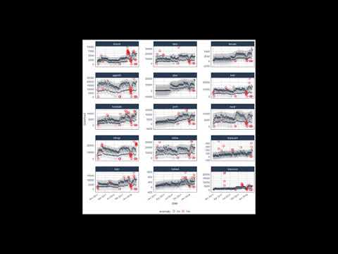 61 |
62 | Check out our entire [Software Intro Series](https://www.youtube.com/watch?v=Gk_HwjhlQJs&list=PLo32uKohmrXsYNhpdwr15W143rX6uMAze) on YouTube!
63 |
64 | ## Installation
65 |
66 | You can install the development version with `devtools` or the most recent CRAN version with `install.packages()`:
67 |
68 | ``` r
69 | # devtools::install_github("business-science/anomalize")
70 | install.packages("anomalize")
71 | ```
72 |
73 | ## How It Works
74 |
75 | `anomalize` has three main functions:
76 |
77 | - `time_decompose()`: Separates the time series into seasonal, trend, and remainder components
78 | - `anomalize()`: Applies anomaly detection methods to the remainder component.
79 | - `time_recompose()`: Calculates limits that separate the "normal" data from the anomalies!
80 |
81 | ## Getting Started
82 |
83 | Load the `anomalize` package. Usually, you will also load the tidyverse as well!
84 |
85 | ```{r, eval = F}
86 | library(anomalize)
87 | library(tidyverse)
88 | # NOTE: timetk now has anomaly detection built in, which
89 | # will get the new functionality going forward.
90 | # Use this script to prevent overwriting legacy anomalize:
91 |
92 | anomalize <- anomalize::anomalize
93 | plot_anomalies <- anomalize::plot_anomalies
94 | ```
95 |
96 |
97 | Next, let's get some data. `anomalize` ships with a data set called `tidyverse_cran_downloads` that contains the daily CRAN download counts for 15 "tidy" packages from 2017-01-01 to 2018-03-01.
98 |
99 | Suppose we want to determine which daily download "counts" are anomalous. It's as easy as using the three main functions (`time_decompose()`, `anomalize()`, and `time_recompose()`) along with a visualization function, `plot_anomalies()`.
100 |
101 | ```{r tidyverse_anoms_1, fig.height=8}
102 | tidyverse_cran_downloads %>%
103 | # Data Manipulation / Anomaly Detection
104 | time_decompose(count, method = "stl") %>%
105 | anomalize(remainder, method = "iqr") %>%
106 | time_recompose() %>%
107 | # Anomaly Visualization
108 | plot_anomalies(time_recomposed = TRUE, ncol = 3, alpha_dots = 0.25) +
109 | ggplot2::labs(title = "Tidyverse Anomalies", subtitle = "STL + IQR Methods")
110 | ```
111 |
112 | Check out the [`anomalize` Quick Start Guide](https://business-science.github.io/anomalize/articles/anomalize_quick_start_guide.html).
113 |
114 | ## Reducing Forecast Error by 32%
115 |
116 | Yes! Anomalize has a new function, `clean_anomalies()`, that can be used to repair time series prior to forecasting. We have a [brand new vignette - Reduce Forecast Error (by 32%) with Cleaned Anomalies](https://business-science.github.io/anomalize/articles/forecasting_with_cleaned_anomalies.html).
117 | ```{r}
118 | tidyverse_cran_downloads %>%
119 | dplyr::filter(package == "lubridate") %>%
120 | dplyr::ungroup() %>%
121 | time_decompose(count) %>%
122 | anomalize(remainder) %>%
123 |
124 | # New function that cleans & repairs anomalies!
125 | clean_anomalies() %>%
126 |
127 | dplyr::select(date, anomaly, observed, observed_cleaned) %>%
128 | dplyr::filter(anomaly == "Yes")
129 | ```
130 |
131 |
132 | ## But Wait, There's More!
133 |
134 | There are a several extra capabilities:
135 |
136 | - `plot_anomaly_decomposition()` for visualizing the inner workings of how algorithm detects anomalies in the "remainder".
137 |
138 | ```{r, fig.height=7}
139 | tidyverse_cran_downloads %>%
140 | dplyr::filter(package == "lubridate") %>%
141 | dplyr::ungroup() %>%
142 | time_decompose(count) %>%
143 | anomalize(remainder) %>%
144 | plot_anomaly_decomposition() +
145 | ggplot2::labs(title = "Decomposition of Anomalized Lubridate Downloads")
146 | ```
147 |
148 | For more information on the `anomalize` methods and the inner workings, please see ["Anomalize Methods" Vignette](https://business-science.github.io/anomalize/articles/anomalize_methods.html).
149 |
150 | ## References
151 |
152 | Several other packages were instrumental in developing anomaly detection methods used in `anomalize`:
153 |
154 | - Twitter's `AnomalyDetection`, which implements decomposition using median spans and the Generalized Extreme Studentized Deviation (GESD) test for anomalies.
155 | - `forecast::tsoutliers()` function, which implements the IQR method.
156 |
157 | # Interested in Learning Anomaly Detection?
158 |
159 | Business Science offers two 1-hour courses on Anomaly Detection:
160 |
161 | - [Learning Lab 18](https://university.business-science.io/p/learning-labs-pro) - Time Series Anomaly Detection with `anomalize`
162 |
163 | - [Learning Lab 17](https://university.business-science.io/p/learning-labs-pro) - Anomaly Detection with `H2O` Machine Learning
164 |
--------------------------------------------------------------------------------
/README.md:
--------------------------------------------------------------------------------
1 |
2 | # Anomalize is being Superceded by Timetk:
3 |
4 | # anomalize
5 |
6 |
7 |
8 | [](https://github.com/business-science/anomalize/actions/workflows/R-CMD-check.yaml)
9 | [](https://lifecycle.r-lib.org/articles/stages.html)
11 | [](https://app.codecov.io/github/business-science/anomalize?branch=master)
13 | [](https://cran.r-project.org/package=anomalize)
14 | 
15 | 
16 |
17 |
18 |
19 |
20 | The `anomalize` package functionality has been superceded by `timetk`.
21 | We suggest you begin to use the `timetk::anomalize()` to benefit from
22 | enhanced functionality to get improvements going forward. [Learn more
23 | about Anomaly Detection with `timetk`
24 | here.](https://business-science.github.io/timetk/articles/TK08_Automatic_Anomaly_Detection.html)
25 |
26 | The original `anomalize` package functionality will be maintained for
27 | previous code bases that use the legacy functionality.
28 |
29 | To prevent the new `timetk` functionality from conflicting with old
30 | `anomalize` code, use these lines:
31 |
32 | ``` r
33 | library(anomalize)
34 |
35 | anomalize <- anomalize::anomalize
36 | plot_anomalies <- anomalize::plot_anomalies
37 | ```
38 |
39 |
40 |
41 | > Tidy anomaly detection
42 |
43 | `anomalize` enables a tidy workflow for detecting anomalies in data. The
44 | main functions are `time_decompose()`, `anomalize()`, and
45 | `time_recompose()`. When combined, it’s quite simple to decompose time
46 | series, detect anomalies, and create bands separating the “normal” data
47 | from the anomalous data.
48 |
49 | ## Anomalize In 2 Minutes (YouTube)
50 |
51 |
53 |
54 | Check out our entire [Software Intro
55 | Series](https://www.youtube.com/watch?v=Gk_HwjhlQJs&list=PLo32uKohmrXsYNhpdwr15W143rX6uMAze)
56 | on YouTube!
57 |
58 | ## Installation
59 |
60 | You can install the development version with `devtools` or the most
61 | recent CRAN version with `install.packages()`:
62 |
63 | ``` r
64 | # devtools::install_github("business-science/anomalize")
65 | install.packages("anomalize")
66 | ```
67 |
68 | ## How It Works
69 |
70 | `anomalize` has three main functions:
71 |
72 | - `time_decompose()`: Separates the time series into seasonal, trend,
73 | and remainder components
74 | - `anomalize()`: Applies anomaly detection methods to the remainder
75 | component.
76 | - `time_recompose()`: Calculates limits that separate the “normal” data
77 | from the anomalies!
78 |
79 | ## Getting Started
80 |
81 | Load the `anomalize` package. Usually, you will also load the tidyverse
82 | as well!
83 |
84 | ``` r
85 | library(anomalize)
86 | library(tidyverse)
87 | # NOTE: timetk now has anomaly detection built in, which
88 | # will get the new functionality going forward.
89 | # Use this script to prevent overwriting legacy anomalize:
90 |
91 | anomalize <- anomalize::anomalize
92 | plot_anomalies <- anomalize::plot_anomalies
93 | ```
94 |
95 | Next, let’s get some data. `anomalize` ships with a data set called
96 | `tidyverse_cran_downloads` that contains the daily CRAN download counts
97 | for 15 “tidy” packages from 2017-01-01 to 2018-03-01.
98 |
99 | Suppose we want to determine which daily download “counts” are
100 | anomalous. It’s as easy as using the three main functions
101 | (`time_decompose()`, `anomalize()`, and `time_recompose()`) along with a
102 | visualization function, `plot_anomalies()`.
103 |
104 | ``` r
105 | tidyverse_cran_downloads %>%
106 | # Data Manipulation / Anomaly Detection
107 | time_decompose(count, method = "stl") %>%
108 | anomalize(remainder, method = "iqr") %>%
109 | time_recompose() %>%
110 | # Anomaly Visualization
111 | plot_anomalies(time_recomposed = TRUE, ncol = 3, alpha_dots = 0.25) +
112 | ggplot2::labs(title = "Tidyverse Anomalies", subtitle = "STL + IQR Methods")
113 | ```
114 |
115 |
61 |
62 | Check out our entire [Software Intro Series](https://www.youtube.com/watch?v=Gk_HwjhlQJs&list=PLo32uKohmrXsYNhpdwr15W143rX6uMAze) on YouTube!
63 |
64 | ## Installation
65 |
66 | You can install the development version with `devtools` or the most recent CRAN version with `install.packages()`:
67 |
68 | ``` r
69 | # devtools::install_github("business-science/anomalize")
70 | install.packages("anomalize")
71 | ```
72 |
73 | ## How It Works
74 |
75 | `anomalize` has three main functions:
76 |
77 | - `time_decompose()`: Separates the time series into seasonal, trend, and remainder components
78 | - `anomalize()`: Applies anomaly detection methods to the remainder component.
79 | - `time_recompose()`: Calculates limits that separate the "normal" data from the anomalies!
80 |
81 | ## Getting Started
82 |
83 | Load the `anomalize` package. Usually, you will also load the tidyverse as well!
84 |
85 | ```{r, eval = F}
86 | library(anomalize)
87 | library(tidyverse)
88 | # NOTE: timetk now has anomaly detection built in, which
89 | # will get the new functionality going forward.
90 | # Use this script to prevent overwriting legacy anomalize:
91 |
92 | anomalize <- anomalize::anomalize
93 | plot_anomalies <- anomalize::plot_anomalies
94 | ```
95 |
96 |
97 | Next, let's get some data. `anomalize` ships with a data set called `tidyverse_cran_downloads` that contains the daily CRAN download counts for 15 "tidy" packages from 2017-01-01 to 2018-03-01.
98 |
99 | Suppose we want to determine which daily download "counts" are anomalous. It's as easy as using the three main functions (`time_decompose()`, `anomalize()`, and `time_recompose()`) along with a visualization function, `plot_anomalies()`.
100 |
101 | ```{r tidyverse_anoms_1, fig.height=8}
102 | tidyverse_cran_downloads %>%
103 | # Data Manipulation / Anomaly Detection
104 | time_decompose(count, method = "stl") %>%
105 | anomalize(remainder, method = "iqr") %>%
106 | time_recompose() %>%
107 | # Anomaly Visualization
108 | plot_anomalies(time_recomposed = TRUE, ncol = 3, alpha_dots = 0.25) +
109 | ggplot2::labs(title = "Tidyverse Anomalies", subtitle = "STL + IQR Methods")
110 | ```
111 |
112 | Check out the [`anomalize` Quick Start Guide](https://business-science.github.io/anomalize/articles/anomalize_quick_start_guide.html).
113 |
114 | ## Reducing Forecast Error by 32%
115 |
116 | Yes! Anomalize has a new function, `clean_anomalies()`, that can be used to repair time series prior to forecasting. We have a [brand new vignette - Reduce Forecast Error (by 32%) with Cleaned Anomalies](https://business-science.github.io/anomalize/articles/forecasting_with_cleaned_anomalies.html).
117 | ```{r}
118 | tidyverse_cran_downloads %>%
119 | dplyr::filter(package == "lubridate") %>%
120 | dplyr::ungroup() %>%
121 | time_decompose(count) %>%
122 | anomalize(remainder) %>%
123 |
124 | # New function that cleans & repairs anomalies!
125 | clean_anomalies() %>%
126 |
127 | dplyr::select(date, anomaly, observed, observed_cleaned) %>%
128 | dplyr::filter(anomaly == "Yes")
129 | ```
130 |
131 |
132 | ## But Wait, There's More!
133 |
134 | There are a several extra capabilities:
135 |
136 | - `plot_anomaly_decomposition()` for visualizing the inner workings of how algorithm detects anomalies in the "remainder".
137 |
138 | ```{r, fig.height=7}
139 | tidyverse_cran_downloads %>%
140 | dplyr::filter(package == "lubridate") %>%
141 | dplyr::ungroup() %>%
142 | time_decompose(count) %>%
143 | anomalize(remainder) %>%
144 | plot_anomaly_decomposition() +
145 | ggplot2::labs(title = "Decomposition of Anomalized Lubridate Downloads")
146 | ```
147 |
148 | For more information on the `anomalize` methods and the inner workings, please see ["Anomalize Methods" Vignette](https://business-science.github.io/anomalize/articles/anomalize_methods.html).
149 |
150 | ## References
151 |
152 | Several other packages were instrumental in developing anomaly detection methods used in `anomalize`:
153 |
154 | - Twitter's `AnomalyDetection`, which implements decomposition using median spans and the Generalized Extreme Studentized Deviation (GESD) test for anomalies.
155 | - `forecast::tsoutliers()` function, which implements the IQR method.
156 |
157 | # Interested in Learning Anomaly Detection?
158 |
159 | Business Science offers two 1-hour courses on Anomaly Detection:
160 |
161 | - [Learning Lab 18](https://university.business-science.io/p/learning-labs-pro) - Time Series Anomaly Detection with `anomalize`
162 |
163 | - [Learning Lab 17](https://university.business-science.io/p/learning-labs-pro) - Anomaly Detection with `H2O` Machine Learning
164 |
--------------------------------------------------------------------------------
/README.md:
--------------------------------------------------------------------------------
1 |
2 | # Anomalize is being Superceded by Timetk:
3 |
4 | # anomalize
5 |
6 |
7 |
8 | [](https://github.com/business-science/anomalize/actions/workflows/R-CMD-check.yaml)
9 | [](https://lifecycle.r-lib.org/articles/stages.html)
11 | [](https://app.codecov.io/github/business-science/anomalize?branch=master)
13 | [](https://cran.r-project.org/package=anomalize)
14 | 
15 | 
16 |
17 |
18 |
19 |
20 | The `anomalize` package functionality has been superceded by `timetk`.
21 | We suggest you begin to use the `timetk::anomalize()` to benefit from
22 | enhanced functionality to get improvements going forward. [Learn more
23 | about Anomaly Detection with `timetk`
24 | here.](https://business-science.github.io/timetk/articles/TK08_Automatic_Anomaly_Detection.html)
25 |
26 | The original `anomalize` package functionality will be maintained for
27 | previous code bases that use the legacy functionality.
28 |
29 | To prevent the new `timetk` functionality from conflicting with old
30 | `anomalize` code, use these lines:
31 |
32 | ``` r
33 | library(anomalize)
34 |
35 | anomalize <- anomalize::anomalize
36 | plot_anomalies <- anomalize::plot_anomalies
37 | ```
38 |
39 |
40 |
41 | > Tidy anomaly detection
42 |
43 | `anomalize` enables a tidy workflow for detecting anomalies in data. The
44 | main functions are `time_decompose()`, `anomalize()`, and
45 | `time_recompose()`. When combined, it’s quite simple to decompose time
46 | series, detect anomalies, and create bands separating the “normal” data
47 | from the anomalous data.
48 |
49 | ## Anomalize In 2 Minutes (YouTube)
50 |
51 |
53 |
54 | Check out our entire [Software Intro
55 | Series](https://www.youtube.com/watch?v=Gk_HwjhlQJs&list=PLo32uKohmrXsYNhpdwr15W143rX6uMAze)
56 | on YouTube!
57 |
58 | ## Installation
59 |
60 | You can install the development version with `devtools` or the most
61 | recent CRAN version with `install.packages()`:
62 |
63 | ``` r
64 | # devtools::install_github("business-science/anomalize")
65 | install.packages("anomalize")
66 | ```
67 |
68 | ## How It Works
69 |
70 | `anomalize` has three main functions:
71 |
72 | - `time_decompose()`: Separates the time series into seasonal, trend,
73 | and remainder components
74 | - `anomalize()`: Applies anomaly detection methods to the remainder
75 | component.
76 | - `time_recompose()`: Calculates limits that separate the “normal” data
77 | from the anomalies!
78 |
79 | ## Getting Started
80 |
81 | Load the `anomalize` package. Usually, you will also load the tidyverse
82 | as well!
83 |
84 | ``` r
85 | library(anomalize)
86 | library(tidyverse)
87 | # NOTE: timetk now has anomaly detection built in, which
88 | # will get the new functionality going forward.
89 | # Use this script to prevent overwriting legacy anomalize:
90 |
91 | anomalize <- anomalize::anomalize
92 | plot_anomalies <- anomalize::plot_anomalies
93 | ```
94 |
95 | Next, let’s get some data. `anomalize` ships with a data set called
96 | `tidyverse_cran_downloads` that contains the daily CRAN download counts
97 | for 15 “tidy” packages from 2017-01-01 to 2018-03-01.
98 |
99 | Suppose we want to determine which daily download “counts” are
100 | anomalous. It’s as easy as using the three main functions
101 | (`time_decompose()`, `anomalize()`, and `time_recompose()`) along with a
102 | visualization function, `plot_anomalies()`.
103 |
104 | ``` r
105 | tidyverse_cran_downloads %>%
106 | # Data Manipulation / Anomaly Detection
107 | time_decompose(count, method = "stl") %>%
108 | anomalize(remainder, method = "iqr") %>%
109 | time_recompose() %>%
110 | # Anomaly Visualization
111 | plot_anomalies(time_recomposed = TRUE, ncol = 3, alpha_dots = 0.25) +
112 | ggplot2::labs(title = "Tidyverse Anomalies", subtitle = "STL + IQR Methods")
113 | ```
114 |
115 |  116 |
117 | Check out the [`anomalize` Quick Start
118 | Guide](https://business-science.github.io/anomalize/articles/anomalize_quick_start_guide.html).
119 |
120 | ## Reducing Forecast Error by 32%
121 |
122 | Yes! Anomalize has a new function, `clean_anomalies()`, that can be used
123 | to repair time series prior to forecasting. We have a [brand new
124 | vignette - Reduce Forecast Error (by 32%) with Cleaned
125 | Anomalies](https://business-science.github.io/anomalize/articles/forecasting_with_cleaned_anomalies.html).
126 |
127 | ``` r
128 | tidyverse_cran_downloads %>%
129 | dplyr::filter(package == "lubridate") %>%
130 | dplyr::ungroup() %>%
131 | time_decompose(count) %>%
132 | anomalize(remainder) %>%
133 |
134 | # New function that cleans & repairs anomalies!
135 | clean_anomalies() %>%
136 |
137 | dplyr::select(date, anomaly, observed, observed_cleaned) %>%
138 | dplyr::filter(anomaly == "Yes")
139 | #> # A time tibble: 19 × 4
140 | #> # Index: date
141 | #> date anomaly observed observed_cleaned
142 | #>
143 | #> 1 2017-01-12 Yes -1.14e-13 3522.
144 | #> 2 2017-04-19 Yes 8.55e+ 3 5202.
145 | #> 3 2017-09-01 Yes 3.98e-13 4137.
146 | #> 4 2017-09-07 Yes 9.49e+ 3 4871.
147 | #> 5 2017-10-30 Yes 1.20e+ 4 6413.
148 | #> 6 2017-11-13 Yes 1.03e+ 4 6641.
149 | #> 7 2017-11-14 Yes 1.15e+ 4 7250.
150 | #> 8 2017-12-04 Yes 1.03e+ 4 6519.
151 | #> 9 2017-12-05 Yes 1.06e+ 4 7099.
152 | #> 10 2017-12-27 Yes 3.69e+ 3 7073.
153 | #> 11 2018-01-01 Yes 1.87e+ 3 6418.
154 | #> 12 2018-01-05 Yes -5.68e-14 6293.
155 | #> 13 2018-01-13 Yes 7.64e+ 3 4141.
156 | #> 14 2018-02-07 Yes 1.19e+ 4 8539.
157 | #> 15 2018-02-08 Yes 1.17e+ 4 8237.
158 | #> 16 2018-02-09 Yes -5.68e-14 7780.
159 | #> 17 2018-02-10 Yes 0 5478.
160 | #> 18 2018-02-23 Yes -5.68e-14 8519.
161 | #> 19 2018-02-24 Yes 0 6218.
162 | ```
163 |
164 | ## But Wait, There’s More!
165 |
166 | There are a several extra capabilities:
167 |
168 | - `plot_anomaly_decomposition()` for visualizing the inner workings of
169 | how algorithm detects anomalies in the “remainder”.
170 |
171 | ``` r
172 | tidyverse_cran_downloads %>%
173 | dplyr::filter(package == "lubridate") %>%
174 | dplyr::ungroup() %>%
175 | time_decompose(count) %>%
176 | anomalize(remainder) %>%
177 | plot_anomaly_decomposition() +
178 | ggplot2::labs(title = "Decomposition of Anomalized Lubridate Downloads")
179 | ```
180 |
181 |
116 |
117 | Check out the [`anomalize` Quick Start
118 | Guide](https://business-science.github.io/anomalize/articles/anomalize_quick_start_guide.html).
119 |
120 | ## Reducing Forecast Error by 32%
121 |
122 | Yes! Anomalize has a new function, `clean_anomalies()`, that can be used
123 | to repair time series prior to forecasting. We have a [brand new
124 | vignette - Reduce Forecast Error (by 32%) with Cleaned
125 | Anomalies](https://business-science.github.io/anomalize/articles/forecasting_with_cleaned_anomalies.html).
126 |
127 | ``` r
128 | tidyverse_cran_downloads %>%
129 | dplyr::filter(package == "lubridate") %>%
130 | dplyr::ungroup() %>%
131 | time_decompose(count) %>%
132 | anomalize(remainder) %>%
133 |
134 | # New function that cleans & repairs anomalies!
135 | clean_anomalies() %>%
136 |
137 | dplyr::select(date, anomaly, observed, observed_cleaned) %>%
138 | dplyr::filter(anomaly == "Yes")
139 | #> # A time tibble: 19 × 4
140 | #> # Index: date
141 | #> date anomaly observed observed_cleaned
142 | #>
143 | #> 1 2017-01-12 Yes -1.14e-13 3522.
144 | #> 2 2017-04-19 Yes 8.55e+ 3 5202.
145 | #> 3 2017-09-01 Yes 3.98e-13 4137.
146 | #> 4 2017-09-07 Yes 9.49e+ 3 4871.
147 | #> 5 2017-10-30 Yes 1.20e+ 4 6413.
148 | #> 6 2017-11-13 Yes 1.03e+ 4 6641.
149 | #> 7 2017-11-14 Yes 1.15e+ 4 7250.
150 | #> 8 2017-12-04 Yes 1.03e+ 4 6519.
151 | #> 9 2017-12-05 Yes 1.06e+ 4 7099.
152 | #> 10 2017-12-27 Yes 3.69e+ 3 7073.
153 | #> 11 2018-01-01 Yes 1.87e+ 3 6418.
154 | #> 12 2018-01-05 Yes -5.68e-14 6293.
155 | #> 13 2018-01-13 Yes 7.64e+ 3 4141.
156 | #> 14 2018-02-07 Yes 1.19e+ 4 8539.
157 | #> 15 2018-02-08 Yes 1.17e+ 4 8237.
158 | #> 16 2018-02-09 Yes -5.68e-14 7780.
159 | #> 17 2018-02-10 Yes 0 5478.
160 | #> 18 2018-02-23 Yes -5.68e-14 8519.
161 | #> 19 2018-02-24 Yes 0 6218.
162 | ```
163 |
164 | ## But Wait, There’s More!
165 |
166 | There are a several extra capabilities:
167 |
168 | - `plot_anomaly_decomposition()` for visualizing the inner workings of
169 | how algorithm detects anomalies in the “remainder”.
170 |
171 | ``` r
172 | tidyverse_cran_downloads %>%
173 | dplyr::filter(package == "lubridate") %>%
174 | dplyr::ungroup() %>%
175 | time_decompose(count) %>%
176 | anomalize(remainder) %>%
177 | plot_anomaly_decomposition() +
178 | ggplot2::labs(title = "Decomposition of Anomalized Lubridate Downloads")
179 | ```
180 |
181 |  182 |
183 | For more information on the `anomalize` methods and the inner workings,
184 | please see [“Anomalize Methods”
185 | Vignette](https://business-science.github.io/anomalize/articles/anomalize_methods.html).
186 |
187 | ## References
188 |
189 | Several other packages were instrumental in developing anomaly detection
190 | methods used in `anomalize`:
191 |
192 | - Twitter’s `AnomalyDetection`, which implements decomposition using
193 | median spans and the Generalized Extreme Studentized Deviation (GESD)
194 | test for anomalies.
195 | - `forecast::tsoutliers()` function, which implements the IQR method.
196 |
197 | # Interested in Learning Anomaly Detection?
198 |
199 | Business Science offers two 1-hour courses on Anomaly Detection:
200 |
201 | - [Learning Lab
202 | 18](https://university.business-science.io/p/learning-labs-pro) - Time
203 | Series Anomaly Detection with `anomalize`
204 |
205 | - [Learning Lab
206 | 17](https://university.business-science.io/p/learning-labs-pro) -
207 | Anomaly Detection with `H2O` Machine Learning
208 |
--------------------------------------------------------------------------------
/_pkgdown.yml:
--------------------------------------------------------------------------------
1 | url: https://business-science.github.io/anomalize/
2 | template:
3 | bootstrap: 5
4 | bootswatch: flatly
5 | params:
6 | ganalytics: UA-76139189-1
7 | navbar:
8 | bg: primary
9 | title: timetk
10 | left:
11 | - icon: fa-home
12 | href: index.html
13 | - text: Start
14 | href: articles/anomalize_quick_start_guide.html
15 | - text: Articles
16 | href: articles/index.html
17 | - text: API
18 | href: reference/index.html
19 | menu:
20 | - text: API Functions
21 | - icon: fa-home
22 | text: Function Reference
23 | href: reference/index.html
24 | - text: '---'
25 | - text: Change History
26 | - text: News
27 | href: news/index.html
28 | right:
29 | - icon: fa-github
30 | href: https://github.com/business-science/timetk
31 | reference:
32 | - title: General
33 | contents: tidyverse_cran_downloads
34 | - title: Anomalize workflow
35 | desc: __The main functions used to anomalize time series data.__
36 | contents:
37 | - starts_with("time_decompose")
38 | - anomalize
39 | - starts_with("time_recompose")
40 | - clean_anomalies
41 | - title: Visualization functions
42 | desc: __Plotting utilities for visualizing anomalies.__
43 | contents: starts_with("plot_")
44 | - title: Frequency and trend
45 | desc: __Working with the frequency, trend, and time scale.__
46 | contents:
47 | - ends_with("frequency")
48 | - ends_with("trend")
49 | - contains("time_scale")
50 | - title: Methods
51 | desc: __Functions that power the main anomalize functions.__
52 | contents:
53 | - starts_with("decompose_")
54 | - iqr
55 | - gesd
56 | - title: Misc
57 | desc: __Miscellaneous functions and utilites.__
58 | contents:
59 | - starts_with("prep_")
60 | - time_apply
61 |
62 |
--------------------------------------------------------------------------------
/anomalize.Rproj:
--------------------------------------------------------------------------------
1 | Version: 1.0
2 |
3 | RestoreWorkspace: Default
4 | SaveWorkspace: Default
5 | AlwaysSaveHistory: Default
6 |
7 | EnableCodeIndexing: Yes
8 | UseSpacesForTab: Yes
9 | NumSpacesForTab: 4
10 | Encoding: UTF-8
11 |
12 | RnwWeave: Sweave
13 | LaTeX: pdfLaTeX
14 |
15 | AutoAppendNewline: Yes
16 | StripTrailingWhitespace: Yes
17 |
18 | BuildType: Package
19 | PackageUseDevtools: Yes
20 | PackageInstallArgs: --no-multiarch --with-keep.source
21 | PackageRoxygenize: rd,collate,namespace
22 |
23 | UseNativePipeOperator: No
24 |
25 | SpellingDictionary: en_US
26 |
--------------------------------------------------------------------------------
/codecov.yml:
--------------------------------------------------------------------------------
1 | comment: false
2 |
3 | coverage:
4 | status:
5 | project:
6 | default:
7 | target: auto
8 | threshold: 1%
9 | patch:
10 | default:
11 | target: auto
12 | threshold: 1%
13 |
--------------------------------------------------------------------------------
/cran-comments.md:
--------------------------------------------------------------------------------
1 | ## Test environments
2 | * local OS X install, R 3.5.3
3 | * ubuntu 14.04 (on travis-ci), R 3.5.3
4 | * win-builder (devel and release)
5 |
6 | ## R CMD check results
7 |
8 | 0 errors | 0 warnings | 0 notes
9 |
10 | * This is a new release.
11 |
--------------------------------------------------------------------------------
/data-raw/tidyverse_cran_downloads.R:
--------------------------------------------------------------------------------
1 | library(dplyr)
2 | library(tibbletime)
3 | library(cranlogs)
4 |
5 | pkgs <- c(
6 | "tidyr", "lubridate", "dplyr",
7 | "broom", "tidyquant", "tidytext",
8 | "ggplot2", "purrr", "glue",
9 | "stringr", "forcats", "knitr",
10 | "readr", "tibble", "tidyverse"
11 | )
12 |
13 | tidyverse_cran_downloads <- cran_downloads(pkgs, from = "2017-01-01", to = "2018-03-01") %>%
14 | group_by(package) %>%
15 | as_tbl_time(date)
16 |
17 | tidyverse_cran_downloads
18 |
--------------------------------------------------------------------------------
/data/tidyverse_cran_downloads.rda:
--------------------------------------------------------------------------------
https://raw.githubusercontent.com/business-science/anomalize/f5d37063c83bb0b4b4256aed81dead489414b89c/data/tidyverse_cran_downloads.rda
--------------------------------------------------------------------------------
/man/anomalize-package.Rd:
--------------------------------------------------------------------------------
1 | % Generated by roxygen2: do not edit by hand
2 | % Please edit documentation in R/anomalize-package.R
3 | \docType{package}
4 | \name{anomalize-package}
5 | \alias{anomalize-package}
6 | \alias{_PACKAGE}
7 | \title{anomalize: Tidy Anomaly Detection}
8 | \description{
9 | The 'anomalize' package enables a "tidy" workflow for detecting anomalies in data.
10 | The main functions are time_decompose(), anomalize(), and time_recompose().
11 | When combined, it's quite simple to decompose time series, detect anomalies,
12 | and create bands separating the "normal" data from the anomalous data at scale (i.e. for multiple time series).
13 | Time series decomposition is used to remove trend and seasonal components via the time_decompose() function
14 | and methods include seasonal decomposition of time series by Loess and
15 | seasonal decomposition by piecewise medians. The anomalize() function implements
16 | two methods for anomaly detection of residuals including using an inner quartile range
17 | and generalized extreme studentized deviation. These methods are based on
18 | those used in the \code{forecast} package and the Twitter \code{AnomalyDetection} package.
19 | Refer to the associated functions for specific references for these methods.
20 |
21 | To learn more about \code{anomalize}, start with the vignettes:
22 | \code{browseVignettes(package = "anomalize")}
23 | }
24 | \seealso{
25 | Useful links:
26 | \itemize{
27 | \item \url{https://business-science.github.io/anomalize/}
28 | \item \url{https://github.com/business-science/anomalize}
29 | \item Report bugs at \url{https://github.com/business-science/anomalize/issues}
30 | }
31 |
32 | }
33 | \author{
34 | \strong{Maintainer}: Matt Dancho \email{mdancho@business-science.io}
35 |
36 | Authors:
37 | \itemize{
38 | \item Davis Vaughan \email{dvaughan@business-science.io}
39 | }
40 |
41 | }
42 | \keyword{internal}
43 |
--------------------------------------------------------------------------------
/man/anomalize.Rd:
--------------------------------------------------------------------------------
1 | % Generated by roxygen2: do not edit by hand
2 | % Please edit documentation in R/anomalize.R
3 | \name{anomalize}
4 | \alias{anomalize}
5 | \title{Detect anomalies using the tidyverse}
6 | \usage{
7 | anomalize(
8 | data,
9 | target,
10 | method = c("iqr", "gesd"),
11 | alpha = 0.05,
12 | max_anoms = 0.2,
13 | verbose = FALSE
14 | )
15 | }
16 | \arguments{
17 | \item{data}{A \code{tibble} or \code{tbl_time} object.}
18 |
19 | \item{target}{A column to apply the function to}
20 |
21 | \item{method}{The anomaly detection method. One of \code{"iqr"} or \code{"gesd"}.
22 | The IQR method is faster at the expense of possibly not being quite as accurate.
23 | The GESD method has the best properties for outlier detection, but is loop-based
24 | and therefore a bit slower.}
25 |
26 | \item{alpha}{Controls the width of the "normal" range.
27 | Lower values are more conservative while higher values are less prone
28 | to incorrectly classifying "normal" observations.}
29 |
30 | \item{max_anoms}{The maximum percent of anomalies permitted to be identified.}
31 |
32 | \item{verbose}{A boolean. If \code{TRUE}, will return a list containing useful information
33 | about the anomalies. If \code{FALSE}, just returns the data expanded with the anomalies and
34 | the lower (l1) and upper (l2) bounds.}
35 | }
36 | \value{
37 | Returns a \code{tibble} / \code{tbl_time} object or list depending on the value of \code{verbose}.
38 | }
39 | \description{
40 | The \code{anomalize()} function is used to detect outliers in a distribution
41 | with no trend or seasonality present. It takes the output of \code{\link[=time_decompose]{time_decompose()}},
42 | which has be de-trended and applies anomaly detection methods to identify outliers.
43 | }
44 | \details{
45 | The return has three columns:
46 | "remainder_l1" (lower limit for anomalies), "remainder_l2" (upper limit for
47 | anomalies), and "anomaly" (Yes/No).
48 |
49 | Use \code{\link[=time_decompose]{time_decompose()}} to decompose a time series prior to performing
50 | anomaly detection with \code{anomalize()}. Typically, \code{anomalize()} is
51 | performed on the "remainder" of the time series decomposition.
52 |
53 | For non-time series data (data without trend), the \code{anomalize()} function can
54 | be used without time series decomposition.
55 |
56 | The \code{anomalize()} function uses two methods for outlier detection
57 | each with benefits.
58 |
59 | \strong{IQR}:
60 |
61 | The IQR Method uses an innerquartile range of 25\% and 75\% to establish a baseline distribution around
62 | the median. With the default \code{alpha = 0.05}, the limits are established by expanding
63 | the 25/75 baseline by an IQR Factor of 3 (3X). The IQR Factor = 0.15 / alpha (hense 3X with alpha = 0.05).
64 | To increase the IQR Factor controling the limits, decrease the alpha, which makes
65 | it more difficult to be an outlier. Increase alpha to make it easier to be an outlier.
66 |
67 | The IQR method is used in \href{https://github.com/robjhyndman/forecast}{\code{forecast::tsoutliers()}}.
68 |
69 | \strong{GESD}:
70 |
71 | The GESD Method (Generlized Extreme Studentized Deviate Test) progressively
72 | eliminates outliers using a Student's T-Test comparing the test statistic to a critical value.
73 | Each time an outlier is removed, the test statistic is updated. Once test statistic
74 | drops below the critical value, all outliers are considered removed. Because this method
75 | involves continuous updating via a loop, it is slower than the IQR method. However, it
76 | tends to be the best performing method for outlier removal.
77 |
78 | The GESD method is used in \href{https://github.com/twitter/AnomalyDetection}{\code{AnomalyDection::AnomalyDetectionTs()}}.
79 | }
80 | \examples{
81 | \dontrun{
82 | library(dplyr)
83 |
84 | # Needed to pass CRAN check / This is loaded by default
85 | set_time_scale_template(time_scale_template())
86 |
87 | tidyverse_cran_downloads \%>\%
88 | time_decompose(count, method = "stl") \%>\%
89 | anomalize(remainder, method = "iqr")
90 | }
91 |
92 | }
93 | \references{
94 | \enumerate{
95 | \item \href{https://stats.stackexchange.com/questions/69874/how-to-correct-outliers-once-detected-for-time-series-data-forecasting}{How to correct outliers once detected for time series data forecasting? Cross Validated, https://stats.stackexchange.com}
96 | \item \href{https://stats.stackexchange.com/questions/1142/simple-algorithm-for-online-outlier-detection-of-a-generic-time-series?}{Cross Validated: Simple algorithm for online outlier detection of a generic time series. Cross Validated, https://stats.stackexchange.com}
97 | \item \href{https://www.usenix.org/system/files/conference/hotcloud14/hotcloud14-vallis.pdf}{Owen S. Vallis, Jordan Hochenbaum and Arun Kejariwal (2014). A Novel Technique for Long-Term Anomaly Detection in the Cloud. Twitter Inc.}
98 | \item \href{https://github.com/twitter/AnomalyDetection}{Owen S. Vallis, Jordan Hochenbaum and Arun Kejariwal (2014). AnomalyDetection: Anomaly Detection Using Seasonal Hybrid Extreme Studentized Deviate Test. R package version 1.0.}
99 | \item Alex T.C. Lau (November/December 2015). GESD - A Robust and Effective Technique for Dealing with Multiple Outliers. ASTM Standardization News. www.astm.org/sn
100 | }
101 | }
102 | \seealso{
103 | Anomaly Detection Methods (Powers \code{anomalize})
104 | \itemize{
105 | \item \code{\link[=iqr]{iqr()}}
106 | \item \code{\link[=gesd]{gesd()}}
107 | }
108 |
109 | Time Series Anomaly Detection Functions (anomaly detection workflow):
110 | \itemize{
111 | \item \code{\link[=time_decompose]{time_decompose()}}
112 | \item \code{\link[=time_recompose]{time_recompose()}}
113 | }
114 | }
115 |
--------------------------------------------------------------------------------
/man/anomalize_methods.Rd:
--------------------------------------------------------------------------------
1 | % Generated by roxygen2: do not edit by hand
2 | % Please edit documentation in R/anomalize_methods.R
3 | \name{anomalize_methods}
4 | \alias{anomalize_methods}
5 | \alias{iqr}
6 | \alias{gesd}
7 | \title{Methods that power anomalize()}
8 | \usage{
9 | iqr(x, alpha = 0.05, max_anoms = 0.2, verbose = FALSE)
10 |
11 | gesd(x, alpha = 0.05, max_anoms = 0.2, verbose = FALSE)
12 | }
13 | \arguments{
14 | \item{x}{A vector of numeric data.}
15 |
16 | \item{alpha}{Controls the width of the "normal" range.
17 | Lower values are more conservative while higher values are less prone
18 | to incorrectly classifying "normal" observations.}
19 |
20 | \item{max_anoms}{The maximum percent of anomalies permitted to be identified.}
21 |
22 | \item{verbose}{A boolean. If \code{TRUE}, will return a list containing useful information
23 | about the anomalies. If \code{FALSE}, just returns a vector of "Yes" / "No" values.}
24 | }
25 | \value{
26 | Returns character vector or list depending on the value of \code{verbose}.
27 | }
28 | \description{
29 | Methods that power anomalize()
30 | }
31 | \examples{
32 |
33 | set.seed(100)
34 | x <- rnorm(100)
35 | idx_outliers <- sample(100, size = 5)
36 | x[idx_outliers] <- x[idx_outliers] + 10
37 |
38 | iqr(x, alpha = 0.05, max_anoms = 0.2)
39 | iqr(x, alpha = 0.05, max_anoms = 0.2, verbose = TRUE)
40 |
41 | gesd(x, alpha = 0.05, max_anoms = 0.2)
42 | gesd(x, alpha = 0.05, max_anoms = 0.2, verbose = TRUE)
43 |
44 |
45 | }
46 | \references{
47 | \itemize{
48 | \item The IQR method is used in \href{https://github.com/robjhyndman/forecast/blob/master/R/clean.R}{\code{forecast::tsoutliers()}}
49 | \item The GESD method is used in Twitter's \href{https://github.com/twitter/AnomalyDetection}{\code{AnomalyDetection}} package and is also available as a function in \href{https://github.com/raunakms/GESD/blob/master/runGESD.R}{@raunakms's GESD method}
50 | }
51 | }
52 | \seealso{
53 | \code{\link[=anomalize]{anomalize()}}
54 | }
55 |
--------------------------------------------------------------------------------
/man/clean_anomalies.Rd:
--------------------------------------------------------------------------------
1 | % Generated by roxygen2: do not edit by hand
2 | % Please edit documentation in R/anomalize_clean.R
3 | \name{clean_anomalies}
4 | \alias{clean_anomalies}
5 | \title{Clean anomalies from anomalized data}
6 | \usage{
7 | clean_anomalies(data)
8 | }
9 | \arguments{
10 | \item{data}{A \code{tibble} or \code{tbl_time} object.}
11 | }
12 | \value{
13 | Returns a \code{tibble} / \code{tbl_time} object with a new column "observed_cleaned".
14 | }
15 | \description{
16 | Clean anomalies from anomalized data
17 | }
18 | \details{
19 | The \code{clean_anomalies()} function is used to replace outliers with the seasonal and trend component.
20 | This is often desirable when forecasting with noisy time series data to improve trend detection.
21 |
22 | To clean anomalies, the input data must be detrended with \code{time_decompose()} and anomalized with \code{anomalize()}.
23 | The data can also be recomposed with \code{time_recompose()}.
24 | }
25 | \examples{
26 |
27 | \dontrun{
28 | library(dplyr)
29 |
30 | # Needed to pass CRAN check / This is loaded by default
31 | set_time_scale_template(time_scale_template())
32 |
33 | data(tidyverse_cran_downloads)
34 |
35 | tidyverse_cran_downloads \%>\%
36 | time_decompose(count, method = "stl") \%>\%
37 | anomalize(remainder, method = "iqr") \%>\%
38 | clean_anomalies()
39 | }
40 |
41 | }
42 | \seealso{
43 | Time Series Anomaly Detection Functions (anomaly detection workflow):
44 | \itemize{
45 | \item \code{\link[=time_decompose]{time_decompose()}}
46 | \item \code{\link[=anomalize]{anomalize()}}
47 | \item \code{\link[=time_recompose]{time_recompose()}}
48 | }
49 | }
50 |
--------------------------------------------------------------------------------
/man/decompose_methods.Rd:
--------------------------------------------------------------------------------
1 | % Generated by roxygen2: do not edit by hand
2 | % Please edit documentation in R/time_decompose_methods.R
3 | \name{decompose_methods}
4 | \alias{decompose_methods}
5 | \alias{decompose_twitter}
6 | \alias{decompose_stl}
7 | \title{Methods that power time_decompose()}
8 | \usage{
9 | decompose_twitter(
10 | data,
11 | target,
12 | frequency = "auto",
13 | trend = "auto",
14 | message = TRUE
15 | )
16 |
17 | decompose_stl(data, target, frequency = "auto", trend = "auto", message = TRUE)
18 | }
19 | \arguments{
20 | \item{data}{A \code{tibble} or \code{tbl_time} object.}
21 |
22 | \item{target}{A column to apply the function to}
23 |
24 | \item{frequency}{Controls the seasonal adjustment (removal of seasonality).
25 | Input can be either "auto", a time-based definition (e.g. "1 week"),
26 | or a numeric number of observations per frequency (e.g. 10).
27 | Refer to \code{\link[=time_frequency]{time_frequency()}}.}
28 |
29 | \item{trend}{Controls the trend component
30 | For stl, the trend controls the sensitivity of the lowess smoother, which is used to remove the remainder.
31 | For twitter, the trend controls the period width of the median, which are used to remove the trend and center the remainder.}
32 |
33 | \item{message}{A boolean. If \code{TRUE}, will output information related to \code{tbl_time} conversions, frequencies,
34 | and trend / median spans (if applicable).}
35 | }
36 | \value{
37 | A \code{tbl_time} object containing the time series decomposition.
38 | }
39 | \description{
40 | Methods that power time_decompose()
41 | }
42 | \examples{
43 |
44 | library(dplyr)
45 |
46 | tidyverse_cran_downloads \%>\%
47 | ungroup() \%>\%
48 | filter(package == "tidyquant") \%>\%
49 | decompose_stl(count)
50 |
51 |
52 | }
53 | \references{
54 | \itemize{
55 | \item The "twitter" method is used in Twitter's \href{https://github.com/twitter/AnomalyDetection}{\code{AnomalyDetection} package}
56 | }
57 | }
58 | \seealso{
59 | \code{\link[=time_decompose]{time_decompose()}}
60 | }
61 |
--------------------------------------------------------------------------------
/man/figures/README-tidyverse_anoms_1-1.png:
--------------------------------------------------------------------------------
https://raw.githubusercontent.com/business-science/anomalize/f5d37063c83bb0b4b4256aed81dead489414b89c/man/figures/README-tidyverse_anoms_1-1.png
--------------------------------------------------------------------------------
/man/figures/README-unnamed-chunk-3-1.png:
--------------------------------------------------------------------------------
https://raw.githubusercontent.com/business-science/anomalize/f5d37063c83bb0b4b4256aed81dead489414b89c/man/figures/README-unnamed-chunk-3-1.png
--------------------------------------------------------------------------------
/man/figures/logo.png:
--------------------------------------------------------------------------------
https://raw.githubusercontent.com/business-science/anomalize/f5d37063c83bb0b4b4256aed81dead489414b89c/man/figures/logo.png
--------------------------------------------------------------------------------
/man/plot_anomalies.Rd:
--------------------------------------------------------------------------------
1 | % Generated by roxygen2: do not edit by hand
2 | % Please edit documentation in R/plot_anomalies.R
3 | \name{plot_anomalies}
4 | \alias{plot_anomalies}
5 | \title{Visualize the anomalies in one or multiple time series}
6 | \usage{
7 | plot_anomalies(
8 | data,
9 | time_recomposed = FALSE,
10 | ncol = 1,
11 | color_no = "#2c3e50",
12 | color_yes = "#e31a1c",
13 | fill_ribbon = "grey70",
14 | alpha_dots = 1,
15 | alpha_circles = 1,
16 | alpha_ribbon = 1,
17 | size_dots = 1.5,
18 | size_circles = 4
19 | )
20 | }
21 | \arguments{
22 | \item{data}{A \code{tibble} or \code{tbl_time} object.}
23 |
24 | \item{time_recomposed}{A boolean. If \code{TRUE}, will use the \code{time_recompose()} bands to
25 | place bands as approximate limits around the "normal" data.}
26 |
27 | \item{ncol}{Number of columns to display. Set to 1 for single column by default.}
28 |
29 | \item{color_no}{Color for non-anomalous data.}
30 |
31 | \item{color_yes}{Color for anomalous data.}
32 |
33 | \item{fill_ribbon}{Fill color for the time_recomposed ribbon.}
34 |
35 | \item{alpha_dots}{Controls the transparency of the dots. Reduce when too many dots on the screen.}
36 |
37 | \item{alpha_circles}{Controls the transparency of the circles that identify anomalies.}
38 |
39 | \item{alpha_ribbon}{Controls the transparency of the time_recomposed ribbon.}
40 |
41 | \item{size_dots}{Controls the size of the dots.}
42 |
43 | \item{size_circles}{Controls the size of the circles that identify anomalies.}
44 | }
45 | \value{
46 | Returns a \code{ggplot} object.
47 | }
48 | \description{
49 | Visualize the anomalies in one or multiple time series
50 | }
51 | \details{
52 | Plotting function for visualizing anomalies on one or more time series.
53 | Multiple time series must be grouped using \code{dplyr::group_by()}.
54 | }
55 | \examples{
56 |
57 | \dontrun{
58 | library(dplyr)
59 | library(ggplot2)
60 |
61 |
62 | #### SINGLE TIME SERIES ####
63 | tidyverse_cran_downloads \%>\%
64 | filter(package == "tidyquant") \%>\%
65 | ungroup() \%>\%
66 | time_decompose(count, method = "stl") \%>\%
67 | anomalize(remainder, method = "iqr") \%>\%
68 | time_recompose() \%>\%
69 | plot_anomalies(time_recomposed = TRUE)
70 |
71 |
72 | #### MULTIPLE TIME SERIES ####
73 | tidyverse_cran_downloads \%>\%
74 | time_decompose(count, method = "stl") \%>\%
75 | anomalize(remainder, method = "iqr") \%>\%
76 | time_recompose() \%>\%
77 | plot_anomalies(time_recomposed = TRUE, ncol = 3)
78 | }
79 |
80 | }
81 | \seealso{
82 | \code{\link[=plot_anomaly_decomposition]{plot_anomaly_decomposition()}}
83 | }
84 |
--------------------------------------------------------------------------------
/man/plot_anomaly_decomposition.Rd:
--------------------------------------------------------------------------------
1 | % Generated by roxygen2: do not edit by hand
2 | % Please edit documentation in R/plot_anomaly_decomposition.R
3 | \name{plot_anomaly_decomposition}
4 | \alias{plot_anomaly_decomposition}
5 | \title{Visualize the time series decomposition with anomalies shown}
6 | \usage{
7 | plot_anomaly_decomposition(
8 | data,
9 | ncol = 1,
10 | color_no = "#2c3e50",
11 | color_yes = "#e31a1c",
12 | alpha_dots = 1,
13 | alpha_circles = 1,
14 | size_dots = 1.5,
15 | size_circles = 4,
16 | strip.position = "right"
17 | )
18 | }
19 | \arguments{
20 | \item{data}{A \code{tibble} or \code{tbl_time} object.}
21 |
22 | \item{ncol}{Number of columns to display. Set to 1 for single column by default.}
23 |
24 | \item{color_no}{Color for non-anomalous data.}
25 |
26 | \item{color_yes}{Color for anomalous data.}
27 |
28 | \item{alpha_dots}{Controls the transparency of the dots. Reduce when too many dots on the screen.}
29 |
30 | \item{alpha_circles}{Controls the transparency of the circles that identify anomalies.}
31 |
32 | \item{size_dots}{Controls the size of the dots.}
33 |
34 | \item{size_circles}{Controls the size of the circles that identify anomalies.}
35 |
36 | \item{strip.position}{Controls the placement of the strip that identifies the time series decomposition components.}
37 | }
38 | \value{
39 | Returns a \code{ggplot} object.
40 | }
41 | \description{
42 | Visualize the time series decomposition with anomalies shown
43 | }
44 | \details{
45 | The first step in reviewing the anomaly detection process is to evaluate
46 | a single times series to observe how the algorithm is selecting anomalies.
47 | The \code{plot_anomaly_decomposition()} function is used to gain
48 | an understanding as to whether or not the method is detecting anomalies correctly and
49 | whether or not parameters such as decomposition method, anomalize method,
50 | alpha, frequency, and so on should be adjusted.
51 | }
52 | \examples{
53 |
54 | library(dplyr)
55 | library(ggplot2)
56 |
57 | tidyverse_cran_downloads \%>\%
58 | filter(package == "tidyquant") \%>\%
59 | ungroup() \%>\%
60 | time_decompose(count, method = "stl") \%>\%
61 | anomalize(remainder, method = "iqr") \%>\%
62 | plot_anomaly_decomposition()
63 |
64 | }
65 | \seealso{
66 | \code{\link[=plot_anomalies]{plot_anomalies()}}
67 | }
68 |
--------------------------------------------------------------------------------
/man/prep_tbl_time.Rd:
--------------------------------------------------------------------------------
1 | % Generated by roxygen2: do not edit by hand
2 | % Please edit documentation in R/prep_tbl_time.R
3 | \name{prep_tbl_time}
4 | \alias{prep_tbl_time}
5 | \title{Automatically create tibbletime objects from tibbles}
6 | \usage{
7 | prep_tbl_time(data, message = FALSE)
8 | }
9 | \arguments{
10 | \item{data}{A \code{tibble}.}
11 |
12 | \item{message}{A boolean. If \code{TRUE}, returns a message indicating any
13 | conversion details important to know during the conversion to \code{tbl_time} class.}
14 | }
15 | \value{
16 | Returns a \code{tibbletime} object of class \code{tbl_time}.
17 | }
18 | \description{
19 | Automatically create tibbletime objects from tibbles
20 | }
21 | \details{
22 | Detects a date or datetime index column and automatically
23 | }
24 | \examples{
25 |
26 | library(dplyr)
27 | library(tibbletime)
28 |
29 | data_tbl <- tibble(
30 | date = seq.Date(from = as.Date("2018-01-01"), by = "day", length.out = 10),
31 | value = rnorm(10)
32 | )
33 |
34 | prep_tbl_time(data_tbl)
35 |
36 | }
37 |
--------------------------------------------------------------------------------
/man/tidyverse_cran_downloads.Rd:
--------------------------------------------------------------------------------
1 | % Generated by roxygen2: do not edit by hand
2 | % Please edit documentation in R/tidyverse_cran_downloads.R
3 | \docType{data}
4 | \name{tidyverse_cran_downloads}
5 | \alias{tidyverse_cran_downloads}
6 | \title{Downloads of various "tidyverse" packages from CRAN}
7 | \format{
8 | A \code{grouped_tbl_time} object with 6,375 rows and 3 variables:
9 | \describe{
10 | \item{date}{Date of the daily observation}
11 | \item{count}{Number of downloads that day}
12 | \item{package}{The package corresponding to the daily download number}
13 | }
14 | }
15 | \source{
16 | The package downloads come from CRAN by way of the \code{cranlogs} package.
17 | }
18 | \usage{
19 | tidyverse_cran_downloads
20 | }
21 | \description{
22 | A dataset containing the daily download counts from 2017-01-01 to 2018-03-01
23 | for the following tidyverse packages:
24 | \itemize{
25 | \item \code{tidyr}
26 | \item \code{lubridate}
27 | \item \code{dplyr}
28 | \item \code{broom}
29 | \item \code{tidyquant}
30 | \item \code{tidytext}
31 | \item \code{ggplot2}
32 | \item \code{purrr}
33 | \item \code{stringr}
34 | \item \code{forcats}
35 | \item \code{knitr}
36 | \item \code{readr}
37 | \item \code{tibble}
38 | \item \code{tidyverse}
39 | }
40 | }
41 | \keyword{datasets}
42 |
--------------------------------------------------------------------------------
/man/time_apply.Rd:
--------------------------------------------------------------------------------
1 | % Generated by roxygen2: do not edit by hand
2 | % Please edit documentation in R/time_apply.R
3 | \name{time_apply}
4 | \alias{time_apply}
5 | \title{Apply a function to a time series by period}
6 | \usage{
7 | time_apply(
8 | data,
9 | target,
10 | period,
11 | .fun,
12 | ...,
13 | start_date = NULL,
14 | side = "end",
15 | clean = FALSE,
16 | message = TRUE
17 | )
18 | }
19 | \arguments{
20 | \item{data}{A \code{tibble} with a date or datetime index.}
21 |
22 | \item{target}{A column to apply the function to}
23 |
24 | \item{period}{A time-based definition (e.g. "1 week").
25 | or a numeric number of observations per frequency (e.g. 10).
26 | See \code{\link[tibbletime:collapse_by]{tibbletime::collapse_by()}} for period notation.}
27 |
28 | \item{.fun}{A function to apply (e.g. \code{median})}
29 |
30 | \item{...}{Additional parameters passed to the function, \code{.fun}}
31 |
32 | \item{start_date}{Optional argument used to
33 | specify the start date for the
34 | first group. The default is to start at the closest period boundary
35 | below the minimum date in the supplied index.}
36 |
37 | \item{side}{Whether to return the date at the beginning or the end of
38 | the new period. By default, the "end" of the period.
39 | Use "start" to change to the start of the period.}
40 |
41 | \item{clean}{Whether or not to round the collapsed index up / down to the next
42 | period boundary. The decision to round up / down is controlled by the side
43 | argument.}
44 |
45 | \item{message}{A boolean. If \code{message = TRUE}, the frequency used is output
46 | along with the units in the scale of the data.}
47 | }
48 | \value{
49 | Returns a \code{tibbletime} object of class \code{tbl_time}.
50 | }
51 | \description{
52 | Apply a function to a time series by period
53 | }
54 | \details{
55 | Uses a time-based period to apply functions to. This is useful in circumstances where you want to
56 | compare the observation values to aggregated values such as \code{mean()} or \code{median()}
57 | during a set time-based period. The returned output extends the
58 | length of the data frame so the differences can easily be computed.
59 | }
60 | \examples{
61 |
62 | library(dplyr)
63 |
64 | # Basic Usage
65 | tidyverse_cran_downloads \%>\%
66 | time_apply(count, period = "1 week", .fun = mean, na.rm = TRUE)
67 |
68 | }
69 |
--------------------------------------------------------------------------------
/man/time_decompose.Rd:
--------------------------------------------------------------------------------
1 | % Generated by roxygen2: do not edit by hand
2 | % Please edit documentation in R/time_decompose.R
3 | \name{time_decompose}
4 | \alias{time_decompose}
5 | \title{Decompose a time series in preparation for anomaly detection}
6 | \usage{
7 | time_decompose(
8 | data,
9 | target,
10 | method = c("stl", "twitter"),
11 | frequency = "auto",
12 | trend = "auto",
13 | ...,
14 | merge = FALSE,
15 | message = TRUE
16 | )
17 | }
18 | \arguments{
19 | \item{data}{A \code{tibble} or \code{tbl_time} object.}
20 |
21 | \item{target}{A column to apply the function to}
22 |
23 | \item{method}{The time series decomposition method. One of \code{"stl"} or \code{"twitter"}.
24 | The STL method uses seasonal decomposition (see \code{\link[=decompose_stl]{decompose_stl()}}).
25 | The Twitter method uses \code{trend} to remove the trend (see \code{\link[=decompose_twitter]{decompose_twitter()}}).}
26 |
27 | \item{frequency}{Controls the seasonal adjustment (removal of seasonality).
28 | Input can be either "auto", a time-based definition (e.g. "1 week"),
29 | or a numeric number of observations per frequency (e.g. 10).
30 | Refer to \code{\link[=time_frequency]{time_frequency()}}.}
31 |
32 | \item{trend}{Controls the trend component
33 | For stl, the trend controls the sensitivity of the lowess smoother, which is used to remove the remainder.
34 | For twitter, the trend controls the period width of the median, which are used to remove the trend and center the remainder.}
35 |
36 | \item{...}{Additional parameters passed to the underlying method functions.}
37 |
38 | \item{merge}{A boolean. \code{FALSE} by default. If \code{TRUE}, will append results to the original data.}
39 |
40 | \item{message}{A boolean. If \code{TRUE}, will output information related to \code{tbl_time} conversions, frequencies,
41 | and trend / median spans (if applicable).}
42 | }
43 | \value{
44 | Returns a \code{tbl_time} object.
45 | }
46 | \description{
47 | Decompose a time series in preparation for anomaly detection
48 | }
49 | \details{
50 | The \code{time_decompose()} function generates a time series decomposition on
51 | \code{tbl_time} objects. The function is "tidy" in the sense that it works
52 | on data frames. It is designed to work with time-based data, and as such
53 | must have a column that contains date or datetime information. The function
54 | also works with grouped data. The function implements several methods
55 | of time series decomposition, each with benefits.
56 |
57 | \strong{STL}:
58 |
59 | The STL method (\code{method = "stl"}) implements time series decomposition using
60 | the underlying \code{\link[=decompose_stl]{decompose_stl()}} function. If you are familiar with \code{\link[stats:stl]{stats::stl()}},
61 | the function is a "tidy" version that is designed to work with \code{tbl_time} objects.
62 | The decomposition separates the "season" and "trend" components from
63 | the "observed" values leaving the "remainder" for anomaly detection.
64 | The user can control two parameters: \code{frequency} and \code{trend}.
65 | The \code{frequency} parameter adjusts the "season" component that is removed
66 | from the "observed" values. The \code{trend} parameter adjusts the
67 | trend window (\code{t.window} parameter from \code{stl()}) that is used.
68 | The user may supply both \code{frequency}
69 | and \code{trend} as time-based durations (e.g. "90 days") or numeric values
70 | (e.g. 180) or "auto", which predetermines the frequency and/or trend
71 | based on the scale of the time series.
72 |
73 | \strong{Twitter}:
74 |
75 | The Twitter method (\code{method = "twitter"}) implements time series decomposition using
76 | the methodology from the Twitter \href{https://github.com/twitter/AnomalyDetection}{AnomalyDetection} package.
77 | The decomposition separates the "seasonal" component and then removes
78 | the median data, which is a different approach than the STL method for removing
79 | the trend. This approach works very well for low-growth + high seasonality data.
80 | STL may be a better approach when trend is a large factor.
81 | The user can control two parameters: \code{frequency} and \code{trend}.
82 | The \code{frequency} parameter adjusts the "season" component that is removed
83 | from the "observed" values. The \code{trend} parameter adjusts the
84 | period width of the median spans that are used. The user may supply both \code{frequency}
85 | and \code{trend} as time-based durations (e.g. "90 days") or numeric values
86 | (e.g. 180) or "auto", which predetermines the frequency and/or median spans
87 | based on the scale of the time series.
88 | }
89 | \examples{
90 |
91 | library(dplyr)
92 |
93 | # Basic Usage
94 | tidyverse_cran_downloads \%>\%
95 | time_decompose(count, method = "stl")
96 |
97 | # twitter
98 | tidyverse_cran_downloads \%>\%
99 | time_decompose(count,
100 | method = "twitter",
101 | frequency = "1 week",
102 | trend = "2 months",
103 | merge = TRUE,
104 | message = FALSE)
105 |
106 | }
107 | \references{
108 | \enumerate{
109 | \item CLEVELAND, R. B., CLEVELAND, W. S., MCRAE, J. E., AND TERPENNING, I.
110 | STL: A Seasonal-Trend Decomposition Procedure Based on Loess. Journal of Official Statistics, Vol. 6, No. 1 (1990), pp. 3-73.
111 | \item \href{https://www.usenix.org/system/files/conference/hotcloud14/hotcloud14-vallis.pdf}{Owen S. Vallis, Jordan Hochenbaum and Arun Kejariwal (2014). A Novel Technique for Long-Term Anomaly Detection in the Cloud. Twitter Inc.}
112 | \item \href{https://github.com/twitter/AnomalyDetection}{Owen S. Vallis, Jordan Hochenbaum and Arun Kejariwal (2014). AnomalyDetection: Anomaly Detection Using Seasonal Hybrid Extreme Studentized Deviate Test. R package version 1.0.}
113 | }
114 | }
115 | \seealso{
116 | Decomposition Methods (Powers \code{time_decompose})
117 | \itemize{
118 | \item \code{\link[=decompose_stl]{decompose_stl()}}
119 | \item \code{\link[=decompose_twitter]{decompose_twitter()}}
120 | }
121 |
122 | Time Series Anomaly Detection Functions (anomaly detection workflow):
123 | \itemize{
124 | \item \code{\link[=anomalize]{anomalize()}}
125 | \item \code{\link[=time_recompose]{time_recompose()}}
126 | }
127 | }
128 |
--------------------------------------------------------------------------------
/man/time_frequency.Rd:
--------------------------------------------------------------------------------
1 | % Generated by roxygen2: do not edit by hand
2 | % Please edit documentation in R/time_frequency.R
3 | \name{time_frequency}
4 | \alias{time_frequency}
5 | \alias{time_trend}
6 | \title{Generate a time series frequency from a periodicity}
7 | \usage{
8 | time_frequency(data, period = "auto", message = TRUE)
9 |
10 | time_trend(data, period = "auto", message = TRUE)
11 | }
12 | \arguments{
13 | \item{data}{A \code{tibble} with a date or datetime index.}
14 |
15 | \item{period}{Either "auto", a time-based definition (e.g. "14 days"),
16 | or a numeric number of observations per frequency (e.g. 10).
17 | See \code{\link[tibbletime:collapse_by]{tibbletime::collapse_by()}} for period notation.}
18 |
19 | \item{message}{A boolean. If \code{message = TRUE}, the frequency used is output
20 | along with the units in the scale of the data.}
21 | }
22 | \value{
23 | Returns a scalar numeric value indicating the number of observations in the frequency or trend span.
24 | }
25 | \description{
26 | Generate a time series frequency from a periodicity
27 | }
28 | \details{
29 | A frequency is loosely defined as the number of observations that comprise a cycle
30 | in a data set. The trend is loosely defined as time span that can
31 | be aggregated across to visualize the central tendency of the data.
32 | It's often easiest to think of frequency and trend in terms of the time-based units
33 | that the data is already in. \strong{This is what \code{time_frequency()} and \code{time_trend()}
34 | enable: using time-based periods to define the frequency or trend.}
35 |
36 | \strong{Frequency}:
37 |
38 | As an example, a weekly cycle is often 5-days (for working
39 | days) or 7-days (for calendar days). Rather than specify a frequency of 5 or 7,
40 | the user can specify \code{period = "1 week"}, and
41 | time_frequency()` will detect the scale of the time series and return 5 or 7
42 | based on the actual data.
43 |
44 | The \code{period} argument has three basic options for returning a frequency.
45 | Options include:
46 | \itemize{
47 | \item \code{"auto"}: A target frequency is determined using a pre-defined template (see \code{template} below).
48 | \item \verb{time-based duration}: (e.g. "1 week" or "2 quarters" per cycle)
49 | \item \verb{numeric number of observations}: (e.g. 5 for 5 observations per cycle)
50 | }
51 |
52 | The \code{template} argument is only used when \code{period = "auto"}. The template is a tibble
53 | of three features: \code{time_scale}, \code{frequency}, and \code{trend}. The algorithm will inspect
54 | the scale of the time series and select the best frequency that matches the scale and
55 | number of observations per target frequency. A frequency is then chosen on be the
56 | best match. The predefined template is stored in a function \code{time_scale_template()}.
57 | However, the user can come up with his or her own template changing the values
58 | for frequency in the data frame and saving it to \code{anomalize_options$time_scale_template}.
59 |
60 | \strong{Trend}:
61 |
62 | As an example, the trend of daily data is often best aggregated by evaluating
63 | the moving average over a quarter or a month span. Rather than specify the number
64 | of days in a quarter or month, the user can specify "1 quarter" or "1 month",
65 | and the \code{time_trend()} function will return the correct number of observations
66 | per trend cycle. In addition, there is an option, \code{period = "auto"}, to
67 | auto-detect an appropriate trend span depending on the data. The \code{template}
68 | is used to define the appropriate trend span.
69 | }
70 | \examples{
71 |
72 | library(dplyr)
73 |
74 | data(tidyverse_cran_downloads)
75 |
76 | #### FREQUENCY DETECTION ####
77 |
78 | # period = "auto"
79 | tidyverse_cran_downloads \%>\%
80 | filter(package == "tidyquant") \%>\%
81 | ungroup() \%>\%
82 | time_frequency(period = "auto")
83 |
84 | time_scale_template()
85 |
86 | # period = "1 month"
87 | tidyverse_cran_downloads \%>\%
88 | filter(package == "tidyquant") \%>\%
89 | ungroup() \%>\%
90 | time_frequency(period = "1 month")
91 |
92 | #### TREND DETECTION ####
93 |
94 | tidyverse_cran_downloads \%>\%
95 | filter(package == "tidyquant") \%>\%
96 | ungroup() \%>\%
97 | time_trend(period = "auto")
98 | }
99 |
--------------------------------------------------------------------------------
/man/time_recompose.Rd:
--------------------------------------------------------------------------------
1 | % Generated by roxygen2: do not edit by hand
2 | % Please edit documentation in R/time_recompose.R
3 | \name{time_recompose}
4 | \alias{time_recompose}
5 | \title{Recompose bands separating anomalies from "normal" observations}
6 | \usage{
7 | time_recompose(data)
8 | }
9 | \arguments{
10 | \item{data}{A \code{tibble} or \code{tbl_time} object that has been
11 | processed with \code{time_decompose()} and \code{anomalize()}.}
12 | }
13 | \value{
14 | Returns a \code{tbl_time} object.
15 | }
16 | \description{
17 | Recompose bands separating anomalies from "normal" observations
18 | }
19 | \details{
20 | The \code{time_recompose()} function is used to generate bands around the
21 | "normal" levels of observed values. The function uses the remainder_l1
22 | and remainder_l2 levels produced during the \code{\link[=anomalize]{anomalize()}} step
23 | and the season and trend/median_spans values from the \code{\link[=time_decompose]{time_decompose()}}
24 | step to reconstruct bands around the normal values.
25 |
26 | The following key names are required: observed:remainder from the
27 | \code{time_decompose()} step and remainder_l1 and remainder_l2 from the
28 | \code{anomalize()} step.
29 | }
30 | \examples{
31 |
32 | library(dplyr)
33 |
34 | data(tidyverse_cran_downloads)
35 |
36 | # Basic Usage
37 | tidyverse_cran_downloads \%>\%
38 | time_decompose(count, method = "stl") \%>\%
39 | anomalize(remainder, method = "iqr") \%>\%
40 | time_recompose()
41 |
42 |
43 | }
44 | \seealso{
45 | Time Series Anomaly Detection Functions (anomaly detection workflow):
46 | \itemize{
47 | \item \code{\link[=time_decompose]{time_decompose()}}
48 | \item \code{\link[=anomalize]{anomalize()}}
49 | }
50 | }
51 |
--------------------------------------------------------------------------------
/man/time_scale_template.Rd:
--------------------------------------------------------------------------------
1 | % Generated by roxygen2: do not edit by hand
2 | % Please edit documentation in R/time_scale_template.R
3 | \name{set_time_scale_template}
4 | \alias{set_time_scale_template}
5 | \alias{get_time_scale_template}
6 | \alias{time_scale_template}
7 | \title{Get and modify time scale template}
8 | \usage{
9 | set_time_scale_template(data)
10 |
11 | get_time_scale_template()
12 |
13 | time_scale_template()
14 | }
15 | \arguments{
16 | \item{data}{A \code{tibble} with a "time_scale", "frequency", and "trend" columns.}
17 | }
18 | \description{
19 | Get and modify time scale template
20 | }
21 | \details{
22 | Used to get and set the time scale template, which is used by \code{time_frequency()}
23 | and \code{time_trend()} when \code{period = "auto"}.
24 | }
25 | \examples{
26 |
27 | get_time_scale_template()
28 |
29 | set_time_scale_template(time_scale_template())
30 |
31 | }
32 | \seealso{
33 | \code{\link[=time_frequency]{time_frequency()}}, \code{\link[=time_trend]{time_trend()}}
34 | }
35 |
--------------------------------------------------------------------------------
/pkgdown/extra.css:
--------------------------------------------------------------------------------
1 |
2 | .navbar-brand {
3 | color: #FFFFFF !important;
4 | }
5 |
6 | .nav-link {
7 | color: #FFFFFF !important;
8 | }
9 |
10 | .navbar-dark .navbar-nav .active>.nav-link {
11 | background-color: #18bc9c;
12 | }
13 |
14 | pre.downlit.sourceCode{
15 | border-color: #7daad7 !important;
16 | border-radius: 3px;
17 | box-shadow: 2px 2px 2px #999;
18 | }
19 |
20 | .navbar-dark input[type="search"] {
21 | background-color:white;
22 | color: #2c3e50;
23 | }
24 |
25 | a {
26 | color: #18bc9c;
27 | }
28 |
29 | code a:any-link {
30 | color: #18bc9c !important;
31 | text-decoration-color: #919aa1;
32 | }
33 |
34 | h1, h2, h3, h4 {
35 | padding-top: 20px;
36 | }
37 |
38 | body {
39 | font-weight: 400 !important;
40 | }
41 |
42 |
43 | thead {
44 | font-size: 20px;
45 | }
46 |
47 |
48 | div.comparison thead tr th:first-child,
49 | div.comparison tbody tr td:first-child {
50 | width: 12em;
51 | min-width: 12em;
52 | max-width: 12em;
53 | word-break: break-all;
54 | }
55 |
56 | div.comparison table {
57 | border-collapse: collapse;
58 | }
59 |
60 | div.comparison tr {
61 | border-color: #b4bcc2;
62 | border: solid;
63 | border-width: 1px 0;
64 | }
65 |
66 | div.comparison .header {
67 | border-color: #b4bcc2;
68 | border: solid;
69 | border-width: 2px 0;
70 | }
71 |
72 | .ref-index h3 {
73 | color: #18bc9c;
74 | }
75 |
76 |
77 | /*-- scss:defaults --*/
78 |
79 | .navbar {
80 | background-color: #2C3E50 !important;
81 | }
82 |
83 |
84 | /* sidebar formatting */
85 |
86 | .sidebar a.nav-link {
87 | font-size: 14.4px;
88 | font-weight: 400;
89 | }
90 |
91 | .sidebar code:not(.sourceCode) {
92 | font-size: 11px !important;
93 | }
94 |
95 | .sidebar-item-container .text-start {
96 | font-weight: 600;
97 | font-size: 14.4px !important;
98 | }
99 |
100 | .sidebar-item-text {
101 | /*color: rgba(60, 60, 60, 0.7);*/
102 | font-weight: 500;
103 | font-size: 14px;
104 | line-height: 22px;
105 | }
106 |
107 | .sidebar-item {
108 | margin-top: 0px;
109 | }
110 |
111 | .sidebar-item-section {
112 | padding-top: 16px;
113 | }
114 |
115 | .sidebar-section {
116 | padding-left: 0px !important;
117 | }
118 |
119 | .sidebar-item-section .sidebar-item-section {
120 | padding-top: 0px;
121 | padding-left: 10px;
122 | }
123 |
124 |
125 | /* navbar formatting */
126 |
127 | @media (max-device-width: 600px) {
128 | .navbar {
129 | padding-top: 1rem !important;
130 | padding-bottom: 1rem !important;
131 | }
132 | .navbar-title {
133 | font-size: 0.8rem !important;
134 | }
135 | }
136 |
137 |
138 | .cell {
139 | margin-bottom: 1rem;
140 | }
141 |
142 | .cell > .sourceCode {
143 | margin-bottom: 0;
144 | }
145 |
146 | .cell-output > pre {
147 | margin-bottom: 0;
148 | }
149 |
150 | .cell-output > pre, .cell-output > .sourceCode > pre, .cell-output-stdout > pre {
151 | margin-left: 0.8rem;
152 | margin-top: 0;
153 | background: none;
154 | border-left: 2px solid #18bc9c;
155 | border-top-left-radius: 0;
156 | border-top-right-radius: 0;
157 | }
158 |
159 | .cell-output > .sourceCode {
160 | border: none;
161 | background: none;
162 | margin-top: 0;
163 | }
164 |
165 | .cell-output > div {
166 | display: inline-block;
167 | }
168 |
169 | div.description {
170 | padding-left: 2px;
171 | padding-top: 5px;
172 | font-style: italic;
173 | font-size: 135%;
174 | opacity: 70%;
175 | }
176 |
177 | /* show_doc signature */
178 | blockquote > pre {
179 | font-size: 14px;
180 | }
181 |
182 | .table {
183 | font-size: 16px;
184 | /* disable striped tables */
185 | --bs-table-striped-bg: var(--bs-table-bg);
186 | }
187 |
188 | .quarto-figure-center > figure > figcaption {
189 | text-align: center;
190 | }
191 |
192 | .figure-caption {
193 | font-size: 75%;
194 | font-style: italic;
195 | }
196 |
197 | /* new */
198 | // @font-face {
199 | // font-family: 'Inter';
200 | // src: url('./assets/Inter-VariableFont.ttf') format('ttf')
201 | // }
202 |
203 | :root {
204 | --primary: #2c3350;
205 | --secondary: #18bc9c;
206 | }
207 |
208 | html, body {
209 | color: #374151;
210 | font-family: 'Inter', sans-serif;
211 | }
212 |
213 | header {
214 | transform: translateY(0) !important;
215 | }
216 |
217 | #title-block-header {
218 | margin-block-end: 2rem;
219 | }
220 |
221 | #quarto-sidebar {
222 | top: 62px !important;
223 | z-index: 100;
224 | }
225 |
226 | .content a {
227 | color: #18bc9c;
228 | text-decoration: none;
229 | font-weight: 600;
230 | border-bottom: 1px solid var(--secondary);
231 | }
232 |
233 | .content a:hover {
234 | border-bottom: 2px solid var(--secondary);
235 | }
236 |
237 | a > code {
238 | background-color: transparent !important;
239 | }
240 |
241 | a > code:hover {
242 | color: var(--primary) !important;
243 | }
244 |
245 |
246 | .aa-SubmitIcon {
247 | // fill: rgba(17, 24,39, 0.6) !important;
248 | height: 20px !important;
249 | margin-top: -2px;
250 | }
251 |
252 | .navbar-brand-logo {
253 | -webkit-filter: drop-shadow(3px 3px 3px #222);
254 | }
255 |
256 | .navbar #quarto-search {
257 | margin-left: -2px;
258 | }
259 |
260 | .navbar-container {
261 | max-width: 1280px;
262 | margin: 0 auto;
263 | }
264 |
265 | .content {
266 | width: 100%;
267 | }
268 |
269 | h1, h2, h3, h4, h5, h6 {
270 | margin-top: 3rem !important;
271 | text-transform: none;
272 | }
273 |
274 | .dropdown-header {
275 | margin-top: 1rem !important;
276 | }
277 |
278 | h1.title {
279 | font-weight: 800;
280 | font-size: 1.875rem;
281 | line-height: 2.25rem;
282 | }
283 |
284 | div.description {
285 | font-style: normal;
286 | font-size: .875rem;
287 | line-height: 1.25rem;
288 | }
289 |
290 | p {
291 | margin-bottom: 1.25rem;
292 | }
293 |
294 | /* menu */
295 | .sidebar-menu-container > ul > li:first-child > .sidebar-item-container > a > span {
296 | font-weight: 600 !important;
297 | font-size: 0.875rem;
298 | color: var(--secondary);
299 | }
300 |
301 | div.sidebar-item-container {
302 | color: #323232;
303 | }
304 |
305 | .sidebar-divider.hi {
306 | color: rgb(0,0,0, 0.2);
307 | margin-top: 0.5rem;
308 | margin-bottom: 1rem;
309 | }
310 |
311 | #quarto-margin-sidebar {
312 | top: 63px !important;
313 | }
314 |
315 | .menu-text {
316 | font-weight: 400;
317 | }
318 |
319 |
320 | ul.sidebar-section {
321 | padding-left: 0;
322 | }
323 |
324 | .sidebar-link {
325 | line-height: 2.125rem;
326 | padding: 0 0.5rem;
327 | }
328 |
329 | .sidebar-menu-container {
330 | padding-right: 0 !important;
331 | }
332 |
333 | ul.sidebar-section .sidebar-link {
334 | padding-left: 1rem;
335 | width: 100%;
336 | }
337 |
338 | .sidebar-link.active {
339 | background: rgba(255, 112, 0, 0.1);
340 | border-radius: 0.25rem;
341 | }
342 |
343 | .sidebar-link.active span {
344 | font-weight: 600 !important;
345 | color: var(--secondary);
346 | }
347 |
348 | .callout {
349 | border-left: auto !important;
350 | border-radius: 1rem;
351 | padding: 0.75rem;
352 | }
353 |
354 | .callout-tip {
355 | background: rgba(63,182,24, 0.05);
356 | border: 1px solid rgba(63,182,24, 0.25) !important;
357 | }
358 |
359 | .callout-note {
360 | background: rgba(59 , 130, 246, 0.05);
361 | border: 1px solid rgba(59, 130, 246, 0.25) !important;
362 | }
363 |
364 | .callout-style-default > .callout-header {
365 | background: none !important;
366 | }
367 |
368 |
369 |
370 | .cell-output {
371 | margin-top: 1rem;
372 | }
373 |
374 | .cell-output pre {
375 | border-radius: 0.375rem;
376 | }
377 |
378 | .cell-output > div {
379 | overflow-x: scroll;
380 | }
381 |
382 | .code-copy-button {
383 | margin: 0.5rem;
384 | }
385 |
386 |
387 |
388 | .cell-output > div {
389 | border: 1px solid rgba(100, 116, 139, 0.2) !important;
390 | border-radius: 1rem;
391 | margin-bottom: 3rem;
392 | margin-top: 3rem;
393 | }
394 |
395 | table, .table {
396 |
397 | font-size: 0.875rem;
398 | margin-bottom: 0;
399 | max-width: 100%;
400 | overflow-x: scroll;
401 | display: block;
402 | }
403 |
404 | thead {
405 | background: rgba(12, 18, 26, 0.02);
406 | border-bottom-color: rgba(100, 116, 139, 0.2) !important;
407 | }
408 |
409 | thead tr:first-child {
410 | background-color: rgb(249, 250, 251, 0.7) !important;
411 | }
412 |
413 | thead tr:first-child th:first-child {
414 | border-radius: 1rem 0 0 0;
415 | }
416 |
417 | thead tr:first-child th:last-child {
418 | border-radius: 0 1rem 0 0;
419 | }
420 |
421 | th, td {
422 | padding: 0.5rem 1rem !important;
423 | white-space: nowrap !important;
424 | text-transform: none !important;
425 | }
426 |
427 | td a, td a code {
428 | white-space: nowrap !important;
429 | }
430 |
431 | tbody {
432 | border-color: transparent !important;
433 | border-top: none !important;
434 | }
435 |
436 | tbody tr:last-child td:first-child {
437 | border-radius: 0 0 0 1rem;
438 | }
439 |
440 | tr.even, tr.odd {
441 | line-height: 2rem;
442 | }
443 |
444 | tr:hover {
445 | background-color: rgba(17, 24, 39, 0.05);
446 | }
447 |
448 | td:first-child, td:last-child {
449 | padding: 0.25rem 1rem !important;
450 | }
451 |
452 | .dropdown-menu.show {
453 | background: white;
454 | border: none;
455 | border-radius: 0.5rem;
456 | box-shadow: 0 2px 4px rgba(0,0,0,0.1);
457 | padding-top: 0.5rem !important;
458 | padding-bottom: 0.25rem !important;
459 | }
460 |
461 | .dropdown-menu li {
462 | padding: 0.25rem 1rem !important;
463 | }
464 |
465 | .dropdown-menu li:hover {
466 | background-color: #e9ecef;
467 | }
468 |
469 | .js-plotly-plot .plotly {
470 | border: none !important;
471 | }
472 |
473 | .svg-container {
474 | border: none !important;
475 | }
476 |
477 | .svg-container > svg {
478 | border-radius: 2rem;
479 | }
480 |
481 | // .plotly-graph-div {
482 | // border-radius: 5rem;
483 | // }
484 |
485 | @media (max-width: 991.98px) {
486 | #quarto-sidebar-glass.show {
487 | z-index: 10001;
488 | }
489 |
490 | #quarto-sidebar {
491 | top: 0 !important;
492 | z-index: 10002 !important;
493 | }
494 |
495 | #quarto-sidebar .sidebar-menu-container {
496 | min-width: unset;
497 | width: calc(100% - 32px);
498 | }
499 |
500 | #quarto-sidebar.show {
501 | max-width: calc(100vw - 32px);
502 | width: 320px !important;
503 | }
504 | }
505 |
--------------------------------------------------------------------------------
/pkgdown/favicon/apple-touch-icon-120x120.png:
--------------------------------------------------------------------------------
https://raw.githubusercontent.com/business-science/anomalize/f5d37063c83bb0b4b4256aed81dead489414b89c/pkgdown/favicon/apple-touch-icon-120x120.png
--------------------------------------------------------------------------------
/pkgdown/favicon/apple-touch-icon-152x152.png:
--------------------------------------------------------------------------------
https://raw.githubusercontent.com/business-science/anomalize/f5d37063c83bb0b4b4256aed81dead489414b89c/pkgdown/favicon/apple-touch-icon-152x152.png
--------------------------------------------------------------------------------
/pkgdown/favicon/apple-touch-icon-180x180.png:
--------------------------------------------------------------------------------
https://raw.githubusercontent.com/business-science/anomalize/f5d37063c83bb0b4b4256aed81dead489414b89c/pkgdown/favicon/apple-touch-icon-180x180.png
--------------------------------------------------------------------------------
/pkgdown/favicon/apple-touch-icon-60x60.png:
--------------------------------------------------------------------------------
https://raw.githubusercontent.com/business-science/anomalize/f5d37063c83bb0b4b4256aed81dead489414b89c/pkgdown/favicon/apple-touch-icon-60x60.png
--------------------------------------------------------------------------------
/pkgdown/favicon/apple-touch-icon-76x76.png:
--------------------------------------------------------------------------------
https://raw.githubusercontent.com/business-science/anomalize/f5d37063c83bb0b4b4256aed81dead489414b89c/pkgdown/favicon/apple-touch-icon-76x76.png
--------------------------------------------------------------------------------
/pkgdown/favicon/apple-touch-icon.png:
--------------------------------------------------------------------------------
https://raw.githubusercontent.com/business-science/anomalize/f5d37063c83bb0b4b4256aed81dead489414b89c/pkgdown/favicon/apple-touch-icon.png
--------------------------------------------------------------------------------
/pkgdown/favicon/favicon-16x16.png:
--------------------------------------------------------------------------------
https://raw.githubusercontent.com/business-science/anomalize/f5d37063c83bb0b4b4256aed81dead489414b89c/pkgdown/favicon/favicon-16x16.png
--------------------------------------------------------------------------------
/pkgdown/favicon/favicon-32x32.png:
--------------------------------------------------------------------------------
https://raw.githubusercontent.com/business-science/anomalize/f5d37063c83bb0b4b4256aed81dead489414b89c/pkgdown/favicon/favicon-32x32.png
--------------------------------------------------------------------------------
/pkgdown/favicon/favicon.ico:
--------------------------------------------------------------------------------
https://raw.githubusercontent.com/business-science/anomalize/f5d37063c83bb0b4b4256aed81dead489414b89c/pkgdown/favicon/favicon.ico
--------------------------------------------------------------------------------
/tests/testthat.R:
--------------------------------------------------------------------------------
1 | # This file is part of the standard setup for testthat.
2 | # It is recommended that you do not modify it.
3 | #
4 | # Where should you do additional test configuration?
5 | # Learn more about the roles of various files in:
6 | # * https://r-pkgs.org/testing-design.html#sec-tests-files-overview
7 | # * https://testthat.r-lib.org/articles/special-files.html
8 |
9 | library(testthat)
10 | library(anomalize)
11 |
12 | test_check("anomalize")
13 |
--------------------------------------------------------------------------------
/tests/testthat/_snaps/anomalize.md:
--------------------------------------------------------------------------------
1 | # gesd can handle low variance data
2 |
3 | Code
4 | low_var %>% time_decompose(count, method = "twitter") %>% anomalize(remainder,
5 | method = "gesd") %>% expect_message("Converting")
6 | Message
7 | frequency = 7 days
8 | median_span = 2090 days
9 |
10 |
--------------------------------------------------------------------------------
/tests/testthat/_snaps/plot_anomaly_decomposition.md:
--------------------------------------------------------------------------------
1 | # returns a ggplot
2 |
3 | Code
4 | g <- tidyverse_cran_downloads %>% dplyr::filter(package == "tidyquant") %>%
5 | dplyr::ungroup() %>% time_decompose(count, method = "stl") %>% anomalize(
6 | remainder, method = "iqr")
7 | Message
8 | frequency = 7 days
9 | trend = 91 days
10 |
11 |
--------------------------------------------------------------------------------
/tests/testthat/_snaps/time_decompose.md:
--------------------------------------------------------------------------------
1 | # single tbl_df
2 |
3 | Code
4 | stl_tbl_time <- tidyverse_cran_downloads %>% dplyr::filter(package ==
5 | "lubridate") %>% dplyr::ungroup() %>% dplyr::as_tibble() %>% time_decompose(
6 | count, method = "stl", frequency = "auto", trend = "auto")
7 | Message
8 | Converting from tbl_df to tbl_time.
9 | Auto-index message: index = date
10 | frequency = 7 days
11 | trend = 91 days
12 |
13 |
--------------------------------------------------------------------------------
/tests/testthat/_snaps/time_recompose.md:
--------------------------------------------------------------------------------
1 | # time_recompose works on tbl_time
2 |
3 | Code
4 | single_recomp <- tidyverse_cran_downloads %>% dplyr::filter(package ==
5 | "tidyquant") %>% dplyr::ungroup() %>% time_decompose(count, method = "stl") %>%
6 | anomalize(remainder, method = "iqr") %>% time_recompose()
7 | Message
8 | frequency = 7 days
9 | trend = 91 days
10 |
11 |
--------------------------------------------------------------------------------
/tests/testthat/test-anomalize.R:
--------------------------------------------------------------------------------
1 | # Setup
2 | tq_dloads <- tidyverse_cran_downloads %>%
3 | dplyr::ungroup() %>%
4 | dplyr::filter(package == "tidyquant")
5 |
6 | # Low-variance data
7 | low_var <- dplyr::tibble(
8 | time = Sys.Date(),
9 | count = c(
10 | 0, 1, 1, 0, 1, 0, 0, 0, 0, 0, 0, 0, 0, 0, 0, 0, 0, 0, 0, 2,
11 | 0, 0, 0, 0, 0, 0, 0, 0, 0, 0, 0, 0, 0, 0, 0, 0, 0, 0, 0, 0, 1,
12 | 0, 0, 0, 0, 0, 0, 0, 1, 0, 0, 1, 0, 0, 0, 0, 0, 0, 0, 1, 1, 1,
13 | 1, 1, 0, 0, 0, 0, 0, 0, 0, 0, 0, 0, 0, 0, 0, 0, 1, 0, 0, 0, 1,
14 | 0, 0, 0, 1, 0, 0, 0, 0, 0, 0, 0, 0, 0, 0, 0, 0, 0, 0, 0, 0, 2,
15 | 1, 0, 0, 0, 0, 0, 0, 0, 0, 0, 0, 0, 1, 0, 0, 0, 0, 0, 0, 0, 0,
16 | 0, 3, 2, 0, 0, 0, 0, 0, 0, 0, 0, 0, 0, 0, 0, 0, 0, 0, 0, 1, 1,
17 | 0, 0, 0, 0, 0, 0, 0, 1, 0, 2, 0, 0, 0, 0, 0, 2, 0, 0, 1, 0, 0,
18 | 0, 0, 0, 0, 0, 0, 1, 0, 0, 0, 0, 0, 0, 0, 0, 0, 0, 0, 0, 1, 0,
19 | 0, 0, 0, 0, 0, 0, 0, 1, 0, 0, 0, 0, 0, 0, 0, 0, 0, 0, 0, 0, 0,
20 | 2, 0, 0, 1, 0, 0, 0, 0, 0, 0, 0, 0, 2, 0, 0, 0, 0, 0, 0, 0, 0,
21 | 0, 1, 0, 0, 0, 0, 1, 0, 0, 0, 1, 0, 0, 0, 0, 0, 0, 0, 1, 0, 0,
22 | 0, 0, 0, 0, 0, 0, 0, 0, 0, 1, 0, 0, 0, 0, 0, 1, 0, 0, 0, 0, 0,
23 | 0, 0, 0, 0, 0, 0, 0, 0, 0, 1, 0, 0, 0, 0, 2, 0, 0, 0, 0, 0, 0,
24 | 0, 0, 0, 0, 0, 0, 0, 0, 1, 0, 0, 0, 0, 0, 0, 0, 1, 0, 0, 0, 0,
25 | 0, 0, 0, 0, 0, 0, 0, 0, 1, 0, 1, 0, 0, 0, 2, 0, 2, 0, 0, 0, 0,
26 | 0, 0, 0, 0, 0, 1, 0, 0, 0, 1, 0, 0, 0, 0, 0, 1, 0, 0, 0, 0, 0,
27 | 0, 0, 0, 1, 1, 0, 0, 0, 1, 0, 0, 0, 0, 0, 0, 0, 0, 0, 0, 0, 0,
28 | 0, 0, 0, 0, 0, 1, 0, 0, 1, 0, 0, 0, 0, 0, 2, 0, 0, 0, 0, 1, 0,
29 | 0, 0, 0, 0, 0, 0, 0, 0, 0, 0, 0, 0, 0, 1, 0, 0, 0, 0, 0, 0, 0,
30 | 0, 0, 0, 0, 0, 0, 0, 0, 0, 0, 1, 1, 0, 1, 0, 0, 0, 0, 0, 1, 0,
31 | 0, 0, 1, 0, 0, 0, 0, 0, 0, 1, 0, 1, 0, 1, 1, 0, 0, 0, 0, 0, 0,
32 | 0, 0, 0, 0, 0, 0, 0, 0, 0, 1, 0, 0, 0, 0, 0, 0, 0, 0, 0, 0, 1,
33 | 0, 0, 0, 1, 1, 0, 0, 0, 0, 0, 0, 0, 0, 0, 0, 1, 0, 0, 0, 0, 1,
34 | 1, 1, 0, 1, 0, 0, 0, 0, 0, 1, 0, 0, 1, 0, 0, 0, 0, 1, 0, 0, 1,
35 | 0, 0, 0, 0, 1, 0, 0, 0, 0, 0, 0, 0, 2, 0, 0, 1, 1, 0, 1, 0, 0,
36 | 0, 0, 0, 0, 0, 1, 0, 0, 0, 0, 0, 2, 0, 0, 0, 0, 0, 0, 1, 1, 0,
37 | 1, 0, 0, 0, 0, 0, 0, 1, 0, 0, 0, 0, 0, 0, 0, 0, 0, 0, 1, 0, 0,
38 | 0, 0, 1, 0, 0, 1, 2, 0, 0, 0, 0, 0, 0, 1, 1, 0, 0, 0, 1, 0, 0,
39 | 1, 1, 1, 1, 1, 0, 0, 0, 0, 1, 0, 0, 1, 0, 0, 1, 0, 0, 0, 1, 0,
40 | 0, 0, 1, 0, 0, 0, 0, 0, 0, 0, 1, 0, 0, 1, 0, 0, 0, 0, 1, 0, 0,
41 | 0, 0, 0, 0, 0, 1, 2, 2, 0, 0, 0, 0, 0, 0, 0, 1, 1, 1, 1, 1, 0,
42 | 0, 0, 0, 0, 0, 0, 0, 0, 0, 0, 0, 0, 0, 0, 0, 0, 0, 0, 0, 0, 0,
43 | 0, 1, 1, 0, 0, 0, 0, 0, 0, 0, 0, 1, 0, 0, 0, 0, 1, 0, 0, 0, 0,
44 | 0, 0, 0, 0, 0, 0, 0, 0, 1, 0, 0, 1, 0, 0, 0, 0, 0, 1, 0, 0, 1,
45 | 0, 0, 1, 0, 0, 0, 1, 0, 0, 0, 0, 1, 0, 0, 0, 1, 0, 0, 0, 0, 0,
46 | 1, 0, 1, 0, 0, 0, 0, 0, 0, 0, 0, 0, 0, 0, 0, 0, 0, 0, 1, 0, 1,
47 | 0, 0, 0, 0, 1, 2, 0, 0, 0, 0, 0, 1, 1, 0, 0, 0, 0, 0, 0, 1, 0,
48 | 0, 0, 0, 0, 0, 0, 0, 0, 0, 0, 0, 0, 0, 0, 0, 1, 0, 1, 1, 0, 0,
49 | 0, 0, 0, 0, 0, 0, 1, 0, 1, 3, 0, 1, 0, 0, 1, 0, 1, 0, 0, 0, 0,
50 | 0, 2, 0, 0, 0, 0, 0, 0, 1, 0, 1, 1, 0, 0, 0, 0, 0, 0, 0, 0, 1,
51 | 0, 2, 0, 0, 0, 0, 0, 1, 0, 0, 0, 1, 0, 0, 0, 0, 2, 0, 1, 1, 0,
52 | 0, 0, 0, 0, 3, 0, 0, 1, 2, 2, 1, 0, 0, 0, 0, 0, 1, 0, 1, 1, 0,
53 | 0, 1, 0, 0, 0, 0, 1, 1, 0, 1, 0, 0, 0, 0, 0, 0, 0, 0, 0, 0, 0,
54 | 0, 0, 0, 0, 0, 0, 0, 1, 0, 0, 0, 0, 0, 0, 0, 0, 0, 1, 0, 2, 1,
55 | 0, 1, 0, 0, 1, 1, 1, 0, 1, 0, 0, 0, 0, 0, 0, 0, 1, 1, 1, 0, 0,
56 | 0, 0, 0, 0, 0, 0, 0, 0, 0, 0, 0, 0, 0, 0, 0, 0, 0, 0, 1, 0, 0,
57 | 0, 0, 0, 0, 1, 0, 0, 0, 0, 0, 0, 0, 1, 0, 0, 0, 0, 1, 0, 2, 1,
58 | 0, 1, 0, 0, 0, 1, 0, 1, 0, 0, 0, 0, 0, 2, 1, 3, 0, 2, 0, 0, 0,
59 | 0, 0, 0, 0, 0, 1, 0, 0, 2, 0, 1, 2, 1, 0, 0, 0, 0, 1, 0, 0, 2,
60 | 0, 0, 5, 0, 0, 0, 0, 0, 0, 0, 0, 0, 0, 0, 0, 0, 0, 1, 0, 0, 0,
61 | 0, 0, 0, 0, 0, 0, 0, 0, 1, 0, 1, 0, 1, 0, 0, 0, 0, 0, 0, 0, 0,
62 | 0, 0, 2, 2, 0, 0, 0, 0, 0, 1, 0, 0, 1, 0, 0, 0, 0, 0, 0, 1, 0,
63 | 0, 0, 1, 0, 0, 0, 0, 0, 0, 0, 0, 0, 1, 0, 0, 0, 1, 0, 0, 0, 1,
64 | 1, 1, 0, 0, 1, 0, 1, 0, 2, 0, 0, 1, 1, 0, 0, 2, 0, 0, 0, 0, 0,
65 | 0, 0, 0, 2, 0, 0, 0, 1, 0, 0, 0, 0, 0, 0, 0, 0, 0, 1, 0, 0, 0,
66 | 0, 0, 1, 0, 0, 1, 3, 0, 1, 0, 0, 3, 0, 0, 0, 0, 2, 1, 0, 0, 1,
67 | 0, 0, 2, 0, 0, 1, 0, 0, 1, 0, 0, 0, 0, 0, 0, 0, 0, 0, 3, 1, 1,
68 | 1, 0, 1, 0, 1, 0, 0, 0, 0, 0, 0, 0, 1, 0, 1, 0, 1, 0, 2, 0, 0,
69 | 0, 1, 1, 1, 0, 0, 0, 0, 0, 1, 0, 1, 0, 0, 1, 0, 0, 1, 0, 0, 2,
70 | 1, 3, 0, 0, 0, 0, 1, 0, 0, 0, 1, 0, 0, 0, 0, 2, 0, 0, 1, 0, 0,
71 | 1, 0, 0, 0, 0, 0, 0, 0, 0, 0, 0, 0, 0, 1, 0, 2, 0, 0, 0, 0, 1,
72 | 0, 0, 0, 0, 0, 0, 0, 0, 0, 0, 0, 0, 1, 0, 0, 0, 0, 0, 0, 2, 2,
73 | 0, 0, 0, 2, 0, 0, 0, 0, 0, 0, 1, 0, 0, 0, 0, 0, 1, 1, 1, 0, 0,
74 | 0, 0, 0, 0, 2, 0, 0, 1, 0, 0, 0, 0, 0, 0, 0, 0, 0, 0, 0, 0, 0,
75 | 0, 0, 0, 0, 2, 2, 0, 0, 0, 1, 0, 0, 0, 0, 0, 1, 0, 0, 0, 1, 1,
76 | 1, 2, 0, 1, 1, 2, 0, 0, 0, 0, 2, 1, 0, 1, 1, 0, 0, 1, 0, 0, 0,
77 | 1, 0, 0, 1, 0, 0, 0, 0, 0, 0, 0, 0, 0, 0, 0, 1, 0, 0, 2, 0, 1,
78 | 3, 2, 2, 0, 1, 1, 0, 1, 1, 0, 0, 0, 0, 1, 0, 0, 0, 0, 0, 0, 0,
79 | 0, 0, 0, 0, 2, 0, 0, 0, 1, 5, 1, 0, 1, 0, 0, 0, 0, 0, 1, 0, 0,
80 | 0, 0, 1, 0, 0, 0, 0, 0, 1, 0, 3, 0, 0, 1, 0, 0, 0, 0, 0, 0, 0,
81 | 0, 1, 0, 0, 0, 0, 0, 0, 0, 0, 0, 0, 0, 0, 1, 4, 0, 0, 0, 0, 0,
82 | 2, 1, 0, 0, 0, 0, 0, 1, 0, 1, 1, 0, 0, 0, 1, 0, 1, 0, 0, 0, 0,
83 | 1, 0, 2, 0, 2, 0, 0, 0, 0, 1, 0, 0, 0, 0, 0, 2, 1, 0, 0, 0, 0,
84 | 0, 0, 0, 0, 0, 0, 0, 0, 0, 0, 0, 1, 0, 1, 0, 0, 0, 1, 0, 0, 0,
85 | 0, 0, 1, 0, 0, 1, 1, 1, 1, 0, 0, 2, 1, 3, 2, 0, 0, 0, 0, 0, 0,
86 | 0, 0, 0, 0, 0, 0, 1, 2, 0, 0, 0, 0, 0, 0, 2, 0, 0, 0, 0, 1, 0,
87 | 0, 1, 0, 0, 0, 1, 0, 1, 0, 0, 0, 0, 1, 0, 0, 0, 1, 0, 0, 0, 0,
88 | 0, 0, 0, 1, 0, 0, 0, 0, 0, 0, 0, 1, 0, 0, 0, 1, 0, 1, 1, 0, 0,
89 | 0, 0, 1, 0, 1, 0, 0, 0, 0, 0, 1, 0, 1, 1, 1, 1, 0, 0, 0, 0, 0,
90 | 0, 0, 0, 0, 0, 0, 0, 0, 0, 0, 0, 1, 1, 0, 0, 1, 1, 0, 0, 0, 1,
91 | 0, 0, 0, 0, 0, 0, 0, 0, 0, 0, 0, 0, 0, 0, 0, 0, 1, 0, 0, 0, 0,
92 | 0, 0, 0, 0, 0, 1, 1, 0, 0, 0, 0, 0, 0, 0, 0, 0, 0, 0, 0, 1, 0,
93 | 0, 0, 0, 1, 0, 0, 0, 0, 0, 1, 0, 0, 1, 1, 0, 1, 0, 0, 1, 0, 0,
94 | 0, 0, 0, 0, 0, 0, 0, 0, 1, 1, 2, 1, 1, 0, 0, 0, 1, 0, 0, 0, 0,
95 | 0, 0, 1, 0, 0, 0, 0, 1, 0, 1, 1, 0, 0, 0, 0, 0, 0, 0, 1, 0, 0,
96 | 0, 0, 0, 0, 0, 2, 0, 0, 2, 0, 0, 0, 0, 0, 1, 0, 0, 0, 0, 0, 0,
97 | 1, 0, 0, 0, 0, 0, 0, 0, 0, 0, 0, 0, 0, 1, 0, 0, 0, 0, 0, 0, 0,
98 | 0, 0, 2, 0, 0, 0, 1, 0, 0, 0, 0, 0, 0, 0, 0, 0, 0, 2, 1, 0, 0,
99 | 1, 2, 0, 0, 1, 0, 0, 1, 0, 0, 1, 0, 0, 0, 0, 0, 1, 0, 0, 0, 0,
100 | 0, 0, 0, 1, 0, 0, 1, 0, 0, 0, 0, 0, 0, 0, 2, 0, 1, 0, 0, 0, 1,
101 | 0, 0, 0, 1, 1, 1, 0, 0, 0, 0, 0, 1, 0, 1, 0, 4, 0, 0, 0, 0, 0,
102 | 0, 1, 1, 0, 0, 1, 1, 0, 0, 0, 0, 1, 0, 0, 1, 0, 0, 0, 2, 0, 1,
103 | 0, 0, 0, 1, 0, 0, 0, 0, 1, 0, 1, 0, 0, 1, 0, 1, 0, 0, 2, 0, 0,
104 | 0, 0, 0, 0, 0, 1, 0, 0, 0, 0, 0, 0, 0, 0, 0, 1, 0, 1, 0, 1, 0,
105 | 0, 0, 2, 0, 0, 2, 0, 0, 0, 0, 2, 0, 0, 0, 1, 0, 1, 0, 0, 0, 0,
106 | 0, 0, 0, 0, 0, 0, 0, 0, 1, 0, 0, 1, 0, 0, 1, 1, 0, 0, 0, 0, 1,
107 | 0, 0, 0, 0, 0, 1, 0, 0, 0, 0, 0, 0, 1, 0, 2, 0, 1, 0, 1, 0, 0,
108 | 0, 2, 1, 1, 0, 0, 1, 2, 0, 2, 0, 0, 1, 0, 0, 0, 0, 1, 0, 0, 0,
109 | 0, 0, 0, 0, 0, 0, 0, 0, 1, 0, 0, 0
110 | )
111 | ) %>%
112 | dplyr::mutate(time = time + dplyr::row_number())
113 |
114 | # Tests
115 |
116 | test_that("iqr_tbl_df works", {
117 |
118 | iqr_tbl_df <- tq_dloads %>%
119 | anomalize(count, method = "iqr")
120 |
121 | expect_equal(nrow(iqr_tbl_df), 425)
122 | expect_equal(ncol(iqr_tbl_df), 6)
123 |
124 | })
125 |
126 | test_that("gesd_tbl_df works", {
127 |
128 | gesd_tbl_df <- tq_dloads %>%
129 | anomalize(count, method = "gesd")
130 |
131 | expect_equal(nrow(gesd_tbl_df), 425)
132 | expect_equal(ncol(gesd_tbl_df), 6)
133 |
134 | })
135 |
136 | test_that("gesd can handle low variance data", {
137 |
138 | low_var %>%
139 | anomalize(count, method = "gesd") %>%
140 | expect_no_error()
141 | # Capture messages in snapshots
142 | low_var %>%
143 | time_decompose(count, method = "stl") %>%
144 | anomalize(remainder, method = "gesd") %>%
145 | expect_message("Converting") %>%
146 | expect_message("frequency") %>%
147 | expect_message("trend")
148 | expect_snapshot({
149 |
150 |
151 | low_var %>%
152 | time_decompose(count, method = "twitter") %>%
153 | anomalize(remainder, method = "gesd") %>%
154 | expect_message("Converting")
155 | })
156 |
157 |
158 |
159 | })
160 |
161 | test_that("iqr_grouped_df works", {
162 |
163 | iqr_grouped_df <- tidyverse_cran_downloads %>%
164 | dplyr::ungroup() %>%
165 | dplyr::filter(package %in% c("tidyquant", "tidytext")) %>%
166 | dplyr::group_by(package) %>%
167 | anomalize(count, method = "iqr")
168 |
169 | expect_equal(nrow(iqr_grouped_df), 850)
170 | expect_equal(ncol(iqr_grouped_df), 6)
171 |
172 | })
173 |
174 | test_that("gesd_grouped_df works", {
175 |
176 | gesd_grouped_df <- tidyverse_cran_downloads %>%
177 | dplyr::ungroup() %>%
178 | dplyr::filter(package %in% c("tidyquant", "tidytext")) %>%
179 | dplyr::group_by(package) %>%
180 | anomalize(count, method = "gesd")
181 |
182 | expect_equal(nrow(gesd_grouped_df), 850)
183 | expect_equal(ncol(gesd_grouped_df), 6)
184 |
185 | })
186 |
--------------------------------------------------------------------------------
/tests/testthat/test-clean_anomalies.R:
--------------------------------------------------------------------------------
1 |
2 |
3 | data_stl <- tidyverse_cran_downloads %>%
4 | time_decompose(count, method = "stl") %>%
5 | anomalize(remainder, method = "iqr")
6 |
7 | data_twitter <- tidyverse_cran_downloads %>%
8 | time_decompose(count, method = "twitter") %>%
9 | anomalize(remainder, method = "iqr")
10 |
11 |
12 | test_that("bad data returns error", {
13 |
14 | expect_error(clean_anomalies(2))
15 |
16 | })
17 |
18 | test_that("Clean Anomalies from STL Method", {
19 | expect_match(names(clean_anomalies(data_stl)), "observed_cleaned", all = FALSE)
20 | })
21 |
22 | test_that("Clean Anomalies from Twitter Method", {
23 | expect_match(names(clean_anomalies(data_twitter)), "observed_cleaned", all = FALSE)
24 | })
25 |
--------------------------------------------------------------------------------
/tests/testthat/test-plot_anomalies.R:
--------------------------------------------------------------------------------
1 | test_that("errors on incorrect input", {
2 | expect_error(plot_anomalies(3))
3 | })
4 |
5 | test_that("returns a ggplot", {
6 | g <- tidyverse_cran_downloads %>%
7 | time_decompose(count, method = "stl") %>%
8 | anomalize(remainder, method = "iqr") %>%
9 | time_recompose() %>%
10 | plot_anomalies(time_recomposed = TRUE, ncol = 3)
11 | expect_s3_class(g, "ggplot")
12 | })
13 |
--------------------------------------------------------------------------------
/tests/testthat/test-plot_anomaly_decomposition.R:
--------------------------------------------------------------------------------
1 | test_that("errors on incorrect input", {
2 | expect_error(plot_anomaly_decomposition(3))
3 | })
4 |
5 | test_that("returns a ggplot", {
6 | expect_snapshot(
7 | g <- tidyverse_cran_downloads %>%
8 | dplyr::filter(package == "tidyquant") %>%
9 | dplyr::ungroup() %>%
10 | time_decompose(count, method = "stl") %>%
11 | anomalize(remainder, method = "iqr")
12 | )
13 |
14 | expect_s3_class(plot_anomaly_decomposition(g), "ggplot")
15 | })
16 |
--------------------------------------------------------------------------------
/tests/testthat/test-prep_tbl_time.R:
--------------------------------------------------------------------------------
1 | test_that("prep_tbl_time errors on incorrect input", {
2 | expect_error(prep_tbl_time(1))
3 | expect_error(prep_tbl_time(dplyr::tibble(x = stats::rnorm(100))))
4 | })
5 |
6 | test_that("converts tibble to tbl_time", {
7 | data_tbl <- dplyr::tibble(
8 | date = seq.Date(from = as.Date("2018-01-01"), by = "day", length.out = 10),
9 | value = rnorm(10)
10 | )
11 |
12 | expect_s3_class(prep_tbl_time(data_tbl), class = "tbl_time")
13 | expect_message(prep_tbl_time(data_tbl, message = T))
14 | })
15 |
16 | test_that("tbl_time returns tbl_time", {
17 | data_tbl <- dplyr::tibble(
18 | date = seq.Date(from = as.Date("2018-01-01"), by = "day", length.out = 10),
19 | value = rnorm(10)
20 | ) %>%
21 | tibbletime::as_tbl_time(date)
22 |
23 | expect_s3_class(prep_tbl_time(data_tbl), class = "tbl_time")
24 |
25 | })
26 |
--------------------------------------------------------------------------------
/tests/testthat/test-time_apply.R:
--------------------------------------------------------------------------------
1 | test_that("errors on incorrect input", {
2 | expect_error(time_apply(2))
3 | expect_error(tidyverse_cran_downloads %>% time_apply())
4 | })
5 |
6 |
7 | test_that("grouped_tbl_time works", {
8 | grouped_tbl_time_mean <- tidyverse_cran_downloads %>%
9 | time_apply(count, period = "1 week", .fun = mean, na.rm = TRUE)
10 | expect_equal(ncol(grouped_tbl_time_mean), 4)
11 | })
12 |
13 | test_that("tbl_time works", {
14 | grouped_tbl_time_mean <- tidyverse_cran_downloads %>%
15 | dplyr::filter(package == "tidyquant") %>%
16 | dplyr::ungroup() %>%
17 | time_apply(count, period = "1 week", .fun = mean, na.rm = TRUE)
18 | expect_equal(ncol(grouped_tbl_time_mean), 4)
19 | })
20 |
21 |
--------------------------------------------------------------------------------
/tests/testthat/test-time_decompose.R:
--------------------------------------------------------------------------------
1 | test_that("Incorrect data type errors", {
2 | expect_error(time_decompose(5))
3 | })
4 |
5 | test_that("No target errors", {
6 | expect_error(time_decompose(tidyverse_cran_downloads))
7 | expect_error(time_decompose(dplyr::ungroup(tidyverse_cran_downloads)))
8 | })
9 |
10 | test_that("single tbl_df", {
11 | # Capture output
12 | expect_snapshot(
13 | stl_tbl_time <- tidyverse_cran_downloads %>%
14 | dplyr::filter(package == "lubridate") %>%
15 | dplyr::ungroup() %>%
16 | dplyr::as_tibble() %>%
17 | time_decompose(count, method = "stl", frequency = "auto", trend = "auto")
18 | )
19 | expect_equal(ncol(stl_tbl_time), 5)
20 | expect_equal(nrow(stl_tbl_time), 425)
21 |
22 | })
23 |
24 | test_that("grouped tbl_df", {
25 | stl_tbl_time <- tidyverse_cran_downloads %>%
26 | dplyr::as_tibble() %>%
27 | dplyr::group_by(package) %>%
28 | time_decompose(count, method = "stl", frequency = "auto", trend = "auto")
29 |
30 | expect_equal(ncol(stl_tbl_time), 6)
31 | expect_equal(nrow(stl_tbl_time), 6375)
32 |
33 | })
34 |
35 | test_that("method = stl, auto freq/trend", {
36 | stl_tbl_time <- tidyverse_cran_downloads %>%
37 | time_decompose(count, method = "stl", frequency = "auto", trend = "auto")
38 |
39 | expect_equal(ncol(stl_tbl_time), 6)
40 | expect_equal(nrow(stl_tbl_time), 6375)
41 | expect_equal(dplyr::n_groups(stl_tbl_time), 15)
42 |
43 | })
44 |
45 | test_that("method = stl, character freq/trend", {
46 | stl_tbl_time <- tidyverse_cran_downloads %>%
47 | time_decompose(count, method = "stl", frequency = "1 month", trend = "3 months")
48 |
49 | expect_equal(ncol(stl_tbl_time), 6)
50 | expect_equal(nrow(stl_tbl_time), 6375)
51 | expect_equal(dplyr::n_groups(stl_tbl_time), 15)
52 |
53 | })
54 |
55 | test_that("method = stl, numeric freq/trend", {
56 | stl_tbl_time <- tidyverse_cran_downloads %>%
57 | time_decompose(count, method = "stl", frequency = 7, trend = 30)
58 |
59 | expect_equal(ncol(stl_tbl_time), 6)
60 | expect_equal(nrow(stl_tbl_time), 6375)
61 | expect_equal(dplyr::n_groups(stl_tbl_time), 15)
62 |
63 | })
64 |
65 | test_that("method = twitter, auto freq/trend", {
66 | twitter_tbl_time <- tidyverse_cran_downloads %>%
67 | time_decompose(count, method = "twitter", frequency = "auto", trend = "auto")
68 |
69 | expect_equal(ncol(twitter_tbl_time), 6)
70 | expect_equal(nrow(twitter_tbl_time), 6375)
71 | expect_equal(dplyr::n_groups(twitter_tbl_time), 15)
72 |
73 | })
74 |
75 | test_that("method = twitter, character freq/trend", {
76 | twitter_tbl_time <- tidyverse_cran_downloads %>%
77 | time_decompose(count, method = "twitter", frequency = "1 week", trend = "1 month")
78 |
79 | expect_equal(ncol(twitter_tbl_time), 6)
80 | expect_equal(nrow(twitter_tbl_time), 6375)
81 | expect_equal(dplyr::n_groups(twitter_tbl_time), 15)
82 |
83 | })
84 |
85 | test_that("method = twitter, numeric freq/trend", {
86 | twitter_tbl_time <- tidyverse_cran_downloads %>%
87 | time_decompose(count, method = "twitter", frequency = 7, trend = 90)
88 |
89 | expect_equal(ncol(twitter_tbl_time), 6)
90 | expect_equal(nrow(twitter_tbl_time), 6375)
91 | expect_equal(dplyr::n_groups(twitter_tbl_time), 15)
92 |
93 | })
94 |
95 | # test_that("method = multiplicative, auto freq/trend", {
96 | # mult_tbl_time <- tidyverse_cran_downloads %>%
97 | # time_decompose(count, method = "multiplicative", frequency = "auto", trend = "auto")
98 | #
99 | # expect_equal(ncol(mult_tbl_time), 6)
100 | # expect_equal(nrow(mult_tbl_time), 6375)
101 | # expect_equal(dplyr::n_groups(mult_tbl_time), 15)
102 | #
103 | # })
104 | #
105 | # test_that("method = multiplicative, character freq/trend", {
106 | # mult_tbl_time <- tidyverse_cran_downloads %>%
107 | # time_decompose(count, method = "multiplicative", frequency = "1 week", trend = "1 month")
108 | #
109 | # expect_equal(ncol(mult_tbl_time), 6)
110 | # expect_equal(nrow(mult_tbl_time), 6375)
111 | # expect_equal(dplyr::n_groups(mult_tbl_time), 15)
112 | #
113 | # })
114 | #
115 | # test_that("method = multiplicative, numeric freq/trend", {
116 | # mult_tbl_time <- tidyverse_cran_downloads %>%
117 | # time_decompose(count, method = "multiplicative", frequency = 7, trend = 90)
118 | #
119 | # expect_equal(ncol(mult_tbl_time), 6)
120 | # expect_equal(nrow(mult_tbl_time), 6375)
121 | # expect_equal(dplyr::n_groups(mult_tbl_time), 15)
122 | #
123 | # })
124 |
125 | test_that("grouped_df works", {
126 | grouped_data <- tidyverse_cran_downloads %>%
127 | dplyr::as_tibble() %>%
128 | dplyr::group_by(package) %>%
129 | time_decompose(count)
130 |
131 | expect_equal(ncol(grouped_data), 6)
132 | expect_equal(nrow(grouped_data), 6375)
133 | expect_equal(dplyr::n_groups(grouped_data), 15)
134 |
135 | })
136 |
--------------------------------------------------------------------------------
/tests/testthat/test-time_frequency.R:
--------------------------------------------------------------------------------
1 | # Setup
2 |
3 | tq_dloads <- tidyverse_cran_downloads %>%
4 | dplyr::ungroup() %>%
5 | dplyr::filter(package == "tidyquant")
6 |
7 | tq_dloads_small <- tq_dloads %>%
8 | dplyr::slice_head(n = 60)
9 |
10 | # Tests
11 |
12 | test_that("time_frequency fails with incorrect input", {
13 | expect_error(time_frequency(5))
14 | expect_error(time_frequency(tidyverse_cran_downloads))
15 | })
16 |
17 | test_that("time_trend fails with incorrect input", {
18 | expect_error(time_trend(5))
19 | expect_error(time_trend(tidyverse_cran_downloads))
20 | })
21 |
22 | test_that("time_frequency works: period = 'auto'", {
23 |
24 | expect_message(freq <- time_frequency(tq_dloads))
25 |
26 | expect_equal(freq, 7)
27 |
28 | })
29 |
30 | test_that("time_frequency works: period = '1 month'", {
31 |
32 | expect_message(freq <- time_frequency(tq_dloads, period = "1 month"))
33 |
34 | expect_equal(freq, 31)
35 |
36 | })
37 |
38 | test_that("time_frequency works: period = 5", {
39 |
40 | expect_message(freq <- time_frequency(tq_dloads, period = 5))
41 |
42 | expect_equal(freq, 5)
43 |
44 | })
45 |
46 |
47 |
48 | test_that("time_trend works: period = 'auto'", {
49 |
50 | expect_message(trend <- time_trend(tq_dloads))
51 |
52 | expect_equal(trend, 91)
53 |
54 | })
55 |
56 | test_that("time_trend works: period = '90 days'", {
57 |
58 | expect_message(trend <- time_trend(tq_dloads, period = "30 days"))
59 |
60 | expect_equal(trend, 30)
61 |
62 | })
63 |
64 | test_that("time_trend works: period = 90", {
65 |
66 | expect_message(trend <- time_trend(tq_dloads, period = 90))
67 |
68 | expect_equal(trend, 90)
69 |
70 | })
71 |
72 | test_that("time_trend works with small data: period = 'auto'", {
73 |
74 | expect_message(trend <- time_trend(tq_dloads_small))
75 |
76 | expect_equal(trend, 28)
77 |
78 | })
79 |
80 |
--------------------------------------------------------------------------------
/tests/testthat/test-time_recompose.R:
--------------------------------------------------------------------------------
1 | test_that("errors on incorrect input", {
2 | expect_error(time_recompose(5))
3 | })
4 |
5 | test_that("time_recompose works on grouped_tbl_time", {
6 | grouped_recomp <- tidyverse_cran_downloads %>%
7 | time_decompose(count, method = "stl") %>%
8 | anomalize(remainder, method = "iqr") %>%
9 | time_recompose()
10 | expect_contains(names(grouped_recomp), "recomposed_l2")
11 | })
12 |
13 | test_that("time_recompose works on tbl_time", {
14 | expect_snapshot(
15 | single_recomp <- tidyverse_cran_downloads %>%
16 | dplyr::filter(package == "tidyquant") %>%
17 | dplyr::ungroup() %>%
18 | time_decompose(count, method = "stl") %>%
19 | anomalize(remainder, method = "iqr") %>%
20 | time_recompose()
21 | )
22 | expect_contains(names(single_recomp), "recomposed_l2")
23 | })
24 |
25 |
--------------------------------------------------------------------------------
/tests/testthat/test-utils.R:
--------------------------------------------------------------------------------
1 | test_that("utils: time_decompose `merge = TRUE` works", {
2 | merged_decomposition <- tidyverse_cran_downloads %>%
3 | time_decompose(count, merge = TRUE)
4 | expect_equal(ncol(merged_decomposition), 7)
5 | })
6 |
--------------------------------------------------------------------------------
/vignettes/.gitignore:
--------------------------------------------------------------------------------
1 | *.html
2 | *.R
3 |
--------------------------------------------------------------------------------
/vignettes/anomalize_methods.Rmd:
--------------------------------------------------------------------------------
1 | ---
2 | title: "Anomalize Methods"
3 | author: "Business Science"
4 | date: "`r Sys.Date()`"
5 | output:
6 | rmarkdown::html_vignette:
7 | toc: TRUE
8 | vignette: >
9 | %\VignetteIndexEntry{Anomalize Methods}
10 | %\VignetteEngine{knitr::rmarkdown}
11 | %\VignetteEncoding{UTF-8}
12 | ---
13 |
14 | ```{r setup, include = FALSE}
15 | knitr::opts_chunk$set(
16 | collapse = TRUE,
17 | comment = "#>",
18 | warning = F,
19 | fig.align = "center"
20 | )
21 |
22 | library(anomalize)
23 | # load necessary tidyverse packages for analysis
24 | library(dplyr)
25 | library(ggplot2)
26 |
27 | # NOTE: timetk now has anomaly detection built in, which
28 | # will get the new functionality going forward.
29 |
30 | anomalize <- anomalize::anomalize
31 | plot_anomalies <- anomalize::plot_anomalies
32 | ```
33 |
34 | Anomaly detection is critical to many disciplines, but possibly none more important than in __time series analysis__. A time series is the sequential set of values tracked over a time duration. The definition we use for an __anomaly__ is simple: an anomaly is something that happens that (1) was unexpected or (2) was caused by an abnormal event. Therefore, the problem we intend to solve with `anomalize` is providing methods to accurately detect these "anomalous" events.
35 |
36 | The methods that `anomalize` uses can be separated into two main tasks:
37 |
38 | 1. Generating Time Series Analysis Remainders
39 | 2. Detecting Anomalies in the Remainders
40 |
41 | ## 1. Generating Time Series Analysis Remainders
42 |
43 | Anomaly detection is performed on __remainders__ from a time series analysis that have had removed both:
44 |
45 | * __Seasonal Components__: Cyclic pattern usually occurring on a daily cycle for minute or hour data or a weekly cycle for daily data
46 | * __Trend Components__: Longer term growth that happens over many observations.
47 |
48 | Therefore, the first objective is to generate remainders from a time series. Some analysis techniques are better for this task then others, and it's probably not the ones you would think.
49 |
50 | There are many ways that a time series can be deconstructed to produce residuals. We have tried many including using ARIMA, Machine Learning (Regression), Seasonal Decomposition, and so on. For anomaly detection, we have seen the best performance using __seasonal decomposition__. Most high performance machine learning techniques perform poorly for anomaly detection because of _overfitting_, which downplays the difference between the actual value and the fitted value. This is not the objective of anomaly detection wherein we need to highlight the anomaly. Seasonal decomposition does very well for this task, removing the right features (i.e. seasonal and trend components) while preserving the characteristics of anomalies in the residuals.
51 |
52 | The `anomalize` package implements two techniques for seasonal decomposition:
53 |
54 | 1. __STL__: Seasonal Decomposition of Time Series by Loess
55 | 2. __Twitter__: Seasonal Decomposition of Time Series by Median
56 |
57 | Each method has pros and cons.
58 |
59 | ### 1.A. STL
60 |
61 | The STL method uses the `stl()` function from the `stats` package. STL works very well in circumstances where a long term trend is present. The Loess algorithm typically does a very good job at detecting the trend. However, it circumstances when the seasonal component is more dominant than the trend, Twitter tends to perform better.
62 |
63 | ### 1.B. Twitter
64 |
65 | The Twitter method is a similar decomposition method to that used in Twitter's `AnomalyDetection` package. The Twitter method works identically to STL for removing the seasonal component. The main difference is in removing the trend, which is performed by removing the median of the data rather than fitting a smoother. The median works well when a long-term trend is less dominant that the short-term seasonal component. This is because the smoother tends to overfit the anomalies.
66 |
67 | ### 1.C. Comparison of STL and Twitter Decomposition Methods
68 |
69 | Load two libraries to perform the comparison.
70 |
71 | ```r
72 | library(tidyverse)
73 | library(anomalize)
74 |
75 | # NOTE: timetk now has anomaly detection built in, which
76 | # will get the new functionality going forward.
77 |
78 | anomalize <- anomalize::anomalize
79 | plot_anomalies <- anomalize::plot_anomalies
80 | ```
81 |
82 |
83 | Collect data on the daily downloads of the `lubridate` package. This comes from the data set, `tidyverse_cran_downloads` that is part of `anomalize` package.
84 |
85 | ```{r}
86 | # Data on `lubridate` package daily downloads
87 | lubridate_download_history <- tidyverse_cran_downloads %>%
88 | filter(package == "lubridate") %>%
89 | ungroup()
90 |
91 | # Output first 10 observations
92 | lubridate_download_history %>%
93 | head(10) %>%
94 | knitr::kable()
95 | ```
96 |
97 | We can visualize the differences between the two decomposition methods.
98 |
99 |
100 | ```{r, fig.show='hold', fig.height=7, fig.align='default'}
101 | # STL Decomposition Method
102 | p1 <- lubridate_download_history %>%
103 | time_decompose(count,
104 | method = "stl",
105 | frequency = "1 week",
106 | trend = "3 months") %>%
107 | anomalize(remainder) %>%
108 | plot_anomaly_decomposition() +
109 | ggtitle("STL Decomposition")
110 |
111 | # Twitter Decomposition Method
112 | p2 <- lubridate_download_history %>%
113 | time_decompose(count,
114 | method = "twitter",
115 | frequency = "1 week",
116 | trend = "3 months") %>%
117 | anomalize(remainder) %>%
118 | plot_anomaly_decomposition() +
119 | ggtitle("Twitter Decomposition")
120 |
121 | # Show plots
122 | p1
123 | p2
124 | ```
125 |
126 |
127 | We can see that the season components for both STL and Twitter decomposition are exactly the same. The difference is the trend component:
128 |
129 | * STL: The STL trend follows a smoothed Loess with a Loess trend window at 91 days (as defined by `trend = "3 months"`). The remainder of the decomposition is centered.
130 |
131 | * Twitter: The Twitter trend is a series of medians that are removed. The median span logic is such that the medians are selected to have equal distribution of observations. Because of this, the trend span is 85 days, which is slightly less than the 91 days (or 3 months).
132 |
133 | ### 1.D. Transformations
134 |
135 | In certain circumstances such as multiplicative trends in which the residuals (remainders) have heteroskedastic properties, which is when the variance changes as the time series sequence progresses (e.g. the remainders fan out), it becomes difficult to detect anomalies in especially in the low variance regions. Logarithmic or power transformations can help in these situations. This is beyond the scope of the methods and is not implemented in the current version of `anomalize`. However, these transformations can be performed on the incoming target and the output can be inverse-transformed.
136 |
137 |
138 | ## 2. Detecting Anomalies in the Remainders
139 |
140 | Once a time series analysis is completed and the remainder has the desired characteristics, the remainders can be analyzed. The challenge is that anomalies are high leverage points that distort the distribution. The `anomalize` package implements two methods that are resistant to the high leverage points:
141 |
142 | 1. __IQR__: Inner Quartile Range
143 | 2. __GESD__: Generalized Extreme Studentized Deviate Test
144 |
145 | Both methods have pros and cons.
146 |
147 |
148 | ### 2.A. IQR
149 |
150 | The IQR method is a similar method to that used in the `forecast` package for anomaly removal within the `tsoutliers()` function. It takes a distribution and uses the 25% and 75% inner quartile range to establish the distribution of the remainder. Limits are set by default to a factor of 3X above and below the inner quartile range, and any remainders beyond the limits are considered anomalies.
151 |
152 | The `alpha` parameter adjusts the 3X factor. By default, `alpha = 0.05` for consistency with the GESD method. An `alpha = 0.025`, results in a 6X factor, expanding the limits and making it more difficult for data to be an anomaly. Conversely, an `alpha = 0.10` contracts the limits to a factor of 1.5X making it more easy for data to be an anomaly.
153 |
154 | The IQR method does not depend on any loops and is therefore faster and more easily scaled than the GESD method. However, it may not be as accurate in detecting anomalies since the high leverage anomalies can skew the centerline (median) of the IQR.
155 |
156 | ### 2.B. GESD
157 |
158 | The GESD method is used in Twitter's `AnomalyDetection` package. It involves an iterative evaluation of the Generalized Extreme Studentized Deviate test, which progressively evaluates anomalies, removing the worst offenders and recalculating the test statistic and critical value. The critical values progressively contract as more high leverage points are removed.
159 |
160 | The `alpha` parameter adjusts the width of the critical values. By default, `alpha = 0.05`.
161 |
162 | The GESD method is iterative, and therefore more expensive that the IQR method. The main benefit is that GESD is less resistant to high leverage points since the distribution of the data is progressively analyzed as anomalies are removed.
163 |
164 | ### 2.C Comparison of IQR and GESD Methods
165 |
166 | We can generate anomalous data to illustrate how each method work compares to each other.
167 |
168 | ```{r, fig.height=3, fig.width=5}
169 | # Generate anomalies
170 | set.seed(100)
171 | x <- rnorm(100)
172 | idx_outliers <- sample(100, size = 5)
173 | x[idx_outliers] <- x[idx_outliers] + 10
174 |
175 | # Visualize simulated anomalies
176 | qplot(1:length(x), x,
177 | main = "Simulated Anomalies",
178 | xlab = "Index")
179 | ```
180 |
181 | Two functions power `anomalize()`, which are `iqr()` and `gesd()`. We can use these intermediate functions to illustrate the anomaly detection characteristics.
182 |
183 | ```{r, fig.show="hold", fig.width=5}
184 | # Analyze outliers: Outlier Report is available with verbose = TRUE
185 | iqr_outliers <- iqr(x, alpha = 0.05, max_anoms = 0.2, verbose = TRUE)$outlier_report
186 |
187 | gesd_outliers <- gesd(x, alpha = 0.05, max_anoms = 0.2, verbose = TRUE)$outlier_report
188 |
189 | # ploting function for anomaly plots
190 | ggsetup <- function(data) {
191 | data %>%
192 | ggplot(aes(rank, value, color = outlier)) +
193 | geom_point() +
194 | geom_line(aes(y = limit_upper), color = "red", linetype = 2) +
195 | geom_line(aes(y = limit_lower), color = "red", linetype = 2) +
196 | geom_text(aes(label = index), vjust = -1.25) +
197 | theme_bw() +
198 | scale_color_manual(values = c("No" = "#2c3e50", "Yes" = "#e31a1c")) +
199 | expand_limits(y = 13) +
200 | theme(legend.position = "bottom")
201 | }
202 |
203 |
204 | # Visualize
205 | p3 <- iqr_outliers %>%
206 | ggsetup() +
207 | ggtitle("IQR: Top outliers sorted by rank")
208 |
209 | p4 <- gesd_outliers %>%
210 | ggsetup() +
211 | ggtitle("GESD: Top outliers sorted by rank")
212 |
213 | # Show plots
214 | p3
215 | p4
216 | ```
217 |
218 |
219 | We can see that the IQR limits don't vary whereas the GESD limits get more stringent as anomalies are removed from the data. As a result, the GESD method tends to be more accurate in detecting anomalies at the expense of incurring more processing time for the looped anomaly removal. This expense is most noticeable with larger data sets (many observations or many time series).
220 |
221 | ## 3. Conclusion
222 |
223 | The `anomalize` package implements several useful and accurate techniques for implementing anomaly detection. The user should now have a better understanding of how the algorithms work along with the strengths and weaknesses of each method.
224 |
225 | ## 4. References
226 |
227 |
228 | 1. [How to correct outliers once detected for time series data forecasting? Cross Validated, https://stats.stackexchange.com](https://stats.stackexchange.com/questions/69874/how-to-correct-outliers-once-detected-for-time-series-data-forecasting)
229 |
230 | 2. [Cross Validated: Simple algorithm for online outlier detection of a generic time series. Cross Validated, https://stats.stackexchange.com](https://stats.stackexchange.com/questions/1142/simple-algorithm-for-online-outlier-detection-of-a-generic-time-series?)
231 |
232 | 3. [Owen S. Vallis, Jordan Hochenbaum and Arun Kejariwal (2014). A Novel Technique for Long-Term Anomaly Detection in the Cloud. Twitter Inc.](https://www.usenix.org/system/files/conference/hotcloud14/hotcloud14-vallis.pdf)
233 |
234 | 4. [Owen S. Vallis, Jordan Hochenbaum and Arun Kejariwal (2014). AnomalyDetection: Anomaly Detection Using Seasonal Hybrid Extreme Studentized Deviate Test. R package version 1.0.](https://github.com/twitter/AnomalyDetection)
235 |
236 | 5. Alex T.C. Lau (November/December 2015). GESD - A Robust and Effective Technique for Dealing with Multiple Outliers. ASTM Standardization News. www.astm.org/sn
237 |
238 |
239 | # Interested in Learning Anomaly Detection?
240 |
241 | Business Science offers two 1-hour courses on Anomaly Detection:
242 |
243 | - [Learning Lab 18](https://university.business-science.io/p/learning-labs-pro) - Time Series Anomaly Detection with `anomalize`
244 |
245 | - [Learning Lab 17](https://university.business-science.io/p/learning-labs-pro) - Anomaly Detection with `H2O` Machine Learning
246 |
247 |
--------------------------------------------------------------------------------
/vignettes/anomalize_quick_start_guide.Rmd:
--------------------------------------------------------------------------------
1 | ---
2 | title: "Anomalize Quick Start Guide"
3 | author: "Business Science"
4 | date: "`r Sys.Date()`"
5 | output:
6 | rmarkdown::html_vignette:
7 | toc: TRUE
8 | toc_depth: 2
9 | vignette: >
10 | %\VignetteIndexEntry{Anomalize Quick Start Guide}
11 | %\VignetteEngine{knitr::rmarkdown}
12 | %\VignetteEncoding{UTF-8}
13 | ---
14 |
15 |
16 | ```{r setup, include = FALSE}
17 | knitr::opts_chunk$set(
18 | collapse = TRUE,
19 | comment = "#>",
20 | warning = F,
21 | fig.align = "center"
22 | )
23 |
24 | library(tibbletime)
25 | library(dplyr)
26 | library(ggplot2)
27 | library(anomalize)
28 | # NOTE: timetk now has anomaly detection built in, which
29 | # will get the new functionality going forward.
30 |
31 | anomalize <- anomalize::anomalize
32 | plot_anomalies <- anomalize::plot_anomalies
33 | ```
34 |
35 | The `anomalize` package is a feature rich package for performing anomaly detection. It's geared towards time series analysis, which is one of the biggest needs for understanding when anomalies occur. We have a quick start section called "5-Minutes to Anomalize" for those looking to jump right in. We also have a detailed section on parameter adjustment for those looking to understand what nobs they can turn. Finally, for those really looking to get under the hood, we have another vignette called "Anomalize Methods" that gets into a deep discussion on STL, Twitter, IQR and GESD methods that are used to power `anomalize`.
36 |
37 | ## Anomalize Intro on YouTube
38 |
39 | As a first step, you may wish to watch our `anomalize` introduction video on YouTube.
40 |
41 |
43 |
44 | Check out our entire [Software Intro Series](https://www.youtube.com/watch?v=Gk_HwjhlQJs&list=PLo32uKohmrXsYNhpdwr15W143rX6uMAze) on YouTube!
45 |
46 | ## 5-Minutes To Anomalize
47 |
48 | Load libraries.
49 |
50 | ```r
51 | library(tidyverse)
52 | library(tibbletime)
53 | library(anomalize)
54 |
55 | # NOTE: timetk now has anomaly detection built in, which
56 | # will get the new functionality going forward.
57 |
58 | anomalize <- anomalize::anomalize
59 | plot_anomalies <- anomalize::plot_anomalies
60 | ```
61 |
62 | Get some data. We'll use the `tidyverse_cran_downloads` data set that comes with `anomalize`. A few points:
63 |
64 | * It's a `tibbletime` object (class `tbl_time`), which is the object structure that `anomalize` works with because it's time aware! Tibbles (class `tbl_df`) will automatically be converted.
65 |
66 | * It contains daily download counts on 15 "tidy" packages spanning 2017-01-01 to 2018-03-01. The 15 packages are already grouped for your convenience.
67 |
68 | * It's all setup and ready to analyze with `anomalize`!
69 |
70 | ```{r}
71 | tidyverse_cran_downloads
72 | ```
73 |
74 | We can use the general workflow for anomaly detection, which involves three main functions:
75 |
76 | 1. `time_decompose()`: Separates the time series into seasonal, trend, and remainder components
77 | 2. `anomalize()`: Applies anomaly detection methods to the remainder component.
78 | 3. `time_recompose()`: Calculates limits that separate the "normal" data from the anomalies!
79 |
80 | ```{r}
81 | tidyverse_cran_downloads_anomalized <- tidyverse_cran_downloads %>%
82 | time_decompose(count, merge = TRUE) %>%
83 | anomalize(remainder) %>%
84 | time_recompose()
85 |
86 | tidyverse_cran_downloads_anomalized %>% glimpse()
87 | ```
88 |
89 | Let's explain what happened:
90 |
91 | 1. `time_decompose(count, merge = TRUE)`: This performs a time series decomposition on the "count" column using seasonal decomposition. It created four columns:
92 | * "observed": The observed values (actuals)
93 | * "season": The seasonal or cyclic trend. The default for daily data is a weekly seasonality.
94 | * "trend": This is the long term trend. The default is a Loess smoother using spans of 3-months for daily data.
95 | * "remainder": This is what we want to analyze for outliers. It is simply the observed minus both the season and trend.
96 | * Setting `merge = TRUE` keeps the original data with the newly created columns.
97 |
98 | 2. `anomalize(remainder)`: This performs anomaly detection on the remainder column. It creates three new columns:
99 | * "remainder_l1": The lower limit of the remainder
100 | * "remainder_l2": The upper limit of the remainder
101 | * "anomaly": Yes/No telling us whether or not the observation is an anomaly
102 |
103 | 3. `time_recompose()`: This recomposes the season, trend and remainder_l1 and remainder_l2 columns into new limits that bound the observed values. The two new columns created are:
104 | * "recomposed_l1": The lower bound of outliers around the observed value
105 | * "recomposed_l2": The upper bound of outliers around the observed value
106 |
107 | We can then visualize the anomalies using the `plot_anomalies()` function.
108 |
109 | ```{r, fig.height=8, fig.width=6}
110 | tidyverse_cran_downloads_anomalized %>%
111 | plot_anomalies(ncol = 3, alpha_dots = 0.25)
112 | ```
113 |
114 |
115 | ## Parameter Adjustment
116 |
117 | Now that you have an overview of the package, you can begin to adjust the parameter settings. The first settings you may wish to explore are related to time series decomposition: trend and seasonality. The second are related to anomaly detection: alpha and max anoms.
118 |
119 | ### Adjusting Decomposition Trend and Seasonality
120 |
121 | Adjusting the trend and seasonality are fundamental to time series analysis and specifically time series decomposition. With `anomalize`, it's simple to make adjustments because everything is done with date or datetime information so you can intuitively select increments by time spans that make sense (e.g. "5 minutes" or "1 month").
122 |
123 | To get started, let's isolate one of the time series packages: lubridate.
124 |
125 | ```{r}
126 | lubridate_daily_downloads <- tidyverse_cran_downloads %>%
127 | filter(package == "lubridate") %>%
128 | ungroup()
129 |
130 | lubridate_daily_downloads
131 | ```
132 |
133 | Next, let's perform anomaly detection.
134 |
135 | ```{r}
136 | lubridate_daily_downloads_anomalized <- lubridate_daily_downloads %>%
137 | time_decompose(count) %>%
138 | anomalize(remainder) %>%
139 | time_recompose()
140 |
141 | lubridate_daily_downloads_anomalized %>% glimpse()
142 | ```
143 |
144 | First, notice that a `frequency` and a `trend` were automatically selected for us. This is by design. The arguments `frequency = "auto"` and `trend = "auto"` are the defaults. We can visualize this decomposition using `plot_anomaly_decomposition()`.
145 |
146 | ```{r, fig.width=5, fig.height=6}
147 | p1 <- lubridate_daily_downloads_anomalized %>%
148 | plot_anomaly_decomposition() +
149 | ggtitle("Freq/Trend = 'auto'")
150 |
151 | p1
152 | ```
153 |
154 |
155 |
156 | When "auto" is used, a `get_time_scale_template()` is used to determine logical frequency and trend spans based on the scale of the data. You can uncover the logic:
157 |
158 | ```{r}
159 | get_time_scale_template()
160 | ```
161 |
162 | What this means is that if the scale is 1 day (meaning the difference between each data point is 1 day), then the frequency will be 7 days (or 1 week) and the trend will be around 90 days (or 3 months). This logic tends to work quite well for anomaly detection, but you may wish to adjust it. There are two ways:
163 |
164 | 1. Local parameter adjustment
165 | 2. Global parameter adjustment
166 |
167 | #### Local Parameter Adjustment
168 |
169 | Local parameter adjustment can be performed by tweaking the in-function parameters. Below we adjust `trend = "14 days"` which makes for a quite overfit trend.
170 |
171 | ```{r, fig.show="hold", fig.height=6, fig.align="default"}
172 | # Local adjustment via time_decompose
173 | p2 <- lubridate_daily_downloads %>%
174 | time_decompose(count,
175 | frequency = "auto",
176 | trend = "14 days") %>%
177 | anomalize(remainder) %>%
178 | plot_anomaly_decomposition() +
179 | ggtitle("Trend = 14 Days (Local)")
180 |
181 | # Show plots
182 | p1
183 | p2
184 | ```
185 |
186 | #### Global Parameter Adjustement
187 |
188 | We can also adjust globally by using `set_time_scale_template()` to update the default template to one that we prefer. We'll change the "3 month" trend to "2 weeks" for time scale = "day". Use `time_scale_template()` to retrieve the time scale template that `anomalize` begins with, them `mutate()` the trend field in the desired location, and use `set_time_scale_template()` to update the template in the global options. We can retrieve the updated template using `get_time_scale_template()` to verify the change has been executed properly.
189 |
190 | ```{r}
191 | # Globally change time scale template options
192 | time_scale_template() %>%
193 | mutate(trend = ifelse(time_scale == "day", "14 days", trend)) %>%
194 | set_time_scale_template()
195 |
196 | get_time_scale_template()
197 | ```
198 |
199 | Finally we can re-run the `time_decompose()` with defaults, and we can see that the trend is "14 days".
200 |
201 | ```{r, fig.width=5, fig.height=6}
202 | p3 <- lubridate_daily_downloads %>%
203 | time_decompose(count) %>%
204 | anomalize(remainder) %>%
205 | plot_anomaly_decomposition() +
206 | ggtitle("Trend = 14 Days (Global)")
207 |
208 | p3
209 | ```
210 |
211 | Let's reset the time scale template defaults back to the original defaults.
212 |
213 | ```{r}
214 | # Set time scale template to the original defaults
215 | time_scale_template() %>%
216 | set_time_scale_template()
217 |
218 | # Verify the change
219 | get_time_scale_template()
220 | ```
221 |
222 |
223 | ### Adjusting Anomaly Detection Alpha and Max Anoms
224 |
225 | The `alpha` and `max_anoms` are the two parameters that control the `anomalize()` function. Here's how they work.
226 |
227 | #### Alpha
228 |
229 | We can adjust `alpha`, which is set to 0.05 by default. By default the bands just cover the outside of the range.
230 |
231 | ```{r, fig.height=5, fig.width=5}
232 | p4 <- lubridate_daily_downloads %>%
233 | time_decompose(count) %>%
234 | anomalize(remainder, alpha = 0.05, max_anoms = 0.2) %>%
235 | time_recompose() %>%
236 | plot_anomalies(time_recomposed = TRUE) +
237 | ggtitle("alpha = 0.05")
238 |
239 | p4
240 | ```
241 |
242 | We can decrease `alpha`, which increases the bands making it more difficult to be an outlier. See that the bands doubled in size.
243 |
244 | ```{r, fig.show="hold", fig.align="default"}
245 | p5 <- lubridate_daily_downloads %>%
246 | time_decompose(count) %>%
247 | anomalize(remainder, alpha = 0.025, max_anoms = 0.2) %>%
248 | time_recompose() %>%
249 | plot_anomalies(time_recomposed = TRUE) +
250 | ggtitle("alpha = 0.025")
251 |
252 | p4
253 | p5
254 | ```
255 |
256 | #### Max Anoms
257 |
258 | The `max_anoms` parameter is used to control the maximum percentage of data that can be an anomaly. This is useful in cases where `alpha` is too difficult to tune, and you really want to focus on the most aggregious anomalies.
259 |
260 | Let's adjust `alpha = 0.3` so pretty much anything is an outlier. Now let's try a comparison between `max_anoms = 0.2` (20% anomalies allowed) and `max_anoms = 0.05` (5% anomalies allowed).
261 |
262 | ```{r, fig.show="hold", fig.align="default"}
263 | p6 <- lubridate_daily_downloads %>%
264 | time_decompose(count) %>%
265 | anomalize(remainder, alpha = 0.3, max_anoms = 0.2) %>%
266 | time_recompose() %>%
267 | plot_anomalies(time_recomposed = TRUE) +
268 | ggtitle("20% Anomalies")
269 |
270 | p7 <- lubridate_daily_downloads %>%
271 | time_decompose(count) %>%
272 | anomalize(remainder, alpha = 0.3, max_anoms = 0.05) %>%
273 | time_recompose() %>%
274 | plot_anomalies(time_recomposed = TRUE) +
275 | ggtitle("5% Anomalies")
276 |
277 | p6
278 | p7
279 | ```
280 |
281 | In reality, you'll probably want to leave `alpha` in the range of 0.10 to 0.02, but it makes a nice illustration of how you can also use `max_anoms` to ensure only the most aggregious anomalies are identified.
282 |
283 |
284 |
285 | ## Further Understanding: Methods
286 |
287 | If you haven't had your fill and want to dive into the methods that power anomalize, check out the vignette, "Anomalize Methods".
288 |
289 |
290 | # Interested in Learning Anomaly Detection?
291 |
292 | Business Science offers two 1-hour courses on Anomaly Detection:
293 |
294 | - [Learning Lab 18](https://university.business-science.io/p/learning-labs-pro) - Time Series Anomaly Detection with `anomalize`
295 |
296 | - [Learning Lab 17](https://university.business-science.io/p/learning-labs-pro) - Anomaly Detection with `H2O` Machine Learning
297 |
--------------------------------------------------------------------------------
/vignettes/forecasting_with_cleaned_anomalies.Rmd:
--------------------------------------------------------------------------------
1 | ---
2 | title: "Reduce Forecast Error with Cleaned Anomalies"
3 | author: "Business Science"
4 | date: "`r Sys.Date()`"
5 | output: rmarkdown::html_vignette
6 | vignette: >
7 | %\VignetteIndexEntry{Reduce Forecast Error with Cleaned Anomalies}
8 | %\VignetteEngine{knitr::rmarkdown}
9 | %\VignetteEncoding{UTF-8}
10 | ---
11 |
12 | ```{r, include = FALSE}
13 | knitr::opts_chunk$set(
14 | collapse = TRUE,
15 | comment = "#>",
16 | warning = F,
17 | fig.align = "center"
18 | )
19 |
20 | library(dplyr)
21 | library(ggplot2)
22 | library(tidyquant)
23 | library(anomalize)
24 | library(timetk)
25 | ```
26 |
27 |
28 |
29 | > Forecasting error can often be reduced 20% to 50% by repairing anomolous data
30 |
31 | ## Example - Reducing Forecasting Error by 32%
32 |
33 | We can often get better forecast performance by cleaning anomalous data prior to forecasting. This is the perfect use case for integrating the `clean_anomalies()` function into your ___forecast workflow___.
34 |
35 | ```r
36 | library(tidyverse)
37 | library(tidyquant)
38 | library(anomalize)
39 | library(timetk)
40 | ```
41 |
42 | ```{r}
43 | # NOTE: timetk now has anomaly detection built in, which
44 | # will get the new functionality going forward.
45 | # Use this script to prevent overwriting legacy anomalize:
46 |
47 | anomalize <- anomalize::anomalize
48 | plot_anomalies <- anomalize::plot_anomalies
49 | ```
50 |
51 | Here is a short example with the `tidyverse_cran_downloads` dataset that comes with `anomalize`. __We'll see how we can reduce the forecast error by 32% simply by repairing anomalies.__
52 |
53 | ```{r}
54 | tidyverse_cran_downloads
55 | ```
56 |
57 | Let's take one package with some extreme events. We can hone in on `lubridate`, which has some outliers that we can fix.
58 |
59 | ```{r, fig.height=8, fig.width=6}
60 | tidyverse_cran_downloads %>%
61 | ggplot(aes(date, count, color = package)) +
62 | geom_point(alpha = 0.5) +
63 | facet_wrap(~ package, ncol = 3, scales = "free_y") +
64 | scale_color_viridis_d() +
65 | theme_tq()
66 | ```
67 |
68 |
69 | ## Forecasting Lubridate Downloads
70 |
71 | Let's focus on downloads of the `lubridate` R package.
72 |
73 | ```{r}
74 | lubridate_tbl <- tidyverse_cran_downloads %>%
75 | ungroup() %>%
76 | filter(package == "lubridate")
77 | ```
78 |
79 | First, we'll make a function, `forecast_mae()`, that can take the input of both cleaned and uncleaned anomalies and calculate forecast error of future uncleaned anomalies.
80 |
81 | The modeling function uses the following criteria:
82 |
83 | - Split the `data` into training and testing data that maintains the correct time-series sequence using the `prop` argument.
84 | - Models the daily time series of the training data set from observed (demonstrates no cleaning) or observed and cleaned (demonstrates improvement from cleaning). Specified by the `col_train` argument.
85 | - Compares the predictions to the observed values. Specified by the `col_test` argument.
86 |
87 | ```{r}
88 | forecast_mae <- function(data, col_train, col_test, prop = 0.8) {
89 |
90 | predict_expr <- enquo(col_train)
91 | actual_expr <- enquo(col_test)
92 |
93 | idx_train <- 1:(floor(prop * nrow(data)))
94 |
95 | train_tbl <- data %>% filter(row_number() %in% idx_train)
96 | test_tbl <- data %>% filter(!row_number() %in% idx_train)
97 |
98 | # Model using training data (training)
99 | model_formula <- as.formula(paste0(quo_name(predict_expr), " ~ index.num + year + quarter + month.lbl + day + wday.lbl"))
100 |
101 | model_glm <- train_tbl %>%
102 | tk_augment_timeseries_signature() %>%
103 | glm(model_formula, data = .)
104 |
105 | # Make Prediction
106 | suppressWarnings({
107 | # Suppress rank-deficit warning
108 | prediction <- predict(model_glm, newdata = test_tbl %>% tk_augment_timeseries_signature())
109 | actual <- test_tbl %>% pull(!! actual_expr)
110 | })
111 |
112 | # Calculate MAE
113 | mae <- mean(abs(prediction - actual))
114 |
115 | return(mae)
116 |
117 | }
118 | ```
119 |
120 | ## Workflow for Cleaning Anomalies
121 |
122 | We will use the `anomalize` workflow of decomposing (`time_decompose()`) and identifying anomalies (`anomalize()`). We use the function, __`clean_anomalies()`, to add new column called "observed_cleaned" that is repaired by replacing all anomalies with the trend + seasonal components from the decompose operation__. We can now experiment to see the improvment in forecasting performance by comparing a forecast made with "observed" versus "observed_cleaned"
123 |
124 | ```{r}
125 | lubridate_anomalized_tbl <- lubridate_tbl %>%
126 | time_decompose(count) %>%
127 | anomalize(remainder) %>%
128 |
129 | # Function to clean & repair anomalous data
130 | clean_anomalies()
131 |
132 | lubridate_anomalized_tbl
133 | ```
134 |
135 | ## Before Cleaning with anomalize
136 |
137 | ```{r}
138 | lubridate_anomalized_tbl %>%
139 | forecast_mae(col_train = observed, col_test = observed, prop = 0.8)
140 | ```
141 |
142 | ## After Cleaning with anomalize
143 |
144 | ```{r}
145 | lubridate_anomalized_tbl %>%
146 | forecast_mae(col_train = observed_cleaned, col_test = observed, prop = 0.8)
147 | ```
148 |
149 | ## 32% Reduction in Forecast Error
150 |
151 | This is approximately a 32% reduction in forecast error as measure by Mean Absolute Error (MAE).
152 |
153 | ```{r}
154 | (2755 - 4054) / 4054
155 | ```
156 |
157 | # Interested in Learning Anomaly Detection?
158 |
159 | Business Science offers two 1-hour courses on Anomaly Detection:
160 |
161 | - [Learning Lab 18](https://university.business-science.io/p/learning-labs-pro) - Time Series Anomaly Detection with `anomalize`
162 |
163 | - [Learning Lab 17](https://university.business-science.io/p/learning-labs-pro) - Anomaly Detection with `H2O` Machine Learning
164 |
--------------------------------------------------------------------------------
182 |
183 | For more information on the `anomalize` methods and the inner workings,
184 | please see [“Anomalize Methods”
185 | Vignette](https://business-science.github.io/anomalize/articles/anomalize_methods.html).
186 |
187 | ## References
188 |
189 | Several other packages were instrumental in developing anomaly detection
190 | methods used in `anomalize`:
191 |
192 | - Twitter’s `AnomalyDetection`, which implements decomposition using
193 | median spans and the Generalized Extreme Studentized Deviation (GESD)
194 | test for anomalies.
195 | - `forecast::tsoutliers()` function, which implements the IQR method.
196 |
197 | # Interested in Learning Anomaly Detection?
198 |
199 | Business Science offers two 1-hour courses on Anomaly Detection:
200 |
201 | - [Learning Lab
202 | 18](https://university.business-science.io/p/learning-labs-pro) - Time
203 | Series Anomaly Detection with `anomalize`
204 |
205 | - [Learning Lab
206 | 17](https://university.business-science.io/p/learning-labs-pro) -
207 | Anomaly Detection with `H2O` Machine Learning
208 |
--------------------------------------------------------------------------------
/_pkgdown.yml:
--------------------------------------------------------------------------------
1 | url: https://business-science.github.io/anomalize/
2 | template:
3 | bootstrap: 5
4 | bootswatch: flatly
5 | params:
6 | ganalytics: UA-76139189-1
7 | navbar:
8 | bg: primary
9 | title: timetk
10 | left:
11 | - icon: fa-home
12 | href: index.html
13 | - text: Start
14 | href: articles/anomalize_quick_start_guide.html
15 | - text: Articles
16 | href: articles/index.html
17 | - text: API
18 | href: reference/index.html
19 | menu:
20 | - text: API Functions
21 | - icon: fa-home
22 | text: Function Reference
23 | href: reference/index.html
24 | - text: '---'
25 | - text: Change History
26 | - text: News
27 | href: news/index.html
28 | right:
29 | - icon: fa-github
30 | href: https://github.com/business-science/timetk
31 | reference:
32 | - title: General
33 | contents: tidyverse_cran_downloads
34 | - title: Anomalize workflow
35 | desc: __The main functions used to anomalize time series data.__
36 | contents:
37 | - starts_with("time_decompose")
38 | - anomalize
39 | - starts_with("time_recompose")
40 | - clean_anomalies
41 | - title: Visualization functions
42 | desc: __Plotting utilities for visualizing anomalies.__
43 | contents: starts_with("plot_")
44 | - title: Frequency and trend
45 | desc: __Working with the frequency, trend, and time scale.__
46 | contents:
47 | - ends_with("frequency")
48 | - ends_with("trend")
49 | - contains("time_scale")
50 | - title: Methods
51 | desc: __Functions that power the main anomalize functions.__
52 | contents:
53 | - starts_with("decompose_")
54 | - iqr
55 | - gesd
56 | - title: Misc
57 | desc: __Miscellaneous functions and utilites.__
58 | contents:
59 | - starts_with("prep_")
60 | - time_apply
61 |
62 |
--------------------------------------------------------------------------------
/anomalize.Rproj:
--------------------------------------------------------------------------------
1 | Version: 1.0
2 |
3 | RestoreWorkspace: Default
4 | SaveWorkspace: Default
5 | AlwaysSaveHistory: Default
6 |
7 | EnableCodeIndexing: Yes
8 | UseSpacesForTab: Yes
9 | NumSpacesForTab: 4
10 | Encoding: UTF-8
11 |
12 | RnwWeave: Sweave
13 | LaTeX: pdfLaTeX
14 |
15 | AutoAppendNewline: Yes
16 | StripTrailingWhitespace: Yes
17 |
18 | BuildType: Package
19 | PackageUseDevtools: Yes
20 | PackageInstallArgs: --no-multiarch --with-keep.source
21 | PackageRoxygenize: rd,collate,namespace
22 |
23 | UseNativePipeOperator: No
24 |
25 | SpellingDictionary: en_US
26 |
--------------------------------------------------------------------------------
/codecov.yml:
--------------------------------------------------------------------------------
1 | comment: false
2 |
3 | coverage:
4 | status:
5 | project:
6 | default:
7 | target: auto
8 | threshold: 1%
9 | patch:
10 | default:
11 | target: auto
12 | threshold: 1%
13 |
--------------------------------------------------------------------------------
/cran-comments.md:
--------------------------------------------------------------------------------
1 | ## Test environments
2 | * local OS X install, R 3.5.3
3 | * ubuntu 14.04 (on travis-ci), R 3.5.3
4 | * win-builder (devel and release)
5 |
6 | ## R CMD check results
7 |
8 | 0 errors | 0 warnings | 0 notes
9 |
10 | * This is a new release.
11 |
--------------------------------------------------------------------------------
/data-raw/tidyverse_cran_downloads.R:
--------------------------------------------------------------------------------
1 | library(dplyr)
2 | library(tibbletime)
3 | library(cranlogs)
4 |
5 | pkgs <- c(
6 | "tidyr", "lubridate", "dplyr",
7 | "broom", "tidyquant", "tidytext",
8 | "ggplot2", "purrr", "glue",
9 | "stringr", "forcats", "knitr",
10 | "readr", "tibble", "tidyverse"
11 | )
12 |
13 | tidyverse_cran_downloads <- cran_downloads(pkgs, from = "2017-01-01", to = "2018-03-01") %>%
14 | group_by(package) %>%
15 | as_tbl_time(date)
16 |
17 | tidyverse_cran_downloads
18 |
--------------------------------------------------------------------------------
/data/tidyverse_cran_downloads.rda:
--------------------------------------------------------------------------------
https://raw.githubusercontent.com/business-science/anomalize/f5d37063c83bb0b4b4256aed81dead489414b89c/data/tidyverse_cran_downloads.rda
--------------------------------------------------------------------------------
/man/anomalize-package.Rd:
--------------------------------------------------------------------------------
1 | % Generated by roxygen2: do not edit by hand
2 | % Please edit documentation in R/anomalize-package.R
3 | \docType{package}
4 | \name{anomalize-package}
5 | \alias{anomalize-package}
6 | \alias{_PACKAGE}
7 | \title{anomalize: Tidy Anomaly Detection}
8 | \description{
9 | The 'anomalize' package enables a "tidy" workflow for detecting anomalies in data.
10 | The main functions are time_decompose(), anomalize(), and time_recompose().
11 | When combined, it's quite simple to decompose time series, detect anomalies,
12 | and create bands separating the "normal" data from the anomalous data at scale (i.e. for multiple time series).
13 | Time series decomposition is used to remove trend and seasonal components via the time_decompose() function
14 | and methods include seasonal decomposition of time series by Loess and
15 | seasonal decomposition by piecewise medians. The anomalize() function implements
16 | two methods for anomaly detection of residuals including using an inner quartile range
17 | and generalized extreme studentized deviation. These methods are based on
18 | those used in the \code{forecast} package and the Twitter \code{AnomalyDetection} package.
19 | Refer to the associated functions for specific references for these methods.
20 |
21 | To learn more about \code{anomalize}, start with the vignettes:
22 | \code{browseVignettes(package = "anomalize")}
23 | }
24 | \seealso{
25 | Useful links:
26 | \itemize{
27 | \item \url{https://business-science.github.io/anomalize/}
28 | \item \url{https://github.com/business-science/anomalize}
29 | \item Report bugs at \url{https://github.com/business-science/anomalize/issues}
30 | }
31 |
32 | }
33 | \author{
34 | \strong{Maintainer}: Matt Dancho \email{mdancho@business-science.io}
35 |
36 | Authors:
37 | \itemize{
38 | \item Davis Vaughan \email{dvaughan@business-science.io}
39 | }
40 |
41 | }
42 | \keyword{internal}
43 |
--------------------------------------------------------------------------------
/man/anomalize.Rd:
--------------------------------------------------------------------------------
1 | % Generated by roxygen2: do not edit by hand
2 | % Please edit documentation in R/anomalize.R
3 | \name{anomalize}
4 | \alias{anomalize}
5 | \title{Detect anomalies using the tidyverse}
6 | \usage{
7 | anomalize(
8 | data,
9 | target,
10 | method = c("iqr", "gesd"),
11 | alpha = 0.05,
12 | max_anoms = 0.2,
13 | verbose = FALSE
14 | )
15 | }
16 | \arguments{
17 | \item{data}{A \code{tibble} or \code{tbl_time} object.}
18 |
19 | \item{target}{A column to apply the function to}
20 |
21 | \item{method}{The anomaly detection method. One of \code{"iqr"} or \code{"gesd"}.
22 | The IQR method is faster at the expense of possibly not being quite as accurate.
23 | The GESD method has the best properties for outlier detection, but is loop-based
24 | and therefore a bit slower.}
25 |
26 | \item{alpha}{Controls the width of the "normal" range.
27 | Lower values are more conservative while higher values are less prone
28 | to incorrectly classifying "normal" observations.}
29 |
30 | \item{max_anoms}{The maximum percent of anomalies permitted to be identified.}
31 |
32 | \item{verbose}{A boolean. If \code{TRUE}, will return a list containing useful information
33 | about the anomalies. If \code{FALSE}, just returns the data expanded with the anomalies and
34 | the lower (l1) and upper (l2) bounds.}
35 | }
36 | \value{
37 | Returns a \code{tibble} / \code{tbl_time} object or list depending on the value of \code{verbose}.
38 | }
39 | \description{
40 | The \code{anomalize()} function is used to detect outliers in a distribution
41 | with no trend or seasonality present. It takes the output of \code{\link[=time_decompose]{time_decompose()}},
42 | which has be de-trended and applies anomaly detection methods to identify outliers.
43 | }
44 | \details{
45 | The return has three columns:
46 | "remainder_l1" (lower limit for anomalies), "remainder_l2" (upper limit for
47 | anomalies), and "anomaly" (Yes/No).
48 |
49 | Use \code{\link[=time_decompose]{time_decompose()}} to decompose a time series prior to performing
50 | anomaly detection with \code{anomalize()}. Typically, \code{anomalize()} is
51 | performed on the "remainder" of the time series decomposition.
52 |
53 | For non-time series data (data without trend), the \code{anomalize()} function can
54 | be used without time series decomposition.
55 |
56 | The \code{anomalize()} function uses two methods for outlier detection
57 | each with benefits.
58 |
59 | \strong{IQR}:
60 |
61 | The IQR Method uses an innerquartile range of 25\% and 75\% to establish a baseline distribution around
62 | the median. With the default \code{alpha = 0.05}, the limits are established by expanding
63 | the 25/75 baseline by an IQR Factor of 3 (3X). The IQR Factor = 0.15 / alpha (hense 3X with alpha = 0.05).
64 | To increase the IQR Factor controling the limits, decrease the alpha, which makes
65 | it more difficult to be an outlier. Increase alpha to make it easier to be an outlier.
66 |
67 | The IQR method is used in \href{https://github.com/robjhyndman/forecast}{\code{forecast::tsoutliers()}}.
68 |
69 | \strong{GESD}:
70 |
71 | The GESD Method (Generlized Extreme Studentized Deviate Test) progressively
72 | eliminates outliers using a Student's T-Test comparing the test statistic to a critical value.
73 | Each time an outlier is removed, the test statistic is updated. Once test statistic
74 | drops below the critical value, all outliers are considered removed. Because this method
75 | involves continuous updating via a loop, it is slower than the IQR method. However, it
76 | tends to be the best performing method for outlier removal.
77 |
78 | The GESD method is used in \href{https://github.com/twitter/AnomalyDetection}{\code{AnomalyDection::AnomalyDetectionTs()}}.
79 | }
80 | \examples{
81 | \dontrun{
82 | library(dplyr)
83 |
84 | # Needed to pass CRAN check / This is loaded by default
85 | set_time_scale_template(time_scale_template())
86 |
87 | tidyverse_cran_downloads \%>\%
88 | time_decompose(count, method = "stl") \%>\%
89 | anomalize(remainder, method = "iqr")
90 | }
91 |
92 | }
93 | \references{
94 | \enumerate{
95 | \item \href{https://stats.stackexchange.com/questions/69874/how-to-correct-outliers-once-detected-for-time-series-data-forecasting}{How to correct outliers once detected for time series data forecasting? Cross Validated, https://stats.stackexchange.com}
96 | \item \href{https://stats.stackexchange.com/questions/1142/simple-algorithm-for-online-outlier-detection-of-a-generic-time-series?}{Cross Validated: Simple algorithm for online outlier detection of a generic time series. Cross Validated, https://stats.stackexchange.com}
97 | \item \href{https://www.usenix.org/system/files/conference/hotcloud14/hotcloud14-vallis.pdf}{Owen S. Vallis, Jordan Hochenbaum and Arun Kejariwal (2014). A Novel Technique for Long-Term Anomaly Detection in the Cloud. Twitter Inc.}
98 | \item \href{https://github.com/twitter/AnomalyDetection}{Owen S. Vallis, Jordan Hochenbaum and Arun Kejariwal (2014). AnomalyDetection: Anomaly Detection Using Seasonal Hybrid Extreme Studentized Deviate Test. R package version 1.0.}
99 | \item Alex T.C. Lau (November/December 2015). GESD - A Robust and Effective Technique for Dealing with Multiple Outliers. ASTM Standardization News. www.astm.org/sn
100 | }
101 | }
102 | \seealso{
103 | Anomaly Detection Methods (Powers \code{anomalize})
104 | \itemize{
105 | \item \code{\link[=iqr]{iqr()}}
106 | \item \code{\link[=gesd]{gesd()}}
107 | }
108 |
109 | Time Series Anomaly Detection Functions (anomaly detection workflow):
110 | \itemize{
111 | \item \code{\link[=time_decompose]{time_decompose()}}
112 | \item \code{\link[=time_recompose]{time_recompose()}}
113 | }
114 | }
115 |
--------------------------------------------------------------------------------
/man/anomalize_methods.Rd:
--------------------------------------------------------------------------------
1 | % Generated by roxygen2: do not edit by hand
2 | % Please edit documentation in R/anomalize_methods.R
3 | \name{anomalize_methods}
4 | \alias{anomalize_methods}
5 | \alias{iqr}
6 | \alias{gesd}
7 | \title{Methods that power anomalize()}
8 | \usage{
9 | iqr(x, alpha = 0.05, max_anoms = 0.2, verbose = FALSE)
10 |
11 | gesd(x, alpha = 0.05, max_anoms = 0.2, verbose = FALSE)
12 | }
13 | \arguments{
14 | \item{x}{A vector of numeric data.}
15 |
16 | \item{alpha}{Controls the width of the "normal" range.
17 | Lower values are more conservative while higher values are less prone
18 | to incorrectly classifying "normal" observations.}
19 |
20 | \item{max_anoms}{The maximum percent of anomalies permitted to be identified.}
21 |
22 | \item{verbose}{A boolean. If \code{TRUE}, will return a list containing useful information
23 | about the anomalies. If \code{FALSE}, just returns a vector of "Yes" / "No" values.}
24 | }
25 | \value{
26 | Returns character vector or list depending on the value of \code{verbose}.
27 | }
28 | \description{
29 | Methods that power anomalize()
30 | }
31 | \examples{
32 |
33 | set.seed(100)
34 | x <- rnorm(100)
35 | idx_outliers <- sample(100, size = 5)
36 | x[idx_outliers] <- x[idx_outliers] + 10
37 |
38 | iqr(x, alpha = 0.05, max_anoms = 0.2)
39 | iqr(x, alpha = 0.05, max_anoms = 0.2, verbose = TRUE)
40 |
41 | gesd(x, alpha = 0.05, max_anoms = 0.2)
42 | gesd(x, alpha = 0.05, max_anoms = 0.2, verbose = TRUE)
43 |
44 |
45 | }
46 | \references{
47 | \itemize{
48 | \item The IQR method is used in \href{https://github.com/robjhyndman/forecast/blob/master/R/clean.R}{\code{forecast::tsoutliers()}}
49 | \item The GESD method is used in Twitter's \href{https://github.com/twitter/AnomalyDetection}{\code{AnomalyDetection}} package and is also available as a function in \href{https://github.com/raunakms/GESD/blob/master/runGESD.R}{@raunakms's GESD method}
50 | }
51 | }
52 | \seealso{
53 | \code{\link[=anomalize]{anomalize()}}
54 | }
55 |
--------------------------------------------------------------------------------
/man/clean_anomalies.Rd:
--------------------------------------------------------------------------------
1 | % Generated by roxygen2: do not edit by hand
2 | % Please edit documentation in R/anomalize_clean.R
3 | \name{clean_anomalies}
4 | \alias{clean_anomalies}
5 | \title{Clean anomalies from anomalized data}
6 | \usage{
7 | clean_anomalies(data)
8 | }
9 | \arguments{
10 | \item{data}{A \code{tibble} or \code{tbl_time} object.}
11 | }
12 | \value{
13 | Returns a \code{tibble} / \code{tbl_time} object with a new column "observed_cleaned".
14 | }
15 | \description{
16 | Clean anomalies from anomalized data
17 | }
18 | \details{
19 | The \code{clean_anomalies()} function is used to replace outliers with the seasonal and trend component.
20 | This is often desirable when forecasting with noisy time series data to improve trend detection.
21 |
22 | To clean anomalies, the input data must be detrended with \code{time_decompose()} and anomalized with \code{anomalize()}.
23 | The data can also be recomposed with \code{time_recompose()}.
24 | }
25 | \examples{
26 |
27 | \dontrun{
28 | library(dplyr)
29 |
30 | # Needed to pass CRAN check / This is loaded by default
31 | set_time_scale_template(time_scale_template())
32 |
33 | data(tidyverse_cran_downloads)
34 |
35 | tidyverse_cran_downloads \%>\%
36 | time_decompose(count, method = "stl") \%>\%
37 | anomalize(remainder, method = "iqr") \%>\%
38 | clean_anomalies()
39 | }
40 |
41 | }
42 | \seealso{
43 | Time Series Anomaly Detection Functions (anomaly detection workflow):
44 | \itemize{
45 | \item \code{\link[=time_decompose]{time_decompose()}}
46 | \item \code{\link[=anomalize]{anomalize()}}
47 | \item \code{\link[=time_recompose]{time_recompose()}}
48 | }
49 | }
50 |
--------------------------------------------------------------------------------
/man/decompose_methods.Rd:
--------------------------------------------------------------------------------
1 | % Generated by roxygen2: do not edit by hand
2 | % Please edit documentation in R/time_decompose_methods.R
3 | \name{decompose_methods}
4 | \alias{decompose_methods}
5 | \alias{decompose_twitter}
6 | \alias{decompose_stl}
7 | \title{Methods that power time_decompose()}
8 | \usage{
9 | decompose_twitter(
10 | data,
11 | target,
12 | frequency = "auto",
13 | trend = "auto",
14 | message = TRUE
15 | )
16 |
17 | decompose_stl(data, target, frequency = "auto", trend = "auto", message = TRUE)
18 | }
19 | \arguments{
20 | \item{data}{A \code{tibble} or \code{tbl_time} object.}
21 |
22 | \item{target}{A column to apply the function to}
23 |
24 | \item{frequency}{Controls the seasonal adjustment (removal of seasonality).
25 | Input can be either "auto", a time-based definition (e.g. "1 week"),
26 | or a numeric number of observations per frequency (e.g. 10).
27 | Refer to \code{\link[=time_frequency]{time_frequency()}}.}
28 |
29 | \item{trend}{Controls the trend component
30 | For stl, the trend controls the sensitivity of the lowess smoother, which is used to remove the remainder.
31 | For twitter, the trend controls the period width of the median, which are used to remove the trend and center the remainder.}
32 |
33 | \item{message}{A boolean. If \code{TRUE}, will output information related to \code{tbl_time} conversions, frequencies,
34 | and trend / median spans (if applicable).}
35 | }
36 | \value{
37 | A \code{tbl_time} object containing the time series decomposition.
38 | }
39 | \description{
40 | Methods that power time_decompose()
41 | }
42 | \examples{
43 |
44 | library(dplyr)
45 |
46 | tidyverse_cran_downloads \%>\%
47 | ungroup() \%>\%
48 | filter(package == "tidyquant") \%>\%
49 | decompose_stl(count)
50 |
51 |
52 | }
53 | \references{
54 | \itemize{
55 | \item The "twitter" method is used in Twitter's \href{https://github.com/twitter/AnomalyDetection}{\code{AnomalyDetection} package}
56 | }
57 | }
58 | \seealso{
59 | \code{\link[=time_decompose]{time_decompose()}}
60 | }
61 |
--------------------------------------------------------------------------------
/man/figures/README-tidyverse_anoms_1-1.png:
--------------------------------------------------------------------------------
https://raw.githubusercontent.com/business-science/anomalize/f5d37063c83bb0b4b4256aed81dead489414b89c/man/figures/README-tidyverse_anoms_1-1.png
--------------------------------------------------------------------------------
/man/figures/README-unnamed-chunk-3-1.png:
--------------------------------------------------------------------------------
https://raw.githubusercontent.com/business-science/anomalize/f5d37063c83bb0b4b4256aed81dead489414b89c/man/figures/README-unnamed-chunk-3-1.png
--------------------------------------------------------------------------------
/man/figures/logo.png:
--------------------------------------------------------------------------------
https://raw.githubusercontent.com/business-science/anomalize/f5d37063c83bb0b4b4256aed81dead489414b89c/man/figures/logo.png
--------------------------------------------------------------------------------
/man/plot_anomalies.Rd:
--------------------------------------------------------------------------------
1 | % Generated by roxygen2: do not edit by hand
2 | % Please edit documentation in R/plot_anomalies.R
3 | \name{plot_anomalies}
4 | \alias{plot_anomalies}
5 | \title{Visualize the anomalies in one or multiple time series}
6 | \usage{
7 | plot_anomalies(
8 | data,
9 | time_recomposed = FALSE,
10 | ncol = 1,
11 | color_no = "#2c3e50",
12 | color_yes = "#e31a1c",
13 | fill_ribbon = "grey70",
14 | alpha_dots = 1,
15 | alpha_circles = 1,
16 | alpha_ribbon = 1,
17 | size_dots = 1.5,
18 | size_circles = 4
19 | )
20 | }
21 | \arguments{
22 | \item{data}{A \code{tibble} or \code{tbl_time} object.}
23 |
24 | \item{time_recomposed}{A boolean. If \code{TRUE}, will use the \code{time_recompose()} bands to
25 | place bands as approximate limits around the "normal" data.}
26 |
27 | \item{ncol}{Number of columns to display. Set to 1 for single column by default.}
28 |
29 | \item{color_no}{Color for non-anomalous data.}
30 |
31 | \item{color_yes}{Color for anomalous data.}
32 |
33 | \item{fill_ribbon}{Fill color for the time_recomposed ribbon.}
34 |
35 | \item{alpha_dots}{Controls the transparency of the dots. Reduce when too many dots on the screen.}
36 |
37 | \item{alpha_circles}{Controls the transparency of the circles that identify anomalies.}
38 |
39 | \item{alpha_ribbon}{Controls the transparency of the time_recomposed ribbon.}
40 |
41 | \item{size_dots}{Controls the size of the dots.}
42 |
43 | \item{size_circles}{Controls the size of the circles that identify anomalies.}
44 | }
45 | \value{
46 | Returns a \code{ggplot} object.
47 | }
48 | \description{
49 | Visualize the anomalies in one or multiple time series
50 | }
51 | \details{
52 | Plotting function for visualizing anomalies on one or more time series.
53 | Multiple time series must be grouped using \code{dplyr::group_by()}.
54 | }
55 | \examples{
56 |
57 | \dontrun{
58 | library(dplyr)
59 | library(ggplot2)
60 |
61 |
62 | #### SINGLE TIME SERIES ####
63 | tidyverse_cran_downloads \%>\%
64 | filter(package == "tidyquant") \%>\%
65 | ungroup() \%>\%
66 | time_decompose(count, method = "stl") \%>\%
67 | anomalize(remainder, method = "iqr") \%>\%
68 | time_recompose() \%>\%
69 | plot_anomalies(time_recomposed = TRUE)
70 |
71 |
72 | #### MULTIPLE TIME SERIES ####
73 | tidyverse_cran_downloads \%>\%
74 | time_decompose(count, method = "stl") \%>\%
75 | anomalize(remainder, method = "iqr") \%>\%
76 | time_recompose() \%>\%
77 | plot_anomalies(time_recomposed = TRUE, ncol = 3)
78 | }
79 |
80 | }
81 | \seealso{
82 | \code{\link[=plot_anomaly_decomposition]{plot_anomaly_decomposition()}}
83 | }
84 |
--------------------------------------------------------------------------------
/man/plot_anomaly_decomposition.Rd:
--------------------------------------------------------------------------------
1 | % Generated by roxygen2: do not edit by hand
2 | % Please edit documentation in R/plot_anomaly_decomposition.R
3 | \name{plot_anomaly_decomposition}
4 | \alias{plot_anomaly_decomposition}
5 | \title{Visualize the time series decomposition with anomalies shown}
6 | \usage{
7 | plot_anomaly_decomposition(
8 | data,
9 | ncol = 1,
10 | color_no = "#2c3e50",
11 | color_yes = "#e31a1c",
12 | alpha_dots = 1,
13 | alpha_circles = 1,
14 | size_dots = 1.5,
15 | size_circles = 4,
16 | strip.position = "right"
17 | )
18 | }
19 | \arguments{
20 | \item{data}{A \code{tibble} or \code{tbl_time} object.}
21 |
22 | \item{ncol}{Number of columns to display. Set to 1 for single column by default.}
23 |
24 | \item{color_no}{Color for non-anomalous data.}
25 |
26 | \item{color_yes}{Color for anomalous data.}
27 |
28 | \item{alpha_dots}{Controls the transparency of the dots. Reduce when too many dots on the screen.}
29 |
30 | \item{alpha_circles}{Controls the transparency of the circles that identify anomalies.}
31 |
32 | \item{size_dots}{Controls the size of the dots.}
33 |
34 | \item{size_circles}{Controls the size of the circles that identify anomalies.}
35 |
36 | \item{strip.position}{Controls the placement of the strip that identifies the time series decomposition components.}
37 | }
38 | \value{
39 | Returns a \code{ggplot} object.
40 | }
41 | \description{
42 | Visualize the time series decomposition with anomalies shown
43 | }
44 | \details{
45 | The first step in reviewing the anomaly detection process is to evaluate
46 | a single times series to observe how the algorithm is selecting anomalies.
47 | The \code{plot_anomaly_decomposition()} function is used to gain
48 | an understanding as to whether or not the method is detecting anomalies correctly and
49 | whether or not parameters such as decomposition method, anomalize method,
50 | alpha, frequency, and so on should be adjusted.
51 | }
52 | \examples{
53 |
54 | library(dplyr)
55 | library(ggplot2)
56 |
57 | tidyverse_cran_downloads \%>\%
58 | filter(package == "tidyquant") \%>\%
59 | ungroup() \%>\%
60 | time_decompose(count, method = "stl") \%>\%
61 | anomalize(remainder, method = "iqr") \%>\%
62 | plot_anomaly_decomposition()
63 |
64 | }
65 | \seealso{
66 | \code{\link[=plot_anomalies]{plot_anomalies()}}
67 | }
68 |
--------------------------------------------------------------------------------
/man/prep_tbl_time.Rd:
--------------------------------------------------------------------------------
1 | % Generated by roxygen2: do not edit by hand
2 | % Please edit documentation in R/prep_tbl_time.R
3 | \name{prep_tbl_time}
4 | \alias{prep_tbl_time}
5 | \title{Automatically create tibbletime objects from tibbles}
6 | \usage{
7 | prep_tbl_time(data, message = FALSE)
8 | }
9 | \arguments{
10 | \item{data}{A \code{tibble}.}
11 |
12 | \item{message}{A boolean. If \code{TRUE}, returns a message indicating any
13 | conversion details important to know during the conversion to \code{tbl_time} class.}
14 | }
15 | \value{
16 | Returns a \code{tibbletime} object of class \code{tbl_time}.
17 | }
18 | \description{
19 | Automatically create tibbletime objects from tibbles
20 | }
21 | \details{
22 | Detects a date or datetime index column and automatically
23 | }
24 | \examples{
25 |
26 | library(dplyr)
27 | library(tibbletime)
28 |
29 | data_tbl <- tibble(
30 | date = seq.Date(from = as.Date("2018-01-01"), by = "day", length.out = 10),
31 | value = rnorm(10)
32 | )
33 |
34 | prep_tbl_time(data_tbl)
35 |
36 | }
37 |
--------------------------------------------------------------------------------
/man/tidyverse_cran_downloads.Rd:
--------------------------------------------------------------------------------
1 | % Generated by roxygen2: do not edit by hand
2 | % Please edit documentation in R/tidyverse_cran_downloads.R
3 | \docType{data}
4 | \name{tidyverse_cran_downloads}
5 | \alias{tidyverse_cran_downloads}
6 | \title{Downloads of various "tidyverse" packages from CRAN}
7 | \format{
8 | A \code{grouped_tbl_time} object with 6,375 rows and 3 variables:
9 | \describe{
10 | \item{date}{Date of the daily observation}
11 | \item{count}{Number of downloads that day}
12 | \item{package}{The package corresponding to the daily download number}
13 | }
14 | }
15 | \source{
16 | The package downloads come from CRAN by way of the \code{cranlogs} package.
17 | }
18 | \usage{
19 | tidyverse_cran_downloads
20 | }
21 | \description{
22 | A dataset containing the daily download counts from 2017-01-01 to 2018-03-01
23 | for the following tidyverse packages:
24 | \itemize{
25 | \item \code{tidyr}
26 | \item \code{lubridate}
27 | \item \code{dplyr}
28 | \item \code{broom}
29 | \item \code{tidyquant}
30 | \item \code{tidytext}
31 | \item \code{ggplot2}
32 | \item \code{purrr}
33 | \item \code{stringr}
34 | \item \code{forcats}
35 | \item \code{knitr}
36 | \item \code{readr}
37 | \item \code{tibble}
38 | \item \code{tidyverse}
39 | }
40 | }
41 | \keyword{datasets}
42 |
--------------------------------------------------------------------------------
/man/time_apply.Rd:
--------------------------------------------------------------------------------
1 | % Generated by roxygen2: do not edit by hand
2 | % Please edit documentation in R/time_apply.R
3 | \name{time_apply}
4 | \alias{time_apply}
5 | \title{Apply a function to a time series by period}
6 | \usage{
7 | time_apply(
8 | data,
9 | target,
10 | period,
11 | .fun,
12 | ...,
13 | start_date = NULL,
14 | side = "end",
15 | clean = FALSE,
16 | message = TRUE
17 | )
18 | }
19 | \arguments{
20 | \item{data}{A \code{tibble} with a date or datetime index.}
21 |
22 | \item{target}{A column to apply the function to}
23 |
24 | \item{period}{A time-based definition (e.g. "1 week").
25 | or a numeric number of observations per frequency (e.g. 10).
26 | See \code{\link[tibbletime:collapse_by]{tibbletime::collapse_by()}} for period notation.}
27 |
28 | \item{.fun}{A function to apply (e.g. \code{median})}
29 |
30 | \item{...}{Additional parameters passed to the function, \code{.fun}}
31 |
32 | \item{start_date}{Optional argument used to
33 | specify the start date for the
34 | first group. The default is to start at the closest period boundary
35 | below the minimum date in the supplied index.}
36 |
37 | \item{side}{Whether to return the date at the beginning or the end of
38 | the new period. By default, the "end" of the period.
39 | Use "start" to change to the start of the period.}
40 |
41 | \item{clean}{Whether or not to round the collapsed index up / down to the next
42 | period boundary. The decision to round up / down is controlled by the side
43 | argument.}
44 |
45 | \item{message}{A boolean. If \code{message = TRUE}, the frequency used is output
46 | along with the units in the scale of the data.}
47 | }
48 | \value{
49 | Returns a \code{tibbletime} object of class \code{tbl_time}.
50 | }
51 | \description{
52 | Apply a function to a time series by period
53 | }
54 | \details{
55 | Uses a time-based period to apply functions to. This is useful in circumstances where you want to
56 | compare the observation values to aggregated values such as \code{mean()} or \code{median()}
57 | during a set time-based period. The returned output extends the
58 | length of the data frame so the differences can easily be computed.
59 | }
60 | \examples{
61 |
62 | library(dplyr)
63 |
64 | # Basic Usage
65 | tidyverse_cran_downloads \%>\%
66 | time_apply(count, period = "1 week", .fun = mean, na.rm = TRUE)
67 |
68 | }
69 |
--------------------------------------------------------------------------------
/man/time_decompose.Rd:
--------------------------------------------------------------------------------
1 | % Generated by roxygen2: do not edit by hand
2 | % Please edit documentation in R/time_decompose.R
3 | \name{time_decompose}
4 | \alias{time_decompose}
5 | \title{Decompose a time series in preparation for anomaly detection}
6 | \usage{
7 | time_decompose(
8 | data,
9 | target,
10 | method = c("stl", "twitter"),
11 | frequency = "auto",
12 | trend = "auto",
13 | ...,
14 | merge = FALSE,
15 | message = TRUE
16 | )
17 | }
18 | \arguments{
19 | \item{data}{A \code{tibble} or \code{tbl_time} object.}
20 |
21 | \item{target}{A column to apply the function to}
22 |
23 | \item{method}{The time series decomposition method. One of \code{"stl"} or \code{"twitter"}.
24 | The STL method uses seasonal decomposition (see \code{\link[=decompose_stl]{decompose_stl()}}).
25 | The Twitter method uses \code{trend} to remove the trend (see \code{\link[=decompose_twitter]{decompose_twitter()}}).}
26 |
27 | \item{frequency}{Controls the seasonal adjustment (removal of seasonality).
28 | Input can be either "auto", a time-based definition (e.g. "1 week"),
29 | or a numeric number of observations per frequency (e.g. 10).
30 | Refer to \code{\link[=time_frequency]{time_frequency()}}.}
31 |
32 | \item{trend}{Controls the trend component
33 | For stl, the trend controls the sensitivity of the lowess smoother, which is used to remove the remainder.
34 | For twitter, the trend controls the period width of the median, which are used to remove the trend and center the remainder.}
35 |
36 | \item{...}{Additional parameters passed to the underlying method functions.}
37 |
38 | \item{merge}{A boolean. \code{FALSE} by default. If \code{TRUE}, will append results to the original data.}
39 |
40 | \item{message}{A boolean. If \code{TRUE}, will output information related to \code{tbl_time} conversions, frequencies,
41 | and trend / median spans (if applicable).}
42 | }
43 | \value{
44 | Returns a \code{tbl_time} object.
45 | }
46 | \description{
47 | Decompose a time series in preparation for anomaly detection
48 | }
49 | \details{
50 | The \code{time_decompose()} function generates a time series decomposition on
51 | \code{tbl_time} objects. The function is "tidy" in the sense that it works
52 | on data frames. It is designed to work with time-based data, and as such
53 | must have a column that contains date or datetime information. The function
54 | also works with grouped data. The function implements several methods
55 | of time series decomposition, each with benefits.
56 |
57 | \strong{STL}:
58 |
59 | The STL method (\code{method = "stl"}) implements time series decomposition using
60 | the underlying \code{\link[=decompose_stl]{decompose_stl()}} function. If you are familiar with \code{\link[stats:stl]{stats::stl()}},
61 | the function is a "tidy" version that is designed to work with \code{tbl_time} objects.
62 | The decomposition separates the "season" and "trend" components from
63 | the "observed" values leaving the "remainder" for anomaly detection.
64 | The user can control two parameters: \code{frequency} and \code{trend}.
65 | The \code{frequency} parameter adjusts the "season" component that is removed
66 | from the "observed" values. The \code{trend} parameter adjusts the
67 | trend window (\code{t.window} parameter from \code{stl()}) that is used.
68 | The user may supply both \code{frequency}
69 | and \code{trend} as time-based durations (e.g. "90 days") or numeric values
70 | (e.g. 180) or "auto", which predetermines the frequency and/or trend
71 | based on the scale of the time series.
72 |
73 | \strong{Twitter}:
74 |
75 | The Twitter method (\code{method = "twitter"}) implements time series decomposition using
76 | the methodology from the Twitter \href{https://github.com/twitter/AnomalyDetection}{AnomalyDetection} package.
77 | The decomposition separates the "seasonal" component and then removes
78 | the median data, which is a different approach than the STL method for removing
79 | the trend. This approach works very well for low-growth + high seasonality data.
80 | STL may be a better approach when trend is a large factor.
81 | The user can control two parameters: \code{frequency} and \code{trend}.
82 | The \code{frequency} parameter adjusts the "season" component that is removed
83 | from the "observed" values. The \code{trend} parameter adjusts the
84 | period width of the median spans that are used. The user may supply both \code{frequency}
85 | and \code{trend} as time-based durations (e.g. "90 days") or numeric values
86 | (e.g. 180) or "auto", which predetermines the frequency and/or median spans
87 | based on the scale of the time series.
88 | }
89 | \examples{
90 |
91 | library(dplyr)
92 |
93 | # Basic Usage
94 | tidyverse_cran_downloads \%>\%
95 | time_decompose(count, method = "stl")
96 |
97 | # twitter
98 | tidyverse_cran_downloads \%>\%
99 | time_decompose(count,
100 | method = "twitter",
101 | frequency = "1 week",
102 | trend = "2 months",
103 | merge = TRUE,
104 | message = FALSE)
105 |
106 | }
107 | \references{
108 | \enumerate{
109 | \item CLEVELAND, R. B., CLEVELAND, W. S., MCRAE, J. E., AND TERPENNING, I.
110 | STL: A Seasonal-Trend Decomposition Procedure Based on Loess. Journal of Official Statistics, Vol. 6, No. 1 (1990), pp. 3-73.
111 | \item \href{https://www.usenix.org/system/files/conference/hotcloud14/hotcloud14-vallis.pdf}{Owen S. Vallis, Jordan Hochenbaum and Arun Kejariwal (2014). A Novel Technique for Long-Term Anomaly Detection in the Cloud. Twitter Inc.}
112 | \item \href{https://github.com/twitter/AnomalyDetection}{Owen S. Vallis, Jordan Hochenbaum and Arun Kejariwal (2014). AnomalyDetection: Anomaly Detection Using Seasonal Hybrid Extreme Studentized Deviate Test. R package version 1.0.}
113 | }
114 | }
115 | \seealso{
116 | Decomposition Methods (Powers \code{time_decompose})
117 | \itemize{
118 | \item \code{\link[=decompose_stl]{decompose_stl()}}
119 | \item \code{\link[=decompose_twitter]{decompose_twitter()}}
120 | }
121 |
122 | Time Series Anomaly Detection Functions (anomaly detection workflow):
123 | \itemize{
124 | \item \code{\link[=anomalize]{anomalize()}}
125 | \item \code{\link[=time_recompose]{time_recompose()}}
126 | }
127 | }
128 |
--------------------------------------------------------------------------------
/man/time_frequency.Rd:
--------------------------------------------------------------------------------
1 | % Generated by roxygen2: do not edit by hand
2 | % Please edit documentation in R/time_frequency.R
3 | \name{time_frequency}
4 | \alias{time_frequency}
5 | \alias{time_trend}
6 | \title{Generate a time series frequency from a periodicity}
7 | \usage{
8 | time_frequency(data, period = "auto", message = TRUE)
9 |
10 | time_trend(data, period = "auto", message = TRUE)
11 | }
12 | \arguments{
13 | \item{data}{A \code{tibble} with a date or datetime index.}
14 |
15 | \item{period}{Either "auto", a time-based definition (e.g. "14 days"),
16 | or a numeric number of observations per frequency (e.g. 10).
17 | See \code{\link[tibbletime:collapse_by]{tibbletime::collapse_by()}} for period notation.}
18 |
19 | \item{message}{A boolean. If \code{message = TRUE}, the frequency used is output
20 | along with the units in the scale of the data.}
21 | }
22 | \value{
23 | Returns a scalar numeric value indicating the number of observations in the frequency or trend span.
24 | }
25 | \description{
26 | Generate a time series frequency from a periodicity
27 | }
28 | \details{
29 | A frequency is loosely defined as the number of observations that comprise a cycle
30 | in a data set. The trend is loosely defined as time span that can
31 | be aggregated across to visualize the central tendency of the data.
32 | It's often easiest to think of frequency and trend in terms of the time-based units
33 | that the data is already in. \strong{This is what \code{time_frequency()} and \code{time_trend()}
34 | enable: using time-based periods to define the frequency or trend.}
35 |
36 | \strong{Frequency}:
37 |
38 | As an example, a weekly cycle is often 5-days (for working
39 | days) or 7-days (for calendar days). Rather than specify a frequency of 5 or 7,
40 | the user can specify \code{period = "1 week"}, and
41 | time_frequency()` will detect the scale of the time series and return 5 or 7
42 | based on the actual data.
43 |
44 | The \code{period} argument has three basic options for returning a frequency.
45 | Options include:
46 | \itemize{
47 | \item \code{"auto"}: A target frequency is determined using a pre-defined template (see \code{template} below).
48 | \item \verb{time-based duration}: (e.g. "1 week" or "2 quarters" per cycle)
49 | \item \verb{numeric number of observations}: (e.g. 5 for 5 observations per cycle)
50 | }
51 |
52 | The \code{template} argument is only used when \code{period = "auto"}. The template is a tibble
53 | of three features: \code{time_scale}, \code{frequency}, and \code{trend}. The algorithm will inspect
54 | the scale of the time series and select the best frequency that matches the scale and
55 | number of observations per target frequency. A frequency is then chosen on be the
56 | best match. The predefined template is stored in a function \code{time_scale_template()}.
57 | However, the user can come up with his or her own template changing the values
58 | for frequency in the data frame and saving it to \code{anomalize_options$time_scale_template}.
59 |
60 | \strong{Trend}:
61 |
62 | As an example, the trend of daily data is often best aggregated by evaluating
63 | the moving average over a quarter or a month span. Rather than specify the number
64 | of days in a quarter or month, the user can specify "1 quarter" or "1 month",
65 | and the \code{time_trend()} function will return the correct number of observations
66 | per trend cycle. In addition, there is an option, \code{period = "auto"}, to
67 | auto-detect an appropriate trend span depending on the data. The \code{template}
68 | is used to define the appropriate trend span.
69 | }
70 | \examples{
71 |
72 | library(dplyr)
73 |
74 | data(tidyverse_cran_downloads)
75 |
76 | #### FREQUENCY DETECTION ####
77 |
78 | # period = "auto"
79 | tidyverse_cran_downloads \%>\%
80 | filter(package == "tidyquant") \%>\%
81 | ungroup() \%>\%
82 | time_frequency(period = "auto")
83 |
84 | time_scale_template()
85 |
86 | # period = "1 month"
87 | tidyverse_cran_downloads \%>\%
88 | filter(package == "tidyquant") \%>\%
89 | ungroup() \%>\%
90 | time_frequency(period = "1 month")
91 |
92 | #### TREND DETECTION ####
93 |
94 | tidyverse_cran_downloads \%>\%
95 | filter(package == "tidyquant") \%>\%
96 | ungroup() \%>\%
97 | time_trend(period = "auto")
98 | }
99 |
--------------------------------------------------------------------------------
/man/time_recompose.Rd:
--------------------------------------------------------------------------------
1 | % Generated by roxygen2: do not edit by hand
2 | % Please edit documentation in R/time_recompose.R
3 | \name{time_recompose}
4 | \alias{time_recompose}
5 | \title{Recompose bands separating anomalies from "normal" observations}
6 | \usage{
7 | time_recompose(data)
8 | }
9 | \arguments{
10 | \item{data}{A \code{tibble} or \code{tbl_time} object that has been
11 | processed with \code{time_decompose()} and \code{anomalize()}.}
12 | }
13 | \value{
14 | Returns a \code{tbl_time} object.
15 | }
16 | \description{
17 | Recompose bands separating anomalies from "normal" observations
18 | }
19 | \details{
20 | The \code{time_recompose()} function is used to generate bands around the
21 | "normal" levels of observed values. The function uses the remainder_l1
22 | and remainder_l2 levels produced during the \code{\link[=anomalize]{anomalize()}} step
23 | and the season and trend/median_spans values from the \code{\link[=time_decompose]{time_decompose()}}
24 | step to reconstruct bands around the normal values.
25 |
26 | The following key names are required: observed:remainder from the
27 | \code{time_decompose()} step and remainder_l1 and remainder_l2 from the
28 | \code{anomalize()} step.
29 | }
30 | \examples{
31 |
32 | library(dplyr)
33 |
34 | data(tidyverse_cran_downloads)
35 |
36 | # Basic Usage
37 | tidyverse_cran_downloads \%>\%
38 | time_decompose(count, method = "stl") \%>\%
39 | anomalize(remainder, method = "iqr") \%>\%
40 | time_recompose()
41 |
42 |
43 | }
44 | \seealso{
45 | Time Series Anomaly Detection Functions (anomaly detection workflow):
46 | \itemize{
47 | \item \code{\link[=time_decompose]{time_decompose()}}
48 | \item \code{\link[=anomalize]{anomalize()}}
49 | }
50 | }
51 |
--------------------------------------------------------------------------------
/man/time_scale_template.Rd:
--------------------------------------------------------------------------------
1 | % Generated by roxygen2: do not edit by hand
2 | % Please edit documentation in R/time_scale_template.R
3 | \name{set_time_scale_template}
4 | \alias{set_time_scale_template}
5 | \alias{get_time_scale_template}
6 | \alias{time_scale_template}
7 | \title{Get and modify time scale template}
8 | \usage{
9 | set_time_scale_template(data)
10 |
11 | get_time_scale_template()
12 |
13 | time_scale_template()
14 | }
15 | \arguments{
16 | \item{data}{A \code{tibble} with a "time_scale", "frequency", and "trend" columns.}
17 | }
18 | \description{
19 | Get and modify time scale template
20 | }
21 | \details{
22 | Used to get and set the time scale template, which is used by \code{time_frequency()}
23 | and \code{time_trend()} when \code{period = "auto"}.
24 | }
25 | \examples{
26 |
27 | get_time_scale_template()
28 |
29 | set_time_scale_template(time_scale_template())
30 |
31 | }
32 | \seealso{
33 | \code{\link[=time_frequency]{time_frequency()}}, \code{\link[=time_trend]{time_trend()}}
34 | }
35 |
--------------------------------------------------------------------------------
/pkgdown/extra.css:
--------------------------------------------------------------------------------
1 |
2 | .navbar-brand {
3 | color: #FFFFFF !important;
4 | }
5 |
6 | .nav-link {
7 | color: #FFFFFF !important;
8 | }
9 |
10 | .navbar-dark .navbar-nav .active>.nav-link {
11 | background-color: #18bc9c;
12 | }
13 |
14 | pre.downlit.sourceCode{
15 | border-color: #7daad7 !important;
16 | border-radius: 3px;
17 | box-shadow: 2px 2px 2px #999;
18 | }
19 |
20 | .navbar-dark input[type="search"] {
21 | background-color:white;
22 | color: #2c3e50;
23 | }
24 |
25 | a {
26 | color: #18bc9c;
27 | }
28 |
29 | code a:any-link {
30 | color: #18bc9c !important;
31 | text-decoration-color: #919aa1;
32 | }
33 |
34 | h1, h2, h3, h4 {
35 | padding-top: 20px;
36 | }
37 |
38 | body {
39 | font-weight: 400 !important;
40 | }
41 |
42 |
43 | thead {
44 | font-size: 20px;
45 | }
46 |
47 |
48 | div.comparison thead tr th:first-child,
49 | div.comparison tbody tr td:first-child {
50 | width: 12em;
51 | min-width: 12em;
52 | max-width: 12em;
53 | word-break: break-all;
54 | }
55 |
56 | div.comparison table {
57 | border-collapse: collapse;
58 | }
59 |
60 | div.comparison tr {
61 | border-color: #b4bcc2;
62 | border: solid;
63 | border-width: 1px 0;
64 | }
65 |
66 | div.comparison .header {
67 | border-color: #b4bcc2;
68 | border: solid;
69 | border-width: 2px 0;
70 | }
71 |
72 | .ref-index h3 {
73 | color: #18bc9c;
74 | }
75 |
76 |
77 | /*-- scss:defaults --*/
78 |
79 | .navbar {
80 | background-color: #2C3E50 !important;
81 | }
82 |
83 |
84 | /* sidebar formatting */
85 |
86 | .sidebar a.nav-link {
87 | font-size: 14.4px;
88 | font-weight: 400;
89 | }
90 |
91 | .sidebar code:not(.sourceCode) {
92 | font-size: 11px !important;
93 | }
94 |
95 | .sidebar-item-container .text-start {
96 | font-weight: 600;
97 | font-size: 14.4px !important;
98 | }
99 |
100 | .sidebar-item-text {
101 | /*color: rgba(60, 60, 60, 0.7);*/
102 | font-weight: 500;
103 | font-size: 14px;
104 | line-height: 22px;
105 | }
106 |
107 | .sidebar-item {
108 | margin-top: 0px;
109 | }
110 |
111 | .sidebar-item-section {
112 | padding-top: 16px;
113 | }
114 |
115 | .sidebar-section {
116 | padding-left: 0px !important;
117 | }
118 |
119 | .sidebar-item-section .sidebar-item-section {
120 | padding-top: 0px;
121 | padding-left: 10px;
122 | }
123 |
124 |
125 | /* navbar formatting */
126 |
127 | @media (max-device-width: 600px) {
128 | .navbar {
129 | padding-top: 1rem !important;
130 | padding-bottom: 1rem !important;
131 | }
132 | .navbar-title {
133 | font-size: 0.8rem !important;
134 | }
135 | }
136 |
137 |
138 | .cell {
139 | margin-bottom: 1rem;
140 | }
141 |
142 | .cell > .sourceCode {
143 | margin-bottom: 0;
144 | }
145 |
146 | .cell-output > pre {
147 | margin-bottom: 0;
148 | }
149 |
150 | .cell-output > pre, .cell-output > .sourceCode > pre, .cell-output-stdout > pre {
151 | margin-left: 0.8rem;
152 | margin-top: 0;
153 | background: none;
154 | border-left: 2px solid #18bc9c;
155 | border-top-left-radius: 0;
156 | border-top-right-radius: 0;
157 | }
158 |
159 | .cell-output > .sourceCode {
160 | border: none;
161 | background: none;
162 | margin-top: 0;
163 | }
164 |
165 | .cell-output > div {
166 | display: inline-block;
167 | }
168 |
169 | div.description {
170 | padding-left: 2px;
171 | padding-top: 5px;
172 | font-style: italic;
173 | font-size: 135%;
174 | opacity: 70%;
175 | }
176 |
177 | /* show_doc signature */
178 | blockquote > pre {
179 | font-size: 14px;
180 | }
181 |
182 | .table {
183 | font-size: 16px;
184 | /* disable striped tables */
185 | --bs-table-striped-bg: var(--bs-table-bg);
186 | }
187 |
188 | .quarto-figure-center > figure > figcaption {
189 | text-align: center;
190 | }
191 |
192 | .figure-caption {
193 | font-size: 75%;
194 | font-style: italic;
195 | }
196 |
197 | /* new */
198 | // @font-face {
199 | // font-family: 'Inter';
200 | // src: url('./assets/Inter-VariableFont.ttf') format('ttf')
201 | // }
202 |
203 | :root {
204 | --primary: #2c3350;
205 | --secondary: #18bc9c;
206 | }
207 |
208 | html, body {
209 | color: #374151;
210 | font-family: 'Inter', sans-serif;
211 | }
212 |
213 | header {
214 | transform: translateY(0) !important;
215 | }
216 |
217 | #title-block-header {
218 | margin-block-end: 2rem;
219 | }
220 |
221 | #quarto-sidebar {
222 | top: 62px !important;
223 | z-index: 100;
224 | }
225 |
226 | .content a {
227 | color: #18bc9c;
228 | text-decoration: none;
229 | font-weight: 600;
230 | border-bottom: 1px solid var(--secondary);
231 | }
232 |
233 | .content a:hover {
234 | border-bottom: 2px solid var(--secondary);
235 | }
236 |
237 | a > code {
238 | background-color: transparent !important;
239 | }
240 |
241 | a > code:hover {
242 | color: var(--primary) !important;
243 | }
244 |
245 |
246 | .aa-SubmitIcon {
247 | // fill: rgba(17, 24,39, 0.6) !important;
248 | height: 20px !important;
249 | margin-top: -2px;
250 | }
251 |
252 | .navbar-brand-logo {
253 | -webkit-filter: drop-shadow(3px 3px 3px #222);
254 | }
255 |
256 | .navbar #quarto-search {
257 | margin-left: -2px;
258 | }
259 |
260 | .navbar-container {
261 | max-width: 1280px;
262 | margin: 0 auto;
263 | }
264 |
265 | .content {
266 | width: 100%;
267 | }
268 |
269 | h1, h2, h3, h4, h5, h6 {
270 | margin-top: 3rem !important;
271 | text-transform: none;
272 | }
273 |
274 | .dropdown-header {
275 | margin-top: 1rem !important;
276 | }
277 |
278 | h1.title {
279 | font-weight: 800;
280 | font-size: 1.875rem;
281 | line-height: 2.25rem;
282 | }
283 |
284 | div.description {
285 | font-style: normal;
286 | font-size: .875rem;
287 | line-height: 1.25rem;
288 | }
289 |
290 | p {
291 | margin-bottom: 1.25rem;
292 | }
293 |
294 | /* menu */
295 | .sidebar-menu-container > ul > li:first-child > .sidebar-item-container > a > span {
296 | font-weight: 600 !important;
297 | font-size: 0.875rem;
298 | color: var(--secondary);
299 | }
300 |
301 | div.sidebar-item-container {
302 | color: #323232;
303 | }
304 |
305 | .sidebar-divider.hi {
306 | color: rgb(0,0,0, 0.2);
307 | margin-top: 0.5rem;
308 | margin-bottom: 1rem;
309 | }
310 |
311 | #quarto-margin-sidebar {
312 | top: 63px !important;
313 | }
314 |
315 | .menu-text {
316 | font-weight: 400;
317 | }
318 |
319 |
320 | ul.sidebar-section {
321 | padding-left: 0;
322 | }
323 |
324 | .sidebar-link {
325 | line-height: 2.125rem;
326 | padding: 0 0.5rem;
327 | }
328 |
329 | .sidebar-menu-container {
330 | padding-right: 0 !important;
331 | }
332 |
333 | ul.sidebar-section .sidebar-link {
334 | padding-left: 1rem;
335 | width: 100%;
336 | }
337 |
338 | .sidebar-link.active {
339 | background: rgba(255, 112, 0, 0.1);
340 | border-radius: 0.25rem;
341 | }
342 |
343 | .sidebar-link.active span {
344 | font-weight: 600 !important;
345 | color: var(--secondary);
346 | }
347 |
348 | .callout {
349 | border-left: auto !important;
350 | border-radius: 1rem;
351 | padding: 0.75rem;
352 | }
353 |
354 | .callout-tip {
355 | background: rgba(63,182,24, 0.05);
356 | border: 1px solid rgba(63,182,24, 0.25) !important;
357 | }
358 |
359 | .callout-note {
360 | background: rgba(59 , 130, 246, 0.05);
361 | border: 1px solid rgba(59, 130, 246, 0.25) !important;
362 | }
363 |
364 | .callout-style-default > .callout-header {
365 | background: none !important;
366 | }
367 |
368 |
369 |
370 | .cell-output {
371 | margin-top: 1rem;
372 | }
373 |
374 | .cell-output pre {
375 | border-radius: 0.375rem;
376 | }
377 |
378 | .cell-output > div {
379 | overflow-x: scroll;
380 | }
381 |
382 | .code-copy-button {
383 | margin: 0.5rem;
384 | }
385 |
386 |
387 |
388 | .cell-output > div {
389 | border: 1px solid rgba(100, 116, 139, 0.2) !important;
390 | border-radius: 1rem;
391 | margin-bottom: 3rem;
392 | margin-top: 3rem;
393 | }
394 |
395 | table, .table {
396 |
397 | font-size: 0.875rem;
398 | margin-bottom: 0;
399 | max-width: 100%;
400 | overflow-x: scroll;
401 | display: block;
402 | }
403 |
404 | thead {
405 | background: rgba(12, 18, 26, 0.02);
406 | border-bottom-color: rgba(100, 116, 139, 0.2) !important;
407 | }
408 |
409 | thead tr:first-child {
410 | background-color: rgb(249, 250, 251, 0.7) !important;
411 | }
412 |
413 | thead tr:first-child th:first-child {
414 | border-radius: 1rem 0 0 0;
415 | }
416 |
417 | thead tr:first-child th:last-child {
418 | border-radius: 0 1rem 0 0;
419 | }
420 |
421 | th, td {
422 | padding: 0.5rem 1rem !important;
423 | white-space: nowrap !important;
424 | text-transform: none !important;
425 | }
426 |
427 | td a, td a code {
428 | white-space: nowrap !important;
429 | }
430 |
431 | tbody {
432 | border-color: transparent !important;
433 | border-top: none !important;
434 | }
435 |
436 | tbody tr:last-child td:first-child {
437 | border-radius: 0 0 0 1rem;
438 | }
439 |
440 | tr.even, tr.odd {
441 | line-height: 2rem;
442 | }
443 |
444 | tr:hover {
445 | background-color: rgba(17, 24, 39, 0.05);
446 | }
447 |
448 | td:first-child, td:last-child {
449 | padding: 0.25rem 1rem !important;
450 | }
451 |
452 | .dropdown-menu.show {
453 | background: white;
454 | border: none;
455 | border-radius: 0.5rem;
456 | box-shadow: 0 2px 4px rgba(0,0,0,0.1);
457 | padding-top: 0.5rem !important;
458 | padding-bottom: 0.25rem !important;
459 | }
460 |
461 | .dropdown-menu li {
462 | padding: 0.25rem 1rem !important;
463 | }
464 |
465 | .dropdown-menu li:hover {
466 | background-color: #e9ecef;
467 | }
468 |
469 | .js-plotly-plot .plotly {
470 | border: none !important;
471 | }
472 |
473 | .svg-container {
474 | border: none !important;
475 | }
476 |
477 | .svg-container > svg {
478 | border-radius: 2rem;
479 | }
480 |
481 | // .plotly-graph-div {
482 | // border-radius: 5rem;
483 | // }
484 |
485 | @media (max-width: 991.98px) {
486 | #quarto-sidebar-glass.show {
487 | z-index: 10001;
488 | }
489 |
490 | #quarto-sidebar {
491 | top: 0 !important;
492 | z-index: 10002 !important;
493 | }
494 |
495 | #quarto-sidebar .sidebar-menu-container {
496 | min-width: unset;
497 | width: calc(100% - 32px);
498 | }
499 |
500 | #quarto-sidebar.show {
501 | max-width: calc(100vw - 32px);
502 | width: 320px !important;
503 | }
504 | }
505 |
--------------------------------------------------------------------------------
/pkgdown/favicon/apple-touch-icon-120x120.png:
--------------------------------------------------------------------------------
https://raw.githubusercontent.com/business-science/anomalize/f5d37063c83bb0b4b4256aed81dead489414b89c/pkgdown/favicon/apple-touch-icon-120x120.png
--------------------------------------------------------------------------------
/pkgdown/favicon/apple-touch-icon-152x152.png:
--------------------------------------------------------------------------------
https://raw.githubusercontent.com/business-science/anomalize/f5d37063c83bb0b4b4256aed81dead489414b89c/pkgdown/favicon/apple-touch-icon-152x152.png
--------------------------------------------------------------------------------
/pkgdown/favicon/apple-touch-icon-180x180.png:
--------------------------------------------------------------------------------
https://raw.githubusercontent.com/business-science/anomalize/f5d37063c83bb0b4b4256aed81dead489414b89c/pkgdown/favicon/apple-touch-icon-180x180.png
--------------------------------------------------------------------------------
/pkgdown/favicon/apple-touch-icon-60x60.png:
--------------------------------------------------------------------------------
https://raw.githubusercontent.com/business-science/anomalize/f5d37063c83bb0b4b4256aed81dead489414b89c/pkgdown/favicon/apple-touch-icon-60x60.png
--------------------------------------------------------------------------------
/pkgdown/favicon/apple-touch-icon-76x76.png:
--------------------------------------------------------------------------------
https://raw.githubusercontent.com/business-science/anomalize/f5d37063c83bb0b4b4256aed81dead489414b89c/pkgdown/favicon/apple-touch-icon-76x76.png
--------------------------------------------------------------------------------
/pkgdown/favicon/apple-touch-icon.png:
--------------------------------------------------------------------------------
https://raw.githubusercontent.com/business-science/anomalize/f5d37063c83bb0b4b4256aed81dead489414b89c/pkgdown/favicon/apple-touch-icon.png
--------------------------------------------------------------------------------
/pkgdown/favicon/favicon-16x16.png:
--------------------------------------------------------------------------------
https://raw.githubusercontent.com/business-science/anomalize/f5d37063c83bb0b4b4256aed81dead489414b89c/pkgdown/favicon/favicon-16x16.png
--------------------------------------------------------------------------------
/pkgdown/favicon/favicon-32x32.png:
--------------------------------------------------------------------------------
https://raw.githubusercontent.com/business-science/anomalize/f5d37063c83bb0b4b4256aed81dead489414b89c/pkgdown/favicon/favicon-32x32.png
--------------------------------------------------------------------------------
/pkgdown/favicon/favicon.ico:
--------------------------------------------------------------------------------
https://raw.githubusercontent.com/business-science/anomalize/f5d37063c83bb0b4b4256aed81dead489414b89c/pkgdown/favicon/favicon.ico
--------------------------------------------------------------------------------
/tests/testthat.R:
--------------------------------------------------------------------------------
1 | # This file is part of the standard setup for testthat.
2 | # It is recommended that you do not modify it.
3 | #
4 | # Where should you do additional test configuration?
5 | # Learn more about the roles of various files in:
6 | # * https://r-pkgs.org/testing-design.html#sec-tests-files-overview
7 | # * https://testthat.r-lib.org/articles/special-files.html
8 |
9 | library(testthat)
10 | library(anomalize)
11 |
12 | test_check("anomalize")
13 |
--------------------------------------------------------------------------------
/tests/testthat/_snaps/anomalize.md:
--------------------------------------------------------------------------------
1 | # gesd can handle low variance data
2 |
3 | Code
4 | low_var %>% time_decompose(count, method = "twitter") %>% anomalize(remainder,
5 | method = "gesd") %>% expect_message("Converting")
6 | Message
7 | frequency = 7 days
8 | median_span = 2090 days
9 |
10 |
--------------------------------------------------------------------------------
/tests/testthat/_snaps/plot_anomaly_decomposition.md:
--------------------------------------------------------------------------------
1 | # returns a ggplot
2 |
3 | Code
4 | g <- tidyverse_cran_downloads %>% dplyr::filter(package == "tidyquant") %>%
5 | dplyr::ungroup() %>% time_decompose(count, method = "stl") %>% anomalize(
6 | remainder, method = "iqr")
7 | Message
8 | frequency = 7 days
9 | trend = 91 days
10 |
11 |
--------------------------------------------------------------------------------
/tests/testthat/_snaps/time_decompose.md:
--------------------------------------------------------------------------------
1 | # single tbl_df
2 |
3 | Code
4 | stl_tbl_time <- tidyverse_cran_downloads %>% dplyr::filter(package ==
5 | "lubridate") %>% dplyr::ungroup() %>% dplyr::as_tibble() %>% time_decompose(
6 | count, method = "stl", frequency = "auto", trend = "auto")
7 | Message
8 | Converting from tbl_df to tbl_time.
9 | Auto-index message: index = date
10 | frequency = 7 days
11 | trend = 91 days
12 |
13 |
--------------------------------------------------------------------------------
/tests/testthat/_snaps/time_recompose.md:
--------------------------------------------------------------------------------
1 | # time_recompose works on tbl_time
2 |
3 | Code
4 | single_recomp <- tidyverse_cran_downloads %>% dplyr::filter(package ==
5 | "tidyquant") %>% dplyr::ungroup() %>% time_decompose(count, method = "stl") %>%
6 | anomalize(remainder, method = "iqr") %>% time_recompose()
7 | Message
8 | frequency = 7 days
9 | trend = 91 days
10 |
11 |
--------------------------------------------------------------------------------
/tests/testthat/test-anomalize.R:
--------------------------------------------------------------------------------
1 | # Setup
2 | tq_dloads <- tidyverse_cran_downloads %>%
3 | dplyr::ungroup() %>%
4 | dplyr::filter(package == "tidyquant")
5 |
6 | # Low-variance data
7 | low_var <- dplyr::tibble(
8 | time = Sys.Date(),
9 | count = c(
10 | 0, 1, 1, 0, 1, 0, 0, 0, 0, 0, 0, 0, 0, 0, 0, 0, 0, 0, 0, 2,
11 | 0, 0, 0, 0, 0, 0, 0, 0, 0, 0, 0, 0, 0, 0, 0, 0, 0, 0, 0, 0, 1,
12 | 0, 0, 0, 0, 0, 0, 0, 1, 0, 0, 1, 0, 0, 0, 0, 0, 0, 0, 1, 1, 1,
13 | 1, 1, 0, 0, 0, 0, 0, 0, 0, 0, 0, 0, 0, 0, 0, 0, 1, 0, 0, 0, 1,
14 | 0, 0, 0, 1, 0, 0, 0, 0, 0, 0, 0, 0, 0, 0, 0, 0, 0, 0, 0, 0, 2,
15 | 1, 0, 0, 0, 0, 0, 0, 0, 0, 0, 0, 0, 1, 0, 0, 0, 0, 0, 0, 0, 0,
16 | 0, 3, 2, 0, 0, 0, 0, 0, 0, 0, 0, 0, 0, 0, 0, 0, 0, 0, 0, 1, 1,
17 | 0, 0, 0, 0, 0, 0, 0, 1, 0, 2, 0, 0, 0, 0, 0, 2, 0, 0, 1, 0, 0,
18 | 0, 0, 0, 0, 0, 0, 1, 0, 0, 0, 0, 0, 0, 0, 0, 0, 0, 0, 0, 1, 0,
19 | 0, 0, 0, 0, 0, 0, 0, 1, 0, 0, 0, 0, 0, 0, 0, 0, 0, 0, 0, 0, 0,
20 | 2, 0, 0, 1, 0, 0, 0, 0, 0, 0, 0, 0, 2, 0, 0, 0, 0, 0, 0, 0, 0,
21 | 0, 1, 0, 0, 0, 0, 1, 0, 0, 0, 1, 0, 0, 0, 0, 0, 0, 0, 1, 0, 0,
22 | 0, 0, 0, 0, 0, 0, 0, 0, 0, 1, 0, 0, 0, 0, 0, 1, 0, 0, 0, 0, 0,
23 | 0, 0, 0, 0, 0, 0, 0, 0, 0, 1, 0, 0, 0, 0, 2, 0, 0, 0, 0, 0, 0,
24 | 0, 0, 0, 0, 0, 0, 0, 0, 1, 0, 0, 0, 0, 0, 0, 0, 1, 0, 0, 0, 0,
25 | 0, 0, 0, 0, 0, 0, 0, 0, 1, 0, 1, 0, 0, 0, 2, 0, 2, 0, 0, 0, 0,
26 | 0, 0, 0, 0, 0, 1, 0, 0, 0, 1, 0, 0, 0, 0, 0, 1, 0, 0, 0, 0, 0,
27 | 0, 0, 0, 1, 1, 0, 0, 0, 1, 0, 0, 0, 0, 0, 0, 0, 0, 0, 0, 0, 0,
28 | 0, 0, 0, 0, 0, 1, 0, 0, 1, 0, 0, 0, 0, 0, 2, 0, 0, 0, 0, 1, 0,
29 | 0, 0, 0, 0, 0, 0, 0, 0, 0, 0, 0, 0, 0, 1, 0, 0, 0, 0, 0, 0, 0,
30 | 0, 0, 0, 0, 0, 0, 0, 0, 0, 0, 1, 1, 0, 1, 0, 0, 0, 0, 0, 1, 0,
31 | 0, 0, 1, 0, 0, 0, 0, 0, 0, 1, 0, 1, 0, 1, 1, 0, 0, 0, 0, 0, 0,
32 | 0, 0, 0, 0, 0, 0, 0, 0, 0, 1, 0, 0, 0, 0, 0, 0, 0, 0, 0, 0, 1,
33 | 0, 0, 0, 1, 1, 0, 0, 0, 0, 0, 0, 0, 0, 0, 0, 1, 0, 0, 0, 0, 1,
34 | 1, 1, 0, 1, 0, 0, 0, 0, 0, 1, 0, 0, 1, 0, 0, 0, 0, 1, 0, 0, 1,
35 | 0, 0, 0, 0, 1, 0, 0, 0, 0, 0, 0, 0, 2, 0, 0, 1, 1, 0, 1, 0, 0,
36 | 0, 0, 0, 0, 0, 1, 0, 0, 0, 0, 0, 2, 0, 0, 0, 0, 0, 0, 1, 1, 0,
37 | 1, 0, 0, 0, 0, 0, 0, 1, 0, 0, 0, 0, 0, 0, 0, 0, 0, 0, 1, 0, 0,
38 | 0, 0, 1, 0, 0, 1, 2, 0, 0, 0, 0, 0, 0, 1, 1, 0, 0, 0, 1, 0, 0,
39 | 1, 1, 1, 1, 1, 0, 0, 0, 0, 1, 0, 0, 1, 0, 0, 1, 0, 0, 0, 1, 0,
40 | 0, 0, 1, 0, 0, 0, 0, 0, 0, 0, 1, 0, 0, 1, 0, 0, 0, 0, 1, 0, 0,
41 | 0, 0, 0, 0, 0, 1, 2, 2, 0, 0, 0, 0, 0, 0, 0, 1, 1, 1, 1, 1, 0,
42 | 0, 0, 0, 0, 0, 0, 0, 0, 0, 0, 0, 0, 0, 0, 0, 0, 0, 0, 0, 0, 0,
43 | 0, 1, 1, 0, 0, 0, 0, 0, 0, 0, 0, 1, 0, 0, 0, 0, 1, 0, 0, 0, 0,
44 | 0, 0, 0, 0, 0, 0, 0, 0, 1, 0, 0, 1, 0, 0, 0, 0, 0, 1, 0, 0, 1,
45 | 0, 0, 1, 0, 0, 0, 1, 0, 0, 0, 0, 1, 0, 0, 0, 1, 0, 0, 0, 0, 0,
46 | 1, 0, 1, 0, 0, 0, 0, 0, 0, 0, 0, 0, 0, 0, 0, 0, 0, 0, 1, 0, 1,
47 | 0, 0, 0, 0, 1, 2, 0, 0, 0, 0, 0, 1, 1, 0, 0, 0, 0, 0, 0, 1, 0,
48 | 0, 0, 0, 0, 0, 0, 0, 0, 0, 0, 0, 0, 0, 0, 0, 1, 0, 1, 1, 0, 0,
49 | 0, 0, 0, 0, 0, 0, 1, 0, 1, 3, 0, 1, 0, 0, 1, 0, 1, 0, 0, 0, 0,
50 | 0, 2, 0, 0, 0, 0, 0, 0, 1, 0, 1, 1, 0, 0, 0, 0, 0, 0, 0, 0, 1,
51 | 0, 2, 0, 0, 0, 0, 0, 1, 0, 0, 0, 1, 0, 0, 0, 0, 2, 0, 1, 1, 0,
52 | 0, 0, 0, 0, 3, 0, 0, 1, 2, 2, 1, 0, 0, 0, 0, 0, 1, 0, 1, 1, 0,
53 | 0, 1, 0, 0, 0, 0, 1, 1, 0, 1, 0, 0, 0, 0, 0, 0, 0, 0, 0, 0, 0,
54 | 0, 0, 0, 0, 0, 0, 0, 1, 0, 0, 0, 0, 0, 0, 0, 0, 0, 1, 0, 2, 1,
55 | 0, 1, 0, 0, 1, 1, 1, 0, 1, 0, 0, 0, 0, 0, 0, 0, 1, 1, 1, 0, 0,
56 | 0, 0, 0, 0, 0, 0, 0, 0, 0, 0, 0, 0, 0, 0, 0, 0, 0, 0, 1, 0, 0,
57 | 0, 0, 0, 0, 1, 0, 0, 0, 0, 0, 0, 0, 1, 0, 0, 0, 0, 1, 0, 2, 1,
58 | 0, 1, 0, 0, 0, 1, 0, 1, 0, 0, 0, 0, 0, 2, 1, 3, 0, 2, 0, 0, 0,
59 | 0, 0, 0, 0, 0, 1, 0, 0, 2, 0, 1, 2, 1, 0, 0, 0, 0, 1, 0, 0, 2,
60 | 0, 0, 5, 0, 0, 0, 0, 0, 0, 0, 0, 0, 0, 0, 0, 0, 0, 1, 0, 0, 0,
61 | 0, 0, 0, 0, 0, 0, 0, 0, 1, 0, 1, 0, 1, 0, 0, 0, 0, 0, 0, 0, 0,
62 | 0, 0, 2, 2, 0, 0, 0, 0, 0, 1, 0, 0, 1, 0, 0, 0, 0, 0, 0, 1, 0,
63 | 0, 0, 1, 0, 0, 0, 0, 0, 0, 0, 0, 0, 1, 0, 0, 0, 1, 0, 0, 0, 1,
64 | 1, 1, 0, 0, 1, 0, 1, 0, 2, 0, 0, 1, 1, 0, 0, 2, 0, 0, 0, 0, 0,
65 | 0, 0, 0, 2, 0, 0, 0, 1, 0, 0, 0, 0, 0, 0, 0, 0, 0, 1, 0, 0, 0,
66 | 0, 0, 1, 0, 0, 1, 3, 0, 1, 0, 0, 3, 0, 0, 0, 0, 2, 1, 0, 0, 1,
67 | 0, 0, 2, 0, 0, 1, 0, 0, 1, 0, 0, 0, 0, 0, 0, 0, 0, 0, 3, 1, 1,
68 | 1, 0, 1, 0, 1, 0, 0, 0, 0, 0, 0, 0, 1, 0, 1, 0, 1, 0, 2, 0, 0,
69 | 0, 1, 1, 1, 0, 0, 0, 0, 0, 1, 0, 1, 0, 0, 1, 0, 0, 1, 0, 0, 2,
70 | 1, 3, 0, 0, 0, 0, 1, 0, 0, 0, 1, 0, 0, 0, 0, 2, 0, 0, 1, 0, 0,
71 | 1, 0, 0, 0, 0, 0, 0, 0, 0, 0, 0, 0, 0, 1, 0, 2, 0, 0, 0, 0, 1,
72 | 0, 0, 0, 0, 0, 0, 0, 0, 0, 0, 0, 0, 1, 0, 0, 0, 0, 0, 0, 2, 2,
73 | 0, 0, 0, 2, 0, 0, 0, 0, 0, 0, 1, 0, 0, 0, 0, 0, 1, 1, 1, 0, 0,
74 | 0, 0, 0, 0, 2, 0, 0, 1, 0, 0, 0, 0, 0, 0, 0, 0, 0, 0, 0, 0, 0,
75 | 0, 0, 0, 0, 2, 2, 0, 0, 0, 1, 0, 0, 0, 0, 0, 1, 0, 0, 0, 1, 1,
76 | 1, 2, 0, 1, 1, 2, 0, 0, 0, 0, 2, 1, 0, 1, 1, 0, 0, 1, 0, 0, 0,
77 | 1, 0, 0, 1, 0, 0, 0, 0, 0, 0, 0, 0, 0, 0, 0, 1, 0, 0, 2, 0, 1,
78 | 3, 2, 2, 0, 1, 1, 0, 1, 1, 0, 0, 0, 0, 1, 0, 0, 0, 0, 0, 0, 0,
79 | 0, 0, 0, 0, 2, 0, 0, 0, 1, 5, 1, 0, 1, 0, 0, 0, 0, 0, 1, 0, 0,
80 | 0, 0, 1, 0, 0, 0, 0, 0, 1, 0, 3, 0, 0, 1, 0, 0, 0, 0, 0, 0, 0,
81 | 0, 1, 0, 0, 0, 0, 0, 0, 0, 0, 0, 0, 0, 0, 1, 4, 0, 0, 0, 0, 0,
82 | 2, 1, 0, 0, 0, 0, 0, 1, 0, 1, 1, 0, 0, 0, 1, 0, 1, 0, 0, 0, 0,
83 | 1, 0, 2, 0, 2, 0, 0, 0, 0, 1, 0, 0, 0, 0, 0, 2, 1, 0, 0, 0, 0,
84 | 0, 0, 0, 0, 0, 0, 0, 0, 0, 0, 0, 1, 0, 1, 0, 0, 0, 1, 0, 0, 0,
85 | 0, 0, 1, 0, 0, 1, 1, 1, 1, 0, 0, 2, 1, 3, 2, 0, 0, 0, 0, 0, 0,
86 | 0, 0, 0, 0, 0, 0, 1, 2, 0, 0, 0, 0, 0, 0, 2, 0, 0, 0, 0, 1, 0,
87 | 0, 1, 0, 0, 0, 1, 0, 1, 0, 0, 0, 0, 1, 0, 0, 0, 1, 0, 0, 0, 0,
88 | 0, 0, 0, 1, 0, 0, 0, 0, 0, 0, 0, 1, 0, 0, 0, 1, 0, 1, 1, 0, 0,
89 | 0, 0, 1, 0, 1, 0, 0, 0, 0, 0, 1, 0, 1, 1, 1, 1, 0, 0, 0, 0, 0,
90 | 0, 0, 0, 0, 0, 0, 0, 0, 0, 0, 0, 1, 1, 0, 0, 1, 1, 0, 0, 0, 1,
91 | 0, 0, 0, 0, 0, 0, 0, 0, 0, 0, 0, 0, 0, 0, 0, 0, 1, 0, 0, 0, 0,
92 | 0, 0, 0, 0, 0, 1, 1, 0, 0, 0, 0, 0, 0, 0, 0, 0, 0, 0, 0, 1, 0,
93 | 0, 0, 0, 1, 0, 0, 0, 0, 0, 1, 0, 0, 1, 1, 0, 1, 0, 0, 1, 0, 0,
94 | 0, 0, 0, 0, 0, 0, 0, 0, 1, 1, 2, 1, 1, 0, 0, 0, 1, 0, 0, 0, 0,
95 | 0, 0, 1, 0, 0, 0, 0, 1, 0, 1, 1, 0, 0, 0, 0, 0, 0, 0, 1, 0, 0,
96 | 0, 0, 0, 0, 0, 2, 0, 0, 2, 0, 0, 0, 0, 0, 1, 0, 0, 0, 0, 0, 0,
97 | 1, 0, 0, 0, 0, 0, 0, 0, 0, 0, 0, 0, 0, 1, 0, 0, 0, 0, 0, 0, 0,
98 | 0, 0, 2, 0, 0, 0, 1, 0, 0, 0, 0, 0, 0, 0, 0, 0, 0, 2, 1, 0, 0,
99 | 1, 2, 0, 0, 1, 0, 0, 1, 0, 0, 1, 0, 0, 0, 0, 0, 1, 0, 0, 0, 0,
100 | 0, 0, 0, 1, 0, 0, 1, 0, 0, 0, 0, 0, 0, 0, 2, 0, 1, 0, 0, 0, 1,
101 | 0, 0, 0, 1, 1, 1, 0, 0, 0, 0, 0, 1, 0, 1, 0, 4, 0, 0, 0, 0, 0,
102 | 0, 1, 1, 0, 0, 1, 1, 0, 0, 0, 0, 1, 0, 0, 1, 0, 0, 0, 2, 0, 1,
103 | 0, 0, 0, 1, 0, 0, 0, 0, 1, 0, 1, 0, 0, 1, 0, 1, 0, 0, 2, 0, 0,
104 | 0, 0, 0, 0, 0, 1, 0, 0, 0, 0, 0, 0, 0, 0, 0, 1, 0, 1, 0, 1, 0,
105 | 0, 0, 2, 0, 0, 2, 0, 0, 0, 0, 2, 0, 0, 0, 1, 0, 1, 0, 0, 0, 0,
106 | 0, 0, 0, 0, 0, 0, 0, 0, 1, 0, 0, 1, 0, 0, 1, 1, 0, 0, 0, 0, 1,
107 | 0, 0, 0, 0, 0, 1, 0, 0, 0, 0, 0, 0, 1, 0, 2, 0, 1, 0, 1, 0, 0,
108 | 0, 2, 1, 1, 0, 0, 1, 2, 0, 2, 0, 0, 1, 0, 0, 0, 0, 1, 0, 0, 0,
109 | 0, 0, 0, 0, 0, 0, 0, 0, 1, 0, 0, 0
110 | )
111 | ) %>%
112 | dplyr::mutate(time = time + dplyr::row_number())
113 |
114 | # Tests
115 |
116 | test_that("iqr_tbl_df works", {
117 |
118 | iqr_tbl_df <- tq_dloads %>%
119 | anomalize(count, method = "iqr")
120 |
121 | expect_equal(nrow(iqr_tbl_df), 425)
122 | expect_equal(ncol(iqr_tbl_df), 6)
123 |
124 | })
125 |
126 | test_that("gesd_tbl_df works", {
127 |
128 | gesd_tbl_df <- tq_dloads %>%
129 | anomalize(count, method = "gesd")
130 |
131 | expect_equal(nrow(gesd_tbl_df), 425)
132 | expect_equal(ncol(gesd_tbl_df), 6)
133 |
134 | })
135 |
136 | test_that("gesd can handle low variance data", {
137 |
138 | low_var %>%
139 | anomalize(count, method = "gesd") %>%
140 | expect_no_error()
141 | # Capture messages in snapshots
142 | low_var %>%
143 | time_decompose(count, method = "stl") %>%
144 | anomalize(remainder, method = "gesd") %>%
145 | expect_message("Converting") %>%
146 | expect_message("frequency") %>%
147 | expect_message("trend")
148 | expect_snapshot({
149 |
150 |
151 | low_var %>%
152 | time_decompose(count, method = "twitter") %>%
153 | anomalize(remainder, method = "gesd") %>%
154 | expect_message("Converting")
155 | })
156 |
157 |
158 |
159 | })
160 |
161 | test_that("iqr_grouped_df works", {
162 |
163 | iqr_grouped_df <- tidyverse_cran_downloads %>%
164 | dplyr::ungroup() %>%
165 | dplyr::filter(package %in% c("tidyquant", "tidytext")) %>%
166 | dplyr::group_by(package) %>%
167 | anomalize(count, method = "iqr")
168 |
169 | expect_equal(nrow(iqr_grouped_df), 850)
170 | expect_equal(ncol(iqr_grouped_df), 6)
171 |
172 | })
173 |
174 | test_that("gesd_grouped_df works", {
175 |
176 | gesd_grouped_df <- tidyverse_cran_downloads %>%
177 | dplyr::ungroup() %>%
178 | dplyr::filter(package %in% c("tidyquant", "tidytext")) %>%
179 | dplyr::group_by(package) %>%
180 | anomalize(count, method = "gesd")
181 |
182 | expect_equal(nrow(gesd_grouped_df), 850)
183 | expect_equal(ncol(gesd_grouped_df), 6)
184 |
185 | })
186 |
--------------------------------------------------------------------------------
/tests/testthat/test-clean_anomalies.R:
--------------------------------------------------------------------------------
1 |
2 |
3 | data_stl <- tidyverse_cran_downloads %>%
4 | time_decompose(count, method = "stl") %>%
5 | anomalize(remainder, method = "iqr")
6 |
7 | data_twitter <- tidyverse_cran_downloads %>%
8 | time_decompose(count, method = "twitter") %>%
9 | anomalize(remainder, method = "iqr")
10 |
11 |
12 | test_that("bad data returns error", {
13 |
14 | expect_error(clean_anomalies(2))
15 |
16 | })
17 |
18 | test_that("Clean Anomalies from STL Method", {
19 | expect_match(names(clean_anomalies(data_stl)), "observed_cleaned", all = FALSE)
20 | })
21 |
22 | test_that("Clean Anomalies from Twitter Method", {
23 | expect_match(names(clean_anomalies(data_twitter)), "observed_cleaned", all = FALSE)
24 | })
25 |
--------------------------------------------------------------------------------
/tests/testthat/test-plot_anomalies.R:
--------------------------------------------------------------------------------
1 | test_that("errors on incorrect input", {
2 | expect_error(plot_anomalies(3))
3 | })
4 |
5 | test_that("returns a ggplot", {
6 | g <- tidyverse_cran_downloads %>%
7 | time_decompose(count, method = "stl") %>%
8 | anomalize(remainder, method = "iqr") %>%
9 | time_recompose() %>%
10 | plot_anomalies(time_recomposed = TRUE, ncol = 3)
11 | expect_s3_class(g, "ggplot")
12 | })
13 |
--------------------------------------------------------------------------------
/tests/testthat/test-plot_anomaly_decomposition.R:
--------------------------------------------------------------------------------
1 | test_that("errors on incorrect input", {
2 | expect_error(plot_anomaly_decomposition(3))
3 | })
4 |
5 | test_that("returns a ggplot", {
6 | expect_snapshot(
7 | g <- tidyverse_cran_downloads %>%
8 | dplyr::filter(package == "tidyquant") %>%
9 | dplyr::ungroup() %>%
10 | time_decompose(count, method = "stl") %>%
11 | anomalize(remainder, method = "iqr")
12 | )
13 |
14 | expect_s3_class(plot_anomaly_decomposition(g), "ggplot")
15 | })
16 |
--------------------------------------------------------------------------------
/tests/testthat/test-prep_tbl_time.R:
--------------------------------------------------------------------------------
1 | test_that("prep_tbl_time errors on incorrect input", {
2 | expect_error(prep_tbl_time(1))
3 | expect_error(prep_tbl_time(dplyr::tibble(x = stats::rnorm(100))))
4 | })
5 |
6 | test_that("converts tibble to tbl_time", {
7 | data_tbl <- dplyr::tibble(
8 | date = seq.Date(from = as.Date("2018-01-01"), by = "day", length.out = 10),
9 | value = rnorm(10)
10 | )
11 |
12 | expect_s3_class(prep_tbl_time(data_tbl), class = "tbl_time")
13 | expect_message(prep_tbl_time(data_tbl, message = T))
14 | })
15 |
16 | test_that("tbl_time returns tbl_time", {
17 | data_tbl <- dplyr::tibble(
18 | date = seq.Date(from = as.Date("2018-01-01"), by = "day", length.out = 10),
19 | value = rnorm(10)
20 | ) %>%
21 | tibbletime::as_tbl_time(date)
22 |
23 | expect_s3_class(prep_tbl_time(data_tbl), class = "tbl_time")
24 |
25 | })
26 |
--------------------------------------------------------------------------------
/tests/testthat/test-time_apply.R:
--------------------------------------------------------------------------------
1 | test_that("errors on incorrect input", {
2 | expect_error(time_apply(2))
3 | expect_error(tidyverse_cran_downloads %>% time_apply())
4 | })
5 |
6 |
7 | test_that("grouped_tbl_time works", {
8 | grouped_tbl_time_mean <- tidyverse_cran_downloads %>%
9 | time_apply(count, period = "1 week", .fun = mean, na.rm = TRUE)
10 | expect_equal(ncol(grouped_tbl_time_mean), 4)
11 | })
12 |
13 | test_that("tbl_time works", {
14 | grouped_tbl_time_mean <- tidyverse_cran_downloads %>%
15 | dplyr::filter(package == "tidyquant") %>%
16 | dplyr::ungroup() %>%
17 | time_apply(count, period = "1 week", .fun = mean, na.rm = TRUE)
18 | expect_equal(ncol(grouped_tbl_time_mean), 4)
19 | })
20 |
21 |
--------------------------------------------------------------------------------
/tests/testthat/test-time_decompose.R:
--------------------------------------------------------------------------------
1 | test_that("Incorrect data type errors", {
2 | expect_error(time_decompose(5))
3 | })
4 |
5 | test_that("No target errors", {
6 | expect_error(time_decompose(tidyverse_cran_downloads))
7 | expect_error(time_decompose(dplyr::ungroup(tidyverse_cran_downloads)))
8 | })
9 |
10 | test_that("single tbl_df", {
11 | # Capture output
12 | expect_snapshot(
13 | stl_tbl_time <- tidyverse_cran_downloads %>%
14 | dplyr::filter(package == "lubridate") %>%
15 | dplyr::ungroup() %>%
16 | dplyr::as_tibble() %>%
17 | time_decompose(count, method = "stl", frequency = "auto", trend = "auto")
18 | )
19 | expect_equal(ncol(stl_tbl_time), 5)
20 | expect_equal(nrow(stl_tbl_time), 425)
21 |
22 | })
23 |
24 | test_that("grouped tbl_df", {
25 | stl_tbl_time <- tidyverse_cran_downloads %>%
26 | dplyr::as_tibble() %>%
27 | dplyr::group_by(package) %>%
28 | time_decompose(count, method = "stl", frequency = "auto", trend = "auto")
29 |
30 | expect_equal(ncol(stl_tbl_time), 6)
31 | expect_equal(nrow(stl_tbl_time), 6375)
32 |
33 | })
34 |
35 | test_that("method = stl, auto freq/trend", {
36 | stl_tbl_time <- tidyverse_cran_downloads %>%
37 | time_decompose(count, method = "stl", frequency = "auto", trend = "auto")
38 |
39 | expect_equal(ncol(stl_tbl_time), 6)
40 | expect_equal(nrow(stl_tbl_time), 6375)
41 | expect_equal(dplyr::n_groups(stl_tbl_time), 15)
42 |
43 | })
44 |
45 | test_that("method = stl, character freq/trend", {
46 | stl_tbl_time <- tidyverse_cran_downloads %>%
47 | time_decompose(count, method = "stl", frequency = "1 month", trend = "3 months")
48 |
49 | expect_equal(ncol(stl_tbl_time), 6)
50 | expect_equal(nrow(stl_tbl_time), 6375)
51 | expect_equal(dplyr::n_groups(stl_tbl_time), 15)
52 |
53 | })
54 |
55 | test_that("method = stl, numeric freq/trend", {
56 | stl_tbl_time <- tidyverse_cran_downloads %>%
57 | time_decompose(count, method = "stl", frequency = 7, trend = 30)
58 |
59 | expect_equal(ncol(stl_tbl_time), 6)
60 | expect_equal(nrow(stl_tbl_time), 6375)
61 | expect_equal(dplyr::n_groups(stl_tbl_time), 15)
62 |
63 | })
64 |
65 | test_that("method = twitter, auto freq/trend", {
66 | twitter_tbl_time <- tidyverse_cran_downloads %>%
67 | time_decompose(count, method = "twitter", frequency = "auto", trend = "auto")
68 |
69 | expect_equal(ncol(twitter_tbl_time), 6)
70 | expect_equal(nrow(twitter_tbl_time), 6375)
71 | expect_equal(dplyr::n_groups(twitter_tbl_time), 15)
72 |
73 | })
74 |
75 | test_that("method = twitter, character freq/trend", {
76 | twitter_tbl_time <- tidyverse_cran_downloads %>%
77 | time_decompose(count, method = "twitter", frequency = "1 week", trend = "1 month")
78 |
79 | expect_equal(ncol(twitter_tbl_time), 6)
80 | expect_equal(nrow(twitter_tbl_time), 6375)
81 | expect_equal(dplyr::n_groups(twitter_tbl_time), 15)
82 |
83 | })
84 |
85 | test_that("method = twitter, numeric freq/trend", {
86 | twitter_tbl_time <- tidyverse_cran_downloads %>%
87 | time_decompose(count, method = "twitter", frequency = 7, trend = 90)
88 |
89 | expect_equal(ncol(twitter_tbl_time), 6)
90 | expect_equal(nrow(twitter_tbl_time), 6375)
91 | expect_equal(dplyr::n_groups(twitter_tbl_time), 15)
92 |
93 | })
94 |
95 | # test_that("method = multiplicative, auto freq/trend", {
96 | # mult_tbl_time <- tidyverse_cran_downloads %>%
97 | # time_decompose(count, method = "multiplicative", frequency = "auto", trend = "auto")
98 | #
99 | # expect_equal(ncol(mult_tbl_time), 6)
100 | # expect_equal(nrow(mult_tbl_time), 6375)
101 | # expect_equal(dplyr::n_groups(mult_tbl_time), 15)
102 | #
103 | # })
104 | #
105 | # test_that("method = multiplicative, character freq/trend", {
106 | # mult_tbl_time <- tidyverse_cran_downloads %>%
107 | # time_decompose(count, method = "multiplicative", frequency = "1 week", trend = "1 month")
108 | #
109 | # expect_equal(ncol(mult_tbl_time), 6)
110 | # expect_equal(nrow(mult_tbl_time), 6375)
111 | # expect_equal(dplyr::n_groups(mult_tbl_time), 15)
112 | #
113 | # })
114 | #
115 | # test_that("method = multiplicative, numeric freq/trend", {
116 | # mult_tbl_time <- tidyverse_cran_downloads %>%
117 | # time_decompose(count, method = "multiplicative", frequency = 7, trend = 90)
118 | #
119 | # expect_equal(ncol(mult_tbl_time), 6)
120 | # expect_equal(nrow(mult_tbl_time), 6375)
121 | # expect_equal(dplyr::n_groups(mult_tbl_time), 15)
122 | #
123 | # })
124 |
125 | test_that("grouped_df works", {
126 | grouped_data <- tidyverse_cran_downloads %>%
127 | dplyr::as_tibble() %>%
128 | dplyr::group_by(package) %>%
129 | time_decompose(count)
130 |
131 | expect_equal(ncol(grouped_data), 6)
132 | expect_equal(nrow(grouped_data), 6375)
133 | expect_equal(dplyr::n_groups(grouped_data), 15)
134 |
135 | })
136 |
--------------------------------------------------------------------------------
/tests/testthat/test-time_frequency.R:
--------------------------------------------------------------------------------
1 | # Setup
2 |
3 | tq_dloads <- tidyverse_cran_downloads %>%
4 | dplyr::ungroup() %>%
5 | dplyr::filter(package == "tidyquant")
6 |
7 | tq_dloads_small <- tq_dloads %>%
8 | dplyr::slice_head(n = 60)
9 |
10 | # Tests
11 |
12 | test_that("time_frequency fails with incorrect input", {
13 | expect_error(time_frequency(5))
14 | expect_error(time_frequency(tidyverse_cran_downloads))
15 | })
16 |
17 | test_that("time_trend fails with incorrect input", {
18 | expect_error(time_trend(5))
19 | expect_error(time_trend(tidyverse_cran_downloads))
20 | })
21 |
22 | test_that("time_frequency works: period = 'auto'", {
23 |
24 | expect_message(freq <- time_frequency(tq_dloads))
25 |
26 | expect_equal(freq, 7)
27 |
28 | })
29 |
30 | test_that("time_frequency works: period = '1 month'", {
31 |
32 | expect_message(freq <- time_frequency(tq_dloads, period = "1 month"))
33 |
34 | expect_equal(freq, 31)
35 |
36 | })
37 |
38 | test_that("time_frequency works: period = 5", {
39 |
40 | expect_message(freq <- time_frequency(tq_dloads, period = 5))
41 |
42 | expect_equal(freq, 5)
43 |
44 | })
45 |
46 |
47 |
48 | test_that("time_trend works: period = 'auto'", {
49 |
50 | expect_message(trend <- time_trend(tq_dloads))
51 |
52 | expect_equal(trend, 91)
53 |
54 | })
55 |
56 | test_that("time_trend works: period = '90 days'", {
57 |
58 | expect_message(trend <- time_trend(tq_dloads, period = "30 days"))
59 |
60 | expect_equal(trend, 30)
61 |
62 | })
63 |
64 | test_that("time_trend works: period = 90", {
65 |
66 | expect_message(trend <- time_trend(tq_dloads, period = 90))
67 |
68 | expect_equal(trend, 90)
69 |
70 | })
71 |
72 | test_that("time_trend works with small data: period = 'auto'", {
73 |
74 | expect_message(trend <- time_trend(tq_dloads_small))
75 |
76 | expect_equal(trend, 28)
77 |
78 | })
79 |
80 |
--------------------------------------------------------------------------------
/tests/testthat/test-time_recompose.R:
--------------------------------------------------------------------------------
1 | test_that("errors on incorrect input", {
2 | expect_error(time_recompose(5))
3 | })
4 |
5 | test_that("time_recompose works on grouped_tbl_time", {
6 | grouped_recomp <- tidyverse_cran_downloads %>%
7 | time_decompose(count, method = "stl") %>%
8 | anomalize(remainder, method = "iqr") %>%
9 | time_recompose()
10 | expect_contains(names(grouped_recomp), "recomposed_l2")
11 | })
12 |
13 | test_that("time_recompose works on tbl_time", {
14 | expect_snapshot(
15 | single_recomp <- tidyverse_cran_downloads %>%
16 | dplyr::filter(package == "tidyquant") %>%
17 | dplyr::ungroup() %>%
18 | time_decompose(count, method = "stl") %>%
19 | anomalize(remainder, method = "iqr") %>%
20 | time_recompose()
21 | )
22 | expect_contains(names(single_recomp), "recomposed_l2")
23 | })
24 |
25 |
--------------------------------------------------------------------------------
/tests/testthat/test-utils.R:
--------------------------------------------------------------------------------
1 | test_that("utils: time_decompose `merge = TRUE` works", {
2 | merged_decomposition <- tidyverse_cran_downloads %>%
3 | time_decompose(count, merge = TRUE)
4 | expect_equal(ncol(merged_decomposition), 7)
5 | })
6 |
--------------------------------------------------------------------------------
/vignettes/.gitignore:
--------------------------------------------------------------------------------
1 | *.html
2 | *.R
3 |
--------------------------------------------------------------------------------
/vignettes/anomalize_methods.Rmd:
--------------------------------------------------------------------------------
1 | ---
2 | title: "Anomalize Methods"
3 | author: "Business Science"
4 | date: "`r Sys.Date()`"
5 | output:
6 | rmarkdown::html_vignette:
7 | toc: TRUE
8 | vignette: >
9 | %\VignetteIndexEntry{Anomalize Methods}
10 | %\VignetteEngine{knitr::rmarkdown}
11 | %\VignetteEncoding{UTF-8}
12 | ---
13 |
14 | ```{r setup, include = FALSE}
15 | knitr::opts_chunk$set(
16 | collapse = TRUE,
17 | comment = "#>",
18 | warning = F,
19 | fig.align = "center"
20 | )
21 |
22 | library(anomalize)
23 | # load necessary tidyverse packages for analysis
24 | library(dplyr)
25 | library(ggplot2)
26 |
27 | # NOTE: timetk now has anomaly detection built in, which
28 | # will get the new functionality going forward.
29 |
30 | anomalize <- anomalize::anomalize
31 | plot_anomalies <- anomalize::plot_anomalies
32 | ```
33 |
34 | Anomaly detection is critical to many disciplines, but possibly none more important than in __time series analysis__. A time series is the sequential set of values tracked over a time duration. The definition we use for an __anomaly__ is simple: an anomaly is something that happens that (1) was unexpected or (2) was caused by an abnormal event. Therefore, the problem we intend to solve with `anomalize` is providing methods to accurately detect these "anomalous" events.
35 |
36 | The methods that `anomalize` uses can be separated into two main tasks:
37 |
38 | 1. Generating Time Series Analysis Remainders
39 | 2. Detecting Anomalies in the Remainders
40 |
41 | ## 1. Generating Time Series Analysis Remainders
42 |
43 | Anomaly detection is performed on __remainders__ from a time series analysis that have had removed both:
44 |
45 | * __Seasonal Components__: Cyclic pattern usually occurring on a daily cycle for minute or hour data or a weekly cycle for daily data
46 | * __Trend Components__: Longer term growth that happens over many observations.
47 |
48 | Therefore, the first objective is to generate remainders from a time series. Some analysis techniques are better for this task then others, and it's probably not the ones you would think.
49 |
50 | There are many ways that a time series can be deconstructed to produce residuals. We have tried many including using ARIMA, Machine Learning (Regression), Seasonal Decomposition, and so on. For anomaly detection, we have seen the best performance using __seasonal decomposition__. Most high performance machine learning techniques perform poorly for anomaly detection because of _overfitting_, which downplays the difference between the actual value and the fitted value. This is not the objective of anomaly detection wherein we need to highlight the anomaly. Seasonal decomposition does very well for this task, removing the right features (i.e. seasonal and trend components) while preserving the characteristics of anomalies in the residuals.
51 |
52 | The `anomalize` package implements two techniques for seasonal decomposition:
53 |
54 | 1. __STL__: Seasonal Decomposition of Time Series by Loess
55 | 2. __Twitter__: Seasonal Decomposition of Time Series by Median
56 |
57 | Each method has pros and cons.
58 |
59 | ### 1.A. STL
60 |
61 | The STL method uses the `stl()` function from the `stats` package. STL works very well in circumstances where a long term trend is present. The Loess algorithm typically does a very good job at detecting the trend. However, it circumstances when the seasonal component is more dominant than the trend, Twitter tends to perform better.
62 |
63 | ### 1.B. Twitter
64 |
65 | The Twitter method is a similar decomposition method to that used in Twitter's `AnomalyDetection` package. The Twitter method works identically to STL for removing the seasonal component. The main difference is in removing the trend, which is performed by removing the median of the data rather than fitting a smoother. The median works well when a long-term trend is less dominant that the short-term seasonal component. This is because the smoother tends to overfit the anomalies.
66 |
67 | ### 1.C. Comparison of STL and Twitter Decomposition Methods
68 |
69 | Load two libraries to perform the comparison.
70 |
71 | ```r
72 | library(tidyverse)
73 | library(anomalize)
74 |
75 | # NOTE: timetk now has anomaly detection built in, which
76 | # will get the new functionality going forward.
77 |
78 | anomalize <- anomalize::anomalize
79 | plot_anomalies <- anomalize::plot_anomalies
80 | ```
81 |
82 |
83 | Collect data on the daily downloads of the `lubridate` package. This comes from the data set, `tidyverse_cran_downloads` that is part of `anomalize` package.
84 |
85 | ```{r}
86 | # Data on `lubridate` package daily downloads
87 | lubridate_download_history <- tidyverse_cran_downloads %>%
88 | filter(package == "lubridate") %>%
89 | ungroup()
90 |
91 | # Output first 10 observations
92 | lubridate_download_history %>%
93 | head(10) %>%
94 | knitr::kable()
95 | ```
96 |
97 | We can visualize the differences between the two decomposition methods.
98 |
99 |
100 | ```{r, fig.show='hold', fig.height=7, fig.align='default'}
101 | # STL Decomposition Method
102 | p1 <- lubridate_download_history %>%
103 | time_decompose(count,
104 | method = "stl",
105 | frequency = "1 week",
106 | trend = "3 months") %>%
107 | anomalize(remainder) %>%
108 | plot_anomaly_decomposition() +
109 | ggtitle("STL Decomposition")
110 |
111 | # Twitter Decomposition Method
112 | p2 <- lubridate_download_history %>%
113 | time_decompose(count,
114 | method = "twitter",
115 | frequency = "1 week",
116 | trend = "3 months") %>%
117 | anomalize(remainder) %>%
118 | plot_anomaly_decomposition() +
119 | ggtitle("Twitter Decomposition")
120 |
121 | # Show plots
122 | p1
123 | p2
124 | ```
125 |
126 |
127 | We can see that the season components for both STL and Twitter decomposition are exactly the same. The difference is the trend component:
128 |
129 | * STL: The STL trend follows a smoothed Loess with a Loess trend window at 91 days (as defined by `trend = "3 months"`). The remainder of the decomposition is centered.
130 |
131 | * Twitter: The Twitter trend is a series of medians that are removed. The median span logic is such that the medians are selected to have equal distribution of observations. Because of this, the trend span is 85 days, which is slightly less than the 91 days (or 3 months).
132 |
133 | ### 1.D. Transformations
134 |
135 | In certain circumstances such as multiplicative trends in which the residuals (remainders) have heteroskedastic properties, which is when the variance changes as the time series sequence progresses (e.g. the remainders fan out), it becomes difficult to detect anomalies in especially in the low variance regions. Logarithmic or power transformations can help in these situations. This is beyond the scope of the methods and is not implemented in the current version of `anomalize`. However, these transformations can be performed on the incoming target and the output can be inverse-transformed.
136 |
137 |
138 | ## 2. Detecting Anomalies in the Remainders
139 |
140 | Once a time series analysis is completed and the remainder has the desired characteristics, the remainders can be analyzed. The challenge is that anomalies are high leverage points that distort the distribution. The `anomalize` package implements two methods that are resistant to the high leverage points:
141 |
142 | 1. __IQR__: Inner Quartile Range
143 | 2. __GESD__: Generalized Extreme Studentized Deviate Test
144 |
145 | Both methods have pros and cons.
146 |
147 |
148 | ### 2.A. IQR
149 |
150 | The IQR method is a similar method to that used in the `forecast` package for anomaly removal within the `tsoutliers()` function. It takes a distribution and uses the 25% and 75% inner quartile range to establish the distribution of the remainder. Limits are set by default to a factor of 3X above and below the inner quartile range, and any remainders beyond the limits are considered anomalies.
151 |
152 | The `alpha` parameter adjusts the 3X factor. By default, `alpha = 0.05` for consistency with the GESD method. An `alpha = 0.025`, results in a 6X factor, expanding the limits and making it more difficult for data to be an anomaly. Conversely, an `alpha = 0.10` contracts the limits to a factor of 1.5X making it more easy for data to be an anomaly.
153 |
154 | The IQR method does not depend on any loops and is therefore faster and more easily scaled than the GESD method. However, it may not be as accurate in detecting anomalies since the high leverage anomalies can skew the centerline (median) of the IQR.
155 |
156 | ### 2.B. GESD
157 |
158 | The GESD method is used in Twitter's `AnomalyDetection` package. It involves an iterative evaluation of the Generalized Extreme Studentized Deviate test, which progressively evaluates anomalies, removing the worst offenders and recalculating the test statistic and critical value. The critical values progressively contract as more high leverage points are removed.
159 |
160 | The `alpha` parameter adjusts the width of the critical values. By default, `alpha = 0.05`.
161 |
162 | The GESD method is iterative, and therefore more expensive that the IQR method. The main benefit is that GESD is less resistant to high leverage points since the distribution of the data is progressively analyzed as anomalies are removed.
163 |
164 | ### 2.C Comparison of IQR and GESD Methods
165 |
166 | We can generate anomalous data to illustrate how each method work compares to each other.
167 |
168 | ```{r, fig.height=3, fig.width=5}
169 | # Generate anomalies
170 | set.seed(100)
171 | x <- rnorm(100)
172 | idx_outliers <- sample(100, size = 5)
173 | x[idx_outliers] <- x[idx_outliers] + 10
174 |
175 | # Visualize simulated anomalies
176 | qplot(1:length(x), x,
177 | main = "Simulated Anomalies",
178 | xlab = "Index")
179 | ```
180 |
181 | Two functions power `anomalize()`, which are `iqr()` and `gesd()`. We can use these intermediate functions to illustrate the anomaly detection characteristics.
182 |
183 | ```{r, fig.show="hold", fig.width=5}
184 | # Analyze outliers: Outlier Report is available with verbose = TRUE
185 | iqr_outliers <- iqr(x, alpha = 0.05, max_anoms = 0.2, verbose = TRUE)$outlier_report
186 |
187 | gesd_outliers <- gesd(x, alpha = 0.05, max_anoms = 0.2, verbose = TRUE)$outlier_report
188 |
189 | # ploting function for anomaly plots
190 | ggsetup <- function(data) {
191 | data %>%
192 | ggplot(aes(rank, value, color = outlier)) +
193 | geom_point() +
194 | geom_line(aes(y = limit_upper), color = "red", linetype = 2) +
195 | geom_line(aes(y = limit_lower), color = "red", linetype = 2) +
196 | geom_text(aes(label = index), vjust = -1.25) +
197 | theme_bw() +
198 | scale_color_manual(values = c("No" = "#2c3e50", "Yes" = "#e31a1c")) +
199 | expand_limits(y = 13) +
200 | theme(legend.position = "bottom")
201 | }
202 |
203 |
204 | # Visualize
205 | p3 <- iqr_outliers %>%
206 | ggsetup() +
207 | ggtitle("IQR: Top outliers sorted by rank")
208 |
209 | p4 <- gesd_outliers %>%
210 | ggsetup() +
211 | ggtitle("GESD: Top outliers sorted by rank")
212 |
213 | # Show plots
214 | p3
215 | p4
216 | ```
217 |
218 |
219 | We can see that the IQR limits don't vary whereas the GESD limits get more stringent as anomalies are removed from the data. As a result, the GESD method tends to be more accurate in detecting anomalies at the expense of incurring more processing time for the looped anomaly removal. This expense is most noticeable with larger data sets (many observations or many time series).
220 |
221 | ## 3. Conclusion
222 |
223 | The `anomalize` package implements several useful and accurate techniques for implementing anomaly detection. The user should now have a better understanding of how the algorithms work along with the strengths and weaknesses of each method.
224 |
225 | ## 4. References
226 |
227 |
228 | 1. [How to correct outliers once detected for time series data forecasting? Cross Validated, https://stats.stackexchange.com](https://stats.stackexchange.com/questions/69874/how-to-correct-outliers-once-detected-for-time-series-data-forecasting)
229 |
230 | 2. [Cross Validated: Simple algorithm for online outlier detection of a generic time series. Cross Validated, https://stats.stackexchange.com](https://stats.stackexchange.com/questions/1142/simple-algorithm-for-online-outlier-detection-of-a-generic-time-series?)
231 |
232 | 3. [Owen S. Vallis, Jordan Hochenbaum and Arun Kejariwal (2014). A Novel Technique for Long-Term Anomaly Detection in the Cloud. Twitter Inc.](https://www.usenix.org/system/files/conference/hotcloud14/hotcloud14-vallis.pdf)
233 |
234 | 4. [Owen S. Vallis, Jordan Hochenbaum and Arun Kejariwal (2014). AnomalyDetection: Anomaly Detection Using Seasonal Hybrid Extreme Studentized Deviate Test. R package version 1.0.](https://github.com/twitter/AnomalyDetection)
235 |
236 | 5. Alex T.C. Lau (November/December 2015). GESD - A Robust and Effective Technique for Dealing with Multiple Outliers. ASTM Standardization News. www.astm.org/sn
237 |
238 |
239 | # Interested in Learning Anomaly Detection?
240 |
241 | Business Science offers two 1-hour courses on Anomaly Detection:
242 |
243 | - [Learning Lab 18](https://university.business-science.io/p/learning-labs-pro) - Time Series Anomaly Detection with `anomalize`
244 |
245 | - [Learning Lab 17](https://university.business-science.io/p/learning-labs-pro) - Anomaly Detection with `H2O` Machine Learning
246 |
247 |
--------------------------------------------------------------------------------
/vignettes/anomalize_quick_start_guide.Rmd:
--------------------------------------------------------------------------------
1 | ---
2 | title: "Anomalize Quick Start Guide"
3 | author: "Business Science"
4 | date: "`r Sys.Date()`"
5 | output:
6 | rmarkdown::html_vignette:
7 | toc: TRUE
8 | toc_depth: 2
9 | vignette: >
10 | %\VignetteIndexEntry{Anomalize Quick Start Guide}
11 | %\VignetteEngine{knitr::rmarkdown}
12 | %\VignetteEncoding{UTF-8}
13 | ---
14 |
15 |
16 | ```{r setup, include = FALSE}
17 | knitr::opts_chunk$set(
18 | collapse = TRUE,
19 | comment = "#>",
20 | warning = F,
21 | fig.align = "center"
22 | )
23 |
24 | library(tibbletime)
25 | library(dplyr)
26 | library(ggplot2)
27 | library(anomalize)
28 | # NOTE: timetk now has anomaly detection built in, which
29 | # will get the new functionality going forward.
30 |
31 | anomalize <- anomalize::anomalize
32 | plot_anomalies <- anomalize::plot_anomalies
33 | ```
34 |
35 | The `anomalize` package is a feature rich package for performing anomaly detection. It's geared towards time series analysis, which is one of the biggest needs for understanding when anomalies occur. We have a quick start section called "5-Minutes to Anomalize" for those looking to jump right in. We also have a detailed section on parameter adjustment for those looking to understand what nobs they can turn. Finally, for those really looking to get under the hood, we have another vignette called "Anomalize Methods" that gets into a deep discussion on STL, Twitter, IQR and GESD methods that are used to power `anomalize`.
36 |
37 | ## Anomalize Intro on YouTube
38 |
39 | As a first step, you may wish to watch our `anomalize` introduction video on YouTube.
40 |
41 |
43 |
44 | Check out our entire [Software Intro Series](https://www.youtube.com/watch?v=Gk_HwjhlQJs&list=PLo32uKohmrXsYNhpdwr15W143rX6uMAze) on YouTube!
45 |
46 | ## 5-Minutes To Anomalize
47 |
48 | Load libraries.
49 |
50 | ```r
51 | library(tidyverse)
52 | library(tibbletime)
53 | library(anomalize)
54 |
55 | # NOTE: timetk now has anomaly detection built in, which
56 | # will get the new functionality going forward.
57 |
58 | anomalize <- anomalize::anomalize
59 | plot_anomalies <- anomalize::plot_anomalies
60 | ```
61 |
62 | Get some data. We'll use the `tidyverse_cran_downloads` data set that comes with `anomalize`. A few points:
63 |
64 | * It's a `tibbletime` object (class `tbl_time`), which is the object structure that `anomalize` works with because it's time aware! Tibbles (class `tbl_df`) will automatically be converted.
65 |
66 | * It contains daily download counts on 15 "tidy" packages spanning 2017-01-01 to 2018-03-01. The 15 packages are already grouped for your convenience.
67 |
68 | * It's all setup and ready to analyze with `anomalize`!
69 |
70 | ```{r}
71 | tidyverse_cran_downloads
72 | ```
73 |
74 | We can use the general workflow for anomaly detection, which involves three main functions:
75 |
76 | 1. `time_decompose()`: Separates the time series into seasonal, trend, and remainder components
77 | 2. `anomalize()`: Applies anomaly detection methods to the remainder component.
78 | 3. `time_recompose()`: Calculates limits that separate the "normal" data from the anomalies!
79 |
80 | ```{r}
81 | tidyverse_cran_downloads_anomalized <- tidyverse_cran_downloads %>%
82 | time_decompose(count, merge = TRUE) %>%
83 | anomalize(remainder) %>%
84 | time_recompose()
85 |
86 | tidyverse_cran_downloads_anomalized %>% glimpse()
87 | ```
88 |
89 | Let's explain what happened:
90 |
91 | 1. `time_decompose(count, merge = TRUE)`: This performs a time series decomposition on the "count" column using seasonal decomposition. It created four columns:
92 | * "observed": The observed values (actuals)
93 | * "season": The seasonal or cyclic trend. The default for daily data is a weekly seasonality.
94 | * "trend": This is the long term trend. The default is a Loess smoother using spans of 3-months for daily data.
95 | * "remainder": This is what we want to analyze for outliers. It is simply the observed minus both the season and trend.
96 | * Setting `merge = TRUE` keeps the original data with the newly created columns.
97 |
98 | 2. `anomalize(remainder)`: This performs anomaly detection on the remainder column. It creates three new columns:
99 | * "remainder_l1": The lower limit of the remainder
100 | * "remainder_l2": The upper limit of the remainder
101 | * "anomaly": Yes/No telling us whether or not the observation is an anomaly
102 |
103 | 3. `time_recompose()`: This recomposes the season, trend and remainder_l1 and remainder_l2 columns into new limits that bound the observed values. The two new columns created are:
104 | * "recomposed_l1": The lower bound of outliers around the observed value
105 | * "recomposed_l2": The upper bound of outliers around the observed value
106 |
107 | We can then visualize the anomalies using the `plot_anomalies()` function.
108 |
109 | ```{r, fig.height=8, fig.width=6}
110 | tidyverse_cran_downloads_anomalized %>%
111 | plot_anomalies(ncol = 3, alpha_dots = 0.25)
112 | ```
113 |
114 |
115 | ## Parameter Adjustment
116 |
117 | Now that you have an overview of the package, you can begin to adjust the parameter settings. The first settings you may wish to explore are related to time series decomposition: trend and seasonality. The second are related to anomaly detection: alpha and max anoms.
118 |
119 | ### Adjusting Decomposition Trend and Seasonality
120 |
121 | Adjusting the trend and seasonality are fundamental to time series analysis and specifically time series decomposition. With `anomalize`, it's simple to make adjustments because everything is done with date or datetime information so you can intuitively select increments by time spans that make sense (e.g. "5 minutes" or "1 month").
122 |
123 | To get started, let's isolate one of the time series packages: lubridate.
124 |
125 | ```{r}
126 | lubridate_daily_downloads <- tidyverse_cran_downloads %>%
127 | filter(package == "lubridate") %>%
128 | ungroup()
129 |
130 | lubridate_daily_downloads
131 | ```
132 |
133 | Next, let's perform anomaly detection.
134 |
135 | ```{r}
136 | lubridate_daily_downloads_anomalized <- lubridate_daily_downloads %>%
137 | time_decompose(count) %>%
138 | anomalize(remainder) %>%
139 | time_recompose()
140 |
141 | lubridate_daily_downloads_anomalized %>% glimpse()
142 | ```
143 |
144 | First, notice that a `frequency` and a `trend` were automatically selected for us. This is by design. The arguments `frequency = "auto"` and `trend = "auto"` are the defaults. We can visualize this decomposition using `plot_anomaly_decomposition()`.
145 |
146 | ```{r, fig.width=5, fig.height=6}
147 | p1 <- lubridate_daily_downloads_anomalized %>%
148 | plot_anomaly_decomposition() +
149 | ggtitle("Freq/Trend = 'auto'")
150 |
151 | p1
152 | ```
153 |
154 |
155 |
156 | When "auto" is used, a `get_time_scale_template()` is used to determine logical frequency and trend spans based on the scale of the data. You can uncover the logic:
157 |
158 | ```{r}
159 | get_time_scale_template()
160 | ```
161 |
162 | What this means is that if the scale is 1 day (meaning the difference between each data point is 1 day), then the frequency will be 7 days (or 1 week) and the trend will be around 90 days (or 3 months). This logic tends to work quite well for anomaly detection, but you may wish to adjust it. There are two ways:
163 |
164 | 1. Local parameter adjustment
165 | 2. Global parameter adjustment
166 |
167 | #### Local Parameter Adjustment
168 |
169 | Local parameter adjustment can be performed by tweaking the in-function parameters. Below we adjust `trend = "14 days"` which makes for a quite overfit trend.
170 |
171 | ```{r, fig.show="hold", fig.height=6, fig.align="default"}
172 | # Local adjustment via time_decompose
173 | p2 <- lubridate_daily_downloads %>%
174 | time_decompose(count,
175 | frequency = "auto",
176 | trend = "14 days") %>%
177 | anomalize(remainder) %>%
178 | plot_anomaly_decomposition() +
179 | ggtitle("Trend = 14 Days (Local)")
180 |
181 | # Show plots
182 | p1
183 | p2
184 | ```
185 |
186 | #### Global Parameter Adjustement
187 |
188 | We can also adjust globally by using `set_time_scale_template()` to update the default template to one that we prefer. We'll change the "3 month" trend to "2 weeks" for time scale = "day". Use `time_scale_template()` to retrieve the time scale template that `anomalize` begins with, them `mutate()` the trend field in the desired location, and use `set_time_scale_template()` to update the template in the global options. We can retrieve the updated template using `get_time_scale_template()` to verify the change has been executed properly.
189 |
190 | ```{r}
191 | # Globally change time scale template options
192 | time_scale_template() %>%
193 | mutate(trend = ifelse(time_scale == "day", "14 days", trend)) %>%
194 | set_time_scale_template()
195 |
196 | get_time_scale_template()
197 | ```
198 |
199 | Finally we can re-run the `time_decompose()` with defaults, and we can see that the trend is "14 days".
200 |
201 | ```{r, fig.width=5, fig.height=6}
202 | p3 <- lubridate_daily_downloads %>%
203 | time_decompose(count) %>%
204 | anomalize(remainder) %>%
205 | plot_anomaly_decomposition() +
206 | ggtitle("Trend = 14 Days (Global)")
207 |
208 | p3
209 | ```
210 |
211 | Let's reset the time scale template defaults back to the original defaults.
212 |
213 | ```{r}
214 | # Set time scale template to the original defaults
215 | time_scale_template() %>%
216 | set_time_scale_template()
217 |
218 | # Verify the change
219 | get_time_scale_template()
220 | ```
221 |
222 |
223 | ### Adjusting Anomaly Detection Alpha and Max Anoms
224 |
225 | The `alpha` and `max_anoms` are the two parameters that control the `anomalize()` function. Here's how they work.
226 |
227 | #### Alpha
228 |
229 | We can adjust `alpha`, which is set to 0.05 by default. By default the bands just cover the outside of the range.
230 |
231 | ```{r, fig.height=5, fig.width=5}
232 | p4 <- lubridate_daily_downloads %>%
233 | time_decompose(count) %>%
234 | anomalize(remainder, alpha = 0.05, max_anoms = 0.2) %>%
235 | time_recompose() %>%
236 | plot_anomalies(time_recomposed = TRUE) +
237 | ggtitle("alpha = 0.05")
238 |
239 | p4
240 | ```
241 |
242 | We can decrease `alpha`, which increases the bands making it more difficult to be an outlier. See that the bands doubled in size.
243 |
244 | ```{r, fig.show="hold", fig.align="default"}
245 | p5 <- lubridate_daily_downloads %>%
246 | time_decompose(count) %>%
247 | anomalize(remainder, alpha = 0.025, max_anoms = 0.2) %>%
248 | time_recompose() %>%
249 | plot_anomalies(time_recomposed = TRUE) +
250 | ggtitle("alpha = 0.025")
251 |
252 | p4
253 | p5
254 | ```
255 |
256 | #### Max Anoms
257 |
258 | The `max_anoms` parameter is used to control the maximum percentage of data that can be an anomaly. This is useful in cases where `alpha` is too difficult to tune, and you really want to focus on the most aggregious anomalies.
259 |
260 | Let's adjust `alpha = 0.3` so pretty much anything is an outlier. Now let's try a comparison between `max_anoms = 0.2` (20% anomalies allowed) and `max_anoms = 0.05` (5% anomalies allowed).
261 |
262 | ```{r, fig.show="hold", fig.align="default"}
263 | p6 <- lubridate_daily_downloads %>%
264 | time_decompose(count) %>%
265 | anomalize(remainder, alpha = 0.3, max_anoms = 0.2) %>%
266 | time_recompose() %>%
267 | plot_anomalies(time_recomposed = TRUE) +
268 | ggtitle("20% Anomalies")
269 |
270 | p7 <- lubridate_daily_downloads %>%
271 | time_decompose(count) %>%
272 | anomalize(remainder, alpha = 0.3, max_anoms = 0.05) %>%
273 | time_recompose() %>%
274 | plot_anomalies(time_recomposed = TRUE) +
275 | ggtitle("5% Anomalies")
276 |
277 | p6
278 | p7
279 | ```
280 |
281 | In reality, you'll probably want to leave `alpha` in the range of 0.10 to 0.02, but it makes a nice illustration of how you can also use `max_anoms` to ensure only the most aggregious anomalies are identified.
282 |
283 |
284 |
285 | ## Further Understanding: Methods
286 |
287 | If you haven't had your fill and want to dive into the methods that power anomalize, check out the vignette, "Anomalize Methods".
288 |
289 |
290 | # Interested in Learning Anomaly Detection?
291 |
292 | Business Science offers two 1-hour courses on Anomaly Detection:
293 |
294 | - [Learning Lab 18](https://university.business-science.io/p/learning-labs-pro) - Time Series Anomaly Detection with `anomalize`
295 |
296 | - [Learning Lab 17](https://university.business-science.io/p/learning-labs-pro) - Anomaly Detection with `H2O` Machine Learning
297 |
--------------------------------------------------------------------------------
/vignettes/forecasting_with_cleaned_anomalies.Rmd:
--------------------------------------------------------------------------------
1 | ---
2 | title: "Reduce Forecast Error with Cleaned Anomalies"
3 | author: "Business Science"
4 | date: "`r Sys.Date()`"
5 | output: rmarkdown::html_vignette
6 | vignette: >
7 | %\VignetteIndexEntry{Reduce Forecast Error with Cleaned Anomalies}
8 | %\VignetteEngine{knitr::rmarkdown}
9 | %\VignetteEncoding{UTF-8}
10 | ---
11 |
12 | ```{r, include = FALSE}
13 | knitr::opts_chunk$set(
14 | collapse = TRUE,
15 | comment = "#>",
16 | warning = F,
17 | fig.align = "center"
18 | )
19 |
20 | library(dplyr)
21 | library(ggplot2)
22 | library(tidyquant)
23 | library(anomalize)
24 | library(timetk)
25 | ```
26 |
27 |
28 |
29 | > Forecasting error can often be reduced 20% to 50% by repairing anomolous data
30 |
31 | ## Example - Reducing Forecasting Error by 32%
32 |
33 | We can often get better forecast performance by cleaning anomalous data prior to forecasting. This is the perfect use case for integrating the `clean_anomalies()` function into your ___forecast workflow___.
34 |
35 | ```r
36 | library(tidyverse)
37 | library(tidyquant)
38 | library(anomalize)
39 | library(timetk)
40 | ```
41 |
42 | ```{r}
43 | # NOTE: timetk now has anomaly detection built in, which
44 | # will get the new functionality going forward.
45 | # Use this script to prevent overwriting legacy anomalize:
46 |
47 | anomalize <- anomalize::anomalize
48 | plot_anomalies <- anomalize::plot_anomalies
49 | ```
50 |
51 | Here is a short example with the `tidyverse_cran_downloads` dataset that comes with `anomalize`. __We'll see how we can reduce the forecast error by 32% simply by repairing anomalies.__
52 |
53 | ```{r}
54 | tidyverse_cran_downloads
55 | ```
56 |
57 | Let's take one package with some extreme events. We can hone in on `lubridate`, which has some outliers that we can fix.
58 |
59 | ```{r, fig.height=8, fig.width=6}
60 | tidyverse_cran_downloads %>%
61 | ggplot(aes(date, count, color = package)) +
62 | geom_point(alpha = 0.5) +
63 | facet_wrap(~ package, ncol = 3, scales = "free_y") +
64 | scale_color_viridis_d() +
65 | theme_tq()
66 | ```
67 |
68 |
69 | ## Forecasting Lubridate Downloads
70 |
71 | Let's focus on downloads of the `lubridate` R package.
72 |
73 | ```{r}
74 | lubridate_tbl <- tidyverse_cran_downloads %>%
75 | ungroup() %>%
76 | filter(package == "lubridate")
77 | ```
78 |
79 | First, we'll make a function, `forecast_mae()`, that can take the input of both cleaned and uncleaned anomalies and calculate forecast error of future uncleaned anomalies.
80 |
81 | The modeling function uses the following criteria:
82 |
83 | - Split the `data` into training and testing data that maintains the correct time-series sequence using the `prop` argument.
84 | - Models the daily time series of the training data set from observed (demonstrates no cleaning) or observed and cleaned (demonstrates improvement from cleaning). Specified by the `col_train` argument.
85 | - Compares the predictions to the observed values. Specified by the `col_test` argument.
86 |
87 | ```{r}
88 | forecast_mae <- function(data, col_train, col_test, prop = 0.8) {
89 |
90 | predict_expr <- enquo(col_train)
91 | actual_expr <- enquo(col_test)
92 |
93 | idx_train <- 1:(floor(prop * nrow(data)))
94 |
95 | train_tbl <- data %>% filter(row_number() %in% idx_train)
96 | test_tbl <- data %>% filter(!row_number() %in% idx_train)
97 |
98 | # Model using training data (training)
99 | model_formula <- as.formula(paste0(quo_name(predict_expr), " ~ index.num + year + quarter + month.lbl + day + wday.lbl"))
100 |
101 | model_glm <- train_tbl %>%
102 | tk_augment_timeseries_signature() %>%
103 | glm(model_formula, data = .)
104 |
105 | # Make Prediction
106 | suppressWarnings({
107 | # Suppress rank-deficit warning
108 | prediction <- predict(model_glm, newdata = test_tbl %>% tk_augment_timeseries_signature())
109 | actual <- test_tbl %>% pull(!! actual_expr)
110 | })
111 |
112 | # Calculate MAE
113 | mae <- mean(abs(prediction - actual))
114 |
115 | return(mae)
116 |
117 | }
118 | ```
119 |
120 | ## Workflow for Cleaning Anomalies
121 |
122 | We will use the `anomalize` workflow of decomposing (`time_decompose()`) and identifying anomalies (`anomalize()`). We use the function, __`clean_anomalies()`, to add new column called "observed_cleaned" that is repaired by replacing all anomalies with the trend + seasonal components from the decompose operation__. We can now experiment to see the improvment in forecasting performance by comparing a forecast made with "observed" versus "observed_cleaned"
123 |
124 | ```{r}
125 | lubridate_anomalized_tbl <- lubridate_tbl %>%
126 | time_decompose(count) %>%
127 | anomalize(remainder) %>%
128 |
129 | # Function to clean & repair anomalous data
130 | clean_anomalies()
131 |
132 | lubridate_anomalized_tbl
133 | ```
134 |
135 | ## Before Cleaning with anomalize
136 |
137 | ```{r}
138 | lubridate_anomalized_tbl %>%
139 | forecast_mae(col_train = observed, col_test = observed, prop = 0.8)
140 | ```
141 |
142 | ## After Cleaning with anomalize
143 |
144 | ```{r}
145 | lubridate_anomalized_tbl %>%
146 | forecast_mae(col_train = observed_cleaned, col_test = observed, prop = 0.8)
147 | ```
148 |
149 | ## 32% Reduction in Forecast Error
150 |
151 | This is approximately a 32% reduction in forecast error as measure by Mean Absolute Error (MAE).
152 |
153 | ```{r}
154 | (2755 - 4054) / 4054
155 | ```
156 |
157 | # Interested in Learning Anomaly Detection?
158 |
159 | Business Science offers two 1-hour courses on Anomaly Detection:
160 |
161 | - [Learning Lab 18](https://university.business-science.io/p/learning-labs-pro) - Time Series Anomaly Detection with `anomalize`
162 |
163 | - [Learning Lab 17](https://university.business-science.io/p/learning-labs-pro) - Anomaly Detection with `H2O` Machine Learning
164 |
--------------------------------------------------------------------------------