├── .gitignore
├── LICENSE
├── README.md
├── data
├── 2014-08-04-gaussian-mixture-models-tutorial-and-matlab-code.markdown
├── 2016-04-19-word2vec-tutorial-the-skip-gram-model.markdown
└── dictionary.txt.bz2
├── keysearch.py
├── log.txt
├── make_wikicorpus.py
├── run_search.py
├── searchWithSimSearch.py
├── simsearch.py
└── topic_words.txt
/.gitignore:
--------------------------------------------------------------------------------
1 | # Byte-compiled / optimized / DLL files
2 | __pycache__/
3 | *.py[cod]
4 | *$py.class
5 |
6 | # C extensions
7 | *.so
8 |
9 | # Distribution / packaging
10 | .Python
11 | env/
12 | build/
13 | develop-eggs/
14 | dist/
15 | downloads/
16 | eggs/
17 | .eggs/
18 | lib/
19 | lib64/
20 | parts/
21 | sdist/
22 | var/
23 | *.egg-info/
24 | .installed.cfg
25 | *.egg
26 |
27 | # PyInstaller
28 | # Usually these files are written by a python script from a template
29 | # before PyInstaller builds the exe, so as to inject date/other infos into it.
30 | *.manifest
31 | *.spec
32 |
33 | # Installer logs
34 | pip-log.txt
35 | pip-delete-this-directory.txt
36 |
37 | # Unit test / coverage reports
38 | htmlcov/
39 | .tox/
40 | .coverage
41 | .coverage.*
42 | .cache
43 | nosetests.xml
44 | coverage.xml
45 | *,cover
46 | .hypothesis/
47 |
48 | # Translations
49 | *.mo
50 | *.pot
51 |
52 | # Django stuff:
53 | *.log
54 | local_settings.py
55 |
56 | # Flask stuff:
57 | instance/
58 | .webassets-cache
59 |
60 | # Scrapy stuff:
61 | .scrapy
62 |
63 | # Sphinx documentation
64 | docs/_build/
65 |
66 | # PyBuilder
67 | target/
68 |
69 | # IPython Notebook
70 | .ipynb_checkpoints
71 |
72 | # pyenv
73 | .python-version
74 |
75 | # celery beat schedule file
76 | celerybeat-schedule
77 |
78 | # dotenv
79 | .env
80 |
81 | # virtualenv
82 | venv/
83 | ENV/
84 |
85 | # Spyder project settings
86 | .spyderproject
87 |
88 | # Rope project settings
89 | .ropeproject
90 | data/enwiki-latest-pages-articles.xml.bz2
91 | data/tfidf.tfidf_model
92 | data/bow.mm
93 |
--------------------------------------------------------------------------------
/LICENSE:
--------------------------------------------------------------------------------
1 | MIT License
2 |
3 | Copyright (c) 2017 chrisjmccormick
4 |
5 | Permission is hereby granted, free of charge, to any person obtaining a copy
6 | of this software and associated documentation files (the "Software"), to deal
7 | in the Software without restriction, including without limitation the rights
8 | to use, copy, modify, merge, publish, distribute, sublicense, and/or sell
9 | copies of the Software, and to permit persons to whom the Software is
10 | furnished to do so, subject to the following conditions:
11 |
12 | The above copyright notice and this permission notice shall be included in all
13 | copies or substantial portions of the Software.
14 |
15 | THE SOFTWARE IS PROVIDED "AS IS", WITHOUT WARRANTY OF ANY KIND, EXPRESS OR
16 | IMPLIED, INCLUDING BUT NOT LIMITED TO THE WARRANTIES OF MERCHANTABILITY,
17 | FITNESS FOR A PARTICULAR PURPOSE AND NONINFRINGEMENT. IN NO EVENT SHALL THE
18 | AUTHORS OR COPYRIGHT HOLDERS BE LIABLE FOR ANY CLAIM, DAMAGES OR OTHER
19 | LIABILITY, WHETHER IN AN ACTION OF CONTRACT, TORT OR OTHERWISE, ARISING FROM,
20 | OUT OF OR IN CONNECTION WITH THE SOFTWARE OR THE USE OR OTHER DEALINGS IN THE
21 | SOFTWARE.
22 |
--------------------------------------------------------------------------------
/README.md:
--------------------------------------------------------------------------------
1 | # wiki-sim-search #
2 | Similarity search on Wikipedia using gensim in Python.
3 |
4 | The goals of this project are the following two features:
5 |
6 | 1. Create LSI vector representations of all the articles in English Wikipedia using a modified version of the make_wikicorpus.py script in gensim.
7 | 2. Perform concept searches and other fun text analysis on Wikipedia, also using gensim functionality.
8 |
9 | ## Generating Vector Representations ##
10 |
11 | I started with the [make_wikicorpus.py](https://github.com/RaRe-Technologies/gensim/blob/develop/gensim/scripts/make_wikicorpus.py) script from gensim, and the results of my script are nearly identical.
12 |
13 | My changes were the following:
14 | * I broke out each of the steps and commented the hell out of them to explain what was going on in each.
15 | * For clarity and simplicity, I removed the "online" mode of operation.
16 | * I modified the script to save out the names of all of the Wikipedia articles as well, so that you could perform searches against the dataset and get the names of the matching articles.
17 | * I added the conversion to LSI step.
18 |
19 | ### What to expect ###
20 |
21 | I pulled down the latest Wikipedia dump on 1/18/17; here are some statistics on it:
22 |
23 |
24 | | 17,180,273 | Total number of articles (without any filtering) |
25 | | 4,198,780 | Number of articles after filtering out "article redirects" and "short stubs" |
26 | | 2,355,066,808 | Total number of tokens in all articles (without any filtering) |
27 | | 2,292,505,314 | Total number of tokens after filtering articles |
28 | | 8,746,676 | Total number of unique words found in all articles (*after* filtering articles) |
29 |
30 |
31 | Vectorizing all of Wikipedia is a fairly lengthy process, and the data files are large. Here is what you can expect from each step of the process.
32 |
33 | These numbers are from running on my desktop PC, which has an Intel Core i7 4770, 16GB of RAM, and an SSD.
34 |
35 |
36 | | # | Step | Time (h:m) | Output File | File Size |
37 | | 0 | Download Wikipedia Dump | -- | enwiki-latest-pages-articles.xml.bz2 | 12.6 GB |
38 | | 1 | Parse Wikipedia & Build Dictionary | 3:12 | dictionary.txt.bz2 | 769 KB |
39 | | 2 | Convert articles to bag-of-words vectors | 3:32 | bow.mm | 9.44 GB |
40 | | 2a. | Store article titles | -- | bow.mm.metadata.cpickle | 152 MB |
41 | | 3 | Learn tf-idf model from document statistics | 0:47 | tfidf.tfidf_model | 4.01 MB |
42 | | 4 | Convert articles to tf-idf | 1:40 | corpus_tfidf.mm | 17.9 GB |
43 | | 5 | Learn LSI model with 300 topics | 2:07 | lsi.lsi_model | 3.46 MB |
44 | | | | lsi.lsi_model.projection | 3 KB |
45 | | | | lsi.lsi_model.projection.u.npy | 228 MB |
46 | | 6 | Convert articles to LSI | 0:58 | lsi_index.mm | 1 KB |
47 | | | | lsi_index.mm.index.npy | 4.69 GB |
48 | | TOTALS | 12:16 | | 45 GB |
49 |
50 |
51 | I recommend converting the LSI vectors directly to a MatrixSimilarity class rather than performing the intermediate step of creating and saving an "LSI corpus". If you do, it takes longer and the resulting file is huge:
52 |
53 |
54 | | 6 | Convert articles to LSI and save as MmCorpus | 2:34 | corpus_lsi.mm | 33.2 GB |
55 |
56 |
57 | The final LSI matrix is pretty huge. We have ~4.2M articles with 300 features, and the features are 32-bit (4-byte) floats.
58 |
59 | To store this matrix in memory, we need (4.2E6 * 300 * 4) / (2^30) = 4.69GB of RAM!
60 |
61 | Once the script is done, you can delete bow.mm (9.44 GB), but the rest of the data you'll want to keep for performing searches.
62 |
63 | ### Running the script ###
64 |
65 | Before running the script, download the latest Wikipedia dump here:
66 | https://dumps.wikimedia.org/enwiki/latest/enwiki-latest-pages-articles.xml.bz2
67 |
68 | Save the dump file in the ./data/ directory of this project.
69 |
70 | Then, run `make_wikicorpus.py` to fully parse Wikipedia and generate the LSI index!
71 |
72 | The script enables gensim logging, and saves all the logging to `log.txt` in the project directory. I've included an example log.txt in the project. You can open this log while the script is running to get more detailed progress updates.
73 |
74 | The script also prints an overview to the console; here is an exmaple output:
75 |
76 | ```
77 | Parsing Wikipedia to build Dictionary...
78 | Building dictionary took 3:05
79 | 8746676 unique tokens before pruning.
80 |
81 | Converting to bag of words...
82 | Conversion to bag-of-words took 3:47
83 |
84 | Learning tf-idf model from data...
85 | Building tf-idf model took 0:47
86 |
87 | Applying tf-idf model to all vectors...
88 | Applying tf-idf model took 1:40
89 |
90 | Learning LSI model from the tf-idf vectors...
91 | Building LSI model took 2:07
92 |
93 | Applying LSI model to all vectors...
94 | Applying LSI model took 2:00
95 | ```
96 |
97 | ## Concept Searches on Wikipedia ##
98 | Once you have the LSI vectors for Wikipedia, you're ready to perform similarity searches.
99 |
100 | ### Basic Search Script ###
101 | The script `run_search.py` shows a bare bones approach to performing a similarity search with gensim.
102 |
103 | Here is the example output:
104 |
105 | ```
106 | Loading Wikipedia LSI index (15-30sec.)...
107 | Loading LSI vectors took 13.03 seconds
108 |
109 | Loading Wikipedia article titles...
110 |
111 | Searching for articles similar to 'Topic model':
112 | Similarity search took 320 ms
113 | Sorting took 8.45 seconds
114 |
115 | Results:
116 | Topic model
117 | Online content analysis
118 | Semantic similarity
119 | Information retrieval
120 | Data-oriented parsing
121 | Concept search
122 | Object-role modeling
123 | Software analysis pattern
124 | Content analysis
125 | Adaptive hypermedia
126 | ```
127 |
128 | ### Advanced Search with SimSearch ###
129 | For some more bells and whistles, I've pulled over my SimSearch project.
130 |
131 | The SimSearch and KeySearch classes (in `simsearch.py` and `keysearch.py`) add a number of features:
132 |
133 | * Supply new text as the input to a similarity search.
134 | * Interpret similarity matches by looking at which words contributed most to the similarity.
135 | * Identify top words in clusters of documents.
136 |
137 | To see some of these features, look at and run `searchWithSimSearch.py`
138 |
139 | #### Example 1 #####
140 | Example 1 searches for articles similar to the article 'Topic model', and also interprets the top match.
141 |
142 | Example output:
143 |
144 | ```
145 | Loading Wikipedia article titles
146 |
147 | Loading dictionary...
148 | Took 0.81 seconds
149 |
150 | Loading tf-idf model...
151 | Took 0.08 seconds
152 |
153 | Creating tf-idf corpus object (leaves the vectors on disk)...
154 | Took 0.82 seconds
155 |
156 | Loading LSI model...
157 | Took 0.73 seconds
158 |
159 | Loading Wikipedia LSI index...
160 | Took 13.21 seconds
161 |
162 | Searching for similar articles...
163 | Most similar documents:
164 | 0.90 Online content analysis
165 | 0.90 Semantic similarity
166 | 0.89 Information retrieval
167 | 0.89 Data-oriented parsing
168 | 0.89 Concept search
169 | 0.89 Object-role modeling
170 | 0.89 Software analysis pattern
171 | 0.88 Content analysis
172 | 0.88 Adaptive hypermedia
173 | 0.88 Model-driven architecture
174 |
175 | Search and sort took 9.59 seconds
176 |
177 | Interpreting the match between 'Topic model' and 'Online content analysis' ...
178 |
179 | Words in doc 1 which contribute most to similarity:
180 | text +0.065
181 | data +0.059
182 | model +0.053
183 | models +0.043
184 | topic +0.034
185 | modeling +0.031
186 | software +0.028
187 | analysis +0.019
188 | topics +0.019
189 | algorithms +0.014
190 | digital +0.014
191 | words +0.012
192 | example +0.012
193 | document +0.011
194 | information +0.010
195 | language +0.010
196 | social +0.009
197 | matrix +0.008
198 | identify +0.008
199 | semantic +0.008
200 |
201 | Words in doc 2 which contribute most to similarity:
202 | analysis +0.070 trains -0.001
203 | text +0.067
204 | content +0.054
205 | methods +0.035
206 | algorithm +0.029
207 | research +0.027
208 | online +0.026
209 | models +0.026
210 | data +0.014
211 | researchers +0.014
212 | words +0.013
213 | how +0.013
214 | communication +0.013
215 | sample +0.012
216 | coding +0.009
217 | internet +0.009
218 | web +0.009
219 | categories +0.008
220 | human +0.008
221 | random +0.008
222 |
223 | Interpreting match took 0.75 seconds
224 | ```
225 |
226 | #### Example 2 ####
227 | Example 2 demonstrates searching using some new input text as the query. I've included the markdown for a couple of my blog articles as example material for the search.
228 |
229 | #### Example 3 ####
230 | Prints the top 10 words associated with each of the topics, and also writes these out to `topic_words.txt`
231 |
--------------------------------------------------------------------------------
/data/2014-08-04-gaussian-mixture-models-tutorial-and-matlab-code.markdown:
--------------------------------------------------------------------------------
1 | ---
2 | author: chrisjmccormick
3 | comments: true
4 | date: 2014-08-04 19:19:59 -0800
5 | layout: post
6 | link: https://chrisjmccormick.wordpress.com/2014/08/04/gaussian-mixture-models-tutorial-and-matlab-code/
7 | slug: gaussian-mixture-models-tutorial-and-matlab-code
8 | title: Gaussian Mixture Models Tutorial and MATLAB Code
9 | wordpress_id: 5969
10 | tags:
11 | - Clustering
12 | - Covariance
13 | - Expectation Maximization
14 | - Gaussian Mixture Models
15 | - Machine Learning
16 | - MATLAB
17 | - Multivariate Gaussian
18 | - Octave
19 | - Stanford CS229
20 | - Statistics
21 | - Unsupervised Learning
22 | ---
23 |
24 | You can think of building a Gaussian Mixture Model as a type of clustering algorithm. Using an iterative technique called Expectation Maximization, the process and result is very similar to k-means clustering. The difference is that the clusters are assumed to each have an independent Gaussian distribution, each with their own mean and covariance matrix.
25 |
26 |
27 | ### Comparison To K-Means Clustering
28 |
29 |
30 | When performing k-means clustering, you assign points to clusters using the straight Euclidean distance. The Euclidean distance is a poor metric, however, when the cluster contains significant covariance. In the below example, we have a group of points exhibiting some correlation. The red and green x's are equidistant from the cluster mean using the Euclidean distance, but we can see intuitively that the red X doesn't match the statistics of this cluster near as well as the green X.
31 |
32 | [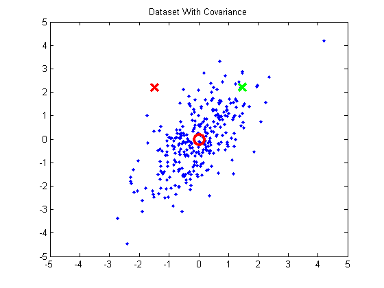](http://chrisjmccormick.files.wordpress.com/2014/07/datasetwithcovariance.png)
33 |
34 | If you were to take these points and normalize them to remove the covariance (using a process called whitening), the green X becomes much closer to the mean than the red X.
35 |
36 | [](http://chrisjmccormick.files.wordpress.com/2014/07/datasetnormalized.png)
37 |
38 | The Gaussian Mixture Models approach will take cluster covariance into account when forming the clusters.
39 |
40 | Another important difference with k-means is that standard k-means performs a hard assignment of data points to clusters--each point is assigned to the closest cluster. With Gaussian Mixture Models, what we will end up is a collection of independent Gaussian distributions, and so for each data point, we will have a probability that it belongs to each of these distributions / clusters.
41 |
42 |
43 | ### Expectation Maximization
44 |
45 |
46 | For GMMs, we will find the clusters using a technique called "Expectation Maximization". This is an iterative technique that feels a lot like the iterative approach used in k-means clustering.
47 |
48 | In the "Expectation" step, we will calculate the probability that each data point belongs to each cluster (using our current estimated mean vectors and covariance matrices). This seems analogous to the cluster assignment step in k-means.
49 |
50 | In the "Maximization" step, we'll re-calculate the cluster means and covariances based on the probabilities calculated in the expectation step. This seems analogous to the cluster movement step in k-means.
51 |
52 |
53 | ### Initialization
54 |
55 |
56 | To kickstart the EM algorithm, we'll randomly select data points to use as the initial means, and we'll set the covariance matrix for each cluster to be equal to the covariance of the full training set. Also, we'll give each cluster equal "prior probability". A cluster's "prior probability" is just the fraction of the dataset that belongs to each cluster. We'll start by assuming the dataset is equally divided between the clusters.
57 |
58 |
59 | ### Expectation
60 |
61 |
62 | In the "Expectation" step, we calculate the probability that each data point belongs to each cluster.
63 |
64 | We'll need the equation for the probability density function of a multivariate Gaussian. A multivariate Gaussian ("multivariate" just means multiple input variables) is more complex because there is the possibility for the different variables to have different variances, and even for there to be correlation between the variables. These properties are captured by the covariance matrix.
65 |
66 | [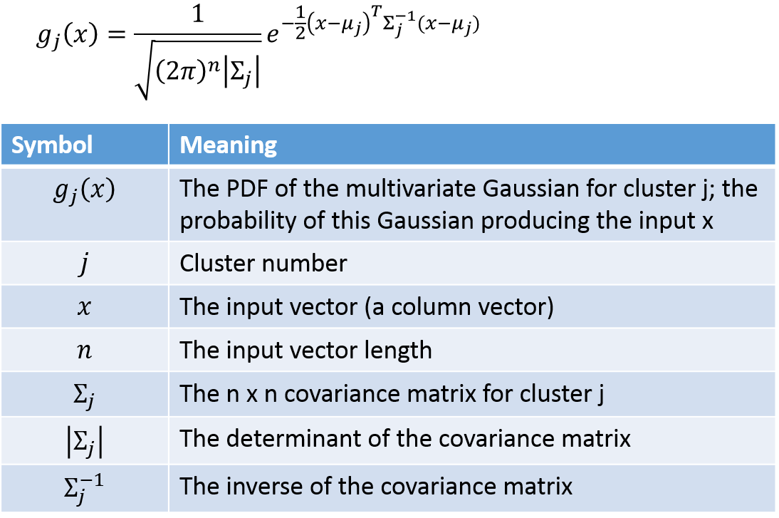](https://chrisjmccormick.files.wordpress.com/2014/08/multivariategaussian_eq.png)
67 |
68 | The probability that example point i belongs to cluster j can be calculated using the following:
69 |
70 | [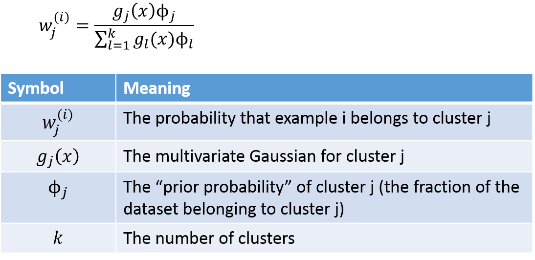](https://chrisjmccormick.files.wordpress.com/2014/08/membershipprobability_eq.png)
71 |
72 | We'll apply this equation to every example and every cluster, giving us a matrix with one row per example and one column per cluster.
73 |
74 |
75 | ### Maximization
76 |
77 |
78 | You can gain some useful intuition about the maximization equations if you're familiar with the equation for taking a weighted average. To find the average value of a set of _m_ values, where you have a weight _w _defined for each of the values, you can use the following equation:
79 |
80 | [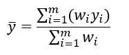](http://chrisjmccormick.files.wordpress.com/2014/02/weightedaverage1.png)
81 |
82 |
83 |
84 | With this in mind, the update rules for the maximization step are below. I've copied these from the [lecture notes on GMMs](http://cs229.stanford.edu/notes/cs229-notes7b.pdf) for Stanford's CS229 course on machine learning (those lecture notes are a great reference, by the way).
85 |
86 |
87 |
88 | [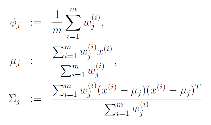](https://chrisjmccormick.files.wordpress.com/2014/08/maximizationequations1.png)
89 |
90 | The equation for mean (mu) of cluster j is just the average of all data points in the training set, with each example weighted by its probability of belonging to cluster j.
91 |
92 | Similary, the equation for the covariance matrix is the same as the equation you would use to estimate the covariance of a dataset, except that the contribution of each example is again weighted by the probability that it belongs to cluster j.
93 |
94 | The prior probability of cluster j, denoted as phi, is calculated as the average probability that a data point belongs to cluster j.
95 |
96 |
97 | ### MATLAB Example Code
98 |
99 |
100 | I've implemented Expectation Maximization for both a 1D and a 2D example. Run 'GMMExample_1D.m' and 'GMMExample_2D.m', respectively. The 1D example is easier to follow, but the 2D example can be extended to n-dimensional data.
101 |
102 | [GMM Example Code](https://dl.dropboxusercontent.com/u/94180423/GMM_Examples_v2014_08_04.zip)
103 |
104 | If you are simply interested in using GMMs and don't care how they're implemented, you might consider using the vlfeat implementation, which includes a nice tutorial [here](http://www.vlfeat.org/overview/gmm.html). Or if you are using Octave, there may be an open-source version of Matlab's 'fitgmdist' function from their Statistics Toolbox.
105 |
106 | The 1D example will output a plot showing the original data points and their PDFs in blue and red. The PDFs estimated by the EM algorithm are plotted in black for comparison.
107 |
108 |
109 | ### [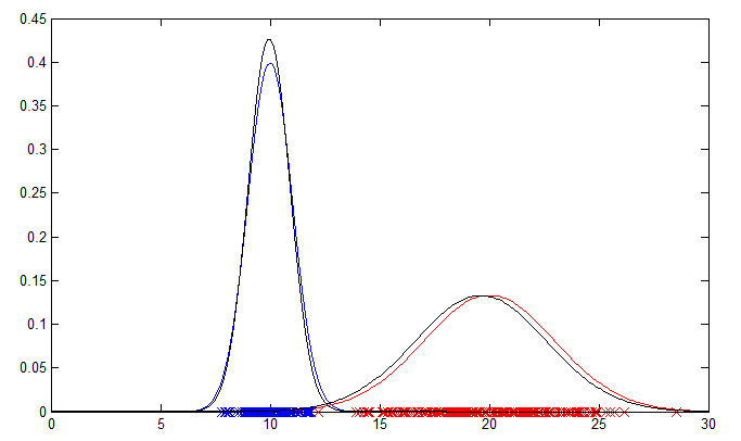](https://chrisjmccormick.files.wordpress.com/2014/08/1d_example.png)
110 |
111 |
112 | The 2D example is based on Matlab's own GMM tutorial [here](http://www.mathworks.com/help/stats/gaussian-mixture-models.html), but without any dependency on the Statistics Toolbox. The 2D example plots the PDFs using contour plots; you should see one plot of the original PDFs and another showing the estimated PDFs.
113 |
114 | [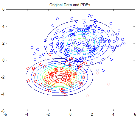](https://chrisjmccormick.files.wordpress.com/2014/08/2d_example_origdata1.png)
115 |
116 |
117 |
118 | [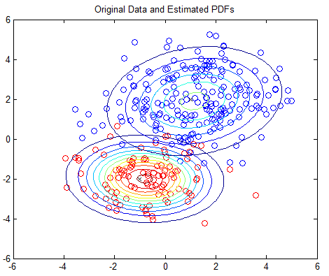](https://chrisjmccormick.files.wordpress.com/2014/08/2d_example_estpdfs.png)
119 |
--------------------------------------------------------------------------------
/data/2016-04-19-word2vec-tutorial-the-skip-gram-model.markdown:
--------------------------------------------------------------------------------
1 | ---
2 | layout: post
3 | title: "Word2Vec Tutorial - The Skip-Gram Model"
4 | date: 2016-04-19 22:00:00 -0800
5 | comments: true
6 | image: /assets/word2vec/skip_gram_net_arch.png
7 | tags: Word2Vec, Skip Gram, tutorial, neural network, NLP, word vectors
8 | ---
9 |
10 | This tutorial covers the skip gram neural network architecture for Word2Vec. My intention with this tutorial was to skip over the usual introductory and abstract insights about Word2Vec, and get into more of the details. Specifically here I'm diving into the skip gram neural network model.
11 |
12 | The Model
13 | =========
14 | The skip-gram neural network model is actually surprisingly simple in its most basic form; I think it's the all the little tweaks and enhancements that start to clutter the explanation.
15 |
16 | Let's start with a high-level insight about where we're going. Word2Vec uses a trick you may have seen elsewhere in machine learning. We're going to train a simple neural network with a single hidden layer to perform a certain task, but then we're not actually going to use that neural network for the task we trained it on! Instead, the goal is actually just to learn the weights of the hidden layer--we'll see that these weights are actually the "word vectors" that we're trying to learn.
17 |
18 |
19 | Another place you may have seen this trick is in unsupervised feature learning, where you train an auto-encoder to compress an input vector in the hidden layer, and decompress it back to the original in the output layer. After training it, you strip off the output layer (the decompression step) and just use the hidden layer--it's a trick for learning good image features without having labeled training data.
20 |
21 |
22 | The Fake Task
23 | =============
24 | So now we need to talk about this "fake" task that we're going to build the neural network to perform, and then we'll come back later to how this indirectly gives us those word vectors that we are really after.
25 |
26 | We're going to train the neural network to do the following. Given a specific word in the middle of a sentence (the input word), look at the words nearby and pick one at random. The network is going to tell us the probability for every word in our vocabulary of being the "nearby word" that we chose.
27 |
28 | When I say "nearby", there is actually a "window size" parameter to the algorithm. A typical window size might be 5, meaning 5 words behind and 5 words ahead (10 in total).
29 |
30 | The output probabilities are going to relate to how likely it is find each vocabulary word nearby our input word. For example, if you gave the trained network the input word "Soviet", the output probabilities are going to be much higher for words like "Union" and "Russia" than for unrelated words like "watermelon" and "kangaroo".
31 |
32 | We'll train the neural network to do this by feeding it word pairs found in our training documents. The below example shows some of the training samples (word pairs) we would take from the sentence "The quick brown fox jumps over the lazy dog." I've used a small window size of 2 just for the example. The word highlighted in blue is the input word.
33 |
34 | [![Training Data][training_data]][training_data]
35 |
36 | The network is going to learn the statistics from the number of times each pairing shows up. So, for example, the network is probably going to get many more training samples of ("Soviet", "Union") than it is of ("Soviet", "Sasquatch"). When the training is finished, if you give it the word "Soviet" as input, then it will output a much higher probability for "Union" or "Russia" than it will for "Sasquatch".
37 |
38 | Model Details
39 | =============
40 |
41 | So how is this all represented?
42 |
43 | First of all, you know you can't feed a word just as a text string to a neural network, so we need a way to represent the words to the network. To do this, we first build a vocabulary of words from our training documents--let's say we have a vocabulary of 10,000 unique words.
44 |
45 | We're going to represent an input word like "ants" as a one-hot vector. This vector will have 10,000 components (one for every word in our vocabulary) and we'll place a "1" in the position corresponding to the word "ants", and 0s in all of the other positions.
46 |
47 | The output of the network is a single vector (also with 10,000 components) containing, for every word in our vocabulary, the probability that a randomly selected nearby word is that vocabulary word.
48 |
49 | Here's the architecture of our neural network.
50 |
51 | [![Skip-gram Neural Network Architecture][skip_gram_net_arch]][skip_gram_net_arch]
52 |
53 | There is no activation function on the hidden layer neurons, but the output neurons use softmax. We'll come back to this later.
54 |
55 | When *training* this network on word pairs, the input is a one-hot vector representing the input word and the training output is also a one-hot vector representing the output word. But when you evaluate the trained network on an input word, the output vector will actually be a probability distribution (i.e., a bunch of floating point values, *not* a one-hot vector).
56 |
57 | The Hidden Layer
58 | ================
59 |
60 | For our example, we're going to say that we're learning word vectors with 300 features. So the hidden layer is going to be represented by a weight matrix with 10,000 rows (one for every word in our vocabulary) and 300 columns (one for every hidden neuron).
61 |
62 | If you look at the *rows* of this weight matrix, these are actually what will be our word vectors!
63 |
64 | [![Hidden Layer Weight Matrix][weight_matrix]][weight_matrix]
65 |
66 | So the end goal of all of this is really just to learn this hidden layer weight matrix -- the output layer we'll just toss when we're done!
67 |
68 | Let's get back, though, to working through the definition of this model that we're going to train.
69 |
70 | Now, you might be asking yourself--"That one-hot vector is almost all zeros... what's the effect of that?" If you multiply a 1 x 10,000 one-hot vector by a 10,000 x 300 matrix, it will effectively just *select* the matrix row corresponding to the "1". Here's a small example to give you a visual.
71 |
72 | [![Effect of matrix multiplication with a one-hot vector][matrix_mult_w_one_hot]][matrix_mult_w_one_hot]
73 |
74 | This means that the hidden layer of this model is really just operating as a lookup table. The output of the hidden layer is just the "word vector" for the input word.
75 |
76 | The Output Layer
77 | ================
78 |
79 | The `1 x 300` word vector for "ants" then gets fed to the output layer. The output layer is a softmax regression classifier. There's an in-depth tutorial on Softmax Regression [here](http://ufldl.stanford.edu/tutorial/supervised/SoftmaxRegression/), but the gist of it is that each output neuron (one per word in our vocabulary!) will produce an output between 0 and 1, and the sum of all these output values will add up to 1.
80 |
81 | Specifically, each output neuron has a weight vector which it multiplies against the word vector from the hidden layer, then it applies the function `exp(x)` to the result. Finally, in order to get the outputs to sum up to 1, we divide this result by the sum of the results from *all* 10,000 output nodes.
82 |
83 | Here's an illustration of calculating the output of the output neuron for the word "car".
84 |
85 | [![Behavior of the output neuron][output_neuron]][output_neuron]
86 |
87 |
88 | Note that neural network does not know anything about the offset of the output word relative to the input word. It does not learn a different set of probabilities for the word before the input versus the word after.
89 |
90 | To understand the implication, let's say that in our training corpus, every single occurrence of the word 'York' is preceded by the word 'New'. That is, at least according to the training data, there is a 100% probability that 'New' will be in the vicinity of 'York'. However, if we take the 10 words in the vicinity of 'York' and randomly pick one of them, the probability of it being 'New' is not 100%; you may have picked one of the other words in the vicinity.
91 |
92 |
93 | Intuition
94 | =========
95 | Ok, are you ready for an exciting bit of insight into this network?
96 |
97 | If two different words have very similar "contexts" (that is, what words are likely to appear around them), then our model needs to output very similar results for these two words. And one way for the network to output similar context predictions for these two words is if *the word vectors are similar*. So, if two words have similar contexts, then our network is motivated to learn similar word vectors for these two words! Ta da!
98 |
99 | And what does it mean for two words to have similar contexts? I think you could expect that synonyms like "intelligent" and "smart" would have very similar contexts. Or that words that are related, like "engine" and "transmission", would probably have similar contexts as well.
100 |
101 | This can also handle stemming for you -- the network will likely learn similar word vectors for the words "ant" and "ants" because these should have similar contexts.
102 |
103 | Next Up
104 | =======
105 | You may have noticed that the skip-gram neural network contains a huge number of weights... For our example with 300 features and a vocab of 10,000 words, that's 3M weights in the hidden layer and output layer each! Training this on a large dataset would be prohibitive, so the word2vec authors introduced a number of tweaks to make training feasible. These are covered in [part 2 of this tutorial](http://mccormickml.com/2017/01/11/word2vec-tutorial-part-2-negative-sampling/).
106 |
107 | Other Resources
108 | ===============
109 | I've also created a [post][word2vec_res] with links to and descriptions of other word2vec tutorials, papers, and implementations.
110 |
111 | [training_data]: {{ site.url }}/assets/word2vec/training_data.png
112 | [skip_gram_net_arch]: {{ site.url }}/assets/word2vec/skip_gram_net_arch.png
113 | [weight_matrix]: {{ site.url }}/assets/word2vec/word2vec_weight_matrix_lookup_table.png
114 | [matrix_mult_w_one_hot]: {{ site.url }}/assets/word2vec/matrix_mult_w_one_hot.png
115 | [output_neuron]: {{ site.url }}/assets/word2vec/output_weights_function.png
116 | [word2vec_res]: {{ site.url }}/2016/04/27/word2vec-resources/
--------------------------------------------------------------------------------
/data/dictionary.txt.bz2:
--------------------------------------------------------------------------------
https://raw.githubusercontent.com/chrisjmccormick/wiki-sim-search/f03795548fd7bf1e4e056b1ba77085e2bdec3958/data/dictionary.txt.bz2
--------------------------------------------------------------------------------
/keysearch.py:
--------------------------------------------------------------------------------
1 | # -*- coding: utf-8 -*-
2 | """
3 | Created on Tue Nov 22 11:31:44 2016
4 |
5 | @author: Chris
6 | """
7 |
8 | import textwrap
9 | import pickle
10 | import nltk
11 | from gensim import corpora
12 | from gensim.models import TfidfModel
13 |
14 |
15 | # I lazily made this a global constant so that I wouldn't have to include
16 | # it in the save and load features.
17 | enc_format='utf-8'
18 |
19 | class KeySearch(object):
20 | """
21 | KeySearch, which is short for "keyword search" stores a completed gensim
22 | tf-idf corpus. Whereas SimSearch stores an LSI model, and only understands
23 | conceptual relationships between documents, KeySearch actually knows what
24 | words occur in each document.
25 |
26 | It has several key functions:
27 | 1. It has functions for converting new text sources (that is, texts not
28 | already in the corpus) into tf-idf vectors.
29 | 2. It stores the corpus vocabulary in the form of a gensim dictionary.
30 | 3. It supports boolean keyword search (though this is NOT indexed!).
31 | 4. It stores the document metadata:
32 | - Title
33 | - Text source file
34 | - Line numbers in source file
35 | - Tags
36 |
37 |
38 | Saving & Loading
39 | ================
40 | The KeySearch object can be saved to and loaded from a directory
41 | using `save` and `load`. The typical useage, however is to simply save and
42 | load the SimSearch object (which also saves the underlying KeySearch).
43 |
44 | When saving the KeySearch, only the dictionary, feature vectors, and
45 | and document metadata are saved. The original text is not saved in any
46 | form.
47 |
48 | """
49 | def __init__(self, dictionary, tfidf_model, corpus_tfidf, titles,
50 | tagsToDocs={}, docsToTags={}, files=[], doc_line_nums=[]):
51 | """
52 | KeySearch requires a completed gensim corpus, along with some
53 | additional metadata
54 |
55 | Parameters:
56 | dictionary - gensim dictionary
57 | tfidf_model - gensim TfidfModel
58 | corpus_tfidf - gensim corpora
59 | titles - List of string titles.
60 | tagsToDocs - Mapping of tags to doc ids
61 | docsToTags - List of tags for each doc
62 | files - Unique files in the corpus
63 | doc_line_nums -
64 | """
65 | self.dictionary = dictionary
66 | self.tfidf_model = tfidf_model
67 | self.corpus_tfidf = corpus_tfidf
68 |
69 | self.titles = titles
70 |
71 | # Create mappings for the entry tags.
72 | self.tagsToDocs = tagsToDocs
73 | self.docsToTags = docsToTags
74 |
75 | self.files = files
76 | self.doc_line_nums = doc_line_nums
77 |
78 | def printTags(self):
79 | """
80 | Print all of the tags present in the corpus, plus the number of docs
81 | tagged with each.
82 | """
83 | print 'All tags in corpus (# of documents):'
84 |
85 | # Get all the tags and sort them alphabetically.
86 | tags = self.tagsToDocs.keys()
87 | tags.sort()
88 |
89 | # Print each tag followed by the number of documents.
90 | for tag in tags:
91 | print '%20s %3d' % (tag, len(self.tagsToDocs[tag]))
92 |
93 | def getTfidfForText(self, text):
94 | """
95 | This function takes new input `text` (not part of the original corpus),
96 | and processes it into a tf-idf vector.
97 |
98 | The input text should be a single string.
99 | """
100 | # If the string is not already unicode, decode the string into unicode
101 | # so the NLTK can handle it.
102 | if isinstance(text, str):
103 | try:
104 | text = text.decode(enc_format)
105 | except:
106 | print '======== Failed to decode input text! ========'
107 | print 'Make sure text is encoded in', enc_format
108 | print 'Input text:'
109 | print text
110 | return []
111 |
112 | # If the string ends in a newline, remove it.
113 | text = text.replace('\n', ' ')
114 |
115 | # Convert everything to lowercase, then use NLTK to tokenize.
116 | tokens = nltk.word_tokenize(text.lower())
117 |
118 | # We don't need to do any special filtering of tokens here (stopwords,
119 | # infrequent words, etc.). If a token is not in the dictionary, it is
120 | # simply ignored. So the dictionary effectively does the token
121 | # filtering for us.
122 |
123 | # Convert the tokenized text into a bag of words representation.
124 | bow_vec = self.dictionary.doc2bow(tokens)
125 |
126 | # Convert the bag-of-words representation to tf-idf
127 | return self.tfidf_model[bow_vec]
128 |
129 | def getTfidfForFile(self, filename):
130 | """
131 | Convert the text in the provided file to a tf-idf vector.
132 | """
133 | # Open the file and read all lines.
134 | with open(filename) as f:
135 | text = f.readlines()
136 |
137 | # Combine the lines into a single string.
138 | text = " ".join(text)
139 |
140 | # Pass the text down.
141 | return self.getTfidfForText(text)
142 |
143 | def getTfidfForDoc(self, doc_id):
144 | """
145 | Return the tf-idf vector for the specified document.
146 | """
147 | return self.corpus_tfidf[doc_id]
148 |
149 | def keywordSearch(self, includes=[], excludes=[], docs=[]):
150 | """
151 | Performs a boolean keyword search over the corpus.
152 |
153 | All words in the dictionary are lower case. This function will convert
154 | all supplied keywords to lower case.
155 |
156 | Parameters:
157 | includes A list of words (as strings) that the documents
158 | *must include*.
159 | excludes A list of words (as strings) that the documents
160 | *must not include*.
161 | docs The list of documents to search in, represented by
162 | by doc_ids. If this list is empty, the entire corpus
163 | is searched.
164 | """
165 |
166 | # If no doc ids were supplied, search the entire corpus.
167 | if not docs:
168 | docs = range(0, len(self.corpus_tfidf))
169 |
170 | # Convert all the keywords to their IDs.
171 | # Force them to lower case in the process.
172 | include_ids = []
173 | exclude_ids = []
174 |
175 | for word in includes:
176 | # Lookup the ID for the word.
177 | word_id = self.getIDForWord(word.lower())
178 |
179 | # Verify the word exists in the dictionary.
180 | if word_id == -1:
181 | print 'WARNING: Word \'' + word.lower() + '\'not in dictionary!'
182 | continue
183 |
184 | # Add the word id to the list.
185 | include_ids.append(word_id)
186 |
187 | for word in excludes:
188 | exclude_ids.append(self.getIDForWord(word.lower()))
189 |
190 | results = []
191 |
192 | # For each of the documents to search...
193 |
194 | for doc_id in docs:
195 | # Get the sparse tf-idf vector for the next document.
196 | vec_tfidf = self.corpus_tfidf[doc_id]
197 |
198 | # Create a list of the word ids in this document.
199 | doc_words = [tfidf[0] for tfidf in vec_tfidf]
200 |
201 | match = True
202 |
203 | # Check for words that must be present.
204 | for word_id in include_ids:
205 | if not word_id in doc_words:
206 | match = False
207 | break
208 |
209 | # If we failed the 'includes' test, skip to the next document.
210 | if not match:
211 | continue
212 |
213 | # Check for words that must not be present.
214 | for word_id in exclude_ids:
215 | if word_id in doc_words:
216 | match = False
217 | break
218 |
219 | # If we passed the 'excludes' test, this is a valid result.
220 | if match:
221 | results.append(doc_id)
222 |
223 | return results
224 |
225 |
226 | def printTopNWords(self, topn=10):
227 | """
228 | Print the 'topn' most frequent words in the corpus.
229 |
230 | This is useful for checking to see if you have any common, bogus tokens
231 | that need to be filtered out of the corpus.
232 | """
233 |
234 | # Get the dictionary as a list of tuples.
235 | # The tuple is (word_id, count)
236 | word_counts = [(key, value) for (key, value) in self.dictionary.dfs.iteritems()]
237 |
238 | # Sort the list by the 'value' of the tuple (incidence count)
239 | from operator import itemgetter
240 | word_counts = sorted(word_counts, key=itemgetter(1))
241 |
242 | # Print the most common words.
243 | # The list is sorted smallest to biggest, so...
244 | print 'Top', topn, 'most frequent words'
245 | for i in range(-1, -topn, -1):
246 | print ' %s %d' % (self.dictionary[word_counts[i][0]].ljust(10), word_counts[i][1])
247 |
248 | def getVocabSize(self):
249 | """
250 | Returns the number of unique words in the final vocabulary (after all
251 | filtering).
252 | """
253 | return len(self.dictionary.keys())
254 |
255 | def getIDForWord(self, input_word):
256 | """
257 | Lookup the ID for a specific word.
258 |
259 | Returns -1 if the word isn't in the dictionary.
260 | """
261 |
262 | # All words in dictionary are lower case.
263 | input_word = input_word.lower()
264 |
265 | # First check if the word exists in the dictionary.
266 | if not input_word in self.dictionary.values():
267 | return -1
268 | # If it is, look up the ID.
269 | else:
270 | return self.dictionary.token2id[input_word]
271 |
272 | def getDocLocation(self, doc_id):
273 | """
274 | Return the filename and line numbers that 'doc_id' came from.
275 | """
276 | line_nums = self.doc_line_nums[doc_id]
277 | filename = self.files[line_nums[0]]
278 | return filename, line_nums[1], line_nums[2]
279 |
280 | def readDocSource(self, doc_id):
281 | """
282 | Reads the original source file for the document 'doc_id' and retrieves
283 | the source lines.
284 | """
285 | # Lookup the source for the doc.
286 | line_nums = self.doc_line_nums[doc_id]
287 |
288 | filename = self.files[line_nums[0]]
289 | line_start = line_nums[1]
290 | line_end = line_nums[2]
291 |
292 | results = []
293 |
294 | # Open the file and read just the specified lines.
295 | with open(filename) as fp:
296 | for i, line in enumerate(fp):
297 | # 'i' starts at 0 but line numbers start at 1.
298 | line_num = i + 1
299 |
300 | if line_num > line_end:
301 | break
302 |
303 | if line_num >= line_start:
304 | results.append(line)
305 |
306 | return results
307 |
308 | def printDocSourcePretty(self, doc_id, max_lines=8, indent=' '):
309 | """
310 | Prints the original source lines for the document 'doc_id'.
311 |
312 | This function leverages the 'textwrap' Python module to limit the
313 | print output to 80 columns.
314 | """
315 |
316 | # Read in the document.
317 | lines = self.readDocSource(doc_id)
318 |
319 | # Limit the result to 'max_lines'.
320 | truncated = False
321 | if len(lines) > max_lines:
322 | truncated = True
323 | lines = lines[0:max_lines]
324 |
325 | # Convert the list of strings to a single string.
326 | lines = '\n'.join(lines)
327 |
328 | # Remove indentations in the source text.
329 | dedented_text = textwrap.dedent(lines).strip()
330 |
331 | # Add an ellipsis to the end to show we truncated the doc.
332 | if truncated:
333 | dedented_text = dedented_text + ' ...'
334 |
335 | # Wrap the text so it prints nicely--within 80 columns.
336 | # Print the text indented slightly.
337 | pretty_text = textwrap.fill(dedented_text, initial_indent=indent, subsequent_indent=indent, width=80)
338 |
339 | print pretty_text
340 |
341 | def save(self, save_dir='./'):
342 | """
343 | Write out the built corpus to a save directory.
344 | """
345 | # Store the tag tables.
346 | pickle.dump((self.tagsToDocs, self.docsToTags), open(save_dir + 'tag-tables.pickle', 'wb'))
347 |
348 | # Store the document titles.
349 | pickle.dump(self.titles, open(save_dir + 'titles.pickle', 'wb'))
350 |
351 | # Write out the tfidf model.
352 | self.tfidf_model.save(save_dir + 'documents.tfidf_model')
353 |
354 | # Write out the tfidf corpus.
355 | corpora.MmCorpus.serialize(save_dir + 'documents_tfidf.mm', self.corpus_tfidf)
356 |
357 | # Write out the dictionary.
358 | self.dictionary.save(save_dir + 'documents.dict')
359 |
360 | # Save the filenames.
361 | pickle.dump(self.files, open(save_dir + 'files.pickle', 'wb'))
362 |
363 | # Save the file ID and line numbers for each document.
364 | pickle.dump(self.doc_line_nums, open(save_dir + 'doc_line_nums.pickle', 'wb'))
365 |
366 | # Objects that are not saved:
367 | # - stop_list - You don't need to filter stop words for new input
368 | # text, they simply aren't found in the dictionary.
369 | # - frequency - This preliminary word count object is only used for
370 | # removing infrequent words. Final word counts are in
371 | # the `dictionary` object.
372 |
373 | @classmethod
374 | def load(cls, save_dir='./'):
375 | """
376 | Load the corpus from a save directory.
377 | """
378 | tables = pickle.load(open(save_dir + 'tag-tables.pickle', 'rb'))
379 | tagsToDocs = tables[0]
380 | docsToTags = tables[1]
381 | titles = pickle.load(open(save_dir + 'titles.pickle', 'rb'))
382 | tfidf_model = TfidfModel.load(fname=save_dir + 'documents.tfidf_model')
383 | corpus_tfidf = corpora.MmCorpus(save_dir + 'documents_tfidf.mm')
384 | dictionary = corpora.Dictionary.load(fname=save_dir + 'documents.dict')
385 | files = pickle.load(open(save_dir + 'files.pickle', 'rb'))
386 | doc_line_nums = pickle.load(open(save_dir + 'doc_line_nums.pickle', 'rb'))
387 |
388 | ksearch = KeySearch(dictionary, tfidf_model,
389 | corpus_tfidf, titles, tagsToDocs,
390 | docsToTags, files, doc_line_nums)
391 |
392 | return ksearch
393 |
--------------------------------------------------------------------------------
/make_wikicorpus.py:
--------------------------------------------------------------------------------
1 | # -*- coding: utf-8 -*-
2 |
3 | """
4 | Convert articles from a Wikipedia dump to (sparse) vectors. The input is a
5 | bz2-compressed dump of Wikipedia articles, in XML format.
6 |
7 | This script was built on the one provided in gensim:
8 | `gensim.scripts.make_wikicorpus`
9 |
10 | """
11 |
12 | from gensim.models import TfidfModel, LsiModel
13 | from gensim.corpora import Dictionary, WikiCorpus, MmCorpus
14 | from gensim import similarities
15 | from gensim import utils
16 | import time
17 | import sys
18 | import logging
19 | import os
20 |
21 |
22 | def formatTime(seconds):
23 | """
24 | Takes a number of elapsed seconds and returns a string in the format h:mm.
25 | """
26 | m, s = divmod(seconds, 60)
27 | h, m = divmod(m, 60)
28 | return "%d:%02d" % (h, m)
29 |
30 |
31 | # ======== main ========
32 | # Main entry point for the script.
33 | # This little check has to do with the multiprocess module (which is used by
34 | # WikiCorpus). Without it, the code will spawn infinite processes and hang!
35 | if __name__ == '__main__':
36 |
37 | # Set up logging.
38 |
39 | # This little snippet is to fix an issue with qtconsole that you may or
40 | # may not have... Without this, I don't see any logs in Spyder.
41 | # Source: http://stackoverflow.com/questions/24259952/logging-module-does-not-print-in-ipython
42 | root = logging.getLogger()
43 | for handler in root.handlers[:]:
44 | root.removeHandler(handler)
45 |
46 | # Create a logger
47 | program = os.path.basename(sys.argv[0])
48 | logger = logging.getLogger(program)
49 |
50 | # Set the timestamp format to just hours, minutes, and seconds (no ms)
51 | #
52 | # Record the log to a file 'log.txt'--There is just under 5,000 lines of
53 | # logging statements, so I've chosen to write these to a file instead of
54 | # to the console. It's safe to have the log file open while the script is
55 | # running, so you can check progress that way if you'd like.
56 | logging.basicConfig(filename='log.txt', format='%(asctime)s : %(levelname)s : %(message)s', datefmt='%H:%M:%S')
57 | logging.root.setLevel(level=logging.INFO)
58 |
59 | # Download this file to get the latest wikipedia dump:
60 | # https://dumps.wikimedia.org/enwiki/latest/enwiki-latest-pages-articles.xml.bz2
61 | # On Jan 18th, 2017 it was ~13GB
62 | dump_file = './data/enwiki-latest-pages-articles.xml.bz2'
63 |
64 | # ======== STEP 1: Build Dictionary =========
65 | # The first step is to parse through all of Wikipedia and identify all of
66 | # the unique words that we want to have in our dictionary.
67 | # This is a long process--it took 3.2hrs. on my Intel Core i7 4770
68 | if True:
69 |
70 | # Create an empty dictionary
71 | dictionary = Dictionary()
72 |
73 | # Create the WikiCorpus object. This doesn't do any processing yet since
74 | # we've supplied the dictionary.
75 | wiki = WikiCorpus(dump_file, dictionary=dictionary)
76 |
77 | print('Parsing Wikipedia to build Dictionary...')
78 | sys.stdout.flush()
79 |
80 | t0 = time.time()
81 |
82 | # Now it's time to parse all of Wikipedia and build the dictionary.
83 | # This is a long process, 3.2hrs. on my Intel i7 4770. It will update
84 | # you at every 10,000 documents.
85 | #
86 | # wiki.get_texts() will only return articles which pass a couple
87 | # filters that weed out stubs, redirects, etc. If you included all of
88 | # those, Wikpedia is more like ~17M articles.
89 | #
90 | # For each article, it's going to add the words in the article to the
91 | # dictionary.
92 | #
93 | # If you look inside add_documents, you'll see that it calls doc2bow--
94 | # this generates a bag of words vector, but we're not keeping it. The
95 | # dictionary isn't finalized until all of the articles have been
96 | # scanned, so we don't know the right mapping of words to ids yet.
97 | #
98 | # You can use the prune_at parameter to prevent the dictionary from
99 | # growing too large during this process, but I think it's interesting
100 | # to see the total count of unique tokens before pruning.
101 | dictionary.add_documents(wiki.get_texts(), prune_at=None)
102 |
103 | print(' Building dictionary took %s' % formatTime(time.time() - t0))
104 | print(' %d unique tokens before pruning.' % len(dictionary))
105 | sys.stdout.flush()
106 |
107 | keep_words = 100000
108 |
109 | # The initial dictionary is huge (~8.75M words in my Wikipedia dump),
110 | # so let's filter it down. We want to keep the words that are neither
111 | # very rare or overly common. To do this, we will keep only words that
112 | # exist within at least 20 articles, but not more than 10% of all
113 | # documents. Finally, we'll also put a hard limit on the dictionary
114 | # size and just keep the 'keep_words' most frequent works.
115 | wiki.dictionary.filter_extremes(no_below=20, no_above=0.1, keep_n=keep_words)
116 |
117 | # Write out the dictionary to disk.
118 | # For my run, this file is 769KB when compressed.
119 | # TODO -- This text format lets you peruse it, but you can
120 | # compress it better as binary...
121 | wiki.dictionary.save_as_text('./data/dictionary.txt.bz2')
122 | else:
123 | # Nothing to do here.
124 | print('')
125 |
126 | # ======== STEP 2: Convert Articles To Bag-of-words ========
127 | # Now that we have our finalized dictionary, we can create bag-of-words
128 | # representations for the Wikipedia articles. This means taking another
129 | # pass over the Wikipedia dump!
130 | if True:
131 |
132 | # Load the dictionary if you're just running this section.
133 | dictionary = Dictionary.load_from_text('./data/dictionary.txt.bz2')
134 | wiki = WikiCorpus(dump_file, dictionary=dictionary)
135 |
136 | # Turn on metadata so that wiki.get_texts() returns the article titles.
137 | wiki.metadata = True
138 |
139 | print('\nConverting to bag of words...')
140 | sys.stdout.flush()
141 |
142 | t0 = time.time()
143 |
144 | # Generate bag-of-words vectors (term-document frequency matrix) and
145 | # write these directly to disk.
146 | # On my machine, this took 3.53 hrs.
147 | # By setting metadata = True, this will also record all of the article
148 | # titles into a separate pickle file, 'bow.mm.metadata.cpickle'
149 | MmCorpus.serialize('./data/bow.mm', wiki, metadata=True, progress_cnt=10000)
150 |
151 | print(' Conversion to bag-of-words took %s' % formatTime(time.time() - t0))
152 | sys.stdout.flush()
153 |
154 | # Load the article titles back
155 | id_to_titles = utils.unpickle('./data/bow.mm.metadata.cpickle')
156 |
157 | # Create the reverse mapping, from article title to index.
158 | titles_to_id = {}
159 |
160 | # For each article...
161 | for at in id_to_titles.items():
162 | # `at` is (index, (pageid, article_title)) e.g., (0, ('12', 'Anarchism'))
163 | # at[1][1] is the article title.
164 | # The pagied property is unused.
165 | titles_to_id[at[1][1]] = at[0]
166 |
167 | # Store the resulting map.
168 | utils.pickle(titles_to_id, './data/titles_to_id.pickle')
169 |
170 | # We're done with the article titles so free up their memory.
171 | del id_to_titles
172 | del titles_to_id
173 |
174 |
175 | # To clean up some memory, we can delete our original dictionary and
176 | # wiki objects, and load back the dictionary directly from the file.
177 | del dictionary
178 | del wiki
179 |
180 | # Load the dictionary back from disk.
181 | # (0.86sec on my machine loading from an SSD)
182 | dictionary = Dictionary.load_from_text('./data/dictionary.txt.bz2')
183 |
184 | # Load the bag-of-words vectors back from disk.
185 | # (0.8sec on my machine loading from an SSD)
186 | corpus_bow = MmCorpus('./data/bow.mm')
187 |
188 | # If we previously completed this step, just load the pieces we need.
189 | else:
190 | print('\nLoading the bag-of-words corpus from disk.')
191 | # Load the bag-of-words vectors back from disk.
192 | # (0.8sec on my machine loading from an SSD)
193 | corpus_bow = MmCorpus('./data/bow.mm')
194 |
195 |
196 | # ======== STEP 3: Learn tf-idf model ========
197 | # At this point, we're all done with the original Wikipedia text, and we
198 | # just have our bag-of-words representation.
199 | # Now we can look at the word frequencies and document frequencies to
200 | # build a tf-idf model which we'll use in the next step.
201 | if True:
202 | print('\nLearning tf-idf model from data...')
203 | t0 = time.time()
204 |
205 | # Build a Tfidf Model from the bag-of-words dataset.
206 | # This took 47 min. on my machine.
207 | # TODO - Why not normalize?
208 | model_tfidf = TfidfModel(corpus_bow, id2word=dictionary, normalize=False)
209 |
210 | print(' Building tf-idf model took %s' % formatTime(time.time() - t0))
211 | model_tfidf.save('./data/tfidf.tfidf_model')
212 |
213 | # If we previously completed this step, just load the pieces we need.
214 | else:
215 | print('\nLoading the tf-idf model from disk.')
216 | model_tfidf = TfidfModel.load('./data/tfidf.tfidf_model')
217 |
218 |
219 | # ======== STEP 4: Convert articles to tf-idf ========
220 | # We've learned the word statistics and built a tf-idf model, now it's time
221 | # to apply it and convert the vectors to the tf-idf representation.
222 | if True:
223 | print('\nApplying tf-idf model to all vectors...')
224 | t0 = time.time()
225 |
226 | # Apply the tf-idf model to all of the vectors.
227 | # This took 1hr. and 40min. on my machine.
228 | # The resulting corpus file is large--17.9 GB for me.
229 | MmCorpus.serialize('./data/corpus_tfidf.mm', model_tfidf[corpus_bow], progress_cnt=10000)
230 |
231 | print(' Applying tf-idf model took %s' % formatTime(time.time() - t0))
232 | else:
233 | # Nothing to do here.
234 | print('')
235 |
236 | # ======== STEP 5: Train LSI on the articles ========
237 | # Learn an LSI model from the tf-idf vectors.
238 | if True:
239 |
240 | # The number of topics to use.
241 | num_topics = 300
242 |
243 | # Load the tf-idf corpus back from disk.
244 | corpus_tfidf = MmCorpus('./data/corpus_tfidf.mm')
245 |
246 | # Train LSI
247 | print('\nLearning LSI model from the tf-idf vectors...')
248 | t0 = time.time()
249 |
250 | # Build the LSI model
251 | # This took 2hrs. and 7min. on my machine.
252 | model_lsi = LsiModel(corpus_tfidf, num_topics=num_topics, id2word=dictionary)
253 |
254 | print(' Building LSI model took %s' % formatTime(time.time() - t0))
255 |
256 | # Write out the LSI model to disk.
257 | # The LSI model is big but not as big as the corpus.
258 | # The largest piece is the projection matrix:
259 | # 100,000 words x 300 topics x 8-bytes per val x (1MB / 2^20 bytes) = ~229MB
260 | # This is saved as `lsi.lsi_model.projection.u.npy`
261 | model_lsi.save('./data/lsi.lsi_model')
262 |
263 | # If we previously completed this step, just load the pieces we need.
264 | else:
265 | # Load the tf-idf corpus and trained LSI model back from disk.
266 | corpus_tfidf = MmCorpus('./data/corpus_tfidf.mm')
267 | model_lsi = LsiModel.load('./data/lsi.lsi_model')
268 |
269 | # ========= STEP 6: Convert articles to LSI with index ========
270 | # Transform corpus to LSI space and index it
271 | if True:
272 |
273 | print('\nApplying LSI model to all vectors...')
274 | t0 = time.time()
275 |
276 | # You could apply Apply the LSI model to all of the tf-idf vectors and
277 | # write them to disk as an MmCorpus, but this is huge--33.2GB.
278 | #MmCorpus.serialize('./data/corpus_lsi.mm', model_lsi[corpus_tfidf], progress_cnt=10000)
279 |
280 | # Instead, we'll convert the vectors to LSI and store them as a dense
281 | # matrix, all in one step.
282 | index = similarities.MatrixSimilarity(model_lsi[corpus_tfidf], num_features=num_topics)
283 | index.save('./data/lsi_index.mm')
284 |
285 | print(' Applying LSI model took %s' % formatTime(time.time() - t0))
286 |
--------------------------------------------------------------------------------
/run_search.py:
--------------------------------------------------------------------------------
1 | # -*- coding: utf-8 -*-
2 | """
3 | Created on Wed Feb 15 12:10:20 2017
4 |
5 | @author: Chris
6 | """
7 | from gensim import similarities
8 | from gensim import utils
9 | import time
10 | import sys
11 | import operator
12 |
13 | # Load the Wikipedia LSI vectors.
14 | # This matrix is large (4.69 GB for me) and takes ~15 seconds to load.
15 | print 'Loading Wikipedia LSI index (15-30sec.)...'
16 | t0 = time.time()
17 |
18 | index = similarities.MatrixSimilarity.load('./data/lsi_index.mm')
19 |
20 | print ' Loading LSI vectors took %.2f seconds' % (time.time() - t0)
21 |
22 | # Load the article titles. These have the format (pageid, article title)
23 | print '\nLoading Wikipedia article titles...'
24 |
25 | id_to_titles = utils.unpickle('./data/bow.mm.metadata.cpickle')
26 | titles_to_id = utils.unpickle('./data/titles_to_id.pickle')
27 |
28 | # Name of the article to use as the input to the search.
29 | query_title = 'Topic model'
30 |
31 | print '\nSearching for articles similar to \'' + query_title + '\':'
32 |
33 | # Lookup the index of the query article.
34 | query_id = titles_to_id[query_title]
35 |
36 | # Select the row corresponding to the query vector.
37 | # The .index property is a numpy.ndarray storing all of the LSI vectors,
38 | # it's [~4.2M x 300].
39 | query_vec = index.index[query_id, :]
40 |
41 | t0 = time.time()
42 |
43 | # Perform the similarity search!
44 | sims = index[query_vec]
45 |
46 | print ' Similarity search took %.0f ms' % ((time.time() - t0) * 1000)
47 |
48 | t0 = time.time()
49 |
50 | # Sort in descending order.
51 | # `sims` is of type numpy.ndarray, so the sort() method is different...
52 | sims = sorted(enumerate(sims), key=lambda item: -item[1])
53 |
54 | print ' Sorting took %.2f seconds' % (time.time() - t0)
55 |
56 | print '\nResults:'
57 |
58 | # Display the top 10 results
59 | for i in range(0, 10):
60 |
61 | # Get the index of the result.
62 | result_index = sims[i][0]
63 |
64 | print ' ' + id_to_titles[result_index][1]
65 |
66 |
--------------------------------------------------------------------------------
/searchWithSimSearch.py:
--------------------------------------------------------------------------------
1 | # -*- coding: utf-8 -*-
2 | """
3 | Created on Wed Feb 22 14:19:43 2017
4 |
5 | @author: Chris
6 | """
7 |
8 | from simsearch import SimSearch
9 | from keysearch import KeySearch
10 |
11 | from gensim.models import TfidfModel, LsiModel
12 | from gensim.corpora import Dictionary, MmCorpus
13 | from gensim.similarities import MatrixSimilarity
14 | from gensim import utils
15 |
16 | import time
17 |
18 | import sys
19 |
20 | def fprint(msg):
21 | """
22 | Print function with stdout flush to force print statements to show.
23 | """
24 | print(msg)
25 | sys.stdout.flush()
26 |
27 | def createSearchObjs():
28 | """
29 | Creates the SimSearch and KeySearch objects using the data structures
30 | created in `make_wikicorpus.py`.
31 | Returns (simsearch, keysearch, titles_to_id)
32 | """
33 |
34 | # Load the article titles. These have the format (pageid, article title)
35 | fprint('Loading Wikipedia article titles...')
36 | t0 = time.time()
37 |
38 | id_to_titles = utils.unpickle('./data/bow.mm.metadata.cpickle')
39 | titles_to_id = utils.unpickle('./data/titles_to_id.pickle')
40 |
41 | # id_to_titles is actually a map of indeces to (pageid, article title)
42 | # The 'pageid' property is unused.
43 | # Convert id_to_titles into a simple list of titles.
44 | titles = [item[1][1] for item in id_to_titles.items()]
45 |
46 | fprint(' Took %.2f seconds' % (time.time() - t0))
47 |
48 | # Load the dictionary (830ms on my machine)
49 | fprint('\nLoading dictionary...')
50 | t0 = time.time()
51 |
52 | dictionary = Dictionary.load_from_text('./data/dictionary.txt.bz2')
53 |
54 | fprint(' Took %.2f seconds' % (time.time() - t0))
55 |
56 | # Load tf-idf model (60ms on my machine).
57 | fprint('\nLoading tf-idf model...')
58 | t0 = time.time()
59 |
60 | tfidf_model = TfidfModel.load('./data/tfidf.tfidf_model')
61 |
62 | fprint(' Took %.2f seconds' % (time.time() - t0))
63 |
64 | # We must not use `load`--that would attempt to load the corpus into
65 | # memory, and it's 16.7 GB!!
66 | #corpus_tfidf = MmCorpus.load('./data/corpus_tfidf.mm')
67 |
68 | fprint('\nCreating tf-idf corpus object (leaves the vectors on disk)...')
69 | t0 = time.time()
70 |
71 | corpus_tfidf = MmCorpus('./data/corpus_tfidf.mm')
72 |
73 | fprint(' Took %.2f seconds' % (time.time() - t0))
74 |
75 | # Create the KeySearch and SimSearch objects.
76 | ksearch = KeySearch(dictionary, tfidf_model, corpus_tfidf, titles)
77 | simsearch = SimSearch(ksearch)
78 |
79 | # TODO - SimSearch doesn't currently have a clean way to provide the index
80 | # and model.
81 |
82 | fprint('\nLoading LSI model...')
83 | t0 = time.time()
84 | simsearch.lsi = LsiModel.load('./data/lsi.lsi_model')
85 |
86 | fprint(' Took %.2f seconds' % (time.time() - t0))
87 |
88 | # Load the Wikipedia LSI vectors into memory.
89 | # The matrix is 4.69GB for me, and takes ~15 seconds on my machine to load.
90 | fprint('\nLoading Wikipedia LSI index...')
91 | t0 = time.time()
92 |
93 | simsearch.index = MatrixSimilarity.load('./data/lsi_index.mm')
94 |
95 | fprint(' Took %.2f seconds' % (time.time() - t0))
96 |
97 | # TODO - It would be interesting to try the 'Similarity' class which
98 | # shards the dataset on disk for you...
99 |
100 | return (simsearch, ksearch, titles_to_id)
101 |
102 | # ======== Example 1 ========
103 | # Searches for top 10 articles most similar to a query article.
104 | # Interprets the top match by showing which words contributed most to the
105 | # similarity.
106 | def example1(simsearch, ksearch, titles_to_id):
107 |
108 | query_article = 'Topic model'
109 |
110 | fprint('\nSearching for similar articles...')
111 | t0 = time.time()
112 |
113 | # Search for the top 10 most similar Wikipedia articles to the query.
114 | # This takes about 12 seconds on my machine, mostly in the sorting step.
115 | results = simsearch.findSimilarToDoc(titles_to_id[query_article], topn=10)
116 | simsearch.printResultsByTitle(results)
117 |
118 | fprint('\nSearch and sort took %.2f seconds' % (time.time() - t0))
119 |
120 | # Lookup the name of the top matching article.
121 | top_match_article = ksearch.titles[results[0][0]]
122 |
123 | fprint('\nInterpreting the match between \'' + query_article + '\' and \'' + top_match_article + '\' ...\n')
124 | t0 = time.time()
125 |
126 | # Get the tf-idf vectors for the two articles (the input and the top match).
127 | vec1_tfidf = ksearch.getTfidfForDoc(titles_to_id[query_article])
128 | vec2_tfidf = ksearch.getTfidfForDoc(results[0][0])
129 |
130 | # Interpret the top match match. Turn off filtering since the contributions
131 | # appear to be small with so many words.
132 | simsearch.interpretMatch(vec1_tfidf, vec2_tfidf, topn=20, min_pos=0, max_neg=-0.001)
133 |
134 | fprint('Interpreting match took %.2f seconds' % (time.time() - t0))
135 |
136 | # ======== Example 2 ========
137 | # Use an example file as input to a search.
138 | # For this example, I've supplied the markdown for a couple of my blog posts.
139 | # TODO - Discuss results.
140 | def example2(simsearch, ksearch, titles_to_id):
141 |
142 | fprint('\nSearching for articles similar to my word2vec tutorial...')
143 | t0 = time.time()
144 |
145 | # Get a tf-idf representation of my blog post.
146 | #input_tfidf = ksearch.getTfidfForFile('./data/2016-04-19-word2vec-tutorial-the-skip-gram-model.markdown')
147 | input_tfidf = ksearch.getTfidfForFile('./data/2014-08-04-gaussian-mixture-models-tutorial-and-matlab-code.markdown')
148 |
149 | # Search for Wikipedia articles similar to my word2vec blog post.
150 | results = simsearch.findSimilarToVector(input_tfidf)
151 |
152 | # You can also search directly from the file.
153 | #results = simsearch.findSimilarToFile('./data/2016-04-19-word2vec-tutorial-the-skip-gram-model.markdown')
154 |
155 | simsearch.printResultsByTitle(results)
156 |
157 | topmatch_tfidf = ksearch.getTfidfForDoc(results[0][0])
158 |
159 | # Lookup the name of the top matching article.
160 | top_match_article = ksearch.titles[results[0][0]]
161 |
162 | fprint('\nInterpreting the match between my blog post and \'' + top_match_article + '\' ...\n')
163 |
164 | # Interpret the top match.
165 | simsearch.interpretMatch(input_tfidf, topmatch_tfidf, topn=10, min_pos=0, max_neg=-0.001)
166 |
167 | fprint('\nSearch and sort took %.2f seconds' % (time.time() - t0))
168 |
169 | # ======== Example 3 ========
170 | # Display and record the topic words.
171 | def example3(simsearch, ksearch, titles_to_id):
172 | # Get the top 10 words for every topic.
173 | # `topics` is a list of length 300.
174 | topics = simsearch.lsi.show_topics(num_topics=-1, num_words=10, log=False, formatted=False)
175 |
176 | with open('./topic_words.txt', 'wb') as f:
177 |
178 | # `topic_words` has the form (topic_id, topic_words)
179 | for topic_words in topics:
180 |
181 | # Put all the words into one line.
182 | topic_line = ''
183 |
184 | # `word` has the form (word, weight)
185 | for word in topic_words[1]:
186 | topic_line += word[0] + ', '
187 |
188 | # Print line.
189 | print topic_line
190 |
191 | # Write the topic to the text file.
192 | f.write(topic_line.encode('utf-8') + '\n')
193 |
194 |
195 | # ======== main ========
196 | # Entry point to the script.
197 |
198 | # Load the corpus, model, etc.
199 | # This takes about 15 second on my machine (I have an SSD), and requires at
200 | # least 5GB of RAM.
201 | simsearch, ksearch, titles_to_id = createSearchObjs()
202 |
203 | # Search for articles similar to 'Topic model'
204 | example1(simsearch, ksearch, titles_to_id)
205 |
206 | # Search for articles similar to one of my blog posts.
207 | #example2(simsearch, ksearch, titles_to_id)
208 |
209 | # Display and record the top words for each topic.
210 | #example3(simsearch, ksearch, titles_to_id)
211 |
--------------------------------------------------------------------------------
/simsearch.py:
--------------------------------------------------------------------------------
1 | # -*- coding: utf-8 -*-
2 | """
3 | Created on Fri Oct 14 21:00:58 2016
4 |
5 | @author: Chris
6 | """
7 |
8 | from gensim.models import LsiModel
9 | from gensim import similarities
10 | from keysearch import KeySearch
11 | import numpy as np
12 |
13 | class SimSearch(object):
14 | """
15 | SimSearch allows you to search a collection of documents by providing
16 | conceptually similar text as the search query, as opposed to the typical
17 | keyword-based approach. This technique is also referred to as semantic
18 | search or concept search.
19 | """
20 |
21 | def __init__(self, key_search):
22 | """
23 | Initialize the SimSearch with a KeySearch object, which holds:
24 | - The dictionary
25 | - The tf-idf model and corpus
26 | - The document metadata.
27 |
28 | """
29 | self.ksearch = key_search
30 |
31 |
32 | def trainLSI(self, num_topics=100):
33 | """
34 | Train the Latent Semantic Indexing model.
35 | """
36 | self.num_topics = num_topics
37 | # Train LSA
38 |
39 | # Look-up the number of features in the tfidf model.
40 | #self.num_tfidf_features = max(self.corpus_tfidf.dfs) + 1
41 |
42 | self.lsi = LsiModel(self.ksearch.corpus_tfidf, num_topics=self.num_topics, id2word=self.ksearch.dictionary)
43 |
44 | # Transform corpus to LSI space and index it
45 | self.index = similarities.MatrixSimilarity(self.lsi[self.ksearch.corpus_tfidf], num_features=num_topics)
46 |
47 |
48 | def findSimilarToVector(self, input_tfidf, topn=10, in_corpus=False):
49 | """
50 | Find documents in the corpus similar to the provided document,
51 | represented by its tf-idf vector 'input_tfidf'.
52 | """
53 |
54 | # Find the most similar entries to the input tf-idf vector.
55 | # 1. Project it onto the LSI vector space.
56 | # 2. Compare the LSI vector to the entire collection.
57 | sims = self.index[self.lsi[input_tfidf]]
58 |
59 | # Sort the similarities from largest to smallest.
60 | # 'sims' becomes a list of tuples of the form:
61 | # (doc_id, similarity_value)
62 | sims = sorted(enumerate(sims), key=lambda item: -item[1])
63 |
64 | # Select just the top N results.
65 | # If the input vector exists in the corpus, skip the first one since
66 | # this will just be the document itself.
67 | if in_corpus:
68 | # Select just the top N results, skipping the first one.
69 | results = sims[1:1 + topn]
70 | else:
71 | results = sims[0:topn]
72 |
73 | return results
74 |
75 | def findSimilarToVectors(self, input_tfidfs, exclude_ids=[], topn=10):
76 | """
77 | Find documents similar to a collection of input vectors.
78 |
79 | Combines the similarity scores from multiple query vectors.
80 | """
81 | # Calculate the combined similarities for all input vectors.
82 | sims_sum = []
83 |
84 | for input_vec in input_tfidfs:
85 |
86 | # Calculate the similarities between this and all other entries.
87 | sims = self.index[self.lsi[input_vec]]
88 |
89 | # Accumulate the similarities across all input vectors.
90 | if len(sims_sum) == 0:
91 | sims_sum = sims
92 | else:
93 | sims_sum = np.sum([sims, sims_sum], axis=0)
94 |
95 | # Sort the combined similarities.
96 | sims_sum = sorted(enumerate(sims_sum), key=lambda item: -item[1])
97 |
98 | # Look through the results until we've gathered 'topn' results.
99 | results = []
100 | for i in range(0, len(sims_sum)):
101 |
102 | # Get the doc id for this result.
103 | doc_id = sims_sum[i][0]
104 |
105 | # If the result is not one of the inputs, and not in the exclude
106 | # list, it's a valid result.
107 | if doc_id not in exclude_ids:
108 | results.append(sims_sum[i])
109 |
110 | # Break when we've gathered 'topn' results.
111 | if len(results) == topn:
112 | break
113 |
114 | return results
115 |
116 |
117 | def findSimilarToText(self, text, topn=10):
118 | """
119 | Find documents in the corpus similar to the provided input text.
120 |
121 | `text` should be a single string. It will be parsed, tokenized, and
122 | converted to a tf-idf vector by KeySearch.
123 |
124 | Returns the results as a list of tuples in the form:
125 | (doc_id, similarity_value)
126 | """
127 | # Parse the input text and create a tf-idf representation.
128 | tfidf_vec = self.ksearch.getTfidfForText(text)
129 |
130 | # Pass the call down.
131 | return self.findSimilarToVector(tfidf_vec, topn=topn, in_corpus=False)
132 |
133 | def findSimilarToFile(self, filename, topn=10):
134 | """
135 | Find documents in the corpus similar to the provided text file.
136 |
137 | `filename` should be a valid path to a file. The entire file will be
138 | read, parsed, tokenized, and converted to a vector.
139 |
140 | Returns the results as a list of tuples in the form:
141 | (doc_id, similarity_value)
142 | """
143 |
144 | # Convert the file to tf-idf.
145 | input_tfidf = self.ksearch.getTfidfForFile(filename)
146 |
147 | # Pass the call down.
148 | return self.findSimilarToVector(input_tfidf, topn)
149 |
150 | def findSimilarToDoc(self, doc_id, topn=10):
151 | """
152 | Find documents similar to the specified entry number in the corpus.
153 |
154 | This will not return the input document in the results list.
155 |
156 | Returns the results as a list of tuples in the form:
157 | (doc_id, similarity_value)
158 | """
159 |
160 | # Find the most similar entries to 'doc_id'
161 | # 1. Look up the tf-idf vector for the entry.
162 | # 2. Project it onto the LSI vector space.
163 | # 3. Compare the LSI vector to the entire collection.
164 | tfidf_vec = self.ksearch.corpus_tfidf[doc_id]
165 |
166 | # Pass the call down, specifying that the input is a part of the
167 | # corpus.
168 | return self.findSimilarToVector(tfidf_vec, topn=topn, in_corpus=True)
169 |
170 |
171 | def findMoreOfTag(self, tag, topn=10):
172 | """
173 | Find entries in the corpus which are similar to those tagged with
174 | 'tag'. That is, find more entries in the corpus that we might want to
175 | tag with 'tag'.
176 |
177 | """
178 |
179 | # All tags should be lower case to avoid mistakes.
180 | tag = tag.lower()
181 |
182 | # I pre-pend a '!' to indicate that a document does not belong under
183 | # a specific tag (I do this to create negative samples)
184 | if ('!' + tag) in self.ksearch.tagsToEntries:
185 | exclude_ids = set(self.ksearch.tagsToEntries['!' + tag])
186 | else:
187 | exclude_ids = set()
188 |
189 | # Find all documents marked with 'tag'.
190 | input_ids = self.ksearch.tagsToEntries[tag]
191 |
192 | # Calculate the combined similarities for all input vectors.
193 | sims_sum = []
194 |
195 | for i in input_ids:
196 | # Get the LSI vector for this document.
197 | input_vec = self.lsi[self.ksearch.corpus_tfidf[i]]
198 |
199 | print ' ' + self.ksearch.titles[i]
200 |
201 | # Calculate the similarities between this and all other entries.
202 | sims = self.index[input_vec]
203 |
204 | # Accumulate the similarities across all input vectors.
205 | if len(sims_sum) == 0:
206 | sims_sum = sims
207 | else:
208 | sims_sum = np.sum([sims, sims_sum], axis=0)
209 |
210 | # Sort the combined similarities.
211 | sims_sum = sorted(enumerate(sims_sum), key=lambda item: -item[1])
212 |
213 | # Append the input ids to the list of those to exclude from the results
214 | exclude_ids = exclude_ids + input_ids
215 |
216 | # Lookup the vectors for all of the input docs.
217 | input_vecs = [self.ksearch.getTfidfForDoc(doc_id) for doc_id in input_ids]
218 |
219 | # Pass the call down.
220 | return self.findSimilarToVecs(input_vecs, exclude_ids=exclude_ids, topn=topn)
221 |
222 | def sparseToDense(self, sparse_vec, length):
223 | """
224 | Convert from a sparse vector representation to a dense vector.
225 |
226 | A sparse vector is represented by a list of (index, value) tuples.
227 | A dense vector is a fixed length array of values.
228 | """
229 | # Create an empty dense vector.
230 | vec = np.zeros(length)
231 |
232 | # Copy over the values into their correct positions.
233 | for i in range(0, len(sparse_vec)):
234 | j = sparse_vec[i][0]
235 | value = sparse_vec[i][1]
236 | vec[j] = value
237 |
238 | return vec
239 |
240 |
241 | def getSimilarityByWord(self, vec1_tfidf, vec2_tfidf):
242 | """
243 | Calculates the individual contribution of each word in document 1 to
244 | the total similarity between documents 1 and 2.
245 |
246 | Returns a list of tuples in the form:
247 | (word_id, sim_value)
248 | """
249 | # Get the tf-idf and LSI vectors for the two documents, and convert them to
250 | # dense representations.
251 | vec1_lsi = self.sparseToDense(self.lsi[vec1_tfidf], self.lsi.num_topics)
252 | vec2_lsi = self.sparseToDense(self.lsi[vec2_tfidf], self.lsi.num_topics)
253 | vec1_tfidf = self.sparseToDense(vec1_tfidf, self.ksearch.getVocabSize())
254 | #vec2_tfidf = self.sparseToDense(self.ksearch.corpus_tfidf[id2], self.ksearch.getVocabSize())
255 |
256 | # Calculate the norms of the two LSI vectors.
257 | norms = np.linalg.norm(vec1_lsi) * np.linalg.norm(vec2_lsi)
258 |
259 | # Create a vector to hold the similarity contribution of each word.
260 | word_sims = np.zeros(self.ksearch.getVocabSize())
261 |
262 | # For each word in the vocabulary...
263 | for word_id in range(0, self.ksearch.getVocabSize()):
264 |
265 | # Get the weights vector for this word. This vector has one weight
266 | # for each topic
267 | word_weights = np.asarray(self.lsi.projection.u[word_id, :]).flatten()
268 |
269 | # Calculate the contribution of this word in doc1 to the total similarity.
270 | word_sims[word_id] = vec1_tfidf[word_id] * np.dot(word_weights, vec2_lsi) / norms;
271 |
272 | # print 'Total word contributions:', np.sum(word_sims)
273 | return word_sims
274 |
275 | def printWordSims(self, word_sims, topn, min_pos, max_neg):
276 | """
277 | Internal function used by `interpretMatch` to display the contributing
278 | words.
279 | """
280 | # TODO - First create the list of results in interpretMatch, then
281 | # in this function just do the printing, and adapt the column
282 | # width to the maximum word length in the results...
283 |
284 | # Build up the table of results to display.
285 | tableStr = ''
286 | for i in range(0, topn):
287 | pos_word_id, pos_word_val = word_sims[i]
288 | neg_word_id, neg_word_val = word_sims[-(i + 1)]
289 |
290 | pos_word = self.ksearch.dictionary[pos_word_id]
291 | neg_word = self.ksearch.dictionary[neg_word_id]
292 |
293 | # If neither words pass the thresholds, break.
294 | if ((pos_word_val <= min_pos) and (neg_word_val >= max_neg)):
295 | break
296 |
297 | # Only display the positive word if the value passes the threshold.
298 | if (pos_word_val > min_pos):
299 | tableStr += ' %15s +%.3f' % (pos_word, pos_word_val)
300 | # Otherwise add empty space.
301 | else:
302 | # e.g., ' freedom +0.440'
303 | tableStr += ' '
304 |
305 | # Only display the negative word if the value passes the threshold.
306 | if (neg_word_val < max_neg):
307 | tableStr += ' %15s %.3f\n' % (neg_word, neg_word_val)
308 | # Otherwise just end the line.
309 | else:
310 | tableStr += '\n'
311 |
312 | print(tableStr)
313 |
314 | def interpretMatch(self, vec1_tfidf, vec2_tfidf, topn=10, min_pos=0.1, max_neg=-0.01):
315 | """
316 | Displays the words in each document which contribute the most
317 | (positively or negatively) to the total similarity between the two
318 | specified documents.
319 |
320 | At most `topn` positive words and `topn` negative words will be
321 | displayed.
322 |
323 | Only words which contribute a positive similarity above `min_pos` are
324 | shown. Similarly, only words which contribute a negative similarity
325 | below `max_neg` are shown.
326 |
327 | """
328 |
329 | # Calculate the contribution of each word in doc 1 to the similarity.
330 | word_sims = self.getSimilarityByWord(vec1_tfidf, vec2_tfidf)
331 |
332 | # Sort the similarities, biggest to smallest.
333 | word_sims = sorted(enumerate(word_sims), key=lambda item: -item[1])
334 |
335 | print 'Words in doc 1 which contribute most to similarity:'
336 | self.printWordSims(word_sims, topn, min_pos, max_neg)
337 |
338 | # Calculate the contribution of each word in doc 2 to the similarity.
339 | word_sims = self.getSimilarityByWord(vec2_tfidf, vec1_tfidf)
340 |
341 | # Sort the similarities, biggest to smallest.
342 | word_sims = sorted(enumerate(word_sims), key=lambda item: -item[1])
343 |
344 | print 'Words in doc 2 which contribute most to similarity:'
345 | self.printWordSims(word_sims, topn, min_pos, max_neg)
346 |
347 |
348 | def getTopWordsInCluster(self, doc_ids, topn=10):
349 | """
350 | Returns the most significant words in a specified group of documents.
351 |
352 | This is accomplished by summing together the tf-idf vectors for all the
353 | documents, then sorting the tf-idf values in descending order.
354 | """
355 | # Create a vector to hold the sum
356 | tfidf_sum = np.zeros(self.ksearch.getVocabSize())
357 |
358 | for doc_id in doc_ids:
359 |
360 | # Get the tf-idf vector for this document, and convert it to
361 | # its dense representation.
362 | vec_tfidf = self.ksearch.getTfidfForDoc(doc_id)
363 | vec_tfidf = self.sparseToDense(vec_tfidf, self.ksearch.getVocabSize())
364 |
365 | # Add the tf-idf vector to the sum.
366 | tfidf_sum += vec_tfidf
367 |
368 | # Sort the per-word tf-idf values, biggest to smallest.
369 | word_ids = sorted(enumerate(tfidf_sum), key=lambda item: -item[1])
370 |
371 | # Create a list of the top words (as strings)
372 | top_words = []
373 | for i in range(0, topn):
374 | word_id = word_ids[i][0]
375 | top_words.append(self.ksearch.dictionary[word_id])
376 |
377 | return top_words
378 |
379 |
380 | def printResultsByTitle(self, results):
381 | """
382 | Print the supplied list of search results in the format:
383 | [similarity] [document title]
384 | [similarity] [document title]
385 | ...
386 | """
387 | print 'Most similar documents:'
388 | for i in range(0, len(results)):
389 | # Print the similarity value followed by the entry title.
390 | print ' %.2f %s' % (results[i][1], self.ksearch.titles[results[i][0]])
391 |
392 | def printResultsByLineNumbers(self, results):
393 | """
394 | Print the supplied list of search results in the format:
395 | [similarity] [source filename] [line numbers]
396 | [similarity] [source filename] [line numbers]
397 | ...
398 | """
399 | print 'Most similar documents:'
400 | for i in range(0, len(results)):
401 | # Print the similarity value followed by the source file and line
402 | # numbers.
403 | line_nums = self.ksearch.getDocLocation(results[i][0])
404 |
405 | print ' %.2f %s Lines: %d - %d' % (results[i][1], line_nums[0], line_nums[1], line_nums[2])
406 |
407 | def printResultsBySourceText(self, results, max_lines=10):
408 | """
409 | Print the supplied list of search results with their original source
410 | text.
411 | """
412 | print 'Most similar documents:\n'
413 | for i in range(0, len(results)):
414 | # Print the similarity value followed by the source file and line
415 | # numbers.
416 | line_nums = self.ksearch.getDocLocation(results[i][0])
417 |
418 | print ' %.2f %s Lines: %d - %d' % (results[i][1], line_nums[0], line_nums[1], line_nums[2])
419 |
420 | # Call down to the KeySearch to print out the doc.
421 | self.ksearch.printDocSourcePretty(results[i][0], max_lines)
422 |
423 | # Separate the results with a line.
424 | if len(results) > 1:
425 | print '\n'
426 | print '--------------------------------------------------------------------------------'
427 | print '\n'
428 |
429 |
430 | def save(self, save_dir='./'):
431 | """
432 | Save this SimSearch object to disk for later use.
433 |
434 | This also saves the underlying KeySearch object to disk.
435 | """
436 |
437 | # Save the LSI model and the LSI index.
438 | self.index.save(save_dir + 'index.mm')
439 | self.lsi.save(save_dir + 'lsi.model')
440 |
441 | # Save the underlying KeySearch as well.
442 | self.ksearch.save(save_dir)
443 |
444 | @classmethod
445 | def load(cls, save_dir='./'):
446 | """
447 | Load a SimSearch object and it's underlying KeySearch from the
448 | specified directory. Returns both objects.
449 | """
450 |
451 | # First create and load the underlying KeySearch.
452 | ksearch = KeySearch.load(save_dir)
453 |
454 | # Create a SimSearch object.
455 | ssearch = SimSearch(ksearch)
456 |
457 | # Load the LSI index.
458 | ssearch.index = similarities.MatrixSimilarity.load(save_dir + 'index.mm')
459 |
460 | # Load the LSI model.
461 | ssearch.lsi = LsiModel.load(save_dir + 'lsi.model')
462 |
463 | return (ksearch, ssearch)
464 |
--------------------------------------------------------------------------------
/topic_words.txt:
--------------------------------------------------------------------------------
1 | spacewatch, kitt, lemmon, socorro, peak, linear, mount, survey, palomar, neat,
2 | socorro, linear, lemmon, spacewatch, kitt, mount, neat, palomar, loneos, peak,
3 | royal, lt, reg, capt, pte, corps, arty, temp, maj, army,
4 | lt, reg, pte, px, arty, capt, tmp, royal, inf, maj,
5 | hn, nada, px, davies, margaret, leslie, pauline, parsons, alan, valerie,
6 | px, si, township, amendment, regulations, act, hn, prohibition, temporary, traffic,
7 | si, regulations, amendment, prohibition, temporary, act, traffic, trunk, px, motorway,
8 | reg, pte, temp, regiment, arty, lieutenant, tmp, artillery, sergeant, inf,
9 | align, yes, right, bgcolor, text, fw, mf, temp, style, reg,
10 | yes, align, ps, defunct, temp, right, reg, pte, init, regiment,
11 | ret, racing, act, dns, dnq, honda, race, championship, si, game,
12 | mm, rifle, automatic, pistol, parabellum, semi, nato, us, acp, gun,
13 | act, ret, si, game, amendment, fm, league, township, games, cup,
14 | township, fm, pennsylvania, radio, act, px, subdistrict, mhz, district, creek,
15 | fm, township, radio, act, mhz, am, pennsylvania, lp, broadcasting, game,
16 | act, temp, amendment, air, game, squadron, si, lt, capt, league,
17 | alt, selector, braille, temp, lt, capt, maj, services, officer, act,
18 | temp, lt, capt, maj, alt, act, services, viola, league, sergeant,
19 | viola, piano, op, conservative, labour, orchestra, album, liberal, concerto, services,
20 | conservative, viola, labour, liberal, act, piano, squadron, party, air, op,
21 | viola, conservative, labour, op, piano, liberal, album, services, league, party,
22 | na, conservative, labour, act, jp, liberal, squadron, township, district, air,
23 | na, conservative, labour, district, act, viola, township, pennsylvania, squadron, services,
24 | linnaeus, hübner, zeller, denis, coleophora, herrich, schäffer, eupithecia, fabricius, haworth,
25 | usv, conservative, squadron, air, airport, gen, infantry, regiment, nov, labour,
26 | statistical, micropolitan, metropolitan, combined, nov, sp, airport, valid, gen, species,
27 | nov, sp, valid, species, statistical, gen, conservative, et, republican, democratic,
28 | nov, republican, democratic, conservative, valid, sp, squadron, statistical, airport, labour,
29 | pennsylvania, district, usv, regiment, infantry, republican, church, airport, grade, battalion,
30 | bar, statistical, airport, till, text, color, micropolitan, republican, road, river,
31 | bar, till, text, color, airport, statistical, fontsize, road, station, usv,
32 | district, pennsylvania, squadron, game, album, yard, raf, grade, sqn, trump,
33 | bn, umno, pr, mca, dap, pas, pkr, mohd, yp, squadron,
34 | yp, bn, game, yard, umno, racing, yards, touchdown, race, cup,
35 | yp, airport, url, racing, game, squadron, trump, pt, hillary, yard,
36 | airport, yp, squadron, raf, sqn, url, church, uss, regulations, pt,
37 | democratic, republican, trump, hillary, racing, airport, pt, huckabee, obama, clinton,
38 | regulations, usv, amendment, act, uss, brig, gen, si, url, district,
39 | uss, lst, regulations, dd, amendment, palomar, act, neat, lemmon, si,
40 | palomar, neat, lemmon, socorro, uss, mount, spacewatch, linear, kitt, loneos,
41 | charli, kellie, usv, album, airport, gsm, kathleen, nathan, url, uss,
42 | pt, charli, airport, usv, regulations, url, amendment, matrices, kellie, brig,
43 | pt, charli, kellie, url, matrices, gsm, pe, kathleen, nathan, uss,
44 | gsm, usv, regulations, pt, lte, amendment, operational, umts, uss, url,
45 | url, gsm, paintings, lte, pt, usv, umts, operational, charli, airport,
46 | gsm, lte, url, umts, operational, democratic, republican, bc, fc, unknown,
47 | bwv, blu, url, bc, dvd, str, ray, viola, satb, pt,
48 | conus, blu, synonym, dvd, ray, url, bwv, bc, album, pt,
49 | conus, blu, dvd, ray, synonym, bwv, bc, url, str, album,
50 | blu, dvd, ray, charli, minister, airport, republican, bwv, prime, president,
51 | ef, tornado, tropical, airport, church, damage, utc, storm, url, fc,
52 | blu, church, bwv, dvd, station, ray, sqn, airport, url, raf,
53 | ef, fc, tornado, women, men, kg, league, colspan, utc, damage,
54 | pf, arr, viola, piano, bc, général, ef, sqn, president, district,
55 | pf, arr, sqn, raf, viola, piano, bc, squadron, bwv, ef,
56 | fc, church, ale, lc, brewing, usa, ef, général, road, url,
57 | général, pf, arr, sqn, church, han, ef, raf, lc, brigade,
58 | fc, us, yard, league, women, yards, colspan, men, kg, touchdown,
59 | général, lc, bwv, han, ale, brewing, game, brigade, services, division,
60 | han, général, bwv, male, services, li, ale, brigade, chinese, emperor,
61 | lc, obama, barack, mccain, trump, romney, mitt, genus, han, lr,
62 | lc, genus, lr, obama, barack, mccain, svg, bat, mitt, romney,
63 | général, comics, batman, blvd, tv, minister, prime, hollywood, dc, vol,
64 | ale, brewing, services, usa, minister, style, général, brewery, prime, president,
65 | tropical, ef, utc, han, tornado, comics, obama, yard, batman, storm,
66 | tropical, ef, utc, carex, svg, storm, tornado, services, file, hurricane,
67 | carex, bwv, sedge, tropical, bc, ef, utc, church, ex, tornado,
68 | svg, file, blvd, church, jpg, ghz, hollywood, mhz, image, lc,
69 | ghz, creek, bwv, mhz, han, bc, river, sqn, al, church,
70 | blvd, hollywood, bwv, han, church, creek, motion, pictures, bc, ghz,
71 | blvd, bwv, bc, hollywood, comics, batman, str, pictures, motion, dc,
72 | bwv, blvd, bc, svg, str, sqn, comics, episode, dungannon, hollywood,
73 | dungannon, omagh, clogher, strabane, général, ghz, mhz, cookstown, ukrainian, al,
74 | dungannon, omagh, clogher, strabane, ghz, général, mhz, cookstown, creek, al,
75 | al, ghz, game, han, mhz, blvd, party, israeli, israel, comics,
76 | ghz, mhz, services, church, lord, bwv, championship, railway, wrestling, nrhp,
77 | général, match, wrestling, colspan, kg, al, ukrainian, championship, men, bwv,
78 | général, district, oblast, tv, colspan, kg, han, lc, svg, services,
79 | hs, ateneo, percussion, ghz, uaap, ukrainian, mhz, independent, scholastic, comics,
80 | ukrainian, hs, party, creek, minister, prime, racing, president, oblast, race,
81 | creek, al, général, ghz, svg, republican, mhz, river, party, services,
82 | railroad, général, railway, nagar, circle, lc, creek, species, commended, virus,
83 | creek, railway, railroad, burney, nagar, circle, ukrainian, général, al, services,
84 | kilkenny, burney, creek, museum, tv, callan, svg, comics, art, ghz,
85 | kilkenny, creek, burney, callan, thomastown, svg, museum, church, park, oblast,
86 | district, oblast, kepler, rural, pennsylvania, général, selsoviet, ukrainian, village, burney,
87 | kepler, transit, vel, commended, road, nagar, radial, route, circle, district,
88 | virus, kepler, burney, kilkenny, lord, railroad, railway, baron, services, mf,
89 | kepler, burney, commended, railway, railroad, transit, wildlife, nagar, circle, vel,
90 | burney, virus, commended, kepler, wrestling, mercer, wildlife, highly, match, al,
91 | burney, hillary, clinton, creek, party, trump, huckabee, undecided, railway, mitt,
92 | virus, commended, creek, wildlife, kepler, road, route, nagar, highly, circle,
93 | virus, creek, railroad, railway, kepler, road, lord, sqn, baron, route,
94 | mf, houten, df, fw, fc, commended, windows, la, nrhp, gehrels,
95 | virus, party, burney, prime, si, mf, minister, president, road, fw,
96 | houten, hillary, clinton, gehrels, groeneveld, neat, silla, van, elst, la,
97 | begonia, houten, hillary, gehrels, han, groeneveld, israel, neat, silla, clinton,
98 | begonia, israel, hillary, wrestling, nrhp, jews, baron, clinton, jewish, yougov,
99 | commended, wildlife, wrestling, open, doubles, highly, dnp, golf, trust, match,
100 | houten, golf, commended, mf, fw, df, club, party, gehrels, groeneveld,
101 | op, viola, pf, arr, commended, concerto, bwv, wildlife, piano, orchestra,
102 | party, diocese, nrhp, op, republican, ukrainian, hillary, division, temporary, sqn,
103 | nrhp, op, india, diocese, viola, australia, golf, houten, test, listed,
104 | al, ps, israel, yougov, jews, jewish, israeli, svg, oblast, han,
105 | golf, diocese, baron, club, ps, prime, minister, han, railroad, party,
106 | diocese, nrhp, squadron, creek, sqn, park, archdiocese, listed, br, ecclesiastical,
107 | party, ship, creek, island, court, han, ps, navy, svg, bgcolor,
108 | ps, gr, han, od, squadron, male, senecio, chinese, golf, australia,
109 | senecio, ps, diocese, nrhp, gr, israel, windows, israeli, al, od,
110 | senecio, park, museum, golf, creek, art, windows, williams, ibm, munch,
111 | senecio, golf, museum, game, ibm, ps, art, diocese, oil, bgcolor,
112 | nrhp, stm, estero, baron, park, listed, diocese, extinct, god, ps,
113 | stm, estero, forests, broadleaf, shrublands, rio, subtropical, palearctic, diocese, utc,
114 | forests, stm, broadleaf, shrublands, estero, subtropical, palearctic, grasslands, moist, utc,
115 | ps, golf, squadron, park, baron, oil, bgcolor, al, police, sqn,
116 | golf, bgcolor, baron, nhl, stm, diocese, extinct, pitcher, estero, sox,
117 | stm, estero, bgcolor, nrhp, rio, batman, spider, ship, williams, squadron,
118 | golf, diocese, nrhp, spider, batman, bgcolor, club, ps, squadron, museum,
119 | squadron, flight, creek, ship, sqn, stm, br, estero, ps, airlines,
120 | spider, batman, meyrick, man, bgcolor, nrhp, golf, marvel, han, game,
121 | bgcolor, golf, spider, colspan, batman, israeli, israel, al, police, man,
122 | meyrick, hampson, turner, walker, spider, batman, guenée, eupithecia, golf, janse,
123 | bgcolor, golf, williams, india, meyrick, park, munch, league, oslo, museum,
124 | batman, nhl, munch, spider, museum, baron, oslo, golf, diocese, episode,
125 | si, prohibition, temporary, traffic, police, trunk, us, str, restriction, motorway,
126 | bgcolor, williams, golf, windows, colspan, batman, nhl, game, ibm, india,
127 | bgcolor, park, williams, spider, police, al, golf, diocese, baron, nrhp,
128 | euphorbia, br, var, ssp, raf, flight, diocese, squadron, ex, eupithecia,
129 | eupithecia, id, linnaeus, rf, inv, meyrick, hübner, nrhp, diocese, valea,
130 | eupithecia, id, rf, inv, park, valea, river, lord, al, artworks,
131 | diocese, nrhp, euphorbia, eupithecia, spider, church, la, nhl, ss, valea,
132 | turbonilla, peñas, rolán, bartsch, synonym, id, dall, rf, inv, conus,
133 | id, rf, inv, artworks, turbonilla, artwork, dz, lord, si, prohibition,
134 | dz, obverse, id, rf, inv, williams, ss, valea, artworks, artwork,
135 | dz, valea, obverse, river, williams, baron, str, lord, ss, police,
136 | obverse, dz, valea, station, river, baron, reverse, sts, ss, comics,
137 | dz, valea, river, creek, ss, lord, ibm, heer, dnp, li,
138 | obverse, valea, dz, river, creek, ss, reverse, str, heer, church,
139 | gorey, dnp, wexford, enniscorthy, ireland, williams, tuam, galway, australia, kilkenny,
140 | valea, munch, oslo, park, church, ibm, norway, river, nrhp, chinese,
141 | dnp, ibm, baron, munch, oslo, ss, diocese, heer, regiment, gorey,
142 | dnp, lord, baron, spider, valea, gorey, bc, extinct, str, wexford,
143 | skole, gorey, lord, police, jpg, dz, wexford, managua, windows, enniscorthy,
144 | dnp, ibm, gorey, wexford, enniscorthy, managua, jpg, spider, ss, file,
145 | skole, valea, mhz, williams, oslo, comics, munch, batman, oil, episode,
146 | skole, managua, gorey, mhz, valea, trust, wexford, enniscorthy, williams, ireland,
147 | skole, managua, barks, gorey, wexford, enniscorthy, munch, carl, spider, us,
148 | barks, managua, mhz, spider, dnp, batman, comics, ghz, carl, skole,
149 | managua, barks, jpg, file, svg, gorey, dnp, soho, munch, skole,
150 | mhz, managua, ghz, barks, station, williams, nm, railroad, radio, gorey,
151 | soho, managua, barks, carl, gorey, dnp, skole, wexford, enniscorthy, tuam,
152 | soho, barks, managua, gorey, tuam, carl, wexford, dnp, enniscorthy, ireland,
153 | barks, ibm, spider, comics, batman, carl, dc, police, mhz, station,
154 | tuam, ballinasloe, gort, galway, police, clifden, station, longford, leitrim, dunmore,
155 | isla, trust, lord, pond, tuam, wildlife, managua, bgcolor, station, women,
156 | pond, wels, lake, barks, valea, twp, ufc, sts, ibm, spider,
157 | williams, pond, managua, munch, oslo, spider, comics, ibm, barks, wels,
158 | nenagh, ormond, thurles, offa, tuam, cashel, tipperary, pond, isla, ballinasloe,
159 | isla, trust, sts, nenagh, br, wildlife, ormond, williams, commended, thurles,
160 | pond, nenagh, ormond, wels, thurles, offa, twp, cashel, ufc, isla,
161 | isla, sts, trust, wildlife, islas, soyuz, commended, nuclear, flight, br,
162 | ufc, trust, yougov, wildlife, commended, ss, coltrane, southampton, bellator, bc,
163 | obama, barack, ufc, hillary, pond, giuliani, sts, km, romney, mitt,
164 | dd, ufc, williams, trust, sts, ibm, station, wildlife, nuclear, obama,
165 | ibm, km, mi, sq, spider, pond, nuclear, women, railroad, heer,
166 | dd, sts, oil, obama, canvas, soyuz, barack, km, williams, hillary,
167 | dd, br, ibm, km, mi, yougov, oil, canvas, flight, episode,
168 | dd, ibm, sts, km, mi, lst, ddg, soyuz, genus, sq,
169 | police, williams, lp, ireland, km, mi, baron, dd, bank, heer,
170 | liberal, labour, ibm, br, ireland, williams, pond, ufc, trust, lord,
171 | br, southampton, sts, km, mi, us, raf, stadium, sq, mr,
172 | br, sts, lp, ibm, baron, ireland, soyuz, trust, southampton, stadium,
173 | oil, canvas, hain, ibm, india, heer, game, ireland, duet, valea,
174 | yougov, sun, station, williams, nuclear, heer, munch, visit, railroad, lp,
175 | br, sts, coltrane, southampton, valea, williams, island, pond, chinese, us,
176 | br, valea, coltrane, raf, ireland, ufc, ibm, station, police, bgcolor,
177 | ireland, lp, valea, br, baron, trust, pond, wildlife, river, extinct,
178 | yougov, lp, baron, coltrane, sf, island, stadium, extinct, battle, ufc,
179 | sf, lp, baron, nuclear, sts, valea, yougov, extinct, lord, clp,
180 | coltrane, yougov, heer, regiment, division, southampton, ss, lp, ireland, tyner,
181 | yougov, br, valea, psip, raf, squadron, river, stadium, nuclear, gt,
182 | liberal, southampton, labour, coltrane, sf, nuclear, chinese, valea, jews, mr,
183 | tcp, sf, williams, island, udp, yougov, coltrane, li, jpg, file,
184 | tcp, municipality, udp, liberal, episode, labour, unofficial, lp, ireland, jews,
185 | castlereagh, roscommon, athlone, boyle, tuam, carrick, shannon, gort, galway, mullingar,
186 | coltrane, sf, liberal, island, sekolah, labour, tcp, kebangsaan, hospital, valea,
187 | tcp, udp, sf, unofficial, island, coltrane, sts, valea, yougov, gt,
188 | sf, island, squadron, br, aero, sts, raf, stadium, flight, air,
189 | sekolah, kebangsaan, menengah, tcp, kuching, udp, valea, river, sf, island,
190 | municipality, sf, coltrane, hospital, island, police, nuclear, gt, saleen, southampton,
191 | tcp, coltrane, island, episode, sf, valea, river, us, southampton, udp,
192 | municipality, gt, saleen, island, pcie, geforce, pennsylvania, river, valea, ddr,
193 | municipality, island, psip, utc, river, castle, valea, ufc, embassy, korea,
194 | municipality, pennsylvania, episode, heer, bank, jg, br, scrapped, yougov, island,
195 | southampton, tcp, division, mm, river, stadium, udp, valea, ibm, nuclear,
196 | southampton, river, fide, sf, valea, municipality, kim, german, mr, ufc,
197 | stadium, hospital, fide, river, division, tcp, valea, kim, municipality, health,
198 | pennsylvania, village, division, ripa, southampton, gt, saleen, rifle, battle, kelly,
199 | fide, hospital, chinese, bank, us, health, li, southampton, ateneo, sf,
200 | barrie, bbc, episode, ateneo, psip, uaap, saleen, gt, radio, hospital,
201 | fide, hospital, us, division, unassigned, coltrane, bank, eg, southampton, scrapped,
202 | battle, monaghan, band, ripa, pennsylvania, kelly, poet, barrie, southampton, iraq,
203 | sf, pennsylvania, fide, art, barrie, chinese, castle, museum, oslo, village,
204 | barrie, editor, village, sound, thursday, saturday, pennsylvania, district, friday, fide,
205 | barrie, saleen, unassigned, gt, village, cytoplasm, district, island, enveloped, pennsylvania,
206 | monaghan, cremorne, trough, clones, barrie, village, bbc, psip, district, ripa,
207 | monaghan, village, barrie, municipality, bbc, cremorne, sf, district, psip, trough,
208 | municipality, southampton, barrie, castle, bbc, pennsylvania, village, ateneo, jews, puerto,
209 | ecm, bbc, village, poet, http, williams, nuclear, monaghan, syllable, island,
210 | municipality, bbc, unassigned, electric, plug, bank, tax, mm, cytoplasm, editor,
211 | village, workplaces, bbc, psip, eg, bars, barrie, restaurants, municipality, pennsylvania,
212 | eg, workplaces, hanged, editor, bars, restaurants, ecm, banned, smoking, enclosed,
213 | eg, unassigned, ecm, editor, cytoplasm, workplaces, ns, enveloped, sound, monopartite,
214 | bbc, barrie, ateneo, uaap, pennsylvania, editor, ripa, unassigned, band, village,
215 | utc, unassigned, editor, workplaces, barrie, solanum, cytoplasm, bars, sound, restaurants,
216 | ripa, kelly, eg, bus, strahan, saleen, workplaces, unassigned, kendriya, us,
217 | solanum, unassigned, workplaces, bars, cytoplasm, restaurants, banned, smoking, bitter, enclosed,
218 | editor, eg, solanum, syllable, barrie, yi, sts, sound, ecm, ira,
219 | editor, ripa, kendriya, sound, vidyalaya, kelly, strahan, barrie, ecm, syllable,
220 | kendriya, vidyalaya, editor, sound, ripa, hanged, unassigned, hospital, island, kelly,
221 | ateneo, battle, uaap, police, ira, workplaces, bars, ripa, nuclear, restaurants,
222 | ripa, embassy, http, solanum, kendriya, kelly, strahan, genus, vidyalaya, utc,
223 | syllable, yi, pennsylvania, saleen, tax, hanged, castle, bus, editor, bbc,
224 | ripa, eg, http, kendriya, hospital, vidyalaya, nic, bus, strahan, saleen,
225 | ecm, ateneo, uaap, editor, ns, hanged, castle, ju, po, sound,
226 | syllable, yi, utc, genus, endemic, comments, embassy, kosmos, metals, lc,
227 | hanged, eg, murder, extinct, village, baron, cd, commune, metals, gaol,
228 | astragalus, hanged, murder, utc, gaol, extinct, ssp, village, ecm, commune,
229 | astragalus, hanged, ecm, ssp, pennsylvania, commune, eg, village, murder, rural,
230 | astragalus, saleen, http, ripa, ecm, genus, eg, nic, extinct, village,
231 | astragalus, syllable, yi, saleen, bridge, utc, metals, editor, lake, mining,
232 | http, nic, village, po, www, ju, metals, inc, astragalus, ang,
233 | genus, eg, ecm, tax, astragalus, kosmos, saleen, poet, hospital, tamil,
234 | village, extinct, baron, cd, lp, ecm, earl, po, castle, astragalus,
235 | po, killarney, ju, tralee, listowel, ang, kenmare, village, dingle, ni,
236 | killarney, tralee, listowel, kenmare, dingle, ecm, village, po, ju, http,
237 | saleen, killarney, tralee, ny, eg, bridge, sr, pcie, lake, cr,
238 | embassy, eg, ss, scrapped, relations, island, village, tamil, ateneo, bank,
239 | http, nic, ecm, saleen, village, www, puerto, bbc, po, oblast,
240 | castle, village, hanged, po, superman, ju, ira, tamil, http, argent,
241 | utc, castle, puerto, metals, flag, municipality, rico, mining, bridge, bank,
242 | utc, genus, kosmos, psip, puerto, sts, tamil, http, island, rico,
243 | ecm, genus, http, kosmos, nic, hanged, metals, tax, gospels, qb,
244 | pakistan, ecm, jg, http, ye, pennsylvania, ss, nic, commune, bridge,
245 | metals, saleen, mining, station, japanese, psip, oblast, ft, japan, village,
246 | ecm, puerto, oblast, embassy, rico, est, qb, kg, san, http,
247 | castle, ecm, argent, gules, psip, bank, azure, utc, town, hanged,
248 | puerto, bridge, rico, ira, est, commune, lake, gospels, tamil, ecm,
249 | psip, jg, argent, bbc, iran, est, gules, iraq, ira, iraqi,
250 | est, bank, tax, superman, kosmos, scrapped, commune, genus, district, kg,
251 | po, ju, commune, ecm, superman, lake, bridge, flag, rural, island,
252 | commune, est, puerto, rural, ecm, province, argent, superman, tamil, village,
253 | est, jg, castle, bridge, ny, superman, bbc, poet, psip, station,
254 | superman, est, castle, psip, oblast, battle, poet, ecm, luthor, term,
255 | jg, psip, commune, argent, embassy, rural, flag, gules, iran, ss,
256 | superman, puerto, est, psip, usf, rico, flag, pakistan, sr, tamil,
257 | est, jg, usf, poet, iran, superman, kosmos, station, iraq, battle,
258 | psip, kosmos, superman, est, endemic, bridge, comments, bbc, puerto, embassy,
259 | usf, est, hewson, andrea, sr, kaye, mcdonald, ni, ang, superman,
260 | usf, jg, hewson, megatron, andrea, poet, kosmos, kaye, mcdonald, iran,
261 | hewson, andrea, sr, kaye, mcdonald, jg, puerto, ni, ang, est,
262 | est, usf, jg, psip, battle, castle, scrapped, ss, bbc, flag,
263 | usf, po, ju, ni, lake, ang, sr, megatron, est, sa,
264 | poet, est, psip, usf, battle, kosmos, hewson, lake, andrea, usa,
265 | usf, poet, scrapped, battle, lake, intel, iso, finalist, din, castle,
266 | mccain, puerto, mitt, kosmos, romney, rico, lv, finalist, lake, pharrell,
267 | mccain, est, scrapped, poet, iso, flag, psip, argent, romney, mitt,
268 | lupinus, po, ju, sm, sr, ni, ang, sa, acacia, ng,
269 | lupinus, sm, acacia, mccain, jg, scrapped, po, poet, ju, ni,
270 | lupinus, jg, est, commune, sr, megatron, pharrell, psip, ss, battle,
271 | bridge, flag, ira, oblast, iso, battle, river, din, embassy, commune,
272 | hala, ft, iso, poet, scrapped, mccain, iran, megatron, tax, din,
273 | hala, ft, mccain, scrapped, iso, poet, est, psip, standard, tax,
274 | commune, mccain, rural, est, castle, kosmos, iso, tamil, din, poet,
275 | iso, din, bridge, saleen, station, intel, ny, cr, iec, river,
276 | mccain, est, ft, iso, castle, singapore, mitt, din, romney, pakistan,
277 | ft, mccain, bridge, din, saint, iso, basilica, tamil, pakistan, cathedral,
278 | ft, poet, castle, megatron, trump, optimus, psip, transformers, ss, singapore,
279 | bridge, piper, battle, elected, poet, endemic, din, ft, councillor, texas,
280 | iso, acacia, din, vf, ft, ye, lupinus, aircraft, pakistan, lismore,
281 | acacia, wattle, lupinus, ft, salvia, subsp, lismore, sm, var, dungarvan,
282 | ft, lismore, bridge, dungarvan, drum, acacia, polish, poet, vf, flag,
283 | lismore, dungarvan, acacia, drum, pharrell, waterford, polish, feat, brewery, vf,
284 | din, iso, texas, lismore, dungarvan, acacia, bridge, vf, fl, drum,
285 | salvia, piper, lismore, flag, pharrell, dungarvan, ft, poet, megatron, drum,
286 | salvia, bridge, lismore, flag, battle, sr, dungarvan, drum, ny, aircraft,
287 | salvia, piper, ft, sr, cousins, bridge, poet, ye, pakistan, polish,
288 | lismore, card, intel, dungarvan, cards, pharrell, cousins, drum, vf, ft,
289 | piper, ft, poet, comics, ye, battle, clp, pakistan, cousins, salvia,
290 | vf, flag, intel, vp, redesignated, hwy, highway, ss, sr, basilica,
291 | flag, pump, pharrell, loch, bga, piu, clp, din, piper, iso,
292 | vf, raphoe, loch, piper, sr, ft, vp, polish, bridge, donegal,
293 | loch, sutherland, poet, piper, wester, castle, lake, galloway, ross, eilean,
294 | raphoe, donegal, letterkenny, strabane, londonderry, dungannon, brewery, sr, piper, intel,
295 | brewery, loch, fermentation, ye, vf, brasserie, flag, ncaa, color, iso,
296 | raphoe, vf, loch, flag, brewery, stiles, bridge, donegal, scott, minesweeper,
297 | brewery, vf, flag, loch, fermentation, brasserie, stiles, minesweeper, mccartney, vp,
298 | brewery, bridge, hwy, ny, highway, fermentation, brasserie, ft, cr, tank,
299 | clp, pharrell, pump, minesweeper, brewery, feat, kosmos, bga, poet, isbn,
300 | color, mbit, ohio, texas, wilson, trump, xs, vf, fontsize, pharrell,
301 |
--------------------------------------------------------------------------------