| title | 6 |tags | 7 |||||
|---|---|---|---|---|---|
| 02. Lagrange Interpolation | 10 |
11 |
|
20 |
| title | 6 |tags | 7 |||||
|---|---|---|---|---|---|
| 01. R1CS_Plonkish | 10 |
11 |
|
20 |
 37 |
37 | | title | 6 |tags | 7 |||||
|---|---|---|---|---|---|
| 03. Permutation | 10 |
11 |
|
20 |
| title | 6 |tags | 7 |||||
|---|---|---|---|---|---|
| 04. Copy Constraints and Optimization | 10 |
11 |
|
20 |
 138 |
--------------------------------------------------------------------------------
/Plonk/lesson 6/poly_commit.py:
--------------------------------------------------------------------------------
1 | from ec import (default_ec, G1Generator, G2Generator)
2 | from poly_utils import PrimeField
3 | import random
4 | from fft import fft
5 | from pairing import ate_pairing
6 | from fields import Fq
7 |
8 | class PolyCommit:
9 | def __init__(self):
10 | self.modulus = default_ec.n
11 | self.pf = PrimeField(self.modulus)
12 | self.secret = random.randint(0, self.modulus -1)
13 | self.G1 = G1Generator()
14 | self.G2 = G2Generator()
15 | self.G1Vec = []
16 | self.G2Vec = []
17 |
18 | def getSetupG1Vec(self, length):
19 | for i in range(len(self.G1Vec), length):
20 | self.G1Vec.append(self.G1 * (self.secret ** i))
21 | return self.G1Vec[0:length]
22 |
23 | def getSetupG2Vec(self, length):
24 | for i in range(len(self.G2Vec), length):
25 | self.G2Vec.append(self.G2 * (self.secret ** i))
26 | return self.G2Vec[0:length]
27 |
28 | # g: root of unity
29 | def getCommitment(self, evals, g):
30 | coeffs = fft(evals, self.modulus, g, True)
31 | g1vec = self.getSetupG1Vec(len(coeffs))
32 | return sum( s * c for s,c in zip(g1vec, coeffs))
33 |
34 | def getCommitmentByCoeffs(self, coeffs):
35 | g1vec = self.getSetupG1Vec(len(coeffs))
36 | return sum( s * c for s,c in zip(g1vec, coeffs))
37 | def getG2CommitmentByCoeffs(self, coeffs):
38 | g2vec = self.getSetupG2Vec(len(coeffs))
39 | return sum( s * c for s,c in zip(g2vec, coeffs))
40 |
41 | def getSingleProofAtEvalIdx(self, evals, g, idx):
42 | # qx = (fx - y0)/ (x = x0)
43 | coeffs = fft(evals, self.modulus, g, True)
44 | x0 = self.pf.exp(g, idx)
45 | y0 = evals[idx]
46 | coeffs[0] = coeffs[0] - y0
47 | qx = self.pf.div_polys(coeffs, [self.modulus - x0, 1])
48 | g1Vec = self.getSetupG1Vec(len(qx))
49 | return x0, y0, sum( s * c for s,c in zip(g1Vec, qx))
50 |
51 | def verifySingleProof(self, commitment, proof, x0, y0):
52 | pairLeft = ate_pairing(commitment + (self.G1 * y0).negate(), self.G2)
53 | g2 = self.getSetupG2Vec(2)[1] # g2 * secret
54 | pairRight = ate_pairing(proof, g2 + (self.G2 * x0).negate())
55 | assert pairLeft == pairRight, "Pairing check failed"
56 |
57 | import unittest
58 | class Test(unittest.TestCase):
59 | def test_single_proof(self):
60 | pc = PolyCommit()
61 | evals = [101,12,13,24] # f(x)
62 | G = pc.pf.exp(7, (pc.pf.modulus -1) // 4)
63 | commitment = pc.getCommitment(evals, G)
64 | print("poly commitment:", commitment)
65 |
66 | # random
67 | idx = random.randint(0, len(evals)-1)
68 | x0, y0, evaluation_proof = pc.getSingleProofAtEvalIdx(evals, G, idx)
69 | print("evaluation point:", idx, x0, y0)
70 | print("evaluation proof:", evaluation_proof)
71 |
72 | pc.verifySingleProof(commitment, evaluation_proof, x0, y0)
73 | print("proof verification check passed")
74 |
75 | def test_multi_openning_proofs(self):
76 | pc = PolyCommit()
77 | G = pc.pf.exp(7, (pc.pf.modulus -1) // 4)
78 | f1_evals = [1,2,3,4]
79 | f2_evals = [4,5,6,7]
80 | commit_f1 = pc.getCommitment(f1_evals, G)
81 | commit_f2 = pc.getCommitment(f2_evals, G)
82 |
83 | ## Verifier send random number v
84 | idx = random.randint(0, max(len(f1_evals), len(f2_evals)) -1)
85 |
86 | ## Prover calculate q(x) = q1(x) + v * q2(x)
87 | x0, y1_0, q1_x = pc.getSingleProofAtEvalIdx(f1_evals, G, idx) # xo is the random number
88 | _, y2_0, q2_x = pc.getSingleProofAtEvalIdx(f2_evals, G, idx)
89 | proof = q1_x + q2_x * x0
90 | ## pairing check
91 | cg = commit_f1 + commit_f2 * x0
92 | yg = y1_0 + y2_0 * x0
93 | pc.verifySingleProof(cg,proof,x0, yg)
94 | print("multi opening proof check passed")
95 |
96 | def test_shplonk(self):
97 | # shplonk
98 | pc = PolyCommit()
99 | f1_evals = [10,20,30,40]
100 | f2_evals = [4,5,6,7]
101 | G = pc.pf.exp(7, (pc.pf.modulus -1) // 4)
102 | idxs_1 = [0,1]
103 | idxs_2 = [0,1,2]
104 |
105 | ## calculate ri(x)
106 | xs_1 = [pc.pf.exp(G, idx) for idx in idxs_1]
107 | ys_1 = [f1_evals[idx] for idx in idxs_1]
108 | rx_1 = pc.pf.lagrange_interp(xs_1, ys_1)
109 |
110 | xs_2 = [pc.pf.exp(G, idx) for idx in idxs_2]
111 | ys_2 = [f2_evals[idx] for idx in idxs_2]
112 | rx_2 = pc.pf.lagrange_interp(xs_2, ys_2)
113 |
114 | ## bind all polynomials of fi(x)
115 | gama = pc.pf.exp(G, random.randint(0, 4))
116 |
117 | print("r1_coeffs:", pc.pf.degree(rx_1))
118 | print("r2_coeffs:", pc.pf.degree(rx_2))
119 |
120 | # Prover makes the bound-together quotient polynomial
121 | # zx_1 = pc.pf.lagrange_interp(xs_1, [0]*len(xs_1))
122 | zx_1 = pc.pf.zpoly(xs_1)
123 | # zx_2 = pc.pf.lagrange_interp(xs_2, [0]*len(xs_2))
124 | zx_2 = pc.pf.zpoly(xs_2)
125 | print("zx_1_coeffs:", pc.pf.degree(zx_1))
126 | print("zx_2_coeffs:", pc.pf.degree(zx_2))
127 | ztx = zx_2
128 | fx_1 = fft(f1_evals, pc.modulus, G, True)
129 | fx_2 = fft(f2_evals, pc.modulus, G, True)
130 | print("fx_1_coeffs:", pc.pf.degree(fx_1))
131 | print("fx_1_coeffs:", pc.pf.degree(fx_2))
132 | hx_1 = pc.pf.div_polys(pc.pf.sub_polys(fx_1, rx_1), zx_1)
133 | hx_2 = pc.pf.div_polys(pc.pf.sub_polys(fx_2, rx_2), zx_2)
134 | print("hx_1_coeffs:", pc.pf.degree(hx_1))
135 | print("hx_2_coeffs:", pc.pf.degree(hx_2))
136 | hx = pc.pf.add_polys(hx_1, pc.pf.mul_by_const(hx_2, gama))
137 | print("hx_coeffs:", pc.pf.degree(hx))
138 |
139 | ## proofs
140 | fx_1_commit = pc.getCommitmentByCoeffs(fx_1) # c1
141 | fx_2_commit = pc.getCommitmentByCoeffs(fx_2) # c2
142 | rx_1_commitG1 = pc.getCommitmentByCoeffs(rx_1)
143 | rx_2_commitG1 = pc.getCommitmentByCoeffs(rx_2)
144 | zt_div_z1_commitG2 = pc.getG2CommitmentByCoeffs(pc.pf.div_polys(ztx, zx_1))
145 | zt_div_z2_commitG2 = pc.getG2CommitmentByCoeffs(pc.pf.div_polys(ztx, zx_2))
146 | ztx_commitG2 = pc.getG2CommitmentByCoeffs(ztx)
147 | proof = pc.getCommitmentByCoeffs(hx)
148 |
149 | ## verfier checks the proofs
150 | pair_left_1 = ate_pairing(fx_1_commit + rx_1_commitG1.negate(), zt_div_z1_commitG2)
151 | pair_left_2 = ate_pairing(
152 | (fx_2_commit + rx_2_commitG1.negate())*gama,
153 | zt_div_z2_commitG2
154 | )
155 | pair_left = pair_left_1 * pair_left_2
156 | pair_right = ate_pairing(proof, ztx_commitG2)
157 | assert pair_left == pair_right, "pairing check failed"
158 |
159 |
160 |
161 |
162 | if __name__ == '__main__':
163 | unittest.main(verbosity=2) # run all test cases
--------------------------------------------------------------------------------
/lattice/co-learn-notes/10.Lattice ZKP Implementation Lantern, Lattirust and Labrador & Greyhound PoC-note-by MT.md:
--------------------------------------------------------------------------------
1 | Author:MT
2 | https://github.com/mountaintower/learningzkp
3 |
4 | # 参考文献
5 |
6 | Lattice-Based Zero-Knowledge Proofs Implementing Lantern
7 | https://lattice-zk.isec.tugraz.at/
8 |
9 | Greyhound PCS PoC https://wiki.lacom.io/wiki/cryptography/greyhound-poc
10 |
11 | https://github.com/lattirust/lattirust
12 |
13 | https://github.com/NethermindEth/latticefold
14 |
15 | https://hackmd.io/@Ingonyama/fast-labrador-prover
16 |
17 | # Lattice-Based Zero-Knowledge Proofs Implementing Lantern
18 |
19 | ## 目录
20 |
21 | 1. [介绍](https://lattice-zk.isec.tugraz.at/#1.-Introduction)
22 |
23 | 1.1 [零知识证明](https://lattice-zk.isec.tugraz.at/#1.1-Zero-Knowledge-Proofs)
24 |
25 | 1.2 [格密码](https://lattice-zk.isec.tugraz.at/#1.2-Lattice-Cryptography)
26 |
27 | 2. [相关工作](https://lattice-zk.isec.tugraz.at/#2.-Related-Work)
28 |
29 | 3. [Lantern 零知识证明方法](https://lattice-zk.isec.tugraz.at/#3.-Lantern-Zero-Knowledge-Proof-Approach)
30 |
31 | 3.1 [承诺方案](https://lattice-zk.isec.tugraz.at/#3.1-Commitment-Scheme)
32 |
33 | 3.2 [线性关系](https://lattice-zk.isec.tugraz.at/#3.2-Linear-Relations)
34 |
35 | 3.3 [二次关系](https://lattice-zk.isec.tugraz.at/#3.3-Quadratic-Relations)
36 |
37 | 4. [实现](https://lattice-zk.isec.tugraz.at/#4.-Implementation)
38 |
39 | 4.1 [预备知识](https://lattice-zk.isec.tugraz.at/#4.1-Preliminaries)
40 |
41 | 4.1.1 [多项式环 Polynomial ring](https://lattice-zk.isec.tugraz.at/#4.1.1-Polynomial-Rings)
42 |
43 | 4.1.2 [随机分布和抽样](https://lattice-zk.isec.tugraz.at/#4.1.2-Random-Distributions-and-Sampling)
44 |
45 | 4.1.3 [拒绝抽样](https://lattice-zk.isec.tugraz.at/#4.1.3-Rejection-Sampling)
46 |
47 | 4.1.4 [挑战空间](https://lattice-zk.isec.tugraz.at/#4.1.4-Challenge-Space)
48 |
49 | 4.2 [ABDLOP 承诺Opening证明——在$\mathcal{R_q}$ 上的线性证明](https://lattice-zk.isec.tugraz.at/#4.2-ABDLOP-Commitment-Opening-Proof-with-Linear-Proofs-over-Rq)
50 |
51 | 4.3 [$\mathbb{Z_q}$上的线性证明](https://lattice-zk.isec.tugraz.at/#4.3-Linear-Proofs-over-Zq)
52 |
53 | 4.4 [$\mathcal{R_q} $上的二次证明](https://lattice-zk.isec.tugraz.at/#4.4-Quadratic-Proofs-over-Rq)
54 |
55 | 4.5 [$\mathbb{Z_q}$ 上的二次证明](https://lattice-zk.isec.tugraz.at/#4.5-Quadratic-Proofs-over-Zq)
56 |
57 | 4.6 [模-LWE 秘密的知识证明](https://lattice-zk.isec.tugraz.at/#4.6-Proving-Knowledge-of-a-Module-LWE-Secret)
58 |
59 | 4.7 [用于证明格关系的工具箱](https://lattice-zk.isec.tugraz.at/#4.7-Toolbox-for-Proving-Lattice-Relations)
60 |
61 | 4.8 [基准代码](https://lattice-zk.isec.tugraz.at/#4.7-Benchmark-Code)
62 |
63 | 5. [基准测试](https://lattice-zk.isec.tugraz.at/#5.-Benchmarks)
64 |
65 | 6. [结论](https://lattice-zk.isec.tugraz.at/#Conclusion)
66 |
67 | ## 1 介绍
68 |
69 | 2022年提出的Lantern(LNP)是高效的对MLWE秘密(及其它格statement)的知识证明算法,比19年基于Hash的Aurora(实际效率基本不可用),证明格statement的效率高。
70 |
71 | 但该算法的Proof大小,验证时间没有那么好,不是简洁的,是交互式的。
72 |
73 | ### 1.1 ZKP
74 |
75 | ZKP三个性质:正确性,可靠性,零知识性。
76 |
77 | 为了达到ZKP先要理解承诺方案:分为两步。一方承诺一个选定值(作为秘密),稍后打开/open这个值;其它方可验证这个值与承诺是对应的。有两个性质:隐藏和绑定。
78 |
79 | 承诺原语一般基于DL。直接给DL承诺,如$g^s$,验证会泄露s。Schnorr协议通过增加对y的承诺$g^y$,公开$z\leftarrow y+ cs$,可以让P证明知识s(验证:$g^z \overset {?}= w t^c$),但不会泄露s给V。
80 |
81 | 但在格里要求范数小的问题会对协议造成困难,原本y只需要在Zq均匀抽样,但这样y就太大导致z太大,而且y的取值还要不能泄露s(格的多边形分布)。那么就需要比较小y,因此y是从高斯分布采样且不是随机的。由于y不是随机的,z需要拒绝采样、防止泄露s的信息。另外,格中的c也要小,要在特定挑战空间中采样。
82 |
83 | ### 1.2 格密码
84 |
85 | Lantern协议建立在多项式环上的MLWE和MSIS问题上。
86 |
87 | MSIS可以用来做承诺:$\bold{t=As}$;打开:$\bold {s}$,要求||$\bold {s}$||小
88 |
89 | 09年Lyubashevsky提出基于格的Schnorr证明,与上面的Schnorr类似,验证:$||\bold{z}|| \overset {?} \leq B, \bold{w \overset {?} = Az} -c\bold{t}$
90 |
91 | 证明了知道一个$\bold {\overline s} \in \mathcal{R_q}$ ,使得$\bold{A\overline s}=c\bold{t}$,且其范数大于||$\bold {s}$||。
92 |
93 | 这里的P计算$\bold{z}$时,需要拒绝采样。具体原因1.1已说明。
94 |
95 | 以上协议已经可以做签名了,比如Dilithium(ML-DSA)就是其非交互式版本。但是上面说的提取的$\bold {\overline s}$范数大于$\bold{s}$ (实际上是个relaxed版本)通常会导致效率或功能问题。比如基于Regev风格的格加密方案:$\bold{A\overline s}=c\bold{t}$,$\bold{s}$(包括明文消息)是随机的,$\bold{t}$是密文。解密时,$\bold{t}$必须有短的原像。但模约简的proof不能保证$\bold{s}$是短的,只能保证$c\bold{t}$有短的原像(解密算法不知道c)。
96 |
97 | 而Lantern就不用放松了,是精确的证明。
98 |
99 | ## 2 相关工作
100 |
101 | Lantern的证明大小最小:13KB,接近最低的8KB。
102 |
103 | ## 3 Lantern 零知识证明方法
104 |
105 | 关键在于证明$\bold{s}$的范数是小的,即$\mathbb{Z}$上的二次关系:$<\bold{s},\bold{s}><=B^2, B \in \mathbb{Z}$。
106 |
107 | 先用承诺方案在$\mathcal{R_q}$上证明线性关系,然后在$\mathbb{Z_q}$上,最后在$\mathbb{Z}$上。
108 |
109 | 然后用承诺方案证明$\mathcal{R_q}$上的二次关系,然后是$\mathbb{Z_q}$上,最后为了在$\mathbb{Z}$上证明二次关系,混合了$\mathbb{Z}$上的线性关系和$\mathbb{Z_q}$上的二次性关系。
110 |
111 | ### 3.1 承诺方案
112 |
113 | 结合Ajtai($\bold{A_1s_1+A_2s_2=t}$)和BDLOP,提出ABDLOP承诺。
114 |
115 | $\bold{s_1}$是秘密,$\bold{s_2}$是随机数。
116 |
117 | ### 3.2 线性关系
118 |
119 | $\mathcal{R_q}$上的线性关系(用Ajtai举例说明):
120 |
121 | 除了对Ajtai承诺($\bold{A_1s_1+A_2s_2=t}$)中的$\bold{s_1} \in \mathcal{R_q}$证明线性关系,再加一个:$\bold{-Rs_1+0 s_2=r}$ 即 $\bold{Rs_1+r =0}$,证明了$\mathcal{R_q}$上的给定线性关系。
122 |
123 | $\mathbb{Z_q}$上的线性关系:
124 |
125 | 接下来可以用代数等式提升证明,得到$\mathbb{Z_q}$上的线性关系。
126 |
127 | 两个多项式系数向量($\bold{a,b} \in \mathcal{R_q}$)内积($\mathbb{Z_q}$上的线性关系)$\langle \mathbf{a},\mathbf{b} \rangle$可以用之前讲的多项式乘积($\mathcal{R_q}$上的线性关系)$ct(\langle\sigma({\mathbf{a}}), \mathbf{b}\rangle)$计算。这里采用的是环自同构结构,与之前讲的$\sigma$不太一样,但结果相同。
128 |
129 | $\mathbb{Z}$上的线性关系:
130 |
131 | 这里用到第8次课 LaBRADOR第6页的JL引理:如果$||\Pi \vec{s}||_2$ 够小,那么$||\vec{s}||_2$ 也够小,其中,$\Pi $是个抽样产生的只包含0(1/2概率),1(1/4概率),-1(1/4概率) 的矩阵。
132 |
133 | Lantern的定理:如果$||\bold{z=y+Cs}\ mod\ q||_2$ 够小,那么$||\bold{z}||_2$ 也够小。但这只是近似的短证明,$\bold{z}$并不是和$\bold{s}$完全一样大,因为有$\bold{y}$和$\bold{C}$,但现在可以近似验证没有大于模q的情况发生。
134 |
135 | ### 3.2 二次关系
136 |
137 | 每个协议都会实现自己的二次关系。
138 |
139 | ## 4 实现
140 |
141 | 注意4.1.2 使用的随机函数random并不安全,实践中应该替换。
142 |
143 |
144 |
145 | # Greyhound PCS PoC
146 |
147 | 1 Gadget矩阵构造
148 |
149 | 1.1 什么是Gadget矩阵
150 |
151 | 1.2 数学定义
152 |
153 | 1.3 二进制分解(Gadget Inverse)
154 |
155 | 1.3.1 算法
156 |
157 | 1.3.2 为什么用二进制分解
158 |
159 | 2 LaBRADOR承诺方案
160 |
161 | 2.1 概述
162 |
163 | 2.2 数学架构
164 |
165 | 2.2.1 内承诺
166 |
167 | 2.2.2 外承诺
168 |
169 | 2.3 承诺打开
170 |
171 | 2.3.1 打开组件
172 |
173 | 2.3.2 验证条件
174 |
175 | 3 证明二次关系
176 |
177 | 3.1 概述
178 |
179 | 3.2 协议结构
180 |
181 | 3.3 验证条件
182 |
183 | 3.4 Prover实现
184 |
185 | 3.5 Verifier实现
186 |
187 | 4 减少证明大小
188 |
189 | 4.1 证据太大的问题
190 |
191 | 4.2 解决办法:承诺w
192 |
193 | 4.3 修改协议
194 |
195 | 4.4 额外验证
196 |
197 | 4.5 实现:优化协议
198 |
199 | 5 多项式求值证明
200 |
201 | 5.1 从二次关系到多项式求值
202 |
203 | 5.2 提高批效率构建
204 |
205 | 5.3 二次关系
206 |
207 | 5.4 协议流
208 |
209 | 5.5 优点
210 |
211 | 5.6 实现:多项式求值
212 |
213 | 5.7 多变量多项式框架
214 |
215 | 5.7.1 向量-矩阵-向量 表示
216 |
217 | 5.8 FS变换
218 |
219 | 6 结论和应用
220 |
221 | 6.1 成果总结
222 |
223 | 6.2 Greyhound PCS的关键优点
224 |
225 | 参考文献:2篇
226 |
227 |
228 |
229 | # 其它
230 |
231 | 今天讲的都是Python,区块链用Rust很多。
232 |
233 | LaBRADOR和Greyhound原文都有C实现,但细节过多,不建议。
234 |
235 | lattirust实现了LaBRADOR:[https://github.com/lattirust/lattirust]()
236 |
237 | 借鉴上面的代码,实现了latticefold:[https://github.com/NethermindEth/latticefold]()
238 |
239 | 比较快的实现了LaBRADOR,可以直接看末尾的rust:[https://hackmd.io/@Ingonyama/fast-labrador-prover]()
240 |
--------------------------------------------------------------------------------
/lattice/co-learn-notes/08.LaBRADOR-note-by MT.md:
--------------------------------------------------------------------------------
1 | Author:MT
2 | https://github.com/mountaintower/learningzkp
3 |
4 | 01
5 | LaBRADOR是基于lattice的SNARKs,声称是第一个和不基于lattice的方案代价相近(即practical)
6 |
7 | 02 术语
8 | $\vec{a} \in \mathbb{Z}_q^m$:m维向量
9 | $\mathbf{a} \in \mathcal{R}_q$:模d阶的多项式环上的多项式,$ct(\mathbf{a})=a_0$,即constant term(多项式的常数项$a_0$)。如果多项式 $\mathbf{a}$ 有d-1阶,那么多项式 $\mathbf{a}$ 可以对应于一个d维向量 $\vec{a}$ (每个分量是多项式的系数)
10 | $\vec{\mathbf{a}} \in \mathcal{R}_q^m$:m维多项式向量
11 |
12 | $\sigma(\mathbf{a})$:与 $\mathbf{a}$ 的系数相同,X的幂次取 $\mathbf{a}$ 对应项幂次的负数
13 |
14 | 内积IP :向量$\vec{a}, \vec{b}$ 内积和多项式向量$\vec{\mathbf{a}}, \vec{\mathbf{b}}$ 内积的计算是类似的,都是做对应维的多项式分量$a_i$和$b_i$的乘积,再求和
15 |
16 | 多项式分量$a_i$和$b_i$的乘积计算:对应多项式$a_i$和$b_i$中每一项的乘积,累加求和得到新的多项式
17 |
18 | $\langle \vec{a},\vec{b} \rangle=ct(\langle\sigma(\vec{\mathbf{a}}), \vec{\mathbf{b}}\rangle)$
19 |
20 | 即:先做多项式向量内积Σ$\sigma(a_i)b_i$,然后对每个多项式$\sigma(a_i)$和$b_i$ 的每一项逐个做乘法,然后累加,没有消掉的X的丢弃,消掉X的是常数项,即两个多项式的系数相乘累加
21 |
22 | 03 LaBRADOR 关系 $\mathcal{R}$
23 | Rank-1 Quadratic Constraint Systems(R1CS)是一种用于描述计算问题的约束系统,由一组线性和二次约束组成,这些约束可以表示为矩阵形式的等式:
24 | $A \vec{z} \circ B \vec{z} = C \vec{z}$
25 | 其中, $\circ$ 表示向量的哈达玛积(即逐元素乘积)。这个等式表示的是,如果存在一个向量 $\vec{z}$,使得 $A \vec{z}$ 和 $B \vec{z}$ 的逐元素乘积等于$C \vec{z}$,则 R1CS 是可满足的。
26 |
27 | 实际上,等于$A$的每一行与向量$\vec{z}$ 做内积 $\circ$ $B$的每一行与向量$\vec{z}$ 做内积 = $C$的每一行与向量$\vec{z}$ 做内积
28 |
29 | LaBRADOR 关系中的$f(\mathbf{\vec{s_1}},...,\mathbf{\vec{s_r}})=\mathbf{0}$ 计算可以覆盖R1CS 的计算,上述R1CS约束中的向量$\vec{z}$ 包含witness 和instance
30 |
31 | f' 用于保证$\mathbf{\vec{s_i}}$ 的范数够小,使用ct 节省了验证开销,只对应256个关系而不是f函数的256*d大小
32 |
33 | Bulletproof也是内积arg,通过将(左右边界)向量压缩减少大小,每一轮减少1/2。
34 | lattice无法直接用bulletproof直接做递归的原因:
35 |
36 | 假设用rewind技巧,把bulletproof的$\vec{s}$ 拆成左L右R两部分,取两次challenge c和c',那么可得到$\vec{s_R} = (c'-c)^{-1}(\vec{s_c'}-\vec{s_c})$
37 |
38 | 首先,c'-c 不一定可逆,第二,即使可逆,由于c 的缘故,$\vec{s_R}$ 的范数不一定够小
39 |
40 | LaBRADOR 用投影解决了这个问题
41 |
42 | 04 概述
43 |
44 | 1)承诺:承诺所有$\mathbf{\vec{s_i}}$ 向量,因为上面的关系未必是绑定的
45 |
46 | 2)投影:重点,证明$\mathbf{\vec{s_i}}$ 向量范数小于$β^2$
47 | 3)聚合结果:但cost还是mr
48 |
49 | 4)摊销:开销变为m
50 |
51 | 5)验证
52 |
53 | 05 承诺的承诺
54 | 第一次承诺:用ajtai承诺r个$\mathbf{\vec{s_i}}$ ,$com=\mathbf{\vec{t_i}}=\mathbf{A\vec{s_i}} \in \mathcal{R_q^K}$,$\mathbf{A}$ 是$k*m$ 的,$\mathbf{\vec{s_i}}$ 是$m*1$ 的,承诺的长度是 r 个 $\mathcal{K}$ 维 $\mathbf{\vec{t_i}}$
55 |
56 | 再次承诺:将上述承诺$\mathbf{\vec{t_i}}$ 串接起来再次承诺。但这样的 $\mathbf{\vec{t_i}}$ 长度无法保证小,所以可以把$\mathbf{\vec{t_i}}$ 二进制分解为多个分向量(只有bit大小),将这些分向量连接起来、再做承诺,这样大小就变小了
57 |
58 | 06 投影:降低范数
59 |
60 | 根据模JL 引理:如果$||\Pi \vec{s}||_2$ 够小,那么$||\vec{s}||_2$ 也够小,其中,$\Pi$ 是个抽样产生的只包含0(1/2概率),1(1/4概率),-1(1/4概率) 的$256*d$ 的矩阵
61 |
62 | 07 投影方法
63 |
64 | 对每个$\vec{s_i}$,选择一个矩阵 $\Pi_i$
65 |
66 | 根据第2页向量内积计算等于多项式向量内积取常数项的公式:$\langle \vec{a},\vec{b} \rangle=ct(\langle\sigma(\vec{\mathbf{a}}), \vec{\mathbf{b}}\rangle)$,把向量$\vec{\pi}_i^{(j)}$ (即$\Pi_i$ 的第$j$ 行) 和 $\vec{s_i}$ 的向量内积转换为多项式向量内积 $\sigma(\bm{\vec{\pi}_i^{(j)}})$ 和$\mathbf{\vec{s_i}}$($\Pi$ 是公开的)
67 |
68 | 首先,保证范数在一定范围内。基于第6页的模JL 引理:
69 |
70 | 先发送 $\Pi \vec{s} =p $ ,再验证$p<\sqrt{30}b$ ,则$\mathbf{\vec{s}}$ 的范数满足要求
71 |
72 | 然后,验证$p$ 是正确的。根据上面所说的把向量内积转换为多项式向量内积的公式验证,实际上就是对应于第3页关系中的f'约束
73 |
74 | 08 压缩
75 | 压缩F’函数和256个投影函数压缩(随机合成)为1个$\mathbb{Z}_q$ 约束(也可以扩展为$\mathcal{R}_q$约束)
76 |
77 | 上面的约束+F函数,再压缩成1个$\mathcal{R}_q$约束
78 |
79 | 09 摊销
80 |
81 | 压缩后只有一个$\mathcal{R}_q$ 约束,形式是第3页的f函数,f函数左边有r个$\mathbf{\vec{s}} ( \vec z )$,故证据proof的大小是mr 个$\mathcal{R}_q$,摊销的目的是把大小减少为m 个$\mathcal{R}_q$
82 |
83 | 根据下一页的具体推导,验证公式中的每一项展开为:
84 |
85 | $f(\mathbf{\vec{s_1}},...,\mathbf{\vec{s_r}})\\ = \Sigma a_{i,j} \langle \mathbf{\vec{s_i}}, \mathbf{\vec{s_j}} \rangle + \Sigma \langle \bm{\vec{\phi_i}}, \mathbf{\vec{s_i}} \rangle - \mathbf{b} \\= \Sigma a_{i,j} g_{ij} + \Sigma h_{i,i} - \mathbf{b} \\= \mathbf{0}$
86 | 注意PPT的公式最右边$\bm{\vec{s_j}}$ 是$\bm{\vec{s_i}}$,只有在$\bm{\phi}$ 和$\bm{s}$ 下标 i=j 的时候,才需要
87 |
88 | 10 摊销方法:对$\mathbf{\vec{s_i}}$ 根据挑战$\mathbf{\vec{c}}$ 进行随机线性组合得到 $\mathbf{\vec z}=\mathbf{c_1} \mathbf{\vec{s_1}} + ... +\mathbf{c_r} \mathbf{\vec{s_r}}$
89 |
90 | 1)对第5页的ajtai承诺 $\mathbf{\vec{t_i}}=\mathbf{A\vec{s_i}}$,需要在不知道$\mathbf{\vec{s}}$ 的情况下,通过$\mathbf{\vec z}$ 来验证:
91 |
92 | 两边都乘以 $\mathbf{A}$,得到:$\mathbf{A\vec{z}}=\Sigma\mathbf{c_i\vec{t_i}}$ ,证明这个等式即可
93 |
94 | 2)对向量$\mathbf{\vec{s_i}}$ 和 $\mathbf{\vec{s_j}}$ 的内积,验证$\mathbf{\vec z}$ 和$\mathbf{\vec z}$ 的内积:
95 |
96 | $\langle \mathbf{\vec z},\mathbf{\vec z} \rangle \\= \langle \mathbf{c_1}\mathbf{\vec{s_1}} + ... +\mathbf{c_r} \mathbf{\vec{s_r}},\mathbf{c_1}\mathbf{\vec{s_1}} + ... + \mathbf{c_r} \mathbf{\vec{s_r}} \rangle \\= \mathbf{c_1}\mathbf{c_1} \langle \mathbf{\vec{s_1}}, \mathbf{\vec{s_1}} \rangle + \mathbf{c_1}\mathbf{c_2} \langle \mathbf{\vec{s_1}}, \mathbf{\vec{s_2}} \rangle + ... + \mathbf{c_1}\mathbf{c_r} \langle \mathbf{\vec{s_1}}, \mathbf{\vec{s_r}} \rangle \\+ \mathbf{c_2}\mathbf{c_1} \langle \mathbf{\vec{s_2}}, \mathbf{\vec{s_1}} \rangle + \mathbf{c_2}\mathbf{c_2} \langle \mathbf{\vec{s_2}}, \mathbf{\vec{s_2}} \rangle + ... + \mathbf{c_2}\mathbf{c_r} \langle \mathbf{\vec{s_2}}, \mathbf{\vec{s_r}} \rangle \\+ ...\\ + \mathbf{c_r}\mathbf{c_1} \langle \mathbf{\vec{s_r}}, \mathbf{\vec{s_1}} \rangle + \mathbf{c_r}\mathbf{c_2} \langle \mathbf{\vec{s_r}}, \mathbf{\vec{s_2}} \rangle + ... + \mathbf{c_r}\mathbf{c_r} \langle \mathbf{\vec{s_r}}, \mathbf{\vec{s_r}} \rangle $
97 |
98 | 这里的$\mathbf{\vec{c}}$ 是r*r 矩阵,与m 无关,每个$\mathbf{\vec{s_i}}$ 和 $\mathbf{\vec{s_j}}$内积和$\mathbf{\vec{c}}$ 无关(由于对称,只需要发送一半$\langle \mathbf{\vec{s_i}}, \mathbf{\vec{s_j}} \rangle$ 即可。实际上,可以设$g_{ij} = \langle \mathbf{\vec{s_i}}, \mathbf{\vec{s_j}} \rangle$,发送矩阵G即可
99 |
100 | 验证$g_{ij}$和$\langle \mathbf{\vec z},\mathbf{\vec z} \rangle$内积是否匹配,从而验证$g_{ij}$ 合法
101 | 3)对$\langle \bm{\vec{\phi_i}}, \mathbf{\vec{s_j}} \rangle$,验证:
102 |
103 | $\langle \bm{\vec{\phi_i}}, \mathbf{\vec{z}} \rangle \\ =\langle \bm{\vec{\phi_i}}, \mathbf{c_1} \mathbf{\vec{s_1}} + ... +\mathbf{c_r} \mathbf{\vec{s_r}} \rangle \\ = c_1\langle \bm{\vec{\phi_i}}, \mathbf{\vec{s_1}}\rangle + c_2\langle \bm{\vec{\phi_i}}, \mathbf{\vec{s_2}}\rangle + ... + c_r\langle \bm{\vec{\phi_i}}, \mathbf{\vec{s_r}}\rangle$
104 |
105 | 展开为r项,i再展开、总共发送$r^2$ 项,实际上也只需要发一半,设$h_{ij} = 1/2 (\langle \bm{\vec{\phi_i}}, \mathbf{\vec{s_j}} \rangle + \langle \bm{\vec{\phi_j}}, \mathbf{\vec{s_i}} \rangle)$ ,只有在$\bm{\phi}$ 和$\bm{s}$ 下标 i=j 的时候,才需要
106 |
107 | 这里的$\bm\phi$ 与后面的$\bm{b}$ 没有关系
108 |
109 | 现在讨论大小。$g_{ij} = \langle \mathbf{\vec{s_i}}, \mathbf{\vec{s_j}} \rangle$ ,故是短的,但$h_{ij}$ 不一定是短的,因为 $\bm\phi$ 可能是长的,可以再做分解
110 |
111 | 11
112 | 递归时,不直接发g,h,需发其承诺(先做分解)
113 |
114 | 12 验证
115 |
116 | P发送:$\bm{\vec t,\vec g,\vec h,\vec z}$
117 |
118 | V依次验证:
119 | 验证承诺:$\mathbf{A\vec{z}}\overset{?}=\Sigma\mathbf{c_i\vec{t_i}}$
120 | 验证$\bm{\vec g,\vec h}$正确:$\langle \mathbf{\vec z},\mathbf{\vec z} \rangle \overset{?}=\Sigma\mathbf{c_i c_j g_{ij}}, \Sigma c_i\langle \bm{\vec{\phi}_i}, \bm{\vec{z}} \rangle \overset{?}= \Sigma c_i c_j h_{ij} $
121 | 验证压缩后约束f:$f(\mathbf{\vec{s_1}},...,\mathbf{\vec{s_r}})\ = \Sigma a_{i,j} g_{ij} + \Sigma h_{i,i} - \mathbf{b} = \mathbf{0}$
122 | 验证$\bm{\vec t,\vec g,\vec h,\vec z}$ 是短的(范数小于β),其大小分别是$r,r^2, r^2, m$ ,若r是很小的常数,那么递归后rm变成m
123 |
124 | 以上是一步递归验证
125 |
126 | 13 递归
127 |
128 | P不发$\bm{\vec t,\vec g,\vec h,\vec z}$ ,将之视为witness,那么又有了一个新的LaBRADOR 关系 $\mathcal{R}$,可以再做一次递归
129 |
130 | z做多次递归会爆炸(见第10页),可以做分解解决
131 |
132 | LaBRADOR是类似Bulletproof,基于IPA的构造,不是基于PIOP+PCS的形式
133 |
134 | LaBRADOR对零知识性质的说明:对亚线性规模的证明系统而言,零知识性质并非关键;当证明长度确实短于见证长度时,非零知识的证明系统反而有有趣的应用场景。此外,只需设计一个简单的线性规模shim协议,即可将输入见证进行掩码,从而轻松实现零知识。该shim可与我们的非零知识证明系统组合,使得组合后的协议仍具备零知识性,且证明长度仅比原系统略有增加。基于上述原因,本文不再关注零知识性质。在与其他证明系统的所有比较中,我们均选用同样不具备零知识性质的版本。
--------------------------------------------------------------------------------
/Plonk/co-learn notes/Eta/05_Polynomial_Commitments.md:
--------------------------------------------------------------------------------
1 | # 05. Polynomial Commitments
2 |
3 |
138 |
--------------------------------------------------------------------------------
/Plonk/lesson 6/poly_commit.py:
--------------------------------------------------------------------------------
1 | from ec import (default_ec, G1Generator, G2Generator)
2 | from poly_utils import PrimeField
3 | import random
4 | from fft import fft
5 | from pairing import ate_pairing
6 | from fields import Fq
7 |
8 | class PolyCommit:
9 | def __init__(self):
10 | self.modulus = default_ec.n
11 | self.pf = PrimeField(self.modulus)
12 | self.secret = random.randint(0, self.modulus -1)
13 | self.G1 = G1Generator()
14 | self.G2 = G2Generator()
15 | self.G1Vec = []
16 | self.G2Vec = []
17 |
18 | def getSetupG1Vec(self, length):
19 | for i in range(len(self.G1Vec), length):
20 | self.G1Vec.append(self.G1 * (self.secret ** i))
21 | return self.G1Vec[0:length]
22 |
23 | def getSetupG2Vec(self, length):
24 | for i in range(len(self.G2Vec), length):
25 | self.G2Vec.append(self.G2 * (self.secret ** i))
26 | return self.G2Vec[0:length]
27 |
28 | # g: root of unity
29 | def getCommitment(self, evals, g):
30 | coeffs = fft(evals, self.modulus, g, True)
31 | g1vec = self.getSetupG1Vec(len(coeffs))
32 | return sum( s * c for s,c in zip(g1vec, coeffs))
33 |
34 | def getCommitmentByCoeffs(self, coeffs):
35 | g1vec = self.getSetupG1Vec(len(coeffs))
36 | return sum( s * c for s,c in zip(g1vec, coeffs))
37 | def getG2CommitmentByCoeffs(self, coeffs):
38 | g2vec = self.getSetupG2Vec(len(coeffs))
39 | return sum( s * c for s,c in zip(g2vec, coeffs))
40 |
41 | def getSingleProofAtEvalIdx(self, evals, g, idx):
42 | # qx = (fx - y0)/ (x = x0)
43 | coeffs = fft(evals, self.modulus, g, True)
44 | x0 = self.pf.exp(g, idx)
45 | y0 = evals[idx]
46 | coeffs[0] = coeffs[0] - y0
47 | qx = self.pf.div_polys(coeffs, [self.modulus - x0, 1])
48 | g1Vec = self.getSetupG1Vec(len(qx))
49 | return x0, y0, sum( s * c for s,c in zip(g1Vec, qx))
50 |
51 | def verifySingleProof(self, commitment, proof, x0, y0):
52 | pairLeft = ate_pairing(commitment + (self.G1 * y0).negate(), self.G2)
53 | g2 = self.getSetupG2Vec(2)[1] # g2 * secret
54 | pairRight = ate_pairing(proof, g2 + (self.G2 * x0).negate())
55 | assert pairLeft == pairRight, "Pairing check failed"
56 |
57 | import unittest
58 | class Test(unittest.TestCase):
59 | def test_single_proof(self):
60 | pc = PolyCommit()
61 | evals = [101,12,13,24] # f(x)
62 | G = pc.pf.exp(7, (pc.pf.modulus -1) // 4)
63 | commitment = pc.getCommitment(evals, G)
64 | print("poly commitment:", commitment)
65 |
66 | # random
67 | idx = random.randint(0, len(evals)-1)
68 | x0, y0, evaluation_proof = pc.getSingleProofAtEvalIdx(evals, G, idx)
69 | print("evaluation point:", idx, x0, y0)
70 | print("evaluation proof:", evaluation_proof)
71 |
72 | pc.verifySingleProof(commitment, evaluation_proof, x0, y0)
73 | print("proof verification check passed")
74 |
75 | def test_multi_openning_proofs(self):
76 | pc = PolyCommit()
77 | G = pc.pf.exp(7, (pc.pf.modulus -1) // 4)
78 | f1_evals = [1,2,3,4]
79 | f2_evals = [4,5,6,7]
80 | commit_f1 = pc.getCommitment(f1_evals, G)
81 | commit_f2 = pc.getCommitment(f2_evals, G)
82 |
83 | ## Verifier send random number v
84 | idx = random.randint(0, max(len(f1_evals), len(f2_evals)) -1)
85 |
86 | ## Prover calculate q(x) = q1(x) + v * q2(x)
87 | x0, y1_0, q1_x = pc.getSingleProofAtEvalIdx(f1_evals, G, idx) # xo is the random number
88 | _, y2_0, q2_x = pc.getSingleProofAtEvalIdx(f2_evals, G, idx)
89 | proof = q1_x + q2_x * x0
90 | ## pairing check
91 | cg = commit_f1 + commit_f2 * x0
92 | yg = y1_0 + y2_0 * x0
93 | pc.verifySingleProof(cg,proof,x0, yg)
94 | print("multi opening proof check passed")
95 |
96 | def test_shplonk(self):
97 | # shplonk
98 | pc = PolyCommit()
99 | f1_evals = [10,20,30,40]
100 | f2_evals = [4,5,6,7]
101 | G = pc.pf.exp(7, (pc.pf.modulus -1) // 4)
102 | idxs_1 = [0,1]
103 | idxs_2 = [0,1,2]
104 |
105 | ## calculate ri(x)
106 | xs_1 = [pc.pf.exp(G, idx) for idx in idxs_1]
107 | ys_1 = [f1_evals[idx] for idx in idxs_1]
108 | rx_1 = pc.pf.lagrange_interp(xs_1, ys_1)
109 |
110 | xs_2 = [pc.pf.exp(G, idx) for idx in idxs_2]
111 | ys_2 = [f2_evals[idx] for idx in idxs_2]
112 | rx_2 = pc.pf.lagrange_interp(xs_2, ys_2)
113 |
114 | ## bind all polynomials of fi(x)
115 | gama = pc.pf.exp(G, random.randint(0, 4))
116 |
117 | print("r1_coeffs:", pc.pf.degree(rx_1))
118 | print("r2_coeffs:", pc.pf.degree(rx_2))
119 |
120 | # Prover makes the bound-together quotient polynomial
121 | # zx_1 = pc.pf.lagrange_interp(xs_1, [0]*len(xs_1))
122 | zx_1 = pc.pf.zpoly(xs_1)
123 | # zx_2 = pc.pf.lagrange_interp(xs_2, [0]*len(xs_2))
124 | zx_2 = pc.pf.zpoly(xs_2)
125 | print("zx_1_coeffs:", pc.pf.degree(zx_1))
126 | print("zx_2_coeffs:", pc.pf.degree(zx_2))
127 | ztx = zx_2
128 | fx_1 = fft(f1_evals, pc.modulus, G, True)
129 | fx_2 = fft(f2_evals, pc.modulus, G, True)
130 | print("fx_1_coeffs:", pc.pf.degree(fx_1))
131 | print("fx_1_coeffs:", pc.pf.degree(fx_2))
132 | hx_1 = pc.pf.div_polys(pc.pf.sub_polys(fx_1, rx_1), zx_1)
133 | hx_2 = pc.pf.div_polys(pc.pf.sub_polys(fx_2, rx_2), zx_2)
134 | print("hx_1_coeffs:", pc.pf.degree(hx_1))
135 | print("hx_2_coeffs:", pc.pf.degree(hx_2))
136 | hx = pc.pf.add_polys(hx_1, pc.pf.mul_by_const(hx_2, gama))
137 | print("hx_coeffs:", pc.pf.degree(hx))
138 |
139 | ## proofs
140 | fx_1_commit = pc.getCommitmentByCoeffs(fx_1) # c1
141 | fx_2_commit = pc.getCommitmentByCoeffs(fx_2) # c2
142 | rx_1_commitG1 = pc.getCommitmentByCoeffs(rx_1)
143 | rx_2_commitG1 = pc.getCommitmentByCoeffs(rx_2)
144 | zt_div_z1_commitG2 = pc.getG2CommitmentByCoeffs(pc.pf.div_polys(ztx, zx_1))
145 | zt_div_z2_commitG2 = pc.getG2CommitmentByCoeffs(pc.pf.div_polys(ztx, zx_2))
146 | ztx_commitG2 = pc.getG2CommitmentByCoeffs(ztx)
147 | proof = pc.getCommitmentByCoeffs(hx)
148 |
149 | ## verfier checks the proofs
150 | pair_left_1 = ate_pairing(fx_1_commit + rx_1_commitG1.negate(), zt_div_z1_commitG2)
151 | pair_left_2 = ate_pairing(
152 | (fx_2_commit + rx_2_commitG1.negate())*gama,
153 | zt_div_z2_commitG2
154 | )
155 | pair_left = pair_left_1 * pair_left_2
156 | pair_right = ate_pairing(proof, ztx_commitG2)
157 | assert pair_left == pair_right, "pairing check failed"
158 |
159 |
160 |
161 |
162 | if __name__ == '__main__':
163 | unittest.main(verbosity=2) # run all test cases
--------------------------------------------------------------------------------
/lattice/co-learn-notes/10.Lattice ZKP Implementation Lantern, Lattirust and Labrador & Greyhound PoC-note-by MT.md:
--------------------------------------------------------------------------------
1 | Author:MT
2 | https://github.com/mountaintower/learningzkp
3 |
4 | # 参考文献
5 |
6 | Lattice-Based Zero-Knowledge Proofs Implementing Lantern
7 | https://lattice-zk.isec.tugraz.at/
8 |
9 | Greyhound PCS PoC https://wiki.lacom.io/wiki/cryptography/greyhound-poc
10 |
11 | https://github.com/lattirust/lattirust
12 |
13 | https://github.com/NethermindEth/latticefold
14 |
15 | https://hackmd.io/@Ingonyama/fast-labrador-prover
16 |
17 | # Lattice-Based Zero-Knowledge Proofs Implementing Lantern
18 |
19 | ## 目录
20 |
21 | 1. [介绍](https://lattice-zk.isec.tugraz.at/#1.-Introduction)
22 |
23 | 1.1 [零知识证明](https://lattice-zk.isec.tugraz.at/#1.1-Zero-Knowledge-Proofs)
24 |
25 | 1.2 [格密码](https://lattice-zk.isec.tugraz.at/#1.2-Lattice-Cryptography)
26 |
27 | 2. [相关工作](https://lattice-zk.isec.tugraz.at/#2.-Related-Work)
28 |
29 | 3. [Lantern 零知识证明方法](https://lattice-zk.isec.tugraz.at/#3.-Lantern-Zero-Knowledge-Proof-Approach)
30 |
31 | 3.1 [承诺方案](https://lattice-zk.isec.tugraz.at/#3.1-Commitment-Scheme)
32 |
33 | 3.2 [线性关系](https://lattice-zk.isec.tugraz.at/#3.2-Linear-Relations)
34 |
35 | 3.3 [二次关系](https://lattice-zk.isec.tugraz.at/#3.3-Quadratic-Relations)
36 |
37 | 4. [实现](https://lattice-zk.isec.tugraz.at/#4.-Implementation)
38 |
39 | 4.1 [预备知识](https://lattice-zk.isec.tugraz.at/#4.1-Preliminaries)
40 |
41 | 4.1.1 [多项式环 Polynomial ring](https://lattice-zk.isec.tugraz.at/#4.1.1-Polynomial-Rings)
42 |
43 | 4.1.2 [随机分布和抽样](https://lattice-zk.isec.tugraz.at/#4.1.2-Random-Distributions-and-Sampling)
44 |
45 | 4.1.3 [拒绝抽样](https://lattice-zk.isec.tugraz.at/#4.1.3-Rejection-Sampling)
46 |
47 | 4.1.4 [挑战空间](https://lattice-zk.isec.tugraz.at/#4.1.4-Challenge-Space)
48 |
49 | 4.2 [ABDLOP 承诺Opening证明——在$\mathcal{R_q}$ 上的线性证明](https://lattice-zk.isec.tugraz.at/#4.2-ABDLOP-Commitment-Opening-Proof-with-Linear-Proofs-over-Rq)
50 |
51 | 4.3 [$\mathbb{Z_q}$上的线性证明](https://lattice-zk.isec.tugraz.at/#4.3-Linear-Proofs-over-Zq)
52 |
53 | 4.4 [$\mathcal{R_q} $上的二次证明](https://lattice-zk.isec.tugraz.at/#4.4-Quadratic-Proofs-over-Rq)
54 |
55 | 4.5 [$\mathbb{Z_q}$ 上的二次证明](https://lattice-zk.isec.tugraz.at/#4.5-Quadratic-Proofs-over-Zq)
56 |
57 | 4.6 [模-LWE 秘密的知识证明](https://lattice-zk.isec.tugraz.at/#4.6-Proving-Knowledge-of-a-Module-LWE-Secret)
58 |
59 | 4.7 [用于证明格关系的工具箱](https://lattice-zk.isec.tugraz.at/#4.7-Toolbox-for-Proving-Lattice-Relations)
60 |
61 | 4.8 [基准代码](https://lattice-zk.isec.tugraz.at/#4.7-Benchmark-Code)
62 |
63 | 5. [基准测试](https://lattice-zk.isec.tugraz.at/#5.-Benchmarks)
64 |
65 | 6. [结论](https://lattice-zk.isec.tugraz.at/#Conclusion)
66 |
67 | ## 1 介绍
68 |
69 | 2022年提出的Lantern(LNP)是高效的对MLWE秘密(及其它格statement)的知识证明算法,比19年基于Hash的Aurora(实际效率基本不可用),证明格statement的效率高。
70 |
71 | 但该算法的Proof大小,验证时间没有那么好,不是简洁的,是交互式的。
72 |
73 | ### 1.1 ZKP
74 |
75 | ZKP三个性质:正确性,可靠性,零知识性。
76 |
77 | 为了达到ZKP先要理解承诺方案:分为两步。一方承诺一个选定值(作为秘密),稍后打开/open这个值;其它方可验证这个值与承诺是对应的。有两个性质:隐藏和绑定。
78 |
79 | 承诺原语一般基于DL。直接给DL承诺,如$g^s$,验证会泄露s。Schnorr协议通过增加对y的承诺$g^y$,公开$z\leftarrow y+ cs$,可以让P证明知识s(验证:$g^z \overset {?}= w t^c$),但不会泄露s给V。
80 |
81 | 但在格里要求范数小的问题会对协议造成困难,原本y只需要在Zq均匀抽样,但这样y就太大导致z太大,而且y的取值还要不能泄露s(格的多边形分布)。那么就需要比较小y,因此y是从高斯分布采样且不是随机的。由于y不是随机的,z需要拒绝采样、防止泄露s的信息。另外,格中的c也要小,要在特定挑战空间中采样。
82 |
83 | ### 1.2 格密码
84 |
85 | Lantern协议建立在多项式环上的MLWE和MSIS问题上。
86 |
87 | MSIS可以用来做承诺:$\bold{t=As}$;打开:$\bold {s}$,要求||$\bold {s}$||小
88 |
89 | 09年Lyubashevsky提出基于格的Schnorr证明,与上面的Schnorr类似,验证:$||\bold{z}|| \overset {?} \leq B, \bold{w \overset {?} = Az} -c\bold{t}$
90 |
91 | 证明了知道一个$\bold {\overline s} \in \mathcal{R_q}$ ,使得$\bold{A\overline s}=c\bold{t}$,且其范数大于||$\bold {s}$||。
92 |
93 | 这里的P计算$\bold{z}$时,需要拒绝采样。具体原因1.1已说明。
94 |
95 | 以上协议已经可以做签名了,比如Dilithium(ML-DSA)就是其非交互式版本。但是上面说的提取的$\bold {\overline s}$范数大于$\bold{s}$ (实际上是个relaxed版本)通常会导致效率或功能问题。比如基于Regev风格的格加密方案:$\bold{A\overline s}=c\bold{t}$,$\bold{s}$(包括明文消息)是随机的,$\bold{t}$是密文。解密时,$\bold{t}$必须有短的原像。但模约简的proof不能保证$\bold{s}$是短的,只能保证$c\bold{t}$有短的原像(解密算法不知道c)。
96 |
97 | 而Lantern就不用放松了,是精确的证明。
98 |
99 | ## 2 相关工作
100 |
101 | Lantern的证明大小最小:13KB,接近最低的8KB。
102 |
103 | ## 3 Lantern 零知识证明方法
104 |
105 | 关键在于证明$\bold{s}$的范数是小的,即$\mathbb{Z}$上的二次关系:$<\bold{s},\bold{s}><=B^2, B \in \mathbb{Z}$。
106 |
107 | 先用承诺方案在$\mathcal{R_q}$上证明线性关系,然后在$\mathbb{Z_q}$上,最后在$\mathbb{Z}$上。
108 |
109 | 然后用承诺方案证明$\mathcal{R_q}$上的二次关系,然后是$\mathbb{Z_q}$上,最后为了在$\mathbb{Z}$上证明二次关系,混合了$\mathbb{Z}$上的线性关系和$\mathbb{Z_q}$上的二次性关系。
110 |
111 | ### 3.1 承诺方案
112 |
113 | 结合Ajtai($\bold{A_1s_1+A_2s_2=t}$)和BDLOP,提出ABDLOP承诺。
114 |
115 | $\bold{s_1}$是秘密,$\bold{s_2}$是随机数。
116 |
117 | ### 3.2 线性关系
118 |
119 | $\mathcal{R_q}$上的线性关系(用Ajtai举例说明):
120 |
121 | 除了对Ajtai承诺($\bold{A_1s_1+A_2s_2=t}$)中的$\bold{s_1} \in \mathcal{R_q}$证明线性关系,再加一个:$\bold{-Rs_1+0 s_2=r}$ 即 $\bold{Rs_1+r =0}$,证明了$\mathcal{R_q}$上的给定线性关系。
122 |
123 | $\mathbb{Z_q}$上的线性关系:
124 |
125 | 接下来可以用代数等式提升证明,得到$\mathbb{Z_q}$上的线性关系。
126 |
127 | 两个多项式系数向量($\bold{a,b} \in \mathcal{R_q}$)内积($\mathbb{Z_q}$上的线性关系)$\langle \mathbf{a},\mathbf{b} \rangle$可以用之前讲的多项式乘积($\mathcal{R_q}$上的线性关系)$ct(\langle\sigma({\mathbf{a}}), \mathbf{b}\rangle)$计算。这里采用的是环自同构结构,与之前讲的$\sigma$不太一样,但结果相同。
128 |
129 | $\mathbb{Z}$上的线性关系:
130 |
131 | 这里用到第8次课 LaBRADOR第6页的JL引理:如果$||\Pi \vec{s}||_2$ 够小,那么$||\vec{s}||_2$ 也够小,其中,$\Pi $是个抽样产生的只包含0(1/2概率),1(1/4概率),-1(1/4概率) 的矩阵。
132 |
133 | Lantern的定理:如果$||\bold{z=y+Cs}\ mod\ q||_2$ 够小,那么$||\bold{z}||_2$ 也够小。但这只是近似的短证明,$\bold{z}$并不是和$\bold{s}$完全一样大,因为有$\bold{y}$和$\bold{C}$,但现在可以近似验证没有大于模q的情况发生。
134 |
135 | ### 3.2 二次关系
136 |
137 | 每个协议都会实现自己的二次关系。
138 |
139 | ## 4 实现
140 |
141 | 注意4.1.2 使用的随机函数random并不安全,实践中应该替换。
142 |
143 |
144 |
145 | # Greyhound PCS PoC
146 |
147 | 1 Gadget矩阵构造
148 |
149 | 1.1 什么是Gadget矩阵
150 |
151 | 1.2 数学定义
152 |
153 | 1.3 二进制分解(Gadget Inverse)
154 |
155 | 1.3.1 算法
156 |
157 | 1.3.2 为什么用二进制分解
158 |
159 | 2 LaBRADOR承诺方案
160 |
161 | 2.1 概述
162 |
163 | 2.2 数学架构
164 |
165 | 2.2.1 内承诺
166 |
167 | 2.2.2 外承诺
168 |
169 | 2.3 承诺打开
170 |
171 | 2.3.1 打开组件
172 |
173 | 2.3.2 验证条件
174 |
175 | 3 证明二次关系
176 |
177 | 3.1 概述
178 |
179 | 3.2 协议结构
180 |
181 | 3.3 验证条件
182 |
183 | 3.4 Prover实现
184 |
185 | 3.5 Verifier实现
186 |
187 | 4 减少证明大小
188 |
189 | 4.1 证据太大的问题
190 |
191 | 4.2 解决办法:承诺w
192 |
193 | 4.3 修改协议
194 |
195 | 4.4 额外验证
196 |
197 | 4.5 实现:优化协议
198 |
199 | 5 多项式求值证明
200 |
201 | 5.1 从二次关系到多项式求值
202 |
203 | 5.2 提高批效率构建
204 |
205 | 5.3 二次关系
206 |
207 | 5.4 协议流
208 |
209 | 5.5 优点
210 |
211 | 5.6 实现:多项式求值
212 |
213 | 5.7 多变量多项式框架
214 |
215 | 5.7.1 向量-矩阵-向量 表示
216 |
217 | 5.8 FS变换
218 |
219 | 6 结论和应用
220 |
221 | 6.1 成果总结
222 |
223 | 6.2 Greyhound PCS的关键优点
224 |
225 | 参考文献:2篇
226 |
227 |
228 |
229 | # 其它
230 |
231 | 今天讲的都是Python,区块链用Rust很多。
232 |
233 | LaBRADOR和Greyhound原文都有C实现,但细节过多,不建议。
234 |
235 | lattirust实现了LaBRADOR:[https://github.com/lattirust/lattirust]()
236 |
237 | 借鉴上面的代码,实现了latticefold:[https://github.com/NethermindEth/latticefold]()
238 |
239 | 比较快的实现了LaBRADOR,可以直接看末尾的rust:[https://hackmd.io/@Ingonyama/fast-labrador-prover]()
240 |
--------------------------------------------------------------------------------
/lattice/co-learn-notes/08.LaBRADOR-note-by MT.md:
--------------------------------------------------------------------------------
1 | Author:MT
2 | https://github.com/mountaintower/learningzkp
3 |
4 | 01
5 | LaBRADOR是基于lattice的SNARKs,声称是第一个和不基于lattice的方案代价相近(即practical)
6 |
7 | 02 术语
8 | $\vec{a} \in \mathbb{Z}_q^m$:m维向量
9 | $\mathbf{a} \in \mathcal{R}_q$:模d阶的多项式环上的多项式,$ct(\mathbf{a})=a_0$,即constant term(多项式的常数项$a_0$)。如果多项式 $\mathbf{a}$ 有d-1阶,那么多项式 $\mathbf{a}$ 可以对应于一个d维向量 $\vec{a}$ (每个分量是多项式的系数)
10 | $\vec{\mathbf{a}} \in \mathcal{R}_q^m$:m维多项式向量
11 |
12 | $\sigma(\mathbf{a})$:与 $\mathbf{a}$ 的系数相同,X的幂次取 $\mathbf{a}$ 对应项幂次的负数
13 |
14 | 内积IP :向量$\vec{a}, \vec{b}$ 内积和多项式向量$\vec{\mathbf{a}}, \vec{\mathbf{b}}$ 内积的计算是类似的,都是做对应维的多项式分量$a_i$和$b_i$的乘积,再求和
15 |
16 | 多项式分量$a_i$和$b_i$的乘积计算:对应多项式$a_i$和$b_i$中每一项的乘积,累加求和得到新的多项式
17 |
18 | $\langle \vec{a},\vec{b} \rangle=ct(\langle\sigma(\vec{\mathbf{a}}), \vec{\mathbf{b}}\rangle)$
19 |
20 | 即:先做多项式向量内积Σ$\sigma(a_i)b_i$,然后对每个多项式$\sigma(a_i)$和$b_i$ 的每一项逐个做乘法,然后累加,没有消掉的X的丢弃,消掉X的是常数项,即两个多项式的系数相乘累加
21 |
22 | 03 LaBRADOR 关系 $\mathcal{R}$
23 | Rank-1 Quadratic Constraint Systems(R1CS)是一种用于描述计算问题的约束系统,由一组线性和二次约束组成,这些约束可以表示为矩阵形式的等式:
24 | $A \vec{z} \circ B \vec{z} = C \vec{z}$
25 | 其中, $\circ$ 表示向量的哈达玛积(即逐元素乘积)。这个等式表示的是,如果存在一个向量 $\vec{z}$,使得 $A \vec{z}$ 和 $B \vec{z}$ 的逐元素乘积等于$C \vec{z}$,则 R1CS 是可满足的。
26 |
27 | 实际上,等于$A$的每一行与向量$\vec{z}$ 做内积 $\circ$ $B$的每一行与向量$\vec{z}$ 做内积 = $C$的每一行与向量$\vec{z}$ 做内积
28 |
29 | LaBRADOR 关系中的$f(\mathbf{\vec{s_1}},...,\mathbf{\vec{s_r}})=\mathbf{0}$ 计算可以覆盖R1CS 的计算,上述R1CS约束中的向量$\vec{z}$ 包含witness 和instance
30 |
31 | f' 用于保证$\mathbf{\vec{s_i}}$ 的范数够小,使用ct 节省了验证开销,只对应256个关系而不是f函数的256*d大小
32 |
33 | Bulletproof也是内积arg,通过将(左右边界)向量压缩减少大小,每一轮减少1/2。
34 | lattice无法直接用bulletproof直接做递归的原因:
35 |
36 | 假设用rewind技巧,把bulletproof的$\vec{s}$ 拆成左L右R两部分,取两次challenge c和c',那么可得到$\vec{s_R} = (c'-c)^{-1}(\vec{s_c'}-\vec{s_c})$
37 |
38 | 首先,c'-c 不一定可逆,第二,即使可逆,由于c 的缘故,$\vec{s_R}$ 的范数不一定够小
39 |
40 | LaBRADOR 用投影解决了这个问题
41 |
42 | 04 概述
43 |
44 | 1)承诺:承诺所有$\mathbf{\vec{s_i}}$ 向量,因为上面的关系未必是绑定的
45 |
46 | 2)投影:重点,证明$\mathbf{\vec{s_i}}$ 向量范数小于$β^2$
47 | 3)聚合结果:但cost还是mr
48 |
49 | 4)摊销:开销变为m
50 |
51 | 5)验证
52 |
53 | 05 承诺的承诺
54 | 第一次承诺:用ajtai承诺r个$\mathbf{\vec{s_i}}$ ,$com=\mathbf{\vec{t_i}}=\mathbf{A\vec{s_i}} \in \mathcal{R_q^K}$,$\mathbf{A}$ 是$k*m$ 的,$\mathbf{\vec{s_i}}$ 是$m*1$ 的,承诺的长度是 r 个 $\mathcal{K}$ 维 $\mathbf{\vec{t_i}}$
55 |
56 | 再次承诺:将上述承诺$\mathbf{\vec{t_i}}$ 串接起来再次承诺。但这样的 $\mathbf{\vec{t_i}}$ 长度无法保证小,所以可以把$\mathbf{\vec{t_i}}$ 二进制分解为多个分向量(只有bit大小),将这些分向量连接起来、再做承诺,这样大小就变小了
57 |
58 | 06 投影:降低范数
59 |
60 | 根据模JL 引理:如果$||\Pi \vec{s}||_2$ 够小,那么$||\vec{s}||_2$ 也够小,其中,$\Pi$ 是个抽样产生的只包含0(1/2概率),1(1/4概率),-1(1/4概率) 的$256*d$ 的矩阵
61 |
62 | 07 投影方法
63 |
64 | 对每个$\vec{s_i}$,选择一个矩阵 $\Pi_i$
65 |
66 | 根据第2页向量内积计算等于多项式向量内积取常数项的公式:$\langle \vec{a},\vec{b} \rangle=ct(\langle\sigma(\vec{\mathbf{a}}), \vec{\mathbf{b}}\rangle)$,把向量$\vec{\pi}_i^{(j)}$ (即$\Pi_i$ 的第$j$ 行) 和 $\vec{s_i}$ 的向量内积转换为多项式向量内积 $\sigma(\bm{\vec{\pi}_i^{(j)}})$ 和$\mathbf{\vec{s_i}}$($\Pi$ 是公开的)
67 |
68 | 首先,保证范数在一定范围内。基于第6页的模JL 引理:
69 |
70 | 先发送 $\Pi \vec{s} =p $ ,再验证$p<\sqrt{30}b$ ,则$\mathbf{\vec{s}}$ 的范数满足要求
71 |
72 | 然后,验证$p$ 是正确的。根据上面所说的把向量内积转换为多项式向量内积的公式验证,实际上就是对应于第3页关系中的f'约束
73 |
74 | 08 压缩
75 | 压缩F’函数和256个投影函数压缩(随机合成)为1个$\mathbb{Z}_q$ 约束(也可以扩展为$\mathcal{R}_q$约束)
76 |
77 | 上面的约束+F函数,再压缩成1个$\mathcal{R}_q$约束
78 |
79 | 09 摊销
80 |
81 | 压缩后只有一个$\mathcal{R}_q$ 约束,形式是第3页的f函数,f函数左边有r个$\mathbf{\vec{s}} ( \vec z )$,故证据proof的大小是mr 个$\mathcal{R}_q$,摊销的目的是把大小减少为m 个$\mathcal{R}_q$
82 |
83 | 根据下一页的具体推导,验证公式中的每一项展开为:
84 |
85 | $f(\mathbf{\vec{s_1}},...,\mathbf{\vec{s_r}})\\ = \Sigma a_{i,j} \langle \mathbf{\vec{s_i}}, \mathbf{\vec{s_j}} \rangle + \Sigma \langle \bm{\vec{\phi_i}}, \mathbf{\vec{s_i}} \rangle - \mathbf{b} \\= \Sigma a_{i,j} g_{ij} + \Sigma h_{i,i} - \mathbf{b} \\= \mathbf{0}$
86 | 注意PPT的公式最右边$\bm{\vec{s_j}}$ 是$\bm{\vec{s_i}}$,只有在$\bm{\phi}$ 和$\bm{s}$ 下标 i=j 的时候,才需要
87 |
88 | 10 摊销方法:对$\mathbf{\vec{s_i}}$ 根据挑战$\mathbf{\vec{c}}$ 进行随机线性组合得到 $\mathbf{\vec z}=\mathbf{c_1} \mathbf{\vec{s_1}} + ... +\mathbf{c_r} \mathbf{\vec{s_r}}$
89 |
90 | 1)对第5页的ajtai承诺 $\mathbf{\vec{t_i}}=\mathbf{A\vec{s_i}}$,需要在不知道$\mathbf{\vec{s}}$ 的情况下,通过$\mathbf{\vec z}$ 来验证:
91 |
92 | 两边都乘以 $\mathbf{A}$,得到:$\mathbf{A\vec{z}}=\Sigma\mathbf{c_i\vec{t_i}}$ ,证明这个等式即可
93 |
94 | 2)对向量$\mathbf{\vec{s_i}}$ 和 $\mathbf{\vec{s_j}}$ 的内积,验证$\mathbf{\vec z}$ 和$\mathbf{\vec z}$ 的内积:
95 |
96 | $\langle \mathbf{\vec z},\mathbf{\vec z} \rangle \\= \langle \mathbf{c_1}\mathbf{\vec{s_1}} + ... +\mathbf{c_r} \mathbf{\vec{s_r}},\mathbf{c_1}\mathbf{\vec{s_1}} + ... + \mathbf{c_r} \mathbf{\vec{s_r}} \rangle \\= \mathbf{c_1}\mathbf{c_1} \langle \mathbf{\vec{s_1}}, \mathbf{\vec{s_1}} \rangle + \mathbf{c_1}\mathbf{c_2} \langle \mathbf{\vec{s_1}}, \mathbf{\vec{s_2}} \rangle + ... + \mathbf{c_1}\mathbf{c_r} \langle \mathbf{\vec{s_1}}, \mathbf{\vec{s_r}} \rangle \\+ \mathbf{c_2}\mathbf{c_1} \langle \mathbf{\vec{s_2}}, \mathbf{\vec{s_1}} \rangle + \mathbf{c_2}\mathbf{c_2} \langle \mathbf{\vec{s_2}}, \mathbf{\vec{s_2}} \rangle + ... + \mathbf{c_2}\mathbf{c_r} \langle \mathbf{\vec{s_2}}, \mathbf{\vec{s_r}} \rangle \\+ ...\\ + \mathbf{c_r}\mathbf{c_1} \langle \mathbf{\vec{s_r}}, \mathbf{\vec{s_1}} \rangle + \mathbf{c_r}\mathbf{c_2} \langle \mathbf{\vec{s_r}}, \mathbf{\vec{s_2}} \rangle + ... + \mathbf{c_r}\mathbf{c_r} \langle \mathbf{\vec{s_r}}, \mathbf{\vec{s_r}} \rangle $
97 |
98 | 这里的$\mathbf{\vec{c}}$ 是r*r 矩阵,与m 无关,每个$\mathbf{\vec{s_i}}$ 和 $\mathbf{\vec{s_j}}$内积和$\mathbf{\vec{c}}$ 无关(由于对称,只需要发送一半$\langle \mathbf{\vec{s_i}}, \mathbf{\vec{s_j}} \rangle$ 即可。实际上,可以设$g_{ij} = \langle \mathbf{\vec{s_i}}, \mathbf{\vec{s_j}} \rangle$,发送矩阵G即可
99 |
100 | 验证$g_{ij}$和$\langle \mathbf{\vec z},\mathbf{\vec z} \rangle$内积是否匹配,从而验证$g_{ij}$ 合法
101 | 3)对$\langle \bm{\vec{\phi_i}}, \mathbf{\vec{s_j}} \rangle$,验证:
102 |
103 | $\langle \bm{\vec{\phi_i}}, \mathbf{\vec{z}} \rangle \\ =\langle \bm{\vec{\phi_i}}, \mathbf{c_1} \mathbf{\vec{s_1}} + ... +\mathbf{c_r} \mathbf{\vec{s_r}} \rangle \\ = c_1\langle \bm{\vec{\phi_i}}, \mathbf{\vec{s_1}}\rangle + c_2\langle \bm{\vec{\phi_i}}, \mathbf{\vec{s_2}}\rangle + ... + c_r\langle \bm{\vec{\phi_i}}, \mathbf{\vec{s_r}}\rangle$
104 |
105 | 展开为r项,i再展开、总共发送$r^2$ 项,实际上也只需要发一半,设$h_{ij} = 1/2 (\langle \bm{\vec{\phi_i}}, \mathbf{\vec{s_j}} \rangle + \langle \bm{\vec{\phi_j}}, \mathbf{\vec{s_i}} \rangle)$ ,只有在$\bm{\phi}$ 和$\bm{s}$ 下标 i=j 的时候,才需要
106 |
107 | 这里的$\bm\phi$ 与后面的$\bm{b}$ 没有关系
108 |
109 | 现在讨论大小。$g_{ij} = \langle \mathbf{\vec{s_i}}, \mathbf{\vec{s_j}} \rangle$ ,故是短的,但$h_{ij}$ 不一定是短的,因为 $\bm\phi$ 可能是长的,可以再做分解
110 |
111 | 11
112 | 递归时,不直接发g,h,需发其承诺(先做分解)
113 |
114 | 12 验证
115 |
116 | P发送:$\bm{\vec t,\vec g,\vec h,\vec z}$
117 |
118 | V依次验证:
119 | 验证承诺:$\mathbf{A\vec{z}}\overset{?}=\Sigma\mathbf{c_i\vec{t_i}}$
120 | 验证$\bm{\vec g,\vec h}$正确:$\langle \mathbf{\vec z},\mathbf{\vec z} \rangle \overset{?}=\Sigma\mathbf{c_i c_j g_{ij}}, \Sigma c_i\langle \bm{\vec{\phi}_i}, \bm{\vec{z}} \rangle \overset{?}= \Sigma c_i c_j h_{ij} $
121 | 验证压缩后约束f:$f(\mathbf{\vec{s_1}},...,\mathbf{\vec{s_r}})\ = \Sigma a_{i,j} g_{ij} + \Sigma h_{i,i} - \mathbf{b} = \mathbf{0}$
122 | 验证$\bm{\vec t,\vec g,\vec h,\vec z}$ 是短的(范数小于β),其大小分别是$r,r^2, r^2, m$ ,若r是很小的常数,那么递归后rm变成m
123 |
124 | 以上是一步递归验证
125 |
126 | 13 递归
127 |
128 | P不发$\bm{\vec t,\vec g,\vec h,\vec z}$ ,将之视为witness,那么又有了一个新的LaBRADOR 关系 $\mathcal{R}$,可以再做一次递归
129 |
130 | z做多次递归会爆炸(见第10页),可以做分解解决
131 |
132 | LaBRADOR是类似Bulletproof,基于IPA的构造,不是基于PIOP+PCS的形式
133 |
134 | LaBRADOR对零知识性质的说明:对亚线性规模的证明系统而言,零知识性质并非关键;当证明长度确实短于见证长度时,非零知识的证明系统反而有有趣的应用场景。此外,只需设计一个简单的线性规模shim协议,即可将输入见证进行掩码,从而轻松实现零知识。该shim可与我们的非零知识证明系统组合,使得组合后的协议仍具备零知识性,且证明长度仅比原系统略有增加。基于上述原因,本文不再关注零知识性质。在与其他证明系统的所有比较中,我们均选用同样不具备零知识性质的版本。
--------------------------------------------------------------------------------
/Plonk/co-learn notes/Eta/05_Polynomial_Commitments.md:
--------------------------------------------------------------------------------
1 | # 05. Polynomial Commitments
2 |
3 | | title | 6 |tags | 7 |||||
|---|---|---|---|---|---|
| 05. Polynomial Commitments | 10 |
11 |
|
20 |


 215 |
--------------------------------------------------------------------------------
/Plonk/lesson 6/poly_utils.py:
--------------------------------------------------------------------------------
1 | # Creates an object that includes convenience operations for numbers
2 | # and polynomials in some prime field
3 | class PrimeField():
4 | def __init__(self, modulus):
5 | assert pow(2, modulus, modulus) == 2
6 | self.modulus = modulus
7 |
8 | def add(self, x, y):
9 | return (x+y) % self.modulus
10 |
11 | def sub(self, x, y):
12 | return (x-y) % self.modulus
13 |
14 | def mul(self, x, y):
15 | return (x*y) % self.modulus
16 |
17 | def exp(self, x, p):
18 | return pow(x, p, self.modulus)
19 |
20 | # evaluate the polynomal in the evaluation form in a coset
21 | # xs[0] must the shifting parameter h
22 | # formula is (x^m - h^m) / (m h^m) * sum(ys[i] * xs[i] / (x - xs[i]))
23 | def eval_barycentric(self, x, xs, ys):
24 | m = len(xs) # coset order
25 | xm = self.exp(x, m)
26 | hm = self.exp(xs[0], m)
27 | s = 0
28 | for i in range(len(xs)):
29 | s = self.add(s, self.div(self.mul(xs[i], ys[i]), self.sub(x, xs[i])))
30 | return self.mul(s, self.div(self.sub(xm, hm), self.mul(m, hm)))
31 |
32 | # evaluate the polynomal in the evaluate form for all cosets
33 | # with some optimization on inversion
34 | def eval_barycentric_all(self, x, xs, ys, m):
35 | ncosets = len(xs) // m
36 | # evaluate all inversions in batch
37 | toinv = [x - xx for xx in xs]
38 | toinv.append(m)
39 | inved = self.multi_inv(toinv)
40 | invm = inved[-1]
41 | xm = self.exp(x, m)
42 | ss = []
43 | modulus = self.modulus
44 | for i in range(ncosets):
45 | s = 0
46 | for j in range(m):
47 | idx = j*ncosets+i
48 | s = (s + xs[idx] * ys[idx] * inved[idx]) % modulus
49 | ss.append(s * (xm - xs[i * m]) * invm * xs[-i * m] % modulus)
50 | return ss
51 |
52 | # Modular inverse using the extended Euclidean algorithm
53 | def inv(self, a):
54 | if a == 0:
55 | return 0
56 | lm, hm = 1, 0
57 | low, high = a % self.modulus, self.modulus
58 | while low > 1:
59 | r = high//low
60 | nm, new = hm-lm*r, high-low*r
61 | lm, low, hm, high = nm, new, lm, low
62 | return lm % self.modulus
63 |
64 | def multi_inv(self, values):
65 | partials = [1]
66 | for i in range(len(values)):
67 | partials.append(self.mul(partials[-1], values[i] or 1))
68 | inv = self.inv(partials[-1])
69 | outputs = [0] * len(values)
70 | for i in range(len(values), 0, -1):
71 | outputs[i-1] = self.mul(partials[i-1], inv) if values[i-1] else 0
72 | inv = self.mul(inv, values[i-1] or 1)
73 | return outputs
74 |
75 | def div(self, x, y):
76 | return self.mul(x, self.inv(y))
77 |
78 | # Evaluate a polynomial at a point
79 | def eval_poly_at(self, p, x):
80 | y = 0
81 | power_of_x = 1
82 | for i, p_coeff in enumerate(p):
83 | y += power_of_x * p_coeff
84 | power_of_x = (power_of_x * x) % self.modulus
85 | return y % self.modulus
86 |
87 | # Arithmetic for polynomials
88 | def add_polys(self, a, b):
89 | return [((a[i] if i < len(a) else 0) + (b[i] if i < len(b) else 0))
90 | % self.modulus for i in range(max(len(a), len(b)))]
91 |
92 | def sub_polys(self, a, b):
93 | return [((a[i] if i < len(a) else 0) - (b[i] if i < len(b) else 0))
94 | % self.modulus for i in range(max(len(a), len(b)))]
95 |
96 | def mul_by_const(self, a, c):
97 | return [(x*c) % self.modulus for x in a]
98 |
99 | def mul_polys(self, a, b):
100 | o = [0] * (len(a) + len(b) - 1)
101 | for i, aval in enumerate(a):
102 | for j, bval in enumerate(b):
103 | o[i+j] += a[i] * b[j]
104 | return [x % self.modulus for x in o]
105 |
106 | def div_polys(self, a, b):
107 | assert len(a) >= len(b)
108 | a = [x for x in a]
109 | o = []
110 | apos = len(a) - 1
111 | bpos = len(b) - 1
112 | diff = apos - bpos
113 | while diff >= 0:
114 | quot = self.div(a[apos], b[bpos])
115 | o.insert(0, quot)
116 | for i in range(bpos, -1, -1):
117 | a[diff+i] -= b[i] * quot
118 | apos -= 1
119 | diff -= 1
120 | return [x % self.modulus for x in o]
121 |
122 | def div_polys_with_rem(self, a, b):
123 | assert len(a) >= len(b)
124 | a = [x for x in a]
125 | o = []
126 | apos = len(a) - 1
127 | bpos = len(b) - 1
128 | diff = apos - bpos
129 | while diff >= 0:
130 | quot = self.div(a[apos], b[bpos])
131 | o.insert(0, quot)
132 | for i in range(bpos, -1, -1):
133 | a[diff+i] -= b[i] * quot
134 | apos -= 1
135 | diff -= 1
136 | return [x % self.modulus for x in o], [x % self.modulus for x in a[:apos-1]]
137 |
138 | def mod_polys(self, a, b):
139 | return self.sub_polys(a, self.mul_polys(b, self.div_polys(a, b)))[:len(b)-1]
140 |
141 | # Build a polynomial from a few coefficients
142 | def sparse(self, coeff_dict):
143 | o = [0] * (max(coeff_dict.keys()) + 1)
144 | for k, v in coeff_dict.items():
145 | o[k] = v % self.modulus
146 | return o
147 |
148 | # Build a polynomial that returns 0 at all specified xs
149 | def zpoly(self, xs):
150 | root = [1]
151 | for x in xs:
152 | root.insert(0, 0)
153 | for j in range(len(root)-1):
154 | root[j] -= root[j+1] * x
155 | return [x % self.modulus for x in root]
156 |
157 | # Get the set of powers of R, until but not including when the powers
158 | # loop back to 1
159 | def get_power_cycle(self, r):
160 | o = [1, r]
161 | while o[-1] != 1:
162 | o.append((o[-1] * r) % self.modulus)
163 | return o[:-1]
164 |
165 | def degree(self, poly):
166 | for i in reversed(range(len(poly))):
167 | if poly[i] != 0:
168 | return i
169 | return 0
170 |
171 | # Given p+1 y values and x values with no errors, recovers the original
172 | # p degree polynomial.
173 | # Lagrange interpolation works roughly in the following way.
174 | # 1. Suppose you have a set of points, eg. x = [1, 2, 3], y = [2, 5, 10]
175 | # 2. For each x, generate a polynomial which equals its corresponding
176 | # y coordinate at that point and 0 at all other points provided.
177 | # 3. Add these polynomials together.
178 |
179 | def lagrange_interp(self, xs, ys):
180 | # Generate master numerator polynomial, eg. (x - x1) * (x - x2) * ... * (x - xn)
181 | root = self.zpoly(xs)
182 | assert len(root) == len(ys) + 1
183 | # print(root)
184 | # Generate per-value numerator polynomials, eg. for x=x2,
185 | # (x - x1) * (x - x3) * ... * (x - xn), by dividing the master
186 | # polynomial back by each x coordinate
187 | nums = [self.div_polys(root, [-x, 1]) for x in xs]
188 | # Generate denominators by evaluating numerator polys at each x
189 | denoms = [self.eval_poly_at(nums[i], xs[i]) for i in range(len(xs))]
190 | invdenoms = self.multi_inv(denoms)
191 | # Generate output polynomial, which is the sum of the per-value numerator
192 | # polynomials rescaled to have the right y values
193 | b = [0 for y in ys]
194 | for i in range(len(xs)):
195 | yslice = self.mul(ys[i], invdenoms[i])
196 | for j in range(len(ys)):
197 | if nums[i][j] and ys[i]:
198 | b[j] += nums[i][j] * yslice
199 | return [x % self.modulus for x in b]
200 |
201 | # Optimized poly evaluation for degree 4
202 | def eval_quartic(self, p, x):
203 | xsq = x * x % self.modulus
204 | xcb = xsq * x
205 | return (p[0] + p[1] * x + p[2] * xsq + p[3] * xcb) % self.modulus
206 |
207 | # Optimized version of the above restricted to deg-4 polynomials
208 | def lagrange_interp_4(self, xs, ys):
209 | x01, x02, x03, x12, x13, x23 = \
210 | xs[0] * xs[1], xs[0] * xs[2], xs[0] * xs[3], xs[1] * xs[2], xs[1] * xs[3], xs[2] * xs[3]
211 | m = self.modulus
212 | eq0 = [-x12 * xs[3] % m, (x12 + x13 + x23), -xs[1]-xs[2]-xs[3], 1]
213 | eq1 = [-x02 * xs[3] % m, (x02 + x03 + x23), -xs[0]-xs[2]-xs[3], 1]
214 | eq2 = [-x01 * xs[3] % m, (x01 + x03 + x13), -xs[0]-xs[1]-xs[3], 1]
215 | eq3 = [-x01 * xs[2] % m, (x01 + x02 + x12), -xs[0]-xs[1]-xs[2], 1]
216 | e0 = self.eval_poly_at(eq0, xs[0])
217 | e1 = self.eval_poly_at(eq1, xs[1])
218 | e2 = self.eval_poly_at(eq2, xs[2])
219 | e3 = self.eval_poly_at(eq3, xs[3])
220 | e01 = e0 * e1
221 | e23 = e2 * e3
222 | invall = self.inv(e01 * e23)
223 | inv_y0 = ys[0] * invall * e1 * e23 % m
224 | inv_y1 = ys[1] * invall * e0 * e23 % m
225 | inv_y2 = ys[2] * invall * e01 * e3 % m
226 | inv_y3 = ys[3] * invall * e01 * e2 % m
227 | return [(eq0[i] * inv_y0 + eq1[i] * inv_y1 + eq2[i] * inv_y2 + eq3[i] * inv_y3) % m for i in range(4)]
228 |
229 | # Optimized version of the above restricted to deg-2 polynomials
230 | def lagrange_interp_2(self, xs, ys):
231 | m = self.modulus
232 | eq0 = [-xs[1] % m, 1]
233 | eq1 = [-xs[0] % m, 1]
234 | e0 = self.eval_poly_at(eq0, xs[0])
235 | e1 = self.eval_poly_at(eq1, xs[1])
236 | invall = self.inv(e0 * e1)
237 | inv_y0 = ys[0] * invall * e1
238 | inv_y1 = ys[1] * invall * e0
239 | return [(eq0[i] * inv_y0 + eq1[i] * inv_y1) % m for i in range(2)]
240 |
241 | # Optimized version of the above restricted to deg-4 polynomials
242 | def multi_interp_4(self, xsets, ysets):
243 | data = []
244 | invtargets = []
245 | for xs, ys in zip(xsets, ysets):
246 | x01, x02, x03, x12, x13, x23 = \
247 | xs[0] * xs[1], xs[0] * xs[2], xs[0] * xs[3], xs[1] * xs[2], xs[1] * xs[3], xs[2] * xs[3]
248 | m = self.modulus
249 | eq0 = [-x12 * xs[3] % m, (x12 + x13 + x23), -xs[1]-xs[2]-xs[3], 1]
250 | eq1 = [-x02 * xs[3] % m, (x02 + x03 + x23), -xs[0]-xs[2]-xs[3], 1]
251 | eq2 = [-x01 * xs[3] % m, (x01 + x03 + x13), -xs[0]-xs[1]-xs[3], 1]
252 | eq3 = [-x01 * xs[2] % m, (x01 + x02 + x12), -xs[0]-xs[1]-xs[2], 1]
253 | e0 = self.eval_quartic(eq0, xs[0])
254 | e1 = self.eval_quartic(eq1, xs[1])
255 | e2 = self.eval_quartic(eq2, xs[2])
256 | e3 = self.eval_quartic(eq3, xs[3])
257 | data.append([ys, eq0, eq1, eq2, eq3])
258 | invtargets.extend([e0, e1, e2, e3])
259 | invalls = self.multi_inv(invtargets)
260 | o = []
261 | for (i, (ys, eq0, eq1, eq2, eq3)) in enumerate(data):
262 | invallz = invalls[i*4:i*4+4]
263 | inv_y0 = ys[0] * invallz[0] % m
264 | inv_y1 = ys[1] * invallz[1] % m
265 | inv_y2 = ys[2] * invallz[2] % m
266 | inv_y3 = ys[3] * invallz[3] % m
267 | o.append([(eq0[i] * inv_y0 + eq1[i] * inv_y1 + eq2[i] * inv_y2 + eq3[i] * inv_y3) % m for i in range(4)])
268 | # assert o == [self.lagrange_interp_4(xs, ys) for xs, ys in zip(xsets, ysets)]
269 | return o
270 |
271 | # Linear combination of polynomals
272 | def linearcomb_polys(self, ps, c):
273 | psc = []
274 | for i in range(len(c)):
275 | psc = self.add_polys(psc, self.mul_by_const(ps[i], c[i]))
276 | return psc
--------------------------------------------------------------------------------
/LICENSE:
--------------------------------------------------------------------------------
1 | Apache License
2 | Version 2.0, January 2004
3 | http://www.apache.org/licenses/
4 |
5 | TERMS AND CONDITIONS FOR USE, REPRODUCTION, AND DISTRIBUTION
6 |
7 | 1. Definitions.
8 |
9 | "License" shall mean the terms and conditions for use, reproduction,
10 | and distribution as defined by Sections 1 through 9 of this document.
11 |
12 | "Licensor" shall mean the copyright owner or entity authorized by
13 | the copyright owner that is granting the License.
14 |
15 | "Legal Entity" shall mean the union of the acting entity and all
16 | other entities that control, are controlled by, or are under common
17 | control with that entity. For the purposes of this definition,
18 | "control" means (i) the power, direct or indirect, to cause the
19 | direction or management of such entity, whether by contract or
20 | otherwise, or (ii) ownership of fifty percent (50%) or more of the
21 | outstanding shares, or (iii) beneficial ownership of such entity.
22 |
23 | "You" (or "Your") shall mean an individual or Legal Entity
24 | exercising permissions granted by this License.
25 |
26 | "Source" form shall mean the preferred form for making modifications,
27 | including but not limited to software source code, documentation
28 | source, and configuration files.
29 |
30 | "Object" form shall mean any form resulting from mechanical
31 | transformation or translation of a Source form, including but
32 | not limited to compiled object code, generated documentation,
33 | and conversions to other media types.
34 |
35 | "Work" shall mean the work of authorship, whether in Source or
36 | Object form, made available under the License, as indicated by a
37 | copyright notice that is included in or attached to the work
38 | (an example is provided in the Appendix below).
39 |
40 | "Derivative Works" shall mean any work, whether in Source or Object
41 | form, that is based on (or derived from) the Work and for which the
42 | editorial revisions, annotations, elaborations, or other modifications
43 | represent, as a whole, an original work of authorship. For the purposes
44 | of this License, Derivative Works shall not include works that remain
45 | separable from, or merely link (or bind by name) to the interfaces of,
46 | the Work and Derivative Works thereof.
47 |
48 | "Contribution" shall mean any work of authorship, including
49 | the original version of the Work and any modifications or additions
50 | to that Work or Derivative Works thereof, that is intentionally
51 | submitted to Licensor for inclusion in the Work by the copyright owner
52 | or by an individual or Legal Entity authorized to submit on behalf of
53 | the copyright owner. For the purposes of this definition, "submitted"
54 | means any form of electronic, verbal, or written communication sent
55 | to the Licensor or its representatives, including but not limited to
56 | communication on electronic mailing lists, source code control systems,
57 | and issue tracking systems that are managed by, or on behalf of, the
58 | Licensor for the purpose of discussing and improving the Work, but
59 | excluding communication that is conspicuously marked or otherwise
60 | designated in writing by the copyright owner as "Not a Contribution."
61 |
62 | "Contributor" shall mean Licensor and any individual or Legal Entity
63 | on behalf of whom a Contribution has been received by Licensor and
64 | subsequently incorporated within the Work.
65 |
66 | 2. Grant of Copyright License. Subject to the terms and conditions of
67 | this License, each Contributor hereby grants to You a perpetual,
68 | worldwide, non-exclusive, no-charge, royalty-free, irrevocable
69 | copyright license to reproduce, prepare Derivative Works of,
70 | publicly display, publicly perform, sublicense, and distribute the
71 | Work and such Derivative Works in Source or Object form.
72 |
73 | 3. Grant of Patent License. Subject to the terms and conditions of
74 | this License, each Contributor hereby grants to You a perpetual,
75 | worldwide, non-exclusive, no-charge, royalty-free, irrevocable
76 | (except as stated in this section) patent license to make, have made,
77 | use, offer to sell, sell, import, and otherwise transfer the Work,
78 | where such license applies only to those patent claims licensable
79 | by such Contributor that are necessarily infringed by their
80 | Contribution(s) alone or by combination of their Contribution(s)
81 | with the Work to which such Contribution(s) was submitted. If You
82 | institute patent litigation against any entity (including a
83 | cross-claim or counterclaim in a lawsuit) alleging that the Work
84 | or a Contribution incorporated within the Work constitutes direct
85 | or contributory patent infringement, then any patent licenses
86 | granted to You under this License for that Work shall terminate
87 | as of the date such litigation is filed.
88 |
89 | 4. Redistribution. You may reproduce and distribute copies of the
90 | Work or Derivative Works thereof in any medium, with or without
91 | modifications, and in Source or Object form, provided that You
92 | meet the following conditions:
93 |
94 | (a) You must give any other recipients of the Work or
95 | Derivative Works a copy of this License; and
96 |
97 | (b) You must cause any modified files to carry prominent notices
98 | stating that You changed the files; and
99 |
100 | (c) You must retain, in the Source form of any Derivative Works
101 | that You distribute, all copyright, patent, trademark, and
102 | attribution notices from the Source form of the Work,
103 | excluding those notices that do not pertain to any part of
104 | the Derivative Works; and
105 |
106 | (d) If the Work includes a "NOTICE" text file as part of its
107 | distribution, then any Derivative Works that You distribute must
108 | include a readable copy of the attribution notices contained
109 | within such NOTICE file, excluding those notices that do not
110 | pertain to any part of the Derivative Works, in at least one
111 | of the following places: within a NOTICE text file distributed
112 | as part of the Derivative Works; within the Source form or
113 | documentation, if provided along with the Derivative Works; or,
114 | within a display generated by the Derivative Works, if and
115 | wherever such third-party notices normally appear. The contents
116 | of the NOTICE file are for informational purposes only and
117 | do not modify the License. You may add Your own attribution
118 | notices within Derivative Works that You distribute, alongside
119 | or as an addendum to the NOTICE text from the Work, provided
120 | that such additional attribution notices cannot be construed
121 | as modifying the License.
122 |
123 | You may add Your own copyright statement to Your modifications and
124 | may provide additional or different license terms and conditions
125 | for use, reproduction, or distribution of Your modifications, or
126 | for any such Derivative Works as a whole, provided Your use,
127 | reproduction, and distribution of the Work otherwise complies with
128 | the conditions stated in this License.
129 |
130 | 5. Submission of Contributions. Unless You explicitly state otherwise,
131 | any Contribution intentionally submitted for inclusion in the Work
132 | by You to the Licensor shall be under the terms and conditions of
133 | this License, without any additional terms or conditions.
134 | Notwithstanding the above, nothing herein shall supersede or modify
135 | the terms of any separate license agreement you may have executed
136 | with Licensor regarding such Contributions.
137 |
138 | 6. Trademarks. This License does not grant permission to use the trade
139 | names, trademarks, service marks, or product names of the Licensor,
140 | except as required for reasonable and customary use in describing the
141 | origin of the Work and reproducing the content of the NOTICE file.
142 |
143 | 7. Disclaimer of Warranty. Unless required by applicable law or
144 | agreed to in writing, Licensor provides the Work (and each
145 | Contributor provides its Contributions) on an "AS IS" BASIS,
146 | WITHOUT WARRANTIES OR CONDITIONS OF ANY KIND, either express or
147 | implied, including, without limitation, any warranties or conditions
148 | of TITLE, NON-INFRINGEMENT, MERCHANTABILITY, or FITNESS FOR A
149 | PARTICULAR PURPOSE. You are solely responsible for determining the
150 | appropriateness of using or redistributing the Work and assume any
151 | risks associated with Your exercise of permissions under this License.
152 |
153 | 8. Limitation of Liability. In no event and under no legal theory,
154 | whether in tort (including negligence), contract, or otherwise,
155 | unless required by applicable law (such as deliberate and grossly
156 | negligent acts) or agreed to in writing, shall any Contributor be
157 | liable to You for damages, including any direct, indirect, special,
158 | incidental, or consequential damages of any character arising as a
159 | result of this License or out of the use or inability to use the
160 | Work (including but not limited to damages for loss of goodwill,
161 | work stoppage, computer failure or malfunction, or any and all
162 | other commercial damages or losses), even if such Contributor
163 | has been advised of the possibility of such damages.
164 |
165 | 9. Accepting Warranty or Additional Liability. While redistributing
166 | the Work or Derivative Works thereof, You may choose to offer,
167 | and charge a fee for, acceptance of support, warranty, indemnity,
168 | or other liability obligations and/or rights consistent with this
169 | License. However, in accepting such obligations, You may act only
170 | on Your own behalf and on Your sole responsibility, not on behalf
171 | of any other Contributor, and only if You agree to indemnify,
172 | defend, and hold each Contributor harmless for any liability
173 | incurred by, or claims asserted against, such Contributor by reason
174 | of your accepting any such warranty or additional liability.
175 |
176 | END OF TERMS AND CONDITIONS
177 |
178 | APPENDIX: How to apply the Apache License to your work.
179 |
180 | To apply the Apache License to your work, attach the following
181 | boilerplate notice, with the fields enclosed by brackets "[]"
182 | replaced with your own identifying information. (Don't include
183 | the brackets!) The text should be enclosed in the appropriate
184 | comment syntax for the file format. We also recommend that a
185 | file or class name and description of purpose be included on the
186 | same "printed page" as the copyright notice for easier
187 | identification within third-party archives.
188 |
189 | Copyright [yyyy] [name of copyright owner]
190 |
191 | Licensed under the Apache License, Version 2.0 (the "License");
192 | you may not use this file except in compliance with the License.
193 | You may obtain a copy of the License at
194 |
195 | http://www.apache.org/licenses/LICENSE-2.0
196 |
197 | Unless required by applicable law or agreed to in writing, software
198 | distributed under the License is distributed on an "AS IS" BASIS,
199 | WITHOUT WARRANTIES OR CONDITIONS OF ANY KIND, either express or implied.
200 | See the License for the specific language governing permissions and
201 | limitations under the License.
202 |
--------------------------------------------------------------------------------
/Plonk/co-learn-notes/co-learn-notes_MartinYeung5.md:
--------------------------------------------------------------------------------
1 | # Plonk 學習
2 |
3 | * "證明"的目的很重要,必須要了解到底證明什麼。
4 |
5 | ZKP有兩個角色, 一個是prover, 一個verifier,
6 | 如果要編寫prover, 有兩點要留意,第一是要產生一個有效的proof, 第二是要注意在產生proof時,有沒有暴露了一些不想公開的訊息。
7 | 如果要編寫verifier,要關注檢查的proof是不是有效的,能否滿足成為有效證明的條件。
8 | prover要用最少的資源去證明一件事,verifier要用最少的資源去驗證一件事。
9 |
10 | 當完成一組代碼後,就算順利完成編譯,也不算是完全沒有bug的。因為代碼的完整性是不能忽視,需要經過測試,不過惡意的prover有很多種,在測試上是存在很大難度,難以完全進行所有測試。畢竟技術也在進步,有時候新的技術可能會欺騙到verifier。
11 | 所以在設計上,最重要的要考慮到自己寫的verifier如何不被惡意prover欺騙。
12 |
13 | 一個協議需要關注以下三部分:
14 | 1. 完整性(completeness)
15 | 能否驗證所有為真的證明
16 |
17 | 2. 可靠性(soundness)
18 | 當證明是真的,就會通過驗證
19 |
20 | 3. 零知識(Zero-knowledge)
21 | 保護個人隱私
22 |
23 | 在prover與verifier之間要有大量交互,在有足夠多的交互下,才可以進一步減低作弊的風險。
24 | 真的證明能通過驗證,是其中一項條件,不代表這就是完整的。
25 | 如果要是假的證明又能通過驗證,這就雖然通過完整性,但就欠缺可靠性。所以兩者需要同時
26 | 如果不能區分假的證明,這就雖然通過可靠性,但就欠缺完整性。
27 | 所以兩者需要同時為真,才可以做到有效的驗證。
28 |
29 | 基於Non-interactive zero-knowledge proof ,用戶可以直接生成proof,然後發送到區塊鏈上進行驗證。
30 | 從而加快驗證效率
31 |
32 | 透過Fiat-Shamir transformation,可以實現Non-interactive zero-knowledge proof,
33 | 令public coin protocol變成Non-interactive proof。
34 | public coin protocol 可以讓誠實的驗證點發出隨機的coin(可以理解為隨機數)作為訊息,然後由prover產生一個proof。
35 | 不過發出隨機的coin的動作不一定由verifier負責,可以由其他人負責。
36 | 所以可以引入random oracle(例如是 cryptographic hash function)來生成隨機數,然後由prover產生一個proof,再直接發送給verifier(on-chain)。因此,也減少了verifier的工作量。
37 |
38 | 
39 |
40 | commitment 有以下特性:
41 | - O(1) size
42 | - Binding, 當commitment出現,其數值就不能被修改。保證其他人拿到你的commitment也不可以再改它。
43 | - Hiding, 當數值不公開,就不能被發現。不被人知道你的輸入資料, 每次生成的commitment都不同。
44 |
45 | Plonk具有 commit-and-prove的特性,
46 |
47 | commitment 有什麼種類?
48 | 1. hash
49 | 2. merkle-tree
50 | 3. pedersen commitment
51 | * 當然是還有其他的,我會繼續去深入了解。
52 |
53 | why zkSNARK?
54 | 1. 可以實現verifier on-chain
55 | 2. recursive proof: 可以進一步優化計算的compression及可以做到不同組合的計算效果.
56 |
57 | why Plonk?
58 | 1. 是一個universal trust setup (KZG10)
59 | 2. Proving O(nlogn), Verifier O(logn), Proof-size O(1)
60 |
61 | Plonk 的組成部分是 arithematic + polynomial IOP。
62 |
63 | circut:
64 | 門是屬於 Polynomial Gates。
65 | 當Circut經過計算之後會產出一堆polynomial。
66 |
67 | polynomial會交給polynomial IOP
68 |
69 | polynomial commitment
70 | 例子 : KZG10, IPM, FRI
71 |
72 | 這裡不是單單驗證一件事,而是驗證整個多項式。
73 |
74 | #### 參考文章:
75 | 1. Fiat-Shamir transformation
76 | * https://www.zkdocs.com/docs/zkdocs/protocol-primitives/fiat-shamir/
77 |
78 | 2. zkSNARK是如何組成的 — 1
79 | * https://medium.com/swf-lab/zksnark%E6%98%AF%E5%A6%82%E4%BD%95%E7%B5%84%E6%88%90%E7%9A%84-1-2c6a474bcb06
80 |
81 | 3. Zero Knowledge Proofs: Example with Pedersen Commitments in Monero
82 | * https://medium.com/coinmonks/zero-knowledge-proofs-um-what-a092f0ee9f28
83 |
84 | 4. Understanding KZG10 Polynomial Commitments
85 | * https://taoa.io/posts/Understanding-KZG10-Polynomial-Commitments
86 |
87 | 5. Recursive zkSNARKs: Exploring New Territory
88 | * https://0xparc.org/blog/groth16-recursion
89 |
90 |
91 | ## PLONK算術化
92 | https://www.youtube.com/watch?v=L3qMBzPgfWY
93 |
94 | Plonkish算术化是PLONK證明系統特有的算术化
95 | 在Plonkish出現之前,其實主流的電路表達形式都是為RICS,而這表達形式已被多個零知識證明算法所使用,包括Groth16。
96 | 學習了加法門和乘法門在運算符中的區分。
97 | * 以下是一個電路例子:
98 |
99 | 
100 | 1. 有3個門、6個輸入及1個輸出。
101 | 2. 滿足了3個約束。
102 | * X1 + X2 = X6
103 | * X3 * X4 = X5
104 | * X6 * X5 = OUT
105 |
106 |
107 | * 以下是一個矩陣W表格:
108 |
109 | 
110 |
111 | * 在表格中的第1行是各欄的標題,i是指門、 WL是指左輸入、WR是指右輸入及WO是指輸出。
112 | 第1列是指第1個門,會看到X6是指左輸入、X5是指右輸入及OUT是指輸出。
113 | 第2列是指第2個門,會看到X1是指左輸入、X2是指右輸入及X6是指輸出。
114 | 第3列是指第3個門,會看到X3是指左輸入、X4是指右輸入及X5是指輸出。
115 |
116 | * 為了能對加法門和乘法門進行區分,會以這個矩陣Q表格作展示:
117 |
118 | 
119 |
120 | * QL 和 QR 來表示加法門的輸入
121 | * QL 是指左輸入
122 | * QR 是指右輸入
123 |
124 | * QM 表示乘法門
125 | * QC 表示常量的數值
126 | * QO 表示輸出
127 |
128 |
129 | ### 認識複製約束
130 | * 由於在矩陣W表格中,可以看到第1個門的左轉入W6不一定等於第2個門的輸出X6。所以需要加入複製約束來確保第1個門的左轉入W6一定等於第2個門的輸出X6。也可以看到加入複製約束可以讓輸出的值會等於另一輸入的值,從入讓事出和輸入形成一種關連,而不是各自各的約束。
131 |
132 | ### 插值 (拉格朗日插值)
133 | 拉格朗日插值法可以找到一個多項式,其恰好在各個觀測的點取到觀測到的值。
134 | 有了一個多項式,可以便利驗證。
135 |
136 | ### 例子解說
137 | 矩陣W表格可以說是Prover需要準備的資料,當準備好之後,可以進行編譯。
138 | 完成後編譯,可以將結果發送給Verifier。
139 | 現在在矩陣W加多一項約束,約束是最終輸出是99。
140 | 因此,新增一條約束後的矩陣W表格會是這個:
141 | 
142 |
143 |
144 | * 由於只是新增輸出一項約束,不會影響算術門的數量及輸入的值。
145 |
146 | 假設參數:
147 | * 第1列是指第1個門,左輸入X6是3、右輸入X5是33及OUT輸出是99。
148 | * 第2列是指第2個門,左輸入X1是1、右輸入X2是2及X6是3。
149 | * 第3列是指第3個門,左輸入X3是3、右輸入X4是11及X5是33。
150 | * 第4列是沒有指向任何門,只是其中一個輸出約束,左輸入是0、右輸入是0及輸出是99。
151 |
152 | 另外,新增一條約束後的矩陣Q表格會是這個:
153 | 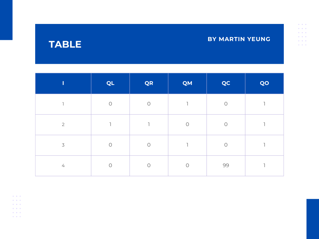
154 |
155 | 當拉格朗日插值需要滿足QL[0,1,0,0]時,即f(0)=0, f(1)=1, f(2)=0, f(3)=0 .
156 | ```math
157 | L_{0}(x) = \frac{(x-1)(x-2)(x-3)}{(0-1)(0-2)(0-3)} = 84*[x^3 - 6*x^2 + 11x -6] = 84x^3 + x^2 + 15x + 1
158 | ```
159 |
160 | ```math
161 | L_{1}(x) = \frac{(x)(x-2)(x-3)}{(1-0)(1-2)(1-3)} = 51*[x^3 - 5*x^2 + 6x] = 51x^3 + 48x^2 + 3x
162 | ```
163 |
164 | ```math
165 | L_{2}(x) = \frac{(x)(x-1)(x-3)}{(2-0)(2-1)(2-3)} = 50*[x^3 - 2*x^2 + 49x] = 50x^3 + 2x^2 + 49x
166 | ```
167 |
168 | ```math
169 | L_{3}(x) = \frac{(x)(x-1)(x-2)}{(3-0)(3-1)(3-2)} = 17x^3 + 50x^2 + 34x
170 | ```
171 |
172 | * 最終的拉格朗日插值式為:
173 | ```math
174 | P(x) = 0*L_{0}(x) + 1*L_{1}(x) + 0*L_{2}(x) + 0*L_{3}(x) = 51x^3 + 48x^2 + 3x
175 | ```
176 |
177 | 當拉格朗日插值需要滿足WL[3,1,3,0]時,即f(0)=3, f(1)=1, f(2)=3, f(3)=0 .
178 | * 最終的拉格朗日插值式為:
179 | ```math
180 | P(x) = 3*L_{0}(x) + 1*L_{1}(x) + 3*L_{2}(x) + 0*L_{3}(x) = 49x^3 + 57x^2 + 94x + 3
181 | ```
182 |
183 | 換言之,要滿足QL[3,1,3,0],就必須在f(0)=3, f(1)=1, f(2)=3, f(3)=0時通過以上多項式。
184 |
185 | ## PLONK中的多項式
186 |
187 | * 透過多項式編碼,可以將多個約束轉換成一個約束。
188 |
189 | ### 多項式的概率檢查
190 | * 要做多項式的概率檢查,需要有2個多項式,而且同為2個次數不多於d的多項式。Verifier只要進行一次多項式隨機挑戰就可以。這是Schwartz-Zippel定理。
191 | * 因為可以進一步地去使用多項式承諾(Polynomial Commitment),讓Prover負責計算x在某一任意地方的值,然後發送證明,這樣Verifier的工作量可以減少。
192 | * 假設要驗證向量a + 向量b是否等於向量c:
193 | 可以先把向量編碼成多項式(系數編碼方式)
194 | ```math
195 | a(x) = a_{0} + a_{1}(x) + a_{2}(x^2) + ... + a_{n-1}(x^n-1)
196 | ```
197 | ```math
198 | b(x) = b_{0} + b_{1}(x) + b_{2}(x^2) + ... + b_{n-1}(x^n-1)
199 | ```
200 | ```math
201 | c(x) = c_{0} + c_{1}(x) + c_{2}(x^2) + ... + c_{n-1}(x^n-1)
202 | ```
203 | Verifier 只需要給出一個隨機挑戰值(任意值) ζ∈F
204 | ```math
205 | a(ζ) + b(ζ) = c(ζ)
206 | ```
207 | 如果成功證明到以上公式,則向量a + 向量b是等於向量c。
208 | 不過當要驗證向量a乘向量b是否等於向量c,就需要用拉格朗日插值的編碼方式,經轉換之後如下:
209 | ```math
210 | a(X)⋅b(X)=c(X),∀X∈H
211 | ```
212 | 但在這公式,Verifier需要挑戰多次才可以縮小出錯概率。
213 | 因此,需要更高效的方法來進行檢測,目標是只用一次就可以檢查出Prover是否存在作弊行為。
214 | ```math
215 | a(X)⋅b(X)−c(X)=q(X)⋅z H(X),∀X∈F
216 | ```
217 | 在公式上可以看到a(X)⋅b(X)−c(X)會等於0,所以q(X)⋅zH(X)也會等於0。
218 | 換言之,在X∈H的條件下,H會是a(X)⋅b(X)−c(X)的根集合。因為X必須要使到a(X)⋅b(X)−c(X)等於0。
219 |
220 | 另外,a(X)⋅b(X)−c(X)可以被多項式zH(X)整除,並得到一個商多項式q(X)。所以只要讓Prover計算出q(X),就可以使到Verifier的工作量減少至只需進行一次隨機檢測就可知道a(X)⋅b(X)−c(X)在X∈H的條件下是否等於0。而Verifier 計算 zH(ζ) 需要 O(n) 的計算量。
221 |
222 | ### 單位根 Roots of Unity
223 | 以單位根作為 H,這可使到zH(ζ)的計算量會減少至O(logn)。
224 |
225 | ## PLONK中的置換證明
226 | Plonk 的複製約束是通過置換證明(Permutation Argument)來實現。
227 | 在這個矩陣W表格中(加入位置標示):
228 | 
229 | 可以看到,WL1 = WO2, WR1 = WO3, WO1 = WO4 。而置換證明可以通過轉換它們的位置,然後再證明置換後的新矩陣是等於矩陣W。
230 |
231 | ### 基礎協議 - Grand Product Argument
232 | 由於進行多項式編碼,所以會把多個單乘法壓縮成單次乘法的驗證。
233 | 這裡可以理解成將多個約束壓縮在一起,轉換成1個可驗證的多項式。
234 | * 引入一個輔助向量r
235 | ```math
236 | r_{0} = 1
237 | ```
238 | * r是每一個對上計算的結果(Accumulator)
239 | ```math
240 | r_{k+1} = q_{k}*r_{k}
241 | ```
242 | 假設現在有3個約束,第1個約束的起始值是1,公式是:
243 | ```math
244 | L_{0}*(r(X)-1) = 0 ,∀X∈H
245 | ```
246 | 第2個約束(遞歸的乘法關系)的公式是:
247 | ```math
248 | q(X)*r(X) = r(w.X) ,∀X∈H∖{ω-^1}
249 | ```
250 | 第3個約束 - 為最後結果是:
251 | ```math
252 | r_{n-1} = p ,∀X∈H
253 | ```
254 | 第3個約束的公式是:
255 | ```math
256 | L_{n-1}*(r(X)-r_{n-1}) = 0 ,∀X∈H
257 | ```
258 | 利用遞歸的乘法關系:
259 | ```math
260 | q(X)*r(X) = r(w.X) ,∀X∈H
261 | ```
262 | 最後得出可以驗證的多項式:(以下是相關步驟)
263 | ```math
264 | q(X)*r(X) - r(w.X) = 0 ,∀X∈H
265 | ```
266 | ```math
267 | L_{0}(X)*(r(X) - 1) + q(X)*r(X) - r(w.X) = 0 ,∀X∈H
268 | ```
269 | ```math
270 | L_{0}(X)*(r(X) - 1) + (α*q(X)*r(X) - r(w.X)) = 0 ,∀X∈H
271 | ```
272 | ```math
273 | L_{0}(X)*(r(X) - 1) + α*(q(X)*r(X) - r(w.X)) = h(X)*Z_{H}(X) ,∀X∈H
274 | ```
275 | 當中α是一個隨機數,h(X)是商多項式,
276 | ```math
277 | Z_{H}(X)是(X-1)(X-W)...(X-W^{n-1})
278 | ```
279 | ### 如何利用連乘證明來實現Multiset等價證明(Multiset Equality Argument)
280 |
281 | 假設向量 {qi} 為一個多項式 q(X) 的根集合,即對向量中的任何一個元素qi,都滿足q(ri)=0。這個多項式可以定義為:
282 | ```math
283 | q(X) = (X - q_{0})(X - q_{1})...(X - q_{n-1})
284 | ```
285 | 如果有另一多項式p(X)與q(x)相同,則會具有相同的根集合。
286 | 可以利用 Schwartz-Zippel 定理做檢驗,只要Verifier輸入一個隨機數 γ,Prover就可以通過下面的公式以證明向量 {pi} 和 {qi} 是在多重集合上是等價。
287 | ```math
288 | \prod_{i\in[n]}(γ-p_{i}) = \prod_{i\in[n]}(γ-q_{i})
289 | ```
290 | 然後,再使用連乘證明完成驗證,通過加入輔助向量,轉換成可以驗證的多項式。在目前例子,兩個連乘公式可以轉換成為一個連乘公式:
291 | ```math
292 | \prod_{i\in[n]}\frac{(γ-p_{i})}{(γ-q_{i})} = 1
293 | ```
294 |
295 | ### 如何證明Multiset與置換證明(Permutation Argument)的關係
296 | 首先,要Prover證明兩個向量是滿足奇偶位置互換的置換情況。
297 | ```math
298 | \vec{a} = (a_{0}, a_{1}, a_{2}, ..., a_{n-1}, a_{n})
299 | ```
300 | ```math
301 | \vec{b} = (b_{0}, b_{1}, b_{2}, ..., b_{n-1}, b_{n})
302 | ```
303 | 可以運用多項式編碼把向量轉換成多項式,同時加入位置向置來表示奇偶位置互換。
304 | ```math
305 | \vec{i} = (0, 1, 2, 3, ..., n-1, n)
306 | ```
307 | ```math
308 | σ = (0, 1, 3, 2, ..., n, n-1)
309 | ```
310 |
311 | 兩個向量以表格形式列出一部分:
312 | 
313 | 之後,再整理一下,將表格中的左面和右面分成2組如下:
314 | ```math
315 | a^{\prime} = (a_{i}, i) , b^{\prime} = (b_{i}, σ(i))
316 | ```
317 | ```math
318 | (a_{0}, 0) , (b_{0} = a_{1}, 1)
319 | ```
320 | ```math
321 | (a_{1}, 1) , (b_{1} = a_{0}, 0)
322 | ```
323 | ```math
324 | \vdots , \vdots
325 | ```
326 | ```math
327 | (a_{n-1}, n-1) , (b_{n-1} = a_{n}, n)
328 | ```
329 | ```math
330 | (a_{n}, n) , (b_{n} = a_{n-1}, n-1)
331 | ```
332 | 根據以上情況,如果2個向量(a, b)滿足奇偶位置互換的置換情況,則以上2個向量(a', b')也會滿足Multiset等價的關系。
333 |
334 | 若要轉換為一個多項式(或一個新的向量),可以加入一個隨機數β,結果如下:
335 | ```math
336 | a_{i}^{\prime} = (a_{i} + β*i) , b_{i}^{\prime} = (b_{i} + β*σ(i))
337 | ```
338 | ```math
339 | (a_{0} + β*0) , (b_{0} + β*1)
340 | ```
341 | ```math
342 | (a_{1} + β*1) , (b_{1} + β*0)
343 | ```
344 | ```math
345 | \vdots , \vdots
346 | ```
347 | ```math
348 | (a_{n-1} + β*(n-1)) , (b_{n-1} + β*(n))
349 | ```
350 | ```math
351 | (a_{n} + β*(n)) , (b_{n} + β*(n-1))
352 | ```
353 |
354 | ## 算術約束與複製約束
355 |
356 | ### 向量的複製約束
357 | 一個向量中,可以證明多個不同位置上的向量元素相等,例子如下:
358 | ```math
359 | \vec{a}= (a_{0} + a_{1} + a_{2} + a_{3})
360 | ```
361 | 如果要證明
362 | ```math
363 | a_{0} = a_{2}
364 | ```
365 | 可以將它們的位置對調,以σ 表示位置向量:
366 | ```math
367 | \vec{a}_{σ} 為置換後的向量
368 | ```
369 | ```math
370 | σ = (2, 1, 0, 3), \vec{a}_{σ} = (a_{2} + a_{1} + a_{0} + a_{3})
371 | ```
372 | 只要Prover證明到置換前的向量和置換後的向量相等,就表示:
373 | ```math
374 | a_{0} = a_{2} 是正確的
375 | ```
376 | ### 向量(多個)的複製約束
377 | * 以下會以例子說明整個流程:
378 | 選用矩陣W表格,同時加入一個輸出的約束。
379 | 
380 | 會留意到有些地方的值是相等的,包括:
381 | ```math
382 | w_{a,1} = w_{c,2}, w_{b,1} = w_{c,3}, w_{c,0} = w_{c,1}
383 | ```
384 | * 對表格中的三列向量用三個置換向量統一地進行位置編碼,結果如下:
385 | 
386 | 置換後的向量為:
387 | ```math
388 | σ_{a} , σ_{b} , σ_{c}
389 | ```
390 | 
391 |
392 | 因此,現在會有2個向量,分別是置換前的向量及置換後的向量。為了進行下一步驗證,需要利用一個隨機數β來進行向量合併。
393 | 之後再利用另一個隨機數γ配合連乘以獲得2個向量的Multisets。
394 | 置換前的向量:
395 | ```math
396 | f_{i} = (w_{a,i} + β*id_{a,i} + γ)(w_{b,i} + β*id_{b,i} + γ)(w_{c,i} + β*id_{c,i} + γ)
397 | ```
398 | 置換後的向量:
399 | ```math
400 | g_{i} = (w^{\prime}_{a,i} + β*σ_{a,i} + γ)(w^{\prime}_{b,i} + β*σ_{b,i} + γ)(w^{\prime}_{c,i} + β*σ_{c,i} + γ)
401 | ```
402 | 進一步演示 - 置換前的向量:
403 | ```math
404 | f_{0} = (w_{a,0} + β*0 + γ)(w_{b,0} + β*4 + γ)(w_{c,0} + β*8 + γ)
405 | ```
406 | ```math
407 | f_{1} = (w_{a,1} + β*1 + γ)(w_{b,1} + β*5 + γ)(w_{c,1} + β*9 + γ)
408 | ```
409 | ```math
410 | f_{2} = (w_{a,2} + β*2 + γ)(w_{b,2} + β*6 + γ)(w_{c,2} + β*10 + γ)
411 | ```
412 | ```math
413 | f_{3} = (w_{a,3} + β*3 + γ)(w_{b,3} + β*7 + γ)(w_{c,3} + β*11 + γ)
414 | ```
415 | 進一步演示 - 置換後的向量:
416 | ```math
417 | g_{0} = (w^{\prime}_{a,0} + β*0 + γ)(w^{\prime}_{b,0} + β*4 + γ)(w^{\prime}_{c,0} + β*9 + γ)
418 | ```
419 | ```math
420 | g_{1} = (w^{\prime}_{a,1} + β*10 + γ)(w^{\prime}_{b,1} + β*11 + γ)(w^{\prime}_{c,1} + β*8 + γ)
421 | ```
422 | ```math
423 | g_{2} = (w^{\prime}_{a,2} + β*2 + γ)(w^{\prime}_{b,2} + β*6 + γ)(w^{\prime}_{c,2} + β*1 + γ)
424 | ```
425 | ```math
426 | g_{3} = (w^{\prime}_{a,3} + β*3 + γ)(w^{\prime}_{b,3} + β*7 + γ)(w^{\prime}_{c,3} + β*5 + γ)
427 | ```
428 | 由於
429 | ```math
430 | w_{a,1} = w^{\prime}_{c,2}
431 | ```
432 | ```math
433 | w_{c,2} = w^{\prime}_{a,1}
434 | ```
435 | 所以:
436 | ```math
437 | (w_{a,1} + β*1 + γ) = (w^{\prime}_{c,2} + β*1 + γ)
438 | ```
439 | ```math
440 | (w_{c,2} + β*10 + γ) = (w^{\prime}_{a,1} + β*10 + γ)
441 | ```
442 | 換言之:
443 | ```math
444 | \prod_{x\in H}f(X) = \prod_{i\in H}g(X)
445 | ```
446 | ```math
447 | \prod_{x\in H}\frac{f(X)}{g(X)}
448 | ```
449 | 現在再利用新的向量z,以表示連乘計算的一系列中的過程。
450 | 需假設:
451 | ```math
452 | Z_{0} = 1, Z_{i+1} = Z_{i}*\frac{f(i)}{g(i)}
453 | ```
454 | Prover可以計算出以下的值:
455 | 
456 | ```math
457 | 如果\vec{f} = \vec{g},則Z_{N}會等於1
458 | ```
459 | 所以:
460 | ```math
461 | Z_{N} = Z_{0} = 1
462 | ```
--------------------------------------------------------------------------------
/FRI&Stark/part2 lesson4/2024-09-05-STARK.md:
--------------------------------------------------------------------------------
1 | ---
2 | layout: post
3 | title: STARK
4 | categories: STARK, soundness
5 | author: Yingfei
6 | ---
7 | 本文主要介绍STRAK协议的形式化定义及安全性讨论,会从密码学的角度描述STRAK协议,主要参考文献为ethSTARK。本文默认读者已经熟悉STARK协议的流程。
8 |
9 | ## STARK协议
10 |
11 | 本节我们将形式化描述STARK协议,首先介绍AIR,随后给出STARK(IOP)协议的细节。
12 |
13 | ### AIR
14 |
15 | **定义1(AIR)** 一个algebraic intermediate representation (AIR)是由tuple $\mathsf{A}=(\mathbb{F}, w, h, d, s, g, I, Cset)$组成的, 其中
16 | - $\mathbb{F}$是一个有限域;
17 | - $w, h, d, s$是一些整数;
18 | - $w$是trace的列数。
19 | - $s$是constraints集合的size。
20 | - $d$是一个constraint的最高degree。
21 | - $h$表示trace domain $\mathsf{H}_0$中使用的乘法子群的size的对数,即,$|\mathsf{H}_0| = 2^h$。
22 | - $g$是乘法群$\mathsf{H}_0 \subset \mathbb{F}^*$的生成元,因此 $|\mathsf{H}_0| =2^h$;
23 | - $I\subseteq \{1,...,w\} \times \{0, ...,2^h-1\}$是mask indices的集合。定义$Y=\{Y_{i,j}:{i,j}\in I\}$是由$I$中元素索引的mask variables;
24 | - $Cset = \{C_1, ... C_s\}$ 是constraints的有限集合,大小为s。每个constraint都由$s$个有序对$C_i = (Q_i, \mathsf{H}_i)$组成。
25 | - $Q_i \in \mathbb{F}^{\leq d}[Y]$是一个关于mask variables的多变量多项式,总degree至多为$d$,称为第$i$个 constraint polynomial.
26 | - $\mathsf{H}_i \subseteq \mathsf{H}_0$是trace domain的子集,称为第$i$个constraint enforcement domain.
27 | - 用$|Cset|$表示the arithmetic complexity of the constraints,定义为$|Cset| \sum^s_{i=1} (|Q_i|+ |\mathsf{H}_i|)$,其中,$|Q_i|$是计算多项式$Q_i$的算术电路,$|\mathsf{H}_i|$是vanishing polynomial $\mathsf{Z}_{\mathsf{H}_i}$的算术复杂度。
28 |
29 | **定义2 (AIR assignment and composition)** 一个AIR assignment是由一组多项式$\vec{P} = (P_1, ..., P_w) \in \mathbb{F}[X]^w$ 组成的。
30 | 给定一个AIR约束多项式$Q\in \mathbb{F}[Y]$,那么$Q$的composition 和 assignment $\vec{P}$ 是一个单变元多项式,用$Q \circ \vec{P} \in \mathbb{F}[X]$表示。它是通过用$P_i(g^j\cdot X) \in \mathbb{F}[X]$ 替换$Q(Y)$中的变量 $Y_{i,j} \in Y$得到的,我们用$Y_{i,j} \gets P_i(g^j \cdot X)$来简化表示这个替换。
31 |
32 | **定义3 (Satisfiability)** 一个AIR assignment $\vec{P} = (P_1, ..., P_w) \in \mathbb{F}[X]^w$满足一个AIR实例$\mathsf{A}=(\mathbb{F}, w, h, d, s, g, I, Cset)$当且仅当
33 | $$\forall i \in [s]: x\in \mathsf{H}_i \to (Q \circ \vec{P})(x) = 0.$$
34 | 换句话说,$\vec{P}$满足$\mathsf{A}$ 当且仅当 对于每个constraint $C_i=(Q_i, \mathsf{H}_i) \in Cset$, $Q \circ \vec{P}$ vanishes on $\mathsf{H}_i$。
35 |
36 | vanish:多项式$\mathsf{Z}_{\mathsf{H}_i}(X)$在$\mathbb{F}[X]$上整除多项式$Q \circ \vec{P}$。
37 |
38 | 用大家习惯的statement和witness的方式来表达,在STARK中,statement是一个AIR实例$\mathsf{A}=(\mathbb{F}, w, h, d, s, g, I, Cset)$,它定义了协议需要的公开参数以及寄存器之间的约束关系,witness则是AIR assignment $\vec{P} = (P_1, ..., P_w)$,也就是trace多项式。
39 |
40 | ### 协议
41 |
42 | 在描述协议之前,我们先介绍一些辅助输入aux。
43 | - $\mathbb{K}$ 是有限域 $\mathbb{F}_q$ 的有限扩张,size为 $q^e, e\geq1$。为了简便,全文符号对 $\mathbb{F}$ 和$\mathbb{F}_q$ 不做区分。
44 | - $\mathsf{D} \subset \mathbb{K}^*$是乘法子群 $\mathsf{D}_0 \subset \mathbb{K}^*$的非平凡陪集。称$\mathsf{D}$为evaluation domain。recall:AIR的trace domain $\mathsf{H}_0 \subset \mathsf{D}_0$。
45 | - $k'$表示$|\mathsf{D}|$的对数,即 $|\mathsf{D}| = 2^{k'}$。
46 | - $\rho = 2^h/2^{k'}$ 表示IOP协议的rate, $\rho^{-1}$为blowup factor.
47 | - $\mathsf{aux}_{\mathsf{FRI}}$定义为FRI协议的辅助输入。
48 |
49 | 在实际协议中,上述$\mathsf{D}$是LDE的input domain。注意,$\mathsf{D}$与AIR的trace domain $\mathsf{H}_0$ (trace函数的input domain)是互不相交的。这是为了避免LDE的商多项式的分母为0。
50 |
51 | 我们还会用到下列符号:
52 | - $\mathsf{Quotient} : \mathsf{D} \to \mathbb{F}$: 对于 $(x_0, y_0) \in \mathbb{K}/\mathsf{D} \times \mathbb{K}$ 和函数$f : \mathsf{D} \to \mathbb{K}$,定义函数$f$的quotient 如下:$$\mathsf{Quotient}(f; x_0, y_0) (x) = \frac{f(x)-y_0}{x-x_0}.$$
53 | - $\mathsf{RS}[\mathbb{K},S, \rho]$ 表示定义在域$\mathbb{K}$上的Reed-Solomon码,其evaluation domain为 $S$,码率 rate是$\rho$。 $$\mathsf{RS}[\mathbb{K},S, \rho] = \{f: S\to \mathbb{K}: deg(f) < \rho|S| \}$$
54 | 下面,我们开始描述协议。
55 |
56 | **$\mathcal{P,V}$ 的公共输入**:AIR实例 $\mathsf{A}=(\mathbb{F}, w, h, d, s, g, I, Cset)$ 和IOP辅助输入 $\mathsf{aux}=(\mathbb{K}, e, \mathsf{D}, k', \mathsf{aux}_{\mathsf{FRI}})$。
57 | **$\mathcal{P}$ 的秘密输入**:AIR assignment $\vec{P} = (P_1, ..., P_w) \in \mathbb{F}[X]^w$。
58 |
59 | 0. **预处理**:
60 | - Constraint weighted degree:对每个constraint $C_i=(Q_i, \mathsf{H}_i) \in Cset$,定义第$i$个composed degree $d_i = deg(Q_i)\cdot (2^h-1) - |\mathsf{H}_i|$。
61 | - Designated degree:定义$d_{max}$是比上述最大的$d_i$严格大的一个2个幂次整数。定义$a= d_{max}/2^h$.
62 | - Degree correction:对每个constraint $C_i=(Q_i, \mathsf{H}_i) \in Cset$,定义degree correction参数$c_i = d_{max}-d_i - 1$。
63 | 这一步的预处理是为了在Step2确定degree adjustment的次数,便于把高次多项式拆成$a$个与trace多项式次数相同的多项式。
64 | 1. **执行trace oracle**:证明者发送oracle functions $f_1, ..., f_w : \mathsf{D} \to \mathbb{K}$。
65 | 函数$f_i$是满足AIR的多项式$P_i(X)\in \mathbb{F}$,在evaluation domain $\mathsf{D}$上计算得到的Evaluation。即,对于 $\forall x \in \mathsf{D}$,计算所有$P_i(x)$的取值组成$f_i$。
66 | note:
67 | - $P_i(X)$的次数 $deg(P_i)<2^h$。
68 | - 如果$\mathsf{D} \subset \mathbb{F}$,那么 $f_1, ..., f_w$的取值就在$\mathbb{F}$上。这与$\mathsf{D}$和AIR的trace domain $\mathsf{H}_0$ 互不相交并不冲突。
69 | 2. **constraints线性组合**:验证者选择$2s$个随机值 $\vec{r} = (r_1, r_1', ..., r_s, r_s') \in \mathbb{K}^{2s}$发送给$\mathcal{P}$。随后$\mathcal{P, V}$共同把AIR实例中的s个constraints全部随机组合起来,得到变量$(X,Y)$的一个rational函数 $Q^{\vec{r}}(X,Y)$:$$Q^{\vec{r}}(X,Y):= \sum_{i=1}^s \left( r_i + r_i' X^{c_i}\right)\cdot \frac{Q_i(Y)}{Z_\mathsf{H_i}(X)}$$
70 | 在prover这端,$Y_{i,j}$已经被$P_i(g^jX)$替换了。由于每个$P_i$的次数严格小于$2^h$,而且$Q \circ \vec{P}$ vanishes on $\mathsf{H}_i$,因此等号右侧可以总结成一个关于变量$X$的多项式$R^{\vec{r}}_i(X)$,该多项式的degree小于$d_{max}$。
71 |
72 | 3. **constraint trace oracle**:$\mathcal{P}$ 发送oracle函数$f_0^{\vec{r}}, ..., f_{a-1}^{\vec{r}} : \mathsf{D} \to \mathbb{K}$。
73 | 每个函数$f_i^{\vec{r}}$都是多项式$P_i^{\vec{r}}(X)$在$\mathsf{D}$上的evaluation,满足:$$\left(Q^{\vec{r}}(X,Y) \circ \vec{P} \right)(X) = \sum^{a-1}_{k=0} X^k \cdot P_k^{\vec{r}}(X^a).$$
74 | 由于在 Step4 中线性组合的多项式 $R^{\vec{r}}_i(X)$ degree小于$d_{max}$,超过了trace evaluation domain的size。为了与trace的多项式$P_i$ 线性组合,一起做FRI验证low degree,所以需要拆成多个小degree组合。
75 |
76 | 拆分方式为:拆成$a= d_{max}/2^h$个多项式,每个$P_i^{\vec{r}}(X)$以$a$为次数的间隔,取原多项式中的对应系数。所以最终得到的每个多项式$P_i^{\vec{r}}(X)$的degree均小于$2^h$。
77 |
78 | 4. **DEEP Query**: $\mathcal{V}$ 从 $\mathbb{K}* \setminus (\mathsf{H}_0 \cap \bar{\mathsf{D}})$ 采样一个随机值 $\mathsf{q}$。集合$\bar{\mathsf{D}} = \{y \in \mathbb{K}* : y^{a} \in \mathsf{D}\}$。排除集合 $\mathsf{H}_0$ 是为了保证计算answer $\alpha$ 时 $\mathsf{q} \cdot g^j$ 不会重叠到另一个$g^k$,排除集合 $\bar{\mathsf{D}}$ 是为了避免计算商多项式时分母为0。
79 |
80 | 5. **DEEP Answer**: $\mathcal{P}$ 发送 answer 序列 $\{\alpha_{i,j}: (i,j) \in I\} \cup \{ \beta_k: k \in\{0, ..., a-1\}\}$。其中:$$\alpha_{i,j} = P_i(\mathsf{q} \cdot g^j), \beta_k = P_k^{\vec{r}}(\mathsf{q}^a)$$
81 | 若等式 $Q^{\vec{r}}(\mathsf{q},\{Y_{i,j} \gets \alpha_{i,j}\}) = \sum^{a-1}_{k=0} \mathsf{q}^k \cdot \beta_k$成立,则称约束$Q^{\vec{r}}(X,Y)$ 在该answer下是验证有效的。 $\{Y_{i,j} \gets \alpha_{i,j}\}$表示用$\alpha_{i,j}$替换$Y_{i,j}$。
82 |
83 | 6. **FRI 线性组合**: $\mathcal{V}$ 采样随机值 $$r^F = \{r^F_{(i,j)}: (i,j) \in I\} \cup \{r^F_k: k \in\{0, ..., a-1\}\} \in \mathbb{K}^{I\cup[a]}$$ 并发送给$\mathcal{P}$。
84 |
85 | 7. **FRI协议**:$\mathcal{P, V}$共同利用FRI协议的辅助输入$\mathsf{aux}_{\mathsf{FRI}}$,执行FRI协议,验证 proximity to 函数 $g_{(\vec{r},q,answer, r^F)}:\mathsf{D} \to \mathbb{K}$ 的RS码 $\mathsf{RS}[\mathbb{K},\mathsf{D}, \rho]$。其中,$$g_{(\vec{r},\mathsf{q}, answer, r^F)}:= \sum_{(i,j) \in I} r^F_{(i,j)}\cdot \mathsf{Quotient}(f_i; \mathsf{q}\cdot g^j, \alpha_{i,j})(x) + \sum_{k=0}^{a-1}\mathsf{Quotient}(f_k^{\vec{r}}; \mathsf{q}^a, \beta_k)(x).$$
86 | 8. **协议验证**:$\mathcal{V}$ 接受条件:
87 | 1. FRI 协议接受$g_{(\vec{r},q,answer, r^F)}$ ;
88 | 2. $Q^{\vec{r}}(X,Y)$ 在该answer下是验证有效的。
89 |
90 |
91 | ## STARK安全性
92 | ### 基础定义
93 |
94 | 下面我们简单描述IOP协议涉及的几个安全性定义。
95 | Completeness 说明了诚实执行协议的证明者与诚实执行协议的验证者交互,最终验证者会(以指数接近1的概率)接受证明。
96 |
97 | Soundness 指的是,如果(恶意的)证明者证明的statement是错误的,在上述协议中,即$\mathsf{A}$不是AIR实例,那么验证者会(以指数接近1的概率,$1-\epsilon$)拒绝证明。
98 |
99 | Knowledge Soundness 是说,如果(恶意的)证明者要证明的statement是正确的,验证者以某一个概率接受了证明,则存在一个概率多项式时间的提取器,可以从证明者与验证者的交互中提取出statement对应的witness。
100 |
101 | 以上述协议为例,如果 $\mathsf{A}$ 是AIR实例,验证者以$\epsilon$概率接受了证明,那么我们可以提取出$\mathsf{A}$对应的trace 多项式$\vec{P}$。
102 |
103 | 这个定义意味着恶意的证明者如果能生成正确的证明,则代表这个证明者获得了statement (AIR实例) 的witness。上述定义中提到的$\epsilon$称为soundness error。
104 |
105 | 做安全性证明需要注意的一些细节:
106 | - 提取器的输入和验证者一样。
107 | - 提取器可以调用恶意的证明者作为自己的子程序,但需要注意这个恶意的证明者也没有witness。
108 |
109 | ### 安全性分析需要用到的几个定理
110 |
111 | 首先,我们需要从编码的角度去看STARK协议中出现的多项式:向量$f$是words,AIR的assignment是RS code的codewords。
112 |
113 | **定理1** (Johnson bound)对于所有的$\eta \in (0, 1-\sqrt{\rho})$,编码$V$是$(1-\sqrt{\rho}-\eta, \frac{1}{2\eta \sqrt{\rho}})$- list-decodable。
114 |
115 | 这个定理说明了,对于一个向量$u \in \mathbb{F}^n_q$,在码 (code) $V\subset \mathbb{F}^n$上,至多存在$\ell = \frac{1}{2\eta \sqrt{\rho}}$个的码字 (codeword),与$u$的相关汉明距离(relative Hamming distance)不超过$\gamma = 1-\sqrt{\rho}-\eta$。
116 |
117 | **定理2** (Guruswami–Sudan list decoding)GS list decoding算法输入一个word $u:\mathsf{D} \to \mathbb{F}_q$,一个RS码$V = \mathsf{RS}[\mathbb{F},\mathsf{D}, \rho]$,一个slackness参数$\eta>0$,输出$V$中agree with $u$ 的一组码字(agreement domain $S$),density至少是D的$\sqrt{\rho} +\eta$。该算法的期望时间是 $n, 1/\rho, 1/\eta$ 和 $\log q$ 的多项式级别。
118 |
119 | agree with:在agreement domain $S$ 上,word $u$ 与码字 $v$ 满足:$\forall x \in S, u(x) = v(x)$。
120 | density:agreement domain的 size 与 word $u$ 的全部input比值 $\sigma \leq|S| / |\mathsf{D}|$。
121 |
122 | 因为agree考虑的是$x$ 从 $S$ 集合中取值时codeword与word的值是否相同,density也考虑的是 $x$ 在 $S$ 集合取值与原本 $x$ 在 $\mathsf{D}$ 中任意取值的情况,即两个集合的size对比。
123 |
124 | 下一部分knowledge soundness的提取器将会用到定理2介绍的解码算法。在此之前,我们需要先扩展上述算法到多组words的联合解码。
125 |
126 | **定义4**(Correlated agreement)定义向量集合$V\subset \mathbb{K}^{\mathsf{D}}$,$W=\{w_1, ..., w_k\}$,其中每个$w_i \in \mathbb{K}^{\mathsf{D}}$。定义agreement参数$\sigma \in [0,1]$。称$W$与$V$在 agreement domain $S \subset \mathsf{D}$ 上以density $\sigma$ 相关一致(correlated agree),如果满足:
127 | - $\sigma \leq|S| / |\mathsf{D}|$,
128 | - 存在$v_1, ..., v_k \in V$,使得,$w_i$ 在 $S$ 上与 $v_i$ agree,即$\forall x \in S, w_i(x) = v_i(x)$。
129 |
130 | 我们称S是一个最大agreement domain如果它不真包含 ($\subsetneq$) 在任何一个agreement domain里。
131 |
132 | 下面我们介绍RS算法的一个推导引理,这个引理将直接用于构造STARK协议的知识提取器。
133 |
134 | **引理1**(Correlated agreement list decoder)定义RS码$V = \mathsf{RS}[\mathbb{F},\mathsf{D}, \rho]$,向量集合$W=\{w_1, ..., w_k\}$,其中每个$w_i \in \mathbb{K}^{\mathsf{D}}$。定义$\sigma = \sqrt{\rho} + \eta, \eta>0$是一个agreement density参数。存在一个随机化算法,期望运行时间是 $1/\rho, 1/\eta, k, \log{|\mathbb{K}|}$ 的多项式级别,该算法输出一个列表$\mathcal{S}=\{S_1, ..., S_{\ell} \}$。该列表是所有density至少为$\sigma$的最大agreement domain,满足$\ell \leq 1/(2\eta\sqrt{\rho})$。此外,每一组$S_i, w_j \in W, v_{i,j} \in V$都满足$w_j$ 在 $S_i$ 上与 $v_{i,j}$ agree。
135 |
136 | 这个算法是通过多次调用GS列表解码算法,并对算法输出的agreement domain逐次求交集得到的,而$\ell \leq 1/(2\eta\sqrt{\rho})$这个条件则是直接应用Johnson bound得到的结论。
137 | 在此暂时忽略该引理的证明。
138 |
139 |
140 | ### 安全性证明
141 |
142 | #### 安全性定理
143 |
144 | 定理3给出了STARK协议的soundness error上界。
145 |
146 | **定理3** (Knowledge Soundness)若验证者 $\mathcal{V}$ 满足条件1和2,则存在一个可以成功输出AIR assignment, 即$\vec{P}= {P_1},...,{P_w}$ 的knowledge extractor $\mathcal{E}(\mathsf{A}=(\mathbb{F}, w, h, d, s, g, I, Cset), \mathsf{aux}, f=(f_1, ..., f_w))$。如果 $\mathcal{V}$ 满足以下条件:
147 | 1. 在FRI的Query阶段,$\mathcal{V}$ 调用FRI的验证者 $\mathsf{s}$ 次。
148 | 2. 存在一个证明者$\mathcal{P}^*(\mathsf{A}, \mathsf{aux})$ 在Step1 oracle发送$f=(f_1, ..., f_w)$, 且$\mathcal{V}$与$\mathcal{P}$交互时,$\mathcal{V}$接受的概率大于 $$\epsilon_{total} = \frac{\ell}{|\mathbb{K}|} + \frac{(d_{max}+2^h + a) \cdot \ell}{|\mathbb{K}|-a|\mathsf{D}| + |\mathsf{H}_0|} + \epsilon_{\mathsf{FRI}}(q,n,\rho, m,s,\vec{t}),$$ 其中整数$m\geq2, \ell=m/\rho$.
149 |
150 | 这个定理说明,存在一个提取器可以提取AIR的witness,但这个提取器要输入LDE的多项式$f$。STARK的PIOP中,$f$不是直接发送给验证者的,因此,我们不能直接利用定理4证明STARK协议的knowledge soundness,需要做一点转化。这个转化需要借用下面的推论。
151 |
152 | **推论1**(Knowledge extraction from sufficiently convincing prover)给定整数$R\geq1, m\geq3$, 给定$\mathsf{A}=(\mathbb{F}, w, h, d, s, g, I, Cset), \mathsf{aux}=(\mathbb{K}, e, \mathsf{D},k',\mathsf{aux}_{\mathsf{FRI}})$以及$\mathsf{aux}_{\mathsf{FRI}}=(\vec{t},s)$, $2^{-R}=2^h/2^{k'}$。假设存在证明者$\mathcal{P}^*$,满足
153 | $$\Pr[\langle \mathcal{V}(\mathsf{A, aux}, ), \mathcal{P}(\mathsf{A, aux})\rangle = accept] \geq 2\cdot \epsilon_{total},$$
154 | 那么, $\mathsf{A} \in \mathcal{L}_{\mathsf{AIR}}$,即 $\mathsf{A}$ 是$\mathsf{AIR}$实例, 且存在一个knowledge extractor $\mathcal{E}'$,在输入$(\mathsf{A, aux})$时,与$\mathcal{P}^*$交互可以输出满足 $\mathsf{A}$的assignment,提取器的期望运行时间为$(w,2^h, d, |Cset|, \log|\mathbb{F}|,1/\epsilon)$的多项式。
155 |
156 | **构造$\mathcal{E}'$**:$\mathcal{E}'$重复执行如下步骤$1/\epsilon_{total}$次
157 | - 调用$\mathcal{P}^*$ 并读取oracle $f = (f_1,...,f_w)$;
158 | - 调用定理4中的提取器$\mathcal{E}(\mathsf{A,aux},f)$。
159 |
160 | $\mathcal{E}'$不需要输入$f$,因此可以直接用在STARK的证明里,因此,我们可以通过合适的取值使得soundness error是一个可忽略的函数(安全参数的指数分之一,例如$2^{-128}$),证明上述STARK协议是一个knowledge soundness error至多为$\epsilon$的Scalalbe Transparent IOP of Knowledge协议,满足completeness和knowledge soundness。
161 |
162 | $\epsilon$ 是随机算法Las Vegas algorithm的优势。
163 |
164 | #### Knowledge Extractor的构造
165 |
166 | 现在介绍如何构造定理3中提到的knowledge extractor $\mathcal{E}$。
167 |
168 | $\mathcal{E}$的输入是$\mathsf{A}=(\mathbb{F}, w, h, d, s, g, I, Cset), \mathsf{aux}, f=(f_1, ..., f_w)$,其中$\mathsf{aux} = (\mathbb{K}, e, \mathsf{D}, k', \mathsf{aux}_{\mathsf{FRI}})$是协议的辅助输入。提取器$\mathcal{E}$可以从证明者的第一个oracle function $(f_1, ..., f_w)$ 中提取AIR的assignment $\vec{P}$。
169 | - 准备:$\rho = 2^h/|\mathsf{D}|$。定义$\rho^+ =\frac{2^h+1}{|\mathsf{D}|}$. $\mathsf{RS}[\mathbb{F},\mathsf{D}, \rho]$的码字都是degree小于$2^h$的多项式的求值,所以$\mathsf{RS}[\mathbb{F},\mathsf{D}, \rho^+]$的码字对应的多项式degree都小于$2^h$。
170 | - $\mathcal{E}$首先以 agreement参数$\sqrt{\rho^+}(1+\frac{1}{2m})$, 向量集合$U=\{f_1, ..., f_w\} \subset (\mathbb{F}^{\mathsf{D}})^w$ 和RS码$\mathsf{RS}[\mathbb{F},\mathsf{D}, \rho^+]$ 调用引理1的解码器。定义列表$\mathcal{S}=\{S_1, ..., S_{\ell} \}$ 为算法输出的agreement domain,其density大于等于$\sqrt{\rho^+}(1+\frac{1}{2m})$。定义$\mathcal{P}=\{\vec{P}_1, ..., \vec{P}_{\ell} \}$ 是对应的多项式集合,其中$\vec{P}_i = {P_{i,1},..., P_{i,w}} \in \mathbb{F}^{\leq 2^h[X]}$是与$f_j$在$S_i$上agree的多项式序列,每个$P_{i,j}$的次数都小于$2^h$。
171 | - 对于$k=1,...,\ell$,依次检验$\vec{P}_k$是否满足AIR实例$\mathsf{A}$,如果满足则输出$\vec{P}_k$作为assignment $\vec{P}$;否则输出失败终止算法。
172 |
173 | 根据定义2,每个$\vec{P}_i$都是一个AIR assignment,$\vec{P}_i$包含的多项式在$\mathbb{F}$上。
174 |
175 | 因为每个$\vec{P}_i$中的多项式$P_{i,j}$都与$f_j$在集合$S_i$中取值一致
176 | 如果$S_i= H_i$,那么$\vec{P}_i$就是assignment。
177 |
178 | #### 证明定理3(Knowledge Soundness)
179 |
180 | 上一节我们已经给出了提取器的构造,这一节,我们继续讨论定理3证明soundness error。
181 |
182 | 在这个证明中我们做一些简化的假设。
183 |
184 | - 证明者$\mathcal{P}(\mathsf{A,aux})$是确定算法。特别是
185 | - 对于每个 $\vec{r}$,Step3中证明者的oracle functions $f^\vec{r}_0, ..., f^\vec{r}_{a-1}$, 由 $\vec{r}$ 唯一确定,
186 | - Step5 中的answer序列 $(\alpha, \beta)$ 由$\vec{r}$ 唯一确定。
187 | - answer序列的有效性验证约束 $Q^\vec{r}(X,Y)$ 对于所有 $\vec{r}$ 和 $\mathsf{q}$都成立。
188 |
189 | 上一部分我们讨论过,提取器$\mathcal{E}$在输入$f_1,...,f_w$时,输出为$(\mathcal{S,P})$,$\mathcal{S}=\{S_1, ..., S_{\ell} \}$是density大于等于$\sqrt{\rho^+}(1+\frac{1}{2m})$的agreement domains集合,$\mathcal{P}=\{ \vec{P}_1,...,\vec{P}_\ell \}$ 都是AIR assignment。$\mathcal{P}$中的每个多项式序列都与$f_1,...,f_w$对应一致。
190 |
191 | 设置$\eta = \frac{\sqrt{\rho^+}}{2m}$, 根据定理1(Johnson bound)我们可以得到$\ell \leq m/\rho^+ \leq m/\rho$。
192 |
193 | 接下来把$(f^\vec{r}_0, ..., f^\vec{r}_{a-1})$加到$(f_1,...,f_w)$后面,得到一个更大的序列。然后应用RS码的解码器Correlated agreement list decoder,设置agreement参数$\sqrt{\rho^+} + \eta, \eta = \frac{\sqrt{\rho^+}}{2m}$。把得到的agreement domain记为$\mathcal{S}^\vec{r} = \{ S_1^\vec{r}, ..., S_\ell^\vec{r} \}$,其density是$\sqrt{\rho^+} + \eta$。
194 |
195 | 因为在相关解码器中,我们一直对$\mathcal{S}$求交集,所以每个 $S_i^\vec{r}$ 都一定包含在某个 $S_k \in \mathcal{S}$中。由于$S_i^\vec{r}$的density大于 $\rho^+$,所以函数$(f_1,...,f_w)$,在$\mathcal{S}_i^\vec{r}$ domain中的所有元素的取值,都与$\vec{P}_k$一致。这种情况我们称为$\mathcal{S}_i^\vec{r}$ 与$\vec{P}_k$相关联(associated with)。
196 |
197 | 定义 $\vec{P}_i^{\vec{r}} = (P_0^{\vec{r}},..., P_{a-1}^{\vec{r}})$ 是次数$\leq 2^h$,与$(f^\vec{r}_0, ..., f^\vec{r}_{a-1})$ 在$S_\ell^\vec{r}$ agree的多项式序列,定义$\mathcal{P}^\vec{r} = \{\vec{P}_1^{\vec{r}},...,\vec{P}_\ell^{\vec{r}}\}$。由于$\mathcal{S}_i^\vec{r}$ 与$\vec{P}_k$相关联,$\vec{P}_i^{\vec{r}}$与$\mathcal{S}_i^\vec{r}$ 相关联,所以我们也称$\vec{P}_i^{\vec{r}}$与$\vec{P}_k$相关联。
198 |
199 | 上述说明了多项式之间的关联是存在的,下面我们希望把这种关联在固定在随机挑战值上,保证证明能被验证者接受,以此证明$\vec{P}_k$是合法的witness。
200 |
201 | 定义Good$(\vec{r},\mathsf{q})$ 为FRI协议接受概率大于$\epsilon_{\mathsf{FRI}}$的取值。
202 |
203 | **引理2** 对于Good$(\vec{r},\mathsf{q})$,存在:
204 | - AIR assignment $\vec{P}_k = \{P_{k,1},..., P_{k,w}\} \in \mathcal{P}$
205 | - 多项式序列$\vec{P}^{\vec{r}} = (P_0^{\vec{r}},..., P_{a-1}^{\vec{r}})$ 与$\vec{P}_k$ 相关联。
206 | - $S_{(\vec{r},\mathsf{q})} \subset S_k$
207 | 使得下列条件都成立:
208 | 1. $|S_{(\vec{r},\mathsf{q})}| > (\sqrt{\rho^+} + \eta) |\mathsf{D}|$
209 | 2. 每个$P_{k,i}$都与$f_i$在$S_{(\vec{r},\mathsf{q})}$ agree
210 | 3. $P_{k,i}$的取值与DEEP answer $\alpha_{i,j}$ 全部匹配。$P_{k,i}(\mathsf{q}g^j) = \alpha_{i,j}$
211 | 4. $P_{l}^{\vec{r}}$与$f_{l}^{\vec{r}}$ 在 $S_{(\vec{r},\mathsf{q})}$ agree
212 | 5. $P_{l}^{\vec{r}}$的取值与DEEP answer $\beta_{l}$ 全部匹配。
213 |
214 | 条件2-5保证了DEEP answer是可以验证有效的。
215 | 这条引理说明了Good$(\vec{r},\mathsf{q})$ 能让验证者接受FRI的证明,也保证DEEP的answer可以验证有效,这两点同时保证了验证者会接受STARK的证明。
216 |
217 | 下面,我们希望说明,满足Good$(\vec{r},\mathsf{q})$的随机值 $(\vec{r},\mathsf{q})$取值有足够多,这一点可以保证我们提取的$\vec{P}_k$是合法的。
218 |
219 | 定义Useful$(\vec{r})$为能保证$\mathsf{q}$ 的取值足够多,的$\vec{r}$的取值。
220 | - $\mathsf{q}$ 的取值指的是让Good$(\vec{r},\mathsf{q})$ 条件在$\vec{P}_k \in \mathcal{P}$成立的那些取值。
221 | - 足够多指的是,$>((a+1) \cdot |\mathsf{H}_0| + a) \cdot \ell= (d_{max} + 2^h + a) \cdot \ell$
222 |
223 | **引理3**对于Useful$(\vec{r})$,函数$Q^{\vec{r}}(X,Y) \circ \vec{P}_k$是有限域$\mathbb{K}$上的多项式。
224 |
225 | **引理4** 如果线性独立的随机值$({r}_1, ..., {r}_{2s}) \in \mathbb{K}^{2s}$都对于某个函数序列$\vec{P}_k$是useful,那么$\vec{P}_k$满足AIR实例$\mathsf{A}$。
226 |
227 | 引理3说明了$\vec{P}_k$是assignment,引理4则说明了$\vec{P}_k$满足我们要求的AIR实例$\mathsf{A}$。这样,我们基本完成了提取器的构造和说明,下面简单讨论soundness error的上界是如何得到的。
228 |
229 | 接下来,我们限制随机值$\vec{r}$ is not useful概率。如果$\vec{r}$ not useful,那么对于每组assignment $\vec{P}_k$,至多有$(d_{max} + 2^h + a) \cdot \ell$个$\mathsf{q}$的取值是Good$(\vec{r},\mathsf{q})$。
230 | 那么对于所有的assignment $\mathcal{P}$,总共有$(d_{max} + 2^h + a) \cdot \ell |\mathcal{P}| = ((a+1) \cdot 2^h + a) \cdot \ell^2$个$\mathsf{q}$的取值使得FRI的接受概率大于等于$\epsilon_{\mathsf{FRI}}$。
231 | 那么,STARK协议在条件为$\vec{r}$ is not useful的接受概率是$\frac{(d_{max} + 2^h + a) \cdot \ell^2}{|\mathbb{K}|-a|\mathsf{D}| + |\mathsf{H}_0|} + \epsilon_{\mathsf{FRI}}$.
232 |
233 | $\vec{r}$ is useful的概率是$\frac{\ell}{|\mathbb{K}|}$。假设$\vec{P}_k$是使得$\vec{r}$ is useful的概率最大的集合。这个概率一定严格大于$\frac{1}{|\mathbb{K}|}$,即从$\mathbb{K}$中随机选一个的概率。因此,useful的$\vec{r}$组成的集合中一定包含了能够张成$\mathbb{K}^{2s}$一组基(线性独立的一组随机值)。根据引理4,这个$\vec{P}_k$是满足AIR实例的assignment,也就是witness。
--------------------------------------------------------------------------------
215 |
--------------------------------------------------------------------------------
/Plonk/lesson 6/poly_utils.py:
--------------------------------------------------------------------------------
1 | # Creates an object that includes convenience operations for numbers
2 | # and polynomials in some prime field
3 | class PrimeField():
4 | def __init__(self, modulus):
5 | assert pow(2, modulus, modulus) == 2
6 | self.modulus = modulus
7 |
8 | def add(self, x, y):
9 | return (x+y) % self.modulus
10 |
11 | def sub(self, x, y):
12 | return (x-y) % self.modulus
13 |
14 | def mul(self, x, y):
15 | return (x*y) % self.modulus
16 |
17 | def exp(self, x, p):
18 | return pow(x, p, self.modulus)
19 |
20 | # evaluate the polynomal in the evaluation form in a coset
21 | # xs[0] must the shifting parameter h
22 | # formula is (x^m - h^m) / (m h^m) * sum(ys[i] * xs[i] / (x - xs[i]))
23 | def eval_barycentric(self, x, xs, ys):
24 | m = len(xs) # coset order
25 | xm = self.exp(x, m)
26 | hm = self.exp(xs[0], m)
27 | s = 0
28 | for i in range(len(xs)):
29 | s = self.add(s, self.div(self.mul(xs[i], ys[i]), self.sub(x, xs[i])))
30 | return self.mul(s, self.div(self.sub(xm, hm), self.mul(m, hm)))
31 |
32 | # evaluate the polynomal in the evaluate form for all cosets
33 | # with some optimization on inversion
34 | def eval_barycentric_all(self, x, xs, ys, m):
35 | ncosets = len(xs) // m
36 | # evaluate all inversions in batch
37 | toinv = [x - xx for xx in xs]
38 | toinv.append(m)
39 | inved = self.multi_inv(toinv)
40 | invm = inved[-1]
41 | xm = self.exp(x, m)
42 | ss = []
43 | modulus = self.modulus
44 | for i in range(ncosets):
45 | s = 0
46 | for j in range(m):
47 | idx = j*ncosets+i
48 | s = (s + xs[idx] * ys[idx] * inved[idx]) % modulus
49 | ss.append(s * (xm - xs[i * m]) * invm * xs[-i * m] % modulus)
50 | return ss
51 |
52 | # Modular inverse using the extended Euclidean algorithm
53 | def inv(self, a):
54 | if a == 0:
55 | return 0
56 | lm, hm = 1, 0
57 | low, high = a % self.modulus, self.modulus
58 | while low > 1:
59 | r = high//low
60 | nm, new = hm-lm*r, high-low*r
61 | lm, low, hm, high = nm, new, lm, low
62 | return lm % self.modulus
63 |
64 | def multi_inv(self, values):
65 | partials = [1]
66 | for i in range(len(values)):
67 | partials.append(self.mul(partials[-1], values[i] or 1))
68 | inv = self.inv(partials[-1])
69 | outputs = [0] * len(values)
70 | for i in range(len(values), 0, -1):
71 | outputs[i-1] = self.mul(partials[i-1], inv) if values[i-1] else 0
72 | inv = self.mul(inv, values[i-1] or 1)
73 | return outputs
74 |
75 | def div(self, x, y):
76 | return self.mul(x, self.inv(y))
77 |
78 | # Evaluate a polynomial at a point
79 | def eval_poly_at(self, p, x):
80 | y = 0
81 | power_of_x = 1
82 | for i, p_coeff in enumerate(p):
83 | y += power_of_x * p_coeff
84 | power_of_x = (power_of_x * x) % self.modulus
85 | return y % self.modulus
86 |
87 | # Arithmetic for polynomials
88 | def add_polys(self, a, b):
89 | return [((a[i] if i < len(a) else 0) + (b[i] if i < len(b) else 0))
90 | % self.modulus for i in range(max(len(a), len(b)))]
91 |
92 | def sub_polys(self, a, b):
93 | return [((a[i] if i < len(a) else 0) - (b[i] if i < len(b) else 0))
94 | % self.modulus for i in range(max(len(a), len(b)))]
95 |
96 | def mul_by_const(self, a, c):
97 | return [(x*c) % self.modulus for x in a]
98 |
99 | def mul_polys(self, a, b):
100 | o = [0] * (len(a) + len(b) - 1)
101 | for i, aval in enumerate(a):
102 | for j, bval in enumerate(b):
103 | o[i+j] += a[i] * b[j]
104 | return [x % self.modulus for x in o]
105 |
106 | def div_polys(self, a, b):
107 | assert len(a) >= len(b)
108 | a = [x for x in a]
109 | o = []
110 | apos = len(a) - 1
111 | bpos = len(b) - 1
112 | diff = apos - bpos
113 | while diff >= 0:
114 | quot = self.div(a[apos], b[bpos])
115 | o.insert(0, quot)
116 | for i in range(bpos, -1, -1):
117 | a[diff+i] -= b[i] * quot
118 | apos -= 1
119 | diff -= 1
120 | return [x % self.modulus for x in o]
121 |
122 | def div_polys_with_rem(self, a, b):
123 | assert len(a) >= len(b)
124 | a = [x for x in a]
125 | o = []
126 | apos = len(a) - 1
127 | bpos = len(b) - 1
128 | diff = apos - bpos
129 | while diff >= 0:
130 | quot = self.div(a[apos], b[bpos])
131 | o.insert(0, quot)
132 | for i in range(bpos, -1, -1):
133 | a[diff+i] -= b[i] * quot
134 | apos -= 1
135 | diff -= 1
136 | return [x % self.modulus for x in o], [x % self.modulus for x in a[:apos-1]]
137 |
138 | def mod_polys(self, a, b):
139 | return self.sub_polys(a, self.mul_polys(b, self.div_polys(a, b)))[:len(b)-1]
140 |
141 | # Build a polynomial from a few coefficients
142 | def sparse(self, coeff_dict):
143 | o = [0] * (max(coeff_dict.keys()) + 1)
144 | for k, v in coeff_dict.items():
145 | o[k] = v % self.modulus
146 | return o
147 |
148 | # Build a polynomial that returns 0 at all specified xs
149 | def zpoly(self, xs):
150 | root = [1]
151 | for x in xs:
152 | root.insert(0, 0)
153 | for j in range(len(root)-1):
154 | root[j] -= root[j+1] * x
155 | return [x % self.modulus for x in root]
156 |
157 | # Get the set of powers of R, until but not including when the powers
158 | # loop back to 1
159 | def get_power_cycle(self, r):
160 | o = [1, r]
161 | while o[-1] != 1:
162 | o.append((o[-1] * r) % self.modulus)
163 | return o[:-1]
164 |
165 | def degree(self, poly):
166 | for i in reversed(range(len(poly))):
167 | if poly[i] != 0:
168 | return i
169 | return 0
170 |
171 | # Given p+1 y values and x values with no errors, recovers the original
172 | # p degree polynomial.
173 | # Lagrange interpolation works roughly in the following way.
174 | # 1. Suppose you have a set of points, eg. x = [1, 2, 3], y = [2, 5, 10]
175 | # 2. For each x, generate a polynomial which equals its corresponding
176 | # y coordinate at that point and 0 at all other points provided.
177 | # 3. Add these polynomials together.
178 |
179 | def lagrange_interp(self, xs, ys):
180 | # Generate master numerator polynomial, eg. (x - x1) * (x - x2) * ... * (x - xn)
181 | root = self.zpoly(xs)
182 | assert len(root) == len(ys) + 1
183 | # print(root)
184 | # Generate per-value numerator polynomials, eg. for x=x2,
185 | # (x - x1) * (x - x3) * ... * (x - xn), by dividing the master
186 | # polynomial back by each x coordinate
187 | nums = [self.div_polys(root, [-x, 1]) for x in xs]
188 | # Generate denominators by evaluating numerator polys at each x
189 | denoms = [self.eval_poly_at(nums[i], xs[i]) for i in range(len(xs))]
190 | invdenoms = self.multi_inv(denoms)
191 | # Generate output polynomial, which is the sum of the per-value numerator
192 | # polynomials rescaled to have the right y values
193 | b = [0 for y in ys]
194 | for i in range(len(xs)):
195 | yslice = self.mul(ys[i], invdenoms[i])
196 | for j in range(len(ys)):
197 | if nums[i][j] and ys[i]:
198 | b[j] += nums[i][j] * yslice
199 | return [x % self.modulus for x in b]
200 |
201 | # Optimized poly evaluation for degree 4
202 | def eval_quartic(self, p, x):
203 | xsq = x * x % self.modulus
204 | xcb = xsq * x
205 | return (p[0] + p[1] * x + p[2] * xsq + p[3] * xcb) % self.modulus
206 |
207 | # Optimized version of the above restricted to deg-4 polynomials
208 | def lagrange_interp_4(self, xs, ys):
209 | x01, x02, x03, x12, x13, x23 = \
210 | xs[0] * xs[1], xs[0] * xs[2], xs[0] * xs[3], xs[1] * xs[2], xs[1] * xs[3], xs[2] * xs[3]
211 | m = self.modulus
212 | eq0 = [-x12 * xs[3] % m, (x12 + x13 + x23), -xs[1]-xs[2]-xs[3], 1]
213 | eq1 = [-x02 * xs[3] % m, (x02 + x03 + x23), -xs[0]-xs[2]-xs[3], 1]
214 | eq2 = [-x01 * xs[3] % m, (x01 + x03 + x13), -xs[0]-xs[1]-xs[3], 1]
215 | eq3 = [-x01 * xs[2] % m, (x01 + x02 + x12), -xs[0]-xs[1]-xs[2], 1]
216 | e0 = self.eval_poly_at(eq0, xs[0])
217 | e1 = self.eval_poly_at(eq1, xs[1])
218 | e2 = self.eval_poly_at(eq2, xs[2])
219 | e3 = self.eval_poly_at(eq3, xs[3])
220 | e01 = e0 * e1
221 | e23 = e2 * e3
222 | invall = self.inv(e01 * e23)
223 | inv_y0 = ys[0] * invall * e1 * e23 % m
224 | inv_y1 = ys[1] * invall * e0 * e23 % m
225 | inv_y2 = ys[2] * invall * e01 * e3 % m
226 | inv_y3 = ys[3] * invall * e01 * e2 % m
227 | return [(eq0[i] * inv_y0 + eq1[i] * inv_y1 + eq2[i] * inv_y2 + eq3[i] * inv_y3) % m for i in range(4)]
228 |
229 | # Optimized version of the above restricted to deg-2 polynomials
230 | def lagrange_interp_2(self, xs, ys):
231 | m = self.modulus
232 | eq0 = [-xs[1] % m, 1]
233 | eq1 = [-xs[0] % m, 1]
234 | e0 = self.eval_poly_at(eq0, xs[0])
235 | e1 = self.eval_poly_at(eq1, xs[1])
236 | invall = self.inv(e0 * e1)
237 | inv_y0 = ys[0] * invall * e1
238 | inv_y1 = ys[1] * invall * e0
239 | return [(eq0[i] * inv_y0 + eq1[i] * inv_y1) % m for i in range(2)]
240 |
241 | # Optimized version of the above restricted to deg-4 polynomials
242 | def multi_interp_4(self, xsets, ysets):
243 | data = []
244 | invtargets = []
245 | for xs, ys in zip(xsets, ysets):
246 | x01, x02, x03, x12, x13, x23 = \
247 | xs[0] * xs[1], xs[0] * xs[2], xs[0] * xs[3], xs[1] * xs[2], xs[1] * xs[3], xs[2] * xs[3]
248 | m = self.modulus
249 | eq0 = [-x12 * xs[3] % m, (x12 + x13 + x23), -xs[1]-xs[2]-xs[3], 1]
250 | eq1 = [-x02 * xs[3] % m, (x02 + x03 + x23), -xs[0]-xs[2]-xs[3], 1]
251 | eq2 = [-x01 * xs[3] % m, (x01 + x03 + x13), -xs[0]-xs[1]-xs[3], 1]
252 | eq3 = [-x01 * xs[2] % m, (x01 + x02 + x12), -xs[0]-xs[1]-xs[2], 1]
253 | e0 = self.eval_quartic(eq0, xs[0])
254 | e1 = self.eval_quartic(eq1, xs[1])
255 | e2 = self.eval_quartic(eq2, xs[2])
256 | e3 = self.eval_quartic(eq3, xs[3])
257 | data.append([ys, eq0, eq1, eq2, eq3])
258 | invtargets.extend([e0, e1, e2, e3])
259 | invalls = self.multi_inv(invtargets)
260 | o = []
261 | for (i, (ys, eq0, eq1, eq2, eq3)) in enumerate(data):
262 | invallz = invalls[i*4:i*4+4]
263 | inv_y0 = ys[0] * invallz[0] % m
264 | inv_y1 = ys[1] * invallz[1] % m
265 | inv_y2 = ys[2] * invallz[2] % m
266 | inv_y3 = ys[3] * invallz[3] % m
267 | o.append([(eq0[i] * inv_y0 + eq1[i] * inv_y1 + eq2[i] * inv_y2 + eq3[i] * inv_y3) % m for i in range(4)])
268 | # assert o == [self.lagrange_interp_4(xs, ys) for xs, ys in zip(xsets, ysets)]
269 | return o
270 |
271 | # Linear combination of polynomals
272 | def linearcomb_polys(self, ps, c):
273 | psc = []
274 | for i in range(len(c)):
275 | psc = self.add_polys(psc, self.mul_by_const(ps[i], c[i]))
276 | return psc
--------------------------------------------------------------------------------
/LICENSE:
--------------------------------------------------------------------------------
1 | Apache License
2 | Version 2.0, January 2004
3 | http://www.apache.org/licenses/
4 |
5 | TERMS AND CONDITIONS FOR USE, REPRODUCTION, AND DISTRIBUTION
6 |
7 | 1. Definitions.
8 |
9 | "License" shall mean the terms and conditions for use, reproduction,
10 | and distribution as defined by Sections 1 through 9 of this document.
11 |
12 | "Licensor" shall mean the copyright owner or entity authorized by
13 | the copyright owner that is granting the License.
14 |
15 | "Legal Entity" shall mean the union of the acting entity and all
16 | other entities that control, are controlled by, or are under common
17 | control with that entity. For the purposes of this definition,
18 | "control" means (i) the power, direct or indirect, to cause the
19 | direction or management of such entity, whether by contract or
20 | otherwise, or (ii) ownership of fifty percent (50%) or more of the
21 | outstanding shares, or (iii) beneficial ownership of such entity.
22 |
23 | "You" (or "Your") shall mean an individual or Legal Entity
24 | exercising permissions granted by this License.
25 |
26 | "Source" form shall mean the preferred form for making modifications,
27 | including but not limited to software source code, documentation
28 | source, and configuration files.
29 |
30 | "Object" form shall mean any form resulting from mechanical
31 | transformation or translation of a Source form, including but
32 | not limited to compiled object code, generated documentation,
33 | and conversions to other media types.
34 |
35 | "Work" shall mean the work of authorship, whether in Source or
36 | Object form, made available under the License, as indicated by a
37 | copyright notice that is included in or attached to the work
38 | (an example is provided in the Appendix below).
39 |
40 | "Derivative Works" shall mean any work, whether in Source or Object
41 | form, that is based on (or derived from) the Work and for which the
42 | editorial revisions, annotations, elaborations, or other modifications
43 | represent, as a whole, an original work of authorship. For the purposes
44 | of this License, Derivative Works shall not include works that remain
45 | separable from, or merely link (or bind by name) to the interfaces of,
46 | the Work and Derivative Works thereof.
47 |
48 | "Contribution" shall mean any work of authorship, including
49 | the original version of the Work and any modifications or additions
50 | to that Work or Derivative Works thereof, that is intentionally
51 | submitted to Licensor for inclusion in the Work by the copyright owner
52 | or by an individual or Legal Entity authorized to submit on behalf of
53 | the copyright owner. For the purposes of this definition, "submitted"
54 | means any form of electronic, verbal, or written communication sent
55 | to the Licensor or its representatives, including but not limited to
56 | communication on electronic mailing lists, source code control systems,
57 | and issue tracking systems that are managed by, or on behalf of, the
58 | Licensor for the purpose of discussing and improving the Work, but
59 | excluding communication that is conspicuously marked or otherwise
60 | designated in writing by the copyright owner as "Not a Contribution."
61 |
62 | "Contributor" shall mean Licensor and any individual or Legal Entity
63 | on behalf of whom a Contribution has been received by Licensor and
64 | subsequently incorporated within the Work.
65 |
66 | 2. Grant of Copyright License. Subject to the terms and conditions of
67 | this License, each Contributor hereby grants to You a perpetual,
68 | worldwide, non-exclusive, no-charge, royalty-free, irrevocable
69 | copyright license to reproduce, prepare Derivative Works of,
70 | publicly display, publicly perform, sublicense, and distribute the
71 | Work and such Derivative Works in Source or Object form.
72 |
73 | 3. Grant of Patent License. Subject to the terms and conditions of
74 | this License, each Contributor hereby grants to You a perpetual,
75 | worldwide, non-exclusive, no-charge, royalty-free, irrevocable
76 | (except as stated in this section) patent license to make, have made,
77 | use, offer to sell, sell, import, and otherwise transfer the Work,
78 | where such license applies only to those patent claims licensable
79 | by such Contributor that are necessarily infringed by their
80 | Contribution(s) alone or by combination of their Contribution(s)
81 | with the Work to which such Contribution(s) was submitted. If You
82 | institute patent litigation against any entity (including a
83 | cross-claim or counterclaim in a lawsuit) alleging that the Work
84 | or a Contribution incorporated within the Work constitutes direct
85 | or contributory patent infringement, then any patent licenses
86 | granted to You under this License for that Work shall terminate
87 | as of the date such litigation is filed.
88 |
89 | 4. Redistribution. You may reproduce and distribute copies of the
90 | Work or Derivative Works thereof in any medium, with or without
91 | modifications, and in Source or Object form, provided that You
92 | meet the following conditions:
93 |
94 | (a) You must give any other recipients of the Work or
95 | Derivative Works a copy of this License; and
96 |
97 | (b) You must cause any modified files to carry prominent notices
98 | stating that You changed the files; and
99 |
100 | (c) You must retain, in the Source form of any Derivative Works
101 | that You distribute, all copyright, patent, trademark, and
102 | attribution notices from the Source form of the Work,
103 | excluding those notices that do not pertain to any part of
104 | the Derivative Works; and
105 |
106 | (d) If the Work includes a "NOTICE" text file as part of its
107 | distribution, then any Derivative Works that You distribute must
108 | include a readable copy of the attribution notices contained
109 | within such NOTICE file, excluding those notices that do not
110 | pertain to any part of the Derivative Works, in at least one
111 | of the following places: within a NOTICE text file distributed
112 | as part of the Derivative Works; within the Source form or
113 | documentation, if provided along with the Derivative Works; or,
114 | within a display generated by the Derivative Works, if and
115 | wherever such third-party notices normally appear. The contents
116 | of the NOTICE file are for informational purposes only and
117 | do not modify the License. You may add Your own attribution
118 | notices within Derivative Works that You distribute, alongside
119 | or as an addendum to the NOTICE text from the Work, provided
120 | that such additional attribution notices cannot be construed
121 | as modifying the License.
122 |
123 | You may add Your own copyright statement to Your modifications and
124 | may provide additional or different license terms and conditions
125 | for use, reproduction, or distribution of Your modifications, or
126 | for any such Derivative Works as a whole, provided Your use,
127 | reproduction, and distribution of the Work otherwise complies with
128 | the conditions stated in this License.
129 |
130 | 5. Submission of Contributions. Unless You explicitly state otherwise,
131 | any Contribution intentionally submitted for inclusion in the Work
132 | by You to the Licensor shall be under the terms and conditions of
133 | this License, without any additional terms or conditions.
134 | Notwithstanding the above, nothing herein shall supersede or modify
135 | the terms of any separate license agreement you may have executed
136 | with Licensor regarding such Contributions.
137 |
138 | 6. Trademarks. This License does not grant permission to use the trade
139 | names, trademarks, service marks, or product names of the Licensor,
140 | except as required for reasonable and customary use in describing the
141 | origin of the Work and reproducing the content of the NOTICE file.
142 |
143 | 7. Disclaimer of Warranty. Unless required by applicable law or
144 | agreed to in writing, Licensor provides the Work (and each
145 | Contributor provides its Contributions) on an "AS IS" BASIS,
146 | WITHOUT WARRANTIES OR CONDITIONS OF ANY KIND, either express or
147 | implied, including, without limitation, any warranties or conditions
148 | of TITLE, NON-INFRINGEMENT, MERCHANTABILITY, or FITNESS FOR A
149 | PARTICULAR PURPOSE. You are solely responsible for determining the
150 | appropriateness of using or redistributing the Work and assume any
151 | risks associated with Your exercise of permissions under this License.
152 |
153 | 8. Limitation of Liability. In no event and under no legal theory,
154 | whether in tort (including negligence), contract, or otherwise,
155 | unless required by applicable law (such as deliberate and grossly
156 | negligent acts) or agreed to in writing, shall any Contributor be
157 | liable to You for damages, including any direct, indirect, special,
158 | incidental, or consequential damages of any character arising as a
159 | result of this License or out of the use or inability to use the
160 | Work (including but not limited to damages for loss of goodwill,
161 | work stoppage, computer failure or malfunction, or any and all
162 | other commercial damages or losses), even if such Contributor
163 | has been advised of the possibility of such damages.
164 |
165 | 9. Accepting Warranty or Additional Liability. While redistributing
166 | the Work or Derivative Works thereof, You may choose to offer,
167 | and charge a fee for, acceptance of support, warranty, indemnity,
168 | or other liability obligations and/or rights consistent with this
169 | License. However, in accepting such obligations, You may act only
170 | on Your own behalf and on Your sole responsibility, not on behalf
171 | of any other Contributor, and only if You agree to indemnify,
172 | defend, and hold each Contributor harmless for any liability
173 | incurred by, or claims asserted against, such Contributor by reason
174 | of your accepting any such warranty or additional liability.
175 |
176 | END OF TERMS AND CONDITIONS
177 |
178 | APPENDIX: How to apply the Apache License to your work.
179 |
180 | To apply the Apache License to your work, attach the following
181 | boilerplate notice, with the fields enclosed by brackets "[]"
182 | replaced with your own identifying information. (Don't include
183 | the brackets!) The text should be enclosed in the appropriate
184 | comment syntax for the file format. We also recommend that a
185 | file or class name and description of purpose be included on the
186 | same "printed page" as the copyright notice for easier
187 | identification within third-party archives.
188 |
189 | Copyright [yyyy] [name of copyright owner]
190 |
191 | Licensed under the Apache License, Version 2.0 (the "License");
192 | you may not use this file except in compliance with the License.
193 | You may obtain a copy of the License at
194 |
195 | http://www.apache.org/licenses/LICENSE-2.0
196 |
197 | Unless required by applicable law or agreed to in writing, software
198 | distributed under the License is distributed on an "AS IS" BASIS,
199 | WITHOUT WARRANTIES OR CONDITIONS OF ANY KIND, either express or implied.
200 | See the License for the specific language governing permissions and
201 | limitations under the License.
202 |
--------------------------------------------------------------------------------
/Plonk/co-learn-notes/co-learn-notes_MartinYeung5.md:
--------------------------------------------------------------------------------
1 | # Plonk 學習
2 |
3 | * "證明"的目的很重要,必須要了解到底證明什麼。
4 |
5 | ZKP有兩個角色, 一個是prover, 一個verifier,
6 | 如果要編寫prover, 有兩點要留意,第一是要產生一個有效的proof, 第二是要注意在產生proof時,有沒有暴露了一些不想公開的訊息。
7 | 如果要編寫verifier,要關注檢查的proof是不是有效的,能否滿足成為有效證明的條件。
8 | prover要用最少的資源去證明一件事,verifier要用最少的資源去驗證一件事。
9 |
10 | 當完成一組代碼後,就算順利完成編譯,也不算是完全沒有bug的。因為代碼的完整性是不能忽視,需要經過測試,不過惡意的prover有很多種,在測試上是存在很大難度,難以完全進行所有測試。畢竟技術也在進步,有時候新的技術可能會欺騙到verifier。
11 | 所以在設計上,最重要的要考慮到自己寫的verifier如何不被惡意prover欺騙。
12 |
13 | 一個協議需要關注以下三部分:
14 | 1. 完整性(completeness)
15 | 能否驗證所有為真的證明
16 |
17 | 2. 可靠性(soundness)
18 | 當證明是真的,就會通過驗證
19 |
20 | 3. 零知識(Zero-knowledge)
21 | 保護個人隱私
22 |
23 | 在prover與verifier之間要有大量交互,在有足夠多的交互下,才可以進一步減低作弊的風險。
24 | 真的證明能通過驗證,是其中一項條件,不代表這就是完整的。
25 | 如果要是假的證明又能通過驗證,這就雖然通過完整性,但就欠缺可靠性。所以兩者需要同時
26 | 如果不能區分假的證明,這就雖然通過可靠性,但就欠缺完整性。
27 | 所以兩者需要同時為真,才可以做到有效的驗證。
28 |
29 | 基於Non-interactive zero-knowledge proof ,用戶可以直接生成proof,然後發送到區塊鏈上進行驗證。
30 | 從而加快驗證效率
31 |
32 | 透過Fiat-Shamir transformation,可以實現Non-interactive zero-knowledge proof,
33 | 令public coin protocol變成Non-interactive proof。
34 | public coin protocol 可以讓誠實的驗證點發出隨機的coin(可以理解為隨機數)作為訊息,然後由prover產生一個proof。
35 | 不過發出隨機的coin的動作不一定由verifier負責,可以由其他人負責。
36 | 所以可以引入random oracle(例如是 cryptographic hash function)來生成隨機數,然後由prover產生一個proof,再直接發送給verifier(on-chain)。因此,也減少了verifier的工作量。
37 |
38 | 
39 |
40 | commitment 有以下特性:
41 | - O(1) size
42 | - Binding, 當commitment出現,其數值就不能被修改。保證其他人拿到你的commitment也不可以再改它。
43 | - Hiding, 當數值不公開,就不能被發現。不被人知道你的輸入資料, 每次生成的commitment都不同。
44 |
45 | Plonk具有 commit-and-prove的特性,
46 |
47 | commitment 有什麼種類?
48 | 1. hash
49 | 2. merkle-tree
50 | 3. pedersen commitment
51 | * 當然是還有其他的,我會繼續去深入了解。
52 |
53 | why zkSNARK?
54 | 1. 可以實現verifier on-chain
55 | 2. recursive proof: 可以進一步優化計算的compression及可以做到不同組合的計算效果.
56 |
57 | why Plonk?
58 | 1. 是一個universal trust setup (KZG10)
59 | 2. Proving O(nlogn), Verifier O(logn), Proof-size O(1)
60 |
61 | Plonk 的組成部分是 arithematic + polynomial IOP。
62 |
63 | circut:
64 | 門是屬於 Polynomial Gates。
65 | 當Circut經過計算之後會產出一堆polynomial。
66 |
67 | polynomial會交給polynomial IOP
68 |
69 | polynomial commitment
70 | 例子 : KZG10, IPM, FRI
71 |
72 | 這裡不是單單驗證一件事,而是驗證整個多項式。
73 |
74 | #### 參考文章:
75 | 1. Fiat-Shamir transformation
76 | * https://www.zkdocs.com/docs/zkdocs/protocol-primitives/fiat-shamir/
77 |
78 | 2. zkSNARK是如何組成的 — 1
79 | * https://medium.com/swf-lab/zksnark%E6%98%AF%E5%A6%82%E4%BD%95%E7%B5%84%E6%88%90%E7%9A%84-1-2c6a474bcb06
80 |
81 | 3. Zero Knowledge Proofs: Example with Pedersen Commitments in Monero
82 | * https://medium.com/coinmonks/zero-knowledge-proofs-um-what-a092f0ee9f28
83 |
84 | 4. Understanding KZG10 Polynomial Commitments
85 | * https://taoa.io/posts/Understanding-KZG10-Polynomial-Commitments
86 |
87 | 5. Recursive zkSNARKs: Exploring New Territory
88 | * https://0xparc.org/blog/groth16-recursion
89 |
90 |
91 | ## PLONK算術化
92 | https://www.youtube.com/watch?v=L3qMBzPgfWY
93 |
94 | Plonkish算术化是PLONK證明系統特有的算术化
95 | 在Plonkish出現之前,其實主流的電路表達形式都是為RICS,而這表達形式已被多個零知識證明算法所使用,包括Groth16。
96 | 學習了加法門和乘法門在運算符中的區分。
97 | * 以下是一個電路例子:
98 |
99 | 
100 | 1. 有3個門、6個輸入及1個輸出。
101 | 2. 滿足了3個約束。
102 | * X1 + X2 = X6
103 | * X3 * X4 = X5
104 | * X6 * X5 = OUT
105 |
106 |
107 | * 以下是一個矩陣W表格:
108 |
109 | 
110 |
111 | * 在表格中的第1行是各欄的標題,i是指門、 WL是指左輸入、WR是指右輸入及WO是指輸出。
112 | 第1列是指第1個門,會看到X6是指左輸入、X5是指右輸入及OUT是指輸出。
113 | 第2列是指第2個門,會看到X1是指左輸入、X2是指右輸入及X6是指輸出。
114 | 第3列是指第3個門,會看到X3是指左輸入、X4是指右輸入及X5是指輸出。
115 |
116 | * 為了能對加法門和乘法門進行區分,會以這個矩陣Q表格作展示:
117 |
118 | 
119 |
120 | * QL 和 QR 來表示加法門的輸入
121 | * QL 是指左輸入
122 | * QR 是指右輸入
123 |
124 | * QM 表示乘法門
125 | * QC 表示常量的數值
126 | * QO 表示輸出
127 |
128 |
129 | ### 認識複製約束
130 | * 由於在矩陣W表格中,可以看到第1個門的左轉入W6不一定等於第2個門的輸出X6。所以需要加入複製約束來確保第1個門的左轉入W6一定等於第2個門的輸出X6。也可以看到加入複製約束可以讓輸出的值會等於另一輸入的值,從入讓事出和輸入形成一種關連,而不是各自各的約束。
131 |
132 | ### 插值 (拉格朗日插值)
133 | 拉格朗日插值法可以找到一個多項式,其恰好在各個觀測的點取到觀測到的值。
134 | 有了一個多項式,可以便利驗證。
135 |
136 | ### 例子解說
137 | 矩陣W表格可以說是Prover需要準備的資料,當準備好之後,可以進行編譯。
138 | 完成後編譯,可以將結果發送給Verifier。
139 | 現在在矩陣W加多一項約束,約束是最終輸出是99。
140 | 因此,新增一條約束後的矩陣W表格會是這個:
141 | 
142 |
143 |
144 | * 由於只是新增輸出一項約束,不會影響算術門的數量及輸入的值。
145 |
146 | 假設參數:
147 | * 第1列是指第1個門,左輸入X6是3、右輸入X5是33及OUT輸出是99。
148 | * 第2列是指第2個門,左輸入X1是1、右輸入X2是2及X6是3。
149 | * 第3列是指第3個門,左輸入X3是3、右輸入X4是11及X5是33。
150 | * 第4列是沒有指向任何門,只是其中一個輸出約束,左輸入是0、右輸入是0及輸出是99。
151 |
152 | 另外,新增一條約束後的矩陣Q表格會是這個:
153 | 
154 |
155 | 當拉格朗日插值需要滿足QL[0,1,0,0]時,即f(0)=0, f(1)=1, f(2)=0, f(3)=0 .
156 | ```math
157 | L_{0}(x) = \frac{(x-1)(x-2)(x-3)}{(0-1)(0-2)(0-3)} = 84*[x^3 - 6*x^2 + 11x -6] = 84x^3 + x^2 + 15x + 1
158 | ```
159 |
160 | ```math
161 | L_{1}(x) = \frac{(x)(x-2)(x-3)}{(1-0)(1-2)(1-3)} = 51*[x^3 - 5*x^2 + 6x] = 51x^3 + 48x^2 + 3x
162 | ```
163 |
164 | ```math
165 | L_{2}(x) = \frac{(x)(x-1)(x-3)}{(2-0)(2-1)(2-3)} = 50*[x^3 - 2*x^2 + 49x] = 50x^3 + 2x^2 + 49x
166 | ```
167 |
168 | ```math
169 | L_{3}(x) = \frac{(x)(x-1)(x-2)}{(3-0)(3-1)(3-2)} = 17x^3 + 50x^2 + 34x
170 | ```
171 |
172 | * 最終的拉格朗日插值式為:
173 | ```math
174 | P(x) = 0*L_{0}(x) + 1*L_{1}(x) + 0*L_{2}(x) + 0*L_{3}(x) = 51x^3 + 48x^2 + 3x
175 | ```
176 |
177 | 當拉格朗日插值需要滿足WL[3,1,3,0]時,即f(0)=3, f(1)=1, f(2)=3, f(3)=0 .
178 | * 最終的拉格朗日插值式為:
179 | ```math
180 | P(x) = 3*L_{0}(x) + 1*L_{1}(x) + 3*L_{2}(x) + 0*L_{3}(x) = 49x^3 + 57x^2 + 94x + 3
181 | ```
182 |
183 | 換言之,要滿足QL[3,1,3,0],就必須在f(0)=3, f(1)=1, f(2)=3, f(3)=0時通過以上多項式。
184 |
185 | ## PLONK中的多項式
186 |
187 | * 透過多項式編碼,可以將多個約束轉換成一個約束。
188 |
189 | ### 多項式的概率檢查
190 | * 要做多項式的概率檢查,需要有2個多項式,而且同為2個次數不多於d的多項式。Verifier只要進行一次多項式隨機挑戰就可以。這是Schwartz-Zippel定理。
191 | * 因為可以進一步地去使用多項式承諾(Polynomial Commitment),讓Prover負責計算x在某一任意地方的值,然後發送證明,這樣Verifier的工作量可以減少。
192 | * 假設要驗證向量a + 向量b是否等於向量c:
193 | 可以先把向量編碼成多項式(系數編碼方式)
194 | ```math
195 | a(x) = a_{0} + a_{1}(x) + a_{2}(x^2) + ... + a_{n-1}(x^n-1)
196 | ```
197 | ```math
198 | b(x) = b_{0} + b_{1}(x) + b_{2}(x^2) + ... + b_{n-1}(x^n-1)
199 | ```
200 | ```math
201 | c(x) = c_{0} + c_{1}(x) + c_{2}(x^2) + ... + c_{n-1}(x^n-1)
202 | ```
203 | Verifier 只需要給出一個隨機挑戰值(任意值) ζ∈F
204 | ```math
205 | a(ζ) + b(ζ) = c(ζ)
206 | ```
207 | 如果成功證明到以上公式,則向量a + 向量b是等於向量c。
208 | 不過當要驗證向量a乘向量b是否等於向量c,就需要用拉格朗日插值的編碼方式,經轉換之後如下:
209 | ```math
210 | a(X)⋅b(X)=c(X),∀X∈H
211 | ```
212 | 但在這公式,Verifier需要挑戰多次才可以縮小出錯概率。
213 | 因此,需要更高效的方法來進行檢測,目標是只用一次就可以檢查出Prover是否存在作弊行為。
214 | ```math
215 | a(X)⋅b(X)−c(X)=q(X)⋅z H(X),∀X∈F
216 | ```
217 | 在公式上可以看到a(X)⋅b(X)−c(X)會等於0,所以q(X)⋅zH(X)也會等於0。
218 | 換言之,在X∈H的條件下,H會是a(X)⋅b(X)−c(X)的根集合。因為X必須要使到a(X)⋅b(X)−c(X)等於0。
219 |
220 | 另外,a(X)⋅b(X)−c(X)可以被多項式zH(X)整除,並得到一個商多項式q(X)。所以只要讓Prover計算出q(X),就可以使到Verifier的工作量減少至只需進行一次隨機檢測就可知道a(X)⋅b(X)−c(X)在X∈H的條件下是否等於0。而Verifier 計算 zH(ζ) 需要 O(n) 的計算量。
221 |
222 | ### 單位根 Roots of Unity
223 | 以單位根作為 H,這可使到zH(ζ)的計算量會減少至O(logn)。
224 |
225 | ## PLONK中的置換證明
226 | Plonk 的複製約束是通過置換證明(Permutation Argument)來實現。
227 | 在這個矩陣W表格中(加入位置標示):
228 | 
229 | 可以看到,WL1 = WO2, WR1 = WO3, WO1 = WO4 。而置換證明可以通過轉換它們的位置,然後再證明置換後的新矩陣是等於矩陣W。
230 |
231 | ### 基礎協議 - Grand Product Argument
232 | 由於進行多項式編碼,所以會把多個單乘法壓縮成單次乘法的驗證。
233 | 這裡可以理解成將多個約束壓縮在一起,轉換成1個可驗證的多項式。
234 | * 引入一個輔助向量r
235 | ```math
236 | r_{0} = 1
237 | ```
238 | * r是每一個對上計算的結果(Accumulator)
239 | ```math
240 | r_{k+1} = q_{k}*r_{k}
241 | ```
242 | 假設現在有3個約束,第1個約束的起始值是1,公式是:
243 | ```math
244 | L_{0}*(r(X)-1) = 0 ,∀X∈H
245 | ```
246 | 第2個約束(遞歸的乘法關系)的公式是:
247 | ```math
248 | q(X)*r(X) = r(w.X) ,∀X∈H∖{ω-^1}
249 | ```
250 | 第3個約束 - 為最後結果是:
251 | ```math
252 | r_{n-1} = p ,∀X∈H
253 | ```
254 | 第3個約束的公式是:
255 | ```math
256 | L_{n-1}*(r(X)-r_{n-1}) = 0 ,∀X∈H
257 | ```
258 | 利用遞歸的乘法關系:
259 | ```math
260 | q(X)*r(X) = r(w.X) ,∀X∈H
261 | ```
262 | 最後得出可以驗證的多項式:(以下是相關步驟)
263 | ```math
264 | q(X)*r(X) - r(w.X) = 0 ,∀X∈H
265 | ```
266 | ```math
267 | L_{0}(X)*(r(X) - 1) + q(X)*r(X) - r(w.X) = 0 ,∀X∈H
268 | ```
269 | ```math
270 | L_{0}(X)*(r(X) - 1) + (α*q(X)*r(X) - r(w.X)) = 0 ,∀X∈H
271 | ```
272 | ```math
273 | L_{0}(X)*(r(X) - 1) + α*(q(X)*r(X) - r(w.X)) = h(X)*Z_{H}(X) ,∀X∈H
274 | ```
275 | 當中α是一個隨機數,h(X)是商多項式,
276 | ```math
277 | Z_{H}(X)是(X-1)(X-W)...(X-W^{n-1})
278 | ```
279 | ### 如何利用連乘證明來實現Multiset等價證明(Multiset Equality Argument)
280 |
281 | 假設向量 {qi} 為一個多項式 q(X) 的根集合,即對向量中的任何一個元素qi,都滿足q(ri)=0。這個多項式可以定義為:
282 | ```math
283 | q(X) = (X - q_{0})(X - q_{1})...(X - q_{n-1})
284 | ```
285 | 如果有另一多項式p(X)與q(x)相同,則會具有相同的根集合。
286 | 可以利用 Schwartz-Zippel 定理做檢驗,只要Verifier輸入一個隨機數 γ,Prover就可以通過下面的公式以證明向量 {pi} 和 {qi} 是在多重集合上是等價。
287 | ```math
288 | \prod_{i\in[n]}(γ-p_{i}) = \prod_{i\in[n]}(γ-q_{i})
289 | ```
290 | 然後,再使用連乘證明完成驗證,通過加入輔助向量,轉換成可以驗證的多項式。在目前例子,兩個連乘公式可以轉換成為一個連乘公式:
291 | ```math
292 | \prod_{i\in[n]}\frac{(γ-p_{i})}{(γ-q_{i})} = 1
293 | ```
294 |
295 | ### 如何證明Multiset與置換證明(Permutation Argument)的關係
296 | 首先,要Prover證明兩個向量是滿足奇偶位置互換的置換情況。
297 | ```math
298 | \vec{a} = (a_{0}, a_{1}, a_{2}, ..., a_{n-1}, a_{n})
299 | ```
300 | ```math
301 | \vec{b} = (b_{0}, b_{1}, b_{2}, ..., b_{n-1}, b_{n})
302 | ```
303 | 可以運用多項式編碼把向量轉換成多項式,同時加入位置向置來表示奇偶位置互換。
304 | ```math
305 | \vec{i} = (0, 1, 2, 3, ..., n-1, n)
306 | ```
307 | ```math
308 | σ = (0, 1, 3, 2, ..., n, n-1)
309 | ```
310 |
311 | 兩個向量以表格形式列出一部分:
312 | 
313 | 之後,再整理一下,將表格中的左面和右面分成2組如下:
314 | ```math
315 | a^{\prime} = (a_{i}, i) , b^{\prime} = (b_{i}, σ(i))
316 | ```
317 | ```math
318 | (a_{0}, 0) , (b_{0} = a_{1}, 1)
319 | ```
320 | ```math
321 | (a_{1}, 1) , (b_{1} = a_{0}, 0)
322 | ```
323 | ```math
324 | \vdots , \vdots
325 | ```
326 | ```math
327 | (a_{n-1}, n-1) , (b_{n-1} = a_{n}, n)
328 | ```
329 | ```math
330 | (a_{n}, n) , (b_{n} = a_{n-1}, n-1)
331 | ```
332 | 根據以上情況,如果2個向量(a, b)滿足奇偶位置互換的置換情況,則以上2個向量(a', b')也會滿足Multiset等價的關系。
333 |
334 | 若要轉換為一個多項式(或一個新的向量),可以加入一個隨機數β,結果如下:
335 | ```math
336 | a_{i}^{\prime} = (a_{i} + β*i) , b_{i}^{\prime} = (b_{i} + β*σ(i))
337 | ```
338 | ```math
339 | (a_{0} + β*0) , (b_{0} + β*1)
340 | ```
341 | ```math
342 | (a_{1} + β*1) , (b_{1} + β*0)
343 | ```
344 | ```math
345 | \vdots , \vdots
346 | ```
347 | ```math
348 | (a_{n-1} + β*(n-1)) , (b_{n-1} + β*(n))
349 | ```
350 | ```math
351 | (a_{n} + β*(n)) , (b_{n} + β*(n-1))
352 | ```
353 |
354 | ## 算術約束與複製約束
355 |
356 | ### 向量的複製約束
357 | 一個向量中,可以證明多個不同位置上的向量元素相等,例子如下:
358 | ```math
359 | \vec{a}= (a_{0} + a_{1} + a_{2} + a_{3})
360 | ```
361 | 如果要證明
362 | ```math
363 | a_{0} = a_{2}
364 | ```
365 | 可以將它們的位置對調,以σ 表示位置向量:
366 | ```math
367 | \vec{a}_{σ} 為置換後的向量
368 | ```
369 | ```math
370 | σ = (2, 1, 0, 3), \vec{a}_{σ} = (a_{2} + a_{1} + a_{0} + a_{3})
371 | ```
372 | 只要Prover證明到置換前的向量和置換後的向量相等,就表示:
373 | ```math
374 | a_{0} = a_{2} 是正確的
375 | ```
376 | ### 向量(多個)的複製約束
377 | * 以下會以例子說明整個流程:
378 | 選用矩陣W表格,同時加入一個輸出的約束。
379 | 
380 | 會留意到有些地方的值是相等的,包括:
381 | ```math
382 | w_{a,1} = w_{c,2}, w_{b,1} = w_{c,3}, w_{c,0} = w_{c,1}
383 | ```
384 | * 對表格中的三列向量用三個置換向量統一地進行位置編碼,結果如下:
385 | 
386 | 置換後的向量為:
387 | ```math
388 | σ_{a} , σ_{b} , σ_{c}
389 | ```
390 | 
391 |
392 | 因此,現在會有2個向量,分別是置換前的向量及置換後的向量。為了進行下一步驗證,需要利用一個隨機數β來進行向量合併。
393 | 之後再利用另一個隨機數γ配合連乘以獲得2個向量的Multisets。
394 | 置換前的向量:
395 | ```math
396 | f_{i} = (w_{a,i} + β*id_{a,i} + γ)(w_{b,i} + β*id_{b,i} + γ)(w_{c,i} + β*id_{c,i} + γ)
397 | ```
398 | 置換後的向量:
399 | ```math
400 | g_{i} = (w^{\prime}_{a,i} + β*σ_{a,i} + γ)(w^{\prime}_{b,i} + β*σ_{b,i} + γ)(w^{\prime}_{c,i} + β*σ_{c,i} + γ)
401 | ```
402 | 進一步演示 - 置換前的向量:
403 | ```math
404 | f_{0} = (w_{a,0} + β*0 + γ)(w_{b,0} + β*4 + γ)(w_{c,0} + β*8 + γ)
405 | ```
406 | ```math
407 | f_{1} = (w_{a,1} + β*1 + γ)(w_{b,1} + β*5 + γ)(w_{c,1} + β*9 + γ)
408 | ```
409 | ```math
410 | f_{2} = (w_{a,2} + β*2 + γ)(w_{b,2} + β*6 + γ)(w_{c,2} + β*10 + γ)
411 | ```
412 | ```math
413 | f_{3} = (w_{a,3} + β*3 + γ)(w_{b,3} + β*7 + γ)(w_{c,3} + β*11 + γ)
414 | ```
415 | 進一步演示 - 置換後的向量:
416 | ```math
417 | g_{0} = (w^{\prime}_{a,0} + β*0 + γ)(w^{\prime}_{b,0} + β*4 + γ)(w^{\prime}_{c,0} + β*9 + γ)
418 | ```
419 | ```math
420 | g_{1} = (w^{\prime}_{a,1} + β*10 + γ)(w^{\prime}_{b,1} + β*11 + γ)(w^{\prime}_{c,1} + β*8 + γ)
421 | ```
422 | ```math
423 | g_{2} = (w^{\prime}_{a,2} + β*2 + γ)(w^{\prime}_{b,2} + β*6 + γ)(w^{\prime}_{c,2} + β*1 + γ)
424 | ```
425 | ```math
426 | g_{3} = (w^{\prime}_{a,3} + β*3 + γ)(w^{\prime}_{b,3} + β*7 + γ)(w^{\prime}_{c,3} + β*5 + γ)
427 | ```
428 | 由於
429 | ```math
430 | w_{a,1} = w^{\prime}_{c,2}
431 | ```
432 | ```math
433 | w_{c,2} = w^{\prime}_{a,1}
434 | ```
435 | 所以:
436 | ```math
437 | (w_{a,1} + β*1 + γ) = (w^{\prime}_{c,2} + β*1 + γ)
438 | ```
439 | ```math
440 | (w_{c,2} + β*10 + γ) = (w^{\prime}_{a,1} + β*10 + γ)
441 | ```
442 | 換言之:
443 | ```math
444 | \prod_{x\in H}f(X) = \prod_{i\in H}g(X)
445 | ```
446 | ```math
447 | \prod_{x\in H}\frac{f(X)}{g(X)}
448 | ```
449 | 現在再利用新的向量z,以表示連乘計算的一系列中的過程。
450 | 需假設:
451 | ```math
452 | Z_{0} = 1, Z_{i+1} = Z_{i}*\frac{f(i)}{g(i)}
453 | ```
454 | Prover可以計算出以下的值:
455 | 
456 | ```math
457 | 如果\vec{f} = \vec{g},則Z_{N}會等於1
458 | ```
459 | 所以:
460 | ```math
461 | Z_{N} = Z_{0} = 1
462 | ```
--------------------------------------------------------------------------------
/FRI&Stark/part2 lesson4/2024-09-05-STARK.md:
--------------------------------------------------------------------------------
1 | ---
2 | layout: post
3 | title: STARK
4 | categories: STARK, soundness
5 | author: Yingfei
6 | ---
7 | 本文主要介绍STRAK协议的形式化定义及安全性讨论,会从密码学的角度描述STRAK协议,主要参考文献为ethSTARK。本文默认读者已经熟悉STARK协议的流程。
8 |
9 | ## STARK协议
10 |
11 | 本节我们将形式化描述STARK协议,首先介绍AIR,随后给出STARK(IOP)协议的细节。
12 |
13 | ### AIR
14 |
15 | **定义1(AIR)** 一个algebraic intermediate representation (AIR)是由tuple $\mathsf{A}=(\mathbb{F}, w, h, d, s, g, I, Cset)$组成的, 其中
16 | - $\mathbb{F}$是一个有限域;
17 | - $w, h, d, s$是一些整数;
18 | - $w$是trace的列数。
19 | - $s$是constraints集合的size。
20 | - $d$是一个constraint的最高degree。
21 | - $h$表示trace domain $\mathsf{H}_0$中使用的乘法子群的size的对数,即,$|\mathsf{H}_0| = 2^h$。
22 | - $g$是乘法群$\mathsf{H}_0 \subset \mathbb{F}^*$的生成元,因此 $|\mathsf{H}_0| =2^h$;
23 | - $I\subseteq \{1,...,w\} \times \{0, ...,2^h-1\}$是mask indices的集合。定义$Y=\{Y_{i,j}:{i,j}\in I\}$是由$I$中元素索引的mask variables;
24 | - $Cset = \{C_1, ... C_s\}$ 是constraints的有限集合,大小为s。每个constraint都由$s$个有序对$C_i = (Q_i, \mathsf{H}_i)$组成。
25 | - $Q_i \in \mathbb{F}^{\leq d}[Y]$是一个关于mask variables的多变量多项式,总degree至多为$d$,称为第$i$个 constraint polynomial.
26 | - $\mathsf{H}_i \subseteq \mathsf{H}_0$是trace domain的子集,称为第$i$个constraint enforcement domain.
27 | - 用$|Cset|$表示the arithmetic complexity of the constraints,定义为$|Cset| \sum^s_{i=1} (|Q_i|+ |\mathsf{H}_i|)$,其中,$|Q_i|$是计算多项式$Q_i$的算术电路,$|\mathsf{H}_i|$是vanishing polynomial $\mathsf{Z}_{\mathsf{H}_i}$的算术复杂度。
28 |
29 | **定义2 (AIR assignment and composition)** 一个AIR assignment是由一组多项式$\vec{P} = (P_1, ..., P_w) \in \mathbb{F}[X]^w$ 组成的。
30 | 给定一个AIR约束多项式$Q\in \mathbb{F}[Y]$,那么$Q$的composition 和 assignment $\vec{P}$ 是一个单变元多项式,用$Q \circ \vec{P} \in \mathbb{F}[X]$表示。它是通过用$P_i(g^j\cdot X) \in \mathbb{F}[X]$ 替换$Q(Y)$中的变量 $Y_{i,j} \in Y$得到的,我们用$Y_{i,j} \gets P_i(g^j \cdot X)$来简化表示这个替换。
31 |
32 | **定义3 (Satisfiability)** 一个AIR assignment $\vec{P} = (P_1, ..., P_w) \in \mathbb{F}[X]^w$满足一个AIR实例$\mathsf{A}=(\mathbb{F}, w, h, d, s, g, I, Cset)$当且仅当
33 | $$\forall i \in [s]: x\in \mathsf{H}_i \to (Q \circ \vec{P})(x) = 0.$$
34 | 换句话说,$\vec{P}$满足$\mathsf{A}$ 当且仅当 对于每个constraint $C_i=(Q_i, \mathsf{H}_i) \in Cset$, $Q \circ \vec{P}$ vanishes on $\mathsf{H}_i$。
35 |
36 | vanish:多项式$\mathsf{Z}_{\mathsf{H}_i}(X)$在$\mathbb{F}[X]$上整除多项式$Q \circ \vec{P}$。
37 |
38 | 用大家习惯的statement和witness的方式来表达,在STARK中,statement是一个AIR实例$\mathsf{A}=(\mathbb{F}, w, h, d, s, g, I, Cset)$,它定义了协议需要的公开参数以及寄存器之间的约束关系,witness则是AIR assignment $\vec{P} = (P_1, ..., P_w)$,也就是trace多项式。
39 |
40 | ### 协议
41 |
42 | 在描述协议之前,我们先介绍一些辅助输入aux。
43 | - $\mathbb{K}$ 是有限域 $\mathbb{F}_q$ 的有限扩张,size为 $q^e, e\geq1$。为了简便,全文符号对 $\mathbb{F}$ 和$\mathbb{F}_q$ 不做区分。
44 | - $\mathsf{D} \subset \mathbb{K}^*$是乘法子群 $\mathsf{D}_0 \subset \mathbb{K}^*$的非平凡陪集。称$\mathsf{D}$为evaluation domain。recall:AIR的trace domain $\mathsf{H}_0 \subset \mathsf{D}_0$。
45 | - $k'$表示$|\mathsf{D}|$的对数,即 $|\mathsf{D}| = 2^{k'}$。
46 | - $\rho = 2^h/2^{k'}$ 表示IOP协议的rate, $\rho^{-1}$为blowup factor.
47 | - $\mathsf{aux}_{\mathsf{FRI}}$定义为FRI协议的辅助输入。
48 |
49 | 在实际协议中,上述$\mathsf{D}$是LDE的input domain。注意,$\mathsf{D}$与AIR的trace domain $\mathsf{H}_0$ (trace函数的input domain)是互不相交的。这是为了避免LDE的商多项式的分母为0。
50 |
51 | 我们还会用到下列符号:
52 | - $\mathsf{Quotient} : \mathsf{D} \to \mathbb{F}$: 对于 $(x_0, y_0) \in \mathbb{K}/\mathsf{D} \times \mathbb{K}$ 和函数$f : \mathsf{D} \to \mathbb{K}$,定义函数$f$的quotient 如下:$$\mathsf{Quotient}(f; x_0, y_0) (x) = \frac{f(x)-y_0}{x-x_0}.$$
53 | - $\mathsf{RS}[\mathbb{K},S, \rho]$ 表示定义在域$\mathbb{K}$上的Reed-Solomon码,其evaluation domain为 $S$,码率 rate是$\rho$。 $$\mathsf{RS}[\mathbb{K},S, \rho] = \{f: S\to \mathbb{K}: deg(f) < \rho|S| \}$$
54 | 下面,我们开始描述协议。
55 |
56 | **$\mathcal{P,V}$ 的公共输入**:AIR实例 $\mathsf{A}=(\mathbb{F}, w, h, d, s, g, I, Cset)$ 和IOP辅助输入 $\mathsf{aux}=(\mathbb{K}, e, \mathsf{D}, k', \mathsf{aux}_{\mathsf{FRI}})$。
57 | **$\mathcal{P}$ 的秘密输入**:AIR assignment $\vec{P} = (P_1, ..., P_w) \in \mathbb{F}[X]^w$。
58 |
59 | 0. **预处理**:
60 | - Constraint weighted degree:对每个constraint $C_i=(Q_i, \mathsf{H}_i) \in Cset$,定义第$i$个composed degree $d_i = deg(Q_i)\cdot (2^h-1) - |\mathsf{H}_i|$。
61 | - Designated degree:定义$d_{max}$是比上述最大的$d_i$严格大的一个2个幂次整数。定义$a= d_{max}/2^h$.
62 | - Degree correction:对每个constraint $C_i=(Q_i, \mathsf{H}_i) \in Cset$,定义degree correction参数$c_i = d_{max}-d_i - 1$。
63 | 这一步的预处理是为了在Step2确定degree adjustment的次数,便于把高次多项式拆成$a$个与trace多项式次数相同的多项式。
64 | 1. **执行trace oracle**:证明者发送oracle functions $f_1, ..., f_w : \mathsf{D} \to \mathbb{K}$。
65 | 函数$f_i$是满足AIR的多项式$P_i(X)\in \mathbb{F}$,在evaluation domain $\mathsf{D}$上计算得到的Evaluation。即,对于 $\forall x \in \mathsf{D}$,计算所有$P_i(x)$的取值组成$f_i$。
66 | note:
67 | - $P_i(X)$的次数 $deg(P_i)<2^h$。
68 | - 如果$\mathsf{D} \subset \mathbb{F}$,那么 $f_1, ..., f_w$的取值就在$\mathbb{F}$上。这与$\mathsf{D}$和AIR的trace domain $\mathsf{H}_0$ 互不相交并不冲突。
69 | 2. **constraints线性组合**:验证者选择$2s$个随机值 $\vec{r} = (r_1, r_1', ..., r_s, r_s') \in \mathbb{K}^{2s}$发送给$\mathcal{P}$。随后$\mathcal{P, V}$共同把AIR实例中的s个constraints全部随机组合起来,得到变量$(X,Y)$的一个rational函数 $Q^{\vec{r}}(X,Y)$:$$Q^{\vec{r}}(X,Y):= \sum_{i=1}^s \left( r_i + r_i' X^{c_i}\right)\cdot \frac{Q_i(Y)}{Z_\mathsf{H_i}(X)}$$
70 | 在prover这端,$Y_{i,j}$已经被$P_i(g^jX)$替换了。由于每个$P_i$的次数严格小于$2^h$,而且$Q \circ \vec{P}$ vanishes on $\mathsf{H}_i$,因此等号右侧可以总结成一个关于变量$X$的多项式$R^{\vec{r}}_i(X)$,该多项式的degree小于$d_{max}$。
71 |
72 | 3. **constraint trace oracle**:$\mathcal{P}$ 发送oracle函数$f_0^{\vec{r}}, ..., f_{a-1}^{\vec{r}} : \mathsf{D} \to \mathbb{K}$。
73 | 每个函数$f_i^{\vec{r}}$都是多项式$P_i^{\vec{r}}(X)$在$\mathsf{D}$上的evaluation,满足:$$\left(Q^{\vec{r}}(X,Y) \circ \vec{P} \right)(X) = \sum^{a-1}_{k=0} X^k \cdot P_k^{\vec{r}}(X^a).$$
74 | 由于在 Step4 中线性组合的多项式 $R^{\vec{r}}_i(X)$ degree小于$d_{max}$,超过了trace evaluation domain的size。为了与trace的多项式$P_i$ 线性组合,一起做FRI验证low degree,所以需要拆成多个小degree组合。
75 |
76 | 拆分方式为:拆成$a= d_{max}/2^h$个多项式,每个$P_i^{\vec{r}}(X)$以$a$为次数的间隔,取原多项式中的对应系数。所以最终得到的每个多项式$P_i^{\vec{r}}(X)$的degree均小于$2^h$。
77 |
78 | 4. **DEEP Query**: $\mathcal{V}$ 从 $\mathbb{K}* \setminus (\mathsf{H}_0 \cap \bar{\mathsf{D}})$ 采样一个随机值 $\mathsf{q}$。集合$\bar{\mathsf{D}} = \{y \in \mathbb{K}* : y^{a} \in \mathsf{D}\}$。排除集合 $\mathsf{H}_0$ 是为了保证计算answer $\alpha$ 时 $\mathsf{q} \cdot g^j$ 不会重叠到另一个$g^k$,排除集合 $\bar{\mathsf{D}}$ 是为了避免计算商多项式时分母为0。
79 |
80 | 5. **DEEP Answer**: $\mathcal{P}$ 发送 answer 序列 $\{\alpha_{i,j}: (i,j) \in I\} \cup \{ \beta_k: k \in\{0, ..., a-1\}\}$。其中:$$\alpha_{i,j} = P_i(\mathsf{q} \cdot g^j), \beta_k = P_k^{\vec{r}}(\mathsf{q}^a)$$
81 | 若等式 $Q^{\vec{r}}(\mathsf{q},\{Y_{i,j} \gets \alpha_{i,j}\}) = \sum^{a-1}_{k=0} \mathsf{q}^k \cdot \beta_k$成立,则称约束$Q^{\vec{r}}(X,Y)$ 在该answer下是验证有效的。 $\{Y_{i,j} \gets \alpha_{i,j}\}$表示用$\alpha_{i,j}$替换$Y_{i,j}$。
82 |
83 | 6. **FRI 线性组合**: $\mathcal{V}$ 采样随机值 $$r^F = \{r^F_{(i,j)}: (i,j) \in I\} \cup \{r^F_k: k \in\{0, ..., a-1\}\} \in \mathbb{K}^{I\cup[a]}$$ 并发送给$\mathcal{P}$。
84 |
85 | 7. **FRI协议**:$\mathcal{P, V}$共同利用FRI协议的辅助输入$\mathsf{aux}_{\mathsf{FRI}}$,执行FRI协议,验证 proximity to 函数 $g_{(\vec{r},q,answer, r^F)}:\mathsf{D} \to \mathbb{K}$ 的RS码 $\mathsf{RS}[\mathbb{K},\mathsf{D}, \rho]$。其中,$$g_{(\vec{r},\mathsf{q}, answer, r^F)}:= \sum_{(i,j) \in I} r^F_{(i,j)}\cdot \mathsf{Quotient}(f_i; \mathsf{q}\cdot g^j, \alpha_{i,j})(x) + \sum_{k=0}^{a-1}\mathsf{Quotient}(f_k^{\vec{r}}; \mathsf{q}^a, \beta_k)(x).$$
86 | 8. **协议验证**:$\mathcal{V}$ 接受条件:
87 | 1. FRI 协议接受$g_{(\vec{r},q,answer, r^F)}$ ;
88 | 2. $Q^{\vec{r}}(X,Y)$ 在该answer下是验证有效的。
89 |
90 |
91 | ## STARK安全性
92 | ### 基础定义
93 |
94 | 下面我们简单描述IOP协议涉及的几个安全性定义。
95 | Completeness 说明了诚实执行协议的证明者与诚实执行协议的验证者交互,最终验证者会(以指数接近1的概率)接受证明。
96 |
97 | Soundness 指的是,如果(恶意的)证明者证明的statement是错误的,在上述协议中,即$\mathsf{A}$不是AIR实例,那么验证者会(以指数接近1的概率,$1-\epsilon$)拒绝证明。
98 |
99 | Knowledge Soundness 是说,如果(恶意的)证明者要证明的statement是正确的,验证者以某一个概率接受了证明,则存在一个概率多项式时间的提取器,可以从证明者与验证者的交互中提取出statement对应的witness。
100 |
101 | 以上述协议为例,如果 $\mathsf{A}$ 是AIR实例,验证者以$\epsilon$概率接受了证明,那么我们可以提取出$\mathsf{A}$对应的trace 多项式$\vec{P}$。
102 |
103 | 这个定义意味着恶意的证明者如果能生成正确的证明,则代表这个证明者获得了statement (AIR实例) 的witness。上述定义中提到的$\epsilon$称为soundness error。
104 |
105 | 做安全性证明需要注意的一些细节:
106 | - 提取器的输入和验证者一样。
107 | - 提取器可以调用恶意的证明者作为自己的子程序,但需要注意这个恶意的证明者也没有witness。
108 |
109 | ### 安全性分析需要用到的几个定理
110 |
111 | 首先,我们需要从编码的角度去看STARK协议中出现的多项式:向量$f$是words,AIR的assignment是RS code的codewords。
112 |
113 | **定理1** (Johnson bound)对于所有的$\eta \in (0, 1-\sqrt{\rho})$,编码$V$是$(1-\sqrt{\rho}-\eta, \frac{1}{2\eta \sqrt{\rho}})$- list-decodable。
114 |
115 | 这个定理说明了,对于一个向量$u \in \mathbb{F}^n_q$,在码 (code) $V\subset \mathbb{F}^n$上,至多存在$\ell = \frac{1}{2\eta \sqrt{\rho}}$个的码字 (codeword),与$u$的相关汉明距离(relative Hamming distance)不超过$\gamma = 1-\sqrt{\rho}-\eta$。
116 |
117 | **定理2** (Guruswami–Sudan list decoding)GS list decoding算法输入一个word $u:\mathsf{D} \to \mathbb{F}_q$,一个RS码$V = \mathsf{RS}[\mathbb{F},\mathsf{D}, \rho]$,一个slackness参数$\eta>0$,输出$V$中agree with $u$ 的一组码字(agreement domain $S$),density至少是D的$\sqrt{\rho} +\eta$。该算法的期望时间是 $n, 1/\rho, 1/\eta$ 和 $\log q$ 的多项式级别。
118 |
119 | agree with:在agreement domain $S$ 上,word $u$ 与码字 $v$ 满足:$\forall x \in S, u(x) = v(x)$。
120 | density:agreement domain的 size 与 word $u$ 的全部input比值 $\sigma \leq|S| / |\mathsf{D}|$。
121 |
122 | 因为agree考虑的是$x$ 从 $S$ 集合中取值时codeword与word的值是否相同,density也考虑的是 $x$ 在 $S$ 集合取值与原本 $x$ 在 $\mathsf{D}$ 中任意取值的情况,即两个集合的size对比。
123 |
124 | 下一部分knowledge soundness的提取器将会用到定理2介绍的解码算法。在此之前,我们需要先扩展上述算法到多组words的联合解码。
125 |
126 | **定义4**(Correlated agreement)定义向量集合$V\subset \mathbb{K}^{\mathsf{D}}$,$W=\{w_1, ..., w_k\}$,其中每个$w_i \in \mathbb{K}^{\mathsf{D}}$。定义agreement参数$\sigma \in [0,1]$。称$W$与$V$在 agreement domain $S \subset \mathsf{D}$ 上以density $\sigma$ 相关一致(correlated agree),如果满足:
127 | - $\sigma \leq|S| / |\mathsf{D}|$,
128 | - 存在$v_1, ..., v_k \in V$,使得,$w_i$ 在 $S$ 上与 $v_i$ agree,即$\forall x \in S, w_i(x) = v_i(x)$。
129 |
130 | 我们称S是一个最大agreement domain如果它不真包含 ($\subsetneq$) 在任何一个agreement domain里。
131 |
132 | 下面我们介绍RS算法的一个推导引理,这个引理将直接用于构造STARK协议的知识提取器。
133 |
134 | **引理1**(Correlated agreement list decoder)定义RS码$V = \mathsf{RS}[\mathbb{F},\mathsf{D}, \rho]$,向量集合$W=\{w_1, ..., w_k\}$,其中每个$w_i \in \mathbb{K}^{\mathsf{D}}$。定义$\sigma = \sqrt{\rho} + \eta, \eta>0$是一个agreement density参数。存在一个随机化算法,期望运行时间是 $1/\rho, 1/\eta, k, \log{|\mathbb{K}|}$ 的多项式级别,该算法输出一个列表$\mathcal{S}=\{S_1, ..., S_{\ell} \}$。该列表是所有density至少为$\sigma$的最大agreement domain,满足$\ell \leq 1/(2\eta\sqrt{\rho})$。此外,每一组$S_i, w_j \in W, v_{i,j} \in V$都满足$w_j$ 在 $S_i$ 上与 $v_{i,j}$ agree。
135 |
136 | 这个算法是通过多次调用GS列表解码算法,并对算法输出的agreement domain逐次求交集得到的,而$\ell \leq 1/(2\eta\sqrt{\rho})$这个条件则是直接应用Johnson bound得到的结论。
137 | 在此暂时忽略该引理的证明。
138 |
139 |
140 | ### 安全性证明
141 |
142 | #### 安全性定理
143 |
144 | 定理3给出了STARK协议的soundness error上界。
145 |
146 | **定理3** (Knowledge Soundness)若验证者 $\mathcal{V}$ 满足条件1和2,则存在一个可以成功输出AIR assignment, 即$\vec{P}= {P_1},...,{P_w}$ 的knowledge extractor $\mathcal{E}(\mathsf{A}=(\mathbb{F}, w, h, d, s, g, I, Cset), \mathsf{aux}, f=(f_1, ..., f_w))$。如果 $\mathcal{V}$ 满足以下条件:
147 | 1. 在FRI的Query阶段,$\mathcal{V}$ 调用FRI的验证者 $\mathsf{s}$ 次。
148 | 2. 存在一个证明者$\mathcal{P}^*(\mathsf{A}, \mathsf{aux})$ 在Step1 oracle发送$f=(f_1, ..., f_w)$, 且$\mathcal{V}$与$\mathcal{P}$交互时,$\mathcal{V}$接受的概率大于 $$\epsilon_{total} = \frac{\ell}{|\mathbb{K}|} + \frac{(d_{max}+2^h + a) \cdot \ell}{|\mathbb{K}|-a|\mathsf{D}| + |\mathsf{H}_0|} + \epsilon_{\mathsf{FRI}}(q,n,\rho, m,s,\vec{t}),$$ 其中整数$m\geq2, \ell=m/\rho$.
149 |
150 | 这个定理说明,存在一个提取器可以提取AIR的witness,但这个提取器要输入LDE的多项式$f$。STARK的PIOP中,$f$不是直接发送给验证者的,因此,我们不能直接利用定理4证明STARK协议的knowledge soundness,需要做一点转化。这个转化需要借用下面的推论。
151 |
152 | **推论1**(Knowledge extraction from sufficiently convincing prover)给定整数$R\geq1, m\geq3$, 给定$\mathsf{A}=(\mathbb{F}, w, h, d, s, g, I, Cset), \mathsf{aux}=(\mathbb{K}, e, \mathsf{D},k',\mathsf{aux}_{\mathsf{FRI}})$以及$\mathsf{aux}_{\mathsf{FRI}}=(\vec{t},s)$, $2^{-R}=2^h/2^{k'}$。假设存在证明者$\mathcal{P}^*$,满足
153 | $$\Pr[\langle \mathcal{V}(\mathsf{A, aux}, ), \mathcal{P}(\mathsf{A, aux})\rangle = accept] \geq 2\cdot \epsilon_{total},$$
154 | 那么, $\mathsf{A} \in \mathcal{L}_{\mathsf{AIR}}$,即 $\mathsf{A}$ 是$\mathsf{AIR}$实例, 且存在一个knowledge extractor $\mathcal{E}'$,在输入$(\mathsf{A, aux})$时,与$\mathcal{P}^*$交互可以输出满足 $\mathsf{A}$的assignment,提取器的期望运行时间为$(w,2^h, d, |Cset|, \log|\mathbb{F}|,1/\epsilon)$的多项式。
155 |
156 | **构造$\mathcal{E}'$**:$\mathcal{E}'$重复执行如下步骤$1/\epsilon_{total}$次
157 | - 调用$\mathcal{P}^*$ 并读取oracle $f = (f_1,...,f_w)$;
158 | - 调用定理4中的提取器$\mathcal{E}(\mathsf{A,aux},f)$。
159 |
160 | $\mathcal{E}'$不需要输入$f$,因此可以直接用在STARK的证明里,因此,我们可以通过合适的取值使得soundness error是一个可忽略的函数(安全参数的指数分之一,例如$2^{-128}$),证明上述STARK协议是一个knowledge soundness error至多为$\epsilon$的Scalalbe Transparent IOP of Knowledge协议,满足completeness和knowledge soundness。
161 |
162 | $\epsilon$ 是随机算法Las Vegas algorithm的优势。
163 |
164 | #### Knowledge Extractor的构造
165 |
166 | 现在介绍如何构造定理3中提到的knowledge extractor $\mathcal{E}$。
167 |
168 | $\mathcal{E}$的输入是$\mathsf{A}=(\mathbb{F}, w, h, d, s, g, I, Cset), \mathsf{aux}, f=(f_1, ..., f_w)$,其中$\mathsf{aux} = (\mathbb{K}, e, \mathsf{D}, k', \mathsf{aux}_{\mathsf{FRI}})$是协议的辅助输入。提取器$\mathcal{E}$可以从证明者的第一个oracle function $(f_1, ..., f_w)$ 中提取AIR的assignment $\vec{P}$。
169 | - 准备:$\rho = 2^h/|\mathsf{D}|$。定义$\rho^+ =\frac{2^h+1}{|\mathsf{D}|}$. $\mathsf{RS}[\mathbb{F},\mathsf{D}, \rho]$的码字都是degree小于$2^h$的多项式的求值,所以$\mathsf{RS}[\mathbb{F},\mathsf{D}, \rho^+]$的码字对应的多项式degree都小于$2^h$。
170 | - $\mathcal{E}$首先以 agreement参数$\sqrt{\rho^+}(1+\frac{1}{2m})$, 向量集合$U=\{f_1, ..., f_w\} \subset (\mathbb{F}^{\mathsf{D}})^w$ 和RS码$\mathsf{RS}[\mathbb{F},\mathsf{D}, \rho^+]$ 调用引理1的解码器。定义列表$\mathcal{S}=\{S_1, ..., S_{\ell} \}$ 为算法输出的agreement domain,其density大于等于$\sqrt{\rho^+}(1+\frac{1}{2m})$。定义$\mathcal{P}=\{\vec{P}_1, ..., \vec{P}_{\ell} \}$ 是对应的多项式集合,其中$\vec{P}_i = {P_{i,1},..., P_{i,w}} \in \mathbb{F}^{\leq 2^h[X]}$是与$f_j$在$S_i$上agree的多项式序列,每个$P_{i,j}$的次数都小于$2^h$。
171 | - 对于$k=1,...,\ell$,依次检验$\vec{P}_k$是否满足AIR实例$\mathsf{A}$,如果满足则输出$\vec{P}_k$作为assignment $\vec{P}$;否则输出失败终止算法。
172 |
173 | 根据定义2,每个$\vec{P}_i$都是一个AIR assignment,$\vec{P}_i$包含的多项式在$\mathbb{F}$上。
174 |
175 | 因为每个$\vec{P}_i$中的多项式$P_{i,j}$都与$f_j$在集合$S_i$中取值一致
176 | 如果$S_i= H_i$,那么$\vec{P}_i$就是assignment。
177 |
178 | #### 证明定理3(Knowledge Soundness)
179 |
180 | 上一节我们已经给出了提取器的构造,这一节,我们继续讨论定理3证明soundness error。
181 |
182 | 在这个证明中我们做一些简化的假设。
183 |
184 | - 证明者$\mathcal{P}(\mathsf{A,aux})$是确定算法。特别是
185 | - 对于每个 $\vec{r}$,Step3中证明者的oracle functions $f^\vec{r}_0, ..., f^\vec{r}_{a-1}$, 由 $\vec{r}$ 唯一确定,
186 | - Step5 中的answer序列 $(\alpha, \beta)$ 由$\vec{r}$ 唯一确定。
187 | - answer序列的有效性验证约束 $Q^\vec{r}(X,Y)$ 对于所有 $\vec{r}$ 和 $\mathsf{q}$都成立。
188 |
189 | 上一部分我们讨论过,提取器$\mathcal{E}$在输入$f_1,...,f_w$时,输出为$(\mathcal{S,P})$,$\mathcal{S}=\{S_1, ..., S_{\ell} \}$是density大于等于$\sqrt{\rho^+}(1+\frac{1}{2m})$的agreement domains集合,$\mathcal{P}=\{ \vec{P}_1,...,\vec{P}_\ell \}$ 都是AIR assignment。$\mathcal{P}$中的每个多项式序列都与$f_1,...,f_w$对应一致。
190 |
191 | 设置$\eta = \frac{\sqrt{\rho^+}}{2m}$, 根据定理1(Johnson bound)我们可以得到$\ell \leq m/\rho^+ \leq m/\rho$。
192 |
193 | 接下来把$(f^\vec{r}_0, ..., f^\vec{r}_{a-1})$加到$(f_1,...,f_w)$后面,得到一个更大的序列。然后应用RS码的解码器Correlated agreement list decoder,设置agreement参数$\sqrt{\rho^+} + \eta, \eta = \frac{\sqrt{\rho^+}}{2m}$。把得到的agreement domain记为$\mathcal{S}^\vec{r} = \{ S_1^\vec{r}, ..., S_\ell^\vec{r} \}$,其density是$\sqrt{\rho^+} + \eta$。
194 |
195 | 因为在相关解码器中,我们一直对$\mathcal{S}$求交集,所以每个 $S_i^\vec{r}$ 都一定包含在某个 $S_k \in \mathcal{S}$中。由于$S_i^\vec{r}$的density大于 $\rho^+$,所以函数$(f_1,...,f_w)$,在$\mathcal{S}_i^\vec{r}$ domain中的所有元素的取值,都与$\vec{P}_k$一致。这种情况我们称为$\mathcal{S}_i^\vec{r}$ 与$\vec{P}_k$相关联(associated with)。
196 |
197 | 定义 $\vec{P}_i^{\vec{r}} = (P_0^{\vec{r}},..., P_{a-1}^{\vec{r}})$ 是次数$\leq 2^h$,与$(f^\vec{r}_0, ..., f^\vec{r}_{a-1})$ 在$S_\ell^\vec{r}$ agree的多项式序列,定义$\mathcal{P}^\vec{r} = \{\vec{P}_1^{\vec{r}},...,\vec{P}_\ell^{\vec{r}}\}$。由于$\mathcal{S}_i^\vec{r}$ 与$\vec{P}_k$相关联,$\vec{P}_i^{\vec{r}}$与$\mathcal{S}_i^\vec{r}$ 相关联,所以我们也称$\vec{P}_i^{\vec{r}}$与$\vec{P}_k$相关联。
198 |
199 | 上述说明了多项式之间的关联是存在的,下面我们希望把这种关联在固定在随机挑战值上,保证证明能被验证者接受,以此证明$\vec{P}_k$是合法的witness。
200 |
201 | 定义Good$(\vec{r},\mathsf{q})$ 为FRI协议接受概率大于$\epsilon_{\mathsf{FRI}}$的取值。
202 |
203 | **引理2** 对于Good$(\vec{r},\mathsf{q})$,存在:
204 | - AIR assignment $\vec{P}_k = \{P_{k,1},..., P_{k,w}\} \in \mathcal{P}$
205 | - 多项式序列$\vec{P}^{\vec{r}} = (P_0^{\vec{r}},..., P_{a-1}^{\vec{r}})$ 与$\vec{P}_k$ 相关联。
206 | - $S_{(\vec{r},\mathsf{q})} \subset S_k$
207 | 使得下列条件都成立:
208 | 1. $|S_{(\vec{r},\mathsf{q})}| > (\sqrt{\rho^+} + \eta) |\mathsf{D}|$
209 | 2. 每个$P_{k,i}$都与$f_i$在$S_{(\vec{r},\mathsf{q})}$ agree
210 | 3. $P_{k,i}$的取值与DEEP answer $\alpha_{i,j}$ 全部匹配。$P_{k,i}(\mathsf{q}g^j) = \alpha_{i,j}$
211 | 4. $P_{l}^{\vec{r}}$与$f_{l}^{\vec{r}}$ 在 $S_{(\vec{r},\mathsf{q})}$ agree
212 | 5. $P_{l}^{\vec{r}}$的取值与DEEP answer $\beta_{l}$ 全部匹配。
213 |
214 | 条件2-5保证了DEEP answer是可以验证有效的。
215 | 这条引理说明了Good$(\vec{r},\mathsf{q})$ 能让验证者接受FRI的证明,也保证DEEP的answer可以验证有效,这两点同时保证了验证者会接受STARK的证明。
216 |
217 | 下面,我们希望说明,满足Good$(\vec{r},\mathsf{q})$的随机值 $(\vec{r},\mathsf{q})$取值有足够多,这一点可以保证我们提取的$\vec{P}_k$是合法的。
218 |
219 | 定义Useful$(\vec{r})$为能保证$\mathsf{q}$ 的取值足够多,的$\vec{r}$的取值。
220 | - $\mathsf{q}$ 的取值指的是让Good$(\vec{r},\mathsf{q})$ 条件在$\vec{P}_k \in \mathcal{P}$成立的那些取值。
221 | - 足够多指的是,$>((a+1) \cdot |\mathsf{H}_0| + a) \cdot \ell= (d_{max} + 2^h + a) \cdot \ell$
222 |
223 | **引理3**对于Useful$(\vec{r})$,函数$Q^{\vec{r}}(X,Y) \circ \vec{P}_k$是有限域$\mathbb{K}$上的多项式。
224 |
225 | **引理4** 如果线性独立的随机值$({r}_1, ..., {r}_{2s}) \in \mathbb{K}^{2s}$都对于某个函数序列$\vec{P}_k$是useful,那么$\vec{P}_k$满足AIR实例$\mathsf{A}$。
226 |
227 | 引理3说明了$\vec{P}_k$是assignment,引理4则说明了$\vec{P}_k$满足我们要求的AIR实例$\mathsf{A}$。这样,我们基本完成了提取器的构造和说明,下面简单讨论soundness error的上界是如何得到的。
228 |
229 | 接下来,我们限制随机值$\vec{r}$ is not useful概率。如果$\vec{r}$ not useful,那么对于每组assignment $\vec{P}_k$,至多有$(d_{max} + 2^h + a) \cdot \ell$个$\mathsf{q}$的取值是Good$(\vec{r},\mathsf{q})$。
230 | 那么对于所有的assignment $\mathcal{P}$,总共有$(d_{max} + 2^h + a) \cdot \ell |\mathcal{P}| = ((a+1) \cdot 2^h + a) \cdot \ell^2$个$\mathsf{q}$的取值使得FRI的接受概率大于等于$\epsilon_{\mathsf{FRI}}$。
231 | 那么,STARK协议在条件为$\vec{r}$ is not useful的接受概率是$\frac{(d_{max} + 2^h + a) \cdot \ell^2}{|\mathbb{K}|-a|\mathsf{D}| + |\mathsf{H}_0|} + \epsilon_{\mathsf{FRI}}$.
232 |
233 | $\vec{r}$ is useful的概率是$\frac{\ell}{|\mathbb{K}|}$。假设$\vec{P}_k$是使得$\vec{r}$ is useful的概率最大的集合。这个概率一定严格大于$\frac{1}{|\mathbb{K}|}$,即从$\mathbb{K}$中随机选一个的概率。因此,useful的$\vec{r}$组成的集合中一定包含了能够张成$\mathbb{K}^{2s}$一组基(线性独立的一组随机值)。根据引理4,这个$\vec{P}_k$是满足AIR实例的assignment,也就是witness。
--------------------------------------------------------------------------------