├── book
├── statistics
│ ├── consistency.md
│ ├── sufficiency.md
│ ├── information-geometry.md
│ ├── lhc_stats_thumbnail.md
│ ├── neyman_pearson.md
│ ├── neyman_construction.md
│ ├── estimators.md
│ ├── statistical_decision_theory.md
│ ├── cramer-rao-bound.md
│ └── bias-variance.md
├── test-sphinxext-opengraph.md
├── logo.png
├── assets
│ ├── dag.png
│ ├── mvp.png
│ ├── vmp.png
│ ├── graphs.png
│ ├── pAandB.png
│ ├── backward.png
│ ├── forward.png
│ ├── AperpBmidC.png
│ ├── composition.png
│ ├── conditional.png
│ ├── intro_bwd.png
│ ├── intro_fwd.png
│ ├── pA_and_pB.png
│ ├── schmidhuber.png
│ ├── prob_cousins.png
│ ├── Data_Science_VD.png
│ ├── atlas-higgs-2012.png
│ ├── autodiff_systems.png
│ ├── intro_autodiff.png
│ ├── nbgrader-fetch.png
│ ├── schematic_p_xy.png
│ ├── change_kernel_lab.png
│ ├── change_kernel_new.png
│ ├── nbgrader-validate.png
│ ├── 001_vanilla_ellipse.png
│ ├── change_kernel_classic.png
│ ├── nbgrader-assignments.png
│ ├── schematic_p_x_given_y.png
│ ├── schematic_p_y_given_x.png
│ ├── LHC-stats-thumbnail.001.png
│ ├── Bayes-theorem-in-pictures.png
│ ├── HCPSS-stats-lectures-2020.001.png
│ ├── HCPSS-stats-lectures-2020.002.png
│ ├── Neyman-pearson
│ │ ├── Neyman-pearson.001.png
│ │ ├── Neyman-pearson.002.png
│ │ ├── Neyman-pearson.003.png
│ │ ├── Neyman-pearson.004.png
│ │ ├── Neyman-pearson.005.png
│ │ └── Neyman-pearson.006.png
│ ├── Neyman-construction
│ │ ├── Neyman-construction.001.png
│ │ ├── Neyman-construction.002.png
│ │ ├── Neyman-construction.003.png
│ │ ├── Neyman-construction.004.png
│ │ ├── Neyman-construction.005.png
│ │ ├── Neyman-construction.006.png
│ │ ├── Neyman-construction.007.png
│ │ ├── Neyman-construction.008.png
│ │ ├── Neyman-construction.009.png
│ │ ├── Neyman-construction.010.png
│ │ ├── Neyman-construction.011.png
│ │ └── Neyman-construction.012.png
│ └── wilks-delta-log-likelihood
│ │ ├── wilks-delta-log-likelihood-1.gif
│ │ └── wilks-delta-log-likelihood-2.gif
├── bibliography.md
├── chapter.md
├── pgm
│ └── exoplanets.png
├── content.md
├── introduction.md
├── central-limit-theorem
│ └── introduction.md
├── error-propagation
│ └── introduction.md
├── requirements.txt
├── discussion_forum.md
├── prml_notebooks
│ ├── attribution.md
│ └── ch08_Graphical_Models.ipynb
├── empirical_distribution.md
├── test_embed_video.md
├── _static
│ ├── pdf_print.css
│ └── save_state.js
├── color-in-equations.md
├── computing-topics.md
├── expectation.md
├── ml-topics.md
├── preliminaries.md
├── built-on.ipynb
├── statistics-topics.md
├── datasaurus.md
├── independence.md
├── _config.yml
├── probability-topics.md
├── section.md
├── other_resources
├── jupyterhub.md
├── distributions
│ ├── introduction.md
│ └── Binomial-Distribution.ipynb
├── intro.md
├── _toc.yml
├── notebooks.ipynb
├── markdown.md
├── nbgrader.md
├── measures_of_dependence.md
├── other_resources.md
├── references.bib
├── data-science-topics.md
├── conditional.md
├── random_variables.md
├── bayes_theorem.md
├── correlation.md
└── schedule.md
├── requirements.txt
├── .gitattributes
├── Makefile
├── binder
├── postBuild
└── trigger_binder.sh
├── .github
└── workflows
│ ├── merged.yml
│ └── deploy-jupyter-book.yml
├── README.md
├── LICENSE
└── .gitignore
/book/statistics/consistency.md:
--------------------------------------------------------------------------------
1 | # Consistency
2 |
3 | coming soon
--------------------------------------------------------------------------------
/book/statistics/sufficiency.md:
--------------------------------------------------------------------------------
1 | # Sufficiency
2 |
3 | coming soon
--------------------------------------------------------------------------------
/book/test-sphinxext-opengraph.md:
--------------------------------------------------------------------------------
1 | # Test Sphinxext-opengraph
2 |
3 | fixed?
--------------------------------------------------------------------------------
/requirements.txt:
--------------------------------------------------------------------------------
1 | jupyter~=1.0
2 | jupyterlab~=2.0
3 | jupyter-book~=0.8.3
4 |
--------------------------------------------------------------------------------
/book/statistics/information-geometry.md:
--------------------------------------------------------------------------------
1 | # Information Geometry
2 |
3 | coming soon
--------------------------------------------------------------------------------
/.gitattributes:
--------------------------------------------------------------------------------
1 | # Auto detect text files and perform LF normalization
2 | * text=auto
3 |
--------------------------------------------------------------------------------
/book/logo.png:
--------------------------------------------------------------------------------
https://raw.githubusercontent.com/cranmer/stats-ds-book/master/book/logo.png
--------------------------------------------------------------------------------
/book/assets/dag.png:
--------------------------------------------------------------------------------
https://raw.githubusercontent.com/cranmer/stats-ds-book/master/book/assets/dag.png
--------------------------------------------------------------------------------
/book/assets/mvp.png:
--------------------------------------------------------------------------------
https://raw.githubusercontent.com/cranmer/stats-ds-book/master/book/assets/mvp.png
--------------------------------------------------------------------------------
/book/assets/vmp.png:
--------------------------------------------------------------------------------
https://raw.githubusercontent.com/cranmer/stats-ds-book/master/book/assets/vmp.png
--------------------------------------------------------------------------------
/book/bibliography.md:
--------------------------------------------------------------------------------
1 | # Bibliography
2 |
3 | ```{bibliography} references.bib
4 | ```
5 |
6 |
--------------------------------------------------------------------------------
/book/assets/graphs.png:
--------------------------------------------------------------------------------
https://raw.githubusercontent.com/cranmer/stats-ds-book/master/book/assets/graphs.png
--------------------------------------------------------------------------------
/book/assets/pAandB.png:
--------------------------------------------------------------------------------
https://raw.githubusercontent.com/cranmer/stats-ds-book/master/book/assets/pAandB.png
--------------------------------------------------------------------------------
/book/assets/backward.png:
--------------------------------------------------------------------------------
https://raw.githubusercontent.com/cranmer/stats-ds-book/master/book/assets/backward.png
--------------------------------------------------------------------------------
/book/assets/forward.png:
--------------------------------------------------------------------------------
https://raw.githubusercontent.com/cranmer/stats-ds-book/master/book/assets/forward.png
--------------------------------------------------------------------------------
/book/chapter.md:
--------------------------------------------------------------------------------
1 | # Chapter title
2 |
3 | Some text so that following files may be treated like sections
4 |
--------------------------------------------------------------------------------
/book/pgm/exoplanets.png:
--------------------------------------------------------------------------------
https://raw.githubusercontent.com/cranmer/stats-ds-book/master/book/pgm/exoplanets.png
--------------------------------------------------------------------------------
/book/assets/AperpBmidC.png:
--------------------------------------------------------------------------------
https://raw.githubusercontent.com/cranmer/stats-ds-book/master/book/assets/AperpBmidC.png
--------------------------------------------------------------------------------
/book/assets/composition.png:
--------------------------------------------------------------------------------
https://raw.githubusercontent.com/cranmer/stats-ds-book/master/book/assets/composition.png
--------------------------------------------------------------------------------
/book/assets/conditional.png:
--------------------------------------------------------------------------------
https://raw.githubusercontent.com/cranmer/stats-ds-book/master/book/assets/conditional.png
--------------------------------------------------------------------------------
/book/assets/intro_bwd.png:
--------------------------------------------------------------------------------
https://raw.githubusercontent.com/cranmer/stats-ds-book/master/book/assets/intro_bwd.png
--------------------------------------------------------------------------------
/book/assets/intro_fwd.png:
--------------------------------------------------------------------------------
https://raw.githubusercontent.com/cranmer/stats-ds-book/master/book/assets/intro_fwd.png
--------------------------------------------------------------------------------
/book/assets/pA_and_pB.png:
--------------------------------------------------------------------------------
https://raw.githubusercontent.com/cranmer/stats-ds-book/master/book/assets/pA_and_pB.png
--------------------------------------------------------------------------------
/book/assets/schmidhuber.png:
--------------------------------------------------------------------------------
https://raw.githubusercontent.com/cranmer/stats-ds-book/master/book/assets/schmidhuber.png
--------------------------------------------------------------------------------
/book/assets/prob_cousins.png:
--------------------------------------------------------------------------------
https://raw.githubusercontent.com/cranmer/stats-ds-book/master/book/assets/prob_cousins.png
--------------------------------------------------------------------------------
/book/assets/Data_Science_VD.png:
--------------------------------------------------------------------------------
https://raw.githubusercontent.com/cranmer/stats-ds-book/master/book/assets/Data_Science_VD.png
--------------------------------------------------------------------------------
/book/assets/atlas-higgs-2012.png:
--------------------------------------------------------------------------------
https://raw.githubusercontent.com/cranmer/stats-ds-book/master/book/assets/atlas-higgs-2012.png
--------------------------------------------------------------------------------
/book/assets/autodiff_systems.png:
--------------------------------------------------------------------------------
https://raw.githubusercontent.com/cranmer/stats-ds-book/master/book/assets/autodiff_systems.png
--------------------------------------------------------------------------------
/book/assets/intro_autodiff.png:
--------------------------------------------------------------------------------
https://raw.githubusercontent.com/cranmer/stats-ds-book/master/book/assets/intro_autodiff.png
--------------------------------------------------------------------------------
/book/assets/nbgrader-fetch.png:
--------------------------------------------------------------------------------
https://raw.githubusercontent.com/cranmer/stats-ds-book/master/book/assets/nbgrader-fetch.png
--------------------------------------------------------------------------------
/book/assets/schematic_p_xy.png:
--------------------------------------------------------------------------------
https://raw.githubusercontent.com/cranmer/stats-ds-book/master/book/assets/schematic_p_xy.png
--------------------------------------------------------------------------------
/book/assets/change_kernel_lab.png:
--------------------------------------------------------------------------------
https://raw.githubusercontent.com/cranmer/stats-ds-book/master/book/assets/change_kernel_lab.png
--------------------------------------------------------------------------------
/book/assets/change_kernel_new.png:
--------------------------------------------------------------------------------
https://raw.githubusercontent.com/cranmer/stats-ds-book/master/book/assets/change_kernel_new.png
--------------------------------------------------------------------------------
/book/assets/nbgrader-validate.png:
--------------------------------------------------------------------------------
https://raw.githubusercontent.com/cranmer/stats-ds-book/master/book/assets/nbgrader-validate.png
--------------------------------------------------------------------------------
/book/assets/001_vanilla_ellipse.png:
--------------------------------------------------------------------------------
https://raw.githubusercontent.com/cranmer/stats-ds-book/master/book/assets/001_vanilla_ellipse.png
--------------------------------------------------------------------------------
/book/assets/change_kernel_classic.png:
--------------------------------------------------------------------------------
https://raw.githubusercontent.com/cranmer/stats-ds-book/master/book/assets/change_kernel_classic.png
--------------------------------------------------------------------------------
/book/assets/nbgrader-assignments.png:
--------------------------------------------------------------------------------
https://raw.githubusercontent.com/cranmer/stats-ds-book/master/book/assets/nbgrader-assignments.png
--------------------------------------------------------------------------------
/book/assets/schematic_p_x_given_y.png:
--------------------------------------------------------------------------------
https://raw.githubusercontent.com/cranmer/stats-ds-book/master/book/assets/schematic_p_x_given_y.png
--------------------------------------------------------------------------------
/book/assets/schematic_p_y_given_x.png:
--------------------------------------------------------------------------------
https://raw.githubusercontent.com/cranmer/stats-ds-book/master/book/assets/schematic_p_y_given_x.png
--------------------------------------------------------------------------------
/book/assets/LHC-stats-thumbnail.001.png:
--------------------------------------------------------------------------------
https://raw.githubusercontent.com/cranmer/stats-ds-book/master/book/assets/LHC-stats-thumbnail.001.png
--------------------------------------------------------------------------------
/book/assets/Bayes-theorem-in-pictures.png:
--------------------------------------------------------------------------------
https://raw.githubusercontent.com/cranmer/stats-ds-book/master/book/assets/Bayes-theorem-in-pictures.png
--------------------------------------------------------------------------------
/book/assets/HCPSS-stats-lectures-2020.001.png:
--------------------------------------------------------------------------------
https://raw.githubusercontent.com/cranmer/stats-ds-book/master/book/assets/HCPSS-stats-lectures-2020.001.png
--------------------------------------------------------------------------------
/book/assets/HCPSS-stats-lectures-2020.002.png:
--------------------------------------------------------------------------------
https://raw.githubusercontent.com/cranmer/stats-ds-book/master/book/assets/HCPSS-stats-lectures-2020.002.png
--------------------------------------------------------------------------------
/book/statistics/lhc_stats_thumbnail.md:
--------------------------------------------------------------------------------
1 | # Thumbnail of LHC Statistical Procedures
2 |
3 | ```{figure} ../assets/LHC-stats-thumbnail.001.png
4 | ```
5 |
--------------------------------------------------------------------------------
/Makefile:
--------------------------------------------------------------------------------
1 | all: build
2 |
3 | default: build
4 |
5 | build:
6 | jupyter-book build book/
7 |
8 | clean: book/_build
9 | rm -rf book/_build
10 |
--------------------------------------------------------------------------------
/book/assets/Neyman-pearson/Neyman-pearson.001.png:
--------------------------------------------------------------------------------
https://raw.githubusercontent.com/cranmer/stats-ds-book/master/book/assets/Neyman-pearson/Neyman-pearson.001.png
--------------------------------------------------------------------------------
/book/assets/Neyman-pearson/Neyman-pearson.002.png:
--------------------------------------------------------------------------------
https://raw.githubusercontent.com/cranmer/stats-ds-book/master/book/assets/Neyman-pearson/Neyman-pearson.002.png
--------------------------------------------------------------------------------
/book/assets/Neyman-pearson/Neyman-pearson.003.png:
--------------------------------------------------------------------------------
https://raw.githubusercontent.com/cranmer/stats-ds-book/master/book/assets/Neyman-pearson/Neyman-pearson.003.png
--------------------------------------------------------------------------------
/book/assets/Neyman-pearson/Neyman-pearson.004.png:
--------------------------------------------------------------------------------
https://raw.githubusercontent.com/cranmer/stats-ds-book/master/book/assets/Neyman-pearson/Neyman-pearson.004.png
--------------------------------------------------------------------------------
/book/assets/Neyman-pearson/Neyman-pearson.005.png:
--------------------------------------------------------------------------------
https://raw.githubusercontent.com/cranmer/stats-ds-book/master/book/assets/Neyman-pearson/Neyman-pearson.005.png
--------------------------------------------------------------------------------
/book/assets/Neyman-pearson/Neyman-pearson.006.png:
--------------------------------------------------------------------------------
https://raw.githubusercontent.com/cranmer/stats-ds-book/master/book/assets/Neyman-pearson/Neyman-pearson.006.png
--------------------------------------------------------------------------------
/book/assets/Neyman-construction/Neyman-construction.001.png:
--------------------------------------------------------------------------------
https://raw.githubusercontent.com/cranmer/stats-ds-book/master/book/assets/Neyman-construction/Neyman-construction.001.png
--------------------------------------------------------------------------------
/book/assets/Neyman-construction/Neyman-construction.002.png:
--------------------------------------------------------------------------------
https://raw.githubusercontent.com/cranmer/stats-ds-book/master/book/assets/Neyman-construction/Neyman-construction.002.png
--------------------------------------------------------------------------------
/book/assets/Neyman-construction/Neyman-construction.003.png:
--------------------------------------------------------------------------------
https://raw.githubusercontent.com/cranmer/stats-ds-book/master/book/assets/Neyman-construction/Neyman-construction.003.png
--------------------------------------------------------------------------------
/book/assets/Neyman-construction/Neyman-construction.004.png:
--------------------------------------------------------------------------------
https://raw.githubusercontent.com/cranmer/stats-ds-book/master/book/assets/Neyman-construction/Neyman-construction.004.png
--------------------------------------------------------------------------------
/book/assets/Neyman-construction/Neyman-construction.005.png:
--------------------------------------------------------------------------------
https://raw.githubusercontent.com/cranmer/stats-ds-book/master/book/assets/Neyman-construction/Neyman-construction.005.png
--------------------------------------------------------------------------------
/book/assets/Neyman-construction/Neyman-construction.006.png:
--------------------------------------------------------------------------------
https://raw.githubusercontent.com/cranmer/stats-ds-book/master/book/assets/Neyman-construction/Neyman-construction.006.png
--------------------------------------------------------------------------------
/book/assets/Neyman-construction/Neyman-construction.007.png:
--------------------------------------------------------------------------------
https://raw.githubusercontent.com/cranmer/stats-ds-book/master/book/assets/Neyman-construction/Neyman-construction.007.png
--------------------------------------------------------------------------------
/book/assets/Neyman-construction/Neyman-construction.008.png:
--------------------------------------------------------------------------------
https://raw.githubusercontent.com/cranmer/stats-ds-book/master/book/assets/Neyman-construction/Neyman-construction.008.png
--------------------------------------------------------------------------------
/book/assets/Neyman-construction/Neyman-construction.009.png:
--------------------------------------------------------------------------------
https://raw.githubusercontent.com/cranmer/stats-ds-book/master/book/assets/Neyman-construction/Neyman-construction.009.png
--------------------------------------------------------------------------------
/book/assets/Neyman-construction/Neyman-construction.010.png:
--------------------------------------------------------------------------------
https://raw.githubusercontent.com/cranmer/stats-ds-book/master/book/assets/Neyman-construction/Neyman-construction.010.png
--------------------------------------------------------------------------------
/book/assets/Neyman-construction/Neyman-construction.011.png:
--------------------------------------------------------------------------------
https://raw.githubusercontent.com/cranmer/stats-ds-book/master/book/assets/Neyman-construction/Neyman-construction.011.png
--------------------------------------------------------------------------------
/book/assets/Neyman-construction/Neyman-construction.012.png:
--------------------------------------------------------------------------------
https://raw.githubusercontent.com/cranmer/stats-ds-book/master/book/assets/Neyman-construction/Neyman-construction.012.png
--------------------------------------------------------------------------------
/book/content.md:
--------------------------------------------------------------------------------
1 | Content in Jupyter Book
2 | =======================
3 |
4 | There are many ways to write content in Jupyter Book. This short section
5 | covers a few tips for how to do so.
6 |
--------------------------------------------------------------------------------
/book/assets/wilks-delta-log-likelihood/wilks-delta-log-likelihood-1.gif:
--------------------------------------------------------------------------------
https://raw.githubusercontent.com/cranmer/stats-ds-book/master/book/assets/wilks-delta-log-likelihood/wilks-delta-log-likelihood-1.gif
--------------------------------------------------------------------------------
/book/assets/wilks-delta-log-likelihood/wilks-delta-log-likelihood-2.gif:
--------------------------------------------------------------------------------
https://raw.githubusercontent.com/cranmer/stats-ds-book/master/book/assets/wilks-delta-log-likelihood/wilks-delta-log-likelihood-2.gif
--------------------------------------------------------------------------------
/book/introduction.md:
--------------------------------------------------------------------------------
1 | # Central Limit Theorem
2 |
3 | Some words
4 |
5 | Some equations $e^{i\pi}+1=0$
6 |
7 | \begin{equation}
8 | \frac{1}{\sqrt{2 \pi} \sigma}
9 | \end{equation}
10 |
11 |
--------------------------------------------------------------------------------
/book/central-limit-theorem/introduction.md:
--------------------------------------------------------------------------------
1 | # Central Limit Theorem
2 |
3 | Some words
4 |
5 | Some equations $e^{i\pi}+1=0$
6 |
7 | \begin{equation}
8 | \frac{1}{\sqrt{2 \pi} \sigma}
9 | \end{equation}
10 |
11 |
--------------------------------------------------------------------------------
/book/error-propagation/introduction.md:
--------------------------------------------------------------------------------
1 | # Error propagation
2 |
3 | is often taught poorly
4 |
5 | Some equations $e^{i\pi}+1=0$
6 |
7 | \begin{equation}
8 | \frac{1}{\sqrt{2 \pi} \sigma}
9 | \end{equation}
10 |
11 |
--------------------------------------------------------------------------------
/binder/postBuild:
--------------------------------------------------------------------------------
1 | python -m pip install --no-cache-dir -r requirements.txt
2 | python -m pip install --no-cache-dir -r book/requirements.txt
3 | jupyter labextension install jupyterlab-jupytext --no-build
4 | jupyter labextension install nbdime-jupyterlab --no-build
5 | jupyter lab build -y
6 | jupyter lab clean -y
7 |
--------------------------------------------------------------------------------
/book/requirements.txt:
--------------------------------------------------------------------------------
1 | datascience~=0.17.0 # Gets scipy, numpy, pandas, folium, bokeh, and plotly
2 | nbinteract~=0.2
3 | sympy~=1.7.0
4 | jax~=0.2.7
5 | jaxlib~=0.1.57
6 | pyprob~=1.2.5 # Gets scikit-learn
7 | pyhf~=0.5
8 | daft~=0.1.0
9 | seaborn~=0.11.0 # Gets matplotlib
10 | altair~=4.1.0
11 | jupytext~=1.7
12 | sphinx-click~=2.5
13 | sphinx-tabs~=1.3
14 | sphinx-panels~=0.5
15 | sphinxext-opengraph~=0.3
16 | sphinxcontrib-bibtex<2.0.0
17 | git+https://github.com/ctgk/PRML.git
18 |
--------------------------------------------------------------------------------
/book/discussion_forum.md:
--------------------------------------------------------------------------------
1 | # Discussion Forum
2 |
3 |
4 | While it's not totally decided, the original plan was to use piazza for the course discussion forum.
5 |
6 | ```{admonition} Piazza Discussion Forum
7 | [https://piazza.com/nyu/fall2020/physga2059/home](https://piazza.com/nyu/fall2020/physga2059/home)
8 | ```
9 |
10 | ## A short video about piazza
11 |
12 |
--------------------------------------------------------------------------------
/.github/workflows/merged.yml:
--------------------------------------------------------------------------------
1 | name: Merged PR
2 |
3 | on:
4 | pull_request:
5 | types: [closed]
6 |
7 | jobs:
8 | binder:
9 | name: Trigger Binder build
10 | runs-on: ubuntu-latest
11 | if: github.event.pull_request.merged
12 | steps:
13 | - uses: actions/checkout@v2
14 | - name: Trigger Binder build
15 | run: |
16 | # Use Binder build API to trigger repo2docker to build image on Google Cloud cluster of Binder Federation
17 | bash binder/trigger_binder.sh https://gke.mybinder.org/build/gh/cranmer/stats-ds-book/master
18 |
--------------------------------------------------------------------------------
/book/prml_notebooks/attribution.md:
--------------------------------------------------------------------------------
1 | # PRML Examples
2 |
3 |
4 | The repository provides python implementation of the algorithms described in [Pattern Recognition and Machine Learning (Christopher Bishop)](https://research.microsoft.com/en-us/um/people/cmbishop/PRML/).
5 | It's highly recommended, but unfortunately not free online.
6 |
7 | ```{admonition} Attribution
8 | These notebooks and the underlying `prml` library are from the wonderful repository: [https://github.com/ctgk/PRML](https://github.com/ctgk/PRML)
9 | ```
10 |
11 |
12 | ```{image} https://davidrosenberg.github.io/ml2017/images/bishop-2x.jpg
13 | :name: bishop-cover
14 | ```
--------------------------------------------------------------------------------
/book/empirical_distribution.md:
--------------------------------------------------------------------------------
1 | # Empirical Distribution
2 |
3 | Often we are working directly with data and we don't know the parent distribution that generated the data.
4 |
5 | We often denote a dataset with $N$ data points indexed by $i$ as $\{x_i\}_{i=1}^N$.
6 |
7 | Sometimes this dataset is thought of a samples or realizatiosn from some parent distribution. For instance, we often assume that we have **independent and identically distributed (iid)** data $x_i \sim p_X$ for $i=1\dots N$.
8 |
9 | In other cases one thinks of this data set as an **emperical distribution**
10 |
11 | $$
12 | p_\textrm{emp, X} = \frac{1}{N} \sum_{i=1}^N \delta(x-x_i)
13 | $$
14 |
15 |
16 |
--------------------------------------------------------------------------------
/binder/trigger_binder.sh:
--------------------------------------------------------------------------------
1 | #!/usr/bin/env bash
2 |
3 | function trigger_binder() {
4 | local URL="${1}"
5 |
6 | curl -L --connect-timeout 10 --max-time 30 "${URL}"
7 | curl_return=$?
8 |
9 | # Return code 28 is when the --max-time is reached
10 | if [ "${curl_return}" -eq 0 ] || [ "${curl_return}" -eq 28 ]; then
11 | if [[ "${curl_return}" -eq 28 ]]; then
12 | printf "\nBinder build started.\nCheck back soon.\n"
13 | fi
14 | else
15 | return "${curl_return}"
16 | fi
17 |
18 | return 0
19 | }
20 |
21 | function main() {
22 | # 1: the Binder build API URL to curl
23 | trigger_binder $1
24 | }
25 |
26 | main "$@" || exit 1
27 |
--------------------------------------------------------------------------------
/book/statistics/neyman_pearson.md:
--------------------------------------------------------------------------------
1 | # Neyman-Pearson lemma
2 |
3 |
4 |
5 | `````{tabs}
6 | ````{tab} Step 1
7 |
8 | ```{figure} ../assets/Neyman-pearson/Neyman-pearson.001.png
9 | ```
10 |
11 | ````
12 | ````{tab} Step 2
13 |
14 | ```{figure} ../assets/Neyman-pearson/Neyman-pearson.002.png
15 | ```
16 |
17 | ````
18 | ````{tab} Step 3
19 |
20 | ```{figure} ../assets/Neyman-pearson/Neyman-pearson.003.png
21 | ```
22 |
23 | ````
24 | ````{tab} Step 4
25 |
26 | ```{figure} ../assets/Neyman-pearson/Neyman-pearson.004.png
27 | ```
28 |
29 | ````
30 | ````{tab} Step 5
31 |
32 | ```{figure} ../assets/Neyman-pearson/Neyman-pearson.005.png
33 | ```
34 |
35 | ````
36 | ````{tab} Step 6
37 |
38 | ```{figure} ../assets/Neyman-pearson/Neyman-pearson.006.png
39 | ```
40 |
41 | ````
42 | `````
43 |
44 |
--------------------------------------------------------------------------------
/book/test_embed_video.md:
--------------------------------------------------------------------------------
1 | # Test Embed Video
2 |
3 | Below is a Video
4 |
5 |
6 |
7 |
8 |
9 |
10 |
11 |
12 |
13 |
14 | ```{warning}
15 | This fa role doesn't seem to work.
16 | ```
17 |
18 | {fa}`check,text-success mr-1`
--------------------------------------------------------------------------------
/README.md:
--------------------------------------------------------------------------------
1 | # Statistics and Data Science Jupyter Book
2 |
3 | [](https://github.com/cranmer/stats-ds-book/actions?query=workflow%3A%22Deploy+Jupyter+Book%22+branch%3Amaster)
4 | [](https://mybinder.org/v2/gh/cranmer/stats-ds-book/master?urlpath=lab/tree/book)
5 |
6 | This is the start of a book for Statistics and Data Science course for Fall 2020 at NYU Physics.
7 |
8 | This uses [Jupyter book](https://jupyterbook.org/customize/toc.html)
9 |
10 | The book itself is here: [http://cranmer.github.io/stats-ds-book](http://cranmer.github.io/stats-ds-book)
11 |
12 |
13 | Many thanks to Jupyter book team, Matthew Feickert for some assistance, and ctgk for the wonderful [ctgk/PRML](https://github.com/ctgk/PRML) repository.
14 |
--------------------------------------------------------------------------------
/book/_static/pdf_print.css:
--------------------------------------------------------------------------------
1 | /*********************************************
2 | * Print-specific CSS *
3 | *********************************************/
4 |
5 | @media print {
6 |
7 | div.topbar {
8 | display: none;
9 | }
10 |
11 | .pr-md-0 {
12 | flex: 0 0 100% !important;
13 | max-width: 100% !important;
14 | }
15 |
16 | .page_break {
17 | /*
18 | Control where and how page-breaks happen in pdf prints
19 | This page has a nice guide: https://tympanus.net/codrops/css_reference/break-before/
20 | This SO link describes how to use it: https://stackoverflow.com/a/1664058
21 | Simply add an empty div with this class where you want a page break
22 | like so: ;
23 | */
24 | clear: both;
25 | page-break-after: always !important;
26 | break-after: always !important;
27 | }
28 |
29 | }
--------------------------------------------------------------------------------
/book/color-in-equations.md:
--------------------------------------------------------------------------------
1 | # Color in equations
2 |
3 | Test 1:
4 |
5 | ```
6 | $${\color{#0271AE}{\int dx e^-x}}$$
7 | ```
8 |
9 | yields
10 |
11 | $$
12 | {\color{#0271AE}{\int dx e^-x}}
13 | $$
14 |
15 | Test 2:
16 |
17 | ```
18 | $$(x={\color{#DC2830}{c_1}} \cdot {\color{#0271AE}{x_1}} + {\color{#DC2830}{c_2}} \cdot {\color{#0271AE}{x_2}})$$
19 | ```
20 | yields
21 |
22 | $$
23 | (x={\color{#DC2830}{c_1}} \cdot {\color{#0271AE}{x_1}} + {\color{#DC2830}{c_2}} \cdot {\color{#0271AE}{x_2}})
24 | $$
25 |
26 | Test macro:
27 |
28 | ```
29 | $$
30 | A = \bmat{} 1 & 1 \\ 2 & 1\\ 3 & 2 \emat{},\ b=\bmat{} 2\\ 3 \\ 4\emat{},\ \gamma = 0.5
31 | $$
32 | ```
33 |
34 | yields
35 |
36 | $$
37 | A = \bmat{} 1 & 1 \\ 2 & 1\\ 3 & 2 \emat{},\ b=\bmat{} 2\\ 3 \\ 4\emat{},\ \gamma = 0.5
38 | $$
39 |
40 | test sphinx shortcut for color
41 |
42 | ```$$\bered{\int dx e^-x}$$```
43 |
44 | yields
45 |
46 | $$
47 | \bered{\int dx e^-x}
48 | $$
49 |
--------------------------------------------------------------------------------
/book/computing-topics.md:
--------------------------------------------------------------------------------
1 | # Software & Computing Topics
2 |
3 | 1. Basics
4 | 1. Shell / POSIX [Software Carpentries](http://swcarpentry.github.io/shell-novice/)
5 | 1. Version Control
6 | 1. Git [Software Carpentries](http://swcarpentry.github.io/git-novice/)
7 | 1. GitHub
8 | 1. Basic Model
9 | 1. Pull Requests
10 | 1. Actions
11 | 1. Licenses
12 | 1. Binder
13 | 1. Colab
14 | 1. Continuous Integration [HSF training](https://hsf-training.github.io/hsf-training-cicd/index.html)
15 | 1. Cloud computing
16 | 1. Containers
17 | 1. Docker
18 | 1. Singularity
19 | 1. Kubernetes
20 | 1. AWS
21 | 1. GKE
22 | 1. Environment management
23 | 1. [conda](https://docs.conda.io/projects/conda/en/latest/user-guide/cheatsheet.html)
24 | 1. virtual env
25 | 1. jupyter
26 | 1. Jupyter Lab
27 | 1. Voila
28 | 1. Configuration
29 | 1. JSON
30 | 1. YAML
31 | 1. XML
32 | 1. Testing
33 | 1. Documentation
34 | 1. DOIs
35 | 1. GitHub
36 | 1. Zenodo
37 |
38 |
--------------------------------------------------------------------------------
/book/_static/save_state.js:
--------------------------------------------------------------------------------
1 |
2 | /* This code is copied verbatim from this SO post by Rory McCrossan: https://stackoverflow.com/a/51543474/2217577.
3 | The code was shared under the CC BY-SA 4.0 license: https://creativecommons.org/licenses/by-sa/4.0/
4 | It's purpose is to simply store the state of checked boxes locally as a localStorage object.
5 | To use it, simply add checkboxes as normal within your md files:
6 | Item 1
7 | Item 2
8 | Item 3
9 | */
10 |
11 | function onClickBox() {
12 | var arr = $('.box').map(function() {
13 | return this.checked;
14 | }).get();
15 | localStorage.setItem("checked", JSON.stringify(arr));
16 | }
17 |
18 | $(document).ready(function() {
19 | var arr = JSON.parse(localStorage.getItem('checked')) || [];
20 | arr.forEach(function(checked, i) {
21 | $('.box').eq(i).prop('checked', checked);
22 | });
23 |
24 | $(".box").click(onClickBox);
25 | });
--------------------------------------------------------------------------------
/book/expectation.md:
--------------------------------------------------------------------------------
1 | # Expectation
2 |
3 | If a $X$ is a random variable, then a function $g(x)$ is also a random variable. We will touch on this again we talk about [How do distributions transform under a change of variables?](distributions/change-of-variables).
4 |
5 | The **expected value** of a function $g(x)$, which may just be $x$ itself or a component of $x$, is defined by
6 |
7 | $$
8 | \mathbb{E}[g(x)] := \int g(x) p_X(x) dx
9 | $$
10 |
11 | ```{admonition} Synonymous terms:
12 | Expected value, expectation, mean, or average, or first moment .
13 | ```
14 |
15 | Note in physics, one would often write $\langle g \rangle$ for the expected value of $g$.
16 |
17 | Note, sometimes one writes $\mathbb{E}_{p_X}$ to make the distribution $p_X$ more explicit.
18 |
19 | ## Expectations with emperical data
20 |
21 | If $\{x_i\}_{i=1}^N$ is a dataset (emperical distribution) with independent and identically distributed (iid) $x_i \sim p_X$, then one can estimate the expectation with the **sample mean**
22 |
23 | $$
24 | \mathbb{E}[g(x)] \approx \frac{1}{N} \sum_{i=1}^N g(x_i)
25 | $$
26 |
27 |
--------------------------------------------------------------------------------
/LICENSE:
--------------------------------------------------------------------------------
1 | MIT License
2 |
3 | Copyright (c) 2020 Kyle Cranmer
4 |
5 | Permission is hereby granted, free of charge, to any person obtaining a copy
6 | of this software and associated documentation files (the "Software"), to deal
7 | in the Software without restriction, including without limitation the rights
8 | to use, copy, modify, merge, publish, distribute, sublicense, and/or sell
9 | copies of the Software, and to permit persons to whom the Software is
10 | furnished to do so, subject to the following conditions:
11 |
12 | The above copyright notice and this permission notice shall be included in all
13 | copies or substantial portions of the Software.
14 |
15 | THE SOFTWARE IS PROVIDED "AS IS", WITHOUT WARRANTY OF ANY KIND, EXPRESS OR
16 | IMPLIED, INCLUDING BUT NOT LIMITED TO THE WARRANTIES OF MERCHANTABILITY,
17 | FITNESS FOR A PARTICULAR PURPOSE AND NONINFRINGEMENT. IN NO EVENT SHALL THE
18 | AUTHORS OR COPYRIGHT HOLDERS BE LIABLE FOR ANY CLAIM, DAMAGES OR OTHER
19 | LIABILITY, WHETHER IN AN ACTION OF CONTRACT, TORT OR OTHERWISE, ARISING FROM,
20 | OUT OF OR IN CONNECTION WITH THE SOFTWARE OR THE USE OR OTHER DEALINGS IN THE
21 | SOFTWARE.
22 |
--------------------------------------------------------------------------------
/book/ml-topics.md:
--------------------------------------------------------------------------------
1 | # Machine Learning Topics
2 |
3 | 1. Loss, Risk
4 | 1. Emperical Risk
5 | 1. Generalization
6 | 1. Train / Test
7 | 1. Loss functions
8 | 1. classification
9 | 1. density estimation
10 | 1. Regression
11 | 1. linear regression
12 | 1. logistic regression
13 | 1. Gaussian Processes
14 | 1. Models
15 | 1. Decision trees
16 | 1. Support Vector Machines
17 | 1. Neural Networks
18 | 1. MLP
19 | 1. conv nets
20 | 1. RNN
21 | 1. Graph Networks
22 | 1. Paradigms
23 | 1. supervised
24 | 1. unsupervised
25 | 1. reinforcement
26 | 1. BackProp and AutoDiff
27 | 1. Forward mode
28 | 1. Reverse Mode
29 | 1. Fixed point / implicit
30 | 1. Learning Algorithms
31 | 1. Gradient Descent
32 | 1. SGD
33 | 1. Adam etc.
34 | 1. Natural Gradients
35 | 1. Domain adaptation
36 | 1. Transfer learning
37 | 1. No free lunch
38 | 1. Inductive Bias
39 | 1. Differentiable Programming
40 | 1. sorting
41 | 1. Gumbel
42 | 1. Probabilistic ML
43 | 1. VAE
44 | 1. GAN
45 | 1. Normalizing Flows
46 | 1. Blackbox optimization
47 | 1. Multiarm bandits
48 | 1. Bayesian Optimization
49 | 1. Hyperparameter optimization
50 |
51 |
--------------------------------------------------------------------------------
/book/preliminaries.md:
--------------------------------------------------------------------------------
1 | # Preliminaries
2 |
3 |
4 | The status of this checklist should be stored in your browser locally, so that you can come back to the same page and update the checkboxes.
5 | Note that this will NOT work across browsers, across devices, likely will not work in privacy/incognito browsing mode, and definitly will not work if you clear/reset your cache and temporary files.
6 |
7 |
8 |
9 |
10 |
11 |
12 |
13 |
14 |
15 |
16 |
17 |
18 |
--------------------------------------------------------------------------------
/.github/workflows/deploy-jupyter-book.yml:
--------------------------------------------------------------------------------
1 | name: Deploy Jupyter Book
2 |
3 | on:
4 | push:
5 | pull_request:
6 |
7 | jobs:
8 |
9 | deploy-book:
10 | runs-on: ubuntu-latest
11 |
12 | steps:
13 | - uses: actions/checkout@v2
14 |
15 | - name: Set up Python 3.8
16 | uses: actions/setup-python@v2
17 | with:
18 | python-version: 3.8
19 |
20 | - name: Install dependencies
21 | run: |
22 | python -m pip install --upgrade pip setuptools wheel
23 | python -m pip install --no-cache-dir -r requirements.txt
24 | python -m pip install --no-cache-dir -r book/requirements.txt
25 | python -m pip list
26 |
27 | - name: Build the book
28 | run: |
29 | jupyter-book build book/
30 | # cp book/_static/* book/_build/html/_static
31 |
32 | - name: Deploy Jupyter book to GitHub pages
33 | if: success() && github.event_name == 'push' && github.ref == 'refs/heads/master' && github.repository == 'cranmer/stats-ds-book'
34 | uses: peaceiris/actions-gh-pages@v3
35 | with:
36 | github_token: ${{ secrets.GITHUB_TOKEN }}
37 | publish_dir: book/_build/html
38 | force_orphan: true
39 | user_name: 'github-actions[bot]'
40 | user_email: 'github-actions[bot]@users.noreply.github.com'
41 | commit_message: Deploy to GitHub pages
42 |
--------------------------------------------------------------------------------
/book/built-on.ipynb:
--------------------------------------------------------------------------------
1 | {
2 | "cells": [
3 | {
4 | "cell_type": "markdown",
5 | "metadata": {},
6 | "source": [
7 | "# Built on"
8 | ]
9 | },
10 | {
11 | "cell_type": "code",
12 | "execution_count": 3,
13 | "metadata": {},
14 | "outputs": [
15 | {
16 | "name": "stdout",
17 | "output_type": "stream",
18 | "text": [
19 | "Wed Aug 19 17:30:25 CDT 2020\r\n"
20 | ]
21 | }
22 | ],
23 | "source": [
24 | "!date"
25 | ]
26 | },
27 | {
28 | "cell_type": "markdown",
29 | "metadata": {},
30 | "source": [
31 | "## Status\n",
32 | "\n",
33 | "[](https://github.com/cranmer/stats-ds-book/actions?query=workflow%3A%22Deploy+Jupyter+Book%22+branch%3Amaster)\n"
34 | ]
35 | },
36 | {
37 | "cell_type": "code",
38 | "execution_count": null,
39 | "metadata": {},
40 | "outputs": [],
41 | "source": []
42 | }
43 | ],
44 | "metadata": {
45 | "kernelspec": {
46 | "display_name": "Python 3",
47 | "language": "python",
48 | "name": "python3"
49 | },
50 | "language_info": {
51 | "codemirror_mode": {
52 | "name": "ipython",
53 | "version": 3
54 | },
55 | "file_extension": ".py",
56 | "mimetype": "text/x-python",
57 | "name": "python",
58 | "nbconvert_exporter": "python",
59 | "pygments_lexer": "ipython3",
60 | "version": "3.8.5"
61 | }
62 | },
63 | "nbformat": 4,
64 | "nbformat_minor": 2
65 | }
66 |
--------------------------------------------------------------------------------
/book/statistics-topics.md:
--------------------------------------------------------------------------------
1 | # Statistics Topics
2 |
3 |
4 | 1. Estimators
5 | 1. Bias, Variance, MSE
6 | 1. Cramer-Rao bound
7 | 1. Information Geometry
8 | 1. Sufficiency
9 | 1. Consistency
10 | 1. Asymptotic Properties
11 | 1. Maximum likelihood
12 | 1. Bias-Variance Tradeoff
13 | 1. [James-Stein Paradox](https://en.wikipedia.org/wiki/James–Stein_estimator)
14 | 1. Goodness of fit
15 | 1. chi-square test
16 | 1. other tests
17 | 1. anomoly detection
18 | 1. Hypothesis Testing
19 | 1. Simple vs. Compound hypotheses
20 | 1. Nuisance Parameters
21 | 1. TypeI and TypeII error
22 | 1. Test statistics
23 | 1. Neyman-Pearson Lemma
24 | 1. Connection to classification
25 | 1. multiple testing
26 | 1. look elsewhere effect
27 | 1. Family wise error rate
28 | 1. False Discovery Rate
29 | 1. [Asymptotics, Daves, Gross and Vitells](https://arxiv.org/abs/1005.1891)
30 | 1. Confidence Intervals
31 | 1. Interpretation
32 | 1. Coverage
33 | 1. Power
34 | 1. No UMPU Tests
35 | 1. Neyman-Construction
36 | 1. Likelihood-Ratio tests
37 | 1. Profile likelihood
38 | 1. Profile construction
39 | 1. Asymptotic Properties of Likelihood Ratio
40 | 1. Bayesian Model Selection
41 | 1. Bayes Factors
42 | 1. BIC, etc.
43 | 1. Bayesian Credible Intervals
44 | 1. Interpretation
45 | 1. Metropolis Hastings
46 | 1. Variational Inference
47 | 1. LDA
48 | 1. Causal Inference
49 | 1. [Elements of Causal Inference by Jonas Peters, Dominik Janzing and Bernhard Schölkopf](https://mitpress.mit.edu/books/elements-causal-inference) [free PDF](https://www.dropbox.com/s/dl/gkmsow492w3oolt/11283.pdf)
50 | 1. Statistical Decision Theory
51 | 1. [Admissible decision rule](https://en.wikipedia.org/wiki/Admissible_decision_rule)
52 | 1. Experimental Design
53 | 1. Expected Information Gain
54 | 1. Bayesian Optimization
55 |
56 |
--------------------------------------------------------------------------------
/book/datasaurus.md:
--------------------------------------------------------------------------------
1 |
2 | # Linear summary statistics and visualization
3 |
4 | ## Correlation and Dependence
5 |
6 | http://en.wikipedia.org/wiki/Correlation_and_dependence
7 |
8 | https://en.wikipedia.org/wiki/Anscombe%27s_quartet
9 |
10 | ## Draw my data
11 |
12 | http://robertgrantstats.co.uk/drawmydata.html
13 |
14 | ## Datasaurus
15 |
16 | [data source](https://www.autodeskresearch.com/publications/samestats)
17 |
18 | Justin Matejka, George Fitzmaurice (2017)
19 | Same Stats, Different Graphs: Generating Datasets with Varied Appearance and Identical Statistics through Simulated Annealing
20 | CHI 2017 Conference proceedings:
21 | ACM SIGCHI Conference on Human Factors in Computing Systems
22 |
23 |
24 | https://twitter.com/JustinMatejka/status/859075295059562498?s=20
25 |
26 |
27 |
28 |
29 |
30 | https://youtu.be/DbJyPELmhJc
31 |
32 |
--------------------------------------------------------------------------------
/book/independence.md:
--------------------------------------------------------------------------------
1 | # Independence
2 | ```{math}
3 | \newcommand\indep{\perp\kern-5pt\perp}
4 | ```
5 |
6 | As discussed in the previous section, **conditional probabilities** quantify the extent to which the knowledge of the occurrence of a certain event affects the probability of another event [^footnote1].
7 | In some cases, it makes no difference: the events are independent. More formally, events $A$ and $B$ are **independent** if and only if
8 |
9 | $$
10 | P (A|B) = P (A) .
11 | $$
12 |
13 | This definition is not valid if $P (B) = 0$. The following definition covers this case and is otherwise
14 | equivalent.
15 |
16 | ```{admonition} Definition (Independence).
17 | Let $(\Omega,\mathcal{F},P)$ be a probability space. Two events $A,B \in \mathcal{F}$
18 | are independent if and only if
19 |
20 | $$
21 | P (A \cap B) = P (A) P (B) .
22 | $$
23 | ```
24 | ```{admonition} Notation
25 | This is often denoted $ A \indep B $
26 | ```
27 |
28 | Similarly, we can define **conditional independence** between two events given a third event.
29 | $A$ and $B$ are conditionally independent given $C$ if and only if
30 |
31 | $$
32 | P (A|B, C) = P (A|C) ,
33 | $$
34 |
35 | where $P (A|B, C) := P (A|B \cap C)$. Intuitively, this means that the probability of $A$ is not affected by whether $B$ occurs or not, as long as $C$ occurs.
36 |
37 | ```{admonition} Notation
38 | This is often denoted $ A \indep B \mid C$
39 | ```
40 |
41 | ## Graphical Models
42 |
43 | There is a graphical model representation for joint distributions $P(A,B,C)$ that encodes their conditional (in)dependence known as a **probabilistic graphical model**. For this situation $ A \indep B \mid C$, the graphical model looks like this:
44 |
45 |  46 |
47 | The lack of an edge directly between $A$ and $B$ indicates that the two varaibles are conditionally independent. This image was produced with `daft`, and there are more examples in [Visualizing Graphical Models](./pgm/daft).
48 |
49 | [^footnote1]: This text is based on excerpts from Section 1.3 of [NYU CDS lecture notes on Probability and Statistics](https://cims.nyu.edu/~cfgranda/pages/stuff/probability_stats_for_DS.pdf)
50 |
--------------------------------------------------------------------------------
/book/_config.yml:
--------------------------------------------------------------------------------
1 | # Book settings
2 | title: Statistics and Data Science
3 | author: Kyle Cranmer
4 | logo: logo.png
5 | copyright: ""
6 |
7 | parse:
8 | myst_extended_syntax: true
9 |
10 | execute:
11 | exclude_patterns : ["*/Central-Limit-Theorem.ipynb","*/prop-error-plots.ipynb","*/track-example.ipynb"]
12 | execute_notebooks : off # force, off, auto
13 |
14 | # Information about where the book exists on the web
15 | repository:
16 | url: https://github.com/cranmer/stats-ds-book
17 | path_to_book: book
18 | branch: master
19 |
20 | html:
21 | home_page_in_navbar : true
22 | use_repository_button: true
23 | use_issues_button: true
24 | use_edit_page_button: true
25 | google_analytics_id: UA-178330963-1
26 | comments:
27 | hypothesis: true
28 | extra_footer : |
29 |
33 |
34 | sphinx:
35 | extra_extensions:
36 | - sphinx_tabs.tabs
37 | - sphinxext.opengraph
38 | html_show_copyright: false
39 | config:
40 | ogp_site_url: "https://cranmer.github.io/stats-ds-book/"
41 | ogp_image: "https://cranmer.github.io/stats-ds-book/_images/Neyman-pearson.006.png"
42 | ogp_description_length: 200
43 | mathjax_config:
44 | TeX:
45 | Macros:
46 | "N": "\\mathbb{N}"
47 | "indep": "{\\perp\\kern-5pt\\perp}"
48 | "floor": ["\\lfloor#1\\rfloor", 1]
49 | "bmat": ["\\left[\\begin{array}"]
50 | "emat": ["\\end{array}\\right]"]
51 | "bered": ["\\color{#DC2830}{#1}",1]
52 | "ecol": ["}}"]
53 |
54 | # Launch button settings
55 | launch_buttons:
56 | notebook_interface: classic #jupyterlab
57 | binderhub_url: https://mybinder.org
58 | colab_url: https://colab.research.google.com
59 |
60 | latex:
61 | latex_documents:
62 | targetname: book.tex
63 |
64 | extra_extensions:
65 | - sphinx_click.ext
66 | - sphinx_tabs.tabs
67 | - sphinx_panels
--------------------------------------------------------------------------------
/book/probability-topics.md:
--------------------------------------------------------------------------------
1 | # Probability Topics
2 |
3 | 1. Probability models
4 | 1. Probability denstiy functions
5 | 1. Classic distributons
6 | 1. Bernouli
7 | 1. Binomial
8 | 1. Poisson
9 | 1. Gaussian
10 | 1. Chi-Square
11 | 1. Exponential family
12 | 1. Multivariate distributions
13 | 1. Independence
14 | 1. Covariance
15 | 1. Conditional distributions
16 | 1. Marginal distributions
17 | 1. Graphical Models
18 | 1. [https://github.com/pgmpy/pgmpy](https://github.com/pgmpy/pgmpy)
19 | 1. [https://github.com/jmschrei/pomegranate](https://github.com/jmschrei/pomegranate)
20 | 1. [Video](https://youtu.be/DEHqIxX1Kq4)
21 | 1. Copula
22 | 1. Information theory
23 | 1. Entropy
24 | 1. Mutual information
25 | 1. KL divergence
26 | 1. cross entropy
27 | 1. Divergences
28 | 1. KL Divergence
29 | 1. Fisher distance
30 | 1. Optimal Transport
31 | 1. Hellinger distance
32 | 1. f-divergences
33 | 1. Stein divergence
34 | 1. Implicit probabity models
35 | 1. Simulators
36 | 1. Probabilistic Programming
37 | 1. https://docs.pymc.io
38 | 1. [ppymc3 vs. stan vs edward](https://statmodeling.stat.columbia.edu/2017/05/31/compare-stan-pymc3-edward-hello-world/)
39 | 1. pyro
40 | 1. pyprob
41 | 1. Likelihood function
42 | 1. [Axioms of probability](https://en.wikipedia.org/wiki/Probability_axioms)
43 | 1. [Probability Space](https://en.wikipedia.org/wiki/Probability_space)
44 | 1. Transformation properties
45 | 1. Change of variables
46 | 1. Propagation of errors
47 | 1. Reparameterization
48 | 1. Bayes Theorem
49 | 1. Subjective priors
50 | 1. Emperical Bayes
51 | 1. Jeffreys' prior
52 | 1. Unfiform priors
53 | 1. Reference Priors
54 | 1. Transformation Properties
55 | 1. Convolutions and the Central Limit Theorem
56 | 1. Binomial example
57 | 1. Convolutions in Fourier domain
58 | 1. [Extreme Value Theory](https://en.wikipedia.org/wiki/Extreme_value_theory)
59 | 1. Weibull law
60 | 1. Gumbel law
61 | 1. Fréchet Law
62 |
63 |
64 |
--------------------------------------------------------------------------------
/book/statistics/neyman_construction.md:
--------------------------------------------------------------------------------
1 | # Neyman construction
2 |
3 |
4 | `````{tabs}
5 | ````{tab} Step 1
6 |
7 | ```{figure} ../assets/Neyman-construction/Neyman-construction.001.png
8 | ```
9 |
10 | ````
11 | ````{tab} Step 2
12 |
13 | ```{figure} ../assets/Neyman-construction/Neyman-construction.002.png
14 | ```
15 |
16 | ````
17 | ````{tab} Step 3
18 |
19 | ```{figure} ../assets/Neyman-construction/Neyman-construction.003.png
20 | ```
21 |
22 | ````
23 | ````{tab} Step 4
24 |
25 | ```{figure} ../assets/Neyman-construction/Neyman-construction.004.png
26 | ```
27 |
28 | ````
29 | ````{tab} Step 5
30 |
31 | ```{figure} ../assets/Neyman-construction/Neyman-construction.005.png
32 | ```
33 |
34 | ````
35 | ````{tab} Step 6
36 |
37 | ```{figure} ../assets/Neyman-construction/Neyman-construction.006.png
38 | ```
39 |
40 | ````
41 | ````{tab} Step 7
42 |
43 | ```{figure} ../assets/Neyman-construction/Neyman-construction.007.png
44 | ```
45 |
46 | ````
47 | ````{tab} Step 8
48 |
49 | ```{figure} ../assets/Neyman-construction/Neyman-construction.008.png
50 | ```
51 |
52 | ````
53 | ````{tab} Step 9
54 |
55 | ```{figure} ../assets/Neyman-construction/Neyman-construction.009.png
56 | ```
57 |
58 | ````
59 | ````{tab} Step 10
60 |
61 | ```{figure} ../assets/Neyman-construction/Neyman-construction.010.png
62 | ```
63 |
64 | ````
65 | ````{tab} Step 11
66 |
67 | ```{figure} ../assets/Neyman-construction/Neyman-construction.011.png
68 | ```
69 |
70 | ````
71 | ````{tab} Step 12
72 |
73 | ```{figure} ../assets/Neyman-construction/Neyman-construction.012.png
74 | ```
75 |
76 | ````
77 | `````
78 |
79 |
80 | ## Generalizing to higher dimensional data
81 |
82 | ```{figure} ../assets/HCPSS-stats-lectures-2020.001.png
83 | ```
84 |
85 | ```{figure} ../assets/HCPSS-stats-lectures-2020.002.png
86 | ```
87 |
88 |
89 |
90 | ## Connection to Wilks's theorem
91 |
92 |
93 |
94 | `````{tabs}
95 | ````{tab} Step 1
96 |
97 | ```{figure} ../assets/wilks-delta-log-likelihood/wilks-delta-log-likelihood-1.gif
98 | ```
99 |
100 | ````
101 | ````{tab} Step 2
102 |
103 | ```{figure} ../assets/wilks-delta-log-likelihood/wilks-delta-log-likelihood-2.gif
104 | ```
105 |
106 | ````
107 | `````
--------------------------------------------------------------------------------
/book/section.md:
--------------------------------------------------------------------------------
1 | # Section title
2 |
3 | The "Section title" still uses a single #
4 |
5 | # Syllabus
6 |
7 | * Basics of probability
8 | * Probability models
9 | * Probability denstiy functions
10 | * Classic distributons
11 | * Bernouli
12 | * Binomial
13 | * Poisson
14 | * Gaussian
15 | * Chi-Square
16 | * Exponential family
17 | * Multivariate distributions
18 | * Independence
19 | * Covariance
20 | * Conditional distributions
21 | * Marginal distributions
22 | * Graphical Models
23 | * Copula
24 | * Information theory
25 | * Entropy
26 | * Mutual information
27 | * Implicit probabity models
28 | * Simulators
29 | * Probabilistic Programming
30 | * Likelihood function
31 | * Axioms of probability
32 | * Transformation properties
33 | * Change of variables
34 | * Propagation of errors
35 | * Reparameterization
36 | * Bayes Theorem
37 | * Subjective priors
38 | * Emperical Bayes
39 | * Jeffreys' prior
40 | * Unfiform priors
41 | * Reference Priors
42 | * Transformation Properties
43 | * Convolutions and the Central Limit Theorem
44 | * Binomial example
45 | * Convolutions in Fourier domain
46 | * Estimators
47 | * Bias, Variance, MSE
48 | * Cramer-Rao bound
49 | * Information Geometry
50 | * Sufficiency
51 | * Bias-Variance Tradeoff
52 | * James-Stein Paradox
53 | * Statistical Decision Theory
54 | * Hypothesis Testing
55 | * Simple vs. Compound hypotheses
56 | * Nuisance Parameters
57 | * TypeI and TypeII error
58 | * Test statistics
59 | * Neyman-Pearson Lemma
60 | * Confidence Intervals
61 | * Interpretation
62 | * Coverage
63 | * Power
64 | * No UMPU Tests
65 | * Neyman-Construction
66 | * Likelihood-Ratio tests
67 | * Profile likelihood
68 | * Profile construction
69 | * Asymptotic Properties of Likelihood Ratio
70 |
71 | * Bayesian Model Selection
72 | * Bayes Factors
73 | * BIC, etc.
74 | * Bayesian Credible Intervals
75 | * Interpretation
76 | * Metropolis Hastings
77 | * Variational Inference
78 | * LDA
79 | * Causality
80 |
81 |
82 |
83 |
--------------------------------------------------------------------------------
/.gitignore:
--------------------------------------------------------------------------------
1 | # Byte-compiled / optimized / DLL files
2 | __pycache__/
3 | *.py[cod]
4 | *$py.class
5 |
6 | # C extensions
7 | *.so
8 |
9 | # Distribution / packaging
10 | .Python
11 | build/
12 | develop-eggs/
13 | dist/
14 | downloads/
15 | eggs/
16 | .eggs/
17 | lib/
18 | lib64/
19 | parts/
20 | sdist/
21 | var/
22 | wheels/
23 | pip-wheel-metadata/
24 | share/python-wheels/
25 | *.egg-info/
26 | .installed.cfg
27 | *.egg
28 | MANIFEST
29 |
30 | # PyInstaller
31 | # Usually these files are written by a python script from a template
32 | # before PyInstaller builds the exe, so as to inject date/other infos into it.
33 | *.manifest
34 | *.spec
35 |
36 | # Installer logs
37 | pip-log.txt
38 | pip-delete-this-directory.txt
39 |
40 | # Unit test / coverage reports
41 | htmlcov/
42 | .tox/
43 | .nox/
44 | .coverage
45 | .coverage.*
46 | .cache
47 | nosetests.xml
48 | coverage.xml
49 | *.cover
50 | *.py,cover
51 | .hypothesis/
52 | .pytest_cache/
53 |
54 | # Translations
55 | *.mo
56 | *.pot
57 |
58 | # Django stuff:
59 | *.log
60 | local_settings.py
61 | db.sqlite3
62 | db.sqlite3-journal
63 |
64 | # Flask stuff:
65 | instance/
66 | .webassets-cache
67 |
68 | # Scrapy stuff:
69 | .scrapy
70 |
71 | # Sphinx documentation
72 | docs/_build/
73 |
74 | # PyBuilder
75 | target/
76 |
77 | # Jupyter Notebook
78 | .ipynb_checkpoints
79 |
80 | # IPython
81 | profile_default/
82 | ipython_config.py
83 |
84 | # pyenv
85 | .python-version
86 |
87 | # pipenv
88 | # According to pypa/pipenv#598, it is recommended to include Pipfile.lock in version control.
89 | # However, in case of collaboration, if having platform-specific dependencies or dependencies
90 | # having no cross-platform support, pipenv may install dependencies that don't work, or not
91 | # install all needed dependencies.
92 | #Pipfile.lock
93 |
94 | # PEP 582; used by e.g. github.com/David-OConnor/pyflow
95 | __pypackages__/
96 |
97 | # Celery stuff
98 | celerybeat-schedule
99 | celerybeat.pid
100 |
101 | # SageMath parsed files
102 | *.sage.py
103 |
104 | # Environments
105 | .env
106 | .venv
107 | env/
108 | venv/
109 | ENV/
110 | env.bak/
111 | venv.bak/
112 |
113 | # Spyder project settings
114 | .spyderproject
115 | .spyproject
116 |
117 | # Rope project settings
118 | .ropeproject
119 |
120 | # mkdocs documentation
121 | /site
122 |
123 | # mypy
124 | .mypy_cache/
125 | .dmypy.json
126 | dmypy.json
127 |
128 | # Pyre type checker
129 | .pyre/
130 |
131 | # General
132 | .DS_Store
133 |
134 | # Jupyter book
135 | _build/
136 | plots/
137 |
--------------------------------------------------------------------------------
/book/statistics/estimators.md:
--------------------------------------------------------------------------------
1 | # Estimators
2 |
3 | One of the main differences between topics of probability and topics in statistics is that in statistics we have some task in mind.
4 | While a probability model $P_X(X \mid \theta)$ is an object of study when discussing probability, in statistics we usually want to
5 | *do* something with it.
6 |
7 | The first example that we will consider is to estimate the true, unknown value $\theta^*$ given some dataset $\{x_i\}_{i=1}^N$
8 | assuming that the data were drawn from $X_i \sim p_X(X|\theta^*)$.
9 |
10 | ```{admonition} Definition
11 | An estimator $\hat{\theta}(x_1, \dots, x_N)$ is a function of the data (that aims to estimate the true, unknown value $\theta^*$ assuming that the data were drawn from $X_i \sim p_X(X|\theta^*)$.
12 | ```
13 |
14 | There are several concrete estimators for different quantities, but this is an abstract definition of what is meant by an estimator. It is useful to think of the estimator as a procedure that you apply to the data, and then you can ask about the properties of a given procedure.
15 |
16 |
17 | ```{admonition} Terminology
18 | These closely related terms have slightly different meanings:
19 | * The *estimand* refers to the parameter $\theta$ being estimated.
20 | * The *estimator* refers to the function or procedure $\hat{\theta}(x_1, \dots, x_N)$
21 | * The specific value that an estimator takes (returns) for specific data is known as the *estimate*.
22 | ```
23 |
24 | We already introduced two estimators when studying [Transformation properties of the likelihood and posterior](.distributions/invariance-of-likelihood-to-reparameterizaton.html#equivariance-of-the-mle):
25 | * The maximum likelihood estimator: $\hat{\theta}_\textrm{MLE} := \textrm{argmax}_\theta p(X=x \mid \theta)$
26 | * The maximum a posteriori estimator: $\hat{\theta}_{MAP} := \textrm{argmax}_\theta p(\theta \mid X=x)$
27 |
28 | Note both of these estimators are defined by procedures that you apply once you have specific data.
29 |
30 |
31 | ```{admonition} Notation
32 | The estimate $\hat{\theta}(X_1, \dots, X_N)$ depends on the random variables $X_i$, so it is itself a random variable (unlike the parameter $\theta$).
33 | Often the estimate is denoted $\hat{\theta}$ and the dependence on the data is implicit.
34 | Subscripts are often used to indicate which estimator is being used, eg. the maximum likelihood estimator $\hat{\theta}_\textrm{MLE}$ and the maximum a posteriori estimator $\hat{\theta}_\textrm{MAP}$.
35 | ```
36 |
37 | ```{hint}
38 | It is often useful to consider two straw man estimators:
39 | * A constant estimator: $\hat{\theta}_\textrm{const} = \theta_0$ for $\theta_0 \in \Theta$
40 | * A random estimator: $\hat{\theta}_\textrm{random} =$ some random value for $\theta$ independent of the data
41 | Neither of these are useful estimators, but they can be used to help clarify your thinking due to their obvious properties.
42 | ```
43 |
--------------------------------------------------------------------------------
/book/other_resources:
--------------------------------------------------------------------------------
1 |
2 | Note this is not a markdown file.
3 |
4 | 1. Introduction to Causal Inference by Brady Neal [Course website](https://www.bradyneal.com/causal-inference-course)
5 | 1. [Elements of Causal Inference by Jonas Peters, Dominik Janzing and Bernhard Schölkopf](https://mitpress.mit.edu/books/elements-causal-inference) [free PDF](https://www.dropbox.com/s/dl/gkmsow492w3oolt/11283.pdf)
6 |
7 | 1. [Probability and Statistics](https://cims.nyu.edu/~cfgranda/pages/DSGA1002_fall17/index.html)
8 | 1. [Inference and Representation](https://inf16nyu.github.io/home/)
9 | 1. [Big Data 2015](https://www.vistrails.org/index.php/Course:_Big_Data_2015)
10 | 1. [Stanford Prob](http://cs229.stanford.edu/section/cs229-prob.pdf)
11 | 1. Linear Algebra links:
12 | 1. [Essence of linear algebra youtube videos by 3blue1brown](https://www.youtube.com/playlist?list=PLZHQObOWTQDPD3MizzM2xVFitgF8hE_ab)
13 | 1. [Introduction to Applied Linear Algebra – Vectors, Matrices, and Least Squares, Stephen Boyd and Lieven Vandenberghe](http://vmls-book.stanford.edu)
14 | 1. [Linear dynamical systems](https://www.youtube.com/watch?v=bf1264iFr-w&list=PLzvEnvQ9sS15pwCo8DYnJ-gArIkKZwJjF)
15 | 1. [Linear Algebra done right](https://linear.axler.net)
16 | 1. [NUMERICAL LINEAR ALGEBRA Lloyd N. Trefethen and David Bau, III](https://people.maths.ox.ac.uk/trefethen/text.html)
17 | 1. [Scientific Computing for PhDs](http://podcasts.ox.ac.uk/series/scientific-computing-dphil-students)
18 | 1. [Machine Learning](https://davidrosenberg.github.io/ml2017/#resources)
19 | 1. [PRML](https://github.com/cranmer/PRML)
20 | 1. [Mathematics for Machine Learning](https://mml-book.github.io)
21 | 1. Algorithms for Convex Optimization by Nisheeth K. Vishnoi [Course website](https://convex-optimization.github.io)
22 | 1. [Basic Python](https://swcarpentry.github.io/python-novice-inflammation/)
23 | 1. [Plotting and Programming with Python](https://swcarpentry.github.io/python-novice-gapminder/)
24 | 1. [Gentle Introduction to Automatic Differentiation on Kaggle](https://www.kaggle.com/borisettinger/gentle-introduction-to-automatic-differentiation)
25 |
26 | 1. [NeurIPS astro tutorial with datasets etc.](https://dwh.gg/NeurIPSastro)
27 |
28 | 1. [Paper about statistical combinations](https://arxiv.org/abs/2012.09874)
29 |
30 |
31 |
32 |
33 |
34 |
--------------------------------------------------------------------------------
/book/jupyterhub.md:
--------------------------------------------------------------------------------
1 | # JupyterHub for class
2 |
3 | In doing your work, you will need a python3 environment with several libraries installed. To streamline this, we created a JupyterHub instance with the necessary environment pre-installed. We will use this JupyterHub for some homework assignments that are graded with `nbgrader`. Below are the links to the
4 | * For students: [https://physga-2059-fall.rcnyu.org](https://physga-2059-fall.rcnyu.org)
5 | * For instructors: [https://physga-2059-fall-instructor.rcnyu.org](https://physga-2059-fall-instructor.rcnyu.org)
6 |
7 | Please give it a try and let us know how it works for you
8 |
9 | ```{tip}
10 | Course material will be put in the `shared` folder, which is read-only. You will need to copy the files to your home area to modify them.
11 | ```
12 |
13 |
14 | ```{tip}
15 | If you prefer the Jupyter Lab interface over the classic notebook, change the last part of the URL to "lab", e.g. [https://physga-2059-fall.rcnyu.org/user//lab/](https://physga-2059-fall.rcnyu.org/user//lab/) (and replace `` with your netid)
16 | ```
17 |
18 |
19 | ```{tip}
20 | The server will shutdown after 15 min of inactivity or (3 hours hard time limit). If you know you are done, click `Control Panel` in the top right and shutdown your server.
21 | ```
22 |
23 |
24 | ## Changing Kernels
25 |
26 | ```{tip}
27 | The default environment (kernel) is `Python 3`, you will need to change it to `Python [conda env:course]` to pick up the right environment with the installed libraries.
28 | ```
29 |
30 |
31 | `````{tabs}
32 | ````{tab} New Kernel
33 |
34 | ```{figure} ./assets/change_kernel_new.png
35 |
36 | Selecting the kernel for a new notebook
37 | ```
38 |
39 | ````
40 | ````{tab} Classic Notebook
41 |
42 | ```{figure} ./assets/change_kernel_classic.png
43 |
44 | Selecting the kernel for a the classic notebook
45 | ```
46 |
47 | ````
48 | ````{tab} Jupyter Lab
49 |
50 | ```{figure} ./assets/change_kernel_lab.png
51 |
52 | Selecting the kernel in Jupyter Lab
53 | ```
54 |
55 | ````
56 | `````
57 |
58 |
59 |
60 | %```{figure} ./assets/change_kernel_classic.png
61 | %
62 | %Selecting the kernel for a the classic notebook
63 | %```
64 | %
65 | %```{figure} ./assets/change_kernel_lab.png
66 | %
67 | %Selecting the kernel in Jupyter Lab
68 | %```
69 | %
70 | %```{figure} ./assets/change_kernel_new.png
71 | %
72 | %Selecting the kernel for a new notebook
73 | %```
74 |
75 | ## Documentation
76 |
77 | Overview and instructions
78 | [https://sites.google.com/a/nyu.edu/nyu-hpc/services/resources-for-classes/rc-jupyterhub](https://sites.google.com/a/nyu.edu/nyu-hpc/services/resources-for-classes/rc-jupyterhub)
79 |
80 | FAQ
81 | [https://sites.google.com/a/nyu.edu/nyu-hpc/services/resources-for-classes/rc-jupyterhub/faq](https://sites.google.com/a/nyu.edu/nyu-hpc/services/resources-for-classes/rc-jupyterhub/faq)
82 |
83 | Support
84 | [https://sites.google.com/a/nyu.edu/nyu-hpc/services/resources-for-classes/rc-jupyterhub/support](https://sites.google.com/a/nyu.edu/nyu-hpc/services/resources-for-classes/rc-jupyterhub/support)
85 |
86 |
87 |
--------------------------------------------------------------------------------
/book/distributions/introduction.md:
--------------------------------------------------------------------------------
1 | # Distributions
2 |
3 | When measuring a continuous quantity x the probability to get exactly a specific value of x is usually 0. Instead, one asks what is the probability to get x in some range.
4 | The probability to find x in the range [x,x+dx] is f(x) dx, where f(x) is called a probability density function, or “distribution” for short.
5 | Normalization
6 | The probability that one obtains x in the full range must be one, so we have the
7 | normalization condition Z
8 | f(x)dx = 1
9 | Change of variables
10 | If we change variables from x to y(x) then we should have P(a 1.
42 |
43 | ## Poisson Distribution [Ch 11]
44 |
45 | The Poisson distribution describes the probability to have n events occur when μ are expected. For example, if one expects μ =3.14 decays of a radioactive particle in one day, it gives the probability to observe n=0,1,2,3,4,.... decays in a day. Note, this is not a probability density because n is discrete.
46 | μn e�μ
47 | Poisp(n|μ) =
48 | �=μ n ̄=μ
49 | μ and σ=√μ. Notice that the relative uncertainty drops like: σ/μ ~ 1/√μ .
50 |
51 | ## Binomial Distribution [Ch 10]
52 | The binomial distribution describes the probability to have exactly k successes given n independent trials, when p is the probability of success for a single trial. The first part of the equation is a “combinatorial factor” that describes for all the ways one can have k successes. When n is much larger than k it is approximately a Poisson distribution.
53 | PAGE 2 OF 7
54 | PROF. KYLE CRANMER
55 | Binomial(k|n,p)=
56 | n! k n�k
57 | � (k)=np(1�p)
58 | p (1�p) k=np
59 |
60 |
61 |
--------------------------------------------------------------------------------
/book/intro.md:
--------------------------------------------------------------------------------
1 | # Statistics and Data Science
2 |
3 | This is the start of a book for a graduate-level course at NYU Physics titled *Statistics and Data Science*.
4 |
5 | Here are some of the objectives of this course:
6 |
7 | * **Learn essential concepts of probability**
8 |
9 | * Become familiar with how intuitive notions of probability are connected to formal foundations.
10 | * Overcome barriers presented by unfamiliar notation and terminology.
11 | * Internalize the transformation properties of distributions, the likelihood function, and other probabilistic objects.
12 | * Understand the differences between Bayesian and Frequentist approaches, particularly in the context of physical theories.
13 | * Connect these concepts to modern data science tools and techniques like the scientific python ecosystem and automatic differentiation.
14 |
15 | * **Learn essential concepts of statistics**
16 |
17 | * Learn classical statistical procedures: point estimates, goodness of fit tests, hypothesis tests, confidence intervals and credible intervals.
18 | * Become familiar with statistical decision theory
19 | * Recognize probabilistic programs as statistical models
20 | * Become familiar with the computational challenges found in statistical inference and techniques developed to overcome them.
21 | * Understand the difference between statistical associations and causal inference
22 |
23 | * **Learn essential concepts of software and computing**
24 |
25 | * Become familiar with the scientific python ecosystem
26 | * Become familiar with software testing via use of nbgrader
27 | * Become familiar with automatic differentiation & differentiable programming
28 | * Become familiar with probabilistic programming
29 |
30 | * **Learn essential concepts of machine learning**
31 |
32 | * Become familiar with core tasks such as classification and regression
33 | * Understand the notion of generalization
34 | * Understand the role of regularization and inductive bias
35 | * Become familiar with the taxonomy of different types of models found in machine learning: linear models, kernel methods, neural networks, deep learning
36 | * Become familiar with the interplay of model, data, and learning (optimization) algorithms
37 | * Touch on different learning settings: supervised learning, unsupervised learning, reinforcement learning
38 |
39 | * **Learn essential concepts of data science**
40 |
41 | * Understand how data science connects to the topics above
42 | * Gain confidence in using scientific python and modern data science tools to analyze real data
43 |
44 | ```{warning} Please note that the class website is under active development, and content will be added throughout the duration of the course.
45 | ```
46 |
47 |
48 | ```{tip} If you would like to audit this class, email Prof. Cranmer (kyle.cranmer at nyu ) with your NYU netID
49 | ```
50 |
51 | ```{note}
52 | In approaching this book I am torn between different styles. I like very much the atomic nature of [Quantum Field Theory by Mark Srednicki](https://www.amazon.com/Quantum-Field-Theory-Mark-Srednicki/dp/0521864496) as it is readable and a useful reference without too much narrative. On the other hand, I want to blend together the hands-on coding elements with fundamental concepts, and I am inspired by the book [Functional Differential Geometry by Gerald Jay Sussman and Jack Wisdom](https://mitpress.mit.edu/books/functional-differential-geometry).
53 | ```
--------------------------------------------------------------------------------
/book/_toc.yml:
--------------------------------------------------------------------------------
1 | - file: intro
2 |
3 | - part: About the course
4 | chapters:
5 | - file: schedule
6 | - file: jupyterhub
7 | - file: nbgrader
8 | - file: discussion_forum
9 | - file: preliminaries
10 |
11 | - part: Probability
12 | chapters:
13 | - file: probability-topics
14 | expand_sections: true
15 | sections:
16 | - file: random_variables
17 | - file: conditional
18 | - file: bayes_theorem
19 | - file: independence
20 | - file: empirical_distribution
21 | - file: expectation
22 | - file: correlation
23 | - file: datasaurus-long
24 | - file: distributions/visualize_marginals
25 | - file: measures_of_dependence
26 | - file: distributions/change-of-variables
27 | - file: distributions/one-over-x-flow
28 | - file: distributions/likelihood-change-obs
29 | - file: distributions/invariance-of-likelihood-to-reparameterizaton
30 | - file: error-propagation/investigating-propagation-of-errors
31 | - file: error-propagation/error_propagation_with_jax
32 | - file: distributions/accept-reject
33 | - file: distributions/Binomial_histograms-interactive
34 | - file: pgm/daft
35 | #- file: central-limit-theorem/Central-Limit-Theorem
36 |
37 | - part: Statistics
38 | chapters:
39 | - file: statistics-topics
40 | expand_sections: true
41 | sections:
42 | - file: statistics/estimators
43 | - file: statistics/bias-variance
44 | - file: statistics/investigation-bessels-correction
45 | - file: statistics/cramer-rao-bound
46 | - file: statistics/consistency
47 | - file: statistics/Neyman-Scott-phenomena
48 | - file: statistics/sufficiency
49 | - file: statistics/information-geometry
50 | - file: statistics/neyman_pearson
51 | - file: statistics/neyman_construction
52 | - file: statistics/lhc_stats_thumbnail
53 | - file: statistics/statistical_decision_theory
54 | - file: probprog/MarkovPath
55 |
56 | - part: Machine Learning
57 | chapters:
58 | - file: prml_notebooks/attribution
59 | expand_sections: true
60 | sections:
61 | - file: prml_notebooks/ch01_Introduction.ipynb
62 | - file: prml_notebooks/ch02_Probability_Distributions.ipynb
63 | - file: prml_notebooks/ch03_Linear_Models_for_Regression.ipynb
64 | - file: prml_notebooks/ch04_Linear_Models_for_Classfication.ipynb
65 | - file: prml_notebooks/ch05_Neural_Networks.ipynb
66 | - file: prml_notebooks/ch06_Kernel_Methods.ipynb
67 | - file: prml_notebooks/ch07_Sparse_Kernel_Machines.ipynb
68 | - file: prml_notebooks/ch08_Graphical_Models.ipynb
69 | - file: prml_notebooks/ch09_Mixture_Models_and_EM.ipynb
70 | - file: prml_notebooks/ch10_Approximate_Inference.ipynb
71 | - file: prml_notebooks/ch11_Sampling_Methods.ipynb
72 | - file: prml_notebooks/ch12_Continuous_Latent_Variables.ipynb
73 | - file: prml_notebooks/ch13_Sequential_Data.ipynb
74 |
75 | - part: Software and Computing
76 | chapters:
77 | - file: computing-topics
78 | - file: autodiff-tutorial
79 |
80 | - part: Data Science
81 | chapters:
82 | - file: data-science-topics
83 |
84 |
85 | - part: References
86 | chapters:
87 | - file: other_resources
88 | - file: bibliography
89 | - file: built-on
90 |
91 | - part: Jupyter Book Reference
92 | chapters:
93 | - file: markdown
94 | - file: cheatsheet
95 | - file: notebooks
96 | - file: interactive
97 | - file: test_embed_video
98 | - file: color-in-equations
99 | - file: test-sphinxext-opengraph
100 |
--------------------------------------------------------------------------------
/book/notebooks.ipynb:
--------------------------------------------------------------------------------
1 | {
2 | "cells": [
3 | {
4 | "cell_type": "markdown",
5 | "metadata": {},
6 | "source": [
7 | "# Content with notebooks\n",
8 | "\n",
9 | "You can also create content with Jupyter Notebooks. This means that you can include\n",
10 | "code blocks and their outputs in your book.\n",
11 | "\n",
12 | "## Markdown + notebooks\n",
13 | "\n",
14 | "As it is markdown, you can embed images, HTML, etc into your posts!\n",
15 | "\n",
16 | "\n",
17 | "\n",
18 | "You an also $add_{math}$ and\n",
19 | "\n",
20 | "$$\n",
21 | "math^{blocks}\n",
22 | "$$\n",
23 | "\n",
24 | "or\n",
25 | "\n",
26 | "$$\n",
27 | "\\begin{aligned}\n",
28 | "\\mbox{mean} la_{tex} \\\\ \\\\\n",
29 | "math blocks\n",
30 | "\\end{aligned}\n",
31 | "$$\n",
32 | "\n",
33 | "But make sure you \\$Escape \\$your \\$dollar signs \\$you want to keep!\n",
34 | "\n",
35 | "## MyST markdown\n",
36 | "\n",
37 | "MyST markdown works in Jupyter Notebooks as well. For more information about MyST markdown, check\n",
38 | "out [the MyST guide in Jupyter Book](https://jupyterbook.org/content/myst.html),\n",
39 | "or see [the MyST markdown documentation](https://myst-parser.readthedocs.io/en/latest/).\n",
40 | "\n",
41 | "## Code blocks and outputs\n",
42 | "\n",
43 | "Jupyter Book will also embed your code blocks and output in your book.\n",
44 | "For example, here's some sample Matplotlib code:"
45 | ]
46 | },
47 | {
48 | "cell_type": "code",
49 | "execution_count": null,
50 | "metadata": {},
51 | "outputs": [],
52 | "source": [
53 | "from matplotlib import rcParams, cycler\n",
54 | "import matplotlib.pyplot as plt\n",
55 | "import numpy as np\n",
56 | "plt.ion()"
57 | ]
58 | },
59 | {
60 | "cell_type": "code",
61 | "execution_count": null,
62 | "metadata": {},
63 | "outputs": [],
64 | "source": [
65 | "# Fixing random state for reproducibility\n",
66 | "np.random.seed(19680801)\n",
67 | "\n",
68 | "N = 10\n",
69 | "data = [np.logspace(0, 1, 100) + np.random.randn(100) + ii for ii in range(N)]\n",
70 | "data = np.array(data).T\n",
71 | "cmap = plt.cm.coolwarm\n",
72 | "rcParams['axes.prop_cycle'] = cycler(color=cmap(np.linspace(0, 1, N)))\n",
73 | "\n",
74 | "\n",
75 | "from matplotlib.lines import Line2D\n",
76 | "custom_lines = [Line2D([0], [0], color=cmap(0.), lw=4),\n",
77 | " Line2D([0], [0], color=cmap(.5), lw=4),\n",
78 | " Line2D([0], [0], color=cmap(1.), lw=4)]\n",
79 | "\n",
80 | "fig, ax = plt.subplots(figsize=(10, 5))\n",
81 | "lines = ax.plot(data)\n",
82 | "ax.legend(custom_lines, ['Cold', 'Medium', 'Hot']);"
83 | ]
84 | },
85 | {
86 | "cell_type": "markdown",
87 | "metadata": {},
88 | "source": [
89 | "There is a lot more that you can do with outputs (such as including interactive outputs)\n",
90 | "with your book. For more information about this, see [the Jupyter Book documentation](https://executablebooks.github.io/cli/start/overview.html)"
91 | ]
92 | }
93 | ],
94 | "metadata": {
95 | "kernelspec": {
96 | "display_name": "Python 3",
97 | "language": "python",
98 | "name": "python3"
99 | },
100 | "language_info": {
101 | "codemirror_mode": {
102 | "name": "ipython",
103 | "version": 3
104 | },
105 | "file_extension": ".py",
106 | "mimetype": "text/x-python",
107 | "name": "python",
108 | "nbconvert_exporter": "python",
109 | "pygments_lexer": "ipython3",
110 | "version": "3.8.0"
111 | },
112 | "widgets": {
113 | "application/vnd.jupyter.widget-state+json": {
114 | "state": {},
115 | "version_major": 2,
116 | "version_minor": 0
117 | }
118 | }
119 | },
120 | "nbformat": 4,
121 | "nbformat_minor": 4
122 | }
123 |
--------------------------------------------------------------------------------
/book/statistics/statistical_decision_theory.md:
--------------------------------------------------------------------------------
1 | # Statistical decision theory
2 |
3 | Work in progress, initially just copying over from Wikipedia article: [Admissible decision rule](https://en.wikipedia.org/wiki/Admissible_decision_rule)
4 |
5 | Define sets $\Theta$, ${\mathcal {X}}$, and ${\mathcal {A}}$, where
6 | * $\Theta$ are the states of nature,
7 | * ${\mathcal {X}}$ the possible observations, and
8 | * ${\mathcal {A}}$ the actions that may be taken.
9 |
10 | An observation $x\in {\mathcal {X}}$ is distributed as $F(x\mid \theta )$ and therefore provides evidence about the state of nature
11 | $\theta \in \Theta$.
12 |
13 | A decision rule is a function
14 | $\delta :{{\mathcal {X}}}\rightarrow {{\mathcal {A}}}$, where upon observing $x\in {\mathcal {X}}$, we choose to take action $\delta (x)\in {\mathcal {A}}$.
15 |
16 | Also define a loss function $L:\Theta \times {\mathcal {A}}\rightarrow {\mathbb {R}}$, which specifies the loss we would incur by taking action
17 | $a\in {\mathcal {A}}$ when the true state of nature is $\theta \in \Theta$. Usually we will take this action after observing data $x\in {\mathcal {X}}$, so that the loss will be $L(\theta ,\delta (x))$. (It is possible though unconventional to recast the following definitions in terms of a utility function, which is the negative of the loss.)
18 |
19 | Define the risk function as the expectation $R(\theta ,\delta )=\operatorname {E}_{{F(x\mid \theta )}}[{L(\theta ,\delta (x))]}.\,\!$
20 |
21 | Whether a decision rule $\delta\,\!$ has low risk depends on the true state of nature $\theta$. A decision rule $\delta ^{*}$ dominates a decision rule $\delta$ if and only if $R(\theta ,\delta ^{*})\leq R(\theta ,\delta )$ for all
22 | $\theta$, and the inequality is strict for some
23 | $\theta$.
24 |
25 | ## Bayes rules:
26 |
27 | Let $\pi (\theta )$ be a probability distribution on the states of nature. From a Bayesian point of view, we would regard it as a prior distribution. That is, it is our believed probability distribution on the states of nature, prior to observing data. For a frequentist, it is merely a function on
28 | $\Theta$ with no such special interpretation. The Bayes risk of the decision rule
29 | $\delta$ with respect to $\pi (\theta )$ is the expectation
30 | \begin{equation}
31 | r(\pi ,\delta )=\operatorname {E}_{{\pi (\theta )}}[R(\theta ,\delta )].
32 | \end{equation}
33 | A decision rule $\delta$ that minimizes
34 | $r(\pi ,\delta )$ is called a Bayes rule with respect to $\pi (\theta )$. There may be more than one such Bayes rule.
35 |
36 |
37 | ## Generalized Bayes rules:
38 |
39 | In the Bayesian approach to decision theory, the observed
40 | $x$ is considered fixed. Whereas the frequentist approach (i.e., risk) averages over possible samples
41 | $x\in {\mathcal {X}}$ the Bayesian would fix the observed sample
42 | $x$ and average over hypotheses
43 | $\theta \in \Theta$. Thus, the Bayesian approach is to consider for our observed $x$ the expected loss.
44 | \begin{equation}
45 | \rho (\pi ,\delta \mid x)=\operatorname {E}_{{\pi (\theta \mid x)}}[L(\theta ,\delta (x))]
46 | \end{equation}
47 | where the expectation is over the posterior of
48 | $\theta$ given $x$ (obtained from
49 | $\pi (\theta )$ and
50 | $F(x\mid \theta )$ using Bayes' theorem).
51 |
52 | Having made explicit the expected loss for each given
53 | $x$ separately, we can define a decision rule
54 | $\delta$ by specifying for each
55 | $x$ an action
56 | $\delta (x)$ that minimizes the expected loss. This is known as a generalized Bayes rule with respect to
57 | $\pi (\theta )$. There may be more than one generalized Bayes rule, since there may be multiple choices of
58 | $\delta (x)$ that achieve the same expected loss.
59 |
60 | According to the complete class theorems, under mild conditions every admissible rule is a (generalized) Bayes rule (with respect to \textit{some} prior
61 | $\pi (\theta )$ —- possibly an improper one -— that favors distributions
62 | $\theta$ where that rule achieves low risk). Thus, in frequentist decision theory it is sufficient to consider only (generalized) Bayes rules.
63 |
--------------------------------------------------------------------------------
/book/markdown.md:
--------------------------------------------------------------------------------
1 | # Markdown Files
2 |
3 | Whether you write your book's content in Jupyter Notebooks (`.ipynb`) or
4 | in regular markdown files (`.md`), you'll write in the same flavor of markdown
5 | called **MyST Markdown**.
6 |
7 | ## What is MyST?
8 |
9 | MyST stands for "Markedly Structured Text". It
10 | is a slight variation on a flavor of markdown called "CommonMark" markdown,
11 | with small syntax extensions to allow you to write **roles** and **directives**
12 | in the Sphinx ecosystem.
13 |
14 | ## What are roles and directives?
15 |
16 | Roles and directives are two of the most powerful tools in Jupyter Book. They
17 | are kind of like functions, but written in a markup language. They both
18 | serve a similar purpose, but **roles are written in one line**, whereas
19 | **directives span many lines**. They both accept different kinds of inputs,
20 | and what they do with those inputs depends on the specific role or directive
21 | that is being called.
22 |
23 | ### Using a directive
24 |
25 | At its simplest, you can insert a directive into your book's content like so:
26 |
27 | ````
28 | ```{mydirectivename}
29 | My directive content
30 | ```
31 | ````
32 |
33 | This will only work if a directive with name `mydirectivename` already exists
34 | (which it doesn't). There are many pre-defined directives associated with
35 | Jupyter Book. For example, to insert a note box into your content, you can
36 | use the following directive:
37 |
38 | ````
39 | ```{note}
40 | Here is a note
41 | ```
42 | ````
43 |
44 | This results in:
45 |
46 | ```{note}
47 | Here is a note
48 | ```
49 |
50 | In your built book.
51 |
52 | For more information on writing directives, see the
53 | [MyST documentation](https://myst-parser.readthedocs.io/).
54 |
55 |
56 | ## Refering to equation
57 |
58 | By adding `` {eq}`my_label` `` {eq}`autoregressive`
59 |
60 | ### Using a role
61 |
62 | Roles are very similar to directives, but they are less-complex and written
63 | entirely on one line. You can insert a role into your book's content with
64 | this pattern:
65 |
66 | ```
67 | Some content {rolename}`and here is my role's content!`
68 | ```
69 |
70 | Again, roles will only work if `rolename` is a valid role's name. For example,
71 | the `doc` role can be used to refer to another page in your book. You can
72 | refer directly to another page by its relative path. For example, the
73 | role syntax `` {doc}`intro` `` will result in: {doc}`intro`.
74 |
75 | For more information on writing roles, see the
76 | [MyST documentation](https://myst-parser.readthedocs.io/).
77 |
78 |
79 | ### Adding a citation
80 |
81 | You can also cite references that are stored in a `bibtex` file. For example,
82 | the following syntax: `` {cite}`holdgraf_evidence_2014` `` will render like
83 | this: {cite}`holdgraf_evidence_2014`.
84 |
85 | Moreoever, you can insert a bibliography into your page with this syntax:
86 | The `{bibliography}` directive must be used for all the `{cite}` roles to
87 | render properly.
88 | For example, if the references for your book are stored in `references.bib`,
89 | then the bibliography is inserted with:
90 |
91 | ````
92 | ```{bibliography} references.bib
93 | ```
94 | ````
95 |
96 | Resulting in a rendered bibliography that looks like:
97 |
98 | ```{bibliography} references.bib
99 | ```
100 |
101 |
102 | ### Executing code in your markdown files
103 |
104 | If you'd like to include computational content inside these markdown files,
105 | you can use MyST Markdown to define cells that will be executed when your
106 | book is built. Jupyter Book uses *jupytext* to do this.
107 |
108 | First, add Jupytext metadata to the file. For example, to add Jupytext metadata
109 | to this markdown page, run this command:
110 |
111 | ```
112 | jupyter-book myst init markdown.md
113 | ```
114 |
115 | Once a markdown file has Jupytext metadata in it, you can add the following
116 | directive to run the code at build time:
117 |
118 | ````
119 | ```{code-cell}
120 | print("Here is some code to execute")
121 | ```
122 | ````
123 |
124 | When your book is built, the contents of any `{code-cell}` blocks will be
125 | executed with your default Jupyter kernel, and their outputs will be displayed
126 | in-line with the rest of your content.
127 |
128 | For more information about executing computational content with Jupyter Book,
129 | see [The MyST-NB documentation](https://myst-nb.readthedocs.io/).
130 |
--------------------------------------------------------------------------------
/book/nbgrader.md:
--------------------------------------------------------------------------------
1 | # nbgrader
2 |
3 | Please watch this video to become familiar with how assignments via the notebook work.
4 |
5 |
6 |
7 | [Documentation:](https://nbgrader.readthedocs.io/en/stable/)
8 |
9 |
10 | ## Instructions:
11 |
12 |
13 | 1. login to JupyterHub: [https://physga-2059-fall.rcnyu.org](https://physga-2059-fall.rcnyu.org)
14 |
15 | 1. You will see the files in your home area and tabs for Files, Running, Clusters, Assignments, Nbextensions. **Click the Assignments tab**.
16 |
17 |
18 | 1. You should see Released Assignments, Downloaded Assignments, and Submitted Assignments. If there are new assignments, then you should have a Fetch button. **Click the Fetch button**.
19 |
20 | 1. This should create a new folder in your home area with the name of the assignment, and it may have more than one notebook inside.
21 |
22 | ```{figure} ./assets/nbgrader-fetch.png
23 | ```
24 |
25 | 1. In the Downloaded assignments area, you will see the assignment name with an arrow. **Click the arrow to see the notebooks inside**.
26 |
27 | ```{figure} ./assets/nbgrader-assignments.png
28 | ```
29 | 1. DO NOT click the Submit button yet.
30 | 1. You can click the validate button to see what happens. It will show several messages with `NotImplementedError`: -- that's expected, how nbgrader indicates that you need to fill in some code.
31 |
32 | 1. Click on one of the notebooks. (This will take you to the classic notebook interface. If you want, you can use JupyterLab. At this point the notebook is just like any other notebook in your home directory. You can make some changes, save them, logout, come back, make more changes, etc. no problem. )
33 | 1. Now you should go throught the notebook starting at the top. Read the code and the notes carefully to understand what is going on. You can execute the cells one by one (Shift-Enter) as you go along. At some point you will find
34 | ```python
35 | # YOUR CODE HERE
36 | raise NotImplementedError()
37 | ```
38 | If you run this cell it will raise an error. **You should replace `raise NotImplementedError()` with your implementation** (which maybe a several lines long). Usually there will be a comment just above this that describes what the function or code snippet should do.
39 | 1. Once you've written that code, you should be able to execute the cell without errors and continue.
40 |
41 | 1. Later in the notebook you will encouter some tests. They look like something like this usually:
42 | ```python
43 | """Check that mu1 returns the correct output for several inputs"""
44 | assert_almost_equal(myfunction(some_input), expected_value)
45 | ```
46 | This is how nbgrader will automatically grade the assignments. It's also closely connected to the idea of unit testing in software development.
47 | The tests should be there so that you can be reasonably sure that the code is doing what it is supposed to do.
48 | 1. If the tests fail, then you should go back and work on your implementation until the tests pass.
49 | 1. WARNING! You probably want to restart the kernel and rerun all the cells (up to the part you are on) everytime you change things. If you execute the cells out of order, then global variables may have different values than they would have if you just ran the notebook from scratch.
50 | 1. Note: there can be some additional hidden tests that are used during grading, but not visible to you.
51 |
52 | 1. Once you make it to the end of the notebook and you are satisfied, then you are almost ready to submit.
53 | 1. Make sure you save the notebook
54 | ```{figure} ./assets/nbgrader-validate.png
55 | ```
56 |
57 | 1. In the menu bar you should see a button that says "Validate". Click it to check that all the checks pass.
58 | 1. Alternatively, you can validate the notebook from the Assignments tab in the Jupyter Homepage
59 | 1. Go back to Jupyter homepage (you can click on the Jupyter logo in the top left of the notebook)
60 | 1. Click on the assignments tab
61 | 1. Expand the list of notebooks in the assignment
62 | 1. If you haven't already, you can click Validate for the notebooks
63 | 1. If they pass, then click Submit
64 | ```{figure} ./assets/nbgrader-assignments.png
65 | ```
66 |
67 |
--------------------------------------------------------------------------------
/book/measures_of_dependence.md:
--------------------------------------------------------------------------------
1 | # Quantifying statistical dependence
2 |
3 | ```{math}
4 | \newcommand\indep{\perp\kern-5pt\perp}
5 | ```
6 |
7 |
8 | As we saw earlier, two random variables may be *uncorrelated* (the covariance of two random variables may be zero), but that does not imply the two variables are independent.
9 | This figure from the wikipedia article on [Correlation and Dependence](http://en.wikipedia.org/wiki/Correlation_and_dependence) is a good illustration. The bottom row shows examples of two variables that are uncorrelated, but not statistically independent (eg. we can't factorize the joint $p(X,Y)$ as $p(X)p(Y)$).
10 |
11 |
46 |
47 | The lack of an edge directly between $A$ and $B$ indicates that the two varaibles are conditionally independent. This image was produced with `daft`, and there are more examples in [Visualizing Graphical Models](./pgm/daft).
48 |
49 | [^footnote1]: This text is based on excerpts from Section 1.3 of [NYU CDS lecture notes on Probability and Statistics](https://cims.nyu.edu/~cfgranda/pages/stuff/probability_stats_for_DS.pdf)
50 |
--------------------------------------------------------------------------------
/book/_config.yml:
--------------------------------------------------------------------------------
1 | # Book settings
2 | title: Statistics and Data Science
3 | author: Kyle Cranmer
4 | logo: logo.png
5 | copyright: ""
6 |
7 | parse:
8 | myst_extended_syntax: true
9 |
10 | execute:
11 | exclude_patterns : ["*/Central-Limit-Theorem.ipynb","*/prop-error-plots.ipynb","*/track-example.ipynb"]
12 | execute_notebooks : off # force, off, auto
13 |
14 | # Information about where the book exists on the web
15 | repository:
16 | url: https://github.com/cranmer/stats-ds-book
17 | path_to_book: book
18 | branch: master
19 |
20 | html:
21 | home_page_in_navbar : true
22 | use_repository_button: true
23 | use_issues_button: true
24 | use_edit_page_button: true
25 | google_analytics_id: UA-178330963-1
26 | comments:
27 | hypothesis: true
28 | extra_footer : |
29 |
33 |
34 | sphinx:
35 | extra_extensions:
36 | - sphinx_tabs.tabs
37 | - sphinxext.opengraph
38 | html_show_copyright: false
39 | config:
40 | ogp_site_url: "https://cranmer.github.io/stats-ds-book/"
41 | ogp_image: "https://cranmer.github.io/stats-ds-book/_images/Neyman-pearson.006.png"
42 | ogp_description_length: 200
43 | mathjax_config:
44 | TeX:
45 | Macros:
46 | "N": "\\mathbb{N}"
47 | "indep": "{\\perp\\kern-5pt\\perp}"
48 | "floor": ["\\lfloor#1\\rfloor", 1]
49 | "bmat": ["\\left[\\begin{array}"]
50 | "emat": ["\\end{array}\\right]"]
51 | "bered": ["\\color{#DC2830}{#1}",1]
52 | "ecol": ["}}"]
53 |
54 | # Launch button settings
55 | launch_buttons:
56 | notebook_interface: classic #jupyterlab
57 | binderhub_url: https://mybinder.org
58 | colab_url: https://colab.research.google.com
59 |
60 | latex:
61 | latex_documents:
62 | targetname: book.tex
63 |
64 | extra_extensions:
65 | - sphinx_click.ext
66 | - sphinx_tabs.tabs
67 | - sphinx_panels
--------------------------------------------------------------------------------
/book/probability-topics.md:
--------------------------------------------------------------------------------
1 | # Probability Topics
2 |
3 | 1. Probability models
4 | 1. Probability denstiy functions
5 | 1. Classic distributons
6 | 1. Bernouli
7 | 1. Binomial
8 | 1. Poisson
9 | 1. Gaussian
10 | 1. Chi-Square
11 | 1. Exponential family
12 | 1. Multivariate distributions
13 | 1. Independence
14 | 1. Covariance
15 | 1. Conditional distributions
16 | 1. Marginal distributions
17 | 1. Graphical Models
18 | 1. [https://github.com/pgmpy/pgmpy](https://github.com/pgmpy/pgmpy)
19 | 1. [https://github.com/jmschrei/pomegranate](https://github.com/jmschrei/pomegranate)
20 | 1. [Video](https://youtu.be/DEHqIxX1Kq4)
21 | 1. Copula
22 | 1. Information theory
23 | 1. Entropy
24 | 1. Mutual information
25 | 1. KL divergence
26 | 1. cross entropy
27 | 1. Divergences
28 | 1. KL Divergence
29 | 1. Fisher distance
30 | 1. Optimal Transport
31 | 1. Hellinger distance
32 | 1. f-divergences
33 | 1. Stein divergence
34 | 1. Implicit probabity models
35 | 1. Simulators
36 | 1. Probabilistic Programming
37 | 1. https://docs.pymc.io
38 | 1. [ppymc3 vs. stan vs edward](https://statmodeling.stat.columbia.edu/2017/05/31/compare-stan-pymc3-edward-hello-world/)
39 | 1. pyro
40 | 1. pyprob
41 | 1. Likelihood function
42 | 1. [Axioms of probability](https://en.wikipedia.org/wiki/Probability_axioms)
43 | 1. [Probability Space](https://en.wikipedia.org/wiki/Probability_space)
44 | 1. Transformation properties
45 | 1. Change of variables
46 | 1. Propagation of errors
47 | 1. Reparameterization
48 | 1. Bayes Theorem
49 | 1. Subjective priors
50 | 1. Emperical Bayes
51 | 1. Jeffreys' prior
52 | 1. Unfiform priors
53 | 1. Reference Priors
54 | 1. Transformation Properties
55 | 1. Convolutions and the Central Limit Theorem
56 | 1. Binomial example
57 | 1. Convolutions in Fourier domain
58 | 1. [Extreme Value Theory](https://en.wikipedia.org/wiki/Extreme_value_theory)
59 | 1. Weibull law
60 | 1. Gumbel law
61 | 1. Fréchet Law
62 |
63 |
64 |
--------------------------------------------------------------------------------
/book/statistics/neyman_construction.md:
--------------------------------------------------------------------------------
1 | # Neyman construction
2 |
3 |
4 | `````{tabs}
5 | ````{tab} Step 1
6 |
7 | ```{figure} ../assets/Neyman-construction/Neyman-construction.001.png
8 | ```
9 |
10 | ````
11 | ````{tab} Step 2
12 |
13 | ```{figure} ../assets/Neyman-construction/Neyman-construction.002.png
14 | ```
15 |
16 | ````
17 | ````{tab} Step 3
18 |
19 | ```{figure} ../assets/Neyman-construction/Neyman-construction.003.png
20 | ```
21 |
22 | ````
23 | ````{tab} Step 4
24 |
25 | ```{figure} ../assets/Neyman-construction/Neyman-construction.004.png
26 | ```
27 |
28 | ````
29 | ````{tab} Step 5
30 |
31 | ```{figure} ../assets/Neyman-construction/Neyman-construction.005.png
32 | ```
33 |
34 | ````
35 | ````{tab} Step 6
36 |
37 | ```{figure} ../assets/Neyman-construction/Neyman-construction.006.png
38 | ```
39 |
40 | ````
41 | ````{tab} Step 7
42 |
43 | ```{figure} ../assets/Neyman-construction/Neyman-construction.007.png
44 | ```
45 |
46 | ````
47 | ````{tab} Step 8
48 |
49 | ```{figure} ../assets/Neyman-construction/Neyman-construction.008.png
50 | ```
51 |
52 | ````
53 | ````{tab} Step 9
54 |
55 | ```{figure} ../assets/Neyman-construction/Neyman-construction.009.png
56 | ```
57 |
58 | ````
59 | ````{tab} Step 10
60 |
61 | ```{figure} ../assets/Neyman-construction/Neyman-construction.010.png
62 | ```
63 |
64 | ````
65 | ````{tab} Step 11
66 |
67 | ```{figure} ../assets/Neyman-construction/Neyman-construction.011.png
68 | ```
69 |
70 | ````
71 | ````{tab} Step 12
72 |
73 | ```{figure} ../assets/Neyman-construction/Neyman-construction.012.png
74 | ```
75 |
76 | ````
77 | `````
78 |
79 |
80 | ## Generalizing to higher dimensional data
81 |
82 | ```{figure} ../assets/HCPSS-stats-lectures-2020.001.png
83 | ```
84 |
85 | ```{figure} ../assets/HCPSS-stats-lectures-2020.002.png
86 | ```
87 |
88 |
89 |
90 | ## Connection to Wilks's theorem
91 |
92 |
93 |
94 | `````{tabs}
95 | ````{tab} Step 1
96 |
97 | ```{figure} ../assets/wilks-delta-log-likelihood/wilks-delta-log-likelihood-1.gif
98 | ```
99 |
100 | ````
101 | ````{tab} Step 2
102 |
103 | ```{figure} ../assets/wilks-delta-log-likelihood/wilks-delta-log-likelihood-2.gif
104 | ```
105 |
106 | ````
107 | `````
--------------------------------------------------------------------------------
/book/section.md:
--------------------------------------------------------------------------------
1 | # Section title
2 |
3 | The "Section title" still uses a single #
4 |
5 | # Syllabus
6 |
7 | * Basics of probability
8 | * Probability models
9 | * Probability denstiy functions
10 | * Classic distributons
11 | * Bernouli
12 | * Binomial
13 | * Poisson
14 | * Gaussian
15 | * Chi-Square
16 | * Exponential family
17 | * Multivariate distributions
18 | * Independence
19 | * Covariance
20 | * Conditional distributions
21 | * Marginal distributions
22 | * Graphical Models
23 | * Copula
24 | * Information theory
25 | * Entropy
26 | * Mutual information
27 | * Implicit probabity models
28 | * Simulators
29 | * Probabilistic Programming
30 | * Likelihood function
31 | * Axioms of probability
32 | * Transformation properties
33 | * Change of variables
34 | * Propagation of errors
35 | * Reparameterization
36 | * Bayes Theorem
37 | * Subjective priors
38 | * Emperical Bayes
39 | * Jeffreys' prior
40 | * Unfiform priors
41 | * Reference Priors
42 | * Transformation Properties
43 | * Convolutions and the Central Limit Theorem
44 | * Binomial example
45 | * Convolutions in Fourier domain
46 | * Estimators
47 | * Bias, Variance, MSE
48 | * Cramer-Rao bound
49 | * Information Geometry
50 | * Sufficiency
51 | * Bias-Variance Tradeoff
52 | * James-Stein Paradox
53 | * Statistical Decision Theory
54 | * Hypothesis Testing
55 | * Simple vs. Compound hypotheses
56 | * Nuisance Parameters
57 | * TypeI and TypeII error
58 | * Test statistics
59 | * Neyman-Pearson Lemma
60 | * Confidence Intervals
61 | * Interpretation
62 | * Coverage
63 | * Power
64 | * No UMPU Tests
65 | * Neyman-Construction
66 | * Likelihood-Ratio tests
67 | * Profile likelihood
68 | * Profile construction
69 | * Asymptotic Properties of Likelihood Ratio
70 |
71 | * Bayesian Model Selection
72 | * Bayes Factors
73 | * BIC, etc.
74 | * Bayesian Credible Intervals
75 | * Interpretation
76 | * Metropolis Hastings
77 | * Variational Inference
78 | * LDA
79 | * Causality
80 |
81 |
82 |
83 |
--------------------------------------------------------------------------------
/.gitignore:
--------------------------------------------------------------------------------
1 | # Byte-compiled / optimized / DLL files
2 | __pycache__/
3 | *.py[cod]
4 | *$py.class
5 |
6 | # C extensions
7 | *.so
8 |
9 | # Distribution / packaging
10 | .Python
11 | build/
12 | develop-eggs/
13 | dist/
14 | downloads/
15 | eggs/
16 | .eggs/
17 | lib/
18 | lib64/
19 | parts/
20 | sdist/
21 | var/
22 | wheels/
23 | pip-wheel-metadata/
24 | share/python-wheels/
25 | *.egg-info/
26 | .installed.cfg
27 | *.egg
28 | MANIFEST
29 |
30 | # PyInstaller
31 | # Usually these files are written by a python script from a template
32 | # before PyInstaller builds the exe, so as to inject date/other infos into it.
33 | *.manifest
34 | *.spec
35 |
36 | # Installer logs
37 | pip-log.txt
38 | pip-delete-this-directory.txt
39 |
40 | # Unit test / coverage reports
41 | htmlcov/
42 | .tox/
43 | .nox/
44 | .coverage
45 | .coverage.*
46 | .cache
47 | nosetests.xml
48 | coverage.xml
49 | *.cover
50 | *.py,cover
51 | .hypothesis/
52 | .pytest_cache/
53 |
54 | # Translations
55 | *.mo
56 | *.pot
57 |
58 | # Django stuff:
59 | *.log
60 | local_settings.py
61 | db.sqlite3
62 | db.sqlite3-journal
63 |
64 | # Flask stuff:
65 | instance/
66 | .webassets-cache
67 |
68 | # Scrapy stuff:
69 | .scrapy
70 |
71 | # Sphinx documentation
72 | docs/_build/
73 |
74 | # PyBuilder
75 | target/
76 |
77 | # Jupyter Notebook
78 | .ipynb_checkpoints
79 |
80 | # IPython
81 | profile_default/
82 | ipython_config.py
83 |
84 | # pyenv
85 | .python-version
86 |
87 | # pipenv
88 | # According to pypa/pipenv#598, it is recommended to include Pipfile.lock in version control.
89 | # However, in case of collaboration, if having platform-specific dependencies or dependencies
90 | # having no cross-platform support, pipenv may install dependencies that don't work, or not
91 | # install all needed dependencies.
92 | #Pipfile.lock
93 |
94 | # PEP 582; used by e.g. github.com/David-OConnor/pyflow
95 | __pypackages__/
96 |
97 | # Celery stuff
98 | celerybeat-schedule
99 | celerybeat.pid
100 |
101 | # SageMath parsed files
102 | *.sage.py
103 |
104 | # Environments
105 | .env
106 | .venv
107 | env/
108 | venv/
109 | ENV/
110 | env.bak/
111 | venv.bak/
112 |
113 | # Spyder project settings
114 | .spyderproject
115 | .spyproject
116 |
117 | # Rope project settings
118 | .ropeproject
119 |
120 | # mkdocs documentation
121 | /site
122 |
123 | # mypy
124 | .mypy_cache/
125 | .dmypy.json
126 | dmypy.json
127 |
128 | # Pyre type checker
129 | .pyre/
130 |
131 | # General
132 | .DS_Store
133 |
134 | # Jupyter book
135 | _build/
136 | plots/
137 |
--------------------------------------------------------------------------------
/book/statistics/estimators.md:
--------------------------------------------------------------------------------
1 | # Estimators
2 |
3 | One of the main differences between topics of probability and topics in statistics is that in statistics we have some task in mind.
4 | While a probability model $P_X(X \mid \theta)$ is an object of study when discussing probability, in statistics we usually want to
5 | *do* something with it.
6 |
7 | The first example that we will consider is to estimate the true, unknown value $\theta^*$ given some dataset $\{x_i\}_{i=1}^N$
8 | assuming that the data were drawn from $X_i \sim p_X(X|\theta^*)$.
9 |
10 | ```{admonition} Definition
11 | An estimator $\hat{\theta}(x_1, \dots, x_N)$ is a function of the data (that aims to estimate the true, unknown value $\theta^*$ assuming that the data were drawn from $X_i \sim p_X(X|\theta^*)$.
12 | ```
13 |
14 | There are several concrete estimators for different quantities, but this is an abstract definition of what is meant by an estimator. It is useful to think of the estimator as a procedure that you apply to the data, and then you can ask about the properties of a given procedure.
15 |
16 |
17 | ```{admonition} Terminology
18 | These closely related terms have slightly different meanings:
19 | * The *estimand* refers to the parameter $\theta$ being estimated.
20 | * The *estimator* refers to the function or procedure $\hat{\theta}(x_1, \dots, x_N)$
21 | * The specific value that an estimator takes (returns) for specific data is known as the *estimate*.
22 | ```
23 |
24 | We already introduced two estimators when studying [Transformation properties of the likelihood and posterior](.distributions/invariance-of-likelihood-to-reparameterizaton.html#equivariance-of-the-mle):
25 | * The maximum likelihood estimator: $\hat{\theta}_\textrm{MLE} := \textrm{argmax}_\theta p(X=x \mid \theta)$
26 | * The maximum a posteriori estimator: $\hat{\theta}_{MAP} := \textrm{argmax}_\theta p(\theta \mid X=x)$
27 |
28 | Note both of these estimators are defined by procedures that you apply once you have specific data.
29 |
30 |
31 | ```{admonition} Notation
32 | The estimate $\hat{\theta}(X_1, \dots, X_N)$ depends on the random variables $X_i$, so it is itself a random variable (unlike the parameter $\theta$).
33 | Often the estimate is denoted $\hat{\theta}$ and the dependence on the data is implicit.
34 | Subscripts are often used to indicate which estimator is being used, eg. the maximum likelihood estimator $\hat{\theta}_\textrm{MLE}$ and the maximum a posteriori estimator $\hat{\theta}_\textrm{MAP}$.
35 | ```
36 |
37 | ```{hint}
38 | It is often useful to consider two straw man estimators:
39 | * A constant estimator: $\hat{\theta}_\textrm{const} = \theta_0$ for $\theta_0 \in \Theta$
40 | * A random estimator: $\hat{\theta}_\textrm{random} =$ some random value for $\theta$ independent of the data
41 | Neither of these are useful estimators, but they can be used to help clarify your thinking due to their obvious properties.
42 | ```
43 |
--------------------------------------------------------------------------------
/book/other_resources:
--------------------------------------------------------------------------------
1 |
2 | Note this is not a markdown file.
3 |
4 | 1. Introduction to Causal Inference by Brady Neal [Course website](https://www.bradyneal.com/causal-inference-course)
5 | 1. [Elements of Causal Inference by Jonas Peters, Dominik Janzing and Bernhard Schölkopf](https://mitpress.mit.edu/books/elements-causal-inference) [free PDF](https://www.dropbox.com/s/dl/gkmsow492w3oolt/11283.pdf)
6 |
7 | 1. [Probability and Statistics](https://cims.nyu.edu/~cfgranda/pages/DSGA1002_fall17/index.html)
8 | 1. [Inference and Representation](https://inf16nyu.github.io/home/)
9 | 1. [Big Data 2015](https://www.vistrails.org/index.php/Course:_Big_Data_2015)
10 | 1. [Stanford Prob](http://cs229.stanford.edu/section/cs229-prob.pdf)
11 | 1. Linear Algebra links:
12 | 1. [Essence of linear algebra youtube videos by 3blue1brown](https://www.youtube.com/playlist?list=PLZHQObOWTQDPD3MizzM2xVFitgF8hE_ab)
13 | 1. [Introduction to Applied Linear Algebra – Vectors, Matrices, and Least Squares, Stephen Boyd and Lieven Vandenberghe](http://vmls-book.stanford.edu)
14 | 1. [Linear dynamical systems](https://www.youtube.com/watch?v=bf1264iFr-w&list=PLzvEnvQ9sS15pwCo8DYnJ-gArIkKZwJjF)
15 | 1. [Linear Algebra done right](https://linear.axler.net)
16 | 1. [NUMERICAL LINEAR ALGEBRA Lloyd N. Trefethen and David Bau, III](https://people.maths.ox.ac.uk/trefethen/text.html)
17 | 1. [Scientific Computing for PhDs](http://podcasts.ox.ac.uk/series/scientific-computing-dphil-students)
18 | 1. [Machine Learning](https://davidrosenberg.github.io/ml2017/#resources)
19 | 1. [PRML](https://github.com/cranmer/PRML)
20 | 1. [Mathematics for Machine Learning](https://mml-book.github.io)
21 | 1. Algorithms for Convex Optimization by Nisheeth K. Vishnoi [Course website](https://convex-optimization.github.io)
22 | 1. [Basic Python](https://swcarpentry.github.io/python-novice-inflammation/)
23 | 1. [Plotting and Programming with Python](https://swcarpentry.github.io/python-novice-gapminder/)
24 | 1. [Gentle Introduction to Automatic Differentiation on Kaggle](https://www.kaggle.com/borisettinger/gentle-introduction-to-automatic-differentiation)
25 |
26 | 1. [NeurIPS astro tutorial with datasets etc.](https://dwh.gg/NeurIPSastro)
27 |
28 | 1. [Paper about statistical combinations](https://arxiv.org/abs/2012.09874)
29 |
30 |
31 |
32 |
33 |
34 |
--------------------------------------------------------------------------------
/book/jupyterhub.md:
--------------------------------------------------------------------------------
1 | # JupyterHub for class
2 |
3 | In doing your work, you will need a python3 environment with several libraries installed. To streamline this, we created a JupyterHub instance with the necessary environment pre-installed. We will use this JupyterHub for some homework assignments that are graded with `nbgrader`. Below are the links to the
4 | * For students: [https://physga-2059-fall.rcnyu.org](https://physga-2059-fall.rcnyu.org)
5 | * For instructors: [https://physga-2059-fall-instructor.rcnyu.org](https://physga-2059-fall-instructor.rcnyu.org)
6 |
7 | Please give it a try and let us know how it works for you
8 |
9 | ```{tip}
10 | Course material will be put in the `shared` folder, which is read-only. You will need to copy the files to your home area to modify them.
11 | ```
12 |
13 |
14 | ```{tip}
15 | If you prefer the Jupyter Lab interface over the classic notebook, change the last part of the URL to "lab", e.g. [https://physga-2059-fall.rcnyu.org/user//lab/](https://physga-2059-fall.rcnyu.org/user//lab/) (and replace `` with your netid)
16 | ```
17 |
18 |
19 | ```{tip}
20 | The server will shutdown after 15 min of inactivity or (3 hours hard time limit). If you know you are done, click `Control Panel` in the top right and shutdown your server.
21 | ```
22 |
23 |
24 | ## Changing Kernels
25 |
26 | ```{tip}
27 | The default environment (kernel) is `Python 3`, you will need to change it to `Python [conda env:course]` to pick up the right environment with the installed libraries.
28 | ```
29 |
30 |
31 | `````{tabs}
32 | ````{tab} New Kernel
33 |
34 | ```{figure} ./assets/change_kernel_new.png
35 |
36 | Selecting the kernel for a new notebook
37 | ```
38 |
39 | ````
40 | ````{tab} Classic Notebook
41 |
42 | ```{figure} ./assets/change_kernel_classic.png
43 |
44 | Selecting the kernel for a the classic notebook
45 | ```
46 |
47 | ````
48 | ````{tab} Jupyter Lab
49 |
50 | ```{figure} ./assets/change_kernel_lab.png
51 |
52 | Selecting the kernel in Jupyter Lab
53 | ```
54 |
55 | ````
56 | `````
57 |
58 |
59 |
60 | %```{figure} ./assets/change_kernel_classic.png
61 | %
62 | %Selecting the kernel for a the classic notebook
63 | %```
64 | %
65 | %```{figure} ./assets/change_kernel_lab.png
66 | %
67 | %Selecting the kernel in Jupyter Lab
68 | %```
69 | %
70 | %```{figure} ./assets/change_kernel_new.png
71 | %
72 | %Selecting the kernel for a new notebook
73 | %```
74 |
75 | ## Documentation
76 |
77 | Overview and instructions
78 | [https://sites.google.com/a/nyu.edu/nyu-hpc/services/resources-for-classes/rc-jupyterhub](https://sites.google.com/a/nyu.edu/nyu-hpc/services/resources-for-classes/rc-jupyterhub)
79 |
80 | FAQ
81 | [https://sites.google.com/a/nyu.edu/nyu-hpc/services/resources-for-classes/rc-jupyterhub/faq](https://sites.google.com/a/nyu.edu/nyu-hpc/services/resources-for-classes/rc-jupyterhub/faq)
82 |
83 | Support
84 | [https://sites.google.com/a/nyu.edu/nyu-hpc/services/resources-for-classes/rc-jupyterhub/support](https://sites.google.com/a/nyu.edu/nyu-hpc/services/resources-for-classes/rc-jupyterhub/support)
85 |
86 |
87 |
--------------------------------------------------------------------------------
/book/distributions/introduction.md:
--------------------------------------------------------------------------------
1 | # Distributions
2 |
3 | When measuring a continuous quantity x the probability to get exactly a specific value of x is usually 0. Instead, one asks what is the probability to get x in some range.
4 | The probability to find x in the range [x,x+dx] is f(x) dx, where f(x) is called a probability density function, or “distribution” for short.
5 | Normalization
6 | The probability that one obtains x in the full range must be one, so we have the
7 | normalization condition Z
8 | f(x)dx = 1
9 | Change of variables
10 | If we change variables from x to y(x) then we should have P(a 1.
42 |
43 | ## Poisson Distribution [Ch 11]
44 |
45 | The Poisson distribution describes the probability to have n events occur when μ are expected. For example, if one expects μ =3.14 decays of a radioactive particle in one day, it gives the probability to observe n=0,1,2,3,4,.... decays in a day. Note, this is not a probability density because n is discrete.
46 | μn e�μ
47 | Poisp(n|μ) =
48 | �=μ n ̄=μ
49 | μ and σ=√μ. Notice that the relative uncertainty drops like: σ/μ ~ 1/√μ .
50 |
51 | ## Binomial Distribution [Ch 10]
52 | The binomial distribution describes the probability to have exactly k successes given n independent trials, when p is the probability of success for a single trial. The first part of the equation is a “combinatorial factor” that describes for all the ways one can have k successes. When n is much larger than k it is approximately a Poisson distribution.
53 | PAGE 2 OF 7
54 | PROF. KYLE CRANMER
55 | Binomial(k|n,p)=
56 | n! k n�k
57 | � (k)=np(1�p)
58 | p (1�p) k=np
59 |
60 |
61 |
--------------------------------------------------------------------------------
/book/intro.md:
--------------------------------------------------------------------------------
1 | # Statistics and Data Science
2 |
3 | This is the start of a book for a graduate-level course at NYU Physics titled *Statistics and Data Science*.
4 |
5 | Here are some of the objectives of this course:
6 |
7 | * **Learn essential concepts of probability**
8 |
9 | * Become familiar with how intuitive notions of probability are connected to formal foundations.
10 | * Overcome barriers presented by unfamiliar notation and terminology.
11 | * Internalize the transformation properties of distributions, the likelihood function, and other probabilistic objects.
12 | * Understand the differences between Bayesian and Frequentist approaches, particularly in the context of physical theories.
13 | * Connect these concepts to modern data science tools and techniques like the scientific python ecosystem and automatic differentiation.
14 |
15 | * **Learn essential concepts of statistics**
16 |
17 | * Learn classical statistical procedures: point estimates, goodness of fit tests, hypothesis tests, confidence intervals and credible intervals.
18 | * Become familiar with statistical decision theory
19 | * Recognize probabilistic programs as statistical models
20 | * Become familiar with the computational challenges found in statistical inference and techniques developed to overcome them.
21 | * Understand the difference between statistical associations and causal inference
22 |
23 | * **Learn essential concepts of software and computing**
24 |
25 | * Become familiar with the scientific python ecosystem
26 | * Become familiar with software testing via use of nbgrader
27 | * Become familiar with automatic differentiation & differentiable programming
28 | * Become familiar with probabilistic programming
29 |
30 | * **Learn essential concepts of machine learning**
31 |
32 | * Become familiar with core tasks such as classification and regression
33 | * Understand the notion of generalization
34 | * Understand the role of regularization and inductive bias
35 | * Become familiar with the taxonomy of different types of models found in machine learning: linear models, kernel methods, neural networks, deep learning
36 | * Become familiar with the interplay of model, data, and learning (optimization) algorithms
37 | * Touch on different learning settings: supervised learning, unsupervised learning, reinforcement learning
38 |
39 | * **Learn essential concepts of data science**
40 |
41 | * Understand how data science connects to the topics above
42 | * Gain confidence in using scientific python and modern data science tools to analyze real data
43 |
44 | ```{warning} Please note that the class website is under active development, and content will be added throughout the duration of the course.
45 | ```
46 |
47 |
48 | ```{tip} If you would like to audit this class, email Prof. Cranmer (kyle.cranmer at nyu ) with your NYU netID
49 | ```
50 |
51 | ```{note}
52 | In approaching this book I am torn between different styles. I like very much the atomic nature of [Quantum Field Theory by Mark Srednicki](https://www.amazon.com/Quantum-Field-Theory-Mark-Srednicki/dp/0521864496) as it is readable and a useful reference without too much narrative. On the other hand, I want to blend together the hands-on coding elements with fundamental concepts, and I am inspired by the book [Functional Differential Geometry by Gerald Jay Sussman and Jack Wisdom](https://mitpress.mit.edu/books/functional-differential-geometry).
53 | ```
--------------------------------------------------------------------------------
/book/_toc.yml:
--------------------------------------------------------------------------------
1 | - file: intro
2 |
3 | - part: About the course
4 | chapters:
5 | - file: schedule
6 | - file: jupyterhub
7 | - file: nbgrader
8 | - file: discussion_forum
9 | - file: preliminaries
10 |
11 | - part: Probability
12 | chapters:
13 | - file: probability-topics
14 | expand_sections: true
15 | sections:
16 | - file: random_variables
17 | - file: conditional
18 | - file: bayes_theorem
19 | - file: independence
20 | - file: empirical_distribution
21 | - file: expectation
22 | - file: correlation
23 | - file: datasaurus-long
24 | - file: distributions/visualize_marginals
25 | - file: measures_of_dependence
26 | - file: distributions/change-of-variables
27 | - file: distributions/one-over-x-flow
28 | - file: distributions/likelihood-change-obs
29 | - file: distributions/invariance-of-likelihood-to-reparameterizaton
30 | - file: error-propagation/investigating-propagation-of-errors
31 | - file: error-propagation/error_propagation_with_jax
32 | - file: distributions/accept-reject
33 | - file: distributions/Binomial_histograms-interactive
34 | - file: pgm/daft
35 | #- file: central-limit-theorem/Central-Limit-Theorem
36 |
37 | - part: Statistics
38 | chapters:
39 | - file: statistics-topics
40 | expand_sections: true
41 | sections:
42 | - file: statistics/estimators
43 | - file: statistics/bias-variance
44 | - file: statistics/investigation-bessels-correction
45 | - file: statistics/cramer-rao-bound
46 | - file: statistics/consistency
47 | - file: statistics/Neyman-Scott-phenomena
48 | - file: statistics/sufficiency
49 | - file: statistics/information-geometry
50 | - file: statistics/neyman_pearson
51 | - file: statistics/neyman_construction
52 | - file: statistics/lhc_stats_thumbnail
53 | - file: statistics/statistical_decision_theory
54 | - file: probprog/MarkovPath
55 |
56 | - part: Machine Learning
57 | chapters:
58 | - file: prml_notebooks/attribution
59 | expand_sections: true
60 | sections:
61 | - file: prml_notebooks/ch01_Introduction.ipynb
62 | - file: prml_notebooks/ch02_Probability_Distributions.ipynb
63 | - file: prml_notebooks/ch03_Linear_Models_for_Regression.ipynb
64 | - file: prml_notebooks/ch04_Linear_Models_for_Classfication.ipynb
65 | - file: prml_notebooks/ch05_Neural_Networks.ipynb
66 | - file: prml_notebooks/ch06_Kernel_Methods.ipynb
67 | - file: prml_notebooks/ch07_Sparse_Kernel_Machines.ipynb
68 | - file: prml_notebooks/ch08_Graphical_Models.ipynb
69 | - file: prml_notebooks/ch09_Mixture_Models_and_EM.ipynb
70 | - file: prml_notebooks/ch10_Approximate_Inference.ipynb
71 | - file: prml_notebooks/ch11_Sampling_Methods.ipynb
72 | - file: prml_notebooks/ch12_Continuous_Latent_Variables.ipynb
73 | - file: prml_notebooks/ch13_Sequential_Data.ipynb
74 |
75 | - part: Software and Computing
76 | chapters:
77 | - file: computing-topics
78 | - file: autodiff-tutorial
79 |
80 | - part: Data Science
81 | chapters:
82 | - file: data-science-topics
83 |
84 |
85 | - part: References
86 | chapters:
87 | - file: other_resources
88 | - file: bibliography
89 | - file: built-on
90 |
91 | - part: Jupyter Book Reference
92 | chapters:
93 | - file: markdown
94 | - file: cheatsheet
95 | - file: notebooks
96 | - file: interactive
97 | - file: test_embed_video
98 | - file: color-in-equations
99 | - file: test-sphinxext-opengraph
100 |
--------------------------------------------------------------------------------
/book/notebooks.ipynb:
--------------------------------------------------------------------------------
1 | {
2 | "cells": [
3 | {
4 | "cell_type": "markdown",
5 | "metadata": {},
6 | "source": [
7 | "# Content with notebooks\n",
8 | "\n",
9 | "You can also create content with Jupyter Notebooks. This means that you can include\n",
10 | "code blocks and their outputs in your book.\n",
11 | "\n",
12 | "## Markdown + notebooks\n",
13 | "\n",
14 | "As it is markdown, you can embed images, HTML, etc into your posts!\n",
15 | "\n",
16 | "\n",
17 | "\n",
18 | "You an also $add_{math}$ and\n",
19 | "\n",
20 | "$$\n",
21 | "math^{blocks}\n",
22 | "$$\n",
23 | "\n",
24 | "or\n",
25 | "\n",
26 | "$$\n",
27 | "\\begin{aligned}\n",
28 | "\\mbox{mean} la_{tex} \\\\ \\\\\n",
29 | "math blocks\n",
30 | "\\end{aligned}\n",
31 | "$$\n",
32 | "\n",
33 | "But make sure you \\$Escape \\$your \\$dollar signs \\$you want to keep!\n",
34 | "\n",
35 | "## MyST markdown\n",
36 | "\n",
37 | "MyST markdown works in Jupyter Notebooks as well. For more information about MyST markdown, check\n",
38 | "out [the MyST guide in Jupyter Book](https://jupyterbook.org/content/myst.html),\n",
39 | "or see [the MyST markdown documentation](https://myst-parser.readthedocs.io/en/latest/).\n",
40 | "\n",
41 | "## Code blocks and outputs\n",
42 | "\n",
43 | "Jupyter Book will also embed your code blocks and output in your book.\n",
44 | "For example, here's some sample Matplotlib code:"
45 | ]
46 | },
47 | {
48 | "cell_type": "code",
49 | "execution_count": null,
50 | "metadata": {},
51 | "outputs": [],
52 | "source": [
53 | "from matplotlib import rcParams, cycler\n",
54 | "import matplotlib.pyplot as plt\n",
55 | "import numpy as np\n",
56 | "plt.ion()"
57 | ]
58 | },
59 | {
60 | "cell_type": "code",
61 | "execution_count": null,
62 | "metadata": {},
63 | "outputs": [],
64 | "source": [
65 | "# Fixing random state for reproducibility\n",
66 | "np.random.seed(19680801)\n",
67 | "\n",
68 | "N = 10\n",
69 | "data = [np.logspace(0, 1, 100) + np.random.randn(100) + ii for ii in range(N)]\n",
70 | "data = np.array(data).T\n",
71 | "cmap = plt.cm.coolwarm\n",
72 | "rcParams['axes.prop_cycle'] = cycler(color=cmap(np.linspace(0, 1, N)))\n",
73 | "\n",
74 | "\n",
75 | "from matplotlib.lines import Line2D\n",
76 | "custom_lines = [Line2D([0], [0], color=cmap(0.), lw=4),\n",
77 | " Line2D([0], [0], color=cmap(.5), lw=4),\n",
78 | " Line2D([0], [0], color=cmap(1.), lw=4)]\n",
79 | "\n",
80 | "fig, ax = plt.subplots(figsize=(10, 5))\n",
81 | "lines = ax.plot(data)\n",
82 | "ax.legend(custom_lines, ['Cold', 'Medium', 'Hot']);"
83 | ]
84 | },
85 | {
86 | "cell_type": "markdown",
87 | "metadata": {},
88 | "source": [
89 | "There is a lot more that you can do with outputs (such as including interactive outputs)\n",
90 | "with your book. For more information about this, see [the Jupyter Book documentation](https://executablebooks.github.io/cli/start/overview.html)"
91 | ]
92 | }
93 | ],
94 | "metadata": {
95 | "kernelspec": {
96 | "display_name": "Python 3",
97 | "language": "python",
98 | "name": "python3"
99 | },
100 | "language_info": {
101 | "codemirror_mode": {
102 | "name": "ipython",
103 | "version": 3
104 | },
105 | "file_extension": ".py",
106 | "mimetype": "text/x-python",
107 | "name": "python",
108 | "nbconvert_exporter": "python",
109 | "pygments_lexer": "ipython3",
110 | "version": "3.8.0"
111 | },
112 | "widgets": {
113 | "application/vnd.jupyter.widget-state+json": {
114 | "state": {},
115 | "version_major": 2,
116 | "version_minor": 0
117 | }
118 | }
119 | },
120 | "nbformat": 4,
121 | "nbformat_minor": 4
122 | }
123 |
--------------------------------------------------------------------------------
/book/statistics/statistical_decision_theory.md:
--------------------------------------------------------------------------------
1 | # Statistical decision theory
2 |
3 | Work in progress, initially just copying over from Wikipedia article: [Admissible decision rule](https://en.wikipedia.org/wiki/Admissible_decision_rule)
4 |
5 | Define sets $\Theta$, ${\mathcal {X}}$, and ${\mathcal {A}}$, where
6 | * $\Theta$ are the states of nature,
7 | * ${\mathcal {X}}$ the possible observations, and
8 | * ${\mathcal {A}}$ the actions that may be taken.
9 |
10 | An observation $x\in {\mathcal {X}}$ is distributed as $F(x\mid \theta )$ and therefore provides evidence about the state of nature
11 | $\theta \in \Theta$.
12 |
13 | A decision rule is a function
14 | $\delta :{{\mathcal {X}}}\rightarrow {{\mathcal {A}}}$, where upon observing $x\in {\mathcal {X}}$, we choose to take action $\delta (x)\in {\mathcal {A}}$.
15 |
16 | Also define a loss function $L:\Theta \times {\mathcal {A}}\rightarrow {\mathbb {R}}$, which specifies the loss we would incur by taking action
17 | $a\in {\mathcal {A}}$ when the true state of nature is $\theta \in \Theta$. Usually we will take this action after observing data $x\in {\mathcal {X}}$, so that the loss will be $L(\theta ,\delta (x))$. (It is possible though unconventional to recast the following definitions in terms of a utility function, which is the negative of the loss.)
18 |
19 | Define the risk function as the expectation $R(\theta ,\delta )=\operatorname {E}_{{F(x\mid \theta )}}[{L(\theta ,\delta (x))]}.\,\!$
20 |
21 | Whether a decision rule $\delta\,\!$ has low risk depends on the true state of nature $\theta$. A decision rule $\delta ^{*}$ dominates a decision rule $\delta$ if and only if $R(\theta ,\delta ^{*})\leq R(\theta ,\delta )$ for all
22 | $\theta$, and the inequality is strict for some
23 | $\theta$.
24 |
25 | ## Bayes rules:
26 |
27 | Let $\pi (\theta )$ be a probability distribution on the states of nature. From a Bayesian point of view, we would regard it as a prior distribution. That is, it is our believed probability distribution on the states of nature, prior to observing data. For a frequentist, it is merely a function on
28 | $\Theta$ with no such special interpretation. The Bayes risk of the decision rule
29 | $\delta$ with respect to $\pi (\theta )$ is the expectation
30 | \begin{equation}
31 | r(\pi ,\delta )=\operatorname {E}_{{\pi (\theta )}}[R(\theta ,\delta )].
32 | \end{equation}
33 | A decision rule $\delta$ that minimizes
34 | $r(\pi ,\delta )$ is called a Bayes rule with respect to $\pi (\theta )$. There may be more than one such Bayes rule.
35 |
36 |
37 | ## Generalized Bayes rules:
38 |
39 | In the Bayesian approach to decision theory, the observed
40 | $x$ is considered fixed. Whereas the frequentist approach (i.e., risk) averages over possible samples
41 | $x\in {\mathcal {X}}$ the Bayesian would fix the observed sample
42 | $x$ and average over hypotheses
43 | $\theta \in \Theta$. Thus, the Bayesian approach is to consider for our observed $x$ the expected loss.
44 | \begin{equation}
45 | \rho (\pi ,\delta \mid x)=\operatorname {E}_{{\pi (\theta \mid x)}}[L(\theta ,\delta (x))]
46 | \end{equation}
47 | where the expectation is over the posterior of
48 | $\theta$ given $x$ (obtained from
49 | $\pi (\theta )$ and
50 | $F(x\mid \theta )$ using Bayes' theorem).
51 |
52 | Having made explicit the expected loss for each given
53 | $x$ separately, we can define a decision rule
54 | $\delta$ by specifying for each
55 | $x$ an action
56 | $\delta (x)$ that minimizes the expected loss. This is known as a generalized Bayes rule with respect to
57 | $\pi (\theta )$. There may be more than one generalized Bayes rule, since there may be multiple choices of
58 | $\delta (x)$ that achieve the same expected loss.
59 |
60 | According to the complete class theorems, under mild conditions every admissible rule is a (generalized) Bayes rule (with respect to \textit{some} prior
61 | $\pi (\theta )$ —- possibly an improper one -— that favors distributions
62 | $\theta$ where that rule achieves low risk). Thus, in frequentist decision theory it is sufficient to consider only (generalized) Bayes rules.
63 |
--------------------------------------------------------------------------------
/book/markdown.md:
--------------------------------------------------------------------------------
1 | # Markdown Files
2 |
3 | Whether you write your book's content in Jupyter Notebooks (`.ipynb`) or
4 | in regular markdown files (`.md`), you'll write in the same flavor of markdown
5 | called **MyST Markdown**.
6 |
7 | ## What is MyST?
8 |
9 | MyST stands for "Markedly Structured Text". It
10 | is a slight variation on a flavor of markdown called "CommonMark" markdown,
11 | with small syntax extensions to allow you to write **roles** and **directives**
12 | in the Sphinx ecosystem.
13 |
14 | ## What are roles and directives?
15 |
16 | Roles and directives are two of the most powerful tools in Jupyter Book. They
17 | are kind of like functions, but written in a markup language. They both
18 | serve a similar purpose, but **roles are written in one line**, whereas
19 | **directives span many lines**. They both accept different kinds of inputs,
20 | and what they do with those inputs depends on the specific role or directive
21 | that is being called.
22 |
23 | ### Using a directive
24 |
25 | At its simplest, you can insert a directive into your book's content like so:
26 |
27 | ````
28 | ```{mydirectivename}
29 | My directive content
30 | ```
31 | ````
32 |
33 | This will only work if a directive with name `mydirectivename` already exists
34 | (which it doesn't). There are many pre-defined directives associated with
35 | Jupyter Book. For example, to insert a note box into your content, you can
36 | use the following directive:
37 |
38 | ````
39 | ```{note}
40 | Here is a note
41 | ```
42 | ````
43 |
44 | This results in:
45 |
46 | ```{note}
47 | Here is a note
48 | ```
49 |
50 | In your built book.
51 |
52 | For more information on writing directives, see the
53 | [MyST documentation](https://myst-parser.readthedocs.io/).
54 |
55 |
56 | ## Refering to equation
57 |
58 | By adding `` {eq}`my_label` `` {eq}`autoregressive`
59 |
60 | ### Using a role
61 |
62 | Roles are very similar to directives, but they are less-complex and written
63 | entirely on one line. You can insert a role into your book's content with
64 | this pattern:
65 |
66 | ```
67 | Some content {rolename}`and here is my role's content!`
68 | ```
69 |
70 | Again, roles will only work if `rolename` is a valid role's name. For example,
71 | the `doc` role can be used to refer to another page in your book. You can
72 | refer directly to another page by its relative path. For example, the
73 | role syntax `` {doc}`intro` `` will result in: {doc}`intro`.
74 |
75 | For more information on writing roles, see the
76 | [MyST documentation](https://myst-parser.readthedocs.io/).
77 |
78 |
79 | ### Adding a citation
80 |
81 | You can also cite references that are stored in a `bibtex` file. For example,
82 | the following syntax: `` {cite}`holdgraf_evidence_2014` `` will render like
83 | this: {cite}`holdgraf_evidence_2014`.
84 |
85 | Moreoever, you can insert a bibliography into your page with this syntax:
86 | The `{bibliography}` directive must be used for all the `{cite}` roles to
87 | render properly.
88 | For example, if the references for your book are stored in `references.bib`,
89 | then the bibliography is inserted with:
90 |
91 | ````
92 | ```{bibliography} references.bib
93 | ```
94 | ````
95 |
96 | Resulting in a rendered bibliography that looks like:
97 |
98 | ```{bibliography} references.bib
99 | ```
100 |
101 |
102 | ### Executing code in your markdown files
103 |
104 | If you'd like to include computational content inside these markdown files,
105 | you can use MyST Markdown to define cells that will be executed when your
106 | book is built. Jupyter Book uses *jupytext* to do this.
107 |
108 | First, add Jupytext metadata to the file. For example, to add Jupytext metadata
109 | to this markdown page, run this command:
110 |
111 | ```
112 | jupyter-book myst init markdown.md
113 | ```
114 |
115 | Once a markdown file has Jupytext metadata in it, you can add the following
116 | directive to run the code at build time:
117 |
118 | ````
119 | ```{code-cell}
120 | print("Here is some code to execute")
121 | ```
122 | ````
123 |
124 | When your book is built, the contents of any `{code-cell}` blocks will be
125 | executed with your default Jupyter kernel, and their outputs will be displayed
126 | in-line with the rest of your content.
127 |
128 | For more information about executing computational content with Jupyter Book,
129 | see [The MyST-NB documentation](https://myst-nb.readthedocs.io/).
130 |
--------------------------------------------------------------------------------
/book/nbgrader.md:
--------------------------------------------------------------------------------
1 | # nbgrader
2 |
3 | Please watch this video to become familiar with how assignments via the notebook work.
4 |
5 |
6 |
7 | [Documentation:](https://nbgrader.readthedocs.io/en/stable/)
8 |
9 |
10 | ## Instructions:
11 |
12 |
13 | 1. login to JupyterHub: [https://physga-2059-fall.rcnyu.org](https://physga-2059-fall.rcnyu.org)
14 |
15 | 1. You will see the files in your home area and tabs for Files, Running, Clusters, Assignments, Nbextensions. **Click the Assignments tab**.
16 |
17 |
18 | 1. You should see Released Assignments, Downloaded Assignments, and Submitted Assignments. If there are new assignments, then you should have a Fetch button. **Click the Fetch button**.
19 |
20 | 1. This should create a new folder in your home area with the name of the assignment, and it may have more than one notebook inside.
21 |
22 | ```{figure} ./assets/nbgrader-fetch.png
23 | ```
24 |
25 | 1. In the Downloaded assignments area, you will see the assignment name with an arrow. **Click the arrow to see the notebooks inside**.
26 |
27 | ```{figure} ./assets/nbgrader-assignments.png
28 | ```
29 | 1. DO NOT click the Submit button yet.
30 | 1. You can click the validate button to see what happens. It will show several messages with `NotImplementedError`: -- that's expected, how nbgrader indicates that you need to fill in some code.
31 |
32 | 1. Click on one of the notebooks. (This will take you to the classic notebook interface. If you want, you can use JupyterLab. At this point the notebook is just like any other notebook in your home directory. You can make some changes, save them, logout, come back, make more changes, etc. no problem. )
33 | 1. Now you should go throught the notebook starting at the top. Read the code and the notes carefully to understand what is going on. You can execute the cells one by one (Shift-Enter) as you go along. At some point you will find
34 | ```python
35 | # YOUR CODE HERE
36 | raise NotImplementedError()
37 | ```
38 | If you run this cell it will raise an error. **You should replace `raise NotImplementedError()` with your implementation** (which maybe a several lines long). Usually there will be a comment just above this that describes what the function or code snippet should do.
39 | 1. Once you've written that code, you should be able to execute the cell without errors and continue.
40 |
41 | 1. Later in the notebook you will encouter some tests. They look like something like this usually:
42 | ```python
43 | """Check that mu1 returns the correct output for several inputs"""
44 | assert_almost_equal(myfunction(some_input), expected_value)
45 | ```
46 | This is how nbgrader will automatically grade the assignments. It's also closely connected to the idea of unit testing in software development.
47 | The tests should be there so that you can be reasonably sure that the code is doing what it is supposed to do.
48 | 1. If the tests fail, then you should go back and work on your implementation until the tests pass.
49 | 1. WARNING! You probably want to restart the kernel and rerun all the cells (up to the part you are on) everytime you change things. If you execute the cells out of order, then global variables may have different values than they would have if you just ran the notebook from scratch.
50 | 1. Note: there can be some additional hidden tests that are used during grading, but not visible to you.
51 |
52 | 1. Once you make it to the end of the notebook and you are satisfied, then you are almost ready to submit.
53 | 1. Make sure you save the notebook
54 | ```{figure} ./assets/nbgrader-validate.png
55 | ```
56 |
57 | 1. In the menu bar you should see a button that says "Validate". Click it to check that all the checks pass.
58 | 1. Alternatively, you can validate the notebook from the Assignments tab in the Jupyter Homepage
59 | 1. Go back to Jupyter homepage (you can click on the Jupyter logo in the top left of the notebook)
60 | 1. Click on the assignments tab
61 | 1. Expand the list of notebooks in the assignment
62 | 1. If you haven't already, you can click Validate for the notebooks
63 | 1. If they pass, then click Submit
64 | ```{figure} ./assets/nbgrader-assignments.png
65 | ```
66 |
67 |
--------------------------------------------------------------------------------
/book/measures_of_dependence.md:
--------------------------------------------------------------------------------
1 | # Quantifying statistical dependence
2 |
3 | ```{math}
4 | \newcommand\indep{\perp\kern-5pt\perp}
5 | ```
6 |
7 |
8 | As we saw earlier, two random variables may be *uncorrelated* (the covariance of two random variables may be zero), but that does not imply the two variables are independent.
9 | This figure from the wikipedia article on [Correlation and Dependence](http://en.wikipedia.org/wiki/Correlation_and_dependence) is a good illustration. The bottom row shows examples of two variables that are uncorrelated, but not statistically independent (eg. we can't factorize the joint $p(X,Y)$ as $p(X)p(Y)$).
10 |
11 | 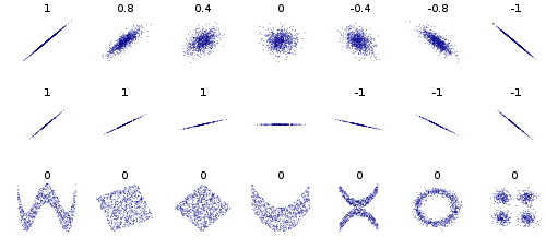 12 |
12 |
13 |
14 | So how can we quantify if and two what degree two variables are statistically dependent?
15 |
16 | ## Mutual Information
17 |
18 | The [**Mutual information**](https://en.wikipedia.org/wiki/Mutual_information) is
19 | of two random variables is a measure of the mutual dependence between the two variables. It quantifies the "amount of information" obtained about one random variable through observing the other random variable. The concept of mutual information is intimately linked to that of entropy of a random variable, a fundamental notion in information theory that quantifies the expected "amount of information" held in a random variable.[^footnote1]
20 |
21 | ```{important} The **mutual information** $I(X;Y)=0$ *if and only if* $X \indep Y$.
22 |
23 | ```
24 |
25 |
26 | The mutual information of two jointly discrete random variables
27 | $X$ and $Y$ is calculated as a double sum
28 |
29 | $$
30 | {\displaystyle \operatorname {I} (X;Y)=\sum _{y\in {\mathcal {Y}}}\sum _{x\in {\mathcal {X}}}{p_{(X,Y)}(x,y)\log {\left({\frac {p_{(X,Y)}(x,y)}{p_{X}(x)\,p_{Y}(y)}}\right)}},}
31 | $$
32 |
33 | where ${\displaystyle p_{(X,Y)}}$ is the joint probability mass function of $X$ and $Y$ and $p_{X}$ and $p_Y$ are the marginal probability mass functions.$X$ and $Y$ respectively.
34 |
35 | In the case of jointly continuous random variables, the double sum is replaced by a double integral
36 |
37 | $$
38 | {\displaystyle \operatorname {I} (X;Y)=\int _{\mathcal {Y}}\int _{\mathcal {X}}{p_{(X,Y)}(x,y)\log {\left({\frac {p_{(X,Y)}(x,y)}{p_{X}(x)\,p_{Y}(y)}}\right)}}\;dx\,dy,}
39 | $$
40 |
41 | where ${\displaystyle p_{(X,Y)}}$ is now the joint probability density function and $p_{X}$ and $p_Y$ are the marginal probability density functions.
42 |
43 | If the log base 2 is used, the units of mutual information are bits.
44 |
45 | An equivalent formulation is
46 |
47 | $$
48 | {\displaystyle I(X;Y)=D_{\mathrm {KL} }(P_{(X,Y)}\|P_{X}\otimes P_{Y})}
49 | $$
50 |
51 | where
52 | $D_{{{\mathrm {KL}}}}$ is the [Kullback–Leibler](https://en.wikipedia.org/wiki/Kullback–Leibler_divergence) divergence, which we will return to later in the course. Here we see that it is the KL distance between the joint and the product of the two marginals, and so it is only zero if the those are identical, which is equivalent to saying $p(X,Y)= p(X)p(Y)$, which is the definition of independence.
53 |
54 | Another useful identity is:
55 |
56 | $$
57 | {\displaystyle {\begin{aligned}\operatorname {I} (X;Y)&{}\equiv \mathrm {H} (X)-\mathrm {H} (X|Y)\\&{}\equiv \mathrm {H} (Y)-\mathrm {H} (Y|X)\\&{}\equiv \mathrm {H} (X)+\mathrm {H} (Y)-\mathrm {H} (X,Y)\\&{}\equiv \mathrm {H} (X,Y)-\mathrm {H} (X|Y)-\mathrm {H} (Y|X)\end{aligned}}}
58 | $$
59 |
60 | where ${\displaystyle \mathrm {H} (X)}$ and ${\displaystyle \mathrm {H} (Y)}$ are the marginal [entropies](https://en.wikipedia.org/wiki/Information_entropy),
61 | ${\displaystyle \mathrm {H} (X|Y)}$ and ${\displaystyle \mathrm {H} (Y|X)}$ are the [conditional entropies](https://en.wikipedia.org/wiki/Conditional_entropy), and
62 | ${\displaystyle \mathrm {H} (X,Y)}$ is the [joint entropy](https://en.wikipedia.org/wiki/Joint_entropy) of $X$ and $Y$.
63 |
64 | ```{note} The mutual information is symmetric $I(X;Y)=I(Y;X)$ and non-negative $I(X;Y)\ge 0$.
65 |
66 | ```
67 |
68 | ## Distance Correlation
69 |
70 | [Distance Correlation](https://en.wikipedia.org/wiki/Distance_correlation) is a measure of dependence between two paired random vectors of arbitrary, not necessarily equal, dimension.
71 | Thus, distance correlation measures both linear and nonlinear association between two random variables or random vectors. This is in contrast to Pearson's correlation, which can only detect linear association between two random variables [^footnote2].
72 |
73 | ```{important} The **distance correlation** is zero *if and only if* $X \indep Y$.
74 |
75 | ```
76 |
77 | [^footnote1]: Adapted from [https://en.wikipedia.org/wiki/Mutual_information](https://en.wikipedia.org/wiki/Mutual_information)
78 |
79 | [^footnote2]: Adapted from [https://en.wikipedia.org/wiki/Distance_correlation](https://en.wikipedia.org/wiki/Distance_correlation)
--------------------------------------------------------------------------------
/book/other_resources.md:
--------------------------------------------------------------------------------
1 | # Other Resources
2 |
3 |
4 |
5 | ## Courses
6 | 1. [NYU CDS: Probability and Statistics](https://cims.nyu.edu/~cfgranda/pages/DSGA1002_fall17/index.html)
7 | 1. [Stanford Probability and Statistics](http://cs229.stanford.edu/section/cs229-prob.pdf)
8 | 1. [NYU CDS: Inference and Representation](https://inf16nyu.github.io/home/)
9 | 1. [NYU CDS: Big Data 2015](https://www.vistrails.org/index.php/Course:_Big_Data_2015)
10 | 1. [NYU CDS: Machine Learning](https://davidrosenberg.github.io/ml2017/#resources)
11 | 1. [Foundations of Graphical Models by David Blei](http://www.cs.columbia.edu/~blei/fogm/2016F/) -- see [Basics of Graphical Models](http://www.cs.columbia.edu/~blei/fogm/2016F/doc/graphical-models.pdf)
12 | 1. see also [a video on d-separation by Pieter Abbeel](https://www.youtube.com/watch?v=yDs_q6jKHb0)
13 | 1. semantics of graphical models (here called "Boiler plate diagrams") and an extended visual language [Directed Factor Graph Notation for Generative Models
14 | Laura Dietz](https://github.com/jluttine/tikz-bayesnet/blob/master/dietz-techreport.pdf), which is the basis of the `tikz-bayesnet` package
15 | 1. [Algorithms for Convex Optimization by Nisheeth K. Vishnoi](https://convex-optimization.github.io)
16 | 1. [Introduction to Causal Inference by Brady Neal](https://www.bradyneal.com/causal-inference-course)
17 | 1. [Michael Jordan's lecture notes on notes on Probabilistic Graphical Models](https://people.eecs.berkeley.edu/%7Ejordan/prelims/)
18 | 1. [MIT lecture notes on algorithms for inference](http://ocw.mit.edu/courses/electrical-engineering-and-computer-science/6-438-algorithms-for-inference-fall-2014/lecture-notes/)
19 | 1. [Kevin Murphy, Machine Learning: a Probabilistic Perspective (4th eddition)](http://www.cs.ubc.ca/%7Emurphyk/MLbook/index.html) | [online @ NYU Libraries](http://site.ebrary.com/lib/nyulibrary/detail.action?docID=10597102).
20 | 1. [Probabilistic Programming and Bayesian Methods for Hackers by Cam Davidson Pilon](https://camdavidsonpilon.github.io/Probabilistic-Programming-and-Bayesian-Methods-for-Hackers/)
21 |
22 | ## Short courses / tutorials
23 |
24 | 1. [Basic Python](https://swcarpentry.github.io/python-novice-inflammation/)
25 | 1. [Plotting and Programming with Python](https://swcarpentry.github.io/python-novice-gapminder/)
26 |
27 |
28 | ## Linear Algebra
29 | 1. [Essence of linear algebra youtube videos by 3blue1brown](https://www.youtube.com/playlist?list=PLZHQObOWTQDPD3MizzM2xVFitgF8hE_ab)
30 | 1. [Introduction to Applied Linear Algebra – Vectors, Matrices, and Least Squares, Stephen Boyd and Lieven Vandenberghe](http://vmls-book.stanford.edu)
31 | 1. [Linear dynamical systems](https://www.youtube.com/watch?v=bf1264iFr-w&list=PLzvEnvQ9sS15pwCo8DYnJ-gArIkKZwJjF)
32 | 1. [Linear Algebra done right](https://linear.axler.net)
33 | 1. [NUMERICAL LINEAR ALGEBRA Lloyd N. Trefethen and David Bau, III](https://people.maths.ox.ac.uk/trefethen/text.html)
34 | 1. [Scientific Computing for PhDs](http://podcasts.ox.ac.uk/series/scientific-computing-dphil-students)
35 |
36 |
37 | ## Books
38 |
39 | 1. [All of Statistics by Wasserman](https://www.amazon.com/All-Statistics-Statistical-Inference-Springer/dp/1441923225)
40 | 1. [PRML](https://github.com/cranmer/PRML)
41 | 1. [Mathematics for Machine Learning](https://mml-book.github.io)
42 | 1. [Elements of Causal Inference by Jonas Peters, Dominik Janzing and Bernhard Schölkopf](https://mitpress.mit.edu/books/elements-causal-inference) [free PDF](https://www.dropbox.com/s/dl/gkmsow492w3oolt/11283.pdf)
43 | 1. [Trevor Hastie, Rob Tibshirani, and Jerry Friedman, Elements of Statistical Learning, Second Edition, Springer, 2009](https://web.stanford.edu/~hastie/ElemStatLearn//)
44 |
45 | ## Influential texts
46 |
47 | 1. [Knuth Calculus](https://micromath.wordpress.com/2008/04/14/donald-knuth-calculus-via-o-notation/)
48 | 1. [Functional Differential Geometry by Gerald Jay Sussman and Jack Wisdom](https://mitpress.mit.edu/books/functional-differential-geometry)
49 |
50 | ## Misc
51 |
52 | 1. [NeurIPS astro tutorial with datasets etc.](https://dwh.gg/NeurIPSastro)
53 | 1. [Paper about statistical combinations from phys/astro authors](https://arxiv.org/abs/2012.09874)
54 | 1. [Gentle Introduction to Automatic Differentiation on Kaggle](https://www.kaggle.com/borisettinger/gentle-introduction-to-automatic-differentiation)
55 | 1. [Short notes on divergence measures by Danilo Rezende](https://danilorezende.com/wp-content/uploads/2018/07/divergences.pdf)
56 | 1. [Lecture notes on: Information-theoretic methods for high-dimensional statistics, by Yihong Wu](http://www.stat.yale.edu/~yw562/teaching/it-stats.pdf)
57 |
58 |
59 |
60 | ## Meta
61 |
62 |
63 |
--------------------------------------------------------------------------------
/book/references.bib:
--------------------------------------------------------------------------------
1 | ---
2 | ---
3 |
4 | @book{bishop_pattern_2006,
5 | author = {Bishop, Christopher M},
6 | publisher = {Springer},
7 | address = {New York},
8 | isbn = {0387310738, 9780387310732},
9 | title = {Pattern recognition and machine learning},
10 | date = 2006,
11 | language = {eng},
12 | keywords = {Pattern perception, Pattern recognition systems, Machine learning}
13 | }
14 |
15 | @inproceedings{holdgraf_evidence_2014,
16 | address = {Brisbane, Australia, Australia},
17 | title = {Evidence for {Predictive} {Coding} in {Human} {Auditory} {Cortex}},
18 | booktitle = {International {Conference} on {Cognitive} {Neuroscience}},
19 | publisher = {Frontiers in Neuroscience},
20 | author = {Holdgraf, Christopher Ramsay and de Heer, Wendy and Pasley, Brian N. and Knight, Robert T.},
21 | year = {2014}
22 | }
23 |
24 | @article{holdgraf_rapid_2016,
25 | title = {Rapid tuning shifts in human auditory cortex enhance speech intelligibility},
26 | volume = {7},
27 | issn = {2041-1723},
28 | url = {http://www.nature.com/doifinder/10.1038/ncomms13654},
29 | doi = {10.1038/ncomms13654},
30 | number = {May},
31 | journal = {Nature Communications},
32 | author = {Holdgraf, Christopher Ramsay and de Heer, Wendy and Pasley, Brian N. and Rieger, Jochem W. and Crone, Nathan and Lin, Jack J. and Knight, Robert T. and Theunissen, Frédéric E.},
33 | year = {2016},
34 | pages = {13654},
35 | file = {Holdgraf et al. - 2016 - Rapid tuning shifts in human auditory cortex enhance speech intelligibility.pdf:C\:\\Users\\chold\\Zotero\\storage\\MDQP3JWE\\Holdgraf et al. - 2016 - Rapid tuning shifts in human auditory cortex enhance speech intelligibility.pdf:application/pdf}
36 | }
37 |
38 | @inproceedings{holdgraf_portable_2017,
39 | title = {Portable learning environments for hands-on computational instruction using container-and cloud-based technology to teach data science},
40 | volume = {Part F1287},
41 | isbn = {978-1-4503-5272-7},
42 | doi = {10.1145/3093338.3093370},
43 | abstract = {© 2017 ACM. There is an increasing interest in learning outside of the traditional classroom setting. This is especially true for topics covering computational tools and data science, as both are challenging to incorporate in the standard curriculum. These atypical learning environments offer new opportunities for teaching, particularly when it comes to combining conceptual knowledge with hands-on experience/expertise with methods and skills. Advances in cloud computing and containerized environments provide an attractive opportunity to improve the effciency and ease with which students can learn. This manuscript details recent advances towards using commonly-Available cloud computing services and advanced cyberinfrastructure support for improving the learning experience in bootcamp-style events. We cover the benets (and challenges) of using a server hosted remotely instead of relying on student laptops, discuss the technology that was used in order to make this possible, and give suggestions for how others could implement and improve upon this model for pedagogy and reproducibility.},
44 | booktitle = {{ACM} {International} {Conference} {Proceeding} {Series}},
45 | author = {Holdgraf, Christopher Ramsay and Culich, A. and Rokem, A. and Deniz, F. and Alegro, M. and Ushizima, D.},
46 | year = {2017},
47 | keywords = {Teaching, Bootcamps, Cloud computing, Data science, Docker, Pedagogy}
48 | }
49 |
50 | @article{holdgraf_encoding_2017,
51 | title = {Encoding and decoding models in cognitive electrophysiology},
52 | volume = {11},
53 | issn = {16625137},
54 | doi = {10.3389/fnsys.2017.00061},
55 | abstract = {© 2017 Holdgraf, Rieger, Micheli, Martin, Knight and Theunissen. Cognitive neuroscience has seen rapid growth in the size and complexity of data recorded from the human brain as well as in the computational tools available to analyze this data. This data explosion has resulted in an increased use of multivariate, model-based methods for asking neuroscience questions, allowing scientists to investigate multiple hypotheses with a single dataset, to use complex, time-varying stimuli, and to study the human brain under more naturalistic conditions. These tools come in the form of “Encoding” models, in which stimulus features are used to model brain activity, and “Decoding” models, in which neural features are used to generated a stimulus output. Here we review the current state of encoding and decoding models in cognitive electrophysiology and provide a practical guide toward conducting experiments and analyses in this emerging field. Our examples focus on using linear models in the study of human language and audition. We show how to calculate auditory receptive fields from natural sounds as well as how to decode neural recordings to predict speech. The paper aims to be a useful tutorial to these approaches, and a practical introduction to using machine learning and applied statistics to build models of neural activity. The data analytic approaches we discuss may also be applied to other sensory modalities, motor systems, and cognitive systems, and we cover some examples in these areas. In addition, a collection of Jupyter notebooks is publicly available as a complement to the material covered in this paper, providing code examples and tutorials for predictive modeling in python. The aimis to provide a practical understanding of predictivemodeling of human brain data and to propose best-practices in conducting these analyses.},
56 | journal = {Frontiers in Systems Neuroscience},
57 | author = {Holdgraf, Christopher Ramsay and Rieger, J.W. and Micheli, C. and Martin, S. and Knight, R.T. and Theunissen, F.E.},
58 | year = {2017},
59 | keywords = {Decoding models, Encoding models, Electrocorticography (ECoG), Electrophysiology/evoked potentials, Machine learning applied to neuroscience, Natural stimuli, Predictive modeling, Tutorials}
60 | }
61 |
62 | @book{ruby,
63 | title = {The Ruby Programming Language},
64 | author = {Flanagan, David and Matsumoto, Yukihiro},
65 | year = {2008},
66 | publisher = {O'Reilly Media}
67 | }
68 |
--------------------------------------------------------------------------------
/book/statistics/cramer-rao-bound.md:
--------------------------------------------------------------------------------
1 | # Cramér-Rao Bound
2 |
3 | The [Cramér-Rao Bound](https://en.wikipedia.org/wiki/Cramér–Rao_bound) is a fascinating result.
4 | If we just start by thinking of estimators as functions of the data that try to estimate the parameter, you might imagine that there if you work really hard you might be able to come up with a better estimator. The Cramér-Rao bound says there is a limit to how well you can do. It's a limit on the (co)variance of the estimator and it is based on information theoretic quantities for the statistical model $p_X(X|\theta)$.
5 |
6 | ## Univariate case
7 |
8 | First let's consider the univariate case where $\theta \in \mathbb{R}$. First we will consider the special case of unbiased estimators, and then generalized to estimators that may be biased.
9 |
10 | ### Unbiased estimator
11 |
12 | In the unbiased case, the Cramér-Rao states
13 |
14 | $$
15 | \operatorname{var}[\hat{\theta} \mid \theta] \ge \frac{1}{I(\theta)}
16 | $$
17 |
18 | where $I(\theta)$ is the Fisher information
19 |
20 | $$
21 | I(\theta) = \mathbb{E}_{p(X|\theta)}\left[ \left ( \frac{\partial}{\partial \theta} \log p(X \mid \theta) \right )^2 \right ] = \int \left ( \frac{\partial}{\partial \theta} \log p(x \mid \theta) \right )^2 p(x|\theta) dx
22 | $$
23 |
24 | Under some mild assumptions, you can rewrite this Fisher information as
25 |
26 | $$
27 | I(\theta) = \mathbb{E}_{p(X|\theta)}\left[ -\frac{\partial^2}{\partial \theta^2} \log p(X \mid \theta) \right ]
28 | $$
29 |
30 | ```{admonition} Terminology
31 | The **efficiency** of an unbiased estimator
32 | $\hat{\theta}$ measures how close this estimator's variance comes to this lower bound; estimator efficiency is defined as
33 |
34 | $$
35 | {\displaystyle e({\hat {\theta }})={\frac {I(\theta )^{-1}}{\operatorname {var} ({\hat {\theta }})}}}
36 | $$
37 |
38 | ```
39 | ```{admonition} Terminology
40 | The term $\frac{\partial}{\partial \theta} \log p(X \mid \theta)$ is called the **score function**.
41 | ```
42 |
43 | ```{admonition} Example
44 | Consider the straw man estimator that always returns a constant value $\hat{\theta}_{const} = \theta_0$. The variance of the estimator is 0!
45 | The $b(\theta_0)=0$ as well, is this a violation of the ramér-Rao Bound? While the bias is 0 at that particular point, it's biased everywhere else $b(\theta_0)=\theta_0 - \theta$, so this form of the bound isn't applicable, we need a generalization that works with biased estimators.
46 | ```
47 |
48 |
49 | ### General case with biased estimators
50 |
51 | $$
52 | {\displaystyle \operatorname {var} \left({\hat {\theta }}\right)\geq {\frac {[1+\color{#DC2830}{\frac{d b(\theta )}{d\theta}} ]^{2}}{I(\theta )}}.}
53 | $$
54 |
55 | where we use $b(\theta )$ as shorthand for $\operatorname{bias}(\hat{\theta} \mid \theta)$ to emphasize the dependence on $\theta$.
56 |
57 | ```{admonition} Example continued
58 | The resolution to the example with the straw man estimator that always returns a constant value $\hat{\theta}_\textrm{const} = \theta_0$ involves the generalization of the Cramér-Rao Bound? The bias $b(\theta_0)=\theta_0 - \theta$, so the derivative is $\color{#DC2830}{\frac{d b(\theta )}{d\theta}}=-1$, and the generalized bound is $\displaystyle \operatorname {var} \left({\hat {\theta }}\right) \geq 0$, so all is well.
59 | ```
60 |
61 | ## Multivariate case
62 |
63 | There is a corresponding formulation for the multivariate case where $\theta \in \mathbb{R}^n$.
64 |
65 | ### Unbiased estimator
66 |
67 | Let's consider the unbiased case first, and generalize variance to covariance. We have
68 |
69 | $$
70 | \operatorname{cov}[\hat{\theta}_i, \hat{\theta}_j \mid \theta] \ge I^{-1}_{ij}(\theta)
71 | $$
72 |
73 | where $I^{-1}_{ij}(\theta)$ is the inverse of the Fisher information matrix
74 |
75 | $$
76 | I_{ij}(\theta) &=& \mathbb{E}_{p(X|\theta)}\left[ \frac{\partial}{\partial \theta_i} \log p(X \mid \theta) \frac{\partial}{\partial \theta_j} \log p(X \mid \theta) \right ] \\
77 | &=& \int \left[ \frac{\partial}{\partial \theta_i} \log p(x \mid \theta) \frac{\partial}{\partial \theta_j} \log p(x \mid \theta) \right ] p(x|\theta) dx
78 | $$
79 |
80 | Under some mild assumptions, you can rewrite this Fisher information matrix as
81 |
82 | $$
83 | I_{ij}(\theta) = \mathbb{E}_{p(X|\theta)}\left[ -\frac{\partial^2}{\partial \theta_i\partial \theta_j} \log p(X \mid \theta) \right ]
84 | $$
85 |
86 | ```{tip}
87 | The generalization of the score function $\nabla_\theta \log p(X \mid \theta)$ is now a vector.
88 | ```
89 |
90 | ### General case with biased estimators
91 |
92 | There is also a corresponding generalization for biased, multivariate estimators.
93 | The general form of the Cramér–Rao bound then states that the covariance matrix of ${\boldsymbol {\hat\theta}}(X)$ satisfies
94 |
95 | $$
96 | {\displaystyle \operatorname {cov}_{\boldsymbol {\theta }}\left({\boldsymbol {\hat\theta}}(X)\right)\geq {\frac {\partial {\boldsymbol {\psi }}\left({\boldsymbol {\theta }}\right)}{\partial {\boldsymbol {\theta }}}}[I\left({\boldsymbol {\theta }}\right)]^{-1}\left({\frac {\partial {\boldsymbol {\psi }}\left({\boldsymbol {\theta }}\right)}{\partial {\boldsymbol {\theta }}}}\right)^{T}}
97 | $$
98 |
99 | where ${\boldsymbol {\psi }}({\boldsymbol {\theta })}$ denotes the expectation ${\displaystyle \operatorname {E} [{\boldsymbol {\hat\theta}}(X)]}$.
100 |
101 |
102 | ## Connections
103 |
104 | ### Asymptotic properties of maximum likelihood estimators
105 |
106 | Importantly, [under some regularity conditions maximum likelihood estimators are **asymptotically unbiased and efficient** ](https://en.wikipedia.org/wiki/Maximum_likelihood_estimation) (ie. they saturate the inequality).
107 |
108 | ### Information Geometry
109 |
110 | Later we will connect the Fisher information matrix to the topic of [Information Geometry](statistics/information-geometry), where we can interpret $I_{ij}(\theta)$ as the metric tensor for a statistical manifold, where $\theta$ are coordinates on the manifold. This is nicely connected to General Relativity, and we will see that the geometry is intrensic (equivariant to change of coordinates) and distances are diffeomorphism invariant.
111 |
112 | ### Sufficiency and the Expoential Family
113 |
114 | We will also see connections to the concept of [Sufficiency](statistics/sufficiency) and [the exponential family](distributions/exponential-family).
115 |
116 |
--------------------------------------------------------------------------------
/book/data-science-topics.md:
--------------------------------------------------------------------------------
1 | # Data Science, what is it?
2 |
3 | The image below comes from [Drew Conway's original Venn Diagram blog post](http://drewconway.com/zia/2013/3/26/the-data-science-venn-diagram). As he states, "I think the term "data science" is a bit of a misnomer," and then he muses on what what is unique about Data Sciene and how it is somewhat distinct from traditional statistics or machine learning.
4 |
5 | ```{figure} ./assets/Data_Science_VD.png
6 | [Drew Conway's original Venn Diagram](http://drewconway.com/zia/2013/3/26/the-data-science-venn-diagram).
7 | ```
8 |
9 |
10 | There have since been [an enormous number of variations on this diagram](https://www.google.com/search?tbm=isch&as_q=data+science+venn+diagrams&tbs=isz:lt,islt:4mp,sur:fmc), various forms of criticism, etc.; however, it does fit fairly well for this course. This course is primarily aimed at physicists, where it is expected that you will bring your **Substantive Expertise** in physics to bear on problems.
11 |
12 | ```{warning}
13 | Notice that the intersection of Hacking Skills and Substantive Expertise (without Math / Statistics Knowledge) is labeled as **Danger Zone!**.
14 | Much of my goal in this class is to teach you enough statistics that you can avoid the Danger Zone.
15 | ```
16 |
17 | Much of the material in this course is aimed at statistics, where I have emphasized first principles and conceptual thinking (eg. transformation properties of the likelihood and posteriors, the interpretation of the prior for parameters that describe fundamental constants of nature, etc.). And you see that much of "traditional research" sits in this overlap. The additonal ingredient that Drew introduces is "Hacking Skills", which is often misunderstood or misinterpreted. "Hacking" here does not refer to computer security or something nefarious -- in fact, quite the opposite. It's probably better to look at something like a [hackathon](https://www.rasmussen.edu/degrees/technology/blog/what-is-a-hackathon/) or [AstroHackWeek](http://astrohackweek.org/2020/), to get a feeling for what is meant.
18 |
19 | ```{admonition} Working definition of "Hacking"
20 | The way that I think of it is the ability to fluently use computing and technology to achieve a goal without being bogged down by those technical details and loosing site of the goal.
21 | ```
22 |
23 | ```{admonition} Hackathon
24 | “Computer programmers and software designers collaborate and create a solution to an existing problem using technology,” Moore explains. Those participating in a hackathon will work with like-minded individuals to utilize new technologies and hack together tons of code from different sources to achieve the goal, according to Sean Hsieh [source](https://www.rasmussen.edu/degrees/technology/blog/what-is-a-hackathon/),
25 | ```
26 |
27 | ```{admonition} AstroHackWeek
28 | AstroHackWeek is, in part, a summer school. The mornings will offer lectures and exercises covering essential skills for working effectively with large astronomical datasets. Past years have seen topics such as machine learning, Bayesian inference, frequentist statistics, databases, numerical Python, and visualization.
29 | ```
30 |
31 | You can also see that the intersection of Hacking Skills (think computing) with Math / Statistics Knowledge is labeled as Machine Learning, which I think is reasonable for machine learning in practice (though not for the theory of machine learning). Of course, computationally-minded statisticians often find the terms Machine Learning and Data Science as somewhat offensive, and some people use the term [Computational Statistics](https://en.wikipedia.org/wiki/Computational_statistics).
32 |
33 | Since the diagram is about Data Science, of course it has to be in the middle of the Venn diagram. Importantly, it includes Substantive Expertise. In industry this would mean knowing something about your industry, while in science it means having expertise in your field. For this reason, several people have criticized the "land grab" of statistics and computer science departments trying to claim the term "Data Science" (in an academic context) without [explicitly connecting to domains of practice](http://msdse.org/files/Creating_Institutional_Change.pdf) (eg. physics or astronomy).
34 |
35 |
36 | ```{admonition} Origin
37 | The term “data science” was first coined in 2008 by [D.J. Patil](https://en.wikipedia.org/wiki/DJ_Patil), and [Jeff Hammerbacher](https://en.wikipedia.org/wiki/Jeff_Hammerbacher), the pioneer leads of data and analytics efforts at LinkedIn and Facebook ([Source](https://aponia.co/development-data-science-ny/)). See also the [interview with D.J. Patil in the Observer](https://observer.com/2019/11/data-scientist-inventor-dj-patil-interview-linkedin-job-market-trend/)
38 | ```
39 |
40 | Industrial data science often has a lot of overlap with "Big Data", and there is no shortage of figures outlining the essential tools and skills of industrial data science.
41 | These diagrams can be quite intimidating and should probably be interepreted as the union of the tools and skills that are found and not the intersection of the tools and skills you would need to master.
42 |
43 | ```{figure} http://nirvacana.com/thoughts/wp-content/uploads/2013/07/RoadToDataScientist1.png
44 | :width: 50%
45 | An example from the myriad of such diagrams mapping the essential tools and skills of industrial data science. ([Source](https://aponia.co/development-data-science-ny/))
46 | ```
47 | ```{figure} https://hackr.io/blog/uploads/images/1570190916VwRfvnEiWq.jpg
48 | :width: 50%
49 | Another example from the myriad of such diagrams mapping the essential tools and skills of industrial data science. ([Source](https://hackr.io/blog/what-is-data-science))
50 | ```
51 |
52 | ```{warning}
53 | This portion of the site is the least well developed, but for now here are some references:
54 | ```
55 |
56 | ## Some References
57 |
58 | 1. [Veridical Data Science by Bin Yu and Karl Kumbier](https://www.stat.berkeley.edu/~binyu/ps/papers2020/VDS20-YuKumbier.pdf)
59 | 1. [other good resources from Rebecca Barter](http://www.rebeccabarter.com/useful_resources/)
60 | 1. Scientific Python & Tools
61 | 1. Wonderful jupyterbook by Ryan Abernathey covering many of the topics below [An Introduction to Earth and Environmental Data Science](https://earth-env-data-science.github.io./intro.html)
62 | 1. [Basic Python](https://swcarpentry.github.io/python-novice-inflammation/)
63 | 1. [Plotting and Programming with Python](https://swcarpentry.github.io/python-novice-gapminder/)
64 | 1. numpy
65 | 1. pandas
66 | 1. xarray
67 | 1. sympy
68 | 1. scikit-learn
69 | 1. tensorflow, pytorch, mxnet, jax
70 | 1. Visualization
71 | 1. matplotlib
72 | 1. 3-d plotting [notes](https://jakevdp.github.io/PythonDataScienceHandbook/04.12-three-dimensional-plotting.html)
73 | 1. seaborn
74 | 1. bokeh
75 | 1. Dask
76 | 1. [Image processing](https://datacarpentry.org/image-processing/)
77 |
--------------------------------------------------------------------------------
/book/statistics/bias-variance.md:
--------------------------------------------------------------------------------
1 | # Bias-Variance Tradeoff
2 |
3 | One of the most important concepts in statistics and machine learning is the Bias-Variance tradeoff.
4 | Before we can discuss it, let's define a few concepts.
5 |
6 | ## The bias of an estimator
7 |
8 | ```{admonition} Bias of an estimator
9 |
10 | The bias of an estimator, denoted $\textrm{bias}(\hat{\theta} \mid \theta)$, is defined as:
11 |
12 | $$
13 | \textrm{bias}(\hat{\theta} \mid \theta) = \mathbb{E}[\hat{\theta} \mid \theta ] - \theta = \mathbb{E}[\hat{\theta} - \theta \mid \theta ] =\int (\hat{\theta}(x) - \theta) p(x | \theta) dx
14 | $$
15 |
16 | **Note** the bias isn't a single number, but a function of the true, unknown value of $\theta$. Sometimes the estimator is implicit and you may see the bias denoted $b(\theta)$, or the dependence on $\theta$ is left implicit and you may see it denoted $b(\hat{\theta})$.
17 | ```
18 |
19 | If $\theta$ has several components, the expectations and bias are calculated per component.
20 |
21 | ```{admonition} Terminology
22 | If the bias is 0 for all values of $\theta$, the estimator is said to be **unbiased**.
23 | ```
24 |
25 | Usually physicists would react poorly to a biased estimator.
26 | This is partially due to the fact that "bias" is a loaded term with negative connotations.
27 | We will come back to this later... how bad is it if your estimator is biased?
28 |
29 |
30 | ## The variance of an estimator
31 |
32 | ```{admonition} Variance of an estimator
33 |
34 | The variance of an estimator uses the same definition as the variance of any random variable
35 |
36 | $$
37 | \textrm{var}(\hat{\theta} \mid \theta) = \mathbb{E}[\left( \hat{\theta} - \mathbb{E}[\hat{\theta}\mid \theta ] \right)^2 \mid \theta ]
38 | $$
39 |
40 | **Note** the variance also depends on the true, unknown value of $\theta$.
41 | ```
42 |
43 | If $\theta$ has several components, the notion of variance is generalized to [covariance](./correlation) as for any other multivariate random variable.
44 |
45 | Intuitively, we would like the variance of the estimator to be small
46 | Interestingly, there is a theoretical lower bound on the variance of an estimator, which is called the [Cramér-Rao bound](./statistics/cramer-rao-bound).
47 | Just because the variance of an estimator is small, doesn't mean that it's close to the true value.
48 | For instance, our straw man constant estimator $\hat{\theta}_\textrm{const} = \theta_0$ has zero variance, but it's not very userful.
49 |
50 | Note, this is closely connected to the idea of "precision" in the "accuracy vs. precision" dichotomy.
51 |
52 |
53 | ## The mean squared error of an estimator
54 |
55 | ```{admonition} Mean squared error
56 |
57 | The mean squared error of an estimator is defined by
58 |
59 | $$
60 | \textrm{MSE}(\hat{\theta} \mid \theta) = \mathbb{E}[\left( \hat{\theta} - \theta \right)^2 \mid \theta ] = \textrm{var}(\hat{\theta} \mid \theta)) + (\textrm{bias}(\hat{\theta} \mid \theta))^2
61 | $$
62 |
63 | **Note** the MSE also depends on the true, unknown value of $\theta$.
64 | ```
65 |
66 | ## The bias-variance tradeoff
67 |
68 | ```{admonition} Food for thought
69 | :class: tip
70 | Which is better:
71 | * an estimator $\hat{\theta}_1$ that always has smaller bias than another $\hat{\theta}_2$,
72 | * the estimator $\hat{\theta}_2$ that is always "closer" to the true value than $\hat{\theta}_1$ (smaller MSE).
73 | ```
74 |
75 | Note how the MSE decomposes into two terms, the variance and the squared bias. This is one manifestation of the bias-variance tradeoff.
76 | If you care about being close to the true value (smaller MSE), then you would be willing to trade a little bit of bias for a large reduction in variance.
77 | As we will see, Bayesian estimators are often biased, and in some cases the MLE is (asymptotically) unbiased, but has large variance.
78 | This is less of an issue when trying to infer a low-dimensional parameter $\theta$, but it becomes increasingly important as the dimensionality of $\theta$ increases.
79 |
80 | ```{important}
81 | There's no reason to confine yourself to bias, variance, or MSE to characterize the quality of your estimator. You could consider the bias to be 100 times more important than the variance, $\textrm{var}(\hat{\theta} \mid \theta)) + 100*(\textrm{bias}(\hat{\theta} \mid \theta))^2$, or a non-linear function of these two terms, or something that doesn't explicitly involve bias or variance at all.
82 | We can generalize these notions with the notions of **loss** and **risk** in [Statistical decision theory](statistics/statistical_decision_theory).
83 | ```
84 |
85 |
86 | ## Asymptotic bias and variance
87 |
88 | Often it is useful to think about the properties of estimators as you add more data or "in the limit of a lot of data". Those are informal concepts, that can be formalized by
89 | considering a sequence of estimators $\hat{\theta}_k$ with $k=1, \dots$ where for each $k$ the estimator takes as input $k$ iid observations $\{X_i\}_{i=1}^k$ with $X_i \sim p(X \mid \theta)$.
90 | We can then study the *asymptotic limit*:
91 |
92 | $$
93 | \lim_{k\to \infty} \textrm{SomeProperty}[\hat{\theta}_k \mid \theta ]
94 | $$
95 |
96 | ```{admonition} Example:
97 |
98 | Consider a Gaussian distribution $G(X|\mu,\sigma^2)$ and we wish to estimate the mean $\mu$ and variance $\sigma^2$ based on a dataset $\{x_i\}_{i=1}^N$.
99 | This may seem like a boring example, and you may recognize the $N$ vs. $N-1$ from some previous classes, but there are two lessons here, so let's go through it.
100 |
101 | The maximum likelihood estimator for $\mu$ is given by
102 |
103 | $$
104 | \frac{\partial}{\partial \mu} \left( \sum_{i=1}^N -\log G(x_i | \mu, \sigma) \right) \bigg\rvert_{\hat{\mu}} = 0
105 | $$
106 |
107 | which leads to the familiar sample mean $\hat{\mu}_\textrm{MLE} = \bar{x} = \frac{1}{N} \sum_{i=1}^N x_i$.
108 |
109 | And if we think of the Gaussian parameterized in terms of the variance $\sigma^2$, instead of the standard deviation $\sigma$, we find
110 |
111 | $$
112 | \frac{\partial}{\partial \sigma^2} \left( \sum_{i=1}^N -\log G(x_i | \mu, \sigma) \right) \bigg\rvert_{\widehat{\sigma^2}} = 0 &=& \frac{\partial}{\partial\sigma^2} \sum_{i=1}^N \left( \frac{(x_i - \mu)^2}{2\sigma^2} + \log \sqrt{2 \pi \sigma^2} \right) \\
113 | &=& \sum_{i=1}^N \left( -\frac{(x_i - \mu)^2}{2(\sigma^2)^2} + \frac{1}{2\sigma^2} \right)
114 | $$
115 |
116 | Therefore
117 |
118 | $$
119 | \widehat{\sigma^2}_\textrm{MLE} = S_N^2 = {\color{#DC2830}{\frac{1}{N}}} \sum_{i=1}^N (x_i - \bar{x})^2
120 | $$
121 |
122 | (Note the MLE is equivariant to reparameterization, so we could have done $\partial/\partial \sigma)$ and we would arrive at the same answer.)
123 |
124 | You may remember that this estimator is biased and that it is Better™ to use instead the unbiased estimator for the variance that includes [Bessel's correction](https://en.wikipedia.org/wiki/Bessel%27s_correction)
125 |
126 | $$
127 | \widehat{\sigma^2}_\textrm{Bessel} = S^2 = {\color{#0271AE}{\frac{1}{N-1}}} \sum_{i=1}^N (x_i - \bar{x})^2
128 | $$
129 |
130 | You may have even had some points deducted on homework or tests because you forgot to use $N-1$ instead of $N$. And you may also remember thinking "That's silly! What's the big deal, $\color{#DC2830}{\frac{1}{N}}$ and $\color{#0271AE}{\frac{1}{N-1}}$ are essentially the same for large $N$. And you would be right.
131 | That's the statement that the maximum likelihood estimator is **asymptotically unbiased**.
132 |
133 | You may have also wanted to estimate the standard deviation and used the seemingly obvious corrolary $\sqrt{ \color{#0271AE}{\frac{1}{N-1}} \sum_{i=1}^N (x_i - \bar{x})^2}$, being careful to use $N-1$ like a diligent student of [poorly taught statistics](https://www.google.com/search?tbm=isch&as_q=standard+deviation+N-1). However, that seemingly obvious corrolary is not actually motivated. While ${\color{#0271AE}{\frac{1}{N-1}}} \sum_{i=1}^N (x_i - \bar{x})^2$ is an unbiased estimator for the variance $\sigma^2$, $\sqrt{ \color{#0271AE}{\frac{1}{N-1}} \sum_{i=1}^N (x_i - \bar{x})^2}$ is a biased estimator of $\sigma$!
134 | ```
135 |
136 |
137 | ```{warning}
138 | The bias estimator is not equivariant to transformation of the estimator/estimand. This follows from the transformation properties of the the distribution when changing random variables, the Jacobian factor influences the mean.
139 | ```
140 |
141 | ```{caution}
142 | What convention is used in `np.var(x)` and `np.std(x)`? Check the documentation [numpy.std](https://numpy.org/doc/stable/reference/generated/numpy.std.html#numpy.std) and [numpy.var](https://numpy.org/doc/stable/reference/generated/numpy.var).
143 | ```
144 |
--------------------------------------------------------------------------------
/book/conditional.md:
--------------------------------------------------------------------------------
1 | # Conditonal Probability
2 |
3 | Let us start with a graphical introduction to the notion of conditional probability [^footnote1].
4 | Imagine you are throwing darts, and the darts uniformly hit the rectangular dartboard below.
5 |
6 | ```{figure} ./assets/prob_cousins.png
7 | :name: prob_cousins
8 | :width: 50%
9 |
10 | A visual representation of events $A$ and $B$ in a larger sample space $\Omega$ [^footnote1].
11 | ```
12 |
13 | The dark board has two oval shaped pieces of paper labeled $A$ and $B$. We can graphically convey the probability of hitting $A$ and the probability of hitting $B$ with the images below.
14 |
15 | ```{figure} ./assets/pA_and_pB.png
16 | :name: cousins_and
17 |
18 | A visual representation of $P(A)$ and $P(B)$ [^footnote1].
19 | ```
20 |
21 | And we can also talk about the probability of hitting $A$ **and** $B$, which is often written as $A \cap B$, as the image below.
22 |
23 | ```{figure} ./assets/pAandB.png
24 | :name: cousins_and
25 |
26 | A visual representation of $P(A \cap B)$ [^footnote1].
27 | ```
28 |
29 | In both cases the denominator is the full entire sample space $\Omega$ (the rectangle).
30 |
31 | Now let's consider the **conditional probability** $P(A \mid B)$, which is said "probability of $A$ **given** $B$". We know that the dart hit $B$, so the denominator is no longer the entire sample space $\Omega$ (the rectangle). Instead, it the denominator is $B$. Similarly, the numerator is no longer all of $A$, because some parts of $A$ aren't also in $B$. Instead, the numertor is the intersection $A \cap B$. We can visualize this as:
32 |
33 | ```{figure} ./assets/conditional.png
34 | :name: cousins_conditional
35 |
36 | A visual representation of $P(A \mid B)$ [^footnote1].
37 | ```
38 |
39 | We will extend this visual representation in the section on [Bayes' Theorem](./bayes_theorem).
40 |
41 |
42 |
43 |
44 | ## Visualizing conditional distributions for continuous data
45 |
46 | Consider the arbitrary joint distribution $p_{XY}(X,Y)$ shown below
47 |
48 | ```{figure} ./assets/schematic_p_xy.png
49 | :name: schematic_p_x_given_y
50 |
51 | A schematic of the joint $p(X,Y)$
52 | ```
53 |
54 | If we want to condition on the random varaible $Y$ taking on the value $y=-1.15$, then the conditional distribution $p_{X\mid Y}(X|Y)$ is just a normalized version of a slice through the joint:
55 |
56 | $$
57 | p_{X\mid Y}(X \mid Y=y) = \frac{p_{XY}(X,Y=y)}{\int p_{XY}(x,y) dx} = \frac{p_{XY}(X,Y=y)}{p_Y(Y=y)}
58 | $$(conditional_x_given_y)
59 |
60 | ```{figure} ./assets/schematic_p_x_given_y.png
61 | :name: schematic_p_x_given_y
62 |
63 | A schematic of the slice through the joint $p(X,Y=y)$ and the normalized conditional $p(X|Y)$.
64 | ```
65 |
66 | Similarly, if we want to condition on the random varaible $X$ taking on the value $x=1.75$, then the conditional distribution $p_{Y\mid X}(Y|X)$ is just a normalized version of a slice through the joint:
67 |
68 | $$
69 | p_{Y\mid X}(Y \mid X=x) = \frac{p_{XY}(X=x,Y)}{\int p_{XY}(x,y) dy} = \frac{p_{XY}(X=x,Y)}{p_X(X=x)}
70 | $$(conditional_y_given_x)
71 |
72 | ```{figure} ./assets/schematic_p_y_given_x.png
73 | :name: schematic_p_y_given_x
74 |
75 | A schematic of the slice through the joint $p(X=x,Y)$ and the normalized conditional $p(Y|X)$.
76 | ```
77 |
78 | ```{note}
79 | Here's a [link to the notebook](correlation_schematic.ipynb) I used to make these images in case it is useful.
80 |
81 | ```
82 |
83 | ## Marginal Distributions
84 |
85 | The normalization factors in the denominator of Equations {eq}`conditional_x_given_y` and {eq}`conditional_y_given_x` involve probability distributions over an individual variables $p_X(X)$ or $p_Y(Y)$ without conditioning on the other. These are called **marginal distributions** and they correspond to integrating out (or *marginalizing*) the other variable(s). Eg.
86 |
87 | $$
88 | p_X(x) = \int p_{XY}(x,y) dy
89 | $$(marginalization_over_y)
90 |
91 | In many ways, marginalization is the opposite of conditioning.
92 |
93 | For high dimensional problems, marginalization is difficult as it involves high dimensional integrals. Naive numerical integration is often not tractable, which has motivated a number of different approaches to approximate the integrals, such as Monte Carlo integration.
94 |
95 |
96 | ## Chain Rule of Probability
97 |
98 | One very powerful and useful result is that, without loss of generality, one can decompose a joint distribution into the appropriate product of conditionals. For example, one can always write the joint distribution for $X$ and $Y$ as
99 |
100 | $$
101 | p(X,Y) = p(X|Y) p(Y)
102 | $$
103 |
104 | Similarly, one can always decompose the the joint for three variables as
105 |
106 | $$
107 | p(X,Y,Z) = p(X|Y,Z) p(Y|Z) p(Z)
108 | $$
109 |
110 | And this type of decomposition for the joint for $N$ random variables $X_1, \dots, X_N$ is often written in this way:
111 |
112 | $$
113 | p_N(X_1, \dots, X_N) = \prod_{i=2}^N p_i(X_i|X_{i-1}, \dots X_{1}) p_1(X_{1})
114 | $$
115 |
116 | Note that here I've added subscripts to the distributions as they are all different in general. In some cases, one uses this same kind of decomposition and additionally assumes that there is some structure across the different distributions (eg. in a Markov process or an autoregressive model).
117 |
118 | An alternative notation that is often found is:
119 |
120 | $$
121 | p(X_1, \dots, X_N) = \prod_{i=1}^N p(X_i|X_{< i})
122 | $$
123 |
124 | where the first term $p(X_{1})$ without any conditioning is implied.
125 |
126 |
127 | ### A more general formulation
128 |
129 | The formulation of the chairn rule
130 | See [Theorem 1.2.2 (Chain rule) in the NYU CDS lecture notes on Probability and Statistics](https://cims.nyu.edu/~cfgranda/pages/stuff/probability_stats_for_DS.pdf) for a more general formulation
131 |
132 | ## A mnemonic on conditional distributions: Units
133 |
134 | We will see many different types of conditional distributions in this course, and manipulating them can be error prone and confusing. Manipulating conditional distributions takes some practice, it is not much different than learning to manipulate upper- and lower-indices in special realtivity and Einstein notation. As we will see later, some distributions have additional structure -- some variables may be (assmed to be) independent or conditionally independent -- and in these cases the decomposition isn't completely general, but it there are still some rules.
135 |
136 | For example, I know that $p(X,Y|Z)p(X)$ is not a valid decomposition of any joint $p(X,Y,Z)$ or conditional $p(X,Y|Z)$. I know this immediately by inspection because the $X$ appears on the left of the $\mid$ more than once. If $X,Y,Z$ are continuous and have units, then the units of this expression would be $[Y]^{-1}[X]^{-2}$. Similarly, if I wanted to check that it was normalized I would want to integrate it. While I can assume $\int p(x,y|z) dx dy= 1$ and $\int p(x) dx = 1$, there is no reason for $\int p(x,y|z)p(x)$ will be 1, and it will still have units of $[X]^{-1}$.
137 |
138 | Personally, I like to sort the terms like this $p(X,Y) = p(X|Y) p(Y)$ instead of like this $p(X,Y) = p(Y) p(X|Y)$. Or like this $P(A \cap B) = P(A \mid B) p(B)$ instead of like this $P(A \cap B) = p(B) P(A \mid B)$. In both cases, what one can form a joint distribution by starting with a conditioanl and then multiplying by a distribution for what is being conditioned on. I find that putting the terms in this order helps me avoid mistakes and it's easier to connect to the chian rule of probability.
139 |
140 | ### Exercise
141 |
142 | Which of the following are valid (not necessarily general) decompositions of some probability distribution?
143 |
144 |
145 |
146 |
147 |
148 |
149 |
150 |
151 |
152 |
153 |
154 |
155 |
156 |
157 |
158 |
159 |
160 |
161 |
162 |
163 | [^footnote1]: These images are adapted from lectures by Bob Cousins.
164 |
--------------------------------------------------------------------------------
/book/random_variables.md:
--------------------------------------------------------------------------------
1 | # Random Variables
2 |
3 | The basic idea of **random variables** is inuitive and familiar for physicists, and it is perhapse *the* fundamental idea in probabilistic thinking.
4 | At the same time, randomness is at the heart of some of the deepest mysteries of physics: the transition from the determinism of classical mechanics to indeterminism in quantum mechanics.
5 | Furthermore, the notation and terminology used by statisticians is often unfamiliar or awkward to physicists and the rigorous mathematical treatment of random variables may seem overly formal and opaque.
6 |
7 | ```{note}
8 | The [Stanford lectures on Probability and statistics](http://cs229.stanford.edu/section/cs229-prob.pdf) and the [NYU CDS lecture notes on Probability and Statistics](https://cims.nyu.edu/~cfgranda/pages/stuff/probability_stats_for_DS.pdf) both start from the formal definition of Probability Spaces, but let's start with something a little more intuitive.
9 | ```
10 |
11 |
12 | To start with we will make the distinction between two types of random variables:
13 | * **Discrete random variables** : e.g. the flip of a coin, the roll of a die, the number of decays of a radioactive substance in a fixed time interval, etc.
14 | * **Continuous random variables** : e.g. the height of a person, the mass of a star, the time interval between two subsequent radioactive decays, etc.
15 |
16 | In both cases we have in mind the notion of an underlying **population** and the particular values that different instances (or **realizations**) that these random values may take. The realizations are random draws from some population: e.g. the height of a particular person drawn from a population of people, the mass of a particular star drawn from a population of stars, the result of a particular flip of a coin drawn from a (potentially hypothetical) population of coin flips. Consider this quote from the [NYU CDS lecture notes on Probability and Statistics](https://cims.nyu.edu/~cfgranda/pages/stuff/probability_stats_for_DS.pdf):
17 |
18 | ```{admonition} Notation
19 | :class: note
20 | A random variable quantifies our uncertainty about the quantity it represents, not the value that it happens to finally take once the outcome is revealed. You should *never* think of a random variable as having a fixed numerical value. If the outcome is known, then that determines a realization of the random variable. In order to stress the difference between random variables and their realizations, we denote the former with uppercase letters $(X, Y , . . . )$ and the latter with lowercase letters $(x, y, . . . )$.
21 | ```
22 |
23 | We often say that the random variable $X$ is **distributed** according to a certain distribution denoted $p_X$. It is also useful to denote $\mathbb{X}$ for the space that the realizations $x$ live in (eg. natural numbers $\mathbb{N}$, real numbers $\mathbb{R}$, d-dimensional Euclidean space $\mathbb{R}^d$, etc.), In order to refer to the probability (density) that the random variable $X$ takes on the value $x$, we write $p_X(X=x)$ (often shortened to $p_X(x)$ or just $p(x)$ if the context is clear).
24 |
25 | ```{admonition} Terminology
26 | Statisticians often links the type of random variable with its distribution (eg. "a Poisson random variable" or "a Gaussian random variable") as opposed to the data type the realization take on (i.e. a natural number or a real number).
27 | ````
28 |
29 | It is important to make the distinction between the discrete and continous cases:
30 | * **Probability Mass Function** (pmf) describes the distribution of a discrete random variables (eg. $x\in \mathbb{N}$), and $p_X(x)$ is unitless (or has "units of probability")
31 | * **Probability Density Functions** (pdf) describes the distribution of a continuous random variable (eg. $x \in \mathbb{R}$), and $p_X(x)$ has units of probability per unit $X$.
32 |
33 | This is analogous to thinking of point masses or point charges in space versus mass-density or charge-density distributed along a line, surface, or volume.
34 | Just as the mass or charge in a region is the integral of this mass-density or charge-density in that region, the probability that a continous $x$ falls in some region $W \in \mathbb{X}$ is $P(x\in W) = \int_W p_X(x) dx$.
35 |
36 | These distributions have a few intuitive properties, which correspond to the [axioms of probability](axioms_of_prob):
37 | * $\sum_{x} p_X(x) = 1$ or in the continous case $\int dx p_X(x) = 1$
38 | * $p_X(x) \ge 0$ for all $x$
39 | * if $A$ and $B$ are mutually exclusive (or disjoint so that their intersection is empy, $A \cap B = \emptyset$ ), then $p(A \cup B) = p(A)+p(B)$. For continuous variables, you could write $\int_{A \cup B} p_X(x) dx = \int_{A} p_X(x) dx + \int_{B} p_X(x) dx$
40 |
41 | ```{note}
42 | In the continous case it is totally fine for the probability density $p_X(x)>1$. Consider a Gaussian distribution with $\sigma = 0.01$.
43 | ```
44 |
45 | ```{note}
46 | It is somewhat common that probability density functions are denoted $f(X)$ instead of $p(X)$ or to use a capital $P(X)$ to denote probability and a lower-case $p(X)$ to denote a probability density. Usually, this can be sorted out from context.
47 | ```
48 | In terms of notation, it is common to see $X \sim p_X$, which is read as "(the random variable) $X$ is distributed as (the distribution) $p_X$". Sometimes one may also see $X \sim p_X(\cdot)$. This notation really emphasizes $X$ as a random variable and $p_X$ as a distribution, and with this notation it does not make sense to write $x \sim p_X$. However, it is fairly common in some areas of physics to write $p(x)$ to refer to the distribution with the idea that $x$ is the explicit realization of a random variable, but the argument to a function. These notational issues may seem overstated in this document, but it is my experience that it is a barier to physicists reading the statistics literature and a fundamental cause of needless reinvention of the wheel.
49 |
50 | ## Cumulative distributions
51 |
52 | A related concepts is the **cumulative distribution function** (cdf) for a real-valued random variable $X$, which is defined as the probability the random variable $X$ is less than or equal to some particular value $x$
53 |
54 | $$
55 | F_X(x) := P(X \le x)
56 | $$
57 |
58 | I think that it is inuitive for physicists to think of a proability density function as the fundamental object and to define $F_X(x) = \int_{-\infty}^x p_X(x) dx$; however, typically the formal approach is the opposite and one defines
59 |
60 | $$
61 | p_X(x) := \frac{dF_X}{dx} .
62 | $$
63 |
64 | This kind of fine print matters is important formally in cases where the derivative of $F_X(x)$ does not exist, but rarely matters in practice.
65 |
66 | So what about continous multivariate data $x \in \mathbb{R}^d$? How does one define a cumulative distribuiton in that case? The integral "from minus infinity to $x$" doesn't seem to make sense, or at least it is ambiguous. Say we have two continous random variables $X$ and $Y$, then one can define the **joint cumulative distribution function**
67 |
68 | $$
69 | F_{XY}(x,y) := P(X\le x, Y\le y),
70 | $$
71 |
72 | ie. the probability that the random variable $X \le x$ *and* $Y \le y$. Personally, this always bothered me as a physicist because it seems like it is sensitive to an arbitrary choice of axes for my two dimensional data. But mathematically, it works for formally defining what to me is a more natural **joint probability density function**
73 |
74 | $$
75 | p_{XY}(x,y) := \frac{\partial^2 F_{XY}(x,y)}{\partial x \partial y}.
76 | $$
77 |
78 | The generalizatio to data in $\mathbb{R}^d$ is straight forward with the $d^\textrm{th}$ partial derivative. (Note, at this point in Secton 3.2 of [NYU CDS lecture notes on Probability and Statistics](https://cims.nyu.edu/~cfgranda/pages/stuff/probability_stats_for_DS.pdf) the notation for the joint pdf changes to $f_{XY}(x,y)$)
79 |
80 | ## Futher reading
81 |
82 | With this introduction, I invite you to read the [NYU CDS lecture notes on Probability and Statistics](https://cims.nyu.edu/~cfgranda/pages/stuff/probability_stats_for_DS.pdf) Sections 2.1-2.3, 3.1-3.3.
83 | As you will find, this requires understanding the notion of a **probability space**, a **sample space**, a **probability measure**, and the mathematical concept of a $\sigma$**-algebra**. These are defined and discussed in Section 1.
84 |
85 | You may also be interested in reading about the idea of a [Copula](https://en.wikipedia.org/wiki/Copula_(probability_theory)), which relates the cumulative distribution functions for individual random variables (marginals) $X$ and $Y$ to the joint distribution.
86 |
87 | ```{warning}
88 | The formal treatments of probability spaces makes subtle distinctions between terms like *event*, *observation*, *sample*, and *outcome*, which physicists may tend to use interchangibly. Furthermore, in causal inference there is a distinction made between *observational studies* and *experiments*.
89 | ```
90 |
91 |
--------------------------------------------------------------------------------
/book/bayes_theorem.md:
--------------------------------------------------------------------------------
1 | # Bayes' Theorem
2 |
3 | Earlier we discussed [**conditional probability**](./conditional) for an event $A$ **given** another event $B$: $P(A \mid B)$.
4 | Examples:
5 |
6 | * the probability to have $N$ neutrons in an atom given an atomic number of $Z$ [plot](https://upload.wikimedia.org/wikipedia/commons/thumb/8/80/Isotopes_and_half-life.svg/1280px-Isotopes_and_half-life.svg.png)
7 |
8 | * the distribution of height $h$ given that you are a professional basketball player
9 |
10 | * the disribution of some generic data $X$ given a theory with parameters $\theta$
11 |
12 | * the probability of testing negative for COVID19 given that you actually have COVID19
13 |
14 |
15 | Bayes' rule allows us to invert the relationship from $P(A \mid B)$ to $P(B \mid A)$.
16 | It can also be thought of as updating our **prior probability** for $B$ to a **posterior probability** for $B$ given that we observe $A$.
17 |
18 |
19 | ```{admonition} Theorem (Bayes’ rule)
20 | For any events $A$ and $B$ in a probability space $(\Omega,\mathcal{F},P)$
21 |
22 | $$
23 | P(B \mid A) = \frac{P (A \mid B)P (B)}{P(A)}
24 | $$
25 | as long as $P (A) > 0$.
26 | ```
27 |
28 | In our examples this would turn into:
29 |
30 | * the probability for an atom to have an atomic number of $Z$ given that it has $N$ neutrons
31 |
32 | * the probability to be a professional basketball player given your height is $h$
33 |
34 | * the probability disribution for a theory's parameters $\theta$ given data $X$
35 |
36 | * the probability of actually having COVID19 given that you tested negative for COVID19
37 |
38 |
39 | ## Bayes' rule in pictures
40 |
41 | ```{figure} ./assets/Bayes-theorem-in-pictures.png
42 |
43 | These images are adapted from lectures by Bob Cousins.
44 |
45 | ```
46 |
47 |
48 |
49 |
50 | ## Breaking down the terms
51 |
52 | Each of the terms in Bayes' rule has a name and interpretation. For this I think it is useful to think not of generic $A$ and $B$, but to think of some theory of the Universe with parameters $\theta$ (like the Higgs mass or the cosmological constant) and the predictions for what the data $X$ would look like given $\theta$. Then Bayes Rule is
53 |
54 | $$
55 | p(\theta \mid X ) = \frac{p(X \mid \theta) p(\theta)}{p(X)}
56 | $$
57 |
58 | * $p(X \mid \theta)$: the **likelihood**: the probability distributon of the data $X$ given the theoretical parameters $\theta$
59 | * $p(\theta)$: the **prior probability** for the parameter $\theta$
60 | * $p(\theta \mid X)$: the **posterior probability** of $\theta$ given $X$
61 | * $p(X)$: the normalizing constant often referred to as the **evidence**.
62 |
63 |
64 |
65 | ## An example:
66 |
67 | To be concrete, consider this [plot from the ATLAS experiment at the Large Hadron Collider](https://indico.cern.ch/event/197461/) from July 2012. It shows the distribution of a random variable $m_{4l}$) given three different hypothesized Higgs boson masses $m_H=(125, 150, 190)$ GeV. You can think of the data as $\{m_{4l}\}=X$ and the parameter as $m_H=\theta$.
68 |
69 | ```{figure} ./assets/atlas-higgs-2012.png
70 | :width: 60%
71 |
72 | A [plot from the ATLAS experiment at the Large Hadron Collider](https://indico.cern.ch/event/197461/) from July 2012. It shows histograms for the observed data (black dots) as well as the expected distribution for a random variable denoted $m_{4l}$ given different hypothesized Higgs boson basses $m_H$ (blue, orange, grey, which are stacked on top of the common $m_H$-independent backgrounds red+purple).
73 |
74 | ```
75 |
76 | If we ask ourselves, what is the probability distribution for the Higgs mass given the data $p(m_H \mid \{ m_{4l}\} )$ Bayes theorem tells us we need the likelihood $p(\{m_{4l}\} \mid m_H)$, which we can calculate using Quantum Field Theory *and* the prior probability $p(m_H)$. But where does $p(m_H)$ come from? We cannot calculate that from Quantum Field Theory, it is simply a parameter of the theory. If we were to say that our prior $p(m_H)$ is informed by some other experimental evidence $Y$, and it is really a posterior $p(m_H \mid Y)$, we would just find ourselves in the same situation for that previous measurement. Eventually we will be led to some original prior on $m_H$, which is not supported by experimental evidence or theoretical argument. More over, if we *define* probability in as the frequency that an event occurs in a large number of trials, what is the ensemble of trials? These would correspond to different universes. That interpretation may be ok if you embrace the idea of the Multiverse (in fact, this is at the heart of the [anthropic principle](https://en.wikipedia.org/wiki/Anthropic_principle)), but if you imagine a single universe with an unknown true value for $m_H$, then $p(m_H)$ is simply not defined and it makes no sense to talk about a prior or a posterior on the parameter.
77 |
78 |
79 | (axioms_of_prob)=
80 | ## Axioms of probability
81 |
82 |
83 | It may be surprising to first learn that there is not a unique definition of probability given how mathematical and formal probability and statistics are. There are two main "schools" usually refered to as Frequentist and Bayesian statistics. Frequentists do not deny that Bayes' theorem is true -- it's a thoerem after all -- but they do define probability in terms of the limit of long term frequency of an event occuring in multiple trials and, therefore, deny assigning probabilities to some quantities. Eg. the Higgs boson mass $m_H$ is not a random variable, but simply a parameter that indexes (or parameterizes) of a family of distributions. In contrast, Bayesians tend to promote these parameters to random variables with corresponding probability distributions. How is this probability defined? There are many potential [interpretations of probability](https://plato.stanford.edu/archives/sum2003/entries/probability-interpret/#1), but a common interpretation for Bayesian statistics is a **subjective degree of belief**. It may seem surprising that one could use a subjective degree of belief in such a mathematical topic, but the formal mathematics of probability and statistics is sound as long as the probability function (or measure) $P$ in the probability space $(\Omega, \mathcal{F}, P)$ satisfies [Kolmogorov's axioms of probability](https://en.wikipedia.org/wiki/Probability_axioms) (see also [Stanford Encyclopedia of Philosophy](https://plato.stanford.edu/archives/sum2003/entries/probability-interpret/#1)). We saw these axioms when we first introduced [random variables](./random_variables).
84 |
85 | The frequentist definition of probability in terms of limiting frequency of events across many trials satisfies Kolmogorov's axioms (see criticism [here](http://plato.stanford.edu/archives/sum2003/entries/probability-interpret/#3.1)). But **how do you quantify subjective degree of belief**? There is a nice article in the [Stanford Encyclopedia of Philosophy](https://plato.stanford.edu/archives/sum2003/entries/probability-interpret/#3.5), which I will quote from:
86 |
87 |
88 | Subjective probabilities are traditionally analyzed in terms of betting behavior. Here is a classic statement by de Finetti (1980):
89 |
90 | > Let us suppose that an individual is obliged to evaluate the rate p at which he would be ready to exchange the possession of an arbitrary sum $S$ (positive or negative) dependent on the occurrence of a given event $E$, for the possession of the sum $pS$; we will say by definition that this number $p$ is the measure of the degree of probability attributed by the individual considered to the event $E$, or, more simply, that $p$ is the probability of $E$ (according to the individual considered; this specification can be implicit if there is no ambiguity).
91 |
92 | This boils down to the following analysis:
93 |
94 | > Your degree of belief in $E$ is $p$ iff $p$ units of utility is the price at which you would buy or sell a bet that pays 1 unit of utility if $E$, 0 if not $E$.
95 |
96 | A **Dutch book** (against an agent) is a series of bets, each acceptable to the agent, but which collectively guarantee her loss, however the world turns out. Ramsey notes, and it can be easily proven (e.g., Skyrms 1984), that if your subjective probabilities violate the probability calculus, then you are susceptible to a Dutch book. For example, suppose that you violate the additivity axiom by assigning $P(A \cup B) < P(A) + P(B)$, where A and B are mutually exclusive. Then a cunning bettor could buy from you a bet on $A \cup B$ for $P(A \cup B)$ units, and sell you bets on $A$ and $B$ individually for $P(A)$ and $P(B)$ units respectively. He pockets an initial profit of $P(A) + P(B) - P(A \cup B)$, and retains it whatever happens. Ramsey offers the following influential gloss: “If anyone's mental condition violated these laws [of the probability calculus], his choice would depend on the precise form in which the options were offered him, which would be absurd.” (1980, 41)
97 |
98 | Equally important, and often neglected, is the converse theorem that establishes how you can avoid such a predicament. If your subjective probabilities conform to the probability calculus, then no Dutch book can be made against you (Kemeny 1955); your probability assignments are then said to be **coherent**. In a nutshell, conformity to the probability calculus is necessary and sufficient for coherence.
--------------------------------------------------------------------------------
/book/correlation.md:
--------------------------------------------------------------------------------
1 | # Covariance and Correlation
2 |
3 | ## Variance for a single variable
4 | The expected value or mean of a random variable is the first moment, analogous to a center of mass for a rigid body. The **variance** of a single random variable is the second moment: it is the expectation of the squared deviation of a random variable from its mean. It is analogous to the moment of inertia about the center of mass.
5 |
6 | $$
7 | \operatorname{Var} (X)=\mathbb{E} \left[(X-\mu )^{2}\right] = \int (x-\mu)^2 p(x) dx,
8 | $$
9 | where $\mu = \mathbb{E}[X]$
10 |
11 | The units of $\operatorname{Var} (X)$ are $[\operatorname{Var} (X)] = [X]^2$. For that reason, it is often more intuitive to work with the **standard deviation** of $X$, usually denoted $\sigma_X$, which is the square root of the variance:
12 |
13 | $$
14 | \sigma_X^2 = \operatorname{Var} (X)
15 | $$
16 |
17 | In statistical mechanics, you may have seen notation like this: $\sigma_X = \sqrt{ \left\langle \left( X - \langle X \rangle \right)^2 \right\rangle }$
18 |
19 | ## Covariance
20 |
21 | When dealing with multivariate data, the notion of variance must be lifted to the concept of **covariance**. Covariance captures how one variable deviates from its mean as another variable deviates from it's mean. Say we have two variables $X$ and $Y$, then the covariance for the two variables is defined as
22 |
23 | $$
24 | \textrm{cov} (X,Y)=\mathbb{E} {{\big [}(X-\mathbb{E} [X])(Y-\mathbb{E} [Y]){\big ]}}
25 | $$(covariance)
26 |
27 | If $X$ is on average greater than its mean when $Y$ is greater than its mean (and, similarly, if $X$ is on average less than its mean when $Y$ is less than its mean), then we say the two variables are **positively correlated**. In the opposit case, when $X$ is on average less than its mean when $Y$ is greater than its mean (and vice versa), then we say the two variables are **negatively correlated**. If $\operatorname{Cov}(X,Y) = 0$, then we say the two variables are **uncorrelated**.
28 |
29 | A useful identity
30 |
31 | $$
32 | {\displaystyle {\begin{aligned}\textrm{cov} (X,Y)&=\mathbb {E} \left[\left(X-\mathbb {E} \left[X\right]\right)\left(Y-\mathbb {E} \left[Y\right]\right)\right]\\&=\mathbb {E} \left[XY-X\mathbb {E} \left[Y\right]-\mathbb {E} \left[X\right]Y+\mathbb {E} \left[X\right]\mathbb {E} \left[Y\right]\right]\\&=\mathbb {E} \left[XY\right]-\mathbb {E} \left[X\right]\mathbb {E} \left[Y\right]-\mathbb {E} \left[X\right]\mathbb {E} \left[Y\right]+\mathbb {E} \left[X\right]\mathbb {E} \left[Y\right]\\&=\mathbb {E} \left[XY\right]-\mathbb {E} \left[X\right]\mathbb {E} \left[Y\right],\end{aligned}}}
33 | $$
34 |
35 |
36 | ## Correlation coefficient
37 |
38 | The covariance $\operatorname{Cov}(X,Y)$ has units $([X][Y])^{-1}$, and thus depends on the units for $X$ and $Y$. It is desireable to have a unitless measure of how "correlated" the two variables are. One way to do this is through the [**Correlation coefficient**](https://en.wikipedia.org/wiki/Pearson_correlation_coefficient) $\displaystyle \rho _{X,Y}$, which simply divides out the standard deviation of $X$ and $Y$
39 |
40 | $$
41 | {\displaystyle \rho _{X,Y}={\frac {\textrm{cov} (X,Y)}{\sigma _{X}\sigma _{Y}}}},
42 | $$(correlation_coefficient)
43 |
44 | where $\sigma_X^2 = \textrm{cov}(X,X)$ and $\sigma_Y^2 = \textrm{cov}(Y,Y)$
45 |
46 | ```{warning}
47 |
48 | It is common to mistakenly think that if two variables $X$ and $Y$ are "uncorrelated" that they are [statistically independent](./independence), but this is not the case.
49 | It is true that if two variables $X$ and $Y$ are "correlated" (have non-zero covariance), then the two variables are [statistically dependent](./independence), but the converse is not true in general.
50 | We will see this in our [Simple Data Exploration](datasaurus-long).
51 | ```
52 |
53 | ## Covariance matrix
54 |
55 | When dealing with more than two variables, there is a straightforward generalization of covariance (and correlation) in terms of a **covariance matrix** [^footnote1]. Given random variables $X_1, \dots, X_N$, the covariance matrix is an $N\times N$ matrix whose $(i,j)$ entry is the covariance
56 |
57 | $$
58 | {\displaystyle \operatorname {K} _{X_{i}X_{j}}=\operatorname {cov} [X_{i},X_{j}]=\mathbb{E} [(X_{i}-\mathbb{E} [X_{i}])(X_{j}-\mathbb{E} [X_{j}])]}
59 | $$
60 |
61 | If the entries are represented as a column vector ${\displaystyle \mathbf {X} =(X_{1},X_{2},...,X_{n})^{\mathrm {T} }}$, then the covariance matrix can be written as
62 |
63 | $$
64 | {\displaystyle \operatorname {K} _{\mathbf {X} \mathbf {X} }=\operatorname {cov} [\mathbf {X} ,\mathbf {X} ]=\mathbb{E} [(\mathbf {X} -\mathbf {\mu _{X}} )(\mathbf {X} -\mathbf {\mu _{X}} )^{\rm {T}}]=\mathbb{E} [\mathbf {X} \mathbf {X} ^{T}]-\mathbf {\mu _{X}} \mathbf {\mu _{X}} ^{T}}
65 | $$
66 |
67 | with ${\displaystyle \mathbf {\mu _{X}} =\mathbb{E} [\mathbf {X} ]}$ also represented as a column vector.
68 |
69 | ```{note}
70 | The inverse of this matrix,
71 | ${\displaystyle \operatorname {K} _{\mathbf {X} \mathbf {X} }^{-1}}$, if it exists, is also known as the **concentration matrix** or **precision matrix**.
72 | ```
73 |
74 | ## Correlation Matrix
75 |
76 | An entity closely related to the covariance matrix is the **correlation matrix** [^footnote1],
77 |
78 | $$
79 | {\displaystyle \operatorname {corr} (\mathbf {X} )={\begin{bmatrix}1&{\frac {\mathbb{E} [(X_{1}-\mu _{1})(X_{2}-\mu _{2})]}{\sigma (X_{1})\sigma (X_{2})}}&\cdots &{\frac {\mathbb{E} [(X_{1}-\mu _{1})(X_{n}-\mu _{n})]}{\sigma (X_{1})\sigma (X_{n})}}\\\\{\frac {\mathbb{E} [(X_{2}-\mu _{2})(X_{1}-\mu _{1})]}{\sigma (X_{2})\sigma (X_{1})}}&1&\cdots &{\frac {\mathbb{E} [(X_{2}-\mu _{2})(X_{n}-\mu _{n})]}{\sigma (X_{2})\sigma (X_{n})}}\\\\\vdots &\vdots &\ddots &\vdots \\\\{\frac {\mathbb{E} [(X_{n}-\mu _{n})(X_{1}-\mu _{1})]}{\sigma (X_{n})\sigma (X_{1})}}&{\frac {\mathbb{E} [(X_{n}-\mu _{n})(X_{2}-\mu _{2})]}{\sigma (X_{n})\sigma (X_{2})}}&\cdots &1\end{bmatrix}}.}
80 | $$
81 |
82 | Each element on the principal diagonal of a correlation matrix is the correlation of a random variable with itself, which always equals 1.
83 |
84 | Equivalently, the correlation matrix can be written in vector-matrix form as
85 |
86 | $$
87 | {\displaystyle \operatorname {corr} (\mathbf {X} )={\big (}\operatorname {diag} (\operatorname {K} _{\mathbf {X} \mathbf {X} }){\big )}^{-{\frac {1}{2}}}\,\operatorname {K} _{\mathbf {X} \mathbf {X} }\,{\big (}\operatorname {diag} (\operatorname {K} _{\mathbf {X} \mathbf {X} }){\big )}^{-{\frac {1}{2}}},}
88 | $$
89 |
90 | where
91 | ${\displaystyle \operatorname {diag} (\operatorname {K} _{\mathbf {X} \mathbf {X} })}$ is the matrix of the diagonal elements of
92 | ${\displaystyle \operatorname {K} _{\mathbf {X} \mathbf {X} }}$ (i.e., a diagonal matrix of the variances of
93 | $X_{i}$ for $i=1,\dots ,n)$.
94 |
95 |
96 |
97 | ### Visualizing covariance as an ellipse
98 |
99 | Often an ellipse is used to visualize a covariance matrix, but why? This is only well-motivated if one expects the data to be normally distributed (aka Gaussian distributed). This is because the contours of a 2-d normal are ellipses, and in higher dimensions the contours are ellipsoids.
100 |
101 |
102 | ```{figure} ./assets/001_vanilla_ellipse.png
103 | width: 30%
104 |
105 | A scatter plot of two correlated, normally-distributed variables and the error ellipse from [*An Alternative Way to Plot the Covariance Ellipse* by Carsten Schelp](https://carstenschelp.github.io/2018/09/14/Plot_Confidence_Ellipse_001.html).
106 | ```
107 |
108 | Consider a random variable $X$ that is distributed as a multivariate normal (aka multivariate Gaussian) distribution, e.g. ${\displaystyle \mathbf {X} \ \sim \ {\mathcal {N}}({\boldsymbol {\mu }},\,{\boldsymbol {\Sigma }}})$, where $\boldsymbol{\mu}$ is the multivariate mean and $\Sigma$ is the covariane matrix. The probability density for the multivariate normal is given by
109 |
110 | $$
111 | \displaystyle p_{\mathbf {X} }(x_{1},\ldots ,x_{k} | \boldsymbol {\mu }, {\boldsymbol {\Sigma })=
112 | {\frac {\exp \left(-{\frac {1}{2}}({\mathbf {x} }-{\boldsymbol {\mu }})^{\mathrm {T} }{\boldsymbol {\Sigma }}^{-1}({\mathbf {x} }-{\boldsymbol {\mu }})\right)}{\sqrt {(2\pi )^{k}|{\boldsymbol {\Sigma }}|}}}}
113 | $$
114 |
115 | The contours correspond to values of $\mathbf{X}$ where $({\mathbf {x} }-{\boldsymbol {\mu }})^{\mathrm {T} }{\boldsymbol {\Sigma }}^{-1}({\mathbf {x} }-{\boldsymbol {\mu }}) = \textrm{Constant}$.
116 |
117 |
118 | Understanding the geometry of this ellipse requires the linear algebra of the covariance matrix, and it's a useful excercise to go through:
119 | * [This notebook](./covariance_ellipse) is duplicated from the repository linked to in this article: [*An Alternative Way to Plot the Covariance Ellipse* by Carsten Schelp](https://carstenschelp.github.io/2018/09/14/Plot_Confidence_Ellipse_001.html), which has a GPL-3.0 License.
120 | * This is also a nice [page](https://cookierobotics.com/007/)
121 |
122 |
123 | ## With empirical data
124 |
125 | We can estimate the covariance of the parent distribution $p_{XY}$ with the sample covariance, using the sample mean in place of the expectation $\mathbb{E}_{p_X}$.
126 |
127 |
128 | [^footnote1]: Adapted from [Wikipedia article on Covariance Matrix](https://en.wikipedia.org/wiki/Covariance_matrix)
129 |
130 | As we will see in our [Simple Data Exploration](datasaurus-long) and [Visualizing joint and marginal distributions](distributions/visualize_marginals), the sample covariance and correlation matrices can be conveniently computed for a `pandas` dataframe with `dataframe.cov()` and `dataframe.corr()`
--------------------------------------------------------------------------------
/book/schedule.md:
--------------------------------------------------------------------------------
1 | # Draft Schedule
2 |
3 |
4 | Recording of lectures are accessible [here](https://applications.zoom.us/lti/rich?lti_scid=53e5b6ade1d092bbd38974bc31813aa0b9c9d37154d82fb28fd97562e49a6c2c&oauth_consumer_key=egAB3MeoRVG9kMt4z8eEXA).
5 |
6 | 1. Week 1
7 | 1. 9/2: Intro [Recording](https://nyu.zoom.us/rec/play/uA6Jy6FEsbZpQRfmeQ6jJV7ISs37lvdKMnwsJhuql9O445ANIB0TbmflpCqFPjqczKuhAr3k9voEv8Tc.K2AoCHSjTknMuoAA)
8 | 1. syllabus
9 | 1. juypter book
10 | 1. review survey
11 | 1. about me and my research and a preview for the course
12 | 2. Week 2
13 | 1. 9/9: Basic prob theory [Recording](https://nyu.zoom.us/rec/play/Y6tMRTUxNDhU2n_pw9cPJr1kqmZDMcfCuqLGRqWuLIQ42M9AhGtuhjS-vi_XfaNzNr2i-nFlBPrSJdRa.eh480MdOBuleGYe2)
14 | 1. Random Variables
15 | 1. Probability space
16 | 1. Probability Mass and Density functions
17 | 1. Conditional Probability
18 | 1. Bayes Theorem
19 | 1. Quantifying prior odds via betting
20 | 1. Incoherent beliefs
21 | 1. Axioms of probability
22 | 1. Examples
23 | 3. Week 3
24 | 1. 9/14: Class [Recording](https://nyu.zoom.us/rec/play/6Wvz4mMAK3qWkBLhOP98kLQMNcEc-H6rZg9zWUao-DTzme6TBAblX8Q7d_0Imyzjts9o48IAOG6reJst.KSmnHtGH6BTNiCvb)
25 | 1. Conditional probability for continuous variables
26 | 1. Chain rule of probability
27 | 1. Sneak peek at graphical models
28 | 1. The Drake equation
29 | 1. Phosphine on Venus and Bayes Theorem
30 | 1. Marginal Distributions
31 | 1. Independence
32 | 1. Emperical Distribution
33 | 1. Expectation
34 | 1. Variance, Covariance, Correlation
35 | 1. Mutual Information
36 | 1. Simple Data Exploration
37 | 1. 9/16: Class [Recording](https://nyu.zoom.us/rec/play/ryKzr2yN2nWSWtMzavZivnrJDZ7rQFoowx5Pk6mWdFKq5ESJFjk0zCGQEtk6G1qCDM2VvdDez6t5Tdzk.OSHZVTqbRrQ-i_wa)
38 | 1. Likelihood
39 | 1. Change of variables
40 | 1. Demo change of variables with autodiff
41 | 1. Independence and correlation
42 | 1. Conditioning
43 | 1. Autoregressive Expansion
44 | 1. Graphical Models
45 | 4. Week 4
46 | 1. 9/21: [Recording](https://nyu.zoom.us/rec/play/uSMzP3UYoZBRnDjAQfdzDKC5_WHAmX_tenfl7jduYPoTRqAXfuBYyC-tALiVJEWNNNYChZ-BwDoxe2lz.JdLbnvKxO5vZmXDv)
47 | 1. Change of variables formula
48 | 1. Probability Integral Transform
49 | 1. Intro to automatic differentiation
50 | 1. Demo with automatic differentiation
51 | 1. Transformation properties of the likelihood
52 | 1. Transformation properties of the MLE
53 | 1. Transformation properties of the prior and posterior
54 | 1. Transformation properties of the MAP
55 | 1. 9/23: Estimators
56 | 1. Skipped material from last lecture
57 | 1. Lorentz-invariant phase space
58 | 1. Normalizing Flows
59 | 1. Copula
60 | 1. Bias, Variance, and Mean Squared Error
61 | 1. Simple Examples: Poisson and Gaussian
62 | 1. Cramer-Rao bound & Information Matrix
63 | 1. Bias-Variance tradeoff
64 | 1. James-Stein Demo
65 | 1. Shrinkage
66 | 1. HW:
67 | 1. James Stein
68 | 5. Week 5
69 | 1. 9/28 (Yom Kippur): Random Numbers [Recording](https://nyu.zoom.us/rec/play/L-BkDSdARQfotstBjZjW8WzTzF2g35bvftQIXWVe5MEmYDyJzscjqs3qrwDrAjKKV8lgHi04hw6EjyLZ.6DP4VVZA6_LvfkWE)
70 | 1. Decision Theory
71 | 1. [Admissible decision rule](https://en.wikipedia.org/wiki/Admissible_decision_rule)
72 | 1. generalized decision rules ("for some prior")
73 | 1. Consistency
74 | 1. Sufficiency
75 | 1. Exponential Family
76 | 1. Score Statistic
77 | 1. Information Matrix
78 | 1. Information Geometry
79 | 1. Transformation properties of Information Matrix
80 | 1. Jeffreys' prior
81 | 1. Transformation properties
82 | 1. Reference Prior
83 | 1. Sensitivity analysis
84 | 1. likelihood principle
85 | 1. 9/30: Lecture 8: Consistency and homework
86 | 1. [Neyman Scott phenomena](https://www.stat.berkeley.edu/~census/neyscpar.pdf) (an example of inconsistent MLE)
87 | 1. Note: [Elizabeth Scott](https://en.wikipedia.org/wiki/Elizabeth_Scott_(mathematician)) was an astronomer by background. In 1957 Scott noted a bias in the observation of galaxy clusters. She noticed that for an observer to find a very distant cluster, it must contain brighter-than-normal galaxies and must also contain a large number of galaxies. She proposed a correction formula to adjust for (what came to be known as) the Scott effect.
88 | 1. Note: [Revisiting the Neyman-Scott model: an Inconsistent MLE or an Ill-defined Model?](https://arxiv.org/abs/1301.6278)
89 | 1. walk through of nbgrader and home work assignment
90 | 6. Week 6
91 | 1. 10/5: Lecture 9: Propagaion of Errors
92 | 1. a simple example from physics 1: estimating $g$
93 | 1. Change of variables vs. Error propagation
94 | 1. Demo Error propagation fails
95 | 1. Error propagation and Marginalization
96 | 1. Convolution
97 | 1. Central Limit Theorem
98 | 1. Error propagation with correlation
99 | 1. track example
100 | 1. 10/7: Lecture 10: Likelihood-based modeling
101 | 1. Building a probabilistic model for simple physics 1 example
102 | 1. Connection of MLE to traditional algebraic estimator
103 | 1. Connection to least squares regression
104 | 7. Week 7
105 | 1. 10/12 Lecture 11: Sampling
106 | 1. Motiving examples:
107 | 1. Estimating high dimensional integrals and expectations
108 | 1. Bayesian credible intervals
109 | 1. Marginals are trivial with samples
110 | 1. Generating Random numbers
111 | 1. Scipy distributions
112 | 1. Probability Integral Transform
113 | 1. Accept-Reject MC
114 | 1. Acceptance and efficiency
115 | 1. native python loops vs. numpy broadcasting
116 | 1. Importance Sampling & Unweighting
117 | 1. [Vegas](https://en.wikipedia.org/wiki/VEGAS_algorithm)
118 | 1. Connetion to Bayesian Credible Intervals
119 | 1. Metropolis Hastings MCMC
120 | 1. Proposal functions
121 | 1. Hamiltonian Monte Carlo
122 | 1. Excerpts from [A Conceptual Introduction to Hamiltonian Monte Carlo by Michael Betancourt](https://arxiv.org/abs/1701.02434)
123 | 1. Stan and PyMC3
124 | 1. 10/14: Lecture 12: Hypothesis Testing and Confidence Intervals
125 | 1. Simple vs. Compound hypotheses
126 | 1. TypeI and TypeII error
127 | 1. critical / acceptance region
128 | 1. Neyman-Pearson Lemma
129 | 1. Test statistics
130 | 1. Confidence Intervals
131 | 1. Interpretation
132 | 1. Coverage
133 | 1. Power
134 | 1. No UMPU Tests
135 | 1. Neyman-Construction
136 | 1. Likelihood-Ratio tests
137 | 1. Connection to binary classification
138 | 1. prior and domain shift
139 | 8. Week 8
140 | 1. 10/19: Lecture 13:
141 | 1. Simple vs. Compound hypotheses
142 | 1. Nuisance Parameters
143 | 1. Profile likelihood
144 | 1. Profile construction
145 | 1. Pivotal quantity
146 | 1. Asymptotic Properties of Likelihood Ratio
147 | 1. Wilks
148 | 1. Wald
149 | 1. 10/21 Canceled
150 | 9. Week 9
151 | 1. 10/26: Lecture 14
152 | 1. Upper Limits, Lower Limits, Central Limits, Discovery
153 | 1. Power, Expected Limits, Bands
154 | 1. Sensitivity Problem for uppper limits
155 | 1. CLs
156 | 1. power-constrained limits
157 | 1. 10/28: Lecture 15 flip-flopping, multiple testing
158 | 1. flip flopping
159 | 1. multiple testing
160 | 1. look elsewhere effect
161 | 1. Familywise error rate
162 | 1. False Discovery Rate
163 | 1. Hypothesis testing when nuisance parameter is present only under the alternative
164 | 1. [Asymptotics, Daves, Gross and Vitells](https://arxiv.org/abs/1005.1891)
165 | 10. Week 10
166 | 1. 11/2 Lecture 16 Combinations, probabilistic modelling languages, probabilistic programming
167 | 1. Combinations
168 | 1. Combining p-values
169 | 1. combining posteriors
170 | 1. likelihood-based combinations
171 | 1. likelihood publishing
172 | 1. probabilistic modelling languages
173 | 1. computational graphs
174 | 1. Probabilistic Programming
175 | 1. First order PPLs
176 | 1. Stan
177 | 1. Universal Probabilistic Programming
178 | 1. pyro
179 | 1. pyprob and ppx
180 | 1. Inference compilation
181 | 1. 11/4 Lecture 17: Goodness of fit
182 | 1. conceptual framing
183 | 1. difference to hypothesis testing
184 | 1. chi-square test
185 | 1. Kolmogorov-Smirnov
186 | 1. Anderson-Darling
187 | 1. Zhang's tests
188 | 1. Bayesian Information Criteria
189 | 1. software
190 | 1. anomaly detection
191 | 11. Week 11
192 | 1. 11/9: Lecture 18 Intro to machine learning
193 | 1. Supervised Learning
194 | 1. Statistical Learning Theory
195 | 1. Loss, Risk, Emperical Risk
196 | 1. Generalization
197 | 1. VC dimension and Emperical risk minimization
198 | 1. No Free Lunch
199 | 1. Cross-validation test/train
200 | 1. Preview: the mystery of deep learning
201 | 1. Least Squares
202 | 1. Regularized least squares
203 | 1. Bayesian Curve fitting
204 | 1. Bias-Variance tradeoff
205 | 1. 11/11 Lecture 19
206 | 1. Generalization
207 | 1. Loss functions for regression
208 | 1. loss function for classification
209 | 1. Information theory background
210 | 1. Entropy
211 | 1. Mutual information
212 | 1. cross entropy
213 | 1. Relative Entropy
214 | 12. Week 12
215 | 1. 11/16: Lecture 20 Density Estimation, Deep Generative Models
216 | 1. Unsupervised learning
217 | 1. Loss functions for density estimation
218 | 1. Divergences
219 | 1. KL Divergence
220 | 1. Fisher distance
221 | 1. Optimal Transport
222 | 1. Hellinger distance
223 | 1. f-divergences
224 | 1. Stein divergence
225 | 1. Maximum likelihood (Forward KL)
226 | 1. can approximate with samples, don't need target distribution
227 | 1. Variational Inference (Reverse KL)
228 | 1. Connecton to statistical physics
229 | 1. LDA (Topic Modelling)
230 | 1. BBVI
231 | 1. Deep Generative models
232 | 1. Normalizing Flows intro
233 | 1. background on auto-encoders
234 | 1. Variational Auto-encoder intro
235 |
236 | 1. 11/18: Lecture 21 Deep Generative Models
237 | 1. Deep Generative models comparison
238 | 1. Normalizing Flows
239 | 1. Autoregresive models
240 | 1. Variational Auto-encoder
241 | 1. GANs
242 | 13. Week 13
243 | 1. 11/23: Lecture 22 The data manifold
244 | 1. what is it, why is it there
245 | 1. in real data
246 | 1. in GANs etc.
247 | 1. How it complicates distances based on likelihood ratios
248 | 1. Optimal transport
249 | 1. 11/25 Lecture 23 Optimization
250 | 1. Gradient descent
251 | 1. Momentum, Adam
252 | 1. Differences of likelihood fits in classical statistics and loss landscape of deep learning models
253 | 1. stochastic gradient descent and mini-batching intro
254 | 1. what is it
255 | 14. Week 14
256 | 1. 11/30: Lecture 23 Stochastic gradient descent
257 | 1. Robbins-Monro
258 | 1. connection to Langevin dynamics and approximate Bayesian inference
259 | 1. 12/2: Lecture 24 Implicit bias and regularization in learning algorithms
260 | 1. dynamics of gradient descent
261 | 1. Double descent
262 | 15. Week 15
263 | 1. 12/7 Lecture 25 Deep Learning
264 | 1. Loss landscape
265 | 1. random matrix theory
266 | 1. connection to statistical mechanics
267 | 1. Deep Model Zoo
268 | 1. MLP
269 | 1. Convolutions
270 | 1. Sequence Models: RNN and Tree RNN
271 | 1. vanishing and exploding gradients
272 | 1. Graph Networks
273 | 1. Transformers
274 | 1. images, sets, sequences, graphs, hyper-graphs
275 | 1. DL and functional programming
276 | 1. Differentiable programming
277 | 1. 12/9: Review
278 | 1. Review
279 |
280 |
281 |
282 |
283 | ## Other topics that we touched on or planned to touch on.
284 |
285 | I need to move some of these topics that we discussed into the schedule.
286 | This is a place holder for now.
287 |
288 | 1. examples
289 | 1. unbinned likelihood exponential example
290 | 1. HW ideas
291 | 1. Conditional Distribuutions
292 | 1. Bernouli to Binomial
293 | 1. Binomial to Poisson
294 | 1. Poisson to Gaussian
295 | 1. Product of Poissons vs. Multinomial
296 | 1. CLT to Extreme Value Theory
297 | 1. [Neyman Scott Phenomena](https://blog.richmond.edu/physicsbunn/2016/11/28/the-neyman-scott-paradox/)
298 | 1. some other shrinkage?
299 | 1. Jeffreys for examples
300 | 1. prior odds via betting example
301 | 1. [Negatively biased relevant subsets](https://arxiv.org/abs/1109.2023)
302 | 1. Group Project: interactive Neyman-Construction Demo
303 | 1. Simulation-based inference
304 | 1. ABC
305 | 1. Diggle
306 | 1. likleihood ratio
307 | 1. likelihood
308 | 1. posterior
309 | 1. Mining Gold
310 | 1. Topics to Reschedule
311 | 1. Parametric vs. non-parametric
312 | 1. Non-parametric
313 | 1. Histograms
314 | 1. Binomial / Poisson statistical uncertainty
315 | 1. weighted entries
316 | 1. Kernel Density Estimation
317 | 1. bandwidth and boundaries
318 | 1. K-D Trees
319 | 1. Parameterized
320 | 1. Unsupervised learning
321 | 1. Maximum likelihood
322 | 1. loss function
323 | 1. Neural Denstiy Estimation
324 | 1. Adversarial Training
325 | 1. GANs
326 | 1. WGAN
327 | 1. Latent Variable Models
328 | 1. Simulators
329 | 1. Connections
330 | 1. graphical models
331 | 1. probability spaces
332 | 1. Change of variables
333 | 1. GANs
334 | 1. Classification
335 | 1. Binary vs. Multi-class classification
336 | 1. Loss functions
337 | 1. logistic regression
338 | 1. Softmax
339 | 1. Neural Networks
340 | 1. Domain Adaptation and Algorithmic Fairness
341 | 1. Kernel Machines and Gaussian Processes
342 | 1. Warm up with N-Dim Gaussian
343 | 1. Theory
344 | 1. Examples
345 | 1. Causal Inference
346 | 1. ladder of causality
347 | 1. simple examples
348 | 1. Domain shift, inductive bias
349 | 1. Statistical Invariance, pivotal quantities, Causal invariance
350 | 1. [Elements of Causal Inference by Jonas Peters, Dominik Janzing and Bernhard Schölkopf](https://mitpress.mit.edu/books/elements-causal-inference) [free PDF](https://www.dropbox.com/s/dl/gkmsow492w3oolt/11283.pdf)
--------------------------------------------------------------------------------
/book/prml_notebooks/ch08_Graphical_Models.ipynb:
--------------------------------------------------------------------------------
1 | {
2 | "cells": [
3 | {
4 | "cell_type": "markdown",
5 | "metadata": {},
6 | "source": [
7 | "# 8. Graphical Models"
8 | ]
9 | },
10 | {
11 | "cell_type": "code",
12 | "execution_count": 1,
13 | "metadata": {},
14 | "outputs": [],
15 | "source": [
16 | "%matplotlib inline\n",
17 | "import itertools\n",
18 | "import matplotlib.pyplot as plt\n",
19 | "import numpy as np\n",
20 | "from sklearn.datasets import fetch_openml\n",
21 | "from prml import bayesnet as bn\n",
22 | "\n",
23 | "\n",
24 | "np.random.seed(1234)"
25 | ]
26 | },
27 | {
28 | "cell_type": "code",
29 | "execution_count": 2,
30 | "metadata": {},
31 | "outputs": [],
32 | "source": [
33 | "b = bn.discrete([0.1, 0.9])\n",
34 | "f = bn.discrete([0.1, 0.9])\n",
35 | "\n",
36 | "g = bn.discrete([[[0.9, 0.8], [0.8, 0.2]], [[0.1, 0.2], [0.2, 0.8]]], b, f)"
37 | ]
38 | },
39 | {
40 | "cell_type": "code",
41 | "execution_count": 3,
42 | "metadata": {},
43 | "outputs": [
44 | {
45 | "name": "stdout",
46 | "output_type": "stream",
47 | "text": [
48 | "b: DiscreteVariable(proba=[0.1 0.9])\n",
49 | "f: DiscreteVariable(proba=[0.1 0.9])\n",
50 | "g: DiscreteVariable(proba=[0.315 0.685])\n"
51 | ]
52 | }
53 | ],
54 | "source": [
55 | "print(\"b:\", b)\n",
56 | "print(\"f:\", f)\n",
57 | "print(\"g:\", g)"
58 | ]
59 | },
60 | {
61 | "cell_type": "code",
62 | "execution_count": 4,
63 | "metadata": {},
64 | "outputs": [],
65 | "source": [
66 | "g.observe(0)"
67 | ]
68 | },
69 | {
70 | "cell_type": "code",
71 | "execution_count": 5,
72 | "metadata": {},
73 | "outputs": [
74 | {
75 | "name": "stdout",
76 | "output_type": "stream",
77 | "text": [
78 | "b: DiscreteVariable(proba=[0.25714286 0.74285714])\n",
79 | "f: DiscreteVariable(proba=[0.25714286 0.74285714])\n",
80 | "g: DiscreteVariable(observed=[1. 0.])\n"
81 | ]
82 | }
83 | ],
84 | "source": [
85 | "print(\"b:\", b)\n",
86 | "print(\"f:\", f)\n",
87 | "print(\"g:\", g)"
88 | ]
89 | },
90 | {
91 | "cell_type": "code",
92 | "execution_count": 6,
93 | "metadata": {},
94 | "outputs": [],
95 | "source": [
96 | "b.observe(0)"
97 | ]
98 | },
99 | {
100 | "cell_type": "code",
101 | "execution_count": 7,
102 | "metadata": {},
103 | "outputs": [
104 | {
105 | "name": "stdout",
106 | "output_type": "stream",
107 | "text": [
108 | "b: DiscreteVariable(observed=[1. 0.])\n",
109 | "f: DiscreteVariable(proba=[0.11111111 0.88888889])\n",
110 | "g: DiscreteVariable(observed=[1. 0.])\n"
111 | ]
112 | }
113 | ],
114 | "source": [
115 | "print(\"b:\", b)\n",
116 | "print(\"f:\", f)\n",
117 | "print(\"g:\", g)"
118 | ]
119 | },
120 | {
121 | "cell_type": "markdown",
122 | "metadata": {},
123 | "source": [
124 | "### 8.3.3 Illustration: Image de-noising"
125 | ]
126 | },
127 | {
128 | "cell_type": "code",
129 | "execution_count": 8,
130 | "metadata": {},
131 | "outputs": [
132 | {
133 | "data": {
134 | "text/plain": [
135 | ""
136 | ]
137 | },
138 | "execution_count": 8,
139 | "metadata": {},
140 | "output_type": "execute_result"
141 | },
142 | {
143 | "data": {
144 | "image/png": "iVBORw0KGgoAAAANSUhEUgAAAPsAAAD4CAYAAAAq5pAIAAAABHNCSVQICAgIfAhkiAAAAAlwSFlzAAALEgAACxIB0t1+/AAAADh0RVh0U29mdHdhcmUAbWF0cGxvdGxpYiB2ZXJzaW9uMy4yLjAsIGh0dHA6Ly9tYXRwbG90bGliLm9yZy8GearUAAALNElEQVR4nO3dT6hm9X3H8fenJtkYoWOlwzAxNS3usjBFXEmxiwTrZsxG4mpCCjeLWtJdJFlECIFQ2nRZMEQyLakhoNZBShMrIWYVHMXqqCTaMJIZxhlkWmpWafTbxT0jN+P9N895znOeO9/3Cx6e5zn3ued8Pd7P/H7n97vn/lJVSLr2/d7cBUhaDcMuNWHYpSYMu9SEYZea+NAqD5bEoX9pYlWV7baPatmT3J3k50neSPLgmH1JmlYWnWdPch3wC+DTwFngOeD+qnp1l++xZZcmNkXLfgfwRlX9sqp+A3wfODZif5ImNCbsR4FfbXl/dtj2O5JsJDmV5NSIY0kaafIBuqp6GHgY7MZLcxrTsp8Dbt7y/mPDNklraEzYnwNuTfKJJB8BPgecXE5ZkpZt4W58Vf02yQPAD4HrgEeq6pWlVSZpqRaeelvoYF6zS5Ob5JdqJB0chl1qwrBLTRh2qQnDLjVh2KUmDLvUhGGXmjDsUhOGXWrCsEtNGHapCcMuNWHYpSYMu9SEYZeaMOxSE4ZdasKwS00YdqkJwy41YdilJgy71IRhl5ow7FIThl1qwrBLTRh2qQnDLjWx8JLN0lhjVxBOtl2sdGn7H3PsdTQq7EnOAO8A7wK/rarbl1GUpOVbRsv+51X19hL2I2lCXrNLTYwNewE/SvJ8ko3tPpBkI8mpJKdGHkvSCBkziJHkaFWdS/KHwNPAX1fVs7t8froREx04DtBNo6q2LW5Uy15V54bni8ATwB1j9idpOguHPcn1SW64/Br4DHB6WYVJWq4xo/GHgSeG7syHgH+pqn9fSlW6KlN2V9dZ1//uRY26Zr/qg3nNPgl/6Fev3TW7pIPDsEtNGHapCcMuNWHYpSa8xXUFHC1fzDqPeB9EtuxSE4ZdasKwS00YdqkJwy41YdilJgy71IRhl5ow7FIThl1qwrBLTRh2qQnDLjVh2KUmDLvUhPezr8DYlUuu1ZVPvM9/tWzZpSYMu9SEYZeaMOxSE4ZdasKwS00YdqkJ59nXwJx/H73rsTvas2VP8kiSi0lOb9l2Y5Knk7w+PB+atkxJY+2nG/9d4O4rtj0IPFNVtwLPDO8lrbE9w15VzwKXrth8DDgxvD4B3LvkuiQt2aLX7Ier6vzw+i3g8E4fTLIBbCx4HElLMnqArqoqyY53NFTVw8DDALt9TtK0Fp16u5DkCMDwfHF5JUmawqJhPwkcH14fB55cTjmSppJ93Ev9KHAXcBNwAfga8K/AD4CPA28C91XVlYN42+3LbvwEDur97JpGVW37P23PsC+TYZ+GYddWO4XdX5eVmjDsUhOGXWrCsEtNGHapCW9xvQbsNmLun2vWZbbsUhOGXWrCsEtNGHapCcMuNWHYpSYMu9SE8+zXuLHLPY+dp/euufVhyy41YdilJgy71IRhl5ow7FIThl1qwrBLTTjP3tzYefi97Pb9zsGvli271IRhl5ow7FIThl1qwrBLTRh2qQnDLjXhPLt2NeU8vPfKr9aeLXuSR5JcTHJ6y7aHkpxL8uLwuGfaMiWNtZ9u/HeBu7fZ/g9Vddvw+LflliVp2fYMe1U9C1xaQS2SJjRmgO6BJC8N3fxDO30oyUaSU0lOjTiWpJGyn0GSJLcAT1XVJ4f3h4G3gQK+Dhypqi/sYz+uMniNmXPhSAfotldV256YhVr2qrpQVe9W1XvAt4E7xhQnaXoLhT3JkS1vPwuc3umzktbDnvPsSR4F7gJuSnIW+BpwV5Lb2OzGnwG+OGGNWmNjutJT3isPdvOvtK9r9qUdzGt2bTH1z17XsC/1ml3SwWPYpSYMu9SEYZeaMOxSE4ZdasKwS00YdqkJwy41YdilJgy71IRhl5ow7FIT/ilpjTLnX6rR1bFll5ow7FIThl1qwrBLTRh2qQnDLjVh2KUmnGdvznnyPmzZpSYMu9SEYZeaMOxSE4ZdasKwS00YdqkJ59mvcQd5Hr3rKqxT2bNlT3Jzkh8neTXJK0m+NGy/McnTSV4fng9NX66kRe25PnuSI8CRqnohyQ3A88C9wOeBS1X1zSQPAoeq6st77OvgNjMHlC17Pwuvz15V56vqheH1O8BrwFHgGHBi+NgJNv8BkLSmruqaPcktwKeAnwGHq+r88KW3gMM7fM8GsLF4iZKWYc9u/PsfTD4K/AT4RlU9nuR/qur3t3z9v6tq1+t2u/GrZze+n4W78QBJPgw8Bnyvqh4fNl8YrucvX9dfXEahkqaxn9H4AN8BXquqb2350kng+PD6OPDk8ssTbLbOiz7mlmThh5ZrP6PxdwI/BV4G3hs2f4XN6/YfAB8H3gTuq6pLe+xr/p++A2gdQrsoQ7t6O3Xj933NvgyGfTGGXVdj1DW7pIPPsEtNGHapCcMuNWHYpSa8xXUJDvJo+V4cTb922LJLTRh2qQnDLjVh2KUmDLvUhGGXmjDsUhPOsw+u5bny3TiP3octu9SEYZeaMOxSE4ZdasKwS00YdqkJwy410Wae/VqeR3euXPthyy41YdilJgy71IRhl5ow7FIThl1qwrBLTexnffabk/w4yatJXknypWH7Q0nOJXlxeNwzfbmLG7NO+Lo/pP3Yz/rsR4AjVfVCkhuA54F7gfuAX1fV3+37YC7ZLE1upyWb9/wNuqo6D5wfXr+T5DXg6HLLkzS1q7pmT3IL8CngZ8OmB5K8lOSRJId2+J6NJKeSnBpVqaRR9uzGv//B5KPAT4BvVNXjSQ4DbwMFfJ3Nrv4X9tiH3XhpYjt14/cV9iQfBp4CflhV39rm67cAT1XVJ/fYj2GXJrZT2PczGh/gO8BrW4M+DNxd9lng9NgiJU1nP6PxdwI/BV4G3hs2fwW4H7iNzW78GeCLw2DebvuyZZcmNqobvyyGXZrewt14SdcGwy41YdilJgy71IRhl5ow7FIThl1qwrBLTRh2qQnDLjVh2KUmDLvUhGGXmjDsUhOrXrL5beDNLe9vGrato3WtbV3rAmtb1DJr+6OdvrDS+9k/cPDkVFXdPlsBu1jX2ta1LrC2Ra2qNrvxUhOGXWpi7rA/PPPxd7Outa1rXWBti1pJbbNes0tanblbdkkrYtilJmYJe5K7k/w8yRtJHpyjhp0kOZPk5WEZ6lnXpxvW0LuY5PSWbTcmeTrJ68PztmvszVTbWizjvcsy47Oeu7mXP1/5NXuS64BfAJ8GzgLPAfdX1asrLWQHSc4At1fV7L+AkeTPgF8D/3R5aa0kfwtcqqpvDv9QHqqqL69JbQ9xlct4T1TbTsuMf54Zz90ylz9fxBwt+x3AG1X1y6r6DfB94NgMday9qnoWuHTF5mPAieH1CTZ/WFZuh9rWQlWdr6oXhtfvAJeXGZ/13O1S10rMEfajwK+2vD/Leq33XsCPkjyfZGPuYrZxeMsyW28Bh+csZht7LuO9SlcsM742526R5c/HcoDug+6sqj8F/gL4q6G7upZq8xpsneZO/xH4EzbXADwP/P2cxQzLjD8G/E1V/e/Wr8157rapayXnbY6wnwNu3vL+Y8O2tVBV54bni8ATbF52rJMLl1fQHZ4vzlzP+6rqQlW9W1XvAd9mxnM3LDP+GPC9qnp82Dz7uduurlWdtznC/hxwa5JPJPkI8Dng5Ax1fECS64eBE5JcD3yG9VuK+iRwfHh9HHhyxlp+x7os473TMuPMfO5mX/68qlb+AO5hc0T+v4CvzlHDDnX9MfCfw+OVuWsDHmWzW/d/bI5t/CXwB8AzwOvAfwA3rlFt/8zm0t4vsRmsIzPVdiebXfSXgBeHxz1zn7td6lrJefPXZaUmHKCTmjDsUhOGXWrCsEtNGHapCcMuNWHYpSb+H6RpBIl+5K8zAAAAAElFTkSuQmCC\n",
145 | "text/plain": [
146 | ""
147 | ]
148 | },
149 | "metadata": {
150 | "needs_background": "light"
151 | },
152 | "output_type": "display_data"
153 | }
154 | ],
155 | "source": [
156 | "mnist = fetch_openml(\"mnist_784\")\n",
157 | "x = mnist.data[0]\n",
158 | "binarized_img = (x > 127).astype(np.int).reshape(28, 28)\n",
159 | "plt.imshow(binarized_img, cmap=\"gray\")"
160 | ]
161 | },
162 | {
163 | "cell_type": "code",
164 | "execution_count": 9,
165 | "metadata": {},
166 | "outputs": [
167 | {
168 | "data": {
169 | "text/plain": [
170 | ""
171 | ]
172 | },
173 | "execution_count": 9,
174 | "metadata": {},
175 | "output_type": "execute_result"
176 | },
177 | {
178 | "data": {
179 | "image/png": "iVBORw0KGgoAAAANSUhEUgAAAPsAAAD4CAYAAAAq5pAIAAAABHNCSVQICAgIfAhkiAAAAAlwSFlzAAALEgAACxIB0t1+/AAAADh0RVh0U29mdHdhcmUAbWF0cGxvdGxpYiB2ZXJzaW9uMy4yLjAsIGh0dHA6Ly9tYXRwbG90bGliLm9yZy8GearUAAAMsklEQVR4nO3dT6hc5R3G8eep2o0KTWp7ucTY2OLOhfZesgrFLpQ0m+hGdBWx9Lqoxe4UuzAgQiitxVUh1mAsVhGMNYhUUxHjSnIT0pg/1FiJmBBzlbQ0rqzm18WcyDXOn5s558w5Z37fDwwz98zcOb97Zp573vO+M+d1RAjA9PtW0wUAmAzCDiRB2IEkCDuQBGEHkrh8kiuzPZVd/3Nzc0Pv379/f2Prr3vdXdX0a1aniHC/5S4z9GZ7o6QnJF0m6U8RsW3E46cy7KO2od13209k/XWvu6uafs3qVHnYbV8m6T1Jt0o6KWmfpLsj4uiQ3yHsE15/l9+0dWr6NavToLCXOWZfL+n9iPggIj6X9LykzSWeD0CNyoR9jaSPlv18slj2NbYXbC/aXiyxLgAl1d5BFxHbJW2XprcZD3RBmT37KUlrl/18bbEMQAuVCfs+STfYvt72tyXdJWl3NWUBqNrYzfiI+ML2/ZJeU2/obUdEHKmssg5puud22Pqnude5jIx/d6lx9kteGcfsE0fY86lj6A1AhxB2IAnCDiRB2IEkCDuQBGEHkpjo99mbVHaIsc4hqjqHxxhamz7D3i/z8/MD72PPDiRB2IEkCDuQBGEHkiDsQBKEHUgizdDbqCGoJie4ZHgMl2Lc9wt7diAJwg4kQdiBJAg7kARhB5Ig7EAShB1IIs04+yjTOtbd9Fd765x0ssxXgzOedZc9O5AEYQeSIOxAEoQdSIKwA0kQdiAJwg4kMTXj7HWPm5YZL25yTLfL48VlPyNQ5vencRy+VNhtn5B0TtKXkr6IiMEnrQbQqCr27D+NiE8reB4ANeKYHUiibNhD0uu299te6PcA2wu2F20vllwXgBJcphPD9pqIOGX7+5L2SPpVROwd8vjazupIB1071bndmtTm1ywi+hZXas8eEaeK6yVJL0laX+b5ANRn7LDbvtL21RduS7pN0uGqCgNQrTK98TOSXiqaM5dL+ktE/K1MMW1u7ra82dZ0CWPpat1dVeqY/ZJXNuKYfVpPRtBkfwLq0fJ//tUfswPoDsIOJEHYgSQIO5AEYQeSaNVXXMv0cLa5dxTj4TWtFnt2IAnCDiRB2IEkCDuQBGEHkiDsQBKEHUiiVePsZbT5W2+jdLl2dAd7diAJwg4kQdiBJAg7kARhB5Ig7EAShB1IYmrG2duMmU/6a/PfPY3YswNJEHYgCcIOJEHYgSQIO5AEYQeSIOxAEp0aZx82Ltvm73y3+fvqda+7q69Z3ZrYLiP37LZ32F6yfXjZstW299g+XlyvqqU6AJVZSTP+aUkbL1r2kKQ3IuIGSW8UPwNosZFhj4i9ks5etHizpJ3F7Z2Sbq+4LgAVG/eYfSYiThe3P5Y0M+iBthckLYy5HgAVKd1BFxFhe2BvQ0Rsl7RdkoY9DkC9xh16O2N7VpKK66XqSgJQh3HDvlvSluL2FkkvV1MOgLp4BWPAz0m6RdI1ks5IekTSXyW9IOk6SR9KujMiLu7E6/dcNONbps2fARilzPfh2/x3lRURff+4kWGvEmFvH8I+fQaFnY/LAkkQdiAJwg4kQdiBJAg7kARfcZ2AJnu8mz5dc52vWZtf8zZizw4kQdiBJAg7kARhB5Ig7EAShB1IgrADSXRqnL2ryk7ZXGY8ue7pouusvcvfyKvTsO0yPz8/8D727EAShB1IgrADSRB2IAnCDiRB2IEkCDuQxETPLjs/Px+Li4uDi2FMtnOaPMNrm1/zhs9hwNllgcwIO5AEYQeSIOxAEoQdSIKwA0kQdiAJZnGtQJvHe+vW5Hnpp3m7ljH2OLvtHbaXbB9etmyr7VO2DxaXTVUWC6B6K2nGPy1pY5/lf4iIm4rLq9WWBaBqI8MeEXslnZ1ALQBqVKaD7n7bh4pm/qpBD7K9YHvR9uAPxQOo3Yo66Gyvk/RKRNxY/Dwj6VNJIelRSbMRce8KnocOuilDB137VPpFmIg4ExFfRsR5SU9KWl+mOAD1GyvstmeX/XiHpMODHgugHUaeN972c5JukXSN7ZOSHpF0i+2b1GvGn5B0X401tl7m5mSd5yBAtfhQDRpT9r2X+Z/sMJy8AkiOsANJEHYgCcIOJEHYgSRaNWVz5k+i1WWat+k0/211YM8OJEHYgSQIO5AEYQeSIOxAEoQdSIKwA0m0apy9q+OibR7vrXvdfE11PMO2W12vGXt2IAnCDiRB2IEkCDuQBGEHkiDsQBKEHUhiomGfm5tTRAy8jFLX75b9fdtDL11WdrtNq7LbpYn3C3t2IAnCDiRB2IEkCDuQBGEHkiDsQBKEHUiCWVynXJfHwpv8jEKbz1EwytizuNpea/tN20dtH7H9QLF8te09to8X16uqLhpAdUbu2W3PSpqNiAO2r5a0X9Ltku6RdDYittl+SNKqiHhwxHN1dzfTUezZx5Nyzx4RpyPiQHH7nKRjktZI2ixpZ/Gwner9AwDQUpd0Djrb6yTdLOkdSTMRcbq462NJMwN+Z0HSwvglAqjCijvobF8l6S1Jj0XELtv/iYjvLLv/3xEx9LidZvzk0YwfT8pmvCTZvkLSi5KejYhdxeIzxfH8heP6pSoKBVCPkc149/6FPSXpWEQ8vuyu3ZK2SNpWXL9cS4XLNHH63bavu+3avAccpqt1D7OS3vgNkt6W9K6k88Xih9U7bn9B0nWSPpR0Z0ScHfFcpd61bQ0cYR9sGkPTdoOa8Z36UE1bA0fYByPsk1fqmB1A9xF2IAnCDiRB2IEkCDuQRKumbB6lrT27Xe4tH6Wt2xyXjj07kARhB5Ig7EAShB1IgrADSRB2IAnCDiTRqXH2Ok3zWPkwWcfRu3wmmnGxZweSIOxAEoQdSIKwA0kQdiAJwg4kQdiBJNKMs0/zOPqwMeFp/rvLaPM4el2fAWDPDiRB2IEkCDuQBGEHkiDsQBKEHUiCsANJrGR+9rWSnpE0IykkbY+IJ2xvlfQLSZ8UD304Il6tq9CyRo1NTuv3m7tad2Z1vWYrmZ99VtJsRBywfbWk/ZJul3SnpM8i4ncrXlnJKZvrNK1hRz6DpmweuWePiNOSThe3z9k+JmlNteUBqNslHbPbXifpZknvFIvut33I9g7bqwb8zoLtRduLpSoFUMrIZvxXD7SvkvSWpMciYpftGUmfqncc/6h6Tf17RzwHzXigZoOa8SsKu+0rJL0i6bWIeLzP/eskvRIRN454HsIO1GxQ2Ec24917lz8l6djyoBcddxfcIelw2SIB1GclvfEbJL0t6V1J54vFD0u6W9JN6jXjT0i6r+jMG/Zcnd2zD1N2r0+ron26/JqUasZXhbCPt+42v7GmVZdfk7Gb8QCmA2EHkiDsQBKEHUiCsANJEHYgiYmeSnpubk6Li/V8RL7sUEiTQyl1Dt0xLDieafy72LMDSRB2IAnCDiRB2IEkCDuQBGEHkiDsQBKT/orrJ5I+XLboGvVObdVGba2trXVJ1DauKmv7QUR8r98dEw37N1ZuL0bEfGMFDNHW2tpal0Rt45pUbTTjgSQIO5BE02Hf3vD6h2lrbW2tS6K2cU2ktkaP2QFMTtN7dgATQtiBJBoJu+2Ntv9p+33bDzVRwyC2T9h+1/bBpuenK+bQW7J9eNmy1bb32D5eXPedY6+h2rbaPlVsu4O2NzVU21rbb9o+avuI7QeK5Y1uuyF1TWS7TfyY3fZlkt6TdKukk5L2Sbo7Io5OtJABbJ+QNB8RjX8Aw/ZPJH0m6ZkLU2vZ/q2ksxGxrfhHuSoiHmxJbVt1idN411TboGnG71GD267K6c/H0cSefb2k9yPig4j4XNLzkjY3UEfrRcReSWcvWrxZ0s7i9k713iwTN6C2VoiI0xFxoLh9TtKFacYb3XZD6pqIJsK+RtJHy34+qXbN9x6SXre93/ZC08X0MbNsmq2PJc00WUwfI6fxnqSLphlvzbYbZ/rzsuig+6YNEfFjST+T9MuiudpK0TsGa9PY6R8l/Ui9OQBPS/p9k8UU04y/KOnXEfHf5fc1ue361DWR7dZE2E9JWrvs52uLZa0QEaeK6yVJL6l32NEmZy7MoFtcLzVcz1ci4kxEfBkR5yU9qQa3XTHN+IuSno2IXcXixrddv7omtd2aCPs+STfYvt72tyXdJWl3A3V8g+0ri44T2b5S0m1q31TUuyVtKW5vkfRyg7V8TVum8R40zbga3naNT38eERO/SNqkXo/8vyT9pokaBtT1Q0n/KC5Hmq5N0nPqNev+p17fxs8lfVfSG5KOS/q7pNUtqu3P6k3tfUi9YM02VNsG9ZrohyQdLC6bmt52Q+qayHbj47JAEnTQAUkQdiAJwg4kQdiBJAg7kARhB5Ig7EAS/wcn8WtNY83dTgAAAABJRU5ErkJggg==\n",
180 | "text/plain": [
181 | ""
182 | ]
183 | },
184 | "metadata": {
185 | "needs_background": "light"
186 | },
187 | "output_type": "display_data"
188 | }
189 | ],
190 | "source": [
191 | "indices = np.random.choice(binarized_img.size, size=int(binarized_img.size * 0.1), replace=False)\n",
192 | "noisy_img = np.copy(binarized_img)\n",
193 | "noisy_img.ravel()[indices] = 1 - noisy_img.ravel()[indices]\n",
194 | "plt.imshow(noisy_img, cmap=\"gray\")"
195 | ]
196 | },
197 | {
198 | "cell_type": "code",
199 | "execution_count": 10,
200 | "metadata": {},
201 | "outputs": [],
202 | "source": [
203 | "markov_random_field = np.array([\n",
204 | " [[bn.discrete([0.5, 0.5], name=f\"p(z_({i},{j}))\") for j in range(28)] for i in range(28)], \n",
205 | " [[bn.DiscreteVariable(2) for _ in range(28)] for _ in range(28)]])\n",
206 | "a = 0.9\n",
207 | "b = 0.9\n",
208 | "pa = [[a, 1 - a], [1 - a, a]]\n",
209 | "pb = [[b, 1 - b], [1 - b, b]]\n",
210 | "for i, j in itertools.product(range(28), range(28)):\n",
211 | " bn.discrete(pb, markov_random_field[0, i, j], out=markov_random_field[1, i, j], name=f\"p(x_({i},{j})|z_({i},{j}))\")\n",
212 | " if i != 27:\n",
213 | " bn.discrete(pa, out=[markov_random_field[0, i, j], markov_random_field[0, i + 1, j]], name=f\"p(z_({i},{j}), z_({i+1},{j}))\")\n",
214 | " if j != 27:\n",
215 | " bn.discrete(pa, out=[markov_random_field[0, i, j], markov_random_field[0, i, j + 1]], name=f\"p(z_({i},{j}), z_({i},{j+1}))\")\n",
216 | " markov_random_field[1, i, j].observe(noisy_img[i, j], proprange=0)"
217 | ]
218 | },
219 | {
220 | "cell_type": "code",
221 | "execution_count": 11,
222 | "metadata": {},
223 | "outputs": [
224 | {
225 | "data": {
226 | "text/plain": [
227 | ""
228 | ]
229 | },
230 | "execution_count": 11,
231 | "metadata": {},
232 | "output_type": "execute_result"
233 | },
234 | {
235 | "data": {
236 | "image/png": "iVBORw0KGgoAAAANSUhEUgAAAPsAAAD4CAYAAAAq5pAIAAAABHNCSVQICAgIfAhkiAAAAAlwSFlzAAALEgAACxIB0t1+/AAAADh0RVh0U29mdHdhcmUAbWF0cGxvdGxpYiB2ZXJzaW9uMy4yLjAsIGh0dHA6Ly9tYXRwbG90bGliLm9yZy8GearUAAALWklEQVR4nO3dT6yldX3H8fenqBsk6VDayQSx2IadCyyEFWnoQkPZgBsiqzE2uS5KY3cSXUhiTEzT2mUTjMRpYzEmQCGkqVJixJVhIBQGiELNEGcyzJRMjbiywreL+wy5wv035znnPM+93/crOTnnPOfcc77zzP3c3+/5/c5zfqkqJB1+vzd1AZLWw7BLTRh2qQnDLjVh2KUmPrDON0vi0L+0YlWV7baPatmT3J7kp0leS3LfmNeStFpZdJ49yRXAz4BPAmeAZ4B7qurlXX7Gll1asVW07LcAr1XVz6vqN8B3gTtHvJ6kFRoT9muBX2y5f2bY9juSbCQ5meTkiPeSNNLKB+iq6gHgAbAbL01pTMt+Frhuy/2PDNskzdCYsD8D3JDkY0k+BHwGeHw5ZUlatoW78VX12yT3At8HrgAerKqXllaZpKVaeOptoTfzmF1auZV8qEbSwWHYpSYMu9SEYZeaMOxSE4ZdamKt57PP2V5TkMm2sxnSgWHLLjVh2KUmDLvUhGGXmjDsUhOGXWrCqbeBU2s67GzZpSYMu9SEYZeaMOxSE4ZdasKwS00YdqkJ59l1aO122nLHz1XYsktNGHapCcMuNWHYpSYMu9SEYZeaMOxSE86za6XWuUrw5Rhb10Gcpx8V9iSngbeAt4HfVtXNyyhK0vIto2X/i6p6cwmvI2mFPGaXmhgb9gJ+kOTZJBvbPSHJRpKTSU6OfC9JI2TMQEWSa6vqbJI/Ap4E/qaqnt7l+fMcrdHKzHWAbqw5D9BV1bbFjWrZq+rscH0BeBS4ZczrSVqdhcOe5MokV126DXwKOLWswiQt15jR+KPAo0N35gPAv1bVfyylqkNm1ctBH9auspZr1DH7Zb9Z02N2w374tDtml3RwGHapCcMuNWHYpSYMu9SEp7hqtuY84n0Q2bJLTRh2qQnDLjVh2KUmDLvUhGGXmjDsUhPOs8/Aqs+Kk8CWXWrDsEtNGHapCcMuNWHYpSYMu9SEYZeacJ59BuY8j77Kb76d87/7MLJll5ow7FIThl1qwrBLTRh2qQnDLjVh2KUmnGdfg87zyZ3/7XOzZ8ue5MEkF5Kc2rLt6iRPJnl1uD6y2jIljbWfbvy3gdvfs+0+4KmqugF4argvacb2DHtVPQ1cfM/mO4ETw+0TwF1LrkvSki16zH60qs4Nt98Aju70xCQbwMaC7yNpSUYP0FVVJdnxbIeqegB4AGC350larUWn3s4nOQYwXF9YXkmSVmHRsD8OHB9uHwceW045klYl+/jO8oeA24BrgPPAV4B/A74HfBR4Hbi7qt47iLfda9mNXzO/k76fqtr2P3XPsC+TYV8/w97PTmH347JSE4ZdasKwS00YdqkJwy414Smuh9xeo+2O1vdhyy41YdilJgy71IRhl5ow7FIThl1qwrBLTTjP3tyq59Fdsnk+bNmlJgy71IRhl5ow7FIThl1qwrBLTRh2qQnn2TXKKr+d2HPtl8uWXWrCsEtNGHapCcMuNWHYpSYMu9SEYZeacJ5dk1nnCsLaR8ue5MEkF5Kc2rLt/iRnkzw/XO5YbZmSxtpPN/7bwO3bbP/HqrpxuPz7csuStGx7hr2qngYurqEWSSs0ZoDu3iQvDN38Izs9KclGkpNJTo54L0kjZT+DJEmuB56oqo8P948CbwIFfBU4VlWf28frOCJzyEw5yOaJMNurqm13zEIte1Wdr6q3q+od4JvALWOKk7R6C4U9ybEtdz8NnNrpuZLmYc959iQPAbcB1yQ5A3wFuC3JjWx2408Dn19hjZqxMV1p59nXa1/H7Et7M4/ZtcXY3z2P2be31GN2SQePYZeaMOxSE4ZdasKwS014iqsOLL9q+vLYsktNGHapCcMuNWHYpSYMu9SEYZeaMOxSE86zaxRPUz04bNmlJgy71IRhl5ow7FIThl1qwrBLTRh2qQnn2bUr59EPD1t2qQnDLjVh2KUmDLvUhGGXmjDsUhOGXWrCefZD7iDPk/u978u1Z8ue5LokP0zycpKXknxh2H51kieTvDpcH1l9uZIWtef67EmOAceq6rkkVwHPAncBnwUuVtXXk9wHHKmqL+7xWge3mTmgbNn7WXh99qo6V1XPDbffAl4BrgXuBE4MTzvB5h8ASTN1WcfsSa4HPgH8BDhaVeeGh94Aju7wMxvAxuIlSlqGPbvx7z4x+TDwI+BrVfVIkl9W1e9vefx/q2rX43a78etnN76fhbvxAEk+CDwMfKeqHhk2nx+O5y8d119YRqGSVmM/o/EBvgW8UlXf2PLQ48Dx4fZx4LHllyfYbJ0XvUwtycIXLdd+RuNvBX4MvAi8M2z+EpvH7d8DPgq8DtxdVRf3eK3pf/sOoDmEdlGGdv126sbv+5h9GQz7Ygy7LseoY3ZJB59hl5ow7FIThl1qwrBLTXiK6z4d5BHxMRxNPzxs2aUmDLvUhGGXmjDsUhOGXWrCsEtNGHapCefZB86j67CzZZeaMOxSE4ZdasKwS00YdqkJwy41YdilJpxnP+ScR9cltuxSE4ZdasKwS00YdqkJwy41YdilJgy71MR+1me/LskPk7yc5KUkXxi235/kbJLnh8sdqy93nsasQb7qi3TJftZnPwYcq6rnklwFPAvcBdwN/Lqq/n7fbzbjJZvHfHmFodKc7LRk856foKuqc8C54fZbSV4Brl1ueZJW7bKO2ZNcD3wC+Mmw6d4kLyR5MMmRHX5mI8nJJCdHVSpplD278e8+Mfkw8CPga1X1SJKjwJtAAV9ls6v/uT1ew268tGI7deP3FfYkHwSeAL5fVd/Y5vHrgSeq6uN7vI5hl1Zsp7DvZzQ+wLeAV7YGfRi4u+TTwKmxRUpanf2Mxt8K/Bh4EXhn2Pwl4B7gRja78aeBzw+Debu91oFt2W29dVCM6sYvi2GXVm/hbrykw8GwS00YdqkJwy41YdilJgy71MRaw37TTTdRVSu5jOWpojrsbNmlJgy71IRhl5ow7FIThl1qwrBLTRh2qYl1n+L6P8DrWzZdw+ZXW83RXGuba11gbYtaZm1/XFV/uN0Daw37+948OVlVN09WwC7mWttc6wJrW9S6arMbLzVh2KUmpg77AxO//27mWttc6wJrW9Raapv0mF3S+kzdsktaE8MuNTFJ2JPcnuSnSV5Lct8UNewkyekkLw7LUE+6Pt2wht6FJKe2bLs6yZNJXh2ut11jb6LaZrGM9y7LjE+676Ze/nztx+xJrgB+BnwSOAM8A9xTVS+vtZAdJDkN3FxVk38AI8mfA78G/vnS0lpJ/g64WFVfH/5QHqmqL86ktvu5zGW8V1TbTsuMf5YJ990ylz9fxBQt+y3Aa1X186r6DfBd4M4J6pi9qnoauPiezXcCJ4bbJ9j8ZVm7HWqbhao6V1XPDbffAi4tMz7pvtulrrWYIuzXAr/Ycv8M81rvvYAfJHk2ycbUxWzj6JZltt4Ajk5ZzDb2XMZ7nd6zzPhs9t0iy5+P5QDd+91aVX8G/CXw10N3dZZq8xhsTnOn/wT8KZtrAJ4D/mHKYoZlxh8G/raqfrX1sSn33TZ1rWW/TRH2s8B1W+5/ZNg2C1V1dri+ADzK5mHHnJy/tILucH1h4nreVVXnq+rtqnoH+CYT7rthmfGHge9U1SPD5sn33XZ1rWu/TRH2Z4AbknwsyYeAzwCPT1DH+yS5chg4IcmVwKeY31LUjwPHh9vHgccmrOV3zGUZ752WGWfifTf58uer+mrnPb72+Q42R+T/G/jyFDXsUNefAP81XF6aujbgITa7df/H5tjGXwF/ADwFvAr8J3D1jGr7FzaX9n6BzWAdm6i2W9nsor8APD9c7ph63+1S11r2mx+XlZpwgE5qwrBLTRh2qQnDLjVh2KUmDLvUhGGXmvh/16RS7OjrAx4AAAAASUVORK5CYII=\n",
237 | "text/plain": [
238 | ""
239 | ]
240 | },
241 | "metadata": {
242 | "needs_background": "light"
243 | },
244 | "output_type": "display_data"
245 | }
246 | ],
247 | "source": [
248 | "for _ in range(10000):\n",
249 | " i, j = np.random.choice(28, 2)\n",
250 | " markov_random_field[1, i, j].send_message(proprange=3)\n",
251 | "restored_img = np.zeros_like(noisy_img)\n",
252 | "for i, j in itertools.product(range(28), range(28)):\n",
253 | " restored_img[i, j] = np.argmax(markov_random_field[0, i, j].proba)\n",
254 | "plt.imshow(restored_img, cmap=\"gray\")"
255 | ]
256 | },
257 | {
258 | "cell_type": "code",
259 | "execution_count": null,
260 | "metadata": {},
261 | "outputs": [],
262 | "source": []
263 | }
264 | ],
265 | "metadata": {
266 | "kernelspec": {
267 | "display_name": "Python 3",
268 | "language": "python",
269 | "name": "python3"
270 | },
271 | "language_info": {
272 | "codemirror_mode": {
273 | "name": "ipython",
274 | "version": 3
275 | },
276 | "file_extension": ".py",
277 | "mimetype": "text/x-python",
278 | "name": "python",
279 | "nbconvert_exporter": "python",
280 | "pygments_lexer": "ipython3",
281 | "version": "3.7.3"
282 | }
283 | },
284 | "nbformat": 4,
285 | "nbformat_minor": 2
286 | }
287 |
--------------------------------------------------------------------------------
/book/distributions/Binomial-Distribution.ipynb:
--------------------------------------------------------------------------------
1 | {
2 | "cells": [
3 | {
4 | "cell_type": "code",
5 | "execution_count": 25,
6 | "metadata": {},
7 | "outputs": [],
8 | "source": [
9 | "import numpy as np\n",
10 | "import matplotlib.pyplot as plt"
11 | ]
12 | },
13 | {
14 | "cell_type": "code",
15 | "execution_count": 31,
16 | "metadata": {},
17 | "outputs": [
18 | {
19 | "data": {
20 | "text/plain": [
21 | "array(['dragon', 'dragon', 'green', 'dragon', 'dragon'], dtype='"
219 | ]
220 | },
221 | "execution_count": 196,
222 | "metadata": {},
223 | "output_type": "execute_result"
224 | },
225 | {
226 | "data": {
227 | "image/png": "iVBORw0KGgoAAAANSUhEUgAAAYAAAAD8CAYAAAB+UHOxAAAABHNCSVQICAgIfAhkiAAAAAlwSFlzAAALEgAACxIB0t1+/AAAADl0RVh0U29mdHdhcmUAbWF0cGxvdGxpYiB2ZXJzaW9uIDMuMC4zLCBodHRwOi8vbWF0cGxvdGxpYi5vcmcvnQurowAAEnxJREFUeJzt3X+QXeVdx/H3x0SotipUVkfzwwSNtalV0G2qtqJjaUkHh/BHGVNbJzo4mTpEq9XRVB2ocTpDq1P1j2jJ2GhHKRHB0R1ZRaZUHarULAWLATMsKZI1KLEB6tgWGvr1jz3Vy3bDnt27mxvyvF8zO3ue5zzPud8zydzPPefcczZVhSSpPV826gIkSaNhAEhSowwASWqUASBJjTIAJKlRBoAkNcoAkKRGGQCS1CgDQJIatXrUBcx1wQUX1IYNG0ZdhiS9oNxzzz3/VVVji5lzxgXAhg0bmJqaGnUZkvSCkuTfFjvHU0CS1CgDQJIaZQBIUqMMAElqVK8ASLI1yeEk00l2z7P+bUnuT3JfkruSbO76NyT5bNd/X5L3L/cOSJKWZsFvASVZBewFXg/MAAeTTFTVAwPDPlRV7+/GXwG8D9jarXu4qi5a3rIlScPqcwSwBZiuqiNV9QxwANg2OKCqPj3QfDHgnxmTpDNcnwBYAxwdaM90fc+R5JokDwPvBX5mYNXGJPcm+bsk3z9UtZKkZdMnADJP35d8wq+qvVX1zcAvAb/adT8GrK+qi4F3AB9K8tVf8gLJziRTSaaOHz/ev3pJ0pL1CYAZYN1Aey1w7HnGHwCuBKiqp6vqU93yPcDDwLfOnVBV+6pqvKrGx8YWdSfzWeFd73rXqEuQ1KA+j4I4CGxKshH4d2A78KODA5JsqqqHuublwENd/xhwoqqeTXIhsAk4slzFn0k27L5tyXP/7T2/xh9+7lVLnv/I9Zcvea6kdi0YAFV1Msku4HZgFbC/qg4l2QNMVdUEsCvJpcDngSeAHd30S4A9SU4CzwJvq6oTK7EjkqTF6fUwuKqaBCbn9F07sPz2U8y7Fbh1mAIlSSvDO4ElqVEGgCQ1ygCQpEYZAJLUKANAkhplAEhSowwASWqUASBJjTIAJKlRBoAkNcoAkKRGGQCS1CgDQJIaZQBIUqMMAElqlAEgSY0yACSpUQaAJDXKAJCkRhkAktQoA0CSGtUrAJJsTXI4yXSS3fOsf1uS+5Pcl+SuJJsH1r2zm3c4yWXLWbwkaekWDIAkq4C9wBuBzcCbB9/gOx+qqldW1UXAe4H3dXM3A9uBVwBbgd/ttidJGrE+RwBbgOmqOlJVzwAHgG2DA6rq0wPNFwPVLW8DDlTV01X1SWC6254kacRW9xizBjg60J4BXj13UJJrgHcA5wA/NDD37jlz1yypUknSsupzBJB5+upLOqr2VtU3A78E/Opi5ibZmWQqydTx48d7lCRJGlafAJgB1g201wLHnmf8AeDKxcytqn1VNV5V42NjYz1KkiQNq08AHAQ2JdmY5BxmL+pODA5IsmmgeTnwULc8AWxPcm6SjcAm4J+GL1uSNKwFrwFU1ckku4DbgVXA/qo6lGQPMFVVE8CuJJcCnweeAHZ0cw8luRl4ADgJXFNVz67QvkiSFqHPRWCqahKYnNN37cDy259n7ruBdy+1QEnSyvBOYElqlAEgSY0yACSpUQaAJDXKAJCkRhkAktQoA0CSGtXrPgCd2Tbsvm3Jc5+860bOe+1bljT3kesvX/LrSho9jwAa99RHbxp1CZJGxACQpEYZAJLUKANAkhplAEhSowwASWqUASBJjTIAJKlRBoAkNcoAkKRGGQCS1CgDQJIaZQBIUqN6BUCSrUkOJ5lOsnue9e9I8kCSTyT5cJJvGlj3bJL7up+J5SxekrR0Cz4OOskqYC/wemAGOJhkoqoeGBh2LzBeVZ9J8lPAe4Ef6dZ9tqouWua6JUlD6nMEsAWYrqojVfUMcADYNjigqj5SVZ/pmncDa5e3TEnScusTAGuAowPtma7vVK4G/mqg/aIkU0nuTnLlfBOS7OzGTB0/frxHSZKkYfX5i2CZp6/mHZi8FRgHfmCge31VHUtyIXBnkvur6uHnbKxqH7APYHx8fN5tS5KWV58jgBlg3UB7LXBs7qAklwK/AlxRVU9/sb+qjnW/jwB/C1w8RL2SpGXSJwAOApuSbExyDrAdeM63eZJcDNzA7Jv/4wP95yc5t1u+AHgNMHjxWJI0IgueAqqqk0l2AbcDq4D9VXUoyR5gqqomgN8AXgL8aRKAR6vqCuDlwA1JvsBs2Fw/59tDkqQR6XMNgKqaBCbn9F07sHzpKeb9A/DKYQqUJK0M7wSWpEYZAJLUKANAkhplAEhSowwASWqUASBJjTIAJKlRBoAkNcoAkKRGGQCS1CgDQJIaZQBIUqMMAElqlAEgSY0yACSpUQaAJDXKAJCkRhkAktQoA0CSGmUASFKjegVAkq1JDieZTrJ7nvXvSPJAkk8k+XCSbxpYtyPJQ93PjuUsXpK0dAsGQJJVwF7gjcBm4M1JNs8Zdi8wXlXfAdwCvLeb+1LgOuDVwBbguiTnL1/5kqSl6nMEsAWYrqojVfUMcADYNjigqj5SVZ/pmncDa7vly4A7qupEVT0B3AFsXZ7SJUnD6BMAa4CjA+2Zru9Urgb+aolzJUmnyeoeYzJPX807MHkrMA78wGLmJtkJ7ARYv359j5IkScPqcwQwA6wbaK8Fjs0dlORS4FeAK6rq6cXMrap9VTVeVeNjY2N9a5ckDaFPABwENiXZmOQcYDswMTggycXADcy++T8+sOp24A1Jzu8u/r6h65MkjdiCp4Cq6mSSXcy+ca8C9lfVoSR7gKmqmgB+A3gJ8KdJAB6tqiuq6kSSX2c2RAD2VNWJFdkTSdKi9LkGQFVNApNz+q4dWL70eebuB/YvtcDF2rD7tiXPffKuGznvtW9Zxmok6czlncADnvroTaMuQZJOGwNAkhplAEhSowwASWqUASBJjTIAJKlRBoAkNcoAkKRGGQCS1CgDQJIaZQBIUqMMAElqlAEgSY0yACSpUQaAJDXKAJCkRhkAktQoA0CSGmUASFKjDABJapQBIEmN6hUASbYmOZxkOsnuedZfkuTjSU4medOcdc8mua/7mViuwiVJw1m90IAkq4C9wOuBGeBgkomqemBg2KPAjwO/MM8mPltVFy1DrZKkZbRgAABbgOmqOgKQ5ACwDfi/AKiqR7p1X1iBGiVJK6DPKaA1wNGB9kzX19eLkkwluTvJlYuqTpK0YvocAWSevlrEa6yvqmNJLgTuTHJ/VT38nBdIdgI7AdavX7+ITUuSlqrPEcAMsG6gvRY41vcFqupY9/sI8LfAxfOM2VdV41U1PjY21nfTkqQh9AmAg8CmJBuTnANsB3p9myfJ+UnO7ZYvAF7DwLUDSdLoLBgAVXUS2AXcDjwI3FxVh5LsSXIFQJJXJZkBrgJuSHKom/5yYCrJPwMfAa6f8+0hSdKI9LkGQFVNApNz+q4dWD7I7KmhufP+AXjlkDVKklaAdwJLUqMMAElqlAEgSY0yACSpUQaAJDXKAJCkRvX6Gqg0nw27b1vy3CfvupHzXvuWJc195PrLl/y6kv6fRwAaiac+etOoS5CaZwBIUqMMAElqlAEgSY0yACSpUQaAJDXKAJCkRhkAktQoA0CSGmUASFKjDABJapQBIEmNMgAkqVEGgCQ1qlcAJNma5HCS6SS751l/SZKPJzmZ5E1z1u1I8lD3s2O5CpckDWfBAEiyCtgLvBHYDLw5yeY5wx4Ffhz40Jy5LwWuA14NbAGuS3L+8GVLkobV5whgCzBdVUeq6hngALBtcEBVPVJVnwC+MGfuZcAdVXWiqp4A7gC2LkPdkqQh9QmANcDRgfZM19dHr7lJdiaZSjJ1/PjxnpuWJA2jTwBknr7quf1ec6tqX1WNV9X42NhYz01LkobRJwBmgHUD7bXAsZ7bH2auJGkF9QmAg8CmJBuTnANsByZ6bv924A1Jzu8u/r6h65MkjdiCAVBVJ4FdzL5xPwjcXFWHkuxJcgVAklclmQGuAm5IcqibewL4dWZD5CCwp+uTJI3Y6j6DqmoSmJzTd+3A8kFmT+/MN3c/sH+IGiVJK8A7gSWpUQaAJDXKAJCkRhkAktQoA0CSGmUASFKjDABJapQBIEmNMgAkqVEGgCQ1ygCQpEYZAJLUKANAkhplAEhSowwASWqUASBJjTIAJKlRBoAkNcoAkKRGGQCS1KheAZBka5LDSaaT7J5n/blJ/qRb/7EkG7r+DUk+m+S+7uf9y1u+JGmpVi80IMkqYC/wemAGOJhkoqoeGBh2NfBEVX1Lku3Ae4Af6dY9XFUXLXPdkqQh9TkC2AJMV9WRqnoGOABsmzNmG/DBbvkW4HVJsnxlSpKWW58AWAMcHWjPdH3zjqmqk8BTwNd26zYmuTfJ3yX5/iHrlSQtkwVPAQHzfZKvnmMeA9ZX1aeSfDfw50leUVWffs7kZCewE2D9+vU9SpIkDavPEcAMsG6gvRY4dqoxSVYDXwOcqKqnq+pTAFV1D/Aw8K1zX6Cq9lXVeFWNj42NLX4vJEmL1icADgKbkmxMcg6wHZiYM2YC2NEtvwm4s6oqyVh3EZkkFwKbgCPLU7okaRgLngKqqpNJdgG3A6uA/VV1KMkeYKqqJoAPAH+UZBo4wWxIAFwC7ElyEngWeFtVnViJHZEkLU6fawBU1SQwOafv2oHlzwFXzTPvVuDWIWuUJK0A7wSWpEYZAJLUqF6ngKQzyYbdtw01/8m7buS8175lSXMfuf7yoV5bOpN4BKDmPPXRm0ZdgnRGMAAkqVEGgCQ1ygCQpEYZAJLUKANAkhplAEhSowwASWqUASBJjTIAJKlRBoAkNcoAkKRGGQCS1CgDQJIaZQBIUqMMAElqlAEgSY3yL4JJizDMXyPzL5HpTNPrCCDJ1iSHk0wn2T3P+nOT/Em3/mNJNgyse2fXfzjJZctXuvTC4l8i05lmwQBIsgrYC7wR2Ay8OcnmOcOuBp6oqm8Bfgt4Tzd3M7AdeAWwFfjdbnuSpBHrcwSwBZiuqiNV9QxwANg2Z8w24IPd8i3A65Kk6z9QVU9X1SeB6W57kqQR63MNYA1wdKA9A7z6VGOq6mSSp4Cv7frvnjN3zZKrlRo1zLUH8PqD5peqev4ByVXAZVX1k137x4AtVfXTA2MOdWNmuvbDzH7S3wP8Y1X9cdf/AWCyqm6d8xo7gZ1d82XA4WXYt6W4APivEb32qLjPbWhtn1vbX4CXVdVXLWZCnyOAGWDdQHstcOwUY2aSrAa+BjjRcy5VtQ/Y17/slZFkqqrGR13H6eQ+t6G1fW5tf2F2nxc7p881gIPApiQbk5zD7EXdiTljJoAd3fKbgDtr9tBiAtjefUtoI7AJ+KfFFilJWn4LHgF05/R3AbcDq4D9VXUoyR5gqqomgA8Af5RkmtlP/tu7uYeS3Aw8AJwErqmqZ1doXyRJi9DrRrCqmgQm5/RdO7D8OeCqU8x9N/DuIWo8nUZ+GmoE3Oc2tLbPre0vLGGfF7wILEk6O/ksIElqlAHAwo+6ONskWZfkI0keTHIoydtHXdPpkmRVknuT/OWoazkdkpyX5JYk/9r9e3/vqGtaaUl+rvt//S9JbkryolHXtNyS7E/yeJJ/Geh7aZI7kjzU/T5/oe00HwA9H3VxtjkJ/HxVvRz4HuCaBvb5i94OPDjqIk6j3wH+uqq+DfhOzvJ9T7IG+BlgvKq+ndkvrmwfbVUr4g+ZfbzOoN3Ah6tqE/Dhrv28mg8A+j3q4qxSVY9V1ce75f9m9k3hrL9DO8la4HLg90ddy+mQ5KuBS5j9lh5V9UxVPTnaqk6L1cBXdPckfSXz3Hv0QldVf8/sNy4HDT6S54PAlQttxwCY/1EXZ/2b4Rd1T269GPjYaCs5LX4b+EXgC6Mu5DS5EDgO/EF32uv3k7x41EWtpKr6d+A3gUeBx4CnqupvRlvVafP1VfUYzH7IA75uoQkGAGSevia+GpXkJcCtwM9W1adHXc9KSvLDwONVdc+oazmNVgPfBfxeVV0M/A89Tgu8kHXnvbcBG4FvBF6c5K2jrerMZQD0fFzF2SbJlzP75n9jVf3ZqOs5DV4DXJHkEWZP8/1Qkj8ebUkrbgaYqaovHt3dwmwgnM0uBT5ZVcer6vPAnwHfN+KaTpf/TPINAN3vxxeaYAD0e9TFWaV7VPcHgAer6n2jrud0qKp3VtXaqtrA7L/xnVV1Vn8yrKr/AI4meVnX9Tpm78o/mz0KfE+Sr+z+n7+Os/zC94DBR/LsAP5ioQnN/0nIUz3qYsRlrbTXAD8G3J/kvq7vl7s7vnV2+Wngxu7DzRHgJ0Zcz4qqqo8luQX4OLPfdruXs/Cu4CQ3AT8IXJBkBrgOuB64OcnVzAbhvE9neM52vBNYktrkKSBJapQBIEmNMgAkqVEGgCQ1ygCQpEYZAJLUKANAkhplAEhSo/4XGLNXWNs73CcAAAAASUVORK5CYII=\n",
228 | "text/plain": [
229 | ""
230 | ]
231 | },
232 | "metadata": {
233 | "needs_background": "light"
234 | },
235 | "output_type": "display_data"
236 | }
237 | ],
238 | "source": [
239 | "plt.hist(n_aces, bins=mybins, density=True)\n",
240 | "plt.vlines(k_array, 0, rv.pmf(k_array), colors='k', linestyles='-', lw=1, label='frozen pmf')"
241 | ]
242 | },
243 | {
244 | "cell_type": "code",
245 | "execution_count": 158,
246 | "metadata": {},
247 | "outputs": [
248 | {
249 | "data": {
250 | "text/plain": [
251 | "0.13169"
252 | ]
253 | },
254 | "execution_count": 158,
255 | "metadata": {},
256 | "output_type": "execute_result"
257 | }
258 | ],
259 | "source": [
260 | "np.sum(n_aces==3)/N_experiments"
261 | ]
262 | },
263 | {
264 | "cell_type": "code",
265 | "execution_count": 164,
266 | "metadata": {},
267 | "outputs": [],
268 | "source": [
269 | "import scipy.special"
270 | ]
271 | },
272 | {
273 | "cell_type": "code",
274 | "execution_count": 167,
275 | "metadata": {},
276 | "outputs": [
277 | {
278 | "data": {
279 | "text/plain": [
280 | "84.0"
281 | ]
282 | },
283 | "execution_count": 167,
284 | "metadata": {},
285 | "output_type": "execute_result"
286 | }
287 | ],
288 | "source": [
289 | "scipy.special.binom(9,3)"
290 | ]
291 | },
292 | {
293 | "cell_type": "code",
294 | "execution_count": 168,
295 | "metadata": {},
296 | "outputs": [
297 | {
298 | "data": {
299 | "text/plain": [
300 | "0.1302381020423716"
301 | ]
302 | },
303 | "execution_count": 168,
304 | "metadata": {},
305 | "output_type": "execute_result"
306 | }
307 | ],
308 | "source": [
309 | "scipy.special.binom(9,3)*np.power(1./6,3)*np.power(5./6,6)"
310 | ]
311 | },
312 | {
313 | "cell_type": "code",
314 | "execution_count": 169,
315 | "metadata": {},
316 | "outputs": [
317 | {
318 | "data": {
319 | "text/plain": [
320 | "0.2790816472336535"
321 | ]
322 | },
323 | "execution_count": 169,
324 | "metadata": {},
325 | "output_type": "execute_result"
326 | }
327 | ],
328 | "source": [
329 | "scipy.special.binom(9,2)*np.power(1./6,2)*np.power(5./6,7)"
330 | ]
331 | },
332 | {
333 | "cell_type": "code",
334 | "execution_count": 170,
335 | "metadata": {},
336 | "outputs": [
337 | {
338 | "data": {
339 | "text/plain": [
340 | "0.27899"
341 | ]
342 | },
343 | "execution_count": 170,
344 | "metadata": {},
345 | "output_type": "execute_result"
346 | }
347 | ],
348 | "source": [
349 | "np.sum(n_aces==2)/N_experiments"
350 | ]
351 | },
352 | {
353 | "cell_type": "markdown",
354 | "metadata": {},
355 | "source": [
356 | "## From scipy"
357 | ]
358 | },
359 | {
360 | "cell_type": "code",
361 | "execution_count": 171,
362 | "metadata": {},
363 | "outputs": [],
364 | "source": [
365 | "from scipy.stats import binom"
366 | ]
367 | },
368 | {
369 | "cell_type": "code",
370 | "execution_count": 180,
371 | "metadata": {},
372 | "outputs": [],
373 | "source": [
374 | "n, p = 50, 0.1"
375 | ]
376 | },
377 | {
378 | "cell_type": "code",
379 | "execution_count": 181,
380 | "metadata": {},
381 | "outputs": [],
382 | "source": [
383 | "x = np.arange(0,n)\n",
384 | "# Fancy way\n",
385 | "#x = np.arange(binom.ppf(0.01, n, p), binom.ppf(0.99, n, p))"
386 | ]
387 | },
388 | {
389 | "cell_type": "code",
390 | "execution_count": 182,
391 | "metadata": {},
392 | "outputs": [
393 | {
394 | "data": {
395 | "text/plain": [
396 | ""
397 | ]
398 | },
399 | "execution_count": 182,
400 | "metadata": {},
401 | "output_type": "execute_result"
402 | },
403 | {
404 | "data": {
405 | "image/png": "iVBORw0KGgoAAAANSUhEUgAAAX0AAAD8CAYAAACb4nSYAAAABHNCSVQICAgIfAhkiAAAAAlwSFlzAAALEgAACxIB0t1+/AAAADl0RVh0U29mdHdhcmUAbWF0cGxvdGxpYiB2ZXJzaW9uIDMuMC4zLCBodHRwOi8vbWF0cGxvdGxpYi5vcmcvnQurowAAE3VJREFUeJzt3X9s3Hd9x/HXCzeF05hwS800X2KSimAoCqvFkTJ1Y9DROgzWWlkRQWMKUqdoEpWYNjwl2x9lQShllrb9U2lUazXEfpSuBM8aQl5HyzahUeLgQkiLRZqV1jajhdRjE6c2Sd/7475uz+Yu/l5yP3zfz/MhWbnv5z7f+34++Hj52/f3e59zRAgAkIZX9HoAAIDuIfQBICGEPgAkhNAHgIQQ+gCQEEIfABJC6ANAQgh9AEgIoQ8ACbms1wNY76qrrort27f3ehgA0FeOHz/+o4gY2qjfpgv97du3a25urtfDAIC+Yvv7efpR3gGAhBD6AJAQQh8AEpIr9G3vsb1g+5Ttgw2e/wPbj9n+tu2v2H593XP7bX8v+9nfzsEDAFqzYejbHpB0l6T3SrpG0odsX7Ou27ykSkS8VdIDkv4s2/dKSXdIuk7Sbkl32L6ifcMHALQiz5n+bkmnIuJ0RLwg6T5Jt9R3iIiHI+Kn2ebXJW3NHo9LejAizkTEc5IelLSnPUMHALQqT+iXJT1dt72YtTVzm6QvX+S+AIAOynOfvhu0NfyORdsfllSR9Gut7Gv7gKQDkjQyMpJjSACAi5HnTH9R0ra67a2Sltd3sv0eSX8i6eaIeL6VfSPi7oioRERlaGjDD5QBAC5SntA/Jmmn7R22L5e0T9JMfQfbY5I+o1rgP1P31Kykm2xfkV3AvSlrAwD0wIblnYg4Z/t21cJ6QNK9EXHS9mFJcxExI2lK0qsl/aNtSXoqIm6OiDO2P6naHw5JOhwRZzoyEwDAhhzRsDzfM5VKJVh7BwBaY/t4RFQ26scncgEgIYQ+ACSE0AeAhBD6AJAQQh8AEkLoA0BCNt3XJfaj6fklTc0uaHmlquHBkibHRzUxxhJDADYfQv8STc8v6dDRE6qePS9JWlqp6tDRE5JE8APYdCjvXKKp2YWXAn9V9ex5Tc0u9GhEANAcoX+JlleqLbUDQC9R3mlBo9r98GBJSw0Cfniw1IMRAsCFcaaf02rtfmmlqtDLtft3v2lIpS0Da/qWtgxocny0NwMFgAsg9HNqVrt/+LvP6sjeXSoPlmRJ5cGSjuzdxUVcAJsS5Z2cLlS7nxgrE/IA+gJn+jk1q9FTuwfQTwj9nCbHR6ndA+h7lHdyWi3f8MlbAP2M0G8BtXsA/Y7yDgAkhNAHgIQQ+gCQEEIfABJC6ANAQgh9AEgIoQ8ACSH0ASAhhD4AJITQB4CEEPoAkBBCHwASQugDQEIIfQBICKEPAAkh9AEgIYQ+ACSEb87qoOn5Jb5eEcCmQuh3yPT8kg4dPaHq2fOSpKWVqg4dPSFJBD+AnqG80yFTswsvBf6q6tnzmppd6NGIACBn6NveY3vB9inbBxs8/07b37R9zvat6547b/vR7GemXQPf7JZXqi21A0A3bFjesT0g6S5JN0palHTM9kxEPFbX7SlJH5H08QYvUY2Ia9sw1r4yPFjSUoOAHx4s9WA0AFCT50x/t6RTEXE6Il6QdJ+kW+o7RMSTEfFtSS92YIx9aXJ8VKUtA2vaSlsGNDk+2qMRAUC+0C9LerpuezFry+tVtudsf932REuj62MTY2Ud2btL5cGSLKk8WNKRvbu4iAugp/LcveMGbdHCMUYiYtn21ZIesn0iIp5YcwD7gKQDkjQyMtLCS29uE2NlQh7AppLnTH9R0ra67a2SlvMeICKWs39PS/qqpLEGfe6OiEpEVIaGhvK+NACgRXlC/5iknbZ32L5c0j5Jue7CsX2F7Vdmj6+SdL2kxy68FwCgUzYM/Yg4J+l2SbOSHpd0f0SctH3Y9s2SZPvtthclfUDSZ2yfzHZ/s6Q529+S9LCkO9fd9QMA6CJHtFKe77xKpRJzc3O9HgYA9BXbxyOislE/PpELAAkh9AEgISy4tg4rYwIoMkK/DitjAig6yjt1WBkTQNER+nVYGRNA0RH6dZqtgMnKmACKgtCvw8qYAIqOC7l1Vi/WcvcOgKIi9NdhZUwARUZ5BwASQugDQEIIfQBICKEPAAkh9AEgIYQ+ACSE0AeAhBD6AJAQQh8AEkLoA0BCCH0ASAihDwAJIfQBICGEPgAkhNAHgIQQ+gCQEEIfABJC6ANAQgh9AEgIoQ8ACSH0ASAhl/V6ACmanl/S1OyClleqGh4saXJ8VBNj5V4PC0ACCP0um55f0qGjJ1Q9e16StLRS1aGjJySJ4AfQcZR3umxqduGlwF9VPXteU7MLPRoRgJQQ+l22vFJtqR0A2onQ77LhwVJL7QDQToR+l02Oj6q0ZWBNW2nLgCbHR3s0IgApyRX6tvfYXrB9yvbBBs+/0/Y3bZ+zfeu65/bb/l72s79dA+9XE2NlHdm7S+XBkiypPFjSkb27uIgLoCs2vHvH9oCkuyTdKGlR0jHbMxHxWF23pyR9RNLH1+17paQ7JFUkhaTj2b7PtWf4/WlirEzIA+iJPGf6uyWdiojTEfGCpPsk3VLfISKejIhvS3px3b7jkh6MiDNZ0D8oaU8bxg0AuAh5Qr8s6em67cWsLY9L2RcA0GZ5Qt8N2iLn6+fa1/YB23O255599tmcLw0AaFWe0F+UtK1ue6uk5Zyvn2vfiLg7IioRURkaGsr50gCAVuUJ/WOSdtreYftySfskzeR8/VlJN9m+wvYVkm7K2gAAPbBh6EfEOUm3qxbWj0u6PyJO2j5s+2ZJsv1224uSPiDpM7ZPZvuekfRJ1f5wHJN0OGsDAPSAI/KW57ujUqnE3Nxcr4cBAH3F9vGIqGzUj0/kAkBCCH0ASAihDwAJIfQBICGEPgAkhNAHgIQQ+gCQEEIfABJC6ANAQgh9AEgIoQ8ACSH0ASAhhD4AJGTDL0Yvqun5JU3NLmh5parhwZImx0f5snIAhZdk6E/PL+nQ0ROqnj0vSVpaqerQ0ROSRPADKLQkyztTswsvBf6q6tnzmppd6NGIAKA7kgz95ZVqS+0AUBRJhv7wYKmldgAoiiRDf3J8VKUtA2vaSlsGNDk+2qMRAUB3JHkhd/ViLXfvAEhNkqEv1YKfkAeQmiTLOwCQKkIfABJC6ANAQgh9AEhIshdyNyPWAwLQaYT+JsF6QAC6gfLOJsF6QAC6gdDfJFgPCEA3EPqbBOsBAegGQn+TYD0gAN3AhdxNgvWAAHQDob+JsB4QgE6jvAMACSH0ASAhhD4AJITQB4CEEPoAkJBcoW97j+0F26dsH2zw/Cttfz57/hHb27P27barth/Nfv6qvcMHALRiw1s2bQ9IukvSjZIWJR2zPRMRj9V1u03ScxHxBtv7JH1a0gez556IiGvbPG4AwEXIc6a/W9KpiDgdES9Iuk/SLev63CLps9njByT9um23b5gAgHbIE/plSU/XbS9mbQ37RMQ5Sf8j6bXZcztsz9v+N9u/eonjBQBcgjyfyG10xh45+/xA0khE/Nj22yRN235LRPxkzc72AUkHJGlkZCTHkAAAFyPPmf6ipG1121slLTfrY/sySa+RdCYino+IH0tSRByX9ISkN64/QETcHRGViKgMDQ21PgsAQC55Qv+YpJ22d9i+XNI+STPr+sxI2p89vlXSQxERtoeyC8GyfbWknZJOt2foAIBWbVjeiYhztm+XNCtpQNK9EXHS9mFJcxExI+keSZ+zfUrSGdX+MEjSOyUdtn1O0nlJvxcRZzoxEQDAxhyxvjzfW5VKJebm5no9DADoK7aPR0Rlo358IhcAEkLoA0BCCH0ASAihDwAJIfQBICGEPgAkhNAHgITkWXsHm8D0/JKmZhe0vFLV8GBJk+Ojmhhbv+4dAFwYod8HpueXdOjoCVXPnpckLa1UdejoCUki+AG0hPJOH5iaXXgp8FdVz57X1OxCj0YEoF8R+n1geaXaUjsANFP48k4RauHDgyUtNQj44cFSD0YDoJ8V+kx/tRa+tFJV6OVa+PT8Uq+H1pLJ8VGVtgysaSttGdDk+GiPRgSgXxU69ItSC58YK+vI3l0qD5ZkSeXBko7s3dV3/8UCoPcKXd4pUi18YqxMyAO4ZIU+029W86YWDiBVhQ59auEAsFahyzur5ZB+v3sHANql0KEvUQsHgHqFLu8AANYi9AEgIYQ+ACSE0AeAhBD6AJCQwt+9U3RFWFAOQPcQ+n2ML1cB0CrKO32sKAvKAegeQr+PFWlBOQDdQej3MRaUA9AqQr+PsaAcgFZxIbePsaAcgFYR+n2OBeUAtILQLyju3wfQSGFCn5B7GffvA2imEBdyV0NuaaWq0MshNz2/1Ouh9QT37wNophChT8itxf37AJopRHmHkFtreLCkpQZzHx4sUQYDEpfrTN/2HtsLtk/ZPtjg+Vfa/nz2/CO2t9c9dyhrX7A93r6hv4wPKa3V7P79d79pqGkZbHp+Sdff+ZB2HPySrr/zoWRLY0DRbXimb3tA0l2SbpS0KOmY7ZmIeKyu222SnouIN9jeJ+nTkj5o+xpJ+yS9RdKwpH+1/caIWFuLuUST46NrLlxKaX9Iqdn9+83KYJ+YOannz73Y9MJvs/866HS71PwCfT8dg2Pze72U12o3R8SFO9i/LOkTETGebR+SpIg4UtdnNuvzn7Yvk/TfkoYkHazvW9+v2fEqlUrMzc21PBHKFhvbcfBLuvBve61y9r9joz+ov/W2sr5wfKlj7Uf27pKkjh67G8fg2PxeL+W1Wskw28cjorJhvxyhf6ukPRHxu9n270i6LiJur+vznazPYrb9hKTrJH1C0tcj4m+z9nskfTkiHmh2vIsNfWzs+jsfaljrb8Zqfn1gwNb5Bu+ddrWXs9JcJ4/djWNw7O4fuyjzKw+W9LWDN/xMezN5Qz/PhVw3aFs/wmZ98uwr2wckHZCkkZGRHEPCxWh21v6qLa/Qcz89+zP9hwdLTS+GN3qTtrP9Qhfh++kYHLv7xy7K/Dp1I0qeC7mLkrbVbW+VtNysT1beeY2kMzn3VUTcHRGViKgMDQ3lHz1aMjFW1pG9u1QeLMmqnUkc2btLd/zmW5ou3NbsYviAG/09b1/78GCp48fuxjE4dvePXZT5depGlDyhf0zSTts7bF+u2oXZmXV9ZiTtzx7fKumhqNWNZiTty+7u2SFpp6RvtGfouBgTY2V97eAN+q8736evHbzhpbV7Gv0xmBgrN70T6EPXbeto++T4aMeP3Y1jcOzuH7so8+vUjSgblnci4pzt2yXNShqQdG9EnLR9WNJcRMxIukfS52yfUu0Mf1+270nb90t6TNI5SR9t9507aI9mC7ddaCXPyuuv7Gj7qn4/Bsfm93qpr9VOG17I7TYu5AJA6/JeyC3EMgwAgHwIfQBICKEPAAkh9AEgIYQ+ACSE0AeAhBD6AJAQQh8AEkLoA0BCCH0ASAihDwAJIfQBICGEPgAkhNAHgIQQ+gCQEEIfABJC6ANAQgh9AEjIpvu6RNvPSvr+JbzEVZJ+1Kbh9BPmnRbmnZY88359RAxt9EKbLvQvle25PN8TWTTMOy3MOy3tnDflHQBICKEPAAkpYujf3esB9AjzTgvzTkvb5l24mj4AoLkinukDAJooTOjb3mN7wfYp2wd7PZ5Osn2v7Wdsf6eu7UrbD9r+XvbvFb0cY7vZ3mb7YduP2z5p+2NZe9Hn/Srb37D9rWzef5q177D9SDbvz9u+vNdj7QTbA7bnbf9ztp3KvJ+0fcL2o7bnsra2vNcLEfq2ByTdJem9kq6R9CHb1/R2VB31N5L2rGs7KOkrEbFT0ley7SI5J+kPI+LNkt4h6aPZ77jo835e0g0R8UuSrpW0x/Y7JH1a0l9k835O0m09HGMnfUzS43Xbqcxbkt4dEdfW3arZlvd6IUJf0m5JpyLidES8IOk+Sbf0eEwdExH/LunMuuZbJH02e/xZSRNdHVSHRcQPIuKb2eP/VS0Iyir+vCMi/i/b3JL9hKQbJD2QtRdu3pJke6uk90n662zbSmDeF9CW93pRQr8s6em67cWsLSW/EBE/kGoBKel1PR5Px9jeLmlM0iNKYN5ZieNRSc9IelDSE5JWIuJc1qWo7/e/lPRHkl7Mtl+rNOYt1f6w/4vt47YPZG1tea9f1qYB9pobtHFbUgHZfrWkL0j6/Yj4Se3kr9gi4ryka20PSvqipDc36tbdUXWW7fdLeiYijtt+12pzg66Fmned6yNi2fbrJD1o+7vteuGinOkvStpWt71V0nKPxtIrP7T9i5KU/ftMj8fTdra3qBb4fxcRR7Pmws97VUSsSPqqatc0Bm2vnrQV8f1+vaSbbT+pWrn2BtXO/Is+b0lSRCxn/z6j2h/63WrTe70ooX9M0s7syv7lkvZJmunxmLptRtL+7PF+Sf/Uw7G0XVbPvUfS4xHx53VPFX3eQ9kZvmyXJL1HtesZD0u6NetWuHlHxKGI2BoR21X7//NDEfHbKvi8Jcn2z9n++dXHkm6S9B216b1emA9n2f4N1c4EBiTdGxGf6vGQOsb2P0h6l2or7/1Q0h2SpiXdL2lE0lOSPhAR6y/29i3bvyLpPySd0Ms13j9Wra5f5Hm/VbWLdgOqnaTdHxGHbV+t2hnwlZLmJX04Ip7v3Ug7JyvvfDwi3p/CvLM5fjHbvEzS30fEp2y/Vm14rxcm9AEAGytKeQcAkAOhDwAJIfQBICGEPgAkhNAHgIQQ+gCQEEIfABJC6ANAQv4f84fC98m9WusAAAAASUVORK5CYII=\n",
406 | "text/plain": [
407 | ""
408 | ]
409 | },
410 | "metadata": {
411 | "needs_background": "light"
412 | },
413 | "output_type": "display_data"
414 | }
415 | ],
416 | "source": [
417 | "plt.scatter(x,binom.pmf(x,n,p))"
418 | ]
419 | },
420 | {
421 | "cell_type": "code",
422 | "execution_count": null,
423 | "metadata": {},
424 | "outputs": [],
425 | "source": []
426 | }
427 | ],
428 | "metadata": {
429 | "kernelspec": {
430 | "display_name": "Python 3",
431 | "language": "python",
432 | "name": "python3"
433 | },
434 | "language_info": {
435 | "codemirror_mode": {
436 | "name": "ipython",
437 | "version": 3
438 | },
439 | "file_extension": ".py",
440 | "mimetype": "text/x-python",
441 | "name": "python",
442 | "nbconvert_exporter": "python",
443 | "pygments_lexer": "ipython3",
444 | "version": "3.6.8"
445 | }
446 | },
447 | "nbformat": 4,
448 | "nbformat_minor": 2
449 | }
450 |
--------------------------------------------------------------------------------
 31 | All content on this site (unless otherwise specified) is licensed under the CC BY-NC-SA 4.0 license
32 |
31 | All content on this site (unless otherwise specified) is licensed under the CC BY-NC-SA 4.0 license
32 |  12 |
12 |