├── publish.yml
├── .Rbuildignore
├── styles.css
├── images
├── console.jpg
├── quarto.jpg
├── install_r.jpg
├── projects.jpg
├── rfun_logo.png
├── tidy_data.png
├── data_import.jpg
├── join_diagram.png
├── packages_run.jpg
├── github_download.jpg
├── packages_load.jpg
├── quarto_project.jpg
├── data_import_code.jpg
├── install_packages.jpg
├── package_tidyverse.jpg
├── gganmimate_example.gif
├── new_quarto_document.jpg
├── visualization-themes.png
├── prefers_global_options.jpg
├── DALL-E_2023-07-13_learn_R.png
├── prefers_global_options_pipe.jpg
├── prefers_global_options_general.jpg
├── DALL-E_2023-07-12_learn_R-coding.png
├── DALL-E_2023-07-13_learn_R_orignal.png
└── Little_reproducibility_project_pyramid.jpg
├── data
├── Employee_Sample_Data.csv
├── student_satisfaction_test-data_from_qualtrics.sav
├── 538_favorability_popularity.csv
└── brodhead_center.csv
├── .gitignore
├── _publish.yml
├── _freeze
├── viz
│ └── figure-html
│ │ ├── plot-sleep-labs-1.png
│ │ ├── unnamed-chunk-10-1.png
│ │ ├── unnamed-chunk-11-1.png
│ │ ├── unnamed-chunk-12-1.png
│ │ ├── unnamed-chunk-13-1.png
│ │ ├── unnamed-chunk-14-1.png
│ │ ├── unnamed-chunk-15-1.png
│ │ ├── unnamed-chunk-16-1.png
│ │ ├── unnamed-chunk-17-1.png
│ │ ├── unnamed-chunk-18-1.png
│ │ ├── unnamed-chunk-19-1.png
│ │ ├── unnamed-chunk-2-1.png
│ │ ├── unnamed-chunk-20-1.png
│ │ ├── unnamed-chunk-21-1.png
│ │ ├── unnamed-chunk-22-1.png
│ │ ├── unnamed-chunk-23-1.png
│ │ ├── unnamed-chunk-24-1.png
│ │ ├── unnamed-chunk-25-1.png
│ │ ├── unnamed-chunk-27-1.png
│ │ ├── unnamed-chunk-28-1.png
│ │ ├── unnamed-chunk-29-1.png
│ │ ├── unnamed-chunk-30-1.png
│ │ ├── unnamed-chunk-4-1.png
│ │ ├── unnamed-chunk-5-1.png
│ │ ├── unnamed-chunk-6-1.png
│ │ ├── unnamed-chunk-7-1.png
│ │ ├── unnamed-chunk-8-1.png
│ │ ├── unnamed-chunk-9-1.png
│ │ └── patchwork-example-1.png
├── import
│ └── figure-html
│ │ ├── unnamed-chunk-4-1.png
│ │ ├── unnamed-chunk-5-1.png
│ │ └── unnamed-chunk-6-1.png
├── purrr
│ └── figure-html
│ │ ├── unnamed-chunk-10-1.png
│ │ └── unnamed-chunk-10-2.png
├── functions
│ └── figure-html
│ │ ├── unnamed-chunk-2-1.png
│ │ ├── unnamed-chunk-2-2.png
│ │ └── unnamed-chunk-3-1.png
├── site_libs
│ ├── ionicons-2.0.1
│ │ ├── fonts
│ │ │ ├── ionicons.eot
│ │ │ ├── ionicons.ttf
│ │ │ ├── ionicons.woff
│ │ │ ├── FontAwesome.otf
│ │ │ ├── fontawesome-webfont.eot
│ │ │ ├── fontawesome-webfont.ttf
│ │ │ ├── fontawesome-webfont.woff
│ │ │ ├── glyphicons-halflings-regular.eot
│ │ │ ├── glyphicons-halflings-regular.ttf
│ │ │ └── glyphicons-halflings-regular.woff
│ │ ├── images
│ │ │ ├── markers-soft.png
│ │ │ ├── markers-matte.png
│ │ │ ├── markers-plain.png
│ │ │ ├── markers-shadow.png
│ │ │ ├── markers-matte@2x.png
│ │ │ ├── markers-shadow@2x.png
│ │ │ └── markers-soft@2x.png
│ │ ├── leaflet.awesome-markers.min.js
│ │ ├── leaflet.awesome-markers.css
│ │ └── leaflet.awesome-markers.js
│ ├── leaflet-1.3.1
│ │ └── images
│ │ │ ├── layers.png
│ │ │ ├── layers-2x.png
│ │ │ ├── marker-icon.png
│ │ │ ├── marker-shadow.png
│ │ │ └── marker-icon-2x.png
│ ├── reactable-0.4.4
│ │ ├── reactable.yaml
│ │ └── reactable.server.js.LICENSE.txt
│ ├── dygraphs-1.1.1
│ │ ├── dygraph.css
│ │ └── shapes.js
│ ├── rstudio_leaflet-1.3.1
│ │ ├── images
│ │ │ └── 1px.png
│ │ └── rstudio_leaflet.css
│ ├── leaflet-locationfilter2-0.1.1
│ │ ├── img
│ │ │ ├── filter-icon.png
│ │ │ ├── move-handle.png
│ │ │ └── resize-handle.png
│ │ ├── locationfilter-bindings.js
│ │ └── locationfilter.css
│ ├── plotly-htmlwidgets-css-2.11.1
│ │ └── plotly-htmlwidgets.css
│ ├── ionrangeslider-css-2.3.1
│ │ ├── scss
│ │ │ ├── _mixins.scss
│ │ │ ├── _base.scss
│ │ │ └── shiny.scss
│ │ └── css
│ │ │ └── ion.rangeSlider.css
│ ├── ionrangeslider-javascript-2.3.1
│ │ ├── scss
│ │ │ ├── _mixins.scss
│ │ │ ├── _base.scss
│ │ │ └── shiny.scss
│ │ └── css
│ │ │ └── ion.rangeSlider.css
│ ├── moment-fquarter-1.0.0
│ │ └── moment-fquarter.min.js
│ ├── dt-ext-scroller-bootstrap-1.13.4
│ │ ├── css
│ │ │ └── scroller.bootstrap.min.css
│ │ └── js
│ │ │ └── scroller.bootstrap.min.js
│ ├── dt-ext-scroller-bootstrap-1.13.6
│ │ ├── js
│ │ │ └── scroller.bootstrap.min.js
│ │ └── css
│ │ │ └── scroller.bootstrap.min.css
│ ├── leafletfix-1.0.0
│ │ └── leafletfix.css
│ ├── leaflet-easybutton-1.3.1
│ │ ├── LICENSE
│ │ ├── EasyButton-binding.js
│ │ └── easy-button.css
│ ├── core-js-2.5.3
│ │ ├── LICENSE
│ │ └── package.json
│ ├── react-17.0.0
│ │ └── LICENSE.txt
│ ├── react-18.2.0
│ │ └── LICENSE.txt
│ ├── crosstalk-1.2.0
│ │ ├── css
│ │ │ └── crosstalk.min.css
│ │ └── scss
│ │ │ └── crosstalk.scss
│ ├── datatables-css-0.0.0
│ │ └── datatables-crosstalk.css
│ ├── dt-core-bootstrap-1.13.6
│ │ ├── js
│ │ │ └── dataTables.bootstrap.min.js
│ │ └── css
│ │ │ └── dataTables.bootstrap.extra.css
│ ├── dt-core-bootstrap-1.13.4
│ │ ├── js
│ │ │ └── dataTables.bootstrap.min.js
│ │ └── css
│ │ │ └── dataTables.bootstrap.extra.css
│ ├── pagedtable-1.1
│ │ └── css
│ │ │ └── pagedtable.css
│ └── strftime-0.9.2
│ │ └── strftime-min.js
├── regression
│ └── figure-html
│ │ ├── unnamed-chunk-15-1.png
│ │ ├── unnamed-chunk-15-2.png
│ │ └── unnamed-chunk-6-1.png
├── longer_wider
│ └── figure-html
│ │ ├── unnamed-chunk-10-1.png
│ │ ├── unnamed-chunk-11-1.png
│ │ ├── unnamed-chunk-12-1.png
│ │ ├── unnamed-chunk-7-1.png
│ │ ├── unnamed-chunk-8-1.png
│ │ └── unnamed-chunk-9-1.png
└── tidy_tuesday_itra
│ └── figure-html
│ ├── unnamed-chunk-19-1.png
│ ├── unnamed-chunk-20-1.png
│ ├── unnamed-chunk-21-1.png
│ ├── unnamed-chunk-22-1.png
│ ├── unnamed-chunk-23-1.png
│ ├── unnamed-chunk-24-1.png
│ ├── unnamed-chunk-25-1.png
│ ├── unnamed-chunk-27-1.png
│ └── unnamed-chunk-27-2.png
├── .gitattributes
├── Intro2R.Rproj
├── _redirects
├── netlify.toml
├── _exercises
├── 05_functions_exercise.qmd
├── answers
│ ├── 05_functions_answers.qmd
│ ├── 02_viz_interactivity_answers.qmd
│ ├── 04_join_answers.qmd
│ ├── 03_pivot_answers.qmd
│ ├── 00_import_answers.qmd
│ ├── 06_nest_answers.Rmd
│ ├── 02_viz_ggplot2_answers.qmd
│ └── 01_dplyr_answers.qmd
├── 02_viz_interactivity.qmd
├── 04_join.qmd
├── 03_pivot.qmd
├── 02_viz.qmd
├── 06_nest_exercise.Rmd
├── 01_dplyr.qmd
└── 00_import_data.qmd
├── map_import_clean_regex.qmd
├── README.md
├── tidymodels.qmd
├── about.qmd
├── eda.qmd
├── quarto.qmd
├── references.bib
├── widgets.qmd
├── schedule.qmd
├── join.qmd
├── packages.qmd
├── wrangle.qmd
├── _quarto.yml
├── data-sources-for-regression-analysis.qmd
├── index.qmd
└── import.qmd
/publish.yml:
--------------------------------------------------------------------------------
1 |
--------------------------------------------------------------------------------
/.Rbuildignore:
--------------------------------------------------------------------------------
1 | ^LICENSE\.md$
2 |
--------------------------------------------------------------------------------
/styles.css:
--------------------------------------------------------------------------------
1 | /* css styles */
2 |
--------------------------------------------------------------------------------
/images/console.jpg:
--------------------------------------------------------------------------------
https://raw.githubusercontent.com/data-and-visualization/Intro2R/HEAD/images/console.jpg
--------------------------------------------------------------------------------
/images/quarto.jpg:
--------------------------------------------------------------------------------
https://raw.githubusercontent.com/data-and-visualization/Intro2R/HEAD/images/quarto.jpg
--------------------------------------------------------------------------------
/images/install_r.jpg:
--------------------------------------------------------------------------------
https://raw.githubusercontent.com/data-and-visualization/Intro2R/HEAD/images/install_r.jpg
--------------------------------------------------------------------------------
/images/projects.jpg:
--------------------------------------------------------------------------------
https://raw.githubusercontent.com/data-and-visualization/Intro2R/HEAD/images/projects.jpg
--------------------------------------------------------------------------------
/images/rfun_logo.png:
--------------------------------------------------------------------------------
https://raw.githubusercontent.com/data-and-visualization/Intro2R/HEAD/images/rfun_logo.png
--------------------------------------------------------------------------------
/images/tidy_data.png:
--------------------------------------------------------------------------------
https://raw.githubusercontent.com/data-and-visualization/Intro2R/HEAD/images/tidy_data.png
--------------------------------------------------------------------------------
/images/data_import.jpg:
--------------------------------------------------------------------------------
https://raw.githubusercontent.com/data-and-visualization/Intro2R/HEAD/images/data_import.jpg
--------------------------------------------------------------------------------
/images/join_diagram.png:
--------------------------------------------------------------------------------
https://raw.githubusercontent.com/data-and-visualization/Intro2R/HEAD/images/join_diagram.png
--------------------------------------------------------------------------------
/images/packages_run.jpg:
--------------------------------------------------------------------------------
https://raw.githubusercontent.com/data-and-visualization/Intro2R/HEAD/images/packages_run.jpg
--------------------------------------------------------------------------------
/images/github_download.jpg:
--------------------------------------------------------------------------------
https://raw.githubusercontent.com/data-and-visualization/Intro2R/HEAD/images/github_download.jpg
--------------------------------------------------------------------------------
/images/packages_load.jpg:
--------------------------------------------------------------------------------
https://raw.githubusercontent.com/data-and-visualization/Intro2R/HEAD/images/packages_load.jpg
--------------------------------------------------------------------------------
/images/quarto_project.jpg:
--------------------------------------------------------------------------------
https://raw.githubusercontent.com/data-and-visualization/Intro2R/HEAD/images/quarto_project.jpg
--------------------------------------------------------------------------------
/images/data_import_code.jpg:
--------------------------------------------------------------------------------
https://raw.githubusercontent.com/data-and-visualization/Intro2R/HEAD/images/data_import_code.jpg
--------------------------------------------------------------------------------
/images/install_packages.jpg:
--------------------------------------------------------------------------------
https://raw.githubusercontent.com/data-and-visualization/Intro2R/HEAD/images/install_packages.jpg
--------------------------------------------------------------------------------
/images/package_tidyverse.jpg:
--------------------------------------------------------------------------------
https://raw.githubusercontent.com/data-and-visualization/Intro2R/HEAD/images/package_tidyverse.jpg
--------------------------------------------------------------------------------
/data/Employee_Sample_Data.csv:
--------------------------------------------------------------------------------
https://raw.githubusercontent.com/data-and-visualization/Intro2R/HEAD/data/Employee_Sample_Data.csv
--------------------------------------------------------------------------------
/images/gganmimate_example.gif:
--------------------------------------------------------------------------------
https://raw.githubusercontent.com/data-and-visualization/Intro2R/HEAD/images/gganmimate_example.gif
--------------------------------------------------------------------------------
/images/new_quarto_document.jpg:
--------------------------------------------------------------------------------
https://raw.githubusercontent.com/data-and-visualization/Intro2R/HEAD/images/new_quarto_document.jpg
--------------------------------------------------------------------------------
/images/visualization-themes.png:
--------------------------------------------------------------------------------
https://raw.githubusercontent.com/data-and-visualization/Intro2R/HEAD/images/visualization-themes.png
--------------------------------------------------------------------------------
/images/prefers_global_options.jpg:
--------------------------------------------------------------------------------
https://raw.githubusercontent.com/data-and-visualization/Intro2R/HEAD/images/prefers_global_options.jpg
--------------------------------------------------------------------------------
/.gitignore:
--------------------------------------------------------------------------------
1 | .Rproj.user
2 | .Rhistory
3 | .Rdata
4 | .httr-oauth
5 | .DS_Store
6 | .quarto
7 |
8 | /.quarto/
9 | /_site/
10 |
--------------------------------------------------------------------------------
/images/DALL-E_2023-07-13_learn_R.png:
--------------------------------------------------------------------------------
https://raw.githubusercontent.com/data-and-visualization/Intro2R/HEAD/images/DALL-E_2023-07-13_learn_R.png
--------------------------------------------------------------------------------
/images/prefers_global_options_pipe.jpg:
--------------------------------------------------------------------------------
https://raw.githubusercontent.com/data-and-visualization/Intro2R/HEAD/images/prefers_global_options_pipe.jpg
--------------------------------------------------------------------------------
/images/prefers_global_options_general.jpg:
--------------------------------------------------------------------------------
https://raw.githubusercontent.com/data-and-visualization/Intro2R/HEAD/images/prefers_global_options_general.jpg
--------------------------------------------------------------------------------
/_publish.yml:
--------------------------------------------------------------------------------
1 | - source: project
2 | netlify:
3 | - id: 77b7ca51-64d2-4322-aa81-165791d19879
4 | url: 'https://intro2r.library.duke.edu'
5 |
--------------------------------------------------------------------------------
/images/DALL-E_2023-07-12_learn_R-coding.png:
--------------------------------------------------------------------------------
https://raw.githubusercontent.com/data-and-visualization/Intro2R/HEAD/images/DALL-E_2023-07-12_learn_R-coding.png
--------------------------------------------------------------------------------
/_freeze/viz/figure-html/plot-sleep-labs-1.png:
--------------------------------------------------------------------------------
https://raw.githubusercontent.com/data-and-visualization/Intro2R/HEAD/_freeze/viz/figure-html/plot-sleep-labs-1.png
--------------------------------------------------------------------------------
/_freeze/viz/figure-html/unnamed-chunk-10-1.png:
--------------------------------------------------------------------------------
https://raw.githubusercontent.com/data-and-visualization/Intro2R/HEAD/_freeze/viz/figure-html/unnamed-chunk-10-1.png
--------------------------------------------------------------------------------
/_freeze/viz/figure-html/unnamed-chunk-11-1.png:
--------------------------------------------------------------------------------
https://raw.githubusercontent.com/data-and-visualization/Intro2R/HEAD/_freeze/viz/figure-html/unnamed-chunk-11-1.png
--------------------------------------------------------------------------------
/_freeze/viz/figure-html/unnamed-chunk-12-1.png:
--------------------------------------------------------------------------------
https://raw.githubusercontent.com/data-and-visualization/Intro2R/HEAD/_freeze/viz/figure-html/unnamed-chunk-12-1.png
--------------------------------------------------------------------------------
/_freeze/viz/figure-html/unnamed-chunk-13-1.png:
--------------------------------------------------------------------------------
https://raw.githubusercontent.com/data-and-visualization/Intro2R/HEAD/_freeze/viz/figure-html/unnamed-chunk-13-1.png
--------------------------------------------------------------------------------
/_freeze/viz/figure-html/unnamed-chunk-14-1.png:
--------------------------------------------------------------------------------
https://raw.githubusercontent.com/data-and-visualization/Intro2R/HEAD/_freeze/viz/figure-html/unnamed-chunk-14-1.png
--------------------------------------------------------------------------------
/_freeze/viz/figure-html/unnamed-chunk-15-1.png:
--------------------------------------------------------------------------------
https://raw.githubusercontent.com/data-and-visualization/Intro2R/HEAD/_freeze/viz/figure-html/unnamed-chunk-15-1.png
--------------------------------------------------------------------------------
/_freeze/viz/figure-html/unnamed-chunk-16-1.png:
--------------------------------------------------------------------------------
https://raw.githubusercontent.com/data-and-visualization/Intro2R/HEAD/_freeze/viz/figure-html/unnamed-chunk-16-1.png
--------------------------------------------------------------------------------
/_freeze/viz/figure-html/unnamed-chunk-17-1.png:
--------------------------------------------------------------------------------
https://raw.githubusercontent.com/data-and-visualization/Intro2R/HEAD/_freeze/viz/figure-html/unnamed-chunk-17-1.png
--------------------------------------------------------------------------------
/_freeze/viz/figure-html/unnamed-chunk-18-1.png:
--------------------------------------------------------------------------------
https://raw.githubusercontent.com/data-and-visualization/Intro2R/HEAD/_freeze/viz/figure-html/unnamed-chunk-18-1.png
--------------------------------------------------------------------------------
/_freeze/viz/figure-html/unnamed-chunk-19-1.png:
--------------------------------------------------------------------------------
https://raw.githubusercontent.com/data-and-visualization/Intro2R/HEAD/_freeze/viz/figure-html/unnamed-chunk-19-1.png
--------------------------------------------------------------------------------
/_freeze/viz/figure-html/unnamed-chunk-2-1.png:
--------------------------------------------------------------------------------
https://raw.githubusercontent.com/data-and-visualization/Intro2R/HEAD/_freeze/viz/figure-html/unnamed-chunk-2-1.png
--------------------------------------------------------------------------------
/_freeze/viz/figure-html/unnamed-chunk-20-1.png:
--------------------------------------------------------------------------------
https://raw.githubusercontent.com/data-and-visualization/Intro2R/HEAD/_freeze/viz/figure-html/unnamed-chunk-20-1.png
--------------------------------------------------------------------------------
/_freeze/viz/figure-html/unnamed-chunk-21-1.png:
--------------------------------------------------------------------------------
https://raw.githubusercontent.com/data-and-visualization/Intro2R/HEAD/_freeze/viz/figure-html/unnamed-chunk-21-1.png
--------------------------------------------------------------------------------
/_freeze/viz/figure-html/unnamed-chunk-22-1.png:
--------------------------------------------------------------------------------
https://raw.githubusercontent.com/data-and-visualization/Intro2R/HEAD/_freeze/viz/figure-html/unnamed-chunk-22-1.png
--------------------------------------------------------------------------------
/_freeze/viz/figure-html/unnamed-chunk-23-1.png:
--------------------------------------------------------------------------------
https://raw.githubusercontent.com/data-and-visualization/Intro2R/HEAD/_freeze/viz/figure-html/unnamed-chunk-23-1.png
--------------------------------------------------------------------------------
/_freeze/viz/figure-html/unnamed-chunk-24-1.png:
--------------------------------------------------------------------------------
https://raw.githubusercontent.com/data-and-visualization/Intro2R/HEAD/_freeze/viz/figure-html/unnamed-chunk-24-1.png
--------------------------------------------------------------------------------
/_freeze/viz/figure-html/unnamed-chunk-25-1.png:
--------------------------------------------------------------------------------
https://raw.githubusercontent.com/data-and-visualization/Intro2R/HEAD/_freeze/viz/figure-html/unnamed-chunk-25-1.png
--------------------------------------------------------------------------------
/_freeze/viz/figure-html/unnamed-chunk-27-1.png:
--------------------------------------------------------------------------------
https://raw.githubusercontent.com/data-and-visualization/Intro2R/HEAD/_freeze/viz/figure-html/unnamed-chunk-27-1.png
--------------------------------------------------------------------------------
/_freeze/viz/figure-html/unnamed-chunk-28-1.png:
--------------------------------------------------------------------------------
https://raw.githubusercontent.com/data-and-visualization/Intro2R/HEAD/_freeze/viz/figure-html/unnamed-chunk-28-1.png
--------------------------------------------------------------------------------
/_freeze/viz/figure-html/unnamed-chunk-29-1.png:
--------------------------------------------------------------------------------
https://raw.githubusercontent.com/data-and-visualization/Intro2R/HEAD/_freeze/viz/figure-html/unnamed-chunk-29-1.png
--------------------------------------------------------------------------------
/_freeze/viz/figure-html/unnamed-chunk-30-1.png:
--------------------------------------------------------------------------------
https://raw.githubusercontent.com/data-and-visualization/Intro2R/HEAD/_freeze/viz/figure-html/unnamed-chunk-30-1.png
--------------------------------------------------------------------------------
/_freeze/viz/figure-html/unnamed-chunk-4-1.png:
--------------------------------------------------------------------------------
https://raw.githubusercontent.com/data-and-visualization/Intro2R/HEAD/_freeze/viz/figure-html/unnamed-chunk-4-1.png
--------------------------------------------------------------------------------
/_freeze/viz/figure-html/unnamed-chunk-5-1.png:
--------------------------------------------------------------------------------
https://raw.githubusercontent.com/data-and-visualization/Intro2R/HEAD/_freeze/viz/figure-html/unnamed-chunk-5-1.png
--------------------------------------------------------------------------------
/_freeze/viz/figure-html/unnamed-chunk-6-1.png:
--------------------------------------------------------------------------------
https://raw.githubusercontent.com/data-and-visualization/Intro2R/HEAD/_freeze/viz/figure-html/unnamed-chunk-6-1.png
--------------------------------------------------------------------------------
/_freeze/viz/figure-html/unnamed-chunk-7-1.png:
--------------------------------------------------------------------------------
https://raw.githubusercontent.com/data-and-visualization/Intro2R/HEAD/_freeze/viz/figure-html/unnamed-chunk-7-1.png
--------------------------------------------------------------------------------
/_freeze/viz/figure-html/unnamed-chunk-8-1.png:
--------------------------------------------------------------------------------
https://raw.githubusercontent.com/data-and-visualization/Intro2R/HEAD/_freeze/viz/figure-html/unnamed-chunk-8-1.png
--------------------------------------------------------------------------------
/_freeze/viz/figure-html/unnamed-chunk-9-1.png:
--------------------------------------------------------------------------------
https://raw.githubusercontent.com/data-and-visualization/Intro2R/HEAD/_freeze/viz/figure-html/unnamed-chunk-9-1.png
--------------------------------------------------------------------------------
/images/DALL-E_2023-07-13_learn_R_orignal.png:
--------------------------------------------------------------------------------
https://raw.githubusercontent.com/data-and-visualization/Intro2R/HEAD/images/DALL-E_2023-07-13_learn_R_orignal.png
--------------------------------------------------------------------------------
/_freeze/import/figure-html/unnamed-chunk-4-1.png:
--------------------------------------------------------------------------------
https://raw.githubusercontent.com/data-and-visualization/Intro2R/HEAD/_freeze/import/figure-html/unnamed-chunk-4-1.png
--------------------------------------------------------------------------------
/_freeze/import/figure-html/unnamed-chunk-5-1.png:
--------------------------------------------------------------------------------
https://raw.githubusercontent.com/data-and-visualization/Intro2R/HEAD/_freeze/import/figure-html/unnamed-chunk-5-1.png
--------------------------------------------------------------------------------
/_freeze/import/figure-html/unnamed-chunk-6-1.png:
--------------------------------------------------------------------------------
https://raw.githubusercontent.com/data-and-visualization/Intro2R/HEAD/_freeze/import/figure-html/unnamed-chunk-6-1.png
--------------------------------------------------------------------------------
/_freeze/purrr/figure-html/unnamed-chunk-10-1.png:
--------------------------------------------------------------------------------
https://raw.githubusercontent.com/data-and-visualization/Intro2R/HEAD/_freeze/purrr/figure-html/unnamed-chunk-10-1.png
--------------------------------------------------------------------------------
/_freeze/purrr/figure-html/unnamed-chunk-10-2.png:
--------------------------------------------------------------------------------
https://raw.githubusercontent.com/data-and-visualization/Intro2R/HEAD/_freeze/purrr/figure-html/unnamed-chunk-10-2.png
--------------------------------------------------------------------------------
/_freeze/viz/figure-html/patchwork-example-1.png:
--------------------------------------------------------------------------------
https://raw.githubusercontent.com/data-and-visualization/Intro2R/HEAD/_freeze/viz/figure-html/patchwork-example-1.png
--------------------------------------------------------------------------------
/_freeze/functions/figure-html/unnamed-chunk-2-1.png:
--------------------------------------------------------------------------------
https://raw.githubusercontent.com/data-and-visualization/Intro2R/HEAD/_freeze/functions/figure-html/unnamed-chunk-2-1.png
--------------------------------------------------------------------------------
/_freeze/functions/figure-html/unnamed-chunk-2-2.png:
--------------------------------------------------------------------------------
https://raw.githubusercontent.com/data-and-visualization/Intro2R/HEAD/_freeze/functions/figure-html/unnamed-chunk-2-2.png
--------------------------------------------------------------------------------
/_freeze/functions/figure-html/unnamed-chunk-3-1.png:
--------------------------------------------------------------------------------
https://raw.githubusercontent.com/data-and-visualization/Intro2R/HEAD/_freeze/functions/figure-html/unnamed-chunk-3-1.png
--------------------------------------------------------------------------------
/_freeze/site_libs/ionicons-2.0.1/fonts/ionicons.eot:
--------------------------------------------------------------------------------
https://raw.githubusercontent.com/data-and-visualization/Intro2R/HEAD/_freeze/site_libs/ionicons-2.0.1/fonts/ionicons.eot
--------------------------------------------------------------------------------
/_freeze/site_libs/ionicons-2.0.1/fonts/ionicons.ttf:
--------------------------------------------------------------------------------
https://raw.githubusercontent.com/data-and-visualization/Intro2R/HEAD/_freeze/site_libs/ionicons-2.0.1/fonts/ionicons.ttf
--------------------------------------------------------------------------------
/_freeze/site_libs/leaflet-1.3.1/images/layers.png:
--------------------------------------------------------------------------------
https://raw.githubusercontent.com/data-and-visualization/Intro2R/HEAD/_freeze/site_libs/leaflet-1.3.1/images/layers.png
--------------------------------------------------------------------------------
/images/Little_reproducibility_project_pyramid.jpg:
--------------------------------------------------------------------------------
https://raw.githubusercontent.com/data-and-visualization/Intro2R/HEAD/images/Little_reproducibility_project_pyramid.jpg
--------------------------------------------------------------------------------
/_freeze/regression/figure-html/unnamed-chunk-15-1.png:
--------------------------------------------------------------------------------
https://raw.githubusercontent.com/data-and-visualization/Intro2R/HEAD/_freeze/regression/figure-html/unnamed-chunk-15-1.png
--------------------------------------------------------------------------------
/_freeze/regression/figure-html/unnamed-chunk-15-2.png:
--------------------------------------------------------------------------------
https://raw.githubusercontent.com/data-and-visualization/Intro2R/HEAD/_freeze/regression/figure-html/unnamed-chunk-15-2.png
--------------------------------------------------------------------------------
/_freeze/regression/figure-html/unnamed-chunk-6-1.png:
--------------------------------------------------------------------------------
https://raw.githubusercontent.com/data-and-visualization/Intro2R/HEAD/_freeze/regression/figure-html/unnamed-chunk-6-1.png
--------------------------------------------------------------------------------
/_freeze/site_libs/ionicons-2.0.1/fonts/ionicons.woff:
--------------------------------------------------------------------------------
https://raw.githubusercontent.com/data-and-visualization/Intro2R/HEAD/_freeze/site_libs/ionicons-2.0.1/fonts/ionicons.woff
--------------------------------------------------------------------------------
/_freeze/site_libs/leaflet-1.3.1/images/layers-2x.png:
--------------------------------------------------------------------------------
https://raw.githubusercontent.com/data-and-visualization/Intro2R/HEAD/_freeze/site_libs/leaflet-1.3.1/images/layers-2x.png
--------------------------------------------------------------------------------
/_freeze/site_libs/reactable-0.4.4/reactable.yaml:
--------------------------------------------------------------------------------
1 | dependencies:
2 | - name: reactable
3 | version: 0.4.4
4 | src: htmlwidgets
5 | stylesheet: reactable.css
6 |
--------------------------------------------------------------------------------
/_freeze/longer_wider/figure-html/unnamed-chunk-10-1.png:
--------------------------------------------------------------------------------
https://raw.githubusercontent.com/data-and-visualization/Intro2R/HEAD/_freeze/longer_wider/figure-html/unnamed-chunk-10-1.png
--------------------------------------------------------------------------------
/_freeze/longer_wider/figure-html/unnamed-chunk-11-1.png:
--------------------------------------------------------------------------------
https://raw.githubusercontent.com/data-and-visualization/Intro2R/HEAD/_freeze/longer_wider/figure-html/unnamed-chunk-11-1.png
--------------------------------------------------------------------------------
/_freeze/longer_wider/figure-html/unnamed-chunk-12-1.png:
--------------------------------------------------------------------------------
https://raw.githubusercontent.com/data-and-visualization/Intro2R/HEAD/_freeze/longer_wider/figure-html/unnamed-chunk-12-1.png
--------------------------------------------------------------------------------
/_freeze/longer_wider/figure-html/unnamed-chunk-7-1.png:
--------------------------------------------------------------------------------
https://raw.githubusercontent.com/data-and-visualization/Intro2R/HEAD/_freeze/longer_wider/figure-html/unnamed-chunk-7-1.png
--------------------------------------------------------------------------------
/_freeze/longer_wider/figure-html/unnamed-chunk-8-1.png:
--------------------------------------------------------------------------------
https://raw.githubusercontent.com/data-and-visualization/Intro2R/HEAD/_freeze/longer_wider/figure-html/unnamed-chunk-8-1.png
--------------------------------------------------------------------------------
/_freeze/longer_wider/figure-html/unnamed-chunk-9-1.png:
--------------------------------------------------------------------------------
https://raw.githubusercontent.com/data-and-visualization/Intro2R/HEAD/_freeze/longer_wider/figure-html/unnamed-chunk-9-1.png
--------------------------------------------------------------------------------
/_freeze/site_libs/dygraphs-1.1.1/dygraph.css:
--------------------------------------------------------------------------------
1 |
2 | div .dygraphs input[type="text"] {
3 | width: 25px;
4 | }
5 |
6 | div .qt .dygraph-axis-label {
7 | font-size: 11px;
8 | }
--------------------------------------------------------------------------------
/_freeze/site_libs/ionicons-2.0.1/fonts/FontAwesome.otf:
--------------------------------------------------------------------------------
https://raw.githubusercontent.com/data-and-visualization/Intro2R/HEAD/_freeze/site_libs/ionicons-2.0.1/fonts/FontAwesome.otf
--------------------------------------------------------------------------------
/_freeze/site_libs/ionicons-2.0.1/images/markers-soft.png:
--------------------------------------------------------------------------------
https://raw.githubusercontent.com/data-and-visualization/Intro2R/HEAD/_freeze/site_libs/ionicons-2.0.1/images/markers-soft.png
--------------------------------------------------------------------------------
/_freeze/site_libs/leaflet-1.3.1/images/marker-icon.png:
--------------------------------------------------------------------------------
https://raw.githubusercontent.com/data-and-visualization/Intro2R/HEAD/_freeze/site_libs/leaflet-1.3.1/images/marker-icon.png
--------------------------------------------------------------------------------
/_freeze/site_libs/leaflet-1.3.1/images/marker-shadow.png:
--------------------------------------------------------------------------------
https://raw.githubusercontent.com/data-and-visualization/Intro2R/HEAD/_freeze/site_libs/leaflet-1.3.1/images/marker-shadow.png
--------------------------------------------------------------------------------
/_freeze/site_libs/rstudio_leaflet-1.3.1/images/1px.png:
--------------------------------------------------------------------------------
https://raw.githubusercontent.com/data-and-visualization/Intro2R/HEAD/_freeze/site_libs/rstudio_leaflet-1.3.1/images/1px.png
--------------------------------------------------------------------------------
/data/student_satisfaction_test-data_from_qualtrics.sav:
--------------------------------------------------------------------------------
https://raw.githubusercontent.com/data-and-visualization/Intro2R/HEAD/data/student_satisfaction_test-data_from_qualtrics.sav
--------------------------------------------------------------------------------
/_freeze/site_libs/ionicons-2.0.1/images/markers-matte.png:
--------------------------------------------------------------------------------
https://raw.githubusercontent.com/data-and-visualization/Intro2R/HEAD/_freeze/site_libs/ionicons-2.0.1/images/markers-matte.png
--------------------------------------------------------------------------------
/_freeze/site_libs/ionicons-2.0.1/images/markers-plain.png:
--------------------------------------------------------------------------------
https://raw.githubusercontent.com/data-and-visualization/Intro2R/HEAD/_freeze/site_libs/ionicons-2.0.1/images/markers-plain.png
--------------------------------------------------------------------------------
/_freeze/site_libs/ionicons-2.0.1/images/markers-shadow.png:
--------------------------------------------------------------------------------
https://raw.githubusercontent.com/data-and-visualization/Intro2R/HEAD/_freeze/site_libs/ionicons-2.0.1/images/markers-shadow.png
--------------------------------------------------------------------------------
/_freeze/site_libs/leaflet-1.3.1/images/marker-icon-2x.png:
--------------------------------------------------------------------------------
https://raw.githubusercontent.com/data-and-visualization/Intro2R/HEAD/_freeze/site_libs/leaflet-1.3.1/images/marker-icon-2x.png
--------------------------------------------------------------------------------
/_freeze/site_libs/ionicons-2.0.1/images/markers-matte@2x.png:
--------------------------------------------------------------------------------
https://raw.githubusercontent.com/data-and-visualization/Intro2R/HEAD/_freeze/site_libs/ionicons-2.0.1/images/markers-matte@2x.png
--------------------------------------------------------------------------------
/_freeze/site_libs/ionicons-2.0.1/images/markers-shadow@2x.png:
--------------------------------------------------------------------------------
https://raw.githubusercontent.com/data-and-visualization/Intro2R/HEAD/_freeze/site_libs/ionicons-2.0.1/images/markers-shadow@2x.png
--------------------------------------------------------------------------------
/_freeze/site_libs/ionicons-2.0.1/images/markers-soft@2x.png:
--------------------------------------------------------------------------------
https://raw.githubusercontent.com/data-and-visualization/Intro2R/HEAD/_freeze/site_libs/ionicons-2.0.1/images/markers-soft@2x.png
--------------------------------------------------------------------------------
/_freeze/tidy_tuesday_itra/figure-html/unnamed-chunk-19-1.png:
--------------------------------------------------------------------------------
https://raw.githubusercontent.com/data-and-visualization/Intro2R/HEAD/_freeze/tidy_tuesday_itra/figure-html/unnamed-chunk-19-1.png
--------------------------------------------------------------------------------
/_freeze/tidy_tuesday_itra/figure-html/unnamed-chunk-20-1.png:
--------------------------------------------------------------------------------
https://raw.githubusercontent.com/data-and-visualization/Intro2R/HEAD/_freeze/tidy_tuesday_itra/figure-html/unnamed-chunk-20-1.png
--------------------------------------------------------------------------------
/_freeze/tidy_tuesday_itra/figure-html/unnamed-chunk-21-1.png:
--------------------------------------------------------------------------------
https://raw.githubusercontent.com/data-and-visualization/Intro2R/HEAD/_freeze/tidy_tuesday_itra/figure-html/unnamed-chunk-21-1.png
--------------------------------------------------------------------------------
/_freeze/tidy_tuesday_itra/figure-html/unnamed-chunk-22-1.png:
--------------------------------------------------------------------------------
https://raw.githubusercontent.com/data-and-visualization/Intro2R/HEAD/_freeze/tidy_tuesday_itra/figure-html/unnamed-chunk-22-1.png
--------------------------------------------------------------------------------
/_freeze/tidy_tuesday_itra/figure-html/unnamed-chunk-23-1.png:
--------------------------------------------------------------------------------
https://raw.githubusercontent.com/data-and-visualization/Intro2R/HEAD/_freeze/tidy_tuesday_itra/figure-html/unnamed-chunk-23-1.png
--------------------------------------------------------------------------------
/_freeze/tidy_tuesday_itra/figure-html/unnamed-chunk-24-1.png:
--------------------------------------------------------------------------------
https://raw.githubusercontent.com/data-and-visualization/Intro2R/HEAD/_freeze/tidy_tuesday_itra/figure-html/unnamed-chunk-24-1.png
--------------------------------------------------------------------------------
/_freeze/tidy_tuesday_itra/figure-html/unnamed-chunk-25-1.png:
--------------------------------------------------------------------------------
https://raw.githubusercontent.com/data-and-visualization/Intro2R/HEAD/_freeze/tidy_tuesday_itra/figure-html/unnamed-chunk-25-1.png
--------------------------------------------------------------------------------
/_freeze/tidy_tuesday_itra/figure-html/unnamed-chunk-27-1.png:
--------------------------------------------------------------------------------
https://raw.githubusercontent.com/data-and-visualization/Intro2R/HEAD/_freeze/tidy_tuesday_itra/figure-html/unnamed-chunk-27-1.png
--------------------------------------------------------------------------------
/_freeze/tidy_tuesday_itra/figure-html/unnamed-chunk-27-2.png:
--------------------------------------------------------------------------------
https://raw.githubusercontent.com/data-and-visualization/Intro2R/HEAD/_freeze/tidy_tuesday_itra/figure-html/unnamed-chunk-27-2.png
--------------------------------------------------------------------------------
/_freeze/site_libs/ionicons-2.0.1/fonts/fontawesome-webfont.eot:
--------------------------------------------------------------------------------
https://raw.githubusercontent.com/data-and-visualization/Intro2R/HEAD/_freeze/site_libs/ionicons-2.0.1/fonts/fontawesome-webfont.eot
--------------------------------------------------------------------------------
/_freeze/site_libs/ionicons-2.0.1/fonts/fontawesome-webfont.ttf:
--------------------------------------------------------------------------------
https://raw.githubusercontent.com/data-and-visualization/Intro2R/HEAD/_freeze/site_libs/ionicons-2.0.1/fonts/fontawesome-webfont.ttf
--------------------------------------------------------------------------------
/_freeze/site_libs/ionicons-2.0.1/fonts/fontawesome-webfont.woff:
--------------------------------------------------------------------------------
https://raw.githubusercontent.com/data-and-visualization/Intro2R/HEAD/_freeze/site_libs/ionicons-2.0.1/fonts/fontawesome-webfont.woff
--------------------------------------------------------------------------------
/.gitattributes:
--------------------------------------------------------------------------------
1 | *.Rmd linguist-language=R
2 | *.R linguist-language=R
3 | *.qmd linguist-language=R
4 | *.html linguist-documentation
5 | *.css linguist-documentation
6 | *.js linguist-documentation
7 |
--------------------------------------------------------------------------------
/_freeze/site_libs/leaflet-locationfilter2-0.1.1/img/filter-icon.png:
--------------------------------------------------------------------------------
https://raw.githubusercontent.com/data-and-visualization/Intro2R/HEAD/_freeze/site_libs/leaflet-locationfilter2-0.1.1/img/filter-icon.png
--------------------------------------------------------------------------------
/_freeze/site_libs/leaflet-locationfilter2-0.1.1/img/move-handle.png:
--------------------------------------------------------------------------------
https://raw.githubusercontent.com/data-and-visualization/Intro2R/HEAD/_freeze/site_libs/leaflet-locationfilter2-0.1.1/img/move-handle.png
--------------------------------------------------------------------------------
/_freeze/site_libs/ionicons-2.0.1/fonts/glyphicons-halflings-regular.eot:
--------------------------------------------------------------------------------
https://raw.githubusercontent.com/data-and-visualization/Intro2R/HEAD/_freeze/site_libs/ionicons-2.0.1/fonts/glyphicons-halflings-regular.eot
--------------------------------------------------------------------------------
/_freeze/site_libs/ionicons-2.0.1/fonts/glyphicons-halflings-regular.ttf:
--------------------------------------------------------------------------------
https://raw.githubusercontent.com/data-and-visualization/Intro2R/HEAD/_freeze/site_libs/ionicons-2.0.1/fonts/glyphicons-halflings-regular.ttf
--------------------------------------------------------------------------------
/_freeze/site_libs/leaflet-locationfilter2-0.1.1/img/resize-handle.png:
--------------------------------------------------------------------------------
https://raw.githubusercontent.com/data-and-visualization/Intro2R/HEAD/_freeze/site_libs/leaflet-locationfilter2-0.1.1/img/resize-handle.png
--------------------------------------------------------------------------------
/_freeze/site_libs/ionicons-2.0.1/fonts/glyphicons-halflings-regular.woff:
--------------------------------------------------------------------------------
https://raw.githubusercontent.com/data-and-visualization/Intro2R/HEAD/_freeze/site_libs/ionicons-2.0.1/fonts/glyphicons-halflings-regular.woff
--------------------------------------------------------------------------------
/Intro2R.Rproj:
--------------------------------------------------------------------------------
1 | Version: 1.0
2 |
3 | RestoreWorkspace: Default
4 | SaveWorkspace: Default
5 | AlwaysSaveHistory: Default
6 |
7 | EnableCodeIndexing: Yes
8 | UseSpacesForTab: Yes
9 | NumSpacesForTab: 2
10 | Encoding: UTF-8
11 |
12 | RnwWeave: Sweave
13 | LaTeX: pdfLaTeX
14 |
--------------------------------------------------------------------------------
/_freeze/site_libs/plotly-htmlwidgets-css-2.11.1/plotly-htmlwidgets.css:
--------------------------------------------------------------------------------
1 | /*
2 | just here so that plotly works
3 | correctly with ioslides.
4 | see https://github.com/ropensci/plotly/issues/463
5 | */
6 |
7 | slide:not(.current) .plotly.html-widget{
8 | display: none;
9 | }
10 |
--------------------------------------------------------------------------------
/_redirects:
--------------------------------------------------------------------------------
1 | # redirects from older version of website i.e. https://github.com/data-and-visualization/Intro2R/releases/tag/v1.0
2 | /data_management.html /import.html
3 | /data_wrangling.html /wrangle.html
4 | /visualization.html /viz.html
5 | /gis.html https://map-rfun.library.duke.edu/
6 | /version_control.html https://git-rfun.library.duke.edu/
--------------------------------------------------------------------------------
/_freeze/site_libs/ionrangeslider-css-2.3.1/scss/_mixins.scss:
--------------------------------------------------------------------------------
1 | @mixin no-click() {
2 | -webkit-user-select: none;
3 | -khtml-user-select: none;
4 | -moz-user-select: none;
5 | -ms-user-select: none;
6 | user-select: none;
7 | }
8 |
9 | @mixin pos-r() {
10 | position: relative;
11 | display: block;
12 | }
13 |
14 | @mixin pos-a() {
15 | position: absolute;
16 | display: block;
17 | }
18 |
--------------------------------------------------------------------------------
/_freeze/site_libs/ionrangeslider-javascript-2.3.1/scss/_mixins.scss:
--------------------------------------------------------------------------------
1 | @mixin no-click() {
2 | -webkit-user-select: none;
3 | -khtml-user-select: none;
4 | -moz-user-select: none;
5 | -ms-user-select: none;
6 | user-select: none;
7 | }
8 |
9 | @mixin pos-r() {
10 | position: relative;
11 | display: block;
12 | }
13 |
14 | @mixin pos-a() {
15 | position: absolute;
16 | display: block;
17 | }
18 |
--------------------------------------------------------------------------------
/netlify.toml:
--------------------------------------------------------------------------------
1 | # COMMENT: redirect rules with all the fields expanded
2 | # According to netlify domain management
3 | # https://app.netlify.com/sites/intro2r/settings/domain#domains
4 | # # Redirect default Netlify subdomain to primary domain
5 | # https://intro2r.netlify.com/* https://intro2r.library.duke.edu/:splat 301!
6 | [[redirects]]
7 | from = "https://intro2r.netlify.com/*"
8 | to = "https://intro2r.library.duke.edu/:splat"
9 | status = 301
10 | force = true
11 |
--------------------------------------------------------------------------------
/_freeze/site_libs/moment-fquarter-1.0.0/moment-fquarter.min.js:
--------------------------------------------------------------------------------
1 | (function(){function n(n){return n.fn.fquarter=function(n){var u=this.lang()._quarter||"Q",t={},r,i=null;return n=n||4,n>1?(r=this.subtract("months",n-1),i=r.clone().add("years",1)):r=this,t.quarter=Math.ceil((r.month()+1)/3),t.year=r.year(),t.nextYear=i?i.year():i,t.toString=function(){var n=u+t.quarter+" "+t.year;return i?n+"/"+i.format("YY"):n},t},n}typeof define=="function"&&define.amd?define("moment-fquarter",["moment"],n):typeof module!="undefined"?module.exports=n(require("moment")):typeof window!="undefined"&&window.moment&&n(window.moment)}).apply(this);
--------------------------------------------------------------------------------
/_freeze/site_libs/dt-ext-scroller-bootstrap-1.13.4/css/scroller.bootstrap.min.css:
--------------------------------------------------------------------------------
1 | div.dts{display:block !important}div.dts tbody th,div.dts tbody td{white-space:nowrap}div.dts div.dts_loading{z-index:1}div.dts div.dts_label{position:absolute;right:10px;background:rgba(0, 0, 0, 0.8);color:white;box-shadow:3px 3px 10px rgba(0, 0, 0, 0.5);text-align:right;border-radius:3px;padding:.4em;z-index:2;display:none}div.dts div.dataTables_scrollBody{background:repeating-linear-gradient(45deg, #edeeff, #edeeff 10px, white 10px, white 20px)}div.dts div.dataTables_scrollBody table{background-color:white;z-index:2}div.dts div.dataTables_paginate,div.dts div.dataTables_length{display:none}div.DTS tbody tr{background-color:white}
2 |
--------------------------------------------------------------------------------
/_exercises/05_functions_exercise.qmd:
--------------------------------------------------------------------------------
1 | ---
2 | title: "Exercise 03"
3 | subtitle: "functions"
4 | ---
5 |
6 | Compose a function to take the square root, `sqrt()`, of a number which is multiplied by 10
7 |
8 | ```{r}
9 | library(tidyverse)
10 | ```
11 |
12 | ```{r}
13 | sqrt_by_10 <- function(my_x) {
14 | _____(my_x * __)
15 | }
16 | ```
17 |
18 | Execute the function
19 |
20 | ```{r}
21 | sqrt_by_10(______)
22 |
23 | sqrt(3 * 10)
24 | ```
25 |
26 | Compose a function that multiplies two numbers
27 |
28 | ```{r}
29 | multiply_two_numbers <- function(_ , _) {
30 | (_ * _)
31 | }
32 | ```
33 |
34 | Execute the function
35 |
36 | ```{r}
37 | starwars |>
38 | mutate(new_number = multiply_two_numbers(___, ____), .after = mass)
39 | ```
40 |
--------------------------------------------------------------------------------
/_exercises/answers/05_functions_answers.qmd:
--------------------------------------------------------------------------------
1 | ---
2 | title: "Exercise 03"
3 | subtitle: "functions"
4 | ---
5 |
6 | Compose a function to take the square root, `sqrt()`, of a number which is multiplied by 10
7 |
8 | ```{r}
9 | library(tidyverse)
10 | ```
11 |
12 | ```{r}
13 | sqrt_by_10 <- function(my_x) {
14 | sqrt(my_x * 10)
15 | }
16 | ```
17 |
18 | Execute the function
19 |
20 | ```{r}
21 | sqrt_by_10(3)
22 |
23 | sqrt(3 * 10)
24 | ```
25 |
26 | Compose a function that multiplies two numbers
27 |
28 | ```{r}
29 | multiply_two_numbers <- function(x, y) {
30 | (x * y)
31 | }
32 | ```
33 |
34 | Execute the function
35 |
36 | ```{r}
37 | starwars |>
38 | mutate(new_number = multiply_two_numbers(mass, height), .after = mass)
39 | ```
40 |
--------------------------------------------------------------------------------
/_freeze/site_libs/dt-ext-scroller-bootstrap-1.13.4/js/scroller.bootstrap.min.js:
--------------------------------------------------------------------------------
1 | /*! Bootstrap 3 styling wrapper for Scroller
2 | * © SpryMedia Ltd - datatables.net/license
3 | */
4 | !function(t){var o,d;"function"==typeof define&&define.amd?define(["jquery","datatables.net-bs","datatables.net-scroller"],function(e){return t(e,window,document)}):"object"==typeof exports?(o=require("jquery"),d=function(e,n){n.fn.dataTable||require("datatables.net-bs")(e,n),n.fn.dataTable.Scroller||require("datatables.net-scroller")(e,n)},"undefined"!=typeof window?module.exports=function(e,n){return e=e||window,n=n||o(e),d(e,n),t(n,0,e.document)}:(d(window,o),module.exports=t(o,window,window.document))):t(jQuery,window,document)}(function(e,n,t,o){"use strict";return e.fn.dataTable});
--------------------------------------------------------------------------------
/_freeze/site_libs/dt-ext-scroller-bootstrap-1.13.6/js/scroller.bootstrap.min.js:
--------------------------------------------------------------------------------
1 | /*! Bootstrap 3 styling wrapper for Scroller
2 | * © SpryMedia Ltd - datatables.net/license
3 | */
4 | !function(t){var o,d;"function"==typeof define&&define.amd?define(["jquery","datatables.net-bs","datatables.net-scroller"],function(e){return t(e,window,document)}):"object"==typeof exports?(o=require("jquery"),d=function(e,n){n.fn.dataTable||require("datatables.net-bs")(e,n),n.fn.dataTable.Scroller||require("datatables.net-scroller")(e,n)},"undefined"==typeof window?module.exports=function(e,n){return e=e||window,n=n||o(e),d(e,n),t(n,0,e.document)}:(d(window,o),module.exports=t(o,window,window.document))):t(jQuery,window,document)}(function(e,n,t,o){"use strict";return e.fn.dataTable});
--------------------------------------------------------------------------------
/_exercises/answers/02_viz_interactivity_answers.qmd:
--------------------------------------------------------------------------------
1 | ---
2 | title: "Visualization interactivity"
3 | ---
4 |
5 | ## Load library package
6 |
7 | ```{r}
8 | #| warning: false
9 | #| message: false
10 | library(tidyverse)
11 | ```
12 |
13 | Make a barplot of the `gender` of starwars charactesrs
14 |
15 | ```{r}
16 | starwars |>
17 | ggplot(aes(gender)) +
18 | geom_bar()
19 |
20 | ```
21 |
22 | Make a stacked barplot using the `fill` argument. Stack the bars with the values of the `sex` variable. Assign the plot to an object name: `star_gender`.
23 |
24 | ```{r}
25 | star_gender <- starwars |>
26 | ggplot(aes(gender)) +
27 | geom_bar(aes(fill = sex))
28 | star_gender
29 | ```
30 |
31 | ```{r}
32 | library(plotly)
33 | ```
34 |
35 | ```{r}
36 | ggplotly(star_gender)
37 | ```
38 |
--------------------------------------------------------------------------------
/_exercises/02_viz_interactivity.qmd:
--------------------------------------------------------------------------------
1 | ---
2 | title: "Visualization interactivity"
3 | ---
4 |
5 | ## Load library package
6 |
7 | ```{r}
8 | #| warning: false
9 | #| message: false
10 | library(tidyverse)
11 | ```
12 |
13 | Make a barplot of the `gender` of starwars charactesrs
14 |
15 | ```{r}
16 | starwars |>
17 | ggplot(aes(gender)) +
18 | geom_bar()
19 |
20 | ```
21 |
22 | Make a stacked bar plot, as above, using the `fill` argument. Stack the bars with the values of the `sex` variable. Assign the plot to an object name of `star_gender`.
23 |
24 | ```{r}
25 | _________ <- starwars |>
26 | ggplot(aes(gender)) +
27 | geom_bar(aes(____ = sex))
28 | star_gender
29 | ```
30 |
31 | Using the {`plotly`} package
32 |
33 | ```{r}
34 | library(plotly)
35 | ```
36 |
37 | Make the `star_gender` object interactive
38 |
39 | ```{r}
40 | ggplotly(________)
41 | ```
42 |
--------------------------------------------------------------------------------
/_freeze/site_libs/leafletfix-1.0.0/leafletfix.css:
--------------------------------------------------------------------------------
1 | /* Work around CSS properties introduced on img by bootstrap */
2 | img.leaflet-tile {
3 | padding: 0;
4 | margin: 0;
5 | border-radius: 0;
6 | border: none;
7 | }
8 | .leaflet .info {
9 | padding: 6px 8px;
10 | font: 14px/16px Arial, Helvetica, sans-serif;
11 | background: white;
12 | background: rgba(255,255,255,0.8);
13 | box-shadow: 0 0 15px rgba(0,0,0,0.2);
14 | border-radius: 5px;
15 | }
16 | .leaflet .legend {
17 | line-height: 18px;
18 | color: #555;
19 | }
20 | .leaflet .legend svg text {
21 | fill: #555;
22 | }
23 | .leaflet .legend svg line {
24 | stroke: #555;
25 | }
26 | .leaflet .legend i {
27 | width: 18px;
28 | height: 18px;
29 | margin-right: 4px;
30 | opacity: 0.7;
31 | display: inline-block;
32 | vertical-align: top;
33 | /*For IE 7*/
34 | zoom: 1;
35 | *display: inline;
36 | }
37 |
--------------------------------------------------------------------------------
/data/538_favorability_popularity.csv:
--------------------------------------------------------------------------------
1 | # These data are from https://github.com/fivethirtyeight/data/tree/master/star-wars-survey
2 | # They are transformed to keep only columns 16-29
3 | # sw_characters_favorability <- read_csv(
4 | # "https://raw.githubusercontent.com/fivethirtyeight/data/master/star-wars-survey/StarWars.csv",
5 | # skip = 1)[,16:29]
6 | # They are transformed in the following manner
7 | # favorability_popularity_rating <- sw_characters_favorability %>%
8 | # map_dfr(fct_count) %>%
9 | # filter(f == "Very favorably") %>%
10 | # add_column(name = colnames(sw_characters_favorability)) %>%
11 | # select(name, fav_rating = n)
12 | name,fav_rating
13 | Han Solo,610
14 | Luke Skywalker,552
15 | Princess Leia Organa,547
16 | Anakin Skywalker,245
17 | Obi Wan Kenobi,591
18 | Emperor Palpatine,110
19 | Darth Vader,310
20 | Lando Calrissian,142
21 | Boba Fett,138
22 | C-3P0,474
23 | R2 D2,562
24 | Jar Jar Binks,112
25 | Padme Amidala,168
26 | Yoda,605
27 |
--------------------------------------------------------------------------------
/_freeze/site_libs/leaflet-easybutton-1.3.1/LICENSE:
--------------------------------------------------------------------------------
1 | Copyright (C) 2014 Daniel Montague
2 |
3 | Permission is hereby granted, free of charge, to any person obtaining a copy of this software and associated documentation files (the "Software"), to deal in the Software without restriction, including without limitation the rights to use, copy, modify, merge, publish, distribute, sublicense, and/or sell copies of the Software, and to permit persons to whom the Software is furnished to do so, subject to the following conditions:
4 |
5 | The above copyright notice and this permission notice shall be included in all copies or substantial portions of the Software.
6 |
7 | THE SOFTWARE IS PROVIDED "AS IS", WITHOUT WARRANTY OF ANY KIND, EXPRESS OR IMPLIED, INCLUDING BUT NOT LIMITED TO THE WARRANTIES OF MERCHANTABILITY, FITNESS FOR A PARTICULAR PURPOSE AND NONINFRINGEMENT. IN NO EVENT SHALL THE AUTHORS OR COPYRIGHT HOLDERS BE LIABLE FOR ANY CLAIM, DAMAGES OR OTHER LIABILITY, WHETHER IN AN ACTION OF CONTRACT, TORT OR OTHERWISE, ARISING FROM, OUT OF OR IN CONNECTION WITH THE SOFTWARE OR THE USE OR OTHER DEALINGS IN THE SOFTWARE.
8 |
--------------------------------------------------------------------------------
/_freeze/site_libs/dt-ext-scroller-bootstrap-1.13.6/css/scroller.bootstrap.min.css:
--------------------------------------------------------------------------------
1 | div.dts{display:block !important}div.dts tbody th,div.dts tbody td{white-space:nowrap}div.dts div.dts_loading{z-index:1}div.dts div.dts_label{position:absolute;right:20px;background:rgba(0, 0, 0, 0.8);color:white;box-shadow:3px 3px 10px rgba(0, 0, 0, 0.5);text-align:right;border-radius:3px;padding:.4em;z-index:2;display:none}div.dts div.dataTables_scrollBody{background:repeating-linear-gradient(45deg, rgba(0, 0, 0, 0.025), rgba(0, 0, 0, 0.025) 10px, rgba(0, 0, 0, 0) 10px, rgba(0, 0, 0, 0) 20px)}div.dts div.dataTables_scrollBody table{background-color:white;z-index:2}div.dts div.dataTables_paginate,div.dts div.dataTables_length{display:none}html.dark div.dts div.dts_label{background:rgba(255, 255, 255, 0.8);color:black}html.dark div.dts div.dataTables_scrollBody{background:repeating-linear-gradient(45deg, rgba(255, 255, 255, 0.025), rgba(255, 255, 255, 0.025) 10px, rgba(255, 255, 255, 0) 10px, rgba(255, 255, 255, 0) 20px)}html.dark div.dts div.dataTables_scrollBody table{background-color:var(--dt-html-background);z-index:2}div.DTS tbody tr{background-color:white}
2 |
--------------------------------------------------------------------------------
/_exercises/answers/04_join_answers.qmd:
--------------------------------------------------------------------------------
1 | ---
2 | title: "join"
3 |
4 | date-modified: 'today'
5 | date-format: long
6 |
7 | format:
8 | html:
9 | footer: "CC BY 4.0 John R Little"
10 |
11 | license: CC BY
12 | ---
13 |
14 | ```{r}
15 | library(tidyverse)
16 | ```
17 |
18 | ## Join
19 |
20 | There are a series of [join commands](https://dplyr.tidyverse.org/reference/index.html#section-two-table-verbs)
21 |
22 | - left_join, inner_join, right_join, full_join,
23 | - semi_join, anti_join
24 |
25 | 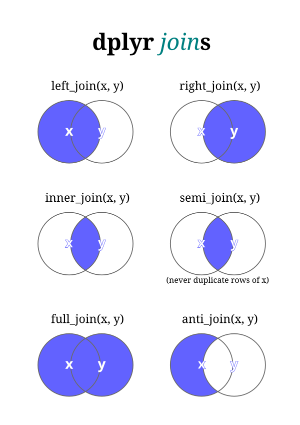
26 |
27 | ## data
28 |
29 | These exercises use the following [`dplyr` datasets](https://ggplot2.tidyverse.org/reference/index.html#section-data)
30 |
31 | - dplyr::band_instruments
32 | - dplyr::band_members
33 |
34 | ```{r}
35 | band_members
36 | band_instruments
37 | ```
38 |
39 | ## Goal
40 |
41 | Make one big data frame that joins `band_members` with `band_instruments`. Using the template below you need to identify what type of join to use and identify the join key.
42 |
43 | ```{r}
44 | band_members |>
45 | left_join(band_instruments, by = "name")
46 | ```
47 |
--------------------------------------------------------------------------------
/_freeze/site_libs/leaflet-easybutton-1.3.1/EasyButton-binding.js:
--------------------------------------------------------------------------------
1 | getEasyButton = function(button) {
2 |
3 | var options = {};
4 |
5 | options.position = button.position;
6 |
7 | // only add ID if provided
8 | if(button.id) {
9 | options.id = button.id;
10 | }
11 |
12 | // if custom states provided use that
13 | // else use provided icon and onClick
14 | if(button.states) {
15 | options.states = button.states;
16 | return L.easyButton(options);
17 | } else {
18 | return L.easyButton(button.icon, button.onClick,
19 | button.title, options );
20 | }
21 | };
22 |
23 | LeafletWidget.methods.addEasyButton = function(button) {
24 | getEasyButton(button).addTo(this);
25 | };
26 |
27 | LeafletWidget.methods.addEasyButtonBar = function(buttons, position, id) {
28 |
29 | var options = {};
30 |
31 | options.position = position;
32 |
33 | // only add ID if provided
34 | if(id) {
35 | options.id = id;
36 | }
37 |
38 | var easyButtons = [];
39 | for(var i=0; i < buttons.length; i++) {
40 | easyButtons[i] = getEasyButton(buttons[i]);
41 | }
42 | L.easyBar(easyButtons).addTo(this);
43 |
44 | };
45 |
--------------------------------------------------------------------------------
/_exercises/04_join.qmd:
--------------------------------------------------------------------------------
1 | ---
2 | title: "join"
3 |
4 | date-modified: 'today'
5 | date-format: long
6 |
7 | format:
8 | html:
9 | footer: "CC BY 4.0 John R Little"
10 |
11 | license: CC BY
12 | ---
13 |
14 | ```{r}
15 | library(tidyverse)
16 | ```
17 |
18 | ## Join
19 |
20 | There are a series of [join commands](https://dplyr.tidyverse.org/reference/index.html#section-two-table-verbs)
21 |
22 | - left_join, inner_join, right_join, full_join,
23 | - semi_join, anti_join
24 |
25 | 
26 |
27 | ## data
28 |
29 | These exercises use the following [`dplyr` datasets](https://ggplot2.tidyverse.org/reference/index.html#section-data)
30 |
31 | - dplyr::band_instruments
32 | - dplyr::band_members
33 |
34 | ```{r}
35 | band_members
36 | band_instruments
37 | ```
38 |
39 | ## Goal
40 |
41 | Make one big data frame that joins `band_members` with `band_instruments`. Using the template below you need to identify what type of join to use and identify the join key.
42 |
43 | ```{r}
44 | #| eval: false
45 | band_members |>
46 | ----_join(band_instruments, by = "----")
47 | ```
48 |
--------------------------------------------------------------------------------
/_freeze/site_libs/core-js-2.5.3/LICENSE:
--------------------------------------------------------------------------------
1 | Copyright (c) 2014-2017 Denis Pushkarev
2 |
3 | Permission is hereby granted, free of charge, to any person obtaining a copy
4 | of this software and associated documentation files (the "Software"), to deal
5 | in the Software without restriction, including without limitation the rights
6 | to use, copy, modify, merge, publish, distribute, sublicense, and/or sell
7 | copies of the Software, and to permit persons to whom the Software is
8 | furnished to do so, subject to the following conditions:
9 |
10 | The above copyright notice and this permission notice shall be included in
11 | all copies or substantial portions of the Software.
12 |
13 | THE SOFTWARE IS PROVIDED "AS IS", WITHOUT WARRANTY OF ANY KIND, EXPRESS OR
14 | IMPLIED, INCLUDING BUT NOT LIMITED TO THE WARRANTIES OF MERCHANTABILITY,
15 | FITNESS FOR A PARTICULAR PURPOSE AND NONINFRINGEMENT. IN NO EVENT SHALL THE
16 | AUTHORS OR COPYRIGHT HOLDERS BE LIABLE FOR ANY CLAIM, DAMAGES OR OTHER
17 | LIABILITY, WHETHER IN AN ACTION OF CONTRACT, TORT OR OTHERWISE, ARISING FROM,
18 | OUT OF OR IN CONNECTION WITH THE SOFTWARE OR THE USE OR OTHER DEALINGS IN
19 | THE SOFTWARE.
20 |
--------------------------------------------------------------------------------
/_freeze/site_libs/react-17.0.0/LICENSE.txt:
--------------------------------------------------------------------------------
1 | MIT License
2 |
3 | Copyright (c) 2013-present, Facebook, Inc.
4 |
5 | Permission is hereby granted, free of charge, to any person obtaining a copy
6 | of this software and associated documentation files (the "Software"), to deal
7 | in the Software without restriction, including without limitation the rights
8 | to use, copy, modify, merge, publish, distribute, sublicense, and/or sell
9 | copies of the Software, and to permit persons to whom the Software is
10 | furnished to do so, subject to the following conditions:
11 |
12 | The above copyright notice and this permission notice shall be included in all
13 | copies or substantial portions of the Software.
14 |
15 | THE SOFTWARE IS PROVIDED "AS IS", WITHOUT WARRANTY OF ANY KIND, EXPRESS OR
16 | IMPLIED, INCLUDING BUT NOT LIMITED TO THE WARRANTIES OF MERCHANTABILITY,
17 | FITNESS FOR A PARTICULAR PURPOSE AND NONINFRINGEMENT. IN NO EVENT SHALL THE
18 | AUTHORS OR COPYRIGHT HOLDERS BE LIABLE FOR ANY CLAIM, DAMAGES OR OTHER
19 | LIABILITY, WHETHER IN AN ACTION OF CONTRACT, TORT OR OTHERWISE, ARISING FROM,
20 | OUT OF OR IN CONNECTION WITH THE SOFTWARE OR THE USE OR OTHER DEALINGS IN THE
21 | SOFTWARE.
22 |
--------------------------------------------------------------------------------
/_freeze/site_libs/react-18.2.0/LICENSE.txt:
--------------------------------------------------------------------------------
1 | MIT License
2 |
3 | Copyright (c) 2013-present, Facebook, Inc.
4 |
5 | Permission is hereby granted, free of charge, to any person obtaining a copy
6 | of this software and associated documentation files (the "Software"), to deal
7 | in the Software without restriction, including without limitation the rights
8 | to use, copy, modify, merge, publish, distribute, sublicense, and/or sell
9 | copies of the Software, and to permit persons to whom the Software is
10 | furnished to do so, subject to the following conditions:
11 |
12 | The above copyright notice and this permission notice shall be included in all
13 | copies or substantial portions of the Software.
14 |
15 | THE SOFTWARE IS PROVIDED "AS IS", WITHOUT WARRANTY OF ANY KIND, EXPRESS OR
16 | IMPLIED, INCLUDING BUT NOT LIMITED TO THE WARRANTIES OF MERCHANTABILITY,
17 | FITNESS FOR A PARTICULAR PURPOSE AND NONINFRINGEMENT. IN NO EVENT SHALL THE
18 | AUTHORS OR COPYRIGHT HOLDERS BE LIABLE FOR ANY CLAIM, DAMAGES OR OTHER
19 | LIABILITY, WHETHER IN AN ACTION OF CONTRACT, TORT OR OTHERWISE, ARISING FROM,
20 | OUT OF OR IN CONNECTION WITH THE SOFTWARE OR THE USE OR OTHER DEALINGS IN THE
21 | SOFTWARE.
22 |
--------------------------------------------------------------------------------
/map_import_clean_regex.qmd:
--------------------------------------------------------------------------------
1 | ---
2 | title: "Import multiple Excel files"
3 | subtitle: "Casestudy of purrr::map() to make one big data frame"
4 | ---
5 |
6 | The [code](https://github.com/libjohn/workshop_rfun_iterate) and companion [youtube playlist](https://www.youtube.com/watch?v=QgasjZGhWlk&list=PLIUcX1JrVUNWW7RgPh9ysmJM3mBpIAlYG&index=1) show practical R/data-wrangling **tips** and **tricks**. This case study demonstrates custom *functions*, *regex* (regular expressions), and *iteration*. The workflow shows techniques for common needs such: data-scraping, ingesting multiple files, transforming messy data into tidy data, quickly cleaning column names, separating multivalue fields, uniting variable values, and nesting data.
7 |
8 | ## Playlist
9 |
10 |
13 |
14 | ## Code and data
15 |
16 | Github ▶️ [libjohn/workshop_rfun/iterate](https://github.com/libjohn/workshop_rfun_iterate)
17 |
--------------------------------------------------------------------------------
/_exercises/03_pivot.qmd:
--------------------------------------------------------------------------------
1 | ---
2 | title: "03 pivot data"
3 | author: "John Little"
4 |
5 | date-modified: 'today'
6 | date-format: long
7 |
8 | format:
9 | html:
10 | footer: "CC BY 4.0 John R Little"
11 |
12 | license: CC BY
13 | ---
14 |
15 | ```{r}
16 | library(tidyverse)
17 | ```
18 |
19 | ## data
20 |
21 | These exercises use the following [`ggplot2` training datasets](https://ggplot2.tidyverse.org/reference/index.html#section-data)
22 |
23 | - ggplot2::economics
24 |
25 | ## Pivot
26 |
27 | Below are two data frames. One is wide data, the other is long.
28 |
29 | ```{r}
30 | economics
31 | economics_long %>% arrange(date)
32 | ```
33 |
34 | ## Goal
35 |
36 | Using one of the dplyr pivot functions, pivot the economics data to long format
37 |
38 | ```{r}
39 | economics %>%
40 | pivot_------(cols = pce:unemploy,
41 | names_to = "variable",
42 | values_to = "value")
43 | ```
44 |
45 | Now that the data are long. Can you use the `facet_wrap()` function to make multiple line plots, one line plot for each `variable` category?
46 |
47 | ```{r}
48 | economics |>
49 | pivot_longer(-date, names_to = "variable", values_to = "value") |>
50 | ggplot(aes(date, value)) +
51 | geom____() +
52 | facet_wrap(vars(_______))
53 | ```
54 |
--------------------------------------------------------------------------------
/_freeze/site_libs/leaflet-easybutton-1.3.1/easy-button.css:
--------------------------------------------------------------------------------
1 | .leaflet-bar button,
2 | .leaflet-bar button:hover {
3 | background-color: #fff;
4 | border: none;
5 | border-bottom: 1px solid #ccc;
6 | width: 26px;
7 | height: 26px;
8 | line-height: 26px;
9 | display: block;
10 | text-align: center;
11 | text-decoration: none;
12 | color: black;
13 | }
14 |
15 | .leaflet-bar button {
16 | background-position: 50% 50%;
17 | background-repeat: no-repeat;
18 | overflow: hidden;
19 | display: block;
20 | }
21 |
22 | .leaflet-bar button:hover {
23 | background-color: #f4f4f4;
24 | }
25 |
26 | .leaflet-bar button:first-of-type {
27 | border-top-left-radius: 4px;
28 | border-top-right-radius: 4px;
29 | }
30 |
31 | .leaflet-bar button:last-of-type {
32 | border-bottom-left-radius: 4px;
33 | border-bottom-right-radius: 4px;
34 | border-bottom: none;
35 | }
36 |
37 | .leaflet-bar.disabled,
38 | .leaflet-bar button.disabled {
39 | cursor: default;
40 | pointer-events: none;
41 | opacity: .4;
42 | }
43 |
44 | .easy-button-button .button-state{
45 | display: block;
46 | width: 100%;
47 | height: 100%;
48 | position: relative;
49 | }
50 |
51 |
52 | .leaflet-touch .leaflet-bar button {
53 | width: 30px;
54 | height: 30px;
55 | line-height: 30px;
56 | }
57 |
--------------------------------------------------------------------------------
/README.md:
--------------------------------------------------------------------------------
1 | # Introduction to R workshop
2 |
3 |
4 |
5 |
6 |
7 | For more information or resource on learning R, please visit the [Rfun learning series](https://Rfun.library.duke.edu).
8 |
9 | This website is composed in the [RStudio IDE](https://posit.co/download/rstudio-desktop/), as [R code](https://en.wikipedia.org/wiki/R_(programming_language)) authored as a [Quarto](https://quarto.org/) notebooks. With Quarto it is easy to render multiple report formats, such as a PDF document or this website. In this case the report format is a [web site hosted](https://intro2R.library.duke.edu/) at netlify. The code for this workshop and this webpage are all part of a single RStudio project that can be [found in a GitHub repository](https://github.com/data-and-visualization/Intro2R/).
10 |
11 | The code-along exercises for this workshop are in the GitHub repository but they are not part of the web site. You can work through the exercises by first downloading the GitHub repository. Then, find the exercises within the `_exercises` directory.
12 |
13 | ```{=html}
14 |
21 | ```
22 |
--------------------------------------------------------------------------------
/_freeze/site_libs/rstudio_leaflet-1.3.1/rstudio_leaflet.css:
--------------------------------------------------------------------------------
1 | .leaflet-tooltip.leaflet-tooltip-text-only,
2 | .leaflet-tooltip.leaflet-tooltip-text-only:before,
3 | .leaflet-tooltip.leaflet-tooltip-text-only:after {
4 | background: none;
5 | border: none;
6 | box-shadow: none;
7 | }
8 |
9 | .leaflet-tooltip.leaflet-tooltip-text-only.leaflet-tooltip-left {
10 | margin-left: 5px;
11 | }
12 |
13 | .leaflet-tooltip.leaflet-tooltip-text-only.leaflet-tooltip-right {
14 | margin-left: -5px;
15 | }
16 |
17 | .leaflet-tooltip:after {
18 | border-right: 6px solid transparent;
19 | /* right: -16px; */
20 | }
21 |
22 | .leaflet-popup-pane .leaflet-popup-tip-container {
23 | /* when the tooltip container is clicked, it is closed */
24 | pointer-events: all;
25 | /* tooltips should display the "hand" icon, just like .leaflet-interactive*/
26 | cursor: pointer;
27 | }
28 |
29 | /* have the widget be displayed in the right 'layer' */
30 | .leaflet-map-pane {
31 | z-index: auto;
32 | }
33 |
34 | /* Add missing rule from leaflet for img.
35 | This complete existing leaflet.css.
36 | Fix for https://github.com/rstudio/rmarkdown/issues/1949 */
37 | .leaflet-container .leaflet-right-pane img,
38 | .leaflet-container .leaflet-left-pane img {
39 | max-width: none !important;
40 | max-height: none !important;
41 | }
42 |
--------------------------------------------------------------------------------
/_freeze/site_libs/crosstalk-1.2.0/css/crosstalk.min.css:
--------------------------------------------------------------------------------
1 | .container-fluid.crosstalk-bscols{margin-left:-30px;margin-right:-30px;white-space:normal}body>.container-fluid.crosstalk-bscols{margin-left:auto;margin-right:auto}.crosstalk-input-checkboxgroup .crosstalk-options-group .crosstalk-options-column{display:inline-block;padding-right:12px;vertical-align:top}@media only screen and (max-width: 480px){.crosstalk-input-checkboxgroup .crosstalk-options-group .crosstalk-options-column{display:block;padding-right:inherit}}.crosstalk-input{margin-bottom:15px}.crosstalk-input .control-label{margin-bottom:0;vertical-align:middle}.crosstalk-input input[type="checkbox"]{margin:4px 0 0;margin-top:1px;line-height:normal}.crosstalk-input .checkbox{position:relative;display:block;margin-top:10px;margin-bottom:10px}.crosstalk-input .checkbox>label{padding-left:20px;margin-bottom:0;font-weight:400;cursor:pointer}.crosstalk-input .checkbox input[type="checkbox"],.crosstalk-input .checkbox-inline input[type="checkbox"]{position:absolute;margin-top:2px;margin-left:-20px}.crosstalk-input .checkbox+.checkbox{margin-top:-5px}.crosstalk-input .checkbox-inline{position:relative;display:inline-block;padding-left:20px;margin-bottom:0;font-weight:400;vertical-align:middle;cursor:pointer}.crosstalk-input .checkbox-inline+.checkbox-inline{margin-top:0;margin-left:10px}
2 |
--------------------------------------------------------------------------------
/_exercises/answers/03_pivot_answers.qmd:
--------------------------------------------------------------------------------
1 | ---
2 | title: "03 pivot data"
3 | author: "John Little"
4 |
5 | date-modified: 'today'
6 | date-format: long
7 |
8 | format:
9 | html:
10 | footer: "CC BY 4.0 John R Little"
11 |
12 | license: CC BY
13 | ---
14 |
15 | ```{r}
16 | library(tidyverse)
17 | ```
18 |
19 | ## data
20 |
21 | These exercises use the following [`ggplot2` training datasets](https://ggplot2.tidyverse.org/reference/index.html#section-data)
22 |
23 | - ggplot2::economics
24 |
25 | ## Pivot
26 |
27 | Below are two data frames. One is wide data, the other is long.
28 |
29 | ```{r}
30 | economics
31 | economics_long %>% arrange(date)
32 | ```
33 |
34 | ## Goal
35 |
36 | Using one of the dplyr pivot functions, pivot the economics data to long format
37 |
38 | ```{r}
39 | economics %>%
40 | pivot_longer(cols = pce:unemploy,
41 | names_to = "variable",
42 | values_to = "value")
43 | ```
44 |
45 | or
46 |
47 | ```{r}
48 | economics |>
49 | pivot_longer(-date, names_to = "variable", values_to = "value")
50 | ```
51 |
52 | Now that the data are long. Can you use the `facet_wrap()` function to make multiple line plots, one line plot for each `variable` category?
53 |
54 | ```{r}
55 | economics |>
56 | pivot_longer(-date, names_to = "variable", values_to = "value") |>
57 | ggplot(aes(date, value)) +
58 | geom_line() +
59 | facet_wrap(vars(variable))
60 | ```
61 |
--------------------------------------------------------------------------------
/tidymodels.qmd:
--------------------------------------------------------------------------------
1 | ---
2 | title: "Tidymodels and machine learning"
3 | date-modified: 'today'
4 | date-format: long
5 |
6 | license: CC BY-NC
7 | bibliography: references.bib
8 | ---
9 |
10 | The {tidymodels} concept [@kuhn2022] is a group of packages in support of modeling and machine learning. In the [last section](regression.html) we learned how to manipulate a basic linear model though a combination of the base-R `lm()` function and the tidyverse {broom} package along with the `nest()` function. However, modeling can be much more involved. This basic overview introduces tidymodels, a conceptual approach to integrating tidyverse principles with modeling, machine learning, feature selection and tuning.
11 |
12 | Beyond the core of integrating machine learning and modeling with the tidyverse, tidymodels supports a variety of useful analytical and computational approaches. A short list of examples includes **statistical analysis** (e.g. bootstrapping, hypothesis testing, k-means clustering, logistic regression, etc.), **robust modeling** (e.g. classification, least squares, resampling), creating **performance metrics**, **tuning, clustering, classification, text analysis, neural networks**, and more.
13 |
14 | ## Get started
15 |
16 | Modelers and ML coders can approach tidymodels by
17 |
18 | 1. Engaging with the [five-step tutorial](https://www.tidymodels.org/start/) (build a model, use recipes to pre-process data, evaluate with resampling, tune, and predict.
19 |
20 | 2. [Dive deeper to find articles that help apply the tidymodels approach](https://www.tidymodels.org/learn/) to your needs.
21 |
--------------------------------------------------------------------------------
/_freeze/site_libs/reactable-0.4.4/reactable.server.js.LICENSE.txt:
--------------------------------------------------------------------------------
1 | /*
2 | object-assign
3 | (c) Sindre Sorhus
4 | @license MIT
5 | */
6 |
7 | /*!
8 | * The buffer module from node.js, for the browser.
9 | *
10 | * @author Feross Aboukhadijeh
11 | * @license MIT
12 | */
13 |
14 | /*! ieee754. BSD-3-Clause License. Feross Aboukhadijeh */
15 |
16 | /*! safe-buffer. MIT License. Feross Aboukhadijeh */
17 |
18 | /** @license React v0.20.2
19 | * scheduler.production.min.js
20 | *
21 | * Copyright (c) Facebook, Inc. and its affiliates.
22 | *
23 | * This source code is licensed under the MIT license found in the
24 | * LICENSE file in the root directory of this source tree.
25 | */
26 |
27 | /** @license React v17.0.2
28 | * react-dom-server.node.production.min.js
29 | *
30 | * Copyright (c) Facebook, Inc. and its affiliates.
31 | *
32 | * This source code is licensed under the MIT license found in the
33 | * LICENSE file in the root directory of this source tree.
34 | */
35 |
36 | /** @license React v17.0.2
37 | * react-dom.production.min.js
38 | *
39 | * Copyright (c) Facebook, Inc. and its affiliates.
40 | *
41 | * This source code is licensed under the MIT license found in the
42 | * LICENSE file in the root directory of this source tree.
43 | */
44 |
45 | /** @license React v17.0.2
46 | * react.production.min.js
47 | *
48 | * Copyright (c) Facebook, Inc. and its affiliates.
49 | *
50 | * This source code is licensed under the MIT license found in the
51 | * LICENSE file in the root directory of this source tree.
52 | */
53 |
--------------------------------------------------------------------------------
/_freeze/site_libs/datatables-css-0.0.0/datatables-crosstalk.css:
--------------------------------------------------------------------------------
1 | .dt-crosstalk-fade {
2 | opacity: 0.2;
3 | }
4 |
5 | html body div.DTS div.dataTables_scrollBody {
6 | background: none;
7 | }
8 |
9 |
10 | /*
11 | Fix https://github.com/rstudio/DT/issues/563
12 | If the `table.display` is set to "block" (e.g., pkgdown), the browser will display
13 | datatable objects strangely. The search panel and the page buttons will still be
14 | in full-width but the table body will be "compact" and shorter.
15 | In therory, having this attributes will affect `dom="t"`
16 | with `display: block` users. But in reality, there should be no one.
17 | We may remove the below lines in the future if the upstream agree to have this there.
18 | See https://github.com/DataTables/DataTablesSrc/issues/160
19 | */
20 |
21 | table.dataTable {
22 | display: table;
23 | }
24 |
25 |
26 | /*
27 | When DTOutput(fill = TRUE), it receives a .html-fill-item class (via htmltools::bindFillRole()), which effectively amounts to `flex: 1 1 auto`. That's mostly fine, but the case where `fillContainer=TRUE`+`height:auto`+`flex-basis:auto` and the container (e.g., a bslib::card()) doesn't have a defined height is a bit problematic since the table wants to fit the parent but the parent wants to fit the table, which results pretty small table height (maybe because there is a minimum height somewhere?). It seems better in this case to impose a 400px height default for the table, which we can do by setting `flex-basis` to 400px (the table is still allowed to grow/shrink when the container has an opinionated height).
28 | */
29 |
30 | .html-fill-container > .html-fill-item.datatables {
31 | flex-basis: 400px;
32 | }
33 |
--------------------------------------------------------------------------------
/about.qmd:
--------------------------------------------------------------------------------
1 | ---
2 | title: "About"
3 |
4 | date-modified: 'today'
5 | date-format: long
6 |
7 | license: CC BY-NC
8 | bibliography: references.bib
9 | ---
10 |
11 | This website is hosted by the [Center for Data & Visualization Sciences](https://library.duke.edu/data/), part of the [Duke University Libraries](https://library.duke.edu). composed in the [RStudio IDE](https://posit.co/download/rstudio-desktop/), as [R code](https://en.wikipedia.org/wiki/R_(programming_language)) authored as a [Quarto](https://quarto.org/) notebooks. With Quarto it is easy to render multiple report formats such as a PDF document or this website. In this case the report format is a [web site hosted](https://intro2R.library.duke.edu/) gratis at netlify.
12 |
13 | ::: {style="text-align: center"}
14 | 
15 | :::
16 |
17 | Formerly, this site was known as the Rfun site. The content from that site has been consolidated here.
18 |
19 | The code for this workshop and this webpage are all part of a single RStudio project that can be [found in a GitHub repository](https://github.com/data-and-visualization/Intro2R). The code-along exercises for this workshop are in the GitHub repository but they are not part of the web site. You can work through the exercises by first downloading the GitHub repository. Then find the exercises within the `_exercises` directory.
20 |
21 | You can find an [**outline** for this](outline.html) workshop. For more information or resource on learning R, please also visit the [Rfun learning series](https://Rfun.library.duke.edu).
22 |
23 | ## Misc
24 |
25 | ::: {.callout-note collapse="true"}
26 | ## Earlier version of a package?
27 |
28 | `remotes::install_version("knitr", "1.42")`
29 | :::
30 |
--------------------------------------------------------------------------------
/_freeze/site_libs/leaflet-locationfilter2-0.1.1/locationfilter-bindings.js:
--------------------------------------------------------------------------------
1 | /* global LeafletWidget, L, Shiny, HTMLWidgets, $ */
2 |
3 | function getLocationFilterBounds(locationFilter) {
4 | if(locationFilter && locationFilter.getBounds) {
5 | var bounds = locationFilter.getBounds();
6 | var boundsJSON =
7 | {
8 | "sw_lat" : bounds.getSouth(),
9 | "sw_lng" : bounds.getWest(),
10 | "ne_lat" : bounds.getNorth(),
11 | "ne_lng" : bounds.getEast()
12 | };
13 | return boundsJSON;
14 | } else {
15 | return null;
16 | }
17 | }
18 |
19 | LeafletWidget.methods.addLocationFilter = function(options) {
20 | (function() {
21 | var map = this;
22 |
23 | if(map.locationFilter) {
24 | map.locationFilter.remove();
25 | map.locationFilter = null;
26 | }
27 |
28 | if(!$.isEmptyObject(options.bounds)) {
29 | options.bounds = L.latLngBounds(options.bounds);
30 | }
31 |
32 | map.locationFilter = new L.LocationFilter(options);
33 |
34 | map.locationFilter.on("change", function(e) {
35 | if (!HTMLWidgets.shinyMode) return;
36 | Shiny.onInputChange(map.id+"_location_filter_changed",
37 | getLocationFilterBounds(map.locationFilter));
38 | });
39 | map.locationFilter.on("enabled", function(e) {
40 | if (!HTMLWidgets.shinyMode) return;
41 | Shiny.onInputChange(map.id+"_location_filter_enabled",
42 | getLocationFilterBounds(map.locationFilter));
43 | });
44 | map.locationFilter.on("disabled", function(e) {
45 | if (!HTMLWidgets.shinyMode) return;
46 | Shiny.onInputChange(map.id+"_location_filter_disabled",
47 | getLocationFilterBounds(map.locationFilter));
48 | });
49 |
50 | map.locationFilter.addTo(map);
51 |
52 | }).call(this);
53 | };
54 |
55 | LeafletWidget.methods.removeLocationFilter = function() {
56 | (function() {
57 | var map = this;
58 |
59 | if(map.locationFilter) {
60 | map.locationFilter.remove();
61 | map.locationFilter = null;
62 | }
63 |
64 | }).call(this);
65 | };
66 |
67 |
--------------------------------------------------------------------------------
/_freeze/site_libs/crosstalk-1.2.0/scss/crosstalk.scss:
--------------------------------------------------------------------------------
1 | /* Adjust margins outwards, so column contents line up with the edges of the
2 | parent of container-fluid. */
3 | .container-fluid.crosstalk-bscols {
4 | margin-left: -30px;
5 | margin-right: -30px;
6 | white-space: normal;
7 | }
8 |
9 | /* But don't adjust the margins outwards if we're directly under the body,
10 | i.e. we were the top-level of something at the console. */
11 | body > .container-fluid.crosstalk-bscols {
12 | margin-left: auto;
13 | margin-right: auto;
14 | }
15 |
16 | .crosstalk-input-checkboxgroup .crosstalk-options-group .crosstalk-options-column {
17 | display: inline-block;
18 | padding-right: 12px;
19 | vertical-align: top;
20 | }
21 |
22 | @media only screen and (max-width:480px) {
23 | .crosstalk-input-checkboxgroup .crosstalk-options-group .crosstalk-options-column {
24 | display: block;
25 | padding-right: inherit;
26 | }
27 | }
28 |
29 | /* Relevant BS3 styles to make filter_checkbox() look reasonable without Bootstrap */
30 | .crosstalk-input {
31 | margin-bottom: 15px; /* a la .form-group */
32 | .control-label {
33 | margin-bottom: 0;
34 | vertical-align: middle;
35 | }
36 | input[type="checkbox"] {
37 | margin: 4px 0 0;
38 | margin-top: 1px;
39 | line-height: normal;
40 | }
41 | .checkbox {
42 | position: relative;
43 | display: block;
44 | margin-top: 10px;
45 | margin-bottom: 10px;
46 | }
47 | .checkbox > label{
48 | padding-left: 20px;
49 | margin-bottom: 0;
50 | font-weight: 400;
51 | cursor: pointer;
52 | }
53 | .checkbox input[type="checkbox"],
54 | .checkbox-inline input[type="checkbox"] {
55 | position: absolute;
56 | margin-top: 2px;
57 | margin-left: -20px;
58 | }
59 | .checkbox + .checkbox {
60 | margin-top: -5px;
61 | }
62 | .checkbox-inline {
63 | position: relative;
64 | display: inline-block;
65 | padding-left: 20px;
66 | margin-bottom: 0;
67 | font-weight: 400;
68 | vertical-align: middle;
69 | cursor: pointer;
70 | }
71 | .checkbox-inline + .checkbox-inline {
72 | margin-top: 0;
73 | margin-left: 10px;
74 | }
75 | }
76 |
--------------------------------------------------------------------------------
/eda.qmd:
--------------------------------------------------------------------------------
1 | ---
2 | title: "Exploratory Data Analysis packages"
3 | date-modified: 'today'
4 | date-format: long
5 |
6 | license: CC BY-NC
7 | bibliography: references.bib
8 | ---
9 |
10 | EDA, or Exploratory Data Analysis can take many forms. This brief section will recommend a few packages which can be used to explore your data, more or less, automagically. The packages can be complex and may take some effort to learn. However, if you're brand new to data mining, you may benefit from reading these package documentation pages, and then applying their functions to your data.
11 |
12 | Recommended EDA packages
13 |
14 | - {skimr} - [https://docs.ropensci.org/skimr](https://docs.ropensci.org/skimrhttps://github.com/taiyun/corrplot/)\
15 | a frictionless approach to summary statistics
16 |
17 | - {gtExtras} - [https://jthomasmock.github.io/gtExtras/reference/gt_plt_summary.html](https://jthomasmock.github.io/gtExtras/reference/gt_plt_summary.htmlhttps://jthomasmock.github.io/gtExtras/reference/gt_plt_summary.html)\
18 | create a summary table with historgrams or area bar chatrs from a dataframe
19 |
20 | - {DataExplorer} - [https://boxuancui.github.io/DataExplorer/reference/plot_intro.html](https://boxuancui.github.io/DataExplorer/reference/plot_intro.htmlhttps://boxuancui.github.io/DataExplorer/reference/plot_intro.html)\
21 | Plot basic information
22 |
23 | - {corrplot} - [https://github.com/taiyun/corrplot](https://github.com/taiyun/corrplot/)\
24 | a visual exploratory tool on correlation matrix that supports automatic variable reordering
25 |
26 | - {summarytools} - [https://github.com/dcomtois/summarytools](https://github.com/dcomtois/summarytoolshttps://github.com/dcomtois/summarytools)\
27 | or data cleaning, exploring, and simple reporting
28 |
29 | - {tableone} - [https://github.com/kaz-yos/tableone](https://github.com/kaz-yos/tableonehttps://github.com/kaz-yos/tableone)\
30 | create "Table 1", description of baseline characteristics
31 |
32 | - {dtracker} - [https://terminological.github.io/dtrackr](https://terminological.github.io/dtrackr/)\
33 | Accurate documentation of a data pipeline is a first step to reproducibility, and a flow chart describing the steps taken to prepare data
34 |
--------------------------------------------------------------------------------
/_freeze/site_libs/dt-core-bootstrap-1.13.6/js/dataTables.bootstrap.min.js:
--------------------------------------------------------------------------------
1 | /*! DataTables Bootstrap 3 integration
2 | * ©2011-2015 SpryMedia Ltd - datatables.net/license
3 | */
4 | !function(t){var n,i;"function"==typeof define&&define.amd?define(["jquery","datatables.net"],function(e){return t(e,window,document)}):"object"==typeof exports?(n=require("jquery"),i=function(e,a){a.fn.dataTable||require("datatables.net")(e,a)},"undefined"==typeof window?module.exports=function(e,a){return e=e||window,a=a||n(e),i(e,a),t(a,0,e.document)}:(i(window,n),module.exports=t(n,window,window.document))):t(jQuery,window,document)}(function(x,e,n,i){"use strict";var r=x.fn.dataTable;return x.extend(!0,r.defaults,{dom:"<'row'<'col-sm-6'l><'col-sm-6'f>><'row'<'col-sm-12'tr>><'row'<'col-sm-5'i><'col-sm-7'p>>",renderer:"bootstrap"}),x.extend(r.ext.classes,{sWrapper:"dataTables_wrapper form-inline dt-bootstrap",sFilterInput:"form-control input-sm",sLengthSelect:"form-control input-sm",sProcessing:"dataTables_processing panel panel-default"}),r.ext.renderer.pageButton.bootstrap=function(s,e,d,a,l,c){function u(e,a){for(var t,n,i=function(e){e.preventDefault(),x(e.currentTarget).hasClass("disabled")||b.page()==e.data.action||b.page(e.data.action).draw("page")},r=0,o=a.length;r",{class:m.sPageButton+" "+f,id:0===d&&"string"==typeof t?s.sTableId+"_"+t:null}).append(x("",{href:n?null:"#","aria-controls":s.sTableId,"aria-disabled":n?"true":null,"aria-label":w[t],role:"link","aria-current":"active"===f?"page":null,"data-dt-idx":t,tabindex:n?-1:s.iTabIndex}).html(p)).appendTo(e),s.oApi._fnBindAction(n,{action:t},i))}}var p,f,t,b=new r.Api(s),m=s.oClasses,g=s.oLanguage.oPaginate,w=s.oLanguage.oAria.paginate||{};try{t=x(e).find(n.activeElement).data("dt-idx")}catch(e){}u(x(e).empty().html('').children("ul"),a),t!==i&&x(e).find("[data-dt-idx="+t+"]").trigger("focus")},r});
--------------------------------------------------------------------------------
/_freeze/site_libs/dt-core-bootstrap-1.13.4/js/dataTables.bootstrap.min.js:
--------------------------------------------------------------------------------
1 | /*! DataTables Bootstrap 3 integration
2 | * ©2011-2015 SpryMedia Ltd - datatables.net/license
3 | */
4 | !function(t){var n,i;"function"==typeof define&&define.amd?define(["jquery","datatables.net"],function(e){return t(e,window,document)}):"object"==typeof exports?(n=require("jquery"),i=function(e,a){a.fn.dataTable||require("datatables.net")(e,a)},"undefined"!=typeof window?module.exports=function(e,a){return e=e||window,a=a||n(e),i(e,a),t(a,0,e.document)}:(i(window,n),module.exports=t(n,window,window.document))):t(jQuery,window,document)}(function(x,e,n,i){"use strict";var r=x.fn.dataTable;return x.extend(!0,r.defaults,{dom:"<'row'<'col-sm-6'l><'col-sm-6'f>><'row'<'col-sm-12'tr>><'row'<'col-sm-5'i><'col-sm-7'p>>",renderer:"bootstrap"}),x.extend(r.ext.classes,{sWrapper:"dataTables_wrapper form-inline dt-bootstrap",sFilterInput:"form-control input-sm",sLengthSelect:"form-control input-sm",sProcessing:"dataTables_processing panel panel-default"}),r.ext.renderer.pageButton.bootstrap=function(s,e,d,a,l,c){function u(e,a){for(var t,n,i=function(e){e.preventDefault(),x(e.currentTarget).hasClass("disabled")||b.page()==e.data.action||b.page(e.data.action).draw("page")},r=0,o=a.length;r",{class:m.sPageButton+" "+f,id:0===d&&"string"==typeof t?s.sTableId+"_"+t:null}).append(x("",{href:n?null:"#","aria-controls":s.sTableId,"aria-disabled":n?"true":null,"aria-label":w[t],"aria-role":"link","aria-current":"active"===f?"page":null,"data-dt-idx":t,tabindex:s.iTabIndex}).html(p)).appendTo(e),s.oApi._fnBindAction(n,{action:t},i))}}var p,f,t,b=new r.Api(s),m=s.oClasses,g=s.oLanguage.oPaginate,w=s.oLanguage.oAria.paginate||{};try{t=x(e).find(n.activeElement).data("dt-idx")}catch(e){}u(x(e).empty().html('').children("ul"),a),t!==i&&x(e).find("[data-dt-idx="+t+"]").trigger("focus")},r});
--------------------------------------------------------------------------------
/_exercises/answers/00_import_answers.qmd:
--------------------------------------------------------------------------------
1 | ---
2 | title: "Answers - Excercise 00"
3 |
4 | date-modified: 'today'
5 | date-format: long
6 |
7 | format:
8 | html:
9 | footer: "CC BY 4.0 John R Little"
10 |
11 | license: CC BY
12 | ---
13 |
14 | ## exercise 00:
15 |
16 | 1. Load the tidyverse libary package
17 |
18 | ```{r}
19 | #| message: false
20 | #| warning: false
21 | library(tidyverse)
22 | ```
23 |
24 | 2. Fill in the blanks. Using what you've seen in class, if `data/brodhead_center.csv` is a CSV (comma separated values) file, how would you load the file into a new object called `brodhead`?
25 |
26 | ```{r}
27 | #| message: false
28 | #| warning: false
29 | brodhead <- read_csv("../../data/brodhead_center.csv")
30 |
31 | # or
32 | # brodhead <- read_csv(here::here("data", "brodhead_center.csv"))
33 | ```
34 |
35 | 3. Display your new `brodhead` data frame?
36 |
37 | ```{r}
38 | brodhead
39 | ```
40 |
41 | 4. `starwars` is an on-board dataset that comes with the tidyverse. Insert a new code chunk and display that data.
42 |
43 | ```{r}
44 | starwars
45 | ```
46 |
47 | 5. Copy and paste the following code into a new code chunk in your new file.
48 |
49 | ```{r}
50 | starwars %>%
51 | ggplot(aes(fct_infreq(hair_color))) +
52 | geom_bar() +
53 | ggtitle("Hair Color Frequency of Star Wars Characters")
54 | ```
55 |
56 | 6. Take a look at the structure of the `brodhead` object.
57 | - How many observations (rows) are there?
58 | - How many variables (columns) are there?
59 | - How many of the variables are numeric data?
60 |
61 | ```{r}
62 | glimpse(brodhead)
63 | ```
64 |
65 | ## Bonus 2
66 |
67 | Importing labeled vectors from an spss file format. Import via the `haven::read_sav()` function
68 |
69 | ```{r}
70 | library(haven)
71 | library(here)
72 |
73 | my_labeled_vectors_df <-
74 | read_sav(here("data", "student_satisfaction_test-data_from_qualtrics.sav"))
75 |
76 | my_labeled_vectors_df
77 |
78 | my_labeled_vectors_df |>
79 | select(Q2) |>
80 | mutate(Q2_labels = as_factor(Q2))
81 |
82 | my_labeled_vectors_df |>
83 | select(ResponseId, starts_with("Q")) |>
84 | mutate(across(is.labelled, function(x) as_factor(x), .names = "{.col}_label")) |>
85 | select(ResponseId, sort(tidyselect::peek_vars()))
86 |
87 | ```
88 |
--------------------------------------------------------------------------------
/_exercises/02_viz.qmd:
--------------------------------------------------------------------------------
1 | ---
2 | title: "Visualize Data in R with ggplot2"
3 | subtitle: "Exercises"
4 | abstract: "These exercises are adapted in whole or in part based on the Master the Tidyverse work by Garrett Grolemund at RStudio. \nCC BY Garrett Grolemund, RStudio ; BY-NC John Little"
5 |
6 | date-modified: 'today'
7 | date-format: long
8 |
9 | format:
10 | html:
11 | footer: "CC BY 4.0 John R Little"
12 |
13 | license: CC BY
14 | ---
15 |
16 | These exercises support your learning after watching the [instructional video](https://warpwire.duke.edu/w/80YEAA/)
17 |
18 | ```{r setup}
19 | #| echo: true
20 | #| warning: false
21 | #| message: false
22 | library(tidyverse)
23 | ```
24 |
25 | The dataset, `mpg`, is an onboard dataset, part of the `ggplot2` package. You can learn more about it by searching the help tab for "mpg", or type `?mpg` in the console.
26 |
27 | ```{r}
28 | mpg
29 | ```
30 |
31 | ## Your Turn 1
32 |
33 | IN THE code-chunk, **below**, manually type the following code:
34 |
35 | ggplot(data = mpg) + geom_point(mapping = aes(x = displ, y = hwy))
36 |
37 | Pay strict attention to spelling, capitalization, and parentheses! Try not to copy and paste, just this once.
38 |
39 | ```{r}
40 | #| eval: false
41 | ```
42 |
43 | ## Your Turn 2
44 |
45 | Add `color`, `size`, `alpha`, and `shape` aesthetics to your graph. Experiment.
46 |
47 | ```{r}
48 | mpg %>%
49 | ggplot() +
50 | geom_point(mapping = aes(x = displ, y = hwy))
51 | ```
52 |
53 | ## Your Turn 3
54 |
55 | Replace this scatter plot with one that draws box plots. Use the cheat sheet. Try your best guess.
56 |
57 | ```{r}
58 | mpg %>%
59 | ggplot() +
60 | geom_point(aes(class, hwy))
61 | ```
62 |
63 | ## Your Turn 4
64 |
65 | Make a histogram of the `hwy` variable from `mpg`.
66 |
67 | ```{r}
68 |
69 | ```
70 |
71 | ## Your Turn 5
72 |
73 | Make a density plot of `hwy` colored by `class`.
74 |
75 | ```{r}
76 |
77 | ```
78 |
79 | ## Your Turn 6
80 |
81 | Make a bar chart `hwy` colored by `class`.
82 |
83 | ```{r}
84 |
85 | ```
86 |
87 | ## Your Turn 7
88 |
89 | Predict what this code will do. Then run it.
90 |
91 | ```{r}
92 | mpg %>%
93 | ggplot() +
94 | geom_point(aes(displ, hwy)) +
95 | geom_smooth(aes(displ, hwy))
96 | ```
97 |
98 | ## Your Turn 8
99 |
100 | Save the last plot
101 |
102 | ```{r}
103 | ggsave(_____)
104 | # or right-click the image
105 | ```
106 |
--------------------------------------------------------------------------------
/_freeze/site_libs/dt-core-bootstrap-1.13.4/css/dataTables.bootstrap.extra.css:
--------------------------------------------------------------------------------
1 | table.dataTable th.dt-left,
2 | table.dataTable td.dt-left {
3 | text-align: left;
4 | }
5 | table.dataTable th.dt-center,
6 | table.dataTable td.dt-center,
7 | table.dataTable td.dataTables_empty {
8 | text-align: center;
9 | }
10 | table.dataTable th.dt-right,
11 | table.dataTable td.dt-right {
12 | text-align: right;
13 | }
14 | table.dataTable th.dt-justify,
15 | table.dataTable td.dt-justify {
16 | text-align: justify;
17 | }
18 | table.dataTable th.dt-nowrap,
19 | table.dataTable td.dt-nowrap {
20 | white-space: nowrap;
21 | }
22 | table.dataTable thead th.dt-head-left,
23 | table.dataTable thead td.dt-head-left,
24 | table.dataTable tfoot th.dt-head-left,
25 | table.dataTable tfoot td.dt-head-left {
26 | text-align: left;
27 | }
28 | table.dataTable thead th.dt-head-center,
29 | table.dataTable thead td.dt-head-center,
30 | table.dataTable tfoot th.dt-head-center,
31 | table.dataTable tfoot td.dt-head-center {
32 | text-align: center;
33 | }
34 | table.dataTable thead th.dt-head-right,
35 | table.dataTable thead td.dt-head-right,
36 | table.dataTable tfoot th.dt-head-right,
37 | table.dataTable tfoot td.dt-head-right {
38 | text-align: right;
39 | }
40 | table.dataTable thead th.dt-head-justify,
41 | table.dataTable thead td.dt-head-justify,
42 | table.dataTable tfoot th.dt-head-justify,
43 | table.dataTable tfoot td.dt-head-justify {
44 | text-align: justify;
45 | }
46 | table.dataTable thead th.dt-head-nowrap,
47 | table.dataTable thead td.dt-head-nowrap,
48 | table.dataTable tfoot th.dt-head-nowrap,
49 | table.dataTable tfoot td.dt-head-nowrap {
50 | white-space: nowrap;
51 | }
52 | table.dataTable tbody th.dt-body-left,
53 | table.dataTable tbody td.dt-body-left {
54 | text-align: left;
55 | }
56 | table.dataTable tbody th.dt-body-center,
57 | table.dataTable tbody td.dt-body-center {
58 | text-align: center;
59 | }
60 | table.dataTable tbody th.dt-body-right,
61 | table.dataTable tbody td.dt-body-right {
62 | text-align: right;
63 | }
64 | table.dataTable tbody th.dt-body-justify,
65 | table.dataTable tbody td.dt-body-justify {
66 | text-align: justify;
67 | }
68 | table.dataTable tbody th.dt-body-nowrap,
69 | table.dataTable tbody td.dt-body-nowrap {
70 | white-space: nowrap;
71 | }
72 | .table.dataTable tbody td.active, .table.dataTable tbody tr.active td {
73 | background-color: #337ab7;
74 | color: white;
75 | }
76 | .dataTables_scrollBody .dataTables_sizing {
77 | visibility: hidden;
78 | }
79 |
--------------------------------------------------------------------------------
/_freeze/site_libs/dt-core-bootstrap-1.13.6/css/dataTables.bootstrap.extra.css:
--------------------------------------------------------------------------------
1 | table.dataTable th.dt-left,
2 | table.dataTable td.dt-left {
3 | text-align: left;
4 | }
5 | table.dataTable th.dt-center,
6 | table.dataTable td.dt-center,
7 | table.dataTable td.dataTables_empty {
8 | text-align: center;
9 | }
10 | table.dataTable th.dt-right,
11 | table.dataTable td.dt-right {
12 | text-align: right;
13 | }
14 | table.dataTable th.dt-justify,
15 | table.dataTable td.dt-justify {
16 | text-align: justify;
17 | }
18 | table.dataTable th.dt-nowrap,
19 | table.dataTable td.dt-nowrap {
20 | white-space: nowrap;
21 | }
22 | table.dataTable thead th.dt-head-left,
23 | table.dataTable thead td.dt-head-left,
24 | table.dataTable tfoot th.dt-head-left,
25 | table.dataTable tfoot td.dt-head-left {
26 | text-align: left;
27 | }
28 | table.dataTable thead th.dt-head-center,
29 | table.dataTable thead td.dt-head-center,
30 | table.dataTable tfoot th.dt-head-center,
31 | table.dataTable tfoot td.dt-head-center {
32 | text-align: center;
33 | }
34 | table.dataTable thead th.dt-head-right,
35 | table.dataTable thead td.dt-head-right,
36 | table.dataTable tfoot th.dt-head-right,
37 | table.dataTable tfoot td.dt-head-right {
38 | text-align: right;
39 | }
40 | table.dataTable thead th.dt-head-justify,
41 | table.dataTable thead td.dt-head-justify,
42 | table.dataTable tfoot th.dt-head-justify,
43 | table.dataTable tfoot td.dt-head-justify {
44 | text-align: justify;
45 | }
46 | table.dataTable thead th.dt-head-nowrap,
47 | table.dataTable thead td.dt-head-nowrap,
48 | table.dataTable tfoot th.dt-head-nowrap,
49 | table.dataTable tfoot td.dt-head-nowrap {
50 | white-space: nowrap;
51 | }
52 | table.dataTable tbody th.dt-body-left,
53 | table.dataTable tbody td.dt-body-left {
54 | text-align: left;
55 | }
56 | table.dataTable tbody th.dt-body-center,
57 | table.dataTable tbody td.dt-body-center {
58 | text-align: center;
59 | }
60 | table.dataTable tbody th.dt-body-right,
61 | table.dataTable tbody td.dt-body-right {
62 | text-align: right;
63 | }
64 | table.dataTable tbody th.dt-body-justify,
65 | table.dataTable tbody td.dt-body-justify {
66 | text-align: justify;
67 | }
68 | table.dataTable tbody th.dt-body-nowrap,
69 | table.dataTable tbody td.dt-body-nowrap {
70 | white-space: nowrap;
71 | }
72 | .table.dataTable tbody td.active, .table.dataTable tbody tr.active td {
73 | background-color: #337ab7;
74 | color: white;
75 | }
76 | .dataTables_scrollBody .dataTables_sizing {
77 | visibility: hidden;
78 | }
79 |
--------------------------------------------------------------------------------
/_exercises/answers/06_nest_answers.Rmd:
--------------------------------------------------------------------------------
1 | ---
2 | title: "Exercise 04"
3 | subtitle: "nest a list column of data frames and iterate a function with `purrr::map()`"
4 | ---
5 |
6 | ```{r}
7 | library(tidyverse)
8 | library(lubridate)
9 | library(gapminder)
10 | ```
11 |
12 | Using one of the on-board data sets, nest data by a categorical element. Note: the data type you use for nesting does not have to be a factor data type. Feel free to use your own data set if you prefer, but the following are easily accessible, especially if you've previously loaded either the tidyverse or gapminder packages: `starwars`; `fish_encounters`; `mpg`; `mtcars`; `economics_long`; `lubridate::lakers`; `gapminder::gapminder`
13 |
14 | ```{r}
15 | gapminder::gapminder |>
16 | nest(-continent)
17 |
18 | gapminder::gapminder |>
19 | group_by(year) |>
20 | nest()
21 | ```
22 |
23 | ## A function
24 |
25 | Here's a function that you can use. Execute the code chunk below an move to the next section.
26 |
27 | ```{r}
28 | my_first_plot_function <- function(my_df) {
29 | my_df |>
30 | ggplot(aes(year, pop)) +
31 | geom_line(aes(color = country))
32 | }
33 | ```
34 |
35 | ## Practice iterating
36 |
37 | Use the above function, `my_first_plot_function`, with `purrr::map()`
38 |
39 | You many need to install the {`gapminder`} package. Make a nested data frame by `continent`. Use `purr::map()` to apply the custom function, `my_first_plot_function`, to the gapminder data-set as a new variable: `my_plot`. Then, use the `pull()` function to view the new plots
40 |
41 | ```{r}
42 | gapminder::gapminder |>
43 | nest(-continent) |>
44 | mutate(my_plot = map(data, my_first_plot_function)) #|> pull(my_plot)
45 | ```
46 |
47 | You can create the same outcome as above with an anonymous function.
48 |
49 | ```{r}
50 | gapminder::gapminder |>
51 | nest(-continent) |>
52 | mutate(my_plot = map(data, function(x) x |> ggplot(aes(year, pop)) + geom_line(aes(color = country)))) |>
53 | pull(my_plot)
54 |
55 | ```
56 |
57 | Below is an artifact of troubleshooting. As time allows, I'll demonstrate this process in the workshop.
58 |
59 | ```{r}
60 | make_my_plot <- function(my_df, my_name) {
61 | my_df |>
62 | ggplot(aes(year, total)) +
63 | geom_point() +
64 | geom_line(aes(group = {{my_name}})) +
65 | labs(title = {{my_name}})
66 | }
67 |
68 | babynames::babynames |>
69 | filter(name == "John" | name == "Elizabeth") |>
70 | group_by(year, name) |>
71 | summarise(total = sum(n), .groups = "drop") |>
72 | nest(-name) |> # head(1) |> unnest() # |>
73 | # ggplot(aes(year, total)) +
74 | # geom_point()
75 | # mutate(my_plot = map(data, make_my_plot)) |>
76 | mutate(my_plot = map2(data, name, make_my_plot)) |>
77 | pull(my_plot)
78 |
79 | ```
80 |
--------------------------------------------------------------------------------
/_exercises/answers/02_viz_ggplot2_answers.qmd:
--------------------------------------------------------------------------------
1 | ---
2 | title: "Visualize Data in R with ggplot2"
3 | subtitle: "Exercises"
4 | abstract: "These exercises are adapated in whole or in part based on the Master the Tidyverse work by Garrett Grolemund at RStudio. \nCC BY Garrett Grolemund, RStudio ; BY-NC John Little"
5 |
6 | date-modified: 'today'
7 | date-format: long
8 |
9 | format:
10 | html:
11 | footer: "CC BY 4.0 John R Little"
12 |
13 | license: CC BY
14 | ---
15 |
16 | ```{r setup}
17 | library(tidyverse)
18 | ```
19 |
20 | ```{r}
21 | mpg
22 | ```
23 |
24 | ## Your Turn 1
25 |
26 | Run the code on the slide to make a graph. Pay strict attention to spelling, capitalization, and parentheses!
27 |
28 | ```{r}
29 | ggplot(data = mpg) +
30 | geom_point(mapping = aes(x = displ, y = hwy))
31 | ```
32 |
33 | ## Your Turn 2
34 |
35 | Add `color`, `size`, `alpha`, and `shape` aesthetics to your graph. Experiment.
36 |
37 | ```{r}
38 | #| fig-height: 7
39 | mpg %>%
40 | ggplot() +
41 | geom_point(mapping = aes(x = displ, y = hwy,
42 | color = class,
43 | size = cyl,
44 | shape = drv,
45 | alpha = hwy))
46 | ```
47 |
48 | ## Your Turn 3
49 |
50 | Replace this scatterplot with one that draws boxplots. Use the cheatsheet. Try your best guess.
51 |
52 | ```{r}
53 | mpg %>%
54 | ggplot() +
55 | geom_point(aes(class, hwy))
56 |
57 | mpg %>%
58 | ggplot() +
59 | geom_boxplot(aes(class, hwy))
60 | ```
61 |
62 | ## Your Turn 4
63 |
64 | Make a histogram of the `hwy` variable from `mpg`.
65 |
66 | ```{r}
67 | mpg %>%
68 | ggplot() +
69 | geom_histogram(aes(hwy))
70 | ```
71 |
72 | ```{r}
73 | mpg %>%
74 | ggplot() +
75 | geom_histogram(aes(hwy), binwidth = 2)
76 | ```
77 |
78 | ## Your Turn 5
79 |
80 | Make a density plot of `hwy` colored by `class`.
81 |
82 | ```{r}
83 | mpg %>%
84 | ggplot() +
85 | geom_density(mapping = aes(x = hwy, color = class))
86 | ```
87 |
88 | ## Your Turn 6
89 |
90 | Make a bar chart `hwy` colored by `class`.
91 |
92 | ```{r}
93 | mpg %>%
94 | ggplot() +
95 | geom_bar(mapping = aes(x = class, color = class))
96 | ```
97 |
98 | ```{r}
99 | mpg %>%
100 | ggplot() +
101 | geom_bar(mapping = aes(x = class, fill = class))
102 | ```
103 |
104 | ## Your Turn 7
105 |
106 | Predict what this code will do. Then run it.
107 |
108 | ```{r}
109 | mpg %>%
110 | ggplot() +
111 | geom_point(aes(displ, hwy)) +
112 | geom_smooth(aes(displ, hwy))
113 | ```
114 |
115 | ## Your Turn 8
116 |
117 | Save the last plot.
118 |
119 | ``` r
120 | ggsave("mylastplot.png")
121 | # or right-click the image
122 | ```
123 |
--------------------------------------------------------------------------------
/_exercises/06_nest_exercise.Rmd:
--------------------------------------------------------------------------------
1 | ---
2 | title: "Exercise 04"
3 | subtitle: "nest a list column of data frames and iterate a function with `purrr::map()`"
4 | ---
5 |
6 | ```{r}
7 | library(tidyverse)
8 | library(lubridate)
9 | # library(gapminder)
10 | ```
11 |
12 | Using one of the on-board data sets, nest data by a categorical element. Note: the data type you use for nesting does not have to be a factor data type. Feel free to use your own data set if you prefer, but the following are easily accessible, especially if you've previously loaded either the tidyverse or gapminder packages: `starwars`; `fish_encounters`; `mpg`; `mtcars`; `economics_long`; `lubridate::lakers`; `gapminder::gapminder`
13 |
14 | ```{r}
15 | gapminder::gapminder |>
16 | nest(-________)
17 |
18 | gapminder::gapminder |>
19 | group_by(_______) |>
20 | nest()
21 | ```
22 |
23 | ## A function
24 |
25 | Here's a function that you can use. Execute the code chunk below an move to the next section.
26 |
27 | ```{r}
28 | my_first_plot_function <- function(my_df) {
29 | my_df |>
30 | ggplot(aes(year, pop)) +
31 | geom_line(aes(color = country))
32 | }
33 | ```
34 |
35 | ## Practice iterating
36 |
37 | Use the above function, `my_first_plot_function`, with `purrr::map()`
38 |
39 | You many need to install the {`gapminder`} package. Make a nested data frame by `continent`. Use `purr::map()` to apply the custom function, `my_first_plot_function`, to the gapminder data set as a new variable: `my_plot`. Then, use the `pull()` function to view the new plots
40 |
41 | ```{r}
42 | gapminder::gapminder |>
43 | nest(-continent) |>
44 | mutate(my_plot = map(data, ____________)) #|> pull(my_plot)
45 | ```
46 |
47 | You can create the same outcome as above with an anonymous function.\
48 | a. What is `.x`?\
49 | b. what is `~`?
50 |
51 | ```{r}
52 | gapminder::gapminder |>
53 | nest(-continent) |>
54 | mutate(my_plot = map(data, ~ .x |> ggplot(aes(year, pop)) + geom_line(aes(color = country)))) |>
55 | pull(my_plot)
56 |
57 | ```
58 |
59 | Below is an artifact of troubleshooting. As time allows, I'll demonstrate this process in the workshop.
60 |
61 | ```{r}
62 | make_my_plot <- function(my_df, my_name) {
63 | my_df |>
64 | ggplot(aes(year, total)) +
65 | geom_point() +
66 | geom_line(aes(group = {{my_name}})) +
67 | labs(title = {{my_name}})
68 | }
69 |
70 | babynames::babynames |>
71 | filter(name == "John" | name == "Elizabeth") |>
72 | group_by(year, name) |>
73 | summarise(total = sum(n), .groups = "drop") |>
74 | nest(-name) |> # head(1) |> unnest() # |>
75 | # ggplot(aes(year, total)) +
76 | # geom_point()
77 | # mutate(my_plot = map(data, make_my_plot)) |>
78 | mutate(my_plot = map2(data, name, make_my_plot)) |>
79 | pull(my_plot)
80 |
81 | ```
82 |
--------------------------------------------------------------------------------
/quarto.qmd:
--------------------------------------------------------------------------------
1 | ---
2 | title: "Start coding"
3 | subtitle: "Console, script,or Notebook"
4 | ---
5 |
6 | After installing R, RStudio, and the Tidyverse packages, you're ready to send commands to the R-interpreter.
7 |
8 | ::: {.callout-warning collapse="true"}
9 | ## Best Practice: start with a Project, then edit code
10 |
11 | Reproducibility starts at the [foundation](proj.html#reproducibility)! Always begin by opening a project. See [New Projects](proj.html) for tips.
12 |
13 | We recommend entering your code in code-chunks (Insert \> code-chunks) within [coding notebooks](quarto.html#notebooks---recomended).
14 | :::
15 |
16 | ## Console
17 |
18 | {style="float:left; padding:20px;" width="369"}
19 |
20 | \
21 |
22 | A very simple way to code is to send commands directly to the *console* (bottom-left quadrant in RStudio). For example: in the RStudio console, type *cars ---* then hit the enter key.
23 |
24 | This approach is convenient but not very [reproducible](proj.html#reproducibility).
25 |
26 | ## Notebooks - RECOMENDED
27 |
28 | We recommend using Quarto Documents. This provides a visual notebook where coders blend code with prose, then render publishable documents from the quarto-document. Another option is R Markdown documents; R Markdown is the predecessor to Quarto.
29 |
30 | ::: column-margin
31 | [](https://quarto.org/docs/get-started/hello/rstudio.html#authoring)
32 | :::
33 |
34 | The basic steps are
35 |
36 | 1. Begin new Quarto document (`File > New file > Quarto document`)
37 | 2. Compose explanation of goals and code-chunks using *natural language* (i.e. prose)
38 | 3. Add code-chunks (`Ctrl-Alt-i`) to compose code. (intersperse code-chunks with prose)
39 | 4. Render document into a publishable report[^1]
40 |
41 | [^1]: Many report formats are available including: PDF, MS Word, Slides, PPTX, HTML, EPUB, Web sites, Blogs, Interactive interfaces.
42 |
43 | ### Recommended Quarto links
44 |
45 | - [Quarto tutorial](https://quarto.org/docs/get-started/hello/rstudio.html) (Includes step-by-step [hello.qmd document](https://quarto.org/docs/get-started/hello/rstudio/_hello.qmd): from authoring to rendering )
46 |
47 | - Quarto [FAQ for R Markdown](https://quarto.org/docs/faq/rmarkdown.html) users
48 |
49 | - Quarto [example](https://quarto.org/docs/gallery/) publication types. Plus [guides](https://quarto.org/docs/guide/) and [deep-references docs](https://quarto.org/docs/reference/)
50 |
51 | ## Scripts - plain vanilla
52 |
53 | You can also code the old fashion way using a plain vanilla .R script.[^2]
54 |
55 | [^2]: `File > New file > R script`. There is no mandate to join the twenty-first century and honor academic values like *reproducibility, such as* rendering reports from code. You do you. I don't judge 😃
56 |
--------------------------------------------------------------------------------
/_freeze/site_libs/ionicons-2.0.1/leaflet.awesome-markers.min.js:
--------------------------------------------------------------------------------
1 | (function(window,document,undefined){"use strict";L.AwesomeMarkers={};L.AwesomeMarkers.version="2.0.1";L.AwesomeMarkers.Icon=L.Icon.extend({options:{iconSize:[35,45],iconAnchor:[17,42],popupAnchor:[1,-32],shadowAnchor:[10,12],shadowSize:[36,16],className:"awesome-marker",prefix:"glyphicon",spinClass:"fa-spin",extraClasses:"",icon:"home",markerColor:"blue",iconColor:"white",iconRotate:0,font:"monospace"},initialize:function(options){options=L.Util.setOptions(this,options)},createIcon:function(){var div=document.createElement("div"),options=this.options;if(options.icon){div.innerHTML=this._createInner()}if(options.bgPos){div.style.backgroundPosition=-options.bgPos.x+"px "+-options.bgPos.y+"px"}this._setIconStyles(div,"icon-"+options.markerColor);return div},_createInner:function(){var iconClass,iconSpinClass="",iconColorClass="",iconColorStyle="",options=this.options;if(!options.prefix||options.icon.slice(0,options.prefix.length+1)===options.prefix+"-"){iconClass=options.icon}else{iconClass=options.prefix+"-"+options.icon}if(options.spin&&typeof options.spinClass==="string"){iconSpinClass=options.spinClass}if(options.iconColor){if((options.iconColor==="white"||options.iconColor==="black")&&options.prefix!=="fa"){iconColorClass="icon-"+options.iconColor}else if(options.prefix==="fa"&&options.iconColor==="white"){iconColorClass="fa-inverse"}else{iconColorStyle="color: "+options.iconColor+";"}}if(options.font&&options.text){iconColorStyle+="font-family: "+options.font+";"}if(options.iconRotate&&options.iconRotate!==0){iconColorStyle+="-webkit-transform: rotate("+options.iconRotate+"deg);";iconColorStyle+="-moz-transform: rotate("+options.iconRotate+"deg);";iconColorStyle+="-o-transform: rotate("+options.iconRotate+"deg);";iconColorStyle+="-ms-transform: rotate("+options.iconRotate+"deg);";iconColorStyle+="transform: rotate("+options.iconRotate+"deg);"}if(options.text){return""}return""},_setIconStyles:function(img,name){var options=this.options,size=L.point(options[name==="shadow"?"shadowSize":"iconSize"]),anchor;if(name==="shadow"){anchor=L.point(options.shadowAnchor||options.iconAnchor)}else{anchor=L.point(options.iconAnchor)}if(!anchor&&size){anchor=size.divideBy(2,true)}img.className="awesome-marker-"+name+" "+options.className;if(anchor){img.style.marginLeft=-anchor.x+"px";img.style.marginTop=-anchor.y+"px"}if(size){img.style.width=size.x+"px";img.style.height=size.y+"px"}},createShadow:function(){var div=document.createElement("div");this._setIconStyles(div,"shadow");return div}});L.AwesomeMarkers.icon=function(options){return new L.AwesomeMarkers.Icon(options)}})(this,document);
2 |
--------------------------------------------------------------------------------
/_freeze/site_libs/pagedtable-1.1/css/pagedtable.css:
--------------------------------------------------------------------------------
1 | .pagedtable {
2 | overflow: auto;
3 | padding-left: 8px;
4 | padding-right: 8px;
5 | }
6 |
7 | .pagedtable-wrapper {
8 | border: 1px solid #ccc;
9 | border-radius: 4px;
10 | margin-bottom: 10px;
11 | }
12 |
13 | .pagedtable table {
14 | width: 100%;
15 | max-width: 100%;
16 | margin: 0;
17 | }
18 |
19 | .pagedtable th {
20 | padding: 0 5px 0 5px;
21 | border: none;
22 | border-bottom: 2px solid #dddddd;
23 |
24 | min-width: 45px;
25 | }
26 |
27 | .pagedtable-empty th {
28 | display: none;
29 | }
30 |
31 | .pagedtable td {
32 | padding: 0 4px 0 4px;
33 | }
34 |
35 | .pagedtable .even {
36 | background-color: rgba(140, 140, 140, 0.1);
37 | }
38 |
39 | .pagedtable-padding-col {
40 | display: none;
41 | }
42 |
43 | .pagedtable a {
44 | -webkit-touch-callout: none;
45 | -webkit-user-select: none;
46 | -khtml-user-select: none;
47 | -moz-user-select: none;
48 | -ms-user-select: none;
49 | user-select: none;
50 | }
51 |
52 | .pagedtable-index-nav {
53 | cursor: pointer;
54 | padding: 0 5px 0 5px;
55 | float: right;
56 | border: 0;
57 | }
58 |
59 | .pagedtable-index-nav-disabled {
60 | cursor: default;
61 | text-decoration: none;
62 | color: #999;
63 | }
64 |
65 | a.pagedtable-index-nav-disabled:hover {
66 | text-decoration: none;
67 | color: #999;
68 | }
69 |
70 | .pagedtable-indexes {
71 | cursor: pointer;
72 | float: right;
73 | border: 0;
74 | }
75 |
76 | .pagedtable-index-current {
77 | cursor: default;
78 | text-decoration: none;
79 | font-weight: bold;
80 | color: #333;
81 | border: 0;
82 | }
83 |
84 | a.pagedtable-index-current:hover {
85 | text-decoration: none;
86 | font-weight: bold;
87 | color: #333;
88 | }
89 |
90 | .pagedtable-index {
91 | width: 30px;
92 | display: inline-block;
93 | text-align: center;
94 | border: 0;
95 | }
96 |
97 | .pagedtable-index-separator-left {
98 | display: inline-block;
99 | color: #333;
100 | font-size: 9px;
101 | padding: 0 0 0 0;
102 | cursor: default;
103 | }
104 |
105 | .pagedtable-index-separator-right {
106 | display: inline-block;
107 | color: #333;
108 | font-size: 9px;
109 | padding: 0 4px 0 0;
110 | cursor: default;
111 | }
112 |
113 | .pagedtable-footer {
114 | padding-top: 4px;
115 | padding-bottom: 5px;
116 | }
117 |
118 | .pagedtable-not-empty .pagedtable-footer {
119 | border-top: 2px solid #dddddd;
120 | }
121 |
122 | .pagedtable-info {
123 | overflow: hidden;
124 | color: #999;
125 | white-space: nowrap;
126 | text-overflow: ellipsis;
127 | }
128 |
129 | .pagedtable-header-name {
130 | overflow: hidden;
131 | text-overflow: ellipsis;
132 | }
133 |
134 | .pagedtable-header-type {
135 | color: #999;
136 | font-weight: 400;
137 | }
138 |
139 | .pagedtable-na-cell {
140 | font-style: italic;
141 | opacity: 0.3;
142 | }
143 |
--------------------------------------------------------------------------------
/_freeze/site_libs/ionicons-2.0.1/leaflet.awesome-markers.css:
--------------------------------------------------------------------------------
1 | /*
2 | Author: L. Voogdt
3 | License: MIT
4 | Version: 1.0
5 | */
6 |
7 | /* Marker setup */
8 | .awesome-marker {
9 | background: url('images/markers-soft.png') no-repeat 0 0;
10 | width: 35px;
11 | height: 46px;
12 | position:absolute;
13 | left:0;
14 | top:0;
15 | display: block;
16 | text-align: center;
17 | }
18 |
19 | .awesome-marker-shadow {
20 | background: url('images/markers-shadow.png') no-repeat 0 0;
21 | width: 36px;
22 | height: 16px;
23 | }
24 |
25 | /* Retina displays */
26 | @media (min--moz-device-pixel-ratio: 1.5),(-o-min-device-pixel-ratio: 3/2),
27 | (-webkit-min-device-pixel-ratio: 1.5),(min-device-pixel-ratio: 1.5),(min-resolution: 1.5dppx) {
28 | .awesome-marker {
29 | background-image: url('images/markers-soft@2x.png');
30 | background-size: 720px 92px;
31 | }
32 | .awesome-marker-shadow {
33 | background-image: url('images/markers-shadow@2x.png');
34 | background-size: 35px 16px;
35 | }
36 | }
37 |
38 | .awesome-marker i {
39 | color: #333;
40 | margin-top: 10px;
41 | display: inline-block;
42 | font-size: 14px;
43 | }
44 |
45 | .awesome-marker .icon-white {
46 | color: #fff;
47 | }
48 |
49 | /* Colors */
50 | .awesome-marker-icon-red {
51 | background-position: 0 0;
52 | }
53 |
54 | .awesome-marker-icon-darkred {
55 | background-position: -180px 0;
56 | }
57 |
58 | .awesome-marker-icon-lightred {
59 | background-position: -360px 0;
60 | }
61 |
62 | .awesome-marker-icon-orange {
63 | background-position: -36px 0;
64 | }
65 |
66 | .awesome-marker-icon-beige {
67 | background-position: -396px 0;
68 | }
69 |
70 | .awesome-marker-icon-green {
71 | background-position: -72px 0;
72 | }
73 |
74 | .awesome-marker-icon-darkgreen {
75 | background-position: -252px 0;
76 | }
77 |
78 | .awesome-marker-icon-lightgreen {
79 | background-position: -432px 0;
80 | }
81 |
82 | .awesome-marker-icon-blue {
83 | background-position: -108px 0;
84 | }
85 |
86 | .awesome-marker-icon-darkblue {
87 | background-position: -216px 0;
88 | }
89 |
90 | .awesome-marker-icon-lightblue {
91 | background-position: -468px 0;
92 | }
93 |
94 | .awesome-marker-icon-purple {
95 | background-position: -144px 0;
96 | }
97 |
98 | .awesome-marker-icon-darkpurple {
99 | background-position: -288px 0;
100 | }
101 |
102 | .awesome-marker-icon-pink {
103 | background-position: -504px 0;
104 | }
105 |
106 | .awesome-marker-icon-cadetblue {
107 | background-position: -324px 0;
108 | }
109 |
110 | .awesome-marker-icon-white {
111 | background-position: -576px 0;
112 | }
113 |
114 | .awesome-marker-icon-gray {
115 | background-position: -648px 0;
116 | }
117 |
118 | .awesome-marker-icon-lightgray {
119 | background-position: -612px 0;
120 | }
121 |
122 | .awesome-marker-icon-black {
123 | background-position: -682px 0;
124 | }
125 |
126 | .awesome-marker-square {
127 | background-position-y: -46px;
128 | }
129 |
--------------------------------------------------------------------------------
/_exercises/01_dplyr.qmd:
--------------------------------------------------------------------------------
1 | ---
2 | title: "Exercise 01 - dplyr -- data wrangling"
3 |
4 | date-modified: 'today'
5 | date-format: long
6 |
7 | format:
8 | html:
9 | footer: "CC BY 4.0 John R Little"
10 |
11 | license: CC BY
12 | ---
13 |
14 | ## Goals:
15 |
16 | Use dplyr functions to wrangle data
17 |
18 | In this exercise you'll practice the `dplyr` verbs (i.e. *functions*) mentioned in the demonstration.
19 |
20 | - `arrange()`
21 | - `filter()`
22 | - `mutate()`
23 | - `select()`
24 | - `count()`
25 |
26 | ## Directions
27 |
28 | ### Setup
29 |
30 | We've prebuilt a data set that has information about menus in Duke's Brodhead Center (dining hall) from three restaurants. Create a new R Notebook, load the *tidyverse* package, and **load the dining hall dataset**, *as a tibble*. The broadhead dataset is a CSV file in the `data` directory.
31 |
32 | a. Add a code chunk and Load the `tidyverse` library package
33 |
34 | ```{r}
35 | #| warning: false
36 | #| message: false
37 | library(tidyverse)
38 | ```
39 |
40 | b. Insert a code chunk and import (`read_csv()`) the brodhead practice data from the `data` directory. Assign the imported data to an object name, e.g. "brodhead"
41 |
42 | ```{r}
43 | #| warning: false
44 | #| message: false
45 | brodhead <- read_csv("../data/brodhead_center.csv")
46 | ```
47 |
48 | Now you are ready to make new code chunks and follow the steps in Exercise 1 (below).
49 |
50 | > Answers can be found in the exercise_01_answers.Rmd file
51 |
52 | ### Exercise: Data Wrangling
53 |
54 | All of the following questions are based on the sample of restaurants represented in the dataset which is accurate as of September 2, 2016.
55 |
56 | 1. Which restaurant has the lowest cost item and what is the item?
57 |
58 | ```{r}
59 | brodhead %>%
60 | _______(cost) %>%
61 | select(name, type, itemName, cost)
62 | ```
63 |
64 | 2. Which restaurant has the most expensive item(s)? What are those item(s)?
65 |
66 | ```{r}
67 | brodhead %>%
68 | ____(____(cost)) %>%
69 | select(name, type, itemName, cost)
70 | ```
71 |
72 | 3. At the Brodhead Center, how many of the entrees (found in the `menuType` variable) cost eight dollars?
73 |
74 | ```{r}
75 | brodhead %>%
76 | ______(cost == _, menuType == "______") %>%
77 | select(name, menuType, itemName, cost)
78 | ```
79 |
80 | 4. The head of Duke dining is considering reducing prices at the Brodhead Center. Using what we've learned in class, write code that will calculate a new variable (`halfPrice`) that contains items at half price.
81 |
82 | ```{r}
83 | brodhead %>%
84 | ______(halfPrice = (____ / 2)) %>%
85 | select(name, itemName, cost, halfPrice)
86 | ```
87 |
88 | 5. How many entrees are in the dataset (`menuType` variable)? How many desserts
89 |
90 | ```{r}
91 | brodhead %>%
92 | _____(menuType)
93 | # You can use `filter()` to limit by menuType
94 | ```
95 |
96 | ## Answers
97 |
98 | > Answers can be found in the `_exercise_01/answers/01_dplyr_answers.qmd` file
99 |
100 | ## Optional
101 |
102 | [Interactive quiz](https://posit.cloud/learn/primers/2.2)
103 |
--------------------------------------------------------------------------------
/_exercises/00_import_data.qmd:
--------------------------------------------------------------------------------
1 | ---
2 | title: "Exercise 0"
3 |
4 | date-modified: 'today'
5 | date-format: long
6 |
7 | format:
8 | html:
9 | footer: "CC BY 4.0 John R Little"
10 |
11 | license: CC BY
12 | ---
13 |
14 | Goals:
15 |
16 | - Create a R Notebook
17 | - Import a dataset using `reader::read_csv()`
18 |
19 | > ANSWER can be found in exercise_00_answers.Rmd file
20 |
21 | ## Exercise: Data Structures & Vector Types
22 |
23 | 1. Load the tidyverse libary package
24 |
25 | ```{r}
26 | #| message: false
27 | #| warning: false
28 | library(tidyverse)
29 | ```
30 |
31 | 2. Fill in the blanks. Using what you've seen in class, if `data/brodhead_center.csv` is a CSV (comma separated values) file, how would you load the file into a new object called `brodhead`?
32 | - Hint 1. the `data` directory is parallel (over from) the `exercises` directory. You'll need to use relative file paths to refer to this location: \/data/file\
33 | Often people find using the {here} package is easiest. e.g. `read_csv(here::here("data", "file")`
34 | - Hint 2. the `data` directory is parallel (over from) the `exercises` directory. `..` is a way to move up a directory. `../data` is a way to indicate the location of the data directory. Then add the filename after the slash. Or use the Import Data wizard from the *Environment* tab -- but be sure to copy the code from the wizard into the code-chunk in the notebook.
35 |
36 | ```{r}
37 | _____ <- read_csv(________)
38 | ```
39 |
40 | 3. Display your new `brodhead` data frame?
41 |
42 | ```{r}
43 |
44 | ```
45 |
46 | 4. `starwars` is an on-board dataset that comes with the tidyverse. Insert a new code chunk and display that data.
47 |
48 | 5. Copy and paste the following code into a new code chunk in your new file.
49 |
50 | ```{r}
51 | starwars %>%
52 | ggplot(aes(fct_infreq(hair_color))) +
53 | geom_bar() +
54 | ggtitle("Hair color frequency for Star Wars Characters")
55 | ```
56 |
57 | ### BONUS 1
58 |
59 | 6. Take a look at the structure of the `brodhead` object.
60 |
61 | - How many observations (rows) are there?
62 | - How many variables (columns) are there?
63 | - How many of the variables are numeric data?
64 |
65 | HINT: You can use the `glimpse()` function
66 |
67 | > ANSWER can be found in exercise_00_answers.Rmd file
68 |
69 | ### BONUS 2
70 |
71 | 1. Import SPSS data containing labeled vectors: `data/student_satisfaction_test_data_from_qualtrics.sav`
72 |
73 | 2. Convert the labeled vector field `Q2` to its labeled values with `haven::as_factor()` and `mutate()`
74 |
75 | Hints:
76 |
77 | - The {`here`} package is helpful for navigating to the data directory
78 |
79 | - Notice the data-types of the variables. Using `glimpse()` or simply displaying the data frame, notice the data type: `` used for some columns.
80 |
81 | ```{r}
82 | library(haven)
83 | library(here)
84 |
85 | my_labeled_vectors_df <-
86 | read_sav(here("data", "student_satisfaction_test-data_from_qualtrics.sav"))
87 | ```
88 |
89 | ```{r}
90 | my_labeled_vectors_df
91 |
92 | my_labeled_vectors_df |>
93 | select(Q2) |>
94 | mutate(Q2_labels = _________(Q2))
95 | ```
96 |
--------------------------------------------------------------------------------
/references.bib:
--------------------------------------------------------------------------------
1 |
2 | @article{wickham2014,
3 | title = {Tidy Data},
4 | author = {Wickham, Hadley},
5 | year = {2014},
6 | date = {2014},
7 | journal = {Journal of Statistical Software},
8 | volume = {59},
9 | number = {10},
10 | doi = {10.18637/jss.v059.i10},
11 | url = {http://dx.doi.org/10.18637/jss.v059.i10},
12 | langid = {en}
13 | }
14 |
15 | @article{wickham2019,
16 | title = {Welcome to the Tidyverse},
17 | author = {Wickham, Hadley and Averick, Mara and Bryan, Jennifer and Chang, Winston and McGowan, Lucy and {François}, Romain and Grolemund, Garrett and Hayes, Alex and Henry, Lionel and Hester, Jim and Kuhn, Max and Pedersen, Thomas and Miller, Evan and Bache, Stephan and {Müller}, Kirill and Ooms, Jeroen and Robinson, David and Seidel, Dana and Spinu, Vitalie and Takahashi, Kohske and Vaughan, Davis and Wilke, Claus and Woo, Kara and Yutani, Hiroaki},
18 | year = {2019},
19 | month = {11},
20 | date = {2019-11-21},
21 | journal = {Journal of Open Source Software},
22 | pages = {1686},
23 | volume = {4},
24 | number = {43},
25 | doi = {10.21105/joss.01686},
26 | url = {http://dx.doi.org/10.21105/joss.01686}
27 | }
28 |
29 | @article{knuth1984,
30 | title = {Literate Programming},
31 | author = {Knuth, D. E.},
32 | year = {1984},
33 | month = {01},
34 | date = {1984-01-01},
35 | journal = {The Computer Journal},
36 | pages = {97--111},
37 | volume = {27},
38 | number = {2},
39 | doi = {10.1093/comjnl/27.2.97},
40 | url = {https://doi.org/10.1093/comjnl/27.2.97}
41 | }
42 |
43 | @article{kim2021,
44 | title = {Take a moderndive into introductory linear regression with R},
45 | author = {Kim, Albert and Ismay, Chester and Kuhn, Max},
46 | year = {2021},
47 | month = {07},
48 | date = {2021-07-21},
49 | journal = {Journal of Open Source Education},
50 | pages = {115},
51 | volume = {4},
52 | number = {41},
53 | doi = {10.21105/jose.00115},
54 | url = {http://dx.doi.org/10.21105/jose.00115}
55 | }
56 |
57 | @Manual{Wickham2023,
58 | title = {dplyr: A Grammar of Data Manipulation},
59 | author = {Hadley Wickham and Romain François and Lionel Henry and Kirill Müller and Davis Vaughan},
60 | year = {2023},
61 | note = {https://dplyr.tidyverse.org, https://github.com/tidyverse/dplyr},
62 | }
63 |
64 | @book{sievert2020,
65 | title = {Interactive web-based data visualization with R, plotly, and shiny},
66 | author = {Sievert, Carson},
67 | year = {2020},
68 | date = {2020},
69 | publisher = {CRC Press, Taylor and Francis Group},
70 | series = {Chapman & Hall/CRC the R series (CRC Press)},
71 | url = {https://public.ebookcentral.proquest.com/choice/publicfullrecord.aspx?p=6031995},
72 | note = {OCLC: 1140127165},
73 | address = {Boca Raton, FL},
74 | langid = {eng}
75 | }
76 |
77 | @book{kuhn2022,
78 | title = {Tidy modeling with R : a framework for modeling in the tidyverse},
79 | author = {Kuhn, Max and Silge, Julia},
80 | year = {2022},
81 | date = {2022},
82 | publisher = {Sebastopol, CA : O'Reilly Media, 2022.}
83 | }
84 |
85 | @book{wickham2023,
86 | title = {R for data science : import, tidy, transform, visualize, and model data},
87 | author = {Wickham, Hadley and {Çetinkaya-Rundel}, Mine and Grolemund, Garrett},
88 | year = {2023},
89 | date = {2023},
90 | publisher = {O'Reilly Media, Inc.},
91 | edition = {2nd edition},
92 | address = {Sebastopol, CA},
93 | langid = {eng}
94 | }
95 |
--------------------------------------------------------------------------------
/widgets.qmd:
--------------------------------------------------------------------------------
1 | ---
2 | title: "Easy interactive viz"
3 | subtitle: "{plotly} and other HTML Widgets"
4 |
5 | date-modified: 'today'
6 | date-format: long
7 |
8 | license: CC BY-NC
9 | bibliography: references.bib
10 | ---
11 |
12 | The gg`plotly` function of the {plotly} package [@sievert2020] is an example implementation of [HTML Widgets for R](https://www.htmlwidgets.org/). Beyond {plotly} there are [**many** widgets](http://gallery.htmlwidgets.org/) to choose from. Widgets can be chained together via {[crosstalk](https://rstudio.github.io/crosstalk/)} to support cross-widget interactions such as linked brushing and filtering. The HTML widgets approach is simpler to implement than Shiny and delivers powerful interactive visualizations to your audience.
13 |
14 | ## Examples
15 |
16 | ## plotly
17 |
18 | In the [previous ggplot2 section on interactivity](viz.html#interactive-plots), we briefly introduced an example interactive bar chart using `ggplotly` to transform a {ggplot2} object. {[plotly](https://plotly.com/ggplot2/)} has its own rich syntax and can do more than make interactive ggplot2 plots. Here's another quick example. Follow the links, above, to more documentation and examples. Try the examples below.
19 |
20 | ```{r}
21 | #| label: plotly
22 | #| message: false
23 | #| warning: false
24 |
25 | library(dplyr)
26 | library(plotly)
27 |
28 | my_df <- starwars |> filter(mass < 500)
29 |
30 | plot_ly(my_df, x = my_df$height, y = my_df$mass,
31 | text = my_df$name,
32 | mode = "markers", color = my_df$gender)
33 |
34 |
35 | ```
36 |
37 | ## dygraphs
38 |
39 | Another HTML widget is {[dygraph](https://rstudio.github.io/dygraphs/)} for time-series data
40 |
41 | ```{r}
42 | library(dygraphs)
43 | dygraph(nhtemp, main = "New Haven Temperatures") %>%
44 | dyRangeSelector(dateWindow = c("1920-01-01", "1960-01-01"))
45 | ```
46 |
47 | ## crosstalk and leaflet
48 |
49 | Using {[`crosstalk`](https://rstudio.github.io/crosstalk/)} for cross widget interaction (linked brushing and filtering) between two HTML widgets. In this example we link {leaflet} and {DT} widgets
50 |
51 | ::: column-page
52 | ```{r}
53 | #| code-fold: true
54 | #| warning: false
55 | #| message: false
56 |
57 | library(crosstalk)
58 | library(leaflet)
59 | library(DT)
60 |
61 | # Wrap data frame in SharedData
62 | sd <- SharedData$new(quakes[sample(nrow(quakes), 100),])
63 |
64 | # Create a filter input
65 | filter_slider("mag", "Magnitude", sd, column=~mag, step=0.1, width=250)
66 |
67 | # Use SharedData like a dataframe with Crosstalk-enabled widgets
68 | bscols(
69 | leaflet(sd) %>% addTiles() %>% addMarkers(),
70 | datatable(sd, extensions="Scroller", style="bootstrap", class="compact", width="100%",
71 | options=list(deferRender=TRUE, scrollY=300, scroller=TRUE))
72 | )
73 | ```
74 | :::
75 |
76 | ## reactable
77 |
78 | Or use {[`reactable`](https://glin.github.io/reactable/index.html)} another easy-to-use interactive data tables package.
79 |
80 | ::: column-page
81 |
82 | ```{r}
83 | library(reactable)
84 |
85 | ggplot2::mpg |>
86 | slice_head(n = 20) |>
87 | reactable(searchable = TRUE, minRows = 10)
88 |
89 | ```
90 | :::
91 |
92 | ## More
93 |
94 | See more HTML widgets at the [HTML Widgets for R gallery](http://gallery.htmlwidgets.org/).
95 |
96 | In the [next section](interactive.html) we'll introduce a very powerful interactive tool that works with Quarto: ObservableJS.
97 |
--------------------------------------------------------------------------------
/_freeze/site_libs/ionrangeslider-css-2.3.1/scss/_base.scss:
--------------------------------------------------------------------------------
1 | @import "_mixins";
2 |
3 | .irs {
4 | @include pos-r();
5 | -webkit-touch-callout: none;
6 | @include no-click();
7 | /* https://github.com/rstudio/shiny/issues/3443 */
8 | /* https://css-tricks.com/inheriting-box-sizing-probably-slightly-better-best-practice/ */
9 | box-sizing: border-box;
10 | *, *:before, *:after {
11 | box-sizing: inherit;
12 | }
13 |
14 | &-line {
15 | @include pos-r();
16 | overflow: hidden;
17 | outline: none !important;
18 | }
19 |
20 | &-bar {
21 | @include pos-a();
22 | left: 0;
23 | width: 0;
24 | }
25 |
26 | &-shadow {
27 | position: absolute;
28 | display: none;
29 | left: 0;
30 | width: 0;
31 | }
32 |
33 | &-handle {
34 | @include pos-a();
35 | box-sizing: border-box;
36 | cursor: pointer;
37 | z-index: 1;
38 |
39 | &.single,
40 | &.from,
41 | &.to {}
42 |
43 | &.type_last {
44 | z-index: 2;
45 | }
46 | }
47 |
48 | &-min,
49 | &-max {
50 | @include pos-a();
51 | cursor: default;
52 | }
53 |
54 | &-min {
55 | left: 0;
56 | }
57 |
58 | &-max {
59 | right: 0;
60 | }
61 |
62 | &-from,
63 | &-to,
64 | &-single {
65 | @include pos-a();
66 | top: 0;
67 | left: 0;
68 | cursor: default;
69 | white-space: nowrap;
70 | }
71 |
72 | &-grid {
73 | position: absolute;
74 | display: none;
75 | bottom: 0;
76 | left: 0;
77 | width: 100%;
78 | height: 20px;
79 |
80 | .irs-with-grid & {
81 | display: block;
82 | }
83 |
84 | &-pol {
85 | position: absolute;
86 | top: 0;
87 | left: 0;
88 | width: 1px;
89 | height: 8px;
90 |
91 | &.small {
92 | height: 4px;
93 | }
94 | }
95 |
96 | &-text {
97 | position: absolute;
98 | bottom: 0;
99 | left: 0;
100 | white-space: nowrap;
101 | text-align: center;
102 | font-size: 9px;
103 | line-height: 9px;
104 | padding: 0 3px;
105 | }
106 | }
107 |
108 | &-disable-mask {
109 | @include pos-a();
110 | top: 0;
111 | left: -1%;
112 | width: 102%;
113 | height: 100%;
114 | cursor: default;
115 | background: rgba(0,0,0,0.0);
116 | z-index: 2;
117 |
118 | .lt-ie9 & {
119 | background: #000;
120 | filter: alpha(opacity=0);
121 | cursor: not-allowed;
122 | }
123 | }
124 |
125 | &-disabled {
126 | opacity: 0.4;
127 | }
128 |
129 | &-hidden-input {
130 | position: absolute !important;
131 | display: block !important;
132 | top: 0 !important;
133 | left: 0 !important;
134 | width: 0 !important;
135 | height: 0 !important;
136 | font-size: 0 !important;
137 | line-height: 0 !important;
138 | padding: 0 !important;
139 | margin: 0 !important;
140 | overflow: hidden;
141 | outline: none !important;
142 | z-index: -9999 !important;
143 | background: none !important;
144 | border-style: solid !important;
145 | border-color: transparent !important;
146 | }
147 | }
148 |
--------------------------------------------------------------------------------
/_freeze/site_libs/ionrangeslider-javascript-2.3.1/scss/_base.scss:
--------------------------------------------------------------------------------
1 | @import "_mixins";
2 |
3 | .irs {
4 | @include pos-r();
5 | -webkit-touch-callout: none;
6 | @include no-click();
7 | /* https://github.com/rstudio/shiny/issues/3443 */
8 | /* https://css-tricks.com/inheriting-box-sizing-probably-slightly-better-best-practice/ */
9 | box-sizing: border-box;
10 | *, *:before, *:after {
11 | box-sizing: inherit;
12 | }
13 |
14 | &-line {
15 | @include pos-r();
16 | overflow: hidden;
17 | outline: none !important;
18 | }
19 |
20 | &-bar {
21 | @include pos-a();
22 | left: 0;
23 | width: 0;
24 | }
25 |
26 | &-shadow {
27 | position: absolute;
28 | display: none;
29 | left: 0;
30 | width: 0;
31 | }
32 |
33 | &-handle {
34 | @include pos-a();
35 | box-sizing: border-box;
36 | cursor: pointer;
37 | z-index: 1;
38 |
39 | &.single,
40 | &.from,
41 | &.to {}
42 |
43 | &.type_last {
44 | z-index: 2;
45 | }
46 | }
47 |
48 | &-min,
49 | &-max {
50 | @include pos-a();
51 | cursor: default;
52 | }
53 |
54 | &-min {
55 | left: 0;
56 | }
57 |
58 | &-max {
59 | right: 0;
60 | }
61 |
62 | &-from,
63 | &-to,
64 | &-single {
65 | @include pos-a();
66 | top: 0;
67 | left: 0;
68 | cursor: default;
69 | white-space: nowrap;
70 | }
71 |
72 | &-grid {
73 | position: absolute;
74 | display: none;
75 | bottom: 0;
76 | left: 0;
77 | width: 100%;
78 | height: 20px;
79 |
80 | .irs-with-grid & {
81 | display: block;
82 | }
83 |
84 | &-pol {
85 | position: absolute;
86 | top: 0;
87 | left: 0;
88 | width: 1px;
89 | height: 8px;
90 |
91 | &.small {
92 | height: 4px;
93 | }
94 | }
95 |
96 | &-text {
97 | position: absolute;
98 | bottom: 0;
99 | left: 0;
100 | white-space: nowrap;
101 | text-align: center;
102 | font-size: 9px;
103 | line-height: 9px;
104 | padding: 0 3px;
105 | }
106 | }
107 |
108 | &-disable-mask {
109 | @include pos-a();
110 | top: 0;
111 | left: -1%;
112 | width: 102%;
113 | height: 100%;
114 | cursor: default;
115 | background: rgba(0,0,0,0.0);
116 | z-index: 2;
117 |
118 | .lt-ie9 & {
119 | background: #000;
120 | filter: alpha(opacity=0);
121 | cursor: not-allowed;
122 | }
123 | }
124 |
125 | &-disabled {
126 | opacity: 0.4;
127 | }
128 |
129 | &-hidden-input {
130 | position: absolute !important;
131 | display: block !important;
132 | top: 0 !important;
133 | left: 0 !important;
134 | width: 0 !important;
135 | height: 0 !important;
136 | font-size: 0 !important;
137 | line-height: 0 !important;
138 | padding: 0 !important;
139 | margin: 0 !important;
140 | overflow: hidden;
141 | outline: none !important;
142 | z-index: -9999 !important;
143 | background: none !important;
144 | border-style: solid !important;
145 | border-color: transparent !important;
146 | }
147 | }
148 |
--------------------------------------------------------------------------------
/schedule.qmd:
--------------------------------------------------------------------------------
1 | ---
2 | title: "R for Lunch: schedule"
3 | subtitle: "Fall semester, 2023"
4 | author: "John Little"
5 | ---
6 |
7 | In this series we'll learn to use R for reproducible computational thinking. Each one-hour session builds upon the last. Sessions will be **in-person**; recordings released at a later date (TBD).
8 |
9 | ::: callout-warning
10 | Lunch will NOT be provided but you are welcome to bring your own!
11 | :::
12 |
13 | **Attendees** will use their **personal laptops**. Preparation: The R application, RStudio, the Tidyverse, and Quarto will be **installed, in advance, by attendees.** ([Instructions will be available](https://intro2r.library.duke.edu/packages).)
14 |
15 | ## Schedule
16 |
17 | ### Getting started: **import data, data wrangling**
18 |
19 | [**Thursday - 8/31/23** ; 12:30pm.]{style="color: #D3D3D3; font-size: small"} [Register for location](https://library.duke.edu/data/workshops){style="font-size: x-small"}.
20 |
21 | Learn how to import data following a brief tour of the RStudio IDE and an introduction to coding notebooks. Five essential {`dplyr`} data wrangling verbs are introduced and a sample visualization is presented.
22 |
23 | ### Data wrangling with dplyr
24 |
25 | [**Friday** - 9/1/23 ; 12:30.]{style="color: #D3D3D3; font-size: small"} [Register for location](https://library.duke.edu/data/workshops){style="font-size: x-small"}.
26 |
27 | We explore the five essential {`dplyr`} data wrangling verbs. We demonstrate and apply data pipes inside code-chunks within coding notebooks, which were discussed in the previous session.
28 |
29 | ### Visualization with ggplot2
30 |
31 | [Friday - 9/8/23 ; 12:30.]{style="color: #D3D3D3; font-size: small"} [Register for location](https://library.duke.edu/data/workshops){style="font-size: x-small"}.
32 |
33 | We visualize data by leveraging previously discussed reproducible coding techniques, including the {dplyr} verbs. We apply the *grammar of graphics* to our coding workflow.
34 |
35 | ### Coding with ChatGPT
36 |
37 | [Friday - 9/15/23 ; 12:30.]{style="color: #D3D3D3; font-size: small"} [Register for location](https://library.duke.edu/data/workshops){style="font-size: x-small"}.
38 |
39 | Ai-assisted coding can improve efficiency. Learn a few basics about Large Language Models (LLMs); LLMs can help and sometimes bedevil us. Discover which LLMs work best with R. Techniques and add-ins are shared to save time and learn more.
40 |
41 | ### Tidy data, pivot, join, and iteration (part 1)
42 |
43 | [Friday - 9/22/23 ; 12:30.]{style="color: #D3D3D3; font-size: small"} [Register for location](https://library.duke.edu/data/workshops){style="font-size: x-small"}.
44 |
45 | Building on the last session and our goal of efficiency, we create strategies to avoid LLM barriers. Begin to engage the power of *functional programming* as applied in the tidy-data context.
46 |
47 | ### Functions & {purrr}; iteration part2
48 |
49 | [Friday - 9/22/23 ; 12:30.]{style="color: #D3D3D3; font-size: small"} [Register for location](https://library.duke.edu/data/workshops){style="font-size: x-small"}.
50 |
51 | FOR loops? Maybe FOR loops are a bit dated. Let's surf past the next level and apply custom functions to larger quantities of data while using fewer coding steps.
52 |
53 | ### Regression and tidymodels
54 |
55 | [Friday - 10/6/23 ; **1:30**.]{style="color: #D3D3D3; font-size: small"} [Register for location](https://library.duke.edu/data/workshops){style="font-size: x-small"}.
56 |
57 | R is a great tool for academic computational workflow and R is borne from the statistics discipline. Wading only ankle deep, we learn computation techniques for modeling. Please note: this is not a refresher workshop on picking or interpreting models. This is a workshop on efficient syntax to apply models.
58 |
--------------------------------------------------------------------------------
/join.qmd:
--------------------------------------------------------------------------------
1 | ---
2 | title: "Join two data frames"
3 | date-modified: 'today'
4 | date-format: long
5 |
6 | license: CC BY-NC
7 | bibliography: references.bib
8 | ---
9 |
10 | ```{r}
11 | #| warning: false
12 | #| message: false
13 | library(tidyverse)
14 | ```
15 |
16 | ## Join
17 |
18 | There are a series of [join commands](https://dplyr.tidyverse.org/reference/index.html#section-two-table-verbs)
19 |
20 | - left_join, inner_join, right_join, full_join,
21 | - semi_join, anti_join
22 |
23 | 
24 |
25 | First let's import the favorability ratings data from fivethirtyeight.com
26 |
27 | ## data
28 |
29 | These exercises use the following [`ggplot2` training datasets](https://ggplot2.tidyverse.org/reference/index.html#section-data)
30 |
31 | - dplyr::starwars
32 | - Data from fivethrityeight.org (modified)
33 |
34 | ```{r}
35 | #| message: false
36 | #| warning: false
37 | fav_ratings <- read_csv("data/538_favorability_popularity.csv", skip = 11)
38 | fav_ratings
39 | ```
40 |
41 | ```{r}
42 | starwars
43 | ```
44 |
45 | Join on a **key** that is common across two data frames. For best results use a numeric key that promotes precision. Unfortunately our data frames do not have a numeric key to use as our join key. We'll use an alphabetic key, `name`, and this will highlight what can go wrong. along with troubleshooting strategies.
46 |
47 | The `name` variable is the key because it is common to both tables: `fav_ratings` and `starwars`.
48 |
49 | ::: column-margin
50 | ```{=html}
51 |
52 | ```
53 | :::
54 |
55 | ```{r}
56 | fav_ratings |>
57 | left_join(starwars, by = join_by(name)) |>
58 | arrange(desc(fav_rating))
59 | ```
60 |
61 | ### anti_join
62 |
63 | anti_join will determine data values that are in the left table and not the right table.
64 |
65 | ```{r}
66 | anti_join(fav_ratings, starwars) |> arrange(name)
67 | anti_join(starwars, fav_ratings) |> arrange(name)
68 | ```
69 |
70 | ### semi_join or inner_join
71 |
72 | Join only the rows that match.
73 |
74 | ```{r}
75 | fav_ratings |>
76 | semi_join(starwars)
77 | ```
78 |
79 | ### Regex
80 |
81 | Regular expressions (regex) and {stringr} can be handy when manipulating character variables into join keys. We use regex when troubleshooting what is not matching. In other computatons we might also use regex for more sophisticated text manipulations, specifically for finding patterns in text.
82 |
83 | - str_detect()
84 | - str_to_lower()
85 | - str_remove()
86 | - str_trim()
87 | - str_extract()
88 |
89 | ::: column-margin
90 | ```{=html}
91 |
92 | ```
93 | :::
94 |
95 | ```{r}
96 | starwars %>%
97 | filter(str_detect(name,
98 | regex("3p|palpatine|obi|amidala|leia|d2",
99 | ignore_case = TRUE))) %>%
100 | arrange(name)
101 | ```
102 |
103 | ```{r}
104 | fav_ratings %>%
105 | filter(str_detect(name,
106 | regex("3p|palpatine|obi|amidala|leia|d2",
107 | ignore_case = TRUE))) %>%
108 | arrange(name)
109 | ```
110 |
111 | ## See Also
112 |
113 | - dplyr::**bind_rows**()
114 |
115 | - dplyr::**bind_cols**()
116 |
--------------------------------------------------------------------------------
/data/brodhead_center.csv:
--------------------------------------------------------------------------------
1 | name,type,menuType,itemType,itemName,cost,rating
2 | Devils Krafthouse,bar and grill,appetizer,snack,sweet potato tots,4,8
3 | Devils Krafthouse,bar and grill,appetizer,snack,french fries,4,10
4 | Devils Krafthouse,bar and grill,appetizer,snack,quesadillas,6,5
5 | Devils Krafthouse,bar and grill,appetizer,snack,southwest chili wings,8,6
6 | Devils Krafthouse,bar and grill,appetizer,snack,chicken tenders,7,7
7 | Devils Krafthouse,bar and grill,appetizer,snack,nachos,8,8
8 | Devils Krafthouse,bar and grill,appetizer,snack,peel and eat shrimp,9,5
9 | Devils Krafthouse,bar and grill,appetizer,snack,tortilla chips and salsa,4,6
10 | Devils Krafthouse,bar and grill,entree,sandwich,turkey club double decker,9,5
11 | Devils Krafthouse,bar and grill,entree,sandwich,fried chicken sandwich,9,5
12 | Devils Krafthouse,bar and grill,entree,sandwich,philly cheese steak,9,6
13 | Devils Krafthouse,bar and grill,entree,sandwich,grilled cheese,8,6
14 | Devils Krafthouse,bar and grill,side,soup,black bean tortilla soup,4,8
15 | Devils Krafthouse,bar and grill,side,soup,texas style beef chili,7,6
16 | Devils Krafthouse,bar and grill,side,salad,southwest chopped salad,7,7
17 | Devils Krafthouse,bar and grill,side,salad,ceasar salad,7,5
18 | Devils Krafthouse,bar and grill,side,salad,spinach salad,8,6
19 | Devils Krafthouse,bar and grill,entree,burger,devil's classic,8,5
20 | Devils Krafthouse,bar and grill,entree,burger,sloppy,9,4
21 | Devils Krafthouse,bar and grill,entree,burger,southwestern,9,5
22 | Devils Krafthouse,bar and grill,entree,burger,french,9,6
23 | Devils Krafthouse,bar and grill,entree,burger,krafthouse krazy burger,10,7
24 | Devils Krafthouse,bar and grill,entree,sausage,italian sausage,8,6
25 | Devils Krafthouse,bar and grill,entree,sausage,bratwurst,8,7
26 | Devils Krafthouse,bar and grill,entree,sausage,chili dog,7,6
27 | Devils Krafthouse,bar and grill,dessert,dessert,chocolate brownie,8,8
28 | Devils Krafthouse,bar and grill,dessert,dessert,banana split,6,9
29 | Devils Krafthouse,bar and grill,dessert,dessert,key lime pie,6,10
30 | Devils Krafthouse,bar and grill,entree,tacos,grilled fish,10,10
31 | Devils Krafthouse,bar and grill,entree,tacos,pork carnitas,8,8
32 | Devils Krafthouse,bar and grill,entree,tacos,grilled chicken,8,6
33 | Devils Krafthouse,bar and grill,entree,tacos,ground beef,8,7
34 | Tandoor,restaurant,appetizer,appetizer,vegetable samosa,4,8
35 | Tandoor,restaurant,appetizer,appetizer,lamb samosa,5,6
36 | Tandoor,restaurant,appetizer,appetizer,gobi pakora,4,
37 | Tandoor,restaurant,appetizer,appetizer,aloo bhonda,4,
38 | Tandoor,restaurant,appetizer,appetizer,vegetable pakora,4,9
39 | Tandoor,restaurant,appetizer,appetizer,madala dosai,8,10
40 | Tandoor,restaurant,appetizer,appetizer,chicken tikka dosai,10,8
41 | Tandoor,restaurant,appetizer,appetizer,sada dosai,6,
42 | Tandoor,restaurant,appetizer,appetizer,vegetable dosai,8,7
43 | Tandoor,restaurant,entree,chicken,chicken korma,10,8
44 | Tandoor,restaurant,entree,lamb,lamb korma,12,7
45 | Tandoor,restaurant,entree,beef,beef bhunas,12,6
46 | Tandoor,restaurant,entree,shrimp,shrimp bhunas,12,5
47 | Tandoor,restaurant,appetizer,bread,naan,2,10
48 | Tandoor,restaurant,appetizer,bread,onion kulcha,3,8
49 | Tandoor,restaurant,appetizer,bread,garlic naan,3,10
50 | Tandoor,restaurant,appetizer,bread,peswari naan,4,7
51 | Tandoor,restaurant,appetizer,bread,chicken tikka naan,5,6
52 | Tandoor,restaurant,appetizer,bread,panir kulcha,4,7
53 | Cafe,cafe,entree,sandwich,croque monsieur,7,8
54 | Cafe,cafe,entree,sandwich,truffled hummus crepe,7,7
55 | Cafe,cafe,entree,sandwich,chicken pesto crepe,8,6
56 | Cafe,cafe,entree,sandwich,apple and brie crepe,7,9
57 | Cafe,cafe,dessert,dessert,cinnamon sugar,5,9
58 | Cafe,cafe,dessert,dessert,nutella,6,8
59 | Cafe,cafe,dessert,dessert,banana foster,6,7
60 | Cafe,cafe,dessert,dessert,crepe suzette,6,8
--------------------------------------------------------------------------------
/_exercises/answers/01_dplyr_answers.qmd:
--------------------------------------------------------------------------------
1 | ---
2 | title: "Answers 01 - dplyr -- data wrangling"
3 |
4 | date-modified: 'today'
5 | date-format: long
6 |
7 | format:
8 | html:
9 | footer: "CC BY 4.0 John R Little"
10 |
11 | license: CC BY
12 | ---
13 |
14 | ### Setup
15 |
16 | a. Load the `tidyverse` library package
17 |
18 | ```{r}
19 | #| message: false
20 | #| warning: false
21 | library(tidyverse)
22 | ```
23 |
24 | b. Import data
25 |
26 | ```{r}
27 | #| message: false
28 | #| warning: false
29 | library(here)
30 | brodhead <- read_csv(here("data", "brodhead_center.csv"))
31 | ```
32 |
33 | ### exercise_01 -- Data Wrangling
34 |
35 | 1. Which restaurant has the lowest cost item and what is the item?
36 |
37 | ```{r}
38 | brodhead %>%
39 | arrange(cost) %>%
40 | select(name, type, itemName, cost)
41 | ```
42 |
43 | #### Alternative Answer
44 |
45 | ```{r}
46 | lowest_cost_item <- brodhead %>%
47 | arrange(cost) %>%
48 | select(name) %>%
49 | slice_head() %>%
50 | pull()
51 | lowest_cost_item
52 | ```
53 |
54 | The lowest cost item can be found at `r lowest_cost_item`.
55 |
56 | 2. Which restaurant has the most expensive item(s)? What are those item(s)?
57 |
58 | ```{r}
59 | brodhead %>%
60 | arrange(desc(cost)) %>%
61 | select(name, type, itemName, cost)
62 | ```
63 |
64 | #### Alternative Answers
65 |
66 | ```{r}
67 | answer2 <- brodhead %>%
68 | select(name, type, itemName, cost) %>%
69 | filter(type == "restaurant",
70 | cost == max(cost))
71 | answer2
72 | ```
73 |
74 | ```{r}
75 | expensive_items <- brodhead %>%
76 | select(name, type, itemName, cost) %>%
77 | filter(type == "restaurant",
78 | cost == max(cost)) %>%
79 | select(name, itemName)
80 |
81 | expensive_items
82 | ```
83 |
84 | **Example of inline coding** (Render report to see result.)
85 |
86 | The `r unique(expensive_items$name)` restaurant offers the following items at the highest cost: `r expensive_items$itemName`.
87 |
88 | 3. At the Brodhead Center, how many of the entrees (found in the `menuType` variable) cost eight dollars?
89 |
90 | ```{r}
91 | brodhead %>%
92 | filter(cost == 8, menuType == "entree") %>%
93 | select(name, menuType, itemName, cost)
94 | ```
95 |
96 | The **answer** is 8. You know this because the Tibble (data frame) has 8 rows.
97 |
98 | #### Alternative Answer
99 |
100 | ```{r}
101 | brodhead %>%
102 | filter(cost == 8, menuType == "entree") %>%
103 | select(name, menuType, itemName, cost) %>%
104 | count(menuType)
105 | ```
106 |
107 | #### Alternative Answer
108 |
109 | ```{r}
110 | eight_dollar_items <- brodhead %>%
111 | filter(cost == 8, menuType == "entree") %>%
112 | select(name, menuType, itemName, cost)
113 |
114 | length(eight_dollar_items$itemName)
115 | ```
116 |
117 | 4. The head of Duke dining is considering reducing prices at the Brodhead Center. Using what we've learned in class, write code that will calculate a new variable (`halfPrice`) that contains items at half price.
118 |
119 | ```{r}
120 | brodhead %>%
121 | mutate(halfPrice = (cost / 2)) %>%
122 | select(name, itemName, cost, halfPrice) %>%
123 | mutate(halfPrice = scales::dollar(halfPrice))
124 | ```
125 |
126 | 5. How many entrees are in the dataset (`menuType` variable)? How many desserts
127 |
128 | ```{r}
129 | brodhead %>%
130 | count(menuType)
131 | # You can use `filter()` to limit by menuType
132 | ```
133 |
134 | #### Alternative Answer
135 |
136 | ```{r}
137 | brodhead %>%
138 | count(menuType) %>%
139 | filter(menuType == "entree") %>%
140 | pull(n)
141 | ```
142 |
143 | ```{r}
144 | #| echo: false
145 | my_answer <- brodhead %>%
146 | count(menuType) %>%
147 | filter(menuType == "entree") %>%
148 | pull(n)
149 | ```
150 |
151 | There are `r my_answer` entrees.
152 |
--------------------------------------------------------------------------------
/_freeze/site_libs/dygraphs-1.1.1/shapes.js:
--------------------------------------------------------------------------------
1 | /**
2 | * @license
3 | * Copyright 2011 Dan Vanderkam (danvdk@gmail.com)
4 | * MIT-licensed (http://opensource.org/licenses/MIT)
5 | */
6 |
7 | /**
8 | * @fileoverview
9 | * Including this file will add several additional shapes to Dygraph.Circles
10 | * which can be passed to drawPointCallback.
11 | * See tests/custom-circles.html for usage.
12 | */
13 |
14 | (function() {
15 |
16 | /**
17 | * @param {!CanvasRenderingContext2D} ctx the canvas context
18 | * @param {number} sides the number of sides in the shape.
19 | * @param {number} radius the radius of the image.
20 | * @param {number} cx center x coordate
21 | * @param {number} cy center y coordinate
22 | * @param {number=} rotationRadians the shift of the initial angle, in radians.
23 | * @param {number=} delta the angle shift for each line. If missing, creates a
24 | * regular polygon.
25 | */
26 | var regularShape = function(
27 | ctx, sides, radius, cx, cy, rotationRadians, delta) {
28 | rotationRadians = rotationRadians || 0;
29 | delta = delta || Math.PI * 2 / sides;
30 |
31 | ctx.beginPath();
32 | var initialAngle = rotationRadians;
33 | var angle = initialAngle;
34 |
35 | var computeCoordinates = function() {
36 | var x = cx + (Math.sin(angle) * radius);
37 | var y = cy + (-Math.cos(angle) * radius);
38 | return [x, y];
39 | };
40 |
41 | var initialCoordinates = computeCoordinates();
42 | var x = initialCoordinates[0];
43 | var y = initialCoordinates[1];
44 | ctx.moveTo(x, y);
45 |
46 | for (var idx = 0; idx < sides; idx++) {
47 | angle = (idx == sides - 1) ? initialAngle : (angle + delta);
48 | var coords = computeCoordinates();
49 | ctx.lineTo(coords[0], coords[1]);
50 | }
51 | ctx.fill();
52 | ctx.stroke();
53 | };
54 |
55 | /**
56 | * TODO(danvk): be more specific on the return type.
57 | * @param {number} sides
58 | * @param {number=} rotationRadians
59 | * @param {number=} delta
60 | * @return {Function}
61 | * @private
62 | */
63 | var shapeFunction = function(sides, rotationRadians, delta) {
64 | return function(g, name, ctx, cx, cy, color, radius) {
65 | ctx.strokeStyle = color;
66 | ctx.fillStyle = "white";
67 | regularShape(ctx, sides, radius, cx, cy, rotationRadians, delta);
68 | };
69 | };
70 |
71 | var customCircles = {
72 | TRIANGLE : shapeFunction(3),
73 | SQUARE : shapeFunction(4, Math.PI / 4),
74 | DIAMOND : shapeFunction(4),
75 | PENTAGON : shapeFunction(5),
76 | HEXAGON : shapeFunction(6),
77 | CIRCLE : function(g, name, ctx, cx, cy, color, radius) {
78 | ctx.beginPath();
79 | ctx.strokeStyle = color;
80 | ctx.fillStyle = "white";
81 | ctx.arc(cx, cy, radius, 0, 2 * Math.PI, false);
82 | ctx.fill();
83 | ctx.stroke();
84 | },
85 | STAR : shapeFunction(5, 0, 4 * Math.PI / 5),
86 | PLUS : function(g, name, ctx, cx, cy, color, radius) {
87 | ctx.strokeStyle = color;
88 |
89 | ctx.beginPath();
90 | ctx.moveTo(cx + radius, cy);
91 | ctx.lineTo(cx - radius, cy);
92 | ctx.closePath();
93 | ctx.stroke();
94 |
95 | ctx.beginPath();
96 | ctx.moveTo(cx, cy + radius);
97 | ctx.lineTo(cx, cy - radius);
98 | ctx.closePath();
99 | ctx.stroke();
100 | },
101 | EX : function(g, name, ctx, cx, cy, color, radius) {
102 | ctx.strokeStyle = color;
103 |
104 | ctx.beginPath();
105 | ctx.moveTo(cx + radius, cy + radius);
106 | ctx.lineTo(cx - radius, cy - radius);
107 | ctx.closePath();
108 | ctx.stroke();
109 |
110 | ctx.beginPath();
111 | ctx.moveTo(cx + radius, cy - radius);
112 | ctx.lineTo(cx - radius, cy + radius);
113 | ctx.closePath();
114 | ctx.stroke();
115 | }
116 | };
117 |
118 | for (var k in customCircles) {
119 | if (!customCircles.hasOwnProperty(k)) continue;
120 | Dygraph.Circles[k] = customCircles[k];
121 | }
122 |
123 | })();
124 |
--------------------------------------------------------------------------------
/packages.qmd:
--------------------------------------------------------------------------------
1 | ---
2 | title: "R & RStudio, packages, tidyverse"
3 | subtitle: "Downloading and installing"
4 |
5 | date-modified: 'today'
6 | date-format: long
7 |
8 | license: CC BY-NC
9 | bibliography: references.bib
10 | ---
11 |
12 | ## Download R & RStudio
13 |
14 | R and RStudio are not the same thing. Both are open source applications and it is a good idea to have up-to-date installations. As of this writing, the easiest way to find both applications for local download are from the posit.co page. There are cloud versions of RStudio available for the Duke University community at the [VCM containers page](https://cmgr.oit.duke.edu/containers).
15 |
16 | 
17 |
18 | ## Install R, RStudio, R packages
19 |
20 | After downloading R and R Studio, it's time to install each application. I recommend this Interactive [tutorial](https://tutorials.shinyapps.io/00-setup/ "how to install R, RStudio, and packages") for a guided overview of installing R, RStudio, and packages. A summary of installing packages is below.
21 |
22 | ## Packages
23 |
24 | In R, a package is a collection of R functions, and/or data, and/or documentation. R users find and install packages via centralized package-hubs (e.g. [Metacran](https://www.r-pkg.org/), CRAN, [Bioconductor](https://bioconductor.org/), [R-universe](https://r-universe.dev/search/), Github) to aid in the specialization and efficiency of R coding.
25 |
26 | Packages can be installed with the `install.packages()` function. Alternatively, from within RStudio \> Packages \> install
27 |
28 | ::: column-margin
29 | ```{=html}
30 |
31 | ```
32 | :::
33 |
34 | 
35 |
36 | ::: callout-important
37 | ## Install Once!
38 |
39 | You only have to install a package once and should avoid putting the `install.packages()` function in your scripts. Of course, you will need to update packages from time to time.
40 | :::
41 |
42 | ### Load packages
43 |
44 | You should load packages at the top of your script. Write your script, then click the green arrow in the code-chunks; or Run All (Ctrl-Alt-R)
45 |
46 | ::: {layout-ncol="2"}
47 | [{fig-alt="Load packages"}](images/packages_load.jpg)
48 |
49 | [{fig-alt="Run packages" width="175"}](images/packages_run.jpg)
50 | :::
51 |
52 | ## Tidyverse
53 |
54 | {style="float:right;"}
55 |
56 | Tidyverse [@wickham2019] is a concept but also a package. When we load the tidyverse we load a meta-package that includes eight other packages. After the command load(tidyverse), there's no need to also load ggplot2, dplyr, lubridate or any of the packages. Those packages are included. Redundantly, it's fine to load the same package twice. Check the feedback from the code-chunk to see what is loaded by `library(tidyverse)`.
57 |
58 |
59 |
60 | > `install.packages("tidyverse")` (do once)
`library(tidyverse)` (each session)
61 |
62 | ## Quarto installation
63 |
64 | Quarto comes pre-installed with the latest versions of RStudio. However, if you want to install Quarto again, or for use with VSCode, learn how at [Quarto.org](https://quarto.org/docs/get-started/ "Get Started with Quarto")
65 |
66 | ::: {.callout-tip collapse="true"}
67 | ## What is Quarto?
68 |
69 | [Quarto](https://quarto.org) is a scientific publishing system. As a next-genderation R Markdown, it offers new features, tight integration, and consistent documentation that make it a better choice for reproducible coding.
70 |
71 | For example, Quarto can render documents in more output formats than R Markdown, including HTML, PDF, EPUB, and slides. The visual editor makes it easy to combine code, text, and figures in a single document.
72 | :::
73 |
74 | ##
75 |
--------------------------------------------------------------------------------
/wrangle.qmd:
--------------------------------------------------------------------------------
1 | ---
2 | title: "Wrangle Data with {dplyr}"
3 | date-modified: 'today'
4 | date-format: long
5 |
6 | license: CC BY-NC
7 | bibliography: references.bib
8 | ---
9 |
10 | {[`dplyr`](https://dplyr.tidyverse.org)} verbs help you wrangle, clean, and normalize your data
11 |
12 | ::: column-margin
13 | ```{=html}
14 |
15 | ```
16 | :::
17 |
18 | | dplyr function | use for |
19 | |----------------|--------------------------------------------|
20 | | `select()` | subset columns |
21 | | `filter()` | subset rows |
22 | | `arrange()` | sort rows by column variable values |
23 | | `mutate()` | Create new, or modify variables |
24 | | `group_by()` | use with summarize for subtotals |
25 | | `summarize()` | generate column totals and subtotals, etc. |
26 | | `count()` | a specialized `summarize()` function |
27 |
28 | ### Examples
29 |
30 | First we need to load the {dplyr} package for wrangling and the {readr} package for importing CSV data. In our case, we'll do that by loading the tidyverse which loads {dplyr}, {readr} and several other helpful packages. Then we need to load our data
31 |
32 | ```{r}
33 | #| warning: false
34 | #| message: false
35 |
36 | library(tidyverse)
37 | brodhead_center <- read_csv("data/brodhead_center.csv")
38 | ```
39 |
40 | #### `select()`
41 |
42 | ```{r}
43 | brodhead_center |>
44 | select(name, type)
45 | ```
46 |
47 | ::: column-margin
48 | [{fig-alt="Select columns"}](https://dplyr.tidyverse.org/reference/select.html)
49 | :::
50 |
51 | #### `filter()`
52 |
53 | ```{r}
54 | brodhead_center |>
55 | filter(menuType == "dessert")
56 | ```
57 |
58 | ::: column-margin
59 | [{fig-alt="Filter by rows"}](https://dplyr.tidyverse.org/reference/filter.html)
60 | :::
61 |
62 | #### `arrange()`
63 |
64 | ```{r}
65 | brodhead_center |>
66 | arrange(cost)
67 | ```
68 |
69 | ::: column-margin
70 | [{fig-alt="Arrange rows by the values in a column"}](https://dplyr.tidyverse.org/reference/arrange.html)
71 | :::
72 |
73 | #### `mutate()`
74 |
75 | ```{r}
76 | brodhead_center |>
77 | mutate(ratings_high = rating * 2)
78 | ```
79 |
80 | ::: column-margin
81 | [{fig-alt="Create new variable or modify variable with mutate()"}](https://dplyr.tidyverse.org/reference/mutate.html)
82 | :::
83 |
84 | We can also mutate data by groups or categories
85 |
86 | ```{r}
87 | brodhead_center |>
88 | mutate(avg_item_rating_rest = mean(rating, na.rm = TRUE),
89 | .by = name,
90 | .after = name)
91 | ```
92 |
93 | #### `count()`
94 |
95 | ```{r}
96 | #| label: margin-picture-count
97 | #| echo: false
98 | #| column: margin
99 |
100 | brodhead_center |>
101 | count(menuType) |>
102 | arrange(desc(n)) |>
103 | gt::gt() |>
104 | gt::tab_header(title = "Count values in a group")
105 | ```
106 |
107 | ```{r}
108 | brodhead_center |>
109 | count(menuType)
110 | ```
111 |
112 | #### `group_by()` & `summarise()`
113 |
114 | ```{r}
115 | #| label: margin-picture-summarize
116 | #| echo: false
117 | #| column: margin
118 |
119 | brodhead_center |>
120 | summarise(Sum_of_cost = sum(cost)) |>
121 | gt::gt() |>
122 | gt::tab_header(title = "Summarise column")
123 | ```
124 |
125 | ```{r}
126 | brodhead_center |>
127 | group_by(name) |>
128 | summarise(min_cost = min(cost), mean_cost = mean(cost), max_cost = max(cost))
129 | ```
130 |
131 | ##### or
132 |
133 | Summarize by groups, without `group_by()`
134 |
135 | ```{r}
136 | brodhead_center |>
137 | summarise(min_cost = min(cost), .by = name)
138 | ```
139 |
--------------------------------------------------------------------------------
/_freeze/site_libs/core-js-2.5.3/package.json:
--------------------------------------------------------------------------------
1 | {
2 | "devDependencies": {
3 | "@babel/cli": "^7.7.7",
4 | "@babel/core": "^7.7.7",
5 | "@babel/plugin-proposal-nullish-coalescing-operator": "^7.7.4",
6 | "@babel/plugin-proposal-optional-catch-binding": "^7.7.4",
7 | "@babel/plugin-proposal-optional-chaining": "^7.7.5",
8 | "@babel/plugin-transform-arrow-functions": "^7.7.4",
9 | "@babel/plugin-transform-block-scoped-functions": "^7.7.4",
10 | "@babel/plugin-transform-block-scoping": "^7.7.4",
11 | "@babel/plugin-transform-classes": "^7.7.4",
12 | "@babel/plugin-transform-computed-properties": "^7.7.4",
13 | "@babel/plugin-transform-destructuring": "^7.7.4",
14 | "@babel/plugin-transform-exponentiation-operator": "^7.7.4",
15 | "@babel/plugin-transform-literals": "^7.7.4",
16 | "@babel/plugin-transform-member-expression-literals": "^7.7.4",
17 | "@babel/plugin-transform-parameters": "^7.7.7",
18 | "@babel/plugin-transform-property-literals": "^7.7.4",
19 | "@babel/plugin-transform-shorthand-properties": "^7.7.4",
20 | "@babel/plugin-transform-spread": "^7.7.4",
21 | "@babel/plugin-transform-template-literals": "^7.7.4",
22 | "babel-loader": "^8.0.6",
23 | "babel-plugin-transform-es2015-modules-simple-commonjs": "~0.3.0",
24 | "babel-plugin-transform-for-of-as-array": "^1.1.1",
25 | "es-observable": "git+https://github.com/tc39/proposal-observable.git#bf4d87144b6189e793593868e3c022eb51a7d292",
26 | "eslint": "^6.8.0",
27 | "eslint-import-resolver-webpack": "^0.12.0",
28 | "eslint-plugin-import": "^2.19.1",
29 | "eslint-plugin-node": "^10.0.0",
30 | "eslint-plugin-optimize-regex": "^1.1.7",
31 | "eslint-plugin-qunit": "^4.0.0",
32 | "eslint-plugin-sonarjs": "^0.5.0",
33 | "eslint-plugin-unicorn": "^15.0.0",
34 | "grunt": "^1.0.4",
35 | "grunt-cli": "^1.3.2",
36 | "grunt-contrib-clean": "^2.0.0",
37 | "grunt-contrib-copy": "^1.0.0",
38 | "grunt-contrib-uglify": "^4.0.1",
39 | "grunt-karma": "^3.0.2",
40 | "grunt-webpack": "^3.1.3",
41 | "karma": "^4.4.1",
42 | "karma-chrome-launcher": "^3.1.0",
43 | "karma-phantomjs-launcher": "~1.0.4",
44 | "karma-qunit": "^4.0.0",
45 | "lerna": "^3.19.0",
46 | "moon-unit": "^0.2.2",
47 | "phantomjs-prebuilt": "~2.1.16",
48 | "promises-aplus-tests": "^2.1.2",
49 | "puppeteer": "~2.0.0",
50 | "qunit": "~2.9.3",
51 | "webpack": "^4.41.4"
52 | },
53 | "license": "MIT",
54 | "repository": {
55 | "type": "git",
56 | "url": "https://github.com/zloirock/core-js.git"
57 | },
58 | "scripts": {
59 | "bootstrap": "lerna bootstrap --no-ci",
60 | "build": "grunt clean copy && npm run bootstrap && npm run build-compat && grunt bundle uglify",
61 | "build-compat": "npm run build-compat-data && npm run build-compat-entries && npm run build-compat-modules-by-versions",
62 | "build-compat-data": "node packages/core-js-compat/src/build-data",
63 | "build-compat-entries": "node packages/core-js-compat/src/build-entries",
64 | "build-compat-modules-by-versions": "node packages/core-js-compat/src/build-modules-by-versions",
65 | "lint": "grunt clean copy && npm run bootstrap && npm run build-compat && eslint ./",
66 | "unit-tests": "grunt clean copy && npm run bootstrap && npm run build-compat && grunt bundle webpack:helpers webpack:tests karma:tests",
67 | "unit-tests-pure": "grunt clean copy && npm run build-compat && grunt webpack:helpers webpack:pure karma:pure",
68 | "bundle-promises-tests": "grunt webpack:promises-aplus-tests",
69 | "promises-tests": "promises-aplus-tests tests/promises-aplus/adapter --timeout 1000",
70 | "observables-tests": "babel node_modules/es-observable/test/ -d tests/bundles/observables-tests/ && node tests/observables/adapter && node tests/observables/adapter-pure",
71 | "commonjs-tests": "node tests/commonjs",
72 | "commonjs-entries-content": "node tests/commonjs-entries-content",
73 | "targets-parser-tests": "node tests/targets-parser",
74 | "test": "grunt clean copy && npm run bootstrap && npm run build-compat && eslint ./ && grunt webpack:helpers webpack:tests bundle uglify karma:tests webpack:helpers webpack:pure karma:pure && npm run promises-tests && npm run observables-tests && npm run commonjs-tests && npm run commonjs-entries-content && npm run targets-parser-tests"
75 | },
76 | "engines": {
77 | "node": ">=8.9.0"
78 | }
79 | }
80 |
--------------------------------------------------------------------------------
/_quarto.yml:
--------------------------------------------------------------------------------
1 | project:
2 | type: website
3 |
4 | execute:
5 | freeze: auto
6 |
7 | website:
8 | title: "R/Tidyverse/Quarto - get started"
9 | favicon: "images/rfun_logo.png"
10 | repo-url: https://github.com/data-and-visualization/Intro2R
11 | repo-actions: [edit, issue]
12 | page-footer:
13 | background: light
14 | left: "Rfun"
15 | center: "Center for Data & Visualization Sciences"
16 | right: "Duke University Libraries"
17 | navbar:
18 | logo: "images/rfun_logo.png"
19 | background: "primary"
20 | right:
21 | - text: About
22 | href: about.qmd
23 | - icon: github
24 | aria-label: GitHub
25 | menu:
26 | - text: Source Code
27 | url: https://github.com/data-and-visualization/Intro2R
28 | - text: Report Bug/Error
29 | url: https://github.com/data-and-visualization/Intro2R/issues/new
30 | - icon: house-door-fill
31 | aria-label: Home
32 | menu:
33 | - text: "Rfun: An R learning resource"
34 | url: https://rfun.library.duke.edu
35 | - text: Center for Data & Visualization Sciences
36 | url: https://library.duke.edu/data/
37 | sidebar:
38 | style: "floating"
39 | collapse-level: 1
40 | search: false
41 | logo: "images/rfun_logo.png"
42 | contents:
43 | - section: Home
44 | contents:
45 | - href: index.qmd
46 | - text: Get RStudio - Packages
47 | href: packages.qmd
48 | - section: Get started
49 | contents:
50 | - text: start **Coding**
51 | href: quarto.qmd
52 | - text: Projects (Reproducibility)
53 | href: proj.qmd
54 | - text: Import data
55 | href: import.qmd
56 | - text: Wrangle {dplyr}
57 | href: wrangle.qmd
58 | - text: Pivot data (tall or wide)
59 | href: longer_wider.qmd
60 | - text: Join data frames
61 | href: join.qmd
62 | - text: EDA
63 | href: eda.qmd
64 | - section: Visualization
65 | contents:
66 | - text: ggplot2
67 | href: viz.qmd
68 | - text: plotly | HTML widgets
69 | href: widgets.qmd
70 | - text: More interactivity {ojs}
71 | href: interactive.qmd
72 | - section: Mapping
73 | contents:
74 | - text: "Link out to Rfun/map ->"
75 | href: https://map-rfun.library.duke.edu/
76 | aria-label: Link out to Rfun Maps
77 | - section: Ai-assist code (ChatGPT)
78 | contents:
79 | - text: How to
80 | href: ai.qmd
81 | - section: Functions & iteration
82 | contents:
83 | - text: Custom functions
84 | href: functions.qmd
85 | - text: Iteration with {purrr}
86 | href: purrr.qmd
87 | - text: "Iterate workshop (videos)"
88 | href: https://www.youtube.com/playlist?list=PLIUcX1JrVUNWW7RgPh9ysmJM3mBpIAlYG
89 | - section: Models/Regression
90 | contents:
91 | - text: Regression
92 | href: regression.qmd
93 | - text: Tidymodels
94 | href: tidymodels.qmd
95 | - section: Sentiment analysis
96 | contents:
97 | - text: "Link out to Rfun/sentiment ->"
98 | href: https://github.com/libjohn/workshop_textmining
99 | - section: Web scraping
100 | contents:
101 | - text: "Link out to data scraping ->"
102 | href: https://github.com/libjohn/workshop_webscraping
103 | - section: Examples
104 | contents:
105 | - text: Exploratory Data Analysis
106 | href: tidy_tuesday_itra.qmd
107 | - text: "`map()` iterate functions over many files"
108 | href: map_import_clean_regex.qmd
109 | - text: Case Studies (videos)
110 | href: https://www.youtube.com/playlist?list=PLIUcX1JrVUNV_ihIoJX96I_c32Gp8_3h2
111 | - section: Exercises
112 | contents:
113 | - text: "Link out to code exercises ->"
114 | href: https://github.com/libjohn/rforlunch_exercises/tree/main
115 | - section: Data sources
116 | contents:
117 | - text: for Regression
118 | href: data-sources-for-regression-analysis.qmd
119 |
120 | format:
121 | html:
122 | df-print: paged
123 | theme: sandstone
124 | css: styles.css
125 | toc: true
126 |
127 | editor: visual
128 |
129 |
130 |
131 |
--------------------------------------------------------------------------------
/data-sources-for-regression-analysis.qmd:
--------------------------------------------------------------------------------
1 | ---
2 | title: "R Data Sources for Regression Analysis"
3 | author: "Joel Herndon"
4 |
5 |
6 | date: "2018-10-19"
7 | date-format: long
8 |
9 | license: CC BY-NC
10 | bibliography: references.bib
11 | ---
12 |
13 | While Duke Libraries Data and Visualization Services provides a number of workshops on learning how to use R for data management, mapping, and visualization, we also receive a several questions each year from students searching for datasets to use in applied statistics courses at Duke. As others have noted, finding data sets that are engaging (for students) that provide a range of data types for analysis **and** don’t present too many data loading/cleaning challenges is harder than one might think.
14 |
15 | In the hope of making the search a little easier, we offer this blog post to share some considerations for choosing a dataset for an applied statistics course. We also suggests few "curated" datasets designed to ease the process of data access in R.
16 |
17 | ### Guidelines
18 | We work with a number of students using linear models in R. Three of the largest data access and management challenges for students in these courses include:
19 |
20 | - **Format** - Are the data in a format that is easy to import into R? R can readily input delimited files. Using packages like [googlesheets](https://cran.r-project.org/web/packages/googlesheets/vignettes/basic-usage.html), [readxl](https://readxl.tidyverse.org/), and [haven](https://haven.tidyverse.org/) allows one to import google sheets, excel worksheets, and statistical formats. No matter which package you employ, it's always a great idea to run descriptive statistics on your data after loading any data into R.
21 |
22 | - **Missing data** - It's important to determine if there are enough observations of the variables of interest in your data. Fortunately, R makes it fairly easy to generate summary statistics and identify [missing observations](https://www.statmethods.net/input/missingdata.html).
23 |
24 | - **Factors** - Several years ago we had many questions about how to deal with non-numeric data that R automatically transformed into factors. With the rise of the [tidyverse](https://www.tidyverse.org/), these questions have declined, but it remains important to know how to create (and occasionally remove) factors for statistical analysis.
25 |
26 | ### R Datasets from DVS
27 | Data and Visualization Services has created a set of four datasets that we often suggest as a starting point for students who want to explore survey data that has been subsetted for use in R. In addition to these four datasets, we also offer a few other sources that have been popular with Duke students.
28 |
29 | [ANES 2012 Survey](https://guides.library.duke.edu/stat101/anes)
30 | The American National Elections Study (ANES) contains a variety of attitudinal and voter intention questions and is conducted both before and after an election. This allows the study to compare intentions and beliefs before an election, and actions following an election.
31 |
32 | [General Social Survey (R Subset)](https://guides.library.duke.edu/stat101/anes)
33 | The General Social Survey (GSS) contains both a standard core of demographic, behavioral, and attitudinal questions, and a second group of questions on special topics that are not asked every year. This survey has been periodically conducted in the United States since 1972, and the cumulative dataset will provide respondents from all survey years. This subset mostly includes only questions that were included every year or almost every year.
34 |
35 | [World Values Survey (R Subset)](https://guides.library.duke.edu/stat101/wvs)
36 | The [World Values Survey]( www.worldvaluessurvey.org) is a global network of social scientists studying changing values and their impact on social and political life, led by an international team of scholars, with the WVS association and secretariat headquartered in Stockholm, Sweden. This particular extract covers wave 6 of the WVS (2010-2014).
37 |
38 | [Behavioral Risk Factors Surveillance System (BRFSS)]( https://guides.library.duke.edu/stat101/brfss )
39 | BRFSS is an ongoing public health surveillance system designed to measure behavioral risk factors for the non-institutionalized adult population (18 years of age and older) residing in the US. This extract of the BRFSS provides data from 2013.
40 |
41 | ### Other Datasets/Data Sources of Interest
42 |
43 | [IMDb Datasets](https://www.imdb.com/interfaces/)
44 | Dataset(s) of movie information underlying the popular IMDB database
45 |
46 | [ICPSR](https://www.icpsr.umich.edu/icpsrweb/ICPSR/)
47 | The world's largest social science data repository. Some datasets are readily available for R, but many will require some processing or conversion.
48 |
49 | DVS is always happy to consult with Duke affiliates on other possibilities, please contact us at askdata@duke.edu for further possibilities.
50 |
--------------------------------------------------------------------------------
/_freeze/site_libs/leaflet-locationfilter2-0.1.1/locationfilter.css:
--------------------------------------------------------------------------------
1 | div.leaflet-marker-icon.location-filter.resize-marker {
2 | background: url(img/resize-handle.png) no-repeat;
3 | cursor: move;
4 | }
5 | div.leaflet-marker-icon.location-filter.move-marker {
6 | background: url(img/move-handle.png) no-repeat;
7 | cursor: move;
8 | }
9 |
10 | div.location-filter.button-container {
11 | background: #bfbfbf;
12 | background: rgba(0, 0, 0, 0.25);
13 | -moz-border-radius: 7px;
14 | -webkit-border-radius: 7px;
15 | border-radius: 7px;
16 | padding: 5px;
17 | }
18 | .leaflet-container div.location-filter.button-container a {
19 | display: inline-block;
20 | color: #0F2416;
21 | font-size: 11px;
22 | font-weight: normal;
23 | text-shadow: #A1BB9C 0 1px;
24 | padding: 6px 7px;
25 | border: 1px solid #9CC5A4;
26 | -moz-border-radius: 3px;
27 | -webkit-border-radius: 3px;
28 | border-radius: 3px;
29 | -webkit-box-shadow: inset rgba(255,255,255,0.75) 0 1px 1px;
30 | -moz-box-shadow: inset rgba(255,255,255,0.75) 0 1px 1px;
31 | box-shadow: inset rgba(255,255,255,0.75) 0 1px 1px;
32 | background: #c4e3b9;
33 | background: rgba(218, 252, 205, 0.9);
34 | background: -webkit-gradient(linear, left top, left bottom, color-stop(0%, rgba(218, 252, 205, 0.9)), color-stop(100%, rgba(173, 226, 176, 0.9)));
35 | background: -webkit-linear-gradient(top, rgba(218, 252, 205, 0.9) 0%, rgba(173, 226, 176, 0.9) 100%);
36 | background: -moz-linear-gradient(top, rgba(218, 252, 205, 0.9) 0%, rgba(173, 226, 176, 0.9) 100%);
37 | background: -ms-linear-gradient(top, rgba(218, 252, 205, 0.9) 0%, rgba(173, 226, 176, 0.9) 100%);
38 | background: -o-linear-gradient(top, rgba(218, 252, 205, 0.9) 0%, rgba(173, 226, 176, 0.9) 100%);
39 | background: linear-gradient(to bottom, rgba(218, 252, 205, 0.9) 0%, rgba(173, 226, 176, 0.9) 100%);
40 | }
41 | .leaflet-container div.location-filter.button-container a:hover {
42 | color: #263F1C;
43 | background: #dde6d8;
44 | background: rgba(245, 255, 240, 0.9);
45 | background: -webkit-gradient(linear, left top, left bottom, color-stop(0%, rgba(245, 255, 240, 0.9)), color-stop(100%, rgba(203, 228, 205, 0.9)));
46 | background: -webkit-linear-gradient(top, rgba(245, 255, 240, 0.9) 0%, rgba(203, 228, 205, 0.9) 100%);
47 | background: -moz-linear-gradient(top, rgba(245, 255, 240, 0.9) 0%, rgba(203, 228, 205, 0.9) 100%);
48 | background: -ms-linear-gradient(top, rgba(245, 255, 240, 0.9) 0%, rgba(203, 228, 205, 0.9) 100%);
49 | background: -o-linear-gradient(top, rgba(245, 255, 240, 0.9) 0%, rgba(203, 228, 205, 0.9) 100%);
50 | background: linear-gradient(to bottom, rgba(245, 255, 240, 0.9) 0%, rgba(203, 228, 205, 0.9) 100%);
51 | }
52 |
53 | .leaflet-container div.location-filter.button-container a.enable-button {
54 | padding: 6px 7px 6px 25px;
55 | background-image: url(img/filter-icon.png), -webkit-gradient(linear, left top, left bottom, color-stop(0%, rgba(218, 252, 205, 0.9)), color-stop(100%, rgba(173, 226, 176, 0.9)));
56 | background-image: url(img/filter-icon.png), -webkit-linear-gradient(top, rgba(218, 252, 205, 0.9) 0%, rgba(173, 226, 176, 0.9) 100%);
57 | background-image: url(img/filter-icon.png), -moz-linear-gradient(top, rgba(218, 252, 205, 0.9) 0%, rgba(173, 226, 176, 0.9) 100%);
58 | background-image: url(img/filter-icon.png), -ms-linear-gradient(top, rgba(218, 252, 205, 0.9) 0%, rgba(173, 226, 176, 0.9) 100%);
59 | background-image: url(img/filter-icon.png), -o-linear-gradient(top, rgba(218, 252, 205, 0.9) 0%, rgba(173, 226, 176, 0.9) 100%);
60 | background-image: url(img/filter-icon.png), linear-gradient(to bottom, rgba(218, 252, 205, 0.9) 0%, rgba(173, 226, 176, 0.9) 100%);
61 | background-repeat: no-repeat;
62 | background-position: left center;
63 | }
64 | .leaflet-container div.location-filter.button-container a.enable-button:hover,
65 | .leaflet-container div.location-filter.button-container.enabled a.enable-button {
66 | background-image: url(img/filter-icon.png), -webkit-gradient(linear, left top, left bottom, color-stop(0%, rgba(245, 255, 240, 0.9)), color-stop(100%, rgba(203, 228, 205, 0.9)));
67 | background-image: url(img/filter-icon.png), -webkit-linear-gradient(top, rgba(245, 255, 240, 0.9) 0%, rgba(203, 228, 205, 0.9) 100%);
68 | background-image: url(img/filter-icon.png), -moz-linear-gradient(top, rgba(245, 255, 240, 0.9) 0%, rgba(203, 228, 205, 0.9) 100%);
69 | background-image: url(img/filter-icon.png), -ms-linear-gradient(top, rgba(245, 255, 240, 0.9) 0%, rgba(203, 228, 205, 0.9) 100%);
70 | background-image: url(img/filter-icon.png), -o-linear-gradient(top, rgba(245, 255, 240, 0.9) 0%, rgba(203, 228, 205, 0.9) 100%);
71 | background-image: url(img/filter-icon.png), linear-gradient(to bottom, rgba(245, 255, 240, 0.9) 0%, rgba(203, 228, 205, 0.9) 100%);
72 | background-repeat: no-repeat;
73 | background-position: left center;
74 | }
75 |
76 | .leaflet-container div.location-filter.button-container a.adjust-button {
77 | margin-left: 2px;
78 | }
79 |
--------------------------------------------------------------------------------
/index.qmd:
--------------------------------------------------------------------------------
1 | ---
2 | title: "R workshop - get started"
3 | date-modified: 'today'
4 | date-format: long
5 |
6 | license: CC BY-NC
7 | bibliography: references.bib
8 | ---
9 |
10 | **Let's learn R**
11 |
12 | ::: column-margin
13 | [{fig-alt="Learn R"}](images/DALL-E_2023-07-13_learn_R.png)
14 | :::
15 |
16 | - Basic
17 |
18 | - RStudio **projects** and **reproducibility** with Quarto
19 |
20 | - Import, wrangle, and summarize data
21 |
22 | - Visualize --- plus simple *interactivity*
23 |
24 | - Tidy data --- plus *pivoting* and *joining* data frames
25 |
26 | - Regression --- just a taste
27 |
28 | - An example of joining data and Exploratory Data Analysis
29 |
30 | - Advanced
31 |
32 | - Interactive visualization with ObservableJS
33 |
34 | - Custom functions
35 |
36 | - Iteration with {purrr}
37 |
38 | - Tidymodels
39 |
40 | ::: callout-tip
41 | ## Quarto and reproducibility
42 |
43 | This is a [Quarto website](https://quarto.org/docs/websites "quarto website documentation") authored with [R](https://www.r-project.org/ "download R") and the [RStudio IDE](https://posit.co/products/open-source/rstudio/ "Download RStudio"). Quarto is part of your reproducible workflow and helps you render your analysis into various formats (PDF, Word, Website, Interactive, etc.)
44 | :::
45 |
46 | ## First steps
47 |
48 | 1. Tour of your Local File System
49 | - R / RStudio
50 | - Clone code from GitHub
51 | 2. Start a new project by importing the github repository for this workshop
52 | -
53 | 3. Open the `import.qmd` notebook-file from the *Files* tab in the RStudio IDE
54 |
55 | ## Download Project (data and code)
56 |
57 | All data and code are readily available for this workshop.
58 |
59 | ### Data
60 |
61 | Whenever possible on-board datasets are used. Therefore, you may not have to load any data at all. For most of the data you only to [load a library](packages.html#load-packages). For example the `starwars` dataset is part of the {dplyr} package --- `library(dplyr)` to access the starwars data frame. Alternatively, you can access the data with the fully verbose *package::function* syntax --- `dplyr::starwars`.
62 |
63 | Some data sets are imported via the `read_csv` function and you can download the data and code from github (See GitHub icon; right-hand side of this webpage header), expand the zipped file. You'll find a data folder with CSV files used in this workshop. Refer to the [import](import.html) page for tips on importing data.
64 |
65 | ### Code
66 |
67 | You can download the data and code from github (See GitHub icon; right-hand side of this webpage header), expand the zipped file. Double click the Intro2R.Rproj file to launch all of the code directly into an RStudio project.
68 |
69 | ::: column-margin
70 | {fig-alt="download code"}
71 | :::
72 |
73 | Or
74 |
75 | Use this link to [the GitHub repo](https://github.com/data-and-visualization/Intro2R.git "github code repo"),
76 |
77 | 1. Click the green code button
78 | 2. Download ZIP
79 | 3. Unzip and double click the `Intro2R.Rproj` file
80 |
81 | ## Pipes and Assignment
82 |
83 | Some coding syntax is unique in R and the Tidyverse. You will see these symbols frequently.
84 |
85 | ::: column-margin
86 | ```{=html}
87 |
88 | ```
89 | :::
90 |
91 | ::: callout-note
92 | ## `<-` Assignment - "*gets value from*"
93 |
94 | By convention we use two assignment symbols when creating object names
95 |
96 | > `<-` typically used at the beginning of a pipeline or function
97 | >
98 | > `=` typically used within the `mutate` function
99 |
100 | **Keystroke**:\
101 | Alt-dash
102 |
103 | **Example**:\
104 | `my_vector <- c(2, 4, 6:9)`
105 | :::
106 |
107 | ::: callout-note
108 | ## `%>%` Pipes and pipelines - "*and then*"
109 |
110 | We can create *data sentences*, or **pipelines**, by chaining many functions together from left to right.
111 |
112 | There are at least three main pipe symbols
113 |
114 | > `|>` or `%>%`
115 | >
116 | > `+` only used in ggplot2 pipelines
117 |
118 | **Keystroke**:\
119 | Ctrl-shift-M or Cmd-shift-M
120 |
121 | **Example:**\
122 | `cars |> select(speed)`
123 | :::
124 |
125 | ## More workshops
126 |
127 | [This workshop and many others](https://library.duke.edu/data/workshops) covering topics in data science, visualization, mapping and GIS, and data management are hosted each semester by the **Center for Data and Visualization Sciences** (CDVS). All workshops are recorded with shareable code, data, slides and recordings. You can find the [R-specific resources at our Rfun](https://rfun.library.duke.edu) site. Meanwhile, *all CDVS workshop* materials are available at our [online learning page](https://library.duke.edu/data/workshops) --- including duplicates of the R materials found at Rfun.
128 |
--------------------------------------------------------------------------------
/_freeze/site_libs/ionrangeslider-css-2.3.1/scss/shiny.scss:
--------------------------------------------------------------------------------
1 | /* 'shiny' skin for Ion.RangeSlider, largely based on the 'big' skin, but with smaller dimensions, grayscale grid text, and without gradients
2 | © RStudio, Inc, 2014
3 | © Denis Ineshin, 2014 https://github.com/IonDen
4 | © guybowden, 2014 https://github.com/guybowden
5 | */
6 |
7 | @import "_base";
8 |
9 | // Both BS3 and BS4 define a border radius mixin, but just in case
10 | // we're trying to compile this without bootstrapSass
11 | @mixin border-radius-shim($radius) {
12 | @if mixin-exists("border-radius") {
13 | @include border-radius($radius);
14 | } @else {
15 | border-radius: $radius;
16 | }
17 | }
18 |
19 |
20 | ////////////////////////////////////////////////////////////////////////////
21 |
22 | $font-family: $font-family-base !default;
23 | .irs {
24 | font-family: $font-family;
25 | }
26 |
27 | .irs--shiny {
28 | $name: irs !default;
29 |
30 | // Sizing controls
31 | $top: 25px !default;
32 | $line_height: 8px !default;
33 | $handle_width: 22px !default;
34 | $handle_height: 22px !default;
35 | $custom_radius: 3px !default;
36 |
37 | // "High-level" coloring
38 | $bg: $body-bg !default;
39 | $fg: color-contrast($body-bg) !default;
40 | $accent: #428bca !default;
41 |
42 | // "Low-level" coloring, borders, and fonts
43 | $line_bg: linear-gradient(to bottom, mix($bg, $fg, 87%) -50%, $bg 150%) !default;
44 | $line_bg_color: mix($bg, $fg, 93%) !default;
45 | $line_border: 1px solid mix($bg, $fg, 80%) !default;
46 |
47 | $bar_color: $accent !default;
48 |
49 | $handle_color: mix($bg, $fg, 87%) !default;
50 | $handle_color_hover: $bg !default;
51 | $handle_border: 1px solid mix($bg, $fg, 67%) !default;
52 | $handle_box_shadow: 1px 1px 3px rgba($bg, 0.3) !default;
53 |
54 | $minmax_text_color: null !default;
55 | $minmax_bg_color: rgba($fg, 0.1) !default;
56 | $minmax_font_size: 10px !default;
57 | $minmax_line_height: 1.333 !default;
58 |
59 | $fromto_bg_color: $accent !default;
60 | $fromto_color: color-contrast($fromto_bg_color) !default;
61 | $fromto_font_size: 11px !default;
62 | $fromto_line_height: 1.333 !default;
63 |
64 | $grid_major_color: $fg !default;
65 | $grid_minor_color: mix($bg, $fg, 60%) !default;
66 | $grid_text_color: null !default;
67 |
68 |
69 | height: 40px;
70 |
71 | &.irs-with-grid {
72 | height: 60px;
73 | }
74 |
75 | .#{$name}-line {
76 | top: $top;
77 | height: $line_height;
78 | background: $line_bg;
79 | background-color: $line_bg_color;
80 | border: $line_border;
81 | @include border-radius-shim($line_height);
82 | }
83 |
84 | .#{$name}-bar {
85 | top: $top;
86 | height: $line_height;
87 | border-top: 1px solid $bar_color;
88 | border-bottom: 1px solid $bar_color;
89 | background: $bar_color;
90 |
91 | &--single {
92 | @include border-radius-shim($line_height 0 0 $line_height);
93 | }
94 | }
95 |
96 | // sliderInput() doesn't currently support from_min/from_max, so this isn't relevant
97 | .#{$name}-shadow {
98 | top: 38px;
99 | height: 2px;
100 | background: rgba($fg, 0.3);
101 | @include border-radius-shim(5px);
102 | }
103 | .lt-ie9 .#{$name}-shadow {
104 | filter: alpha(opacity=30);
105 | }
106 |
107 | // .irs-slider changed to .irs-handle in v2.3.0
108 | // https://github.com/IonDen/ion.rangeSlider/commit/c98c10d3d360aa52e997bb8e4fd371c958f78e4b#diff-91cc6fde25fe380ac2a7ac58e1538dceR140
109 | .#{$name}-handle {
110 | top: 17px;
111 | width: $handle_width;
112 | height: $handle_height;
113 | border: $handle_border;
114 | background-color: $handle_color;
115 | box-shadow: $handle_box_shadow;
116 | border-radius: $handle_width;
117 |
118 | &.state_hover,
119 | &:hover {
120 | background: $handle_color_hover;
121 | }
122 | }
123 |
124 | .#{$name}-min,
125 | .#{$name}-max {
126 | top: 0;
127 | padding: 1px 3px;
128 | color: $minmax_text_color;
129 | text-shadow: none;
130 | background-color: $minmax_bg_color;
131 | @include border-radius-shim($custom_radius);
132 | font-size: $minmax_font_size;
133 | line-height: $minmax_line_height;
134 | }
135 |
136 | .lt-ie9 .#{$name}-min,
137 | .lt-ie9 .#{$name}-max {
138 | background: mix($bg, $fg, 80%);
139 | }
140 |
141 | .#{$name}-from,
142 | .#{$name}-to,
143 | .#{$name}-single {
144 | color: $fromto_color;
145 | text-shadow: none;
146 | padding: 1px 3px;
147 | background-color: $fromto_bg_color;
148 | @include border-radius-shim($custom_radius);
149 | font-size: $fromto_font_size;
150 | line-height: $fromto_line_height;
151 | }
152 |
153 | .lt-ie9 .#{$name}-from,
154 | .lt-ie9 .#{$name}-to,
155 | .lt-ie9 .#{$name}-single {
156 | background: mix($bg, $fg, 60%);
157 | }
158 |
159 | .#{$name}-grid {
160 | height: 27px;
161 | &-pol {
162 | background-color: $grid_major_color;
163 | }
164 | &-text {
165 | bottom: 5px;
166 | color: $grid_text_color;
167 | }
168 | &-pol.small {
169 | background-color: $grid_minor_color;
170 | }
171 | }
172 |
173 | }
174 |
--------------------------------------------------------------------------------
/_freeze/site_libs/ionrangeslider-javascript-2.3.1/scss/shiny.scss:
--------------------------------------------------------------------------------
1 | /* 'shiny' skin for Ion.RangeSlider, largely based on the 'big' skin, but with smaller dimensions, grayscale grid text, and without gradients
2 | © RStudio, Inc, 2014
3 | © Denis Ineshin, 2014 https://github.com/IonDen
4 | © guybowden, 2014 https://github.com/guybowden
5 | */
6 |
7 | @import "_base";
8 |
9 | // Both BS3 and BS4 define a border radius mixin, but just in case
10 | // we're trying to compile this without bootstrapSass
11 | @mixin border-radius-shim($radius) {
12 | @if mixin-exists("border-radius") {
13 | @include border-radius($radius);
14 | } @else {
15 | border-radius: $radius;
16 | }
17 | }
18 |
19 |
20 | ////////////////////////////////////////////////////////////////////////////
21 |
22 | $font-family: $font-family-base !default;
23 | .irs {
24 | font-family: $font-family;
25 | }
26 |
27 | .irs--shiny {
28 | $name: irs !default;
29 |
30 | // Sizing controls
31 | $top: 25px !default;
32 | $line_height: 8px !default;
33 | $handle_width: 22px !default;
34 | $handle_height: 22px !default;
35 | $custom_radius: 3px !default;
36 |
37 | // "High-level" coloring
38 | $bg: $body-bg !default;
39 | $fg: color-contrast($body-bg) !default;
40 | $accent: #428bca !default;
41 |
42 | // "Low-level" coloring, borders, and fonts
43 | $line_bg: linear-gradient(to bottom, mix($bg, $fg, 87%) -50%, $bg 150%) !default;
44 | $line_bg_color: mix($bg, $fg, 93%) !default;
45 | $line_border: 1px solid mix($bg, $fg, 80%) !default;
46 |
47 | $bar_color: $accent !default;
48 |
49 | $handle_color: mix($bg, $fg, 87%) !default;
50 | $handle_color_hover: $bg !default;
51 | $handle_border: 1px solid mix($bg, $fg, 67%) !default;
52 | $handle_box_shadow: 1px 1px 3px rgba($bg, 0.3) !default;
53 |
54 | $minmax_text_color: null !default;
55 | $minmax_bg_color: rgba($fg, 0.1) !default;
56 | $minmax_font_size: 10px !default;
57 | $minmax_line_height: 1.333 !default;
58 |
59 | $fromto_bg_color: $accent !default;
60 | $fromto_color: color-contrast($fromto_bg_color) !default;
61 | $fromto_font_size: 11px !default;
62 | $fromto_line_height: 1.333 !default;
63 |
64 | $grid_major_color: $fg !default;
65 | $grid_minor_color: mix($bg, $fg, 60%) !default;
66 | $grid_text_color: null !default;
67 |
68 |
69 | height: 40px;
70 |
71 | &.irs-with-grid {
72 | height: 60px;
73 | }
74 |
75 | .#{$name}-line {
76 | top: $top;
77 | height: $line_height;
78 | background: $line_bg;
79 | background-color: $line_bg_color;
80 | border: $line_border;
81 | @include border-radius-shim($line_height);
82 | }
83 |
84 | .#{$name}-bar {
85 | top: $top;
86 | height: $line_height;
87 | border-top: 1px solid $bar_color;
88 | border-bottom: 1px solid $bar_color;
89 | background: $bar_color;
90 |
91 | &--single {
92 | @include border-radius-shim($line_height 0 0 $line_height);
93 | }
94 | }
95 |
96 | // sliderInput() doesn't currently support from_min/from_max, so this isn't relevant
97 | .#{$name}-shadow {
98 | top: 38px;
99 | height: 2px;
100 | background: rgba($fg, 0.3);
101 | @include border-radius-shim(5px);
102 | }
103 | .lt-ie9 .#{$name}-shadow {
104 | filter: alpha(opacity=30);
105 | }
106 |
107 | // .irs-slider changed to .irs-handle in v2.3.0
108 | // https://github.com/IonDen/ion.rangeSlider/commit/c98c10d3d360aa52e997bb8e4fd371c958f78e4b#diff-91cc6fde25fe380ac2a7ac58e1538dceR140
109 | .#{$name}-handle {
110 | top: 17px;
111 | width: $handle_width;
112 | height: $handle_height;
113 | border: $handle_border;
114 | background-color: $handle_color;
115 | box-shadow: $handle_box_shadow;
116 | border-radius: $handle_width;
117 |
118 | &.state_hover,
119 | &:hover {
120 | background: $handle_color_hover;
121 | }
122 | }
123 |
124 | .#{$name}-min,
125 | .#{$name}-max {
126 | top: 0;
127 | padding: 1px 3px;
128 | color: $minmax_text_color;
129 | text-shadow: none;
130 | background-color: $minmax_bg_color;
131 | @include border-radius-shim($custom_radius);
132 | font-size: $minmax_font_size;
133 | line-height: $minmax_line_height;
134 | }
135 |
136 | .lt-ie9 .#{$name}-min,
137 | .lt-ie9 .#{$name}-max {
138 | background: mix($bg, $fg, 80%);
139 | }
140 |
141 | .#{$name}-from,
142 | .#{$name}-to,
143 | .#{$name}-single {
144 | color: $fromto_color;
145 | text-shadow: none;
146 | padding: 1px 3px;
147 | background-color: $fromto_bg_color;
148 | @include border-radius-shim($custom_radius);
149 | font-size: $fromto_font_size;
150 | line-height: $fromto_line_height;
151 | }
152 |
153 | .lt-ie9 .#{$name}-from,
154 | .lt-ie9 .#{$name}-to,
155 | .lt-ie9 .#{$name}-single {
156 | background: mix($bg, $fg, 60%);
157 | }
158 |
159 | .#{$name}-grid {
160 | height: 27px;
161 | &-pol {
162 | background-color: $grid_major_color;
163 | }
164 | &-text {
165 | bottom: 5px;
166 | color: $grid_text_color;
167 | }
168 | &-pol.small {
169 | background-color: $grid_minor_color;
170 | }
171 | }
172 |
173 | }
174 |
--------------------------------------------------------------------------------
/_freeze/site_libs/strftime-0.9.2/strftime-min.js:
--------------------------------------------------------------------------------
1 | (function(){function k(b,a){s[b]||(typeof console!=="undefined"&&typeof console.warn=="function"&&console.warn("[WARNING] "+b+" is deprecated and will be removed in version 1.0. Instead, use `"+a+"`."),s[b]=!0)}function t(b){b.localize=i.localize.bind(i);b.timezone=i.timezone.bind(i);b.utc=i.utc.bind(i)}function r(b,a,e){a&&a.days&&(e=a,a=void 0);e&&k("`"+g+"(format, [date], [locale])`","var s = "+g+".localize(locale); s(format, [date])");return(e?i.localize(e):i)(b,a)}function u(b,a,e){e?k("`"+g+
2 | ".strftime(format, [date], [locale])`","var s = "+g+".localize(locale); s(format, [date])"):k("`"+g+".strftime(format, [date])`",g+"(format, [date])");return(e?i.localize(e):i)(b,a)}function p(b,a,e){function g(b,c,h,a){for(var d="",f=null,e=!1,i=b.length,j=!1,o=0;o99?Math.floor(a%1E3):Math.floor(a%1E3)>9?"0"+Math.floor(a%1E3):"00"+Math.floor(a%1E3);break;case 77:d+=l(c.getMinutes(),f);break;case 80:d+=c.getHours()<12?h.am:h.pm;break;case 82:d+=
4 | g(h.formats.R,c,h,a);break;case 83:d+=l(c.getSeconds(),f);break;case 84:d+=g(h.formats.T,c,h,a);break;case 85:d+=l(w(c,"sunday"),f);break;case 87:d+=l(w(c,"monday"),f);break;case 88:d+=g(h.formats.X,c,h,a);break;case 89:d+=c.getFullYear();break;case 90:k&&m===0?d+="GMT":(f=c.toString().match(/\(([\w\s]+)\)/),d+=f&&f[1]||"");break;case 97:d+=h.shortDays[c.getDay()];break;case 98:d+=h.shortMonths[c.getMonth()];break;case 99:d+=g(h.formats.c,c,h,a);break;case 100:d+=l(c.getDate(),f);break;case 101:d+=
5 | l(c.getDate(),f==null?" ":f);break;case 104:d+=h.shortMonths[c.getMonth()];break;case 106:f=new Date(c.getFullYear(),0,1);f=Math.ceil((c.getTime()-f.getTime())/864E5);d+=f>99?f:f>9?"0"+f:"00"+f;break;case 107:d+=l(c.getHours(),f==null?" ":f);break;case 108:d+=l(v(c.getHours()),f==null?" ":f);break;case 109:d+=l(c.getMonth()+1,f);break;case 110:d+="\n";break;case 111:d+=String(c.getDate())+A(c.getDate());break;case 112:d+=c.getHours()<12?h.AM:h.PM;break;case 114:d+=g(h.formats.r,c,h,a);break;case 115:d+=
6 | Math.floor(a/1E3);break;case 116:d+="\t";break;case 117:f=c.getDay();d+=f===0?7:f;break;case 118:d+=g(h.formats.v,c,h,a);break;case 119:d+=c.getDay();break;case 120:d+=g(h.formats.x,c,h,a);break;case 121:d+=(""+c.getFullYear()).slice(2);break;case 122:k&&m===0?d+=j?"+00:00":"+0000":(f=m!==0?m/6E4:-c.getTimezoneOffset(),e=j?":":"",n=Math.abs(f%60),d+=(f<0?"-":"+")+l(Math.floor(Math.abs(f/60)))+e+l(n));break;default:d+=b[o]}f=null;e=!1}else n===37?e=!0:d+=b[o]}return d}var i=b||x,m=a||0,k=e||!1,j=0,
7 | q,b=function(b,c){var a;c?(a=c.getTime(),k&&(c=new Date(c.getTime()+(c.getTimezoneOffset()||0)*6E4+m))):(a=Date.now(),a>j?(j=a,q=new Date(j),a=j,k&&(q=new Date(j+(q.getTimezoneOffset()||0)*6E4+m))):a=j,c=q);return g(b,c,i,a)};b.localize=function(a){return new p(a||i,m,k)};b.timezone=function(a){var c=m,b=k,e=typeof a;if(e==="number"||e==="string")b=!0,e==="string"?(c=a[0]==="-"?-1:1,e=parseInt(a.slice(1,3),10),a=parseInt(a.slice(3,5),10),c=c*(60*e+a)*6E4):e==="number"&&(c=a*6E4);return new p(i,c,
8 | b)};b.utc=function(){return new p(i,m,!0)};return b}function l(b,a){if(a===""||b>9)return b;a==null&&(a="0");return a+b}function v(b){if(b===0)return 12;else if(b>12)return b-12;return b}function w(b,a){var a=a||"sunday",e=b.getDay();a==="monday"&&(e===0?e=6:e--);var g=Date.UTC(b.getFullYear(),0,1),i=Date.UTC(b.getFullYear(),b.getMonth(),b.getDate());return Math.floor((Math.floor((i-g)/864E5)+7-e)/7)}function A(b){var a=b%10;b%=100;if(b>=11&&b<=13||a===0||a>=4)return"th";switch(a){case 1:return"st";
9 | case 2:return"nd";case 3:return"rd"}}var x={days:["Sunday","Monday","Tuesday","Wednesday","Thursday","Friday","Saturday"],shortDays:["Sun","Mon","Tue","Wed","Thu","Fri","Sat"],months:["January","February","March","April","May","June","July","August","September","October","November","December"],shortMonths:["Jan","Feb","Mar","Apr","May","Jun","Jul","Aug","Sep","Oct","Nov","Dec"],AM:"AM",PM:"PM",am:"am",pm:"pm",formats:{D:"%m/%d/%y",F:"%Y-%m-%d",R:"%H:%M",T:"%H:%M:%S",X:"%T",c:"%a %b %d %X %Y",r:"%I:%M:%S %p",
10 | v:"%e-%b-%Y",x:"%D"}},i=new p(x,0,!1),y=typeof module!=="undefined",j;y?(j=module.exports=r,j.strftime=u):(j=function(){return this||(0,eval)("this")}(),j.strftime=r);var g=y?"require('strftime')":"strftime",s={};j.strftimeTZ=function(b,a,e,j){if((typeof e=="number"||typeof e=="string")&&j==null)j=e,e=void 0;e?k("`"+g+".strftimeTZ(format, date, locale, tz)`","var s = "+g+".localize(locale).timezone(tz); s(format, [date])` or `var s = "+g+".localize(locale); s.timezone(tz)(format, [date])"):k("`"+
11 | g+".strftimeTZ(format, date, tz)`","var s = "+g+".timezone(tz); s(format, [date])` or `"+g+".timezone(tz)(format, [date])");return(e?i.localize(e):i).timezone(j)(b,a)};j.strftimeUTC=function(b,a,e){e?k("`"+g+".strftimeUTC(format, date, locale)`","var s = "+g+".localize(locale).utc(); s(format, [date])"):k("`"+g+".strftimeUTC(format, [date])`","var s = "+g+".utc(); s(format, [date])");return(e?z.localize(e):z)(b,a)};j.localizedStrftime=function(b){k("`"+g+".localizedStrftime(locale)`",g+".localize(locale)");
12 | return i.localize(b)};t(r);t(u);var z=i.utc();if(typeof Date.now!=="function")Date.now=function(){return+new Date}})();
13 |
--------------------------------------------------------------------------------
/_freeze/site_libs/ionicons-2.0.1/leaflet.awesome-markers.js:
--------------------------------------------------------------------------------
1 | /*
2 | Leaflet.AwesomeMarkers, a plugin that adds colorful iconic markers for Leaflet, based on the Font Awesome icons
3 | (c) 2012-2013, Lennard Voogdt
4 |
5 | https://leafletjs.com
6 | https://github.com/lvoogdt
7 | */
8 |
9 | /*global L*/
10 |
11 | (function (window, document, undefined) {
12 | "use strict";
13 | /*
14 | * Leaflet.AwesomeMarkers assumes that you have already included the Leaflet library.
15 | */
16 |
17 | L.AwesomeMarkers = {};
18 |
19 | L.AwesomeMarkers.version = '2.0.1';
20 |
21 | L.AwesomeMarkers.Icon = L.Icon.extend({
22 | options: {
23 | iconSize: [35, 45],
24 | iconAnchor: [17, 42],
25 | popupAnchor: [1, -32],
26 | shadowAnchor: [10, 12],
27 | shadowSize: [36, 16],
28 | className: 'awesome-marker',
29 | prefix: 'glyphicon',
30 | spinClass: 'fa-spin',
31 | extraClasses: '',
32 | icon: 'home',
33 | markerColor: 'blue',
34 | iconColor: 'white',
35 | iconRotate: 0,
36 | font: 'monospace'
37 | },
38 |
39 | initialize: function (options) {
40 | options = L.Util.setOptions(this, options);
41 | },
42 |
43 | createIcon: function () {
44 | var div = document.createElement('div'),
45 | options = this.options;
46 |
47 | if (options.icon) {
48 | div.innerHTML = this._createInner();
49 | }
50 |
51 | if (options.bgPos) {
52 | div.style.backgroundPosition =
53 | (-options.bgPos.x) + 'px ' + (-options.bgPos.y) + 'px';
54 | }
55 |
56 | this._setIconStyles(div, 'icon-' + options.markerColor);
57 | return div;
58 | },
59 |
60 | _createInner: function() {
61 | var iconClass,
62 | iconSpinClass = "",
63 | iconColorClass = "",
64 | iconColorStyle = "",
65 | options = this.options;
66 |
67 | if(!options.prefix || (options.icon.slice(0,options.prefix.length+1) === options.prefix + "-")) {
68 | iconClass = options.icon;
69 | } else {
70 | iconClass = options.prefix + "-" + options.icon;
71 | }
72 |
73 | if(options.spin && typeof options.spinClass === "string") {
74 | iconSpinClass = options.spinClass;
75 | }
76 |
77 | if(options.iconColor) {
78 | if ((options.iconColor === 'white' || options.iconColor === 'black') &&
79 | options.prefix !== 'fa') {
80 | iconColorClass = "icon-" + options.iconColor;
81 | } else if (options.prefix === 'fa' && options.iconColor === 'white') {
82 | iconColorClass = "fa-inverse";
83 | } else {
84 | iconColorStyle = "color: " + options.iconColor + ";";
85 | }
86 | }
87 | if(options.font && options.text) {
88 | iconColorStyle += "font-family: " + options.font + ";";
89 | }
90 |
91 | if(options.iconRotate && options.iconRotate !== 0) {
92 | iconColorStyle += "-webkit-transform: rotate(" + options.iconRotate + "deg);";
93 | iconColorStyle += "-moz-transform: rotate(" + options.iconRotate + "deg);";
94 | iconColorStyle += "-o-transform: rotate(" + options.iconRotate + "deg);";
95 | iconColorStyle += "-ms-transform: rotate(" + options.iconRotate + "deg);";
96 | iconColorStyle += "transform: rotate(" + options.iconRotate + "deg);";
97 | }
98 |
99 | if (options.text) {
100 | return "";
101 | }
102 |
103 | return "";
104 | },
105 |
106 | _setIconStyles: function (img, name) {
107 | var options = this.options,
108 | size = L.point(options[name === 'shadow' ? 'shadowSize' : 'iconSize']),
109 | anchor;
110 |
111 | if (name === 'shadow') {
112 | anchor = L.point(options.shadowAnchor || options.iconAnchor);
113 | } else {
114 | anchor = L.point(options.iconAnchor);
115 | }
116 |
117 | if (!anchor && size) {
118 | anchor = size.divideBy(2, true);
119 | }
120 |
121 | img.className = 'awesome-marker-' + name + ' ' + options.className;
122 |
123 | if (anchor) {
124 | img.style.marginLeft = (-anchor.x) + 'px';
125 | img.style.marginTop = (-anchor.y) + 'px';
126 | }
127 |
128 | if (size) {
129 | img.style.width = size.x + 'px';
130 | img.style.height = size.y + 'px';
131 | }
132 | },
133 |
134 | createShadow: function () {
135 | var div = document.createElement('div');
136 |
137 | this._setIconStyles(div, 'shadow');
138 | return div;
139 | }
140 | });
141 |
142 | L.AwesomeMarkers.icon = function (options) {
143 | return new L.AwesomeMarkers.Icon(options);
144 | };
145 |
146 | }(this, document));
147 |
--------------------------------------------------------------------------------
/import.qmd:
--------------------------------------------------------------------------------
1 | ---
2 | title: "Import Data"
3 |
4 | date-modified: 'today'
5 | date-format: long
6 |
7 | license: CC BY-NC
8 | bibliography: references.bib
9 | ---
10 |
11 | ::: callout-warning
12 | ## Did you start with a Project?
13 |
14 | Reproducibility starts at the [foundation](proj.html#reproducibility)! Always begin by opening a project. See [New Projects](proj.html) for tips.
15 |
16 | We **recommend** entering your code in **code-chunks** within [**coding notebooks**](quarto.html#notebooks---recomended).
17 | :::
18 |
19 | In this workshop we recommend the [Tidyverse](https://tidyverse.org) approach to learning and using R
20 |
21 | Below are some of the core [*tidyverse*](https://tidyverse.tidyverse.org/) packages that are loaded with the function: `library(tidyverse)`.
22 |
23 | | package | use | package | use |
24 | |--------------|------------------------|--------------|---------------------|
25 | | `dplyr` | data wrangling | `forcats` | categorical data / factors |
26 | | `ggplot2` | visualization | `lubridate` | dates and times |
27 | | `readr` | import CSV | `stringr` | regular expressions / strings |
28 | | `purrr` | iteration / functional programing | `tidyr` | pivot data |
29 | | `readxl` | import Excel files | `haven` | import SPSS/Stata/SAS |
30 |
31 | ## Data import wizard
32 |
33 | The data import wizard is a quick and easy way to import your data
34 |
35 | [{fig-alt="import dataset"}](images/data_import.jpg)
36 |
37 | It's actually way **better** to follow the **reproducible steps** -- and hardly any more effort -- below...
38 |
39 | ## Load library packages
40 |
41 | Open a Quarto document, Insert a code-chunk (Ctrl-Alt-I) and copy the following code. Then execute the code. You may first have to [install the tidyverse-package](packages.html#install-packages) if you have not already[^1].
42 |
43 | [^1]: In R, a package is a collection of R functions, and/or data, and/or documentation. R users find and install packages via centralized package-hubs (e.g. [Metacran](https://www.r-pkg.org/), CRAN, [Bioconductor](https://bioconductor.org/), [R-universe](https://r-universe.dev/search/), Github) to aid in the specialization and efficiency of R coding.
44 |
45 | ```{r}
46 | #| warning: false
47 | #| message: false
48 | library(tidyverse)
49 | ```
50 |
51 | ## Import data
52 |
53 | In RStudio, in the Files quadrant and tab, click the `data` folder, then left-click the `brodhead_center.csv` file. Using the context menu, choose the *Import Dataset...* option. Once inside the data wizard, you can copy the code int he code-preview window, then paste the code into the code chunk of your quarto document or r script.
54 |
55 | ::: column-margin
56 | ```{=html}
57 |
58 | ```
59 | :::
60 |
61 | ```{r}
62 | #| label: import-data
63 | #| warning: false
64 | #| message: false
65 | # library(readr)
66 | brodhead_center <- read_csv("data/brodhead_center.csv")
67 | # view(brodheadCenter)
68 | ```
69 |
70 | ::: callout-tip
71 | ## Composing the data import code...
72 |
73 | Writing the import data function can be tricky. Try the import wizard pictured above. THEN, paste the code from the **Code Preview** section into your script.
74 |
75 | [{fig-alt="Easily write import data function" width="800"}](images/data_import_code.jpg)
76 | :::
77 |
78 | ## Excel, SPSS, SAS, etc.
79 |
80 | The data import wizard will help you find the proper package for importing your data. For example, use...
81 |
82 | - `library(readxl)` for Excel data
83 | - `library(haven)` for SPSS, SAS, Stata
84 | - `lirary(readr)` for CSV or other delimeters
85 |
86 | Just start with `File > Import Dataset` to get started composing that code, then paste your code into a script.
87 |
88 | ## Look at the data object
89 |
90 | Now that you've [assigned](index.htm#pipes-and-assignment "Assign and object with <-") the output from the `read_csv` function to the name `brodhead_center`, simply call that object name in a code chunk.
91 |
92 | ```{r}
93 | brodhead_center
94 | ```
95 |
96 | ## Visualize your data with {[ggplot2](https://ggplot2.tidyverse.org)}
97 |
98 | Here's a quick teaser on visualizing data. Read more in the [visualization chapter](viz.html).
99 |
100 | ```{r}
101 | #| warning: false
102 | #| message: false
103 | brodhead_center |>
104 | ggplot(aes(x = name, y = cost)) +
105 | geom_boxplot()
106 | ```
107 |
108 | ```{r}
109 | #| warning: false
110 | #| message: false
111 | brodhead_center |>
112 | filter(name != "Tandoor") |>
113 | ggplot(aes(x = rating, y = cost)) +
114 | geom_jitter(aes(color = name))
115 | ```
116 |
117 | ```{r}
118 | #| code-fold: true
119 | #| code-summary: "Show the code"
120 | brodhead_center |>
121 | drop_na(rating, cost, name) |>
122 | filter(name != "Tandoor") |>
123 | ggplot(aes(x = factor(rating), y = cost)) +
124 | geom_tile(aes(fill = name), alpha = .3) +
125 | scale_y_continuous(label = scales::dollar) +
126 | scale_fill_brewer(palette = "Dark2") +
127 | labs(x = "rating", y = NULL, title = "Heatmap: cost over ratings",
128 | caption = "Source: https://github.com/data-and-visualization/Intro2R",
129 | fill = "Restaurant name") +
130 | theme_classic() +
131 | theme(plot.title.position = "plot")
132 |
133 | ```
134 |
--------------------------------------------------------------------------------
/_freeze/site_libs/ionrangeslider-css-2.3.1/css/ion.rangeSlider.css:
--------------------------------------------------------------------------------
1 | @charset "UTF-8";
2 | /* 'shiny' skin for Ion.RangeSlider, largely based on the 'big' skin, but with smaller dimensions, grayscale grid text, and without gradients
3 | © RStudio, Inc, 2014
4 | © Denis Ineshin, 2014 https://github.com/IonDen
5 | © guybowden, 2014 https://github.com/guybowden
6 | */
7 | .irs {
8 | position: relative;
9 | display: block;
10 | -webkit-touch-callout: none;
11 | -webkit-user-select: none;
12 | -khtml-user-select: none;
13 | -moz-user-select: none;
14 | -ms-user-select: none;
15 | user-select: none;
16 | /* https://github.com/rstudio/shiny/issues/3443 */
17 | /* https://css-tricks.com/inheriting-box-sizing-probably-slightly-better-best-practice/ */
18 | box-sizing: border-box;
19 | }
20 |
21 | .irs *, .irs *:before, .irs *:after {
22 | box-sizing: inherit;
23 | }
24 |
25 | .irs-line {
26 | position: relative;
27 | display: block;
28 | overflow: hidden;
29 | outline: none !important;
30 | }
31 |
32 | .irs-bar {
33 | position: absolute;
34 | display: block;
35 | left: 0;
36 | width: 0;
37 | }
38 |
39 | .irs-shadow {
40 | position: absolute;
41 | display: none;
42 | left: 0;
43 | width: 0;
44 | }
45 |
46 | .irs-handle {
47 | position: absolute;
48 | display: block;
49 | box-sizing: border-box;
50 | cursor: pointer;
51 | z-index: 1;
52 | }
53 |
54 | .irs-handle.type_last {
55 | z-index: 2;
56 | }
57 |
58 | .irs-min, .irs-max {
59 | position: absolute;
60 | display: block;
61 | cursor: default;
62 | }
63 |
64 | .irs-min {
65 | left: 0;
66 | }
67 |
68 | .irs-max {
69 | right: 0;
70 | }
71 |
72 | .irs-from, .irs-to, .irs-single {
73 | position: absolute;
74 | display: block;
75 | top: 0;
76 | left: 0;
77 | cursor: default;
78 | white-space: nowrap;
79 | }
80 |
81 | .irs-grid {
82 | position: absolute;
83 | display: none;
84 | bottom: 0;
85 | left: 0;
86 | width: 100%;
87 | height: 20px;
88 | }
89 |
90 | .irs-with-grid .irs-grid {
91 | display: block;
92 | }
93 |
94 | .irs-grid-pol {
95 | position: absolute;
96 | top: 0;
97 | left: 0;
98 | width: 1px;
99 | height: 8px;
100 | }
101 |
102 | .irs-grid-pol.small {
103 | height: 4px;
104 | }
105 |
106 | .irs-grid-text {
107 | position: absolute;
108 | bottom: 0;
109 | left: 0;
110 | white-space: nowrap;
111 | text-align: center;
112 | font-size: 9px;
113 | line-height: 9px;
114 | padding: 0 3px;
115 | }
116 |
117 | .irs-disable-mask {
118 | position: absolute;
119 | display: block;
120 | top: 0;
121 | left: -1%;
122 | width: 102%;
123 | height: 100%;
124 | cursor: default;
125 | background: rgba(0, 0, 0, 0);
126 | z-index: 2;
127 | }
128 |
129 | .lt-ie9 .irs-disable-mask {
130 | background: #000;
131 | filter: alpha(opacity=0);
132 | cursor: not-allowed;
133 | }
134 |
135 | .irs-disabled {
136 | opacity: 0.4;
137 | }
138 |
139 | .irs-hidden-input {
140 | position: absolute !important;
141 | display: block !important;
142 | top: 0 !important;
143 | left: 0 !important;
144 | width: 0 !important;
145 | height: 0 !important;
146 | font-size: 0 !important;
147 | line-height: 0 !important;
148 | padding: 0 !important;
149 | margin: 0 !important;
150 | overflow: hidden;
151 | outline: none !important;
152 | z-index: -9999 !important;
153 | background: none !important;
154 | border-style: solid !important;
155 | border-color: transparent !important;
156 | }
157 |
158 | .irs {
159 | font-family: "Helvetica Neue", Helvetica, Arial, sans-serif;
160 | }
161 |
162 | .irs--shiny {
163 | height: 40px;
164 | }
165 |
166 | .irs--shiny.irs-with-grid {
167 | height: 60px;
168 | }
169 |
170 | .irs--shiny .irs-line {
171 | top: 25px;
172 | height: 8px;
173 | background: linear-gradient(to bottom, #dedede -50%, #fff 150%);
174 | background-color: #ededed;
175 | border: 1px solid #cccccc;
176 | border-radius: 8px;
177 | }
178 |
179 | .irs--shiny .irs-bar {
180 | top: 25px;
181 | height: 8px;
182 | border-top: 1px solid #428bca;
183 | border-bottom: 1px solid #428bca;
184 | background: #428bca;
185 | }
186 |
187 | .irs--shiny .irs-bar--single {
188 | border-radius: 8px 0 0 8px;
189 | }
190 |
191 | .irs--shiny .irs-shadow {
192 | top: 38px;
193 | height: 2px;
194 | background: rgba(0, 0, 0, 0.3);
195 | border-radius: 5px;
196 | }
197 |
198 | .irs--shiny .lt-ie9 .irs-shadow {
199 | filter: alpha(opacity=30);
200 | }
201 |
202 | .irs--shiny .irs-handle {
203 | top: 17px;
204 | width: 22px;
205 | height: 22px;
206 | border: 1px solid #ababab;
207 | background-color: #dedede;
208 | box-shadow: 1px 1px 3px rgba(255, 255, 255, 0.3);
209 | border-radius: 22px;
210 | }
211 |
212 | .irs--shiny .irs-handle.state_hover, .irs--shiny .irs-handle:hover {
213 | background: #fff;
214 | }
215 |
216 | .irs--shiny .irs-min,
217 | .irs--shiny .irs-max {
218 | top: 0;
219 | padding: 1px 3px;
220 | text-shadow: none;
221 | background-color: rgba(0, 0, 0, 0.1);
222 | border-radius: 3px;
223 | font-size: 10px;
224 | line-height: 1.333;
225 | }
226 |
227 | .irs--shiny .lt-ie9 .irs-min,
228 | .irs--shiny .lt-ie9 .irs-max {
229 | background: #cccccc;
230 | }
231 |
232 | .irs--shiny .irs-from,
233 | .irs--shiny .irs-to,
234 | .irs--shiny .irs-single {
235 | color: #fff;
236 | text-shadow: none;
237 | padding: 1px 3px;
238 | background-color: #428bca;
239 | border-radius: 3px;
240 | font-size: 11px;
241 | line-height: 1.333;
242 | }
243 |
244 | .irs--shiny .lt-ie9 .irs-from,
245 | .irs--shiny .lt-ie9 .irs-to,
246 | .irs--shiny .lt-ie9 .irs-single {
247 | background: #999999;
248 | }
249 |
250 | .irs--shiny .irs-grid {
251 | height: 27px;
252 | }
253 |
254 | .irs--shiny .irs-grid-pol {
255 | background-color: #000;
256 | }
257 |
258 | .irs--shiny .irs-grid-text {
259 | bottom: 5px;
260 | }
261 |
262 | .irs--shiny .irs-grid-pol.small {
263 | background-color: #999999;
264 | }
265 |
--------------------------------------------------------------------------------
/_freeze/site_libs/ionrangeslider-javascript-2.3.1/css/ion.rangeSlider.css:
--------------------------------------------------------------------------------
1 | @charset "UTF-8";
2 | /* 'shiny' skin for Ion.RangeSlider, largely based on the 'big' skin, but with smaller dimensions, grayscale grid text, and without gradients
3 | © RStudio, Inc, 2014
4 | © Denis Ineshin, 2014 https://github.com/IonDen
5 | © guybowden, 2014 https://github.com/guybowden
6 | */
7 | .irs {
8 | position: relative;
9 | display: block;
10 | -webkit-touch-callout: none;
11 | -webkit-user-select: none;
12 | -khtml-user-select: none;
13 | -moz-user-select: none;
14 | -ms-user-select: none;
15 | user-select: none;
16 | /* https://github.com/rstudio/shiny/issues/3443 */
17 | /* https://css-tricks.com/inheriting-box-sizing-probably-slightly-better-best-practice/ */
18 | box-sizing: border-box;
19 | }
20 |
21 | .irs *, .irs *:before, .irs *:after {
22 | box-sizing: inherit;
23 | }
24 |
25 | .irs-line {
26 | position: relative;
27 | display: block;
28 | overflow: hidden;
29 | outline: none !important;
30 | }
31 |
32 | .irs-bar {
33 | position: absolute;
34 | display: block;
35 | left: 0;
36 | width: 0;
37 | }
38 |
39 | .irs-shadow {
40 | position: absolute;
41 | display: none;
42 | left: 0;
43 | width: 0;
44 | }
45 |
46 | .irs-handle {
47 | position: absolute;
48 | display: block;
49 | box-sizing: border-box;
50 | cursor: pointer;
51 | z-index: 1;
52 | }
53 |
54 | .irs-handle.type_last {
55 | z-index: 2;
56 | }
57 |
58 | .irs-min, .irs-max {
59 | position: absolute;
60 | display: block;
61 | cursor: default;
62 | }
63 |
64 | .irs-min {
65 | left: 0;
66 | }
67 |
68 | .irs-max {
69 | right: 0;
70 | }
71 |
72 | .irs-from, .irs-to, .irs-single {
73 | position: absolute;
74 | display: block;
75 | top: 0;
76 | left: 0;
77 | cursor: default;
78 | white-space: nowrap;
79 | }
80 |
81 | .irs-grid {
82 | position: absolute;
83 | display: none;
84 | bottom: 0;
85 | left: 0;
86 | width: 100%;
87 | height: 20px;
88 | }
89 |
90 | .irs-with-grid .irs-grid {
91 | display: block;
92 | }
93 |
94 | .irs-grid-pol {
95 | position: absolute;
96 | top: 0;
97 | left: 0;
98 | width: 1px;
99 | height: 8px;
100 | }
101 |
102 | .irs-grid-pol.small {
103 | height: 4px;
104 | }
105 |
106 | .irs-grid-text {
107 | position: absolute;
108 | bottom: 0;
109 | left: 0;
110 | white-space: nowrap;
111 | text-align: center;
112 | font-size: 9px;
113 | line-height: 9px;
114 | padding: 0 3px;
115 | }
116 |
117 | .irs-disable-mask {
118 | position: absolute;
119 | display: block;
120 | top: 0;
121 | left: -1%;
122 | width: 102%;
123 | height: 100%;
124 | cursor: default;
125 | background: rgba(0, 0, 0, 0);
126 | z-index: 2;
127 | }
128 |
129 | .lt-ie9 .irs-disable-mask {
130 | background: #000;
131 | filter: alpha(opacity=0);
132 | cursor: not-allowed;
133 | }
134 |
135 | .irs-disabled {
136 | opacity: 0.4;
137 | }
138 |
139 | .irs-hidden-input {
140 | position: absolute !important;
141 | display: block !important;
142 | top: 0 !important;
143 | left: 0 !important;
144 | width: 0 !important;
145 | height: 0 !important;
146 | font-size: 0 !important;
147 | line-height: 0 !important;
148 | padding: 0 !important;
149 | margin: 0 !important;
150 | overflow: hidden;
151 | outline: none !important;
152 | z-index: -9999 !important;
153 | background: none !important;
154 | border-style: solid !important;
155 | border-color: transparent !important;
156 | }
157 |
158 | .irs {
159 | font-family: "Helvetica Neue", Helvetica, Arial, sans-serif;
160 | }
161 |
162 | .irs--shiny {
163 | height: 40px;
164 | }
165 |
166 | .irs--shiny.irs-with-grid {
167 | height: 60px;
168 | }
169 |
170 | .irs--shiny .irs-line {
171 | top: 25px;
172 | height: 8px;
173 | background: linear-gradient(to bottom, #dedede -50%, #fff 150%);
174 | background-color: #ededed;
175 | border: 1px solid #cccccc;
176 | border-radius: 8px;
177 | }
178 |
179 | .irs--shiny .irs-bar {
180 | top: 25px;
181 | height: 8px;
182 | border-top: 1px solid #428bca;
183 | border-bottom: 1px solid #428bca;
184 | background: #428bca;
185 | }
186 |
187 | .irs--shiny .irs-bar--single {
188 | border-radius: 8px 0 0 8px;
189 | }
190 |
191 | .irs--shiny .irs-shadow {
192 | top: 38px;
193 | height: 2px;
194 | background: rgba(0, 0, 0, 0.3);
195 | border-radius: 5px;
196 | }
197 |
198 | .irs--shiny .lt-ie9 .irs-shadow {
199 | filter: alpha(opacity=30);
200 | }
201 |
202 | .irs--shiny .irs-handle {
203 | top: 17px;
204 | width: 22px;
205 | height: 22px;
206 | border: 1px solid #ababab;
207 | background-color: #dedede;
208 | box-shadow: 1px 1px 3px rgba(255, 255, 255, 0.3);
209 | border-radius: 22px;
210 | }
211 |
212 | .irs--shiny .irs-handle.state_hover, .irs--shiny .irs-handle:hover {
213 | background: #fff;
214 | }
215 |
216 | .irs--shiny .irs-min,
217 | .irs--shiny .irs-max {
218 | top: 0;
219 | padding: 1px 3px;
220 | text-shadow: none;
221 | background-color: rgba(0, 0, 0, 0.1);
222 | border-radius: 3px;
223 | font-size: 10px;
224 | line-height: 1.333;
225 | }
226 |
227 | .irs--shiny .lt-ie9 .irs-min,
228 | .irs--shiny .lt-ie9 .irs-max {
229 | background: #cccccc;
230 | }
231 |
232 | .irs--shiny .irs-from,
233 | .irs--shiny .irs-to,
234 | .irs--shiny .irs-single {
235 | color: #fff;
236 | text-shadow: none;
237 | padding: 1px 3px;
238 | background-color: #428bca;
239 | border-radius: 3px;
240 | font-size: 11px;
241 | line-height: 1.333;
242 | }
243 |
244 | .irs--shiny .lt-ie9 .irs-from,
245 | .irs--shiny .lt-ie9 .irs-to,
246 | .irs--shiny .lt-ie9 .irs-single {
247 | background: #999999;
248 | }
249 |
250 | .irs--shiny .irs-grid {
251 | height: 27px;
252 | }
253 |
254 | .irs--shiny .irs-grid-pol {
255 | background-color: #000;
256 | }
257 |
258 | .irs--shiny .irs-grid-text {
259 | bottom: 5px;
260 | }
261 |
262 | .irs--shiny .irs-grid-pol.small {
263 | background-color: #999999;
264 | }
265 |
--------------------------------------------------------------------------------