├── README.md
├── requirements.sh
├── .gitignore
├── img
├── author_image.png
└── shield_image.png
├── requirements.r
├── course.yml
├── chapter1.md
├── datasets
└── 2011_february_us_airport_traffic.csv
└── chapter2.md
/README.md:
--------------------------------------------------------------------------------
1 | # Plotly with R
2 |
3 | Open course on Plotly with R
4 |
--------------------------------------------------------------------------------
/requirements.sh:
--------------------------------------------------------------------------------
1 | apt-get update && apt-get install -y libxml2-dev
2 |
--------------------------------------------------------------------------------
/.gitignore:
--------------------------------------------------------------------------------
1 | .Rproj.user/*
2 | .Rproj.user
3 | .cache
4 | .DS_STORE
5 | .Rhistory
6 | .RData
7 | .Rdata
8 | .rdata
9 |
--------------------------------------------------------------------------------
/img/author_image.png:
--------------------------------------------------------------------------------
https://raw.githubusercontent.com/datacamp/community-courses-education-data-analysis-primer-r-dplyr-and-plotly/master/img/author_image.png
--------------------------------------------------------------------------------
/img/shield_image.png:
--------------------------------------------------------------------------------
https://raw.githubusercontent.com/datacamp/community-courses-education-data-analysis-primer-r-dplyr-and-plotly/master/img/shield_image.png
--------------------------------------------------------------------------------
/requirements.r:
--------------------------------------------------------------------------------
1 | devtools::install_version("dplyr", "0.5.0")
2 | devtools::install_github("joshuaulrich/quantmod")
3 | devtools::install_version("zoo", "1.7-14")
4 | devtools::install_version("xts", "0.9-7")
5 | devtools::install_version("TTR", "0.23-1")
6 | devtools::install_version("MUCflights", "0.0-3")
7 | devtools::install_version("ggplot2", "2.1.0")
8 | devtools::install_version("plotly", "4.5.2")
9 |
--------------------------------------------------------------------------------
/course.yml:
--------------------------------------------------------------------------------
1 | id: 1959
2 | title : "Plotly Tutorial: Plotly and R"
3 | author_field: The DataCamp Team
4 | description : This Plotly tutorial will show you how you can use plotly to easily create stunning data visualizations with R. Impress your boss, co-workers and friends with interactive, high quality charts and graphs today!
5 | university : DataCamp
6 | author_bio: DataCamp is a young team of data analytics enthusiasts that provide affordable interactive data science and statistics education to the world. We do not believe in an educational framework that centers on passively reading books, or on watching YouTube videos that put a focus on the instructor, and not the scholar. We provide courses for both the novice and the experienced data scientist, and even allow passionate users to freely use the learning platform to create their own interactive courses.
7 | from: 'r-base-prod:27'
8 |
--------------------------------------------------------------------------------
/chapter1.md:
--------------------------------------------------------------------------------
1 | ---
2 | title : Getting Started With Plotly
3 | description : This chapter will introduce you to plotly and how you can use R and plotly together to create stunning data visualizations.
4 |
5 | --- type:NormalExercise lang:r xp:100 skills:1 key:7dc7c83d61
6 | ## Let's get started
7 |
8 | Meet Plotly.
9 |
10 | [Plotly](https://plot.ly/) provides online graphing, analytics, and statistics tools. Using their technology anyone, including yourself, can make beautiful, interactive web-based graphs.
11 |
12 | In this short tutorial, you'll be introduced to the [R package for plotly](https://www.rdocumentation.org/packages/plotly/versions/4.5.2?), a high-level interface to the open source JavaScript graphing library plotly.js.
13 |
14 | Plotly for R runs locally in your web browser or in the R Studio viewer. You can publish your charts to the web with [plotly's web service](https://cpsievert.github.io/plotly_book/plot-ly-for-collaboration.html).
15 | Let's get started by loading the `plotly` library.
16 |
17 | *** =instructions
18 | - Load the `plotly` R package.
19 | - Click *Submit Answer* to run the code
20 |
21 | *** =hint
22 | - Use `library()` to load the plotly R package.
23 |
24 | *** =pre_exercise_code
25 | ```{r}
26 |
27 | ```
28 |
29 | *** =sample_code
30 | ```{r}
31 | # load the `plotly` package
32 |
33 |
34 | # This will create your very first plotly visualization
35 | plot_ly(z = ~volcano)
36 |
37 | ```
38 |
39 | *** =solution
40 | ```{r}
41 | # load the `plotly` package
42 | library(plotly)
43 |
44 | # This will create your very first plotly visualization
45 | plot_ly(z = ~volcano)
46 |
47 | ```
48 |
49 | *** =sct
50 | ```{r}
51 | test_library_function("plotly")
52 |
53 | msg <- "You don't have to change the [`plot_ly`](https://www.rdocumentation.org/packages/plotly/versions/4.5.2/topics/plotly) command, it was predefined for you."
54 | test_function("plot_ly", args = "z", index = 1, incorrect_msg = msg)
55 |
56 | test_error()
57 | success_msg("That was not that hard. Now it is time to create your very own plot.")
58 |
59 | ```
60 |
61 | --- type:NormalExercise lang:r xp:100 skills:1 key:804e39053c
62 | ## Plotly diamonds are forever
63 |
64 | You'll use several datasets throughout the tutorial to showcase the power of plotly. In the next exercises you will make use of the [`diamond`](https://www.rdocumentation.org/packages/ggplot2/versions/2.1.0/topics/diamonds) dataset. A dataset containing the prices and other attributes of 1000 diamonds.
65 |
66 |  67 |
68 | Don't forget:
69 |
70 | You're encouraged to think about how the examples can be applied to your own data-sets! Also, Plotly graphs are interactive. So make sure to experiment a bit with your plot: click-drag to zoom, shift-click to pan, double-click to autoscale.
71 |
72 | *** =instructions
73 | - `plotly` has already been loaded for you.
74 | - Take a look at the first `plot_ly()` graph. It plots the `carat` (FYI: the carat is a unit of mass. Hence it gives info on the weight of a diamond,) against the `price` (in US dollars). You don't have to change anything to this command. Tip: note the `~` syntax.
75 | - In the second call of `plot_ly()`, change the `color` argument. The color should be dependent on the weight of the diamond.
76 | - In the third call of `plot_ly()`, change the `size` argument as well. The size should be dependent on the weight of the diamond.
77 |
78 | *** =hint
79 | - The second argument of the second `plot_ly()` should contain argument `color` set to `carat`.
80 |
81 | *** =pre_exercise_code
82 | ```{r}
83 | library(plotly)
84 | library(ggplot2)
85 | diamonds <- diamonds[sample(nrow(diamonds), 1000), ]
86 | ```
87 |
88 | *** =sample_code
89 | ```{r}
90 | # The diamonds dataset
91 | str(diamonds)
92 |
93 | # A firs scatterplot has been made for you
94 | plot_ly(diamonds, x = ~carat, y = ~price)
95 |
96 | # Replace ___ with the correct vector
97 | plot_ly(diamonds, x = ~carat, y = ~price, color = ~___)
98 |
99 | # Replace ___ with the correct vector
100 | plot_ly(diamonds, x = ~carat, y = ~price, color = ~___, size = ~___)
101 | ```
102 |
103 | *** =solution
104 | ```{r}
105 | # The diamonds dataset
106 | str(diamonds)
107 |
108 | # A firs scatterplot has been made for you
109 | plot_ly(diamonds, x = ~carat, y = ~price)
110 |
111 | # Replace ___ with the correct vector
112 | plot_ly(diamonds, x = ~carat, y = ~price, color = ~carat)
113 |
114 | # Replace ___ with the correct vector
115 | plot_ly(diamonds, x = ~carat, y = ~price, color = ~carat, size = ~carat)
116 | ```
117 |
118 | *** =sct
119 | ```{r}
120 | # SCT written with testwhat: https://github.com/datacamp/testwhat/wiki
121 |
122 | # Test str function
123 | msg <- "Call [`str()`](http://www.rdocumentation.org/packages/utils/functions/str) with the `diamonds` dataset as an argument."
124 | test_function("str", "object", not_called_msg = msg, incorrect_msg = msg)
125 |
126 | # Test first plotly function
127 | test_function("plot_ly", args = c("data","x","y"),
128 | not_called_msg = "Have you used `plot_ly()` 3 times for 3 different graphs?",
129 | index = 1,
130 | args_not_specified = c("Have you correctly specified that `data` should be `diamonds`?",
131 | "Have you correctly specified that `x` should be `carat`?",
132 | "Have you correctly specified that `y` should be `price`?"))
133 |
134 | # Test second plotly function
135 | test_function("plot_ly", args = c("data","x","y","color"),
136 | not_called_msg = "Have you used `plot_ly()` 3 times for 3 different graphs?",
137 | index = 2,
138 | args_not_specified = c("Have you correctly specified that `data` should be `diamonds`?",
139 | "Have you correctly specified that `x` should be `carat`?",
140 | "Have you correctly specified that `y` should be `price`?",
141 | "Have you correctly specified that `color` should depend on `carat`?"))
142 |
143 | # Test third plotly function
144 | test_function("plot_ly", args = c("data","x","y","color","size"),
145 | not_called_msg = "Have you used `plot_ly()` 3 times for 3 different graphs?",
146 | index = 3,
147 | args_not_specified = c("Have you correctly specified that `data` should be `diamonds`?",
148 | "Have you correctly specified that `x` should be `carat`?",
149 | "Have you correctly specified that `y` should be `price`?",
150 | "Have you correctly specified that `color` should depend on `carat`?",
151 | "Have you correctly specified that `size` should depend on `carat`?"))
152 |
153 | success_msg("Wow. Those are some nice looking plots! You are a natural.")
154 |
155 | ```
156 |
157 | --- type:NormalExercise lang:r xp:100 skills:1 key:97ba0a444c
158 | ## The interactive bar chart
159 |
160 | You've likely encountered a bar chart before. With plotly you can now turn those dull, basic bar charts into interactive masterpieces!
161 |
162 | You will work again with the `diamonds` dataset. The goal is to create a bar chart that buckets our diamonds based on quality of the `cut`. Next, for each cut, you want to see how many diamonds there are for each `clarity` variable.
163 |
164 | Exciting!
165 |
166 | *** =instructions
167 | - The `plotly` and `dplyr` package are already loaded in.
168 | - Calculate the number of diamonds for each cut/clarity combination using the `count()` function from the [`dplyr`]((https://www.rdocumentation.org/packages/dplyr/versions/0.5.0)) package. Assign the result to `diamonds_bucket`.
169 | - Create a chart of type `"bar"`. The `color` of the bar depends on the `clarity` of the diamond. Bucket your diamonds by the `cut` over the x-axis.
170 |
171 |
172 | *** =hint
173 | - Calculate the numbers of diamonds for each cut/clarity using `count(cut, clarity)`. (Not familiar with dplyr? Check [our course](https://www.datacamp.com/courses/dplyr-data-manipulation-r-tutorial)).
174 | - Indicate you want a bar chart in plotly using `type= "bar"`
175 |
176 | *** =pre_exercise_code
177 | ```{r}
178 | library(plotly)
179 | library(ggplot2)
180 | library(dplyr)
181 | diamonds <- diamonds[sample(nrow(diamonds), 1000), ]
182 | ```
183 |
184 | *** =sample_code
185 | ```{r}
186 |
187 | # Calculate the numbers of diamonds for each cut<->clarity combination
188 | diamonds_bucket <- diamonds %>% count(___, ___)
189 |
190 | # Replace ___ with the correct vector
191 | plot_ly(diamonds_bucket, x = ___, y = ~n, type = ___, color = ___)
192 |
193 | ```
194 |
195 | *** =solution
196 | ```{r}
197 |
198 | # Calculate the numbers of diamonds for each cut<->clarity combination
199 | diamonds_bucket <- diamonds %>% count(cut, clarity)
200 |
201 | # Replace ___ with the correct vector
202 | plot_ly(diamonds_bucket, x = ~cut, y = ~n, type = "bar", color = ~clarity)
203 |
204 | ```
205 |
206 | *** =sct
207 | ```{r}
208 | # SCT written with testwhat: https://github.com/datacamp/testwhat/wiki
209 |
210 | # Test dplyr function
211 | test_error()
212 |
213 | test_function_result("count",
214 | incorrect_msg = paste("Have you correctly performed the count operation?",
215 | "Make sure this is the `dplyr` verb you call on `diamonds`."))
216 |
217 |
218 | # Test first plotly function
219 | test_function("plot_ly", args = c("data","x","y","type","color"),
220 | not_called_msg = "Have you used `plot_ly()` to create a bar chart?",
221 | index = 1,
222 | args_not_specified = c("Have you correctly specified that `data` should be `diamonds_bucket`?",
223 | "Have you correctly specified that `x` should be `cut`?",
224 | "Have you correctly specified that `y` should be `n`?",
225 | "Have you correctly specified that `type` should be `bar`?",
226 | "Have you correctly specified that `color` should be `clarity`?"
227 | ))
228 |
229 | success_msg("Well done. Time to move from the bar to the box...")
230 |
231 | ```
232 | --- type:NormalExercise lang:r xp:100 skills:1 key:126082cf3d
233 | ## From the bar to the box: the box plot
234 |
235 | In the final exercise of this chapter, you will make an interactive box plot in R.
236 |
237 | Using plotly, you can create box plots that are grouped, colored, and that display the underlying data distribution. The code to create a simple box plot using plotly is provided on your right.
238 |
239 | Note how you use `type= "box"` in the function `plot_ly()` to create a box plot. Make sure to run the code (`plotly` is already loaded in).
240 |
241 | *** =instructions
242 | - Create a second, more fancy, box plot using `diamonds`. The y-axis should represent the `price`. The color should depend on the `cut`.
243 | - Create a third box plot where you bucket the diamonds not only by `cut` but also by `clarity`. The color should depend on the `clarity` of the diamond.
244 |
245 |
246 | *** =hint
247 | - For the third box plot the `x` argument should depend on the `cut`.
248 |
249 | *** =pre_exercise_code
250 | ```{r}
251 | library(plotly)
252 | library(ggplot2)
253 | library(dplyr)
254 | diamonds <- diamonds[sample(nrow(diamonds), 1000), ]
255 | ```
256 |
257 | *** =sample_code
258 | ```{r}
259 |
260 | # The Non Fancy Box Plot
261 | plot_ly(y = ~rnorm(50), type = "box")
262 |
263 | # The Fancy Box Plot
264 | plot_ly(diamonds, y = ___, color = ___, type = ___)
265 |
266 | # The Super Fancy Box Plot
267 | plot_ly(diamonds, x = ___, y = ___, color = ___, type = ___) %>%
268 | layout(boxmode = "group")
269 |
270 | ```
271 |
272 | *** =solution
273 | ```{r}
274 |
275 | # The Non Fancy Box Plot
276 | plot_ly(y = ~rnorm(50), type = "box")
277 |
278 | # The Fancy Box Plot
279 | plot_ly(diamonds, y = ~price, color = ~cut, type = "box")
280 |
281 | # The Super Fancy Box Plot
282 | plot_ly(diamonds, x = ~cut, y = ~price, color = ~clarity, type = "box") %>%
283 | layout(boxmode = "group")
284 |
285 | ```
286 |
287 | *** =sct
288 | ```{r}
289 | # Test first plotly function
290 | test_function("plot_ly", index = 1, args = c("y","type"), incorrect_msg = c("You don't have to change the [`plot_ly`](https://www.rdocumentation.org/packages/plotly/versions/4.5.2/topics/plotly) command, it was predefined for you.","You don't have to change the [`plot_ly`](https://www.rdocumentation.org/packages/plotly/versions/4.5.2/topics/plotly) command, it was predefined for you."))
291 |
292 | # Test second plotly function
293 | test_function("plot_ly", args = c("data","y","color","type"),
294 | not_called_msg = "Have you used `plot_ly()` 3 times for 3 different graphs?",
295 | index = 2,
296 | args_not_specified = c("Have you correctly specified that `data` should be `diamonds`?",
297 | "Have you correctly specified that `y` should be `price`?",
298 | "Have you correctly specified that `color` should depend on `cut`?",
299 | "Make sure to let plotly know you need a plot of type box?"))
300 |
301 | # Test third plotly function
302 | test_function("plot_ly", args = c("data","x","y","color","type"),
303 | not_called_msg = "Have you used `plot_ly()` 3 times for 3 different graphs?",
304 | index = 3,
305 | args_not_specified = c("Have you correctly specified that `data` should be `diamonds`?",
306 | "Have you correctly specified that `x` should be `cut`?",
307 | "Have you correctly specified that `y` should be `price`?",
308 | "Have you correctly specified that `color` should depend on `clarity`?",
309 | "Make sure to let plotly know you need a plot of type box?"))
310 |
311 | test_function("layout", args = c("boxmode"),
312 | incorrect_msg = paste("No need to change `layout()`!"))
313 |
314 | success_msg("You really aced this chapter. Time to level up.")
315 |
316 | ```
317 |
--------------------------------------------------------------------------------
/datasets/2011_february_us_airport_traffic.csv:
--------------------------------------------------------------------------------
1 | iata,airport,city,state,country,lat,long,cnt
2 | ORD,Chicago O'Hare International,Chicago,IL,USA,41.979595,-87.90446417,25129
3 | ATL,William B Hartsfield-Atlanta Intl,Atlanta,GA,USA,33.64044444,-84.42694444,21925
4 | DFW,Dallas-Fort Worth International,Dallas-Fort Worth,TX,USA,32.89595056,-97.0372,20662
5 | PHX,Phoenix Sky Harbor International,Phoenix,AZ,USA,33.43416667,-112.0080556,17290
6 | DEN,Denver Intl,Denver,CO,USA,39.85840806,-104.6670019,13781
7 | IAH,George Bush Intercontinental,Houston,TX,USA,29.98047222,-95.33972222,13223
8 | SFO,San Francisco International,San Francisco,CA,USA,37.61900194,-122.3748433,12016
9 | LAX,Los Angeles International,Los Angeles,CA,USA,33.94253611,-118.4080744,11797
10 | MCO,Orlando International,Orlando,FL,USA,28.42888889,-81.31602778,10536
11 | CLT,Charlotte/Douglas International,Charlotte,NC,USA,35.21401111,-80.94312583,10490
12 | SLC,Salt Lake City Intl,Salt Lake City,UT,USA,40.78838778,-111.9777731,9898
13 | TPA,Tampa International ,Tampa,FL,USA,27.97547222,-82.53325,9182
14 | EWR,Newark Intl,Newark,NJ,USA,40.69249722,-74.16866056,8678
15 | LAS,McCarran International,Las Vegas,NV,USA,36.08036111,-115.1523333,8523
16 | PHL,Philadelphia Intl,Philadelphia,PA,USA,39.87195278,-75.24114083,7965
17 | MSP,Minneapolis-St Paul Intl,Minneapolis,MN,USA,44.88054694,-93.2169225,7690
18 | SEA,Seattle-Tacoma Intl,Seattle,WA,USA,47.44898194,-122.3093131,7541
19 | LGA,LaGuardia,New York,NY,USA,40.77724306,-73.87260917,7392
20 | MDW,Chicago Midway,Chicago,IL,USA,41.7859825,-87.75242444,6979
21 | IAD,Washington Dulles International,Chantilly,VA,USA,38.94453194,-77.45580972,6779
22 | SAN,San Diego International-Lindbergh ,San Diego,CA,USA,32.73355611,-117.1896567,6233
23 | STL,Lambert-St Louis International,St Louis,MO,USA,38.74768694,-90.35998972,6204
24 | DTW,Detroit Metropolitan-Wayne County,Detroit,MI,USA,42.21205889,-83.34883583,6044
25 | JFK,John F Kennedy Intl,New York,NY,USA,40.63975111,-73.77892556,5945
26 | MIA,Miami International,Miami,FL,USA,25.79325,-80.29055556,5907
27 | BOS,Gen Edw L Logan Intl,Boston,MA,USA,42.3643475,-71.00517917,5627
28 | SMF,Sacramento International,Sacramento,CA,USA,38.69542167,-121.5907669,4943
29 | BWI,Baltimore-Washington International,Baltimore,MD,USA,39.17540167,-76.66819833,4749
30 | SNA,John Wayne /Orange Co,Santa Ana,CA,USA,33.67565861,-117.8682225,4616
31 | MSY,New Orleans International ,New Orleans,LA,USA,29.99338889,-90.25802778,4432
32 | SJC,San Jose International,San Jose,CA,USA,37.36186194,-121.9290089,4367
33 | DCA,Ronald Reagan Washington National,Arlington,VA,USA,38.85208333,-77.03772222,4332
34 | PDX,Portland Intl,Portland,OR,USA,45.58872222,-122.5975,4071
35 | RSW,Southwest Florida International,Ft. Myers,FL,USA,26.53616667,-81.75516667,4057
36 | PBI,Palm Beach International,West Palm Beach,FL,USA,26.68316194,-80.09559417,3972
37 | RDU,Raleigh-Durham International,Raleigh,NC,USA,35.87763889,-78.78747222,3896
38 | HOU,William P Hobby,Houston,TX,USA,29.64541861,-95.27888889,3824
39 | SAT,San Antonio International,San Antonio,TX,USA,29.53369444,-98.46977778,3654
40 | FLL,Fort Lauderdale-Hollywood Int'l,Ft. Lauderdale,FL,USA,26.07258333,-80.15275,3616
41 | MCI,Kansas City International,Kansas City,MO,USA,39.29760528,-94.71390556,3403
42 | OAK,Metropolitan Oakland International,Oakland,CA,USA,37.72129083,-122.2207167,3386
43 | PIT,Pittsburgh International,Pittsburgh,PA,USA,40.49146583,-80.23287083,3180
44 | MEM,Memphis International,Memphis,TN,USA,35.04241667,-89.97666667,3058
45 | MKE,General Mitchell International,Milwaukee,WI,USA,42.94722222,-87.89658333,3030
46 | CLE,Cleveland-Hopkins Intl,Cleveland,OH,USA,41.41089417,-81.84939667,3015
47 | JAX,Jacksonville International,Jacksonville,FL,USA,30.49405556,-81.68786111,3005
48 | TUS,Tucson International,Tucson,AZ,USA,32.11608333,-110.9410278,2786
49 | IND,Indianapolis International,Indianapolis,IN,USA,39.71732917,-86.29438417,2136
50 | RNO,Reno/Tahoe International,Reno,NV,USA,39.49857611,-119.7680647,2104
51 | OKC,Will Rogers World,Oklahoma City,OK,USA,35.39308833,-97.60073389,2104
52 | PVD,Theodore F Green State,Providence,RI,USA,41.72399917,-71.42822111,2044
53 | TUL,Tulsa International,Tulsa,OK,USA,36.19837222,-95.88824167,2003
54 | CVG,Cincinnati Northern Kentucky Intl,Covington,KY,USA,39.04614278,-84.6621725,1986
55 | CMH,Port Columbus Intl,Columbus,OH,USA,39.99798528,-82.89188278,1752
56 | SDF,Louisville International-Standiford ,Louisville,KY,USA,38.17438889,-85.736,1716
57 | ONT,Ontario International,Ontario,CA,USA,34.056,-117.6011944,1622
58 | LIT,Adams ,Little Rock,AR,USA,34.72939611,-92.22424556,1620
59 | DAL,Dallas Love ,Dallas,TX,USA,32.84711389,-96.85177222,1502
60 | OMA,Eppley Airfield,Omaha,NE,USA,41.30251861,-95.89417306,1474
61 | ORF,Norfolk International,Norfolk,VA,USA,36.89461111,-76.20122222,1439
62 | DAY,James M Cox Dayton Intl,Dayton,OH,USA,39.90237583,-84.219375,1337
63 | ROC,Greater Rochester Int'l,Rochester,NY,USA,43.11886611,-77.67238389,1327
64 | XNA,Northwest Arkansas Regional,Fayetteville/Springdale/Rogers,AR,USA,36.28186944,-94.30681111,1310
65 | BNA,Nashville International,Nashville,TN,USA,36.12447667,-86.67818222,1299
66 | ABQ,Albuquerque International,Albuquerque,NM,USA,35.04022222,-106.6091944,1258
67 | JAN,Jackson International,Jackson,MS,USA,32.31116667,-90.07588889,1224
68 | ELP,El Paso International,El Paso,TX,USA,31.80666667,-106.3778056,1206
69 | RIC,Richmond International,Richmond,VA,USA,37.50516667,-77.31966667,1199
70 | BDL,Bradley International,Windsor Locks,CT,USA,41.93887417,-72.68322833,1162
71 | MAF,Midland International,Midland,TX,USA,31.94252778,-102.2019139,1103
72 | BTR,"Baton Rouge Metropolitan, Ryan ",Baton Rouge,LA,USA,30.53316083,-91.14963444,1095
73 | TYS,McGhee-Tyson,Knoxville,TN,USA,35.81248722,-83.99285583,1052
74 | COS,City of Colorado Springs Muni,Colorado Springs,CO,USA,38.80580556,-104.70025,1040
75 | PNS,Pensacola Regional,Pensacola,FL,USA,30.47330556,-87.18744444,1035
76 | SYR,Syracuse-Hancock Intl,Syracuse,NY,USA,43.11118694,-76.10631056,1006
77 | BHM,Birmingham International,Birmingham,AL,USA,33.56294306,-86.75354972,956
78 | MHT,Manchester,Manchester,NH,USA,42.93451639,-71.43705583,953
79 | PSP,Palm Springs International,Palm Springs,CA,USA,33.82921556,-116.5062531,949
80 | SRQ,Sarasota Bradenton International,Sarasota,FL,USA,27.39533333,-82.55411111,932
81 | CRP,Corpus Christi International,Corpus Christi,TX,USA,27.77036083,-97.50121528,926
82 | HSV,Huntsville International ,Huntsville,AL,USA,34.6404475,-86.77310944,880
83 | CAE,Columbia Metropolitan,Columbia,SC,USA,33.93884,-81.11953944,840
84 | LFT,Lafayette Regional,Lafayette,LA,USA,30.20527972,-91.987655,818
85 | SBA,Santa Barbara Municipal,Santa Barbara,CA,USA,34.42621194,-119.8403733,800
86 | GEG,Spokane Intl,Spokane,WA,USA,47.61985556,-117.5338425,785
87 | MOB,Mobile Regional,Mobile,AL,USA,30.69141667,-88.24283333,768
88 | ICT,Wichita Mid-Continent,Wichita,KS,USA,37.64995889,-97.43304583,747
89 | BUF,Buffalo Niagara Intl,Buffalo,NY,USA,42.94052472,-78.73216667,711
90 | DSM,Des Moines International,Des Moines,IA,USA,41.53493306,-93.66068222,708
91 | MDT,Harrisburg Intl,Harrisburg,PA,USA,40.19349528,-76.76340361,702
92 | PWM,Portland International Jetport,Portland,ME,USA,43.64616667,-70.30875,686
93 | MGM,Montgomery Regional Apt,Montgomery,AL,USA,32.30064417,-86.39397611,686
94 | PHF,Newport News/Williamsburg International,Newport News,VA,USA,37.13189556,-76.4929875,675
95 | HPN,Westchester Cty,White Plains,NY,USA,41.06695778,-73.70757444,664
96 | MRY,Monterey Peninsula,Monterey,CA,USA,36.5869825,-121.8429478,658
97 | GRR,Kent County International,Grand Rapids,MI,USA,42.88081972,-85.52276778,656
98 | ECP,Florida Beach,Beaches,FL,USA,30.448674,-84.550781,653
99 | YUM,Yuma MCAS-Yuma International,Yuma,AZ,USA,32.65658333,-114.6059722,627
100 | ASE,Aspen-Pitkin Co/Sardy ,Aspen,CO,USA,39.22316,-106.868845,611
101 | TLH,Tallahassee Regional,Tallahassee,FL,USA,30.39652778,-84.35033333,608
102 | GPT,Gulfport-Biloxi Regional,Gulfport-Biloxi,MS,USA,30.40728028,-89.07009278,582
103 | RAP,Rapid City Regional,Rapid City,SD,USA,44.04532139,-103.0573708,572
104 | LGB,Long Beach (Daugherty ),Long Beach,CA,USA,33.81772222,-118.1516111,562
105 | ILM,Wilmington International,Wilmington,NC,USA,34.27061111,-77.90255556,553
106 | LEX,Blue Grass ,Lexington,KY,USA,38.03697222,-84.60538889,540
107 | MSN,Dane County Regional,Madison,WI,USA,43.13985778,-89.33751361,538
108 | EUG,Mahlon Sweet ,Eugene,OR,USA,44.12326,-123.2186856,529
109 | SAV,Savannah International,Savannah,GA,USA,32.12758333,-81.20213889,524
110 | LBB,Lubbock International,Lubbock,TX,USA,33.66363889,-101.8227778,518
111 | CID,Eastern Iowa ,Cedar Rapids,IA,USA,41.88458833,-91.71087222,516
112 | GSP,Greenville-Spartanburg,Greer,SC,USA,34.89566722,-82.21885833,479
113 | GSO,Piedmont Triad International,Greensboro,NC,USA,36.09774694,-79.9372975,472
114 | ISP,Long Island - MacArthur,Islip,NY,USA,40.7952425,-73.10021194,460
115 | MLI,Quad City,Moline,IL,USA,41.44852639,-90.50753917,451
116 | AVL,Asheville Regional,Asheville,NC,USA,35.43619444,-82.54180556,448
117 | CAK,Akron-Canton Regional,Akron,OH,USA,40.91631194,-81.44246556,445
118 | BMI,Central Illinois Regional,Bloomington,IL,USA,40.47798556,-88.91595278,426
119 | HRL,Valley International,Harlingen,TX,USA,26.22850611,-97.65439389,414
120 | VPS,Eglin Air Force Base,Valparaiso,FL,USA,30.48325,-86.5254,410
121 | SHV,Shreveport Regional,Shreveport,LA,USA,32.4466275,-93.82559833,410
122 | FAR,Hector International,Fargo,ND,USA,46.91934889,-96.81498889,409
123 | HDN,Yampa Valley,Hayden,CO,USA,40.48118028,-107.2176597,408
124 | MFR,Rogue Valley International,Medford,OR,USA,42.37422778,-122.8734978,404
125 | PIA,Greater Peoria Regional,Peoria,IL,USA,40.66424333,-89.69330556,404
126 | LRD,Laredo International,Laredo,TX,USA,27.54373861,-99.46154361,396
127 | AUS,Austin-Bergstrom International,Austin,TX,USA,30.19453278,-97.66987194,393
128 | ABI,Abilene Regional,Abilene,TX,USA,32.41132,-99.68189722,382
129 | SGF,Springfield-Branson Regional,Springfield,MO,USA,37.24432611,-93.38685806,381
130 | FNT,Bishop,Flint,MI,USA,42.96550333,-83.74345639,379
131 | TRI,Tri-Cities Regional,Bristol,TN,USA,36.47521417,-82.40742056,347
132 | GRK,Robert Gray AAF,Killeen,TX,USA,31.06489778,-97.82779778,346
133 | CHS,Charleston AFB/International,Charleston,SC,USA,32.89864639,-80.04050583,338
134 | GRB,Austin Straubel International,Green Bay,WI,USA,44.48507333,-88.12959,333
135 | RDM,Roberts ,Redmond,OR,USA,44.25406722,-121.1499633,328
136 | CSG,Columbus Metropolitan,Columbus,GA,USA,32.51633333,-84.93886111,324
137 | SBN,South Bend Regional,South Bend,IN,USA,41.70895361,-86.31847417,324
138 | BOI,Boise Air Terminal,Boise,ID,USA,43.56444444,-116.2227778,319
139 | MYR,Myrtle Beach International,Myrtle Beach,SC,USA,33.67975,-78.92833333,314
140 | MOT,Minot International,Minot,ND,USA,48.25937778,-101.2803339,310
141 | CMI,University of Illinois-Willard,Champaign/Urbana,IL,USA,40.03925,-88.27805556,306
142 | ROA,Roanoke Regional/ Woodrum ,Roanoke,VA,USA,37.32546833,-79.97542833,301
143 | EGE,Eagle County Regional,Eagle,CO,USA,39.64256778,-106.9176953,296
144 | JAC,Jackson Hole,Jackson,WY,USA,43.60732417,-110.7377389,295
145 | BZN,Gallatin ,Bozeman,MT,USA,45.77690139,-111.1530072,288
146 | GJT,Walker ,Grand Junction,CO,USA,39.1224125,-108.5267347,285
147 | BUR,Burbank-Glendale-Pasadena,Burbank,CA,USA,34.20061917,-118.3584969,280
148 | EVV,Evansville Regional,Evansville,IN,USA,38.03799139,-87.53062667,270
149 | GUC,Gunnison County,Gunnison,CO,USA,38.53396333,-106.9331817,270
150 | IDA,Idaho Falls Regional,Idaho Falls,ID,USA,43.51455556,-112.0701667,264
151 | FAT,Fresno Yosemite International,Fresno,CA,USA,36.77619444,-119.7181389,264
152 | SPI,Capital,Springfield,IL,USA,39.84395194,-89.67761861,258
153 | MFE,McAllen Miller International,McAllen,TX,USA,26.17583333,-98.23861111,248
154 | RDD,Redding Municipal,Redding,CA,USA,40.50898361,-122.2934019,248
155 | GFK,Grand Forks International,Grand Forks,ND,USA,47.949255,-97.17611111,246
156 | FSD,Joe Foss ,Sioux Falls,SD,USA,43.58135111,-96.74170028,245
157 | TWF,Joslin Field - Magic Valley,Twin Falls,ID,USA,42.48180389,-114.4877356,225
158 | SMX,Santa Maria Pub/Capt G Allan Hancock ,Santa Maria,CA,USA,34.89924833,-120.4575825,216
159 | PIH,Pocatello Regional,Pocatello,ID,USA,42.91130556,-112.5958611,216
160 | DHN,Dothan ,Dothan,AL,USA,31.32133917,-85.44962889,214
161 | OAJ,Albert J Ellis,Jacksonville,NC,USA,34.82916444,-77.61213778,212
162 | MTJ,Montrose Regional,Montrose,CO,USA,38.50886722,-107.8938333,210
163 | BIS,Bismarck Municipal,Bismarck,ND,USA,46.77411111,-100.7467222,208
164 | CPR,Natrona County Intl,Casper,WY,USA,42.90835556,-106.4644661,208
165 | TVC,Cherry Capital,Traverse City,MI,USA,44.74144472,-85.582235,201
166 | MLU,Monroe Regional,Monroe,LA,USA,32.51086556,-92.03768778,199
167 | PSC,Tri-Cities,Pasco,WA,USA,46.26468028,-119.1190292,168
168 | MHK,Manhattan Regional,Manhattan,KS,USA,39.14096722,-96.67083278,168
169 | AEX,Alexandria International,Alexandria,LA,USA,31.32737167,-92.54855611,168
170 | OTH,North Bend Muni,North Bend,OR,USA,43.41713889,-124.2460278,168
171 | SAF,Santa Fe Municipal,Santa Fe,NM,USA,35.61677778,-106.0881389,168
172 | LMT,Klamath Falls International,Klamath Falls,OR,USA,42.15614361,-121.7332081,168
173 | SWF,Stewart,Newburgh,NY,USA,41.50409361,-74.10483833,159
174 | CHO,Charlottesville-Albermarle,Charlottesville,VA,USA,38.13863889,-78.45286111,158
175 | VLD,Valdosta Regional,Valdosta,GA,USA,30.7825,-83.27672222,158
176 | CWA,Central Wisconsin,Mosinee,WI,USA,44.77761917,-89.66677944,156
177 | IYK,Inyokern,Inyokern,CA,USA,35.65884306,-117.8295122,146
178 | ACV,Arcata,Arcata/Eureka,CA,USA,40.97811528,-124.1086189,144
179 | BQK,Glynco Jetport,Brunswick,GA,USA,31.25902778,-81.46630556,140
180 | LNK,Lincoln Municipal,Lincoln,NE,USA,40.85097222,-96.75925,127
181 | FWA,Fort Wayne International,Fort Wayne,IN,USA,40.97846583,-85.19514639,114
182 | COD,Yellowstone Regional,Cody,WY,USA,44.52019417,-109.0237961,112
183 | PAH,Barkley Regional,Paducah,KY,USA,37.06083333,-88.77375,112
184 | SBP,San Luis Obispo Co-McChesney ,San Luis Obispo,CA,USA,35.23705806,-120.6423931,112
185 | AVP,Wilkes-Barre/Scranton Intl,Wilkes-Barre/Scranton,PA,USA,41.33814944,-75.7242675,112
186 | GTR,Golden Triangle Regional,Columbus-Starkville-West Point,MS,USA,33.45033444,-88.59136861,112
187 | GCC,Gillette-Campbell County,Gillette,WY,USA,44.34889806,-105.5393614,112
188 | EWN,Craven County Regional,New Bern,NC,USA,35.07297222,-77.04294444,112
189 | AGS,Bush ,Augusta,GA,USA,33.369955,-81.96449611,112
190 | FSM,Fort Smith Regional,Fort Smith,AR,USA,35.33659028,-94.36744111,112
191 | TYR,Tyler Pounds ,Tyler,TX,USA,32.35413889,-95.40238611,110
192 | HLN,Helena Regional,Helena,MT,USA,46.60681806,-111.9827503,108
193 | GTF,Great Falls Intl,Great Falls,MT,USA,47.48200194,-111.3706853,108
194 | MEI,Key ,Meridian,MS,USA,32.33313333,-88.75120556,104
195 | MQT,Marquette County Airport,,,USA,46.353639,-87.395361,104
196 | TEX,Telluride Regional,Telluride,CO,USA,37.95375861,-107.90848,104
197 | CHA,Lovell ,Chattanooga,TN,USA,35.03526833,-85.20378778,104
198 | LWS,Lewiston-Nez Perce County,Lewiston,ID,USA,46.37449806,-117.0153944,102
199 | CDC,Cedar City Muni,Cedar City,UT,USA,37.70097028,-113.098575,96
200 | ALB,Albany Cty,Albany,NY,USA,42.74811944,-73.80297861,93
201 | BTV,Burlington International,Burlington,VT,USA,44.47300361,-73.1503125,91
202 | FCA,Glacier Park Intl,Kalispell,MT,USA,48.31140472,-114.2550694,90
203 | MLB,Melbourne International ,Melbourne,FL,USA,28.10275,-80.64580556,74
204 | DAB,Daytona Beach International,Daytona Beach,FL,USA,29.17991667,-81.05805556,72
205 | ABE,Lehigh Valley International,Allentown,PA,USA,40.65236278,-75.44040167,60
206 | DLH,Duluth International,Duluth,MN,USA,46.84209028,-92.19364861,58
207 | CYS,Cheyenne,Cheyenne,WY,USA,41.1557225,-104.8118381,56
208 | RKS,Rock Springs-Sweetwater County,Rock Springs,WY,USA,41.5942175,-109.0651928,56
209 | LWB,Greenbrier Valley,Lewisburg,WV,USA,37.85830556,-80.39947222,56
210 | CRW,Yeager,Charleston,WV,USA,38.37315083,-81.59318972,56
211 | BLI,Bellingham Intl,Bellingham,WA,USA,48.79275,-122.5375278,56
212 | MMH,Mammoth Yosemite,Mammoth Lakes,CA,USA,37.62404861,-118.8377722,56
213 | ATW,Outagamie County Regional,Appleton,WI,USA,44.25740806,-88.51947556,56
214 | BKG,Branson Airport,Hollister,MO,USA,36.385913,-92.548828,56
215 | PIE,St. Petersburg-Clearwater International,St. Petersburg,FL,USA,27.91076333,-82.68743944,52
216 | SPS,Sheppard AFB/Wichita Falls Municipal,Wichita Falls,TX,USA,33.98879611,-98.49189333,50
217 | FAY,Fayetteville Municipal,Fayetteville,NC,USA,34.99147222,-78.88,50
218 | EAU,Chippewa Valley Regional,Eau Claire,WI,USA,44.86525722,-91.48507194,48
219 | DBQ,Dubuque Municipal,Dubuque,IA,USA,42.40295944,-90.70916722,48
220 | RST,Rochester International,Rochester,MN,USA,43.90882639,-92.49798722,37
221 | UTM,Tunica Municipal Airport,Tunica,MS,USA,34.681499,-90.348816,32
222 | BIL,Billings Logan Intl,Billings,MT,USA,45.8076625,-108.5428611,23
223 |
--------------------------------------------------------------------------------
/chapter2.md:
--------------------------------------------------------------------------------
1 | ---
2 | title : Getting Fancy With Plotly
3 | description : In this chapter you will bring your plotly skills to the next level. Learn how to use plotly to create heatmaps and 3D surface plots, a choropleth map, and how to add slides. There is even a short meet and greet with ggplotly, the interactive sister of ggplot2.
4 |
5 | --- type:NormalExercise lang:r xp:100 skills:1 key:7dc7c83d61
6 | ## Visualizing volcano data
7 |
8 | Mount Eden is a volcano in the Auckland volcanic field. The [`volcano`](https://www.rdocumentation.org/packages/datasets/versions/3.3.1/topics/volcano) dataset gives topographic information for Mount Eden on a 10m by 10m grid. Run `str(volcano)` to examine the dataset.
9 |
10 |
67 |
68 | Don't forget:
69 |
70 | You're encouraged to think about how the examples can be applied to your own data-sets! Also, Plotly graphs are interactive. So make sure to experiment a bit with your plot: click-drag to zoom, shift-click to pan, double-click to autoscale.
71 |
72 | *** =instructions
73 | - `plotly` has already been loaded for you.
74 | - Take a look at the first `plot_ly()` graph. It plots the `carat` (FYI: the carat is a unit of mass. Hence it gives info on the weight of a diamond,) against the `price` (in US dollars). You don't have to change anything to this command. Tip: note the `~` syntax.
75 | - In the second call of `plot_ly()`, change the `color` argument. The color should be dependent on the weight of the diamond.
76 | - In the third call of `plot_ly()`, change the `size` argument as well. The size should be dependent on the weight of the diamond.
77 |
78 | *** =hint
79 | - The second argument of the second `plot_ly()` should contain argument `color` set to `carat`.
80 |
81 | *** =pre_exercise_code
82 | ```{r}
83 | library(plotly)
84 | library(ggplot2)
85 | diamonds <- diamonds[sample(nrow(diamonds), 1000), ]
86 | ```
87 |
88 | *** =sample_code
89 | ```{r}
90 | # The diamonds dataset
91 | str(diamonds)
92 |
93 | # A firs scatterplot has been made for you
94 | plot_ly(diamonds, x = ~carat, y = ~price)
95 |
96 | # Replace ___ with the correct vector
97 | plot_ly(diamonds, x = ~carat, y = ~price, color = ~___)
98 |
99 | # Replace ___ with the correct vector
100 | plot_ly(diamonds, x = ~carat, y = ~price, color = ~___, size = ~___)
101 | ```
102 |
103 | *** =solution
104 | ```{r}
105 | # The diamonds dataset
106 | str(diamonds)
107 |
108 | # A firs scatterplot has been made for you
109 | plot_ly(diamonds, x = ~carat, y = ~price)
110 |
111 | # Replace ___ with the correct vector
112 | plot_ly(diamonds, x = ~carat, y = ~price, color = ~carat)
113 |
114 | # Replace ___ with the correct vector
115 | plot_ly(diamonds, x = ~carat, y = ~price, color = ~carat, size = ~carat)
116 | ```
117 |
118 | *** =sct
119 | ```{r}
120 | # SCT written with testwhat: https://github.com/datacamp/testwhat/wiki
121 |
122 | # Test str function
123 | msg <- "Call [`str()`](http://www.rdocumentation.org/packages/utils/functions/str) with the `diamonds` dataset as an argument."
124 | test_function("str", "object", not_called_msg = msg, incorrect_msg = msg)
125 |
126 | # Test first plotly function
127 | test_function("plot_ly", args = c("data","x","y"),
128 | not_called_msg = "Have you used `plot_ly()` 3 times for 3 different graphs?",
129 | index = 1,
130 | args_not_specified = c("Have you correctly specified that `data` should be `diamonds`?",
131 | "Have you correctly specified that `x` should be `carat`?",
132 | "Have you correctly specified that `y` should be `price`?"))
133 |
134 | # Test second plotly function
135 | test_function("plot_ly", args = c("data","x","y","color"),
136 | not_called_msg = "Have you used `plot_ly()` 3 times for 3 different graphs?",
137 | index = 2,
138 | args_not_specified = c("Have you correctly specified that `data` should be `diamonds`?",
139 | "Have you correctly specified that `x` should be `carat`?",
140 | "Have you correctly specified that `y` should be `price`?",
141 | "Have you correctly specified that `color` should depend on `carat`?"))
142 |
143 | # Test third plotly function
144 | test_function("plot_ly", args = c("data","x","y","color","size"),
145 | not_called_msg = "Have you used `plot_ly()` 3 times for 3 different graphs?",
146 | index = 3,
147 | args_not_specified = c("Have you correctly specified that `data` should be `diamonds`?",
148 | "Have you correctly specified that `x` should be `carat`?",
149 | "Have you correctly specified that `y` should be `price`?",
150 | "Have you correctly specified that `color` should depend on `carat`?",
151 | "Have you correctly specified that `size` should depend on `carat`?"))
152 |
153 | success_msg("Wow. Those are some nice looking plots! You are a natural.")
154 |
155 | ```
156 |
157 | --- type:NormalExercise lang:r xp:100 skills:1 key:97ba0a444c
158 | ## The interactive bar chart
159 |
160 | You've likely encountered a bar chart before. With plotly you can now turn those dull, basic bar charts into interactive masterpieces!
161 |
162 | You will work again with the `diamonds` dataset. The goal is to create a bar chart that buckets our diamonds based on quality of the `cut`. Next, for each cut, you want to see how many diamonds there are for each `clarity` variable.
163 |
164 | Exciting!
165 |
166 | *** =instructions
167 | - The `plotly` and `dplyr` package are already loaded in.
168 | - Calculate the number of diamonds for each cut/clarity combination using the `count()` function from the [`dplyr`]((https://www.rdocumentation.org/packages/dplyr/versions/0.5.0)) package. Assign the result to `diamonds_bucket`.
169 | - Create a chart of type `"bar"`. The `color` of the bar depends on the `clarity` of the diamond. Bucket your diamonds by the `cut` over the x-axis.
170 |
171 |
172 | *** =hint
173 | - Calculate the numbers of diamonds for each cut/clarity using `count(cut, clarity)`. (Not familiar with dplyr? Check [our course](https://www.datacamp.com/courses/dplyr-data-manipulation-r-tutorial)).
174 | - Indicate you want a bar chart in plotly using `type= "bar"`
175 |
176 | *** =pre_exercise_code
177 | ```{r}
178 | library(plotly)
179 | library(ggplot2)
180 | library(dplyr)
181 | diamonds <- diamonds[sample(nrow(diamonds), 1000), ]
182 | ```
183 |
184 | *** =sample_code
185 | ```{r}
186 |
187 | # Calculate the numbers of diamonds for each cut<->clarity combination
188 | diamonds_bucket <- diamonds %>% count(___, ___)
189 |
190 | # Replace ___ with the correct vector
191 | plot_ly(diamonds_bucket, x = ___, y = ~n, type = ___, color = ___)
192 |
193 | ```
194 |
195 | *** =solution
196 | ```{r}
197 |
198 | # Calculate the numbers of diamonds for each cut<->clarity combination
199 | diamonds_bucket <- diamonds %>% count(cut, clarity)
200 |
201 | # Replace ___ with the correct vector
202 | plot_ly(diamonds_bucket, x = ~cut, y = ~n, type = "bar", color = ~clarity)
203 |
204 | ```
205 |
206 | *** =sct
207 | ```{r}
208 | # SCT written with testwhat: https://github.com/datacamp/testwhat/wiki
209 |
210 | # Test dplyr function
211 | test_error()
212 |
213 | test_function_result("count",
214 | incorrect_msg = paste("Have you correctly performed the count operation?",
215 | "Make sure this is the `dplyr` verb you call on `diamonds`."))
216 |
217 |
218 | # Test first plotly function
219 | test_function("plot_ly", args = c("data","x","y","type","color"),
220 | not_called_msg = "Have you used `plot_ly()` to create a bar chart?",
221 | index = 1,
222 | args_not_specified = c("Have you correctly specified that `data` should be `diamonds_bucket`?",
223 | "Have you correctly specified that `x` should be `cut`?",
224 | "Have you correctly specified that `y` should be `n`?",
225 | "Have you correctly specified that `type` should be `bar`?",
226 | "Have you correctly specified that `color` should be `clarity`?"
227 | ))
228 |
229 | success_msg("Well done. Time to move from the bar to the box...")
230 |
231 | ```
232 | --- type:NormalExercise lang:r xp:100 skills:1 key:126082cf3d
233 | ## From the bar to the box: the box plot
234 |
235 | In the final exercise of this chapter, you will make an interactive box plot in R.
236 |
237 | Using plotly, you can create box plots that are grouped, colored, and that display the underlying data distribution. The code to create a simple box plot using plotly is provided on your right.
238 |
239 | Note how you use `type= "box"` in the function `plot_ly()` to create a box plot. Make sure to run the code (`plotly` is already loaded in).
240 |
241 | *** =instructions
242 | - Create a second, more fancy, box plot using `diamonds`. The y-axis should represent the `price`. The color should depend on the `cut`.
243 | - Create a third box plot where you bucket the diamonds not only by `cut` but also by `clarity`. The color should depend on the `clarity` of the diamond.
244 |
245 |
246 | *** =hint
247 | - For the third box plot the `x` argument should depend on the `cut`.
248 |
249 | *** =pre_exercise_code
250 | ```{r}
251 | library(plotly)
252 | library(ggplot2)
253 | library(dplyr)
254 | diamonds <- diamonds[sample(nrow(diamonds), 1000), ]
255 | ```
256 |
257 | *** =sample_code
258 | ```{r}
259 |
260 | # The Non Fancy Box Plot
261 | plot_ly(y = ~rnorm(50), type = "box")
262 |
263 | # The Fancy Box Plot
264 | plot_ly(diamonds, y = ___, color = ___, type = ___)
265 |
266 | # The Super Fancy Box Plot
267 | plot_ly(diamonds, x = ___, y = ___, color = ___, type = ___) %>%
268 | layout(boxmode = "group")
269 |
270 | ```
271 |
272 | *** =solution
273 | ```{r}
274 |
275 | # The Non Fancy Box Plot
276 | plot_ly(y = ~rnorm(50), type = "box")
277 |
278 | # The Fancy Box Plot
279 | plot_ly(diamonds, y = ~price, color = ~cut, type = "box")
280 |
281 | # The Super Fancy Box Plot
282 | plot_ly(diamonds, x = ~cut, y = ~price, color = ~clarity, type = "box") %>%
283 | layout(boxmode = "group")
284 |
285 | ```
286 |
287 | *** =sct
288 | ```{r}
289 | # Test first plotly function
290 | test_function("plot_ly", index = 1, args = c("y","type"), incorrect_msg = c("You don't have to change the [`plot_ly`](https://www.rdocumentation.org/packages/plotly/versions/4.5.2/topics/plotly) command, it was predefined for you.","You don't have to change the [`plot_ly`](https://www.rdocumentation.org/packages/plotly/versions/4.5.2/topics/plotly) command, it was predefined for you."))
291 |
292 | # Test second plotly function
293 | test_function("plot_ly", args = c("data","y","color","type"),
294 | not_called_msg = "Have you used `plot_ly()` 3 times for 3 different graphs?",
295 | index = 2,
296 | args_not_specified = c("Have you correctly specified that `data` should be `diamonds`?",
297 | "Have you correctly specified that `y` should be `price`?",
298 | "Have you correctly specified that `color` should depend on `cut`?",
299 | "Make sure to let plotly know you need a plot of type box?"))
300 |
301 | # Test third plotly function
302 | test_function("plot_ly", args = c("data","x","y","color","type"),
303 | not_called_msg = "Have you used `plot_ly()` 3 times for 3 different graphs?",
304 | index = 3,
305 | args_not_specified = c("Have you correctly specified that `data` should be `diamonds`?",
306 | "Have you correctly specified that `x` should be `cut`?",
307 | "Have you correctly specified that `y` should be `price`?",
308 | "Have you correctly specified that `color` should depend on `clarity`?",
309 | "Make sure to let plotly know you need a plot of type box?"))
310 |
311 | test_function("layout", args = c("boxmode"),
312 | incorrect_msg = paste("No need to change `layout()`!"))
313 |
314 | success_msg("You really aced this chapter. Time to level up.")
315 |
316 | ```
317 |
--------------------------------------------------------------------------------
/datasets/2011_february_us_airport_traffic.csv:
--------------------------------------------------------------------------------
1 | iata,airport,city,state,country,lat,long,cnt
2 | ORD,Chicago O'Hare International,Chicago,IL,USA,41.979595,-87.90446417,25129
3 | ATL,William B Hartsfield-Atlanta Intl,Atlanta,GA,USA,33.64044444,-84.42694444,21925
4 | DFW,Dallas-Fort Worth International,Dallas-Fort Worth,TX,USA,32.89595056,-97.0372,20662
5 | PHX,Phoenix Sky Harbor International,Phoenix,AZ,USA,33.43416667,-112.0080556,17290
6 | DEN,Denver Intl,Denver,CO,USA,39.85840806,-104.6670019,13781
7 | IAH,George Bush Intercontinental,Houston,TX,USA,29.98047222,-95.33972222,13223
8 | SFO,San Francisco International,San Francisco,CA,USA,37.61900194,-122.3748433,12016
9 | LAX,Los Angeles International,Los Angeles,CA,USA,33.94253611,-118.4080744,11797
10 | MCO,Orlando International,Orlando,FL,USA,28.42888889,-81.31602778,10536
11 | CLT,Charlotte/Douglas International,Charlotte,NC,USA,35.21401111,-80.94312583,10490
12 | SLC,Salt Lake City Intl,Salt Lake City,UT,USA,40.78838778,-111.9777731,9898
13 | TPA,Tampa International ,Tampa,FL,USA,27.97547222,-82.53325,9182
14 | EWR,Newark Intl,Newark,NJ,USA,40.69249722,-74.16866056,8678
15 | LAS,McCarran International,Las Vegas,NV,USA,36.08036111,-115.1523333,8523
16 | PHL,Philadelphia Intl,Philadelphia,PA,USA,39.87195278,-75.24114083,7965
17 | MSP,Minneapolis-St Paul Intl,Minneapolis,MN,USA,44.88054694,-93.2169225,7690
18 | SEA,Seattle-Tacoma Intl,Seattle,WA,USA,47.44898194,-122.3093131,7541
19 | LGA,LaGuardia,New York,NY,USA,40.77724306,-73.87260917,7392
20 | MDW,Chicago Midway,Chicago,IL,USA,41.7859825,-87.75242444,6979
21 | IAD,Washington Dulles International,Chantilly,VA,USA,38.94453194,-77.45580972,6779
22 | SAN,San Diego International-Lindbergh ,San Diego,CA,USA,32.73355611,-117.1896567,6233
23 | STL,Lambert-St Louis International,St Louis,MO,USA,38.74768694,-90.35998972,6204
24 | DTW,Detroit Metropolitan-Wayne County,Detroit,MI,USA,42.21205889,-83.34883583,6044
25 | JFK,John F Kennedy Intl,New York,NY,USA,40.63975111,-73.77892556,5945
26 | MIA,Miami International,Miami,FL,USA,25.79325,-80.29055556,5907
27 | BOS,Gen Edw L Logan Intl,Boston,MA,USA,42.3643475,-71.00517917,5627
28 | SMF,Sacramento International,Sacramento,CA,USA,38.69542167,-121.5907669,4943
29 | BWI,Baltimore-Washington International,Baltimore,MD,USA,39.17540167,-76.66819833,4749
30 | SNA,John Wayne /Orange Co,Santa Ana,CA,USA,33.67565861,-117.8682225,4616
31 | MSY,New Orleans International ,New Orleans,LA,USA,29.99338889,-90.25802778,4432
32 | SJC,San Jose International,San Jose,CA,USA,37.36186194,-121.9290089,4367
33 | DCA,Ronald Reagan Washington National,Arlington,VA,USA,38.85208333,-77.03772222,4332
34 | PDX,Portland Intl,Portland,OR,USA,45.58872222,-122.5975,4071
35 | RSW,Southwest Florida International,Ft. Myers,FL,USA,26.53616667,-81.75516667,4057
36 | PBI,Palm Beach International,West Palm Beach,FL,USA,26.68316194,-80.09559417,3972
37 | RDU,Raleigh-Durham International,Raleigh,NC,USA,35.87763889,-78.78747222,3896
38 | HOU,William P Hobby,Houston,TX,USA,29.64541861,-95.27888889,3824
39 | SAT,San Antonio International,San Antonio,TX,USA,29.53369444,-98.46977778,3654
40 | FLL,Fort Lauderdale-Hollywood Int'l,Ft. Lauderdale,FL,USA,26.07258333,-80.15275,3616
41 | MCI,Kansas City International,Kansas City,MO,USA,39.29760528,-94.71390556,3403
42 | OAK,Metropolitan Oakland International,Oakland,CA,USA,37.72129083,-122.2207167,3386
43 | PIT,Pittsburgh International,Pittsburgh,PA,USA,40.49146583,-80.23287083,3180
44 | MEM,Memphis International,Memphis,TN,USA,35.04241667,-89.97666667,3058
45 | MKE,General Mitchell International,Milwaukee,WI,USA,42.94722222,-87.89658333,3030
46 | CLE,Cleveland-Hopkins Intl,Cleveland,OH,USA,41.41089417,-81.84939667,3015
47 | JAX,Jacksonville International,Jacksonville,FL,USA,30.49405556,-81.68786111,3005
48 | TUS,Tucson International,Tucson,AZ,USA,32.11608333,-110.9410278,2786
49 | IND,Indianapolis International,Indianapolis,IN,USA,39.71732917,-86.29438417,2136
50 | RNO,Reno/Tahoe International,Reno,NV,USA,39.49857611,-119.7680647,2104
51 | OKC,Will Rogers World,Oklahoma City,OK,USA,35.39308833,-97.60073389,2104
52 | PVD,Theodore F Green State,Providence,RI,USA,41.72399917,-71.42822111,2044
53 | TUL,Tulsa International,Tulsa,OK,USA,36.19837222,-95.88824167,2003
54 | CVG,Cincinnati Northern Kentucky Intl,Covington,KY,USA,39.04614278,-84.6621725,1986
55 | CMH,Port Columbus Intl,Columbus,OH,USA,39.99798528,-82.89188278,1752
56 | SDF,Louisville International-Standiford ,Louisville,KY,USA,38.17438889,-85.736,1716
57 | ONT,Ontario International,Ontario,CA,USA,34.056,-117.6011944,1622
58 | LIT,Adams ,Little Rock,AR,USA,34.72939611,-92.22424556,1620
59 | DAL,Dallas Love ,Dallas,TX,USA,32.84711389,-96.85177222,1502
60 | OMA,Eppley Airfield,Omaha,NE,USA,41.30251861,-95.89417306,1474
61 | ORF,Norfolk International,Norfolk,VA,USA,36.89461111,-76.20122222,1439
62 | DAY,James M Cox Dayton Intl,Dayton,OH,USA,39.90237583,-84.219375,1337
63 | ROC,Greater Rochester Int'l,Rochester,NY,USA,43.11886611,-77.67238389,1327
64 | XNA,Northwest Arkansas Regional,Fayetteville/Springdale/Rogers,AR,USA,36.28186944,-94.30681111,1310
65 | BNA,Nashville International,Nashville,TN,USA,36.12447667,-86.67818222,1299
66 | ABQ,Albuquerque International,Albuquerque,NM,USA,35.04022222,-106.6091944,1258
67 | JAN,Jackson International,Jackson,MS,USA,32.31116667,-90.07588889,1224
68 | ELP,El Paso International,El Paso,TX,USA,31.80666667,-106.3778056,1206
69 | RIC,Richmond International,Richmond,VA,USA,37.50516667,-77.31966667,1199
70 | BDL,Bradley International,Windsor Locks,CT,USA,41.93887417,-72.68322833,1162
71 | MAF,Midland International,Midland,TX,USA,31.94252778,-102.2019139,1103
72 | BTR,"Baton Rouge Metropolitan, Ryan ",Baton Rouge,LA,USA,30.53316083,-91.14963444,1095
73 | TYS,McGhee-Tyson,Knoxville,TN,USA,35.81248722,-83.99285583,1052
74 | COS,City of Colorado Springs Muni,Colorado Springs,CO,USA,38.80580556,-104.70025,1040
75 | PNS,Pensacola Regional,Pensacola,FL,USA,30.47330556,-87.18744444,1035
76 | SYR,Syracuse-Hancock Intl,Syracuse,NY,USA,43.11118694,-76.10631056,1006
77 | BHM,Birmingham International,Birmingham,AL,USA,33.56294306,-86.75354972,956
78 | MHT,Manchester,Manchester,NH,USA,42.93451639,-71.43705583,953
79 | PSP,Palm Springs International,Palm Springs,CA,USA,33.82921556,-116.5062531,949
80 | SRQ,Sarasota Bradenton International,Sarasota,FL,USA,27.39533333,-82.55411111,932
81 | CRP,Corpus Christi International,Corpus Christi,TX,USA,27.77036083,-97.50121528,926
82 | HSV,Huntsville International ,Huntsville,AL,USA,34.6404475,-86.77310944,880
83 | CAE,Columbia Metropolitan,Columbia,SC,USA,33.93884,-81.11953944,840
84 | LFT,Lafayette Regional,Lafayette,LA,USA,30.20527972,-91.987655,818
85 | SBA,Santa Barbara Municipal,Santa Barbara,CA,USA,34.42621194,-119.8403733,800
86 | GEG,Spokane Intl,Spokane,WA,USA,47.61985556,-117.5338425,785
87 | MOB,Mobile Regional,Mobile,AL,USA,30.69141667,-88.24283333,768
88 | ICT,Wichita Mid-Continent,Wichita,KS,USA,37.64995889,-97.43304583,747
89 | BUF,Buffalo Niagara Intl,Buffalo,NY,USA,42.94052472,-78.73216667,711
90 | DSM,Des Moines International,Des Moines,IA,USA,41.53493306,-93.66068222,708
91 | MDT,Harrisburg Intl,Harrisburg,PA,USA,40.19349528,-76.76340361,702
92 | PWM,Portland International Jetport,Portland,ME,USA,43.64616667,-70.30875,686
93 | MGM,Montgomery Regional Apt,Montgomery,AL,USA,32.30064417,-86.39397611,686
94 | PHF,Newport News/Williamsburg International,Newport News,VA,USA,37.13189556,-76.4929875,675
95 | HPN,Westchester Cty,White Plains,NY,USA,41.06695778,-73.70757444,664
96 | MRY,Monterey Peninsula,Monterey,CA,USA,36.5869825,-121.8429478,658
97 | GRR,Kent County International,Grand Rapids,MI,USA,42.88081972,-85.52276778,656
98 | ECP,Florida Beach,Beaches,FL,USA,30.448674,-84.550781,653
99 | YUM,Yuma MCAS-Yuma International,Yuma,AZ,USA,32.65658333,-114.6059722,627
100 | ASE,Aspen-Pitkin Co/Sardy ,Aspen,CO,USA,39.22316,-106.868845,611
101 | TLH,Tallahassee Regional,Tallahassee,FL,USA,30.39652778,-84.35033333,608
102 | GPT,Gulfport-Biloxi Regional,Gulfport-Biloxi,MS,USA,30.40728028,-89.07009278,582
103 | RAP,Rapid City Regional,Rapid City,SD,USA,44.04532139,-103.0573708,572
104 | LGB,Long Beach (Daugherty ),Long Beach,CA,USA,33.81772222,-118.1516111,562
105 | ILM,Wilmington International,Wilmington,NC,USA,34.27061111,-77.90255556,553
106 | LEX,Blue Grass ,Lexington,KY,USA,38.03697222,-84.60538889,540
107 | MSN,Dane County Regional,Madison,WI,USA,43.13985778,-89.33751361,538
108 | EUG,Mahlon Sweet ,Eugene,OR,USA,44.12326,-123.2186856,529
109 | SAV,Savannah International,Savannah,GA,USA,32.12758333,-81.20213889,524
110 | LBB,Lubbock International,Lubbock,TX,USA,33.66363889,-101.8227778,518
111 | CID,Eastern Iowa ,Cedar Rapids,IA,USA,41.88458833,-91.71087222,516
112 | GSP,Greenville-Spartanburg,Greer,SC,USA,34.89566722,-82.21885833,479
113 | GSO,Piedmont Triad International,Greensboro,NC,USA,36.09774694,-79.9372975,472
114 | ISP,Long Island - MacArthur,Islip,NY,USA,40.7952425,-73.10021194,460
115 | MLI,Quad City,Moline,IL,USA,41.44852639,-90.50753917,451
116 | AVL,Asheville Regional,Asheville,NC,USA,35.43619444,-82.54180556,448
117 | CAK,Akron-Canton Regional,Akron,OH,USA,40.91631194,-81.44246556,445
118 | BMI,Central Illinois Regional,Bloomington,IL,USA,40.47798556,-88.91595278,426
119 | HRL,Valley International,Harlingen,TX,USA,26.22850611,-97.65439389,414
120 | VPS,Eglin Air Force Base,Valparaiso,FL,USA,30.48325,-86.5254,410
121 | SHV,Shreveport Regional,Shreveport,LA,USA,32.4466275,-93.82559833,410
122 | FAR,Hector International,Fargo,ND,USA,46.91934889,-96.81498889,409
123 | HDN,Yampa Valley,Hayden,CO,USA,40.48118028,-107.2176597,408
124 | MFR,Rogue Valley International,Medford,OR,USA,42.37422778,-122.8734978,404
125 | PIA,Greater Peoria Regional,Peoria,IL,USA,40.66424333,-89.69330556,404
126 | LRD,Laredo International,Laredo,TX,USA,27.54373861,-99.46154361,396
127 | AUS,Austin-Bergstrom International,Austin,TX,USA,30.19453278,-97.66987194,393
128 | ABI,Abilene Regional,Abilene,TX,USA,32.41132,-99.68189722,382
129 | SGF,Springfield-Branson Regional,Springfield,MO,USA,37.24432611,-93.38685806,381
130 | FNT,Bishop,Flint,MI,USA,42.96550333,-83.74345639,379
131 | TRI,Tri-Cities Regional,Bristol,TN,USA,36.47521417,-82.40742056,347
132 | GRK,Robert Gray AAF,Killeen,TX,USA,31.06489778,-97.82779778,346
133 | CHS,Charleston AFB/International,Charleston,SC,USA,32.89864639,-80.04050583,338
134 | GRB,Austin Straubel International,Green Bay,WI,USA,44.48507333,-88.12959,333
135 | RDM,Roberts ,Redmond,OR,USA,44.25406722,-121.1499633,328
136 | CSG,Columbus Metropolitan,Columbus,GA,USA,32.51633333,-84.93886111,324
137 | SBN,South Bend Regional,South Bend,IN,USA,41.70895361,-86.31847417,324
138 | BOI,Boise Air Terminal,Boise,ID,USA,43.56444444,-116.2227778,319
139 | MYR,Myrtle Beach International,Myrtle Beach,SC,USA,33.67975,-78.92833333,314
140 | MOT,Minot International,Minot,ND,USA,48.25937778,-101.2803339,310
141 | CMI,University of Illinois-Willard,Champaign/Urbana,IL,USA,40.03925,-88.27805556,306
142 | ROA,Roanoke Regional/ Woodrum ,Roanoke,VA,USA,37.32546833,-79.97542833,301
143 | EGE,Eagle County Regional,Eagle,CO,USA,39.64256778,-106.9176953,296
144 | JAC,Jackson Hole,Jackson,WY,USA,43.60732417,-110.7377389,295
145 | BZN,Gallatin ,Bozeman,MT,USA,45.77690139,-111.1530072,288
146 | GJT,Walker ,Grand Junction,CO,USA,39.1224125,-108.5267347,285
147 | BUR,Burbank-Glendale-Pasadena,Burbank,CA,USA,34.20061917,-118.3584969,280
148 | EVV,Evansville Regional,Evansville,IN,USA,38.03799139,-87.53062667,270
149 | GUC,Gunnison County,Gunnison,CO,USA,38.53396333,-106.9331817,270
150 | IDA,Idaho Falls Regional,Idaho Falls,ID,USA,43.51455556,-112.0701667,264
151 | FAT,Fresno Yosemite International,Fresno,CA,USA,36.77619444,-119.7181389,264
152 | SPI,Capital,Springfield,IL,USA,39.84395194,-89.67761861,258
153 | MFE,McAllen Miller International,McAllen,TX,USA,26.17583333,-98.23861111,248
154 | RDD,Redding Municipal,Redding,CA,USA,40.50898361,-122.2934019,248
155 | GFK,Grand Forks International,Grand Forks,ND,USA,47.949255,-97.17611111,246
156 | FSD,Joe Foss ,Sioux Falls,SD,USA,43.58135111,-96.74170028,245
157 | TWF,Joslin Field - Magic Valley,Twin Falls,ID,USA,42.48180389,-114.4877356,225
158 | SMX,Santa Maria Pub/Capt G Allan Hancock ,Santa Maria,CA,USA,34.89924833,-120.4575825,216
159 | PIH,Pocatello Regional,Pocatello,ID,USA,42.91130556,-112.5958611,216
160 | DHN,Dothan ,Dothan,AL,USA,31.32133917,-85.44962889,214
161 | OAJ,Albert J Ellis,Jacksonville,NC,USA,34.82916444,-77.61213778,212
162 | MTJ,Montrose Regional,Montrose,CO,USA,38.50886722,-107.8938333,210
163 | BIS,Bismarck Municipal,Bismarck,ND,USA,46.77411111,-100.7467222,208
164 | CPR,Natrona County Intl,Casper,WY,USA,42.90835556,-106.4644661,208
165 | TVC,Cherry Capital,Traverse City,MI,USA,44.74144472,-85.582235,201
166 | MLU,Monroe Regional,Monroe,LA,USA,32.51086556,-92.03768778,199
167 | PSC,Tri-Cities,Pasco,WA,USA,46.26468028,-119.1190292,168
168 | MHK,Manhattan Regional,Manhattan,KS,USA,39.14096722,-96.67083278,168
169 | AEX,Alexandria International,Alexandria,LA,USA,31.32737167,-92.54855611,168
170 | OTH,North Bend Muni,North Bend,OR,USA,43.41713889,-124.2460278,168
171 | SAF,Santa Fe Municipal,Santa Fe,NM,USA,35.61677778,-106.0881389,168
172 | LMT,Klamath Falls International,Klamath Falls,OR,USA,42.15614361,-121.7332081,168
173 | SWF,Stewart,Newburgh,NY,USA,41.50409361,-74.10483833,159
174 | CHO,Charlottesville-Albermarle,Charlottesville,VA,USA,38.13863889,-78.45286111,158
175 | VLD,Valdosta Regional,Valdosta,GA,USA,30.7825,-83.27672222,158
176 | CWA,Central Wisconsin,Mosinee,WI,USA,44.77761917,-89.66677944,156
177 | IYK,Inyokern,Inyokern,CA,USA,35.65884306,-117.8295122,146
178 | ACV,Arcata,Arcata/Eureka,CA,USA,40.97811528,-124.1086189,144
179 | BQK,Glynco Jetport,Brunswick,GA,USA,31.25902778,-81.46630556,140
180 | LNK,Lincoln Municipal,Lincoln,NE,USA,40.85097222,-96.75925,127
181 | FWA,Fort Wayne International,Fort Wayne,IN,USA,40.97846583,-85.19514639,114
182 | COD,Yellowstone Regional,Cody,WY,USA,44.52019417,-109.0237961,112
183 | PAH,Barkley Regional,Paducah,KY,USA,37.06083333,-88.77375,112
184 | SBP,San Luis Obispo Co-McChesney ,San Luis Obispo,CA,USA,35.23705806,-120.6423931,112
185 | AVP,Wilkes-Barre/Scranton Intl,Wilkes-Barre/Scranton,PA,USA,41.33814944,-75.7242675,112
186 | GTR,Golden Triangle Regional,Columbus-Starkville-West Point,MS,USA,33.45033444,-88.59136861,112
187 | GCC,Gillette-Campbell County,Gillette,WY,USA,44.34889806,-105.5393614,112
188 | EWN,Craven County Regional,New Bern,NC,USA,35.07297222,-77.04294444,112
189 | AGS,Bush ,Augusta,GA,USA,33.369955,-81.96449611,112
190 | FSM,Fort Smith Regional,Fort Smith,AR,USA,35.33659028,-94.36744111,112
191 | TYR,Tyler Pounds ,Tyler,TX,USA,32.35413889,-95.40238611,110
192 | HLN,Helena Regional,Helena,MT,USA,46.60681806,-111.9827503,108
193 | GTF,Great Falls Intl,Great Falls,MT,USA,47.48200194,-111.3706853,108
194 | MEI,Key ,Meridian,MS,USA,32.33313333,-88.75120556,104
195 | MQT,Marquette County Airport,,,USA,46.353639,-87.395361,104
196 | TEX,Telluride Regional,Telluride,CO,USA,37.95375861,-107.90848,104
197 | CHA,Lovell ,Chattanooga,TN,USA,35.03526833,-85.20378778,104
198 | LWS,Lewiston-Nez Perce County,Lewiston,ID,USA,46.37449806,-117.0153944,102
199 | CDC,Cedar City Muni,Cedar City,UT,USA,37.70097028,-113.098575,96
200 | ALB,Albany Cty,Albany,NY,USA,42.74811944,-73.80297861,93
201 | BTV,Burlington International,Burlington,VT,USA,44.47300361,-73.1503125,91
202 | FCA,Glacier Park Intl,Kalispell,MT,USA,48.31140472,-114.2550694,90
203 | MLB,Melbourne International ,Melbourne,FL,USA,28.10275,-80.64580556,74
204 | DAB,Daytona Beach International,Daytona Beach,FL,USA,29.17991667,-81.05805556,72
205 | ABE,Lehigh Valley International,Allentown,PA,USA,40.65236278,-75.44040167,60
206 | DLH,Duluth International,Duluth,MN,USA,46.84209028,-92.19364861,58
207 | CYS,Cheyenne,Cheyenne,WY,USA,41.1557225,-104.8118381,56
208 | RKS,Rock Springs-Sweetwater County,Rock Springs,WY,USA,41.5942175,-109.0651928,56
209 | LWB,Greenbrier Valley,Lewisburg,WV,USA,37.85830556,-80.39947222,56
210 | CRW,Yeager,Charleston,WV,USA,38.37315083,-81.59318972,56
211 | BLI,Bellingham Intl,Bellingham,WA,USA,48.79275,-122.5375278,56
212 | MMH,Mammoth Yosemite,Mammoth Lakes,CA,USA,37.62404861,-118.8377722,56
213 | ATW,Outagamie County Regional,Appleton,WI,USA,44.25740806,-88.51947556,56
214 | BKG,Branson Airport,Hollister,MO,USA,36.385913,-92.548828,56
215 | PIE,St. Petersburg-Clearwater International,St. Petersburg,FL,USA,27.91076333,-82.68743944,52
216 | SPS,Sheppard AFB/Wichita Falls Municipal,Wichita Falls,TX,USA,33.98879611,-98.49189333,50
217 | FAY,Fayetteville Municipal,Fayetteville,NC,USA,34.99147222,-78.88,50
218 | EAU,Chippewa Valley Regional,Eau Claire,WI,USA,44.86525722,-91.48507194,48
219 | DBQ,Dubuque Municipal,Dubuque,IA,USA,42.40295944,-90.70916722,48
220 | RST,Rochester International,Rochester,MN,USA,43.90882639,-92.49798722,37
221 | UTM,Tunica Municipal Airport,Tunica,MS,USA,34.681499,-90.348816,32
222 | BIL,Billings Logan Intl,Billings,MT,USA,45.8076625,-108.5428611,23
223 |
--------------------------------------------------------------------------------
/chapter2.md:
--------------------------------------------------------------------------------
1 | ---
2 | title : Getting Fancy With Plotly
3 | description : In this chapter you will bring your plotly skills to the next level. Learn how to use plotly to create heatmaps and 3D surface plots, a choropleth map, and how to add slides. There is even a short meet and greet with ggplotly, the interactive sister of ggplot2.
4 |
5 | --- type:NormalExercise lang:r xp:100 skills:1 key:7dc7c83d61
6 | ## Visualizing volcano data
7 |
8 | Mount Eden is a volcano in the Auckland volcanic field. The [`volcano`](https://www.rdocumentation.org/packages/datasets/versions/3.3.1/topics/volcano) dataset gives topographic information for Mount Eden on a 10m by 10m grid. Run `str(volcano)` to examine the dataset.
9 |
10 | 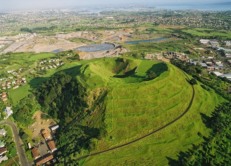 11 |
11 |
12 |
13 | One way to look at the topographic data is via a heatmap. The heatmap's color pattern visualizes how the height of the volcano's surface fluctuates within this 10m by 10m grid.
14 |
15 | Alternatively, you could visualize the data by making a 3D surface plot. Namely, plotly visualizations don't actually require a data frame. This makes chart types that accept a `z` argument especially easy to use if you have a numeric matrix such as our `volcano` dataset.
16 |
17 | Let's try to create that heatmap and 3D surface plot.
18 |
19 | *** =instructions
20 | Create two interactive plots using the volcano dataset:
21 |
22 | - For one the `type` of trace is a `heatmap`.
23 | - For the other `surface` since you also want to see a 3D representation.
24 |
25 | *** =hint
26 | - Remember: for both plots you need to specify the z argument.
27 |
28 | *** =pre_exercise_code
29 | ```{r}
30 | library(plotly)
31 |
32 | ```
33 |
34 | *** =sample_code
35 | ```{r}
36 | # Load the `plotly` library
37 | library(plotly)
38 |
39 | # Your volcano data
40 | str(volcano)
41 |
42 | # The heatmap
43 | plot_ly(___ = ___, type = ___)
44 |
45 | # The 3d surface map
46 | plot_ly(___ = ___, type = ___)
47 |
48 | ```
49 |
50 | *** =solution
51 | ```{r}
52 | # Load the `plotly` library
53 | library(plotly)
54 |
55 | # Your volcano data
56 | str(volcano)
57 |
58 | # The heatmap
59 | plot_ly(z = ~volcano, type = "heatmap")
60 |
61 | # The 3d surface map
62 | plot_ly(z = ~volcano, type = "surface")
63 |
64 | ```
65 |
66 | *** =sct
67 | ```{r}
68 | # SCT written with testwhat: https://github.com/datacamp/testwhat/wiki
69 |
70 | # Test library plotly
71 | test_library_function("plotly")
72 |
73 | # Test str function
74 | msg <- "Call [`str()`](http://www.rdocumentation.org/packages/utils/functions/str) with the `volcano` dataset as an argument."
75 | test_function("str", "object", not_called_msg = msg, incorrect_msg = msg)
76 |
77 | # Test heatmap
78 | test_function("plot_ly", args = c("z","type"),
79 | not_called_msg = "Have you used `plot_ly()` 2 times for 2 different graphs?",
80 | index = 1,
81 | args_not_specified = c("Have you correctly specified that `z` should be `volcano`?",
82 | "Have you correctly specified that `type` should be `heatmap`?"),
83 | incorrect_msg = c("Have you correctly specified that `z` should be `volcano`?",
84 | "Have you correctly specified that `type` should be `heatmap`?"))
85 |
86 | # Test 3d surface map
87 | test_function("plot_ly", args = c("z","type"),
88 | not_called_msg = "Have you used `plot_ly()` 2 times for 2 different graphs?",
89 | index = 2,
90 | args_not_specified = c("Have you correctly specified that `z` should be `volcano`?",
91 | "Have you correctly specified that `type` should be `surface`?"),
92 | incorrect_msg = c("Have you correctly specified that `z` should be `volcano`?",
93 | "Have you correctly specified that `type` should be `surface`?"))
94 |
95 |
96 | success_msg("Congratz! You created your very first heatmap and 3D surface map.")
97 | ```
98 |
99 | --- type:NormalExercise lang:r xp:100 skills:1 key:15071c2604
100 | ## ggplot2, the interactive dimension
101 |
102 | [`ggplot2`](https://www.rdocumentation.org/packages/ggplot2/versions/2.1.0) is probably one of the most well known graphing libraries for R. With [`ggplotly()`](https://www.rdocumentation.org/packages/plotly/versions/4.5.2/topics/ggplotly) from plotly, you can now convert your ggplot2 plots into interactive, web-based versions. See [these examples](https://plot.ly/ggplot2/) on how ggplotly does in converting different ggplot2 examples.
103 |
104 | Try it yourself!
105 |
106 | Converting a ggplot2 chart to an interactive chart is fairly easy. First you create the ggplot2 graph and next you call `ggplotly()`. Like this:
107 |
108 |
109 | qplot(carat, price, data = diamonds,
110 |                    colour = clarity)
111 | ggplotly()
112 |
113 |
114 | Not yet familiar with the ggplot2 syntax? [Consider taking this interactive tutorial](https://www.datacamp.com/courses/data-visualization-with-ggplot2-1).
115 |
116 | *** =instructions
117 | The `mtcars` data frame is available in your workspace. Use `geom_point()` for your plot:
118 |
119 | - Using ggplot2, map `wt` onto the `x` aesthetic, `mpg` onto the `y` aesthetic, and `cyl` onto `color`.
120 | - Use `ggplotly()` to make your plot interactive.
121 |
122 |
123 | *** =hint
124 | - You can make your plot interactive by adding `ggplotly()`
125 |
126 | *** =pre_exercise_code
127 | ```{r}
128 | library(plotly)
129 | library(ggplot2)
130 | diamonds <- diamonds[sample(nrow(diamonds), 1000), ]
131 |
132 | ```
133 |
134 | *** =sample_code
135 | ```{r}
136 |
137 | # Create the ggplot2 graph
138 | ggplot(___, aes(x = ___, y = ___, col = ___)) +
139 | geom_point()
140 |
141 | # Make your plot interactive
142 |
143 |
144 | ```
145 |
146 | *** =solution
147 | ```{r}
148 |
149 | # Create the ggplot2 graph
150 | ggplot(mtcars, aes(x = wt, y = mpg, col = cyl)) +
151 | geom_point()
152 |
153 | # Make your plot interactive
154 | ggplotly()
155 |
156 | ```
157 |
158 | *** =sct
159 | ```{r}
160 |
161 | # Test ggplot2
162 | test_function("ggplot", args = "data")
163 | test_function("aes", args = c("x", "y", "col"), eval = c(F, F, F))
164 | test_function("geom_point")
165 |
166 | # Test ggplotly
167 | test_function("ggplotly")
168 |
169 | success_msg("You successfully turned a static ggplot2 graph into an interactive ggplot2 graph. Woot Woot!")
170 | ```
171 |
172 | --- type:NormalExercise lang:r xp:100 skills:1 key:dc9f2c11f7
173 | ## An interactive airport map
174 |
175 | Ever wonder how some data scientists make these beautiful geographical maps? This exercise shows you how they do it.
176 |
177 | A map provides an easy way to visualize how a measurement varies across a geographic area or the level of variability within a region. An example of such a map is provided on the right. Run the first part of the code and you will see a map of the USA showing the most trafficked airports. Hover over each block to see the name of the airport, city, state and number of arrivals.
178 |
179 | Let's highlight the most important pieces in the code:
180 |
181 |
182 | - To the `lat` and `lon` arguments your provide information regarding the latitude and longitude of the airports locations.
183 | - With `add_markers()` you can add trace(s) to a plotly visualization
184 | - In `geo` you set the reference between the provided geospatial coordinates and a geographic map (e.g. `usa`)
185 | - In `layout()` you modify the layout of a plotly visualization. For example, with `title` you tell plotly what title you want to appear above your plot.
186 |
187 |
188 | *** =instructions
189 | - Based on the code of the "Most trafficked US airports map", create a `world` map that maps all commercial airports in the world (`airports`).
190 | - For a map of the world, the `scope` is the `world`.
191 | - Each airport should be represented by a circle and on hover you should see the `AirportID`, `City` and `Country` of that aiport.
192 | - The color of the airport circle should depend on the country.
193 |
194 |
195 |
196 | *** =hint
197 | - To set the `scope` argument use `scope = 'world'`.
198 |
199 | *** =pre_exercise_code
200 | ```{r}
201 | library(plotly)
202 | library(MUCflights)
203 |
204 |
205 | airport_traffic <-read.csv("http://s3.amazonaws.com/assets.datacamp.com/production/course_1959/datasets/2011_february_us_airport_traffic.csv")
206 |
207 | data(airports)
208 |
209 | ```
210 |
211 | *** =sample_code
212 | ```{r}
213 |
214 | # Most Trafficked US Airports
215 | g <- list(
216 | scope = 'usa',
217 | showland = TRUE,
218 | landcolor = toRGB("gray95")
219 | )
220 |
221 | plot_geo(airport_traffic, lat = ~lat, lon = ~long) %>%
222 | add_markers(
223 | text = ~paste(airport, city, state, paste("Arrivals:", cnt), sep = "
"),
224 | color = ~cnt, symbol = I("square"), size = I(8), hoverinfo = "text"
225 | ) %>%
226 | colorbar(title = "Incoming flights
February 2011") %>%
227 | layout(
228 | title = 'Most trafficked US airports
(Hover for airport)', geo = g
229 | )
230 |
231 |
232 | # Commercial Airports WorldWide
233 | str(airports)
234 |
235 | # Mapping all commercial airports in the world
236 | g <- list(
237 | scope = '___',
238 | showland = TRUE,
239 | landcolor = toRGB("gray95")
240 | )
241 |
242 | plot_geo(___, lat = ~___, lon = ~___) %>%
243 | add_markers(
244 | text = ~paste(___, ___, ___, sep = "
"),
245 | color = ~___, symbol = I("___"), size = I(3), hoverinfo = "text", colors = "Set1"
246 | ) %>%
247 | layout(
248 | title = 'Commercial Airports Worldwide', geo = ___
249 | )
250 |
251 | ```
252 |
253 | *** =solution
254 | ```{r}
255 |
256 | # Most Trafficked US Airports
257 | g <- list(
258 | scope = 'usa',
259 | showland = TRUE,
260 | landcolor = toRGB("gray95")
261 | )
262 |
263 | plot_geo(airport_traffic, lat = ~lat, lon = ~long) %>%
264 | add_markers(
265 | text = ~paste(airport, city, state, paste("Arrivals:", cnt), sep = "
"),
266 | color = ~cnt, symbol = I("square"), size = I(8), hoverinfo = "text"
267 | ) %>%
268 | colorbar(title = "Incoming flights
February 2011") %>%
269 | layout(
270 | title = 'Most trafficked US airports
(Hover for airport)', geo = g
271 | )
272 |
273 |
274 | # Commercial Airports WorldWide
275 | str(airports)
276 |
277 | # Mapping all commercial airports in the world
278 | g <- list(
279 | scope = 'world',
280 | showland = TRUE,
281 | landcolor = toRGB("gray95")
282 | )
283 |
284 | plot_geo(airports, lat = ~Latitude, lon = ~Longitude) %>%
285 | add_markers(
286 | text = ~paste(AirportID, City, Country, sep = "
"),
287 | color = ~Country, symbol = I("circle"), size = I(3), hoverinfo = "text", colors = "Set1"
288 | ) %>%
289 | layout(
290 | title = 'Commercial Airports Worldwide', geo = g
291 | )
292 |
293 |
294 | ```
295 |
296 | *** =sct
297 | ```{r}
298 |
299 | # Test most trafficked airports
300 | test_function("plot_geo", args = c("data","lat","lon"),
301 | not_called_msg = "Have you used `plot_geo()` 2 times for 2 different graphs?",
302 | index = 1,
303 | args_not_specified = c("Have you correctly specified that `data` should be `airport_traffic`?",
304 | "Have you correctly specified that `lat` should be `lat`?",
305 | "Have you correctly specified that `lon` should be `long-states`?"),
306 | incorrect_msg = c("Have you correctly specified that `data` should be `airport_traffic`?",
307 | "Have you correctly specified that `lat` should be `lat`?",
308 | "Have you correctly specified that `lon` should be `long-states`?"))
309 |
310 | test_function("add_markers",args = c("text","color","symbol","size","hoverinfo"),index = 1)
311 | test_function("layout",args = c("geo","title"),index = 1)
312 |
313 | # Test all commercial airports
314 | test_function("plot_geo", args = c("data","lat","lon"),
315 | not_called_msg = "Have you used `plot_geo()` 2 times for 2 different graphs?",
316 | index = 2,
317 | args_not_specified = c("Have you correctly specified that `data` should be `airports`?",
318 | "Have you correctly specified that `lat` should be `lat`?",
319 | "Have you correctly specified that `lon` should be `long-states`?"),
320 | incorrect_msg = c("Have you correctly specified that `data` should be `airport_traffic`?",
321 | "Have you correctly specified that `lat` should be `lat`?",
322 | "Have you correctly specified that `lon` should be `long-states`?"))
323 |
324 | test_function("add_markers",args = c("text","color","symbol","size","hoverinfo","colors"),index = 2)
325 | test_function("layout",args = c("geo","title"),index = 2)
326 |
327 | # Test str function
328 | msg <- "Call [`str()`](http://www.rdocumentation.org/packages/utils/functions/str) with the `airports` dataset as an argument."
329 | test_function("str", "object", not_called_msg = msg, incorrect_msg = msg)
330 |
331 | ```
332 |
333 | --- type:NormalExercise lang:r xp:100 skills:1 key:8e8d273075
334 | ## Sliding into the final exercise
335 |
336 | For the final exercise in this course you will implement a range slider to a stock graph.
337 |
338 | On the right you see the code for a plotly graph to which a range slider is added using `rangeslider()`. The plot looks at a time series `USAccDeaths` that gives the monthly totals of accidental deaths in the USA. Make sure to run the code in your console.
339 |
340 | Loaded in, you will find a dataset on Apple's stock price: `apple_stock_price`. Let's now visualize this stock price over time using an interactive plotly chart. Make sure to add a range slider.
341 |
342 | *** =instructions
343 | - Chart Apple's time-series data in R using `apple_stock_price`. Use the provided sample code.
344 | - Make sure to add a range slider
345 |
346 | *** =hint
347 | - Not sure how to add a range slider? Type `?rangeslider` in the console.
348 |
349 | *** =pre_exercise_code
350 | ```{r}
351 | library(plotly)
352 | library(quantmod)
353 |
354 | getSymbols(Symbols = c("AAPL"))
355 | apple_stock_price <- data.frame(Date = index(AAPL), AAPL[,6])
356 |
357 | ```
358 |
359 | *** =sample_code
360 | ```{r}
361 |
362 | # Monthly totals of accidental deaths in the USA
363 | plot_ly(x = time(USAccDeaths), y = USAccDeaths) %>%
364 | add_lines() %>%
365 | rangeslider()
366 |
367 | # Apple Stock Price
368 | str(apple_stock_price)
369 |
370 |
371 | # Apple Stock Price With Rangeslider
372 | plot_ly(___, x = ~___) %>%
373 | add_lines(y = ~___, name = "Apple") %>%
374 | ___ %>%
375 | layout(
376 | title = "Stock Price Apple",
377 | xaxis = list(title = "Date"),
378 | yaxis = list(title = "Price"))
379 |
380 | ```
381 |
382 | *** =solution
383 | ```{r}
384 |
385 | # Monthly totals of accidental deaths in the USA
386 | plot_ly(x = time(USAccDeaths), y = USAccDeaths) %>%
387 | add_lines() %>%
388 | rangeslider()
389 |
390 | # Apple Stock Price
391 | str(apple_stock_price)
392 |
393 |
394 | # Apple Stock Price With Rangeslider
395 | plot_ly(apple_stock_price, x = ~Date) %>%
396 | add_lines(y = ~AAPL.Adjusted, name = "Apple") %>%
397 | rangeslider() %>%
398 | layout(
399 | title = "Stock Price Apple",
400 | xaxis = list(title = "Date"),
401 | yaxis = list(title = "Price"))
402 |
403 | ```
404 |
405 | *** =sct
406 | ```{r}
407 |
408 | # First Plotly graph
409 | test_function("plot_ly", args = c("x","y"),index = 1, args_not_specified = c("Have you correctly specified that `x` should be `time(USAccDeaths)`?",
410 | "Have you correctly specified that `y` should be `USAccDeaths`?"), incorrect_msg = c("Have you correctly specified that `x` should be `time(USAccDeaths)`?","Have you correctly specified that `y` should be `USAccDeaths`?"))
411 |
412 | test_function("add_lines",index = 1)
413 | test_function("rangeslider",index = 1)
414 |
415 | # Test str function
416 | msg <- "Call [`str()`](http://www.rdocumentation.org/packages/utils/functions/str) with the `apple_stock_price` dataset as an argument."
417 | test_function("str", "object", not_called_msg = msg, incorrect_msg = msg)
418 |
419 |
420 | # Second Plotly graph
421 | test_function("plot_ly", args = c("data","x"),index = 2, args_not_specified = c("Have you correctly specified that `data` should be `apple_stock_price`?",
422 | "Have you correctly specified that `x` should be `Date`?"), incorrect_msg = c("Have you correctly specified that `data` should be `apple_stock_price`?","Have you correctly specified that `x` should be `Date`?"))
423 |
424 | test_function("add_lines",args = c("y","name"), index = 2, args_not_specified = c("Have you correctly specified that `y` should be `AAPL.Adjusted`?",
425 | "Have you correctly specified that `name` should be `Apple`?"))
426 |
427 | test_function("rangeslider",index = 2)
428 |
429 | test_function("layout",args = c("title","xaxis","yaxis"), args_not_specified = c("Have you correctly specified that `title` should be `Stock Price Apple`?","Have you correctly specified that `xaxis` should be `list(title = \"Date\")`?","Have you correctly specified that `yaxis` should be `list(title = \"Price\")`?"))
430 |
431 | ```
432 |
--------------------------------------------------------------------------------