96 |
97 | ## What did I do?
98 |
99 | $history
100 |
101 |
102 |
103 |
104 |
105 |
106 |
107 |
--------------------------------------------------------------------------------
/cheatsheets/shell.pdf:
--------------------------------------------------------------------------------
https://raw.githubusercontent.com/datacarpentry/archive-datacarpentry/6a038e91f7c22d2aeed959b34212d25e8d83148a/cheatsheets/shell.pdf
--------------------------------------------------------------------------------
/cheatsheets/sql.md:
--------------------------------------------------------------------------------
1 | Software Carpentry SQL Cheat Sheet
2 | ==================================
3 |
4 | Basic Queries
5 | -------------
6 |
7 | Select one or more columns of data from a table:
8 |
9 | SELECT column_name_1, column_name_2 FROM table_name;
10 |
11 | Select all of the columns in a table:
12 |
13 | SELECT * FROM table_name;
14 |
15 | Get only unique lines in a query:
16 |
17 | SELECT DISTINCT column_name FROM table_name;
18 |
19 | Perform calculations in a query:
20 |
21 | SELECT column_name_1, ROUND(column_name_2 / 1000.0) FROM table_name;
22 |
23 |
24 | Filtering
25 | ---------
26 |
27 | Select only the data meeting certain criteria:
28 |
29 | SELECT * FROM table_name WHERE column_name = 'Hello World';
30 |
31 | Combine conditions:
32 |
33 | SELECT * FROM table_name WHERE (column_name_1 >= 1000) AND (column_name_2 = 'A' OR column_name_2 = 'B');
34 |
35 |
36 | Sorting
37 | -------
38 |
39 | Sort results using `ASC` for ascending order or `DESC` for descending order:
40 |
41 | SELECT * FROM table_name ORDER BY column_name_1 ASC, column_name_2 DESC;
42 |
43 |
44 | Missing Data
45 | ------------
46 |
47 | Use `NULL` to represent missing data.
48 |
49 | `NULL` is neither true nor false.
50 | Operations involving `NULL` produce `NULL`, e.g., `1+NULL`, `2>NULL`, and `3=NULL` are all `NULL`.
51 |
52 | Test whether a value is null:
53 |
54 | SELECT * FROM table_name WHERE column_name IS NULL;
55 |
56 | Test whether a value is not null:
57 |
58 | SELECT * FROM table_name WHERE column_name IS NOT NULL;
59 |
60 |
61 | Grouping and Aggregation
62 | ------------------------
63 |
64 | Combine data into groups and calculate combined values in groups:
65 |
66 | SELECT column_name_1, SUM(column_name_2), COUNT(*) FROM table_name GROUP BY column_name_1;
67 |
68 |
69 | Joins
70 | -----
71 |
72 | Join data from two tables:
73 |
74 | SELECT * FROM table_name_1 JOIN table_name_2 ON table_name_1.column_name = table_name_2.column_name;
75 |
76 |
77 | Combining Commands
78 | ------------------
79 |
80 | SQL commands must be combined in the following order:
81 | `SELECT`, `FROM`, `JOIN`, `ON`, `WHERE`, `GROUP BY`, `ORDER BY`.
82 |
83 |
84 | Creating Tables
85 | ---------------
86 |
87 | Create tables by specifying column names and types.
88 | Include primary and foreign key relationships and other constraints.
89 |
90 | CREATE TABLE survey(
91 | taken INTEGER NOT NULL,
92 | person TEXT,
93 | quant REAL NOT NULL,
94 | PRIMARY KEY(taken, quant),
95 | FOREIGN KEY(person) REFERENCES person(ident)
96 | );
97 |
98 | Transactions
99 | ------------
100 |
101 | Put multiple queries in a transaction to ensure they are ACID
102 | (atomic, consistent, isolated, and durable):
103 |
104 | BEGIN TRANSACTION;
105 | DELETE FROM table_name_1 WHERE condition;
106 | INSERT INTO table_name_2 values(...);
107 | END TRANSACTION;
108 |
109 | Programming
110 | -----------
111 |
112 | Execute queries in a general-purpose programming language by:
113 |
114 | * loading the appropriate library
115 | * creating a connection
116 | * creating a cursor
117 | * repeatedly:
118 | * execute a query
119 | * fetch some or all results
120 | * disposing of the cursor
121 | * closing the connection
122 |
123 | Python example:
124 |
125 | import sqlite3
126 | connection = sqlite3.connect("database_name")
127 | cursor = connection.cursor()
128 | cursor.execute("...query...")
129 | for r in cursor.fetchall():
130 | ...process result r...
131 | cursor.close()
132 | connection.close()
133 |
--------------------------------------------------------------------------------
/cheatsheets/sql.pdf:
--------------------------------------------------------------------------------
https://raw.githubusercontent.com/datacarpentry/archive-datacarpentry/6a038e91f7c22d2aeed959b34212d25e8d83148a/cheatsheets/sql.pdf
--------------------------------------------------------------------------------
/data/README.md:
--------------------------------------------------------------------------------
1 | #Data Carpentry data
2 |
3 | This directory contains the datasets used as examples for the lessons in the datacarpentry/lessons directory. Here is a list of the subdirectories and contents.
4 |
5 | ##biology
6 |
7 | Example data from the biological sciences.
8 |
9 | ### aphid data
10 |
11 | **Publication**: Bahlai, C.A., Schaafsma, A.W., Lagos, D., Voegtlin, D., Smith, J.L., Welsman, J.A., Xue, Y., DiFonzo, C., Hallett, R.H., 2014. Factors inducing migratory forms of soybean aphid and an examination of North American spatial dynamics of this species in the context of migratory behavior. Agriculture and Forest Entomology. 16, 240-250 http://dx.doi.org/10.1111/afe.12051
12 |
13 | **Downloaded from**: http://lter.kbs.msu.edu/datatables/122
14 |
15 | **Used in**: Excel lessons (datacarpentry/lessons/excel/ecology-examples)
16 |
17 | **Files**
18 |
19 | * Master_suction_trap_data_list_uncleaned.csv : a pre-cleaning version of the dataset
20 | * aphid_data_Bahlai_2014.xlsx : spreadsheet with aphid data
21 |
22 | ### Portal mammals data
23 |
24 | This is data on a small mammal community in southern Arizona over the last 35 years. This is part of a larger project studying the effects of rodents and ants on the plant community. The rodents are sampled on a series of 24 plots, with different experimental manipulations of which rodents are allowed to access the plots.
25 |
26 | **Publication**: S. K. Morgan Ernest, Thomas J. Valone, and James H. Brown. 2009. Long-term monitoring and experimental manipulation of a Chihuahuan Desert ecosystem near Portal, Arizona, USA. Ecology 90:1708.
27 |
28 | **Downloaded from:** [http://esapubs.org/archive/ecol/E090/118/]()
29 |
30 | **Used in:** excel, shell, R, python and SQL lessons
31 |
32 | **Files**
33 |
34 | * plots.csv : a list of the experimental plot IDs and descriptions
35 | * species.csv : a list of the two-letter species code and information about the species
36 | * surveys.csv : the full list of observations of species on plots
37 | * surveys-exercise-extract_month.csv : a small subset of the surveys data used in one of the excel lessons
38 | * portal_mammals.sqlite : a SQLite database of the mammal data; incorporates plots.csv, species.csv and surveys.csv
39 |
40 | ## text_mining
41 | Data used in lessons aimed at text-mining in the social sciences.
42 |
43 | ### plos
44 |
45 | Full-text of several articles from PLOS ONE, PLOS Computational Biology, and PLOS Biology.
46 |
47 | **Downloaded from:** http://www.plosone.org/
48 |
49 | **Used in:** text-mining R lesson in lessons/R/materials/08-text_mining-R
50 |
51 | **Files**
52 |
53 | * plos_1.txt: [DOI:10.1371/journal.pone.0059813](http://dx.doi.org/10.1371/journal.pone.0059813)
54 | * plos_2.txt: [DOI:10.1371/journal.pone.0001248](http://dx.doi.org/10.1371/journal.pone.0001248)
55 | * plos_3.txt: [DOI:10.1371/annotation/69333ae7-757a-4651-831c-f28c5eb02120](http://dx.doi.org/10.1371/annotation/69333ae7-757a-4651-831c-f28c5eb02120)
56 | * plos_4.txt: [DOI:10.1371/journal.pone.0080763](http://dx.doi.org/10.1371/journal.pone.0080763)
57 | * plos_5.txt: [DOI:10.1371/journal.pone.0102437](http://dx.doi.org/10.1371/journal.pone.0102437)
58 | * plos_6.txt: [DOI:10.1371/journal.pone.0017342](http://dx.doi.org/10.1371/journal.pone.0017342)
59 | * plos_7.txt: [DOI:10.1371/journal.pone.0092931](http://dx.doi.org/10.1371/journal.pone.0092931)
60 | * plos_8.txt: [DOI:10.1371/journal.pone.0091497](http://dx.doi.org/10.1371/journal.pone.0091497)
61 | * plos_9.txt: [DOI:10.1371/annotation/28ac6052-4f87-4b88-a817-0cd5743e83d6](http://dx/doi.org/10.1371/annotation/28ac6052-4f87-4b88-a817-0cd5743e83d6)
62 | * plos_10.txt: [DOI:10.1371/journal.pcbi.1003594](http://dx.doi.org/10.1371/journal.pcbi.1003594)
63 | * plos_11.txt: [DOI:10.1371/journal.pbio.002007](http://dx.doi.org/10.1371/journal.pbio.002007)
64 | * plos_12.txt: [DOI:10.1371/journal.pbio.1001702](http://dx.doi.org/10.1371/journal.pbio.1001702)
65 | * plos_13.txt: [DOI:10.1371/journal.pone.0054689](http://dx.doi.org/10.1371/journal.pone.0054689)
66 | * plos_14.txt: [DOI:10.1371/journal.pone.0074321](http://dx.doi.org/10.1371/journal.pone.0074321)
67 | * plos_15.txt: [DOI:10.1371/journal.pbio.1001248](http://dx.doi.org/10.1371/journal.pbio.1001248)
68 | * plos_16.txt: [DOI:10.1371/journal.pbio.0000073](http://dx.doi.org/10.1371/journal.pbio.0000073)
69 | * plos_17.txt: [DOI:10.1371/annotation/bb686276-234c-4881-bcd5-5051d0e66bfc](http://dx.doi.org/10.1371/annotation/bb686276-234c-4881-bcd5-5051d0e66bfc)
70 | * plos_18.txt: [DOI:10.1371/journal.pbio.1001896](http://dx.doi.org/10.1371/journal.pbio.1001896)
71 | * plos_19.txt: [DOI:10.1371/journal.pone.0099750](http://dx.doi.org/10.1371/journal.pone.0099750)
72 | * plos_20.txt: [DOI:10.1371/annotation/48e29578-a073-42e7-bca4-2f96a5998374](http://dx.doi.org/10.1371/annotation/48e29578-a073-42e7-bca4-2f96a5998374)
73 |
74 | ## tidy-data
75 | Sample data for data cleaning exercises. Includes the words spoken by characters of different races and gender in the Lord of the Rings movie trilogy.
76 |
77 | **Publication:** J.R.R. Tolkien. The Lord of the Rings. Ballantine Books, New York. Copyright 1954-1974. Volume I. The Fellowship of the Ring. Volume II. The Two Towers. Volume III. The Return of the King.
78 |
79 | **Downloaded from:** [jennybc on github](https://github.com/jennybc/lotr); original dataset at [manyeyes](http://www-958.ibm.com/software/data/cognos/manyeyes/datasets/words-spoken-by-character-race-scene/versions/1.txt)
80 |
81 | **Used in:** data-tidying R lesson in lessons/tidy-data
82 |
83 | **Files**
84 |
85 | * Male.csv: the word counts for male characters in LOTR
86 | * Female.csv: the word counts for female characters in LOTR
87 | * The_Fellowship_Of_The_Ring.csv: word counts in FOTR
88 | * The_Return_Of_The_King.csv: word counts in ROTK
89 | * The_Two_Towers.csv: word counts in TT
90 | * lotr_clean.tsv: original data in tidy form
91 | * lotr_tidy.tsv: the multi-film, tidy dataset generated at the end of the lessons
92 |
93 |
--------------------------------------------------------------------------------
/data/biology/aphid_data_Bahlai_2014.xlsx:
--------------------------------------------------------------------------------
https://raw.githubusercontent.com/datacarpentry/archive-datacarpentry/6a038e91f7c22d2aeed959b34212d25e8d83148a/data/biology/aphid_data_Bahlai_2014.xlsx
--------------------------------------------------------------------------------
/data/biology/data_orig/species.csv:
--------------------------------------------------------------------------------
1 | species_id,genus,species,taxa
2 | "AB","Amphispiza","bilineata","Bird"
3 | "AH","Ammospermophilus","harrisi","Rodent-not censused"
4 | "AS","Ammodramus","savannarum","Bird"
5 | "BA","Baiomys","taylori","Rodent"
6 | "CB","Campylorhynchus","brunneicapillus","Bird"
7 | "CM","Calamospiza","melanocorys","Bird"
8 | "CQ","Callipepla","squamata","Bird"
9 | "CS","Crotalus","scutalatus","Reptile"
10 | "CT","Cnemidophorus","tigris","Reptile"
11 | "CU","Cnemidophorus","uniparens","Reptile"
12 | "CV","Crotalus","viridis","Reptile"
13 | "DM","Dipodomys","merriami","Rodent"
14 | "DO","Dipodomys","ordii","Rodent"
15 | "DS","Dipodomys","spectabilis","Rodent"
16 | "DX","Dipodomys","sp.","Rodent"
17 | "EO","Eumeces","obsoletus","Reptile"
18 | "GS","Gambelia","silus","Reptile"
19 | "NA","Neotoma","albigula","Rodent"
20 | "NX","Neotoma","sp.","Rodent"
21 | "OL","Onychomys","leucogaster","Rodent"
22 | "OT","Onychomys","torridus","Rodent"
23 | "OX","Onychomys","sp.","Rodent"
24 | "PB","Chaetodipus","baileyi","Rodent"
25 | "PC","Pipilo","chlorurus","Bird"
26 | "PE","Peromyscus","eremicus","Rodent"
27 | "PF","Perognathus","flavus","Rodent"
28 | "PG","Pooecetes","gramineus","Bird"
29 | "PH","Perognathus","hispidus","Rodent"
30 | "PI","Chaetodipus","intermedius","Rodent"
31 | "PL","Peromyscus","leucopus","Rodent"
32 | "PM","Peromyscus","maniculatus","Rodent"
33 | "PP","Chaetodipus","penicillatus","Rodent"
34 | "PU","Pipilo","fuscus","Bird"
35 | "PX","Chaetodipus","sp.","Rodent"
36 | "RF","Reithrodontomys","fulvescens","Rodent"
37 | "RM","Reithrodontomys","megalotis","Rodent"
38 | "RO","Reithrodontomys","montanus","Rodent"
39 | "RX","Reithrodontomys","sp.","Rodent"
40 | "SA","Sylvilagus","audubonii","Rabbit"
41 | "SB","Spizella","breweri","Bird"
42 | "SC","Sceloporus","clarki","Reptile"
43 | "SF","Sigmodon","fulviventer","Rodent"
44 | "SH","Sigmodon","hispidus","Rodent"
45 | "SO","Sigmodon","ochrognathus","Rodent"
46 | "SS","Spermophilus","spilosoma","Rodent-not censused"
47 | "ST","Spermophilus","tereticaudus","Rodent-not censused"
48 | "SU","Sceloporus","undulatus","Reptile"
49 | "SX","Sigmodon","sp.","Rodent"
50 | "UL","Lizard","sp.","Reptile"
51 | "UP","Pipilo","sp.","Bird"
52 | "UR","Rodent","sp.","Rodent"
53 | "US","Sparrow","sp.","Bird"
54 | "XX",,,"Zero Trapping Success"
55 | "ZL","Zonotrichia","leucophrys","Bird"
56 | "ZM","Zenaida","macroura","Bird"
57 |
--------------------------------------------------------------------------------
/data/biology/make_teaching_dataset.R:
--------------------------------------------------------------------------------
1 | ### This script should be executed from the datacarpentry/data/biology
2 | ### folder. It is used to modify the "surveys.csv" and "species.csv"
3 | ### files to make them more suitable to teaching.
4 |
5 | ### Currently, the script renames the species code "NA" to "NL" to
6 | ### avoid the ambiguities associated with missing data when reading
7 | ### the data in R.
8 |
9 | species <- read.csv(file="data_orig/species.csv", na.strings="")
10 | species$species_id <- gsub("^NA$", "NL", species$species_id)
11 | write.csv(species, file="species.csv", row.names=FALSE, na="")
12 |
13 | surveys <- read.csv(file="data_orig/surveys.csv", na.strings="")
14 | surveys$species <- gsub("^NA$", "NL", surveys$species)
15 | write.csv(surveys, file="surveys.csv", row.names=FALSE, na="")
16 |
17 | ## Tests
18 | ## In addition of the change from "NA" to "NL":
19 | ## - there are now quotes around the column titles
20 | ## - digit-only columns are not quoted
21 |
22 | orig_species <- readLines("data_orig/species.csv")
23 | new_species <- readLines("species.csv")
24 | diff_species <- setdiff(new_species, orig_species)
25 |
26 | stopifnot(identical(diff_species,
27 | c("\"species_id\",\"genus\",\"species\",\"taxa\"",
28 | "\"NL\",\"Neotoma\",\"albigula\",\"Rodent\"")))
29 |
30 | new_surveys <- read.csv("surveys.csv", stringsAsFactors=FALSE)
31 | new_species <- read.csv("species.csv", stringsAsFactors=FALSE)
32 | stopifnot(all(new_surveys$species[nzchar(new_surveys$species)] %in% new_species$species_id))
33 |
--------------------------------------------------------------------------------
/data/biology/plots.csv:
--------------------------------------------------------------------------------
1 | plot_id,plot_type
2 | "1","Spectab exclosure"
3 | "2","Control"
4 | "3","Long-term Krat Exclosure"
5 | "4","Control"
6 | "5","Rodent Exclosure"
7 | "6","Short-term Krat Exclosure"
8 | "7","Rodent Exclosure"
9 | "8","Control"
10 | "9","Spectab exclosure"
11 | "10","Rodent Exclosure"
12 | "11","Control"
13 | "12","Control"
14 | "13","Short-term Krat Exclosure"
15 | "14","Control"
16 | "15","Long-term Krat Exclosure"
17 | "16","Rodent Exclosure"
18 | "17","Control"
19 | "18","Short-term Krat Exclosure"
20 | "19","Long-term Krat Exclosure"
21 | "20","Short-term Krat Exclosure"
22 | "21","Long-term Krat Exclosure"
23 | "22","Control"
24 | "23","Rodent Exclosure"
25 | "24","Rodent Exclosure"
26 |
--------------------------------------------------------------------------------
/data/biology/portal_mammals.sqlite:
--------------------------------------------------------------------------------
https://raw.githubusercontent.com/datacarpentry/archive-datacarpentry/6a038e91f7c22d2aeed959b34212d25e8d83148a/data/biology/portal_mammals.sqlite
--------------------------------------------------------------------------------
/data/biology/species.csv:
--------------------------------------------------------------------------------
1 | "species_id","genus","species","taxa"
2 | "AB","Amphispiza","bilineata","Bird"
3 | "AH","Ammospermophilus","harrisi","Rodent-not censused"
4 | "AS","Ammodramus","savannarum","Bird"
5 | "BA","Baiomys","taylori","Rodent"
6 | "CB","Campylorhynchus","brunneicapillus","Bird"
7 | "CM","Calamospiza","melanocorys","Bird"
8 | "CQ","Callipepla","squamata","Bird"
9 | "CS","Crotalus","scutalatus","Reptile"
10 | "CT","Cnemidophorus","tigris","Reptile"
11 | "CU","Cnemidophorus","uniparens","Reptile"
12 | "CV","Crotalus","viridis","Reptile"
13 | "DM","Dipodomys","merriami","Rodent"
14 | "DO","Dipodomys","ordii","Rodent"
15 | "DS","Dipodomys","spectabilis","Rodent"
16 | "DX","Dipodomys","sp.","Rodent"
17 | "EO","Eumeces","obsoletus","Reptile"
18 | "GS","Gambelia","silus","Reptile"
19 | "NL","Neotoma","albigula","Rodent"
20 | "NX","Neotoma","sp.","Rodent"
21 | "OL","Onychomys","leucogaster","Rodent"
22 | "OT","Onychomys","torridus","Rodent"
23 | "OX","Onychomys","sp.","Rodent"
24 | "PB","Chaetodipus","baileyi","Rodent"
25 | "PC","Pipilo","chlorurus","Bird"
26 | "PE","Peromyscus","eremicus","Rodent"
27 | "PF","Perognathus","flavus","Rodent"
28 | "PG","Pooecetes","gramineus","Bird"
29 | "PH","Perognathus","hispidus","Rodent"
30 | "PI","Chaetodipus","intermedius","Rodent"
31 | "PL","Peromyscus","leucopus","Rodent"
32 | "PM","Peromyscus","maniculatus","Rodent"
33 | "PP","Chaetodipus","penicillatus","Rodent"
34 | "PU","Pipilo","fuscus","Bird"
35 | "PX","Chaetodipus","sp.","Rodent"
36 | "RF","Reithrodontomys","fulvescens","Rodent"
37 | "RM","Reithrodontomys","megalotis","Rodent"
38 | "RO","Reithrodontomys","montanus","Rodent"
39 | "RX","Reithrodontomys","sp.","Rodent"
40 | "SA","Sylvilagus","audubonii","Rabbit"
41 | "SB","Spizella","breweri","Bird"
42 | "SC","Sceloporus","clarki","Reptile"
43 | "SF","Sigmodon","fulviventer","Rodent"
44 | "SH","Sigmodon","hispidus","Rodent"
45 | "SO","Sigmodon","ochrognathus","Rodent"
46 | "SS","Spermophilus","spilosoma","Rodent-not censused"
47 | "ST","Spermophilus","tereticaudus","Rodent-not censused"
48 | "SU","Sceloporus","undulatus","Reptile"
49 | "SX","Sigmodon","sp.","Rodent"
50 | "UL","Lizard","sp.","Reptile"
51 | "UP","Pipilo","sp.","Bird"
52 | "UR","Rodent","sp.","Rodent"
53 | "US","Sparrow","sp.","Bird"
54 | "XX",,,"Zero Trapping Success"
55 | "ZL","Zonotrichia","leucophrys","Bird"
56 | "ZM","Zenaida","macroura","Bird"
57 |
--------------------------------------------------------------------------------
/data/biology/surveys-exercise-extract_month.csv:
--------------------------------------------------------------------------------
1 | record_id,date,plot,species,sex,wgt
2 | 35525,31/12/2002,9,OL,M,26
3 | 25749,10/05/1997,7,PM,F,24
4 | 25848,11/05/1997,13,PP,M,18
5 | 25956,09/06/1997,1,OL,M,16
6 | 26012,09/06/1997,2,PB,F,24
7 | 26068,10/06/1997,8,OT,M,28
8 | 26255,09/07/1997,17,PP,M,18
9 | 26373,09/07/1997,16,PP,M,13
10 | 26562,29/07/1997,24,PE,F,22
11 | 26690,30/07/1997,8,PF,F,7
12 | 26948,28/09/1997,11,DO,F,51
13 | 27118,26/10/1997,6,PE,M,20
14 | 27444,31/01/1998,2,DM,F,41
15 |
--------------------------------------------------------------------------------
/data/text_mining/plos/plos_12.txt:
--------------------------------------------------------------------------------
1 | PBIOLOGY-D-13-03393 10.1371/journal.pbio.1001702 Formal Comment The Ecological Footprint Remains a Misleading Metric of Global Sustainability Linus Blomqvist 1 * Barry W. Brook 2 Erle C. Ellis 3 Peter M. Kareiva 4 Ted Nordhaus 1 Michael Shellenberger 1 1 Breakthrough Institute, Oakland, California, United States of America 2 The Environment Institute and School of Earth and Environmental Sciences, The University of Adelaide, Adelaide, South Australia, Australia 3 Department of Geography and Environmental Systems, University of Maryland Baltimore County, Baltimore, Maryland, United States of America 4 The Nature Conservancy, Seattle, Washington, United States of America Georgina M. Mace Academic Editor University College London, United Kingdom * E-mail: linus@thebreakthrough.org This Formal Comment is a response to Rees and Wackernagel (this issue) by the authors of the original Perspective “Does the Shoe Fit? Real versus Imagined Ecological Footprints” (this issue). The author(s) have made the following declarations about their contributions: Wrote the paper: PK LB EE BB TN MS. 11 2013 5 11 2013 11 11 e1001702 2013 Blomqvist et al This is an open-access article distributed under the terms of the Creative Commons Attribution License, which permits unrestricted use, distribution, and reproduction in any medium, provided the original author and source are credited. The Shoe Fits, but the Footprint is Larger than Earth Does the Shoe Fit? Real versus Imagined Ecological Footprints In this Formal Comment, Blomqvist et al. note that the main points of their Perspective, “Does the Shoe Fit? Real versus Imagined Ecological Footprints,” are robust to Rees and Wackernagel's response, “The Shoe Fits, but the Footprint is Larger than Earth.” The authors received no specific funding for this work. The Formal Comment by Rees and Wackernagel [1] raises our concern that this exchange will confuse readers. For this reason, we aim to emphasize a few key points that we believe cannot be disputed. First, the entire global ecological overshoot (footprint of consumption in excess of biocapacity) results from carbon dioxide emissions reframed as the hypothetical forest area needed to offset these emissions. Plantations of fast-growing trees would, by-the-numbers, eliminate the global overshoot. Second, the ecological footprint's (EF) assessments for cropland, grazing land, and built-up land are unable to capture degradation or unsustainable use of any kind. Finally, we conclude from the above and the points made in our original paper [2] that we would be better off discussing greenhouse gas emissions directly in terms of tons of CO 2 -equivalent (and thus focus on solutions to emissions), and developing a more ecological and ecosystem process framework to capture the impacts humans currently have on the planet's natural systems. The appropriate scale for these indicators will, in many cases, be local and regional. At this level, the EF is a measure of net exports or imports of biomass and carbon-absorptive capacity [3] . Any city, for example, would show a deficit, as it relies on food and materials from outside. That in itself, as Robert Costanza has noted, “tells us little if anything about the sustainability of this input [from outside the region] over time” [4] . References 1 WE Rees , M Wackernagel ( 2013 ) The Shoe Fits, but the Footprint is Larger than Earth . PLoS Biol 11 ( 11 ) e1001701 doi: 10.1371/journal.pbio.1001701 2 L Blomqvist , BW Brook , EC Ellis , PM Kareiva , T Nordhaus , et al . ( 2013 ) Does the Shoe Fit? Real versus Imagined Ecological Footprints . PLoS Biol 11 ( 11 ) e1001700 doi: 10.1371/journal.pbio.1001700 3 JCJM van den Bergh , H Verbruggen ( 1999 ) Spatial sustainability, trade and indicators: an evaluation of the “ecological footprint” . Ecol Econ 29 : 61 – 72 . 4 R Costanza ( 2000 ) The dynamics of the ecological footprint concept . Ecol Econ 32 : 341 – 345 .
2 |
--------------------------------------------------------------------------------
/data/text_mining/plos/plos_17.txt:
--------------------------------------------------------------------------------
1 | 3806864 10.1371/annotation/bb686276-234c-4881-bcd5-5051d0e66bfc Correction Correction: Ten Years after the Prestige Oil Spill: Seabird Trophic Ecology as Indicator of Long-Term Effects on the Coastal Marine Ecosystem Correction Rocío Moreno Lluís Jover Carmen Diez Francesc Sardà Carola Sanpera 2013 23 10 2013 8 10 10.1371/annotation/bb686276-234c-4881-bcd5-5051d0e66bfc 2013 This is an open-access article distributed under the terms of the Creative Commons Attribution License , which permits unrestricted use, distribution, and reproduction in any medium, provided the original author and source are credited. Ten Years after the Prestige Oil Spill: Seabird Trophic Ecology as Indicator of Long-Term Effects on the Coastal Marine Ecosystem No competing interests declared. The name of the fourth author was incompletely given. The correct name is: Francesc Sardà-Palomera. The correct citation is: Moreno R, Jover L, Diez C, Sardà-Palomera F, Sanpera C (2013) Ten Years after the Prestige Oil Spill: Seabird Trophic Ecology as Indicator of Long-Term Effects on the Coastal Marine Ecosystem. PLoS ONE 8(10): e77360. doi:10.1371/journal.pone.0077360. The correct abbreviation in the Author Contributions statement is: FSP.
2 |
--------------------------------------------------------------------------------
/data/text_mining/plos/plos_18.txt:
--------------------------------------------------------------------------------
1 | PBIOLOGY-D-14-01787 10.1371/journal.pbio.1001896 Correction Correction: Rates of Dinosaur Body Mass Evolution Indicate 170 Million Years of Sustained Ecological Innovation on the Avian Stem Lineage The PLOS Biology Staff 6 2014 2 6 2014 12 6 e1001896 2014 The PLOS Biology Staff This is an open-access article distributed under the terms of the Creative Commons Attribution License , which permits unrestricted use, distribution, and reproduction in any medium, provided the original author and source are credited. Rates of Dinosaur Body Mass Evolution Indicate 170 Million Years of Sustained Ecological Innovation on the Avian Stem Lineage Notice of Republication This article was republished on May 19, 2014, to replace Figure 3 with a version which is available under the Creative Commons CC0 public domain dedication. The figure caption was also amended to clarify this is the case. Please download this article again to view the correct version. Reference 1 RBJ Benson , NE Campione , MT Carrano , PD Mannion , C Sullivan , et al . ( 2014 ) Rates of Dinosaur Body Mass Evolution Indicate 170 Million Years of Sustained Ecological Innovation on the Avian Stem Lineage . PLoS Biol 12(5) : e1001853 doi: 10.1371/journal.pbio.1001853
2 |
--------------------------------------------------------------------------------
/data/text_mining/plos/plos_19.txt:
--------------------------------------------------------------------------------
1 | PONE-D-14-22343 10.1371/journal.pone.0099750 Correction Correction: Cognitive Ecology in Hummingbirds: The Role of Sexual Dimorphism and Its Anatomical Correlates on Memory The PLOS ONE Staff 2014 2 6 2014 9 6 e99750 2014 The PLOS ONE Staff This is an open-access article distributed under the terms of the Creative Commons Attribution License , which permits unrestricted use, distribution, and reproduction in any medium, provided the original author and source are credited. Cognitive ecology in hummingbirds: the role of sexual dimorphism and its anatomical correlates on memory One of affiliations for author Pablo Razeto-Barry is missing from the published article. Dr. Razeto-Barry is affiliated with the Universidad Diego Portales, Vicerrectoría Académica, Manuel Rodríguez Sur 415, Santiago, Chile, as well as the Instituto de Filosofía y Ciencias de la Complejidad, Santiago, Chile. Reference 1 PL González-Gómez , N Madrid-Lopez , JE Salazar , R Suárez , P Razeto-Barry , et al . ( 2014 ) Cognitive Ecology in Hummingbirds: The Role of Sexual Dimorphism and Its Anatomical Correlates on Memory . PLoS ONE 9(3) : e90165 doi: 10.1371/journal.pone.0090165
2 |
--------------------------------------------------------------------------------
/data/text_mining/plos/plos_20.txt:
--------------------------------------------------------------------------------
1 | 3875299 24386035 10.1371/annotation/48e29578-a073-42e7-bca4-2f96a5998374 Correction Correction: The Ecology of Microbial Communities Associated with Macrocystis pyrifera Correction Vanessa K. Michelou J. Gregory Caporaso Rob Knight Stephen R. Palumbi 2013 20 12 2013 8 12 10.1371/annotation/48e29578-a073-42e7-bca4-2f96a5998374 2013 This is an open-access article distributed under the terms of the Creative Commons Attribution License , which permits unrestricted use, distribution, and reproduction in any medium, provided the original author and source are credited. The Ecology of Microbial Communities Associated with Macrocystis pyrifera No competing interests declared. The labels on panels A and B in Figure 2 were switched. Panel A should be labeled "Gammaproteobacteria" and panel B should be labeled "Alphaproteobacteria." Please see the corrected Figure 2 here:
2 |
--------------------------------------------------------------------------------
/data/text_mining/plos/plos_3.txt:
--------------------------------------------------------------------------------
1 | 3812295 10.1371/annotation/69333ae7-757a-4651-831c-f28c5eb02120 Correction Correction: Ecological Drivers of Biogeographic Patterns of Soil Archaeal Community Correction Yuan-Ming Zheng Peng Cao Bojie Fu Jane M. Hughes Ji-Zheng He 2013 29 10 2013 8 10 10.1371/annotation/69333ae7-757a-4651-831c-f28c5eb02120 2013 This is an open-access article distributed under the terms of the Creative Commons Attribution License , which permits unrestricted use, distribution, and reproduction in any medium, provided the original author and source are credited. Ecological Drivers of Biogeographic Patterns of Soil Archaeal Community No competing interests declared. These authors contributed equally to this work: Yuan-Ming Zheng, State Key Laboratory of Urban and Regional Ecology, Research Center for Eco-Environmental Sciences, Chinese Academy of Sciences, Beijing, China Peng Cao, State Key Laboratory of Urban and Regional Ecology, Research Center for Eco-Environmental Sciences, Chinese Academy of Sciences, Beijing, China
2 |
--------------------------------------------------------------------------------
/data/text_mining/plos/plos_7.txt:
--------------------------------------------------------------------------------
1 | PONE-D-14-09244 10.1371/journal.pone.0092931 Correction Correction: Shifting Baselines on a Tropical Forest Frontier: Extirpations Drive Declines in Local Ecological Knowledge The PLOS ONE Staff 2014 12 3 2014 9 3 e92931 2014 The PLOS ONE Staff This is an open-access article distributed under the terms of the Creative Commons Attribution License , which permits unrestricted use, distribution, and reproduction in any medium, provided the original author and source are credited. Shifting Baselines on a Tropical Forest Frontier: Extirpations Drive Declines in Local Ecological Knowledge There was an error in the Funding statement. The Funding statement should read: “Funding for AFEC-X 2012 was provided by Xishuangbanna Tropical Botanical Garden (XTBG), World Agroforestry Institute (ICRAF, East Asia node) Kunming Office, and the Key Laboratory for Tropical Forest Ecology (XTBG). The funders had no role in study design, data collection and analysis, decision to publish, or preparation of the manuscript.” The publisher apologizes for this error. Reference 1 Z Kai , TS Woan , L Jie , E Goodale , K Kitajima , et al . ( 2014 ) Shifting Baselines on a Tropical Forest Frontier: Extirpations Drive Declines in Local Ecological Knowledge . PLoS ONE 9(1) : e86598 doi: 10.1371/journal.pone.0086598
2 |
--------------------------------------------------------------------------------
/data/text_mining/plos/plos_8.txt:
--------------------------------------------------------------------------------
1 | PONE-D-14-06943 10.1371/journal.pone.0091497 Correction Correction: Delineating Ecological Boundaries of Hanuman Langur Species Complex in Peninsular India Using MaxEnt Modeling Approach The PLOS ONE Staff 2014 28 2 2014 9 2 e91497 2014 The PLOS ONE Staff This is an open-access article distributed under the terms of the Creative Commons Attribution License , which permits unrestricted use, distribution, and reproduction in any medium, provided the original author and source are credited. Delineating Ecological Boundaries of Hanuman Langur Species Complex in Peninsular India Using MaxEnt Modeling Approach The names of all authors are incorrectly represented in the Citation. The correct Citation is: Nag C, Karanth KP, Gururaja KV (2014) Delineating Ecological Boundaries of Hanuman Langur Species Complex in Peninsular India Using MaxEnt Modeling Approach. PLoS ONE 9(2): e87804. doi:10.1371/journal.pone.0087804. Reference 1 N Chetan , KK Praveen , GK Vasudeva ( 2014 ) Delineating Ecological Boundaries of Hanuman Langur Species Complex in Peninsular India Using MaxEnt Modeling Approach . PLoS ONE 9(2) : e87804 doi: 10.1371/journal.pone.0087804
2 |
--------------------------------------------------------------------------------
/data/text_mining/plos/plos_9.txt:
--------------------------------------------------------------------------------
1 | 3654729 10.1371/annotation/28ac6052-4f87-4b88-a817-0cd5743e83d6 Correction Correction: Phylogenetic Patterns of Geographical and Ecological Diversification in the Subgenus Drosophila Correction Ramiro Morales-Hojas Jorge Vieira 2013 14 5 2013 8 5 10.1371/annotation/28ac6052-4f87-4b88-a817-0cd5743e83d6 2013 This is an open-access article distributed under the terms of the Creative Commons Attribution License , which permits unrestricted use, distribution, and reproduction in any medium, provided the original author and source are credited. Phylogenetic Patterns of Geographical and Ecological Diversification in the Subgenus Drosophila No competing interests declared. The versions of Figures 1, 4, and 5 are incomplete. The complete, correct versions of these figures can be found here: Figure 1: Figure 4: Figure 5:
2 |
--------------------------------------------------------------------------------
/data/tidy-data/Female.csv:
--------------------------------------------------------------------------------
1 | Gender,Film,Elf,Hobbit,Man
2 | Female,The Fellowship Of The Ring,1229,14,0
3 | Female,The Two Towers,331,0,401
4 | Female,The Return Of The King,183,2,268
5 |
--------------------------------------------------------------------------------
/data/tidy-data/Male.csv:
--------------------------------------------------------------------------------
1 | Gender,Film,Elf,Hobbit,Man
2 | Male,The Fellowship Of The Ring,971,3644,1995
3 | Male,The Two Towers,513,2463,3589
4 | Male,The Return Of The King,510,2673,2459
5 |
--------------------------------------------------------------------------------
/data/tidy-data/The_Fellowship_Of_The_Ring.csv:
--------------------------------------------------------------------------------
1 | Film,Race,Female,Male
2 | The Fellowship Of The Ring,Elf,1229,971
3 | The Fellowship Of The Ring,Hobbit,14,3644
4 | The Fellowship Of The Ring,Man,0,1995
5 |
--------------------------------------------------------------------------------
/data/tidy-data/The_Return_Of_The_King.csv:
--------------------------------------------------------------------------------
1 | Film,Race,Female,Male
2 | The Return Of The King,Elf,183,510
3 | The Return Of The King,Hobbit,2,2673
4 | The Return Of The King,Man,268,2459
5 |
--------------------------------------------------------------------------------
/data/tidy-data/The_Two_Towers.csv:
--------------------------------------------------------------------------------
1 | Film,Race,Female,Male
2 | The Two Towers,Elf,331,513
3 | The Two Towers,Hobbit,0,2463
4 | The Two Towers,Man,401,3589
5 |
--------------------------------------------------------------------------------
/data/tidy-data/lotr_tidy.csv:
--------------------------------------------------------------------------------
1 | Film,Race,Gender,Words
2 | The Fellowship Of The Ring,Elf,Female,1229
3 | The Fellowship Of The Ring,Hobbit,Female,14
4 | The Fellowship Of The Ring,Man,Female,0
5 | The Two Towers,Elf,Female,331
6 | The Two Towers,Hobbit,Female,0
7 | The Two Towers,Man,Female,401
8 | The Return Of The King,Elf,Female,183
9 | The Return Of The King,Hobbit,Female,2
10 | The Return Of The King,Man,Female,268
11 | The Fellowship Of The Ring,Elf,Male,971
12 | The Fellowship Of The Ring,Hobbit,Male,3644
13 | The Fellowship Of The Ring,Man,Male,1995
14 | The Two Towers,Elf,Male,513
15 | The Two Towers,Hobbit,Male,2463
16 | The Two Towers,Man,Male,3589
17 | The Return Of The King,Elf,Male,510
18 | The Return Of The King,Hobbit,Male,2673
19 | The Return Of The King,Man,Male,2459
20 |
--------------------------------------------------------------------------------
/img/csv-mistake.png:
--------------------------------------------------------------------------------
https://raw.githubusercontent.com/datacarpentry/archive-datacarpentry/6a038e91f7c22d2aeed959b34212d25e8d83148a/img/csv-mistake.png
--------------------------------------------------------------------------------
/img/excel-to-csv.png:
--------------------------------------------------------------------------------
https://raw.githubusercontent.com/datacarpentry/archive-datacarpentry/6a038e91f7c22d2aeed959b34212d25e8d83148a/img/excel-to-csv.png
--------------------------------------------------------------------------------
/img/excel_tables_example_sk_e1_p1_wrl.png:
--------------------------------------------------------------------------------
https://raw.githubusercontent.com/datacarpentry/archive-datacarpentry/6a038e91f7c22d2aeed959b34212d25e8d83148a/img/excel_tables_example_sk_e1_p1_wrl.png
--------------------------------------------------------------------------------
/img/excel_tables_example_sk_e2_p1_wrl.png:
--------------------------------------------------------------------------------
https://raw.githubusercontent.com/datacarpentry/archive-datacarpentry/6a038e91f7c22d2aeed959b34212d25e8d83148a/img/excel_tables_example_sk_e2_p1_wrl.png
--------------------------------------------------------------------------------
/img/excel_tables_example_sk_e2_p2.png:
--------------------------------------------------------------------------------
https://raw.githubusercontent.com/datacarpentry/archive-datacarpentry/6a038e91f7c22d2aeed959b34212d25e8d83148a/img/excel_tables_example_sk_e2_p2.png
--------------------------------------------------------------------------------
/lessons/R/01-intro-to-R.Rmd:
--------------------------------------------------------------------------------
1 | ---
2 | layout: topic
3 | title: Introduction to R
4 | minutes: 45
5 | ---
6 |
7 | ```{r, echo=FALSE, purl=FALSE}
8 | knitr::opts_chunk$set(results='hide', fig.path='img/r-lesson-')
9 | ```
10 |
11 |
12 | > ## Learning Objectives
13 | >
14 | > * Familiarize participants with R syntax
15 | > * Understand the concepts of objects and assignment
16 | > * Understand the concepts of vector and data types
17 | > * Get exposed to a few functions
18 |
19 |
20 | ## The R syntax
21 |
22 | _Start by showing an example of a script_
23 |
24 | * Point to the different parts:
25 | - a function
26 | - the assignment operator `<-`
27 | - the `=` for arguments
28 | - the comments `#` and how they are used to document function and its content
29 | - the `$` operator
30 | * Point to indentation and consistency in spacing to improve clarity
31 |
32 | 
33 |
34 | ## Creating objects
35 |
36 | ```{r, echo=FALSE, purl=TRUE}
37 | ### Creating objects (assignments)
38 | ```
39 |
40 | You can get output from R simply by typing in math in the console
41 |
42 | ```{r, purl=FALSE}
43 | 3 + 5
44 | 12/7
45 | ```
46 |
47 | However, to do useful and interesting things, we need to assign _values_ to
48 | _objects_. To create objects, we need to give it a name followed by the
49 | assignment operator `<-` and the value we want to give it:
50 |
51 | ```{r, purl=FALSE}
52 | weight_kg <- 55
53 | ```
54 |
55 | Objects can be given any name such as `x`, `current_temperature`, or
56 | `subject_id`. You want your object names to be explicit and not too long. They
57 | cannot start with a number (`2x` is not valid but `x2` is). R is case sensitive
58 | (e.g., `weight_kg` is different from `Weight_kg`). There are some names that
59 | cannot be used because they represent the names of fundamental functions in R
60 | (e.g., `if`, `else`, `for`, see
61 | [here](https://stat.ethz.ch/R-manual/R-devel/library/base/html/Reserved.html)
62 | for a complete list). In general, even if it's allowed, it's best to not use
63 | other function names (e.g., `c`, `T`, `mean`, `data`, `df`, `weights`). In doubt
64 | check the help to see if the name is already in use. It's also best to avoid
65 | dots (`.`) within a variable name as in `my.dataset`. There are many functions
66 | in R with dots in their names for historical reasons, but because dots have a
67 | special meaning in R (for methods) and other programming languages, it's best to
68 | avoid them. It is also recommended to use nouns for variable names, and verbs
69 | for function names. It's important to be consistent in the styling of your code
70 | (where you put spaces, how you name variable, etc.). In R, two popular style
71 | guides are [Hadley Wickham's](http://adv-r.had.co.nz/Style.html) and
72 | [Google's](https://google-styleguide.googlecode.com/svn/trunk/Rguide.xml).
73 |
74 | When assigning a value to an object, R does not print anything. You can force to
75 | print the value by using parentheses or by typing the name:
76 |
77 | ```{r, purl=FALSE}
78 | (weight_kg <- 55)
79 | weight_kg
80 | ```
81 |
82 | Now that R has `weight_kg` in memory, we can do arithmetic with it. For
83 | instance, we may want to convert this weight in pounds (weight in pounds is 2.2
84 | times the weight in kg):
85 |
86 | ```{r, purl=FALSE}
87 | 2.2 * weight_kg
88 | ```
89 |
90 | We can also change a variable's value by assigning it a new one:
91 |
92 |
93 | ```{r, purl=FALSE}
94 | weight_kg <- 57.5
95 | 2.2 * weight_kg
96 | ```
97 |
98 | This means that assigning a value to one variable does not change the values of
99 | other variables. For example, let's store the animal's weight in pounds in a
100 | variable.
101 |
102 | ```{r, purl=FALSE}
103 | weight_lb <- 2.2 * weight_kg
104 | ```
105 |
106 | and then change `weight_kg` to 100.
107 |
108 | ```{r, purl=FALSE}
109 | weight_kg <- 100
110 | ```
111 |
112 | What do you think is the current content of the object `weight_lb`? 126.5 or 200?
113 |
114 | ### Exercise
115 |
116 | What are the values after each statement in the following?
117 |
118 | ```{r, purl=FALSE}
119 | mass <- 47.5 # mass?
120 | age <- 122 # age?
121 | mass <- mass * 2.0 # mass?
122 | age <- age - 20 # age?
123 | massIndex <- mass/age # massIndex?
124 | ```
125 |
126 | ## Vectors and data types
127 |
128 | ```{r, echo=FALSE, purl=TRUE}
129 | ### Vectors and data types
130 | ```
131 |
132 | A vector is the most common and basic data structure in R, and is pretty much
133 | the workhorse of R. It's a group of values, mainly either numbers or
134 | characters. You can assign this list of values to a variable, just like you
135 | would for one item. For example we can create a vector of animal weights:
136 |
137 | ```{r, purl=FALSE}
138 | weights <- c(50, 60, 65, 82)
139 | weights
140 | ```
141 |
142 | A vector can also contain characters:
143 |
144 | ```{r, purl=FALSE}
145 | animals <- c("mouse", "rat", "dog")
146 | animals
147 | ```
148 |
149 | There are many functions that allow you to inspect the content of a
150 | vector. `length()` tells you how many elements are in a particular vector:
151 |
152 | ```{r, purl=FALSE}
153 | length(weights)
154 | length(animals)
155 | ```
156 |
157 | `class()` indicates the class (the type of element) of an object:
158 |
159 | ```{r, purl=FALSE}
160 | class(weights)
161 | class(animals)
162 | ```
163 |
164 | The function `str()` provides an overview of the object and the elements it
165 | contains. It is a really useful function when working with large and complex
166 | objects:
167 |
168 | ```{r, purl=FALSE}
169 | str(weights)
170 | str(animals)
171 | ```
172 |
173 | You can add elements to your vector simply by using the `c()` function:
174 |
175 | ```{r, purl=FALSE}
176 | weights <- c(weights, 90) # adding at the end
177 | weights <- c(30, weights) # adding at the beginning
178 | weights
179 | ```
180 |
181 | What happens here is that we take the original vector `weights`, and we are
182 | adding another item first to the end of the other ones, and then another item at
183 | the beginning. We can do this over and over again to build a vector or a
184 | dataset. As we program, this may be useful to autoupdate results that we are
185 | collecting or calculating.
186 |
187 | We just saw 2 of the 6 **data types** that R uses: `"character"` and
188 | `"numeric"`. The other 4 are:
189 | * `"logical"` for `TRUE` and `FALSE` (the boolean data type)
190 | * `"integer"` for integer numbers (e.g., `2L`, the `L` indicates to R that it's an integer)
191 | * `"complex"` to represent complex numbers with real and imaginary parts (e.g.,
192 | `1+4i`) and that's all we're going to say about them
193 | * `"raw"` that we won't discuss further
194 |
195 | Vectors are one of the many **data structures** that R uses. Other important
196 | ones are lists (`list`), matrices (`matrix`), data frames (`data.frame`) and
197 | factors (`factor`).
198 |
199 | We are now going to use our "surveys" dataset to explore the `data.frame` data
200 | structure.
201 |
--------------------------------------------------------------------------------
/lessons/R/Makefile:
--------------------------------------------------------------------------------
1 |
2 | all: pages skeleton-lessons.R
3 |
4 | skeleton-%.R: %.Rmd
5 | Rscript -e "knitr::purl('$<', output='$@', documentation=0L)"
6 |
7 | %.html: %.Rmd
8 | Rscript -e "knitr::knit2html('$<')"
9 |
10 | index.html: index.md
11 | pandoc -o $@ $^
12 | cp index.md README.md
13 |
14 | motivation.html: motivation.md
15 | pandoc -o $@ $^
16 |
17 | skeleton-lessons.R: skeleton-00-before-we-start.R skeleton-01-intro-to-R.R skeleton-02-starting-with-data.R skeleton-03-data-frames.R skeleton-04-manipulating-data.R skeleton-05-analyzing-data.R
18 | for f in $^; do cat $$f; echo "\n"; done > $@
19 | make clean-skeleton
20 |
21 | pages: index.html motivation.html 00-before-we-start.html 01-intro-to-R.html 02-starting-with-data.html 03-data-frames.html 04-manipulating-data.html 05-analyzing-data.html
22 | make clean-md
23 |
24 | clean-skeleton:
25 | -rm skeleton-*-*.R
26 |
27 | clean-md:
28 | -rm *-*.md
29 |
30 | clean-html:
31 | -rm *.html
32 |
33 | clean: clean-skeleton clean-html clean-md
34 |
--------------------------------------------------------------------------------
/lessons/R/README.md:
--------------------------------------------------------------------------------
1 | ---
2 | layout: lesson
3 | title: Data carpentry -- Starting with R for data analysis
4 | keywords: ["R", "subset", "data.frame", "read.csv"]
5 | ---
6 |
7 | This is a an introduction to R designed for participants with no programming
8 | experience. These lessons can be taught in 3/4 of a day. They start with some
9 | basic information about R syntax, the RStudio interface, and move through how to
10 | import CSV files, the structure of data.frame, how to deal with factors, how to
11 | add/remove rows and columns, and finish with how to calculate summary statistics
12 | for each level and a very brief introduction to plotting.
13 |
14 | > ## Prerequisites
15 | >
16 | > * Having RStudio installed
17 |
18 | ## Topics
19 |
20 | * [Before we start](00-before-we-start.html)
21 | * [Introduction to R](01-intro-to-R.html)
22 | * [Starting with data](02-starting-with-data.html)
23 | * [The `data.frame` class](03-data-frames.html)
24 | * [Manipulating data](04-manipulating-data.html)
25 | * [Analyzing and Plotting data](05-analyzing-data.html)
26 |
27 | ## Other resources
28 |
29 | * [Motivation](motivation.html)
30 |
31 | ## Organization of the repository
32 |
33 | The lessons are written in Rmarkdown. A Makefile generates an html page for each
34 | topic using knitr. In the process, knitr creates an intermediate markdown
35 | file. These are removed by the Makefile to avoid clutter.
36 |
37 | The Makefile also generates a "skeleton" file that is intended to be distributed
38 | to the participants. This file includes some of the examples used during
39 | teaching and the titles of the section. It provides a guide that the
40 | participants can fill in as the lesson progresses. It also avoids typos while
41 | typing more complex examples. Each topic generates a skeleton file, and the
42 | files produced are then concatenated to create a single file and the
43 | intermediate files are deleted. To be included in the skeleton file, a chunk of
44 | code needs to have the arguments `purl=TRUE`.
45 |
46 | The `README.md` file is also generated by the Makefile and is simply a copy of
47 | the `index.md`. Only edit `index.md` if you want to make changes.
48 |
49 | ## Old stuff (leftovers from data carpentry at NESCent May 8-9, 2014)
50 |
51 | * distributed - the files that were distributed at the workshop
52 | * materials - the original materials that the lessons were built on. It also includes more advanced lessons
53 | on functions, loops and plotting that we didn't go through
54 | * ref - R references, including a lesson on reshaped and ggplot (ggplot.pdf)
55 |
--------------------------------------------------------------------------------
/lessons/R/distributed/Rfiles.zip:
--------------------------------------------------------------------------------
https://raw.githubusercontent.com/datacarpentry/archive-datacarpentry/6a038e91f7c22d2aeed959b34212d25e8d83148a/lessons/R/distributed/Rfiles.zip
--------------------------------------------------------------------------------
/lessons/R/figure/unnamed-chunk-13-1.png:
--------------------------------------------------------------------------------
https://raw.githubusercontent.com/datacarpentry/archive-datacarpentry/6a038e91f7c22d2aeed959b34212d25e8d83148a/lessons/R/figure/unnamed-chunk-13-1.png
--------------------------------------------------------------------------------
/lessons/R/figure/unnamed-chunk-14-1.png:
--------------------------------------------------------------------------------
https://raw.githubusercontent.com/datacarpentry/archive-datacarpentry/6a038e91f7c22d2aeed959b34212d25e8d83148a/lessons/R/figure/unnamed-chunk-14-1.png
--------------------------------------------------------------------------------
/lessons/R/figure/unnamed-chunk-58-1.png:
--------------------------------------------------------------------------------
https://raw.githubusercontent.com/datacarpentry/archive-datacarpentry/6a038e91f7c22d2aeed959b34212d25e8d83148a/lessons/R/figure/unnamed-chunk-58-1.png
--------------------------------------------------------------------------------
/lessons/R/figure/unnamed-chunk-59-1.png:
--------------------------------------------------------------------------------
https://raw.githubusercontent.com/datacarpentry/archive-datacarpentry/6a038e91f7c22d2aeed959b34212d25e8d83148a/lessons/R/figure/unnamed-chunk-59-1.png
--------------------------------------------------------------------------------
/lessons/R/figure/unnamed-chunk-60-1.png:
--------------------------------------------------------------------------------
https://raw.githubusercontent.com/datacarpentry/archive-datacarpentry/6a038e91f7c22d2aeed959b34212d25e8d83148a/lessons/R/figure/unnamed-chunk-60-1.png
--------------------------------------------------------------------------------
/lessons/R/figure/unnamed-chunk-61-1.png:
--------------------------------------------------------------------------------
https://raw.githubusercontent.com/datacarpentry/archive-datacarpentry/6a038e91f7c22d2aeed959b34212d25e8d83148a/lessons/R/figure/unnamed-chunk-61-1.png
--------------------------------------------------------------------------------
/lessons/R/figure/unnamed-chunk-62-1.png:
--------------------------------------------------------------------------------
https://raw.githubusercontent.com/datacarpentry/archive-datacarpentry/6a038e91f7c22d2aeed959b34212d25e8d83148a/lessons/R/figure/unnamed-chunk-62-1.png
--------------------------------------------------------------------------------
/lessons/R/figure/unnamed-chunk-63-1.png:
--------------------------------------------------------------------------------
https://raw.githubusercontent.com/datacarpentry/archive-datacarpentry/6a038e91f7c22d2aeed959b34212d25e8d83148a/lessons/R/figure/unnamed-chunk-63-1.png
--------------------------------------------------------------------------------
/lessons/R/figure/unnamed-chunk-64-1.png:
--------------------------------------------------------------------------------
https://raw.githubusercontent.com/datacarpentry/archive-datacarpentry/6a038e91f7c22d2aeed959b34212d25e8d83148a/lessons/R/figure/unnamed-chunk-64-1.png
--------------------------------------------------------------------------------
/lessons/R/figure/unnamed-chunk-65-1.png:
--------------------------------------------------------------------------------
https://raw.githubusercontent.com/datacarpentry/archive-datacarpentry/6a038e91f7c22d2aeed959b34212d25e8d83148a/lessons/R/figure/unnamed-chunk-65-1.png
--------------------------------------------------------------------------------
/lessons/R/figure/unnamed-chunk-66-1.png:
--------------------------------------------------------------------------------
https://raw.githubusercontent.com/datacarpentry/archive-datacarpentry/6a038e91f7c22d2aeed959b34212d25e8d83148a/lessons/R/figure/unnamed-chunk-66-1.png
--------------------------------------------------------------------------------
/lessons/R/img/r-lesson-unnamed-chunk-13-1.png:
--------------------------------------------------------------------------------
https://raw.githubusercontent.com/datacarpentry/archive-datacarpentry/6a038e91f7c22d2aeed959b34212d25e8d83148a/lessons/R/img/r-lesson-unnamed-chunk-13-1.png
--------------------------------------------------------------------------------
/lessons/R/img/r-lesson-unnamed-chunk-14-1.png:
--------------------------------------------------------------------------------
https://raw.githubusercontent.com/datacarpentry/archive-datacarpentry/6a038e91f7c22d2aeed959b34212d25e8d83148a/lessons/R/img/r-lesson-unnamed-chunk-14-1.png
--------------------------------------------------------------------------------
/lessons/R/img/r_starting_example_script.png:
--------------------------------------------------------------------------------
https://raw.githubusercontent.com/datacarpentry/archive-datacarpentry/6a038e91f7c22d2aeed959b34212d25e8d83148a/lessons/R/img/r_starting_example_script.png
--------------------------------------------------------------------------------
/lessons/R/img/r_starting_how_it_should_like.png:
--------------------------------------------------------------------------------
https://raw.githubusercontent.com/datacarpentry/archive-datacarpentry/6a038e91f7c22d2aeed959b34212d25e8d83148a/lessons/R/img/r_starting_how_it_should_like.png
--------------------------------------------------------------------------------
/lessons/R/index.html:
--------------------------------------------------------------------------------
1 | This is a an introduction to R designed for participants with no programming experience. These lessons can be taught in 3/4 of a day. They start with some basic information about R syntax, the RStudio interface, and move through how to import CSV files, the structure of data.frame, how to deal with factors, how to add/remove rows and columns, and finish with how to calculate summary statistics for each level and a very brief introduction to plotting.
2 |
3 | Prerequisites
4 |
5 | - Having RStudio installed
6 |
7 |
8 | Topics
9 |
17 | Other resources
18 |
21 | Organization of the repository
22 | The lessons are written in Rmarkdown. A Makefile generates an html page for each topic using knitr. In the process, knitr creates an intermediate markdown file. These are removed by the Makefile to avoid clutter.
23 | The Makefile also generates a "skeleton" file that is intended to be distributed to the participants. This file includes some of the examples used during teaching and the titles of the section. It provides a guide that the participants can fill in as the lesson progresses. It also avoids typos while typing more complex examples. Each topic generates a skeleton file, and the files produced are then concatenated to create a single file and the intermediate files are deleted. To be included in the skeleton file, a chunk of code needs to have the arguments purl=TRUE.
24 | The README.md file is also generated by the Makefile and is simply a copy of the index.md. Only edit index.md if you want to make changes.
25 | Old stuff (leftovers from data carpentry at NESCent May 8-9, 2014)
26 |
27 | - distributed - the files that were distributed at the workshop
28 | - materials - the original materials that the lessons were built on. It also includes more advanced lessons on functions, loops and plotting that we didn't go through
29 | - ref - R references, including a lesson on reshaped and ggplot (ggplot.pdf)
30 |
31 |
--------------------------------------------------------------------------------
/lessons/R/index.md:
--------------------------------------------------------------------------------
1 | ---
2 | layout: lesson
3 | title: Data carpentry -- Starting with R for data analysis
4 | keywords: ["R", "subset", "data.frame", "read.csv"]
5 | ---
6 |
7 | This is an introduction to R designed for participants with no programming
8 | experience. These lessons can be taught in 3/4 of a day. They start with some
9 | basic information about R syntax, the RStudio interface, and move through how to
10 | import CSV files, the structure of data.frame, how to deal with factors, how to
11 | add/remove rows and columns, and finish with how to calculate summary statistics
12 | for each level and a very brief introduction to plotting.
13 |
14 | > ## Prerequisites
15 | >
16 | > * Having RStudio installed
17 |
18 | ## Topics
19 |
20 | * [Before we start](00-before-we-start.html)
21 | * [Introduction to R](01-intro-to-R.html)
22 | * [Starting with data](02-starting-with-data.html)
23 | * [The `data.frame` class](03-data-frames.html)
24 | * [Manipulating data](04-manipulating-data.html)
25 | * [Analyzing and Plotting data](05-analyzing-data.html)
26 |
27 | ## Other resources
28 |
29 | * [Motivation](motivation.html)
30 |
31 | ## Organization of the repository
32 |
33 | The lessons are written in Rmarkdown. A Makefile generates an html page for each
34 | topic using knitr. In the process, knitr creates an intermediate markdown
35 | file. These are removed by the Makefile to avoid clutter.
36 |
37 | The Makefile also generates a "skeleton" file that is intended to be distributed
38 | to the participants. This file includes some of the examples used during
39 | teaching and the titles of the section. It provides a guide that the
40 | participants can fill in as the lesson progresses. It also avoids typos while
41 | typing more complex examples. Each topic generates a skeleton file, and the
42 | files produced are then concatenated to create a single file and the
43 | intermediate files are deleted. To be included in the skeleton file, a chunk of
44 | code needs to have the arguments `purl=TRUE`.
45 |
46 | The `README.md` file is also generated by the Makefile and is simply a copy of
47 | the `index.md`. Only edit `index.md` if you want to make changes.
48 |
49 | ## Old stuff (leftovers from data carpentry at NESCent May 8-9, 2014)
50 |
51 | * distributed - the files that were distributed at the workshop
52 | * materials - the original materials that the lessons were built on. It also includes more advanced lessons
53 | on functions, loops and plotting that we didn't go through
54 | * ref - R references, including a lesson on reshaped and ggplot (ggplot.pdf)
55 |
--------------------------------------------------------------------------------
/lessons/R/materials/06-best_practices-R.Rmd:
--------------------------------------------------------------------------------
1 | ```{r, echo=FALSE}
2 | opts_chunk$set(results='hide')
3 | ```
4 | # Some best practices for using R and designing programs
5 |
6 | 1. Start your code with a description of what it is:
7 |
8 | ```{r}
9 | #This is code to replicate the analyses and figures from my 2014 Science paper.
10 | #Code developed by Sarah Supp, Tracy Teal, and Jon Borelli
11 | ```
12 |
13 | 2. Run all of your import statments (`library` or `require`):
14 |
15 | ```{r, eval=FALSE}
16 | library(ggplot2)
17 | library(reshape)
18 | library(vegan)
19 | ```
20 |
21 | 3. Set your working directory. Avoid changing the working directory once a script is underway. Use `setwd()` first . Do it at the beginning of a R session. Better yet, start R inside a project folder.
22 |
23 | 4. Use `#` or `#-` to set off sections of your code so you can easily scroll through it and find things.
24 |
25 | 5. If you have only one or a few functions, put them at the top of your code, so they are among the first things run. If you written many functions, put them all in their own .R file, and `source` them. Source will run all of these functions so that you can use them as you need them.
26 |
27 | ```{r, eval=FALSE}
28 | source("my_genius_fxns.R")
29 | ```
30 |
31 | 6. Use consistent style within your code.
32 |
33 | 7. Keep your code modular. If a single function or loop gets too long, consider breaking it into smaller pieces.
34 |
35 | 8. Don't repeat yourself. Automate! If you are repeating the same piece of code on multiple objects or files, use a loop or a function to do the same thing. The more you repeat yourself, the more likely you are to make a mistake.
36 |
37 | 9. Manage all of your source files for a project in the same directory. Then use relative paths as necessary. For example, use
38 |
39 | ```{r, eval=FALSE}
40 | dat <- read.csv(file = "/files/dataset-2013-01.csv", header = TRUE)
41 | ```
42 |
43 | rather than:
44 |
45 | ```{r, eval=FALSE}
46 | dat <- read.csv(file = "/Users/Karthik/Documents/sannic-project/files/dataset-2013-01.csv", header = TRUE)
47 | ```
48 |
49 | 10. Don't save a session history (the default option in R, when it asks if you want an `RData` file). Instead, start in a clean environment so that older objects don't contaminate your current environment. This can lead to unexpected results, especially if the code were to be run on someone else's machine.
50 |
51 | 11. Where possible keep track of `sessionInfo()` somewhere in your project folder. Session information is invaluable since it captures all of the packages used in the current project. If a newer version of a project changes the way a function behaves, you can always go back and reinstall the version that worked (Note: At least on CRAN all older versions of packages are permanently archived).
52 |
53 | 12. Collaborate. Grab a buddy and practice "code review". We do it for methods and papers, why not code? Our code is a major scientific product and the result of a lot of hard work!
54 |
55 | 13. Develop your code using version control and frequent updates!
56 |
57 | ### Challenges
58 |
59 | 1. What other suggestions do you have?
60 | 2. How could we restructure the code we worked on today, to make it easier to read? Discsuss with your neighbor.
61 | 3. Make two new R scripts called inflammation.R and inflammation_fxns.R
62 | 4. Copy and paste the code so that inflammation.R "does stuff" and inflammation_fxns.R holds all of your functions. __Hint__: you will need to add `source` code to one of the files.
63 |
64 |
--------------------------------------------------------------------------------
/lessons/R/materials/07-knitr-R.Rmd:
--------------------------------------------------------------------------------
1 | ```{r, echo=FALSE}
2 | opts_chunk$set(results='hide')
3 | ```
4 | # Taking notes and creating reports:
5 |
6 | ## Introducing Knitr
7 |
8 | `Knitr` is an R package that makes your code neat, pretty, and shows your notes, code, and output simultaneously in an `html` document. You create these documents in `.Rmd` files. You can write in `LateX` or `md`.
9 |
10 | knitr extracts R code in the input document (.Rmd), evaluates it and writes the results to the output document (html). There are two types of R code: chunks (code as separate paragraphs) and inline R code.
11 |
12 | ```{r, eval=FALSE}
13 | install.packages("knitr")
14 | ```
15 | ```{r}
16 | library(knitr)
17 | ```
18 |
19 | Restart RStudio.
20 | Open a new `Rmd` file.
21 |
22 | In Rmd, anything between lines that start and end with triple quotes ``` will be run as R code.
23 |
24 | ```{r}
25 | summary(cars)
26 | ```
27 |
28 | ### Challenge
29 |
30 | 1. Open an new .Rmd script and save it as inflammation_report.Rmd
31 | 2. Copy and paste the code as embedded R chunks to read in the data and plot average inflammation, or the heat map that we created.
32 | 3. Add a few notes describing what the code does and what the main findings are.
33 | 4. `KNIT` and view the html
34 |
--------------------------------------------------------------------------------
/lessons/R/materials/README.md:
--------------------------------------------------------------------------------
1 | ---
2 | layout: lesson
3 | root: ../..
4 | title: Programming with R
5 | ---
6 | FIXME: to be written.
7 |
8 |
9 | # Notes on building the novice R material (Diego Barneche on 28/Mar/2014) - I'll use the starting file numbers as headings
10 |
11 | ## 00
12 | * I dropped the command print from most lines as this is not necessary in R
13 |
14 | ## 01
15 | * Do we want to include ggplot here? Isn't it too soon?
16 |
17 | ## 02
18 | * I dropped `return` from the functions as R does return the last line evaluated within the function regardless. It is not mandatory.
19 | * On line 28. R does not require indentation, so I have modified the text.
20 |
21 | ## 03
22 | * line 99. Not true. One may choose not to use `{}` if the for loop has one line implemented. Same applies for functions and if statements. Still using `{}` is good common practice.
23 | * In my opinion, this section about lists and changes should be together in object types, first lesson. I think there is something about lists already there. This will allow people to understand better dataframes, and why you can use `[[]]` to extract values for a dataframe just like using `$`. Also, there is no material for `arrays`, and how `matrix` is an special case of `array`.
24 | * Another thing to think about is the looping concept. While `for` loops may be more used in other languages, vectorized operations can be optimized using the `apply` family. `for` loops become handy when sequential calculations depend on the previous one or when things are cumulative. In my experience, the concept of `for` loops is generally harder to teach than `apply` statements.
25 |
26 | ## 04
27 | * I'd rather write TRUE and FALSE explicitly as good practice, better then T or F because this can cause confusion for people that create objects named T and F. I changed it on line 75.
28 | * Maybe the content from 154 to 161 has a better place in object types?
29 |
30 | ## 05, 06 & 7
31 | * Apparnetly we need to expand on those. I am not sure how much we want to cover for these topics (defensive programming, testing, version control, knitr), but we recently developed some advanced material that could be used for examples:
32 | [Sydney bootcamps](http://nicercode.github.io/2014-02-18-UTS/lessons/)
33 |
34 | ## Simple formatting changes
35 | * I think we need to be consistent with the use of dataframe(s) or data frame(s). I have standardized for the second
36 | * I avoid using `df` for data frames as it can get people confused with degrees of freedom. I changed it to `dat` instead.
37 | * I replaced naming objects as existing functions (e.g. summary in 01 file)
38 | * We also need to be consistent with `<-` vs. `=`. I have changed everythin to `<-`
39 |
40 | ## General comments
41 |
42 | * Sarah did an awesome job with this material (thanks again Sarah!). However, I think we want to be a bit more careful here as we do not want to teach people how to use R as if they were using Python. These languages are inherently different and, in my opinion, so is the way of teaching them. The concepts surely remain, but the approaches may be different. For example, you will notice that I have eliminated already the havy use of `print` statements as those are generally not necessary in R (at least not in the examples given).
43 |
44 | * We may have to think of other examples to get people engaged, particularly when dealing with functions. Something that is more realistic to users. Althought the audience can vary a lot, R users in general are after some stats. Giving examples of stats functinos may be an idea.
45 |
46 | * The same idea apply for the plotting file. There are many plotting situations that we could use that would be much more within the context of a regular biologists, statistician, whatever. Again, based on a more advanced material Rich FitzJohn and Daniel Falster produced for the Sydney bootcamps: [Plotting lesson](http://nicercode.github.io/2014-02-18-UTS/lessons/10-functions/)
47 |
48 |
--------------------------------------------------------------------------------
/lessons/R/materials/figure/unnamed-chunk-10.png:
--------------------------------------------------------------------------------
https://raw.githubusercontent.com/datacarpentry/archive-datacarpentry/6a038e91f7c22d2aeed959b34212d25e8d83148a/lessons/R/materials/figure/unnamed-chunk-10.png
--------------------------------------------------------------------------------
/lessons/R/materials/figure/unnamed-chunk-11.png:
--------------------------------------------------------------------------------
https://raw.githubusercontent.com/datacarpentry/archive-datacarpentry/6a038e91f7c22d2aeed959b34212d25e8d83148a/lessons/R/materials/figure/unnamed-chunk-11.png
--------------------------------------------------------------------------------
/lessons/R/materials/figure/unnamed-chunk-12.png:
--------------------------------------------------------------------------------
https://raw.githubusercontent.com/datacarpentry/archive-datacarpentry/6a038e91f7c22d2aeed959b34212d25e8d83148a/lessons/R/materials/figure/unnamed-chunk-12.png
--------------------------------------------------------------------------------
/lessons/R/materials/figure/unnamed-chunk-13.png:
--------------------------------------------------------------------------------
https://raw.githubusercontent.com/datacarpentry/archive-datacarpentry/6a038e91f7c22d2aeed959b34212d25e8d83148a/lessons/R/materials/figure/unnamed-chunk-13.png
--------------------------------------------------------------------------------
/lessons/R/materials/figure/unnamed-chunk-14.png:
--------------------------------------------------------------------------------
https://raw.githubusercontent.com/datacarpentry/archive-datacarpentry/6a038e91f7c22d2aeed959b34212d25e8d83148a/lessons/R/materials/figure/unnamed-chunk-14.png
--------------------------------------------------------------------------------
/lessons/R/materials/figure/unnamed-chunk-15.png:
--------------------------------------------------------------------------------
https://raw.githubusercontent.com/datacarpentry/archive-datacarpentry/6a038e91f7c22d2aeed959b34212d25e8d83148a/lessons/R/materials/figure/unnamed-chunk-15.png
--------------------------------------------------------------------------------
/lessons/R/materials/figure/unnamed-chunk-21.png:
--------------------------------------------------------------------------------
https://raw.githubusercontent.com/datacarpentry/archive-datacarpentry/6a038e91f7c22d2aeed959b34212d25e8d83148a/lessons/R/materials/figure/unnamed-chunk-21.png
--------------------------------------------------------------------------------
/lessons/R/materials/figure/unnamed-chunk-22.png:
--------------------------------------------------------------------------------
https://raw.githubusercontent.com/datacarpentry/archive-datacarpentry/6a038e91f7c22d2aeed959b34212d25e8d83148a/lessons/R/materials/figure/unnamed-chunk-22.png
--------------------------------------------------------------------------------
/lessons/R/materials/figure/unnamed-chunk-23.png:
--------------------------------------------------------------------------------
https://raw.githubusercontent.com/datacarpentry/archive-datacarpentry/6a038e91f7c22d2aeed959b34212d25e8d83148a/lessons/R/materials/figure/unnamed-chunk-23.png
--------------------------------------------------------------------------------
/lessons/R/materials/figure/unnamed-chunk-241.png:
--------------------------------------------------------------------------------
https://raw.githubusercontent.com/datacarpentry/archive-datacarpentry/6a038e91f7c22d2aeed959b34212d25e8d83148a/lessons/R/materials/figure/unnamed-chunk-241.png
--------------------------------------------------------------------------------
/lessons/R/materials/figure/unnamed-chunk-242.png:
--------------------------------------------------------------------------------
https://raw.githubusercontent.com/datacarpentry/archive-datacarpentry/6a038e91f7c22d2aeed959b34212d25e8d83148a/lessons/R/materials/figure/unnamed-chunk-242.png
--------------------------------------------------------------------------------
/lessons/R/materials/figure/unnamed-chunk-243.png:
--------------------------------------------------------------------------------
https://raw.githubusercontent.com/datacarpentry/archive-datacarpentry/6a038e91f7c22d2aeed959b34212d25e8d83148a/lessons/R/materials/figure/unnamed-chunk-243.png
--------------------------------------------------------------------------------
/lessons/R/materials/figure/unnamed-chunk-244.png:
--------------------------------------------------------------------------------
https://raw.githubusercontent.com/datacarpentry/archive-datacarpentry/6a038e91f7c22d2aeed959b34212d25e8d83148a/lessons/R/materials/figure/unnamed-chunk-244.png
--------------------------------------------------------------------------------
/lessons/R/materials/figure/unnamed-chunk-245.png:
--------------------------------------------------------------------------------
https://raw.githubusercontent.com/datacarpentry/archive-datacarpentry/6a038e91f7c22d2aeed959b34212d25e8d83148a/lessons/R/materials/figure/unnamed-chunk-245.png
--------------------------------------------------------------------------------
/lessons/R/materials/figure/unnamed-chunk-246.png:
--------------------------------------------------------------------------------
https://raw.githubusercontent.com/datacarpentry/archive-datacarpentry/6a038e91f7c22d2aeed959b34212d25e8d83148a/lessons/R/materials/figure/unnamed-chunk-246.png
--------------------------------------------------------------------------------
/lessons/R/materials/figure/unnamed-chunk-247.png:
--------------------------------------------------------------------------------
https://raw.githubusercontent.com/datacarpentry/archive-datacarpentry/6a038e91f7c22d2aeed959b34212d25e8d83148a/lessons/R/materials/figure/unnamed-chunk-247.png
--------------------------------------------------------------------------------
/lessons/R/materials/figure/unnamed-chunk-248.png:
--------------------------------------------------------------------------------
https://raw.githubusercontent.com/datacarpentry/archive-datacarpentry/6a038e91f7c22d2aeed959b34212d25e8d83148a/lessons/R/materials/figure/unnamed-chunk-248.png
--------------------------------------------------------------------------------
/lessons/R/materials/figure/unnamed-chunk-249.png:
--------------------------------------------------------------------------------
https://raw.githubusercontent.com/datacarpentry/archive-datacarpentry/6a038e91f7c22d2aeed959b34212d25e8d83148a/lessons/R/materials/figure/unnamed-chunk-249.png
--------------------------------------------------------------------------------
/lessons/R/materials/figure/unnamed-chunk-26.png:
--------------------------------------------------------------------------------
https://raw.githubusercontent.com/datacarpentry/archive-datacarpentry/6a038e91f7c22d2aeed959b34212d25e8d83148a/lessons/R/materials/figure/unnamed-chunk-26.png
--------------------------------------------------------------------------------
/lessons/R/materials/figure/unnamed-chunk-29.png:
--------------------------------------------------------------------------------
https://raw.githubusercontent.com/datacarpentry/archive-datacarpentry/6a038e91f7c22d2aeed959b34212d25e8d83148a/lessons/R/materials/figure/unnamed-chunk-29.png
--------------------------------------------------------------------------------
/lessons/R/materials/figure/unnamed-chunk-3.png:
--------------------------------------------------------------------------------
https://raw.githubusercontent.com/datacarpentry/archive-datacarpentry/6a038e91f7c22d2aeed959b34212d25e8d83148a/lessons/R/materials/figure/unnamed-chunk-3.png
--------------------------------------------------------------------------------
/lessons/R/materials/figure/unnamed-chunk-30.png:
--------------------------------------------------------------------------------
https://raw.githubusercontent.com/datacarpentry/archive-datacarpentry/6a038e91f7c22d2aeed959b34212d25e8d83148a/lessons/R/materials/figure/unnamed-chunk-30.png
--------------------------------------------------------------------------------
/lessons/R/materials/figure/unnamed-chunk-31.png:
--------------------------------------------------------------------------------
https://raw.githubusercontent.com/datacarpentry/archive-datacarpentry/6a038e91f7c22d2aeed959b34212d25e8d83148a/lessons/R/materials/figure/unnamed-chunk-31.png
--------------------------------------------------------------------------------
/lessons/R/materials/figure/unnamed-chunk-32.png:
--------------------------------------------------------------------------------
https://raw.githubusercontent.com/datacarpentry/archive-datacarpentry/6a038e91f7c22d2aeed959b34212d25e8d83148a/lessons/R/materials/figure/unnamed-chunk-32.png
--------------------------------------------------------------------------------
/lessons/R/materials/figure/unnamed-chunk-33.png:
--------------------------------------------------------------------------------
https://raw.githubusercontent.com/datacarpentry/archive-datacarpentry/6a038e91f7c22d2aeed959b34212d25e8d83148a/lessons/R/materials/figure/unnamed-chunk-33.png
--------------------------------------------------------------------------------
/lessons/R/materials/figure/unnamed-chunk-35.png:
--------------------------------------------------------------------------------
https://raw.githubusercontent.com/datacarpentry/archive-datacarpentry/6a038e91f7c22d2aeed959b34212d25e8d83148a/lessons/R/materials/figure/unnamed-chunk-35.png
--------------------------------------------------------------------------------
/lessons/R/materials/figure/unnamed-chunk-36.png:
--------------------------------------------------------------------------------
https://raw.githubusercontent.com/datacarpentry/archive-datacarpentry/6a038e91f7c22d2aeed959b34212d25e8d83148a/lessons/R/materials/figure/unnamed-chunk-36.png
--------------------------------------------------------------------------------
/lessons/R/materials/figure/unnamed-chunk-361.png:
--------------------------------------------------------------------------------
https://raw.githubusercontent.com/datacarpentry/archive-datacarpentry/6a038e91f7c22d2aeed959b34212d25e8d83148a/lessons/R/materials/figure/unnamed-chunk-361.png
--------------------------------------------------------------------------------
/lessons/R/materials/figure/unnamed-chunk-362.png:
--------------------------------------------------------------------------------
https://raw.githubusercontent.com/datacarpentry/archive-datacarpentry/6a038e91f7c22d2aeed959b34212d25e8d83148a/lessons/R/materials/figure/unnamed-chunk-362.png
--------------------------------------------------------------------------------
/lessons/R/materials/figure/unnamed-chunk-371.png:
--------------------------------------------------------------------------------
https://raw.githubusercontent.com/datacarpentry/archive-datacarpentry/6a038e91f7c22d2aeed959b34212d25e8d83148a/lessons/R/materials/figure/unnamed-chunk-371.png
--------------------------------------------------------------------------------
/lessons/R/materials/figure/unnamed-chunk-372.png:
--------------------------------------------------------------------------------
https://raw.githubusercontent.com/datacarpentry/archive-datacarpentry/6a038e91f7c22d2aeed959b34212d25e8d83148a/lessons/R/materials/figure/unnamed-chunk-372.png
--------------------------------------------------------------------------------
/lessons/R/materials/figure/unnamed-chunk-38.png:
--------------------------------------------------------------------------------
https://raw.githubusercontent.com/datacarpentry/archive-datacarpentry/6a038e91f7c22d2aeed959b34212d25e8d83148a/lessons/R/materials/figure/unnamed-chunk-38.png
--------------------------------------------------------------------------------
/lessons/R/materials/figure/unnamed-chunk-5.png:
--------------------------------------------------------------------------------
https://raw.githubusercontent.com/datacarpentry/archive-datacarpentry/6a038e91f7c22d2aeed959b34212d25e8d83148a/lessons/R/materials/figure/unnamed-chunk-5.png
--------------------------------------------------------------------------------
/lessons/R/materials/figure/unnamed-chunk-6.png:
--------------------------------------------------------------------------------
https://raw.githubusercontent.com/datacarpentry/archive-datacarpentry/6a038e91f7c22d2aeed959b34212d25e8d83148a/lessons/R/materials/figure/unnamed-chunk-6.png
--------------------------------------------------------------------------------
/lessons/R/materials/figure/unnamed-chunk-7.png:
--------------------------------------------------------------------------------
https://raw.githubusercontent.com/datacarpentry/archive-datacarpentry/6a038e91f7c22d2aeed959b34212d25e8d83148a/lessons/R/materials/figure/unnamed-chunk-7.png
--------------------------------------------------------------------------------
/lessons/R/materials/figure/unnamed-chunk-81.png:
--------------------------------------------------------------------------------
https://raw.githubusercontent.com/datacarpentry/archive-datacarpentry/6a038e91f7c22d2aeed959b34212d25e8d83148a/lessons/R/materials/figure/unnamed-chunk-81.png
--------------------------------------------------------------------------------
/lessons/R/materials/figure/unnamed-chunk-82.png:
--------------------------------------------------------------------------------
https://raw.githubusercontent.com/datacarpentry/archive-datacarpentry/6a038e91f7c22d2aeed959b34212d25e8d83148a/lessons/R/materials/figure/unnamed-chunk-82.png
--------------------------------------------------------------------------------
/lessons/R/materials/guide.Rmd:
--------------------------------------------------------------------------------
1 | This lesson is written as an introduction to R,
2 | but its real purpose is to introduce the single most important idea in programming:
3 | how to solve problems by building functions,
4 | each of which can fit in a programmer's working memory.
5 | In order to teach that,
6 | we must teach people a little about
7 | the mechanics of manipulating data with lists and file I/O
8 | so that their functions can do things they actually care about.
9 | Our teaching order tries to show practical uses of every idea as soon as it is introduced;
10 | instructors should resist the temptation to explain
11 | the "other 90%" of the language
12 | as well.
13 |
14 | The secondary goal of this lesson is to give them a usable mental model of how programs run
15 | (what computer science educators call a [notional machine](../../gloss.html#notional-machine)
16 | so that they can debug things when they go wrong.
17 | In particular,
18 | they must understand how function call stacks work.
19 |
20 | The final example asks them to build a command-line tool
21 | that works with the Unix pipe-and-filter model.
22 | We do this because it is a useful skill
23 | and because it helps learners see that the software they use isn't magical.
24 | Tools like `grep` might be more sophisticated than
25 | the programs our learners can write at this point in their careers,
26 | but it's crucial they realize this is a difference of scale rather than kind.
27 |
28 | ## Teaching Notes
29 |
30 | * Watching the instructor grow programs step by step
31 | is as helpful to learners as anything to do with Python.
32 | Resist the urge to update a single cell repeatedly
33 | (which is what you'd probably do in real life).
34 | Instead,
35 | clone the previous cell and write the update in the new copy
36 | so that learners have a complete record of how the program grew.
37 | Once you've done this,
38 | you can say,
39 | "Now why don't we just breaks things into small functions right from the start?"
40 |
41 | * The discussion of command-line scripts
42 | assumes that students understand standard I/O and building filters,
43 | which are covered in the lesson on the shell.
44 |
--------------------------------------------------------------------------------
/lessons/R/materials/guide.md:
--------------------------------------------------------------------------------
1 | This lesson is written as an introduction to R,
2 | but its real purpose is to introduce the single most important idea in programming:
3 | how to solve problems by building functions,
4 | each of which can fit in a programmer's working memory.
5 | In order to teach that,
6 | we must teach people a little about
7 | the mechanics of manipulating data with lists and file I/O
8 | so that their functions can do things they actually care about.
9 | Our teaching order tries to show practical uses of every idea as soon as it is introduced;
10 | instructors should resist the temptation to explain
11 | the "other 90%" of the language
12 | as well.
13 |
14 | The secondary goal of this lesson is to give them a usable mental model of how programs run
15 | (what computer science educators call a [notional machine](../../gloss.html#notional-machine)
16 | so that they can debug things when they go wrong.
17 | In particular,
18 | they must understand how function call stacks work.
19 |
20 | The final example asks them to build a command-line tool
21 | that works with the Unix pipe-and-filter model.
22 | We do this because it is a useful skill
23 | and because it helps learners see that the software they use isn't magical.
24 | Tools like `grep` might be more sophisticated than
25 | the programs our learners can write at this point in their careers,
26 | but it's crucial they realize this is a difference of scale rather than kind.
27 |
28 | ## Teaching Notes
29 |
30 | * Watching the instructor grow programs step by step
31 | is as helpful to learners as anything to do with Python.
32 | Resist the urge to update a single cell repeatedly
33 | (which is what you'd probably do in real life).
34 | Instead,
35 | clone the previous cell and write the update in the new copy
36 | so that learners have a complete record of how the program grew.
37 | Once you've done this,
38 | you can say,
39 | "Now why don't we just breaks things into small functions right from the start?"
40 |
41 | * The discussion of command-line scripts
42 | assumes that students understand standard I/O and building filters,
43 | which are covered in the lesson on the shell.
44 |
--------------------------------------------------------------------------------
/lessons/R/materials/rblocks.R:
--------------------------------------------------------------------------------
1 | #' Creates a block grid of a given data type
2 | #'
3 | #' @param nrow
4 | #' @examples
5 | #' grid1 = block_grid(10, 10)
6 | #' grid1 = block_grid(10, 10, 'matrix')
7 | #' grid1[1] = 'red'
8 | #' grid1
9 | #' grid1 = block_grid(10, type = 'vector')
10 | #' grid1[1] = 'red'
11 | #' grid1
12 | block_grid = function(nrow, ncol = nrow, type = 'data.frame', fill = "#7BEA7B"){
13 | data_ = matrix(fill, nrow, ncol)
14 | blk = switch(type,
15 | "data.frame" = as.data.frame(data_, stringsAsFactors = F),
16 | "data.table" = {library(data.table); data.table(data_)},
17 | "matrix" = data_,
18 | "vector" = rep(fill, nrow)
19 | )
20 | as.block(blk)
21 | }
22 |
23 | #' Display a block grid
24 | #'
25 | #' The implementation here is borrowed from sna::plot.sociomatrix
26 | display = function(block){
27 | if (length(dim(block)) < 2){
28 | data = matrix('white', length(block) - 1, length(block))
29 | data[1,] = block
30 | } else {
31 | data = block
32 | }
33 | n = dim(data)[1]; o = dim(data)[2]
34 | drawlines = TRUE
35 | cur_mar = par('mar')
36 | par(mar = c(0.5, 0.5, 0.5, 0.5))
37 | colors_ = c('#7BEA7B', 'red')
38 | plot(1, 1, xlim = c(0, o + 1), ylim = c(n + 1, 0), type = "n",
39 | axes = FALSE, xlab = "", ylab = ""
40 | )
41 | for (i in 1:n){
42 | for (j in 1:o) {
43 | rect(j - 0.5, i + 0.5, j + 0.5, i - 0.5,
44 | col = data[i, j], xpd = TRUE, border = 'white'
45 | )
46 | }
47 | }
48 | rect(0.5, 0.5, o + 0.5, n + 0.5, col = NA, xpd = TRUE, border = 'white')
49 | par(mar = cur_mar)
50 | }
51 |
52 | print.block = function(x){
53 | display(x)
54 | }
55 |
56 | print_raw = function(x){
57 | class(x) = class(x)[-1]
58 | print(x)
59 | }
60 |
61 | as.block = function(x){
62 | class(x) = c('block', class(x))
63 | return(x)
64 | }
65 |
66 | #' Hook to crop png using imagemagick convert
67 | #'
68 | #'
69 | hook_crop_png = function(before, options, envir){
70 | if (before){
71 | return()
72 | }
73 | ext = tolower(options$fig.ext)
74 | if (ext != "png") {
75 | warning("this hook only works with PNG at the moment")
76 | return()
77 | }
78 | if (!nzchar(Sys.which("convert"))) {
79 | warning("cannot find convert; please install and put it in PATH")
80 | return()
81 | }
82 | paths = knitr:::all_figs(options, ext)
83 | lapply(paths, function(x) {
84 | message("optimizing ", x)
85 | x = shQuote(x)
86 | cmd = paste("convert", if (is.character(options$convert))
87 | options$convert, x, x)
88 | if (.Platform$OS.type == "windows")
89 | cmd = paste(Sys.getenv("COMSPEC"), "/c", cmd)
90 | system(cmd)
91 | })
92 | return()
93 | }
94 |
--------------------------------------------------------------------------------
/lessons/R/motivation.html:
--------------------------------------------------------------------------------
1 | Why learn R?
2 | R is not a GUI, and that's a good thing
3 | The learning curve might be steeper than with other software, but with R, you can save all the steps you used to go from the data to the results. So, if you want to redo your analysis because you collected more data, you don't have to remember which button you clicked in which order to obtain your results, you just have to run your script again.
4 | Working with scripts makes the steps you used in your analysis clear, and the code you write can be inspected by someone else who can give you feedback and spot mistakes.
5 | Working with scripts forces you to have deeper understanding of what you are doing, and facilitates your learning and comprehension of the methods you use.
6 | R code is great for reproducibility
7 | Reproducibility is when someone else (including your future self) can obtain the same results from the same dataset when using the same analysis.
8 | R integrates with other tools to generate manuscripts from your code. If you collect more data, or fix a mistake in your dataset, the figures and the statistical tests in your manuscript are updated automatically.
9 | An increasing number of journals and funding agencies expect analyses to be reproducible, knowing R will give you an edge with these requirements.
10 | R is interdisciplinary and extensible
11 | With 6,000+ packages that can be installed to extend its capabilities, R provides a framework that allows you to combine analyses across many scientific disciplines to best suit the analyses you want to use on your data. For instance, R has packages for image analysis, GIS, time series, population genetics, and a lot more.
12 | R works on data of all shapes and size
13 | The skills you learn with R scale easily with the size of your dataset. Whether your dataset has hundreds or millions of lines, it won't make much difference to you.
14 | R is designed for data analysis. It comes with special data structures and data types that make handling of missing data and statistical factors convenient.
15 | R can connect to spreadsheets, databases, and many other data formats, on your computer or on the web.
16 | R produces high-quality graphics
17 | The plotting functionalities in R are endless, and allow you to adjust any aspect of your graph to convey most effectively the message from your data.
18 |
19 | Thousands of people use R daily. Many of them are willing to help you through mailing lists and stack overflow.
20 |
21 | Anyone can inspect the source code to see how R works. Because of this transparency, there is less chance for mistakes, and if you (or someone else) find some, you can report and fix bugs.
22 |
--------------------------------------------------------------------------------
/lessons/R/motivation.md:
--------------------------------------------------------------------------------
1 |
2 | # Why learn R?
3 |
4 | ## R is not a GUI, and that's a good thing
5 |
6 | The learning curve might be steeper than with other software, but with R, you
7 | can save all the steps you used to go from the data to the results. So, if you
8 | want to redo your analysis because you collected more data, you don't have to
9 | remember which button you clicked in which order to obtain your results, you
10 | just have to run your script again.
11 |
12 | Working with scripts makes the steps you used in your analysis clear, and the
13 | code you write can be inspected by someone else who can give you feedback and
14 | spot mistakes.
15 |
16 | Working with scripts forces you to have deeper understanding of what you are
17 | doing, and facilitates your learning and comprehension of the methods you use.
18 |
19 |
20 | ## R code is great for reproducibility
21 |
22 | Reproducibility is when someone else (including your future self) can obtain the
23 | same results from the same dataset when using the same analysis.
24 |
25 | R integrates with other tools to generate manuscripts from your code. If you
26 | collect more data, or fix a mistake in your dataset, the figures and the
27 | statistical tests in your manuscript are updated automatically.
28 |
29 | An increasing number of journals and funding agencies expect analyses to be
30 | reproducible, knowing R will give you an edge with these requirements.
31 |
32 |
33 | ## R is interdisciplinary and extensible
34 |
35 | With 6,000+ packages that can be installed to extend its capabilities, R
36 | provides a framework that allows you to combine analyses across many scientific
37 | disciplines to best suit the analyses you want to use on your data. For
38 | instance, R has packages for image analysis, GIS, time series, population
39 | genetics, and a lot more.
40 |
41 |
42 | ## R works on data of all shapes and size
43 |
44 | The skills you learn with R scale easily with the size of your dataset. Whether
45 | your dataset has hundreds or millions of lines, it won't make much difference to
46 | you.
47 |
48 | R is designed for data analysis. It comes with special data structures and data
49 | types that make handling of missing data and statistical factors convenient.
50 |
51 | R can connect to spreadsheets, databases, and many other data formats, on your
52 | computer or on the web.
53 |
54 |
55 | ## R produces high-quality graphics
56 |
57 | The plotting functionalities in R are endless, and allow you to adjust any
58 | aspect of your graph to convey most effectively the message from your data.
59 |
60 |
61 | ## R has a large community
62 |
63 | Thousands of people use R daily. Many of them are willing to help you through
64 | mailing lists and stack overflow.
65 |
66 |
67 | ## Not only R is free, but it is also open-source and cross-platform
68 |
69 | Anyone can inspect the source code to see how R works. Because of this
70 | transparency, there is less chance for mistakes, and if you (or someone else)
71 | find some, you can report and fix bugs.
72 |
--------------------------------------------------------------------------------
/lessons/R/r-ggplot2/.gitignore:
--------------------------------------------------------------------------------
1 | *.Rproj
2 | .Rproj.user
3 |
--------------------------------------------------------------------------------
/lessons/R/r-ggplot2/Makefile:
--------------------------------------------------------------------------------
1 | OUTS := $(patsubst %.Rmd,%.md,$(wildcard *.Rmd)) $(patsubst %.Rmd,%.R,$(wildcard *.Rmd)) figure/
2 |
3 | all: $(OUTS)
4 |
5 | clean:
6 | rm -rf $(OUTS)
7 |
8 | %.md: %.Rmd
9 | # knit the file to create a markdown file
10 | Rscript -e 'knitr::knit("$*.Rmd")'
11 | # change the syntax highlighting to coffee instead of r
12 | gsed -i 's/```r/```coffee/g' $*.md
13 |
14 | %.R: %.Rmd
15 | Rscript -e 'knitr::purl("$*.Rmd")'
16 |
--------------------------------------------------------------------------------
/lessons/R/r-ggplot2/README.md:
--------------------------------------------------------------------------------
1 | ---
2 | layout: lesson
3 | root: ../..
4 | title: Data visualization with ggplot2
5 | level: misc
6 | ---
7 |
8 | This lesson contains an Rmd file with code and documentation for an introduction to the **ggplot2** package for data visualization. Upon completing this lesson, learners will be able to use ggplot2 to explore high-dimensional data by faceting and scaling scatter plots in small multiples.
9 |
10 | The first half of the lesson uses the `qplot` convenience function, as it will be intuitive for learners already familiar with **base** graphics. Furthermore, when searching for help with **ggplot2**, learners will inevitably encounter examples using `qplot`.
11 |
12 | The second half of the lesson introduces the grammar of graphics and the more comprehensive `ggplot` function for creating plots layer-by-layer. It introduces learners to the philosophy of `ggplot`, recreates several of the examples in the first half of the lesson using `ggplot`, and demonstrates creating other types of plots with `ggplot`.
13 |
14 | The lesson should take approximately 30 minutes. Learners should already have a basic introduction to R, including:
15 |
16 | * Installing and loading packages
17 | * Loading built-in data with the `data()` function
18 | * Inspecting data frames with `head()`, `str()`, etc.
19 | * Basic plotting using base graphics
20 |
21 | ---
22 |
23 | * FIXME: add more examples of novel types of visualization using `ggplot` other than "named" plots like scatter plots, histograms, etc.
24 | * FIXME: Populate the exercise under the `qplot` section.
25 | * FIXME: Add another exercise at the (current) end of the `ggplot` lesson.
26 |
--------------------------------------------------------------------------------
/lessons/R/r-ggplot2/figure/basediamond.png:
--------------------------------------------------------------------------------
https://raw.githubusercontent.com/datacarpentry/archive-datacarpentry/6a038e91f7c22d2aeed959b34212d25e8d83148a/lessons/R/r-ggplot2/figure/basediamond.png
--------------------------------------------------------------------------------
/lessons/R/r-ggplot2/figure/clarcolor.png:
--------------------------------------------------------------------------------
https://raw.githubusercontent.com/datacarpentry/archive-datacarpentry/6a038e91f7c22d2aeed959b34212d25e8d83148a/lessons/R/r-ggplot2/figure/clarcolor.png
--------------------------------------------------------------------------------
/lessons/R/r-ggplot2/figure/facetclar.png:
--------------------------------------------------------------------------------
https://raw.githubusercontent.com/datacarpentry/archive-datacarpentry/6a038e91f7c22d2aeed959b34212d25e8d83148a/lessons/R/r-ggplot2/figure/facetclar.png
--------------------------------------------------------------------------------
/lessons/R/r-ggplot2/figure/facetclarcol.png:
--------------------------------------------------------------------------------
https://raw.githubusercontent.com/datacarpentry/archive-datacarpentry/6a038e91f7c22d2aeed959b34212d25e8d83148a/lessons/R/r-ggplot2/figure/facetclarcol.png
--------------------------------------------------------------------------------
/lessons/R/r-ggplot2/figure/facetclarcol_colcut.png:
--------------------------------------------------------------------------------
https://raw.githubusercontent.com/datacarpentry/archive-datacarpentry/6a038e91f7c22d2aeed959b34212d25e8d83148a/lessons/R/r-ggplot2/figure/facetclarcol_colcut.png
--------------------------------------------------------------------------------
/lessons/R/r-ggplot2/figure/facetcol.png:
--------------------------------------------------------------------------------
https://raw.githubusercontent.com/datacarpentry/archive-datacarpentry/6a038e91f7c22d2aeed959b34212d25e8d83148a/lessons/R/r-ggplot2/figure/facetcol.png
--------------------------------------------------------------------------------
/lessons/R/r-ggplot2/figure/ggboxplots.png:
--------------------------------------------------------------------------------
https://raw.githubusercontent.com/datacarpentry/archive-datacarpentry/6a038e91f7c22d2aeed959b34212d25e8d83148a/lessons/R/r-ggplot2/figure/ggboxplots.png
--------------------------------------------------------------------------------
/lessons/R/r-ggplot2/figure/ggclarcol.png:
--------------------------------------------------------------------------------
https://raw.githubusercontent.com/datacarpentry/archive-datacarpentry/6a038e91f7c22d2aeed959b34212d25e8d83148a/lessons/R/r-ggplot2/figure/ggclarcol.png
--------------------------------------------------------------------------------
/lessons/R/r-ggplot2/figure/ggdepthdensity.png:
--------------------------------------------------------------------------------
https://raw.githubusercontent.com/datacarpentry/archive-datacarpentry/6a038e91f7c22d2aeed959b34212d25e8d83148a/lessons/R/r-ggplot2/figure/ggdepthdensity.png
--------------------------------------------------------------------------------
/lessons/R/r-ggplot2/figure/ggdiamonds.png:
--------------------------------------------------------------------------------
https://raw.githubusercontent.com/datacarpentry/archive-datacarpentry/6a038e91f7c22d2aeed959b34212d25e8d83148a/lessons/R/r-ggplot2/figure/ggdiamonds.png
--------------------------------------------------------------------------------
/lessons/R/r-ggplot2/figure/ggfacet.png:
--------------------------------------------------------------------------------
https://raw.githubusercontent.com/datacarpentry/archive-datacarpentry/6a038e91f7c22d2aeed959b34212d25e8d83148a/lessons/R/r-ggplot2/figure/ggfacet.png
--------------------------------------------------------------------------------
/lessons/R/r-ggplot2/figure/ggfillhisto.png:
--------------------------------------------------------------------------------
https://raw.githubusercontent.com/datacarpentry/archive-datacarpentry/6a038e91f7c22d2aeed959b34212d25e8d83148a/lessons/R/r-ggplot2/figure/ggfillhisto.png
--------------------------------------------------------------------------------
/lessons/R/r-ggplot2/figure/gghexbin.png:
--------------------------------------------------------------------------------
https://raw.githubusercontent.com/datacarpentry/archive-datacarpentry/6a038e91f7c22d2aeed959b34212d25e8d83148a/lessons/R/r-ggplot2/figure/gghexbin.png
--------------------------------------------------------------------------------
/lessons/R/r-ggplot2/figure/gghexbin2.png:
--------------------------------------------------------------------------------
https://raw.githubusercontent.com/datacarpentry/archive-datacarpentry/6a038e91f7c22d2aeed959b34212d25e8d83148a/lessons/R/r-ggplot2/figure/gghexbin2.png
--------------------------------------------------------------------------------
/lessons/R/r-ggplot2/figure/irisbase.png:
--------------------------------------------------------------------------------
https://raw.githubusercontent.com/datacarpentry/archive-datacarpentry/6a038e91f7c22d2aeed959b34212d25e8d83148a/lessons/R/r-ggplot2/figure/irisbase.png
--------------------------------------------------------------------------------
/lessons/R/r-ggplot2/figure/qplot1.png:
--------------------------------------------------------------------------------
https://raw.githubusercontent.com/datacarpentry/archive-datacarpentry/6a038e91f7c22d2aeed959b34212d25e8d83148a/lessons/R/r-ggplot2/figure/qplot1.png
--------------------------------------------------------------------------------
/lessons/R/r-ggplot2/figure/smoothgam.png:
--------------------------------------------------------------------------------
https://raw.githubusercontent.com/datacarpentry/archive-datacarpentry/6a038e91f7c22d2aeed959b34212d25e8d83148a/lessons/R/r-ggplot2/figure/smoothgam.png
--------------------------------------------------------------------------------
/lessons/R/r-ggplot2/figure/smoothlinear.png:
--------------------------------------------------------------------------------
https://raw.githubusercontent.com/datacarpentry/archive-datacarpentry/6a038e91f7c22d2aeed959b34212d25e8d83148a/lessons/R/r-ggplot2/figure/smoothlinear.png
--------------------------------------------------------------------------------
/lessons/R/r-ggplot2/ggplot2-example.R:
--------------------------------------------------------------------------------
1 |
2 | ## ----, echo=FALSE, message=FALSE, eval=FALSE-----------------------------
3 | ## # Set eval=TRUE to hide all results and figures.
4 | ## # This sets defaults. Can change this manually in individual chunks.
5 | ## # Must load knitr so opts_chunk is in search path.
6 | ## library(knitr)
7 | ## opts_chunk$set(results="hide", fig.show="hide", fig.keep="none")
8 |
9 |
10 | ## ----, echo=FALSE, message=FALSE, eval=TRUE------------------------------
11 | library(knitr)
12 | opts_chunk$set(message=FALSE)
13 |
14 |
15 | ## ----irisbase------------------------------------------------------------
16 | # Load some data and look at the first few lines
17 | data(iris)
18 | head(iris)
19 |
20 | # Make a basic scatter plot
21 | with(iris, plot(Sepal.Length, Petal.Length))
22 |
23 |
24 | ## ----installggplot2, eval=FALSE------------------------------------------
25 | ## # Only need to do this once
26 | ## install.packages("ggplot2")
27 |
28 |
29 | ## ----loadggplot2, message=FALSE------------------------------------------
30 | library(ggplot2)
31 |
32 |
33 | ## ----diamondshead--------------------------------------------------------
34 | data(diamonds)
35 | head(diamonds)
36 | str(diamonds)
37 |
38 |
39 | ## ----basediamond---------------------------------------------------------
40 | with(diamonds, plot(carat, price))
41 |
42 |
43 | ## ----qplot1--------------------------------------------------------------
44 | qplot(carat, price, data = diamonds)
45 |
46 |
47 | ## ----clarcolor-----------------------------------------------------------
48 | qplot(carat, price, data = diamonds, col = clarity)
49 |
50 |
51 | ## ----facetclar-----------------------------------------------------------
52 | qplot(carat, price, data = diamonds, facets = ~ clarity)
53 |
54 |
55 | ## ----facetcol------------------------------------------------------------
56 | qplot(carat, price, data = diamonds, facets = ~ color)
57 |
58 |
59 | ## ----facetclarcol, fig.height=10, fig.width=10---------------------------
60 | qplot(carat, price, data = diamonds, facets = clarity ~ color)
61 |
62 |
63 | ## ----facetclarcol_colcut, fig.height=10, fig.width=10--------------------
64 | qplot(carat, price, data = diamonds, facets = clarity ~ color, col = cut)
65 |
66 |
67 | ## ----ggdiamonds----------------------------------------------------------
68 | # Using the qplot convenience function:
69 | # qplot(carat, price, data = diamonds)
70 |
71 | # Using ggplot:
72 | ggplot(diamonds, aes(carat, price)) + geom_point()
73 |
74 |
75 | ## ----gghexbin------------------------------------------------------------
76 | ggplot(diamonds, aes(carat, price)) + geom_hex()
77 |
78 |
79 | ## ----gghexbin2-----------------------------------------------------------
80 | ggplot(diamonds, aes(carat, price)) + geom_point(alpha=1/5)
81 |
82 |
83 | ## ----smoothgam-----------------------------------------------------------
84 | ggplot(diamonds, aes(carat, price)) + geom_point() + geom_smooth()
85 |
86 |
87 | ## ----smoothlinear--------------------------------------------------------
88 | ggplot(diamonds, aes(carat, price)) + geom_point() + geom_smooth(method="lm")
89 |
90 |
91 | ## ----ggclarcol-----------------------------------------------------------
92 | # Using the qplot convenience function:
93 | # qplot(carat, price, data = diamonds, col = clarity)
94 | # Using ggplot:
95 | ggplot(diamonds, aes(carat, price, col=clarity)) + geom_point()
96 |
97 |
98 | ## ----ggfacet, fig.height=10, fig.width=10--------------------------------
99 | # Using the qplot convenience function:
100 | # qplot(carat, price, data = diamonds, facets = clarity ~ color)
101 | # Using ggplot:
102 | ggplot(diamonds, aes(carat, price)) + geom_point() + facet_grid(clarity ~ color)
103 |
104 |
105 | ## ----ggfillhisto---------------------------------------------------------
106 | ggplot(diamonds, aes(price, fill=clarity)) + geom_histogram(position="fill", binwidth=200)
107 |
108 |
109 | ## ----ggboxplots, fig.width=12--------------------------------------------
110 | ggplot(diamonds, aes(cut, price)) + geom_boxplot(aes(fill=color)) + scale_y_log10()
111 |
112 |
113 | ## ----ggdepthdensity, warning=FALSE---------------------------------------
114 | g <- ggplot(diamonds, aes(depth, fill=cut))
115 | g <- g + geom_density(alpha=1/4)
116 | g <- g + xlim(55, 70)
117 | g <- g + ggtitle("Table Depths by Cut Quality")
118 | g <- g + xlab("Table Depth") + ylab("Density")
119 | g
120 |
121 |
122 | ## ----ggsave, eval=FALSE--------------------------------------------------
123 | ## ggsave(filename="~/Desktop/table-depth-density.png", plot=g)
124 |
125 |
126 |
--------------------------------------------------------------------------------
/lessons/R/ref/ggplot.pdf:
--------------------------------------------------------------------------------
https://raw.githubusercontent.com/datacarpentry/archive-datacarpentry/6a038e91f7c22d2aeed959b34212d25e8d83148a/lessons/R/ref/ggplot.pdf
--------------------------------------------------------------------------------
/lessons/R/ref/objects.Rmd:
--------------------------------------------------------------------------------
1 | # R Objects / Data Structure
2 |
3 | R has many different structures for storing the data you want to
4 | analyze. The most commonly used are
5 |
6 | - vectors,
7 | - lists,
8 | - matrices,
9 | - arrays, and
10 | - data frames.
11 |
12 | It can be determined with the function `class()`.
13 |
14 | The *type* or *mode* of an object defines how it is stored. It could
15 | be
16 |
17 | - a character,
18 | - a numeric value,
19 | - an integer,
20 | - a complex number, or
21 | - a logical value (Boolean value: TRUE/FALSE).
22 |
23 | It can be determined with the function `mode()`.
24 |
25 | Below is a short definition and quick example of each of these data
26 | structures which you can use to decide which is the best for
27 | representing your data in R.
28 |
29 | ## Vectors
30 | It is the most basic data type. Vectors only have one dimension and
31 | all their elements must be the same mode. There are various ways to
32 | create vectors. The simplest one is with the `c` function.
33 |
34 | ```{r}
35 | (v1 <- c(1, 2, 5))
36 | ```
37 |
38 | The `c` function allows to combine its arguments. If the arguments
39 | are of various modes, they will be reduced to their lowest common
40 | type:
41 |
42 | ```{r}
43 | (v2 <- c(1, 3, "a"))
44 | mode(v2)
45 | ```
46 |
47 | Objects can be explicitly coerced with the `as.` function.
48 |
49 | ```{r}
50 | as.character(v1)
51 | ```
52 |
53 | You can also use the `:` operator or the `seq` function:
54 |
55 | ```{r}
56 | 1:10
57 | seq(from = 5, to = 25, by = 5)
58 | ```
59 |
60 | ### Factors
61 | Factor is a special type of vector to store categorical values.
62 |
63 | ```{r}
64 | (breed <- factor(c("Holstein", "Holstein", "Brown Swiss", "Holstein",
65 | "Ayrshire", "Canadian", "Canadian", "Brown Swiss",
66 | "Holstein", "Brown Swiss", "Holstein")))
67 | ```
68 | It stores values as a set of labeled integers. Some functions treat
69 | factors differently from numeric vectors.
70 |
71 | ```{r}
72 | table(breed)
73 | ```
74 |
75 | ## Lists
76 | A list is an ordered collection of objects where the objects can be of
77 | different modes.
78 |
79 | ```{r}
80 | (l <- list("a", "b", "c"))
81 | ```
82 |
83 | Each element of a list can be given a name and referred to by that
84 | name. Elements of a list can be accessed by their number or their name.
85 |
86 | ```{r}
87 | (cow <- list(breed = "Holstein", age = 3, last.prod = c(25, 35, 32)))
88 | cow$breed
89 | cow[[1]]
90 | ```
91 |
92 | Lists can be used to hold together multiple values returned from a
93 | function. For example the elements used to create an histogram can be
94 | saved and returned:
95 |
96 | ```{r}
97 | h <- hist(islands)
98 | str(h)
99 | ```
100 |
101 | The function `str` is used here. It stands for *structure* and shows
102 | the internal structure of an R object.
103 |
104 | ## Matrices
105 | A matrix is a rectangular array of numbers. Technically, it is a
106 | vector with two additional attributes: number of rows and number of
107 | columns. This is what you would use to analyze a spreadsheet full of
108 | only numbers, or only words. You can create a matrix with the `matrix`
109 | function:
110 |
111 | ```{r}
112 | (m <- rbind(c(1, 4), c(2, 2)))
113 | (m <- matrix(data = 1:12, nrow = 4, ncol = 3,
114 | dimnames = list(c("cow1", "cow2", "cow3", "cow4"),
115 | c("milk", "fat", "prot"))))
116 | ```
117 |
118 | ## Arrays
119 | If a matrix is a two-dimensional data structure, we can add *layers*
120 | to the data and have further dimensions in addition to rows and
121 | columns. These datasets would be arrays. It can be
122 | created with the `array` function:
123 |
124 | ```{r}
125 | (a <- array(data = 1:24, dim = c(3, 4, 2)))
126 | ```
127 |
128 | ## Data frames
129 | Data frames are used to store tabular data: multiple rows, columns and
130 | format.
131 |
132 | ```{r}
133 | (df <- data.frame(cow = c("Moo-Moo", "Daisy", "Elsie"),
134 | prod = c(35, 40, 28),
135 | pregnant = c(TRUE, FALSE, TRUE)))
136 | ```
137 |
--------------------------------------------------------------------------------
/lessons/R/skeleton-lessons.R:
--------------------------------------------------------------------------------
1 | ## surveys <- read.csv(file="data/surveys.csv")
2 | args(read.csv)
3 | ## read.csv(file="data/surveys.csv", header=TRUE) # is identical to:
4 | ## read.csv("data/surveys.csv", TRUE)
5 | ## read.csv(file="data/surveys.csv", header=TRUE) # is identical to:
6 | ## read.csv(header=TRUE, file="data/surveys.csv")
7 | ## ?barplot
8 | ## args(lm)
9 | ## ??geom_point
10 | ## help.search("kruskal")
11 | dput(head(iris)) # iris is an example data.frame that comes with R
12 | ## saveRDS(iris, file="/tmp/iris.rds")
13 | ## some_data <- readRDS(file="~/Downloads/iris.rds")
14 | sessionInfo()
15 |
16 |
17 | ### Creating objects (assignments)
18 | ### Vectors and data types
19 |
20 |
21 | # Presentation of the survey data
22 | ## Exercise
23 | ## Based on the output of `str(surveys)`, can you answer the following questions?
24 | ## * What is the class of the object `surveys`?
25 | ## * How many rows and how many columns are in this object?
26 | ## * How many species have been recorded during these surveys?
27 | ### Factors
28 | sex <- factor(c("male", "female", "female", "male"))
29 | food <- factor(c("low", "high", "medium", "high", "low", "medium", "high"))
30 | levels(food)
31 | food <- factor(food, levels=c("low", "medium", "high"))
32 | levels(food)
33 | min(food) ## doesn't work
34 | food <- factor(food, levels=c("low", "medium", "high"), ordered=TRUE)
35 | levels(food)
36 | min(food) ## works!
37 | f <- factor(c(1, 5, 10, 2))
38 | as.numeric(f) ## wrong! and there is no warning...
39 | as.numeric(as.character(f)) ## works...
40 | as.numeric(levels(f))[f] ## The recommended way.
41 | ## Question: How can you recreate this plot but by having "control"
42 | ## being listed last instead of first?
43 | exprmt <- factor(c("treat1", "treat2", "treat1", "treat3", "treat1", "control",
44 | "treat1", "treat2", "treat3"))
45 | table(exprmt)
46 | barplot(table(exprmt))
47 |
48 |
49 | ## The data.frame class
50 | example_data <- data.frame(animal=c("dog", "cat", "sea cucumber", "sea urchin"),
51 | feel=c("furry", "furry", "squishy", "spiny"),
52 | weight=c(45, 8, 1.1, 0.8))
53 | str(example_data)
54 | example_data <- data.frame(animal=c("dog", "cat", "sea cucumber", "sea urchin"),
55 | feel=c("furry", "furry", "squishy", "spiny"),
56 | weight=c(45, 8, 1.1, 0.8), stringsAsFactors=FALSE)
57 | str(example_data)
58 | ## ## There are a few mistakes in this hand crafted `data.frame`,
59 | ## ## can you spot and fix them? Don't hesitate to experiment!
60 | ## author_book <- data.frame(author_first=c("Charles", "Ernst", "Theodosius"),
61 | ## author_last=c(Darwin, Mayr, Dobzhansky),
62 | ## year=c(1942, 1970))
63 | ## Can you predict the class for each of the columns in the following example?
64 | ## Check your guesses using `str(country_climate)`. Are they what you expected?
65 | ## Why? why not?
66 | country_climate <- data.frame(country=c("Canada", "Panama", "South Africa", "Australia"),
67 | climate=c("cold", "hot", "temperate", "hot/temperate"),
68 | temperature=c(10, 30, 18, "15"),
69 | north_hemisphere=c(TRUE, TRUE, FALSE, "FALSE"),
70 | has_kangaroo=c(FALSE, FALSE, FALSE, 1))
71 | ## Indexing and sequences
72 | ### The function `nrow()` on a `data.frame` returns the number of
73 | ### rows. Use it, in conjuction with `seq()` to create a new
74 | ### `data.frame` called `surveys_by_10` that includes every 10th row
75 | ### of the survey data frame starting at row 10 (10, 20, 30, ...)
76 |
77 |
78 | ## subsetting data
79 | ## What does the following do? (Try to guess without executing it)
80 | ## surveys_DO$month[2] <- 8
81 | ## Use the function `subset` twice to create a `data.frame` that
82 | ## contains all individuals of the species "DM" that were collected
83 | ## in 2002.
84 | ## * How many individuals of the species "DM" were collected in 2002?
85 | ## Adding columns
86 | ## species <- read.csv("data/species.csv")
87 | surveys_spid_index <- match(surveys$species, species$species_id)
88 | surveys_genera <- species$genus[surveys_spid_index]
89 | surveys <- cbind(surveys, genus=surveys_genera)
90 | ## Use the same approach to also include the species names in the
91 | ## `surveys` data frame.
92 | ## and check out the result
93 | head(surveys)
94 | ## Adding rows
95 | ## How many columns are now in (1) the `data.frame` `surveys`, (2) the `data.frame`
96 | ## `surveys_index`?
97 |
98 |
99 | ## 1. To determine the number of elements found in a vector, we can use
100 | ## use the function `length()` (e.g., `length(surveys$wgt)`). Using `length()`, how
101 | ## many animals have not had their weights recorded?
102 |
103 | ## 2. What is the median weight for the males?
104 |
105 | ## 3. What is the range (minimum and maximum) weight?
106 |
107 | ## 4. Bonus question: what is the standard error for the weight? (hints: there is
108 | ## no built-in function to compute standard errors, and the function for the
109 | ## square root is `sqrt()`).
110 | ## Statistics across factor levels
111 | ## 1. Create new objects to store: the standard deviation, the maximum and minimum
112 | ## values for the weight of each species
113 | ## 2. How many species do you have these statistics for?
114 | ## 3. Create a new data frame (called `surveys_summary`) that contains as columns:
115 | ## * `species` the 2 letter code for the species names
116 | ## * `mean_wgt` the mean weight for each species
117 | ## * `sd_wgt` the standard deviation for each species
118 | ## * `min_wgt` the minimum weight for each species
119 | ## * `max_wgt` the maximum weight for each species
120 | ## Plotting
121 | ## 1. Create a new plot showing the standard deviation for each species.
122 | ## pdf("mean_per_species.pdf")
123 | ## barplot(surveys_summary$mean_wgt, horiz=TRUE, las=1,
124 | ## col=c("lavender", "lightblue"), xlab="Weight (g)",
125 | ## main="Mean weight per species")
126 | ## dev.off()
127 |
128 |
129 |
--------------------------------------------------------------------------------
/lessons/excel/README.md:
--------------------------------------------------------------------------------
1 | Placeholder for Excel lesson
--------------------------------------------------------------------------------
/lessons/excel/ecology-examples/00-intro.md:
--------------------------------------------------------------------------------
1 | # Using spreadsheet programs for scientific data #
2 |
3 | Authors:**Christie Bahlai**, **Aleksandra Pawlik**
4 | Contributors: **Jennifer Bryan**, **Alexander Duryee**, **Jeffrey Hollister**, **Daisie Huang**, **Owen Jones**, and
5 | **Ben Marwick**
6 |
7 | Spreadsheet programs are very useful graphical interfaces for designing data tables and handling very basic data quality control functions.
8 |
9 | The cardinal rules of using spreadsheet programs for data:
10 |
11 | 1. Put all your variables in columns
12 | 2. Put each observation in its own row
13 | 3. Don’t @#$%! with it
14 | 4. Export to a text based format like CSV.
15 |
16 | In reality, though, many scientists use spreadsheet programs for much more than this. We use them to create data tables for publications, to generate summary statistics, and make figures.
17 | Generating tables for publications in a spreadsheet is not optimal- often, when formatting a data table for publication, we’re reporting key summary statistics in a way that is not really meant to be read as data, and often involves special formatting (merging cells, creating borders, making it pretty). We advise you to do this sort of operation within your document editing software.
18 |
19 | The latter two applications, generating statistics and figures, should be used with caution: because of the graphical, drag and drop nature of spreadsheet programs, it can be very difficult, if not impossible, to replicate your steps (much less retrace anyone else's), particularly if your stats or figures require you to do more complex calculations. Furthermore, in doing calculations in a spreadsheet, it’s easy to accidentally apply a slightly different formula to multiple adjacent cells. When using a command-line based statistics program like R or SAS, it’s practically impossible to accidentally apply a calculation to one observation in your dataset but not another unless you’re doing it on purpose.
20 |
21 | HOWEVER, there are circumstances where you might want to use a spreadsheet program to produce “quick and dirty” calculations or figures, and some of these features can be used in data cleaning, prior to importation into a statistical analysis program. We will show you how to use some features of spreadsheet programs to check your data quality along the way and produce preliminary summary statistics.
22 |
23 | In this lesson, we will assume that you are most likely using Excel as your primary spreadsheet program- there are others (gnumeric, Calc from OpenOffice), and their functionality is similar, but Excel seems to be the program most used by biologists and ecologists.
24 |
25 | 
26 |
27 | In this lesson, we’re going to talk about:
28 |
29 | 1. [Formatting data tables in spreadsheets.](01-format-data.md)
30 | 2. [Common formatting mistakes by spreadsheet users.](02-common-mistakes.md)
31 | 3. [Dates as data.](03-dates-as-data.md)
32 | 4. [Basic quality control and data manipulation in spreadsheets.](04-quality-control.md)
33 | 5. [Exporting data from spreadsheets.](05-exporting-data.md)
34 |
35 | Next: [Formatting data tables in spreadsheets.](01-format-data.md)
36 |
--------------------------------------------------------------------------------
/lessons/excel/ecology-examples/01-format-data.md:
--------------------------------------------------------------------------------
1 | # Formatting data tables in Spreadsheets #
2 |
3 | Authors:**Christie Bahlai**, **Aleksandra Pawlik**
4 | Contributors: **Jennifer Bryan**, **Alexander Duryee**, **Jeffrey Hollister**, **Daisie Huang**, **Owen Jones**, and
5 | **Ben Marwick**
6 |
7 |
8 | The most common mistake a casual spreadsheet user makes is by treating the program like it is a lab notebook- that is, relying on context, notes in the margin, spatial layout of data and fields to convey information. As humans, we can (usually) interpret these things, but computers are dumb, and unless we explain to the computer what every single thing means, it will not be able to see how our data fit together.
9 |
10 | This is why it’s extremely important to set up well-formatted tables from the outset- before you even start entering data from your very first preliminary experiment. Spreadsheets are powerful because they allow us to connect things that relate to each other in a machine-readable way. Failing to use this functionality is essentially the same as scanning your datasheets and saving them as jpegs- digitally backed up, but not really doing anything for anybody. When you don’t set up your spreadsheet in a way which allows the computer to see how things are connected, you’re either creating a lot of work for you or for someone else, or dooming your data to obscurity.
11 | There are two simple rules you should keep in mind when entering your data into any spreadsheet:
12 |
13 | 1. Each data cell is an observation that must have all the relevant information connected to it for it to stand on its own.
14 |
15 | 2. You must make it clear to the computer how the data cells relate to the relevant information and each other.
16 |
17 | So, you can see how these two points apply directly to how you set up your spreadsheets.
18 |
19 | The rule of thumb, when setting up a datasheet, is columns= variables, rows = observations, cells=data (values).
20 | Let's try this with an example using some of our sample data: [a list of species](../../../data/biology/species.csv) and [a list of plots](../../../data/biology/plots.csv). You can do that by simply opening the `*.csv` files in Excel. Excel will automatically try to fit the data from the `*.csv` file and put the first value in column A and the second value in column B.
21 |
22 | The output should look like this:
23 |
24 | 
25 |
26 | 
27 |
28 |
29 |
30 | A common grad student error I’ve seen is creating multiple data tables within one spreadsheet. NEVER DO THIS. When you create multiple tables within one spreadsheet, you’re drawing false associations between things for the computer, which sees each row as an observation. You’re also potentially using the same field name in multiple places, which will make it harder to clean your data up into a usable form. The example below depicts the problem:
31 |
32 | 
33 |
34 |
35 | But what about worksheet tabs? That seems like an easy way to organize data, right? Well, yes and no. When you create extra tabs, you fail to allow the computer to see connections in the data that are there. Say, for instance, you make a separate tab for each day you take a measurement.
36 |
39 | 
40 |
41 |
42 | This is bad practice for two reasons: 1) you are more likely to accidentally add inconsistencies to your data if each time you take a measurement, you start recording data in a new tab, and 2) even if you manage to prevent all inconsistencies from creeping in, you will add an extra step for yourself before you analyze the data because you will have to combine these data into a single datatable. You will have to explicitly tell the computer how to combine tabs- and if the tabs are inconsistently formatted, you might even have to do it by hand!
43 |
44 | The next time you’re entering data, and you go to create another tab or table, I want you to ask yourself “Self, could I avoid adding this tab by adding another column to my original spreadsheet?”
45 |
46 | Your data sheet might get very long over the course of experiment. This makes it harder to enter data if you can’t see your headers at the top of the spreadsheet. But do NOT repeat headers. These can easily get mixed into the data, leading to problems down the road.
47 |
48 | [Show an example of how to freeze panes in Excel]
49 |
50 |
51 | Previous: [Introduction](00-intro.md) Next: [Common formatting mistakes by spreadsheet users.](02-common-mistakes.md)
52 |
--------------------------------------------------------------------------------
/lessons/excel/ecology-examples/02-common-mistakes.md:
--------------------------------------------------------------------------------
1 | ## Common mistakes by spreadsheet users
2 |
3 | Authors:**Christie Bahlai**, **Aleksandra Pawlik**
4 | Contributors: **Jennifer Bryan**, **Alexander Duryee**, **Jeffrey Hollister**, **Daisie Huang**, **Owen Jones**, and
5 | **Ben Marwick**
6 |
7 | ## Not filling in zeroes ##
8 | **Example**: When entering count data for a community, nonzero observations may be rare- why bother if they’re mostly zeroes?
9 |
10 | **Solution**: Spreadsheets and statistical programs will likely mis-interpret blank cells that are meant to be zero. This is equivalent to leaving out data. Zero observations are real data! Leaving zero data blank is not good in a written lab notebook, but NEVER okay when you move your data into a digital format.
11 |
12 | [create an example of this in Excel]
13 | ## Using bad null values ##
14 | **Example**: using -999 or other numerical values (or zero).
15 |
16 | **Solution**: Many statistical programs will not recognize that numeric values of null are indeed null. It will depend on the final application of your data and how you intend to analyse it, but it is essential to use a clearly defined and CONSISTENT null indicator. Blanks (most applications) and NA (for R) are good choices.
17 |
18 | From White et al, 2013, [Nine simple ways to make it easier to (re)use your data.](http://library.queensu.ca/ojs/index.php/IEE/article/view/4608/4898) Ideas in Ecology and Evolution:
19 |
20 | 
21 | ## Using formatting to convey information ##
22 | **Example**: highlighting cells, rows or columns that should be excluded from an analysis, leaving blank rows to indicate separations in data.
23 |
24 | **Solution**: create a new field to encode which data should be excluded.
25 |
26 | [create an example of this in Excel]
27 |
28 | ## Using formatting to make the data sheet look pretty ##
29 | **Example**: merging cells.
30 |
31 | **Solution**: If you’re not careful, formatting a worksheet to be more aesthetically pleasing can compromise your computer’s ability to see associations in the data. Merged cells are an absolute formatting NO-NO if you want to make your data readable by statistics software. Consider restructuring your data in such a way that you will not need to merge cells to organize your data
32 |
33 | [create an example of this in Excel]
34 |
35 | 
36 |
37 |
38 | ## Placing comments or units in cells ##
39 | **Example**: Your data was collected, in part, by a summer student you later found out was mis-identifying some of your species, some of the time. You want a way to note these data are suspect.
40 | **Solution**: Most statistical programs can’t see Excel’s comments, and would be confused by comments placed within your data cells. Create another field if you need to add notes to cells. Similarly, don’t include units- ideally, all the measurements you place in one column should be in the same unit, but if for some reason they aren’t, create another field and specify the units the cell is in.
41 |
42 | [create an example of this in Excel]
43 |
44 | ## More than one piece of information in a cell ##
45 | **Example**: You find one male, and one female of the same species. You enter this as 1M, 1F.
46 | **Solution**: Never, ever, EVER include more than one piece of information in a cell. If you need both these measurements, design your data sheet to include this information.
47 |
48 | 
49 | 
50 |
51 | ## Field name problems ##
52 | Choose descriptive field names, but be careful not to include: spaces, numbers, or special characters of any kind. Spaces can be misinterpreted and some programs don’t like field names that are text strings that start with numbers.
53 |
54 | [work through good examples of field names]
55 |
56 |
57 | ##Special characters in data ##
58 |
59 | **Example**: You treat Excel as a word processor when writing notes, even copying data directly from Word or other applications.
60 |
61 | **Solution**: This is a common mistake. For example, when writing longer text in a cell, people often include line breaks, em-dashes, et al in their spreadsheet. Worse yet, when copying data in from applications such as Word, formatting and fancy non-standard characters (such as left- and right-aligned quotation marks) are included. When exporting this data into a coding/statistical environment or into a relational database, dangerous things may occur, such as lines being cut in half and encoding errors being thrown.
62 |
63 | General best practice is to avoid adding characters such as newlines, tabs, and vertical tabs. In other words, treat a text cell as if it were a simple web form that can only contain text and spaces.
64 |
65 | [ include sample of problematic data, and cleaned version ]
66 |
67 | Previous: [Formatting data tables in spreadsheets.](01-format-data.md) Next: [Dates as data.](03-dates-as-data.md)
68 |
--------------------------------------------------------------------------------
/lessons/excel/ecology-examples/03-dates-as-data.md:
--------------------------------------------------------------------------------
1 | ## Dates as data ##
2 |
3 | Authors:**Christie Bahlai**, **Aleksandra Pawlik**
4 | Contributors: **Jennifer Bryan**, **Alexander Duryee**, **Jeffrey Hollister**, **Daisie Huang**, **Owen Jones**, and
5 | **Ben Marwick**
6 |
7 | Spreadsheet programs have numerous “useful features” which allow them to “handle” dates in a variety of ways.
8 |
9 | 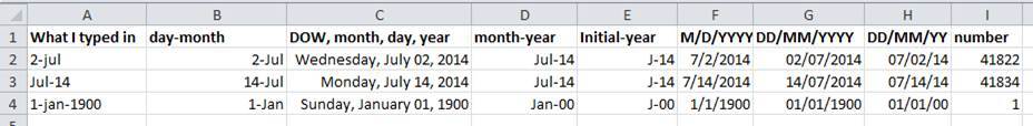
10 |
11 | But these ‘features’ often allow ambiguity to creep into your data. Ideally, data should be as unambiguous as possible. The first thing you need to know is that Excel stores dates as a number- see the last column in the above figure. Essentially, it counts the days from a default of December 31, 1899, and thus stores July 2, 2014 as the serial number 41822.
12 |
13 | (But wait. That’s the default on my version of Excel. We’ll get into how this can introduce problems down the line later in this lesson. )
14 |
15 | This serial number thing can actually be useful in some circumstances. Say you had a sampling plan where you needed to sample every thirty seven days. In another cell, you could type:
16 |
17 | =B2+37
18 |
19 | And it would return
20 |
21 | 8-Aug
22 |
23 | because it understands the date as a number 41822, and 41822 +37 =41859 which Excel interprets as August 8, 2014. It retains the format (for the most part) of the cell that is being operated upon, (unless you did some sort of formatting to the cell before, and then all bets are off)
24 |
25 | Which brings us to the many ‘wonderful’ customizations Excel provides in how it displays dates. If you refer to the figure above, you’ll see that there are many, MANY ways that ambiguity creeps into your data depending on the format you chose when you enter your data, and if you’re not fully cognizant of which format you’re using, you can end up actually entering your data in a way that Excel will badly misinterpret. Worse yet, when exporting into a text-based format (such as CSV), Excel will export its internal date integer instead of a useful value.
26 |
27 | Once, I received a dataset from a colleague representing insect counts that were taken every few days over the summer, and things went something like this:
28 |
29 | 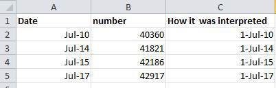
30 |
31 |
32 | If Excel was to be believed, my colleague had been collecting bugs IN THE FUTURE. Now, I have no doubt this person is highly capable, but I believe time travel was beyond even his grasp.
33 |
34 | Thus, in dealing with dates in spreadsheets, we recommend separating date data into separate fields, which will eliminate any chance of ambiguity.
35 |
36 | In my own work, I tend to store my dates in two fields: year, and day of year (DOY). Why? Because this is what’s useful to me, and there is practically no possibility for ambiguity creeping in.
37 |
38 | The types of statistical models I build usually incorporate year as a factor, to account for year-to-year variation, and then I use DOY to measure the passage of time within a year.
39 |
40 | So, can you convert all your dates into DOY format? Well, in excel, here’s a handy dandy guide:
41 |
42 | 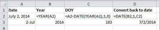
43 |
44 |
45 |
46 | #### Exercise: pulling month out of Excel dates ####
47 |
48 | + In the `data` subdirectory there is an example dataset: [a short list of species](../../../data/biology/surveys-exercise-extract_month.csv) with one of the columns containing dates.
49 | + Extract month from the dates to the new column.
50 | + Hint: use the dedicated function MONTH.
51 |
52 | **Note**: Excel is unable to parse dates from before 1899-12-31, and will thus leave these untouched. If you’re mixing historic data from before and after this date, Excel will translate only the post-1900 dates into its internal format, thus resulting in mixed data. If you’re working with historic data, be extremely careful with your dates!
53 | Excel also entertains a second date system, the 1904 date system, as the default in Excel for Macintosh. This system will assign a different serial number than the [1900 date system](https://support.microsoft.com/kb/180162). Because of this, [dates must be checked for accuracy when exporting data from Excel](http://datapub.cdlib.org/2014/04/10/abandon-all-hope-ye-who-enter-dates-in-excel/) (look for dates that are ~4 years off).
54 |
55 | Previous: [Common formatting mistakes by spreadsheet users.](02-common-mistakes.md) Next: [Basic quality control and data manipulation in spreadsheets.](04-quality-control.md)
56 |
--------------------------------------------------------------------------------
/lessons/excel/ecology-examples/04-quality-control.md:
--------------------------------------------------------------------------------
1 | # Basic quality control and data manipulation in spreadsheets #
2 |
3 | Authors:**Christie Bahlai**, **Aleksandra Pawlik**
4 | Contributors: **Jennifer Bryan**, **Alexander Duryee**, **Jeffrey Hollister**, **Daisie Huang**, **Owen Jones**, and
5 | **Ben Marwick**
6 |
7 | When you have a well-structured data table, you can use several simple techniques within your spreadsheet to ensure the data you’ve entered is free of errors.
8 |
9 | **Tip!** *Before doing any quality control operations, save your original file with the formulas and a name indicating it is the original data. Create a separate file with appropriate naming and versioning, and ensure your data is stored as “values” and not as formulas. Because formulas refer to other cells, and you may be moving cells around, you may compromise the integrity of your data if you do not take this step!*
10 |
11 | **readMe files:** As you start manipulating your data files, create a readMe document / text file to keep track of your files and document your manipulations so that they may be easily understood and replicated, either by your future self or by an independent researcher. Your readMe file should document all of the files in your data set (including documentation), describe their content and format, and lay out the organizing principles of folders and subfolders. For each of the separate files listed, it is a good idea to document the manipulations or analyses that were carried out on those data.
12 |
13 | [Example: converting all data to values: use soybean aphid suction trap dataset for this section]
14 |
15 | ## Sorting ##
16 | Bad values often sort to bottom or top of the column. For example, if your data should be numeric, then alphabetical and null data will group at the ends of the sorted data. Sort your data by each field, one at a time. Scan through each column, but pay the most attention to the top and the bottom of a column.
17 | If your dataset is well-structured and does not contain formulas, sorting should never affect the integrity of your dataset.
18 |
19 | [Example: sorting]
20 |
21 | ## Conditional formatting ##
22 | Use with caution! But a great way to flag inconsistent values when entering data.
23 |
24 | [Example: conditional formatting]
25 |
26 | ## Check on cell formats ##
27 | A good way to check if you’ve got data of the wrong type in a column is by checking column format. This can also help prevent issues when you export your data.
28 |
29 | [Example: variable format]
30 |
31 | ## Pivot tables ##
32 | Pivot tables are a very powerful tool in Excel. They’re useful to check for issues with data integrity because they provide a quick, visual way to spot things that are amiss, including with categorical variables. They are also great for reshaping data and obtaining summary statistics quickly in a drag and drop interface.
33 |
34 | [Example in Pivot Table]
35 |
36 | Why would I need to reshape my data? Different analyses require data to be in different formats- example: taking a species list to a diversity analysis.
37 |
38 | [Use species list example]
39 |
40 | Note: these operations can be done in most statistical or programming packages (i.e. using reshape2, plyr in R)
41 |
42 | Previous:[Dates as data.](03-dates-as-data.md) Next: [Exporting data from spreadsheets.](05-exporting-data.md)
43 |
--------------------------------------------------------------------------------
/lessons/excel/ecology-examples/05-exporting-data.md:
--------------------------------------------------------------------------------
1 | # Exporting data from spreadsheets #
2 |
3 | Authors:**Christie Bahlai**, **Aleksandra Pawlik**
4 | Contributors: **Jennifer Bryan**, **Alexander Duryee**, **Jeffrey Hollister**, **Daisie Huang**, **Owen Jones**, and
5 | **Ben Marwick**
6 |
7 | ###Spreadsheet data formats
8 |
9 | Storing data in Excel default file format (`*.xls` or `*.xlsx` - depending on the Excel version) is a bad idea. Why? Because it is a proprietary format, and it is possible that in the future, technology won’t exist (or will become sufficiently rare) to make it inconvenient, if not impossible, to open the file.
10 |
11 | Think about zipdisks. How many old theses in your lab are “backed up” and stored on zipdisks? Ever wanted to pull out the raw data from one of those?
12 | *Exactly.*
13 |
14 | Also, other spreadsheet software may not be able to open the files saved in a proprietary Excel format.
15 |
16 | But more insidiously- different versions of Excel may be changed so they handle data differently, leading to inconsistencies.
17 |
18 | As an example, do you remember how we talked about how Excel stores dates earlier? Turns out there are multiple defaults for different versions of the software. And you can switch between them all willy-nilly. So, say you’re compiling Excel-stored data from multiple sources. There’s dates in each file- Excel interprets them as their own internally consistent serial numbers. When you combine the data, Excel will take the serial number from the place you’re importing it from, and interpret it using the rule set for the version of Excel you’re using. Essentially, you could be adding a huge error to your data, and it wouldn’t necessarily be flagged by any data cleaning methods if your ranges overlap.
19 |
20 | Storing data in a universal, open, static format will help deal with this problem. Try tab-delimited or CSV (more common). CSV files are plain text files where the columns are separated by commas, hence 'comma separated variables' or CSV. The advantage of a CSV over an Excel/SPSS/etc. file is that we can open and read a CSV file using just about any software, including a simple text editor. Data in a CSV can also be easily imported into other formats and environments, such as SQLite and R. We're not tied to a certain version of a certain expensive program when we work with CSV, so it's a good format to work with for maximum portability and endurance. Most spreadsheet programs can save to delimited text formats like CSV easily, although they complain and make you feel like you’re doing something wrong along the way.
21 |
22 | To save a file you have opened in Excel into the `*.csv` format:
23 |
24 | 1. From the top menu select 'File' and 'Save as'.
25 | 2. In the 'Format' field, from the list, select 'Comma Separated Values' (`*.csv`).
26 | 3. Double check the file name and the location where you want to save it and hit 'Save'.
27 |
28 | 
29 |
30 | An important note for backwards compatibility: you can open CSVs in Excel!
31 |
32 | ## A Note on Cross-platform Operability##
33 | (or, how typewriters are ruining your work)
34 |
35 | By default, most coding and statistical environments expect UNIX-style line endings (`\n`) as representing line breaks. However, Windows uses an alternate line ending signifier (`\r\n`) by default for legacy compatibility with Teletype-based systems. As such, when exporting to CSV using Excel, your data will look like this:
36 |
37 | >data1,data2\r\n1,2\r\n4,5\r\n…
38 |
39 | which, upon passing into most environments (which split on `\n`), will parse as:
40 |
41 | >data1
42 | >data2\r
43 | >1
44 | >2\r
45 | >...
46 |
47 | thus causing terrible things to happen to your data. For example, `2\r` is not a valid integer, and thus will throw an error (if you’re lucky) when you attempt to operate on it in R or Python. Note that this happens on Excel for OSX as well as Windows, due to legacy Windows compatibility.
48 |
49 | There are a handful of solutions for enforcing uniform UNIX-style line endings on your exported CSVs:
50 |
51 | 1. When exporting from Excel, save as a “Windows comma separated (.csv)” file
52 | 2. If you store your data file under version control (which you should be doing!) using Git, edit the `.git/config` file in your repository to automatically translate `\r\n` line endings into `\n`.
53 | Add the follwing to the file ([see the detailed tutorial](http://nicercode.github.io/blog/2013-04-30-excel-and-line-endings)):
54 |
55 | [filter "cr"]
56 | clean = LC_CTYPE=C awk '{printf(\"%s\\n\", $0)}' | LC_CTYPE=C tr '\\r' '\\n'
57 | smudge = tr '\\n' '\\r'`
58 |
59 | and then create a file `.gitattributes` that contains the line:
60 |
61 | *.csv filter=cr
62 |
63 |
64 | 3. Use [dos2unix](http://dos2unix.sourceforge.net/) (available on OSX, *nix, and Cygwin) on local files to standardize line endings.
65 |
66 |
67 | Previous: [Basic quality control and data manipulation in spreadsheets.](04-quality-control.md)
68 |
--------------------------------------------------------------------------------
/lessons/excel/ecology-examples/06-data-formats-caveats.md:
--------------------------------------------------------------------------------
1 | # Caveats of popular data and file formats #
2 |
3 | Materials by: **Jeffrey Hollister**, **Alexander Duryee**, **Jennifer Bryan**, **Daisie Huang**, **Ben Marwick**, **Christie Bahlai**, **Owen Jones**, **Aleksandra Pawlik**
4 |
5 | ###Commas as part of data values in `*.csv` files
6 |
7 | In the [previous lesson](05-exporting-data.md) we discussed how to export Excel file formats into `*.csv`. Whilst Comma Separated Value files are indeed very useful allowing for easily exchanging and sharing data.
8 |
9 | However, there are some significant problems with this particular format. Quite often the data values themselves may include commas (,). In that case, the software which you use (including Excel) will most likely incorrectly display the data in columns. It is because the commas which are a part of the data values will be interpreted as a delimiter.
10 |
11 | For example, our data could look like this:
12 |
13 | species_id,genus,species,taxa
14 | AB,Amphispiza,bilineata,Bird
15 | AH,Ammospermophilus,harrisi,Rodent-not,censused
16 | AS,Ammodramus,savannarum,Bird
17 |
18 | In record `AH,Ammospermophilus,harrisi,Rodent-not,censused` the value for *taxa* includes a comma (`Rodent-not,censused`).
19 | If we try to read the above into Excel (or other spreadsheet programme), we will get something like this:
20 |
21 | 
22 |
23 | The value for 'taxa' was split into two columns (instead of being put in one column `D`). This can propagate to a number of further errors. For example, the "extra" column will be interpreted as a column with many missing values (and without a proper header!). In addition to that, the value in column `D` for the record in row 3 (so the one where the value for 'taxa' contained the comma) is now incorrect.
24 |
25 |
26 | ### Dealing with commas as part of data values in `*.csv` files
27 |
28 | If you want to store your data in `*.csv` and expect that your data may contain commas in their values, you can avoid the problem discussed above by putting the values in quotes (""). This [example data file](../../../data/biology/species.csv) applies this rule so the actual data looks like:
29 |
30 | species_id,genus,species,taxa
31 | "AB","Amphispiza","bilineata","Bird"
32 | "AH","Ammospermophilus","harrisi","Rodent-not censused"
33 | "AS","Ammodramus","savannarum","Bird"
34 | "BA","Baiomys","taylori","Rodent"
35 | "CB","Campylorhynchus","brunneicapillus","Bird"
36 | "CM","Calamospiza","melanocorys","Bird"
37 | "CQ","Callipepla","squamata","Bird"
38 | "CS","Crotalus","scutalatus","Reptile"
39 | "CT","Cnemidophorus","tigris","Reptile"
40 | "CU","Cnemidophorus","uniparens","Reptile"
41 |
42 | This original file does not contain commas in the values.
43 |
44 | But let's see what would happen if we introduced a comma into `"Rodent-not censused"` - so that it looks like this: `"Rodent-not, censused"`.
45 |
46 | 1. Open the [species.csv](../../../data/biology/species.csv) file in Excel (or Calc in Libre Office).
47 | 2. Add the comma (,) in `"Rodent-not censused"`.
48 | 3. Save the file under a **different name** (but also in the `csv` format) and reopen it in Excel.
49 | 4. The issue with the "extra" incorrect column should not appear.
50 |
51 | However, if you are working with already existing dataset in which the data values are not included in "" and but which have commas as both delimiters and parts of data values, you are potentially facing a major problem with **data cleaning**.
52 |
53 | If the dataset you're dealing with contains hundreds or thousands of records, cleaning them up manually (by either removing commas from the data values or putting the values into quotes - "") is not only going to take hours and hours but may potentially end up with you accidentally introducing many errors.
54 |
55 | Cleaning up datasets is one of major problems in many scientific disciplines. The approach almost always depends on the particular context. However, it is a good practice to clean the data in an automated fashion, for example by writing and running a script. Other lessons in Data Carpentry covering shell, Python and R will give you the basis for developing skills to build relevant scripts.
56 |
57 |
58 | ###Tab Separated Values format
59 |
60 | ###Other delimiters for data formats
61 |
62 | Previous: [Exporting data from spreadsheets.](05-exporting-data.md)
--------------------------------------------------------------------------------
/lessons/excel/images/1_helpful_clippy.jpg:
--------------------------------------------------------------------------------
https://raw.githubusercontent.com/datacarpentry/archive-datacarpentry/6a038e91f7c22d2aeed959b34212d25e8d83148a/lessons/excel/images/1_helpful_clippy.jpg
--------------------------------------------------------------------------------
/lessons/excel/images/2_datasheet_example.jpg:
--------------------------------------------------------------------------------
https://raw.githubusercontent.com/datacarpentry/archive-datacarpentry/6a038e91f7c22d2aeed959b34212d25e8d83148a/lessons/excel/images/2_datasheet_example.jpg
--------------------------------------------------------------------------------
/lessons/excel/images/3_white_table_1.jpg:
--------------------------------------------------------------------------------
https://raw.githubusercontent.com/datacarpentry/archive-datacarpentry/6a038e91f7c22d2aeed959b34212d25e8d83148a/lessons/excel/images/3_white_table_1.jpg
--------------------------------------------------------------------------------
/lessons/excel/images/4_merged_cells.jpg:
--------------------------------------------------------------------------------
https://raw.githubusercontent.com/datacarpentry/archive-datacarpentry/6a038e91f7c22d2aeed959b34212d25e8d83148a/lessons/excel/images/4_merged_cells.jpg
--------------------------------------------------------------------------------
/lessons/excel/images/5_excel_dates_1.jpg:
--------------------------------------------------------------------------------
https://raw.githubusercontent.com/datacarpentry/archive-datacarpentry/6a038e91f7c22d2aeed959b34212d25e8d83148a/lessons/excel/images/5_excel_dates_1.jpg
--------------------------------------------------------------------------------
/lessons/excel/images/6_excel_dates_2.jpg:
--------------------------------------------------------------------------------
https://raw.githubusercontent.com/datacarpentry/archive-datacarpentry/6a038e91f7c22d2aeed959b34212d25e8d83148a/lessons/excel/images/6_excel_dates_2.jpg
--------------------------------------------------------------------------------
/lessons/excel/images/7_excel_dates_3.jpg:
--------------------------------------------------------------------------------
https://raw.githubusercontent.com/datacarpentry/archive-datacarpentry/6a038e91f7c22d2aeed959b34212d25e8d83148a/lessons/excel/images/7_excel_dates_3.jpg
--------------------------------------------------------------------------------
/lessons/excel/images/excel_tables_example.png:
--------------------------------------------------------------------------------
https://raw.githubusercontent.com/datacarpentry/archive-datacarpentry/6a038e91f7c22d2aeed959b34212d25e8d83148a/lessons/excel/images/excel_tables_example.png
--------------------------------------------------------------------------------
/lessons/excel/images/excel_tables_example1.png:
--------------------------------------------------------------------------------
https://raw.githubusercontent.com/datacarpentry/archive-datacarpentry/6a038e91f7c22d2aeed959b34212d25e8d83148a/lessons/excel/images/excel_tables_example1.png
--------------------------------------------------------------------------------
/lessons/planning/README.md:
--------------------------------------------------------------------------------
1 | Placeholder for planning lessons
2 |
--------------------------------------------------------------------------------
/lessons/python/00-short-introduction-to-Python.md:
--------------------------------------------------------------------------------
1 | ---
2 | layout: lesson
3 | root: ../..
4 | title: Short Introduction to Programming in Python
5 | ---
6 |
7 | # The Basics of Python
8 |
9 | Python is a general purpose programming language, focused on rapid development of scripts and applications.
10 |
11 | Python's main advantages:
12 | * Open Source software, supported by Python Software Foundation
13 | * Available on all platforms
14 | * "Batteries Included" philosophy - libraries for common tasks available in standard installation
15 | * supports multiple programming paradigms
16 | * very large community
17 |
18 | ## Interpreter
19 |
20 | Python is interpreted language. As a consequence, we can use it in two ways:
21 | * using interpreter as an "advanced calculator" in interactive mode
22 |
23 | ```python
24 | user:host:~$ python
25 | Python 2.7.7 (default, Jun 3 2014, 16:16:56)
26 | [GCC 4.8.3] on linux2
27 | Type "help", "copyright", "credits" or "license" for more information.
28 | >>> 2 + 2
29 | 4
30 | >>> print "Hello World"
31 | Hello World
32 | ```
33 | * executing programs/scripts saved as a text file, usually with `*.py` extension
34 |
35 | ```
36 | user:host:~$ python my_script.py
37 | Hello World
38 | ```
39 |
40 | ## Introduction to Python build-in data types
41 |
42 | ### Strings, integers and floats
43 |
44 | Most basic data types in Pythons are strings, integers and floats
45 |
46 | ```python
47 | text = "Data Carpentry"
48 | number = 42
49 | pi_value = 3.1415
50 | ```
51 |
52 | Here we've assigned data to variables, namely `text`, `number` and `pi_value`,
53 | using the assignment operator `=`. Python variables don't have to hold specific
54 | data types - we can reassign them - but be careful as this can be confusing.
55 |
56 | To print out the value stored in a variable we can simply type the name of the
57 | variable into the interpreter
58 |
59 | ```python
60 | >>> text
61 | "Data Carpentry"
62 | ```
63 |
64 | but this only works in the interpreter. In scripts we must use the `print` command
65 |
66 | ```python
67 | # Comments starts with #
68 | # Next line will print out text
69 | print text
70 | "Data Carpentry"
71 | ```
72 |
73 | ### Operators
74 |
75 | We can do math in Python using the basic operators `+, -, /, *, %`
76 |
77 | ```python
78 | >>> 2 + 2
79 | 4
80 | >>> 6 * 7
81 | 42
82 | >>> 2 ** 16 # power
83 | 65536
84 | >>> 3 % 2 # modulo
85 | 1
86 | ```
87 |
88 | We can also use comparison and logic operators:
89 | `<, >, ==, !=, <=, >=, etc.`
90 | `and, or, not`
91 |
92 | ```python
93 | >>> 3 > 4
94 | False
95 | >>> True and True
96 | True
97 | >>> True or False
98 | True
99 | ```
100 |
101 | ## Sequential types: Lists and Dictionaries
102 |
103 | ### Lists
104 |
105 | **Lists** are the most common data structure that can hold a sequence of elements. Each element can be accessed by it's index:
106 |
107 | ```python
108 | >>> numbers = [1,2,3]
109 | >>> l[0]
110 | 1
111 | ```
112 |
113 | A `for` loop can be used to access the elements in the sequence one at a time:
114 |
115 | ```python
116 | for num in numbers:
117 | print num
118 | 1
119 | 2
120 | 3
121 | ```
122 |
123 | **Indentation** is very important in Python. Note that second line in above example is indented - this is Python's way of marking a block of code. We will discuss this in more detail later.
124 |
125 | To add elements to the list, we can use the method `append`.
126 |
127 | ```python
128 | >>> numbers.append(4)
129 | >>> print numbers
130 | [1,2,3,4]
131 | ```
132 |
133 | Methods are a way to interact with an object - like a list. Accessing them is
134 | done by using the dot `.`.
135 | To find out what methods are available, we can use the built-in `help` command:
136 |
137 | ```python
138 | help(numbers)
139 |
140 | Help on list object:
141 |
142 | class list(object)
143 | | list() -> new empty list
144 | | list(iterable) -> new list initialized from iterable's items
145 | ...
146 | ```
147 |
148 | or we can get a list of methods by using `dir`. Some methods names are surrounded by double underscores. Those methods are called "special", and usually we access them in a different way. For example `__add__` method is responsible for `+` operator.
149 |
150 | ```python
151 | dir(numbers)
152 | >>> dir(numbers)
153 | ['__add__', '__class__', '__contains__', ...]
154 | ```
155 |
156 | ### Dictionaries
157 |
158 | A **dictionary** is a container that holds pairs of objects - keys and values.
159 |
160 | ```python
161 | >>> translation = {"one" : 1, "two" : 2}
162 | >>> translation["one"]
163 | 1
164 | ```
165 |
166 | Dictionaries work a lot like lists - except that you can index them with
167 | *keys*. Keys can only have particular types - they have to be
168 | "hashable". Strings and numeric types are acceptable, but lists aren't.
169 |
170 | ```python
171 | >>> rev = {1 : "one", 2 : "two"}
172 | >>> rev[1]
173 | 'one'
174 | >>> bad = {[1,2,3] : 3}
175 | ...
176 | TypeError: unhashable type: 'list'
177 | ```
178 |
179 | To add an item to the dictionary we assign a value to a new key:
180 |
181 | ```python
182 | >>> rev = {1 : "one", 2 : "two"}
183 | >>> rev[3] = "three"
184 | >>> rev
185 | {1: 'one', 2: 'two', 3: 'three'}
186 | ```
187 |
188 | Using `for` loops with dictionaries is a little more complicated. We can do this in two ways:
189 | ```python
190 | >>> for key, value in rev.items():
191 | ... print key, "->", value
192 | ...
193 | 1 -> one
194 | 2 -> two
195 | 3 -> three
196 | ```
197 | or
198 | ```python
199 | >>> for key in rev.keys():
200 | ... print key, "->", rev[key]
201 | ...
202 | 1 -> one
203 | 2 -> two
204 | 3 -> three
205 | >>>
206 | ```
207 |
208 | ## Functions
209 |
210 | Defining part of a program in Python as a function is done using the `def`
211 | keyword. For example a function that takes two arguments and returns the sum of
212 | them can be defined as:
213 |
214 | ```python
215 | def add_function(a, b):
216 | result = a + b
217 | return result
218 |
219 | z = add_function(20, 22)
220 | print z
221 | 42
222 | ```
223 |
224 | Key points here:
225 | - definition starts with `def`
226 | - function body is indented
227 | - `return` keyword precedes returned value
228 |
--------------------------------------------------------------------------------
/lessons/python/03-checking_your_data.md:
--------------------------------------------------------------------------------
1 | ##Checking your data
2 |
3 | One of the most basic functions in which we might be interested is to make sure our data are what we think they are. If we have some code that changes a certain number to another number, this will only work when all our values are numbers.
4 |
5 | Remember that in base python we can check the type of an object like this:
6 |
7 | ```UNIX
8 | type()
9 | ```
10 |
11 | In pandas, checking the dtype of a column is easy. The basic pseudocode looks like this:
12 |
13 | ```UNIX
14 | df[column_name].dtype
15 | ```
16 | An example would be:
17 |
18 | ```python
19 | df['record_id'].dtype
20 | dtype('int64')
21 | ```
22 |
23 | where 'df' is whatever name you gave your data frame.
24 |
25 | 'int64' might be a little bit unusual. We've seen int in our novice materials, with an integer being a whole number. int64 can hold large numbers; in fact int64 holds as many number as a Nintendo64 can hold. This type of precision might not always be important to you, but in certain mathematical operations, this may be very important. If we have a column that contains both ints and floats, Pandas will default to float for the whole column, so as not to lose the decimal points.
26 |
27 | Please see the table below for different, common data types:
28 |
29 | |Name of Pandas type | Function | Base Python Equivalent |
30 | |------------|---------|-------------------------|
31 | |Object | The most general dtype. Will be assigned to your column if column has mixed types (numbers and strings). | String |
32 | |int64 | Numerical characters. 64 refers to the memory allocated to hold this character. | Int. |
33 | | float64 | Numerical characters with decimals. If a column contains numbers and NaNs(see below), pandas will default to float64, in case your missing value has a decimal. | float |
34 | |datetime64, timedelta[ns] | Values meant to hold time data. Look into these for time series experiments. | -- |
35 |
36 |
37 | We probably don't want to examine the dtype of each column by hand. We can easily automate this.
38 |
39 | ```python
40 | for col in df:
41 | print col, df[col].dtypes
42 | record_id int64
43 | day int64
44 | year int64
45 | plot int64
46 | species object
47 | sex object
48 | wgt float64
49 | ```
50 |
51 | In this way, we can do a simple sanity check: Are our data what we thought? If not, we might want to refer to the [Masking]() section to investigate ways to remove unexpected values.
52 |
53 | Weight is a characteristic that we might want to use in future calculations, like approximations of metabolic rate. We might want these values to be integers. Using Pandas' apply functionality, transforming these values looks like this:
54 |
55 | ```python
56 | df['wgt'] = df['wgt'].astype('float64')
57 |
58 | df['record_id'].dtype
59 | dtype('int64')
60 | ```
61 |
62 | Back the train up. We did some weird stuff there. The first thing we did was cast each value as a float64. If we use these in further calculations, Python will save the results as floats, **even if the other values involved are ints. Maybe clarify this? Not sure what you mean by 'other values involved'.**
63 |
64 | **wgt was already type float64. where does record_id come into this?**
65 |
66 | You might wonder why we still have NaN values. *NaN* values are values that cannot be represented mathematically, or are undefined. Pandas, for example, will read an empty cell in a CSV or Excel sheet as a NaN. NaNs have some desirable properties: if we were to average the 'wgt' column without replacing our NaNs, we would get something like this:
67 |
68 | ```python
69 | df['wgt'].mean()
70 | 42.672428212991356
71 | ```
72 |
73 | But if we were to filter the NaNs and turn them into zeroes (after making a copy of the data so we don't lose our work), we would get something like this:
74 |
75 | ```python
76 | df1 = df
77 | df1['wgt'] = df1['wgt'].fillna(0)
78 |
79 | df1['wgt'].mean()
80 | 38.751976145601844
81 | ```
82 |
83 | While not a large difference, this might be important to the math we'd like to do with our values. When deciding how to manage missing data, it's important to think about how these data will be used. For example, we could fill our missing values with the column average value:
84 |
85 | ```python
86 | df1['wgt'] = df['wgt'].fillna(df['wgt'].mean())
87 | ```
88 |
89 | But what would be an appropriate situation in which to do this? Pandas gives us many options; it's up to us to find the appropraite ones for our work. Download a few data sets from a commonly-used data repository in your field and have a look at how missing data is represented. In Pandas, values that are not numbers and are not NaN can cause your calculations to fail. Choosing a missing data representation is a function of
90 | + How your data will be read and understood by others
91 | and
92 | + How your data will be read and understood by the computer.
93 |
94 | ##Recap
95 |
96 | What we've learned:
97 |
98 | + How to ensure your data types are what you think they are
99 | + What NaN values are, how they might be represented, and what this means for your work
100 | + How to replace NaN values, if desired
101 |
102 |
103 |
104 |
105 |
106 |
107 |
108 |
109 |
--------------------------------------------------------------------------------
/lessons/python/04-data_as_read-only.md:
--------------------------------------------------------------------------------
1 | ##Treating your data as read-only
2 |
3 | In today's scientific climate, there is more attention being paid to reproducibilty and data availability. Upon publication, you may be asked to provide both raw and processed data. Likewise, funding agencies may require that your data is made open-access or deposited in public repositories. In the absence of external pressure, you still likely want to have your raw data around, in case you decide to reanalyze it or use it for meta-analysis in the future. This tutorial is intended to offer you a short look at the os module, and how you can leverage it to help you keep your raw and processed data separated.
4 |
5 | ##os module
6 |
7 | The os module is included in the base Python library and can be loaded in the standard way:
8 |
9 | ```python
10 | import os
11 | ```
12 |
13 | This library offers assorted functions for interacting with the operating system. In this lesson, we'll be looking at creating and populating directories from within a script.
14 |
15 | ##Data as read-only
16 |
17 | Data as read-only means exactly that: when you interact with a file, you don't make changes to that file. Instead, you make your edits programmatically and save the edited files to a separate location. Let's grab our survey data:
18 |
19 | ```python
20 | import pandas as pd
21 | mydata = pd.read_csv("data/surveys.csv")
22 | ```
23 |
24 | As a refresher, here is a function from lesson 3 that fills in missing data with zeros:
25 |
26 | ```python
27 | mydata['wgt'] = mydata['wgt'].fillna(0)
28 | ```
29 |
30 | We've already learned how to write this to a file. And for many purposes, writing to a file might be sufficient. But other people don't know our data as well as we do. Delineating between raw and processed files can be very helpful when others need to interact with our data.
31 |
32 | We're going to start out by checking to see if we have a directory for our processed data.
33 |
34 | ```python
35 |
36 | if 'processed' in os.listdir('.'):
37 | print 'yay'
38 | else:
39 | print 'nay'
40 | ```
41 |
42 | What we've done above is used the os module to list all the directories in our current directory, denoted as '.' (If this syntax is unfamiliar, have a look through our shell [materials](https://github.com/datacarpentry/datacarpentry/blob/master/lessons/shell/01-filedir.md)). If our current directory contains a directory called 'processed', we celebrate in a restrained and dignified way. If not, we don't.
43 |
44 | Just printing things isn't that useful. Let's try something else:
45 |
46 | ```python
47 | if 'processed' in os.listdir('.'):
48 | print 'Processed directory exists'
49 | else:
50 | os.mkdir('processed')
51 | print 'Processed directory created'
52 | ```
53 |
54 | Now, what our code does is creates a directory and informs us of this fact.
55 |
56 | We can combine this with what we've learned about writing output from Pandas to treat our data as read-only:
57 |
58 | ```python
59 |
60 |
61 | mydata.to_csv('processed/surveys.csv')
62 |
63 | ```
64 |
65 | ##Wrap-Up
66 |
67 | What we've covered in this lesson is:
68 |
69 | * What it means to treat data as read-only.
70 | * Why we might want to treat our data as read-only.
71 | * How we can use the os module to keep our processed and raw data straight.
72 |
73 |
74 |
--------------------------------------------------------------------------------
/lessons/python/README.md:
--------------------------------------------------------------------------------
1 | ---
2 | layout: lesson
3 | root: ../..
4 | title: Programming with Python
5 | ---
6 |
7 | ## Python lessons for Data Carpentry
8 |
9 | There are several files and directories in this repository
10 |
11 | * 00-short-introduction-to-Python.md - the Python intro including information on data types
12 |
--------------------------------------------------------------------------------
/lessons/python/pics/barplot.png:
--------------------------------------------------------------------------------
https://raw.githubusercontent.com/datacarpentry/archive-datacarpentry/6a038e91f7c22d2aeed959b34212d25e8d83148a/lessons/python/pics/barplot.png
--------------------------------------------------------------------------------
/lessons/python/pics/myplot.png:
--------------------------------------------------------------------------------
https://raw.githubusercontent.com/datacarpentry/archive-datacarpentry/6a038e91f7c22d2aeed959b34212d25e8d83148a/lessons/python/pics/myplot.png
--------------------------------------------------------------------------------
/lessons/rnaseq-data-analysis/.gitignore:
--------------------------------------------------------------------------------
1 | results/
2 |
--------------------------------------------------------------------------------
/lessons/rnaseq-data-analysis/Makefile:
--------------------------------------------------------------------------------
1 | OUTS := $(patsubst %.Rmd,%.md,$(wildcard *.Rmd)) # figure/
2 |
3 | all: $(OUTS)
4 |
5 | clean:
6 | rm -rf $(OUTS)
7 |
8 | %.md: %.Rmd
9 | ## knit the file to create a markdown file
10 | Rscript -e 'knitr::knit("$*.Rmd")'
11 |
12 | ## change the syntax highlighting to coffee instead of r
13 | # gsed -i 's/```r/```coffee/g' $*.md
14 |
15 | ## Uncomment below if your code generates figures
16 | ## Because jekyll creates a new directory with an index.html file,
17 | ## You'll need to reference the parent directory when including figures.
18 | # gsed -i 's~figure/~../figure/~g' $*.md
19 |
--------------------------------------------------------------------------------
/lessons/rnaseq-data-analysis/README.md:
--------------------------------------------------------------------------------
1 | ---
2 | layout: page
3 | ---
4 |
5 | # RNA-seq data analysis
6 |
7 | This workshop on RNA-seq data analysis directed toward life scientists with little to no experience with statistical computing or bioinformatics. Part I (QC, alignment, & counting) assumes basic familiarity with the Unix shell. Part II (differential expression analysis) assumes basic familiarity with R.
8 |
9 | By the end of the workshop, participants will: (1) know how to align and quantitate gene expression with RNA-seq data, and (2) know what packages to use and what steps to take to analyze RNA-seq data for differentially expressed genes.
10 |
11 | The alignment step in this workshop requires a couple GB of RAM. This can be hard to manage if students are running a VM on a laptop. Further, there are several tools required for the workshop. This workshop runs best on an m3.xlarge AWS EC2 instance using the image ID ami-f462ef9c (username and password both "bioinfo"), which has all the software necessary for this analysis pre-installed. If not using this image, participants need to install:
12 |
13 | * Basic shell utilities: gcc, make, ruby, curl, git, parallel, unzip, default-jre
14 | * bowtie2:
15 | * tophat2:
16 | * featureCounts (part of subread):
17 | * samtools:
18 | * fastx-toolkit:
19 | * FastQC:
20 | * R:
21 | * RStudio:
22 | * R packages: Bioconductor core (i.e., `biocLite()`), DESeq2
23 |
--------------------------------------------------------------------------------
/lessons/rnaseq-data-analysis/data/coldata.csv:
--------------------------------------------------------------------------------
1 | sample,condition
2 | ctl1,ctl
3 | ctl2,ctl
4 | ctl3,ctl
5 | uvb1,uvb
6 | uvb2,uvb
7 | uvb3,uvb
8 |
--------------------------------------------------------------------------------
/lessons/rnaseq-data-analysis/data/ctl1.fastq.gz:
--------------------------------------------------------------------------------
https://raw.githubusercontent.com/datacarpentry/archive-datacarpentry/6a038e91f7c22d2aeed959b34212d25e8d83148a/lessons/rnaseq-data-analysis/data/ctl1.fastq.gz
--------------------------------------------------------------------------------
/lessons/rnaseq-data-analysis/data/ctl2.fastq.gz:
--------------------------------------------------------------------------------
https://raw.githubusercontent.com/datacarpentry/archive-datacarpentry/6a038e91f7c22d2aeed959b34212d25e8d83148a/lessons/rnaseq-data-analysis/data/ctl2.fastq.gz
--------------------------------------------------------------------------------
/lessons/rnaseq-data-analysis/data/ctl3.fastq.gz:
--------------------------------------------------------------------------------
https://raw.githubusercontent.com/datacarpentry/archive-datacarpentry/6a038e91f7c22d2aeed959b34212d25e8d83148a/lessons/rnaseq-data-analysis/data/ctl3.fastq.gz
--------------------------------------------------------------------------------
/lessons/rnaseq-data-analysis/data/uvb1.fastq.gz:
--------------------------------------------------------------------------------
https://raw.githubusercontent.com/datacarpentry/archive-datacarpentry/6a038e91f7c22d2aeed959b34212d25e8d83148a/lessons/rnaseq-data-analysis/data/uvb1.fastq.gz
--------------------------------------------------------------------------------
/lessons/rnaseq-data-analysis/data/uvb2.fastq.gz:
--------------------------------------------------------------------------------
https://raw.githubusercontent.com/datacarpentry/archive-datacarpentry/6a038e91f7c22d2aeed959b34212d25e8d83148a/lessons/rnaseq-data-analysis/data/uvb2.fastq.gz
--------------------------------------------------------------------------------
/lessons/rnaseq-data-analysis/data/uvb3.fastq.gz:
--------------------------------------------------------------------------------
https://raw.githubusercontent.com/datacarpentry/archive-datacarpentry/6a038e91f7c22d2aeed959b34212d25e8d83148a/lessons/rnaseq-data-analysis/data/uvb3.fastq.gz
--------------------------------------------------------------------------------
/lessons/scripting/README.md:
--------------------------------------------------------------------------------
1 | # Resources
2 |
3 | * `filesystem`: filesystem used in "Files and Directories"
4 | * `creatures`: DNA data used in "Loops"
5 | * `finding`: data using in "Finding Things"
6 | * `molecules`: PDB files used in "Pipes and Filters"
7 | * `scripting`: files and directories used in "Shell Scripts"
8 |
--------------------------------------------------------------------------------
/lessons/scripting/index.md:
--------------------------------------------------------------------------------
1 | ---
2 | layout: lesson
3 | root: ../..
4 | title: Unix Shell Scripting
5 | ---
6 |
7 | The Unix shell is a power tool that allows people to do complex things
8 | with just a few keystrokes. However, more importantly for those trying
9 | to work more efficiently with data, the Unix shell allows combining
10 | existing programs in new ways, and to create automated executable data
11 | pipelines that can be repeated, modified, and built upon.
12 |
13 |
14 |
15 | 1. [Shell Scripts](01-script.html)
16 | 3. [Data pipelines](02-pipeline.html)
17 |
18 |
19 |
--------------------------------------------------------------------------------
/lessons/scripting/scripts/barplot-figure.R:
--------------------------------------------------------------------------------
1 | ################################
2 | # Prefix part: setting variables
3 | ################################
4 | # working directory if needed, e.g.:
5 | #setwd("~/Documents/git/new/2014-05-08-datacarpentry/lessons/R")
6 |
7 | # data input
8 | # - original csv file:
9 | #data.in <- "surveys.csv"
10 | # - csv file dumped from sqlite:
11 | data.in <- "result.csv"
12 |
13 | # plot output
14 | plot.out <- "R_plot.pdf"
15 |
16 | ##########################################################
17 | # Main part: execution of data loading, analysis, plotting
18 | ##########################################################
19 | dat <- read.csv(data.in, header=TRUE, na.strings="")
20 | dat2 <- dat[complete.cases(dat$wgt),]
21 |
22 | # aggregate by species, or change to genus for joined dataset
23 | meanvals <- aggregate(wgt~species, data=dat2, mean)
24 |
25 | pdf(plot.out)
26 | # change to species to genus for joined dataset
27 | barplot(meanvals$wgt, names.arg=meanvals$species, cex.names=0.4, col=c("blue"))
28 | dev.off()
29 |
--------------------------------------------------------------------------------
/lessons/scripting/scripts/gen-stamped-files.sh:
--------------------------------------------------------------------------------
1 | #!/bin/bash
2 |
3 | # create directory in which to create the renamed files
4 | mkdir exc1
5 |
6 | # for each file on the command line, grab basename up to first dot
7 | for f in `ls $* | cut -d . -f 1` ; do
8 | # copy to new directory, time-stamping and changing extension to .xls
9 | cp -p $f.*csv exc1/$f-`date +%Y%m`.xls
10 | done
11 |
--------------------------------------------------------------------------------
/lessons/scripting/scripts/numcols.sh:
--------------------------------------------------------------------------------
1 | #!/bin/bash
2 |
3 | for csvfile in "$@" ; do
4 | numcols=$(expr `head -n 1 $csvfile | tr -d -c , | wc -c` + 1)
5 | echo "$csvfile: $numcols columns"
6 | done
7 |
--------------------------------------------------------------------------------
/lessons/scripting/scripts/sqlite-import.sql:
--------------------------------------------------------------------------------
1 | .mode csv
2 | .import plots.csv plots
3 | .import species.csv species
4 | .import surveys.csv surveys
5 | .headers on
6 | .output stdout
7 | SELECT species.genus, species.species AS speciesname, surveys.*
8 | FROM surveys
9 | JOIN species ON surveys.species = species.species_id
10 | WHERE species.taxa = 'Rodent';
11 |
--------------------------------------------------------------------------------
/lessons/scripting/scripts/sqlite-script.sql:
--------------------------------------------------------------------------------
1 | .mode csv
2 | .import surveys.csv surveys
3 | SELECT * FROM surveys;
4 |
--------------------------------------------------------------------------------
/lessons/scripting/scripts/sqlite-select-from-db.sql:
--------------------------------------------------------------------------------
1 | .mode csv
2 | .header on
3 | SELECT species.genus, species.species AS speciesname, surveys.*
4 | FROM surveys
5 | JOIN species ON surveys.species = species.species_id
6 | WHERE species.taxa = 'Rodent';
7 |
--------------------------------------------------------------------------------
/lessons/scripting/scripts/workflow.sh:
--------------------------------------------------------------------------------
1 | #!/bin/bash
2 |
3 | # paths to programs
4 | sqlite=/usr/local/opt/sqlite/bin/sqlite3
5 | R=R
6 |
7 | # Load the data into database, combine, filter, export
8 | cat sqlite-import.sql | $sqlite > result.csv
9 |
10 | # for old versions of sqlite
11 | # cat sqlite-select-from-db.sql | $sqlite portal_mammals.sqlite > result.csv
12 |
13 | # Load into R for analysis and plotting
14 | $R CMD BATCH barplot-figure.R
15 |
--------------------------------------------------------------------------------
/lessons/shell/00-intro.md:
--------------------------------------------------------------------------------
1 | ---
2 | layout: lesson
3 | root: ../..
4 | title: Introducing the Shell
5 | ---
6 |
7 |
8 | #### Objectives
9 | * Explain how the shell relates to the keyboard, the screen, the operating system, and users' programs.
10 | * Explain when and why command-line interfaces should be used instead of graphical interfaces.
11 |
12 |
13 |
14 | #### What and Why
15 |
16 | At a high level, computers do four things:
17 |
18 | - run programs;
19 | - store data;
20 | - communicate with each other; and
21 | - interact with us.
22 |
23 | They can do the last of these in many different ways,
24 | including direct brain-computer links and speech interfaces.
25 | Since these are still in their infancy,
26 | most of us use windows, icons, mice, and pointers.
27 | These technologies didn't become widespread until the 1980s,
28 | but their roots go back to Doug Engelbart's work in the 1960s,
29 | which you can see in what has been called
30 | "[The Mother of All Demos](http://www.youtube.com/watch?v=a11JDLBXtPQ)".
31 |
32 | Going back even further,
33 | the only way to interact with early computers was to rewire them.
34 | But in between,
35 | from the 1950s to the 1980s,
36 | most people used line printers.
37 | These devices only allowed input and output of the letters, numbers, and punctuation found on a standard keyboard,
38 | so programming languages and interfaces had to be designed around that constraint.
39 |
40 | This kind of interface is called a
41 | [command-line interface](../../gloss.html#cli), or CLI,
42 | to distinguish it from the
43 | [graphical user interface](../../gloss.html#gui), or GUI,
44 | that most people now use.
45 | The heart of a CLI is a [read-evaluate-print loop](../../gloss.html#repl), or REPL:
46 | when the user types a command and then presses the enter (or return) key,
47 | the computer reads it,
48 | executes it,
49 | and prints its output.
50 | The user then types another command,
51 | and so on until the user logs off.
52 |
53 | This description makes it sound as though the user sends commands directly to the computer,
54 | and the computer sends output directly to the user.
55 | In fact,
56 | there is usually a program in between called a
57 | [command shell](../../gloss.html#shell).
58 | What the user types goes into the shell;
59 | it figures out what commands to run and orders the computer to execute them.
60 |
61 | A shell is a program like any other.
62 | What's special about it is that its job is to run other programs
63 | rather than to do calculations itself.
64 | The most popular Unix shell is Bash,
65 | the Bourne Again SHell
66 | (so-called because it's derived from a shell written by Stephen Bourne—this
67 | is what passes for wit among programmers).
68 | Bash is the default shell on most modern implementations of Unix,
69 | and in most packages that provide Unix-like tools for Windows.
70 |
71 | Using Bash or any other shell
72 | sometimes feels more like programming than like using a mouse.
73 | Commands are terse (often only a couple of characters long),
74 | their names are frequently cryptic,
75 | and their output is lines of text rather than something visual like a graph.
76 | On the other hand,
77 | the shell allows us to combine existing tools in powerful ways with only a few keystrokes
78 | and to set up pipelines to handle large volumes of data automatically.
79 | In addition,
80 | the command line is often the easiest way to interact with remote machines.
81 | As clusters and cloud computing become more popular for scientific data crunching,
82 | being able to drive them is becoming a necessary skill.
83 |
84 |
85 |
86 | #### Key Points
87 | * A shell is a program whose primary purpose is to read commands and run other programs.
88 | * The shell's main advantages are its high action-to-keystroke ratio,
89 | its support for automating repetitive tasks,
90 | and that it can be used to access networked machines.
91 | * The shell's main disadvantages are its primarily textual nature
92 | and how cryptic its commands and operation can be.
93 |
94 |
95 |
--------------------------------------------------------------------------------
/lessons/shell/README.txt:
--------------------------------------------------------------------------------
1 | Material for introduction to the shell.
2 |
3 | Heavily influenced by the Software Carpentry novice materials; these are the numbered lessons (00 through 06). The web versions can be found at:
4 |
5 | http://software-carpentry.org/v5/novice/shell/index.html
6 |
7 | The shell.md file is the specific lesson for Data Carpentry. Also see the cheatsheet in cheatsheet directory.
8 |
9 | The data files are:
10 | * surveys.csv
11 | * plots.csv
12 | * species.csv
13 |
14 | which come from Ernest et al 2009:
15 |
16 | http://esapubs.org/archive/ecol/E090/118/metadata.htm
17 |
--------------------------------------------------------------------------------
/lessons/shell/img/filesystem-challenge.odg:
--------------------------------------------------------------------------------
https://raw.githubusercontent.com/datacarpentry/archive-datacarpentry/6a038e91f7c22d2aeed959b34212d25e8d83148a/lessons/shell/img/filesystem-challenge.odg
--------------------------------------------------------------------------------
/lessons/shell/img/filesystem.odg:
--------------------------------------------------------------------------------
https://raw.githubusercontent.com/datacarpentry/archive-datacarpentry/6a038e91f7c22d2aeed959b34212d25e8d83148a/lessons/shell/img/filesystem.odg
--------------------------------------------------------------------------------
/lessons/shell/img/find-file-tree.odg:
--------------------------------------------------------------------------------
https://raw.githubusercontent.com/datacarpentry/archive-datacarpentry/6a038e91f7c22d2aeed959b34212d25e8d83148a/lessons/shell/img/find-file-tree.odg
--------------------------------------------------------------------------------
/lessons/shell/img/home-directories.odg:
--------------------------------------------------------------------------------
https://raw.githubusercontent.com/datacarpentry/archive-datacarpentry/6a038e91f7c22d2aeed959b34212d25e8d83148a/lessons/shell/img/home-directories.odg
--------------------------------------------------------------------------------
/lessons/shell/img/nano-screenshot.png:
--------------------------------------------------------------------------------
https://raw.githubusercontent.com/datacarpentry/archive-datacarpentry/6a038e91f7c22d2aeed959b34212d25e8d83148a/lessons/shell/img/nano-screenshot.png
--------------------------------------------------------------------------------
/lessons/shell/img/vlad-homedir.odg:
--------------------------------------------------------------------------------
https://raw.githubusercontent.com/datacarpentry/archive-datacarpentry/6a038e91f7c22d2aeed959b34212d25e8d83148a/lessons/shell/img/vlad-homedir.odg
--------------------------------------------------------------------------------
/lessons/shell/index.md:
--------------------------------------------------------------------------------
1 | ---
2 | layout: lesson
3 | root: ../..
4 | title: The Unix Shell
5 | ---
6 | The Unix shell has been around longer than most of its users have been alive.
7 | It has survived so long because it's a power tool
8 | that allows people to do complex things with just a few keystrokes.
9 | More importantly,
10 | it helps them combine existing programs in new ways
11 | and automate repetitive tasks
12 | so that they don't have to type the same things over and over again.
13 |
14 |
15 |
16 | 1. [Introducing the Shell](00-intro.html)
17 | 2. [Files and Directories](01-filedir.html)
18 | 3. [Creating Things](02-create.html)
19 | 4. [Pipes and Filters](03-pipefilter.html)
20 | 5. [Loops](04-loop.html)
21 | 6. [Shell Scripts](05-script.html)
22 | 7. [Finding Things](06-find.html)
23 |
24 |
25 |
--------------------------------------------------------------------------------
/lessons/shell/shell.md:
--------------------------------------------------------------------------------
1 | #Introduction to the shell
2 |
3 | Based on the very detailed material at [http://software-carpentry.org/v5/novice/shell/index.html](http://software-carpentry.org/v5/novice/shell/index.html).
4 |
5 | Assume that students have a set of three data files (plots.csv, surveys.csv and species.csv) from the et al publication, either from a github repo or from some other mechanism.
6 |
7 | ##Objectives
8 |
9 | * Understand the advantages of text files over other file types
10 | * Introduce the concept of command-line interface
11 | * Explain how to navigate your computer's directory structures and understand paths
12 | * Bash commands: using flags, finding documentation
13 | * Move, copy and delete files
14 | * Using tab completion for efficiency
15 | * Use of wildcards for pattern matching
16 |
17 | ## Text files
18 | Let's start by opening Word (other other word processing software such as Libre Office or Open Office). Type some text:
19 |
20 | $ This is not a text file
21 |
22 | Save in native format (that might be text.doc, text.docx, text.odt, depending on your word processor). Then, also Save As a text document (text.txt)
23 |
24 | Now, open these two files in our text editor - Notepadd++ on Windows or Text Wrangler on Mac. Discuss the simplicity of the text document and the complexity of the non-text document. All of the tools we will use over the next few days can operate on text files. Using text makes it easier to read, manipulate, analyze and share your data. In 20 years, we will still be able to read text files. No such guarantee about Office docs or other proprietary format.
25 |
26 | ##Using the shell
27 |
28 | The shell is an example of a command-line interface (CLI). See the material in 00-intro.md, online at [http://software-carpentry.org/v5/novice/shell/00-intro.html](Software Carpentry) for details on introducing the shell.
29 |
30 | ### Navigating, creating and moving things
31 |
32 | Refer to the Software Carpentry material in 01-filedir.md, online at [http://software-carpentry.org/v5/novice/shell/01-filedir.html](Software Carpentry) for detailed descriptions of commands.
33 |
34 | Print working directory:
35 |
36 | $ pwd
37 |
38 | Discuss the path and how that relates to the directory structure you see in the file browser on your computer.
39 |
40 | List contents of a directory:
41 |
42 | $ ls
43 |
44 | Introduce the concept of a command having one or more flags / paramters:
45 |
46 | $ ls -F
47 | $ ls -lh
48 |
49 | The -F flag is useful when you do not have colours set on your shell to help distinguish files from directories. This will be true for most participants, while most instructors probably have colours.
50 |
51 | Note that spaces are important. ls-F and ls - F do not work.
52 |
53 | Change directories:
54 |
55 | $ cd
56 | $ cd ..
57 |
58 | Create and remove directories:
59 |
60 | $ mkdir
61 | $ rmdir
62 |
63 | Make a directory for this course. Now, let us put some files in that directory.
64 |
65 | Introduce how to Copy, move, delete files:
66 |
67 | $ cp
68 | $ mv
69 | $ rm
70 |
71 | Warn folks about rm - there is no Trash with bash.
72 |
73 | *Hint: tab completion makes you more efficient and less error-prone*
74 |
75 | Exercise: move the three .csv data files into a directory called 'data' in the directory for the course. Change to this directory.
76 |
77 | Create and edit a file:
78 |
79 | $ touch readme.txt
80 | $ nano readme.txt
81 |
82 | Put some information about these files in a README.txt file and save.
83 |
84 | ###Working with file contents
85 |
86 | Seeing the contents of a file:
87 |
88 | $ cat species.csv
89 | $ cat plots.csv
90 | $ cat surveys.csv
91 | $ cat plots.csv species.csv
92 |
93 | Can have multiple arguments. Note that this works well for the small files but not so well for the large file. How can we look at only the top of the file?
94 |
95 | $ less
96 | $ head
97 | $ tail
98 |
99 | How big is this file?
100 |
101 | $ ls -lh
102 | $ wc
103 | $ wc -l
104 |
105 | Using wildcards:
106 |
107 | $ ls *.csv
108 | $ wc -l *.csv
109 |
110 | Redirecting output to a file:
111 |
112 | $ wc -l *.csv > number_lines.csv
113 |
114 | Sorting the contents of a file:
115 |
116 | $ sort number_lines.csv
117 |
118 | Pipe commands together:
119 |
120 | $ wc -l *.csv | sort
121 |
122 | Getting subset of rows:
123 |
124 | $ head
125 | $ head -n 20
126 | $ tail
127 |
128 | Exercise: get rows 100 through 200 using head, tail and pipe
129 |
130 | Getting subset of columns (in this case, year of the surveys.csv file):
131 |
132 | $ cut -f 4 -d , surveys.csv
133 |
134 | Talk about how to get help on commands from man pages; show where to find this information in the web browser (because git bash does not have man).
135 |
136 | $ cut -f 4 -d , surveys.csv | sort
137 | $ cut -f 4 -d , surveys.csv | sort -r
138 |
139 | How many different genders are there?
140 |
141 | $ cut -f 7 -d , surveys.csv | uniq
142 |
143 | Did that work? Why not and how could we fix it? (cut | sort | uniq)
144 |
145 | ## Finding things
146 |
147 | Finding specific text in files using grep:
148 |
149 | $ grep 2000 surveys.csv
150 | $ grep -w 2000 surveys.csv
151 |
152 | Exercise: get all rows with species="DM" and put these in a new file. How many are there?
153 |
154 | Bonus: How would we put a header row on this new file?
155 |
156 | $ head -n 1 > header.csv
157 | $ cat header.csv file.csv > newfile.csv
158 |
159 | Find files:
160 |
161 | $find ~/ -name "*.csv" -print
162 |
163 | Note tab completion if you hit tab after ~/
164 | Look at man page for find and see how many different ways we can search.
165 |
166 | As a final demo, show something more complicated. Where are the python scripts where I used the csv library?
167 |
168 | $ grep -w 'import csv' $(find ~/Documents -name "*.py" -print)
169 |
170 | If you have time, unpack this:
171 | You are storing this output:
172 | $ find ./ -name "*.py"
173 | in a variable. Try storing what is in the $() as a named variable:
174 |
175 | $ PYFILES=$(find ./ -name "*.py")
176 |
177 | print it to the screen:
178 | $ echo $PYFILE
179 |
180 | Now use this in the grep command:
181 |
182 | $ grep -w 'import csv' $PYFILE
183 |
184 | This is the same as:
185 |
186 | $ grep -w 'import csv' $(find ./ -name "*.py")
187 |
188 | ## What did I do?
189 |
190 | $ history
191 | $ history > my_swc_history.txt
192 |
193 |
194 |
195 |
196 |
197 |
--------------------------------------------------------------------------------
/lessons/social_sciences_tm/00-intro.md:
--------------------------------------------------------------------------------
1 | ---
2 | layout: lesson
3 | root: ../..
4 | title: Introducing text analysis of survey data
5 | ---
6 |
7 |
8 |
9 | #### Objectives
10 | * Explain when a quantitative approach is useful when analysing text
11 | * Explain how text can be used as quantitative data
12 |
13 |
14 |
15 | A convenient way to collect information from people is to ask them to type responses to a set of questions. This is especially useful when it's tricky to anticipate the range of responses that is to be collected and when it's not practical or desirable to offer checkboxes or dropdown menus. Collection of free text allows respondents to be unconstrained by the data collection instrument (although the size limit of the text field is a practical constraint).
16 |
17 | Let's say we want to do a survey to understand people's needs about training in data and programming skills. We don't have much prior knowledge about the people taking the survey, so we might use a combination of likert scales ('how often do you program?' with six buttons ranging between 'never' and 'daily' ) and free text responses for questions like 'Briefly list 1-2 specific skills relating to data and software you'd like to acquire'. If 10-20 people take the survey we can easily scan the free text responses and get a sense of what skills people are interested in. But if 100 or more people take the survey, we can't count on a casual glance of the text to get a reliable summary of the responses.
18 |
19 | The challenge that we'll tackle here is how to programmatically quantify the free text responses so we can quickly see what the range of responses are, and rank their frequencies to see what the most popular skills are.
20 |
21 | The next lessons will show:
22 | - how to get survey data like this into R
23 | - how to use the tm package in R to convert the text into numbers, which is what R is especially well suited to working with
24 | - how to manipulate and analyse the data in R to summarise the free text data
25 | - how to visualize the results of the analysis with the ggplot2 package
26 |
27 | ### What and Why
28 |
29 | At the simplest level, the main task in using a programming language to analyse free text data is to convert the words to numbers, upon which we can then perform simple transformations and arithmetic. This would be an extremely tedious task to perform manually, and fortunately there are some quite mature free and open source software packages for R that do it very efficiently. Advantages of using this software include the ability to automate and reproduce the analysis and the transparency of the method that allows others to easily see the choices you've made during the analysis.
30 |
31 | The most important data structure that results from this conversion is the document-term matrix. This is a table of numbers where each column represents a word and each row represents a document. In the case of a survey, we might have one document-term matrix per question, and each row would represent one respondent. Using this data structure, one person's response to a question can be represented as a vector of numbers that express the frequency of various words in their response. Obviously this vector makes little sense if we try to read it as a normal sentence, but it's very useful for working at a large scale and identifying high-frequency words and word associations. One of the key advantages of this structure is storage efficiency. By storing a count of a word in a document we don't need to store all its individual occurrences. And thanks to a format called 'simple triplet matrix' we don't need to store zeros at all. This means that a document-term matrix takes much less memory that the original text it represents, so it's faster to operate on and easier to store and transmit.
32 |
33 | These lessons are designed to be worked through interactively at the R console. At several points we'll be iterating over functions, experimenting with different parameter values. This is a typical process for exploratory data analysis, working interactively and trying several different methods before we get something meaningful.
34 |
35 |
36 |
37 | #### Key Points
38 | * Free text responses is a valuable survey method, but can be challenging to analyse
39 | * A quantitative approach to analysing free text is advantageous because it can be automated, reproduced and audited.
40 | * The document-term matrix is an important data structure for quantitative analysis of free text
41 | * An exploratory, iterative approach is valuable when encountering new data for the first time
42 |
43 |
44 |
45 |
--------------------------------------------------------------------------------
/lessons/social_sciences_tm/01-data-input.md:
--------------------------------------------------------------------------------
1 | ---
2 | layout: lesson
3 | root: ../..
4 | title: Getting text data into R
5 | ---
6 |
7 |
8 | #### Objectives
9 | * Input the survey data into R
10 | * Inspect the data in R
11 |
12 |
13 |
14 |
15 | Surveys are mostly conducted online using a web form. Most online survey applications provide a simple way to get the data by exporting a CSV file. CSV files are plain text files where the columns are separated by commas, hence 'comma separated variables' or CSV. The advantage of a CSV over an Excel or SPSS file is that we can open and read a CSV file using just about any software, including a simple text editor. We're not tied to a certain version of a certain expensive program when we work with CSV, so it's a good format to work with for maximum portability and endurance. We could also import text files, PDF files or other file formats for this kind of text analysis. For simplicity here we have a CSV file with just one column. This is an excerpt from real survey data that have been anonymised and de-identified.
16 |
17 | Built into R is a convenient function for importing CSV files into the R environment:
18 |
19 |
20 | ```r
21 | survey_data <- read.csv("survey_data.csv", stringsAsFactors = FALSE)
22 | ```
23 |
24 | You need to give R the full path to the CSV file on your computer, or you can use the function `setwd` to set a working directory for your R session before the `read.csv` line. Once you specify the appropriate working directory you can just refer to the CSV file by its name rather than the whole path. The argument `stringsAsFactors = FALSE` keeps the text as a character type, rather than converting it to a factor, which is the default setting. Factors are useful in many settings, but not this one.
25 |
26 | Now that we have the CSV data in our R environment, we want to inspect it to see that the import process went as expected. There are two handy functions we can use for this `str` will report on the structure of our data, and `head` will show us the first five rows of the data. We're looking to see that the data in R resembles what we see in the CSV file (which we can inspect in a spreadsheet program).
27 |
28 |
29 | ```r
30 | str(survey_data)
31 | head(survey_data)
32 | ```
33 |
34 | And we see that it looks pretty good. The output from `str` shows we have 73 observations (rows) and 1 variable (column), our data is formatted as 'character' (indicated by 'chr'). The output from `head` shows there are no weird characters, in the first five rows at least. One detail we can change to improve usability is the column name, it's rather long an unwieldy, so let's shorten it. First we'll see exactly what it is, then we'll replace it:
35 |
36 |
37 | ```r
38 | names(survey_data) # inspect col names, wow so long and unreadable!
39 | names(survey_data) <- "skills_to_acquire" # replace
40 | names(survey_data) # check that the replacement worked as intended
41 | ```
42 |
43 | Now we have the data in, and we're confident that the import process went well, we can carry on with quantification.
44 |
45 |
46 |
47 |
48 | #### Key Points
49 | * Survey responses can be collected online and the data can be exported as a CSV file
50 | * CSV files are advantageous because they're not bound to certain programs
51 | * R easily imports CSV files
52 | * R has convenient functions for inspecting and modifying data after import
53 |
54 |
55 |
--------------------------------------------------------------------------------
/lessons/social_sciences_tm/02-getting-tm.md:
--------------------------------------------------------------------------------
1 | ---
2 | layout: lesson
3 | root: ../..
4 | title: Creating a document-term matrix
5 | ---
6 |
7 |
8 | #### Objectives
9 | * Install and use the tm package for R
10 | * Quantify the text by converting it to a document-term matrix
11 |
12 |
13 |
14 |
15 | With our data in R, we are now ready to begin manipulations and analyses. Note that we're not working directly on the CSV file, we're working on a copy of the data in R. This means that if we make a change to the data that we don't like, we can start over by importing the original CSV file again. Keeping the original data intact like this is good practice for ensuring a reproducible workflow.
16 |
17 | The basic install of R does not come with many useful functions for working with text. However, there is a very powerful contributed package called `tm` (for 'text mining') which is collection of functions for working with text that we will use. We'll need to download this package and then make these functions available to our R session. You only need to do this once per computer, so if you've already downloaded the `tm` package onto your computer in the recent past you can skip that line, but don't skip `library(tm)`, that's necessary each time you open R:
18 |
19 |
20 | ```r
21 | install.packages("tm", repos = 'http://cran.us.r-project.org') # download the tm package from the web
22 | library(tm) # make the functions available to our session
23 | ```
24 |
25 | One of the strengths of working with R is that there is often a lot of documentation, and often this contains examples of how to use the functions. The `tm` package is a reasonably good example of this and we can see the documentation using:
26 |
27 |
28 | ```r
29 | help(package = tm)
30 | ```
31 |
32 | From here we can browse the functions and access the vignettes which give a detailed guide to using the most important functions. You'll also find a lot of information on the stackoverflow Q&A website under the `tm` tag (http://stackoverflow.com/questions/tagged/tm) that can be hard to find in the documentation (or is not there at all). We'll go directly on and continue working with the survey data by converting the free text into a document-term matrix. First we convert to a corpus, a file format in the tm package for a collection of documents containing text in the same format the we read it in the CSV file. Then we convert to a document-term matrix, and then have a look to see that the number of documents in the document-term matrix matches the number of rows in our CSV.
33 |
34 |
35 | ```r
36 | my_corpus <- Corpus(DataframeSource(survey_data))
37 | my_corpus # inspect
38 | my_dtm <- DocumentTermMatrix(my_corpus)
39 | my_dtm # inspect
40 | ```
41 |
42 | We can also see the number of unique words in the data, referenced as `terms` in the document-term matrix. The value for `Maximal term length` tells us the number of characters in the longest word. Is this case it's very long, usually a result of punctuation joining words together like 'document-term'. We'll do something about this in a moment.
43 |
44 | We want to see the actual rows and columns of the document-term matrix to verify that the conversion went as expected, so we use the function `inspect`, and we can subset the document-term matrix to inspect certain rows and columns (since it can be unwieldy to scroll through the whole document-term matrix). The `inspect` function can also be used on `my_corpus` if you want to see how that looks.
45 |
46 |
47 | ```r
48 | inspect(my_dtm) # see rather too much to make sense of
49 | inspect(my_dtm[1:10, 1:10]) # see just the first 10 rows and columns
50 | ```
51 |
52 | The most striking detail here is that the matrix is mostly zeros, this is quite normal, since not every word will be in every response. We can also see a lot of punctuation stuck on the words that we don't want. In the next lesson we'll tackle those.
53 |
54 |
55 |
56 | #### Key Points
57 | * Key text analysis functions are in the contributed package tm
58 | * The tm package can be downloaded and installed using R
59 | * The documentation can be easily accessed using R
60 | * The free text can be easily converted to a document-term matrix
61 | * The document-term matrix needs some work before it's ready for analysis, for example removal of punctuation.
62 |
63 |
64 |
--------------------------------------------------------------------------------
/lessons/social_sciences_tm/03-preparing-dtm.md:
--------------------------------------------------------------------------------
1 | ---
2 | layout: lesson
3 | root: ../..
4 | title: Preparing the document-term matrix
5 | ---
6 |
7 |
8 | #### Objectives
9 | * Prepare the document-term matrix for analysis
10 | * Remove wanted elements from the text
11 |
12 |
13 |
14 |
15 | Now we've sailed through getting the data into R and getting it into the document-term matrix format we can see that there are few problems that we need to deal with before we can get on with the analysis. When we inspected the document-term matrix we saw that the text is polluted with punctuation, and probably other things like sneaky white spaces that are hard to spot, and numbers (meaning digits). We want to remove all of that before we move on.
16 |
17 | But there are also some other things we should also remove. To get to the words that we're interested in, we can remove all the uninteresting words such as 'a', 'the', and so on. These uninteresting words are often called stopwords and we can delete them from our data to simplify and speed up our operations. We can also convert all the words to lower case, since upper and lower case have no semantic difference here (for the most part, an abbreviation is an obvious exception, if we were expecting those to be important we might skip the case conversion).
18 |
19 | The `tm` package contains convenient functions for removed these things from text data. There are many other related functions of course, such as stemming (which will reduce 'learning' and 'learned' to 'learn'), part-of-speech tagging (for example, to select only the nouns), weighting, and so on, that similarly clean and transform the data, but we'll stick with the simple ones for now. We can easily do this cleaning during the process of converting the corpus to a document-term matrix:
20 |
21 |
22 | ```r
23 | my_dtm <- DocumentTermMatrix(my_corpus,
24 | control = list(removePunctuation = TRUE,
25 | stripWhitespace = TRUE,
26 | removeNumbers = TRUE,
27 | stopwords = TRUE,
28 | tolower = TRUE,
29 | wordLengths=c(1,Inf)))
30 | # This last line with 'wordLengths' overrides the default minimum
31 | # word length of 3 characters. We're expecting a few important single
32 | # character words, so we set the function to keep those. Normally words
33 | # with <3 characters are uninteresting in most text mining applications
34 | my_dtm # inspect
35 | inspect(my_dtm[1:10, 1:10]) # inspect again
36 | ```
37 |
38 | And now we see that when we inspect the document-term matrix the punctuation has gone. We can also see that the number of terms has been reduced, and the `Maximal term length` value has also dropped. We can have a look through the words that are remaining after this data cleaning:
39 |
40 |
41 | ```r
42 | Terms(my_dtm)
43 | ```
44 |
45 | The majority of words look fine, there are a few odd ones in there that we're left with after removing punctuation. We can work on these removing sparse terms, since these long words probably only occur once in the corpus. We'll use the function `removeSparseTerms` which takes an argument between <1 (ie. 0.9999) and zero for how sparse the resulting document-term matrix should be. Typically we'll need to make several passes at this to find a suitable sparsity value. Too close to zero and we'll have hardly any words left, so it's useful to experiment with a bunch of different values here.
46 |
47 |
48 | ```r
49 | my_dtm_sparse <- removeSparseTerms(my_dtm, 0.98)
50 | my_dtm_sparse # inspect
51 | ```
52 |
53 | Now we've got a dataset that has be cleaned of most of the unwanted items such as punctuation, numerals and very common words that are of little interest. We're ready to learn something from the data!
54 |
55 |
56 |
57 | #### Key Points
58 | * Text needs to be cleaned before analysis to remove uninteresting elements
59 | * The tm package has convenient functions for cleaning the text
60 | * Inspecting the output after each transformation helps to assess the effectiveness of the data cleaning, and some transformations need to be iterated over to suit the data
61 |
62 |
63 |
--------------------------------------------------------------------------------
/lessons/social_sciences_tm/04-analysing-dtm.md:
--------------------------------------------------------------------------------
1 | ---
2 | layout: lesson
3 | root: ../..
4 | title: Analysing the document-term matrix
5 | ---
6 |
7 |
8 | #### Objectives
9 | * Analyse the document-term matrix to find most frequent words
10 | * Identify associations between words
11 |
12 |
13 |
14 | Now we are at the point where we can start to extract useful new information from our data. The first step is to find the words that appear most frequently in our data and the second step is to find associations between words to help us understand how the words are being used. Since this is an exploratory data analysis you will need to repeat the analysis over and over with slight variations in the parameters until we get output that is interesting.
15 |
16 | To identify the most frequent words we can use the `findFreqTerms` function in `tm`. We could also convert the document-term matrix to a regular matrix and sort the matrix. However, this is problematic for larger document-term matrices, since the resulting matrix can be too big to store in memory (since the regular matrix has to allocate memory for each zero in the matrix, but the document-term matrix does not). Here we'll stick with using `findFreqTerms` since that's more versatile. The `lowfreq` argument specifies the minimum number of times the word should occur in the data:
17 |
18 |
19 | ```r
20 | findFreqTerms(my_dtm_sparse, lowfreq=5)
21 | ```
22 |
23 | We'll need to experiment with a bunch of different values for `lowfreq`, and even so, we might find that some of the words we're getting are uninteresting, such as 'able', 'also', 'use' and so on. One way to deal with those is to make a custom stopword list and run the remove stopwords function again. However, we can take a bit of a shortcut with stopwords. Instead of going back to the corpus, removing stopwords and numbers and so on, we can simply subset the columns of the document-term matrix using `[` to exclude the words we don't want any more. This `[` is a fundamental and widely used function in R that can be used to subset many kinds of data, not just text.
24 |
25 |
26 | ```r
27 | remove <- c("able", "also", "use", "like", "id", "better", "basic", "will", "something") # words we probably don't want in our data
28 | my_dtm_sparse_stopwords <- my_dtm_sparse[ , !(Terms(my_dtm_sparse) %in% remove) ] # subset to remove those words
29 | # when using [ to subset, the pattern is [ rows , columns ] so if we have a
30 | # function before the comma then we're operating on the rows, and after the
31 | # comma is operating on the columns. In this case we are operating on the columns.
32 | # The exclamation mark at the start of our column operation signifies
33 | # 'exclude', then we call the list of words in our data with
34 | # Terms(my_term) then we use %in% to literally mean 'in'
35 | # and then we provide our list of stopwords. So we're telling R to give us
36 | # all of the words in our data except those in our custom stopwordlist.
37 | ```
38 |
39 | Let's have a look at our frequent terms now and see what's left, some experimentation might still be needed with the `lowfreq` value:
40 |
41 |
42 | ```r
43 | findFreqTerms(my_dtm_sparse_stopwords, lowfreq=5)
44 | ```
45 |
46 | That gives us a nice manageable set of words that are highly relevant to our main question of what skills people want to learn. We can squeeze a bit more information out of these words by looking to see what other words they are often used with. The function `findAssocs` is ideal for this, and like the other functions in this lesson, requires an iterative approach to get the most informative output. So let's experiment with different values of `corlimit` (the lower limit of the correlation value between our word of interest and the rest of the words in our data):
47 |
48 |
49 | ```r
50 | findAssocs(my_dtm_sparse_stopwords, 'stata', corlimit = 0.25)
51 | ```
52 |
53 | In this case we've learned that stata seems to be what some people are currently using, and is mentioned with SPSS, a sensible pairing as both are commercial software packages that are widely used in some research areas. But analysing these correlations one word at a time is tedious, so let's speed it up a bit by analysing a vector of words all at once. Let's do all of the high frequency words, first we'll store them in a vector object, then we'll pass that object to the `findAssocs` function (notice how we can drop the word `corlimit` in the `findAssocs`? Since it only takes one numeric argument it's unambiguous, so we can just pop the number in there without a label):
54 |
55 |
56 | ```r
57 | my_highfreqs <- findFreqTerms(my_dtm_sparse_stopwords, lowfreq = 5)
58 | my_highfreqs_assocs <- findAssocs(my_dtm_sparse_stopwords, my_highfreqs, 0.25)
59 | my_highfreqs_assocs # have a look
60 | my_highfreqs_assocs$python
61 | ```
62 |
63 | This is where we can learn a lot about our respondents. For example 'learn' is associated with 'basics', 'linear' and 'modelling', indicating that our respondents are keen to learn more about linear modelling. 'Modelling' seems particularly frequent across many of the high frequency terms. We see 'visualization' associated with 'spatial' and 'modelling', and we see 'tools' associated with 'plot' suggesting a strong interest in learning about tools for data visualisation. 'R' is correlated with 'statistical', indicated that our respondents are aware of the unique strength of that programming language. And so on, now we have some quite specific insights into our respondents.
64 |
65 | So we've improved our understanding our our respondents nicely and we have a good sense of what's on their minds. The next step is to put these words in order of frequency so we know which are the most important in our survey, and visualise the data so we can easily see what's going on.
66 |
67 |
68 |
69 | #### Key Points
70 | * We can subset the document-term matrix using the `[` function to remove additional stopwords
71 | * Once stopwords are removed, the high-frequency words offer insights into the data
72 | * Analysing the words associated with the high-frequency words gives further insights into the context, meaning and use of the high-frequency words
73 | * We can automate the correlation analysis by passing a vector of words to the function, rather than just analysing one word at a time
74 |
75 |
76 |
--------------------------------------------------------------------------------
/lessons/tidy-data/00-set-data-dir.R:
--------------------------------------------------------------------------------
1 | ## stores the path to the data used in this lesson
2 | ## Data Carpentry does NOT want data down in the lessons
3 |
4 | data_dir <- file.path("..", "..", "data", "tidy-data")
5 | data_dir <- normalizePath(data_dir)
6 |
--------------------------------------------------------------------------------
/lessons/tidy-data/01-intro_files/figure-html/barchart-lotr-words-by-film-race.png:
--------------------------------------------------------------------------------
https://raw.githubusercontent.com/datacarpentry/archive-datacarpentry/6a038e91f7c22d2aeed959b34212d25e8d83148a/lessons/tidy-data/01-intro_files/figure-html/barchart-lotr-words-by-film-race.png
--------------------------------------------------------------------------------
/lessons/tidy-data/README.md:
--------------------------------------------------------------------------------
1 | This is a lesson on tidying data. Specifically, what to do when a conceptual variable is spread out over 2 or more variables in a data frame.
2 |
3 | Data used: words spoken by characters of different races and gender in the Lord of the Rings movie trilogy
4 |
5 | * [01-intro](01-intro.md) shows untidy and tidy data. Then we demonstrate how tidy data is more useful for analysis and visualization. Includes references, resources, and exercises.
6 | * [02-tidy](02-tidy.md) shows __how__ to tidy data, using `gather()` from the `tidyr` package. Includes references, resources, and exercises.
7 | * [03-tidy-bonus-content](03-tidy-bonus-content.md) is not part of the lesson but may be useful as learners try to apply the principles of tidy data in more general settings. Includes links to packages used.
8 |
9 | Learner-facing dependencies:
10 |
11 | * files in the `tidy-data` sub-directory of the Data Carpentry `data` directory
12 | * `tidyr` package (only true dependency)
13 | * `ggplot2` is used for illustration but is not mission critical
14 | * `dplyr` and `reshape2` are used in the bonus content
15 |
16 | Instructor dependencies:
17 |
18 | * `curl` if you execute the code to grab the Lord of the Rings data used in examples from GitHub. Note that the files are also included in the `datacarpentry/data/tidy-data` directory, so data download is avoidable.
19 | * `rmarkdown`, `knitr`, and `xtable` if you want to compile the `Rmd` to `md` and `html`
20 |
21 | Possible to do's
22 |
23 | * Domain-specific exercises could be added instead of or in addition to the existing exercises. Instructor could show basic principles and code using the LOTR data via projector and then pose challenges for the students using completely different data.
24 | * Cover more common data tidying tasks, such as:
25 | - split a variable that contains values and units into two separate variables, e.g. `10 km_square` becomes `10` and `km_square`
26 | - simple joins or merges of two data tables, e.g. add info on LOTR film duration or box office gross
27 | - renaming variables, revaluing factors, etc. to make data more self-documenting
--------------------------------------------------------------------------------