164 |
165 | using namespace cv;
166 | using namespace std;
167 |
168 | int main(int argc, char* argv[])
169 | {
170 | Mat img = imread("D:/image/yuner.jpg");
171 | if (img.empty())
172 | {
173 | cout << "无法读取图像" << endl;
174 | return 0;
175 | }
176 |
177 | int height = img.rows;
178 | int width = img.cols;
179 | // 缩小图像,比例为(0.2, 0.2)
180 | Size dsize = Size(round(0.2 * width), round(0.2 * height));
181 | Mat shrink;
182 | //使用双线性插值
183 | resize(img, shrink, dsize, 0, 0, INTER_LINEAR);
184 |
185 | // 在缩小图像的基础上,放大图像,比例为(1.5, 1.5)
186 | float fx = 1.5;
187 | float fy = 1.5;
188 | Mat enlarge1, enlarge2;
189 | resize(shrink, enlarge1, Size(), fx, fy, INTER_NEAREST);
190 | resize(shrink, enlarge2, Size(), fx, fy, INTER_LINEAR);
191 |
192 | // 显示
193 | imshow("src", img);
194 | imshow("shrink", shrink);
195 | imshow("INTER_NEAREST", enlarge1);
196 | imshow("INTER_LINEAR", enlarge2);
197 | waitKey(0);
198 | return 0;
199 | }
200 | ```
201 | **原图**
202 |
203 |
204 |
205 | **0.2倍缩小,双线性插值**
206 |
207 |
208 |
209 |
210 | **1.5倍放大,最近邻插值**
211 |
212 |
213 |
214 |
215 | **1.5倍放大,双线性插值**
216 |
217 |
218 |
219 |
220 | ### 1.5.2 Python
221 |
222 | **函数原型:**
223 | >cv2.resize(src, dsize[, dst[, fx[, fy[, interpolation]]]])
224 |
225 | **参数:**
226 |
227 | | 参数 | 描述 |
228 | |--|--|
229 | | src | 【必需】原图像 |
230 | | dsize | 【必需】输出图像所需大小 |
231 | | fx | 【可选】沿水平轴的比例因子 |
232 | | fy | 【可选】沿垂直轴的比例因子 |
233 | | interpolation | 【可选】插值方式 |
234 |
235 | **插值方式:**
236 | | | |
237 | |--|--|
238 | | cv.INTER_NEAREST | 最近邻插值 |
239 | | cv.INTER_LINEAR | 双线性插值 |
240 | | cv.INTER_CUBIC | 基于4x4像素邻域的3次插值法 |
241 | | cv.INTER_AREA | 基于局部像素的重采样 |
242 |
243 | >通常,缩小使用cv.INTER_AREA,放缩使用cv.INTER_CUBIC(较慢)和cv.INTER_LINEAR(较快效果也不错)。默认情况下,所有的放缩都使用cv.INTER_LINEAR。
244 |
245 | **代码实践:**
246 | ```python
247 | import cv2
248 |
249 | if __name__ == "__main__":
250 | img = cv2.imread('D:/image/yuner.jpg', cv2.IMREAD_UNCHANGED)
251 |
252 | print('Original Dimensions : ',img.shape)
253 |
254 | scale_percent = 30 # percent of original size
255 | width = int(img.shape[1] * scale_percent / 100)
256 | height = int(img.shape[0] * scale_percent / 100)
257 | dim = (width, height)
258 | # resize image
259 | resized = cv2.resize(img, dim, interpolation = cv2.INTER_LINEAR)
260 |
261 | fx = 1.5
262 | fy = 1.5
263 |
264 | resized1 = cv2.resize(resized, dsize=None, fx=fx, fy=fy, interpolation = cv2.INTER_NEAREST)
265 |
266 | resized2 = cv2.resize(resized, dsize=None, fx=fx, fy=fy, interpolation = cv2.INTER_LINEAR)
267 | print('Resized Dimensions : ',resized.shape)
268 |
269 | cv2.imshow("Resized image", resized)
270 | cv2.imshow("INTER_NEAREST image", resized1)
271 | cv2.imshow("INTER_LINEAR image", resized2)
272 | cv2.waitKey(0)
273 | cv2.destroyAllWindows()
274 | ```
275 | **0.3倍缩小,双线性插值**
276 |
277 |
278 |
279 | **1.5倍放大,最近邻插值**
280 |
281 |
282 |
283 | **1.5倍放大,双线性插值**
284 |
285 |
286 |
287 |
288 | - 推荐书籍:学习OpenCV中文版
289 | - 推荐博客:https://blog.csdn.net/hongbin_xu/category_6936122.html
290 |
291 |
292 |
293 |
294 | ## 1.6 总结
295 |
296 | 插值算法是很多几何变换的基础和前置条件,对插值算法细节的掌握有助于对其他算法的理解,为自己的学习打下坚实的基础。
297 |
298 | ---
299 | **Task01 OpenCV框架与图像插值算法 END.**
300 |
301 | --- ***By: Aaron***
302 |
303 |
304 | >博客:https://sandy1230.github.io/
305 |
306 | >博客:https://blog.csdn.net/weixin_39940512
307 |
308 | **关于Datawhale**:
309 |
310 | >Datawhale是一个专注于数据科学与AI领域的开源组织,汇集了众多领域院校和知名企业的优秀学习者,聚合了一群有开源精神和探索精神的团队成员。Datawhale以“for the learner,和学习者一起成长”为愿景,鼓励真实地展现自我、开放包容、互信互助、敢于试错和勇于担当。同时Datawhale 用开源的理念去探索开源内容、开源学习和开源方案,赋能人才培养,助力人才成长,建立起人与人,人与知识,人与企业和人与未来的联结。
311 |
312 |
--------------------------------------------------------------------------------
/ImageProcessingFundamentals/07 Harris特征点检测.md:
--------------------------------------------------------------------------------
1 | # 07 Harris特征点检测器-兴趣点检测
2 |
3 | ## 1.1 简介
4 | 在图像处理领域中,特征点又被称为兴趣点或者角点,它通常具有旋转不变性和光照不变性和视角不变性等优点,是图像的重要特征之一,常被应用到目标匹配、目标跟踪、三维重建等应用中。点特征主要指图像中的明显点,如突出的角点、边缘端点、极值点等等,用于点特征提取的算子称为兴趣点提取(检测)算子,常用的有Harris角点检测、FAST特征检测、SIFT特征检测及SURF特征检测。
5 | 本次任务学习较为常用而且较为基础的Harris角点检测算法,它的思想以及数学理论能够很好地帮助我们了解兴趣点检测的相关原理。
6 |
7 | ## 1.2 学习目标
8 |
9 | * 理解Harris特征点检测算法的思想和数学原理
10 | * 学会利用OpenCV的Harris算子进行兴趣点检测
11 |
12 | ## 1.3 内容大纲
13 |
14 | - 基础知识
15 | - Harris角点检测算法原理
16 | - OpenCV实现
17 |
18 | ## 1.4 内容介绍
19 |
20 | ### 1.4.1 基础知识
21 | ### 1.角点
22 | 使用一个滑动窗口在下面三幅图中滑动,可以得出以下结论:
23 | * 左图表示一个平坦区域,在各方向移动,窗口内像素值均没有太大变化;
24 | * 中图表示一个边缘特征(Edges),如果沿着水平方向移动(梯度方向),像素值会发生跳变;如果沿着边缘移动(平行于边缘) ,像素值不会发生变化;
25 | * 右图表示一个角(Corners),不管你把它朝哪个方向移动,像素值都会发生很大变化。
26 | 
27 |
28 | 所以,右图是一个角点。
29 |
30 | ### 2.角点类型
31 | 下图展示了不同角点的类型,可以发现:如果使用一个滑动窗口以角点为中心在图像上滑动,存在朝多个方向上的移动会引起该区域的像素值发生很大变化的现象。
32 | 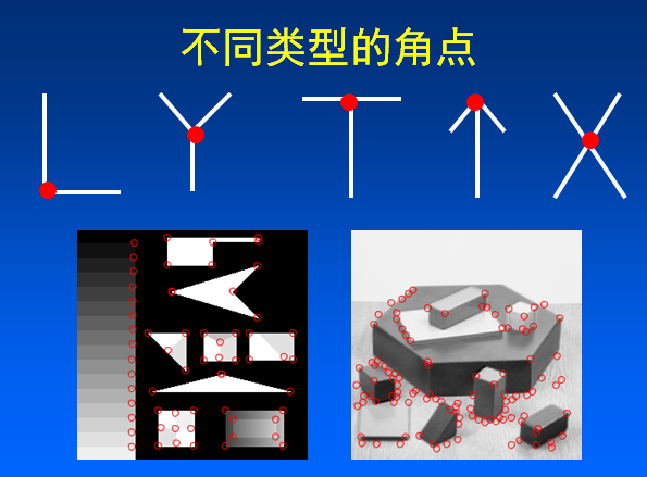
33 | ### 3.图像梯度
34 | “*像素值发生很大变化*”这一现象可以用图像梯度进行描述。在图像局部内,图像梯度越大表示该局部内像素值变化越大(灰度的变化率越大)。
35 | 而图像的梯度在数学上可用**微分或者导数**来表示。对于数字图像来说,相当于是**二维离散函数求梯度**,并使用差分来近似导数:
36 | $G_x(x,y)=H(x+1,y)-H(x-1,y)$
37 | $G_y(x,y)=H(x,y+1)-H(x,y-1)$
38 | 在实际操作中,对图像求梯度通常是考虑图像的每个像素的某个邻域内的灰度变化,因此通常对原始图像中像素某个邻域设置梯度算子,然后采用小区域模板进行卷积来计算,常用的有Prewitt算子、Sobel算子、Robinson算子、Laplace算子等。
39 |
40 | ### 1.4.2 Harris角点检测算法原理
41 | ### 1. 算法思想
42 | 算法的核心是利用局部窗口在图像上进行移动,判断灰度是否发生较大的变化。如果窗口内的灰度值(在梯度图上)都有较大的变化,那么这个窗口所在区域就存在角点。
43 |
44 | 这样就可以将 Harris 角点检测算法分为以下三步:
45 |
46 | * 当窗口(局部区域)同时向 x (水平)和 y(垂直) 两个方向移动时,计算窗口内部的像素值变化量 $E(x,y)$ ;
47 | * 对于每个窗口,都计算其对应的一个角点响应函数 $R$;
48 | * 然后对该函数进行阈值处理,如果 $R > threshold$,表示该窗口对应一个角点特征。
49 |
50 | ### 2. 第一步 — 建立数学模型
51 |
52 | **第一步是通过建立数学模型,确定哪些窗口会引起较大的灰度值变化。**
53 | 让一个窗口的中心位于灰度图像的一个位置$(x,y)$,这个位置的像素灰度值为$I(x,y)$ ,如果这个窗口分别向 $x$ 和 $y$ 方向移动一个小的位移$u$和$v$,到一个新的位置 $(x+u,y+v)$ ,这个位置的像素灰度值就是$I(x+u,y+v)$ 。
54 |
55 | $|I(x+u,y+v)-I(x,y)|$就是窗口移动引起的灰度值的变化值。
56 |
57 | 设$w(x,y)$为位置$(x,y)$处的窗口函数,表示窗口内各像素的权重,最简单的就是把窗口内所有像素的权重都设为1,即一个均值滤波核。
58 |
59 | 当然,也可以把 $w(x,y)$设定为以窗口中心为原点的高斯分布,即一个高斯核。如果窗口中心点像素是角点,那么窗口移动前后,中心点的灰度值变化非常强烈,所以该点权重系数应该设大一点,表示该点对灰度变化的贡献较大;而离窗口中心(角点)较远的点,这些点的灰度变化比较小,于是将权重系数设小一点,表示该点对灰度变化的贡献较小。
60 |
61 | 则窗口在各个方向上移动 $(u,v)$所造成的像素灰度值的变化量公式如下:
62 |
63 | 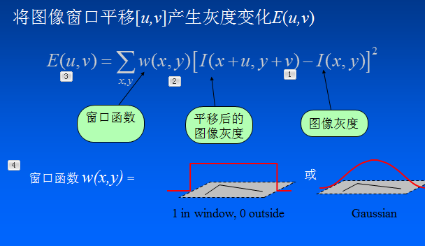
64 | 若窗口内是一个角点,则$E(u,v)$的计算结果将会很大。
65 |
66 | 为了提高计算效率,对上述公式进行简化,利用泰勒级数展开来得到这个公式的近似形式:
67 |
68 | 对于二维的泰勒展开式公式为:
69 | $T(x,y)=f(u,v)+(x-u)f_x(u,v)+(y-v)f_y(u,v)+....$
70 |
71 | 则$I(x+u,y+v)$ 为:
72 | $I(x+u,y+v)=I(x,y)+uI_x+vI_y$
73 |
74 | 其中$I_x$和$I_y$是$I$的微分(偏导),在图像中就是求$x$ 和 $y$ 方向的**梯度图**:
75 |
76 | $I_x=\frac{\partial I(x,y)}{\partial x}$
77 |
78 | $I_y=\frac{\partial I(x,y)}{\partial y}$
79 |
80 | 将$I(x+u,y+v)=I(x,y)+uI_x+vI_y$代入$E(u,v)$可得:
81 |
82 | 
83 |
84 | 提出 u 和 v ,得到最终的近似形式:
85 | 
86 |
87 | 其中矩阵M为:
88 |
89 | 
90 |
91 | 最后是把实对称矩阵对角化处理后的结果,可以把R看成旋转因子,其不影响两个正交方向的变化分量。
92 |
93 | 经对角化处理后,将两个正交方向的变化分量提取出来,就是 λ1 和 λ2(特征值)。
94 | 这里利用了**线性代数中的实对称矩阵对角化**的相关知识,有兴趣的同学可以进一步查阅相关资料。
95 |
96 |
97 | ### 3. 第二步—角点响应函数R
98 | 现在我们已经得到 $E(u,v)$的最终形式,别忘了我们的目的是要找到会引起较大的灰度值变化的那些窗口。
99 |
100 | 灰度值变化的大小则取决于矩阵M,M为梯度的协方差矩阵。在实际应用中为了能够应用更好的编程,所以定义了角点响应函数R,通过判定R大小来判断像素是否为角点。
101 |
102 | 计算每个窗口对应的得分(角点响应函数R定义):
103 | 
104 | 其中 $det(M)=\lambda_1\lambda_2$是矩阵的行列式, $trace(M)=\lambda_1+\lambda_2$ 是矩阵的迹。
105 |
106 | $λ1$ 和 $λ2$ 是矩阵$M$的特征值, $k$是一个经验常数,在范围 (0.04, 0.06) 之间。
107 |
108 | $R$的值取决于$M$的特征值,对于角点$|R|$很大,平坦的区域$|R|$很小,边缘的$R$为负值。
109 |
110 | ### 4. 第三步—角点判定
111 | 根据 R 的值,将这个窗口所在的区域划分为平面、边缘或角点。为了得到最优的角点,我们还可以使用非极大值抑制。
112 |
113 | 注意:Harris 检测器具有旋转不变性,但不具有尺度不变性,也就是说尺度变化可能会导致角点变为边缘。想要尺度不变特性的话,可以关注SIFT特征。
114 |
115 | 因为特征值 λ1 和 λ2 决定了 R 的值,所以我们可以用特征值来决定一个窗口是平面、边缘还是角点:
116 |
117 | * 平面::该窗口在平坦区域上滑动,窗口内的灰度值基本不会发生变化,所以 $|R|$ 值非常小,在水平和竖直方向的变化量均较小,即 $I_x$和 $I_y$都较小,那么 λ1 和 λ2 都较小;
118 | * 边缘:$|R|$值为负数,仅在水平或竖直方向有较大的变化量,即 $I_x$和 $I_y$只有一个较大,也就是 λ1>>λ2 或 λ2>>λ1;
119 | * 角点:[公式] 值很大,在水平、竖直两个方向上变化均较大的点,即 $I_x$和 $I_y$ 都较大,也就是 λ1 和 λ2 都很大。
120 |
121 | 如下图所示:
122 |
123 | 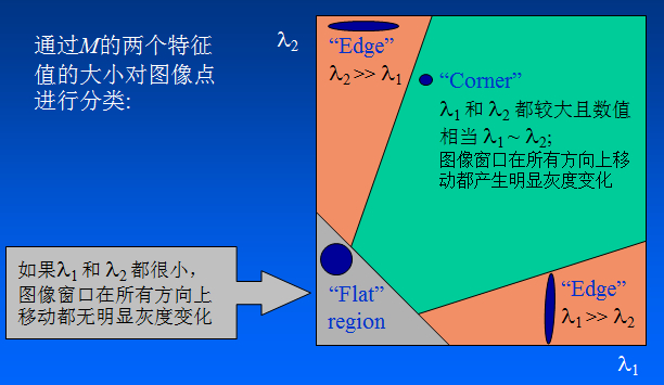
124 |
125 | Harris 角点检测的结果是带有这些分数 R 的灰度图像,设定一个阈值,分数大于这个阈值的像素就对应角点。
126 | ## 1.5 基于OpenCV的实现
127 |
128 | ### 1. API
129 | 在opencv中有提供实现 Harris 角点检测的函数 cv2.cornerHarris,我们直接调用的就可以,非常方便。
130 |
131 | 函数原型:`cv2.cornerHarris(src, blockSize, ksize, k[, dst[, borderType]])`
132 |
133 | 对于每一个像素 (x,y),在 (blockSize x blockSize) 邻域内,计算梯度图的协方差矩阵 $M(x,y)$,然后通过上面第二步中的角点响应函数得到结果图。图像中的角点可以为该结果图的局部最大值。
134 |
135 | 即可以得到输出图中的局部最大值,这些值就对应图像中的角点。
136 |
137 | 参数解释:
138 | * src - 输入灰度图像,float32类型
139 | * blockSize - 用于角点检测的邻域大小,就是上面提到的窗口的尺寸
140 | * ksize - 用于计算梯度图的Sobel算子的尺寸
141 | * k - 用于计算角点响应函数的参数k,取值范围常在0.04~0.06之间
142 |
143 | ### 代码示例
144 | ```python
145 | import cv2 as cv
146 | from matplotlib import pyplot as plt
147 | import numpy as np
148 |
149 | # detector parameters
150 | block_size = 3
151 | sobel_size = 3
152 | k = 0.06
153 |
154 | image = cv.imread('Scenery.jpg')
155 |
156 | print(image.shape)
157 | height = image.shape[0]
158 | width = image.shape[1]
159 | channels = image.shape[2]
160 | print("width: %s height: %s channels: %s"%(width, height, channels))
161 |
162 | gray_img = cv.cvtColor(image, cv2.COLOR_BGR2GRAY)
163 |
164 |
165 | # modify the data type setting to 32-bit floating point
166 | gray_img = np.float32(gray_img)
167 |
168 | # detect the corners with appropriate values as input parameters
169 | corners_img = cv.cornerHarris(gray_img, block_size, sobel_size, k)
170 |
171 | # result is dilated for marking the corners, not necessary
172 | kernel = cv2.getStructuringElement(cv2.MORPH_RECT,(3, 3))
173 | dst = cv.dilate(corners_img, kernel)
174 |
175 | # Threshold for an optimal value, marking the corners in Green
176 | #image[corners_img>0.01*corners_img.max()] = [0,0,255]
177 |
178 | for r in range(height):
179 | for c in range(width):
180 | pix=dst[r,c]
181 | if pix>0.05*dst.max():
182 | cv2.circle(image,(c,r),5,(0,0,255),0)
183 |
184 | image = cv.cvtColor(image, cv2.COLOR_BGR2RGB)
185 | plt.imshow(image)
186 | plt.show()
187 | ```
188 |
189 | ### 结果:
190 | 
191 | 
192 |
193 |
194 | ## 1.6 总结
195 | 本小节对Harris角点检测算法进行了学习。通过这次学习我们了解了角点的概念、图像梯度等基本知识,也认识了基本的角点检测算法思想。
196 |
197 | Harris角点检测的性质可总结如下:
198 | * **阈值决定角点的数量**
199 | * **Harris角点检测算子对亮度和对比度的变化不敏感(光照不变性)**
200 | 在进行Harris角点检测时,使用了微分算子对图像进行微分运算,而微分运算对图像密度的拉升或收缩和对亮度的抬高或下降不敏感。换言之,对亮度和对比度的仿射变换并不改变Harris响应的极值点出现的位置,但是,由于阈值的选择,可能会影响角点检测的数量。
201 | 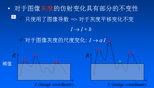
202 |
203 |
204 | * **Harris角点检测算子具有旋转不变性**
205 | Harris角点检测算子使用的是角点附近的区域灰度二阶矩矩阵。而二阶矩矩阵可以表示成一个椭圆,椭圆的长短轴正是二阶矩矩阵特征值平方根的倒数。当特征椭圆转动时,特征值并不发生变化,所以判断角点响应值也不发生变化,由此说明Harris角点检测算子具有旋转不变性。
206 | 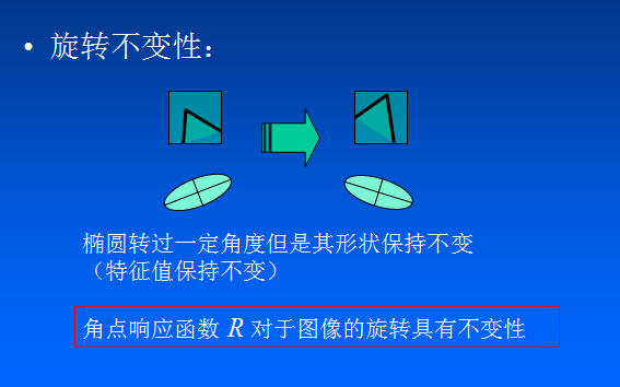
207 |
208 | * **Harris角点检测算子不具有尺度不变性**
209 | 尺度的变化会将角点变为边缘,或者边缘变为角点,Harris的理论基础并不具有尺度不变性。
210 | 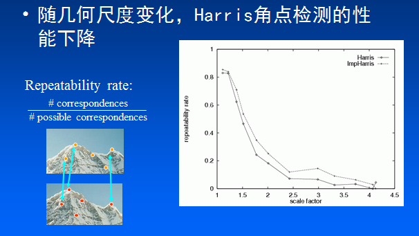
211 | ## 相关技术文档、论文推荐
212 | * [论文:《C.Harris, M.Stephens. “A Combined Corner and Edge Detector”. Proc. of 4th Alvey Vision Conference》](http://citeseerx.ist.psu.edu/viewdoc/download?doi=10.1.1.434.4816&rep=rep1&type=pdf)
213 | * [Harris角点算法](https://www.cnblogs.com/polly333/p/5416172.html)
214 | * [角点检测:Harris 与 Shi-Tomasi](https://zhuanlan.zhihu.com/p/83064609)
215 | * [https://www.cnblogs.com/ronny/p/4009425.html](https://www.cnblogs.com/ronny/p/4009425.html)
216 |
217 | ---
218 | **Task01 Harris特征点检测 END.**
219 |
220 | --- ***By: 小武***
221 |
222 |
223 | >博客:[https://blog.csdn.net/weixin_40647819](https://blog.csdn.net/weixin_40647819)
224 |
225 |
226 | **关于Datawhale**:
227 |
228 | >Datawhale是一个专注于数据科学与AI领域的开源组织,汇集了众多领域院校和知名企业的优秀学习者,聚合了一群有开源精神和探索精神的团队成员。Datawhale以“for the learner,和学习者一起成长”为愿景,鼓励真实地展现自我、开放包容、互信互助、敢于试错和勇于担当。同时Datawhale 用开源的理念去探索开源内容、开源学习和开源方案,赋能人才培养,助力人才成长,建立起人与人,人与知识,人与企业和人与未来的联结。
229 |
230 |
--------------------------------------------------------------------------------
/ImageProcessingFundamentals/03 彩色空间互转.md:
--------------------------------------------------------------------------------
1 | # 03 彩色空间互转
2 |
3 | ## 3.1 简介
4 |
5 | 图像彩色空间互转在图像处理中应用非常广泛,而且很多算法只对灰度图有效;另外,相比RGB,其他颜色空间(比如HSV、HSI)更具可分离性和可操作性,所以很多图像算法需要将图像从RGB转为其他颜色空间,所以图像彩色互转是十分重要和关键的。
6 |
7 |
8 | ## 3.2 学习目标
9 |
10 | * 了解相关颜色空间的基础知识
11 | * 理解彩色空间互转的理论
12 | * 掌握OpenCV框架下颜色空间互转API的使用
13 |
14 | ## 3.3 内容介绍
15 |
16 | 1.相关颜色空间的原理介绍
17 |
18 | 2.颜色空间互转理论的介绍
19 |
20 | 3.OpenCV代码实践
21 |
22 | 4.动手实践并打卡(读者完成)
23 |
24 | ## 3.4 算法理论介绍与资料推荐
25 |
26 | ### 3.4.1 RGB与灰度图互转
27 |
28 | RGB(红绿蓝)是依据人眼识别的颜色定义出的空间,可表示大部分颜色。但在科学研究一般不采用RGB颜色空间,因为它的细节难以进行数字化的调整。它将色调,亮度,饱和度三个量放在一起表示,很难分开。它是最通用的面向硬件的彩色模型。该模型用于彩色监视器和一大类彩色视频摄像。
29 |
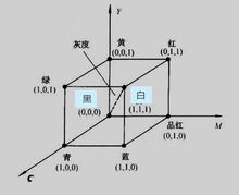
30 | RGB颜色空间 基于颜色的加法混色原理,从黑色不断叠加Red,Green,Blue的颜色,最终可以得到白色,如图:
31 |
32 |
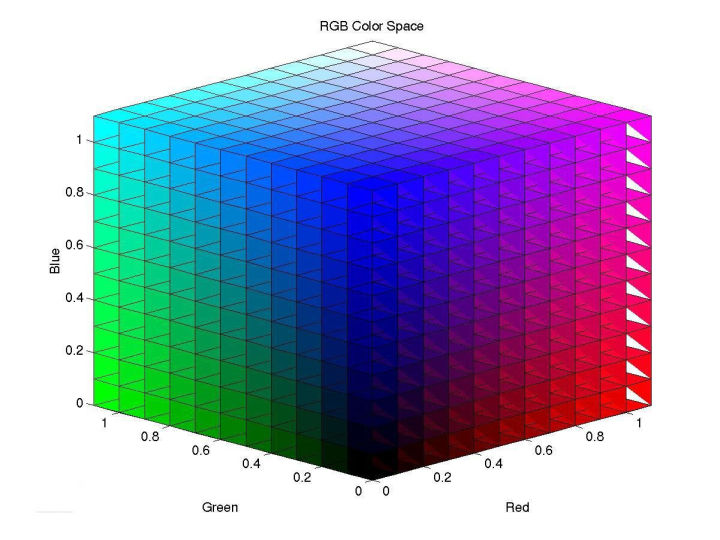
33 | 将R、G、B三个通道作为笛卡尔坐标系中的X、Y、Z轴,就得到了一种对于颜色的空间描述,如图:
34 |
35 |
36 |
37 |
38 | **对于彩色图转灰度图,有一个很著名的心理学公式:**
39 |
40 | Gray = R * 0.299 + G * 0.587 + B * 0.114
41 |
42 |
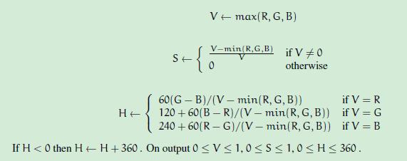
43 | ### 3.4.2 RGB与HSV互转
44 |
45 | HSV是一种将RGB色彩空间中的点在倒圆锥体中的表示方法。HSV即色相(Hue)、饱和度(Saturation)、明度(Value),又称HSB(B即Brightness)。色相是色彩的基本属性,就是平常说的颜色的名称,如红色、黄色等。饱和度(S)是指色彩的纯度,越高色彩越纯,低则逐渐变灰,取0-100%的数值。明度(V),取0-max(计算机中HSV取值范围和存储的长度有关)。HSV颜色空间可以用一个圆锥空间模型来描述。圆锥的顶点处,V=0,H和S无定义,代表黑色。圆锥的顶面中心处V=max,S=0,H无定义,代表白色。
46 |
47 | RGB颜色空间中,三种颜色分量的取值与所生成的颜色之间的联系并不直观。而HSV颜色空间,更类似于人类感觉颜色的方式,封装了关于颜色的信息:“这是什么颜色?深浅如何?明暗如何?
48 |
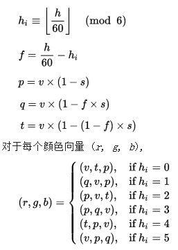
49 | #### HSV模型
50 |