├── 01_encoding_decoding_ckks.ipynb
├── README.md
└── images
├── discrete_gaussian.PNG
├── encryption_decryption.PNG
├── overview_ckks.PNG
└── roots.PNG
/01_encoding_decoding_ckks.ipynb:
--------------------------------------------------------------------------------
1 | {
2 | "cells": [
3 | {
4 | "cell_type": "markdown",
5 | "metadata": {},
6 | "source": [
7 | "# Introduction to encoding in CKKS"
8 | ]
9 | },
10 | {
11 | "cell_type": "markdown",
12 | "metadata": {},
13 | "source": [
14 | "CKKS exploits the rich structure of integer polynomial rings for its plaintext and ciphertext spaces. Nonetheless, data comes more often in the form of vectors than polynomials.\n",
15 | "\n",
16 | "Therefore it becomes necessary to encode our input $z \\in \\mathbb{C}^{N/2}$, into a polynomial $m(X) \\in \\mathbb{Z}[X]/(X^N + 1)$. \n",
17 | "\n",
18 | "We will denote by $N$ the degree of our polynomial degree modulus, which will be a power of 2. We denote by $\\Phi_M(X) = X^N + 1$ the $m$-th [cyclotomic polynomial](https://en.wikipedia.org/wiki/Cyclotomic_polynomial) (note that $M=2N$). The plaintext space will be the polynomial ring $\\mathcal{R} = \\mathbb{Z}[X]/(X^N + 1)$. Let us denote by $\\xi_M$, the $M$-th root of unity : $\\xi_M = e^{2 i \\pi / M}$.\n",
19 | "\n",
20 | "To understand how we can encode a vector into a polynomial, and how the computation performed on the polynomial will be reflected in the underlying vector, we will first see a vanilla example, where we simply encode a vector $z \\in \\mathbb{C}^{N}$ into a polynomial $m(X) \\in \\mathbb{C}[X]/(X^N + 1)$. Then we will cover the actual encoding of CKKS, which takes a vector $z \\in \\mathbb{C}^{N/2}$, and encodes it in a polynomial $m(X) \\in \\mathbb{Z}[X]/(X^N + 1)$.\n",
21 | "\n",
22 | "## Vanilla encoding\n",
23 | "\n",
24 | "Here we will cover the simple case of encoding $z \\in \\mathbb{C}^{N}$, into a polynomial $m(X) \\in \\mathbb{C}[X]/(X^N + 1)$. \n",
25 | "\n",
26 | "To do so, we will use the [canonical embedding](https://en.wikipedia.org/wiki/Embedding) $\\sigma : \\mathbb{C}[X]/(X^N +1) \\rightarrow \\mathbb{C}^N$, which will serve to decode and encode our vectors.\n",
27 | "\n",
28 | "The idea is simple, to decode a polynomial $m(X)$ into a vector $z$, we will simply evaluate the polynomial on certain values, which will be the roots of the cyclotomic polynomial $\\Phi_M(X) = X^N + 1$. Those $N$ roots are : $\\xi, \\xi^3, ..., \\xi^{2 N - 1}$. \n",
29 | "\n",
30 | "So to decode a polynomial $m(X)$, we will simply define $\\sigma(m) = (m(\\xi), m(\\xi^3), ..., m(\\xi^{2 N - 1})) \\in \\mathbb{C}^N$. Note that $\\sigma$ defines an isomorphism, which means it is a bijective homomorphism, therefore any vector will be uniquely encoded into its corresponding polynomial, and vice-versa.\n",
31 | "\n",
32 | "The tricky part is the encoding of a vector $z \\in \\mathbb{C}^N$ into the corresponding polynomial, which means computing the inverse $\\sigma^{-1}$. The problem is therefore to find a polynomial $m(X) = \\sum_{i=0}^{N-1} \\alpha_i X^i \\in \\mathbb{C}[X]/(X^N + 1)$, given a vector $z \\in \\mathbb{C}^N$, such that $\\sigma(m) = (m(\\xi), m(\\xi^3), ..., m(\\xi^{2 N - 1})) = (z_1,...,z_N)$.\n",
33 | "\n",
34 | "Nonetheless, if we write this down, this means that we have the following system : \n",
35 | "\n",
36 | "$\\sum_{j=0}^{N-1} \\alpha_j (\\xi^{2 i - 1})^j = z_i, i=1,...,N$.\n",
37 | "\n",
38 | "This can be viewed as a linear equation : \n",
39 | "\n",
40 | "$A \\alpha = z$, with $A$ the [Vandermonde matrix](https://en.wikipedia.org/wiki/Vandermonde_matrix) of the $(\\xi^{2 i -1})_{i=1,...,N}$, $\\alpha$ the vector of the polynomial coefficients, and $z$ the vector we want to encode.\n",
41 | "\n",
42 | "Therefore we have that : $\\alpha = A^{-1} z$, and that $\\sigma^{-1}(z) = \\sum_{i=0}^{N-1} \\alpha_i X^i \\in \\mathbb{C}[X]/(X^N + 1)$."
43 | ]
44 | },
45 | {
46 | "cell_type": "markdown",
47 | "metadata": {},
48 | "source": [
49 | "### Example"
50 | ]
51 | },
52 | {
53 | "cell_type": "markdown",
54 | "metadata": {},
55 | "source": [
56 | "We will see an example now to better understand what this means.\n",
57 | "\n",
58 | "Let $M = 8$, $N = \\frac{M}{2}= 4$, $\\Phi_M(X) = X^4 + 1$, and $\\omega = e^{\\frac{2 i \\pi}{8}} = e^{\\frac{i \\pi}{4}}$.\n",
59 | "Our goal here is to encode the following vectors : $[1, 2, 3, 4]$ and $[-1, -2, -3, -4]$, decode them, add and multiply their polynomial and decode it."
60 | ]
61 | },
62 | {
63 | "cell_type": "markdown",
64 | "metadata": {
65 | "ExecuteTime": {
66 | "end_time": "2020-05-19T12:37:43.119584Z",
67 | "start_time": "2020-05-19T12:37:42.812917Z"
68 | }
69 | },
70 | "source": [
71 | "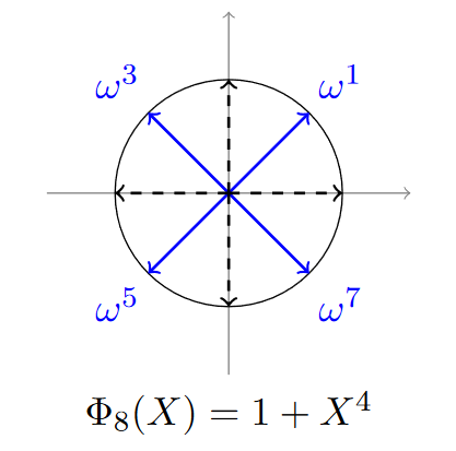\n",
72 | "Roots of $X^4 + 1$ (source : Cryptography from Rings, HEAT summer school 2016)"
73 | ]
74 | },
75 | {
76 | "cell_type": "markdown",
77 | "metadata": {},
78 | "source": [
79 | "As we saw, in order to decode a polynomial, we simply need to evaluate it on powers of an $M$-th root of unity. Here we choose $\\xi_M = \\omega = e^{\\frac{i \\pi}{4}}$.\n",
80 | "\n",
81 | "Once we have $\\xi$ and $M$, we can define both $\\sigma$ and its inverse $\\sigma^{-1}$, respectively the decoding and the encoding."
82 | ]
83 | },
84 | {
85 | "cell_type": "code",
86 | "execution_count": 1,
87 | "metadata": {
88 | "ExecuteTime": {
89 | "end_time": "2020-05-23T17:09:55.396205Z",
90 | "start_time": "2020-05-23T17:09:55.177934Z"
91 | }
92 | },
93 | "outputs": [
94 | {
95 | "data": {
96 | "text/plain": [
97 | "(0.7071067811865476+0.7071067811865475j)"
98 | ]
99 | },
100 | "execution_count": 1,
101 | "metadata": {},
102 | "output_type": "execute_result"
103 | }
104 | ],
105 | "source": [
106 | "import numpy as np\n",
107 | "\n",
108 | "# First we set the parameters\n",
109 | "M = 8\n",
110 | "N = M //2\n",
111 | "\n",
112 | "# We set xi, which will be used in our computations\n",
113 | "xi = np.exp(2 * np.pi * 1j / M)\n",
114 | "xi"
115 | ]
116 | },
117 | {
118 | "cell_type": "code",
119 | "execution_count": 2,
120 | "metadata": {
121 | "ExecuteTime": {
122 | "end_time": "2020-05-23T17:09:55.414687Z",
123 | "start_time": "2020-05-23T17:09:55.402321Z"
124 | }
125 | },
126 | "outputs": [],
127 | "source": [
128 | "from numpy.polynomial import Polynomial\n",
129 | "\n",
130 | "class CKKSEncoder:\n",
131 | " \"\"\"Basic CKKS encoder to encode complex vectors into polynomials.\"\"\"\n",
132 | " \n",
133 | " def __init__(self, M: int):\n",
134 | " \"\"\"Initialization of the encoder for M a power of 2. \n",
135 | " \n",
136 | " xi, which is an M-th root of unity will, be used as a basis for our computations.\n",
137 | " \"\"\"\n",
138 | " self.xi = np.exp(2 * np.pi * 1j / M)\n",
139 | " self.M = M\n",
140 | " \n",
141 | " @staticmethod\n",
142 | " def vandermonde(xi: np.complex128, M: int) -> np.array:\n",
143 | " \"\"\"Computes the Vandermonde matrix from a m-th root of unity.\"\"\"\n",
144 | " \n",
145 | " N = M //2\n",
146 | " matrix = []\n",
147 | " # We will generate each row of the matrix\n",
148 | " for i in range(N):\n",
149 | " # For each row we select a different root\n",
150 | " root = xi ** (2 * i + 1)\n",
151 | " row = []\n",
152 | "\n",
153 | " # Then we store its powers\n",
154 | " for j in range(N):\n",
155 | " row.append(root ** j)\n",
156 | " matrix.append(row)\n",
157 | " return matrix\n",
158 | " \n",
159 | " def sigma_inverse(self, b: np.array) -> Polynomial:\n",
160 | " \"\"\"Encodes the vector b in a polynomial using an M-th root of unity.\"\"\"\n",
161 | "\n",
162 | " # First we create the Vandermonde matrix\n",
163 | " A = CKKSEncoder.vandermonde(self.xi, M)\n",
164 | "\n",
165 | " # Then we solve the system\n",
166 | " coeffs = np.linalg.solve(A, b)\n",
167 | "\n",
168 | " # Finally we output the polynomial\n",
169 | " p = Polynomial(coeffs)\n",
170 | " return p\n",
171 | "\n",
172 | " def sigma(self, p: Polynomial) -> np.array:\n",
173 | " \"\"\"Decodes a polynomial by applying it to the M-th roots of unity.\"\"\"\n",
174 | "\n",
175 | " outputs = []\n",
176 | " N = self.M //2\n",
177 | "\n",
178 | " # We simply apply the polynomial on the roots\n",
179 | " for i in range(N):\n",
180 | " root = self.xi ** (2 * i + 1)\n",
181 | " output = p(root)\n",
182 | " outputs.append(output)\n",
183 | " return np.array(outputs)"
184 | ]
185 | },
186 | {
187 | "cell_type": "markdown",
188 | "metadata": {},
189 | "source": [
190 | "Now we can start experimenting with real values, let's first encode a vector and see how it is encoded."
191 | ]
192 | },
193 | {
194 | "cell_type": "code",
195 | "execution_count": 3,
196 | "metadata": {
197 | "ExecuteTime": {
198 | "end_time": "2020-05-23T17:09:55.436335Z",
199 | "start_time": "2020-05-23T17:09:55.420552Z"
200 | }
201 | },
202 | "outputs": [],
203 | "source": [
204 | "# First we initialize our encoder\n",
205 | "encoder = CKKSEncoder(M)"
206 | ]
207 | },
208 | {
209 | "cell_type": "code",
210 | "execution_count": 4,
211 | "metadata": {
212 | "ExecuteTime": {
213 | "end_time": "2020-05-23T17:09:55.453314Z",
214 | "start_time": "2020-05-23T17:09:55.442307Z"
215 | }
216 | },
217 | "outputs": [
218 | {
219 | "data": {
220 | "text/plain": [
221 | "array([1, 2, 3, 4])"
222 | ]
223 | },
224 | "execution_count": 4,
225 | "metadata": {},
226 | "output_type": "execute_result"
227 | }
228 | ],
229 | "source": [
230 | "b = np.array([1, 2, 3, 4])\n",
231 | "b"
232 | ]
233 | },
234 | {
235 | "cell_type": "markdown",
236 | "metadata": {},
237 | "source": [
238 | "Let's encode the vector now."
239 | ]
240 | },
241 | {
242 | "cell_type": "code",
243 | "execution_count": 5,
244 | "metadata": {
245 | "ExecuteTime": {
246 | "end_time": "2020-05-23T17:09:55.469589Z",
247 | "start_time": "2020-05-23T17:09:55.459420Z"
248 | }
249 | },
250 | "outputs": [
251 | {
252 | "data": {
253 | "text/latex": [
254 | "$x \\mapsto \\text{(2.5+4.440892098500626e-16j)} + (\\text{(-4.996003610813204e-16+0.7071067811865479j)})\\,x + (\\text{(-3.4694469519536176e-16+0.5000000000000003j)})\\,x^{2} + (\\text{(-8.326672684688674e-16+0.7071067811865472j)})\\,x^{3}$"
255 | ],
256 | "text/plain": [
257 | "Polynomial([ 2.50000000e+00+4.44089210e-16j, -4.99600361e-16+7.07106781e-01j,\n",
258 | " -3.46944695e-16+5.00000000e-01j, -8.32667268e-16+7.07106781e-01j], domain=[-1, 1], window=[-1, 1])"
259 | ]
260 | },
261 | "execution_count": 5,
262 | "metadata": {},
263 | "output_type": "execute_result"
264 | }
265 | ],
266 | "source": [
267 | "p = encoder.sigma_inverse(b)\n",
268 | "p"
269 | ]
270 | },
271 | {
272 | "cell_type": "markdown",
273 | "metadata": {},
274 | "source": [
275 | "Let's see now how we can extract the vector we had initially from the polynomial: "
276 | ]
277 | },
278 | {
279 | "cell_type": "code",
280 | "execution_count": 6,
281 | "metadata": {
282 | "ExecuteTime": {
283 | "end_time": "2020-05-23T17:09:55.486646Z",
284 | "start_time": "2020-05-23T17:09:55.475335Z"
285 | }
286 | },
287 | "outputs": [
288 | {
289 | "data": {
290 | "text/plain": [
291 | "array([1.-1.11022302e-16j, 2.-4.71844785e-16j, 3.+2.77555756e-17j,\n",
292 | " 4.+2.22044605e-16j])"
293 | ]
294 | },
295 | "execution_count": 6,
296 | "metadata": {},
297 | "output_type": "execute_result"
298 | }
299 | ],
300 | "source": [
301 | "b_reconstructed = encoder.sigma(p)\n",
302 | "b_reconstructed"
303 | ]
304 | },
305 | {
306 | "cell_type": "markdown",
307 | "metadata": {},
308 | "source": [
309 | "We can see that the reconstruction and the initial vector are very close."
310 | ]
311 | },
312 | {
313 | "cell_type": "code",
314 | "execution_count": 7,
315 | "metadata": {
316 | "ExecuteTime": {
317 | "end_time": "2020-05-23T17:09:55.507427Z",
318 | "start_time": "2020-05-23T17:09:55.491379Z"
319 | }
320 | },
321 | "outputs": [
322 | {
323 | "data": {
324 | "text/plain": [
325 | "6.944442800358888e-16"
326 | ]
327 | },
328 | "execution_count": 7,
329 | "metadata": {},
330 | "output_type": "execute_result"
331 | }
332 | ],
333 | "source": [
334 | "np.linalg.norm(b_reconstructed - b)"
335 | ]
336 | },
337 | {
338 | "cell_type": "markdown",
339 | "metadata": {},
340 | "source": [
341 | "As stated before, $\\sigma$ is not chosen randomly to encode and decode, but has a lot of nice properties. Among them, $\\sigma$ is an isomorphism, therefore addition and multiplication on polynomials will result in coefficient wise addition and multiplication on the encoded vectors.\n",
342 | "\n",
343 | "The homomorphic property of $\\sigma$ is due to the fact that $X^N = 1$ and $\\xi^N = 1$.\n",
344 | "\n",
345 | "We can now start to encode several vectors, and see how we can perform homomorphic operations on them and decode it."
346 | ]
347 | },
348 | {
349 | "cell_type": "code",
350 | "execution_count": 8,
351 | "metadata": {
352 | "ExecuteTime": {
353 | "end_time": "2020-05-23T17:09:55.519400Z",
354 | "start_time": "2020-05-23T17:09:55.512068Z"
355 | }
356 | },
357 | "outputs": [],
358 | "source": [
359 | "m1 = np.array([1, 2, 3, 4])\n",
360 | "m2 = np.array([1, -2, 3, -4])"
361 | ]
362 | },
363 | {
364 | "cell_type": "code",
365 | "execution_count": 9,
366 | "metadata": {
367 | "ExecuteTime": {
368 | "end_time": "2020-05-23T17:09:55.533113Z",
369 | "start_time": "2020-05-23T17:09:55.522145Z"
370 | }
371 | },
372 | "outputs": [],
373 | "source": [
374 | "p1 = encoder.sigma_inverse(m1)\n",
375 | "p2 = encoder.sigma_inverse(m2)"
376 | ]
377 | },
378 | {
379 | "cell_type": "markdown",
380 | "metadata": {},
381 | "source": [
382 | "We can see that addition is pretty straightforward."
383 | ]
384 | },
385 | {
386 | "cell_type": "code",
387 | "execution_count": 10,
388 | "metadata": {
389 | "ExecuteTime": {
390 | "end_time": "2020-05-23T17:09:55.554656Z",
391 | "start_time": "2020-05-23T17:09:55.535927Z"
392 | }
393 | },
394 | "outputs": [
395 | {
396 | "data": {
397 | "text/latex": [
398 | "$x \\mapsto \\text{(2.0000000000000004+1.1102230246251565e-16j)} + (\\text{(-0.7071067811865477+0.707106781186547j)})\\,x + (\\text{(2.1094237467877966e-15-1.9999999999999996j)})\\,x^{2} + (\\text{(0.7071067811865466+0.707106781186549j)})\\,x^{3}$"
399 | ],
400 | "text/plain": [
401 | "Polynomial([ 2.00000000e+00+1.11022302e-16j, -7.07106781e-01+7.07106781e-01j,\n",
402 | " 2.10942375e-15-2.00000000e+00j, 7.07106781e-01+7.07106781e-01j], domain=[-1., 1.], window=[-1., 1.])"
403 | ]
404 | },
405 | "execution_count": 10,
406 | "metadata": {},
407 | "output_type": "execute_result"
408 | }
409 | ],
410 | "source": [
411 | "p_add = p1 + p2\n",
412 | "p_add"
413 | ]
414 | },
415 | {
416 | "cell_type": "markdown",
417 | "metadata": {},
418 | "source": [
419 | "Here as expected, we see that p1 + p2 decodes correctly to $[2, 0, 6, 0]$."
420 | ]
421 | },
422 | {
423 | "cell_type": "code",
424 | "execution_count": 11,
425 | "metadata": {
426 | "ExecuteTime": {
427 | "end_time": "2020-05-23T17:09:55.570005Z",
428 | "start_time": "2020-05-23T17:09:55.559203Z"
429 | }
430 | },
431 | "outputs": [
432 | {
433 | "data": {
434 | "text/plain": [
435 | "array([2.0000000e+00+3.25176795e-17j, 4.4408921e-16-4.44089210e-16j,\n",
436 | " 6.0000000e+00+1.11022302e-16j, 4.4408921e-16+3.33066907e-16j])"
437 | ]
438 | },
439 | "execution_count": 11,
440 | "metadata": {},
441 | "output_type": "execute_result"
442 | }
443 | ],
444 | "source": [
445 | "encoder.sigma(p_add)"
446 | ]
447 | },
448 | {
449 | "cell_type": "markdown",
450 | "metadata": {},
451 | "source": [
452 | "Because when doing multiplication we might have terms whose degree is higher than $N$, we will need to do a modulo operation using $X^N + 1$."
453 | ]
454 | },
455 | {
456 | "cell_type": "markdown",
457 | "metadata": {},
458 | "source": [
459 | "To perform multiplication, we first need to define the polynomial modulus which we will use."
460 | ]
461 | },
462 | {
463 | "cell_type": "code",
464 | "execution_count": 12,
465 | "metadata": {
466 | "ExecuteTime": {
467 | "end_time": "2020-05-23T17:09:55.586175Z",
468 | "start_time": "2020-05-23T17:09:55.572615Z"
469 | }
470 | },
471 | "outputs": [
472 | {
473 | "data": {
474 | "text/latex": [
475 | "$x \\mapsto \\text{1.0}\\color{LightGray}{ + \\text{0.0}\\,x}\\color{LightGray}{ + \\text{0.0}\\,x^{2}}\\color{LightGray}{ + \\text{0.0}\\,x^{3}} + \\text{1.0}\\,x^{4}$"
476 | ],
477 | "text/plain": [
478 | "Polynomial([1., 0., 0., 0., 1.], domain=[-1, 1], window=[-1, 1])"
479 | ]
480 | },
481 | "execution_count": 12,
482 | "metadata": {},
483 | "output_type": "execute_result"
484 | }
485 | ],
486 | "source": [
487 | "poly_modulo = Polynomial([1,0,0,0,1])\n",
488 | "poly_modulo"
489 | ]
490 | },
491 | {
492 | "cell_type": "markdown",
493 | "metadata": {},
494 | "source": [
495 | "Now we can perform multiplication."
496 | ]
497 | },
498 | {
499 | "cell_type": "code",
500 | "execution_count": 13,
501 | "metadata": {
502 | "ExecuteTime": {
503 | "end_time": "2020-05-23T17:09:55.598563Z",
504 | "start_time": "2020-05-23T17:09:55.588519Z"
505 | }
506 | },
507 | "outputs": [],
508 | "source": [
509 | "p_mult = p1 * p2 % poly_modulo"
510 | ]
511 | },
512 | {
513 | "cell_type": "markdown",
514 | "metadata": {},
515 | "source": [
516 | "Finally if we decode it, we can see that we have the expected result."
517 | ]
518 | },
519 | {
520 | "cell_type": "code",
521 | "execution_count": 14,
522 | "metadata": {
523 | "ExecuteTime": {
524 | "end_time": "2020-05-23T17:09:55.614745Z",
525 | "start_time": "2020-05-23T17:09:55.601665Z"
526 | }
527 | },
528 | "outputs": [
529 | {
530 | "data": {
531 | "text/plain": [
532 | "array([ 1.-8.67361738e-16j, -4.+6.86950496e-16j, 9.+6.86950496e-16j,\n",
533 | " -16.-9.08301212e-15j])"
534 | ]
535 | },
536 | "execution_count": 14,
537 | "metadata": {},
538 | "output_type": "execute_result"
539 | }
540 | ],
541 | "source": [
542 | "encoder.sigma(p_mult)"
543 | ]
544 | },
545 | {
546 | "cell_type": "markdown",
547 | "metadata": {},
548 | "source": [
549 | "## CKKS encoding\n",
550 | "\n",
551 | "Now that we saw how we can encode complex vectors into polynomials, let's see how it is done in CKKS.\n",
552 | "\n",
553 | "The difference with what we did previously, is that the plaintext space of the encoded polynomial is $\\mathcal{R} = \\mathbb{Z}[X]/(X^N + 1)$, therefore the coefficients of the polynomial of encoded values must have integer coefficients, and we saw before that it is not neccessarily the case.\n",
554 | "\n",
555 | "To solve this issue, one must first look at the image of the canonical embedding $\\sigma$ on $\\mathcal{R}$.\n",
556 | "\n",
557 | "Because polynomials in $\\mathcal{R}$ have integer coefficients, therefore real coefficients, and we evaluate them on complex roots, where half are the conjugates of the other (see the previous figure), we have that :\n",
558 | "$\\sigma(\\mathcal{R}) \\subseteq \\mathbb{H} = \\{z \\in \\mathbb{C}^{N} : z_j = \\overline{z_{-j}} \\}$. \n",
559 | "\n",
560 | "Recall the picture earlier when $M = 8$ :"
561 | ]
562 | },
563 | {
564 | "cell_type": "markdown",
565 | "metadata": {},
566 | "source": [
567 | "\n",
568 | "Roots of $X^4 + 1$ (source : Cryptography from Rings, HEAT summer school 2016)"
569 | ]
570 | },
571 | {
572 | "cell_type": "markdown",
573 | "metadata": {},
574 | "source": [
575 | "We can see on this picture that $\\omega^1 = \\overline{\\omega^7}$, and $\\omega^3 = \\overline{\\omega^5}$. In general, this means that because we evaluate a real polynomial on them, we will also have that for any polynomial $m(X) \\in \\mathcal{R}, m(\\xi^j) = \\overline{m(\\xi^{-j} )} = m(\\overline{\\xi^{-j}})$.\n",
576 | "\n",
577 | "Therefore, any element of $\\sigma(\\mathcal{R})$ is actually in a space of dimension $N/2$, not $N$. Therefore when we want to encode a vector in CKKS we use complex vectors of size $N/2$, then we need to expand them by copying the other half of conjugate roots.\n",
578 | "\n",
579 | "This operation, which takes an element of $\\mathbb{H}$ and projects it to $\\mathbb{C}^{N/2}$ is called $\\pi$ in the CKKS paper. Note that this defines a isomorphism as well. \n",
580 | "\n",
581 | "So now we can start with $z \\in \\mathbb{C}^{N/2}$, expand it using $\\pi^{-1}$ (note that $\\pi$ projects, $\\pi^{-1}$ expands), so we get $\\pi^{-1}(z) \\in \\mathbb{H}$.\n",
582 | "\n",
583 | "The problem that we have is that we cannot directly use $\\sigma : \\mathcal{R} = \\mathbb{Z}[X]/(X^N +1) \\rightarrow \\sigma(\\mathcal{R}) \\subseteq \\mathbb{H}$, because an element of $\\mathbb{H}$ is not necessarily in $\\sigma(\\mathcal{R})$. $\\sigma$ does define an isomorphism, but only from $\\mathcal{R}$ to $\\sigma(\\mathcal{R})$. To convince yourself that $\\sigma(\\mathcal{R})$ is not equal to $\\mathbb{H}$, you can notice that $\\mathcal{R}$ is countable, therefore $\\sigma(\\mathcal{R})$ as well, but $\\mathbb{H}$ is not, as it is isomorph to $\\mathbb{C}^{N/2}$.\n",
584 | "\n",
585 | "This detail is important, because it means that we must find a way to project $\\pi^{-1}(z)$ on $\\sigma(\\mathcal{R})$. To do so, we will use a technique called \"coordinate-wise random rounding\", defined in [A Toolkit for Ring-LWE Cryptography](https://web.eecs.umich.edu/~cpeikert/pubs/toolkit.pdf). \n",
586 | "\n",
587 | "The idea is simple, $\\mathcal{R}$ has an orthogonal $\\mathbb{Z}$-basis $\\{1,X,...,X^{N-1} \\}$, and given that $\\sigma$ is an isomorphism, $\\sigma(\\mathcal{R})$ has an orthogonal $\\mathbb{Z}$-basis $\\beta = (b_1,b_2,...,b_N) = (\\sigma(1),\\sigma(X),...,\\sigma(X^{N-1}) )$. Therefore for any $z \\in \\mathbb{H}$, we will simply project it on $\\beta$ :\n",
588 | "\n",
589 | "$z = \\sum_{i=1}^{N} z_i b_i$, with $z_i = \\frac{}{||bi||^2} \\in \\mathbb{R}$ because the basis is orthogonal and not orthonormal. Note that we are using the hermitian product here : $ = \\sum_{i=1}^{N} x_i \\overline{y_i}$. Here the hermitian product gives real outputs because we apply it on elements of $\\mathbb{H}$, you can compute to convince yourself, or notice that you can find an isometric isomorphism between $\\mathbb{H}$ and $\\mathbb{R}^N$, therefore inner product in $\\mathbb{H}$ will yield real output.\n",
590 | "\n",
591 | "Finally once we have the $z_i$, we simply need to round them randomly, to the higher or the lower integer, using the \"coordinate-wise random rounding\".\n",
592 | "\n",
593 | "Once we have projected on $\\sigma(\\mathcal{R})$, we can simply apply $\\sigma^{-1}$ which will output an element of $\\mathcal{R}$ which was what we wanted ! \n",
594 | "\n",
595 | "One final detail : because the rounding might destroy some significant numbers, we actually need to multply by $\\Delta > 0$ which gives us some precision. \n",
596 | "\n",
597 | "So the final encoding procedure is : \n",
598 | "- take an element of $z \\in \\mathcal{C}^{N/2}$\n",
599 | "- expand it to $\\pi^{-1}(z) \\in \\mathbb{H}$\n",
600 | "- multiply it by $\\Delta$ for precision\n",
601 | "- project it on $\\sigma(\\mathcal{R})$ : $\\lfloor \\Delta . \\pi^{-1}(z) \\rceil_{\\sigma(\\mathcal{R})} \\in \\sigma(\\mathcal{R})$\n",
602 | "- encode it using $\\sigma$ : $m(X) = \\sigma^{-1} (\\lfloor \\Delta . \\pi^{-1}(z) \\rceil_{\\sigma(\\mathbb{R})}) \\in \\mathcal{R}$.\n",
603 | "\n",
604 | "The decoding procedure is much simpler, from a polynomial $m(X)$ we simply get $z = \\pi \\circ \\sigma(\\Delta^{-1} . m)$\n",
605 | "\n",
606 | "Pfiou that was long, but that was all the math, now it will be pretty straightforward to implement in the code so let's do it ! "
607 | ]
608 | },
609 | {
610 | "cell_type": "markdown",
611 | "metadata": {},
612 | "source": [
613 | "## Example"
614 | ]
615 | },
616 | {
617 | "cell_type": "markdown",
618 | "metadata": {},
619 | "source": [
620 | "Here for the rest of the notebook we choose to keep building upon the `CKKSEncoder` class we have defined earlier. Instead of redefining the class each time we want to add or change methods, we will simply use `patch_to` from the `fastcore` package from [Fastai](https://github.com/fastai/fastai). This allows to monkey patch objects that have already been defined. This is purely for conveniency, and you could just redefine the `CKKSEncoder` at each cell with the added methods."
621 | ]
622 | },
623 | {
624 | "cell_type": "code",
625 | "execution_count": 15,
626 | "metadata": {
627 | "ExecuteTime": {
628 | "end_time": "2020-05-23T17:09:55.999586Z",
629 | "start_time": "2020-05-23T17:09:55.617615Z"
630 | }
631 | },
632 | "outputs": [],
633 | "source": [
634 | "# !pip3 install fastcore\n",
635 | "\n",
636 | "from fastcore.foundation import patch_to"
637 | ]
638 | },
639 | {
640 | "cell_type": "code",
641 | "execution_count": 16,
642 | "metadata": {
643 | "ExecuteTime": {
644 | "end_time": "2020-05-23T17:09:56.009762Z",
645 | "start_time": "2020-05-23T17:09:56.001929Z"
646 | }
647 | },
648 | "outputs": [],
649 | "source": [
650 | "@patch_to(CKKSEncoder)\n",
651 | "def pi(self, z: np.array) -> np.array:\n",
652 | " \"\"\"Projects a vector of H into C^{N/2}.\"\"\"\n",
653 | " \n",
654 | " N = self.M // 4\n",
655 | " return z[:N]\n",
656 | "\n",
657 | "@patch_to(CKKSEncoder)\n",
658 | "def pi_inverse(self, z: np.array) -> np.array:\n",
659 | " \"\"\"Expands a vector of C^{N/2} by expanding it with its\n",
660 | " complex conjugate.\"\"\"\n",
661 | " \n",
662 | " z_conjugate = z[::-1]\n",
663 | " z_conjugate = [np.conjugate(x) for x in z_conjugate]\n",
664 | " return np.concatenate([z, z_conjugate])\n",
665 | "\n",
666 | "# We can now initialize our encoder with the added methods\n",
667 | "encoder = CKKSEncoder(M)"
668 | ]
669 | },
670 | {
671 | "cell_type": "code",
672 | "execution_count": 17,
673 | "metadata": {
674 | "ExecuteTime": {
675 | "end_time": "2020-05-23T17:09:56.026175Z",
676 | "start_time": "2020-05-23T17:09:56.014037Z"
677 | }
678 | },
679 | "outputs": [],
680 | "source": [
681 | "z = np.array([0,1])"
682 | ]
683 | },
684 | {
685 | "cell_type": "code",
686 | "execution_count": 18,
687 | "metadata": {
688 | "ExecuteTime": {
689 | "end_time": "2020-05-23T17:09:56.042695Z",
690 | "start_time": "2020-05-23T17:09:56.029673Z"
691 | }
692 | },
693 | "outputs": [
694 | {
695 | "data": {
696 | "text/plain": [
697 | "array([0, 1, 1, 0])"
698 | ]
699 | },
700 | "execution_count": 18,
701 | "metadata": {},
702 | "output_type": "execute_result"
703 | }
704 | ],
705 | "source": [
706 | "encoder.pi_inverse(z)"
707 | ]
708 | },
709 | {
710 | "cell_type": "code",
711 | "execution_count": 19,
712 | "metadata": {
713 | "ExecuteTime": {
714 | "end_time": "2020-05-23T17:09:56.055281Z",
715 | "start_time": "2020-05-23T17:09:56.046534Z"
716 | }
717 | },
718 | "outputs": [],
719 | "source": [
720 | "@patch_to(CKKSEncoder)\n",
721 | "def create_sigma_R_basis(self):\n",
722 | " \"\"\"Creates the basis (sigma(1), sigma(X), ..., sigma(X** N-1)).\"\"\"\n",
723 | "\n",
724 | " self.sigma_R_basis = np.array(self.vandermonde(self.xi, self.M)).T\n",
725 | " \n",
726 | "@patch_to(CKKSEncoder)\n",
727 | "def __init__(self, M):\n",
728 | " \"\"\"Initialize with the basis\"\"\"\n",
729 | " self.xi = np.exp(2 * np.pi * 1j / M)\n",
730 | " self.M = M\n",
731 | " self.create_sigma_R_basis()\n",
732 | " \n",
733 | "encoder = CKKSEncoder(M)"
734 | ]
735 | },
736 | {
737 | "cell_type": "markdown",
738 | "metadata": {},
739 | "source": [
740 | "We can now have a look at the basis $\\sigma(1), \\sigma(X), \\sigma(X^2), \\sigma(X^3)$."
741 | ]
742 | },
743 | {
744 | "cell_type": "code",
745 | "execution_count": 20,
746 | "metadata": {
747 | "ExecuteTime": {
748 | "end_time": "2020-05-23T17:09:56.075264Z",
749 | "start_time": "2020-05-23T17:09:56.059839Z"
750 | }
751 | },
752 | "outputs": [
753 | {
754 | "data": {
755 | "text/plain": [
756 | "array([[ 1.00000000e+00+0.j , 1.00000000e+00+0.j ,\n",
757 | " 1.00000000e+00+0.j , 1.00000000e+00+0.j ],\n",
758 | " [ 7.07106781e-01+0.70710678j, -7.07106781e-01+0.70710678j,\n",
759 | " -7.07106781e-01-0.70710678j, 7.07106781e-01-0.70710678j],\n",
760 | " [ 2.22044605e-16+1.j , -4.44089210e-16-1.j ,\n",
761 | " 1.11022302e-15+1.j , -1.38777878e-15-1.j ],\n",
762 | " [-7.07106781e-01+0.70710678j, 7.07106781e-01+0.70710678j,\n",
763 | " 7.07106781e-01-0.70710678j, -7.07106781e-01-0.70710678j]])"
764 | ]
765 | },
766 | "execution_count": 20,
767 | "metadata": {},
768 | "output_type": "execute_result"
769 | }
770 | ],
771 | "source": [
772 | "encoder.sigma_R_basis"
773 | ]
774 | },
775 | {
776 | "cell_type": "markdown",
777 | "metadata": {},
778 | "source": [
779 | "Here we will check that elements of $\\mathbb{Z} \\{ \\sigma(1), \\sigma(X), \\sigma(X^2), \\sigma(X^3) \\}$ are encoded as integer polynomials."
780 | ]
781 | },
782 | {
783 | "cell_type": "code",
784 | "execution_count": 21,
785 | "metadata": {
786 | "ExecuteTime": {
787 | "end_time": "2020-05-23T17:09:56.090570Z",
788 | "start_time": "2020-05-23T17:09:56.078736Z"
789 | }
790 | },
791 | "outputs": [
792 | {
793 | "data": {
794 | "text/plain": [
795 | "array([1.+2.41421356j, 1.+0.41421356j, 1.-0.41421356j, 1.-2.41421356j])"
796 | ]
797 | },
798 | "execution_count": 21,
799 | "metadata": {},
800 | "output_type": "execute_result"
801 | }
802 | ],
803 | "source": [
804 | "# Here we simply take a vector whose coordinates are (1,1,1,1) in the lattice basis\n",
805 | "coordinates = [1,1,1,1]\n",
806 | "\n",
807 | "b = np.matmul(encoder.sigma_R_basis.T, coordinates)\n",
808 | "b"
809 | ]
810 | },
811 | {
812 | "cell_type": "markdown",
813 | "metadata": {},
814 | "source": [
815 | "We can check now that it does encode to an integer polynomial."
816 | ]
817 | },
818 | {
819 | "cell_type": "code",
820 | "execution_count": 22,
821 | "metadata": {
822 | "ExecuteTime": {
823 | "end_time": "2020-05-23T17:09:56.106987Z",
824 | "start_time": "2020-05-23T17:09:56.095166Z"
825 | }
826 | },
827 | "outputs": [
828 | {
829 | "data": {
830 | "text/latex": [
831 | "$x \\mapsto \\text{(1+2.220446049250313e-16j)} + (\\text{(1+0j)})\\,x + (\\text{(0.9999999999999998+2.7755575615628716e-17j)})\\,x^{2} + (\\text{(1+2.220446049250313e-16j)})\\,x^{3}$"
832 | ],
833 | "text/plain": [
834 | "Polynomial([1.+2.22044605e-16j, 1.+0.00000000e+00j, 1.+2.77555756e-17j,\n",
835 | " 1.+2.22044605e-16j], domain=[-1, 1], window=[-1, 1])"
836 | ]
837 | },
838 | "execution_count": 22,
839 | "metadata": {},
840 | "output_type": "execute_result"
841 | }
842 | ],
843 | "source": [
844 | "p = encoder.sigma_inverse(b)\n",
845 | "p"
846 | ]
847 | },
848 | {
849 | "cell_type": "code",
850 | "execution_count": 23,
851 | "metadata": {
852 | "ExecuteTime": {
853 | "end_time": "2020-05-23T17:09:56.122465Z",
854 | "start_time": "2020-05-23T17:09:56.111492Z"
855 | }
856 | },
857 | "outputs": [],
858 | "source": [
859 | "@patch_to(CKKSEncoder)\n",
860 | "def compute_basis_coordinates(self, z):\n",
861 | " \"\"\"Computes the coordinates of a vector with respect to the orthogonal lattice basis.\"\"\"\n",
862 | " output = np.array([np.real(np.vdot(z, b) / np.vdot(b,b)) for b in self.sigma_R_basis])\n",
863 | " return output\n",
864 | "\n",
865 | "def round_coordinates(coordinates):\n",
866 | " \"\"\"Gives the integral rest.\"\"\"\n",
867 | " coordinates = coordinates - np.floor(coordinates)\n",
868 | " return coordinates\n",
869 | "\n",
870 | "def coordinate_wise_random_rounding(coordinates):\n",
871 | " \"\"\"Rounds coordinates randonmly.\"\"\"\n",
872 | " r = round_coordinates(coordinates)\n",
873 | " f = np.array([np.random.choice([c, c-1], 1, p=[1-c, c]) for c in r]).reshape(-1)\n",
874 | " \n",
875 | " rounded_coordinates = coordinates - f\n",
876 | " rounded_coordinates = [int(coeff) for coeff in rounded_coordinates]\n",
877 | " return rounded_coordinates\n",
878 | "\n",
879 | "@patch_to(CKKSEncoder)\n",
880 | "def sigma_R_discretization(self, z):\n",
881 | " \"\"\"Projects a vector on the lattice using coordinate wise random rounding.\"\"\"\n",
882 | " coordinates = self.compute_basis_coordinates(z)\n",
883 | " \n",
884 | " rounded_coordinates = coordinate_wise_random_rounding(coordinates)\n",
885 | " y = np.matmul(self.sigma_R_basis.T, rounded_coordinates)\n",
886 | " return y\n",
887 | "\n",
888 | "encoder = CKKSEncoder(M)"
889 | ]
890 | },
891 | {
892 | "cell_type": "markdown",
893 | "metadata": {},
894 | "source": [
895 | "Finally, because there might be loss of precisions during the rounding step, we had the scale parameter $\\delta$, to allow a fixed level of precision."
896 | ]
897 | },
898 | {
899 | "cell_type": "code",
900 | "execution_count": 24,
901 | "metadata": {
902 | "ExecuteTime": {
903 | "end_time": "2020-05-23T17:09:56.137266Z",
904 | "start_time": "2020-05-23T17:09:56.127876Z"
905 | }
906 | },
907 | "outputs": [],
908 | "source": [
909 | "@patch_to(CKKSEncoder)\n",
910 | "def __init__(self, M:int, scale:float):\n",
911 | " \"\"\"Initializes with scale.\"\"\"\n",
912 | " self.xi = np.exp(2 * np.pi * 1j / M)\n",
913 | " self.M = M\n",
914 | " self.create_sigma_R_basis()\n",
915 | " self.scale = scale\n",
916 | " \n",
917 | "@patch_to(CKKSEncoder)\n",
918 | "def encode(self, z: np.array) -> Polynomial:\n",
919 | " \"\"\"Encodes a vector by expanding it first to H,\n",
920 | " scale it, project it on the lattice of sigma(R), and performs\n",
921 | " sigma inverse.\n",
922 | " \"\"\"\n",
923 | " pi_z = self.pi_inverse(z)\n",
924 | " scaled_pi_z = self.scale * pi_z\n",
925 | " rounded_scale_pi_zi = self.sigma_R_discretization(scaled_pi_z)\n",
926 | " p = self.sigma_inverse(rounded_scale_pi_zi)\n",
927 | " \n",
928 | " # We round it afterwards due to numerical imprecision\n",
929 | " coef = np.round(np.real(p.coef)).astype(int)\n",
930 | " p = Polynomial(coef)\n",
931 | " return p\n",
932 | "\n",
933 | "@patch_to(CKKSEncoder)\n",
934 | "def decode(self, p: Polynomial) -> np.array:\n",
935 | " \"\"\"Decodes a polynomial by removing the scale, \n",
936 | " evaluating on the roots, and project it on C^(N/2)\"\"\"\n",
937 | " rescaled_p = p / self.scale\n",
938 | " z = self.sigma(rescaled_p)\n",
939 | " pi_z = self.pi(z)\n",
940 | " return pi_z\n",
941 | "\n",
942 | "scale = 64\n",
943 | "\n",
944 | "encoder = CKKSEncoder(M, scale)"
945 | ]
946 | },
947 | {
948 | "cell_type": "markdown",
949 | "metadata": {},
950 | "source": [
951 | "We can now see it on action, the full encoder used by CKKS : "
952 | ]
953 | },
954 | {
955 | "cell_type": "code",
956 | "execution_count": 25,
957 | "metadata": {
958 | "ExecuteTime": {
959 | "end_time": "2020-05-23T17:09:56.154616Z",
960 | "start_time": "2020-05-23T17:09:56.142612Z"
961 | }
962 | },
963 | "outputs": [
964 | {
965 | "data": {
966 | "text/plain": [
967 | "array([3.+4.j, 2.-1.j])"
968 | ]
969 | },
970 | "execution_count": 25,
971 | "metadata": {},
972 | "output_type": "execute_result"
973 | }
974 | ],
975 | "source": [
976 | "z = np.array([3 +4j, 2 - 1j])\n",
977 | "z"
978 | ]
979 | },
980 | {
981 | "cell_type": "markdown",
982 | "metadata": {},
983 | "source": [
984 | "We can see that we now have an integer polynomial as our encoding."
985 | ]
986 | },
987 | {
988 | "cell_type": "code",
989 | "execution_count": 26,
990 | "metadata": {
991 | "ExecuteTime": {
992 | "end_time": "2020-05-23T17:09:56.174750Z",
993 | "start_time": "2020-05-23T17:09:56.158397Z"
994 | }
995 | },
996 | "outputs": [
997 | {
998 | "data": {
999 | "text/latex": [
1000 | "$x \\mapsto \\text{160.0} + \\text{90.0}\\,x + \\text{160.0}\\,x^{2} + \\text{45.0}\\,x^{3}$"
1001 | ],
1002 | "text/plain": [
1003 | "Polynomial([160., 90., 160., 45.], domain=[-1, 1], window=[-1, 1])"
1004 | ]
1005 | },
1006 | "execution_count": 26,
1007 | "metadata": {},
1008 | "output_type": "execute_result"
1009 | }
1010 | ],
1011 | "source": [
1012 | "p = encoder.encode(z)\n",
1013 | "p"
1014 | ]
1015 | },
1016 | {
1017 | "cell_type": "markdown",
1018 | "metadata": {},
1019 | "source": [
1020 | "And it actually decodes well ! "
1021 | ]
1022 | },
1023 | {
1024 | "cell_type": "code",
1025 | "execution_count": 28,
1026 | "metadata": {
1027 | "ExecuteTime": {
1028 | "end_time": "2020-05-23T17:09:56.205155Z",
1029 | "start_time": "2020-05-23T17:09:56.191067Z"
1030 | }
1031 | },
1032 | "outputs": [
1033 | {
1034 | "data": {
1035 | "text/plain": [
1036 | "array([2.99718446+3.99155337j, 2.00281554-1.00844663j])"
1037 | ]
1038 | },
1039 | "execution_count": 28,
1040 | "metadata": {},
1041 | "output_type": "execute_result"
1042 | }
1043 | ],
1044 | "source": [
1045 | "encoder.decode(p)"
1046 | ]
1047 | },
1048 | {
1049 | "cell_type": "markdown",
1050 | "metadata": {},
1051 | "source": [
1052 | "If you do not like to use `patch_to` or want to have the actual full code for the CKKSEncoder, here is the full class : "
1053 | ]
1054 | },
1055 | {
1056 | "cell_type": "code",
1057 | "execution_count": 29,
1058 | "metadata": {
1059 | "ExecuteTime": {
1060 | "end_time": "2020-05-23T17:09:56.235474Z",
1061 | "start_time": "2020-05-23T17:09:56.210037Z"
1062 | }
1063 | },
1064 | "outputs": [],
1065 | "source": [
1066 | "from numpy.polynomial import Polynomial\n",
1067 | "import numpy as np\n",
1068 | "\n",
1069 | "def round_coordinates(coordinates):\n",
1070 | " \"\"\"Gives the integral rest.\"\"\"\n",
1071 | " coordinates = coordinates - np.floor(coordinates)\n",
1072 | " return coordinates\n",
1073 | "\n",
1074 | "def coordinate_wise_random_rounding(coordinates):\n",
1075 | " \"\"\"Rounds coordinates randonmly.\"\"\"\n",
1076 | " r = round_coordinates(coordinates)\n",
1077 | " f = np.array([np.random.choice([c, c-1], 1, p=[1-c, c]) for c in r]).reshape(-1)\n",
1078 | " \n",
1079 | " rounded_coordinates = coordinates - f\n",
1080 | " rounded_coordinates = [int(coeff) for coeff in rounded_coordinates]\n",
1081 | " return rounded_coordinates\n",
1082 | "\n",
1083 | "class CKKSEncoder:\n",
1084 | " \"\"\"Basic CKKS encoder to encode complex vectors into polynomials.\"\"\"\n",
1085 | " \n",
1086 | " def __init__(self, M:int, scale:float):\n",
1087 | " \"\"\"Initializes with scale.\"\"\"\n",
1088 | " self.xi = np.exp(2 * np.pi * 1j / M)\n",
1089 | " self.M = M\n",
1090 | " self.create_sigma_R_basis()\n",
1091 | " self.scale = scale\n",
1092 | " \n",
1093 | " @staticmethod\n",
1094 | " def vandermonde(xi: np.complex128, M: int) -> np.array:\n",
1095 | " \"\"\"Computes the Vandermonde matrix from a m-th root of unity.\"\"\"\n",
1096 | " \n",
1097 | " N = M //2\n",
1098 | " matrix = []\n",
1099 | " # We will generate each row of the matrix\n",
1100 | " for i in range(N):\n",
1101 | " # For each row we select a different root\n",
1102 | " root = xi ** (2 * i + 1)\n",
1103 | " row = []\n",
1104 | "\n",
1105 | " # Then we store its powers\n",
1106 | " for j in range(N):\n",
1107 | " row.append(root ** j)\n",
1108 | " matrix.append(row)\n",
1109 | " return matrix\n",
1110 | " \n",
1111 | " def sigma_inverse(self, b: np.array) -> Polynomial:\n",
1112 | " \"\"\"Encodes the vector b in a polynomial using an M-th root of unity.\"\"\"\n",
1113 | "\n",
1114 | " # First we create the Vandermonde matrix\n",
1115 | " A = CKKSEncoder.vandermonde(self.xi, M)\n",
1116 | "\n",
1117 | " # Then we solve the system\n",
1118 | " coeffs = np.linalg.solve(A, b)\n",
1119 | "\n",
1120 | " # Finally we output the polynomial\n",
1121 | " p = Polynomial(coeffs)\n",
1122 | " return p\n",
1123 | "\n",
1124 | " def sigma(self, p: Polynomial) -> np.array:\n",
1125 | " \"\"\"Decodes a polynomial by applying it to the M-th roots of unity.\"\"\"\n",
1126 | "\n",
1127 | " outputs = []\n",
1128 | " N = self.M //2\n",
1129 | "\n",
1130 | " # We simply apply the polynomial on the roots\n",
1131 | " for i in range(N):\n",
1132 | " root = self.xi ** (2 * i + 1)\n",
1133 | " output = p(root)\n",
1134 | " outputs.append(output)\n",
1135 | " return np.array(outputs)\n",
1136 | " \n",
1137 | "\n",
1138 | " def pi(self, z: np.array) -> np.array:\n",
1139 | " \"\"\"Projects a vector of H into C^{N/2}.\"\"\"\n",
1140 | "\n",
1141 | " N = self.M // 4\n",
1142 | " return z[:N]\n",
1143 | "\n",
1144 | "\n",
1145 | " def pi_inverse(self, z: np.array) -> np.array:\n",
1146 | " \"\"\"Expands a vector of C^{N/2} by expanding it with its\n",
1147 | " complex conjugate.\"\"\"\n",
1148 | "\n",
1149 | " z_conjugate = z[::-1]\n",
1150 | " z_conjugate = [np.conjugate(x) for x in z_conjugate]\n",
1151 | " return np.concatenate([z, z_conjugate])\n",
1152 | " \n",
1153 | " def create_sigma_R_basis(self):\n",
1154 | " \"\"\"Creates the basis (sigma(1), sigma(X), ..., sigma(X** N-1)).\"\"\"\n",
1155 | "\n",
1156 | " self.sigma_R_basis = np.array(self.vandermonde(self.xi, self.M)).T\n",
1157 | " \n",
1158 | "\n",
1159 | " def compute_basis_coordinates(self, z):\n",
1160 | " \"\"\"Computes the coordinates of a vector with respect to the orthogonal lattice basis.\"\"\"\n",
1161 | " output = np.array([np.real(np.vdot(z, b) / np.vdot(b,b)) for b in self.sigma_R_basis])\n",
1162 | " return output\n",
1163 | "\n",
1164 | " def sigma_R_discretization(self, z):\n",
1165 | " \"\"\"Projects a vector on the lattice using coordinate wise random rounding.\"\"\"\n",
1166 | " coordinates = self.compute_basis_coordinates(z)\n",
1167 | "\n",
1168 | " rounded_coordinates = coordinate_wise_random_rounding(coordinates)\n",
1169 | " y = np.matmul(self.sigma_R_basis.T, rounded_coordinates)\n",
1170 | " return y\n",
1171 | "\n",
1172 | "\n",
1173 | " def encode(self, z: np.array) -> Polynomial:\n",
1174 | " \"\"\"Encodes a vector by expanding it first to H,\n",
1175 | " scale it, project it on the lattice of sigma(R), and performs\n",
1176 | " sigma inverse.\n",
1177 | " \"\"\"\n",
1178 | " pi_z = self.pi_inverse(z)\n",
1179 | " scaled_pi_z = self.scale * pi_z\n",
1180 | " rounded_scale_pi_zi = self.sigma_R_discretization(scaled_pi_z)\n",
1181 | " p = self.sigma_inverse(rounded_scale_pi_zi)\n",
1182 | "\n",
1183 | " # We round it afterwards due to numerical imprecision\n",
1184 | " coef = np.round(np.real(p.coef)).astype(int)\n",
1185 | " p = Polynomial(coef)\n",
1186 | " return p\n",
1187 | "\n",
1188 | "\n",
1189 | " def decode(self, p: Polynomial) -> np.array:\n",
1190 | " \"\"\"Decodes a polynomial by removing the scale, \n",
1191 | " evaluating on the roots, and project it on C^(N/2)\"\"\"\n",
1192 | " rescaled_p = p / self.scale\n",
1193 | " z = self.sigma(rescaled_p)\n",
1194 | " pi_z = self.pi(z)\n",
1195 | " return pi_z"
1196 | ]
1197 | },
1198 | {
1199 | "cell_type": "markdown",
1200 | "metadata": {},
1201 | "source": [
1202 | "So I hope you enjoyed this little introduction to encoding complex numbers into polynomials for homomorphic encryption. We will deep dive into this further in the following articles so stay tuned !"
1203 | ]
1204 | }
1205 | ],
1206 | "metadata": {
1207 | "kernelspec": {
1208 | "display_name": "Python 3",
1209 | "language": "python",
1210 | "name": "python3"
1211 | },
1212 | "language_info": {
1213 | "codemirror_mode": {
1214 | "name": "ipython",
1215 | "version": 3
1216 | },
1217 | "file_extension": ".py",
1218 | "mimetype": "text/x-python",
1219 | "name": "python",
1220 | "nbconvert_exporter": "python",
1221 | "pygments_lexer": "ipython3",
1222 | "version": "3.8.2"
1223 | },
1224 | "toc": {
1225 | "base_numbering": 1,
1226 | "nav_menu": {},
1227 | "number_sections": true,
1228 | "sideBar": true,
1229 | "skip_h1_title": false,
1230 | "title_cell": "Table of Contents",
1231 | "title_sidebar": "Contents",
1232 | "toc_cell": false,
1233 | "toc_position": {},
1234 | "toc_section_display": true,
1235 | "toc_window_display": false
1236 | }
1237 | },
1238 | "nbformat": 4,
1239 | "nbformat_minor": 4
1240 | }
1241 |
--------------------------------------------------------------------------------
/README.md:
--------------------------------------------------------------------------------
1 | # homomorphic_encryption_intro
2 | Notebooks for the HE introduction
3 |
--------------------------------------------------------------------------------
/images/discrete_gaussian.PNG:
--------------------------------------------------------------------------------
https://raw.githubusercontent.com/dhuynh95/homomorphic_encryption_intro/aecf07eec1074f816dddc7c0d1027290ef5121ba/images/discrete_gaussian.PNG
--------------------------------------------------------------------------------
/images/encryption_decryption.PNG:
--------------------------------------------------------------------------------
https://raw.githubusercontent.com/dhuynh95/homomorphic_encryption_intro/aecf07eec1074f816dddc7c0d1027290ef5121ba/images/encryption_decryption.PNG
--------------------------------------------------------------------------------
/images/overview_ckks.PNG:
--------------------------------------------------------------------------------
https://raw.githubusercontent.com/dhuynh95/homomorphic_encryption_intro/aecf07eec1074f816dddc7c0d1027290ef5121ba/images/overview_ckks.PNG
--------------------------------------------------------------------------------
/images/roots.PNG:
--------------------------------------------------------------------------------
https://raw.githubusercontent.com/dhuynh95/homomorphic_encryption_intro/aecf07eec1074f816dddc7c0d1027290ef5121ba/images/roots.PNG
--------------------------------------------------------------------------------