` tags *inside* of a `` tag.
143 | * Enter CSS
144 |
145 | ## CSS
146 |
147 | * CSS = Cascading Style Sheet.
148 | * CSS defines how HTML elements are to be displayed
149 | * HTML came first. But it was only meant to define content, not format it. While HTML contains tags like `` and ``, this is a very inefficient way to develop a website.
150 | * To solve this problem, CSS was created specifically to display content on a webpage. Now, one can change the look of an entire website just by changing one file.
151 | * Most web designers litter the HTML markup with tons of `class`'s and `id`'s to provide "hooks" for their CSS.
152 | * You can piggyback on these "hooks" to jump to the parts of the markup that contain the data you need.
153 | * The infographic [here](http://www.codingdojo.com/blog/html-vs-css-inforgraphic/) shows the difference between HTML and CSS and how together they form a web page:
154 |
155 | 
156 |
157 | ## CSS Anatomy: Selectors
158 |
159 | | Type | HTML | CSS Selector |
160 | | :----- | :-------: | -------------: |
161 | | Element | ``, | `a`
`p a`|
162 | | Class | `` | `.blue`
`a.blue` |
163 | | ID | `` | `#blue`
`a#blue` |
164 |
165 | ## CSS Anatomy: Declarations
166 |
167 | - Selector: `a`
168 | - Property: `background-color`
169 | - Value: `yellow`
170 |
171 | ## CSS Anatomy: Hooks
172 |
173 | 
174 |
175 | ## CSS + HTML
176 |
177 | What does the following HTML render to?
178 |
179 | ```html
180 |
181 |
182 |
183 | |
184 | Kurtis
185 | |
186 |
187 | McCoy
188 | |
189 |
190 |
191 | |
192 | Leah
193 | |
194 |
195 | Guerrero
196 | |
197 |
198 |
199 |
200 | ```
201 |
202 | > #### Exercises 1
203 | >
204 | > Find the CSS selectors for the following elements in the HTML above.
205 | > (Hint: There will be multiple solutions for each)
206 | >
207 | > 1. The entire table
208 | > 2. Just the row containing "Kurtis McCoy"
209 | > 3. Just the elements containing first names
210 |
211 | > #### Exercises 2
212 | >
213 | > A great resource to practice your CSS selection skills is http://flukeout.github.io/
214 | > Complete the first 10 exercises
215 |
216 | ## Inspect Element
217 |
218 | Google Chrome comes with great developer tools to help parse a webpage.
219 |
220 |  221 |
222 | The inspector gives you the HTML tree, as well as all the CSS selectors and style information.
223 |
224 | ## Inspect Element
225 |
226 | 
227 |
228 | ---
229 | > #### Exercise 3
230 | >
231 | > Go to http://rochelleterman.github.io/. Using Google Chrome's inspect element:
232 | >
233 | > 1. Change the background color of each of the rows in the table
234 | > 2. Find the image source URL
235 | > 3. Find the HREF attribute of the link.
236 | >
237 | > Useful CSS declarations [here](http://miriamposner.com/blog/wp-content
238 | > uploads/2011/11/usefulcss.pdf)
239 |
240 | > #### Extra Challenge:
241 | >
242 | > Go to any website, and redesign the site using Google Chrome's inspect
243 | > element.
244 | >
245 |
246 | ## Putting it all together:
247 |
248 | 1. Use Inspect Element to see how your data is structured
249 | 2. Pay attention to HTML tags and CSS selectors
250 | 3. Pray that there is some kind of pattern
251 | 4. Leverage that pattern using Python
252 |
253 | ## Scraping Multiple Pages and Difficult sites
254 |
255 | * We're start by scrape one webpage. But what if you wanted to do many?
256 | * Two solutions:
257 | - URL patterns
258 | - Crawling ([Scrapy](http://scrapy.org/))
259 | * Lots of javascript or other problems? Check out [Selenium for Python](https://selenium-python.readthedocs.org/)
260 |
261 |
262 | **To the iPython Notebook!**
--------------------------------------------------------------------------------
/1_APIs/2_api_full-notes.md:
--------------------------------------------------------------------------------
1 | ---
2 | title: "Accessing Databases via Web APIs: Lecture Notes"
3 | author: "PS239T"
4 | date: "Fall 2015"
5 | output: html_document
6 | ---
7 |
8 | ### Accessing Data: Some Preliminary Considerations
9 |
10 | Whenever you're trying to get information from the web, it's very important to first know whether you're accessing it through appropriate means.
11 |
12 | The UC Berkeley library has some excellent resources on this topic. Here is a flowchart that can help guide your course of action.
13 |
14 | 
15 |
16 | You can see the library's licensed sources [here](http://guides.lib.berkeley.edu/text-mining).
17 |
18 | ### What is an API?
19 |
20 | * API stands for **Application Programming Interface**
21 |
22 | * Broadly defined: a set of rules and procedures that facilitate interactions between computers and their applications
23 |
24 | * A very common type of API is the Web API, which (among other things) allows users to query a remote database over the internet
25 |
26 | * Web APIs take on a variety of formats, but the vast majority adhere to a particular style known as **Representational State Transfer** or **REST**
27 |
28 | * What makes these "RESTful" APIs so convenient is that we can use them to query databases using URLs
29 |
30 | ### RESTful Web APIs are All Around You...
31 |
32 | Consider a simple Google search:
33 |
34 | 
35 |
36 | Ever wonder what all that extra stuff in the address bar was all about? In this case, the full address is Google's way of sending a query to its databases asking requesting information related to the search term "golden state warriors".
37 |
38 | 
39 |
40 | In fact, it looks like Google makes its query by taking the search terms, separating each of them with a "+", and appending them to the link "https://www.google.com/#q=". Therefore, we should be able to actually change our Google search by adding some terms to the URL and following the general format...
41 |
42 | 
43 |
44 | Learning how to use RESTful APIs is all about learning how to format these URLs so that you can get the response you want.
45 |
46 | ### Some Basic Terminology
47 |
48 | * **Uniform Resource Location (URL)**: a string of characters that, when interpreted via the Hypertext Transfer Protocol (HTTP), points to a data resource, notably files written in Hypertext Markup Language (HTML) or a subset of a database. This is often referred to as a "call".
49 |
50 | * **HTTP Methods/Verbs**:
51 |
52 | + *GET*: requests a representation of a data resource corresponding to a particular URL. The process of executing the GET method is often referred to as a "GET request" and is the main method used for querying RESTful databases.
53 |
54 | + *HEAD*, *POST*, *PUT*, *DELETE*: other common methods, though mostly never used for database querying.
55 |
56 | ### How Do GET Requests Work? A Web Browsing Example
57 |
58 | As you might suspect from the example above, surfing the web is basically equivalent to sending a bunch of GET requests to different servers and asking for different files written in HTML.
59 |
60 | Suppose, for instance, I wanted to look something up on Wikipedia. My first step would be to open my web browser and type in http://www.wikipedia.org. Once I hit return, I'd see the page below.
61 |
62 | 
63 |
64 | Several different processes occured, however, between me hitting "return" and the page finally being rendered. In order:
65 |
66 | 1. The web browser took the entered character string and used the command-line tool "Curl" to write a properly formatted HTTP GET request and submitted it to the server that hosts the Wikipedia homepage.
67 |
68 | 2. After receiving this request, the server sent an HTTP response, from which Curl extracted the HTML code for the page (partially shown below).
69 |
70 | 3. The raw HTML code was parsed and then executed by the web browser, rendering the page as seen in the window.
71 |
72 | ```
73 | [1] "\n\n\n\n\nWikipedia\n\n
2 |
3 |
4 |
5 | PS239T: Welcome!
6 |
166 |
167 |
168 |
343 |
344 |
347 |
348 |
349 |
350 |
--------------------------------------------------------------------------------
/1_APIs/all-formated.csv:
--------------------------------------------------------------------------------
1 | headline,word_count,keywords,date,id
2 | "Review: Alvin Ailey, at City Center, Maintains Polished Approach to Familiar Footwork",403,"['Dancing', 'Battle, Robert', 'New York City Center Theater', 'Ailey, Alvin, American Dance Theater', 'Blues Suite (Dance)', 'Revelations (Dance)']",2015-12-18,56733bdc38f0d85bed90f410
3 | New York Celebrates Billy Strayhorn’s Centennial With Special ‘A Train’ Ride,256,"['Ellington, Duke', 'Marsalis, Wynton', 'Jazz at Lincoln Center', 'New York Transit Museum', 'Jazz', 'Music', 'Subways']",2015-11-27,56589a4238f0d86d6ede4595
4 | Dance Listings for Dec. 18-24,1330,"['Culture (Arts)', 'Dancing']",2015-12-18,567447b338f0d805d002ea19
5 | Dance Listings for Dec. 11-17,2208,"['Dancing', 'Culture (Arts)']",2015-12-11,566a0bfa38f0d857ec8b0964
6 | Washington’s Shaw Neighborhood Is Remade for Young Urbanites,1194,"['Real Estate and Housing (Residential)', 'Real Estate (Commercial)', 'Washington (DC)', 'JBG Cos']",2015-12-02,565e1ee538f0d8640ffa095b
7 | "The Mets, the Royals and Charlie Parker, Linked by Autumn in New York",1078,"['Baseball', 'Ellington, Duke', 'Parker, Charlie', 'Kansas City Royals', 'New York Mets', 'World Series', 'Music', 'Kansas City (Kan)', 'New York City', 'Jazz', 'Birdland (Manhattan, NY)', 'Count Basie Orchestra', 'New York Giants (Baseball)', 'Coltrane, John', 'Armstrong, Louis']",2015-11-01,563331ad38f0d8310a2a0755
8 | "Gene Norman, Music Producer With an Ear for Jazz, Dies at 93",582,"['Deaths (Obituaries)', 'Jazz', 'Norman, Gene (1922-2015)']",2015-11-16,56464e6138f0d853f8379b62
9 | Fantasy Football Week 10: Rankings and Matchup Analysis,3588,"['Football', 'Fantasy Sports']",2015-11-14,56460b1838f0d8244c6375ad
10 | "New Music From Nate Wooley, Alicia Hall Moran and Adam Larson",882,"['Music', 'Third Man Records', 'Moran, Alicia Hall', 'Wooley, Nate', 'Larson, Adam R (1990- )', 'Von Hausswolff, Anna']",2015-11-08,563a318338f0d8786b6fe694
11 | Green-Wood Is the Brooklyn Cemetery With a Velvet Rope,1462,"['Cemeteries', 'Green-Wood Cemetery (Brooklyn, NY)', 'Parties (Social)', 'Brooklyn (NYC)']",2015-11-01,5633ed9338f0d85e68a21e53
12 | Review: Dance Heginbotham Shows Off Its Eccentric Style at the Joyce,371,"['Dancing', 'Heginbotham, John', 'Joyce Theater', 'Dance Heginbotham']",2015-10-13,561c30a038f0d84d2f3b8a88
13 | Fantasy Football Week 6: Rankings and Matchup Analysis,3078,"['Football', 'Fantasy Sports']",2015-10-17,5620f27f38f0d84dbbafe2d5
14 | Fantasy Football Week 5: Rankings and Matchup Analysis,2909,"['Football', 'Fantasy Sports', 'Freeman, Devonta (1992- )']",2015-10-10,5618111e38f0d814e13702e1
15 | "Phil Woods, Saxophonist Revered in Jazz and Heard on Hits, Dies at 83",724,"['Deaths (Obituaries)', 'Jazz', 'Saxophones', 'Woods, Phil (1931-2015)']",2015-09-30,560b30a238f0d84e27991244
16 | Jazz Listings for Oct. 2-8,1769,"['Music', 'Jazz']",2015-10-02,560db8bb38f0d81aa77a51d2
17 | Nancy Harms Celebrates Duke Ellington,326,"['Music', 'Jazz', 'Metropolitan Room', 'Harms, Nancy (Singer)']",2015-09-09,55ef4b7638f0d867b4c8968b
18 | "Gary Keys, Filmmaker Who Documented Duke Ellington, Dies at 81",523,"['Deaths (Obituaries)', 'Documentary Films and Programs', 'Ellington, Duke', 'Jazz', 'Keys, Gary (1934-2015)']",2015-08-31,55e39f4738f0d84c14715dc4
19 | "Review: ‘Negroland,’ by Margo Jefferson, on Growing Up Black and Privileged",1122,"['Books and Literature', 'Jefferson, Margo', 'Blacks', 'Negroland: A Memoir (Book)']",2015-09-11,55f1fcd138f0d824d9bc6c83
20 | "Corrections: September 3, 2015",594,[],2015-09-03,55e7e91638f0d80b7eeea706
21 | "Paid Notice: Deaths KEYS, GARY",195,"['KEYS, GARY']",2015-08-18,55dd2c6838f0d8657895ea0f
22 | "Paid Notice: Deaths KEYS, GARY ",194,[],2015-08-17,55d2f42038f0d80f08415c0c
23 | "Kevin Henkes’s ‘Waiting,’ and More",1059,"['Books and Literature', 'Henkes, Kevin', 'Daywalt, Drew (1970- )', 'Pinkney, Brian', 'Jeffers, Oliver', 'Waiting (Book)', 'The Day the Crayons Came Home (Book)', 'On the Ball (Book)']",2015-08-23,55d741ff38f0d81d6b2f0148
24 | ‘Cuba: The Conversation Continues’ and ‘Live in Cuba’ Expand a Musical Dialogue,960,"['Music', 'Cuba', 'Jazz', 'United States International Relations', 'Marsalis, Wynton', ""O'Farrill, Arturo"", 'Jazz at Lincoln Center Orchestra', 'Afro Latin Jazz Orchestra']",2015-08-22,55d7998838f0d83feb7c3fa0
25 | Beyond Green Eggs and Ham,2697,['News'],2015-07-29,55b890f738f0d878f9fef7ef
26 | Times Critics’ Guide: What to Do This Week,476,['Culture (Arts)'],2015-07-21,55acf7df38f0d83cdf2a9bc9
27 | Jazz Listings for July 17-23,1583,"['Music', 'Jazz']",2015-07-17,55a824ac38f0d87d1f9a7d7b
28 | Review: ‘Thelonious’ is a Tap Tribute to a Musician,418,"['Dancing', 'American Tap Dance Foundation', 'Monk, Thelonious', 'Music']",2015-07-11,55a031e738f0d8721baf65b2
29 | "Charles Winick, Author Who Challenged Views on Drugs and Gender, Dies at 92",998,"['Deaths (Obituaries)', 'Archaeology and Anthropology', 'City University of New York', 'Winick, Charles (1922-2015)']",2015-07-13,55a30e1738f0d80f8ac35d4c
30 | "Masabumi Kikuchi, Jazz Pianist Who Embraced Individualism, Dies at 75",557,"['Deaths (Obituaries)', 'Music', 'Jazz', 'Kikuchi, Masabumi']",2015-07-10,559f266538f0d8526a38bba9
31 | Gunther Schuller Dies at 89; Composer Synthesized Classical and Jazz,1879,"['Deaths (Obituaries)', 'Music', 'Jazz', 'Classical Music', 'Schuller, Gunther']",2015-06-22,5587636b38f0d810c2364153
32 | Review: Aaron Diehl’s ‘Space Time Continuum’ Is a Jubilant New Album,461,"['Music', 'Jazz', 'Golson, Benny', 'Temperley, Joe', 'Diehl, Aaron']",2015-06-11,5578932638f0d808b502d28c
33 | "Mario Cooper, Nexus Between AIDS Activists and Black Leaders, Dies at 61",810,"['Deaths (Obituaries)', 'Acquired Immune Deficiency Syndrome', 'Blacks', 'Cooper, Mario (1954-2015)']",2015-06-07,556facf238f0d865b59b35b9
34 | "Review: Maria Schneider Orchestra’s ‘The Thompson Fields,’ Connections to the Natural World",385,"['Music', 'Jazz', 'Schneider, Maria']",2015-06-02,556cc2e238f0d81d5c02cd44
35 | "Dudley Williams, Eloquent Dancer Who Defied Age, Dies at 76",1136,"['Deaths (Obituaries)', 'Dancing', 'Williams, Dudley', 'Ailey, Alvin, American Dance Theater']",2015-06-04,556f9c0738f0d865b59b3596
36 | Paperback Row,486,['Books and Literature'],2015-05-31,55688d4838f0d87c79ae5ee9
37 | Cara McCarty,508,"['Cooper Hewitt, Smithsonian Design Museum', 'McCarty, Cara (1956- )']",2015-05-17,55578cc138f0d86cbb7b7a2e
38 | "Stan Cornyn, Creative Record Executive, Is Dead at 81",765,"['Deaths (Obituaries)', 'Grammy Awards', 'Music', 'Warner Brothers', 'Cornyn, Stan (1933-2015)']",2015-05-16,555560ce38f0d833d435341f
39 | Word of the Day | cantankerous,214,[],2015-05-05,5548411638f0d81a8df26666
40 | ‘Harlem Nights/U Street Lights’ Samples Two Jazz Sources,152,['Jazz'],2015-05-03,554794e438f0d8091569448a
41 | "Louis Armstrong, the Real Ambassador",858,"['Music', 'Cold War Era', 'Blacks', 'United States International Relations', 'Jazz', 'Race and Ethnicity', 'Armstrong, Louis']",2015-05-02,55443d7638f0d85f67dd3571
42 | Jazz Listings for May 1-7,2340,"['Music', 'Jazz']",2015-05-01,5542a23338f0d83d46e51e6b
43 | "$1 Million Homes in Washington, D.C., Denver and Vermont",1070,"['Real Estate and Housing (Residential)', 'Denver (Colo)', 'Vermont', 'Washington (DC)']",2015-04-19,552e67a338f0d87fbef52e0d
44 | "In ‘Something Rotten!,’ if Music Be the Food of Farce, Play On",1761,"['Theater', 'Shakespeare, William', 'Kirkpatrick, Wayne (1961- )', 'Kirkpatrick, Karey (1964- )', 'Nicholaw, Casey', ""O'Farrell, John (1962- )"", 'Something Rotten! (Play)']",2015-04-19,552fa44838f0d824112d690a
45 | Jazz Listings for April 17-23,2079,"['Music', 'Jazz']",2015-04-17,553032fc38f0d847eef0f56a
46 | A Piece of Harlem History Turns to Dust,591,"['Renaissance Theater and Casino (Manhattan, NY)', 'Historic Buildings and Sites', 'Harlem (Manhattan, NY)', 'Demolition', 'Blacks']",2015-04-12,55282ccc38f0d855b3a9512b
47 | "Sugar Hill, Rich in Culture, and Affordable",1273,"['Real Estate and Housing (Residential)', 'Sugar Hill (Manhattan, NY)', 'Historic Buildings and Sites']",2015-04-12,552525df38f0d873d654723e
48 | Jazz Listings for April 10-16,2087,"['Music', 'Jazz']",2015-04-10,5526fc9538f0d8359e979810
49 | In Performance: T. Oliver Reid,205,"['Ellington, Duke', 'Jazz', 'Music', 'Reid, T Oliver', 'Theater']",2015-03-17,550817e338f0d87501d7055d
50 | In Performance | T. Oliver Reid,34,"['Theater', 'Ellington, Duke', 'Metropolitan Room', 'Music', 'Reid, T Oliver']",2015-03-16,55071c2638f0d87501d70245
51 | In Performance: T. Oliver Reid,31,"['Reid, T Oliver', 'Theater', 'Music', 'Metropolitan Room', 'Ellington, Duke']",2015-03-16,550717ef38f0d87501d70232
52 | Ecuatoriana Restaurant Is a Link to Ecuador in Harlem,567,"['Restaurants', 'Hamilton Heights (Manhattan, NY)', 'Ecuadorean-Americans', 'Ecuatoriana Restaurant (Manhattan, NY, Restaurant)']",2015-03-29,5515cf5a38f0d84d44f0de14
53 | Letters: The Content of Character,878,['Books and Literature'],2015-03-22,550b211b38f0d8631c7b1049
54 | Jazz Listings for March 20-26,2214,"['Music', 'Jazz']",2015-03-20,550b526d38f0d8631c7b112a
55 | "Orrin Keepnews, Record Executive and Producer of Jazz Classics, Dies at 91",984,"['Deaths (Obituaries)', 'Jazz', 'Music', 'Keepnews, Orrin (1923-2015)']",2015-03-02,54f357ef38f0d84018916389
56 | Jazz That Spans Generations,939,"['Music', 'Jazz', 'New Haven (Conn)', 'Yale School of Music', 'Diehl, Aaron']",2015-03-01,54f23e4738f0d8529ba34a08
57 | William Dieterle’s ‘Syncopation’ on DVD: Bending Notes and Jazz History,1267,"['Movies', 'Jazz', 'Video Releases (Entertainment)', 'William Dieterle (1893-1972)', 'Clarke, Shirley', 'Music', 'Syncopation (Movie)', 'The Connection (Movie)']",2015-03-01,54effca438f0d85d8e627423
58 | "Clark Terry, Master of Jazz Trumpet, Dies at 94",1453,"['Deaths (Obituaries)', 'Music', 'Jazz', 'Terry, Clark (1920-2015)']",2015-02-23,54e9eb3538f0d8377bb76cbd
59 | Amiri Baraka’s ‘S O S’,1185,"['Books and Literature', 'Baraka, Amiri', 'Poetry and Poets', 'S O S: Poems 1961-2013 (Book)']",2015-02-15,54db6e7938f0d8613900777f
60 | Been Rich All My Life,43,[],2015-01-29,54ca014938f0d8372df4ba64
61 | Which Literary Figure Is Overdue for a Biography?,1601,"['Books and Literature', 'Writing and Writers', 'Murray, Albert (1916-2013)', 'Wolfe, Tom']",2015-01-25,54be80b338f0d807ab72e00d
62 | "Ervin Drake, Composer of Pop Songs, Dies at 95",686,"['Deaths (Obituaries)', 'Music', 'Drake, Ervin']",2015-01-17,54b9cc0e38f0d83735b5a8ca
63 | Paperback Row,472,['Books and Literature'],2015-01-18,54b95f6238f0d83735b5a631
64 | Peggy Cooper Cafritz: Everything in a Big Way,1802,"['Cafritz, Peggy Cooper', 'Interior Design and Furnishings', 'Art', 'Fires and Firefighters', 'Minorities']",2015-01-15,54b6fd1438f0d8598e1e88bf
65 | Romantic Fancy in French Flavors,1296,"['Movies', 'Video Releases (Entertainment)', 'Gondry, Michel', 'Rohmer, Eric', 'Mood Indigo (Movie)', ""A Summer's Tale (Movie)""]",2015-01-11,54afe61038f0d84dd51add1e
66 | Duke Ellington: Memories Of Duke,0,[],2015-01-01,54a55dce38f0d83a07dc783f
67 |
--------------------------------------------------------------------------------
/2_HTML_CSS/1_HTML_slides.html:
--------------------------------------------------------------------------------
1 |
2 |
3 |
4 |
5 | PS239T: Welcome!
6 |
166 |
167 |
168 |
453 |
454 |
457 |
458 |
459 |
460 |
--------------------------------------------------------------------------------
/LICENSE:
--------------------------------------------------------------------------------
1 |
2 | Creative Commons Attribution-NonCommercial 4.0 International Public License
3 |
4 | By exercising the Licensed Rights (defined below), You accept and agree to be bound by the terms and conditions of this Creative Commons Attribution-NonCommercial 4.0 International Public License ("Public License"). To the extent this Public License may be interpreted as a contract, You are granted the Licensed Rights in consideration of Your acceptance of these terms and conditions, and the Licensor grants You such rights in consideration of benefits the Licensor receives from making the Licensed Material available under these terms and conditions.
5 |
6 | Section 1 – Definitions.
7 |
8 | Adapted Material means material subject to Copyright and Similar Rights that is derived from or based upon the Licensed Material and in which the Licensed Material is translated, altered, arranged, transformed, or otherwise modified in a manner requiring permission under the Copyright and Similar Rights held by the Licensor. For purposes of this Public License, where the Licensed Material is a musical work, performance, or sound recording, Adapted Material is always produced where the Licensed Material is synched in timed relation with a moving image.
9 | Adapter's License means the license You apply to Your Copyright and Similar Rights in Your contributions to Adapted Material in accordance with the terms and conditions of this Public License.
10 | Copyright and Similar Rights means copyright and/or similar rights closely related to copyright including, without limitation, performance, broadcast, sound recording, and Sui Generis Database Rights, without regard to how the rights are labeled or categorized. For purposes of this Public License, the rights specified in Section 2(b)(1)-(2) are not Copyright and Similar Rights.
11 | Effective Technological Measures means those measures that, in the absence of proper authority, may not be circumvented under laws fulfilling obligations under Article 11 of the WIPO Copyright Treaty adopted on December 20, 1996, and/or similar international agreements.
12 | Exceptions and Limitations means fair use, fair dealing, and/or any other exception or limitation to Copyright and Similar Rights that applies to Your use of the Licensed Material.
13 | Licensed Material means the artistic or literary work, database, or other material to which the Licensor applied this Public License.
14 | Licensed Rights means the rights granted to You subject to the terms and conditions of this Public License, which are limited to all Copyright and Similar Rights that apply to Your use of the Licensed Material and that the Licensor has authority to license.
15 | Licensor means the individual(s) or entity(ies) granting rights under this Public License.
16 | NonCommercial means not primarily intended for or directed towards commercial advantage or monetary compensation. For purposes of this Public License, the exchange of the Licensed Material for other material subject to Copyright and Similar Rights by digital file-sharing or similar means is NonCommercial provided there is no payment of monetary compensation in connection with the exchange.
17 | Share means to provide material to the public by any means or process that requires permission under the Licensed Rights, such as reproduction, public display, public performance, distribution, dissemination, communication, or importation, and to make material available to the public including in ways that members of the public may access the material from a place and at a time individually chosen by them.
18 | Sui Generis Database Rights means rights other than copyright resulting from Directive 96/9/EC of the European Parliament and of the Council of 11 March 1996 on the legal protection of databases, as amended and/or succeeded, as well as other essentially equivalent rights anywhere in the world.
19 | You means the individual or entity exercising the Licensed Rights under this Public License. Your has a corresponding meaning.
20 | Section 2 – Scope.
21 |
22 | License grant.
23 | Subject to the terms and conditions of this Public License, the Licensor hereby grants You a worldwide, royalty-free, non-sublicensable, non-exclusive, irrevocable license to exercise the Licensed Rights in the Licensed Material to:
24 | reproduce and Share the Licensed Material, in whole or in part, for NonCommercial purposes only; and
25 | produce, reproduce, and Share Adapted Material for NonCommercial purposes only.
26 | Exceptions and Limitations. For the avoidance of doubt, where Exceptions and Limitations apply to Your use, this Public License does not apply, and You do not need to comply with its terms and conditions.
27 | Term. The term of this Public License is specified in Section 6(a).
28 | Media and formats; technical modifications allowed. The Licensor authorizes You to exercise the Licensed Rights in all media and formats whether now known or hereafter created, and to make technical modifications necessary to do so. The Licensor waives and/or agrees not to assert any right or authority to forbid You from making technical modifications necessary to exercise the Licensed Rights, including technical modifications necessary to circumvent Effective Technological Measures. For purposes of this Public License, simply making modifications authorized by this Section 2(a)(4) never produces Adapted Material.
29 | Downstream recipients.
30 | Offer from the Licensor – Licensed Material. Every recipient of the Licensed Material automatically receives an offer from the Licensor to exercise the Licensed Rights under the terms and conditions of this Public License.
31 | No downstream restrictions. You may not offer or impose any additional or different terms or conditions on, or apply any Effective Technological Measures to, the Licensed Material if doing so restricts exercise of the Licensed Rights by any recipient of the Licensed Material.
32 | No endorsement. Nothing in this Public License constitutes or may be construed as permission to assert or imply that You are, or that Your use of the Licensed Material is, connected with, or sponsored, endorsed, or granted official status by, the Licensor or others designated to receive attribution as provided in Section 3(a)(1)(A)(i).
33 | Other rights.
34 |
35 | Moral rights, such as the right of integrity, are not licensed under this Public License, nor are publicity, privacy, and/or other similar personality rights; however, to the extent possible, the Licensor waives and/or agrees not to assert any such rights held by the Licensor to the limited extent necessary to allow You to exercise the Licensed Rights, but not otherwise.
36 | Patent and trademark rights are not licensed under this Public License.
37 | To the extent possible, the Licensor waives any right to collect royalties from You for the exercise of the Licensed Rights, whether directly or through a collecting society under any voluntary or waivable statutory or compulsory licensing scheme. In all other cases the Licensor expressly reserves any right to collect such royalties, including when the Licensed Material is used other than for NonCommercial purposes.
38 | Section 3 – License Conditions.
39 |
40 | Your exercise of the Licensed Rights is expressly made subject to the following conditions.
41 |
42 | Attribution.
43 |
44 | If You Share the Licensed Material (including in modified form), You must:
45 |
46 | retain the following if it is supplied by the Licensor with the Licensed Material:
47 | identification of the creator(s) of the Licensed Material and any others designated to receive attribution, in any reasonable manner requested by the Licensor (including by pseudonym if designated);
48 | a copyright notice;
49 | a notice that refers to this Public License;
50 | a notice that refers to the disclaimer of warranties;
51 | a URI or hyperlink to the Licensed Material to the extent reasonably practicable;
52 | indicate if You modified the Licensed Material and retain an indication of any previous modifications; and
53 | indicate the Licensed Material is licensed under this Public License, and include the text of, or the URI or hyperlink to, this Public License.
54 | You may satisfy the conditions in Section 3(a)(1) in any reasonable manner based on the medium, means, and context in which You Share the Licensed Material. For example, it may be reasonable to satisfy the conditions by providing a URI or hyperlink to a resource that includes the required information.
55 | If requested by the Licensor, You must remove any of the information required by Section 3(a)(1)(A) to the extent reasonably practicable.
56 | If You Share Adapted Material You produce, the Adapter's License You apply must not prevent recipients of the Adapted Material from complying with this Public License.
57 | Section 4 – Sui Generis Database Rights.
58 |
59 | Where the Licensed Rights include Sui Generis Database Rights that apply to Your use of the Licensed Material:
60 |
61 | for the avoidance of doubt, Section 2(a)(1) grants You the right to extract, reuse, reproduce, and Share all or a substantial portion of the contents of the database for NonCommercial purposes only;
62 | if You include all or a substantial portion of the database contents in a database in which You have Sui Generis Database Rights, then the database in which You have Sui Generis Database Rights (but not its individual contents) is Adapted Material; and
63 | You must comply with the conditions in Section 3(a) if You Share all or a substantial portion of the contents of the database.
64 | For the avoidance of doubt, this Section 4 supplements and does not replace Your obligations under this Public License where the Licensed Rights include other Copyright and Similar Rights.
65 | Section 5 – Disclaimer of Warranties and Limitation of Liability.
66 |
67 | Unless otherwise separately undertaken by the Licensor, to the extent possible, the Licensor offers the Licensed Material as-is and as-available, and makes no representations or warranties of any kind concerning the Licensed Material, whether express, implied, statutory, or other. This includes, without limitation, warranties of title, merchantability, fitness for a particular purpose, non-infringement, absence of latent or other defects, accuracy, or the presence or absence of errors, whether or not known or discoverable. Where disclaimers of warranties are not allowed in full or in part, this disclaimer may not apply to You.
68 | To the extent possible, in no event will the Licensor be liable to You on any legal theory (including, without limitation, negligence) or otherwise for any direct, special, indirect, incidental, consequential, punitive, exemplary, or other losses, costs, expenses, or damages arising out of this Public License or use of the Licensed Material, even if the Licensor has been advised of the possibility of such losses, costs, expenses, or damages. Where a limitation of liability is not allowed in full or in part, this limitation may not apply to You.
69 | The disclaimer of warranties and limitation of liability provided above shall be interpreted in a manner that, to the extent possible, most closely approximates an absolute disclaimer and waiver of all liability.
70 | Section 6 – Term and Termination.
71 |
72 | This Public License applies for the term of the Copyright and Similar Rights licensed here. However, if You fail to comply with this Public License, then Your rights under this Public License terminate automatically.
73 | Where Your right to use the Licensed Material has terminated under Section 6(a), it reinstates:
74 |
75 | automatically as of the date the violation is cured, provided it is cured within 30 days of Your discovery of the violation; or
76 | upon express reinstatement by the Licensor.
77 | For the avoidance of doubt, this Section 6(b) does not affect any right the Licensor may have to seek remedies for Your violations of this Public License.
78 | For the avoidance of doubt, the Licensor may also offer the Licensed Material under separate terms or conditions or stop distributing the Licensed Material at any time; however, doing so will not terminate this Public License.
79 | Sections 1, 5, 6, 7, and 8 survive termination of this Public License.
80 | Section 7 – Other Terms and Conditions.
81 |
82 | The Licensor shall not be bound by any additional or different terms or conditions communicated by You unless expressly agreed.
83 | Any arrangements, understandings, or agreements regarding the Licensed Material not stated herein are separate from and independent of the terms and conditions of this Public License.
84 | Section 8 – Interpretation.
85 |
86 | For the avoidance of doubt, this Public License does not, and shall not be interpreted to, reduce, limit, restrict, or impose conditions on any use of the Licensed Material that could lawfully be made without permission under this Public License.
87 | To the extent possible, if any provision of this Public License is deemed unenforceable, it shall be automatically reformed to the minimum extent necessary to make it enforceable. If the provision cannot be reformed, it shall be severed from this Public License without affecting the enforceability of the remaining terms and conditions.
88 | No term or condition of this Public License will be waived and no failure to comply consented to unless expressly agreed to by the Licensor.
89 | Nothing in this Public License constitutes or may be interpreted as a limitation upon, or waiver of, any privileges and immunities that apply to the Licensor or You, including from the legal processes of any jurisdiction or authority.
90 |
--------------------------------------------------------------------------------
/4_Selenium/Selenium.ipynb:
--------------------------------------------------------------------------------
1 | {
2 | "cells": [
3 | {
4 | "cell_type": "markdown",
5 | "metadata": {},
6 | "source": [
7 | "### Accessing Data: Some Preliminary Considerations\n",
8 | "\n",
9 | "Whenever you're trying to get information from the web, it's very important to first know whether you're accessing it through appropriate means.\n",
10 | "\n",
11 | "The UC Berkeley library has some excellent resources on this topic. Here is a flowchart that can help guide your course of action.\n",
12 | "\n",
13 | "\n",
14 | "\n",
15 | "You can see the library's licensed sources [here](http://guides.lib.berkeley.edu/text-mining)."
16 | ]
17 | },
18 | {
19 | "cell_type": "markdown",
20 | "metadata": {},
21 | "source": [
22 | "# Installing Selenium\n",
23 | "\n",
24 | "We're going to use Selenium for Firefox, which means we'll have to install `geckodriver`. You can download it [here](https://github.com/mozilla/geckodriver/releases/). Download the right version for your system, and then unzip it.\n",
25 | "\n",
26 | "You'll need to then move it to the correct path. This workshop expects you to be running Python 3.X with Anaconda. If you drag geckodriver into your anaconda/bin folder, then you should be all set."
27 | ]
28 | },
29 | {
30 | "cell_type": "markdown",
31 | "metadata": {},
32 | "source": [
33 | "# Selenium\n",
34 | "\n",
35 | "Very helpful documentation on how to navigate a webpage with selenium can be found [here](http://selenium-python.readthedocs.io/navigating.html). There are a lot of different ways to navigate, so you'll want to refer to this throughout the workshops, as well as when you're working on your own projects in the future."
36 | ]
37 | },
38 | {
39 | "cell_type": "code",
40 | "execution_count": null,
41 | "metadata": {
42 | "collapsed": true
43 | },
44 | "outputs": [],
45 | "source": [
46 | "from selenium import webdriver\n",
47 | "from selenium.webdriver.common.keys import Keys\n",
48 | "from selenium.webdriver.support.ui import Select\n",
49 | "from bs4 import BeautifulSoup"
50 | ]
51 | },
52 | {
53 | "cell_type": "markdown",
54 | "metadata": {},
55 | "source": [
56 | "First we'll set up the (web)driver. This will open up a Firefox window."
57 | ]
58 | },
59 | {
60 | "cell_type": "code",
61 | "execution_count": null,
62 | "metadata": {
63 | "collapsed": true
64 | },
65 | "outputs": [],
66 | "source": [
67 | "# setup driver\n",
68 | "driver = webdriver.Firefox()"
69 | ]
70 | },
71 | {
72 | "cell_type": "markdown",
73 | "metadata": {},
74 | "source": [
75 | "To go to a webpage, we just enter the url as the argument of the `get` method."
76 | ]
77 | },
78 | {
79 | "cell_type": "code",
80 | "execution_count": null,
81 | "metadata": {
82 | "collapsed": true
83 | },
84 | "outputs": [],
85 | "source": [
86 | "driver.get(\"http://www.google.com\")"
87 | ]
88 | },
89 | {
90 | "cell_type": "code",
91 | "execution_count": null,
92 | "metadata": {
93 | "collapsed": true
94 | },
95 | "outputs": [],
96 | "source": [
97 | "# go to page\n",
98 | "driver.get(\"http://wbsec.gov.in/(S(eoxjutirydhdvx550untivvu))/DetailedResult/Detailed_gp_2013.aspx\")"
99 | ]
100 | },
101 | {
102 | "cell_type": "markdown",
103 | "metadata": {},
104 | "source": [
105 | "### Zilla Parishad Name"
106 | ]
107 | },
108 | {
109 | "cell_type": "markdown",
110 | "metadata": {},
111 | "source": [
112 | "We can use the method `find_element_by_name` to find an element on the page by its name. An easy way to do this is to inspect the element."
113 | ]
114 | },
115 | {
116 | "cell_type": "code",
117 | "execution_count": null,
118 | "metadata": {
119 | "collapsed": true
120 | },
121 | "outputs": [],
122 | "source": [
123 | "# find \"district\" drop down\n",
124 | "district = driver.find_element_by_name(\"ddldistrict\")"
125 | ]
126 | },
127 | {
128 | "cell_type": "markdown",
129 | "metadata": {},
130 | "source": [
131 | "Now if we want to get the different options in this drop down, we can do the same. You'll notice that each name is associated with a unique value. Here since we're getting multiple elements, we'll use `find_elements_by_tag_name`"
132 | ]
133 | },
134 | {
135 | "cell_type": "code",
136 | "execution_count": null,
137 | "metadata": {
138 | "collapsed": true
139 | },
140 | "outputs": [],
141 | "source": [
142 | "# find options in that drop down\n",
143 | "district_options = district.find_elements_by_tag_name(\"option\")\n",
144 | "\n",
145 | "print(district_options[1].get_attribute(\"value\"))\n",
146 | "print(district_options[1].text)"
147 | ]
148 | },
149 | {
150 | "cell_type": "markdown",
151 | "metadata": {},
152 | "source": [
153 | "Now we'll make a dictionary associating each name with its value."
154 | ]
155 | },
156 | {
157 | "cell_type": "code",
158 | "execution_count": null,
159 | "metadata": {
160 | "collapsed": true
161 | },
162 | "outputs": [],
163 | "source": [
164 | "d_options = {option.text.strip(): option.get_attribute(\"value\") for option in district_options if option.get_attribute(\"value\").isdigit()}\n",
165 | "print(d_options)"
166 | ]
167 | },
168 | {
169 | "cell_type": "markdown",
170 | "metadata": {},
171 | "source": [
172 | "Now we can select a district by using its name and our dictionary. First we'll make our own function using Selenium's `Select`, and then we'll call it on \"Bankura\"."
173 | ]
174 | },
175 | {
176 | "cell_type": "code",
177 | "execution_count": null,
178 | "metadata": {
179 | "collapsed": true
180 | },
181 | "outputs": [],
182 | "source": [
183 | "district_select = Select(district)\n",
184 | "district_select.select_by_value(d_options[\"Bankura\"])"
185 | ]
186 | },
187 | {
188 | "cell_type": "markdown",
189 | "metadata": {},
190 | "source": [
191 | "### Panchayat Samity Name"
192 | ]
193 | },
194 | {
195 | "cell_type": "markdown",
196 | "metadata": {},
197 | "source": [
198 | "We can do the same as we did above to find the different blocks."
199 | ]
200 | },
201 | {
202 | "cell_type": "code",
203 | "execution_count": null,
204 | "metadata": {
205 | "collapsed": true
206 | },
207 | "outputs": [],
208 | "source": [
209 | "# find the \"block\" drop down\n",
210 | "block = driver.find_element_by_name(\"ddlblock\")"
211 | ]
212 | },
213 | {
214 | "cell_type": "code",
215 | "execution_count": null,
216 | "metadata": {
217 | "collapsed": true
218 | },
219 | "outputs": [],
220 | "source": [
221 | "# get options\n",
222 | "block_options = block.find_elements_by_tag_name(\"option\")\n",
223 | "\n",
224 | "print(block_options[1].get_attribute(\"value\"))\n",
225 | "print(block_options[1].text)"
226 | ]
227 | },
228 | {
229 | "cell_type": "code",
230 | "execution_count": null,
231 | "metadata": {
232 | "collapsed": true
233 | },
234 | "outputs": [],
235 | "source": [
236 | "b_options = {option.text.strip(): option.get_attribute(\"value\") for option in block_options if option.get_attribute(\"value\").isdigit()}\n",
237 | "print(b_options)"
238 | ]
239 | },
240 | {
241 | "cell_type": "code",
242 | "execution_count": null,
243 | "metadata": {
244 | "collapsed": true
245 | },
246 | "outputs": [],
247 | "source": [
248 | "block_select = Select(block)\n",
249 | "block_select.select_by_value(b_options[\"BANKURA-I\"])"
250 | ]
251 | },
252 | {
253 | "cell_type": "markdown",
254 | "metadata": {},
255 | "source": [
256 | "### Gram Panchayat Name"
257 | ]
258 | },
259 | {
260 | "cell_type": "markdown",
261 | "metadata": {},
262 | "source": [
263 | "Let's do it again for the third drop down menu."
264 | ]
265 | },
266 | {
267 | "cell_type": "code",
268 | "execution_count": null,
269 | "metadata": {
270 | "collapsed": true
271 | },
272 | "outputs": [],
273 | "source": [
274 | "# get options\n",
275 | "gp = driver.find_element_by_name(\"ddlgp\")\n",
276 | "gp_options = gp.find_elements_by_tag_name(\"option\")\n",
277 | "\n",
278 | "print(gp_options[1].get_attribute(\"value\"))\n",
279 | "print(gp_options[1].text)"
280 | ]
281 | },
282 | {
283 | "cell_type": "code",
284 | "execution_count": null,
285 | "metadata": {
286 | "collapsed": true
287 | },
288 | "outputs": [],
289 | "source": [
290 | "gp_options = {option.text.strip(): option.get_attribute(\"value\") for option in gp_options if option.get_attribute(\"value\").isdigit()}\n",
291 | "print(gp_options)"
292 | ]
293 | },
294 | {
295 | "cell_type": "code",
296 | "execution_count": null,
297 | "metadata": {
298 | "collapsed": true
299 | },
300 | "outputs": [],
301 | "source": [
302 | "gp_select = Select(gp)\n",
303 | "gp_select.select_by_value(gp_options[\"ANCHURI\"])"
304 | ]
305 | },
306 | {
307 | "cell_type": "markdown",
308 | "metadata": {},
309 | "source": [
310 | "### Save data from the generated table"
311 | ]
312 | },
313 | {
314 | "cell_type": "markdown",
315 | "metadata": {},
316 | "source": [
317 | "Our selections brought us to a table. Now let's get the underlying html. First we'll identify it by its CSS selector, and then use the `get_attribute` method."
318 | ]
319 | },
320 | {
321 | "cell_type": "code",
322 | "execution_count": null,
323 | "metadata": {
324 | "collapsed": true
325 | },
326 | "outputs": [],
327 | "source": [
328 | "# get the html for the table\n",
329 | "table = driver.find_element_by_css_selector(\"#DataGrid1\").get_attribute('innerHTML')"
330 | ]
331 | },
332 | {
333 | "cell_type": "markdown",
334 | "metadata": {},
335 | "source": [
336 | "To parse the html, we'll use BeautifulSoup."
337 | ]
338 | },
339 | {
340 | "cell_type": "code",
341 | "execution_count": null,
342 | "metadata": {
343 | "collapsed": true
344 | },
345 | "outputs": [],
346 | "source": [
347 | "# soup-ify\n",
348 | "table = BeautifulSoup(table, 'lxml')"
349 | ]
350 | },
351 | {
352 | "cell_type": "code",
353 | "execution_count": null,
354 | "metadata": {
355 | "collapsed": true
356 | },
357 | "outputs": [],
358 | "source": [
359 | "table"
360 | ]
361 | },
362 | {
363 | "cell_type": "markdown",
364 | "metadata": {},
365 | "source": [
366 | "First we'll get all the rows of the table using the `tr` selector."
367 | ]
368 | },
369 | {
370 | "cell_type": "code",
371 | "execution_count": null,
372 | "metadata": {
373 | "collapsed": true
374 | },
375 | "outputs": [],
376 | "source": [
377 | "# get list of rows\n",
378 | "rows = [row for row in table.select(\"tr\")]"
379 | ]
380 | },
381 | {
382 | "cell_type": "markdown",
383 | "metadata": {},
384 | "source": [
385 | "But the first row is the header so we don't want that."
386 | ]
387 | },
388 | {
389 | "cell_type": "code",
390 | "execution_count": null,
391 | "metadata": {
392 | "collapsed": true
393 | },
394 | "outputs": [],
395 | "source": [
396 | "print(rows[0])\n",
397 | "print()\n",
398 | "print(rows[1])\n",
399 | "\n",
400 | "rows = rows[1:]"
401 | ]
402 | },
403 | {
404 | "cell_type": "markdown",
405 | "metadata": {},
406 | "source": [
407 | "Each cell in the row corresponds to the data we want."
408 | ]
409 | },
410 | {
411 | "cell_type": "code",
412 | "execution_count": null,
413 | "metadata": {
414 | "collapsed": true
415 | },
416 | "outputs": [],
417 | "source": [
418 | "rows[0].select('td')"
419 | ]
420 | },
421 | {
422 | "cell_type": "markdown",
423 | "metadata": {},
424 | "source": [
425 | "Now it's just a matter of looping through the rows and getting the information we want from each one."
426 | ]
427 | },
428 | {
429 | "cell_type": "code",
430 | "execution_count": null,
431 | "metadata": {
432 | "collapsed": true
433 | },
434 | "outputs": [],
435 | "source": [
436 | "#for row in rows:\n",
437 | "data = []\n",
438 | "for row in rows:\n",
439 | " dic = {}\n",
440 | " dic['seat'] = row.select('td')[0].text\n",
441 | " dic['electors'] = row.select('td')[1].text\n",
442 | " dic['polled'] = row.select('td')[2].text\n",
443 | " dic['rejected'] = row.select('td')[3].text\n",
444 | " dic['osn'] = row.select('td')[4].text\n",
445 | " dic['candidate'] = row.select('td')[5].text\n",
446 | " dic['party'] = row.select('td')[6].text\n",
447 | " dic['secured'] = row.select('td')[7].text\n",
448 | " data.append(dic)"
449 | ]
450 | },
451 | {
452 | "cell_type": "markdown",
453 | "metadata": {},
454 | "source": [
455 | "Let's clean up the text a little bit."
456 | ]
457 | },
458 | {
459 | "cell_type": "code",
460 | "execution_count": null,
461 | "metadata": {
462 | "collapsed": true
463 | },
464 | "outputs": [],
465 | "source": [
466 | "# strip whitespace\n",
467 | "for dic in data:\n",
468 | " for key in dic:\n",
469 | " dic[key] = dic[key].strip()"
470 | ]
471 | },
472 | {
473 | "cell_type": "code",
474 | "execution_count": null,
475 | "metadata": {
476 | "collapsed": true
477 | },
478 | "outputs": [],
479 | "source": [
480 | "not data[0]['seat']"
481 | ]
482 | },
483 | {
484 | "cell_type": "markdown",
485 | "metadata": {},
486 | "source": [
487 | "You'll notice that some of the information, such as total electors, is not supplied for each canddiate. This code will add that information for the candidates who don't have it."
488 | ]
489 | },
490 | {
491 | "cell_type": "code",
492 | "execution_count": null,
493 | "metadata": {
494 | "collapsed": true
495 | },
496 | "outputs": [],
497 | "source": [
498 | "#fill out info\n",
499 | "\n",
500 | "i = 0\n",
501 | "while i < len(data):\n",
502 | " if data[i]['seat']:\n",
503 | " seat = data[i]['seat']\n",
504 | " electors = data[i]['electors']\n",
505 | " polled = data[i]['polled']\n",
506 | " rejected = data[i]['rejected']\n",
507 | " i = i+1\n",
508 | " else:\n",
509 | " data[i]['seat'] = seat\n",
510 | " data[i]['electors'] = electors\n",
511 | " data[i]['polled'] = polled\n",
512 | " data[i]['rejected'] = rejected\n",
513 | " i = i+1"
514 | ]
515 | },
516 | {
517 | "cell_type": "code",
518 | "execution_count": null,
519 | "metadata": {
520 | "collapsed": true
521 | },
522 | "outputs": [],
523 | "source": [
524 | "data"
525 | ]
526 | }
527 | ],
528 | "metadata": {
529 | "anaconda-cloud": {},
530 | "kernelspec": {
531 | "display_name": "Python 3",
532 | "language": "python",
533 | "name": "python3"
534 | },
535 | "language_info": {
536 | "codemirror_mode": {
537 | "name": "ipython",
538 | "version": 3
539 | },
540 | "file_extension": ".py",
541 | "mimetype": "text/x-python",
542 | "name": "python",
543 | "nbconvert_exporter": "python",
544 | "pygments_lexer": "ipython3",
545 | "version": "3.6.3"
546 | }
547 | },
548 | "nbformat": 4,
549 | "nbformat_minor": 1
550 | }
551 |
--------------------------------------------------------------------------------
/1_APIs/3_api_workbook.ipynb:
--------------------------------------------------------------------------------
1 | {
2 | "cells": [
3 | {
4 | "cell_type": "markdown",
5 | "metadata": {},
6 | "source": [
7 | "# Accessing Databases via Web APIs\n",
8 | "* * * * *"
9 | ]
10 | },
11 | {
12 | "cell_type": "code",
13 | "execution_count": null,
14 | "metadata": {
15 | "collapsed": false
16 | },
17 | "outputs": [],
18 | "source": [
19 | "# Import required libraries\n",
20 | "import requests\n",
21 | "import json\n",
22 | "from __future__ import division\n",
23 | "import math\n",
24 | "import csv\n",
25 | "import matplotlib.pyplot as plt\n",
26 | "import time"
27 | ]
28 | },
29 | {
30 | "cell_type": "markdown",
31 | "metadata": {},
32 | "source": [
33 | "## 1. Constructing API GET Request\n",
34 | "*****\n",
35 | "\n",
36 | "In the first place, we know that every call will require us to provide:\n",
37 | "\n",
38 | "1. a base URL for the API, and\n",
39 | "2. some authorization code or key.\n",
40 | "\n",
41 | "So let's store those in some variables."
42 | ]
43 | },
44 | {
45 | "cell_type": "markdown",
46 | "metadata": {},
47 | "source": [
48 | "To get the base url, we can simply use the [documentation](https://developer.nytimes.com/). The New York Times has a lot of different APIs. If we scroll down, the second one is the [Article Search API](https://developer.nytimes.com/article_search_v2.json), which is what we want. From that page we can find the url. Now let's assign it to a variable."
49 | ]
50 | },
51 | {
52 | "cell_type": "code",
53 | "execution_count": null,
54 | "metadata": {
55 | "collapsed": true
56 | },
57 | "outputs": [],
58 | "source": [
59 | "# set base url\n",
60 | "base_url = \"https://api.nytimes.com/svc/search/v2/articlesearch.json\""
61 | ]
62 | },
63 | {
64 | "cell_type": "markdown",
65 | "metadata": {},
66 | "source": [
67 | "For the API key, we'll use the following demonstration keys for now, but in the future, [get your own](https://developer.nytimes.com/signup), it only takes a few seconds!\n",
68 | "\n",
69 | "1. ef9055ba947dd842effe0ecf5e338af9:15:72340235\n",
70 | "2. 25e91a4f7ee4a54813dca78f474e45a0:15:73273810\n",
71 | "3. e15cea455f73cc47d6d971667e09c31c:19:44644296\n",
72 | "4. b931c838cdb745bbab0f213cfc16b7a5:12:44644296\n",
73 | "5. 1dc1475b6e7d5ff5a982804cc565cd0b:6:44644296\n",
74 | "6. 18046cd15e21e1b9996ddfb6dafbb578:4:44644296\n",
75 | "7. be8992a420bfd16cf65e8757f77a5403:8:44644296"
76 | ]
77 | },
78 | {
79 | "cell_type": "code",
80 | "execution_count": null,
81 | "metadata": {
82 | "collapsed": true
83 | },
84 | "outputs": [],
85 | "source": [
86 | "# set key\n",
87 | "key = \"be8992a420bfd16cf65e8757f77a5403:8:44644296\""
88 | ]
89 | },
90 | {
91 | "cell_type": "markdown",
92 | "metadata": {},
93 | "source": [
94 | "For many API's, you'll have to specify the response format, such as xml or JSON. But for this particular API, the only possible response format is JSON, as we can see in the url, so we don't have to name it explicitly."
95 | ]
96 | },
97 | {
98 | "cell_type": "markdown",
99 | "metadata": {},
100 | "source": [
101 | "Now we need to send some sort of data in the URL’s query string. This data tells the API what information we want. In our case, we want articles about Duke Ellington. Requests allows you to provide these arguments as a dictionary, using the `params` keyword argument. In addition to the search term `q`, we have to put in the `api-key` term."
102 | ]
103 | },
104 | {
105 | "cell_type": "code",
106 | "execution_count": null,
107 | "metadata": {
108 | "collapsed": true
109 | },
110 | "outputs": [],
111 | "source": [
112 | "# set search parameters\n",
113 | "search_params = {\"q\": \"Duke Ellington\",\n",
114 | " \"api-key\": key}"
115 | ]
116 | },
117 | {
118 | "cell_type": "markdown",
119 | "metadata": {},
120 | "source": [
121 | "Now we're ready to make the request. We use the `.get` method from the `requests` library to make an HTTP GET Request."
122 | ]
123 | },
124 | {
125 | "cell_type": "code",
126 | "execution_count": null,
127 | "metadata": {
128 | "collapsed": false
129 | },
130 | "outputs": [],
131 | "source": [
132 | "# make request\n",
133 | "r = requests.get(base_url, params=search_params)"
134 | ]
135 | },
136 | {
137 | "cell_type": "markdown",
138 | "metadata": {},
139 | "source": [
140 | "Now, we have a [response](http://docs.python-requests.org/en/latest/api/#requests.Response) object called `r`. We can get all the information we need from this object. For instance, we can see that the URL has been correctly encoded by printing the URL. Click on the link to see what happens."
141 | ]
142 | },
143 | {
144 | "cell_type": "code",
145 | "execution_count": null,
146 | "metadata": {
147 | "collapsed": false
148 | },
149 | "outputs": [],
150 | "source": [
151 | "print(r.url)"
152 | ]
153 | },
154 | {
155 | "cell_type": "markdown",
156 | "metadata": {},
157 | "source": [
158 | "Click on that link to see what it returns!\n",
159 | "\n",
160 | "It's not very pleasant looking, but in the next section we will work on parsing it into something more palatable. For now let's try adding some parameters to our search."
161 | ]
162 | },
163 | {
164 | "cell_type": "markdown",
165 | "metadata": {},
166 | "source": [
167 | "### Challenge 1: Adding a date range\n",
168 | "\n",
169 | "What if we only want to search within a particular date range? The NYT Article Search API allows us to specify start and end dates.\n",
170 | "\n",
171 | "Alter `search_params` so that the request only searches for articles in the year 2015. Remember, since `search_params` is a dictionary, we can simply add the new keys to it.\n",
172 | "\n",
173 | "Use the [documentation](https://developer.nytimes.com/article_search_v2.json#/Documentation/GET/articlesearch.json) to see how to format the new parameters."
174 | ]
175 | },
176 | {
177 | "cell_type": "code",
178 | "execution_count": null,
179 | "metadata": {
180 | "collapsed": true
181 | },
182 | "outputs": [],
183 | "source": [
184 | "# set date parameters here"
185 | ]
186 | },
187 | {
188 | "cell_type": "code",
189 | "execution_count": null,
190 | "metadata": {
191 | "collapsed": false
192 | },
193 | "outputs": [],
194 | "source": [
195 | "# Uncomment to test\n",
196 | "# r = requests.get(base_url, params=search_params)\n",
197 | "# print(r.url)"
198 | ]
199 | },
200 | {
201 | "cell_type": "markdown",
202 | "metadata": {},
203 | "source": [
204 | "### Challenge 2: Specifying a results page\n",
205 | "\n",
206 | "The above will return the first 10 results. To get the next ten, you need to add a \"page\" parameter. Change the search parameters above to get the second 10 results. "
207 | ]
208 | },
209 | {
210 | "cell_type": "code",
211 | "execution_count": null,
212 | "metadata": {
213 | "collapsed": true
214 | },
215 | "outputs": [],
216 | "source": [
217 | "# set page parameters here"
218 | ]
219 | },
220 | {
221 | "cell_type": "code",
222 | "execution_count": null,
223 | "metadata": {
224 | "collapsed": false
225 | },
226 | "outputs": [],
227 | "source": [
228 | "# Uncomment to test\n",
229 | "# r = requests.get(base_url, params=search_params)\n",
230 | "# print(r.url)"
231 | ]
232 | },
233 | {
234 | "cell_type": "markdown",
235 | "metadata": {},
236 | "source": [
237 | "## 2. Parsing the response text\n",
238 | "*****"
239 | ]
240 | },
241 | {
242 | "cell_type": "markdown",
243 | "metadata": {},
244 | "source": [
245 | "We can read the content of the server’s response using `.text` from `requests`."
246 | ]
247 | },
248 | {
249 | "cell_type": "code",
250 | "execution_count": null,
251 | "metadata": {
252 | "collapsed": false
253 | },
254 | "outputs": [],
255 | "source": [
256 | "# Inspect the content of the response, parsing the result as text\n",
257 | "response_text = r.text\n",
258 | "print(response_text[:1000])"
259 | ]
260 | },
261 | {
262 | "cell_type": "markdown",
263 | "metadata": {},
264 | "source": [
265 | "What you see here is JSON text, encoded as unicode text. JSON stands for \"Javascript object notation.\" It has a very similar structure to a python dictionary -- both are built on key/value pairs. This makes it easy to convert JSON response to a python dictionary. We do this with the `json.loads()` function."
266 | ]
267 | },
268 | {
269 | "cell_type": "code",
270 | "execution_count": null,
271 | "metadata": {
272 | "collapsed": false
273 | },
274 | "outputs": [],
275 | "source": [
276 | "# Convert JSON response to a dictionary\n",
277 | "data = json.loads(response_text)\n",
278 | "print(data)"
279 | ]
280 | },
281 | {
282 | "cell_type": "markdown",
283 | "metadata": {},
284 | "source": [
285 | "That looks intimidating! But it's really just a big dictionary. Let's see what keys we got in there."
286 | ]
287 | },
288 | {
289 | "cell_type": "code",
290 | "execution_count": null,
291 | "metadata": {
292 | "collapsed": false
293 | },
294 | "outputs": [],
295 | "source": [
296 | "print(data.keys())"
297 | ]
298 | },
299 | {
300 | "cell_type": "code",
301 | "execution_count": null,
302 | "metadata": {
303 | "collapsed": false
304 | },
305 | "outputs": [],
306 | "source": [
307 | "# this is boring\n",
308 | "data['status']"
309 | ]
310 | },
311 | {
312 | "cell_type": "code",
313 | "execution_count": null,
314 | "metadata": {
315 | "collapsed": false
316 | },
317 | "outputs": [],
318 | "source": [
319 | "# so is this\n",
320 | "data['copyright']"
321 | ]
322 | },
323 | {
324 | "cell_type": "code",
325 | "execution_count": null,
326 | "metadata": {
327 | "collapsed": false
328 | },
329 | "outputs": [],
330 | "source": [
331 | "# this looks more promising\n",
332 | "data['response']"
333 | ]
334 | },
335 | {
336 | "cell_type": "markdown",
337 | "metadata": {},
338 | "source": [
339 | "We'll need to parse this dictionary even further. Let's look at its keys."
340 | ]
341 | },
342 | {
343 | "cell_type": "code",
344 | "execution_count": null,
345 | "metadata": {
346 | "collapsed": false
347 | },
348 | "outputs": [],
349 | "source": [
350 | "data['response'].keys()"
351 | ]
352 | },
353 | {
354 | "cell_type": "code",
355 | "execution_count": null,
356 | "metadata": {
357 | "collapsed": false
358 | },
359 | "outputs": [],
360 | "source": [
361 | "data['response']['meta']"
362 | ]
363 | },
364 | {
365 | "cell_type": "markdown",
366 | "metadata": {
367 | "collapsed": false
368 | },
369 | "source": [
370 | "Looks like we probably want `docs`."
371 | ]
372 | },
373 | {
374 | "cell_type": "code",
375 | "execution_count": null,
376 | "metadata": {
377 | "collapsed": false
378 | },
379 | "outputs": [],
380 | "source": [
381 | "print(data['response']['docs'])"
382 | ]
383 | },
384 | {
385 | "cell_type": "markdown",
386 | "metadata": {},
387 | "source": [
388 | "That looks what we want! Let's assign that to its own variable."
389 | ]
390 | },
391 | {
392 | "cell_type": "code",
393 | "execution_count": null,
394 | "metadata": {
395 | "collapsed": false
396 | },
397 | "outputs": [],
398 | "source": [
399 | "docs = data['response']['docs']"
400 | ]
401 | },
402 | {
403 | "cell_type": "markdown",
404 | "metadata": {},
405 | "source": [
406 | "So that we can further manipulate this, we need to know what type of object it is."
407 | ]
408 | },
409 | {
410 | "cell_type": "code",
411 | "execution_count": null,
412 | "metadata": {
413 | "collapsed": false
414 | },
415 | "outputs": [],
416 | "source": [
417 | "type(docs)"
418 | ]
419 | },
420 | {
421 | "cell_type": "markdown",
422 | "metadata": {},
423 | "source": [
424 | "That makes things easy. Let's take a look at the first doc."
425 | ]
426 | },
427 | {
428 | "cell_type": "code",
429 | "execution_count": null,
430 | "metadata": {
431 | "collapsed": false
432 | },
433 | "outputs": [],
434 | "source": [
435 | "docs[0]"
436 | ]
437 | },
438 | {
439 | "cell_type": "markdown",
440 | "metadata": {},
441 | "source": [
442 | "## 3. Putting everything together to get all the articles.\n",
443 | "*****"
444 | ]
445 | },
446 | {
447 | "cell_type": "markdown",
448 | "metadata": {},
449 | "source": [
450 | "That's great. But we only have 10 items. The original response said we had 65 hits! Which means we have to make 65 /10, or 7 requests to get them all. Sounds like a job for a loop! \n",
451 | "\n",
452 | "But first, let's review what we've done so far."
453 | ]
454 | },
455 | {
456 | "cell_type": "code",
457 | "execution_count": null,
458 | "metadata": {
459 | "collapsed": false
460 | },
461 | "outputs": [],
462 | "source": [
463 | "# set key\n",
464 | "key = \"be8992a420bfd16cf65e8757f77a5403:8:44644296\"\n",
465 | "\n",
466 | "# set base url\n",
467 | "base_url = \"https://api.nytimes.com/svc/search/v2/articlesearch.json\"\n",
468 | "\n",
469 | "# set search parameters\n",
470 | "search_params = {\"q\": \"Duke Ellington\",\n",
471 | " \"api-key\": key,\n",
472 | " \"begin_date\": \"20150101\", # date must be in YYYYMMDD format\n",
473 | " \"end_date\": \"20151231\"}\n",
474 | "\n",
475 | "# make request\n",
476 | "r = requests.get(base_url, params=search_params)\n",
477 | "\n",
478 | "# wait 3 seconds for the GET request\n",
479 | "time.sleep(3)\n",
480 | "\n",
481 | "# convert to a dictionary\n",
482 | "data = json.loads(r.text)\n",
483 | "\n",
484 | "# get number of hits\n",
485 | "hits = data['response']['meta']['hits']\n",
486 | "print(\"number of hits: \", str(hits))\n",
487 | "\n",
488 | "# get number of pages\n",
489 | "pages = int(math.ceil(hits / 10))\n",
490 | "print(\"number of pages: \", str(pages))"
491 | ]
492 | },
493 | {
494 | "cell_type": "markdown",
495 | "metadata": {},
496 | "source": [
497 | "Now we're ready to loop through our pages. We'll start off by creating an empty list `all_docs` which will be our accumulator variable. Then we'll loop through `pages` and make a request for each one."
498 | ]
499 | },
500 | {
501 | "cell_type": "code",
502 | "execution_count": null,
503 | "metadata": {
504 | "collapsed": false
505 | },
506 | "outputs": [],
507 | "source": [
508 | "# make an empty list where we'll hold all of our docs for every page\n",
509 | "all_docs = []\n",
510 | "\n",
511 | "# now we're ready to loop through the pages\n",
512 | "for i in range(pages):\n",
513 | " print(\"collecting page\", str(i))\n",
514 | "\n",
515 | " # set the page parameter\n",
516 | " search_params['page'] = i\n",
517 | "\n",
518 | " # make request\n",
519 | " r = requests.get(base_url, params=search_params)\n",
520 | "\n",
521 | " # get text and convert to a dictionary\n",
522 | " data = json.loads(r.text)\n",
523 | "\n",
524 | " # get just the docs\n",
525 | " docs = data['response']['docs']\n",
526 | "\n",
527 | " # add those docs to the big list\n",
528 | " all_docs = all_docs + docs\n",
529 | "\n",
530 | " time.sleep(3) # pause between calls"
531 | ]
532 | },
533 | {
534 | "cell_type": "markdown",
535 | "metadata": {},
536 | "source": [
537 | "Let's make sure we got all the articles."
538 | ]
539 | },
540 | {
541 | "cell_type": "code",
542 | "execution_count": null,
543 | "metadata": {
544 | "collapsed": false
545 | },
546 | "outputs": [],
547 | "source": [
548 | "assert len(all_docs) == data['response']['meta']['hits']"
549 | ]
550 | },
551 | {
552 | "cell_type": "markdown",
553 | "metadata": {},
554 | "source": [
555 | "We did it!"
556 | ]
557 | },
558 | {
559 | "cell_type": "markdown",
560 | "metadata": {},
561 | "source": [
562 | "### Challenge 3: Make a function\n",
563 | "\n",
564 | "Using the code above, create a function called `get_api_data()` with the parameters `term` and a `year` that returns all the documents containing that search term in that year."
565 | ]
566 | },
567 | {
568 | "cell_type": "code",
569 | "execution_count": null,
570 | "metadata": {
571 | "collapsed": true
572 | },
573 | "outputs": [],
574 | "source": [
575 | "#DEFINE YOUR FUNCTION HERE"
576 | ]
577 | },
578 | {
579 | "cell_type": "code",
580 | "execution_count": null,
581 | "metadata": {
582 | "collapsed": false
583 | },
584 | "outputs": [],
585 | "source": [
586 | "# uncomment to test\n",
587 | "# get_api_data(\"Duke Ellington\", 2014)"
588 | ]
589 | },
590 | {
591 | "cell_type": "markdown",
592 | "metadata": {},
593 | "source": [
594 | "## 4. Formatting\n",
595 | "*****\n",
596 | "\n",
597 | "Let's take another look at one of these documents."
598 | ]
599 | },
600 | {
601 | "cell_type": "code",
602 | "execution_count": null,
603 | "metadata": {
604 | "collapsed": false
605 | },
606 | "outputs": [],
607 | "source": [
608 | "all_docs[0]"
609 | ]
610 | },
611 | {
612 | "cell_type": "markdown",
613 | "metadata": {},
614 | "source": [
615 | "This is all great, but it's pretty messy. What we’d really like to to have, eventually, is a CSV, with each row representing an article, and each column representing something about that article (header, date, etc). As we saw before, the best way to do this is to make a list of dictionaries, with each dictionary representing an article and each dictionary representing a field of metadata from that article (e.g. headline, date, etc.) We can do this with a custom function:"
616 | ]
617 | },
618 | {
619 | "cell_type": "code",
620 | "execution_count": null,
621 | "metadata": {
622 | "collapsed": true
623 | },
624 | "outputs": [],
625 | "source": [
626 | "def format_articles(unformatted_docs):\n",
627 | " '''\n",
628 | " This function takes in a list of documents returned by the NYT api \n",
629 | " and parses the documents into a list of dictionaries, \n",
630 | " with 'id', 'header', and 'date' keys\n",
631 | " '''\n",
632 | " formatted = []\n",
633 | " for i in unformatted_docs:\n",
634 | " dic = {}\n",
635 | " dic['id'] = i['_id']\n",
636 | " dic['headline'] = i['headline']['main']\n",
637 | " dic['date'] = i['pub_date'][0:10] # cutting time of day.\n",
638 | " formatted.append(dic)\n",
639 | " return(formatted)"
640 | ]
641 | },
642 | {
643 | "cell_type": "code",
644 | "execution_count": null,
645 | "metadata": {
646 | "collapsed": false
647 | },
648 | "outputs": [],
649 | "source": [
650 | "all_formatted = format_articles(all_docs)"
651 | ]
652 | },
653 | {
654 | "cell_type": "code",
655 | "execution_count": null,
656 | "metadata": {
657 | "collapsed": false
658 | },
659 | "outputs": [],
660 | "source": [
661 | "all_formatted[:5]"
662 | ]
663 | },
664 | {
665 | "cell_type": "markdown",
666 | "metadata": {},
667 | "source": [
668 | "### Challenge 4: Collect more fields\n",
669 | "\n",
670 | "Edit the function above so that we include the `lead_paragraph` and `word_count` fields.\n",
671 | "\n",
672 | "**HINT**: Some articles may not contain a lead_paragraph, in which case, it'll throw an error if you try to address this value (which doesn't exist.) You need to add a conditional statement that takes this into consideration. If\n",
673 | "\n",
674 | "**Advanced**: Add another key that returns a list of `keywords` associated with the article."
675 | ]
676 | },
677 | {
678 | "cell_type": "code",
679 | "execution_count": null,
680 | "metadata": {
681 | "collapsed": true
682 | },
683 | "outputs": [],
684 | "source": [
685 | "def format_articles(unformatted_docs):\n",
686 | " '''\n",
687 | " This function takes in a list of documents returned by the NYT api \n",
688 | " and parses the documents into a list of dictionaries, \n",
689 | " with 'id', 'header', 'date', 'lead paragrph' and 'word count' keys\n",
690 | " '''\n",
691 | " formatted = []\n",
692 | " for i in unformatted_docs:\n",
693 | " dic = {}\n",
694 | " dic['id'] = i['_id']\n",
695 | " dic['headline'] = i['headline']['main']\n",
696 | " dic['date'] = i['pub_date'][0:10] # cutting time of day.\n",
697 | "\n",
698 | " # YOUR CODE HERE\n",
699 | "\n",
700 | " formatted.append(dic)\n",
701 | " \n",
702 | " return(formatted)"
703 | ]
704 | },
705 | {
706 | "cell_type": "code",
707 | "execution_count": null,
708 | "metadata": {
709 | "collapsed": false
710 | },
711 | "outputs": [],
712 | "source": [
713 | "# uncomment to test\n",
714 | "all_formatted = format_articles(all_docs)\n",
715 | "all_formatted[:5]"
716 | ]
717 | },
718 | {
719 | "cell_type": "markdown",
720 | "metadata": {},
721 | "source": [
722 | "## 5. Exporting\n",
723 | "*****\n",
724 | "\n",
725 | "We can now export the data to a CSV."
726 | ]
727 | },
728 | {
729 | "cell_type": "code",
730 | "execution_count": null,
731 | "metadata": {
732 | "collapsed": false
733 | },
734 | "outputs": [],
735 | "source": [
736 | "keys = all_formatted[1]\n",
737 | "# writing the rest\n",
738 | "with open('all-formated.csv', 'w') as output_file:\n",
739 | " dict_writer = csv.DictWriter(output_file, keys)\n",
740 | " dict_writer.writeheader()\n",
741 | " dict_writer.writerows(all_formatted)"
742 | ]
743 | },
744 | {
745 | "cell_type": "markdown",
746 | "metadata": {},
747 | "source": [
748 | "## Capstone Challenge\n",
749 | "\n",
750 | "Using what you learned, tell me if Chris' claim (i.e. that Duke Ellington has gotten more popular lately) holds water."
751 | ]
752 | },
753 | {
754 | "cell_type": "code",
755 | "execution_count": null,
756 | "metadata": {
757 | "collapsed": true
758 | },
759 | "outputs": [],
760 | "source": [
761 | "# YOUR CODE HERE\n"
762 | ]
763 | }
764 | ],
765 | "metadata": {
766 | "anaconda-cloud": {},
767 | "kernelspec": {
768 | "display_name": "Python 3",
769 | "language": "python",
770 | "name": "python3"
771 | },
772 | "language_info": {
773 | "codemirror_mode": {
774 | "name": "ipython",
775 | "version": 3
776 | },
777 | "file_extension": ".py",
778 | "mimetype": "text/x-python",
779 | "name": "python",
780 | "nbconvert_exporter": "python",
781 | "pygments_lexer": "ipython3",
782 | "version": "3.5.1"
783 | }
784 | },
785 | "nbformat": 4,
786 | "nbformat_minor": 0
787 | }
788 |
--------------------------------------------------------------------------------
/3_Beautiful_Soup/2_bs_solutions.ipynb:
--------------------------------------------------------------------------------
1 | {
2 | "cells": [
3 | {
4 | "cell_type": "markdown",
5 | "metadata": {},
6 | "source": [
7 | "# Webscraping with Beautiful Soup\n",
8 | "*****\n",
9 | "\n",
10 | "\n",
11 | "## Intro\n",
12 | "\n",
13 | "In this tutorial, we'll be scraping information on the state senators of Illinois, available [here](http://www.ilga.gov/senate), as well as the list of bills each senator has sponsored (e.g., [here](http://www.ilga.gov/senate/SenatorBills.asp?MemberID=1911&GA=98&Primary=True)."
14 | ]
15 | },
16 | {
17 | "cell_type": "markdown",
18 | "metadata": {},
19 | "source": [
20 | "## The Tools\n",
21 | "\n",
22 | "1. [Requests](http://docs.python-requests.org/en/latest/user/quickstart/)\n",
23 | "2. [Beautiful Soup](http://www.crummy.com/software/BeautifulSoup/bs4/doc/)"
24 | ]
25 | },
26 | {
27 | "cell_type": "code",
28 | "execution_count": null,
29 | "metadata": {},
30 | "outputs": [],
31 | "source": [
32 | "# import required modules\n",
33 | "import requests\n",
34 | "from bs4 import BeautifulSoup\n",
35 | "from datetime import datetime\n",
36 | "import time\n",
37 | "import re\n",
38 | "import sys"
39 | ]
40 | },
41 | {
42 | "cell_type": "markdown",
43 | "metadata": {},
44 | "source": [
45 | "# Part 1: Using Beautiful Soup\n",
46 | "*****"
47 | ]
48 | },
49 | {
50 | "cell_type": "markdown",
51 | "metadata": {},
52 | "source": [
53 | "## 1.1 Make a Get Request and Read in HTML\n",
54 | "\n",
55 | "We use `requests` library to:\n",
56 | "1. make a GET request to the page\n",
57 | "2. read in the html of the page"
58 | ]
59 | },
60 | {
61 | "cell_type": "code",
62 | "execution_count": null,
63 | "metadata": {},
64 | "outputs": [],
65 | "source": [
66 | "# make a GET request\n",
67 | "req = requests.get('http://www.ilga.gov/senate/default.asp')\n",
68 | "# read the content of the server’s response\n",
69 | "src = req.text"
70 | ]
71 | },
72 | {
73 | "cell_type": "markdown",
74 | "metadata": {},
75 | "source": [
76 | "## 1.2 Soup it\n",
77 | "\n",
78 | "Now we use the `BeautifulSoup` function to parse the reponse into an HTML tree. This returns an object (called a **soup object**) which contains all of the HTML in the original document."
79 | ]
80 | },
81 | {
82 | "cell_type": "code",
83 | "execution_count": null,
84 | "metadata": {},
85 | "outputs": [],
86 | "source": [
87 | "# parse the response into an HTML tree\n",
88 | "soup = BeautifulSoup(src, 'lxml')\n",
89 | "# take a look\n",
90 | "print(soup.prettify()[:1000])"
91 | ]
92 | },
93 | {
94 | "cell_type": "markdown",
95 | "metadata": {},
96 | "source": [
97 | "## 1.3 Find Elements\n",
98 | "\n",
99 | "BeautifulSoup has a number of functions to find things on a page. Like other webscraping tools, Beautiful Soup lets you find elements by their:\n",
100 | "\n",
101 | "1. HTML tags\n",
102 | "2. HTML Attributes\n",
103 | "3. CSS Selectors\n",
104 | "\n",
105 | "\n",
106 | "Let's search first for **HTML tags**. \n",
107 | "\n",
108 | "The function `find_all` searches the `soup` tree to find all the elements with an a particular HTML tag, and returns all of those elements.\n",
109 | "\n",
110 | "What does the example below do?"
111 | ]
112 | },
113 | {
114 | "cell_type": "code",
115 | "execution_count": null,
116 | "metadata": {},
117 | "outputs": [],
118 | "source": [
119 | "# find all elements in a certain tag\n",
120 | "# these two lines of code are equivilant\n",
121 | "\n",
122 | "# soup.find_all(\"a\")"
123 | ]
124 | },
125 | {
126 | "cell_type": "markdown",
127 | "metadata": {},
128 | "source": [
129 | "**NB**: Because `find_all()` is the most popular method in the Beautiful Soup search API, you can use a shortcut for it. If you treat the BeautifulSoup object as though it were a function, then it’s the same as calling `find_all()` on that object. \n",
130 | "\n",
131 | "These two lines of code are equivalent:"
132 | ]
133 | },
134 | {
135 | "cell_type": "code",
136 | "execution_count": null,
137 | "metadata": {},
138 | "outputs": [],
139 | "source": [
140 | "# soup.find_all(\"a\")\n",
141 | "# soup(\"a\")"
142 | ]
143 | },
144 | {
145 | "cell_type": "markdown",
146 | "metadata": {},
147 | "source": [
148 | "That's a lot! Many elements on a page will have the same html tag. For instance, if you search for everything with the `a` tag, you're likely to get a lot of stuff, much of which you don't want. What if we wanted to search for HTML tags ONLY with certain attributes, like particular CSS classes? \n",
149 | "\n",
150 | "We can do this by adding an additional argument to the `find_all`\n",
151 | "\n",
152 | "In the example below, we are finding all the `a` tags, and then filtering those with `class = \"sidemenu\"`."
153 | ]
154 | },
155 | {
156 | "cell_type": "code",
157 | "execution_count": null,
158 | "metadata": {},
159 | "outputs": [],
160 | "source": [
161 | "# Get only the 'a' tags in 'sidemenu' class\n",
162 | "soup(\"a\", class_=\"sidemenu\")"
163 | ]
164 | },
165 | {
166 | "cell_type": "markdown",
167 | "metadata": {},
168 | "source": [
169 | "Oftentimes a more efficient way to search and find things on a website is by **CSS selector.** For this we have to use a different method, `select()`. Just pass a string into the `.select()` to get all elements with that string as a valid CSS selector.\n",
170 | "\n",
171 | "In the example above, we can use \"a.sidemenu\" as a CSS selector, which returns all `a` tags with class `sidemenu`."
172 | ]
173 | },
174 | {
175 | "cell_type": "code",
176 | "execution_count": null,
177 | "metadata": {},
178 | "outputs": [],
179 | "source": [
180 | "# get elements with \"a.sidemenu\" CSS Selector.\n",
181 | "soup.select(\"a.sidemenu\")"
182 | ]
183 | },
184 | {
185 | "cell_type": "markdown",
186 | "metadata": {},
187 | "source": [
188 | "## Challenge 1\n",
189 | "\n",
190 | "Find all the `` elements in class `mainmenu`"
191 | ]
192 | },
193 | {
194 | "cell_type": "code",
195 | "execution_count": null,
196 | "metadata": {},
197 | "outputs": [],
198 | "source": [
199 | "# SOLUTION\n",
200 | "soup.select(\"a.mainmenu\")"
201 | ]
202 | },
203 | {
204 | "cell_type": "markdown",
205 | "metadata": {},
206 | "source": [
207 | "## 1.4 Get Attributes and Text of Elements\n",
208 | "\n",
209 | "Once we identify elements, we want the access information in that element. Oftentimes this means two things:\n",
210 | "\n",
211 | "1. Text\n",
212 | "2. Attributes\n",
213 | "\n",
214 | "Getting the text inside an element is easy. All we have to do is use the `text` member of a `tag` object:"
215 | ]
216 | },
217 | {
218 | "cell_type": "code",
219 | "execution_count": null,
220 | "metadata": {},
221 | "outputs": [],
222 | "source": [
223 | "# this is a list\n",
224 | "soup.select(\"a.sidemenu\")\n",
225 | "\n",
226 | "# we first want to get an individual tag object\n",
227 | "first_link = soup.select(\"a.sidemenu\")[0]\n",
228 | "\n",
229 | "# check out its class\n",
230 | "type(first_link)"
231 | ]
232 | },
233 | {
234 | "cell_type": "markdown",
235 | "metadata": {},
236 | "source": [
237 | "It's a tag! Which means it has a `text` member:"
238 | ]
239 | },
240 | {
241 | "cell_type": "code",
242 | "execution_count": null,
243 | "metadata": {},
244 | "outputs": [],
245 | "source": [
246 | "print(first_link.text)"
247 | ]
248 | },
249 | {
250 | "cell_type": "markdown",
251 | "metadata": {},
252 | "source": [
253 | "Sometimes we want the value of certain attributes. This is particularly relevant for `a` tags, or links, where the `href` attribute tells us where the link goes.\n",
254 | "\n",
255 | "You can access a tag’s attributes by treating the tag like a dictionary:"
256 | ]
257 | },
258 | {
259 | "cell_type": "code",
260 | "execution_count": null,
261 | "metadata": {},
262 | "outputs": [],
263 | "source": [
264 | "print(first_link['href'])"
265 | ]
266 | },
267 | {
268 | "cell_type": "markdown",
269 | "metadata": {},
270 | "source": [
271 | "## Challenge 2\n",
272 | "\n",
273 | "Find all the `href` attributes (url) from the mainmenu."
274 | ]
275 | },
276 | {
277 | "cell_type": "code",
278 | "execution_count": null,
279 | "metadata": {},
280 | "outputs": [],
281 | "source": [
282 | "# SOLUTION\n",
283 | "[link['href'] for link in soup.select(\"a.mainmenu\")]"
284 | ]
285 | },
286 | {
287 | "cell_type": "markdown",
288 | "metadata": {},
289 | "source": [
290 | "# Part 2\n",
291 | "*****\n",
292 | "\n",
293 | "Believe it or not, that's all you need to scrape a website. Let's apply these skills to scrape http://www.ilga.gov/senate/default.asp?GA=98\n",
294 | "\n",
295 | "**NB: we're just going to scrape the 98th general assembly.**\n",
296 | "\n",
297 | "Our goal is to scrape information on each senator, including their:\n",
298 | " - name\n",
299 | " - district\n",
300 | " - party\n",
301 | "\n",
302 | "## 2.1 First, make the get request and soup it."
303 | ]
304 | },
305 | {
306 | "cell_type": "code",
307 | "execution_count": null,
308 | "metadata": {},
309 | "outputs": [],
310 | "source": [
311 | "# make a GET request\n",
312 | "req = requests.get('http://www.ilga.gov/senate/default.asp?GA=98')\n",
313 | "# read the content of the server’s response\n",
314 | "src = req.text\n",
315 | "# soup it\n",
316 | "soup = BeautifulSoup(src, \"lxml\")"
317 | ]
318 | },
319 | {
320 | "cell_type": "markdown",
321 | "metadata": {},
322 | "source": [
323 | "## 2.2 Find the right elements and text.\n",
324 | "\n",
325 | "Now let's try to get a list of rows in that table. Remember that rows are identified by the `tr` tag."
326 | ]
327 | },
328 | {
329 | "cell_type": "code",
330 | "execution_count": null,
331 | "metadata": {},
332 | "outputs": [],
333 | "source": [
334 | "# get all tr elements\n",
335 | "rows = soup.find_all(\"tr\")\n",
336 | "len(rows)"
337 | ]
338 | },
339 | {
340 | "cell_type": "markdown",
341 | "metadata": {},
342 | "source": [
343 | "But remember, `find_all` gets all the elements with the `tr` tag. We can use smart CSS selectors to get only the rows we want."
344 | ]
345 | },
346 | {
347 | "cell_type": "code",
348 | "execution_count": null,
349 | "metadata": {},
350 | "outputs": [],
351 | "source": [
352 | "# returns every ‘tr tr tr’ css selector in the page\n",
353 | "rows = soup.select('tr tr tr')\n",
354 | "print(rows[2].prettify())"
355 | ]
356 | },
357 | {
358 | "cell_type": "markdown",
359 | "metadata": {},
360 | "source": [
361 | "We can use the `select` method on anything. Let's say we want to find everything with the CSS selector `td.detail` in an item of the list we created above."
362 | ]
363 | },
364 | {
365 | "cell_type": "code",
366 | "execution_count": null,
367 | "metadata": {
368 | "scrolled": false
369 | },
370 | "outputs": [],
371 | "source": [
372 | "# select only those 'td' tags with class 'detail'\n",
373 | "row = rows[2]\n",
374 | "detailCells = row.select('td.detail')\n",
375 | "detailCells"
376 | ]
377 | },
378 | {
379 | "cell_type": "markdown",
380 | "metadata": {},
381 | "source": [
382 | "Most of the time, we're interested in the actual **text** of a website, not its tags. Remember, to get the text of an HTML element, use the `text` member."
383 | ]
384 | },
385 | {
386 | "cell_type": "code",
387 | "execution_count": null,
388 | "metadata": {},
389 | "outputs": [],
390 | "source": [
391 | "# Keep only the text in each of those cells\n",
392 | "rowData = [cell.text for cell in detailCells]"
393 | ]
394 | },
395 | {
396 | "cell_type": "markdown",
397 | "metadata": {},
398 | "source": [
399 | "Now we can combine the beautifulsoup tools with our basic python skills to scrape an entire web page."
400 | ]
401 | },
402 | {
403 | "cell_type": "code",
404 | "execution_count": null,
405 | "metadata": {},
406 | "outputs": [],
407 | "source": [
408 | "# check em out\n",
409 | "print(rowData[0]) # Name\n",
410 | "print(rowData[3]) # district\n",
411 | "print(rowData[4]) # party"
412 | ]
413 | },
414 | {
415 | "cell_type": "markdown",
416 | "metadata": {},
417 | "source": [
418 | "## 2.3 Loop it all together\n",
419 | "\n",
420 | "Let's use a for loop to get 'em all!"
421 | ]
422 | },
423 | {
424 | "cell_type": "code",
425 | "execution_count": null,
426 | "metadata": {},
427 | "outputs": [],
428 | "source": [
429 | "# make a GET request\n",
430 | "req = requests.get('http://www.ilga.gov/senate/default.asp?GA=98')\n",
431 | "\n",
432 | "# read the content of the server’s response\n",
433 | "src = req.text\n",
434 | "\n",
435 | "# soup it\n",
436 | "soup = BeautifulSoup(src, \"lxml\")\n",
437 | "\n",
438 | "# Create empty list to store our data\n",
439 | "members = []\n",
440 | "\n",
441 | "# returns every ‘tr tr tr’ css selector in the page\n",
442 | "rows = soup.select('tr tr tr')\n",
443 | "\n",
444 | "# loop through all rows\n",
445 | "for row in rows:\n",
446 | " # select only those 'td' tags with class 'detail'\n",
447 | " detailCells = row.select('td.detail')\n",
448 | " \n",
449 | " # get rid of junk rows\n",
450 | " if len(detailCells) is not 5: \n",
451 | " continue\n",
452 | " \n",
453 | " # Keep only the text in each of those cells\n",
454 | " rowData = [cell.text for cell in detailCells]\n",
455 | " \n",
456 | " # Collect information\n",
457 | " name = rowData[0]\n",
458 | " district = int(rowData[3])\n",
459 | " party = rowData[4]\n",
460 | " \n",
461 | " # Store in a tuple\n",
462 | " tup = (name,district,party)\n",
463 | " \n",
464 | " # Append to list\n",
465 | " members.append(tup)"
466 | ]
467 | },
468 | {
469 | "cell_type": "code",
470 | "execution_count": null,
471 | "metadata": {},
472 | "outputs": [],
473 | "source": [
474 | "len(members)"
475 | ]
476 | },
477 | {
478 | "cell_type": "markdown",
479 | "metadata": {},
480 | "source": [
481 | "## Challege 3: Get HREF element pointing to members' bills. \n",
482 | "\n",
483 | "The code above retrieves information on: \n",
484 | "\n",
485 | " - the senator's name\n",
486 | " - their district number\n",
487 | " - and their party\n",
488 | "\n",
489 | "We now want to retrieve the URL for each senator's list of bills. The format for the list of bills for a given senator is:\n",
490 | "\n",
491 | "http://www.ilga.gov/senate/SenatorBills.asp + ? + GA=98 + &MemberID=**_memberID_** + &Primary=True\n",
492 | "\n",
493 | "to get something like:\n",
494 | "\n",
495 | "http://www.ilga.gov/senate/SenatorBills.asp?MemberID=1911&GA=98&Primary=True\n",
496 | "\n",
497 | "You should be able to see that, unfortunately, _memberID_ is not currently something pulled out in our scraping code.\n",
498 | "\n",
499 | "Your initial task is to modify the code above so that we also **retrieve the full URL which points to the corresponding page of primary-sponsored bills**, for each member, and return it along with their name, district, and party.\n",
500 | "\n",
501 | "Tips: \n",
502 | "\n",
503 | "* To do this, you will want to get the appropriate anchor element (``) in each legislator's row of the table. You can again use the `.select()` method on the `row` object in the loop to do this — similar to the command that finds all of the `td.detail` cells in the row. Remember that we only want the link to the legislator's bills, not the committees or the legislator's profile page.\n",
504 | "* The anchor elements' HTML will look like `Bills`. The string in the `href` attribute contains the **relative** link we are after. You can access an attribute of a BeatifulSoup `Tag` object the same way you access a Python dictionary: `anchor['attributeName']`. (See the documentation for more details).\n",
505 | "* NOTE: There are a _lot_ of different ways to use BeautifulSoup to get things done; whatever you need to do to pull that HREF out is fine. Posting on the etherpad is recommended for discussing different strategies."
506 | ]
507 | },
508 | {
509 | "cell_type": "code",
510 | "execution_count": null,
511 | "metadata": {
512 | "collapsed": true
513 | },
514 | "outputs": [],
515 | "source": [
516 | "# SOLUTION\n",
517 | "\n",
518 | "# make a GET request\n",
519 | "req = requests.get('http://www.ilga.gov/senate/default.asp?GA=98')\n",
520 | "\n",
521 | "# read the content of the server’s response\n",
522 | "src = req.text\n",
523 | "\n",
524 | "# soup it\n",
525 | "soup = BeautifulSoup(src, \"lxml\")\n",
526 | "\n",
527 | "# Create empty list to store our data\n",
528 | "members = []\n",
529 | "\n",
530 | "# returns every ‘tr tr tr’ css selector in the page\n",
531 | "rows = soup.select('tr tr tr')\n",
532 | "\n",
533 | "# loop through all rows\n",
534 | "for row in rows:\n",
535 | " # select only those 'td' tags with class 'detail'\n",
536 | " detailCells = row.select('td.detail')\n",
537 | " \n",
538 | " # get rid of junk rows\n",
539 | " if len(detailCells) is not 5: \n",
540 | " continue\n",
541 | " \n",
542 | " # Keep only the text in each of those cells\n",
543 | " rowData = [cell.text for cell in detailCells]\n",
544 | " \n",
545 | " # Collect information\n",
546 | " name = rowData[0]\n",
547 | " district = int(rowData[3])\n",
548 | " party = rowData[4]\n",
549 | " \n",
550 | " # add href\n",
551 | " href = row.select('a')[1]['href']\n",
552 | " \n",
553 | " # add full path\n",
554 | " full_path = \"http://www.ilga.gov/senate/\" + href + \"&Primary=True\"\n",
555 | " \n",
556 | " # Store in a tuple\n",
557 | " tup = (name,district,party, full_path)\n",
558 | " \n",
559 | " # Append to list\n",
560 | " members.append(tup)"
561 | ]
562 | },
563 | {
564 | "cell_type": "code",
565 | "execution_count": null,
566 | "metadata": {},
567 | "outputs": [],
568 | "source": [
569 | "members[:5]"
570 | ]
571 | },
572 | {
573 | "cell_type": "markdown",
574 | "metadata": {},
575 | "source": [
576 | "## Challenge 4: Make a function\n",
577 | "\n",
578 | "Turn the code above into a function that accepts a URL, scrapes the URL for its senators, and returns a list of tuples containing information about each senator. "
579 | ]
580 | },
581 | {
582 | "cell_type": "code",
583 | "execution_count": null,
584 | "metadata": {},
585 | "outputs": [],
586 | "source": [
587 | "# SOLUTION\n",
588 | "def get_members(url):\n",
589 | " src = requests.get(url).text\n",
590 | " soup = BeautifulSoup(src, \"lxml\")\n",
591 | " rows = soup.select('tr')\n",
592 | " members = []\n",
593 | " for row in rows:\n",
594 | " detailCells = row.select('td.detail')\n",
595 | " if len(detailCells) is not 5:\n",
596 | " continue\n",
597 | " rowData = [cell.text for cell in detailCells]\n",
598 | " name = rowData[0]\n",
599 | " district = int(rowData[3])\n",
600 | " party = rowData[4]\n",
601 | " href = row.select('a')[1]['href']\n",
602 | " full_path = \"http://www.ilga.gov/senate/\" + href + \"&Primary=True\"\n",
603 | " tup = (name,district,party,full_path)\n",
604 | " members.append(tup)\n",
605 | " return(members)"
606 | ]
607 | },
608 | {
609 | "cell_type": "code",
610 | "execution_count": null,
611 | "metadata": {},
612 | "outputs": [],
613 | "source": [
614 | "# Test you code!\n",
615 | "senateMembers = get_members('http://www.ilga.gov/senate/default.asp?GA=98')\n",
616 | "len(senateMembers)"
617 | ]
618 | },
619 | {
620 | "cell_type": "markdown",
621 | "metadata": {},
622 | "source": [
623 | "# Part 3: Scrape Bills\n",
624 | "*****\n",
625 | "\n",
626 | "## 3.1 Writing a Scraper Function\n",
627 | "\n",
628 | "Now we want to scrape the webpages corresponding to bills sponsored by each bills.\n",
629 | "\n",
630 | "Write a function called `get_bills(url)` to parse a given Bills URL. This will involve:\n",
631 | "\n",
632 | " - requesting the URL using the `requests` library\n",
633 | " - using the features of the `BeautifulSoup` library to find all of the `
221 |
222 | The inspector gives you the HTML tree, as well as all the CSS selectors and style information.
223 |
224 | ## Inspect Element
225 |
226 | 
227 |
228 | ---
229 | > #### Exercise 3
230 | >
231 | > Go to http://rochelleterman.github.io/. Using Google Chrome's inspect element:
232 | >
233 | > 1. Change the background color of each of the rows in the table
234 | > 2. Find the image source URL
235 | > 3. Find the HREF attribute of the link.
236 | >
237 | > Useful CSS declarations [here](http://miriamposner.com/blog/wp-content
238 | > uploads/2011/11/usefulcss.pdf)
239 |
240 | > #### Extra Challenge:
241 | >
242 | > Go to any website, and redesign the site using Google Chrome's inspect
243 | > element.
244 | >
245 |
246 | ## Putting it all together:
247 |
248 | 1. Use Inspect Element to see how your data is structured
249 | 2. Pay attention to HTML tags and CSS selectors
250 | 3. Pray that there is some kind of pattern
251 | 4. Leverage that pattern using Python
252 |
253 | ## Scraping Multiple Pages and Difficult sites
254 |
255 | * We're start by scrape one webpage. But what if you wanted to do many?
256 | * Two solutions:
257 | - URL patterns
258 | - Crawling ([Scrapy](http://scrapy.org/))
259 | * Lots of javascript or other problems? Check out [Selenium for Python](https://selenium-python.readthedocs.org/)
260 |
261 |
262 | **To the iPython Notebook!**
--------------------------------------------------------------------------------
/1_APIs/2_api_full-notes.md:
--------------------------------------------------------------------------------
1 | ---
2 | title: "Accessing Databases via Web APIs: Lecture Notes"
3 | author: "PS239T"
4 | date: "Fall 2015"
5 | output: html_document
6 | ---
7 |
8 | ### Accessing Data: Some Preliminary Considerations
9 |
10 | Whenever you're trying to get information from the web, it's very important to first know whether you're accessing it through appropriate means.
11 |
12 | The UC Berkeley library has some excellent resources on this topic. Here is a flowchart that can help guide your course of action.
13 |
14 | 
15 |
16 | You can see the library's licensed sources [here](http://guides.lib.berkeley.edu/text-mining).
17 |
18 | ### What is an API?
19 |
20 | * API stands for **Application Programming Interface**
21 |
22 | * Broadly defined: a set of rules and procedures that facilitate interactions between computers and their applications
23 |
24 | * A very common type of API is the Web API, which (among other things) allows users to query a remote database over the internet
25 |
26 | * Web APIs take on a variety of formats, but the vast majority adhere to a particular style known as **Representational State Transfer** or **REST**
27 |
28 | * What makes these "RESTful" APIs so convenient is that we can use them to query databases using URLs
29 |
30 | ### RESTful Web APIs are All Around You...
31 |
32 | Consider a simple Google search:
33 |
34 | 
35 |
36 | Ever wonder what all that extra stuff in the address bar was all about? In this case, the full address is Google's way of sending a query to its databases asking requesting information related to the search term "golden state warriors".
37 |
38 | 
39 |
40 | In fact, it looks like Google makes its query by taking the search terms, separating each of them with a "+", and appending them to the link "https://www.google.com/#q=". Therefore, we should be able to actually change our Google search by adding some terms to the URL and following the general format...
41 |
42 | 
43 |
44 | Learning how to use RESTful APIs is all about learning how to format these URLs so that you can get the response you want.
45 |
46 | ### Some Basic Terminology
47 |
48 | * **Uniform Resource Location (URL)**: a string of characters that, when interpreted via the Hypertext Transfer Protocol (HTTP), points to a data resource, notably files written in Hypertext Markup Language (HTML) or a subset of a database. This is often referred to as a "call".
49 |
50 | * **HTTP Methods/Verbs**:
51 |
52 | + *GET*: requests a representation of a data resource corresponding to a particular URL. The process of executing the GET method is often referred to as a "GET request" and is the main method used for querying RESTful databases.
53 |
54 | + *HEAD*, *POST*, *PUT*, *DELETE*: other common methods, though mostly never used for database querying.
55 |
56 | ### How Do GET Requests Work? A Web Browsing Example
57 |
58 | As you might suspect from the example above, surfing the web is basically equivalent to sending a bunch of GET requests to different servers and asking for different files written in HTML.
59 |
60 | Suppose, for instance, I wanted to look something up on Wikipedia. My first step would be to open my web browser and type in http://www.wikipedia.org. Once I hit return, I'd see the page below.
61 |
62 | 
63 |
64 | Several different processes occured, however, between me hitting "return" and the page finally being rendered. In order:
65 |
66 | 1. The web browser took the entered character string and used the command-line tool "Curl" to write a properly formatted HTTP GET request and submitted it to the server that hosts the Wikipedia homepage.
67 |
68 | 2. After receiving this request, the server sent an HTTP response, from which Curl extracted the HTML code for the page (partially shown below).
69 |
70 | 3. The raw HTML code was parsed and then executed by the web browser, rendering the page as seen in the window.
71 |
72 | ```
73 | [1] "\n\n\n\n\nWikipedia\n\n
2 |
3 |
4 |
5 | PS239T: Welcome!
6 |
166 |
167 |
168 |
343 |
344 |
347 |
348 |
349 |
350 |
--------------------------------------------------------------------------------
/1_APIs/all-formated.csv:
--------------------------------------------------------------------------------
1 | headline,word_count,keywords,date,id
2 | "Review: Alvin Ailey, at City Center, Maintains Polished Approach to Familiar Footwork",403,"['Dancing', 'Battle, Robert', 'New York City Center Theater', 'Ailey, Alvin, American Dance Theater', 'Blues Suite (Dance)', 'Revelations (Dance)']",2015-12-18,56733bdc38f0d85bed90f410
3 | New York Celebrates Billy Strayhorn’s Centennial With Special ‘A Train’ Ride,256,"['Ellington, Duke', 'Marsalis, Wynton', 'Jazz at Lincoln Center', 'New York Transit Museum', 'Jazz', 'Music', 'Subways']",2015-11-27,56589a4238f0d86d6ede4595
4 | Dance Listings for Dec. 18-24,1330,"['Culture (Arts)', 'Dancing']",2015-12-18,567447b338f0d805d002ea19
5 | Dance Listings for Dec. 11-17,2208,"['Dancing', 'Culture (Arts)']",2015-12-11,566a0bfa38f0d857ec8b0964
6 | Washington’s Shaw Neighborhood Is Remade for Young Urbanites,1194,"['Real Estate and Housing (Residential)', 'Real Estate (Commercial)', 'Washington (DC)', 'JBG Cos']",2015-12-02,565e1ee538f0d8640ffa095b
7 | "The Mets, the Royals and Charlie Parker, Linked by Autumn in New York",1078,"['Baseball', 'Ellington, Duke', 'Parker, Charlie', 'Kansas City Royals', 'New York Mets', 'World Series', 'Music', 'Kansas City (Kan)', 'New York City', 'Jazz', 'Birdland (Manhattan, NY)', 'Count Basie Orchestra', 'New York Giants (Baseball)', 'Coltrane, John', 'Armstrong, Louis']",2015-11-01,563331ad38f0d8310a2a0755
8 | "Gene Norman, Music Producer With an Ear for Jazz, Dies at 93",582,"['Deaths (Obituaries)', 'Jazz', 'Norman, Gene (1922-2015)']",2015-11-16,56464e6138f0d853f8379b62
9 | Fantasy Football Week 10: Rankings and Matchup Analysis,3588,"['Football', 'Fantasy Sports']",2015-11-14,56460b1838f0d8244c6375ad
10 | "New Music From Nate Wooley, Alicia Hall Moran and Adam Larson",882,"['Music', 'Third Man Records', 'Moran, Alicia Hall', 'Wooley, Nate', 'Larson, Adam R (1990- )', 'Von Hausswolff, Anna']",2015-11-08,563a318338f0d8786b6fe694
11 | Green-Wood Is the Brooklyn Cemetery With a Velvet Rope,1462,"['Cemeteries', 'Green-Wood Cemetery (Brooklyn, NY)', 'Parties (Social)', 'Brooklyn (NYC)']",2015-11-01,5633ed9338f0d85e68a21e53
12 | Review: Dance Heginbotham Shows Off Its Eccentric Style at the Joyce,371,"['Dancing', 'Heginbotham, John', 'Joyce Theater', 'Dance Heginbotham']",2015-10-13,561c30a038f0d84d2f3b8a88
13 | Fantasy Football Week 6: Rankings and Matchup Analysis,3078,"['Football', 'Fantasy Sports']",2015-10-17,5620f27f38f0d84dbbafe2d5
14 | Fantasy Football Week 5: Rankings and Matchup Analysis,2909,"['Football', 'Fantasy Sports', 'Freeman, Devonta (1992- )']",2015-10-10,5618111e38f0d814e13702e1
15 | "Phil Woods, Saxophonist Revered in Jazz and Heard on Hits, Dies at 83",724,"['Deaths (Obituaries)', 'Jazz', 'Saxophones', 'Woods, Phil (1931-2015)']",2015-09-30,560b30a238f0d84e27991244
16 | Jazz Listings for Oct. 2-8,1769,"['Music', 'Jazz']",2015-10-02,560db8bb38f0d81aa77a51d2
17 | Nancy Harms Celebrates Duke Ellington,326,"['Music', 'Jazz', 'Metropolitan Room', 'Harms, Nancy (Singer)']",2015-09-09,55ef4b7638f0d867b4c8968b
18 | "Gary Keys, Filmmaker Who Documented Duke Ellington, Dies at 81",523,"['Deaths (Obituaries)', 'Documentary Films and Programs', 'Ellington, Duke', 'Jazz', 'Keys, Gary (1934-2015)']",2015-08-31,55e39f4738f0d84c14715dc4
19 | "Review: ‘Negroland,’ by Margo Jefferson, on Growing Up Black and Privileged",1122,"['Books and Literature', 'Jefferson, Margo', 'Blacks', 'Negroland: A Memoir (Book)']",2015-09-11,55f1fcd138f0d824d9bc6c83
20 | "Corrections: September 3, 2015",594,[],2015-09-03,55e7e91638f0d80b7eeea706
21 | "Paid Notice: Deaths KEYS, GARY",195,"['KEYS, GARY']",2015-08-18,55dd2c6838f0d8657895ea0f
22 | "Paid Notice: Deaths KEYS, GARY ",194,[],2015-08-17,55d2f42038f0d80f08415c0c
23 | "Kevin Henkes’s ‘Waiting,’ and More",1059,"['Books and Literature', 'Henkes, Kevin', 'Daywalt, Drew (1970- )', 'Pinkney, Brian', 'Jeffers, Oliver', 'Waiting (Book)', 'The Day the Crayons Came Home (Book)', 'On the Ball (Book)']",2015-08-23,55d741ff38f0d81d6b2f0148
24 | ‘Cuba: The Conversation Continues’ and ‘Live in Cuba’ Expand a Musical Dialogue,960,"['Music', 'Cuba', 'Jazz', 'United States International Relations', 'Marsalis, Wynton', ""O'Farrill, Arturo"", 'Jazz at Lincoln Center Orchestra', 'Afro Latin Jazz Orchestra']",2015-08-22,55d7998838f0d83feb7c3fa0
25 | Beyond Green Eggs and Ham,2697,['News'],2015-07-29,55b890f738f0d878f9fef7ef
26 | Times Critics’ Guide: What to Do This Week,476,['Culture (Arts)'],2015-07-21,55acf7df38f0d83cdf2a9bc9
27 | Jazz Listings for July 17-23,1583,"['Music', 'Jazz']",2015-07-17,55a824ac38f0d87d1f9a7d7b
28 | Review: ‘Thelonious’ is a Tap Tribute to a Musician,418,"['Dancing', 'American Tap Dance Foundation', 'Monk, Thelonious', 'Music']",2015-07-11,55a031e738f0d8721baf65b2
29 | "Charles Winick, Author Who Challenged Views on Drugs and Gender, Dies at 92",998,"['Deaths (Obituaries)', 'Archaeology and Anthropology', 'City University of New York', 'Winick, Charles (1922-2015)']",2015-07-13,55a30e1738f0d80f8ac35d4c
30 | "Masabumi Kikuchi, Jazz Pianist Who Embraced Individualism, Dies at 75",557,"['Deaths (Obituaries)', 'Music', 'Jazz', 'Kikuchi, Masabumi']",2015-07-10,559f266538f0d8526a38bba9
31 | Gunther Schuller Dies at 89; Composer Synthesized Classical and Jazz,1879,"['Deaths (Obituaries)', 'Music', 'Jazz', 'Classical Music', 'Schuller, Gunther']",2015-06-22,5587636b38f0d810c2364153
32 | Review: Aaron Diehl’s ‘Space Time Continuum’ Is a Jubilant New Album,461,"['Music', 'Jazz', 'Golson, Benny', 'Temperley, Joe', 'Diehl, Aaron']",2015-06-11,5578932638f0d808b502d28c
33 | "Mario Cooper, Nexus Between AIDS Activists and Black Leaders, Dies at 61",810,"['Deaths (Obituaries)', 'Acquired Immune Deficiency Syndrome', 'Blacks', 'Cooper, Mario (1954-2015)']",2015-06-07,556facf238f0d865b59b35b9
34 | "Review: Maria Schneider Orchestra’s ‘The Thompson Fields,’ Connections to the Natural World",385,"['Music', 'Jazz', 'Schneider, Maria']",2015-06-02,556cc2e238f0d81d5c02cd44
35 | "Dudley Williams, Eloquent Dancer Who Defied Age, Dies at 76",1136,"['Deaths (Obituaries)', 'Dancing', 'Williams, Dudley', 'Ailey, Alvin, American Dance Theater']",2015-06-04,556f9c0738f0d865b59b3596
36 | Paperback Row,486,['Books and Literature'],2015-05-31,55688d4838f0d87c79ae5ee9
37 | Cara McCarty,508,"['Cooper Hewitt, Smithsonian Design Museum', 'McCarty, Cara (1956- )']",2015-05-17,55578cc138f0d86cbb7b7a2e
38 | "Stan Cornyn, Creative Record Executive, Is Dead at 81",765,"['Deaths (Obituaries)', 'Grammy Awards', 'Music', 'Warner Brothers', 'Cornyn, Stan (1933-2015)']",2015-05-16,555560ce38f0d833d435341f
39 | Word of the Day | cantankerous,214,[],2015-05-05,5548411638f0d81a8df26666
40 | ‘Harlem Nights/U Street Lights’ Samples Two Jazz Sources,152,['Jazz'],2015-05-03,554794e438f0d8091569448a
41 | "Louis Armstrong, the Real Ambassador",858,"['Music', 'Cold War Era', 'Blacks', 'United States International Relations', 'Jazz', 'Race and Ethnicity', 'Armstrong, Louis']",2015-05-02,55443d7638f0d85f67dd3571
42 | Jazz Listings for May 1-7,2340,"['Music', 'Jazz']",2015-05-01,5542a23338f0d83d46e51e6b
43 | "$1 Million Homes in Washington, D.C., Denver and Vermont",1070,"['Real Estate and Housing (Residential)', 'Denver (Colo)', 'Vermont', 'Washington (DC)']",2015-04-19,552e67a338f0d87fbef52e0d
44 | "In ‘Something Rotten!,’ if Music Be the Food of Farce, Play On",1761,"['Theater', 'Shakespeare, William', 'Kirkpatrick, Wayne (1961- )', 'Kirkpatrick, Karey (1964- )', 'Nicholaw, Casey', ""O'Farrell, John (1962- )"", 'Something Rotten! (Play)']",2015-04-19,552fa44838f0d824112d690a
45 | Jazz Listings for April 17-23,2079,"['Music', 'Jazz']",2015-04-17,553032fc38f0d847eef0f56a
46 | A Piece of Harlem History Turns to Dust,591,"['Renaissance Theater and Casino (Manhattan, NY)', 'Historic Buildings and Sites', 'Harlem (Manhattan, NY)', 'Demolition', 'Blacks']",2015-04-12,55282ccc38f0d855b3a9512b
47 | "Sugar Hill, Rich in Culture, and Affordable",1273,"['Real Estate and Housing (Residential)', 'Sugar Hill (Manhattan, NY)', 'Historic Buildings and Sites']",2015-04-12,552525df38f0d873d654723e
48 | Jazz Listings for April 10-16,2087,"['Music', 'Jazz']",2015-04-10,5526fc9538f0d8359e979810
49 | In Performance: T. Oliver Reid,205,"['Ellington, Duke', 'Jazz', 'Music', 'Reid, T Oliver', 'Theater']",2015-03-17,550817e338f0d87501d7055d
50 | In Performance | T. Oliver Reid,34,"['Theater', 'Ellington, Duke', 'Metropolitan Room', 'Music', 'Reid, T Oliver']",2015-03-16,55071c2638f0d87501d70245
51 | In Performance: T. Oliver Reid,31,"['Reid, T Oliver', 'Theater', 'Music', 'Metropolitan Room', 'Ellington, Duke']",2015-03-16,550717ef38f0d87501d70232
52 | Ecuatoriana Restaurant Is a Link to Ecuador in Harlem,567,"['Restaurants', 'Hamilton Heights (Manhattan, NY)', 'Ecuadorean-Americans', 'Ecuatoriana Restaurant (Manhattan, NY, Restaurant)']",2015-03-29,5515cf5a38f0d84d44f0de14
53 | Letters: The Content of Character,878,['Books and Literature'],2015-03-22,550b211b38f0d8631c7b1049
54 | Jazz Listings for March 20-26,2214,"['Music', 'Jazz']",2015-03-20,550b526d38f0d8631c7b112a
55 | "Orrin Keepnews, Record Executive and Producer of Jazz Classics, Dies at 91",984,"['Deaths (Obituaries)', 'Jazz', 'Music', 'Keepnews, Orrin (1923-2015)']",2015-03-02,54f357ef38f0d84018916389
56 | Jazz That Spans Generations,939,"['Music', 'Jazz', 'New Haven (Conn)', 'Yale School of Music', 'Diehl, Aaron']",2015-03-01,54f23e4738f0d8529ba34a08
57 | William Dieterle’s ‘Syncopation’ on DVD: Bending Notes and Jazz History,1267,"['Movies', 'Jazz', 'Video Releases (Entertainment)', 'William Dieterle (1893-1972)', 'Clarke, Shirley', 'Music', 'Syncopation (Movie)', 'The Connection (Movie)']",2015-03-01,54effca438f0d85d8e627423
58 | "Clark Terry, Master of Jazz Trumpet, Dies at 94",1453,"['Deaths (Obituaries)', 'Music', 'Jazz', 'Terry, Clark (1920-2015)']",2015-02-23,54e9eb3538f0d8377bb76cbd
59 | Amiri Baraka’s ‘S O S’,1185,"['Books and Literature', 'Baraka, Amiri', 'Poetry and Poets', 'S O S: Poems 1961-2013 (Book)']",2015-02-15,54db6e7938f0d8613900777f
60 | Been Rich All My Life,43,[],2015-01-29,54ca014938f0d8372df4ba64
61 | Which Literary Figure Is Overdue for a Biography?,1601,"['Books and Literature', 'Writing and Writers', 'Murray, Albert (1916-2013)', 'Wolfe, Tom']",2015-01-25,54be80b338f0d807ab72e00d
62 | "Ervin Drake, Composer of Pop Songs, Dies at 95",686,"['Deaths (Obituaries)', 'Music', 'Drake, Ervin']",2015-01-17,54b9cc0e38f0d83735b5a8ca
63 | Paperback Row,472,['Books and Literature'],2015-01-18,54b95f6238f0d83735b5a631
64 | Peggy Cooper Cafritz: Everything in a Big Way,1802,"['Cafritz, Peggy Cooper', 'Interior Design and Furnishings', 'Art', 'Fires and Firefighters', 'Minorities']",2015-01-15,54b6fd1438f0d8598e1e88bf
65 | Romantic Fancy in French Flavors,1296,"['Movies', 'Video Releases (Entertainment)', 'Gondry, Michel', 'Rohmer, Eric', 'Mood Indigo (Movie)', ""A Summer's Tale (Movie)""]",2015-01-11,54afe61038f0d84dd51add1e
66 | Duke Ellington: Memories Of Duke,0,[],2015-01-01,54a55dce38f0d83a07dc783f
67 |
--------------------------------------------------------------------------------
/2_HTML_CSS/1_HTML_slides.html:
--------------------------------------------------------------------------------
1 |
2 |
3 |
4 |
5 | PS239T: Welcome!
6 |
166 |
167 |
168 |
453 |
454 |
457 |
458 |
459 |
460 |
--------------------------------------------------------------------------------
/LICENSE:
--------------------------------------------------------------------------------
1 |
2 | Creative Commons Attribution-NonCommercial 4.0 International Public License
3 |
4 | By exercising the Licensed Rights (defined below), You accept and agree to be bound by the terms and conditions of this Creative Commons Attribution-NonCommercial 4.0 International Public License ("Public License"). To the extent this Public License may be interpreted as a contract, You are granted the Licensed Rights in consideration of Your acceptance of these terms and conditions, and the Licensor grants You such rights in consideration of benefits the Licensor receives from making the Licensed Material available under these terms and conditions.
5 |
6 | Section 1 – Definitions.
7 |
8 | Adapted Material means material subject to Copyright and Similar Rights that is derived from or based upon the Licensed Material and in which the Licensed Material is translated, altered, arranged, transformed, or otherwise modified in a manner requiring permission under the Copyright and Similar Rights held by the Licensor. For purposes of this Public License, where the Licensed Material is a musical work, performance, or sound recording, Adapted Material is always produced where the Licensed Material is synched in timed relation with a moving image.
9 | Adapter's License means the license You apply to Your Copyright and Similar Rights in Your contributions to Adapted Material in accordance with the terms and conditions of this Public License.
10 | Copyright and Similar Rights means copyright and/or similar rights closely related to copyright including, without limitation, performance, broadcast, sound recording, and Sui Generis Database Rights, without regard to how the rights are labeled or categorized. For purposes of this Public License, the rights specified in Section 2(b)(1)-(2) are not Copyright and Similar Rights.
11 | Effective Technological Measures means those measures that, in the absence of proper authority, may not be circumvented under laws fulfilling obligations under Article 11 of the WIPO Copyright Treaty adopted on December 20, 1996, and/or similar international agreements.
12 | Exceptions and Limitations means fair use, fair dealing, and/or any other exception or limitation to Copyright and Similar Rights that applies to Your use of the Licensed Material.
13 | Licensed Material means the artistic or literary work, database, or other material to which the Licensor applied this Public License.
14 | Licensed Rights means the rights granted to You subject to the terms and conditions of this Public License, which are limited to all Copyright and Similar Rights that apply to Your use of the Licensed Material and that the Licensor has authority to license.
15 | Licensor means the individual(s) or entity(ies) granting rights under this Public License.
16 | NonCommercial means not primarily intended for or directed towards commercial advantage or monetary compensation. For purposes of this Public License, the exchange of the Licensed Material for other material subject to Copyright and Similar Rights by digital file-sharing or similar means is NonCommercial provided there is no payment of monetary compensation in connection with the exchange.
17 | Share means to provide material to the public by any means or process that requires permission under the Licensed Rights, such as reproduction, public display, public performance, distribution, dissemination, communication, or importation, and to make material available to the public including in ways that members of the public may access the material from a place and at a time individually chosen by them.
18 | Sui Generis Database Rights means rights other than copyright resulting from Directive 96/9/EC of the European Parliament and of the Council of 11 March 1996 on the legal protection of databases, as amended and/or succeeded, as well as other essentially equivalent rights anywhere in the world.
19 | You means the individual or entity exercising the Licensed Rights under this Public License. Your has a corresponding meaning.
20 | Section 2 – Scope.
21 |
22 | License grant.
23 | Subject to the terms and conditions of this Public License, the Licensor hereby grants You a worldwide, royalty-free, non-sublicensable, non-exclusive, irrevocable license to exercise the Licensed Rights in the Licensed Material to:
24 | reproduce and Share the Licensed Material, in whole or in part, for NonCommercial purposes only; and
25 | produce, reproduce, and Share Adapted Material for NonCommercial purposes only.
26 | Exceptions and Limitations. For the avoidance of doubt, where Exceptions and Limitations apply to Your use, this Public License does not apply, and You do not need to comply with its terms and conditions.
27 | Term. The term of this Public License is specified in Section 6(a).
28 | Media and formats; technical modifications allowed. The Licensor authorizes You to exercise the Licensed Rights in all media and formats whether now known or hereafter created, and to make technical modifications necessary to do so. The Licensor waives and/or agrees not to assert any right or authority to forbid You from making technical modifications necessary to exercise the Licensed Rights, including technical modifications necessary to circumvent Effective Technological Measures. For purposes of this Public License, simply making modifications authorized by this Section 2(a)(4) never produces Adapted Material.
29 | Downstream recipients.
30 | Offer from the Licensor – Licensed Material. Every recipient of the Licensed Material automatically receives an offer from the Licensor to exercise the Licensed Rights under the terms and conditions of this Public License.
31 | No downstream restrictions. You may not offer or impose any additional or different terms or conditions on, or apply any Effective Technological Measures to, the Licensed Material if doing so restricts exercise of the Licensed Rights by any recipient of the Licensed Material.
32 | No endorsement. Nothing in this Public License constitutes or may be construed as permission to assert or imply that You are, or that Your use of the Licensed Material is, connected with, or sponsored, endorsed, or granted official status by, the Licensor or others designated to receive attribution as provided in Section 3(a)(1)(A)(i).
33 | Other rights.
34 |
35 | Moral rights, such as the right of integrity, are not licensed under this Public License, nor are publicity, privacy, and/or other similar personality rights; however, to the extent possible, the Licensor waives and/or agrees not to assert any such rights held by the Licensor to the limited extent necessary to allow You to exercise the Licensed Rights, but not otherwise.
36 | Patent and trademark rights are not licensed under this Public License.
37 | To the extent possible, the Licensor waives any right to collect royalties from You for the exercise of the Licensed Rights, whether directly or through a collecting society under any voluntary or waivable statutory or compulsory licensing scheme. In all other cases the Licensor expressly reserves any right to collect such royalties, including when the Licensed Material is used other than for NonCommercial purposes.
38 | Section 3 – License Conditions.
39 |
40 | Your exercise of the Licensed Rights is expressly made subject to the following conditions.
41 |
42 | Attribution.
43 |
44 | If You Share the Licensed Material (including in modified form), You must:
45 |
46 | retain the following if it is supplied by the Licensor with the Licensed Material:
47 | identification of the creator(s) of the Licensed Material and any others designated to receive attribution, in any reasonable manner requested by the Licensor (including by pseudonym if designated);
48 | a copyright notice;
49 | a notice that refers to this Public License;
50 | a notice that refers to the disclaimer of warranties;
51 | a URI or hyperlink to the Licensed Material to the extent reasonably practicable;
52 | indicate if You modified the Licensed Material and retain an indication of any previous modifications; and
53 | indicate the Licensed Material is licensed under this Public License, and include the text of, or the URI or hyperlink to, this Public License.
54 | You may satisfy the conditions in Section 3(a)(1) in any reasonable manner based on the medium, means, and context in which You Share the Licensed Material. For example, it may be reasonable to satisfy the conditions by providing a URI or hyperlink to a resource that includes the required information.
55 | If requested by the Licensor, You must remove any of the information required by Section 3(a)(1)(A) to the extent reasonably practicable.
56 | If You Share Adapted Material You produce, the Adapter's License You apply must not prevent recipients of the Adapted Material from complying with this Public License.
57 | Section 4 – Sui Generis Database Rights.
58 |
59 | Where the Licensed Rights include Sui Generis Database Rights that apply to Your use of the Licensed Material:
60 |
61 | for the avoidance of doubt, Section 2(a)(1) grants You the right to extract, reuse, reproduce, and Share all or a substantial portion of the contents of the database for NonCommercial purposes only;
62 | if You include all or a substantial portion of the database contents in a database in which You have Sui Generis Database Rights, then the database in which You have Sui Generis Database Rights (but not its individual contents) is Adapted Material; and
63 | You must comply with the conditions in Section 3(a) if You Share all or a substantial portion of the contents of the database.
64 | For the avoidance of doubt, this Section 4 supplements and does not replace Your obligations under this Public License where the Licensed Rights include other Copyright and Similar Rights.
65 | Section 5 – Disclaimer of Warranties and Limitation of Liability.
66 |
67 | Unless otherwise separately undertaken by the Licensor, to the extent possible, the Licensor offers the Licensed Material as-is and as-available, and makes no representations or warranties of any kind concerning the Licensed Material, whether express, implied, statutory, or other. This includes, without limitation, warranties of title, merchantability, fitness for a particular purpose, non-infringement, absence of latent or other defects, accuracy, or the presence or absence of errors, whether or not known or discoverable. Where disclaimers of warranties are not allowed in full or in part, this disclaimer may not apply to You.
68 | To the extent possible, in no event will the Licensor be liable to You on any legal theory (including, without limitation, negligence) or otherwise for any direct, special, indirect, incidental, consequential, punitive, exemplary, or other losses, costs, expenses, or damages arising out of this Public License or use of the Licensed Material, even if the Licensor has been advised of the possibility of such losses, costs, expenses, or damages. Where a limitation of liability is not allowed in full or in part, this limitation may not apply to You.
69 | The disclaimer of warranties and limitation of liability provided above shall be interpreted in a manner that, to the extent possible, most closely approximates an absolute disclaimer and waiver of all liability.
70 | Section 6 – Term and Termination.
71 |
72 | This Public License applies for the term of the Copyright and Similar Rights licensed here. However, if You fail to comply with this Public License, then Your rights under this Public License terminate automatically.
73 | Where Your right to use the Licensed Material has terminated under Section 6(a), it reinstates:
74 |
75 | automatically as of the date the violation is cured, provided it is cured within 30 days of Your discovery of the violation; or
76 | upon express reinstatement by the Licensor.
77 | For the avoidance of doubt, this Section 6(b) does not affect any right the Licensor may have to seek remedies for Your violations of this Public License.
78 | For the avoidance of doubt, the Licensor may also offer the Licensed Material under separate terms or conditions or stop distributing the Licensed Material at any time; however, doing so will not terminate this Public License.
79 | Sections 1, 5, 6, 7, and 8 survive termination of this Public License.
80 | Section 7 – Other Terms and Conditions.
81 |
82 | The Licensor shall not be bound by any additional or different terms or conditions communicated by You unless expressly agreed.
83 | Any arrangements, understandings, or agreements regarding the Licensed Material not stated herein are separate from and independent of the terms and conditions of this Public License.
84 | Section 8 – Interpretation.
85 |
86 | For the avoidance of doubt, this Public License does not, and shall not be interpreted to, reduce, limit, restrict, or impose conditions on any use of the Licensed Material that could lawfully be made without permission under this Public License.
87 | To the extent possible, if any provision of this Public License is deemed unenforceable, it shall be automatically reformed to the minimum extent necessary to make it enforceable. If the provision cannot be reformed, it shall be severed from this Public License without affecting the enforceability of the remaining terms and conditions.
88 | No term or condition of this Public License will be waived and no failure to comply consented to unless expressly agreed to by the Licensor.
89 | Nothing in this Public License constitutes or may be interpreted as a limitation upon, or waiver of, any privileges and immunities that apply to the Licensor or You, including from the legal processes of any jurisdiction or authority.
90 |
--------------------------------------------------------------------------------
/4_Selenium/Selenium.ipynb:
--------------------------------------------------------------------------------
1 | {
2 | "cells": [
3 | {
4 | "cell_type": "markdown",
5 | "metadata": {},
6 | "source": [
7 | "### Accessing Data: Some Preliminary Considerations\n",
8 | "\n",
9 | "Whenever you're trying to get information from the web, it's very important to first know whether you're accessing it through appropriate means.\n",
10 | "\n",
11 | "The UC Berkeley library has some excellent resources on this topic. Here is a flowchart that can help guide your course of action.\n",
12 | "\n",
13 | "\n",
14 | "\n",
15 | "You can see the library's licensed sources [here](http://guides.lib.berkeley.edu/text-mining)."
16 | ]
17 | },
18 | {
19 | "cell_type": "markdown",
20 | "metadata": {},
21 | "source": [
22 | "# Installing Selenium\n",
23 | "\n",
24 | "We're going to use Selenium for Firefox, which means we'll have to install `geckodriver`. You can download it [here](https://github.com/mozilla/geckodriver/releases/). Download the right version for your system, and then unzip it.\n",
25 | "\n",
26 | "You'll need to then move it to the correct path. This workshop expects you to be running Python 3.X with Anaconda. If you drag geckodriver into your anaconda/bin folder, then you should be all set."
27 | ]
28 | },
29 | {
30 | "cell_type": "markdown",
31 | "metadata": {},
32 | "source": [
33 | "# Selenium\n",
34 | "\n",
35 | "Very helpful documentation on how to navigate a webpage with selenium can be found [here](http://selenium-python.readthedocs.io/navigating.html). There are a lot of different ways to navigate, so you'll want to refer to this throughout the workshops, as well as when you're working on your own projects in the future."
36 | ]
37 | },
38 | {
39 | "cell_type": "code",
40 | "execution_count": null,
41 | "metadata": {
42 | "collapsed": true
43 | },
44 | "outputs": [],
45 | "source": [
46 | "from selenium import webdriver\n",
47 | "from selenium.webdriver.common.keys import Keys\n",
48 | "from selenium.webdriver.support.ui import Select\n",
49 | "from bs4 import BeautifulSoup"
50 | ]
51 | },
52 | {
53 | "cell_type": "markdown",
54 | "metadata": {},
55 | "source": [
56 | "First we'll set up the (web)driver. This will open up a Firefox window."
57 | ]
58 | },
59 | {
60 | "cell_type": "code",
61 | "execution_count": null,
62 | "metadata": {
63 | "collapsed": true
64 | },
65 | "outputs": [],
66 | "source": [
67 | "# setup driver\n",
68 | "driver = webdriver.Firefox()"
69 | ]
70 | },
71 | {
72 | "cell_type": "markdown",
73 | "metadata": {},
74 | "source": [
75 | "To go to a webpage, we just enter the url as the argument of the `get` method."
76 | ]
77 | },
78 | {
79 | "cell_type": "code",
80 | "execution_count": null,
81 | "metadata": {
82 | "collapsed": true
83 | },
84 | "outputs": [],
85 | "source": [
86 | "driver.get(\"http://www.google.com\")"
87 | ]
88 | },
89 | {
90 | "cell_type": "code",
91 | "execution_count": null,
92 | "metadata": {
93 | "collapsed": true
94 | },
95 | "outputs": [],
96 | "source": [
97 | "# go to page\n",
98 | "driver.get(\"http://wbsec.gov.in/(S(eoxjutirydhdvx550untivvu))/DetailedResult/Detailed_gp_2013.aspx\")"
99 | ]
100 | },
101 | {
102 | "cell_type": "markdown",
103 | "metadata": {},
104 | "source": [
105 | "### Zilla Parishad Name"
106 | ]
107 | },
108 | {
109 | "cell_type": "markdown",
110 | "metadata": {},
111 | "source": [
112 | "We can use the method `find_element_by_name` to find an element on the page by its name. An easy way to do this is to inspect the element."
113 | ]
114 | },
115 | {
116 | "cell_type": "code",
117 | "execution_count": null,
118 | "metadata": {
119 | "collapsed": true
120 | },
121 | "outputs": [],
122 | "source": [
123 | "# find \"district\" drop down\n",
124 | "district = driver.find_element_by_name(\"ddldistrict\")"
125 | ]
126 | },
127 | {
128 | "cell_type": "markdown",
129 | "metadata": {},
130 | "source": [
131 | "Now if we want to get the different options in this drop down, we can do the same. You'll notice that each name is associated with a unique value. Here since we're getting multiple elements, we'll use `find_elements_by_tag_name`"
132 | ]
133 | },
134 | {
135 | "cell_type": "code",
136 | "execution_count": null,
137 | "metadata": {
138 | "collapsed": true
139 | },
140 | "outputs": [],
141 | "source": [
142 | "# find options in that drop down\n",
143 | "district_options = district.find_elements_by_tag_name(\"option\")\n",
144 | "\n",
145 | "print(district_options[1].get_attribute(\"value\"))\n",
146 | "print(district_options[1].text)"
147 | ]
148 | },
149 | {
150 | "cell_type": "markdown",
151 | "metadata": {},
152 | "source": [
153 | "Now we'll make a dictionary associating each name with its value."
154 | ]
155 | },
156 | {
157 | "cell_type": "code",
158 | "execution_count": null,
159 | "metadata": {
160 | "collapsed": true
161 | },
162 | "outputs": [],
163 | "source": [
164 | "d_options = {option.text.strip(): option.get_attribute(\"value\") for option in district_options if option.get_attribute(\"value\").isdigit()}\n",
165 | "print(d_options)"
166 | ]
167 | },
168 | {
169 | "cell_type": "markdown",
170 | "metadata": {},
171 | "source": [
172 | "Now we can select a district by using its name and our dictionary. First we'll make our own function using Selenium's `Select`, and then we'll call it on \"Bankura\"."
173 | ]
174 | },
175 | {
176 | "cell_type": "code",
177 | "execution_count": null,
178 | "metadata": {
179 | "collapsed": true
180 | },
181 | "outputs": [],
182 | "source": [
183 | "district_select = Select(district)\n",
184 | "district_select.select_by_value(d_options[\"Bankura\"])"
185 | ]
186 | },
187 | {
188 | "cell_type": "markdown",
189 | "metadata": {},
190 | "source": [
191 | "### Panchayat Samity Name"
192 | ]
193 | },
194 | {
195 | "cell_type": "markdown",
196 | "metadata": {},
197 | "source": [
198 | "We can do the same as we did above to find the different blocks."
199 | ]
200 | },
201 | {
202 | "cell_type": "code",
203 | "execution_count": null,
204 | "metadata": {
205 | "collapsed": true
206 | },
207 | "outputs": [],
208 | "source": [
209 | "# find the \"block\" drop down\n",
210 | "block = driver.find_element_by_name(\"ddlblock\")"
211 | ]
212 | },
213 | {
214 | "cell_type": "code",
215 | "execution_count": null,
216 | "metadata": {
217 | "collapsed": true
218 | },
219 | "outputs": [],
220 | "source": [
221 | "# get options\n",
222 | "block_options = block.find_elements_by_tag_name(\"option\")\n",
223 | "\n",
224 | "print(block_options[1].get_attribute(\"value\"))\n",
225 | "print(block_options[1].text)"
226 | ]
227 | },
228 | {
229 | "cell_type": "code",
230 | "execution_count": null,
231 | "metadata": {
232 | "collapsed": true
233 | },
234 | "outputs": [],
235 | "source": [
236 | "b_options = {option.text.strip(): option.get_attribute(\"value\") for option in block_options if option.get_attribute(\"value\").isdigit()}\n",
237 | "print(b_options)"
238 | ]
239 | },
240 | {
241 | "cell_type": "code",
242 | "execution_count": null,
243 | "metadata": {
244 | "collapsed": true
245 | },
246 | "outputs": [],
247 | "source": [
248 | "block_select = Select(block)\n",
249 | "block_select.select_by_value(b_options[\"BANKURA-I\"])"
250 | ]
251 | },
252 | {
253 | "cell_type": "markdown",
254 | "metadata": {},
255 | "source": [
256 | "### Gram Panchayat Name"
257 | ]
258 | },
259 | {
260 | "cell_type": "markdown",
261 | "metadata": {},
262 | "source": [
263 | "Let's do it again for the third drop down menu."
264 | ]
265 | },
266 | {
267 | "cell_type": "code",
268 | "execution_count": null,
269 | "metadata": {
270 | "collapsed": true
271 | },
272 | "outputs": [],
273 | "source": [
274 | "# get options\n",
275 | "gp = driver.find_element_by_name(\"ddlgp\")\n",
276 | "gp_options = gp.find_elements_by_tag_name(\"option\")\n",
277 | "\n",
278 | "print(gp_options[1].get_attribute(\"value\"))\n",
279 | "print(gp_options[1].text)"
280 | ]
281 | },
282 | {
283 | "cell_type": "code",
284 | "execution_count": null,
285 | "metadata": {
286 | "collapsed": true
287 | },
288 | "outputs": [],
289 | "source": [
290 | "gp_options = {option.text.strip(): option.get_attribute(\"value\") for option in gp_options if option.get_attribute(\"value\").isdigit()}\n",
291 | "print(gp_options)"
292 | ]
293 | },
294 | {
295 | "cell_type": "code",
296 | "execution_count": null,
297 | "metadata": {
298 | "collapsed": true
299 | },
300 | "outputs": [],
301 | "source": [
302 | "gp_select = Select(gp)\n",
303 | "gp_select.select_by_value(gp_options[\"ANCHURI\"])"
304 | ]
305 | },
306 | {
307 | "cell_type": "markdown",
308 | "metadata": {},
309 | "source": [
310 | "### Save data from the generated table"
311 | ]
312 | },
313 | {
314 | "cell_type": "markdown",
315 | "metadata": {},
316 | "source": [
317 | "Our selections brought us to a table. Now let's get the underlying html. First we'll identify it by its CSS selector, and then use the `get_attribute` method."
318 | ]
319 | },
320 | {
321 | "cell_type": "code",
322 | "execution_count": null,
323 | "metadata": {
324 | "collapsed": true
325 | },
326 | "outputs": [],
327 | "source": [
328 | "# get the html for the table\n",
329 | "table = driver.find_element_by_css_selector(\"#DataGrid1\").get_attribute('innerHTML')"
330 | ]
331 | },
332 | {
333 | "cell_type": "markdown",
334 | "metadata": {},
335 | "source": [
336 | "To parse the html, we'll use BeautifulSoup."
337 | ]
338 | },
339 | {
340 | "cell_type": "code",
341 | "execution_count": null,
342 | "metadata": {
343 | "collapsed": true
344 | },
345 | "outputs": [],
346 | "source": [
347 | "# soup-ify\n",
348 | "table = BeautifulSoup(table, 'lxml')"
349 | ]
350 | },
351 | {
352 | "cell_type": "code",
353 | "execution_count": null,
354 | "metadata": {
355 | "collapsed": true
356 | },
357 | "outputs": [],
358 | "source": [
359 | "table"
360 | ]
361 | },
362 | {
363 | "cell_type": "markdown",
364 | "metadata": {},
365 | "source": [
366 | "First we'll get all the rows of the table using the `tr` selector."
367 | ]
368 | },
369 | {
370 | "cell_type": "code",
371 | "execution_count": null,
372 | "metadata": {
373 | "collapsed": true
374 | },
375 | "outputs": [],
376 | "source": [
377 | "# get list of rows\n",
378 | "rows = [row for row in table.select(\"tr\")]"
379 | ]
380 | },
381 | {
382 | "cell_type": "markdown",
383 | "metadata": {},
384 | "source": [
385 | "But the first row is the header so we don't want that."
386 | ]
387 | },
388 | {
389 | "cell_type": "code",
390 | "execution_count": null,
391 | "metadata": {
392 | "collapsed": true
393 | },
394 | "outputs": [],
395 | "source": [
396 | "print(rows[0])\n",
397 | "print()\n",
398 | "print(rows[1])\n",
399 | "\n",
400 | "rows = rows[1:]"
401 | ]
402 | },
403 | {
404 | "cell_type": "markdown",
405 | "metadata": {},
406 | "source": [
407 | "Each cell in the row corresponds to the data we want."
408 | ]
409 | },
410 | {
411 | "cell_type": "code",
412 | "execution_count": null,
413 | "metadata": {
414 | "collapsed": true
415 | },
416 | "outputs": [],
417 | "source": [
418 | "rows[0].select('td')"
419 | ]
420 | },
421 | {
422 | "cell_type": "markdown",
423 | "metadata": {},
424 | "source": [
425 | "Now it's just a matter of looping through the rows and getting the information we want from each one."
426 | ]
427 | },
428 | {
429 | "cell_type": "code",
430 | "execution_count": null,
431 | "metadata": {
432 | "collapsed": true
433 | },
434 | "outputs": [],
435 | "source": [
436 | "#for row in rows:\n",
437 | "data = []\n",
438 | "for row in rows:\n",
439 | " dic = {}\n",
440 | " dic['seat'] = row.select('td')[0].text\n",
441 | " dic['electors'] = row.select('td')[1].text\n",
442 | " dic['polled'] = row.select('td')[2].text\n",
443 | " dic['rejected'] = row.select('td')[3].text\n",
444 | " dic['osn'] = row.select('td')[4].text\n",
445 | " dic['candidate'] = row.select('td')[5].text\n",
446 | " dic['party'] = row.select('td')[6].text\n",
447 | " dic['secured'] = row.select('td')[7].text\n",
448 | " data.append(dic)"
449 | ]
450 | },
451 | {
452 | "cell_type": "markdown",
453 | "metadata": {},
454 | "source": [
455 | "Let's clean up the text a little bit."
456 | ]
457 | },
458 | {
459 | "cell_type": "code",
460 | "execution_count": null,
461 | "metadata": {
462 | "collapsed": true
463 | },
464 | "outputs": [],
465 | "source": [
466 | "# strip whitespace\n",
467 | "for dic in data:\n",
468 | " for key in dic:\n",
469 | " dic[key] = dic[key].strip()"
470 | ]
471 | },
472 | {
473 | "cell_type": "code",
474 | "execution_count": null,
475 | "metadata": {
476 | "collapsed": true
477 | },
478 | "outputs": [],
479 | "source": [
480 | "not data[0]['seat']"
481 | ]
482 | },
483 | {
484 | "cell_type": "markdown",
485 | "metadata": {},
486 | "source": [
487 | "You'll notice that some of the information, such as total electors, is not supplied for each canddiate. This code will add that information for the candidates who don't have it."
488 | ]
489 | },
490 | {
491 | "cell_type": "code",
492 | "execution_count": null,
493 | "metadata": {
494 | "collapsed": true
495 | },
496 | "outputs": [],
497 | "source": [
498 | "#fill out info\n",
499 | "\n",
500 | "i = 0\n",
501 | "while i < len(data):\n",
502 | " if data[i]['seat']:\n",
503 | " seat = data[i]['seat']\n",
504 | " electors = data[i]['electors']\n",
505 | " polled = data[i]['polled']\n",
506 | " rejected = data[i]['rejected']\n",
507 | " i = i+1\n",
508 | " else:\n",
509 | " data[i]['seat'] = seat\n",
510 | " data[i]['electors'] = electors\n",
511 | " data[i]['polled'] = polled\n",
512 | " data[i]['rejected'] = rejected\n",
513 | " i = i+1"
514 | ]
515 | },
516 | {
517 | "cell_type": "code",
518 | "execution_count": null,
519 | "metadata": {
520 | "collapsed": true
521 | },
522 | "outputs": [],
523 | "source": [
524 | "data"
525 | ]
526 | }
527 | ],
528 | "metadata": {
529 | "anaconda-cloud": {},
530 | "kernelspec": {
531 | "display_name": "Python 3",
532 | "language": "python",
533 | "name": "python3"
534 | },
535 | "language_info": {
536 | "codemirror_mode": {
537 | "name": "ipython",
538 | "version": 3
539 | },
540 | "file_extension": ".py",
541 | "mimetype": "text/x-python",
542 | "name": "python",
543 | "nbconvert_exporter": "python",
544 | "pygments_lexer": "ipython3",
545 | "version": "3.6.3"
546 | }
547 | },
548 | "nbformat": 4,
549 | "nbformat_minor": 1
550 | }
551 |
--------------------------------------------------------------------------------
/1_APIs/3_api_workbook.ipynb:
--------------------------------------------------------------------------------
1 | {
2 | "cells": [
3 | {
4 | "cell_type": "markdown",
5 | "metadata": {},
6 | "source": [
7 | "# Accessing Databases via Web APIs\n",
8 | "* * * * *"
9 | ]
10 | },
11 | {
12 | "cell_type": "code",
13 | "execution_count": null,
14 | "metadata": {
15 | "collapsed": false
16 | },
17 | "outputs": [],
18 | "source": [
19 | "# Import required libraries\n",
20 | "import requests\n",
21 | "import json\n",
22 | "from __future__ import division\n",
23 | "import math\n",
24 | "import csv\n",
25 | "import matplotlib.pyplot as plt\n",
26 | "import time"
27 | ]
28 | },
29 | {
30 | "cell_type": "markdown",
31 | "metadata": {},
32 | "source": [
33 | "## 1. Constructing API GET Request\n",
34 | "*****\n",
35 | "\n",
36 | "In the first place, we know that every call will require us to provide:\n",
37 | "\n",
38 | "1. a base URL for the API, and\n",
39 | "2. some authorization code or key.\n",
40 | "\n",
41 | "So let's store those in some variables."
42 | ]
43 | },
44 | {
45 | "cell_type": "markdown",
46 | "metadata": {},
47 | "source": [
48 | "To get the base url, we can simply use the [documentation](https://developer.nytimes.com/). The New York Times has a lot of different APIs. If we scroll down, the second one is the [Article Search API](https://developer.nytimes.com/article_search_v2.json), which is what we want. From that page we can find the url. Now let's assign it to a variable."
49 | ]
50 | },
51 | {
52 | "cell_type": "code",
53 | "execution_count": null,
54 | "metadata": {
55 | "collapsed": true
56 | },
57 | "outputs": [],
58 | "source": [
59 | "# set base url\n",
60 | "base_url = \"https://api.nytimes.com/svc/search/v2/articlesearch.json\""
61 | ]
62 | },
63 | {
64 | "cell_type": "markdown",
65 | "metadata": {},
66 | "source": [
67 | "For the API key, we'll use the following demonstration keys for now, but in the future, [get your own](https://developer.nytimes.com/signup), it only takes a few seconds!\n",
68 | "\n",
69 | "1. ef9055ba947dd842effe0ecf5e338af9:15:72340235\n",
70 | "2. 25e91a4f7ee4a54813dca78f474e45a0:15:73273810\n",
71 | "3. e15cea455f73cc47d6d971667e09c31c:19:44644296\n",
72 | "4. b931c838cdb745bbab0f213cfc16b7a5:12:44644296\n",
73 | "5. 1dc1475b6e7d5ff5a982804cc565cd0b:6:44644296\n",
74 | "6. 18046cd15e21e1b9996ddfb6dafbb578:4:44644296\n",
75 | "7. be8992a420bfd16cf65e8757f77a5403:8:44644296"
76 | ]
77 | },
78 | {
79 | "cell_type": "code",
80 | "execution_count": null,
81 | "metadata": {
82 | "collapsed": true
83 | },
84 | "outputs": [],
85 | "source": [
86 | "# set key\n",
87 | "key = \"be8992a420bfd16cf65e8757f77a5403:8:44644296\""
88 | ]
89 | },
90 | {
91 | "cell_type": "markdown",
92 | "metadata": {},
93 | "source": [
94 | "For many API's, you'll have to specify the response format, such as xml or JSON. But for this particular API, the only possible response format is JSON, as we can see in the url, so we don't have to name it explicitly."
95 | ]
96 | },
97 | {
98 | "cell_type": "markdown",
99 | "metadata": {},
100 | "source": [
101 | "Now we need to send some sort of data in the URL’s query string. This data tells the API what information we want. In our case, we want articles about Duke Ellington. Requests allows you to provide these arguments as a dictionary, using the `params` keyword argument. In addition to the search term `q`, we have to put in the `api-key` term."
102 | ]
103 | },
104 | {
105 | "cell_type": "code",
106 | "execution_count": null,
107 | "metadata": {
108 | "collapsed": true
109 | },
110 | "outputs": [],
111 | "source": [
112 | "# set search parameters\n",
113 | "search_params = {\"q\": \"Duke Ellington\",\n",
114 | " \"api-key\": key}"
115 | ]
116 | },
117 | {
118 | "cell_type": "markdown",
119 | "metadata": {},
120 | "source": [
121 | "Now we're ready to make the request. We use the `.get` method from the `requests` library to make an HTTP GET Request."
122 | ]
123 | },
124 | {
125 | "cell_type": "code",
126 | "execution_count": null,
127 | "metadata": {
128 | "collapsed": false
129 | },
130 | "outputs": [],
131 | "source": [
132 | "# make request\n",
133 | "r = requests.get(base_url, params=search_params)"
134 | ]
135 | },
136 | {
137 | "cell_type": "markdown",
138 | "metadata": {},
139 | "source": [
140 | "Now, we have a [response](http://docs.python-requests.org/en/latest/api/#requests.Response) object called `r`. We can get all the information we need from this object. For instance, we can see that the URL has been correctly encoded by printing the URL. Click on the link to see what happens."
141 | ]
142 | },
143 | {
144 | "cell_type": "code",
145 | "execution_count": null,
146 | "metadata": {
147 | "collapsed": false
148 | },
149 | "outputs": [],
150 | "source": [
151 | "print(r.url)"
152 | ]
153 | },
154 | {
155 | "cell_type": "markdown",
156 | "metadata": {},
157 | "source": [
158 | "Click on that link to see what it returns!\n",
159 | "\n",
160 | "It's not very pleasant looking, but in the next section we will work on parsing it into something more palatable. For now let's try adding some parameters to our search."
161 | ]
162 | },
163 | {
164 | "cell_type": "markdown",
165 | "metadata": {},
166 | "source": [
167 | "### Challenge 1: Adding a date range\n",
168 | "\n",
169 | "What if we only want to search within a particular date range? The NYT Article Search API allows us to specify start and end dates.\n",
170 | "\n",
171 | "Alter `search_params` so that the request only searches for articles in the year 2015. Remember, since `search_params` is a dictionary, we can simply add the new keys to it.\n",
172 | "\n",
173 | "Use the [documentation](https://developer.nytimes.com/article_search_v2.json#/Documentation/GET/articlesearch.json) to see how to format the new parameters."
174 | ]
175 | },
176 | {
177 | "cell_type": "code",
178 | "execution_count": null,
179 | "metadata": {
180 | "collapsed": true
181 | },
182 | "outputs": [],
183 | "source": [
184 | "# set date parameters here"
185 | ]
186 | },
187 | {
188 | "cell_type": "code",
189 | "execution_count": null,
190 | "metadata": {
191 | "collapsed": false
192 | },
193 | "outputs": [],
194 | "source": [
195 | "# Uncomment to test\n",
196 | "# r = requests.get(base_url, params=search_params)\n",
197 | "# print(r.url)"
198 | ]
199 | },
200 | {
201 | "cell_type": "markdown",
202 | "metadata": {},
203 | "source": [
204 | "### Challenge 2: Specifying a results page\n",
205 | "\n",
206 | "The above will return the first 10 results. To get the next ten, you need to add a \"page\" parameter. Change the search parameters above to get the second 10 results. "
207 | ]
208 | },
209 | {
210 | "cell_type": "code",
211 | "execution_count": null,
212 | "metadata": {
213 | "collapsed": true
214 | },
215 | "outputs": [],
216 | "source": [
217 | "# set page parameters here"
218 | ]
219 | },
220 | {
221 | "cell_type": "code",
222 | "execution_count": null,
223 | "metadata": {
224 | "collapsed": false
225 | },
226 | "outputs": [],
227 | "source": [
228 | "# Uncomment to test\n",
229 | "# r = requests.get(base_url, params=search_params)\n",
230 | "# print(r.url)"
231 | ]
232 | },
233 | {
234 | "cell_type": "markdown",
235 | "metadata": {},
236 | "source": [
237 | "## 2. Parsing the response text\n",
238 | "*****"
239 | ]
240 | },
241 | {
242 | "cell_type": "markdown",
243 | "metadata": {},
244 | "source": [
245 | "We can read the content of the server’s response using `.text` from `requests`."
246 | ]
247 | },
248 | {
249 | "cell_type": "code",
250 | "execution_count": null,
251 | "metadata": {
252 | "collapsed": false
253 | },
254 | "outputs": [],
255 | "source": [
256 | "# Inspect the content of the response, parsing the result as text\n",
257 | "response_text = r.text\n",
258 | "print(response_text[:1000])"
259 | ]
260 | },
261 | {
262 | "cell_type": "markdown",
263 | "metadata": {},
264 | "source": [
265 | "What you see here is JSON text, encoded as unicode text. JSON stands for \"Javascript object notation.\" It has a very similar structure to a python dictionary -- both are built on key/value pairs. This makes it easy to convert JSON response to a python dictionary. We do this with the `json.loads()` function."
266 | ]
267 | },
268 | {
269 | "cell_type": "code",
270 | "execution_count": null,
271 | "metadata": {
272 | "collapsed": false
273 | },
274 | "outputs": [],
275 | "source": [
276 | "# Convert JSON response to a dictionary\n",
277 | "data = json.loads(response_text)\n",
278 | "print(data)"
279 | ]
280 | },
281 | {
282 | "cell_type": "markdown",
283 | "metadata": {},
284 | "source": [
285 | "That looks intimidating! But it's really just a big dictionary. Let's see what keys we got in there."
286 | ]
287 | },
288 | {
289 | "cell_type": "code",
290 | "execution_count": null,
291 | "metadata": {
292 | "collapsed": false
293 | },
294 | "outputs": [],
295 | "source": [
296 | "print(data.keys())"
297 | ]
298 | },
299 | {
300 | "cell_type": "code",
301 | "execution_count": null,
302 | "metadata": {
303 | "collapsed": false
304 | },
305 | "outputs": [],
306 | "source": [
307 | "# this is boring\n",
308 | "data['status']"
309 | ]
310 | },
311 | {
312 | "cell_type": "code",
313 | "execution_count": null,
314 | "metadata": {
315 | "collapsed": false
316 | },
317 | "outputs": [],
318 | "source": [
319 | "# so is this\n",
320 | "data['copyright']"
321 | ]
322 | },
323 | {
324 | "cell_type": "code",
325 | "execution_count": null,
326 | "metadata": {
327 | "collapsed": false
328 | },
329 | "outputs": [],
330 | "source": [
331 | "# this looks more promising\n",
332 | "data['response']"
333 | ]
334 | },
335 | {
336 | "cell_type": "markdown",
337 | "metadata": {},
338 | "source": [
339 | "We'll need to parse this dictionary even further. Let's look at its keys."
340 | ]
341 | },
342 | {
343 | "cell_type": "code",
344 | "execution_count": null,
345 | "metadata": {
346 | "collapsed": false
347 | },
348 | "outputs": [],
349 | "source": [
350 | "data['response'].keys()"
351 | ]
352 | },
353 | {
354 | "cell_type": "code",
355 | "execution_count": null,
356 | "metadata": {
357 | "collapsed": false
358 | },
359 | "outputs": [],
360 | "source": [
361 | "data['response']['meta']"
362 | ]
363 | },
364 | {
365 | "cell_type": "markdown",
366 | "metadata": {
367 | "collapsed": false
368 | },
369 | "source": [
370 | "Looks like we probably want `docs`."
371 | ]
372 | },
373 | {
374 | "cell_type": "code",
375 | "execution_count": null,
376 | "metadata": {
377 | "collapsed": false
378 | },
379 | "outputs": [],
380 | "source": [
381 | "print(data['response']['docs'])"
382 | ]
383 | },
384 | {
385 | "cell_type": "markdown",
386 | "metadata": {},
387 | "source": [
388 | "That looks what we want! Let's assign that to its own variable."
389 | ]
390 | },
391 | {
392 | "cell_type": "code",
393 | "execution_count": null,
394 | "metadata": {
395 | "collapsed": false
396 | },
397 | "outputs": [],
398 | "source": [
399 | "docs = data['response']['docs']"
400 | ]
401 | },
402 | {
403 | "cell_type": "markdown",
404 | "metadata": {},
405 | "source": [
406 | "So that we can further manipulate this, we need to know what type of object it is."
407 | ]
408 | },
409 | {
410 | "cell_type": "code",
411 | "execution_count": null,
412 | "metadata": {
413 | "collapsed": false
414 | },
415 | "outputs": [],
416 | "source": [
417 | "type(docs)"
418 | ]
419 | },
420 | {
421 | "cell_type": "markdown",
422 | "metadata": {},
423 | "source": [
424 | "That makes things easy. Let's take a look at the first doc."
425 | ]
426 | },
427 | {
428 | "cell_type": "code",
429 | "execution_count": null,
430 | "metadata": {
431 | "collapsed": false
432 | },
433 | "outputs": [],
434 | "source": [
435 | "docs[0]"
436 | ]
437 | },
438 | {
439 | "cell_type": "markdown",
440 | "metadata": {},
441 | "source": [
442 | "## 3. Putting everything together to get all the articles.\n",
443 | "*****"
444 | ]
445 | },
446 | {
447 | "cell_type": "markdown",
448 | "metadata": {},
449 | "source": [
450 | "That's great. But we only have 10 items. The original response said we had 65 hits! Which means we have to make 65 /10, or 7 requests to get them all. Sounds like a job for a loop! \n",
451 | "\n",
452 | "But first, let's review what we've done so far."
453 | ]
454 | },
455 | {
456 | "cell_type": "code",
457 | "execution_count": null,
458 | "metadata": {
459 | "collapsed": false
460 | },
461 | "outputs": [],
462 | "source": [
463 | "# set key\n",
464 | "key = \"be8992a420bfd16cf65e8757f77a5403:8:44644296\"\n",
465 | "\n",
466 | "# set base url\n",
467 | "base_url = \"https://api.nytimes.com/svc/search/v2/articlesearch.json\"\n",
468 | "\n",
469 | "# set search parameters\n",
470 | "search_params = {\"q\": \"Duke Ellington\",\n",
471 | " \"api-key\": key,\n",
472 | " \"begin_date\": \"20150101\", # date must be in YYYYMMDD format\n",
473 | " \"end_date\": \"20151231\"}\n",
474 | "\n",
475 | "# make request\n",
476 | "r = requests.get(base_url, params=search_params)\n",
477 | "\n",
478 | "# wait 3 seconds for the GET request\n",
479 | "time.sleep(3)\n",
480 | "\n",
481 | "# convert to a dictionary\n",
482 | "data = json.loads(r.text)\n",
483 | "\n",
484 | "# get number of hits\n",
485 | "hits = data['response']['meta']['hits']\n",
486 | "print(\"number of hits: \", str(hits))\n",
487 | "\n",
488 | "# get number of pages\n",
489 | "pages = int(math.ceil(hits / 10))\n",
490 | "print(\"number of pages: \", str(pages))"
491 | ]
492 | },
493 | {
494 | "cell_type": "markdown",
495 | "metadata": {},
496 | "source": [
497 | "Now we're ready to loop through our pages. We'll start off by creating an empty list `all_docs` which will be our accumulator variable. Then we'll loop through `pages` and make a request for each one."
498 | ]
499 | },
500 | {
501 | "cell_type": "code",
502 | "execution_count": null,
503 | "metadata": {
504 | "collapsed": false
505 | },
506 | "outputs": [],
507 | "source": [
508 | "# make an empty list where we'll hold all of our docs for every page\n",
509 | "all_docs = []\n",
510 | "\n",
511 | "# now we're ready to loop through the pages\n",
512 | "for i in range(pages):\n",
513 | " print(\"collecting page\", str(i))\n",
514 | "\n",
515 | " # set the page parameter\n",
516 | " search_params['page'] = i\n",
517 | "\n",
518 | " # make request\n",
519 | " r = requests.get(base_url, params=search_params)\n",
520 | "\n",
521 | " # get text and convert to a dictionary\n",
522 | " data = json.loads(r.text)\n",
523 | "\n",
524 | " # get just the docs\n",
525 | " docs = data['response']['docs']\n",
526 | "\n",
527 | " # add those docs to the big list\n",
528 | " all_docs = all_docs + docs\n",
529 | "\n",
530 | " time.sleep(3) # pause between calls"
531 | ]
532 | },
533 | {
534 | "cell_type": "markdown",
535 | "metadata": {},
536 | "source": [
537 | "Let's make sure we got all the articles."
538 | ]
539 | },
540 | {
541 | "cell_type": "code",
542 | "execution_count": null,
543 | "metadata": {
544 | "collapsed": false
545 | },
546 | "outputs": [],
547 | "source": [
548 | "assert len(all_docs) == data['response']['meta']['hits']"
549 | ]
550 | },
551 | {
552 | "cell_type": "markdown",
553 | "metadata": {},
554 | "source": [
555 | "We did it!"
556 | ]
557 | },
558 | {
559 | "cell_type": "markdown",
560 | "metadata": {},
561 | "source": [
562 | "### Challenge 3: Make a function\n",
563 | "\n",
564 | "Using the code above, create a function called `get_api_data()` with the parameters `term` and a `year` that returns all the documents containing that search term in that year."
565 | ]
566 | },
567 | {
568 | "cell_type": "code",
569 | "execution_count": null,
570 | "metadata": {
571 | "collapsed": true
572 | },
573 | "outputs": [],
574 | "source": [
575 | "#DEFINE YOUR FUNCTION HERE"
576 | ]
577 | },
578 | {
579 | "cell_type": "code",
580 | "execution_count": null,
581 | "metadata": {
582 | "collapsed": false
583 | },
584 | "outputs": [],
585 | "source": [
586 | "# uncomment to test\n",
587 | "# get_api_data(\"Duke Ellington\", 2014)"
588 | ]
589 | },
590 | {
591 | "cell_type": "markdown",
592 | "metadata": {},
593 | "source": [
594 | "## 4. Formatting\n",
595 | "*****\n",
596 | "\n",
597 | "Let's take another look at one of these documents."
598 | ]
599 | },
600 | {
601 | "cell_type": "code",
602 | "execution_count": null,
603 | "metadata": {
604 | "collapsed": false
605 | },
606 | "outputs": [],
607 | "source": [
608 | "all_docs[0]"
609 | ]
610 | },
611 | {
612 | "cell_type": "markdown",
613 | "metadata": {},
614 | "source": [
615 | "This is all great, but it's pretty messy. What we’d really like to to have, eventually, is a CSV, with each row representing an article, and each column representing something about that article (header, date, etc). As we saw before, the best way to do this is to make a list of dictionaries, with each dictionary representing an article and each dictionary representing a field of metadata from that article (e.g. headline, date, etc.) We can do this with a custom function:"
616 | ]
617 | },
618 | {
619 | "cell_type": "code",
620 | "execution_count": null,
621 | "metadata": {
622 | "collapsed": true
623 | },
624 | "outputs": [],
625 | "source": [
626 | "def format_articles(unformatted_docs):\n",
627 | " '''\n",
628 | " This function takes in a list of documents returned by the NYT api \n",
629 | " and parses the documents into a list of dictionaries, \n",
630 | " with 'id', 'header', and 'date' keys\n",
631 | " '''\n",
632 | " formatted = []\n",
633 | " for i in unformatted_docs:\n",
634 | " dic = {}\n",
635 | " dic['id'] = i['_id']\n",
636 | " dic['headline'] = i['headline']['main']\n",
637 | " dic['date'] = i['pub_date'][0:10] # cutting time of day.\n",
638 | " formatted.append(dic)\n",
639 | " return(formatted)"
640 | ]
641 | },
642 | {
643 | "cell_type": "code",
644 | "execution_count": null,
645 | "metadata": {
646 | "collapsed": false
647 | },
648 | "outputs": [],
649 | "source": [
650 | "all_formatted = format_articles(all_docs)"
651 | ]
652 | },
653 | {
654 | "cell_type": "code",
655 | "execution_count": null,
656 | "metadata": {
657 | "collapsed": false
658 | },
659 | "outputs": [],
660 | "source": [
661 | "all_formatted[:5]"
662 | ]
663 | },
664 | {
665 | "cell_type": "markdown",
666 | "metadata": {},
667 | "source": [
668 | "### Challenge 4: Collect more fields\n",
669 | "\n",
670 | "Edit the function above so that we include the `lead_paragraph` and `word_count` fields.\n",
671 | "\n",
672 | "**HINT**: Some articles may not contain a lead_paragraph, in which case, it'll throw an error if you try to address this value (which doesn't exist.) You need to add a conditional statement that takes this into consideration. If\n",
673 | "\n",
674 | "**Advanced**: Add another key that returns a list of `keywords` associated with the article."
675 | ]
676 | },
677 | {
678 | "cell_type": "code",
679 | "execution_count": null,
680 | "metadata": {
681 | "collapsed": true
682 | },
683 | "outputs": [],
684 | "source": [
685 | "def format_articles(unformatted_docs):\n",
686 | " '''\n",
687 | " This function takes in a list of documents returned by the NYT api \n",
688 | " and parses the documents into a list of dictionaries, \n",
689 | " with 'id', 'header', 'date', 'lead paragrph' and 'word count' keys\n",
690 | " '''\n",
691 | " formatted = []\n",
692 | " for i in unformatted_docs:\n",
693 | " dic = {}\n",
694 | " dic['id'] = i['_id']\n",
695 | " dic['headline'] = i['headline']['main']\n",
696 | " dic['date'] = i['pub_date'][0:10] # cutting time of day.\n",
697 | "\n",
698 | " # YOUR CODE HERE\n",
699 | "\n",
700 | " formatted.append(dic)\n",
701 | " \n",
702 | " return(formatted)"
703 | ]
704 | },
705 | {
706 | "cell_type": "code",
707 | "execution_count": null,
708 | "metadata": {
709 | "collapsed": false
710 | },
711 | "outputs": [],
712 | "source": [
713 | "# uncomment to test\n",
714 | "all_formatted = format_articles(all_docs)\n",
715 | "all_formatted[:5]"
716 | ]
717 | },
718 | {
719 | "cell_type": "markdown",
720 | "metadata": {},
721 | "source": [
722 | "## 5. Exporting\n",
723 | "*****\n",
724 | "\n",
725 | "We can now export the data to a CSV."
726 | ]
727 | },
728 | {
729 | "cell_type": "code",
730 | "execution_count": null,
731 | "metadata": {
732 | "collapsed": false
733 | },
734 | "outputs": [],
735 | "source": [
736 | "keys = all_formatted[1]\n",
737 | "# writing the rest\n",
738 | "with open('all-formated.csv', 'w') as output_file:\n",
739 | " dict_writer = csv.DictWriter(output_file, keys)\n",
740 | " dict_writer.writeheader()\n",
741 | " dict_writer.writerows(all_formatted)"
742 | ]
743 | },
744 | {
745 | "cell_type": "markdown",
746 | "metadata": {},
747 | "source": [
748 | "## Capstone Challenge\n",
749 | "\n",
750 | "Using what you learned, tell me if Chris' claim (i.e. that Duke Ellington has gotten more popular lately) holds water."
751 | ]
752 | },
753 | {
754 | "cell_type": "code",
755 | "execution_count": null,
756 | "metadata": {
757 | "collapsed": true
758 | },
759 | "outputs": [],
760 | "source": [
761 | "# YOUR CODE HERE\n"
762 | ]
763 | }
764 | ],
765 | "metadata": {
766 | "anaconda-cloud": {},
767 | "kernelspec": {
768 | "display_name": "Python 3",
769 | "language": "python",
770 | "name": "python3"
771 | },
772 | "language_info": {
773 | "codemirror_mode": {
774 | "name": "ipython",
775 | "version": 3
776 | },
777 | "file_extension": ".py",
778 | "mimetype": "text/x-python",
779 | "name": "python",
780 | "nbconvert_exporter": "python",
781 | "pygments_lexer": "ipython3",
782 | "version": "3.5.1"
783 | }
784 | },
785 | "nbformat": 4,
786 | "nbformat_minor": 0
787 | }
788 |
--------------------------------------------------------------------------------
/3_Beautiful_Soup/2_bs_solutions.ipynb:
--------------------------------------------------------------------------------
1 | {
2 | "cells": [
3 | {
4 | "cell_type": "markdown",
5 | "metadata": {},
6 | "source": [
7 | "# Webscraping with Beautiful Soup\n",
8 | "*****\n",
9 | "\n",
10 | "\n",
11 | "## Intro\n",
12 | "\n",
13 | "In this tutorial, we'll be scraping information on the state senators of Illinois, available [here](http://www.ilga.gov/senate), as well as the list of bills each senator has sponsored (e.g., [here](http://www.ilga.gov/senate/SenatorBills.asp?MemberID=1911&GA=98&Primary=True)."
14 | ]
15 | },
16 | {
17 | "cell_type": "markdown",
18 | "metadata": {},
19 | "source": [
20 | "## The Tools\n",
21 | "\n",
22 | "1. [Requests](http://docs.python-requests.org/en/latest/user/quickstart/)\n",
23 | "2. [Beautiful Soup](http://www.crummy.com/software/BeautifulSoup/bs4/doc/)"
24 | ]
25 | },
26 | {
27 | "cell_type": "code",
28 | "execution_count": null,
29 | "metadata": {},
30 | "outputs": [],
31 | "source": [
32 | "# import required modules\n",
33 | "import requests\n",
34 | "from bs4 import BeautifulSoup\n",
35 | "from datetime import datetime\n",
36 | "import time\n",
37 | "import re\n",
38 | "import sys"
39 | ]
40 | },
41 | {
42 | "cell_type": "markdown",
43 | "metadata": {},
44 | "source": [
45 | "# Part 1: Using Beautiful Soup\n",
46 | "*****"
47 | ]
48 | },
49 | {
50 | "cell_type": "markdown",
51 | "metadata": {},
52 | "source": [
53 | "## 1.1 Make a Get Request and Read in HTML\n",
54 | "\n",
55 | "We use `requests` library to:\n",
56 | "1. make a GET request to the page\n",
57 | "2. read in the html of the page"
58 | ]
59 | },
60 | {
61 | "cell_type": "code",
62 | "execution_count": null,
63 | "metadata": {},
64 | "outputs": [],
65 | "source": [
66 | "# make a GET request\n",
67 | "req = requests.get('http://www.ilga.gov/senate/default.asp')\n",
68 | "# read the content of the server’s response\n",
69 | "src = req.text"
70 | ]
71 | },
72 | {
73 | "cell_type": "markdown",
74 | "metadata": {},
75 | "source": [
76 | "## 1.2 Soup it\n",
77 | "\n",
78 | "Now we use the `BeautifulSoup` function to parse the reponse into an HTML tree. This returns an object (called a **soup object**) which contains all of the HTML in the original document."
79 | ]
80 | },
81 | {
82 | "cell_type": "code",
83 | "execution_count": null,
84 | "metadata": {},
85 | "outputs": [],
86 | "source": [
87 | "# parse the response into an HTML tree\n",
88 | "soup = BeautifulSoup(src, 'lxml')\n",
89 | "# take a look\n",
90 | "print(soup.prettify()[:1000])"
91 | ]
92 | },
93 | {
94 | "cell_type": "markdown",
95 | "metadata": {},
96 | "source": [
97 | "## 1.3 Find Elements\n",
98 | "\n",
99 | "BeautifulSoup has a number of functions to find things on a page. Like other webscraping tools, Beautiful Soup lets you find elements by their:\n",
100 | "\n",
101 | "1. HTML tags\n",
102 | "2. HTML Attributes\n",
103 | "3. CSS Selectors\n",
104 | "\n",
105 | "\n",
106 | "Let's search first for **HTML tags**. \n",
107 | "\n",
108 | "The function `find_all` searches the `soup` tree to find all the elements with an a particular HTML tag, and returns all of those elements.\n",
109 | "\n",
110 | "What does the example below do?"
111 | ]
112 | },
113 | {
114 | "cell_type": "code",
115 | "execution_count": null,
116 | "metadata": {},
117 | "outputs": [],
118 | "source": [
119 | "# find all elements in a certain tag\n",
120 | "# these two lines of code are equivilant\n",
121 | "\n",
122 | "# soup.find_all(\"a\")"
123 | ]
124 | },
125 | {
126 | "cell_type": "markdown",
127 | "metadata": {},
128 | "source": [
129 | "**NB**: Because `find_all()` is the most popular method in the Beautiful Soup search API, you can use a shortcut for it. If you treat the BeautifulSoup object as though it were a function, then it’s the same as calling `find_all()` on that object. \n",
130 | "\n",
131 | "These two lines of code are equivalent:"
132 | ]
133 | },
134 | {
135 | "cell_type": "code",
136 | "execution_count": null,
137 | "metadata": {},
138 | "outputs": [],
139 | "source": [
140 | "# soup.find_all(\"a\")\n",
141 | "# soup(\"a\")"
142 | ]
143 | },
144 | {
145 | "cell_type": "markdown",
146 | "metadata": {},
147 | "source": [
148 | "That's a lot! Many elements on a page will have the same html tag. For instance, if you search for everything with the `a` tag, you're likely to get a lot of stuff, much of which you don't want. What if we wanted to search for HTML tags ONLY with certain attributes, like particular CSS classes? \n",
149 | "\n",
150 | "We can do this by adding an additional argument to the `find_all`\n",
151 | "\n",
152 | "In the example below, we are finding all the `a` tags, and then filtering those with `class = \"sidemenu\"`."
153 | ]
154 | },
155 | {
156 | "cell_type": "code",
157 | "execution_count": null,
158 | "metadata": {},
159 | "outputs": [],
160 | "source": [
161 | "# Get only the 'a' tags in 'sidemenu' class\n",
162 | "soup(\"a\", class_=\"sidemenu\")"
163 | ]
164 | },
165 | {
166 | "cell_type": "markdown",
167 | "metadata": {},
168 | "source": [
169 | "Oftentimes a more efficient way to search and find things on a website is by **CSS selector.** For this we have to use a different method, `select()`. Just pass a string into the `.select()` to get all elements with that string as a valid CSS selector.\n",
170 | "\n",
171 | "In the example above, we can use \"a.sidemenu\" as a CSS selector, which returns all `a` tags with class `sidemenu`."
172 | ]
173 | },
174 | {
175 | "cell_type": "code",
176 | "execution_count": null,
177 | "metadata": {},
178 | "outputs": [],
179 | "source": [
180 | "# get elements with \"a.sidemenu\" CSS Selector.\n",
181 | "soup.select(\"a.sidemenu\")"
182 | ]
183 | },
184 | {
185 | "cell_type": "markdown",
186 | "metadata": {},
187 | "source": [
188 | "## Challenge 1\n",
189 | "\n",
190 | "Find all the `` elements in class `mainmenu`"
191 | ]
192 | },
193 | {
194 | "cell_type": "code",
195 | "execution_count": null,
196 | "metadata": {},
197 | "outputs": [],
198 | "source": [
199 | "# SOLUTION\n",
200 | "soup.select(\"a.mainmenu\")"
201 | ]
202 | },
203 | {
204 | "cell_type": "markdown",
205 | "metadata": {},
206 | "source": [
207 | "## 1.4 Get Attributes and Text of Elements\n",
208 | "\n",
209 | "Once we identify elements, we want the access information in that element. Oftentimes this means two things:\n",
210 | "\n",
211 | "1. Text\n",
212 | "2. Attributes\n",
213 | "\n",
214 | "Getting the text inside an element is easy. All we have to do is use the `text` member of a `tag` object:"
215 | ]
216 | },
217 | {
218 | "cell_type": "code",
219 | "execution_count": null,
220 | "metadata": {},
221 | "outputs": [],
222 | "source": [
223 | "# this is a list\n",
224 | "soup.select(\"a.sidemenu\")\n",
225 | "\n",
226 | "# we first want to get an individual tag object\n",
227 | "first_link = soup.select(\"a.sidemenu\")[0]\n",
228 | "\n",
229 | "# check out its class\n",
230 | "type(first_link)"
231 | ]
232 | },
233 | {
234 | "cell_type": "markdown",
235 | "metadata": {},
236 | "source": [
237 | "It's a tag! Which means it has a `text` member:"
238 | ]
239 | },
240 | {
241 | "cell_type": "code",
242 | "execution_count": null,
243 | "metadata": {},
244 | "outputs": [],
245 | "source": [
246 | "print(first_link.text)"
247 | ]
248 | },
249 | {
250 | "cell_type": "markdown",
251 | "metadata": {},
252 | "source": [
253 | "Sometimes we want the value of certain attributes. This is particularly relevant for `a` tags, or links, where the `href` attribute tells us where the link goes.\n",
254 | "\n",
255 | "You can access a tag’s attributes by treating the tag like a dictionary:"
256 | ]
257 | },
258 | {
259 | "cell_type": "code",
260 | "execution_count": null,
261 | "metadata": {},
262 | "outputs": [],
263 | "source": [
264 | "print(first_link['href'])"
265 | ]
266 | },
267 | {
268 | "cell_type": "markdown",
269 | "metadata": {},
270 | "source": [
271 | "## Challenge 2\n",
272 | "\n",
273 | "Find all the `href` attributes (url) from the mainmenu."
274 | ]
275 | },
276 | {
277 | "cell_type": "code",
278 | "execution_count": null,
279 | "metadata": {},
280 | "outputs": [],
281 | "source": [
282 | "# SOLUTION\n",
283 | "[link['href'] for link in soup.select(\"a.mainmenu\")]"
284 | ]
285 | },
286 | {
287 | "cell_type": "markdown",
288 | "metadata": {},
289 | "source": [
290 | "# Part 2\n",
291 | "*****\n",
292 | "\n",
293 | "Believe it or not, that's all you need to scrape a website. Let's apply these skills to scrape http://www.ilga.gov/senate/default.asp?GA=98\n",
294 | "\n",
295 | "**NB: we're just going to scrape the 98th general assembly.**\n",
296 | "\n",
297 | "Our goal is to scrape information on each senator, including their:\n",
298 | " - name\n",
299 | " - district\n",
300 | " - party\n",
301 | "\n",
302 | "## 2.1 First, make the get request and soup it."
303 | ]
304 | },
305 | {
306 | "cell_type": "code",
307 | "execution_count": null,
308 | "metadata": {},
309 | "outputs": [],
310 | "source": [
311 | "# make a GET request\n",
312 | "req = requests.get('http://www.ilga.gov/senate/default.asp?GA=98')\n",
313 | "# read the content of the server’s response\n",
314 | "src = req.text\n",
315 | "# soup it\n",
316 | "soup = BeautifulSoup(src, \"lxml\")"
317 | ]
318 | },
319 | {
320 | "cell_type": "markdown",
321 | "metadata": {},
322 | "source": [
323 | "## 2.2 Find the right elements and text.\n",
324 | "\n",
325 | "Now let's try to get a list of rows in that table. Remember that rows are identified by the `tr` tag."
326 | ]
327 | },
328 | {
329 | "cell_type": "code",
330 | "execution_count": null,
331 | "metadata": {},
332 | "outputs": [],
333 | "source": [
334 | "# get all tr elements\n",
335 | "rows = soup.find_all(\"tr\")\n",
336 | "len(rows)"
337 | ]
338 | },
339 | {
340 | "cell_type": "markdown",
341 | "metadata": {},
342 | "source": [
343 | "But remember, `find_all` gets all the elements with the `tr` tag. We can use smart CSS selectors to get only the rows we want."
344 | ]
345 | },
346 | {
347 | "cell_type": "code",
348 | "execution_count": null,
349 | "metadata": {},
350 | "outputs": [],
351 | "source": [
352 | "# returns every ‘tr tr tr’ css selector in the page\n",
353 | "rows = soup.select('tr tr tr')\n",
354 | "print(rows[2].prettify())"
355 | ]
356 | },
357 | {
358 | "cell_type": "markdown",
359 | "metadata": {},
360 | "source": [
361 | "We can use the `select` method on anything. Let's say we want to find everything with the CSS selector `td.detail` in an item of the list we created above."
362 | ]
363 | },
364 | {
365 | "cell_type": "code",
366 | "execution_count": null,
367 | "metadata": {
368 | "scrolled": false
369 | },
370 | "outputs": [],
371 | "source": [
372 | "# select only those 'td' tags with class 'detail'\n",
373 | "row = rows[2]\n",
374 | "detailCells = row.select('td.detail')\n",
375 | "detailCells"
376 | ]
377 | },
378 | {
379 | "cell_type": "markdown",
380 | "metadata": {},
381 | "source": [
382 | "Most of the time, we're interested in the actual **text** of a website, not its tags. Remember, to get the text of an HTML element, use the `text` member."
383 | ]
384 | },
385 | {
386 | "cell_type": "code",
387 | "execution_count": null,
388 | "metadata": {},
389 | "outputs": [],
390 | "source": [
391 | "# Keep only the text in each of those cells\n",
392 | "rowData = [cell.text for cell in detailCells]"
393 | ]
394 | },
395 | {
396 | "cell_type": "markdown",
397 | "metadata": {},
398 | "source": [
399 | "Now we can combine the beautifulsoup tools with our basic python skills to scrape an entire web page."
400 | ]
401 | },
402 | {
403 | "cell_type": "code",
404 | "execution_count": null,
405 | "metadata": {},
406 | "outputs": [],
407 | "source": [
408 | "# check em out\n",
409 | "print(rowData[0]) # Name\n",
410 | "print(rowData[3]) # district\n",
411 | "print(rowData[4]) # party"
412 | ]
413 | },
414 | {
415 | "cell_type": "markdown",
416 | "metadata": {},
417 | "source": [
418 | "## 2.3 Loop it all together\n",
419 | "\n",
420 | "Let's use a for loop to get 'em all!"
421 | ]
422 | },
423 | {
424 | "cell_type": "code",
425 | "execution_count": null,
426 | "metadata": {},
427 | "outputs": [],
428 | "source": [
429 | "# make a GET request\n",
430 | "req = requests.get('http://www.ilga.gov/senate/default.asp?GA=98')\n",
431 | "\n",
432 | "# read the content of the server’s response\n",
433 | "src = req.text\n",
434 | "\n",
435 | "# soup it\n",
436 | "soup = BeautifulSoup(src, \"lxml\")\n",
437 | "\n",
438 | "# Create empty list to store our data\n",
439 | "members = []\n",
440 | "\n",
441 | "# returns every ‘tr tr tr’ css selector in the page\n",
442 | "rows = soup.select('tr tr tr')\n",
443 | "\n",
444 | "# loop through all rows\n",
445 | "for row in rows:\n",
446 | " # select only those 'td' tags with class 'detail'\n",
447 | " detailCells = row.select('td.detail')\n",
448 | " \n",
449 | " # get rid of junk rows\n",
450 | " if len(detailCells) is not 5: \n",
451 | " continue\n",
452 | " \n",
453 | " # Keep only the text in each of those cells\n",
454 | " rowData = [cell.text for cell in detailCells]\n",
455 | " \n",
456 | " # Collect information\n",
457 | " name = rowData[0]\n",
458 | " district = int(rowData[3])\n",
459 | " party = rowData[4]\n",
460 | " \n",
461 | " # Store in a tuple\n",
462 | " tup = (name,district,party)\n",
463 | " \n",
464 | " # Append to list\n",
465 | " members.append(tup)"
466 | ]
467 | },
468 | {
469 | "cell_type": "code",
470 | "execution_count": null,
471 | "metadata": {},
472 | "outputs": [],
473 | "source": [
474 | "len(members)"
475 | ]
476 | },
477 | {
478 | "cell_type": "markdown",
479 | "metadata": {},
480 | "source": [
481 | "## Challege 3: Get HREF element pointing to members' bills. \n",
482 | "\n",
483 | "The code above retrieves information on: \n",
484 | "\n",
485 | " - the senator's name\n",
486 | " - their district number\n",
487 | " - and their party\n",
488 | "\n",
489 | "We now want to retrieve the URL for each senator's list of bills. The format for the list of bills for a given senator is:\n",
490 | "\n",
491 | "http://www.ilga.gov/senate/SenatorBills.asp + ? + GA=98 + &MemberID=**_memberID_** + &Primary=True\n",
492 | "\n",
493 | "to get something like:\n",
494 | "\n",
495 | "http://www.ilga.gov/senate/SenatorBills.asp?MemberID=1911&GA=98&Primary=True\n",
496 | "\n",
497 | "You should be able to see that, unfortunately, _memberID_ is not currently something pulled out in our scraping code.\n",
498 | "\n",
499 | "Your initial task is to modify the code above so that we also **retrieve the full URL which points to the corresponding page of primary-sponsored bills**, for each member, and return it along with their name, district, and party.\n",
500 | "\n",
501 | "Tips: \n",
502 | "\n",
503 | "* To do this, you will want to get the appropriate anchor element (``) in each legislator's row of the table. You can again use the `.select()` method on the `row` object in the loop to do this — similar to the command that finds all of the `td.detail` cells in the row. Remember that we only want the link to the legislator's bills, not the committees or the legislator's profile page.\n",
504 | "* The anchor elements' HTML will look like `Bills`. The string in the `href` attribute contains the **relative** link we are after. You can access an attribute of a BeatifulSoup `Tag` object the same way you access a Python dictionary: `anchor['attributeName']`. (See the documentation for more details).\n",
505 | "* NOTE: There are a _lot_ of different ways to use BeautifulSoup to get things done; whatever you need to do to pull that HREF out is fine. Posting on the etherpad is recommended for discussing different strategies."
506 | ]
507 | },
508 | {
509 | "cell_type": "code",
510 | "execution_count": null,
511 | "metadata": {
512 | "collapsed": true
513 | },
514 | "outputs": [],
515 | "source": [
516 | "# SOLUTION\n",
517 | "\n",
518 | "# make a GET request\n",
519 | "req = requests.get('http://www.ilga.gov/senate/default.asp?GA=98')\n",
520 | "\n",
521 | "# read the content of the server’s response\n",
522 | "src = req.text\n",
523 | "\n",
524 | "# soup it\n",
525 | "soup = BeautifulSoup(src, \"lxml\")\n",
526 | "\n",
527 | "# Create empty list to store our data\n",
528 | "members = []\n",
529 | "\n",
530 | "# returns every ‘tr tr tr’ css selector in the page\n",
531 | "rows = soup.select('tr tr tr')\n",
532 | "\n",
533 | "# loop through all rows\n",
534 | "for row in rows:\n",
535 | " # select only those 'td' tags with class 'detail'\n",
536 | " detailCells = row.select('td.detail')\n",
537 | " \n",
538 | " # get rid of junk rows\n",
539 | " if len(detailCells) is not 5: \n",
540 | " continue\n",
541 | " \n",
542 | " # Keep only the text in each of those cells\n",
543 | " rowData = [cell.text for cell in detailCells]\n",
544 | " \n",
545 | " # Collect information\n",
546 | " name = rowData[0]\n",
547 | " district = int(rowData[3])\n",
548 | " party = rowData[4]\n",
549 | " \n",
550 | " # add href\n",
551 | " href = row.select('a')[1]['href']\n",
552 | " \n",
553 | " # add full path\n",
554 | " full_path = \"http://www.ilga.gov/senate/\" + href + \"&Primary=True\"\n",
555 | " \n",
556 | " # Store in a tuple\n",
557 | " tup = (name,district,party, full_path)\n",
558 | " \n",
559 | " # Append to list\n",
560 | " members.append(tup)"
561 | ]
562 | },
563 | {
564 | "cell_type": "code",
565 | "execution_count": null,
566 | "metadata": {},
567 | "outputs": [],
568 | "source": [
569 | "members[:5]"
570 | ]
571 | },
572 | {
573 | "cell_type": "markdown",
574 | "metadata": {},
575 | "source": [
576 | "## Challenge 4: Make a function\n",
577 | "\n",
578 | "Turn the code above into a function that accepts a URL, scrapes the URL for its senators, and returns a list of tuples containing information about each senator. "
579 | ]
580 | },
581 | {
582 | "cell_type": "code",
583 | "execution_count": null,
584 | "metadata": {},
585 | "outputs": [],
586 | "source": [
587 | "# SOLUTION\n",
588 | "def get_members(url):\n",
589 | " src = requests.get(url).text\n",
590 | " soup = BeautifulSoup(src, \"lxml\")\n",
591 | " rows = soup.select('tr')\n",
592 | " members = []\n",
593 | " for row in rows:\n",
594 | " detailCells = row.select('td.detail')\n",
595 | " if len(detailCells) is not 5:\n",
596 | " continue\n",
597 | " rowData = [cell.text for cell in detailCells]\n",
598 | " name = rowData[0]\n",
599 | " district = int(rowData[3])\n",
600 | " party = rowData[4]\n",
601 | " href = row.select('a')[1]['href']\n",
602 | " full_path = \"http://www.ilga.gov/senate/\" + href + \"&Primary=True\"\n",
603 | " tup = (name,district,party,full_path)\n",
604 | " members.append(tup)\n",
605 | " return(members)"
606 | ]
607 | },
608 | {
609 | "cell_type": "code",
610 | "execution_count": null,
611 | "metadata": {},
612 | "outputs": [],
613 | "source": [
614 | "# Test you code!\n",
615 | "senateMembers = get_members('http://www.ilga.gov/senate/default.asp?GA=98')\n",
616 | "len(senateMembers)"
617 | ]
618 | },
619 | {
620 | "cell_type": "markdown",
621 | "metadata": {},
622 | "source": [
623 | "# Part 3: Scrape Bills\n",
624 | "*****\n",
625 | "\n",
626 | "## 3.1 Writing a Scraper Function\n",
627 | "\n",
628 | "Now we want to scrape the webpages corresponding to bills sponsored by each bills.\n",
629 | "\n",
630 | "Write a function called `get_bills(url)` to parse a given Bills URL. This will involve:\n",
631 | "\n",
632 | " - requesting the URL using the `requests` library\n",
633 | " - using the features of the `BeautifulSoup` library to find all of the `` elements with the class `billlist`\n",
634 | " - return a _list_ of tuples, each with:\n",
635 | " - description (2nd column)\n",
636 | " - chamber (S or H) (3rd column)\n",
637 | " - the last action (4th column)\n",
638 | " - the last action date (5th column)\n",
639 | " \n",
640 | "I've started the function for you. Fill in the rest."
641 | ]
642 | },
643 | {
644 | "cell_type": "code",
645 | "execution_count": null,
646 | "metadata": {
647 | "collapsed": true
648 | },
649 | "outputs": [],
650 | "source": [
651 | "# SOLUTION\n",
652 | "def get_bills(url):\n",
653 | " src = requests.get(url).text\n",
654 | " soup = BeautifulSoup(src, \"lxml\")\n",
655 | " rows = soup.select('tr tr tr')\n",
656 | " bills = []\n",
657 | " rowData = []\n",
658 | " for row in rows:\n",
659 | " detailCells = row.select('td.billlist')\n",
660 | " if len(detailCells) is not 5:\n",
661 | " continue\n",
662 | " rowData = [cell.text for cell in row]\n",
663 | " bill_id = rowData[0]\n",
664 | " description = rowData[2]\n",
665 | " champber = rowData[3]\n",
666 | " last_action = rowData[4]\n",
667 | " last_action_date = rowData[5] \n",
668 | " tup = (bill_id,description,champber,last_action,last_action_date)\n",
669 | " bills.append(tup)\n",
670 | " return(bills)"
671 | ]
672 | },
673 | {
674 | "cell_type": "code",
675 | "execution_count": null,
676 | "metadata": {},
677 | "outputs": [],
678 | "source": [
679 | "# uncomment to test your code:\n",
680 | "test_url = senateMembers[0][3]\n",
681 | "get_bills(test_url)[0:5]"
682 | ]
683 | },
684 | {
685 | "cell_type": "markdown",
686 | "metadata": {},
687 | "source": [
688 | "## 3.2 Get all the bills\n",
689 | "\n",
690 | "Finally, create a dictionary `bills_dict` which maps a district number (the key) onto a list_of_bills (the value) eminating from that district. You can do this by looping over all of the senate members in `members_dict` and calling `get_bills()` for each of their associated bill URLs.\n",
691 | "\n",
692 | "NOTE: please call the function `time.sleep(0.5)` for each iteration of the loop, so that we don't destroy the state's web site."
693 | ]
694 | },
695 | {
696 | "cell_type": "code",
697 | "execution_count": null,
698 | "metadata": {},
699 | "outputs": [],
700 | "source": [
701 | "# SOLUTION\n",
702 | "bills_dict = {}\n",
703 | "for member in senateMembers[:5]:\n",
704 | " bills_dict[member[1]] = get_bills(member[3])\n",
705 | " time.sleep(1)"
706 | ]
707 | },
708 | {
709 | "cell_type": "code",
710 | "execution_count": null,
711 | "metadata": {},
712 | "outputs": [],
713 | "source": [
714 | "bills_dict[52]"
715 | ]
716 | },
717 | {
718 | "cell_type": "code",
719 | "execution_count": null,
720 | "metadata": {
721 | "collapsed": true
722 | },
723 | "outputs": [],
724 | "source": []
725 | }
726 | ],
727 | "metadata": {
728 | "anaconda-cloud": {},
729 | "kernelspec": {
730 | "display_name": "Python 3",
731 | "language": "python",
732 | "name": "python3"
733 | },
734 | "language_info": {
735 | "codemirror_mode": {
736 | "name": "ipython",
737 | "version": 3
738 | },
739 | "file_extension": ".py",
740 | "mimetype": "text/x-python",
741 | "name": "python",
742 | "nbconvert_exporter": "python",
743 | "pygments_lexer": "ipython3",
744 | "version": "3.6.1"
745 | }
746 | },
747 | "nbformat": 4,
748 | "nbformat_minor": 1
749 | }
750 |
--------------------------------------------------------------------------------
/1_APIs/4_api_solutions.ipynb:
--------------------------------------------------------------------------------
1 | {
2 | "cells": [
3 | {
4 | "cell_type": "markdown",
5 | "metadata": {},
6 | "source": [
7 | "# Accessing Databases via Web APIs\n",
8 | "* * * * *"
9 | ]
10 | },
11 | {
12 | "cell_type": "code",
13 | "execution_count": null,
14 | "metadata": {
15 | "collapsed": false
16 | },
17 | "outputs": [],
18 | "source": [
19 | "# Import required libraries\n",
20 | "import requests\n",
21 | "import json\n",
22 | "from __future__ import division\n",
23 | "import math\n",
24 | "import csv\n",
25 | "import matplotlib.pyplot as plt\n",
26 | "import time"
27 | ]
28 | },
29 | {
30 | "cell_type": "markdown",
31 | "metadata": {},
32 | "source": [
33 | "## 1. Constructing API GET Request\n",
34 | "*****\n",
35 | "\n",
36 | "In the first place, we know that every call will require us to provide:\n",
37 | "\n",
38 | "1. a base URL for the API, and\n",
39 | "2. some authorization code or key.\n",
40 | "\n",
41 | "So let's store those in some variables."
42 | ]
43 | },
44 | {
45 | "cell_type": "markdown",
46 | "metadata": {},
47 | "source": [
48 | "To get the base url, we can simply use the [documentation](https://developer.nytimes.com/). The New York Times has a lot of different APIs. If we scroll down, the second one is the [Article Search API](https://developer.nytimes.com/article_search_v2.json), which is what we want. From that page we can find the url. Now let's assign it to a variable."
49 | ]
50 | },
51 | {
52 | "cell_type": "code",
53 | "execution_count": null,
54 | "metadata": {
55 | "collapsed": true
56 | },
57 | "outputs": [],
58 | "source": [
59 | "# set base url\n",
60 | "base_url = \"https://api.nytimes.com/svc/search/v2/articlesearch.json\""
61 | ]
62 | },
63 | {
64 | "cell_type": "markdown",
65 | "metadata": {},
66 | "source": [
67 | "For the API key, we'll use the following demonstration keys for now, but in the future, [get your own](https://developer.nytimes.com/signup), it only takes a few seconds!\n",
68 | "\n",
69 | "1. ef9055ba947dd842effe0ecf5e338af9:15:72340235\n",
70 | "2. 25e91a4f7ee4a54813dca78f474e45a0:15:73273810\n",
71 | "3. e15cea455f73cc47d6d971667e09c31c:19:44644296\n",
72 | "4. b931c838cdb745bbab0f213cfc16b7a5:12:44644296\n",
73 | "5. 1dc1475b6e7d5ff5a982804cc565cd0b:6:44644296\n",
74 | "6. 18046cd15e21e1b9996ddfb6dafbb578:4:44644296\n",
75 | "7. be8992a420bfd16cf65e8757f77a5403:8:44644296"
76 | ]
77 | },
78 | {
79 | "cell_type": "code",
80 | "execution_count": null,
81 | "metadata": {
82 | "collapsed": true
83 | },
84 | "outputs": [],
85 | "source": [
86 | "# set key\n",
87 | "key = \"be8992a420bfd16cf65e8757f77a5403:8:44644296\""
88 | ]
89 | },
90 | {
91 | "cell_type": "markdown",
92 | "metadata": {},
93 | "source": [
94 | "For many API's, you'll have to specify the response format, such as xml or JSON. But for this particular API, the only possible response format is JSON, as we can see in the url, so we don't have to name it explicitly."
95 | ]
96 | },
97 | {
98 | "cell_type": "markdown",
99 | "metadata": {},
100 | "source": [
101 | "Now we need to send some sort of data in the URL’s query string. This data tells the API what information we want. In our case, we want articles about Duke Ellington. Requests allows you to provide these arguments as a dictionary, using the `params` keyword argument. In addition to the search term `q`, we have to put in the `api-key` term."
102 | ]
103 | },
104 | {
105 | "cell_type": "code",
106 | "execution_count": null,
107 | "metadata": {
108 | "collapsed": true
109 | },
110 | "outputs": [],
111 | "source": [
112 | "# set search parameters\n",
113 | "search_params = {\"q\": \"Duke Ellington\",\n",
114 | " \"api-key\": key}"
115 | ]
116 | },
117 | {
118 | "cell_type": "markdown",
119 | "metadata": {},
120 | "source": [
121 | "Now we're ready to make the request. We use the `.get` method from the `requests` library to make an HTTP GET Request."
122 | ]
123 | },
124 | {
125 | "cell_type": "code",
126 | "execution_count": null,
127 | "metadata": {
128 | "collapsed": false
129 | },
130 | "outputs": [],
131 | "source": [
132 | "# make request\n",
133 | "r = requests.get(base_url, params=search_params)"
134 | ]
135 | },
136 | {
137 | "cell_type": "markdown",
138 | "metadata": {},
139 | "source": [
140 | "Now, we have a [response](http://docs.python-requests.org/en/latest/api/#requests.Response) object called `r`. We can get all the information we need from this object. For instance, we can see that the URL has been correctly encoded by printing the URL. Click on the link to see what happens."
141 | ]
142 | },
143 | {
144 | "cell_type": "code",
145 | "execution_count": null,
146 | "metadata": {
147 | "collapsed": false
148 | },
149 | "outputs": [],
150 | "source": [
151 | "print(r.url)"
152 | ]
153 | },
154 | {
155 | "cell_type": "markdown",
156 | "metadata": {},
157 | "source": [
158 | "Click on that link to see what it returns!\n",
159 | "\n",
160 | "It's not very pleasant looking, but in the next section we will work on parsing it into something more palatable. For now let's try adding some parameters to our search."
161 | ]
162 | },
163 | {
164 | "cell_type": "markdown",
165 | "metadata": {},
166 | "source": [
167 | "### Challenge 1: Adding a date range\n",
168 | "\n",
169 | "What if we only want to search within a particular date range? The NYT Article Search API allows us to specify start and end dates.\n",
170 | "\n",
171 | "Alter `search_params` so that the request only searches for articles in the year 2015. Remember, since `search_params` is a dictionary, we can simply add the new keys to it.\n",
172 | "\n",
173 | "Use the [documentation](https://developer.nytimes.com/article_search_v2.json#/Documentation/GET/articlesearch.json) to see how to format the new parameters."
174 | ]
175 | },
176 | {
177 | "cell_type": "code",
178 | "execution_count": null,
179 | "metadata": {
180 | "collapsed": true
181 | },
182 | "outputs": [],
183 | "source": [
184 | "# set date parameters here\n",
185 | "search_params[\"begin_date\"] = \"20150101\"\n",
186 | "search_params[\"end_date\"] = \"20151231\""
187 | ]
188 | },
189 | {
190 | "cell_type": "code",
191 | "execution_count": null,
192 | "metadata": {
193 | "collapsed": false
194 | },
195 | "outputs": [],
196 | "source": [
197 | "# Uncomment to test\n",
198 | "# r = requests.get(base_url, params=search_params)\n",
199 | "# print(r.url)"
200 | ]
201 | },
202 | {
203 | "cell_type": "markdown",
204 | "metadata": {},
205 | "source": [
206 | "### Challenge 2: Specifying a results page\n",
207 | "\n",
208 | "The above will return the first 10 results. To get the next ten, you need to add a \"page\" parameter. Change the search parameters above to get the second 10 results. "
209 | ]
210 | },
211 | {
212 | "cell_type": "code",
213 | "execution_count": null,
214 | "metadata": {
215 | "collapsed": true
216 | },
217 | "outputs": [],
218 | "source": [
219 | "# set page parameters here\n",
220 | "search_params[\"page\"] = 1"
221 | ]
222 | },
223 | {
224 | "cell_type": "code",
225 | "execution_count": null,
226 | "metadata": {
227 | "collapsed": false
228 | },
229 | "outputs": [],
230 | "source": [
231 | "# Uncomment to test\n",
232 | "# r = requests.get(base_url, params=search_params)\n",
233 | "# print(r.url)"
234 | ]
235 | },
236 | {
237 | "cell_type": "markdown",
238 | "metadata": {},
239 | "source": [
240 | "## 2. Parsing the response text\n",
241 | "*****"
242 | ]
243 | },
244 | {
245 | "cell_type": "markdown",
246 | "metadata": {},
247 | "source": [
248 | "We can read the content of the server’s response using `.text` from `requests`."
249 | ]
250 | },
251 | {
252 | "cell_type": "code",
253 | "execution_count": null,
254 | "metadata": {
255 | "collapsed": false
256 | },
257 | "outputs": [],
258 | "source": [
259 | "# Inspect the content of the response, parsing the result as text\n",
260 | "response_text = r.text\n",
261 | "print(response_text[:1000])"
262 | ]
263 | },
264 | {
265 | "cell_type": "markdown",
266 | "metadata": {},
267 | "source": [
268 | "What you see here is JSON text, encoded as unicode text. JSON stands for \"Javascript object notation.\" It has a very similar structure to a python dictionary -- both are built on key/value pairs. This makes it easy to convert JSON response to a python dictionary. We do this with the `json.loads()` function."
269 | ]
270 | },
271 | {
272 | "cell_type": "code",
273 | "execution_count": null,
274 | "metadata": {
275 | "collapsed": false
276 | },
277 | "outputs": [],
278 | "source": [
279 | "# Convert JSON response to a dictionary\n",
280 | "data = json.loads(response_text)\n",
281 | "print(data)"
282 | ]
283 | },
284 | {
285 | "cell_type": "markdown",
286 | "metadata": {},
287 | "source": [
288 | "That looks intimidating! But it's really just a big dictionary. Let's see what keys we got in there."
289 | ]
290 | },
291 | {
292 | "cell_type": "code",
293 | "execution_count": null,
294 | "metadata": {
295 | "collapsed": false
296 | },
297 | "outputs": [],
298 | "source": [
299 | "print(data.keys())"
300 | ]
301 | },
302 | {
303 | "cell_type": "code",
304 | "execution_count": null,
305 | "metadata": {
306 | "collapsed": false
307 | },
308 | "outputs": [],
309 | "source": [
310 | "# this is boring\n",
311 | "data['status']"
312 | ]
313 | },
314 | {
315 | "cell_type": "code",
316 | "execution_count": null,
317 | "metadata": {
318 | "collapsed": false
319 | },
320 | "outputs": [],
321 | "source": [
322 | "# so is this\n",
323 | "data['copyright']"
324 | ]
325 | },
326 | {
327 | "cell_type": "code",
328 | "execution_count": null,
329 | "metadata": {
330 | "collapsed": false
331 | },
332 | "outputs": [],
333 | "source": [
334 | "# this looks more promising\n",
335 | "data['response']"
336 | ]
337 | },
338 | {
339 | "cell_type": "markdown",
340 | "metadata": {},
341 | "source": [
342 | "We'll need to parse this dictionary even further. Let's look at its keys."
343 | ]
344 | },
345 | {
346 | "cell_type": "code",
347 | "execution_count": null,
348 | "metadata": {
349 | "collapsed": false
350 | },
351 | "outputs": [],
352 | "source": [
353 | "data['response'].keys()"
354 | ]
355 | },
356 | {
357 | "cell_type": "code",
358 | "execution_count": null,
359 | "metadata": {
360 | "collapsed": false
361 | },
362 | "outputs": [],
363 | "source": [
364 | "data['response']['meta']"
365 | ]
366 | },
367 | {
368 | "cell_type": "markdown",
369 | "metadata": {
370 | "collapsed": false
371 | },
372 | "source": [
373 | "Looks like we probably want `docs`."
374 | ]
375 | },
376 | {
377 | "cell_type": "code",
378 | "execution_count": null,
379 | "metadata": {
380 | "collapsed": false
381 | },
382 | "outputs": [],
383 | "source": [
384 | "print(data['response']['docs'])"
385 | ]
386 | },
387 | {
388 | "cell_type": "markdown",
389 | "metadata": {},
390 | "source": [
391 | "That looks what we want! Let's assign that to its own variable."
392 | ]
393 | },
394 | {
395 | "cell_type": "code",
396 | "execution_count": null,
397 | "metadata": {
398 | "collapsed": false
399 | },
400 | "outputs": [],
401 | "source": [
402 | "docs = data['response']['docs']"
403 | ]
404 | },
405 | {
406 | "cell_type": "markdown",
407 | "metadata": {},
408 | "source": [
409 | "So that we can further manipulate this, we need to know what type of object it is."
410 | ]
411 | },
412 | {
413 | "cell_type": "code",
414 | "execution_count": null,
415 | "metadata": {
416 | "collapsed": false
417 | },
418 | "outputs": [],
419 | "source": [
420 | "type(docs)"
421 | ]
422 | },
423 | {
424 | "cell_type": "markdown",
425 | "metadata": {},
426 | "source": [
427 | "That makes things easy. Let's take a look at the first doc."
428 | ]
429 | },
430 | {
431 | "cell_type": "code",
432 | "execution_count": null,
433 | "metadata": {
434 | "collapsed": false
435 | },
436 | "outputs": [],
437 | "source": [
438 | "docs[0]"
439 | ]
440 | },
441 | {
442 | "cell_type": "markdown",
443 | "metadata": {},
444 | "source": [
445 | "## 3. Putting everything together to get all the articles.\n",
446 | "*****"
447 | ]
448 | },
449 | {
450 | "cell_type": "markdown",
451 | "metadata": {},
452 | "source": [
453 | "That's great. But we only have 10 items. The original response said we had 65 hits! Which means we have to make 65 /10, or 7 requests to get them all. Sounds like a job for a loop! \n",
454 | "\n",
455 | "But first, let's review what we've done so far."
456 | ]
457 | },
458 | {
459 | "cell_type": "code",
460 | "execution_count": null,
461 | "metadata": {
462 | "collapsed": false
463 | },
464 | "outputs": [],
465 | "source": [
466 | "# set key\n",
467 | "key = \"be8992a420bfd16cf65e8757f77a5403:8:44644296\"\n",
468 | "\n",
469 | "# set base url\n",
470 | "base_url = \"https://api.nytimes.com/svc/search/v2/articlesearch.json\"\n",
471 | "\n",
472 | "# set search parameters\n",
473 | "search_params = {\"q\": \"Duke Ellington\",\n",
474 | " \"api-key\": key,\n",
475 | " \"begin_date\": \"20150101\", # date must be in YYYYMMDD format\n",
476 | " \"end_date\": \"20151231\"}\n",
477 | "\n",
478 | "# make request\n",
479 | "r = requests.get(base_url, params=search_params)\n",
480 | "\n",
481 | "# wait 3 seconds for the GET request\n",
482 | "time.sleep(3)\n",
483 | "\n",
484 | "# convert to a dictionary\n",
485 | "data = json.loads(r.text)\n",
486 | "\n",
487 | "# get number of hits\n",
488 | "hits = data['response']['meta']['hits']\n",
489 | "print(\"number of hits: \", str(hits))\n",
490 | "\n",
491 | "# get number of pages\n",
492 | "pages = int(math.ceil(hits / 10))\n",
493 | "print(\"number of pages: \", str(pages))"
494 | ]
495 | },
496 | {
497 | "cell_type": "markdown",
498 | "metadata": {},
499 | "source": [
500 | "Now we're ready to loop through our pages. We'll start off by creating an empty list `all_docs` which will be our accumulator variable. Then we'll loop through `pages` and make a request for each one."
501 | ]
502 | },
503 | {
504 | "cell_type": "code",
505 | "execution_count": null,
506 | "metadata": {
507 | "collapsed": false
508 | },
509 | "outputs": [],
510 | "source": [
511 | "# make an empty list where we'll hold all of our docs for every page\n",
512 | "all_docs = []\n",
513 | "\n",
514 | "# now we're ready to loop through the pages\n",
515 | "for i in range(pages):\n",
516 | " print(\"collecting page\", str(i))\n",
517 | "\n",
518 | " # set the page parameter\n",
519 | " search_params['page'] = i\n",
520 | "\n",
521 | " # make request\n",
522 | " r = requests.get(base_url, params=search_params)\n",
523 | "\n",
524 | " # get text and convert to a dictionary\n",
525 | " data = json.loads(r.text)\n",
526 | "\n",
527 | " # get just the docs\n",
528 | " docs = data['response']['docs']\n",
529 | "\n",
530 | " # add those docs to the big list\n",
531 | " all_docs = all_docs + docs\n",
532 | "\n",
533 | " time.sleep(3) # pause between calls"
534 | ]
535 | },
536 | {
537 | "cell_type": "markdown",
538 | "metadata": {},
539 | "source": [
540 | "Let's make sure we got all the articles."
541 | ]
542 | },
543 | {
544 | "cell_type": "code",
545 | "execution_count": null,
546 | "metadata": {
547 | "collapsed": false
548 | },
549 | "outputs": [],
550 | "source": [
551 | "assert len(all_docs) == data['response']['meta']['hits']"
552 | ]
553 | },
554 | {
555 | "cell_type": "markdown",
556 | "metadata": {},
557 | "source": [
558 | "We did it!"
559 | ]
560 | },
561 | {
562 | "cell_type": "markdown",
563 | "metadata": {},
564 | "source": [
565 | "### Challenge 3: Make a function\n",
566 | "\n",
567 | "Using the code above, create a function called `get_api_data()` with the parameters `term` and a `year` that returns all the documents containing that search term in that year."
568 | ]
569 | },
570 | {
571 | "cell_type": "code",
572 | "execution_count": null,
573 | "metadata": {
574 | "collapsed": true
575 | },
576 | "outputs": [],
577 | "source": [
578 | "#DEFINE YOUR FUNCTION HERE\n",
579 | "\n",
580 | "def get_api_data(term, year):\n",
581 | " \n",
582 | " # set base url\n",
583 | " base_url = \"http://api.nytimes.com/svc/search/v2/articlesearch\"\n",
584 | "\n",
585 | " # set search parameters\n",
586 | " search_params = {\"q\": term,\n",
587 | " \"api-key\": key,\n",
588 | " # date must be in YYYYMMDD format\n",
589 | " \"begin_date\": str(year) + \"0101\",\n",
590 | " \"end_date\": str(year) + \"1231\"}\n",
591 | "\n",
592 | " # make request\n",
593 | " r = requests.get(base_url, params=search_params)\n",
594 | " time.sleep(3)\n",
595 | "\n",
596 | " # convert to a dictionary\n",
597 | " data = json.loads(r.text)\n",
598 | "\n",
599 | " # get number of hits\n",
600 | " hits = data['response']['meta']['hits']\n",
601 | " print(\"number of hits:\", str(hits))\n",
602 | "\n",
603 | " # get number of pages\n",
604 | " pages = int(math.ceil(hits / 10))\n",
605 | "\n",
606 | " # make an empty list where we'll hold all of our docs for every page\n",
607 | " all_docs = []\n",
608 | "\n",
609 | " # now we're ready to loop through the pages\n",
610 | " for i in range(pages):\n",
611 | " print(\"collecting page\", str(i))\n",
612 | "\n",
613 | " # set the page parameter\n",
614 | " search_params['page'] = i\n",
615 | "\n",
616 | " # make request\n",
617 | " r = requests.get(base_url, params=search_params)\n",
618 | "\n",
619 | " # get text and convert to a dictionary\n",
620 | " data = json.loads(r.text)\n",
621 | "\n",
622 | " # get just the docs\n",
623 | " docs = data['response']['docs']\n",
624 | "\n",
625 | " # add those docs to the big list\n",
626 | " all_docs = all_docs + docs\n",
627 | "\n",
628 | " time.sleep(3) # pause between calls\n",
629 | "\n",
630 | " return(all_docs)"
631 | ]
632 | },
633 | {
634 | "cell_type": "code",
635 | "execution_count": null,
636 | "metadata": {
637 | "collapsed": false
638 | },
639 | "outputs": [],
640 | "source": [
641 | "# uncomment to test\n",
642 | "get_api_data(\"Duke Ellington\", 2014)"
643 | ]
644 | },
645 | {
646 | "cell_type": "markdown",
647 | "metadata": {},
648 | "source": [
649 | "## 4. Formatting\n",
650 | "*****\n",
651 | "\n",
652 | "Let's take another look at one of these documents."
653 | ]
654 | },
655 | {
656 | "cell_type": "code",
657 | "execution_count": null,
658 | "metadata": {
659 | "collapsed": false
660 | },
661 | "outputs": [],
662 | "source": [
663 | "all_docs[0]"
664 | ]
665 | },
666 | {
667 | "cell_type": "markdown",
668 | "metadata": {},
669 | "source": [
670 | "This is all great, but it's pretty messy. What we’d really like to to have, eventually, is a CSV, with each row representing an article, and each column representing something about that article (header, date, etc). As we saw before, the best way to do this is to make a list of dictionaries, with each dictionary representing an article and each dictionary representing a field of metadata from that article (e.g. headline, date, etc.) We can do this with a custom function:"
671 | ]
672 | },
673 | {
674 | "cell_type": "code",
675 | "execution_count": null,
676 | "metadata": {
677 | "collapsed": true
678 | },
679 | "outputs": [],
680 | "source": [
681 | "def format_articles(unformatted_docs):\n",
682 | " '''\n",
683 | " This function takes in a list of documents returned by the NYT api \n",
684 | " and parses the documents into a list of dictionaries, \n",
685 | " with 'id', 'header', and 'date' keys\n",
686 | " '''\n",
687 | " formatted = []\n",
688 | " for i in unformatted_docs:\n",
689 | " dic = {}\n",
690 | " dic['id'] = i['_id']\n",
691 | " dic['headline'] = i['headline']['main']\n",
692 | " dic['date'] = i['pub_date'][0:10] # cutting time of day.\n",
693 | " formatted.append(dic)\n",
694 | " return(formatted)"
695 | ]
696 | },
697 | {
698 | "cell_type": "code",
699 | "execution_count": null,
700 | "metadata": {
701 | "collapsed": false
702 | },
703 | "outputs": [],
704 | "source": [
705 | "all_formatted = format_articles(all_docs)"
706 | ]
707 | },
708 | {
709 | "cell_type": "code",
710 | "execution_count": null,
711 | "metadata": {
712 | "collapsed": false
713 | },
714 | "outputs": [],
715 | "source": [
716 | "all_formatted[:5]"
717 | ]
718 | },
719 | {
720 | "cell_type": "markdown",
721 | "metadata": {},
722 | "source": [
723 | "### Challenge 4: Collect more fields\n",
724 | "\n",
725 | "Edit the function above so that we include the `lead_paragraph` and `word_count` fields.\n",
726 | "\n",
727 | "**HINT**: Some articles may not contain a lead_paragraph, in which case, it'll throw an error if you try to address this value (which doesn't exist.) You need to add a conditional statement that takes this into consideration. If\n",
728 | "\n",
729 | "**Advanced**: Add another key that returns a list of `keywords` associated with the article."
730 | ]
731 | },
732 | {
733 | "cell_type": "code",
734 | "execution_count": null,
735 | "metadata": {
736 | "collapsed": true
737 | },
738 | "outputs": [],
739 | "source": [
740 | "def format_articles(unformatted_docs):\n",
741 | " '''\n",
742 | " This function takes in a list of documents returned by the NYT api \n",
743 | " and parses the documents into a list of dictionaries, \n",
744 | " with 'id', 'header', 'date', 'lead paragrph' and 'word count' keys\n",
745 | " '''\n",
746 | " formatted = []\n",
747 | " for i in unformatted_docs:\n",
748 | " dic = {}\n",
749 | " dic['id'] = i['_id']\n",
750 | " dic['headline'] = i['headline']['main']\n",
751 | " dic['date'] = i['pub_date'][0:10] # cutting time of day.\n",
752 | "\n",
753 | " # YOUR CODE HERE\n",
754 | " \n",
755 | " if 'lead_paragraph' in i.keys():\n",
756 | " dic['lead_paragraph'] = i['lead_paragraph']\n",
757 | " dic['word_count'] = i['word_count']\n",
758 | " dic['keywords'] = [keyword['value'] for keyword in i['keywords']]\n",
759 | "\n",
760 | " formatted.append(dic)\n",
761 | " \n",
762 | " return(formatted)"
763 | ]
764 | },
765 | {
766 | "cell_type": "code",
767 | "execution_count": null,
768 | "metadata": {
769 | "collapsed": false
770 | },
771 | "outputs": [],
772 | "source": [
773 | "# uncomment to test\n",
774 | "all_formatted = format_articles(all_docs)\n",
775 | "all_formatted[:5]"
776 | ]
777 | },
778 | {
779 | "cell_type": "markdown",
780 | "metadata": {},
781 | "source": [
782 | "## 5. Exporting\n",
783 | "*****\n",
784 | "\n",
785 | "We can now export the data to a CSV."
786 | ]
787 | },
788 | {
789 | "cell_type": "code",
790 | "execution_count": null,
791 | "metadata": {
792 | "collapsed": false
793 | },
794 | "outputs": [],
795 | "source": [
796 | "keys = all_formatted[1]\n",
797 | "# writing the rest\n",
798 | "with open('all-formated.csv', 'w') as output_file:\n",
799 | " dict_writer = csv.DictWriter(output_file, keys)\n",
800 | " dict_writer.writeheader()\n",
801 | " dict_writer.writerows(all_formatted)"
802 | ]
803 | },
804 | {
805 | "cell_type": "markdown",
806 | "metadata": {},
807 | "source": [
808 | "## Capstone Challenge\n",
809 | "\n",
810 | "Using what you learned, tell me if Chris' claim (i.e. that Duke Ellington has gotten more popular lately) holds water."
811 | ]
812 | },
813 | {
814 | "cell_type": "code",
815 | "execution_count": null,
816 | "metadata": {
817 | "collapsed": true
818 | },
819 | "outputs": [],
820 | "source": [
821 | "# YOUR CODE HERE\n",
822 | "\n",
823 | "# for this challenge, we just need the number of hits.\n",
824 | "def get_api_hits(term, year):\n",
825 | " '''\n",
826 | " returns an integer, the number of hits (or articles) mentioning the given term\n",
827 | " in the given year\n",
828 | " '''\n",
829 | " # set base url\n",
830 | " base_url = \"http://api.nytimes.com/svc/search/v2/articlesearch\"\n",
831 | "\n",
832 | " # set search parameters\n",
833 | " search_params = {\"q\": term,\n",
834 | " \"api-key\": key,\n",
835 | " # date must be in YYYYMMDD format\n",
836 | " \"begin_date\": str(year) + \"0101\",\n",
837 | " \"end_date\": str(year) + \"1231\"}\n",
838 | "\n",
839 | " # make request\n",
840 | " r = requests.get(base_url + response_format, params=search_params)\n",
841 | "\n",
842 | " # convert to a dictionary\n",
843 | " data = json.loads(r.text)\n",
844 | "\n",
845 | " # get number of hits\n",
846 | " hits = data['response']['meta']['hits']\n",
847 | " return(hits)"
848 | ]
849 | },
850 | {
851 | "cell_type": "code",
852 | "execution_count": null,
853 | "metadata": {
854 | "collapsed": true
855 | },
856 | "outputs": [],
857 | "source": [
858 | "get_api_hits(\"Duke Ellington\", 2014)"
859 | ]
860 | },
861 | {
862 | "cell_type": "code",
863 | "execution_count": null,
864 | "metadata": {
865 | "collapsed": true
866 | },
867 | "outputs": [],
868 | "source": [
869 | "# collect data\n",
870 | "years = range(2005, 2016)\n",
871 | "years\n",
872 | "\n",
873 | "all_duke = []\n",
874 | "for i in years:\n",
875 | " all_duke.append(get_api_hits(\"Duke Ellington\", i))\n",
876 | " time.sleep(3) # pause between calls"
877 | ]
878 | },
879 | {
880 | "cell_type": "code",
881 | "execution_count": null,
882 | "metadata": {
883 | "collapsed": true
884 | },
885 | "outputs": [],
886 | "source": [
887 | "all_duke"
888 | ]
889 | },
890 | {
891 | "cell_type": "code",
892 | "execution_count": null,
893 | "metadata": {
894 | "collapsed": true
895 | },
896 | "outputs": [],
897 | "source": [
898 | "%matplotlib inline\n",
899 | "plt.plot(years, all_duke)\n",
900 | "plt.axis([2005, 2015, 0, 200])"
901 | ]
902 | }
903 | ],
904 | "metadata": {
905 | "anaconda-cloud": {},
906 | "kernelspec": {
907 | "display_name": "Python 3",
908 | "language": "python",
909 | "name": "python3"
910 | },
911 | "language_info": {
912 | "codemirror_mode": {
913 | "name": "ipython",
914 | "version": 3
915 | },
916 | "file_extension": ".py",
917 | "mimetype": "text/x-python",
918 | "name": "python",
919 | "nbconvert_exporter": "python",
920 | "pygments_lexer": "ipython3",
921 | "version": "3.5.1"
922 | }
923 | },
924 | "nbformat": 4,
925 | "nbformat_minor": 0
926 | }
927 |
--------------------------------------------------------------------------------
/3_Beautiful_Soup/1_bs_workbook.ipynb:
--------------------------------------------------------------------------------
1 | {
2 | "cells": [
3 | {
4 | "cell_type": "markdown",
5 | "metadata": {},
6 | "source": [
7 | "### Accessing Data: Some Preliminary Considerations\n",
8 | "\n",
9 | "Whenever you're trying to get information from the web, it's very important to first know whether you're accessing it through appropriate means.\n",
10 | "\n",
11 | "The UC Berkeley library has some excellent resources on this topic. Here is a flowchart that can help guide your course of action.\n",
12 | "\n",
13 | "\n",
14 | "\n",
15 | "You can see the library's licensed sources [here](http://guides.lib.berkeley.edu/text-mining)."
16 | ]
17 | },
18 | {
19 | "cell_type": "markdown",
20 | "metadata": {},
21 | "source": [
22 | "# Webscraping with Beautiful Soup\n",
23 | "*****\n",
24 | "\n",
25 | "\n",
26 | "## Intro\n",
27 | "\n",
28 | "In this tutorial, we'll be scraping information on the state senators of Illinois, available [here](http://www.ilga.gov/senate), as well as the list of bills each senator has sponsored (e.g., [here](http://www.ilga.gov/senate/SenatorBills.asp?MemberID=1911&GA=98&Primary=True)."
29 | ]
30 | },
31 | {
32 | "cell_type": "markdown",
33 | "metadata": {},
34 | "source": [
35 | "## The Tools\n",
36 | "\n",
37 | "1. [Requests](http://docs.python-requests.org/en/latest/user/quickstart/)\n",
38 | "2. [Beautiful Soup](http://www.crummy.com/software/BeautifulSoup/bs4/doc/)"
39 | ]
40 | },
41 | {
42 | "cell_type": "markdown",
43 | "metadata": {},
44 | "source": [
45 | "If you haven't already installed Beautiful Soup, go to the command line and enter this command:\n",
46 | "\n",
47 | "`pip install beautifulsoup4`"
48 | ]
49 | },
50 | {
51 | "cell_type": "code",
52 | "execution_count": null,
53 | "metadata": {
54 | "collapsed": true
55 | },
56 | "outputs": [],
57 | "source": [
58 | "# import required modules\n",
59 | "import requests\n",
60 | "from bs4 import BeautifulSoup\n",
61 | "from datetime import datetime\n",
62 | "import time\n",
63 | "import re\n",
64 | "import sys"
65 | ]
66 | },
67 | {
68 | "cell_type": "markdown",
69 | "metadata": {},
70 | "source": [
71 | "# Part 1: Using Beautiful Soup\n",
72 | "*****"
73 | ]
74 | },
75 | {
76 | "cell_type": "markdown",
77 | "metadata": {},
78 | "source": [
79 | "## 1.1 Make a GET Request and Read in HTML\n",
80 | "\n",
81 | "We can use the `requests` library to:\n",
82 | "1. make a GET request to the page\n",
83 | "2. read in the html of the page\n",
84 | "\n",
85 | "This should be somewhat familiar from when we used it with APIs. Now we're making a request directly to the website, and we're going to have to parse the html, instead of something more straightforward like json or xml."
86 | ]
87 | },
88 | {
89 | "cell_type": "code",
90 | "execution_count": null,
91 | "metadata": {
92 | "collapsed": true
93 | },
94 | "outputs": [],
95 | "source": [
96 | "# make a GET request\n",
97 | "req = requests.get('http://www.ilga.gov/senate/default.asp')\n",
98 | "# read the content of the server’s response\n",
99 | "src = req.text"
100 | ]
101 | },
102 | {
103 | "cell_type": "markdown",
104 | "metadata": {},
105 | "source": [
106 | "## 1.2 Soup it\n",
107 | "\n",
108 | "Now we use the `BeautifulSoup` function to parse the reponse into an HTML tree. This returns an object (called a **soup object**) which contains all of the HTML in the original document."
109 | ]
110 | },
111 | {
112 | "cell_type": "code",
113 | "execution_count": null,
114 | "metadata": {},
115 | "outputs": [],
116 | "source": [
117 | "# parse the response into an HTML tree\n",
118 | "soup = BeautifulSoup(src, 'lxml')\n",
119 | "# take a look\n",
120 | "print(soup.prettify()[:1000])"
121 | ]
122 | },
123 | {
124 | "cell_type": "markdown",
125 | "metadata": {},
126 | "source": [
127 | "## 1.3 Find Elements\n",
128 | "\n",
129 | "BeautifulSoup has a number of functions to find things on a page. Like other webscraping tools, Beautiful Soup lets you find elements by their:\n",
130 | "\n",
131 | "1. HTML tags\n",
132 | "2. HTML Attributes\n",
133 | "3. CSS Selectors\n",
134 | "\n",
135 | "\n",
136 | "Let's search first for **HTML tags**. \n",
137 | "\n",
138 | "The function `find_all` searches the `soup` tree to find all the elements with an a particular HTML tag, and returns all of those elements.\n",
139 | "\n",
140 | "What does the example below do?"
141 | ]
142 | },
143 | {
144 | "cell_type": "code",
145 | "execution_count": null,
146 | "metadata": {},
147 | "outputs": [],
148 | "source": [
149 | "# find all elements with a certain tag\n",
150 | "\n",
151 | "soup.find_all(\"a\")"
152 | ]
153 | },
154 | {
155 | "cell_type": "markdown",
156 | "metadata": {},
157 | "source": [
158 | "**NB**: Because `find_all()` is the most popular method in the Beautiful Soup search API, you can use a shortcut for it. If you treat the BeautifulSoup object as though it were a function, then it’s the same as calling `find_all()` on that object. \n",
159 | "\n",
160 | "These two lines of code are equivalent:"
161 | ]
162 | },
163 | {
164 | "cell_type": "code",
165 | "execution_count": null,
166 | "metadata": {
167 | "collapsed": true
168 | },
169 | "outputs": [],
170 | "source": [
171 | "soup.find_all(\"a\")\n",
172 | "soup(\"a\")"
173 | ]
174 | },
175 | {
176 | "cell_type": "markdown",
177 | "metadata": {},
178 | "source": [
179 | "That's a lot! Many elements on a page will have the same html tag. For instance, if you search for everything with the `a` tag, you're likely to get a lot of stuff, much of which you don't want. Remember, the `a` tag defines a hyperlink, so they'rell often be a lot of those on a page.\n",
180 | "\n",
181 | "What if we wanted to search for HTML tags ONLY with certain attributes, like particular CSS classes? \n",
182 | "\n",
183 | "We can do this by adding an additional argument to the `find_all`\n",
184 | "\n",
185 | "In the example below, we are finding all the `a` tags, and then filtering those with `class = \"sidemenu\"`."
186 | ]
187 | },
188 | {
189 | "cell_type": "code",
190 | "execution_count": null,
191 | "metadata": {
192 | "collapsed": true
193 | },
194 | "outputs": [],
195 | "source": [
196 | "# Get only the 'a' tags in 'sidemenu' class\n",
197 | "soup(\"a\", class_=\"sidemenu\")"
198 | ]
199 | },
200 | {
201 | "cell_type": "markdown",
202 | "metadata": {},
203 | "source": [
204 | "Oftentimes a more efficient way to search and find things on a website is by **CSS selector.** For this we have to use a different method, `select()`. Just pass a string into the `.select()` to get all elements with that string as a valid CSS selector.\n",
205 | "\n",
206 | "In the example above, we can use \"a.sidemenu\" as a CSS selector, which returns all `a` tags with class `sidemenu`."
207 | ]
208 | },
209 | {
210 | "cell_type": "code",
211 | "execution_count": null,
212 | "metadata": {
213 | "collapsed": true
214 | },
215 | "outputs": [],
216 | "source": [
217 | "# get elements with \"a.sidemenu\" CSS Selector.\n",
218 | "soup.select(\"a.sidemenu\")"
219 | ]
220 | },
221 | {
222 | "cell_type": "markdown",
223 | "metadata": {},
224 | "source": [
225 | "## Challenge 1\n",
226 | "\n",
227 | "Find all the `` elements in class `mainmenu`"
228 | ]
229 | },
230 | {
231 | "cell_type": "code",
232 | "execution_count": null,
233 | "metadata": {
234 | "collapsed": true
235 | },
236 | "outputs": [],
237 | "source": [
238 | "# YOUR CODE HERE\n"
239 | ]
240 | },
241 | {
242 | "cell_type": "markdown",
243 | "metadata": {},
244 | "source": [
245 | "## 1.4 Get Attributes and Text of Elements\n",
246 | "\n",
247 | "Once we identify elements, we want the access information in that element. Oftentimes this means two things:\n",
248 | "\n",
249 | "1. Text\n",
250 | "2. Attributes\n",
251 | "\n",
252 | "Getting the text inside an element is easy. All we have to do is use the `text` member of a `tag` object:"
253 | ]
254 | },
255 | {
256 | "cell_type": "code",
257 | "execution_count": null,
258 | "metadata": {
259 | "collapsed": true
260 | },
261 | "outputs": [],
262 | "source": [
263 | "# this is a list\n",
264 | "soup.select(\"a.sidemenu\")\n",
265 | "\n",
266 | "# we first want to get an individual tag object\n",
267 | "first_link = soup.select(\"a.sidemenu\")[0]\n",
268 | "\n",
269 | "# check out its class\n",
270 | "type(first_link)"
271 | ]
272 | },
273 | {
274 | "cell_type": "markdown",
275 | "metadata": {},
276 | "source": [
277 | "It's a tag! Which means it has a `text` member:"
278 | ]
279 | },
280 | {
281 | "cell_type": "code",
282 | "execution_count": null,
283 | "metadata": {
284 | "collapsed": true
285 | },
286 | "outputs": [],
287 | "source": [
288 | "print(first_link.text)"
289 | ]
290 | },
291 | {
292 | "cell_type": "markdown",
293 | "metadata": {},
294 | "source": [
295 | "Sometimes we want the value of certain attributes. This is particularly relevant for `a` tags, or links, where the `href` attribute tells us where the link goes.\n",
296 | "\n",
297 | "You can access a tag’s attributes by treating the tag like a dictionary:"
298 | ]
299 | },
300 | {
301 | "cell_type": "code",
302 | "execution_count": null,
303 | "metadata": {
304 | "collapsed": true
305 | },
306 | "outputs": [],
307 | "source": [
308 | "print(first_link['href'])"
309 | ]
310 | },
311 | {
312 | "cell_type": "markdown",
313 | "metadata": {},
314 | "source": [
315 | "## Challenge 2\n",
316 | "\n",
317 | "Find all the `href` attributes (url) from the mainmenu."
318 | ]
319 | },
320 | {
321 | "cell_type": "code",
322 | "execution_count": null,
323 | "metadata": {
324 | "collapsed": true
325 | },
326 | "outputs": [],
327 | "source": [
328 | "# YOUR CODE HERE"
329 | ]
330 | },
331 | {
332 | "cell_type": "markdown",
333 | "metadata": {},
334 | "source": [
335 | "# Part 2\n",
336 | "****\n",
337 | "\n",
338 | "Believe it or not, those are really the fundamental tools you need to scrape a website. Once you spend more time familiarizing yourself with HTML and CSS, then it's simply a matter of understanding the structure of a particular website and intelligently applying the tools of BeautifulSoup and Python.\n",
339 | "\n",
340 | "Let's apply these skills to scrape http://www.ilga.gov/senate/default.asp?GA=98\n",
341 | "\n",
342 | "**NB: we're just going to scrape the 98th general assembly.**\n",
343 | "\n",
344 | "Our goal is to scrape information on each senator, including their:\n",
345 | " - name\n",
346 | " - district\n",
347 | " - party\n",
348 | "\n",
349 | "## 2.1 First, make the get request and soup it."
350 | ]
351 | },
352 | {
353 | "cell_type": "code",
354 | "execution_count": null,
355 | "metadata": {
356 | "collapsed": true
357 | },
358 | "outputs": [],
359 | "source": [
360 | "# import required modules from previous session\n",
361 | "import requests\n",
362 | "from bs4 import BeautifulSoup\n",
363 | "from datetime import datetime\n",
364 | "import time\n",
365 | "import re\n",
366 | "import sys"
367 | ]
368 | },
369 | {
370 | "cell_type": "code",
371 | "execution_count": null,
372 | "metadata": {
373 | "collapsed": true
374 | },
375 | "outputs": [],
376 | "source": [
377 | "# make a GET request\n",
378 | "req = requests.get('http://www.ilga.gov/senate/default.asp?GA=98')\n",
379 | "# read the content of the server’s response\n",
380 | "src = req.text\n",
381 | "# soup it\n",
382 | "soup = BeautifulSoup(src, \"lxml\")"
383 | ]
384 | },
385 | {
386 | "cell_type": "markdown",
387 | "metadata": {},
388 | "source": [
389 | "## 2.2 Find the right elements and text.\n",
390 | "\n",
391 | "Now let's try to get a list of rows in that table. Remember that rows are identified by the `tr` tag."
392 | ]
393 | },
394 | {
395 | "cell_type": "code",
396 | "execution_count": null,
397 | "metadata": {},
398 | "outputs": [],
399 | "source": [
400 | "# get all tr elements\n",
401 | "rows = soup.find_all(\"tr\")\n",
402 | "len(rows)"
403 | ]
404 | },
405 | {
406 | "cell_type": "markdown",
407 | "metadata": {},
408 | "source": [
409 | "But remember, `find_all` gets *all* the elements with the `tr` tag. We only want some of them. If we use the 'Inspect' function in Google Chrome and look carefully, then we can use some CSS selectors to get just the rows we're interested in."
410 | ]
411 | },
412 | {
413 | "cell_type": "code",
414 | "execution_count": null,
415 | "metadata": {},
416 | "outputs": [],
417 | "source": [
418 | "# returns every ‘tr tr tr’ css selector in the page\n",
419 | "rows = soup.select('tr tr tr')\n",
420 | "\n",
421 | "for r in rows[:5]:\n",
422 | " print(r)\n",
423 | " print()"
424 | ]
425 | },
426 | {
427 | "cell_type": "markdown",
428 | "metadata": {},
429 | "source": [
430 | "Looks like we want everything after the first two rows. Let's work with a single row to start, and then from that we'll build our loop."
431 | ]
432 | },
433 | {
434 | "cell_type": "code",
435 | "execution_count": null,
436 | "metadata": {},
437 | "outputs": [],
438 | "source": [
439 | "print(rows[2].prettify())"
440 | ]
441 | },
442 | {
443 | "cell_type": "markdown",
444 | "metadata": {},
445 | "source": [
446 | "Let's break this row down into its component cells/columns using the `select` method with CSS selectors. Looking closely at the HTML, there are a couple of ways we could do this.\n",
447 | "\n",
448 | "* We could identify the cells by their tag `td`.\n",
449 | "\n",
450 | "* We could use the the class name `.detail`.\n",
451 | "\n",
452 | "* We could combine both and use the selector `td.detail`."
453 | ]
454 | },
455 | {
456 | "cell_type": "code",
457 | "execution_count": null,
458 | "metadata": {},
459 | "outputs": [],
460 | "source": [
461 | "for cell in rows[2].select('td'):\n",
462 | " print(cell)\n",
463 | "print()\n",
464 | "\n",
465 | "for cell in rows[2].select('.detail'):\n",
466 | " print(cell)\n",
467 | "print()\n",
468 | "\n",
469 | "for cell in rows[2].select('td.detail'):\n",
470 | " print(cell)\n",
471 | "print()"
472 | ]
473 | },
474 | {
475 | "cell_type": "markdown",
476 | "metadata": {},
477 | "source": [
478 | "We can confirm that these are all the same."
479 | ]
480 | },
481 | {
482 | "cell_type": "code",
483 | "execution_count": null,
484 | "metadata": {
485 | "collapsed": true
486 | },
487 | "outputs": [],
488 | "source": [
489 | "assert rows[2].select('td') == rows[2].select('.detail') == rows[2].select('td.detail')"
490 | ]
491 | },
492 | {
493 | "cell_type": "markdown",
494 | "metadata": {},
495 | "source": [
496 | "Let's go with `td.detail` to be as specific as possible."
497 | ]
498 | },
499 | {
500 | "cell_type": "code",
501 | "execution_count": null,
502 | "metadata": {
503 | "scrolled": false
504 | },
505 | "outputs": [],
506 | "source": [
507 | "# select only those 'td' tags with class 'detail'\n",
508 | "row = rows[2] \n",
509 | "detailCells = row.select('td.detail')\n",
510 | "detailCells"
511 | ]
512 | },
513 | {
514 | "cell_type": "markdown",
515 | "metadata": {},
516 | "source": [
517 | "Most of the time, we're interested in the actual **text** of a website, not its tags. Remember, to get the text of an HTML element, use the `text` member."
518 | ]
519 | },
520 | {
521 | "cell_type": "code",
522 | "execution_count": null,
523 | "metadata": {},
524 | "outputs": [],
525 | "source": [
526 | "# Keep only the text in each of those cells\n",
527 | "rowData = [cell.text for cell in detailCells]\n",
528 | "\n",
529 | "print(rowData)"
530 | ]
531 | },
532 | {
533 | "cell_type": "markdown",
534 | "metadata": {},
535 | "source": [
536 | "Looks good! Now we just use our basic Python knowledge to get the elements of this list that we want. Remember, we want the senator's name, their district, and their party."
537 | ]
538 | },
539 | {
540 | "cell_type": "code",
541 | "execution_count": null,
542 | "metadata": {},
543 | "outputs": [],
544 | "source": [
545 | "# check em out\n",
546 | "print(rowData[0]) # Name\n",
547 | "print(rowData[3]) # district\n",
548 | "print(rowData[4]) # party"
549 | ]
550 | },
551 | {
552 | "cell_type": "markdown",
553 | "metadata": {},
554 | "source": [
555 | "## 2.3 Getting rid of junk rows\n",
556 | "\n",
557 | "We saw at the beginning that not all of the rows we got actually correspond to a senator."
558 | ]
559 | },
560 | {
561 | "cell_type": "code",
562 | "execution_count": null,
563 | "metadata": {},
564 | "outputs": [],
565 | "source": [
566 | "# bad rows\n",
567 | "print(rows[0])\n",
568 | "print()\n",
569 | "print(rows[-1])"
570 | ]
571 | },
572 | {
573 | "cell_type": "markdown",
574 | "metadata": {},
575 | "source": [
576 | "When we write our for loop, we only want it to apply to the relevant rows. So we'll need to filter out the irrelevant rows. The way to do this is to compare some of these to the rows we do want, see how they differ, and then formulate that in a conditional.\n",
577 | "\n",
578 | "As you can imagine, there a lot of possible ways to do this, and it'll depend on the website. We'll show some here to give you an idea of how to do this."
579 | ]
580 | },
581 | {
582 | "cell_type": "code",
583 | "execution_count": null,
584 | "metadata": {},
585 | "outputs": [],
586 | "source": [
587 | "# bad row\n",
588 | "print(len(rows[0]))\n",
589 | "print(len(rows[1]))\n",
590 | "\n",
591 | "# good row\n",
592 | "print(len(rows[2]))\n",
593 | "print(len(rows[3]))\n",
594 | "\n",
595 | "# maybe this will work?\n",
596 | "good_rows = [r for r in rows if len(r) == 5]\n",
597 | "\n",
598 | "# doesn't look like it\n",
599 | "print(good_rows[-1])"
600 | ]
601 | },
602 | {
603 | "cell_type": "code",
604 | "execution_count": null,
605 | "metadata": {},
606 | "outputs": [],
607 | "source": [
608 | "# bad row\n",
609 | "print(rows[-1].select('td.detail'))\n",
610 | "print()\n",
611 | "\n",
612 | "# good row\n",
613 | "print(rows[5].select('td.detail'))\n",
614 | "print()\n",
615 | "\n",
616 | "# how about this?\n",
617 | "good_rows = [r for r in rows if r.select('td.detail')]\n",
618 | "\n",
619 | "print(\"Checking rows...\\n\")\n",
620 | "print(good_rows[0])\n",
621 | "print()\n",
622 | "print(good_rows[-1])"
623 | ]
624 | },
625 | {
626 | "cell_type": "markdown",
627 | "metadata": {},
628 | "source": [
629 | "Looks like we found something that worked!"
630 | ]
631 | },
632 | {
633 | "cell_type": "markdown",
634 | "metadata": {},
635 | "source": [
636 | "## 2.4 Loop it all together\n",
637 | "\n",
638 | "Now that we've seen how to get the data we want from one row, as well as filter out the rows we don't want, let's put it all together into a loop."
639 | ]
640 | },
641 | {
642 | "cell_type": "code",
643 | "execution_count": null,
644 | "metadata": {
645 | "collapsed": true
646 | },
647 | "outputs": [],
648 | "source": [
649 | "# make a GET request\n",
650 | "req = requests.get('http://www.ilga.gov/senate/default.asp?GA=98')\n",
651 | "\n",
652 | "# read the content of the server’s response\n",
653 | "src = req.text\n",
654 | "\n",
655 | "# soup it\n",
656 | "soup = BeautifulSoup(src, \"lxml\")\n",
657 | "\n",
658 | "# Create empty list to store our data\n",
659 | "members = []\n",
660 | "\n",
661 | "# returns every ‘tr tr tr’ css selector in the page\n",
662 | "rows = soup.select('tr tr tr')\n",
663 | "\n",
664 | "# get rid of junk rows\n",
665 | "rows = [r for r in rows if r.select('td.detail')]\n",
666 | "\n",
667 | "# loop through all rows\n",
668 | "for row in rows:\n",
669 | " # select only those 'td' tags with class 'detail'\n",
670 | " detailCells = row.select('td.detail')\n",
671 | " \n",
672 | " # Keep only the text in each of those cells\n",
673 | " rowData = [cell.text for cell in detailCells]\n",
674 | " \n",
675 | " # Collect information\n",
676 | " name = rowData[0]\n",
677 | " district = int(rowData[3])\n",
678 | " party = rowData[4]\n",
679 | " \n",
680 | " # Store in a tuple\n",
681 | " tup = (name,district,party)\n",
682 | " \n",
683 | " # Append to list\n",
684 | " members.append(tup)"
685 | ]
686 | },
687 | {
688 | "cell_type": "code",
689 | "execution_count": null,
690 | "metadata": {},
691 | "outputs": [],
692 | "source": [
693 | "# should be 61\n",
694 | "len(members)"
695 | ]
696 | },
697 | {
698 | "cell_type": "markdown",
699 | "metadata": {},
700 | "source": [
701 | "Let's take a look at what we have in `members`."
702 | ]
703 | },
704 | {
705 | "cell_type": "code",
706 | "execution_count": null,
707 | "metadata": {},
708 | "outputs": [],
709 | "source": [
710 | "print(members[:5])"
711 | ]
712 | },
713 | {
714 | "cell_type": "markdown",
715 | "metadata": {},
716 | "source": [
717 | "## Challege 3: Get HREF element pointing to members' bills. \n",
718 | "\n",
719 | "The code above retrieves information on: \n",
720 | "\n",
721 | " - the senator's name\n",
722 | " - their district number\n",
723 | " - and their party\n",
724 | "\n",
725 | "We now want to retrieve the URL for each senator's list of bills. The format for the list of bills for a given senator is:\n",
726 | "\n",
727 | "http://www.ilga.gov/senate/SenatorBills.asp + ? + GA=98 + &MemberID=**_memberID_** + &Primary=True\n",
728 | "\n",
729 | "to get something like:\n",
730 | "\n",
731 | "http://www.ilga.gov/senate/SenatorBills.asp?MemberID=1911&GA=98&Primary=True\n",
732 | "\n",
733 | "You should be able to see that, unfortunately, _memberID_ is not currently something pulled out in our scraping code.\n",
734 | "\n",
735 | "Your initial task is to modify the code above so that we also **retrieve the full URL which points to the corresponding page of primary-sponsored bills**, for each member, and return it along with their name, district, and party.\n",
736 | "\n",
737 | "Tips: \n",
738 | "\n",
739 | "* To do this, you will want to get the appropriate anchor element (``) in each legislator's row of the table. You can again use the `.select()` method on the `row` object in the loop to do this — similar to the command that finds all of the `td.detail` cells in the row. Remember that we only want the link to the legislator's bills, not the committees or the legislator's profile page.\n",
740 | "* The anchor elements' HTML will look like `Bills`. The string in the `href` attribute contains the **relative** link we are after. You can access an attribute of a BeatifulSoup `Tag` object the same way you access a Python dictionary: `anchor['attributeName']`. (See the documentation for more details).\n",
741 | "* There are a _lot_ of different ways to use BeautifulSoup to get things done; whatever you need to do to pull that HREF out is fine.\n",
742 | "\n",
743 | "I've started out the code for you. Fill it in where it says `#YOUR CODE HERE` (Save the path into an object called `full_path`"
744 | ]
745 | },
746 | {
747 | "cell_type": "code",
748 | "execution_count": null,
749 | "metadata": {
750 | "collapsed": true
751 | },
752 | "outputs": [],
753 | "source": [
754 | "# make a GET request\n",
755 | "req = requests.get('http://www.ilga.gov/senate/default.asp?GA=98')\n",
756 | "\n",
757 | "# read the content of the server’s response\n",
758 | "src = req.text\n",
759 | "\n",
760 | "# soup it\n",
761 | "soup = BeautifulSoup(src, \"lxml\")\n",
762 | "\n",
763 | "# Create empty list to store our data\n",
764 | "members = []\n",
765 | "\n",
766 | "# returns every ‘tr tr tr’ css selector in the page\n",
767 | "rows = soup.select('tr tr tr')\n",
768 | "\n",
769 | "# get rid of junk rows\n",
770 | "rows = [r for r in rows if r.select('td.detail')]\n",
771 | "\n",
772 | "# loop through all rows\n",
773 | "for row in rows:\n",
774 | " # select only those 'td' tags with class 'detail'\n",
775 | " detailCells = row.select('td.detail')\n",
776 | " \n",
777 | " # Keep only the text in each of those cells\n",
778 | " rowData = [cell.text for cell in detailCells]\n",
779 | " \n",
780 | " # Collect information\n",
781 | " name = rowData[0]\n",
782 | " district = int(rowData[3])\n",
783 | " party = rowData[4]\n",
784 | " \n",
785 | " # YOUR CODE HERE.\n",
786 | " \n",
787 | " \n",
788 | " \n",
789 | " \n",
790 | " # Store in a tuple\n",
791 | " tup = (name, district, party, full_path)\n",
792 | " \n",
793 | " # Append to list\n",
794 | " members.append(tup)"
795 | ]
796 | },
797 | {
798 | "cell_type": "code",
799 | "execution_count": null,
800 | "metadata": {
801 | "collapsed": true
802 | },
803 | "outputs": [],
804 | "source": [
805 | "# Uncomment to test \n",
806 | "\n",
807 | "# members[:5]"
808 | ]
809 | },
810 | {
811 | "cell_type": "markdown",
812 | "metadata": {},
813 | "source": [
814 | "## Challenge 4: Make a function\n",
815 | "\n",
816 | "Turn the code above into a function that accepts a URL, scrapes the URL for its senators, and returns a list of tuples containing information about each senator. "
817 | ]
818 | },
819 | {
820 | "cell_type": "code",
821 | "execution_count": null,
822 | "metadata": {
823 | "collapsed": true
824 | },
825 | "outputs": [],
826 | "source": [
827 | "# YOUR FUNCTION HERE"
828 | ]
829 | },
830 | {
831 | "cell_type": "code",
832 | "execution_count": null,
833 | "metadata": {
834 | "collapsed": true
835 | },
836 | "outputs": [],
837 | "source": [
838 | "# Uncomment to test your code!\n",
839 | "\n",
840 | "# senateMembers = get_members('http://www.ilga.gov/senate/default.asp?GA=98')\n",
841 | "# len(senateMembers)"
842 | ]
843 | },
844 | {
845 | "cell_type": "markdown",
846 | "metadata": {},
847 | "source": [
848 | "# Part 3: Scrape Bills\n",
849 | "****\n",
850 | "\n",
851 | "## 3.1 Writing a Scraper Function\n",
852 | "\n",
853 | "Now we want to scrape the webpages corresponding to bills sponsored by each bills.\n",
854 | "\n",
855 | "Write a function called `get_bills(url)` to parse a given Bills URL. This will involve:\n",
856 | "\n",
857 | " - requesting the URL using the `requests` library\n",
858 | " - using the features of the `BeautifulSoup` library to find all of the ` | ` elements with the class `billlist`\n",
859 | " - return a _list_ of tuples, each with:\n",
860 | " - description (2nd column)\n",
861 | " - chamber (S or H) (3rd column)\n",
862 | " - the last action (4th column)\n",
863 | " - the last action date (5th column)\n",
864 | " \n",
865 | "I've started the function for you. Fill in the rest."
866 | ]
867 | },
868 | {
869 | "cell_type": "code",
870 | "execution_count": null,
871 | "metadata": {
872 | "collapsed": true
873 | },
874 | "outputs": [],
875 | "source": [
876 | "# COMPLETE THIS FUNCTION\n",
877 | "def get_bills(url):\n",
878 | " src = requests.get(url).text\n",
879 | " soup = BeautifulSoup(src)\n",
880 | " rows = soup.select('tr')\n",
881 | " bills = []\n",
882 | " for row in rows:\n",
883 | " \n",
884 | " # YOUR CODE HERE\n",
885 | " \n",
886 | " tup = (bill_id, description, chamber, last_action, last_action_date)\n",
887 | " bills.append(tup)\n",
888 | " return(bills)"
889 | ]
890 | },
891 | {
892 | "cell_type": "code",
893 | "execution_count": null,
894 | "metadata": {
895 | "collapsed": true
896 | },
897 | "outputs": [],
898 | "source": [
899 | "# uncomment to test your code:\n",
900 | "# test_url = senateMembers[0][3]\n",
901 | "# get_bills(test_url)[0:5]"
902 | ]
903 | },
904 | {
905 | "cell_type": "markdown",
906 | "metadata": {},
907 | "source": [
908 | "## 3.2 Get all the bills\n",
909 | "\n",
910 | "Finally, create a dictionary `bills_dict` which maps a district number (the key) onto a list_of_bills (the value) eminating from that district. You can do this by looping over all of the senate members in `members_dict` and calling `get_bills()` for each of their associated bill URLs.\n",
911 | "\n",
912 | "NOTE: please call the function `time.sleep(1)` for each iteration of the loop, so that we don't destroy the state's web site."
913 | ]
914 | },
915 | {
916 | "cell_type": "code",
917 | "execution_count": null,
918 | "metadata": {
919 | "collapsed": true
920 | },
921 | "outputs": [],
922 | "source": [
923 | "# YOUR CODE HERE"
924 | ]
925 | },
926 | {
927 | "cell_type": "code",
928 | "execution_count": null,
929 | "metadata": {
930 | "collapsed": true
931 | },
932 | "outputs": [],
933 | "source": [
934 | "# Uncomment to test\n",
935 | "# bills_dict[52]"
936 | ]
937 | },
938 | {
939 | "cell_type": "code",
940 | "execution_count": null,
941 | "metadata": {
942 | "collapsed": true
943 | },
944 | "outputs": [],
945 | "source": []
946 | }
947 | ],
948 | "metadata": {
949 | "anaconda-cloud": {},
950 | "kernelspec": {
951 | "display_name": "Python 3",
952 | "language": "python",
953 | "name": "python3"
954 | },
955 | "language_info": {
956 | "codemirror_mode": {
957 | "name": "ipython",
958 | "version": 3
959 | },
960 | "file_extension": ".py",
961 | "mimetype": "text/x-python",
962 | "name": "python",
963 | "nbconvert_exporter": "python",
964 | "pygments_lexer": "ipython3",
965 | "version": "3.6.3"
966 | }
967 | },
968 | "nbformat": 4,
969 | "nbformat_minor": 1
970 | }
971 |
--------------------------------------------------------------------------------
|
 40 | ~~~
41 |
42 | Find the HREF attribute of the link.
43 |
44 | ~~~
45 |
40 | ~~~
41 |
42 | Find the HREF attribute of the link.
43 |
44 | ~~~
45 | 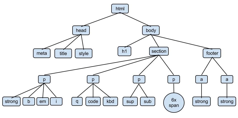 98 |
99 | Each branch of the tree is called an *element*
100 |
101 | ## HTML Elements
102 |
103 | Generally speaking, an HTML element has three components:
104 |
105 | 1. Tags (starting and ending the element)
106 | 2. Atributes (giving information about the element)
107 | 3. Text, or Content (the text inside the element)
108 |
109 | 
110 |
111 | ## HTML: Tags
112 |
113 | 
114 |
115 | [Image credit](http://miriamposner.com/blog/wp-content/uploads/2011/11/html-handout.pdf)
116 |
117 | ## Common HTML tags
118 |
119 | | Tag | Meaning |
120 | | ------------- |------------- |
121 | | `` | page header (metadata, etc |
122 | | `` | holds all of the content |
123 | | `
98 |
99 | Each branch of the tree is called an *element*
100 |
101 | ## HTML Elements
102 |
103 | Generally speaking, an HTML element has three components:
104 |
105 | 1. Tags (starting and ending the element)
106 | 2. Atributes (giving information about the element)
107 | 3. Text, or Content (the text inside the element)
108 |
109 | 
110 |
111 | ## HTML: Tags
112 |
113 | 
114 |
115 | [Image credit](http://miriamposner.com/blog/wp-content/uploads/2011/11/html-handout.pdf)
116 |
117 | ## Common HTML tags
118 |
119 | | Tag | Meaning |
120 | | ------------- |------------- |
121 | | `` | page header (metadata, etc |
122 | | `` | holds all of the content |
123 | | `