├── .gitignore
├── README.md
├── docs
├── anaconda-install.md
├── collections-study.ipynb
├── matplotlib-study.ipynb
├── numpy-study.ipynb
├── opencv
│ ├── canny.py
│ ├── lane-line-detection.py
│ ├── opencv-study.ipynb
│ └── opencv-study.py
└── pytorch-study.ipynb
├── experiment
├── Face-Detection-opencv
│ ├── README.md
│ ├── data
│ │ ├── haarcascade_frontalface_default.xml
│ │ └── lbpcascade_frontalface.xml
│ ├── face-detection.ipynb
│ ├── img
│ │ ├── multi.jpg
│ │ ├── multi2.jpg
│ │ └── single.jpg
│ ├── video-face-detection.py
│ └── video
│ │ ├── output.mp4
│ │ └── video.MOV
├── GAN
│ ├── README.md
│ └── gan.py
├── Image-Super-Resolution
│ ├── README.md
│ └── models.py
├── MNIST-Classification
│ └── MNIST-classification.ipynb
├── Mento-Carlo
│ ├── MenteCarlo.ipynb
│ └── README.md
├── Regression
│ ├── DNN-generation.ipynb
│ ├── function-fitting-batch.ipynb
│ └── function-fitting.ipynb
├── Style-Transfer
│ ├── README.md
│ └── networks.py
├── ViT
│ └── vit.py
└── YOLO
│ └── README.md
├── homework
├── CNN-MNIST
│ ├── README.md
│ └── W6_MNIST_FC.ipynb
├── DNN
│ ├── README.md
│ └── W5_Homework.ipynb
└── gradient-calc
│ ├── gradient-calc.ipynb
│ └── gradient-calc.md
├── paper-reading-list.md
└── resources
├── doubleZ.jpg
├── face-detection
├── gaussian.png
├── output.gif
└── threshold.png
├── opencv
├── canny.jpg
├── card.jpg
├── hough.jpg
├── lane.jpg
├── lane2.jpg
├── lena.jpg
└── match_shape.jpg
├── paper-reading-list
├── Attention-Aware-overview.png
├── Cascade-Cost-Volume-overview.png
├── Cost-Volume-Pyramid-overview.png
├── MVSNet-overview.png
├── P-mvsnet-overview.png
├── PatchmatchNet-overview.png
├── R-MVSNet-overview.png
└── point-mvs-overview.png
└── poster.jpg
/.gitignore:
--------------------------------------------------------------------------------
1 | .DS_Store
2 | __pycache__
3 | .idea/
4 | .vscode/
5 | doubleZ-*
6 | resources/opencv/lane.mp4
7 | t10k*
8 | train-labels-idx*
9 | train-images-idx*
10 | *.pt
11 | README.assets/
--------------------------------------------------------------------------------
/README.md:
--------------------------------------------------------------------------------
1 | # PKU计算机视觉课程材料
2 |
3 | > 北京大学深圳研究生院信息工程学院2021秋计算机视觉(04711432)课程材料
4 |
5 | ## 课程作业
6 |
7 |
40 |
41 |
42 | | 课时/时间 | 主题 | 作业内容 | 腾讯文档汇总版 |
43 | | :---------------------------- | ------------------ | ------------------------------------------------------------ | ------------------------------------------------------------ |
44 | | ✅第一次作业
(2021.09.21) | 课程导论 | 📃[计算机视觉课论文列表](https://github.com/doubleZ0108/Computer-Vision-PKU/blob/master/paper-reading-list.md) | [计算机视觉课论文汇总](https://docs.qq.com/doc/DSGNEZVlES3R0REt0) |
45 | | ✅第二次作业
(2021.09.28) | 基础知识(OpenCV等) | ⚗️[OpenCV人脸检测demo](https://github.com/doubleZ0108/Computer-Vision-PKU/blob/master/experiment/Face-Detection-opencv/face-detection.ipynb)
📝[Anaconda安装及使用](https://github.com/doubleZ0108/Computer-Vision-PKU/blob/master/docs/anaconda-install.md)
📔[Matplotlib学习](https://github.com/doubleZ0108/Computer-Vision-PKU/blob/master/docs/matplotlib-study.ipynb)
📔[NumPy学习](https://github.com/doubleZ0108/Computer-Vision-PKU/blob/master/docs/numpy-study.ipynb)
📔[OpenCV学习](https://github.com/doubleZ0108/Computer-Vision-PKU/blob/master/docs/opencv/opencv-study.ipynb)
📔[collections容器学习](https://github.com/doubleZ0108/Computer-Vision-PKU/blob/master/docs/collections-study.ipynb) | / |
46 | | ✅第三次作业
(2021.10.12) | 基础知识(PyTorch) | :pencil:[视频人脸检测](https://github.com/doubleZ0108/Computer-Vision-PKU/tree/master/experiment/Face-Detection-opencv) \| ⚗️[code](https://github.com/doubleZ0108/Computer-Vision-PKU/blob/master/experiment/Face-Detection-opencv/video-face-detection.py)
📔[PyTorch学习](https://github.com/doubleZ0108/Computer-Vision-PKU/blob/master/docs/pytorch-study.ipynb)
:alembic:[传统方法车道线检测](https://github.com/doubleZ0108/Computer-Vision-PKU/blob/master/docs/opencv/lane-line-detection.py)
:alembic:[Canny边缘检测动态展示](https://github.com/doubleZ0108/Computer-Vision-PKU/blob/master/docs/opencv/canny.py) | [第三次作业汇总](https://docs.qq.com/doc/DSFNJSUZlTXNZRFFC) |
47 | | ✅第四次作业
(2021.10.19) | 矩阵求导 | :pencil:[矩阵求导问题](https://github.com/doubleZ0108/Computer-Vision-PKU/blob/master/homework/gradient-calc/gradient-calc.ipynb) | [第四次作业汇总](https://docs.qq.com/pdf/DSGhVTmNNeXNtTkZj) |
48 | | ✅第五次作业
(2021.10.26) | 初识神经网络 | :alembic:[两层全连接网络拟合曲线](https://github.com/doubleZ0108/Computer-Vision-PKU/blob/master/homework/DNN/W5_Homework.ipynb)
:pencil:[两层全连接网络逐步衍化](https://github.com/doubleZ0108/Computer-Vision-PKU/blob/master/experiment/Regression/DNN-generation.ipynb) | [第五次作业汇总](https://docs.qq.com/pdf/DSEpHR0xSU1FRQWVT) |
49 | | ✅第六次作业
(2021.11.03) | 卷积神经网络 | :alembic:[CNN处理MNIST手写数字识别问题](https://github.com/doubleZ0108/Computer-Vision-PKU/blob/master/homework/CNN-MNIST/W6_MNIST_FC.ipynb)
:pencil:[CNN处理MNIST手写数字识别问题](https://github.com/doubleZ0108/Computer-Vision-PKU/tree/master/homework/CNN-MNIST) | [第六次作业汇总](https://docs.qq.com/pdf/DSGN4eHBJTGF3cm9p) |
50 | | ✅第七次作业
(2021.11.10) | 图像超分 | :pencil:[图像超分辨率](https://github.com/doubleZ0108/Computer-Vision-PKU/tree/master/experiment/Image-Super-Resolution) | [第七次作业汇总](https://docs.qq.com/pdf/DSENtVE55eXNlS2JY) |
51 | | ✅第八次作业
(2021.11.17) | GAN生成对抗网络 | :pencil:[GAN论文阅读和实验](https://github.com/doubleZ0108/Computer-Vision-PKU/tree/master/experiment/GAN) | [第八次作业汇总](https://docs.qq.com/pdf/DSExKV21SY3lLc2FT) |
52 | | ✅第九次作业
(2021.11.24) | 风格迁移 | :alembic:[风格迁移实验](https://github.com/doubleZ0108/Computer-Vision-PKU/tree/master/experiment/Style-Transfer)
🌐[风格迁移Demo网站](https://doublez0108.github.io/CV/Style-Transfer/style-transfer.html) | [第九次作业汇总](https://docs.qq.com/pdf/DSHFhVlV2ZGdJYUpi) |
53 | | ✅第十次作业
(2021.12.01) | YOLO目标检测 | :pencil:[YOLO目标检测实验](https://github.com/doubleZ0108/Computer-Vision-PKU/tree/master/experiment/YOLO) | [第十次作业汇总](https://docs.qq.com/pdf/DSFhzaUpNTW5jVU5J) |
54 |
55 |
56 |
57 | ## 期末展示
58 |
59 | 
60 |
61 |
62 |
63 | ## 关于作者
64 |
65 | - **姓名/学号**:张喆 2101212846
66 | - **学院/专业**:北京大学信息工程学院 计算机应用技术
67 | - **课程**:计算机视觉(04711432)
68 | - **指导老师**:[张健助理教授](http://www.ece.pku.edu.cn/info/1012/1075.htm)
69 | - **联系方式**:[doublez@stu.pku.edu.cn](mailto:doublez@stu.pku.edu.cn)
70 |
--------------------------------------------------------------------------------
/docs/anaconda-install.md:
--------------------------------------------------------------------------------
1 | # Anaconda安装及使用
2 |
3 | * [系统环境](#系统环境)
4 | * [Anaconda GUI](#anaconda-gui)
5 | * [安装](#安装)
6 | * [使用](#使用)
7 | * [Anaconda 命令行](#anaconda-命令行)
8 | * [安装](#安装-1)
9 | * [使用](#使用-1)
10 | * [Anaconda配置CV所需环境](#anaconda配置cv所需环境)
11 |
12 | ------
13 |
14 | 【Anaconda官网】[Anaconda | Individual Edition](https://www.anaconda.com/products/individual#Downloads)
15 |
16 |
17 |
18 | ## 系统环境
19 |
20 | - 本地**操作系统**:macOS Big Sur 11.6
21 | - 服务器操作系统:Ubuntu 18.04
22 |
23 | ---
24 |
25 | ## Anaconda GUI
26 |
27 | ### 安装
28 |
29 | 在官网下载安装包,根据提示一步步进行安装即可
30 |
31 |  32 |
33 |
32 |
33 |  34 |
35 | ### 使用
36 |
37 | 1. 创建虚拟环境
38 |
39 |
34 |
35 | ### 使用
36 |
37 | 1. 创建虚拟环境
38 |
39 |  40 |
41 | 2. 选择所需包进行安装
42 |
43 |
40 |
41 | 2. 选择所需包进行安装
42 |
43 |  44 |
45 | 3. 在IDE中使用虚拟环境进行测试
46 |
47 | > 需要安装`ipykernel`
48 |
49 |
44 |
45 | 3. 在IDE中使用虚拟环境进行测试
46 |
47 | > 需要安装`ipykernel`
48 |
49 | 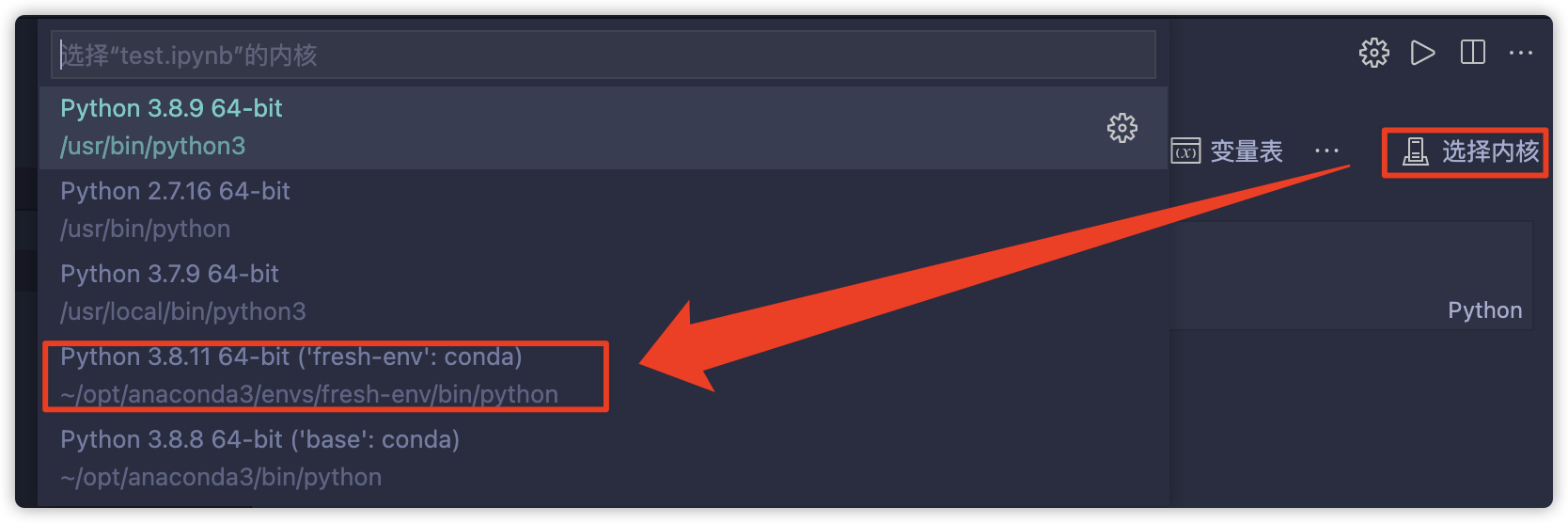 50 |
51 |
50 |
51 | 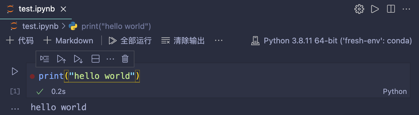 52 |
53 | 4. 删除虚拟环境
54 |
55 |
52 |
53 | 4. 删除虚拟环境
54 |
55 |  56 |
57 | ---
58 |
59 | ## Anaconda 命令行
60 |
61 | ### 安装
62 |
63 | 1. 在官网下载Anaconda安装包
64 | 2. 按照官网建议通过SHA-256验证数据的正确性
65 |
66 | ```bash
67 | sha256sum /path/filename
68 | ```
69 |
70 | 3. 运行shell脚本
71 | 4. 根据提示进行安装
72 | 5. 写入环境变量
73 | 6. 最后通过`conda —version`验证是否安装成功
74 |
75 | > 由于服务器上之前已经安装好Anaconda,这里不再展示安装步骤截图
76 |
77 | ### 使用
78 |
79 | ```bash
80 | # 创建虚拟环境
81 | conda create -n [env_name]
82 |
83 | # 查看所有环境信息
84 | conda info --envs
85 |
86 | # 激活某个环境
87 | conda activate [env_name]
88 |
89 | # 退出激活的环境
90 | conda deactivate
91 |
92 | # 删除某个环境
93 | conda remove -n [env_name] --all
94 | ```
95 |
96 | 下图为在Ubuntu下的实际操作:
97 |
98 |
56 |
57 | ---
58 |
59 | ## Anaconda 命令行
60 |
61 | ### 安装
62 |
63 | 1. 在官网下载Anaconda安装包
64 | 2. 按照官网建议通过SHA-256验证数据的正确性
65 |
66 | ```bash
67 | sha256sum /path/filename
68 | ```
69 |
70 | 3. 运行shell脚本
71 | 4. 根据提示进行安装
72 | 5. 写入环境变量
73 | 6. 最后通过`conda —version`验证是否安装成功
74 |
75 | > 由于服务器上之前已经安装好Anaconda,这里不再展示安装步骤截图
76 |
77 | ### 使用
78 |
79 | ```bash
80 | # 创建虚拟环境
81 | conda create -n [env_name]
82 |
83 | # 查看所有环境信息
84 | conda info --envs
85 |
86 | # 激活某个环境
87 | conda activate [env_name]
88 |
89 | # 退出激活的环境
90 | conda deactivate
91 |
92 | # 删除某个环境
93 | conda remove -n [env_name] --all
94 | ```
95 |
96 | 下图为在Ubuntu下的实际操作:
97 |
98 | 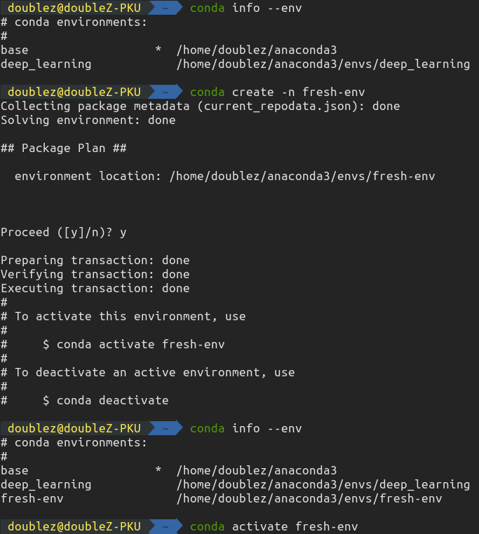 99 |
100 |
99 |
100 | 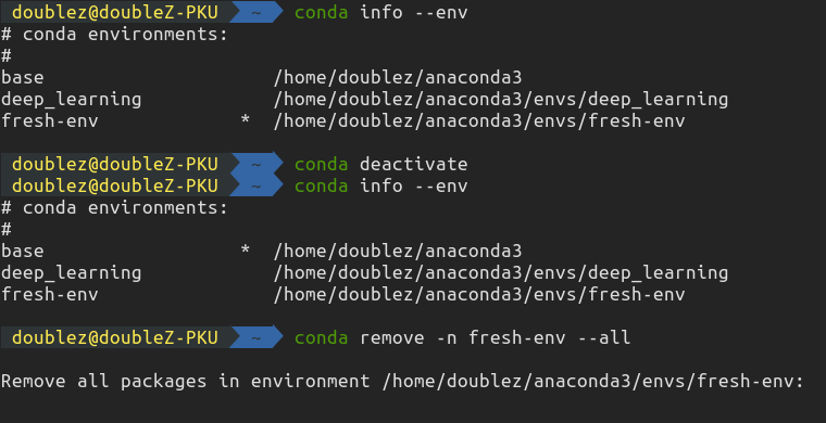 101 |
102 |
101 |
102 | 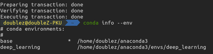 103 |
104 | ---
105 |
106 | ## Anaconda配置CV所需环境
107 |
108 | 由于最新版的anaconda默认python版本是3.8导致opencv不支持,因此首先把conda的python版本降为3.7
109 |
110 | ```bash
111 | conda install python=3.7 anaconda=custom
112 | ```
113 |
114 | 之后创建虚拟环境并安装所需python包
115 |
116 | ```bash
117 | conda create -n cv
118 | conda activate cv
119 | conda install opencv, numpy, matplotlib
120 | ```
121 |
122 |
103 |
104 | ---
105 |
106 | ## Anaconda配置CV所需环境
107 |
108 | 由于最新版的anaconda默认python版本是3.8导致opencv不支持,因此首先把conda的python版本降为3.7
109 |
110 | ```bash
111 | conda install python=3.7 anaconda=custom
112 | ```
113 |
114 | 之后创建虚拟环境并安装所需python包
115 |
116 | ```bash
117 | conda create -n cv
118 | conda activate cv
119 | conda install opencv, numpy, matplotlib
120 | ```
121 |
122 | 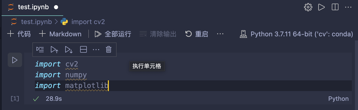 123 |
124 |
125 |
126 |
--------------------------------------------------------------------------------
/docs/collections-study.ipynb:
--------------------------------------------------------------------------------
1 | {
2 | "cells": [
3 | {
4 | "cell_type": "markdown",
5 | "metadata": {},
6 | "source": [
7 | "# collection容器库"
8 | ]
9 | },
10 | {
11 | "cell_type": "code",
12 | "execution_count": 113,
13 | "metadata": {},
14 | "outputs": [],
15 | "source": [
16 | "import collections\n",
17 | "from collections import Counter, deque, defaultdict, OrderedDict, namedtuple, ChainMap"
18 | ]
19 | },
20 | {
21 | "cell_type": "code",
22 | "execution_count": 114,
23 | "metadata": {},
24 | "outputs": [
25 | {
26 | "name": "stdout",
27 | "output_type": "stream",
28 | "text": [
29 | "['deque', 'defaultdict', 'namedtuple', 'UserDict', 'UserList', 'UserString', 'Counter', 'OrderedDict', 'ChainMap', 'Awaitable', 'Coroutine', 'AsyncIterable', 'AsyncIterator', 'AsyncGenerator', 'Hashable', 'Iterable', 'Iterator', 'Generator', 'Reversible', 'Sized', 'Container', 'Callable', 'Collection', 'Set', 'MutableSet', 'Mapping', 'MutableMapping', 'MappingView', 'KeysView', 'ItemsView', 'ValuesView', 'Sequence', 'MutableSequence', 'ByteString']\n"
30 | ]
31 | }
32 | ],
33 | "source": [
34 | "print(collections.__all__)"
35 | ]
36 | },
37 | {
38 | "cell_type": "markdown",
39 | "metadata": {},
40 | "source": [
41 | "## Counter\n",
42 | "\n",
43 | "- 基础用法跟正常的dict()是一样的\n",
44 | " - `elements()`, `items()`\n",
45 | "- `most_common(n)`:出现次数最多的n个\n",
46 | "- 可以对两个Counter对象`+` `-` `&` `|`"
47 | ]
48 | },
49 | {
50 | "cell_type": "code",
51 | "execution_count": 115,
52 | "metadata": {},
53 | "outputs": [
54 | {
55 | "data": {
56 | "text/plain": [
57 | "Counter({'red': 2, 'blue': 3, 'green': 1})"
58 | ]
59 | },
60 | "execution_count": 115,
61 | "metadata": {},
62 | "output_type": "execute_result"
63 | }
64 | ],
65 | "source": [
66 | "colors = ['red', 'blue', 'red', 'green', 'blue', 'blue']\n",
67 | "c = Counter(colors)\n",
68 | "\n",
69 | "d = {'red': 2, 'blue': 3, 'green': 1}\n",
70 | "c = Counter(d)\n",
71 | "c"
72 | ]
73 | },
74 | {
75 | "cell_type": "code",
76 | "execution_count": 116,
77 | "metadata": {},
78 | "outputs": [
79 | {
80 | "name": "stdout",
81 | "output_type": "stream",
82 | "text": [
83 | "['red', 'red', 'blue', 'blue', 'blue', 'green']\n",
84 | "red 2\n",
85 | "blue 3\n",
86 | "green 1\n"
87 | ]
88 | }
89 | ],
90 | "source": [
91 | "print(list(c.elements()))\n",
92 | "for key, val in c.items():\n",
93 | " print(key, val)"
94 | ]
95 | },
96 | {
97 | "cell_type": "code",
98 | "execution_count": 117,
99 | "metadata": {},
100 | "outputs": [
101 | {
102 | "data": {
103 | "text/plain": [
104 | "[('blue', 3), ('red', 2)]"
105 | ]
106 | },
107 | "execution_count": 117,
108 | "metadata": {},
109 | "output_type": "execute_result"
110 | }
111 | ],
112 | "source": [
113 | "# 相同计数的按照首次出现的顺序排序\n",
114 | "c.most_common(2)"
115 | ]
116 | },
117 | {
118 | "cell_type": "code",
119 | "execution_count": 118,
120 | "metadata": {},
121 | "outputs": [
122 | {
123 | "data": {
124 | "text/plain": [
125 | "Counter({'red': 1, 'blue': 2, 'green': 1})"
126 | ]
127 | },
128 | "execution_count": 118,
129 | "metadata": {},
130 | "output_type": "execute_result"
131 | }
132 | ],
133 | "source": [
134 | "c.subtract(['red', 'blue'])\n",
135 | "c"
136 | ]
137 | },
138 | {
139 | "cell_type": "code",
140 | "execution_count": 119,
141 | "metadata": {},
142 | "outputs": [
143 | {
144 | "name": "stdout",
145 | "output_type": "stream",
146 | "text": [
147 | "Counter({'blue': 4, 'red': 2, 'green': 2})\n",
148 | "Counter({'blue': 2})\n",
149 | "Counter({'red': 4, 'blue': 2, 'green': 1})\n"
150 | ]
151 | }
152 | ],
153 | "source": [
154 | "print(c + c) # add\n",
155 | "print(c & Counter(blue=3)) # intersection\n",
156 | "print(c | Counter(red=4)) # union"
157 | ]
158 | },
159 | {
160 | "cell_type": "markdown",
161 | "metadata": {},
162 | "source": [
163 | "## deque\n",
164 | "\n",
165 | "- `count()`\n",
166 | "- `clear()`\n",
167 | "- `append()`, `appendleft()`\n",
168 | "- `extend()`, `extendleft()`:添加iterable中的元素\n",
169 | "- `index()`:返回第一次匹配的位置\n",
170 | "- `insert(pos, val)`:在pos位置插入元素\n",
171 | "- `pop()`, `popleft()`\n",
172 | "- `remove(val)`:移除deque里第一个匹配的val值\n",
173 | "- `rotate(x)`:向右循环x步,等价于`d.appendleft(d.pop())`"
174 | ]
175 | },
176 | {
177 | "cell_type": "code",
178 | "execution_count": 120,
179 | "metadata": {},
180 | "outputs": [
181 | {
182 | "name": "stdout",
183 | "output_type": "stream",
184 | "text": [
185 | "deque([1, 2, 3])\n",
186 | "deque([1, 2, 3, 4])\n",
187 | "deque([0, 1, 2, 3, 4])\n"
188 | ]
189 | }
190 | ],
191 | "source": [
192 | "d = deque([1,2,3])\n",
193 | "print(d)\n",
194 | "\n",
195 | "d.append(4)\n",
196 | "print(d)\n",
197 | "\n",
198 | "d.appendleft(0)\n",
199 | "print(d)"
200 | ]
201 | },
202 | {
203 | "cell_type": "code",
204 | "execution_count": 121,
205 | "metadata": {},
206 | "outputs": [
207 | {
208 | "name": "stdout",
209 | "output_type": "stream",
210 | "text": [
211 | "deque([0, 1, 2, 3, 4, 7, 8, 9])\n",
212 | "deque([-3, -2, -1, 0, 1, 2, 3, 4, 7, 8, 9])\n"
213 | ]
214 | }
215 | ],
216 | "source": [
217 | "d.extend([7,8,9])\n",
218 | "print(d)\n",
219 | "\n",
220 | "d.extendleft([-1,-2,-3]) # 注意在左面添加会反过来的\n",
221 | "print(d)"
222 | ]
223 | },
224 | {
225 | "cell_type": "code",
226 | "execution_count": 122,
227 | "metadata": {},
228 | "outputs": [
229 | {
230 | "name": "stdout",
231 | "output_type": "stream",
232 | "text": [
233 | "3\n",
234 | "deque([-3, 'a', -2, -1, 0, 1, 2, 3, 4, 7, 8, 9])\n"
235 | ]
236 | }
237 | ],
238 | "source": [
239 | "print(d.index(0))\n",
240 | "\n",
241 | "d.insert(1, 'a')\n",
242 | "print(d)"
243 | ]
244 | },
245 | {
246 | "cell_type": "code",
247 | "execution_count": 123,
248 | "metadata": {},
249 | "outputs": [
250 | {
251 | "name": "stdout",
252 | "output_type": "stream",
253 | "text": [
254 | "deque([-3, -2, -1, 0, 1, 2, 3, 4, 7, 8, 9])\n"
255 | ]
256 | }
257 | ],
258 | "source": [
259 | "d.remove('a')\n",
260 | "print(d)"
261 | ]
262 | },
263 | {
264 | "cell_type": "code",
265 | "execution_count": 124,
266 | "metadata": {},
267 | "outputs": [
268 | {
269 | "name": "stdout",
270 | "output_type": "stream",
271 | "text": [
272 | "deque([9, -3, -2, -1, 0, 1, 2, 3, 4, 7, 8])\n"
273 | ]
274 | }
275 | ],
276 | "source": [
277 | "d.rotate(1)\n",
278 | "print(d)"
279 | ]
280 | },
281 | {
282 | "cell_type": "markdown",
283 | "metadata": {},
284 | "source": [
285 | "## defaultdict\n",
286 | "\n",
287 | "主要用来解决默认dict值不存在时会报错(例如+1必须要特判)\n",
288 | "\n",
289 | "通过设定类型可指定默认值(例如list缺失值是`[]`,int缺失值是0)"
290 | ]
291 | },
292 | {
293 | "cell_type": "code",
294 | "execution_count": 125,
295 | "metadata": {},
296 | "outputs": [
297 | {
298 | "data": {
299 | "text/plain": [
300 | "dict_items([('yellow', [1, 3]), ('blue', [2, 4]), ('red', [1])])"
301 | ]
302 | },
303 | "execution_count": 125,
304 | "metadata": {},
305 | "output_type": "execute_result"
306 | }
307 | ],
308 | "source": [
309 | "# 将 键-值对 转换为 键-列表\n",
310 | "s = [('yellow', 1), ('blue', 2), ('yellow', 3), ('blue', 4), ('red', 1)]\n",
311 | "\n",
312 | "d = defaultdict(list)\n",
313 | "for k, v in s:\n",
314 | " d[k].append(v)\n",
315 | "\n",
316 | "d.items()"
317 | ]
318 | },
319 | {
320 | "cell_type": "code",
321 | "execution_count": 126,
322 | "metadata": {},
323 | "outputs": [
324 | {
325 | "data": {
326 | "text/plain": [
327 | "dict_items([('h', 1), ('e', 1), ('l', 3), ('o', 2), ('w', 1), ('r', 1), ('d', 1)])"
328 | ]
329 | },
330 | "execution_count": 126,
331 | "metadata": {},
332 | "output_type": "execute_result"
333 | }
334 | ],
335 | "source": [
336 | "# 计数\n",
337 | "s = \"helloworld\"\n",
338 | "d = defaultdict(int)\n",
339 | "for k in s:\n",
340 | " d[k] += 1\n",
341 | "d.items()"
342 | ]
343 | },
344 | {
345 | "cell_type": "markdown",
346 | "metadata": {},
347 | "source": [
348 | "## OrderedDict\n",
349 | "\n",
350 | "因为是有序的字典,因此可以记住顺序\n",
351 | "\n",
352 | "- `popitem()`\n",
353 | "- `move_to_end()`"
354 | ]
355 | },
356 | {
357 | "cell_type": "code",
358 | "execution_count": 127,
359 | "metadata": {},
360 | "outputs": [
361 | {
362 | "name": "stdout",
363 | "output_type": "stream",
364 | "text": [
365 | "OrderedDict([('a', None), ('b', None)])\n",
366 | "OrderedDict([('b', None), ('a', None)])\n"
367 | ]
368 | }
369 | ],
370 | "source": [
371 | "od = OrderedDict.fromkeys('abc')\n",
372 | "\n",
373 | "od.popitem(last=True)\n",
374 | "print(od)\n",
375 | "\n",
376 | "od.move_to_end('a', last=True)\n",
377 | "print(od)"
378 | ]
379 | },
380 | {
381 | "cell_type": "markdown",
382 | "metadata": {},
383 | "source": [
384 | "## namedtyple\n",
385 | "\n",
386 | "允许自定义名字的tuple子类"
387 | ]
388 | },
389 | {
390 | "cell_type": "code",
391 | "execution_count": 128,
392 | "metadata": {},
393 | "outputs": [
394 | {
395 | "name": "stdout",
396 | "output_type": "stream",
397 | "text": [
398 | "3\n"
399 | ]
400 | },
401 | {
402 | "data": {
403 | "text/plain": [
404 | "OrderedDict([('x', 1), ('y', 2)])"
405 | ]
406 | },
407 | "execution_count": 128,
408 | "metadata": {},
409 | "output_type": "execute_result"
410 | }
411 | ],
412 | "source": [
413 | "Point = namedtuple('Point', ['x','y'])\n",
414 | "\n",
415 | "p = Point(x=1,y=2)\n",
416 | "print(p.x + p[1])\n",
417 | "\n",
418 | "p._asdict()"
419 | ]
420 | },
421 | {
422 | "cell_type": "markdown",
423 | "metadata": {},
424 | "source": [
425 | "## ChainMap\n",
426 | "\n",
427 | "把多个字典融合成一个\n",
428 | "\n",
429 | "当多个字典有重复的key时,按照链的顺序第一次查找的返回\n",
430 | "\n",
431 | "例如应用在:命令行参数、系统环境参数、默认参数 的优先级决策上\n"
432 | ]
433 | },
434 | {
435 | "cell_type": "code",
436 | "execution_count": 129,
437 | "metadata": {},
438 | "outputs": [
439 | {
440 | "name": "stdout",
441 | "output_type": "stream",
442 | "text": [
443 | "10\n"
444 | ]
445 | }
446 | ],
447 | "source": [
448 | "colors = {'red': 3, 'blue': 1}\n",
449 | "phones = {'iPhone': 10, 'Huawei': 5}\n",
450 | "langs = {'python': 2, 'js': 3}\n",
451 | "\n",
452 | "chainmap = ChainMap(colors, phones, langs)\n",
453 | "\n",
454 | "print(chainmap['iPhone'])"
455 | ]
456 | },
457 | {
458 | "cell_type": "code",
459 | "execution_count": 130,
460 | "metadata": {},
461 | "outputs": [
462 | {
463 | "name": "stdout",
464 | "output_type": "stream",
465 | "text": [
466 | "ChainMap({'red': 3, 'blue': 1}, {'iPhone': 10, 'Huawei': 5}, {'python': 2, 'js': 3, 'c': 10})\n"
467 | ]
468 | }
469 | ],
470 | "source": [
471 | "langs['c'] = 10\n",
472 | "print(chainmap) # chainmap会自动更新"
473 | ]
474 | },
475 | {
476 | "cell_type": "code",
477 | "execution_count": 131,
478 | "metadata": {},
479 | "outputs": [
480 | {
481 | "name": "stdout",
482 | "output_type": "stream",
483 | "text": [
484 | "ChainMap({'red': 3}, {'iPhone': 10, 'Huawei': 5}, {'python': 2, 'js': 3, 'c': 10})\n",
485 | "{'red': 3}\n"
486 | ]
487 | }
488 | ],
489 | "source": [
490 | "chainmap.pop('blue')\n",
491 | "\n",
492 | "print(chainmap)\n",
493 | "print(colors) # chainmap中删除,原字典也会同步删除"
494 | ]
495 | }
496 | ],
497 | "metadata": {
498 | "kernelspec": {
499 | "display_name": "Python 3.6.13 ('ourmvsnet')",
500 | "language": "python",
501 | "name": "python3"
502 | },
503 | "language_info": {
504 | "codemirror_mode": {
505 | "name": "ipython",
506 | "version": 3
507 | },
508 | "file_extension": ".py",
509 | "mimetype": "text/x-python",
510 | "name": "python",
511 | "nbconvert_exporter": "python",
512 | "pygments_lexer": "ipython3",
513 | "version": "3.6.13"
514 | },
515 | "orig_nbformat": 4,
516 | "vscode": {
517 | "interpreter": {
518 | "hash": "ce3435b4fd239f1f6f12780933ef58404daca4493791636b6dc56d0922f97ec9"
519 | }
520 | }
521 | },
522 | "nbformat": 4,
523 | "nbformat_minor": 2
524 | }
525 |
--------------------------------------------------------------------------------
/docs/numpy-study.ipynb:
--------------------------------------------------------------------------------
1 | {
2 | "cells": [
3 | {
4 | "cell_type": "markdown",
5 | "source": [
6 | "# NumPy学习"
7 | ],
8 | "metadata": {}
9 | },
10 | {
11 | "cell_type": "markdown",
12 | "source": [
13 | "**Table of Content**\n",
14 | "* 属性\n",
15 | "* 创建\n",
16 | " * 随机数\n",
17 | "* 运算\n",
18 | " * 聚合函数\n",
19 | "* 索引\n",
20 | "* 数组操作\n",
21 | "* 拷贝\n",
22 | "\n",
23 | "[Numpy中文网](https://www.numpy.org.cn)\n",
24 | "\n",
25 | "采用C语言编写,采用矩阵运算,消耗资源少,比自带数据结构的运算款很多\n",
26 | "\n",
27 | "Vectorization is one of the main reasons why NumPy is so powerful."
28 | ],
29 | "metadata": {}
30 | },
31 | {
32 | "cell_type": "markdown",
33 | "source": [
34 | "## 属性"
35 | ],
36 | "metadata": {}
37 | },
38 | {
39 | "cell_type": "code",
40 | "execution_count": 1,
41 | "source": [
42 | "import numpy as np"
43 | ],
44 | "outputs": [],
45 | "metadata": {}
46 | },
47 | {
48 | "cell_type": "code",
49 | "execution_count": 2,
50 | "source": [
51 | "array = np.array([[1,2,3],[4,5,6]])\n",
52 | "print(array)"
53 | ],
54 | "outputs": [
55 | {
56 | "output_type": "stream",
57 | "name": "stdout",
58 | "text": [
59 | "[[1 2 3]\n",
60 | " [4 5 6]]\n"
61 | ]
62 | }
63 | ],
64 | "metadata": {}
65 | },
66 | {
67 | "cell_type": "code",
68 | "execution_count": 3,
69 | "source": [
70 | "# 维度\n",
71 | "print(array.ndim)\n",
72 | "\n",
73 | "# 行列数\n",
74 | "print(array.shape)\n",
75 | "\n",
76 | "# 元素个数\n",
77 | "print(array.size)"
78 | ],
79 | "outputs": [
80 | {
81 | "output_type": "stream",
82 | "name": "stdout",
83 | "text": [
84 | "2\n",
85 | "(2, 3)\n",
86 | "6\n"
87 | ]
88 | }
89 | ],
90 | "metadata": {}
91 | },
92 | {
93 | "cell_type": "markdown",
94 | "source": [
95 | "## 创建"
96 | ],
97 | "metadata": {}
98 | },
99 | {
100 | "cell_type": "code",
101 | "execution_count": 8,
102 | "source": [
103 | "# 指定数据类型\n",
104 | "a = np.array([1, 2, 3], dtype=np.int32)\n",
105 | "b = np.array([1, 2, 3], dtype=np.float64)\n",
106 | "\n",
107 | "print(a)\n",
108 | "print(b)"
109 | ],
110 | "outputs": [
111 | {
112 | "output_type": "stream",
113 | "name": "stdout",
114 | "text": [
115 | "[1 2 3] [1. 2. 3.]\n",
116 | "[[0. 0. 0. 0.]\n",
117 | " [0. 0. 0. 0.]\n",
118 | " [0. 0. 0. 0.]]\n",
119 | "[[1 1 1]\n",
120 | " [1 1 1]]\n"
121 | ]
122 | }
123 | ],
124 | "metadata": {}
125 | },
126 | {
127 | "cell_type": "code",
128 | "execution_count": 3,
129 | "source": [
130 | "# 快速创建\n",
131 | "zero = np.zeros((3, 4))\n",
132 | "one = np.ones((2, 3), dtype=np.int32)\n",
133 | "empty = np.empty((2, 3)) # 接近零的数\n",
134 | "full = np.full((2, 3), 7) # 全为某值的矩阵\n",
135 | "identity = np.eye(3) # 对角矩阵\n",
136 | "\n",
137 | "print(zero)\n",
138 | "print(one)\n",
139 | "print(empty)\n",
140 | "print(full)\n",
141 | "print(identity)"
142 | ],
143 | "outputs": [
144 | {
145 | "output_type": "stream",
146 | "name": "stdout",
147 | "text": [
148 | "[[0. 0. 0. 0.]\n",
149 | " [0. 0. 0. 0.]\n",
150 | " [0. 0. 0. 0.]]\n",
151 | "[[1 1 1]\n",
152 | " [1 1 1]]\n",
153 | "[[-1.72723371e-077 1.29073736e-231 1.97626258e-323]\n",
154 | " [ 0.00000000e+000 0.00000000e+000 4.17201348e-309]]\n",
155 | "[[7 7 7]\n",
156 | " [7 7 7]]\n",
157 | "[[1. 0. 0.]\n",
158 | " [0. 1. 0.]\n",
159 | " [0. 0. 1.]]\n"
160 | ]
161 | }
162 | ],
163 | "metadata": {}
164 | },
165 | {
166 | "cell_type": "code",
167 | "execution_count": 13,
168 | "source": [
169 | "# 连续数字\n",
170 | "arange = np.arange(1, 10, 2) # 步长为2\n",
171 | "\n",
172 | "# 线段形数据\n",
173 | "linspace = np.linspace(1, 10, 8) # 分割成8个点\n",
174 | "\n",
175 | "# 改变形状\n",
176 | "reshape = np.arange(20).reshape(4, 5) # 参数为-1则会自动计算\n",
177 | "\n",
178 | "print(arange)\n",
179 | "print(linspace)\n",
180 | "print(reshape)"
181 | ],
182 | "outputs": [
183 | {
184 | "output_type": "stream",
185 | "name": "stdout",
186 | "text": [
187 | "[1 3 5 7 9]\n",
188 | "[ 1. 2.28571429 3.57142857 4.85714286 6.14285714 7.42857143\n",
189 | " 8.71428571 10. ]\n",
190 | "[[ 0 1 2 3 4]\n",
191 | " [ 5 6 7 8 9]\n",
192 | " [10 11 12 13 14]\n",
193 | " [15 16 17 18 19]]\n"
194 | ]
195 | }
196 | ],
197 | "metadata": {}
198 | },
199 | {
200 | "cell_type": "markdown",
201 | "source": [
202 | "### 随机数"
203 | ],
204 | "metadata": {}
205 | },
206 | {
207 | "cell_type": "code",
208 | "execution_count": 131,
209 | "source": [
210 | "# 0~1间的浮点数\n",
211 | "r = np.random.rand(2, 3)\n",
212 | "print(\"rand: \", r)\n",
213 | "\n",
214 | "# 0~1间均匀取样随机数\n",
215 | "r = np.random.random((2, 4))\n",
216 | "print(\"random: \", r)\n",
217 | "\n",
218 | "# [0, 10)间的随机整数\n",
219 | "r = np.random.randint(10)\n",
220 | "print(\"randint: \", r)\n",
221 | "\n",
222 | "# 基于给定值生成随机数\n",
223 | "r = np.random.choice([3, 5, 7, 9], size=(2, 3))\n",
224 | "print(\"choice: \", r)\n",
225 | "\n",
226 | "# 均匀分布随机数 [low, high)\n",
227 | "r = np.random.uniform(1, 10, (3, 2))\n",
228 | "print(\"uniform: \", r)\n",
229 | "\n",
230 | "# 标准正态分布 均值0 方差1\n",
231 | "r = np.random.randn(3, 2)\n",
232 | "print(\"randn: \", r)\n",
233 | "\n",
234 | "# 正态分布 均值10 方差1\n",
235 | "r = np.random.normal(10, 1, (3, 2))\n",
236 | "print(\"normal: \", r)"
237 | ],
238 | "outputs": [
239 | {
240 | "output_type": "stream",
241 | "name": "stdout",
242 | "text": [
243 | "rand: [[0.44155749 0.44601869 0.05318859]\n",
244 | " [0.28594465 0.72112534 0.91809614]]\n",
245 | "random: [[0.07914297 0.68466181 0.49258672 0.1509604 ]\n",
246 | " [0.63843674 0.85319365 0.3285023 0.60701208]]\n",
247 | "randint: 2\n",
248 | "choice: [[3 9 9]\n",
249 | " [7 3 5]]\n",
250 | "uniform: [[2.87500892 9.01628853]\n",
251 | " [1.99811272 3.47776626]\n",
252 | " [7.94675885 4.08628526]]\n",
253 | "randn: [[-0.8897855 0.66911561]\n",
254 | " [ 1.32854304 0.34210128]\n",
255 | " [-1.62014918 -0.21174625]]\n",
256 | "[[10.49353599 10.8195831 ]\n",
257 | " [ 9.44557101 8.93493195]\n",
258 | " [10.00297058 9.5695596 ]]\n"
259 | ]
260 | }
261 | ],
262 | "metadata": {}
263 | },
264 | {
265 | "cell_type": "markdown",
266 | "source": [
267 | "## 运算"
268 | ],
269 | "metadata": {}
270 | },
271 | {
272 | "cell_type": "code",
273 | "execution_count": 5,
274 | "source": [
275 | "a = np.array([[1,2], [3, 4]])\n",
276 | "b = np.arange(4).reshape((2,2))\n",
277 | "\n",
278 | "# 矩阵乘法\n",
279 | "print(np.dot(a, b))\n",
280 | "print(a.dot(b))\n",
281 | "\n",
282 | "# 对位乘法\n",
283 | "print(a * b)\n",
284 | "print(np.multiply(a, b))\n",
285 | "\n",
286 | "print(a ** 2)"
287 | ],
288 | "outputs": [
289 | {
290 | "output_type": "stream",
291 | "name": "stdout",
292 | "text": [
293 | "[[ 4 7]\n",
294 | " [ 8 15]]\n",
295 | "[[ 4 7]\n",
296 | " [ 8 15]]\n",
297 | "[[ 0 2]\n",
298 | " [ 6 12]]\n",
299 | "[[ 0 2]\n",
300 | " [ 6 12]]\n",
301 | "[[ 1 4]\n",
302 | " [ 9 16]]\n"
303 | ]
304 | }
305 | ],
306 | "metadata": {}
307 | },
308 | {
309 | "cell_type": "code",
310 | "execution_count": 27,
311 | "source": [
312 | "# 一些数学函数\n",
313 | "e = np.sin(a)\n",
314 | "print(e)"
315 | ],
316 | "outputs": [
317 | {
318 | "output_type": "stream",
319 | "name": "stdout",
320 | "text": [
321 | "[[ 0.84147098 0.90929743]\n",
322 | " [ 0.14112001 -0.7568025 ]]\n"
323 | ]
324 | }
325 | ],
326 | "metadata": {}
327 | },
328 | {
329 | "cell_type": "code",
330 | "execution_count": 28,
331 | "source": [
332 | "# 逻辑判断\n",
333 | "print(b < 3)"
334 | ],
335 | "outputs": [
336 | {
337 | "output_type": "stream",
338 | "name": "stdout",
339 | "text": [
340 | "[[ True True]\n",
341 | " [ True False]]\n"
342 | ]
343 | }
344 | ],
345 | "metadata": {}
346 | },
347 | {
348 | "cell_type": "markdown",
349 | "source": [
350 | "### 聚合函数"
351 | ],
352 | "metadata": {}
353 | },
354 | {
355 | "cell_type": "code",
356 | "execution_count": 154,
357 | "source": [
358 | "r = np.random.randint(0, 100, (2, 5))\n",
359 | "print(r)\n",
360 | "\n",
361 | "print(\"sum: \", np.sum(r))\n",
362 | "print(\"sum[axis=0]: \", np.sum(r, axis=0)) # 列为方向\n",
363 | "print(\"sum[axis=1]: \", np.sum(r, axis=1)) # 一行运算一次\n",
364 | "\n",
365 | "print(\"min: \", np.min(r))\n",
366 | "print(\"min[axis=0]: \", np.min(r, axis=0))\n",
367 | "print(\"min[axis=1]: \", np.min(r, axis=1))\n",
368 | "\n",
369 | "print(\"argmax: \", np.argmax(r))\n",
370 | "print(\"argmax[axis=0]: \", np.argmax(r, axis=0))\n",
371 | "print(\"argmax[axis=1]: \", np.argmax(r, axis=1))\n",
372 | "\n",
373 | "print(\"mean: \", np.mean(r))\n",
374 | "print(\"average: \", np.average(r))\n",
375 | "print(\"median: \", np.median(r))"
376 | ],
377 | "outputs": [
378 | {
379 | "output_type": "stream",
380 | "name": "stdout",
381 | "text": [
382 | "[[ 7 60 21 79 84]\n",
383 | " [72 82 40 36 1]]\n",
384 | "sum: 482\n",
385 | "sum[axis=0]: [ 79 142 61 115 85]\n",
386 | "sum[axis=1]: [251 231]\n",
387 | "min: 1\n",
388 | "min[axis=0]: [ 7 60 21 36 1]\n",
389 | "min[axis=1]: [7 1]\n",
390 | "argmax: 4\n",
391 | "argmax[axis=0]: [1 1 1 0 0]\n",
392 | "argmax[axis=1]: [4 1]\n",
393 | "mean: 48.2\n",
394 | "average: 48.2\n",
395 | "median: 50.0\n"
396 | ]
397 | }
398 | ],
399 | "metadata": {}
400 | },
401 | {
402 | "cell_type": "code",
403 | "execution_count": 156,
404 | "source": [
405 | "r = np.random.randint(0, 10, (2, 3))\n",
406 | "print(r)\n",
407 | "\n",
408 | "# 将非零元素的行与列分隔开,冲构成两个分别关于行与列的矩阵\n",
409 | "print(np.nonzero(r))"
410 | ],
411 | "outputs": [
412 | {
413 | "output_type": "stream",
414 | "name": "stdout",
415 | "text": [
416 | "[[6 1 0]\n",
417 | " [8 8 9]]\n",
418 | "(array([0, 0, 1, 1, 1]), array([0, 1, 0, 1, 2]))\n"
419 | ]
420 | }
421 | ],
422 | "metadata": {}
423 | },
424 | {
425 | "cell_type": "code",
426 | "execution_count": 160,
427 | "source": [
428 | "a = np.arange(6, 0, -1).reshape(2, 3)\n",
429 | "print(a)\n",
430 | "\n",
431 | "print(np.sort(a)) # 行内排序\n",
432 | "print(np.sort(a, axis=0)) # 列内排序\n"
433 | ],
434 | "outputs": [
435 | {
436 | "output_type": "stream",
437 | "name": "stdout",
438 | "text": [
439 | "[[6 5 4]\n",
440 | " [3 2 1]]\n",
441 | "[[4 5 6]\n",
442 | " [1 2 3]]\n",
443 | "[[3 2 1]\n",
444 | " [6 5 4]]\n"
445 | ]
446 | }
447 | ],
448 | "metadata": {}
449 | },
450 | {
451 | "cell_type": "code",
452 | "execution_count": 161,
453 | "source": [
454 | "# 两种转置表达方式\n",
455 | "print(np.transpose(a))\n",
456 | "print(a.T)"
457 | ],
458 | "outputs": [
459 | {
460 | "output_type": "stream",
461 | "name": "stdout",
462 | "text": [
463 | "[[6 3]\n",
464 | " [5 2]\n",
465 | " [4 1]]\n",
466 | "[[6 3]\n",
467 | " [5 2]\n",
468 | " [4 1]]\n"
469 | ]
470 | }
471 | ],
472 | "metadata": {}
473 | },
474 | {
475 | "cell_type": "code",
476 | "execution_count": 165,
477 | "source": [
478 | "# 将数组中过大过小的数据进行裁切\n",
479 | "a = np.arange(0, 10).reshape(2, 5)\n",
480 | "print(a)\n",
481 | "\n",
482 | "# 小于3的都变为3, 大于8的都变为8\n",
483 | "print(np.clip(a, 3, 8))"
484 | ],
485 | "outputs": [
486 | {
487 | "output_type": "stream",
488 | "name": "stdout",
489 | "text": [
490 | "[[0 1 2 3 4]\n",
491 | " [5 6 7 8 9]]\n",
492 | "[[3 3 3 3 4]\n",
493 | " [5 6 7 8 8]]\n"
494 | ]
495 | }
496 | ],
497 | "metadata": {}
498 | },
499 | {
500 | "cell_type": "markdown",
501 | "source": [
502 | "## 索引"
503 | ],
504 | "metadata": {}
505 | },
506 | {
507 | "cell_type": "code",
508 | "execution_count": 6,
509 | "source": [
510 | "a = np.arange(6)\n",
511 | "\n",
512 | "print(a)\n",
513 | "print(a[1])\n",
514 | "\n",
515 | "a = a.reshape((2, 3))\n",
516 | "print(a)\n",
517 | "print(a[1]) # 矩阵的第二行\n",
518 | "print(a[1][2], a[1, 2]) # 第二行第三个元素(两种表示)"
519 | ],
520 | "outputs": [
521 | {
522 | "output_type": "stream",
523 | "name": "stdout",
524 | "text": [
525 | "[0 1 2 3 4 5]\n",
526 | "1\n",
527 | "[[0 1 2]\n",
528 | " [3 4 5]]\n",
529 | "[3 4 5]\n",
530 | "5 5\n"
531 | ]
532 | }
533 | ],
534 | "metadata": {}
535 | },
536 | {
537 | "cell_type": "code",
538 | "execution_count": 8,
539 | "source": [
540 | "# 切片\n",
541 | "print(a)\n",
542 | "print(a[1, 1:3])\n",
543 | "print(a[:, 1])\n",
544 | "\n",
545 | "print(a[:, ::-1]) # 交换每一行的顺序\n",
546 | "print(a[np.arange(2), [1, 2]]) # [0,1] [1,2] 取(0 1) (1 2)两个元素"
547 | ],
548 | "outputs": [
549 | {
550 | "output_type": "stream",
551 | "name": "stdout",
552 | "text": [
553 | "[[0 1 2]\n",
554 | " [3 4 5]]\n",
555 | "[4 5]\n",
556 | "[1 4]\n",
557 | "[[2 1 0]\n",
558 | " [5 4 3]]\n",
559 | "[1 5]\n"
560 | ]
561 | }
562 | ],
563 | "metadata": {}
564 | },
565 | {
566 | "cell_type": "code",
567 | "execution_count": 9,
568 | "source": [
569 | "a[a > 3] = 999\n",
570 | "print(a)"
571 | ],
572 | "outputs": [
573 | {
574 | "output_type": "stream",
575 | "name": "stdout",
576 | "text": [
577 | "[[ 0 1 2]\n",
578 | " [ 3 999 999]]\n"
579 | ]
580 | }
581 | ],
582 | "metadata": {}
583 | },
584 | {
585 | "cell_type": "code",
586 | "execution_count": 183,
587 | "source": [
588 | "# 遍历\n",
589 | "for row in a:\n",
590 | " for item in row:\n",
591 | " print(item, end=\" \")\n",
592 | "\n",
593 | "print()\n",
594 | "\n",
595 | "for item in a.flat: # a.flatten() 将多维矩阵展开成1行的矩阵 flatten()直接是数组,flat是迭代器\n",
596 | " print(item, end=\" \")"
597 | ],
598 | "outputs": [
599 | {
600 | "output_type": "stream",
601 | "name": "stdout",
602 | "text": [
603 | "0 1 2 3 4 5 \n",
604 | "0 1 2 3 4 5 "
605 | ]
606 | }
607 | ],
608 | "metadata": {}
609 | },
610 | {
611 | "cell_type": "markdown",
612 | "source": [
613 | "## 数组操作"
614 | ],
615 | "metadata": {}
616 | },
617 | {
618 | "cell_type": "code",
619 | "execution_count": 185,
620 | "source": [
621 | "# 合并\n",
622 | "a = np.array([1, 1, 1])\n",
623 | "b = np.array([2, 2, 2])\n",
624 | "\n",
625 | "# 垂直拼接\n",
626 | "print(np.vstack((a, b)))\n",
627 | "\n",
628 | "# 水平拼接\n",
629 | "print(np.hstack((a, b)))"
630 | ],
631 | "outputs": [
632 | {
633 | "output_type": "stream",
634 | "name": "stdout",
635 | "text": [
636 | "[[1 1 1]\n",
637 | " [2 2 2]]\n",
638 | "[1 1 1 2 2 2]\n"
639 | ]
640 | }
641 | ],
642 | "metadata": {}
643 | },
644 | {
645 | "cell_type": "code",
646 | "execution_count": 194,
647 | "source": [
648 | "# 添加维度\n",
649 | "# 一维数组转置会没有效果的\n",
650 | "print(a.T)\n",
651 | "\n",
652 | "print(a[np.newaxis, :]) # 一行三列\n",
653 | "print(a[:, np.newaxis]) # 三行一列\n",
654 | "\n",
655 | "print(a[np.newaxis, :].T)\n",
656 | "print(a[:, np.newaxis].shape)"
657 | ],
658 | "outputs": [
659 | {
660 | "output_type": "stream",
661 | "name": "stdout",
662 | "text": [
663 | "[1 1 1]\n",
664 | "[[1 1 1]]\n",
665 | "[[1]\n",
666 | " [1]\n",
667 | " [1]]\n",
668 | "[[1]\n",
669 | " [1]\n",
670 | " [1]]\n",
671 | "(3, 1)\n"
672 | ]
673 | }
674 | ],
675 | "metadata": {}
676 | },
677 | {
678 | "cell_type": "code",
679 | "execution_count": 200,
680 | "source": [
681 | "# 合并多个矩阵\n",
682 | "a, b = np.array([1, 1, 1]), np.array([2, 2, 2])\n",
683 | "a, b = a[:, np.newaxis], b[:, np.newaxis]\n",
684 | "\n",
685 | "print(np.concatenate((a,b,b,a), axis=0))\n",
686 | "print(np.concatenate((a,b,b,a), axis=1))"
687 | ],
688 | "outputs": [
689 | {
690 | "output_type": "stream",
691 | "name": "stdout",
692 | "text": [
693 | "[[1]\n",
694 | " [1]\n",
695 | " [1]\n",
696 | " [2]\n",
697 | " [2]\n",
698 | " [2]\n",
699 | " [2]\n",
700 | " [2]\n",
701 | " [2]\n",
702 | " [1]\n",
703 | " [1]\n",
704 | " [1]]\n",
705 | "[[1 2 2 1]\n",
706 | " [1 2 2 1]\n",
707 | " [1 2 2 1]]\n"
708 | ]
709 | }
710 | ],
711 | "metadata": {}
712 | },
713 | {
714 | "cell_type": "code",
715 | "execution_count": 206,
716 | "source": [
717 | "# 分割\n",
718 | "a = np.arange(12).reshape(3, -1)\n",
719 | "print(a)\n",
720 | "\n",
721 | "# 横向切\n",
722 | "print(np.split(a, 3, axis=0))\n",
723 | "print(np.vsplit(a, 3))\n",
724 | "\n",
725 | "# 纵向切\n",
726 | "print(np.split(a, 2, axis=1))\n",
727 | "print(np.hsplit(a, 2))\n",
728 | "\n",
729 | "# 不等量切割\n",
730 | "print(np.array_split(a, 3, axis=1))\n"
731 | ],
732 | "outputs": [
733 | {
734 | "output_type": "stream",
735 | "name": "stdout",
736 | "text": [
737 | "[[ 0 1 2 3]\n",
738 | " [ 4 5 6 7]\n",
739 | " [ 8 9 10 11]]\n",
740 | "[array([[0, 1, 2, 3]]), array([[4, 5, 6, 7]]), array([[ 8, 9, 10, 11]])]\n",
741 | "[array([[0, 1, 2, 3]]), array([[4, 5, 6, 7]]), array([[ 8, 9, 10, 11]])]\n",
742 | "[array([[0, 1],\n",
743 | " [4, 5],\n",
744 | " [8, 9]]), array([[ 2, 3],\n",
745 | " [ 6, 7],\n",
746 | " [10, 11]])]\n",
747 | "[array([[0, 1],\n",
748 | " [4, 5],\n",
749 | " [8, 9]]), array([[ 2, 3],\n",
750 | " [ 6, 7],\n",
751 | " [10, 11]])]\n",
752 | "[array([[0, 1],\n",
753 | " [4, 5],\n",
754 | " [8, 9]]), array([[ 2],\n",
755 | " [ 6],\n",
756 | " [10]]), array([[ 3],\n",
757 | " [ 7],\n",
758 | " [11]])]\n"
759 | ]
760 | }
761 | ],
762 | "metadata": {}
763 | },
764 | {
765 | "cell_type": "markdown",
766 | "source": [
767 | "## 拷贝"
768 | ],
769 | "metadata": {}
770 | },
771 | {
772 | "cell_type": "code",
773 | "execution_count": 208,
774 | "source": [
775 | "# 浅拷贝\n",
776 | "a = np.arange(3)\n",
777 | "b = a\n",
778 | "b[1] = 100\n",
779 | "print(a, b, b is a)"
780 | ],
781 | "outputs": [
782 | {
783 | "output_type": "stream",
784 | "name": "stdout",
785 | "text": [
786 | "[ 0 100 2] [ 0 100 2] True\n"
787 | ]
788 | }
789 | ],
790 | "metadata": {}
791 | },
792 | {
793 | "cell_type": "code",
794 | "execution_count": 210,
795 | "source": [
796 | "# 深拷贝\n",
797 | "b = a.copy()\n",
798 | "a[2] = 99\n",
799 | "print(a, b, a is b)"
800 | ],
801 | "outputs": [
802 | {
803 | "output_type": "stream",
804 | "name": "stdout",
805 | "text": [
806 | "[ 0 100 99] [ 0 100 99] False\n"
807 | ]
808 | }
809 | ],
810 | "metadata": {}
811 | }
812 | ],
813 | "metadata": {
814 | "orig_nbformat": 4,
815 | "language_info": {
816 | "name": "python",
817 | "version": "3.7.11",
818 | "mimetype": "text/x-python",
819 | "codemirror_mode": {
820 | "name": "ipython",
821 | "version": 3
822 | },
823 | "pygments_lexer": "ipython3",
824 | "nbconvert_exporter": "python",
825 | "file_extension": ".py"
826 | },
827 | "kernelspec": {
828 | "name": "python3",
829 | "display_name": "Python 3.7.11 64-bit ('cv': conda)"
830 | },
831 | "interpreter": {
832 | "hash": "fae0b8db5daef04bdef6b28b91130d8cf2746b07f3f9c6da64121295d3f83694"
833 | }
834 | },
835 | "nbformat": 4,
836 | "nbformat_minor": 2
837 | }
--------------------------------------------------------------------------------
/docs/opencv/canny.py:
--------------------------------------------------------------------------------
1 | import cv2
2 |
3 | img = cv2.imread('../../resources/opencv/card.jpg')
4 | img = cv2.resize(img, (1000, 500))
5 | gray = cv2.cvtColor(img, cv2.COLOR_RGB2GRAY)
6 | _, th = cv2.threshold(gray, 0, 255, cv2.THRESH_BINARY + cv2.THRESH_OTSU)
7 |
8 | cv2.namedWindow('canny')
9 | cv2.createTrackbar('minVal', 'canny', 0, 225, lambda x: x)
10 | cv2.createTrackbar('maxVal', 'canny', 0, 255, lambda x: x)
11 | cv2.setTrackbarPos('minVal', 'canny', 0)
12 | cv2.setTrackbarPos('maxVal', 'canny', 20)
13 |
14 | while True:
15 | minVal, maxVal = cv2.getTrackbarPos('minVal', 'canny'), cv2.getTrackbarPos('maxVal', 'canny')
16 |
17 | # ⚠️要在gray上做才能看到效果,threshold已经滤波的差不多了根本看不出来差距
18 | # canny = cv2.Canny(th, minVal, maxVal)
19 | canny = cv2.Canny(gray, minVal, maxVal)
20 |
21 | cv2.imshow('canny', canny)
22 | if cv2.waitKey(1) == 27:
23 | break
24 |
25 | cv2.destroyAllWindows()
--------------------------------------------------------------------------------
/docs/opencv/lane-line-detection.py:
--------------------------------------------------------------------------------
1 | import cv2
2 | import matplotlib.pyplot as plt
3 | import numpy as np
4 | from moviepy.editor import VideoFileClip
5 |
6 | PLOT_FLAG = False
7 |
8 | def pre_process(img, blur_ksize=5, canny_low=50, canny_high=100):
9 | """
10 | (1) 图像预处理:灰度-高斯模糊-Canny边缘检测
11 | @param img: 原RGB图像
12 | @param blur_ksize: 高斯卷积核
13 | @param canny_low: canny最低阈值
14 | @param canny_high: canny最高阈值
15 | @return: 只含有边缘信息的图像
16 | """
17 | gray = cv2.cvtColor(img, cv2.COLOR_RGB2GRAY)
18 | blur = cv2.GaussianBlur(gray, (blur_ksize, blur_ksize), 1)
19 | edges = cv2.Canny(blur, canny_low, canny_high)
20 |
21 | if PLOT_FLAG:
22 | plt.imshow(edges, cmap='gray'), plt.title("pre process: edges"), plt.show()
23 |
24 | return edges
25 |
26 |
27 | def roi_extract(img, boundary):
28 | """
29 | (2) 感兴趣区域提取
30 | @param img: 包含边缘信息的图像
31 | @return: 提取感兴趣区域后的边缘信息图像
32 | """
33 | rows, cols = img.shape[:2]
34 | points = np.array([[(0, rows), (460, boundary), (520, boundary), (cols, rows)]])
35 |
36 | mask = np.zeros_like(img)
37 | cv2.fillPoly(mask, points, 255)
38 | if PLOT_FLAG:
39 | plt.imshow(mask, cmap='gray'), plt.title("roi mask"), plt.show()
40 |
41 | roi = cv2.bitwise_and(img, mask)
42 | if PLOT_FLAG:
43 | plt.imshow(roi, cmap='gray'), plt.title("roi"), plt.show()
44 |
45 | return roi
46 |
47 |
48 | def hough_extract(img, rho=1, theta=np.pi/180, threshold=15, min_line_len=40, max_line_gap=20):
49 | """
50 | (3) 霍夫变换
51 | @param img: 提取感兴趣区域后的边缘信息图像
52 | @param rho, theta, threshold, min_line_len, max_line_gap: 霍夫变换参数
53 | @return: 提取的直线信息
54 | """
55 | lines = cv2.HoughLinesP(img, rho, theta, threshold, minLineLength=min_line_len, maxLineGap=max_line_gap)
56 |
57 | if PLOT_FLAG:
58 | drawing = np.zeros_like(img)
59 | for line in lines:
60 | for x1, y1, x2, y2 in line:
61 | cv2.line(drawing, (x1,y1), (x2,y2), 255, 2)
62 | plt.imshow(drawing, cmap='gray'), plt.title("hough lines"), plt.show()
63 | print("Total of Hough lines: ", len(lines))
64 |
65 | return lines
66 |
67 |
68 | def line_fit(lines, boundary, width):
69 | """
70 | (4): 通过霍夫变换检测的直线拟合最终的左右车道
71 | @param lines: 霍夫变换得到的直线
72 | @param boundary: 裁剪的roi边界(车道下方在图像的边界,尽头是上面roi定义的325)
73 | @param width: 图像下边界
74 | @return:
75 | """
76 | # 按照斜率正负划分直线
77 | left_lines, right_lines = [], []
78 | for line in lines:
79 | for x1, y1, x2, y2 in line:
80 | k = (y2 - y1) / (x2 - x1)
81 | left_lines.append(line) if k < 0 else right_lines.append(line)
82 |
83 | # 直线过滤
84 | # left_lines = line_filter(left_lines)
85 | # right_lines = line_filter(right_lines)
86 | # print(len(left_lines)+len(right_lines))
87 |
88 | # 将所有点汇总
89 | left_points = [(x1, y1) for line in left_lines for x1, y1, x2, y2 in line] + [(x2, y2) for line in left_lines for
90 | x1, y1, x2, y2 in line]
91 | right_points = [(x1, y1) for line in right_lines for x1, y1, x2, y2 in line] + [(x2, y2) for line in right_lines for
92 | x1, y1, x2, y2 in line]
93 | # 最小二乘法拟合这些点为直线
94 | left_results = least_squares_fit(left_points, boundary, width)
95 | right_results = least_squares_fit(right_points, boundary, width)
96 |
97 | # 最终区域定点的坐标
98 | vtxs = np.array([[left_results[1], left_results[0], right_results[0], right_results[1]]])
99 | return vtxs
100 |
101 |
102 | def line_filter(lines, offset=0.1):
103 | """
104 | (4'): 直线过滤
105 | @param lines: 霍夫变换直接提取的所有直线
106 | @param offset: 斜率大于此偏移量的直线将被筛出
107 | @return: 筛出后的直线
108 | """
109 | slope = [(y2-y1)/(x2-x1) for line in lines for x1, y1, x2, y2 in line]
110 | while len(lines) > 0:
111 | mean = np.mean(slope)
112 | diff = [abs(s - mean) for s in slope]
113 | index = np.argmax(diff)
114 | if diff[index] > offset:
115 | slope.pop(index)
116 | lines.pop(index)
117 | else:
118 | break
119 | return lines
120 |
121 |
122 | def least_squares_fit(points, ymin, ymax):
123 | x = [p[0] for p in points]
124 | y = [p[1] for p in points]
125 |
126 | fit = np.polyfit(y, x, 1)
127 | fit_fn = np.poly1d(fit)
128 |
129 | # 我们知道的是车道线的y坐标,通过拟合的函数求出x坐标
130 | xmin, xmax = int(fit_fn(ymin)), int(fit_fn(ymax))
131 | return [(xmin, ymin), (xmax, ymax)]
132 |
133 |
134 | def lane_line_detection(img):
135 | pre_process_img = pre_process(img)
136 |
137 | roi_img = roi_extract(pre_process_img, boundary=325)
138 |
139 | lines = hough_extract(roi_img)
140 |
141 | vtxs = line_fit(lines, 325, img.shape[0])
142 |
143 | cv2.fillPoly(img, vtxs, (0, 255, 0))
144 | if PLOT_FLAG:
145 | plt.imshow(img[:, :, ::-1]), plt.title("final output"), plt.show()
146 | return img
147 |
148 |
149 | if __name__ == '__main__':
150 | # img = cv2.imread('../../resources/opencv/lane2.jpg')
151 | # detected_img = lane_line_detection(img)
152 |
153 | clip = VideoFileClip('../../resources/opencv/lane.mp4')
154 | out_clip = clip.fl_image(lane_line_detection)
155 | out_clip.write_videofile('lane-detected.mp4', audio=False)
156 |
157 |
--------------------------------------------------------------------------------
/docs/opencv/opencv-study.py:
--------------------------------------------------------------------------------
1 | import cv2
2 | import numpy as np
3 | import matplotlib.pyplot as plt
4 |
5 | def call_back_func(x):
6 | print(x)
7 |
8 |
9 | def mouse_event(event, x, y, flags, param):
10 | if event == cv2.EVENT_LBUTTONDOWN:
11 | print(x,y)
12 |
13 | img = cv2.imread("../resources/lena.jpg")
14 | cv2.namedWindow('image')
15 | cv2.createTrackbar('attr', 'image', 0, 255, call_back_func)
16 | while True:
17 | cv2.imshow('image', img)
18 | if cv2.waitKey(1) == 27:
19 | break
20 |
21 | # attr = cv2.getTrackbarPos('attr', 'image')
22 | # img[:] = [attr, attr, attr]
23 |
24 | cv2.setMouseCallback('image', mouse_event)
25 |
26 |
27 | ###
28 |
--------------------------------------------------------------------------------
/docs/pytorch-study.ipynb:
--------------------------------------------------------------------------------
1 | {
2 | "cells": [
3 | {
4 | "cell_type": "code",
5 | "execution_count": 1,
6 | "metadata": {},
7 | "outputs": [],
8 | "source": [
9 | "import torch\n",
10 | "import numpy as np"
11 | ]
12 | },
13 | {
14 | "cell_type": "markdown",
15 | "metadata": {},
16 | "source": [
17 | "## Tensor"
18 | ]
19 | },
20 | {
21 | "cell_type": "code",
22 | "execution_count": 26,
23 | "metadata": {},
24 | "outputs": [
25 | {
26 | "name": "stdout",
27 | "output_type": "stream",
28 | "text": [
29 | "Numpy: [[1. 1. 1. 1.]\n",
30 | " [1. 1. 1. 1.]\n",
31 | " [1. 1. 1. 1.]]\n",
32 | "Tensor: tensor([[0, 0, 0, 0],\n",
33 | " [0, 0, 0, 0],\n",
34 | " [0, 0, 0, 0]])\n",
35 | "tensor([-1.9611, -0.2047, 0.6853])\n",
36 | "tensor([[7959390389040738153, 2318285298082652788, 8675445202132104482],\n",
37 | " [7957695011165139568, 2318365875964093043, 7233184988217307170]])\n"
38 | ]
39 | }
40 | ],
41 | "source": [
42 | "# 创建tensor\n",
43 | "n = np.ones((3, 4))\n",
44 | "\n",
45 | "t = torch.ones(3, 4)\n",
46 | "t = torch.rand(5, 3)\n",
47 | "t = torch.zeros(3, 4, dtype=torch.long)\n",
48 | "\n",
49 | "a = torch.tensor([1, 2, 3])\n",
50 | "a = torch.randn_like(a, dtype=torch.float)\n",
51 | "\n",
52 | "y = t.new_empty(2, 3) # 复用t的其他属性\n",
53 | "\n",
54 | "print(\"Numpy: \", n)\n",
55 | "print(\"Tensor: \", t)\n",
56 | "print(a)\n",
57 | "print(y)"
58 | ]
59 | },
60 | {
61 | "cell_type": "code",
62 | "execution_count": 27,
63 | "metadata": {},
64 | "outputs": [
65 | {
66 | "name": "stdout",
67 | "output_type": "stream",
68 | "text": [
69 | "torch.Size([3, 4])\n",
70 | "torch.Size([3, 4])\n"
71 | ]
72 | }
73 | ],
74 | "source": [
75 | "# 基础属性\n",
76 | "print(t.size())\n",
77 | "print(t.shape)"
78 | ]
79 | },
80 | {
81 | "cell_type": "code",
82 | "execution_count": 29,
83 | "metadata": {},
84 | "outputs": [
85 | {
86 | "name": "stdout",
87 | "output_type": "stream",
88 | "text": [
89 | "tensor([[1.1634, 1.8894, 1.0713],\n",
90 | " [0.5683, 1.0986, 0.8609]])\n",
91 | "tensor([[1.1634, 1.8894, 1.0713],\n",
92 | " [0.5683, 1.0986, 0.8609]])\n"
93 | ]
94 | }
95 | ],
96 | "source": [
97 | "# 简单运算\n",
98 | "x = torch.rand(2, 3)\n",
99 | "y = torch.rand_like(x)\n",
100 | "\n",
101 | "print(x + y)\n",
102 | "print(torch.add(x, y))"
103 | ]
104 | },
105 | {
106 | "cell_type": "code",
107 | "execution_count": 30,
108 | "metadata": {},
109 | "outputs": [
110 | {
111 | "name": "stdout",
112 | "output_type": "stream",
113 | "text": [
114 | "tensor([[1.1634, 1.8894, 1.0713],\n",
115 | " [0.5683, 1.0986, 0.8609]])\n"
116 | ]
117 | }
118 | ],
119 | "source": [
120 | "# in-place运算 会改变变量的值\n",
121 | "y.add_(x)\n",
122 | "print(y)"
123 | ]
124 | },
125 | {
126 | "cell_type": "code",
127 | "execution_count": 31,
128 | "metadata": {},
129 | "outputs": [
130 | {
131 | "name": "stdout",
132 | "output_type": "stream",
133 | "text": [
134 | "tensor([0.9541, 0.4638])\n"
135 | ]
136 | }
137 | ],
138 | "source": [
139 | "# 切片\n",
140 | "print(x[:, 1])"
141 | ]
142 | },
143 | {
144 | "cell_type": "code",
145 | "execution_count": 32,
146 | "metadata": {},
147 | "outputs": [
148 | {
149 | "name": "stdout",
150 | "output_type": "stream",
151 | "text": [
152 | "torch.Size([4, 4]) torch.Size([16]) torch.Size([2, 2, 4])\n"
153 | ]
154 | }
155 | ],
156 | "source": [
157 | "# resize\n",
158 | "x = torch.randn(4, 4)\n",
159 | "y = x.view(16)\n",
160 | "z = x.view(-1, 2, 4)\n",
161 | "\n",
162 | "print(x.size(), y.size(), z.size())"
163 | ]
164 | },
165 | {
166 | "cell_type": "code",
167 | "execution_count": 33,
168 | "metadata": {},
169 | "outputs": [
170 | {
171 | "name": "stdout",
172 | "output_type": "stream",
173 | "text": [
174 | "tensor([0.1197])\n",
175 | "0.11974674463272095\n"
176 | ]
177 | }
178 | ],
179 | "source": [
180 | "# get value(if only have one element)\n",
181 | "x = torch.rand(1)\n",
182 | "print(x)\n",
183 | "print(x.item())"
184 | ]
185 | },
186 | {
187 | "cell_type": "markdown",
188 | "metadata": {},
189 | "source": [
190 | "### Tensor与Numpy转换"
191 | ]
192 | },
193 | {
194 | "cell_type": "code",
195 | "execution_count": 39,
196 | "metadata": {},
197 | "outputs": [
198 | {
199 | "name": "stdout",
200 | "output_type": "stream",
201 | "text": [
202 | "tensor([[0.2107, 0.2437, 0.0706],\n",
203 | " [0.6233, 0.4380, 0.4589]])\n",
204 | "[[0.21070534 0.24373996 0.07062978]\n",
205 | " [0.6232684 0.43795878 0.45893037]]\n"
206 | ]
207 | }
208 | ],
209 | "source": [
210 | "# torch -> numpy\n",
211 | "t = torch.rand(2, 3)\n",
212 | "n = t.numpy()\n",
213 | "\n",
214 | "print(t)\n",
215 | "print(n)"
216 | ]
217 | },
218 | {
219 | "cell_type": "code",
220 | "execution_count": 37,
221 | "metadata": {},
222 | "outputs": [
223 | {
224 | "name": "stdout",
225 | "output_type": "stream",
226 | "text": [
227 | "[[0.16070166 0.54871463]\n",
228 | " [0.07759188 0.32236617]\n",
229 | " [0.14265208 0.4026539 ]]\n",
230 | "tensor([[0.1607, 0.5487],\n",
231 | " [0.0776, 0.3224],\n",
232 | " [0.1427, 0.4027]], dtype=torch.float64)\n"
233 | ]
234 | }
235 | ],
236 | "source": [
237 | "# numpy -> tensor\n",
238 | "n = np.random.rand(3, 2)\n",
239 | "t = torch.from_numpy(n)\n",
240 | "\n",
241 | "print(n)\n",
242 | "print(t)"
243 | ]
244 | },
245 | {
246 | "cell_type": "code",
247 | "execution_count": 40,
248 | "metadata": {},
249 | "outputs": [
250 | {
251 | "name": "stdout",
252 | "output_type": "stream",
253 | "text": [
254 | "tensor([[1.2107, 1.2437, 1.0706],\n",
255 | " [1.6233, 1.4380, 1.4589]])\n",
256 | "[[1.2107053 1.24374 1.0706298]\n",
257 | " [1.6232684 1.4379587 1.4589304]]\n"
258 | ]
259 | }
260 | ],
261 | "source": [
262 | "# 修改一个两个都会跟着改的\n",
263 | "t.add_(1)\n",
264 | "\n",
265 | "print(t)\n",
266 | "print(n)"
267 | ]
268 | },
269 | {
270 | "cell_type": "code",
271 | "execution_count": 6,
272 | "metadata": {},
273 | "outputs": [
274 | {
275 | "name": "stdout",
276 | "output_type": "stream",
277 | "text": [
278 | "[[0.30370266 0.36835002 0.99111293]\n",
279 | " [0.36966819 0.68330543 0.12247895]]\n",
280 | "tensor([[0.5291, 0.4583, 0.6517],\n",
281 | " [0.5869, 0.5024, 0.0601]])\n"
282 | ]
283 | }
284 | ],
285 | "source": [
286 | "# 复制之后就不会共享内存了\n",
287 | "t = torch.rand(2, 3)\n",
288 | "n = np.random.rand(2, 3)\n",
289 | "\n",
290 | "# 二者的函数名是不一样的\n",
291 | "t_ = n.copy()\n",
292 | "n_ = t.clone()\n",
293 | "\n",
294 | "t.zero_()\n",
295 | "n = np.zeros((2, 3))\n",
296 | "\n",
297 | "print(t_)\n",
298 | "print(n_)"
299 | ]
300 | },
301 | {
302 | "cell_type": "code",
303 | "execution_count": 57,
304 | "metadata": {},
305 | "outputs": [],
306 | "source": [
307 | "# 如果添加了求导,则需要将data转换为numpy\n",
308 | "n = torch.rand(2, 3, requires_grad=True)\n",
309 | "t = n.data.numpy()"
310 | ]
311 | },
312 | {
313 | "cell_type": "markdown",
314 | "metadata": {},
315 | "source": [
316 | "### CUDA"
317 | ]
318 | },
319 | {
320 | "cell_type": "code",
321 | "execution_count": 46,
322 | "metadata": {},
323 | "outputs": [
324 | {
325 | "name": "stdout",
326 | "output_type": "stream",
327 | "text": [
328 | "tensor([[1.3248, 0.3975, 0.7192],\n",
329 | " [0.7229, 0.7046, 0.7572]], device='cuda:0')\n",
330 | "tensor([[1.3248, 0.3975, 0.7192],\n",
331 | " [0.7229, 0.7046, 0.7572]])\n"
332 | ]
333 | }
334 | ],
335 | "source": [
336 | "if torch.cuda.is_available():\n",
337 | " device = torch.device(\"cuda\")\n",
338 | " y = torch.rand(2, 3, device=device)\n",
339 | " x = torch.rand(2, 3)\n",
340 | " x = x.to(device)\n",
341 | "\n",
342 | " z = x + y\n",
343 | " print(z)\n",
344 | " print(z.to(\"cpu\"))"
345 | ]
346 | },
347 | {
348 | "cell_type": "markdown",
349 | "metadata": {},
350 | "source": [
351 | "## 自动求导"
352 | ]
353 | },
354 | {
355 | "cell_type": "code",
356 | "execution_count": 50,
357 | "metadata": {},
358 | "outputs": [
359 | {
360 | "name": "stdout",
361 | "output_type": "stream",
362 | "text": [
363 | "tensor([[1.7932]], grad_fn=)\n"
364 | ]
365 | }
366 | ],
367 | "source": [
368 | "x = torch.randn(4, 1, requires_grad=True)\n",
369 | "b = torch.randn(4, 1, requires_grad=True)\n",
370 | "W = torch.randn(4, 4)\n",
371 | "\n",
372 | "# y = torch.mm(torch.mm(torch.t(x), W), b)\n",
373 | "y = x.t().mm(W).mm(b)\n",
374 | "print(y)"
375 | ]
376 | },
377 | {
378 | "cell_type": "code",
379 | "execution_count": 51,
380 | "metadata": {},
381 | "outputs": [
382 | {
383 | "name": "stdout",
384 | "output_type": "stream",
385 | "text": [
386 | "None\n",
387 | "tensor([[ 0.4634],\n",
388 | " [-1.1022],\n",
389 | " [-3.5316],\n",
390 | " [ 1.3660]])\n"
391 | ]
392 | }
393 | ],
394 | "source": [
395 | "print(x.grad)\n",
396 | "\n",
397 | "y.backward()\n",
398 | "\n",
399 | "print(x.grad)"
400 | ]
401 | },
402 | {
403 | "cell_type": "code",
404 | "execution_count": 24,
405 | "metadata": {},
406 | "outputs": [
407 | {
408 | "name": "stdout",
409 | "output_type": "stream",
410 | "text": [
411 | "tensor([[-0.7865],\n",
412 | " [-0.1405],\n",
413 | " [-0.2294],\n",
414 | " [ 0.3251]], requires_grad=True)\n",
415 | "tensor([[0.7966]], grad_fn=)\n",
416 | "tensor([[-1.5730],\n",
417 | " [-0.2811],\n",
418 | " [-0.4588],\n",
419 | " [ 0.6501]])\n"
420 | ]
421 | }
422 | ],
423 | "source": [
424 | "x = torch.randn(4, 1, requires_grad=True)\n",
425 | "y = torch.mm(torch.t(x), x)\n",
426 | "print(x)\n",
427 | "print(y)\n",
428 | "\n",
429 | "y.backward(retain_graph=True) # 可以再次求导,否则只能backward一次\n",
430 | "print(x.grad)"
431 | ]
432 | },
433 | {
434 | "cell_type": "code",
435 | "execution_count": 25,
436 | "metadata": {},
437 | "outputs": [
438 | {
439 | "name": "stdout",
440 | "output_type": "stream",
441 | "text": [
442 | "tensor([[-0.7865],\n",
443 | " [-0.1405],\n",
444 | " [-0.2294],\n",
445 | " [ 0.3251]], requires_grad=True)\n",
446 | "tensor([[0.7966]], grad_fn=)\n",
447 | "tensor([[-3.1460],\n",
448 | " [-0.5622],\n",
449 | " [-0.9177],\n",
450 | " [ 1.3003]])\n"
451 | ]
452 | }
453 | ],
454 | "source": [
455 | "print(x)\n",
456 | "print(y)\n",
457 | "\n",
458 | "y.backward(retain_graph=True)\n",
459 | "print(x.grad)"
460 | ]
461 | },
462 | {
463 | "cell_type": "code",
464 | "execution_count": 26,
465 | "metadata": {},
466 | "outputs": [
467 | {
468 | "name": "stdout",
469 | "output_type": "stream",
470 | "text": [
471 | "tensor([[-1.5730],\n",
472 | " [-0.2811],\n",
473 | " [-0.4588],\n",
474 | " [ 0.6501]])\n"
475 | ]
476 | }
477 | ],
478 | "source": [
479 | "x.grad.zero_() # 梯度清零\n",
480 | "y.backward()\n",
481 | "print(x.grad) # 跟第一次的值相同"
482 | ]
483 | },
484 | {
485 | "cell_type": "markdown",
486 | "metadata": {},
487 | "source": [
488 | "## 全连接"
489 | ]
490 | },
491 | {
492 | "cell_type": "code",
493 | "execution_count": 5,
494 | "metadata": {},
495 | "outputs": [
496 | {
497 | "name": "stdout",
498 | "output_type": "stream",
499 | "text": [
500 | "torch.Size([10, 200])\n",
501 | "weight : torch.Size([200, 100])\n",
502 | "bias : torch.Size([200])\n"
503 | ]
504 | }
505 | ],
506 | "source": [
507 | "input = torch.randn(10, 100) # 第一个10是batch size\n",
508 | "linear_network = torch.nn.Linear(100, 200)\n",
509 | "output = linear_network(input)\n",
510 | "\n",
511 | "print(output.shape)\n",
512 | "\n",
513 | "for name, parameter in linear_network.named_parameters():\n",
514 | " print(name, ':', parameter.size())"
515 | ]
516 | },
517 | {
518 | "cell_type": "markdown",
519 | "metadata": {},
520 | "source": [
521 | "## CNN"
522 | ]
523 | },
524 | {
525 | "cell_type": "code",
526 | "execution_count": 4,
527 | "metadata": {},
528 | "outputs": [
529 | {
530 | "name": "stdout",
531 | "output_type": "stream",
532 | "text": [
533 | "torch.Size([1, 5, 28, 28])\n",
534 | "weight : torch.Size([5, 1, 3, 3])\n",
535 | "bias : torch.Size([5])\n"
536 | ]
537 | }
538 | ],
539 | "source": [
540 | "input = torch.randn(1, 1, 28, 28) # batch, channel, height, width\n",
541 | "conv = torch.nn.Conv2d(in_channels=1, out_channels=5, kernel_size=3, padding=1, stride=1, bias=True)\n",
542 | "output = conv(input)\n",
543 | "\n",
544 | "print(output.shape)\n",
545 | "\n",
546 | "for name, parameters in conv.named_parameters():\n",
547 | " print(name, ':', parameters.shape)\n",
548 | "\n",
549 | "# weight : torch.Size([5, 1, 3, 3])\n",
550 | "# out_channels, channel, kernel_size, kernel_size"
551 | ]
552 | },
553 | {
554 | "cell_type": "code",
555 | "execution_count": 5,
556 | "metadata": {},
557 | "outputs": [
558 | {
559 | "name": "stdout",
560 | "output_type": "stream",
561 | "text": [
562 | "torch.Size([1, 5, 14, 14])\n"
563 | ]
564 | }
565 | ],
566 | "source": [
567 | "input = torch.randn(1, 1, 28, 28)\n",
568 | "conv = torch.nn.Conv2d(in_channels=1, out_channels=5, kernel_size=3, padding=1, stride=2)\n",
569 | "output = conv(input)\n",
570 | "print(output.shape) # (input - kernel + 2*padding) / stride + 1"
571 | ]
572 | },
573 | {
574 | "cell_type": "code",
575 | "execution_count": null,
576 | "metadata": {},
577 | "outputs": [],
578 | "source": []
579 | }
580 | ],
581 | "metadata": {
582 | "interpreter": {
583 | "hash": "a3b0ff572e5cd24ec265c5b4da969dd40707626c6e113422fd84bd2b9440fcfc"
584 | },
585 | "kernelspec": {
586 | "display_name": "Python 3.9.7 64-bit ('deep_learning': conda)",
587 | "name": "python3"
588 | },
589 | "language_info": {
590 | "codemirror_mode": {
591 | "name": "ipython",
592 | "version": 3
593 | },
594 | "file_extension": ".py",
595 | "mimetype": "text/x-python",
596 | "name": "python",
597 | "nbconvert_exporter": "python",
598 | "pygments_lexer": "ipython3",
599 | "version": "3.9.7"
600 | },
601 | "orig_nbformat": 4
602 | },
603 | "nbformat": 4,
604 | "nbformat_minor": 2
605 | }
606 |
--------------------------------------------------------------------------------
/experiment/Face-Detection-opencv/README.md:
--------------------------------------------------------------------------------
1 | # 视频人脸检测
2 |
3 | 姓名:张喆 学号:2101212846 指导老师:张健助理教授
4 |
5 | * [具体实现](#具体实现)
6 | * [结果展示](#结果展示)
7 | * [扩展分析](#扩展分析)
8 |
9 | -----
10 |
11 | ## 具体实现
12 |
13 | 本实验主要分为两大模块:视频处理 + 图像人脸检测
14 |
15 | 图像人脸检测部分与作业二类似,依然采用OpenCV中的`detectMultiScale()方法,模型选用`haarcascade`。
16 |
17 | 视频处理模块代码如下:
18 |
19 | ```python
20 | capture = cv2.VideoCapture('video/video.MOV')
21 |
22 | width, height = int(capture.get(cv2.CAP_PROP_FRAME_WIDTH)), int(capture.get(cv2.CAP_PROP_FRAME_HEIGHT))
23 | fourcc = cv2.VideoWriter_fourcc(*'mp4v')
24 | writer = cv2.VideoWriter('video/output.mp4', fourcc, 25, (width, height))
25 |
26 | if capture.isOpened():
27 | ret, frame = capture.read()
28 | else:
29 | ret = False
30 |
31 | while ret:
32 | detected_frame = face_detection(frame)
33 | writer.write(detected_frame)
34 | ret, frame = capture.read()
35 |
36 | writer.release()
37 | ```
38 |
39 | ## 结果展示
40 |
41 | > 输出的视频通过`ffmpeg -i output.mp4 -vf scale=640:-1 output.gif`导出为gif展示
42 |
43 | 
44 |
45 | ## 扩展分析
46 |
47 | 在初始实验时将原始帧图像转换为灰度图后就进行人脸检测,输出的结果中有较多人脸没有被很好检测,尤其是带墨镜的男生存在较多的帧未能检测。因此我又多次尝试调整了`minNeighbors`和`minSize`的阈值,过小时会有很多噪声(非人脸区域被框选),过大时女生人脸也难以被正确检测。因此又尝试了些图像处理的简单方法加以改进。
48 |
49 | 1. 高斯滤波器
50 |
51 | ```python
52 | blur = cv2.GaussianBlur(gray, (3,3), 0)
53 | ```
54 |
55 | 采用高斯滤波器后图像得到一定的平滑,噪声得到一定程度的消除,从结果来看效果较好
56 |
57 | 
58 |
59 | 2. 阈值分割处理
60 |
61 | ```python
62 | _, th = cv2.threshold(blur, 0, 255, cv2.THRESH_BINARY + cv2.THRESH_OTSU)
63 | ```
64 |
65 | 在高斯滤波基础上又采用了阈值分割处理,这里是用的是Otsu自适应阈值分割算法,但从中间输出的灰度图中可以看到人脸经过阈值处理后细节丢失了很多,可能对于检测器而言变得特征不明显,因此大量人脸无法被正确标注
66 |
67 | 
68 |
69 | 最终本实验选择先将原图转换为灰度图后进行高斯滤波处理,处理后的图像再进行人脸检测已经能得到比较满意的效果。
--------------------------------------------------------------------------------
/experiment/Face-Detection-opencv/img/multi.jpg:
--------------------------------------------------------------------------------
https://raw.githubusercontent.com/doubleZ0108/Computer-Vision-PKU/4ab2fa3deb1edfd65943f52b1e0d8dc0d8ee6d0e/experiment/Face-Detection-opencv/img/multi.jpg
--------------------------------------------------------------------------------
/experiment/Face-Detection-opencv/img/multi2.jpg:
--------------------------------------------------------------------------------
https://raw.githubusercontent.com/doubleZ0108/Computer-Vision-PKU/4ab2fa3deb1edfd65943f52b1e0d8dc0d8ee6d0e/experiment/Face-Detection-opencv/img/multi2.jpg
--------------------------------------------------------------------------------
/experiment/Face-Detection-opencv/img/single.jpg:
--------------------------------------------------------------------------------
https://raw.githubusercontent.com/doubleZ0108/Computer-Vision-PKU/4ab2fa3deb1edfd65943f52b1e0d8dc0d8ee6d0e/experiment/Face-Detection-opencv/img/single.jpg
--------------------------------------------------------------------------------
/experiment/Face-Detection-opencv/video-face-detection.py:
--------------------------------------------------------------------------------
1 | import cv2
2 | from matplotlib import pyplot as plt
3 |
4 | face_detector = cv2.CascadeClassifier('data/haarcascade_frontalface_default.xml')
5 |
6 | def face_detection(img):
7 | global face_detector
8 |
9 | gray = cv2.cvtColor(img, cv2.COLOR_BGR2GRAY)
10 | blur = cv2.GaussianBlur(gray, (3,3), 0)
11 | # _, th = cv2.threshold(blur, 0, 255, cv2.THRESH_BINARY + cv2.THRESH_OTSU)
12 | faces = face_detector.detectMultiScale(blur, scaleFactor=1.1, minNeighbors=19, minSize=(60, 60))
13 | # cv2.putText(img, '%s faces detected' % len(faces), (faces[0][0], faces[0][1]-100), cv2.FONT_HERSHEY_SIMPLEX, 2, (18,0,139), 10)
14 | for x, y, w, h in faces:
15 | cv2.rectangle(img, pt1=(x, y), pt2=(x+w, y+h), color=(18,0,139), thickness=img.shape[0]//100)
16 |
17 | return img
18 |
19 | def main():
20 | capture = cv2.VideoCapture('video/video.MOV')
21 |
22 | width, height = int(capture.get(cv2.CAP_PROP_FRAME_WIDTH)), int(capture.get(cv2.CAP_PROP_FRAME_HEIGHT))
23 | fourcc = cv2.VideoWriter_fourcc(*'mp4v')
24 | writer = cv2.VideoWriter('video/output.mp4', fourcc, 25, (width, height))
25 |
26 | if capture.isOpened():
27 | ret, frame = capture.read()
28 | else:
29 | ret = False
30 |
31 | while ret:
32 | detected_frame = face_detection(frame)
33 | writer.write(detected_frame)
34 | ret, frame = capture.read()
35 |
36 | writer.release()
37 |
38 | if __name__ == '__main__':
39 | main()
--------------------------------------------------------------------------------
/experiment/Face-Detection-opencv/video/output.mp4:
--------------------------------------------------------------------------------
https://raw.githubusercontent.com/doubleZ0108/Computer-Vision-PKU/4ab2fa3deb1edfd65943f52b1e0d8dc0d8ee6d0e/experiment/Face-Detection-opencv/video/output.mp4
--------------------------------------------------------------------------------
/experiment/Face-Detection-opencv/video/video.MOV:
--------------------------------------------------------------------------------
https://raw.githubusercontent.com/doubleZ0108/Computer-Vision-PKU/4ab2fa3deb1edfd65943f52b1e0d8dc0d8ee6d0e/experiment/Face-Detection-opencv/video/video.MOV
--------------------------------------------------------------------------------
/experiment/GAN/README.md:
--------------------------------------------------------------------------------
1 | # 第八次作业 - 生成对抗网络GAN
2 |
3 | 姓名:张喆 学号:2101212846 指导老师:张健老师
4 |
5 | ## 论文阅读总结
6 |
7 | 所选论文为经典的GAN开山之作: [Generative Adversarial nets](https://arxiv.org/abs/1406.2661)。
8 |
9 | GAN的核心思想是构建两个模型:生成器模型G和判别器模型D。G用于捕捉原始数据的分布模式,即尽可能将输入的随机分布数据变为满足期望数据的分布模式;D要求尽可能将G生成的数据和原数据进行区分。整个过程类似于minimax的双人博弈问题,而博弈的最优解是G生成的数据与原始训练数据一模一样,而D判别数据时恒等于$\frac{1}{2}$,即完全无法将G生成的数据和原始数据进行区分。
10 |
11 | GAN的思想可以用造假币和警察的故事进行比喻:造假币的人试图学习如何骗过警察,而警察需要从很多钱中发现假币的存在,最开始造假币的人可能并不会造假币,很容易就被识破,而最开始警察也难以发现制作精湛的假币,但随着二者的不断迭代成长,造假币人的技术不断精湛,警察甄别假币的能力也不断提升。从某种程度上说,G和D学习到了之前未掌握的方法和模式。如作者在最后部分说到的,生成网络并不是直接通过数据样本进行更新,而是通过判别器判别后的梯度进行更新的。
12 |
13 | GAN所要优化的函数如下所示。式中第一项代表最大化判别器D正确识别真数据,第二项代表最小化生成器生成的G通过D辨别后被识别的值。
14 | $$
15 | \min _{G} \max _{D} V(D, G)=\mathbb{E}_{\boldsymbol{x} \sim p_{\text {data }}(\boldsymbol{x})}[\log D(\boldsymbol{x})]+\mathbb{E}_{\boldsymbol{z} \sim p_{\boldsymbol{z}}(\boldsymbol{z})}[\log (1-D(G(\boldsymbol{z})))]
16 | $$
17 | 在论文中,作者还通过详细的推导证明如下两个命题:
18 |
19 | 1. 对于固定的G,最优的判别器为$D_{G}^{*}(\boldsymbol{x})=\frac{p_{\text {data }}(\boldsymbol{x})}{p_{\text {data }}(\boldsymbol{x})+p_{g}(\boldsymbol{x})}$
20 | 2. 如果每一步迭代D都能达到上述(1)中完美分类的话,按照$p_g$更新的标准$\mathbb{E}_{\boldsymbol{x} \sim p_{\text {data }}}\left[\log D_{G}^{*}(\boldsymbol{x})\right]+\mathbb{E}_{\boldsymbol{x} \sim p_{g}}\left[\log \left(1-D_{G}^{*}(\boldsymbol{x})\right)\right]$,$p_g$将最终收敛到$p_{data}$上
21 |
22 | 在真正构建训练时作者也采取了一些其他策略进行简化和优化:1)k次更新D,1次更新G(但在实验中k=1) 2)将G的优化问题从$log(1-D(G(z)))$放缩为$logD(G(z))$,主要用于解决梯度过小不好训练的问题。
23 |
24 | 经过了在MNIST、Toronto人脸数据集、CIFAR-10数据集上的实验,作者指出GAN确实学习到了数据的分布特征而不单纯的是记住了数据集中的数据样本,同时作者也想强调了生成的图片没有经过精心挑选,是很可靠的。
25 |
26 | 最后作者也指出了未来可进行扩展的方向,这些方向也正是后续GAN被广泛应用和优化的大方向,从中足见GAN初创团队理解的深入和远见:
27 |
28 | - 对G和D引入条件生成模型$p(x|c)$
29 | - 构建辅助网络首先将$x$变为$z$再进行学习
30 | - 通过引入数据的真值标签进行半自监督的学习
31 | - 通过更好的协调G和D,或采用更好的分布采样z可能加速训练
32 |
33 | ## 代码分析
34 |
35 | 依照论文中的核心算法部分,代码实现中的相应代码如下:
36 |
37 | ```python
38 | # ========== Train Generator ========== #
39 | # Sample noise as generator input 输入的随机分布数据
40 | z = Variable(Tensor(np.random.normal(0, 1, (imgs.shape[0], opt.latent_dim))))
41 |
42 | # Generate a batch of images 通过生成器处理随机分布数据,希望骗过D
43 | gen_imgs = generator(z)
44 |
45 | # Loss measures generator's ability to fool the discriminator
46 | # 生成器loss 论文中公式(1)G的部分,同时进行简化 logD(G(z))
47 | g_loss = adversarial_loss(discriminator(gen_imgs), valid)
48 |
49 | # ========== Train Discriminator ========== #
50 | # Measure discriminator's ability to classify real from generated samples
51 | # 判别器loss
52 | real_loss = adversarial_loss(discriminator(real_imgs), valid)
53 | fake_loss = adversarial_loss(discriminator(gen_imgs.detach()), fake)
54 | d_loss = (real_loss + fake_loss) / 2
55 | ```
56 |
57 |
123 |
124 |
125 |
126 |
--------------------------------------------------------------------------------
/docs/collections-study.ipynb:
--------------------------------------------------------------------------------
1 | {
2 | "cells": [
3 | {
4 | "cell_type": "markdown",
5 | "metadata": {},
6 | "source": [
7 | "# collection容器库"
8 | ]
9 | },
10 | {
11 | "cell_type": "code",
12 | "execution_count": 113,
13 | "metadata": {},
14 | "outputs": [],
15 | "source": [
16 | "import collections\n",
17 | "from collections import Counter, deque, defaultdict, OrderedDict, namedtuple, ChainMap"
18 | ]
19 | },
20 | {
21 | "cell_type": "code",
22 | "execution_count": 114,
23 | "metadata": {},
24 | "outputs": [
25 | {
26 | "name": "stdout",
27 | "output_type": "stream",
28 | "text": [
29 | "['deque', 'defaultdict', 'namedtuple', 'UserDict', 'UserList', 'UserString', 'Counter', 'OrderedDict', 'ChainMap', 'Awaitable', 'Coroutine', 'AsyncIterable', 'AsyncIterator', 'AsyncGenerator', 'Hashable', 'Iterable', 'Iterator', 'Generator', 'Reversible', 'Sized', 'Container', 'Callable', 'Collection', 'Set', 'MutableSet', 'Mapping', 'MutableMapping', 'MappingView', 'KeysView', 'ItemsView', 'ValuesView', 'Sequence', 'MutableSequence', 'ByteString']\n"
30 | ]
31 | }
32 | ],
33 | "source": [
34 | "print(collections.__all__)"
35 | ]
36 | },
37 | {
38 | "cell_type": "markdown",
39 | "metadata": {},
40 | "source": [
41 | "## Counter\n",
42 | "\n",
43 | "- 基础用法跟正常的dict()是一样的\n",
44 | " - `elements()`, `items()`\n",
45 | "- `most_common(n)`:出现次数最多的n个\n",
46 | "- 可以对两个Counter对象`+` `-` `&` `|`"
47 | ]
48 | },
49 | {
50 | "cell_type": "code",
51 | "execution_count": 115,
52 | "metadata": {},
53 | "outputs": [
54 | {
55 | "data": {
56 | "text/plain": [
57 | "Counter({'red': 2, 'blue': 3, 'green': 1})"
58 | ]
59 | },
60 | "execution_count": 115,
61 | "metadata": {},
62 | "output_type": "execute_result"
63 | }
64 | ],
65 | "source": [
66 | "colors = ['red', 'blue', 'red', 'green', 'blue', 'blue']\n",
67 | "c = Counter(colors)\n",
68 | "\n",
69 | "d = {'red': 2, 'blue': 3, 'green': 1}\n",
70 | "c = Counter(d)\n",
71 | "c"
72 | ]
73 | },
74 | {
75 | "cell_type": "code",
76 | "execution_count": 116,
77 | "metadata": {},
78 | "outputs": [
79 | {
80 | "name": "stdout",
81 | "output_type": "stream",
82 | "text": [
83 | "['red', 'red', 'blue', 'blue', 'blue', 'green']\n",
84 | "red 2\n",
85 | "blue 3\n",
86 | "green 1\n"
87 | ]
88 | }
89 | ],
90 | "source": [
91 | "print(list(c.elements()))\n",
92 | "for key, val in c.items():\n",
93 | " print(key, val)"
94 | ]
95 | },
96 | {
97 | "cell_type": "code",
98 | "execution_count": 117,
99 | "metadata": {},
100 | "outputs": [
101 | {
102 | "data": {
103 | "text/plain": [
104 | "[('blue', 3), ('red', 2)]"
105 | ]
106 | },
107 | "execution_count": 117,
108 | "metadata": {},
109 | "output_type": "execute_result"
110 | }
111 | ],
112 | "source": [
113 | "# 相同计数的按照首次出现的顺序排序\n",
114 | "c.most_common(2)"
115 | ]
116 | },
117 | {
118 | "cell_type": "code",
119 | "execution_count": 118,
120 | "metadata": {},
121 | "outputs": [
122 | {
123 | "data": {
124 | "text/plain": [
125 | "Counter({'red': 1, 'blue': 2, 'green': 1})"
126 | ]
127 | },
128 | "execution_count": 118,
129 | "metadata": {},
130 | "output_type": "execute_result"
131 | }
132 | ],
133 | "source": [
134 | "c.subtract(['red', 'blue'])\n",
135 | "c"
136 | ]
137 | },
138 | {
139 | "cell_type": "code",
140 | "execution_count": 119,
141 | "metadata": {},
142 | "outputs": [
143 | {
144 | "name": "stdout",
145 | "output_type": "stream",
146 | "text": [
147 | "Counter({'blue': 4, 'red': 2, 'green': 2})\n",
148 | "Counter({'blue': 2})\n",
149 | "Counter({'red': 4, 'blue': 2, 'green': 1})\n"
150 | ]
151 | }
152 | ],
153 | "source": [
154 | "print(c + c) # add\n",
155 | "print(c & Counter(blue=3)) # intersection\n",
156 | "print(c | Counter(red=4)) # union"
157 | ]
158 | },
159 | {
160 | "cell_type": "markdown",
161 | "metadata": {},
162 | "source": [
163 | "## deque\n",
164 | "\n",
165 | "- `count()`\n",
166 | "- `clear()`\n",
167 | "- `append()`, `appendleft()`\n",
168 | "- `extend()`, `extendleft()`:添加iterable中的元素\n",
169 | "- `index()`:返回第一次匹配的位置\n",
170 | "- `insert(pos, val)`:在pos位置插入元素\n",
171 | "- `pop()`, `popleft()`\n",
172 | "- `remove(val)`:移除deque里第一个匹配的val值\n",
173 | "- `rotate(x)`:向右循环x步,等价于`d.appendleft(d.pop())`"
174 | ]
175 | },
176 | {
177 | "cell_type": "code",
178 | "execution_count": 120,
179 | "metadata": {},
180 | "outputs": [
181 | {
182 | "name": "stdout",
183 | "output_type": "stream",
184 | "text": [
185 | "deque([1, 2, 3])\n",
186 | "deque([1, 2, 3, 4])\n",
187 | "deque([0, 1, 2, 3, 4])\n"
188 | ]
189 | }
190 | ],
191 | "source": [
192 | "d = deque([1,2,3])\n",
193 | "print(d)\n",
194 | "\n",
195 | "d.append(4)\n",
196 | "print(d)\n",
197 | "\n",
198 | "d.appendleft(0)\n",
199 | "print(d)"
200 | ]
201 | },
202 | {
203 | "cell_type": "code",
204 | "execution_count": 121,
205 | "metadata": {},
206 | "outputs": [
207 | {
208 | "name": "stdout",
209 | "output_type": "stream",
210 | "text": [
211 | "deque([0, 1, 2, 3, 4, 7, 8, 9])\n",
212 | "deque([-3, -2, -1, 0, 1, 2, 3, 4, 7, 8, 9])\n"
213 | ]
214 | }
215 | ],
216 | "source": [
217 | "d.extend([7,8,9])\n",
218 | "print(d)\n",
219 | "\n",
220 | "d.extendleft([-1,-2,-3]) # 注意在左面添加会反过来的\n",
221 | "print(d)"
222 | ]
223 | },
224 | {
225 | "cell_type": "code",
226 | "execution_count": 122,
227 | "metadata": {},
228 | "outputs": [
229 | {
230 | "name": "stdout",
231 | "output_type": "stream",
232 | "text": [
233 | "3\n",
234 | "deque([-3, 'a', -2, -1, 0, 1, 2, 3, 4, 7, 8, 9])\n"
235 | ]
236 | }
237 | ],
238 | "source": [
239 | "print(d.index(0))\n",
240 | "\n",
241 | "d.insert(1, 'a')\n",
242 | "print(d)"
243 | ]
244 | },
245 | {
246 | "cell_type": "code",
247 | "execution_count": 123,
248 | "metadata": {},
249 | "outputs": [
250 | {
251 | "name": "stdout",
252 | "output_type": "stream",
253 | "text": [
254 | "deque([-3, -2, -1, 0, 1, 2, 3, 4, 7, 8, 9])\n"
255 | ]
256 | }
257 | ],
258 | "source": [
259 | "d.remove('a')\n",
260 | "print(d)"
261 | ]
262 | },
263 | {
264 | "cell_type": "code",
265 | "execution_count": 124,
266 | "metadata": {},
267 | "outputs": [
268 | {
269 | "name": "stdout",
270 | "output_type": "stream",
271 | "text": [
272 | "deque([9, -3, -2, -1, 0, 1, 2, 3, 4, 7, 8])\n"
273 | ]
274 | }
275 | ],
276 | "source": [
277 | "d.rotate(1)\n",
278 | "print(d)"
279 | ]
280 | },
281 | {
282 | "cell_type": "markdown",
283 | "metadata": {},
284 | "source": [
285 | "## defaultdict\n",
286 | "\n",
287 | "主要用来解决默认dict值不存在时会报错(例如+1必须要特判)\n",
288 | "\n",
289 | "通过设定类型可指定默认值(例如list缺失值是`[]`,int缺失值是0)"
290 | ]
291 | },
292 | {
293 | "cell_type": "code",
294 | "execution_count": 125,
295 | "metadata": {},
296 | "outputs": [
297 | {
298 | "data": {
299 | "text/plain": [
300 | "dict_items([('yellow', [1, 3]), ('blue', [2, 4]), ('red', [1])])"
301 | ]
302 | },
303 | "execution_count": 125,
304 | "metadata": {},
305 | "output_type": "execute_result"
306 | }
307 | ],
308 | "source": [
309 | "# 将 键-值对 转换为 键-列表\n",
310 | "s = [('yellow', 1), ('blue', 2), ('yellow', 3), ('blue', 4), ('red', 1)]\n",
311 | "\n",
312 | "d = defaultdict(list)\n",
313 | "for k, v in s:\n",
314 | " d[k].append(v)\n",
315 | "\n",
316 | "d.items()"
317 | ]
318 | },
319 | {
320 | "cell_type": "code",
321 | "execution_count": 126,
322 | "metadata": {},
323 | "outputs": [
324 | {
325 | "data": {
326 | "text/plain": [
327 | "dict_items([('h', 1), ('e', 1), ('l', 3), ('o', 2), ('w', 1), ('r', 1), ('d', 1)])"
328 | ]
329 | },
330 | "execution_count": 126,
331 | "metadata": {},
332 | "output_type": "execute_result"
333 | }
334 | ],
335 | "source": [
336 | "# 计数\n",
337 | "s = \"helloworld\"\n",
338 | "d = defaultdict(int)\n",
339 | "for k in s:\n",
340 | " d[k] += 1\n",
341 | "d.items()"
342 | ]
343 | },
344 | {
345 | "cell_type": "markdown",
346 | "metadata": {},
347 | "source": [
348 | "## OrderedDict\n",
349 | "\n",
350 | "因为是有序的字典,因此可以记住顺序\n",
351 | "\n",
352 | "- `popitem()`\n",
353 | "- `move_to_end()`"
354 | ]
355 | },
356 | {
357 | "cell_type": "code",
358 | "execution_count": 127,
359 | "metadata": {},
360 | "outputs": [
361 | {
362 | "name": "stdout",
363 | "output_type": "stream",
364 | "text": [
365 | "OrderedDict([('a', None), ('b', None)])\n",
366 | "OrderedDict([('b', None), ('a', None)])\n"
367 | ]
368 | }
369 | ],
370 | "source": [
371 | "od = OrderedDict.fromkeys('abc')\n",
372 | "\n",
373 | "od.popitem(last=True)\n",
374 | "print(od)\n",
375 | "\n",
376 | "od.move_to_end('a', last=True)\n",
377 | "print(od)"
378 | ]
379 | },
380 | {
381 | "cell_type": "markdown",
382 | "metadata": {},
383 | "source": [
384 | "## namedtyple\n",
385 | "\n",
386 | "允许自定义名字的tuple子类"
387 | ]
388 | },
389 | {
390 | "cell_type": "code",
391 | "execution_count": 128,
392 | "metadata": {},
393 | "outputs": [
394 | {
395 | "name": "stdout",
396 | "output_type": "stream",
397 | "text": [
398 | "3\n"
399 | ]
400 | },
401 | {
402 | "data": {
403 | "text/plain": [
404 | "OrderedDict([('x', 1), ('y', 2)])"
405 | ]
406 | },
407 | "execution_count": 128,
408 | "metadata": {},
409 | "output_type": "execute_result"
410 | }
411 | ],
412 | "source": [
413 | "Point = namedtuple('Point', ['x','y'])\n",
414 | "\n",
415 | "p = Point(x=1,y=2)\n",
416 | "print(p.x + p[1])\n",
417 | "\n",
418 | "p._asdict()"
419 | ]
420 | },
421 | {
422 | "cell_type": "markdown",
423 | "metadata": {},
424 | "source": [
425 | "## ChainMap\n",
426 | "\n",
427 | "把多个字典融合成一个\n",
428 | "\n",
429 | "当多个字典有重复的key时,按照链的顺序第一次查找的返回\n",
430 | "\n",
431 | "例如应用在:命令行参数、系统环境参数、默认参数 的优先级决策上\n"
432 | ]
433 | },
434 | {
435 | "cell_type": "code",
436 | "execution_count": 129,
437 | "metadata": {},
438 | "outputs": [
439 | {
440 | "name": "stdout",
441 | "output_type": "stream",
442 | "text": [
443 | "10\n"
444 | ]
445 | }
446 | ],
447 | "source": [
448 | "colors = {'red': 3, 'blue': 1}\n",
449 | "phones = {'iPhone': 10, 'Huawei': 5}\n",
450 | "langs = {'python': 2, 'js': 3}\n",
451 | "\n",
452 | "chainmap = ChainMap(colors, phones, langs)\n",
453 | "\n",
454 | "print(chainmap['iPhone'])"
455 | ]
456 | },
457 | {
458 | "cell_type": "code",
459 | "execution_count": 130,
460 | "metadata": {},
461 | "outputs": [
462 | {
463 | "name": "stdout",
464 | "output_type": "stream",
465 | "text": [
466 | "ChainMap({'red': 3, 'blue': 1}, {'iPhone': 10, 'Huawei': 5}, {'python': 2, 'js': 3, 'c': 10})\n"
467 | ]
468 | }
469 | ],
470 | "source": [
471 | "langs['c'] = 10\n",
472 | "print(chainmap) # chainmap会自动更新"
473 | ]
474 | },
475 | {
476 | "cell_type": "code",
477 | "execution_count": 131,
478 | "metadata": {},
479 | "outputs": [
480 | {
481 | "name": "stdout",
482 | "output_type": "stream",
483 | "text": [
484 | "ChainMap({'red': 3}, {'iPhone': 10, 'Huawei': 5}, {'python': 2, 'js': 3, 'c': 10})\n",
485 | "{'red': 3}\n"
486 | ]
487 | }
488 | ],
489 | "source": [
490 | "chainmap.pop('blue')\n",
491 | "\n",
492 | "print(chainmap)\n",
493 | "print(colors) # chainmap中删除,原字典也会同步删除"
494 | ]
495 | }
496 | ],
497 | "metadata": {
498 | "kernelspec": {
499 | "display_name": "Python 3.6.13 ('ourmvsnet')",
500 | "language": "python",
501 | "name": "python3"
502 | },
503 | "language_info": {
504 | "codemirror_mode": {
505 | "name": "ipython",
506 | "version": 3
507 | },
508 | "file_extension": ".py",
509 | "mimetype": "text/x-python",
510 | "name": "python",
511 | "nbconvert_exporter": "python",
512 | "pygments_lexer": "ipython3",
513 | "version": "3.6.13"
514 | },
515 | "orig_nbformat": 4,
516 | "vscode": {
517 | "interpreter": {
518 | "hash": "ce3435b4fd239f1f6f12780933ef58404daca4493791636b6dc56d0922f97ec9"
519 | }
520 | }
521 | },
522 | "nbformat": 4,
523 | "nbformat_minor": 2
524 | }
525 |
--------------------------------------------------------------------------------
/docs/numpy-study.ipynb:
--------------------------------------------------------------------------------
1 | {
2 | "cells": [
3 | {
4 | "cell_type": "markdown",
5 | "source": [
6 | "# NumPy学习"
7 | ],
8 | "metadata": {}
9 | },
10 | {
11 | "cell_type": "markdown",
12 | "source": [
13 | "**Table of Content**\n",
14 | "* 属性\n",
15 | "* 创建\n",
16 | " * 随机数\n",
17 | "* 运算\n",
18 | " * 聚合函数\n",
19 | "* 索引\n",
20 | "* 数组操作\n",
21 | "* 拷贝\n",
22 | "\n",
23 | "[Numpy中文网](https://www.numpy.org.cn)\n",
24 | "\n",
25 | "采用C语言编写,采用矩阵运算,消耗资源少,比自带数据结构的运算款很多\n",
26 | "\n",
27 | "Vectorization is one of the main reasons why NumPy is so powerful."
28 | ],
29 | "metadata": {}
30 | },
31 | {
32 | "cell_type": "markdown",
33 | "source": [
34 | "## 属性"
35 | ],
36 | "metadata": {}
37 | },
38 | {
39 | "cell_type": "code",
40 | "execution_count": 1,
41 | "source": [
42 | "import numpy as np"
43 | ],
44 | "outputs": [],
45 | "metadata": {}
46 | },
47 | {
48 | "cell_type": "code",
49 | "execution_count": 2,
50 | "source": [
51 | "array = np.array([[1,2,3],[4,5,6]])\n",
52 | "print(array)"
53 | ],
54 | "outputs": [
55 | {
56 | "output_type": "stream",
57 | "name": "stdout",
58 | "text": [
59 | "[[1 2 3]\n",
60 | " [4 5 6]]\n"
61 | ]
62 | }
63 | ],
64 | "metadata": {}
65 | },
66 | {
67 | "cell_type": "code",
68 | "execution_count": 3,
69 | "source": [
70 | "# 维度\n",
71 | "print(array.ndim)\n",
72 | "\n",
73 | "# 行列数\n",
74 | "print(array.shape)\n",
75 | "\n",
76 | "# 元素个数\n",
77 | "print(array.size)"
78 | ],
79 | "outputs": [
80 | {
81 | "output_type": "stream",
82 | "name": "stdout",
83 | "text": [
84 | "2\n",
85 | "(2, 3)\n",
86 | "6\n"
87 | ]
88 | }
89 | ],
90 | "metadata": {}
91 | },
92 | {
93 | "cell_type": "markdown",
94 | "source": [
95 | "## 创建"
96 | ],
97 | "metadata": {}
98 | },
99 | {
100 | "cell_type": "code",
101 | "execution_count": 8,
102 | "source": [
103 | "# 指定数据类型\n",
104 | "a = np.array([1, 2, 3], dtype=np.int32)\n",
105 | "b = np.array([1, 2, 3], dtype=np.float64)\n",
106 | "\n",
107 | "print(a)\n",
108 | "print(b)"
109 | ],
110 | "outputs": [
111 | {
112 | "output_type": "stream",
113 | "name": "stdout",
114 | "text": [
115 | "[1 2 3] [1. 2. 3.]\n",
116 | "[[0. 0. 0. 0.]\n",
117 | " [0. 0. 0. 0.]\n",
118 | " [0. 0. 0. 0.]]\n",
119 | "[[1 1 1]\n",
120 | " [1 1 1]]\n"
121 | ]
122 | }
123 | ],
124 | "metadata": {}
125 | },
126 | {
127 | "cell_type": "code",
128 | "execution_count": 3,
129 | "source": [
130 | "# 快速创建\n",
131 | "zero = np.zeros((3, 4))\n",
132 | "one = np.ones((2, 3), dtype=np.int32)\n",
133 | "empty = np.empty((2, 3)) # 接近零的数\n",
134 | "full = np.full((2, 3), 7) # 全为某值的矩阵\n",
135 | "identity = np.eye(3) # 对角矩阵\n",
136 | "\n",
137 | "print(zero)\n",
138 | "print(one)\n",
139 | "print(empty)\n",
140 | "print(full)\n",
141 | "print(identity)"
142 | ],
143 | "outputs": [
144 | {
145 | "output_type": "stream",
146 | "name": "stdout",
147 | "text": [
148 | "[[0. 0. 0. 0.]\n",
149 | " [0. 0. 0. 0.]\n",
150 | " [0. 0. 0. 0.]]\n",
151 | "[[1 1 1]\n",
152 | " [1 1 1]]\n",
153 | "[[-1.72723371e-077 1.29073736e-231 1.97626258e-323]\n",
154 | " [ 0.00000000e+000 0.00000000e+000 4.17201348e-309]]\n",
155 | "[[7 7 7]\n",
156 | " [7 7 7]]\n",
157 | "[[1. 0. 0.]\n",
158 | " [0. 1. 0.]\n",
159 | " [0. 0. 1.]]\n"
160 | ]
161 | }
162 | ],
163 | "metadata": {}
164 | },
165 | {
166 | "cell_type": "code",
167 | "execution_count": 13,
168 | "source": [
169 | "# 连续数字\n",
170 | "arange = np.arange(1, 10, 2) # 步长为2\n",
171 | "\n",
172 | "# 线段形数据\n",
173 | "linspace = np.linspace(1, 10, 8) # 分割成8个点\n",
174 | "\n",
175 | "# 改变形状\n",
176 | "reshape = np.arange(20).reshape(4, 5) # 参数为-1则会自动计算\n",
177 | "\n",
178 | "print(arange)\n",
179 | "print(linspace)\n",
180 | "print(reshape)"
181 | ],
182 | "outputs": [
183 | {
184 | "output_type": "stream",
185 | "name": "stdout",
186 | "text": [
187 | "[1 3 5 7 9]\n",
188 | "[ 1. 2.28571429 3.57142857 4.85714286 6.14285714 7.42857143\n",
189 | " 8.71428571 10. ]\n",
190 | "[[ 0 1 2 3 4]\n",
191 | " [ 5 6 7 8 9]\n",
192 | " [10 11 12 13 14]\n",
193 | " [15 16 17 18 19]]\n"
194 | ]
195 | }
196 | ],
197 | "metadata": {}
198 | },
199 | {
200 | "cell_type": "markdown",
201 | "source": [
202 | "### 随机数"
203 | ],
204 | "metadata": {}
205 | },
206 | {
207 | "cell_type": "code",
208 | "execution_count": 131,
209 | "source": [
210 | "# 0~1间的浮点数\n",
211 | "r = np.random.rand(2, 3)\n",
212 | "print(\"rand: \", r)\n",
213 | "\n",
214 | "# 0~1间均匀取样随机数\n",
215 | "r = np.random.random((2, 4))\n",
216 | "print(\"random: \", r)\n",
217 | "\n",
218 | "# [0, 10)间的随机整数\n",
219 | "r = np.random.randint(10)\n",
220 | "print(\"randint: \", r)\n",
221 | "\n",
222 | "# 基于给定值生成随机数\n",
223 | "r = np.random.choice([3, 5, 7, 9], size=(2, 3))\n",
224 | "print(\"choice: \", r)\n",
225 | "\n",
226 | "# 均匀分布随机数 [low, high)\n",
227 | "r = np.random.uniform(1, 10, (3, 2))\n",
228 | "print(\"uniform: \", r)\n",
229 | "\n",
230 | "# 标准正态分布 均值0 方差1\n",
231 | "r = np.random.randn(3, 2)\n",
232 | "print(\"randn: \", r)\n",
233 | "\n",
234 | "# 正态分布 均值10 方差1\n",
235 | "r = np.random.normal(10, 1, (3, 2))\n",
236 | "print(\"normal: \", r)"
237 | ],
238 | "outputs": [
239 | {
240 | "output_type": "stream",
241 | "name": "stdout",
242 | "text": [
243 | "rand: [[0.44155749 0.44601869 0.05318859]\n",
244 | " [0.28594465 0.72112534 0.91809614]]\n",
245 | "random: [[0.07914297 0.68466181 0.49258672 0.1509604 ]\n",
246 | " [0.63843674 0.85319365 0.3285023 0.60701208]]\n",
247 | "randint: 2\n",
248 | "choice: [[3 9 9]\n",
249 | " [7 3 5]]\n",
250 | "uniform: [[2.87500892 9.01628853]\n",
251 | " [1.99811272 3.47776626]\n",
252 | " [7.94675885 4.08628526]]\n",
253 | "randn: [[-0.8897855 0.66911561]\n",
254 | " [ 1.32854304 0.34210128]\n",
255 | " [-1.62014918 -0.21174625]]\n",
256 | "[[10.49353599 10.8195831 ]\n",
257 | " [ 9.44557101 8.93493195]\n",
258 | " [10.00297058 9.5695596 ]]\n"
259 | ]
260 | }
261 | ],
262 | "metadata": {}
263 | },
264 | {
265 | "cell_type": "markdown",
266 | "source": [
267 | "## 运算"
268 | ],
269 | "metadata": {}
270 | },
271 | {
272 | "cell_type": "code",
273 | "execution_count": 5,
274 | "source": [
275 | "a = np.array([[1,2], [3, 4]])\n",
276 | "b = np.arange(4).reshape((2,2))\n",
277 | "\n",
278 | "# 矩阵乘法\n",
279 | "print(np.dot(a, b))\n",
280 | "print(a.dot(b))\n",
281 | "\n",
282 | "# 对位乘法\n",
283 | "print(a * b)\n",
284 | "print(np.multiply(a, b))\n",
285 | "\n",
286 | "print(a ** 2)"
287 | ],
288 | "outputs": [
289 | {
290 | "output_type": "stream",
291 | "name": "stdout",
292 | "text": [
293 | "[[ 4 7]\n",
294 | " [ 8 15]]\n",
295 | "[[ 4 7]\n",
296 | " [ 8 15]]\n",
297 | "[[ 0 2]\n",
298 | " [ 6 12]]\n",
299 | "[[ 0 2]\n",
300 | " [ 6 12]]\n",
301 | "[[ 1 4]\n",
302 | " [ 9 16]]\n"
303 | ]
304 | }
305 | ],
306 | "metadata": {}
307 | },
308 | {
309 | "cell_type": "code",
310 | "execution_count": 27,
311 | "source": [
312 | "# 一些数学函数\n",
313 | "e = np.sin(a)\n",
314 | "print(e)"
315 | ],
316 | "outputs": [
317 | {
318 | "output_type": "stream",
319 | "name": "stdout",
320 | "text": [
321 | "[[ 0.84147098 0.90929743]\n",
322 | " [ 0.14112001 -0.7568025 ]]\n"
323 | ]
324 | }
325 | ],
326 | "metadata": {}
327 | },
328 | {
329 | "cell_type": "code",
330 | "execution_count": 28,
331 | "source": [
332 | "# 逻辑判断\n",
333 | "print(b < 3)"
334 | ],
335 | "outputs": [
336 | {
337 | "output_type": "stream",
338 | "name": "stdout",
339 | "text": [
340 | "[[ True True]\n",
341 | " [ True False]]\n"
342 | ]
343 | }
344 | ],
345 | "metadata": {}
346 | },
347 | {
348 | "cell_type": "markdown",
349 | "source": [
350 | "### 聚合函数"
351 | ],
352 | "metadata": {}
353 | },
354 | {
355 | "cell_type": "code",
356 | "execution_count": 154,
357 | "source": [
358 | "r = np.random.randint(0, 100, (2, 5))\n",
359 | "print(r)\n",
360 | "\n",
361 | "print(\"sum: \", np.sum(r))\n",
362 | "print(\"sum[axis=0]: \", np.sum(r, axis=0)) # 列为方向\n",
363 | "print(\"sum[axis=1]: \", np.sum(r, axis=1)) # 一行运算一次\n",
364 | "\n",
365 | "print(\"min: \", np.min(r))\n",
366 | "print(\"min[axis=0]: \", np.min(r, axis=0))\n",
367 | "print(\"min[axis=1]: \", np.min(r, axis=1))\n",
368 | "\n",
369 | "print(\"argmax: \", np.argmax(r))\n",
370 | "print(\"argmax[axis=0]: \", np.argmax(r, axis=0))\n",
371 | "print(\"argmax[axis=1]: \", np.argmax(r, axis=1))\n",
372 | "\n",
373 | "print(\"mean: \", np.mean(r))\n",
374 | "print(\"average: \", np.average(r))\n",
375 | "print(\"median: \", np.median(r))"
376 | ],
377 | "outputs": [
378 | {
379 | "output_type": "stream",
380 | "name": "stdout",
381 | "text": [
382 | "[[ 7 60 21 79 84]\n",
383 | " [72 82 40 36 1]]\n",
384 | "sum: 482\n",
385 | "sum[axis=0]: [ 79 142 61 115 85]\n",
386 | "sum[axis=1]: [251 231]\n",
387 | "min: 1\n",
388 | "min[axis=0]: [ 7 60 21 36 1]\n",
389 | "min[axis=1]: [7 1]\n",
390 | "argmax: 4\n",
391 | "argmax[axis=0]: [1 1 1 0 0]\n",
392 | "argmax[axis=1]: [4 1]\n",
393 | "mean: 48.2\n",
394 | "average: 48.2\n",
395 | "median: 50.0\n"
396 | ]
397 | }
398 | ],
399 | "metadata": {}
400 | },
401 | {
402 | "cell_type": "code",
403 | "execution_count": 156,
404 | "source": [
405 | "r = np.random.randint(0, 10, (2, 3))\n",
406 | "print(r)\n",
407 | "\n",
408 | "# 将非零元素的行与列分隔开,冲构成两个分别关于行与列的矩阵\n",
409 | "print(np.nonzero(r))"
410 | ],
411 | "outputs": [
412 | {
413 | "output_type": "stream",
414 | "name": "stdout",
415 | "text": [
416 | "[[6 1 0]\n",
417 | " [8 8 9]]\n",
418 | "(array([0, 0, 1, 1, 1]), array([0, 1, 0, 1, 2]))\n"
419 | ]
420 | }
421 | ],
422 | "metadata": {}
423 | },
424 | {
425 | "cell_type": "code",
426 | "execution_count": 160,
427 | "source": [
428 | "a = np.arange(6, 0, -1).reshape(2, 3)\n",
429 | "print(a)\n",
430 | "\n",
431 | "print(np.sort(a)) # 行内排序\n",
432 | "print(np.sort(a, axis=0)) # 列内排序\n"
433 | ],
434 | "outputs": [
435 | {
436 | "output_type": "stream",
437 | "name": "stdout",
438 | "text": [
439 | "[[6 5 4]\n",
440 | " [3 2 1]]\n",
441 | "[[4 5 6]\n",
442 | " [1 2 3]]\n",
443 | "[[3 2 1]\n",
444 | " [6 5 4]]\n"
445 | ]
446 | }
447 | ],
448 | "metadata": {}
449 | },
450 | {
451 | "cell_type": "code",
452 | "execution_count": 161,
453 | "source": [
454 | "# 两种转置表达方式\n",
455 | "print(np.transpose(a))\n",
456 | "print(a.T)"
457 | ],
458 | "outputs": [
459 | {
460 | "output_type": "stream",
461 | "name": "stdout",
462 | "text": [
463 | "[[6 3]\n",
464 | " [5 2]\n",
465 | " [4 1]]\n",
466 | "[[6 3]\n",
467 | " [5 2]\n",
468 | " [4 1]]\n"
469 | ]
470 | }
471 | ],
472 | "metadata": {}
473 | },
474 | {
475 | "cell_type": "code",
476 | "execution_count": 165,
477 | "source": [
478 | "# 将数组中过大过小的数据进行裁切\n",
479 | "a = np.arange(0, 10).reshape(2, 5)\n",
480 | "print(a)\n",
481 | "\n",
482 | "# 小于3的都变为3, 大于8的都变为8\n",
483 | "print(np.clip(a, 3, 8))"
484 | ],
485 | "outputs": [
486 | {
487 | "output_type": "stream",
488 | "name": "stdout",
489 | "text": [
490 | "[[0 1 2 3 4]\n",
491 | " [5 6 7 8 9]]\n",
492 | "[[3 3 3 3 4]\n",
493 | " [5 6 7 8 8]]\n"
494 | ]
495 | }
496 | ],
497 | "metadata": {}
498 | },
499 | {
500 | "cell_type": "markdown",
501 | "source": [
502 | "## 索引"
503 | ],
504 | "metadata": {}
505 | },
506 | {
507 | "cell_type": "code",
508 | "execution_count": 6,
509 | "source": [
510 | "a = np.arange(6)\n",
511 | "\n",
512 | "print(a)\n",
513 | "print(a[1])\n",
514 | "\n",
515 | "a = a.reshape((2, 3))\n",
516 | "print(a)\n",
517 | "print(a[1]) # 矩阵的第二行\n",
518 | "print(a[1][2], a[1, 2]) # 第二行第三个元素(两种表示)"
519 | ],
520 | "outputs": [
521 | {
522 | "output_type": "stream",
523 | "name": "stdout",
524 | "text": [
525 | "[0 1 2 3 4 5]\n",
526 | "1\n",
527 | "[[0 1 2]\n",
528 | " [3 4 5]]\n",
529 | "[3 4 5]\n",
530 | "5 5\n"
531 | ]
532 | }
533 | ],
534 | "metadata": {}
535 | },
536 | {
537 | "cell_type": "code",
538 | "execution_count": 8,
539 | "source": [
540 | "# 切片\n",
541 | "print(a)\n",
542 | "print(a[1, 1:3])\n",
543 | "print(a[:, 1])\n",
544 | "\n",
545 | "print(a[:, ::-1]) # 交换每一行的顺序\n",
546 | "print(a[np.arange(2), [1, 2]]) # [0,1] [1,2] 取(0 1) (1 2)两个元素"
547 | ],
548 | "outputs": [
549 | {
550 | "output_type": "stream",
551 | "name": "stdout",
552 | "text": [
553 | "[[0 1 2]\n",
554 | " [3 4 5]]\n",
555 | "[4 5]\n",
556 | "[1 4]\n",
557 | "[[2 1 0]\n",
558 | " [5 4 3]]\n",
559 | "[1 5]\n"
560 | ]
561 | }
562 | ],
563 | "metadata": {}
564 | },
565 | {
566 | "cell_type": "code",
567 | "execution_count": 9,
568 | "source": [
569 | "a[a > 3] = 999\n",
570 | "print(a)"
571 | ],
572 | "outputs": [
573 | {
574 | "output_type": "stream",
575 | "name": "stdout",
576 | "text": [
577 | "[[ 0 1 2]\n",
578 | " [ 3 999 999]]\n"
579 | ]
580 | }
581 | ],
582 | "metadata": {}
583 | },
584 | {
585 | "cell_type": "code",
586 | "execution_count": 183,
587 | "source": [
588 | "# 遍历\n",
589 | "for row in a:\n",
590 | " for item in row:\n",
591 | " print(item, end=\" \")\n",
592 | "\n",
593 | "print()\n",
594 | "\n",
595 | "for item in a.flat: # a.flatten() 将多维矩阵展开成1行的矩阵 flatten()直接是数组,flat是迭代器\n",
596 | " print(item, end=\" \")"
597 | ],
598 | "outputs": [
599 | {
600 | "output_type": "stream",
601 | "name": "stdout",
602 | "text": [
603 | "0 1 2 3 4 5 \n",
604 | "0 1 2 3 4 5 "
605 | ]
606 | }
607 | ],
608 | "metadata": {}
609 | },
610 | {
611 | "cell_type": "markdown",
612 | "source": [
613 | "## 数组操作"
614 | ],
615 | "metadata": {}
616 | },
617 | {
618 | "cell_type": "code",
619 | "execution_count": 185,
620 | "source": [
621 | "# 合并\n",
622 | "a = np.array([1, 1, 1])\n",
623 | "b = np.array([2, 2, 2])\n",
624 | "\n",
625 | "# 垂直拼接\n",
626 | "print(np.vstack((a, b)))\n",
627 | "\n",
628 | "# 水平拼接\n",
629 | "print(np.hstack((a, b)))"
630 | ],
631 | "outputs": [
632 | {
633 | "output_type": "stream",
634 | "name": "stdout",
635 | "text": [
636 | "[[1 1 1]\n",
637 | " [2 2 2]]\n",
638 | "[1 1 1 2 2 2]\n"
639 | ]
640 | }
641 | ],
642 | "metadata": {}
643 | },
644 | {
645 | "cell_type": "code",
646 | "execution_count": 194,
647 | "source": [
648 | "# 添加维度\n",
649 | "# 一维数组转置会没有效果的\n",
650 | "print(a.T)\n",
651 | "\n",
652 | "print(a[np.newaxis, :]) # 一行三列\n",
653 | "print(a[:, np.newaxis]) # 三行一列\n",
654 | "\n",
655 | "print(a[np.newaxis, :].T)\n",
656 | "print(a[:, np.newaxis].shape)"
657 | ],
658 | "outputs": [
659 | {
660 | "output_type": "stream",
661 | "name": "stdout",
662 | "text": [
663 | "[1 1 1]\n",
664 | "[[1 1 1]]\n",
665 | "[[1]\n",
666 | " [1]\n",
667 | " [1]]\n",
668 | "[[1]\n",
669 | " [1]\n",
670 | " [1]]\n",
671 | "(3, 1)\n"
672 | ]
673 | }
674 | ],
675 | "metadata": {}
676 | },
677 | {
678 | "cell_type": "code",
679 | "execution_count": 200,
680 | "source": [
681 | "# 合并多个矩阵\n",
682 | "a, b = np.array([1, 1, 1]), np.array([2, 2, 2])\n",
683 | "a, b = a[:, np.newaxis], b[:, np.newaxis]\n",
684 | "\n",
685 | "print(np.concatenate((a,b,b,a), axis=0))\n",
686 | "print(np.concatenate((a,b,b,a), axis=1))"
687 | ],
688 | "outputs": [
689 | {
690 | "output_type": "stream",
691 | "name": "stdout",
692 | "text": [
693 | "[[1]\n",
694 | " [1]\n",
695 | " [1]\n",
696 | " [2]\n",
697 | " [2]\n",
698 | " [2]\n",
699 | " [2]\n",
700 | " [2]\n",
701 | " [2]\n",
702 | " [1]\n",
703 | " [1]\n",
704 | " [1]]\n",
705 | "[[1 2 2 1]\n",
706 | " [1 2 2 1]\n",
707 | " [1 2 2 1]]\n"
708 | ]
709 | }
710 | ],
711 | "metadata": {}
712 | },
713 | {
714 | "cell_type": "code",
715 | "execution_count": 206,
716 | "source": [
717 | "# 分割\n",
718 | "a = np.arange(12).reshape(3, -1)\n",
719 | "print(a)\n",
720 | "\n",
721 | "# 横向切\n",
722 | "print(np.split(a, 3, axis=0))\n",
723 | "print(np.vsplit(a, 3))\n",
724 | "\n",
725 | "# 纵向切\n",
726 | "print(np.split(a, 2, axis=1))\n",
727 | "print(np.hsplit(a, 2))\n",
728 | "\n",
729 | "# 不等量切割\n",
730 | "print(np.array_split(a, 3, axis=1))\n"
731 | ],
732 | "outputs": [
733 | {
734 | "output_type": "stream",
735 | "name": "stdout",
736 | "text": [
737 | "[[ 0 1 2 3]\n",
738 | " [ 4 5 6 7]\n",
739 | " [ 8 9 10 11]]\n",
740 | "[array([[0, 1, 2, 3]]), array([[4, 5, 6, 7]]), array([[ 8, 9, 10, 11]])]\n",
741 | "[array([[0, 1, 2, 3]]), array([[4, 5, 6, 7]]), array([[ 8, 9, 10, 11]])]\n",
742 | "[array([[0, 1],\n",
743 | " [4, 5],\n",
744 | " [8, 9]]), array([[ 2, 3],\n",
745 | " [ 6, 7],\n",
746 | " [10, 11]])]\n",
747 | "[array([[0, 1],\n",
748 | " [4, 5],\n",
749 | " [8, 9]]), array([[ 2, 3],\n",
750 | " [ 6, 7],\n",
751 | " [10, 11]])]\n",
752 | "[array([[0, 1],\n",
753 | " [4, 5],\n",
754 | " [8, 9]]), array([[ 2],\n",
755 | " [ 6],\n",
756 | " [10]]), array([[ 3],\n",
757 | " [ 7],\n",
758 | " [11]])]\n"
759 | ]
760 | }
761 | ],
762 | "metadata": {}
763 | },
764 | {
765 | "cell_type": "markdown",
766 | "source": [
767 | "## 拷贝"
768 | ],
769 | "metadata": {}
770 | },
771 | {
772 | "cell_type": "code",
773 | "execution_count": 208,
774 | "source": [
775 | "# 浅拷贝\n",
776 | "a = np.arange(3)\n",
777 | "b = a\n",
778 | "b[1] = 100\n",
779 | "print(a, b, b is a)"
780 | ],
781 | "outputs": [
782 | {
783 | "output_type": "stream",
784 | "name": "stdout",
785 | "text": [
786 | "[ 0 100 2] [ 0 100 2] True\n"
787 | ]
788 | }
789 | ],
790 | "metadata": {}
791 | },
792 | {
793 | "cell_type": "code",
794 | "execution_count": 210,
795 | "source": [
796 | "# 深拷贝\n",
797 | "b = a.copy()\n",
798 | "a[2] = 99\n",
799 | "print(a, b, a is b)"
800 | ],
801 | "outputs": [
802 | {
803 | "output_type": "stream",
804 | "name": "stdout",
805 | "text": [
806 | "[ 0 100 99] [ 0 100 99] False\n"
807 | ]
808 | }
809 | ],
810 | "metadata": {}
811 | }
812 | ],
813 | "metadata": {
814 | "orig_nbformat": 4,
815 | "language_info": {
816 | "name": "python",
817 | "version": "3.7.11",
818 | "mimetype": "text/x-python",
819 | "codemirror_mode": {
820 | "name": "ipython",
821 | "version": 3
822 | },
823 | "pygments_lexer": "ipython3",
824 | "nbconvert_exporter": "python",
825 | "file_extension": ".py"
826 | },
827 | "kernelspec": {
828 | "name": "python3",
829 | "display_name": "Python 3.7.11 64-bit ('cv': conda)"
830 | },
831 | "interpreter": {
832 | "hash": "fae0b8db5daef04bdef6b28b91130d8cf2746b07f3f9c6da64121295d3f83694"
833 | }
834 | },
835 | "nbformat": 4,
836 | "nbformat_minor": 2
837 | }
--------------------------------------------------------------------------------
/docs/opencv/canny.py:
--------------------------------------------------------------------------------
1 | import cv2
2 |
3 | img = cv2.imread('../../resources/opencv/card.jpg')
4 | img = cv2.resize(img, (1000, 500))
5 | gray = cv2.cvtColor(img, cv2.COLOR_RGB2GRAY)
6 | _, th = cv2.threshold(gray, 0, 255, cv2.THRESH_BINARY + cv2.THRESH_OTSU)
7 |
8 | cv2.namedWindow('canny')
9 | cv2.createTrackbar('minVal', 'canny', 0, 225, lambda x: x)
10 | cv2.createTrackbar('maxVal', 'canny', 0, 255, lambda x: x)
11 | cv2.setTrackbarPos('minVal', 'canny', 0)
12 | cv2.setTrackbarPos('maxVal', 'canny', 20)
13 |
14 | while True:
15 | minVal, maxVal = cv2.getTrackbarPos('minVal', 'canny'), cv2.getTrackbarPos('maxVal', 'canny')
16 |
17 | # ⚠️要在gray上做才能看到效果,threshold已经滤波的差不多了根本看不出来差距
18 | # canny = cv2.Canny(th, minVal, maxVal)
19 | canny = cv2.Canny(gray, minVal, maxVal)
20 |
21 | cv2.imshow('canny', canny)
22 | if cv2.waitKey(1) == 27:
23 | break
24 |
25 | cv2.destroyAllWindows()
--------------------------------------------------------------------------------
/docs/opencv/lane-line-detection.py:
--------------------------------------------------------------------------------
1 | import cv2
2 | import matplotlib.pyplot as plt
3 | import numpy as np
4 | from moviepy.editor import VideoFileClip
5 |
6 | PLOT_FLAG = False
7 |
8 | def pre_process(img, blur_ksize=5, canny_low=50, canny_high=100):
9 | """
10 | (1) 图像预处理:灰度-高斯模糊-Canny边缘检测
11 | @param img: 原RGB图像
12 | @param blur_ksize: 高斯卷积核
13 | @param canny_low: canny最低阈值
14 | @param canny_high: canny最高阈值
15 | @return: 只含有边缘信息的图像
16 | """
17 | gray = cv2.cvtColor(img, cv2.COLOR_RGB2GRAY)
18 | blur = cv2.GaussianBlur(gray, (blur_ksize, blur_ksize), 1)
19 | edges = cv2.Canny(blur, canny_low, canny_high)
20 |
21 | if PLOT_FLAG:
22 | plt.imshow(edges, cmap='gray'), plt.title("pre process: edges"), plt.show()
23 |
24 | return edges
25 |
26 |
27 | def roi_extract(img, boundary):
28 | """
29 | (2) 感兴趣区域提取
30 | @param img: 包含边缘信息的图像
31 | @return: 提取感兴趣区域后的边缘信息图像
32 | """
33 | rows, cols = img.shape[:2]
34 | points = np.array([[(0, rows), (460, boundary), (520, boundary), (cols, rows)]])
35 |
36 | mask = np.zeros_like(img)
37 | cv2.fillPoly(mask, points, 255)
38 | if PLOT_FLAG:
39 | plt.imshow(mask, cmap='gray'), plt.title("roi mask"), plt.show()
40 |
41 | roi = cv2.bitwise_and(img, mask)
42 | if PLOT_FLAG:
43 | plt.imshow(roi, cmap='gray'), plt.title("roi"), plt.show()
44 |
45 | return roi
46 |
47 |
48 | def hough_extract(img, rho=1, theta=np.pi/180, threshold=15, min_line_len=40, max_line_gap=20):
49 | """
50 | (3) 霍夫变换
51 | @param img: 提取感兴趣区域后的边缘信息图像
52 | @param rho, theta, threshold, min_line_len, max_line_gap: 霍夫变换参数
53 | @return: 提取的直线信息
54 | """
55 | lines = cv2.HoughLinesP(img, rho, theta, threshold, minLineLength=min_line_len, maxLineGap=max_line_gap)
56 |
57 | if PLOT_FLAG:
58 | drawing = np.zeros_like(img)
59 | for line in lines:
60 | for x1, y1, x2, y2 in line:
61 | cv2.line(drawing, (x1,y1), (x2,y2), 255, 2)
62 | plt.imshow(drawing, cmap='gray'), plt.title("hough lines"), plt.show()
63 | print("Total of Hough lines: ", len(lines))
64 |
65 | return lines
66 |
67 |
68 | def line_fit(lines, boundary, width):
69 | """
70 | (4): 通过霍夫变换检测的直线拟合最终的左右车道
71 | @param lines: 霍夫变换得到的直线
72 | @param boundary: 裁剪的roi边界(车道下方在图像的边界,尽头是上面roi定义的325)
73 | @param width: 图像下边界
74 | @return:
75 | """
76 | # 按照斜率正负划分直线
77 | left_lines, right_lines = [], []
78 | for line in lines:
79 | for x1, y1, x2, y2 in line:
80 | k = (y2 - y1) / (x2 - x1)
81 | left_lines.append(line) if k < 0 else right_lines.append(line)
82 |
83 | # 直线过滤
84 | # left_lines = line_filter(left_lines)
85 | # right_lines = line_filter(right_lines)
86 | # print(len(left_lines)+len(right_lines))
87 |
88 | # 将所有点汇总
89 | left_points = [(x1, y1) for line in left_lines for x1, y1, x2, y2 in line] + [(x2, y2) for line in left_lines for
90 | x1, y1, x2, y2 in line]
91 | right_points = [(x1, y1) for line in right_lines for x1, y1, x2, y2 in line] + [(x2, y2) for line in right_lines for
92 | x1, y1, x2, y2 in line]
93 | # 最小二乘法拟合这些点为直线
94 | left_results = least_squares_fit(left_points, boundary, width)
95 | right_results = least_squares_fit(right_points, boundary, width)
96 |
97 | # 最终区域定点的坐标
98 | vtxs = np.array([[left_results[1], left_results[0], right_results[0], right_results[1]]])
99 | return vtxs
100 |
101 |
102 | def line_filter(lines, offset=0.1):
103 | """
104 | (4'): 直线过滤
105 | @param lines: 霍夫变换直接提取的所有直线
106 | @param offset: 斜率大于此偏移量的直线将被筛出
107 | @return: 筛出后的直线
108 | """
109 | slope = [(y2-y1)/(x2-x1) for line in lines for x1, y1, x2, y2 in line]
110 | while len(lines) > 0:
111 | mean = np.mean(slope)
112 | diff = [abs(s - mean) for s in slope]
113 | index = np.argmax(diff)
114 | if diff[index] > offset:
115 | slope.pop(index)
116 | lines.pop(index)
117 | else:
118 | break
119 | return lines
120 |
121 |
122 | def least_squares_fit(points, ymin, ymax):
123 | x = [p[0] for p in points]
124 | y = [p[1] for p in points]
125 |
126 | fit = np.polyfit(y, x, 1)
127 | fit_fn = np.poly1d(fit)
128 |
129 | # 我们知道的是车道线的y坐标,通过拟合的函数求出x坐标
130 | xmin, xmax = int(fit_fn(ymin)), int(fit_fn(ymax))
131 | return [(xmin, ymin), (xmax, ymax)]
132 |
133 |
134 | def lane_line_detection(img):
135 | pre_process_img = pre_process(img)
136 |
137 | roi_img = roi_extract(pre_process_img, boundary=325)
138 |
139 | lines = hough_extract(roi_img)
140 |
141 | vtxs = line_fit(lines, 325, img.shape[0])
142 |
143 | cv2.fillPoly(img, vtxs, (0, 255, 0))
144 | if PLOT_FLAG:
145 | plt.imshow(img[:, :, ::-1]), plt.title("final output"), plt.show()
146 | return img
147 |
148 |
149 | if __name__ == '__main__':
150 | # img = cv2.imread('../../resources/opencv/lane2.jpg')
151 | # detected_img = lane_line_detection(img)
152 |
153 | clip = VideoFileClip('../../resources/opencv/lane.mp4')
154 | out_clip = clip.fl_image(lane_line_detection)
155 | out_clip.write_videofile('lane-detected.mp4', audio=False)
156 |
157 |
--------------------------------------------------------------------------------
/docs/opencv/opencv-study.py:
--------------------------------------------------------------------------------
1 | import cv2
2 | import numpy as np
3 | import matplotlib.pyplot as plt
4 |
5 | def call_back_func(x):
6 | print(x)
7 |
8 |
9 | def mouse_event(event, x, y, flags, param):
10 | if event == cv2.EVENT_LBUTTONDOWN:
11 | print(x,y)
12 |
13 | img = cv2.imread("../resources/lena.jpg")
14 | cv2.namedWindow('image')
15 | cv2.createTrackbar('attr', 'image', 0, 255, call_back_func)
16 | while True:
17 | cv2.imshow('image', img)
18 | if cv2.waitKey(1) == 27:
19 | break
20 |
21 | # attr = cv2.getTrackbarPos('attr', 'image')
22 | # img[:] = [attr, attr, attr]
23 |
24 | cv2.setMouseCallback('image', mouse_event)
25 |
26 |
27 | ###
28 |
--------------------------------------------------------------------------------
/docs/pytorch-study.ipynb:
--------------------------------------------------------------------------------
1 | {
2 | "cells": [
3 | {
4 | "cell_type": "code",
5 | "execution_count": 1,
6 | "metadata": {},
7 | "outputs": [],
8 | "source": [
9 | "import torch\n",
10 | "import numpy as np"
11 | ]
12 | },
13 | {
14 | "cell_type": "markdown",
15 | "metadata": {},
16 | "source": [
17 | "## Tensor"
18 | ]
19 | },
20 | {
21 | "cell_type": "code",
22 | "execution_count": 26,
23 | "metadata": {},
24 | "outputs": [
25 | {
26 | "name": "stdout",
27 | "output_type": "stream",
28 | "text": [
29 | "Numpy: [[1. 1. 1. 1.]\n",
30 | " [1. 1. 1. 1.]\n",
31 | " [1. 1. 1. 1.]]\n",
32 | "Tensor: tensor([[0, 0, 0, 0],\n",
33 | " [0, 0, 0, 0],\n",
34 | " [0, 0, 0, 0]])\n",
35 | "tensor([-1.9611, -0.2047, 0.6853])\n",
36 | "tensor([[7959390389040738153, 2318285298082652788, 8675445202132104482],\n",
37 | " [7957695011165139568, 2318365875964093043, 7233184988217307170]])\n"
38 | ]
39 | }
40 | ],
41 | "source": [
42 | "# 创建tensor\n",
43 | "n = np.ones((3, 4))\n",
44 | "\n",
45 | "t = torch.ones(3, 4)\n",
46 | "t = torch.rand(5, 3)\n",
47 | "t = torch.zeros(3, 4, dtype=torch.long)\n",
48 | "\n",
49 | "a = torch.tensor([1, 2, 3])\n",
50 | "a = torch.randn_like(a, dtype=torch.float)\n",
51 | "\n",
52 | "y = t.new_empty(2, 3) # 复用t的其他属性\n",
53 | "\n",
54 | "print(\"Numpy: \", n)\n",
55 | "print(\"Tensor: \", t)\n",
56 | "print(a)\n",
57 | "print(y)"
58 | ]
59 | },
60 | {
61 | "cell_type": "code",
62 | "execution_count": 27,
63 | "metadata": {},
64 | "outputs": [
65 | {
66 | "name": "stdout",
67 | "output_type": "stream",
68 | "text": [
69 | "torch.Size([3, 4])\n",
70 | "torch.Size([3, 4])\n"
71 | ]
72 | }
73 | ],
74 | "source": [
75 | "# 基础属性\n",
76 | "print(t.size())\n",
77 | "print(t.shape)"
78 | ]
79 | },
80 | {
81 | "cell_type": "code",
82 | "execution_count": 29,
83 | "metadata": {},
84 | "outputs": [
85 | {
86 | "name": "stdout",
87 | "output_type": "stream",
88 | "text": [
89 | "tensor([[1.1634, 1.8894, 1.0713],\n",
90 | " [0.5683, 1.0986, 0.8609]])\n",
91 | "tensor([[1.1634, 1.8894, 1.0713],\n",
92 | " [0.5683, 1.0986, 0.8609]])\n"
93 | ]
94 | }
95 | ],
96 | "source": [
97 | "# 简单运算\n",
98 | "x = torch.rand(2, 3)\n",
99 | "y = torch.rand_like(x)\n",
100 | "\n",
101 | "print(x + y)\n",
102 | "print(torch.add(x, y))"
103 | ]
104 | },
105 | {
106 | "cell_type": "code",
107 | "execution_count": 30,
108 | "metadata": {},
109 | "outputs": [
110 | {
111 | "name": "stdout",
112 | "output_type": "stream",
113 | "text": [
114 | "tensor([[1.1634, 1.8894, 1.0713],\n",
115 | " [0.5683, 1.0986, 0.8609]])\n"
116 | ]
117 | }
118 | ],
119 | "source": [
120 | "# in-place运算 会改变变量的值\n",
121 | "y.add_(x)\n",
122 | "print(y)"
123 | ]
124 | },
125 | {
126 | "cell_type": "code",
127 | "execution_count": 31,
128 | "metadata": {},
129 | "outputs": [
130 | {
131 | "name": "stdout",
132 | "output_type": "stream",
133 | "text": [
134 | "tensor([0.9541, 0.4638])\n"
135 | ]
136 | }
137 | ],
138 | "source": [
139 | "# 切片\n",
140 | "print(x[:, 1])"
141 | ]
142 | },
143 | {
144 | "cell_type": "code",
145 | "execution_count": 32,
146 | "metadata": {},
147 | "outputs": [
148 | {
149 | "name": "stdout",
150 | "output_type": "stream",
151 | "text": [
152 | "torch.Size([4, 4]) torch.Size([16]) torch.Size([2, 2, 4])\n"
153 | ]
154 | }
155 | ],
156 | "source": [
157 | "# resize\n",
158 | "x = torch.randn(4, 4)\n",
159 | "y = x.view(16)\n",
160 | "z = x.view(-1, 2, 4)\n",
161 | "\n",
162 | "print(x.size(), y.size(), z.size())"
163 | ]
164 | },
165 | {
166 | "cell_type": "code",
167 | "execution_count": 33,
168 | "metadata": {},
169 | "outputs": [
170 | {
171 | "name": "stdout",
172 | "output_type": "stream",
173 | "text": [
174 | "tensor([0.1197])\n",
175 | "0.11974674463272095\n"
176 | ]
177 | }
178 | ],
179 | "source": [
180 | "# get value(if only have one element)\n",
181 | "x = torch.rand(1)\n",
182 | "print(x)\n",
183 | "print(x.item())"
184 | ]
185 | },
186 | {
187 | "cell_type": "markdown",
188 | "metadata": {},
189 | "source": [
190 | "### Tensor与Numpy转换"
191 | ]
192 | },
193 | {
194 | "cell_type": "code",
195 | "execution_count": 39,
196 | "metadata": {},
197 | "outputs": [
198 | {
199 | "name": "stdout",
200 | "output_type": "stream",
201 | "text": [
202 | "tensor([[0.2107, 0.2437, 0.0706],\n",
203 | " [0.6233, 0.4380, 0.4589]])\n",
204 | "[[0.21070534 0.24373996 0.07062978]\n",
205 | " [0.6232684 0.43795878 0.45893037]]\n"
206 | ]
207 | }
208 | ],
209 | "source": [
210 | "# torch -> numpy\n",
211 | "t = torch.rand(2, 3)\n",
212 | "n = t.numpy()\n",
213 | "\n",
214 | "print(t)\n",
215 | "print(n)"
216 | ]
217 | },
218 | {
219 | "cell_type": "code",
220 | "execution_count": 37,
221 | "metadata": {},
222 | "outputs": [
223 | {
224 | "name": "stdout",
225 | "output_type": "stream",
226 | "text": [
227 | "[[0.16070166 0.54871463]\n",
228 | " [0.07759188 0.32236617]\n",
229 | " [0.14265208 0.4026539 ]]\n",
230 | "tensor([[0.1607, 0.5487],\n",
231 | " [0.0776, 0.3224],\n",
232 | " [0.1427, 0.4027]], dtype=torch.float64)\n"
233 | ]
234 | }
235 | ],
236 | "source": [
237 | "# numpy -> tensor\n",
238 | "n = np.random.rand(3, 2)\n",
239 | "t = torch.from_numpy(n)\n",
240 | "\n",
241 | "print(n)\n",
242 | "print(t)"
243 | ]
244 | },
245 | {
246 | "cell_type": "code",
247 | "execution_count": 40,
248 | "metadata": {},
249 | "outputs": [
250 | {
251 | "name": "stdout",
252 | "output_type": "stream",
253 | "text": [
254 | "tensor([[1.2107, 1.2437, 1.0706],\n",
255 | " [1.6233, 1.4380, 1.4589]])\n",
256 | "[[1.2107053 1.24374 1.0706298]\n",
257 | " [1.6232684 1.4379587 1.4589304]]\n"
258 | ]
259 | }
260 | ],
261 | "source": [
262 | "# 修改一个两个都会跟着改的\n",
263 | "t.add_(1)\n",
264 | "\n",
265 | "print(t)\n",
266 | "print(n)"
267 | ]
268 | },
269 | {
270 | "cell_type": "code",
271 | "execution_count": 6,
272 | "metadata": {},
273 | "outputs": [
274 | {
275 | "name": "stdout",
276 | "output_type": "stream",
277 | "text": [
278 | "[[0.30370266 0.36835002 0.99111293]\n",
279 | " [0.36966819 0.68330543 0.12247895]]\n",
280 | "tensor([[0.5291, 0.4583, 0.6517],\n",
281 | " [0.5869, 0.5024, 0.0601]])\n"
282 | ]
283 | }
284 | ],
285 | "source": [
286 | "# 复制之后就不会共享内存了\n",
287 | "t = torch.rand(2, 3)\n",
288 | "n = np.random.rand(2, 3)\n",
289 | "\n",
290 | "# 二者的函数名是不一样的\n",
291 | "t_ = n.copy()\n",
292 | "n_ = t.clone()\n",
293 | "\n",
294 | "t.zero_()\n",
295 | "n = np.zeros((2, 3))\n",
296 | "\n",
297 | "print(t_)\n",
298 | "print(n_)"
299 | ]
300 | },
301 | {
302 | "cell_type": "code",
303 | "execution_count": 57,
304 | "metadata": {},
305 | "outputs": [],
306 | "source": [
307 | "# 如果添加了求导,则需要将data转换为numpy\n",
308 | "n = torch.rand(2, 3, requires_grad=True)\n",
309 | "t = n.data.numpy()"
310 | ]
311 | },
312 | {
313 | "cell_type": "markdown",
314 | "metadata": {},
315 | "source": [
316 | "### CUDA"
317 | ]
318 | },
319 | {
320 | "cell_type": "code",
321 | "execution_count": 46,
322 | "metadata": {},
323 | "outputs": [
324 | {
325 | "name": "stdout",
326 | "output_type": "stream",
327 | "text": [
328 | "tensor([[1.3248, 0.3975, 0.7192],\n",
329 | " [0.7229, 0.7046, 0.7572]], device='cuda:0')\n",
330 | "tensor([[1.3248, 0.3975, 0.7192],\n",
331 | " [0.7229, 0.7046, 0.7572]])\n"
332 | ]
333 | }
334 | ],
335 | "source": [
336 | "if torch.cuda.is_available():\n",
337 | " device = torch.device(\"cuda\")\n",
338 | " y = torch.rand(2, 3, device=device)\n",
339 | " x = torch.rand(2, 3)\n",
340 | " x = x.to(device)\n",
341 | "\n",
342 | " z = x + y\n",
343 | " print(z)\n",
344 | " print(z.to(\"cpu\"))"
345 | ]
346 | },
347 | {
348 | "cell_type": "markdown",
349 | "metadata": {},
350 | "source": [
351 | "## 自动求导"
352 | ]
353 | },
354 | {
355 | "cell_type": "code",
356 | "execution_count": 50,
357 | "metadata": {},
358 | "outputs": [
359 | {
360 | "name": "stdout",
361 | "output_type": "stream",
362 | "text": [
363 | "tensor([[1.7932]], grad_fn=)\n"
364 | ]
365 | }
366 | ],
367 | "source": [
368 | "x = torch.randn(4, 1, requires_grad=True)\n",
369 | "b = torch.randn(4, 1, requires_grad=True)\n",
370 | "W = torch.randn(4, 4)\n",
371 | "\n",
372 | "# y = torch.mm(torch.mm(torch.t(x), W), b)\n",
373 | "y = x.t().mm(W).mm(b)\n",
374 | "print(y)"
375 | ]
376 | },
377 | {
378 | "cell_type": "code",
379 | "execution_count": 51,
380 | "metadata": {},
381 | "outputs": [
382 | {
383 | "name": "stdout",
384 | "output_type": "stream",
385 | "text": [
386 | "None\n",
387 | "tensor([[ 0.4634],\n",
388 | " [-1.1022],\n",
389 | " [-3.5316],\n",
390 | " [ 1.3660]])\n"
391 | ]
392 | }
393 | ],
394 | "source": [
395 | "print(x.grad)\n",
396 | "\n",
397 | "y.backward()\n",
398 | "\n",
399 | "print(x.grad)"
400 | ]
401 | },
402 | {
403 | "cell_type": "code",
404 | "execution_count": 24,
405 | "metadata": {},
406 | "outputs": [
407 | {
408 | "name": "stdout",
409 | "output_type": "stream",
410 | "text": [
411 | "tensor([[-0.7865],\n",
412 | " [-0.1405],\n",
413 | " [-0.2294],\n",
414 | " [ 0.3251]], requires_grad=True)\n",
415 | "tensor([[0.7966]], grad_fn=)\n",
416 | "tensor([[-1.5730],\n",
417 | " [-0.2811],\n",
418 | " [-0.4588],\n",
419 | " [ 0.6501]])\n"
420 | ]
421 | }
422 | ],
423 | "source": [
424 | "x = torch.randn(4, 1, requires_grad=True)\n",
425 | "y = torch.mm(torch.t(x), x)\n",
426 | "print(x)\n",
427 | "print(y)\n",
428 | "\n",
429 | "y.backward(retain_graph=True) # 可以再次求导,否则只能backward一次\n",
430 | "print(x.grad)"
431 | ]
432 | },
433 | {
434 | "cell_type": "code",
435 | "execution_count": 25,
436 | "metadata": {},
437 | "outputs": [
438 | {
439 | "name": "stdout",
440 | "output_type": "stream",
441 | "text": [
442 | "tensor([[-0.7865],\n",
443 | " [-0.1405],\n",
444 | " [-0.2294],\n",
445 | " [ 0.3251]], requires_grad=True)\n",
446 | "tensor([[0.7966]], grad_fn=)\n",
447 | "tensor([[-3.1460],\n",
448 | " [-0.5622],\n",
449 | " [-0.9177],\n",
450 | " [ 1.3003]])\n"
451 | ]
452 | }
453 | ],
454 | "source": [
455 | "print(x)\n",
456 | "print(y)\n",
457 | "\n",
458 | "y.backward(retain_graph=True)\n",
459 | "print(x.grad)"
460 | ]
461 | },
462 | {
463 | "cell_type": "code",
464 | "execution_count": 26,
465 | "metadata": {},
466 | "outputs": [
467 | {
468 | "name": "stdout",
469 | "output_type": "stream",
470 | "text": [
471 | "tensor([[-1.5730],\n",
472 | " [-0.2811],\n",
473 | " [-0.4588],\n",
474 | " [ 0.6501]])\n"
475 | ]
476 | }
477 | ],
478 | "source": [
479 | "x.grad.zero_() # 梯度清零\n",
480 | "y.backward()\n",
481 | "print(x.grad) # 跟第一次的值相同"
482 | ]
483 | },
484 | {
485 | "cell_type": "markdown",
486 | "metadata": {},
487 | "source": [
488 | "## 全连接"
489 | ]
490 | },
491 | {
492 | "cell_type": "code",
493 | "execution_count": 5,
494 | "metadata": {},
495 | "outputs": [
496 | {
497 | "name": "stdout",
498 | "output_type": "stream",
499 | "text": [
500 | "torch.Size([10, 200])\n",
501 | "weight : torch.Size([200, 100])\n",
502 | "bias : torch.Size([200])\n"
503 | ]
504 | }
505 | ],
506 | "source": [
507 | "input = torch.randn(10, 100) # 第一个10是batch size\n",
508 | "linear_network = torch.nn.Linear(100, 200)\n",
509 | "output = linear_network(input)\n",
510 | "\n",
511 | "print(output.shape)\n",
512 | "\n",
513 | "for name, parameter in linear_network.named_parameters():\n",
514 | " print(name, ':', parameter.size())"
515 | ]
516 | },
517 | {
518 | "cell_type": "markdown",
519 | "metadata": {},
520 | "source": [
521 | "## CNN"
522 | ]
523 | },
524 | {
525 | "cell_type": "code",
526 | "execution_count": 4,
527 | "metadata": {},
528 | "outputs": [
529 | {
530 | "name": "stdout",
531 | "output_type": "stream",
532 | "text": [
533 | "torch.Size([1, 5, 28, 28])\n",
534 | "weight : torch.Size([5, 1, 3, 3])\n",
535 | "bias : torch.Size([5])\n"
536 | ]
537 | }
538 | ],
539 | "source": [
540 | "input = torch.randn(1, 1, 28, 28) # batch, channel, height, width\n",
541 | "conv = torch.nn.Conv2d(in_channels=1, out_channels=5, kernel_size=3, padding=1, stride=1, bias=True)\n",
542 | "output = conv(input)\n",
543 | "\n",
544 | "print(output.shape)\n",
545 | "\n",
546 | "for name, parameters in conv.named_parameters():\n",
547 | " print(name, ':', parameters.shape)\n",
548 | "\n",
549 | "# weight : torch.Size([5, 1, 3, 3])\n",
550 | "# out_channels, channel, kernel_size, kernel_size"
551 | ]
552 | },
553 | {
554 | "cell_type": "code",
555 | "execution_count": 5,
556 | "metadata": {},
557 | "outputs": [
558 | {
559 | "name": "stdout",
560 | "output_type": "stream",
561 | "text": [
562 | "torch.Size([1, 5, 14, 14])\n"
563 | ]
564 | }
565 | ],
566 | "source": [
567 | "input = torch.randn(1, 1, 28, 28)\n",
568 | "conv = torch.nn.Conv2d(in_channels=1, out_channels=5, kernel_size=3, padding=1, stride=2)\n",
569 | "output = conv(input)\n",
570 | "print(output.shape) # (input - kernel + 2*padding) / stride + 1"
571 | ]
572 | },
573 | {
574 | "cell_type": "code",
575 | "execution_count": null,
576 | "metadata": {},
577 | "outputs": [],
578 | "source": []
579 | }
580 | ],
581 | "metadata": {
582 | "interpreter": {
583 | "hash": "a3b0ff572e5cd24ec265c5b4da969dd40707626c6e113422fd84bd2b9440fcfc"
584 | },
585 | "kernelspec": {
586 | "display_name": "Python 3.9.7 64-bit ('deep_learning': conda)",
587 | "name": "python3"
588 | },
589 | "language_info": {
590 | "codemirror_mode": {
591 | "name": "ipython",
592 | "version": 3
593 | },
594 | "file_extension": ".py",
595 | "mimetype": "text/x-python",
596 | "name": "python",
597 | "nbconvert_exporter": "python",
598 | "pygments_lexer": "ipython3",
599 | "version": "3.9.7"
600 | },
601 | "orig_nbformat": 4
602 | },
603 | "nbformat": 4,
604 | "nbformat_minor": 2
605 | }
606 |
--------------------------------------------------------------------------------
/experiment/Face-Detection-opencv/README.md:
--------------------------------------------------------------------------------
1 | # 视频人脸检测
2 |
3 | 姓名:张喆 学号:2101212846 指导老师:张健助理教授
4 |
5 | * [具体实现](#具体实现)
6 | * [结果展示](#结果展示)
7 | * [扩展分析](#扩展分析)
8 |
9 | -----
10 |
11 | ## 具体实现
12 |
13 | 本实验主要分为两大模块:视频处理 + 图像人脸检测
14 |
15 | 图像人脸检测部分与作业二类似,依然采用OpenCV中的`detectMultiScale()方法,模型选用`haarcascade`。
16 |
17 | 视频处理模块代码如下:
18 |
19 | ```python
20 | capture = cv2.VideoCapture('video/video.MOV')
21 |
22 | width, height = int(capture.get(cv2.CAP_PROP_FRAME_WIDTH)), int(capture.get(cv2.CAP_PROP_FRAME_HEIGHT))
23 | fourcc = cv2.VideoWriter_fourcc(*'mp4v')
24 | writer = cv2.VideoWriter('video/output.mp4', fourcc, 25, (width, height))
25 |
26 | if capture.isOpened():
27 | ret, frame = capture.read()
28 | else:
29 | ret = False
30 |
31 | while ret:
32 | detected_frame = face_detection(frame)
33 | writer.write(detected_frame)
34 | ret, frame = capture.read()
35 |
36 | writer.release()
37 | ```
38 |
39 | ## 结果展示
40 |
41 | > 输出的视频通过`ffmpeg -i output.mp4 -vf scale=640:-1 output.gif`导出为gif展示
42 |
43 | 
44 |
45 | ## 扩展分析
46 |
47 | 在初始实验时将原始帧图像转换为灰度图后就进行人脸检测,输出的结果中有较多人脸没有被很好检测,尤其是带墨镜的男生存在较多的帧未能检测。因此我又多次尝试调整了`minNeighbors`和`minSize`的阈值,过小时会有很多噪声(非人脸区域被框选),过大时女生人脸也难以被正确检测。因此又尝试了些图像处理的简单方法加以改进。
48 |
49 | 1. 高斯滤波器
50 |
51 | ```python
52 | blur = cv2.GaussianBlur(gray, (3,3), 0)
53 | ```
54 |
55 | 采用高斯滤波器后图像得到一定的平滑,噪声得到一定程度的消除,从结果来看效果较好
56 |
57 | 
58 |
59 | 2. 阈值分割处理
60 |
61 | ```python
62 | _, th = cv2.threshold(blur, 0, 255, cv2.THRESH_BINARY + cv2.THRESH_OTSU)
63 | ```
64 |
65 | 在高斯滤波基础上又采用了阈值分割处理,这里是用的是Otsu自适应阈值分割算法,但从中间输出的灰度图中可以看到人脸经过阈值处理后细节丢失了很多,可能对于检测器而言变得特征不明显,因此大量人脸无法被正确标注
66 |
67 | 
68 |
69 | 最终本实验选择先将原图转换为灰度图后进行高斯滤波处理,处理后的图像再进行人脸检测已经能得到比较满意的效果。
--------------------------------------------------------------------------------
/experiment/Face-Detection-opencv/img/multi.jpg:
--------------------------------------------------------------------------------
https://raw.githubusercontent.com/doubleZ0108/Computer-Vision-PKU/4ab2fa3deb1edfd65943f52b1e0d8dc0d8ee6d0e/experiment/Face-Detection-opencv/img/multi.jpg
--------------------------------------------------------------------------------
/experiment/Face-Detection-opencv/img/multi2.jpg:
--------------------------------------------------------------------------------
https://raw.githubusercontent.com/doubleZ0108/Computer-Vision-PKU/4ab2fa3deb1edfd65943f52b1e0d8dc0d8ee6d0e/experiment/Face-Detection-opencv/img/multi2.jpg
--------------------------------------------------------------------------------
/experiment/Face-Detection-opencv/img/single.jpg:
--------------------------------------------------------------------------------
https://raw.githubusercontent.com/doubleZ0108/Computer-Vision-PKU/4ab2fa3deb1edfd65943f52b1e0d8dc0d8ee6d0e/experiment/Face-Detection-opencv/img/single.jpg
--------------------------------------------------------------------------------
/experiment/Face-Detection-opencv/video-face-detection.py:
--------------------------------------------------------------------------------
1 | import cv2
2 | from matplotlib import pyplot as plt
3 |
4 | face_detector = cv2.CascadeClassifier('data/haarcascade_frontalface_default.xml')
5 |
6 | def face_detection(img):
7 | global face_detector
8 |
9 | gray = cv2.cvtColor(img, cv2.COLOR_BGR2GRAY)
10 | blur = cv2.GaussianBlur(gray, (3,3), 0)
11 | # _, th = cv2.threshold(blur, 0, 255, cv2.THRESH_BINARY + cv2.THRESH_OTSU)
12 | faces = face_detector.detectMultiScale(blur, scaleFactor=1.1, minNeighbors=19, minSize=(60, 60))
13 | # cv2.putText(img, '%s faces detected' % len(faces), (faces[0][0], faces[0][1]-100), cv2.FONT_HERSHEY_SIMPLEX, 2, (18,0,139), 10)
14 | for x, y, w, h in faces:
15 | cv2.rectangle(img, pt1=(x, y), pt2=(x+w, y+h), color=(18,0,139), thickness=img.shape[0]//100)
16 |
17 | return img
18 |
19 | def main():
20 | capture = cv2.VideoCapture('video/video.MOV')
21 |
22 | width, height = int(capture.get(cv2.CAP_PROP_FRAME_WIDTH)), int(capture.get(cv2.CAP_PROP_FRAME_HEIGHT))
23 | fourcc = cv2.VideoWriter_fourcc(*'mp4v')
24 | writer = cv2.VideoWriter('video/output.mp4', fourcc, 25, (width, height))
25 |
26 | if capture.isOpened():
27 | ret, frame = capture.read()
28 | else:
29 | ret = False
30 |
31 | while ret:
32 | detected_frame = face_detection(frame)
33 | writer.write(detected_frame)
34 | ret, frame = capture.read()
35 |
36 | writer.release()
37 |
38 | if __name__ == '__main__':
39 | main()
--------------------------------------------------------------------------------
/experiment/Face-Detection-opencv/video/output.mp4:
--------------------------------------------------------------------------------
https://raw.githubusercontent.com/doubleZ0108/Computer-Vision-PKU/4ab2fa3deb1edfd65943f52b1e0d8dc0d8ee6d0e/experiment/Face-Detection-opencv/video/output.mp4
--------------------------------------------------------------------------------
/experiment/Face-Detection-opencv/video/video.MOV:
--------------------------------------------------------------------------------
https://raw.githubusercontent.com/doubleZ0108/Computer-Vision-PKU/4ab2fa3deb1edfd65943f52b1e0d8dc0d8ee6d0e/experiment/Face-Detection-opencv/video/video.MOV
--------------------------------------------------------------------------------
/experiment/GAN/README.md:
--------------------------------------------------------------------------------
1 | # 第八次作业 - 生成对抗网络GAN
2 |
3 | 姓名:张喆 学号:2101212846 指导老师:张健老师
4 |
5 | ## 论文阅读总结
6 |
7 | 所选论文为经典的GAN开山之作: [Generative Adversarial nets](https://arxiv.org/abs/1406.2661)。
8 |
9 | GAN的核心思想是构建两个模型:生成器模型G和判别器模型D。G用于捕捉原始数据的分布模式,即尽可能将输入的随机分布数据变为满足期望数据的分布模式;D要求尽可能将G生成的数据和原数据进行区分。整个过程类似于minimax的双人博弈问题,而博弈的最优解是G生成的数据与原始训练数据一模一样,而D判别数据时恒等于$\frac{1}{2}$,即完全无法将G生成的数据和原始数据进行区分。
10 |
11 | GAN的思想可以用造假币和警察的故事进行比喻:造假币的人试图学习如何骗过警察,而警察需要从很多钱中发现假币的存在,最开始造假币的人可能并不会造假币,很容易就被识破,而最开始警察也难以发现制作精湛的假币,但随着二者的不断迭代成长,造假币人的技术不断精湛,警察甄别假币的能力也不断提升。从某种程度上说,G和D学习到了之前未掌握的方法和模式。如作者在最后部分说到的,生成网络并不是直接通过数据样本进行更新,而是通过判别器判别后的梯度进行更新的。
12 |
13 | GAN所要优化的函数如下所示。式中第一项代表最大化判别器D正确识别真数据,第二项代表最小化生成器生成的G通过D辨别后被识别的值。
14 | $$
15 | \min _{G} \max _{D} V(D, G)=\mathbb{E}_{\boldsymbol{x} \sim p_{\text {data }}(\boldsymbol{x})}[\log D(\boldsymbol{x})]+\mathbb{E}_{\boldsymbol{z} \sim p_{\boldsymbol{z}}(\boldsymbol{z})}[\log (1-D(G(\boldsymbol{z})))]
16 | $$
17 | 在论文中,作者还通过详细的推导证明如下两个命题:
18 |
19 | 1. 对于固定的G,最优的判别器为$D_{G}^{*}(\boldsymbol{x})=\frac{p_{\text {data }}(\boldsymbol{x})}{p_{\text {data }}(\boldsymbol{x})+p_{g}(\boldsymbol{x})}$
20 | 2. 如果每一步迭代D都能达到上述(1)中完美分类的话,按照$p_g$更新的标准$\mathbb{E}_{\boldsymbol{x} \sim p_{\text {data }}}\left[\log D_{G}^{*}(\boldsymbol{x})\right]+\mathbb{E}_{\boldsymbol{x} \sim p_{g}}\left[\log \left(1-D_{G}^{*}(\boldsymbol{x})\right)\right]$,$p_g$将最终收敛到$p_{data}$上
21 |
22 | 在真正构建训练时作者也采取了一些其他策略进行简化和优化:1)k次更新D,1次更新G(但在实验中k=1) 2)将G的优化问题从$log(1-D(G(z)))$放缩为$logD(G(z))$,主要用于解决梯度过小不好训练的问题。
23 |
24 | 经过了在MNIST、Toronto人脸数据集、CIFAR-10数据集上的实验,作者指出GAN确实学习到了数据的分布特征而不单纯的是记住了数据集中的数据样本,同时作者也想强调了生成的图片没有经过精心挑选,是很可靠的。
25 |
26 | 最后作者也指出了未来可进行扩展的方向,这些方向也正是后续GAN被广泛应用和优化的大方向,从中足见GAN初创团队理解的深入和远见:
27 |
28 | - 对G和D引入条件生成模型$p(x|c)$
29 | - 构建辅助网络首先将$x$变为$z$再进行学习
30 | - 通过引入数据的真值标签进行半自监督的学习
31 | - 通过更好的协调G和D,或采用更好的分布采样z可能加速训练
32 |
33 | ## 代码分析
34 |
35 | 依照论文中的核心算法部分,代码实现中的相应代码如下:
36 |
37 | ```python
38 | # ========== Train Generator ========== #
39 | # Sample noise as generator input 输入的随机分布数据
40 | z = Variable(Tensor(np.random.normal(0, 1, (imgs.shape[0], opt.latent_dim))))
41 |
42 | # Generate a batch of images 通过生成器处理随机分布数据,希望骗过D
43 | gen_imgs = generator(z)
44 |
45 | # Loss measures generator's ability to fool the discriminator
46 | # 生成器loss 论文中公式(1)G的部分,同时进行简化 logD(G(z))
47 | g_loss = adversarial_loss(discriminator(gen_imgs), valid)
48 |
49 | # ========== Train Discriminator ========== #
50 | # Measure discriminator's ability to classify real from generated samples
51 | # 判别器loss
52 | real_loss = adversarial_loss(discriminator(real_imgs), valid)
53 | fake_loss = adversarial_loss(discriminator(gen_imgs.detach()), fake)
54 | d_loss = (real_loss + fake_loss) / 2
55 | ```
56 |
57 |  58 |
59 | 生成器和判别器的网络结构在代码中的定义如下:
60 |
61 |
58 |
59 | 生成器和判别器的网络结构在代码中的定义如下:
60 |
61 |  62 |
63 | ## 实验结果
64 |
65 | 通过[PyTorch-GAN](https://github.com/eriklindernoren/PyTorch-GAN/blob/master/implementations/gan/gan.py)中的开源代码进行实验,共训练186400 step,记录训练过程中的生成效果,汇总如下:
66 |
67 |
62 |
63 | ## 实验结果
64 |
65 | 通过[PyTorch-GAN](https://github.com/eriklindernoren/PyTorch-GAN/blob/master/implementations/gan/gan.py)中的开源代码进行实验,共训练186400 step,记录训练过程中的生成效果,汇总如下:
66 |
67 |  68 |
69 |
--------------------------------------------------------------------------------
/experiment/GAN/gan.py:
--------------------------------------------------------------------------------
1 | import argparse
2 | import os
3 | import numpy as np
4 | import math
5 |
6 | import torchvision.transforms as transforms
7 | from torchvision.utils import save_image
8 |
9 | from torch.utils.data import DataLoader
10 | from torchvision import datasets
11 | from torch.autograd import Variable
12 |
13 | import torch.nn as nn
14 | import torch.nn.functional as F
15 | import torch
16 |
17 | os.makedirs("images", exist_ok=True)
18 |
19 | parser = argparse.ArgumentParser()
20 | parser.add_argument("--n_epochs", type=int, default=200, help="number of epochs of training")
21 | parser.add_argument("--batch_size", type=int, default=64, help="size of the batches")
22 | parser.add_argument("--lr", type=float, default=0.0002, help="adam: learning rate")
23 | parser.add_argument("--b1", type=float, default=0.5, help="adam: decay of first order momentum of gradient")
24 | parser.add_argument("--b2", type=float, default=0.999, help="adam: decay of first order momentum of gradient")
25 | parser.add_argument("--n_cpu", type=int, default=8, help="number of cpu threads to use during batch generation")
26 | parser.add_argument("--latent_dim", type=int, default=100, help="dimensionality of the latent space")
27 | parser.add_argument("--img_size", type=int, default=28, help="size of each image dimension")
28 | parser.add_argument("--channels", type=int, default=1, help="number of image channels")
29 | parser.add_argument("--sample_interval", type=int, default=400, help="interval betwen image samples")
30 | opt = parser.parse_args()
31 | print(opt)
32 |
33 | img_shape = (opt.channels, opt.img_size, opt.img_size)
34 |
35 | cuda = True if torch.cuda.is_available() else False
36 |
37 |
38 | class Generator(nn.Module):
39 | def __init__(self):
40 | super(Generator, self).__init__()
41 |
42 | def block(in_feat, out_feat, normalize=True):
43 | layers = [nn.Linear(in_feat, out_feat)]
44 | if normalize:
45 | layers.append(nn.BatchNorm1d(out_feat, 0.8))
46 | layers.append(nn.LeakyReLU(0.2, inplace=True))
47 | return layers
48 |
49 | self.model = nn.Sequential(
50 | *block(opt.latent_dim, 128, normalize=False),
51 | *block(128, 256),
52 | *block(256, 512),
53 | *block(512, 1024),
54 | nn.Linear(1024, int(np.prod(img_shape))), # 计算数组乘积
55 | nn.Tanh()
56 | )
57 |
58 | def forward(self, z):
59 | img = self.model(z)
60 | img = img.view(img.size(0), *img_shape)
61 | return img
62 |
63 |
64 | class Discriminator(nn.Module):
65 | def __init__(self):
66 | super(Discriminator, self).__init__()
67 |
68 | self.model = nn.Sequential(
69 | nn.Linear(int(np.prod(img_shape)), 512),
70 | nn.LeakyReLU(0.2, inplace=True),
71 | nn.Linear(512, 256),
72 | nn.LeakyReLU(0.2, inplace=True),
73 | nn.Linear(256, 1),
74 | nn.Sigmoid(),
75 | )
76 |
77 | def forward(self, img):
78 | img_flat = img.view(img.size(0), -1)
79 | validity = self.model(img_flat)
80 |
81 | return validity
82 |
83 |
84 | # Loss function
85 | # 二元Cross Entropy
86 | adversarial_loss = torch.nn.BCELoss()
87 |
88 | # Initialize generator and discriminator
89 | generator = Generator()
90 | discriminator = Discriminator()
91 |
92 | if cuda:
93 | generator.cuda()
94 | discriminator.cuda()
95 | adversarial_loss.cuda()
96 |
97 | # Configure data loader
98 | os.makedirs("../../data/mnist", exist_ok=True)
99 | dataloader = torch.utils.data.DataLoader(
100 | datasets.MNIST(
101 | "../../data/mnist",
102 | train=True,
103 | download=True,
104 | transform=transforms.Compose(
105 | [transforms.Resize(opt.img_size), transforms.ToTensor(), transforms.Normalize([0.5], [0.5])]
106 | ),
107 | ),
108 | batch_size=opt.batch_size,
109 | shuffle=True,
110 | )
111 |
112 | # Optimizers
113 | optimizer_G = torch.optim.Adam(generator.parameters(), lr=opt.lr, betas=(opt.b1, opt.b2))
114 | optimizer_D = torch.optim.Adam(discriminator.parameters(), lr=opt.lr, betas=(opt.b1, opt.b2))
115 |
116 | Tensor = torch.cuda.FloatTensor if cuda else torch.FloatTensor
117 |
118 | # ----------
119 | # Training
120 | # ----------
121 |
122 | for epoch in range(opt.n_epochs):
123 | for i, (imgs, _) in enumerate(dataloader):
124 |
125 | # Adversarial ground truths
126 | valid = Variable(Tensor(imgs.size(0), 1).fill_(1.0), requires_grad=False)
127 | fake = Variable(Tensor(imgs.size(0), 1).fill_(0.0), requires_grad=False)
128 |
129 | # Configure input
130 | real_imgs = Variable(imgs.type(Tensor))
131 |
132 | # -----------------
133 | # Train Generator
134 | # -----------------
135 |
136 | optimizer_G.zero_grad()
137 |
138 | # Sample noise as generator input
139 | z = Variable(Tensor(np.random.normal(0, 1, (imgs.shape[0], opt.latent_dim))))
140 |
141 | # Generate a batch of images
142 | gen_imgs = generator(z)
143 |
144 | # Loss measures generator's ability to fool the discriminator
145 | # 论文中公式(1)G的部分,同时进行简化 logD(G(z))
146 | g_loss = adversarial_loss(discriminator(gen_imgs), valid)
147 |
148 | g_loss.backward()
149 | optimizer_G.step()
150 |
151 | # ---------------------
152 | # Train Discriminator
153 | # ---------------------
154 |
155 | optimizer_D.zero_grad()
156 |
157 | # Measure discriminator's ability to classify real from generated samples
158 | real_loss = adversarial_loss(discriminator(real_imgs), valid)
159 | fake_loss = adversarial_loss(discriminator(gen_imgs.detach()), fake)
160 | d_loss = (real_loss + fake_loss) / 2
161 |
162 | d_loss.backward()
163 | optimizer_D.step()
164 |
165 | print(
166 | "[Epoch %d/%d] [Batch %d/%d] [D loss: %f] [G loss: %f]"
167 | % (epoch, opt.n_epochs, i, len(dataloader), d_loss.item(), g_loss.item())
168 | )
169 |
170 | batches_done = epoch * len(dataloader) + i
171 | if batches_done % opt.sample_interval == 0:
172 | save_image(gen_imgs.data[:25], "images/%d.png" % batches_done, nrow=5, normalize=True)
173 |
--------------------------------------------------------------------------------
/experiment/Image-Super-Resolution/README.md:
--------------------------------------------------------------------------------
1 | # 第七次作业 - 图像超分辨率
2 |
3 | 姓名:张喆 学号:2101212846 指导老师:张健老师
4 |
5 | [toc]
6 |
7 | -----
8 |
9 | ## 问题描述
10 |
11 | Github或者主页下载运行一个超分算法,获得结果试着训练一两个Epoch,给出超分结果
12 |
13 | ## 算法简介
14 |
15 | 在本次作业中选取基于深度学习超分的经典算法SRCNN进行实验 ([论文](https://arxiv.org/pdf/1501.00092.pdf) | [代码](https://github.com/yjn870/SRCNN-pytorch))
16 |
17 | SRCNN作为基于深度学习进行图像超分的开山之作,网络结构比较简单,如下所示:
18 |
19 | 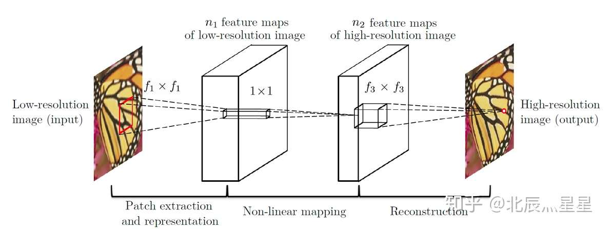
20 |
21 | 首先使用双三次插值将第分辨率图像放大成目标尺寸,接着通过三层卷积网络充当非线性函数映射,最终输出高分辨率图像,网络结构PyTorch版本实现如下:
22 |
23 | ```python
24 | self.conv1 = nn.Conv2d(num_channels, 64, kernel_size=9, padding=9 // 2)
25 | self.conv2 = nn.Conv2d(64, 32, kernel_size=5, padding=5 // 2)
26 | self.conv3 = nn.Conv2d(32, num_channels, kernel_size=5, padding=5 // 2)
27 | self.relu = nn.ReLU(inplace=True)
28 | ```
29 |
30 | ## 代码模块分析
31 |
32 | **文件**主要分为以下几个部分:
33 |
34 | - 数据集
35 | - `data`: 测试数据
36 | - `train`: 训练数据(`.h5`格式)
37 | - `eval`: 验证数据集
38 | - 模型
39 | - `output`: 自己创建用于保存模型输出
40 | - `weights`: 预训练模型
41 |
42 | **代码部分**主要分为以下几个部分:
43 |
44 | - `train.py`: 整体训练过程文件,核心包括参数读取,模型、loss、优化器定义,数据集载入,每个epoch训练和验证等
45 | - `test.py`: 针对一张测试图片,对其降采样,并通过bicubic和SRCNN进行超分,输出结果
46 | - `models.py`: 定义SRCNN整体网络结构
47 | - `datasets.py`: 训练和测试数据集数据结构,主要用在DataLoader中以batch为单位进行处理中
48 | - `prepare.py`: 构建自定义数据集
49 |
50 | ## 环境搭建及实验
51 |
52 | **实验环境**:
53 |
54 | - 操作系统:Ubnutu 18.04
55 | - 语言:Python 3.7
56 | - 深度学习框架: PyTorch 1.9.1
57 |
58 | **训练完所有epoch的截图**:
59 |
60 | 
61 |
62 | **使用官方数据集进行测试**:
63 |
64 | 
65 |
66 | 
67 |
68 | **使用自己采集的数据进行测试**:
69 |
70 | 
71 |
72 | 
--------------------------------------------------------------------------------
/experiment/Image-Super-Resolution/models.py:
--------------------------------------------------------------------------------
1 | from torch import nn
2 |
3 |
4 | class SRCNN(nn.Module):
5 | def __init__(self, num_channels=1):
6 | super(SRCNN, self).__init__()
7 | self.conv1 = nn.Conv2d(num_channels, 64, kernel_size=9, padding=9 // 2)
8 | self.conv2 = nn.Conv2d(64, 32, kernel_size=5, padding=5 // 2)
9 | self.conv3 = nn.Conv2d(32, num_channels, kernel_size=5, padding=5 // 2)
10 | self.relu = nn.ReLU(inplace=True)
11 |
12 | def forward(self, x):
13 | x = self.relu(self.conv1(x))
14 | x = self.relu(self.conv2(x))
15 | x = self.conv3(x)
16 | return x
17 |
--------------------------------------------------------------------------------
/experiment/Mento-Carlo/README.md:
--------------------------------------------------------------------------------
1 | # 算法第十四次作业
2 |
3 | 姓名:张喆 学号:2101212846 指导老师:张健老师
4 |
5 | ## 实验要求
6 |
7 | 写一个程序,用蒙特卡洛法求圆周率pi
8 |
9 | ## 实验思路
10 |
11 | 蒙特卡洛算法的核心思想是“repeated random sampling to obtain numerical results”
12 |
13 | 因此实验首先划定$[0,1]\times[1,0]$的单位空间,随机生成$N$个点,计算点落入$x^2+y^2<=1, (0 \leq x \leq 1,0\leq y \le1)$中的个数占总体的比例,以此逼近$\pi$
14 |
15 | ## 实验结果
16 |
17 | 随机撒落1000个点进行模拟,最终拟合的结果$\hat \pi = 3.156$
18 |
19 | 
20 |
21 | 又从100~100000进行更多的实验,绘制曲线如下,可以观察到由于蒙特卡洛算法的随机性,即使增大到非常大量的数量级,依然存在着拟合的波动(并不像期待的平滑曲线不断趋近真值),但随着点数的增加拟合效果的偶然性更小,结果理论上更可信
22 |
23 | 
24 |
25 | ## 代码
26 |
27 | ```python
28 | import numpy as np
29 | import matplotlib.pyplot as plt
30 |
31 | totalNum = 100
32 |
33 | x, y = np.random.rand((totalNum)), np.random.rand((totalNum))
34 | my_pi = np.where(np.sqrt(x**2 + y**2) < 1)[0].shape[0] / totalNum * 4
35 | print(my_pi)
36 |
37 | plt.figure(figsize=(5,5))
38 | plt.scatter(x, y)
39 | circle = plt.Circle((0,0), 1, color='r', fill=False)
40 | plt.gcf().gca().add_artist(circle)
41 | plt.show()
42 | ```
43 |
44 | ```python
45 | X, Y = [], []
46 | for totalNum in range(100, 100000, 500):
47 | x, y = np.random.rand((totalNum)), np.random.rand((totalNum))
48 | X.append(totalNum)
49 | Y.append(np.where(np.sqrt(x**2 + y**2) < 1)[0].shape[0] / totalNum * 4)
50 |
51 | plt.plot(X, Y)
52 |
53 | plt.plot([0, X[-1]], [np.pi, np.pi], 'r--')
54 | plt.annotate(np.pi,
55 | xy=(X[len(X)//2], np.pi), xycoords='data',
56 | xytext=(-30, -40), textcoords='offset points', fontsize=16,
57 | arrowprops=dict(arrowstyle='->', connectionstyle='arc3, rad=.2'))
58 | ```
59 |
60 |
--------------------------------------------------------------------------------
/experiment/Regression/DNN-generation.ipynb:
--------------------------------------------------------------------------------
1 | {
2 | "cells": [
3 | {
4 | "cell_type": "markdown",
5 | "metadata": {},
6 | "source": [
7 | "# 两层全连接神经网络\n",
8 | "- 输入1000个节点,隐藏层100个,输出10个\n",
9 | "- 只考虑W不考虑b\n",
10 | "- 全连接ReLU神经网络\n",
11 | "\n",
12 | "---\n",
13 | "\n",
14 | "- $h = W_1X$\n",
15 | "- $h_{relu} = max(0, h)$\n",
16 | "- $y_{pred} = W_2h_{relu}$\n",
17 | "- $f = || y - y_{pred} ||^2_F$\n",
18 | "\n",
19 | "---\n",
20 | "- $\\frac{\\partial f}{\\partial y_{pred}} = 2(y_{pred} - y)$\n",
21 | "- $\\frac{\\partial f}{\\partial h_{relu}} = \\frac{\\partial f}{\\partial y_{pred}}W_2^T$\n",
22 | "- $\\frac{\\partial f}{\\partial W_2} = h_{relu}^T \\frac{\\partial f}{\\partial y_{pred}}$\n",
23 | "- $\\frac{\\partial f}{\\partial h} = \\frac{\\partial f}{\\partial h_{relu}} \\odot \\sigma(h)$\n",
24 | "- $\\frac{\\partial f}{\\partial x} = x^T\\frac{\\partial f}{\\partial h}$"
25 | ]
26 | },
27 | {
28 | "cell_type": "code",
29 | "execution_count": 1,
30 | "metadata": {},
31 | "outputs": [],
32 | "source": [
33 | "import numpy as np\n",
34 | "import torch\n",
35 | "import matplotlib.pyplot as plt"
36 | ]
37 | },
38 | {
39 | "cell_type": "code",
40 | "execution_count": 2,
41 | "metadata": {},
42 | "outputs": [],
43 | "source": [
44 | "BATCH = 64\n",
45 | "EPOCH = 500\n",
46 | "N_in, N_hidden, N_out = 1000, 100, 10\n",
47 | "LR = 1e-6"
48 | ]
49 | },
50 | {
51 | "cell_type": "markdown",
52 | "metadata": {},
53 | "source": [
54 | "## 一. Numpy手动计算梯度"
55 | ]
56 | },
57 | {
58 | "cell_type": "code",
59 | "execution_count": 7,
60 | "metadata": {},
61 | "outputs": [
62 | {
63 | "name": "stdout",
64 | "output_type": "stream",
65 | "text": [
66 | "Epoch 0: Loss 35408475.5708653\n",
67 | "Epoch 50: Loss 13210.723218441559\n",
68 | "Epoch 100: Loss 424.07916714308783\n",
69 | "Epoch 150: Loss 24.458366132394872\n",
70 | "Epoch 200: Loss 1.7288604054217553\n",
71 | "Epoch 250: Loss 0.13823869620770285\n",
72 | "Epoch 300: Loss 0.012206723331863328\n",
73 | "Epoch 350: Loss 0.0011717242860535743\n",
74 | "Epoch 400: Loss 0.0001203650115225353\n",
75 | "Epoch 450: Loss 1.3028675705281583e-05\n"
76 | ]
77 | }
78 | ],
79 | "source": [
80 | "x = np.random.randn(BATCH, N_in)\n",
81 | "y = np.random.randn(BATCH, N_out)\n",
82 | "\n",
83 | "w1 = np.random.randn(N_in, N_hidden)\n",
84 | "w2 = np.random.randn(N_hidden, N_out)\n",
85 | "\n",
86 | "for it in range(EPOCH):\n",
87 | " # forward pass\n",
88 | " h = x.dot(w1)\n",
89 | " h_relu = np.maximum(h, 0)\n",
90 | " y_pred = h_relu.dot(w2)\n",
91 | "\n",
92 | " # compute loss\n",
93 | " loss = np.square(y_pred - y).sum()\n",
94 | " if it % 50 == 0: print(\"Epoch {}: Loss {}\".format(it, loss))\n",
95 | "\n",
96 | " # backward pass\n",
97 | " grad_y_pred = 2 * (y_pred - y)\n",
98 | " grad_w2 = h_relu.T.dot(grad_y_pred)\n",
99 | " grad_h_relu = grad_y_pred.dot(w2.T)\n",
100 | " grad_h = grad_h_relu.copy()\n",
101 | " grad_h[h < 0] = 0\n",
102 | " grad_w1 = x.T.dot(grad_h)\n",
103 | "\n",
104 | " # update weights\n",
105 | " w1 -= LR * grad_w1\n",
106 | " w2 -= LR * grad_w2"
107 | ]
108 | },
109 | {
110 | "cell_type": "markdown",
111 | "metadata": {},
112 | "source": [
113 | "## 二. Torch手动计算梯度"
114 | ]
115 | },
116 | {
117 | "cell_type": "code",
118 | "execution_count": 12,
119 | "metadata": {},
120 | "outputs": [
121 | {
122 | "name": "stdout",
123 | "output_type": "stream",
124 | "text": [
125 | "Epoch 0: Loss 26807970.0\n",
126 | "Epoch 50: Loss 10895.0634765625\n",
127 | "Epoch 100: Loss 404.9765930175781\n",
128 | "Epoch 150: Loss 27.17841339111328\n",
129 | "Epoch 200: Loss 2.4550464153289795\n",
130 | "Epoch 250: Loss 0.2618061602115631\n",
131 | "Epoch 300: Loss 0.030567120760679245\n",
132 | "Epoch 350: Loss 0.003984278533607721\n",
133 | "Epoch 400: Loss 0.0007121993694454432\n",
134 | "Epoch 450: Loss 0.00019911790150217712\n"
135 | ]
136 | }
137 | ],
138 | "source": [
139 | "x = torch.randn(BATCH, N_in)\n",
140 | "y = torch.randn(BATCH, N_out)\n",
141 | "\n",
142 | "w1 = torch.randn(N_in, N_hidden)\n",
143 | "w2 = torch.randn(N_hidden, N_out)\n",
144 | "\n",
145 | "for it in range(EPOCH):\n",
146 | " h = x.mm(w1)\n",
147 | " h_relu = h.clamp(min=0)\n",
148 | " y_pred = h_relu.mm(w2)\n",
149 | "\n",
150 | " loss = (y_pred - y).pow(2).sum()\n",
151 | " if it % 50 == 0: print(\"Epoch {}: Loss {}\".format(it, loss))\n",
152 | "\n",
153 | " grad_y_pred = 2*(y_pred - y)\n",
154 | " grad_w2 = h_relu.t().mm(grad_y_pred)\n",
155 | " grad_h_relu = grad_y_pred.mm(w2.t())\n",
156 | " grad_h = grad_h_relu.clone()\n",
157 | " grad_h[h<0] = 0\n",
158 | " grad_w1 = x.t().mm(grad_h)\n",
159 | "\n",
160 | " w1 -= LR * grad_w1\n",
161 | " w2 -= LR * grad_w2"
162 | ]
163 | },
164 | {
165 | "cell_type": "markdown",
166 | "metadata": {},
167 | "source": [
168 | "## PyTorch"
169 | ]
170 | },
171 | {
172 | "cell_type": "markdown",
173 | "metadata": {},
174 | "source": [
175 | "### 三. Autograd"
176 | ]
177 | },
178 | {
179 | "cell_type": "code",
180 | "execution_count": 14,
181 | "metadata": {},
182 | "outputs": [
183 | {
184 | "name": "stdout",
185 | "output_type": "stream",
186 | "text": [
187 | "Epoch 0: Loss 32670436.0\n",
188 | "Epoch 50: Loss 20055.0078125\n",
189 | "Epoch 100: Loss 1657.7003173828125\n",
190 | "Epoch 150: Loss 257.3371887207031\n",
191 | "Epoch 200: Loss 46.99903869628906\n",
192 | "Epoch 250: Loss 9.062090873718262\n",
193 | "Epoch 300: Loss 1.7900952100753784\n",
194 | "Epoch 350: Loss 0.35835203528404236\n",
195 | "Epoch 400: Loss 0.07240660488605499\n",
196 | "Epoch 450: Loss 0.014984498731791973\n"
197 | ]
198 | }
199 | ],
200 | "source": [
201 | "x = torch.randn(BATCH, N_in)\n",
202 | "y = torch.randn(BATCH, N_out)\n",
203 | "\n",
204 | "w1 = torch.randn(N_in, N_hidden, requires_grad=True)\n",
205 | "w2 = torch.randn(N_hidden, N_out, requires_grad=True)\n",
206 | "\n",
207 | "for it in range(EPOCH):\n",
208 | " y_pred = x.mm(w1).clamp(min=0).mm(w2)\n",
209 | "\n",
210 | " loss = (y_pred - y).pow(2).sum()\n",
211 | " if it % 50 == 0: print(\"Epoch {}: Loss {}\".format(it, loss))\n",
212 | "\n",
213 | " loss.backward()\n",
214 | "\n",
215 | " with torch.no_grad():\n",
216 | " w1 -= LR * w1.grad\n",
217 | " w2 -= LR * w2.grad\n",
218 | " w1.grad.zero_()\n",
219 | " w2.grad.zero_()"
220 | ]
221 | },
222 | {
223 | "cell_type": "markdown",
224 | "metadata": {},
225 | "source": [
226 | "### 四. Optim"
227 | ]
228 | },
229 | {
230 | "cell_type": "code",
231 | "execution_count": 17,
232 | "metadata": {},
233 | "outputs": [
234 | {
235 | "name": "stdout",
236 | "output_type": "stream",
237 | "text": [
238 | "Epoch 0: Loss 34224736.0\n",
239 | "Epoch 50: Loss 13434.0263671875\n",
240 | "Epoch 100: Loss 644.0214233398438\n",
241 | "Epoch 150: Loss 51.45646286010742\n",
242 | "Epoch 200: Loss 5.0250163078308105\n",
243 | "Epoch 250: Loss 0.5542936325073242\n",
244 | "Epoch 300: Loss 0.0669383704662323\n",
245 | "Epoch 350: Loss 0.008839967660605907\n",
246 | "Epoch 400: Loss 0.0014848707942292094\n",
247 | "Epoch 450: Loss 0.00039268750697374344\n"
248 | ]
249 | }
250 | ],
251 | "source": [
252 | "x = torch.randn(BATCH, N_in)\n",
253 | "y = torch.randn(BATCH, N_out)\n",
254 | "\n",
255 | "w1 = torch.randn(N_in, N_hidden, requires_grad=True)\n",
256 | "w2 = torch.randn(N_hidden, N_out, requires_grad=True)\n",
257 | "\n",
258 | "optimizer = torch.optim.SGD([w1, w2], lr=LR)\n",
259 | "\n",
260 | "for it in range(EPOCH):\n",
261 | " y_pred = x.mm(w1).clamp(min=0).mm(w2)\n",
262 | "\n",
263 | " loss = (y_pred - y).pow(2).sum()\n",
264 | " if it % 50 == 0: print(\"Epoch {}: Loss {}\".format(it, loss))\n",
265 | "\n",
266 | " loss.backward()\n",
267 | " optimizer.step()\n",
268 | " optimizer.zero_grad()"
269 | ]
270 | },
271 | {
272 | "cell_type": "markdown",
273 | "metadata": {},
274 | "source": [
275 | "### 五. Loss"
276 | ]
277 | },
278 | {
279 | "cell_type": "code",
280 | "execution_count": 18,
281 | "metadata": {},
282 | "outputs": [
283 | {
284 | "name": "stdout",
285 | "output_type": "stream",
286 | "text": [
287 | "Epoch 0: Loss 30201670.0\n",
288 | "Epoch 50: Loss 19577.216796875\n",
289 | "Epoch 100: Loss 1194.46875\n",
290 | "Epoch 150: Loss 116.95330810546875\n",
291 | "Epoch 200: Loss 14.979321479797363\n",
292 | "Epoch 250: Loss 2.248992443084717\n",
293 | "Epoch 300: Loss 0.367341548204422\n",
294 | "Epoch 350: Loss 0.06274251639842987\n",
295 | "Epoch 400: Loss 0.011243206448853016\n",
296 | "Epoch 450: Loss 0.0023114148061722517\n"
297 | ]
298 | }
299 | ],
300 | "source": [
301 | "x = torch.randn(BATCH, N_in)\n",
302 | "y = torch.randn(BATCH, N_out)\n",
303 | "\n",
304 | "w1 = torch.randn(N_in, N_hidden, requires_grad=True)\n",
305 | "w2 = torch.randn(N_hidden, N_out, requires_grad=True)\n",
306 | "\n",
307 | "optimizer = torch.optim.SGD([w1, w2], lr=LR)\n",
308 | "loss_func = torch.nn.MSELoss(reduction='sum')\n",
309 | "\n",
310 | "for it in range(EPOCH):\n",
311 | " y_pred = x.mm(w1).clamp(min=0).mm(w2)\n",
312 | "\n",
313 | " loss = loss_func(y_pred, y)\n",
314 | " if it % 50 == 0: print(\"Epoch {}: Loss {}\".format(it, loss))\n",
315 | "\n",
316 | " loss.backward()\n",
317 | " optimizer.step()\n",
318 | " optimizer.zero_grad()"
319 | ]
320 | },
321 | {
322 | "cell_type": "markdown",
323 | "metadata": {},
324 | "source": [
325 | "### 六. Sequential"
326 | ]
327 | },
328 | {
329 | "cell_type": "code",
330 | "execution_count": 21,
331 | "metadata": {},
332 | "outputs": [
333 | {
334 | "name": "stdout",
335 | "output_type": "stream",
336 | "text": [
337 | "Epoch 0: Loss 33341480.0\n",
338 | "Epoch 50: Loss 15438.4150390625\n",
339 | "Epoch 100: Loss 652.8851928710938\n",
340 | "Epoch 150: Loss 58.59893798828125\n",
341 | "Epoch 200: Loss 7.505269527435303\n",
342 | "Epoch 250: Loss 1.141122579574585\n",
343 | "Epoch 300: Loss 0.18748416006565094\n",
344 | "Epoch 350: Loss 0.0320446640253067\n",
345 | "Epoch 400: Loss 0.005843315739184618\n",
346 | "Epoch 450: Loss 0.001299908384680748\n"
347 | ]
348 | }
349 | ],
350 | "source": [
351 | "x = torch.randn(BATCH, N_in)\n",
352 | "y = torch.randn(BATCH, N_out)\n",
353 | "\n",
354 | "model = torch.nn.Sequential(\n",
355 | " torch.nn.Linear(N_in, N_hidden, bias=False),\n",
356 | " torch.nn.ReLU(),\n",
357 | " torch.nn.Linear(N_hidden, N_out, bias=False)\n",
358 | ")\n",
359 | "\n",
360 | "torch.nn.init.normal_(model[0].weight)\n",
361 | "torch.nn.init.normal_(model[2].weight)\n",
362 | "\n",
363 | "loss_func = torch.nn.MSELoss(reduction='sum')\n",
364 | "\n",
365 | "for it in range(EPOCH):\n",
366 | " y_pred = model(x)\n",
367 | "\n",
368 | " loss = loss_func(y_pred, y)\n",
369 | " if it % 50 == 0: print(\"Epoch {}: Loss {}\".format(it, loss))\n",
370 | "\n",
371 | " loss.backward()\n",
372 | "\n",
373 | " with torch.no_grad():\n",
374 | " for param in model.parameters():\n",
375 | " param -= LR * param.grad\n",
376 | " \n",
377 | " model.zero_grad()"
378 | ]
379 | },
380 | {
381 | "cell_type": "markdown",
382 | "metadata": {},
383 | "source": [
384 | "### 七. Sequential + Optim"
385 | ]
386 | },
387 | {
388 | "cell_type": "code",
389 | "execution_count": 27,
390 | "metadata": {},
391 | "outputs": [
392 | {
393 | "name": "stdout",
394 | "output_type": "stream",
395 | "text": [
396 | "Epoch 0: Loss 31621422.0\n",
397 | "Epoch 50: Loss 9968.7177734375\n",
398 | "Epoch 100: Loss 345.5548095703125\n",
399 | "Epoch 150: Loss 21.064655303955078\n",
400 | "Epoch 200: Loss 1.687893033027649\n",
401 | "Epoch 250: Loss 0.1620352864265442\n",
402 | "Epoch 300: Loss 0.017796725034713745\n",
403 | "Epoch 350: Loss 0.0024050897918641567\n",
404 | "Epoch 400: Loss 0.0004838006279896945\n",
405 | "Epoch 450: Loss 0.0001473624724894762\n"
406 | ]
407 | }
408 | ],
409 | "source": [
410 | "x = torch.randn(BATCH, N_in)\n",
411 | "y = torch.randn(BATCH, N_out)\n",
412 | "\n",
413 | "model = torch.nn.Sequential(\n",
414 | " torch.nn.Linear(N_in, N_hidden, bias=False),\n",
415 | " torch.nn.ReLU(),\n",
416 | " torch.nn.Linear(N_hidden, N_out, bias=False)\n",
417 | ")\n",
418 | "\n",
419 | "torch.nn.init.normal_(model[0].weight)\n",
420 | "torch.nn.init.normal_(model[2].weight)\n",
421 | "\n",
422 | "loss_func = torch.nn.MSELoss(reduction='sum')\n",
423 | "optimizer = torch.optim.SGD(model.parameters(), lr=LR)\n",
424 | "\n",
425 | "for it in range(EPOCH):\n",
426 | " y_pred = model(x)\n",
427 | "\n",
428 | " loss = loss_func(y_pred, y)\n",
429 | " if it % 50 == 0: print(\"Epoch {}: Loss {}\".format(it, loss))\n",
430 | "\n",
431 | " loss.backward()\n",
432 | " optimizer.step()\n",
433 | " optimizer.zero_grad()"
434 | ]
435 | },
436 | {
437 | "cell_type": "markdown",
438 | "metadata": {},
439 | "source": [
440 | "### 八. 自定义网络(显式参数)"
441 | ]
442 | },
443 | {
444 | "cell_type": "code",
445 | "execution_count": 50,
446 | "metadata": {},
447 | "outputs": [
448 | {
449 | "name": "stdout",
450 | "output_type": "stream",
451 | "text": [
452 | "Epoch 0: Loss 34467236.0\n",
453 | "Epoch 50: Loss 12329.94140625\n",
454 | "Epoch 100: Loss 551.3489990234375\n",
455 | "Epoch 150: Loss 40.532169342041016\n",
456 | "Epoch 200: Loss 3.521925687789917\n",
457 | "Epoch 250: Loss 0.33698779344558716\n",
458 | "Epoch 300: Loss 0.03455748409032822\n",
459 | "Epoch 350: Loss 0.003984588198363781\n",
460 | "Epoch 400: Loss 0.0006867757765576243\n",
461 | "Epoch 450: Loss 0.00020060440874658525\n"
462 | ]
463 | }
464 | ],
465 | "source": [
466 | "x = torch.randn(BATCH, N_in)\n",
467 | "y = torch.randn(BATCH, N_out)\n",
468 | "\n",
469 | "class Net(torch.nn.Module):\n",
470 | " def __init__(self):\n",
471 | " super(Net, self).__init__()\n",
472 | "\n",
473 | " # self.w1 = torch.nn.Parameter(torch.nn.init.xavier_normal_(torch.Tensor(N_in, N_hidden)))\n",
474 | " # self.w2 = torch.nn.Parameter(torch.nn.init.xavier_normal_(torch.Tensor(N_hidden, N_out)))\n",
475 | " self.w1 = torch.nn.Parameter(torch.nn.init.normal_(torch.Tensor(N_in, N_hidden)))\n",
476 | " self.w2 = torch.nn.Parameter(torch.nn.init.normal_(torch.randn(N_hidden, N_out)))\n",
477 | "\n",
478 | " def forward(self, x):\n",
479 | " y_pred = x.mm(self.w1).clamp(min=0).mm(self.w2)\n",
480 | " return y_pred\n",
481 | "\n",
482 | "model = Net()\n",
483 | "loss_func = torch.nn.MSELoss(reduction='sum')\n",
484 | "optimizer = torch.optim.SGD(model.parameters(), lr=LR)\n",
485 | "\n",
486 | "for it in range(EPOCH):\n",
487 | " y_pred = model(x)\n",
488 | "\n",
489 | " loss = loss_func(y_pred, y)\n",
490 | " if it % 50 == 0: print(\"Epoch {}: Loss {}\".format(it, loss))\n",
491 | "\n",
492 | " loss.backward()\n",
493 | " optimizer.step()\n",
494 | " optimizer.zero_grad()"
495 | ]
496 | },
497 | {
498 | "cell_type": "markdown",
499 | "metadata": {},
500 | "source": [
501 | "### 九. 自定义网络(隐式参数)"
502 | ]
503 | },
504 | {
505 | "cell_type": "code",
506 | "execution_count": 43,
507 | "metadata": {},
508 | "outputs": [
509 | {
510 | "name": "stdout",
511 | "output_type": "stream",
512 | "text": [
513 | "Epoch 0: Loss 40366000.0\n",
514 | "Epoch 50: Loss 12587.9111328125\n",
515 | "Epoch 100: Loss 353.7375183105469\n",
516 | "Epoch 150: Loss 16.398738861083984\n",
517 | "Epoch 200: Loss 0.9396277666091919\n",
518 | "Epoch 250: Loss 0.0601460263133049\n",
519 | "Epoch 300: Loss 0.00429706322029233\n",
520 | "Epoch 350: Loss 0.0005215808050706983\n",
521 | "Epoch 400: Loss 0.00013343743921723217\n",
522 | "Epoch 450: Loss 5.4725031077396125e-05\n"
523 | ]
524 | }
525 | ],
526 | "source": [
527 | "x = torch.randn(BATCH, N_in)\n",
528 | "y = torch.randn(BATCH, N_out)\n",
529 | "\n",
530 | "class Net(torch.nn.Module):\n",
531 | " def __init__(self):\n",
532 | " super(Net, self).__init__()\n",
533 | " self.linear1 = torch.nn.Linear(N_in, N_hidden, bias=False)\n",
534 | " self.linear2 = torch.nn.Linear(N_hidden, N_out, bias=False)\n",
535 | "\n",
536 | " torch.nn.init.normal_(self.linear1.weight)\n",
537 | " torch.nn.init.normal_(self.linear2.weight)\n",
538 | "\n",
539 | " def forward(self, x):\n",
540 | " y_pred = self.linear2(self.linear1(x).clamp(min=0))\n",
541 | " return y_pred\n",
542 | "\n",
543 | "model = Net()\n",
544 | "loss_func = torch.nn.MSELoss(reduction='sum')\n",
545 | "optimizer = torch.optim.SGD(model.parameters(), lr=LR)\n",
546 | "\n",
547 | "for it in range(EPOCH):\n",
548 | " y_pred = model(x)\n",
549 | "\n",
550 | " loss = loss_func(y_pred, y)\n",
551 | " if it % 50 == 0: print(\"Epoch {}: Loss {}\".format(it, loss))\n",
552 | "\n",
553 | " loss.backward()\n",
554 | " optimizer.step()\n",
555 | " optimizer.zero_grad()"
556 | ]
557 | }
558 | ],
559 | "metadata": {
560 | "interpreter": {
561 | "hash": "a3b0ff572e5cd24ec265c5b4da969dd40707626c6e113422fd84bd2b9440fcfc"
562 | },
563 | "kernelspec": {
564 | "display_name": "Python 3.9.7 64-bit ('deep_learning': conda)",
565 | "name": "python3"
566 | },
567 | "language_info": {
568 | "codemirror_mode": {
569 | "name": "ipython",
570 | "version": 3
571 | },
572 | "file_extension": ".py",
573 | "mimetype": "text/x-python",
574 | "name": "python",
575 | "nbconvert_exporter": "python",
576 | "pygments_lexer": "ipython3",
577 | "version": "3.9.7"
578 | },
579 | "orig_nbformat": 4
580 | },
581 | "nbformat": 4,
582 | "nbformat_minor": 2
583 | }
584 |
--------------------------------------------------------------------------------
/experiment/Regression/function-fitting.ipynb:
--------------------------------------------------------------------------------
1 | {
2 | "cells": [
3 | {
4 | "cell_type": "code",
5 | "execution_count": 1,
6 | "metadata": {},
7 | "outputs": [],
8 | "source": [
9 | "import torch\n",
10 | "from torch.autograd import Variable\n",
11 | "import torch.nn.functional as F\n",
12 | "import matplotlib.pyplot as plt\n",
13 | "from IPython import display"
14 | ]
15 | },
16 | {
17 | "cell_type": "code",
18 | "execution_count": 2,
19 | "metadata": {},
20 | "outputs": [
21 | {
22 | "data": {
23 | "image/png": "iVBORw0KGgoAAAANSUhEUgAAAXIAAAD4CAYAAADxeG0DAAAAOXRFWHRTb2Z0d2FyZQBNYXRwbG90bGliIHZlcnNpb24zLjQuMiwgaHR0cHM6Ly9tYXRwbG90bGliLm9yZy8rg+JYAAAACXBIWXMAAAsTAAALEwEAmpwYAAAa50lEQVR4nO3dfYxcZ3XH8d/xZkLGQLNJYwreJDi01LQQsGEFKa4omJaE8OYGqIN4LUgRqmixVdwuQipUUMWtCw5VKVUaqGiLwBUElxKooTUI1ZSIdbwQgjFvCpB1gIVmA623sHFO/5i5zvXd+zZ7nztz7+z3I1m7Oy93nsxOjh+f5zznMXcXAKC91o16AACAagjkANByBHIAaDkCOQC0HIEcAFrunFG86EUXXeSbNm0axUsDQGsdPXr0h+6+IXn7SAL5pk2bNDs7O4qXBoDWMrNvp91OagUAWo5ADgAtRyAHgJYjkANAyxHIAaDlRlK1AgDj7uCxee07dEInF5e0cbKrPVdu1o6tU7W8lo2i++H09LRTfghgXB08Nq833ny7lpZPn7mts870kPPO0eKp5VUHdjM76u7TyduZkQNAYPsOnTgriEvS8v2ue04tS5LmF5f0xptvl6Qgs3Ry5AAQyMFj89q297DmF5cKH7u0fFr7Dp0I8rrMyAEggLR0SpGTJQJ+GczIASCAtHRKkY2T3SCvTSAHgADyZteT3Y46E3bWbd3OhPZcuTnIaxPIASCArNn11GRXc29+lva96AmamuzK+rddf83lwcoRyZEDQAlFdeF7rty8Ikcen3Xv2DpVWx05gRwACiQXMtPKB6Ovw9oEFEcgB4ACaQuZUflgPFDXOevOQ44cAApkLWSGKh+sihk5AMSk5cI3TnZTN/mEKh+sil4rANCXtqnHJHnsa6TbmdD111wuaXh5cXqtAECBtFy4x75GwXyqH7AlFS6CDkOQHLmZ7TazO8zsy2b2ATM7L8R1AWAYyvZIiYL4kZnt2rF1KncRdJgqB3Izm5L0B5Km3f1xkiYkXVv1ugAwDFE6pUyjK+nsBc6mLIKGqlo5R1LXzM6RtF7SyUDXBYBaDdojJb7AmbXYOexF0MqB3N3nJf2lpO9IulvSve7+yarXBYBhyJs9W+LnZH+UPVduVrczkfuYYQiRWrlA0gskXSZpo6QHm9nLUh53nZnNmtnswsJC1ZcFgCDyeqTs37kltT9KlFPffWBODzpnnS5Y36mlh0pZlcsPzezFkq5y99f0f36FpCvc/feynkP5IYCmSCs5jEoL0wLyoI8PKav8MESO/DuSrjCz9WZmkp4p6XiA6wJA7XZsndL111xeujNhUypV4irXkbv7rWb2IUm3SbpP0jFJN1a9LgAMyyA9UppSqRIXZEOQu79Z0ptDXAsAmqyJ2/VpmgWglaIFx8tmbtG2vYd18Nj8UF63KZUqcWzRB9A6ZfqD12WUfcezEMgBtE7Z/uB1GVXf8SykVgC0ThMXHEeJQA6gdZqyNb4pCOQAWqeJC46jRI4cQOs0ccFxlAjkAFqp6oJj2pFubf2LgEAOoDWqBt/o+fOLS2cd3Taqk31CIUcOoBXiB0C4Hgi+ZTcCJQ+QSLYLHHW/lCqYkQNohaLa8aLZepkDJNpavkggB9AKebXjaTs9dx+Y064Dc2cOSi4TpNtavkggB9Bo0Uw76+SEjZPd1Nl2PP+9+8Bc5vMjbS5fJEcOoLGKDkaOgm/RbDsriEdHuY3qZJ9QmJEDqN1qq03y8tpTsetElSiDmGp5yWEcgRxArcp2KkwL9lkzbZN0ZGb7mZ/3XLl5xfFreZLPbztSKwBqVeZotKzSwsn1ndRrJhcl48e1SQ+kTLK0dVEzCzNyALUq06kwK9gvLZ8+a+OOlL0oGd/pmbXxJ+/5bUYgB1CrvKPR4gE3i0tngnHZvHZaUB+HrfhZzL2oKCe86elpn52dHfrrAhi+ZI5c6s2KX/ikKX346HzpvPbUZHes8tqrYWZH3X06eTs5cgC1iuevTQ+U+n36qwulg7jU3l2Xw0BqBUDt0joV7j4wN9A1xm2BMiRm5ABGIiswT3Y7HBoxIAI5gJHIOuXnLc9/bGoqZtwWKEMitQJgqOJVJOd3Ozqvs06Lp5ZXVJQQuMsjkAMYmmQFy+LSsrqdCe3fuYXAXQGpFQBDU2aXJwZHIAcwNGV2eWJwBHIAQ5NVqUJpYTUEcgCVHDw2r217D+uymVu0be/h3DM0sypVKC2sJship5lNSrpJ0uPUa4nwanf/rxDXBtA8eafRR0esTXY7MlNqRcq49z4ZtlBVK++U9G/u/iIzO1fS+kDXBdAwycqTZLem6OfFpeUztyV7kBO4w6ocyM3s5yQ9TdKrJMndfybpZ1WvC2D0kjXfZtI9p5aLn5gifuI9wgqRI3+UpAVJf29mx8zsJjN7cPJBZnadmc2a2ezCwkKAlwVQp+RhD4tLy6sO4hGqU+oRIpCfI+mJkt7t7lsl/a+kmeSD3P1Gd5929+kNGzYEeFkAIWQtVuadl7laVKfUI0SO/C5Jd7n7rf2fP6SUQA6gOfIWK6Nc9iCz5+gaydN44qhOqU/lGbm7f0/Sd80s+g09U9JXql4XQD3iKRNpZeCNctllZ89Tk13t37lFd+59jvbv3HKm2dVkt6ML1ndofDUEoapWfl/S+/sVK9+S9LuBrgsgsDIpk5OLS9q/c0vuyfTdzsSK4ExFymgECeTuPidpxfFDAJqnTMpk42R3Rc33+Tl14Rgtuh8Ca0zWYciReC6bGXY7sEUfWGPStslb/yu57HZiRg6sMXnb5KNqlt0H5kiftAiBHFiD0lImya33yW31aC5SKwAkcehDmxHIAUji0Ic2I7UCjJl4o6tB8txZ1Sxsq28+ZuTAGEk2uory3HmHPUQ49KG9mJEDLZU2887LcxfNyjn0ob0I5EALZVWYZG2nL5vnZgNQO5FaAVooa+Y9YZb6eJcKz9NEezEjBxqoaMEya4Z92l3dzkTqzJy68PHFjBxomDILllmVJNEW+6mM+5eWT2vXgTlm52OGQA4MUdZpPHFlNubkVZjs2DqlIzPblZ5k6RmkmgXNZ+5Z53nUZ3p62mdnZ4f+usAoJRcopfSe3pfN3JJ5ys5krJXs+RnfxytY8rocSr0Z/JGZ7SH+8zAEZnbU3Ve0DGdGDgxJ2S3weRtwogOQo8OQ/2/5fr30ikv10/vuP3N7NNt+xmM2rJi1J7FrczwQyIEhKbsFPi1tkmVp+bQ+cOt3U/+C+PRXF3Lz5RK7NscFgRwYkqygmbx9x9apwgAcdzojPXpycelMvvyGnVvYtTnGCOTAkBRtgY8vhO47dEJ7rtxcKphn1Y7H/4KI/+XAYcjjhzpyIJCi2u+iAx3Sdmq+8ElT+vDR+dwDkNMekzbbZtfm+CKQAwGUPZQhK5hmLYRGee6iA5CnH3khPVLWMAI5EECVZlVS/kJomZk0s+21jRw5EEDVQxnKLoQCaQjkQABVAzG9wFEFgRwIoGogpqoEVZAjBwIIcSgDeW6sFr1WgBqs9txMIE9WrxVm5EBgZUsRgVAI5MCAimbbVUsRgUEFC+RmNiFpVtK8uz831HWBJkmbbe8+MKddB+Y01Q/qg5QikoJBCCGrVl4v6XjA6wGNkzbbjlaZohTK5PpO6nOT52aWOQkIKCNIIDeziyU9R9JNIa4HjErRCT5FG3yWlk/LXZltaOPBumx/cqBIqBn5DZL+SNL9WQ8ws+vMbNbMZhcWFgK9LBBOlbMy4+5dWi48NzNKp6ThsAcMqnIgN7PnSvqBux/Ne5y73+ju0+4+vWHDhqovCwS32rMykzZOdgvPzYxy4lnPBwYRYka+TdLzzexOSR+UtN3M/inAdYGhypshRymX3Qfm9KBz1umCfh48GaiTuznzgjXb8hFK5UDu7m9094vdfZOkayUddveXVR4ZMGRZQff8bueslEt0VuYNO7do/84tudvqi067Z1s+Qgi6s9PMni7pDUXlh+zsRBNlnXJ/Xmed7jm1vOLxZU+gp8QQoQxlZ6e7f0bSZ0JeE6hikCCa7JcSHeKQFsSl8ouS9FBB3djZibFVdqt8WrCXtGJ2nsSiJJqCQI6xVWarfFawP6+zLjeIsyiJJiGQY2yVqdPOCvZ5QXyKPDcahkCOsROlSrKW8aOt8nl9UbKUXeAEhokTgjBW4rsz8xT1RZnsdqjxRmswI8dYSUuVZFlaPq0HnbNO3c7EipLDtzz/sWeuR9kgmo5AjrEyaKrk3qVl7d+5JTNgE7jRBgRyjJWNk93UtMqEmU6nbH6L+qIQsNFm5MgxVrK2xL/kKZeQ88bYYkaO1iizSzPvNPvpR164Ytfm7gNz2nfoBPlvtFrQXitl0WsFg0rrg2LqlRIOWted1VOFhlVouqxeK6RW0Apljlgre0QaJ/Ng3BDI0QpljlgrG4g5mQfjhkCOVijToKpsIOZkHowbAjlaocwRa8lT6ge5FhUsaDOqVtAK8WqU+cWlMwudSVmtarOuxa5NjAOqVtBKUSliVk8VmlthHFG1grFS5pR6YK0gkKPVWLgECORoORYuARY70XIsXAIEcowBuhdirSOQoxZlGlzV8VxgLaL8EMFVaUoVsjkWMG6yyg+ZkaOS+Ow5ag17z6nlFY+LeqEUBeEyzbEkTu4B4gjkGFh8M058h+Xi0soAHpes7U5LoZRtjkUgBx5AIMdAkqmPQRJz8dru5HXip9qnzejj2OwDnI1AjoEMckp9XLK2O6sn+NLy6cw+KhE2+wBnI5BjIKuZDactUuZdx/XAAmcyqLPZB1ip8s5OM7vEzD5tZsfN7A4ze32IgaGZBpkNdzsTumHnFh2Z2b4ip110nahKZf/OLZqa7Mr6P3McG7BSiBn5fZL+0N1vM7OHSjpqZp9y968EuDYaZs+VmzPLAyf7VSuLp5YL67/TrpN0cnGJzT5ACZUDubvfLenu/vc/MbPjkqYkEcjHUKgt8cn+4mnIhQPlBM2Rm9kmSVsl3Zpy33WSrpOkSy+9NOTLomZpZYIhen1Hs+2sDUTkwoFygnU/NLOHSPqwpF3u/uPk/e5+o7tPu/v0hg0bQr0sahYF2fnFJbkGP7G+jB1bp3T9NZeTCwdWKciM3Mw66gXx97v7zSGuiWbIKhNc7aacrD4q5MKB1ascyM3MJL1H0nF3f0f1IaFJssoEBylDzNoJypZ7IIwQqZVtkl4uabuZzfX/XB3gumiAqifwxFMz0sqNPtHsHsDqhaha+U8p8+hENMRqW8OmlQkOshBZZicoW+6BatjZuQZk9TWRilMaVcsNywRpygyBagjkYyyem04aZMGyykLkxsluZp24RJkhEAKHL4+pZG46TVpb2W17D+uymVu0be/hICWGaYcjR3k4ygyBMJiRj6kyuekybWWlahUlHI4M1I9APqaKctNl28qGOMSBGnGgXqRWxlTeAmI8pRGlU7JSMPOLS8HSLADqwYx8TGWVDV5/zeWSejPwXQfmCg9xkNi4AzQdgbyliurCs3LTklZ1VBtnZQLNRSBvobILk2m56W17D6/qqDaJjTtAU5Ejb6G8hckiZYLxhKVv1GXjDtBMBPIWqtLIqigYdzsTeslTLllR+83GHaC5COQtVKWRVZkNOm/bcTn9wYEWIUfecGmLmlUaWZXdoEPtN9Ae5l62biGc6elpn52dHfrrtk3WEWjxEkJ2SwJrh5kddffp5O3MyBssb1HzyMx2AjcASeTIGy3E6TwAxh+BvMGyFi9dYts8gDMI5A2WVmESyTrNvo5WtACajUDeYDu2Tp0pA0yT3AQU70Huyg72AMYLgbzhdmyd0pGZ7ZmHosbz5VV2fAJoLwJ5S+RtAipqRcviKDDeCOQtkZYv73Ym9IzHbCg80o0eKcB4o468IVbblrboSDd6pADjj52dDZC2gzM68GGqYNfmZTO3ZPYUL3ougHZhZ2fDxGfg68x0OvEXavRT0ek8Gye7qWmVqcmujsxsDz5uAM1DjnwEkmWCySCelFd5kpU7J50CrB3MyEegKK+dJqvypGw3QwDji0Beg6KFy9WUA+ZVntByFljbCOQVpAVsSYXnaWbltSf6ufLkyfakSgDkIUe+Slnb4f/0X+8o3F2Zldd+++88QXfufY7279zC6TwASgsyIzezqyS9U9KEpJvcfW+I6zZZ1nb4rNz3/OKStu09fFaaJSv9QqoEwCAqB3Izm5D0Lkm/JekuSV8ws4+6+1eqXrvJVpPnTqZZCNYAQgiRWnmypG+4+7fc/WeSPijpBQGu22h5i49ZDa4kmlgBCC9EIJ+S9N3Yz3f1bzuLmV1nZrNmNruwsBDgZetV1Nc7r1e4Kz+Y08QKQEghcuRpMWvFDhd3v1HSjVJvi36A161Ncsv8/OKSdh+Y064Dcyu2ve87dCK1AsX1QBVKEk2sAIQUYkZ+l6RLYj9fLOlkgOuOTNpCZnLL/MFj84W9wk+7r5i1mx5Y+OTABwAhhAjkX5D0aDO7zMzOlXStpI8GuO7IFKU+knnurBl2VDoYnfATrw/n9B4AoVQO5O5+n6TXSTok6bikf3b3O6ped5TKpD7iwT6v30k0a5+a7K7IN7HwCSCEIBuC3P3j7v7L7v6L7v5nIa45SnkLmZF4sI+frZm1iSdrls/CJ4Cq2KKfIrmQWWbLfFFdeNa2fBY+AVTFFv0MUUokuWV+stvReZ112n1gbqAFS9rNAqgLM/ISotl2Wlli3qEPyWtItJsFEB6BfABZ/VX2HTpRKiCzLR9AHdZkII+3nz2/25GZtHhquXCWzIIlgCZac4E8mR5ZXFo+c99qz8dkwRLAKK25xc6iY9aWlk9rV8ZCJguWAJpozc3Iy6ZB0mbnLFgCaKKxDeRZ52ZmpUfSpC1ksmAJoGnGMrWSdQzbwWPzpXZtxrGQCaDpxjKQF5UJxrfTT3Y7umB9J/NaLGQCaLqxTK0UlQmmpUeS1SwSC5kA2mEsZ+RZs+i82XWZxlcA0ERjOSPfc+XmVc2uWcgE0EatDORZFSkRygQBrCWtC+RlG1cxuwawVrQuR55XkQIAa1FrAvnBY/Patvdw5mYeDjQGsFa1IrWSVhqYJq/pVVFeHQDaqhUz8qJGV3FpaZa8nZ4A0HatCOSDbpNPplnIqwMYZ61IrWQ1upow02n3lGecnWbhQAgA46wVM/KsPuAvecoluQ2woln3anZ6AkBbtCKQZ22ff9uOy8/cnuXk4hIHQgAYa61IrUjZG3yi27NKEzdOdtnpCWCstSaQFynqr8JOTwDjamwCObNuAGvV2ARyiVk3gLWpFYudAIBslQK5me0zs6+a2ZfM7CNmNhloXACAkqrOyD8l6XHu/nhJX5P0xupDAgAMolIgd/dPuvt9/R8/L+ni6kMCAAwiZI781ZI+kXWnmV1nZrNmNruwsBDwZQFgbTPP6FVy5gFm/y7p4Sl3vcnd/6X/mDdJmpZ0jRddsPf4BUnfHny4kqSLJP1wlc+tE+MaDOMaDOMaTFPHJVUb2yPdfUPyxsJAXsTMXinptZKe6e6nKl2s3OvNuvt03a8zKMY1GMY1GMY1mKaOS6pnbJXqyM3sKkl/LOk3hhHEAQArVc2R/7Wkh0r6lJnNmdnfBhgTAGAAlWbk7v5LoQYygBtH8JplMK7BMK7BMK7BNHVcUg1jq5wjBwCMFlv0AaDlCOQA0HKNDORm9mIzu8PM7jezzDIdM7vKzE6Y2TfMbCZ2+4Vm9ikz+3r/6wWBxlV4XTPb3F/4jf782Mx29e97i5nNx+67eljj6j/uTjO7vf/as4M+v45xmdklZvZpMzve/52/PnZf0Pcr6/MSu9/M7K/693/JzJ5Y9rk1j+ul/fF8ycw+Z2ZPiN2X+jsd0riebmb3xn4/f1L2uTWPa09sTF82s9NmdmH/vlreLzN7r5n9wMy+nHF/vZ8td2/cH0m/ImmzpM9Ims54zISkb0p6lKRzJX1R0q/27/sLSTP972ck/XmgcQ103f4Yv6deEb8kvUXSG2p4v0qNS9Kdki6q+t8VclySHiHpif3vH6pez57o9xjs/cr7vMQec7V6u5NN0hWSbi373JrH9VRJF/S/f3Y0rrzf6ZDG9XRJH1vNc+scV+Lxz5N0eAjv19MkPVHSlzPur/Wz1cgZubsfd/cTBQ97sqRvuPu33P1nkj4o6QX9+14g6X39798naUegoQ163WdK+qa7r3YXa1lV/3tH9n65+93uflv/+59IOi6pjqbyeZ+X+Hj/wXs+L2nSzB5R8rm1jcvdP+fu9/R/HFZPoyr/zSN9vxJeIukDgV47k7t/VtJ/5zyk1s9WIwN5SVOSvhv7+S49EAB+wd3vlnqBQtLDAr3moNe9Vis/RK/r/9PqvaFSGAOMyyV90syOmtl1q3h+XeOSJJnZJklbJd0auznU+5X3eSl6TJnn1jmuuNfo7J5GWb/TYY3r18zsi2b2CTN77IDPrXNcMrP1kq6S9OHYzXW9X0Vq/WyN7IQgK9HDpegSKbdVrqXMG9eA1zlX0vN1dmvfd0t6q3rjfKukt6vXbGxY49rm7ifN7GHqbeL6an8msWoB36+HqPc/3C53/3H/5lW/X2kvkXJb8vOS9ZhaPmsFr7nygWbPUC+Q/3rs5uC/0wHGdZt6acP/6a9fHJT06JLPrXNckedJOuLu8ZlyXe9XkVo/WyML5O7+mxUvcZekS2I/XyzpZP/775vZI9z97v4/X34QYlxmNsh1ny3pNnf/fuzaZ743s7+T9LFhjsvdT/a//sDMPqLeP+s+qxG/X2bWUS+Iv9/db45de9XvV4q8z0vRY84t8dw6xyUze7ykmyQ9291/FN2e8zutfVyxv3Dl7h83s78xs4vKPLfOccWs+Bdxje9XkVo/W21OrXxB0qPN7LL+7PdaSR/t3/dRSa/sf/9KSWVm+GUMct0Vubl+MIv8tqTUFe46xmVmDzazh0bfS3pW7PVH9n6ZmUl6j6Tj7v6OxH0h36+8z0t8vK/oVxhcIenefkqozHNrG5eZXSrpZkkvd/evxW7P+50OY1wP7//+ZGZPVi+e/KjMc+scV38850v6DcU+czW/X0Xq/WyFXr0N8Ue9/2nvkvRTSd+XdKh/+0ZJH4897mr1qhy+qV5KJrr95yX9h6Sv979eGGhcqddNGdd69T7Q5yee/4+Sbpf0pf4v6xHDGpd6q+Jf7P+5oynvl3ppAu+/J3P9P1fX8X6lfV7U69z52v73Juld/ftvV6xiKuuzFuh9KhrXTZLuib0/s0W/0yGN63X91/2ieouwT23C+9X/+VWSPph4Xm3vl3qTtrslLasXu14zzM8WW/QBoOXanFoBAIhADgCtRyAHgJYjkANAyxHIAaDlCOQA0HIEcgBouf8HibME8D/I68EAAAAASUVORK5CYII=",
24 | "text/plain": [
25 | ""
26 | ]
27 | },
28 | "metadata": {
29 | "needs_background": "light"
30 | },
31 | "output_type": "display_data"
32 | },
33 | {
34 | "data": {
35 | "text/plain": [
36 | "(, None)"
37 | ]
38 | },
39 | "execution_count": 2,
40 | "metadata": {},
41 | "output_type": "execute_result"
42 | }
43 | ],
44 | "source": [
45 | "x = torch.linspace(-1, 1, 100)\n",
46 | "x = torch.unsqueeze(x, dim=1) # [100] -> [100, 1]否则train的时候会报错维度不一致\n",
47 | "\n",
48 | "y = 5 * x + 3 + torch.rand(x.size())\n",
49 | "# y = x.pow(2) + 0.2 * torch.rand(x.size())\n",
50 | "\n",
51 | "x, y = Variable(x), Variable(y)\n",
52 | "\n",
53 | "plt.scatter(x.data.numpy(), y.data.numpy()), plt.show()"
54 | ]
55 | },
56 | {
57 | "cell_type": "markdown",
58 | "metadata": {},
59 | "source": [
60 | "拟合一元函数其实两个参数就够用了,现在第一层有10个节点,输出层还有10个节点,w和b其实一共有40个参数了\n",
61 | "\n",
62 | "forward中其实也不需要relu进行激活,因为本来就是线性函数\n",
63 | "\n",
64 | "之所以要初始化网络参数,是因为如果初始就正好是正中间一个水平的直线,其实loss直接为0,根本不会训起来的"
65 | ]
66 | },
67 | {
68 | "cell_type": "code",
69 | "execution_count": 3,
70 | "metadata": {},
71 | "outputs": [
72 | {
73 | "name": "stdout",
74 | "output_type": "stream",
75 | "text": [
76 | "Net(\n",
77 | " (hidden): Linear(in_features=1, out_features=10, bias=True)\n",
78 | " (predict): Linear(in_features=10, out_features=1, bias=True)\n",
79 | ")\n"
80 | ]
81 | }
82 | ],
83 | "source": [
84 | "class Net(torch.nn.Module):\n",
85 | " def __init__(self):\n",
86 | " super(Net, self).__init__()\n",
87 | " self.hidden = torch.nn.Linear(1, 10)\n",
88 | " self.predict = torch.nn.Linear(10, 1)\n",
89 | "\n",
90 | " # 初始化网络参数\n",
91 | " torch.nn.init.uniform_(self.hidden.weight, a=-0.1, b=0.1)\n",
92 | " torch.nn.init.normal_(self.predict.weight, mean=0, std=1)\n",
93 | " \n",
94 | " def forward(self, x):\n",
95 | " x = F.relu(self.hidden(x))\n",
96 | " x = self.predict(x)\n",
97 | " return x\n",
98 | "\n",
99 | "net = Net()\n",
100 | "print(net)"
101 | ]
102 | },
103 | {
104 | "cell_type": "markdown",
105 | "metadata": {},
106 | "source": [
107 | "SGD直接不下降,Adam可以很好的克服这些问题"
108 | ]
109 | },
110 | {
111 | "cell_type": "code",
112 | "execution_count": 4,
113 | "metadata": {},
114 | "outputs": [],
115 | "source": [
116 | "optimizer = torch.optim.SGD(net.parameters(), lr=0.1)\n",
117 | "loss_func = torch.nn.MSELoss()"
118 | ]
119 | },
120 | {
121 | "cell_type": "code",
122 | "execution_count": 5,
123 | "metadata": {},
124 | "outputs": [
125 | {
126 | "data": {
127 | "image/png": "iVBORw0KGgoAAAANSUhEUgAAAXYAAAD8CAYAAABjAo9vAAAAOXRFWHRTb2Z0d2FyZQBNYXRwbG90bGliIHZlcnNpb24zLjQuMiwgaHR0cHM6Ly9tYXRwbG90bGliLm9yZy8rg+JYAAAACXBIWXMAAAsTAAALEwEAmpwYAAAryklEQVR4nO3de5zMZf/H8ddlrYwcllR31mG5iwqF3DqoFHdOldCBTrhvxR3lUNxW1K3UTSjq7vBLKjrrILcih7tVoZN1lkOliN2I2JC11rp+f8zMNjs7szNrv7NmZt/Px8Oj3Znv95rL7PTZy+e6rs9lrLWIiEj8KHeiOyAiIs5SYBcRiTMK7CIicUaBXUQkziiwi4jEGQV2EZE4E3OB3RjT70T3IRD1q3jUr+JRv4onWvsFpdO3mAvsQLT+wNSv4lG/ikf9Kp5o7ReUQt9iMbCLiEgRzInYeVqzZk2bkpJyXPfu3r2bU0891dkOOUD9Kh71q3jUr+KJ1n5Byfq2YsWKPdbakDeXP67WSyglJYX09PQT8dIiIjHLGLMtnOuUihERiTMK7CIicUaBXUQkziiwi4jEGQV2EZE4c0JWxYiIxLvZqzKYuGAzmVnZ1EpyMbxDI7o2Ty6V1z4h69hbtmxptdxRROLV7FUZjJy1juzcvPzHEssZKlcsT9ah3OMO9MaYFdbalqGu04hdRMRhExdsLhDUAXKPWfYdygUgIyubkbPWAURkFK8cu4iIQ2avyqD1+DQysrJDXpudm8fEBZsj0g+N2EVEHBAo/RJKZhi/AI6HRuwiIg4IlH4JpVaSKyJ9UWAXEXFAUaPvJFciiQmmwGOuxASGd2gUkb4osIuIOCDY6Ds5ycXqf7Vn4g3nk5zkwngeG9e9acSWPyrHLiIShlDr0od3aFQox+47Ku/aPLnU1rErsIuIhOA/MRpouaL3vydqU5IvBXYRkRACTYx6lyv6Bu7SHJUXRTl2EZEQgk2MFnu54pIlcOyYAz0qmgK7iIgP7yaj+qlzaT0+jdmrMoJOjIa9XHHjRujcGS6/HGbNcrC3gSkVIyLiESiXPnTmaixgAN/KWt6J0SInVX/9FcaMgeeeg8qVYdIkuPbaiP89FNhFRDwC5dKtz3+9wT3ZE8CBgJOqJvcI1y2bDQ8/DPv3Q//+8NBDUEoHbDsS2I0xQ4E7cP+d1wF/s9YedqJtEZFI8466Q9V48Qb1ZaltAWg9Pq3gLwJruWTj5zR/7g74NQPat4fHH4cmTSLY+8JKHNiNMcnAIOBca222MeZtoCcwvaRti4hEWnFrvPhOmPp+3Wj3Vh74+AUu3baGLTVqw9y50KkTGBOomYhyKhVTHnAZY3KBSkCmQ+2KiERUcWu8+E6Y1kpycTjjZ+5d+ho91yzkwEmV+Ndf+7P4iu581rl9JLoblhIHdmtthjFmEvATkA0stNYuLHHPRERKQVFLFoNNmAKQk8PzO9Oo98JkKubm8EqLq5nS+haOVE1iXOfGEe1zKCVe7miMqQ5cB9QHagEnG2NuC3BdP2NMujEmfffu3SV9WRERRxRV42Vyj2aF67s0q8XXk6aSUas+TZ58lJX1mnLjwOd5+K/9qXzGaRGtAQPU9MZRz59+gS4q8dF4xpgbgY7W2r6e73sBF1lrBwS7R0fjiUi0CJRjdyUmBA7QK1ey584B1Fz5FZtq1uPRtn1ZUr9F8OsdVppH4/0EXGSMqYQ7FdMOUNQWkZgQVo2Xn3+GUaNg+nQSKlVlVPsBvHV+B/LKJQCBywucSE7k2L8yxrwLrASOAquAqSVtV0SktASt8ZKdDU88AePGwZEjMGwYbXJbsv+kkwtdGqnTkI6HIyUFrLX/staeba1tYq293Vqb40S7IiInhLXw1ltw9tkwejRcdRVs2AATJlDl9JoBb4nUaUjHQ7ViRCQmBarp4oivv4ZLL4Wbb4YaNWDxYnj/fTjzTMBdd92VmFDglkiehnQ8VFJARGJOOPXRi237dhg5El5/HU4/HaZNgz59IKFgEI+muuvBKLCLSMwJtz56WH7/HSZMgIkT3SV1778fUlOhSpWgt0RL3fVgFNhFJOY4Uh/92DH36Dw1FTIzoUcPGD8eUlKc6eQJpBy7iMScEtdHX7YMLrwQevWCWrVg6VL3ZGkcBHVQYBeRGHTcE5hbt7pH5pde6h6lz5gBX30FrVtHrrMngFIxIhJzij2BeeCAey36E09AuXLw4IPwz3/CyYXXo8cDBXYRiUlhTWDm5cH06e5do7t2wW23uQN87dqeGuxfRe3KlpJQYBeRmFHkMXT+PvkEhg6F1avh4othzhxmJyYz8bXNZGStKVC50ZHlklFEOXYRiQnetesZWdlY/gjGhTYmbdkC3bvDlVfC3r3uSdFly5idmJx/PxQsxwt/LJeMBwrsIhITilq7DvDhZxt54/IeHGl4NofmfsSGgSNg0yb3ZKkxYR2oEU31XkpCqRgRiQnBgu6uvQdZff84LnlyPEmHDvBO078y6fLb2VO5BvahtPyDp8MJ2tFU76UkFNhFJKp58+qBTo647MeVPPTpSzTYtZUv6zRh7E138s3pfy5wTUZWNkNnrg54v69oq/dSEgrsIhK1gh00/edft3P/4pdot2U5v9euxz+63s/8hhcHPTg6WFD3TqAma1WMiEjxFGs1iw//vHi17AMMXvYmt6+aS05iRdYPGU2T8aNZN3kZFDM/Hm/B3JcCu4hEVLiVGAMFf29evHzeUW5d/RFDl75OlZxDvHV+e25dMIMmp50GuHeiBhrZB2OAZaltHfxbRhcFdhGJqHAqMQYL/kmu8jRb/wWj017kz3t3sKReMx5pdwcHzzqHWz1BHQruRM3Iyi6wRj2QeJkkDUaBXUQiKpxKjIGCf53MLYxOe5HLt65iS41k+l7/AB//uRWuCuUZF2CS03cnqnf0HyjIx9MkaTAK7CISUbWSXPmbgvwf9w3AXjUO/ca9S17j5jULOFjBxUPt7uT15p05kpAYdl48UJCPx9IBwRhrQy0Ccl7Lli1tenp6qb+uiJS+QCtbXIkJXH9BMu+tyMh/vMLRXHqv+IB7Pn+LSrmHebXF1TzZ+mayXFUB92RnPOfFw2GMWWGtbRnqOo3YRSSiglVizE+/WEv7777k/sUvkZL1M2kNWvLolX3ZUrNOgXbiZVdoaVBgF5GIC1SJcejM1Zy76wceSHuBi39ax7en1KXXjQ/xWYMLArYR7xOeTlJgF5HSt3MnT338DFenzyfLVYXR7Qfw5vkdyCuXQJIrkZyjxwqlbuJ9wtNJCuwiUnqys2HyZBg3jqsP5zD9om5MufAm9lesDLgD+JgujYFiHKIhhSiwi0jkWQtvvw0jRsC2bXx27iX8q3Vv9iWnkGDAHMotFMAVyI+fAruIRNby5e4DL5Yt47eG5zLotvF8mtzE/Vx2Lq7EBCb3aKZA7iDVYxeRyMjIgN69oVUr+O47eOEFruk95Y+g7hFPB1xECwV2EXHWoUPw0EPQsKH79KIRI9yB/Y472LH/SMBbtJTRWUrFiIgzjh2DN96AkSNhxw648UZ47DGoXz//kqJ2oYpzHBmxG2OSjDHvGmM2GWM2GmMudqJdEYl+s1dl0P+u/7Cm9tlw++3sq1IDPvvMPVnqE9TBXYXRlZhQ4DEtZXSeUyP2J4H51tobjDEVgEoOtSsiUchbf4Vt2xjx6XSe3/gZOyvX4L7OQ3m/yZUcm7ufpLSFGANZAVa8aCljZJU4sBtjqgKXA30ArLVHgMCJNBGJebNXZTD2ra/ps2Qmdy5/H4AnL+nJ8xdez6EKf6RUsrJz87/2r8GuQB5ZTozYGwC7gZeNMecDK4DB1trfHWhbRE4g38qI1VyJlLPHaPf1fD767BVO+30f/z2nDY9d0ZvMqqeFbMu/BrtEjhOBvTzQArjHWvuVMeZJIBV4wPciY0w/oB9A3bp1HXhZEYkk/6qMjTav5IG0aTTZtYVVZzSif7dRrEo+u1htavVLidU0xviWxp1qrZ3qf5ETgX0HsMNa+5Xn+3dxB/YCPC8+Fdxlex14XRFxQLB65d7qi3X3/czIT16m07efk1HlVAZdO4w557QJenB0UbT6pcT2lErZXmvtTmPMdmNMI2vtZqAdsKGk7YpI5AQ7Ycg3F35g1x5SP5/J31bM4Wi58ky67Dam/aUrhxMrFmrP20ZRR9Jp9UvpcWpVzD3A654VMT8Af3OoXRFxmH+KxT8Q5+QcYfPYx/l04ctU/z2Ld5u0Y8LlvfilyikB2/M91cg/Jx9sVYxEliOB3Vq7Ggj5zwMROfECnS/q1XrrakanTeOc3VvZ0/xCrm9xKytqNgh4rSsxgXHdmxYI1lrxEh1UUkCkjAk0gVl/bwYvvPcwr88cTeUj2Yy+5UFqrviC2wd2JznJhQGSXIlUr5SIwT1K9w/qEj1UUkCkjPHd1l/18EEGL3uTXis/5HD5Coxv04c3L+7GQzddAMZoBB6jFNhFypjhHRrxwDur6Lb8Q4YufYOqOb/z9nlX8fhlt3FSci0eUi485imwi5QxXXeupd2bQ6my9XuW1TuPqdfdTbc+nUn3mfwcOnO1JjxjmAK7SFmxYQPcdx/Mn0+Vs86C//6X1tdeS2vPenT/1TL+ZQAkdmjyVCTe7dkDd98N550HX3wBjz8O69dDly4FNhkFWi2jQzBik0bsIvHqyBF4+ml4+GE4eBD+8Q8YMwZq1gx4ebDt/ioDEHs0YheJM7NX7mBEr7H8+KcUuO8+djVuDmvWuIN8kKAOwbf7qwxA7FFgF4kjaTMXcfr11/DYqw+SZxLoc8MYrmg7gtlHkkLeq0Mw4odSMSIxynf7fuOEbJ7e+D5tZr/F/pNO5sG/9ueNZp04mlAewiyXq0Mw4ocCu0gM8q5gOZadTf/0OQz8YiYVjx5h+gXX8mTrm9lfsXKB68PNk2tDUnxQYBeJQRPnb+KKdZ8y8pOXqfvbLhad2Yp/X9mXn06pTZ4tXF/RAq3Hp2kEXkYosItEoWA10gFYsYLJzw6m1Y5v2FSzHrf2eIRlKc3cz1mLKzEhYJEvrUsvO4wN8Ns90lq2bGnT09NDXyhSBvlvFAL3JObky06l4xv/gVdeYV+laky89FZmnteevHJ/THh6S+h6a60Hk6z8eUwyxqwolYM2RCR8RY7EPfw3ClXMPcwdy96nzWPvgTkGw4ez7Oo+vL9oG3l+wd/bXtfmydRPnRv00AuN3uObArtIKQl3y37+RKe1dNn4GSM+mU7ygd3Ma3gJz3TsR+bJZ5A17wequRKpmFiOrEO5+YdaDJ25mokLNjO8Q6MCVRwD0eHS8Uvr2EVKSbhb9msluWiesYlZrw3jqQ8msq9SVW66ZTwDut3PN66a7DuUiwWysnM5nHuMWy+qS87RY/mPe39hXHn2qYXWpfvTrtL4pBG7SCkJa8v+9u289dl/qPPRbH45uTrDOw3m3abtsCbwGCw7N483v9peaCVMdm4eizftZlz3pkXm27WrND4psIuUkmCpkVpJLnctlwkTYNIk6ljL5r6DGFinPd+HMaAOtLwR3L8wvPn2YBOy2lUan5SKESklgbbsVypveOrIWmjYEMaOZdFZF3Fpn2f5+5nXcXeXZiSHMaJO8KnQ6Mt3NN61eTLjujfNP+ZOR9vFNy13FHFIOCtefK/ptO87Hl3yMtU3rmVvk+YMbHk7X5zeMP9aV2IC11+QzHsrMoIePh3smkAHTUvs03JHkVIU7oqXrs2T6Zp0BEaMgHfegdq14bXX6LLtdHbszynQpn+ePDMrO3/1S9ah3AK/PFrWq6EaL5JPI3YRB7QenxYwf56c5GJZalv3N/v3w7//DZMnQ/ny7uA+bBhUqhR0zbkBfhx/dUT7LrFDI3aRUlTkipdjx2D6dBg5En75BXr1cgf45D9G1EVOrIoUkyZPRRwQLAC3O7ANLr4Y+vaFM8+Er7+GGTMKBHVQLXRxlgK7iAP8A7PryGEe+fh5pj07EH76CV55BZYuhb/8JeD9WrUiTlIqRsQBvodU1F63nCfmP0mtfTth0CAYOxaqVg2rDQVycYJG7CIO6dqoOst2fcDMN0eSVKkCA+98gvqu9rR+Np3ZqzJOdPekDNGIXcQJn38OffrAd9/xw029uTHlOn41FQBVUpTS51hgN8YkAOlAhrX2GqfaFYk2vpuMUk4ux9Tv/stZr02FevUgLY3bv7L86rfCRZUUpTQ5OWIfDGwEQicTRWKU70akZpmbmTR3Mmfu3cHrzToyvetABiY1JDNrdcB7Ay2JDGe3qkhxOZJjN8bUBq4GpjnRnki0mrhgM3nZh/nnp9N577XhuHJzuO2msYzqcDffZRtGzlpHUqXEgPd6zx315tu9vyQysrILlNtVPl5KyqkR+xTgn0AVh9oTOSFCjaBP2biWl+ZNptGen5jZ9CoeaXcHB046Of/57Nw8TipfLqxzR4uqz65Ru5REiUfsxphrgF+stStCXNfPGJNujEnfvXt3SV9WxHFFjqCPHIEHHmDWa/dR7fBB+twwhhGdBxcI6l6/Zefmr0kPxBu8w6rPLlJQTW8c9fzpF+giJ0bsrYEuxpjOQEWgqjHmNWvtbb4XWWunAlPBXSvGgdcVcVSwEfTslz+k66fPwtq1ZF5zAzc2uold5SsFbadWkivkuaPefxGojIAU055wasWUeMRurR1pra1trU0BegJp/kFdJBb4j5TL5x1l8NI3eOGZgRzO3Mk/e42lTeM+5FSpRnVPHt2/Erp/GYBgQdqb5lEZAYkErWMX8fAdQTfavZXH506mya4tzGt6JQ+3v4udnlF6VnYursQEpvRoBlBkTn54h0ZBTy7y3a2qVTHiJJXtFfGYvSqD0e+uptfStxmy9A32VzyZhzrfw9Kml7HvUG6h6wuU5A3RroK3OEFle0UoXlDtetJvtJk9iuob1jC30aVM6nIPWZWTAgZ1CH+SUzVgpLSpVozErXDXic9O/4lnOvUj57zzMVt/5Ovxz5H75lvsPKlq0KAOmuSU6KURu8StcNaJ/+/9z0i5pz9dMzYxv+HFjG4/gN8P1qTiB98EPWcUNMkp0U2BXeJWkevE8/LgySe5bMRIsstXYNC1w5lzzuVgDOTmFRnUk5UnlyinwC5xx5tXD7YsoO6+TNac2Yzzt65nyZmtGNnhbnZXrhFW2+FOmIqcSArsEld8i3T5M/YYvVbOJfWT6RxJKM+ILsNY2OKv7Ms+WujaJFciOUePBVymKBLtFNglrgTKqwPUydrJxHlTuGj7ehY3uIDUjvewq0pNkjCF6rq4EhMY06VxfntapiixRoFd4op/Xt3YY9y6ej4jF79EninH8E6DeKfpVe5cOu66LpN7NAsawBXIJRYpsEtc8d09mvzbLzz20ZNcum0NS1KaM6LTPWRWPa3Q9VpnLvFG69glrgzv0AhX+XL0XD2fBS8NpNnP3/Jg53tY8MR09p1yRoFrlTOXeKWSAhIzwtpFun07u266ndO//JRl9c7jiR4juL1nG7o2Ty5wfzVXIsZA1qFc5c8lZoRbUkCBXWJCoNUuBvepRMlJLoa3b0jXNYtgyBA4ehQmTIC77oJyhf9RGqgtV2IC47o3VXCXqBZuYFcqRmJCoNUu3iFJ7vYdVO/RHf7+d2jWDNatg4EDAwb1YG15d6SKxAMFdokJAXeRWku39WksenEArbauZco1A2DxYmjQoPhtFfG4SKzRqhiJCf6nDZ16cB+PLnyG9t99SXryOQzrPIRtNZIZEmSUXlRbvo+LxAON2CUm5J82ZC1dNnzKwhcH0OaHFTxy5d+56ZbxbK2RjAVaj08rVL0xaFs+tEJG4olG7BITujZPpsLePbiG3MOV65ew6oxGDLt6CFtOqVPgOm9pXu89wdoC7SqV+KXALrHh3XfpfNddsH8/jBvHT+1u5vDHWyBASsW/NG8g2pQk8UypGIlue/ZAz55w442QkgIrV0JqKtf9pR7LUtsWOkzaSxOhUpYpsEv0mj0bGjeGWbNg7Fj44gv39z6CTXhqIlTKMgV2iT5798Jtt0G3blCrFqSnw+jRUL5w5lAToSKFKccu0eXDD+HOO90pmH/9C0aNgsTEoJdrIlSkMAV2iQ5ZWe5yADNmQNOmMG8eNG8e1q2aCBUpSIFdIiKsgl1eH33kHqXv3AmjRvHfLn2ZsOBHMmfO1Qhc5DioCJg4LuwiW/v3w333wbRpcO65MGMGsxPOKLrYl4K8lGHhFgHTiF1KJFAp3H2HcgtdV2ht+aJF0LcvZGTAiBEwZgxUrMjE8WlBi32Fs/lIRBTY5Th4g3lGVnb+aBogK7twQPeVmZUNBw7A8OHw/PMcSPkz9/Z/iv+RQq0pnzO8Q6OQ68/D2XwkUtYpsEux+KdZipPIu+bXTdB0IPz0E9/d3p8ba3Uiy/MR9I7GkyolBhzx+9LmI5GiKbBLsQSqZR6K68hhRi+Zwa3pH8CZZ8KSJfRZkkOWX4DOzs0jOzevwL8CAtHmI5GiaYOSFEtxR8uttq/nfzPucQf1wYNhzRpo3brIdizklwrwLxmgzUcioZU4sBtj6hhjFhtjNhpjvjHGDHaiYxKdwh0tV8w9zMOLX2DmmyNJTnLBJ5/AlClQqVJY7XhXwUzu0YzkJBfG872OrxMJzYlUzFHgPmvtSmNMFWCFMWaRtXaDA21LlBneoVHQ5YhJnlUxDb5dy+T5U6j7awYMGACPPQaVK4dsx19mVrY2H4kchxIHdmvtz8DPnq8PGGM2AsmAAnscKnILf3Y2PPggvPE41K0Lb38MbduGbCfQaUagXLrI8XJ0g5IxJgX4DGhird3v91w/oB9A3bp1L9i2bZtjryuRFdYu0q++gj59YNMm6NcPJk2CKlXCbj+sDU0iZZwxZhuwx+ehqdbaqf7XObYqxhhTGXgPGOIf1AE8Lz4V3DtPnXpdiSz/oFtok1BOjntz0YQJ7kqMCxZA+/bFeg0V8hIJ255S23lqjEnEHdRft9bOcqJNiQ6BljfmbxLK+9k9Sv/mG/jb32DyZKhWrcj2go3+lUsXcU6JA7sxxgAvAhuttU+UvEsSTQItS0zMy6XnnFdh9Ltw+ukwdy507hy0jWA7VVUiQCQynFjH3hq4HWhrjFnt+RP8/3KJKf4TmI13bWHOjKHc88VM92EY69eHDOojZ63LnyD1z8F5R/8i4hwnVsUspfA+EokyxSqj68O7LDH3cA4Dv3ibu7+YSValqnw5+WUuGtIn5P3h7FRViQARZ6mkQBkQcgK0CF2bJ1P12w0k3zuMRpnfs6BZO45OnsLVVzQJ67XDCdpa1ijiLAX2OOab2/YXVpXEo0dhwgTajhkD1avDrFl06NatWH2oleQKuk4dVCJAJBIU2ONUoLXh/vxH077pmktydvH0wqeovmEN3HQTPPMM1KxZ7H4UtVNVB2eIRIYCe5wKJ7ftmwLx/iLIyTlCv+Xvc++S1zhUoRJfj3+OViP+cdz90Bp1kdKnwB6nQuW2/VMgExds5oyd25g0bzItMjczv+HFjG4/gJNsLZaVsC9aoy5SuhTY41RRuW3fFMjsVRk8/tEGOv5vJsOXvMrh8hUYdO0w5pzTBoyBrGxaj0/TKFskhiiwx6lAuW1v/RVwj9CHzFxNyr5MHp83hVY7NrDozFbc3+FudleuUaAtbSQSiS0K7DEq1Lr0YLltgJGz1nH4SC69V84l9ZPpHEkoz71XD2VW47buUXoAOmtUJHYosMegcNelB8pttx6fRs3dGUycN4WLtq8nrUFLRna8m11VQq940UYikdigwB6DiizMVdSI+tgxrlz8HiMXv0SeKcfwToN4p+lVhUbpCcaQF6CcszYSicQGnXkag4KNnIscUW/bBu3b88jCZ1mRfA4d+z7NO+e1LxTUXYkJ3HxhHVyJCYUe10YikdigEXsMCrbiJeCI2lqYNg3uvReA1fePp785j+yjx/IvCbRhqGW9Glp7LhKjHD1BKVwtW7a06enppf66sSjQJCkQ3olD27fDnXe6D79o2xZefBFSUo67IJiInFjGmBXhHLShwB7FijoyDorYzWktTJ8OQ4bk13vhrrugnDJvIrEs3MCuVEwUK2qSdFlq28Cj7MxM95mjc+fC5ZfDyy9Dgwal1GMRiQYawkWxYk2SWguvvgqNG0NaGkyZAosXK6iLlEEK7FEs2PJCi3s9+uxVGe4Hdu6Ebt2gVy8491xYswYGD1bqRaSM0v/5UWx4h0aFlh16ZWRlM/K9tSwf94x7lD5/PkyaxOwn36T1e9upnzq3YPAXkTJDOfYo5lsWwH954ym/ZzF24bP85dvP4cILYfp0ZmdXOe6TkkQkfmjEHuW6Nk9mWWrbAofKdtq0lIUvDqDdlq8Z36YPLF0KZ59d5GSriJQdGrHHiFpJLg5l7uThRf/HtZuWsOZPZzGs8xAOnXU2Z6/bFfQIPFCNF5GyRoE9RjxR4Uf+/NIwqmYfZNJlt/HcRTdS4aQKXH/2qSGPwFONF5GyRYE9SgTdDbp3LwwaxIWvv05Wo8bc0WEwS1y18q8JdQSearyIlD3aeRoFAu0wNcCV33/NhIVPUyN7P+VGjYJRoyAxscC99VPnEuwnqMOiReKLdp5GOd8Rejm/MrlVDx/kwY9f4Ib1H7Px1BT69XiIXtd1o6tfUIfgBcGSk1wsS20b0b+DiEQnrYo5Abwj9IysbCwUCOpXbElnwYsD6frNYv5zcQ+69J7MylPqB13ZEmitu9IvImWbRuwnQKC8eOWcQ4xOm0bPtQv59pS69Os+mnVnnJX/fLCVLcGOwFP6RaTsUmCPgFBlcf2DdOutq5kw70n+dPBXnrvwBqZcegs55SsUuKaolS2BjsATkbJLgb0EwqmVHmj3pzcvfnLOIUZ+8jK3rf6ILTVqc+PtE1l5RiP8j5NWakVEisORHLsxpqMxZrMx5ntjTKoTbUY7/zy5N4A/9ME3IXd/Du/QiDYZ65n/8j3csno+z7fqzvV3Pk2vIT3YOv5qJvdoRnKSC4N7ErTQARoiIkUo8XJHY0wC8C1wFbADWA7cbK3dEOyeeFju2Hp8WtCdnsEkJ7lIvbwO1775FDz9ND+dkszQjkPY2aSF8uIiElJpLndsBXxvrf3B88JvAdcBQQN7PDiebfq11i3n/Mduxf62CzNkCHUffZT3KlWKQO9EpCxzIhWTDGz3+X6H57G4VtRkpn+OvGLuYR74+AVmvjESCwy88wmYPBkU1EUkApwYsfvHMaDwZkhjTD+gH0DdunUdeNnICrWyZXiHRkFrtFjcb4oFWuzYyKR5k2mwL5PpLa7hsTZ9OFyhYqn9PUQkrtQ0xvjmsadaa6f6X+REYN8B1PH5vjaQ6X+R58WngjvH7sDrRoz/Fv+MrGyGzlzNkJmrC23TD1ZVscLRI9y39HX6fv0+mVVP5eaej/JFvfMBd65dROQ47Aknx+5EKmY5cJYxpr4xpgLQE5jjQLsnTKANRN7fRN7VL7NXZQSslQ7QLHMzc18eRL+v3uOd5h3p+Lf/5Ad142lDpxuJSKSUOLBba48CdwMLgI3A29bab0ra7okUamLUf/miN99e4Wgu//x0Ou+9NhxXbg5D/v4YFadNJen0U4A/0jNQ8BeEiIiTHFnHbq2dZ61taK39s7X2USfaPJHCqV/uG/yHd2hEy91b+GDGYAZ8+S5vN/0rXfs/xxV335o/qk9OchWaeNDpRiISCSoCFkBRh0h75Qf/I0foOuv/eHvGvdQ48jt9bhjD0zePYNQtFxVZRiDU4yIix0slBQLwnxj1TaGAzxb/VaugTx9Yu5ZyvXtz6pQpTE9KCthmsPK6Ot1IRJymEXsQ3hSK/xb/JFcilcsd48d7/snRln/hcOZOmDMHpk+HIEEdVF5XREqPRuxh8FZPnL0qg5f+bw7//u/jNNm1hffPvYLHOg0gtXYLuobRBqi8rohEngJ7uI4eZVfqg7z7v1f4rWJl+ne7nwUNLwHcwTqcAK3yuiJSGspkYPfdVVrNlYgxkHUoN/goesMG6NOH/suX88HZl/HgVf9gX6Vq+U9rAlREokmZC+z+u0qzsnPznytUOz0vDx5/HB54AKpWZfQtD/JanVaF2tQEqIhEkzI3eRpoV6mv7Nw8hsxczc33zWBv81YwYgRccw188w0th/XTBKiIRL0yN2IPlTYpdyyPv6XPYfiSVzmceBLL//00f0kdAMbQ9TT3NZoAFZFoFreBPVh1xmDryQEu2LGB+xe/xAWZm1h05oXc3+FuKphaLDN/VIPRBKiIRLu4DOyBqjN6c+f+5XbLHcuj6c7vGbzsTdr+kM7uk5MYevW9vN/4SjAGo4lREYkxcRnYA+XRs3PzeHrOav7XvgYpeavYungZKdu/o9HubbiO5pBVsTLj2/RhRotryPapl66JURGJNXEZ2DP3HeL0g79y7i8/cs4vP3Lurh8495cfSNn3M4yxNAOaVa8OzZpBz6uhWTOWpbRkxqKfCvxC0MSoiMSi2Avs1sLevZCR4f6Tmen+4/06I4PVG7+jWvaB/Fu2Jf2JDac1IO2Cq7hj0PXugF67Nvjkzq8GcqtU08SoiMS82Arsw4fDf/4DOTmFn6tZE5KToVYt9qacw1O/V2XtKfXYdFp9Dpx0Mq7EBMZ1bwpFBGpNjIpIPIitwN6qFQwaxFp7Mm9nHmOTqYxNTqZ394vocmGD/MvqA01XZTB/wWYOZmUXOs5ORCSeGWtL//jRli1b2vT09NAXBuC/4gXIH40rcItIPDPGrCitM09LVbAVLzqJSETELWYC++xVGbQenxZ0c5EOiBYRcYuJHHug9EsghYp4+bWhFS8iUhbExIg9VOEuX4HSMt5fDBlZ2Vj++AWg0b2IxKOYCOzFrXfun5ZRXl5EypKYSMUEK9yVYAx5QVb1+KZlgv1i0AEZIhKPYmLEHuwg6JsvrFPocV/eUXmwei+qAyMi8SgmAnvX5smM696U5CQXBkhOcjGue1Me6do0//FgMrOyg/5iUB0YEYlHMZGKgeDb/b2PB1sKWSvJlX+fVsWISFkQM4E9FP8661BwVK46MCJSVsRNYNeoXETELW4CO2hULiICJZw8NcZMNMZsMsasNca8b4xJcqhfIiJynEq6KmYR0MRaex7wLTCy5F0SEZGSKFFgt9YutNYe9Xz7JVC75F0SEZGScHId+9+BjxxsT0REjkPIyVNjzP+APwV4apS19r+ea0YBR4HXi2inH9APoG7dusfVWRGRMq6mMcb3lKKp1tqp/heV+AQlY0xv4B9AO2vtoTDv2Q1sO86XrAnsOc57I0n9Kh71q3jUr+KJ1n5ByfpWz1p7aqiLShTYjTEdgSeANtba3cfdUPFeMz2co6FKm/pVPOpX8ahfxROt/YLS6VtJc+xPA1WARcaY1caY/3OgTyIiUgIl2qBkrT3TqY6IiIgzYqK6o59CEwVRQv0qHvWreNSv4onWfkEp9K3Ek6ciIhJdYnHELiIiRYjKwG6MudEY840x5pgxJujssTGmozFmszHme2NMqs/jNYwxi4wx33n+W92hfoVs1xjTyDOR7P2z3xgzxPPcGGNMhs9znUurX57rthpj1nleO72490eiX8aYOsaYxcaYjZ6f+WCf5xx9v4J9XnyeN8aYpzzPrzXGtAj33gj361ZPf9YaYz43xpzv81zAn2kp9esKY8xvPj+fB8O9N8L9Gu7Tp/XGmDxjTA3PcxF5v4wxLxljfjHGrA/yfOl+tqy1UfcHOAdoBHwCtAxyTQKwBWgAVADWAOd6npsApHq+TgUec6hfxWrX08eduNeeAowBhkXg/QqrX8BWoGZJ/15O9gs4A2jh+boK7ppD3p+jY+9XUZ8Xn2s64949bYCLgK/CvTfC/boEqO75upO3X0X9TEupX1cAHx7PvZHsl9/11wJppfB+XQ60ANYHeb5UP1tROWK31m601m4OcVkr4Htr7Q/W2iPAW8B1nueuA2Z4vp4BdHWoa8Vttx2wxVp7vJuxwlXSv+8Je7+stT9ba1d6vj4AbAQiUXu5qM+Lb39fsW5fAknGmDPCvDdi/bLWfm6t3ef5trRqMpXk73xC3y8/NwNvOvTaQVlrPwP2FnFJqX62ojKwhykZ2O7z/Q7+CAinW2t/BnfgAE5z6DWL225PCn+o7vb8U+wlp1IexeiXBRYaY1YYd4mH4t4fqX4BYIxJAZoDX/k87NT7VdTnJdQ14dwbyX756kvBmkzBfqal1a+LjTFrjDEfGWMaF/PeSPYLY0wloCPwns/DkXq/QinVz9YJO2jDhFGDJlQTAR4r8RKfovpVzHYqAF0oWMr4OWAs7n6OBR7HXTyttPrV2lqbaYw5Dfemsk2ekcZxc/D9qoz7f8Ah1tr9noeP+/0K9BIBHvP/vAS7JiKftRCvWfhCY67EHdgv9XnY8Z9pMfq1Enea8aBn/mM2cFaY90ayX17XAsustb4j6Ui9X6GU6mfrhAV2a+1fS9jEDqCOz/e1gUzP17uMMWdYa3/2/HPnFyf6ZYwpTrudgJXW2l0+bed/bYx5AfiwNPtlrc30/PcXY8z7uP8Z+Bkn+P0yxiTiDuqvW2tn+bR93O9XAEV9XkJdUyGMeyPZL4wx5wHTgE7W2l+9jxfxM414v3x+AWOtnWeMedYYUzOceyPZLx+F/sUcwfcrlFL9bMVyKmY5cJYxpr5ndNwTmON5bg7Q2/N1byCcfwGEozjtFsrteYKbVzcg4Ax6JPpljDnZGFPF+zXQ3uf1T9j7ZYwxwIvARmvtE37POfl+FfV58e1vL88KhouA3zwppHDujVi/jDF1gVnA7dbab30eL+pnWhr9+pPn54cxphXuePJrOPdGsl+e/lQD2uDzmYvw+xVK6X62nJ4dduIP7v+JdwA5wC5ggefxWsA8n+s6415FsQV3Csf7+CnAx8B3nv/WcKhfAdsN0K9KuD/g1fzufxVYB6z1/PDOKK1+4Z51X+P58020vF+40wrW856s9vzpHIn3K9DnBXdl0n94vjbAM57n1+GzIivYZ82h9ylUv6YB+3zen/RQP9NS6tfdntddg3tS95JoeL883/cB3vK7L2LvF+5B3M9ALu7Y1fdEfra081REJM7EcipGREQCUGAXEYkzCuwiInFGgV1EJM4osIuIxBkFdhGROKPALiISZxTYRUTizP8DxdeqcfS8ytAAAAAASUVORK5CYII=",
128 | "text/plain": [
129 | ""
130 | ]
131 | },
132 | "metadata": {
133 | "needs_background": "light"
134 | },
135 | "output_type": "display_data"
136 | }
137 | ],
138 | "source": [
139 | "plt.ion()\n",
140 | "for _ in range(100):\n",
141 | " prediction = net(x)\n",
142 | " loss = loss_func(prediction, y)\n",
143 | "\n",
144 | " optimizer.zero_grad()\n",
145 | " loss.backward()\n",
146 | " optimizer.step()\n",
147 | "\n",
148 | " if _ % 10 == 0:\n",
149 | " plt.cla()\n",
150 | " display.clear_output(wait=True)\n",
151 | " plt.scatter(x.data.numpy(), y.data.numpy())\n",
152 | " plt.plot(x.data.numpy(), prediction.data.numpy(), 'r-')\n",
153 | " plt.pause(0.5)\n",
154 | "plt.ioff()\n",
155 | "plt.show()"
156 | ]
157 | }
158 | ],
159 | "metadata": {
160 | "interpreter": {
161 | "hash": "a3b0ff572e5cd24ec265c5b4da969dd40707626c6e113422fd84bd2b9440fcfc"
162 | },
163 | "kernelspec": {
164 | "display_name": "Python 3.9.7 64-bit ('deep_learning': conda)",
165 | "name": "python3"
166 | },
167 | "language_info": {
168 | "codemirror_mode": {
169 | "name": "ipython",
170 | "version": 3
171 | },
172 | "file_extension": ".py",
173 | "mimetype": "text/x-python",
174 | "name": "python",
175 | "nbconvert_exporter": "python",
176 | "pygments_lexer": "ipython3",
177 | "version": "3.9.7"
178 | },
179 | "orig_nbformat": 4
180 | },
181 | "nbformat": 4,
182 | "nbformat_minor": 2
183 | }
184 |
--------------------------------------------------------------------------------
/experiment/Style-Transfer/README.md:
--------------------------------------------------------------------------------
1 | # 第九次作业 - 风格迁移
2 |
3 | 姓名:张喆 学号:2101212846 指导老师:张健老师
4 |
5 | [toc]
6 |
7 | -----
8 |
9 | ## 问题描述
10 |
11 | - 寻找一篇2020/2021年风格迁移的文章
12 | - 翻译其摘要和贡献;对代码主体部分进行注释,截图
13 | - 配置环境,测试自己的图片进行风格迁移的结果,截图
14 |
15 | ## 论文阅读
16 |
17 | AdaAttN: Revisit Attention Mechanism in Arbitrary Neural Style Transfer
18 |
19 | - ICCV 2021
20 | - 百度CV组,南京大学,国防科技大学
21 | - [paper](https://openaccess.thecvf.com/content/ICCV2021/html/Liu_AdaAttN_Revisit_Attention_Mechanism_in_Arbitrary_Neural_Style_Transfer_ICCV_2021_paper.html) | [code](https://github.com/Huage001/AdaAttN)
22 |
23 | ### 摘要
24 |
25 | 由于快速任意神经网络风格迁移在各类应用中的灵活性,被学术界、工业界和艺术团体广泛关注。现有的方法要么直接将深度风格特征融合到深度内容特征中而不考虑特征分布,要么根据风格自适应的对深度内容特征进行归一化,以让全据统计信息匹配。虽然有效,但浅层信息和局部特征统计没被考虑,它们容易产生不自然的局部分布输出。为了克服这个问题,我们在这篇文章中提出了全新的注意力和归一化模块,称作自适应注意力归一化(**Ada**ptive **Att**ention **N**ormalization, AdaAttN),逐点的基础上自适应地进行注意力归一化。具体来说,空间注意力评分通过内容和风格图像的浅层和深层特征学习到。然后,将一个风格特征点视为所有风格特征点的注意力加权输出的分布,计算每点的甲醛统计量。最后,进行内容特征的归一化使得它们表现出与驻点加权风格特征同意相同的局部特征统计。此外,在AdaAttN的基础上,我们还提出了一种新的局部特征损失方法用以提高局部视觉质量。我们还对AdaAttN进行扩展,使得它可以稍作修改就能进行视频风格迁移。实验展示出了我们的方法对人意的图像和视频风格迁移任务做到了最先进的结果。
26 |
27 | ### 贡献
28 |
29 | 在这篇文章里,我们提出了新颖的AdaAttN模块用于任意风格的迁移任务。AdaAttN通过对风格特征的每点进行注意力加权的均值和方差处理,达到特征统计的传递。注意力权重通过特征和内容从低层到高层的全部信息构建。只需通过很小的修改,我们的方法就可以对视频进行风格迁移。实验结果表示我们的方法可以对图像和视频生成高质量的风格迁移结果。AdaAttN有潜力改善其他图像处理或翻译任务,我们将在未来的工作中探索这一点。
30 |
31 | ### 网络架构
32 |
33 |
68 |
69 |
--------------------------------------------------------------------------------
/experiment/GAN/gan.py:
--------------------------------------------------------------------------------
1 | import argparse
2 | import os
3 | import numpy as np
4 | import math
5 |
6 | import torchvision.transforms as transforms
7 | from torchvision.utils import save_image
8 |
9 | from torch.utils.data import DataLoader
10 | from torchvision import datasets
11 | from torch.autograd import Variable
12 |
13 | import torch.nn as nn
14 | import torch.nn.functional as F
15 | import torch
16 |
17 | os.makedirs("images", exist_ok=True)
18 |
19 | parser = argparse.ArgumentParser()
20 | parser.add_argument("--n_epochs", type=int, default=200, help="number of epochs of training")
21 | parser.add_argument("--batch_size", type=int, default=64, help="size of the batches")
22 | parser.add_argument("--lr", type=float, default=0.0002, help="adam: learning rate")
23 | parser.add_argument("--b1", type=float, default=0.5, help="adam: decay of first order momentum of gradient")
24 | parser.add_argument("--b2", type=float, default=0.999, help="adam: decay of first order momentum of gradient")
25 | parser.add_argument("--n_cpu", type=int, default=8, help="number of cpu threads to use during batch generation")
26 | parser.add_argument("--latent_dim", type=int, default=100, help="dimensionality of the latent space")
27 | parser.add_argument("--img_size", type=int, default=28, help="size of each image dimension")
28 | parser.add_argument("--channels", type=int, default=1, help="number of image channels")
29 | parser.add_argument("--sample_interval", type=int, default=400, help="interval betwen image samples")
30 | opt = parser.parse_args()
31 | print(opt)
32 |
33 | img_shape = (opt.channels, opt.img_size, opt.img_size)
34 |
35 | cuda = True if torch.cuda.is_available() else False
36 |
37 |
38 | class Generator(nn.Module):
39 | def __init__(self):
40 | super(Generator, self).__init__()
41 |
42 | def block(in_feat, out_feat, normalize=True):
43 | layers = [nn.Linear(in_feat, out_feat)]
44 | if normalize:
45 | layers.append(nn.BatchNorm1d(out_feat, 0.8))
46 | layers.append(nn.LeakyReLU(0.2, inplace=True))
47 | return layers
48 |
49 | self.model = nn.Sequential(
50 | *block(opt.latent_dim, 128, normalize=False),
51 | *block(128, 256),
52 | *block(256, 512),
53 | *block(512, 1024),
54 | nn.Linear(1024, int(np.prod(img_shape))), # 计算数组乘积
55 | nn.Tanh()
56 | )
57 |
58 | def forward(self, z):
59 | img = self.model(z)
60 | img = img.view(img.size(0), *img_shape)
61 | return img
62 |
63 |
64 | class Discriminator(nn.Module):
65 | def __init__(self):
66 | super(Discriminator, self).__init__()
67 |
68 | self.model = nn.Sequential(
69 | nn.Linear(int(np.prod(img_shape)), 512),
70 | nn.LeakyReLU(0.2, inplace=True),
71 | nn.Linear(512, 256),
72 | nn.LeakyReLU(0.2, inplace=True),
73 | nn.Linear(256, 1),
74 | nn.Sigmoid(),
75 | )
76 |
77 | def forward(self, img):
78 | img_flat = img.view(img.size(0), -1)
79 | validity = self.model(img_flat)
80 |
81 | return validity
82 |
83 |
84 | # Loss function
85 | # 二元Cross Entropy
86 | adversarial_loss = torch.nn.BCELoss()
87 |
88 | # Initialize generator and discriminator
89 | generator = Generator()
90 | discriminator = Discriminator()
91 |
92 | if cuda:
93 | generator.cuda()
94 | discriminator.cuda()
95 | adversarial_loss.cuda()
96 |
97 | # Configure data loader
98 | os.makedirs("../../data/mnist", exist_ok=True)
99 | dataloader = torch.utils.data.DataLoader(
100 | datasets.MNIST(
101 | "../../data/mnist",
102 | train=True,
103 | download=True,
104 | transform=transforms.Compose(
105 | [transforms.Resize(opt.img_size), transforms.ToTensor(), transforms.Normalize([0.5], [0.5])]
106 | ),
107 | ),
108 | batch_size=opt.batch_size,
109 | shuffle=True,
110 | )
111 |
112 | # Optimizers
113 | optimizer_G = torch.optim.Adam(generator.parameters(), lr=opt.lr, betas=(opt.b1, opt.b2))
114 | optimizer_D = torch.optim.Adam(discriminator.parameters(), lr=opt.lr, betas=(opt.b1, opt.b2))
115 |
116 | Tensor = torch.cuda.FloatTensor if cuda else torch.FloatTensor
117 |
118 | # ----------
119 | # Training
120 | # ----------
121 |
122 | for epoch in range(opt.n_epochs):
123 | for i, (imgs, _) in enumerate(dataloader):
124 |
125 | # Adversarial ground truths
126 | valid = Variable(Tensor(imgs.size(0), 1).fill_(1.0), requires_grad=False)
127 | fake = Variable(Tensor(imgs.size(0), 1).fill_(0.0), requires_grad=False)
128 |
129 | # Configure input
130 | real_imgs = Variable(imgs.type(Tensor))
131 |
132 | # -----------------
133 | # Train Generator
134 | # -----------------
135 |
136 | optimizer_G.zero_grad()
137 |
138 | # Sample noise as generator input
139 | z = Variable(Tensor(np.random.normal(0, 1, (imgs.shape[0], opt.latent_dim))))
140 |
141 | # Generate a batch of images
142 | gen_imgs = generator(z)
143 |
144 | # Loss measures generator's ability to fool the discriminator
145 | # 论文中公式(1)G的部分,同时进行简化 logD(G(z))
146 | g_loss = adversarial_loss(discriminator(gen_imgs), valid)
147 |
148 | g_loss.backward()
149 | optimizer_G.step()
150 |
151 | # ---------------------
152 | # Train Discriminator
153 | # ---------------------
154 |
155 | optimizer_D.zero_grad()
156 |
157 | # Measure discriminator's ability to classify real from generated samples
158 | real_loss = adversarial_loss(discriminator(real_imgs), valid)
159 | fake_loss = adversarial_loss(discriminator(gen_imgs.detach()), fake)
160 | d_loss = (real_loss + fake_loss) / 2
161 |
162 | d_loss.backward()
163 | optimizer_D.step()
164 |
165 | print(
166 | "[Epoch %d/%d] [Batch %d/%d] [D loss: %f] [G loss: %f]"
167 | % (epoch, opt.n_epochs, i, len(dataloader), d_loss.item(), g_loss.item())
168 | )
169 |
170 | batches_done = epoch * len(dataloader) + i
171 | if batches_done % opt.sample_interval == 0:
172 | save_image(gen_imgs.data[:25], "images/%d.png" % batches_done, nrow=5, normalize=True)
173 |
--------------------------------------------------------------------------------
/experiment/Image-Super-Resolution/README.md:
--------------------------------------------------------------------------------
1 | # 第七次作业 - 图像超分辨率
2 |
3 | 姓名:张喆 学号:2101212846 指导老师:张健老师
4 |
5 | [toc]
6 |
7 | -----
8 |
9 | ## 问题描述
10 |
11 | Github或者主页下载运行一个超分算法,获得结果试着训练一两个Epoch,给出超分结果
12 |
13 | ## 算法简介
14 |
15 | 在本次作业中选取基于深度学习超分的经典算法SRCNN进行实验 ([论文](https://arxiv.org/pdf/1501.00092.pdf) | [代码](https://github.com/yjn870/SRCNN-pytorch))
16 |
17 | SRCNN作为基于深度学习进行图像超分的开山之作,网络结构比较简单,如下所示:
18 |
19 | 
20 |
21 | 首先使用双三次插值将第分辨率图像放大成目标尺寸,接着通过三层卷积网络充当非线性函数映射,最终输出高分辨率图像,网络结构PyTorch版本实现如下:
22 |
23 | ```python
24 | self.conv1 = nn.Conv2d(num_channels, 64, kernel_size=9, padding=9 // 2)
25 | self.conv2 = nn.Conv2d(64, 32, kernel_size=5, padding=5 // 2)
26 | self.conv3 = nn.Conv2d(32, num_channels, kernel_size=5, padding=5 // 2)
27 | self.relu = nn.ReLU(inplace=True)
28 | ```
29 |
30 | ## 代码模块分析
31 |
32 | **文件**主要分为以下几个部分:
33 |
34 | - 数据集
35 | - `data`: 测试数据
36 | - `train`: 训练数据(`.h5`格式)
37 | - `eval`: 验证数据集
38 | - 模型
39 | - `output`: 自己创建用于保存模型输出
40 | - `weights`: 预训练模型
41 |
42 | **代码部分**主要分为以下几个部分:
43 |
44 | - `train.py`: 整体训练过程文件,核心包括参数读取,模型、loss、优化器定义,数据集载入,每个epoch训练和验证等
45 | - `test.py`: 针对一张测试图片,对其降采样,并通过bicubic和SRCNN进行超分,输出结果
46 | - `models.py`: 定义SRCNN整体网络结构
47 | - `datasets.py`: 训练和测试数据集数据结构,主要用在DataLoader中以batch为单位进行处理中
48 | - `prepare.py`: 构建自定义数据集
49 |
50 | ## 环境搭建及实验
51 |
52 | **实验环境**:
53 |
54 | - 操作系统:Ubnutu 18.04
55 | - 语言:Python 3.7
56 | - 深度学习框架: PyTorch 1.9.1
57 |
58 | **训练完所有epoch的截图**:
59 |
60 | 
61 |
62 | **使用官方数据集进行测试**:
63 |
64 | 
65 |
66 | 
67 |
68 | **使用自己采集的数据进行测试**:
69 |
70 | 
71 |
72 | 
--------------------------------------------------------------------------------
/experiment/Image-Super-Resolution/models.py:
--------------------------------------------------------------------------------
1 | from torch import nn
2 |
3 |
4 | class SRCNN(nn.Module):
5 | def __init__(self, num_channels=1):
6 | super(SRCNN, self).__init__()
7 | self.conv1 = nn.Conv2d(num_channels, 64, kernel_size=9, padding=9 // 2)
8 | self.conv2 = nn.Conv2d(64, 32, kernel_size=5, padding=5 // 2)
9 | self.conv3 = nn.Conv2d(32, num_channels, kernel_size=5, padding=5 // 2)
10 | self.relu = nn.ReLU(inplace=True)
11 |
12 | def forward(self, x):
13 | x = self.relu(self.conv1(x))
14 | x = self.relu(self.conv2(x))
15 | x = self.conv3(x)
16 | return x
17 |
--------------------------------------------------------------------------------
/experiment/Mento-Carlo/README.md:
--------------------------------------------------------------------------------
1 | # 算法第十四次作业
2 |
3 | 姓名:张喆 学号:2101212846 指导老师:张健老师
4 |
5 | ## 实验要求
6 |
7 | 写一个程序,用蒙特卡洛法求圆周率pi
8 |
9 | ## 实验思路
10 |
11 | 蒙特卡洛算法的核心思想是“repeated random sampling to obtain numerical results”
12 |
13 | 因此实验首先划定$[0,1]\times[1,0]$的单位空间,随机生成$N$个点,计算点落入$x^2+y^2<=1, (0 \leq x \leq 1,0\leq y \le1)$中的个数占总体的比例,以此逼近$\pi$
14 |
15 | ## 实验结果
16 |
17 | 随机撒落1000个点进行模拟,最终拟合的结果$\hat \pi = 3.156$
18 |
19 | 
20 |
21 | 又从100~100000进行更多的实验,绘制曲线如下,可以观察到由于蒙特卡洛算法的随机性,即使增大到非常大量的数量级,依然存在着拟合的波动(并不像期待的平滑曲线不断趋近真值),但随着点数的增加拟合效果的偶然性更小,结果理论上更可信
22 |
23 | 
24 |
25 | ## 代码
26 |
27 | ```python
28 | import numpy as np
29 | import matplotlib.pyplot as plt
30 |
31 | totalNum = 100
32 |
33 | x, y = np.random.rand((totalNum)), np.random.rand((totalNum))
34 | my_pi = np.where(np.sqrt(x**2 + y**2) < 1)[0].shape[0] / totalNum * 4
35 | print(my_pi)
36 |
37 | plt.figure(figsize=(5,5))
38 | plt.scatter(x, y)
39 | circle = plt.Circle((0,0), 1, color='r', fill=False)
40 | plt.gcf().gca().add_artist(circle)
41 | plt.show()
42 | ```
43 |
44 | ```python
45 | X, Y = [], []
46 | for totalNum in range(100, 100000, 500):
47 | x, y = np.random.rand((totalNum)), np.random.rand((totalNum))
48 | X.append(totalNum)
49 | Y.append(np.where(np.sqrt(x**2 + y**2) < 1)[0].shape[0] / totalNum * 4)
50 |
51 | plt.plot(X, Y)
52 |
53 | plt.plot([0, X[-1]], [np.pi, np.pi], 'r--')
54 | plt.annotate(np.pi,
55 | xy=(X[len(X)//2], np.pi), xycoords='data',
56 | xytext=(-30, -40), textcoords='offset points', fontsize=16,
57 | arrowprops=dict(arrowstyle='->', connectionstyle='arc3, rad=.2'))
58 | ```
59 |
60 |
--------------------------------------------------------------------------------
/experiment/Regression/DNN-generation.ipynb:
--------------------------------------------------------------------------------
1 | {
2 | "cells": [
3 | {
4 | "cell_type": "markdown",
5 | "metadata": {},
6 | "source": [
7 | "# 两层全连接神经网络\n",
8 | "- 输入1000个节点,隐藏层100个,输出10个\n",
9 | "- 只考虑W不考虑b\n",
10 | "- 全连接ReLU神经网络\n",
11 | "\n",
12 | "---\n",
13 | "\n",
14 | "- $h = W_1X$\n",
15 | "- $h_{relu} = max(0, h)$\n",
16 | "- $y_{pred} = W_2h_{relu}$\n",
17 | "- $f = || y - y_{pred} ||^2_F$\n",
18 | "\n",
19 | "---\n",
20 | "- $\\frac{\\partial f}{\\partial y_{pred}} = 2(y_{pred} - y)$\n",
21 | "- $\\frac{\\partial f}{\\partial h_{relu}} = \\frac{\\partial f}{\\partial y_{pred}}W_2^T$\n",
22 | "- $\\frac{\\partial f}{\\partial W_2} = h_{relu}^T \\frac{\\partial f}{\\partial y_{pred}}$\n",
23 | "- $\\frac{\\partial f}{\\partial h} = \\frac{\\partial f}{\\partial h_{relu}} \\odot \\sigma(h)$\n",
24 | "- $\\frac{\\partial f}{\\partial x} = x^T\\frac{\\partial f}{\\partial h}$"
25 | ]
26 | },
27 | {
28 | "cell_type": "code",
29 | "execution_count": 1,
30 | "metadata": {},
31 | "outputs": [],
32 | "source": [
33 | "import numpy as np\n",
34 | "import torch\n",
35 | "import matplotlib.pyplot as plt"
36 | ]
37 | },
38 | {
39 | "cell_type": "code",
40 | "execution_count": 2,
41 | "metadata": {},
42 | "outputs": [],
43 | "source": [
44 | "BATCH = 64\n",
45 | "EPOCH = 500\n",
46 | "N_in, N_hidden, N_out = 1000, 100, 10\n",
47 | "LR = 1e-6"
48 | ]
49 | },
50 | {
51 | "cell_type": "markdown",
52 | "metadata": {},
53 | "source": [
54 | "## 一. Numpy手动计算梯度"
55 | ]
56 | },
57 | {
58 | "cell_type": "code",
59 | "execution_count": 7,
60 | "metadata": {},
61 | "outputs": [
62 | {
63 | "name": "stdout",
64 | "output_type": "stream",
65 | "text": [
66 | "Epoch 0: Loss 35408475.5708653\n",
67 | "Epoch 50: Loss 13210.723218441559\n",
68 | "Epoch 100: Loss 424.07916714308783\n",
69 | "Epoch 150: Loss 24.458366132394872\n",
70 | "Epoch 200: Loss 1.7288604054217553\n",
71 | "Epoch 250: Loss 0.13823869620770285\n",
72 | "Epoch 300: Loss 0.012206723331863328\n",
73 | "Epoch 350: Loss 0.0011717242860535743\n",
74 | "Epoch 400: Loss 0.0001203650115225353\n",
75 | "Epoch 450: Loss 1.3028675705281583e-05\n"
76 | ]
77 | }
78 | ],
79 | "source": [
80 | "x = np.random.randn(BATCH, N_in)\n",
81 | "y = np.random.randn(BATCH, N_out)\n",
82 | "\n",
83 | "w1 = np.random.randn(N_in, N_hidden)\n",
84 | "w2 = np.random.randn(N_hidden, N_out)\n",
85 | "\n",
86 | "for it in range(EPOCH):\n",
87 | " # forward pass\n",
88 | " h = x.dot(w1)\n",
89 | " h_relu = np.maximum(h, 0)\n",
90 | " y_pred = h_relu.dot(w2)\n",
91 | "\n",
92 | " # compute loss\n",
93 | " loss = np.square(y_pred - y).sum()\n",
94 | " if it % 50 == 0: print(\"Epoch {}: Loss {}\".format(it, loss))\n",
95 | "\n",
96 | " # backward pass\n",
97 | " grad_y_pred = 2 * (y_pred - y)\n",
98 | " grad_w2 = h_relu.T.dot(grad_y_pred)\n",
99 | " grad_h_relu = grad_y_pred.dot(w2.T)\n",
100 | " grad_h = grad_h_relu.copy()\n",
101 | " grad_h[h < 0] = 0\n",
102 | " grad_w1 = x.T.dot(grad_h)\n",
103 | "\n",
104 | " # update weights\n",
105 | " w1 -= LR * grad_w1\n",
106 | " w2 -= LR * grad_w2"
107 | ]
108 | },
109 | {
110 | "cell_type": "markdown",
111 | "metadata": {},
112 | "source": [
113 | "## 二. Torch手动计算梯度"
114 | ]
115 | },
116 | {
117 | "cell_type": "code",
118 | "execution_count": 12,
119 | "metadata": {},
120 | "outputs": [
121 | {
122 | "name": "stdout",
123 | "output_type": "stream",
124 | "text": [
125 | "Epoch 0: Loss 26807970.0\n",
126 | "Epoch 50: Loss 10895.0634765625\n",
127 | "Epoch 100: Loss 404.9765930175781\n",
128 | "Epoch 150: Loss 27.17841339111328\n",
129 | "Epoch 200: Loss 2.4550464153289795\n",
130 | "Epoch 250: Loss 0.2618061602115631\n",
131 | "Epoch 300: Loss 0.030567120760679245\n",
132 | "Epoch 350: Loss 0.003984278533607721\n",
133 | "Epoch 400: Loss 0.0007121993694454432\n",
134 | "Epoch 450: Loss 0.00019911790150217712\n"
135 | ]
136 | }
137 | ],
138 | "source": [
139 | "x = torch.randn(BATCH, N_in)\n",
140 | "y = torch.randn(BATCH, N_out)\n",
141 | "\n",
142 | "w1 = torch.randn(N_in, N_hidden)\n",
143 | "w2 = torch.randn(N_hidden, N_out)\n",
144 | "\n",
145 | "for it in range(EPOCH):\n",
146 | " h = x.mm(w1)\n",
147 | " h_relu = h.clamp(min=0)\n",
148 | " y_pred = h_relu.mm(w2)\n",
149 | "\n",
150 | " loss = (y_pred - y).pow(2).sum()\n",
151 | " if it % 50 == 0: print(\"Epoch {}: Loss {}\".format(it, loss))\n",
152 | "\n",
153 | " grad_y_pred = 2*(y_pred - y)\n",
154 | " grad_w2 = h_relu.t().mm(grad_y_pred)\n",
155 | " grad_h_relu = grad_y_pred.mm(w2.t())\n",
156 | " grad_h = grad_h_relu.clone()\n",
157 | " grad_h[h<0] = 0\n",
158 | " grad_w1 = x.t().mm(grad_h)\n",
159 | "\n",
160 | " w1 -= LR * grad_w1\n",
161 | " w2 -= LR * grad_w2"
162 | ]
163 | },
164 | {
165 | "cell_type": "markdown",
166 | "metadata": {},
167 | "source": [
168 | "## PyTorch"
169 | ]
170 | },
171 | {
172 | "cell_type": "markdown",
173 | "metadata": {},
174 | "source": [
175 | "### 三. Autograd"
176 | ]
177 | },
178 | {
179 | "cell_type": "code",
180 | "execution_count": 14,
181 | "metadata": {},
182 | "outputs": [
183 | {
184 | "name": "stdout",
185 | "output_type": "stream",
186 | "text": [
187 | "Epoch 0: Loss 32670436.0\n",
188 | "Epoch 50: Loss 20055.0078125\n",
189 | "Epoch 100: Loss 1657.7003173828125\n",
190 | "Epoch 150: Loss 257.3371887207031\n",
191 | "Epoch 200: Loss 46.99903869628906\n",
192 | "Epoch 250: Loss 9.062090873718262\n",
193 | "Epoch 300: Loss 1.7900952100753784\n",
194 | "Epoch 350: Loss 0.35835203528404236\n",
195 | "Epoch 400: Loss 0.07240660488605499\n",
196 | "Epoch 450: Loss 0.014984498731791973\n"
197 | ]
198 | }
199 | ],
200 | "source": [
201 | "x = torch.randn(BATCH, N_in)\n",
202 | "y = torch.randn(BATCH, N_out)\n",
203 | "\n",
204 | "w1 = torch.randn(N_in, N_hidden, requires_grad=True)\n",
205 | "w2 = torch.randn(N_hidden, N_out, requires_grad=True)\n",
206 | "\n",
207 | "for it in range(EPOCH):\n",
208 | " y_pred = x.mm(w1).clamp(min=0).mm(w2)\n",
209 | "\n",
210 | " loss = (y_pred - y).pow(2).sum()\n",
211 | " if it % 50 == 0: print(\"Epoch {}: Loss {}\".format(it, loss))\n",
212 | "\n",
213 | " loss.backward()\n",
214 | "\n",
215 | " with torch.no_grad():\n",
216 | " w1 -= LR * w1.grad\n",
217 | " w2 -= LR * w2.grad\n",
218 | " w1.grad.zero_()\n",
219 | " w2.grad.zero_()"
220 | ]
221 | },
222 | {
223 | "cell_type": "markdown",
224 | "metadata": {},
225 | "source": [
226 | "### 四. Optim"
227 | ]
228 | },
229 | {
230 | "cell_type": "code",
231 | "execution_count": 17,
232 | "metadata": {},
233 | "outputs": [
234 | {
235 | "name": "stdout",
236 | "output_type": "stream",
237 | "text": [
238 | "Epoch 0: Loss 34224736.0\n",
239 | "Epoch 50: Loss 13434.0263671875\n",
240 | "Epoch 100: Loss 644.0214233398438\n",
241 | "Epoch 150: Loss 51.45646286010742\n",
242 | "Epoch 200: Loss 5.0250163078308105\n",
243 | "Epoch 250: Loss 0.5542936325073242\n",
244 | "Epoch 300: Loss 0.0669383704662323\n",
245 | "Epoch 350: Loss 0.008839967660605907\n",
246 | "Epoch 400: Loss 0.0014848707942292094\n",
247 | "Epoch 450: Loss 0.00039268750697374344\n"
248 | ]
249 | }
250 | ],
251 | "source": [
252 | "x = torch.randn(BATCH, N_in)\n",
253 | "y = torch.randn(BATCH, N_out)\n",
254 | "\n",
255 | "w1 = torch.randn(N_in, N_hidden, requires_grad=True)\n",
256 | "w2 = torch.randn(N_hidden, N_out, requires_grad=True)\n",
257 | "\n",
258 | "optimizer = torch.optim.SGD([w1, w2], lr=LR)\n",
259 | "\n",
260 | "for it in range(EPOCH):\n",
261 | " y_pred = x.mm(w1).clamp(min=0).mm(w2)\n",
262 | "\n",
263 | " loss = (y_pred - y).pow(2).sum()\n",
264 | " if it % 50 == 0: print(\"Epoch {}: Loss {}\".format(it, loss))\n",
265 | "\n",
266 | " loss.backward()\n",
267 | " optimizer.step()\n",
268 | " optimizer.zero_grad()"
269 | ]
270 | },
271 | {
272 | "cell_type": "markdown",
273 | "metadata": {},
274 | "source": [
275 | "### 五. Loss"
276 | ]
277 | },
278 | {
279 | "cell_type": "code",
280 | "execution_count": 18,
281 | "metadata": {},
282 | "outputs": [
283 | {
284 | "name": "stdout",
285 | "output_type": "stream",
286 | "text": [
287 | "Epoch 0: Loss 30201670.0\n",
288 | "Epoch 50: Loss 19577.216796875\n",
289 | "Epoch 100: Loss 1194.46875\n",
290 | "Epoch 150: Loss 116.95330810546875\n",
291 | "Epoch 200: Loss 14.979321479797363\n",
292 | "Epoch 250: Loss 2.248992443084717\n",
293 | "Epoch 300: Loss 0.367341548204422\n",
294 | "Epoch 350: Loss 0.06274251639842987\n",
295 | "Epoch 400: Loss 0.011243206448853016\n",
296 | "Epoch 450: Loss 0.0023114148061722517\n"
297 | ]
298 | }
299 | ],
300 | "source": [
301 | "x = torch.randn(BATCH, N_in)\n",
302 | "y = torch.randn(BATCH, N_out)\n",
303 | "\n",
304 | "w1 = torch.randn(N_in, N_hidden, requires_grad=True)\n",
305 | "w2 = torch.randn(N_hidden, N_out, requires_grad=True)\n",
306 | "\n",
307 | "optimizer = torch.optim.SGD([w1, w2], lr=LR)\n",
308 | "loss_func = torch.nn.MSELoss(reduction='sum')\n",
309 | "\n",
310 | "for it in range(EPOCH):\n",
311 | " y_pred = x.mm(w1).clamp(min=0).mm(w2)\n",
312 | "\n",
313 | " loss = loss_func(y_pred, y)\n",
314 | " if it % 50 == 0: print(\"Epoch {}: Loss {}\".format(it, loss))\n",
315 | "\n",
316 | " loss.backward()\n",
317 | " optimizer.step()\n",
318 | " optimizer.zero_grad()"
319 | ]
320 | },
321 | {
322 | "cell_type": "markdown",
323 | "metadata": {},
324 | "source": [
325 | "### 六. Sequential"
326 | ]
327 | },
328 | {
329 | "cell_type": "code",
330 | "execution_count": 21,
331 | "metadata": {},
332 | "outputs": [
333 | {
334 | "name": "stdout",
335 | "output_type": "stream",
336 | "text": [
337 | "Epoch 0: Loss 33341480.0\n",
338 | "Epoch 50: Loss 15438.4150390625\n",
339 | "Epoch 100: Loss 652.8851928710938\n",
340 | "Epoch 150: Loss 58.59893798828125\n",
341 | "Epoch 200: Loss 7.505269527435303\n",
342 | "Epoch 250: Loss 1.141122579574585\n",
343 | "Epoch 300: Loss 0.18748416006565094\n",
344 | "Epoch 350: Loss 0.0320446640253067\n",
345 | "Epoch 400: Loss 0.005843315739184618\n",
346 | "Epoch 450: Loss 0.001299908384680748\n"
347 | ]
348 | }
349 | ],
350 | "source": [
351 | "x = torch.randn(BATCH, N_in)\n",
352 | "y = torch.randn(BATCH, N_out)\n",
353 | "\n",
354 | "model = torch.nn.Sequential(\n",
355 | " torch.nn.Linear(N_in, N_hidden, bias=False),\n",
356 | " torch.nn.ReLU(),\n",
357 | " torch.nn.Linear(N_hidden, N_out, bias=False)\n",
358 | ")\n",
359 | "\n",
360 | "torch.nn.init.normal_(model[0].weight)\n",
361 | "torch.nn.init.normal_(model[2].weight)\n",
362 | "\n",
363 | "loss_func = torch.nn.MSELoss(reduction='sum')\n",
364 | "\n",
365 | "for it in range(EPOCH):\n",
366 | " y_pred = model(x)\n",
367 | "\n",
368 | " loss = loss_func(y_pred, y)\n",
369 | " if it % 50 == 0: print(\"Epoch {}: Loss {}\".format(it, loss))\n",
370 | "\n",
371 | " loss.backward()\n",
372 | "\n",
373 | " with torch.no_grad():\n",
374 | " for param in model.parameters():\n",
375 | " param -= LR * param.grad\n",
376 | " \n",
377 | " model.zero_grad()"
378 | ]
379 | },
380 | {
381 | "cell_type": "markdown",
382 | "metadata": {},
383 | "source": [
384 | "### 七. Sequential + Optim"
385 | ]
386 | },
387 | {
388 | "cell_type": "code",
389 | "execution_count": 27,
390 | "metadata": {},
391 | "outputs": [
392 | {
393 | "name": "stdout",
394 | "output_type": "stream",
395 | "text": [
396 | "Epoch 0: Loss 31621422.0\n",
397 | "Epoch 50: Loss 9968.7177734375\n",
398 | "Epoch 100: Loss 345.5548095703125\n",
399 | "Epoch 150: Loss 21.064655303955078\n",
400 | "Epoch 200: Loss 1.687893033027649\n",
401 | "Epoch 250: Loss 0.1620352864265442\n",
402 | "Epoch 300: Loss 0.017796725034713745\n",
403 | "Epoch 350: Loss 0.0024050897918641567\n",
404 | "Epoch 400: Loss 0.0004838006279896945\n",
405 | "Epoch 450: Loss 0.0001473624724894762\n"
406 | ]
407 | }
408 | ],
409 | "source": [
410 | "x = torch.randn(BATCH, N_in)\n",
411 | "y = torch.randn(BATCH, N_out)\n",
412 | "\n",
413 | "model = torch.nn.Sequential(\n",
414 | " torch.nn.Linear(N_in, N_hidden, bias=False),\n",
415 | " torch.nn.ReLU(),\n",
416 | " torch.nn.Linear(N_hidden, N_out, bias=False)\n",
417 | ")\n",
418 | "\n",
419 | "torch.nn.init.normal_(model[0].weight)\n",
420 | "torch.nn.init.normal_(model[2].weight)\n",
421 | "\n",
422 | "loss_func = torch.nn.MSELoss(reduction='sum')\n",
423 | "optimizer = torch.optim.SGD(model.parameters(), lr=LR)\n",
424 | "\n",
425 | "for it in range(EPOCH):\n",
426 | " y_pred = model(x)\n",
427 | "\n",
428 | " loss = loss_func(y_pred, y)\n",
429 | " if it % 50 == 0: print(\"Epoch {}: Loss {}\".format(it, loss))\n",
430 | "\n",
431 | " loss.backward()\n",
432 | " optimizer.step()\n",
433 | " optimizer.zero_grad()"
434 | ]
435 | },
436 | {
437 | "cell_type": "markdown",
438 | "metadata": {},
439 | "source": [
440 | "### 八. 自定义网络(显式参数)"
441 | ]
442 | },
443 | {
444 | "cell_type": "code",
445 | "execution_count": 50,
446 | "metadata": {},
447 | "outputs": [
448 | {
449 | "name": "stdout",
450 | "output_type": "stream",
451 | "text": [
452 | "Epoch 0: Loss 34467236.0\n",
453 | "Epoch 50: Loss 12329.94140625\n",
454 | "Epoch 100: Loss 551.3489990234375\n",
455 | "Epoch 150: Loss 40.532169342041016\n",
456 | "Epoch 200: Loss 3.521925687789917\n",
457 | "Epoch 250: Loss 0.33698779344558716\n",
458 | "Epoch 300: Loss 0.03455748409032822\n",
459 | "Epoch 350: Loss 0.003984588198363781\n",
460 | "Epoch 400: Loss 0.0006867757765576243\n",
461 | "Epoch 450: Loss 0.00020060440874658525\n"
462 | ]
463 | }
464 | ],
465 | "source": [
466 | "x = torch.randn(BATCH, N_in)\n",
467 | "y = torch.randn(BATCH, N_out)\n",
468 | "\n",
469 | "class Net(torch.nn.Module):\n",
470 | " def __init__(self):\n",
471 | " super(Net, self).__init__()\n",
472 | "\n",
473 | " # self.w1 = torch.nn.Parameter(torch.nn.init.xavier_normal_(torch.Tensor(N_in, N_hidden)))\n",
474 | " # self.w2 = torch.nn.Parameter(torch.nn.init.xavier_normal_(torch.Tensor(N_hidden, N_out)))\n",
475 | " self.w1 = torch.nn.Parameter(torch.nn.init.normal_(torch.Tensor(N_in, N_hidden)))\n",
476 | " self.w2 = torch.nn.Parameter(torch.nn.init.normal_(torch.randn(N_hidden, N_out)))\n",
477 | "\n",
478 | " def forward(self, x):\n",
479 | " y_pred = x.mm(self.w1).clamp(min=0).mm(self.w2)\n",
480 | " return y_pred\n",
481 | "\n",
482 | "model = Net()\n",
483 | "loss_func = torch.nn.MSELoss(reduction='sum')\n",
484 | "optimizer = torch.optim.SGD(model.parameters(), lr=LR)\n",
485 | "\n",
486 | "for it in range(EPOCH):\n",
487 | " y_pred = model(x)\n",
488 | "\n",
489 | " loss = loss_func(y_pred, y)\n",
490 | " if it % 50 == 0: print(\"Epoch {}: Loss {}\".format(it, loss))\n",
491 | "\n",
492 | " loss.backward()\n",
493 | " optimizer.step()\n",
494 | " optimizer.zero_grad()"
495 | ]
496 | },
497 | {
498 | "cell_type": "markdown",
499 | "metadata": {},
500 | "source": [
501 | "### 九. 自定义网络(隐式参数)"
502 | ]
503 | },
504 | {
505 | "cell_type": "code",
506 | "execution_count": 43,
507 | "metadata": {},
508 | "outputs": [
509 | {
510 | "name": "stdout",
511 | "output_type": "stream",
512 | "text": [
513 | "Epoch 0: Loss 40366000.0\n",
514 | "Epoch 50: Loss 12587.9111328125\n",
515 | "Epoch 100: Loss 353.7375183105469\n",
516 | "Epoch 150: Loss 16.398738861083984\n",
517 | "Epoch 200: Loss 0.9396277666091919\n",
518 | "Epoch 250: Loss 0.0601460263133049\n",
519 | "Epoch 300: Loss 0.00429706322029233\n",
520 | "Epoch 350: Loss 0.0005215808050706983\n",
521 | "Epoch 400: Loss 0.00013343743921723217\n",
522 | "Epoch 450: Loss 5.4725031077396125e-05\n"
523 | ]
524 | }
525 | ],
526 | "source": [
527 | "x = torch.randn(BATCH, N_in)\n",
528 | "y = torch.randn(BATCH, N_out)\n",
529 | "\n",
530 | "class Net(torch.nn.Module):\n",
531 | " def __init__(self):\n",
532 | " super(Net, self).__init__()\n",
533 | " self.linear1 = torch.nn.Linear(N_in, N_hidden, bias=False)\n",
534 | " self.linear2 = torch.nn.Linear(N_hidden, N_out, bias=False)\n",
535 | "\n",
536 | " torch.nn.init.normal_(self.linear1.weight)\n",
537 | " torch.nn.init.normal_(self.linear2.weight)\n",
538 | "\n",
539 | " def forward(self, x):\n",
540 | " y_pred = self.linear2(self.linear1(x).clamp(min=0))\n",
541 | " return y_pred\n",
542 | "\n",
543 | "model = Net()\n",
544 | "loss_func = torch.nn.MSELoss(reduction='sum')\n",
545 | "optimizer = torch.optim.SGD(model.parameters(), lr=LR)\n",
546 | "\n",
547 | "for it in range(EPOCH):\n",
548 | " y_pred = model(x)\n",
549 | "\n",
550 | " loss = loss_func(y_pred, y)\n",
551 | " if it % 50 == 0: print(\"Epoch {}: Loss {}\".format(it, loss))\n",
552 | "\n",
553 | " loss.backward()\n",
554 | " optimizer.step()\n",
555 | " optimizer.zero_grad()"
556 | ]
557 | }
558 | ],
559 | "metadata": {
560 | "interpreter": {
561 | "hash": "a3b0ff572e5cd24ec265c5b4da969dd40707626c6e113422fd84bd2b9440fcfc"
562 | },
563 | "kernelspec": {
564 | "display_name": "Python 3.9.7 64-bit ('deep_learning': conda)",
565 | "name": "python3"
566 | },
567 | "language_info": {
568 | "codemirror_mode": {
569 | "name": "ipython",
570 | "version": 3
571 | },
572 | "file_extension": ".py",
573 | "mimetype": "text/x-python",
574 | "name": "python",
575 | "nbconvert_exporter": "python",
576 | "pygments_lexer": "ipython3",
577 | "version": "3.9.7"
578 | },
579 | "orig_nbformat": 4
580 | },
581 | "nbformat": 4,
582 | "nbformat_minor": 2
583 | }
584 |
--------------------------------------------------------------------------------
/experiment/Regression/function-fitting.ipynb:
--------------------------------------------------------------------------------
1 | {
2 | "cells": [
3 | {
4 | "cell_type": "code",
5 | "execution_count": 1,
6 | "metadata": {},
7 | "outputs": [],
8 | "source": [
9 | "import torch\n",
10 | "from torch.autograd import Variable\n",
11 | "import torch.nn.functional as F\n",
12 | "import matplotlib.pyplot as plt\n",
13 | "from IPython import display"
14 | ]
15 | },
16 | {
17 | "cell_type": "code",
18 | "execution_count": 2,
19 | "metadata": {},
20 | "outputs": [
21 | {
22 | "data": {
23 | "image/png": "iVBORw0KGgoAAAANSUhEUgAAAXIAAAD4CAYAAADxeG0DAAAAOXRFWHRTb2Z0d2FyZQBNYXRwbG90bGliIHZlcnNpb24zLjQuMiwgaHR0cHM6Ly9tYXRwbG90bGliLm9yZy8rg+JYAAAACXBIWXMAAAsTAAALEwEAmpwYAAAa50lEQVR4nO3dfYxcZ3XH8d/xZkLGQLNJYwreJDi01LQQsGEFKa4omJaE8OYGqIN4LUgRqmixVdwuQipUUMWtCw5VKVUaqGiLwBUElxKooTUI1ZSIdbwQgjFvCpB1gIVmA623sHFO/5i5zvXd+zZ7nztz7+z3I1m7Oy93nsxOjh+f5zznMXcXAKC91o16AACAagjkANByBHIAaDkCOQC0HIEcAFrunFG86EUXXeSbNm0axUsDQGsdPXr0h+6+IXn7SAL5pk2bNDs7O4qXBoDWMrNvp91OagUAWo5ADgAtRyAHgJYjkANAyxHIAaDlRlK1AgDj7uCxee07dEInF5e0cbKrPVdu1o6tU7W8lo2i++H09LRTfghgXB08Nq833ny7lpZPn7mts870kPPO0eKp5VUHdjM76u7TyduZkQNAYPsOnTgriEvS8v2ue04tS5LmF5f0xptvl6Qgs3Ry5AAQyMFj89q297DmF5cKH7u0fFr7Dp0I8rrMyAEggLR0SpGTJQJ+GczIASCAtHRKkY2T3SCvTSAHgADyZteT3Y46E3bWbd3OhPZcuTnIaxPIASCArNn11GRXc29+lva96AmamuzK+rddf83lwcoRyZEDQAlFdeF7rty8Ikcen3Xv2DpVWx05gRwACiQXMtPKB6Ovw9oEFEcgB4ACaQuZUflgPFDXOevOQ44cAApkLWSGKh+sihk5AMSk5cI3TnZTN/mEKh+sil4rANCXtqnHJHnsa6TbmdD111wuaXh5cXqtAECBtFy4x75GwXyqH7AlFS6CDkOQHLmZ7TazO8zsy2b2ATM7L8R1AWAYyvZIiYL4kZnt2rF1KncRdJgqB3Izm5L0B5Km3f1xkiYkXVv1ugAwDFE6pUyjK+nsBc6mLIKGqlo5R1LXzM6RtF7SyUDXBYBaDdojJb7AmbXYOexF0MqB3N3nJf2lpO9IulvSve7+yarXBYBhyJs9W+LnZH+UPVduVrczkfuYYQiRWrlA0gskXSZpo6QHm9nLUh53nZnNmtnswsJC1ZcFgCDyeqTs37kltT9KlFPffWBODzpnnS5Y36mlh0pZlcsPzezFkq5y99f0f36FpCvc/feynkP5IYCmSCs5jEoL0wLyoI8PKav8MESO/DuSrjCz9WZmkp4p6XiA6wJA7XZsndL111xeujNhUypV4irXkbv7rWb2IUm3SbpP0jFJN1a9LgAMyyA9UppSqRIXZEOQu79Z0ptDXAsAmqyJ2/VpmgWglaIFx8tmbtG2vYd18Nj8UF63KZUqcWzRB9A6ZfqD12WUfcezEMgBtE7Z/uB1GVXf8SykVgC0ThMXHEeJQA6gdZqyNb4pCOQAWqeJC46jRI4cQOs0ccFxlAjkAFqp6oJj2pFubf2LgEAOoDWqBt/o+fOLS2cd3Taqk31CIUcOoBXiB0C4Hgi+ZTcCJQ+QSLYLHHW/lCqYkQNohaLa8aLZepkDJNpavkggB9AKebXjaTs9dx+Y064Dc2cOSi4TpNtavkggB9Bo0Uw76+SEjZPd1Nl2PP+9+8Bc5vMjbS5fJEcOoLGKDkaOgm/RbDsriEdHuY3qZJ9QmJEDqN1qq03y8tpTsetElSiDmGp5yWEcgRxArcp2KkwL9lkzbZN0ZGb7mZ/3XLl5xfFreZLPbztSKwBqVeZotKzSwsn1ndRrJhcl48e1SQ+kTLK0dVEzCzNyALUq06kwK9gvLZ8+a+OOlL0oGd/pmbXxJ+/5bUYgB1CrvKPR4gE3i0tngnHZvHZaUB+HrfhZzL2oKCe86elpn52dHfrrAhi+ZI5c6s2KX/ikKX346HzpvPbUZHes8tqrYWZH3X06eTs5cgC1iuevTQ+U+n36qwulg7jU3l2Xw0BqBUDt0joV7j4wN9A1xm2BMiRm5ABGIiswT3Y7HBoxIAI5gJHIOuXnLc9/bGoqZtwWKEMitQJgqOJVJOd3Ozqvs06Lp5ZXVJQQuMsjkAMYmmQFy+LSsrqdCe3fuYXAXQGpFQBDU2aXJwZHIAcwNGV2eWJwBHIAQ5NVqUJpYTUEcgCVHDw2r217D+uymVu0be/h3DM0sypVKC2sJship5lNSrpJ0uPUa4nwanf/rxDXBtA8eafRR0esTXY7MlNqRcq49z4ZtlBVK++U9G/u/iIzO1fS+kDXBdAwycqTZLem6OfFpeUztyV7kBO4w6ocyM3s5yQ9TdKrJMndfybpZ1WvC2D0kjXfZtI9p5aLn5gifuI9wgqRI3+UpAVJf29mx8zsJjN7cPJBZnadmc2a2ezCwkKAlwVQp+RhD4tLy6sO4hGqU+oRIpCfI+mJkt7t7lsl/a+kmeSD3P1Gd5929+kNGzYEeFkAIWQtVuadl7laVKfUI0SO/C5Jd7n7rf2fP6SUQA6gOfIWK6Nc9iCz5+gaydN44qhOqU/lGbm7f0/Sd80s+g09U9JXql4XQD3iKRNpZeCNctllZ89Tk13t37lFd+59jvbv3HKm2dVkt6ML1ndofDUEoapWfl/S+/sVK9+S9LuBrgsgsDIpk5OLS9q/c0vuyfTdzsSK4ExFymgECeTuPidpxfFDAJqnTMpk42R3Rc33+Tl14Rgtuh8Ca0zWYciReC6bGXY7sEUfWGPStslb/yu57HZiRg6sMXnb5KNqlt0H5kiftAiBHFiD0lImya33yW31aC5SKwAkcehDmxHIAUji0Ic2I7UCjJl4o6tB8txZ1Sxsq28+ZuTAGEk2uory3HmHPUQ49KG9mJEDLZU2887LcxfNyjn0ob0I5EALZVWYZG2nL5vnZgNQO5FaAVooa+Y9YZb6eJcKz9NEezEjBxqoaMEya4Z92l3dzkTqzJy68PHFjBxomDILllmVJNEW+6mM+5eWT2vXgTlm52OGQA4MUdZpPHFlNubkVZjs2DqlIzPblZ5k6RmkmgXNZ+5Z53nUZ3p62mdnZ4f+usAoJRcopfSe3pfN3JJ5ys5krJXs+RnfxytY8rocSr0Z/JGZ7SH+8zAEZnbU3Ve0DGdGDgxJ2S3weRtwogOQo8OQ/2/5fr30ikv10/vuP3N7NNt+xmM2rJi1J7FrczwQyIEhKbsFPi1tkmVp+bQ+cOt3U/+C+PRXF3Lz5RK7NscFgRwYkqygmbx9x9apwgAcdzojPXpycelMvvyGnVvYtTnGCOTAkBRtgY8vhO47dEJ7rtxcKphn1Y7H/4KI/+XAYcjjhzpyIJCi2u+iAx3Sdmq+8ElT+vDR+dwDkNMekzbbZtfm+CKQAwGUPZQhK5hmLYRGee6iA5CnH3khPVLWMAI5EECVZlVS/kJomZk0s+21jRw5EEDVQxnKLoQCaQjkQABVAzG9wFEFgRwIoGogpqoEVZAjBwIIcSgDeW6sFr1WgBqs9txMIE9WrxVm5EBgZUsRgVAI5MCAimbbVUsRgUEFC+RmNiFpVtK8uz831HWBJkmbbe8+MKddB+Y01Q/qg5QikoJBCCGrVl4v6XjA6wGNkzbbjlaZohTK5PpO6nOT52aWOQkIKCNIIDeziyU9R9JNIa4HjErRCT5FG3yWlk/LXZltaOPBumx/cqBIqBn5DZL+SNL9WQ8ws+vMbNbMZhcWFgK9LBBOlbMy4+5dWi48NzNKp6ThsAcMqnIgN7PnSvqBux/Ne5y73+ju0+4+vWHDhqovCwS32rMykzZOdgvPzYxy4lnPBwYRYka+TdLzzexOSR+UtN3M/inAdYGhypshRymX3Qfm9KBz1umCfh48GaiTuznzgjXb8hFK5UDu7m9094vdfZOkayUddveXVR4ZMGRZQff8bueslEt0VuYNO7do/84tudvqi067Z1s+Qgi6s9PMni7pDUXlh+zsRBNlnXJ/Xmed7jm1vOLxZU+gp8QQoQxlZ6e7f0bSZ0JeE6hikCCa7JcSHeKQFsSl8ouS9FBB3djZibFVdqt8WrCXtGJ2nsSiJJqCQI6xVWarfFawP6+zLjeIsyiJJiGQY2yVqdPOCvZ5QXyKPDcahkCOsROlSrKW8aOt8nl9UbKUXeAEhokTgjBW4rsz8xT1RZnsdqjxRmswI8dYSUuVZFlaPq0HnbNO3c7EipLDtzz/sWeuR9kgmo5AjrEyaKrk3qVl7d+5JTNgE7jRBgRyjJWNk93UtMqEmU6nbH6L+qIQsNFm5MgxVrK2xL/kKZeQ88bYYkaO1iizSzPvNPvpR164Ytfm7gNz2nfoBPlvtFrQXitl0WsFg0rrg2LqlRIOWted1VOFhlVouqxeK6RW0Apljlgre0QaJ/Ng3BDI0QpljlgrG4g5mQfjhkCOVijToKpsIOZkHowbAjlaocwRa8lT6ge5FhUsaDOqVtAK8WqU+cWlMwudSVmtarOuxa5NjAOqVtBKUSliVk8VmlthHFG1grFS5pR6YK0gkKPVWLgECORoORYuARY70XIsXAIEcowBuhdirSOQoxZlGlzV8VxgLaL8EMFVaUoVsjkWMG6yyg+ZkaOS+Ow5ag17z6nlFY+LeqEUBeEyzbEkTu4B4gjkGFh8M058h+Xi0soAHpes7U5LoZRtjkUgBx5AIMdAkqmPQRJz8dru5HXip9qnzejj2OwDnI1AjoEMckp9XLK2O6sn+NLy6cw+KhE2+wBnI5BjIKuZDactUuZdx/XAAmcyqLPZB1ip8s5OM7vEzD5tZsfN7A4ze32IgaGZBpkNdzsTumHnFh2Z2b4ip110nahKZf/OLZqa7Mr6P3McG7BSiBn5fZL+0N1vM7OHSjpqZp9y968EuDYaZs+VmzPLAyf7VSuLp5YL67/TrpN0cnGJzT5ACZUDubvfLenu/vc/MbPjkqYkEcjHUKgt8cn+4mnIhQPlBM2Rm9kmSVsl3Zpy33WSrpOkSy+9NOTLomZpZYIhen1Hs+2sDUTkwoFygnU/NLOHSPqwpF3u/uPk/e5+o7tPu/v0hg0bQr0sahYF2fnFJbkGP7G+jB1bp3T9NZeTCwdWKciM3Mw66gXx97v7zSGuiWbIKhNc7aacrD4q5MKB1ascyM3MJL1H0nF3f0f1IaFJssoEBylDzNoJypZ7IIwQqZVtkl4uabuZzfX/XB3gumiAqifwxFMz0sqNPtHsHsDqhaha+U8p8+hENMRqW8OmlQkOshBZZicoW+6BatjZuQZk9TWRilMaVcsNywRpygyBagjkYyyem04aZMGyykLkxsluZp24RJkhEAKHL4+pZG46TVpb2W17D+uymVu0be/hICWGaYcjR3k4ygyBMJiRj6kyuekybWWlahUlHI4M1I9APqaKctNl28qGOMSBGnGgXqRWxlTeAmI8pRGlU7JSMPOLS8HSLADqwYx8TGWVDV5/zeWSejPwXQfmCg9xkNi4AzQdgbyliurCs3LTklZ1VBtnZQLNRSBvobILk2m56W17D6/qqDaJjTtAU5Ejb6G8hckiZYLxhKVv1GXjDtBMBPIWqtLIqigYdzsTeslTLllR+83GHaC5COQtVKWRVZkNOm/bcTn9wYEWIUfecGmLmlUaWZXdoEPtN9Ae5l62biGc6elpn52dHfrrtk3WEWjxEkJ2SwJrh5kddffp5O3MyBssb1HzyMx2AjcASeTIGy3E6TwAxh+BvMGyFi9dYts8gDMI5A2WVmESyTrNvo5WtACajUDeYDu2Tp0pA0yT3AQU70Huyg72AMYLgbzhdmyd0pGZ7ZmHosbz5VV2fAJoLwJ5S+RtAipqRcviKDDeCOQtkZYv73Ym9IzHbCg80o0eKcB4o468IVbblrboSDd6pADjj52dDZC2gzM68GGqYNfmZTO3ZPYUL3ougHZhZ2fDxGfg68x0OvEXavRT0ek8Gye7qWmVqcmujsxsDz5uAM1DjnwEkmWCySCelFd5kpU7J50CrB3MyEegKK+dJqvypGw3QwDji0Beg6KFy9WUA+ZVntByFljbCOQVpAVsSYXnaWbltSf6ufLkyfakSgDkIUe+Slnb4f/0X+8o3F2Zldd+++88QXfufY7279zC6TwASgsyIzezqyS9U9KEpJvcfW+I6zZZ1nb4rNz3/OKStu09fFaaJSv9QqoEwCAqB3Izm5D0Lkm/JekuSV8ws4+6+1eqXrvJVpPnTqZZCNYAQgiRWnmypG+4+7fc/WeSPijpBQGu22h5i49ZDa4kmlgBCC9EIJ+S9N3Yz3f1bzuLmV1nZrNmNruwsBDgZetV1Nc7r1e4Kz+Y08QKQEghcuRpMWvFDhd3v1HSjVJvi36A161Ncsv8/OKSdh+Y064Dcyu2ve87dCK1AsX1QBVKEk2sAIQUYkZ+l6RLYj9fLOlkgOuOTNpCZnLL/MFj84W9wk+7r5i1mx5Y+OTABwAhhAjkX5D0aDO7zMzOlXStpI8GuO7IFKU+knnurBl2VDoYnfATrw/n9B4AoVQO5O5+n6TXSTok6bikf3b3O6ped5TKpD7iwT6v30k0a5+a7K7IN7HwCSCEIBuC3P3j7v7L7v6L7v5nIa45SnkLmZF4sI+frZm1iSdrls/CJ4Cq2KKfIrmQWWbLfFFdeNa2fBY+AVTFFv0MUUokuWV+stvReZ112n1gbqAFS9rNAqgLM/ISotl2Wlli3qEPyWtItJsFEB6BfABZ/VX2HTpRKiCzLR9AHdZkII+3nz2/25GZtHhquXCWzIIlgCZac4E8mR5ZXFo+c99qz8dkwRLAKK25xc6iY9aWlk9rV8ZCJguWAJpozc3Iy6ZB0mbnLFgCaKKxDeRZ52ZmpUfSpC1ksmAJoGnGMrWSdQzbwWPzpXZtxrGQCaDpxjKQF5UJxrfTT3Y7umB9J/NaLGQCaLqxTK0UlQmmpUeS1SwSC5kA2mEsZ+RZs+i82XWZxlcA0ERjOSPfc+XmVc2uWcgE0EatDORZFSkRygQBrCWtC+RlG1cxuwawVrQuR55XkQIAa1FrAvnBY/Patvdw5mYeDjQGsFa1IrWSVhqYJq/pVVFeHQDaqhUz8qJGV3FpaZa8nZ4A0HatCOSDbpNPplnIqwMYZ61IrWQ1upow02n3lGecnWbhQAgA46wVM/KsPuAvecoluQ2woln3anZ6AkBbtCKQZ22ff9uOy8/cnuXk4hIHQgAYa61IrUjZG3yi27NKEzdOdtnpCWCstSaQFynqr8JOTwDjamwCObNuAGvV2ARyiVk3gLWpFYudAIBslQK5me0zs6+a2ZfM7CNmNhloXACAkqrOyD8l6XHu/nhJX5P0xupDAgAMolIgd/dPuvt9/R8/L+ni6kMCAAwiZI781ZI+kXWnmV1nZrNmNruwsBDwZQFgbTPP6FVy5gFm/y7p4Sl3vcnd/6X/mDdJmpZ0jRddsPf4BUnfHny4kqSLJP1wlc+tE+MaDOMaDOMaTFPHJVUb2yPdfUPyxsJAXsTMXinptZKe6e6nKl2s3OvNuvt03a8zKMY1GMY1GMY1mKaOS6pnbJXqyM3sKkl/LOk3hhHEAQArVc2R/7Wkh0r6lJnNmdnfBhgTAGAAlWbk7v5LoQYygBtH8JplMK7BMK7BMK7BNHVcUg1jq5wjBwCMFlv0AaDlCOQA0HKNDORm9mIzu8PM7jezzDIdM7vKzE6Y2TfMbCZ2+4Vm9ikz+3r/6wWBxlV4XTPb3F/4jf782Mx29e97i5nNx+67eljj6j/uTjO7vf/as4M+v45xmdklZvZpMzve/52/PnZf0Pcr6/MSu9/M7K/693/JzJ5Y9rk1j+ul/fF8ycw+Z2ZPiN2X+jsd0riebmb3xn4/f1L2uTWPa09sTF82s9NmdmH/vlreLzN7r5n9wMy+nHF/vZ8td2/cH0m/ImmzpM9Ims54zISkb0p6lKRzJX1R0q/27/sLSTP972ck/XmgcQ103f4Yv6deEb8kvUXSG2p4v0qNS9Kdki6q+t8VclySHiHpif3vH6pez57o9xjs/cr7vMQec7V6u5NN0hWSbi373JrH9VRJF/S/f3Y0rrzf6ZDG9XRJH1vNc+scV+Lxz5N0eAjv19MkPVHSlzPur/Wz1cgZubsfd/cTBQ97sqRvuPu33P1nkj4o6QX9+14g6X39798naUegoQ163WdK+qa7r3YXa1lV/3tH9n65+93uflv/+59IOi6pjqbyeZ+X+Hj/wXs+L2nSzB5R8rm1jcvdP+fu9/R/HFZPoyr/zSN9vxJeIukDgV47k7t/VtJ/5zyk1s9WIwN5SVOSvhv7+S49EAB+wd3vlnqBQtLDAr3moNe9Vis/RK/r/9PqvaFSGAOMyyV90syOmtl1q3h+XeOSJJnZJklbJd0auznU+5X3eSl6TJnn1jmuuNfo7J5GWb/TYY3r18zsi2b2CTN77IDPrXNcMrP1kq6S9OHYzXW9X0Vq/WyN7IQgK9HDpegSKbdVrqXMG9eA1zlX0vN1dmvfd0t6q3rjfKukt6vXbGxY49rm7ifN7GHqbeL6an8msWoB36+HqPc/3C53/3H/5lW/X2kvkXJb8vOS9ZhaPmsFr7nygWbPUC+Q/3rs5uC/0wHGdZt6acP/6a9fHJT06JLPrXNckedJOuLu8ZlyXe9XkVo/WyML5O7+mxUvcZekS2I/XyzpZP/775vZI9z97v4/X34QYlxmNsh1ny3pNnf/fuzaZ743s7+T9LFhjsvdT/a//sDMPqLeP+s+qxG/X2bWUS+Iv9/db45de9XvV4q8z0vRY84t8dw6xyUze7ykmyQ9291/FN2e8zutfVyxv3Dl7h83s78xs4vKPLfOccWs+Bdxje9XkVo/W21OrXxB0qPN7LL+7PdaSR/t3/dRSa/sf/9KSWVm+GUMct0Vubl+MIv8tqTUFe46xmVmDzazh0bfS3pW7PVH9n6ZmUl6j6Tj7v6OxH0h36+8z0t8vK/oVxhcIenefkqozHNrG5eZXSrpZkkvd/evxW7P+50OY1wP7//+ZGZPVi+e/KjMc+scV38850v6DcU+czW/X0Xq/WyFXr0N8Ue9/2nvkvRTSd+XdKh/+0ZJH4897mr1qhy+qV5KJrr95yX9h6Sv979eGGhcqddNGdd69T7Q5yee/4+Sbpf0pf4v6xHDGpd6q+Jf7P+5oynvl3ppAu+/J3P9P1fX8X6lfV7U69z52v73Juld/ftvV6xiKuuzFuh9KhrXTZLuib0/s0W/0yGN63X91/2ieouwT23C+9X/+VWSPph4Xm3vl3qTtrslLasXu14zzM8WW/QBoOXanFoBAIhADgCtRyAHgJYjkANAyxHIAaDlCOQA0HIEcgBouf8HibME8D/I68EAAAAASUVORK5CYII=",
24 | "text/plain": [
25 | ""
26 | ]
27 | },
28 | "metadata": {
29 | "needs_background": "light"
30 | },
31 | "output_type": "display_data"
32 | },
33 | {
34 | "data": {
35 | "text/plain": [
36 | "(, None)"
37 | ]
38 | },
39 | "execution_count": 2,
40 | "metadata": {},
41 | "output_type": "execute_result"
42 | }
43 | ],
44 | "source": [
45 | "x = torch.linspace(-1, 1, 100)\n",
46 | "x = torch.unsqueeze(x, dim=1) # [100] -> [100, 1]否则train的时候会报错维度不一致\n",
47 | "\n",
48 | "y = 5 * x + 3 + torch.rand(x.size())\n",
49 | "# y = x.pow(2) + 0.2 * torch.rand(x.size())\n",
50 | "\n",
51 | "x, y = Variable(x), Variable(y)\n",
52 | "\n",
53 | "plt.scatter(x.data.numpy(), y.data.numpy()), plt.show()"
54 | ]
55 | },
56 | {
57 | "cell_type": "markdown",
58 | "metadata": {},
59 | "source": [
60 | "拟合一元函数其实两个参数就够用了,现在第一层有10个节点,输出层还有10个节点,w和b其实一共有40个参数了\n",
61 | "\n",
62 | "forward中其实也不需要relu进行激活,因为本来就是线性函数\n",
63 | "\n",
64 | "之所以要初始化网络参数,是因为如果初始就正好是正中间一个水平的直线,其实loss直接为0,根本不会训起来的"
65 | ]
66 | },
67 | {
68 | "cell_type": "code",
69 | "execution_count": 3,
70 | "metadata": {},
71 | "outputs": [
72 | {
73 | "name": "stdout",
74 | "output_type": "stream",
75 | "text": [
76 | "Net(\n",
77 | " (hidden): Linear(in_features=1, out_features=10, bias=True)\n",
78 | " (predict): Linear(in_features=10, out_features=1, bias=True)\n",
79 | ")\n"
80 | ]
81 | }
82 | ],
83 | "source": [
84 | "class Net(torch.nn.Module):\n",
85 | " def __init__(self):\n",
86 | " super(Net, self).__init__()\n",
87 | " self.hidden = torch.nn.Linear(1, 10)\n",
88 | " self.predict = torch.nn.Linear(10, 1)\n",
89 | "\n",
90 | " # 初始化网络参数\n",
91 | " torch.nn.init.uniform_(self.hidden.weight, a=-0.1, b=0.1)\n",
92 | " torch.nn.init.normal_(self.predict.weight, mean=0, std=1)\n",
93 | " \n",
94 | " def forward(self, x):\n",
95 | " x = F.relu(self.hidden(x))\n",
96 | " x = self.predict(x)\n",
97 | " return x\n",
98 | "\n",
99 | "net = Net()\n",
100 | "print(net)"
101 | ]
102 | },
103 | {
104 | "cell_type": "markdown",
105 | "metadata": {},
106 | "source": [
107 | "SGD直接不下降,Adam可以很好的克服这些问题"
108 | ]
109 | },
110 | {
111 | "cell_type": "code",
112 | "execution_count": 4,
113 | "metadata": {},
114 | "outputs": [],
115 | "source": [
116 | "optimizer = torch.optim.SGD(net.parameters(), lr=0.1)\n",
117 | "loss_func = torch.nn.MSELoss()"
118 | ]
119 | },
120 | {
121 | "cell_type": "code",
122 | "execution_count": 5,
123 | "metadata": {},
124 | "outputs": [
125 | {
126 | "data": {
127 | "image/png": "iVBORw0KGgoAAAANSUhEUgAAAXYAAAD8CAYAAABjAo9vAAAAOXRFWHRTb2Z0d2FyZQBNYXRwbG90bGliIHZlcnNpb24zLjQuMiwgaHR0cHM6Ly9tYXRwbG90bGliLm9yZy8rg+JYAAAACXBIWXMAAAsTAAALEwEAmpwYAAAryklEQVR4nO3de5zMZf/H8ddlrYwcllR31mG5iwqF3DqoFHdOldCBTrhvxR3lUNxW1K3UTSjq7vBLKjrrILcih7tVoZN1lkOliN2I2JC11rp+f8zMNjs7szNrv7NmZt/Px8Oj3Znv95rL7PTZy+e6rs9lrLWIiEj8KHeiOyAiIs5SYBcRiTMK7CIicUaBXUQkziiwi4jEGQV2EZE4E3OB3RjT70T3IRD1q3jUr+JRv4onWvsFpdO3mAvsQLT+wNSv4lG/ikf9Kp5o7ReUQt9iMbCLiEgRzInYeVqzZk2bkpJyXPfu3r2bU0891dkOOUD9Kh71q3jUr+KJ1n5Byfq2YsWKPdbakDeXP67WSyglJYX09PQT8dIiIjHLGLMtnOuUihERiTMK7CIicUaBXUQkziiwi4jEGQV2EZE4c0JWxYiIxLvZqzKYuGAzmVnZ1EpyMbxDI7o2Ty6V1z4h69hbtmxptdxRROLV7FUZjJy1juzcvPzHEssZKlcsT9ah3OMO9MaYFdbalqGu04hdRMRhExdsLhDUAXKPWfYdygUgIyubkbPWAURkFK8cu4iIQ2avyqD1+DQysrJDXpudm8fEBZsj0g+N2EVEHBAo/RJKZhi/AI6HRuwiIg4IlH4JpVaSKyJ9UWAXEXFAUaPvJFciiQmmwGOuxASGd2gUkb4osIuIOCDY6Ds5ycXqf7Vn4g3nk5zkwngeG9e9acSWPyrHLiIShlDr0od3aFQox+47Ku/aPLnU1rErsIuIhOA/MRpouaL3vydqU5IvBXYRkRACTYx6lyv6Bu7SHJUXRTl2EZEQgk2MFnu54pIlcOyYAz0qmgK7iIgP7yaj+qlzaT0+jdmrMoJOjIa9XHHjRujcGS6/HGbNcrC3gSkVIyLiESiXPnTmaixgAN/KWt6J0SInVX/9FcaMgeeeg8qVYdIkuPbaiP89FNhFRDwC5dKtz3+9wT3ZE8CBgJOqJvcI1y2bDQ8/DPv3Q//+8NBDUEoHbDsS2I0xQ4E7cP+d1wF/s9YedqJtEZFI8466Q9V48Qb1ZaltAWg9Pq3gLwJruWTj5zR/7g74NQPat4fHH4cmTSLY+8JKHNiNMcnAIOBca222MeZtoCcwvaRti4hEWnFrvPhOmPp+3Wj3Vh74+AUu3baGLTVqw9y50KkTGBOomYhyKhVTHnAZY3KBSkCmQ+2KiERUcWu8+E6Y1kpycTjjZ+5d+ho91yzkwEmV+Ndf+7P4iu581rl9JLoblhIHdmtthjFmEvATkA0stNYuLHHPRERKQVFLFoNNmAKQk8PzO9Oo98JkKubm8EqLq5nS+haOVE1iXOfGEe1zKCVe7miMqQ5cB9QHagEnG2NuC3BdP2NMujEmfffu3SV9WRERRxRV42Vyj2aF67s0q8XXk6aSUas+TZ58lJX1mnLjwOd5+K/9qXzGaRGtAQPU9MZRz59+gS4q8dF4xpgbgY7W2r6e73sBF1lrBwS7R0fjiUi0CJRjdyUmBA7QK1ey584B1Fz5FZtq1uPRtn1ZUr9F8OsdVppH4/0EXGSMqYQ7FdMOUNQWkZgQVo2Xn3+GUaNg+nQSKlVlVPsBvHV+B/LKJQCBywucSE7k2L8yxrwLrASOAquAqSVtV0SktASt8ZKdDU88AePGwZEjMGwYbXJbsv+kkwtdGqnTkI6HIyUFrLX/staeba1tYq293Vqb40S7IiInhLXw1ltw9tkwejRcdRVs2AATJlDl9JoBb4nUaUjHQ7ViRCQmBarp4oivv4ZLL4Wbb4YaNWDxYnj/fTjzTMBdd92VmFDglkiehnQ8VFJARGJOOPXRi237dhg5El5/HU4/HaZNgz59IKFgEI+muuvBKLCLSMwJtz56WH7/HSZMgIkT3SV1778fUlOhSpWgt0RL3fVgFNhFJOY4Uh/92DH36Dw1FTIzoUcPGD8eUlKc6eQJpBy7iMScEtdHX7YMLrwQevWCWrVg6VL3ZGkcBHVQYBeRGHTcE5hbt7pH5pde6h6lz5gBX30FrVtHrrMngFIxIhJzij2BeeCAey36E09AuXLw4IPwz3/CyYXXo8cDBXYRiUlhTWDm5cH06e5do7t2wW23uQN87dqeGuxfRe3KlpJQYBeRmFHkMXT+PvkEhg6F1avh4othzhxmJyYz8bXNZGStKVC50ZHlklFEOXYRiQnetesZWdlY/gjGhTYmbdkC3bvDlVfC3r3uSdFly5idmJx/PxQsxwt/LJeMBwrsIhITilq7DvDhZxt54/IeHGl4NofmfsSGgSNg0yb3ZKkxYR2oEU31XkpCqRgRiQnBgu6uvQdZff84LnlyPEmHDvBO078y6fLb2VO5BvahtPyDp8MJ2tFU76UkFNhFJKp58+qBTo647MeVPPTpSzTYtZUv6zRh7E138s3pfy5wTUZWNkNnrg54v69oq/dSEgrsIhK1gh00/edft3P/4pdot2U5v9euxz+63s/8hhcHPTg6WFD3TqAma1WMiEjxFGs1iw//vHi17AMMXvYmt6+aS05iRdYPGU2T8aNZN3kZFDM/Hm/B3JcCu4hEVLiVGAMFf29evHzeUW5d/RFDl75OlZxDvHV+e25dMIMmp50GuHeiBhrZB2OAZaltHfxbRhcFdhGJqHAqMQYL/kmu8jRb/wWj017kz3t3sKReMx5pdwcHzzqHWz1BHQruRM3Iyi6wRj2QeJkkDUaBXUQiKpxKjIGCf53MLYxOe5HLt65iS41k+l7/AB//uRWuCuUZF2CS03cnqnf0HyjIx9MkaTAK7CISUbWSXPmbgvwf9w3AXjUO/ca9S17j5jULOFjBxUPt7uT15p05kpAYdl48UJCPx9IBwRhrQy0Ccl7Lli1tenp6qb+uiJS+QCtbXIkJXH9BMu+tyMh/vMLRXHqv+IB7Pn+LSrmHebXF1TzZ+mayXFUB92RnPOfFw2GMWWGtbRnqOo3YRSSiglVizE+/WEv7777k/sUvkZL1M2kNWvLolX3ZUrNOgXbiZVdoaVBgF5GIC1SJcejM1Zy76wceSHuBi39ax7en1KXXjQ/xWYMLArYR7xOeTlJgF5HSt3MnT338DFenzyfLVYXR7Qfw5vkdyCuXQJIrkZyjxwqlbuJ9wtNJCuwiUnqys2HyZBg3jqsP5zD9om5MufAm9lesDLgD+JgujYFiHKIhhSiwi0jkWQtvvw0jRsC2bXx27iX8q3Vv9iWnkGDAHMotFMAVyI+fAruIRNby5e4DL5Yt47eG5zLotvF8mtzE/Vx2Lq7EBCb3aKZA7iDVYxeRyMjIgN69oVUr+O47eOEFruk95Y+g7hFPB1xECwV2EXHWoUPw0EPQsKH79KIRI9yB/Y472LH/SMBbtJTRWUrFiIgzjh2DN96AkSNhxw648UZ47DGoXz//kqJ2oYpzHBmxG2OSjDHvGmM2GWM2GmMudqJdEYl+s1dl0P+u/7Cm9tlw++3sq1IDPvvMPVnqE9TBXYXRlZhQ4DEtZXSeUyP2J4H51tobjDEVgEoOtSsiUchbf4Vt2xjx6XSe3/gZOyvX4L7OQ3m/yZUcm7ufpLSFGANZAVa8aCljZJU4sBtjqgKXA30ArLVHgMCJNBGJebNXZTD2ra/ps2Qmdy5/H4AnL+nJ8xdez6EKf6RUsrJz87/2r8GuQB5ZTozYGwC7gZeNMecDK4DB1trfHWhbRE4g38qI1VyJlLPHaPf1fD767BVO+30f/z2nDY9d0ZvMqqeFbMu/BrtEjhOBvTzQArjHWvuVMeZJIBV4wPciY0w/oB9A3bp1HXhZEYkk/6qMjTav5IG0aTTZtYVVZzSif7dRrEo+u1htavVLidU0xviWxp1qrZ3qf5ETgX0HsMNa+5Xn+3dxB/YCPC8+Fdxlex14XRFxQLB65d7qi3X3/czIT16m07efk1HlVAZdO4w557QJenB0UbT6pcT2lErZXmvtTmPMdmNMI2vtZqAdsKGk7YpI5AQ7Ycg3F35g1x5SP5/J31bM4Wi58ky67Dam/aUrhxMrFmrP20ZRR9Jp9UvpcWpVzD3A654VMT8Af3OoXRFxmH+KxT8Q5+QcYfPYx/l04ctU/z2Ld5u0Y8LlvfilyikB2/M91cg/Jx9sVYxEliOB3Vq7Ggj5zwMROfECnS/q1XrrakanTeOc3VvZ0/xCrm9xKytqNgh4rSsxgXHdmxYI1lrxEh1UUkCkjAk0gVl/bwYvvPcwr88cTeUj2Yy+5UFqrviC2wd2JznJhQGSXIlUr5SIwT1K9w/qEj1UUkCkjPHd1l/18EEGL3uTXis/5HD5Coxv04c3L+7GQzddAMZoBB6jFNhFypjhHRrxwDur6Lb8Q4YufYOqOb/z9nlX8fhlt3FSci0eUi485imwi5QxXXeupd2bQ6my9XuW1TuPqdfdTbc+nUn3mfwcOnO1JjxjmAK7SFmxYQPcdx/Mn0+Vs86C//6X1tdeS2vPenT/1TL+ZQAkdmjyVCTe7dkDd98N550HX3wBjz8O69dDly4FNhkFWi2jQzBik0bsIvHqyBF4+ml4+GE4eBD+8Q8YMwZq1gx4ebDt/ioDEHs0YheJM7NX7mBEr7H8+KcUuO8+djVuDmvWuIN8kKAOwbf7qwxA7FFgF4kjaTMXcfr11/DYqw+SZxLoc8MYrmg7gtlHkkLeq0Mw4odSMSIxynf7fuOEbJ7e+D5tZr/F/pNO5sG/9ueNZp04mlAewiyXq0Mw4ocCu0gM8q5gOZadTf/0OQz8YiYVjx5h+gXX8mTrm9lfsXKB68PNk2tDUnxQYBeJQRPnb+KKdZ8y8pOXqfvbLhad2Yp/X9mXn06pTZ4tXF/RAq3Hp2kEXkYosItEoWA10gFYsYLJzw6m1Y5v2FSzHrf2eIRlKc3cz1mLKzEhYJEvrUsvO4wN8Ns90lq2bGnT09NDXyhSBvlvFAL3JObky06l4xv/gVdeYV+laky89FZmnteevHJ/THh6S+h6a60Hk6z8eUwyxqwolYM2RCR8RY7EPfw3ClXMPcwdy96nzWPvgTkGw4ez7Oo+vL9oG3l+wd/bXtfmydRPnRv00AuN3uObArtIKQl3y37+RKe1dNn4GSM+mU7ygd3Ma3gJz3TsR+bJZ5A17wequRKpmFiOrEO5+YdaDJ25mokLNjO8Q6MCVRwD0eHS8Uvr2EVKSbhb9msluWiesYlZrw3jqQ8msq9SVW66ZTwDut3PN66a7DuUiwWysnM5nHuMWy+qS87RY/mPe39hXHn2qYXWpfvTrtL4pBG7SCkJa8v+9u289dl/qPPRbH45uTrDOw3m3abtsCbwGCw7N483v9peaCVMdm4eizftZlz3pkXm27WrND4psIuUkmCpkVpJLnctlwkTYNIk6ljL5r6DGFinPd+HMaAOtLwR3L8wvPn2YBOy2lUan5SKESklgbbsVypveOrIWmjYEMaOZdFZF3Fpn2f5+5nXcXeXZiSHMaJO8KnQ6Mt3NN61eTLjujfNP+ZOR9vFNy13FHFIOCtefK/ptO87Hl3yMtU3rmVvk+YMbHk7X5zeMP9aV2IC11+QzHsrMoIePh3smkAHTUvs03JHkVIU7oqXrs2T6Zp0BEaMgHfegdq14bXX6LLtdHbszynQpn+ePDMrO3/1S9ah3AK/PFrWq6EaL5JPI3YRB7QenxYwf56c5GJZalv3N/v3w7//DZMnQ/ny7uA+bBhUqhR0zbkBfhx/dUT7LrFDI3aRUlTkipdjx2D6dBg5En75BXr1cgf45D9G1EVOrIoUkyZPRRwQLAC3O7ANLr4Y+vaFM8+Er7+GGTMKBHVQLXRxlgK7iAP8A7PryGEe+fh5pj07EH76CV55BZYuhb/8JeD9WrUiTlIqRsQBvodU1F63nCfmP0mtfTth0CAYOxaqVg2rDQVycYJG7CIO6dqoOst2fcDMN0eSVKkCA+98gvqu9rR+Np3ZqzJOdPekDNGIXcQJn38OffrAd9/xw029uTHlOn41FQBVUpTS51hgN8YkAOlAhrX2GqfaFYk2vpuMUk4ux9Tv/stZr02FevUgLY3bv7L86rfCRZUUpTQ5OWIfDGwEQicTRWKU70akZpmbmTR3Mmfu3cHrzToyvetABiY1JDNrdcB7Ay2JDGe3qkhxOZJjN8bUBq4GpjnRnki0mrhgM3nZh/nnp9N577XhuHJzuO2msYzqcDffZRtGzlpHUqXEgPd6zx315tu9vyQysrILlNtVPl5KyqkR+xTgn0AVh9oTOSFCjaBP2biWl+ZNptGen5jZ9CoeaXcHB046Of/57Nw8TipfLqxzR4uqz65Ru5REiUfsxphrgF+stStCXNfPGJNujEnfvXt3SV9WxHFFjqCPHIEHHmDWa/dR7fBB+twwhhGdBxcI6l6/Zefmr0kPxBu8w6rPLlJQTW8c9fzpF+giJ0bsrYEuxpjOQEWgqjHmNWvtbb4XWWunAlPBXSvGgdcVcVSwEfTslz+k66fPwtq1ZF5zAzc2uold5SsFbadWkivkuaPefxGojIAU055wasWUeMRurR1pra1trU0BegJp/kFdJBb4j5TL5x1l8NI3eOGZgRzO3Mk/e42lTeM+5FSpRnVPHt2/Erp/GYBgQdqb5lEZAYkErWMX8fAdQTfavZXH506mya4tzGt6JQ+3v4udnlF6VnYursQEpvRoBlBkTn54h0ZBTy7y3a2qVTHiJJXtFfGYvSqD0e+uptfStxmy9A32VzyZhzrfw9Kml7HvUG6h6wuU5A3RroK3OEFle0UoXlDtetJvtJk9iuob1jC30aVM6nIPWZWTAgZ1CH+SUzVgpLSpVozErXDXic9O/4lnOvUj57zzMVt/5Ovxz5H75lvsPKlq0KAOmuSU6KURu8StcNaJ/+/9z0i5pz9dMzYxv+HFjG4/gN8P1qTiB98EPWcUNMkp0U2BXeJWkevE8/LgySe5bMRIsstXYNC1w5lzzuVgDOTmFRnUk5UnlyinwC5xx5tXD7YsoO6+TNac2Yzzt65nyZmtGNnhbnZXrhFW2+FOmIqcSArsEld8i3T5M/YYvVbOJfWT6RxJKM+ILsNY2OKv7Ms+WujaJFciOUePBVymKBLtFNglrgTKqwPUydrJxHlTuGj7ehY3uIDUjvewq0pNkjCF6rq4EhMY06VxfntapiixRoFd4op/Xt3YY9y6ej4jF79EninH8E6DeKfpVe5cOu66LpN7NAsawBXIJRYpsEtc8d09mvzbLzz20ZNcum0NS1KaM6LTPWRWPa3Q9VpnLvFG69glrgzv0AhX+XL0XD2fBS8NpNnP3/Jg53tY8MR09p1yRoFrlTOXeKWSAhIzwtpFun07u266ndO//JRl9c7jiR4juL1nG7o2Ty5wfzVXIsZA1qFc5c8lZoRbUkCBXWJCoNUuBvepRMlJLoa3b0jXNYtgyBA4ehQmTIC77oJyhf9RGqgtV2IC47o3VXCXqBZuYFcqRmJCoNUu3iFJ7vYdVO/RHf7+d2jWDNatg4EDAwb1YG15d6SKxAMFdokJAXeRWku39WksenEArbauZco1A2DxYmjQoPhtFfG4SKzRqhiJCf6nDZ16cB+PLnyG9t99SXryOQzrPIRtNZIZEmSUXlRbvo+LxAON2CUm5J82ZC1dNnzKwhcH0OaHFTxy5d+56ZbxbK2RjAVaj08rVL0xaFs+tEJG4olG7BITujZPpsLePbiG3MOV65ew6oxGDLt6CFtOqVPgOm9pXu89wdoC7SqV+KXALrHh3XfpfNddsH8/jBvHT+1u5vDHWyBASsW/NG8g2pQk8UypGIlue/ZAz55w442QkgIrV0JqKtf9pR7LUtsWOkzaSxOhUpYpsEv0mj0bGjeGWbNg7Fj44gv39z6CTXhqIlTKMgV2iT5798Jtt0G3blCrFqSnw+jRUL5w5lAToSKFKccu0eXDD+HOO90pmH/9C0aNgsTEoJdrIlSkMAV2iQ5ZWe5yADNmQNOmMG8eNG8e1q2aCBUpSIFdIiKsgl1eH33kHqXv3AmjRvHfLn2ZsOBHMmfO1Qhc5DioCJg4LuwiW/v3w333wbRpcO65MGMGsxPOKLrYl4K8lGHhFgHTiF1KJFAp3H2HcgtdV2ht+aJF0LcvZGTAiBEwZgxUrMjE8WlBi32Fs/lIRBTY5Th4g3lGVnb+aBogK7twQPeVmZUNBw7A8OHw/PMcSPkz9/Z/iv+RQq0pnzO8Q6OQ68/D2XwkUtYpsEux+KdZipPIu+bXTdB0IPz0E9/d3p8ba3Uiy/MR9I7GkyolBhzx+9LmI5GiKbBLsQSqZR6K68hhRi+Zwa3pH8CZZ8KSJfRZkkOWX4DOzs0jOzevwL8CAtHmI5GiaYOSFEtxR8uttq/nfzPucQf1wYNhzRpo3brIdizklwrwLxmgzUcioZU4sBtj6hhjFhtjNhpjvjHGDHaiYxKdwh0tV8w9zMOLX2DmmyNJTnLBJ5/AlClQqVJY7XhXwUzu0YzkJBfG872OrxMJzYlUzFHgPmvtSmNMFWCFMWaRtXaDA21LlBneoVHQ5YhJnlUxDb5dy+T5U6j7awYMGACPPQaVK4dsx19mVrY2H4kchxIHdmvtz8DPnq8PGGM2AsmAAnscKnILf3Y2PPggvPE41K0Lb38MbduGbCfQaUagXLrI8XJ0g5IxJgX4DGhird3v91w/oB9A3bp1L9i2bZtjryuRFdYu0q++gj59YNMm6NcPJk2CKlXCbj+sDU0iZZwxZhuwx+ehqdbaqf7XObYqxhhTGXgPGOIf1AE8Lz4V3DtPnXpdiSz/oFtok1BOjntz0YQJ7kqMCxZA+/bFeg0V8hIJ255S23lqjEnEHdRft9bOcqJNiQ6BljfmbxLK+9k9Sv/mG/jb32DyZKhWrcj2go3+lUsXcU6JA7sxxgAvAhuttU+UvEsSTQItS0zMy6XnnFdh9Ltw+ukwdy507hy0jWA7VVUiQCQynFjH3hq4HWhrjFnt+RP8/3KJKf4TmI13bWHOjKHc88VM92EY69eHDOojZ63LnyD1z8F5R/8i4hwnVsUspfA+EokyxSqj68O7LDH3cA4Dv3ibu7+YSValqnw5+WUuGtIn5P3h7FRViQARZ6mkQBkQcgK0CF2bJ1P12w0k3zuMRpnfs6BZO45OnsLVVzQJ67XDCdpa1ijiLAX2OOab2/YXVpXEo0dhwgTajhkD1avDrFl06NatWH2oleQKuk4dVCJAJBIU2ONUoLXh/vxH077pmktydvH0wqeovmEN3HQTPPMM1KxZ7H4UtVNVB2eIRIYCe5wKJ7ftmwLx/iLIyTlCv+Xvc++S1zhUoRJfj3+OViP+cdz90Bp1kdKnwB6nQuW2/VMgExds5oyd25g0bzItMjczv+HFjG4/gJNsLZaVsC9aoy5SuhTY41RRuW3fFMjsVRk8/tEGOv5vJsOXvMrh8hUYdO0w5pzTBoyBrGxaj0/TKFskhiiwx6lAuW1v/RVwj9CHzFxNyr5MHp83hVY7NrDozFbc3+FudleuUaAtbSQSiS0K7DEq1Lr0YLltgJGz1nH4SC69V84l9ZPpHEkoz71XD2VW47buUXoAOmtUJHYosMegcNelB8pttx6fRs3dGUycN4WLtq8nrUFLRna8m11VQq940UYikdigwB6DiizMVdSI+tgxrlz8HiMXv0SeKcfwToN4p+lVhUbpCcaQF6CcszYSicQGnXkag4KNnIscUW/bBu3b88jCZ1mRfA4d+z7NO+e1LxTUXYkJ3HxhHVyJCYUe10YikdigEXsMCrbiJeCI2lqYNg3uvReA1fePp785j+yjx/IvCbRhqGW9Glp7LhKjHD1BKVwtW7a06enppf66sSjQJCkQ3olD27fDnXe6D79o2xZefBFSUo67IJiInFjGmBXhHLShwB7FijoyDorYzWktTJ8OQ4bk13vhrrugnDJvIrEs3MCuVEwUK2qSdFlq28Cj7MxM95mjc+fC5ZfDyy9Dgwal1GMRiQYawkWxYk2SWguvvgqNG0NaGkyZAosXK6iLlEEK7FEs2PJCi3s9+uxVGe4Hdu6Ebt2gVy8491xYswYGD1bqRaSM0v/5UWx4h0aFlh16ZWRlM/K9tSwf94x7lD5/PkyaxOwn36T1e9upnzq3YPAXkTJDOfYo5lsWwH954ym/ZzF24bP85dvP4cILYfp0ZmdXOe6TkkQkfmjEHuW6Nk9mWWrbAofKdtq0lIUvDqDdlq8Z36YPLF0KZ59d5GSriJQdGrHHiFpJLg5l7uThRf/HtZuWsOZPZzGs8xAOnXU2Z6/bFfQIPFCNF5GyRoE9RjxR4Uf+/NIwqmYfZNJlt/HcRTdS4aQKXH/2qSGPwFONF5GyRYE9SgTdDbp3LwwaxIWvv05Wo8bc0WEwS1y18q8JdQSearyIlD3aeRoFAu0wNcCV33/NhIVPUyN7P+VGjYJRoyAxscC99VPnEuwnqMOiReKLdp5GOd8Rejm/MrlVDx/kwY9f4Ib1H7Px1BT69XiIXtd1o6tfUIfgBcGSk1wsS20b0b+DiEQnrYo5Abwj9IysbCwUCOpXbElnwYsD6frNYv5zcQ+69J7MylPqB13ZEmitu9IvImWbRuwnQKC8eOWcQ4xOm0bPtQv59pS69Os+mnVnnJX/fLCVLcGOwFP6RaTsUmCPgFBlcf2DdOutq5kw70n+dPBXnrvwBqZcegs55SsUuKaolS2BjsATkbJLgb0EwqmVHmj3pzcvfnLOIUZ+8jK3rf6ILTVqc+PtE1l5RiP8j5NWakVEisORHLsxpqMxZrMx5ntjTKoTbUY7/zy5N4A/9ME3IXd/Du/QiDYZ65n/8j3csno+z7fqzvV3Pk2vIT3YOv5qJvdoRnKSC4N7ErTQARoiIkUo8XJHY0wC8C1wFbADWA7cbK3dEOyeeFju2Hp8WtCdnsEkJ7lIvbwO1775FDz9ND+dkszQjkPY2aSF8uIiElJpLndsBXxvrf3B88JvAdcBQQN7PDiebfq11i3n/Mduxf62CzNkCHUffZT3KlWKQO9EpCxzIhWTDGz3+X6H57G4VtRkpn+OvGLuYR74+AVmvjESCwy88wmYPBkU1EUkApwYsfvHMaDwZkhjTD+gH0DdunUdeNnICrWyZXiHRkFrtFjcb4oFWuzYyKR5k2mwL5PpLa7hsTZ9OFyhYqn9PUQkrtQ0xvjmsadaa6f6X+REYN8B1PH5vjaQ6X+R58WngjvH7sDrRoz/Fv+MrGyGzlzNkJmrC23TD1ZVscLRI9y39HX6fv0+mVVP5eaej/JFvfMBd65dROQ47Aknx+5EKmY5cJYxpr4xpgLQE5jjQLsnTKANRN7fRN7VL7NXZQSslQ7QLHMzc18eRL+v3uOd5h3p+Lf/5Ad142lDpxuJSKSUOLBba48CdwMLgI3A29bab0ra7okUamLUf/miN99e4Wgu//x0Ou+9NhxXbg5D/v4YFadNJen0U4A/0jNQ8BeEiIiTHFnHbq2dZ61taK39s7X2USfaPJHCqV/uG/yHd2hEy91b+GDGYAZ8+S5vN/0rXfs/xxV335o/qk9OchWaeNDpRiISCSoCFkBRh0h75Qf/I0foOuv/eHvGvdQ48jt9bhjD0zePYNQtFxVZRiDU4yIix0slBQLwnxj1TaGAzxb/VaugTx9Yu5ZyvXtz6pQpTE9KCthmsPK6Ot1IRJymEXsQ3hSK/xb/JFcilcsd48d7/snRln/hcOZOmDMHpk+HIEEdVF5XREqPRuxh8FZPnL0qg5f+bw7//u/jNNm1hffPvYLHOg0gtXYLuobRBqi8rohEngJ7uI4eZVfqg7z7v1f4rWJl+ne7nwUNLwHcwTqcAK3yuiJSGspkYPfdVVrNlYgxkHUoN/goesMG6NOH/suX88HZl/HgVf9gX6Vq+U9rAlREokmZC+z+u0qzsnPznytUOz0vDx5/HB54AKpWZfQtD/JanVaF2tQEqIhEkzI3eRpoV6mv7Nw8hsxczc33zWBv81YwYgRccw188w0th/XTBKiIRL0yN2IPlTYpdyyPv6XPYfiSVzmceBLL//00f0kdAMbQ9TT3NZoAFZFoFreBPVh1xmDryQEu2LGB+xe/xAWZm1h05oXc3+FuKphaLDN/VIPRBKiIRLu4DOyBqjN6c+f+5XbLHcuj6c7vGbzsTdr+kM7uk5MYevW9vN/4SjAGo4lREYkxcRnYA+XRs3PzeHrOav7XvgYpeavYungZKdu/o9HubbiO5pBVsTLj2/RhRotryPapl66JURGJNXEZ2DP3HeL0g79y7i8/cs4vP3Lurh8495cfSNn3M4yxNAOaVa8OzZpBz6uhWTOWpbRkxqKfCvxC0MSoiMSi2Avs1sLevZCR4f6Tmen+4/06I4PVG7+jWvaB/Fu2Jf2JDac1IO2Cq7hj0PXugF67Nvjkzq8GcqtU08SoiMS82Arsw4fDf/4DOTmFn6tZE5KToVYt9qacw1O/V2XtKfXYdFp9Dpx0Mq7EBMZ1bwpFBGpNjIpIPIitwN6qFQwaxFp7Mm9nHmOTqYxNTqZ394vocmGD/MvqA01XZTB/wWYOZmUXOs5ORCSeGWtL//jRli1b2vT09NAXBuC/4gXIH40rcItIPDPGrCitM09LVbAVLzqJSETELWYC++xVGbQenxZ0c5EOiBYRcYuJHHug9EsghYp4+bWhFS8iUhbExIg9VOEuX4HSMt5fDBlZ2Vj++AWg0b2IxKOYCOzFrXfun5ZRXl5EypKYSMUEK9yVYAx5QVb1+KZlgv1i0AEZIhKPYmLEHuwg6JsvrFPocV/eUXmwei+qAyMi8SgmAnvX5smM696U5CQXBkhOcjGue1Me6do0//FgMrOyg/5iUB0YEYlHMZGKgeDb/b2PB1sKWSvJlX+fVsWISFkQM4E9FP8661BwVK46MCJSVsRNYNeoXETELW4CO2hULiICJZw8NcZMNMZsMsasNca8b4xJcqhfIiJynEq6KmYR0MRaex7wLTCy5F0SEZGSKFFgt9YutNYe9Xz7JVC75F0SEZGScHId+9+BjxxsT0REjkPIyVNjzP+APwV4apS19r+ea0YBR4HXi2inH9APoG7dusfVWRGRMq6mMcb3lKKp1tqp/heV+AQlY0xv4B9AO2vtoTDv2Q1sO86XrAnsOc57I0n9Kh71q3jUr+KJ1n5ByfpWz1p7aqiLShTYjTEdgSeANtba3cfdUPFeMz2co6FKm/pVPOpX8ahfxROt/YLS6VtJc+xPA1WARcaY1caY/3OgTyIiUgIl2qBkrT3TqY6IiIgzYqK6o59CEwVRQv0qHvWreNSv4onWfkEp9K3Ek6ciIhJdYnHELiIiRYjKwG6MudEY840x5pgxJujssTGmozFmszHme2NMqs/jNYwxi4wx33n+W92hfoVs1xjTyDOR7P2z3xgzxPPcGGNMhs9znUurX57rthpj1nleO72490eiX8aYOsaYxcaYjZ6f+WCf5xx9v4J9XnyeN8aYpzzPrzXGtAj33gj361ZPf9YaYz43xpzv81zAn2kp9esKY8xvPj+fB8O9N8L9Gu7Tp/XGmDxjTA3PcxF5v4wxLxljfjHGrA/yfOl+tqy1UfcHOAdoBHwCtAxyTQKwBWgAVADWAOd6npsApHq+TgUec6hfxWrX08eduNeeAowBhkXg/QqrX8BWoGZJ/15O9gs4A2jh+boK7ppD3p+jY+9XUZ8Xn2s64949bYCLgK/CvTfC/boEqO75upO3X0X9TEupX1cAHx7PvZHsl9/11wJppfB+XQ60ANYHeb5UP1tROWK31m601m4OcVkr4Htr7Q/W2iPAW8B1nueuA2Z4vp4BdHWoa8Vttx2wxVp7vJuxwlXSv+8Je7+stT9ba1d6vj4AbAQiUXu5qM+Lb39fsW5fAknGmDPCvDdi/bLWfm6t3ef5trRqMpXk73xC3y8/NwNvOvTaQVlrPwP2FnFJqX62ojKwhykZ2O7z/Q7+CAinW2t/BnfgAE5z6DWL225PCn+o7vb8U+wlp1IexeiXBRYaY1YYd4mH4t4fqX4BYIxJAZoDX/k87NT7VdTnJdQ14dwbyX756kvBmkzBfqal1a+LjTFrjDEfGWMaF/PeSPYLY0wloCPwns/DkXq/QinVz9YJO2jDhFGDJlQTAR4r8RKfovpVzHYqAF0oWMr4OWAs7n6OBR7HXTyttPrV2lqbaYw5Dfemsk2ekcZxc/D9qoz7f8Ah1tr9noeP+/0K9BIBHvP/vAS7JiKftRCvWfhCY67EHdgv9XnY8Z9pMfq1Enea8aBn/mM2cFaY90ayX17XAsustb4j6Ui9X6GU6mfrhAV2a+1fS9jEDqCOz/e1gUzP17uMMWdYa3/2/HPnFyf6ZYwpTrudgJXW2l0+bed/bYx5AfiwNPtlrc30/PcXY8z7uP8Z+Bkn+P0yxiTiDuqvW2tn+bR93O9XAEV9XkJdUyGMeyPZL4wx5wHTgE7W2l+9jxfxM414v3x+AWOtnWeMedYYUzOceyPZLx+F/sUcwfcrlFL9bMVyKmY5cJYxpr5ndNwTmON5bg7Q2/N1byCcfwGEozjtFsrteYKbVzcg4Ax6JPpljDnZGFPF+zXQ3uf1T9j7ZYwxwIvARmvtE37POfl+FfV58e1vL88KhouA3zwppHDujVi/jDF1gVnA7dbab30eL+pnWhr9+pPn54cxphXuePJrOPdGsl+e/lQD2uDzmYvw+xVK6X62nJ4dduIP7v+JdwA5wC5ggefxWsA8n+s6415FsQV3Csf7+CnAx8B3nv/WcKhfAdsN0K9KuD/g1fzufxVYB6z1/PDOKK1+4Z51X+P58020vF+40wrW856s9vzpHIn3K9DnBXdl0n94vjbAM57n1+GzIivYZ82h9ylUv6YB+3zen/RQP9NS6tfdntddg3tS95JoeL883/cB3vK7L2LvF+5B3M9ALu7Y1fdEfra081REJM7EcipGREQCUGAXEYkzCuwiInFGgV1EJM4osIuIxBkFdhGROKPALiISZxTYRUTizP8DxdeqcfS8ytAAAAAASUVORK5CYII=",
128 | "text/plain": [
129 | ""
130 | ]
131 | },
132 | "metadata": {
133 | "needs_background": "light"
134 | },
135 | "output_type": "display_data"
136 | }
137 | ],
138 | "source": [
139 | "plt.ion()\n",
140 | "for _ in range(100):\n",
141 | " prediction = net(x)\n",
142 | " loss = loss_func(prediction, y)\n",
143 | "\n",
144 | " optimizer.zero_grad()\n",
145 | " loss.backward()\n",
146 | " optimizer.step()\n",
147 | "\n",
148 | " if _ % 10 == 0:\n",
149 | " plt.cla()\n",
150 | " display.clear_output(wait=True)\n",
151 | " plt.scatter(x.data.numpy(), y.data.numpy())\n",
152 | " plt.plot(x.data.numpy(), prediction.data.numpy(), 'r-')\n",
153 | " plt.pause(0.5)\n",
154 | "plt.ioff()\n",
155 | "plt.show()"
156 | ]
157 | }
158 | ],
159 | "metadata": {
160 | "interpreter": {
161 | "hash": "a3b0ff572e5cd24ec265c5b4da969dd40707626c6e113422fd84bd2b9440fcfc"
162 | },
163 | "kernelspec": {
164 | "display_name": "Python 3.9.7 64-bit ('deep_learning': conda)",
165 | "name": "python3"
166 | },
167 | "language_info": {
168 | "codemirror_mode": {
169 | "name": "ipython",
170 | "version": 3
171 | },
172 | "file_extension": ".py",
173 | "mimetype": "text/x-python",
174 | "name": "python",
175 | "nbconvert_exporter": "python",
176 | "pygments_lexer": "ipython3",
177 | "version": "3.9.7"
178 | },
179 | "orig_nbformat": 4
180 | },
181 | "nbformat": 4,
182 | "nbformat_minor": 2
183 | }
184 |
--------------------------------------------------------------------------------
/experiment/Style-Transfer/README.md:
--------------------------------------------------------------------------------
1 | # 第九次作业 - 风格迁移
2 |
3 | 姓名:张喆 学号:2101212846 指导老师:张健老师
4 |
5 | [toc]
6 |
7 | -----
8 |
9 | ## 问题描述
10 |
11 | - 寻找一篇2020/2021年风格迁移的文章
12 | - 翻译其摘要和贡献;对代码主体部分进行注释,截图
13 | - 配置环境,测试自己的图片进行风格迁移的结果,截图
14 |
15 | ## 论文阅读
16 |
17 | AdaAttN: Revisit Attention Mechanism in Arbitrary Neural Style Transfer
18 |
19 | - ICCV 2021
20 | - 百度CV组,南京大学,国防科技大学
21 | - [paper](https://openaccess.thecvf.com/content/ICCV2021/html/Liu_AdaAttN_Revisit_Attention_Mechanism_in_Arbitrary_Neural_Style_Transfer_ICCV_2021_paper.html) | [code](https://github.com/Huage001/AdaAttN)
22 |
23 | ### 摘要
24 |
25 | 由于快速任意神经网络风格迁移在各类应用中的灵活性,被学术界、工业界和艺术团体广泛关注。现有的方法要么直接将深度风格特征融合到深度内容特征中而不考虑特征分布,要么根据风格自适应的对深度内容特征进行归一化,以让全据统计信息匹配。虽然有效,但浅层信息和局部特征统计没被考虑,它们容易产生不自然的局部分布输出。为了克服这个问题,我们在这篇文章中提出了全新的注意力和归一化模块,称作自适应注意力归一化(**Ada**ptive **Att**ention **N**ormalization, AdaAttN),逐点的基础上自适应地进行注意力归一化。具体来说,空间注意力评分通过内容和风格图像的浅层和深层特征学习到。然后,将一个风格特征点视为所有风格特征点的注意力加权输出的分布,计算每点的甲醛统计量。最后,进行内容特征的归一化使得它们表现出与驻点加权风格特征同意相同的局部特征统计。此外,在AdaAttN的基础上,我们还提出了一种新的局部特征损失方法用以提高局部视觉质量。我们还对AdaAttN进行扩展,使得它可以稍作修改就能进行视频风格迁移。实验展示出了我们的方法对人意的图像和视频风格迁移任务做到了最先进的结果。
26 |
27 | ### 贡献
28 |
29 | 在这篇文章里,我们提出了新颖的AdaAttN模块用于任意风格的迁移任务。AdaAttN通过对风格特征的每点进行注意力加权的均值和方差处理,达到特征统计的传递。注意力权重通过特征和内容从低层到高层的全部信息构建。只需通过很小的修改,我们的方法就可以对视频进行风格迁移。实验结果表示我们的方法可以对图像和视频生成高质量的风格迁移结果。AdaAttN有潜力改善其他图像处理或翻译任务,我们将在未来的工作中探索这一点。
30 |
31 | ### 网络架构
32 |
33 |  34 |
35 | ## 实验结果
36 |
37 | 在Linux环境中配置该项目,按照官方README中的inference说明进行配置,过程中没有遇到特殊的问题。
38 |
39 | 在进行测试时由于内存限制,需要对图像尺寸进行一定程度的缩小,同时默认情况下图像要求为正方形(如果调整为ratio为小数,有可能在tensor维度中对不齐),因此首先先对图像进行了中心区域的提取和维度的同意,代码如下:
40 |
41 | ```python
42 | def mycrop(img, target=1200):
43 | img = Image.fromarray(np.uint8(img))
44 | w, h = img.size
45 | left, right = (w-target)//2, (w+target)//2
46 | top, bottom = (h-target)//2, (h+target)//2
47 | crop = img.crop((left, top, right, bottom))
48 | return np.asarray(crop)
49 | ```
50 |
51 | 将会生成``index.html`文件,汇总所有的生成图片。最终的结果可以在[Style Transfer Demo网站](https://doublez0108.github.io/CV/Style-Transfer/style-transfer.html)上查看。
52 |
53 |
34 |
35 | ## 实验结果
36 |
37 | 在Linux环境中配置该项目,按照官方README中的inference说明进行配置,过程中没有遇到特殊的问题。
38 |
39 | 在进行测试时由于内存限制,需要对图像尺寸进行一定程度的缩小,同时默认情况下图像要求为正方形(如果调整为ratio为小数,有可能在tensor维度中对不齐),因此首先先对图像进行了中心区域的提取和维度的同意,代码如下:
40 |
41 | ```python
42 | def mycrop(img, target=1200):
43 | img = Image.fromarray(np.uint8(img))
44 | w, h = img.size
45 | left, right = (w-target)//2, (w+target)//2
46 | top, bottom = (h-target)//2, (h+target)//2
47 | crop = img.crop((left, top, right, bottom))
48 | return np.asarray(crop)
49 | ```
50 |
51 | 将会生成``index.html`文件,汇总所有的生成图片。最终的结果可以在[Style Transfer Demo网站](https://doublez0108.github.io/CV/Style-Transfer/style-transfer.html)上查看。
52 |
53 |  54 |
55 | ## 代码阅读
56 |
57 | 核心网络架构模块主要是位于`models`中的三个文件:
58 |
59 | - `base_model.py`: 定义addattn所需的基类
60 | - `networks.py`: 定义主要的网络模块,包括`AdaAttN`, `Transformer`, `Decoder`
61 | - `adaattn_model.py`: 根据以上两文件构建最终的AdaAttN网络模块
62 |
63 | 其他文件结构作用大致分析如下:
64 |
65 | - `checkpoints/`: 保存AdaAttN训练模型,同时包含VGG的预训练网络模型
66 | - `data/`: 处理输入数据的部分,主要用以将数据打包成batch输入网络,以及进行数据的预处理
67 | - `datasets/`: 包含内容图片库和风格图片库,用于测试
68 | - `options/`: 处理输入模型的参数
69 | - `results/`: 存储测试后的结果,其中包含一个`.html`文件方便查看
70 | - `utils/`: 在数据处理,模型保存,生成html网页中所需的工具方法
71 |
72 | test.py: 模型测试宏观步骤
73 |
74 |
54 |
55 | ## 代码阅读
56 |
57 | 核心网络架构模块主要是位于`models`中的三个文件:
58 |
59 | - `base_model.py`: 定义addattn所需的基类
60 | - `networks.py`: 定义主要的网络模块,包括`AdaAttN`, `Transformer`, `Decoder`
61 | - `adaattn_model.py`: 根据以上两文件构建最终的AdaAttN网络模块
62 |
63 | 其他文件结构作用大致分析如下:
64 |
65 | - `checkpoints/`: 保存AdaAttN训练模型,同时包含VGG的预训练网络模型
66 | - `data/`: 处理输入数据的部分,主要用以将数据打包成batch输入网络,以及进行数据的预处理
67 | - `datasets/`: 包含内容图片库和风格图片库,用于测试
68 | - `options/`: 处理输入模型的参数
69 | - `results/`: 存储测试后的结果,其中包含一个`.html`文件方便查看
70 | - `utils/`: 在数据处理,模型保存,生成html网页中所需的工具方法
71 |
72 | test.py: 模型测试宏观步骤
73 |
74 |  75 |
76 | adaattn_model.py: loss计算
77 |
78 | ```python
79 | # loss = a * L_content + b * L_style
80 | def compute_losses(self):
81 | stylized_feats = self.encode_with_intermediate(self.cs)
82 | self.compute_content_loss(stylized_feats)
83 | self.compute_style_loss(stylized_feats)
84 | self.loss_content = self.loss_content * self.opt.lambda_content
85 | self.loss_local = self.loss_local * self.opt.lambda_local
86 | self.loss_global = self.loss_global * self.opt.lambda_global
87 | ```
88 |
89 | networks.py: 论文核心创新点AdaAttN模块
90 |
91 |
75 |
76 | adaattn_model.py: loss计算
77 |
78 | ```python
79 | # loss = a * L_content + b * L_style
80 | def compute_losses(self):
81 | stylized_feats = self.encode_with_intermediate(self.cs)
82 | self.compute_content_loss(stylized_feats)
83 | self.compute_style_loss(stylized_feats)
84 | self.loss_content = self.loss_content * self.opt.lambda_content
85 | self.loss_local = self.loss_local * self.opt.lambda_local
86 | self.loss_global = self.loss_global * self.opt.lambda_global
87 | ```
88 |
89 | networks.py: 论文核心创新点AdaAttN模块
90 |
91 |  --------------------------------------------------------------------------------
/experiment/Style-Transfer/networks.py:
--------------------------------------------------------------------------------
1 | import torch
2 | import torch.nn as nn
3 | import functools
4 | from torch.nn import init
5 | from torch.optim import lr_scheduler
6 |
7 |
8 | def get_scheduler(optimizer, opt):
9 | """Return a learning rate scheduler
10 |
11 | Parameters:
12 | optimizer -- the optimizer of the network
13 | opt (option class) -- stores all the experiment flags; needs to be a subclass of BaseOptions.
14 | opt.lr_policy is the name of learning rate policy: linear | step | plateau | cosine
15 |
16 | For 'linear', we keep the same learning rate for the first epochs
17 | and linearly decay the rate to zero over the next epochs.
18 | For other schedulers (step, plateau, and cosine), we use the default PyTorch schedulers.
19 | See https://pytorch.org/docs/stable/optim.html for more details.
20 | """
21 | if opt.lr_policy == 'linear':
22 | def lambda_rule(epoch):
23 | # lr_l = 1.0 - max(0, epoch + opt.epoch_count - opt.n_epochs) / float(opt.n_epochs_decay + 1)
24 | lr_l = 0.3 ** max(0, epoch + opt.epoch_count - opt.n_epochs)
25 | return lr_l
26 |
27 | scheduler = lr_scheduler.LambdaLR(optimizer, lr_lambda=lambda_rule)
28 | elif opt.lr_policy == 'step':
29 | scheduler = lr_scheduler.StepLR(optimizer, step_size=opt.lr_decay_iters, gamma=0.1)
30 | elif opt.lr_policy == 'plateau':
31 | scheduler = lr_scheduler.ReduceLROnPlateau(optimizer, mode='min', factor=0.2, threshold=0.01, patience=5)
32 | elif opt.lr_policy == 'cosine':
33 | scheduler = lr_scheduler.CosineAnnealingLR(optimizer, T_max=opt.n_epochs, eta_min=0)
34 | else:
35 | return NotImplementedError('learning rate policy [%s] is not implemented', opt.lr_policy)
36 | return scheduler
37 |
38 |
39 | def init_weights(net, init_type='normal', init_gain=0.02):
40 | """Initialize network weights.
41 |
42 | Parameters:
43 | net (network) -- network to be initialized
44 | init_type (str) -- the name of an initialization method: normal | xavier | kaiming | orthogonal
45 | init_gain (float) -- scaling factor for normal, xavier and orthogonal.
46 |
47 | We use 'normal' in the original pix2pix and CycleGAN paper. But xavier and kaiming might
48 | work better for some applications. Feel free to try yourself.
49 | """
50 |
51 | def init_func(m): # define the initialization function
52 | classname = m.__class__.__name__
53 | if hasattr(m, 'weight') and (classname.find('Conv') != -1 or classname.find('Linear') != -1):
54 | if init_type == 'normal':
55 | init.normal_(m.weight.data, 0.0, init_gain)
56 | elif init_type == 'xavier':
57 | init.xavier_normal_(m.weight.data, gain=init_gain)
58 | elif init_type == 'kaiming':
59 | init.kaiming_normal_(m.weight.data, a=0, mode='fan_in')
60 | elif init_type == 'orthogonal':
61 | init.orthogonal_(m.weight.data, gain=init_gain)
62 | else:
63 | raise NotImplementedError('initialization method [%s] is not implemented' % init_type)
64 | if hasattr(m, 'bias') and m.bias is not None:
65 | init.constant_(m.bias.data, 0.0)
66 | elif classname.find(
67 | 'BatchNorm2d') != -1: # BatchNorm Layer's weight is not a matrix; only normal distribution applies.
68 | init.normal_(m.weight.data, 1.0, init_gain)
69 | init.constant_(m.bias.data, 0.0)
70 |
71 | print('initialize network with %s' % init_type)
72 | net.apply(init_func) # apply the initialization function
73 |
74 |
75 | def init_net(net, init_type='normal', init_gain=0.02, gpu_ids=()):
76 | """Initialize a network: 1. register CPU/GPU device (with multi-GPU support); 2. initialize the network weights
77 | Parameters:
78 | net (network) -- the network to be initialized
79 | init_type (str) -- the name of an initialization method: normal | xavier | kaiming | orthogonal
80 | init_gain (float) -- scaling factor for normal, xavier and orthogonal.
81 | gpu_ids (int list) -- which GPUs the network runs on: e.g., 0,1,2
82 |
83 | Return an initialized network.
84 | """
85 | if len(gpu_ids) > 0:
86 | assert (torch.cuda.is_available())
87 | net.to(gpu_ids[0])
88 | net = torch.nn.DataParallel(net, gpu_ids) # multi-GPUs
89 | init_weights(net, init_type, init_gain=init_gain)
90 | return net
91 |
92 |
93 | def calc_mean_std(feat, eps=1e-5):
94 | # eps is a small value added to the variance to avoid divide-by-zero.
95 | size = feat.size()
96 | assert (len(size) == 4)
97 | N, C = size[:2]
98 | feat_var = feat.view(N, C, -1).var(dim=2) + eps
99 | feat_std = feat_var.sqrt().view(N, C, 1, 1)
100 | feat_mean = feat.view(N, C, -1).mean(dim=2).view(N, C, 1, 1)
101 | return feat_mean, feat_std
102 |
103 |
104 | def mean_variance_norm(feat):
105 | size = feat.size()
106 | mean, std = calc_mean_std(feat)
107 | normalized_feat = (feat - mean.expand(size)) / std.expand(size)
108 | return normalized_feat
109 |
110 |
111 | class AdaAttN(nn.Module):
112 |
113 | def __init__(self, in_planes, max_sample=256 * 256, key_planes=None):
114 | super(AdaAttN, self).__init__()
115 | if key_planes is None:
116 | key_planes = in_planes
117 | self.f = nn.Conv2d(key_planes, key_planes, (1, 1))
118 | self.g = nn.Conv2d(key_planes, key_planes, (1, 1))
119 | self.h = nn.Conv2d(in_planes, in_planes, (1, 1))
120 | self.sm = nn.Softmax(dim=-1)
121 | self.max_sample = max_sample
122 |
123 | def forward(self, content, style, content_key, style_key, seed=None):
124 | F = self.f(content_key)
125 | G = self.g(style_key)
126 | H = self.h(style)
127 | b, _, h_g, w_g = G.size()
128 | G = G.view(b, -1, w_g * h_g).contiguous()
129 | if w_g * h_g > self.max_sample:
130 | if seed is not None:
131 | torch.manual_seed(seed)
132 | index = torch.randperm(w_g * h_g).to(content.device)[:self.max_sample]
133 | G = G[:, :, index]
134 | style_flat = H.view(b, -1, w_g * h_g)[:, :, index].transpose(1, 2).contiguous()
135 | else:
136 | style_flat = H.view(b, -1, w_g * h_g).transpose(1, 2).contiguous()
137 | b, _, h, w = F.size()
138 | F = F.view(b, -1, w * h).permute(0, 2, 1)
139 | S = torch.bmm(F, G)
140 | # S: b, n_c, n_s
141 | S = self.sm(S)
142 |
143 | # 对应论文中融合mean和std
144 | # mean: b, n_c, c
145 | mean = torch.bmm(S, style_flat)
146 | # std: b, n_c, c
147 | std = torch.sqrt(torch.relu(torch.bmm(S, style_flat ** 2) - mean ** 2))
148 | # mean, std: b, c, h, w
149 | mean = mean.view(b, h, w, -1).permute(0, 3, 1, 2).contiguous()
150 | std = std.view(b, h, w, -1).permute(0, 3, 1, 2).contiguous()
151 | return std * mean_variance_norm(content) + mean
152 |
153 |
154 | class Transformer(nn.Module):
155 |
156 | def __init__(self, in_planes, key_planes=None, shallow_layer=False):
157 | super(Transformer, self).__init__()
158 | self.attn_adain_4_1 = AdaAttN(in_planes=in_planes, key_planes=key_planes)
159 | self.attn_adain_5_1 = AdaAttN(in_planes=in_planes,
160 | key_planes=key_planes + 512 if shallow_layer else key_planes)
161 | self.upsample5_1 = nn.Upsample(scale_factor=2, mode='nearest')
162 | self.merge_conv_pad = nn.ReflectionPad2d((1, 1, 1, 1))
163 | self.merge_conv = nn.Conv2d(in_planes, in_planes, (3, 3))
164 |
165 | def forward(self, content4_1, style4_1, content5_1, style5_1,
166 | content4_1_key, style4_1_key, content5_1_key, style5_1_key, seed=None):
167 | return self.merge_conv(self.merge_conv_pad(
168 | self.attn_adain_4_1(content4_1, style4_1, content4_1_key, style4_1_key, seed=seed) +
169 | self.upsample5_1(self.attn_adain_5_1(content5_1, style5_1, content5_1_key, style5_1_key, seed=seed))))
170 |
171 |
172 | class Decoder(nn.Module):
173 |
174 | def __init__(self, skip_connection_3=False):
175 | super(Decoder, self).__init__()
176 | self.decoder_layer_1 = nn.Sequential(
177 | nn.ReflectionPad2d((1, 1, 1, 1)),
178 | nn.Conv2d(512, 256, (3, 3)),
179 | nn.ReLU(),
180 | nn.Upsample(scale_factor=2, mode='nearest')
181 | )
182 | self.decoder_layer_2 = nn.Sequential(
183 | nn.ReflectionPad2d((1, 1, 1, 1)),
184 | nn.Conv2d(256 + 256 if skip_connection_3 else 256, 256, (3, 3)),
185 | nn.ReLU(),
186 | nn.ReflectionPad2d((1, 1, 1, 1)),
187 | nn.Conv2d(256, 256, (3, 3)),
188 | nn.ReLU(),
189 | nn.ReflectionPad2d((1, 1, 1, 1)),
190 | nn.Conv2d(256, 256, (3, 3)),
191 | nn.ReLU(),
192 | nn.ReflectionPad2d((1, 1, 1, 1)),
193 | nn.Conv2d(256, 128, (3, 3)),
194 | nn.ReLU(),
195 | nn.Upsample(scale_factor=2, mode='nearest'),
196 | nn.ReflectionPad2d((1, 1, 1, 1)),
197 | nn.Conv2d(128, 128, (3, 3)),
198 | nn.ReLU(),
199 | nn.ReflectionPad2d((1, 1, 1, 1)),
200 | nn.Conv2d(128, 64, (3, 3)),
201 | nn.ReLU(),
202 | nn.Upsample(scale_factor=2, mode='nearest'),
203 | nn.ReflectionPad2d((1, 1, 1, 1)),
204 | nn.Conv2d(64, 64, (3, 3)),
205 | nn.ReLU(),
206 | nn.ReflectionPad2d((1, 1, 1, 1)),
207 | nn.Conv2d(64, 3, (3, 3))
208 | )
209 |
210 | def forward(self, cs, c_adain_3_feat=None):
211 | cs = self.decoder_layer_1(cs)
212 | if c_adain_3_feat is None:
213 | cs = self.decoder_layer_2(cs)
214 | else:
215 | cs = self.decoder_layer_2(torch.cat((cs, c_adain_3_feat), dim=1))
216 | return cs
217 |
218 |
--------------------------------------------------------------------------------
/experiment/ViT/vit.py:
--------------------------------------------------------------------------------
1 | import torch
2 | from torch import nn
3 |
4 | from einops import rearrange, repeat
5 | from einops.layers.torch import Rearrange
6 |
7 | # helpers
8 |
9 | def pair(t):
10 | return t if isinstance(t, tuple) else (t, t)
11 |
12 | # classes
13 |
14 | class PreNorm(nn.Module):
15 | def __init__(self, dim, fn):
16 | super().__init__()
17 | self.norm = nn.LayerNorm(dim)
18 | self.fn = fn
19 | def forward(self, x, **kwargs):
20 | return self.fn(self.norm(x), **kwargs)
21 |
22 | class FeedForward(nn.Module):
23 | def __init__(self, dim, hidden_dim, dropout = 0.):
24 | super().__init__()
25 | self.net = nn.Sequential(
26 | nn.Linear(dim, hidden_dim),
27 | nn.GELU(),
28 | nn.Dropout(dropout),
29 | nn.Linear(hidden_dim, dim),
30 | nn.Dropout(dropout)
31 | )
32 | def forward(self, x):
33 | return self.net(x)
34 |
35 | class Attention(nn.Module):
36 | def __init__(self, dim, heads = 8, dim_head = 64, dropout = 0.):
37 | super().__init__()
38 | inner_dim = dim_head * heads
39 | project_out = not (heads == 1 and dim_head == dim)
40 |
41 | self.heads = heads
42 | self.scale = dim_head ** -0.5
43 |
44 | self.attend = nn.Softmax(dim = -1)
45 | self.to_qkv = nn.Linear(dim, inner_dim * 3, bias = False)
46 |
47 | self.to_out = nn.Sequential(
48 | nn.Linear(inner_dim, dim),
49 | nn.Dropout(dropout)
50 | ) if project_out else nn.Identity()
51 |
52 | def forward(self, x):
53 | qkv = self.to_qkv(x).chunk(3, dim = -1)
54 | q, k, v = map(lambda t: rearrange(t, 'b n (h d) -> b h n d', h = self.heads), qkv) # [B, 16, 65, 64]
55 |
56 | dots = torch.matmul(q, k.transpose(-1, -2)) * self.scale
57 |
58 | attn = self.attend(dots)
59 |
60 | out = torch.matmul(attn, v)
61 | out = rearrange(out, 'b h n d -> b n (h d)') # [B, 65, 1024]
62 | return self.to_out(out)
63 |
64 | class Transformer(nn.Module):
65 | def __init__(self, dim, depth, heads, dim_head, mlp_dim, dropout = 0.):
66 | super().__init__()
67 | self.layers = nn.ModuleList([])
68 | for _ in range(depth):
69 | self.layers.append(nn.ModuleList([
70 | PreNorm(dim, Attention(dim, heads = heads, dim_head = dim_head, dropout = dropout)),
71 | PreNorm(dim, FeedForward(dim, mlp_dim, dropout = dropout))
72 | ]))
73 | def forward(self, x):
74 | for attn, ff in self.layers:
75 | x = attn(x) + x
76 | x = ff(x) + x
77 | return x
78 |
79 | class ViT(nn.Module):
80 | def __init__(self, *, image_size, patch_size, num_classes, dim, depth, heads, mlp_dim, pool = 'cls', channels = 3, dim_head = 64, dropout = 0., emb_dropout = 0.):
81 | super().__init__()
82 | image_height, image_width = pair(image_size)
83 | patch_height, patch_width = pair(patch_size)
84 |
85 | assert image_height % patch_height == 0 and image_width % patch_width == 0, 'Image dimensions must be divisible by the patch size.'
86 |
87 | num_patches = (image_height // patch_height) * (image_width // patch_width)
88 | patch_dim = channels * patch_height * patch_width
89 | assert pool in {'cls', 'mean'}, 'pool type must be either cls (cls token) or mean (mean pooling)'
90 |
91 | self.to_patch_embedding = nn.Sequential(
92 | Rearrange('b c (h p1) (w p2) -> b (h w) (p1 p2 c)', p1 = patch_height, p2 = patch_width),
93 | nn.Linear(patch_dim, dim),
94 | )
95 |
96 | self.pos_embedding = nn.Parameter(torch.randn(1, num_patches + 1, dim))
97 | self.cls_token = nn.Parameter(torch.randn(1, 1, dim))
98 | self.dropout = nn.Dropout(emb_dropout)
99 |
100 | self.transformer = Transformer(dim, depth, heads, dim_head, mlp_dim, dropout)
101 |
102 | self.pool = pool
103 | self.to_latent = nn.Identity()
104 |
105 | self.mlp_head = nn.Sequential(
106 | nn.LayerNorm(dim),
107 | nn.Linear(dim, num_classes)
108 | )
109 |
110 | def forward(self, img): # [B, 3, 256, 256]
111 | x = self.to_patch_embedding(img) # [B, 64, 1024] 将原始图像打成patch(256/32=8*8个小块),同时通过Linear变为dim维的向量
112 | b, n, _ = x.shape
113 |
114 | cls_tokens = repeat(self.cls_token, '() n d -> b n d', b = b) # [B, 1, 1024] 0号添加的起始符
115 | x = torch.cat((cls_tokens, x), dim=1) # [B, 65, 1024] 起始符和所有patch拼起来
116 | x += self.pos_embedding[:, :(n + 1)] # [B, 65, 1024] 给每个token添加位置编码 每个位置编码也是[B, 1, 1024],与原token直接相加
117 | x = self.dropout(x)
118 |
119 | x = self.transformer(x) # [B, 65, 1024] 将图像块的向量表示通过Transformer建立每块间的attention联系
120 |
121 | x = x.mean(dim = 1) if self.pool == 'mean' else x[:, 0] # [B, 1024] 最后通过取平均或直接取0号位置的结果作为输出
122 |
123 | x = self.to_latent(x)
124 | return self.mlp_head(x) # [B, 1000] 通过全连接变为其他任务所需的特征维度
125 |
126 | if __name__ == '__main__':
127 |
128 | v = ViT(
129 | image_size = 256,
130 | patch_size = 32,
131 | num_classes = 1000,
132 | dim = 1024,
133 | depth = 6,
134 | heads = 16,
135 | mlp_dim = 2048,
136 | dropout = 0.1,
137 | emb_dropout = 0.1
138 | )
139 |
140 | img = torch.randn(1, 3, 256, 256)
141 |
142 | preds = v(img) # (1, 1000)
143 |
144 | print(preds.shape)
--------------------------------------------------------------------------------
/experiment/YOLO/README.md:
--------------------------------------------------------------------------------
1 | # 第十次作业 - YOLO目标检测
2 |
3 | 姓名:张喆 学号:2101212846 指导老师:张健老师
4 |
5 | [toc]
6 |
7 | -----
8 |
9 | ## 问题描述
10 |
11 | - 下载运行 YOLOv4( YOLOv5).py代码,测试5幅图
12 | - 文档中说明跟之前版本的具体改进和不同
13 |
14 | ## 实验
15 |
16 | 由于之前做过YOLO相关较完善的实验,因此本次作业想回顾并总结之前的YOLO训练自定义数据集的项目。
17 |
18 | - [玩具识别](https://github.com/doubleZ0108/IDEA-Lab-Summer-Camp)
19 | - [方便面识别](https://github.com/doubleZ0108/Instant-Noodles-Detection)
20 | - [Jetson Nano 使用Yolov3进行目标检测](https://github.com/doubleZ0108/Play-with-NVIDIA-Jetson-Nano/blob/master/experiment/yolov3.md)
21 | - [Jetson Nano使用TensorRT加速yolov3-tiny目标识别](https://github.com/doubleZ0108/Play-with-NVIDIA-Jetson-Nano/blob/master/experiment/trt-yolov3.md)
22 | - [数据集扩充/增强方法和实验](https://github.com/doubleZ0108/Data-Augmentation)
23 |
24 | ### 实验效果
25 |
26 |
--------------------------------------------------------------------------------
/experiment/Style-Transfer/networks.py:
--------------------------------------------------------------------------------
1 | import torch
2 | import torch.nn as nn
3 | import functools
4 | from torch.nn import init
5 | from torch.optim import lr_scheduler
6 |
7 |
8 | def get_scheduler(optimizer, opt):
9 | """Return a learning rate scheduler
10 |
11 | Parameters:
12 | optimizer -- the optimizer of the network
13 | opt (option class) -- stores all the experiment flags; needs to be a subclass of BaseOptions.
14 | opt.lr_policy is the name of learning rate policy: linear | step | plateau | cosine
15 |
16 | For 'linear', we keep the same learning rate for the first epochs
17 | and linearly decay the rate to zero over the next epochs.
18 | For other schedulers (step, plateau, and cosine), we use the default PyTorch schedulers.
19 | See https://pytorch.org/docs/stable/optim.html for more details.
20 | """
21 | if opt.lr_policy == 'linear':
22 | def lambda_rule(epoch):
23 | # lr_l = 1.0 - max(0, epoch + opt.epoch_count - opt.n_epochs) / float(opt.n_epochs_decay + 1)
24 | lr_l = 0.3 ** max(0, epoch + opt.epoch_count - opt.n_epochs)
25 | return lr_l
26 |
27 | scheduler = lr_scheduler.LambdaLR(optimizer, lr_lambda=lambda_rule)
28 | elif opt.lr_policy == 'step':
29 | scheduler = lr_scheduler.StepLR(optimizer, step_size=opt.lr_decay_iters, gamma=0.1)
30 | elif opt.lr_policy == 'plateau':
31 | scheduler = lr_scheduler.ReduceLROnPlateau(optimizer, mode='min', factor=0.2, threshold=0.01, patience=5)
32 | elif opt.lr_policy == 'cosine':
33 | scheduler = lr_scheduler.CosineAnnealingLR(optimizer, T_max=opt.n_epochs, eta_min=0)
34 | else:
35 | return NotImplementedError('learning rate policy [%s] is not implemented', opt.lr_policy)
36 | return scheduler
37 |
38 |
39 | def init_weights(net, init_type='normal', init_gain=0.02):
40 | """Initialize network weights.
41 |
42 | Parameters:
43 | net (network) -- network to be initialized
44 | init_type (str) -- the name of an initialization method: normal | xavier | kaiming | orthogonal
45 | init_gain (float) -- scaling factor for normal, xavier and orthogonal.
46 |
47 | We use 'normal' in the original pix2pix and CycleGAN paper. But xavier and kaiming might
48 | work better for some applications. Feel free to try yourself.
49 | """
50 |
51 | def init_func(m): # define the initialization function
52 | classname = m.__class__.__name__
53 | if hasattr(m, 'weight') and (classname.find('Conv') != -1 or classname.find('Linear') != -1):
54 | if init_type == 'normal':
55 | init.normal_(m.weight.data, 0.0, init_gain)
56 | elif init_type == 'xavier':
57 | init.xavier_normal_(m.weight.data, gain=init_gain)
58 | elif init_type == 'kaiming':
59 | init.kaiming_normal_(m.weight.data, a=0, mode='fan_in')
60 | elif init_type == 'orthogonal':
61 | init.orthogonal_(m.weight.data, gain=init_gain)
62 | else:
63 | raise NotImplementedError('initialization method [%s] is not implemented' % init_type)
64 | if hasattr(m, 'bias') and m.bias is not None:
65 | init.constant_(m.bias.data, 0.0)
66 | elif classname.find(
67 | 'BatchNorm2d') != -1: # BatchNorm Layer's weight is not a matrix; only normal distribution applies.
68 | init.normal_(m.weight.data, 1.0, init_gain)
69 | init.constant_(m.bias.data, 0.0)
70 |
71 | print('initialize network with %s' % init_type)
72 | net.apply(init_func) # apply the initialization function
73 |
74 |
75 | def init_net(net, init_type='normal', init_gain=0.02, gpu_ids=()):
76 | """Initialize a network: 1. register CPU/GPU device (with multi-GPU support); 2. initialize the network weights
77 | Parameters:
78 | net (network) -- the network to be initialized
79 | init_type (str) -- the name of an initialization method: normal | xavier | kaiming | orthogonal
80 | init_gain (float) -- scaling factor for normal, xavier and orthogonal.
81 | gpu_ids (int list) -- which GPUs the network runs on: e.g., 0,1,2
82 |
83 | Return an initialized network.
84 | """
85 | if len(gpu_ids) > 0:
86 | assert (torch.cuda.is_available())
87 | net.to(gpu_ids[0])
88 | net = torch.nn.DataParallel(net, gpu_ids) # multi-GPUs
89 | init_weights(net, init_type, init_gain=init_gain)
90 | return net
91 |
92 |
93 | def calc_mean_std(feat, eps=1e-5):
94 | # eps is a small value added to the variance to avoid divide-by-zero.
95 | size = feat.size()
96 | assert (len(size) == 4)
97 | N, C = size[:2]
98 | feat_var = feat.view(N, C, -1).var(dim=2) + eps
99 | feat_std = feat_var.sqrt().view(N, C, 1, 1)
100 | feat_mean = feat.view(N, C, -1).mean(dim=2).view(N, C, 1, 1)
101 | return feat_mean, feat_std
102 |
103 |
104 | def mean_variance_norm(feat):
105 | size = feat.size()
106 | mean, std = calc_mean_std(feat)
107 | normalized_feat = (feat - mean.expand(size)) / std.expand(size)
108 | return normalized_feat
109 |
110 |
111 | class AdaAttN(nn.Module):
112 |
113 | def __init__(self, in_planes, max_sample=256 * 256, key_planes=None):
114 | super(AdaAttN, self).__init__()
115 | if key_planes is None:
116 | key_planes = in_planes
117 | self.f = nn.Conv2d(key_planes, key_planes, (1, 1))
118 | self.g = nn.Conv2d(key_planes, key_planes, (1, 1))
119 | self.h = nn.Conv2d(in_planes, in_planes, (1, 1))
120 | self.sm = nn.Softmax(dim=-1)
121 | self.max_sample = max_sample
122 |
123 | def forward(self, content, style, content_key, style_key, seed=None):
124 | F = self.f(content_key)
125 | G = self.g(style_key)
126 | H = self.h(style)
127 | b, _, h_g, w_g = G.size()
128 | G = G.view(b, -1, w_g * h_g).contiguous()
129 | if w_g * h_g > self.max_sample:
130 | if seed is not None:
131 | torch.manual_seed(seed)
132 | index = torch.randperm(w_g * h_g).to(content.device)[:self.max_sample]
133 | G = G[:, :, index]
134 | style_flat = H.view(b, -1, w_g * h_g)[:, :, index].transpose(1, 2).contiguous()
135 | else:
136 | style_flat = H.view(b, -1, w_g * h_g).transpose(1, 2).contiguous()
137 | b, _, h, w = F.size()
138 | F = F.view(b, -1, w * h).permute(0, 2, 1)
139 | S = torch.bmm(F, G)
140 | # S: b, n_c, n_s
141 | S = self.sm(S)
142 |
143 | # 对应论文中融合mean和std
144 | # mean: b, n_c, c
145 | mean = torch.bmm(S, style_flat)
146 | # std: b, n_c, c
147 | std = torch.sqrt(torch.relu(torch.bmm(S, style_flat ** 2) - mean ** 2))
148 | # mean, std: b, c, h, w
149 | mean = mean.view(b, h, w, -1).permute(0, 3, 1, 2).contiguous()
150 | std = std.view(b, h, w, -1).permute(0, 3, 1, 2).contiguous()
151 | return std * mean_variance_norm(content) + mean
152 |
153 |
154 | class Transformer(nn.Module):
155 |
156 | def __init__(self, in_planes, key_planes=None, shallow_layer=False):
157 | super(Transformer, self).__init__()
158 | self.attn_adain_4_1 = AdaAttN(in_planes=in_planes, key_planes=key_planes)
159 | self.attn_adain_5_1 = AdaAttN(in_planes=in_planes,
160 | key_planes=key_planes + 512 if shallow_layer else key_planes)
161 | self.upsample5_1 = nn.Upsample(scale_factor=2, mode='nearest')
162 | self.merge_conv_pad = nn.ReflectionPad2d((1, 1, 1, 1))
163 | self.merge_conv = nn.Conv2d(in_planes, in_planes, (3, 3))
164 |
165 | def forward(self, content4_1, style4_1, content5_1, style5_1,
166 | content4_1_key, style4_1_key, content5_1_key, style5_1_key, seed=None):
167 | return self.merge_conv(self.merge_conv_pad(
168 | self.attn_adain_4_1(content4_1, style4_1, content4_1_key, style4_1_key, seed=seed) +
169 | self.upsample5_1(self.attn_adain_5_1(content5_1, style5_1, content5_1_key, style5_1_key, seed=seed))))
170 |
171 |
172 | class Decoder(nn.Module):
173 |
174 | def __init__(self, skip_connection_3=False):
175 | super(Decoder, self).__init__()
176 | self.decoder_layer_1 = nn.Sequential(
177 | nn.ReflectionPad2d((1, 1, 1, 1)),
178 | nn.Conv2d(512, 256, (3, 3)),
179 | nn.ReLU(),
180 | nn.Upsample(scale_factor=2, mode='nearest')
181 | )
182 | self.decoder_layer_2 = nn.Sequential(
183 | nn.ReflectionPad2d((1, 1, 1, 1)),
184 | nn.Conv2d(256 + 256 if skip_connection_3 else 256, 256, (3, 3)),
185 | nn.ReLU(),
186 | nn.ReflectionPad2d((1, 1, 1, 1)),
187 | nn.Conv2d(256, 256, (3, 3)),
188 | nn.ReLU(),
189 | nn.ReflectionPad2d((1, 1, 1, 1)),
190 | nn.Conv2d(256, 256, (3, 3)),
191 | nn.ReLU(),
192 | nn.ReflectionPad2d((1, 1, 1, 1)),
193 | nn.Conv2d(256, 128, (3, 3)),
194 | nn.ReLU(),
195 | nn.Upsample(scale_factor=2, mode='nearest'),
196 | nn.ReflectionPad2d((1, 1, 1, 1)),
197 | nn.Conv2d(128, 128, (3, 3)),
198 | nn.ReLU(),
199 | nn.ReflectionPad2d((1, 1, 1, 1)),
200 | nn.Conv2d(128, 64, (3, 3)),
201 | nn.ReLU(),
202 | nn.Upsample(scale_factor=2, mode='nearest'),
203 | nn.ReflectionPad2d((1, 1, 1, 1)),
204 | nn.Conv2d(64, 64, (3, 3)),
205 | nn.ReLU(),
206 | nn.ReflectionPad2d((1, 1, 1, 1)),
207 | nn.Conv2d(64, 3, (3, 3))
208 | )
209 |
210 | def forward(self, cs, c_adain_3_feat=None):
211 | cs = self.decoder_layer_1(cs)
212 | if c_adain_3_feat is None:
213 | cs = self.decoder_layer_2(cs)
214 | else:
215 | cs = self.decoder_layer_2(torch.cat((cs, c_adain_3_feat), dim=1))
216 | return cs
217 |
218 |
--------------------------------------------------------------------------------
/experiment/ViT/vit.py:
--------------------------------------------------------------------------------
1 | import torch
2 | from torch import nn
3 |
4 | from einops import rearrange, repeat
5 | from einops.layers.torch import Rearrange
6 |
7 | # helpers
8 |
9 | def pair(t):
10 | return t if isinstance(t, tuple) else (t, t)
11 |
12 | # classes
13 |
14 | class PreNorm(nn.Module):
15 | def __init__(self, dim, fn):
16 | super().__init__()
17 | self.norm = nn.LayerNorm(dim)
18 | self.fn = fn
19 | def forward(self, x, **kwargs):
20 | return self.fn(self.norm(x), **kwargs)
21 |
22 | class FeedForward(nn.Module):
23 | def __init__(self, dim, hidden_dim, dropout = 0.):
24 | super().__init__()
25 | self.net = nn.Sequential(
26 | nn.Linear(dim, hidden_dim),
27 | nn.GELU(),
28 | nn.Dropout(dropout),
29 | nn.Linear(hidden_dim, dim),
30 | nn.Dropout(dropout)
31 | )
32 | def forward(self, x):
33 | return self.net(x)
34 |
35 | class Attention(nn.Module):
36 | def __init__(self, dim, heads = 8, dim_head = 64, dropout = 0.):
37 | super().__init__()
38 | inner_dim = dim_head * heads
39 | project_out = not (heads == 1 and dim_head == dim)
40 |
41 | self.heads = heads
42 | self.scale = dim_head ** -0.5
43 |
44 | self.attend = nn.Softmax(dim = -1)
45 | self.to_qkv = nn.Linear(dim, inner_dim * 3, bias = False)
46 |
47 | self.to_out = nn.Sequential(
48 | nn.Linear(inner_dim, dim),
49 | nn.Dropout(dropout)
50 | ) if project_out else nn.Identity()
51 |
52 | def forward(self, x):
53 | qkv = self.to_qkv(x).chunk(3, dim = -1)
54 | q, k, v = map(lambda t: rearrange(t, 'b n (h d) -> b h n d', h = self.heads), qkv) # [B, 16, 65, 64]
55 |
56 | dots = torch.matmul(q, k.transpose(-1, -2)) * self.scale
57 |
58 | attn = self.attend(dots)
59 |
60 | out = torch.matmul(attn, v)
61 | out = rearrange(out, 'b h n d -> b n (h d)') # [B, 65, 1024]
62 | return self.to_out(out)
63 |
64 | class Transformer(nn.Module):
65 | def __init__(self, dim, depth, heads, dim_head, mlp_dim, dropout = 0.):
66 | super().__init__()
67 | self.layers = nn.ModuleList([])
68 | for _ in range(depth):
69 | self.layers.append(nn.ModuleList([
70 | PreNorm(dim, Attention(dim, heads = heads, dim_head = dim_head, dropout = dropout)),
71 | PreNorm(dim, FeedForward(dim, mlp_dim, dropout = dropout))
72 | ]))
73 | def forward(self, x):
74 | for attn, ff in self.layers:
75 | x = attn(x) + x
76 | x = ff(x) + x
77 | return x
78 |
79 | class ViT(nn.Module):
80 | def __init__(self, *, image_size, patch_size, num_classes, dim, depth, heads, mlp_dim, pool = 'cls', channels = 3, dim_head = 64, dropout = 0., emb_dropout = 0.):
81 | super().__init__()
82 | image_height, image_width = pair(image_size)
83 | patch_height, patch_width = pair(patch_size)
84 |
85 | assert image_height % patch_height == 0 and image_width % patch_width == 0, 'Image dimensions must be divisible by the patch size.'
86 |
87 | num_patches = (image_height // patch_height) * (image_width // patch_width)
88 | patch_dim = channels * patch_height * patch_width
89 | assert pool in {'cls', 'mean'}, 'pool type must be either cls (cls token) or mean (mean pooling)'
90 |
91 | self.to_patch_embedding = nn.Sequential(
92 | Rearrange('b c (h p1) (w p2) -> b (h w) (p1 p2 c)', p1 = patch_height, p2 = patch_width),
93 | nn.Linear(patch_dim, dim),
94 | )
95 |
96 | self.pos_embedding = nn.Parameter(torch.randn(1, num_patches + 1, dim))
97 | self.cls_token = nn.Parameter(torch.randn(1, 1, dim))
98 | self.dropout = nn.Dropout(emb_dropout)
99 |
100 | self.transformer = Transformer(dim, depth, heads, dim_head, mlp_dim, dropout)
101 |
102 | self.pool = pool
103 | self.to_latent = nn.Identity()
104 |
105 | self.mlp_head = nn.Sequential(
106 | nn.LayerNorm(dim),
107 | nn.Linear(dim, num_classes)
108 | )
109 |
110 | def forward(self, img): # [B, 3, 256, 256]
111 | x = self.to_patch_embedding(img) # [B, 64, 1024] 将原始图像打成patch(256/32=8*8个小块),同时通过Linear变为dim维的向量
112 | b, n, _ = x.shape
113 |
114 | cls_tokens = repeat(self.cls_token, '() n d -> b n d', b = b) # [B, 1, 1024] 0号添加的起始符
115 | x = torch.cat((cls_tokens, x), dim=1) # [B, 65, 1024] 起始符和所有patch拼起来
116 | x += self.pos_embedding[:, :(n + 1)] # [B, 65, 1024] 给每个token添加位置编码 每个位置编码也是[B, 1, 1024],与原token直接相加
117 | x = self.dropout(x)
118 |
119 | x = self.transformer(x) # [B, 65, 1024] 将图像块的向量表示通过Transformer建立每块间的attention联系
120 |
121 | x = x.mean(dim = 1) if self.pool == 'mean' else x[:, 0] # [B, 1024] 最后通过取平均或直接取0号位置的结果作为输出
122 |
123 | x = self.to_latent(x)
124 | return self.mlp_head(x) # [B, 1000] 通过全连接变为其他任务所需的特征维度
125 |
126 | if __name__ == '__main__':
127 |
128 | v = ViT(
129 | image_size = 256,
130 | patch_size = 32,
131 | num_classes = 1000,
132 | dim = 1024,
133 | depth = 6,
134 | heads = 16,
135 | mlp_dim = 2048,
136 | dropout = 0.1,
137 | emb_dropout = 0.1
138 | )
139 |
140 | img = torch.randn(1, 3, 256, 256)
141 |
142 | preds = v(img) # (1, 1000)
143 |
144 | print(preds.shape)
--------------------------------------------------------------------------------
/experiment/YOLO/README.md:
--------------------------------------------------------------------------------
1 | # 第十次作业 - YOLO目标检测
2 |
3 | 姓名:张喆 学号:2101212846 指导老师:张健老师
4 |
5 | [toc]
6 |
7 | -----
8 |
9 | ## 问题描述
10 |
11 | - 下载运行 YOLOv4( YOLOv5).py代码,测试5幅图
12 | - 文档中说明跟之前版本的具体改进和不同
13 |
14 | ## 实验
15 |
16 | 由于之前做过YOLO相关较完善的实验,因此本次作业想回顾并总结之前的YOLO训练自定义数据集的项目。
17 |
18 | - [玩具识别](https://github.com/doubleZ0108/IDEA-Lab-Summer-Camp)
19 | - [方便面识别](https://github.com/doubleZ0108/Instant-Noodles-Detection)
20 | - [Jetson Nano 使用Yolov3进行目标检测](https://github.com/doubleZ0108/Play-with-NVIDIA-Jetson-Nano/blob/master/experiment/yolov3.md)
21 | - [Jetson Nano使用TensorRT加速yolov3-tiny目标识别](https://github.com/doubleZ0108/Play-with-NVIDIA-Jetson-Nano/blob/master/experiment/trt-yolov3.md)
22 | - [数据集扩充/增强方法和实验](https://github.com/doubleZ0108/Data-Augmentation)
23 |
24 | ### 实验效果
25 |
26 |  27 |
28 |
27 |
28 |  29 |
30 |
29 |
30 |  31 |
32 |
31 |
32 |  33 |
34 | ### 数据采集
35 |
36 | - 拍摄设备:iPhone 11
37 |
38 | - 辅助设备:DJI OSMO Mobile3
39 |
40 |
33 |
34 | ### 数据采集
35 |
36 | - 拍摄设备:iPhone 11
37 |
38 | - 辅助设备:DJI OSMO Mobile3
39 |
40 |  41 |
42 | 在拍摄的时候尽可能使的画面稳定,iso和曝光大致相同,且不同角度尽可能反映好玩具的不同侧面的样子,因此采用云台的自动跟踪模式进行焦点跟踪
43 |
44 | 选取了两个场景
45 |
46 | - 偏暖色调的沙发
47 | - 偏冷色调的墙壁
48 |
49 | 这两个场景分别与长颈鹿、云与羊颜色相近,也进一步加强目标检测网络的能力
50 |
51 |
41 |
42 | 在拍摄的时候尽可能使的画面稳定,iso和曝光大致相同,且不同角度尽可能反映好玩具的不同侧面的样子,因此采用云台的自动跟踪模式进行焦点跟踪
43 |
44 | 选取了两个场景
45 |
46 | - 偏暖色调的沙发
47 | - 偏冷色调的墙壁
48 |
49 | 这两个场景分别与长颈鹿、云与羊颜色相近,也进一步加强目标检测网络的能力
50 |
51 |  52 |
53 | 最终筛除掉一些比较劣质的数据,共得到93张有效数据,数量并不是很多,这是因为想通过学习数据集扩充的方法减少人力劳动。
54 |
55 | 同时由于手机像素比较高,每张图片在4M左右,数据量过千之后会训练造成不少的时间消耗,因此在处理之前首先进行[图像压缩预处理](https://github.com/doubleZ0108/IDEA-Lab-Summer-Camp/blob/master/src/util/data_compression.py),压缩后的图像大概在500k左右。
56 |
57 | ### 数据增强
58 |
59 |
52 |
53 | 最终筛除掉一些比较劣质的数据,共得到93张有效数据,数量并不是很多,这是因为想通过学习数据集扩充的方法减少人力劳动。
54 |
55 | 同时由于手机像素比较高,每张图片在4M左右,数据量过千之后会训练造成不少的时间消耗,因此在处理之前首先进行[图像压缩预处理](https://github.com/doubleZ0108/IDEA-Lab-Summer-Camp/blob/master/src/util/data_compression.py),压缩后的图像大概在500k左右。
56 |
57 | ### 数据增强
58 |
59 |  60 |
61 | 详细的说明可以参考仓库:https://github.com/doubleZ0108/Data-Augmentation
62 |
63 | 共使用了11种方法进行数据集的扩充
64 |
65 | - 图像强度变换
66 | - 亮度变化: [lightness](https://github.com/doubleZ0108/IDEA-Lab-Summer-Camp/blob/master/src/data-augmentation/lightness.py)
67 | - 对比度变化:[contrast](https://github.com/doubleZ0108/IDEA-Lab-Summer-Camp/blob/master/src/data-augmentation/contrast.py)
68 | - 图像滤波
69 | - 锐化:[sharpen](https://github.com/doubleZ0108/IDEA-Lab-Summer-Camp/blob/master/src/data-augmentation/sharpen.py)
70 | - 高斯模糊:[blur](https://github.com/doubleZ0108/IDEA-Lab-Summer-Camp/blob/master/src/data-augmentation/blur.py)
71 | - 透视变换
72 | - 镜像翻转:[flip](https://github.com/doubleZ0108/IDEA-Lab-Summer-Camp/blob/master/src/data-augmentation/flip.py)
73 | - 图像裁剪:[crop](https://github.com/doubleZ0108/IDEA-Lab-Summer-Camp/blob/master/src/data-augmentation/crop.py)
74 | - 图像拉伸:[deform](https://github.com/doubleZ0108/IDEA-Lab-Summer-Camp/blob/master/src/data-augmentation/deform.py)
75 | - 镜头畸变:[distortion](https://github.com/doubleZ0108/IDEA-Lab-Summer-Camp/blob/master/src/data-augmentation/distortion.py)
76 | - 注入噪声
77 | - 椒盐噪声:[noise](https://github.com/doubleZ0108/IDEA-Lab-Summer-Camp/blob/master/src/data-augmentation/noise.py)
78 | - 渐晕:[vignetting](https://github.com/doubleZ0108/IDEA-Lab-Summer-Camp/blob/master/src/data-augmentation/vignetting.py)
79 | - 其他
80 | - 随机抠除:[cutout](https://github.com/doubleZ0108/IDEA-Lab-Summer-Camp/blob/master/src/data-augmentation/cutout.py)
81 |
82 | ### 数据标注
83 |
84 | 采用[labelImage](https://github.com/doubleZ0108/IDEA-Lab-Summer-Camp/blob/master/doc/Study-Notes/labelImg工具.md)工具标注拍到的93张图片,这些图片存放在`main/`目录下,为所有数据中最原始的未处理数据;之后手工标注`_crop`, `_deform`, `_distortion`处理过的数据集,因为这部分如果采用脚本自动生成的话效果会很差,不能达到train集的素质,因此采用手工标注;`_flip`处理过的数据可以通过脚本自动生成有逻辑的标注,其余图像处理也可以直接复制之前手工标注的`main/`中的数据。
85 |
86 |
60 |
61 | 详细的说明可以参考仓库:https://github.com/doubleZ0108/Data-Augmentation
62 |
63 | 共使用了11种方法进行数据集的扩充
64 |
65 | - 图像强度变换
66 | - 亮度变化: [lightness](https://github.com/doubleZ0108/IDEA-Lab-Summer-Camp/blob/master/src/data-augmentation/lightness.py)
67 | - 对比度变化:[contrast](https://github.com/doubleZ0108/IDEA-Lab-Summer-Camp/blob/master/src/data-augmentation/contrast.py)
68 | - 图像滤波
69 | - 锐化:[sharpen](https://github.com/doubleZ0108/IDEA-Lab-Summer-Camp/blob/master/src/data-augmentation/sharpen.py)
70 | - 高斯模糊:[blur](https://github.com/doubleZ0108/IDEA-Lab-Summer-Camp/blob/master/src/data-augmentation/blur.py)
71 | - 透视变换
72 | - 镜像翻转:[flip](https://github.com/doubleZ0108/IDEA-Lab-Summer-Camp/blob/master/src/data-augmentation/flip.py)
73 | - 图像裁剪:[crop](https://github.com/doubleZ0108/IDEA-Lab-Summer-Camp/blob/master/src/data-augmentation/crop.py)
74 | - 图像拉伸:[deform](https://github.com/doubleZ0108/IDEA-Lab-Summer-Camp/blob/master/src/data-augmentation/deform.py)
75 | - 镜头畸变:[distortion](https://github.com/doubleZ0108/IDEA-Lab-Summer-Camp/blob/master/src/data-augmentation/distortion.py)
76 | - 注入噪声
77 | - 椒盐噪声:[noise](https://github.com/doubleZ0108/IDEA-Lab-Summer-Camp/blob/master/src/data-augmentation/noise.py)
78 | - 渐晕:[vignetting](https://github.com/doubleZ0108/IDEA-Lab-Summer-Camp/blob/master/src/data-augmentation/vignetting.py)
79 | - 其他
80 | - 随机抠除:[cutout](https://github.com/doubleZ0108/IDEA-Lab-Summer-Camp/blob/master/src/data-augmentation/cutout.py)
81 |
82 | ### 数据标注
83 |
84 | 采用[labelImage](https://github.com/doubleZ0108/IDEA-Lab-Summer-Camp/blob/master/doc/Study-Notes/labelImg工具.md)工具标注拍到的93张图片,这些图片存放在`main/`目录下,为所有数据中最原始的未处理数据;之后手工标注`_crop`, `_deform`, `_distortion`处理过的数据集,因为这部分如果采用脚本自动生成的话效果会很差,不能达到train集的素质,因此采用手工标注;`_flip`处理过的数据可以通过脚本自动生成有逻辑的标注,其余图像处理也可以直接复制之前手工标注的`main/`中的数据。
85 |
86 |  87 |
88 | **文件命名方法**
89 |
90 | `giraffe_10_sharpen.jpg`
91 |
92 | - pos0:类别名(people, sheep, giraffe, cloud, two, three, four, etc.)
93 | - pos1: 在此类别中的编号
94 | - pos2: 经过何种图像处理方法
95 |
96 | ### YOLOv4环境搭建
97 |
98 | 1. Cloning and Building Darknet
99 |
100 | clone darknet from AlexeyAB's famous repository,
101 |
102 | ```bash
103 | git clone https://github.com/AlexeyAB/darknet
104 | ```
105 |
106 | adjust the Makefile to enable OPENCV and GPU for darknet
107 |
108 | ```bash
109 | cd darknet
110 | sed -i 's/OPENCV=0/OPENCV=1/' Makefile
111 | sed -i 's/GPU=0/GPU=1/' Makefile
112 | sed -i 's/CUDNN=0/CUDNN=1/' Makefile
113 | sed -i 's/CUDNN_HALF=0/CUDNN_HALF=1/' Makefile
114 | ```
115 |
116 | build darknet
117 |
118 | ```bash
119 | make
120 | ```
121 |
122 | 2. Pre-trained yolov4 weights
123 |
124 | YOLOv4 has been trained already on the coco dataset which has 80 classes that it can predict.
125 |
126 | ```bash
127 | wget https://github.com/AlexeyAB/darknet/releases/download/darknet_yolo_v3_optimal/yolov4.weights
128 | ```
129 |
130 | 3. Test env Enabled
131 |
132 | ```bash
133 | ./darknet detector test cfg/coco.data cfg/yolov4.cfg yolov4.weights data/person.jpg
134 | ```
135 |
136 |
87 |
88 | **文件命名方法**
89 |
90 | `giraffe_10_sharpen.jpg`
91 |
92 | - pos0:类别名(people, sheep, giraffe, cloud, two, three, four, etc.)
93 | - pos1: 在此类别中的编号
94 | - pos2: 经过何种图像处理方法
95 |
96 | ### YOLOv4环境搭建
97 |
98 | 1. Cloning and Building Darknet
99 |
100 | clone darknet from AlexeyAB's famous repository,
101 |
102 | ```bash
103 | git clone https://github.com/AlexeyAB/darknet
104 | ```
105 |
106 | adjust the Makefile to enable OPENCV and GPU for darknet
107 |
108 | ```bash
109 | cd darknet
110 | sed -i 's/OPENCV=0/OPENCV=1/' Makefile
111 | sed -i 's/GPU=0/GPU=1/' Makefile
112 | sed -i 's/CUDNN=0/CUDNN=1/' Makefile
113 | sed -i 's/CUDNN_HALF=0/CUDNN_HALF=1/' Makefile
114 | ```
115 |
116 | build darknet
117 |
118 | ```bash
119 | make
120 | ```
121 |
122 | 2. Pre-trained yolov4 weights
123 |
124 | YOLOv4 has been trained already on the coco dataset which has 80 classes that it can predict.
125 |
126 | ```bash
127 | wget https://github.com/AlexeyAB/darknet/releases/download/darknet_yolo_v3_optimal/yolov4.weights
128 | ```
129 |
130 | 3. Test env Enabled
131 |
132 | ```bash
133 | ./darknet detector test cfg/coco.data cfg/yolov4.cfg yolov4.weights data/person.jpg
134 | ```
135 |
136 |  137 |
138 | ### 训练自定义数据集
139 |
140 | - Labeled Custom Dataset
141 | - Custom .cfg file
142 | - obj.data and obj.names files
143 | - train.txt file (test.txt is optional here as well)
144 |
145 | 1. Gathering and Labeling a Custom Dataset
146 |
147 | 2. Configuring Files for Training
148 |
149 | 【cfg file】
150 |
151 | edit the `yolov4.cfg` to fit the needs based on the object detector
152 |
153 | - `bash=64` & `subdivisions=16`:网上比较推荐的参数
154 |
155 | - `classes=4` in the three YOLO layers
156 |
157 | - `filters=(classes + 5) * 3`: three convolutional layers before the YOLO layers
158 |
159 | - `width=416` & `height=416`: any multiple of 32, 416 is standard
160 |
161 | - improve results by making value larger like 608 but will slow down training
162 |
163 | - `max_batches=(# of classes) * 2000`: but no less than 6000
164 |
165 | - `steps=(80% of max_batches), (90% of max_batches)`
166 |
167 | - `random=1`: if run into memory issues or find the training taking a super long time, change three yolo layers from 1 to 0 to speed up training but slightly reduce accurancy of model
168 |
169 | 【obj.names】
170 |
171 | one class name per line in the same order as dataset generation step
172 |
173 | ```names
174 | sheep
175 | giraffe
176 | cloud
177 | snow
178 | ```
179 |
180 | 【obj.data】
181 |
182 | ```data
183 | classes= 4
184 | train = data/train.txt
185 | valid = data/test.txt
186 | names = data/obj.names
187 | backup = backup
188 | ```
189 |
190 | - `backup`: where save the weights to of the model throughout training
191 |
192 | 【train.txt and test.txt】
193 |
194 | hold the reletive paths to all the training images and valididation images, it contain one line for each training image path or validation image path
195 |
196 | 3. Train Custom Object Detector
197 |
198 | Download pre-trained weights for the convolutional layers. By using these weights it helps custom object detector to be way more accurate and not have to train as long.
199 |
200 | ```bash
201 | wget https://github.com/AlexeyAB/darknet/releases/download/darknet_yolo_v3_optimal/yolov4.conv.137
202 | ```
203 |
204 | train
205 |
206 | ```bash
207 | ./darknet detector train ../../data/obj.data cfg/yolov4_custom.cfg yolov4.conv.137 -dont_show
208 | ```
209 |
210 | ## YOLOv4改进点
211 |
212 | 从YOLOv4开始,YOLO的原作者 **Joseph Redmon**宣布退出CV领域,AlexeyAB接手继续完善并发布了YOLOv4,在性能上较YOLOv4大幅提升。
213 |
214 | YOLOv4对比了大量当时最新提出的深度学习技巧,例如Swish、Mish激活函数,CutOut和CutMix数据增强方法,DropPath和DropBlock正则化方法,同时主要围绕五大方面进行改进:Mosaic、自对抗训练数据增强方法、修改版本的 SAM 和 PAN、跨Batch的批归一化(BN)。同时权衡了时间和精度使得在一块普通GPU上就能训练的同时能够达到实时性,从而能够在生产环境中部署。
215 |
216 | 作者提到只在训练过程耗时增多但不影响推理耗时又增强模型性能的技巧为bag of freebies;稍微提高推理耗时但显著提升性能的称为bag of specials:
217 |
218 | - **bag of freebies**:例如进行数据增强,正则化方法(Drop, DropConnect, DropBlock),平衡正负样本(Focal loss, OHEM),改进loss(GIoU, DIoU, CIoU)等
219 | - **bag of specials**:例如增大感受野,注意力机制(Squeeze-and-Excitation(SE), Spatial Attention Module(SAM)),特征融合(FPN, SFAM, BiFPN),激活函数(LReLU, PReLU),非最大值抑制后处理(soft-NMS, DIoU NMS)等
220 |
221 | 四张图片拼接为一张图片的Mosaic方法,相当于进一步增加了训练的样本数,同时降低batch数量
222 |
223 |
137 |
138 | ### 训练自定义数据集
139 |
140 | - Labeled Custom Dataset
141 | - Custom .cfg file
142 | - obj.data and obj.names files
143 | - train.txt file (test.txt is optional here as well)
144 |
145 | 1. Gathering and Labeling a Custom Dataset
146 |
147 | 2. Configuring Files for Training
148 |
149 | 【cfg file】
150 |
151 | edit the `yolov4.cfg` to fit the needs based on the object detector
152 |
153 | - `bash=64` & `subdivisions=16`:网上比较推荐的参数
154 |
155 | - `classes=4` in the three YOLO layers
156 |
157 | - `filters=(classes + 5) * 3`: three convolutional layers before the YOLO layers
158 |
159 | - `width=416` & `height=416`: any multiple of 32, 416 is standard
160 |
161 | - improve results by making value larger like 608 but will slow down training
162 |
163 | - `max_batches=(# of classes) * 2000`: but no less than 6000
164 |
165 | - `steps=(80% of max_batches), (90% of max_batches)`
166 |
167 | - `random=1`: if run into memory issues or find the training taking a super long time, change three yolo layers from 1 to 0 to speed up training but slightly reduce accurancy of model
168 |
169 | 【obj.names】
170 |
171 | one class name per line in the same order as dataset generation step
172 |
173 | ```names
174 | sheep
175 | giraffe
176 | cloud
177 | snow
178 | ```
179 |
180 | 【obj.data】
181 |
182 | ```data
183 | classes= 4
184 | train = data/train.txt
185 | valid = data/test.txt
186 | names = data/obj.names
187 | backup = backup
188 | ```
189 |
190 | - `backup`: where save the weights to of the model throughout training
191 |
192 | 【train.txt and test.txt】
193 |
194 | hold the reletive paths to all the training images and valididation images, it contain one line for each training image path or validation image path
195 |
196 | 3. Train Custom Object Detector
197 |
198 | Download pre-trained weights for the convolutional layers. By using these weights it helps custom object detector to be way more accurate and not have to train as long.
199 |
200 | ```bash
201 | wget https://github.com/AlexeyAB/darknet/releases/download/darknet_yolo_v3_optimal/yolov4.conv.137
202 | ```
203 |
204 | train
205 |
206 | ```bash
207 | ./darknet detector train ../../data/obj.data cfg/yolov4_custom.cfg yolov4.conv.137 -dont_show
208 | ```
209 |
210 | ## YOLOv4改进点
211 |
212 | 从YOLOv4开始,YOLO的原作者 **Joseph Redmon**宣布退出CV领域,AlexeyAB接手继续完善并发布了YOLOv4,在性能上较YOLOv4大幅提升。
213 |
214 | YOLOv4对比了大量当时最新提出的深度学习技巧,例如Swish、Mish激活函数,CutOut和CutMix数据增强方法,DropPath和DropBlock正则化方法,同时主要围绕五大方面进行改进:Mosaic、自对抗训练数据增强方法、修改版本的 SAM 和 PAN、跨Batch的批归一化(BN)。同时权衡了时间和精度使得在一块普通GPU上就能训练的同时能够达到实时性,从而能够在生产环境中部署。
215 |
216 | 作者提到只在训练过程耗时增多但不影响推理耗时又增强模型性能的技巧为bag of freebies;稍微提高推理耗时但显著提升性能的称为bag of specials:
217 |
218 | - **bag of freebies**:例如进行数据增强,正则化方法(Drop, DropConnect, DropBlock),平衡正负样本(Focal loss, OHEM),改进loss(GIoU, DIoU, CIoU)等
219 | - **bag of specials**:例如增大感受野,注意力机制(Squeeze-and-Excitation(SE), Spatial Attention Module(SAM)),特征融合(FPN, SFAM, BiFPN),激活函数(LReLU, PReLU),非最大值抑制后处理(soft-NMS, DIoU NMS)等
220 |
221 | 四张图片拼接为一张图片的Mosaic方法,相当于进一步增加了训练的样本数,同时降低batch数量
222 |
223 |  224 |
225 | 还有很多其他改进和技巧不再复述,最终的YOLOv4由三部分组成
226 |
227 | - CSPDarknet53(backbone)
228 | - SAP + PAN
229 | - YOLOv3
230 |
231 | ## 参考
232 |
233 | [深入浅出Yolo系列之Yolov3&Yolov4&Yolov5&Yolox核心基础知识完整讲解](https://zhuanlan.zhihu.com/p/143747206)
234 |
235 | [YOLOv4重磅发布,五大改进,二十多项技巧实验,堪称最强目标检测万花筒](https://zhuanlan.zhihu.com/p/135980432)
--------------------------------------------------------------------------------
/homework/CNN-MNIST/README.md:
--------------------------------------------------------------------------------
1 | # 第六次作业 - CNN处理MNIST手写数字识别问题
2 |
3 | 姓名:张喆 学号:2101212846 指导老师:张健老师
4 |
5 | [toc]
6 |
7 | -----
8 |
9 | ## 问题描述
10 |
11 | 在W6_MNIST_FC.ipynb基础上,增加卷积层结构/增加 dropout或者BN技术等,训练出尽可能高的MNIST分类效果。
12 |
13 | ## 框架搭建
14 |
15 | 老师提供的代码已经可以直接运行训练并进行测试,因此大体框架已经比较完善,以下仅做扩展:
16 |
17 | - **增加loss和acc绘图模块**
18 |
19 |
224 |
225 | 还有很多其他改进和技巧不再复述,最终的YOLOv4由三部分组成
226 |
227 | - CSPDarknet53(backbone)
228 | - SAP + PAN
229 | - YOLOv3
230 |
231 | ## 参考
232 |
233 | [深入浅出Yolo系列之Yolov3&Yolov4&Yolov5&Yolox核心基础知识完整讲解](https://zhuanlan.zhihu.com/p/143747206)
234 |
235 | [YOLOv4重磅发布,五大改进,二十多项技巧实验,堪称最强目标检测万花筒](https://zhuanlan.zhihu.com/p/135980432)
--------------------------------------------------------------------------------
/homework/CNN-MNIST/README.md:
--------------------------------------------------------------------------------
1 | # 第六次作业 - CNN处理MNIST手写数字识别问题
2 |
3 | 姓名:张喆 学号:2101212846 指导老师:张健老师
4 |
5 | [toc]
6 |
7 | -----
8 |
9 | ## 问题描述
10 |
11 | 在W6_MNIST_FC.ipynb基础上,增加卷积层结构/增加 dropout或者BN技术等,训练出尽可能高的MNIST分类效果。
12 |
13 | ## 框架搭建
14 |
15 | 老师提供的代码已经可以直接运行训练并进行测试,因此大体框架已经比较完善,以下仅做扩展:
16 |
17 | - **增加loss和acc绘图模块**
18 |
19 |  20 |
21 | - **使用GPU加速**:在model和数据定义与传输部分加入`tocuda()`以使用GPU加速训练过程
22 |
23 | - **将全连接网络替换为CNN网络**:将在第三部分详细描述
24 |
25 | ## CNN网络搭建及实验
26 |
27 | 首先先搭建基础的CNN网络结构:
28 |
29 | - 采用两个卷积层,每个卷积层的`kernel=5` `stride=1` `padding=2`,因此卷积层不改变数据维度
30 | - 每个卷积层之后采用最大池化层进行数据抽象和降维
31 | - 最后通过一层全连接层输出10类分类结果
32 |
33 | ```python
34 | class CNN(nn.Module):
35 | def __init__(self):
36 | super(CNN, self).__init__()
37 | self.cnn = torch.nn.Sequential(
38 | torch.nn.Conv2d(in_channels=1, out_channels=16, kernel_size=5, stride=1, padding=2),
39 | torch.nn.MaxPool2d(kernel_size=2),
40 | torch.nn.ReLU(),
41 | torch.nn.Conv2d(16, 32, 5, 1, 2),
42 | torch.nn.MaxPool2d(2)
43 | )
44 | self.linear = torch.nn.Linear(32*7*7, 10)
45 |
46 | def forward(self, x):
47 | x = self.cnn(x)
48 | x = x.view(x.size(0), -1)
49 | x = self.linear(x)
50 | output = x
51 | return output
52 | ```
53 |
54 | 接下来将在基础CNN网络架构上进行一些技术扩建以寻求较优配置,每次运行完记录训练的`loss`和测试的准确性`accuracy`
55 |
56 | 实验的参数如下:
57 |
58 | - `epoch = 2`
59 | - `learning_rate = 0.001`
60 | - `batch_size = 100`
61 | - `Adam`优化器
62 | - `CrossEntropy`损失函数
63 | - 用前2000个测试数据进行测试
64 |
65 | | 网络架构 | 训练损失(*loss*) | 测试准确性(*accuracy*) |
66 | | ------------------- | ---------------- | ---------------------- |
67 | | base | 0.1230 | 0.959 |
68 | | stride=2代替MaxPool | 0.3318 | 0.914 |
69 | | 增加BatchNorm | 0.0647 | 0.970 |
70 | | 增加Dropout | 0.2234 | 0.945 |
71 | | 改用Sigmoid激活函数 | 0.3467 | 0.896 |
72 | | 增加网络中节点数量 | 0.1190 | 0.971 |
73 | | 增加网络深度 | 0.0775 | 0.960 |
74 | | 改进最后全连接网络 | 0.0672 | 0.968 |
75 |
76 | 从以上不甚完全的实验中可以看到MaxPool、BatchNorm、增加节点数、增加网络深度、改进全连接等都对训练结果起到比较正向的影响,且部分技术让结果提升比较显著。但该实验由于缺少组合验证以及多次大规模的重复实验,因此不能确定其他技术例如Dropout是否对结果提升有帮助。
77 |
78 | ## 最终实验结果
79 |
80 | 最终设置参数如下:
81 |
82 | - `epoch = 20`
83 | - `learning_rate = 0.0005`
84 | - `batch_size = 100`
85 |
86 | 同时增加了数据集扩充方法,并使用全部测试数据进行测试
87 |
88 | ```python
89 | train_tfm = transforms.Compose([
90 | transforms.AutoAugment(),
91 | transforms.RandomAffine(20),
92 | transforms.RandomRotation(20),
93 | transforms.ToTensor()
94 | ])
95 | ```
96 |
97 | 网络结构定义如下:
98 |
99 | ```python
100 | self.cnn = torch.nn.Sequential(
101 | torch.nn.Conv2d(in_channels=1, out_channels=16, kernel_size=5, stride=1, padding=2),
102 | torch.nn.BatchNorm2d(16),
103 | torch.nn.ReLU(),
104 | torch.nn.Dropout2d(p=0.1),
105 | torch.nn.MaxPool2d(kernel_size=2),
106 |
107 | torch.nn.Conv2d(16, 32, 5, 1, 2),
108 | torch.nn.BatchNorm2d(32),
109 | torch.nn.ReLU(),
110 | torch.nn.Dropout2d(p=0.2),
111 | torch.nn.MaxPool2d(2),
112 |
113 | torch.nn.Conv2d(32, 64, 5, 1, 2),
114 | torch.nn.ReLU(),
115 | torch.nn.BatchNorm2d(64),
116 | torch.nn.Dropout2d(p=0.2)
117 | )
118 |
119 | self.linear = torch.nn.Sequential(
120 | torch.nn.Linear(64*7*7, 100),
121 | torch.nn.BatchNorm1d(100),
122 | torch.nn.Dropout(0.2),
123 | torch.nn.Linear(100, 10),
124 | torch.nn.ReLU()
125 | )
126 | ```
127 |
128 | > 最终的准确率`acc=0.992`
129 |
130 | 
131 |
132 | ## 实验中的问题
133 |
134 | 1. **显存爆炸**:在实验中当网络层过深时由于GPU资源有限会出现out of memory问题,即使在开头指定最多使用80%的资源仍然会有问题
135 |
136 | > 最终找到问题在test的时候依然保留梯度计算导致占用过大,在test部分增加如下代码即可消除内存爆炸问题
137 | >
138 | > ```python
139 | > with torch.no_grad():
140 | > test_output = model(test_x.cuda())
141 | > ```
142 |
143 | 2. **激活函数对结果精度和内存消耗的影响**:实验中发现如果先通过激活函数,再进行Dropout、池化等操作当层数加深之后会占用大量内存导致显存爆炸,但在增加的层中不增加激活函数处理则不会有问题;同时增加激活函数可以一定程度上的提升精度
144 |
145 | > 【内存消耗统计】
146 | >
147 | > - test时torch.no_grad
148 | > - BN - ReLU - Dropout - MaxPool: 4895M
149 | > - BN - ReLU(inplace=True) - Dropout - MaxPool: 4895M
150 | > - BN - Dropout - ReLU - MaxPool: 4895M
151 | > - BN - Dropout - MaxPool - ReLU: 4891M
152 | > - test时不取消梯度计算
153 | > - BN - ReLU - Dropout - MaxPool: 大概7G显存爆炸
154 | >
155 | > 粗略的实验说明inplace并不能降低内存消耗,还是要记得test的时候把梯度计算取消
156 |
157 | ## 附录:实验中网络的实际代码
158 |
159 | 1. base
160 |
161 | ```python
162 | self.cnn = torch.nn.Sequential(
163 | torch.nn.Conv2d(in_channels=1, out_channels=16, kernel_size=5, stride=1, padding=2),
164 | torch.nn.MaxPool2d(kernel_size=2),
165 | torch.nn.ReLU(),
166 | torch.nn.Conv2d(16, 32, 5, 1, 2),
167 | torch.nn.MaxPool2d(2)
168 | )
169 | ```
170 |
171 | 2. stride=2代替MaxPool
172 |
173 | ```python
174 | self.cnn = torch.nn.Sequential(
175 | torch.nn.Conv2d(in_channels=1, out_channels=16, kernel_size=5, stride=2, padding=2),
176 | torch.nn.ReLU(),
177 | torch.nn.Conv2d(16, 32, 5, 2, 2),
178 | )
179 |
180 | 3. 增加BatchNorm
181 |
182 | ```python
183 | self.cnn = torch.nn.Sequential(
184 | torch.nn.Conv2d(in_channels=1, out_channels=16, kernel_size=5, stride=1, padding=2),
185 | torch.nn.BatchNorm2d(16),
186 | torch.nn.MaxPool2d(kernel_size=2),
187 | torch.nn.ReLU(),
188 | torch.nn.Conv2d(16, 32, 5, 1, 2),
189 | torch.nn.BatchNorm2d(32),
190 | torch.nn.MaxPool2d(2)
191 | )
192 |
193 | 4. 增加Dropout
194 |
195 | ```python
196 | self.cnn = torch.nn.Sequential(
197 | torch.nn.Conv2d(in_channels=1, out_channels=16, kernel_size=5, stride=1, padding=2),
198 | torch.nn.Dropout(p=0.2),
199 | torch.nn.MaxPool2d(kernel_size=2),
200 | torch.nn.ReLU(),
201 | torch.nn.Conv2d(16, 32, 5, 1, 2),
202 | torch.nn.Dropout(0.2),
203 | torch.nn.MaxPool2d(2)
204 | )
205 |
206 | 5. 改用Sigmoid激活函数
207 |
208 | ```python
209 | self.cnn = torch.nn.Sequential(
210 | torch.nn.Conv2d(in_channels=1, out_channels=16, kernel_size=5, stride=1, padding=2),
211 | torch.nn.MaxPool2d(kernel_size=2),
212 | torch.nn.Sigmoid(),
213 | torch.nn.Conv2d(16, 32, 5, 1, 2),
214 | torch.nn.MaxPool2d(2)
215 | )
216 |
217 | 6. 增加网络中节点数量
218 |
219 | ```python
220 | self.cnn = torch.nn.Sequential(
221 | torch.nn.Conv2d(in_channels=1, out_channels=32, kernel_size=5, stride=1, padding=2),
222 | torch.nn.MaxPool2d(kernel_size=2),
223 | torch.nn.ReLU(),
224 | torch.nn.Conv2d(32, 64, 5, 1, 2),
225 | torch.nn.MaxPool2d(2)
226 | )
227 | self.linear = torch.nn.Linear(64*7*7, 10)
228 |
229 | 7. 增加网络深度
230 |
231 | ```python
232 | self.cnn = torch.nn.Sequential(
233 | torch.nn.Conv2d(in_channels=1, out_channels=16, kernel_size=5, stride=1, padding=2),
234 | torch.nn.MaxPool2d(kernel_size=2),
235 | torch.nn.ReLU(),
236 | torch.nn.Conv2d(16, 32, 5, 1, 2),
237 | torch.nn.MaxPool2d(2),
238 | torch.nn.Conv2d(32, 32, 5, 1, 2)
239 | )
240 |
241 | 8. 改进最后全连接网络
242 |
243 | ```python
244 | self.linear = torch.nn.Sequential(
245 | torch.nn.Linear(32*7*7, 500),
246 | torch.nn.BatchNorm1d(500),
247 | torch.nn.Dropout(0.2),
248 | torch.nn.Linear(500, 10)
249 | )
--------------------------------------------------------------------------------
/homework/DNN/README.md:
--------------------------------------------------------------------------------
1 | # 第五周作业 - 搭建两层全连接网络
2 |
3 | 姓名:张喆 学号:2101212846 指导老师:张健老师
4 |
5 | [toc]
6 |
7 | ## 问题描述
8 |
9 |
20 |
21 | - **使用GPU加速**:在model和数据定义与传输部分加入`tocuda()`以使用GPU加速训练过程
22 |
23 | - **将全连接网络替换为CNN网络**:将在第三部分详细描述
24 |
25 | ## CNN网络搭建及实验
26 |
27 | 首先先搭建基础的CNN网络结构:
28 |
29 | - 采用两个卷积层,每个卷积层的`kernel=5` `stride=1` `padding=2`,因此卷积层不改变数据维度
30 | - 每个卷积层之后采用最大池化层进行数据抽象和降维
31 | - 最后通过一层全连接层输出10类分类结果
32 |
33 | ```python
34 | class CNN(nn.Module):
35 | def __init__(self):
36 | super(CNN, self).__init__()
37 | self.cnn = torch.nn.Sequential(
38 | torch.nn.Conv2d(in_channels=1, out_channels=16, kernel_size=5, stride=1, padding=2),
39 | torch.nn.MaxPool2d(kernel_size=2),
40 | torch.nn.ReLU(),
41 | torch.nn.Conv2d(16, 32, 5, 1, 2),
42 | torch.nn.MaxPool2d(2)
43 | )
44 | self.linear = torch.nn.Linear(32*7*7, 10)
45 |
46 | def forward(self, x):
47 | x = self.cnn(x)
48 | x = x.view(x.size(0), -1)
49 | x = self.linear(x)
50 | output = x
51 | return output
52 | ```
53 |
54 | 接下来将在基础CNN网络架构上进行一些技术扩建以寻求较优配置,每次运行完记录训练的`loss`和测试的准确性`accuracy`
55 |
56 | 实验的参数如下:
57 |
58 | - `epoch = 2`
59 | - `learning_rate = 0.001`
60 | - `batch_size = 100`
61 | - `Adam`优化器
62 | - `CrossEntropy`损失函数
63 | - 用前2000个测试数据进行测试
64 |
65 | | 网络架构 | 训练损失(*loss*) | 测试准确性(*accuracy*) |
66 | | ------------------- | ---------------- | ---------------------- |
67 | | base | 0.1230 | 0.959 |
68 | | stride=2代替MaxPool | 0.3318 | 0.914 |
69 | | 增加BatchNorm | 0.0647 | 0.970 |
70 | | 增加Dropout | 0.2234 | 0.945 |
71 | | 改用Sigmoid激活函数 | 0.3467 | 0.896 |
72 | | 增加网络中节点数量 | 0.1190 | 0.971 |
73 | | 增加网络深度 | 0.0775 | 0.960 |
74 | | 改进最后全连接网络 | 0.0672 | 0.968 |
75 |
76 | 从以上不甚完全的实验中可以看到MaxPool、BatchNorm、增加节点数、增加网络深度、改进全连接等都对训练结果起到比较正向的影响,且部分技术让结果提升比较显著。但该实验由于缺少组合验证以及多次大规模的重复实验,因此不能确定其他技术例如Dropout是否对结果提升有帮助。
77 |
78 | ## 最终实验结果
79 |
80 | 最终设置参数如下:
81 |
82 | - `epoch = 20`
83 | - `learning_rate = 0.0005`
84 | - `batch_size = 100`
85 |
86 | 同时增加了数据集扩充方法,并使用全部测试数据进行测试
87 |
88 | ```python
89 | train_tfm = transforms.Compose([
90 | transforms.AutoAugment(),
91 | transforms.RandomAffine(20),
92 | transforms.RandomRotation(20),
93 | transforms.ToTensor()
94 | ])
95 | ```
96 |
97 | 网络结构定义如下:
98 |
99 | ```python
100 | self.cnn = torch.nn.Sequential(
101 | torch.nn.Conv2d(in_channels=1, out_channels=16, kernel_size=5, stride=1, padding=2),
102 | torch.nn.BatchNorm2d(16),
103 | torch.nn.ReLU(),
104 | torch.nn.Dropout2d(p=0.1),
105 | torch.nn.MaxPool2d(kernel_size=2),
106 |
107 | torch.nn.Conv2d(16, 32, 5, 1, 2),
108 | torch.nn.BatchNorm2d(32),
109 | torch.nn.ReLU(),
110 | torch.nn.Dropout2d(p=0.2),
111 | torch.nn.MaxPool2d(2),
112 |
113 | torch.nn.Conv2d(32, 64, 5, 1, 2),
114 | torch.nn.ReLU(),
115 | torch.nn.BatchNorm2d(64),
116 | torch.nn.Dropout2d(p=0.2)
117 | )
118 |
119 | self.linear = torch.nn.Sequential(
120 | torch.nn.Linear(64*7*7, 100),
121 | torch.nn.BatchNorm1d(100),
122 | torch.nn.Dropout(0.2),
123 | torch.nn.Linear(100, 10),
124 | torch.nn.ReLU()
125 | )
126 | ```
127 |
128 | > 最终的准确率`acc=0.992`
129 |
130 | 
131 |
132 | ## 实验中的问题
133 |
134 | 1. **显存爆炸**:在实验中当网络层过深时由于GPU资源有限会出现out of memory问题,即使在开头指定最多使用80%的资源仍然会有问题
135 |
136 | > 最终找到问题在test的时候依然保留梯度计算导致占用过大,在test部分增加如下代码即可消除内存爆炸问题
137 | >
138 | > ```python
139 | > with torch.no_grad():
140 | > test_output = model(test_x.cuda())
141 | > ```
142 |
143 | 2. **激活函数对结果精度和内存消耗的影响**:实验中发现如果先通过激活函数,再进行Dropout、池化等操作当层数加深之后会占用大量内存导致显存爆炸,但在增加的层中不增加激活函数处理则不会有问题;同时增加激活函数可以一定程度上的提升精度
144 |
145 | > 【内存消耗统计】
146 | >
147 | > - test时torch.no_grad
148 | > - BN - ReLU - Dropout - MaxPool: 4895M
149 | > - BN - ReLU(inplace=True) - Dropout - MaxPool: 4895M
150 | > - BN - Dropout - ReLU - MaxPool: 4895M
151 | > - BN - Dropout - MaxPool - ReLU: 4891M
152 | > - test时不取消梯度计算
153 | > - BN - ReLU - Dropout - MaxPool: 大概7G显存爆炸
154 | >
155 | > 粗略的实验说明inplace并不能降低内存消耗,还是要记得test的时候把梯度计算取消
156 |
157 | ## 附录:实验中网络的实际代码
158 |
159 | 1. base
160 |
161 | ```python
162 | self.cnn = torch.nn.Sequential(
163 | torch.nn.Conv2d(in_channels=1, out_channels=16, kernel_size=5, stride=1, padding=2),
164 | torch.nn.MaxPool2d(kernel_size=2),
165 | torch.nn.ReLU(),
166 | torch.nn.Conv2d(16, 32, 5, 1, 2),
167 | torch.nn.MaxPool2d(2)
168 | )
169 | ```
170 |
171 | 2. stride=2代替MaxPool
172 |
173 | ```python
174 | self.cnn = torch.nn.Sequential(
175 | torch.nn.Conv2d(in_channels=1, out_channels=16, kernel_size=5, stride=2, padding=2),
176 | torch.nn.ReLU(),
177 | torch.nn.Conv2d(16, 32, 5, 2, 2),
178 | )
179 |
180 | 3. 增加BatchNorm
181 |
182 | ```python
183 | self.cnn = torch.nn.Sequential(
184 | torch.nn.Conv2d(in_channels=1, out_channels=16, kernel_size=5, stride=1, padding=2),
185 | torch.nn.BatchNorm2d(16),
186 | torch.nn.MaxPool2d(kernel_size=2),
187 | torch.nn.ReLU(),
188 | torch.nn.Conv2d(16, 32, 5, 1, 2),
189 | torch.nn.BatchNorm2d(32),
190 | torch.nn.MaxPool2d(2)
191 | )
192 |
193 | 4. 增加Dropout
194 |
195 | ```python
196 | self.cnn = torch.nn.Sequential(
197 | torch.nn.Conv2d(in_channels=1, out_channels=16, kernel_size=5, stride=1, padding=2),
198 | torch.nn.Dropout(p=0.2),
199 | torch.nn.MaxPool2d(kernel_size=2),
200 | torch.nn.ReLU(),
201 | torch.nn.Conv2d(16, 32, 5, 1, 2),
202 | torch.nn.Dropout(0.2),
203 | torch.nn.MaxPool2d(2)
204 | )
205 |
206 | 5. 改用Sigmoid激活函数
207 |
208 | ```python
209 | self.cnn = torch.nn.Sequential(
210 | torch.nn.Conv2d(in_channels=1, out_channels=16, kernel_size=5, stride=1, padding=2),
211 | torch.nn.MaxPool2d(kernel_size=2),
212 | torch.nn.Sigmoid(),
213 | torch.nn.Conv2d(16, 32, 5, 1, 2),
214 | torch.nn.MaxPool2d(2)
215 | )
216 |
217 | 6. 增加网络中节点数量
218 |
219 | ```python
220 | self.cnn = torch.nn.Sequential(
221 | torch.nn.Conv2d(in_channels=1, out_channels=32, kernel_size=5, stride=1, padding=2),
222 | torch.nn.MaxPool2d(kernel_size=2),
223 | torch.nn.ReLU(),
224 | torch.nn.Conv2d(32, 64, 5, 1, 2),
225 | torch.nn.MaxPool2d(2)
226 | )
227 | self.linear = torch.nn.Linear(64*7*7, 10)
228 |
229 | 7. 增加网络深度
230 |
231 | ```python
232 | self.cnn = torch.nn.Sequential(
233 | torch.nn.Conv2d(in_channels=1, out_channels=16, kernel_size=5, stride=1, padding=2),
234 | torch.nn.MaxPool2d(kernel_size=2),
235 | torch.nn.ReLU(),
236 | torch.nn.Conv2d(16, 32, 5, 1, 2),
237 | torch.nn.MaxPool2d(2),
238 | torch.nn.Conv2d(32, 32, 5, 1, 2)
239 | )
240 |
241 | 8. 改进最后全连接网络
242 |
243 | ```python
244 | self.linear = torch.nn.Sequential(
245 | torch.nn.Linear(32*7*7, 500),
246 | torch.nn.BatchNorm1d(500),
247 | torch.nn.Dropout(0.2),
248 | torch.nn.Linear(500, 10)
249 | )
--------------------------------------------------------------------------------
/homework/DNN/README.md:
--------------------------------------------------------------------------------
1 | # 第五周作业 - 搭建两层全连接网络
2 |
3 | 姓名:张喆 学号:2101212846 指导老师:张健老师
4 |
5 | [toc]
6 |
7 | ## 问题描述
8 |
9 |  10 |
11 | ## PyTorch实践
12 |
13 | ### 补全全连接网络结构
14 |
15 | 在网络`Net()`定义中进行完善
16 |
17 | ```python
18 | def __init__(self, n_feature, n_hidden, n_output):
19 | super(Net, self).__init__()
20 | self.net = torch.nn.Sequential(
21 | torch.nn.Linear(n_feature, n_hidden, bias=True),
22 | torch.nn.Sigmoid(),
23 | torch.nn.Linear(n_hidden, n_output, bias=True)
24 | )
25 | def forward(self, x):
26 | x = self.net(x)
27 | return x
28 | ```
29 |
30 | 或将隐藏层和输出层单独构建
31 |
32 | ```python
33 | def __init__(self, n_feature, n_hidden, n_output):
34 | super(Net, self).__init__()
35 | self.hidden = torch.nn.Linear(n_feature, n_hidden, bias=True)
36 | self.predict = torch.nn.Linear(n_hidden, n_output, bias=True)
37 | def forward(self, x):
38 | x = F.sigmoid(self.hidden(x))
39 | x = self.predict(x)
40 | return x
41 | ```
42 |
43 | 其他代码保持不变进行训练,发现经过200次迭代之后仍然无法收敛,结果如下左图所示:
44 |
45 |
10 |
11 | ## PyTorch实践
12 |
13 | ### 补全全连接网络结构
14 |
15 | 在网络`Net()`定义中进行完善
16 |
17 | ```python
18 | def __init__(self, n_feature, n_hidden, n_output):
19 | super(Net, self).__init__()
20 | self.net = torch.nn.Sequential(
21 | torch.nn.Linear(n_feature, n_hidden, bias=True),
22 | torch.nn.Sigmoid(),
23 | torch.nn.Linear(n_hidden, n_output, bias=True)
24 | )
25 | def forward(self, x):
26 | x = self.net(x)
27 | return x
28 | ```
29 |
30 | 或将隐藏层和输出层单独构建
31 |
32 | ```python
33 | def __init__(self, n_feature, n_hidden, n_output):
34 | super(Net, self).__init__()
35 | self.hidden = torch.nn.Linear(n_feature, n_hidden, bias=True)
36 | self.predict = torch.nn.Linear(n_hidden, n_output, bias=True)
37 | def forward(self, x):
38 | x = F.sigmoid(self.hidden(x))
39 | x = self.predict(x)
40 | return x
41 | ```
42 |
43 | 其他代码保持不变进行训练,发现经过200次迭代之后仍然无法收敛,结果如下左图所示:
44 |
45 | 

 52 |
53 | ### 激活函数改进
54 |
55 | 在使用规定的sigmoid中发现,模型在前1000次训练时几乎都卡在初始状态,只有当迭代足够多次时才能拟合,猜想是激活函数选取的不是很妥当,改为使用relu函数,并仅训练200次,结果如下左图,可以看到当前模型拟合虽然不完美,但并没有sigmoid激活函数训练200次类似的“水平”问题,继续增加训练次数倒2000轮,效果如右图所示,从结果中来看,并没有sigmoid激活函数训练同样轮次的模型平滑
56 |
57 |
52 |
53 | ### 激活函数改进
54 |
55 | 在使用规定的sigmoid中发现,模型在前1000次训练时几乎都卡在初始状态,只有当迭代足够多次时才能拟合,猜想是激活函数选取的不是很妥当,改为使用relu函数,并仅训练200次,结果如下左图,可以看到当前模型拟合虽然不完美,但并没有sigmoid激活函数训练200次类似的“水平”问题,继续增加训练次数倒2000轮,效果如右图所示,从结果中来看,并没有sigmoid激活函数训练同样轮次的模型平滑
56 |
57 | 

8 |
9 | ## 论文汇总
10 |
11 | | | 论文题目 | 出处(年份) | 原文|代码 |
12 | | ---------- | ------------------------------------------------------------ | --------------- | ------------------------------------------------------------ |
13 | | [[1*]](#mvsnet) | MVSNet: Depth Inference for Unstructured Multi-view Stereo | ECCV(2018) | [paper](https://openaccess.thecvf.com/content_ECCV_2018/html/Yao_Yao_MVSNet_Depth_Inference_ECCV_2018_paper.html) \| [code](https://github.com/YoYo000/MVSNet) |
14 | | [[2*]](#patchmatchnet) | PatchmatchNet: Learned Multi-View Patchmatch Stereo | CVPR(2021) oral | [paper](https://openaccess.thecvf.com/content/CVPR2021/html/Wang_PatchmatchNet_Learned_Multi-View_Patchmatch_Stereo_CVPR_2021_paper.html) \| [code](https://github.com/FangjinhuaWang/PatchmatchNet) |
15 | | [[3]](#r-mvsnet) | Recurrent MVSNet for High-resolution Multi-view Stereo Depth Inference | CVPR(2019) | [paper](https://openaccess.thecvf.com/content_CVPR_2019/html/Yao_Recurrent_MVSNet_for_High-Resolution_Multi-View_Stereo_Depth_Inference_CVPR_2019_paper.html) \| [code](https://github.com/YoYo000/MVSNet) |
16 | | [[4]](#point-mvs) | Point-based multi-view stereo network | ICCV(2019) oral | [paper](https://openaccess.thecvf.com/content_ICCV_2019/html/Chen_Point-Based_Multi-View_Stereo_Network_ICCV_2019_paper.html) \| [code](https://github.com/callmeray/PointMVSNet) |
17 | | [[5]](#cascade-cost-volume) | Cascade Cost Volume for High-Resolution Multi-View Stereo and Stereo Matching | CVPR(2020) oral | [paper](https://openaccess.thecvf.com/content_CVPR_2020/html/Gu_Cascade_Cost_Volume_for_High-Resolution_Multi-View_Stereo_and_Stereo_Matching_CVPR_2020_paper.html) \| [code](https://github.com/alibaba/cascade-stereo) |
18 | | [[6]](#cost-volume-pyramid) | Cost Volume Pyramid Based Depth Inference for Multi-View Stereo | CVPR(2020) oral | [paper](https://openaccess.thecvf.com/content_CVPR_2020/html/Yang_Cost_Volume_Pyramid_Based_Depth_Inference_for_Multi-View_Stereo_CVPR_2020_paper.html) \| [code](https://github.com/JiayuYANG/CVP-MVSNet) |
19 | | [[7]](#p-mvsnet) | P-MVSNet: Learning Patch-wise Matching Confidence Aggregation for Multi-View Stereo | ICCV(2019) | [paper](https://openaccess.thecvf.com/content_ICCV_2019/html/Luo_P-MVSNet_Learning_Patch-Wise_Matching_Confidence_Aggregation_for_Multi-View_Stereo_ICCV_2019_paper.html) \| code |
20 | | [[8]](#attention-aware) | Attention-Aware Multi-View Stereo | CVPR(2020) | [paper](https://openaccess.thecvf.com/content_CVPR_2020/html/Luo_Attention-Aware_Multi-View_Stereo_CVPR_2020_paper.html) \| code |
21 |
22 | > `*`为精读文章,其余为泛读文章
23 |
24 |
25 |
26 | ## 精读论文
27 |
28 | 1. **MVSNet: Depth Inference for Unstructured Multi-view Stereo**
29 | - **团队**:香港科技大学权龙教授团队
30 | - **作者**:Yao Yao, Zixin Luo, Shiwei Li, Tian Fang, Long Quan
31 | - **出处**:ECCV(2018)
32 | - **说明**:基于深度学习的MVS问题开山之作
33 | - **原文及代码**:[paper](https://openaccess.thecvf.com/content_ECCV_2018/html/Yao_Yao_MVSNet_Depth_Inference_ECCV_2018_paper.html) \| [code](https://github.com/YoYo000/MVSNet)
34 |
35 |  36 |
37 | 2. **PatchmatchNet: Learned Multi-View Patchmatch Stereo**
38 | - **团队**:苏黎世联邦理工学院
39 | - **作者**:Fangjinhua Wang, Silvano Galliani, Christoph Vogel, Pablo Speciale, Marc Pollefeys
40 | - **出处**:CVPR(2021) oral
41 | - **原文及代码**:[paper](https://openaccess.thecvf.com/content/CVPR2021/html/Wang_PatchmatchNet_Learned_Multi-View_Patchmatch_Stereo_CVPR_2021_paper.html) \| [code](https://github.com/FangjinhuaWang/PatchmatchNet)
42 |
43 |
36 |
37 | 2. **PatchmatchNet: Learned Multi-View Patchmatch Stereo**
38 | - **团队**:苏黎世联邦理工学院
39 | - **作者**:Fangjinhua Wang, Silvano Galliani, Christoph Vogel, Pablo Speciale, Marc Pollefeys
40 | - **出处**:CVPR(2021) oral
41 | - **原文及代码**:[paper](https://openaccess.thecvf.com/content/CVPR2021/html/Wang_PatchmatchNet_Learned_Multi-View_Patchmatch_Stereo_CVPR_2021_paper.html) \| [code](https://github.com/FangjinhuaWang/PatchmatchNet)
42 |
43 |  44 |
45 |
44 |
45 |
46 |
47 | ## 泛读论文
48 |
49 | 3. Recurrent MVSNet for High-resolution Multi-view Stereo Depth Inference
50 |
51 | CVPR(2019) [paper](https://openaccess.thecvf.com/content_CVPR_2019/html/Yao_Recurrent_MVSNet_for_High-Resolution_Multi-View_Stereo_Depth_Inference_CVPR_2019_paper.html) \| [code](https://github.com/YoYo000/MVSNet)
52 |
53 |
54 |
55 | 详细信息
56 |
57 | Yao Yao, Zixin Luo, Shiwei Li, Tianwei Shen, Tian Fang, Long Quan
58 |
59 | 香港科技大学权龙教授团队(与MVSNet出自同手,二者共享代码仓库)
60 |
61 |  62 |
63 |
62 |
63 |
64 |
65 | 4. Point-based multi-view stereo network
66 |
67 | ICCV(2019) oral [paper](https://openaccess.thecvf.com/content_ICCV_2019/html/Chen_Point-Based_Multi-View_Stereo_Network_ICCV_2019_paper.html) \| [code](https://github.com/callmeray/PointMVSNet)
68 |
69 |
70 |
71 | 详细信息
72 |
73 | Rui Chen, Songfang Han, Jing Xu, Hao Su(清华大学,香港科技大学)
74 |
75 |  76 |
77 |
76 |
77 |
78 |
79 | 5. Cascade Cost Volume for High-Resolution Multi-View Stereo and Stereo Matching
80 |
81 | CVPR(2020) oral [paper](https://openaccess.thecvf.com/content_CVPR_2020/html/Gu_Cascade_Cost_Volume_for_High-Resolution_Multi-View_Stereo_and_Stereo_Matching_CVPR_2020_paper.html) \| [code](https://github.com/alibaba/cascade-stereo)
82 |
83 |
84 |
85 | 详细信息
86 |
87 | Xiaodong Gu, Zhiwen Fan, Siyu Zhu, Zuozhuo Dai, Feitong Tan, Ping Tan(阿里巴巴AI Lab)
88 |
89 |  90 |
91 |
90 |
91 |
92 |
93 | 6. Cost Volume Pyramid Based Depth Inference for Multi-View Stereo
94 |
95 | CVPR(2020) oral [paper](https://openaccess.thecvf.com/content_CVPR_2020/html/Yang_Cost_Volume_Pyramid_Based_Depth_Inference_for_Multi-View_Stereo_CVPR_2020_paper.html) \| [code](https://github.com/JiayuYANG/CVP-MVSNet)
96 |
97 |
98 |
99 | 详细信息
100 |
101 | Jiayu Yang, Wei Mao, Jose M. Alvarez, Miaomiao Liu(澳大利亚国立大学)
102 |
103 |  104 |
105 |
104 |
105 |
106 |
107 | 7. P-MVSNet: Learning Patch-wise Matching Confidence Aggregation for Multi-View Stereo
108 |
109 | ICCV(2019) [paper](https://openaccess.thecvf.com/content_ICCV_2019/html/Luo_P-MVSNet_Learning_Patch-Wise_Matching_Confidence_Aggregation_for_Multi-View_Stereo_ICCV_2019_paper.html) \| code
110 |
111 |
112 |
113 | 详细信息
114 |
115 | Keyang Luo, Tao Guan, Lili Ju, Haipeng Huang, Yawei Luo(华中科技大学)
116 |
117 |  118 |
119 |
118 |
119 |
120 |
121 | 8. Attention-Aware Multi-View Stereo
122 |
123 | CVPR(2020) [paper](https://openaccess.thecvf.com/content_CVPR_2020/html/Luo_Attention-Aware_Multi-View_Stereo_CVPR_2020_paper.html) \| code
124 |
125 |
126 |
127 | 详细信息
128 |
129 | Keyang Luo, Tao Guan, Lili Ju, Yuesong Wang, Zhuo Chen, Yawei Luo(华中科技大学)
130 |
131 |  132 |
133 |
132 |
133 |
134 |
135 |
136 |
137 | ## 关于作者
138 |
139 | - **姓名**:张喆
140 | - **学号**:2101212846
141 | - **学院**:北京大学信息工程学院
142 | - **课程**:计算机视觉(04711432)
143 | - **指导老师**:[张健助理教授](http://www.ece.pku.edu.cn/info/1012/1075.htm)
144 | - **联系方式**:[doublez@stu.pku.edu.cn](mailto:doublez@stu.pku.edu.cn)
145 |
146 |
--------------------------------------------------------------------------------
/resources/doubleZ.jpg:
--------------------------------------------------------------------------------
https://raw.githubusercontent.com/doubleZ0108/Computer-Vision-PKU/4ab2fa3deb1edfd65943f52b1e0d8dc0d8ee6d0e/resources/doubleZ.jpg
--------------------------------------------------------------------------------
/resources/face-detection/gaussian.png:
--------------------------------------------------------------------------------
https://raw.githubusercontent.com/doubleZ0108/Computer-Vision-PKU/4ab2fa3deb1edfd65943f52b1e0d8dc0d8ee6d0e/resources/face-detection/gaussian.png
--------------------------------------------------------------------------------
/resources/face-detection/output.gif:
--------------------------------------------------------------------------------
https://raw.githubusercontent.com/doubleZ0108/Computer-Vision-PKU/4ab2fa3deb1edfd65943f52b1e0d8dc0d8ee6d0e/resources/face-detection/output.gif
--------------------------------------------------------------------------------
/resources/face-detection/threshold.png:
--------------------------------------------------------------------------------
https://raw.githubusercontent.com/doubleZ0108/Computer-Vision-PKU/4ab2fa3deb1edfd65943f52b1e0d8dc0d8ee6d0e/resources/face-detection/threshold.png
--------------------------------------------------------------------------------
/resources/opencv/canny.jpg:
--------------------------------------------------------------------------------
https://raw.githubusercontent.com/doubleZ0108/Computer-Vision-PKU/4ab2fa3deb1edfd65943f52b1e0d8dc0d8ee6d0e/resources/opencv/canny.jpg
--------------------------------------------------------------------------------
/resources/opencv/card.jpg:
--------------------------------------------------------------------------------
https://raw.githubusercontent.com/doubleZ0108/Computer-Vision-PKU/4ab2fa3deb1edfd65943f52b1e0d8dc0d8ee6d0e/resources/opencv/card.jpg
--------------------------------------------------------------------------------
/resources/opencv/hough.jpg:
--------------------------------------------------------------------------------
https://raw.githubusercontent.com/doubleZ0108/Computer-Vision-PKU/4ab2fa3deb1edfd65943f52b1e0d8dc0d8ee6d0e/resources/opencv/hough.jpg
--------------------------------------------------------------------------------
/resources/opencv/lane.jpg:
--------------------------------------------------------------------------------
https://raw.githubusercontent.com/doubleZ0108/Computer-Vision-PKU/4ab2fa3deb1edfd65943f52b1e0d8dc0d8ee6d0e/resources/opencv/lane.jpg
--------------------------------------------------------------------------------
/resources/opencv/lane2.jpg:
--------------------------------------------------------------------------------
https://raw.githubusercontent.com/doubleZ0108/Computer-Vision-PKU/4ab2fa3deb1edfd65943f52b1e0d8dc0d8ee6d0e/resources/opencv/lane2.jpg
--------------------------------------------------------------------------------
/resources/opencv/lena.jpg:
--------------------------------------------------------------------------------
https://raw.githubusercontent.com/doubleZ0108/Computer-Vision-PKU/4ab2fa3deb1edfd65943f52b1e0d8dc0d8ee6d0e/resources/opencv/lena.jpg
--------------------------------------------------------------------------------
/resources/opencv/match_shape.jpg:
--------------------------------------------------------------------------------
https://raw.githubusercontent.com/doubleZ0108/Computer-Vision-PKU/4ab2fa3deb1edfd65943f52b1e0d8dc0d8ee6d0e/resources/opencv/match_shape.jpg
--------------------------------------------------------------------------------
/resources/paper-reading-list/Attention-Aware-overview.png:
--------------------------------------------------------------------------------
https://raw.githubusercontent.com/doubleZ0108/Computer-Vision-PKU/4ab2fa3deb1edfd65943f52b1e0d8dc0d8ee6d0e/resources/paper-reading-list/Attention-Aware-overview.png
--------------------------------------------------------------------------------
/resources/paper-reading-list/Cascade-Cost-Volume-overview.png:
--------------------------------------------------------------------------------
https://raw.githubusercontent.com/doubleZ0108/Computer-Vision-PKU/4ab2fa3deb1edfd65943f52b1e0d8dc0d8ee6d0e/resources/paper-reading-list/Cascade-Cost-Volume-overview.png
--------------------------------------------------------------------------------
/resources/paper-reading-list/Cost-Volume-Pyramid-overview.png:
--------------------------------------------------------------------------------
https://raw.githubusercontent.com/doubleZ0108/Computer-Vision-PKU/4ab2fa3deb1edfd65943f52b1e0d8dc0d8ee6d0e/resources/paper-reading-list/Cost-Volume-Pyramid-overview.png
--------------------------------------------------------------------------------
/resources/paper-reading-list/MVSNet-overview.png:
--------------------------------------------------------------------------------
https://raw.githubusercontent.com/doubleZ0108/Computer-Vision-PKU/4ab2fa3deb1edfd65943f52b1e0d8dc0d8ee6d0e/resources/paper-reading-list/MVSNet-overview.png
--------------------------------------------------------------------------------
/resources/paper-reading-list/P-mvsnet-overview.png:
--------------------------------------------------------------------------------
https://raw.githubusercontent.com/doubleZ0108/Computer-Vision-PKU/4ab2fa3deb1edfd65943f52b1e0d8dc0d8ee6d0e/resources/paper-reading-list/P-mvsnet-overview.png
--------------------------------------------------------------------------------
/resources/paper-reading-list/PatchmatchNet-overview.png:
--------------------------------------------------------------------------------
https://raw.githubusercontent.com/doubleZ0108/Computer-Vision-PKU/4ab2fa3deb1edfd65943f52b1e0d8dc0d8ee6d0e/resources/paper-reading-list/PatchmatchNet-overview.png
--------------------------------------------------------------------------------
/resources/paper-reading-list/R-MVSNet-overview.png:
--------------------------------------------------------------------------------
https://raw.githubusercontent.com/doubleZ0108/Computer-Vision-PKU/4ab2fa3deb1edfd65943f52b1e0d8dc0d8ee6d0e/resources/paper-reading-list/R-MVSNet-overview.png
--------------------------------------------------------------------------------
/resources/paper-reading-list/point-mvs-overview.png:
--------------------------------------------------------------------------------
https://raw.githubusercontent.com/doubleZ0108/Computer-Vision-PKU/4ab2fa3deb1edfd65943f52b1e0d8dc0d8ee6d0e/resources/paper-reading-list/point-mvs-overview.png
--------------------------------------------------------------------------------
/resources/poster.jpg:
--------------------------------------------------------------------------------
https://raw.githubusercontent.com/doubleZ0108/Computer-Vision-PKU/4ab2fa3deb1edfd65943f52b1e0d8dc0d8ee6d0e/resources/poster.jpg
--------------------------------------------------------------------------------