├── .gitignore
├── LICENSE
├── README.md
└── labs
├── BagOfWordsMeetsBagsOfPopcorn
├── BagOfWordsMeetsBagsOfPopcorn.snb
├── README.md
└── images
│ ├── recallPrecision.png
│ └── roc.png
├── DLFramework
├── DLFramework.snb
└── README.md
├── DataAnalysisToolbox
├── DataAnalysisToolbox.snb
├── README.md
├── images
│ ├── ageHist.png
│ ├── ageHistPerClass.png
│ ├── ageHistPerClassStacked.png
│ └── plotFunction.png
└── titanic.csv
├── IntroToMLandSparkMLPipelines
├── Intro To Machine Learning and SparkML Pipelines.snb
├── README.md
└── data
│ └── data.adult.csv
├── IntroToMachineLearning
├── IntroToMachineLearning.snb
├── README.md
├── data.adult.csv
└── images
│ ├── ageHistData.png
│ ├── cgainHistData.png
│ ├── fnlwgtHistData.png
│ ├── lrAvgMetrics.png
│ ├── rfAvgMetrics.png
│ ├── rfAvgMetrics2.png
│ └── treeAvgMetrics.png
└── TitanicSurvivalExploration
├── README.md
├── TitanicSurvivalExploration.snb
└── data
└── titanic_train.csv
/.gitignore:
--------------------------------------------------------------------------------
1 | # Byte-compiled / optimized / DLL files
2 | __pycache__/
3 | *.py[cod]
4 | *$py.class
5 |
6 | # C extensions
7 | *.so
8 |
9 | # Distribution / packaging
10 | .Python
11 | env/
12 | build/
13 | develop-eggs/
14 | dist/
15 | downloads/
16 | eggs/
17 | .eggs/
18 | lib/
19 | lib64/
20 | parts/
21 | sdist/
22 | var/
23 | *.egg-info/
24 | .installed.cfg
25 | *.egg
26 |
27 | # PyInstaller
28 | # Usually these files are written by a python script from a template
29 | # before PyInstaller builds the exe, so as to inject date/other infos into it.
30 | *.manifest
31 | *.spec
32 |
33 | # Installer logs
34 | pip-log.txt
35 | pip-delete-this-directory.txt
36 |
37 | # Unit test / coverage reports
38 | htmlcov/
39 | .tox/
40 | .coverage
41 | .coverage.*
42 | .cache
43 | nosetests.xml
44 | coverage.xml
45 | *,cover
46 | .hypothesis/
47 |
48 | # Translations
49 | *.mo
50 | *.pot
51 |
52 | # Django stuff:
53 | *.log
54 | local_settings.py
55 |
56 | # Flask instance folder
57 | instance/
58 |
59 | # Scrapy stuff:
60 | .scrapy
61 |
62 | # Sphinx documentation
63 | docs/_build/
64 |
65 | # PyBuilder
66 | target/
67 |
68 | # IPython Notebook
69 | .ipynb_checkpoints
70 |
71 | # pyenv
72 | .python-version
73 |
74 | # celery beat schedule file
75 | celerybeat-schedule
76 |
77 | # dotenv
78 | .env
79 |
80 | # virtualenv
81 | venv/
82 | ENV/
83 |
84 | # Spyder project settings
85 | .spyderproject
86 |
87 |
88 | *.class
89 | *.log
90 |
91 | # sbt specific
92 | .cache
93 | .history
94 | .lib/
95 | dist/*
96 | target/
97 | lib_managed/
98 | src_managed/
99 | project/boot/
100 | project/plugins/project/
101 |
102 | # Scala-IDE specific
103 | .scala_dependencies
104 | .worksheet
--------------------------------------------------------------------------------
/LICENSE:
--------------------------------------------------------------------------------
1 | The MIT License (MIT)
2 |
3 | Copyright (c) 2016 Andrey Romanov
4 |
5 | Permission is hereby granted, free of charge, to any person obtaining a copy
6 | of this software and associated documentation files (the "Software"), to deal
7 | in the Software without restriction, including without limitation the rights
8 | to use, copy, modify, merge, publish, distribute, sublicense, and/or sell
9 | copies of the Software, and to permit persons to whom the Software is
10 | furnished to do so, subject to the following conditions:
11 |
12 | The above copyright notice and this permission notice shall be included in all
13 | copies or substantial portions of the Software.
14 |
15 | THE SOFTWARE IS PROVIDED "AS IS", WITHOUT WARRANTY OF ANY KIND, EXPRESS OR
16 | IMPLIED, INCLUDING BUT NOT LIMITED TO THE WARRANTIES OF MERCHANTABILITY,
17 | FITNESS FOR A PARTICULAR PURPOSE AND NONINFRINGEMENT. IN NO EVENT SHALL THE
18 | AUTHORS OR COPYRIGHT HOLDERS BE LIABLE FOR ANY CLAIM, DAMAGES OR OTHER
19 | LIABILITY, WHETHER IN AN ACTION OF CONTRACT, TORT OR OTHERWISE, ARISING FROM,
20 | OUT OF OR IN CONNECTION WITH THE SOFTWARE OR THE USE OR OTHER DEALINGS IN THE
21 | SOFTWARE.
22 |
--------------------------------------------------------------------------------
/README.md:
--------------------------------------------------------------------------------
1 | # spark-notebook-ml-labs
2 | All labs are implemented in [Spark Notebook](https://github.com/andypetrella/spark-notebook). In particular spark-notebook-0.6.3 with scala-2.10.5 and spark-1.6.1 was used for the most of the labs.
3 | In these labs we are going to get familiar with tools for data analysis and machine learning:
4 | * [breeze](https://github.com/scalanlp/breeze)
5 | * [spark dataframes](http://spark.apache.org/docs/latest/sql-programming-guide)
6 | * [spark.ml](http://spark.apache.org/docs/latest/ml-guide.html)
7 | * spark-notebook visualization capabilities
8 |
9 | Available labs:
10 | * [Data Analysis Toolbox](https://github.com/drewnoff/spark-notebook-ml-labs/tree/master/labs/DataAnalysisToolbox)
11 | * [Titanic Survival Exploration](https://github.com/drewnoff/spark-notebook-ml-labs/tree/master/labs/TitanicSurvivalExploration)
12 | * [Introduction To Machine Learning and Spark ML Pipelines](https://github.com/drewnoff/spark-notebook-ml-labs/tree/master/labs/IntroToMLandSparkMLPipelines)
13 | * [Bag of Words Meets Bags of Popcorn](https://github.com/drewnoff/spark-notebook-ml-labs/tree/master/labs/BagOfWordsMeetsBagsOfPopcorn)
14 | * [Neural Networks & Backpropagation with ND4J](https://github.com/drewnoff/spark-notebook-ml-labs/tree/master/labs/DLFramework)
15 |
--------------------------------------------------------------------------------
/labs/BagOfWordsMeetsBagsOfPopcorn/images/recallPrecision.png:
--------------------------------------------------------------------------------
https://raw.githubusercontent.com/drewnoff/spark-notebook-ml-labs/26f80824cece2c3b78c050937ccb62e843e0de65/labs/BagOfWordsMeetsBagsOfPopcorn/images/recallPrecision.png
--------------------------------------------------------------------------------
/labs/BagOfWordsMeetsBagsOfPopcorn/images/roc.png:
--------------------------------------------------------------------------------
https://raw.githubusercontent.com/drewnoff/spark-notebook-ml-labs/26f80824cece2c3b78c050937ccb62e843e0de65/labs/BagOfWordsMeetsBagsOfPopcorn/images/roc.png
--------------------------------------------------------------------------------
/labs/DLFramework/README.md:
--------------------------------------------------------------------------------
1 | # Neural Networks & Backpropagation with ND4J
2 |
3 | In this lab we're going to implement a small framework for training neural networks for classification tasks using [ND4J](http://nd4j.org/) numerical computing library .
4 |
5 | This lab is not intended to provide full explanation of underlying theory. Recommended materials: [deeplearningbook.org](http://www.deeplearningbook.org/), [Introduction to Deep Learning leacture slides](https://m2dsupsdlclass.github.io/lectures-labs/).
6 |
7 | Our framework will support following neural network layers.
8 |
9 |  10 |
11 |
12 | - **Fully-connected layer (or dense layer)**. Neurons in a fully connected layer have full connections to all activations in the previous layer. Their activations can hence be computed with a matrix multiplication followed by a bias offset.*
13 |
14 |
10 |
11 |
12 | - **Fully-connected layer (or dense layer)**. Neurons in a fully connected layer have full connections to all activations in the previous layer. Their activations can hence be computed with a matrix multiplication followed by a bias offset.*
13 |
14 |  ,
15 |
16 | where
17 |
,
15 |
16 | where
17 |  - weight matrix,
18 |
- weight matrix,
18 |  - bias offset.
19 |
20 |
21 | - **Sigmoid activation layer**.
22 |
23 |
- bias offset.
19 |
20 |
21 | - **Sigmoid activation layer**.
22 |
23 |  24 |
25 |
26 | - **[Dropout layer](https://www.cs.toronto.edu/~hinton/absps/JMLRdropout.pdf)**. It's introduced to prevent overfitting.
27 | It takes parameter $d$ which is equal to probability of individual neuron being "dropped out" during the *training stage* independently for each training example. The removed nodes are then reinserted into the network with their original weights. At *testing stage* we're using the full network with each neuron's output weighted by a factor of $1-d$, so the expected value of the output of any neuron is the same as in the training stages.
28 |
29 |
24 |
25 |
26 | - **[Dropout layer](https://www.cs.toronto.edu/~hinton/absps/JMLRdropout.pdf)**. It's introduced to prevent overfitting.
27 | It takes parameter $d$ which is equal to probability of individual neuron being "dropped out" during the *training stage* independently for each training example. The removed nodes are then reinserted into the network with their original weights. At *testing stage* we're using the full network with each neuron's output weighted by a factor of $1-d$, so the expected value of the output of any neuron is the same as in the training stages.
28 |
29 |  30 |
31 |
32 | - **Softmax classifier layer**. It's a generalization of binary Logistic Regression classifier to multiple classes. The Softmax classifier gives normalized class probabilities as its output.
33 |
34 |
30 |
31 |
32 | - **Softmax classifier layer**. It's a generalization of binary Logistic Regression classifier to multiple classes. The Softmax classifier gives normalized class probabilities as its output.
33 |
34 |  35 |
36 | We will use the Softmax classifier together with **cross-entropy loss** which is a generalization of binary log loss for multiple classes.
37 | The cross-entropy between a “true” distribution $p$ and an estimated distribution $q$ is defined as:
38 |
39 |
35 |
36 | We will use the Softmax classifier together with **cross-entropy loss** which is a generalization of binary log loss for multiple classes.
37 | The cross-entropy between a “true” distribution $p$ and an estimated distribution $q$ is defined as:
38 |
39 |  40 |
41 | The Softmax classifier is hence minimizing the cross-entropy between the estimated class probabilities and the “true” distribution, where "true" distribution
40 |
41 | The Softmax classifier is hence minimizing the cross-entropy between the estimated class probabilities and the “true” distribution, where "true" distribution ![$\textbf{p}=\left[p_{1}...p_{i}...\right]$](http://telegra.ph/file/62ef1f14d98148e90ea40.png) with only one element is equal to $1$ (true class) and all the other are equal to $0$.
42 |
43 | ## Install ND4J
44 |
45 | ### Prerequisites
46 |
47 | - [JavaCPP](http://nd4j.org/getstarted#javacpp)
48 | - [BLAS (ATLAS, MKL, or OpenBLAS)](http://nd4j.org/getstarted#blas)
49 |
50 | These will vary depending on whether you’re running on CPUs or GPUs.
51 | The default backend for CPUs is `nd4j-native-platform`, and for CUDA it is `nd4j-cuda-7.5-platform`.
52 |
53 | Assuming the default backend for CPUs is used, `customDeps` section of Spark Notebook metadata (`Edit` -> `Edit Notebook Metadata`) should look like following:
54 |
55 | ```
56 | "customDeps": [
57 | "org.bytedeco % javacpp % 1.3.2",
58 | "org.nd4j % nd4j-native-platform % 0.8.0",
59 | "org.nd4j %% nd4s % 0.8.0",
60 | "org.deeplearning4j % deeplearning4j-core % 0.8.0"
61 | ]
62 | ```
63 |
64 | **[ND4J user guide](http://nd4j.org/userguide)** might be of the great help to track neural network components implementation.
65 |
66 | ```scala
67 | import org.nd4j.linalg.factory.Nd4j
68 | import org.nd4j.linalg.api.ndarray.INDArray
69 | import org.nd4j.linalg.ops.transforms.Transforms
70 | import org.nd4s.Implicits._
71 |
72 | import org.nd4j.linalg.cpu.nativecpu.rng.CpuNativeRandom
73 | ```
74 |
75 | ```scala
76 | val rngSEED = 181
77 | val RNG = new CpuNativeRandom(rngSEED)
78 | ```
79 |
80 | ## Sigmoid & Softmax functions
81 |
82 | First let's implement **`sigmoid`** and **`sigmoidGrad`** functions:
83 |
84 | - **`sigmoid`** function applies sigmoid transformation in an element-wise manner to each row of the input;
85 | - **`sigmoidGrad`** computes the gradient for the sigmoid function. It takes sigmoid function value as an input.
86 |
87 | ```scala
88 | def sigmoid(x: INDArray): INDArray = {
89 | Transforms.pow(Transforms.exp(-x) + 1, -1)
90 | }
91 |
92 |
93 | def sigmoidGrad(f: INDArray): INDArray = {
94 | f * (-f + 1)
95 | }
96 | ```
97 |
98 | We used [`Transform ops`](http://nd4j.org/userguide#opstransform) to apply element-wise `exp` and `pow`.
99 |
100 | **`softmax`** computes the softmax function for each row of the input.
101 |
102 | ```scala
103 | def softmax(x: INDArray): INDArray = {
104 | val exps = Transforms.exp(x.addColumnVector(-x.max(1)))
105 | exps.divColumnVector(exps.sum(1))
106 | }
107 | ```
108 |
109 | In addition to previously seen `Transforms ops` we also used [`Vector ops`](http://nd4j.org/userguide#opsbroadcast) here to subtract from each row its max element and divide each row by the sum of its elements.
110 |
111 | ```scala
112 | def sigmoidTest(): Unit = {
113 | val x = Array(Array(1, 2), Array(-1, -2)).toNDArray
114 | val f = sigmoid(x)
115 | val g = sigmoidGrad(f)
116 | val sigmoidVals = Array(Array(0.73105858, 0.88079708),
117 | Array(0.26894142, 0.11920292)).toNDArray
118 | val gradVals = Array(Array(0.19661193, 0.10499359),
119 | Array(0.19661193, 0.10499359)).toNDArray
120 | assert((f - Transforms.abs(sigmoidVals)).max(1) < 1e-6)
121 | assert((g - Transforms.abs(gradVals)).max(1) < 1e-6)
122 | println("sigmoid tests passed")
123 | }
124 |
125 |
126 | def softmaxTest(): Unit = {
127 | val x = Array(Array(1001, 1002),
128 | Array(3, 4)).toNDArray
129 | val logits = softmax(x)
130 | val expectedLogits = Array(Array(0.26894142, 0.73105858),
131 | Array(0.26894142, 0.73105858)).toNDArray
132 | assert((logits - Transforms.abs(expectedLogits)).max(1) < 1e-6)
133 | assert(
134 | (softmax(Array(1, 1).toNDArray) - Transforms.abs(Array(0.5, 0.5).toNDArray)).max(1) < 1e-6
135 | )
136 | println("softmax tests passed")
137 | }
138 | ```
139 |
140 | ```scala
141 | sigmoidTest
142 | softmaxTest
143 | ```
144 |
145 | ## Network Layers
146 |
147 | Let's define `NetLayer` trait for building network layers. We need to provide two methods:
148 | - `forwardProp` for forward propagation of input through the neural network in order to generate the network's output.
149 | - `backProp` for delta backpropagation and weights update.
150 | `backProp` takes the weight's output gradients with respect to layer's inputs. The weight's output gradient and input activation are multiplied to find the gradient of the weight. A ratio (gets tuned by `learningRate`) of the weight's gradient is subtracted from the weight.
151 |
152 | ```scala
153 | trait NetLayer {
154 | def forwardProp(inputs: INDArray, isTrain: Boolean): INDArray
155 | def backProp(outputsGrad: INDArray): INDArray
156 | }
157 | ```
158 |
159 | ```scala
160 | class Dense(inputDim: Int, outputDim: Int, val learningRate: Double) extends NetLayer {
161 | private val W = Nd4j.rand(Array(inputDim, outputDim), -0.01, 0.01, RNG)
162 | private val b = Nd4j.rand(Array(1, outputDim), -0.01, 0.01, RNG)
163 | private var _inputs = Nd4j.zeros(1, inputDim)
164 |
165 | def forwardProp(inputs: INDArray, isTrain: Boolean): INDArray = {
166 | _inputs = inputs
167 | (inputs mmul W) addRowVector b
168 | }
169 |
170 | def backProp(outputsGrad: INDArray): INDArray = {
171 | val gradW = _inputs.T mmul outputsGrad
172 | val gradb = outputsGrad.sum(0)
173 | val prop = outputsGrad mmul W.T
174 | W -= gradW * learningRate
175 | b -= gradb * learningRate
176 | prop
177 | }
178 | }
179 | ```
180 |
181 | ```scala
182 | class SigmoidActivation extends NetLayer {
183 | private var _outputs = Nd4j.zeros(1)
184 |
185 | def forwardProp(inputs: INDArray, isTrain: Boolean): INDArray = {
186 | _outputs = sigmoid(inputs)
187 | _outputs
188 | }
189 |
190 | def backProp(outputsGrad: INDArray): INDArray = {
191 | outputsGrad * sigmoidGrad(_outputs)
192 | }
193 | }
194 | ```
195 |
196 | ```scala
197 | class Dropout(val dropRate: Double = 0.0) extends NetLayer {
198 | var mask: INDArray = Nd4j.zeros(1)
199 | def forwardProp(inputs: INDArray, isTrain: Boolean): INDArray = {
200 | if (isTrain) {
201 | mask = Nd4j.zeros(1, inputs.shape()(1))
202 | Nd4j.choice(Array(0, 1).toNDArray, Array(dropRate, 1 - dropRate).toNDArray, mask)
203 | inputs.mulRowVector(mask)
204 | } else {
205 | inputs * (1 - dropRate)
206 | }
207 | }
208 |
209 | def backProp(outputsGrad: INDArray): INDArray = {
210 | outputsGrad.mulRowVector(mask)
211 | }
212 | }
213 | ```
214 |
215 | We assume that the **Softmax** is always the last layer of the network.
216 |
217 | Also it can be shown that the gradient of cross-entropy loss of the outputs of softmax layer with respect to softmax layer's input has a simple form:
218 |
219 |
with only one element is equal to $1$ (true class) and all the other are equal to $0$.
42 |
43 | ## Install ND4J
44 |
45 | ### Prerequisites
46 |
47 | - [JavaCPP](http://nd4j.org/getstarted#javacpp)
48 | - [BLAS (ATLAS, MKL, or OpenBLAS)](http://nd4j.org/getstarted#blas)
49 |
50 | These will vary depending on whether you’re running on CPUs or GPUs.
51 | The default backend for CPUs is `nd4j-native-platform`, and for CUDA it is `nd4j-cuda-7.5-platform`.
52 |
53 | Assuming the default backend for CPUs is used, `customDeps` section of Spark Notebook metadata (`Edit` -> `Edit Notebook Metadata`) should look like following:
54 |
55 | ```
56 | "customDeps": [
57 | "org.bytedeco % javacpp % 1.3.2",
58 | "org.nd4j % nd4j-native-platform % 0.8.0",
59 | "org.nd4j %% nd4s % 0.8.0",
60 | "org.deeplearning4j % deeplearning4j-core % 0.8.0"
61 | ]
62 | ```
63 |
64 | **[ND4J user guide](http://nd4j.org/userguide)** might be of the great help to track neural network components implementation.
65 |
66 | ```scala
67 | import org.nd4j.linalg.factory.Nd4j
68 | import org.nd4j.linalg.api.ndarray.INDArray
69 | import org.nd4j.linalg.ops.transforms.Transforms
70 | import org.nd4s.Implicits._
71 |
72 | import org.nd4j.linalg.cpu.nativecpu.rng.CpuNativeRandom
73 | ```
74 |
75 | ```scala
76 | val rngSEED = 181
77 | val RNG = new CpuNativeRandom(rngSEED)
78 | ```
79 |
80 | ## Sigmoid & Softmax functions
81 |
82 | First let's implement **`sigmoid`** and **`sigmoidGrad`** functions:
83 |
84 | - **`sigmoid`** function applies sigmoid transformation in an element-wise manner to each row of the input;
85 | - **`sigmoidGrad`** computes the gradient for the sigmoid function. It takes sigmoid function value as an input.
86 |
87 | ```scala
88 | def sigmoid(x: INDArray): INDArray = {
89 | Transforms.pow(Transforms.exp(-x) + 1, -1)
90 | }
91 |
92 |
93 | def sigmoidGrad(f: INDArray): INDArray = {
94 | f * (-f + 1)
95 | }
96 | ```
97 |
98 | We used [`Transform ops`](http://nd4j.org/userguide#opstransform) to apply element-wise `exp` and `pow`.
99 |
100 | **`softmax`** computes the softmax function for each row of the input.
101 |
102 | ```scala
103 | def softmax(x: INDArray): INDArray = {
104 | val exps = Transforms.exp(x.addColumnVector(-x.max(1)))
105 | exps.divColumnVector(exps.sum(1))
106 | }
107 | ```
108 |
109 | In addition to previously seen `Transforms ops` we also used [`Vector ops`](http://nd4j.org/userguide#opsbroadcast) here to subtract from each row its max element and divide each row by the sum of its elements.
110 |
111 | ```scala
112 | def sigmoidTest(): Unit = {
113 | val x = Array(Array(1, 2), Array(-1, -2)).toNDArray
114 | val f = sigmoid(x)
115 | val g = sigmoidGrad(f)
116 | val sigmoidVals = Array(Array(0.73105858, 0.88079708),
117 | Array(0.26894142, 0.11920292)).toNDArray
118 | val gradVals = Array(Array(0.19661193, 0.10499359),
119 | Array(0.19661193, 0.10499359)).toNDArray
120 | assert((f - Transforms.abs(sigmoidVals)).max(1) < 1e-6)
121 | assert((g - Transforms.abs(gradVals)).max(1) < 1e-6)
122 | println("sigmoid tests passed")
123 | }
124 |
125 |
126 | def softmaxTest(): Unit = {
127 | val x = Array(Array(1001, 1002),
128 | Array(3, 4)).toNDArray
129 | val logits = softmax(x)
130 | val expectedLogits = Array(Array(0.26894142, 0.73105858),
131 | Array(0.26894142, 0.73105858)).toNDArray
132 | assert((logits - Transforms.abs(expectedLogits)).max(1) < 1e-6)
133 | assert(
134 | (softmax(Array(1, 1).toNDArray) - Transforms.abs(Array(0.5, 0.5).toNDArray)).max(1) < 1e-6
135 | )
136 | println("softmax tests passed")
137 | }
138 | ```
139 |
140 | ```scala
141 | sigmoidTest
142 | softmaxTest
143 | ```
144 |
145 | ## Network Layers
146 |
147 | Let's define `NetLayer` trait for building network layers. We need to provide two methods:
148 | - `forwardProp` for forward propagation of input through the neural network in order to generate the network's output.
149 | - `backProp` for delta backpropagation and weights update.
150 | `backProp` takes the weight's output gradients with respect to layer's inputs. The weight's output gradient and input activation are multiplied to find the gradient of the weight. A ratio (gets tuned by `learningRate`) of the weight's gradient is subtracted from the weight.
151 |
152 | ```scala
153 | trait NetLayer {
154 | def forwardProp(inputs: INDArray, isTrain: Boolean): INDArray
155 | def backProp(outputsGrad: INDArray): INDArray
156 | }
157 | ```
158 |
159 | ```scala
160 | class Dense(inputDim: Int, outputDim: Int, val learningRate: Double) extends NetLayer {
161 | private val W = Nd4j.rand(Array(inputDim, outputDim), -0.01, 0.01, RNG)
162 | private val b = Nd4j.rand(Array(1, outputDim), -0.01, 0.01, RNG)
163 | private var _inputs = Nd4j.zeros(1, inputDim)
164 |
165 | def forwardProp(inputs: INDArray, isTrain: Boolean): INDArray = {
166 | _inputs = inputs
167 | (inputs mmul W) addRowVector b
168 | }
169 |
170 | def backProp(outputsGrad: INDArray): INDArray = {
171 | val gradW = _inputs.T mmul outputsGrad
172 | val gradb = outputsGrad.sum(0)
173 | val prop = outputsGrad mmul W.T
174 | W -= gradW * learningRate
175 | b -= gradb * learningRate
176 | prop
177 | }
178 | }
179 | ```
180 |
181 | ```scala
182 | class SigmoidActivation extends NetLayer {
183 | private var _outputs = Nd4j.zeros(1)
184 |
185 | def forwardProp(inputs: INDArray, isTrain: Boolean): INDArray = {
186 | _outputs = sigmoid(inputs)
187 | _outputs
188 | }
189 |
190 | def backProp(outputsGrad: INDArray): INDArray = {
191 | outputsGrad * sigmoidGrad(_outputs)
192 | }
193 | }
194 | ```
195 |
196 | ```scala
197 | class Dropout(val dropRate: Double = 0.0) extends NetLayer {
198 | var mask: INDArray = Nd4j.zeros(1)
199 | def forwardProp(inputs: INDArray, isTrain: Boolean): INDArray = {
200 | if (isTrain) {
201 | mask = Nd4j.zeros(1, inputs.shape()(1))
202 | Nd4j.choice(Array(0, 1).toNDArray, Array(dropRate, 1 - dropRate).toNDArray, mask)
203 | inputs.mulRowVector(mask)
204 | } else {
205 | inputs * (1 - dropRate)
206 | }
207 | }
208 |
209 | def backProp(outputsGrad: INDArray): INDArray = {
210 | outputsGrad.mulRowVector(mask)
211 | }
212 | }
213 | ```
214 |
215 | We assume that the **Softmax** is always the last layer of the network.
216 |
217 | Also it can be shown that the gradient of cross-entropy loss of the outputs of softmax layer with respect to softmax layer's input has a simple form:
218 |
219 |  220 |
221 | So to start backpropagation stage let's take the `Softmax` output probabilities alongside with true labels as an input for `backProp` method of the `Softmax` layer.
222 |
223 |
224 | ```scala
225 | import org.nd4s.Implicits._
226 |
227 | class Softmax extends NetLayer {
228 | def forwardProp(inputs: INDArray, isTrain: Boolean): INDArray = {
229 | softmax(inputs)
230 | }
231 |
232 | def backProp(outputsGrad: INDArray): INDArray = {
233 | val predictions = outputsGrad(0, ->)
234 | val labels = outputsGrad(1, ->)
235 | predictions - labels
236 | }
237 | }
238 | ```
239 |
240 | ```scala
241 | def crossEntropy(predictions: INDArray, labels: INDArray): Double = {
242 | val cost = - (Transforms.log(predictions) * labels).sumNumber.asInstanceOf[Double]
243 | cost / labels.shape()(0)
244 | }
245 | ```
246 |
247 | ```scala
248 | def accuracy(predictions: INDArray, labels: INDArray): Double = {
249 | val samplesNum = labels.shape()(0)
250 | val matchesNum = (Nd4j.argMax(predictions, 1) eq Nd4j.argMax(labels, 1)).sumNumber.asInstanceOf[Double]
251 | 100.0 * matchesNum / samplesNum
252 | }
253 | ```
254 |
255 | ## Neural Network
256 |
257 | ```scala
258 | import org.nd4j.linalg.dataset.api.iterator.DataSetIterator
259 | import org.nd4j.linalg.dataset.DataSet
260 | ```
261 |
262 | ```scala
263 | case class Metric(epoch: Int, acc: Double, loss: Double)
264 | ```
265 |
266 | We will use the class called `DataSetIterator` to fetch `DataSet`s.
267 |
268 | ```scala
269 | import scala.collection.JavaConverters._
270 |
271 |
272 | case class NeuralNet(layers: Vector[NetLayer] = Vector()) {
273 |
274 | def addLayer(layer: NetLayer): NeuralNet = {
275 | this.copy(layers :+ layer)
276 | }
277 |
278 | def fit(trainData: DataSetIterator, numEpochs: Int, validationData: DataSet): Seq[Metric] = {
279 | val history = (1 to numEpochs).foldLeft(List[Metric]()){ (history, epoch) =>
280 | trainData.reset()
281 | trainData.asScala.foreach ( ds => trainBatch(ds.getFeatures, ds.getLabels) )
282 |
283 | // validate on validation Dataset
284 | val prediction = this.predict(validationData.getFeatures)
285 | val loss = crossEntropy(prediction, validationData.getLabels)
286 | val acc = accuracy(prediction, validationData.getLabels)
287 |
288 | println(s"Epoch: $epoch/$numEpochs - loss: $loss - acc: $acc")
289 |
290 | Metric(epoch, acc, loss) :: history
291 | }
292 | history.reverse
293 | }
294 |
295 | def predict(X: INDArray): INDArray = {
296 | layers.foldLeft(X){
297 | (input, layer) => layer.forwardProp(input, isTrain=false)
298 | }
299 | }
300 |
301 | private def trainBatch(X: INDArray, Y: INDArray): Unit = {
302 | val YPredict = layers.foldLeft(X){
303 | (input, layer) => layer.forwardProp(input, isTrain=true)
304 | }
305 | val shape = Y.shape
306 | layers.reverse.foldLeft(
307 | Nd4j.vstack(YPredict, Y).reshape(2, shape(0), shape(1))
308 | ){
309 | (deriv, layer) => layer.backProp(deriv)
310 | }
311 | }
312 | }
313 | ```
314 |
315 | ## MNIST
316 |
317 | Now let's apply our framework to build neural network for MNIST dataset classification.
318 | The `DatasetIterator` implementation called `MnistDataSetIterator` is available in `deeplearning4j` to iterate over MNIST dataset.
319 |
320 | ```scala
321 | import org.deeplearning4j.datasets.iterator.impl.MnistDataSetIterator
322 | ```
323 |
324 | ```scala
325 | val learningRate = 0.01
326 | val batchSize = 128
327 |
328 | val mnistTrain = new MnistDataSetIterator(batchSize, true, rngSEED)
329 | val mnistTest = new MnistDataSetIterator(batchSize, false, rngSEED)
330 |
331 | val inputDim = mnistTest.next.getFeatures.shape()(1)
332 | val totalTestExamples = mnistTest.numExamples()
333 | ```
334 |
335 | ```scala
336 | val model = NeuralNet()
337 | .addLayer(new Dense(inputDim=inputDim, outputDim=512, learningRate=learningRate))
338 | .addLayer(new SigmoidActivation())
339 | .addLayer(new Dropout(dropRate=0.3))
340 | .addLayer(new Dense(512, 512, learningRate))
341 | .addLayer(new SigmoidActivation())
342 | .addLayer(new Dropout(0.3))
343 | .addLayer(new Dense(512, 10, learningRate))
344 | .addLayer(new Softmax())
345 | ```
346 |
347 | ```scala
348 | val history = model.fit(mnistTrain, 40, (new MnistDataSetIterator(totalTestExamples, false, rngSEED)).next)
349 | ```
350 | > Epoch: 1/40 - loss: 0.57162705078125 - acc: 81.94
351 | Epoch: 2/40 - loss: 0.348628173828125 - acc: 89.34
352 | Epoch: 3/40 - loss: 0.273960546875 - acc: 91.83
353 | Epoch: 4/40 - loss: 0.2305306396484375 - acc: 92.76
354 | Epoch: 5/40 - loss: 0.20194395751953126 - acc: 93.76
355 | Epoch: 6/40 - loss: 0.17214320068359376 - acc: 94.87
356 | Epoch: 7/40 - loss: 0.15777041015625 - acc: 95.29
357 | Epoch: 8/40 - loss: 0.1411923583984375 - acc: 95.75
358 | Epoch: 9/40 - loss: 0.1371442138671875 - acc: 95.65
359 | Epoch: 10/40 - loss: 0.1223932373046875 - acc: 96.2
360 | Epoch: 11/40 - loss: 0.11889525146484375 - acc: 96.35
361 | Epoch: 12/40 - loss: 0.11355523681640625 - acc: 96.5
362 | Epoch: 13/40 - loss: 0.10255557861328125 - acc: 96.63
363 | Epoch: 14/40 - loss: 0.10248739013671875 - acc: 96.67
364 | Epoch: 15/40 - loss: 0.10121082153320313 - acc: 96.76
365 | Epoch: 16/40 - loss: 0.09314661254882813 - acc: 97.05
366 | Epoch: 17/40 - loss: 0.0908234619140625 - acc: 97.09
367 | Epoch: 18/40 - loss: 0.08782809448242188 - acc: 97.21
368 | Epoch: 19/40 - loss: 0.084460498046875 - acc: 97.25
369 | Epoch: 20/40 - loss: 0.08508148803710938 - acc: 97.32
370 | Epoch: 21/40 - loss: 0.08242890625 - acc: 97.49
371 | Epoch: 22/40 - loss: 0.07931015014648438 - acc: 97.55
372 | Epoch: 23/40 - loss: 0.07825602416992188 - acc: 97.6
373 | Epoch: 24/40 - loss: 0.07847127685546874 - acc: 97.47
374 | Epoch: 25/40 - loss: 0.07547276611328126 - acc: 97.6
375 | Epoch: 26/40 - loss: 0.074110009765625 - acc: 97.64
376 | Epoch: 27/40 - loss: 0.07486264038085938 - acc: 97.69
377 | Epoch: 28/40 - loss: 0.07151276245117187 - acc: 97.73
378 | Epoch: 29/40 - loss: 0.07469411010742187 - acc: 97.76
379 | Epoch: 30/40 - loss: 0.06966272583007813 - acc: 97.88
380 | Epoch: 31/40 - loss: 0.066982666015625 - acc: 97.84
381 | Epoch: 32/40 - loss: 0.06796741333007812 - acc: 97.87
382 | Epoch: 33/40 - loss: 0.06789564208984375 - acc: 97.95
383 | Epoch: 34/40 - loss: 0.065538916015625 - acc: 98.03
384 | Epoch: 35/40 - loss: 0.066549365234375 - acc: 97.88
385 | Epoch: 36/40 - loss: 0.06736263427734375 - acc: 97.83
386 | Epoch: 37/40 - loss: 0.0646685302734375 - acc: 97.98
387 | Epoch: 38/40 - loss: 0.0628564208984375 - acc: 97.97
388 | Epoch: 39/40 - loss: 0.0657330322265625 - acc: 98.0
389 | Epoch: 40/40 - loss: 0.063365771484375 - acc: 97.98
390 |
391 | ```scala
392 | CustomPlotlyChart(history,
393 | layout="{title: 'Accuracy on validation set', xaxis: {title: 'epoch'}, yaxis: {title: '%'}}",
394 | dataOptions="{mode: 'lines'}",
395 | dataSources="{x: 'epoch', y: 'acc'}")
396 | ```
397 |
398 |
220 |
221 | So to start backpropagation stage let's take the `Softmax` output probabilities alongside with true labels as an input for `backProp` method of the `Softmax` layer.
222 |
223 |
224 | ```scala
225 | import org.nd4s.Implicits._
226 |
227 | class Softmax extends NetLayer {
228 | def forwardProp(inputs: INDArray, isTrain: Boolean): INDArray = {
229 | softmax(inputs)
230 | }
231 |
232 | def backProp(outputsGrad: INDArray): INDArray = {
233 | val predictions = outputsGrad(0, ->)
234 | val labels = outputsGrad(1, ->)
235 | predictions - labels
236 | }
237 | }
238 | ```
239 |
240 | ```scala
241 | def crossEntropy(predictions: INDArray, labels: INDArray): Double = {
242 | val cost = - (Transforms.log(predictions) * labels).sumNumber.asInstanceOf[Double]
243 | cost / labels.shape()(0)
244 | }
245 | ```
246 |
247 | ```scala
248 | def accuracy(predictions: INDArray, labels: INDArray): Double = {
249 | val samplesNum = labels.shape()(0)
250 | val matchesNum = (Nd4j.argMax(predictions, 1) eq Nd4j.argMax(labels, 1)).sumNumber.asInstanceOf[Double]
251 | 100.0 * matchesNum / samplesNum
252 | }
253 | ```
254 |
255 | ## Neural Network
256 |
257 | ```scala
258 | import org.nd4j.linalg.dataset.api.iterator.DataSetIterator
259 | import org.nd4j.linalg.dataset.DataSet
260 | ```
261 |
262 | ```scala
263 | case class Metric(epoch: Int, acc: Double, loss: Double)
264 | ```
265 |
266 | We will use the class called `DataSetIterator` to fetch `DataSet`s.
267 |
268 | ```scala
269 | import scala.collection.JavaConverters._
270 |
271 |
272 | case class NeuralNet(layers: Vector[NetLayer] = Vector()) {
273 |
274 | def addLayer(layer: NetLayer): NeuralNet = {
275 | this.copy(layers :+ layer)
276 | }
277 |
278 | def fit(trainData: DataSetIterator, numEpochs: Int, validationData: DataSet): Seq[Metric] = {
279 | val history = (1 to numEpochs).foldLeft(List[Metric]()){ (history, epoch) =>
280 | trainData.reset()
281 | trainData.asScala.foreach ( ds => trainBatch(ds.getFeatures, ds.getLabels) )
282 |
283 | // validate on validation Dataset
284 | val prediction = this.predict(validationData.getFeatures)
285 | val loss = crossEntropy(prediction, validationData.getLabels)
286 | val acc = accuracy(prediction, validationData.getLabels)
287 |
288 | println(s"Epoch: $epoch/$numEpochs - loss: $loss - acc: $acc")
289 |
290 | Metric(epoch, acc, loss) :: history
291 | }
292 | history.reverse
293 | }
294 |
295 | def predict(X: INDArray): INDArray = {
296 | layers.foldLeft(X){
297 | (input, layer) => layer.forwardProp(input, isTrain=false)
298 | }
299 | }
300 |
301 | private def trainBatch(X: INDArray, Y: INDArray): Unit = {
302 | val YPredict = layers.foldLeft(X){
303 | (input, layer) => layer.forwardProp(input, isTrain=true)
304 | }
305 | val shape = Y.shape
306 | layers.reverse.foldLeft(
307 | Nd4j.vstack(YPredict, Y).reshape(2, shape(0), shape(1))
308 | ){
309 | (deriv, layer) => layer.backProp(deriv)
310 | }
311 | }
312 | }
313 | ```
314 |
315 | ## MNIST
316 |
317 | Now let's apply our framework to build neural network for MNIST dataset classification.
318 | The `DatasetIterator` implementation called `MnistDataSetIterator` is available in `deeplearning4j` to iterate over MNIST dataset.
319 |
320 | ```scala
321 | import org.deeplearning4j.datasets.iterator.impl.MnistDataSetIterator
322 | ```
323 |
324 | ```scala
325 | val learningRate = 0.01
326 | val batchSize = 128
327 |
328 | val mnistTrain = new MnistDataSetIterator(batchSize, true, rngSEED)
329 | val mnistTest = new MnistDataSetIterator(batchSize, false, rngSEED)
330 |
331 | val inputDim = mnistTest.next.getFeatures.shape()(1)
332 | val totalTestExamples = mnistTest.numExamples()
333 | ```
334 |
335 | ```scala
336 | val model = NeuralNet()
337 | .addLayer(new Dense(inputDim=inputDim, outputDim=512, learningRate=learningRate))
338 | .addLayer(new SigmoidActivation())
339 | .addLayer(new Dropout(dropRate=0.3))
340 | .addLayer(new Dense(512, 512, learningRate))
341 | .addLayer(new SigmoidActivation())
342 | .addLayer(new Dropout(0.3))
343 | .addLayer(new Dense(512, 10, learningRate))
344 | .addLayer(new Softmax())
345 | ```
346 |
347 | ```scala
348 | val history = model.fit(mnistTrain, 40, (new MnistDataSetIterator(totalTestExamples, false, rngSEED)).next)
349 | ```
350 | > Epoch: 1/40 - loss: 0.57162705078125 - acc: 81.94
351 | Epoch: 2/40 - loss: 0.348628173828125 - acc: 89.34
352 | Epoch: 3/40 - loss: 0.273960546875 - acc: 91.83
353 | Epoch: 4/40 - loss: 0.2305306396484375 - acc: 92.76
354 | Epoch: 5/40 - loss: 0.20194395751953126 - acc: 93.76
355 | Epoch: 6/40 - loss: 0.17214320068359376 - acc: 94.87
356 | Epoch: 7/40 - loss: 0.15777041015625 - acc: 95.29
357 | Epoch: 8/40 - loss: 0.1411923583984375 - acc: 95.75
358 | Epoch: 9/40 - loss: 0.1371442138671875 - acc: 95.65
359 | Epoch: 10/40 - loss: 0.1223932373046875 - acc: 96.2
360 | Epoch: 11/40 - loss: 0.11889525146484375 - acc: 96.35
361 | Epoch: 12/40 - loss: 0.11355523681640625 - acc: 96.5
362 | Epoch: 13/40 - loss: 0.10255557861328125 - acc: 96.63
363 | Epoch: 14/40 - loss: 0.10248739013671875 - acc: 96.67
364 | Epoch: 15/40 - loss: 0.10121082153320313 - acc: 96.76
365 | Epoch: 16/40 - loss: 0.09314661254882813 - acc: 97.05
366 | Epoch: 17/40 - loss: 0.0908234619140625 - acc: 97.09
367 | Epoch: 18/40 - loss: 0.08782809448242188 - acc: 97.21
368 | Epoch: 19/40 - loss: 0.084460498046875 - acc: 97.25
369 | Epoch: 20/40 - loss: 0.08508148803710938 - acc: 97.32
370 | Epoch: 21/40 - loss: 0.08242890625 - acc: 97.49
371 | Epoch: 22/40 - loss: 0.07931015014648438 - acc: 97.55
372 | Epoch: 23/40 - loss: 0.07825602416992188 - acc: 97.6
373 | Epoch: 24/40 - loss: 0.07847127685546874 - acc: 97.47
374 | Epoch: 25/40 - loss: 0.07547276611328126 - acc: 97.6
375 | Epoch: 26/40 - loss: 0.074110009765625 - acc: 97.64
376 | Epoch: 27/40 - loss: 0.07486264038085938 - acc: 97.69
377 | Epoch: 28/40 - loss: 0.07151276245117187 - acc: 97.73
378 | Epoch: 29/40 - loss: 0.07469411010742187 - acc: 97.76
379 | Epoch: 30/40 - loss: 0.06966272583007813 - acc: 97.88
380 | Epoch: 31/40 - loss: 0.066982666015625 - acc: 97.84
381 | Epoch: 32/40 - loss: 0.06796741333007812 - acc: 97.87
382 | Epoch: 33/40 - loss: 0.06789564208984375 - acc: 97.95
383 | Epoch: 34/40 - loss: 0.065538916015625 - acc: 98.03
384 | Epoch: 35/40 - loss: 0.066549365234375 - acc: 97.88
385 | Epoch: 36/40 - loss: 0.06736263427734375 - acc: 97.83
386 | Epoch: 37/40 - loss: 0.0646685302734375 - acc: 97.98
387 | Epoch: 38/40 - loss: 0.0628564208984375 - acc: 97.97
388 | Epoch: 39/40 - loss: 0.0657330322265625 - acc: 98.0
389 | Epoch: 40/40 - loss: 0.063365771484375 - acc: 97.98
390 |
391 | ```scala
392 | CustomPlotlyChart(history,
393 | layout="{title: 'Accuracy on validation set', xaxis: {title: 'epoch'}, yaxis: {title: '%'}}",
394 | dataOptions="{mode: 'lines'}",
395 | dataSources="{x: 'epoch', y: 'acc'}")
396 | ```
397 |
398 |  399 |
400 |
401 | ```scala
402 | CustomPlotlyChart(history,
403 | layout="{title: 'Cross entropy on validation set', xaxis: {title: 'epoch'}, yaxis: {title: 'loss'}}",
404 | dataOptions="""{
405 | mode: 'lines',
406 | line: {
407 | color: 'green',
408 | width: 3
409 | }
410 | }""",
411 | dataSources="{x: 'epoch', y: 'loss'}")
412 | ```
413 |
414 |
399 |
400 |
401 | ```scala
402 | CustomPlotlyChart(history,
403 | layout="{title: 'Cross entropy on validation set', xaxis: {title: 'epoch'}, yaxis: {title: 'loss'}}",
404 | dataOptions="""{
405 | mode: 'lines',
406 | line: {
407 | color: 'green',
408 | width: 3
409 | }
410 | }""",
411 | dataSources="{x: 'epoch', y: 'loss'}")
412 | ```
413 |
414 |  415 |
416 |
417 | ## On your own:
418 | - Implement [rectified linear unit (ReLU)](https://en.wikipedia.org/wiki/Rectifier_(neural_networks)) activation.
419 | - Add support for *L2* regularization on `Dense` layer weights.
420 | - Train similar neural network with `relu` activation instead of `sigmoid` activation and added support for `L2` regularization. Compare obtained results.
421 |
--------------------------------------------------------------------------------
/labs/DataAnalysisToolbox/README.md:
--------------------------------------------------------------------------------
1 | ## Data Analysis Toolbox
2 | In this lab we are going to get familiar with **Breeze** numerical processing library, Spark **DataFrames** (distributed collections of data organized into named columns) and **C3 Charts** library in a way of solving little challenges. At the beginning of each section are reference materials necessary for solving the problems.
3 | ### Breeze
4 | * [Quick start tutorial](https://github.com/scalanlp/breeze/wiki/Quickstart)
5 |
6 | ```scala
7 | import breeze.linalg._
8 | import breeze.stats.{mean, stddev}
9 | import breeze.stats.distributions._
10 | ```
11 |
12 |
13 | >
415 |
416 |
417 | ## On your own:
418 | - Implement [rectified linear unit (ReLU)](https://en.wikipedia.org/wiki/Rectifier_(neural_networks)) activation.
419 | - Add support for *L2* regularization on `Dense` layer weights.
420 | - Train similar neural network with `relu` activation instead of `sigmoid` activation and added support for `L2` regularization. Compare obtained results.
421 |
--------------------------------------------------------------------------------
/labs/DataAnalysisToolbox/README.md:
--------------------------------------------------------------------------------
1 | ## Data Analysis Toolbox
2 | In this lab we are going to get familiar with **Breeze** numerical processing library, Spark **DataFrames** (distributed collections of data organized into named columns) and **C3 Charts** library in a way of solving little challenges. At the beginning of each section are reference materials necessary for solving the problems.
3 | ### Breeze
4 | * [Quick start tutorial](https://github.com/scalanlp/breeze/wiki/Quickstart)
5 |
6 | ```scala
7 | import breeze.linalg._
8 | import breeze.stats.{mean, stddev}
9 | import breeze.stats.distributions._
10 | ```
11 |
12 |
13 | >
 14 | > import breeze.linalg._
 15 | > import breeze.stats.{mean, stddev}
 16 | > import breeze.stats.distributions._
 17 | >
18 |
19 |
20 |
21 | ** Problem 1.** Implement a method that takes Matrix X and two sequences ii and jj of equal size as an input and produces breeze.linalg.DenseVector[Double] of elements [X[ii[0], jj[0]], X[ii[1], jj[1]], ..., X[ii[N-1], jj[N-1]]].
22 |
23 | ```scala
24 | def constructVector(X: Matrix[Double], ii: Seq[Int], jj: Seq[Int]): DenseVector[Double] = ???
25 | ```
26 |
27 |
28 | >
 29 | > constructVector: (X: breeze.linalg.Matrix[Double], ii: Seq[Int], jj: Seq[Int])breeze.linalg.DenseVector[Double]
 30 | >
31 |
32 |
33 |
34 |
35 | ```scala
36 | // Solution for problem 1
37 | def constructVector(X: Matrix[Double], ii: Seq[Int], jj: Seq[Int]): DenseVector[Double] =
38 | DenseVector(ii.zip(jj).map(ix => X(ix._1, ix._2)).toArray)
39 |
40 | constructVector(DenseMatrix((1.0,2.0,3.0),
41 | (4.0,5.0,6.0),
42 | (7.0, 8.0, 9.0)),
43 | List(0, 1, 2), List(0, 1, 2))
44 | ```
45 |
46 |
47 | >
 48 | > constructVector: (X: breeze.linalg.Matrix[Double], ii: Seq[Int], jj: Seq[Int])breeze.linalg.DenseVector[Double]
 49 | > res4: breeze.linalg.DenseVector[Double] = DenseVector(1.0, 5.0, 9.0)
 50 | >
51 |
52 | > DenseVector(1.0, 5.0, 9.0)
53 |
54 | ** Problem 2. ** Write a method to calculate the product of nonzero elements on the diagonal of a rectangular matrix. For example, for X = Matrix((1.0, 0.0, 1.0), (2.0, 0.0, 2.0), (3.0, 0.0, 3.0), (4.0, 4.0, 4.0)) the answer is Some(3). If there are no nonzero elements, the method should return None.
55 |
56 | ```scala
57 | def nonzeroProduct(X: Matrix[Double]): Option[Double] = ???
58 | ```
59 |
60 |
61 | >
 62 | > nonzeroProduct: (X: breeze.linalg.Matrix[Double])Option[Double]
 63 | >
64 |
65 |
66 |
67 |
68 | ```scala
69 | // Solution for problem 2
70 | def nonzeroProduct(X: Matrix[Double]): Option[Double] =
71 | (0 until min(X.rows, X.cols)).map(i => X(i, i)).filter(_ != 0) match {
72 | case Seq() => None
73 | case xs => Some(xs.reduce(_ * _))
74 | }
75 |
76 | nonzeroProduct(Matrix((1.0, 0.0, 1.0), (2.0, 0.0, 2.0), (3.0, 0.0, 3.0), (4.0, 4.0, 4.0)))
77 | ```
78 |
79 |
80 | >
 81 | > nonzeroProduct: (X: breeze.linalg.Matrix[Double])Option[Double]
 82 | > res7: Option[Double] = Some(3.0)
 83 | >
84 |
85 | > Some(3.0)
86 |
87 | ** Problem 3. ** Write a method to find the maximum element of the vector with the preceding zero element. For example, for Vector(6, 2, 0, 3, 0, 0, 5, 7, 0) the answer is Some(5). If there are no such an elements, the method should return None.
88 |
89 | ```scala
90 | def maxAfterZeroElement(vec: Vector[Double]): Option[Double] = ???
91 | ```
92 |
93 |
94 | >
 95 | > maxAfterZeroElement: (vec: breeze.linalg.Vector[Double])Option[Double]
 96 | >
97 |
98 |
99 |
100 |
101 | ```scala
102 | def maxAfterZeroElement(vec: Vector[Double]): Option[Double] =
103 | vec.toArray.foldLeft((None, false): (Option[Double], Boolean))(
104 | (prev: (Option[Double], Boolean), el: Double) =>
105 | if (el == 0) {
106 | (prev._1, true)
107 | } else {
108 | prev match {
109 | case (p, false) => (p, false)
110 | case (None, true) => (Some(el), false)
111 | case (Some(m), true) => ({if (el > m) Some(el) else Some(m)}, false)
112 | }
113 | }
114 | )._1
115 | ```
116 |
117 |
118 | >
119 | > maxAfterZeroElement: (vec: breeze.linalg.Vector[Double])Option[Double]
120 | >
121 |
122 |
123 |
124 | ** Problem 4. ** Write a method that takes Matrix X and some number Double v and returns closest matrix element to given number v. For example: for X = new DenseMatrix(2, 5, DenseVector.range(0, 10).mapValues(_.toDouble).toArray) and v = 3.6 the answer would be 4.0.
125 |
126 | ```scala
127 | def closestValue(X: DenseMatrix[Double], v: Double): Double = ???
128 | ```
129 |
130 |
131 | >
132 | > closestValue: (X: breeze.linalg.DenseMatrix[Double], v: Double)Double
133 | >
134 |
135 |
136 |
137 |
138 | ```scala
139 | // Solution for problem 4
140 | import scala.math.abs
141 |
142 | def closestValue(X: DenseMatrix[Double], v: Double): Double =
143 | X(argmin(X.map(e => abs(e - v))))
144 | ```
145 |
146 |
147 | >
148 | > import scala.math.abs
149 | > closestValue: (X: breeze.linalg.DenseMatrix[Double], v: Double)Double
150 | >
151 |
152 |
153 |
154 |
155 | ```scala
156 | // Another solution for problem 4
157 | import breeze.numerics.abs
158 |
159 | def closestValue(X: DenseMatrix[Double], v: Double): Double =
160 | X(argmin(abs(X - v)))
161 | ```
162 |
163 |
164 | >
165 | > import breeze.numerics.abs
166 | > closestValue: (X: breeze.linalg.DenseMatrix[Double], v: Double)Double
167 | >
168 |
169 |
170 |
171 | ** Problem 5. ** Write a method that takes Matrix X and scales each column of this matrix by subtracting mean value and dividing by standard deviation of the column. For testing one can generate random matrix. Avoid division by zero.
172 |
173 | ```scala
174 | def scale(X: DenseMatrix[Double]): Unit = ???
175 | ```
176 |
177 |
178 | >
179 | > scale: (X: breeze.linalg.DenseMatrix[Double])Unit
180 | >
181 |
182 |
183 |
184 |
185 | ```scala
186 | // Solution for problem 5
187 | def scale(X: DenseMatrix[Double]): Unit = {
188 | val mm = mean(X(::, *)) // using broadcasting
189 | val std = stddev(X(::, *)) // https://github.com/scalanlp/breeze/wiki/Quickstart#broadcasting
190 | (0 until X.cols).foreach{i =>
191 | if (std(0, i) == 0.0) {
192 | X(::, i) := 0.0
193 | } else {
194 | X(::, i) := (X(::, i) - mm(0, i)) :/ std(0, i)
195 | }
196 | }
197 | }
198 | ```
199 |
200 |
201 | >
202 | > scale: (X: breeze.linalg.DenseMatrix[Double])Unit
203 | >
204 |
205 |
206 |
207 |
208 | ```scala
209 | // Another solution for problem 5
210 | def scale(X: DenseMatrix[Double]): Unit =
211 | (0 until X.cols).map{i =>
212 | val col = X(::, i)
213 | val std = stddev(col)
214 | if (std != 0.0) {
215 | X(::, i) := (col - mean(col)) / std
216 | } else {
217 | X(::, i) := DenseVector.zeros[Double](col.size)
218 | }
219 | }
220 | ```
221 |
222 |
223 | >
224 | > scale: (X: breeze.linalg.DenseMatrix[Double])Unit
225 | >
226 |
227 |
228 |
229 |
230 | ```scala
231 | // Let's test our scale method on random data
232 | val nd = new Gaussian(12, 20)
233 | val m = DenseMatrix.rand(10, 3, nd)
234 | println(m)
235 | println("============")
236 | scale(m)
237 | println(m)
238 | ```
239 |
240 |
241 | >
242 | > 15.590452840444563  26.751701453651677   -3.87442957211206
243 | > 20.327157147052404  4.872835405186789    -1.723076564770194
244 | > 8.623837647458954   -12.515032706820008  17.23652514034355
245 | > -22.6959606971933   -3.5252869052855402  -28.569802562830404
246 | > 5.084148521366598   6.537587281421278    1.27947368109675
247 | > 45.550604542120766  33.63584014298664    14.398835562651708
248 | > 28.39067989774948   21.884251067827837   26.21188242480804
249 | > 35.760270426060366  33.15913097645061    43.652905311745315
250 | > -6.957271573704126  30.631777233387844   4.858850308567796
251 | > 32.17744687777203   8.983683803901943    4.909365750891229
252 | > ============
253 | > -0.02858428109928919  0.714489638531793    -0.6056134391326071
254 | > 0.1990918470152323    -0.6204508202172598  -0.4943741445319128
255 | > -0.36344410568028807  -1.6813727428933674  0.48596367654601474
256 | > -1.8688727663822855   -1.132862808340346   -1.882528878864535
257 | > -0.5335840727948753   -0.5188758744023809  -0.3391222773517981
258 | > 1.411491116397139     1.1345258158947291   0.33923620511713787
259 | > 0.5866760236928795    0.41750183136681246  0.9500494912429874
260 | > 0.9409054052767336    1.1054393745747901   1.8518666623146085
261 | > -1.1123712899791023   0.9512327188133928   -0.1540446402595702
262 | > 0.7686921235538567    -0.3696271333281644  -0.15143265508032536
263 | > nd: breeze.stats.distributions.Gaussian = Gaussian(12.0, 20.0)
264 | > m: breeze.linalg.DenseMatrix[Double] =
265 | > -0.02858428109928919  0.714489638531793    -0.6056134391326071
266 | > 0.1990918470152323    -0.6204508202172598  -0.4943741445319128
267 | > -0.36344410568028807  -1.6813727428933674  0.48596367654601474
268 | > -1.8688727663822855   -1.132862808340346   -1.882528878864535
269 | > -0.5335840727948753   -0.5188758744023809  -0.3391222773517981
270 | > 1.411491116397139     1.1345258158947291   0.33923620511713787
271 | > 0.5866760236928795    0.41750183136681246  0.9500494912429874
272 | > 0.9409054052767336    1.1054393745747901   1.8518666623146085
273 | > -1.1123712899791023   0.9512327188133928   -0.1540446402595702
274 | > 0.7686921235538567    -0.3696271333281644  -0.15143265508032536
275 | >
276 |
277 |
278 |
279 | ** Problem 6. ** Implement a method that for given matrix X finds:
280 | * the determinant
281 | * the trace
282 | * max and min elements
283 | * Frobenius Norm
284 | * eigenvalues
285 | * inverse matrix
286 |
287 | For testing one can generate random matrix from normal distribution $N(10, 1)$.
288 |
289 | ```scala
290 | def getStats(X: Matrix[Double]): Unit = ???
291 | ```
292 |
293 |
294 | >
295 | > getStats: (X: breeze.linalg.Matrix[Double])Unit
296 | >
297 |
298 |
299 |
300 |
301 | ```scala
302 | // Solution for problem 6
303 | def getStats(X: DenseMatrix[Double]): String = {
304 | val dt = det(X)
305 | val tr = trace(X)
306 | val minE = min(X)
307 | val maxE = max(X)
308 | val frob = breeze.linalg.norm(X.toDenseVector)
309 | val ev = eig(X).eigenvalues
310 | val invM = inv(X)
311 |
312 | s"""Stats:
313 | determinant: $dt
314 | trace: $tr
315 | min element: $minE
316 | max element: $maxE
317 | Frobenius Norm: $frob
318 | eigenvalues: $ev
319 | inverse matrix:\n$invM""".stripMargin
320 | }
321 | ```
322 |
323 |
324 | >
325 | > getStats: (X: breeze.linalg.DenseMatrix[Double])String
326 | >
327 |
328 |
329 |
330 |
331 | ```scala
332 | // Let's test our scale method on random data
333 | val nd = new Gaussian(10, 1)
334 | val X = DenseMatrix.rand(4, 4, nd)
335 | ```
336 |
337 |
338 | >
339 | > nd: breeze.stats.distributions.Gaussian = Gaussian(10.0, 1.0)
340 | > X: breeze.linalg.DenseMatrix[Double] =
341 | > 10.15867550081024   10.713391519035639  10.18898336794234   11.633517053992334
342 | > 9.077895190590993   10.687077605375258  9.75691251834008    10.289451974113568
343 | > 12.419948133142773  8.799359381094582   12.333412584337028  9.616047767507087
344 | > 9.018762639197664   11.122058811926983  9.603119538562519   10.441697550864596
345 | >
346 |
347 |
348 |
349 |
350 | ```scala
351 | println(getStats(X))
352 | ```
353 |
354 |
355 | >
356 | > Stats:
357 | > determinant: -14.64894396592202
358 | > trace: 43.62086324138712
359 | > min element: 8.799359381094582
360 | > max element: 12.419948133142773
361 | > Frobenius Norm: 41.681818838737364
362 | > eigenvalues: DenseVector(41.461632636433905, 1.182643130384728, 1.182643130384728, -0.20605565581625584)
363 | > inverse matrix:
364 | > 0.37634342430946144  -4.699111409373191   0.45067158561397047   3.796260506021671
365 | > -0.3874775018168392  -1.7712409918032728  0.09247520887399419   2.0919567065524114
366 | > -0.6039672881460412  4.807753751137877    -0.20653804947039545  -3.8745431604779714
367 | > 0.6431296809327107   1.523754431265583    -0.297806479947489    -1.8480459447576396
368 | >
369 |
370 |
371 |
372 | ### DataFrames
373 | * https://databricks.com/blog/2015/02/17/introducing-dataframes-in-spark-for-large-scale-data-science.html
374 | * http://spark.apache.org/docs/latest/sql-programming-guide.html
375 |
376 | In this lab we will be using [data](https://www.kaggle.com/c/titanic/download/train.csv) from [Titanic dataset](https://www.kaggle.com/c/titanic/data).
377 | To load data from csv file direct to Spark's Dataframe we will use [spark-csv](http://spark-packages.org/package/databricks/spark-csv) package.
378 | To add spark-csv package to spark notebook one could add "com.databricks:spark-csv_2.10:1.4.0" (or "com.databricks:spark-csv_2.11:1.4.0" for Scala 2.11) dependency into customDeps conf section. Alternatively one could specify this dependency in `--packages` command line option while submiting spark application to a cluster (`spark-submit`) or launching spark shell (`spark-shell`).
379 |
380 | ```scala
381 | import org.apache.spark.sql.SQLContext
382 | ```
383 |
384 |
385 | >
386 | > import org.apache.spark.sql.SQLContext
387 | >
388 |
389 |
390 |
391 |
392 | ```scala
393 | val sqlContext = new SQLContext(sc)
394 |
395 | val df = sqlContext.read
396 | .format("com.databricks.spark.csv")
397 | .option("header", "true")
398 | .option("inferSchema", "true")
399 | .load("notebooks/labs/DataAnalysisToolbox/titanic.csv")
400 | ```
401 |
402 |
403 | >
404 | > sqlContext: org.apache.spark.sql.SQLContext = org.apache.spark.sql.SQLContext@31b5f894
405 | > df: org.apache.spark.sql.DataFrame = [PassengerId: int, Survived: int, Pclass: int, Name: string, Sex: string, Age: double, SibSp: int, Parch: int, Ticket: string, Fare: double, Cabin: string, Embarked: string]
406 | >
407 |
408 |
409 |
410 |
411 | ```scala
412 | // df.show()
413 | df.limit(5)
414 | ```
415 |
416 |
417 | >
418 | > res26: org.apache.spark.sql.DataFrame = [PassengerId: int, Survived: int, Pclass: int, Name: string, Sex: string, Age: double, SibSp: int, Parch: int, Ticket: string, Fare: double, Cabin: string, Embarked: string]
419 | >
420 |
421 |
422 |
423 | **Problem 1.** Describe given dataset by answering following questions. How many women and men were on board? How many passengers were in each class? What is the average/minimum/maximum age of passengers? What can you say about the number of the surviving passengers?
424 |
425 | ```scala
426 | // Solution for problem 1
427 | import org.apache.spark.sql.functions.{min, max, mean}
428 |
429 | df.groupBy("Sex").count().show()
430 | df.groupBy("Pclass").count().show()
431 | df.select(mean("Age").alias("Average Age"), min("Age"), max("Age")).show()
432 |
433 | val totalPassengers = df.count()
434 | val survived = df.groupBy("Survived").count()
435 | survived.withColumn("%", (survived("count") / totalPassengers) * 100).show()
436 | ```
437 |
438 |
439 | >
440 | > +------+-----+
441 | > |   Sex|count|
442 | > +------+-----+
443 | > |female|  314|
444 | > |  male|  577|
445 | > +------+-----+
446 | >
447 | > +------+-----+
448 | > |Pclass|count|
449 | > +------+-----+
450 | > |     1|  216|
451 | > |     2|  184|
452 | > |     3|  491|
453 | > +------+-----+
454 | >
455 | > +-----------------+--------+--------+
456 | > |      Average Age|min(Age)|max(Age)|
457 | > +-----------------+--------+--------+
458 | > |29.69911764705882|    0.42|    80.0|
459 | > +-----------------+--------+--------+
460 | >
461 | > +--------+-----+-----------------+
462 | > |Survived|count|                %|
463 | > +--------+-----+-----------------+
464 | > |       0|  549|61.61616161616161|
465 | > |       1|  342|38.38383838383838|
466 | > +--------+-----+-----------------+
467 | >
468 | > import org.apache.spark.sql.functions.{min, max, mean}
469 | > totalPassengers: Long = 891
470 | > survived: org.apache.spark.sql.DataFrame = [Survived: int, count: bigint]
471 | >
472 |
473 |
474 |
475 | **Problem 2.** Is it true that women were more likely to survive than men? Who had more chances to survive: the passenger with a cheap ticket or the passenger with an expensive one? Is that true that youngest passengers had more chances to survive?
476 |
477 | ```scala
478 | import org.apache.spark.sql.functions.{sum, count}
479 | import org.apache.spark.sql.types.IntegerType
480 | ```
481 |
482 |
483 | >
484 | > import org.apache.spark.sql.functions.{sum, count}
485 | > import org.apache.spark.sql.types.IntegerType
486 | >
487 |
488 |
489 |
490 |
491 | ```scala
492 | // Answer for q1
493 | df.groupBy("Sex")
494 | .agg((sum("Survived") / count("Survived"))
495 | .alias("survived part"))
496 | .show()
497 | ```
498 |
499 |
500 | >
501 | > +------+-------------------+
502 | > |   Sex|      survived part|
503 | > +------+-------------------+
504 | > |female| 0.7420382165605095|
505 | > |  male|0.18890814558058924|
506 | > +------+-------------------+
507 | >
508 |
509 |
510 |
511 | Women were more likely to survive.
512 |
513 | ```scala
514 | // Answer for q2
515 | val survivedByFareRange = df.select(df("Survived"),
516 | ((df("Fare") / (df("SibSp") + df("Parch") + 1) / 5).cast(IntegerType)
517 | ).alias("fareRange"))
518 |
519 | survivedByFareRange.groupBy("fareRange")
520 | .agg((sum("Survived") / count("Survived")).alias("Survived part"),
521 | count("Survived").alias("passengers num"))
522 | .sort("fareRange")
523 | .show()
524 | ```
525 |
526 |
527 | >
528 | > +---------+-------------------+--------------+
529 | > |fareRange|      Survived part|passengers num|
530 | > +---------+-------------------+--------------+
531 | > |        0|0.26744186046511625|            86|
532 | > |        1|0.27058823529411763|           425|
533 | > |        2| 0.4122137404580153|           131|
534 | > |        3| 0.5652173913043478|            23|
535 | > |        4| 0.2222222222222222|             9|
536 | > |        5| 0.5714285714285714|            70|
537 | > |        6|             0.5625|            32|
538 | > |        7|               0.56|            25|
539 | > |        8|                0.6|            15|
540 | > |        9|               0.75|             8|
541 | > |       10| 0.4166666666666667|            12|
542 | > |       11|                0.8|            10|
543 | > |       13|                1.0|             3|
544 | > |       14|               0.25|             4|
545 | > |       15| 0.6666666666666666|             9|
546 | > |       16|                1.0|             3|
547 | > |       17|                1.0|             3|
548 | > |       18|                1.0|             1|
549 | > |       21|                1.0|             3|
550 | > |       22|                1.0|             2|
551 | > +---------+-------------------+--------------+
552 | > only showing top 20 rows
553 | >
554 | > survivedByFareRange: org.apache.spark.sql.DataFrame = [Survived: int, fareRange: int]
555 | >
556 |
557 |
558 |
559 | We can see that passengers with cheapest tickets had lowest chances to survive. To obtain ticket cost per passenger we had to divide ticket fare by number of persons (one person itself + number of Siblings/Spouses aboard + number of parents/children aboard) included in fare.
560 |
561 | ```scala
562 | // Answer for q3
563 | val survivedByAgeDecade = df.select(df("Survived"),
564 | ((df("Age") / 10).cast(IntegerType)).alias("decade"))
565 | survivedByAgeDecade.filter(survivedByAgeDecade("decade").isNotNull).
566 | groupBy("decade")
567 | .agg((sum("Survived") / count("Survived")).alias("Survived part"),
568 | count("Survived").alias("passengers num"))
569 | .sort("decade")
570 | .show()
571 | ```
572 |
573 |
574 | >
575 | > +------+-------------------+--------------+
576 | > |decade|      Survived part|passengers num|
577 | > +------+-------------------+--------------+
578 | > |     0| 0.6129032258064516|            62|
579 | > |     1| 0.4019607843137255|           102|
580 | > |     2|               0.35|           220|
581 | > |     3|  0.437125748502994|           167|
582 | > |     4|0.38202247191011235|            89|
583 | > |     5| 0.4166666666666667|            48|
584 | > |     6| 0.3157894736842105|            19|
585 | > |     7|                0.0|             6|
586 | > |     8|                1.0|             1|
587 | > +------+-------------------+--------------+
588 | >
589 | > survivedByAgeDecade: org.apache.spark.sql.DataFrame = [Survived: int, decade: int]
590 | >
591 |
592 |
593 |
594 | Here we can see that youngest passengers had more chances to survive
595 | **Problem 3.** Find all features with missing values. Suggest ways of handling features with missing values and specify their advantages nad disadvantages. Apply these methods to a given data set.
596 | **A.** Missing values can be replaced by the mean, the median or the most frequent value. The mean is not a robust tool since it is largely influenced by outliers and is better suited for normaly distributed features. The median is a more robust estimator for data with high magnitude variables and is generally used for skewed distributions. Fost frequent value is better suited for categorical features.
597 |
598 | ```scala
599 | df.columns.filter(col => df.filter(df(col).isNull).count > 0)
600 | ```
601 |
602 |
603 | >
604 | > res37: Array[String] = Array(Age)
605 | >
606 |
607 |
608 |
609 |
610 | ```scala
611 | // using mean value
612 | val meanAge = df.select(mean("Age")).first.getDouble(0)
613 | df.select("Age").na.fill(meanAge).limit(10)
614 | ```
615 |
616 |
617 | >
618 | > meanAge: Double = 29.69911764705882
619 | > res39: org.apache.spark.sql.DataFrame = [Age: double]
620 | >
621 |
622 |
623 |
624 |
625 | ```scala
626 | // using median value
627 | import org.apache.spark.SparkContext._
628 |
629 | def getMedian(rdd: RDD[Double]): Double = {
630 | val sorted = rdd.sortBy(identity).zipWithIndex().map {
631 | case (v, idx) => (idx, v)
632 | }
633 |
634 | val count = sorted.count()
635 |
636 | if (count % 2 == 0) {
637 | val l = count / 2 - 1
638 | val r = l + 1
639 | (sorted.lookup(l).head + sorted.lookup(r).head).toDouble / 2
640 | } else sorted.lookup(count / 2).head.toDouble
641 | }
642 | val ageRDD = df.filter(df("Age").isNotNull).select("Age").map(row => row.getDouble(0))
643 | val medianAge = getMedian(ageRDD)
644 |
645 | df.select("Age").na.fill(medianAge).limit(10)
646 | ```
647 |
648 |
649 | >
650 | > import org.apache.spark.SparkContext._
651 | > getMedian: (rdd: org.apache.spark.rdd.RDD[Double])Double
652 | > ageRDD: org.apache.spark.rdd.RDD[Double] = MapPartitionsRDD[282] at map at :91
653 | > medianAge: Double = 28.0
654 | > res41: org.apache.spark.sql.DataFrame = [Age: double]
655 | >
656 |
657 |
658 |
659 | ### C3 Charts
660 | * http://c3js.org/examples.html
661 | * also have a look at `viz/Simple & Flexible Custom C3 Charts` notebook supplied with spark-notebook distribution.
662 |
663 | ```scala
664 | import notebook.front.widgets.CustomC3Chart
665 | ```
666 |
667 |
668 | >
669 | > import notebook.front.widgets.CustomC3Chart
670 | >
671 |
672 |
673 |
674 | ** Problem 1. ** Plot funtion y(x) with blue color and it's confidence interval with green shaded area on the graph using data generated by following function.
675 |
676 | ```scala
677 | import breeze.linalg._
678 | import breeze.numerics._
679 | import breeze.stats.distributions._
680 | import math.{Pi=>pi}
681 |
682 | val genData = () => {
683 | val x = linspace(0, 30, 100)
684 | val y = sin(x*pi/6.0) + DenseVector.rand(x.size, new Gaussian(0, 0.02))
685 | val error = DenseVector.rand(y.size, new Gaussian(0.1, 0.02))
686 | (x, y, error)
687 | }
688 | ```
689 |
690 |
691 | >
692 | > import breeze.linalg._
693 | > import breeze.numerics._
694 | > import breeze.stats.distributions._
695 | > import math.{Pi=>pi}
696 | > genData: () => (breeze.linalg.DenseVector[Double], breeze.linalg.DenseVector[Double], breeze.linalg.DenseVector[Double]) =
697 | >
698 |
699 |
700 |
701 |
702 | ```scala
703 | // Incomplete solution (follow the issue https://github.com/c3js/c3/issues/402)
704 |
705 | val (x, y, error) = genData()
706 |
707 | case class Point(x: Double, y: Double, plusError: Double, minusError: Double)
708 |
709 | val plotData = x.toArray.zip(y.toArray).zip(error.toArray).map(pp => Point(pp._1._1,
710 | pp._1._2,
711 | pp._1._2 + pp._2,
712 | pp._1._2 - pp._2))
713 | CustomC3Chart(plotData,
714 | """{ data: { x: 'x',
715 | types: {y: 'line', plusError: 'line', minusError: 'line'},
716 | colors: {y: 'blue',
717 | plusError: 'green',
718 | minusError: 'green'}
719 | },
720 | point: {
721 | show: false
722 | }
723 | }""")
724 | ```
725 |
726 |
727 | >
728 | > x: breeze.linalg.DenseVector[Double] = DenseVector(0.0, 0.30303030303030304, 0.6060606060606061, 0.9090909090909092, 1.2121212121212122, 1.5151515151515151, 1.8181818181818183, 2.121212121212121, 2.4242424242424243, 2.7272727272727275, 3.0303030303030303, 3.3333333333333335, 3.6363636363636367, 3.9393939393939394, 4.242424242424242, 4.545454545454546, 4.848484848484849, 5.151515151515151, 5.454545454545455, 5.757575757575758, 6.0606060606060606, 6.363636363636364, 6.666666666666667, 6.96969696969697, 7.272727272727273, 7.575757575757576, 7.878787878787879, 8.181818181818182, 8.484848484848484, 8.787878787878789, 9.090909090909092, 9.393939393939394, 9.696969696969697, 10.0, 10.303030303030303, 10.606060606060606, 10.90909090909091, 11.212121212121213, 11.515151515151516, 11.818181818181...
729 | >
730 |
731 |  732 |
733 |
734 | ** Problem 2. ** Plot histogram of ages for each passenger class (use data from Titanic dataset).
735 |
736 | ```scala
737 | // Let's start with histogram of ages of all passengers.
738 | val ageRdd = df.select("Age").rdd.map(r => r.getAs[Double](0))
739 | val ageHist = ageRdd.histogram(10)
740 |
741 | case class AgeHistPoint(ageBucket: Double, age: Long)
742 |
743 | val ageHistData = ageHist._1.zip(ageHist._2).map(pp => AgeHistPoint(pp._1, pp._2))
744 |
745 | CustomC3Chart(ageHistData,
746 | chartOptions = """
747 | { data: { x: 'ageBucket',
748 | type: 'bar'},
749 | bar: {
750 | width: {ratio: 0.9}
751 | },
752 | axis: {
753 | y: {
754 | label: 'Count'
755 | }
756 | }
757 | }
758 | """)
759 | ```
760 |
761 |
762 | >
732 |
733 |
734 | ** Problem 2. ** Plot histogram of ages for each passenger class (use data from Titanic dataset).
735 |
736 | ```scala
737 | // Let's start with histogram of ages of all passengers.
738 | val ageRdd = df.select("Age").rdd.map(r => r.getAs[Double](0))
739 | val ageHist = ageRdd.histogram(10)
740 |
741 | case class AgeHistPoint(ageBucket: Double, age: Long)
742 |
743 | val ageHistData = ageHist._1.zip(ageHist._2).map(pp => AgeHistPoint(pp._1, pp._2))
744 |
745 | CustomC3Chart(ageHistData,
746 | chartOptions = """
747 | { data: { x: 'ageBucket',
748 | type: 'bar'},
749 | bar: {
750 | width: {ratio: 0.9}
751 | },
752 | axis: {
753 | y: {
754 | label: 'Count'
755 | }
756 | }
757 | }
758 | """)
759 | ```
760 |
761 |
762 | >
763 | > ageRdd: org.apache.spark.rdd.RDD[Double] = MapPartitionsRDD[312] at map at :36
764 | > ageHist: (Array[Double], Array[Long]) = (Array(0.0, 8.0, 16.0, 24.0, 32.0, 40.0, 48.0, 56.0, 64.0, 72.0, 80.0),Array(227, 33, 164, 181, 123, 74, 50, 26, 11, 2))
765 | > defined class AgeHistPoint
766 | > ageHistData: Array[AgeHistPoint] = Array(AgeHistPoint(0.0,227), AgeHistPoint(8.0,33), AgeHistPoint(16.0,164), AgeHistPoint(24.0,181), AgeHistPoint(32.0,123), AgeHistPoint(40.0,74), AgeHistPoint(48.0,50), AgeHistPoint(56.0,26), AgeHistPoint(64.0,11), AgeHistPoint(72.0,2))
767 | > res47: notebook.front.widgets.CustomC3Chart[Array[AgeHistPoint]] =
768 | >
769 |
770 |  771 |
772 |
773 | ```scala
774 | // Now let's expand our solution.
775 | val buckets = linspace(0, 100, 11).toArray
776 | val p1AgesHist = df.filter(df("Pclass")===1)
777 | .select("Age")
778 | .rdd
779 | .map(r => r.getAs[Double](0))
780 | .histogram(buckets)
781 | val p2AgesHist = df.filter(df("Pclass")===2)
782 | .select("Age")
783 | .rdd
784 | .map(r => r.getAs[Double](0))
785 | .histogram(buckets)
786 | val p3AgesHist = df.filter(df("Pclass")===3)
787 | .select("Age")
788 | .rdd
789 | .map(r => r.getAs[Double](0))
790 | .histogram(buckets)
791 | ```
792 |
793 |
794 | >
771 |
772 |
773 | ```scala
774 | // Now let's expand our solution.
775 | val buckets = linspace(0, 100, 11).toArray
776 | val p1AgesHist = df.filter(df("Pclass")===1)
777 | .select("Age")
778 | .rdd
779 | .map(r => r.getAs[Double](0))
780 | .histogram(buckets)
781 | val p2AgesHist = df.filter(df("Pclass")===2)
782 | .select("Age")
783 | .rdd
784 | .map(r => r.getAs[Double](0))
785 | .histogram(buckets)
786 | val p3AgesHist = df.filter(df("Pclass")===3)
787 | .select("Age")
788 | .rdd
789 | .map(r => r.getAs[Double](0))
790 | .histogram(buckets)
791 | ```
792 |
793 |
794 | >
795 | > buckets: Array[Double] = Array(0.0, 10.0, 20.0, 30.0, 40.0, 50.0, 60.0, 70.0, 80.0, 90.0, 100.0)
796 | > p1AgesHist: Array[Long] = Array(33, 18, 34, 50, 37, 27, 13, 3, 1, 0)
797 | > p2AgesHist: Array[Long] = Array(28, 18, 53, 48, 18, 15, 3, 1, 0, 0)
798 | > p3AgesHist: Array[Long] = Array(178, 66, 133, 69, 34, 6, 3, 2, 0, 0)
799 | >
800 |
801 |
802 |
803 |
804 | ```scala
805 | case class AgeHistPoint(ageBucket: Double, c1: Long, c2: Long, c3: Long)
806 |
807 | val ageHistData = (0 until buckets.length - 1).map(i => AgeHistPoint(buckets(i), p1AgesHist(i), p2AgesHist(i), p3AgesHist(i))).toArray
808 | ```
809 |
810 |
811 | >
812 | > defined class AgeHistPoint
813 | > ageHistData: Array[AgeHistPoint] = Array(AgeHistPoint(0.0,33,28,178), AgeHistPoint(10.0,18,18,66), AgeHistPoint(20.0,34,53,133), AgeHistPoint(30.0,50,48,69), AgeHistPoint(40.0,37,18,34), AgeHistPoint(50.0,27,15,6), AgeHistPoint(60.0,13,3,3), AgeHistPoint(70.0,3,1,2), AgeHistPoint(80.0,1,0,0), AgeHistPoint(90.0,0,0,0))
814 | >
815 |
816 |
817 |
818 |
819 | ```scala
820 | CustomC3Chart(ageHistData,
821 | chartOptions = """
822 | { data: { x: 'ageBucket',
823 | type: 'bar'},
824 | bar: {
825 | width: {ratio: 0.9}
826 | },
827 | axis: {
828 | y: {label: 'Count'}
829 | }
830 | }
831 | """)
832 | ```
833 |
834 |
835 | >
836 | > res51: notebook.front.widgets.CustomC3Chart[Array[AgeHistPoint]] =
837 | >
838 |
839 |  840 |
841 |
842 | ```scala
843 | // Using stacked bar chart
844 | CustomC3Chart(ageHistData,
845 | chartOptions = """
846 | { data: { x: 'ageBucket',
847 | type: 'bar',
848 | groups: [['c1', 'c2', 'c3']]},
849 | bar: {
850 | width: {ratio: 0.9}
851 | },
852 | axis: {
853 | y: {label: 'Count'}
854 | }
855 | }
856 | """)
857 | ```
858 |
859 |
860 | >
840 |
841 |
842 | ```scala
843 | // Using stacked bar chart
844 | CustomC3Chart(ageHistData,
845 | chartOptions = """
846 | { data: { x: 'ageBucket',
847 | type: 'bar',
848 | groups: [['c1', 'c2', 'c3']]},
849 | bar: {
850 | width: {ratio: 0.9}
851 | },
852 | axis: {
853 | y: {label: 'Count'}
854 | }
855 | }
856 | """)
857 | ```
858 |
859 |
860 | >
861 | > res53: notebook.front.widgets.CustomC3Chart[Array[AgeHistPoint]] =
862 | >
863 |
864 |  865 |
--------------------------------------------------------------------------------
/labs/DataAnalysisToolbox/images/ageHist.png:
--------------------------------------------------------------------------------
https://raw.githubusercontent.com/drewnoff/spark-notebook-ml-labs/26f80824cece2c3b78c050937ccb62e843e0de65/labs/DataAnalysisToolbox/images/ageHist.png
--------------------------------------------------------------------------------
/labs/DataAnalysisToolbox/images/ageHistPerClass.png:
--------------------------------------------------------------------------------
https://raw.githubusercontent.com/drewnoff/spark-notebook-ml-labs/26f80824cece2c3b78c050937ccb62e843e0de65/labs/DataAnalysisToolbox/images/ageHistPerClass.png
--------------------------------------------------------------------------------
/labs/DataAnalysisToolbox/images/ageHistPerClassStacked.png:
--------------------------------------------------------------------------------
https://raw.githubusercontent.com/drewnoff/spark-notebook-ml-labs/26f80824cece2c3b78c050937ccb62e843e0de65/labs/DataAnalysisToolbox/images/ageHistPerClassStacked.png
--------------------------------------------------------------------------------
/labs/DataAnalysisToolbox/images/plotFunction.png:
--------------------------------------------------------------------------------
https://raw.githubusercontent.com/drewnoff/spark-notebook-ml-labs/26f80824cece2c3b78c050937ccb62e843e0de65/labs/DataAnalysisToolbox/images/plotFunction.png
--------------------------------------------------------------------------------
/labs/IntroToMLandSparkMLPipelines/Intro To Machine Learning and SparkML Pipelines.snb:
--------------------------------------------------------------------------------
1 | {
2 | "metadata" : {
3 | "name" : "Intro To Machine Learning and SparkML Pipelines",
4 | "user_save_timestamp" : "1199-01-01T03:00:00.000Z",
5 | "auto_save_timestamp" : "1970-01-01T03:00:00.000Z",
6 | "language_info" : {
7 | "name" : "scala",
8 | "file_extension" : "scala",
9 | "codemirror_mode" : "text/x-scala"
10 | },
11 | "trusted" : true,
12 | "customLocalRepo" : null,
13 | "customRepos" : null,
14 | "customDeps" : null,
15 | "customImports" : null,
16 | "customArgs" : null,
17 | "customSparkConf" : {
18 | "spark.app.name" : "ScalaIO Machine Learning Pipeline",
19 | "spark.master" : "local[4]",
20 | "spark.executor.memory" : "2G"
21 | }
22 | },
23 | "cells" : [ {
24 | "metadata" : {
25 | "id" : "2DD07D009297418F8AD85CE169ABCD6F"
26 | },
27 | "cell_type" : "markdown",
28 | "source" : "# Introduction to Machine Learning and Spark ML Pipelines"
29 | }, {
30 | "metadata" : {
31 | "id" : "3300198B3B0943B080DC7DBE9884D190"
32 | },
33 | "cell_type" : "markdown",
34 | "source" : "
865 |
--------------------------------------------------------------------------------
/labs/DataAnalysisToolbox/images/ageHist.png:
--------------------------------------------------------------------------------
https://raw.githubusercontent.com/drewnoff/spark-notebook-ml-labs/26f80824cece2c3b78c050937ccb62e843e0de65/labs/DataAnalysisToolbox/images/ageHist.png
--------------------------------------------------------------------------------
/labs/DataAnalysisToolbox/images/ageHistPerClass.png:
--------------------------------------------------------------------------------
https://raw.githubusercontent.com/drewnoff/spark-notebook-ml-labs/26f80824cece2c3b78c050937ccb62e843e0de65/labs/DataAnalysisToolbox/images/ageHistPerClass.png
--------------------------------------------------------------------------------
/labs/DataAnalysisToolbox/images/ageHistPerClassStacked.png:
--------------------------------------------------------------------------------
https://raw.githubusercontent.com/drewnoff/spark-notebook-ml-labs/26f80824cece2c3b78c050937ccb62e843e0de65/labs/DataAnalysisToolbox/images/ageHistPerClassStacked.png
--------------------------------------------------------------------------------
/labs/DataAnalysisToolbox/images/plotFunction.png:
--------------------------------------------------------------------------------
https://raw.githubusercontent.com/drewnoff/spark-notebook-ml-labs/26f80824cece2c3b78c050937ccb62e843e0de65/labs/DataAnalysisToolbox/images/plotFunction.png
--------------------------------------------------------------------------------
/labs/IntroToMLandSparkMLPipelines/Intro To Machine Learning and SparkML Pipelines.snb:
--------------------------------------------------------------------------------
1 | {
2 | "metadata" : {
3 | "name" : "Intro To Machine Learning and SparkML Pipelines",
4 | "user_save_timestamp" : "1199-01-01T03:00:00.000Z",
5 | "auto_save_timestamp" : "1970-01-01T03:00:00.000Z",
6 | "language_info" : {
7 | "name" : "scala",
8 | "file_extension" : "scala",
9 | "codemirror_mode" : "text/x-scala"
10 | },
11 | "trusted" : true,
12 | "customLocalRepo" : null,
13 | "customRepos" : null,
14 | "customDeps" : null,
15 | "customImports" : null,
16 | "customArgs" : null,
17 | "customSparkConf" : {
18 | "spark.app.name" : "ScalaIO Machine Learning Pipeline",
19 | "spark.master" : "local[4]",
20 | "spark.executor.memory" : "2G"
21 | }
22 | },
23 | "cells" : [ {
24 | "metadata" : {
25 | "id" : "2DD07D009297418F8AD85CE169ABCD6F"
26 | },
27 | "cell_type" : "markdown",
28 | "source" : "# Introduction to Machine Learning and Spark ML Pipelines"
29 | }, {
30 | "metadata" : {
31 | "id" : "3300198B3B0943B080DC7DBE9884D190"
32 | },
33 | "cell_type" : "markdown",
34 | "source" : "\n

\n

\n
\n

\n
\n

\n
K-fold cross-validation
\n\n

\n
\n By Fabian Flöck (Own work) [CC BY-SA 3.0 (http://creativecommons.org/licenses/by-sa/3.0)], via Wikimedia Commons\n
"
257 | }, {
258 | "metadata" : {
259 | "id" : "EF27CAA566E04232AEC9CFC49A2F2B81"
260 | },
261 | "cell_type" : "markdown",
262 | "source" : "**Problem** Try to find the optimal values of these hyperparameters for each algorithm. Plot the average cross-validation metrics for a given value of hyperparameter for each algorithm (hint: use `avgMetrics` field of resulting `CrossValidatorModel`)."
263 | }, {
264 | "metadata" : {
265 | "trusted" : true,
266 | "input_collapsed" : false,
267 | "collapsed" : false,
268 | "id" : "7BFE57FA1AC340E28BBA55FE9513BD60"
269 | },
270 | "cell_type" : "code",
271 | "source" : "import org.apache.spark.ml.classification.{LogisticRegression, DecisionTreeClassifier, RandomForestClassifier}\nimport org.apache.spark.ml.evaluation.BinaryClassificationEvaluator\nimport org.apache.spark.ml.tuning.{ParamGridBuilder, CrossValidator}\n\n\nval lr = new LogisticRegression()\n .setFeaturesCol(\"numFeatures\")\n .setLabelCol(\"label\")\n\nval lrParamGrid = new ParamGridBuilder()\n .addGrid(lr.regParam, Array(1e-2, 5e-3, 1e-3, 5e-4, 1e-4))\n .build()\n\nval lrCV = new CrossValidator()\n .setEstimator(lr)\n .setEvaluator(new BinaryClassificationEvaluator)\n .setEstimatorParamMaps(lrParamGrid)\n .setNumFolds(5)\n\nval lrCVModel = lrCV.fit(trainData)",
272 | "outputs" : [ ]
273 | }, {
274 | "metadata" : {
275 | "trusted" : true,
276 | "input_collapsed" : false,
277 | "collapsed" : false,
278 | "id" : "8E42871F7DF2428F8C7901A12A063319"
279 | },
280 | "cell_type" : "code",
281 | "source" : "println(\"cross-validated areaUnderROC: \" + lrCVModel.avgMetrics.max)\nprintln(\"test areaUnderROC: \" + eval.evaluate(lrCVModel.transform(testData)))",
282 | "outputs" : [ ]
283 | }, {
284 | "metadata" : {
285 | "trusted" : true,
286 | "input_collapsed" : false,
287 | "collapsed" : false,
288 | "id" : "D2CB230B21174A878C811CE6F13F21A3"
289 | },
290 | "cell_type" : "code",
291 | "source" : "val tree = new DecisionTreeClassifier()\n .setFeaturesCol(\"numFeatures\")\n .setLabelCol(\"label\")\n\nval treeParamGrid = new ParamGridBuilder()\n .addGrid(tree.maxDepth, Array(5, 10, 20, 25, 30))\n .build()\n\nval treeCV = new CrossValidator()\n .setEstimator(tree)\n .setEvaluator(new BinaryClassificationEvaluator)\n .setEstimatorParamMaps(treeParamGrid)\n .setNumFolds(5)\n\nval treeCVModel = treeCV.fit(trainData)",
292 | "outputs" : [ ]
293 | }, {
294 | "metadata" : {
295 | "trusted" : true,
296 | "input_collapsed" : false,
297 | "collapsed" : false,
298 | "id" : "2185D3BB0F144FC284AF94D49B1F3F57"
299 | },
300 | "cell_type" : "code",
301 | "source" : "println(\"cross-validated areaUnderROC: \" + treeCVModel.avgMetrics.max)\nprintln(\"test areaUnderROC: \" + eval.evaluate(treeCVModel.transform(testData)))",
302 | "outputs" : [ ]
303 | }, {
304 | "metadata" : {
305 | "trusted" : true,
306 | "input_collapsed" : false,
307 | "collapsed" : false,
308 | "presentation" : {
309 | "tabs_state" : "{\n \"tab_id\": \"#tab1099791619-2\"\n}",
310 | "pivot_chart_state" : "{\n \"hiddenAttributes\": [],\n \"menuLimit\": 200,\n \"cols\": [],\n \"rows\": [],\n \"vals\": [],\n \"exclusions\": {},\n \"inclusions\": {},\n \"unusedAttrsVertical\": 85,\n \"autoSortUnusedAttrs\": false,\n \"inclusionsInfo\": {},\n \"aggregatorName\": \"Count\",\n \"rendererName\": \"Table\"\n}"
311 | },
312 | "id" : "7D0EFB1819E742B19D2276280F94B5E0"
313 | },
314 | "cell_type" : "code",
315 | "source" : "lrCVModel.getEstimatorParamMaps\n .map(paramMap => paramMap(lr.regParam))\n .zip(lrCVModel.avgMetrics)\n .toSeq.toDF(\"regParam\", \"AUC-ROC\")\n .collect",
316 | "outputs" : [ ]
317 | }, {
318 | "metadata" : {
319 | "trusted" : true,
320 | "input_collapsed" : false,
321 | "collapsed" : false,
322 | "presentation" : {
323 | "tabs_state" : "{\n \"tab_id\": \"#tab1136416947-2\"\n}",
324 | "pivot_chart_state" : "{\n \"hiddenAttributes\": [],\n \"menuLimit\": 200,\n \"cols\": [],\n \"rows\": [],\n \"vals\": [],\n \"exclusions\": {},\n \"inclusions\": {},\n \"unusedAttrsVertical\": 85,\n \"autoSortUnusedAttrs\": false,\n \"inclusionsInfo\": {},\n \"aggregatorName\": \"Count\",\n \"rendererName\": \"Table\"\n}"
325 | },
326 | "id" : "D576959DAFBC443E80CFDA84833A5BBE"
327 | },
328 | "cell_type" : "code",
329 | "source" : "treeCVModel.getEstimatorParamMaps\n .map(paramMap => paramMap(tree.maxDepth))\n .zip(treeCVModel.avgMetrics)\n .toSeq.toDF(\"maxDepth\", \"AUC-ROC\")\n .collect",
330 | "outputs" : [ ]
331 | }, {
332 | "metadata" : {
333 | "id" : "5796CB09E6A04C868B06834372440656"
334 | },
335 | "cell_type" : "markdown",
336 | "source" : "## Adding categorical features"
337 | }, {
338 | "metadata" : {
339 | "id" : "F329C50DFF5F4439BDABB14D308E1632"
340 | },
341 | "cell_type" : "markdown",
342 | "source" : "Up to this point we did not use categorical features from the dataset. Let's see how additional categorical features will affect the quality of the classification. A common technique to convert categorical feature into numerical ones is [one-hot](https://en.wikipedia.org/wiki/One-hot) encoding. This can be done using [StringIndexer](http://spark.apache.org/docs/1.6.1/api/scala/index.html#org.apache.spark.ml.feature.StringIndexer) transformation followed by [OneHotEncoder](http://spark.apache.org/docs/1.6.1/api/scala/index.html#org.apache.spark.ml.feature.OneHotEncoder) transformation.\n\n*Let's start with encoding just one new feature `occupation` and after that generalize encoding step for all categorical features and combine all processing steps using [pipeline](http://spark.apache.org/docs/1.6.1/ml-guide.html#pipeline)*"
343 | }, {
344 | "metadata" : {
345 | "trusted" : true,
346 | "input_collapsed" : false,
347 | "collapsed" : false,
348 | "id" : "1EF8BB8D58BE403AADE26E26E14DEEEE"
349 | },
350 | "cell_type" : "code",
351 | "source" : "data.groupBy(\"occupation\").count.show(truncate=false)\nprintln(data.select(\"occupation\").distinct.count)",
352 | "outputs" : [ ]
353 | }, {
354 | "metadata" : {
355 | "trusted" : true,
356 | "input_collapsed" : false,
357 | "collapsed" : false,
358 | "id" : "80CD66B45BE146998C04BFF9D13FCE6A"
359 | },
360 | "cell_type" : "code",
361 | "source" : "import org.apache.spark.ml.feature.OneHotEncoder\n\nval occupationIndexer = new StringIndexer()\n .setInputCol(\"occupation\")\n .setOutputCol(\"occupationIndex\")\n .fit(training)\n\nval indexedTrainData = occupationIndexer.transform(training)\n\nval occupationEncoder = new OneHotEncoder()\n .setInputCol(\"occupationIndex\")\n .setOutputCol(\"occupationVec\")\n\nval oheEncodedTrainData = occupationEncoder.transform(indexedTrainData)\n\noheEncodedTrainData.select(\"occupation\", \"occupationVec\").limit(5)",
362 | "outputs" : [ ]
363 | }, {
364 | "metadata" : {
365 | "trusted" : true,
366 | "input_collapsed" : false,
367 | "collapsed" : false,
368 | "id" : "2E841C874D65405188408597B0FC8F50"
369 | },
370 | "cell_type" : "code",
371 | "source" : "val assembler = new VectorAssembler()\n .setInputCols(Array(\"age\",\n \"fnlwgt\", \n \"education-num\", \n \"capital-gain\", \n \"capital-loss\",\n \"hours-per-week\",\n \"occupationVec\"))\n .setOutputCol(\"features\")\n\n\nval trainDataWithOccupation = assembler.transform{\n labelIndexer.transform(oheEncodedTrainData)\n }.select(\"label\", \"features\")",
372 | "outputs" : [ ]
373 | }, {
374 | "metadata" : {
375 | "id" : "A165BD5B117349CA91CEF187CEAFF007"
376 | },
377 | "cell_type" : "markdown",
378 | "source" : "*For the sake of brevity, from now let's use only LogisticRegression model.*"
379 | }, {
380 | "metadata" : {
381 | "trusted" : true,
382 | "input_collapsed" : false,
383 | "collapsed" : false,
384 | "id" : "F16D7F76854D452B8E5133CD8A5EBC0F"
385 | },
386 | "cell_type" : "code",
387 | "source" : "val lr = new LogisticRegression()\n .setFeaturesCol(\"features\")\n\nval lrParamGrid = new ParamGridBuilder()\n .addGrid(lr.regParam, Array(1e-2, 5e-3, 1e-3, 5e-4, 1e-4))\n .build()\n\nval lrCV = new CrossValidator()\n .setEstimator(lr)\n .setEvaluator(new BinaryClassificationEvaluator)\n .setEstimatorParamMaps(lrParamGrid)\n .setNumFolds(5)\n\nval lrCVModel = lrCV.fit(trainDataWithOccupation)",
388 | "outputs" : [ ]
389 | }, {
390 | "metadata" : {
391 | "trusted" : true,
392 | "input_collapsed" : false,
393 | "collapsed" : false,
394 | "id" : "CF24B52C5DA141CA865C45735CE4551C"
395 | },
396 | "cell_type" : "code",
397 | "source" : "val testDataWithOccupation = assembler.transform{\n labelIndexer.transform(occupationEncoder.transform(occupationIndexer.transform(test)))\n }.select(\"label\", \"features\")",
398 | "outputs" : [ ]
399 | }, {
400 | "metadata" : {
401 | "trusted" : true,
402 | "input_collapsed" : false,
403 | "collapsed" : false,
404 | "id" : "E7902B1AC34C4B8A8FA321B5951987E0"
405 | },
406 | "cell_type" : "code",
407 | "source" : "println(\"cross-validated areaUnderROC: \" + lrCVModel.avgMetrics.max)\nprintln(\"test areaUnderROC: \" + eval.evaluate(lrCVModel.transform(testDataWithOccupation)))",
408 | "outputs" : [ ]
409 | }, {
410 | "metadata" : {
411 | "id" : "04CDB18D4A9E4A6384B950358A54675C"
412 | },
413 | "cell_type" : "markdown",
414 | "source" : "Adding `occupation` categorical variable yielded an increase in quality."
415 | }, {
416 | "metadata" : {
417 | "id" : "D893CE81ECB84308A552138EB876433A"
418 | },
419 | "cell_type" : "markdown",
420 | "source" : "## Pipelines"
421 | }, {
422 | "metadata" : {
423 | "id" : "D279C9B3198946D48A1A9C9E40A368EE"
424 | },
425 | "cell_type" : "markdown",
426 | "source" : "Using [pipelines](http://spark.apache.org/docs/1.6.1/ml-guide.html#pipeline) one can combine all the processing stages into one pipeline and perform grid search against hyperparameters of all stages included in the pipeline. Also it's easy to extend given pipeline with new steps.\n\nA Pipeline chains multiple Transformers and Estimators together to specify an ML workflow."
427 | }, {
428 | "metadata" : {
429 | "trusted" : true,
430 | "input_collapsed" : false,
431 | "collapsed" : true,
432 | "id" : "8FBBD6915E364B3BBE564CC6DD77A0E6"
433 | },
434 | "cell_type" : "markdown",
435 | "source" : "\n

\n
4 |

5 |

6 |
 (for example, the probability of belonging to the class 1). They then make a decision about the class of the object by comparing the estimates with a certain threshold $\theta$:
19 |
20 |
(for example, the probability of belonging to the class 1). They then make a decision about the class of the object by comparing the estimates with a certain threshold $\theta$:
19 |
20 |  21 |
22 |
23 | In this case, we can consider metrics that are able to work with estimates of belonging to a class.
24 | In this lab, we will work with [AUC-ROC](https://en.wikipedia.org/wiki/Receiver_operating_characteristic#Area_under_the_curve) metric. Detailed understanding of the operating principle of AUC-ROC metric is not required to perform the lab.
25 | ## Model Hyperparameter Tuning
26 | In machine learning problems it is necessary to distinguish the parameters of the model and hyperparameters (structural parameters). The model parameters are adjusted during the training (e.g., weights in the linear model or the structure of the decision tree), while hyperparameters are set in advance (for example, the regularization in linear model or maximum depth of the decision tree). Each model usually has many hyperparameters, and there is no universal set of hyperparameters optimal working in all tasks, for each task one should choose a different set of hyperparameters. _Grid search_ is commonly used to optimize model hyperparameters: for each parameter several values are selected and combination of parameter values where the model shows the best quality (in terms of the metric that is being optimized) is selected. However, in this case, it is necessary to correctly assess the constructed model, namely to do the split into training and test sample. There are several ways how it can be implemented:
27 |
28 | - Split the available samples into training and test samples. In this case, the comparison of a large number of models in the search of parameters leads to a situation when the best model on test data does not maintain its quality on new data. We can say that there is overfitting on the test data.
29 | - To eliminate the problem described above, it is possible to split data into 3 disjoint sub-samples: `train`, `validation` and `test`. The `validation` set is used for models comparison, and `test` set is used for the final quality assessment and comparison of families of models with selected parameters.
30 | - Another way to compare models is [cross-validation](https://en.wikipedia.org/wiki/Cross-validation_(statistics). There are different schemes of cross-validation:
31 | - Leave-one-out cross-validation
32 | - K-fold cross-validation
33 | - Repeated random sub-sampling validation
34 |
35 | Cross-validation is computationally expensive operation, especially if you are doing a grid search with a very large number of combinations. So there are a number of compromises:
36 | - the grid can be made more sparse, touching fewer values for each parameter, however, we must not forget that in such case one can skip a good combination of parameters;
37 | - cross-validation can be done with a smaller number of partitions or folds, but in this case the quality assessment of cross-validation becomes more noisy and increases the risk to choose a suboptimal set of parameters due to the random nature of the split;
38 | - the parameters can be optimized sequentially (greedy) — one after another, and not to iterate over all combinations; this strategy does not always lead to the optimal set;
39 | - enumerate only small number of randomly selected combinations of values of hyperparameters.
40 |
41 | ## Data
42 |
43 | We'are going to solve binary classification problem by building the algorithm which determines whether a person makes over 50K a year. Following variables are available:
44 | * age
45 | * workclass
46 | * fnlwgt
47 | * education
48 | * education-num
49 | * marital-status
50 | * occupation
51 | * relationship
52 | * race
53 | * sex
54 | * capital-gain
55 | * capital-loss
56 | * hours-per-week
57 |
58 | More on this data one can read in [UCI Machine Learning Repository](http://archive.ics.uci.edu/ml/machine-learning-databases/adult/adult.names)
59 |
60 | ```scala
61 | val spark = sparkSession
62 |
63 | val df = spark.read
64 | .option("header", "true")
65 | .option("inferSchema", "true")
66 | .csv("notebooks/spark-notebook-ml-labs/labs/IntroToMLandSparkMLPipelines/data/data.adult.csv")
67 |
68 | df.show(5)
69 | ```
70 |
71 | ```
72 | +---+---------+------+------------+-------------+------------------+---------------+-------------+-----+------+------------+------------+--------------+----------+
73 | |age|workclass|fnlwgt| education|education-num| marital-status| occupation| relationship| race| sex|capital-gain|capital-loss|hours-per-week|>50K,<=50K|
74 | +---+---------+------+------------+-------------+------------------+---------------+-------------+-----+------+------------+------------+--------------+----------+
75 | | 34|Local-gov|284843| HS-grad| 9| Never-married|Farming-fishing|Not-in-family|Black| Male| 594| 0| 60| <=50K|
76 | | 40| Private|190290|Some-college| 10| Divorced| Sales|Not-in-family|White| Male| 0| 0| 40| <=50K|
77 | | 36|Local-gov|177858| Bachelors| 13|Married-civ-spouse| Prof-specialty| Own-child|White| Male| 0| 0| 40| <=50K|
78 | | 22| Private|184756|Some-college| 10| Never-married| Sales| Own-child|White|Female| 0| 0| 30| <=50K|
79 | | 47| Private|149700| Bachelors| 13|Married-civ-spouse| Tech-support| Husband|White| Male| 15024| 0| 40| >50K|
80 | +---+---------+------+------------+-------------+------------------+---------------+-------------+-----+------+------------+------------+--------------+----------+
81 | only showing top 5 rows
82 | ```
83 |
84 | Sometimes there are missing values in the data. Sometimes, in the description of the dataset one can found the description of format of missing values. Particularly in the given dataset missing values are identified by '?' sign.
85 |
86 | **Problem** Find all the variables with missing values. Remove from the dataset all objects with missing values in any variable.
87 |
88 | ```scala
89 | val missingValsFeatures = df.columns.filter(column => df.filter(df(column) === "?").count > 0)
90 |
91 | println("Features with missing values: " + missingValsFeatures.mkString(", "))
92 |
93 | val data = missingValsFeatures.foldLeft(df)((dfstage, column) => dfstage.filter(!dfstage(column).equalTo("?")))
94 | ```
95 |
96 | Split on training and test datasets.
97 |
98 | ```scala
99 | val Array(training, test) = data.randomSplit(Array(0.8, 0.2), seed = 1234)
100 | ```
101 |
102 | ### MLlib Transformers and Estimators
103 |
104 | `Transformer` transforms one `DataFrame` into another `DataFrame`.
105 |
106 |
21 |
22 |
23 | In this case, we can consider metrics that are able to work with estimates of belonging to a class.
24 | In this lab, we will work with [AUC-ROC](https://en.wikipedia.org/wiki/Receiver_operating_characteristic#Area_under_the_curve) metric. Detailed understanding of the operating principle of AUC-ROC metric is not required to perform the lab.
25 | ## Model Hyperparameter Tuning
26 | In machine learning problems it is necessary to distinguish the parameters of the model and hyperparameters (structural parameters). The model parameters are adjusted during the training (e.g., weights in the linear model or the structure of the decision tree), while hyperparameters are set in advance (for example, the regularization in linear model or maximum depth of the decision tree). Each model usually has many hyperparameters, and there is no universal set of hyperparameters optimal working in all tasks, for each task one should choose a different set of hyperparameters. _Grid search_ is commonly used to optimize model hyperparameters: for each parameter several values are selected and combination of parameter values where the model shows the best quality (in terms of the metric that is being optimized) is selected. However, in this case, it is necessary to correctly assess the constructed model, namely to do the split into training and test sample. There are several ways how it can be implemented:
27 |
28 | - Split the available samples into training and test samples. In this case, the comparison of a large number of models in the search of parameters leads to a situation when the best model on test data does not maintain its quality on new data. We can say that there is overfitting on the test data.
29 | - To eliminate the problem described above, it is possible to split data into 3 disjoint sub-samples: `train`, `validation` and `test`. The `validation` set is used for models comparison, and `test` set is used for the final quality assessment and comparison of families of models with selected parameters.
30 | - Another way to compare models is [cross-validation](https://en.wikipedia.org/wiki/Cross-validation_(statistics). There are different schemes of cross-validation:
31 | - Leave-one-out cross-validation
32 | - K-fold cross-validation
33 | - Repeated random sub-sampling validation
34 |
35 | Cross-validation is computationally expensive operation, especially if you are doing a grid search with a very large number of combinations. So there are a number of compromises:
36 | - the grid can be made more sparse, touching fewer values for each parameter, however, we must not forget that in such case one can skip a good combination of parameters;
37 | - cross-validation can be done with a smaller number of partitions or folds, but in this case the quality assessment of cross-validation becomes more noisy and increases the risk to choose a suboptimal set of parameters due to the random nature of the split;
38 | - the parameters can be optimized sequentially (greedy) — one after another, and not to iterate over all combinations; this strategy does not always lead to the optimal set;
39 | - enumerate only small number of randomly selected combinations of values of hyperparameters.
40 |
41 | ## Data
42 |
43 | We'are going to solve binary classification problem by building the algorithm which determines whether a person makes over 50K a year. Following variables are available:
44 | * age
45 | * workclass
46 | * fnlwgt
47 | * education
48 | * education-num
49 | * marital-status
50 | * occupation
51 | * relationship
52 | * race
53 | * sex
54 | * capital-gain
55 | * capital-loss
56 | * hours-per-week
57 |
58 | More on this data one can read in [UCI Machine Learning Repository](http://archive.ics.uci.edu/ml/machine-learning-databases/adult/adult.names)
59 |
60 | ```scala
61 | val spark = sparkSession
62 |
63 | val df = spark.read
64 | .option("header", "true")
65 | .option("inferSchema", "true")
66 | .csv("notebooks/spark-notebook-ml-labs/labs/IntroToMLandSparkMLPipelines/data/data.adult.csv")
67 |
68 | df.show(5)
69 | ```
70 |
71 | ```
72 | +---+---------+------+------------+-------------+------------------+---------------+-------------+-----+------+------------+------------+--------------+----------+
73 | |age|workclass|fnlwgt| education|education-num| marital-status| occupation| relationship| race| sex|capital-gain|capital-loss|hours-per-week|>50K,<=50K|
74 | +---+---------+------+------------+-------------+------------------+---------------+-------------+-----+------+------------+------------+--------------+----------+
75 | | 34|Local-gov|284843| HS-grad| 9| Never-married|Farming-fishing|Not-in-family|Black| Male| 594| 0| 60| <=50K|
76 | | 40| Private|190290|Some-college| 10| Divorced| Sales|Not-in-family|White| Male| 0| 0| 40| <=50K|
77 | | 36|Local-gov|177858| Bachelors| 13|Married-civ-spouse| Prof-specialty| Own-child|White| Male| 0| 0| 40| <=50K|
78 | | 22| Private|184756|Some-college| 10| Never-married| Sales| Own-child|White|Female| 0| 0| 30| <=50K|
79 | | 47| Private|149700| Bachelors| 13|Married-civ-spouse| Tech-support| Husband|White| Male| 15024| 0| 40| >50K|
80 | +---+---------+------+------------+-------------+------------------+---------------+-------------+-----+------+------------+------------+--------------+----------+
81 | only showing top 5 rows
82 | ```
83 |
84 | Sometimes there are missing values in the data. Sometimes, in the description of the dataset one can found the description of format of missing values. Particularly in the given dataset missing values are identified by '?' sign.
85 |
86 | **Problem** Find all the variables with missing values. Remove from the dataset all objects with missing values in any variable.
87 |
88 | ```scala
89 | val missingValsFeatures = df.columns.filter(column => df.filter(df(column) === "?").count > 0)
90 |
91 | println("Features with missing values: " + missingValsFeatures.mkString(", "))
92 |
93 | val data = missingValsFeatures.foldLeft(df)((dfstage, column) => dfstage.filter(!dfstage(column).equalTo("?")))
94 | ```
95 |
96 | Split on training and test datasets.
97 |
98 | ```scala
99 | val Array(training, test) = data.randomSplit(Array(0.8, 0.2), seed = 1234)
100 | ```
101 |
102 | ### MLlib Transformers and Estimators
103 |
104 | `Transformer` transforms one `DataFrame` into another `DataFrame`.
105 |
106 |
107 |

108 |
113 |

114 |
K-fold cross-validation
230 |
231 |
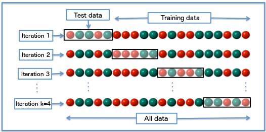
232 |
234 | By Fabian Flöck (Own work) [CC BY-SA 3.0 (http://creativecommons.org/licenses/by-sa/3.0)], via Wikimedia Commons
235 |
236 |
237 | **Problem** Try to find the optimal values of these hyperparameters for each algorithm. Plot the average cross-validation metrics for a given value of hyperparameter for each algorithm (hint: use `avgMetrics` field of resulting `CrossValidatorModel`).
238 |
239 | ```scala
240 | import org.apache.spark.ml.classification.{LogisticRegression, DecisionTreeClassifier, RandomForestClassifier}
241 | import org.apache.spark.ml.evaluation.BinaryClassificationEvaluator
242 | import org.apache.spark.ml.tuning.{ParamGridBuilder, CrossValidator}
243 |
244 |
245 | val lr = new LogisticRegression()
246 | .setFeaturesCol("numFeatures")
247 | .setLabelCol("label")
248 |
249 | val lrParamGrid = new ParamGridBuilder()
250 | .addGrid(lr.regParam, Array(1e-2, 5e-3, 1e-3, 5e-4, 1e-4))
251 | .build()
252 |
253 | val lrCV = new CrossValidator()
254 | .setEstimator(lr)
255 | .setEvaluator(new BinaryClassificationEvaluator)
256 | .setEstimatorParamMaps(lrParamGrid)
257 | .setNumFolds(5)
258 |
259 | val lrCVModel = lrCV.fit(trainData)
260 |
261 | println("cross-validated areaUnderROC: " + lrCVModel.avgMetrics.max)
262 | println("test areaUnderROC: " + eval.evaluate(lrCVModel.transform(testData)))
263 | ```
264 | ```
265 | cross-validated areaUnderROC: 0.8297755442702006
266 | test areaUnderROC: 0.8068812315222861
267 | ```
268 |
269 | ```scala
270 | val tree = new DecisionTreeClassifier()
271 | .setFeaturesCol("numFeatures")
272 | .setLabelCol("label")
273 |
274 | val treeParamGrid = new ParamGridBuilder()
275 | .addGrid(tree.maxDepth, Array(5, 10, 20, 25, 30))
276 | .build()
277 |
278 | val treeCV = new CrossValidator()
279 | .setEstimator(tree)
280 | .setEvaluator(new BinaryClassificationEvaluator)
281 | .setEstimatorParamMaps(treeParamGrid)
282 | .setNumFolds(5)
283 |
284 | val treeCVModel = treeCV.fit(trainData)
285 |
286 | println("cross-validated areaUnderROC: " + treeCVModel.avgMetrics.max)
287 | println("test areaUnderROC: " + eval.evaluate(treeCVModel.transform(testData)))
288 | ```
289 | ```
290 | cross-validated areaUnderROC: 0.7105377328054816
291 | test areaUnderROC: 0.6934402983359256
292 | ```
293 |
294 | ```scala
295 | lrCVModel.getEstimatorParamMaps
296 | .map(paramMap => paramMap(lr.regParam))
297 | .zip(lrCVModel.avgMetrics)
298 | .toSeq.toDF("regParam", "AUC-ROC")
299 | .collect
300 | ```
301 |
302 |  303 |
304 |
305 | ```scala
306 | treeCVModel.getEstimatorParamMaps
307 | .map(paramMap => paramMap(tree.maxDepth))
308 | .zip(treeCVModel.avgMetrics)
309 | .toSeq.toDF("maxDepth", "AUC-ROC")
310 | .collect
311 | ```
312 |
313 |
303 |
304 |
305 | ```scala
306 | treeCVModel.getEstimatorParamMaps
307 | .map(paramMap => paramMap(tree.maxDepth))
308 | .zip(treeCVModel.avgMetrics)
309 | .toSeq.toDF("maxDepth", "AUC-ROC")
310 | .collect
311 | ```
312 |
313 |  314 |
315 |
316 | ## Adding categorical features
317 |
318 | Up to this point we did not use categorical features from the dataset. Let's see how additional categorical features will affect the quality of the classification. A common technique to convert categorical feature into numerical ones is [one-hot](https://en.wikipedia.org/wiki/One-hot) encoding. This can be done using [StringIndexer](http://spark.apache.org/docs/1.6.1/api/scala/index.html#org.apache.spark.ml.feature.StringIndexer) transformation followed by [OneHotEncoder](http://spark.apache.org/docs/1.6.1/api/scala/index.html#org.apache.spark.ml.feature.OneHotEncoder) transformation.
319 |
320 | *Let's start with encoding just one new feature `occupation` and after that generalize encoding step for all categorical features and combine all processing steps using [pipeline](http://spark.apache.org/docs/1.6.1/ml-guide.html#pipeline)*
321 |
322 | ```scala
323 | data.groupBy("occupation").count.show(truncate=false)
324 | println(data.select("occupation").distinct.count)
325 | ```
326 | ```
327 | +-----------------+-----+
328 | |occupation |count|
329 | +-----------------+-----+
330 | |Sales |1840 |
331 | |Exec-managerial |2017 |
332 | |Prof-specialty |2095 |
333 | |Handlers-cleaners|674 |
334 | |Farming-fishing |481 |
335 | |Craft-repair |2057 |
336 | |Transport-moving |799 |
337 | |Priv-house-serv |90 |
338 | |Protective-serv |343 |
339 | |Other-service |1617 |
340 | |Tech-support |464 |
341 | |Machine-op-inspct|1023 |
342 | |Armed-Forces |3 |
343 | |Adm-clerical |1844 |
344 | +-----------------+-----+
345 |
346 | 14
347 | ```
348 |
349 | ```scala
350 | import org.apache.spark.ml.feature.OneHotEncoder
351 |
352 | val occupationIndexer = new StringIndexer()
353 | .setInputCol("occupation")
354 | .setOutputCol("occupationIndex")
355 | .fit(training)
356 |
357 | val indexedTrainData = occupationIndexer.transform(training)
358 |
359 | val occupationEncoder = new OneHotEncoder()
360 | .setInputCol("occupationIndex")
361 | .setOutputCol("occupationVec")
362 |
363 | val oheEncodedTrainData = occupationEncoder.transform(indexedTrainData)
364 |
365 | oheEncodedTrainData.select("occupation", "occupationVec").show(5, truncate=false)
366 | ```
367 | ```
368 | +---------------+--------------+
369 | |occupation |occupationVec |
370 | +---------------+--------------+
371 | |Other-service |(13,[5],[1.0])|
372 | |Adm-clerical |(13,[4],[1.0])|
373 | |Exec-managerial|(13,[2],[1.0])|
374 | |Other-service |(13,[5],[1.0])|
375 | |Other-service |(13,[5],[1.0])|
376 | +---------------+--------------+
377 | only showing top 5 rows
378 | ```
379 |
380 | ```scala
381 | val assembler = new VectorAssembler()
382 | .setInputCols(Array("age",
383 | "fnlwgt",
384 | "education-num",
385 | "capital-gain",
386 | "capital-loss",
387 | "hours-per-week",
388 | "occupationVec"))
389 | .setOutputCol("features")
390 |
391 |
392 | val trainDataWithOccupation = assembler.transform{
393 | labelIndexer.transform(oheEncodedTrainData)
394 | }.select("label", "features")
395 | ```
396 |
397 | *For the sake of brevity, from now let's use only LogisticRegression model.*
398 |
399 | ```scala
400 | val lr = new LogisticRegression()
401 | .setFeaturesCol("features")
402 |
403 | val lrParamGrid = new ParamGridBuilder()
404 | .addGrid(lr.regParam, Array(1e-2, 5e-3, 1e-3, 5e-4, 1e-4))
405 | .build()
406 |
407 | val lrCV = new CrossValidator()
408 | .setEstimator(lr)
409 | .setEvaluator(new BinaryClassificationEvaluator)
410 | .setEstimatorParamMaps(lrParamGrid)
411 | .setNumFolds(5)
412 |
413 | val lrCVModel = lrCV.fit(trainDataWithOccupation)
414 |
415 | val testDataWithOccupation = assembler.transform{
416 | labelIndexer.transform(occupationEncoder.transform(occupationIndexer.transform(test)))
417 | }.select("label", "features")
418 |
419 | println("cross-validated areaUnderROC: " + lrCVModel.avgMetrics.max)
420 | println("test areaUnderROC: " + eval.evaluate(lrCVModel.transform(testDataWithOccupation)))
421 | ```
422 | ```
423 | cross-validated areaUnderROC: 0.8447936545404254
424 | test areaUnderROC: 0.823490779891881
425 | ```
426 |
427 | Adding `occupation` categorical variable yielded an increase in quality.
428 |
429 | ## Pipelines
430 |
431 | Using [pipelines](http://spark.apache.org/docs/1.6.1/ml-guide.html#pipeline) one can combine all the processing stages into one pipeline and perform grid search against hyperparameters of all stages included in the pipeline. Also it's easy to extend given pipeline with new steps.
432 |
433 | A Pipeline chains multiple Transformers and Estimators together to specify an ML workflow.
434 |
435 |
314 |
315 |
316 | ## Adding categorical features
317 |
318 | Up to this point we did not use categorical features from the dataset. Let's see how additional categorical features will affect the quality of the classification. A common technique to convert categorical feature into numerical ones is [one-hot](https://en.wikipedia.org/wiki/One-hot) encoding. This can be done using [StringIndexer](http://spark.apache.org/docs/1.6.1/api/scala/index.html#org.apache.spark.ml.feature.StringIndexer) transformation followed by [OneHotEncoder](http://spark.apache.org/docs/1.6.1/api/scala/index.html#org.apache.spark.ml.feature.OneHotEncoder) transformation.
319 |
320 | *Let's start with encoding just one new feature `occupation` and after that generalize encoding step for all categorical features and combine all processing steps using [pipeline](http://spark.apache.org/docs/1.6.1/ml-guide.html#pipeline)*
321 |
322 | ```scala
323 | data.groupBy("occupation").count.show(truncate=false)
324 | println(data.select("occupation").distinct.count)
325 | ```
326 | ```
327 | +-----------------+-----+
328 | |occupation |count|
329 | +-----------------+-----+
330 | |Sales |1840 |
331 | |Exec-managerial |2017 |
332 | |Prof-specialty |2095 |
333 | |Handlers-cleaners|674 |
334 | |Farming-fishing |481 |
335 | |Craft-repair |2057 |
336 | |Transport-moving |799 |
337 | |Priv-house-serv |90 |
338 | |Protective-serv |343 |
339 | |Other-service |1617 |
340 | |Tech-support |464 |
341 | |Machine-op-inspct|1023 |
342 | |Armed-Forces |3 |
343 | |Adm-clerical |1844 |
344 | +-----------------+-----+
345 |
346 | 14
347 | ```
348 |
349 | ```scala
350 | import org.apache.spark.ml.feature.OneHotEncoder
351 |
352 | val occupationIndexer = new StringIndexer()
353 | .setInputCol("occupation")
354 | .setOutputCol("occupationIndex")
355 | .fit(training)
356 |
357 | val indexedTrainData = occupationIndexer.transform(training)
358 |
359 | val occupationEncoder = new OneHotEncoder()
360 | .setInputCol("occupationIndex")
361 | .setOutputCol("occupationVec")
362 |
363 | val oheEncodedTrainData = occupationEncoder.transform(indexedTrainData)
364 |
365 | oheEncodedTrainData.select("occupation", "occupationVec").show(5, truncate=false)
366 | ```
367 | ```
368 | +---------------+--------------+
369 | |occupation |occupationVec |
370 | +---------------+--------------+
371 | |Other-service |(13,[5],[1.0])|
372 | |Adm-clerical |(13,[4],[1.0])|
373 | |Exec-managerial|(13,[2],[1.0])|
374 | |Other-service |(13,[5],[1.0])|
375 | |Other-service |(13,[5],[1.0])|
376 | +---------------+--------------+
377 | only showing top 5 rows
378 | ```
379 |
380 | ```scala
381 | val assembler = new VectorAssembler()
382 | .setInputCols(Array("age",
383 | "fnlwgt",
384 | "education-num",
385 | "capital-gain",
386 | "capital-loss",
387 | "hours-per-week",
388 | "occupationVec"))
389 | .setOutputCol("features")
390 |
391 |
392 | val trainDataWithOccupation = assembler.transform{
393 | labelIndexer.transform(oheEncodedTrainData)
394 | }.select("label", "features")
395 | ```
396 |
397 | *For the sake of brevity, from now let's use only LogisticRegression model.*
398 |
399 | ```scala
400 | val lr = new LogisticRegression()
401 | .setFeaturesCol("features")
402 |
403 | val lrParamGrid = new ParamGridBuilder()
404 | .addGrid(lr.regParam, Array(1e-2, 5e-3, 1e-3, 5e-4, 1e-4))
405 | .build()
406 |
407 | val lrCV = new CrossValidator()
408 | .setEstimator(lr)
409 | .setEvaluator(new BinaryClassificationEvaluator)
410 | .setEstimatorParamMaps(lrParamGrid)
411 | .setNumFolds(5)
412 |
413 | val lrCVModel = lrCV.fit(trainDataWithOccupation)
414 |
415 | val testDataWithOccupation = assembler.transform{
416 | labelIndexer.transform(occupationEncoder.transform(occupationIndexer.transform(test)))
417 | }.select("label", "features")
418 |
419 | println("cross-validated areaUnderROC: " + lrCVModel.avgMetrics.max)
420 | println("test areaUnderROC: " + eval.evaluate(lrCVModel.transform(testDataWithOccupation)))
421 | ```
422 | ```
423 | cross-validated areaUnderROC: 0.8447936545404254
424 | test areaUnderROC: 0.823490779891881
425 | ```
426 |
427 | Adding `occupation` categorical variable yielded an increase in quality.
428 |
429 | ## Pipelines
430 |
431 | Using [pipelines](http://spark.apache.org/docs/1.6.1/ml-guide.html#pipeline) one can combine all the processing stages into one pipeline and perform grid search against hyperparameters of all stages included in the pipeline. Also it's easy to extend given pipeline with new steps.
432 |
433 | A Pipeline chains multiple Transformers and Estimators together to specify an ML workflow.
434 |
435 |
436 |

437 |
4 |

5 |

6 |
 14 |
15 |
16 | In this first lab we will focus on DataFrames and SQL.
17 | In second lab we will use Spark MLlib for building machine learning pipelines.
18 |
19 | ### Spark Cluster
20 |
21 |
14 |
15 |
16 | In this first lab we will focus on DataFrames and SQL.
17 | In second lab we will use Spark MLlib for building machine learning pipelines.
18 |
19 | ### Spark Cluster
20 |
21 |
22 |

23 |
157 |
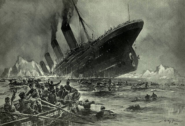
158 |
 330 |
331 |
332 | **Q-3. How many women and men were in each class?**
333 | ```scala
334 | val grByGenderAndClass = passengersDF.groupBy("Pclass", "Sex").count
335 | grByGenderAndClass.show()
336 | ```
337 | ```
338 | +------+------+-----+
339 | |Pclass| Sex|count|
340 | +------+------+-----+
341 | | 2|female| 76|
342 | | 3| male| 347|
343 | | 1| male| 122|
344 | | 3|female| 144|
345 | | 1|female| 94|
346 | | 2| male| 108|
347 | +------+------+-----+
348 | ```
349 |
350 | ```scala
351 | CustomPlotlyChart(grByGenderAndClass,
352 | layout="{title: 'Passengers per class', xaxis: {title: 'Pclass'}, barmode: 'group'}",
353 | dataOptions="{type: 'bar', splitBy: 'Sex'}",
354 | dataSources="{x: 'Pclass', y: 'count'}")
355 | ```
356 |
357 |
330 |
331 |
332 | **Q-3. How many women and men were in each class?**
333 | ```scala
334 | val grByGenderAndClass = passengersDF.groupBy("Pclass", "Sex").count
335 | grByGenderAndClass.show()
336 | ```
337 | ```
338 | +------+------+-----+
339 | |Pclass| Sex|count|
340 | +------+------+-----+
341 | | 2|female| 76|
342 | | 3| male| 347|
343 | | 1| male| 122|
344 | | 3|female| 144|
345 | | 1|female| 94|
346 | | 2| male| 108|
347 | +------+------+-----+
348 | ```
349 |
350 | ```scala
351 | CustomPlotlyChart(grByGenderAndClass,
352 | layout="{title: 'Passengers per class', xaxis: {title: 'Pclass'}, barmode: 'group'}",
353 | dataOptions="{type: 'bar', splitBy: 'Sex'}",
354 | dataSources="{x: 'Pclass', y: 'count'}")
355 | ```
356 |
357 |  358 |
359 |
360 |
361 | ### DataFrame Functions and UDF
362 |
363 | http://spark.apache.org/docs/latest/api/scala/index.html#org.apache.spark.sql.functions$
364 |
365 | ```scala
366 | import org.apache.spark.sql.functions.{mean, min, max}
367 |
368 | passengersDF.select(mean("Age").alias("Average Age"), min("Age"), max("Age")).show()
369 | ```
370 | ```
371 | +-----------------+--------+--------+
372 | | Average Age|min(Age)|max(Age)|
373 | +-----------------+--------+--------+
374 | |29.69911764705882| 0.42| 80.0|
375 | +-----------------+--------+--------+
376 | ```
377 |
378 | ```scala
379 | import org.apache.spark.sql.functions.count
380 |
381 | passengersDF.groupBy("Pclass")
382 | .agg(count("Pclass").alias("class_count"))
383 | .orderBy(-$"class_count")
384 | .show
385 | ```
386 | ```
387 | +------+-----------+
388 | |Pclass|class_count|
389 | +------+-----------+
390 | | 3| 491|
391 | | 1| 216|
392 | | 2| 184|
393 | +------+-----------+
394 | ```
395 |
396 | For more specific tasks one can use User Defined Functions.
397 |
398 | Let's say we want to get a column with full names of port of embarkation.
399 |
400 | ```scala
401 | passengersDF.select("Embarked").distinct.show
402 | ```
403 | ```
404 | +--------+
405 | |Embarked|
406 | +--------+
407 | | Q|
408 | | null|
409 | | C|
410 | | S|
411 | +--------+
412 | ```
413 |
414 | From dataset description we know that C = Cherbourg; Q = Queenstown; S = Southampton.
415 |
416 | ```scala
417 | import org.apache.spark.sql.functions.udf
418 |
419 | val embarkedFullName: (String) => String = (embarked: String) =>
420 | if (embarked == "Q")
421 | "Queenstown"
422 | else if (embarked == "C")
423 | "Cherbourg"
424 | else
425 | "Southampton"
426 |
427 |
428 | val embarkedFullNameUDF = udf(embarkedFullName)
429 | ```
430 |
431 | Also we want to get a column with more verbose survival status of passenger: `survived` and `died`.
432 |
433 | ```scala
434 | val survivedStatus: (Integer) => String = (survived: Integer) =>
435 | if (survived == 1)
436 | "survived"
437 | else
438 | "died"
439 |
440 | val survivedStatusUDF = udf(survivedStatus)
441 |
442 | val pdf = passengersDF
443 | .withColumn("Embarkation", embarkedFullNameUDF($"Embarked"))
444 | .drop("Embarked")
445 | .withColumn("SurvivedStatus", survivedStatusUDF($"Survived"))
446 | .cache()
447 |
448 | pdf.select("Name", "Embarkation", "SurvivedStatus").show(5, truncate=false)
449 | ```
450 | ```
451 | +---------------------------------------------------+-----------+--------------+
452 | |Name |Embarkation|SurvivedStatus|
453 | +---------------------------------------------------+-----------+--------------+
454 | |Braund, Mr. Owen Harris |Southampton|died |
455 | |Cumings, Mrs. John Bradley (Florence Briggs Thayer)|Cherbourg |survived |
456 | |Heikkinen, Miss. Laina |Southampton|survived |
457 | |Futrelle, Mrs. Jacques Heath (Lily May Peel) |Southampton|survived |
458 | |Allen, Mr. William Henry |Southampton|died |
459 | +---------------------------------------------------+-----------+--------------+
460 | only showing top 5 rows
461 | ```
462 |
463 | **Q-5. Count the number and percentage of survivors and dead passengers.**
464 |
465 | ```scala
466 | import org.apache.spark.sql.functions.count
467 |
468 | val numPassengers = pdf.count()
469 |
470 | val grBySurvived = pdf.groupBy("SurvivedStatus")
471 | .agg(count("PassengerId").alias("count"),
472 | ((count("PassengerId") / numPassengers) * 100).alias("%"))
473 | grBySurvived.show
474 | ```
475 | ```
476 | +--------------+-----+-----------------+
477 | |SurvivedStatus|count| %|
478 | +--------------+-----+-----------------+
479 | | died| 549|61.61616161616161|
480 | | survived| 342|38.38383838383838|
481 | +--------------+-----+-----------------+
482 | ```
483 |
484 | **Q-6.**
485 | - **Plot the distribution of dead and surviving passengers.**
486 | - **Plot the distribution of survivors and dead passengers by class.**
487 | - **Plot the distribution of survivors and dead passengers by gender.**
488 | - **Plot the distribution of survivors and dead passengers by port of embarkation.**
489 | - **Plot the % of survivors by port of embarkation.**
490 | - **Plot the distribution of passenger classes by port of embarkation.**
491 |
492 | ```scala
493 | // Distribution of dead and survived passengers
494 |
495 | CustomPlotlyChart(grBySurvived,
496 | layout="{title: 'Passengers by status', xaxis: {title: 'status'}, yaxis: {title: '%'}}",
497 | dataOptions="{type: 'bar'}",
498 | dataSources="{x: 'SurvivedStatus', y: '%'}")
499 | ```
500 |
501 |
358 |
359 |
360 |
361 | ### DataFrame Functions and UDF
362 |
363 | http://spark.apache.org/docs/latest/api/scala/index.html#org.apache.spark.sql.functions$
364 |
365 | ```scala
366 | import org.apache.spark.sql.functions.{mean, min, max}
367 |
368 | passengersDF.select(mean("Age").alias("Average Age"), min("Age"), max("Age")).show()
369 | ```
370 | ```
371 | +-----------------+--------+--------+
372 | | Average Age|min(Age)|max(Age)|
373 | +-----------------+--------+--------+
374 | |29.69911764705882| 0.42| 80.0|
375 | +-----------------+--------+--------+
376 | ```
377 |
378 | ```scala
379 | import org.apache.spark.sql.functions.count
380 |
381 | passengersDF.groupBy("Pclass")
382 | .agg(count("Pclass").alias("class_count"))
383 | .orderBy(-$"class_count")
384 | .show
385 | ```
386 | ```
387 | +------+-----------+
388 | |Pclass|class_count|
389 | +------+-----------+
390 | | 3| 491|
391 | | 1| 216|
392 | | 2| 184|
393 | +------+-----------+
394 | ```
395 |
396 | For more specific tasks one can use User Defined Functions.
397 |
398 | Let's say we want to get a column with full names of port of embarkation.
399 |
400 | ```scala
401 | passengersDF.select("Embarked").distinct.show
402 | ```
403 | ```
404 | +--------+
405 | |Embarked|
406 | +--------+
407 | | Q|
408 | | null|
409 | | C|
410 | | S|
411 | +--------+
412 | ```
413 |
414 | From dataset description we know that C = Cherbourg; Q = Queenstown; S = Southampton.
415 |
416 | ```scala
417 | import org.apache.spark.sql.functions.udf
418 |
419 | val embarkedFullName: (String) => String = (embarked: String) =>
420 | if (embarked == "Q")
421 | "Queenstown"
422 | else if (embarked == "C")
423 | "Cherbourg"
424 | else
425 | "Southampton"
426 |
427 |
428 | val embarkedFullNameUDF = udf(embarkedFullName)
429 | ```
430 |
431 | Also we want to get a column with more verbose survival status of passenger: `survived` and `died`.
432 |
433 | ```scala
434 | val survivedStatus: (Integer) => String = (survived: Integer) =>
435 | if (survived == 1)
436 | "survived"
437 | else
438 | "died"
439 |
440 | val survivedStatusUDF = udf(survivedStatus)
441 |
442 | val pdf = passengersDF
443 | .withColumn("Embarkation", embarkedFullNameUDF($"Embarked"))
444 | .drop("Embarked")
445 | .withColumn("SurvivedStatus", survivedStatusUDF($"Survived"))
446 | .cache()
447 |
448 | pdf.select("Name", "Embarkation", "SurvivedStatus").show(5, truncate=false)
449 | ```
450 | ```
451 | +---------------------------------------------------+-----------+--------------+
452 | |Name |Embarkation|SurvivedStatus|
453 | +---------------------------------------------------+-----------+--------------+
454 | |Braund, Mr. Owen Harris |Southampton|died |
455 | |Cumings, Mrs. John Bradley (Florence Briggs Thayer)|Cherbourg |survived |
456 | |Heikkinen, Miss. Laina |Southampton|survived |
457 | |Futrelle, Mrs. Jacques Heath (Lily May Peel) |Southampton|survived |
458 | |Allen, Mr. William Henry |Southampton|died |
459 | +---------------------------------------------------+-----------+--------------+
460 | only showing top 5 rows
461 | ```
462 |
463 | **Q-5. Count the number and percentage of survivors and dead passengers.**
464 |
465 | ```scala
466 | import org.apache.spark.sql.functions.count
467 |
468 | val numPassengers = pdf.count()
469 |
470 | val grBySurvived = pdf.groupBy("SurvivedStatus")
471 | .agg(count("PassengerId").alias("count"),
472 | ((count("PassengerId") / numPassengers) * 100).alias("%"))
473 | grBySurvived.show
474 | ```
475 | ```
476 | +--------------+-----+-----------------+
477 | |SurvivedStatus|count| %|
478 | +--------------+-----+-----------------+
479 | | died| 549|61.61616161616161|
480 | | survived| 342|38.38383838383838|
481 | +--------------+-----+-----------------+
482 | ```
483 |
484 | **Q-6.**
485 | - **Plot the distribution of dead and surviving passengers.**
486 | - **Plot the distribution of survivors and dead passengers by class.**
487 | - **Plot the distribution of survivors and dead passengers by gender.**
488 | - **Plot the distribution of survivors and dead passengers by port of embarkation.**
489 | - **Plot the % of survivors by port of embarkation.**
490 | - **Plot the distribution of passenger classes by port of embarkation.**
491 |
492 | ```scala
493 | // Distribution of dead and survived passengers
494 |
495 | CustomPlotlyChart(grBySurvived,
496 | layout="{title: 'Passengers by status', xaxis: {title: 'status'}, yaxis: {title: '%'}}",
497 | dataOptions="{type: 'bar'}",
498 | dataSources="{x: 'SurvivedStatus', y: '%'}")
499 | ```
500 |
501 |  502 |
503 |
504 | ```scala
505 | // Distribution of the number of survivors and dead passengers by class.
506 |
507 | CustomPlotlyChart(pdf.groupBy("SurvivedStatus", "Pclass").count,
508 | layout="{title: 'Number of passengers by survival status per class', xaxis: {title: 'Pclass'}, barmode: 'group'}",
509 | dataOptions="{type: 'bar', splitBy: 'SurvivedStatus'}",
510 | dataSources="{x: 'Pclass', y: 'count'}")
511 | ```
512 |
513 |
502 |
503 |
504 | ```scala
505 | // Distribution of the number of survivors and dead passengers by class.
506 |
507 | CustomPlotlyChart(pdf.groupBy("SurvivedStatus", "Pclass").count,
508 | layout="{title: 'Number of passengers by survival status per class', xaxis: {title: 'Pclass'}, barmode: 'group'}",
509 | dataOptions="{type: 'bar', splitBy: 'SurvivedStatus'}",
510 | dataSources="{x: 'Pclass', y: 'count'}")
511 | ```
512 |
513 |  514 |
515 |
516 | ```scala
517 | // Distribution of survivors and dead passengers by gender.
518 |
519 | CustomPlotlyChart(pdf.groupBy("SurvivedStatus", "Sex").count,
520 | layout="{title: 'Number of passengers by status by gender', xaxis: {title: 'Gender'}, barmode: 'group'}",
521 | dataOptions="{type: 'bar', splitBy: 'SurvivedStatus'}",
522 | dataSources="{x: 'Sex', y: 'count'}")
523 | ```
524 |
525 |
514 |
515 |
516 | ```scala
517 | // Distribution of survivors and dead passengers by gender.
518 |
519 | CustomPlotlyChart(pdf.groupBy("SurvivedStatus", "Sex").count,
520 | layout="{title: 'Number of passengers by status by gender', xaxis: {title: 'Gender'}, barmode: 'group'}",
521 | dataOptions="{type: 'bar', splitBy: 'SurvivedStatus'}",
522 | dataSources="{x: 'Sex', y: 'count'}")
523 | ```
524 |
525 |  526 |
527 |
528 | ```scala
529 | // Distribution of survivors and dead passengers by port of embarkation.
530 |
531 | CustomPlotlyChart(pdf.groupBy("Embarkation", "SurvivedStatus").count,
532 | layout="{barmode: 'group'}",
533 | dataOptions="{type: 'bar', splitBy: 'SurvivedStatus'}",
534 | dataSources="{x: 'Embarkation', y: 'count'}")
535 | ```
536 |
537 |
526 |
527 |
528 | ```scala
529 | // Distribution of survivors and dead passengers by port of embarkation.
530 |
531 | CustomPlotlyChart(pdf.groupBy("Embarkation", "SurvivedStatus").count,
532 | layout="{barmode: 'group'}",
533 | dataOptions="{type: 'bar', splitBy: 'SurvivedStatus'}",
534 | dataSources="{x: 'Embarkation', y: 'count'}")
535 | ```
536 |
537 |  538 |
539 |
540 | ```scala
541 | // % of survivors by port of embarkation.
542 |
543 | CustomPlotlyChart(pdf.groupBy("Embarkation").agg((sum("Survived") / count("Survived") * 100).alias("SurvivalRate")),
544 | layout="{title: '% of survival per embarkation'}",
545 | dataOptions="{type: 'bar'}",
546 | dataSources="{x: 'Embarkation', y: 'SurvivalRate'}")
547 | ```
548 |
549 |
538 |
539 |
540 | ```scala
541 | // % of survivors by port of embarkation.
542 |
543 | CustomPlotlyChart(pdf.groupBy("Embarkation").agg((sum("Survived") / count("Survived") * 100).alias("SurvivalRate")),
544 | layout="{title: '% of survival per embarkation'}",
545 | dataOptions="{type: 'bar'}",
546 | dataSources="{x: 'Embarkation', y: 'SurvivalRate'}")
547 | ```
548 |
549 |  550 |
551 |
552 | ```scala
553 | // Distribution of passenger classes by port of embarkation.
554 |
555 | CustomPlotlyChart(pdf.groupBy("Embarkation", "Pclass").count,
556 | layout="{barmode: 'stack', title: 'Pclass distribution by Embarkation'}",
557 | dataOptions="{type: 'bar', splitBy: 'Pclass'}",
558 | dataSources="{x: 'Embarkation', y: 'count'}")
559 | ```
560 |
550 |
551 |
552 | ```scala
553 | // Distribution of passenger classes by port of embarkation.
554 |
555 | CustomPlotlyChart(pdf.groupBy("Embarkation", "Pclass").count,
556 | layout="{barmode: 'stack', title: 'Pclass distribution by Embarkation'}",
557 | dataOptions="{type: 'bar', splitBy: 'Pclass'}",
558 | dataSources="{x: 'Embarkation', y: 'count'}")
559 | ```
560 |  561 |
562 |
563 | How to get the % of survived passengers by port of embarkation in this case?
564 |
565 | ```scala
566 | val byEmbark = pdf.groupBy("Embarkation").agg(count("PassengerId").alias("totalCount"))
567 | val byEmbarkByClass = pdf.groupBy("Embarkation", "Pclass").count
568 |
569 | val embarkClassDistr = byEmbarkByClass.join(byEmbark, usingColumn="Embarkation")
570 | .select($"Embarkation",
571 | $"Pclass",
572 | ($"count" / $"totalCount" * 100).alias("%"))
573 |
574 | CustomPlotlyChart(embarkClassDistr,
575 | layout="{barmode: 'stack', title: 'Pclass distribution by Embarkation', yaxis: {title: '%'}}",
576 | dataOptions="{type: 'bar', splitBy: 'Pclass'}",
577 | dataSources="{x: 'Embarkation', y: '%'}")
578 | ```
579 |
580 |
561 |
562 |
563 | How to get the % of survived passengers by port of embarkation in this case?
564 |
565 | ```scala
566 | val byEmbark = pdf.groupBy("Embarkation").agg(count("PassengerId").alias("totalCount"))
567 | val byEmbarkByClass = pdf.groupBy("Embarkation", "Pclass").count
568 |
569 | val embarkClassDistr = byEmbarkByClass.join(byEmbark, usingColumn="Embarkation")
570 | .select($"Embarkation",
571 | $"Pclass",
572 | ($"count" / $"totalCount" * 100).alias("%"))
573 |
574 | CustomPlotlyChart(embarkClassDistr,
575 | layout="{barmode: 'stack', title: 'Pclass distribution by Embarkation', yaxis: {title: '%'}}",
576 | dataOptions="{type: 'bar', splitBy: 'Pclass'}",
577 | dataSources="{x: 'Embarkation', y: '%'}")
578 | ```
579 |
580 |  581 |
582 |
583 | ### Histograms and Box Plots
584 |
585 | **Q-7 Obtain age distributions by passengers survival status.**
586 |
587 | ```scala
588 | CustomPlotlyChart(pdf,
589 | layout="{title: 'Age distribution by status', xaxis: {title: 'Age'}, barmode: 'overlay'}",
590 | dataOptions="{type: 'histogram', opacity: 0.6, splitBy: 'SurvivedStatus'}",
591 | dataSources="{x: 'Age'}")
592 | ```
593 |
581 |
582 |
583 | ### Histograms and Box Plots
584 |
585 | **Q-7 Obtain age distributions by passengers survival status.**
586 |
587 | ```scala
588 | CustomPlotlyChart(pdf,
589 | layout="{title: 'Age distribution by status', xaxis: {title: 'Age'}, barmode: 'overlay'}",
590 | dataOptions="{type: 'histogram', opacity: 0.6, splitBy: 'SurvivedStatus'}",
591 | dataSources="{x: 'Age'}")
592 | ```
593 |  594 |
595 |
596 | ```scala
597 | CustomPlotlyChart(pdf,
598 | layout="{yaxis: {title: 'Age'}}",
599 | dataOptions="{type: 'box', splitBy: 'SurvivedStatus'}",
600 | dataSources="{y: 'Age'}")
601 | ```
602 |
594 |
595 |
596 | ```scala
597 | CustomPlotlyChart(pdf,
598 | layout="{yaxis: {title: 'Age'}}",
599 | dataOptions="{type: 'box', splitBy: 'SurvivedStatus'}",
600 | dataSources="{y: 'Age'}")
601 | ```
602 |  603 |
604 |
605 | **Q-8. Plot box plots of age distributions by passengers classes.**
606 |
607 | ```scala
608 | CustomPlotlyChart(pdf,
609 | layout="{yaxis: {title: 'Age'}}",
610 | dataOptions="{type: 'box', splitBy: 'Pclass'}",
611 | dataSources="{y: 'Age'}")
612 | ```
613 |
614 |
603 |
604 |
605 | **Q-8. Plot box plots of age distributions by passengers classes.**
606 |
607 | ```scala
608 | CustomPlotlyChart(pdf,
609 | layout="{yaxis: {title: 'Age'}}",
610 | dataOptions="{type: 'box', splitBy: 'Pclass'}",
611 | dataSources="{y: 'Age'}")
612 | ```
613 |
614 |  615 |
616 |
617 | This scatter plots show the dependences of the chances of survival from the cabin class, age and gender:
618 |
619 | ```scala
620 | val survByClassAndAge = List("male", "female").map{
621 | gender =>
622 | CustomPlotlyChart(pdf.filter($"Sex" === gender),
623 | layout=s"""{
624 | title: 'Survival by class and age, $gender.',
625 | yaxis: {title: 'class'},
626 | xaxis: {title: 'age'}
627 | }""",
628 | dataOptions="""{
629 | splitBy: 'SurvivedStatus',
630 | byTrace: {
631 | 'survived': {
632 | mode: 'markers',
633 | marker: {
634 | size: 20,
635 | opacity: 0.3,
636 | color: 'orange'
637 | }
638 | },
639 | 'died': {
640 | mode: 'markers',
641 | marker: {
642 | size: 15,
643 | opacity: 0.9,
644 | color: 'rgba(55, 128, 191, 0.6)'
645 | }
646 | }
647 | }
648 | }""",
649 | dataSources = "{x: 'Age', y: 'Pclass'}"
650 | )
651 | }
652 |
653 | survByClassAndAge(0)
654 | ```
655 |
656 |
615 |
616 |
617 | This scatter plots show the dependences of the chances of survival from the cabin class, age and gender:
618 |
619 | ```scala
620 | val survByClassAndAge = List("male", "female").map{
621 | gender =>
622 | CustomPlotlyChart(pdf.filter($"Sex" === gender),
623 | layout=s"""{
624 | title: 'Survival by class and age, $gender.',
625 | yaxis: {title: 'class'},
626 | xaxis: {title: 'age'}
627 | }""",
628 | dataOptions="""{
629 | splitBy: 'SurvivedStatus',
630 | byTrace: {
631 | 'survived': {
632 | mode: 'markers',
633 | marker: {
634 | size: 20,
635 | opacity: 0.3,
636 | color: 'orange'
637 | }
638 | },
639 | 'died': {
640 | mode: 'markers',
641 | marker: {
642 | size: 15,
643 | opacity: 0.9,
644 | color: 'rgba(55, 128, 191, 0.6)'
645 | }
646 | }
647 | }
648 | }""",
649 | dataSources = "{x: 'Age', y: 'Pclass'}"
650 | )
651 | }
652 |
653 | survByClassAndAge(0)
654 | ```
655 |
656 |  657 |
658 |
659 | ```scala
660 | survByClassAndAge(1)
661 | ```
662 |
663 |
657 |
658 |
659 | ```scala
660 | survByClassAndAge(1)
661 | ```
662 |
663 |  664 |
665 |
666 | ### More practice with UDF and Box Plots
667 |
668 | The titles of passengers could be useful source of information. Let's explore that.
669 |
670 | **Q-9. Plot box plots of age distributions by title.**
671 |
672 | ```scala
673 | pdf.select("Name").show(3, truncate=false)
674 | ```
675 | ```
676 | +---------------------------------------------------+
677 | |Name |
678 | +---------------------------------------------------+
679 | |Braund, Mr. Owen Harris |
680 | |Cumings, Mrs. John Bradley (Florence Briggs Thayer)|
681 | |Heikkinen, Miss. Laina |
682 | +---------------------------------------------------+
683 | only showing top 3 rows
684 | ```
685 |
686 | ```scala
687 | val parseTitle: String => String = (name: String) =>
688 | name.split(", ")(1).split("\\.")(0)
689 |
690 | val parseTitleUDF = udf(parseTitle)
691 |
692 | CustomPlotlyChart(pdf.withColumn("Title", parseTitleUDF($"Name")),
693 | layout="{yaxis: {title: 'Age'}}",
694 | dataOptions="{type: 'box', splitBy: 'Title'}",
695 | dataSources="{y: 'Age'}")
696 | ```
697 |
698 |
664 |
665 |
666 | ### More practice with UDF and Box Plots
667 |
668 | The titles of passengers could be useful source of information. Let's explore that.
669 |
670 | **Q-9. Plot box plots of age distributions by title.**
671 |
672 | ```scala
673 | pdf.select("Name").show(3, truncate=false)
674 | ```
675 | ```
676 | +---------------------------------------------------+
677 | |Name |
678 | +---------------------------------------------------+
679 | |Braund, Mr. Owen Harris |
680 | |Cumings, Mrs. John Bradley (Florence Briggs Thayer)|
681 | |Heikkinen, Miss. Laina |
682 | +---------------------------------------------------+
683 | only showing top 3 rows
684 | ```
685 |
686 | ```scala
687 | val parseTitle: String => String = (name: String) =>
688 | name.split(", ")(1).split("\\.")(0)
689 |
690 | val parseTitleUDF = udf(parseTitle)
691 |
692 | CustomPlotlyChart(pdf.withColumn("Title", parseTitleUDF($"Name")),
693 | layout="{yaxis: {title: 'Age'}}",
694 | dataOptions="{type: 'box', splitBy: 'Title'}",
695 | dataSources="{y: 'Age'}")
696 | ```
697 |
698 |  699 |
700 |
701 | Often it is good practice to group the values of the categorical feature, especially when there are rare individual feature values such as `Don`, `Lady`, `Capt` in our case.
702 |
703 | **Q-10. Write UDF to group all the titles into five groups according to the following table:**
704 |
705 | | Group | Title |
706 | | :------------:|:------------:|
707 | | Aristocratic | Capt, Col, Don, Dr, Jonkheer, Lady, Major, Rev, Sir, Countess |
708 | | Mrs | Mrs, Ms |
709 | | Miss | Miss, Mlle, Mme |
710 | | Mr | Mr |
711 | | Master | Master |
712 |
713 | ** Create new column called 'TitleGroup' and plot box plots of age distributions by title group.**
714 |
715 | ```scala
716 | val titleGroup: String => String = (title: String) => {
717 | val aristocratic = Set("Capt", "Col", "Don", "Dr", "Jonkheer", "Lady", "Major", "Rev", "Sir", "the Countess")
718 | val mrs = Set("Mrs", "Ms")
719 | val miss = Set("Miss", "Mlle", "Mme")
720 | if (aristocratic.contains(title))
721 | "Aristocratic"
722 | else if (mrs.contains(title))
723 | "Mrs"
724 | else if (miss.contains(title))
725 | "Miss"
726 | else
727 | title
728 | }
729 |
730 | // given column with passenger name obtain column with passenger title group.
731 | val parseTitleGroupUDF = udf(parseTitle andThen titleGroup)
732 | ```
733 |
734 | ```scala
735 | val withTitleDF = pdf.withColumn("TitleGroup", parseTitleGroupUDF($"Name"))
736 |
737 | CustomPlotlyChart(withTitleDF,
738 | layout="{yaxis: {title: 'Age'}}",
739 | dataOptions="{type: 'box', splitBy: 'TitleGroup'}",
740 | dataSources="{y: 'Age'}")
741 | ```
742 |
743 |
699 |
700 |
701 | Often it is good practice to group the values of the categorical feature, especially when there are rare individual feature values such as `Don`, `Lady`, `Capt` in our case.
702 |
703 | **Q-10. Write UDF to group all the titles into five groups according to the following table:**
704 |
705 | | Group | Title |
706 | | :------------:|:------------:|
707 | | Aristocratic | Capt, Col, Don, Dr, Jonkheer, Lady, Major, Rev, Sir, Countess |
708 | | Mrs | Mrs, Ms |
709 | | Miss | Miss, Mlle, Mme |
710 | | Mr | Mr |
711 | | Master | Master |
712 |
713 | ** Create new column called 'TitleGroup' and plot box plots of age distributions by title group.**
714 |
715 | ```scala
716 | val titleGroup: String => String = (title: String) => {
717 | val aristocratic = Set("Capt", "Col", "Don", "Dr", "Jonkheer", "Lady", "Major", "Rev", "Sir", "the Countess")
718 | val mrs = Set("Mrs", "Ms")
719 | val miss = Set("Miss", "Mlle", "Mme")
720 | if (aristocratic.contains(title))
721 | "Aristocratic"
722 | else if (mrs.contains(title))
723 | "Mrs"
724 | else if (miss.contains(title))
725 | "Miss"
726 | else
727 | title
728 | }
729 |
730 | // given column with passenger name obtain column with passenger title group.
731 | val parseTitleGroupUDF = udf(parseTitle andThen titleGroup)
732 | ```
733 |
734 | ```scala
735 | val withTitleDF = pdf.withColumn("TitleGroup", parseTitleGroupUDF($"Name"))
736 |
737 | CustomPlotlyChart(withTitleDF,
738 | layout="{yaxis: {title: 'Age'}}",
739 | dataOptions="{type: 'box', splitBy: 'TitleGroup'}",
740 | dataSources="{y: 'Age'}")
741 | ```
742 |
743 |  744 |
745 |
746 |
747 | **Q-11 Plot the distribution of the % of survivors by title group.**
748 |
749 | ```scala
750 | val byTitleGr = withTitleDF
751 | .groupBy("TitleGroup")
752 | .agg((sum("Survived") / count("Survived") * 100).alias("%"))
753 |
754 | CustomPlotlyChart(byTitleGr,
755 | layout="{title: '% of survival by title group'}",
756 | dataOptions="{type: 'bar'}",
757 | dataSources="{x: 'TitleGroup', y: '%'}")
758 | ```
759 |
760 |
744 |
745 |
746 |
747 | **Q-11 Plot the distribution of the % of survivors by title group.**
748 |
749 | ```scala
750 | val byTitleGr = withTitleDF
751 | .groupBy("TitleGroup")
752 | .agg((sum("Survived") / count("Survived") * 100).alias("%"))
753 |
754 | CustomPlotlyChart(byTitleGr,
755 | layout="{title: '% of survival by title group'}",
756 | dataOptions="{type: 'bar'}",
757 | dataSources="{x: 'TitleGroup', y: '%'}")
758 | ```
759 |
760 |  761 |
762 |
763 | ### Handling missing values
764 |
765 | ```scala
766 | import org.apache.spark.sql.functions.isnull
767 |
768 | 100.0 * pdf.filter(isnull($"Age")).count / pdf.count
769 | ```
770 | ```
771 | res209: Double = 19.865319865319865
772 | 19.865319865319865
773 | ```
774 |
775 | ```scala
776 | 100.0 * pdf.filter(isnull($"Cabin")).count / pdf.count
777 | ```
778 | ```
779 | res237: Double = 77.10437710437711
780 | 77.10437710437711
781 | ```
782 |
783 | ```scala
784 | val cabinStatus: (String) => String = (cabin: String) =>
785 | if (cabin == null)
786 | "noname"
787 | else
788 | "hasNumber"
789 |
790 | val cabinStatusUDF = udf(cabinStatus)
791 | ```
792 |
793 | ```scala
794 | val withCabinStatusDF = pdf.withColumn("CabinStatus", cabinStatusUDF($"Cabin"))
795 | ```
796 |
797 | ```scala
798 | CustomPlotlyChart(withCabinStatusDF.groupBy("CabinStatus", "SurvivedStatus").count,
799 | layout="{title: 'Number of passengers by survival status by cabin type', xaxis: {title: 'Cabin'}}",
800 | dataOptions="{type: 'bar', splitBy: 'SurvivedStatus'}",
801 | dataSources="{x: 'CabinStatus', y: 'count'}")
802 | ```
803 |
804 |
761 |
762 |
763 | ### Handling missing values
764 |
765 | ```scala
766 | import org.apache.spark.sql.functions.isnull
767 |
768 | 100.0 * pdf.filter(isnull($"Age")).count / pdf.count
769 | ```
770 | ```
771 | res209: Double = 19.865319865319865
772 | 19.865319865319865
773 | ```
774 |
775 | ```scala
776 | 100.0 * pdf.filter(isnull($"Cabin")).count / pdf.count
777 | ```
778 | ```
779 | res237: Double = 77.10437710437711
780 | 77.10437710437711
781 | ```
782 |
783 | ```scala
784 | val cabinStatus: (String) => String = (cabin: String) =>
785 | if (cabin == null)
786 | "noname"
787 | else
788 | "hasNumber"
789 |
790 | val cabinStatusUDF = udf(cabinStatus)
791 | ```
792 |
793 | ```scala
794 | val withCabinStatusDF = pdf.withColumn("CabinStatus", cabinStatusUDF($"Cabin"))
795 | ```
796 |
797 | ```scala
798 | CustomPlotlyChart(withCabinStatusDF.groupBy("CabinStatus", "SurvivedStatus").count,
799 | layout="{title: 'Number of passengers by survival status by cabin type', xaxis: {title: 'Cabin'}}",
800 | dataOptions="{type: 'bar', splitBy: 'SurvivedStatus'}",
801 | dataSources="{x: 'CabinStatus', y: 'count'}")
802 | ```
803 |
804 |  805 |
806 |
807 | ### On your own
808 |
809 | Explore family relationships variables (SibSp and Parch).
810 | How does the number of siblings/spouses aboard affect the chances of survival?
811 | How does the number of parents/children aboard affect the chances of survival?
812 |
813 | Invent a new variable called `Family` to represent total number of relatives aboard and explore how does it affect hte chances of survival.
814 |
--------------------------------------------------------------------------------
/labs/TitanicSurvivalExploration/TitanicSurvivalExploration.snb:
--------------------------------------------------------------------------------
1 | {
2 | "metadata" : {
3 | "name" : "TitanicSurvivalExploration",
4 | "user_save_timestamp" : "1970-01-01T03:00:00.000Z",
5 | "auto_save_timestamp" : "1970-01-01T03:00:00.000Z",
6 | "language_info" : {
7 | "name" : "scala",
8 | "file_extension" : "scala",
9 | "codemirror_mode" : "text/x-scala"
10 | },
11 | "trusted" : true,
12 | "customLocalRepo" : null,
13 | "customRepos" : null,
14 | "customDeps" : null,
15 | "customImports" : null,
16 | "customArgs" : null,
17 | "customSparkConf" : {
18 | "spark.app.name" : "ScalaIO Getting Started",
19 | "spark.master" : "local[4]",
20 | "spark.executor.memory" : "2G"
21 | }
22 | },
23 | "cells" : [ {
24 | "metadata" : {
25 | "id" : "0BA359D1BEC942DB8031E9858B9DD1AA"
26 | },
27 | "cell_type" : "markdown",
28 | "source" : "# Titanic Survival Exploration"
29 | }, {
30 | "metadata" : {
31 | "id" : "A7F1BB711F984380B18A2940C47EF8E5"
32 | },
33 | "cell_type" : "markdown",
34 | "source" : "
805 |
806 |
807 | ### On your own
808 |
809 | Explore family relationships variables (SibSp and Parch).
810 | How does the number of siblings/spouses aboard affect the chances of survival?
811 | How does the number of parents/children aboard affect the chances of survival?
812 |
813 | Invent a new variable called `Family` to represent total number of relatives aboard and explore how does it affect hte chances of survival.
814 |
--------------------------------------------------------------------------------
/labs/TitanicSurvivalExploration/TitanicSurvivalExploration.snb:
--------------------------------------------------------------------------------
1 | {
2 | "metadata" : {
3 | "name" : "TitanicSurvivalExploration",
4 | "user_save_timestamp" : "1970-01-01T03:00:00.000Z",
5 | "auto_save_timestamp" : "1970-01-01T03:00:00.000Z",
6 | "language_info" : {
7 | "name" : "scala",
8 | "file_extension" : "scala",
9 | "codemirror_mode" : "text/x-scala"
10 | },
11 | "trusted" : true,
12 | "customLocalRepo" : null,
13 | "customRepos" : null,
14 | "customDeps" : null,
15 | "customImports" : null,
16 | "customArgs" : null,
17 | "customSparkConf" : {
18 | "spark.app.name" : "ScalaIO Getting Started",
19 | "spark.master" : "local[4]",
20 | "spark.executor.memory" : "2G"
21 | }
22 | },
23 | "cells" : [ {
24 | "metadata" : {
25 | "id" : "0BA359D1BEC942DB8031E9858B9DD1AA"
26 | },
27 | "cell_type" : "markdown",
28 | "source" : "# Titanic Survival Exploration"
29 | }, {
30 | "metadata" : {
31 | "id" : "A7F1BB711F984380B18A2940C47EF8E5"
32 | },
33 | "cell_type" : "markdown",
34 | "source" : "\n

\n

\n
 \n\n\nIn this first lab we will focus on DataFrames and SQL.\nIn second lab we will use Spark MLlib for building machine learning pipelines."
47 | }, {
48 | "metadata" : {
49 | "id" : "C8DC749EF8F4478DB39C467D73068FF6"
50 | },
51 | "cell_type" : "markdown",
52 | "source" : "### Spark Cluster"
53 | }, {
54 | "metadata" : {
55 | "id" : "4AD326A983274CEA8B87BE4C98D3CDAD"
56 | },
57 | "cell_type" : "markdown",
58 | "source" : "
\n\n\nIn this first lab we will focus on DataFrames and SQL.\nIn second lab we will use Spark MLlib for building machine learning pipelines."
47 | }, {
48 | "metadata" : {
49 | "id" : "C8DC749EF8F4478DB39C467D73068FF6"
50 | },
51 | "cell_type" : "markdown",
52 | "source" : "### Spark Cluster"
53 | }, {
54 | "metadata" : {
55 | "id" : "4AD326A983274CEA8B87BE4C98D3CDAD"
56 | },
57 | "cell_type" : "markdown",
58 | "source" : "\n

\n
\n

\n